www.elsevier.com/locate/optcom

Optics Communications 265 (2006) 73–78

Q parameter estimation using numerical simulations forlinear and nonlinear transmission systems

Marc Eberhard *, Keith J. Blow

Electronic Engineering, Photonics Research Group, Aston University, Aston Triangle, Birmingham B4 7ET, UK

Received 16 December 2005; received in revised form 16 February 2006; accepted 17 February 2006

Abstract

We compare the Q parameter obtained from scalar, semi-analytical and full vector models for realistic transmission systems. One setof systems is operated in the linear regime, while another is using solitons at high peak power. We report in detail on the different resultsobtained for the same system using different models. Polarisation mode dispersion is also taken into account and a novel method to aver-age Q parameters over several independent simulation runs is described.� 2006 Elsevier B.V. All rights reserved.

PACS: 42.65.Sf; 42.65.Yj; 42.81.Dp; 02.50.Ey

Keywords: Photonics; Optical transmission systems; Q parameter

1. Introduction

It was shown in [1–3] that the signal–noise beating termscales differently in scalar and vector models of pulse prop-agation in optical fibres and requires special attention inthe numerical evaluation of the Q parameter. Analyticalmodels as described in the three books [4–6] and numerousreferences therein require the explicit knowledge of theoptical field in both polarisation directions, which is notavailable in a numerical simulation of a scalar nonlinearSchrodinger equation as the optical field is represented bya single scalar array. It is thus impossible to treat the con-tributions due to signal–spontaneous noise and spontane-ous–spontaneous noise differently for the ones and zerosas to do so would require prior knowledge of whether abit slot contains a one or a zero and hence that decisionwould precondition the results of the numerical analysis.A new approach (the semi-analytical model) was developed

0030-4018/$ - see front matter � 2006 Elsevier B.V. All rights reserved.

doi:10.1016/j.optcom.2006.02.042

* Corresponding author. Tel.: +44 121 2043503; fax: +44 121 2043682.E-mail address: m.a.eberhard@aston.ac.uk (M. Eberhard).URL: http://www.aston.ac.uk/~eberhama/ (M. Eberhard).

in [1,2] to deal with the issue and it was demonstrated towork for a transmission system consisting of a chain ofattenuators and amplifiers.

In this paper, more realistic transmission systems areconsidered along with a consideration of Q-parameteraveraging. We will first present a short review of thesemi-analytical model, followed by a description of ournew method to average Q parameters from independentsimulation runs. These results are used for an extendedanalysis of a real 10 GBit/s transmission system with sym-metric dispersion compensation operated at low peakpower levels and a classical same data rate soliton systemat high peak power levels. We will show that the semi-analytical model can give results in good agreement witha full vector simulation. Thus, a full vector simulationshould only be necessary when polarisation modedispersion limits system performance.

2. Review of the semi-analytical model

It was shown in [1,2], that the noise contributions fromnoise–noise beating can be written as

74 M. Eberhard, K.J. Blow / Optics Communications 265 (2006) 73–78

r2n–n ¼

1

2S2

gDmoptDmel; ð1Þ

with Sg being the spectral density of the accumulated noise,Dmopt being the optical bandwidth of the transmission sys-tem and Dmel being the electrical bandwidth of the receiver.The same result is obtained for scalar and vector models aslong as the same total spectral density of Sg is used. How-ever, the signal–noise beating term results in

r2s–n ¼ I sSgDmel for the vector model and r2

s–n ¼ 2I sSgDmel

ð2Þfor the scalar case, with I s being the average receiver cur-rent produced by the transmitted data signal. If the sametotal spectral density of the noise is used, the scalar modeloverestimates the signal–noise beating by a factor of two.

Nevertheless this inaccuracy can be overcome, if weapply only Sg/2 to the actual signal in the scalar simulationand keep track of the remaining Sg/2 in the direction polar-ised perpendicular to the signal. Whenever we add noise tothe signal, we add Sg/2 to Stot holding the total spectraldensity of the noise in the direction perpendicular to thesignal. We know, that rn–n will be half of its correct valueand we will need to correct for this later when calculatingthe Q factor. As we sum the squares of the different noisecontributions, r2

0 and r21 will contain only 1/4 of the correct

r2n–n. S2

totDmelDmopt also contains only 1/4, so we have to add3 times this value to properly correct the Q parameter. Wethus define

r00 ¼ffiffiffiffiffiffiffiffiffiffiffiffiffiffiffiffiffiffiffiffiffiffiffiffiffiffiffiffiffiffiffiffiffiffiffiffiffiffir2

0 þ 3S2totDmoptDmel

qand

r01 ¼ffiffiffiffiffiffiffiffiffiffiffiffiffiffiffiffiffiffiffiffiffiffiffiffiffiffiffiffiffiffiffiffiffiffiffiffiffiffir2

1 þ 3S2totDmoptDmel

qð3Þ

and thereby correct for this omission. The resulting Q

parameter now provides the correct scaling for both thesignal–noise beating term and the noise–noise beating term.

3. Average Q parameter

The numerical estimate of the Q parameter is based onstatistical moments of the distribution of current levelsfor zeros and ones in the receiver. As the noise from opticalamplifiers is instantaneous, it is possible to increase theaccuracy of the estimates of the Q parameter by usinglonger bit patterns in the simulation. The amplifier noisechanges from bit slot to bit slot and thus a longer patternwill provide a better statistical ensemble and thus bet-ter average values. However, CPU time increases withNlog (N) due to the FFT and IFFT used in the propagationstep of the split-step Fourier method. It is thus more eco-nomical to use independent simulations runs as this scaleslinearly with N. Obviously, there is a minimum length ofthe bit pattern required to overcome problems due to thepattern dependence of the error rate.

Additionally, another important issue to be consideredin vector simulations is the inclusion of PMD. In contrastto the noise from optical amplifiers, the particular realisa-

tion of the DGD causing signal impairments throughPMD is the same for all bits in a bit pattern in one simula-tion run. It is thus not an instantaneous effect and it is notpossible to increase the accuracy of the estimates of the Q

parameter by using longer bit patterns.The only way to overcome this issue is to combine the Q

estimates from different simulation runs into one estimateof the Q parameter. It is easy to see, that simply calculatingindependent Q parameters and taking the average is notsensible. The Q parameter is defined as

Q ¼ I1 � I0

r1 þ r0

ð4Þ

and a simple averaging method would only work, if r0 andr1 are identical for all runs and if the number of bits in eachrun is the same. However, with a different realisation ofPMD in each run, there is no guarantee, that the same va-lue of r0 and r1 will occur and thus a different approach isneeded.

The Q parameter is determined by first and secondmoments of the distribution of current values in the recei-ver. Thus, instead of calculating a Q parameter for eachsimulation run, it is also possible to calculate thesemoments over the current values for several simulationruns. It is thus necessary to store the current values forzeros in simulation i and bit j given by I ð0Þi;j and the currentvalues for ones given by I ð1Þi;j from all individual simulationruns and calculate I0, I1, r0 and r1 as averages over allvalues stored.

This clearly raises the question of the synchronisationdelay used in the receiver in different simulation runs toproperly account for timing jitter. Obviously, the bit pat-tern used in each simulation run needs to be of sufficientlength to accommodate for this. Yet, there can still be dif-ferences in the optimum synchronisation delay for differentruns. The question is, if it is more realistic to use the samesynchronisation delay for all runs or if this delay should beoptimised for each individual run.

As the synchronisation delay is not fixed in an experi-ment, but instead is continuously obtained from the clockrecovery unit, it will vary even during one single measure-ment in the laboratory or field. The rate of change dependson the clock recovery unit itself and is usually set to allowfor a slow drift of the delay over many bits, but not forrapid changes between bits as introduced by timing jitter.It is thus more realistic to allow independent optimisationof the synchronisation delay for individual simulation runs.A fixed delay would underestimate the achievable Qparameter compared to the experiment.

4. Attenuator chain transmission system

The 10 GBit/s NRZ optical communication system isapproximated by a chain of attenuators of 8 dB loss to sim-ulate 40 km worth of fibre and optical amplifiers as shownin Fig. 1. The launched peak power is 3 dBm, the modula-

Fig. 1. Transmission system setup with an attenuator chain to emulatereal fibre.

0

5

10

15

20

0 2000 4000 6000 8000 10000

Q

z [km]

vector modelscalar model half noisescalar model full noisesemi-analytical model

Fig. 2. Q parameter over distance for a transmission system setup with anattenuator chain to emulate real fibre.

Tx10 kmSMF

20 kmDCF

10 kmSMF

9 dB

EDFA

2 THz

FLT

Random

PC× 1 . . . 250

Rx

Fig. 3. Linear transmission system setup with a symmetric dispersionmap.

10

15

20

Q

vector modelvector model (PMD)

scalar model half noisescalar model full noisesemi-analytical model

M. Eberhard, K.J. Blow / Optics Communications 265 (2006) 73–78 75

tor has a rise time of 25 ps, no insertion loss and infinitemodulation depth. We use 40 runs of 28 bits in a time win-dow of 25.6 ns length and a numerical resolution of217 bins.

An optical filter with Gaussian shape of order 20 with2 THz bandwidth is included after each amplifier, whichhas 9 dB small signal gain, saturation power of 3 dBmand a noise figure of 1.5. The receiver has a NEP of1.15 pW/

ffiffiffiffiffiffiffiHzp

and is bandwidth limited by another rectan-gular electrical filter with 20 GHz bandwidth. A polarisa-tion scrambler randomly rotates the signal with regard tothe principal polarisation axes of the fibre segments inthe vector simulations.

Fig. 2 clearly shows, that the semi-analytical model pro-duces a Q parameter estimate closest to the prediction of afull vector model with random birefringence [7] comparedto the two possible choices for a standard scalar implemen-tation. This is no surprise as the Q parameter in this systemis entirely dominated by noise as all other detrimentaleffects like dispersion and nonlinearity are excluded.

0

5

0 2000 4000 6000 8000 10000z [km]

Fig. 4. Q parameter over distance for a linear transmission system setupwith a symmetric zero average dispersion map.

5. Real linear transmission system

The setup of the real linear transmission system isalmost identical to the previous one, but replaces theattenuators with a symmetric dispersion map asshown in Fig. 3. The fibre parameters are dispersionD = 18.0 ps/km/nm, dispersion slope S = 0.06 ps/km/nm2,

loss a = 0.2 dB/km and effective area Aeff = 80 lm2 forthe SMF fibre and dispersion D = �18.0 ps/km/nm, dis-persion slope S = �0.06 ps/km/nm2, loss a = 0.2 dB/kmand effective area Aeff = 80 lm2 for the DCF fibresegments.

The first set of results in Fig. 4 is obtained for a mapwith zero average dispersion consisting of two 10 kmSMF sections with a 20 km DCF section in the middle.DPMD is 0.25 ps/

ffiffiffiffiffiffiffikmp

for all vector simulations includingPMD. The results are almost identical to the previoustransmission system with an attenuator chain in Fig. 2and the semi-analytical model produces a Q parameter esti-mate closest to a full vector model with and without PMDincluded. As the dispersion has been carefully compen-sated, the system is again limited by noise and not by otherimpairments. The moderate level of PMD in one set of sim-ulations has no significant impact on overall system perfor-mance and reach.

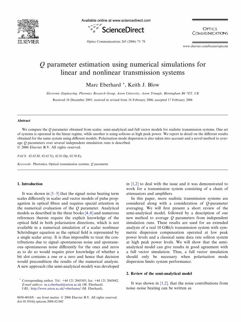
In the second set of results in Fig. 5 the dispersion of theDCF is slightly lowered to D = �17.5 ps/km/nm with allother parameters the same to obtain a map with small aver-age dispersion. The Q parameter estimate for all models isnow the same as the system is limited by dispersion and notby noise.

0

5

10

15

20

0 2000 4000 6000 8000 10000

Q

z [km]

vector modelvector model (PMD)

scalar model half noisescalar model full noisesemi-analytical model

Fig. 5. Q parameter over distance for a linear transmission system setupwith a symmetric nonzero average dispersion map.

0

5

10

15

20

0 2000 4000 6000 8000 10000

Q

z [km]

vector modelvector model (PMD)

scalar model half noisescalar model full noisesemi-analytical model

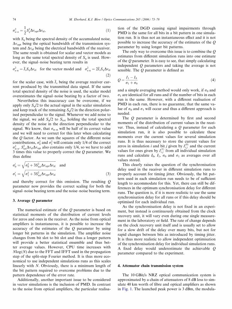
Fig. 7. Q parameter over distance for the soliton transmission systemsetup.

3

3.2

3.4

3.6

P [m

W]

vector modelvector model (PMD)scalar model half noisescalar model full noisesemi-analytical model

76 M. Eberhard, K.J. Blow / Optics Communications 265 (2006) 73–78

6. Soliton transmission system

The 10 GBit/s soliton optical communication systemconsists of a single 40 km section of SMF fibre betweeneach amplifier and uses a launched peak power of26.4 mW with 17.6 ps FWHM Gaussian pulses, the modu-lator has a rise time of 12.5 ps, no insertion loss and 40 dBmodulation depth as shown in Fig. 6. The SMF fibreparameters are dispersion D = 1.0 ps/km/nm, dispersionslope S = 0.06 ps/km/nm2, loss a = 0.2 dB/km and effec-tive area Aeff = 72 lm2. We use again 40 runs 28 bits in atime window of 25.6 ns length and a numerical resolutionof 217 bins. An optical filter with Gaussian shape of order20 with 2 THz bandwidth is included after each amplifier,which has 8 dB small signal gain, infinite saturation powerand a noise figure of 2.0. The receiver has a NEP of1.15 pW/

ffiffiffiffiffiffiffiHzp

and is bandwidth limited by another rectan-gular electrical filter with 20 GHz bandwidth. A polarisa-tion scrambler randomly rotates the signal with regard tothe principal polarisation axes of the fibre segments inthe vector simulations. DPMD is 0.25 ps/

ffiffiffiffiffiffiffikmp

for all vectorsimulations including PMD.

The system parameters were chosen in a way to producea system limited by Gordon–Haus timing jitter and not bynoise. The results in Fig. 7 show clearly, that all modelsproduce similar estimates for the Q parameter. The semi-analytical model produces a Q estimate almost identicalto the scalar case with half the total noise power included.Surprisingly, the estimate from the full vector model yieldsa better performance and system reach compared to the

Tx40 kmSMF

8 dB

EDFA

2 THz

FLT

Random

PC× 1 . . . 250

Rx

Fig. 6. Soliton transmission system setup with a single SMF dispersionmap.

scalar models. While there are no significant differences inthe frequency spectra, the eye diagrams suggest that aslightly lower timing jitter is causing this. The random rota-tion of the polarisation axes in the vector model withoutPMD is the most likely candidate to cause this effect. IfPMD is included, the performance degraded to below theone estimated by the scalar models. Fig. 8 shows a linearincrease in average power for all models as expected foran unsaturated linear optical amplifier. The two slopes cor-respond to the different amounts of noise added at eachamplifier and it is evident, that the full vector models andthe scalar model with full noise show a slope twice as largeas the scalar model with half noise included and the semi-analytical model.

The performance of this soliton system can be improvedby adding an optical filter with Gaussian shape of order 2and 200 GHz bandwidth to the dispersion map as shown inFig. 13. This filter acts as a guiding centre filter and reducestiming jitter. To compensate for the extra loss in the addedfilter, the gain of the optical amplifier was slightly increasedto 8.05 dB. Otherwise the system remains the same.

2.4

2.6

2.8

0 2000 4000 6000 8000 10000

z [km]

Fig. 8. Average power over distance for the soliton transmission systemsetup.

20 vector model

M. Eberhard, K.J. Blow / Optics Communications 265 (2006) 73–78 77

The Q parameter predictions from the vector model andthe scalar model with full noise agree well up to a distanceof about 6000 km as shown in Fig. 9 and are distinct fromthe predictions of the scalar model with half noise and thesemi-analytical model, which agree well up to a distance ofabout 4000 km. At the critical point of Q = 6 the scalarmodel with full noise and the semi-analytical model crossat a distance of around 9000 km, but at different slopes.Interestingly, despite the fact that the semi-analyticalmodel overestimates the Q parameter compared to the fullvector model, it produces a slope of the Q parameter forlarger distances much closer to the full vector model thanany of the scalar models. However, the system performancedegrades strongly when PMD is added. Both full vectorsimulations show an increase in average signal power asshown in Fig. 10, which is not seen in the scalar models.The situation is much worse with PMD included. The exactreason for this difference will be the subject of furtherinvestigations. The vector model without PMD clearlyshows, that vector solitons can exist. However, the system

0

5

10

15

20

0 2000 4000 6000 8000 10000

Q

z [km]

vector modelvector model (PMD)

scalar model half noisescalar model full noisesemi-analytical model

Fig. 9. Q parameter over distance for the soliton transmission systemsetup with guiding centre filter.

2

2.5

3

3.5

4

4.5

5

5.5

6

0 2000 4000 6000 8000 10000

P [m

W]

z [km]

vector modelvector model (PMD)scalar model half noisescalar model full noisesemi-analytical model

Fig. 10. Average power over distance for the soliton transmission systemsetup with guiding centre filter.

performance seems to be sensitive to even small amounts ofPMD leading to a drastic reduction in achievable transmis-sion distance.

It might appear from Fig. 9 as if the differences in aver-age power are to blame for the different results, especiallythe bad performance of the system under PMD. However,even when the average power is artificially clamped to aconstant average power of about 2.45 mW, the situationdoes not change. This can be seen in Fig. 11. The Q param-eter estimate changes only slightly for the different models,while the average power shown in Fig. 12 is now limited toa very narrow range. It can thus be concluded, that theaverage power excursion seen in Fig. 10 is not responsiblefor the degraded performance of the system under PMD.This implies, that the soliton in this system is not stableunder even moderate amounts of PMD.

0

5

10

15

0 2000 4000 6000 8000 10000

Q

z [km]

vector model (PMD)scalar model half noisescalar model full noisesemi-analytical model

Fig. 11. Q parameter over distance for the soliton transmission systemsetup with guiding centre filter and average amplifier output powerclamped.

2.44

2.445

2.45

2.455

2.46

2.465

2.47

2.475

0 2000 4000 6000 8000 10000

P [m

W]

z [km]

vector modelvector model (PMD)scalar model half noisescalar model full noisesemi-analytical model

Fig. 12. Average power over distance for the soliton transmission systemsetup with guiding centre filter and average amplifier output powerclamped.

Tx40 kmSMF

8.05 dB

EDFA

2 THz

FLT1

200 GHz

FLT2

Random

PC× 1 . . . 250

Rx

Fig. 13. Soliton transmission system setup with a single SMF dispersionmap with guiding centre filter.

78 M. Eberhard, K.J. Blow / Optics Communications 265 (2006) 73–78

7. Conclusions

After briefly reviewing the semi-analytical model, wehave shown its validity and accuracy for two real transmis-sion systems. One designed to operate in the linear regimewith a symmetrically compensated dispersion map andanother high peak power nonlinear soliton transmissionsystem. Both show excellent agreement between the fullvector model and the semi-analytical model, while thereare significant differences between these and the scalarmodel for the linear transmission system.

Additionally, we have investigated modified systems,which are limited by other factors than noise. In the caseof the dispersion limited system all models exhibit good

agreement. For the soliton system with guiding centre filterthe situation is less clear. There are significant differencesbetween the scalar models and vector models. Even smallamounts of PMD cause a dramatic decrease of the trans-mission distance.

References

[1] M. Eberhard, K.J. Blow, in: Technical Digest Series, Conference onNonlinear Guided Waves and Their Applications (NLGW), pageMC11, Toronto, Canada, March 2004, Optical Society of America,Washington, DC.

[2] M. Eberhard, K.J. Blow, Opt. Commun. 249 (4–6) (2005) 421.[3] M. Eberhard, K.J. Blow, in: Technical Digest Series, Conference on

Nonlinear Guided Waves and Their Applications (NLGW), pageThB4, Dresden, Germany, September 2005, Optical Society ofAmerica, Washington, DC.

[4] G.P. Agrawal, Fiber-optic Communication Systems, Wiley Inter-science, New York, 2002.

[5] P.C. Becker, N.A. Olsson, J.R. Simpson, Erbium-doped Fiber Ampli-fiers, Academic Press, San Diego, 1999.

[6] A. Bjarklev, Optical Fiber Amplifiers, Artech House, Boston, 1993.[7] D. Marcuse, C.R. Menyuk, P.K.A. Wai, J. Lightwave Technol. 15

(1997) 1735.