1

Public Services and Household Allocation in Africa: Does Gender Matter?

1991

S. Appleton D.L. Bevan K. Burger P. Collier

J.W. Gunning L. Haddad

J. Hoddinott

Centre for the study of African Economies http://www.csae.ox.ac.uk/

2

The project was drawn up with the support of Ann Duncan of the Women in Development Division. After her departure, Shahidur Khandker supervised the project within the Bank. Attributions for design, execution, supervision and synthesis are as follows. Design and synthesis were the responsibility of Paul Collier. Execution of the health and education chapters was the responsibility of Simon Appleton. Execution of the agricultural innovation, extension and household activity choice components of the study was the responsibility of Kees Burger and Jan Willem Gunning. Execution of the expenditure chapter was the responsibility of Lawrence Haddad and John Hoddinott. Execution of the credit and labour market components was the responsibility of John Hoddinott and Paul Collier. Execution of the water and prioritising components was the responsibility of David Bevan. Supervision of each component was primarily the responsibility of David Bevan and Paul Collier, although there was also considerable interaction across the larger group. The material was collated into its present form by Sarah Smith.

3

Chapter 1: Does Gender Matter in Africa? Part I: Public Services Chapter 2: Education Chapter 3: Health Chapter 4: Water Supply, Extension and Credit Part II: Income and Expenditure Chapter 5: Women and the Labour Market Chapter 6: Gender Issues in African Agriculture Chapter 7:Gender Aspects of Household Expenditures and Resource

Allocation in the Cote d'Ivoire References

4

Chapter 1: How Much Does Gender Matter? 1. Introduction 2. Information and Health Care a. The Basic Facts of Differential Usage b. Determinants of Differential Usage of Services, Differential Labour Supply 3. Income Generation 4. Interactions between Differential Usage of Services and the Generation of Income 5. Organisation of the Study

5

1. Introduction This study uses survey data for Kenya, Tanzania and the Cote d'Ivoire collected during the 1980s. With this data we investigate whether African development policy should specifically distinguish between genders. Our main criterion is efficiency rather than inter-gender equity per se. The only distributional issue we consider is the wellbeing of children. That is, considerations of fairness as between men and women are not introduced into this study. We focus upon four services: education, health care, piped water, and information about agricultural techniques. For each of these services, public and private mechanisms of provision co-exist. Although many children get no secondary schooling, many go to private schools which are more expensive than their over-subscribed public equivalents. Although some people receive no health care, others go to private health facilities which are again usually more expensive than their limited-access public equivalents. Although many farmers fail to use best practice techniques, some learn innovative techniques from other farmers while others benefit from extension workers. Many households rely upon fetching water from natural sources while others are able to use publicly installed pipes. A theme of this study is that there is commonly a tendency for private processes of provision to have a gender-bias. Parents are more likely to send boys to private secondary school than girls. Women farmers are less likely to imitate the best practice techniques of neighbours than are male farmers. Water brought from natural sources is largely carried by women. If private processes are biased against women there would seem, prima facie, to be a case for public processes of provision to have an offsetting bias. A second theme is that currently public processes are often biased in the same direction as private processes. African household structures are so different from those found in Asia and Latin America that there is a strong case for analysis to be intra- rather than inter-continental. However, even within Africa there is enormous variation both in household structures and in government policies. The present study includes both East and West Africa, whose rural societies have very different histories of commercialisation. Within East Africa, the study includes the rapidly commercialising region of Central Province in Kenya, a less commercialised area of Kenya, Nyanza, and four Tanzanian regions among which are some isolated and subsistence-oriented localities. Although the survey data for each of the three countries contains much information suitable for the analysis of gender issues, none of it was collected with this end in view. A purpose-designed survey would, for example, have provided more systematic information on an individual rather than a household level. The Kenyan and Tanzanian surveys were designed in common by three of the present authors and are described more fully in Bevan et al. (1989). Their combined sample is 1326 rural households. The survey of the Cote d'Ivoire was designed by the Living Standards Measurement Unit of the World Bank. It has been extensively used for research on other issues and is described in Ainsworth and Munoz (1986). For the applied social scientist, the limits of his data are the limits of his world. It is therefore inevitable that on occasion this

6

study encounters limits imposed by the lack of purpose-designed data sets. The rationale for the study has been that it is generally sensible for the early research on a topic to explore existing data rather than embarking upon the costly and slow task of data collection. Data limitations manifest themselves in two forms. The more obvious is that some issues cannot be explored because there is no information about them. For example, we lack direct information about what goes on in schools: class size, the qualifications and gender of teachers, the extent of teaching materials. An obvious line of enquiry, but one not open to us, is whether the gender of the teacher effects the performance of girls relative to that of boys. The more subtle data limitation is that some of the associations which we identify between variables cannot be attributed to a unique causal interpretation. Sometimes this is because we cannot control for fixed effects. For example, as with many studies on the effects of education, we are not able fully to control for differences in innate ability. Sometimes it is because economic theory offers little guidance. The economic theory of the household usually assumes that it is the household rather than the individual who is the optimising agent. However, we find that the most plausible, though not the only, explanation for some of our observed associations between variables is that men and women have different preferences and that each has a sphere of autonomy which is itself endogenous to the provision of public services. The economic theory of the household usually assigns preferences to the list of things assumed to be exogenous. Yet in analysing why African girls have such radically different educational and work paths both among themselves and when compared with African boys, we have come to regard the endogeneity of preferences as likely to be central. The economic theory of the household usually assumes costless and therefore complete information. Yet in analysing why female-headed households are less likely to adopt particular agricultural innovations than are male-headed households, we find ourselves relying upon differentially costly information as the most likely explanation of our observed associations between variables. The standard economic model of the household, though immensely useful in many contexts, therefore seems to have some limitations as a metaphor of gender-stratified African socio-economic behaviour. The price we pay for agnosticism towards theoretical structure (in particular, of recognising the potential endogeneity of variables usually regarded as exogenous) is, of course, the ambiguity of causal interpretation. The `general-to-specific' econometric approach of Hendry, which we follow, can to an extent resolve this when time series data is involved by recourse to Granger-causality tests. With cross-section data such as our surveys there is no equivalent. When faced with competing causal explanations of a statistically significant empirical association our criteria of adjudication have been plausibility and economy. By the latter we mean that where a single theory accounts for several statistically significant relationships, ceteris paribus, it is preferred to ad hoc theories of each relationship. These criteria, though fragile, may yet be an adequate basis for policy pending the construction of data sets capable of refuting the hypotheses advanced in this study.

7

In the three African countries in our study, economic outcomes such as the amount of education received, the adoption of new crops, and the career path taken, differ radically as between the genders. These different outcomes may be the result of societal discrimination (decision takers consciously favouring males); societal habit (women having lower aspirations because they have fewer role models); or they may be entirely rational. Parents may choose to invest in the education of boys rather than girls either because they regard this as the natural order of priorities or because they anticipate that they will thereby reap higher returns in future remittances. Their anticipation may be correct because of discrimination in the labour market, because of lower aspirations of girls, or because for given earnings, parents are better able to induce sons to make remittances. Women rather than men may fetch water either because this is seen as a fundamental part of gender identities or because the opportunity cost of women's time is lower. In turn, the returns on women's time might be lower because they are less able to get the information and credit needed to access higher return agricultural activities. Again, access to information may differ between the genders either because of fundamental prejudice or rational decision. Copying effects may depend upon role models which are gender-specific: if women copy women and men copy men then large informational differences can develop and persist. Alternatively, extension officers may rationally target their advice at men because only males have the autonomy, or the access to credit, with which to make use of it. Women may have inferior access to credit either because they lack the autonomy with which to build up reputations for credit-worthiness, or because, given practices of the assignment of land rights, they lack collateral. The above examples suggest that a potential explanation is that raw discrimination, habit, and rational calculation interact: discrimination or habit somewhere in the system may make it rational for resources to be used in a gender-differentiated way elsewhere in the system. Potentially the most important instance of this interaction because of its implications for the inter-generational persistence of differentiation, is the gender-specific difference in the provision of education. If, due to discrimination elsewhere in the system, or the lack of role models, the parental return to the education of daughters is lower than that of sons, then the rational parent will perpetuate gender differences in the endowment of human capital. This in turn may perpetuate the gap in role models and in autonomy. In part, this study is an attempt to unravel and quantify these interconnections. We have not attempted to construct a formal dynamic model of social inequality; our primary rigorous focus has not been on the system but rather on some of its key components: access to education, health, information, water, and jobs. The systemic interactions are deduced informally from the components, a procedure justified because the formal modelling of such a complex process would yield results of scant credibility. The outcome of our informal analysis is a prima facie case that the effects of differential stocks of role models give rise to persistent gender inequality. Does persistent gender inequality matter? It is quite possible for substantial gender inequality to have few normative consequences: the bi-gender household may serve as a natural redistributive

8

device so effectively that no public intervention is needed even if feasible. Whereas the first strand of the study is to investigate the determinants of gender-based differentials in the provision of the four services, a second strand of the study is to investigate their consequences. We have explored two possible consequences. The first is the indirect effect on children. We investigated whether better-educated or richer mothers were more beneficial for children than better educated or richer fathers. This can only have potential policy interest if there is a possibility that society places a higher value upon the wellbeing of children than do parents, so that, for example, the education or the feeding of children are merit goods. Much public policy is most readily interpreted as reflecting such a value system, but it is beyond the scope of this study to investigate whether African governments do or indeed should hold these values. Mothers when educated may be better placed to notice illness, and to do something about it; provide children with a better diet; and give priority to their education. We also investigated whether women tended to devote a higher proportion of expenditure upon food for the household, from which children benefit disproportionately, and whether this pattern of expenditure was influenced by the education and income opportunities of the mother. To an extent, if these relationships are statistically significant once allowance has been made for obvious problems of potential endogeneity, they are of policy interest irrespective of causal interpretation. If better-educated mothers are more likely to take sick children to health clinics it is a second-order consideration whether this is due to a change in preferences, to improved understanding, or to greater autonomy within the household, (none of which would fit well with the standard model of the household) or to some causal process entailed by the standard model. Similarly, if the pattern of household expenditure is found to be a function of the gender composition of household income, this is clearly consistent with the bargaining model of the household but need not entail it. The second possible consequence is that over and above the benefits conferred upon children, the social, or even the private return to the provision of education, health care, agricultural information, and water may be higher for women that for men: that is, gender inequality may simply be inefficient. The third and final aspect of the study, conditional upon having established a reasonable case for the existence of a problem, is to identify and quantify the scope for policy intervention. For this we analyze the determinants of the differences among females in the provision of education, jobs, information, and health care. What, for example, determines why some girls get secondary schooling and others do not? Because the study focuses primarily upon components rather than systems, it does not stand or fall as a single entity and can be used piecemeal. However, the study does have an integrating thesis. Some key inputs into income generation tend for various reasons to be underprovided by the market. That is why there is some public provision of education, health care, water and extension. As we show, the private systems of provision of these inputs systematically underprovide women more severely than men (for a variety of reasons). Consequently, by extension from the general case for some public

9

provision of these inputs, there is a reasonable case for an offsetting gender bias in public provision: public provision should favour women. Instead, partly because public provision is rooted in the same social processes which generate unequal private provision, public delivery tends to be biased towards men. Indeed, in some cases access to rationed public provision is so strongly gender-differentiated that it is the private processes which become relatively, or even absolutely offsetting: if public secondary school places are largely reserved for boys then private schooling becomes, along with no schooling, the residual legatee of girls.

2. The Usage of Information and Health Care Much of this study focuses upon education, extension, health care and water. Underlying this is the notion that with information and labour time people can substantially improve their (and their children's) lives. Of course, many other factors matter as well, but they lie beyond the (arbitrary) boundaries of this study. Education and extension are both mechanisms for providing people with information (or the capacity to acquire it). While education in Africa is both publicly and privately provided, extension is almost exclusively a public service. This is not just happenstance, the difficulties of exclusion make agricultural information intrinsically hard to market. There is, however, a private non-market process of agricultural information acquisition, namely copying from neighbours. We investigate, then, four distinct processes of information acquisition, two public and two private. Within this broad structure there are interactions. Access to secondary schooling depends in part upon performance during primary schooling and this is partly dependent upon the home environment. The take-up and use of extension advice may be a substitute for, or a complement of, education. Each of these component mechanisms of information acquisition is investigated in subsequent chapters. Here we aim to provide an overview. The time available for remunerative labour may differ systematically between the genders. One possibility is that women have less good health states than men and so lose more days too ill to work. Factors which effect health states become inputs into the productive process and thereby have differential gender effects. The most obvious such factor is health care (to the extent that it is effective). Other factors investigated are the source of water supplies and the level of education. A second possible reason for differential time available for remunerative labour is differential obligations. Child rearing and water fetching are obvious candidates for investigation. To anticipate our detailed results, we find some evidence for gender differences in each of these areas. However, differential acquisition of information appears to be a far more serious problem than differential labour supply.

10

The Basic Facts of Differential Usage Differential usage may arise because access is differentially rationed by the government, because household decision takers award different priorities among household members, or because the motivation to take up the service differs among potential recipients. We defer these issues as to why provision differs until the next section. Here we are concerned simply to measure the extent to which provision differs systematically by gender. Our discussion considers first the acquisition of information and then labour supply. It takes the form of twelve questions. (i) Do Parents Send the Child to Primary School? In all three of the countries in our study girls are less likely to be sent to primary school than are boys. However, in Kenya and Tanzania enrolment in primary education has been close to universal for some years and so gender dfferences in non-enrolment are not a significant phenomenon. In the Cote D'Ivoire compulsory universal enrolment has only recently been established and so our data permits a detailed analysis of the situation prior to compulsory enrolment, which is not feasible for Kenya and Tanzania. The rationale for the investigation is that it enables an evaluation of the policy of compulsory enrolment which might be applicable in similar countries. Prior to compulsory enrolment, gender differences in access to primary schooling were substantial in the Cote d'Ivoire. Girls were almost fifty percent more likely never to have attended school than boys. Economists are critical of policies which involve compulsion, for good reason generally preferring price incentives. However, atypical failures in intra-household altruism appear not to accord with this presumption. Economists are not widely critical of the existence of laws which forbid the battering of babies. While it would be technically possible to pay parents sufficient to induce one hundred percent school enrolment, a large majority of the population (`society') might regard compulsion as preferable to the enormous fiscal cost of inducing a small minority of malign parents to give their children the opportunity of literacy. (ii) Does the Child Drop Out of Primary School Prior to Completion? Girls are much more likely to drop out of primary school prior to completion than are boys. In Kenya overall around 30% of those children who are enroled are estimated to drop out prior to completion. Girls are around one-third more likely than boys to drop out. In Tanzania overall drop-out rates are lower, but again girls drop out at a higher rate than boys. In rural Cote d'Ivoire drop out rates are extremely high with girls around 14% more likely to drop out than boys. Finally, in urban Cote

11

d'Ivoire drop-out rates are about comparable with those in rural Tanzania. The differential drop-out rate is again significantly higher for girls, being around a quarter higher. (iii) How Does the Child Perform in the Final Primary Examination? For Cote d'Ivoire we have direct observations of the final leaving examination performance. For Kenya and Tanzania we can only infer this from the admissions to public secondary schooling which are conditional upon a critical level of performance. In Kenya, sufficient children continue to public secondary schooling for the `latent' variable of examination performance to be reasonably well determined. In Tanzania, however, only around 4% of children gain entry to secondary schooling and this provided too small a sample. We can therefore only discuss differential examination performance for the cases of the Cote d'Ivoire and Kenya. In both we find strong evidence for differentially poor performance on the part of girls. In the Cote d'Ivoire in our logistic analysis of performance, gender is the most statistically significant of fourteen explanatory variables. In Kenya gender is also highly significant: at the means of other characteristics, girls are around a fifth less likely to pass the examination. These results are the more remarkable because of their sharp divergence from the pattern of girl-boy differences in school performance in other countries. For example, Alderman et al. (1991) report that in rural Pakistan females outperform males in cognitive achievement production functions, ceteris paribus. In developed countries, at the end of primary schooling (and in the somewhat older age ranges at which this takes place in the Cote d'Ivoire and Kenya), girls usually out-perform boys. This suggests that in the countries of our study girls are substantially under-performing relative to their intrinsic abilities: perhaps the home environment is less conducive for girls, perhaps at school girls are receiving differentially fewer inputs, perhaps girls have lower aspirations.

12

(iv) Does the Child go to Public Secondary School? Access to public secondary schooling is subject to the double hazard of government rationing through selection and of parental choice. Public schools tend to be cheaper than private schools and usually of better quality. Hence, parents prefer to send children to public schools. For the child to gain access she or he must both pass the examination and have parents who are willing to meet the costs. For the reasons discussed above, our analysis of secondary schooling is confined to Kenya and the Cote d'Ivoire. While in Tanzania boys have an 86% higher chance of enrolment in public secondary schools than do girls, the stark fact of drastically limited access for all children reduces our sample size to an unusable level. In both the Cote d'Ivoire and Kenya, boys have a higher chance of gaining places in public secondary schools conditional upon completing primary schooling. However, this turns out to be fully explained by the weaker examination performance of girls. Conditional on passing the examination, girls are at least as likely as boys to have parents willing to meet the costs of sending them. (v) In Default of Public Secondary Schooling does the Child go to Private Secondary School? In all three countries, private sector secondary school places are less skewed towards males than government ones. This reflects their role in catering for those students rationed out of the state sector by poor exam performance, a disproportionate number of whom are girls. In Kenya, however, the expansion of private secondary school places for girls was still under way at the time of our survey, so for our sample of young people with primary schooling, we find males had a 60% higher chance of going to private secondary schools, in default of public schools, than females with similar characteristics. In the Cote d'Ivoire, by contrast, girls have a significantly higher chance than boys (though the differential is far more modest). A likely explanation for the Ivorian result is that the bias against girls at prior levels, most notably in entry to primary school and in examination performance, is so large that it more than offsets the inclination of parents to favour boys. That is, there is a sample selection effect: those girls who survive to the stage of being considered for private secondary schooling are substantially brighter than their male peers. (vi) Do Women and Men get Equal Access to Extension Advice? We now turn from education to information about agricultural techniques. We investigate two routes to such information, the publicly provided one of extension services and the privately provided one of copying from neighbours.

13

The three countries had very different provision of extension services. Subsequent to our data collection the Kenyan extension service was reorganised specifically to have greater orientation towards female farmers. We investigated Kenyan extension contact with respect to tea, coffee and hybrid maize. With the exception of tea, female farmers appeared to rely more on traditional sources of information and less upon the extension service. In Tanzania agriculture was far more traditional with far less contact with the extension service. However, to the limited extent that there was contact, there was no evidence of gender bias. In the Cote d'Ivoire extension contact was also very limited, but additionally it was gender-biased. Only 1% of female-headed households, as opposed to 7% of male-headed, reported any contact with the extension service. This was, in turn, entirely explained by the concentration of female-headed households in those agricultural activities which had the most limited extension services. (vii) Are Role Models Gender Specific? People copy other people when taking decisions. This can be regarded either as reflecting a reduction in the costs of information as the outcomes of others' past decisions can be observed, or as a way of avoiding the costs normally incurred in the decision process (the collection and processing of information). Indeed, potentially, these two motives for copying coexist and are distinguishable. The former, copying observed success, is driven by the observed outcomes of the stock of past decisions; the latter, free riding on others' decisions, is driven by the observed flow of decisions rather than their consequences. To the extent that either of these copying processes is important, innovators confer externalities in their capacity as role models for imitators. Potentially, role models are important in a whole range of decisions: the care of children, the aspirations of children in school, entry to the labour market, the adoption of agricultural innovations. They will be a recurring theme in this study. The central idea pursued in our analysis of copying effects is that role models might be gender-specific. There are a priori reasons why this might be the case. The whole rationale for copying is that the observation of similar agents can be a cheap way of reaching the right decision. At the margin between copying and primary research the savings on research costs are just traded off against the errors introduced because the circumstances of other agents (which are only imperfectly observed) are not coincident with those of the copier. Hence, agents who see themselves as atypical of successful innovators are less likely to make use of them as role models. Gender is one of the characteristics which may constrain the domain of imitation. It is, of course, by no means the only characteristic: the poor may be reluctant to imitate the rich, the young to imitate the old. However, unlike these other characteristics, it is a dichotomous rather than a continuous variable and unalterable rather than state-dependent. Thus, there is no blurring of identity: people are either male or female in a way that they are not either rich or poor, young or old. The possibility therefore arises that each gender imitates primarily role models chosen from its own ranks: women copy women, men copy men. In any particular instance

14

such behaviour might be disfunctional: if a useful innovation happens to be introduced first among men, women may stand to gain considerably by imitating. However, the information costs which women would need to incur in order to discover that in this instance it was safe to imitate men are tantamount to the costs of primary research on the benefits of the innovation: in other words, they destroy the very rationale of copying. If role models are an important part of the decision process and if they are gender-specific then there is a potential policy problem, for the externalities conferred by role models would apply only within each gender. Suppose that a good innovation becomes available which for some exogenous but temporary reason is initially adopted only by a few men (the reason may, of course, be a gender bias in some aspect of the system, such as credit or extension). Some other men free ride on the decision and so gradually a stock of innovators accumulates which induces copying of observed success by other men. Because the flow of copying observed success is positively related to the stock of past decision takers, and the flow of free-riding is positively related to the flow of copying observed success, the forces inducing imitation become more powerful over time. However, the increasing power of copying applies only among men. Ex post, we observe that many men but few women have adopted the innovation. The explanation for this gender difference lies not in the current returns to opportunities but in the history of information about those opportunities. In this sense that present outcomes are a function of the past history of the process, gender-specific copying can be thought of as giving rise to hysteresis. Just as randomly assigned temporary unemployment may permanently scar the careers of those who become unemployed (hysteresis in the labour market), so an exogenous temporary innovational advantage for one gender may generate persistent differences. It is one thing to postulate gender-specificity in copying effects, quite another to demonstrate it empirically. Although potentially, such affects apply to the whole range of economic decisions, we were able to investigate them primarily for agricultural innovation and education. Here we discuss only the former. For agricultural innovation the postulated relationship was that the key decision taker would be the household head, so that potentially, female-headed households might copy other female-headed households and conversely among male-headed households. This should not be taken as precluding other gender-specific copying affects in agricultural innovation, but it is a priori the most plausible, and also the most researchable. At a minimum, the sampled population must include a substantial proportion of female-headed households and a lot of agricultural innovation over a fairly short period (so that we can still identify ex ante economic and demographic circumstances). Although we conducted the analysis for all three countries, these conditions were really only met for Kenya. In Tanzania there was little agricultural innovation since agriculture was profoundly and adversely effected by macroeconomic policies, and in the Cote d'Ivoire there were rather few female-headed households. Kenya, by contrast, was close to an ideal sample: there was a high proportion of female-headed households, a history of agricultural innovation, and a burst of innovation in the form of coffee

15

adoption during the period observed by our data set (1975-82) due to the coffee boom. Even with an ideal population, the sampling requirements in order to detect gender-specific copying (even if it is present) are daunting. Copying can be presumed to decay with distance between the innovator and the potential imitator. A proxy for this is the concept of the cluster, a group of 200 contiguous households. By sampling within spatially disparate clusters we are potentially able to detect intra-cluster copying. However, the sampling requirements for such effects to be identified as gender-specific are quite severe: given that we sample only 10% of a cluster, it is quite likely that we fail to detect such effects. It is therefore the more remarkable that for the adoption of Kenyan coffee we were able to demonstrate not only that copying effects were powerful, but that these effects were gender-specific. Male-headed households were much more likely to adopt coffee if other male-headed households had already done so, but did not copy female-headed households. Female-headed households were much more likely to adopt coffee if other female-headed households had already done so, but did not copy male-headed households. To our knowledge this is the first time that a gender-specific copying effect has been demonstrated. Because of its potent implications for policy, it must count as one of the major results of the study. As discussed above, limitations of the sample make the approach largely infeasible for Tanzania and the Cote d'Ivoire. However, for Tanzania we have weaker, but still suggestive, evidence. Households were asked whether they had changed their agricultural techniques in the preceding five years for a range of crops and, if so, how they had come to learn of these techniques. Male-headed households appeared to be considerably more ready to innovate, but a particularly sharp difference was in the attribution of the new information to learning from neighbours: this was a fairly common attribution among male-headed households but it was never cited by female-headed households. We may conclude, then, that gender differences are both powerful and systematic right through the processes of information acquisition. The end result is that women have markedly inferior access to information than men. At this stage we consider neither causes nor consequences. However, it should be evident that the causes must be various: that girls are less likely to be sent to primary school than boys is a purely parental decision, independent of the wishes of the child or the provision of the state. That girls gain fewer offers of places in public secondary schools has, prima facie, little directly to do with the parents (though more on this below) and probably more to do with the motivation of the child and the performance of the state education system. It should also be evident that such large differences in access to information are going to have consequences: it would be incredible for the converse to be the case. The research issue is not whether women are disadvantaged through their inferior access to information, but to identify the salient forms of that disadvantage: where does it matter most? These questions of cause and consequence are taken up below. First, however, we turn to the basic facts of labour supply. We now turn to influences upon labour supply. These are decomposed as follows:

16

(viii) Are Women's Health States Worse than Men's? The surveys gathered very detailed information on health, following symptoms through to actions, and consequences. However, health states were self-assessed. Since illness is a `bad' only to the extent that it is subjectively experienced, this may appear to be a virtue. Indeed, recent studies in developed countries (Idler (1991), Idler and Kasl (1991)) find self-reported data very valuable. Unfortunately, in our samples self-reported data has turned out to be highly problematic. Two people may objectively be equally ill, subjectively feel equally poorly, and yet only one of them may conceptualise this experience as an `illness'. Factors which fundamentally affect how people conceptualise the world, such as education, may therefore appear to be altering health states when in fact they are altering cognition. This problem is particularly acute in the case of child health states, which are maternally reported. Here the reporter does not have any subjective information. The assessment of the health state depends entirely upon the interpretation of objective information, precisely the skill which education develops. With these caveats upon the nature of the data, health states were found to be highly age dependent, especially for women. During the peak child-bearing years women are significantly more prone to illness than are men. In Kenya this is sufficiently pronounced that averaged over all age groups women have about two-fifths more illnesses than men and the typical illness lasts one fifth longer: hence, women suffer nearly two-thirds more days of illness. However, with directly comparable data, no such gender difference is found for Tanzania. For the Cote d'Ivoire our health data are somewhat less detailed. However, there is again no evidence of a higher incidence of illness among women. (ix) Do Women Make Less Use of Health Facilities? Conditional upon being ill, gender appears to be only sporadically significant as a determinant of whether use is made of health facilities. The three data sets do not reveal any clear and consistent pattern such as women using facilities less than men. (x) Does Differential Illness and/or Differential Use of Care Facilities Translate into a Reduced Labour Supply? Women suffer more days illness than men. This is not offset by use of care facilities: women do not make significantly greater use of facilities conditional on illness. The greater number of days of illness is therefore unsurprisingly associated with women also suffering a greater number of days being too ill to work. However, the magnitude of this effect on labour supply is modest (although, potentially it may have a disproportionate effect on productivity because of the unpredictable nature of the

17

interruptions to work effort). (xi) Is Women's Labour Supply Differentially Reduced by Obligations to Fetch Water (and Fuel): i.e.

by Actions which are Public Goods within the Household? The provisioning of the household with water and fuel is an intra-household public good. Overwhelmingly, this service tends to be provided by women. It is very labour intensive. However, it appears that this encroaches primarily on non-productive labour time: women still spend more hours in remunerative work than do men. (xii) Is Women's Labour Supply Differentially Reduced by Obligations of Childcare? We find that on the whole child-rearing does not act as a substantial constraint on women's labour supply. For example, in the Cote d'Ivoire, the number of children is not significant as an influence upon women's labour market participation. This is presumably because the extended family (and elder children) function as an effective child-minding capability. To summarise, although women face differential burdens on labour time, (and this might be regarded as a problem in itself), this does not have substantial repercussions for labour time in remunerative work.

(b) Determinants of Differential Usage of Services and Differential Labour Supply. So far we have established that across a wide range of services, especially those related to information, provision appears to differ systematically by gender. We now analyze the determinants of this differential provision. Two lines of inquiry are pursued. One is to explain why women have inferior provision relative to men: for example, why girls perform less well in the primary school leaving examination. The other is to identify why provision differs among women: for example, why some girls perform better in the primary school leaving examination than others. Both analyses can provide insight into appropriate policy responses. In discussing the determinants of provision we again begin with those services which provide information. (i) Enrolment in Primary Education Recall that in Kenya and Tanzania for some years virtually all children are at some stage enroled in primary education whereas in the Cote d'Ivoire differential access between the genders has only recently been tackled by the introduction of compulsory primary enrolment. The age-gender

18

interaction effects in our models show the narrowing of gender differentials in the lead-up to this policy. Nevertheless, the past determinants of enrolment in the Cote d'Ivoire are of policy interest for similar countries. In this study we found three important gender effects. First, parental education powerfully reduces the gender differential: educated parents are much less likely to discriminate against girls. Girls from uneducated families are predicted to be sixty percent more likely than girls to remain unschooled in rural areas and one hundred and sixty-four percent more likely in urban areas. However, if the father has any primary schooling, the gender difference would fall to twenty-two percent in rural areas and be reversed in favour of girls in urban areas. These results are at the means of other explanatory variables. One aspect that is particularly noteworthy is that the extent of paternal schooling does not matter. That is, paternal education reduces discrimination against girls regardless of the amount acquired: not even the critical minimum for functional literacy appears to matter. This suggests that the effect works not through parental human capital but through parental attitudes and aspirations. Whereas inter-generational effects are therefore highly benign, intra-generational effects are much more problematic due to two effects of siblings. One is that the presence of older brothers strongly detracts from the prospects of younger siblings. This is especially the case if elder brothers are uneducated. By contrast, older sisters have favourable effects on enrolment probabilities. A second inter-generational effect is due to younger siblings and to potential siblings yet unborn. The number of such siblings is proxied by the number of years of child-bearing the mother had left when the child was born. Controlling at the mean of all other characteristics, these potential births have very powerful effects. Increasing the number of child-bearing years from none to twenty increases the chance that the child will not be educated by more than ten percentage points in urban areas (the baseline chance is only 13 percent). An interpretation of this result is that the remaining years of child-bearing represent a set of potential liabilities the magnitude of which is uncertain. The household therefore avoids making long-term, illiquid and continuing investment commitments such as the education of young children. On this interpretation, an implication is that birth control, by enabling the household to contain these liabilities to manageable proportions, might yield an immediate switch of assets into the education of young children of both genders. Taken together, the two sibling effects produce poor intra-generational dynamics. When the household is young there is a discouragement to educating children because of potential future children. Ex post, older brothers reap their revenge on younger siblings by making it less likely that they too will be educated: parents are reluctant to give younger children advantages previously denied to their elder children. The implication for policy is that it is particularly important to attract the first-born child to school at the appropriate time. The final important gender effect of note concerns the effect of women's share of cash income on school enrolment. It was found to significantly increase the probability of boys (only) enroling. This

19

is in line with results discussed later suggesting that the rise in women's income shifts the pattern of household expenditures in favour of child goods and benefits the anthropometric status of boys. (ii) Dropping Out of Primary Education prior to Completion Recall that girls are far more likely to drop out of primary schooling prior to completion in all three countries. We attempted to explain this through a logit analysis (complex because of pervasive right-censoring). Various household characteristics increased or decreased the bias against girls. In Kenya, the distance to the water source significantly increased the female drop-out rate but not that of boys. This is consistent with our evidence that collecting water is a claim on girls' time much more than that of boys. In view of our evidence, discussed in the next sub-section, on the factors influencing girls' underperformance in the examination, one interpretation of this finding is that when a lot of time is spent on collecting water, school performance deteriorates, and the parents are then more inclined to withdraw the child from school prior to completion. The land endowment per capita, by contrast, significantly increased the male drop-out rate but not that of girls. Perhaps this reflects the inheritance patterns: boys will inherit the land rather than girls. Hence, the higher is the household's land endowment the higher are the prospective returns for boys in farming. If the key returns to education are perceived to lie in the labour market, land will therefore reduce the incentive to educate boys rather than girls. This, of course, suggests that over time, as population density rises and agriculture becomes an activity of diminished relative importance, the educational disadvantage of girls would increase in this respect. However, offsetting this trend, the spread of completed primary education among parents will significantly reduce female drop-outs both absolutely and relative to male drop-outs. Finally, we find a powerful discouraging effect from the number of elder siblings: more elder siblings significantly and substantially increases the likelihood of dropping out. One interpretation of this is that it reflects a quantity-quality trade-off: having more children is an alternative to having a few children with a larger per capita educational investment. Importantly, this effect is entirely own-gender specific: having elder sisters does not reduce the educational prospects of boys; having elder brothers does not reduce the educational prospects of girls. It is as if the quantity-quality trade-off was seen within the household as a gender specific decision. The analysis was replicated on our Tanzanian data set with similar results. The distance from the household's water source again significantly increased the likelihood of female drop-out, but not of male drop-out. The land endowment per capita increased the drop out rate of both genders, but much more substantially and significantly so for boys. Finally, the discouraging effect of elder siblings was again powerful and again entirely own-gender-specific: having elder sisters only damaged girls; having elder brothers only damaged boys. The data set for rural Cote d'Ivoire produced somewhat similar, but not identical, results. Distance to water increased the drop-out rate for boys not girls, whilst the land endowment was unimportant. As in Kenya, parental education significantly

20

reduced female drop out while having no effect on that of boys in rural areas. Finally, the number of years until the mother reached the age of forty significantly increased the risk of female drop-out in rural areas. Recall that this variable, interpreted as proxying the number of contingent births, was also significant in discouraging enrolment. (iii) Performance in Primary Schooling Recall that a key `stylised fact' is that girls perform substantially less well than do boys in the end-of-primary examination. This is important both as a measure of the human capital acquired during primary schooling and as a screening device used for enrolment into public secondary education. First consider the effect of general development as measured by an increase in per capita consumption. The underperformance of girls is almost entirely accounted for by those households below mean consumption: girls' performance differentially deteriorates as consumption falls. This suggests that the cause of underperformance lies with the household rather than with the school (although an offsetting emphasis upon the education of girls by schools might be the easiest, and therefore most appropriate policy response). What might be going wrong in poorer households? Our analysis of examination performance established that certain household decisions concerning the allocation of time and of money for the child were important. To perform well, children need to attend school regularly and to devote time to homework. The number of hours the child actually spent at school (rather than being kept at home due to chores or illness), and variables which proxied the time taken gathering fuel wood (a typical children's activity), were both significant determinants of performance. Similarly, the amount of money spent by the household on children's education significantly affected performance. Are there differences in time and money allocation which would account for the differences between the genders in examination performance? For time allocation the evidence is straightforward: on average, the amount of time primary school students spent at school was lower for girls than boys. For expenditure on children's education the story is more complex. On average, girls were not disadvantaged relative to boys. However, we find very powerful effects of household per capita consumption on girls' but not on boys' performance. This suggests that expenditure on girls education is a luxury good in the household. This was indeed observed: although on average girls were not disadvantaged, among the poorest households more was spent on male students' education than on that of female students. Indeed, the same `luxury good' effect was found for time allocation: the gender difference in time spent at school was greater among the poorest households. As with primary enrolment, we consider inter and intra-generational transmission effects. Again the inter-generational effects are benign. Parental education, and especially maternal education, substantially improves the educational performance of both girls and boys. Note that the differentially strong effect of maternal over paternal education indicates that this is nurture rather than nature: that is,

21

the result is not merely proxying for inherited differences in ability. Maternal education thus conveys an inter-generational externality as an input into the primary education production function. The intra-generational transmission effect is, however, again worrying. Recall that having an uneducated elder sibling, and in particular an elder brother, substantially reduced enrolment prospects for younger children. The educational performance of girls is strongly influenced by whether they have an elder sister who has passed the primary examination: without such a sister girls underperform boys, with one they out-perform boys. Why might this be? First, the result might be proxying for inherited ability. However, this can be rejected because were this the explanation the performance of elder brothers would be equally influential whereas in fact it has no effect. Second, the result might be proxying a more favourable household environment, either for children of both genders or a relative bias in favour of girls, either by way of expenditure, time, or space. However, if this were the case then we would expect the same effect to be discernable among boys: boys should perform significantly better if an elder brother has already passed the examination. No such effect is found. This leaves as the most plausible interpretation that of the role model effect. In a male-oriented society, boys have abundant role models for success and do not need the impetus of a successful elder brother. By contrast, girls have a dearth of role models illustrating the benefits of educational success. An educationally successful elder sister can therefore be a powerful stimulus to aspirations. Such a role model effect, when powerful, is important because, as with the gender-specific copying of agricultural innovations, it gives rise to a hysteresis effect. Boys have many role models of educational success, girls have few, and so through the copying of these models, patterns of inequality persist: stocks are driving flows. Note that usually in economics when stocks influence flows the inequalities are self-correcting: if there is too little of capital stock 1 relative to capital stock 2 its returns will be higher and so its rate of accumulation will be larger. Hysteresis occurs where this process is reversed: a recent example unconnected to role models being Lucas' work on the societal returns to education and research. (iv) Entry to Secondary Schooling Recall that entry to public secondary schooling is subject to a double hazard: the child must meet the examination screening criteria of the educational system and have parents able and willing to bear the costs. If the child passes the first of these hazards but not the second, it will not only fail to enter public secondary education but will fail to enter the more expensive alternative of private education. If, however, the child fails the first hazard, it might still get education if the parents are prepared to make the larger expenditures involved in private education. The examination hazard of entry to secondary schooling is coincident with the performance of the child in primary education which we have just discussed. We focus, therefore, on the parental decision to invest in the child. Because public secondary schooling is such a good deal, almost all children who are offered a place take it up.

22

Hence, the cutting edge for parental decision is whether or not to send the child to private schooling conditional on having failed to get a place in the public schooling system. Recall that in our analysis of enrolment to primary education in the Cote d'Ivoire we found that the future child-bearing years of the wife acted as a powerful discouragement to investment by the household in the child's education. In Kenya and Tanzania too few children were not enroled in primary education for a comparable analysis. At the secondary level too few children in rural Tanzania were enroled for analysis to be possible, hence our evidence is confined to Kenya and the Cote d'Ivoire. For Kenya we find that the future child-bearing years of the wife again has a powerful discouraging effect upon investment in private secondary education. At the mean of other variables, the child of a 45 year old mother has a better than 60% chance of being sent to private education if they fail to pass the examination, whereas that of a 30 year old mother has a worse than 40% chance. In the Cote d'Ivoire such effects were not observed. For Kenya we were able to include a variable denoting the proportion of other children in the immediate neighbourhood who were attending private schooling. This was highly significant as a predictor of whether the child would be sent to private school. Of course, to some extent this may pick up omitted variables about the local private school (however, the distance to the school proved insignificant as an explanatory variable). An alternative interpretation is that the pattern of decisions by other households sets norms of behaviour (or that copying is a way of economising on the costs of acquiring information and taking decisions). This may, therefore, be evidence for hysteresis at the level of secondary school enrolment, this time operating at the level of the local community rather than among the siblings of the household. In all three countries, girls are less likely to acquire places in public secondary schools, primarily because they perform less well in the examination. In Kenya they were then less likely to be sent to private schools because their parents seem less willing to pay for them than for boys. In Tanzania a policy was adopted to lower the examination marks for public secondary school entry for girls relative to boys. The effect of this is, of course, to switch public places from boys to girls. We simulated the effect of such a policy in Kenya. Because parents were more willing to pay for boys to go to private schools, the boys displaced by this switch were more likely to receive a secondary education (in the private sector) than the girls taken into the public schools as a result of the extra places for them. The overall effect is that for each place switched from boy to girl, an extra 0.15 place would have been created in the private sector. The government could therefore have cheaply increased secondary school enrolment by switching subsidised public places from boys to girls. Recall that many of the schooling decisions we analyze in Kenya pre-date the large increase in private secondary school places for girls, so the `window of opportunity' for such a policy is likely to have passed. However it may be open to other less educationally developed countries than Kenya and provides an example of a wider

23

principle to which we have alluded: there is a case for public sector subsidies to offset rather than reinforce private sector biases. (v) Extension We attempted to explain contact with extension services through a logit. In Kenya, where the system of contact has anyway changed radically since our data was collected, the logit did not reveal any gender-specific effects. In Tanzania again no gender effects were found. The education of the household head was a significant explanatory variable inducing greater contact. In the Cote d'Ivoire there was a significant pure gender effect: female-headed households were less likely to receive extension contacts, but as in Kenya there was no significant effect of education. (vi) Labour Supply We investigated whether women differentially reduced their labour supply to remunerated work because of poor health states, or household obligations. We found that even where women had differentially inferior health states, this tended not to translate into significantly reduced labour supply (although the random interruptions implied by illness may alter the feasible range of activities in a way we were not able to investigate). The main household obligations we investigated were the fetching of water and the rearing of children, both of which were found to be overwhelmingly female tasks. The provision of piped water was found, not surprisingly, significantly to save time. However, remarkably, there was no evidence that either child care obligations or water fetching reduced female labour supply to remunerated work. This result carried over to female working time in self-employment (including farming). In effect, these tasks reduce women's leisure time or the time for other non-employment tasks. Hence, the provision of piped water, while it considerably increases women's time for other activities, does not appear to have major implications for labour time.

3. Income Generation Women have lower returns to their labour than do men. This is made up partly of effects in the labour market and partly in agriculture. In both cases the central process is that women are disproportionately engaged in activities which have lower returns rather than that they earn less than men within an activity. In the formal labour market, controlling for educational and other characteristics, women did not receive lower pay rates than men. However, conditional upon being in the labour force they were markedly less likely to enter into wage employment. The most immediately plausible explanation for

24

this, child-rearing obligations, turned out not to matter: the number of children did not detract from participation. This suggests that the extended family is able to provide an efficient network of child support. We also able to include as an explanation for low female participation in the market the time taken up with fuel and water collection (either directly observed, and therefore endogenous, or instrumented and therefore exogenous). We found that, as with child care, these obligations did not detract from participation in the labour market. Although we can therefore reject these household obligations as explanations for the low market participation of women, we were unable to distinguish between several other possible explanations. For example, it might be due to a differential reluctance on the part of women to seek wage employment, to employer discrimination, or to lower expected earnings. However, an important finding is that women's participation is far more sensitive than that of men to education. The two most likely routes through which education may be having an effect are directly, via changes in attitudes, and indirectly, via increasing expected earnings. The former might apply if personal educational success functions as a substitute for the dearth of role models. Recall that we have already found evidence consistent with an analogous effect during schooling: girls' exam performance is associated with that of their elder sister, though boys' performance is not associated with that of their elder brother. Below, we describe a further analogous effect within agricultural innovation. Turning to the latter route, although education raises expected earnings in wage employment for both men and women, women's participation may be more sensitive to expected earnings. Is the low participation of women in the labour market a policy problem? If it is due to employer discrimination (an interpretation which we cannot test) then necessarily it is so. Discrimination is both unjust and inefficient: a standard result of economic analysis is that discrimination is costly. If, however, low participation is due to female choice then the issue is less straightforward. In developed countries low female labour participation is to a considerable extent due to the competing obligations of child-rearing placed upon women and additionally due to pay discrimination in the market: controlling for characteristics, women tend to earn far less than men. In Africa these explanations appear not to hold. The time released by women not participating in the labour market is not diverted to non-remunerative, but socially useful activities (child-rearing, fuel and water collection) since these are done regardless. Rather, the time released is devoted to low-remuneration self-employment, particularly on the farm. Either women systematically tend to lack unobserved characteristics which would make them suited for more remunerative activities (for example, they might have higher costs of skill acquisition) so that it is allocatively efficient that they should be concentrated in unremunerative activities, or this skewed labour allocation is symptomatic of resource misallocation. Indeed, potentially, there are two types of misallocation. First, there is a loss due to the returns from women's labour being lower in self-employment that in the labour market: a reallocation would raise the value of output. Second, there is a misallocation among women in self-employment. That is, as discussed in our analysis of the rural labour market, because so little farm

25

labour (female and male) is currently allocated through the market, wide differences in marginal products must necessarily arise between self-employed labour on different farms. The labour market is the `safety value' for very low remuneration self-employment. It works badly enough for men, but for women it is quite radically less effective and so inter-farm misallocation of female labour is likely to be far worse than that of male labour. Potentially, this can be mitigated by male-female labour substitution: in households where there is an abundance of female labour, women may undertake tasks normally done by males while male labour is hired out. To some extent this undoubtedly happens, however, because agricultural tasks often have quite a high degree of gender-specificity, male and female labour are not perfect substitutes. The claim of allocative inefficiency will inevitably seem controversial since modern household economics is theologically committed to the notion of maximisation: the household must be allocating its resources optimally. Inefficiencies could arise, however, either due to externalities from male-female bargaining, or from a lack of information about the returns to skill formation or innovation. Changes in preferences arising from role models fit somewhat awkwardly into the standard metric of efficiency. If, in the absence of a role model, the agent chooses a low-remunerated activity which would not be chosen in the presence of one, we are nevertheless entitled to describe that choice as maximising. However, we are also entitled to describe the change of choice resulting from the introduction of a role model as an improvement in allocative efficiency. If the explanation for low participation in the labour market is primarily a matter of low aspirations due to a dearth of role models, current decisions are being influenced adversely by past decisions: flows are being perversely driven by stocks. In this case, temporary policy intervention (if there are feasible and effective policy instruments) can yield a permanent, sustainable new equilibrium with more female participation in the labour market and thereby an improved allocation of labour. It is one thing for women differentially to choose not to enter the labourforce (as in many developed countries). It is quite another for them to enter the labour force but then differentially to choose activities which have low remuneration. The former choice can be viewed as the household rationally devoting part of its resources to non-remunerated activities; the latter should be regarded as a misallocation of remunerated labour. The most potent direct public labour market intervention is public sector recruitment. Additionally, as noted above, female education substantially increases female labour market (not labourforce) participation relative to male. Hence, there is a case for directing subsidised public educational opportunities towards girls. We now turn from the labour market to agriculture. African agriculture tends to be characterised by substantially different returns between activities. Improved livestock and tree crops usually offer higher returns than food crops (see Bevan et al. (1989)). We investigated whether there were gender effects influencing the choice of agricultural activities. First, using Kenyan data on person-specific labour input into ten major crops, we investigated whether there were `male' crops and `female'

26

crops: that is, whether labour specialisation by gender was pronounced at the level of crops (as opposed to tasks for a particular crop). Overall, most of the labour input into crops is female. However, this is true for all the major crops. For no crop was a majority of plots cultivated exclusively by either female or male labour. For all crops, there were more plots cultivated exclusively by female labour than by male. On those plots where both male and female labour was used, the proportion of labour which was female ranged only between 57% and 76%. In other words, crops do not appear to be very heavily type-cast by gender. This should not be over-stated: there is a clear tendency for women to work disproportionately on the major food crops. The other way in which agricultural activities can be influenced by gender is if the gender of the household head influences the activity mix. Here we distinguished between food crops, cash crops other than tree crops, tree crops and livestock. This could be investigated for all three countries although the Kenyan results are the most robust because of the greater frequency of female-headed households. The analysis showed that in Kenya there were powerful gender effects: female-headed households were far less likely to have tree crops and far less likely to have cattle. In the Cote d'Ivoire a similar pattern was found. The chances of growing tree crops instead of only food crops were around threefold higher if the head was male. No such pattern was found, however, in Tanzania. Hence, within agriculture, gender effects appear to be more pronounced at the level of the household head's choice of activities than at the level of societal specialisation between crops. We turn, therefore, to an analysis of the determination of activity choice, focusing upon the adoption of tree crops and livestock. Among these, for data reasons much our best fitting function was for Kenyan coffee, for which we were able correctly to predict the decision of 83% of potential adoption decisions. Remarkably, the variables measuring factor endowment (land and the labour supply of each gender) were not very significant. By contrast, the information variables were highly important. First, there was both copying of observed success and free-riding upon others' decisions. As discussed above, we found clear evidence of gender specific copying: men copy men, women copy women. The dearth of role models among female-headed households (that is, the lack of a stock of female coffee growers) had very powerful effects decreasing coffee adoption. Keeping other characteristics constant, had the female-headed households which might potentially adopt coffee instead been male-headed, the number of households adopting coffee during the period (1975-82) would have been 46% greater. The second information effect was via education. This was entirely gender specific. Education did not induce extra coffee adoption among male-headed households but significantly increased the likelihood of adoption among female-headed households.1 Recall that a somewhat similar effect of education was found in the 1 Since we are not able to control for fixed effects of innate ability and motivation, the apparent effects of education could be merely an association between innate characteristics and the propensity to acquire education. This is, of course, a common problem with many data sets. However, this is perhaps somewhat less likely than usual as an explanation since the association only applies among women.

27

labour market: education increased the participation of women relative to men. It is possible that the two results share a common explanation, namely that education substitutes for the dearth of role models by raising women's aspirations. To conclude, there is a broad hierarchy of activities in terms of income. Working on food crops is the least well remunerated activity, then come tree crops and improved livestock, with non-agricultural wage employment at the top. Women are very under-represented in the non-agricultural labour market. Within agriculture they are under-represented in the higher income activities and over-represented in food production. However, this effect is more pronounced at the level of the gender of the household head than at the intra-household level. We found that women's participation in the labour market was not explained by their differentially heavy obligations to servicing the household with public goods. Female participation was significantly increased by education. A similarly differential effect of education was found within the choice of agricultural activities. In the labour market there is some unexplained deadweight effect discouraging women from participating. In the higher-income agricultural activities, where similar under-participation is found, we were able to account for it in terms of powerful, but gender-specific, copying effects. Copying gears up the adoption process, but it operated only within genders. Quite modest, or temporary advantages for males, which might account for why males are to be found disproportionately among the pioneer adopters then get blown up by copying into large and persistent differences in economic outcomes between the genders. We speculate, though it is beyond what is feasible to test on our data, that this gearing up through copying is the unexplained deadweight effect in the labour market: there are too few female role models to attract sufficient female entrants. The reader may conclude from the foregoing that we are arguing that women are disproportionately in badly remunerated activities because women are in badly remunerated activities. This would, indeed, be to a large extent correct. The positive way of viewing this is that there is a bootstraps effect: once lifted out, the system does not return to its original position. The negative way is that the automatic forces remedying the problem are weak. Between them these perspectives provide a case for temporary, pump-priming interventions to get women more fully represented in the mainstream of African economic life. How might this be done?

4.Interactions between Differential Access to Services and the Generation of Income Interactions between the access to services and the generation of income potentially provide the means by which policy interventions can enhance women's participation in the better remunerated activities (which we have suggested can then be self-sustaining). Such a large quantitative study inevitably throws up a myriad of variables with significant coefficients. It may help the reader to see the wood for the trees to point out that the powerful interactions largely come down to a case for greater priority for public female education.

28

First, within education there are powerful externalities, some intra-generational, some inter-generational, some intra-household, some intra-community. Girls copy educationally successful elder sisters, boys do not copy elder brothers. Educated mothers tend to be more influential in getting their children into secondary schooling than do educated fathers. Parents are more willing to pay for the education of boys and so public money spent on the education of girls is more cost effective. However, even the education of boys carries some positive externalities for the education of the next generation of girls: educated fathers discriminate less against daughters than uneducated fathers. Second, there are inter-actions between the labour market and education. There is some evidence that parents are in part motivated by the prospect of remittances in deciding upon educational investments in their children (see Hoddinott (1989)). Girls are currently at a disadvantage relative to boys. For a given educational investment, girls are less likely to get wage employment. If they get wage employment, the parents have less control over remittance behaviour than with a boy because usually girls, once married, probably have less control over income than men once married. Note that the latter effect is an externality: the loss to parents is a transfer to another household, implying a social case for differential public subsidy of the education of girls. However, the first effect, the lower probability of labour market participation, is not an externality but rather a deadweight loss: an investment in human capital is not achieving its potential return. Recall that the a possible explanation for the apparent increase in female participation brought about by education is that it changes female aspirations. If female aspirations are differentially low because of a dearth of role models, a corollary is that each extra woman in wage employment gives rise to positive externalities by inducing other women to follow suite. If this effect is sufficiently powerful, then the education of women can have a higher social return in labour market earnings even though the private expected return is lower: education would then increase the probability of the girl participating in the labour market; this in turn would induce other educated women to enter the market. Unfortunately, it is not possible on our data to explore this gender-specific copying effect in the labour market because the relevant role models need not be within the household or the cluster. We are able to demonstrate the following components of the thesis. First, women are far less likely than men to participate in the labour market. Second, this is not due to women's greater household obligations (children, fuel and water gathering). Third, whatever stops women entering the market is reduced by (or at least a reduction is associated with) education. Fourth, in other spheres of choice (educational effort, crop choice), copying effects appear to be important for women. The conclusion from our discussion is that there appear to be some powerful interactions between the labour market and education. Education differentially increases female participation, but low female participation partially explains why girls receive less education (and perform less well at school) than boys. In addition to these interactions, education on our evidence, and wage employment by hypothesis, are both subject to stock effects resulting from copying. Just as, if there were a sufficient

29

stock of educated women there would be much less of a problem of differential educational attainment, so, our contention is that if there were a sufficient stock of women in the labour market there would be much less of a problem of differential aspirations. The sum of these effects is something of a vicious circle: the dearth of labour market role models lowers the expected return to the education of girls; the dearth of educational role models worsens girls' educational performance which further lowers the expected return. Between them, these effects contribute to a differentially small stock of educated women. In turn, this perpetuates the dearth of educational and employment role models. It must be acknowledged that this is an interpretation of the evidence emphasising women's differential preferences rather than employer discrimination, though to some extent the policy implications are not as divergent as might at first be thought. For example, the direct effect that we establish of education on women's participation could be interpreted as indicating an erosion of employer discrimination as the level of applicant education is increased. We have also established gender-differentiated effects of education in the generation of agricultural income. For our analysis of agricultural innovation our data set was best suited to the case of Kenyan coffee adoption. Accordingly, this was by far the best-fitting logit of the adoption process. Here we found that education significantly enhanced the propensity of female-headed households to innovate while having no effect for male-headed households. Hence, in both agriculture and the non-agricultural labour market, education differentially enhances incomes when provided to females. There are also potential interactions between education, income generation and health states. Poor health can obviously impair both performance at school and labour supply. We find that the number of hours spent actually attending school is a significant determinant of examination performance (unsurprisingly), and so child health is inevitably an input into performance. The labour supply effect, to the extent that we have been able to measure it, turns out to be modest, despite the high prevalence of illness in Africa. On the whole, then, health states do not appear to feed back very powerfully onto educational attainment and income generation. This leaves a potential causation in the reverse direction: income levels and education might impinge upon health states. We investigated three aspects of health states: the incidence of illness (in Kenya and Tanzania identified by five sets of symptoms, in the Cote d'Ivoire without symptom specificity), the utilisation of health facilities conditional upon illness, and the duration of illness. Our observations on the incidence of illness derived from self-reported information as opposed to medical diagnosis. We found a fairly consistent pattern across the three countries that education increased the incidence of illness so observed. Before this is dismissed as incredible, it should be noted that the relationship applied to child health (as reported by the parents) much more than to adult health. Treating urban and rural Cote d'Ivoire a distinct data sets, together with the two rural data sets for East Africa, we have four sets of observations. We have various measures of parental education (primary/secondary, father/mother). In all four cases at least one of these measures of parental education was significantly positive as an

30

explanation of the reported incidence of child illness. In total, seven of the measures had significantly positive effects, four of them for fathers, three for mothers. Among adults, in two of the data sets there was no significant effect and in the other two different measures had opposite signs (although women's primary education was consistently positive and significant). The most plausible interpretation appears to be that parental education increases awareness of illness in children. It might be expected that since mothers have far more contact with children than do fathers, especially during sickness, that maternal education would be much more important than paternal in this respect. This was not found on our data sets. However, this may well be an artefact of data collection: child health states were sometimes reported by the father instead of the mother, so paternal education may be receiving undue prominence. A reasonable inference from the results is that maternal education increases the awareness of child illness. Of course, an alternative interpretation of the results, which we can only reject on the basis of intrinsic implausibility, is that parental education causes children to have a higher incidence of sickness. If our interpretation is correct, namely that parental education in general, and maternal education in particular, increases awareness of child illness, we would expect a corollary to be an increased appreciation that medical care is an appropriate response to these illnesses. We investigated actions taken conditional upon having symptoms of illness, where some of these actions involved seeking treatment from health care facilities. A consistent result across the data sets is that maternal education, and only maternal education, significantly increases the propensity for sick children to receive professional treatment. Paternal education has no effect. There is also some tendency for education to increase the propensity of adults to seek treatment for their own illnesses, but with this there is no consistent gender effect. Thus far we have found that maternal education increases awareness of the child's health state: illnesses are more likely to be noticed and identified as such. Further, once noticed, they are more likely to be treated. The final stage at which education might affect illness is if it interacts with treatment to reduce the duration of illness: that is, educated parents may be better able to implement medical advice and so shorten the duration of child illnesses conditional upon the receipt of treatment. The analysis of the effectiveness of treatment, and its interactions with other characteristics, is technically quite problematic. For none of our data sets have we achieved a very satisfactory relationship between inputs and health outcomes. However, for two of the four data sets parental education (maternal and paternal) did significantly reduce the duration of treated illnesses, having no significant effect in the other two cases. To conclude, given the limitations imposed by research technology and data, there seems to be a reasonable, though not a watertight case for concluding that maternal education is beneficial for child health in three distinct respects: illnesses are more likely to be noticed by the mother, once noticed, they are more likely to receive professional treatment; once treated, the child is likely to make a more rapid recovery.

31

A second possible interaction between education and health is via income. As we have seen, education raises income through various routes; if income affects health states then, over-and-above its direct effect, education may affect health. Again we explored the effect on health states through three stages. The effect of income was investigated by using measures of household assets (to avoid endogeneity problems), either directly or to generate predicted values of household consumption. Unlike with education, there was no discernable effect of income, however proxied, upon the incidence of either adult or child morbidity. Similarly, there was no consistent effect of income on the propensity to seek treatment once ill, either for adults or children. Finally, there was no affect on the duration of illness conditional upon treatment. We may conclude that the effects of maternal education do not work via income. Perhaps, then, they work by increasing information or autonomy. We gain further insight into the relationship between health states, income and education, by considering the determinants of child anthropometric status. As with previous researchers, we found no affect on anthropometric status of household expenditure per capita. This result fits well with the above result that health states are independent of income. However, it is in some sense deeply puzzling, since among poor people we would expect to find that higher consumption increased weight and improved health. In other words, in principle extra consumption could clearly be beneficial. That it is not, suggests that the marginal propensity to consume goods which are beneficial for child health is on average very low. This further suggests that given the apparently wide discrepancy between the actual and the potential affects of higher consumption, it is the factors which narrow this discrepancy, that is, alter the pattern of consumption rather than its level, which are important for child health. This raises the question as to whether women and men have the same preferences as regards expenditure patterns, and if not, whether differences have significant implications for children. The clearest test of whether women and men have a common pattern of expenditure is to determine whether the share of income controlled by each gender has any bearing upon the pattern of expenditure. If individual preferences are coincident, or if the household arrives at a harmonious reconciliation of differences independent of relative power, then the shares of income contributed by each gender will be unimportant. This hypothesis is subject to some qualification, discussed in Chapter 7, but the broad proposition is robust. Women may control, or influence, a component of expenditure larger or smaller than their contribution to income. However, it seems likely that, ceteris paribus, women's control over expenditure will be a monotonically increasing function of their contribution to cash income. Put conversely, if earning a greater share of the household's cash income does not empower women in expenditure decisions, it is hard to imagine what other household-level variables might do so. A failure to find a relationship between women's contribution to income and the pattern of expenditure can therefore be interpreted as showing either that women and men have coincident, or reconciled, expenditure patterns, or that women are disempowered regardless of their economic activity. In fact, we found a clear and significant relationship between women's contribution to household

32

income (controlling for its level) and the patterns of expenditure and consumption. Women appear to prioritise expenditure upon (and consumption of) food more highly, and expenditure upon drink and tobacco less highly, than do men.2 Food, akin to water and fuel, is largely jointly consumed but individually provided. Unless intra-household altruism is perfect, the resulting free-rider element in consumption leads to underprovision relative to other goods. Over-and-above this, because at African levels of intake additional food consumption improves child health states, food might have properties of a merit good. That is, children like the disabled and the elderly, are dependent upon intra-household charity. Society may legitimately wish to intervene to improve the health state of children relative to that which would be chosen for them by other household members. Having established that women's control of expenditure altered the pattern in favour of food, the final step in the analysis was to see whether it could be related to child anthropometric status. We found that whereas per capita household income had no effect upon child anthropometric status, the share of household income contributed by women significantly raised that status. We may conclude that an increase in the share of income accruing to women raises child nutritional status as a result of higher food consumption. Let us bring together the three broad results concerning child health/anthropometric status. The first is that raising household income is an ineffective way of helping children. It does not make it more likely that mothers notice illness, nor that if they notice illness they seek treatment, nor that if they seek treatment they effectively complement medical treatment with their own care. It does not raise child anthropometric status. If this is correct then it is profoundly important: it tells us that one fundamental objective of development, improving child health, cannot be achieved through another fundamental objective, raising household incomes. The second result is that maternal education is effective in increasing the amount of health care provided to sick children. It may also be that educated women are better at noticing illness and at complementing medical care with their own actions. Education does not, however, directly improve child anthropometric status. Note that other studies do find a positive relationship between maternal education and child anthropometric status. However, they do not control for the female contribution to cash income. Hence, they may merely be picking up the indirect effect of education via women's earnings. Alternatively, it may be that in countries where child anthropometric status is much inferior to that in the Cote d'Ivoire, a direct relationship sets in. The third result is that increasing women's cash income, controlling for total household income, increases food expenditure and raises child anthropometric status. Taken together, the latter two results constitute a case for public encouragement of girls' education and of women earning cash income. Recalling that education

2 It is possible, though perhaps somewhat contrived, to explain this relationship in terms which do not rely upon conflicting preferences within the household, if the shadow price of women's time relative to that of men influences the optimal share of food consumption. However, since the consequences for the nutrition of children are the same regardless of the explanation for the association, the policy implications are independent of the interpretation.

33

differentially induces female participation in the labour market, and hence the generation of cash income, it is evident that the same policy instrument, namely targeting educational subsidies towards girls, will, over time, achieve both objectives. Taken in conjunction with the first result, the case for targeting educational subsidies towards girls becomes formidable: how else is the fundamental objective of child health improvement to be achieved?

5. Organisation of the Study The rest of the study is organised into two parts. Part I investigates the determinants of use of education, health, water, and extension. Part II investigates aspects of the generation of income and expenditure. First, it analyses the choice of activity within agriculture and the decision whether to participate in the labour market. Since the Ivorian labour data has already been analyzed in a separate study (Appleton et al. (1990)) this component of the study is confined to East African data. As a rough guide, Part I looks at the provision of services whereas Part II looks at consequences. However, at various stages Part I goes well beyond issues of provision (for example, when analysing health we attempt to quantify the efficacy of health care). Similarly, Part II goes beyond the consequences of public services for the generation of income (for example, a major component is the gender bias in private processes of transmission of agricultural information). Part II concludes with an investigation of whether the gender decomposition of the generation of income affects the pattern of household expenditure and the anthropometric status of children. For data reasons this is confined to the Cote d'Ivoire.

34

Part I: Public Services

35

Chapter 2: Education

Introduction 1. General Issues a Choice of Dependent Variables b. The Determinants of Educational Attainment and Achievement c. Causes of Gender Differences in Educational Attainment and Achievement. 2. Primary School Enrolment; Cote d'Ivoire 3. Primary School Drop-Outs; Kenya, Tanzania and the Cote d'Ivoire 4. Secondary School Enrolment; Cote d'Ivoire a. Exam Performance: Analysis of the 1986 Survey b.Exam Performance: Analysis of the 1985-86 and 1986-87 panels c. Enrolment Conditional Upon Exam Performance 5. Secondary School Enrolment; Kenya a. A Mixture Model b. Econometric Results c.Simulating the Effects of a Redistribution of State School Places from Girls to Boys d. Repeating the Primary Leaving Exam

36

Introduction A number of micro-level surveys have concluded that education has a substantial effect on productivity in developing countries: Behrman (1990b), Colclough (1982), Eisemon (1988), Haddad et al (1990), Pscharopoulos (1985, 1988) and Schultz (1988). Similarly, output accounting exercises have attributed a substantial proportion of cross-country differences in labour productivity to different stocks of education: Krueger (1968), Knight and Sabot (1987). The "new economic growth" models attribute a central role to education in the development process: see Behrman (1990c) for a survey. These positive appraisals of the role of schooling have been endorsed by the World Bank in its World Development Reports for 1980, 1981, 1988 and 1990. Given that education is potentially one of the most important government services in Africa, it is of interest to investigate to its allocation and in particular, the extent to which it is skewed towards males. In this chapter household survey data is used to analyse recent enrolment patterns in Kenya, Tanzania and the Cote d'Ivoire in an attempt to explain why girls receive less schooling than boys3. The structure of this chapter is as follows. Section 1 provides a conceptual framework for the subsequent empirical models. The measures of education analysed are defined. Attention is focused upon what theory and the empirical literature suggest are relevant determinants of educational attainment and performance. This framework is then used to consider hypothesised reasons for gender differences. Due to differences in the educational systems of the three countries and to differences in survey design, the questions that can be addressed using our data and the manner in which they can be tackled vary by country. In both Kenya and Tanzania primary schooling is virtually universal; only in Cote d'Ivoire was it possible to carry out econometric analysis of primary school enrolment (Section 2). However, in all three countries, drop-outs from primary school were sufficiently common for interesting empirical work (Section 3). At the secondary school level, enrolment in all three countries is determined first by whether the individual receives a sufficiently high mark in the primary-leaving exam to be eligible for a place at a state school and then by subsequent household decisions. The system in Tanzania is so selective that virtually no-one in our survey had gained admission and enrolment could not be analysed. Good performance in the primary leaving exam is required for entrance to a state secondary school in all three countries, and because whether a person had passed this exam was observed only for the Cote d'Ivoire, the analysis of secondary school enrolment is most complete for this country (Section 4). However, for Kenya some estimates were formed of the different role of rationing and demand factors in determining secondary school enrolment (Section 5). School attainment

3 Except where stated to the contrary, the datasets used are the 1982 World Bank survey of Kenya, the 1983 World Bank Survey of Tanzania and the 1986 LSMS of the Cote d'Ivoire (sometimes referred to as the Cote d'Ivoire Living Standards Survey, CILSS).

37

beyond enrolment in (lower) secondary school was not analysed due to the rather small numbers in our samples who progressed beyond this.

1. General Issues

a Choice of Dependent Variables This chapter examines the determinants of educational attainment at the individual level using household survey data4. Given that education in the three countries studied is predominantly state provided, a critical factor in determining who receives education will be government educational policies. These policies concern: how many schools are built; what fees, if any, are charged; what quality of education provided; what criteria, if any, required for admission. Hence an institutional and political analysis of these policies and what led to their adoption would provide a large part of the answer to the question what determines who receives education. Such an analysis is not attempted here. Instead, the empirical work that follows takes the educational policies as given and tries to explain variation between individuals in their educational attainment. The household surveys provided a number of possible measures of education or schooling5. Generally, attention is focused upon individual specific measures rather than household aggregates. This seems appropriate to the extent that education is a private good. It also simplifies matters: by focusing on individuals it is straightforward to investigate gender differences and to allow for the age and history dependent nature of educational processes6. However, it should be noted that often the household rather than the individual makes educational decisions7. One useful distinction when considering measures of individuals' education is between educational inputs and outputs. By educational inputs is meant household allocations of time and money to the education of their members. Educational outputs are used to refer to the skills and credentials provided by schooling. The surveys provided considerable information on educational

4 Gomes (1984) and Knight and Sabot (1990) both studied access to education in Kenya (and, in the case of the latter, Tanzania) using urban workplace surveys. The present work thus forms a useful complement by covering those in rural areas. Household surveys seem preferable to work places surveys because they involve fewer sample selection problems and collect information closer to the time at which decisions about the education of an individual are taken.

5 Education and schooling are used interchangeably in this chapter. Thus education is used to refer to formal education. Reference to post-school formal education is omitted; insufficient individuals in the surveys received such further education to warrant analysis.

6 By history dependent, it is meant that present schooling opportunities depend on past schooling. For example, only primary school graduates may enter secondary school.

7 Indeed, a useful extension to the subsequent empirical work would be to make more allowance for household specific omitted variables. See Chapter 5 (on health) for a related discussion of the difficulties likely to encountered in making such an extension.

38

inputs, but almost no data on educational outputs8. In particular, only for Cote d'Ivoire was there any information on the highest diploma obtained. This information is partially analysed in Section 5. Of necessity, however, this chapter looks primarily at educational inputs. Two types of inputs were observed: household expenditures on the education of pupils and various measures of the time allocated by individuals' to education. In this chapter, the focus is upon the latter since it is more directly - and, one might speculate, more strongly - related to educational outcomes. Information about time allocated to education was provided by three types of question: on grades of schooling completed; on recent attendance; and on time spent at school by pupils in the last week (available for the Cote d'Ivoire only)9. The latter is considered in Section 4 in the context of explaining gender differences in exam performance. However, the main choice was between modelling grades of schooling obtained or modelling whether an individual was currently in school. A key difference is that the former contains information on past decisions about whether to attend school whilst the latter is concerned only with a contemporaneous decision. As a result, the former is potentially more informative. This is illustrated by the limitations of Glewwe's (1988) analysis of education using the 1985-86 CILSS, which looked at whether an individual was currently attending school. Glewwe claimed too few individuals were currently attending secondary school to warrant formal econometric modelling. However, as will be shown in Section 4, if attention is widened to include those who have recently attended (or could have attended) secondary school, adequate sample sizes can be obtained. For this reason, this chapter analyses dependent variables created from information on grades of school completed rather than current school attendance. Nonetheless, it should be noted that there is likely to be a cost in measurement error to this focus. In particular, the cross-section data used observed household characteristics only at the time of the decision and these may well differ from household characteristics in previous years when earlier schooling decisions were made. This will not be a problem when these characteristics are relatively time invariant; one example being parental education. Where explanatory variables do change overtime - such as asset valuations - use of survey values will induce measurement error, causing the effects of such variables to be understated10. Measures of grades of schooling completed are referred to in the associated literature as measures of educational attainment11,12. Rather than look at total grades of schooling per se, educational

8 One caveat to this is Birdsall's (1982) suggestion that, given the possibility of repeating, grades of schooling completed is in part a measure of an educational output.

9Grades of schooling refer to the institutional divisions of classes (termed Standards and Forms in Kenya and Tanzania) up through which pupils progress, being taught further and more advanced material in each subsequent grade.

10 However, it should be noted that - as will be discussed below - schooling is in part an investment good. Consequently, expected future values of explanatory variables are important, not just values at the time of decision. Hence, use of values of variables at the time of decision can only proxy the relevant vectors of current and expected future values. Values at the time of the survey may not be markedly inferior proxies.

11 This term - like grades of schooling - is potentially confusing becasue it might be thought to refer to measures of academic performance,

39

attainment is disaggregated into three stages to allow for different factors to be important at each stage. Specifically primary schooling enrolment is distinguished from subsequent decisions to leave without completing primary school (to "drop-out") and from secondary school enrollment13. At each stage, progress is modelled conditional upon individuals having reached the prior stage. For example, although lower primary school enrolment and higher rates of drop-out from primary school are important proximate causes for lower female enrolment into secondary school, these are not considered in the sections on entry to secondary school14. Primary and secondary school attainment may be determined by different factors because their costs and benefits are likely to differ considerably. More fundamentally, secondary school attainment is not purely a matter of choice in any of the three countries under study. In particular, the outcomes of the primary-leaving examinations are used to ration state school places. Consequently, it is interesting to be able to separate out the role of such a rationing system in perpetuating gender differences in schooling from the choices of households given those outcomes15. Such a separation requires that secondary school enrollment be modelled per se, rather as part of an aggregate measure of school attainment. The arguments for modelling enrollment into primary school as distinct from drop-outs from it are not as powerful as those for separating primary and secondary schooling. Both sets of outcomes are likely to reflect demand factors. However, for policy purposes, drop-outs from primary school are likely to be of more concern in all three countries than is non-enrollment. In Kenya and Tanzania, primary school enrolment is virtually uiniversal; whilst in the Cote d'Ivoire, primary school enrollment has recently been made compulsory. Conversely, in all three countries, premature withdrawal from primary school is pervasive (see Section 3). Theoretically, the determinants of drop-out decisions may differ from those of enrolment ones in being more sensitive to unexpected changes and less sensitive to permanent factors. This is because

which is not intended. Academic performance is referred to here as educational achievement.

12The number of grades of schooling completed may differ from the number of years spent at school because of grade repetition. Neither total years of schooling nor repeating are directly observed in the questionaires, although for Kenya households were asked a hypothetical question about repeating which is analysed in Section 6.

13 Drop-outs from secondary school were not modelled due to the relatively small numbers of individuals in the surveys who enrolled in secondary school.

14 This conditional approach creates potential sample selection problems. These were not controlled for in the econometric work. This was partly for reasons of cost - the econometric models used were often non-standard and further extensions to control for sample selection would have been non-trivial. Furthermore, the benefits were dubious given the absence of obvious identifying variables. That is to say, there were no variables in the datasets which a priori reasoning suggests are determinants of schooling at an earlier stage but not at a subsequent stage. The costs of primary schooling would have been one such identifying variable, but, as will be explained below, these were not well measured in the surveys. Given this, any correction for sample selection would have had to rely upon functional form for identification and this commonly results in such corrections being insignificant.

15 Gender differences in performance in the primary leaving exam are also of interest in themselves. Exam performance is one measure of what children gain from school; an educational output as opposed to the inputs which are the main focus of this chapter.

40

there are large gains to completing primary school - both as a possible signal of character and as a means of obtaining a nationally recognised exam qualification. To see the implications of this, consider the argument taken to extremes and assume that the gains to primary school accrue only in the last year (the sixth, for the sake of argument). In such a situation, if these benefits are considered worth the costs of 6 years of schooling (ie it is worth enrolling), they will also be worth the costs of 6-n years (ie it will not be worth dropping out at the nth grade). Consequently, in this extreme case, a child will only be induced to drop-out if something unexpected happens after enrollment to lower the perceived net benefits of schooling.

b. The Determinants of Educational Attainment and Achievement. In the empirical work that follows, individual educational attainment is modelled as a function of individual, household and cluster characteristics. Such a function is often regarded as a demand function, with individuals - or households - choosing a certain level of education given prices, incomes and other relevant factors. This perspective underlies the following theoretical discussion of the determinants of education. However, this may be misleading if education is rationed. For example, in all three countries studied, state secondary schooling is rationed according to academic performance. In such a case, individual secondary school enrollment will only reflect demand factors if performance is adequate to guarantee eligibility. Consequently, a single function relating educational attainment to various characteristics will be a hybrid of "demand" and "rationing" processes which is not easy to interpret. This is taken into account in the analysis of secondary school enrolment in Sections 4 and 5 where attempts are made to separately identify the two processes of rationing and demand. However, primary schooling is assumed to be unrationed. This seems legitimate for Kenya and Tanzania, which had declared the achievement of "universal primary education" by the time of the surveys. It is not clear how valid the assumption is for the Cote d'Ivoire, but it seems reasonable. The government has had a favourable attitude to primary school expansion. For example, the UNESCO statistical yearbook reports primary schooling as being compulsory in the Cote d'Ivoire from 1987 onwards, a year after the survey analysed here. Glewwe (1988) also interprets his analysis of primary school enrolments in the Cote d'Ivoire in terms of demand. Perhaps the dominant economic theory of why people demand schooling follows Becker (1975). Schooling is seen as providing the individual with cognitive skills - such literacy and numeracy - which will make them more productive in future work16. Such skills are described as being part of an individual's human capital. This is sometimes contrasted with an alternative economic view of schooling which acknowledges that it may have private monetary returns but denies that they reflect

16 Productivity may also be enhanced by non-cognitive traits acquired at school, such as discipline.

41

any social gains. In particular, schooling is rewarded because it "signals" high pre-existing productivity (Arrow 1973, Stiglitz 1975). More able individuals may receive more schooling either because of rationing by academic achievement or because they find it less costly (for example, less boring). Consequently, if it is costly for employers to measure ability and productivity directly, it may be rational for them to favour more educated members of the labour force. Adjudicating between the screening and human capital theories has implications for the demand for schooling. If schooling has no effect on human capital, the first set of factors identified below as likely to affect the demand for schooling - those concerning the determinants of cognitive skill acquisition from school - will be irrelevant. Interestingly, an adjudication between the two theories has been attempted for two of the countries under study, Kenya and Tanzania, by Bossiere, Knight and Sabot (1985). Their analysis had three stages. First, educational attainment functions were estimated which explained schooling in terms of various determinants, including a measure of reasoning ability which is designed to be independent of formal education (test scores using Raven's progressive matrices). Secondly, educational production functions were estimated which explained human capital (measured as test scores for literacy and numeracy) in terms of schooling and reasoning ability. Thirdly, earnings functions were estimated which decomposed formal labour market earnings into returns to human capital, schooling and reasoning ability. The results for both countries support the human capital theory of the demand for schooling proposed here. In particular, schooling significantly and sizeably increased human capital, independent of reasoning ability. In turn, human capital itself had significant and sizeable positive effects upon earnings, independent of reasoning ability. This evidence seems persuasive, although the measures of ability independent of education and of human capital are likely to be partial only. For example, non-cognitive traits such motivation may be valued by employers and ideally should be considered alongside cognitive skills. Nonetheless, numeracy and literacy are commonly thought to be important components of human capital, whilst Raven's progressive matrices are widely used as measures of reasoning ability which are not affected by education. It should be noted that Bosssiere et al's results do not rule out the possibility of schooling having some effects as a signal of abilities which are not produced by schooling. This is because they find that reasoning ability is associated with greater schooling and both reasoning ability and schooling affect earnings independently of cognitive skills. A simple human capital theory of educational acquisition can provide a useful organising framework around which to discuss the determinants of education. In particular, a unit of education could be regarded as an investment good which will be demanded if the present discounted value of its expected net benefits is positive. Four components of the investment criterion can be usefully distinguished: the addition to human capital provided by the education, H; the rental to human capital, w; the costs of acquiring the education, C; and the cost or availability of funds to finance an investment, sometimes reducible to the discount rate, r. For example, in a very simple case with an

42

infinite horizon, first period costs only and constant w, H and r in subsequent periods, education will be demanded where: C - w.H/r > 0 Each of the four components of this equation are discussed below, followed by consideration of two other aspects - taste effects and intra-household bargaining - which are likely to be important if the simple model is extended. Particular attention is given to the problem of finding adequate empirical proxies for these components. In places, the discussion is somewhat divorced from the empirical work that follows due to data limitations and the reduced form methodology adopted. As an example, of the former, no data was available on individuals' abilities and school characteristics despite the fact that these are likely to be important determinants of the demand for schooling. The reduced form approach is limiting in that many explanatory variables - such as household land or parental education - may affect several of the six sets of considerations discussed below, making interpretation problematic. Gender considerations are abstracted from at this stage since the causes of gender differences in educational attainment will be considered in detail in the next section.

1. The amount of human capital obtained from school How much a child learns from school will depend on many different factors. One could posit a structural relationship, termed an educational production function, between academic achievement and a number of variables. In what follows, the likely elements of such a function are discussed, to draw out the implications for empirical work on school attainment. Of the variables entered as direct determinants of school attainment in subsequent empirical work, parental education has most often been interpreted as operating through its effect on the amount of human capital acquired from school. Many studies have found that parental schooling is positively associated with child schooling: Birdsall (1980) on Colombia; Birdsall (1985) on Brazil; King and Lillard (1983, 1987) on the Philippines and Malaysia; Behrman and Sussangkarn (1989) on Thailand; Armitage and Sabot (1990) on Kenya. The common interpretation of these findings is that parental schooling increases children's ability to acquire cognitive skills from school and hence makes investment in child schooling more productive. The processes by which parental education benefits child academic performance are not well understood. They could be fairly direct: educated parents will be more able to help children learn - for example by reading to them at home. Such effects may be particularly important in the African countries studied here because often the language of educational instruction is not the students' first language. For example, in the Cote d'Ivoire, all instruction in schools is in French but there are many different ethnic languages. Consequently, children from households where adult members speak French - for example, children of well-educated adults - will tend to be at a advantage at school. This is Glewwe's (1988) explanation for his finding that children from French speaking families are more likely to enrol in primary school in the Cote d'Ivoire. However, more subtle processes - involving changes in attitudes and tastes - may also be important explanations

43

of why children with educated parents perform better. Educated parents may value education more. For example, Douglas (1964) and Douglas et al (1968) argued that in the U.K. a key factor was the interest which educated parents took in their childrens' school work because parental interest motivated children to work hard. These arguments suggest including measures of parental education as determinants of school attainment. Maternal and paternal education should be separately entered, since they may have differing effects. For example, mothers may spend more time with their children and hence influence their cognitive development more. There may also be effects via intra-household bargaining, if mothers and fathers place different values upon education and their ability to impose those values depends partly on their education. Maternal and paternal education may also be substitutes (or conceivably complements) for each other, so a term for the interactions between them may be required. Education in the surveys is measured almost exclusively in grades of schooling completed, although for Cote d'Ivoire information is available on diplomas obtained17. Grades of schooling may have non-linear effects: for example, four years of primary schooling is sometimes thought required for functional literacy. Following Glewwe (1988) one could also include a dummy variable for whether anyone in the household spoke French18. When parental education is included as a determinant of schooling attainment, it should be remembered that the variable may capture more than effects via the impact of parental education on the amount of human capital a child is expected to acquire from school. It may reflect the increased income of parents which arises from their education. It may reflect differences of taste, attitudes or information which may cause educated parents to believe schooling to be more valuable than uneducated parents believe. The rental to human capital may indeed be greater for children of educated parents: for example, if there is nepotism in the labour market. Furthermore, estimated effects of parental education may be partly spurious, reflecting endogeneity or omitted variable biases. In line with other studies, parental education is assumed to be exogenous when examining child health and schooling in subsequent emprical work. However, as Behrman (1990b) noted, given the hypothesised effects of parental education upon these outcomes, it would seem rational for parental schooling to have been chosen with regard to these outcomes and hence to be endogenous to them. This might cause biases since households with high unobserved endowments may also have higher parental schooling. This argument relies upon a lifetime planning horizon, but, as Behrman suggests, there are other possible omitted variable biases which do not require this assumption. One example would be genetic effects. Educated parents may tend to have genes more favourable to achievement in general and academic attainment in particular. Consequently, they may provide better home environments and pass on these

17Behrman and Sussangkarn (1989) find that the quality of education parents received (proxied by teachers per student) is also important in determining post-primary school continuation rates in Thailand in the 1980-81 survey.

18 Measured by whether the survey interviews were conducted in French, the interviewers' perferred language.

44

favourable genes to their offspring. With a sample of Nicaraguan women, Behrman and Wolfe (1987) used adult sister deviation estimates to control for unobserved characteristics arising from the mother's family background. This leads to a substantially smaller estimate of the effect of parental education than is obtained from the use of conventional methods. Hence the authors to conclude that standard estimates of the effects of parental education on child schooling may represent the family background of the parents rather than their schooling per se. The authors also find maternal education to exercise a greater effect than paternal education. It has already been noted that the genetic endowment of a child is likely to be a determinant of how much they learn from school and hence may affect the demand for schooling. In their study previously discussed, Bossiere, Knight and Sabot (1985) found that reasoning ability significantly affected the amount of cognitive skills acquired at school and the amount of schooling obtained in Kenya and Tanzania. Behrman and Taubman (1989) claimed that in the U.S., genetic components dominate environmental ones in determining school attainment19. Unfortunately, no measure of genetic endowment was available in the surveys used here and this may produce omitted variable biases such as that on parental education suggested above. Children's ability to learn from school may be affected by their health and nutrition. Ill-health may impede the acquisition of cognitive skills through reducing the amount of time spent in school. Malnutrition may directly retard mental development in two ways. Firstly, prenatal malnutrition may reduce brain growth, although there is some evidence that boys are more vulnerable to this (Mora et al 1979). Secondly, malnutrition may reduce the energy of a child and hence the amount of care and stimulation she can elicit from others. Engle et al (1983) found nutrient supplements provided in four Guatemalan villages had a positive effect upon childrens' mental test performance, although again this was greater for boys. Jamison (1986) found evidence that poor nutritional status, especially height-for-age, adversely affected school performance. This finding was also discovered in Nepal by Moock and Leslie (1986), along with the result that height-for-age affected school enrolment. One problem for empirical work is that child health and nutrition are potentially endogenous to child schooling. Both health and education can be viewed as reflecting investments in children, so it is possible that they will be jointly determined20. Consequently, in what follows, measures of health status are not entered directly as determinants of educational attainment and cognitive skill acquisition. Instead, the reduced form determinants of health used in Chapter 3 are entered. Since health and nutrition are not purely investment goods, measures of household wealth are included amongst these determinants. Many

19 Genetically determined ability may affect school attainment in ways other than just increasing a child's ability to learn from school. As discussed later, it is also likely to affect the rental to human capital. Furthermore, according to the screening hypothesis, ability may lower the costs of schooling.

20Long term indicators anthropometric measures of child health - such as height-for-age - may have smaller endogeneity biases.

45

determinants of health nutrition may have effects on schooling other than those via health and as such will be discussed below. However, measures of health-related household "public" goods, such as sanitation, and distance to health facilities in particular may have effects upon schooling via health. Health and nutrition are not the only likely endogenous determinants in the educational production function. Other examples are the time allocation of the child and the provision of items of educational value, such as books. Section 4 reports considerable variation in the hours spent in school by pupils in the Cote d'Ivoire21. Time spent working outside of school may also be important - including time on household chores. Alessie et al (1990) reported considerable numbers of young people both attending school and working in the Cote d'Ivoire. In what follows, no attempt is made to estimate the direct effects of such variables due to problem of identification22. The time spent at school and educational expenditures are measures of the demand for education along with school attainment and hence will be determined by the same variables - observed and unobserved. Consequently, there are no obvious exclusion restrictions and imposing a zero error covariance seems invalid. Furthermore, under the reduced form approach adopted here, consideration of such effects adds nothing to the empirical specification of schooling attainment functions. Along with genetic endowments of the pupil, another important but unobserved determinant of human capital acquired at school is school quality. Somerset (1974) found that school quality strongly affected performance in the primary-leaving exam in Kenya. However, evidence that such effects also translate into lower demand for schooling is less strong. Birdsall (1985) found mixed effects of school quality (measured by schooling of teachers and teacher payments per child) on school attainment in Brazil. The same was found for the Cote d'Ivoire, using different proxies, by Glewwe (1988). These ambiguous results may partly result from the imperfect measures of school quality used23. In the empirical work that follows, proxies for school quality were available only for rural Cote d'Ivoire. Using the 1985 version of the Ivorian survey, Glewwe (1988) created a number of indicators of low school quality using responses to a community questionnaire inquiry about the villages educational problems. In particular, nought-one dummy variables were defined for bad facilities, difficulties attracting teachers and poor housing for teachers. Glewwe also used the number of classes in the nearest primary school as a quality proxy. This is because if there are less than six classes it will be hard for the school to teach all six grades of primary school. The age of the school may also indicate school quality, because Clignet and Foster (1966) noted that older (secondary) schools in the Cote

21Glewwe and Jacoby (1991) suggest that sporadic attendance in later school years may be a rational method of income smoothing.

22 The exception to this is the work in Section 5 on the determinants of exam success in the Cote d'Ivoire. There the panel aspects of the CILSS are used to enable lagged endogenous values of educational inputs to be used.

23 Hanushek (1986) surveyed of the literature on the relationship between school characteristics and academic performance.

46

d'Ivoire had the most qualified teachers, better physical facilities, more financial aid and a better academic climate. These last two variables - number of classes and age of the school - may also reflect effects of differing school availability, as well as school quality. These measures of school quality are likely to be inadequate: information on school expenditures per pupil, teacher-pupil ratios and teacher qualifications are likely to be more reliable measures. Moreover, less tangible school characteristics - such as the school ethos and teacher attitudes may be of even more importance. Consequently, for the Cote d'Ivoire and even more so for the two countries where school quality is entirely unobserved, there may be omitted variable biases on cluster and household characteristics. Variables for geographical location may help to control for school quality. For example, Prewitt (1974) reported that Central province had twice as many trained primary school teachers as Nyanza, despite having a smaller school age population. This difference cannot be wholly accounted for by different school populations "even where school places are available, the quality of instruction varies enormously" (p205). Amongst the other determinants of cognitive achievement may be the number of siblings and a child's birth order. Sometimes it is argued that children in large families and later born children underperform. However, Caldwell (1977) discusses the educational advantages provided by large families, arguing that older siblings may act as a model to younger ones and assisting them in the learning process, for example, through providing books and conversation. One econometric issue is whether the number of children parents have is endogenous to the schooling of these children, as argued by Becker and Lewis (1973). In what follows, fertility is assumed to be exogenous. A defence of this assumption in the context of female labour supply is provided in the Appendix to Chapter 5. A number of the arguments used there also apply here - such as the lack of a variable which could be used to identify the effects of fertility and the possibility that the three countries were in a state of natural fertility.

2. The rental to human capital In the theoretical literature, schooling is most commonly characterised as bringing returns to higher wages from formal sector employment. Evidence that these returns are sizeable in the countries under study has been found using the same data sets as are analysed here (see Chapter 5 for Kenya and Tanzania and Appleton et al (1990) for Cote d'Ivoire; interesting evidence was also provided for Kenya and Tanzania by Knight and Sabot (1990)). Education may also be important in determining access to formal employment. Indeed Collier, Radwan and Wangwe (1986) argued that, for rural Tanzania, "education is important (in determining earnings from non-shamba employment) principally because it rations access to the remunerative subset of non-shamba employment, rather than determining differences within such employment" (p.89). The evidence that education brings returns in agriculture is more modest than that for formal sector employment. Lockheed, Jamison and Lau (1980) surveyed 37 studies on the effect of education on farm efficiency in developing countries, concluding that the effects tend to be positive, especially in

47

modernising environments. However, studies of the three countries of interest are more muted. In the Cote d'Ivoire, Glewwe (1991) and Deaton and Benjamin (1988) found little evidence that education increased household income in rural areas. For Kenya and Tanzania, there are two forms of more disaggregated evidence. Firstly, various agricultural production functions have been estimated with the education of the household head entered as a shift variable. This kind of evidence has tended to find insignificant effects of education upon on farm efficiency: for Kenya, see Bevan, Collier and Gunning (1989), Bigsten (1984), Moock (1981) and Hopcraft (1974); for Tanzania, see Collier, Radwan and Wangwe (1986)24. The second form of evidence concerns the role of education in determining agricultural innovation, variously measured. For Kenya, the World Bank (1980) found that the adoption of seed and fertiliser were significantly and positive affected by the education of the household head. However, Bigsten (1984) found little evidence for a directly beneficial effect of education upon agricultural innovation, the latter when measured by the number of coffee trees and the quantity of purchased agricultural inputs. However, Bigsten did find evidence in support of Collier and Lal's (1986) finding that agricultural innovation was strongly related to remittances from regular employment and hence indirectly to education. Finding empirical proxies for the rental on human capital is difficult. Conventional Mincerian earnings functions which might be used to estimate returns usually rely almost exclusively upon experience and schooling as explanatory variables, neither of which can be used to analyse prior schooling decisions25. Functions estimating the returns to education in agriculture include some other inputs variables - such as land - which may be fairly time invariant and hence may be legitimate proxies for the return to education. Unfortunately, as has been reported, the significance of education in these functions is low. Moreover, if the returns to education are greater in formal employment than in agriculture, high amounts of land may reduce the demand for schooling by inducing children to seek their future on the family farm, where education is less useful. If examining the returns to education in various activities provides few suggestions for empirical observed proxies to be used to explain school attainment, examining the likelihood of entering each of these sectors may be more helpful. In particular, if education has its highest return in the formal non-agricultural labour market, one might expect higher demand for education amongst those more likely to enter this market, ceteris paribus. Wage employment is much more pervasive in urban areas,

24 Bevan, Collier and Gunning (1989) and Collier, Radwan and Wangwe (1986) noted that some of the effects they estimated were large despite "modest" significance.

25 One exception to this are the earnings functions for Kenya and Tanzania estimated by Bossiere, Knight and Sabot (1985), which also include "innate" reasoning ability as an explanatory variable and find that it has an independent effect. This implies that more able people are more likely to seek schooling in order to obtain formal sector employment. However, as was noted, such a measure is not recorded in the data used here.

48

so one might expect higher demand in these areas26. Indeed, for the Cote d'Ivoire, Appleton et al (1990) report the rural labour market as being virtually non-existent. Proximity to a major urban centre may affect the probability of formal employment, both through its effects on transport costs and through proxying the extent of "cultural shock", as postulated by Bannerjee and Kanbur (1981). Conversely, it seems plausible that children from houses which run their own enterprises are more likely to work in these when adults. Consequently, the dummy variables for agricultural and non-agricultural enterprises may also proxy the rental on human capital. However, as will be noted below, they may also proxy the costs of education and income effects.

3. Costs of Education Four types of cost of schooling may be identified: tuition fees; other educational expenses; travel costs; and the value of time spent in school. There are no tuition fees for state primary schools in any of the three countries being studied. However, this is fairly recent in the case of Kenya, fees for Standard 5 were removed in 1978, those for Standard 6 in 1979 and those for Standard 7 in 1980. Other items of educational expenditure, such as on books and school uniforms, are fairly substantial. In the Cote d'Ivoire, according to the 1985-86 CILSS 20,000 CFAF was spent by parents per child in public primary schools compared to an annual per capita expenditure of 216,500 CFAF (Glewwe 1988). However, such costs are not entered as determinants of school attainment because they are to some extent discretionary and hence partly represent schooling choice variables rather than components of the "price" of schooling. Quite which educational expenditures are discretionary may hard to determine. For example, Gomes (1984) describes parental contributions for primary schooling in Kenya as being disguised as "voluntary". Alderman et al (1991) predict educational expenses by regressing them on household characteristics together with gender, school level, geography, location of school. Household characteristics were then held constant to obtain an exogenous price for schooling. The problem with this procedure is that of identification, previously discussed in the context of time and monetary inputs into educational production functions. One variable commonly used as an exogenous measure of the cost of schooling is the distance of the nearest school from the household. This variable will affect school attainment through the demand function by affecting travel costs. It may also proxy the degree of rationing of school places. However, in the countries studied, distance to school may not be an important determinant. In all three countries, all clusters had a local primary school with the exception of seven in the Cote d'Ivoire. Consequently, distance to school could not be used as a regressor in Kenya and Tanzania: there was insufficient variation. With the Cote d'Ivoire, local primary schools are fairly recent creations in some clusters. Consequently, information on the age of the oldest local primary school was used to construct

26However, urban residence may also increase the demand for schooling because they tend to imply a lower opportunity cost of child labour together with more accessible and higher quality schools.

49

a dummy variable for whether a school existed in the cluster at the time a child was five. This will provide one proxy for the availability or cost of schooling. Conversely, in the case of secondary school, distances are often large but variations in distance may be relatively unimportant27. For the Cote d'Ivoire, Glewwe (1988) noted that Ivorian secondary schools are always in urban areas. Children from rural areas will either board at the school or stay with relatives resident in urban areas28. Prewitt (1974) noted the high degree of student mobility in Kenya, with children moving to where there are more secondary school places. The same was said to be true of Tanzania by Cooskey and Ishumi (1976). One issue that arises from such student mobility is the possible endogeneity of distance to school facilities. In the empirical work that follows, this variable and other community characteristics are assumed to be exogenous to the individual. However, such facilities are potentially endogenous if there is migration in response to different community facilities (Rosenzweig and Wolpin 1989) or if such facilities are located in response to community endowments (Rosenzweig and Wolpin 1986). Following Glewwe (1988), the former problem can be resolved if it assumed that the child may move to be nearer the school but the parents will not. Given such an assumption, the relevant (exogenous) cluster characteristics are those of cluster in which the child's parents live rather than those of cluster with the household in which the child is resident. With the data available, nothing could be done to control for the endogeneity of educational infrastructure arising from government policy. This is a potential problem: Foster (1980) noted that differences in the availability of schools in Africa is often demand determined. Gould (1974) quoted the Chief Education Officer of the Kenyan Ministry of Education in 1967 stating that the government allocates secondary school places in proportion to the size of the regional primary school system. However, this policy may have been reversed in recent times, since Bray et al (1986) cited the official Kenyan response to regional inequalities as being the use of quotas for pupils from disadvantaged areas together with setting up state schools in those regions. The value of time spent in school is likely to be a large component of the cost of schooling. For some, the opportunity cost may be participation in the labour market. This might be as unskilled child labour. However, in the case of some secondary school students - many of whom are in their twenties - it might be in relatively remunerative employment. Alternatively, children of school age may work in household enterprises or household activities such as care for younger siblings. Empirical proxies for the returns to such activities are likely to be highly imperfect. Only for rural Cote d'Ivoire, is a wage for child agricultural labour available. Moreover, even in this case, it may not be relevant where there are obstacles to children's participation in the labour market. One partial proxy for such obstacles is a variable for whether children under the age of twelve work in the village. In Kenya and Tanzania,

27 Moreover, the distance to the nearest secondary school may not be the appropriate proxy for travel costs, since Glewwe (1988) stated that secondary school pupils are "assigned" to a particular school, which may not be the nearest to their home.

28 See Ainsworth (1991a) for an analysis of the widespread practice of child fosterage in the Cote d'Ivoire.

50

reported adult agricultural wage rates may to some extent proxy returns to child labour. However, if the market for child labour is imperfect, the value of child labour may vary from household to household. One might expect households running their own enterprises to be more able to use child labour, perhaps particularly in the case of own agricultural enterprises. Consequently, dummy variables for households running their own businesses or farms were included. Amongst those running their own farms, the shadow wage may rise with the land-labour ratio. For example, Moock (1974) claimed that in Maragoli in Kenya high population density increased the demand for education by reducing the returns to agriculture. Hence, household agricultural land per capita may be an appropriate proxy. However, both this variable, adult wages and the dummy variables for household enterprises may also proxy for effects on school attainment via the rate of return to education and via income effects. Proxies for the value of child labour in household production might include the number of adult women in the household and the number of young children. Assuming diminishing returns and that women specialise in household production, increased numbers of women will lower the returns to household production whilst young children may increase the requirement for such work and hence its returns. The age and education of women in the household may also conceivably affect such returns.

4. Availability of funds to finance schooling In some simple human capital models of schooling, education is a pure investment good and household income does not affect the demand for schooling if capital markets are perfect. If schooling brings returns, individuals from low income households will borrow to finance schooling. With such an perspective, interest rates are ascribed a key role in determining school attainment. However, in the empirical work that follows, interest rates are not entered as determinants of school attainment, since they were not reported in the surveys. This omission is unlikely to be serious, since credit markets are likely to be highly imperfect in the three countries under study; see von Pischke (1977) on Kenya, Collier (1986) on Kenya and Tanzania. Moreover the market for school loans is likely to be even more imperfect than that for other loans because of the young age of the direct recipient of the returns to schooling and the fact that these returns are in the form of labour income. The Kenyan and Tanzanian surveys seem to confirm the irrelevance of credit in financing schooling. A question was asked about how educational expenditures were financed: only 4 students out of 1620 in Kenya were financed by loans; none of the 771 Tanzanian students were so financed. No comparable information was provided for the Cote d'Ivoire, although the surveys reveal that the use of credit in general is markedly higher for the Cote d'Ivoire than for Kenya and Tanzania (see Chapter 4). If capital markets are imperfect, the appropriate discount rate will be subjective and affected by family characteristics. In such circumstances, household income is likely to be particularly important both as an alternative source of funds to credit and perhaps in affecting access to credit. Income may also be important for other reasons. For example - as was noted above - if there are health

51

and nutrition effects on school performance29. Deaton and Muellbauer (1980) also note that the simple view of school attendance as being aimed solely at wealth maximisation is only valid if present and future leisure is exogenous. Consumption benefits of education would provide a fourth reason for income to be a determinant of schooling. The role of income is likely to rise in importance with the size of the costs of schooling, broadly defined. For example, even if there are no tuition fees, poor families may be less able to afford to spare their children's labour. One problem for empirical work is that household income is to some extent endogenous to child schooling. If a child is attending school, they will be less able to contribute to current income. Separation of childrens' contribution to income from that of others cannot be satisfactorily carried out on the data available. Moreover, according to a simple household production model, the labour supply decisions of other household members are likely to be jointly determined with those of children. Consequently, adult members' income will be endogenous to child schooling, being influenced by the same unobservables. For the Kenyan and Tanzanian data sets, there are no obvious exclusion restrictions with which to identify the effect of household income. For example, it has already been noted that measures of household assets such as land may proxy both the costs amd the returns to schooling. Instead, those reduced form determinants of income observed in the survey were entered directly as determinants of schooling. For the Cote d'Ivoire, a different approach was used. Consumption data was available for this country (but not for Kenya and Tanzania) and according to the permanent income model - may be a good measure of household lifetime income. According to a lifecycle perspective, lifetime income is also likely to be endogenous to schooling but this is a problem which also arises with the use of disaggregated measures of assets, such as land and livestock30. To control for more short term sources of endogeneity, such as the current labour supply of those of school age, household consumption was treated as endogenous, with the value of consumer durables used as an identifying instrument. Capital market imperfections may also make birth order an important determinant of child schooling. Other things being equal, a parent would wish to receive the return - particularly in terms of remittances - from education as soon as possible. However, Gomes (1984) noted that in Kenya, once parents start to receive remittances from the elder educated offspring, they can use them to finance the education of younger children. Similarly, Moock (1974) found that in one village in Kenya, older brothers with paid jobs were more likely to pay for the school fees of younger children than were their fathers.

29 Behrman (1990b) makes this point, criticising Pitt and Rosenzweig's "efficient schooling" model,

30 For example, time-invariant unobservables in preferences or productivity are likely to affect both asset accumulation and - independently - the demand for schooling.

52

Extensions to the simple model 5. Taste effects Schooling is unlikely to be regarded purely as an investment, valuable solely for its monetary return. Marvin (1975) challenged the view that African parents value schooling because of its economic benefits, narrowly defined as relating to access to urban employment. He interviewed 49 Ugandan parents, 71% of whom did not mention employment in response to the question why they considered education to be good. Other reasons cited concerned the usefulness of cognitive skills in everyday life and the benefits of a knowledge of history and the natural world. Moock (1974) also noted the importance of education in securing leadership positions within a community, either through the church or local politics. Furthermore, it may be that parents take into account the benefits of schooling on their grandchildrens' health31. If non-monetary benefits of schooling are important, then one cannot view schooling decisions solely in terms of wealth maximisation and heterogeneity in preferences becomes important. Traditionally economists assume tastes to be constant, although Easterlin, Pollack and Wachter (1980) postulated dependence on childhood experiences and cultural consumption norms. Moreover, educated parents may value these "consumption benefits of schooling" more than uneducated parents. This might reflect different information rather than different tastes per se32. However, it may be related to the Easterlin et al hypotheses; for example, parents may want to ensure that their offspring are at least as well educated as themselves. These "taste" effects contrast with the common interpretation of the positive impact of parental education on child schooling as being productivity effects. Attitudes to education may vary along ethnic lines, although ethnicity may have other effects (for example, if there is discrimination in employment)33.

31If this seems implausible, there is a case for state subsidies of education.

32 Parental tastes and perceptions may be important even if schooling is regarded purely as an investment good if risk and imperfect information are taken into account.

33 Data on ethnicity (of the household head) is available for the Cote d'Ivoire only. Six major ethnic groupings are distinguished: the Krou (resident in the South West of the country); the Akan (in the South East; the South Mande (in the Central West); the N.Mande (in the North West); Voltaic (in the North Central and North East); and non-Ivorians (all but two individuals being Africans of some nationality).

53

6. Intra-household Bargaining The account of the simple human capital theory of schooling demand was couched largely in terms of a single agent maximising their own lifetime income or some objective function. In fact, schooling decisions are taken largely by parents on behalf of their children. This may lead to important conflicts of interests. Parents may particularly value that part of the return to schooling which accrues to them, for example via remittances from educated children who find employment. Hoddinott (1990) suggested that in Kenya, such remittances from children are not purely altruistic and instead are made with an eye to future bequests, proxied by the amount of family land. If parents are also self-interested, they may only educate children where they have sufficient potential bequests with which to induce remittances. The analysis may be further complicated by the role of third parties - such as elder siblings - in providing for education. Finally, parents may differ in their preferences. For example, in Haddad and Hoddinott (1991) suggest that women value child goods more than men and that their influence over household decisions rises with their contribution to household income34.

c. Causes of Gender Differences in Educational Attainment and Achievement. In this section, hypothesised explanations for lower levels of educational attainment amongst girls are considered using the taxonomy of theoretical considerations outlined in the previous section. As with the previous section, this discussion does not always tie in directly with the empirical work that follows. In addition to the data and identification problems previously noted in connection with general empirical modelling of the demand for schooling using household data, explanation of gender differences is subject to a further limitation. In particular, the household survey data provided little information is on intra-household differences (such as gender differences) in activities, endowments or resouces. Consequently, empirical work is largely limited to seeing how school attainment variables with various household specific characteristics - such as wealth or distance to school. Such variations in gender differentials may not illuminate the specific causes of gender differentials. One reason is that if, for some exogenous reason, the demand for girls schooling is lower than that for boys, then one would expect it to be subject to greater price and income elasticities. Consequently, the mere fact of observing that gender differentials vary with prices or incomes does not imply much about the causes of lower female school attainment. Nonetheless, discovering such variations in gender differences with exogenous variables may be useful for forecasting and policy, as well as being suggestive about the processes underlying such differences. The six part taxonomy used in the previous section was developed looked at household

34 Haddad and Hoddinott note that alternative interpretations of their results could be provided assuming common preferences. This is because female's share of household income could reflect different opportunity costs rather than relative bargaining power.

54

demands. Consequently, it leaves out the possibility that gender differences are attributable to insufficient supply to meet demand; for example, if there are not enough school places for girls. Were such a situation to exist, an analysis solely in terms of estimated demand functions would be inadequate and some attention would need to be addressed to the rationing process. Gender differences in the availability of school places may be easier to detect where educational systems are predominantly single sex. For example, using data from Pakistan, Alderman et al (1991) observed that boys were twice as likely to have access to local primary schools as are girls. This supply factor was found to account for most of the gender gap in cognitive achievement. A number of other studies of developing countries have also concluded a shortage of school places for girls is a reason for their low educational attainment: for example, Mojekwu (1976) for Nigeria, Smock (1977) for Ghana, and Jayaweera (1987) for Pakistan and Bangladesh. The same is unlikely to be the case for primary schooling in the three countries analysed here, which is largely co-educational and was previously characterised as unrationed. In the case of secondary school enrollment, rationing processes do account for some of the gender differences (see Sections 4 and 5 for a detailed investigation). In all three countries state schools are allocated according to performance in primary-school leaving exams, in which girls tend perform less well than boys. However, the factors behind gender biases in the rationing process can be considered within the taxonomy developed for looking at variations in demand. In particular, the first set of considerations concerns the amount of human capital acquired from school, which may have an indirect effect on the demand for schooling and has a direct effect on the rationing of state secondary school places.

1. The amount of human capital obtained from school In all three countries under study, girls tend to perform less well in the primary-leaving exams. Performance in the primary-leaving exam is one measure of cognitive skills acquired from primary school35. Consequently, these gender differences in school performance suggest that, in the countries under study, girls benefit less from the schooling they receive quite aside from receiving smaller quantities of it. In explaining gender differences in human capital obtained at school, one important distinction is between performance of school children and likely performance of the population at large. In particular, this chapter is predicated on the assumption that school children are a non-random sample of the school age population. Consequently there may be gender differentials in the household characteristics of students despite the fact that boys and girls as a whole are randomly born across households. One might expect such "sample selection" effects to operate so as to increase the performance of female students compared to males. In particular, if, for some exogenous reason, the

35 However, Somerset (1974) strongly criticised the primary leaving exam in Kenya both as a selection device and as a measure of the skills it set out to test.

55

demand for schooling is lower for girls than for boys, those girls who do receive education will be more likely to come from households which have other characteristics favourable to school attainment. Such characteristics which favour educational attainment are also likely to increase academic achievement within schools. For example, one would expect children from households with higher incomes, more educated parents and more pro-education attitudes to both receive more schooling and to perform better at school, ceteris paribus. The same sort of sample selection effect may apply to the characteristics of the children, as well as those of their households. For example, Engle et al (1983) reported that, in four Guatelmalan villages, evidence of ability is more necessary for a girl to be educated than it is for a boy36. One exception to the argument that sample selection effects should favour female students arises when considering age at enrolment. If female students come from more pro-education households than boys, one would expect them to be enroled at an earlier age. Since intelligence and school achievement rise strongly with children's age, the younger age of girls might account in some part for their poorer performance at each grade. This argument has been put forward to explain gender differentials in school performance in the Cote d'Ivoire by Grisay (1984). In what follows, possible causes of gender differences in cognitive achievement from school are considered for the whole population, thus abstracting from the sample selection effects discussed above37. Some of these causes can be associated with the elements of the educational production function previously identified. Gender differences in cognitive achievement may be linked to endowments of parental education. For example, Alderman et al (1991) reported that, in Pakistan, mothers' reasoning ability affected girls' reasoning ability - but not boys' - whilst fathers' reasoning ability affects boys' reasoning ability but not girls'. One explanation of such cross-gender intergenerational associations is that mothers devote more time to daughters and fathers more time to sons. Parallel effects may arise with cognitive skills. Such patterns will tend to perpetuate historic gender differences. Past gender inequalities in schooling imply that fathers are likely to be more literate and numerate than mothers. Consequently, if fathers spend more time with boys, boys will be advantaged in learning at the home, ceteris paribus. This underlies Grisay's (1984) argument that the use of French as a medium of instruction in Ivorian primary schools is one reason for the girls' inferior school performance. Due to past inequalities, men are more likely to speak French than women. Consequently, if boys are more likely to talk to fathers and uncles than girls, they are more likely to benefit from the use of French in schools. Similar "hysteresis" effects may arise within generations if elder siblings of a child's own

36 Conversely, it is conceivable that sample selection effects operate so that female students are less able than male students. For example, suppose individual ability is not an important determinant of school enrolment but socio-economic status. In such a situation, low female enrolment may produce a more privileged but less able female school population than is the case for boys.

37 Looking at effects for the whole population is appropriate when discussing possible ramifications on the demand for schooling.

56

gender act as role models to it. It was noted that an important omitted determinant of cognitive achievement are those individual abilities not produced by schooling. Failure to observe such abilites may not be so serious when analysing gender differences because one might expect genetic abilities to be fairly evenly distributed between boys and girls38. For example, one measure of ability not produced by school is test scores using Raven's progressive matrices. Court (1983) surveyed 45 studies using the test in dozens of countries and concluded that overall gender differentials were not serious. However, none of the countries surveyed was Islamic and, as was mentioned above, Alderman et al (1991) found a significant gender difference in performance using the test in Pakistan. The authors noted that the intra-gender intergenerational effects which they found - also previously discussed - could not be explained in terms of genetics and suggest that pre-school environment may be important. One such environmental factor which may be important is nutrition, given its links with cognitive achievement previously noted. There is considerable evidence that, in some developing countries, boys receive less food than boys: Agarwal (1986), Banerjee (1983), Bardham (1974), Bhuiya et al (1986), Cassen (1978), Chen, Huq and D'Souza (1981), El-Badry (1969), Hammond (1977), Hassan and Ahmad (1984), Preston and Weed (1976), Rosenzweig and Schultz (1982a), Sen (1981), Sen and Sengupta (1983), Taylor and Faruque (1983) and Waldron (1987). Some contrary evidence has been provided by Wheeler (1984), Harriss (1986), Kakwani (1986) and Basu (1987). Given the reduced form approach adopted here, such nutrition effects cannot be separately identified, but imply greater gender differentials within poorer households. Direct inputs to cognitive skill production may also be lower for female students. The lower demand for female schooling may affect even those who attend school. There may be marginal adjustments in the time they spend in school through absenteeism or being late. The household may allow them less time to study out of school, demanding more time spent on chores. Less may be spent on their education. There are also less tangible inputs into learning by children, such as effort. The knowledge that households value their schooling less may discourage girls from their study. This may be particularly true if low demand for their schooling leads girls to anticipate being withdrawn from school in the future and hence gives them less reason to invest in their studies. This will be reinforced to the extent that girls perceive a lower return to education in their expected post-school activities. More generally social convention may inhibit girls performance. Grisay (1984) reported a survey of Ivorian primary school students, revealing that girls asked less questions in class than boys. Grisay explained this by arguing that girls are restrained from actively participating in class by social stereotypes of how a girl should behave: they may fear parents or teachers believing them insolent or gossips. Girls may perform less well than boys because of differences in the quality of schooling

38 Moreover, controlling for age, one might expect girls to be at advantage during primary school because of their faster rate of maturity.

57

received. If measured by conventional indicators such as teacher-pupil ratios, this is unlikely to be detectable unless there is segregation of schooling by sex39. However, it may be that even where boys and girls attend the same schools, they receive different educations. Adams and Kruppenbach (1987) noted the arguments of radical feminists concerning the sexual politics within schools, whereby teachers devote more time to boys and boys ridicule girls' efforts. These arguments suggest that single sex schools would improve girls' relative exam performance. Grisay (1984) suggested that low numbers of female teachers may be one reason for the inferior performance of girls in Ivorian primary schools. Radical feminists - such as Dale Spender - would also attribute some role to the content of education, with a neglect of women's achievements providing few role models for girls. Cooksey (1982) suggested that a large part of the gender difference in the CEPE in the Cameroons stems from the design of the exam. The overall mark in the exam is the sum of the marks in two papers, one in French and the other in arithmetic. There is greater variance in marks for arithmetic - where it is possible to get 100% - than in French. Consequently, combining raw marks in the two subjects rather than standardised scores gives an advantage in the overall grade to those who are relatively good in arithmetic rather than those who are relatively good at French. Boys outperform girls in both subjects, but have a marked comparative advantage in arithmetic. Hence, the use of raw scores creates a much larger gender difference in CEPE pass rates than would use of standardised scores.

2. The rental on human capital It might be that females receive less schooling because the return on skill acquired at school are smaller for them than for males. However, surveys of the relevant literature have tended to find that the paid labour market returns to education are greater for women than for men: Behrman (1991), Psacharopoulos (1985) and Schultz (1991). Some additional evidence can be found in: Behrman and Deolalikar (1990), Birdsall and Sabot (1991) and Khandker (1990)40. Moreover, literature surveys have also concluded that the effects of female education on human resource development, particularly of children, are greater than those for male education, see: Behrman (1990c), Colclough (1982), Cochrane, Leslie and O'Hara (1980, 1982), Chatterjee (1990b), Eisemon (1988), King and Hill (1991), Mensch, Lentzner and Preston (1985), Schultz (1989, 1991), World Bank (1981). These surveys included effects upon morbidity, mortality, nutrient intake, other health inputs and child schooling. Behrman (1990b) provided a critical survey of studies examining the link between female education and non-market productivity in developing countries. Despite this weight of evidence, it is still possible that the returns to education could be lower

39 Furthermore, even in the segregated Pakistani educational system, Alderman et al (1991) found that different school qualities were not responsible for lower cognitive achievement.

40 Note that the available evidence does not separate gender differences in the return to human capital acquired from school from the amount of human capital acquired at school.

58

for females. In particular, educated females are less likely to enter formal employment than educated males. Consequently, the perceived gender difference in returns to education may in part reflect the difference between the returns to education in higher wages for males and the less well understood and non-monetised non-market returns for women. This raises the question of why males and females have different probabilities of entering formal employment as opposed to non-market production. Becker (1981) argued that specialisation in either market or hosuehold production is rational if there are increasing returns to activity-specific investments in human capital. It may be rational for females to specialise in household work because of the physical and emotional commitment involved in their childbearing and childrearing. However, Appleton et al (1990) and Chapter 5 find no evidence that formal employment in the countries under study is incompatible with child rearing. Another explanation is discrimination by employers, either in wages or in hiring. Alternatively, hostility to female employment may arise within the household. Sen (1987) noted that gender bias may arise from perceptions of a legitimate order, with men occupying most positions of employment. Perceptions that female roles are primarily to be wives and that education is not required for this are often reported: see Muckenhirn (1966) for Western Nigeria; Yakin (1976) for Turkey; and Seraj (1976) for Afghanistan. Smock (1977) commented that, in Bangladesh, female education beyond the primary level is often thought undesirable because it may make women reluctant to fulfil their traditional obligations. White (1976) found a strong correlation within 21 Muslim countries of the enforcement of traditional restrictions and low female educational attainment.

3. Costs of education It is conceivable that higher pecuniary or travel costs of schooling account for the lower educational attainment of females. However, as have been pointed out, at the primary school level, these costs are largely discretionary. These factors may be more relevant to secondary education, particularly if single sex schools are pervasive, but the survey data used here provides little information on this. It should be noted that cultural reasons may imply a greater sensitivity of female schooling to distance to school. Tinker and Bramsen (1976) note that travelling long distances or living away from the home in order to attend a faraway school may not be considered acceptable for girls. Perhaps of greater importance in explaining gender differences in schooling is the opportunity cost of time in school. Girls in many developing countries contribute to household work activities to a greater extent and at an earlier age than boys. As Jayaweera noted for Asia, this is particularly true of work in the form of domestic chores. Kelly (1987) reported that in parts of Tanzania, girls aged six or over work on household chores, whilst males begin work much later. In Chapter 4, it is shown, using the same datasets for Kenya and Tanzania as are used here, that girls spend more time collecting water, particularly amongst non-students. Consequently, schooling girls may represent a greater loss to the household in terms of productive labour than schooling boys. For example, in the case of the Cameroons, Cooksey (1982) claimed:

59

"Much more important (than religious differences, in explaining gender differences in educational attainment) is the sexual division of labour which keeps young girls in the home and the fields, cooking, baby-minding, fetching water, carrying firewood and cultivating." Similarly, Mblinyi (1973) claims that a need for female labour is the main reason for female non-enrolment in school in Tanzania. It is not certain to what extent sexual divisions of child labour reflect constraints to the household or choices by household. As an example of the former interpretation, Alderman et al (1991) suggest that gender roles within the household may result in different shadow prices for schooling. However, it is not clear how distinct this explanation is from one which attributes the division of labour to gender biases in parental preferences. Moreover, one could also interpret this division, following Becker (1981), as evidence of girls acquiring human capital specific to household production. If one takes either of these last two interpretations - pure gender bias or the Becker efficient specialisation hypothesis - gender differences in child labour allocation are not causes of gender differences in schooling but merely symptoms of a common cause. However, although these distinctions are important for theoretical and policy purposes, what the focus on the costs of child labour suggests is that gender differences may be greater where child labour is more valuable41. For example, Mblinyi (1974) reported that girls are more likely to drop out of school in Tanzania when money is scarce, especially where the household is engaged in traditional labour intensive agriculture. A final consideration which also concerns the costs of schooling is the incompatibility of child-bearing and schooling. Muckenhirn (1966) noted the effect of early marriage and premarital pregnancy in limiting girls enrolment into secondary school in Western Nigeria. These factors were also identified by the U.N. (1975).

4. The availability of funds to finance schooling Previously, it was suggested that under imperfect capital markets, household income is likely to be a much more important determinant of the demand for schooling than an objective discount rate. Moreover, it may be that households would regard investments in schooling as worthwhile for both boys and girls in the absence of credit rationing. However, in the presence of credit rationing, such households may be unable to finance school for all their children and give preference to boys for whatever reason.

5. Taste effects Boys may be favoured within a household for reasons that are not connected with the household economy. However, it is likely to be difficult to separate of a pure "taste effect" from possibly erroneous beliefs about gender differences in abilities and roles. Household attitudes towards gender equity may cause gender differences to vary with sex composition of children. For example, parents may feel that if they school their sons, they are obliged to

41 This is in addition to the point previously noted, that price elasticities are greater where demand is lower.

60

school their daughters.

6. Intra-household bargaining Individual rates of return to education may not favour males, but parents may expect to receive a larger share of these returns from boys rather than from girls. One reason for this could be customary practices of females shifting their attachment to the family of their husband upon marriage and associated inheritance patterns. As a result of such customs, sons may be more likely to remit any earnings they receive and to provide support to their parents in old age. There is some evidence that this is is likely to be the case in the case of Kenya. In particular, the household survey data implies that adult sons (aged over fifteen years) are both less likely to leave the parental home and more likely to remit if they do leave42. This is also true for the subset of households with an aged head (over sixty years of age). The gender differences both in the proportions leaving the household and the proportions of those non-residents who remitted were all significant at 10% using chi-squared tests. Residence and remittances of adult sons and daughters of the household head; Kenya Kenya All households: Sons Daughters Number 960 754 % Non-resident 47 59 % Non-residents remitting 46 12 Households with aged head: Sons Daughters Number 381 291 % Non-resident 52 68 % Non-residents remitting 53 14

Alternatively, parents may receive more of the returns from male education because a larger share of the returns to female education are in non-market benefits. It may also be true that pro-male bias is stronger when household decision-making in largely in the hands of males. For example, payment of school fees are often the responsibility of the husband in African households. This implies that in empirical work, proxies for the gender differences in bargaining power may affect gender differences in school attainment functions.

42 For Kenya and Tanzania, this could be seen only for sons and daugthers of the household head; parentage of others was not recorded.

61

2. Primary School Enrolment a Descriptive Statistics Women in all three countries under study were far less likely to have received any primary schooling than men. Table 2.1 shows the proportions of household members in our surveys with some primary schooling, broken down by age. Chi-square tests reveal that the differences between the proportions of males and females with some primary schooling were significant at 1% for almost all adult age groups, including 15-19 year olds. However, in Kenya and Tanzania, although past patterns of primary school enrolment may still profoundly affect economic outcomes, present primary school enrolment per se is not a question of current concern for policymakers. Both countries had declared the attainment of "universal primary education" (UPE) by the time of the surveys. These declarations are hard to verify using single shot surveys because of the wide range of ages at which children can enrol in primary school. In particular, large numbers of children who were eligible to be in primary school at the time of the surveys have no primary schooling but may subsequently acquire it. However, looking at children who were so old as to be unlikely to enrol in the future suggests that, on existing trends, almost all children in our samples will receive some primary schooling. In particular, of those household members aged 12-17 in our surveys, only 2% of those in Kenya and 4% of those in Tanzania were reported as having no primary schooling. These unschooled individuals were disproportionately female (60% in the case of Kenya, 75% in the case of Tanzania) but their total numbers were too small, both proportionately and in absolute terms (20 individuals in each case), to warrant an attempt to model what caused these gender differences. Larger samples of unschooled individuals could be obtained by analyzing the primary school enrolment of older age groups, but this would imply using household characteristics observed now to explain schooling decisions taken long before the survey. This would be of questionable value, particularly since parental education is only observed in these surveys for sons and daughters of the household head. In the Cote d'Ivoire, take-up of primary schooling at the time of the survey was much lower than that observed in Kenya and Tanzania. For example, 26% of household members in the Ivorian survey aged 12-17 had no education - as opposed to the earlier Kenyan and Tanzanian figures of under 5%. Again these uneducated youths were disproportionately - 64% - female. Consequently, the data is adequate for econometric modelling of enrolment into primary school in the Cote d'Ivoire and an investigation of how gender differences in enrolment varied with household characteristics.

b Econometric Analysis; Cote d'Ivoire

62

Primary school enrolment in the Cote d'Ivoire was modelled using survival analysis. In particular, the probability of enroling in any one year conditional upon not having enroled before was modelled as a "proportional hazard". That is to say, explanatory variables were assumed to have a constant proportionate effect on the "baseline" conditional probability. No distribution was specified for these "baseline hazards"; instead they were treated as nuisance parameters and estimated directly. Appendix 1 provides a discussion of this model43. The main attraction of survival analysis in this application is that it provides a simple way of dealing with "right censoring" of the data. Those young children who were without schooling at the time of the survey may subsequently be enroled and hence they can be described as "right censored"44. It is potentially misleading to treat such observations as the same as unschooled children who were too old ever to enrol. The problem could be circumvented by selecting a sample of people aged over the effective age of enrolment for primary school. However, such an approach is wasteful because all individuals over the minimum age of enrolment contribute some information about enrolment behaviour. Survival analysis provides a simple method of using all such information. For example, a seven year old who had no schooling is right-censored: she could enrol at age eight, nine etc45. Nonetheless, such an individual provides some information on enrolment behaviour and can be used to help explain what determines whether people enrol at age five, six and seven. This information is exploited through survival analysis, where such an individual would contribute the probability of not enroling before the age of eight to the log-likelihood function. The sample used was of all 5 to 18 year old household members for whom the hypothesised explanatory variables were not missing46. The upper age limit of eighteen was chosen rather

43 Appendix 1 details the estimation method suggested by Han and Hausman (1991). This is applied in Section 4, to analyze drop-outs from primary school. In this section, a closely related method proposed by Meyer (1990) is used. To see if choice of estimation method was important, the Meyer method was applied to drop-outs in Tanzania. The results (unreported) were very similar to those given in the text.

44 Right censoring usually refers to a duration, the end-point of which is unobserved. Here, the relevant duration is the period during which the individual remains unschooled.

45 There may not be an institutional limit on the age at which an individual enrols in primary school. However, according to the data, it appears that almost no one enrols after the age of ten. This is suggested by the age distribution of those at school. Only one of the 231 pupils who reported completing no schooling - and hence were presumably new entrants to primary school - was aged over ten. Only 3 pupils out of 301 who reported completing only the first grade of primary school were aged over ten. Consequently, the following empirical work assumes that individuals aged over ten who were unschooled will remain so.

46 Glewwe (1988) used an alternative sample definition. Household members with non-resident mothers were excluded and non-household members who were offspring of resident women in a household were included. This generates a substantially different sample from that used here because child fostering is common in the Cote d'Ivoire. The justification for Glewwe's procedure is that it is the characteristics of the parental household that are relevant rather than those of the household in which the individual is resident. This argument seems persuasive but Glewwe's procedure was not followed here, having come to the attention of the author rather late. Following Glewwe's procedure would have required re-configuration of the data and re-estimation, which would have been very time consuming.

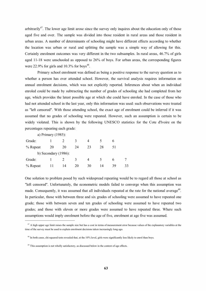
63

arbitrarily47. The lower age limit arose since the survey only inquires about the education only of those aged five and over. The sample was divided into those resident in rural areas and those resident in urban areas. A number of determinants of schooling might have different effects according to whether the location was urban or rural and splitting the sample was a simple way of allowing for this. Certainly enrolment outcomes was very different in the two subsamples. In rural areas, 46.7% of girls aged 11-18 were unschooled as opposed to 26% of boys. For urban areas, the corresponding figures were 22.9% for girls and 10.3% for boys48. Primary school enrolment was defined as being a positive response to the survey question as to whether a person has ever attended school. However, the survival analysis requires information on annual enrolment decisions, which was not explicitly reported. Inferences about when an individual enroled could be made by subtracting the number of grades of schooling she had completed from her age, which provides the latest possible age at which she could have enroled. In the case of those who had not attended school in the last year, only this information was used: such observations were treated as "left censored". With those attending school, the exact age of enrolment could be inferred if it was assumed that no grades of schooling were repeated. However, such an assumption is certain to be widely violated. This is shown by the following UNESCO statistics for the Cote d'Ivoire on the percentages repeating each grade: a) Primary (1985): Grade: 1 2 3 4 5 6 % Repeat 20 20 24 23 28 51 b) Secondary (1986): Grade: 1 2 3 4 5 6 7 % Repeat 11 14 20 30 14 39 33 One solution to problem posed by such widespread repeating would be to regard all those at school as "left censored". Unfortunately, the econometric models failed to converge when this assumption was made. Consequently, it was assumed that all individuals repeated at the rate for the national average49. In particular, those with between three and six grades of schooling were assumed to have repeated one grade; those with between seven and ten grades of schooling were assumed to have repeated two grades; and those with eleven or more grades were assumed to have repeated three. Where such assumptions would imply enrolment before the age of five, enrolment at age five was assumed. 47 A high upper age limit raises the sample size but has a cost in terms of measurement error because values of the explanatory variables at the time of the survey must be used to explain enrolment decisions taken increasingly long ago.

48 In both cases, chi-squared tests revealed that, at the 10% level, girls were significantly less likely to enrol than boys.

49 This assumption is not wholly satisfactory, as discussed below in the context of age effects.

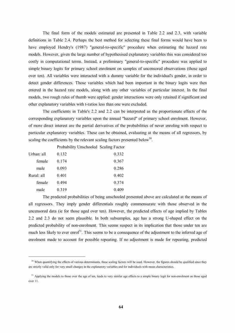
64

The final form of the models estimated are presented in Table 2.2 and 2.3, with variable definitions in Table 2.4. Perhaps the best method for selecting these final forms would have been to have employed Hendry's (1987) "general-to-specific" procedure when estimating the hazard rate models. However, given the large number of hypothesised explanatory variables this was considered too costly in computational terms. Instead, a preliminary "general-to-specific" procedure was applied to simple binary logits for primary school enrolment on samples of uncensored observations (those aged over ten). All variables were interacted with a dummy variable for the individual's gender, in order to detect gender differences. Those variables which had been important in the binary logits were then entered in the hazard rate models, along with any other variables of particular interest. In the final models, two rough rules of thumb were applied: gender interactions were only retained if significant and other explanatory variables with t-ratios less than one were excluded. The coefficients in Table's 2.2 and 2.2 can be interpreted as the proportionate effects of the corresponding explanatory variables upon the annual "hazard" of primary school enrolment. However, of more direct interest are the partial derivatives of the probabilities of never enroling with respect to particular explanatory variables. These can be obtained, evaluating at the means of all regressors, by scaling the coefficients by the relevant scaling factors presented below50. Probability Unschooled Scaling Factor Urban: all 0.132 0.332 female 0.174 0.367 male 0.093 0.286 Rural: all 0.401 0.402 female 0.494 0.374 male 0.319 0.409 The predicted probabilities of being unschooled presented above are calculated at the means of all regressors. They imply gender differentials roughly commensurate with those observed in the uncensored data (ie for those aged over ten). However, the predicted effects of age implied by Tables 2.2 and 2.3 do not seem plausible. In both subsamples, age has a strong U-shaped effect on the predicted probability of non-enrolment. This seems suspect in its implication that those under ten are much less likely to ever enrol51. This seems to be a consequence of the adjustment to the inferred age of enrolment made to account for possible repeating. If no adjustment is made for repeating, predicted

50 When quantifying the effects of various determinants, these scaling factors will be used. However, the figures should be qualified since they are strictly valid only for very small changes in the explanatory variables and for individuals with mean characteristics.

51 Applying the models to those over the age of ten, leads to very similar age effects to a simple binary logit for non-enrolment on those aged over 11.

65

non-enrolment rises markedly with age52. These problems mean that the predicted age effects should be ignored. By contrast, the estimated effects of other variables were robust to whether repeating was corrected for53. Furthermore, both with and without the correction for repeating, it appears that gender differences in enrolment have been falling overtime. This is shown by the negative signs on the female-age interaction variables. A variety of measures of parental education were experimented with. As in Glewwe (1988), a dummy variable for whether the household spoke French significantly increased the probability of primary school enrolment but only in rural areas. The effect is large, raising the probability of enrolment by 11.5 percentage points. The number of grades of schooling of a child's father also increased the probability of enrolment. For example, the effect of complete paternal schooling in urban areas on boys would be to reduce the probability of non-enrolment by 3 percentage points. In rural areas, the effect was of a similar size but insignificant. Grades of maternal schooling were rejected as wholly insignificant in rural areas, although too much emphasis should not be placed on this because of the very low levels of maternal education in such areas. In urban areas, the coefficient upon grades of maternal education was three times as large as that on grades of paternal. The only measure of parental education to have significantly different effects on boys and girls was a dummy variable for whether the father had any primary schooling54. When interacted with a dummy variable for female gender, the interaction terms were significant but the terms themselves had t-ratios less than one and so were rejected from the final forms. The interaction terms imply that having a father who received some primary schooling increases the probability of a girl also receiving some by 14 percentage points in rural areas and by 23 points in urban areas. Evaluating at the means of other variables, these changes imply that having an educated father would cause the probability of a girl being unschooled to fall from 53% to 39% in rural areas; for urban areas the corresponding drop would be from 28.6% to 9.5%. For boys, the changes are under 1 percentage point. These figures imply that gender inequalities in primary school enrolment are in large part confined to households with no adult education. It is notable that only the dummy variable for minimal parental education has significantly effects by gender, rather than measures of grades of schooling. This suggests that the effect may be more attitudinal than to do with any effects of parental education upon children's academic ability. Parents with some schooling may see the schooling of girls as more natural than those without. The effect of some parental schooling upon female enrolment is so strong, that it is worthwhile examining the raw data for corroboration. Table 2.5

52 This is contrary to the predictions of a binary logit on the uncensored data and to what is observed.

53 In particular, apart from variables involving age effects, all other variables which were significant under one assumption were significant under the other, with the same sign and similar magnitude.

54 A dummy variable for whether the mother had some primary schooling had similar gender specific effects but these were not significant.

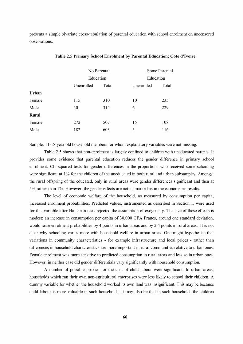
66

presents a simple bivariate cross-tabulation of parental education with school enrolment on uncensored observations.

Table 2.5 Primary School Enrolment by Parental Education; Cote d'Ivoire No Parental Some Parental Education Education Unenrolled Total Unenrolled Total

Urban Female 115 310 10 235 Male 50 314 6 229

Rural Female 272 507 15 108 Male 182 603 5 116 Sample: 11-18 year old household members for whom explanatory variables were not missing. Table 2.5 shows that non-enrolment is largely confined to children with uneducated parents. It provides some evidence that parental education reduces the gender difference in primary school enrolment. Chi-squared tests for gender differences in the proportions who received some schooling were significant at 1% for the children of the uneducated in both rural and urban subsamples. Amongst the rural offspring of the educated, only in rural areas were gender differences significant and then at 5% rather than 1%. However, the gender effects are not as marked as in the econometric results. The level of economic welfare of the household, as measured by consumption per capita, increased enrolment probabilities. Predicted values, instrumented as described in Section 1, were used for this variable after Hausman tests rejected the assumption of exogeneity. The size of these effects is modest: an increase in consumption per capita of 30,000 CFA Francs, around one standard deviation, would raise enrolment probabilities by 4 points in urban areas and by 2.4 points in rural areas. It is not clear why schooling varies more with household welfare in urban areas. One might hypothesise that variations in community characteristics - for example infrastructure and local prices - rather than differences in household characteristics are more important in rural communities relative to urban ones. Female enrolment was more sensitive to predicted consumption in rural areas and less so in urban ones. However, in neither case did gender differentials vary significantly with household consumption. A number of possible proxies for the cost of child labour were significant. In urban areas, households which ran their own non-agricultural enterprises were less likely to school their children. A dummy variable for whether the household worked its own land was insignificant. This may be because child labour is more valuable in such households. It may also be that in such households the children

67

are more likely to inherit such enterprises and hence less likely to seek formal employment for which schooling is required. In rural areas, a richer menu of proxies was available. The local wage for child agricultural labour reduced the probability of enroling in school; an increase in the wage rate of one standard deviation reducing the probability by 3 percentage points55. Boys' enrolment was adversely affected by the distance of the household to its fuelwood source. This effect was even stronger than that of child wages: a one standard deviation (of 3.2 km) increase in fuelwood distance reducing male enrolment probabilities by 5 percentage points. Other proxies for child costs - a dummy variable for whether children under the age of twelve worked in the cluster and distances to household water sources - were either insignificant or perverse. For rural areas, information on school availability and quality could be used. The presence of local primary schools when the individual was five had a powerfully positive effect on enrolment. If there was no school in the cluster when the child was five, the child would be 24 percentage points less likely to ever enrol. The variable did not interact significantly with gender. In preliminary estimates, distance to the nearest secondary school also reduced enrolment probabilities, particularly for girls but these effects were not significant. However, the variables for school quality were all insignificant or perverse. The perverse effects of the dummy variables for bad school facilities and shortage of teachers may reflect the nature of the question from which they were constructed. The relevant question asked for major schooling problems in the cluster. Other responses mentioned lack of money or problems of school availability. Hence if a respondent chose to cite poor school quality as a problem, it may indicate high demand for, and good availability of, schooling56. Consequently, some of the school quality variables may indicate omitted cluster specific factors which entail a high demand for schooling. The possibility of quality-quantity trade-offs in children was investigated using variables for numbers of elder siblings and the age of the mother, the latter being a proxy for numbers of younger and expected siblings. Interestingly, the gender composition of the elder siblings appears important. Numbers of elder brothers reduced the probability of enrolment in both urban and rural areas. Further work disaggregating older brothers into those with and without schooling suggested that only uneducated older brothers were an obstacle to enrolment57. Numbers of elder sisters actually increased 55 The wage for agricultural male labour had been included as a control so that the effect of child wages in particular could be isolated but was rejected as insignificant.

56 This explanation is somewhat weakened by the fact that respondents could cite up to four problems with schooling.

57 This evidence is suggestive only and not included in the main results because of the likely endogeneity of the schooling of elder brothers. Hence the apparent negative impact of elder brothers may be explained by household unobservables which operate against educational attainment rather that the consequences of uneducated elder brothers per se. It is hard to see how this can be investigated further without better data (for example, an identifying variable which would affect the schooling of an elder brother and not a younger one). In particular, a fixed effects logit on the uncensored sample does not seem capable of resolving the issue, because only households within which sibling enrolment differs will contribute to the likelihood function of such a model. With such a selected sample, the enrolment of elder siblings will be biased towards having a negative effect on the enrolment of younger siblings.

68

the proability of enrolment although this effect was significant only in urban areas. These effects are fairly large: an additional three older brothers would reduce the probability of enrolment by nine percentage points in rural areas and by four and a half points in urban areas. Interacting these variables with the gender of the individual whose enrolment was being modelled revealed no significant differences; girls were more sensitive to numbers of elder siblings in rural areas and less in urban areas. One might speculate that the presence of elder brothers diminishes the priority parents attach to the education of their younger children. Numbers of elder sisters may have a more benign effect because they are less likely to be enroled than elder brothers, leaving more household resources to devote to schooling and reducing the need for domestic child labour. Quadratics for the age of a child's mother at the time of the child's birth were not significant but had turning points around the age of forty. Consequently, a variable was constructed for the number of child-bearing years an individual's mother had left when the child was five. This should proxy the existence of younger siblings and indeed had powerful effects. In rural areas, a child whose mother had twenty years to go before she was forty was six percentage points more likely not to enrol as one with a mother who had reached forty. In urban areas, the corresponding change would be ten and a half points. These effects did not differ significantly by gender: preliminary estimates revealed girls were more sensitive to maternal age in urban areas but less so in rural areas. Increased numbers of adults in the household did not have widespread effects. Numbers of men disadvantaged girls in particular, although the effect was not quite significant. Various possible determinants of relative male-female bargaining power within the household were significant. In rural areas, being in a female-headed household increased the probability of enrolment; in urban areas, being in a polygamous household reduced the probability enrolment58. The share of household cash income accruing to women significantly increased the probability of boys (only) enroling59. Hausman tests rejected the assumption that the share of female income was exogenous, so predicted values were used, instrumented as previously described. The effects of the variable are fairly substantial: an increase of 15 percentage points in women's share of cash income (around one standard deviation), would raise the probability of boys enroling by five percentage points in rural areas and six points in urban areas. One could argue that female control over household decisions is greater in female headed households, less in polygamous households and rises with their contribution to household cash income. Consequently, one interpretation of the above three findings is that women have more pro-education attitudes than men and hence enrolment probabilities rise with

58 Preliminary results had shown the effect of female headed households in urban areas to be positive but insignificant, as was that of polygamous households in rural areas.

59 Earlier estimates showed that for girls in rural areas, the variable had a positive insignificant effect; for girls in urban areas it was negative and insignificant.

69

women's their control over household decision-making. That the effect of women's share of household cash income should benefit boys only accords with Haddad and Hoddinott's (1991) finding for pre-schoolers' anthropometric status which used the same dataset. Haddad and Hoddinott suggest that their finding does not necessarily imply that women have a pro-boy bias but could be explained by their greater vulnerability at a young age. The present finding could be interpreted as indicating a pro-boy bias or might possibly be connected with the opportunity cost of female labour. Households with high female contributions to cash income will tend to be one's in which women work less on domestic work and more in wage employment, on growing crops and running businesses. Consequently, girls labour may be more valuable in such households and this may offset any pro-education effects of increased female bargaining power. Some health-related variables had significant effects on schooling. In particular, in rural areas, travel time to health facilities significantly reduced the probability of enrolment60. Increasing travel time by thirty minutes (around the mean and standard deviation), reduces the probability of enrolment by seven percentage points. The effect was stronger for girls, but not significantly so. One economic interpretation of this is that there is a complementarity between child health and education. Where child health has a low cost, it is may be more rational to invest in their education. This is because child survival is likely to be greater or because healthy children are likely to benefit more from schooling. Alternatively, the effect may be spurious on account of correlations between proximity to health facilities and omitted measures of other forms of infrastructure - such as school quality. The measures of household health-related "public goods" - such as drinking water source and sanitation - do not provide further evidence of a health-education complementarity. More "developed" sources of water and sanitation increase the probability of enrolment irrespective of their consequences for health as estimated in Chapter 3. In particular, if the household uses piped or purchased water, the probability of school enrolment rises. This is despite the finding that such water tends to increase the reported incidence of ill-health. The use of pit latrines is found to be beneficial to reported health in Chapter 3. However, pit latrines only increased the probability of enrolment in rural areas (where the default is no toilet); reducing it in urban areas (where the default is a flush toilet). One interpretation is that these variables are operating as proxies for overall household economic welfare, although this should have been controlled for by the use of household consumption. The finding may also reflect an omitted variables (or endogeneity) problem: households with unobserved characteristics that entail school enrolment may also tend to acquire health-related public goods. A considerable number of variables for geographic location, ethnicity and religion affected enrolment. However, these did not generate many significant gender interactions. Children in the

60 The absence of a similar finding for urban areas does not necessarily indicate a lack of robustness. Travel times to health facilities are much lower in urban areas and in Chapter 3 are not found to affect usage.

70

Abidjan were less likely to enrol than those in urban areas. In rural areas, residence in the Savannah regions significantly reduced enrolment probabilities, although girls in the Western Forest region were also disadvantaged. Distance from the nearest paved road significantly reduced enrolment probabilities. This variable may indicate lower access to waged employment. However, as with distance to health facilities, the variable may capture many other spatially correlated effects. In both urban and rural areas, the Southern Mande and the Kru were more likely to enrol whilst non-ivorians were less likely to be enroled. Coming from a family which was neither Christian nor Muslim reduced the probability of enrolment in rural areas, but increased it in urban areas. Muslims in rural areas were less likely to enrol and Catholics in urban areas more likely.

71

3. Primary School Drop-outs; Kenya, Tanzania and the Cote d'Ivoire We analysed what determines whether children drop-out of primary school using samples of household members under the age of 19 who have received some primary schooling. For Kenya and Tanzania, only sons and daughters of the household head are included in the samples because information about parental education and numbers of siblings was available only for these children. As with primary school enrolment in the Cote d'Ivoire, we used an ordered logit model but here the dependent variable was the number of grades of primary school an individual had completed. Once again the main reason for using an ordered logit was its tractability when faced with discrete and right censored data, as explained in Appendix 1. Tables 3.1 to 3.4 give the final forms selected when estimating the ordered logit model to all three countries, separating rural and urban areas in the Cote d'Ivoire. Table 3.5 provides definitions of the variable names used in these tables. Due to the large number of explanatory variables which interact with gender in each equation, the coefficients on the gender dummies may be misleading indicators of overall gender differences in drop-outs. A better guide is provided by comparing the proportions of girls and boys predicted to drop-out. It is hard to check the accuracy of these predictions due to the pervasive right-censoring of the data - most of the samples are still in school and its unknown whether they will ultimately drop-out. However, the estimated drop-out rate for Kenya of 30% does not seem unreasonable given the University Grants Commissions estimate that 38% of those entering Standard 1 in 1980 would drop-out. In all samples, girls are predicted to be more likely to drop-out with the difference being particularly large in Kenya and urban Cote d'Ivoire. Taking the ratio of the predicted proportions, it can be seen that girls in Kenya are 31% more likely to drop-out that boys; whilst in urban Cote d'Ivoire they are 27%; elsewhere the figures are a more modest 14% in rural Cote d'Ivoire and 9% in Tanzania. As shown by the gender interaction terms, these differentials vary with a number of other determinants of drop-outs, as will be explained below61. A series of dummy variables for parental education were entered in preliminary estimates and although the same dummy variables were not always retained as significant the final results indicate that those from more educated families tended to be less likely to drop-out with a few exceptions. Specifically, in all samples except Tanzania, girls with some paternal primary schooling - either partial or complete - were less likely to drop-out. The same was also true for boys, except in rural Cote d'Ivoire. Maternal education only significantly reduced the probability of dropping out in the case of maternal secondary schooling in urban Cote d'Ivoire. Curiously, this effect was somewhat reduced if the mother managed to obtain formal employment62. In Kenya, some maternal

61 Except where stated to the contrary, explanatory variables discussed can be assumed to have t-ratios that are significant at 10%.

62 In comments, Jere Behrman suggested that this may be because the mother is able to allocate less time to the child's learning at home.

72

primary schooling increased the probability of boys dropping out, as did either parent's primary schooling in the case of girls in Tanzania. The distances children had to travel to the nearest primary and secondary schools had either no significant effect upon drop-outs or perverse effects. However, in households where the source of drinking water far away, children tended to be less likely to complete their primary schooling. This may be because in such households, child labour is more valuable and hence there are greater costs to keeping the child in school. Alternatively it may be that in such households children are called on to carry out rather onerous water collecting duties, to the detriment of their school performance, thus reducing the expected benefits of staying in school until the critical primary-leaving exam. In Chapter 4, we find that in our Kenyan sample, children at school appear to be largely exempted from such duties, so this latter effect is perhaps less plausible for that country. In Tanzania, we find no such exemption. For the Cote d'Ivoire, we have no data on who fetches water. Either way it is perhaps surprising that these effects should be marked enough for distance to nearest water supply source to significantly increase the probability of either boys or girls dropping out of primary school in all four samples. Whether boys or girls were the gender affected varied across the samples. In both Kenya and Tanzania, is was only girls who were significantly affected: for boys, distance to water sources had a positive but insignificant effect on progression through primary school. This fits well with the finding in Chapter 4 that water carrying is almost exclusively a female activity in our samples of these two countries. However, for Cote d'Ivoire, the situation is reversed, with distance to water supply having significant negative effects upon boys and positive effects upon girls (significantly perverse only in rural areas). For the Cote d'Ivoire, several other variables were available which may reflect the value of child labour to a household. In rural areas, distance to fuel wood sources also significantly increased the likelihood of drop-outs from primary school. In urban areas, households running their own businesses or working their own fields may be able to make more use of their children's time. Dummy variables for such household activities did significantly increase the likelihood of a child dropping out, although running one's own business affected boys only. In rural areas, children from households with their own non-agricultural enterprises were actually less likely to drop-out. This may be because the default in this sample would not be households whose adults worked as employees as it is in urban areas, but households undertaking purely agricultural activities. Consequently, in rural areas the difference in the value of child labour may vary less with the own business dummy variable. There are two possible explanations for why the variable is significantly positive in rural areas rather than insignificant. Firstly, it may be that households running their non-agricultural ventures are more wealthy than others in some way not controlled for. Alternatively, there may be a higher return to education for children who will inherit such ventures compared to those who are likely to continue farming. Wages for child agricultural labour in the cluster were insignificant.

73

Children from more affluent households appear less likely to drop out of primary school in urban Cote d'Ivoire, but in the rural samples this was not observed. Predicted household consumption per capita significantly reduced the probability of a child dropping out of school in urban areas, but was insignificant for children in rural Cote d'Ivoire and indeed perverse for boys63. In Kenya and Cote d'Ivoire, land holdings per capita were used to try to capture income and wealth effects, but in both countries significantly increased the probability of boys dropping out of school. In Tanzania, land per capita also increased the probability of girls dropping out of school, but the effect was significantly greater for boys. It is possible that the effect of land holdings in these two countries does not reflect perverse wealth effects but some other factors. Ceteris paribus, large amounts of land per capita will lead to a high marginal product of labour when working family land. In the absence of well functioning factor markets, this might induce parents to withdraw children from school to make use of their labour. Alternatively, it may make it more likely that children will work family land when they become adults and consequently mean that there is a lower return to investing in their education than if they were likely to seek formal sector employment. The latter interpretation could also explain why it is boys in particular whose schooling is affected by land holdings rather than girls, since it is likely that girls will leave their parents shamba when they get married. In Kenya, several of the effects of other variables could be interpreted as representing more conventional income or wealth effects. In particular, the value of livestock per capita has a positive effect on the probability of progression through primary school. Conversely, if the main occupation of the male household head is not remunerative (they are unemployed, disabled or retired), his offspring are more likely to drop-out of primary school. Finally, the further clusters are from major urban centres, the less likely are girls to complete primary schooling. This variable may capture an income effect because isolated clusters are likely to be less developed and contain less affluent households. It appears that even after controlling for per capita asset holdings, households in Kenya and Tanzania with large numbers of children are more likely to withdraw their children from primary school. This is one interpretation of the negative effect of numbers of older siblings upon the probability of completing primary school in the two countries. Interestingly, such quality-quantity effects seemed confined within each gender. That is to say, large numbers of older brothers significantly reduce the probability of boys but not girls completing primary school in both countries, whilst large numbers of older sisters do the same for girls but not boys. In fact, in both countries, increasing numbers of older brothers reduce the probability of girls dropping-out of primary school, although this effect is not quite significant. That the quantity-quality effect appears to be intra-gender only suggests that parents regard the schooling of girls and boys are separate goods, allocating a certain amount of resources to each. However, such effects were not observed in Cote d'Ivoire. In rural Cote d'Ivoire, only

63 See Section 2 of Chapter 3 for details of the construction of this variable.

74

numbers of older sisters significantly increased the probability of children dropping out, and this effect held for both male and female children. Possible numbers of future children, as proxied by the number of years the mother had left until she is forty when the child was five, were generally not significant. The exception was in rural Cote d'Ivoire, where increased likelihood of future siblings raised the probability of girls but not boys dropping out. In Kenya, the variable also had a significantly different effect according to the gender of the child, but was not quite significant in its adverse effects upon girls. For Cote d'Ivoire, the predicted share of women's household cash income was available as a regressor. In line with the arguments in Part 3, it may be that women's bargaining power rises with this variable. This would be important if women attach different priorities to education than do men. The variable had opposite effects in rural clusters to those it had in urban areas. In the former, it significantly increased the probability of a child dropping out; in the latter it reduced it, but significantly so only in the case of boys. These opposing effects may reflect differences in preferences between rural and urban samples. Alternatively, they may be connected with the different composition of women's cash income in the two types of area. When compared to urban areas, a larger proportion of women's cash income in rural areas comes from own-farm production of certain food crops, and a smaller proportion is in the form of wage earnings. Interestingly, high wages for female agricultural labour raise the probability of a child completing primary school in rural Cote d'Ivoire, whilst male wages are insignificant. Hence, it may be that this wage variable is proxying women's bargaining power whilst the predicted share of women's cash income reflects other household characteristics such as being skewed into lower return crops (for example, income from coffee and cocoa is defined as "men's income"). Household type - polygamous, female-headed or other - had some significant effects upon drop-outs. Children in rural Cote d'Ivoire from polygamous households were less likely to drop-out, as were boys in Tanzania. However, in Kenya residence in polygamous households increased the probability of drop-outs. Conversely, children from female-headed households in Kenya were less likely to drop-out. Finally, ceteris paribus, boys from Muslim homes were less likely to drop out and girls more likely, although the latter effect was not quite significant.

75

4. Secondary School Enrolment; Cote d'Ivoire

a. Exam Performance: Analysis of the 1986 Survey A logit for the determinants of passing the CEPE was estimated over a sample of is given in Table 4.1. Table 4.2 gives the effects of the explanatory variables on the probability of passing the CEPE evaluated at the mean of the other variables64. Gender specific effects of the hypothesised explanatory variables were investigated by estimating models separately on the subsamples of girls and boys. A likelihood ratio test for whether the two subsamples should be combined gave a statistic of 22.26, rejecting the restriction that the coefficients of all the explanatory variables were the same for both sexes at 5% significance with 13 degrees of freedom65. T-tests of equality of coefficients between the two subsamples revealed significant differences at 5% for the variables AREAPC, KIDWAGE and WATERDIST; hence gender interactions on these terms are used in the final model estimated over the full sample, as presented in Table 4.1. Although individual terms of the consumption per capita cubic were not significantly different, it was evident that the overall effect was markedly different by gender. Where variables were not significant alongside their interaction terms they were excluded from the final model. Given the non-random nature of the sample - including only primary school leavers - it was important to investigate sample selection issues: for example, since fewer girls were observed in the sample, did they come from significantly more affluent families? Hence tests were carried out to see if there were significant differences in the means of the explanatory variables used in the final regression66. At 10% significance, the girls in the sample had higher mean values of all three parental education variables, of the dummy variable for having an older sister with the CEPE and a lower mean value of house area per occupant. To what extent these gender differences in the coefficients and means values of the explanatory variables can account for the observed gender differential in exam performance will be considered below. The results in Table 4.1 suggest that gender differentials in exam performance are powerfully related to a household's economic status and that, other things being equal, girls from fairly affluent families will perform roughly as well as boys. Three alternative flows were entered as measures of a

64The gender differentials in Table 4.2 are less marked than might be expected from the observed differential, but this is because - as will be explained - most of the gender differential arises amongst households with low rates of consumption.

65The model estimated for each sex used the explanatory variables presented in Table 4.1, although gender interaction terms were replaced by the term with which gender was interacting, unless this term was already present, and the female dummy was dropped. It was then tested whether these models could be restricted to one estimated over the whole sample with the same list of determinants plus the female dummy.

66T-tests for differences in sample means were carried out for continuous variables and chi-squared tests used for dichotomous ones.

76

household's economic position: consumption per capita, income per capita and food consumption per capita. When estimated on the subsample of boys, likelihood ratio tests did not reject the hypothesis that all three measures had no effect at 5% significance, whether entered jointly or individually67. For girls, each of the flows appeared to have significant but non-monotonic effects. Cubic terms for consumption of food and non-food per capita were then entered and a likelihood ratio test then did not reject the hypothesis that the income cubic had no effect at 5% significance. Both food consumption and non-food consumption had non-monotonic effects for girls; with local maxima at around 10,000 CFAF pc pa and 45,000 pc pa respectively68. In Table 4.1, the two kinds of consumption per capita have been aggregated for ease of interpretation and entered only as interactions on the FEMALE dummy due to the insignificance of their effect on boys. Figure 4 plots the effects of total consumption per capita on the probability of girls passing the exam predicted by the model in Table 4.1, evaluating at the means of the other regressors. As can be seen, the effect of improvements in households economic position upon the gender differential in exam performance are marked: at the lowest observed rate of consumption in the sample, 30,449 CFAF pc pa, girls are predicted to have only a 36% chance of ever passing the CEPE whilst at the mean rate of consumption they have a 76% chance, higher than that for boys. Although the effects of consumption per capita upon girl's performance are non-monotonic, the perverse effects for relatively well to do families - consuming over around 500,000 CFAF pc pa - do not account for much of the observed gender differential since few girls, only 14% of those in the sample, come from such affluent backgrounds. One measure of the contribution of these perverse consumption effects can be obtained by calculating the pass rates for the sample predicted by the model if observations from households with consumption flows in the range where these effects arise came instead from households with flows below this range. Hence, consumption values in the sample of more than 500,000 CFAF pc pa were replaced with 500,000. The model in Table 4.1 was then used to calculate the expected pass rates of boys and girls in the sample, after their consumption values had been adjusted in this way. This exercise generated an absolute gender differential in the proportions predicted to pass the CEPE of 12.4%. Hence, these perverse consumption effects account for only around 1.4 points of the observed 13.7 percentage point differential. However, it is also not the case that most of the differential arises due to the poor performance of girls from "poor" backgrounds. Replacing sample values of consumption per capita below the lower quartile value, 119,086 CFAF pc pa, with that value yields a predicted absolute gender differential of 12.3%. A corresponding simulation for values below the median of 197,576 CFAF pc pa gives a figure of 8.4% whilst one for below mean almost lowers the differential to a mere 3.4%. These results suggest gender differentials in exam

67These was true both when the flows were entered in linear form and when they were entered as cubics.

68Adult equivalence scales used by the Ghanian Ministry of Health and Nutrition, were used in other estimates (not reported) to generate consumption per adult equivalent variables to replace the per capita measures but the non-monotonicities remained.

77

performance would be almost entirely eliminated by increases in household consumption but the increases would have to be substantial, to around mean levels. The exact mechanism(s) by which household consumption affects exam performance is not revealed by these results and could take any of the forms suggested above. The fact that both food and non-food expenditures were significant suggests that the effects may be partly nutritional but are not entirely so. Measures of various components of the physical assets of a household were entered in preliminary estimates, although only two were retained as significant; namely, the area of the house per occupant and a dummy variable for relying primarily on gas (or electric) for fuel69. The possession of gas heating was selected as possible indicator of relatively wealthy families and has sizable effects, raising the probability of a girl with otherwise average characteristics obtaining the CEPE by a quarter. It may also proxy lower demands on children's time, with no requirement for wood collecting in gas heated households. Interestingly, housing area per occupant only affected girls' exam performance. This may just reflect the fact that - as with consumption - "income/wealth" effects on academic performance seem stronger for girls. However, it may also be that area per occupant has a direct effect beyond merely proxying wealth. In particular, girls may suffer more from overcrowding - perhaps because they are more likely to be assigned "crowd control" duties. These effects are fairly large: evaluating at the mean probability, an increase of one standard deviation in area per capita would increase the probability of a girl passing the CEPE by approximately 9.3 percentage points70. The predictions about parental education enhancing exam performance are to some extent supported. Various measures of paternal education were entered in preliminary estimates but only dummy variables for some schooling were retained, the rest being rejected due to low significance71. As Table 4.2 shows, if either parent has received some schooling, a child's chances in the CEPE are sizably improved: the probability increasing by around a half in the case of paternal education and by around three quarters in the case of maternal education. However, the coefficient for maternal education is insignificant, possibly due to its collinearity with the interaction term for whether both parents have received some schooling and this latter term is perverse in that its negative effects are so large they imply that having neither parent educated is better for exam performance than having both educated. There is no evidence of the suggested gender specific effects of parental education, with none of the relevant the coefficients being significantly different when estimated separately for each gender.

69Those rejected in initial estimates were: the per capita values of production assets and livestock, land acreage used for farming per capita, rooms per occupant, and dummy variables for: home ownership, brick walls, flush toilets, indoor taps and electric lighting.

70This calculation used the approximation, βk.p.(1-p)._Xk, for the effect on the probability, p, predicted by the logit of a small change, _Xk, in an explanatory variable with coefficient, βk.

71Those rejected were three pairs of dummy variables - one for each of the parents: possessing the CEPE; completing primary schooling; and obtaining some secondary schooling.

78

Indeed, in these separate estimates, maternal rather than paternal education has the larger coefficient in the boys' equation whereas the reverse is true for girls. Given that the proportions of girls in the sample with educated parents are significantly higher than the proportions of boys, it is interesting to see what the consequences of this for the overall gender differential in exam performance are. Unfortunately simulating the effects of different distributions of the explanatory variables across genders is problematic: here we calculate the effect evaluated at the mean probability of a change in the values of the parental education dummies from the proportion for girls in the sample to that for boys. In the case of the dummy variable for some paternal schooling, such a change would lower the probability of girls passing the exam by 2 percentage points; for some maternal education the change would be minus 1.5 percentage points; and for the interaction term, the effect would be positive at 2.2%. Hence, the overall sample selection effect of female primary school leavers having on average more educated parents than their male peers girls is - as might be expected - to somewhat offset the tendency for girls to be less likely, ceteris paribus, to attain the CEPE. An attempt was made to test Grisay's hypothesis about French as medium of instruction disadvantaging girls. The surveys recorded whether the interview was recorded in French and so a dummy variable for the response to this question was used as a proxy for the presence of French speaking adults in the household. According to Grisay's argument this variable should positively influence the probability of exam success but, since this effect should be greater for boys, its interaction with the FEMALE dummy should be negative. In fact, when added to the regressors listed in Table 4.1, both terms were insignificant with the opposite signs to those predicted. Nought-one dummy variables for whether an older brother or sister had passed the CEPE were also entered in preliminary estimates, together with corresponding interaction terms with the FEMALE variable. When all four terms were entered jointly, only the interaction between the FEMALE dummy and the dummy variable for having an elder sister who had passed the exam had a t-ratio greater than one; the others had very small coefficients and t-ratios. The likelihood ratio test statistic for excluding the three highly insignificant terms was 0.2, not rejecting the hypothesis that they jointly had no effect. However, it appears from Table 4.2 that girls have their chances of attaining the exam substantially improved by having older sisters who themselves passed the exam; at the mean of other variables, the effect is to raise the probability of passing by 10 percentage points. One interpretation of this effect is that it merely reflects household "fixed effects": unobserved characteristics of households which enhance the exam performance of girls within them. Alternatively, it may reflect older sisters providing "role models" for girls and increasing their motivation. Since more older males are educated than older females, boys will have more educated role models of the same gender than girls and hence may be less influenced by their elder siblings. Furthermore, positive role models may be more important for girls because of the social attitudes described by Grisay which inhibit their academic performance. Various proxies for the opportunity cost of child labour in a household were entered in

79

preliminary estimates, two of which were retained in the final model. The community questionnaire reported agricultural wages for children in rural clusters and this was entered as a proxy for the opportunity cost of child labour together with an interaction with the FEMALE dummy; the variable being set to zero for those in urban clusters. Interestingly, the term had the predicted negative and significant effect but the interaction term had an almost exactly offsetting effect. After the interaction term was respecified to interact with a dummy for being male, the wage variable itself became wholly insignificant and was rejected from the analysis. That the effect is confined to boys would make sense if paid agricultural labour is an activity in which girls do not engage. The effect is very large: evaluating at the mean of other regressors, the probability of a boy in an urban cluster - where the wage is assumed zero - passing is 84%; at the sample mean wage (478 CFAF per day) for those in rural areas the probability is 69% and in the cluster with the highest wage (1,500 CFAF per day), the probability would be a mere 25%. The other significant proxy for the value of child labour is the distance of the house to its water supply, since water fetching may be an activity children perform within the household. The variable itself is perverse in being significantly positive. However, the interaction with the FEMALE dummy has a significant negative coefficient that outweighs the coefficient of the variable itself. This provides some support for the notion that the inferior exam performance of girls is partly attributable to them being more likely to be called upon to carry out domestic work such as water fetching. Evaluating at the mean probability, an increase in the distance of a household's water supply from the house equal to one standard deviation lowers the probability of a girl passing the exam by 5.5 percentage points. Various other proxies for opportunity cost of child labour were rejected due to low significance in preliminary estimates. Although it was thought that households which worked on their own fields or ran their own businesses might be able to make better use of child labour, dummy variables for each of these household activities were insignificant. One possible duty that children may perform is collecting wood for fuel, but distance to the household fuel source was also rejected as insignificant. The dummy variable for non-ivorian nationality has a significant effect on exam chances: as Table 4.2 shows that, controlling for other observed characteristics at their mean values, children of non-Ivorians are only around two-thirds as likely to pass the CEPE as Ivorians. Sixteen girls in the sample are non-Ivorians, as opposed to fourteen boys, and this difference - which is significant on a chi-squared test at 10.9% - accounts for a small part of the overall differential in exam success rates. In particular, evaluating at the mean probability of girls passing the exam, changing the value of the nonivorian dummy from its mean for girls to its mean for boys leads to a 1 percentage point rise in the probability of obtaining the CEPE, compared with the observed difference of 14 percentage points in the proportions of boys and girls passing. Other variables were entered in preliminary estimates to control for other factors but rejected due to low significance. Given that the sample is selected across a range of ages but conditional upon

80

completing primary school, age effects may reflect both how young a person was when she sat the exam as well as changes in the difficulty of the exam overtime. To control for unobserved geographical effects, regional dummy variables were used. The proportion of others in the sample in each cluster who passed the CEPE was used to control for cluster specific effects such as local primary school quality. Dummy variables for parental occupation were entered on the hypothesis that those with parents in wage employment may be more likely to seek such work and hence be more motivated to attain the academic credentials which may be required. However, the variables for private parental employment and paternal government employment had negative signs, possibly reflecting a sample selection effect, whilst that for maternal government employment was positive but with a t-ratio less than one.

81

b. Exam Performance: Analysis of the 1985-86 and 1986-87 Panels The above section analysed whether those aged 12-18 in the 1986 survey who had completed primary school passed the CEPE. This one-shot picture is limited because we only observe the characteristics of individuals after they have sat the exam, when what is really of interest in explaining exam performance is their characteristics prior to the exam. Observed current values may be reasonable proxies for those at the time of the exam since the time elapsed is likely to be relatively short (at most six years). However, given the panel feature of the three available CILS surveys it is worth trying to relate what we observe about primary school students to their subsequent exam results. Half of the 1986 CILSS sample was surveyed before in 1985 whilst the other half is surveyed again in 1987. Hence we model whether those surveyed in both 1985 and 1986 acquired the CEPE in those years and whether likewise for those in both the 1986 and 1987 surveys. We pool the two samples to increase sample size72. This exercise allows data on inputs - both time and money - to primary schooling to be used as explanatory variables of subsequent academic success. Using any one survey alone we have no information on expenditures or time allocation prior to the time diplomas were attained. However, there are drawbacks when compared with the earlier procedures. Most notably, it involves working with a much smaller sample size. Moreover, in contrast to the larger sample and the true national picture, girls in the sample used here do not perform worse than boys. 43 out of the 67 females in the final sample pass the exam, which is proportionately more than the 51 out of 84 males who do likewise. Furthermore, performance in any one year may not be the only factor behind differential exam success due to the possibility of different rates of exam resits. Defining the appropriate sample was problematic. We wish to identify those who either acquired a CEPE pass for the first time between two surveys or who tried unsuccessfully to acquire a pass. However, all we observe besides an individual's qualifications is the highest grade of schooling completed in the two years. The CEPE exam is sat in the last grade of primary school, CM2. Hence, in the absence of repeating, our sample should be those who were at school in the base year with the penultimate grade, CM1, as the highest grade attained and then had completed CM2 by the next. The existence of repeaters creates problems of sample definition since it is unclear whether they would be reported as having completed the grade they are currently repeating or the grade below it. We assume the former response and include those pupils who report CM2 as their highest grade completed in the base year. 53 of our sample of 151 people fall into this category. There is a risk that these individuals are actually in the first year of secondary school but this possibility seems slight for two reasons.

72For ease of exposition we refer to the year in which no one in the sample from one panel has the CEPE as the base year and to the subsequent year as the end year. Hence the base year for those in the 1985-86 panel is 1985; for the 1986-87 panel it is 1986 etc.

82

Firstly, we have excluded those with the CEPE in base year and most secondary school students possess this qualification. Secondly, of the 53, 27 are from rural clusters and hence data from the accompanying community questionnaires on the distance from the cluster to the nearest secondary school can be compared with the household survey data on the distance from the individual's home to the school attended in base year. In all cases, the distance to the school attended is less than that to the nearest secondary school, supporting the assumption that the individuals are repeating their final year of primary school. In preliminary work, exam success was modelled using the same determinants as those used in Table 4.1 with several additions73. These were only available due to the observation of exam candidates prior to the exam. Two of the additional variables measured educational inputs: specifically the hours an individual spent at school in the last week and the money that was spent on their education in the previous year. A number of individuals reported to be attending school spent no time in school in the previous week. It is possible that these individuals were on holiday or sick, and hence that the hours observed were atypical. Hours at school were not reported by those at school but not living at home. For the analysis, hours spent at school by individuals who reported zero or missing values were set to the mean for the rest of the sample74. Educational expenditures consisted of seven categories: contributions to parents' associations; uniforms; books; transport to school; board and lodging; fees; and miscellaneous75. Our sample includes a number of individuals who have completed the final grade of primary school, CM2, in the base year without having acquired the CEPE. The probability of such repeaters acquiring the exam by the end year may differ from that of first time candidates for two reasons. First, they are likely to be less able, being a subset of the previous year's CEPE failures. Against this, repeaters have had the benefits of an extra year's tuition and the experience of sitting the exam before. Distance to primary school was entered as an explanatory variable, since travelling large distances may be deleterious to primary school performance. Against this, distance may also proxy school quality, with parents only being prepared to send their children long distances to a school if it is better than those nearby. Dummy variables for secular and religious primary schools were rejected as insignificant in preliminary estimates. Table 4.3 presents the results of the final form of our model of CEPE acquisitions. Despite beginning with those explanatory variables presented in Table 4.1, most were insignificant in this

73All explanatory variables took the values observed in the relevant base year.

74Excluding individuals with zero or miming values for time spent at school in the last week was attempted but rejected as unsatisfactory. Estimating the model without these individuals, the educational input variables were significant and had the expected signs, but other dummy variables had implausibly large coefficients. This is probably because the sample size, 79 individuals, was too small.

75Where 1985 was the base year, this and other explanatory variables with monetary measures were converted to 1986 values using the IFS CPI.

83

sample. In particular, the only two effects which remain significant here are the adverse effects of high agricultural wages upon boys' exam performance and the perversely beneficial effects - again for boys only - of distance to a water source. Furthermore, a number of regressors found insignificant in Table 4.1 were significant here. This lack of robustness is worrying. However, the two variables of most interest - the measures of educational inputs were significant at 10% with the predicted signs. Evaluating at the mean probability, an extra hour in school a week increases the chances of passing the exam by 1 percentage point. Increasing expenditures on a child's education by one standard deviation (3,634 CFAF), raises the probability of exam success by 14 percentage points. Disaggregating these expenditures into their six categories did not reveal any one category to be driving the result. These results imply that one possible explanation of why girls do less well in the CEPE could be that less is spent on their education. Similarly, hours at school was found to significantly enhance exam performance and hence gender differences in time allocation may also account for girls' poorer performance. Tables 4.4 and 4.5 present the relevant descriptive statistics using two samples. One consists of those in the two grades of primary school who have not attained the CEPE, because this is the sample used for the model in Table 4.3 consists of those in this position in the base year. The other is more general, consisting of all those in school who have completed CM2 (the last grade of primary) or fewer grades. In both samples, female primary school students have more spent on their education. This may be due to a sample selection effect: fewer girls enrol in primary school and tend to come from more affluent households. Consequently, the tables disaggregate according to quartiles for household per capita consumption. This disaggregation is particularly interesting given the finding in the previous section that gender differences in exam performance fall with household consumption per capita. One explanation of this finding would be that in poorer households educational expenditures are more unequally divided by gender: that is to say spending upon female schooling is a luxury good. This explanation is supported by Table 4.4: although female primary school students on average have more spent upon their schooling than male students, the reverse is true for those from households in the poorest per capita consumption quartile. However, even in this quartile, the difference in the means is rather slight and it appears that the real reason why gender inequalities in exam performance vary with consumption may be not so much that poor households are reluctant to allocate cash to girls' schooling but rather that they are reluctant to allocate time to it. Instead of allowing girls to study unhindered, poor households may need them to work on domestic chores or family enterprises. Social convention or other factors may protect boys from having to carry out such duties. Domestic work obligations may hinder school performance by causing fatigue in class or reducing time spend studying at home. These effects cannot be investigated using the survey. However, Table 4.5 suggests that such obligations may be sufficiently onerous as to actually reduce time spent in the class. Amongst both all primary students and those just in the final grade, girls spend significantly less time in school on average. Yet what is particularly interesting is that these gender differences in time allocation are significant only amongst

84

the poorest. Female primary school students from the poorest 25% of households spent an average of four hours less in school in the week prior to the survey than did their male counterparts. Amongst those in the final grade, the difference was an even more substantial eight hours. Given the coefficient upon hours spent in school in Table 4.3, this difference alone would imply an 8 percentage point difference in the chances of girls from such backgrounds passing the exam compared to boys. Consequently, the results in this and the previous section strongly suggest that a major cause of girls' inferior exam performance in the Cote d'Ivoire is that, particularly in less affluent households, they face greater domestic work burdens. Of the other two regressors that are only available due to the panel aspect of the surveys, the dummy variable for repeating implies that the sample selection effect of this variable far outweighs any benefits from greater experience it might capture. At the means of other regressors, repeaters have a 46% chance of failure compared with the 15% risk for first time candidates. Distance to primary school has a significant positive effect, presumably proxying primary school quality rather than the actual effect of distance per se. Amongst the variables included here but rejected as insignificant from Table 4.1 were two measures of household asset and two measures of the opportunity costs of child labour. The former pair are the monetary value of productive assets per capita and a dummy variable for those living in houses with tiled floors. Individuals with more productive assets are more likely to pass the exam, although the quadratic form of this term implies this effect diminishes. The negative effect of the living in a house with tiled floors appears perverse given that the mean income per capita of those in the sample with such a housing characteristic is significantly higher than that for those without. The two significant proxies for households where child labour may be particularly valuable were a dummy variable for those running their own non-agricultural enterprises and the distance to the household's supply of fuel wood, which children may be required to fetch. At the means of other variables, candidates from households running their own businesses have a 61% chance of passing the exam, compared with the 83% chance of others. However, it should be noted that this variable also acts almost as an intercept for the productive assets per capita quadratic since such assets are confined largely to households with their own businesses; only 17% of those in the sample coming from households without their own businesses have positive productive assets. Furthermore, taking account of the mean level of productive assets (15,698 CFAF per capita) of a household with its own business implies that such a background does little to harm academic performance: causing a mere 3 percentage point fall in the probability of passing the CEPE at the mean probability. The interacting effect of productive assets and running a family business seems consistent with the argument that children from households where their labour is valuable may do less well at school. Specifically households with their own enterprises but little productive capital may have to rely more on child labour and it is children from these households which the model predicts are particularly likely to fail the CEPE. Children from households located far from

85

fuel sources are also at a marked disadvantage in the exam. Evaluating at the mean probability, the model predicts that an increase of one standard deviation, 2.7 km, in the distance to the wood used by the household for fuel reduces the probability of passing the exam by 26 percentage points. The two other significant regressors in Table 4.3 are dummy variables for residence in Abidjan and for having a father in government employment. At the means of the other variables, residing in Abidjan reduces the probability of passing the exam from 83% to 46% whilst having a government employee as a father raises it from 72% to 92%.

86

c. Enrolment Conditional Upon Exam Performance So far we have focused upon why less girls pass the primary-leaving exam. Passing this exam is a crucial first step in gaining admittance to a secondary school, as illustrated by Table 4.6 which shows that almost all those with some secondary schooling have first past the exam. In the case of state secondary schooling this is because access is rationed by performance in this exam. Although some people in our survey appear to have gained admission to state secondary schools without having passed the CEPE, these are probably reporting errors, rare exceptions to entry procedures or admissions to less academically demanding technical or vocational schools. Why so few unsuccessful candidates should enter private secondary schools is unclear given the fairly large size of the Ivorian private secondary school sector. Since the returns to schooling are likely to be complementary with ability, it may simply be that households see little return in investing large sums of money in further education of below average ability children. Alternatively, private schools may also ration access by exam grades. Such rationing may make economic sense if less able students have negative external effects on the education of their peers or if parents - unable to observe the ability mix of a school's intake - measure a school's quality by the average performance of its students. Whatever the reason, the low numbers of CEPE failures enroling in either kind of secondary school, meant it was likely to be unrewarding trying to model what characterises such children. Instead, we analysed enrolment into secondary school using a sample containing only successful CEPE candidates. Given that anecdotal evidence suggests that most private school students, although they may have the CEPE, have not received sufficiently high marks in the exam to be eligible to enter state secondary school, the appropriate framework for modelling secondary school enrolment would be a mixture model of the kind applied in the next section to Kenya. However, attempts to estimate such a model were unsuccessful, with a failure to converge to stable parameter values. Consequently we estimated a simple multinominal logit model for whether a child enroled into a state secondary school, a private secondary school or no secondary school at all. This would have a microeconomic foundation if we assume that successful CEPE candidates enrolment is a matter purely of choice for them or their household. Under such assumption, the two latent variables whose determinants are estimated in the logit model - one for enrolment into state secondary school and the other for enrolment into private secondary school - could be interpreted as the indirect utility functions from choosing these outcomes differenced from the indirect utility function from choosing not to go to school. However, it seems more likely that entrants to private school did not choose these schools in preference to government schools but instead failed to obtain sufficiently good grades to be eligible to enter the state sector. Consequently, both sets of latent variables estimated are likely to reflect the sort of factors affecting exam performance considered earlier as well as demand side considerations.

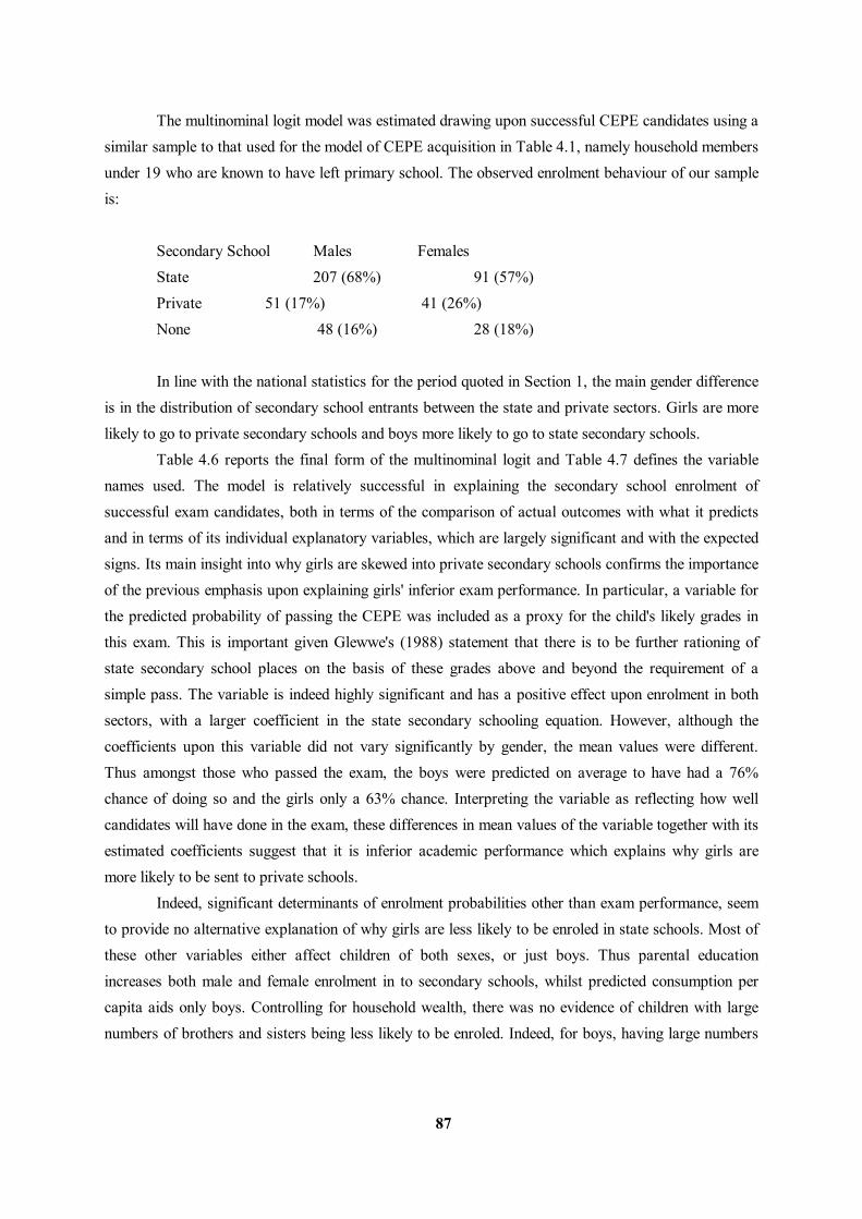
87

The multinominal logit model was estimated drawing upon successful CEPE candidates using a similar sample to that used for the model of CEPE acquisition in Table 4.1, namely household members under 19 who are known to have left primary school. The observed enrolment behaviour of our sample is: Secondary School Males Females State 207 (68%) 91 (57%) Private 51 (17%) 41 (26%) None 48 (16%) 28 (18%) In line with the national statistics for the period quoted in Section 1, the main gender difference is in the distribution of secondary school entrants between the state and private sectors. Girls are more likely to go to private secondary schools and boys more likely to go to state secondary schools. Table 4.6 reports the final form of the multinominal logit and Table 4.7 defines the variable names used. The model is relatively successful in explaining the secondary school enrolment of successful exam candidates, both in terms of the comparison of actual outcomes with what it predicts and in terms of its individual explanatory variables, which are largely significant and with the expected signs. Its main insight into why girls are skewed into private secondary schools confirms the importance of the previous emphasis upon explaining girls' inferior exam performance. In particular, a variable for the predicted probability of passing the CEPE was included as a proxy for the child's likely grades in this exam. This is important given Glewwe's (1988) statement that there is to be further rationing of state secondary school places on the basis of these grades above and beyond the requirement of a simple pass. The variable is indeed highly significant and has a positive effect upon enrolment in both sectors, with a larger coefficient in the state secondary schooling equation. However, although the coefficients upon this variable did not vary significantly by gender, the mean values were different. Thus amongst those who passed the exam, the boys were predicted on average to have had a 76% chance of doing so and the girls only a 63% chance. Interpreting the variable as reflecting how well candidates will have done in the exam, these differences in mean values of the variable together with its estimated coefficients suggest that it is inferior academic performance which explains why girls are more likely to be sent to private schools. Indeed, significant determinants of enrolment probabilities other than exam performance, seem to provide no alternative explanation of why girls are less likely to be enroled in state schools. Most of these other variables either affect children of both sexes, or just boys. Thus parental education increases both male and female enrolment in to secondary schools, whilst predicted consumption per capita aids only boys. Controlling for household wealth, there was no evidence of children with large numbers of brothers and sisters being less likely to be enroled. Indeed, for boys, having large numbers

88

of elder brothers increased the chances of being sent to state secondary schools. Numbers of older sisters and the childbearing years of the mother when the child was five, a proxy for younger siblings, were all rejected as insignificant. According to Appleton et al's (1990) study of labour market participation using the same data set, having a father in paid employment makes one more likely to obtain such employment oneself. Here, such paternal occupation increases the probability of enrolment, significantly so in the case of state schools. User costs of secondary schools, as proxied by the distance of the nearest secondary school, were rejected as insignificant, with perverse effects in preliminary estimates. Some proxies for the value of child labour to the household were significant, although not always with the predicted signs. High cluster wages for child agricultural labour adversely affect girls' chances of enrolment - although the effects were not quite significant - whilst aiding boys'. As with drop-outs from primary school, distance to household drinking water sources significantly reduced boys' chances of going to school but not girls. Distance to fuel wood had perverse effects upon girls' enrolment probabilities. Given that the sample used was three-fifths urban - in part because most secondary schools are cited in such areas - it is likely that, ceteris paribus, households running their own non-agricultural business may value child labour more and education less. In fact such an effect exists only for girls' enrolment into state schools, and works in the opposite direction for boys enrolment. Children from polygamous households had significantly different enrolment probabilities to others. Boys from such households were more likely to be sent to state secondary schools, whilst girls from this background were less likely to be privately enroled.

89

5. Secondary School Enrolment; Kenya

a. A Mixture Model We focus on what determines whether an individual in rural Kenya who has completed primary school then goes on to secondary school. The secondary school system in rural Kenya consists of a subsidised public sector with access rationed by examination and a relatively low quality private sector which is demand determined. Specifically, a pass in the Certificate of Primary Education, CPE, is required for eligibility for entry into a state secondary school. Consequently, a complete analysis of the microeconomic determinants of who enters secondary school should focus first on explaining the determinants of success in the CPE and then on explaining parental choice conditional on the outcome of the exam. Unfortunately, the outcomes of the CPE are not recorded in the survey data used here: all that is known is whether individuals went to secondary school and, if they did, what type of school it was. Nonetheless, we present a model which attempts to estimate the determinants of success in the CPE. This is desirable due to the importance for policy of distinguishing between those factors affecting access to state secondary schooling which are demand factors and those which reflect the rationing process. The determinants of exam success can be inferred from the data since those who entered state secondary schools presumably passed the exam. Strictly speaking, it is unknown whether those who went to Harambee school passed or failed the exam, but in order to aid interpretation of the model, it was assumed that they all failed. This is a strong assumption, as clearly successful CPE candidates have the option of going to a private school: however, in practice, this option is seldom likely to be exercised since commentators (eg. Court and Kinyanjui (1980)) agree that in rural Kenya Harambee schools are both more expensive than state secondary schools and of lower quality. Having made this assumption, the only ambiguity that remains is whether those that did not go to secondary school passed or failed the exam. However, since we have partial observability of exam success - namely this information can be inferred for those that enter secondary school - we can devise a mixture model of entry to secondary school that estimates both the determinants of exam performance and of the demand for schooling conditional on this performance. Three decisions are captured in the model: (1)the decision of the educational authorities as to who is qualified to enter state secondary school ("the

examiner's decision") (2)the decision of those who are qualified to enter state secondary school on whether to go or not to go

to secondary school at all (we are assuming they would not choose to go to a Harambee school) (3)the decision of those who are not qualified to enter a state secondary school on whether to enroll in a

private secondary school.

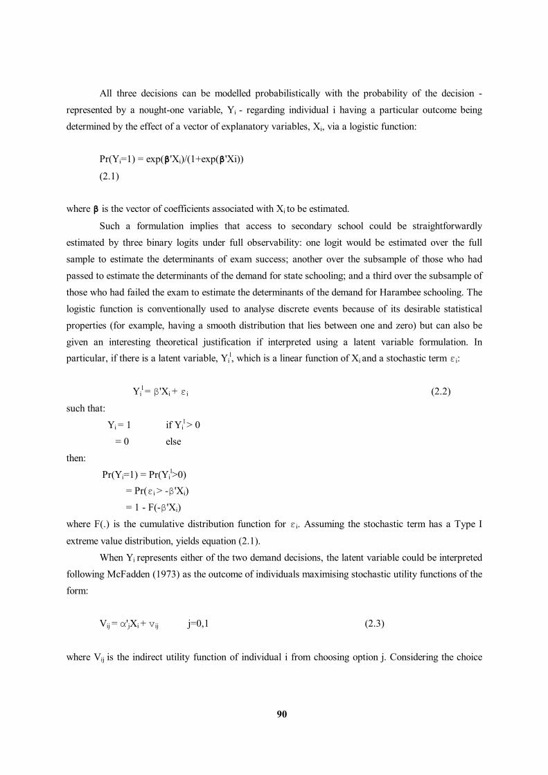
90

All three decisions can be modelled probabilistically with the probability of the decision - represented by a nought-one variable, Yi - regarding individual i having a particular outcome being determined by the effect of a vector of explanatory variables, Xi, via a logistic function: Pr(Yi=1) = exp(β'Xi)/(1+exp(β'Xi))

(2.1) where β is the vector of coefficients associated with Xi to be estimated.

Such a formulation implies that access to secondary school could be straightforwardly estimated by three binary logits under full observability: one logit would be estimated over the full sample to estimate the determinants of exam success; another over the subsample of those who had passed to estimate the determinants of the demand for state schooling; and a third over the subsample of those who had failed the exam to estimate the determinants of the demand for Harambee schooling. The logistic function is conventionally used to analyse discrete events because of its desirable statistical properties (for example, having a smooth distribution that lies between one and zero) but can also be given an interesting theoretical justification if interpreted using a latent variable formulation. In particular, if there is a latent variable, Yi

l, which is a linear function of Xi and a stochastic term εi:

Yi

l = β'Xi + εi (2.2)

such that: Yi = 1 if Yi

l > 0 = 0 else then: Pr(Yi=1) = Pr(Yi

l>0) = Pr(εi > -β'Xi) = 1 - F(-β'Xi) where F(.) is the cumulative distribution function for εi. Assuming the stochastic term has a Type I

extreme value distribution, yields equation (2.1). When Yi represents either of the two demand decisions, the latent variable could be interpreted following McFadden (1973) as the outcome of individuals maximising stochastic utility functions of the form: Vij = α'jXi + vij j=0,1 (2.3)

where Vij is the indirect utility function of individual i from choosing option j. Considering the choice

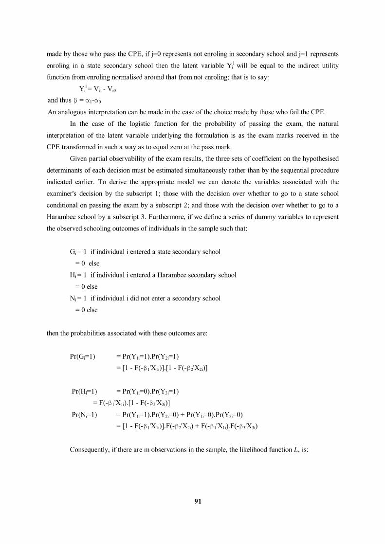
91

made by those who pass the CPE, if j=0 represents not enroling in secondary school and j=1 represents enroling in a state secondary school then the latent variable Yi

l will be equal to the indirect utility function from enroling normalised around that from not enroling; that is to say: Yi

l = Vi1 - Vi0

and thus β = α1-α0

An analogous interpretation can be made in the case of the choice made by those who fail the CPE. In the case of the logistic function for the probability of passing the exam, the natural interpretation of the latent variable underlying the formulation is as the exam marks received in the CPE transformed in such a way as to equal zero at the pass mark. Given partial observability of the exam results, the three sets of coefficient on the hypothesised determinants of each decision must be estimated simultaneously rather than by the sequential procedure indicated earlier. To derive the appropriate model we can denote the variables associated with the examiner's decision by the subscript 1; those with the decision over whether to go to a state school conditional on passing the exam by a subscript 2; and those with the decision over whether to go to a Harambee school by a subscript 3. Furthermore, if we define a series of dummy variables to represent the observed schooling outcomes of individuals in the sample such that: Gi = 1 if individual i entered a state secondary school = 0 else Hi = 1 if individual i entered a Harambee secondary school = 0 else Ni = 1 if individual i did not enter a secondary school = 0 else then the probabilities associated with these outcomes are: Pr(Gi=1) = Pr(Y1i=1).Pr(Y2i=1) = [1 - F(-β1'X1i)].[1 - F(-β2'X2i)]

Pr(Hi=1) = Pr(Y1i=0).Pr(Y3i=1) = F(-β1'X1i).[1 - F(-β3'X3i)]

Pr(Ni=1) = Pr(Y1i=1).Pr(Y2i=0) + Pr(Y1i=0).Pr(Y3i=0) = [1 - F(-β1'X1i)].F(-β2'X2i) + F(-β1'X1i).F(-β3'X3i)

Consequently, if there are m observations in the sample, the likelihood function L, is:

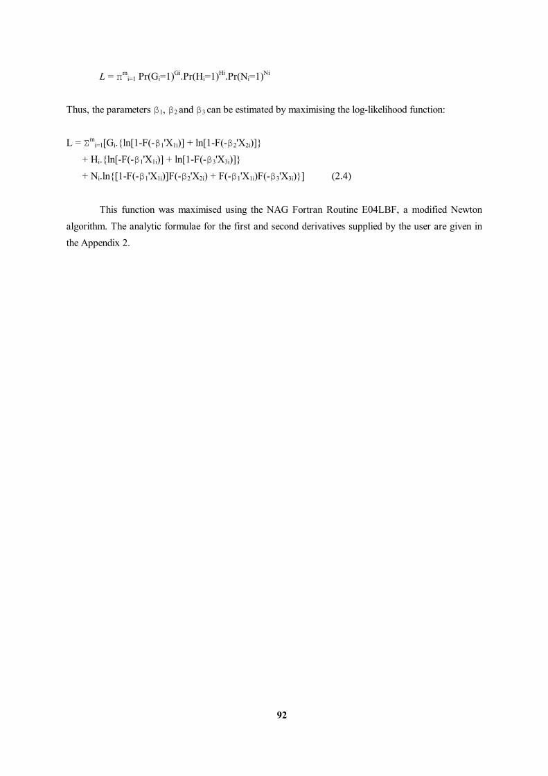
92

L = πmi=1 Pr(Gi=1)Gi.Pr(Hi=1)Hi.Pr(Ni=1)Ni

Thus, the parameters β1, β2 and β3 can be estimated by maximising the log-likelihood function:

L = Σm

i=1[Gi.{ln[1-F(-β1'X1i)] + ln[1-F(-β2'X2i)]} + Hi.{ln[-F(-β1'X1i)] + ln[1-F(-β3'X3i)]} + Ni.ln{[1-F(-β1'X1i)]F(-β2'X2i) + F(-β1'X1i)F(-β3'X3i)}] (2.4)

This function was maximised using the NAG Fortran Routine E04LBF, a modified Newton algorithm. The analytic formulae for the first and second derivatives supplied by the user are given in the Appendix 2.

93

b. Econometric Results The model was estimated over a sample of those aged thirty or under who had complete primary schooling. The high upper age limit was partly because of the relatively old age at which many people enter secondary school, but was also set so as to provide a sufficiently large sample. One adverse effect of such a liberal upper age limit is that entails analysing some secondary school enrolment decisions that may have been taken many years before the time of the survey. The sample was restricted to sons and daughters of household heads, so as to aid in the interpretation of variables for the education and fertility of heads and their spouses. The explanatory variables used in the final form of the model are defined in Table 5.1 and the results presented in Table 5.2. All but three of the explanatory variables are significant at 10%, the exclusion of those that are not significant being rejected by a likelihood ratio test. According to Table 5.3, the model assigns the highest probability to the final schooling outcomes that actually occurred in 65% of cases. It is noticeable that the model predicts that most people who pass the CPE would go to state secondary school. Such a high level of demand is what would be expected a priori, given that state secondary schooling is free but rationed. However, this high propensity makes it difficult to determine the coefficients on the equation for state secondary school choice. Given the non-linear form of the logistic functions underlying the model, the effects of the determinants upon the relevant probabilities vary with the base probability at which the change is assessed; in particular, a given change in the determinants has more effect on those who are at the margin of the decision in question. The convention adopted here was to evaluate the effects of various changes in the exogenous at the means of the other regressors; the results of which are reported in Table 5.4. The probability of going to a state secondary school conditional upon passing the CPE when evaluated at the means of all the regressors is virtually unity (0.98). Hence the effects of various changes on this probability are referred to in the text below but not reported in Table 5.4. This large probability of passing at the means of the other regressors only partly reflects the findings of the model since the corresponding expected probability is 0.87. (Due to the non-linear form of the logit, probabilities evaluated at the means of the regressors can differ from the mean probability.) According to Tables 5.2 and 5.4, gender differentials in schooling behaviour are more marked than appears from simply looking at the figures for the proportions of boys and of girls in state and Harambee schools. Specifically, the coefficient on the FEMALE dummy in X1i is significant at 1% and implies that, at the means of other characteristics, girls are 17% less likely to pass the exam. The corresponds with Grisay's findings for the Cote d'Ivoire. The results in Table 5.2 provide support for the notion that there is lower demand for the secondary schooling of girls, at least as far as the demand for Harambee schooling conditional upon

94

failing the exam is concerned. The coefficient on the FEMALE dummy is sizably negative and highly significant, although the precise effect varies with the age of the individual concerned due to the interaction term FENROL. For someone aged 22, the mean age in the sample used, the effect of being female evaluated at the means of the other variables is to reduce the probability that they will be sent to Harambee school if they fail to become eligible for entry to a state secondary school by 19%. The reason why these predicted differentials are more pronounced than those in the observed numbers going to state schools is due to a third effect from being female which is that they are predicted to be more likely than boys to be sent to state secondary school if they pass. For example, at the means of the other regressors, the probabilities are 99.54% for females and 92.72% for males. Although insignificant, this apparently higher demand for state secondary schooling for girls than for boys appears to contradict opposite finding for the demand for Harambee secondary schooling and is consequently worth trying to explain. It seems reasonable to argue that the finding for Harambee schooling is the more reliable guide to the underlying demand for the secondary schooling of girls relative to that for boys for two related reasons: firstly the coefficient in the former is much more significant and secondly that given the relatively small numbers predicted to pass the exam, the coefficient for Harambee choice can be expected to be the more accurately determined. The second point is rather tentative since the numbers predicted to pass the exam is partly a function of the coefficients on the gender dummy variables. However, to the extent that this number is determined by other factors, it is valid to note the expected number of girls who pass is only 63 and for boys the corresponding number is 101. Indeed, given these numbers, one could argue that the positive coefficient on the FEMALE variable reflects a sample selection effect. In particular, suppose - as seems apparent from Table 5.2 - that girls are less likely to pass the exam and that therefore those that are successful must have either a set of observable characteristics (other than gender) more favourable to passing the exam or some more favourable unobservable circumstances than successful boys. To the extent that the latter is true and that the unobserved determinants of exam success are positively correlated with the demand for schooling, it follows that those girls who pass the exam will be more likely to go to school than boys, ceteris paribus. There seem several plausible hypotheses that predict such a positive correlation: i)"Intelligence" is one unobserved variable that is likely to increase both exam performance and also the

demand for schooling, if intelligence is complementary with years of schooling in determining the returns to education.

ii)A high - parental or other - demand for schooling may motivate a child so as to perform better in the exam

iii)Conversely, a high exam mark may increase the demand for schooling. The possibility of the stochastic determinants of exam success and of schooling choice

95

conditional upon exam performance being positively correlated could be investigated formally but given that the data used does not record examination success, such an analysis was not attempted here. In order to identify possible gender interactions, a more general version of the final version of the model - that is to say, one with an additional number of explanatory variables in the three vectors - was estimated separately for each sex. The likelihood ratio statistic for the null hypothesis that the coefficients on the variables were equal across the two subsamples was 33.55 which, compared with the critical value of 47.4 at 5% significance with 33 degrees of freedom, implies the null could not be rejected. Nonetheless attempts were made to enter various individual gender interaction terms into the model when estimated over the full sample: in particular, terms interacting FEMALE with INCPC, DADSTD1 and MUMSTD1 were all entered but rejected at 5% significance by likelihood ratio tests. The only significant variable which was found to have a differential effect by gender, was ENROL, the gender-specific national gross enrolment ratio when the individual was 15. This was variable was entered as a determinant because, as has already been indicated, we are analysing the schooling histories of individuals of a wide range of ages. To some extent, the variable will control for changes in availability, price and quality of secondary schooling overtime. The gender specific enrolment ratios were taken from UNESCO Statistical Yearbooks76. The choice of the rate for the year at which the individual was 15 was made since 15 is the earliest year at which a significant number of individuals observed in the survey enter secondary school. The enrolment ratio variable was disaggregated (into FENROL and a counterpart for males) to allow girls in the sample to behave differently relative to the national trend for females from the way boys behave relative to the national trend for males. Likelihood ratio tests at 5% significance rejected the restriction to a single variable, ENROL, as a determinant of the demand for Harambee schooling but did not reject the restriction in the other two vectors of coefficients. Further likelihood ratio tests at the same level of confidence did not reject the hypotheses that ENROL had no effect on the probability of individuals passing the exam and that the male counterpart to FENROL was not a determinant of the demand for Harambee schooling. Figures 1 and 2 plot the probabilities - at the means of other regressors - for individuals of different ages of going to secondary school implied by these results. The relevant national enrolment rates for each year are also plotted on each Figure, although these are not comparable with the predicted probabilities for several reasons. In particular: the predicted figures are for two Provinces of Kenya only, do not give the mean (expected) probabilities but rather the probabilities at the means of other explanatory variables and do not allow for the fact the means of these other explanatory variables are likely to have varied overtime. Nonetheless, a strong finding does emerge from the two figures; namely that, although the predicted probability of entering secondary school moves with the relevant national

76

Where various UNESCO yearbooks contradicted themselves, the most recent estimate for a year was used. The missing figures for 1969 being calculated as the average of the 1968 and 1970 figures.

96

enrolment rate in the case of both males and females, in the case of males the predicted expansion overtime consists entirely in increased state school places whilst for females the expansion is almost entirely in increased Harambee school places. This is despite the demand for state schooling of both girls and boys being found to increase with the national enrolment rate. In the case of girls, such a rise in demand is not reflected in an increase in state school places because the even in the absence of such a rise, the probability of those females who do pass the exam going to a state school is very close to unity. In other words, state secondary school places for girls have been so severely rationed that in the absence of a loosening of the rationing by exam performance, an increase in demand is not reflected in an increase in state school places for girls. By contrast, in the earlier years the number of boys who were predicted to pass the exam but not enter to state school is sufficiently high for there to be some increase in state secondary school provision to meet the rise over time in demand. It is unclear why there is no rise predicted in the demand for the private schooling of males conditional upon failing the exam although this may reflect the state school ration for males being sufficiently loose to fully accommodate an increase in the general demand for the secondary schooling of boys. Parental education has powerful effects in the model, although these are not always what one would predict. In particular, the effects of parental education upon exam performance follow a marked non-monotonic pattern. As can be seen from table 5.4, the incremental effects on the probability of passing the exam of parents completing various levels of schooling, when evaluated at the means of the other regressors, are: +17% if the father completes Standard 5 -49% if the father completes Standard 7 +29% if the father completes Standard 8 +42% if the father attains some secondary schooling +18% if the mother completes Standard 1 -33% if the mother completes Standard 3 +20% if the mother completed Standard 4 Considering paternal education first, the positive coefficients are what might be expected if parental human capital complements a child's acquisition of human capital and the human capital parents acquire from school is to some extent "lumpy". For example, at least four years of primary school are conventionally thought to be necessary for the acquisition of basic literacy and numeracy and so one might expect parental acquisition of this to be particularly important in its effects on the demand for schooling. However, explaining the apparently perverse effect of attaining Standard 7 seems to require something other than a human capital mechanism. Standard 8 was effectively

97

abolished in 1964, so it could be that the cumulative dummy variable for attaining Standard 7 is capturing some temporal effect. However, such an explanation does not seem plausible since the abolition came only three years before the youngest individual in the sample could have been born, and thus it is likely that the vast majority of individuals in the sample had fathers who had the opportunity to progress to Standard 8. It might be possible to explain the negative coefficient on DADSTD7 if one assumes both that a child's educational aspirations increase with the educational attainment of their fathers and that a child's exam performance increases with their educational aspirations. However, to fully explain the apparently "perverse" effect of DADSTD7 on exam performance one must also assume that children revise upwards their aspirations if they surpass the level reached by their fathers, perhaps because they feel more confident and their fathers' experience becomes less relevant. To understand this argument, one can separate the effects on exam performance of having j levels of paternal schooling into the sum from 1 to j of the incremental effects, Hs, on a child's exam performance of the human capital the father attained from each level s and other effects, aj associated the influence upon a child's aspirations of having a father who left school at level j. For a negative coefficient on DADSTD7, we thus require: (a7 - a5) + H6-7 < 0 where H6-7, the effect on exam performance of paternal human capital acquisition from Standards 6 and 7, is presumably non-negative. a5 and a7 may both be negative - since having a parent who did not complete primary school lowers a child's expectations and hence possibly their exam performance as well. However, a5 may be less negative than a7 since children who have themselves completed Standard 7 may be less influenced if their fathers did not progress further than Standard 5 than if their fathers did not themselves get past Standard 7. This argument seems to imply that a8 is also a substantially negative number but this is still consistent with a positive coefficient on DADSTD8 so long as: a8 > a7 - H8

This may well hold since the influence upon a child's aspirations of having a father who left after Standard 7 may not be that different from the corresponding influence of having one who left after Standard 8 and H8 may be sizable since parental experience of - and cramming for - the CPE is likely to aid a child sitting the exam. Finally, it can be seen why it might be that the model estimated finds the total effect on exam performance of having a father who left school after completing primary school to be less than that of having a father who left after Standard 5. In particular, this will be true if the negative effect, a8, on exam performance of having a father who probably failed the exam is larger in absolute terms than the corresponding effect, a5, of having a father who left after Standard 5 and the

98

difference is sufficiently great as to offset the benefits to a child's exam performance, H6-7 + H8, of paternal acquisition of human capital from Standards 6, 7 and 8. That this condition does in fact hold is by no means obvious a priori - although it should be noted that the human capital acquired in the period of study leading to the exam may be small for those parents failed the exam. The effect of various levels of maternal education follow a similar pattern to that of paternal education although they occur at lower levels of schooling. These findings could be explicable using the same sort of argument that was used to explain the non-monotonic effects of paternal education. In particular, it could be argued that having a mother who dropped out of school before completing the first half of primary school, lowers a child's own educational aspirations more than if the mother had received no schooling because the latter case is seen as less relevant to children who have themselves spent at least 7 years in school. The former case may still be considered relevant since as can be seen from Table 5.2, for an eldest wife to have completed the first half of primary schooling is an educational attainment similar relative to what other such women attained comparable to what a father's completion of primary school is relative to the schooling achievements of other such men. Parental education also affects the two conditional demand equations. In particular, as shown in Table 5.4, when evaluated at the means of the other regressors, some parental education increases the probability of being sent to a Harambee school conditional upon failing the exam by 26% in the case of paternal education and by 21% in the case of maternal education. Some paternal education also increases the probability of going to a state secondary school conditional upon passing the exam from 89% to 99%. A large number of cumulative dummy variables for parental education (DADSTD5, DADSTD7, DADSTD8, DADSEC, MUMSTD3, MUMSTD4) were initially entered as determinants of state school choice but were all insignificant. Some of these variables had coefficients that were large in absolute value but also had extremely large standard errors. This possibly reflects a feature of the data whereby all or almost all of those who passed the exam and had these parental characteristics chose the same course of action. Similar phenomena have been reported for estimates of the effects of possession of a PhD. on the probability of unemployment where, in the sample used, all those with PhD's are employed. If this explanation is correct it would be invalid to conclude from their low significance that higher levels of parental education have no effect on the demand for state schooling and the most that can be concluded is the data available is insufficient to estimate any effects they may have. DADSEC also had a large coefficient and standard error when entered as a determinant of Harambee choice, but the rejection of other parental education variables, (DADSTD5, DADSTD7, DADSTD8, MUMSTD3, MUMSTD4, MUMSTD8), as determinants of this choice did not pose the same problem for inference. That higher levels of parental education do not increase the demand for Harambee schooling could be explained if some familiarity with schooling that parents have gained from some personal contact with it is of particular importance in leading them to send their children to secondary school: parents will have some idea what is involved in the schooling process; feel it is less

99

alien and so forth. The findings do not seem to support the human capital mechanisms for the effect of parental education upon the demand for schooling mentioned earlier, since these would seem to imply that higher levels of parental education will have positive effects. Household income per capita was significant in all three of its appearances. However, it has a "perverse" sign as a determinant of state school choice and although household income per capita increases ones chances of passing the exam and of going to Harambee school if one fails, it can be seen from Table 5.4 that these effects are not particularly large. At the means of the other regressors, increasing household income per capita by 50% only leads to a 2.5% improvement in ones examination chances and a 5.5% increase in the demand for Harambee schooling should one fail the exam. The view that these effects are not very large should be qualified by noting that the variance of income per capita in the sample is very large, with a standard deviation greater than the mean. Variables reflecting the average schooling behaviour of others in the sample from the same cluster as an individual were entered as determinants of an individual's demand for schooling. Such variables may reflect one of two processes. Most simply, they will capture relevant omitted cluster specific variables, such as cost of local and quality of secondary schools. The variables may also reflect local access to formal sector employment and hence expected returns from secondary schooling. As well as omitted cluster specific variables, the variables would capture any "copying" effects whereby individuals learn from or emulate the behaviour of their neighbours. For the Kenyan mixture model, the proportion of others in the cluster who went to state secondary school (POG) was entered as a determinant of the demand for state secondary schooling. Similarly, the proportion of others - excluding those who went to a state secondary school - in the cluster who went to Harambee schools (POH) was entered as determinant of an individual's demand for Harambee secondary schooling. To try to minimise cluster specific effects, variables were used in preliminary estimates but these were later rejected on the basis of likelihood ratio tests. In particular, the distances of the nearest Harambee and state secondary schools were entered into the relevant demand equations, as was the distance of the cluster from the nearest major urban centre. Both POG and POH were highly significant as determinants of exam performance and the demand for Harambee schooling respectively. The former result is perhaps best interpreted as reflecting omitted cluster specific variables, one of which that might be expected to be important being the quality of the primary school teaching in the area. The latter result could reflect also reflect such omitted variables. One such might be the availability of a low cost Harambee secondary school, although a variable for the distance of the nearest Harambee school was rejected from the analysis as insignificant. It is also possible that the behaviour of POH captures "copying" effects whereby individuals learn from or emulate the behaviour of their neighbours. Both of these classes of explanations might be expected to be more important in determining Harambee choice than government school choice for several reasons. In particular, state schools are likely to be standardised than independent schools and thus to exhibit

100

less spatial variability in their cost and quality. Furthermore, copying may be less important in the context of the relatively established state school sector when compared with the rise of the Harambee school movement. Moreover, as was remarked on earlier, the choice about whether to take advantage of eligibility to the subsidised and relatively high quality state secondary schooling is generally insensitive to the hypothesised determinants. A child's birth order may also be a significant determinant of the demand for his/her schooling. The simplest such argument being that, other things being equal, a parent would wish to receive the return - possibly in the form of remittances - from an investment in schooling, as soon as possible. However, Gomes (1984) has also argued that once they start to receive remittances from the elder educated offspring, parents can use them to finance the schooling of younger children. This suggests a non-linear form for birth order. We found that the birth order of the individual has a non-monotonic effect on the demand for Harambee schooling similar to that discovered by Gomes. The effect is plotted at the means the other regressors in Figure 3. The mean birth order in the sample is around 3, which is also the least advantageous position as regards the probability of being sent to a Harambee school. As might be expected, being the first born is more advantageous, but even more powerful effects arise from coming last in a large family. These effects, which are very powerful when evaluated at the means of the other regressors, can perhaps be explained by Gomes' argument that late comers to the family benefit from the remittances sent by their elder siblings, sometimes sent specifically to fund schooling costs. The behaviour of the birth order quadratic may also reflect the likelihood that those with a large birth order are likely to come from households who have completed or nearly completed their family and thus do not have to save for expenditures on their future children. However, this last effect should to some extent be controlled for by the other fertility terms, which are quadratic in the age of the youngest wife of the household head at the time the individual was 15. This was used as a proxy for expectations of future siblings77. To allow for the fact that fertility does not vary with age differences beyond a certain upper limit - we chose 50 years of age - the variable was set equal to 50 for women above this age. The effects of this AGEW and its square - having been adjusted so that those women aged over 50 are treat as being of age 50 - are plotted at the means of the regressors in Figure 4. The shape of the curve supports the interpretation originally placed upon the variable since the probability rises with the age of the wife, until around 44 years of age, at which increased age of the wife is unlikely to be associated with any further reductions in her fertility. This finding suggests that effective birth control may have powerful effects on educational investment even in the short run. In particular, it

77Sometimes the schooling outcomes being analysed - eg primary school enrolment - reflect schooling decisions over a range of years. Furthermore, it is often not known what year a decision was taken. Consequently, the mothers age when the child was a given age - five in the case of Ivorian primary school enrolment and 15 in the case of Kenyan secondary school enrolment - was used.

101

suggests a method of quantifying this effect if it is assumed that the effects on educational investment of a reduction in the expected number of future children induced by birth control are equivalent to the same reduction caused simply by increased maternal age.

c. Simulating the Effects of a Redistribution of State School Places from Girls to Boys The model estimated above provided evidence that girls in Kenya are at a disadvantage compared to boys in obtaining access to state secondary schooling due to their poorer exam performance. The same phenomenon has been noted in Tanzania and led to the imposition of a system of positive discrimination guaranteeing girls 30% of the total number of state school places. To implement this quota, the exam grades required for entry to state secondary school in Tanzania were set lower for girls than for boys. It is interesting to see what would be effects of similar policies if implemented in Kenya. In particular, the finding of the model that the demand for Harambee schooling of those who fail the CPE is lower for girls than boys, suggests that a pure redistribution of state school places from boys to girls would lead to an increase in total secondary school enrolment. To try to quantify this increase, we use the sample detailed above and the mixture model estimated on it to carry out a simulation of such a switch in state school places from boys to girls. Since the survey was carried out in Central and Nyanza Provinces, the simulation is specific to these regions. Moreover, since the sample covered a fairly wide age range, 15 to 30 year olds, the simulation also implies that the policy change was implemented throughout the period during which their secondary schooling decisions were being taken - a period which could extend back to the late sixties - rather than just at the time of the survey. This qualification is important since the model found evidence of an increase overtime in the demand for Harambee schooling for girls relative to that for boys. Various degrees of redistribution could be simulated but the one chosen here is that the numbers of girls and boys in state secondary school are equalised. This was chosen because given the rather limited sample size, the numbers involved in lesser redistributions - for example equalising the proportions of primary school leavers going to state schools - would be rather small. Furthermore, it was assumed that this switch in places would be implemented simply by altering the CPE grades required for boys and girls to enter to state secondary schools. An alternative and possibly preferable method of implementation might be to try to alter either the nature of the exam and/or of primary schooling teaching. However, simply changing the pass marks is easier to simulate since it implies the determinants of exam performance are unchanged and thus those most likely to be affected by the redistribution can be identified. Given the interpretation of the latent variable underlying the logistic model of exam success as the exam mark transformed in some way so as to equal zero at the pass mark, alterations in the pass mark can be simulated by changing the constant term in the latent variable. Thus instead of requiring

102

Yil > 0 for individual i to pass the exam, after the policy change we will now require:

Yi

l > Cj

where Cj = Cf < 0 for girls and Cj = Cm > 0 for boys Consequently, Cj is added to the constant term in the equation for exam performance. Before these alterations are made, the expected number of girls and boys going to state secondary school implied by the estimates in Table 5.2 are 63.02 and 101.34 respectively. Hence, to equalise the expected numbers of each gender going to state secondary school requires a reallocation of roughly 19 places from girls to boys. The precise values of Cf and Cm necessary to achieve this are such that: Σn

i=1[[1 - F(-β1'X1i + Cj)].[1 - F(-β2'X2i)]] = 82.18 (2.5)

for both Cj = Cf and Cj = Cm, where and β1 and β2 are the coefficients on the equations given in Table 5.2 for exam success

and for the demand for state secondary schooling respectively. Due to the non-linear nature of the logistic function F(.), the values of Cj that satisfy equation (2.5), were found using numerical techniques. In particular, functions equal to the squared difference of the left and right hand sides of equation (2.5) was minimised with respect to Cj using the NAG routine E04KDF. The solutions were: Cf = 0.5734 Cm = -0.4750 Using these values of Cj, and the three sets of coefficients given in Table 5.2, new probabilities for the schooling outcomes of individuals in the sample could be generated. In Table 5.5, we compare the expected numbers of individuals in the sample obtaining each outcome implied by the post-simulation probabilities with those implied by the original ones.

103

Table 5.5: Expected schooling outcomes: before and after equalisation of state school places for girls and boys Outcome Pre-simulation Post Simulation Change State Secondary Boys 101.34 82.18 -19.16 Girls 63.02 82.18 19.16 Total 0.00 Harambee Secondary Boys 90.94 102.38 11.44 Girls 64.52 56.01 -8.52 Total 2.92 No Secondary Boys 117.72 125.44 7.72 Girls 75.46 64.82 -10.64 Total -2.92 Expected Characteristics of those Affected by the Change Girls Boys Annual household income p.c. (K.SH.) 1,113 1,054 Central Province (%) 57% 49% Some paternal education (%) 69% 71% Some maternal education (%) 32% 27% As can be seen from Table 5.5, switching 19.16 state school places from boys to girls increases the total number of secondary school places by 2.92. Hence for every one state school place switched, there is a 15% increase in the total number of children entering secondary school. This may represent a considerable benefit from such a policy if it is a government objective to increase the total number of secondary school education since the 15% increase would not be at the expense of any extra government expenditure on state schools. Some of the expected characteristics of the individuals directly affected by the switch in state school places can also be identified and are shown in Table 5.5. These were derived by weighting each individuals' characteristics by the absolute change in the probability of their enroling in state secondary school as a result of the policy change. As can be seen the redistribution is mildly regressive in terms of mean household incomes per capita and favours those in Central Province. The parents of the gainers (girls) are not unambiguously more educated than those of the losers. A more complete analysis of the proposed policy change would have to go beyond a simple examination of the expected effect on total secondary school enrolment and its distributional

104

consequences to consider in more detail its costs and benefits. On the cost side of the policy, the extra Harambee school places will not be free and to the extent that the government subsidises some private schools then it will have to bear some of the cost. Other reservations arise when considering the benefits of the policy. In particular, a full assessment of the returns to secondary schooling seems required in order to determine the optimum allocation of state school places. For example, if the returns to secondary schooling are higher for males than females, due to the former being more likely to enter formal sector employment given equal education, then the benefits forgone from reducing male enrolment in secondary school may be greater than the benefits gained from a more than compensating rise in female enrolment. A similar proviso might also apply when the quality difference between Harambee and state secondary schools mentioned earlier is taken into account. Nonetheless, the findings of the simulation suggest that further research into the gender differentials in the crowding-out effect of state secondary school places is a necessary component of a complete analysis of the costs and benefits of introducing greater gender equity into the rationing of such places.

105

d. Repeating the Primary Leaving Exam One way in which the household can influence the performance of its children in the primary-leaving exams which are used to allocate state secondary school places, is by getting them to repeat the exam if initially unsuccessful. As noted in the overview, girls in Kenya and Cote d'Ivoire were slightly less likely to repeat the exam. Here we consider the issue further using responses from our Kenya survey to the question of whether a household would get its children to repeat the primary leaving exam if they failed to secure a place in a government secondary school. These responses may be illuminating but do not provide a wholly reliable indicator of repeating since the question is hypothetical and concerns intentions rather than behaviour. A binary probit was used to model "hypothetical repeating" with the gender composition of the students entered as a determinant along with a large number of hypothesised determinants of the demand for schooling. In preliminary estimates, the proportion of children of the household head at primary school who were female had a positive effect upon hypothetical repeating and was near to significance78. Like the descriptive statistics in Table 1.4, this result provides no evidence that girls rates of repeating account for low secondary enrolment79. However, the factors affecting whether a household chooses to have its children repeat the primary leaving exam if unsuccessful do seem to vary according to the gender of the children. This was discovered by interacting variables for the gender composition of students with other explanatory variables. The final form of the probit for repeating taking account of such interactions is given in Table 5.6. One surprising feature of Table 5.6 is how many of the explanatory variables retained as significant are interacted with variables for the gender composition of the students. Almost all of these interaction terms were significant at 10% in preliminary estimates when included alongside the relevant linear terms80. The main benefit from repeating the primary-leaving exam is an increase in one's chances of entering a state secondary school. One measure of the costs of entering state secondary school - distance to the nearest such school - was insignificant as a determinant of repeating; possibly because the benefits from such subsidised schooling are sufficiently high to make this an unimportant

78Dummy variables for whether all students were girls or all boys were wholly insignificant.

79It is possible that how repeating varies with the proportion of female students does not provide an adequate measure of differences in the treatment of boys and girls since the proportion may be endogenous. Thus households with favourable attitudes to schooling may enrol more girls than others and thus the proportion of female primary school students may capture a high demand for schooling rather than gender effects. In a preliminary estimate the proportion of girls amongst all children of the head (not just those children at primary school) was used to avoid this danger but this proportion was also positive and insignificant.

80The one exception to this is the interaction with the average reported wage for agricultural labour in the cluster, which was only significant at 15% when entered jointly with the linear term for the wage itself, which itself had a t-ratio of less than 0.5.

106

consideration. However, proxies for the costs and benefits of the alternatives to state secondary schooling - namely Harambee secondary schooling or no secondary schooling - were significant and with the expected signs, but with only to the extent that they were interacted with the proportion of female primary school students. This gender specificity may reflect the fact that repeating decisions about girls' are more sensitive to variations in expected costs. The first such proxy was the distance to the nearest Harambee secondary school, which may capture some of the user costs involved in such schooling. The second is the average reported wage for agricultural labour in the cluster, which may be a good proxy for the returns to the labour of uneducated teenagers. The probability of hypothetical repeating rises with the schooling of the "senior female" to the extent that the would-be repeaters are boys, but falls with this schooling to the extent that the primary school students are girls. Variables for the education of male heads were rejected as insignificant. Surprisingly, distance to water supply actually increases the probability of hypothetical repeating to the extent that the would-be repeaters are female and reduces it in so far as they are male. This does not seem consistent with the fact that water is largely collected by females and that distance to water sources increases the chances of girls dropping out of primary school. The other significant gender difference is for the Provincial dummy variable: residence in Central Province increases the likelihood of hypothetical repeating amongst girls. Finally, the ability to afford to keep students in school - as measured by income per capita - reduced the probability of repeating. This seems somewhat perverse, given that high income families could better support children at school. Presumably it reflects the fact that more affluent households can afford to send their children to private schools if they fail to gain admission to state schools, perhaps with the intention of switching them into the higher quality state school sector after Form 2. Measures of per capita asset holdings - land acreage, livestock value and numbers of coffee and tea trees - had all been rejected as insignificant before experimenting with income per capita81.

81Parental occupation, household type (female-headed, polygamous, other), the number of children - both in primary school and out - and the age of youngest wife of the head were all rejected from Table 5.6 as insignificant.

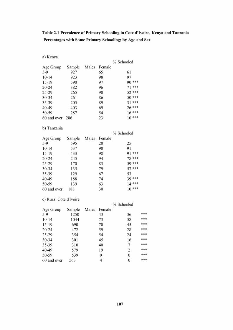
107

Table 2.1 Prevalence of Primary Schooling in Cote d'Ivoire, Kenya and Tanzania Percentages with Some Primary Schooling; by Age and Sex a) Kenya % Schooled Age Group Sample Males Female 5-9 927 65 61 10-14 923 98 97 15-19 590 97 90 *** 20-24 382 96 71 *** 25-29 265 90 52 *** 30-34 261 86 50 *** 35-39 205 89 31 *** 40-49 403 69 26 *** 50-59 287 54 16 *** 60 and over 286 23 10 *** b) Tanzania % Schooled Age Group Sample Males Female 5-9 595 20 25 10-14 537 90 91 15-19 433 98 91 *** 20-24 245 94 78 *** 25-29 170 83 59 *** 30-34 135 79 57 *** 35-39 129 67 53 40-49 188 74 39 *** 50-59 139 63 14 *** 60 and over 188 30 10 *** c) Rural Cote d'Ivoire % Schooled Age Group Sample Males Female 5-9 1250 43 36 *** 10-14 1044 73 58 *** 15-19 690 70 45 *** 20-24 472 59 28 *** 25-29 354 54 24 *** 30-34 301 45 16 *** 35-39 310 40 7 *** 40-49 579 19 2 *** 50-59 539 9 0 *** 60 and over 563 4 0 ***

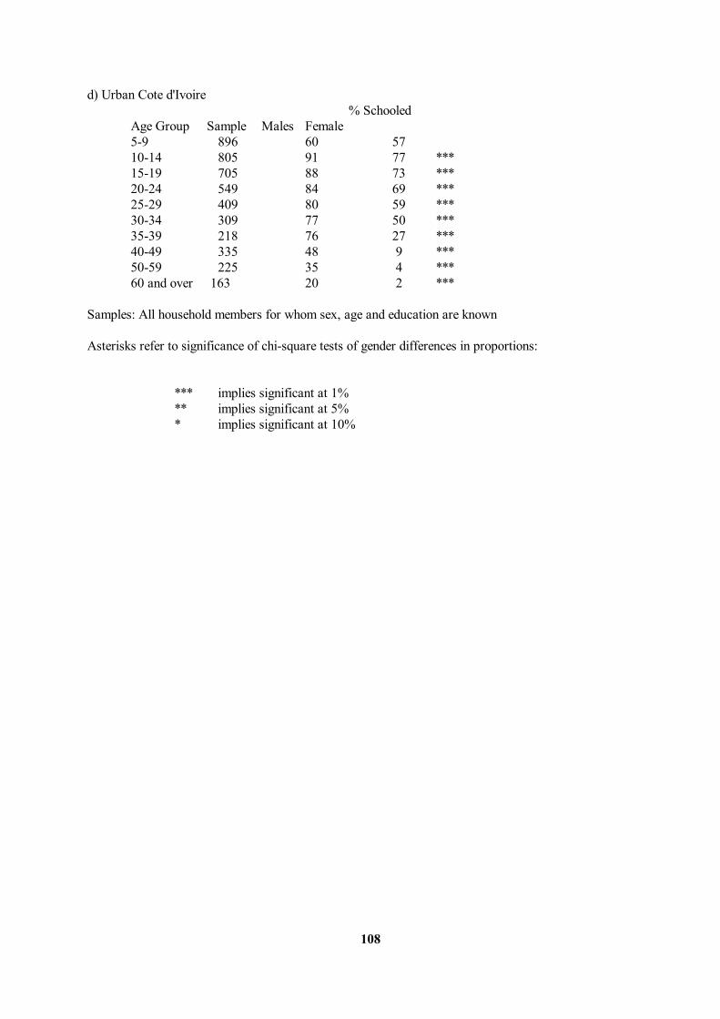
108

d) Urban Cote d'Ivoire % Schooled Age Group Sample Males Female 5-9 896 60 57 10-14 805 91 77 *** 15-19 705 88 73 *** 20-24 549 84 69 *** 25-29 409 80 59 *** 30-34 309 77 50 *** 35-39 218 76 27 *** 40-49 335 48 9 *** 50-59 225 35 4 *** 60 and over 163 20 2 *** Samples: All household members for whom sex, age and education are known Asterisks refer to significance of chi-square tests of gender differences in proportions: *** implies significant at 1% ** implies significant at 5% * implies significant at 10%

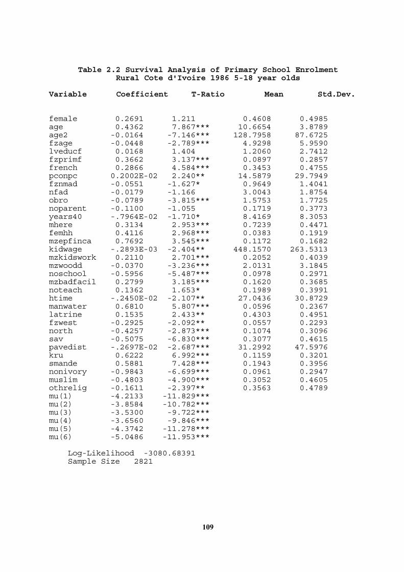
109

Table 2.2 Survival Analysis of Primary School Enrolment Rural Cote d'Ivoire 1986 5-18 year olds Variable Coefficient T-Ratio Mean Std.Dev. female 0.2691 1.211 0.4608 0.4985 age 0.4362 7.867*** 10.6654 3.8789 age2 -0.0164 -7.146*** 128.7958 87.6725 fzage -0.0448 -2.789*** 4.9298 5.9590 lveducf 0.0168 1.404 1.2060 2.7412 fzprimf 0.3662 3.137*** 0.0897 0.2857 french 0.2866 4.584*** 0.3453 0.4755 pconpc 0.2002E-02 2.240** 14.5879 29.7949 fznmad -0.0551 -1.627* 0.9649 1.4041 nfad -0.0179 -1.166 3.0043 1.8754 obro -0.0789 -3.815*** 1.5753 1.7725 noparent -0.1100 -1.055 0.1719 0.3773 years40 -.7964E-02 -1.710* 8.4169 8.3053 mhere 0.3134 2.953*** 0.7239 0.4471 femhh 0.4116 2.968*** 0.0383 0.1919 mzepfinca 0.7692 3.545*** 0.1172 0.1682 kidwage -.2893E-03 -2.404** 448.1570 263.5313 mzkidswork 0.2110 2.701*** 0.2052 0.4039 mzwoodd -0.0370 -3.236*** 2.0131 3.1845 noschool -0.5956 -5.487*** 0.0978 0.2971 mzbadfacil 0.2799 3.185*** 0.1620 0.3685 noteach 0.1362 1.653* 0.1989 0.3991 htime -.2450E-02 -2.107** 27.0436 30.8729 manwater 0.6810 5.807*** 0.0596 0.2367 latrine 0.1535 2.433** 0.4303 0.4951 fzwest -0.2925 -2.092** 0.0557 0.2293 north -0.4257 -2.873*** 0.1074 0.3096 sav -0.5075 -6.830*** 0.3077 0.4615 pavedist -.2697E-02 -2.687*** 31.2992 47.5976 kru 0.6222 6.992*** 0.1159 0.3201 smande 0.5881 7.428*** 0.1943 0.3956 nonivory -0.9843 -6.699*** 0.0961 0.2947 muslim -0.4803 -4.900*** 0.3052 0.4605 othrelig -0.1611 -2.397** 0.3563 0.4789 mu(1) -4.2133 -11.829*** mu(2) -3.8584 -10.782*** mu(3) -3.5300 -9.722*** mu(4) -3.6560 -9.846*** mu(5) -4.3742 -11.278*** mu(6) -5.0486 -11.953*** Log-Likelihood -3080.68391 Sample Size 2821

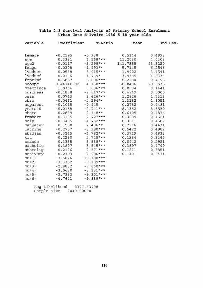
110

Table 2.3 Survival Analysis of Primary School Enrolment Urban Cote d'Ivoire 1986 5-18 year olds Variable Coefficient T-Ratio Mean Std.Dev. female -0.2195 -0.938 0.5144 0.4998 age 0.3331 6.168*** 11.2030 4.0308 age2 -0.0117 -5.298*** 141.7555 93.3220 fzage -0.0308 -1.993** 5.7145 6.2546 lveducm 0.0538 5.015*** 1.9922 3.4541 lveducf 0.0166 1.739* 3.9385 4.8333 fzprimf 0.5857 5.696*** 0.2284 0.4198 pconpc 0.4474E-02 4.138*** 30.0486 29.5635 mzepfinca 1.0364 3.886*** 0.0884 0.1441 business -0.1878 -2.817*** 0.4949 0.5000 osis 0.0743 3.626*** 1.2826 1.7313 obro -0.0461 -2.294** 1.3182 1.8051 noparent -0.1015 -0.945 0.2782 0.4481 years40 -0.0158 -2.741*** 8.1352 8.5530 mhere 0.2839 2.148** 0.6105 0.4876 fzmhere 0.3185 2.727*** 0.3089 0.4621 poly -0.3435 -4.762*** 0.3011 0.4587 manwater 0.1930 2.486** 0.7316 0.4431 latrine -0.2707 -3.990*** 0.5422 0.4982 abidjan -0.3245 -4.782*** 0.3719 0.4833 kru 0.2280 2.745*** 0.1284 0.3345 smande 0.3335 3.538*** 0.0942 0.2921 catholic 0.3897 5.545*** 0.3597 0.4799 othrelig 0.2126 2.571*** 0.1811 0.3851 nonivory -0.2793 -2.906*** 0.1401 0.3471 mu(1) -3.6624 -10.108*** mu(2) -3.3352 -9.189*** mu(3) -2.8882 -7.860*** mu(4) -3.0630 -8.131*** mu(5) -3.7333 -9.301*** mu(6) -4.7641 -9.839*** Log-Likelihood -2397.63998 Sample Size 2049.00000

111

Table 2.4 Variable Definitions for Analysis of Primary School Enrolment in Cote d'Ivoire FEMALE 1 if female, 0 else AGE(2) age in years (AGE2 denotes age squared) Parental Education: LVEDUCF father's grades of schooling LVEDUCM mother's grades of schooling PRIMF 1 if father has some schooling, 0 else FRENCHC 1 if interview in French, 0 else Measures of household economic status: PCONPCpredicted household consumption per capita per annum

(10,000 CFAF) BUSINESS 1 if household runs own non-agricultural business, 0 else Proxies for primary school quality: BADFACIL 1 if bad school facilities are a problem, 0 else NOTEACH 1 if a shortage of teachers is a problem, 0 else Household Demographics: NMAD number of male adults NFAD number of female adults OBRO number of older brothers OSIS number of older sisters NOPARENT 1 if no resident parents, 0 else YEARS40 40 minus mother's age (in years) at individual's birth MHERE 1 if resident mother, 0 else Proxies for school costs: NOSCHOOL no primary school in cluster when individual was age five KIDWAGE cluster wage rate for child agricultural labour (1,000 CFAF per day) KIDSWORK children under 12 reported working in cluster WOODD distance to fuel wood (km) Health related variables: MANWATER 1 if drinking water purchased or piped, 0 else LATRINE 1 if use pit latrine, 0 else HTIME travelling time to nearest health clinic or hospital (minutes) Variables affecting household preferences: MUSLIM 1 if head Muslim, 0 else CATHOLIC 1 if head Catholic, 0 else OTHREL 1 if head neither Muslim nor Christian, 0 else NONIVORY 1 if non-Ivorian, 0 else KRU 1 if head Kru, 0 else SMANDE 1 if head S.Mande, 0 else POLY 1 if polygamous household, 0 else FEMHH 1 if female headed household, 0 else EPFINC predicted female share of cash income Geographic controls: PAVEDIST distance to nearest paved road (km) ABIDJAN 1 if resident in Abidjan, 0 else URBAN 1 if resident in urban cluster, 0 else SAV 1 if resident in South Savannah, 0 else

112

NORTH 1 if resident in North Savannah, 0 else WEST 1 if resident in West Forrest, 0 else Interactions between a variable and FEMALE are denoted by the prefix "FZ" before the name of the relevant variable. Interactions with a dummy variable for male gender are denoted by the prefix "MZ".

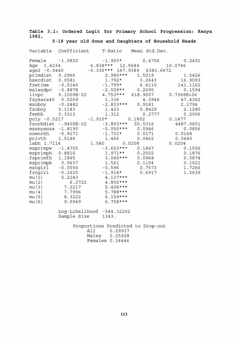
113

Table 3.1: Ordered Logit for Primary School Progression: Kenya 1982, 5-18 year old Sons and Daughters of Household Heads Variable Coefficient T-Ratio Mean Std.Dev. Female -1.0820 -1.903* 0.4706 0.2491 Age 1.4234 6.838*** 12.5644 10.0746 age2 -0.0440 -5.336*** 167.9389 6383.6672 primdist 0.2966 2.980*** 1.5019 1.5426 hsecdist 0.0581 1.792* 3.2643 16.9093 fzwtime -0.0146 -1.799* 6.4110 141.1162 mzlandpc -0.8878 -2.509** 0.2695 0.1594 livpc 0.1009E-02 4.753*** 618.9007 0.7368E+06 fzyears40 0.0269 1.336 4.3946 47.4362 mzoboy -0.2482 -2.833*** 0.9181 2.1794 fzoboy 0.1183 1.423 0.8429 2.1280 femhh 0.3313 1.312 0.2777 0.2006 poly -0.5217 -1.910* 0.1802 0.1477 fzurbdist -.9409E-02 -3.803*** 50.5316 4487.0651 mzsnyanza -1.8190 -5.050*** 0.0946 0.0856 noworkh -0.9171 -1.731* 0.0171 0.0168 privth 1.5146 1.466 0.0462 0.0440 labh 1.7114 1.580 0.0208 0.0204 mzprimpw -1.4705 -3.653*** 0.1847 0.1506 mzprimph 0.8816 1.971** 0.2502 0.1876 fzprimfh 1.1865 3.066*** 0.0968 0.0874 mzprimpb 0.9637 1.561 0.1154 0.1021 mzogirl -0.0556 -0.596 0.7573 1.7266 fzogirl -0.1625 -1.914* 0.6917 1.5639 mu(1) 5.2243 4.137*** mu(2) 6.2722 4.802*** mu(3) 7.2217 5.406*** mu(4) 7.7996 5.788*** mu(5) 8.3222 6.159*** mu(6) 9.0949 6.758*** Log-Likelihood -544.32202 Sample Size 1343. Proportions Predicted to Drop-out All 0.29937 Males 0.25928 Females 0.34446

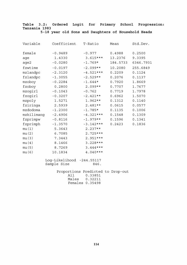
114

Table 3.2: Ordered Logit for Primary School Progression: Tanzania 1983 5-18 year old Sons and Daughters of Household Heads Variable Coefficient T-Ratio Mean Std.Dev. female -0.9489 -0.977 0.4988 0.2500 age 1.4330 3.615*** 13.2376 9.3395 age2 -0.0280 -1.769* 184.5733 6346.7931

fzwtime -0.0197 -2.099** 10.2080 255.6849 mzlandpc -2.3120 -4.521*** 0.2209 0.1124 fzlandpc -1.3055 -2.529** 0.2076 0.1137 mzoboy -0.2284 -1.644* 0.7920 1.8669 fzoboy 0.2800 2.099** 0.7707 1.7677 mzogirl -0.1043 -0.762 0.7719 1.7978 fzogirl -0.3207 -2.421** 0.6962 1.5070 mzpoly 1.5271 1.962** 0.1312 0.1140 fziringa 2.5939 2.481** 0.0615 0.0577 mzdodoma -1.2300 -1.785* 0.1135 0.1006 mzkilimang -2.4906 -4.321*** 0.1548 0.1309 fzprimpw -0.8116 -1.979** 0.1596 0.1341 fzprimph -1.3570 -3.142*** 0.2423 0.1836 mu(1) 5.3643 2.237** mu(2) 6.7085 2.725*** mu(3) 7.3443 2.951*** mu(4) 8.1466 3.228*** mu(5) 8.7269 3.444*** mu(6) 10.1834 4.040*** Log-Likelihood -244.55117 Sample Size 846. Proportions Predicted to Drop-out All 0.33851 Males 0.32211 Females 0.35498

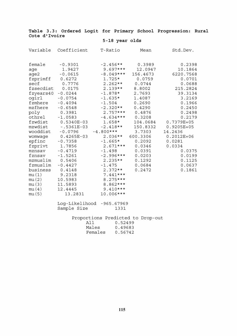
115

Table 3.3: Ordered Logit for Primary School Progression: Rural Cote d'Ivoire 5-18 year olds Variable Coefficient T-Ratio Mean Std.Dev. female -0.9301 -2.456** 0.3989 0.2398 age 1.9427 9.697*** 12.0947 10.1864 age2 -0.0615 -8.049*** 156.4673 6220.7568 fzprimff 0.6272 1.725* 0.0759 0.0701 secf 0.7776 2.262** 0.0744 0.0688 fzsecdist 0.0175 2.139** 8.8002 215.2824 fzyears40 -0.0244 -1.878* 2.7693 39.3134 ogirl -0.0754 -1.635* 1.4087 3.2169 fzmhere -0.4094 -1.504 0.2690 0.1966 mzfhere -0.6548 -2.320** 0.4290 0.2450 poly 0.3981 2.757*** 0.4876 0.2498 othrel -1.0583 -4.634*** 0.3208 0.2179 fzwdist 0.5340E-03 1.658* 104.0684 0.7379E+05 mzwdist -.5361E-03 -2.418** 150.8332 0.9205E+05 wooddist -0.0796 -4.800*** 3.7303 14.2436 womwage 0.4265E-03 2.036** 600.3306 0.2012E+06 epfinc -0.7358 -1.665* 0.2092 0.0281 fzprivt 1.7856 2.671*** 0.0346 0.0334 mznsav -0.4719 -1.498 0.0391 0.0375 fznsav -1.5261 -2.996*** 0.0203 0.0199 mzmuslim 0.5406 2.235** 0.1292 0.1125 fzmuslim -0.4427 -1.475 0.0684 0.0637 business 0.4148 2.372** 0.2472 0.1861 mu(1) 9.2318 7.441*** mu(2) 10.5983 8.275*** mu(3) 11.5893 8.862*** mu(4) 12.4445 9.410*** mu(5) 13.2831 10.006*** Log-Likelihood -965.67969 Sample Size 1331 Proportions Predicted to Drop-out All 0.52499 Males 0.49683 Females 0.56742

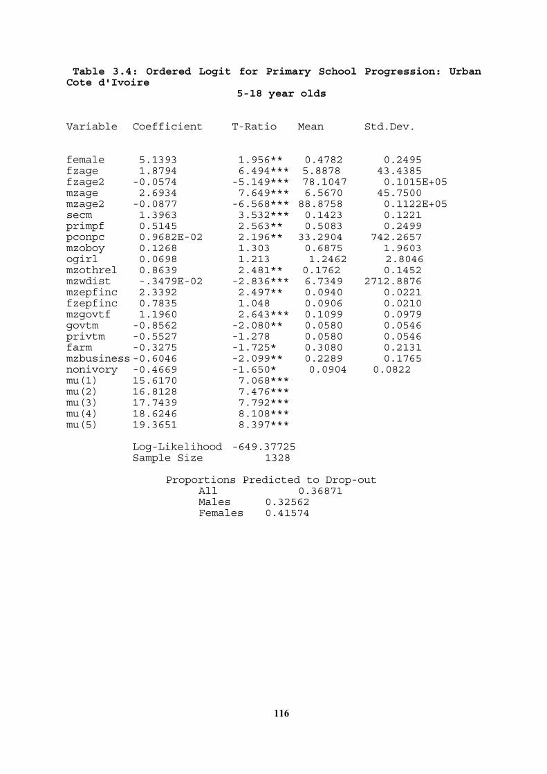
116

Table 3.4: Ordered Logit for Primary School Progression: Urban Cote d'Ivoire 5-18 year olds Variable Coefficient T-Ratio Mean Std.Dev. female 5.1393 1.956** 0.4782 0.2495 fzage 1.8794 6.494*** 5.8878 43.4385 fzage2 -0.0574 -5.149*** 78.1047 0.1015E+05 mzage 2.6934 7.649*** 6.5670 45.7500 mzage2 -0.0877 -6.568*** 88.8758 0.1122E+05 secm 1.3963 3.532*** 0.1423 0.1221 primpf 0.5145 2.563** 0.5083 0.2499 pconpc 0.9682E-02 2.196** 33.2904 742.2657 mzoboy 0.1268 1.303 0.6875 1.9603 ogirl 0.0698 1.213 1.2462 2.8046 mzothrel 0.8639 2.481** 0.1762 0.1452 mzwdist -.3479E-02 -2.836*** 6.7349 2712.8876 mzepfinc 2.3392 2.497** 0.0940 0.0221 fzepfinc 0.7835 1.048 0.0906 0.0210 mzgovtf 1.1960 2.643*** 0.1099 0.0979 govtm -0.8562 -2.080** 0.0580 0.0546 privtm -0.5527 -1.278 0.0580 0.0546 farm -0.3275 -1.725* 0.3080 0.2131 mzbusiness -0.6046 -2.099** 0.2289 0.1765 nonivory -0.4669 -1.650* 0.0904 0.0822 mu(1) 15.6170 7.068*** mu(2) 16.8128 7.476*** mu(3) 17.7439 7.792*** mu(4) 18.6246 8.108*** mu(5) 19.3651 8.397*** Log-Likelihood -649.37725 Sample Size 1328 Proportions Predicted to Drop-out All 0.36871 Males 0.32562 Females 0.41574

117

Table 3.5: Variable Definitions for Analysis of Primary School Drop-Outs82,83 AGE age (years) BUSINESS 1 if household runs its own non-agricultural business, 0 else DODOMA 1 if household resident in Dodoma region EPFINC predicted share of household income accruing to women (%) FARM 1 if household works its own land, 0 else FEMALE 1 if individual is female, 0 else FEMHH 1 if household is female headed, 0 else FHERE 1 if father resident in household, 0 else GOVT 1 if individual's main occupation is as an government employee HSECDIST distance of household to nearest Harambee secondary school miles) IRINGA 1 if household is in Iringa, 0 else KILIMANG 1 if household is in Kilimangaro, 0 else LAB 1 if individual's main occupation is as an agricultural labourer * LANDPC land in use for agriculture by household per capita (acres per head) LIVPC value of household livestock per capita (shillings per head) MHERE 1 if mother resident in household, 0 else MU(j), j=1,6 nuisance parameters MUSLIM 1 if head of household is a muslim, 0 else NONIVORY 1 if individual is of non-ivorian nationality NOWORK 1 if individual's main occupation is not remunerative, 0 else NSAV 1 if household in Northern Savannah, 0 else OBOY number of older brothers OGIRL number of older sisters OTHREL 1 if individual is not a member of the household

head's nuclear family, 0 else PCONPC predicted household consumption per capita per annum

(10,000 CFA Francs) POLY 1 if household is polygamous, 0 else PRIMDIST distance of household to nearest primary school (miles) PRIMF 1 if individual has full primary schooling, 0 else *

82 If followed by: "B" refers to both individual's parents and schooling "F" refers to individual's father's schooling "H" refers to male head of household "M" refers to individual's mother's schooling "W" refers to senior female in household. This key applied to other subsequent asterisked terms also.

83 Squared terms are denoted by the variable name followed by "Z". Gender interactions are given by prefixing FZ and MZ before variable name, e.g. MZAGE is AGE interacted with male dummy variable.

118

PRIMP 1 if individual has some primary schooling, 0 else * SEC 1 if individual has some secondary schooling, 0 else * SECDIST distance of cluster to nearest primary school (km) PRIVT 1 if individual's main occupation is in private non

agricultural employment, 0 else * SSAV 1 if household is in Southern Savannah, 0 else SNYANZA 1 if household in South Nyanza district, 0 else URBDIST distance to nearest large urban centre (Nairobi for

Central, Kisumu for Nyanza) WDIST distance to household drinking water source (metres) WTIME time taken to reach main drinking water source (minutes) WOODDIST distance to fuel wood source (km) YEARS40 number of years until mother (or youngest wife of

household head for Kenya) was forty when the individual was five years old

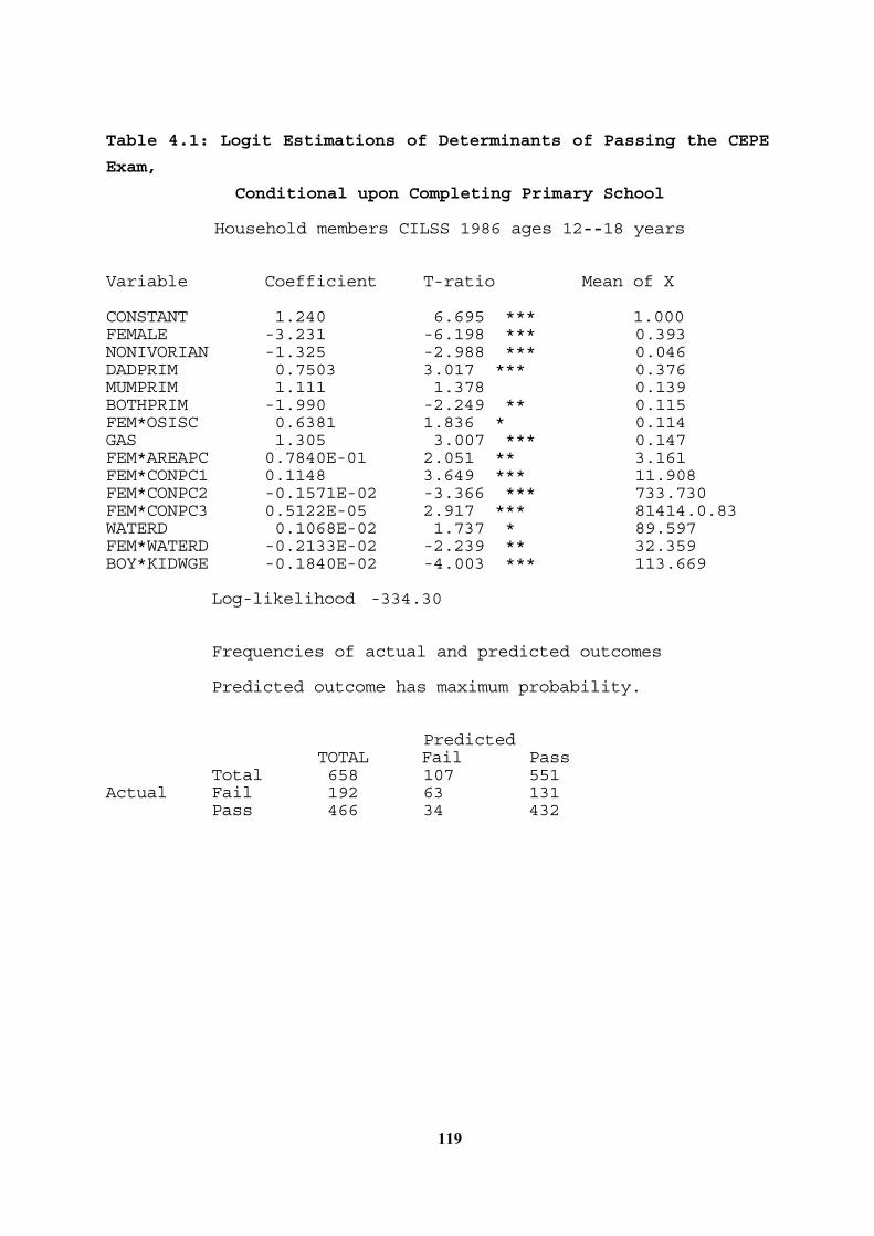
119

Table 4.1: Logit Estimations of Determinants of Passing the CEPE

Exam,

Conditional upon Completing Primary School Household members CILSS 1986 ages 12--18 years Variable Coefficient T-ratio Mean of X CONSTANT 1.240 6.695 *** 1.000 FEMALE -3.231 -6.198 *** 0.393 NONIVORIAN -1.325 -2.988 *** 0.046 DADPRIM 0.7503 3.017 *** 0.376 MUMPRIM 1.111 1.378 0.139 BOTHPRIM -1.990 -2.249 ** 0.115 FEM*OSISC 0.6381 1.836 * 0.114 GAS 1.305 3.007 *** 0.147 FEM*AREAPC 0.7840E-01 2.051 ** 3.161 FEM*CONPC1 0.1148 3.649 *** 11.908 FEM*CONPC2 -0.1571E-02 -3.366 *** 733.730 FEM*CONPC3 0.5122E-05 2.917 *** 81414.0.83 WATERD 0.1068E-02 1.737 * 89.597 FEM*WATERD -0.2133E-02 -2.239 ** 32.359 BOY*KIDWGE -0.1840E-02 -4.003 *** 113.669 Log-likelihood -334.30 Frequencies of actual and predicted outcomes Predicted outcome has maximum probability. Predicted TOTAL Fail Pass Total 658 107 551 Actual Fail 192 63 131 Pass 466 34 432

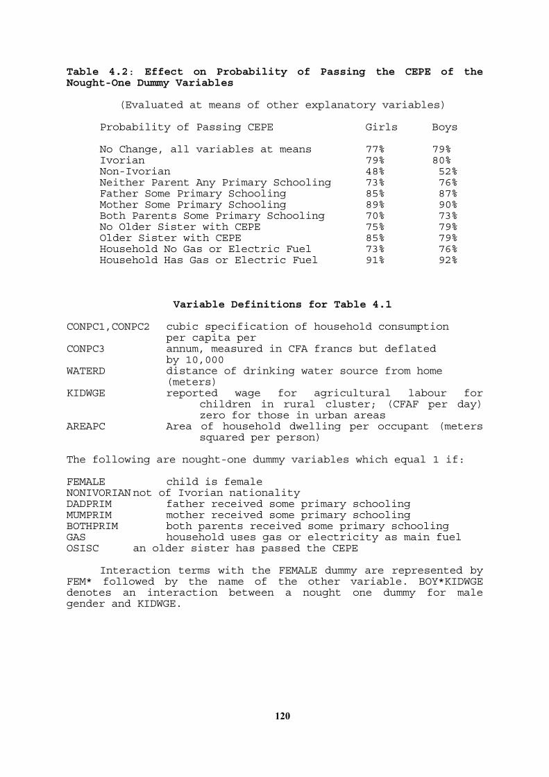
120

Table 4.2: Effect on Probability of Passing the CEPE of the Nought-One Dummy Variables (Evaluated at means of other explanatory variables) Probability of Passing CEPE Girls Boys No Change, all variables at means 77% 79% Ivorian 79% 80% Non-Ivorian 48% 52% Neither Parent Any Primary Schooling 73% 76% Father Some Primary Schooling 85% 87% Mother Some Primary Schooling 89% 90% Both Parents Some Primary Schooling 70% 73% No Older Sister with CEPE 75% 79% Older Sister with CEPE 85% 79% Household No Gas or Electric Fuel 73% 76% Household Has Gas or Electric Fuel 91% 92% Variable Definitions for Table 4.1 CONPC1,CONPC2 cubic specification of household consumption per capita per CONPC3 annum, measured in CFA francs but deflated by 10,000 WATERD distance of drinking water source from home (meters) KIDWGE reported wage for agricultural labour for

children in rural cluster; (CFAF per day) zero for those in urban areas

AREAPC Area of household dwelling per occupant (meters squared per person)

The following are nought-one dummy variables which equal 1 if: FEMALE child is female NONIVORIAN not of Ivorian nationality DADPRIM father received some primary schooling MUMPRIM mother received some primary schooling BOTHPRIM both parents received some primary schooling GAS household uses gas or electricity as main fuel OSISC an older sister has passed the CEPE Interaction terms with the FEMALE dummy are represented by FEM* followed by the name of the other variable. BOY*KIDWGE denotes an interaction between a nought one dummy for male gender and KIDWGE.

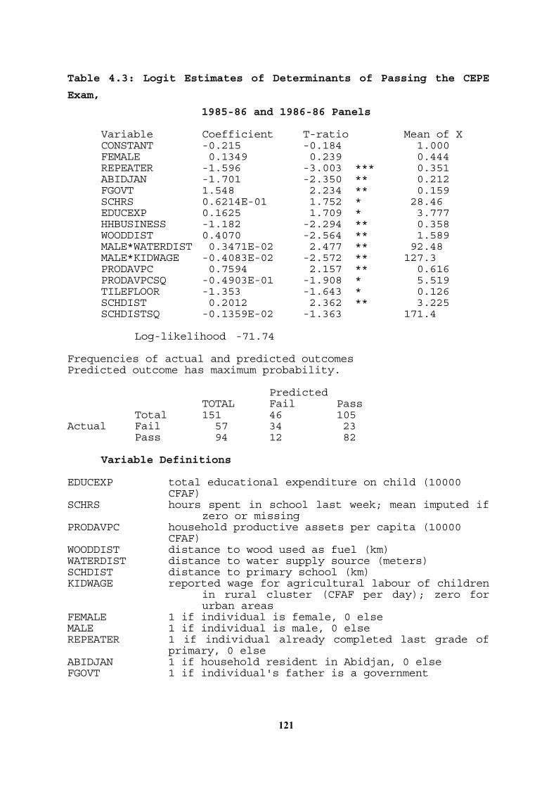
121

Table 4.3: Logit Estimates of Determinants of Passing the CEPE

Exam,

1985-86 and 1986-86 Panels Variable Coefficient T-ratio Mean of X CONSTANT -0.215 -0.184 1.000 FEMALE 0.1349 0.239 0.444 REPEATER -1.596 -3.003 *** 0.351 ABIDJAN -1.701 -2.350 ** 0.212 FGOVT 1.548 2.234 ** 0.159 SCHRS 0.6214E-01 1.752 * 28.46 EDUCEXP 0.1625 1.709 * 3.777 HHBUSINESS -1.182 -2.294 ** 0.358 WOODDIST 0.4070 -2.564 ** 1.589 MALE*WATERDIST 0.3471E-02 2.477 ** 92.48 MALE*KIDWAGE -0.4083E-02 -2.572 ** 127.3 PRODAVPC 0.7594 2.157 ** 0.616 PRODAVPCSQ -0.4903E-01 -1.908 * 5.519 TILEFLOOR -1.353 -1.643 * 0.126 SCHDIST 0.2012 2.362 ** 3.225 SCHDISTSQ -0.1359E-02 -1.363 171.4 Log-likelihood -71.74 Frequencies of actual and predicted outcomes Predicted outcome has maximum probability. Predicted TOTAL Fail Pass Total 151 46 105 Actual Fail 57 34 23 Pass 94 12 82 Variable Definitions EDUCEXP total educational expenditure on child (10000 CFAF) SCHRS hours spent in school last week; mean imputed if

zero or missing PRODAVPC household productive assets per capita (10000 CFAF) WOODDIST distance to wood used as fuel (km) WATERDIST distance to water supply source (meters) SCHDIST distance to primary school (km) KIDWAGE reported wage for agricultural labour of children

in rural cluster (CFAF per day); zero for urban areas

FEMALE 1 if individual is female, 0 else MALE 1 if individual is male, 0 else REPEATER 1 if individual already completed last grade of primary, 0 else ABIDJAN 1 if household resident in Abidjan, 0 else FGOVT 1 if individual's father is a government

122

employee, 0 else HHBUSINESS 1 if household runs its own (non-agricultural) enterprise, 0 else TILEFLOOR 1 if house has a tiled floor, 0 else

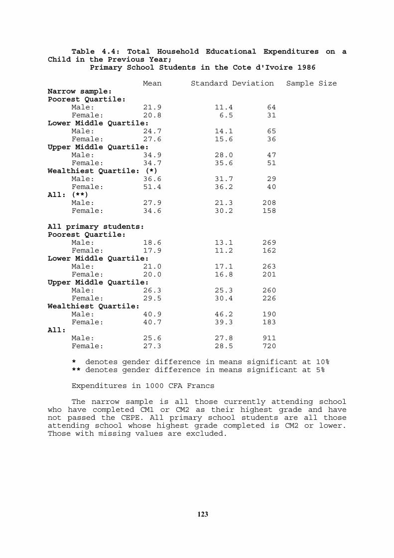
123

Table 4.4: Total Household Educational Expenditures on a Child in the Previous Year; Primary School Students in the Cote d'Ivoire 1986 Mean Standard Deviation Sample Size Narrow sample: Poorest Quartile: Male: 21.9 11.4 64 Female: 20.8 6.5 31 Lower Middle Quartile: Male: 24.7 14.1 65 Female: 27.6 15.6 36 Upper Middle Quartile: Male: 34.9 28.0 47 Female: 34.7 35.6 51 Wealthiest Quartile: (*) Male: 36.6 31.7 29 Female: 51.4 36.2 40 All: (**) Male: 27.9 21.3 208 Female: 34.6 30.2 158 All primary students: Poorest Quartile: Male: 18.6 13.1 269 Female: 17.9 11.2 162 Lower Middle Quartile: Male: 21.0 17.1 263 Female: 20.0 16.8 201 Upper Middle Quartile: Male: 26.3 25.3 260 Female: 29.5 30.4 226 Wealthiest Quartile: Male: 40.9 46.2 190 Female: 40.7 39.3 183 All: Male: 25.6 27.8 911 Female: 27.3 28.5 720 * denotes gender difference in means significant at 10% ** denotes gender difference in means significant at 5% Expenditures in 1000 CFA Francs The narrow sample is all those currently attending school who have completed CM1 or CM2 as their highest grade and have not passed the CEPE. All primary school students are all those attending school whose highest grade completed is CM2 or lower. Those with missing values are excluded.

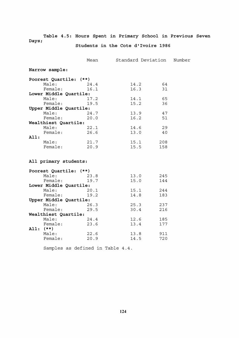
124

Table 4.5: Hours Spent in Primary School in Previous Seven Days; Students in the Cote d'Ivoire 1986 Mean Standard Deviation Number Narrow sample: Poorest Quartile: (**) Male: 24.4 14.2 64 Female: 16.1 16.3 31 Lower Middle Quartile: Male: 17.2 14.1 65 Female: 19.5 15.2 36 Upper Middle Quartile: Male: 24.7 13.9 47 Female: 20.0 16.2 51 Wealthiest Quartile: Male: 22.1 14.6 29 Female: 26.6 13.0 40 All: Male: 21.7 15.1 208 Female: 20.9 15.5 158 All primary students: Poorest Quartile: (**) Male: 23.8 13.0 245 Female: 19.7 15.0 144 Lower Middle Quartile: Male: 20.1 15.1 244 Female: 19.2 14.8 183 Upper Middle Quartile: Male: 26.3 25.3 237 Female: 29.5 30.4 216 Wealthiest Quartile: Male: 24.4 12.6 185 Female: 23.6 13.4 177 All: (**) Male: 22.6 13.8 911 Female: 20.9 14.5 720 Samples as defined in Table 4.4.

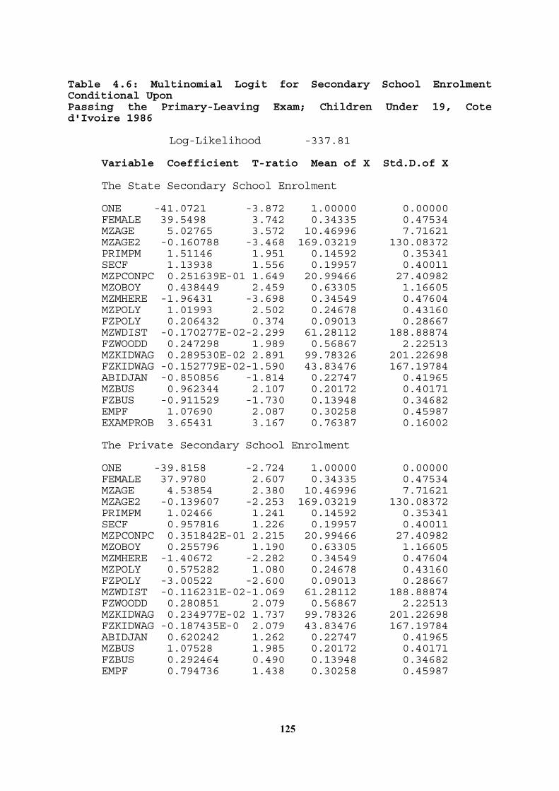
125

Table 4.6: Multinomial Logit for Secondary School Enrolment Conditional Upon Passing the Primary-Leaving Exam; Children Under 19, Cote d'Ivoire 1986 Log-Likelihood -337.81 Variable Coefficient T-ratio Mean of X Std.D.of X The State Secondary School Enrolment ONE -41.0721 -3.872 1.00000 0.00000 FEMALE 39.5498 3.742 0.34335 0.47534 MZAGE 5.02765 3.572 10.46996 7.71621 MZAGE2 -0.160788 -3.468 169.03219 130.08372 PRIMPM 1.51146 1.951 0.14592 0.35341 SECF 1.13938 1.556 0.19957 0.40011 MZPCONPC 0.251639E-01 1.649 20.99466 27.40982 MZOBOY 0.438449 2.459 0.63305 1.16605 MZMHERE -1.96431 -3.698 0.34549 0.47604 MZPOLY 1.01993 2.502 0.24678 0.43160 FZPOLY 0.206432 0.374 0.09013 0.28667 MZWDIST -0.170277E-02-2.299 61.28112 188.88874 FZWOODD 0.247298 1.989 0.56867 2.22513 MZKIDWAG 0.289530E-02 2.891 99.78326 201.22698 FZKIDWAG -0.152779E-02-1.590 43.83476 167.19784 ABIDJAN -0.850856 -1.814 0.22747 0.41965 MZBUS 0.962344 2.107 0.20172 0.40171 FZBUS -0.911529 -1.730 0.13948 0.34682 EMPF 1.07690 2.087 0.30258 0.45987 EXAMPROB 3.65431 3.167 0.76387 0.16002 The Private Secondary School Enrolment ONE -39.8158 -2.724 1.00000 0.00000 FEMALE 37.9780 2.607 0.34335 0.47534 MZAGE 4.53854 2.380 10.46996 7.71621 MZAGE2 -0.139607 -2.253 169.03219 130.08372 PRIMPM 1.02466 1.241 0.14592 0.35341 SECF 0.957816 1.226 0.19957 0.40011 MZPCONPC 0.351842E-01 2.215 20.99466 27.40982 MZOBOY 0.255796 1.190 0.63305 1.16605 MZMHERE -1.40672 -2.282 0.34549 0.47604 MZPOLY 0.575282 1.080 0.24678 0.43160 FZPOLY -3.00522 -2.600 0.09013 0.28667 MZWDIST -0.116231E-02-1.069 61.28112 188.88874 FZWOODD 0.280851 2.079 0.56867 2.22513 MZKIDWAG 0.234977E-02 1.737 99.78326 201.22698 FZKIDWAG -0.187435E-0 2.079 43.83476 167.19784 ABIDJAN 0.620242 1.262 0.22747 0.41965 MZBUS 1.07528 1.985 0.20172 0.40171 FZBUS 0.292464 0.490 0.13948 0.34682 EMPF 0.794736 1.438 0.30258 0.45987

126

EXAMPROB 2.53706 1.898 0.76387 0.16002

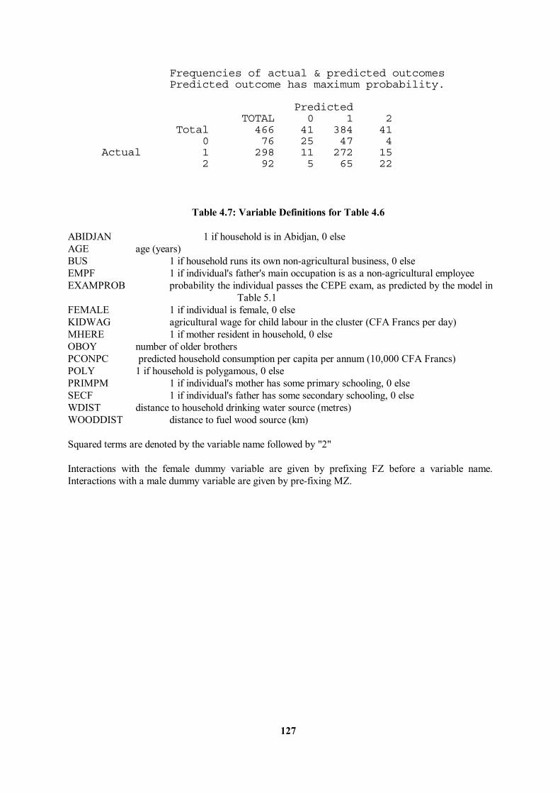
127

Frequencies of actual & predicted outcomes Predicted outcome has maximum probability. Predicted TOTAL 0 1 2 Total 466 41 384 41 0 76 25 47 4 Actual 1 298 11 272 15 2 92 5 65 22 Table 4.7: Variable Definitions for Table 4.6 ABIDJAN 1 if household is in Abidjan, 0 else AGE age (years) BUS 1 if household runs its own non-agricultural business, 0 else EMPF 1 if individual's father's main occupation is as a non-agricultural employee EXAMPROB probability the individual passes the CEPE exam, as predicted by the model in

Table 5.1 FEMALE 1 if individual is female, 0 else KIDWAG agricultural wage for child labour in the cluster (CFA Francs per day) MHERE 1 if mother resident in household, 0 else OBOY number of older brothers PCONPC predicted household consumption per capita per annum (10,000 CFA Francs) POLY 1 if household is polygamous, 0 else PRIMPM 1 if individual's mother has some primary schooling, 0 else SECF 1 if individual's father has some secondary schooling, 0 else WDIST distance to household drinking water source (metres) WOODDIST distance to fuel wood source (km) Squared terms are denoted by the variable name followed by "2" Interactions with the female dummy variable are given by prefixing FZ before a variable name. Interactions with a male dummy variable are given by pre-fixing MZ.

128

Table 5.1: Variables Used in the Kenyan Mixture Model INCPC household income per annum per capita. Measured in Kenyan shillings but deflated by 10,000 ENROL gender specific national gross secondary school enrolment ratio in the year when the

individual was 15. Measures secondary school students of own gender as a percentage of those of own gender aged 12-17.

FENROL equal to ENROL if individual is female, else equal to 0 POG percentage of others from the same cluster and in subsample used for this analysis who

have entered state secondary school. POH percentage of others from the same cluster, in the subsample used for this analysis and

who have not entered state secondary school, who have entered Harambee school.

AGEW(SQ) age and age squared of youngest wife of household head at the time the individual was

15 and adjusted so that those ages over 50 are treat as 50 BIRTH(SQ) birth order and birth order squared of individual The following are nought-one dummy variables which equal one if: FEMALE if individual is female DADSTD1 if father has attained Standard 1 or higher DADSTD5 if father has attained Standard 5 or higher DADSTD7 if father has attained Standard 7 or higher DADSTD8 if father has attained Standard 8 or higher DADSEC if father has attained secondary schooling or higher MUMSTD1 if eldest wife of household head has attained Standard 1 or higher MUMSTD3 if eldest wife of household head has attained Standard 3 or higher MUMSTD4 if eldest wife of household head has attained Standard 4 or higher

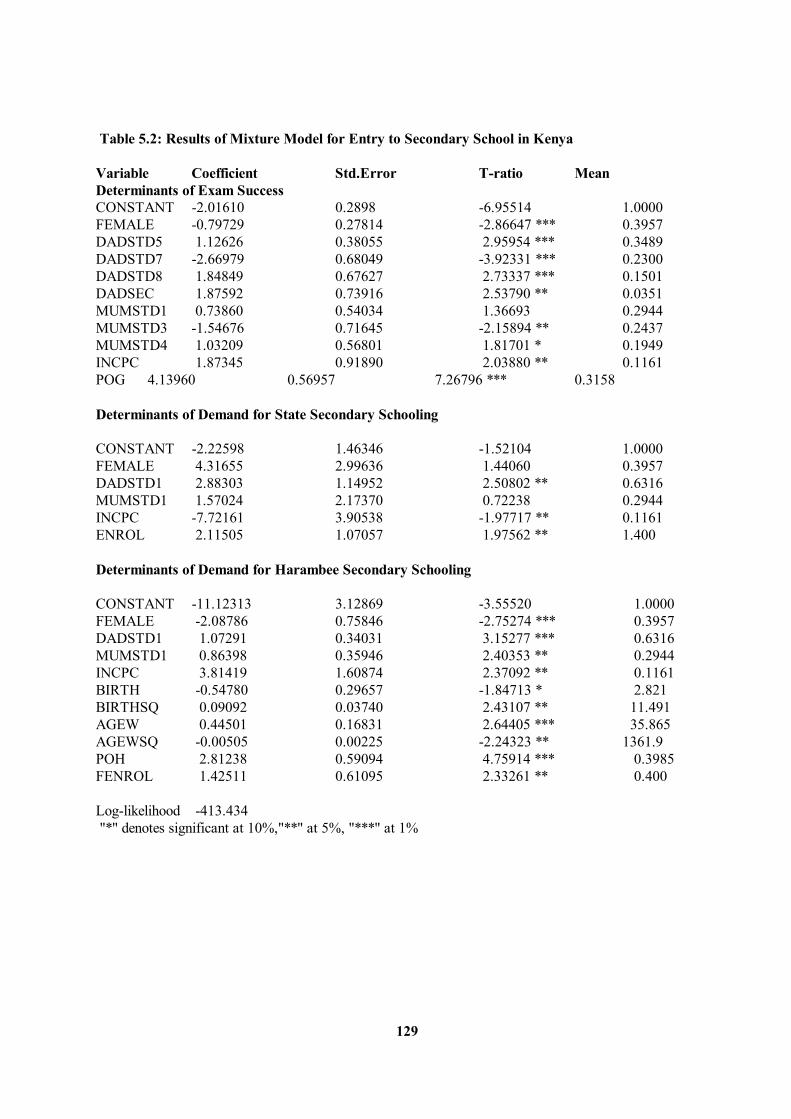
129

Table 5.2: Results of Mixture Model for Entry to Secondary School in Kenya Variable Coefficient Std.Error T-ratio Mean Determinants of Exam Success CONSTANT -2.01610 0.2898 -6.95514 1.0000 FEMALE -0.79729 0.27814 -2.86647 *** 0.3957 DADSTD5 1.12626 0.38055 2.95954 *** 0.3489 DADSTD7 -2.66979 0.68049 -3.92331 *** 0.2300 DADSTD8 1.84849 0.67627 2.73337 *** 0.1501 DADSEC 1.87592 0.73916 2.53790 ** 0.0351 MUMSTD1 0.73860 0.54034 1.36693 0.2944 MUMSTD3 -1.54676 0.71645 -2.15894 ** 0.2437 MUMSTD4 1.03209 0.56801 1.81701 * 0.1949 INCPC 1.87345 0.91890 2.03880 ** 0.1161 POG 4.13960 0.56957 7.26796 *** 0.3158 Determinants of Demand for State Secondary Schooling CONSTANT -2.22598 1.46346 -1.52104 1.0000 FEMALE 4.31655 2.99636 1.44060 0.3957 DADSTD1 2.88303 1.14952 2.50802 ** 0.6316 MUMSTD1 1.57024 2.17370 0.72238 0.2944 INCPC -7.72161 3.90538 -1.97717 ** 0.1161 ENROL 2.11505 1.07057 1.97562 ** 1.400 Determinants of Demand for Harambee Secondary Schooling CONSTANT -11.12313 3.12869 -3.55520 1.0000 FEMALE -2.08786 0.75846 -2.75274 *** 0.3957 DADSTD1 1.07291 0.34031 3.15277 *** 0.6316 MUMSTD1 0.86398 0.35946 2.40353 ** 0.2944 INCPC 3.81419 1.60874 2.37092 ** 0.1161 BIRTH -0.54780 0.29657 -1.84713 * 2.821 BIRTHSQ 0.09092 0.03740 2.43107 ** 11.491 AGEW 0.44501 0.16831 2.64405 *** 35.865 AGEWSQ -0.00505 0.00225 -2.24323 ** 1361.9 POH 2.81238 0.59094 4.75914 *** 0.3985 FENROL 1.42511 0.61095 2.33261 ** 0.400 Log-likelihood -413.434 "*" denotes significant at 10%,"**" at 5%, "***" at 1%

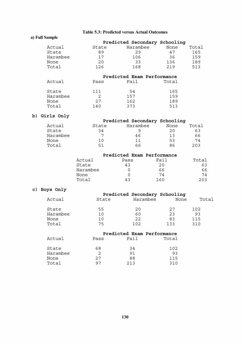
130

Table 5.3: Predicted versus Actual Outcomes a) Full Sample Predicted Secondary Schooling Actual State Harambee None Total State 89 29 47 165 Harambee 17 106 36 159 None 20 33 136 189 Total 126 168 219 513 Predicted Exam Performance Actual Pass Fail Total State 111 54 165 Harambee 2 157 159 None 27 162 189 Total 140 373 513 b) Girls Only Predicted Secondary Schooling Actual State Harambee None Total State 34 9 20 63 Harambee 7 46 13 66 None 10 11 53 74 Total 51 66 86 203 Predicted Exam Performance Actual Pass Fail Total State 43 20 63 Harambee 0 66 66 None 0 74 74 Total 43 160 203 c) Boys Only Predicted Secondary Schooling Actual State Harambee None Total State 55 20 27 102 Harambee 10 60 23 93 None 10 22 83 115 Total 75 102 133 310 Predicted Exam Performance Actual Pass Fail Total State 68 34 102 Harambee 2 91 93 None 27 88 115 Total 97 213 310

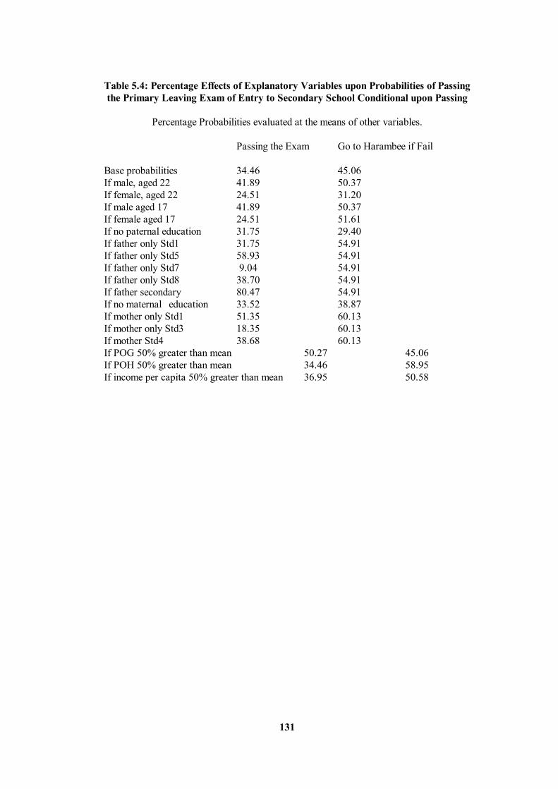
131

Table 5.4: Percentage Effects of Explanatory Variables upon Probabilities of Passing the Primary Leaving Exam of Entry to Secondary School Conditional upon Passing Percentage Probabilities evaluated at the means of other variables. Passing the Exam Go to Harambee if Fail Base probabilities 34.46 45.06 If male, aged 22 41.89 50.37 If female, aged 22 24.51 31.20 If male aged 17 41.89 50.37 If female aged 17 24.51 51.61 If no paternal education 31.75 29.40 If father only Std1 31.75 54.91 If father only Std5 58.93 54.91 If father only Std7 9.04 54.91 If father only Std8 38.70 54.91 If father secondary 80.47 54.91 If no maternal education 33.52 38.87 If mother only Std1 51.35 60.13 If mother only Std3 18.35 60.13 If mother Std4 38.68 60.13 If POG 50% greater than mean 50.27 45.06 If POH 50% greater than mean 34.46 58.95 If income per capita 50% greater than mean 36.95 50.58

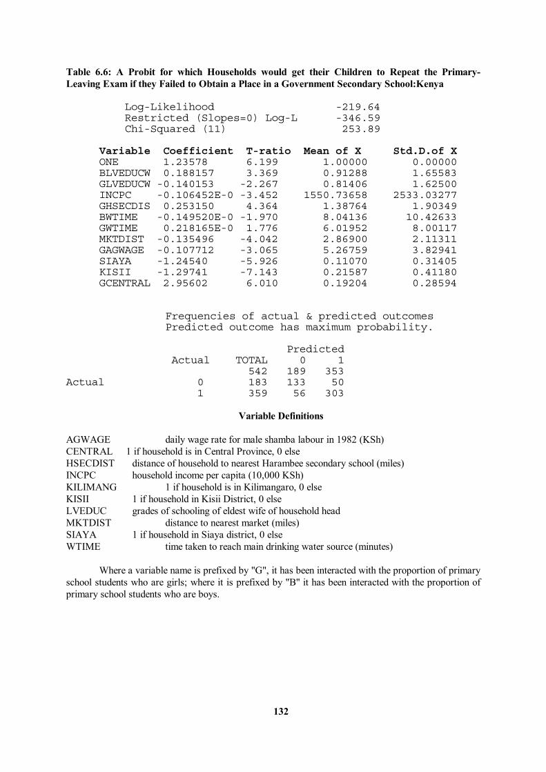
132

Table 6.6: A Probit for which Households would get their Children to Repeat the Primary-Leaving Exam if they Failed to Obtain a Place in a Government Secondary School:Kenya Log-Likelihood -219.64 Restricted (Slopes=0) Log-L -346.59 Chi-Squared (11) 253.89 Variable Coefficient T-ratio Mean of X Std.D.of X ONE 1.23578 6.199 1.00000 0.00000 BLVEDUCW 0.188157 3.369 0.91288 1.65583 GLVEDUCW -0.140153 -2.267 0.81406 1.62500 INCPC -0.106452E-0 -3.452 1550.73658 2533.03277 GHSECDIS 0.253150 4.364 1.38764 1.90349 BWTIME -0.149520E-0 -1.970 8.04136 10.42633 GWTIME 0.218165E-0 1.776 6.01952 8.00117 MKTDIST -0.135496 -4.042 2.86900 2.11311 GAGWAGE -0.107712 -3.065 5.26759 3.82941 SIAYA -1.24540 -5.926 0.11070 0.31405 KISII -1.29741 -7.143 0.21587 0.41180 GCENTRAL 2.95602 6.010 0.19204 0.28594 Frequencies of actual & predicted outcomes Predicted outcome has maximum probability. Predicted Actual TOTAL 0 1 542 189 353 Actual 0 183 133 50 1 359 56 303 Variable Definitions AGWAGE daily wage rate for male shamba labour in 1982 (KSh) CENTRAL 1 if household is in Central Province, 0 else HSECDIST distance of household to nearest Harambee secondary school (miles) INCPC household income per capita (10,000 KSh) KILIMANG 1 if household is in Kilimangaro, 0 else KISII 1 if household in Kisii District, 0 else LVEDUC grades of schooling of eldest wife of household head MKTDIST distance to nearest market (miles) SIAYA 1 if household in Siaya district, 0 else WTIME time taken to reach main drinking water source (minutes) Where a variable name is prefixed by "G", it has been interacted with the proportion of primary school students who are girls; where it is prefixed by "B" it has been interacted with the proportion of primary school students who are boys.

133

Chapter 3: Health

1 Introduction 2 Modelling Health Care and Health Outcomes a.A Household Production Model of Health Care and Health Outcomes b.The Determinants of the Demand for Health Care and Health Outcomes c. Econometric Specification 3 The Incidence of Illness a. Descriptive Statistics b. Econometric Results 4 The Demand for Health Care a. Descriptive Statistics b. Econometric Results 5 The Duration of Illness aa. Descriptive Statistics b. Econometric Results 6 Summary and Conclusions Appendices: 1An Endogenous Dummy Variable Model of the Effect of Treatment upon the Duration of Illness 2Correcting for Morbidity Selectivity; an Application to Kenya

134

1 Introduction This chapter analyses survey data on self-reported morbidity and the use of health facilities in Kenya, Tanzania and the Cote d'Ivoire84. It focuses on three main questions: what determines who falls ill? what determines who seeks treatment when ill? and what determines the duration of illness amongst those who fall ill? These questions raise a number of issues concerning gender and public policy. When considering who seeks treatment when ill, an immediate question concerns gender differences: are girls less likely to be sent for treatment than boys? A further issue is how gender differences vary with factors amenable to policy such as the availability of health facilities and the distribution of income. Of particular interest is the interaction with education. This has two possible gender aspects: is female (especially maternal) education particularly important in affecting take-up of health services by household members? and does education have gender specific effects; for example does maternal education affect girls in particular and paternal education affect boys? Turning to health outcomes, we consider the relative effect of health, education and piped water upon health outcomes. Testing the effectiveness of health services is one reason why we make a distinction between the incidence of illness and the duration of any one bout of illness. We observe whether people seek medical treatment when ill and can use this as a determinant of the duration of illness but not of the incidence of illness. Investigating the effect of treatment upon the duration of illness poses an econometric problem because one might expect those seeking treatment to have more serious illnesses and, to the extent that the surveys do not measure the seriousness of illness, this will downwardly bias an ordinary least squares estimate of the effectiveness of treatment in reducing the duration of illness. We attempt to control for this by using the results of our models of who seeks treatment. The chapter begins with a discussion of the hypothesised determinants of the demand for health care and of health outcomes. Our findings are presented in three sections. The first looks at the incidence of illness, the second at the use of treatment and the third at the duration of illness. In each case, we start by presenting some descriptive statistics and then proceed to report the estimates of our econometric models. Our results are based on data from the 1982 World Bank survey of Central and Nyanza provinces of Kenya; the 1983 World Bank survey of Tanzania; and the 1986 Living Standards and Measurement survey (LSMS) of the Cote d'Ivoire. We divide these surveys into eight subsamples: these are based upon the three countries with the added separation of Cote d'Ivoire into rural and urban areas; for each geographical entity, we separate adults from children. The urban-rural distinction was made because well-measured variables for travel time to health facilities were only available for rural

84 The self-reported nature of the data is a serious limitation. One cannot be sure that differential self-reported health status reflects differences in actual health or merely different propensities to report a given health state as ill health. In what follows, self-reported illness is generally equated with actual illness on the grounds that the former does provide some evidence of the latter. However, in some cases inferring actual illness from self-reported illness may be unjustified: see the discussion of the effects of parental education on the incidence of child illness.

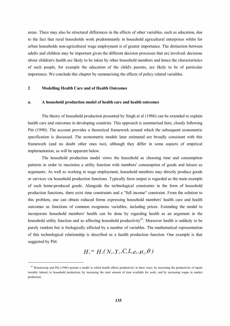
135

areas. There may also be structural differences in the effects of other variables, such as education, due to the fact that rural households work predominantly in household agricultural enterprises whilst for urban households non-agricultural wage employment is of greater importance. The distinction between adults and children may be important given the different decision processes that are involved: decisions about children's health are likely to be taken by other household members and hence the characteristics of such people, for example the education of the child's parents, are likely to be of particular importance. We conclude this chapter by summarising the effects of policy related variables.

2 Modelling Health Care and of Health Outcomes a. A household production model of health care and health outcomes The theory of household production presented by Singh et al (1986) can be extended to explain health care and outcomes in developing countries. This approach is summarised here, closely following Pitt (1990). The account provides a theoretical framework around which the subsequent econometric specification is discussed. The econometric models later estimated are broadly consistent with this framework (and no doubt other ones too), although they differ in some aspects of empirical implementation, as will be apparent below. The household production model views the household as choosing time and consumption patterns in order to maximise a utility function with members' consumption of goods and leisure as arguments. As well as working in wage employment, household members may directly produce goods or services via household production functions. Typically farm output is regarded as the main example of such home-produced goods. Alongside the technological constraints in the form of household production functions, there exist time constraints and a "full income" constraint. From the solution to this problem, one can obtain reduced forms expressing household members' health care and health outcomes as functions of common exogenous variables, including prices. Extending the model to incorporate household members' health can be done by regarding health as an argument in the household utility function and as affecting household productivity85. Moreover health is unlikely to be purely random but is biologically affected by a number of variables. The mathematical representation of this technological relationship is described as a health production function. One example is that suggested by Pitt:

85 Rosenzweig and Pitt (1986) present a model in which health affects productivity in three ways: by increasing the productivity of inputs (notably labour) to household production; by increasing the total amount of time available for work; and by increasing wages in market production.

),,eL,C,,Y,N(H=H iiiiii θμ

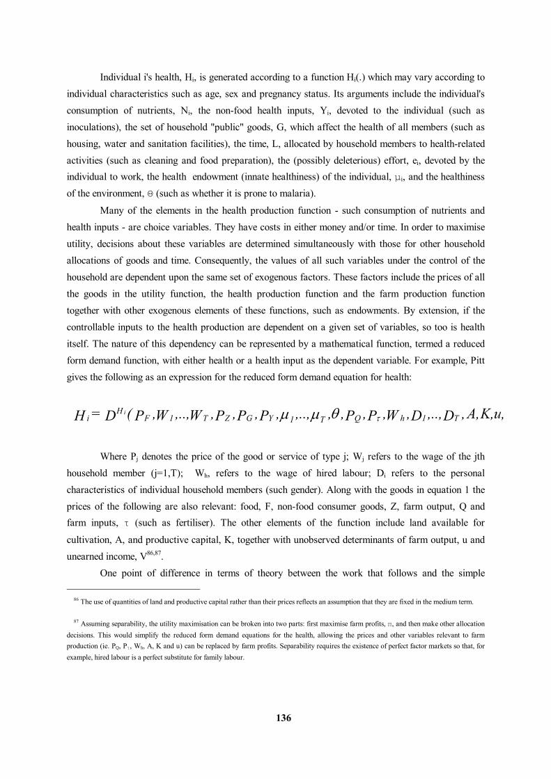
136

Individual i's health, Hi, is generated according to a function Hi(.) which may vary according to individual characteristics such as age, sex and pregnancy status. Its arguments include the individual's consumption of nutrients, Ni, the non-food health inputs, Yi, devoted to the individual (such as inoculations), the set of household "public" goods, G, which affect the health of all members (such as housing, water and sanitation facilities), the time, L, allocated by household members to health-related activities (such as cleaning and food preparation), the (possibly deleterious) effort, ei, devoted by the individual to work, the health endowment (innate healthiness) of the individual, μi, and the healthiness of the environment, Θ (such as whether it is prone to malaria).

Many of the elements in the health production function - such consumption of nutrients and health inputs - are choice variables. They have costs in either money and/or time. In order to maximise utility, decisions about these variables are determined simultaneously with those for other household allocations of goods and time. Consequently, the values of all such variables under the control of the household are dependent upon the same set of exogenous factors. These factors include the prices of all the goods in the utility function, the health production function and the farm production function together with other exogenous elements of these functions, such as endowments. By extension, if the controllable inputs to the health production are dependent on a given set of variables, so too is health itself. The nature of this dependency can be represented by a mathematical function, termed a reduced form demand function, with either health or a health input as the dependent variable. For example, Pitt gives the following as an expression for the reduced form demand equation for health:

Where Pj denotes the price of the good or service of type j; Wj refers to the wage of the jth household member (j=1,T); Wh, refers to the wage of hired labour; Di refers to the personal characteristics of individual household members (such gender). Along with the goods in equation 1 the prices of the following are also relevant: food, F, non-food consumer goods, Z, farm output, Q and farm inputs, τ (such as fertiliser). The other elements of the function include land available for

cultivation, A, and productive capital, K, together with unobserved determinants of farm output, u and unearned income, V86,87. One point of difference in terms of theory between the work that follows and the simple 86 The use of quantities of land and productive capital rather than their prices reflects an assumption that they are fixed in the medium term.

87 Assuming separability, the utility maximisation can be broken into two parts: first maximise farm profits, π, and then make other allocation decisions. This would simplify the reduced form demand equations for the health, allowing the prices and other variables relevant to farm production (ie. PQ, Pτ, Wh, A, K and u) can be replaced by farm profits. Separability requires the existence of perfect factor markets so that, for example, hired labour is a perfect substitute for family labour.

u,K,A,,D,..,D,W,P,P,,,..,,P,P,P,W,..,W,P(D=H T1hQT1YGZT1FH

ii

τθμμ

137

framework outlined above regards the assumption of a single household utility function. Haddad and Hoddinott (1991) argue that household decisions may be characterised as the outcome of a bargaining process between members with diverse preferences88. One implication of this, which is apparent from social choice theory, is that household behaviour might not be consistent with a well-defined household objective function. However, even if it were, individuals' bargaining power is likely to vary with observables. This implies that the weights on individual utilities in any collectively decided household objective function will also vary with observables and thus provide another route by which exogenous variables may affect outcomes. Estimation of a health production function such as that in equation 1 was not attempted due to the lack of data on individual food consumption89. Instead demand equations similar to equation 2 were estimated. As will be explained, our models are not pure reduced forms, since we attempt to uncover a number of structural parameters of interest - notably the effect of health care upon health outcomes. However, most of the explanatory variables used are empirical counterparts to the reduced form determinants of health care and health outcomes identified in equation 2. Consequently, section b presents a description of these variables.

b The determinants of the demand for health care and health outcomes The reduced form demand function in equation 2 suggests the following determinants of health care and health outcomes: 1. Prices of consumer goods, PF and PZ. Unfortunately, price data was not available for most clusters. Only for rural Cote d'Ivoire was a survey of prices in each cluster carried out. This price data was not used as it appeared neither "clean" nor complete. 2. Wage rates, W. For rural sample, basic agricultural wages in the cluster were reported. For rural Cote d'Ivoire, these were disaggregated into those for men, for women and for children. For urban Cote d'Ivoire, no such information was available and conceptually it is not clear that a single wage rate is relevant to all those in the labour force. Instead, wages are likely to be endogenous, depending on education and experience. Furthermore, it is hard to think of instruments which can identify the effect of wages upon

88 Hoddinott and Haddad (1991) is Chapter 7 of the present work.

89Time spent on health-related activities and effort expended at work are also unobserved. Pit and Rosenzweig (1986) overcome the absence of information on individual food consumption by estimating a household health production function. However, this was not attempted here. Total food consumption was not observed for Kenya and Tanzania. Moreover, the approach does not reveal much about the intra-household issues which are an important focus of the current work.

138

household demands - for example, education and age may both have effects that are not via wages. Consequently, for urban areas, directly entering age measures and education should control for wage effects but will not be easily interpretable as such. To a lesser extent, age and education may also reflect wage effects in rural households. In the absence of separability, the shadow price of time for those household members not participating in wage employment will not necessarily be equal to local wages. Appropriate shadow wages will vary with many household characteristics, but particularly important a priori would seem to be whether households operate their own enterprises, either agricultural or non-agricultural. For example, it might be easier for children to work in such activities than outside the household. Consequently, a dummy variable for whether households operated their own small holding was used as a determinant in the Cote d'Ivoire90. These variables were observed only for the Cote d'Ivoire. 3. Price of health inputs, PY. In common with most other studies, a pecuniary price of health care was not obtainable. In the Cote d'Ivoire, this is unproblematic because treatment is provided free by the state. In Kenya and Tanzania there are user fees but these are not very large, being of a similar order of magnitude to the direct monetary costs of travelling to seek treatment (Bevan, Collier and Gunning, 1989). There was no community or provider survey information such fees and it is not clear to what extent the fees for a given course of treatment would vary by cluster. The only data available was from those who sought treatment and using this to construct a measure of cluster-specific costs is likely to provide a very poor proxy. This is because of the small numbers receiving treatment in each cluster; the likelihood that fees vary markedly with the specific type of treatment received; and because of the sample selectivity of the data. Instead, the proxy used for the "price" of health care was the distance of the nearest health facility to the household91. Time costs are likely to be a major part of the cost of seeking treatment and differences due to travel time are likely to be the an important source of variability in expected costs of seeking treatment. For rural Cote d'Ivoire this was measured as the travel time to the nearest health centre or hospital reported in the community questionnaire92,93. For Kenya, the distance to the nearest 90 In rural Kenya and Tanzania all households operated their own shamba (small holding). In Cote d'Ivoire operating a small holding was not perfectly correlated with rural residence: 4.7% of rural households did not do so whilst 21.9% of urban ones did.

91 An important assumption is that the location of health facilities is exogenous. This would be violated if governments allocate health facilities in response to the local health environment - for example, placing them in areas of greatest need (Rosenzweig and Wolpin 1986). Another, perhaps less plausible, source of endogeneity would be if individuals' migration was sensitive to the location of health facilities (Rosenzweig and Wolpin 1989).

92An attempt was made to give travel time a value as an economic cost in rural Cote d'Ivoire by multiplying it by the wage for agricultural labour reported for an individual's cluster in the community questionnaire. However, when entered jointly with the travel time itself (the latter capturing "psychic discomfort" as opposed to economic cost) the wage-time interaction had perverse effects. These may reflect clusters with high wage rates also having better health facilities.

139

dispensary or hospital, as reported in the household questionnaire, was used. For Tanzania and for urban Cote d'Ivoire, no questions were asked about proximity to the nearest health facility. Consequently, such information was inferred from that provided by users of health facilities. In Tanzania, those who were patients in a hospital during the year prior to the survey were asked how far the hospital was from their home. Consequently, for each cluster, the minimum distance given in these responses was identified and entered as an explanatory variable. For urban Cote d'Ivoire, the travel time for those seeking consultations was known and cluster averages of this information used as an explanatory variable94. 4. The price of household public goods, PG. These were unobserved so, following Pitt (1990), the actual existence of the goods was entered as determinants rather than their prices. This may impart some endogeneity bias, although this should be moderated by the fact that the decision to acquire such goods is likely to have been taken long before the period during which health behaviour is analyzed. The particular goods included were water sources and mode of disposal of human waste95. The Kenyan and Tanzanian surveys classified drinking water sources into ten categories. Most households received their drinking water from a stream, so this was taken as the default with a series of dummy variables being entered for other water supply sources. Other classification of drinking water sources were: still ponds; small dams; springs; rainwater; wells; boreholes; communal piped water; and taps in houses96. For Cote d'Ivoire, the classification of drinking water sources was different. Piped water was not separated into private and communal, whilst the other categories were: well with pipe, well without pipe; water vendor or water truck; and water from a river. Human waste disposal was separated into flush toilets, pit latrines and other methods. 5. The personal characteristics of household members, D1,...DT. As suggested in equation 1, an individual's age and sex may have pervasive effects on the nature of the relation between an their health and its determinants. These effects may not be adequately 93 Travel time rather than distance seems the more relevant measure of availability but was only available for Cote d'Ivoire.

94 Cluster averages were used for urban areas, because the travel times were rather small with frequent minima of zero. Consequently, minimum travel times were thought more likely to reflect intra-cluster differences in travel time and average travel time seemed a more appropriate measure of "typical" travel time. For rural Tanzania, variations in distances more obviously reflected variations in distance to facilities visited than in differences in the distance of households to a given facility, so cluster minima were used.

95 There are other household health-related public goods: for example, Pitt refers to housing quality; one could also include refrigeration and disposal of non-human waste. These were not observed for Kenya and Tanzania. For Cote d'Ivoire, we did not isolate these elements because unlike water and sewage, they are less likely to be the subject of targeted government intervention and could instead be regarded, like food consumption, as one means through which overall household income affects health.

96For Kenya and Tanzania, both dry season and wet season water sources were used. Kenya was surveyed in October and December, so the three months prior to the surveys covers part of the period of the short rains; hence wet season drinking water sources were employed. Tanzania was surveyed in September, which is part of the dry season, so dry season water sources were used for that country.

140

be reflected by simply using age and gender as exogenous variables, since they may involve interactions with other variables. The distinction between adults and children seems important since in addition to differences in capabilities, there are also likely to be different decision processes involved, with parents taking decisions on behalf of their children. For this reason, all models were estimated separately for adults and children97. Allowing for differences between males and females is important given the focus of this project. However, it is of particular interest to test if the coefficients on explanatory variables differ significantly between males and females. Consequently, the models were initially estimated on a pooled sample of males and females together with a full set of gender interactions98. Then gender interactions which were insignificant and of no particular interest were excluded. Equation 2 suggests that as well as including age and sex characteristics of the individual for whom health or treatment is observed, the age and sex of other household members should also be included. These are represented by variables for household demographics: total household size together with the proportions of children under 6, the proportions of children aged 6 to 15 and the proportion of female adults99. The head of household and their (eldest) spouse may be of particular importance, so their age and gender were included. Pitt also suggests the inclusion of education amongst other personal characteristics. In fact, the potential health-benefits of education are perhaps understated in Pitt's account, only having an impact via wages. More generally education may induce changes in knowledge, attitudes and practices that enhance the efficiency of household health related activities, T, in health production function. Furthermore, education may affect the nature of the household objective function, either by changing preferences or altering bargaining power. To allow for these effects in samples of adults, the education of individual being analyzed was included together with that of the head of household and their (eldest) spouse. For samples of children, the education of their parents was included100,101. An individual's relationship to household head was thought to be a relevant characteristic for a

97 Children are defined as being under 16.

98This procedure gives identical results to estimating the models separately on male and female subsamples.

99 This assumes that family size is exogenous. For a defence of this assumption see the Appendix to Chapter 5.

100 For Kenya and Tanzania, parentage was not known. Hence paternal education was proxied by the education of the male head and maternal education by the education of the "senior female" (ie female head or eldest wife of the head). This will be reliable in the case of sons and daughters of non-polygamous household heads. For brevity, measures as "paternal education" and "maternal education", using quotation marks as reminders that they are imperfect measures.

101The education of children may be jointly determined with health. In fact, due to the late ages of those in secondary school, a number of adults within the sample may also still be at school. Furthermore, Behrman (1990b) notes that adult education may not be exogenous either because the household adopts a life-cycle perspective in its decisions or for other reasons, such as bias from omitted variables such as "innate ability".

141

number of reasons. For Kenya and Tanzania, it may be relevant since a single household respondent - typically the head - provides the information on the health care and health outcomes of all household members. This information may be systematically biased if the head's recall of others' condition varies according to the relationship between them. Including measures of this relationship may correct for this bias. A related but more fundamental reason for including such measures is that relationship to the head may affect the intra-household allocation. Genetic closeness of individuals to the head might affect the weight the placed on their utility by the head, whose opinions may be particularly important in household decision-making. Dummy variables for the following relationships to the household head were entered: son; daughter; wife; and other relative/non-relative102. Marital status was entered as an individual characteristic, available only for the Cote d'Ivoire. As Pitt notes, the health production function is likely to vary according to whether a woman is pregnant, lactating or neither. Two other individual characteristics - nationality and religion - were observed in the CILSS and were included to control for cultural differences in preferences and possibly other things (such as labour market discrimination). 6. Farm profits, π, (or their determinants) and unearned income, V.

For Kenya and Tanzania, creating estimates of farm profits would have been time consuming and for this reason, together with questionable nature of the separability assumption, it was decided to enter measures of household land, A, and productive capital, K, directly into the demand equations103. For the Cote d'Ivoire, a different approach was attempted, using household consumption per capita as a proxy for full income. This method is favoured by Ainsworth (1991) in her study of fertility using the 1985 CILSS and Alessie et al (1990) in their analysis of the working behaviour of young people using the 1985-85. This has advantages over the direct use of assets in terms of ease of interpretation and a gain in degrees of freedom. In particular, with the range of different assets (many non-monetised) available from the LSMS, it may be difficult to make clear statements about the relation between overall household wealth and individuals' health. Different asset variables may have differing signs and significance, making general assessments of a qualitative nature difficult and those of a quantitative kind impossible. The advantages over using household profits or unearned income and different. Firstly, household consumption is likely to be subject to less measurement error than household profits or unearned income (see Johnson et al (1989), p.20). Secondly, it may be a more

102 One risk with using such variables is their possible endogeneity, with the presence of individuals within a given household possibly being a choice variable. Consequently when interpreting such variables, one must allow for the fact that their effects may not necessarily reflect the consequences of a given relationship to the household head but may instead be the result of the characteristics that predispose an individual to be in a certain relationship. For example, sickly adults may be more likely to stay in the parental household.

103 Once again prices of farm outputs and inputs were not available for Kenya and Tanzania.

142

appropriate measure when consideration is given to intertemporal complications. The household production model presented by Pitt is for one period only, when in reality health is likely to be produced over a long time horizon. For example, an individual's robustness is likely to be a function of health inputs, such as nutrition, made before the year of the survey. Consumption, to the extent that it is likely to better reflect lifetime wealth than current income, may better capture such long term effects. Nonetheless, consumption is likely to be endogenous to current health to some extent, depending as it does on labour supply decisions104. One way to lessen the endogeneity bias is to use a predicted value of consumption per capita, with identification achieved by asset variables. The most important of these in terms of explanatory power were the value of consumer durable goods per capita and its square. Other determinants of predicted consumption per capita were the value of productive assets used for both farm and non-agricultural household businesses, again per capita105; the number of grades of education of the "senior female"; the number of rooms in the household dwelling per occupant; a zero-one dummy for the dwelling having a tiled floor; and the average predicted wage of household members. Predicted wages of household members aged 16-64 years of age in urban areas were calculated using the wage equations reported in Appleton et al (1990); those outside the age range were given a zero predicted wage. For rural areas, the community questionnaire values for wages for male adults, female adults, and child agricultural labour in the cluster were used as appropriate; zero wages being imputed for those over 64 and under 12. Other variables were used as regressors in preliminary regressions of household consumption but not used in the final results since they added little to the overall fit of the equation. When using predicted consumption per capita in a given health equation, the other independent variables in that equation were also used as explanatory variables in the equation to predict consumption per capita. 7. Control for unobservables, μi, Θ and u.

Both Pitt and Behrman and Deolalikar (1988) stress the importance of variables unobserved by the researcher but not by the household. In fact the list of such possible variables is likely to more extensive than that given by Pitt, including household preferences and unobserved productivity in wage and household care activities. Control for individual specific unobservables requires panel data106. Methods exist for controlling for household specific effects but were not attempted here for a number of

104 Current ill-health will lower current labour income. This effect is likely to be small to the extent that the permanent income hypothesis is valid but its validity may be questionable given likely capital market imperfections. More generally there will be an endogeneity bias to the extent that past (and expected future) labour supply decisions are determined by time invariant unobservables - such as tastes and abilities - which, according to a lifecycle household production model, will also determine current health status. However, this form of endogeneity bias would also seem to be present with the alternative regressors proposed by Pitt because land, productive assets and unearned income may also depend on past labour supply decisions.

105Note this valuation excluded land and labour assets.

106 One area of possible further work would be to explore the panel aspects of the CILSS in this respect.

143

reasons. Partly, this was due to their computational cost: most of our dependent variables are discrete and, in the opinion of Pitt, controlling for these omitted household effects is "too difficult to deal with computationally when the dependent variable is not continuous". More generally the gains were considered to be limited. Specifically, there are two possible approaches to the problem: a fixed effects model and a random effects model. An example of the former is the fixed effects conditional logit proposed by Chamberlain (1980). The drawback with this model is not so much that it is computationally difficult as that it would not allow the estimation of the effects of household specific variables. Since these variables include almost all those of policy interest (water supply source, distance to health facilities, household wealth), this drawback makes the model unattractive107. Random effects models by contrast would allow the estimation of the coefficients of household specific variables but are difficult to compute and would not remove any omitted variable bias caused by household unobservables108. Control for regionally correlated omitted variables was provided using dummy variables. Dummy variables were used for districts in Kenya and regions in Tanzania. For the Cote d'Ivoire, the sample was split into rural and urban areas. Dummy variables were then used to separate rural areas into the Eastern Forrest, Western Forrest, South Savannah and North Savannah and to distinguish Abidjan from other urban areas. Other spatial controls used were distance to local markets (unavailable for Tanzania or urban Cote d'Ivoire) and, for Kenya only, distance to the nearest large urban centres - Nairobi for Central Province and Kisumu for Nyanza. 8. Proxies for gender differences in bargaining power As previously noted, the possibility of gender differences in preferences and intra-household bargaining makes interpretation of household demand equations even more difficult than is true assuming common preferences. It also suggests additional explanatory variables to be included in these equations. In particular, following Haddad and Hoddinott (1990), the proportion of cash income accruing to female members of the household is included as a determinant of health care and health outcomes. This is because it may proxy the bargaining power of women within the household109. Gender differences in bargaining power will be important if there are gender differences in preferences110. As noted by Haddad and Hoddinott, women's share of cash income is potentially 107 Household specific variables could be interacted with an individual's gender and hence their effects upon gender differences be estimated. This is done in Chapter 7 when analyzing the anthropometric data from the CILSS.

108The drawbacks with such models are discussed further when presenting the estimated effects of education upon the incidence of illness.

109 Haddad and Hoddinott note that significant effects of the variable could conceivably be explained assuming common preferences.

110 Using the same Ivorian dataset as employed here, Hoddinott and Haddad finds the proportion of female cash income has a significant positive effect upon food expenditures and child height-for-age. Consequently, one might expect the proportion to have a negative effect upon morbidity both because food expenditures are likely to be correlated with nutrient intake, an input to the health production function, and because height-for-age is one measure of health.

144

endogenous because it depends on members' time allocation. This possible endogeneity is controlled for by using predicted values based on the instruments used by Haddad and Hoddinott111. The variable could only be constructed for the Cote d'Ivoire. Similarly, dummy variables for household structure - whether it is female headed or polygamous - are included as determinants of health because these may affect gender differences in bargaining power and hence in activities and outcomes112.

c Econometric specification Three dependent variables are analysed: the incidence of illness, Ii, the receipt of treatment for illness, Ti, and the duration of illness, Di

113. The first and third variables are thus measures of health outcomes for an individual; the treatment variable a measure of health care. Consequently, the first deviation from the paradigm presented by Pitt is to separate health outcomes out into two: the incidence and the duration of illness. There are likely to be different biological processes underlying the two variables and mixing these together by assuming a single health production function may lose some information. For example, contaminated water may affect the incidence of illness more than the duration. More obviously, curative health care - treatment - may reduce the duration of an illness but will not affect its incidence. In order to attempt to estimate the efficacy of treatment, the duration of illness is separated from its incidence. The models of the incidence of illness are demand equations similar to that in equation 2. As noted above, the main differences arise in the case of Cote d'Ivoire, where two endogenous variables are included (household consumption per capita and proportion of household cash income accruing to women)114. For Cote d'Ivoire, the incidence of illness was observed only as a dichotomous variable - a person was either ill or not over the previous four weeks. Consequently, a simple binary probit was used. For Kenya and Tanzania, data on the number of incidences of illness suffered by a person over the three months prior to the surveys was available. This followed a marked pattern: fewer people reported one illness than none, fewer reported two illnesses than one and so forth. This pattern is typical

111 The instruments include the proportion of land operated by women and the proportion of household capital held by women.

112 In commenting on this work, Victor Levy noted that household structure may be endogenous to health care and health outcomes. For example, a wife may come to head the household due to the ill-health (death) of her husband; a head may acquire a second wife due to the ill-health of his first. However, it is hard to conceive of suitable instruments for household structure so one is faced with a choice of either including or excluding them. It was decided to retain the variables as they seem no more - and probably less - endogenous than other household specific determinants assumed exogenous such as land, assets and adult education.

113 Detailed definitions of these dependent variables are presented in the relevant sections of descriptive statistics.

114 Due to the inclusion of such endogenous variables, the models for the Cote d'Ivoire are "quasi-reduced forms" as opposed to reduced forms proper. Note that with both endogenous variables, the endogeneity is controlled for by appropriate techniques.

145

of count data and hence a poisson regression was used for the number of illnesses. The model, discussed in Cameron and Trivedi (1986), postulates: Prob(Ii = m) = Wi

m.exp(-Wi)/m! where ln(Wi) = β'Xi

and Ii is the number of illnesses suffered by person i with a vector of explanatory variables Xi

115. The models of treatment and the duration of illness are also basically demand equations but take advantage of the logical structure between the three dependent variables. Incidence of illness is a precondition of receipt of treatment and a positive duration of illness. Consequently, treatment and duration of illness are analysed for samples of ill people only. Nonetheless, unobserved factors which determine the incidence of illness may also affect the demand for health care and the duration of illness. One example, would be the health endowment, μi, of an individual mentioned by Pitt. For example,

individuals with genetically strong constitutions may be less likely to fall ill and more likely to recover quickly when ill; knowing this, they may also be less likely to seek treatment if ill. Allowing for such a correlation of the error terms is rather cumbersome and was attempted first for Kenya, where preliminary results were most promising. In fact, no strong evidence was found for such a correlation and existing results were not substantially altered. Consequently similar extensions were not attempted for Tanzania and Cote d'Ivoire. Appendix 2 presents the Kenyan results extended to allow for possible sample selection arising from analyzing only the behaviour of the sick. In the main text, treatment and the duration of illness are modelled conditional upon an incidence of illness having arisen. Consequently, for Kenya and Tanzania data on the incidence of illness - its forms and number - can be used as determinants of whether treatment is sought for an illness and of the duration of that illness. This data included: dummy variables for the type of symptom associated with the illness; the numbers of past incidences of all symptoms over the past three months; and a dummy variable for whether the present symptom had been suffered on an earlier occasion. Symptom type was used because illnesses with different symptoms may differ in their duration and in how effectively they can be treated. The number of past illnesses may be relevant because individuals suffering from repeated ill-health may differ from others in how able or willing they are to fight off new bouts of ill health or to endure them untreated. Whether an individual is suffering a repetition of an earlier illness may be important, since they may have acquired some resistance to it116.

115 This model restricts the mean of the dependent variable to equal its variance. This assumption does not seem to be valid for our data and could be relaxed by augmenting (2) with an additive random term that follows a gamma distribution. Unfortunately, we were unsuccessful in our attempts to estimate this augmented model, termed the negative binomial model by Cameron and Trivedi.

116 There is a potential endogeneity problem with this data. Numbers of past illness are explicitly modelled as endogenous, whilst which symptoms are associated with the present illness may not be entirely random. Given the lack of obvious instruments, one is then faced with the decision about whether to include this data in modelling the demand for health care and the duration of illness. It was decided to include it, because it will provide some information about the exogenous "severity" of illness, which it is desirable to control for when modelling the use and

146

Treatment is measured as a binary variable - defined below - and thus modelled using dichotomous probits. These can be interpreted as reduced form (or more properly, "quasi-reduced form") demand equations, conditional upon an incidence of illness. However, when modelling the duration of illness we were interested in recovering one "structural" parameter, namely the effect of treatment upon the duration of illness. This raises a simultaneity problem: according to the household production model presented previously both treatment and the duration of illness are determined by the same set of exogenous variables. In particular, the errors determining the demand for health care and the duration of illness are likely to include common omitted variables. For example, one such variable might be the severity of illness. Individuals who are very ill are more likely to seek treatment and more likely to be ill for longer. Consequently, if treatment is entered as a regressor in the equation for the duration of illness, such a positive error correlation will cause an upward omitted variable (or endogeneity) bias upon the coefficient of the treatment variable. This bias may be sufficiently great to outweigh a true negative structural effect of treatment upon the duration of illness, hence leading to a false impression that treatment causes longer illnesses. We control for this problem using Heckman's (1978) dummy endogenous variable model. This model has been widely applied - for example to estimate the effect of union membership upon wages. In the Appendix 1 the model is set out formally and details provided of the two-stage method used to estimate it. The intuition behind the model in the present context is straightforward: the model allows for there to be some unobserved determinants of the duration of illness, such as the severity of the illness, which also affect whether someone seeks treatment. Hence, it allows for the fact that those who seek treatment differ in some unobserved ways from those who do not and that these differences may affect the duration of illness.117 It controls for this by adding an additional regressor to the duration equation, which is an estimate of the expected residual of the treatment equation. By including this additional term, we control for those unobserved factors which affect both whether a person seeks treatment and the duration of their illness. The coefficient on the term is the estimated covariance between the two terms and its significance provides a test of the null hypothesis of zero covariance. Note that this model of treatment and the duration of illness is not fully simultaneous, since whether treatment is sought is not assumed to depend upon the duration of illness per s. Postulating this would lead to the logical inconsistency problems noted by Maddala (1983, p.118) because the duration of illness is assumed to depend upon whether treatment is received. Indeed, with the endogenous variable model no restrictions are needed to identify the structural form of the duration equation (see Maddala (1983) p120): it is identified by virtue of the treatment variable entering as an indicator

effects of health care.

117It should be apparent that this model is closely related to the standard sample selection and switching regressions models. In fact the dummy endogenous variable model is equivalent to a switching regressions model where the only difference in the two regimes is between the intercepts.

147

variable in the duration equation but as a latent variable in the treatment equation. Such identification from functional forms is not wholly satisfactory. A preferable identifying restriction would be to find a determinant of whether treatment was received which could be excluded a priori as a determinant of the duration of illness. According to the household production model the only valid instrument is the price of treatment, which is proxied by distance to health facilities118. Consequently, this variable is excluded from the duration equations so as not to rely solely upon functional form for identification. As will be evident from the previous section, there are a large number of potential determinants of the demand for health care and health outcomes. A general to specific methodology was applied, beginning with estimates of models with very large numbers of variables and gradually rejecting those of low significance. As a rough rule of thumb, insignificant variables were usually not retained in the final models. If a determinant mentioned above as being available for a particular sample is not discussed below in the presentation of the results for that sample and does not appear in the relevant table of estimation results, then it can be understood to have been rejected as insignificant.

3 The Incidence of Illness

a. Descriptive Statistics The Kenyan and Tanzanian surveys provide information on morbidity over a three month period, whilst the Ivorian survey covers only the last four weeks. For neither survey is the information based on qualified medical diagnosis. In the Kenyan and Tanzanian surveys, morbidity data is reported by the household respondent whilst in the Cote d'Ivoire adults answer on their own behalf and parents for their children. Consequently, some variation in the health measures used here may reflect differences in sensitivity to illness, whether real or illusory, rather than differences in illness itself. This source of error is to some extent controlled for in Tanzania and Kenya by the fact that the surveys record only illnesses which are associated with certain symptoms. The symptom categories were designed to identify real cases of ill health whilst being sufficiently common, obvious and distinct to be capable of accurate self-diagnosis.119 Those chosen were: fever; diarrhea or vomiting; fever and diarrhea or vomiting; cough; and cough with blood in sputum. The major diseases corresponding to these symptoms are malaria, diarrhea diseases and chest infections. The total number of past incidences of these symptoms over the last three months provides our measure for the incidence of illness in Kenya and Tanzania. It is possible that various illnesses would be excluded from this measure because they

118 This should not affect the duration of illness of those who do not use health facilities. However, it may affect the duration of illness of health service users: travelling long distances may be harmful to their health and those facing long distances may make less follow-up consultations.

119The categories were suggested by the late Sir Michael Wood, then Director General of the African Medical and Research Foundation.

148

are not associated with any of the five types of symptoms given in the questionnaire. However, this loss in comprehensiveness is probably justified by the increased likelihood that the illnesses identified are genuine and fairly serious.For the Cote d'Ivoire, we have only binary data on the incidence of illness, with individuals reporting whether or not they have suffered from any illness or injury over the last four weeks. Table 1 provides data on the proportions falling ill during the recall period. Despite the recall period for the Kenyan and Tanzanian surveys being three times as long as that for the Ivorian LSMS, a higher proportion of Ivorians than Kenyans and Tanzanians are reported sick. This may reflect differences in survey design rather than morbidity. In particular, the Kenyan and Tanzanian surveys use a more restricted definition of illness. Moreover, they rely upon a single household respondent who may be more forgetful of other members illnesses than the other members themselves would be. Several other features emerge from Table 1. Boys are more likely to fall ill than girls in all samples except Tanzania. Women are more likely to fall ill than men except in rural Cote d'Ivoire. Chi-squared tests of significance reveal that gender differences in the proportions falling ill are significant at 5% only in rural Cote d'Ivoire and amongst Kenyan adults.

Table 1: Percentages Fallen Ill in Recall Period - by Gender a) Children Sample Sample Size Females Males Kenya 2539 19.2 20.0 Tanzania 1615 18.4 16.4 Rural Cote d'Ivoire 3630 19.7 22.8 Urban Cote d'Ivoire 2473 18.5 20.5 b) Adults Sample Sample Size Females Males Kenya 2383 25.0 18.5 Tanzania 1746 18.3 17.1 Rural Cote d'Ivoire 3536 32.1 35.8 Urban Cote d'Ivoire 2523 26.3 24.6 Table 2 presents descriptive statistics showing the relationship between morbidity and drinking water source. From this table it can be seen that piped water is often associated with a higher than average incidence of illness120. In Kenya, the mean number of incidences of illness amongst individuals using communal piped water is a third higher than that of others. This difference is significant at 5%, as is the higher proportion of illness amongst piped water users in urban Cote d'Ivoire. Boreholes in 120 This not true for Tanzania or for private piped water in Kenya.

149

Kenya are also associated with a significantly higher number of incidences of illnesses. The apparent health effects of wells compared with other sources vary between the two East African countries, whilst in rural Cote d'Ivoire wells without pumps appear markedly safer and wells with pumps markedly more harmful to health. Table 3.1 provides no evidence that maternal education is associated with reduced incidence of child illnesses. Indeed, in so far as any pattern can be detected, there is evidence of the opposite association. In particular, those children whose mother possesses complete primary schooling (with no secondary schooling) have a significantly higher mean incidence of illness in the rural samples of all three countries. For urban Cote d'Ivoire, the difference is in the same direction but is not significant at 10%. These effects are large: children in rural Cote d'Ivoire with mothers with completed primary schooling (only) are more than half as likely to be reported sick in the previous month as those with uneducated mothers. These results may reflect variations in the propensity of mothers to describe a given health status as illness, rather than variations in child illness per se. Table 3.2 shows that personal education is generally associated with reduced incidence of illness amongst adults. The incidence of illness is significantly higher for those with no schooling than for others in all cases except men in Kenya and women in Tanzania. Even in those two cases, the incidence of illness amongst the unschooled is higher on average, but not significantly so. Moreoever, complete primary schooling is generally associated with lower incidence of illness than incomplete primary schooling, the exception being women in Kenya. The comparison between those with complete primary schooling and those with some secondary schooling is less clear, with female secondary schooling being associated with markedly lower incidence of illness in Kenya, but not elsewhere. Gender differences in the incidence of adult incidence amongst the various subsamples of those with different levels of education are generally insignificant in Tanzania and urban Cote d'Ivoire. In rural Cote d'Ivoire, women with no schooling and women with complete primary schooling report significantly lower incidence of illness than correspondingly educated males. In Kenya, the reverse is true: such women report significantly higher incidence of illness than their male peers. However, amongst Kenyans with secondary schooling, women report significantly lower illness than men.

b. Econometric Results The results of the models estimated for the incidence of illness amongst the eight subsamples are given in Tables 5.1 to 5.8121,122. Definitions of the variables used in these tables and subsequent 121 It will be recalled that poisson regressions are used for the number of illnesses in Kenya and Tanzania, whilst for the Cote d'Ivoire binary probits are used for whether any illnesses occurred. The fact that in the former case, the dependent variable is the number of illnesses whilst for the Cote d'Ivoire it is whether one or more illness had arisen does not mean the two sets of results are wholly non-comparable. Preliminary work on the Kenyan and Tanzanian data looking simply at whether any illnesses had been suffered gave qualitatively similar results to poisson regressions of the total number of illnesses; that is to say variables which were significant in one model also tended to be significant in the other.

150

results are given in Table 4. Those findings of particular interest for policy are shown in Summary Table 1. In what follows, all effects of variables discussed are significant at 10% using t-tests upon their coefficients unless stated to the contrary. Age-Gender Effects In all samples, there are a number of gender differences in the effects of explanatory variables and these will be considered when discussing the variables concerned. In Kenya, these differences were so pervasive that it was decided to present separate estimates of the model for men and women rather than a single estimate in which almost all variables would be interacted with gender. Amongst adults in the Cote d'Ivoire, the probability of falling ill rises with age, with a more pronounced effect upon men than women in urban areas. In Kenya and Tanzania, the age effects are non-linear giving markedly different age profiles for the two sexes. Figure 1 shows this, plotting the mean number of illnesses predicted by the models in Tables 5.1 and 5.2 against age.123 In both countries, females of child-bearing age are predicted to have more illnesses than males, but the situation is reversed in old age. For men, the curve depicting the effect of age on the incidence of illness has a U-shape in both countries, with the young and the old being more likely to fall ill. For women, there is a similar U-shape in Tanzania but it is flatter than that for males whilst in Kenya there is an inverse U-shape. 122To interpret the coefficients in these tables note that: a).in the poisson regression, the partial derivative of the mean of the dependent variable with respect to a regressor is given by its coefficient

multiplied by the mean. Hence, the coefficients are an approximation to the proportional effect upon the mean incidence of illness of a unit change in the corresponding regressor.

b)in the probit, the partial derivative of a predicted probability with respect to a regressor is given by its coefficient multiplied by the probability

density of the normal distribution evaluated at the relevant value of the underlying latent variable. Evaluating at the means of all explanatory variables gives the following values for this density for the Ivorian samples:

Men Women Boys Girls Rural Areas: 0.35 0.36 0.29 0.25 Urban Areas: 0.32 0.30 0.28 0.25 Multiplying a probit coefficient by these scaling factors will give an approximation to the effect upon probability of illness of a unit change in the relevant regressor, evaluating at the means of the explanatory variables. Both interpretations should be qualified since they require a very small change in the explanatory variables, but for ease of exposition such calculations will be used in the text without repeating this caveat. The chi-square statistics reported in these and other tables are the likelihood ratio test statistics for the joint hypothesis that all explanatory variables are insignificant.

123Figure 1 was derived by calculating at the gender specific means of explanatory variables other than age.

151

Amongst children, the incidence of illness tends to fall with age, with sharper falls for boys than girls in all three rural areas. In Kenya and rural Cote d'Ivoire these age effects are not captured simply by a linear age term and the quadratics are plotted in Figure 2. In both cases, the only non-monotonicities arise for girls, with a rising risk of illness during the teens. As with Figure 1, these age-gender differences may reflect the additional stress on female health caused by child-bearing. The Effect of Education Contrary to the impression created by the descriptive statistics, the models reveal no clear pattern of favourable effects of education on the incidence of ill-health amongst adults. The only significant effects of education are in Kenya and in rural Cote d'Ivoire. In Kenya, female personal education affects the probability of falling ill, but in a non-monotonic manner. Each grade of primary schooling increases the expected number of illness a woman faces by around 6% whilst each grade of secondary school reduces it by a sizable 26%. By contrast, secondary schooling has a positive effect on the incidence of illness amongst men in Kenya. In rural Cote d'Ivoire, personal education was insignificant whilst that of male heads and "senior females" was significant but with opposite signs, "senior female" education apparently raising the probability of household members falling ill. Amongst children, the econometric results confirm the impression gained from descriptive statistics that maternal education is associated with increased reported instances of ill health. However, in some cases paternal education is retained as significant and maternal education rejected, so these "perverse" effects are more properly those of parental rather than just maternal education. In all four subsamples of children, some measure of parental education has a perverse effect. The only significant favourable effect is found was that of senior female secondary schooling upon the incidence of illness amongst boys in Kenya. Although we describe the unfavourable effects of parental education as perverse, they are conceivable within the household production model. In particular, because education raises the value of parents' time spent in formal employment, it may reduce the time they spend on activities which directly affect child health. An alternative explanation of our findings is that they reflect systematic reporting bias, with more educated parents being more likely to report as ill a child who has a given objective medical condition. For example, educated women may have been taught to identify child illnesses. More generally it might be that educated women have different standards of what constitutes an illness. Uneducated and objectively less healthy households may regard certain conditions of ill health as normal and not worth reporting as illnesses. Restricting the definition of illness to five fairly recognisable symptoms in the case of the Kenyan and Tanzanian surveys was intended to overcome this problem. However, it is still conceivable that parents may differ in their judgements as to what constitutes a fever or cough. Perhaps a more clearly defined symptom type is whether a child has suffered diarrhoea or vomiting. Hence we re-estimated the model in Table 5.5 and

152

5.6 using incidences only of this symptom type as the dependent variable. When this was done, none of the variables for parental education were significant. However, this provides little support for the reporting bias explanation of the perverse effects of these variables in the earlier model. This is because few of the explanatory variables in Table 5.5 and 5.6 were significant when the dependent variable was changed in the way described. This was probably due to the low mean number of incidences of diarrhoea and vomiting: 0.6 in Kenya and 0.1 in Tanzania. Moreover, none of the coefficients upon the parental education variables changed sign as a result of redefining the dependent variable in this way124. One potentially interesting question was whether the education of a parent of a particular gender has different effects on child morbidity according to the gender of the child. Thomas (1991) cites data on height for age for urban Ghana which shows that maternal education is particularly important for girls' health, as gauged by this anthropometric measure, whilst paternal education is particularly important for boys' health. In Tanzania the pattern is similar to that observed by Thomas: our proxy for maternal education affects girls' morbidity and paternal education affects boys' morbidity. However, the signs are "wrong"; that is to say the effects are unfavourable. Distance to Health Facilities Distance to health facilities may proxy the availability of preventative medical services. To the extent that this is so, our models provide little evidence for the effectiveness of such services. For the samples of adults, the relevant measures had perverse effects in all cases apart from women in Tanzania but in all cases these effects were insignificant, except for men in Kenya. For the samples of children, amongst whom preventative care might be more widespread than it is amongst adults, the results were more mixed. For Tanzania, proximity to health facilities reduced the incidence of illness and in urban Cote d'Ivoire, a similar effect was close to significance. However, in rural Cote d'Ivoire and Kenya, the effects were perverse, although insignificant in the former case. There are at least two possible explanations for proximity to health services having a perverse effect upon the incidence of illness. Firstly, it is possible that these effects reflect reverse causality. If health facilities tend to be located in areas of high morbidity, their presence may be positively associated with ill-health even if

124 In most cases, potential reporting bias in the data on child morbidity can be viewed as an unobserved household specific effect. Hence it could be corrected for using the fixed or random effects models discussed earlier. However, as previously noted, using a fixed effects model would not allow the overall effect of maternal education to be estimated at all. With a random effects model, it is important that such a model allows the random effects to be related to exogenous variables, specifically maternal education. One model which does this is Chamberlain's (1980) random effects probit. However, the relevant literature on this model (Chamberlain (1980,1985), Maddala (1987)) does not explicitly consider a specification in which exogenous household specific variables (such as maternal education) influence the random effects but also have a direct effect upon the dependent variable. Hausman and Taylor (1981)) consider such a specification but only in the context of a continuous dependent variable. Given this gap in the theoretical literature and the consequent absence of appropriate software, we did not explore the issue further.

153

they actually reduce sickness. Secondly, there may exist a possible reporting bias similar to that discussed in the context of parental education. In particular, vigorous preventive health care is likely to raise awareness of illness and hence may increase its reported occurrence.125 Household Public Goods Where the household obtains its drinking water from has powerful effects upon morbidity in most of the subsamples. A fairly consistent pattern emerges in all countries, with many man made sources of water - boreholes, communal pipes and in-house taps - being significant health risks when compared with the natural sources. Consider piped water, perhaps the most likely form of government intervention in water supply provision. Nowhere did piped water have significantly favourable effects when compared with the default of getting water from a river or stream. Moreover, it often had significant unfavourable effects. In particular, it increases the incidence of illness amongst adults in urban Cote d'Ivoire and children in rural Cote d'Ivoire. It has the same effects but on females only in three other subsamples: adults in rural Cote d'Ivoire, children in Kenya and adults in Kenya (true for private piped water only). Piped water also appears harmful to the health of boys in Kenya, although this effect was insignificant in the case of communal piped water. These effects were also quite large. Private piped water in Kenya increases the mean incidence of illness by 35% for women, 81% for girls and 114% for boys. In rural Cote d'Ivoire, using piped water increases the probability of falling ill by 13 percentage points for women and 8 points for children.126 In urban Cote d'Ivoire, the corresponding figure is 5 points for adults. Of the remaining water supply variables of interest, boreholes appear to a health hazard comparable to or greater than piped water, having significant positive effects upon the incidence of illness amongst children in Kenya and Tanzania, and amongst adults in Kenya. In the Cote d'Ivoire, purchasing water from a vendor or water truck does not appear to bring health benefits, having a large positive coefficient that is close to significance in the equations for children in rural areas and adults in urban ones. This general pattern of results - that more "developed" sources of water appear to be more dangerous is surprising. It may be that this again reflects upon the quality of the morbidity data, but it

125For Tanzania, the construction of the variables as the minimum distance travelled in the cluster imparts a further upward bias. With higher morbidity and thus health facility usage, a larger sample of hospitals will be visited by cluster residents and so there is more chance of a nearby hospital being attended.

126There is a potential ambiguity of language when describing a change in a percentage probability: a change may be absolute - for example, a five percentage point change from 50% to 55% - or proportional - for example, a five percent change from 50% to 52.5%. Our convention is to describe the values of absolute changes as a given number of percentage points and to avoid expressing changes in predicted probabilities as proportionate changes.

154

seems less plausible that there is a reporting bias associated with these variables than it does with maternal education, for example. Consequently, it may be that the results should be taken at face value: piped water may be more insanitary in the countries studied. For example, temporary breakdowns in the flow of water through pipes may sometimes occur, which cause them to become unsafe. Finally, it could be that piped water is not in itself a greater health risk, but is simply not the health benefit that people perceive it to be and as a consequence people consume it without taking the precautions, such as boiling, which they may do with other natural sources. Also surprising were the findings about the distance to water supply sources. It might be expected that long distances to water sources have an adverse effect on the health of those who have to fetch the water, usually women. However, the only significant effect of this kind we find is for girls in Kenya. A more common finding was that distance to water source has a negative effect upon the incidence of illness. This was true for women in Kenya; men and especially women in Tanzania; boys in Kenya and girls in Tanzania. These latter effects may reflect the beneficial effects of reduced intake of insanitary water. The other health related household public good that was observed for all samples was the method of disposal of human waste. Pit latrines, as opposed to the default of no toilet, had a beneficial effect in reducing the incidence of illness in most rural samples. The exceptions were women in Kenya, where the effect had the right sign but was insignificant, and children in Tanzania, where pit latrines had a significant deleterious effect. For adults in urban Cote d'Ivoire, pit latrines were again beneficial, but this was in their role as the default to a dummy variable for the household using a flush toilet. As with the piped water result, this apparently perverse finding about flush toilets may reflect inadequate maintenance of an a priori more sanitary system. Household Wealth We hypothesised that, as a normal good, the "demand for health" should rise with household wealth. In fact this effect was only clearly observed for adults in urban Cote d'Ivoire, amongst whom predicted household consumption per capita reduced the probability of an individual falling ill. This effect did not vary significantly by gender. For other Ivorian samples, the variable was perverse in its effects upon children and in all cases was rejected as wholly insignificant, with t-ratios less than one. In Kenya, the number of tea and coffee trees per capita had a negative effect upon the incidence of illness, significant for all except men. However, the other two physical asset variables - land and livestock per capita - had mixed effects.127 In particular, the value of livestock per capita had a perverse effect upon adults, whilst land per capita was favourable for women but unfavourable for girls. For

127This illustrates the difficulties of interpretation which may arise when trying to capture wealth effects by a vector of asset variables.

155

Tanzania, land and livestock per capita were rejected as insignificant. Other Individual Characteristics Relation to household head affects the incidence of ill health as reported in the surveys. One rationale for the inclusion of this variable was that household heads might have particularly strong decision-making power within the household and be more altruistic towards those members of the household to whom they were closely related. Our results suggest that, if this argument is true, it does not have any health consequences. Indeed, in all three samples of adults in rural areas, it is those closest to the head - that is to say heads and their wives - who are more likely to be reported ill than are their offspring or others. Furthermore, amongst children, those who are not offspring of the household head tend to be less likely to be reported ill than those who are. This latter effect is significant for all children in urban Cote d'Ivoire and for boys only in all three rural samples. One interpretation of the findings for children is that they reflect reporting bias rather than genuine differences in morbidity itself. In Kenya and Tanzania, the survey respondents are typically household heads and it would not be surprising if they were most aware of the illnesses of their own offspring over the past three months. In the Cote d'Ivoire, a similar effect may be at work because although parents are supposed to respond on behalf of their children, those who are not offspring of the household head are more likely to have non-resident parents and hence to have responses provided on their behalf by household members who may be less intimately concerned than their parents. Amongst adults in Kenya and Tanzania, the findings about the health of household heads and their wives may be explicable in terms of a similar bias arising from the reliance upon a single household respondent. Alternatively, it may be that heads and their wives do suffer greater illness precisely because they have more power over household resources. In particular, greater control over household resources may give greater incentives to devote time to work, possibly at the expense of their health. Never having married appears to reduce the incidence of illness in the Cote d'Ivoire, whilst in urban areas having once married but no longer being so increases it.

156

Other Household Characteristics The effects of the predicted share of household income accruing to women upon the incidence of child illness in Cote d'Ivoire differed significantly according to the gender of the child. However, an opposite pattern emerged in rural areas to that in urban areas. In the former, the variable reduced the incidence of illness amongst girls whilst increasing it amongst boys, whilst in the latter the situation was reversed. However, only one of these four effects was significant, namely the favourable effect upon girls in rural areas. The variable had favourable but insignificant effects upon adults, except for men in urban areas. Household type - polygamous, female headed or other - affected the incidence of illness. Residence in female-headed houses did not have consistent widespread effects, being beneficial for the health of men in Kenya but having harmful effects upon boys in rural Cote d'Ivoire. Residence in polygamous households reduced the incidence of child illness in the Cote d'Ivoire and amongst girls in Kenya. It was also beneficial to the reported health of women in the Cote d'Ivoire; it had adverse effects upon men in Kenya and Tanzania. Household size had a negative sign in almost every subsample - the exceptions being women in rural Cote d'Ivoire and boys in urban Cote d'Ivoire. This was significant for the Kenyan subsamples, for children in rural Cote d'Ivoire and for women and boys in Tanzania. This may reflect economies of scale in health care related activities. Variables for household demographic composition were often significant, but an overall pattern was not discernable. Other Spatial Characteristics Local wages for agricultural labour had effects in rural Cote d'Ivoire. For both adults and children, high wages for men increased the incidence of illness. High wages for children reduced the incidence of adult illness and high wages for women reduced the incidence of ill health amongst children. Distance from local markets increased the incidence of illness in Kenya and amongst women in rural Cote d'Ivoire; it was unobserved for Tanzania and urban Cote d'Ivoire. Considerable spatial variation in morbidity was discovered in all countries as shown by a number of locational dummy variables.

157

4. The Demand for Health Care

a. Descriptive Statistics Our measure of the demand for health care is whether a person sought treatment for their most recent illness. Those who were not ill during the recall period were excluded from the analysis. A person was defined as seeking treatment if she sought qualified medical advice. For the Cote d'Ivoire, this was observed from a question about whether the individual person consulted a qualified medical practitioner. For Kenya and Tanzania, the surveys recorded the first and next actions taken by an individual upon their most recent illness in the last three months and responses were classified into a range of options from doing nothing to going to a hospital. A person was defined as seeking treatment if on the first or second act she went to a dispensary, health centre or hospital. The categories of action which are not covered by this definition are doing nothing, going to bed or buying traditional or other medicine. Consequently, for Kenya and Tanzania, those defined as not receiving treatment were those reporting taking only actions in those residual categories. Treatment was modelled in this way so as to separate the act of seeking medical health, which is likely to be a matter of individual or household choice, from subsequent decisions about referral to various higher medical facilities, which may be determined largely by the health practitioner. Note that "treatment" is thus defined as merely consulting a health practitioner and thus need not necessarily involve receipt of physical medical help. Table 6 shows the gender differentials in the proportions seeking treatment for their most recent illnesses.

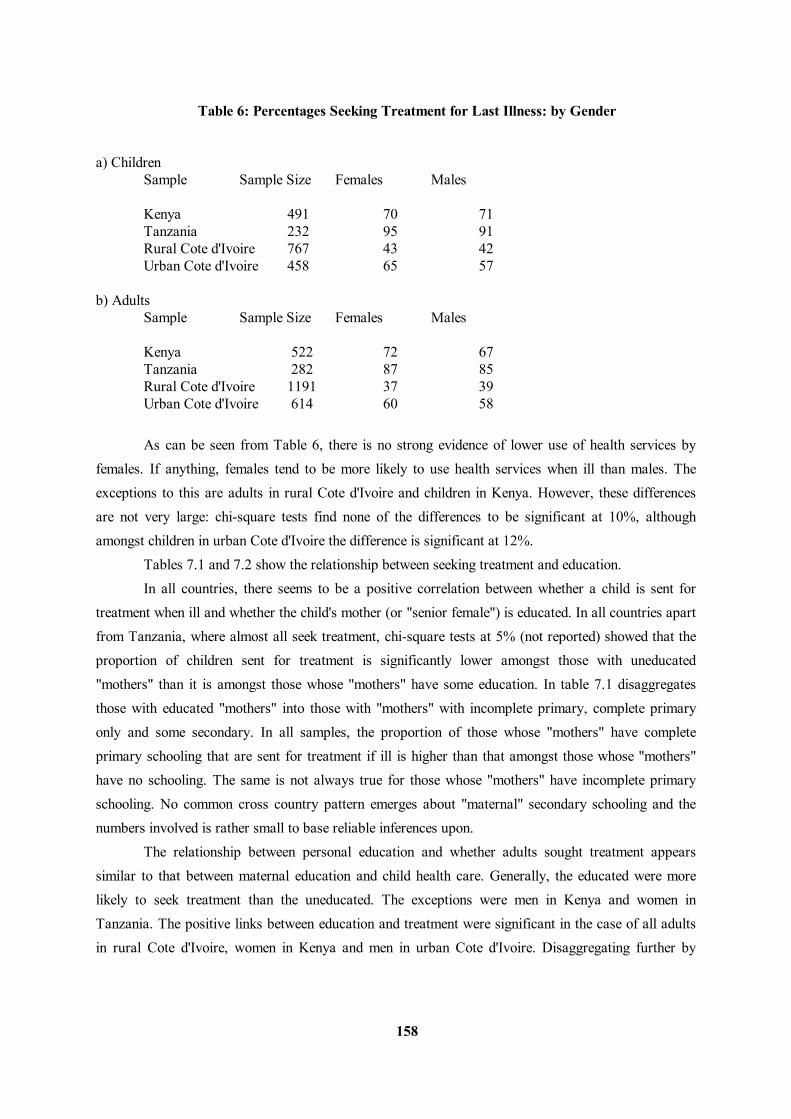
158

Table 6: Percentages Seeking Treatment for Last Illness: by Gender a) Children Sample Sample Size Females Males Kenya 491 70 71 Tanzania 232 95 91 Rural Cote d'Ivoire 767 43 42 Urban Cote d'Ivoire 458 65 57 b) Adults Sample Sample Size Females Males Kenya 522 72 67 Tanzania 282 87 85 Rural Cote d'Ivoire 1191 37 39 Urban Cote d'Ivoire 614 60 58 As can be seen from Table 6, there is no strong evidence of lower use of health services by females. If anything, females tend to be more likely to use health services when ill than males. The exceptions to this are adults in rural Cote d'Ivoire and children in Kenya. However, these differences are not very large: chi-square tests find none of the differences to be significant at 10%, although amongst children in urban Cote d'Ivoire the difference is significant at 12%. Tables 7.1 and 7.2 show the relationship between seeking treatment and education. In all countries, there seems to be a positive correlation between whether a child is sent for treatment when ill and whether the child's mother (or "senior female") is educated. In all countries apart from Tanzania, where almost all seek treatment, chi-square tests at 5% (not reported) showed that the proportion of children sent for treatment is significantly lower amongst those with uneducated "mothers" than it is amongst those whose "mothers" have some education. In table 7.1 disaggregates those with educated "mothers" into those with "mothers" with incomplete primary, complete primary only and some secondary. In all samples, the proportion of those whose "mothers" have complete primary schooling that are sent for treatment if ill is higher than that amongst those whose "mothers" have no schooling. The same is not always true for those whose "mothers" have incomplete primary schooling. No common cross country pattern emerges about "maternal" secondary schooling and the numbers involved is rather small to base reliable inferences upon. The relationship between personal education and whether adults sought treatment appears similar to that between maternal education and child health care. Generally, the educated were more likely to seek treatment than the uneducated. The exceptions were men in Kenya and women in Tanzania. The positive links between education and treatment were significant in the case of all adults in rural Cote d'Ivoire, women in Kenya and men in urban Cote d'Ivoire. Disaggregating further by

159

education in Table 7.2 shows that in all cases apart from women in Tanzania, those with complete primary schooling (only) are more likely to seek treatment if ill than those with no primary schooling. No clear picture emerges about incomplete primary schooling or about secondary schooling. Those with secondary schooling are generally more likely to seek treatment than those with no schooling, but often less likely to do so than those with complete primary schooling only. Within each of the four educational categories, chi-squared tests showed that gender differences were only significant at 10% amongst Kenyan adults with secondary schooling, amongst whom women were markedly more likely to seek treatment than men. The positive links between take-up of health services and education established in these cross-tabulations may not reflect causation. In particular, education may be correlated with other variables - such as assets or infrastructure - which directly affect child health128. The subsequent econometric analysis tests whether the education and health care relationships are robust to controls for these variables.

b. Econometric Results The probits for seeking treatment for the last illness are presented in Tables 8.1 to 8.7129,130. Significant effects of policy related variables are presented in Summary Table 2. Age-Gender Effects For adults, no significant age effects were found for urban Cote d'Ivoire. In the rural samples, the probability of women seeking treatment fell initially with age. One might speculate that the high probability of young women seeking treatment is related to child-bearing at a young age. This receives some support from the behaviour in the sample for rural Cote d'Ivoire of the dummy variable for never

128 "Maternal" education may also proxy for "paternal" education, which is omitted from the bivariate cross-tabulations.

129 Which children were sent for treatment in Tanzania was not modelled because the proportion of sick children not sent for treatment was so low - 6% - and the sample size relatively small.

130As described in Footnote 9, probit coefficients can be interpreted as the derivatives of the predicted probabilities if appropriately scaled. Evaluating at the means of all explanatory variables, the scaling factors are: Location Men Women Boys Girls Kenya 0.34 0.32 0.31 0.34 Tanzania 0.16 0.11 NA NA Rural Cote d'Ivoire 0.38 0.37 0.39 0.39 Urban Cote d'Ivoire 0.39 0.39 0.39 0.37

160

having married (marital status was unobserved for other rural areas.) In the rural Ivorian sample, almost all older women have married, so the dummy variable captures the effect of being single upon younger women. This effect is large and negative, so that it would offset the high probability of seeking treatment of young women in rural Cote d'Ivoire seeking treatment shown in Figure 3b. In rural Cote d'Ivoire, the negative effect of age is scarcely noticeable for middle aged women whilst for Tanzania it is reversed after the age of 30 (figure 3a refers). The only significant age effect for men was for Tanzania, where the predicted probabilities take an inverse U-shape for men. This may be explicable in terms of productivity if treatment is seen as an investment in future labour. In particular, one would expect the productivity of male agricultural labour to vary with age in similar way to the probability curve - rising with experience and then falling with reduced fitness. Amongst children, there were no significant age effects for the rural subsamples. In urban Cote d'Ivoire, usage is predicted to fall with age for the first five years for both sexes and later rises, with the turning point coming sooner for girls. Figure 4 shows predicted gender differences - which mainly favour girls - to be greatest in the six to twelve age range. The Effect of Education

Amongst adults, the probability of seeking treatment tended to rise with education, but which educational variables were important varied across the samples. In all cases, primary but not secondary education was significant. (Too much weight should not be placed upon this finding for rural Cote d'Ivoire and Tanzania, since few people - especially women - possessed such schooling in these samples.) However, in Cote d'Ivoire the relevant variable was personal primary schooling whilst in Kenya and Tanzania it was the primary schooling of the head or senior female. Specifically, in Kenya, the primary schooling of the education of male household heads had positive effects. In Tanzania, the same variable had a negative effect, whilst the primary schooling of the senior female in the household strongly increased the likelihood of women (only) seeking treatment. These effects are quite large, as can be seen from calculations of predicted probabilities for seeking treatment at the means of other variables. Carrying out such calculations for Kenya reveals that coming from a household where the male head had full primary schooling increases the probability of an adult being sent to treatment by 13-14 percentage points compared with coming from a household where the male head has no primary schooling. In Tanzania, completed primary schooling of the senior female raises the probability of a woman seeking treatment from 93% to almost 100%. In Cote d'Ivoire, completed personal primary schooling raises the probability of seeking treatment by 17 percentage points in rural areas and 10-11 points in urban areas. Amongst children, a clear pattern about the effects of education emerged. In particular, for all

161

girls except those in urban Cote d'Ivoire, the primary schooling of the child's mother or the senior female had a significant positive effect upon the probability of the child being sent for treatment if ill. Variables for the education of the child's father or the male head were rejected as wholly significant, except for the positive effect of paternal primary schooling upon boys in urban Cote d'Ivoire, which was close to significance. Only in urban Cote d'Ivoire did the effects of maternal education vary significantly according to the gender of the child. As with the effects of primary schooling upon adults, the effects of maternal primary schooling upon whether children are sent for treatment are quite large. Full primary schooling of the senior female in Kenyan households is predicted to raise the probability of a sick child being sent for treatment by 12 percentage points, evaluating at the means of other variables. In rural Cote d'Ivoire, full maternal primary schooling raises the corresponding probability by 10-11 percentage points. In urban areas, the figure is 15 percentage points, but confined to boys. It is interesting to compare the magnitude of these effects with those of another method of trying to increase take-up of health services, namely reducing their user costs. We were only able to capture user costs by measures of distance to the nearest health facilities. However, one can use the coefficients on these distance variables and the appropriate scaling factors given in footnote 15, to see what sort of reduction in distance to health facilities would be needed to generate a comparable rise in the probability of a sick child being sent to treatment to those brought by complete maternal schooling. For Kenya, cutting distance to health facilities is predicted to affect only boys and a 14 percentage point rise in take up amongst boys such as that generated by complete primary schooling of the senior female would require a 5 kilometre reduction in distance to the nearest dispensary or hospital. In rural Cote d'Ivoire, a 10.5 point increase would require a 52 minute cut in travel time to the nearest clinic or hospital. In both cases, the required reductions in distance are more than the means of the distance variables, which are under 3 km in Kenya and under 30 minutes in rural Cote d'Ivoire. These calculations suggest that reliance upon an expansion of the number of health facilities - even extending to the provision of a clinic or dispensary in each village - might not be able to achieve a comparable increase in the take up of child health care to that brought about by female primary schooling. This argument is based upon results for two rural samples: in urban Cote d'Ivoire, the comparison between maternal schooling and reductions in distance to facilities is even more favourable to the former since we found no significant effects for our measure of distance to health facilities.

162

Distance to Health Facilities

Where a good measure of distance to health facilities was available - that is to say, in Kenya and rural Cote d'Ivoire - it had a significant negative effect on the probability of individuals seeking treatment, except girls in Kenya. The same was also found for men in urban Cote d'Ivoire. The impact of distance to health facilities upon usage varied by gender in several samples. There were significant differences amongst adults in urban Cote d'Ivoire and amongst children in Kenya. In both cases, the effect was more negative for males. Moreover, in Kenya, experimentation with interactions between distance and the symptom type of the illness being suffered revealed a significant negative interaction term between distance and a dummy variable for being a male with a cough. These findings reinforce the impression from the descriptive statistics that the demand for health services is not lower for females, since one would expect greater "price" elasticities for females if this was the case. One qualification to this is in rural Cote d'Ivoire, where allowance for age-gender interactions revealed that it was only for women over 36 that time to the nearest health facility had a significant effect. In particular, we replaced the time to health facilities variable in Table 8.3 with its interactions with nought-one dummy variables for four age-sex categories, namely: men under 36; women under 36; men over 35 and women over 35. Only the coefficient on the latter interaction was significant, indicating that it is older women who have a more elastic demand for health care with respect to travel time. Household Public Goods As stated above, according to the reduced form approach to the household production model, the determinants of the demand for health care include the same variables as the determinants of health outcomes. However, the theory provides no clear predictions about the effects of the various health-related "household public goods", such as water supply sources, upon the demand for health care conditional upon being ill. Few such variables are significant in their effects upon whether individuals seek treatment and there are no clear cross-country patterns. For example, use of piped water increases the probability of men and children in rural Cote d'Ivoire seeking treatment, but has the opposite effect upon men in Tanzania. Interestingly, distance to water sources has a significant negative effect upon the probability of those in Kenya seeking treatment.

163

Household Wealth The behaviour of the various asset variables in tables 8.1-8.7, provides no cross-country evidence that the use of medical facilities rises with affluence. Nor is there across the board evidence that asset effects are more pronounced amongst women, as might be expected if there was less demand for medical services for women. In the Cote d'Ivoire, asset effects are captured by predicted consumption per capita. This has a positive effect upon the probabilities of adults in rural areas and of girls in urban areas seeking treatment. However, the variable's effects are perverse for women in urban areas and for girls in rural areas. In Kenya, none of the measures of physical assets per capita were positive and significant whilst livestock value per capita had perverse effects upon children in Kenya, as land per capita had upon women in Tanzania. Other Individual Characteristics The morbidity data available for Kenya and Tanzania was significant in explaining who sought treatment only amongst adults in Kenya. We have already noted the interactive effects of having a cough and distance to health facilities upon men. One of what might be expected to be the more serious instances of illness - the combination of both fever and diarrhea or vomiting - increased the likelihood of seeking treatment, as did having a simple fever if female. In Cote d'Ivoire, the only country where data on marital status was available, marriage significantly increases the probability of women but not men seeking treatment. This may be related to child bearing, as was discussed in the section on age-gender effects. Relation to the household head was generally unimportant in determining whether treatment was sought, with no evidence that children of other than the household head were significantly less likely to be sent for treatment. Other Household Characteristics

Household demographic characteristics had some significant effects. Higher proportions of children within the household reduces the probability of children in Kenya and in rural areas of Cote d'Ivoire being sent for treatment, although this effect was not observed for urban Cote d'Ivoire. By contrast, high proportions of older children increase the probability of adults seeking treatment, although this was not true for women in rural Cote d'Ivoire and was insignificant for Kenya. Increased proportions of adult females and increased household size both had mixed effects. In rural Cote d'Ivoire, a dummy variable for households operating their own businesses increased the probability of women and children seeking treatment. By contrast, the variable reduced

164

the probability of children in urban areas being sent for treatment. The predicted share of women's cash income within the household - available for the Cote d'Ivoire only - was not a determinant of whether household members sought treatment, nor was the gender of the household head. Being in a polygamous household increases the likelihood of seeking treatment in rural parts of Cote d'Ivoire, but has the opposite effects in urban areas, although the latter were significant for adults only. In Kenya and Tanzania, the only effect of polygamy was to increase the probabilities of heads in Kenya seeking treatment if ill. There is some evidence that gender differences in who seeks treatment are greater in Muslim households (identified only for the Cote d'Ivoire). In particular, coming from a household with a Muslim head increases the probabilities of boys in urban areas being sent for treatment if ill, but reduces it for girls. For adults in rural areas there is also a large gender difference in the effects of this dummy variable for the religion of the head: when interacted with gender dummies, the coefficients are both negative but that for women is twice as large in absolute terms as that for men. Other Spatial Characteristics High reported wages for child agricultural labour reduce the probability of boys being sent for treatment in rural Cote d'Ivoire. For others in all areas of Cote d'Ivoire predicted or local wages had insignificant effects. Even after controlling for proximity to health facilities and for household education and asset holdings, there is evidence that take up of health facilities is lower in less developed areas. In Kenya, proximity to the nearest urban centre increases the probability of boys but not girls seeking treatment. In rural Cote d'Ivoire, proximity to a paved road increases the probability of both genders seeking treatment, but again has a significantly larger effect upon boys. Residence in the less developed Savannah regions of Cote d'Ivoire, especially the very North, reduces the probability of adults seeking treatment.

165

5. The Duration of Illness

a. Descriptive Statistics All surveys made a distinction between how long an illness lasted and how many days the illness was sufficiently severe to curtail normal activity, such as work or school. For the Cote d'Ivoire, both kinds of information were solicited about the most recent illness in the last four weeks. However, the Ivorian information solicited only concerned how many days in the last four weeks an illness lasted. Consequently, the longest possible duration was 28 days. For Kenya and Tanzania, the questionnaire did not ask how long the most recent illness had inhibited normal activity, merely inquiring about its length per se. However, the questionnaire for these countries did record the total number of days during which normal activity had been restricted by illness in the three months prior to the surveys. In the econometrics that follows we use the length of the most recent illness as our dependent variable. This is because it may be a better measure of the duration of illness than the number of days during which a person's normal activity was restricted by illness. In particular, the latter is likely to be more influenced by economic factors such as the returns to the individual's labour and whether they can afford not to work. Moreover, by asking about days too ill to work in the whole of the preceding three months, the relevant variable for Kenya and Tanzania compounds the incidence of illness during that period, which has already analysed, with the duration of any one illness. Nonetheless, it is interesting to see to what extent illness did inhibit labour supply (or time spent at school) and consequently Table 9 presents descriptive statistics on this narrower measure of the duration of illness. To provide a rough measure of the impact of ill health on the population as a whole, total days of work or school lost through illness are presented divided by the number of all individuals rather than just those who are ill.

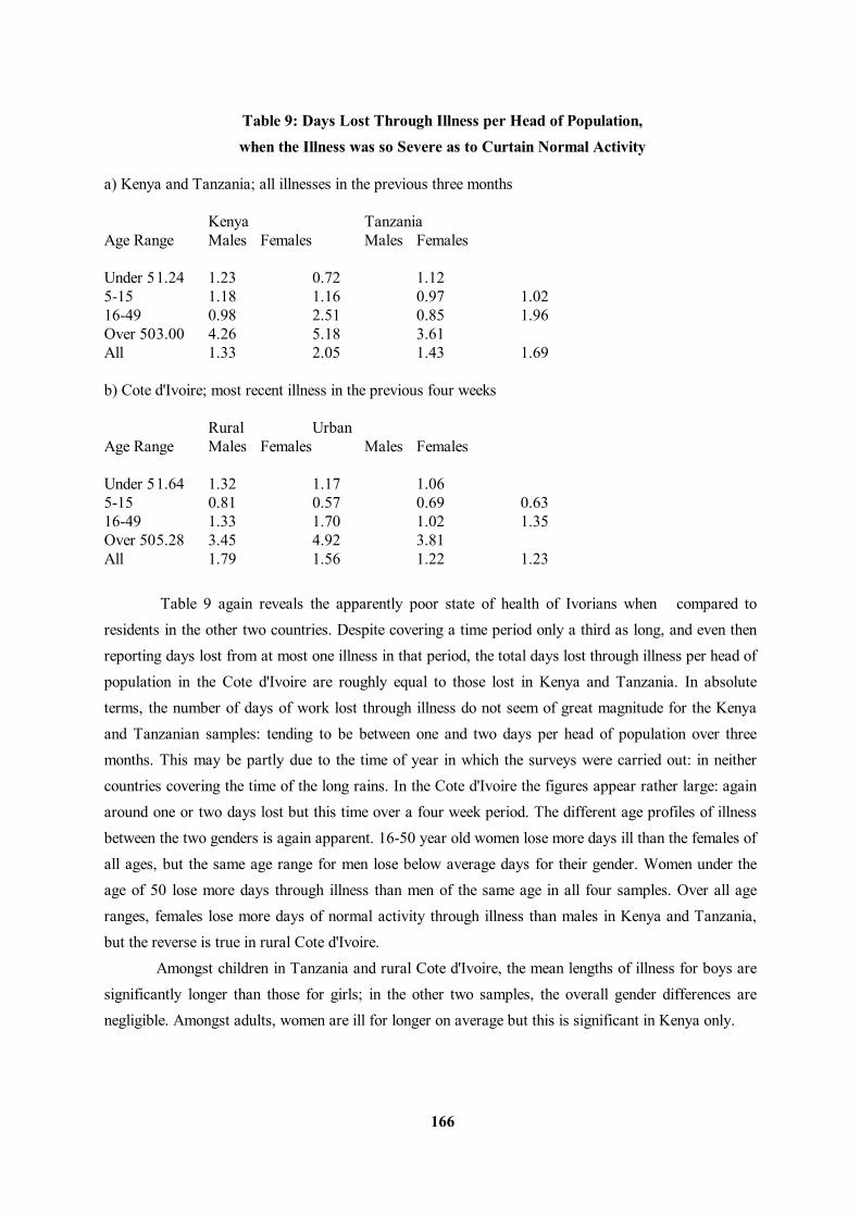
166

Table 9: Days Lost Through Illness per Head of Population, when the Illness was so Severe as to Curtain Normal Activity a) Kenya and Tanzania; all illnesses in the previous three months Kenya Tanzania Age Range Males Females Males Females Under 5 1.24 1.23 0.72 1.12 5-15 1.18 1.16 0.97 1.02 16-49 0.98 2.51 0.85 1.96 Over 50 3.00 4.26 5.18 3.61 All 1.33 2.05 1.43 1.69 b) Cote d'Ivoire; most recent illness in the previous four weeks Rural Urban Age Range Males Females Males Females Under 5 1.64 1.32 1.17 1.06 5-15 0.81 0.57 0.69 0.63 16-49 1.33 1.70 1.02 1.35 Over 50 5.28 3.45 4.92 3.81 All 1.79 1.56 1.22 1.23 Table 9 again reveals the apparently poor state of health of Ivorians when compared to residents in the other two countries. Despite covering a time period only a third as long, and even then reporting days lost from at most one illness in that period, the total days lost through illness per head of population in the Cote d'Ivoire are roughly equal to those lost in Kenya and Tanzania. In absolute terms, the number of days of work lost through illness do not seem of great magnitude for the Kenya and Tanzanian samples: tending to be between one and two days per head of population over three months. This may be partly due to the time of year in which the surveys were carried out: in neither countries covering the time of the long rains. In the Cote d'Ivoire the figures appear rather large: again around one or two days lost but this time over a four week period. The different age profiles of illness between the two genders is again apparent. 16-50 year old women lose more days ill than the females of all ages, but the same age range for men lose below average days for their gender. Women under the age of 50 lose more days through illness than men of the same age in all four samples. Over all age ranges, females lose more days of normal activity through illness than males in Kenya and Tanzania, but the reverse is true in rural Cote d'Ivoire. Amongst children in Tanzania and rural Cote d'Ivoire, the mean lengths of illness for boys are significantly longer than those for girls; in the other two samples, the overall gender differences are negligible. Amongst adults, women are ill for longer on average but this is significant in Kenya only.

167

In all samples, those who seek treatment when ill on average have longer lasting illnesses than those who do not. In Kenya, t-tests reveal this difference is not quite significant for women at 10% whilst being significant at 1% for men. Elsewhere, the difference is always significant at 1% for women but insignificant for men in Tanzania and in rural Cote d'Ivoire. Amongst children, differences in the duration of illness between those who are treated and those who are not are more significant for boys in all samples except those in urban Cote d'Ivoire. Nonetheless at the 5% level, girls who receive treatment are ill for significantly longer than those who do not, except in Tanzania where the numbers not sent for treatment are too small for reliable inferences to be made. These results do not necessarily imply that treatment for an illness perversely increases the length of it. In particular, one would expect those with more serious illnesses to be both more likely to seek treatment and to be ill for longer. Hence in modelling the duration of illness, we attempt to control for this probable feature of the data.

b. Econometric Results The final form of the models for the duration of illness are given in Tables 11.1 to 11.8. For Kenya and Tanzania, simple ordinary least squares regression was used, with the dependent variable, the number of days ill, expressed in logarithmic form in order to make its distribution appear more normal and less skewed.131 The variable was not expressed in logs for the Cote d'Ivoire, but the extensive right-censoring caused by the 28 day upper limit on the reported duration of illness meant that a tobit was used rather than ordinary least squares regression. Significant findings for policy related explanatory variables are given in Summary Table 3. Age-Gender Effects In all the samples of adults, the duration of illness is found to rise with age. This effect is always larger for men than women and is significant for all except women in Kenya and Tanzania. Age effects are less marked for children, being significant for boys only in both Tanzania and rural Cote d'Ivoire. In the latter, the duration of illness is predicted to fall with age whilst in Tanzania, it rises with age until the child is seven and thereafter falls away.

131 Where the dependent variable is in logs, the coefficients in the tables approximate the proportional effect upon the number of days ill of a unit change in the relevant regressor.

168

The Effects of Education Education may indirectly affect the duration of illness through several routes which will be reported later: for example, through increasing take-up of health facilities, household wealth and wages. However, it also exerts some direct effects in several samples. As with parental education and the reporting of the incidence of child illness, these effects may reflect differences in sensitivity to illness rather than differences in objective medical states. They may also capture informational effects and other consequences of education which increase the likelihood of the adoption of good health practices within the household. Amongst adults, these direct effects of education are mixed. Personal education had no significant effects in Kenya and Tanzania, but did in Cote d'Ivoire. In rural Cote d'Ivoire, personal primary schooling increases the duration of illness. Personal secondary schooling reduces the duration of illness in rural Cote d'Ivoire - although the effect is significant only for women - whilst it increases it in urban parts of the country. It is suggestive that personal education was only significant in the Cote d'Ivoire, since it was only here that the morbidity data is reported by each individual rather than by a household respondent. This lends some support to the conjecture that the "perverse" effects of education upon the duration of illness reflect greater sensitivity to illness rather than greater ill-health objectively measured. The significant effects of the education of other adults in the household were also varied: male heads' primary schooling increases the duration of illness in rural Cote d'Ivoire whilst the secondary schooling of such people reduces the duration of illness in urban Cote d'Ivoire. The education of the "senior female" is only significant in Tanzania, where their primary schooling reduces the duration of illness of women only. The effects of parental education upon children were all consistently favourable where significant, but such effects were only found in Kenya and rural Cote d'Ivoire. Specifically, the primary schooling of both male heads and senior females reduced the duration of child illness in Kenya, whilst in rural Cote d'Ivoire paternal primary schooling had a similar effect.

169

Use of Health Facilities Systematic evidence of health gains from the use of health facilities was not obtained. The dummy variable for receiving treatment generally has a positive coefficient where significant, despite the attempt to control for endogeneity. These positive effects vary considerably in size. The largest such effect is amongst adults in Tanzania, where the coefficient on the treatment dummy implies that on average receiving treatment more than doubles the length of a person's illness. Amongst boys in Kenya, treatment increases the mean duration of illness by around a third. Amongst adults in urban Cote d'Ivoire, treatment appears to add an extra three and a half days to the length of the illness, whilst for children in rural areas, it adds over two and a half days. The coefficient upon the treatment variable was also positive but insignificant for men in Kenya and adults in rural Cote d'Ivoire. Treatment effects could not be estimated for children in Tanzania, since who sought treatment was not modelled and so the endogeneity of treatment could not be controlled for. Treatment only appeared to reduce the duration of illness for females in Kenya and children in urban Cote d'Ivoire. The only significant beneficial effect was for women in Kenya, where treatment was predicted to massively cut the duration of illness. Kenya was the only country in which the effects of treatment varied significantly by gender. It is not always the case that, controlling for observed characteristics, those who were more likely to seek treatment were also those likely to be ill for longer. Whether sample selection is a potential problem can be gauged by the significance of the additional regressor introduced to control for the possible endogeneity of treatment132. Using this measure, the null hypothesis of no correlation in the residuals of the treatment probit and an unaugmented duration regression was not rejected for adults in urban Cote d'Ivoire, children in Kenya and children in rural Cote d'Ivoire. Indeed, in all but the last of these three cases, the coefficient upon the endogeneity control was negative, indicating a negative correlation between the residuals. Such a negative coefficient was also found for adults in Tanzania, where it was significant at 10%. The expected positive correlation was significant only for adults in Kenya, adults in rural Cote d'Ivoire and children in urban Cote d'Ivoire. The finding that the treatment dummy variable often has a perverse effect upon the duration of illness raises an important question of interpretation. It is conceivable that treatment has an insignificant effect in reducing illness. Many common ailments may be either hard to treat or of short duration even in the absence of treatment, which may be received late. Medical services may act not so much to reduce the duration of common illnesses as to alleviate pain and to screen a few potentially very dangerous illnesses. Moreover, the quality of the medical facilities may be low: clinics in Tanzania during the period were reported to be short of essential drugs. However, that treatment actually increases the duration of illness does seem very perverse. There seem to be at least two types of

132 A standard t-test on the coefficient of this variable is not valid, so likelihood ratio tests were used instead.

170

response: one being to accept the results as they stand; the other to question whether the endogeneity issue has been satisfactorily resolved. Within the former approach, one could accept that treatment does actually increase the reported duration of illness. This either might be because treatment increases the actual duration of illness or simply because it creates a reporting bias. The former is not impossible. By going to seek treatment, people may have to travel considerable distances to the detriment of their health only to expose themselves to further illness by waiting in rooms full of sick people. However, this interpretation remains rather implausible. One could instead refer to the self-reported nature of the morbidity data. It may be that treatment does not increase the actual duration of illness but does increase peoples' perception of its duration. This argument is not that people who would tend to exaggerate the length of their illnesses regardless of treatment are also more likely to use health facilities, because such an omitted determinant (namely hypochondria) of both the duration of illness and the receipt of treatment should be controlled for by the Heckman procedure. Rather, the argument is that the receipt of treatment itself actually causes an increase in the reported, but not actual, duration of illness. Receiving treatment may confer an additional importance onto ones' illness, making its duration less likely to be under-reported. Furthermore, if a person seeks treatment, she may regard herself as ill until a health practitioner pronounces here fit or until a prescribed course of drugs has finished. A `reporting bias' interpretation of our perverse treatment effects seems particularly plausible in those cases where the duration of illness is reported by another party such as the household head. If treatment is sought for an illness, this act may attract the attention of the household respondent to it, making them less likely to downgrade its severity. The alternative approach to interpreting the results would be dispute that the models have correctly controlled for endogeneity. If this is not correctly controlled for, the significant positive effect of treatment upon duration may still reflect the fact that people with more severe illnesses tend to seek treatment rather than that treatment causes illnesses to become more severe. The control for endogeneity relies upon the first stage probit for whether treatment is sought being adequately modelled. For adults in Tanzania, where treatment has an extremely large positive effect upon the duration of illness, and for adults in urban Cote d'Ivoire, where treatment also has a perverse effect, it is questionable whether this has been attained. However, for the other case where treatment has a significant positive effect upon duration - children in rural Cote d'Ivoire - the modelling of access to treatment appears to be relatively good.

171

Household Public Goods A household's source of drinking water may affect the duration of illness in various ways. Perhaps the most obvious is that, just by affecting exposure to various water born illnesses, water supply sources will affect the mean duration of illness if water-born illnesses differ in length from other illnesses. Hence it could be that a given water source increases the incidence of illness by increasing contact with water-born diseases but actually decreases the duration of illness if these diseases are generally shorter lived than other illnesses. This might be the case with the effects of private piped water on children in Kenya, where such a source increased the incidence of illness but also reduces its duration. Alternatively, the private piped water may be picking up a wealth effect upon the duration of illness since several other measures of household assets also exert a significant negative effect upon the duration of illness in this equation. Piped water also had a favourable effect upon the duration of illness of girls in urban Cote d'Ivoire. Elsewhere, if piped water has any significant effect at all, it is unfavourable. Indeed, although communal piped water did not affect the incidence of illness for adults in Kenya and Tanzania, it does increase the duration of illness. These effects are quite large, increasing the duration of illness by around a third and a quarter respectively. Amongst children in rural Cote d'Ivoire, the unfavourable effect of piped water upon the incidence of illness is reinforced by an adverse effect upon the duration of illness which adds around two and a half days to the expected length of an illness. Similarly, in Kenya, boreholes - which appeared to be the most risky source of water for adults - also increase the duration of adult illness by around a quarter. Distance to water supply sources significantly increased the length of illness of boys in all samples, except Tanzania. This may reflect ill effects of lower consumption of water by sick children, but it is unclear why the effect is confined to boys rather than being true for all children. Toilet facilities had mixed effects. Whereas pit latrines - as opposed to no latrines - reduced the incidence of illness amongst children in Kenya and increased it amongst children in Tanzania, the reverse pattern was observed for their effects upon the duration of illness. Such toilets reduced the duration of illness of adults in Tanzania. Flush toilets in urban Cote d'Ivoire, which had been estimated to increase the incidence of illness but only significantly for adults, now appear to also increase the duration of illness, although only significantly so in the case of girls.

172

Household Wealth Measures of household wealth were never significant determinants of the duration of illness amongst adults and rarely significant amongst children. In Kenya, both household livestock per capita and land per capita reduced the duration of child illness; for adult illness they had the same signs but were insignificant. However, household land per capita increased the duration of child illness in Tanzania and had the same direction of effect amongst adults in that country. Predicted consumption per capita was near to significance in reducing the duration of illness of men in urban Cote d'Ivoire but was wholly insignificant amongst other Ivorian adults. Amongst children in the Cote d'Ivoire, predicted consumption per capita reduced the duration of illness of girls but increased it amongst boys. However, none of these effects were significant. Consequently, although the effects of predicted consumption per capita only differed significantly by gender in rural areas, for neither sex was it significantly different from zero. Other Individual Characteristics The wages predicted for an individual in urban Cote d'Ivoire have a negative effect upon the duration of illness. This may be because those whose time is costly tending take action to avoid being ill for a long period of time. Using cluster agricultural wage rates for rural areas revealed two similar effects. Firstly, the wages for women in rural areas had a significant negative effect upon the duration of women's illness. Secondly, the duration of illness of boys in rural areas is negatively affected by the wages of men in the cluster. One might have thought that a more directly relevant wage in this last case would be that for child labour and in fact this variable did have a negative effect which was near to significance. For adults in rural areas, male wages increased the duration of illness and child wages reduced it but for women only. As might be expected, several of the morbidity variables available for Kenya and Tanzania affect the duration of illness, although these effects are not common to all samples. For example, numbers of recent previous incidences of illness increase the duration of the present illness in Kenya, but are wholly insignificant and take the opposite sign in Tanzania. Relation to household head was sometimes significant, with adults other than the head or their spouse generally being likely to be ill for longer. Amongst children there was no evidence that children of parents other than the head were likely to be ill for significantly longer.

173

Other Household Characteristics

In Cote d'Ivoire, women's share of cash income within the household was insignificant in its effects upon the duration of illness. Household type - polygamous, female-headed or other - was also generally insignificant. Residence in female-headed households was predicted to reduce the length of illness in all samples except children in Tanzania, but these effects were significant only for men in Kenya. By contrast, residence in polygamous households generally increased the duration of illness - the exception being females in Kenya and children in urban Cote d'Ivoire - but this was significant only for women in Tanzania and adults in rural Cote d'Ivoire. Residence in Muslim households reduced the duration of illness in rural Cote d'Ivoire, but was significant for children only. Household size and demographic composition had no widespread and consistent significant effects. Other Spatial Characteristics

Adults living further from major urban centres in Kenya, were predicted to be ill for shorter periods. In rural Cote d'Ivoire, geographic isolation, as measured by distance to the nearest paved road, increased the reported duration of adult illness but reduced that for child illnesses.

174

6. Summary and Conclusions Amongst the determinants of health outcomes examined in this paper are three public services: health facilities, education and water supply provision. We conclude by summarising our findings of the effects of these services together with relevant gender aspects. Consider first the incidence of illness. Our only proxy for the provision of preventative health services, distance to health facilities, generally had weak or perverse effects. Education had mixed effects upon adults whilst parental schooling or its proxies appeared to increase the incidence of illness amongst children. This highlights a weakness of the self-reported nature of the morbidity data, since the most plausible explanation of this result is that it reflects the effects of education upon reported but not actual illness. The source of a household's drinking water had powerful effects upon the incidence of illness. However, several man-made sources of water, notably piped water, appeared in many samples to be significantly more hazardous than natural sources. This suggests that further research into the health effects of piped water is warranted. If our findings are corroborated they suggest that the either quality of such water should be improved or at least people more educated as to its dangers. Turning to the question of who sought treatment when ill, there is no systematic evidence of females having significantly lower use of health facilities than males with similar characteristics, nor was lack of household wealth found to be an obstacle to such usage in all countries. Education generally increased the take-up of health services when ill. In particular, in all cases modelled, maternal schooling was found to significantly increase the probability that a sick child would be sent for treatment whilst paternal schooling was insignificant. The demand for health care did appear to be sensitive to the distance to the nearest health facilities, but there was no evidence that this was more of a deterrent to females. Our estimates of the effects of medical treatment upon the duration of illness provided little evidence that such treatment brought large observable gains in time saved and indeed were sometimes significantly perverse. We suggested that this may be partly due to the self-reported nature of the data: receiving treatment for an illness may give it an added weight in the mind of the respondent, leading to it being ascribed a longer length. However, this is highly speculative. As with its effects on the incidence of illness, education has mixed effects upon the duration of illness, although in this case parental education had either benign or no significant effects upon child health. Water supply sources are once more important, with further evidence that in some cases boreholes and piped water appear to be relatively detrimental to health.

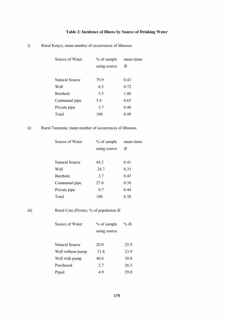
175

Table 2: Incidence of Illness by Source of Drinking Water i) Rural Kenya; mean number of occurrences of illnesses Source of Water % of sample mean times using source ill Natural Source 79.9 0.43 Well 6.5 0.72 Borehole 5.5 1.06 Communal pipe 5.4 0.65 Private pipe 3.7 0.48 Total 100 0.49 ii) Rural Tanzania; mean number of occurrences of illnesses Source of Water % of sample mean times using source ill Natural Source 44.2 0.41 Well 24.7 0.33 Borehole 2.7 0.45 Communal pipe 27.6 0.38 Private pipe 0.7 0.44 Total 100 0.38 iii) Rural Cote d'Ivoire; % of population ill Source of Water % of sample % ill using source Natural Source 20.0 25.9 Well without pump 31.8 23.9 Well with pump 40.6 30.8 Purchased 2.7 26.5 Piped 4.9 29.0

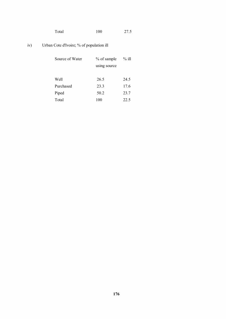
176

Total 100 27.5 iv) Urban Cote d'Ivoire; % of population ill Source of Water % of sample % ill using source Well 26.5 24.5 Purchased 23.3 17.6 Piped 50.2 23.7 Total 100 22.5

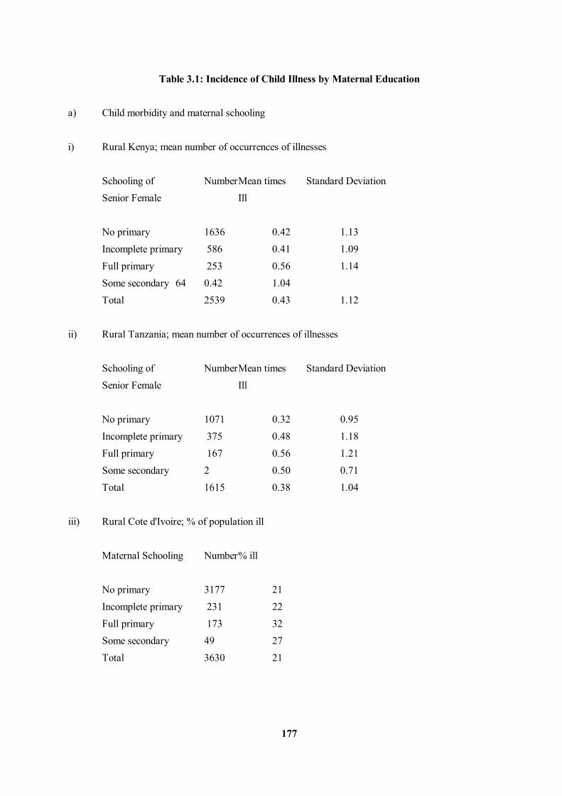
177

Table 3.1: Incidence of Child Illness by Maternal Education a) Child morbidity and maternal schooling i) Rural Kenya; mean number of occurrences of illnesses Schooling of Number Mean times Standard Deviation Senior Female Ill No primary 1636 0.42 1.13 Incomplete primary 586 0.41 1.09 Full primary 253 0.56 1.14 Some secondary 64 0.42 1.04 Total 2539 0.43 1.12 ii) Rural Tanzania; mean number of occurrences of illnesses Schooling of Number Mean times Standard Deviation Senior Female Ill No primary 1071 0.32 0.95 Incomplete primary 375 0.48 1.18 Full primary 167 0.56 1.21 Some secondary 2 0.50 0.71 Total 1615 0.38 1.04 iii) Rural Cote d'Ivoire; % of population ill Maternal Schooling Number % ill No primary 3177 21 Incomplete primary 231 22 Full primary 173 32 Some secondary 49 27 Total 3630 21

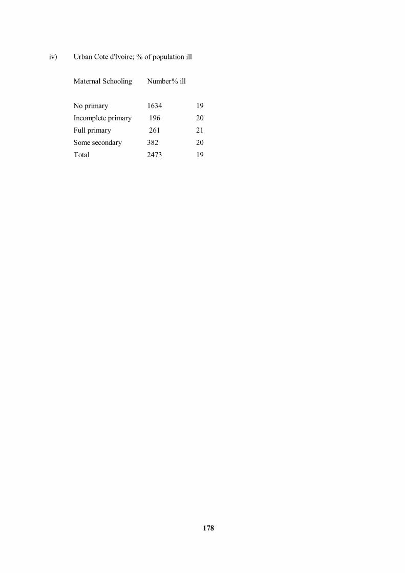
178

iv) Urban Cote d'Ivoire; % of population ill Maternal Schooling Number % ill No primary 1634 19 Incomplete primary 196 20 Full primary 261 21 Some secondary 382 20 Total 2473 19

179

Table 3.2: Incidence of Adult Illness by Personal Education i) Rural Kenya; mean number of occurrences of illnesses Males Females Schooling Number Mean (S.D.) Number Mean (S.D.) No primary 270 0.53 (1.36) 717 0.73 (1.72) Incomplete primary 329 0.49 (1.34) 308 0.49 (1.18) Full primary 295 0.41 (1.17) 182 0.79 (1.53) Some secondary 171 0.40 (1.21) 111 0.19 Total 1065 0.46 (1.28) 1318 0.64 (1.53) ii) Rural Tanzania; mean number of occurrences of illnesses Males Females Schooling Number Mean (S.D.) Number Mean (S.D.) No primary 289 0.53 (1.39) 522 0.40 (1.07) Incomplete primary 239 0.39 (1.09) 193 0.42 (1.04) Full primary 273 0.29 (0.86) 216 0.26 (0.88) Some secondary 16 0 13 0.54 (0.88) Total 817 0.40 (1.14) 944 0.37 (1.03) iii) Rural Cote d'Ivoire; % of population ill Males Females Schooling Number % ill Number % ill No primary 1001 43.2 1723 34.3 Incomplete primary 166 27.7 131 27.5 Full primary 176 18.8 119 10.1 Some secondary 185 19.5 45 20.0 Total 1528 35.8 2018 32.1 iv) Urban Cote d'Ivoire; % of population ill

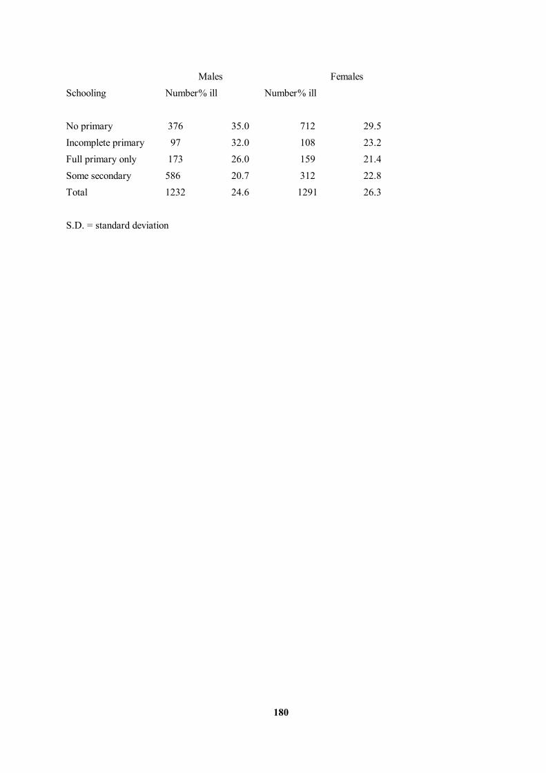
180

Males Females Schooling Number % ill Number % ill No primary 376 35.0 712 29.5 Incomplete primary 97 32.0 108 23.2 Full primary only 173 26.0 159 21.4 Some secondary 586 20.7 312 22.8 Total 1232 24.6 1291 26.3 S.D. = standard deviation

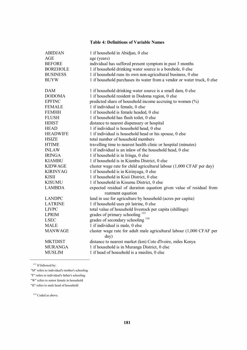
181

Table 4: Definitions of Variable Names ABIDJAN 1 if household in Abidjan, 0 else AGE age (years) BEFORE individual has suffered present symptom in past 3 months BOREHOLE 1 if household drinking water source is a borehole, 0 else BUSINESS 1 if household runs its own non-agricultural business, 0 else BUYW 1 if household purchases its water from a vendor or water truck, 0 else

DAM 1 if household drinking water source is a small dam, 0 else DODOMA 1 if household resident in Dodoma region, 0 else EPFINC predicted share of household income accruing to women (%) FEMALE 1 if individual is female, 0 else FEMHH 1 if household is female headed, 0 else FLUSH 1 if household has flush toilet, 0 else HDIST distance to nearest dispensary or hospital HEAD 1 if individual is household head, 0 else HEADWIFE 1 if individual is household head or his spouse, 0 else HSIZE total number of household members HTIME travelling time to nearest health clinic or hospital (minutes) INLAW 1 if individual is an inlaw of the household head, 0 else IRINGA 1 if household is in Iringa, 0 else KIAMBU 1 if household is in Kiambu District, 0 else KIDWAGE cluster wage rate for child agricultural labour (1,000 CFAF per day) KIRINYAG 1 if household is in Kirinyaga, 0 else KISII 1 if household in Kisii District, 0 else KISUMU 1 if household in Kisumu District, 0 else LAMBDA expected residual of duration equation given value of residual from

reatment equation LANDPC land in use for agriculture by household (acres per capita) LATRINE 1 if household uses pit latrine, 0 else LIVPC total value of household livestock per capita (shillings) LPRIM grades of primary schooling 133 LSEC grades of secondary schooling 134 MALE 1 if individual is male, 0 else MANWAGE cluster wage rate for adult male agricultural labour (1,000 CFAF per

day) MKTDIST distance to nearest market (km) Cote d'Ivoire, miles Kenya MURANGA 1 if household is in Muranga District, 0 else MUSLIM 1 if head of household is a muslim, 0 else 133 If followed by: "M" refers to individual's mother's schooling "F" refers to individual's father's schooling "W" refers to senior female in household "H" refers to male head of household

134 Coded as above.

182

NEVER 1 if individual never married, 0 else NSAV 1 if household in Northern Savannah, 0 else NTILL number of times ill in past 3 months NYANDARU 1 if household is in Nyandarua district, 0 else NYANZA 1 if household is in Nyanza Province, 0 else NYERI 1 if household is in Nyeri district, 0 else OTHREL 1 if individual is not a member of the household head's nuclear family, 0 else PAVEDIST distance of cluster to nearest paved road (km) PCONPC predicted household consumption per capita per annum (10,000 CFA Francs) PFAD proportion of household members women PIPE 1 if household drinking water source is communal piped water, 0 else POKID proportion of household members children aged 6 to 15 POLY 1 if household is polygamous, 0 else POLYHEAD 1 if individual is had of a polygamous household, 0 else POND 1 if household drinking water source is a pond, 0 else PONDDAM 1 if household drinking water source is a pond or dam, 0 else PYKID proportion of household members children aged under RAIN 1 if household drinking water source is rain, 0 else RUVUMA 1 if household is in Ruvuma, 0 else SSAV 1 if household is in Southern Savannah, 0 else SIAYA 1 if household in Siaya district, 0 else SNYANZ 1 if household in South Nyanza district, 0 else SON 1 if individual is son of the household head, 0 else SPRING 1 if household drinking water source is a spring, 0 else TAP 1 if household draws its drinking water from a private tap, 0 else TPC 1 if individual's most recent illness was a cough, 0 else TPCB 1 if individual's most recent illness was a cough with blood in sputum, 0 else TPDV 1 if individual's most recent illness was diarrhoea or vomiting, 0 else TPFDV 1 if individual's present symptom if fever and diarrhoea or vomiting, 0 else TPFDV 1 if individual's most recent illness was fever and diarrhoea and diarrhea or

vomiting, 0 else TREAT 1 if individual sought treatment, 0 else TREEPC number of trees owned by household per capita TRUCK 1 if household waste is disposed of by truck, 0 else URBDIST distance to nearest large urban centre (miles Nairobi for Central,

Kisumu for Nyanza) WAGE formal sector wage predicted for the individual (CFAF per day) WTIME time taken to reach main drinking water source (minutes) WDIST distance to drinking water source (meters) WELL 1 if household drinking water source is a well, 0 else WELLP 1 if household drinking water source is a well with a pump, 0 else WELLNOP 1 if household drinking water source is a well without a pump, 0 else WEST 1 if household in West Forrest, 0 else WIFE 1 if individual is wife of household head, 0 else WOMWAGE cluster wage rate for adult female agricultural labour (1,000 CFAF

per day) Squared terms are denoted by the variable name followed by "2" and cubic terms by the variable name followed by "3". Gender interactions are given by prefixing FZ before the variable name if interacting the variable with FEMALE and by prefixing with MZ if interacting with MALE.

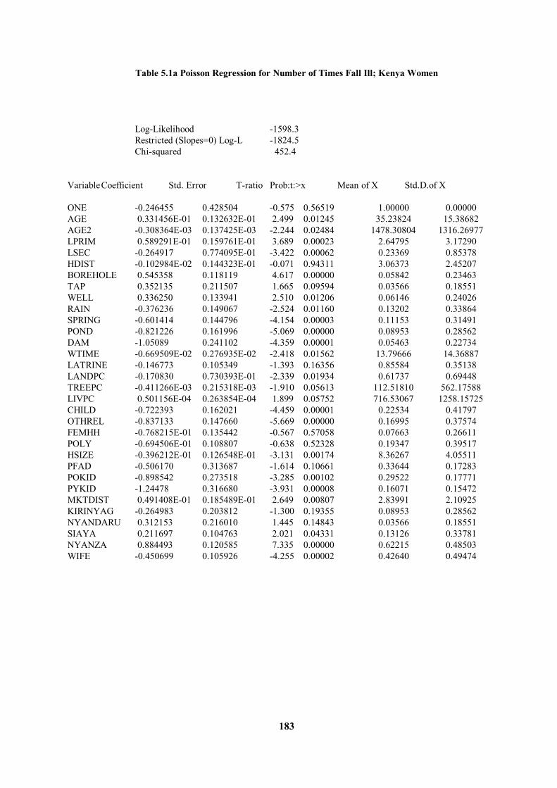
183

Table 5.1a Poisson Regression for Number of Times Fall Ill; Kenya Women Log-Likelihood -1598.3 Restricted (Slopes=0) Log-L -1824.5 Chi-squared 452.4 Variable Coefficient Std. Error T-ratio Prob:t:>x Mean of X Std.D.of X ONE -0.246455 0.428504 -0.575 0.56519 1.00000 0.00000 AGE 0.331456E-01 0.132632E-01 2.499 0.01245 35.23824 15.38682 AGE2 -0.308364E-03 0.137425E-03 -2.244 0.02484 1478.30804 1316.26977 LPRIM 0.589291E-01 0.159761E-01 3.689 0.00023 2.64795 3.17290 LSEC -0.264917 0.774095E-01 -3.422 0.00062 0.23369 0.85378 HDIST -0.102984E-02 0.144323E-01 -0.071 0.94311 3.06373 2.45207 BOREHOLE 0.545358 0.118119 4.617 0.00000 0.05842 0.23463 TAP 0.352135 0.211507 1.665 0.09594 0.03566 0.18551 WELL 0.336250 0.133941 2.510 0.01206 0.06146 0.24026 RAIN -0.376236 0.149067 -2.524 0.01160 0.13202 0.33864 SPRING -0.601414 0.144796 -4.154 0.00003 0.11153 0.31491 POND -0.821226 0.161996 -5.069 0.00000 0.08953 0.28562 DAM -1.05089 0.241102 -4.359 0.00001 0.05463 0.22734 WTIME -0.669509E-02 0.276935E-02 -2.418 0.01562 13.79666 14.36887 LATRINE -0.146773 0.105349 -1.393 0.16356 0.85584 0.35138 LANDPC -0.170830 0.730393E-01 -2.339 0.01934 0.61737 0.69448 TREEPC -0.411266E-03 0.215318E-03 -1.910 0.05613 112.51810 562.17588 LIVPC 0.501156E-04 0.263854E-04 1.899 0.05752 716.53067 1258.15725 CHILD -0.722393 0.162021 -4.459 0.00001 0.22534 0.41797 OTHREL -0.837133 0.147660 -5.669 0.00000 0.16995 0.37574 FEMHH -0.768215E-01 0.135442 -0.567 0.57058 0.07663 0.26611 POLY -0.694506E-01 0.108807 -0.638 0.52328 0.19347 0.39517 HSIZE -0.396212E-01 0.126548E-01 -3.131 0.00174 8.36267 4.05511 PFAD -0.506170 0.313687 -1.614 0.10661 0.33644 0.17283 POKID -0.898542 0.273518 -3.285 0.00102 0.29522 0.17771 PYKID -1.24478 0.316680 -3.931 0.00008 0.16071 0.15472 MKTDIST 0.491408E-01 0.185489E-01 2.649 0.00807 2.83991 2.10925 KIRINYAG -0.264983 0.203812 -1.300 0.19355 0.08953 0.28562 NYANDARU 0.312153 0.216010 1.445 0.14843 0.03566 0.18551 SIAYA 0.211697 0.104763 2.021 0.04331 0.13126 0.33781 NYANZA 0.884493 0.120585 7.335 0.00000 0.62215 0.48503 WIFE -0.450699 0.105926 -4.255 0.00002 0.42640 0.49474

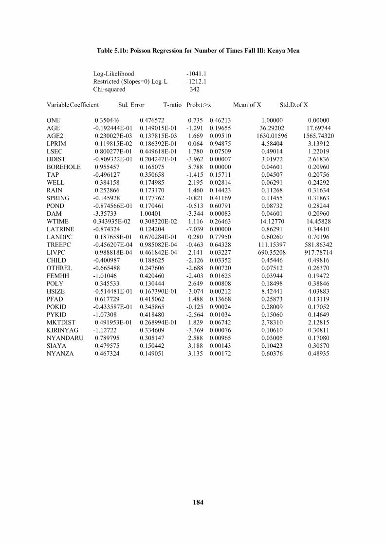
184

Table 5.1b: Poisson Regression for Number of Times Fall Ill: Kenya Men Log-Likelihood -1041.1 Restricted (Slopes=0) Log-L -1212.1 Chi-squared 342 Variable Coefficient Std. Error T-ratio Prob:t:>x Mean of X Std.D.of X ONE 0.350446 0.476572 0.735 0.46213 1.00000 0.00000 AGE -0.192444E-01 0.149015E-01 -1.291 0.19655 36.29202 17.69744 AGE2 0.230027E-03 0.137815E-03 1.669 0.09510 1630.01596 1565.74320 LPRIM 0.119815E-02 0.186392E-01 0.064 0.94875 4.58404 3.13912 LSEC 0.800277E-01 0.449618E-01 1.780 0.07509 0.49014 1.22019 HDIST -0.809322E-01 0.204247E-01 -3.962 0.00007 3.01972 2.61836 BOREHOLE 0.955457 0.165075 5.788 0.00000 0.04601 0.20960 TAP -0.496127 0.350658 -1.415 0.15711 0.04507 0.20756 WELL 0.384158 0.174985 2.195 0.02814 0.06291 0.24292 RAIN 0.252866 0.173170 1.460 0.14423 0.11268 0.31634 SPRING -0.145928 0.177762 -0.821 0.41169 0.11455 0.31863 POND -0.874566E-01 0.170461 -0.513 0.60791 0.08732 0.28244 DAM -3.35733 1.00401 -3.344 0.00083 0.04601 0.20960 WTIME 0.343935E-02 0.308320E-02 1.116 0.26463 14.12770 14.45828 LATRINE -0.874324 0.124204 -7.039 0.00000 0.86291 0.34410 LANDPC 0.187658E-01 0.670284E-01 0.280 0.77950 0.60260 0.70196 TREEPC -0.456207E-04 0.985082E-04 -0.463 0.64328 111.15397 581.86342 LIVPC 0.988818E-04 0.461842E-04 2.141 0.03227 690.35208 917.78714 CHILD -0.400987 0.188625 -2.126 0.03352 0.45446 0.49816 OTHREL -0.665488 0.247606 -2.688 0.00720 0.07512 0.26370 FEMHH -1.01046 0.420460 -2.403 0.01625 0.03944 0.19472 POLY 0.345533 0.130444 2.649 0.00808 0.18498 0.38846 HSIZE -0.514481E-01 0.167390E-01 -3.074 0.00212 8.42441 4.03883 PFAD 0.617729 0.415062 1.488 0.13668 0.25873 0.13119 POKID -0.433587E-01 0.345865 -0.125 0.90024 0.28009 0.17052 PYKID -1.07308 0.418480 -2.564 0.01034 0.15060 0.14649 MKTDIST 0.491953E-01 0.268994E-01 1.829 0.06742 2.78310 2.12815 KIRINYAG -1.12722 0.334609 -3.369 0.00076 0.10610 0.30811 NYANDARU 0.789795 0.305147 2.588 0.00965 0.03005 0.17080 SIAYA 0.479575 0.150442 3.188 0.00143 0.10423 0.30570 NYANZA 0.467324 0.149051 3.135 0.00172 0.60376 0.48935

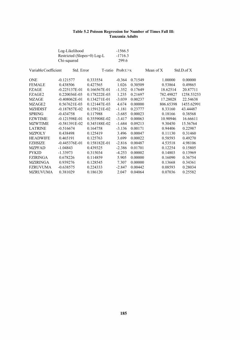
185

Table 5.2 Poisson Regression for Number of Times Fall Ill: Tanzania Adults Log-Likelihood -1566.5 Restricted (Slopes=0) Log-L -1716.3 Chi-squared 299.6 Variable Coefficient Std. Error T-ratio Prob:t:>x Mean of X Std.D.of X ONE -0.121577 0.333554 -0.364 0.71549 1.00000 0.00000 FEMALE 0.438506 0.427565 1.026 0.30509 0.53864 0.49865 FZAGE -0.225137E-01 0.166567E-01 -1.352 0.17649 18.62514 20.87711 FZAGE2 0.220036E-03 0.178222E-03 1.235 0.21697 782.49827 1258.53253 MZAGE -0.408062E-01 0.134271E-01 -3.039 0.00237 17.28028 22.54638 MZAGE2 0.567621E-03 0.121447E-03 4.674 0.00000 806.65398 1455.62991 MZHDIST -0.187857E-02 0.159121E-02 -1.181 0.23777 8.33160 43.44487 SPRING -0.434758 0.117988 -3.685 0.00023 0.18166 0.38568 FZWTIME -0.121598E-01 0.355908E-02 -3.417 0.00063 10.90946 16.66611 MZWTIME -0.581391E-02 0.345188E-02 -1.684 0.09213 9.30450 15.56764 LATRINE -0.516674 0.164758 -3.136 0.00171 0.94406 0.22987 MZPOLY 0.438498 0.125419 3.496 0.00047 0.11130 0.31460 HEADWIFE 0.465191 0.125763 3.699 0.00022 0.58593 0.49270 FZHSIZE -0.445376E-01 0.158182E-01 -2.816 0.00487 4.53518 4.98106 MZPFAD -1.04843 0.439325 -2.386 0.01701 0.12254 0.15805 PYKID -1.33973 0.315034 -4.253 0.00002 0.14803 0.13969 FZIRINGA 0.678226 0.114859 5.905 0.00000 0.16090 0.36754 MZIRINGA 0.939276 0.128545 7.307 0.00000 0.13668 0.34361 FZRUVUMA -0.638575 0.224333 -2.847 0.00442 0.08593 0.28034 MZRUVUMA 0.381029 0.186120 2.047 0.04064 0.07036 0.25582

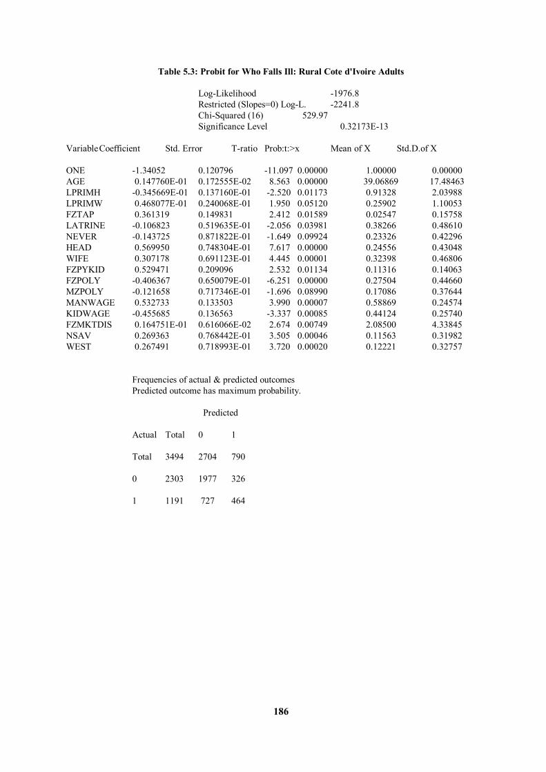
186

Table 5.3: Probit for Who Falls Ill: Rural Cote d'Ivoire Adults Log-Likelihood -1976.8 Restricted (Slopes=0) Log-L. -2241.8 Chi-Squared (16) 529.97 Significance Level 0.32173E-13 Variable Coefficient Std. Error T-ratio Prob:t:>x Mean of X Std.D.of X ONE -1.34052 0.120796 -11.097 0.00000 1.00000 0.00000 AGE 0.147760E-01 0.172555E-02 8.563 0.00000 39.06869 17.48463 LPRIMH -0.345669E-01 0.137160E-01 -2.520 0.01173 0.91328 2.03988 LPRIMW 0.468077E-01 0.240068E-01 1.950 0.05120 0.25902 1.10053 FZTAP 0.361319 0.149831 2.412 0.01589 0.02547 0.15758 LATRINE -0.106823 0.519635E-01 -2.056 0.03981 0.38266 0.48610 NEVER -0.143725 0.871822E-01 -1.649 0.09924 0.23326 0.42296 HEAD 0.569950 0.748304E-01 7.617 0.00000 0.24556 0.43048 WIFE 0.307178 0.691123E-01 4.445 0.00001 0.32398 0.46806 FZPYKID 0.529471 0.209096 2.532 0.01134 0.11316 0.14063 FZPOLY -0.406367 0.650079E-01 -6.251 0.00000 0.27504 0.44660 MZPOLY -0.121658 0.717346E-01 -1.696 0.08990 0.17086 0.37644 MANWAGE 0.532733 0.133503 3.990 0.00007 0.58869 0.24574 KIDWAGE -0.455685 0.136563 -3.337 0.00085 0.44124 0.25740 FZMKTDIS 0.164751E-01 0.616066E-02 2.674 0.00749 2.08500 4.33845 NSAV 0.269363 0.768442E-01 3.505 0.00046 0.11563 0.31982 WEST 0.267491 0.718993E-01 3.720 0.00020 0.12221 0.32757 Frequencies of actual & predicted outcomes Predicted outcome has maximum probability. Predicted Actual Total 0 1 Total 3494 2704 790 0 2303 1977 326 1 1191 727 464

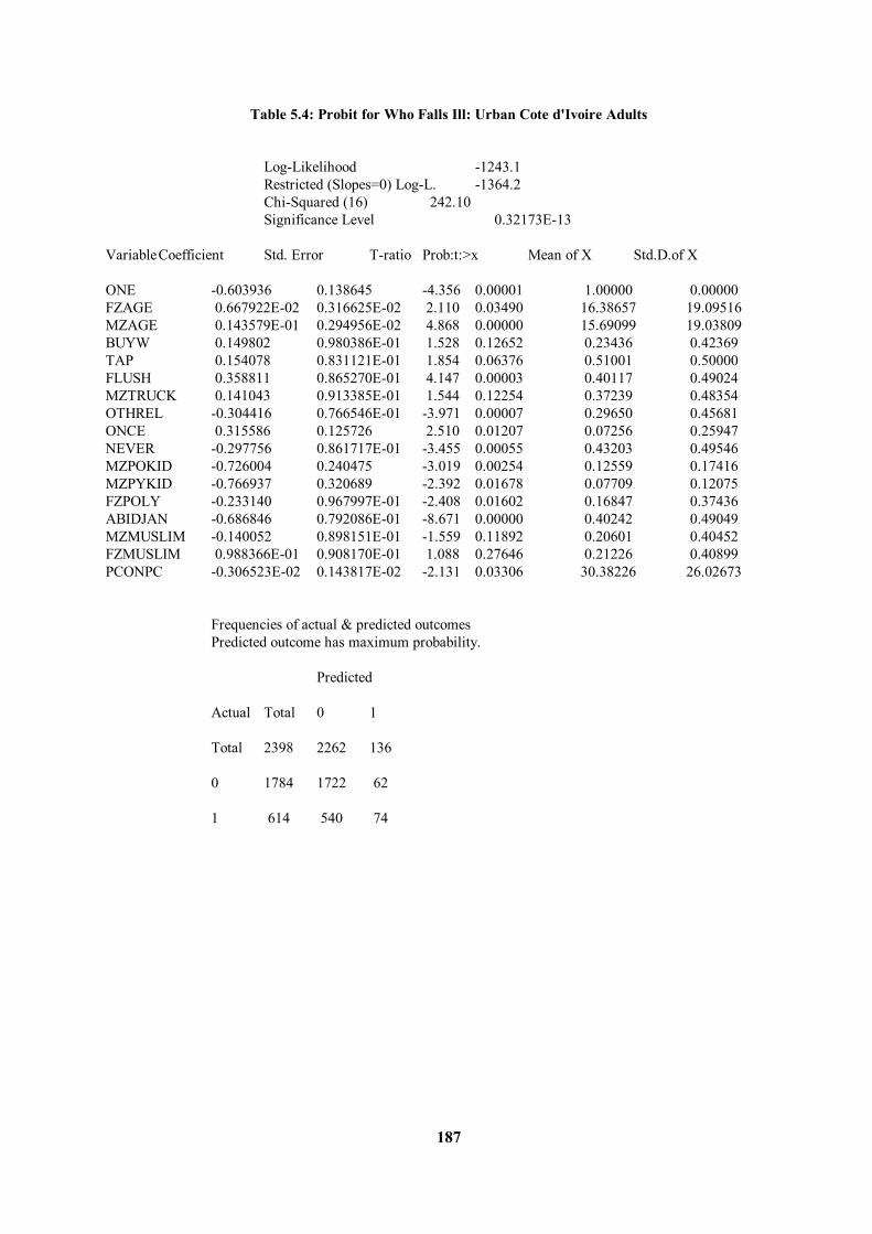
187

Table 5.4: Probit for Who Falls Ill: Urban Cote d'Ivoire Adults Log-Likelihood -1243.1 Restricted (Slopes=0) Log-L. -1364.2 Chi-Squared (16) 242.10 Significance Level 0.32173E-13 Variable Coefficient Std. Error T-ratio Prob:t:>x Mean of X Std.D.of X ONE -0.603936 0.138645 -4.356 0.00001 1.00000 0.00000 FZAGE 0.667922E-02 0.316625E-02 2.110 0.03490 16.38657 19.09516 MZAGE 0.143579E-01 0.294956E-02 4.868 0.00000 15.69099 19.03809 BUYW 0.149802 0.980386E-01 1.528 0.12652 0.23436 0.42369 TAP 0.154078 0.831121E-01 1.854 0.06376 0.51001 0.50000 FLUSH 0.358811 0.865270E-01 4.147 0.00003 0.40117 0.49024 MZTRUCK 0.141043 0.913385E-01 1.544 0.12254 0.37239 0.48354 OTHREL -0.304416 0.766546E-01 -3.971 0.00007 0.29650 0.45681 ONCE 0.315586 0.125726 2.510 0.01207 0.07256 0.25947 NEVER -0.297756 0.861717E-01 -3.455 0.00055 0.43203 0.49546 MZPOKID -0.726004 0.240475 -3.019 0.00254 0.12559 0.17416 MZPYKID -0.766937 0.320689 -2.392 0.01678 0.07709 0.12075 FZPOLY -0.233140 0.967997E-01 -2.408 0.01602 0.16847 0.37436 ABIDJAN -0.686846 0.792086E-01 -8.671 0.00000 0.40242 0.49049 MZMUSLIM -0.140052 0.898151E-01 -1.559 0.11892 0.20601 0.40452 FZMUSLIM 0.988366E-01 0.908170E-01 1.088 0.27646 0.21226 0.40899 PCONPC -0.306523E-02 0.143817E-02 -2.131 0.03306 30.38226 26.02673 Frequencies of actual & predicted outcomes Predicted outcome has maximum probability. Predicted Actual Total 0 1 Total 2398 2262 136 0 1784 1722 62 1 614 540 74

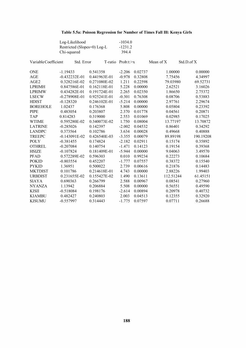
188

Table 5.5a: Poisson Regression for Number of Times Fall Ill: Kenya Girls Log-Likelihood -1034.0 Restricted (Slopes=0) Log-L -1231.2 Chi-squared 394.4 Variable Coefficient Std. Error T-ratio Prob:t:>x Mean of X Std.D.of X ONE -1.19433 0.541358 -2.206 0.02737 1.00000 0.00000 AGE -0.432232E-01 0.441963E-01 -0.978 0.32808 7.75456 4.34997 AGE2 0.328216E-02 0.271080E-02 1.211 0.22598 79.03980 69.52731 LPRIMH 0.847586E-01 0.162118E-01 5.228 0.00000 2.62521 3.16026 LPRIMW 0.434282E-01 0.191724E-01 2.265 0.02350 1.86650 2.75372 LSECW -0.278908E-01 0.925241E-01 -0.301 0.76308 0.08706 0.53883 HDIST -0.128320 0.246102E-01 -5.214 0.00000 2.97761 2.29674 BOREHOLE 1.02437 0.176368 5.808 0.00000 0.05804 0.23392 PIPE 0.483054 0.203807 2.370 0.01778 0.04561 0.20871 TAP 0.814283 0.319000 2.553 0.01069 0.02985 0.17025 WTIME 0.595280E-02 0.340073E-02 1.750 0.08004 13.77197 13.70872 LATRINE -0.285026 0.142397 -2.002 0.04532 0.86401 0.34292 LANDPC 0.373564 0.102786 3.634 0.00028 0.49668 0.40888 TREEPC -0.143091E-02 0.426540E-03 -3.355 0.00079 89.89198 190.19208 POLY -0.381455 0.174824 -2.182 0.02911 0.15174 0.35892 OTHREL -0.207084 0.140754 -1.471 0.14123 0.19154 0.39368 HSIZE -0.107824 0.181409E-01 -5.944 0.00000 9.04063 3.49570 PFAD 0.572289E-02 0.596303 0.010 0.99234 0.22273 0.10684 POKID -0.803554 0.452207 -1.777 0.07557 0.38372 0.15540 PYKID 1.36951 0.500022 2.739 0.00616 0.21876 0.14483 MKTDIST 0.101786 0.214618E-01 4.743 0.00000 2.88226 1.99403 URBDIST 0.231655E-02 0.155427E-02 1.490 0.13611 112.51244 61.45151 SIAYA 0.690363 0.266799 2.588 0.00967 0.08541 0.27960 NYANZA 1.13942 0.206884 5.508 0.00000 0.56551 0.49590 KISII -0.518084 0.198176 -2.614 0.00894 0.20978 0.40732 KIAMBU 0.482427 0.240803 2.003 0.04513 0.12355 0.32920 KISUMU -0.557997 0.314443 -1.775 0.07597 0.07711 0.26688

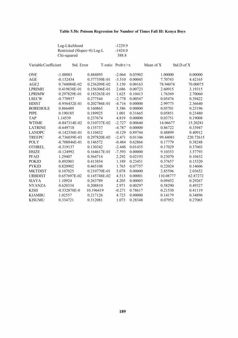
189

Table 5.5b: Poisson Regression for Number of Times Fall Ill: Kenya Boys Log-Likelihood -1229.9 Restricted (Slopes=0) Log-L -1424.0 Chi-squared 388.8 Variable Coefficient Std. Error T-ratio Prob:t:>x Mean of X Std.D.of X ONE -1.00083 0.484895 -2.064 0.03902 1.00000 0.00000 AGE -0.132434 0.377350E-01 -3.510 0.00045 7.70743 4.42165 AGE2 0.744084E-02 0.236209E-02 3.150 0.00163 78.94074 70.00075 LPRIMH 0.419838E-01 0.156306E-01 2.686 0.00723 2.60915 3.19315 LPRIMW 0.297829E-01 0.183263E-01 1.625 0.10413 1.76369 2.70060 LSECW -0.770937 0.277544 -2.778 0.00547 0.05476 0.39422 HDIST -0.956432E-01 0.202786E-01 -4.716 0.00000 2.99775 2.36640 BOREHOLE 0.866489 0.160865 5.386 0.00000 0.05701 0.23196 PIPE 0.190185 0.189925 1.001 0.31665 0.05851 0.23480 TAP 1.14539 0.237674 4.819 0.00000 0.03751 0.19008 WTIME -0.847314E-02 0.310737E-02 -2.727 0.00640 14.06677 15.20281 LATRINE -0.649718 0.135737 -4.787 0.00000 0.86722 0.33947 LANDPC -0.142336E-01 0.110432 -0.129 0.89744 0.48899 0.40912 TREEPC -0.736039E-03 0.297820E-03 -2.471 0.01346 99.44081 220.72615 POLY -0.708846E-01 0.146572 -0.484 0.62866 0.17779 0.38248 OTHREL -0.319137 0.130342 -2.448 0.01435 0.17029 0.37603 HSIZE -0.124992 0.164617E-01 -7.593 0.00000 9.10353 3.57793 PFAD 1.29407 0.564714 2.292 0.02193 0.23070 0.10432 POKID 0.492003 0.413854 1.189 0.23451 0.37657 0.15320 PYKID 0.820902 0.465108 1.765 0.07757 0.22024 0.14606 MKTDIST 0.107025 0.210770E-01 5.078 0.00000 2.85596 2.03652 URBDIST 0.657697E-02 0.145748E-02 4.513 0.00001 110.08777 62.87272 SIAYA 1.10924 0.263789 4.205 0.00003 0.09452 0.29267 NYANZA 0.620334 0.208810 2.971 0.00297 0.58290 0.49327 KISII -0.532870E-0 10.196419 -0.271 0.78617 0.21530 0.41119 KIAMBU 1.02557 0.217126 4.723 0.00000 0.14179 0.34896 KISUMU 0.334721 0.312081 1.073 0.28348 0.07952 0.27065

190

Table 5.6: Poisson Regression for Number of Times Fall Ill: Tanzania Children Log-Likelihood -1431.2 Restricted (Slopes=0) Log-L -1551.4 Chi-squared 240.4 Variable Coefficient Std. Error T-ratio Prob:t:>x Mean of X Std.D.of X ONE -0.142338 0.348537 -0.408 0.68299 1.00000 0.00000 MZAGE -0.111232 0.150574E-01 -7.387 0.00000 3.88758 4.93718 FZAGE -0.514738E-01 0.141918E-01 -3.627 0.00029 3.92671 5.00661 MZLPRIMH 0.130066 0.199704E-01 6.513 0.00000 1.05901 2.14621 FZLPRIMW 0.905717E-01 0.200447E-01 4.518 0.00001 0.82174 1.98061 HDIST 0.238350E-02 0.575103E-03 4.144 0.00003 17.31739 59.32554 BOREHOLE 0.383036 0.228103 1.679 0.09311 0.02795 0.16488 PIPE 0.122646 0.960339E-01 1.277 0.20156 0.27019 0.44419 FZWTIME -0.132757E-01 0.401406E-02 -3.307 0.00094 9.66894 15.66437 LATRINE 0.623388 0.263183 2.369 0.01785 0.94348 0.23100 FZOTHREL -0.299448 0.209144 -1.432 0.15221 0.06087 0.23917 MZOTHREL -0.730006 0.240922 -3.030 0.00245 0.05776 0.23337 MZHSIZE -0.461911E-01 0.160741E-01 -2.874 0.00406 4.37826 4.96956 PFAD -2.49747 0.479597 -5.207 0.00000 0.24003 0.10075 FZPOKID -1.59696 0.419653 -3.805 0.00014 0.18183 0.20768 PYKID -1.67198 0.359057 -4.657 0.00000 0.20084 0.13912 FZIRINGA 0.785856 0.142822 5.502 0.00000 0.15963 0.36637 MZIRINGA 0.246862 0.156290 1.580 0.11422 0.15155 0.35870 DODOMA 0.373802 0.132516 2.821 0.00479 0.25466 0.43580 RUVUMA 0.522102 0.139630 3.739 0.00018 0.16211 0.36867

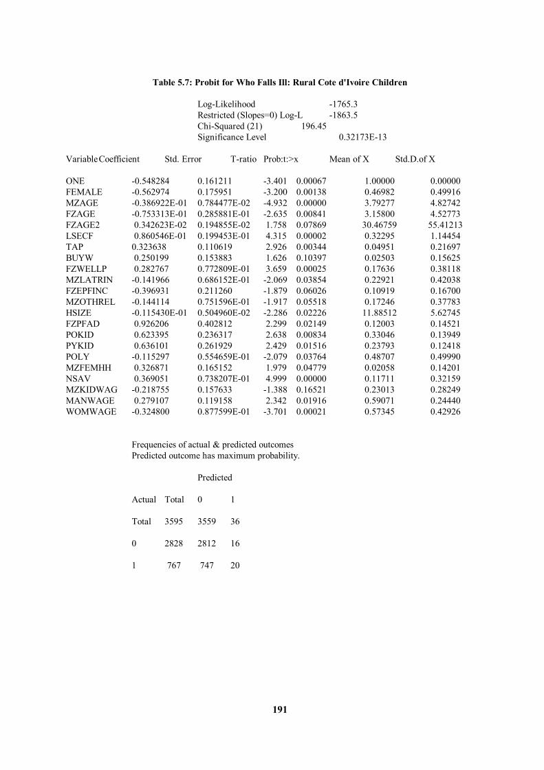
191

Table 5.7: Probit for Who Falls Ill: Rural Cote d'Ivoire Children Log-Likelihood -1765.3 Restricted (Slopes=0) Log-L -1863.5 Chi-Squared (21) 196.45 Significance Level 0.32173E-13 Variable Coefficient Std. Error T-ratio Prob:t:>x Mean of X Std.D.of X ONE -0.548284 0.161211 -3.401 0.00067 1.00000 0.00000 FEMALE -0.562974 0.175951 -3.200 0.00138 0.46982 0.49916 MZAGE -0.386922E-01 0.784477E-02 -4.932 0.00000 3.79277 4.82742 FZAGE -0.753313E-01 0.285881E-01 -2.635 0.00841 3.15800 4.52773 FZAGE2 0.342623E-02 0.194855E-02 1.758 0.07869 30.46759 55.41213 LSECF 0.860546E-01 0.199453E-01 4.315 0.00002 0.32295 1.14454 TAP 0.323638 0.110619 2.926 0.00344 0.04951 0.21697 BUYW 0.250199 0.153883 1.626 0.10397 0.02503 0.15625 FZWELLP 0.282767 0.772809E-01 3.659 0.00025 0.17636 0.38118 MZLATRIN -0.141966 0.686152E-01 -2.069 0.03854 0.22921 0.42038 FZEPFINC -0.396931 0.211260 -1.879 0.06026 0.10919 0.16700 MZOTHREL -0.144114 0.751596E-01 -1.917 0.05518 0.17246 0.37783 HSIZE -0.115430E-01 0.504960E-02 -2.286 0.02226 11.88512 5.62745 FZPFAD 0.926206 0.402812 2.299 0.02149 0.12003 0.14521 POKID 0.623395 0.236317 2.638 0.00834 0.33046 0.13949 PYKID 0.636101 0.261929 2.429 0.01516 0.23793 0.12418 POLY -0.115297 0.554659E-01 -2.079 0.03764 0.48707 0.49990 MZFEMHH 0.326871 0.165152 1.979 0.04779 0.02058 0.14201 NSAV 0.369051 0.738207E-01 4.999 0.00000 0.11711 0.32159 MZKIDWAG -0.218755 0.157633 -1.388 0.16521 0.23013 0.28249 MANWAGE 0.279107 0.119158 2.342 0.01916 0.59071 0.24440 WOMWAGE -0.324800 0.877599E-01 -3.701 0.00021 0.57345 0.42926 Frequencies of actual & predicted outcomes Predicted outcome has maximum probability. Predicted Actual Total 0 1 Total 3595 3559 36 0 2828 2812 16 1 767 747 20

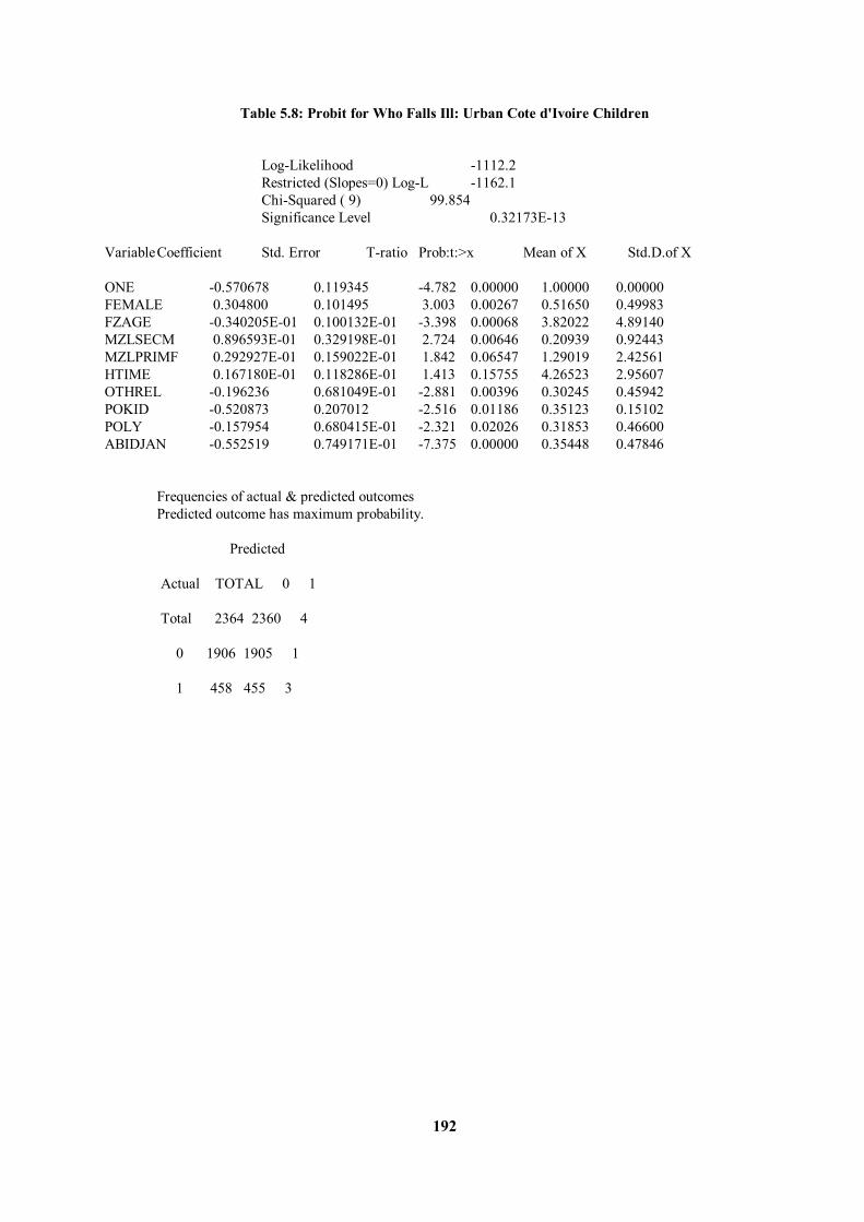
192

Table 5.8: Probit for Who Falls Ill: Urban Cote d'Ivoire Children Log-Likelihood -1112.2 Restricted (Slopes=0) Log-L -1162.1 Chi-Squared ( 9) 99.854 Significance Level 0.32173E-13 Variable Coefficient Std. Error T-ratio Prob:t:>x Mean of X Std.D.of X ONE -0.570678 0.119345 -4.782 0.00000 1.00000 0.00000 FEMALE 0.304800 0.101495 3.003 0.00267 0.51650 0.49983 FZAGE -0.340205E-01 0.100132E-01 -3.398 0.00068 3.82022 4.89140 MZLSECM 0.896593E-01 0.329198E-01 2.724 0.00646 0.20939 0.92443 MZLPRIMF 0.292927E-01 0.159022E-01 1.842 0.06547 1.29019 2.42561 HTIME 0.167180E-01 0.118286E-01 1.413 0.15755 4.26523 2.95607 OTHREL -0.196236 0.681049E-01 -2.881 0.00396 0.30245 0.45942 POKID -0.520873 0.207012 -2.516 0.01186 0.35123 0.15102 POLY -0.157954 0.680415E-01 -2.321 0.02026 0.31853 0.46600 ABIDJAN -0.552519 0.749171E-01 -7.375 0.00000 0.35448 0.47846 Frequencies of actual & predicted outcomes Predicted outcome has maximum probability. Predicted Actual TOTAL 0 1 Total 2364 2360 4 0 1906 1905 1 1 458 455 3

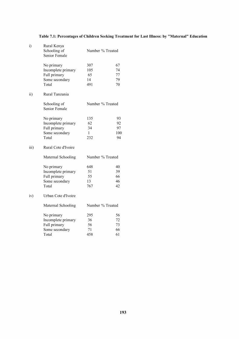
193

Table 7.1: Percentages of Children Seeking Treatment for Last Illness: by "Maternal" Education i) Rural Kenya Schooling of Number % Treated Senior Female No primary 307 67 Incomplete primary 105 74 Full primary 65 77 Some secondary 14 79 Total 491 70 ii) Rural Tanzania Schooling of Number % Treated Senior Female No primary 135 93 Incomplete primary 62 92 Full primary 34 97 Some secondary 1 100 Total 232 94 iii) Rural Cote d'Ivoire Maternal Schooling Number % Treated No primary 648 40 Incomplete primary 51 39 Full primary 55 66 Some secondary 13 46 Total 767 42 iv) Urban Cote d'Ivoire Maternal Schooling Number % Treated No primary 295 56 Incomplete primary 36 72 Full primary 56 73 Some secondary 71 66 Total 458 61

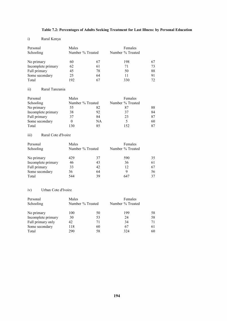
194

Table 7.2: Percentages of Adults Seeking Treatment for Last Illness: by Personal Education i) Rural Kenya Personal Males Females Schooling Number % Treated Number % Treated No primary 60 67 198 67 Incomplete primary 62 61 71 73 Full primary 45 78 50 88 Some secondary 25 64 11 91 Total 192 67 330 72 ii) Rural Tanzania Personal Males Females Schooling Number % Treated Number % Treated No primary 55 82 87 88 Incomplete primary 38 92 37 84 Full primary 37 84 23 87 Some secondary 0 NA 5 60 Total 130 85 152 87 iii) Rural Cote d'Ivoire Personal Males Females Schooling Number % Treated Number % Treated No primary 429 37 590 35 Incomplete primary 46 43 36 61 Full primary 33 42 12 67 Some secondary 36 64 9 56 Total 544 39 647 37 iv) Urban Cote d'Ivoire Personal Males Females Schooling Number % Treated Number % Treated No primary 100 50 199 58 Incomplete primary 30 53 24 58 Full primary only 42 71 34 71 Some secondary 118 60 67 61 Total 290 58 324 60

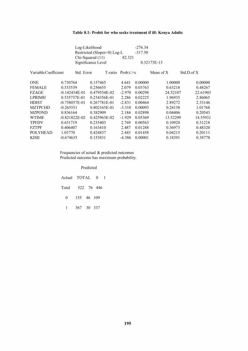
195

Table 8.1: Probit for who seeks treatment if ill: Kenya Adults Log-Likelihood -276.34 Restricted (Slopes=0) Log-L -317.50 Chi-Squared (11) 82.321 Significance Level 0.32173E-13 Variable Coefficient Std. Error T-ratio Prob:t:>x Mean of X Std.D.of X ONE 0.730764 0.157465 4.641 0.00000 1.00000 0.00000 FEMALE 0.533539 0.256655 2.079 0.03763 0.63218 0.48267 FZAGE -0.142434E-01 0.479554E-02 -2.970 0.00298 24.52107 22.61903 LPRIMH 0.535737E-01 0.234356E-01 2.286 0.02225 1.96935 2.86065 HDIST -0.758057E-01 0.267781E-01 -2.831 0.00464 2.89272 2.33146 MZTPCHD -0.265551 0.802165E-01 -3.310 0.00093 0.24138 1.01768 MZPOND 0.836164 0.382909 2.184 0.02898 0.04406 0.20543 WTIME -0.821822E-02 0.425963E-02 -1.929 0.05369 13.52299 14.55931 TPFDV 0.651719 0.235403 2.769 0.00563 0.10920 0.31218 FZTPF 0.406407 0.163410 2.487 0.01288 0.36973 0.48320 POLYHEAD 1.03770 0.424837 2.443 0.01458 0.04215 0.20111 KISII -0.674635 0.153831 -4.386 0.00001 0.18391 0.38778 Frequencies of actual & predicted outcomes Predicted outcome has maximum probability. Predicted Actual TOTAL 0 1 Total 522 76 446 0 155 46 109 1 367 30 337

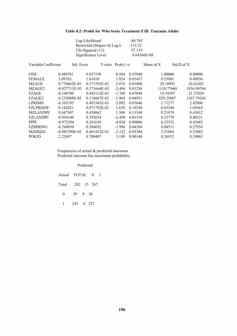
196

Table 8.2: Probit for Who Seeks Treatment if Ill: Tanzania Adults Log-Likelihood -84.765 Restricted (Slopes=0) Log-L -113.32 Chi-Squared (13) 57.119 Significance Level 0.64366E-08 Variable Coefficient Std. Error T-ratio Prob:t:>x Mean of X Std.D.of X ONE 0.488701 0.837198 0.584 0.55940 1.00000 0.00000 FEMALE 3.09765 1.61010 1.924 0.05437 0.53901 0.49936 MZAGE 0.770662E-01 0.371592E-01 2.074 0.03808 20.10993 26.62482 MZAGE2 -0.927711E-03 0.371664E-03 -2.496 0.01256 1110.77660 1936.90704 FZAGE -0.148700 0.845112E-01 -1.760 0.07849 19.34397 21.37029 FZAGE2 0.233088E-02 0.118667E-02 1.964 0.04951 829.25887 1267.79245 LPRIMH -0.103195 0.493341E-01 -2.092 0.03646 1.71277 2.42006 FZLPRIMW 0.142021 0.871792E-01 1.629 0.10330 0.65248 1.69565 MZLANDPC 0.687307 0.458062 1.500 0.13349 0.21979 0.43012 FZLANDPC -0.954140 0.392654 -2.430 0.01510 0.25770 0.40321 PIPE -0.972294 0.241630 -4.024 0.00006 0.25532 0.43682 FZSPRING -0.768030 0.384692 -1.996 0.04588 0.08511 0.27954 MZHSIZE -0.983390E-01 0.463432E-01 -2.122 0.03384 3.51064 4.53082 POKID 2.22697 0.700407 3.180 0.00148 0.26932 0.19065 Frequencies of actual & predicted outcomes Predicted outcome has maximum probability. Predicted Actual TOTAL 0 1 Total 282 15 267 0 39 9 30 1 243 6 237

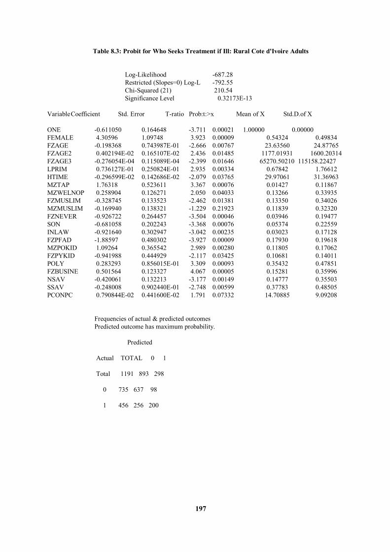
197

Table 8.3: Probit for Who Seeks Treatment if Ill: Rural Cote d'Ivoire Adults Log-Likelihood -687.28 Restricted (Slopes=0) Log-L -792.55 Chi-Squared (21) 210.54 Significance Level 0.32173E-13 Variable Coefficient Std. Error T-ratio Prob:t:>x Mean of X Std.D.of X ONE -0.611050 0.164648 -3.711 0.00021 1.00000 0.00000 FEMALE 4.30596 1.09748 3.923 0.00009 0.54324 0.49834 FZAGE -0.198368 0.743987E-01 -2.666 0.00767 23.63560 24.87765 FZAGE2 0.402194E-02 0.165107E-02 2.436 0.01485 1177.01931 1600.20314 FZAGE3 -0.276054E-04 0.115089E-04 -2.399 0.01646 65270.50210 115158.22427 LPRIM 0.736127E-01 0.250824E-01 2.935 0.00334 0.67842 1.76612 HTIME -0.296599E-02 0.142686E-02 -2.079 0.03765 29.97061 31.36963 MZTAP 1.76318 0.523611 3.367 0.00076 0.01427 0.11867 MZWELNOP 0.258904 0.126271 2.050 0.04033 0.13266 0.33935 FZMUSLIM -0.328745 0.133523 -2.462 0.01381 0.13350 0.34026 MZMUSLIM -0.169940 0.138321 -1.229 0.21923 0.11839 0.32320 FZNEVER -0.926722 0.264457 -3.504 0.00046 0.03946 0.19477 SON -0.681058 0.202243 -3.368 0.00076 0.05374 0.22559 INLAW -0.921640 0.302947 -3.042 0.00235 0.03023 0.17128 FZPFAD -1.88597 0.480302 -3.927 0.00009 0.17930 0.19618 MZPOKID 1.09264 0.365542 2.989 0.00280 0.11805 0.17062 FZPYKID -0.941988 0.444929 -2.117 0.03425 0.10681 0.14011 POLY 0.283293 0.856015E-01 3.309 0.00093 0.35432 0.47851 FZBUSINE 0.501564 0.123327 4.067 0.00005 0.15281 0.35996 NSAV -0.420061 0.132213 -3.177 0.00149 0.14777 0.35503 SSAV -0.248008 0.902440E-01 -2.748 0.00599 0.37783 0.48505 PCONPC 0.790844E-02 0.441600E-02 1.791 0.07332 14.70885 9.09208 Frequencies of actual & predicted outcomes Predicted outcome has maximum probability. Predicted Actual TOTAL 0 1 Total 1191 893 298 0 735 637 98 1 456 256 200

198

Table 8.4: Probit for Who Seeks Treatment if Ill: Urban Cote d'Ivoire Adults Log-Likelihood -394.70 Restricted (Slopes=0) Log-L -416.04 Chi-Squared (9) 42.688 Significance Level 0.15566E-06 Variable Coefficient Std. Error T-ratio Prob:t:>x Mean of X Std.D.of X ONE -0.399596 0.223685 -1.786 0.07403 1.00000 0.00000 MZHTIME -0.712357E-01 0.289900E-01 -2.457 0.01400 1.94625 2.64397 LPRIM 0.476215E-01 0.198930E-01 2.394 0.01667 2.86808 2.89408 BUYW 0.222822 0.142945 1.559 0.11905 0.17915 0.38379 FZMARRIE 0.489269 0.148307 3.299 0.00097 0.32085 0.46718 MZHSIZE 0.354744E-01 0.114393E-01 3.101 0.00193 4.84365 6.73272 PFAD 0.714569 0.403262 1.772 0.07640 0.27401 0.14750 POKID 0.962312 0.337543 2.851 0.00436 0.27430 0.16901 POLY -0.395640 0.127205 -3.110 0.00187 0.28990 0.45409 FZPCONPC -0.498671E-02 0.281433E-02 -1.772 0.07641 15.82853 23.55251 Frequencies of actual & predicted outcomes Predicted outcome has maximum probability. Predicted Actual TOTAL 0 1 Total 614 136 478 0 253 76 177 1 361 60 301

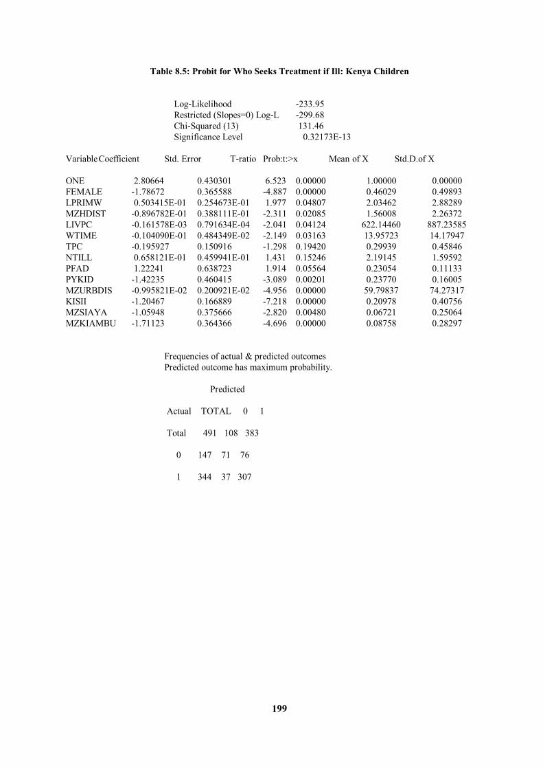
199

Table 8.5: Probit for Who Seeks Treatment if Ill: Kenya Children Log-Likelihood -233.95 Restricted (Slopes=0) Log-L -299.68 Chi-Squared (13) 131.46 Significance Level 0.32173E-13 Variable Coefficient Std. Error T-ratio Prob:t:>x Mean of X Std.D.of X ONE 2.80664 0.430301 6.523 0.00000 1.00000 0.00000 FEMALE -1.78672 0.365588 -4.887 0.00000 0.46029 0.49893 LPRIMW 0.503415E-01 0.254673E-01 1.977 0.04807 2.03462 2.88289 MZHDIST -0.896782E-01 0.388111E-01 -2.311 0.02085 1.56008 2.26372 LIVPC -0.161578E-03 0.791634E-04 -2.041 0.04124 622.14460 887.23585 WTIME -0.104090E-01 0.484349E-02 -2.149 0.03163 13.95723 14.17947 TPC -0.195927 0.150916 -1.298 0.19420 0.29939 0.45846 NTILL 0.658121E-01 0.459941E-01 1.431 0.15246 2.19145 1.59592 PFAD 1.22241 0.638723 1.914 0.05564 0.23054 0.11133 PYKID -1.42235 0.460415 -3.089 0.00201 0.23770 0.16005 MZURBDIS -0.995821E-02 0.200921E-02 -4.956 0.00000 59.79837 74.27317 KISII -1.20467 0.166889 -7.218 0.00000 0.20978 0.40756 MZSIAYA -1.05948 0.375666 -2.820 0.00480 0.06721 0.25064 MZKIAMBU -1.71123 0.364366 -4.696 0.00000 0.08758 0.28297 Frequencies of actual & predicted outcomes Predicted outcome has maximum probability. Predicted Actual TOTAL 0 1 Total 491 108 383 0 147 71 76 1 344 37 307

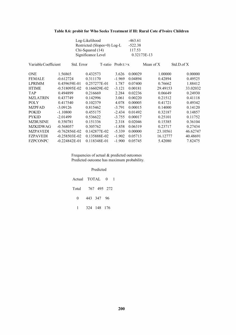
200

Table 8.6: probit for Who Seeks Treatment if Ill: Rural Cote d'Ivoire Children Log-Likelihood -463.61 Restricted (Slopes=0) Log-L -522.38 Chi-Squared (14) 117.53 Significance Level 0.32173E-13 Variable Coefficient Std. Error T-ratio Prob:t:>x Mean of X Std.D.of X ONE 1.56865 0.432573 3.626 0.00029 1.00000 0.00000 FEMALE -0.612724 0.311170 -1.969 0.04894 0.42894 0.49525 LPRIMM 0.459659E-01 0.257277E-01 1.787 0.07400 0.76662 1.88412 HTIME -0.518095E-02 0.166029E-02 -3.121 0.00181 29.49153 33.02032 TAP 0.494899 0.216669 2.284 0.02236 0.06649 0.24930 MZLATRIN 0.437749 0.142996 3.061 0.00220 0.21512 0.41118 POLY 0.417540 0.102379 4.078 0.00005 0.41721 0.49342 MZPFAD -3.09126 0.815462 -3.791 0.00015 0.14000 0.14120 POKID -1.10800 0.455175 -2.434 0.01492 0.32187 0.14857 PYKID -2.01499 0.536622 -3.755 0.00017 0.25101 0.11752 MZBUSINE 0.350781 0.151336 2.318 0.02046 0.15385 0.36104 MZKIDWAG -0.568057 0.305762 -1.858 0.06319 0.23717 0.27434 MZPAVEDI -0.762856E-02 0.142877E-02 -5.339 0.00000 23.10561 46.62747 FZPAVEDI -0.258503E-02 0.135888E-02 -1.902 0.05713 16.12777 40.48691 FZPCONPC -0.224842E-01 0.118348E-01 -1.900 0.05745 5.42080 7.82475 Frequencies of actual & predicted outcomes Predicted outcome has maximum probability. Predicted Actual TOTAL 0 1 Total 767 495 272 0 443 347 96 1 324 148 176

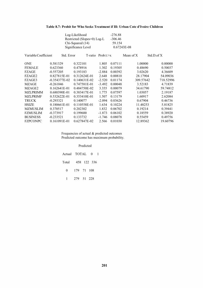
201

Table 8.7: Probit for Who Seeks Treatment if Ill: Urban Cote d'Ivoire Children Log-Likelihood -276.88 Restricted (Slopes=0) Log-L -306.46 Chi-Squared (14) 59.154 Significance Level 0.67243E-08 Variable Coefficient Std. Error T-ratio Prob:t:>x Mean of X Std.D.of X ONE 0.581329 0.322101 1.805 0.07111 1.00000 0.00000 FEMALE 0.623360 0.478916 1.302 0.19305 0.48690 0.50037 FZAGE -0.557205 0.193183 -2.884 0.00392 3.02620 4.36609 FZAGE2 0.827815E-01 0.312624E-01 2.648 0.00810 28.17904 54.09036 FZAGE3 -0.354377E-02 0.140631E-02 -2.520 0.01174 309.57642 718.52996 MZAGE -0.261046 0.747581E-01 -3.492 0.00048 3.52183 4.71839 MZAGE2 0.162641E-01 0.484750E-02 3.355 0.00079 34.61790 59.74812 MZLPRIMM 0.680390E-01 0.383417E-01 1.775 0.07597 1.03057 2.19187 MZLPRIMF 0.532622E-01 0.353410E-01 1.507 0.13179 1.60917 2.62084 TRUCK -0.293321 0.140077 -2.094 0.03626 0.67904 0.46736 HSIZE 0.180661E-01 0.110558E-01 1.634 0.10224 11.48253 5.81825 MZMUSLIM 0.370517 0.202302 1.832 0.06702 0.19214 0.39441 FZMUSLIM -0.373917 0.199600 -1.873 0.06102 0.18559 0.38920 BUSINESS -0.233521 0.133732 -1.746 0.08078 0.55459 0.49756 FZPCONPC 0.161091E-01 0.627847E-02 2.566 0.01030 12.89362 19.60796 Frequencies of actual & predicted outcomes Predicted outcome has maximum probability. Predicted Actual TOTAL 0 1 Total 458 122 336 0 179 71 108 1 279 51 228

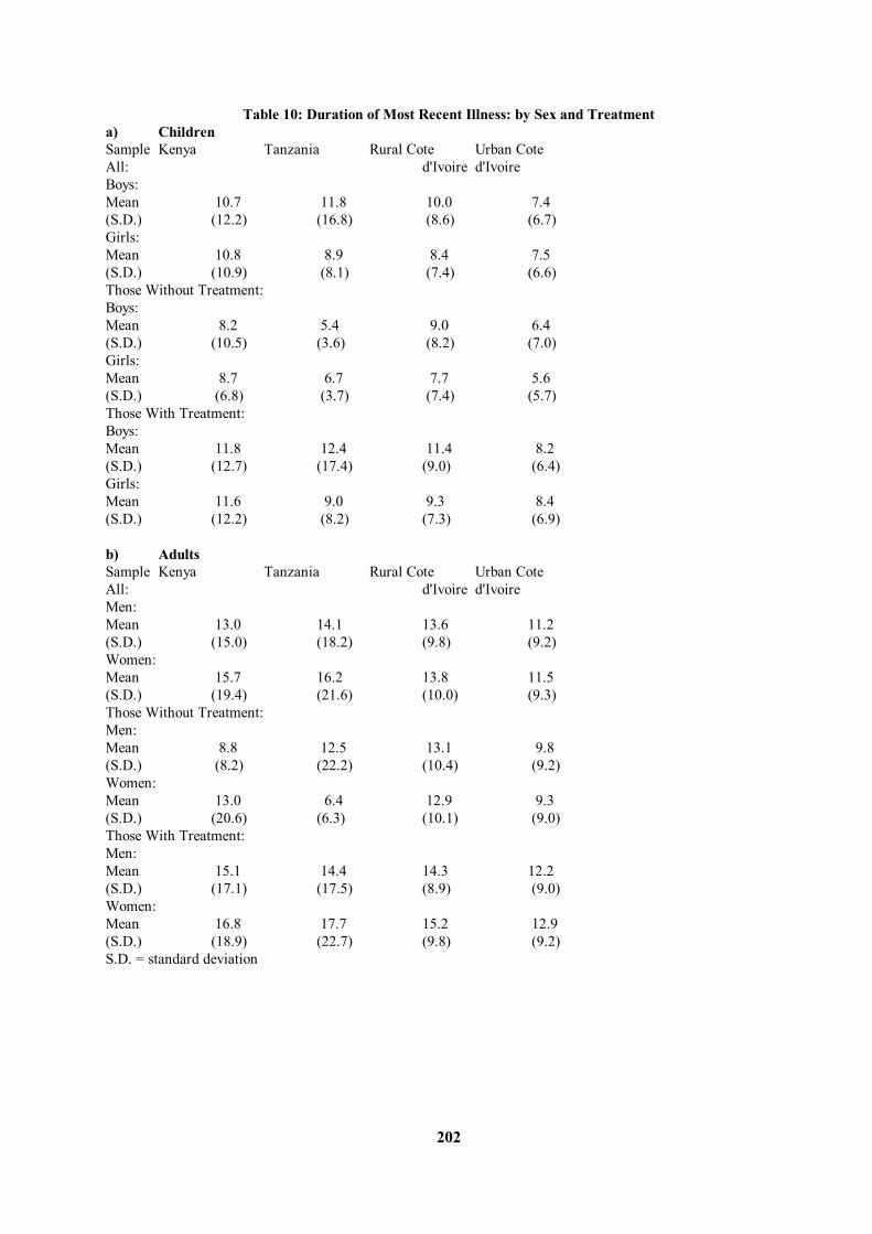
202

Table 10: Duration of Most Recent Illness: by Sex and Treatment a) Children Sample Kenya Tanzania Rural Cote Urban Cote All: d'Ivoire d'Ivoire Boys: Mean 10.7 11.8 10.0 7.4 (S.D.) (12.2) (16.8) (8.6) (6.7) Girls: Mean 10.8 8.9 8.4 7.5 (S.D.) (10.9) (8.1) (7.4) (6.6) Those Without Treatment: Boys: Mean 8.2 5.4 9.0 6.4 (S.D.) (10.5) (3.6) (8.2) (7.0) Girls: Mean 8.7 6.7 7.7 5.6 (S.D.) (6.8) (3.7) (7.4) (5.7) Those With Treatment: Boys: Mean 11.8 12.4 11.4 8.2 (S.D.) (12.7) (17.4) (9.0) (6.4) Girls: Mean 11.6 9.0 9.3 8.4 (S.D.) (12.2) (8.2) (7.3) (6.9) b) Adults Sample Kenya Tanzania Rural Cote Urban Cote All: d'Ivoire d'Ivoire Men: Mean 13.0 14.1 13.6 11.2 (S.D.) (15.0) (18.2) (9.8) (9.2) Women: Mean 15.7 16.2 13.8 11.5 (S.D.) (19.4) (21.6) (10.0) (9.3) Those Without Treatment: Men: Mean 8.8 12.5 13.1 9.8 (S.D.) (8.2) (22.2) (10.4) (9.2) Women: Mean 13.0 6.4 12.9 9.3 (S.D.) (20.6) (6.3) (10.1) (9.0) Those With Treatment: Men: Mean 15.1 14.4 14.3 12.2 (S.D.) (17.1) (17.5) (8.9) (9.0) Women: Mean 16.8 17.7 15.2 12.9 (S.D.) (18.9) (22.7) (9.8) (9.2) S.D. = standard deviation

203

Table 11.1: Ordinary Least Squares Regression of the Log-Duration of Illness: Kenya Adults Number of Observations 522 Mean of Dep. Var. 2.265404 Std. Dev. of Dep. Var. 0.881407 Std. Error of Regr. 0.791948 Sum of Sqrd. Residuals 313.590847 R - squared 0.225231 Adjusted R - Squared 0.192690 Variable Coefficient Std. Error T-ratio Prob:t:>x Mean of X Std.D.of X ONE 1.16480 0.256583 4.540 0.00002 1.00000 0.00000 FEMALE 1.98930 0.385860 5.155 0.00000 0.63218 0.48267 MZAGE 0.142984E-01 0.431206E-02 3.316 0.00114 15.04406 23.04406 BOREHOLE 0.251143 0.140795 1.784 0.07138 0.09195 0.28924 PIPE 0.388784 0.151455 2.567 0.01025 0.06130 0.24011 FZWTIME -0.598727E-02 0.325960E-02 -1.837 0.06340 8.59770 13.21617 TPFDV 0.268095 0.117108 2.289 0.02133 0.10920 0.31218 MZTPDV 0.434373 0.243414 1.785 0.07126 0.02299 0.15001 FZTPC -0.285025 0.132185 -2.156 0.02979 0.10536 0.30732 NTILL 0.632047E-01 0.208089E-01 3.037 0.00268 2.49808 2.04859 FZBEFORE -0.188701 0.104443 -1.807 0.06782 0.28161 0.45022 SON 0.418595 0.179992 2.326 0.01943 0.13027 0.33692 PFAD 0.340850 0.195697 1.742 0.07830 0.33794 0.19460 MZFEMHH -0.802279 0.400214 -2.005 0.04301 0.00958 0.09749 URBDIST -0.358091E-02 0.102436E-02 -3.496 0.00065 106.09004 63.13169 SNYANZA 0.619836 0.156712 3.955 0.00014 0.22414 0.41741 MZKIRINY 0.879681 0.311939 2.820 0.00505 0.01341 0.11513 KISII 0.436578 0.132984 3.283 0.00127 0.18391 0.38778 MZKIAMBU 0.533948 0.222308 2.402 0.01593 0.03640 0.18746 FZTREAT -1.12432 0.356620 -3.153 0.00189 0.45594 0.49853 FZLAMB 0.912171 0.212212 4.298 0.00004 -0.00164 0.58540 MZLAMB 0.394839 0.860049E-01 4.591 0.00001 0.00000 0.41405

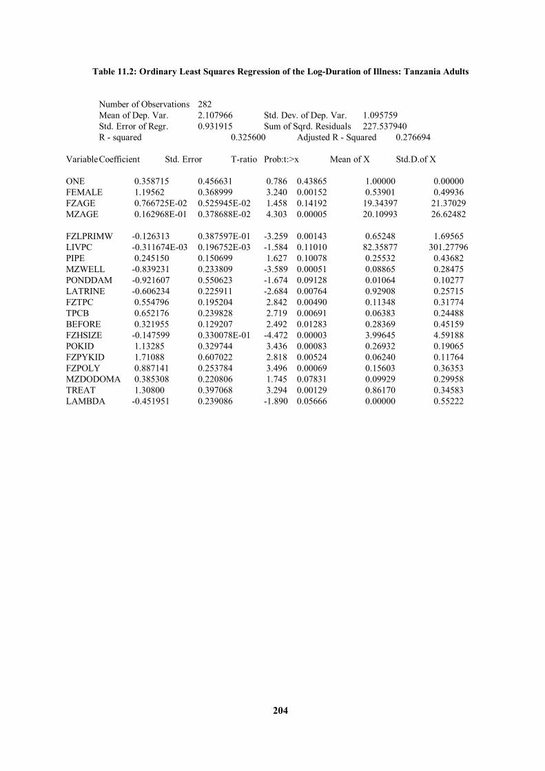
204

Table 11.2: Ordinary Least Squares Regression of the Log-Duration of Illness: Tanzania Adults Number of Observations 282 Mean of Dep. Var. 2.107966 Std. Dev. of Dep. Var. 1.095759 Std. Error of Regr. 0.931915 Sum of Sqrd. Residuals 227.537940 R - squared 0.325600 Adjusted R - Squared 0.276694 Variable Coefficient Std. Error T-ratio Prob:t:>x Mean of X Std.D.of X ONE 0.358715 0.456631 0.786 0.43865 1.00000 0.00000 FEMALE 1.19562 0.368999 3.240 0.00152 0.53901 0.49936 FZAGE 0.766725E-02 0.525945E-02 1.458 0.14192 19.34397 21.37029 MZAGE 0.162968E-01 0.378688E-02 4.303 0.00005 20.10993 26.62482 FZLPRIMW -0.126313 0.387597E-01 -3.259 0.00143 0.65248 1.69565 LIVPC -0.311674E-03 0.196752E-03 -1.584 0.11010 82.35877 301.27796 PIPE 0.245150 0.150699 1.627 0.10078 0.25532 0.43682 MZWELL -0.839231 0.233809 -3.589 0.00051 0.08865 0.28475 PONDDAM -0.921607 0.550623 -1.674 0.09128 0.01064 0.10277 LATRINE -0.606234 0.225911 -2.684 0.00764 0.92908 0.25715 FZTPC 0.554796 0.195204 2.842 0.00490 0.11348 0.31774 TPCB 0.652176 0.239828 2.719 0.00691 0.06383 0.24488 BEFORE 0.321955 0.129207 2.492 0.01283 0.28369 0.45159 FZHSIZE -0.147599 0.330078E-01 -4.472 0.00003 3.99645 4.59188 POKID 1.13285 0.329744 3.436 0.00083 0.26932 0.19065 FZPYKID 1.71088 0.607022 2.818 0.00524 0.06240 0.11764 FZPOLY 0.887141 0.253784 3.496 0.00069 0.15603 0.36353 MZDODOMA 0.385308 0.220806 1.745 0.07831 0.09929 0.29958 TREAT 1.30800 0.397068 3.294 0.00129 0.86170 0.34583 LAMBDA -0.451951 0.239086 -1.890 0.05666 0.00000 0.55222

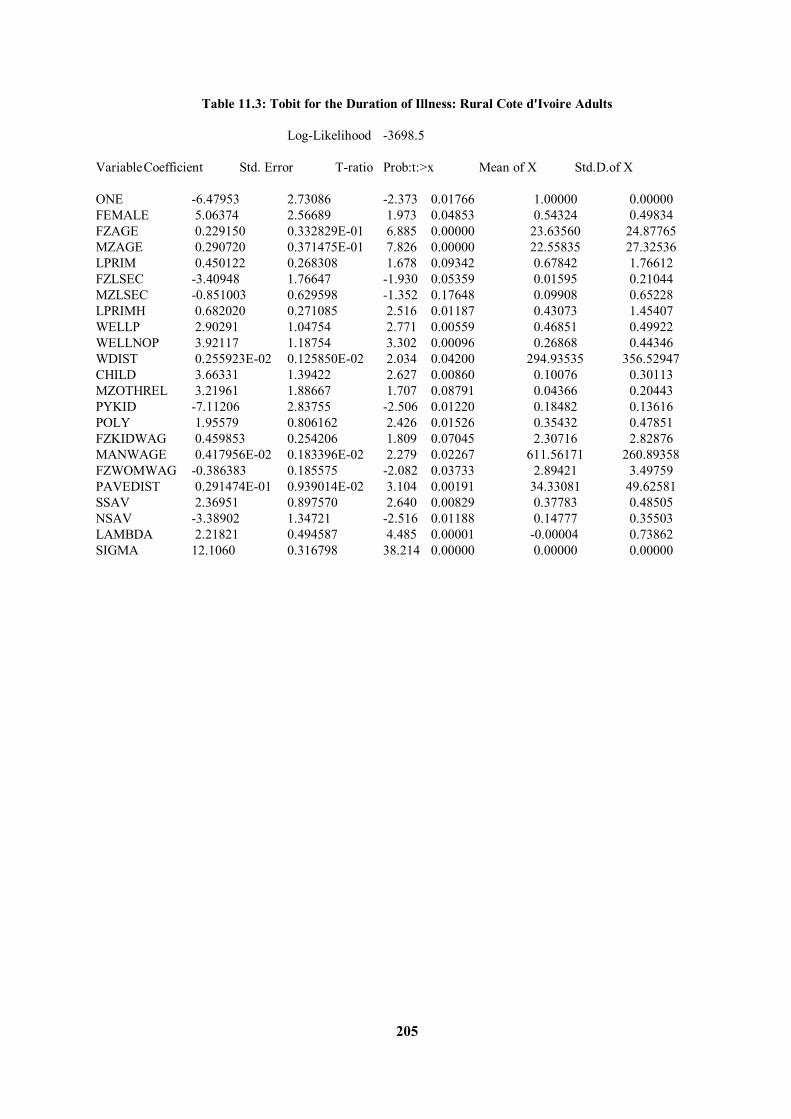
205

Table 11.3: Tobit for the Duration of Illness: Rural Cote d'Ivoire Adults Log-Likelihood -3698.5 Variable Coefficient Std. Error T-ratio Prob:t:>x Mean of X Std.D.of X ONE -6.47953 2.73086 -2.373 0.01766 1.00000 0.00000 FEMALE 5.06374 2.56689 1.973 0.04853 0.54324 0.49834 FZAGE 0.229150 0.332829E-01 6.885 0.00000 23.63560 24.87765 MZAGE 0.290720 0.371475E-01 7.826 0.00000 22.55835 27.32536 LPRIM 0.450122 0.268308 1.678 0.09342 0.67842 1.76612 FZLSEC -3.40948 1.76647 -1.930 0.05359 0.01595 0.21044 MZLSEC -0.851003 0.629598 -1.352 0.17648 0.09908 0.65228 LPRIMH 0.682020 0.271085 2.516 0.01187 0.43073 1.45407 WELLP 2.90291 1.04754 2.771 0.00559 0.46851 0.49922 WELLNOP 3.92117 1.18754 3.302 0.00096 0.26868 0.44346 WDIST 0.255923E-02 0.125850E-02 2.034 0.04200 294.93535 356.52947 CHILD 3.66331 1.39422 2.627 0.00860 0.10076 0.30113 MZOTHREL 3.21961 1.88667 1.707 0.08791 0.04366 0.20443 PYKID -7.11206 2.83755 -2.506 0.01220 0.18482 0.13616 POLY 1.95579 0.806162 2.426 0.01526 0.35432 0.47851 FZKIDWAG 0.459853 0.254206 1.809 0.07045 2.30716 2.82876 MANWAGE 0.417956E-02 0.183396E-02 2.279 0.02267 611.56171 260.89358 FZWOMWAG -0.386383 0.185575 -2.082 0.03733 2.89421 3.49759 PAVEDIST 0.291474E-01 0.939014E-02 3.104 0.00191 34.33081 49.62581 SSAV 2.36951 0.897570 2.640 0.00829 0.37783 0.48505 NSAV -3.38902 1.34721 -2.516 0.01188 0.14777 0.35503 LAMBDA 2.21821 0.494587 4.485 0.00001 -0.00004 0.73862 SIGMA 12.1060 0.316798 38.214 0.00000 0.00000 0.00000

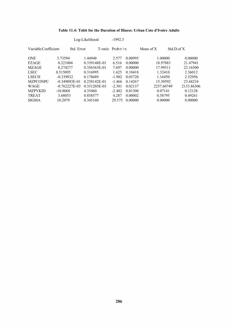
206

Table 11.4: Tobit for the Duration of Illness: Urban Cote d'Ivoire Adults Log-Likelihood -1992.3 Variable Coefficient Std. Error T-ratio Prob:t:>x Mean of X Std.D.of X ONE 3.73594 1.44948 2.577 0.00995 1.00000 0.00000 FZAGE 0.221004 0.339148E-01 6.516 0.00000 18.97883 21.47941 MZAGE 0.274277 0.356363E-01 7.697 0.00000 17.99511 22.16500 LSEC 0.515095 0.316995 1.625 0.10418 1.32410 2.36012 LSECH -0.339832 0.178689 -1.902 0.05720 1.16450 2.52956 MZPCONPC -0.349093E-01 0.238142E-01 -1.466 0.14267 15.30592 23.68234 WAGE -0.762227E-03 0.331203E-03 -2.301 0.02137 2257.60749 2133.86306 MZPYKID -10.8068 4.35460 -2.482 0.01308 0.07141 0.12128 TREAT 3.68053 0.858577 4.287 0.00002 0.58795 0.49261 SIGMA 10.2079 0.345160 29.575 0.00000 0.00000 0.00000

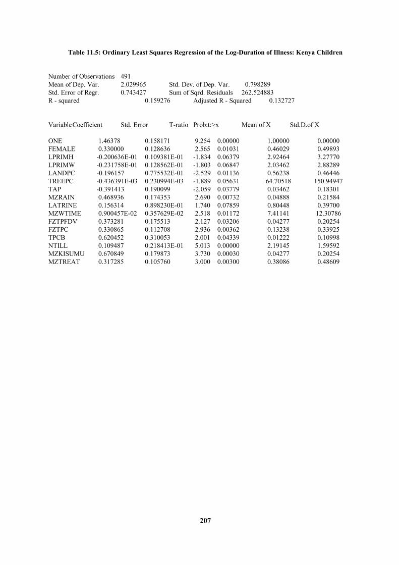
207

Table 11.5: Ordinary Least Squares Regression of the Log-Duration of Illness: Kenya Children Number of Observations 491 Mean of Dep. Var. 2.029965 Std. Dev. of Dep. Var. 0.798289 Std. Error of Regr. 0.743427 Sum of Sqrd. Residuals 262.524883 R - squared 0.159276 Adjusted R - Squared 0.132727 Variable Coefficient Std. Error T-ratio Prob:t:>x Mean of X Std.D.of X ONE 1.46378 0.158171 9.254 0.00000 1.00000 0.00000 FEMALE 0.330000 0.128636 2.565 0.01031 0.46029 0.49893 LPRIMH -0.200636E-01 0.109381E-01 -1.834 0.06379 2.92464 3.27770 LPRIMW -0.231758E-01 0.128562E-01 -1.803 0.06847 2.03462 2.88289 LANDPC -0.196157 0.775532E-01 -2.529 0.01136 0.56238 0.46446 TREEPC -0.436391E-03 0.230994E-03 -1.889 0.05631 64.70518 150.94947 TAP -0.391413 0.190099 -2.059 0.03779 0.03462 0.18301 MZRAIN 0.468936 0.174353 2.690 0.00732 0.04888 0.21584 LATRINE 0.156314 0.898230E-01 1.740 0.07859 0.80448 0.39700 MZWTIME 0.900457E-02 0.357629E-02 2.518 0.01172 7.41141 12.30786 FZTPFDV 0.373281 0.175513 2.127 0.03206 0.04277 0.20254 FZTPC 0.330865 0.112708 2.936 0.00362 0.13238 0.33925 TPCB 0.620452 0.310053 2.001 0.04339 0.01222 0.10998 NTILL 0.109487 0.218413E-01 5.013 0.00000 2.19145 1.59592 MZKISUMU 0.670849 0.179873 3.730 0.00030 0.04277 0.20254 MZTREAT 0.317285 0.105760 3.000 0.00300 0.38086 0.48609

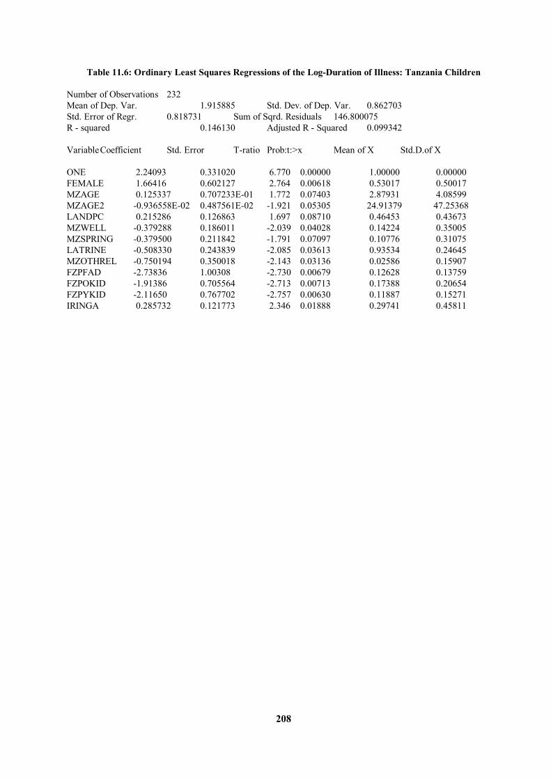
208

Table 11.6: Ordinary Least Squares Regressions of the Log-Duration of Illness: Tanzania Children Number of Observations 232 Mean of Dep. Var. 1.915885 Std. Dev. of Dep. Var. 0.862703 Std. Error of Regr. 0.818731 Sum of Sqrd. Residuals 146.800075 R - squared 0.146130 Adjusted R - Squared 0.099342 Variable Coefficient Std. Error T-ratio Prob:t:>x Mean of X Std.D.of X ONE 2.24093 0.331020 6.770 0.00000 1.00000 0.00000 FEMALE 1.66416 0.602127 2.764 0.00618 0.53017 0.50017 MZAGE 0.125337 0.707233E-01 1.772 0.07403 2.87931 4.08599 MZAGE2 -0.936558E-02 0.487561E-02 -1.921 0.05305 24.91379 47.25368 LANDPC 0.215286 0.126863 1.697 0.08710 0.46453 0.43673 MZWELL -0.379288 0.186011 -2.039 0.04028 0.14224 0.35005 MZSPRING -0.379500 0.211842 -1.791 0.07097 0.10776 0.31075 LATRINE -0.508330 0.243839 -2.085 0.03613 0.93534 0.24645 MZOTHREL -0.750194 0.350018 -2.143 0.03136 0.02586 0.15907 FZPFAD -2.73836 1.00308 -2.730 0.00679 0.12628 0.13759 FZPOKID -1.91386 0.705564 -2.713 0.00713 0.17388 0.20654 FZPYKID -2.11650 0.767702 -2.757 0.00630 0.11887 0.15271 IRINGA 0.285732 0.121773 2.346 0.01888 0.29741 0.45811

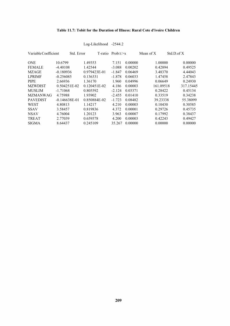
209

Table 11.7: Tobit for the Duration of Illness: Rural Cote d'ivoire Children Log-Likelihood -2544.2 Variable Coefficient Std. Error T-ratio Prob:t:>x Mean of X Std.D.of X ONE 10.6799 1.49353 7.151 0.00000 1.00000 0.00000 FEMALE -4.40108 1.42544 -3.088 0.00202 0.42894 0.49525 MZAGE -0.180936 0.979423E-01 -1.847 0.06469 3.48370 4.44043 LPRIMF -0.256085 0.136331 -1.878 0.06033 1.47458 2.47843 PIPE 2.66936 1.36170 1.960 0.04996 0.06649 0.24930 MZWDIST 0.504251E-02 0.120451E-02 4.186 0.00003 161.09518 317.15445 MUSLIM -1.71068 0.805592 -2.124 0.03371 0.28422 0.45134 MZMANWAG 4.75988 1.93902 -2.455 0.01410 0.33519 0.34238 PAVEDIST -0.146638E-01 0.850884E-02 -1.723 0.08482 39.23338 55.38099 WEST 4.80813 1.14217 4.210 0.00003 0.10430 0.30585 SSAV 3.58457 0.819836 4.372 0.00001 0.29726 0.45735 NSAV 4.76004 1.20123 3.963 0.00007 0.17992 0.38437 TREAT 2.77039 0.659578 4.200 0.00003 0.42243 0.49427 SIGMA 8.64437 0.245109 35.267 0.00000 0.00000 0.00000

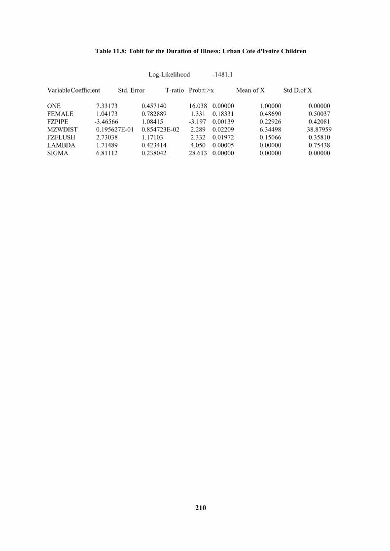
210

Table 11.8: Tobit for the Duration of Illness: Urban Cote d'Ivoire Children Log-Likelihood -1481.1 Variable Coefficient Std. Error T-ratio Prob:t:>x Mean of X Std.D.of X ONE 7.33173 0.457140 16.038 0.00000 1.00000 0.00000 FEMALE 1.04173 0.782889 1.331 0.18331 0.48690 0.50037 FZPIPE -3.46566 1.08415 -3.197 0.00139 0.22926 0.42081 MZWDIST 0.195627E-01 0.854723E-02 2.289 0.02209 6.34498 38.87959 FZFLUSH 2.73038 1.17103 2.332 0.01972 0.15066 0.35810 LAMBDA 1.71489 0.423414 4.050 0.00005 0.00000 0.75438 SIGMA 6.81112 0.238042 28.613 0.00000 0.00000 0.00000

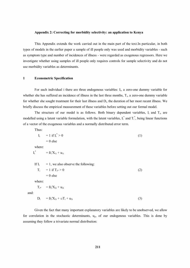
211

Appendix 2: Correcting for morbidity selectivity: an application to Kenya This Appendix extends the work carried out in the main part of the text.In particular, in both types of models in the earlier paper a sample of ill people only was used and morbidity variables - such as symptom type and number of incidences of illness - were regarded as exogenous regressors. Here we investigate whether using samples of ill people only requires controls for sample selectivity and do not use morbidity variables as determinants.

1 Econometric Specification For each individual i there are three endogenous variables: Ii, a zero-one dummy variable for whether she has suffered an incidence of illness in the last three months, Ti, a zero-one dummy variable for whether she sought treatment for their last illness and Di, the duration of her most recent illness. We briefly discuss the empirical measurement of these variables before setting out our formal model. The structure of our model is as follows. Both binary dependent variables, Ii and Ti, are modelled using a latent variable formulation, with the latent variables, Ii

* and Ti*, being linear functions

of a vector of the exogenous variables and a normally distributed error term. Thus: Ii = 1 if Ii

* > 0 (1) = 0 else where: Ii

* = ß1'X1i + u1i

If Ii = 1, we also observe the following: Ti = 1 if Ti* > 0 (2) = 0 else where: Ti* = ß2'X2i + u2i

and: Di = ß3'X3i + αTi + u3i (3)

Given the fact that many important explanatory variables are likely to be unobserved, we allow for correlation in the stochastic determinants, uji, of our endogenous variables. This is done by assuming they follow a trivariate normal distribution:

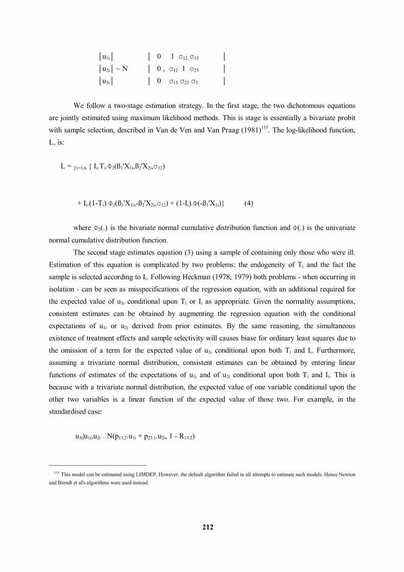
212

│u1i│ │ 0 1 σ12 σ13 │ │u2i│ ~ N │ 0 , σ12 1 σ23 │ │u3i│ │ 0 σ13 σ23 σ3 │

We follow a two-stage estimation strategy. In the first stage, the two dichotomous equations are jointly estimated using maximum likelihood methods. This is stage is essentially a bivariate probit with sample selection, described in Van de Ven and Van Praag (1981)135. The log-likelihood function, L, is: L = Σi=1,n { Ii.Ti.Φ2(ß1'X1i,ß2'X2i,σ12)

+ Ii.(1-Ti).Φ2(ß1'X1i,-ß2'X2i,σ12) + (1-Ii).Φ(-ß1'X1i)} (4)

where Φ2(.) is the bivariate normal cumulative distribution function and Φ(.) is the univariate

normal cumulative distribution function. The second stage estimates equation (3) using a sample of containing only those who were ill. Estimation of this equation is complicated by two problems: the endogeneity of Ti and the fact the sample is selected according to Ii. Following Heckman (1978, 1979) both problems - when occurring in isolation - can be seen as misspecifications of the regression equation, with an additional required for the expected value of u3i conditional upon Ti or Ii as appropriate. Given the normality assumptions, consistent estimates can be obtained by augmenting the regression equation with the conditional expectations of u1i or u2i derived from prior estimates. By the same reasoning, the simultaneous existence of treatment effects and sample selectivity will causes biase for ordinary least squares due to the omission of a term for the expected value of u3i conditional upon both Ti and Ii. Furthermore, assuming a trivariate normal distribution, consistent estimates can be obtained by entering linear functions of estimates of the expectations of u1i and of u2i conditional upon both Ti and Ii. This is because with a trivariate normal distribution, the expected value of one variable conditional upon the other two variables is a linear function of the expected value of those two. For example, in the standardised case: u3i|u1i,u2i ~ N(p13.2.u1i + p23.1.u2i, 1 - R13.2)

135 This model can be estimated using LIMDEP. However, the default algorithm failed in all attempts to estimate such models. Hence Newton and Berndt et al's algorithms were used instead.

213

where pjk.l is the partial correlation coefficient between uij and uik conditional upon uil and R13.2 is the multiple correlation of u3i on u1i and u2i. This estimation method is discussed in the context of multiple criteria for sample selectivity by Maddala (1983, p278-283) and the extension to the case of a single criterion for sample selection coupled with an endogenous variable is straightforward. If there is zero covariance between u1i and u2i, then: E(u3i|Ii=1,Ti) = σ13.φ(ß1'X1i)/Φ(ß1'X1i)

+ Ti.σ23.φ(ß2'X2i)/Φ(ß2'X2i) - (1-Ti).σ23.φ(ß2'X2i)/Φ(-ß2'X2i) (5)

However, in the more general case: E(u3i|Ii=1,Ti) = σ13.M13i + σ23.M23i (6)

where: Mj3i = (1-σ12.σ12)-1.(Eji - σ12.Eki) j,k = 1,2

⌠∞ ⌠W3i Eji = Φ2i

-1 │ │ uji..φ2(u1i,u2i,σ12)du1i.du2i

⌡W1i ⌡W2i W1i = - ß1'X1i W2i = - ß2'X2i if Ti = 1 = - ∞ else W3i = ∞ if Ti = 1 = - ß2'X2i else Φ2i = Φ2(ß1'X1i,ß2'X2i,σ12) if Ti = 1 = Φ2(ß1'X1i,-ß2'X2i,σ12) else

φ2(.) is the probability density function of the bivariate normal distribution. Hence, using the estimates of ß1, ß2 and σ12 obtained from the first stage, one can obtain

estimates of M13i and M23i which can be used to augment equation (3)136. Ordinary least squares regression upon this augmented equation will then yield consistent estimates of ß3. The coefficients

136 Evaluation of double integrals of the sort in equation (6) was done numerically using NAG routine D01GBF.

214

upon M13i and M23i will provide consistent estimates of σ13 and σ23137.

We now report the results of estimating equations (4) and (6) using our data from Kenya. We report in turn the results of estimating the three vectors of coefficients, ßj. We divide the sample into adults and children (those under 16 years of age). The distinction between adults and children may be important given the different decision processes that are involved: decisions about children's health are likely to be taken by other household members and hence the characteristics of such people, for example the education of the child's parents, are likely to be of particular importance. 2 Results138 The results for the determinants of illness obtained from estimating equation (4) are given in Tables 1.1 and 2.1. The variables used in this and subsequent tables are defined in Table 4. For comparison, the results of estimating independent probits (σ12 = 0) are reported in Tables A1.1 and

A2.1. In the case of both adults and children, the estimated covariance of the incidence and treatment residuals, Rho(1,2), is positive. This suggests that those who for unobserved reasons are more likely to fall ill are also more likely to seek treatment if ill. However, in neither case are these covariances significantly different from zero at 10% although their asymptotic t-ratios are greater than one. Likelihood ratio tests for the restriction to a zero covariance give values of 1.5 for adults and 1.86 for children, not rejecting the restriction at 5% significance. The coefficients upon other variables appear insensitive to the imposition of a zero covariance and it is these we now discuss. The determinants of whether individuals sought treatment when ill as estimated by maximising the log-likelihood function in equation (4) are reported in Tables 1.2 and 2.2. Corresponding independent probit estimates are given in the Appendix Tables A1.2 and A2.2. As with the coefficients for the incidence of illness, restricting the error covariance to be zero does not greatly affect other parameters in the model. The final form of the models for the duration of illness estimated with the selectivity and endogeneity corrections described above are given in Tables 1.3 and 2.3. For comparability, the Appendix gives parallel results using more restrictive estimation strategies. Tables A1.3 and A2.3 estimate equation (3) treating treatment as exogenous and making no correction for sample selectivity. Tables A1.4 and A2.4 correct for the endogeneity of treatment, using the results of the independent

137 The standard errors from such a two-stage procedure will be incorrect.

138 Appleton (1991) analysed the number of illnesses suffered by an individual using a poisson regression model. However, in order to address the selectivity of a sample based solely upon those who have been ill, this paper looks merely at whether or not any illnesses occurred. This simplifies the sample selection problem at the cost of discarding information about multiple occurrences of illness.

215

probits for the receipt of treatment as suggested by Heckman (1978), but does not correct for sample selectivity. Tables A1.5 and A2.5 correct for both the endogeneity of treatment and sample selectivity but using the results of the independent probits following equation (5). As can be seen from Tables A1.3 and A2.3, regarding treatment as exogenous produces regression results similar to the simple descriptive statistics reported previously: treatment significantly increases the duration of illness. However, once the additional regressor LAMBDA is introduced into Tables A1.4 and A2.4, to control for the endogeneity of treatment, this result is overturned. For both adults and children, the coefficient upon the treatment variable becomes negative although insignificant. The LAMBDA variable is positive and significant in both cases, confirming one's expectation of a positive covariance between the treatment and duration equations. The correction for using a sample of ill people only is less important than that for the endogeneity of treatment. If incidence and treatment are regarded as independent, as in Tables A1.5 and A2.5, the selectivity term LAMBI1 is insignificant for both adults and children. Perhaps surprisingly, it has a negative coefficient, indicating that those who, for unobservable reasons, are more likely to be ill, are, ceteris paribus, likely to recover more quickly from a given illness. Allowing for the covariance between the errors in the equations for seeking treatment and falling ill, as in Tables 1.3 and 2.3, induces a sign reversal in the estimated covariance between the errors of the duration of illness and of the incidence of illness, and this becomes significantly different from zero in the case of children. Comparing Tables 1.3 and 2.3 with A1.4 and A2.4 reveals that one effect of allowing for sample selectivity to be that the coefficient upon the treatment variable becomes less negative and even less significant. To conclude, this appendix suggests that for Kenya, controlling for sample selectivity arising from looking only at ill people is of marginal importance. In only one case - modelling the duration of illness amongst children - were such controls significant and generally the estimated effects of other variables were robust to such controls. Hence the substantive conclusions reached in the main text may be valid despite its conditioning upon illness.

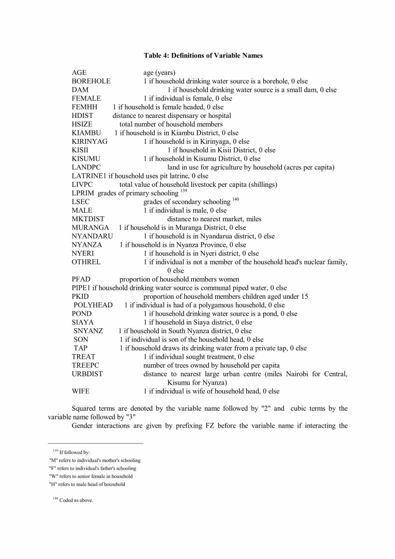
Table 4: Definitions of Variable Names AGE age (years) BOREHOLE 1 if household drinking water source is a borehole, 0 else DAM 1 if household drinking water source is a small dam, 0 else FEMALE 1 if individual is female, 0 else FEMHH 1 if household is female headed, 0 else HDIST distance to nearest dispensary or hospital HSIZE total number of household members KIAMBU 1 if household is in Kiambu District, 0 else KIRINYAG 1 if household is in Kirinyaga, 0 else KISII 1 if household in Kisii District, 0 else KISUMU 1 if household in Kisumu District, 0 else LANDPC land in use for agriculture by household (acres per capita) LATRINE1 if household uses pit latrine, 0 else LIVPC total value of household livestock per capita (shillings) LPRIM grades of primary schooling 139 LSEC grades of secondary schooling 140 MALE 1 if individual is male, 0 else MKTDIST distance to nearest market, miles MURANGA 1 if household is in Muranga District, 0 else NYANDARU 1 if household is in Nyandarua district, 0 else NYANZA 1 if household is in Nyanza Province, 0 else NYERI 1 if household is in Nyeri district, 0 else OTHREL 1 if individual is not a member of the household head's nuclear family,

0 else PFAD proportion of household members women PIPE1 if household drinking water source is communal piped water, 0 else PKID proportion of household members children aged under 15 POLYHEAD 1 if individual is had of a polygamous household, 0 else POND 1 if household drinking water source is a pond, 0 else SIAYA 1 if household in Siaya district, 0 else SNYANZ 1 if household in South Nyanza district, 0 else SON 1 if individual is son of the household head, 0 else TAP 1 if household draws its drinking water from a private tap, 0 else TREAT 1 if individual sought treatment, 0 else TREEPC number of trees owned by household per capita URBDIST distance to nearest large urban centre (miles Nairobi for Central,

Kisumu for Nyanza) WIFE 1 if individual is wife of household head, 0 else Squared terms are denoted by the variable name followed by "2" and cubic terms by the variable name followed by "3" Gender interactions are given by prefixing FZ before the variable name if interacting the

139 If followed by: "M" refers to individual's mother's schooling "F" refers to individual's father's schooling "W" refers to senior female in household "H" refers to male head of household

140 Coded as above.

2

variable with FEMALE and by prefixing with MZ if interacting with MALE.

3

Table 1.1 Probit for the Incidence of Illness; Allowing for Error Correlation with who Seeks Treatment; Kenyan Adults Variable Coefficient Std. Error T-ratio Prob:t:>x Mean of X Std.D. ------------------------------------------------------------------------------ ONE 0.616447E-010.384697 0.160 0.87269 1.00000 0.00000 FEMALE -0.630338 0.369715 -1.705 0.08821 0.55308 0.49728 FZAGE 0.179856E-010.137283E-01 1.310 0.19016 19.48972 20.92758 FZAGE2 -0.156300E-030.148182E-03 -1.055 0.29152 817.62904 1224.06995 MZAGE -0.189981E-010.144536E-01 -1.314 0.18870 16.21947 21.57785 MZAGE2 0.265824E-030.148746E-03 1.787 0.07392 728.47965 1323.66695 LPRIM 0.178163E-010.128055E-01 1.391 0.16414 3.51322 3.30072 FZLSEC -0.182142 0.538734E-01 -3.381 0.00072 0.12925 0.64540 FZHDIST -0.215570E-010.171668E-01 -1.256 0.20921 1.69450 2.37603 MZHDIST -0.494767E-010.220475E-01 -2.244 0.02483 1.34956 2.30593 BOREHOLE 0.444730 0.123836 3.591 0.00033 0.05287 0.22383 FZDAM -0.316677 0.195379 -1.621 0.10505 0.03021 0.17121 MZDAM -1.30355 0.413123 -3.155 0.00160 0.02056 0.14194 MZLATRIN -0.357249 0.144725 -2.468 0.01357 0.38565 0.48685 MZLIVPC 0.107487E-030.498447E-04 2.156 0.03105 308.52915 702.92907 CHILD -0.341069 0.127172 -2.682 0.00732 0.32774 0.46949 OTHREL -0.430919 0.130114 -3.312 0.00093 0.12757 0.33368 HSIZE -0.416374E-010.952278E-02 -4.372 0.00001 8.39026 4.04711 PKID -0.420330 0.169667 -2.477 0.01324 0.44465 0.21363 MKTDIST 0.438467E-010.162273E-01 2.702 0.00689 2.81452 2.11746 FZKIRI -0.225568 0.150941 -1.494 0.13507 0.04952 0.21699 MZKIRI -0.602722 0.214138 -2.815 0.00488 0.04742 0.21258 SIAYA 0.357828 0.988850E-01 3.619 0.00030 0.11918 0.32407 NYANZA 0.217102 0.773014E-01 2.809 0.00498 0.61393 0.48695 WIFE -0.257049 0.100948 -2.546 0.01089 0.23584 0.42461 Rho(1,2) 0.312466 0.212726 1.469 0.14187 0.00000 0.00000 Log-Likelihood.............. -1414.6 (Joint with Table 1.2) Table 1.2 Probit for who Seeks Treatment when Ill; Controlling for the Selectivity of Illness; Kenyan Adults Variable Coefficient Std. Error T-ratio Prob:t:>x Mean of X Std.D ------------------------------------------------------------------------------ ONE 0.750981E-01 1.05905 0.071 0.94347 1.00000 0.00000 FEMALE 0.613564 1.05890 0.579 0.56230 0.63218 0.48267 FZAGE -0.709492E-020.587930E-02 -1.207 0.22752 24.52107 22.61903 MZAGE 0.349883E-010.409871E-01 0.854 0.39330 15.04406 23.04406 MZAGE2 -0.421279E-030.400628E-03 -1.052 0.29301 756.33525 1475.23898 LPRIMH 0.395133E-010.268127E-01 1.474 0.14057 1.31992 2.50741 LPRIM 0.406851E-010.261501E-01 1.556 0.11975 2.91188 3.20087 MZHDIST -0.159127 0.457870E-01 -3.475 0.00051 1.00000 1.92867 FZHDIST -0.644523E-010.317575E-01 -2.030 0.04241 1.89272 2.34705 LANDPC -0.101918 0.715173E-01 -1.425 0.15413 0.68931 0.90868 POND 0.358549 0.219559 1.633 0.10246 0.09387 0.29193 SON -0.577337 0.422530 -1.366 0.17182 0.13027 0.33692 POLYHEAD 0.830250 0.537724 1.544 0.12259 0.04215 0.20111 FZKISII -0.476978 0.191188 -2.495 0.01260 0.11877 0.32383

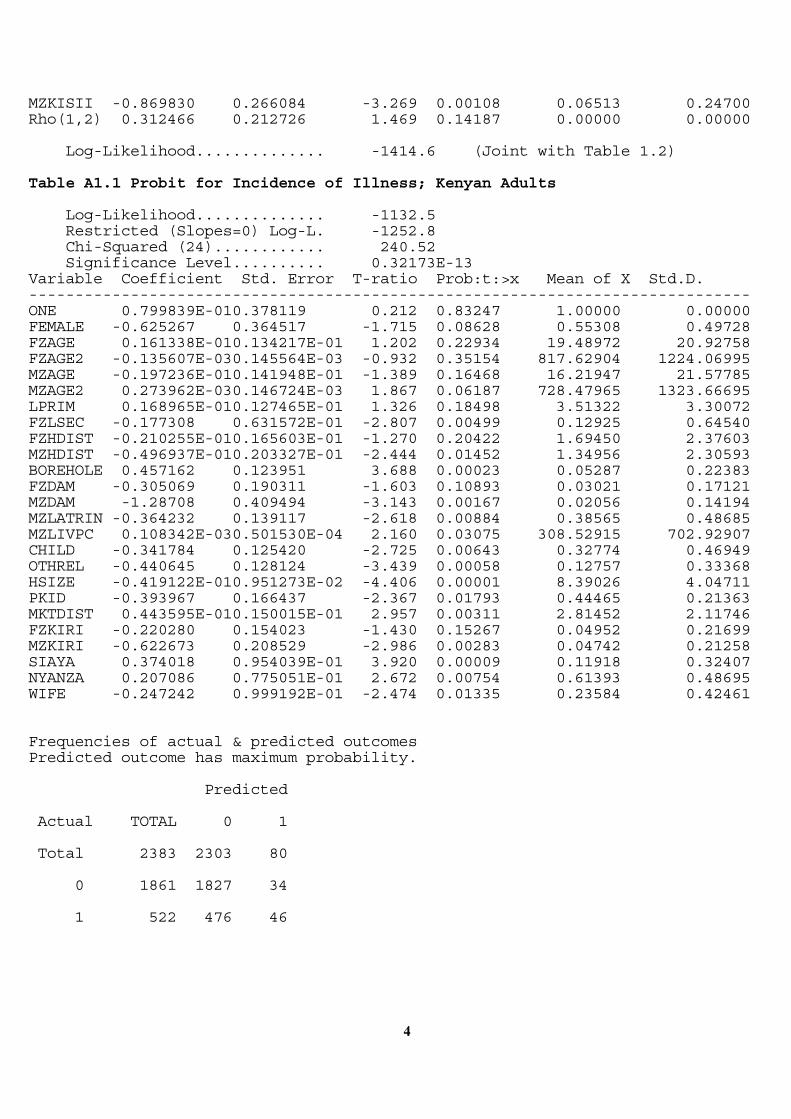
4

MZKISII -0.869830 0.266084 -3.269 0.00108 0.06513 0.24700 Rho(1,2) 0.312466 0.212726 1.469 0.14187 0.00000 0.00000 Log-Likelihood.............. -1414.6 (Joint with Table 1.2) Table A1.1 Probit for Incidence of Illness; Kenyan Adults Log-Likelihood.............. -1132.5 Restricted (Slopes=0) Log-L. -1252.8 Chi-Squared (24)............ 240.52 Significance Level.......... 0.32173E-13 Variable Coefficient Std. Error T-ratio Prob:t:>x Mean of X Std.D. ------------------------------------------------------------------------------ ONE 0.799839E-010.378119 0.212 0.83247 1.00000 0.00000 FEMALE -0.625267 0.364517 -1.715 0.08628 0.55308 0.49728 FZAGE 0.161338E-010.134217E-01 1.202 0.22934 19.48972 20.92758 FZAGE2 -0.135607E-030.145564E-03 -0.932 0.35154 817.62904 1224.06995 MZAGE -0.197236E-010.141948E-01 -1.389 0.16468 16.21947 21.57785 MZAGE2 0.273962E-030.146724E-03 1.867 0.06187 728.47965 1323.66695 LPRIM 0.168965E-010.127465E-01 1.326 0.18498 3.51322 3.30072 FZLSEC -0.177308 0.631572E-01 -2.807 0.00499 0.12925 0.64540 FZHDIST -0.210255E-010.165603E-01 -1.270 0.20422 1.69450 2.37603 MZHDIST -0.496937E-010.203327E-01 -2.444 0.01452 1.34956 2.30593 BOREHOLE 0.457162 0.123951 3.688 0.00023 0.05287 0.22383 FZDAM -0.305069 0.190311 -1.603 0.10893 0.03021 0.17121 MZDAM -1.28708 0.409494 -3.143 0.00167 0.02056 0.14194 MZLATRIN -0.364232 0.139117 -2.618 0.00884 0.38565 0.48685 MZLIVPC 0.108342E-030.501530E-04 2.160 0.03075 308.52915 702.92907 CHILD -0.341784 0.125420 -2.725 0.00643 0.32774 0.46949 OTHREL -0.440645 0.128124 -3.439 0.00058 0.12757 0.33368 HSIZE -0.419122E-010.951273E-02 -4.406 0.00001 8.39026 4.04711 PKID -0.393967 0.166437 -2.367 0.01793 0.44465 0.21363 MKTDIST 0.443595E-010.150015E-01 2.957 0.00311 2.81452 2.11746 FZKIRI -0.220280 0.154023 -1.430 0.15267 0.04952 0.21699 MZKIRI -0.622673 0.208529 -2.986 0.00283 0.04742 0.21258 SIAYA 0.374018 0.954039E-01 3.920 0.00009 0.11918 0.32407 NYANZA 0.207086 0.775051E-01 2.672 0.00754 0.61393 0.48695 WIFE -0.247242 0.999192E-01 -2.474 0.01335 0.23584 0.42461 Frequencies of actual & predicted outcomes Predicted outcome has maximum probability. Predicted Actual TOTAL 0 1 Total 2383 2303 80 0 1861 1827 34 1 522 476 46

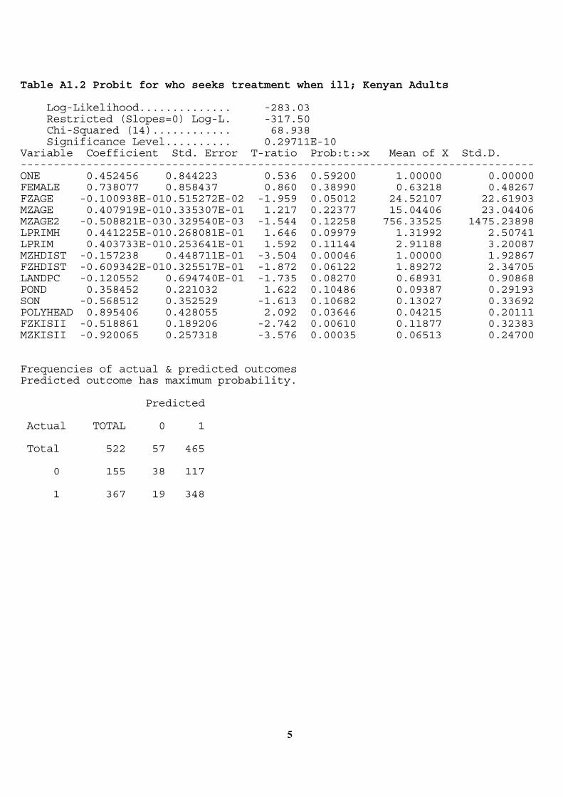
5

Table A1.2 Probit for who seeks treatment when ill; Kenyan Adults Log-Likelihood.............. -283.03 Restricted (Slopes=0) Log-L. -317.50 Chi-Squared (14)............ 68.938 Significance Level.......... 0.29711E-10 Variable Coefficient Std. Error T-ratio Prob:t:>x Mean of X Std.D. ------------------------------------------------------------------------------ ONE 0.452456 0.844223 0.536 0.59200 1.00000 0.00000 FEMALE 0.738077 0.858437 0.860 0.38990 0.63218 0.48267 FZAGE -0.100938E-010.515272E-02 -1.959 0.05012 24.52107 22.61903 MZAGE 0.407919E-010.335307E-01 1.217 0.22377 15.04406 23.04406 MZAGE2 -0.508821E-030.329540E-03 -1.544 0.12258 756.33525 1475.23898 LPRIMH 0.441225E-010.268081E-01 1.646 0.09979 1.31992 2.50741 LPRIM 0.403733E-010.253641E-01 1.592 0.11144 2.91188 3.20087 MZHDIST -0.157238 0.448711E-01 -3.504 0.00046 1.00000 1.92867 FZHDIST -0.609342E-010.325517E-01 -1.872 0.06122 1.89272 2.34705 LANDPC -0.120552 0.694740E-01 -1.735 0.08270 0.68931 0.90868 POND 0.358452 0.221032 1.622 0.10486 0.09387 0.29193 SON -0.568512 0.352529 -1.613 0.10682 0.13027 0.33692 POLYHEAD 0.895406 0.428055 2.092 0.03646 0.04215 0.20111 FZKISII -0.518861 0.189206 -2.742 0.00610 0.11877 0.32383 MZKISII -0.920065 0.257318 -3.576 0.00035 0.06513 0.24700 Frequencies of actual & predicted outcomes Predicted outcome has maximum probability. Predicted Actual TOTAL 0 1 Total 522 57 465 0 155 38 117 1 367 19 348

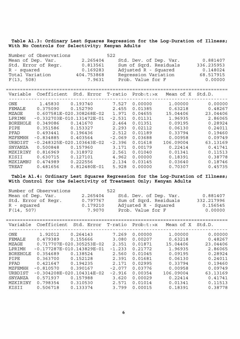
6

Table A1.3: Ordinary Lest Squares Regression for the Log-Duration of Illness; With No Controls for Selectivity; Kenyan Adults Number of Observations 522 Mean of Dep. Var. 2.265404 Std. Dev. of Dep. Var. 0.881407 Std. Error of Regr. 0.813561 Sum of Sqrd. Residuals 336.235953 R - squared 0.169283 Adjusted R - Squared 0.148024 Total Variation 404.753868 Regression Variation 68.517915 F(13, 508) 7.9631 Prob. Value for F 0.00000 =============================================================================== Variable Coefficient Std. Error T-ratio Prob:t:>x Mean of X Std.D. ------------------------------------------------------------------------------ ONE 1.45830 0.193740 7.527 0.00000 1.00000 0.00000 FEMALE 0.375090 0.152790 2.455 0.01385 0.63218 0.48267 MZAGE 0.607581E-020.308268E-02 1.971 0.04655 15.04406 23.04406 LPRIMH -0.332703E-010.131472E-01 -2.531 0.01131 1.96935 2.86065 BOREHOLE 0.349086 0.141670 2.464 0.01351 0.09195 0.28924 PIPE 0.351586 0.153327 2.293 0.02112 0.06130 0.24011 PFAD 0.493441 0.196436 2.512 0.01189 0.33794 0.19460 MZFEMHH -0.834885 0.403564 -2.069 0.03688 0.00958 0.09749 URBDIST -0.248325E-020.103643E-02 -2.396 0.01618 106.09004 63.13169 SNYANZA 0.500848 0.157960 3.171 0.00179 0.22414 0.41741 MZKIRINY 0.816969 0.318972 2.561 0.01040 0.01341 0.11513 KISII 0.630715 0.127101 4.962 0.00000 0.18391 0.38778 MZKIAMBU 0.474989 0.222556 2.134 0.03145 0.03640 0.18746 TREAT 0.481656 0.812480E-01 5.928 0.00000 0.70307 0.45735 Table A1.4: Ordinary Lest Squares Regression for the Log-Duration of Illness; With Control for the Selectivity of Treatment Only; Kenyan Adults Number of Observations 522 Mean of Dep. Var. 2.265404 Std. Dev. of Dep. Var. 0.881407 Std. Error of Regr. 0.797767 Sum of Sqrd. Residuals 332.217996 R - squared 0.179210 Adjusted R - Squared 0.156545 F(14, 507) 7.9070 Prob. Value for F 0.00000 =============================================================================== Variable Coefficient Std. Error T-ratio Prob:t:>x Mean of X Std.D. ------------------------------------------------------------------------------ ONE 1.92012 0.264143 7.269 0.00000 1.00000 0.00000 FEMALE 0.479389 0.155666 3.080 0.00207 0.63218 0.48267 MZAGE 0.717707E-020.305253E-02 2.351 0.01871 15.04406 23.04406 LPRIMH -0.177287E-010.143829E-01 -1.233 0.21772 1.96935 2.86065 BOREHOLE 0.354689 0.138524 2.560 0.01045 0.09195 0.28924 PIPE 0.363700 0.152128 2.391 0.01681 0.06130 0.24011 PFAD 0.421647 0.194235 2.171 0.02995 0.33794 0.19460 MZFEMHH -0.810570 0.390167 -2.077 0.03776 0.00958 0.09749 URBDIST -0.304208E-020.104314E-02 -2.916 0.00354 106.09004 63.13169 SNYANZA 0.571937 0.157988 3.620 0.00029 0.22414 0.41741 MZKIRINY 0.798354 0.310530 2.571 0.01014 0.01341 0.11513 KISII 0.506718 0.133374 3.799 0.00015 0.18391 0.38778

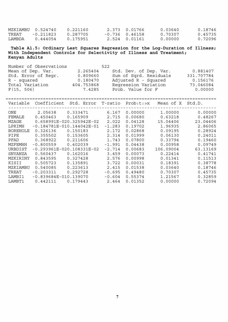
7

MZKIAMBU 0.524740 0.221160 2.373 0.01766 0.03640 0.18746 TREAT -0.211823 0.287705 -0.736 0.46158 0.70307 0.45735 LAMBDA 0.444054 0.175951 2.524 0.01161 0.00000 0.72096 Table A1.5: Ordinary Lest Squares Regression for the Log-Duration of Illness; With Independent Controls for Selectivity of Illness and Treatment; Kenyan Adults Number of Observations 522 Mean of Dep. Var. 2.265404 Std. Dev. of Dep. Var. 0.881407 Std. Error of Regr. 0.809660 Sum of Sqrd. Residuals 331.707784 R - squared 0.180470 Adjusted R - Squared 0.156176 Total Variation 404.753868 Regression Variation 73.046084 F(15, 506) 7.4285 Prob. Value for F 0.00000 =============================================================================== Variable Coefficient Std. Error T-ratio Prob:t:>x Mean of X Std.D. ------------------------------------------------------------------------------ ONE 2.05638 0.333471 6.167 0.00000 1.00000 0.00000 FEMALE 0.450463 0.165909 2.715 0.00680 0.63218 0.48267 MZAGE 0.658991E-020.325942E-02 2.022 0.04128 15.04406 23.04406 LPRIMH -0.184781E-010.144042E-01 -1.283 0.19702 1.96935 2.86065 BOREHOLE 0.326136 0.150183 2.172 0.02868 0.09195 0.28924 PIPE 0.355502 0.153605 2.314 0.01999 0.06130 0.24011 PFAD 0.368922 0.211606 1.743 0.07800 0.33794 0.19460 MZFEMHH -0.800559 0.402039 -1.991 0.04438 0.00958 0.09749 URBDIST -0.293961E-020.108331E-02 -2.714 0.00683 106.09004 63.13169 SNYANZA 0.560437 0.162016 3.459 0.00073 0.22414 0.41741 MZKIRINY 0.843595 0.327428 2.576 0.00998 0.01341 0.11513 KISII 0.505723 0.135891 3.722 0.00031 0.18391 0.38778 MZKIAMBU 0.540085 0.223613 2.415 0.01538 0.03640 0.18746 TREAT -0.203311 0.292728 -0.695 0.49480 0.70307 0.45735 LAMBI1 -0.839684E-010.139070 -0.604 0.55374 1.21567 0.32859 LAMBT1 0.442111 0.179443 2.464 0.01352 0.00000 0.72094

8

Table 1.3: Ordinary Lest Squares Regression for the Log-Duration of Illness; With Joint Controls for Selectivity of Illness and Treatment; Kenyan Adults Number of Observations 522 Mean of Dep. Var. 2.265404 Std. Dev. of Dep. Var. 0.881407 Std. Error of Regr. 0.811994 Sum of Sqrd. Residuals 333.622732 R - squared 0.175739 Adjusted R - Squared 0.151305 F(15, 506) 7.1922 Prob. Value for F 0.00000 =============================================================================== Variable Coefficient Std. Error T-ratio Prob:t:>x Mean of X Std.D. ------------------------------------------------------------------------------ ONE 1.75574 0.297489 5.902 0.00000 1.00000 0.00000 FEMALE 0.462541 0.165516 2.795 0.00543 0.63218 0.48267 MZAGE 0.704007E-020.322411E-02 2.184 0.02784 15.04406 23.04406 LPRIMH -0.231478E-010.141118E-01 -1.640 0.09735 1.96935 2.86065 BOREHOLE 0.326615 0.147824 2.209 0.02609 0.09195 0.28924 PIPE 0.355932 0.153602 2.317 0.01985 0.06130 0.24011 PFAD 0.412676 0.210491 1.961 0.04770 0.33794 0.19460 MZFEMHH -0.819077 0.403073 -2.032 0.04028 0.00958 0.09749 URBDIST -0.284110E-020.107738E-02 -2.637 0.00845 106.09004 63.13169 SNYANZA 0.552762 0.162087 3.410 0.00085 0.22414 0.41741 MZKIRINY 0.824495 0.322100 2.560 0.01045 0.01341 0.11513 KISII 0.556953 0.132159 4.214 0.00006 0.18391 0.38778 MZKIAMBU 0.528423 0.224542 2.353 0.01808 0.03640 0.18746 TREAT -0.234327E-020.260096 -0.009 0.94040 0.70307 0.45735 LAMBI 0.147428E-010.123775 0.119 0.87213 1.22067 0.39544 LAMBT 0.299052 0.158224 1.890 0.05616 0.00638 0.76668

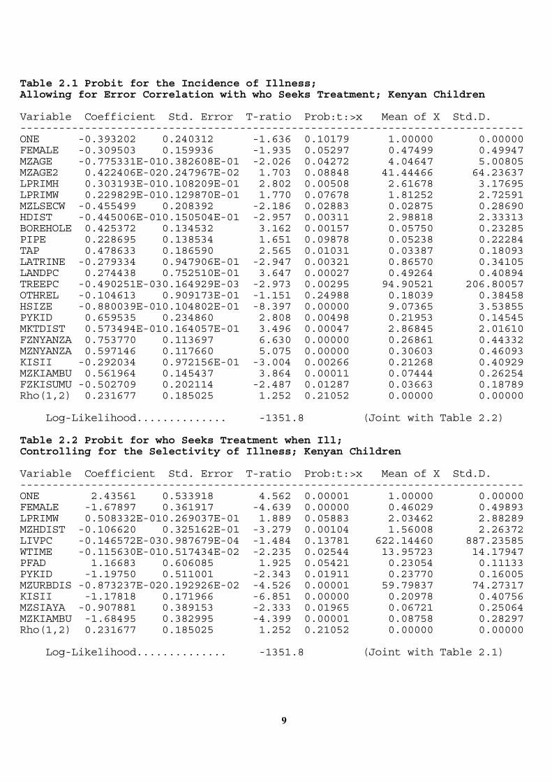
9

Table 2.1 Probit for the Incidence of Illness; Allowing for Error Correlation with who Seeks Treatment; Kenyan Children Variable Coefficient Std. Error T-ratio Prob:t:>x Mean of X Std.D. ------------------------------------------------------------------------------ ONE -0.393202 0.240312 -1.636 0.10179 1.00000 0.00000 FEMALE -0.309503 0.159936 -1.935 0.05297 0.47499 0.49947 MZAGE -0.775331E-010.382608E-01 -2.026 0.04272 4.04647 5.00805 MZAGE2 0.422406E-020.247967E-02 1.703 0.08848 41.44466 64.23637 LPRIMH 0.303193E-010.108209E-01 2.802 0.00508 2.61678 3.17695 LPRIMW 0.229829E-010.129870E-01 1.770 0.07678 1.81252 2.72591 MZLSECW -0.455499 0.208392 -2.186 0.02883 0.02875 0.28690 HDIST -0.445006E-010.150504E-01 -2.957 0.00311 2.98818 2.33313 BOREHOLE 0.425372 0.134532 3.162 0.00157 0.05750 0.23285 PIPE 0.228695 0.138534 1.651 0.09878 0.05238 0.22284 TAP 0.478633 0.186590 2.565 0.01031 0.03387 0.18093 LATRINE -0.279334 0.947906E-01 -2.947 0.00321 0.86570 0.34105 LANDPC 0.274438 0.752510E-01 3.647 0.00027 0.49264 0.40894 TREEPC -0.490251E-030.164929E-03 -2.973 0.00295 94.90521 206.80057 OTHREL -0.104613 0.909173E-01 -1.151 0.24988 0.18039 0.38458 HSIZE -0.880039E-010.104802E-01 -8.397 0.00000 9.07365 3.53855 PYKID 0.659535 0.234860 2.808 0.00498 0.21953 0.14545 MKTDIST 0.573494E-010.164057E-01 3.496 0.00047 2.86845 2.01610 FZNYANZA 0.753770 0.113697 6.630 0.00000 0.26861 0.44332 MZNYANZA 0.597146 0.117660 5.075 0.00000 0.30603 0.46093 KISII -0.292034 0.972156E-01 -3.004 0.00266 0.21268 0.40929 MZKIAMBU 0.561964 0.145437 3.864 0.00011 0.07444 0.26254 FZKISUMU -0.502709 0.202114 -2.487 0.01287 0.03663 0.18789 Rho(1,2) 0.231677 0.185025 1.252 0.21052 0.00000 0.00000 Log-Likelihood.............. -1351.8 (Joint with Table 2.2) Table 2.2 Probit for who Seeks Treatment when Ill; Controlling for the Selectivity of Illness; Kenyan Children Variable Coefficient Std. Error T-ratio Prob:t:>x Mean of X Std.D. ------------------------------------------------------------------------------ ONE 2.43561 0.533918 4.562 0.00001 1.00000 0.00000 FEMALE -1.67897 0.361917 -4.639 0.00000 0.46029 0.49893 LPRIMW 0.508332E-010.269037E-01 1.889 0.05883 2.03462 2.88289 MZHDIST -0.106620 0.325162E-01 -3.279 0.00104 1.56008 2.26372 LIVPC -0.146572E-030.987679E-04 -1.484 0.13781 622.14460 887.23585 WTIME -0.115630E-010.517434E-02 -2.235 0.02544 13.95723 14.17947 PFAD 1.16683 0.606085 1.925 0.05421 0.23054 0.11133 PYKID -1.19750 0.511001 -2.343 0.01911 0.23770 0.16005 MZURBDIS -0.873237E-020.192926E-02 -4.526 0.00001 59.79837 74.27317 KISII -1.17818 0.171966 -6.851 0.00000 0.20978 0.40756 MZSIAYA -0.907881 0.389153 -2.333 0.01965 0.06721 0.25064 MZKIAMBU -1.68495 0.382995 -4.399 0.00001 0.08758 0.28297 Rho(1,2) 0.231677 0.185025 1.252 0.21052 0.00000 0.00000 Log-Likelihood.............. -1351.8 (Joint with Table 2.1)

10

Table A2.1 Probit for Incidence of Illness; Kenyan Children Log-Likelihood.............. -1116.8 Restricted (Slopes=0) Log-L. -1246.9 Chi-Squared (22)............ 260.25 Significance Level.......... 0.32173E-13 Variable Coefficient Std. Error T-ratio Prob:t:>x Mean of X Std.D. ------------------------------------------------------------------------------ ONE -0.381189 0.232967 -1.636 0.10179 1.00000 0.00000 FEMALE -0.322366 0.159209 -2.025 0.04289 0.47499 0.49947 MZAGE -0.777950E-010.377465E-01 -2.061 0.03930 4.04647 5.00805 MZAGE2 0.418168E-020.240103E-02 1.742 0.08158 41.44466 64.23637 LPRIMH 0.312272E-010.104504E-01 2.988 0.00281 2.61678 3.17695 LPRIMW 0.227910E-010.124566E-01 1.830 0.06730 1.81252 2.72591 MZLSECW -0.469171 0.191843 -2.446 0.01446 0.02875 0.28690 HDIST -0.434692E-010.143848E-01 -3.022 0.00251 2.98818 2.33313 BOREHOLE 0.434418 0.132565 3.277 0.00105 0.05750 0.23285 PIPE 0.250278 0.134640 1.859 0.06305 0.05238 0.22284 TAP 0.464746 0.175646 2.646 0.00815 0.03387 0.18093 LATRINE -0.273902 0.928688E-01 -2.949 0.00318 0.86570 0.34105 LANDPC 0.276425 0.732393E-01 3.774 0.00016 0.49264 0.40894 TREEPC -0.507449E-030.185976E-03 -2.729 0.00636 94.90521 206.80057 OTHREL -0.100079 0.874344E-01 -1.145 0.25237 0.18039 0.38458 HSIZE -0.878014E-010.103120E-01 -8.514 0.00000 9.07365 3.53855 PYKID 0.646381 0.230363 2.806 0.00502 0.21953 0.14545 MKTDIST 0.543420E-010.161843E-01 3.358 0.00079 2.86845 2.01610 FZNYANZA 0.754509 0.110889 6.804 0.00000 0.26861 0.44332 MZNYANZA 0.585501 0.114974 5.092 0.00000 0.30603 0.46093 KISII -0.293079 0.961631E-01 -3.048 0.00231 0.21268 0.40929 MZKIAMBU 0.556259 0.144244 3.856 0.00012 0.07444 0.26254 FZKISUMU -0.513186 0.185908 -2.760 0.00577 0.03663 0.18789 Frequencies of actual & predicted outcomes Predicted outcome has maximum probability. Predicted Actual TOTAL 0 1 Total 2539 2487 52 0 2048 2026 22 1 491 461 30

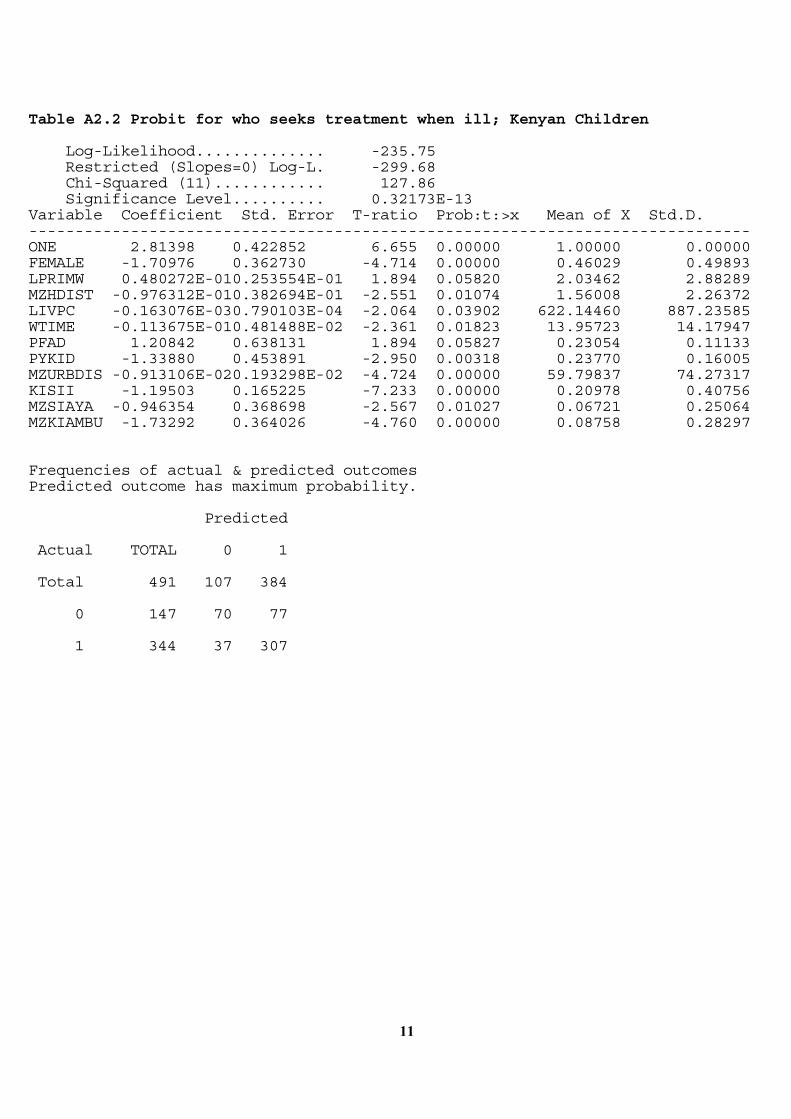
11

Table A2.2 Probit for who seeks treatment when ill; Kenyan Children Log-Likelihood.............. -235.75 Restricted (Slopes=0) Log-L. -299.68 Chi-Squared (11)............ 127.86 Significance Level.......... 0.32173E-13 Variable Coefficient Std. Error T-ratio Prob:t:>x Mean of X Std.D. ------------------------------------------------------------------------------ ONE 2.81398 0.422852 6.655 0.00000 1.00000 0.00000 FEMALE -1.70976 0.362730 -4.714 0.00000 0.46029 0.49893 LPRIMW 0.480272E-010.253554E-01 1.894 0.05820 2.03462 2.88289 MZHDIST -0.976312E-010.382694E-01 -2.551 0.01074 1.56008 2.26372 LIVPC -0.163076E-030.790103E-04 -2.064 0.03902 622.14460 887.23585 WTIME -0.113675E-010.481488E-02 -2.361 0.01823 13.95723 14.17947 PFAD 1.20842 0.638131 1.894 0.05827 0.23054 0.11133 PYKID -1.33880 0.453891 -2.950 0.00318 0.23770 0.16005 MZURBDIS -0.913106E-020.193298E-02 -4.724 0.00000 59.79837 74.27317 KISII -1.19503 0.165225 -7.233 0.00000 0.20978 0.40756 MZSIAYA -0.946354 0.368698 -2.567 0.01027 0.06721 0.25064 MZKIAMBU -1.73292 0.364026 -4.760 0.00000 0.08758 0.28297 Frequencies of actual & predicted outcomes Predicted outcome has maximum probability. Predicted Actual TOTAL 0 1 Total 491 107 384 0 147 70 77 1 344 37 307

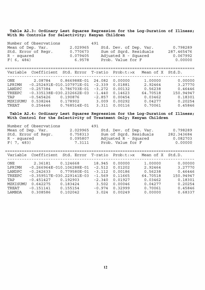
12

Table A2.3: Ordinary Lest Squares Regression for the Log-Duration of Illness; With No Controls for Selectivity; Kenyan Children Number of Observations 491 Mean of Dep. Var. 2.029965 Std. Dev. of Dep. Var. 0.798289 Std. Error of Regr. 0.770673 Sum of Sqrd. Residuals 287.465476 R - squared 0.079405 Adjusted R - Squared 0.067992 F( 6, 484) 6.9578 Prob. Value for F 0.00000 =============================================================================== Variable Coefficient Std. Error T-ratio Prob:t:>x Mean of X Std.D. ------------------------------------------------------------------------------ ONE 2.08784 0.866988E-01 24.082 0.00000 1.00000 0.00000 LPRIMH -0.252491E-010.107971E-01 -2.339 0.01881 2.92464 3.27770 LANDPC -0.257384 0.786703E-01 -3.272 0.00132 0.56238 0.46446 TREEPC -0.335138E-030.232662E-03 -1.440 0.14623 64.70518 150.94947 TAP -0.545426 0.190876 -2.857 0.00454 0.03462 0.18301 MZKISUMU 0.538244 0.178902 3.009 0.00292 0.04277 0.20254 TREAT 0.254446 0.768514E-01 3.311 0.00116 0.70061 0.45846 Table A2.4: Ordinary Lest Squares Regression for the Log-Duration of Illness; With Control for the Selectivity of Treatment Only; Kenyan Children Number of Observations 491 Mean of Dep. Var. 2.029965 Std. Dev. of Dep. Var. 0.798289 Std. Error of Regr. 0.758313 Sum of Sqrd. Residuals 282.343684 R - squared 0.095807 Adjusted R - Squared 0.082703 F( 7, 483) 7.3111 Prob. Value for F 0.00000 =============================================================================== Variable Coefficient Std. Error T-ratio Prob:t:>x Mean of X Std.D. ------------------------------------------------------------------------------ ONE 2.36181 0.124668 18.945 0.00000 1.00000 0.00000 LPRIMH -0.266964E-010.106288E-01 -2.512 0.01202 2.92464 3.27770 LANDPC -0.242633 0.779580E-01 -3.112 0.00186 0.56238 0.46446 TREEPC -0.359517E-030.229141E-03 -1.569 0.11665 64.70518 150.94947 TAP -0.451427 0.192903 -2.340 0.01927 0.03462 0.18301 MZKISUMU 0.642275 0.183424 3.502 0.00046 0.04277 0.20254 TREAT -0.151141 0.155154 -0.974 0.32999 0.70061 0.45846 LAMBDA 0.308586 0.102042 3.024 0.00249 0.00000 0.68337

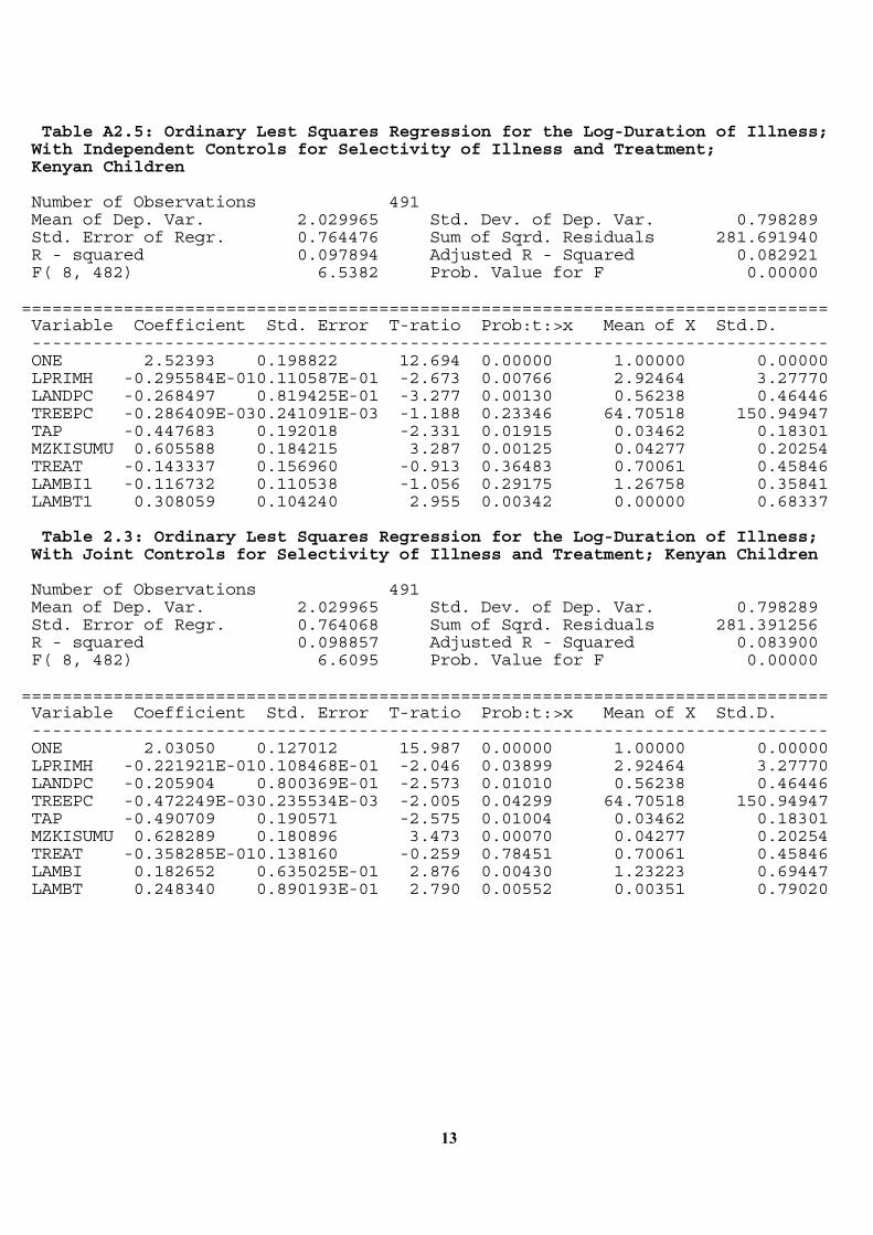
13

Table A2.5: Ordinary Lest Squares Regression for the Log-Duration of Illness; With Independent Controls for Selectivity of Illness and Treatment; Kenyan Children Number of Observations 491 Mean of Dep. Var. 2.029965 Std. Dev. of Dep. Var. 0.798289 Std. Error of Regr. 0.764476 Sum of Sqrd. Residuals 281.691940 R - squared 0.097894 Adjusted R - Squared 0.082921 F( 8, 482) 6.5382 Prob. Value for F 0.00000 =============================================================================== Variable Coefficient Std. Error T-ratio Prob:t:>x Mean of X Std.D. ------------------------------------------------------------------------------ ONE 2.52393 0.198822 12.694 0.00000 1.00000 0.00000 LPRIMH -0.295584E-010.110587E-01 -2.673 0.00766 2.92464 3.27770 LANDPC -0.268497 0.819425E-01 -3.277 0.00130 0.56238 0.46446 TREEPC -0.286409E-030.241091E-03 -1.188 0.23346 64.70518 150.94947 TAP -0.447683 0.192018 -2.331 0.01915 0.03462 0.18301 MZKISUMU 0.605588 0.184215 3.287 0.00125 0.04277 0.20254 TREAT -0.143337 0.156960 -0.913 0.36483 0.70061 0.45846 LAMBI1 -0.116732 0.110538 -1.056 0.29175 1.26758 0.35841 LAMBT1 0.308059 0.104240 2.955 0.00342 0.00000 0.68337 Table 2.3: Ordinary Lest Squares Regression for the Log-Duration of Illness; With Joint Controls for Selectivity of Illness and Treatment; Kenyan Children Number of Observations 491 Mean of Dep. Var. 2.029965 Std. Dev. of Dep. Var. 0.798289 Std. Error of Regr. 0.764068 Sum of Sqrd. Residuals 281.391256 R - squared 0.098857 Adjusted R - Squared 0.083900 F( 8, 482) 6.6095 Prob. Value for F 0.00000 =============================================================================== Variable Coefficient Std. Error T-ratio Prob:t:>x Mean of X Std.D. ------------------------------------------------------------------------------ ONE 2.03050 0.127012 15.987 0.00000 1.00000 0.00000 LPRIMH -0.221921E-010.108468E-01 -2.046 0.03899 2.92464 3.27770 LANDPC -0.205904 0.800369E-01 -2.573 0.01010 0.56238 0.46446 TREEPC -0.472249E-030.235534E-03 -2.005 0.04299 64.70518 150.94947 TAP -0.490709 0.190571 -2.575 0.01004 0.03462 0.18301 MZKISUMU 0.628289 0.180896 3.473 0.00070 0.04277 0.20254 TREAT -0.358285E-010.138160 -0.259 0.78451 0.70061 0.45846 LAMBI 0.182652 0.635025E-01 2.876 0.00430 1.23223 0.69447 LAMBT 0.248340 0.890193E-01 2.790 0.00552 0.00351 0.79020

14

Chapter 4: Water Supply, Extension and Credit Introduction A. Water Supply A.1. Characteristics of those who Fetch Water a. Kenya b. Tanzania c. Conclusion A.2. Time Spent Fetching Water B. Gender Effects and Extension Services B.1. Introduction B.2. Gender Effects and Extension Services a. Kenya b. Tanzania c. Cote d'Ivoire B.3. Conclusions C. Credit C.1. Introduction C.2. Gender Aspects of Rural Financial Markets: a Tabular Analysis a. Access to Credit in Kenya and Tanzania b. Access to Credit in the Cote d'Ivoire c. Access to Deposit Taking Institutions C.3. An Econometric Analysis of Access to Credit in Cote d'Ivoire, Kenya and Tanzania C.4.Determinants of Women's Self Help Group Membership in Western Kenya a. Introduction b. Data and Model c. Results C.5. Conclusion D. Gender and the Prioritization of Public Services in Rural Kenya and Tanzania Conclusion

15

Introduction This chapter examines gender differentiated access to three public services: water supply, extension and credit. Our interest in water supply is two-fold. First, who collects water? While we expect that this is an overwhelmingly female activity, it is useful to examine who within the household fetches water. Second, will the provision of communally piped water significantly reduce time spent fetching it? (Note that the impact of water supply on health has been discussed in chapter 3. The effect of time spent collecting water on labour market participation is examined in chapter 6). With respect to extension and credit, our data only permits analysis of gender differences along the lines of headship. We examine whether female headed households are less likely to have access to extension services and credit. With respect to the former, we also examine whether contact with extension workers has any influence on farming methods employed on the holding. Given the relatively small number of households with access to formal sector loans, we do not examine the impact of credit on farm production. Instead, we briefly examine whether self-help groups can provide a useful mechanism for funnelling funds to women. We focus on the determinants of membership in these groups. If they are dominated by wealthy and well-educated women, then their scope for poverty alleviation may be minimal. In this chapter, we find that women do bear the brunt of water collection and that they appear to have less access to extension services and the credit market. Does this have any influence on the priorities that men and women attach to public services? Using data from the Kenyan and Tanzanian surveys, we undertake a brief analysis of this question. Our principal level of disaggregation is the gender of the head. We also examine whether the gender composition of the household influences its subjective priorities.

16

A. Water Supply in Kenya and Tanzania The burden of fetching water supplies is a heavy one in much of rural Africa and falls overwhelmingly on the female population. In this section we first investigate the characteristics of those who fetch water and then look at the implications of improved supplied for the time devoted to this activity.

A.l. Characteristics of those who Fetch Water a. Kenya Logits were estimated for individuals who fetched water, using the 1982 Kenya survey data. Other than location, the explanatory variables are all related to characteristics of the individual concerned, rather than the household itself. They were AGE (the individual's age) and AGE2 (age squared), LVEDUC (the level of completed education, running over grades of both primary and secondary schooling) and three groups of dummy variables. The first group comprises FEMALE (1 if individual is female, 0 otherwise) and HH (1 if individual is household head, 0 otherwise). The second group covers the individual's main occupation, with the default being work on the household shamba: MAOC2 (1 if work on other farms/estates, 0 otherwise), MAOC3 (1 if rural non-farm, 0 otherwise), MAOC4 (1 if urban employment, 0 otherwise), MAOC5 (1 if not working, 0 otherwise), MAOC6 (1 if studying at school, 0 otherwise). Finally there is a set of district dummy variables, MURANGA, NYERI, NYANDARU, SIAYA, KISUMU, SNYANZA, KISII, KIRINYAG, as in the chapter on health. A logit was fitted to the sample as a whole (Table 1) and to non-students and students separately (tables 2 and 3 respectively). As demonstrated in the chapter on education, differential female drop-out rates are associated with their differential obligations to fetch water. Consequently, the student category is not completely exogenously determined. However, it can be regarded as predetermined from the perspective of current allocation of tasks. What emerges from the overall logit is a strong quadratic relationship in age peaking at age 40 and, as is to be expected, a very strong and significant gender effect. Even when these effects have been taken into account, however, there is also a strong and significant negative coefficient on the household head dummy. As regards occupational status, there are large and highly significant negative coefficients on the student and `not working' dummy variables. Whatever makes those who are not working unavailable or unable to do so also makes them unavailable for carrying water. Similarly being at school either reduces availability to fetch water or leads to the student being protected from this obligation. At the mean, this lowers the probability of

17

fetching water by .152. There are also, unsurprisingly, some significant coefficients on the district dummy variables, inducating that the probability of an individual having to fetch water is dependent on location. Finally the level of education variable has a positive though not very significant coefficient. It is not clear how to interpret this result, but it does at least indicate that water collection is not assigned to the least educated, once occupational effects are taken into account. The logit for those who are not students (Table 2) produces broadly similar results, the main changes being in the locational coefficients. The logit for students, however, is different in a number of interesting ways. First, while there is still a highly significant quadratic relationship in age, this is now inverted, with the probability of having to fetch water falling with age until age 13, and then rising, after controlling for educational level. Second, while females are still much more likely to have to fetch water, the extent of this bias is far less marked than amongst non-students. Finally, the coefficients on the district dummies are both far larger and far more significant than in the non-student case. It appears that location is a highly significant determinant of the liability of school children to have to fetch water. b. Tanzania The exercise was replicated for Tanzania, using the 1983 survey data. In place of the Kenyan district variables there are four regional variables, with RUVUMA as the default, and one of IRINGA, DODOMA and KILIMANJARO taking the value one otherwise. Results are given in Tables 4, 5 and 6. For the full sample, results are broadly similar to the Kenya case, with two exceptions. First, the coefficient on household head, while still negative, becomes completely insignificant. This may simply reflect the lack of female headed households in the Tanzanian sample, which makes it difficult for the logit to separate this effect from the very strong gender effect. The other major different is that the negative coefficient on the student dummy becomes very small and loses all statistical significance. Students appear not to be protected from water fetching duties in Tanzania. Of the two partitioned logits, the one for non-students is very similar to its Kenyan counterpart apart from the lack of significance of household head. In particular, the coefficients on age, age squared, gender and `not working' are relatively close to each other. Since the mean probability is very similar to that for Kenya, .324 as compared to .315, the implications are also very similar. For example, at the mean, being female raises the probability of being a fetcher by .615 in Tanzania and .701 in Kenya; being a non-worker lowers it by .252 in Tanzania and by .257 in Kenya. The logits for students are, however, very different. First, the overall probability is much higher for Tanzania, at .408 as compared to .185 in Kenya. On average students are somewhat more likely to fetch water than non-students in Tanzania, as opposed to much less likely to do so in Kenya. (Of course the overall Tanzania logit suggests that students are no more likely to fetch water once other

18

characteristics have been taken into account). Once again, there is a significant quadratic relationship in age, but unlike the Kenyan case this is initially upward sloping, peaking at around 17 years. Finally, while the coefficients on gender are similar, the probaiblities are not. Being a female student in Tanzania raises the probability of fetching water at the mean by .319, as opposed to only .187 in Kenya. c. Conclusion The main conclusion of these estimations, apart from confirmation of the obvious fact that water collection falls disproportionately on women, is that schooling substantially reduces availability in Kenya but has no effect in Tanzania. Because of the lack of effect in Tanzania, this suggests that the Kenyan result reflects a positive decision by Kenyan households to protect school children from this obligation, rather than a mere physical unavailability. The asymmetry between the countries is entirely consistent with the different structures of schooling in the two countries at the times of the surveys. In Kenya, success at primary school was of direct concern to other household members because of the considerable cost savings and higher returns associated with entry into Government Secondary Schools. The household had a very direct stake in ensuring successful participationin primary school and beyond. In Tanzania, the secondary sector was much smaller and access to it from rural households virtually non-existent. The pay-off to improved performance at primary school was correspondingly greatly reduced, and there was no `beyond'. Consequently, there was no corresponding incentive to protect school children from out-of-school obligations.

Table 1: Logit for Who Collects Water: Kenya Total Number of Individuals 5368 Number Collecting Water 1451 (27.0%) Log-Likelihood -1989.72 Parameter Estimate t-Statistic AGE 0.139322 13.32** AGE2 -0.001732 12.27** LVEDUC 0.013719 0.99 FEMALE 2.54887 27.11** MAOC2 0.081094 0.40 MAOC3 -0.325148 2.84** MAOC4 -0.536552 3.04** MAOC5 -1.03274 9.39** MAOC6 -0.769196 6.78** HH -3.66230 15.62** MURANGA -0.258523 1.42 NYERI -0.885933 4.23**

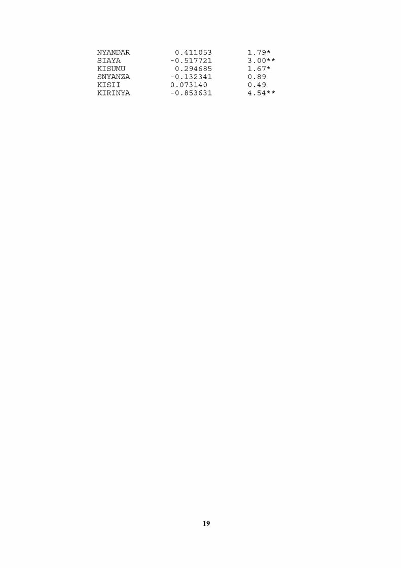
19

NYANDAR 0.411053 1.79* SIAYA -0.517721 3.00** KISUMU 0.294685 1.67* SNYANZA -0.132341 0.89 KISII 0.073140 0.49 KIRINYA -0.853631 4.54**

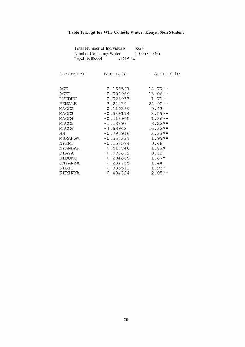
20

Table 2: Logit for Who Collects Water: Kenya, Non-Student Total Number of Individuals 3524 Number Collecting Water 1109 (31.5%) Log-Likelihood -1215.84 Parameter Estimate t-Statistic AGE 0.166521 14.77** AGE2 -0.001969 13.06** LVEDUC 0.028933 1.71* FEMALE 3.24430 24.92** MAOC2 0.110389 0.43 MAOC3 -0.539114 3.59** MAOC4 -0.418905 1.86** MAOC5 -1.18898 8.22** MAOC6 -4.68942 16.32** HH -0.795916 3.33** MURANGA -0.567337 1.99** NYERI -0.153574 0.48 NYANDAR 0.417740 1.83* SIAYA -0.076632 0.32 KISUMU -0.294685 1.67* SNYANZA -0.282755 1.44 KISII -0.385512 1.93* KIRINYA -0.494324 2.05**

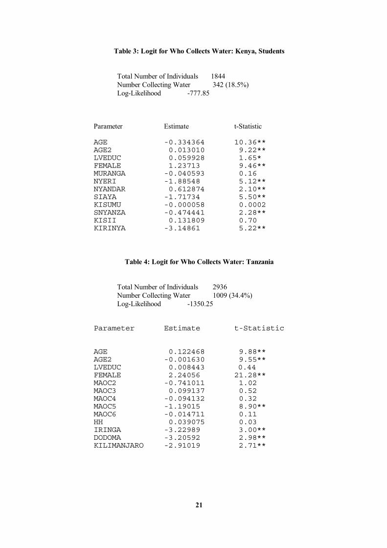
21

Table 3: Logit for Who Collects Water: Kenya, Students Total Number of Individuals 1844 Number Collecting Water 342 (18.5%) Log-Likelihood -777.85 Parameter Estimate t-Statistic AGE -0.334364 10.36** AGE2 0.013010 9.22** LVEDUC 0.059928 1.65* FEMALE 1.23713 9.46** MURANGA -0.040593 0.16 NYERI -1.88548 5.12** NYANDAR 0.612874 2.10** SIAYA -1.71734 5.50** KISUMU -0.000058 0.0002 SNYANZA -0.474441 2.28** KISII 0.131809 0.70 KIRINYA -3.14861 5.22** Table 4: Logit for Who Collects Water: Tanzania Total Number of Individuals 2936 Number Collecting Water 1009 (34.4%) Log-Likelihood -1350.25 Parameter Estimate t-Statistic AGE 0.122468 9.88** AGE2 -0.001630 9.55** LVEDUC 0.008443 0.44 FEMALE 2.24056 21.28** MAOC2 -0.741011 1.02 MAOC3 0.099137 0.52 MAOC4 -0.094132 0.32 MAOC5 -1.19015 8.90** MAOC6 -0.014711 0.11 HH 0.039075 0.03 IRINGA -3.22989 3.00** DODOMA -3.20592 2.98** KILIMANJARO -2.91019 2.71**

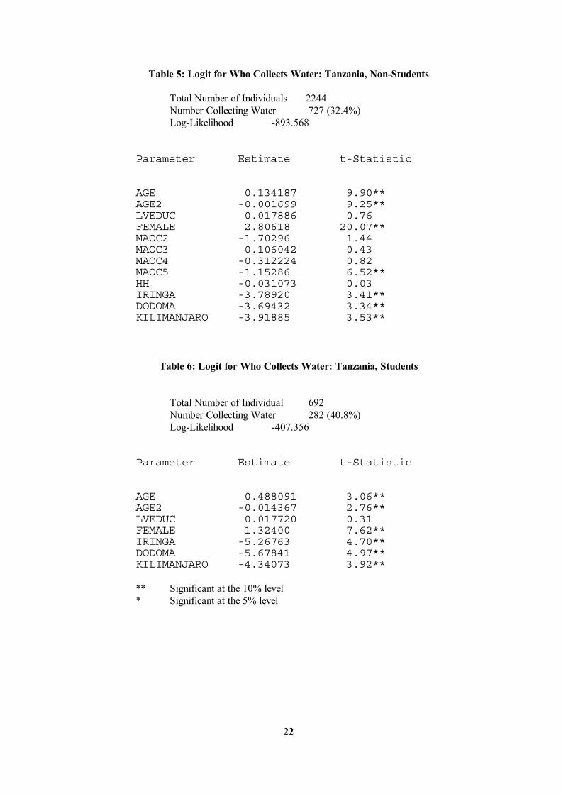
22

Table 5: Logit for Who Collects Water: Tanzania, Non-Students Total Number of Individuals 2244 Number Collecting Water 727 (32.4%) Log-Likelihood -893.568 Parameter Estimate t-Statistic AGE 0.134187 9.90** AGE2 -0.001699 9.25** LVEDUC 0.017886 0.76 FEMALE 2.80618 20.07** MAOC2 -1.70296 1.44 MAOC3 0.106042 0.43 MAOC4 -0.312224 0.82 MAOC5 -1.15286 6.52** HH -0.031073 0.03 IRINGA -3.78920 3.41** DODOMA -3.69432 3.34** KILIMANJARO -3.91885 3.53** Table 6: Logit for Who Collects Water: Tanzania, Students Total Number of Individual 692 Number Collecting Water 282 (40.8%) Log-Likelihood -407.356 Parameter Estimate t-Statistic AGE 0.488091 3.06** AGE2 -0.014367 2.76** LVEDUC 0.017720 0.31 FEMALE 1.32400 7.62** IRINGA -5.26763 4.70** DODOMA -5.67841 4.97** KILIMANJARO -4.34073 3.92** ** Significant at the 10% level * Significant at the 5% level

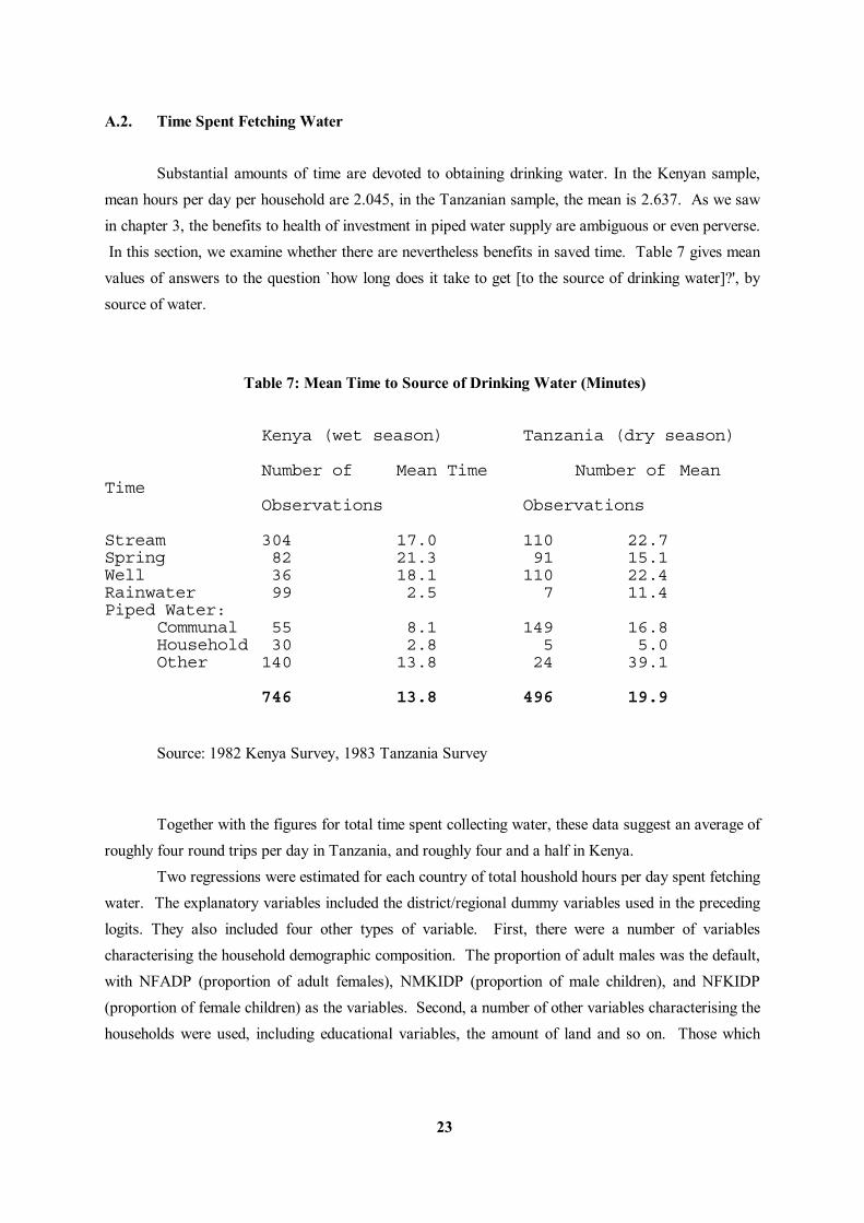
23

A.2. Time Spent Fetching Water Substantial amounts of time are devoted to obtaining drinking water. In the Kenyan sample, mean hours per day per household are 2.045, in the Tanzanian sample, the mean is 2.637. As we saw in chapter 3, the benefits to health of investment in piped water supply are ambiguous or even perverse. In this section, we examine whether there are nevertheless benefits in saved time. Table 7 gives mean values of answers to the question `how long does it take to get [to the source of drinking water]?', by source of water.

Table 7: Mean Time to Source of Drinking Water (Minutes) Kenya (wet season) Tanzania (dry season) Number of Mean Time Number of Mean Time Observations Observations Stream 304 17.0 110 22.7 Spring 82 21.3 91 15.1 Well 36 18.1 110 22.4 Rainwater 99 2.5 7 11.4 Piped Water: Communal 55 8.1 149 16.8 Household 30 2.8 5 5.0 Other 140 13.8 24 39.1 746 13.8 496 19.9 Source: 1982 Kenya Survey, 1983 Tanzania Survey Together with the figures for total time spent collecting water, these data suggest an average of roughly four round trips per day in Tanzania, and roughly four and a half in Kenya. Two regressions were estimated for each country of total houshold hours per day spent fetching water. The explanatory variables included the district/regional dummy variables used in the preceding logits. They also included four other types of variable. First, there were a number of variables characterising the household demographic composition. The proportion of adult males was the default, with NFADP (proportion of adult females), NMKIDP (proportion of male children), and NFKIDP (proportion of female children) as the variables. Second, a number of other variables characterising the households were used, including educational variables, the amount of land and so on. Those which

24

were statistically significant were LIVSTOCK (value of livestock), HSIZE (number of individuals in household) and LVEDUCW (educational level of education of eldest wife). The third group of variables, appearing in one regression, were dummy variables per source of water. The default was stream, and the courses which were significant were DWATS1 (still pond), DWATS2 (small dam), DWATS5 (well), and DWATS8 (rainwater); from a policy point of view we are particularly interested in DWATS9 (piped water: communal) and DWATS3 (piped water: household) so these variables were retained whether significant or not. Finally, as an alternative to the sources of water, the other regression used TIME (time to source). Results are given in Tables 9 to 11. The equations are not particularly impressive. Apart from the locational dummies which exhibit some strong and highly significant effects, the only variable to be consistently significant at the 5% level is the proportion of adult women in the household. However, whereas this substantially raises the time spend collecting water in Kenya, it has an even more powerful effect in lowering it in Tanzania. The interpretation of this is obscure. Another major difference between the results for the two countries relates to the intercept. For Kenya, this is not significantly defferent from zero, whereas for Tanzania it is very large and highly significant. Finally, in the Kenya regressions (but not the Tanzanian ones) household size is significantly and positively related total collection time. All in all, the Tanzanian equations look implausible. From Table 9, the coefficient on time to source is positive and significant for Kenya. Reducing time to source by 1 minute would lower total collection time by 1.4 minutes (0.0234 x 60); the rest of the potential gain being taken in increased water consumption. From Table 7 the reduction in mean time to source in changing from the default source (stream) to piped water is 8.9 minuted (communal) and 14.2 minutes (household). The aggregate daily saving in household time of such a switch would therefore be estimated at 12.5 minutes or 19.9 minutes respectively. These calculations may be compared to the direct coefficients on source in Table 8. It must however be borne in mind that neither of these is statistically significant, particularly that for communal piped water. In any event, the coefficients are -0.13 (communal) and -0.67 (household), implying that a shift from the default to piped water would reduce total collection time by 7.8 minutes (0.13 x 60) and 40.2 minutes (0.67 x 60) respectively. These calculations must be treated with great caution, but they do tend to suggest that the time saving from provision of communal piped water is likely to be small, in the range 8-12 minutes per day. For Tanzania, as none of the relevant coefficients are significant, comparable calculations have not been carried out. The conclusion of this discussion is therefore a very limited one: the Kenya and Tanzania Survey data do not support any inference that the provision of communal piped water would have substantial benefits in releasing household time.

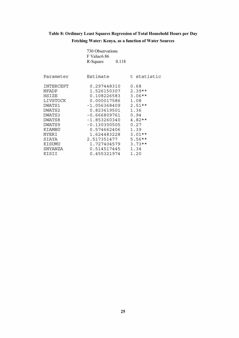
25

Table 8: Ordinary Least Squares Regression of Total Household Hours per Day Fetching Water: Kenya, as a function of Water Sources 730 Observations F Value 6.86 R-Square 0.118 Parameter Estimate t statistic INTERCEPT 0.297448310 0.68 NFADP 1.526150307 2.39** HSIZE 0.108226583 3.06** LIVSTOCK 0.000017586 1.08 DWATS1 -1.056368409 2.51** DWATS2 0.823619501 1.36 DWATS3 -0.666809761 0.94 DWATS8 -1.853260340 4.82** DWATS9 -0.130300505 0.27 KIAMBU 0.574662406 1.39 NYERI 1.624483228 3.01** SIAYA 2.517351477 5.56** KISUMU 1.727404579 3.73** SNYANZA 0.514517445 1.34 KISII 0.455321974 1.20

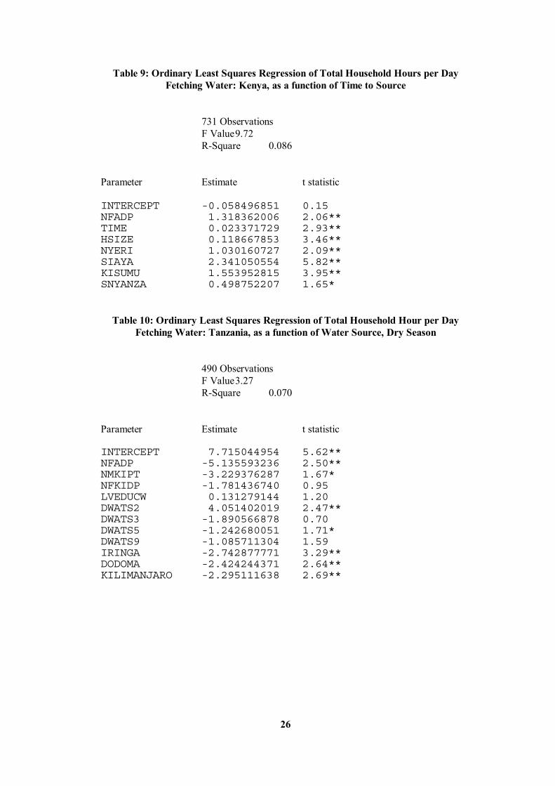
26

Table 9: Ordinary Least Squares Regression of Total Household Hours per Day Fetching Water: Kenya, as a function of Time to Source 731 Observations F Value 9.72 R-Square 0.086 Parameter Estimate t statistic INTERCEPT -0.058496851 0.15 NFADP 1.318362006 2.06** TIME 0.023371729 2.93** HSIZE 0.118667853 3.46** NYERI 1.030160727 2.09** SIAYA 2.341050554 5.82** KISUMU 1.553952815 3.95** SNYANZA 0.498752207 1.65* Table 10: Ordinary Least Squares Regression of Total Household Hour per Day Fetching Water: Tanzania, as a function of Water Source, Dry Season 490 Observations F Value 3.27 R-Square 0.070 Parameter Estimate t statistic INTERCEPT 7.715044954 5.62** NFADP -5.135593236 2.50** NMKIPT -3.229376287 1.67* NFKIDP -1.781436740 0.95 LVEDUCW 0.131279144 1.20 DWATS2 4.051402019 2.47** DWATS3 -1.890566878 0.70 DWATS5 -1.242680051 1.71* DWATS9 -1.085711304 1.59 IRINGA -2.742877771 3.29** DODOMA -2.424244371 2.64** KILIMANJARO -2.295111638 2.69**

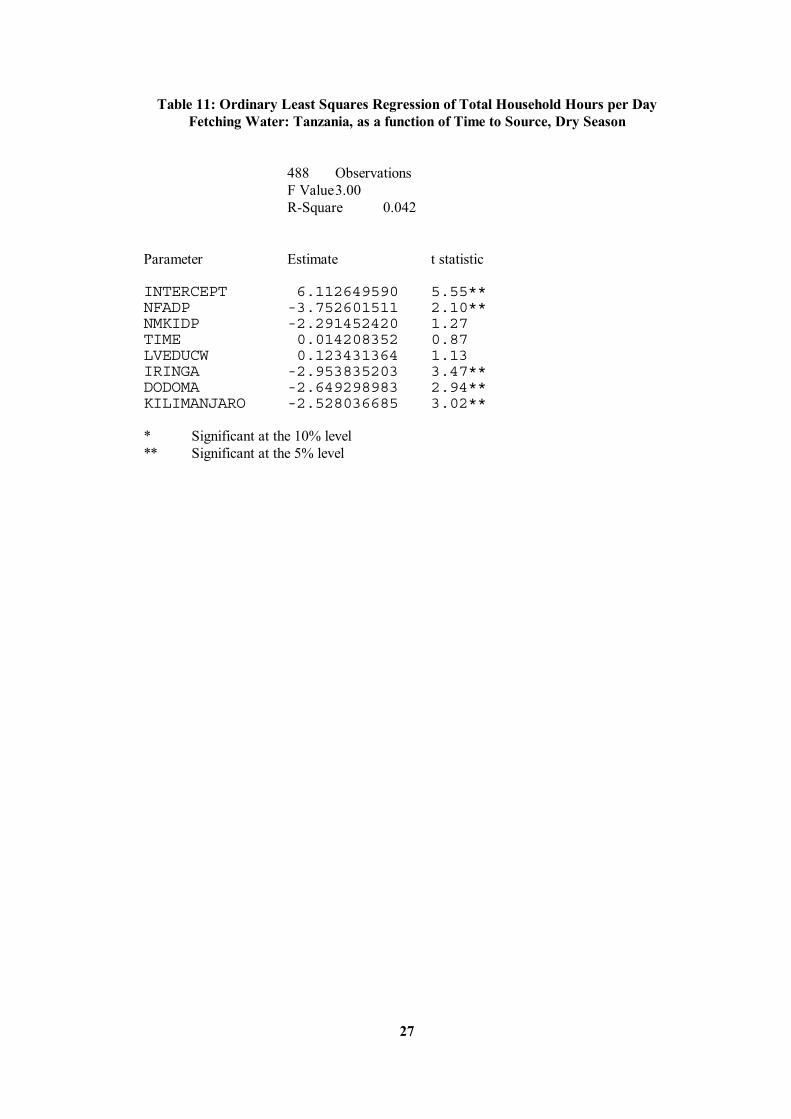
27

Table 11: Ordinary Least Squares Regression of Total Household Hours per Day Fetching Water: Tanzania, as a function of Time to Source, Dry Season 488 Observations F Value 3.00 R-Square 0.042 Parameter Estimate t statistic INTERCEPT 6.112649590 5.55** NFADP -3.752601511 2.10** NMKIDP -2.291452420 1.27 TIME 0.014208352 0.87 LVEDUCW 0.123431364 1.13 IRINGA -2.953835203 3.47** DODOMA -2.649298983 2.94** KILIMANJARO -2.528036685 3.02** * Significant at the 10% level ** Significant at the 5% level

28

B. Gender Effects and Extension Serivces B.1. Introduction In this section we address two questions: whether female headed households are disadvantaged in their access to extension services and, secondly, what consequences lack of access has. Extension has often been regarded as a necessary instrument for the modernization of agriculture. Farmers were supposed to lack knowledge about modern varieties and this not only reduced yields but also made farmers reluctant to adopt modern varieties, because of their perceived riskiness. Extension service would induce more widespread adoption of modern varieties and would lead to better cultivation techniques and higher yields. Extension officers would form the link between agricultural research centres and farmers. They would disseminate the results obtained in the centres, and - in the other direction - collect information on the needs and requirements of farmers. For Africa it has often been suggested that this system does not work. One reason is lack of good agricultural research, and especially the lack of suitable improved grain varieties. Research centres are said to lack skilled personnel and appear not to be sufficiently aware of the environmental and economic circumstances in which farmers operate. As to dissemination, the extension service (and its male officers) has been accused of directing its advice to men only. In general, the extension service has been directed not towards traditional farmers but to farmers who adopt modern cash crops and export crops in particular. Its outreach is often a direct complement of the adoption of those crops, because the purchase of seed or trees or the sale of the crop can only be done through a cooperative society or marketing board and the extension service is connected to it. As we will see, the situation is much like this in the three countries on which we have data. We start with Kenya.

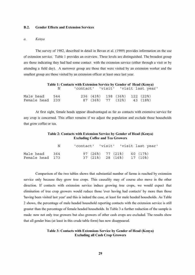
29

B.2. Gender Effects and Extension Services a. Kenya The survey of 1982, described in detail in Bevan et al. (1989) provides information on the use of extension service. Table 1 provides an overview. Three levels are distinguished. The broadest group are those indicating they had had some contact with the extension service (either through a visit or by attending a field day). A narrower group are those that were visited by an extension worker and the smallest group are those visited by an extension officer at least once last year. Table 1: Contacts with Extension Service by Gender of Head (Kenya) N 'contact' 'visit' 'visit last year' Male head 544 236 (43%) 198 (36%) 122 (22%) Female head 239 87 (36%) 77 (32%) 43 (18%)

At first sight, female heads appear disadvantaged as far as contacts with extensive service for any crop is concerned. This effect remains if we adjust the population and exclude those households that grow coffee or tea. Table 2: Contacts with Extension Service by Gender of Head (Kenya) Excluding Coffee and Tea Growers N 'contact' 'visit' 'visit last year' Male head 364 97 (26%) 77 (21%) 60 (17%) Female head 173 37 (21%) 28 (16%) 17 (10%)

Comparison of the two tables shows that substantial number of farms is reached by extension service only because they grow tree crops. This causality may of course also move in the other direction. If contacts with extension service induce growing tree crops, we would expect that elimination of tree crop growers would reduce those 'ever having had contacts' by more than those 'having been visited last year' and this is indeed the case, at least for male headed households. As Table 2 shows, the percentage of male headed household reporting contacts with the extension service is still greater than the percentage of female headed households. In Table 3 a further reduction of the sample is made: now not only tree growers but also growers of other cash crops are excluded. The results show that all gender bias (at least in this crude table form) has now disappeared. Table 3: Contacts with Extensions Service by Gender of Head (Kenya) Excluding all Cash Crop Growers

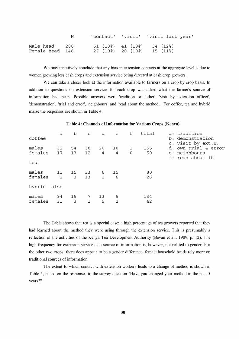
30

N 'contact' 'visit' 'visit last year' Male head 288 51 (18%) 41 (19%) 34 (12%) Female head 146 27 (19%) 20 (19%) 15 (11%)

We may tentatively conclude that any bias in extension contacts at the aggregate level is due to women growing less cash crops and extension service being directed at cash crop growers. We can take a closer look at the information available to farmers on a crop by crop basis. In addition to questions on extension service, for each crop was asked what the farmer's source of information had been. Possible answers were 'tradition or father', 'visit by extension officer', 'demonstration', 'trial and error', 'neighbours' and 'read about the method'. For coffee, tea and hybrid maize the responses are shown in Table 4. Table 4: Channels of Information for Various Crops (Kenya) a b c d e f total a: tradition coffee b: demonstration c: visit by ext.w. males 32 54 38 20 10 1 155 d: own trial & error females 17 13 12 4 4 0 50 e: neighbours f: read about it tea males 11 15 33 6 15 80 females 2 3 13 2 6 26 hybrid maize males 94 15 7 13 5 134 females 31 3 1 5 2 42

The Table shows that tea is a special case: a high percentage of tea growers reported that they had learned about the method they were using through the extension service. This is presumably a reflection of the activities of the Kenya Tea Development Authority (Bevan et al., 1989, p. 12). The high frequency for extension service as a source of information is, however, not related to gender. For the other two crops, there does appear to be a gender difference: female household heads rely more on traditional sources of information. The extent to which contact with extension workers leads to a change of method is shown in Table 5, based on the responses to the survey question "Have you changed your method in the past 5 years?"

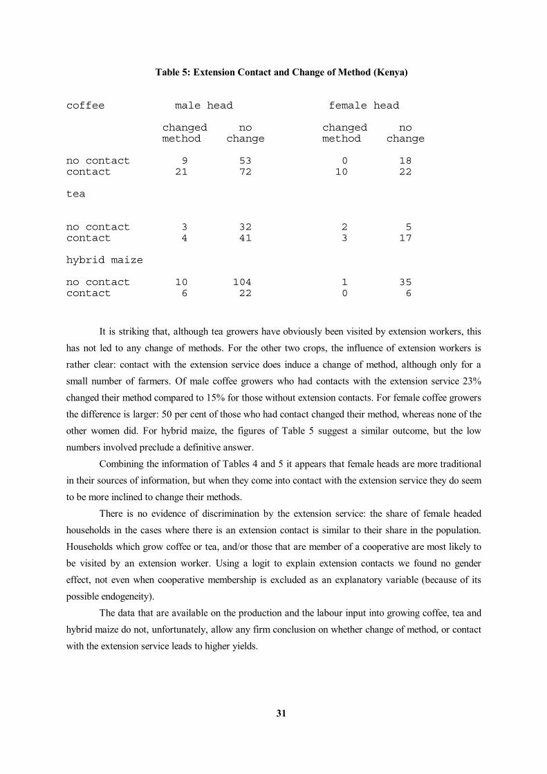
31

Table 5: Extension Contact and Change of Method (Kenya) coffee male head female head changed no changed no method change method change no contact 9 53 0 18 contact 21 72 10 22 tea no contact 3 32 2 5 contact 4 41 3 17 hybrid maize no contact 10 104 1 35 contact 6 22 0 6

It is striking that, although tea growers have obviously been visited by extension workers, this has not led to any change of methods. For the other two crops, the influence of extension workers is rather clear: contact with the extension service does induce a change of method, although only for a small number of farmers. Of male coffee growers who had contacts with the extension service 23% changed their method compared to 15% for those without extension contacts. For female coffee growers the difference is larger: 50 per cent of those who had contact changed their method, whereas none of the other women did. For hybrid maize, the figures of Table 5 suggest a similar outcome, but the low numbers involved preclude a definitive answer. Combining the information of Tables 4 and 5 it appears that female heads are more traditional in their sources of information, but when they come into contact with the extension service they do seem to be more inclined to change their methods. There is no evidence of discrimination by the extension service: the share of female headed households in the cases where there is an extension contact is similar to their share in the population. Households which grow coffee or tea, and/or those that are member of a cooperative are most likely to be visited by an extension worker. Using a logit to explain extension contacts we found no gender effect, not even when cooperative membership is excluded as an explanatory variable (because of its possible endogeneity). The data that are available on the production and the labour input into growing coffee, tea and hybrid maize do not, unfortunately, allow any firm conclusion on whether change of method, or contact with the extension service leads to higher yields.

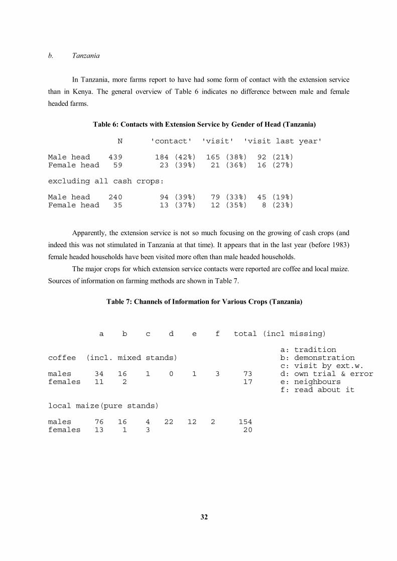
32

b. Tanzania In Tanzania, more farms report to have had some form of contact with the extension service than in Kenya. The general overview of Table 6 indicates no difference between male and female headed farms. Table 6: Contacts with Extension Service by Gender of Head (Tanzania) N 'contact' 'visit' 'visit last year' Male head 439 184 (42%) 165 (38%) 92 (21%) Female head 59 23 (39%) 21 (36%) 16 (27%) excluding all cash crops: Male head 240 94 (39%) 79 (33%) 45 (19%) Female head 35 13 (37%) 12 (35%) 8 (23%)

Apparently, the extension service is not so much focusing on the growing of cash crops (and indeed this was not stimulated in Tanzania at that time). It appears that in the last year (before 1983) female headed households have been visited more often than male headed households. The major crops for which extension service contacts were reported are coffee and local maize. Sources of information on farming methods are shown in Table 7. Table 7: Channels of Information for Various Crops (Tanzania) a b c d e f total (incl missing) a: tradition coffee (incl. mixed stands) b: demonstration c: visit by ext.w. males 34 16 1 0 1 3 73 d: own trial & error females 11 2 17 e: neighbours f: read about it local maize(pure stands) males 76 16 4 22 12 2 154 females 13 1 3 20

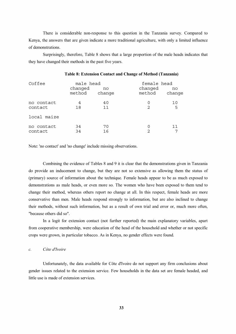
33

There is considerable non-response to this question in the Tanzania survey. Compared to Kenya, the answers that are given indicate a more traditional agriculture, with only a limited influence of demonstrations. Surprisingly, therefore, Table 8 shows that a large proportion of the male heads indicates that they have changed their methods in the past five years. Table 8: Extension Contact and Change of Method (Tanzania) Coffee male head female head changed no changed no method change method change no contact 4 40 0 10 contact 18 11 2 5 local maize no contact 34 70 0 11 contact 34 16 2 7 Note: 'no contact' and 'no change' include missing observations. Combining the evidence of Tables 8 and 9 it is clear that the demonstrations given in Tanzania do provide an inducement to change, but they are not so extensive as allowing them the status of (primary) source of information about the technique. Female heads appear to be as much exposed to demonstrations as male heads, or even more so. The women who have been exposed to them tend to change their method, whereas others report no change at all. In this respect, female heads are more conservative than men. Male heads respond strongly to information, but are also inclined to change their methods, without such information, but as a result of own trial and error or, much more often, "because others did so". In a logit for extension contact (not further reported) the main explanatory variables, apart from cooperative membership, were education of the head of the household and whether or not specific crops were grown, in particular tobacco. As in Kenya, no gender effects were found. c. Côte d'Ivoire Unfortunately, the data available for Côte d'Ivoire do not support any firm conclusions about gender issues related to the extension service. Few households in the data set are female headed, and little use is made of extension services.

34

Nevertheless, there is some indication of female household heads having less contact with the extension service than male heads. Combining the data sets of 1985 and 1987 in order to have as large a sample as possible, we arrive at a sample population of 1890 agricultural households, of which 378 reported the use of extension service for one or more crops. Out of the 1890 households, only 112 are female headed and of those only 5 reported any contact with extension services. Hence only 1 per cent of the female headed households had any contact compared to 7 per cent for male headed households. These differences may be due to other reasons, like differences in the crops grown. Evidence on this is shown in Table 9.

35

Table 9: Côte d'Ivoire: Extension Service by Crop no. of growers no. of contacts total female total female cocoa 454 10 56 1 coffee 519 12 49 1 rice 475 11 34 0 maize 816 16 yam 689 4 cassava 747 1 vegetables 804 1 bananas 537 0

This indicates, not unexpectedly, that extension contact is more likely in the case of cocoa, coffee and rice, crops grown relatively less in female headed households. The only basic variable that remains is the size of the holding. Table 10 reports the extent to which extension contacts are correlated with the size of the holding. Table 10: Number of Households by Land Size and Extension Contracts Côte d'Ivoire, 1985 and 1987 combined) cultivated land (ha) less than 3 3 to 6 6 to 12 12 to 20 over 20 with contacts 54 108 126 52 39 no contacts 495 443 392 133 60 % with contacts 10 20 24 28 39 coffee growers only with contacts 9 25 31 16 19 no contacts 98 250 284 117 57 % with contacts 8 9 10 12 25 cocoa growers only with contacts 5 27 38 16 20 no contacts 81 224 264 110 62 % with contacts 6 11 13 13 24

This shows that for Côte d'Ivoire there is a correlation between size of the holding and the use of extension service. Data do not reveal whether this bias is at the demand side (with the user) or at the

36

supply side (the officer). There is some evidence of gender differences in the sense that women are less frequently contacted by the extension service, but this no longer holds when separate crops are considered. Unfortunately, the data do not enable us to assess the impact of the use of extension service: unlike for Kenya and Tanzania there is no information on change of farming method.

B.3. Conclusion This section described the evidence on channels of information to farmers in Kenya and Tanzania. Female heads appear to be more traditional in their source of information: relatively few women report that they learned the method they are using from other sources such as extension service. The extension services in Kenya and Tanzania appears to reach female headed households as frequently as male headed households. In Côte d'Ivoire this was not the case: the very few female heads that were using extension services were less in number than might be expected on the basis of their share in the population. When analyzed for specific crops in Côte d'Ivoire, the gender aspect becomes less important. What remains as a major factor in the explanation of the use of extension service is the size of the holding: those in the highest group (over 20 ha) use extension service 4 times as much as those in the lowest group (under 3 ha). The Kenyan and Tanzanian evidence suggests that women, if they are reached by extension service (visit, demonstrations etc.) are more inclined to change their methods than men.

37

C. Credit

C.1. Introduction The purpose of this section is twofold. First, it seeks to examine the hypothesis that women have significantly poorer access to financial markets. In the discussion of women's earning generation, it has been argued that women are typically found in lower earning activities. In part, this may reflect particular constraints faced by women that are not faced by men. Here, we investigate the hypothesis that women face discrimination in access to credit. If this is the case, then steps to reduce this constraint will have two beneficial effects. First, it allows household income to rise. Second, evidence presented in chapter 7 shows that raising women's income within the household has beneficial effects on measures of household well-being such as child anthropometric status. If there are systematic gender biases in women's access to credit, then this suggests one avenue for useful policy intervention. But what form should this intervention take? It has been argued (McKee 1989, Schaefer-Kehnert, 1980, Thomas, 1988, World Bank, 1989) that self-help groups are a useful mechanism for channeling credit to smallholders, particularly women, and that these may be a more suitable means than specialised farm credit institutions (see Von Pischke, 1980 for a critical discussion of these). Existing studies of these organisations, such as Thomas (1988), have focused on their effectiveness. However, they have not examined the determinants of membership in these groups. If they are dominated by a few, wealthy women, then although they may be a good channel for credit, their effectiveness in removing credit constraints amongst poor women will be limited. Hence, our second area of interest in the determinants of group membership. The section is structured in the following fashion. We begin with a simple, tabular analysis of gender differences in access to financial markets in Kenya, Tanzania and Cote d'Ivoire. Particular emphasis is placed on access to credit, though access to deposit taking institutions is also discussed. None of the surveys used here identified financial information at the level of the individual household member. Consequently, gender analysis is confined to differences between male and female headed households. We then move on to an econometric evaluation of the hypothesis that female headed households are less likely to have access to credit markets, using a common framework for all three countries. We then look at the determinants of membership in women's groups using data from western Kenya. Concluding notes complete the section.

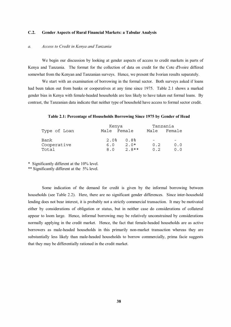
38

C.2. Gender Aspects of Rural Financial Markets: a Tabular Analysis a. Access to Credit in Kenya and Tanzania We begin our discussion by looking at gender aspects of access to credit markets in parts of Kenya and Tanzania. The format for the collection of data on credit for the Cote d'Ivoire differed somewhat from the Kenyan and Tanzanian surveys. Hence, we present the Ivorian results separately. We start with an examination of borrowing in the formal sector. Both surveys asked if loans had been taken out from banks or cooperatives at any time since 1975. Table 2.1 shows a marked gender bias in Kenya with female-headed households are less likely to have taken out formal loans. By contrast, the Tanzanian data indicate that neither type of household have access to formal sector credit.

Table 2.1: Percentage of Households Borrowing Since 1975 by Gender of Head Kenya Tanzania Type of Loan Male Female Male Female Bank 2.0% 0.8% - - Cooperative 6.0 2.0* 0.2 0.0 Total 8.0 2.8** 0.2 0.0 * Significantly different at the 10% level. ** Significantly different at the 5% level. Some indication of the demand for credit is given by the informal borrowing between households (see Table 2.2). Here, there are no significant gender differences. Since inter-household lending does not bear interest, it is probably not a strictly commercial transaction. It may be motivated either by considerations of obligation or status, but in neither case do considerations of collateral appear to loom large. Hence, informal borrowing may be relatively unconstrained by considerations normally applying in the credit market. Hence, the fact that female-headed households are as active borrowers as male-headed households in this primarily non-market transaction whereas they are substantially less likely than male-headed households to borrow commercially, prima facie suggests that they may be differentially rationed in the credit market.

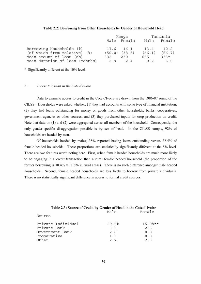
39

Table 2.2: Borrowing from Other Households by Gender of Household Head Kenya Tanzania Male Female Male Female Borrowing Households (%) 17.6 16.1 13.4 10.2 (of which from relative) (%) (50.0) (38.5) (66.1) (66.7) Mean amount of loan (sh) 332 230 655 333* Mean duration of loan (months) 2.9 2.4 9.2 6.0 * Significantly different at the 10% level. b. Access to Credit in the Cote d'Ivoire Data to examine access to credit in the Cote d'Ivoire are drawn from the 1986-87 round of the CILSS. Households were asked whether: (1) they had accounts with some type of financial institution; (2) they had loans outstanding for money or goods from other households, banks, cooperatives, government agencies or other sources; and (3) they purchased inputs for crop production on credit. Note that data on (1) and (2) were aggregated across all members of the household. Consequently, the only gender-specific disaggregation possible is by sex of head. In the CILSS sample, 92% of households are headed by men. Of households headed by males, 38% reported having loans outstanding versus 22.5% of female headed households. These proportions are statistically significantly different at the 5% level. There are two features worth noting here. First, urban female headed households are much more likely to be engaging in a credit transaction than a rural female headed household (the proportion of the former borrowing is 30.4% v 11.8% in rural areas). There is no such difference amongst male headed households. Second, female headed households are less likely to borrow from private individuals. There is no statistically significant difference in access to formal credit sources:

Table 2.3: Source of Credit by Gender of Head in the Cote d'Ivoire Male Female Source Private Individual 29.5% 16.9%** Private Bank 3.3 2.3 Government Bank 2.6 0.8 Cooperative 1.3 0.8 Other 2.7 2.3

40

** significantly different at the 5% level With respect to the size of loans, there is no statistically significant difference between male and female headed households. The mean amount borrowed by the former was 340948CFA and for the latter 354501CFA.141 Also, gender of head does not appear to affect the distribution of borrowing, as shown below:

Table 2.4: Distribution of Borrowing by Gender of Head in the Cote d'Ivoire Male Female (In CFA) <25000 34.6% 36.7% 25000-49999 17.9 13.3 50000-99999 13.8 13.3 100000-199999 10.9 13.3 >200000 22.8 23.3

Though the data indicate some difference in access to credit, this result must be treated with some caution. Recent fieldwork in other west African countries such as Burkina Faso (Christensen 1989, 1990), northern Ghana (Devereux, personal communication) and northern Nigeria (Udry, 1990) suggest the following caveats. The gender disaggregation used here is based on the gender of the head. Only 8% of Ivorian households are female headed, so this disaggregation omits analyzing access to credit amongst the other 92% of households. Further, Christensen (1990) and Udry (1990) have indicated that in Burkina Faso and northern Nigeria, male heads rarely knew about the extent of their spouses credit activities. They argue that adult males and females must be interviewed separately if full information on household credit is to be obtained. This does not appear to have been carried out in the CILSS survey. Consequently, the data available tell us relatively little about female, as opposed to female headed households', access to credit. The CILSS survey collected information on current credit transactions. Consequently, it is not possible to distinguish households unable to obtain loans from those that have borrowed money in the past, but subsequently repaid. A rough indication of the extent of this omission can be had by comparing this data with Christensen's. The proportion of households in his survey having obtained informal credit at least once in the previous year ranged between 78 and 97%. Furthermore, the majority of credit transactions had a duration of less than two months. Devereux's survey indicated 141 The mean for female headed households omits one observation which appears to be an outlier. It had 9700000CFA in loans outstanding, 27 times the mean.

41

that 60% of all households, and 68% of those classified as poor, borrowed money or goods in the previous year. Because no information is available on past credit history, it is possible that the CILSS survey understates the number of households with access to credit. Finally, it is unclear whether all credit activities have been recorded. Bassett has noted that in northern Cote d'Ivoire, some women participate in rotating credit associations. It does not appear that these have been captured in the survey. More importantly, Devereux has argued that in northern Ghana, many transactions are made with only vague intentions regarding future repayment. Both Devereux and Udry have described repayment of loans as state contingent, with repayment depending on future circumstances. Furthermore, many transactions are described as "help", even when repayment is expected. All these considerations suggest that there is scope for the underreporting of household credit activities. The CILSS survey also asked households if they obtained inputs on credit. There was negligible use of credit to purchase containers, sacks or manure. Approximately 9% of households obtained insecticides or seeds on credit. The only input purchased on credit by a substantial number of households was fertiliser, with 52.6% of households reporting doing so. However, 75% of households obtaining credit to purchase fertiliser did so for cotton production. Undoubtedly, this reflects the colonial and Ivorian government's long involvement with this crop (see Weekes-Vagliani, 1985 and Bassett, 1988 for a discussion) Access to credit for the purchase of fertiliser is part of the package offered to farming households. (The impact of cotton production on women in the Cote d'Ivoire has been, to quote a World Bank study (1988, p. 34), "largely negative", with women facing greater labour burdens without gaining access to income generated in this way.) Overall, apart from fertiliser, few households appear to be using credit for the purchase of inputs. c. Access to Deposit Taking Institutions Finally, we consider holdings of financial assets. There are no informal deposit-taking institutions in Kenya or Tanzania. Thus, the range of non-cash financial assets is fully captured by bank, cooperative and post office deposits. The survey did not attempt to identify the amount of these deposits but only whether the household had such deposits and the year in which the account was opened. As shown in Table 2.5, female-headed households are significantly less likely to have such financial assets:

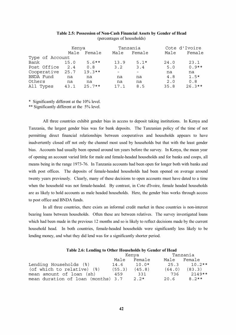
42

Table 2.5: Possession of Non-Cash Financial Assets by Gender of Head (percentages of households) Kenya Tanzania Cote d'Ivoire Male Female Male Female Male Female Type of Account Bank 15.0 5.6** 13.9 5.1* 24.0 23.1 Post Office 2.4 0.8 3.2 3.4 5.0 0.9** Cooperative 25.7 19.3** - - na na BNDA Fund na na na na 4.8 1.5* Others na na na na 2.0 0.8 All Types 43.1 25.7** 17.1 8.5 35.8 26.3** * Significantly different at the 10% level. ** Significantly different at the 5% level. All three countries exhibit gender bias in access to deposit taking institutions. In Kenya and Tanzania, the largest gender bias was for bank deposits. The Tanzanian policy of the time of not permitting direct financial relationships between cooperatives and households appears to have inadvertently closed off not only the channel most used by households but that with the least gender bias. Accounts had usually been opened around ten years before the survey. In Kenya, the mean year of opening an account varied little for male and female-headed households and for banks and coops, all means being in the range 1973-76. In Tanzania accounts had been open for longer both with banks and with post offices. The deposits of female-headed households had been opened on average around twenty years previously. Clearly, many of these decisions to open accounts must have dated to a time when the household was not female-headed. By contrast, in Cote d'Ivoire, female headed households are as likely to hold accounts as male headed households. Here, the gender bias works through access to post office and BNDA funds. In all three countries, there exists an informal credit market in these countries is non-interest bearing loans between households. Often these are between relatives. The survey investigated loans which had been made in the previous 12 months and so is likely to reflect decisions made by the current household head. In both countries, female-headed households were significantly less likely to be lending money, and what they did lend was for a significantly shorter period.

Table 2.6: Lending to Other Households by Gender of Head Kenya Tanzania Male Female Male Female Lending Households (%) 14.6 10.0* 25.3 10.2** (of which to relative) (%) (55.3) (45.8) (64.0) (83.3) mean amount of loan (sh) 459 331 736 2149** mean duration of loan (months) 3.7 2.2* 20.6 8.2**

43

* Significantly different at the 10% level. ** Significantly different at the 5% level. Note that only 6 female headed households in Tanzania reported data on amount and duration of loans. The Ivorian data does not allow us to distinguish between loans to friends, neighbours, relatives or business partners. Consequently, we can only look at lending in the aggregate. What is striking about the Cote d'Ivoire is that both male and female headed households are likely to make such loans (51.6 and 45.4% respectively) - the difference not being statistically significant.

C.3. An Econometric Analysis of Access to Credit in Cote d'Ivoire, Kenya and Tanzania The tabular analysis presented in section C.2 suggests that female headed households are less likely to have access to credit markets. In Kenya, it is the formal sector that exhibits the gender bias (informal credit markets being gender neutral). The opposite is true of the Cote d'Ivoire. However, these results may be driven by other household characteristics. Here, we present some simple econometric results that control for these. A logit was constructed with the dependent variable equalling one if the household currently had a loan outstanding, zero otherwise. Independent variables reflected the gender and age of the head, types of crops grown (which may enable households to gain access to credit either through producer cooperatives, or as a signal of ability to repay bank loans) and proxies for household wealth. Because of the differences in survey design, it was not possible to use an entirely common set of variables across all three countries. Below, we present descriptive statistics and the results of the logits:

Table 3.1a: Summary of Variables Variable Description SEXHH =1 household is female headed AGEHH the age of household head DCOC = 1 if household is growing cocoa (Cote d'Ivoire only) DCOF = 1 if household is growing coffee DCOT = 1 if household is growing cotton DTEA = 1 if household is growing tea (Kenya only) PAREA amount of land owned by household ROOMS the number of rooms in the dwelling if owned by the household (Cote d'Ivoire only) TGOODV the value of consumer durables currently held (Cote d'Ivoire only), '000 CFA DRUR = 1 if household located in rural area (Cote d'Ivoire only) BCCL number of usable bicycles owned by the household (Kenya and Tanzania only) LIVSTOCK value of livestock owned by the household (Kenya and Tanzania only), '000 shillings

44

Table 3.1b: Mean and Standard Deviations of Variables Used Kenya Tanzania Cote d'Ivoire Mean SD Mean SD Mean SD Variable SEXH 0.32 0.47 0.12 0.32 0.06 0.23 AGEHH 49.08 14.67 49.09 16.36 51.76 14.15 DCOC - - - - 0.45 0.50 DCOFFEE 0.31 0.46 0.17 0.38 0.55 0.50 DCOTTON 0.03 0.16 0.01 0.08 0.11 0.32 DTEA 0.19 0.39 - - - - PAREA 5.42 6.16 3.79 3.76 7.75 7.45 ROOMS - - - - 0.24 0.91 TGOODV - - - - 131809.6 640351.3 BCCL 0.22 0.49 0.26 0.56 - - LIVSTOCK 4.56 7.40 10.81 27.67 - - DRUR - - - - 0.57 0.50 (SD - Standard Deviation)

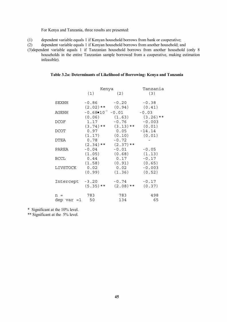
45

For Kenya and Tanzania, three results are presented: (1) dependent variable equals 1 if Kenyan household borrows from bank or cooperative; (2) dependent variable equals 1 if Kenyan household borrows from another household; and (3)dependent variable equals 1 if Tanzanian household borrows from another household (only 8

households in the entire Tanzanian sample borrowed from a cooperative, making estimation infeasible).

Table 3.2a: Determinants of Likelihood of Borrowing: Kenya and Tanzania Kenya Tanzania (1) (2) (3) SEXHH -0.86 -0.20 -0.38 (2.02)** (0.94) (0.41) AGEHH -0.68•10-3 -0.01 -0.03 (0.06) (1.63) (3.26)** DCOF 1.17 -0.76 -0.003 (3.74)** (3.13)** (0.01) DCOT 0.97 0.05 -14.14 (1.17) (0.10) (0.01) DTEA 0.78 -0.72 - (2.34)** (2.37)** PAREA -0.04 -0.01 -0.05 (1.05) (0.68) (1.13) BCCL 0.44 0.17 -0.17 (1.58) (0.91) (0.65) LIVSTOCK 0.02 0.02 -0.003 (0.99) (1.36) (0.52) Intercept -3.20 -0.74 -0.17 (5.35)** (2.08)** (0.37) n = 783 783 498 dep var =1 50 134 65 * Significant at the 10% level. ** Significant at the 5% level.

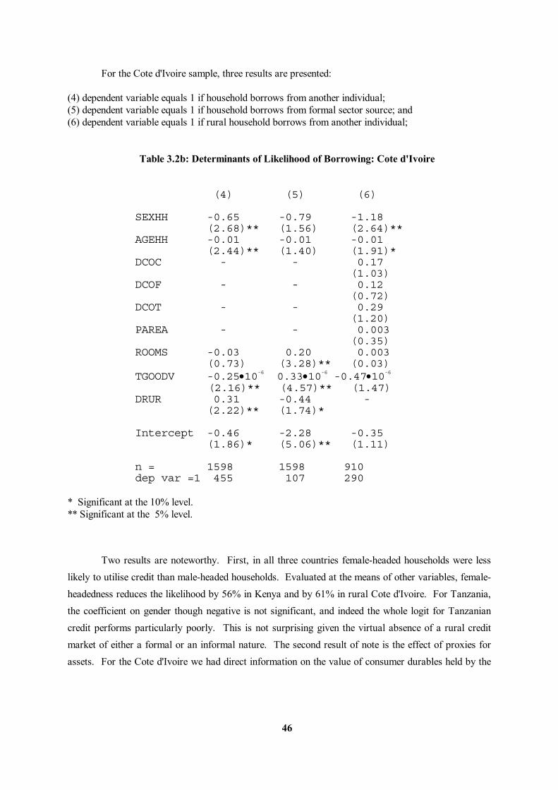
46

For the Cote d'Ivoire sample, three results are presented: (4) dependent variable equals 1 if household borrows from another individual; (5) dependent variable equals 1 if household borrows from formal sector source; and (6) dependent variable equals 1 if rural household borrows from another individual; Table 3.2b: Determinants of Likelihood of Borrowing: Cote d'Ivoire (4) (5) (6) SEXHH -0.65 -0.79 -1.18 (2.68)** (1.56) (2.64)** AGEHH -0.01 -0.01 -0.01 (2.44)** (1.40) (1.91)* DCOC - - 0.17 (1.03) DCOF - - 0.12 (0.72) DCOT - - 0.29 (1.20) PAREA - - 0.003 (0.35) ROOMS -0.03 0.20 0.003 (0.73) (3.28)** (0.03) TGOODV -0.25•10-6 0.33•10-6 -0.47•10-6 (2.16)** (4.57)** (1.47) DRUR 0.31 -0.44 - (2.22)** (1.74)* Intercept -0.46 -2.28 -0.35 (1.86)* (5.06)** (1.11) n = 1598 1598 910 dep var =1 455 107 290 * Significant at the 10% level. ** Significant at the 5% level. Two results are noteworthy. First, in all three countries female-headed households were less likely to utilise credit than male-headed households. Evaluated at the means of other variables, female-headedness reduces the likelihood by 56% in Kenya and by 61% in rural Cote d'Ivoire. For Tanzania, the coefficient on gender though negative is not significant, and indeed the whole logit for Tanzanian credit performs particularly poorly. This is not surprising given the virtual absence of a rural credit market of either a formal or an informal nature. The second result of note is the effect of proxies for assets. For the Cote d'Ivoire we had direct information on the value of consumer durables held by the

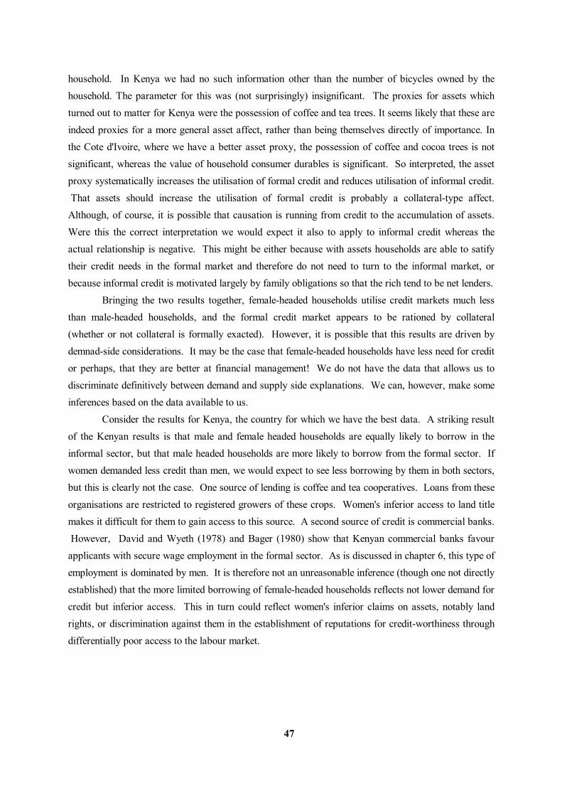
47

household. In Kenya we had no such information other than the number of bicycles owned by the household. The parameter for this was (not surprisingly) insignificant. The proxies for assets which turned out to matter for Kenya were the possession of coffee and tea trees. It seems likely that these are indeed proxies for a more general asset affect, rather than being themselves directly of importance. In the Cote d'Ivoire, where we have a better asset proxy, the possession of coffee and cocoa trees is not significant, whereas the value of household consumer durables is significant. So interpreted, the asset proxy systematically increases the utilisation of formal credit and reduces utilisation of informal credit. That assets should increase the utilisation of formal credit is probably a collateral-type affect. Although, of course, it is possible that causation is running from credit to the accumulation of assets. Were this the correct interpretation we would expect it also to apply to informal credit whereas the actual relationship is negative. This might be either because with assets households are able to satify their credit needs in the formal market and therefore do not need to turn to the informal market, or because informal credit is motivated largely by family obligations so that the rich tend to be net lenders. Bringing the two results together, female-headed households utilise credit markets much less than male-headed households, and the formal credit market appears to be rationed by collateral (whether or not collateral is formally exacted). However, it is possible that this results are driven by demnad-side considerations. It may be the case that female-headed households have less need for credit or perhaps, that they are better at financial management! We do not have the data that allows us to discriminate definitively between demand and supply side explanations. We can, however, make some inferences based on the data available to us. Consider the results for Kenya, the country for which we have the best data. A striking result of the Kenyan results is that male and female headed households are equally likely to borrow in the informal sector, but that male headed households are more likely to borrow from the formal sector. If women demanded less credit than men, we would expect to see less borrowing by them in both sectors, but this is clearly not the case. One source of lending is coffee and tea cooperatives. Loans from these organisations are restricted to registered growers of these crops. Women's inferior access to land title makes it difficult for them to gain access to this source. A second source of credit is commercial banks. However, David and Wyeth (1978) and Bager (1980) show that Kenyan commercial banks favour applicants with secure wage employment in the formal sector. As is discussed in chapter 6, this type of employment is dominated by men. It is therefore not an unreasonable inference (though one not directly established) that the more limited borrowing of female-headed households reflects not lower demand for credit but inferior access. This in turn could reflect women's inferior claims on assets, notably land rights, or discrimination against them in the establishment of reputations for credit-worthiness through differentially poor access to the labour market.

48

C.4. Determinants of Women's Self Help Group Membership in Western Kenya a. Introduction Our discussion in the previous sections has indicated that female-headed households are less likely to have access to credit markets, and where we have been able to disaggregate these, it is the formal sector that exhibits the gender bias (informal credit markets, at least in Kenya, being gender neutral). In this section, we examine the scope for one form of policy intervention in this area - women's self-help groups. It has been argued that women's self-help groups are an effective means of reducing constraints faced by women. Thomas' (1988) evidence suggests that women's associations in central Kenya assist in relieving cash constraints and shortages of labour, and provide access to information, such as health practices and extension services. In addition to poverty alleviation, McKee (1989) suggests these groups provide a means of mobilising and empowering women. For example, this process allows women to overcome barriers to entry into nontraditional activities. As such, it provides a useful 'role-model' exercise for other women. Improving women's access to resources outside the household may also improve their bargaining position within it. Further, by working together, women can accomplish these goals more efficiently than they could if they remained outside these groups. Besley, Coate and Loury (1990) provide a theoretical analysis showing that saving through a rotating savings and credit association is more efficient than 'autarkic saving'. Though there has been relatively wide study of the benefits of these associations (McKee, 1989, contains a useful discussion), there has not been any analysis of the determinants of membership of these organisations. Such an examination is useful. If membership (and hence benefits) are limited to a small group of well-off women, then some advantages, for example in terms of poverty reduction, are dissipated. By contrast, if their membership is drawn predominantly from poorer women, then policy support to these groups would be justified. b. Data and Model Data for this analysis is drawn from a household survey conducted in Karateng sub-location, Kisumu District, Kenya. Karateng is a rural area with a long history of out-migration. It is located approximately 370km west north-west of Nairobi (see Hoddinott, 1989, for a discussion of the survey). Of the 111 women in the sample, 30 (27.2%) currently belong to a women's self-help group.

49

Women's groups in Karateng take two forms. Some are relatively formal organisations, principally devoted to income generation. For example, the Rimoka women's group has three objectives: adult education; home economics; and income generating projects. It has raised money through membership contributions, several harambees (community fund raising drives) and a government grant. These funds were used money to buy land near a busy highway and to construct a small hostel whose rooms are rented out. A second group, Mbakaromo, grew crops and kept bees. The second type of group are examples of rotating savings and credit societies. The Burlowo women's group collects money on a weekly (or sometimes biweekly basis) and the funds given to individual members for funeral contributions, general household expenses and to finance purchases for members running their own businesses. A priori, there are three constraints that might prevent women from participating in these organisations. One is poverty. The poorest women in the area may be unable to make the contributions required to join these groups (indeed, this was a comment made by a number of poorer women in the area). Closely connected to poverty is a time constraint. Some women may find themselves unable to join because there are other demands on their time, for example child care, fetching water or firewood. Some women may find that they need to engage in activities, such as day labouring that bring in an immediate return, rather than participate in an organisation whose payoff comes later. Finally, women with little power within their own households may be prevented from joining these groups. There were hints in some households that husbands forbade, or actively discouraged their wives from joining. On the other hand, very wealthy women may derive little benefit from membership. If this is true, they are also unlikely to join. These considerations motivate the choice of variables used in the empirical analysis. Net annual household income and its square are included to capture the hypothesis that women in the poorest and better off households are less likely to join. A series of dummy variables reflecting women's education are also included for the same reason. Time constraints are captured by including the number of children the woman has, its square, and a dummy variable equalling one if the woman collects water or firewood. The presence of children has been expressed as a quadratic to capture the idea that greater numbers of offspring increase the amount of time devoted to child care, but this effect diminishes as the number of children increases, and older children (particularly girls) assume some responsibilities for their younger siblings. Women's status within the household is reflected in several variables. In this area, older women have more status than younger women, hence the inclusion of women's age. It is possible that women with their own sources of income outside the household may be less likely to have to bow down to their husbands. This is captured here by including women's cash income from employment outside the household and earnings from own business activities. Women's education, as noted above, also

50

captures this concept. A summary of the variables used, with their means and standard deviations, is found in Table 4.1:

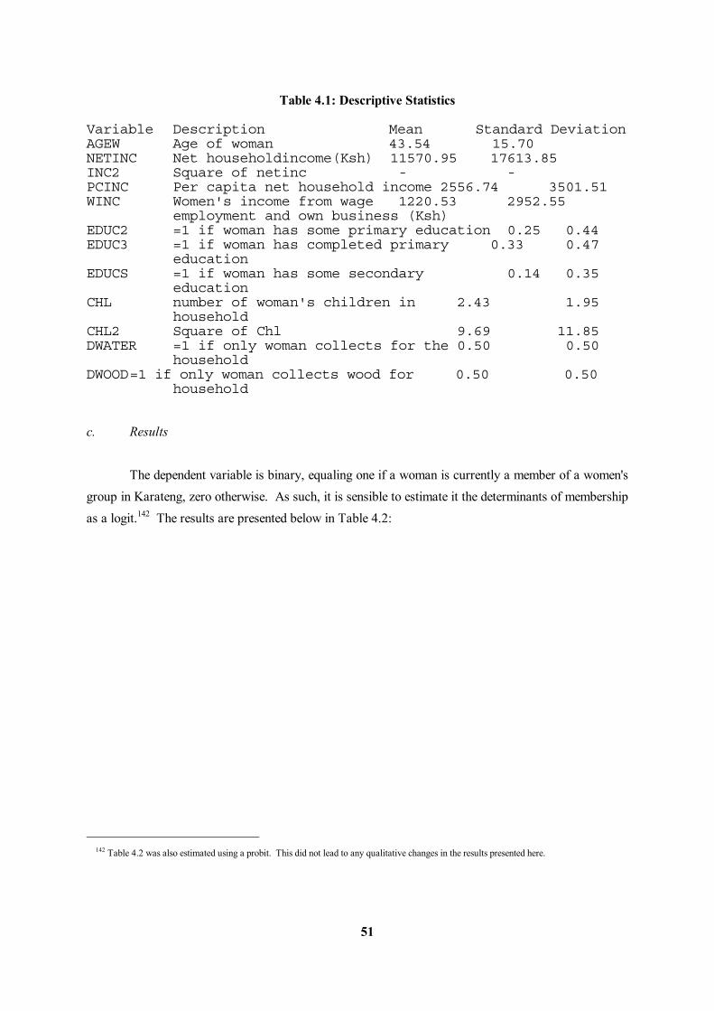
51

Table 4.1: Descriptive Statistics Variable Description Mean Standard Deviation AGEW Age of woman 43.54 15.70 NETINC Net householdincome(Ksh) 11570.95 17613.85 INC2 Square of netinc - - PCINC Per capita net household income 2556.74 3501.51 WINC Women's income from wage 1220.53 2952.55 employment and own business (Ksh) EDUC2 =1 if woman has some primary education 0.25 0.44 EDUC3 =1 if woman has completed primary 0.33 0.47 education EDUCS =1 if woman has some secondary 0.14 0.35 education CHL number of woman's children in 2.43 1.95 household CHL2 Square of Chl 9.69 11.85 DWATER =1 if only woman collects for the 0.50 0.50 household DWOOD =1 if only woman collects wood for 0.50 0.50 household

c. Results The dependent variable is binary, equaling one if a woman is currently a member of a women's group in Karateng, zero otherwise. As such, it is sensible to estimate it the determinants of membership as a logit.142 The results are presented below in Table 4.2:

142 Table 4.2 was also estimated using a probit. This did not lead to any qualitative changes in the results presented here.

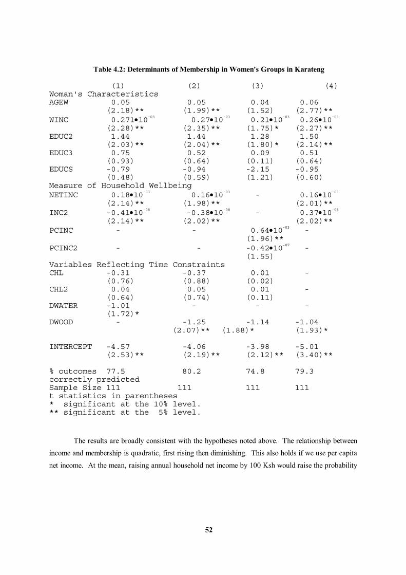
52

Table 4.2: Determinants of Membership in Women's Groups in Karateng (1) (2) (3) (4) Woman's Characteristics AGEW 0.05 0.05 0.04 0.06 (2.18)** (1.99)** (1.52) (2.77)** WINC 0.271•10-03 0.27•10-03 0.21•10-03 0.26•10-03 (2.28)** (2.35)** (1.75)* (2.27)** EDUC2 1.44 1.44 1.28 1.50 (2.03)** (2.04)** (1.80)* (2.14)** EDUC3 0.75 0.52 0.09 0.51 (0.93) (0.64) (0.11) (0.64) EDUCS -0.79 -0.94 -2.15 -0.95 (0.48) (0.59) (1.21) (0.60) Measure of Household Wellbeing NETINC 0.18•10-03 0.16•10-03 - 0.16•10-03 (2.14)** (1.98)** (2.01)** INC2 -0.41•10-08 -0.38•10-08 - 0.37•10-08 (2.14)** (2.02)** (2.02)** PCINC - - 0.64•10-03 - (1.96)** PCINC2 - - -0.42•10-07 - (1.55) Variables Reflecting Time Constraints CHL -0.31 -0.37 0.01 - (0.76) (0.88) (0.02) CHL2 0.04 0.05 0.01 - (0.64) (0.74) (0.11) DWATER -1.01 - - - (1.72)* DWOOD - -1.25 -1.14 -1.04 (2.07)** (1.88)* (1.93)* INTERCEPT -4.57 -4.06 -3.98 -5.01 (2.53)** (2.19)** (2.12)** (3.40)** % outcomes 77.5 80.2 74.8 79.3 correctly predicted Sample Size 111 111 111 111 t statistics in parentheses * significant at the 10% level. ** significant at the 5% level.

The results are broadly consistent with the hypotheses noted above. The relationship between income and membership is quadratic, first rising then diminishing. This also holds if we use per capita net income. At the mean, raising annual household net income by 100 Ksh would raise the probability

53

of membership by 1.5%.143 However, the downturn point is fairly high up, with only 15% of households lying above it. This aspect is re-iterated when looking at women's education which exhibits a similar pattern. Possession of some primary education strongly increases the likelihood of membership. This declines at higher levels of education (this result is robust to alternative specifications of the education variable). The variables reflecting time constraints have relatively weak effects on membership. Neither the number of children nor its square significantly affect the likelihood of joining a women's group. A number of variations, such as a breakdown of children by age and sex and calculations of household dependency ratios, were also tried (this results are not reported here). None yielded any significant effects on membership. It could be argued that because fertility is a choice variable, the number of children should not be included as a regressor. This argument is discussed in more detail in chapter 6. Here, it is worth noting that the effects of other variables are robust to the exclusion of the number of children present. However, if women are required to fetch water for the household, the probability of a woman joining is 11.9%, a fall of more than 50% in the likelihood of membership. Having to fetch wood has a similar effect on the likelihood of membership. Variables reflecting women's independent status have a statistically significant effect on membership. An increase in women's own income of 100 Kenyan shillings raises the likelihood of membership by 2%. Older women are more likely to join than younger women. Each additional year increases the probability of joining by 3.9%. This may reflect increased women's status within the household. It may also reflect an easing of time constraints, with women having more opportunities to earn an independent income. Also, young women may be less likely to join because their husbands are more likely to be away. Consequently, they may spend more time going back and forth to the cities and hence feel they have less to gain from such an organisation (especially those whose return is long term as in Rimoka). Also, they may perceive themselves as having better opportunities if they go it alone. To check for this more closely, dummy variables were included to reflect whether women were the head of household, with husband away, or head of household with husband dead, generated parameter with the correct predicted signs (positive in the first case, negative in the second), but these were not significant.

143 It could be argued that household and women's income may be higher because women belong to these groups. Consequently, income should not be used as a regressor because it is endogenous. However, the women's groups considered here are relatively new and none have distributed a payment to their members. Hence, this criticism does not apply here.

54

C.5. Conclusions It should be stressed that the data set has limitations when applied to credit. In the Cote d'Ivoire, where there is an active informal market, we probably suffer gender-biased under-reporting. In Tanzania there is virtually no rural credit market. With these caveats, we found that female-headed households used both lending and deposit-taking institutions significantly less than did male-headed households. We established that the utilisation of formal credit was positively related to the asset endowment of the household (utilisation of informal credit being negatively related), and interpreted this as rationing by collateral in the formal market. We suggested that the explanation for the lower utilisation of credit by female-headed households may therefore be due to an inferior credit-worthy status in a rationed market, than to a lower demand for credit. We have also examined the determinants of women's participation in self-help groups. It appears that the major constraint is income, with poorer women less likely to join, though this is also true of women from the wealthiest households in the sample. Time constraints play some role in limiting membership, but these effects are not strong.

55

D. Gender and the Prioritization of Public Services in Rural Kenya and Tanzania The Kenya and Tanzania rural surveys included questions on the subjective valuations of government services. Table 1 cross tabulates those past improvements which are most valued against those which are most desired for the future. For both provinces in Kenya, road improvements were cited overwhelmingly most frequently as the most useful of government's past services (42.5% in Central, 55.1% in Nyanza). other highly valued improvements were in primary schools (14.7% in Central, 16.3% in Nyanza), and, for Central, health facilities (14.1%, but only 4.5% in Nyanza) and in water supply (12.4%, but only 3.3% in Nyanza). The most desired improvements were water supply for both provinces (38.5% Central, 25.1% in Nyanza), more roads (25.4% Central, 24.6% Nyanza). In view of the data discussed elsewhere, it is interesting that Nyanza residents should be so much less satisfied with past health improvements, while attaching more importance to these for the future. The great weight attached to water supply improvements might appear ironic in view of their dubious health benefits, but of course they are also valued for reducing time spent on the onerous business of fetching it. Another interesting feature of the table is the low occupancy of the main diagonal. The vast majority of households would most appreciate a different type of improvement from the one they most valued in the past. Indeed well under 10% in each province most want `more of the same thing'. Overall, it appears that people were satisfied with the provision of primary education (at least it remained the leading priority for very few); otherwise, there were proponents for increased provision of all the other categories of spending considered, with the sole exception of extension services in Central (a mere 2.3%). Indeed these services appear to be something of a poor relation, with few households being much impressed by past efforts either (2.3% Central, 3.0% Nyanza). Turning to Tanzania, the most notable difference is the greatly reduced significance attached to road improvements: only 9.9% highly valued those made in the past, and only 7.9% attached a future priority to them. This presumably reflects the fact that Tanzanian peasants were far less integrated into the national economy: they were less dependent on good transport facilities to get their produce to market; the availability problems which were acute at the time of the survey also imply a reduced priority on transport facilities to bring in inputs and consumer goods. Health and water supply were highly rated both retrospectively (25.8%, 15.7%) and prospectively (34.3%, 29.4%). It is true, as for Kenya that primary schools were highly valued (32.5%) but further provision was not a priority (1.1%). Unlike the situation in Kenya, secondary schools hardly figured in priorities. This was literally true for Dodoma and Ruvuma, whereas in Kilimanjaro 4.6% thought it the most useful thing the government had done, and 13.8% rated it a top

56

priority for the future (this regional breakdown is not given in the table). This suggests that perceptions of what is desirable are bounded by actual experience. Prioritization tends to be somewhat incrementalist in nature. A final distinction is that extension services were given a moderate priority (9.4% in each case). Since these data are reported for the household, usually by its head, it is worth investigating whether there are any systematic differences between male and female headed households. Table 2 provides such a comparison for each of the Kenyan and Tanzanian samples. Casual inspection suggests that there is very little difference by gender and more formal analysis bears this out. A number of the Tanzanian cells have counts less than 5, so that the chi square test may not be valid, either for the affected services, or for the set of services as a whole. For the services where a chi square test can be validly carried out (health, water, primary education for past improvements; extension, health, water, `other' for future ones) none of the gender differences is significant even at the 15% level. However, accepting the low significance, the table does suggest that Tanzanian females heads may have been somewhat more enthusiastic, relatively, about past provision of health services over against primary education (chi square probabilities .159 and .173 respectively), whereas the forward looking preferences are remarkably similar. For Kenya, only one past service provision is remotely significant (water supply, where the chi square probability is .128 that male heads are more enthusiastic). As regards forward preferences, male heads are significantly more enthusiastic about extensions services (probability .039). Otherwise, there is a suggestion that female heads are more enthusiastic about further health provision (probability.139) and less so about the `other' category (probability .101). In brief, in only one of the twenty one comparisons which can be subjected to a chi square test are female heads' preferences significantly different at the 5% level, and in a further five and the 20% level. Overall, the prioritization of public services seems not to be very gender specific. The same conclusion holds when the influence of the gender composition of households is taken into account. Households were ranked according to the ratio of adult females to adult males, and then divided into three groups according to whether this ratio was above, below, or at the median value. The last group was dropped, and the preferences of households with high and low proportions of women compared. This exercise was repeated for both male and female headed households, forward and backward looking, in Kenya and in Tanzania. Of the forty comparisons which can be subjected to a chi square test, only three are significantly different at the 5% level. One of these is not very interesting144, but the other two are. Among preferences for future services in female headed households in both Kenya and Tanzania, improved water supply is significantly more favoured by households with

144For male headed Kenyan households, those with relatively few women attached more importance to past improvements in `other' services - 13.7% as compared to 6.4%, probability .019.

57

relatively many women. In Kenya 39.0% of female headed households with relatively many women had this preference, as opposed to 27.1% of those with relatively few (probability .046). In Tanzania, the corresponding figures were 43.3% and 17.2% (probability .030). The greater appreciation of water services amongst households with relatively many women is true for most of the other categories too, but in these cases only achieves any statistical significance for Tanzanian male headed households in the case of past improvements. The corresponding figures are then 19.4% and 11.6% (probability .057). These results are interesting in view of the relatively heavy burden placed on women by the need to fetch water in most rural households, but they are a little hard to interpret, given the lack of significant difference between male and female headed households noted earlier. The only other comparisons to achieve significance at the 10% level relate to female headed Kenyan households and past improvements in schooling. Those with relatively many women attach more weight to secondary school provision (8.1% as compared to 2.6%, probability .068) and less to primary school provision (11.7% as compared to 20.2%, probability .083). Once again, this is a little hard to interpret: there is no comparable pattern in any of the other household groupings, nor between male and female headed households. These exercises based on gender composition therefore reinforce the earlier conclusion, that prioritization of public services appears not to be gender dependent.

58

Conclusion In this chapter, we have examined gender differentiated access to three public services: water, extension and credit. We have also examined whether men and women (principally captured through headship) have different priorities with regard to the provision of services. Here, we briefly summarise the findings of this chapter. Not surprisingly, women bear the brunt of water collection in Kenya and Tanzania. But of particular note here is the extent to which Kenyan households protect students from this task, unlike households in Tanzania. As noted earlier, this is entirely consistent with the different structures of schooling in the two countries. Given the costs savings associated with entry into state secondary schools in Kenya, it is to the household's advantage to ensure good performance on the primary school leaving exam. No such motivation exists in Tanzania. We also examined whether the provision of piped water would reduce collection times in Kenya and Tanzania. Our calculations, which should be treated cautiously, suggest that the amount of time saved would be small. With respect to extension, our data only permits differentiation along the lines of headship. In Kenya and Tanzania, extension services appear to reach female headed households as well as male headed one. However, once contacted, female headed households are more likely to change their farm methods. In Cote d'Ivoire, few female headed households have access to extension services, though this result becomes less important when analysed for specific crops. In reviewing our analysis of credit, it is worth stressing that the data set has a number of limitations. This is particularly true of the Ivorian data. With the caveats noted in the text, we suggest that the lower utilisation of credit by female headed households is a reflection of their inferior credit worthy status in a rationed market. Our examination of the determinants of participation in women's self-help groups indicated that income, rather than time, was the major constraint on membership. However, women from the wealthiest households in the sample also eschew membership - suggesting that these groups may not be wholly unsuitable as a means of targetting credit towards poorer women. Finally, there do not exist strong differences by gender in the prioritising of public services. However, one notable difference is that households with many women in Kenya and Tanzania place stronger emphasis on improving water supplies. Given the time they spend collecting water, this is not surprising.

59

Part II: Income and Expenditure

60

Chapter 5: Women and the Labour Market 1. Introduction 2. Modelling and Earnings a. A Simple Participation Model b. A Sectoral Disaggregation of Participation c. Estimating Discrimination in Earnings 3. Women and the Kenyan Labour Market a. Overview b. Data and Variables c. Results - I d. Results - II e. Job Choice at the Household Level 4. Women and the Tanzanian Labour Market a. Overview b. Data and Variables Used c. Results - I d. Results - II e. Job Choice at the Household Level 5. Conclusions Appendix: Is Fertility Endogenous?

61

1. Introduction We begin our analysis of women and the labour market in Kenya and Tanzania with two observations: (1) women are less likely to participate in off-farm activities - the participation rates being 21.6% and 55.0% respectively in Kenya and 26.6% and 39.1% in Tanzania; and (2) amongst individuals who participate in the labour market (as defined below) women's earnings are lower - 26.15 Ksh/day vs 42.38 Ksh/day for men in Kenya and 33.47 Tsh/day vs 45.36 Tsh/day for men in Tanzania. What are the possible explanations for this? With respect to participation there are three possibilities. This could be a consequence of the division of labour within the household, with women engaged in crop production and child care and men going out to work. In turn, this could be a reflection of their comparative advantages in these areas, a la Becker (1981), or merely differences in outside earnings opportunities between men and women (possibly reflecting differences in educational attainment, as in Low's (1986) model of the household). Alternatively, these participation rates could be a result of differing preferences for off-farm work between men and women. Finally, it could reflect discrimination in terms of access to the labour market. There are also three explanations for the divergence in earnings. Women who do participate may be forced (for whatever reason) into lower earnings sectors. It may be a consequence of pure discrimination. Finally, it could reflect, differences in personal endowments, such as education. Once these are controlled for, the difference in earnings disappears. As in many other studies of women in the labour market (see Cain, 1986 for a summary), we do not have data on the demand for labour. Consequently, with respect to participation, it is not possible for us to distinguish between explanations based on preferences and those based on discrimination. But we can examine the other explanations for these 'stylised' facts. The chapter is structured in the following manner. Section 2 provides background on the theory and econometrics of models of labour market participation. Section 3 contains an analysis of participation and earnings in Kenya. Section 4 replicates this for our Tanzanian data. Concluding notes complete the chapter.

2. Modelling Participation and Earnings a. A Simple Participation Model Our initial interest is in determining whether an individual will participate in labour force activities outside the family farm. These include: working outside the village (either in another rural area, or in an urban area); working as an employee doing non-agricultural work within the cluster; running a business; and working on the farms or estates of others.

62

To model participation and the determinants of earnings, we adopt a two-stage procedure, as suggested by Heckman (1976, 1979) and summarised in the Appleton, Collier and Horsnell (1990). We assume that individuals base their decision to engage in these activities when the wage they receive for doing so exceeds their unobserved reservation wage (WR) which reflects both individual (X) and unobserved characteristics (g). That is, for each individual: WR = WR(X, g) (1) Although, WR is not observed, we do observe a wage (W) for those individuals participating in the labour market. Assume this to be a function of observed (Z) and unobserved characteristics (b). We observe labour market participation if: W(Z,b) > WR(X, g) (2) WR is not observed. Instead, we have a binary variable (P) that equals one if the individual participates, zero otherwise. We can write P as a function of observed characteristics (X), wages and unobserved characteristics (g): P = P(X, W, g) (3) and observed wages as: W = W(Z,b) (4) The key aspect to note about (3) and (4) is that the error terms will embody the unobserved variables g and b. Suppose we estimated (3) and (4) separately, the latter conditional on P equalling one. If g and b are correlated, this will lead to biased estimates of the coefficients associated with Z. Further, if we then try to estimate predicted wages for all individuals in the sample, based on the biased coefficients, this will lead to misleading results for (3). Heckman's solution revolves around the idea that this correlation can be seen as an omitted variables problem (also see Greene, 1990). He suggests that we first estimate a reduced form probit of the participation decision. This includes all exogenous variables in both the participation and earnings equations. From this, the inverse Mill's ratio is calculated. It is included as an additional regressor in the earnings equation which is estimated by ordinary least squares to produce unbiased parameter estimates.

63

There are several econometric issues worth noting before we turn to the data. In order to undertake this estimation procedure, it is necessary that identification problems be overcome. In order to estimate the inverse Mill's ratio, we need some variable that appears in X but not in Z. In sections 3 and 4, we accomplish this by including data on household assets and location. Secondly, in order to include predicted wages in a structural participation equation, it is necessary to find variables that appear in Z but not in X. We could assume that education affects earnings but does not have any influence on participation independent of its effect on earnings. This is equivalent to assuming that education does not affect tastes for work at given wages, a very strong a priori assumption. Consequently, we have chosen to estimate a reduced form version of the participation decision. That is, we substitute the determinants of earnings for W in the participation equation, yielding: P = P(X, Z, g) (5) This methodology can also be used to estimate the number of days worked in various sectors. For example, in section 3, we will examine the impact of education and demographic variables on the amount of labour used on the family farm. To do so, we exclude individuals participating in the labour market. We estimate a labour supply function for those employed on the farm, again correcting for sample selection bias. In order to overcome identification problems, again we need variables that effect participation but not agricultural labour supply. We do so by dropping the location dummy variables from the latter. A second problem is the influence of unobserved characteristics on earnings. Khandker (1990, p. 12) suggests that:

... the unobserved household and community characteristics that often relate to abilities, motivation, quality of schooling, employment opportunities, and role models can influence wages and returns to education. More specifically, if these unobserved factors are correlated with years of schooling, the standard estimation procedure results in biased estimates of the impact of schooling and hence the returns to education.

In his study of labour market participation and returns to education in Peru, Khandker uses a fixed effects estimation procedure to resolve this problem in his estimated wage equation. However, it is not clear whether this approach is appropriate for our Kenyan and Tanzanian data. In both countries, the practice whereby women leave their parents and live with their husbands upon marriage (patrilocal) is the norm virtually everywhere. Consequently, many of the unobserved characteristics cited by Khandker will differ amongst husbands and wives in our sample, reducing their potential biases. Obviously, this does not hold as strongly for sons and daughters in the sample. However, to maintain

64

a consistent estimation strategy for all individuals in the samples, we have not used the fixed effects model. We therefore caution that this may impart biases to our parameter estimates in the wage equations, though we believe that these are probably small. We have assumed that individuals participate on the basis of a comparison of their reservation wage with that available in the market. As such, labour force participation is seen as an individual decision. Yet, within a household, this may not be the case. As Kooreman and Kapteyn (1990, p. 584) note, "... it is likely that there is a tight structural relation between the labour supply decision of the male and female partner within a household ...". With respect to offspring, McElroy (1985) and Hoddinott (1990) has suggested that labour supply and migration decisions can be modelled as the outcome of a bargaining process with parents. However, to implement these models, additional data are required. For example, Kooreman and Kapteyn have information on individual preferences for hours worked, while Schultz (1990) uses gender disaggregated unearned income. These are not available to us here. Consequently, we have retained the individual utility maximising approach, with the caveat that we do not control for the labour supply decisions made by other individuals within the household. In addition, however, we estimated multi-nominal logit models for the outcome of the job decisions of the family as a whole. Here we do as if the family allocates its members according to the assets available. Assets are here taken to be numbers of males, females, children, educated etc. These will be discussed in section 4. b. A Sectoral Disaggregation of Participation In the model of participation presented above, we have assumed that individuals react to the average wage they might command. Yet, it is possible that labour markets are segmented, with different markets offering different rates of return, and possibly possessing different barriers to entry. Both factors will influence the choice of labour market sector. The role of entry barriers is of particular interest here, because we are interested in whether women are pushed into lower earning sectors. To incorporate this aspect into our analysis, we need to expand our model of participation. Here, we draw on the approach originally specified by Domencich and McFadden (1975) and Schmidt and Strauss (1975a, 1975b). Suppose individuals can choose amongst (0) not participating; (1) participating in local, informal sector employment (eg casual agricultural work or running own business); or (2) participating in formal sector employment (either local or non-local). If we call the likelihood of participating in any one of these sectors cj, then: c0 + c1 + c2 = 1 (6) A multinomial logit model expresses these as:

65

cj = [ e`j + aj Xi ] / [ dj e`j + aj Xi ] (7) We normalise here on the 'not participate' choice. Consequently, we estimate two functions of the form: ln (Pj/P0) = P(X, W, g) (8) Note here that again we only observe wages for those individuals who participate in the labour force. This can be dealt with by following the procedure set out be Lee (1983). Initially, we estimate a reduced form multinomial logit containing all variables that affect both participation and earnings. With reservation wages again unobserved, we must normalise on a sector (here, we omit working on the family farm). Having done so, we can then estimate wage equations for each sector, correcting for sample selection bias (see Lee, 1983). As in our discussion of the simple participation model, we do not assume that there exists a variable that affects earnings but not participation. Consequently, we estimate a reduced form version of (8), namely: ln (Pj/P0) = P(X, Z, g) (9) This approach is useful as it eliminates the sample selection problem for the earnings equation and allows for a detailed examination of the determinants of participation by sector. But it is not without its drawbacks and it is useful to be aware of these. The multinomial logit involves estimating a logarithm of the ratio of the probability of two outcomes. It requires that the introduction of a third outcome does not change this ratio. This assumption is known as the independence of irrelevant alternatives (IIA, the `red bus - blue bus' problem). If IIA does not hold, the parameter estimates will be inconsistent (Greene, 1990, p. 702). This is a strong assumption to make. However, a key issue we wish to explore is whether there exists discrimination in terms of earnings. The multinomial logit approach allows us to estimate participation by sector, then estimate earnings equations correcting for sample selection bias. Relaxing the IIA assumption requires the estimation of a nested multinomial logit and it is not clear that doing so will allow us to correct for sample selection bias. An alternative estimation strategy involves using an ordered probit. But this requires a priori assumptions regarding individuals' orderings of occupational choice, without any means of substantiating these. This too is clearly undesirable. Hence, we have maintained the multinomial logit, with the caveat that we make the strong assumption of the independence of irrelevant alternatives. c. Estimating Discrimination in Earnings

66

A key area of interest in this chapter is whether the observed differences in earnings is a consequence of discrimination or of other factors. One means of doing so would be to estimate a wage equation (correcting for sample selection bias) for a sample of men and women and include a dummy variable equally one if a given individual was female. A statistically significant negative parameter for this variable would indicate that, controlling for other factors, women earned less than men. The magnitude of this parameter would give the extent of this divergence. However, this approach requires that the participation decision be estimated for a combined male and female sample. In doing so, it is assumed that variables affecting participation have an equal effect on men and women. This is clearly a strong, and a priori unsubstantiated assumption. An alternative approach, originally due to Oaxaca (1973), is to decompose differences in male-female earnings into that attributable to differences is endowments of wage generating characteristics and that attributable to differences in returns men and women get for the same endowment of wage generating characteristics. To obtain this decomposition, we follow closely Gunderson (1989). The first step is to fit wage equations for separate samples of men and women. As the fitted regression line will pass through the means of the variables, we can write: Wm = am Zm (10) and Wf = af Zf (11) where: Wm, Wf are mean male and female wages respectively; am, af are least squares parameter estimates for men and women; and Zm, Zf are male and female wage generating characteristics. If men and women receive the same return for the same characteristics,then: W*f = am Zf (12) and subtracting (12) from (4) gives, with a little manipulation: Wm - W*f = am (Zm - Zf) (13) Subtracting (11) from (12) gives: W*f - Wf = (am - af) Zf (14)

67

Finally, if we sum (13) and (14), we obtain: Wm - Wf = am (Zm - Zf) + (am - af) Zf (15) That is, the difference between average male and female earnings is the sum of differences in endowments and differences in returns to those endowments. The second component could be used as a measure of discrimination, but it is important to note that it could also reflect other factors, including differences in individual productivity and occupational distribution amongst men and women.

3. Women and the Kenyan Labour Market a. Overview In developed economies the low participation of women relative to men in the labour market is closely related to their low participation in the labourforce. In Kenya, although women have low participation in the labourmarket, the same is not true of their participation in the labourforce. Define the potential labourforce as consisting of those aged between 16 and 60 excluding students. Of this group, 95.9% of women and 93.4% of men were currently working either in self-employment or wage employment. Hence, women have a much lower participation in wage employment despite a higher participation rate in employment. Since for both women and men participation in employment is close to 100%, in investigating participation in the labour market, which is the main thrust of this chapter, it should be understood that the default activity is predominantly self-employment. The participation of rural households in the labour market can usefully be decomposed into four components: work on the smallholdings of neighbours; work in the local non-agricultural job market; work on agricultural estates; and work in the non-local, non-agricultural job market. The latter two will generally require some combination of commuting and absence. In the limit the worker may be regarded as non-resident and his or her participation in the household may be confined largely to remittances. The urban labour market is not the focus of this study; it impinges only to the extent that it provides opportunities for migrants. For recent analyses see Collier and Lal (1986) and Knight and Sabot (1990). Alternatively, the person may participate in the labourforce through rural self-employment, either on the farm or through a non-farm own business. Table 2.1: Labour Time Allocation by Activity Percentage of Time in Five Activities Allocated to Each Central Province Nyanza Males Females Males Females

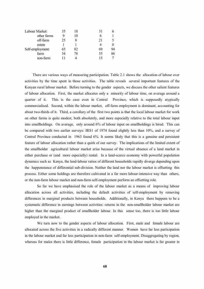
68

Labour Market: 35 18 31 6 other farms 9 10 6 1 off-farm 25 8 21 5 estate 1 1 4 0 Self-employment: 65 82 69 94 farm 54 78 55 86 non-farm 11 4 15 7 There are various ways of measuring participation. Table 2.1 shows the allocation of labour over activities by the time spent in those activities. The table reveals several important features of the Kenyan rural labour market. Before turning to the gender aspects, we discuss the other salient features of labour allocation. First, the market allocates only a minority of labour time, on average around a quarter of it. This is the case even in Central Province, which is supposedly atypically commercialised. Second, within the labour market, off-farm employment is dominant, accounting for about two-thirds of it. Third, a corollary of the first two points is that the local labour market for work on other farms is quite modest, both absolutely, and more especially relative to the total labour input into smallholdings. On average, only around 6% of labour input on smallholdings is hired. This can be compared with two earlier surveys: IRS1 of 1974 found slightly less than 10%, and a survey of Central Province conducted in 1963 found 6%. It seems likely that this is a genuine and persistent feature of labour allocation rather than a quirk of our survey. The implications of the limited extent of the smallholder agricultural labour market arise because of the virtual absence of a land market in either purchase or (and more especially) rental. In a land-scarce economy with powerful population dynamics such as Kenya, the land-labour ratios of different households rapidly diverge depending upon the happenstance of differential sub-division. Neither the land nor the labour market is offsetting this process. Either some holdings are therefore cultivated in a far more labour-intensive way than others, or the non-farm labour market and non-farm self-employment perform an offsetting role. So far we have emphasised the role of the labour market as a means of improving labour allocation across all activities, including the default activities of self-employment by removing differences in marginal products between households. Additionally, in Kenya there happens to be a systematic difference in earnings between activities: returns in the non-smallholder labour market are higher than the marginal product of smallholder labour. In this sense too, there is too little labour employed in the market. We turn now to the gender aspects of labour allocation. First, male and female labour are allocated across the five activities in a radically different manner. Women have far less participation in the labour market and far less participation in non-farm self-employment. Disaggregating by region, whereas for males there is little difference, female participation in the labour market is far greater in

69

Central Province than in Nyanza. In the latter, only 6% of labour time is allocated through the market. This is a remarkably low figure: unless other markets (in male labour, credit, land, inputs and information) operate with superb efficiency, such low reliance upon the labour market is bound to leave female labour mis-allocated in the sense that marginal products are likely to differ radically, one household from another. An interpretation of Table 2.1 would be that quite generally in rural Kenya there is, for reasons yet to be determined, under-utilisation of the labour market with consequent labour misallocation. The problem is less severe in Central Province than Nyanza and less severe for men than for women. As a result there is a hierarchy: men in Central Province have the highest ratio of labour time allocated through the market relative to own farm employment, 0.65, and women in Nyanza have the lowest ratio, 0.07. In between are Nyanzan men (0.56) and Central Province women (0.23). Clearly, the differences between the women of the two regions are far larger, proportionately, than those between the men. Either this is because the two groups of women possess different characteristics, or because the markets are systematically different. b. Data and Variables Used The data used here was collected as part of a rural, multipurpose survey conducted in Central and Nyanza Provinces of Kenya in 1982. A description of survey methodology is provided in Bevan, Collier and Gunning (1989). A feature of the data is that although the place of observation was the rural household, information was also gathered on the `extended household', that is, on non-resident spouses, sons and daughters of the household head. Some of these non-residents had migrated to urban employment. Hence, our sample includes all the ever-resident members of the nuclear household. This enables us to analyze migration as one of the economic options open to the rural labourforce. The sample has been restricted to household heads, spouses, daughters and sons who are non-students, aged between 16 and 60 and who did not leave the household in order to marry. We define participation in a broad manner. An individual who, in the last year, works as a casual farm labourer (locally or on an estate), as an employee in the formal sector (either private or public and local or an another locality) or who runs their own business is defined as a participant. In our Kenyan sample, 21.6% of women and 55.0% of men participated in some manner. We take participation as a function of the following types of variables: individual wage generating characteristics, demographic composition of the household, household wealth, household cropping patterns, household location and hours spent getting water and firewood. Specific variable definitions are given in Table 2.2. Means and standard deviations of these variables for men and women are reported in Table 2.3.

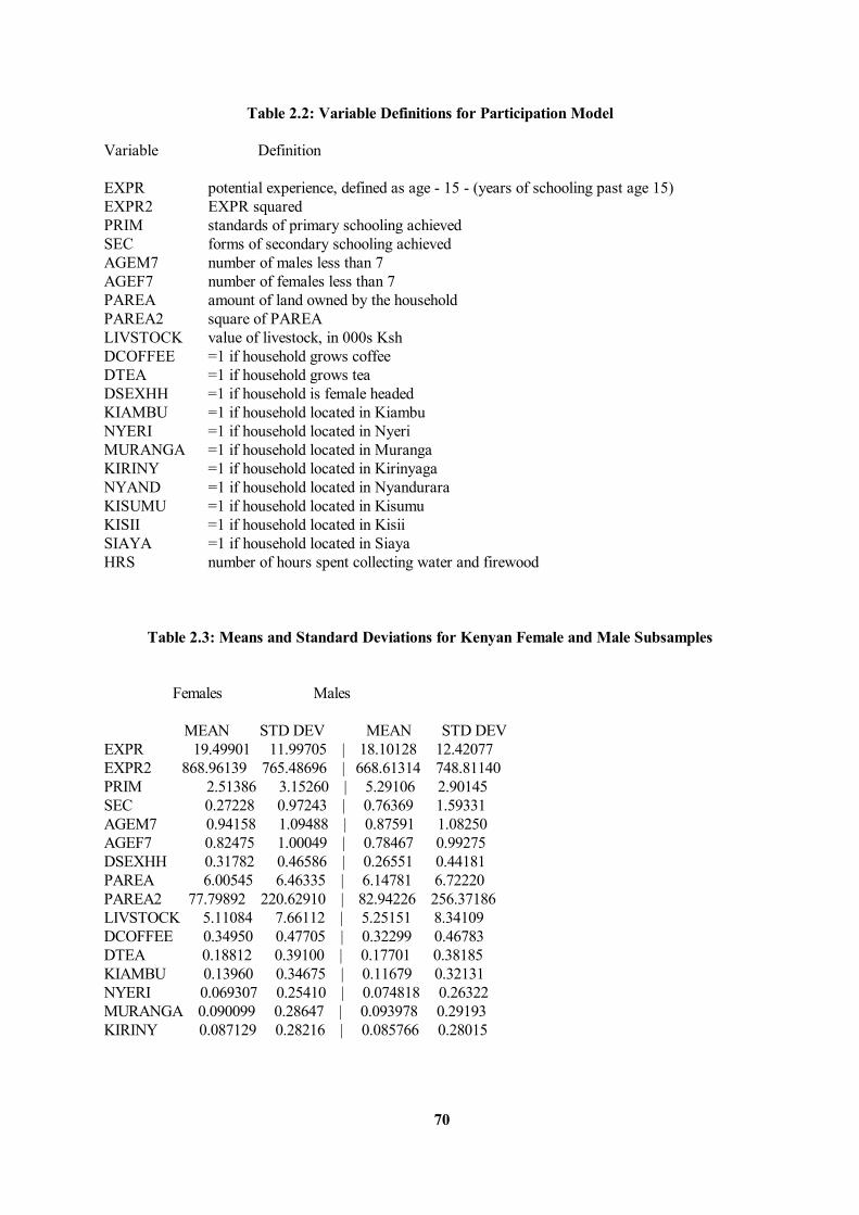
70

Table 2.2: Variable Definitions for Participation Model Variable Definition EXPR potential experience, defined as age - 15 - (years of schooling past age 15) EXPR2 EXPR squared PRIM standards of primary schooling achieved SEC forms of secondary schooling achieved AGEM7 number of males less than 7 AGEF7 number of females less than 7 PAREA amount of land owned by the household PAREA2 square of PAREA LIVSTOCK value of livestock, in 000s Ksh DCOFFEE =1 if household grows coffee DTEA =1 if household grows tea DSEXHH =1 if household is female headed KIAMBU =1 if household located in Kiambu NYERI =1 if household located in Nyeri MURANGA =1 if household located in Muranga KIRINY =1 if household located in Kirinyaga NYAND =1 if household located in Nyandurara KISUMU =1 if household located in Kisumu KISII =1 if household located in Kisii SIAYA =1 if household located in Siaya HRS number of hours spent collecting water and firewood Table 2.3: Means and Standard Deviations for Kenyan Female and Male Subsamples Females Males MEAN STD DEV MEAN STD DEV EXPR 19.49901 11.99705 | 18.10128 12.42077 EXPR2 868.96139 765.48696 | 668.61314 748.81140 PRIM 2.51386 3.15260 | 5.29106 2.90145 SEC 0.27228 0.97243 | 0.76369 1.59331 AGEM7 0.94158 1.09488 | 0.87591 1.08250 AGEF7 0.82475 1.00049 | 0.78467 0.99275 DSEXHH 0.31782 0.46586 | 0.26551 0.44181 PAREA 6.00545 6.46335 | 6.14781 6.72220 PAREA2 77.79892 220.62910 | 82.94226 256.37186 LIVSTOCK 5.11084 7.66112 | 5.25151 8.34109 DCOFFEE 0.34950 0.47705 | 0.32299 0.46783 DTEA 0.18812 0.39100 | 0.17701 0.38185 KIAMBU 0.13960 0.34675 | 0.11679 0.32131 NYERI 0.069307 0.25410 | 0.074818 0.26322 MURANGA 0.090099 0.28647 | 0.093978 0.29193 KIRINY 0.087129 0.28216 | 0.085766 0.28015

71

NYAND 0.041584 0.19974 | 0.032847 0.17832 KISUMU 0.079208 0.27020 | 0.092153 0.28937 KISII 0.19109 0.39335 | 0.15420 0.36130 SIAYA 0.092079 0.28928 | 0.12956 0.33597 HRS 4.52772 4.95807 | 4.54653 5.87741 Sample Size 1010 | 1096

There are several points to note regarding these variables. As we do not have detailed data on individuals' employment histories, we cannot measure actual work experience. Instead, we use potential work experience, defined as age less 15 (assumed to be the minimum age at which an individual could enter the labour market) less years spent in school past age 15. Though this is an imperfect measure of experience, it does avoid problems associated with the fact that actual work experience may be endogenous. We have used standards (and forms) of education completed rather than years of schooling, as a measure of educational attainment. The latter is a poor measure as it can be affected by repetition of grades and temporary dropping out. We have assumed that land ownership and the growing of coffee and tea are exogenous variables. In a life cycle model, this is an incorrect assumption to make. However, survey evidence suggests that landholdings change very slowly over time (see, for example, Hoddinott (1989)). However, in a single period framework, as in that considered here, these can be considered fixed. Singh, Squire and Strauss (1986), Junankar (1989) and Pitt (1990) take this approach. Also note that the number of children, boys and girls, under 7 is taken as exogenous. This assumption is not shared by all analyses of female labour force participation (eg Schultz 1988). The appendix to this chapter sets out our reasons justifying this assumption. Earnings are taken, following Mincer (1974), as a function of experience and education. We have excluded type of employment as it is a choice variable. Education has been separated into standards of primary and secondary education achieved. Previous studies of the Kenyan labour market have noted that the returns to these differ (eg Knight and Sabot 1990) and it seems sensible to maintain this as a working hypothesis here. The variables used in our wage equation are summarised in Table 2.4. Their means and standard deviations are reported in Table 2.5.

Table 2.4: Variable Definitions of Earnings Equation Variable Definition EXPR potential experience, defined as age - 15 - (years of schooling past age 15) EXPR2 EXPR squared PRIM standards of primary schooling achieved SEC forms of secondary schooling achieved @MILLS sample selection correction term

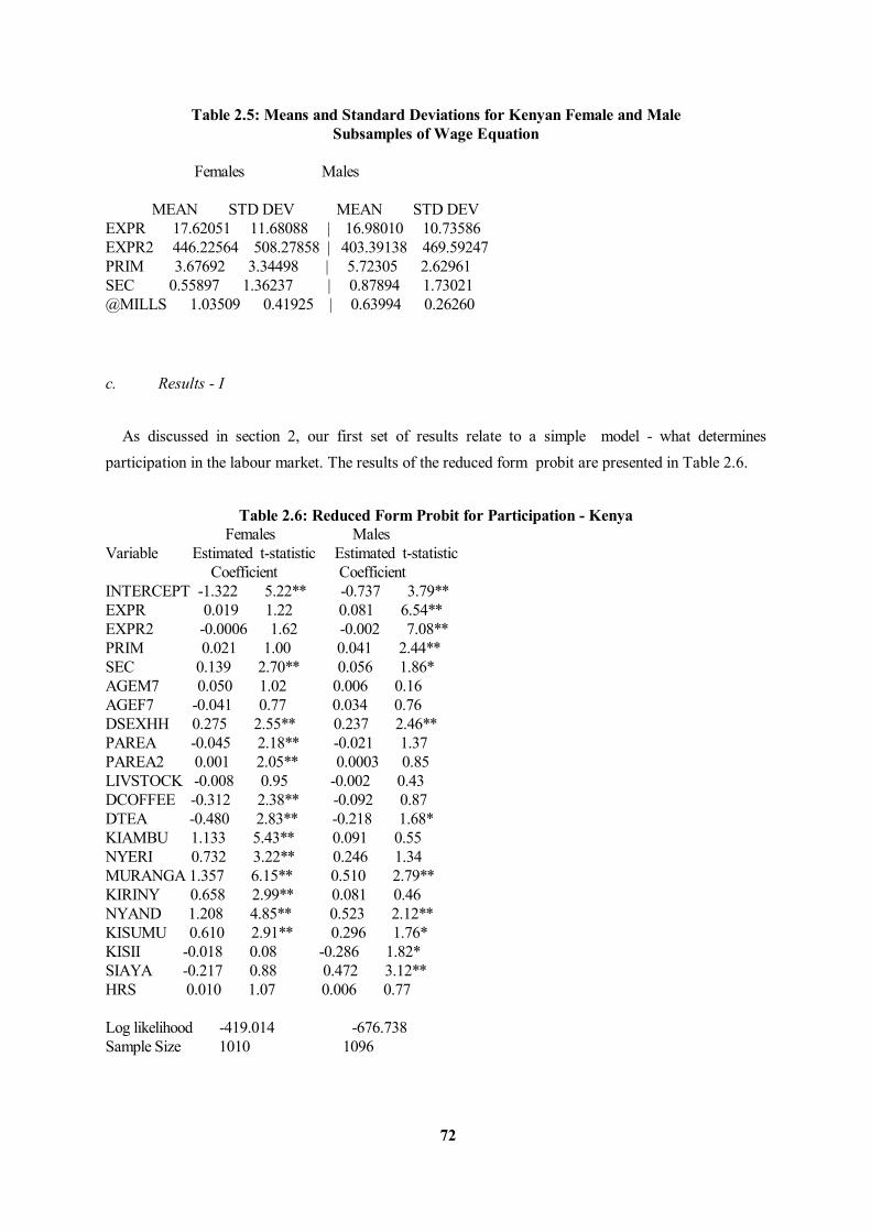
72

Table 2.5: Means and Standard Deviations for Kenyan Female and Male Subsamples of Wage Equation Females Males MEAN STD DEV MEAN STD DEV EXPR 17.62051 11.68088 | 16.98010 10.73586 EXPR2 446.22564 508.27858 | 403.39138 469.59247 PRIM 3.67692 3.34498 | 5.72305 2.62961 SEC 0.55897 1.36237 | 0.87894 1.73021 @MILLS 1.03509 0.41925 | 0.63994 0.26260 c. Results - I As discussed in section 2, our first set of results relate to a simple model - what determines participation in the labour market. The results of the reduced form probit are presented in Table 2.6.

Table 2.6: Reduced Form Probit for Participation - Kenya Females Males Variable Estimated t-statistic Estimated t-statistic Coefficient Coefficient INTERCEPT -1.322 5.22** -0.737 3.79** EXPR 0.019 1.22 0.081 6.54** EXPR2 -0.0006 1.62 -0.002 7.08** PRIM 0.021 1.00 0.041 2.44** SEC 0.139 2.70** 0.056 1.86* AGEM7 0.050 1.02 0.006 0.16 AGEF7 -0.041 0.77 0.034 0.76 DSEXHH 0.275 2.55** 0.237 2.46** PAREA -0.045 2.18** -0.021 1.37 PAREA2 0.001 2.05** 0.0003 0.85 LIVSTOCK -0.008 0.95 -0.002 0.43 DCOFFEE -0.312 2.38** -0.092 0.87 DTEA -0.480 2.83** -0.218 1.68* KIAMBU 1.133 5.43** 0.091 0.55 NYERI 0.732 3.22** 0.246 1.34 MURANGA 1.357 6.15** 0.510 2.79** KIRINY 0.658 2.99** 0.081 0.46 NYAND 1.208 4.85** 0.523 2.12** KISUMU 0.610 2.91** 0.296 1.76* KISII -0.018 0.08 -0.286 1.82* SIAYA -0.217 0.88 0.472 3.12** HRS 0.010 1.07 0.006 0.77 Log likelihood -419.014 -676.738 Sample Size 1010 1096

73

Percent Participating 21.6% 55.0% Percent Correctly 80.2% 65.7% Predicted

The large difference in the intercept terms indicates that at the means of other characteristics women are far less likely to participate in the labour market. Recall that this is not because they are less likely to be in employment but rather that they are more likely to be in self-employment. Whereas for men the probability of participation increases with the number of years experience in the labourforce, there is no such relationship for women. One obvious interpretation of this might be that women gradually acquire child-rearing obligations which offsets the labourforce experience effect. However, such an interpretation is not supported by the analysis. The number of children under the age of seven, whether boys or girls, has no significant effect upon the probability of female participation in the labour market. Since this variable can be regarded as endogenous, while its lack of significance, if genuine, is of importance, we discuss the issue of its potential endogeneity at length in an appendix to the chapter. Whereas women's participation is less sensitive to labourforce experience, it is more sensitive to secondary education, an effect which we will consider in more detail below. The area of the holding and the number of coffee and tree trees all reduce female labour market participation more powerfully than male. This is consistent with the default being primarily self-employment on the holding. All three variables can be expected to raise the marginal product of labour on the holding and most of that labour is female. Additionally, the three variables all have a potential wealth effect, reducing labour supply. The regional dummy variables are far more powerful and significant for women than for men. The most likely interpretation of this is that women are less inter-regionally mobile than men and so participation is more dependent upon opportunities within the locality. Finally, the number of hours spent collecting fuel and water is insignificant as a determinant of participation. Since this is an endogenous variable it was also investigated through instrumenting, but with the same results. This is a surprising result since, as we have seen, women spend a considerable amount of time on these activities. Our next step is to examine the determinants of earnings amongst those individuals who participate. These have been estimated using the methodology outlined in section 2. Note that the standard errors have been made fully consistent, using the approach outlined by Greene (1981). The results are presented below in Table 2.7, with the dependent variable being the log of daily earnings:

Table 2.7: Determinants of Earnings - Kenya Females Males Variable Estimated t-statistic Estimated t-statistic Coefficient Coefficient INTERCEPT 1.620 8.10** 2.398 9.63** EXPR 0.056 3.95** 0.045 2.93** EXPR2 -0.001 3.86** -0.0009 2.24** PRIM 0.041 1.82* 0.046 2.61**

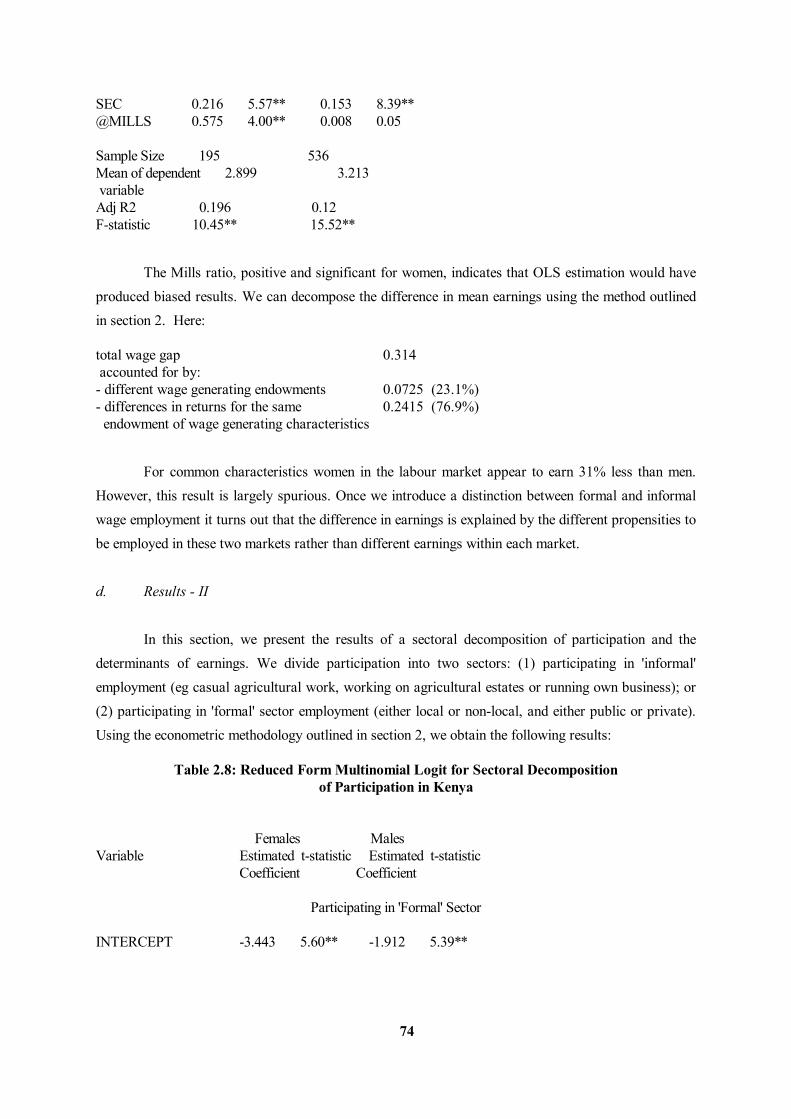
74

SEC 0.216 5.57** 0.153 8.39** @MILLS 0.575 4.00** 0.008 0.05 Sample Size 195 536 Mean of dependent 2.899 3.213 variable Adj R2 0.196 0.12 F-statistic 10.45** 15.52** The Mills ratio, positive and significant for women, indicates that OLS estimation would have produced biased results. We can decompose the difference in mean earnings using the method outlined in section 2. Here: total wage gap 0.314 accounted for by: - different wage generating endowments 0.0725 (23.1%) - differences in returns for the same 0.2415 (76.9%) endowment of wage generating characteristics For common characteristics women in the labour market appear to earn 31% less than men. However, this result is largely spurious. Once we introduce a distinction between formal and informal wage employment it turns out that the difference in earnings is explained by the different propensities to be employed in these two markets rather than different earnings within each market. d. Results - II In this section, we present the results of a sectoral decomposition of participation and the determinants of earnings. We divide participation into two sectors: (1) participating in 'informal' employment (eg casual agricultural work, working on agricultural estates or running own business); or (2) participating in 'formal' sector employment (either local or non-local, and either public or private). Using the econometric methodology outlined in section 2, we obtain the following results: Table 2.8: Reduced Form Multinomial Logit for Sectoral Decomposition of Participation in Kenya Females Males Variable Estimated t-statistic Estimated t-statistic Coefficient Coefficient Participating in 'Formal' Sector INTERCEPT -3.443 5.60** -1.912 5.39**

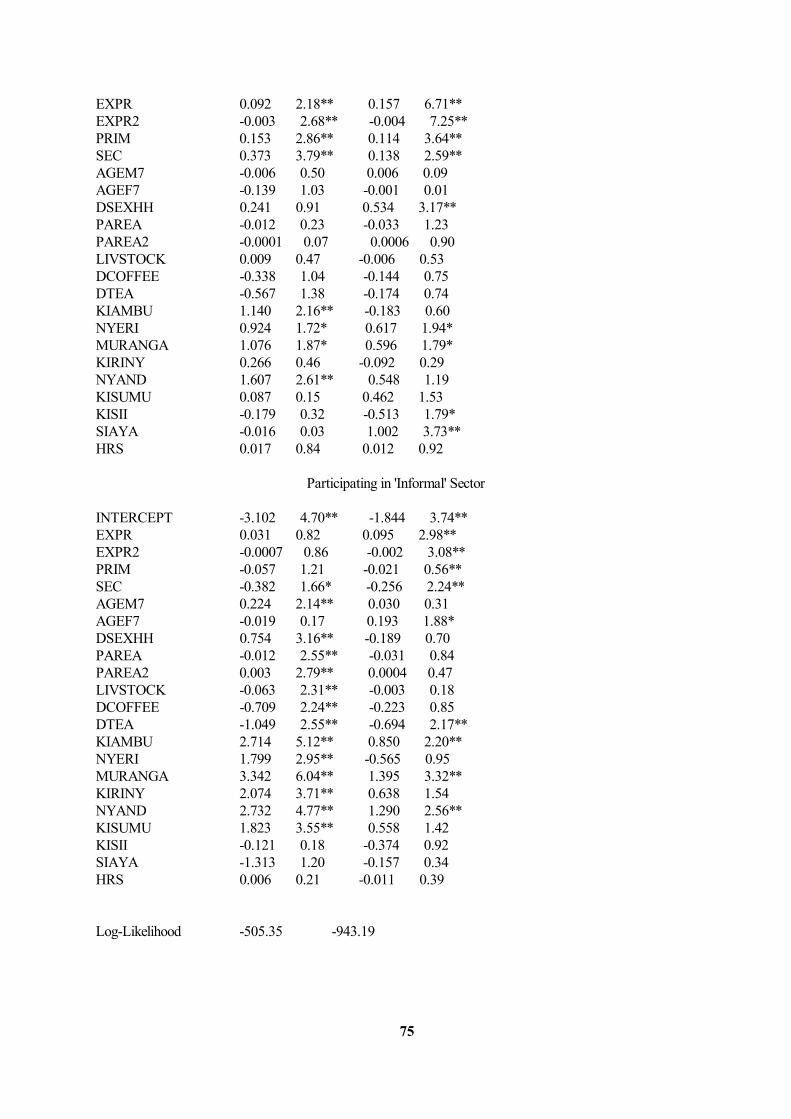
75

EXPR 0.092 2.18** 0.157 6.71** EXPR2 -0.003 2.68** -0.004 7.25** PRIM 0.153 2.86** 0.114 3.64** SEC 0.373 3.79** 0.138 2.59** AGEM7 -0.006 0.50 0.006 0.09 AGEF7 -0.139 1.03 -0.001 0.01 DSEXHH 0.241 0.91 0.534 3.17** PAREA -0.012 0.23 -0.033 1.23 PAREA2 -0.0001 0.07 0.0006 0.90 LIVSTOCK 0.009 0.47 -0.006 0.53 DCOFFEE -0.338 1.04 -0.144 0.75 DTEA -0.567 1.38 -0.174 0.74 KIAMBU 1.140 2.16** -0.183 0.60 NYERI 0.924 1.72* 0.617 1.94* MURANGA 1.076 1.87* 0.596 1.79* KIRINY 0.266 0.46 -0.092 0.29 NYAND 1.607 2.61** 0.548 1.19 KISUMU 0.087 0.15 0.462 1.53 KISII -0.179 0.32 -0.513 1.79* SIAYA -0.016 0.03 1.002 3.73** HRS 0.017 0.84 0.012 0.92 Participating in 'Informal' Sector INTERCEPT -3.102 4.70** -1.844 3.74** EXPR 0.031 0.82 0.095 2.98** EXPR2 -0.0007 0.86 -0.002 3.08** PRIM -0.057 1.21 -0.021 0.56** SEC -0.382 1.66* -0.256 2.24** AGEM7 0.224 2.14** 0.030 0.31 AGEF7 -0.019 0.17 0.193 1.88* DSEXHH 0.754 3.16** -0.189 0.70 PAREA -0.012 2.55** -0.031 0.84 PAREA2 0.003 2.79** 0.0004 0.47 LIVSTOCK -0.063 2.31** -0.003 0.18 DCOFFEE -0.709 2.24** -0.223 0.85 DTEA -1.049 2.55** -0.694 2.17** KIAMBU 2.714 5.12** 0.850 2.20** NYERI 1.799 2.95** -0.565 0.95 MURANGA 3.342 6.04** 1.395 3.32** KIRINY 2.074 3.71** 0.638 1.54 NYAND 2.732 4.77** 1.290 2.56** KISUMU 1.823 3.55** 0.558 1.42 KISII -0.121 0.18 -0.374 0.92 SIAYA -1.313 1.20 -0.157 0.34 HRS 0.006 0.21 -0.011 0.39 Log-Likelihood -505.35 -943.19

76

Predicted v Actual Outcomes Predicted Actual TOTAL 0 1 2 | TOTAL 0 1 2 Total 1010 916 35 59 | 1096 570 500 26 0 792 761 14 17 | 493 341 146 6 1 94 70 20 4 | 456 141 308 7 2 124 85 1 38 | 147 88 46 13 Unsurprisingly, for both genders education increases participation in the formal labour market, however, it does so more powerfully for women, especially secondary education. At the means of other variables the possession of secondary education increases the probability of female participation by 42% (3.9 percentage points) as against 17% for men (7.2 percentage points). The variables proxying the marginal product of labour in agriculture and a wealth effect (land area, coffee and tea trees) are insignificant for formal labour market participation while quite powerful in discouraging women's participation in informal wage employment. This suggests that the decision as to whether a woman should participate in the informal market or work in self-employment is a balance of economic returns at the margin, whereas that to enter formal employment is not. Perhaps for women participation in formal employment is determined by opportunity and/or inclination more than by marginal calculations of comparative returns. As in the more aggregated analysis, neither the number of children under the age of seven nor the number of hours spent collecting fuel and water significantly discourages female participation in formal employment. Participation in the labour market is primarily a discrete variable, and this is how we have analyzed it. By contrast, since the default activity for almost everyone is self-employment on the family farm, the primary participation issue for this activity is the continuous variable of the time spent in the activity. The dependent variable we observe is the number of days worked on the family farm. As discussed above, we exclude those participating in the labour market, and use the location variables to explain the discrete choice as to whether or not to work on the family farm (to overcome identification problems). The resulting labour supply function is reported in Table 2.9. Table 2.9: Number of Days per Year Worked on Family Farm Females Males Variable Estimated t-statistic Estimated t-statistic Coefficient Coefficient C 71.851 3.17** -61.029 1.33 EXPR 5.243 4.08** 9.686 4.35** EXPR2 -0.096 3.48** -0.196 3.86** PRIM 0.199 0.12 0.895 0.41 SEC -4.813 0.86 1.804 0.43 AGEM7 -0.017 0.005 -11.344 2.28** AGEF7 7.398 1.82* 8.782 1.73*

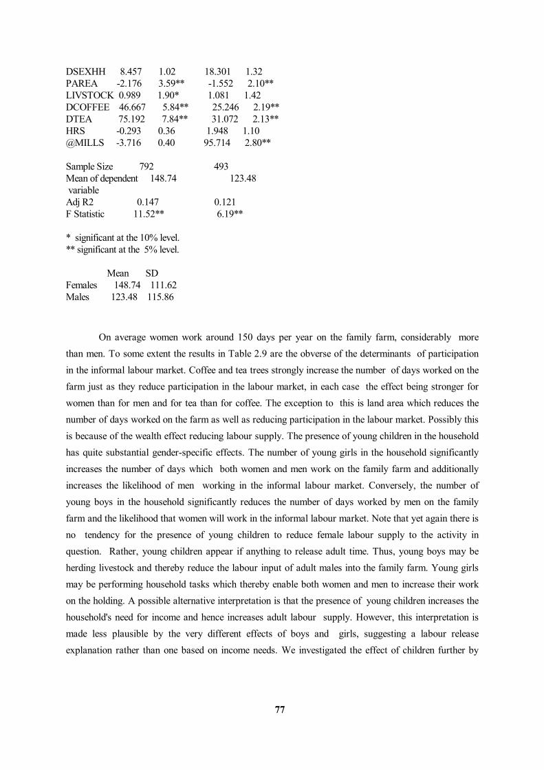
77

DSEXHH 8.457 1.02 18.301 1.32 PAREA -2.176 3.59** -1.552 2.10** LIVSTOCK 0.989 1.90* 1.081 1.42 DCOFFEE 46.667 5.84** 25.246 2.19** DTEA 75.192 7.84** 31.072 2.13** HRS -0.293 0.36 1.948 1.10 @MILLS -3.716 0.40 95.714 2.80** Sample Size 792 493 Mean of dependent 148.74 123.48 variable Adj R2 0.147 0.121 F Statistic 11.52** 6.19** * significant at the 10% level. ** significant at the 5% level. Mean SD Females 148.74 111.62 Males 123.48 115.86 On average women work around 150 days per year on the family farm, considerably more than men. To some extent the results in Table 2.9 are the obverse of the determinants of participation in the informal labour market. Coffee and tea trees strongly increase the number of days worked on the farm just as they reduce participation in the labour market, in each case the effect being stronger for women than for men and for tea than for coffee. The exception to this is land area which reduces the number of days worked on the farm as well as reducing participation in the labour market. Possibly this is because of the wealth effect reducing labour supply. The presence of young children in the household has quite substantial gender-specific effects. The number of young girls in the household significantly increases the number of days which both women and men work on the family farm and additionally increases the likelihood of men working in the informal labour market. Conversely, the number of young boys in the household significantly reduces the number of days worked by men on the family farm and the likelihood that women will work in the informal labour market. Note that yet again there is no tendency for the presence of young children to reduce female labour supply to the activity in question. Rather, young children appear if anything to release adult time. Thus, young boys may be herding livestock and thereby reduce the labour input of adult males into the family farm. Young girls may be performing household tasks which thereby enable both women and men to increase their work on the holding. A possible alternative interpretation is that the presence of young children increases the household's need for income and hence increases adult labour supply. However, this interpretation is made less plausible by the very different effects of boys and girls, suggesting a labour release explanation rather than one based on income needs. We investigated the effect of children further by

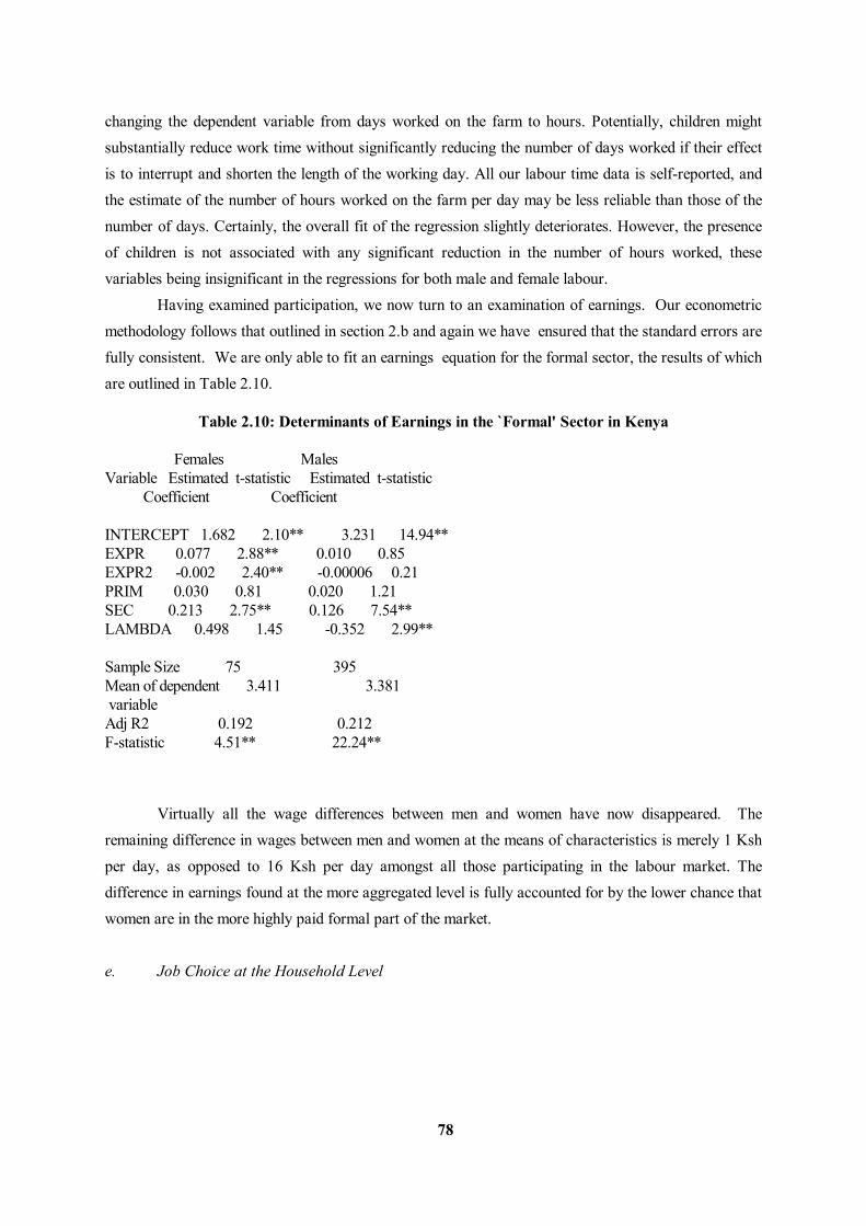
78

changing the dependent variable from days worked on the farm to hours. Potentially, children might substantially reduce work time without significantly reducing the number of days worked if their effect is to interrupt and shorten the length of the working day. All our labour time data is self-reported, and the estimate of the number of hours worked on the farm per day may be less reliable than those of the number of days. Certainly, the overall fit of the regression slightly deteriorates. However, the presence of children is not associated with any significant reduction in the number of hours worked, these variables being insignificant in the regressions for both male and female labour. Having examined participation, we now turn to an examination of earnings. Our econometric methodology follows that outlined in section 2.b and again we have ensured that the standard errors are fully consistent. We are only able to fit an earnings equation for the formal sector, the results of which are outlined in Table 2.10. Table 2.10: Determinants of Earnings in the `Formal' Sector in Kenya Females Males Variable Estimated t-statistic Estimated t-statistic Coefficient Coefficient INTERCEPT 1.682 2.10** 3.231 14.94** EXPR 0.077 2.88** 0.010 0.85 EXPR2 -0.002 2.40** -0.00006 0.21 PRIM 0.030 0.81 0.020 1.21 SEC 0.213 2.75** 0.126 7.54** LAMBDA 0.498 1.45 -0.352 2.99** Sample Size 75 395 Mean of dependent 3.411 3.381 variable Adj R2 0.192 0.212 F-statistic 4.51** 22.24** Virtually all the wage differences between men and women have now disappeared. The remaining difference in wages between men and women at the means of characteristics is merely 1 Ksh per day, as opposed to 16 Ksh per day amongst all those participating in the labour market. The difference in earnings found at the more aggregated level is fully accounted for by the lower chance that women are in the more highly paid formal part of the market. e. Job Choice at the Household Level

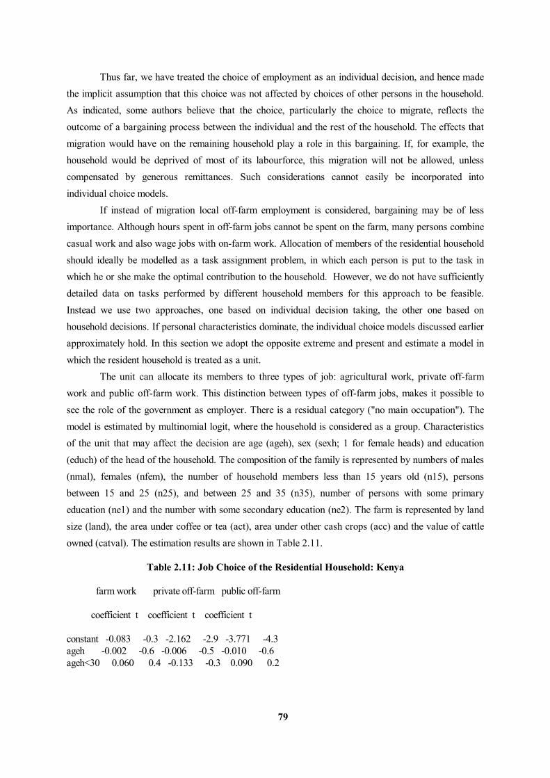
79

Thus far, we have treated the choice of employment as an individual decision, and hence made the implicit assumption that this choice was not affected by choices of other persons in the household. As indicated, some authors believe that the choice, particularly the choice to migrate, reflects the outcome of a bargaining process between the individual and the rest of the household. The effects that migration would have on the remaining household play a role in this bargaining. If, for example, the household would be deprived of most of its labourforce, this migration will not be allowed, unless compensated by generous remittances. Such considerations cannot easily be incorporated into individual choice models. If instead of migration local off-farm employment is considered, bargaining may be of less importance. Although hours spent in off-farm jobs cannot be spent on the farm, many persons combine casual work and also wage jobs with on-farm work. Allocation of members of the residential household should ideally be modelled as a task assignment problem, in which each person is put to the task in which he or she make the optimal contribution to the household. However, we do not have sufficiently detailed data on tasks performed by different household members for this approach to be feasible. Instead we use two approaches, one based on individual decision taking, the other one based on household decisions. If personal characteristics dominate, the individual choice models discussed earlier approximately hold. In this section we adopt the opposite extreme and present and estimate a model in which the resident household is treated as a unit. The unit can allocate its members to three types of job: agricultural work, private off-farm work and public off-farm work. This distinction between types of off-farm jobs, makes it possible to see the role of the government as employer. There is a residual category ("no main occupation"). The model is estimated by multinomial logit, where the household is considered as a group. Characteristics of the unit that may affect the decision are age (ageh), sex (sexh; 1 for female heads) and education (educh) of the head of the household. The composition of the family is represented by numbers of males (nmal), females (nfem), the number of household members less than 15 years old (n15), persons between 15 and 25 (n25), and between 25 and 35 (n35), number of persons with some primary education (ne1) and the number with some secondary education (ne2). The farm is represented by land size (land), the area under coffee or tea (act), area under other cash crops (acc) and the value of cattle owned (catval). The estimation results are shown in Table 2.11. Table 2.11: Job Choice of the Residential Household: Kenya farm work private off-farm public off-farm coefficient t coefficient t coefficient t constant -0.083 -0.3 -2.162 -2.9 -3.771 -4.3 ageh -0.002 -0.6 -0.006 -0.5 -0.010 -0.6 ageh<30 0.060 0.4 -0.133 -0.3 0.090 0.2

80

ageh>50 0.236 2.1 0.197 0.6 -0.198 -0.5 sexh -0.022 -0.3 -0.030 -0.1 0.408 1.4 educh -0.008 -1.6 0.025 1.9 0.053 3.4 n15 -0.390 -9.2 -0.304 -2.3 -0.766 -5.1 n25 -0.167 -3.5 0.014 0.1 -0.682 -3.9 n35 0.023 0.4 0.160 1.1 -0.124 -0.7 nmal 0.228 5.4 0.066 0.5 0.500 3.5 nfem 0.231 5.5 -0.026 -0.2 0.451 3.0 ne1 -0.081 -3.8 0.060 0.9 0.034 0.4 ne2 -0.138 -3.3 -0.024 -0.2 0.755 5.8 atc -0.006 -0.2 -0.016 -0.1 -0.796 -3.3 acc -0.059 -1.7 0.121 1.4 0.130 1.3 land 0.025 1.5 -0.084 -1.4 -0.082 -1.1 catval 0.158 0.4 0.469 0.4 -0.399 -1.8 We start the discussion of the results with the age of the household's head, ageh, which is combined with two variables to allow for additional effects for young and old heads. Only the latter variable is significant and shows a propensity for old heads to have family members working on the farm. Sex of the household head is only mildly significant in increasing the number of persons in public employment. Education of the household head has strong positive effects on both forms of non-agricultural employment. Composition of the household matters naturally most for the allocation of children: the more persons under 15, the more will be allocated to the default category ("no main occupation"). Older children, between 15 and 25, may find some employment in the private sector, as shown by the coefficient of n25. An increase in the number of people with primary education reduces the probability of a household member being assigned to farming. This is a fortiori true for an increase in secondary education. In addition this strongly increases the probability of assignment to public employment. The agricultural variables have some interesting effects: those farms that grow a tree crop tend to have less members working off-farm, but those that grow another cash crop are likely to have a member in public employment. The size of the holding (both in terms of arable land and in terms of the value of cattle) only slightly increases farm employment. The model may be used to analyze the effects of migration. We made the following simulation experiment. We assumed that all household members who had migrated returned to the household and investigated the resulting change in allocation patterns. In general, migrants have better levels of education than resident members, so that it is not surprising to see that many returning sons or daughters would be allocated to public off-farm employment (assuming these jobs would be available). In some households the return of a migrant simply increases employment in one of the categories by one person. In other cases we observe cross effects where employment increases by more than one person

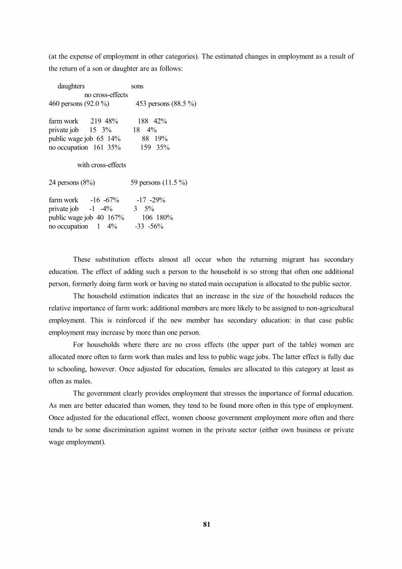
81

(at the expense of employment in other categories). The estimated changes in employment as a result of the return of a son or daughter are as follows: daughters sons no cross-effects 460 persons (92.0 %) 453 persons (88.5 %) farm work 219 48% 188 42% private job 15 3% 18 4% public wage job 65 14% 88 19% no occupation 161 35% 159 35% with cross-effects 24 persons (8%) 59 persons (11.5 %) farm work -16 -67% -17 -29% private job -1 -4% 3 5% public wage job 40 167% 106 180% no occupation 1 4% -33 -56% These substitution effects almost all occur when the returning migrant has secondary education. The effect of adding such a person to the household is so strong that often one additional person, formerly doing farm work or having no stated main occupation is allocated to the public sector. The household estimation indicates that an increase in the size of the household reduces the relative importance of farm work: additional members are more likely to be assigned to non-agricultural employment. This is reinforced if the new member has secondary education: in that case public employment may increase by more than one person. For households where there are no cross effects (the upper part of the table) women are allocated more often to farm work than males and less to public wage jobs. The latter effect is fully due to schooling, however. Once adjusted for education, females are allocated to this category at least as often as males. The government clearly provides employment that stresses the importance of formal education. As men are better educated than women, they tend to be found more often in this type of employment. Once adjusted for the educational effect, women choose government employment more often and there tends to be some discrimination against women in the private sector (either own business or private wage employment).

82

4. Women and the Tanzanian Labour Market a. Overview As in Kenya, among those in the potential labourforce (those aged 16-60 excluding students) the default activity to wage employment is predominantly self-employment rather than non-participation in work. Again this is as true for women as for men. Of the potential labourforce in rural households, 97.7% of women and 98.4% of men are currently working. Hence, the determinants of labour market participation, which we now investigate, are not, even for women, determinants of participation in work. The Tanzanian labour market is on the whole less accessible than its Kenyan counterpart. The smallholder market is negligible - studies tend to find only two or three percent of labour input is hired (Bevan, Collier and Gunning, 1989, Collier et. al., 1986). This is partly because land is relatively abundant (and scale economies very limited), so the basis for substantial labour hiring does not exist, but additionally, at the time of our survey (1983) the hiring of labour by farm households was actively discouraged by the government. In place of an inter-household labour market, the government attempted to introduce labour on the communal farm. There was considerable variation in practice between villages, but generally this labour was virtually unpaid. Village by- laws required each household to contribute labour, typically one person day per week. There is some evidence that richer households were able to avoid or buy out this obligation. Collier et al (1986) found the poorer half of households contributing around 30% more labour than the richer half. Hence, communal labour could be regarded as a regressive labour tax. The urban labour market was to some extent severed from most rural areas by very poor transport. Hence, there was less commuting and split-family residence than in Kenya. The comparison of participation is made in Table 3.1. The almost complete exclusion of women from the rural labour market (whether agricultural or non-agricultural) may account for their relatively high representation in rural non-farm self employment/own business activities. In earlier work (Collier et. al., 1986), it was found that in rural Tanzania, non-farm self-employment was the least well renumerated sector: the activity to which people are driven when they do not have access to alternatives, whereas wage employment was the best-remunerated activity. The poorer half of households worked only 30% as many days per adult in wage employment as the richer half, but worked 60% more days in non-farm self-employment.

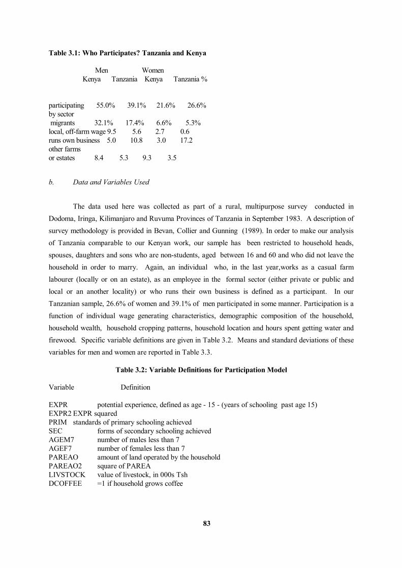
83

Table 3.1: Who Participates? Tanzania and Kenya Men Women Kenya Tanzania Kenya Tanzania % participating 55.0% 39.1% 21.6% 26.6% by sector migrants 32.1% 17.4% 6.6% 5.3% local, off-farm wage 9.5 5.6 2.7 0.6 runs own business 5.0 10.8 3.0 17.2 other farms or estates 8.4 5.3 9.3 3.5 b. Data and Variables Used The data used here was collected as part of a rural, multipurpose survey conducted in Dodoma, Iringa, Kilimanjaro and Ruvuma Provinces of Tanzania in September 1983. A description of survey methodology is provided in Bevan, Collier and Gunning (1989). In order to make our analysis of Tanzania comparable to our Kenyan work, our sample has been restricted to household heads, spouses, daughters and sons who are non-students, aged between 16 and 60 and who did not leave the household in order to marry. Again, an individual who, in the last year,works as a casual farm labourer (locally or on an estate), as an employee in the formal sector (either private or public and local or an another locality) or who runs their own business is defined as a participant. In our Tanzanian sample, 26.6% of women and 39.1% of men participated in some manner. Participation is a function of individual wage generating characteristics, demographic composition of the household, household wealth, household cropping patterns, household location and hours spent getting water and firewood. Specific variable definitions are given in Table 3.2. Means and standard deviations of these variables for men and women are reported in Table 3.3. Table 3.2: Variable Definitions for Participation Model Variable Definition EXPR potential experience, defined as age - 15 - (years of schooling past age 15) EXPR2 EXPR squared PRIM standards of primary schooling achieved SEC forms of secondary schooling achieved AGEM7 number of males less than 7 AGEF7 number of females less than 7 PAREAO amount of land operated by the household PAREAO2 square of PAREA LIVSTOCK value of livestock, in 000s Tsh DCOFFEE =1 if household grows coffee

84

DSEXHH =1 if household is female headed PROV1 =1 if household located in Iringa PROV2 =1 if household located in Dodoma PROV3 =1 if household located in Ruvuma HRS number of hours spent collecting water and firewood

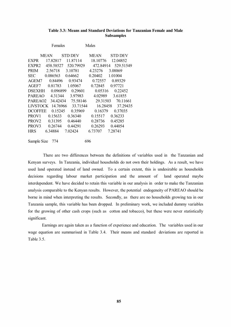
85

Table 3.3: Means and Standard Deviations for Tanzanian Female and Male Subsamples Females Males MEAN STD DEV MEAN STD DEV EXPR 17.82817 11.87114 18.10776 12.04852 EXPR2 458.58527 520.79929 472.84914 529.51549 PRIM 2.56718 3.10781 4.23276 3.08869 SEC 0.086563 0.64662 0.20402 1.01004 AGEM7 0.84496 0.93474 0.72557 0.89329 AGEF7 0.81783 1.05067 0.72845 0.97721 DSEXHH 0.096899 0.29601 0.05316 0.22452 PAREAO 4.31344 3.97983 4.02989 3.61855 PAREAO2 34.42434 75.58146 29.31503 70.11661 LIVSTOCK 14.76966 33.71544 16.28458 37.29435 DCOFFEE 0.15245 0.35969 0.16379 0.37035 PROV1 0.15633 0.36340 0.15517 0.36233 PROV2 0.31395 0.46440 0.28736 0.45285 PROV3 0.26744 0.44291 0.26293 0.44054 HRS 6.34884 7.02424 6.73707 7.28741 Sample Size 774 696 There are two differences between the definitions of variables used in the Tanzanian and Kenyan surveys. In Tanzania, individual households do not own their holdings. As a result, we have used land operated instead of land owned. To a certain extent, this is undesirable as households decisions regarding labour market participation and the amount of land operated maybe interdependent. We have decided to retain this variable in our analysis in order to make the Tanzanian analysis comparable to the Kenyan results. However, the potential endogeneity of PAREAO should be borne in mind when interpreting the results. Secondly, as there are no households growing tea in our Tanzania sample, this variable has been dropped. In preliminary work, we included dummy variables for the growing of other cash crops (such as cotton and tobacco), but these were never statistically significant. Earnings are again taken as a function of experience and education. The variables used in our wage equation are summarised in Table 3.4. Their means and standard deviations are reported in Table 3.5.

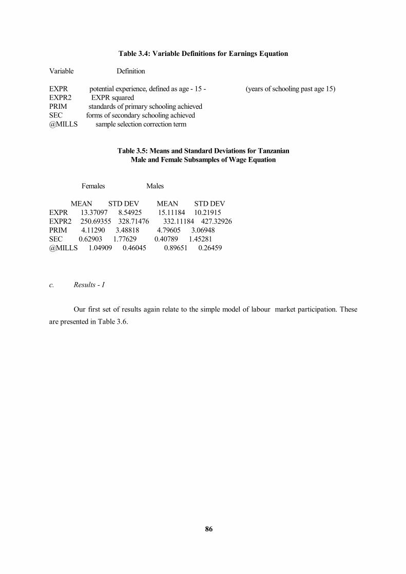
86

Table 3.4: Variable Definitions for Earnings Equation Variable Definition EXPR potential experience, defined as age - 15 - (years of schooling past age 15) EXPR2 EXPR squared PRIM standards of primary schooling achieved SEC forms of secondary schooling achieved @MILLS sample selection correction term Table 3.5: Means and Standard Deviations for Tanzanian Male and Female Subsamples of Wage Equation Females Males MEAN STD DEV MEAN STD DEV EXPR 13.37097 8.54925 15.11184 10.21915 EXPR2 250.69355 328.71476 332.11184 427.32926 PRIM 4.11290 3.48818 4.79605 3.06948 SEC 0.62903 1.77629 0.40789 1.45281 @MILLS 1.04909 0.46045 0.89651 0.26459 c. Results - I Our first set of results again relate to the simple model of labour market participation. These are presented in Table 3.6.

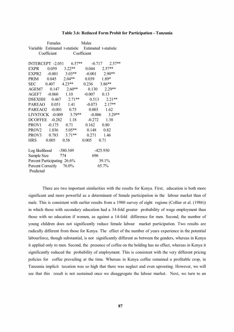
87

Table 3.6: Reduced Form Probit for Participation - Tanzania Females Males Variable Estimated t-statistic Estimated t-statistic Coefficient Coefficient INTERCEPT -2.051 6.57** -0.717 2.57** EXPR 0.059 3.22** 0.044 2.57** EXPR2 -0.001 3.03** -0.001 2.90** PRIM 0.045 2.04** 0.039 1.89* SEC 0.407 4.23** 0.236 3.86** AGEM7 0.147 2.60** 0.130 2.29** AGEF7 -0.060 1.10 -0.007 0.13 DSEXHH 0.467 2.71** 0.513 2.21** PAREAO 0.051 1.41 -0.073 2.17** PAREAO2 -0.001 0.75 0.003 1.62 LIVSTOCK -0.009 3.79** -0.006 3.29** DCOFFEE -0.282 1.18 -0.272 1.38 PROV1 -0.175 0.71 0.162 0.80 PROV2 1.036 5.05** 0.148 0.82 PROV3 0.783 3.71** 0.271 1.46 HRS 0.005 0.58 0.005 0.71 Log likelihood -380.349 -425.930 Sample Size 774 696 Percent Participating 26.6% 39.1% Percent Correctly 76.0% 65.7% Predicted There are two important similarities with the results for Kenya. First, education is both more significant and more powerful as a determinant of female participation in the labour market than of male. This is consistent with earlier results from a 1980 survey of eight regions (Collier et al. (1986)) in which those with secondary education had a 34-fold greater probability of wage employment than those with no education if women, as against a 14-fold difference for men. Second, the number of young children does not significantly reduce female labour market participation. Two results are radically different from those for Kenya. The effect of the number of years experience in the potential labourforce, though substantial, is not significantly different as between the genders, whereas in Kenya it applied only to men. Second, the presence of coffee on the holding has no effect, whereas in Kenya it significantly reduced the probability of employment. This is consistent with the very different pricing policies for coffee prevailing at the time. Whereas in Kenya coffee remained a profitable crop, in Tanzania implicit taxation was so high that there was neglect and even uprooting. However, we will see that this result is not sustained once we disaggregate the labour market. Next, we turn to an

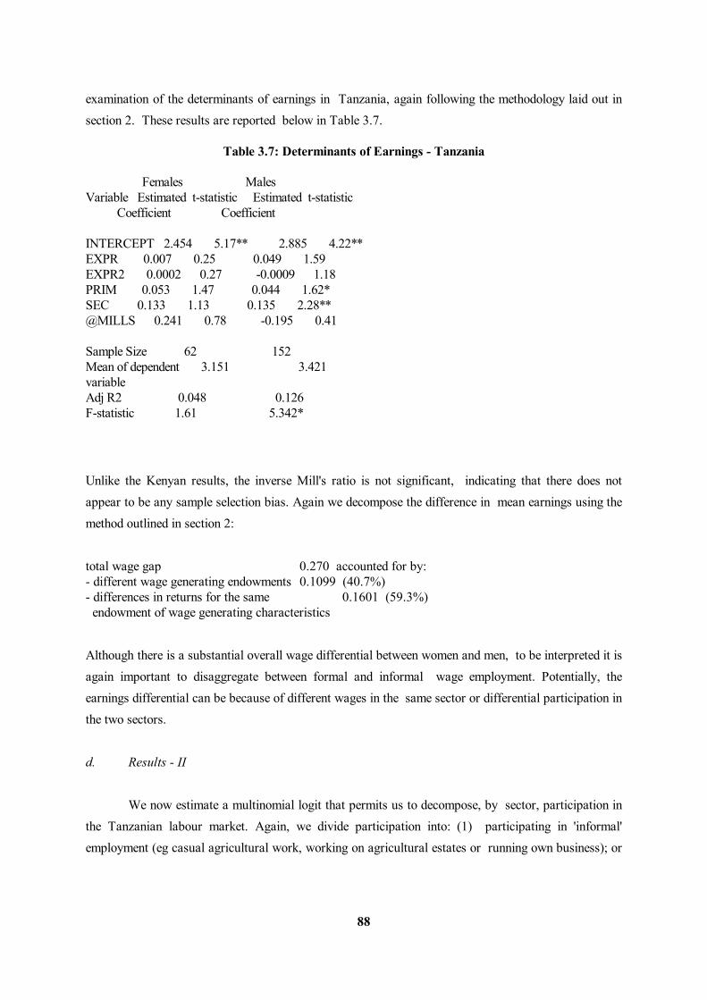
88

examination of the determinants of earnings in Tanzania, again following the methodology laid out in section 2. These results are reported below in Table 3.7. Table 3.7: Determinants of Earnings - Tanzania Females Males Variable Estimated t-statistic Estimated t-statistic Coefficient Coefficient INTERCEPT 2.454 5.17** 2.885 4.22** EXPR 0.007 0.25 0.049 1.59 EXPR2 0.0002 0.27 -0.0009 1.18 PRIM 0.053 1.47 0.044 1.62* SEC 0.133 1.13 0.135 2.28** @MILLS 0.241 0.78 -0.195 0.41 Sample Size 62 152 Mean of dependent 3.151 3.421 variable Adj R2 0.048 0.126 F-statistic 1.61 5.342* Unlike the Kenyan results, the inverse Mill's ratio is not significant, indicating that there does not appear to be any sample selection bias. Again we decompose the difference in mean earnings using the method outlined in section 2: total wage gap 0.270 accounted for by: - different wage generating endowments 0.1099 (40.7%) - differences in returns for the same 0.1601 (59.3%) endowment of wage generating characteristics Although there is a substantial overall wage differential between women and men, to be interpreted it is again important to disaggregate between formal and informal wage employment. Potentially, the earnings differential can be because of different wages in the same sector or differential participation in the two sectors. d. Results - II We now estimate a multinomial logit that permits us to decompose, by sector, participation in the Tanzanian labour market. Again, we divide participation into: (1) participating in 'informal' employment (eg casual agricultural work, working on agricultural estates or running own business); or

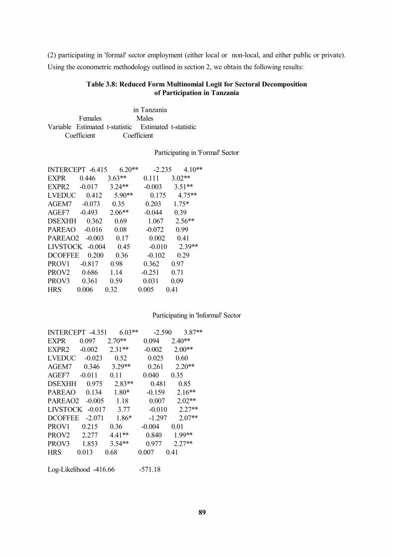
89

(2) participating in 'formal' sector employment (either local or non-local, and either public or private). Using the econometric methodology outlined in section 2, we obtain the following results: Table 3.8: Reduced Form Multinomial Logit for Sectoral Decomposition of Participation in Tanzania in Tanzania Females Males Variable Estimated t-statistic Estimated t-statistic Coefficient Coefficient Participating in 'Formal' Sector INTERCEPT -6.415 6.20** -2.235 4.10** EXPR 0.446 3.63** 0.111 3.02** EXPR2 -0.017 3.24** -0.003 3.51** LVEDUC 0.412 5.90** 0.175 4.75** AGEM7 -0.073 0.35 0.203 1.75* AGEF7 -0.493 2.06** -0.044 0.39 DSEXHH 0.362 0.69 1.067 2.56** PAREAO -0.016 0.08 -0.072 0.99 PAREAO2 -0.003 0.17 0.002 0.41 LIVSTOCK -0.004 0.45 -0.010 2.39** DCOFFEE 0.200 0.36 -0.102 0.29 PROV1 -0.817 0.98 0.362 0.97 PROV2 0.686 1.14 -0.251 0.71 PROV3 0.361 0.59 0.031 0.09 HRS 0.006 0.32 0.005 0.41 Participating in 'Informal' Sector INTERCEPT -4.351 6.03** -2.590 3.87** EXPR 0.097 2.70** 0.094 2.40** EXPR2 -0.002 2.31** -0.002 2.00** LVEDUC -0.023 0.52 0.025 0.60 AGEM7 0.346 3.29** 0.261 2.20** AGEF7 -0.011 0.11 0.040 0.35 DSEXHH 0.975 2.83** 0.481 0.85 PAREAO 0.134 1.80* -0.159 2.16** PAREAO2 -0.005 1.18 0.007 2.02** LIVSTOCK -0.017 3.77 -0.010 2.27** DCOFFEE -2.071 1.86* -1.297 2.07** PROV1 0.215 0.36 -0.004 0.01 PROV2 2.277 4.41** 0.840 1.99** PROV3 1.853 3.54** 0.977 2.27** HRS 0.013 0.68 0.007 0.41 Log-Likelihood -416.66 -571.18

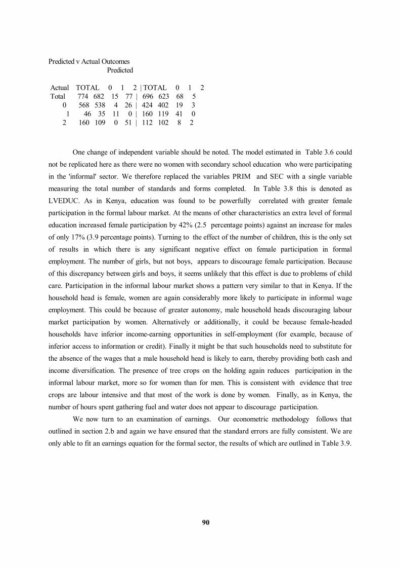
90

Predicted v Actual Outcomes Predicted Actual TOTAL 0 1 2 | TOTAL 0 1 2 Total 774 682 15 77 | 696 623 68 5 0 568 538 4 26 | 424 402 19 3 1 46 35 11 0 | 160 119 41 0 2 160 109 0 51 | 112 102 8 2 One change of independent variable should be noted. The model estimated in Table 3.6 could not be replicated here as there were no women with secondary school education who were participating in the 'informal' sector. We therefore replaced the variables PRIM and SEC with a single variable measuring the total number of standards and forms completed. In Table 3.8 this is denoted as LVEDUC. As in Kenya, education was found to be powerfully correlated with greater female participation in the formal labour market. At the means of other characteristics an extra level of formal education increased female participation by 42% (2.5 percentage points) against an increase for males of only 17% (3.9 percentage points). Turning to the effect of the number of children, this is the only set of results in which there is any significant negative effect on female participation in formal employment. The number of girls, but not boys, appears to discourage female participation. Because of this discrepancy between girls and boys, it seems unlikely that this effect is due to problems of child care. Participation in the informal labour market shows a pattern very similar to that in Kenya. If the household head is female, women are again considerably more likely to participate in informal wage employment. This could be because of greater autonomy, male household heads discouraging labour market participation by women. Alternatively or additionally, it could be because female-headed households have inferior income-earning opportunities in self-employment (for example, because of inferior access to information or credit). Finally it might be that such households need to substitute for the absence of the wages that a male household head is likely to earn, thereby providing both cash and income diversification. The presence of tree crops on the holding again reduces participation in the informal labour market, more so for women than for men. This is consistent with evidence that tree crops are labour intensive and that most of the work is done by women. Finally, as in Kenya, the number of hours spent gathering fuel and water does not appear to discourage participation. We now turn to an examination of earnings. Our econometric methodology follows that outlined in section 2.b and again we have ensured that the standard errors are fully consistent. We are only able to fit an earnings equation for the formal sector, the results of which are outlined in Table 3.9.

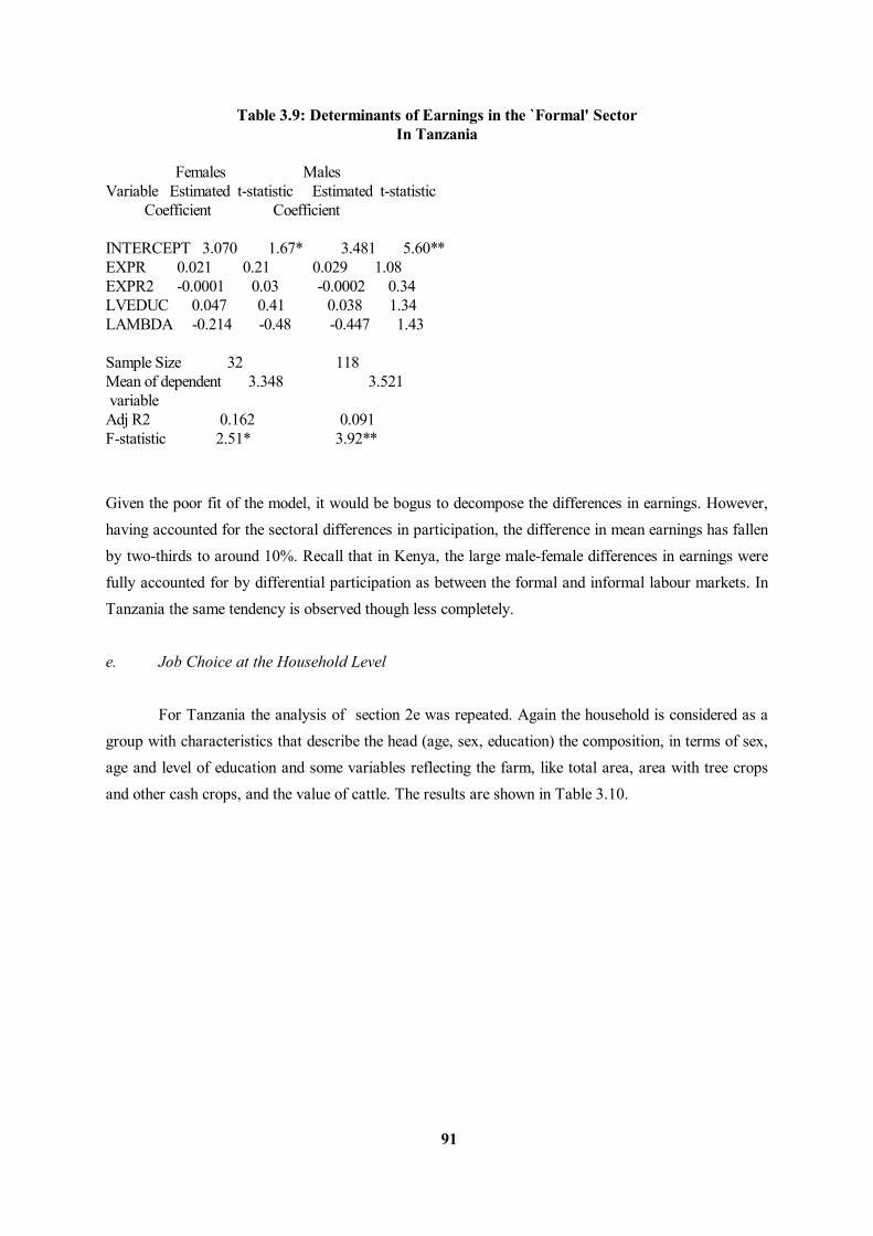
91

Table 3.9: Determinants of Earnings in the `Formal' Sector In Tanzania Females Males Variable Estimated t-statistic Estimated t-statistic Coefficient Coefficient INTERCEPT 3.070 1.67* 3.481 5.60** EXPR 0.021 0.21 0.029 1.08 EXPR2 -0.0001 0.03 -0.0002 0.34 LVEDUC 0.047 0.41 0.038 1.34 LAMBDA -0.214 -0.48 -0.447 1.43 Sample Size 32 118 Mean of dependent 3.348 3.521 variable Adj R2 0.162 0.091 F-statistic 2.51* 3.92** Given the poor fit of the model, it would be bogus to decompose the differences in earnings. However, having accounted for the sectoral differences in participation, the difference in mean earnings has fallen by two-thirds to around 10%. Recall that in Kenya, the large male-female differences in earnings were fully accounted for by differential participation as between the formal and informal labour markets. In Tanzania the same tendency is observed though less completely. e. Job Choice at the Household Level For Tanzania the analysis of section 2e was repeated. Again the household is considered as a group with characteristics that describe the head (age, sex, education) the composition, in terms of sex, age and level of education and some variables reflecting the farm, like total area, area with tree crops and other cash crops, and the value of cattle. The results are shown in Table 3.10.

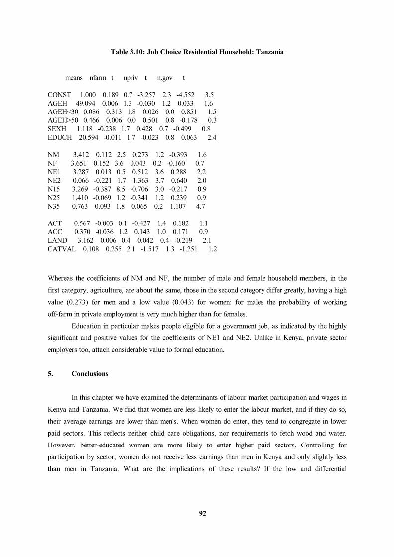
92

Table 3.10: Job Choice Residential Household: Tanzania means nfarm t npriv t n.gov t CONST 1.000 0.189 0.7 -3.257 2.3 -4.552 3.5 AGEH 49.094 0.006 1.3 -0.030 1.2 0.033 1.6 AGEH<30 0.086 0.313 1.8 0.026 0.0 0.851 1.5 AGEH>50 0.466 0.006 0.0 0.501 0.8 -0.178 0.3 SEXH 1.118 -0.238 1.7 0.428 0.7 -0.499 0.8 EDUCH 20.594 -0.011 1.7 -0.023 0.8 0.063 2.4 NM 3.412 0.112 2.5 0.273 1.2 -0.393 1.6 NF 3.651 0.152 3.6 0.043 0.2 -0.160 0.7 NE1 3.287 0.013 0.5 0.512 3.6 0.288 2.2 NE2 0.066 -0.221 1.7 1.363 3.7 0.640 2.0 N15 3.269 -0.387 8.5 -0.706 3.0 -0.217 0.9 N25 1.410 -0.069 1.2 -0.341 1.2 0.239 0.9 N35 0.763 0.093 1.8 0.065 0.2 1.107 4.7 ACT 0.567 -0.003 0.1 -0.427 1.4 0.182 1.1 ACC 0.370 -0.036 1.2 0.143 1.0 0.171 0.9 LAND 3.162 0.006 0.4 -0.042 0.4 -0.219 2.1 CATVAL 0.108 0.255 2.1 -1.517 1.3 -1.251 1.2 Whereas the coefficients of NM and NF, the number of male and female household members, in the first category, agriculture, are about the same, those in the second category differ greatly, having a high value (0.273) for men and a low value (0.043) for women: for males the probability of working off-farm in private employment is very much higher than for females. Education in particular makes people eligible for a government job, as indicated by the highly significant and positive values for the coefficients of NE1 and NE2. Unlike in Kenya, private sector employers too, attach considerable value to formal education.

5. Conclusions In this chapter we have examined the determinants of labour market participation and wages in Kenya and Tanzania. We find that women are less likely to enter the labour market, and if they do so, their average earnings are lower than men's. When women do enter, they tend to congregate in lower paid sectors. This reflects neither child care obligations, nor requirements to fetch wood and water. However, better-educated women are more likely to enter higher paid sectors. Controlling for participation by sector, women do not receive less earnings than men in Kenya and only slightly less than men in Tanzania. What are the implications of these results? If the low and differential

93

participation of women is the result of discrimination (something we cannot confirm) then this clearly represents a misallocation of labour. First, there is a loss due to women working on the family farm rather than in the labour market - here a re-allocation would raise the value of their labour time. Second, given the existing pattern of labour market participation, this reallocation would raise marginal labour productivity on the family farm. If, as we have suggested in Chapter 1, low female labour force participation is partly a function of low aspirations - itself a consequence of the absence of role models, then this suggests two policy interventions. One is to encourage female schooling. As we have noted, this may compensate for the lack of role models. A second is to intervene directly, for example through public sector recruitment practices, to increase women's participation in higher earning sectors, and thus encourage more women to enter the labour market. But these possibilities should be treated cautiously. As we have noted in the chapter, we have taken individual labour supply decisions as being independent of those of other members. Clearly, this is a strong assumption but the results of the multinomial logit estimations at the level of the household appear to point much in the same direction. Secondly, we have not controlled for unobserved household characteristics, and these may be imparting biases to our estimated coefficients. Finally, we have used a multinomial logit. While it is well suited to our purposes, its use rests on fairly strong (and untested) assumptions.

Appendix: Is Fertility Endogenous? In this chapter we have treated fertility as exogenous. We believe that with our samples, any endogeneity bias is likely to be too small to justify the loss in understanding from treating fertility as endogenous. However, since potential endogeneity is important, here, we defend our decision to retain fertility variables in our analysis. Assuming fertility to be endogenous has clear costs in terms of our understanding of structural processes. In particular, there are no valid instruments for fertility in our datasets, so the assuming endogeneity implies removing all measures of family size as explanatory variables. This would imply being unable to answer whether women participate less in the labour market because they have to look after children or because of other reasons (eg discrimination, lack of role models etc). Is it necessary to make this sacrifice? Schultz argues that "as children are to some degree a choice variable, this variable (ie children) is not a legitimate exogenous determinant". There are three points to note regarding this argument. As Schultz notes, endogeneity is a matter of degree: the endogeneity bias may be small or large. However, it is not clear that if the bias is small, it is undesirable to treat the variable as exogenous. In particular this may be true if as in this case the alternative is excluding the variable all together, because of a lack of valid instruments. Thus if fertility is to a large degree exogenous, treating it as wholly exogenous will allow a rough estimate of its effects, with only a small bias. That is to say there is a trade-off between endogeneity bias and understanding. There is a non-trivial sense in which

94

"everything is endogenous"; that is to say everything of interest as a possible regressor may be to some degree endogenous. As Behrman and Schultz point out in their comments on other sections of this report, adult education conventionally treated as exogenous may be associated with unobserved characteristics such as ability, fecundity and parental background. Similarly, both economists have discussed elsewhere the possibility that measures of infrastructure may be endogenous due to migration or policy reactions; parallel arguments could be made about local prices. Finally, the other main category of variable we, and most other researchers (eg Pitt (1990), Strauss (1990)), assume to be exogenous is household assets. These are clearly choice variables over the life cycle and estimates of their effects will be biased by omitted time-invariant measures of household productivity and preferences. We see no reason to suppose that fertility is more of a choice variable than household assets and present some evidence below that suggests the reverse. It may be that proponents of a life-cycle perspective are right that both assets and to a lesser extent fertility will be to some extent affected by endogeneity/omitted variable bias. However, controlling for this requires richer datasets than one-shot cross sectional studies. The latter can nonetheless be informative in providing results on the determinants of current decisions conditional upon previous decisions (reflected in household assets, fertility, location and education). The proposition that fertility is endogenous does not seem compelling if a society is in a state of "natural fertility", that is to say if women do not choose to control their fertility. Thus women may be able to choose their family size but in fact choose not to do so. In such regimes, fertility will be determined solely by biology, tempered by decisions about the proximate determinants of fertility such as the age at marriage and the duration of breastfeeding made independently of considerations about desired family size ("unperceived jointness"). It is possible that there could still be other omitted variable biases through fecundity, for example but these seem less compelling than if fertility was determined by demand side factors, in which case all preferences and constraints that are unobserved but affect lifetime decisions would be potential sources of bias. As the synthesis or Pennsylvania model of fertility shows, natural fertility regimes are perfectly consistent with orthodox economic assumptions if the desired family size is very high which it appears to be for the countries under study or if the costs of contraception, broadly defined, are high. There are an impressive number of studies that have examined the determinants of fertility in south Asia, Latin America and the developed world using the framework suggested by Schultz. However, there do not seem to be a comparable set of studies for sub-Saharan Africa (certainly, none appear in the 1984 World Development Report or Schultz's 1988 survey paper). Indeed, there are some which present evidence contradicting the outcomes suggested by the household model of fertility (for example, Bongaart et. al. (1984) note that fertility first rises with education, then falls. The household model would predict a monotonic decline in fertility). We have not attempted an exhaustive literature review, so we make this point cautiously. However, if we are correct, then Schultz's criticism is not

95

backed up with the empirical evidence available for other areas of the developing world. Further, there exist studies of sub-Saharan Africa that strongly suggest that fertility is not regarded as a choice variable. One such approach is associated with work by Caldwell. He argues that there are only two kinds of demographic states. In one, prior to any demographic transition, net wealth flows from children to parents. Consequently, it is not rational to limit fertility indeed, actual fertility is only limited by physiological features. We maintain that in the areas where our data was collected from, and at the time of the surveys, there is little evidence that women consciously chose to control their fertility. In other words the areas were regimes of natural fertility. One good indicator of whether women in the countries we surveyed were in regimes of natural fertility is the prevalence of contraception, particularly effective (modern) forms. The World Fertility survey of Cote d'Ivoire in 1980-81 found only 3.8% of women using any form of contraception and only 0.6% using a modern form. The 1984 Kenya contraceptive prevalence survey found only 16% of women in rural areas using any form of contraception and only 8.3% using modern methods. It could be argued that these figures reflect supply constraints rather than lack of demand. But this view is contradicted by a recent World Bank study by van de Walle and Foster (1990). They argue that the main reason for low contraceptive use in Africa is high desired family size. The 1991 World Development Report echoes this view. Lockwood (1989) also presents evidence from Tanzania to support the argument that, at the time of our survey, households were experiencing a natural fertility regime. He found no evidence that fertility was controlled/chosen on an individual basis. Rather, the controls were communal (for example, through communal taboos on intercourse after pregnancy, polygamy, divorce and re-marriage etc). Finally, if one had clear a priori expectations as to the nature of the likely endogeneity bias, one might still learn something from entering number of children as an exogenous regressor when it is not. This seems to apply to our labour market results. Assume that fertility is endogenous and hence women's family size decisions are jointly determined with their labour market decisions. One would then expect that women who choose to work because of some omitted measure of tastes or constraints to also tend to have less children as a consequence (if childrearing and waged work are incompatible). Hence, a regression of participation upon fertility would tend to find a negative coefficient when in fact the result reflected reverse causation or at least omitted variable bias. Thus a priori we would expect any endogeneity bias to be downward: the "true" coefficient for the structural effect of fertility upon participation will be less negative from that assuming treating fertility as exogenous. This argument implies that our estimates for the effects of fertility upon participation which treat fertility as exogenous - will give a lower bounds: in fact the true result will be more positive. Thus when we find that fertility has an insignificant negative effect upon participation, this is strong evidence that the true effect is even less likely to be significantly negative. Hence our results even when treat as correlational rather than causal are informative and perhaps surprising to those accustomed to making assumptions about

96

fertility and female employment that are inappropriate to Africa. Indeed, Schultz states "I would be very surprised if when labour force participation is disaggregated between wage and non-wage employment, that there would be no relationship between fertility and wage participation". The lack of such a correlational relationship is exactly what our regressions imply. It is conceivable that the endogeneity bias is not downwards: for example, if omitted variation in child care costs is important, those with lower costs may have more children and be more likely to participate in the labour market. However, such possibilities seem less plausible to us on a priori grounds than the alternative scenario of women who want to work choosing to have less children.

97

Chapter 6: Gender Issues in Agriculture: Evidence from Kenya, Tanzania and Côte d'Ivoire 1. Introduction 2. Gender Effects in Investment Decisions: Coffee, Cocoa and Livestock a. Adoption b. Copying Effects c. Decisions in Kenya d. Investement Decisions in Tanzania e. Investment Decisions in Côte d'Ivoire f. Conclusions 3. Gender Effects in Agricultural Product Mix a. Introduction b. Product Mix in Kenya c. Product Mix in Tanzania d. Product Mix in Côte d'Ivoire e. Conclusion

98

1. Introduction In chapter 5 we have discussed the income earning opportunities for women, with an emphasis on off-farm jobs and the wages paid in those jobs. We showed that, when once we control for the sector (private or public employment) and for education, women do not receive lower wages than man. In general however, wages of women are lower. This is because they tend to be employed in lower paying jobs. In turn this may be due to lower educational levels and, we suggested, to lack of role models or to low aspiration. All these statements should be considered with the caveat that data did not allow us to look at the demand side in these markets. In this chapter we focus on the major income generating employment for rural women, that is the work on the farm itself. Gender issues are investigated here at two levels. One level is that of the decision maker. The question is whether the gender of the head of the household and the gender composition of the family affect the decisions made regarding crop choice. The other level is at the level of the workers. Are women working as much and on the same type of crops on female headed as on male headed farms? In other words, is there a gender effect regarding the allocation of family workers? In the next chapter we will discuss the effects of gender composition of the income earners on the expenditure of income. We shall see that more income earned by women leads to more expenditure on food. The points that are raised in the theoretical discussion there may also apply here: do female headed households grow more food? Do families with more women in the labour force grow more food? If the answers are affirmative, this would point in the same direction as the results of chapter 7. Note however, that this similarity reflects a market imperfection. For if markets for food products were perfect there would be no direct link between what is produced and what is consumed. In the cases considered here food markets certainly are not perfect. Many farms do not sell, nor buy their main staple foods. As shown in Bevan et al. (1989) even household in higher income brackets grow substantial amounts of food for home consumption. Hence there is reason to believe that women favour the production of food crops. We investigate this by considering the determinants of the decision to engage in other activities. In the next section we consider investment decisions for tree crops and livestock and in section 6.3 labour allocation and the choice of annual cash crops.

99

2. Gender Effects in Investment Decisions: Coffee, Cocoa and Livestock a. Adoption In this section we consider the determinants of investment decisions in agriculture. Using rural survey data we estimate logits for the adoption of: coffee growing in Kenya; livestock in both Kenya and Tanzania; and coffee and cocoa in Côte d'Ivoire. For each of these five cases gender effects are considered. The logits capture three possible gender effects: differences between male and female headed households, differences in the effect on adoption of the availability in a household of male and female labour and, finally, the possibility that copying effects in adoption decisions are gender specific. We first discuss the concept and measurement of copying effects and then consider investment decisions in turn for each of the three countries. b. Copying Effects Differences between households in adoption decisions may reflect differences in knowledge. For example, households may differ in their subjective estimates of the risk associated with a new activity such as coffee growing. These estimates of risk will change over time as information is generated by the activities of other households. More generally, the decision to innovate is likely to be influenced by information obtained from other households, either those who have already adopted the innovation or those who are considering the adoption decision. When this influence is positive we refer to it as a copying effect. In a recent article Topol (1991) coined this effect "mimetic contagion" but this term refers to the overall outcome, rather than to the individual's decision. Copying has important policy implications, increasing the effectiveness of policies which directly induce innovation. In addition, the copying mechanism is a potential source of gender effects. For example, women may be more inclined to copy from other women than from men. As yet there is however little evidence on the importance of copying effects, either general or gender specific. Bevan et al. (1989) have considered the question for coffee and tea adoption in Kenya and Tanzania. However, their estimation procedure does not deal adequately with the simultaneity problem. In their model the probability of adoption by household i, is partly explained by a copying variable: the percentage of other adopters in the same cluster. This variable appears to be exogenous to household i, but when the adoption by the others adopters is explained by the same model, this is no longer valid. The numerator of 'the percentage other adopters in the cluster' is the number of households (excluding household i) which adopt. According to the model adoption by each of these households is related to the adoption of household i. Hence the probability that farm i adopts is indirectly related to whether or not farm i adopts. This is one of the "logically inconsistent" models discussed by Maddala

100

(1983, p. 119). A further discussion of this type of simultaneous model, possible when formulated for continuous variables but impossible for discrete variables, is given by Cramer (1986, p. 181). We will adopt an approach which avoids this consistency problem. We distinguish two types of copying: sequential and simultaneous. In the case of sequential copying the adoption of an innovation by a farmer raises the probability that other farmers will subsequently decide to adopt the same innovation. One reason is that later adopters have had an opportunity to observe the results obtained by those who have innovated earlier, the risk involved and the requirements of the new activity (e.g. in terms of cash and labour). This improves their information set and may thereby increase the perceived attractiveness of the innovation. A second mechanism does not require observing the results of the innovation. If a farmer considers the circumstances of earlier adopters similar to his own, then their decision provides him with valuable information. He need not observe the consequences of that decision but only the decision itself. This enables him to act as a free rider. Acquiring and evaluating further information about the new activity is then unnecessary: others have already done that and since they are similar their decision can be copied. Hence one mechanism is based on observation of the results of adopters while the other one involves reliance on their information gathering and decision taking. Both these mechanisms are involved in sequential copying. In most cases, all copying is sequential in the sense that one event occurs at one time and the copied event takes place later. There are situations, however, in which a decision is taken, which 'copies' the supposed behaviour of other people, whose actual decisions are not known. It is a matter of time whether one situation applies or the other. The decision maker may have information on the likely decision to be taken by others, but lacks information on the actual outcomes and can no longer postpone his decision. This would be a case of genuine simultaneous copying. In our case of simultaneous copying the probability that one farmer will adopt is an increasing function of the probability that another farmer will adopt. In this case the copying effect is not based on observing the results of the decisions taken by others: decisions are taken simultaneously or at least so close together in time that the results obtained by early adopters provide little information. In this case there is an external effect but not in the sense of free riding. While a farmer does not wait for others to take the decision, he can discuss the way he evaluates the available information with others. If others are leaning towards adoption this may make the farmer decide in favour of adopting himself. Our application of 'simultaneity' here is dictated by the data that do not allow the precise timing of decisions between 1975 and 1982. Those that adopted in the meantime are taken to have done so 'simultaneously'. For both forms of copying there may be peer group effects so that the effect of actual or intended adoption by others depends on who those others are. In particular, there may be gender effects

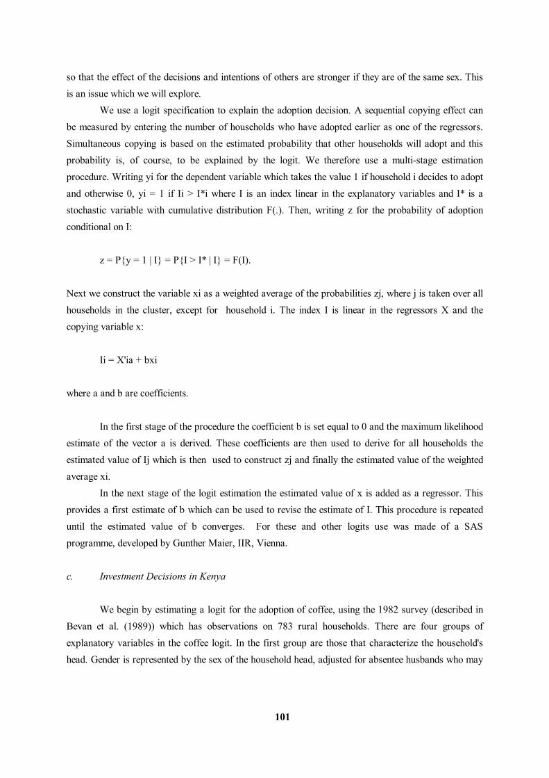
101

so that the effect of the decisions and intentions of others are stronger if they are of the same sex. This is an issue which we will explore. We use a logit specification to explain the adoption decision. A sequential copying effect can be measured by entering the number of households who have adopted earlier as one of the regressors. Simultaneous copying is based on the estimated probability that other households will adopt and this probability is, of course, to be explained by the logit. We therefore use a multi-stage estimation procedure. Writing yi for the dependent variable which takes the value 1 if household i decides to adopt and otherwise 0, yi = 1 if Ii > I*i where I is an index linear in the explanatory variables and I* is a stochastic variable with cumulative distribution F(.). Then, writing z for the probability of adoption conditional on I: z = P{y = 1 | I} = P{I > I* | I} = F(I). Next we construct the variable xi as a weighted average of the probabilities zj, where j is taken over all households in the cluster, except for household i. The index I is linear in the regressors X and the copying variable x: Ii = X'ia + bxi where a and b are coefficients. In the first stage of the procedure the coefficient b is set equal to 0 and the maximum likelihood estimate of the vector a is derived. These coefficients are then used to derive for all households the estimated value of Ij which is then used to construct zj and finally the estimated value of the weighted average xi. In the next stage of the logit estimation the estimated value of x is added as a regressor. This provides a first estimate of b which can be used to revise the estimate of I. This procedure is repeated until the estimated value of b converges. For these and other logits use was made of a SAS programme, developed by Gunther Maier, IIR, Vienna. c. Investment Decisions in Kenya We begin by estimating a logit for the adoption of coffee, using the 1982 survey (described in Bevan et al. (1989)) which has observations on 783 rural households. There are four groups of explanatory variables in the coffee logit. In the first group are those that characterize the household's head. Gender is represented by the sex of the household head, adjusted for absentee husbands who may

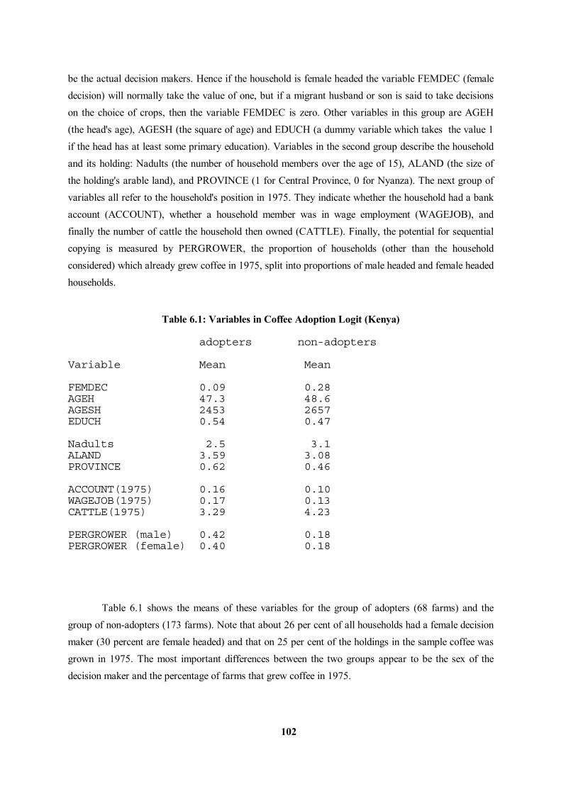
102

be the actual decision makers. Hence if the household is female headed the variable FEMDEC (female decision) will normally take the value of one, but if a migrant husband or son is said to take decisions on the choice of crops, then the variable FEMDEC is zero. Other variables in this group are AGEH (the head's age), AGESH (the square of age) and EDUCH (a dummy variable which takes the value 1 if the head has at least some primary education). Variables in the second group describe the household and its holding: Nadults (the number of household members over the age of 15), ALAND (the size of the holding's arable land), and PROVINCE (1 for Central Province, 0 for Nyanza). The next group of variables all refer to the household's position in 1975. They indicate whether the household had a bank account (ACCOUNT), whether a household member was in wage employment (WAGEJOB), and finally the number of cattle the household then owned (CATTLE). Finally, the potential for sequential copying is measured by PERGROWER, the proportion of households (other than the household considered) which already grew coffee in 1975, split into proportions of male headed and female headed households. Table 6.1: Variables in Coffee Adoption Logit (Kenya) adopters non-adopters Variable Mean Mean FEMDEC 0.09 0.28 AGEH 47.3 48.6 AGESH 2453 2657 EDUCH 0.54 0.47 Nadults 2.5 3.1 ALAND 3.59 3.08 PROVINCE 0.62 0.46 ACCOUNT(1975) 0.16 0.10 WAGEJOB(1975) 0.17 0.13 CATTLE(1975) 3.29 4.23 PERGROWER (male) 0.42 0.18 PERGROWER (female) 0.40 0.18

Table 6.1 shows the means of these variables for the group of adopters (68 farms) and the group of non-adopters (173 farms). Note that about 26 per cent of all households had a female decision maker (30 percent are female headed) and that on 25 per cent of the holdings in the sample coffee was grown in 1975. The most important differences between the two groups appear to be the sex of the decision maker and the percentage of farms that grew coffee in 1975.

103

The means and our logit estimation are restricted to clusters in which coffee can be grown. We take this to be the case if at least one household (out of 20 in a cluster) grew coffee in 1982. In this restricted sample 241 households did not yet grow coffee in 1975. Of these potential adopters 173 still did not grow coffee in 1982, the other 68 had adopted the crop in the period 1975-1982. As noted above, we adopt a multi-stage approach. In the first stage simultaneous copying is ignored: only the variables shown in Table 6.1 enter the logit. This gives the results in the first column of Table 6.2. Here, the two variables referring to 1975 (account and wagejob) have been aggregated into one and a new variable has been added: educh*femdec, which is the product of the two variables. This variable accounts for possible differential effects of education of female vis-a-vis male decision makers. The estimated coefficients are then used to calculate the estimated probability of adoption for each of the households in the sample. The variable SIMCOP, an indicator of simultaneous copying, is then constructed by calculating for each household the average expected probability of the other households in the same cluster. In the next stage SIMCOP is added to the logit. Expected probabilities are then calculated again, now taking into account the effect of SIMCOP on the probability. This procedure is repeated until the coefficient of SIMCOP no longer changes. The results of the final stage are shown in the second column of Table 6.2. Table 6.2: Estimation Results for Coffee Adoption Logit (Kenya) First round Final round t t CONSTANT -5.82 3.1 -5.6 2.9 FEMDEC -2.45 3.0 -2.41 2.9 AGEH 0.13 1.8 0.13 1.7 AGESH -0.0013 1.9 -0.0013 1.8 EDUCH -0.14 0.4 -0.18 0.4 EDUCH*FEMDEC 1.77 1.7 1.79 1.7 Nadults 0.15 1.4 0.15 1.4 ALAND 0.06 1.0 0.07 1.0 PROVINCE 1.43 3.6 1.65 2.4 ACC or WAGE 75 -0.55 1.3 -0.56 1.4 PERGROWER 1.6 5.4 2.0 1.7 SIMCOP --- -1.5 0.4 Predicted 0 1 0 1 Actual 0 155 18 157 16 1 38 30 36 32

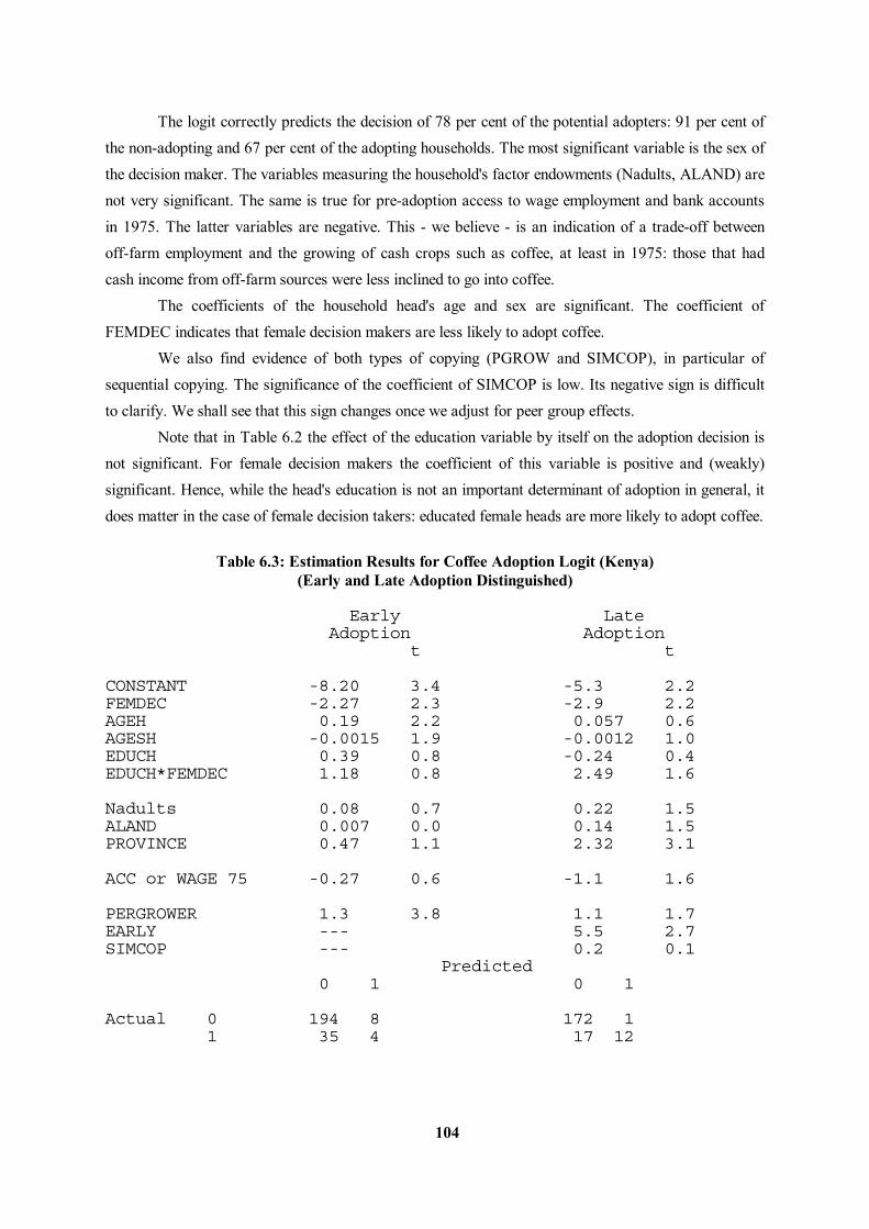
104

The logit correctly predicts the decision of 78 per cent of the potential adopters: 91 per cent of the non-adopting and 67 per cent of the adopting households. The most significant variable is the sex of the decision maker. The variables measuring the household's factor endowments (Nadults, ALAND) are not very significant. The same is true for pre-adoption access to wage employment and bank accounts in 1975. The latter variables are negative. This - we believe - is an indication of a trade-off between off-farm employment and the growing of cash crops such as coffee, at least in 1975: those that had cash income from off-farm sources were less inclined to go into coffee. The coefficients of the household head's age and sex are significant. The coefficient of FEMDEC indicates that female decision makers are less likely to adopt coffee. We also find evidence of both types of copying (PGROW and SIMCOP), in particular of sequential copying. The significance of the coefficient of SIMCOP is low. Its negative sign is difficult to clarify. We shall see that this sign changes once we adjust for peer group effects. Note that in Table 6.2 the effect of the education variable by itself on the adoption decision is not significant. For female decision makers the coefficient of this variable is positive and (weakly) significant. Hence, while the head's education is not an important determinant of adoption in general, it does matter in the case of female decision takers: educated female heads are more likely to adopt coffee. Table 6.3: Estimation Results for Coffee Adoption Logit (Kenya) (Early and Late Adoption Distinguished) Early Late Adoption Adoption t t CONSTANT -8.20 3.4 -5.3 2.2 FEMDEC -2.27 2.3 -2.9 2.2 AGEH 0.19 2.2 0.057 0.6 AGESH -0.0015 1.9 -0.0012 1.0 EDUCH 0.39 0.8 -0.24 0.4 EDUCH*FEMDEC 1.18 0.8 2.49 1.6 Nadults 0.08 0.7 0.22 1.5 ALAND 0.007 0.0 0.14 1.5 PROVINCE 0.47 1.1 2.32 3.1 ACC or WAGE 75 -0.27 0.6 -1.1 1.6 PERGROWER 1.3 3.8 1.1 1.7 EARLY --- 5.5 2.7 SIMCOP --- 0.2 0.1 Predicted 0 1 0 1 Actual 0 194 8 172 1 1 35 4 17 12

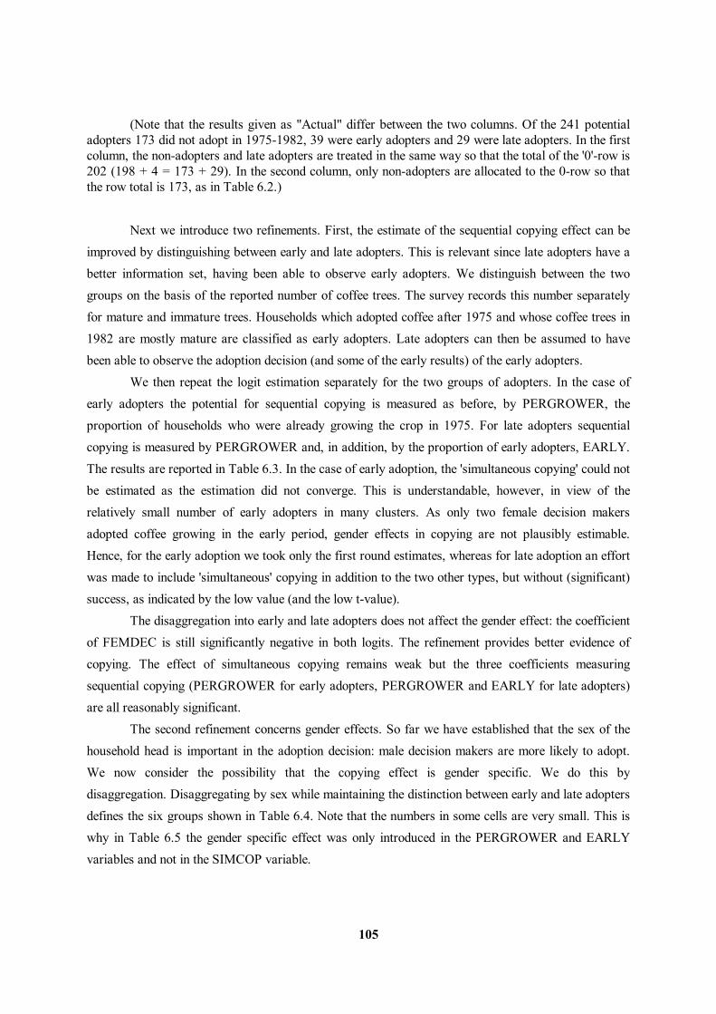
105

(Note that the results given as "Actual" differ between the two columns. Of the 241 potential adopters 173 did not adopt in 1975-1982, 39 were early adopters and 29 were late adopters. In the first column, the non-adopters and late adopters are treated in the same way so that the total of the '0'-row is 202 (198 + 4 = 173 + 29). In the second column, only non-adopters are allocated to the 0-row so that the row total is 173, as in Table 6.2.) Next we introduce two refinements. First, the estimate of the sequential copying effect can be improved by distinguishing between early and late adopters. This is relevant since late adopters have a better information set, having been able to observe early adopters. We distinguish between the two groups on the basis of the reported number of coffee trees. The survey records this number separately for mature and immature trees. Households which adopted coffee after 1975 and whose coffee trees in 1982 are mostly mature are classified as early adopters. Late adopters can then be assumed to have been able to observe the adoption decision (and some of the early results) of the early adopters. We then repeat the logit estimation separately for the two groups of adopters. In the case of early adopters the potential for sequential copying is measured as before, by PERGROWER, the proportion of households who were already growing the crop in 1975. For late adopters sequential copying is measured by PERGROWER and, in addition, by the proportion of early adopters, EARLY. The results are reported in Table 6.3. In the case of early adoption, the 'simultaneous copying' could not be estimated as the estimation did not converge. This is understandable, however, in view of the relatively small number of early adopters in many clusters. As only two female decision makers adopted coffee growing in the early period, gender effects in copying are not plausibly estimable. Hence, for the early adoption we took only the first round estimates, whereas for late adoption an effort was made to include 'simultaneous' copying in addition to the two other types, but without (significant) success, as indicated by the low value (and the low t-value). The disaggregation into early and late adopters does not affect the gender effect: the coefficient of FEMDEC is still significantly negative in both logits. The refinement provides better evidence of copying. The effect of simultaneous copying remains weak but the three coefficients measuring sequential copying (PERGROWER for early adopters, PERGROWER and EARLY for late adopters) are all reasonably significant. The second refinement concerns gender effects. So far we have established that the sex of the household head is important in the adoption decision: male decision makers are more likely to adopt. We now consider the possibility that the copying effect is gender specific. We do this by disaggregation. Disaggregating by sex while maintaining the distinction between early and late adopters defines the six groups shown in Table 6.4. Note that the numbers in some cells are very small. This is why in Table 6.5 the gender specific effect was only introduced in the PERGROWER and EARLY variables and not in the SIMCOP variable.

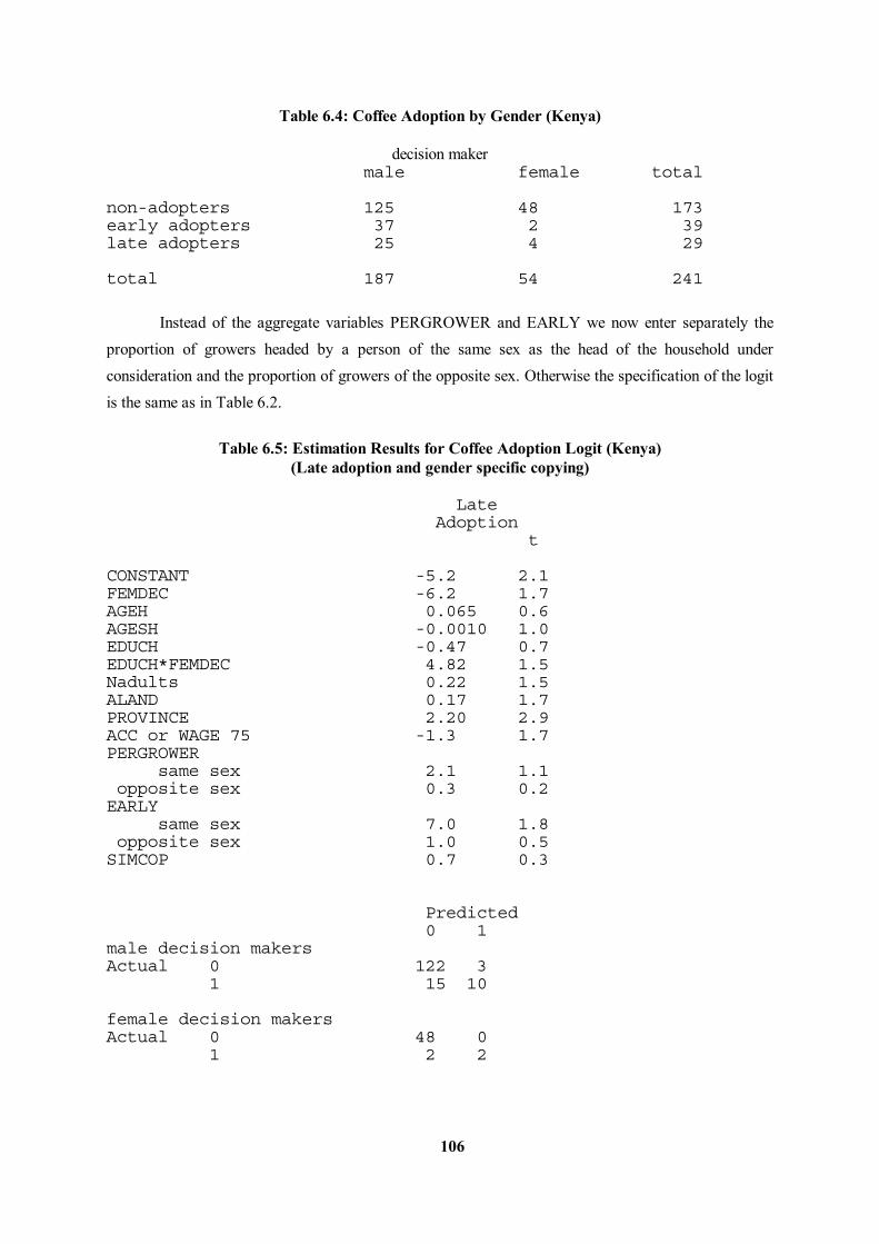
106

Table 6.4: Coffee Adoption by Gender (Kenya) decision maker male female total non-adopters 125 48 173 early adopters 37 2 39 late adopters 25 4 29 total 187 54 241

Instead of the aggregate variables PERGROWER and EARLY we now enter separately the proportion of growers headed by a person of the same sex as the head of the household under consideration and the proportion of growers of the opposite sex. Otherwise the specification of the logit is the same as in Table 6.2. Table 6.5: Estimation Results for Coffee Adoption Logit (Kenya) (Late adoption and gender specific copying) Late Adoption t CONSTANT -5.2 2.1 FEMDEC -6.2 1.7 AGEH 0.065 0.6 AGESH -0.0010 1.0 EDUCH -0.47 0.7 EDUCH*FEMDEC 4.82 1.5 Nadults 0.22 1.5 ALAND 0.17 1.7 PROVINCE 2.20 2.9 ACC or WAGE 75 -1.3 1.7 PERGROWER same sex 2.1 1.1 opposite sex 0.3 0.2 EARLY same sex 7.0 1.8 opposite sex 1.0 0.5 SIMCOP 0.7 0.3 Predicted 0 1 male decision makers Actual 0 122 3 1 15 10 female decision makers Actual 0 48 0 1 2 2

107

Table 6.5 shows the results for this estimation. The coefficient of the dummy for the sex of the decision maker has become larger but not more significant compared to Table 6.2. The results further indicate that sequential copying as measured by PERGROWER (i.e. copying from those who adopted coffee before 1975) is gender specific: household heads are more likely to copy from an adopter of the same sex. In that sense copying does appear to be a gender specific phenomenon. The same applies to the copying of early adopters. This is important because to the extent policies are biased in favour of male headed households this bias will be reinforced if female headed households are more likely to copy female than male headed households. The importance of this gender effect cannot be judged directly on the basis of the estimated coefficient. We therefore use the estimated coefficients in a simulation experiment in which the 74 female headed households are assumed to be male headed. The simulation measures both the direct effect of this change (via the coefficient of femdec and aduch*femdec) and the indirect effect (via copying). The direct results of this change are that the sum of the probabilities of adopting (early or late) in the sample (hence the expected number of adopting households) increases from 68 to 99. The number of households which are predicted to adopt (those with probabilities greater than 0.5) increases from 24 to 91. Hence there is a very strong direct effect: coffee would be much more widely adopted if female headed households were as likely to adopt as male headed households. The 91 adopting households consist of 12 early adopters (of which 4 originally adopted early), and 79 late adopters. Out of these 79, 22 were originally early adopters and 19 were late adopters originally. It is interesting to note that of the 35 farms that were incorrectly predicted not to adopt early, almost two thirds (22/35) are predicted to adopt late. We have estimated a similar adoption logit for the next investment decision, tea adoption, but this logit provides no significant results. The number of adopters is too small: there are only 25 adopting households of which 5 are female headed. Next we consider the adoption of improved livestock. In the relevant population in 1975 there were 242 households (including 54 female headed households) without improved livestock. Over the period 1975-82 78 of those households (including 15 female headed households) adopted improved livestock. This suggests no gender difference: the proportion of female headed households in the group of adopters is about the same as in the group of potential adopters. This impression is confirmed if we control for other differences: in our logit (Table 6.6) the coefficient of SEXH is positive but has a t-value of only 0.2. The variables in the logit have been defined previously except for: the size of the holding (LAND), dummy variables indicating whether "farmer" was the household head's main occupation in 1975 (FARMER) and whether the household then grew coffee or tea (COFFEE, TEA). In analogy with PERGROWER, PEROWNER is the proportion of households (in the same cluster) who already owned

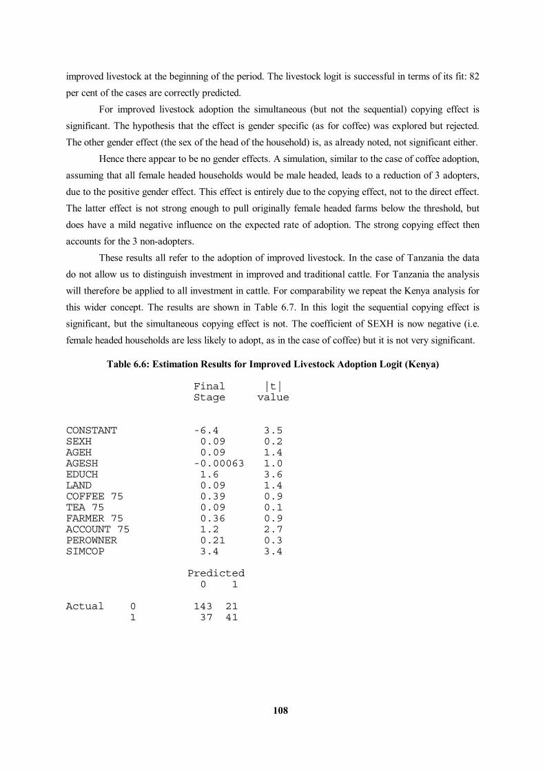
108

improved livestock at the beginning of the period. The livestock logit is successful in terms of its fit: 82 per cent of the cases are correctly predicted. For improved livestock adoption the simultaneous (but not the sequential) copying effect is significant. The hypothesis that the effect is gender specific (as for coffee) was explored but rejected. The other gender effect (the sex of the head of the household) is, as already noted, not significant either. Hence there appear to be no gender effects. A simulation, similar to the case of coffee adoption, assuming that all female headed households would be male headed, leads to a reduction of 3 adopters, due to the positive gender effect. This effect is entirely due to the copying effect, not to the direct effect. The latter effect is not strong enough to pull originally female headed farms below the threshold, but does have a mild negative influence on the expected rate of adoption. The strong copying effect then accounts for the 3 non-adopters. These results all refer to the adoption of improved livestock. In the case of Tanzania the data do not allow us to distinguish investment in improved and traditional cattle. For Tanzania the analysis will therefore be applied to all investment in cattle. For comparability we repeat the Kenya analysis for this wider concept. The results are shown in Table 6.7. In this logit the sequential copying effect is significant, but the simultaneous copying effect is not. The coefficient of SEXH is now negative (i.e. female headed households are less likely to adopt, as in the case of coffee) but it is not very significant. Table 6.6: Estimation Results for Improved Livestock Adoption Logit (Kenya) Final |t| Stage value CONSTANT -6.4 3.5 SEXH 0.09 0.2 AGEH 0.09 1.4 AGESH -0.00063 1.0 EDUCH 1.6 3.6 LAND 0.09 1.4 COFFEE 75 0.39 0.9 TEA 75 0.09 0.1 FARMER 75 0.36 0.9 ACCOUNT 75 1.2 2.7 PEROWNER 0.21 0.3 SIMCOP 3.4 3.4 Predicted 0 1 Actual 0 143 21 1 37 41

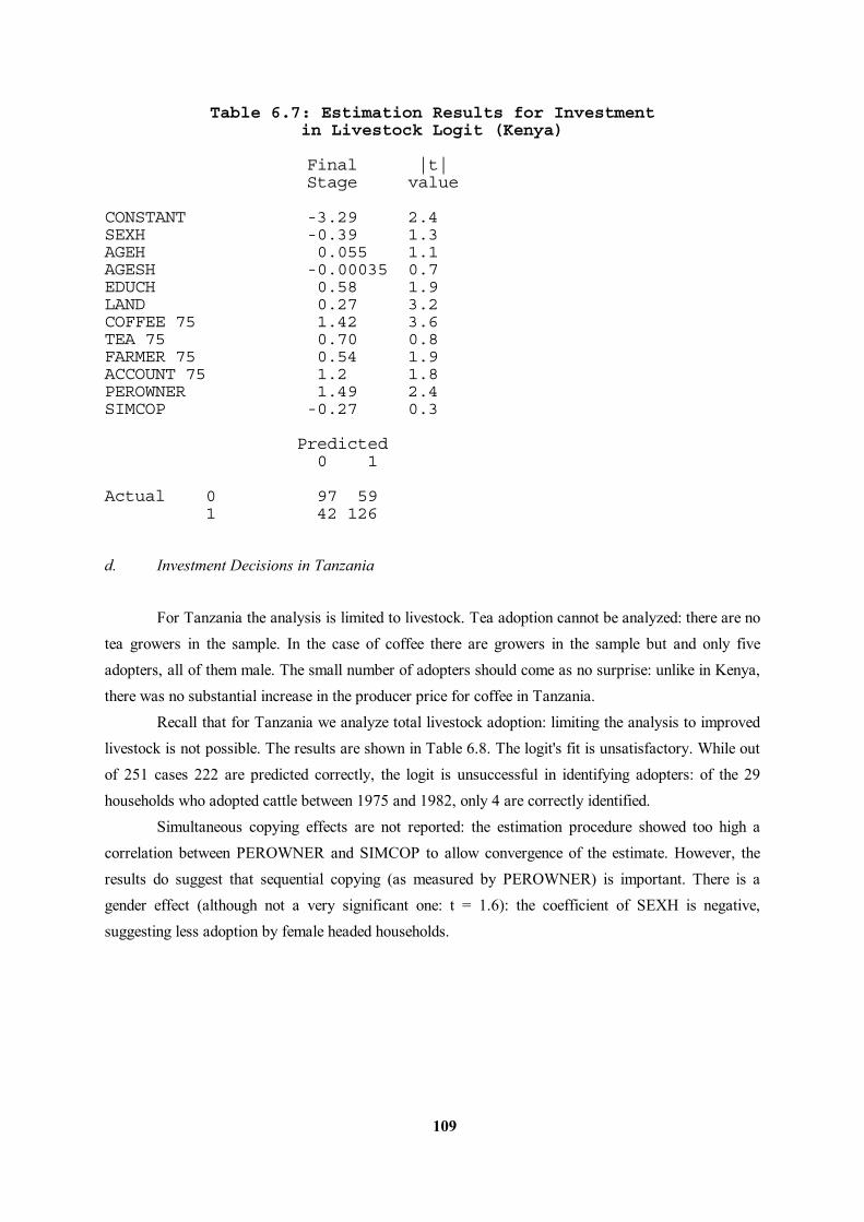
109

Table 6.7: Estimation Results for Investment in Livestock Logit (Kenya) Final |t| Stage value CONSTANT -3.29 2.4 SEXH -0.39 1.3 AGEH 0.055 1.1 AGESH -0.00035 0.7 EDUCH 0.58 1.9 LAND 0.27 3.2 COFFEE 75 1.42 3.6 TEA 75 0.70 0.8 FARMER 75 0.54 1.9 ACCOUNT 75 1.2 1.8 PEROWNER 1.49 2.4 SIMCOP -0.27 0.3 Predicted 0 1 Actual 0 97 59 1 42 126

d. Investment Decisions in Tanzania For Tanzania the analysis is limited to livestock. Tea adoption cannot be analyzed: there are no tea growers in the sample. In the case of coffee there are growers in the sample but and only five adopters, all of them male. The small number of adopters should come as no surprise: unlike in Kenya, there was no substantial increase in the producer price for coffee in Tanzania. Recall that for Tanzania we analyze total livestock adoption: limiting the analysis to improved livestock is not possible. The results are shown in Table 6.8. The logit's fit is unsatisfactory. While out of 251 cases 222 are predicted correctly, the logit is unsuccessful in identifying adopters: of the 29 households who adopted cattle between 1975 and 1982, only 4 are correctly identified. Simultaneous copying effects are not reported: the estimation procedure showed too high a correlation between PEROWNER and SIMCOP to allow convergence of the estimate. However, the results do suggest that sequential copying (as measured by PEROWNER) is important. There is a gender effect (although not a very significant one: t = 1.6): the coefficient of SEXH is negative, suggesting less adoption by female headed households.

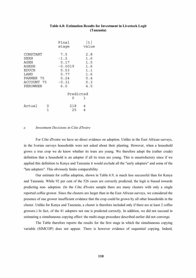
110

Table 6.8: Estimation Results for Investment in Livestock Logit (Tanzania) Final |t| stage value CONSTANT 7.5 2.8 SEXH -1.2 1.6 AGEH 0.17 1.5 AGESH -0.0019 1.6 EDUCH 0.53 1.1 LAND 0.77 1.6 FARMER 75 0.24 0.4 ACCOUNT 75 -0.31 0.3 PEROWNER 6.0 4.5 Predicted 0 1 Actual 0 218 4 1 25 4

e. Investment Decisions in Côte d'Ivoire For Côte d'Ivoire we have no direct evidence on adoption. Unlike in the East African surveys, in the Ivorian surveys households were not asked about their planting. However, when a household grows a tree crop we do know whether its trees are young. We therefore adopt the (rather crude) definition that a household is an adopter if all its trees are young. This is unsatisfactory since if we applied this definition to Kenya and Tanzania it would exclude all the "early adopters" and some of the "late adopters". This obviously limits comparability. Our estimate for coffee adoption, shown in Table 6.9, is much less successful than for Kenya and Tanzania. While 92 per cent of the 526 cases are correctly predicted, the logit is biased towards predicting non- adoption. (In the Côte d'Ivoire sample there are many clusters with only a single reported coffee grower. Since the clusters are larger than in the East African surveys, we considered the presence of one grower insufficient evidence that the crop could be grown by all other households in the cluster. Unlike for Kenya and Tanzania, a cluster is therefore included only if there are at least 2 coffee growers.) In fact, of the 41 adopters not one is predicted correctly. In addition, we did not succeed in estimating a simultaneous copying effect: the multi-stage procedure described earlier did not converge. The Table therefore reports the results for the first stage in which the simultaneous copying variable (SIMCOP) does not appear. There is however evidence of sequential copying. Indeed,

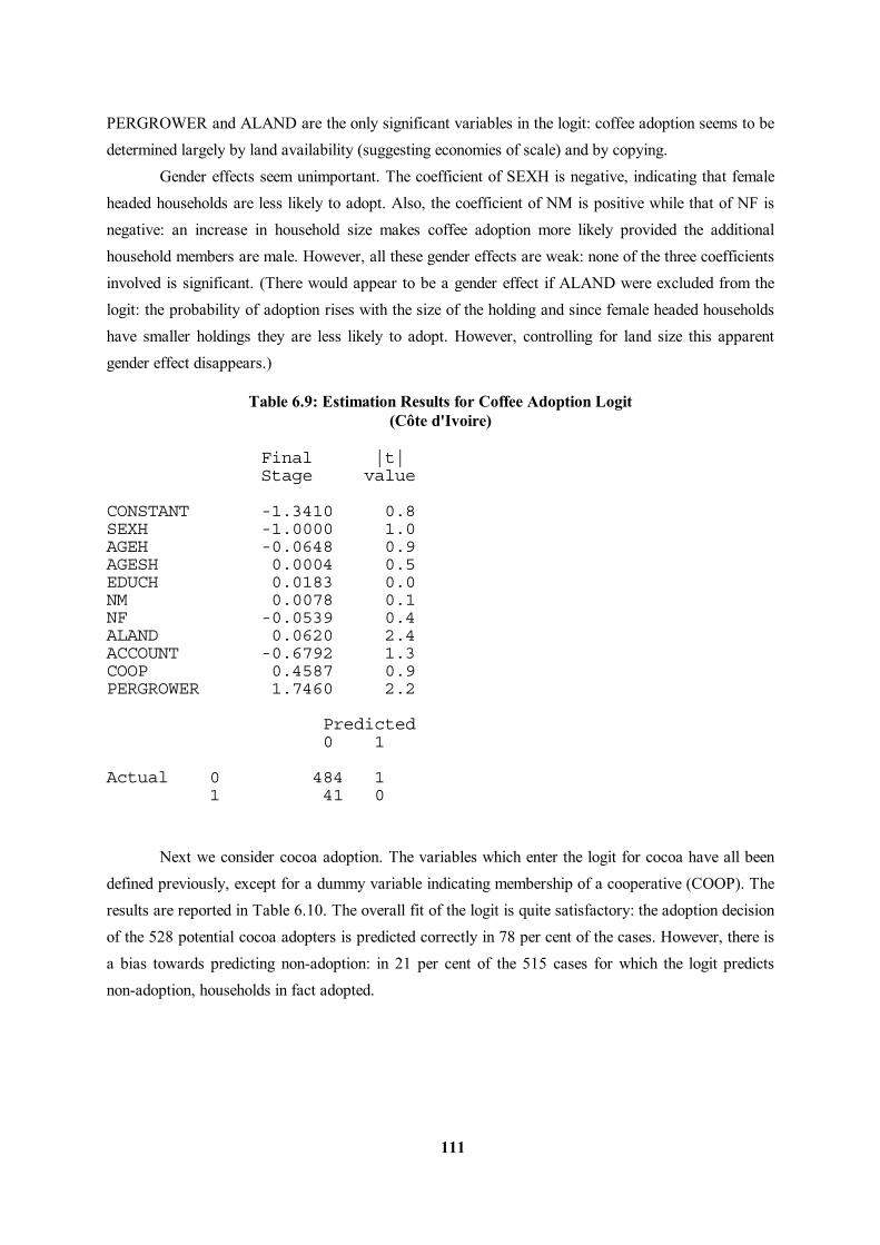
111

PERGROWER and ALAND are the only significant variables in the logit: coffee adoption seems to be determined largely by land availability (suggesting economies of scale) and by copying. Gender effects seem unimportant. The coefficient of SEXH is negative, indicating that female headed households are less likely to adopt. Also, the coefficient of NM is positive while that of NF is negative: an increase in household size makes coffee adoption more likely provided the additional household members are male. However, all these gender effects are weak: none of the three coefficients involved is significant. (There would appear to be a gender effect if ALAND were excluded from the logit: the probability of adoption rises with the size of the holding and since female headed households have smaller holdings they are less likely to adopt. However, controlling for land size this apparent gender effect disappears.) Table 6.9: Estimation Results for Coffee Adoption Logit (Côte d'Ivoire) Final |t| Stage value CONSTANT -1.3410 0.8 SEXH -1.0000 1.0 AGEH -0.0648 0.9 AGESH 0.0004 0.5 EDUCH 0.0183 0.0 NM 0.0078 0.1 NF -0.0539 0.4 ALAND 0.0620 2.4 ACCOUNT -0.6792 1.3 COOP 0.4587 0.9 PERGROWER 1.7460 2.2 Predicted 0 1 Actual 0 484 1 1 41 0

Next we consider cocoa adoption. The variables which enter the logit for cocoa have all been defined previously, except for a dummy variable indicating membership of a cooperative (COOP). The results are reported in Table 6.10. The overall fit of the logit is quite satisfactory: the adoption decision of the 528 potential cocoa adopters is predicted correctly in 78 per cent of the cases. However, there is a bias towards predicting non-adoption: in 21 per cent of the 515 cases for which the logit predicts non-adoption, households in fact adopted.

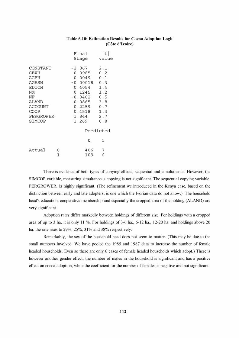
112

Table 6.10: Estimation Results for Cocoa Adoption Logit (Côte d'Ivoire) Final |t| Stage value CONSTANT -2.867 2.1 SEXH 0.0985 0.2 AGEH 0.0049 0.1 AGESH -0.00018 0.3 EDUCH 0.4054 1.4 NM 0.1245 1.2 NF -0.0462 0.5 ALAND 0.0865 3.8 ACCOUNT 0.2259 0.7 COOP 0.4518 1.3 PERGROWER 1.844 2.7 SIMCOP 1.269 0.8 Predicted 0 1 Actual 0 406 7 1 109 6

There is evidence of both types of copying effects, sequential and simultaneous. However, the SIMCOP variable, measuring simultaneous copying is not significant. The sequential copying variable, PERGROWER, is highly significant. (The refinement we introduced in the Kenya case, based on the distinction between early and late adopters, is one which the Ivorian data do not allow.) The household head's education, cooperative membership and especially the cropped area of the holding (ALAND) are very significant. Adoption rates differ markedly between holdings of different size. For holdings with a cropped area of up to 3 ha. it is only 11 %. For holdings of 3-6 ha., 6-12 ha., 12-20 ha. and holdings above 20 ha. the rate rises to 29%, 25%, 31% and 38% respectively. Remarkably, the sex of the household head does not seem to matter. (This may be due to the small numbers involved. We have pooled the 1985 and 1987 data to increase the number of female headed households. Even so there are only 6 cases of female headed households which adopt.) There is however another gender effect: the number of males in the household is significant and has a positive effect on cocoa adoption, while the coefficient for the number of females is negative and not significant.

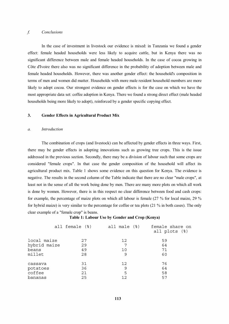
113

f. Conclusions In the case of investment in livestock our evidence is mixed: in Tanzania we found a gender effect: female headed households were less likely to acquire cattle, but in Kenya there was no significant difference between male and female headed households. In the case of cocoa growing in Côte d'Ivoire there also was no significant difference in the probability of adoption between male and female headed households. However, there was another gender effect: the household's composition in terms of men and women did matter. Households with more male resident household members are more likely to adopt cocoa. Our strongest evidence on gender effects is for the case on which we have the most appropriate data set: coffee adoption in Kenya. There we found a strong direct effect (male headed households being more likely to adopt), reinforced by a gender specific copying effect.

3. Gender Effects in Agricultural Product Mix a. Introduction The combination of crops (and livestock) can be affected by gender effects in three ways. First, there may be gender effects in adopting innovations such as growing tree crops. This is the issue addressed in the previous section. Secondly, there may be a division of labour such that some crops are considered "female crops". In that case the gender composition of the household will affect its agricultural product mix. Table 1 shows some evidence on this question for Kenya. The evidence is negative. The results in the second column of the Table indicate that there are no clear "male crops", at least not in the sense of all the work being done by men. There are many more plots on which all work is done by women. However, there is in this respect no clear difference between food and cash crops: for example, the percentage of maize plots on which all labour is female (27 % for local maize, 29 % for hybrid maize) is very similar to the percentage for coffee or tea plots (21 % in both cases). The only clear example of a "female crop" is beans. Table 1: Labour Use by Gender and Crop (Kenya) all female (%) all male (%) female share on all plots (%) local maize 27 12 59 hybrid maize 29 7 64 beans 49 10 71 millet 28 9 60 cassava 31 12 76 potatoes 36 9 64 coffee 21 5 58 bananas 25 12 57

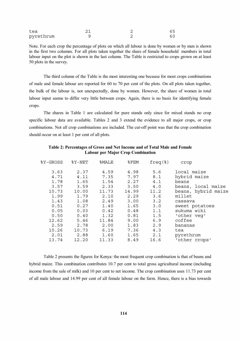
114

tea 21 2 65 pyrethrum 9 2 60 Note. For each crop the percentage of plots on which all labour is done by women or by men is shown in the first two columns. For all plots taken together the share of female household members in total labour input on the plot is shown in the last column. The Table is restricted to crops grown on at least 50 plots in the survey. The third column of the Table is the most interesting one because for most crops combinations of male and female labour are reported for 60 to 70 per cent of the plots. On all plots taken together, the bulk of the labour is, not unexpectedly, done by women. However, the share of women in total labour input seems to differ very little between crops. Again, there is no basis for identifying female crops. The shares in Table 1 are calculated for pure stands only since for mixed stands no crop specific labour data are available. Tables 2 and 3 extend the evidence to all major crops, or crop combinations. Not all crop combinations are included. The cut-off point was that the crop combination should occur on at least 1 per cent of all plots. Table 2: Percentages of Gross and Net Income and of Total Male and Female Labour per Major Crop Combination %Y-GROSS %Y-NET %MALE %FEM freq(%) crop 3.63 2.37 4.59 4.98 5.6 local maize 4.71 4.11 7.35 7.97 8.1 hybrid maize 1.78 1.65 1.54 2.27 4.1 beans 3.57 3.59 2.33 3.50 4.0 beans, local maize 10.73 10.00 11.73 14.99 11.2 beans, hybrid maize 1.99 1.79 2.10 2.29 3.6 millet 1.43 1.08 2.49 3.00 3.2 cassava 0.51 0.27 1.40 1.65 3.0 sweet potatoes 0.05 0.03 0.42 0.48 1.1 sukuma wiki 0.50 0.40 1.32 0.81 1.5 'other veg' 12.62 5.46 11.84 9.00 6.9 coffee 2.59 2.78 2.00 1.83 2.9 bananas 10.26 10.73 6.19 7.36 4.3 tea 2.01 2.88 1.60 1.65 2.1 pyrethrum 13.74 12.20 11.33 8.49 16.6 'other crops'

Table 2 presents the figures for Kenya: the most frequent crop combination is that of beans and hybrid maize. This combination contributes 10.7 per cent to total gross agricultural income (including income from the sale of milk) and 10 per cent to net income. The crop combination uses 11.73 per cent of all male labour and 14.99 per cent of all female labour on the farm. Hence, there is a bias towards

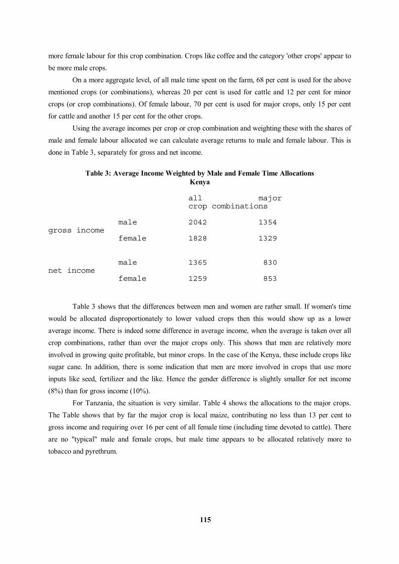
115

more female labour for this crop combination. Crops like coffee and the category 'other crops' appear to be more male crops. On a more aggregate level, of all male time spent on the farm, 68 per cent is used for the above mentioned crops (or combinations), whereas 20 per cent is used for cattle and 12 per cent for minor crops (or crop combinations). Of female labour, 70 per cent is used for major crops, only 15 per cent for cattle and another 15 per cent for the other crops. Using the average incomes per crop or crop combination and weighting these with the shares of male and female labour allocated we can calculate average returns to male and female labour. This is done in Table 3, separately for gross and net income. Table 3: Average Income Weighted by Male and Female Time Allocations Kenya all major crop combinations male 2042 1354 gross income female 1828 1329 male 1365 830 net income female 1259 853

Table 3 shows that the differences between men and women are rather small. If women's time would be allocated disproportionately to lower valued crops then this would show up as a lower average income. There is indeed some difference in average income, when the average is taken over all crop combinations, rather than over the major crops only. This shows that men are relatively more involved in growing quite profitable, but minor crops. In the case of the Kenya, these include crops like sugar cane. In addition, there is some indication that men are more involved in crops that use more inputs like seed, fertilizer and the like. Hence the gender difference is slightly smaller for net income (8%) than for gross income (10%). For Tanzania, the situation is very similar. Table 4 shows the allocations to the major crops. The Table shows that by far the major crop is local maize, contributing no less than 13 per cent to gross income and requiring over 16 per cent of all female time (including time devoted to cattle). There are no "typical" male and female crops, but male time appears to be allocated relatively more to tobacco and pyrethrum.

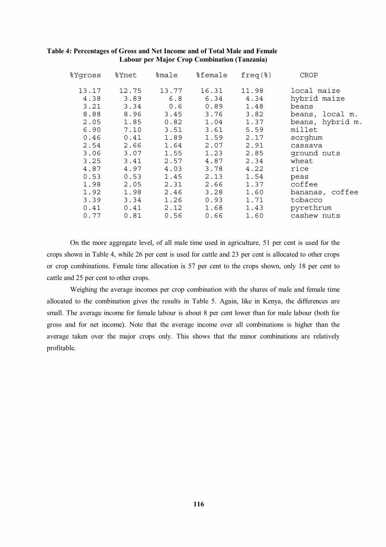
116

Table 4: Percentages of Gross and Net Income and of Total Male and Female Labour per Major Crop Combination (Tanzania) %Ygross %Ynet %male %female freq(%) CROP 13.17 12.75 13.77 16.31 11.98 local maize 4.38 3.89 6.8 6.34 4.34 hybrid maize 3.21 3.34 0.6 0.89 1.48 beans 8.88 8.96 3.45 3.76 3.82 beans, local m. 2.05 1.85 0.82 1.04 1.37 beans, hybrid m. 6.90 7.10 3.51 3.61 5.59 millet 0.46 0.41 1.89 1.59 2.17 sorghum 2.54 2.66 1.64 2.07 2.91 cassava 3.06 3.07 1.55 1.23 2.85 ground nuts 3.25 3.41 2.57 4.87 2.34 wheat 4.87 4.97 4.03 3.78 4.22 rice 0.53 0.53 1.45 2.13 1.54 peas 1.98 2.05 2.31 2.66 1.37 coffee 1.92 1.98 2.46 3.28 1.60 bananas, coffee 3.39 3.34 1.26 0.93 1.71 tobacco 0.41 0.41 2.12 1.68 1.43 pyrethrum 0.77 0.81 0.56 0.66 1.60 cashew nuts

On the more aggregate level, of all male time used in agriculture, 51 per cent is used for the crops shown in Table 4, while 26 per cent is used for cattle and 23 per cent is allocated to other crops or crop combinations. Female time allocation is 57 per cent to the crops shown, only 18 per cent to cattle and 25 per cent to other crops. Weighing the average incomes per crop combination with the shares of male and female time allocated to the combination gives the results in Table 5. Again, like in Kenya, the differences are small. The average income for female labour is about 8 per cent lower than for male labour (both for gross and for net income). Note that the average income over all combinations is higher than the average taken over the major crops only. This shows that the minor combinations are relatively profitable.

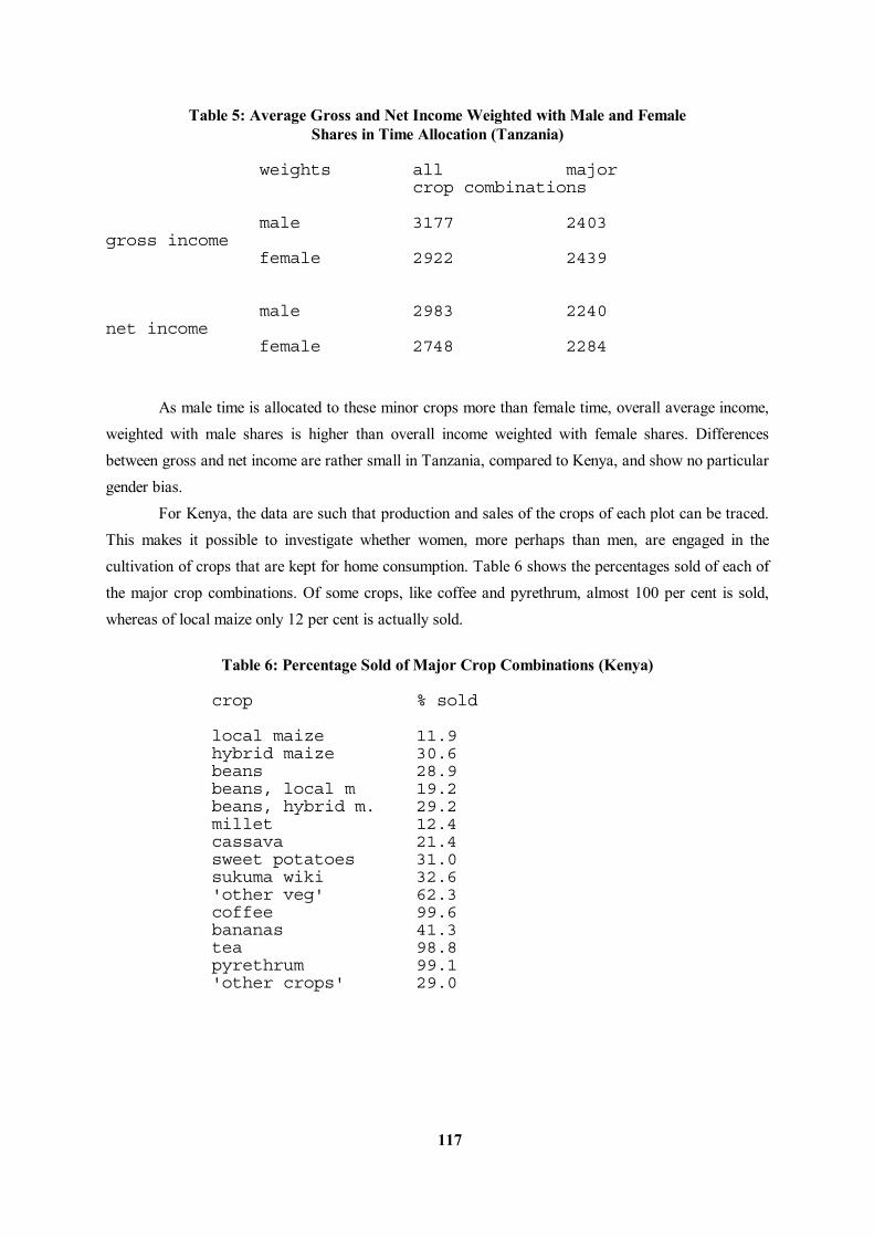
117

Table 5: Average Gross and Net Income Weighted with Male and Female Shares in Time Allocation (Tanzania) weights all major crop combinations male 3177 2403 gross income female 2922 2439 male 2983 2240 net income female 2748 2284

As male time is allocated to these minor crops more than female time, overall average income, weighted with male shares is higher than overall income weighted with female shares. Differences between gross and net income are rather small in Tanzania, compared to Kenya, and show no particular gender bias. For Kenya, the data are such that production and sales of the crops of each plot can be traced. This makes it possible to investigate whether women, more perhaps than men, are engaged in the cultivation of crops that are kept for home consumption. Table 6 shows the percentages sold of each of the major crop combinations. Of some crops, like coffee and pyrethrum, almost 100 per cent is sold, whereas of local maize only 12 per cent is actually sold. Table 6: Percentage Sold of Major Crop Combinations (Kenya) crop % sold local maize 11.9 hybrid maize 30.6 beans 28.9 beans, local m 19.2 beans, hybrid m. 29.2 millet 12.4 cassava 21.4 sweet potatoes 31.0 sukuma wiki 32.6 'other veg' 62.3 coffee 99.6 bananas 41.3 tea 98.8 pyrethrum 99.1 'other crops' 29.0

118

Of these major crop combinations, on average 39.6 per cent was sold. If the mean percentage sold is calculated using the female labour time allocation as weights, we arrive at 45.4 per cent, and if we use male time allocation as weights, we end with 48.2 per cent. This shows that a) more time is allocated to crops that are sold relatively more (this is due to the labour intensive nature of many cash crops), and b) female time, more than male time is allocated to subsistence crops. These percentages are confirmed for the whole of all crop combinations. The 'unweighted' average percentage sold is 38.7 per cent. Using 'female time weights' this mean value rises to 41.7 per cent and with 'male time weights' the value rises further to 45.6 per cent. From the above tables, a first conclusion can be drawn relating to the type of crop being 'handled' by women. In general they tend to devote relatively more time to crops that are not sold and - therefore - meant for home consumption. This may reflect a food bias in the objective functions of women: they attach more value to food crops than to cash crops. It may also be the consequence of economic optimisation: if women are more productive in growing these crops than men, it would seem wise for the household to allocate female time to those crops. Some information to this end is given in Table 7. Here, for the major crops or crop combinations, we list the average net production per family day of work (both male and female working days), divided into male and female headed farms. Table 7: Family Labour Productivity by Crop and by Head's Gender (Kenya) net value per family working day plots MALE HEAD FEMALE HEAD MALE FEMALE local maize 8.54 5.43 102 64 hybrid maize 5.43 7.71 185 57 beans 9.74 9.37 93 27 beans plus l.maize 11.86 11.97 65 52 beans plus h.maize 7.33 6.96 230 98 millet 10.25 10.67 67 39 cassava 5.08 7.80 53 40 potatoes 2.33 2.42 51 41 coffee 11.69 6.28 153 50 bananas 15.77 12.05 65 22 tea 22.31 3.64 94 33 pyrethrum 13.21 6.70 44 20

On male headed farms, the productivity is generally higher, particularly the productivity in cash crop production. On female headed farms, the cropping pattern is not the same, but adjustments are made, in the direction in which female labour (which is more abundantly available on those farms) has a comparative advantage: productivity is higher for hybrid maize, beans+local maize, millet, cassava and potatoes. With the exception of hybrid maize, female headed farms grow relatively more of the other crops: whereas the number of coffee plots falls by two thirds, the number of cassava plots is

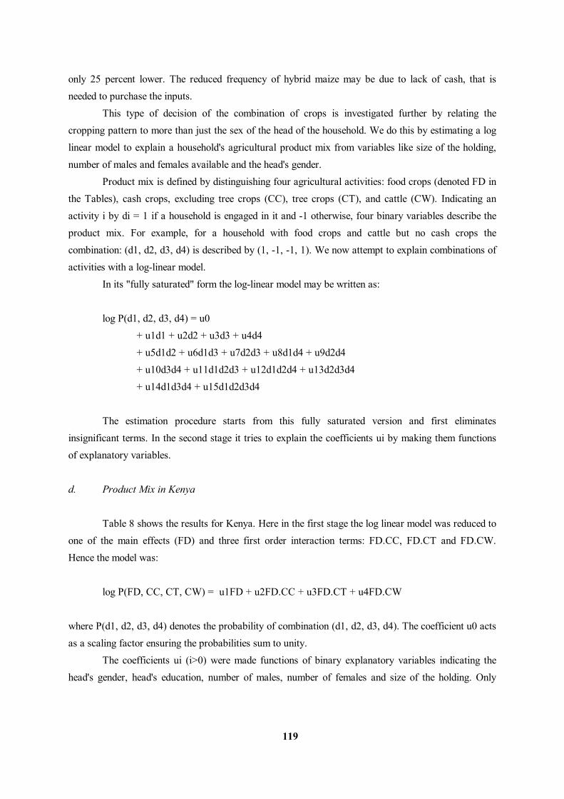
119

only 25 percent lower. The reduced frequency of hybrid maize may be due to lack of cash, that is needed to purchase the inputs. This type of decision of the combination of crops is investigated further by relating the cropping pattern to more than just the sex of the head of the household. We do this by estimating a log linear model to explain a household's agricultural product mix from variables like size of the holding, number of males and females available and the head's gender. Product mix is defined by distinguishing four agricultural activities: food crops (denoted FD in the Tables), cash crops, excluding tree crops (CC), tree crops (CT), and cattle (CW). Indicating an activity i by di = 1 if a household is engaged in it and -1 otherwise, four binary variables describe the product mix. For example, for a household with food crops and cattle but no cash crops the combination: (d1, d2, d3, d4) is described by (1, -1, -1, 1). We now attempt to explain combinations of activities with a log-linear model. In its "fully saturated" form the log-linear model may be written as: log P(d1, d2, d3, d4) = u0 + u1d1 + u2d2 + u3d3 + u4d4 + u5d1d2 + u6d1d3 + u7d2d3 + u8d1d4 + u9d2d4 + u10d3d4 + u11d1d2d3 + u12d1d2d4 + u13d2d3d4 + u14d1d3d4 + u15d1d2d3d4 The estimation procedure starts from this fully saturated version and first eliminates insignificant terms. In the second stage it tries to explain the coefficients ui by making them functions of explanatory variables. d. Product Mix in Kenya Table 8 shows the results for Kenya. Here in the first stage the log linear model was reduced to one of the main effects (FD) and three first order interaction terms: FD.CC, FD.CT and FD.CW. Hence the model was: log P(FD, CC, CT, CW) = u1FD + u2FD.CC + u3FD.CT + u4FD.CW where P(d1, d2, d3, d4) denotes the probability of combination (d1, d2, d3, d4). The coefficient u0 acts as a scaling factor ensuring the probabilities sum to unity. The coefficients ui (i>0) were made functions of binary explanatory variables indicating the head's gender, head's education, number of males, number of females and size of the holding. Only

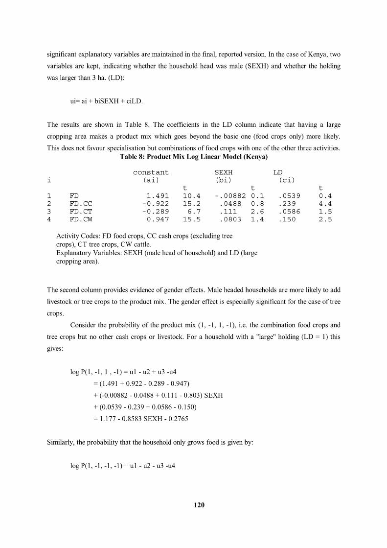
120

significant explanatory variables are maintained in the final, reported version. In the case of Kenya, two variables are kept, indicating whether the household head was male (SEXH) and whether the holding was larger than 3 ha. (LD): ui= ai + biSEXH + ciLD. The results are shown in Table 8. The coefficients in the LD column indicate that having a large cropping area makes a product mix which goes beyond the basic one (food crops only) more likely. This does not favour specialisation but combinations of food crops with one of the other three activities. Table 8: Product Mix Log Linear Model (Kenya) constant SEXH LD i (ai) (bi) (ci) t t t 1 FD 1.491 10.4 -.00882 0.1 .0539 0.4 2 FD.CC -0.922 15.2 .0488 0.8 .239 4.4 3 FD.CT -0.289 6.7 .111 2.6 .0586 1.5 4 FD.CW 0.947 15.5 .0803 1.4 .150 2.5 Activity Codes: FD food crops, CC cash crops (excluding tree crops), CT tree crops, CW cattle. Explanatory Variables: SEXH (male head of household) and LD (large cropping area). The second column provides evidence of gender effects. Male headed households are more likely to add livestock or tree crops to the product mix. The gender effect is especially significant for the case of tree crops. Consider the probability of the product mix (1, -1, 1, -1), i.e. the combination food crops and tree crops but no other cash crops or livestock. For a household with a "large" holding (LD = 1) this gives: log P(1, -1, 1 , -1) = u1 - u2 + u3 -u4 = (1.491 + 0.922 - 0.289 - 0.947) + (-0.00882 - 0.0488 + 0.111 - 0.803) SEXH + (0.0539 - 0.239 + 0.0586 - 0.150) = 1.177 - 0.8583 SEXH - 0.2765 Similarly, the probability that the household only grows food is given by: log P(1, -1, -1, -1) = u1 - u2 - u3 -u4

121

and hence the relative probability of the combination food and cash crops rather than food crops only is: log P(1, -1, 1, -1) / P(1, -1, -1, -1) = 2u3 = 2 (-0.289 + .111 SEXH + 0.0586) Hence the (natural) logarithm of the relative probability is -0.6828 for a female headed household (SEXH = -1) and -0.2388 for a male headed household. This indicates a strong gender effect. For female headed households the probability of the food plus tree crop combination is about 51 % of that for food alone but for male headed households the percentage is much higher: 79%. c. Product Mix in Tanzania Next we consider the same model for Tanzania. There are some important differences. First, while for Kenya the one main effect of the log linear model which was maintained was the one for food crops, for Tanzania we find that all households grow food crops so that the variable FD is not maintained. The other three main effects: CC, CT and CW and one of the first order interaction terms, CT.CW, are maintained so the model is (ignoring u0): log P(FD, CC, CT, CW) = u1CC + u2CT + u3CW + u4CT.CW Secondly, while in the case of Kenya the only explanatory variables maintained were SEXH and LD, for Tanzania we keep in addition EDUCH, the dummy variable indicating whether the household head has had at least some primary education, and a variable indicating whether the household has at least two male members (of age 15 or above), DM. Table 9 shows the results. The household's endowment in terms of male labour affects product mix only to a very limited extent: the explanatory variable DM is significant only for livestock. Whether the household head has some education, a variable which does not explain product mix for Kenya, is a significant determinant of tree crops and livestock (CT, CW and the interaction term CT.CW). Finally, gender effects are significant: SEXH positively affects cash crops and negatively affects tree crops and livestock.

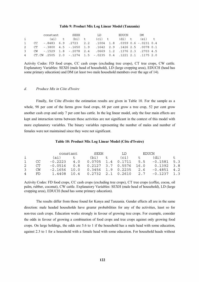
122

Table 9: Product Mix Log Linear Model (Tanzania) constant SEXH LD EDUCH DM i (ai) t (bi) t (ci) t (di) t (ei) t 1 CC -.8483 6.9 .2723 2.2 .1004 1.8 .0359 0.6 -.0231 0.4 2 CT -.3800 4.5 -.1650 1.9 .1642 2.9 .1426 2.5 .0078 0.1 3 CW -.1529 1.8 -.2078 2.4 .0669 1.2 .1376 2.3 .2703 4.5 4 CT.CW .2505 2.0 -.1274 1.5 -.0235 0.4 .1221 2.1 .1175 2.0 Activity Codes: FD food crops, CC cash crops (excluding tree crops), CT tree crops, CW cattle. Explanatory Variables: SEXH (male head of household), LD (large cropping area), EDUCH (head has some primary education) and DM (at least two male household members over the age of 14).

d. Produce Mix in Côte d'Ivoire Finally, for Côte d'Ivoire the estimation results are given in Table 10. For the sample as a whole, 98 per cent of the farms grow food crops, 68 per cent grow a tree crop, 52 per cent grow another cash crop and only 7 per cent has cattle. In the log linear model, only the four main effects are kept and interaction terms between these activities are not significant in the context of this model with more explanatory variables. The binary variables representing the number of males and number of females were not maintained since they were not significant. Table 10: Product Mix Log Linear Model (Côte d'Ivoire) constant SEXH LD EDUCH i (ai) t (bi) t (ci) t (di) t 1 CC -0.2223 4.0 0.0705 1.4 0.1711 5.5 -0.1581 5.3 2 CT -0.0516 0.8 0.2127 3.7 0.5576 16.0 0.1392 3.8 3 CW -2.1656 10.0 0.3456 1.9 0.2235 2.6 -0.4851 4.2 4 FD 1.4408 10.4 0.2732 2.1 0.2610 2.7 -0.1237 1.3 Activity Codes: FD food crops, CC cash crops (excluding tree crops), CT tree crops (coffee, cocoa, oil palm, rubber, coconut), CW cattle. Explanatory Variables: SEXH (male head of household), LD (large cropping area), EDUCH (head has some primary education). The results differ from those found for Kenya and Tanzania. Gender effects all are in the same direction: male headed households have greater probabilities for any of the activities, least so for non-tree cash crops. Education works strongly in favour of growing tree crops. For example, consider the odds in favour of growing a combination of food crops and tree crops against only growing food crops. On large holdings, the odds are 5.6 to 1 if the household has a male head with some education, against 2.3 to 1 for a household with a female head with some education. For household heads without

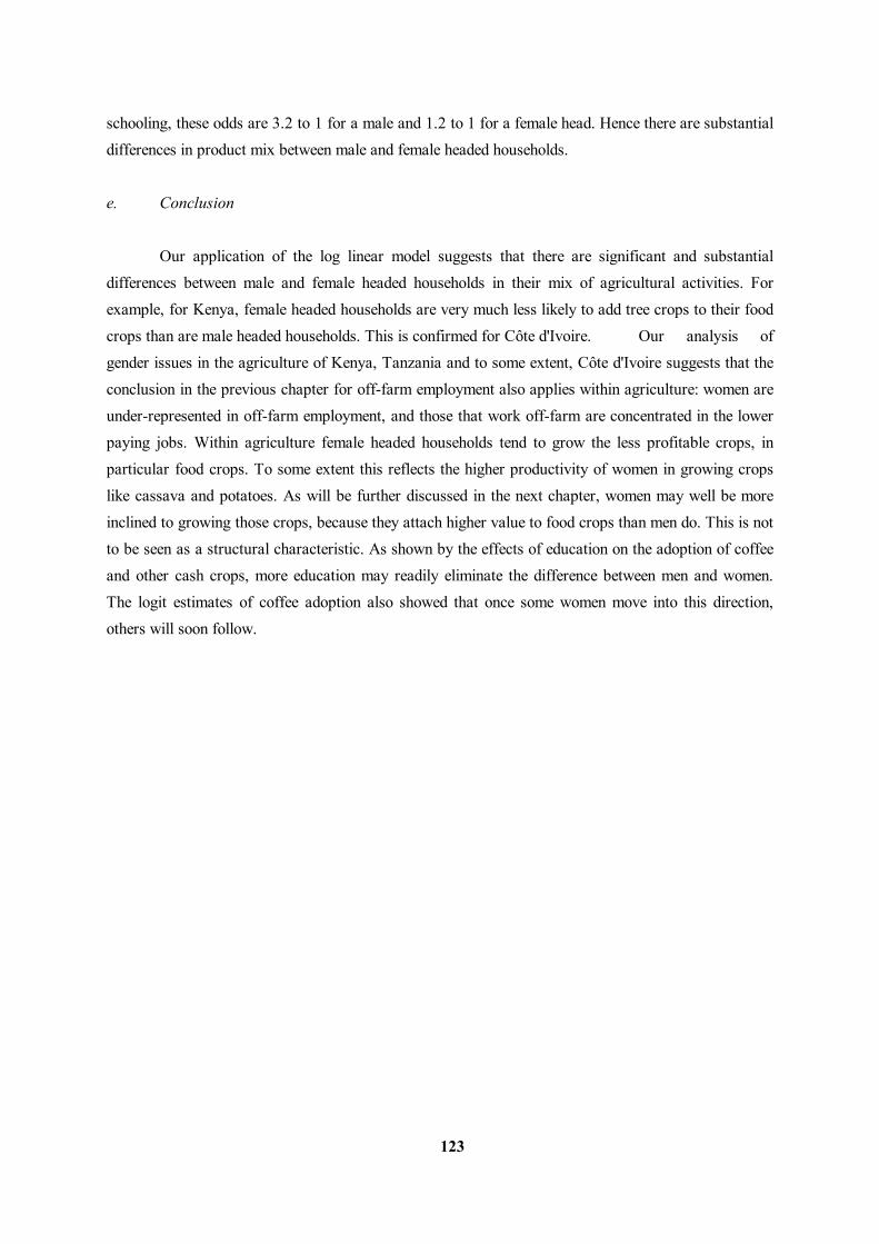
123

schooling, these odds are 3.2 to 1 for a male and 1.2 to 1 for a female head. Hence there are substantial differences in product mix between male and female headed households. e. Conclusion Our application of the log linear model suggests that there are significant and substantial differences between male and female headed households in their mix of agricultural activities. For example, for Kenya, female headed households are very much less likely to add tree crops to their food crops than are male headed households. This is confirmed for Côte d'Ivoire. Our analysis of gender issues in the agriculture of Kenya, Tanzania and to some extent, Côte d'Ivoire suggests that the conclusion in the previous chapter for off-farm employment also applies within agriculture: women are under-represented in off-farm employment, and those that work off-farm are concentrated in the lower paying jobs. Within agriculture female headed households tend to grow the less profitable crops, in particular food crops. To some extent this reflects the higher productivity of women in growing crops like cassava and potatoes. As will be further discussed in the next chapter, women may well be more inclined to growing those crops, because they attach higher value to food crops than men do. This is not to be seen as a structural characteristic. As shown by the effects of education on the adoption of coffee and other cash crops, more education may readily eliminate the difference between men and women. The logit estimates of coffee adoption also showed that once some women move into this direction, others will soon follow.

124

Chapter 7 Gender Aspects of Household Expenditures and Resource Allocation in the Cote d'Ivoire 1. Introductory Notes 2. Household Economics and the Economics of Households. a. Modelling Household Behaviour (i) Theory (11) Evidence b. Gender Aspects of the Allocation of Household Resources (i) Theory (ii) Evidence 3. Household Expenditures and the Intrahousehold Distribution of Income a. Introduction b. The Model c. The Data e. Estimation Issues f. Discussion of the Results g. Final Notes 4. An Outlay Equivalent Analysis of Expenditure on Adult Goods a.Introduction b. Estimation c. Discussion of Results d. Final Notes 5. An Anthropometric Analysis of Gender Differentials a.Introduction b. Data and Variables (i) Sample Size (ii) Dependent Variables (iii) Independent Variables c. Estimation Issues d. Discussion of Results e. Final Notes 6. Conclusions Appendix 1: Instruments for PFINC and Lpcexp Appendix 2: 2SLS Estimations for Possible Adult Goods, Expenditure Shares _____________________ We would like to thank, without implicating in the final product, Harold Alderman, Simon Appleton, David Bevan, Howarth Bouis,

125

Paul Collier, Angus Deaton, Barbara Herz, Shahid Khandker, Regis Mahieu, Martin Ravallion, David Sahn, Duncan Thomas, and seminar participants at the International Centre for Research on Women, IFPRI, Nottingham, Oxford, the School of Oriental and African Studies, and the World Bank, for comments on earlier versions of this chapter.

1

1. Introductory Notes The principal hypothesis of this study is that women suffer greater constraints in their ability to generate income. Reducing these will result in an increase in household income and wellbeing. This chapter examines patterns of household expenditures. It is of direct relevance for two reasons. It is often assumed that men and women have different preferences. Specifically, women are assumed to have a greater propensity to spend money on goods for their children. Men are assumed to be less likely to do so. If women are more likely to spend the additional income in ways normatively perceived as desirable (and with demonstrable consequences such as improved child anthropometric status), then this would suggest a further, powerful reason for mitigating these constraints on their ability to earn income. Secondly, the methodology developed here can also be used to test whether there are differences in the allocation of resources between boys and girls. It has been argued (Appleton, Collier and Horsnell, 1990), that gender inequalities in Ivorian labour markets can be attributed to differential parental investment in human capital, specifically boys are more likely to receive education than are girls. Here, two aspects of this issue are explored: are differences in resource allocations by gender reflected in anthropometric status; and does the presence of additional male children have a greater affect on the consumption of adult goods than additional female children? The chapter is organised in the following fashion. Section 2 contains a review of the theory underlying household models, gender differences in the allocation of resources, and a brief summary of the empirical literature. In section 3, the impact of increasing women's cash income on household expenditures is analysed. In section 4, the impact of children on the consumption of adult goods is examined using outlay equivalents. These provide a means of assessing gender differentials in the allocation of household resources. Section 5 extends the analysis to an examination of the determinants of anthropometric status. Concluding notes complete the chapter 2. Household Economics and the Economics of Households. a. Modelling Household Behaviour (i) Theory The standard approach to modelling household behaviour assumes the existence of a household utility function that reflects the preferences of all household members. Maximising this subject to the appropriate budget constraint yields demand functions for goods and leisure that can be estimated using standard econometric techniques. Implicit in this model are the assumptions that all household resources (capital, labour and land) are pooled, and that all expenditures are made out of pooled income. Pahl (1983) describes this as the shared management system. However, the point of departure in this paper is the hypothesis that men and women have different preferences. The assumption of a household utility function requires that these differing preferences be aggregated. Social choice theory

2

suggests that there are substantial difficulties in doing this (Sen, 1986). How is the issue of preference aggregation resolved at the household level? One possibility, suggested by Samuelson (1956), is that the household utility function reflects a consensus amongst members. But this is unsatisfactory as it does not indicate how such a consensus is reached. Sen (1966) argued that family welfare is the sum of the net utility of all members. Each person's wellbeing is given equal weight. Such a scheme reflects a consensus regarding the weights attached to individuals' wellbeing. Again, no indication is given as to how this might arise. The household utility function could be seen as the outcome of a voting scheme. Yet there are a wide range of circumstances under which this fails to generate a unique ordering of preferences (Sen, 1986). The strongest case is put forward by Becker (1974, 1981) in his celebrated 'rotten kid theorem'. Becker considers the case of a household with two members, a benefactor and a recipient.145 The recipient is selfish in that he derives utility solely from his own consumption. The benefactor is an altruist, deriving utility from both his own consumption, and also that of the recipient. This latter assumption sets up the case where the benefactor can increase his own utility by transferring some of his own consumption to that of the recipient. Now suppose the recipient undertakes some 'rotten' action, that raises his own consumption but lowers that of the benefactor. Here, the benefactor could respond by lowering his transfers to the recipient, so much so that the recipient's new level of consumption is below his original level. Consequently, the recipient will not behave rottenly in the first place. If the rotten kid theorem holds, the problem of preference aggregation is satisfactorily resolved. The household's utility function is that of the altruist. However, it can be shown that the rotten kid theorem only holds under rather restrictive circumstances. Hirshleifer (1977) has suggested that Becker's result is dependent on who makes the last move. Specifically, if the rotten kid can act after the benefactor has transferred consumption (as in Shakespeare's King Lear) he can behave selfishly without fear of retribution. Bernheim and Stark (1988) and Bruce and Waldman (1990) develop another line of criticism known as the Samaritan's Dilemma. Bernheim and Stark assume there are two household members who live for two periods. One is altruistic while the other is selfish. In the second period, the altruist divides his remaining resources between himself and the other person. The selfish member consumes the remainder of his resources and the transfer from the altruist. However, because the selfish agent knows that the altruist will make a transfer to him, he consumes more in the first period than he would in the absence of a transfer. The altruist can only prevent such behaviour by consuming more in the first period than he would do otherwise. This generates inefficiency as the utility of the altruist falls below that which he would have obtained had the selfish member not attempted to freeride. Bernheim,

145 Extension of the model to the case of multiple recipients can be found in Becker (1981, pp. 182-191).

3

Shleifer and Summers (1985) and Hoddinott (forthcoming) develop models where the utility of the benefactor depends on both the consumption of the recipient and the "attention" the latter provides to the benefactor. Empirical tests of these indicate that Becker's model does not hold. Bergstrom (1989) generalises this result and shows that the rotten kid theorem collapses when a second commodity is introduced. Only under the strong condition of transferable utility, does it continue to hold. The foregoing discussion suggests that models based on a household utility function do not satisfactorily address the problem of preference aggregation. An alternative approach is to assume that the household utility function reflects a bargaining process between different household members. Examples of this include Leuthold (1968), Manser and Brown (1980), McElroy and Horney (1981), Ulph (1988), Woolley (1988), McElroy (1990) and Thomas (1990). An informal model that gives a flavour of these approaches is outlined by Sen (1985). He begins by assuming that there are differences in the preferences of men and women within the household. These are resolved through a process described by Sen as 'cooperative conflict'. Individuals can increase their utility through the formation of a household (this feature is the cooperative aspect of the model). However, there are a number of ways in which the gains can be divided. These are decided upon through individuals' bargaining power. This, in turn, will depend on their fall-back positions and their ability to threaten the other party. It is also a function of the perceived contributions of those bargaining. The individual perceived as making the larger contribution can expect to obtain an outcome more favourable to him or her. This bargaining process generates, to use Whitehead's (1981) terminology, a 'conjugal contract' that specifies the rights and obligations of both parties. Within this context, once each party meets their responsibilities, they are then free to allocate their remaining income and time in any way they see fit. Bargaining models resolve the problem of preference aggregation. As such, they have stronger theoretical foundations than the common preference approach and, as noted below, are consistent with existing anthropological evidence. However, they have been criticised on the grounds that they rely on a more complex theoretical structure that fails to provide testable hypotheses that distinguish them from the common preference approach (Rosenzweig and Schultz, 1982, Behrman, 1989). To see this, consider the following:

4

Figure 2.1: Effects of Exogenous Changes on Household Expenditures

┌───────────────┐ │Change in │ │Exogenous │ │Factors │ └──────┬────────┘ │ ┌────────────────────────────────────────┐ │ │ (1) no change │ │ │ (2) changes due to different productive│ leads to ────────┤ efficiencies (common preferences) │ │ (3) changes due to different bargaining│ │ power (individual preferences) │ └───────────────────┬────────────────────┘ ┌─────────────────────────────────┘ ┌──────┴────────┐ │Change in │ │hh income │ │shares │ └───────────────┘ │ ┌────────────────────────────────────────┐ │ │ (1) no change │ │ │ (2) changes due to different purchasing│ leads to ────────┤ or productive efficiencies (common │ │ preferences) │ │ (3) changes due to different bargaining│ │ power (individual preferences) │ └───────────────────┬────────────────────┘ ┌─────────────────────────────────┘ ┌──────┴────────┐ │Change in │ │hh expenditure │ │patterns │ └───────────────┘

Suppose there is some exogenous change at the macro-economic level that raises women's potential earnings outside the household. It is possible that this will alter the allocation of women's time. However, this can be driven by two processes. If the common preference approach is used, than either by Samuelsonian consensus or dictatorial fiat, greater women's labour market participation is observed. If a bargaining approach is used, women may decide to re-negotiate the conjugal contract on the basis of this new (or enhanced) earning opportunity.

5

Using either model, greater women's labour force participation may alter the distribution of income within the household. This may lead to changes in the pattern of household expenditures. But again, it may not be possible to distinguish between the two approaches. If the common preference model is used, the change in expenditures may merely reflect the re-allocation of members' time. For example, households may purchase fuel rather than gather it. Women may purchase maize flour rather than grind maize themselves. Also, the correlation between women's cash income and acquisition of certain goods may reflect differences in purchasing productivities. If women are working as traders in the market place, the household may economise on transactions costs if women purchase food in the market (and the man's income is used for the purchase of other goods).146 Alternatively, the increase in women's income raises their bargaining power because their threat point is higher or because their perceived contribution within the household has increased. The change in household expenditure patterns reflects this. To summarise the problem in the context of this paper, the hypothesis that women spend their income in ways different from men could reflect either re-allocations of expenditures in response to differing allocations of time or differences in preferences amongst household members. It is difficult to distinguish empirically the two approaches. More recently, two approaches have been suggested. One, originally due to Leuthold (1968), is to use unearned income as a regressor. The rationale for its inclusion is neatly summarised by Schultz (1990, pp. 601-602): If nonearned income (or ownership of the underlying asset) influences family demand behavior

differently depending on who in the family controls the income (or owns the asset), then the preferences for that demand must differ across individuals and such families must not completely pool nonearned income.

Wooley (1988) and Thomas (1990) develop theoretical models that incorporate this aspect. Unearned income is a particularly useful means of testing the common preference model against the cooperative conflict approach because it is independent of current household labour allocations (though it may reflect past labour supply decisions). However, it suffers from two drawbacks. It rarely accounts for a significant share of income and is likely subject to measurement error. A second approach is outlined by McElroy (1990). She derives a set of demand functions using a Nash bargaining framework that treats the common preference approach as a special case. In her model, the threat point is the utility available to unmarried (or divorced) men and women. Exogenous changes that alter the threat points affect the bargained solution. This is discussed further in section 3.e.

146 Our thanks to Harold Alderman for clarifying this point.

6

(ii) Evidence While economists, until relatively recently, have paid scant interest in intra-household issues, there is a large anthropological literature. Much of this, as it relates to household expenditure patterns, is summarised by Blumberg (1987). Guyer (1980), Folbre (1986), Bruce (1989) and the special issues of Development and Change (1987) and World Development (1989) contain further details and references. Consequently, rather than provide a detailed literature review, three aspects are noted. Firstly, men and women maintain 'separate purses'. It is rare for all income to be pooled, even in developed countries (Pahl, 1983). One pattern, observed in India, Egypt, Morocco, Mexico, Guatemala, Nigeria and Cameroon is for men to retain a certain amount of their income for their own purposes, regardless of the current economic situation of the household (Bruce, 1989, p. 986; Blumberg, 1987). Secondly, where women earn some cash income, they gain in status and influence within the household. In terms of the models discussed above, there is a positive correlation between perceived contributions and bargaining power. Acharya and Bennett (1983) found that women's influence in household decisionmaking was highest where women were active participants in the market economy. And finally there is the comment of one of the respondents in Rodlan's (1982, 1987) study, (as quoted in Blumberg), "Of course [working for pay] is important because if you earn your own money you yourself distribute it and you do not have to beg for it [from your husband]." The final point, and one that is developed further in this paper, is that women spend their money in different and normatively better ways. Specifically, men are perceived to spend at least some of the income under their control on goods for their own personal consumption. Alcohol, status consumer goods, cigarettes, even 'female companionship' are mentioned in the literature. By contrast, women are more likely to purchase goods for the household, and particularly for children. Blumberg has described this as 'maternal altruism.' Guyer (1980), Tripp (1981) and Kumar (1979) all present evidence in support of this hypothesis. However, this is not always the case. For example, Dey (1981) notes that amongst the Serahuli of the Gambia that men are responsible for purchasing the ingredients for the household stew. Further, in much of sub-Saharan Africa, men are responsible for expenditures on housing and education. The number of economic studies that incorporate the distribution of income within the household in their analyses is relatively small. von Braun (1988) found a positive and significant relationship between the proportion of cereals produced under women's control and household consumption of calories. Garcia (1990) finds that increases in the share of household income accruing to wives increases household acquisition of both calories and protein. Thomas (1990) uses unearned income of men and women as a determinant of nutrient intake, child health and fertility. He finds that women's unearned income has a greater effect on child health, as measured by anthropometric status, and on child survival. But these results cannot be taken as conclusive. Neither von Braun nor Garcia control for the endogeneity of women's income. Thomas' findings may be driven by measurement errors. An alternative approach has been to examine how the gender of the household head affects household well-being and expenditures. Kennedy and Cogill (1987) found that children in western Kenya in households headed

7

by women had, other factors held constant, better anthropometric status than children in households headed by males. Horton and Miller (1987) found that, after accounting for household demographic composition and location, low-income Jamaican households headed by women spent a greater proportion of income on foods of higher nutritional quality. b.Gender Aspects of the Allocation of Household Resources (i) Theory To this point, discussion has focused on how households make decisions regarding expenditures. A related issue is how households allocate goods for consumption amongst its members, particularly children. There are four possible approaches. Three (responses to future earnings, inequality aversion and equity-efficiency trade-offs) reflect an underlying assumption of common parental preferences. The fourth approach is that differences in the allocation of goods amongst reflect differences in parental preferences. As such, these models are consistent with a bargaining framework of household behaviour. Discussion begins with the common preference models. The first approach relates differences in labour market opportunities to intra-household allocation of resources. The classic example here is Rosenzweig and Schultz (1982). They develop a theoretical model in which the household derives utility from the consumption of goods and the number of surviving children. The latter are assumed to have both direct consumption benefits as well as providing pecuniary contributions to their parents.147 Parents through the allocation of resources, can influence the survival of children. Rosenzweig and Schultz argue that in areas where daughters can make a higher economic contribution to the household, parents will allocate more resources to ensure their survival. A second model of intra-household resource allocation is the general preference approach of Behrman, Pollack and Taubman (1982) and Behrman (1988). Here, parents derive utility from the wellbeing of their children (for example, their health status). The utility function chosen reflects parental aversion to inequality amongst their offspring. This is maximised subject to an income constraint and to one reflecting the production of child wellbeing. The latter constraint reflects both purchased inputs and child endowments. Parental utility is weighted according to their concern for each child wellbeing. Differences in the weights amongst children provide evidence for bias against one gender or age group. The third approach, as outlined by Haddad and Kanbur (1990a) and Pitt, Rosenzweig and Hassan (1990) contains elements of the two already noted. Here, households may desire a reasonably equitable distribution of household resources. However, they recognise that skewing resources towards particular members may be necessary to raise productivity (an efficiency wage argument).148 In well-off households, this does not present a

147 Rosenzweig and Schultz (1982, p. 804).

148 Strauss (1986) provides evidence of this from Sierra Leone.

8

problem as they have sufficient resources to provide enough food for all individuals to meet their caloric requirements. However, households below this point may face a trade-off between an equitable distribution of resources and providing additional resources to those members who are best placed to generate additional income. This aspect would account for an unequal allocation of household resources, such as food, amongst members. The final approach drops the assumption of common parental preferences. Instead, differences in the allocation of household resources reflect differing preferences within the household. For example, Folbre (1984, 1986) argues that women are less likely to discriminate against daughters because their labour can be used for domestic tasks that are women's responsibility. Thus, differences in intra-household allocations (as indicated by anthropometric status or food allocation) reflect the low bargaining power of women within the household. This issue has been addressed above. (ii) Evidence There exists an extensive empirical literature on the allocation of household resources amongst children in south Asia (Harriss (1986) and Behrman (1989) provide thorough reviews). Certainly in India, there is evidence that girls receive fewer household resources than boys, as reflected in measures of anthropometric status, food allocations and mortality, though as Harriss cautions this is often locality specific. These results have been used to support all the approaches noted above. For example, Rosenzweig and Schultz argue that as female employment rates rise in rural India, differences in male-female survival rates diminish. Folbre has disputed this result, arguing that it reflects the lower bargaining power on women. In the context of the general preference model, Behrman's (1988) study of nutrient allocation finds a pro-male bias of the order of 5 per cent. Pitt, Rosenzweig and Hassan find that Bangladeshi households tend to skew calories towards those members engaged in more energy intensive activities, though some attempt is also made to equalise intake across individuals. Discussion of these issues in the sub-Saharan African context has been more limited and most analyses tend to be less strongly grounded in the theoretical models discussed above. Here, attention is focussed on gender differences in anthropometric status.149 Existing studies suggest that there is little evidence of discrimination in the allocation of household resources as measured by anthropometric status. Svedberg (1990) has collated the results of fifty surveys conducted in sub-Saharan Africa. He concludes that (Svedberg, 1990, p. 482): The main finding is that females, whatever their age, are not at a disadvantage vis-a-vis males in

anthropometric status. This may not be true in each and every part of the continent, but it is in the great majority of the Sub-Saharan African countries.

Econometric evidence, broadly speaking, bears this out. Results from Kenya (Kennedy and Cogill, 1987, Kennedy, 1989), Ghana (Alderman, 1990, and Haddad, 1990) and Cote d'Ivoire (Strauss, 1990) do not indicate any statistically significant differences in anthropometric status between boys and girls. Indeed, Sahn (1990) and von Braun (1989) suggest that in urban Cote d'Ivore and rural Gambia respectively, boys are worse off in terms

149 Gender diffferences in access to education are discussed in Appleton et. al. (1991).

9

of height-for-age. There have been no direct attempts to model child anthropometric status as the outcome of a bargaining process within the household. A number of studies, such as Tripp's (1981) work in northern Ghana and Sahn's study of the Cote d'Ivoire, indicate that women with greater authority within the household (as proxied by earnings from petty trading and education respectively) are correlated with improved child anthropometric status. However, as Sahn notes, the effect of women's education could also reflect better knowledge of health practices such as oral rehydration techniques. More recently, Thomas (1991), using the Ghanian LSMS data set, finds that women's education has a strong positive effect on their daughters' height (but not on sons) and father's education has a positive effect on their sons' height (but not on daughters). Further, relative to other women, the education of a woman who is better educated than her husband has a large and significant effect on her daughters height. These results (which are robust to alternative specifications of the education variable) are consistent with the argument that better educated women are better placed to direct household resources towards commodities they prefer; in this case, daughters health (Thomas, 1991, p. 12). Attention has been focused on anthropometric status as a measure of the allocation of household resources amongst children principally because there appears to be little other information available. There does not appear to be evidence on allocation of food within the household comparable to the south Asian studies such as Behrman (1988). Deaton (1987, 1989) has suggested that outlay equivalents be used as a means of examining goods allocation within the household. He argues that if households discriminate girls, then the presence of an additional girl will not reduce the consumption of goods consumed by adults as much as the presence of an additional boy (see section 5 for details). Using Ivorian data, Deaton cannot reject the hypothesis that boys and girls have equal effects on the consumption of adult goods.

3. Household Expenditures and the Intrahousehold Distribution of Income a. Introduction This section examines the effect of the intrahousehold distribution of income on household expenditures. At the outset, there are several difficulties to note. As discussed above, it is problematic to distinguish empirically between common preference and bargaining models. Further, using unearned income is not possible because in the data set used here, this variable was not collected on an individual specific basis. Finally, typical of most household surveys, income and expenditure data are not individual specific. These problems suggest that formally developing a bargaining model of household expenditures will be a difficult undertaking. But to wholly abandon a bargaining conceptualisation of the household would be premature. Although they are less elegant as theoretical structures, bargaining models do address the problem of preference aggregation. Secondly, discussions of spousal relations dating from Aristophanes' Lysistrata (411BC) to Kirchler (1990) indicate that there are often disagreements regarding consumption decisions and that a variety

10

of tactics are used to resolve them. These include the use of emotion, physical force, the forming of coalitions within the household or with outsiders, bargaining, reason and acting autonomously. Finally, as discussed above, anthropological evidence from sub-Saharan Africa is not consistent with the assumption implicit in the common preference model that income is pooled. Guyer and Peters (1987) note that particularly in west Africa, there exists a separation of obligations regarding income, expenditures and activities. Consequently, the following approach has been adopted. Because expenditures cannot be made individual specific, the first step is to specify an appropriate model of household expenditures. Next, income is calculated on an individual basis. The share of income accruing to the spouse of the head is then incorporated into the estimated expenditure function. If it is not statistically significant, then there is little more to be said. If it is significant, then a mechanism is required to distinguish between the competing explanations. The approach used here is to restrict the sample to all male and all female households, and controlling for expenditure level, location and demographic composition, and see what differences there are in expenditures. This approach is in the spirit of McElroy (1990), and is discussed in more detail at the end of section 3.e. b. The Model Following Deaton (1987, 1989), the model to be estimated is an extension of the Working-Leser expenditure function. Here, the share of expenditures are a function of the logarithm of total per capita expenditures, the logarithm of household size and the proportions of different demographic groups (for example, sons of the head aged less than 6). A number of locational dummy variables have also been added. A priori, the advantage of this functional form is that it satisfies the constraint that when applied to all goods, the predicted budget shares sum to unity (Deaton and Muellbauer, 1980, Deaton and Case, 1987). Further, it is a useful functional form for the construction of outlay equivalents discussed in section 4. The proportion of household cash income accruing as cash to wives of the head, PFINC, (or widows where the male head is deceased) is also included. Cash income is used as it is more visible within the household and hence, more accurately reflects Sen's notion of a 'perceived contribution'. Accordingly, the expenditure functions to be estimated take the following form:

r-1 s wj = α + β1•lpcexp + β2•lsiz + Σδr•demr + ΣΘs•zs + β3•PFINC + ej (1)

r=1 s=1 where: wj is the budget share of the jth good; lpcexp is the log of total per capita cash expenditures; lsiz is the log of total household size; demr is the proportion of demographic group j in the household; zis a vector of dummy variables indicating household location; PFINC is the proportion of household income accruing as cash to spouses of the head;

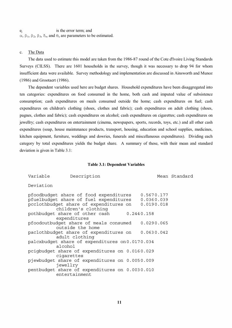
11

ej is the error term; and α, β1, β2, β3, δr, and Θs are parameters to be estimated.

c. The Data The data used to estimate this model are taken from the 1986-87 round of the Cote d'Ivoire Living Standards Surveys (CILSS). There are 1601 households in the survey, though it was necessary to drop 94 for whom insufficient data were available. Survey methodology and implementation are discussed in Ainsworth and Munoz (1986) and Grootaert (1986). The dependent variables used here are budget shares. Household expenditures have been disaggregated into ten categories: expenditures on food consumed in the home, both cash and imputed value of subsistence consumption; cash expenditures on meals consumed outside the home; cash expenditures on fuel; cash expenditures on children's clothing (shoes, clothes and fabric); cash expenditures on adult clothing (shoes, pagnes, clothes and fabric); cash expenditures on alcohol; cash expenditures on cigarettes; cash expenditures on jewellry; cash expenditures on entertainment (cinema, newspapers, sports, records, toys, etc.) and all other cash expenditures (soap, house maintenance products, transport, housing, education and school supplies, medicines, kitchen equipment, furniture, weddings and dowries, funerals and miscellaneous expenditures). Dividing each category by total expenditures yields the budget share. A summary of these, with their mean and standard deviation is given in Table 3.1:

Table 3.1: Dependent Variables Variable Description Mean Standard Deviation pfoodbudget share of food expenditures 0.567 0.177 pfuelbudget share of fuel expenditures 0.036 0.039 pcclothbudget share of expenditures on 0.019 0.018 children's clothing pothbudget share of other cash 0.244 0.158 expenditures pfoodoutbudget share of meals consumed 0.029 0.065 outside the home paclothbudget share of expenditures on 0.063 0.042 adult clothing palcxbudget share of expenditures on 0.017 0.034 alcohol pcigbudget share of expenditures on 0.016 0.029 cigarettes pjewbudget share of expenditures on 0.005 0.009 jewellry pentbudget share of expenditures on 0.003 0.010 entertainment

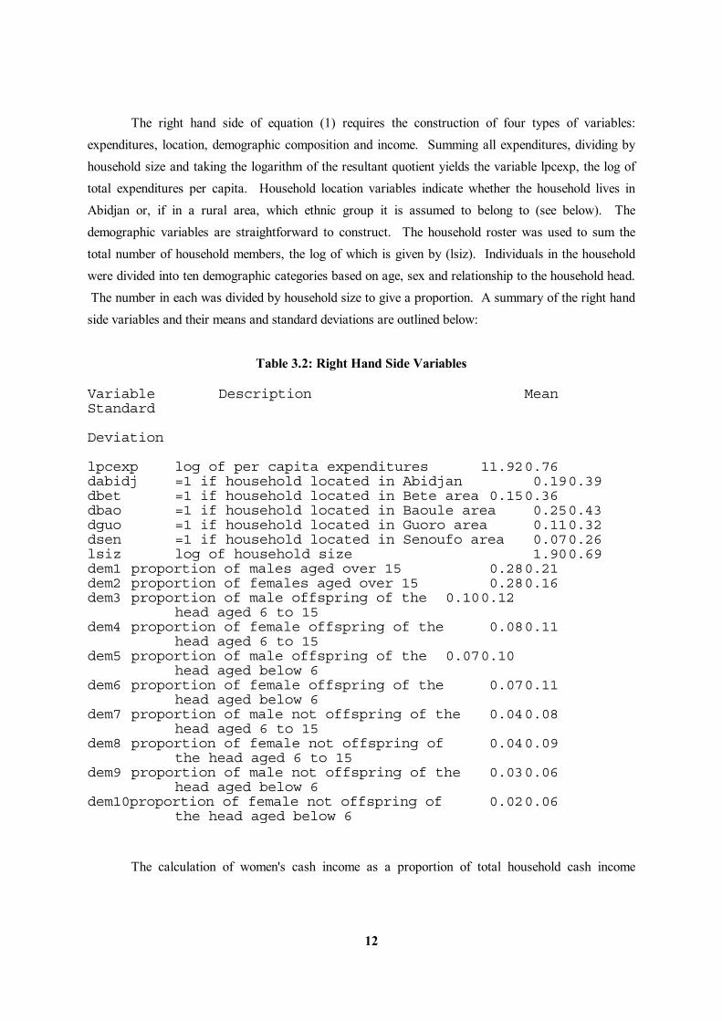
12

The right hand side of equation (1) requires the construction of four types of variables: expenditures, location, demographic composition and income. Summing all expenditures, dividing by household size and taking the logarithm of the resultant quotient yields the variable lpcexp, the log of total expenditures per capita. Household location variables indicate whether the household lives in Abidjan or, if in a rural area, which ethnic group it is assumed to belong to (see below). The demographic variables are straightforward to construct. The household roster was used to sum the total number of household members, the log of which is given by (lsiz). Individuals in the household were divided into ten demographic categories based on age, sex and relationship to the household head. The number in each was divided by household size to give a proportion. A summary of the right hand side variables and their means and standard deviations are outlined below:

Table 3.2: Right Hand Side Variables Variable Description Mean Standard Deviation lpcexp log of per capita expenditures 11.92 0.76 dabidj =1 if household located in Abidjan 0.19 0.39 dbet =1 if household located in Bete area 0.15 0.36 dbao =1 if household located in Baoule area 0.25 0.43 dguo =1 if household located in Guoro area 0.11 0.32 dsen =1 if household located in Senoufo area 0.07 0.26 lsiz log of household size 1.90 0.69 dem1 proportion of males aged over 15 0.28 0.21 dem2 proportion of females aged over 15 0.28 0.16 dem3 proportion of male offspring of the 0.10 0.12 head aged 6 to 15 dem4 proportion of female offspring of the 0.08 0.11 head aged 6 to 15 dem5 proportion of male offspring of the 0.07 0.10 head aged below 6 dem6 proportion of female offspring of the 0.07 0.11 head aged below 6 dem7 proportion of male not offspring of the 0.04 0.08 head aged 6 to 15 dem8 proportion of female not offspring of 0.04 0.09 the head aged 6 to 15 dem9 proportion of male not offspring of the 0.03 0.06 head aged below 6 dem10proportion of female not offspring of 0.02 0.06 the head aged below 6

The calculation of women's cash income as a proportion of total household cash income

13

(PFINC) is not straightforward. Because it embodies a number of strong assumptions, the approach used here is sketched out below. The first step is to calculate total household cash income. This is the sum of income derived from the following sources: sales of crops; net sales of livestock; wage employment; own business activities, remittances and miscellaneous sources. There is not sufficient detail within the survey to disaggregate the latter two by gender. However, it is possible to calculate income by gender for the other three sources. Earnings from wage employment (both in cash and in kind) were recorded on an individual basis. These have been separated into four groups: earnings by male household heads; earnings by their spouses; earnings by all adult males; and earnings by all adult females. The CILSS data set has three sources of information on earnings from own business activities. These are reported earnings from self-employment, estimates of profits from own business activities for a given period and data on income and expenses in the previous period of operation. Reported profits has been used here. This includes profits used for household consumption, profits saved, and the value of consumption of own output. Based on information in the survey data, each have been calculated on an annual basis and summed for each business enterprise. It is assumed that the person described as "the best informed to discuss the business" is the business operator and that he/she controls its profits. Own business income is calculated for the male head; all spouses of the head; all adult males; and all adult females. It should be noted that the questionnaire only records the three 'most important' (Grootaert, 1986) own business activities. Where other, more minor enterprises have been omitted, income from own business activities will be understated.150 Disaggregating the data on income from agriculture by gender is especially problematic because it was not collected on an individual specific basis. However, because the survey was cluster based, the approximate locations of households is known. Cluster locations, from Ainsworth and Munoz (1986) were matched with ethnic groups from Weekes-Vagliani (1985). Ethnographic data from Weekes-Vagliani (1985, 1990), Gastellu (1987), and Bassett (1988) was then used to assign gender control over cash from the sales of crops by cluster. It should be emphasised that the assignment of cash income from crops in this manner suffers from several limitations. Firstly, in some areas both men and women grow the same crops but separately from each other. For example, amongst the Bete, riz fafre is grown by women and riz soderiz is grown by men. There may be cases where income from crops accrues to men, but they 'pay' their wives for assistance in growing the crop. Amongst the Baoule, this is the case for cash income from yams. Here, women's income will be

150 In preliminary work, it was discovered that using income and expenses data generated negative profits for many households, including all those located in rural areas. Since it is unlikely that so many households actually obtained negative profits from own business activities, this source was not used.

14

understated. Where ethnic groups are intermingled, ethnic distinctions between households will not be picked up in the allocation of crops. This is a particular problem for households growing crops in urban areas and pastoralists. Further, variations in crop allocations within ethnic groups are not accounted for. The respondent for the questions on the section on income from crops is the individual most familiar with this information (Grootaert, 1986). Where this was the male head, there are undoubtedly cases where he did not know the extent of production by his spouse(s). Furthermore, there may be cases where women try to hide their income from their husbands. Blumberg (1987), Francis (personal communication), Olsen (1990) and Razavi (1990) report this to be the case in Honduras, western Kenya, south India and Iran respectively. Both possibilities suggest that women's cash income from crops may be understated. In addition to gender distinctions in control of crop income, there may also be generational distinctions. For example, in households headed by elderly widows, the production of certain cash crops, and the control of their income, such as coffee or cocoa, may be the responsibility of adult males. A conservative approach has been taken with the gender distinction over crops in households headed by women being maintained. Finally, it is not possible to attribute some crops to either men or women. These include rubber, wood, tobacco, sugar cane, fruit trees and pineapple and miscellaneous unnamed crops. However, this should not constitute a major problem as they constitute a small proportion of household agricultural income. Mindful of these caveats, it is assumed that cocoa, coffee and yams are always 'male crops'. Coconut palm, oil palm, plantain and bananas, peanuts, cassava, taro, sweet potato and vegetables are considered 'female crops'. Other crops are allocated in the following manner. In Bete clusters: maize and half of rice are male crops; half of rice is a female crop. In Baoule clusters: cotton is a male crop; kola nuts, maize and rice are female crops. In Guoro clusters, kola nuts, cotton, maize, rice and millet are female crops. In Senoufo clusters: cotton, sorghum, millet and maize are male crops; kola nuts and rice are female crops. Finally, it is assumed that income from goats, sheep and cattle accrues to males and that income from poultry and revenues from the transformation of homegrown crops, such as coconut oil, palm wine and ghea butter accrues to women.

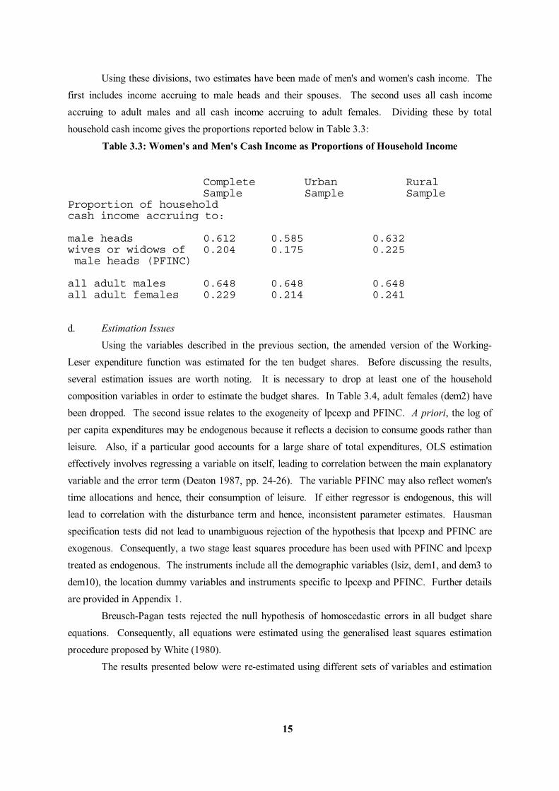
15

Using these divisions, two estimates have been made of men's and women's cash income. The first includes income accruing to male heads and their spouses. The second uses all cash income accruing to adult males and all cash income accruing to adult females. Dividing these by total household cash income gives the proportions reported below in Table 3.3:

Table 3.3: Women's and Men's Cash Income as Proportions of Household Income Complete Urban Rural Sample Sample Sample Proportion of household cash income accruing to: male heads 0.612 0.585 0.632 wives or widows of 0.204 0.175 0.225 male heads (PFINC) all adult males 0.648 0.648 0.648 all adult females 0.229 0.214 0.241

d. Estimation Issues Using the variables described in the previous section, the amended version of the Working-Leser expenditure function was estimated for the ten budget shares. Before discussing the results, several estimation issues are worth noting. It is necessary to drop at least one of the household composition variables in order to estimate the budget shares. In Table 3.4, adult females (dem2) have been dropped. The second issue relates to the exogeneity of lpcexp and PFINC. A priori, the log of per capita expenditures may be endogenous because it reflects a decision to consume goods rather than leisure. Also, if a particular good accounts for a large share of total expenditures, OLS estimation effectively involves regressing a variable on itself, leading to correlation between the main explanatory variable and the error term (Deaton 1987, pp. 24-26). The variable PFINC may also reflect women's time allocations and hence, their consumption of leisure. If either regressor is endogenous, this will lead to correlation with the disturbance term and hence, inconsistent parameter estimates. Hausman specification tests did not lead to unambiguous rejection of the hypothesis that lpcexp and PFINC are exogenous. Consequently, a two stage least squares procedure has been used with PFINC and lpcexp treated as endogenous. The instruments include all the demographic variables (lsiz, dem1, and dem3 to dem10), the location dummy variables and instruments specific to lpcexp and PFINC. Further details are provided in Appendix 1. Breusch-Pagan tests rejected the null hypothesis of homoscedastic errors in all budget share equations. Consequently, all equations were estimated using the generalised least squares estimation procedure proposed by White (1980). The results presented below were re-estimated using different sets of variables and estimation

16

procedures. Employing a generalised seemingly unrelated regression did not yield qualitatively different results. In preliminary runs, the instruments for PFINC, rather than PFINC itself, were included. The parameters for these variables exhibited a similar pattern of sign and significance to PFINC. Finally, the model was estimated using a number of different measures of PFINC. While these generated some changes in the magnitude of the parameters, there was no change in the pattern of the signs.

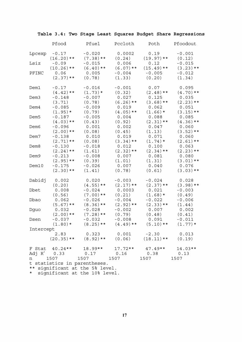
17

Table 3.4: Two Stage Least Squares Budget Share Regressions Pfood Pfuel Pccloth Poth Pfoodout Lpcexp -0.17 -0.020 0.0002 0.19 -0.001 (16.20)** (7.38)** (0.24) (19.97)** (0.12) Lsiz -0.09 -0.015 0.006 0.12 -0.015 (10.26)** (6.40)** (6.07)** (15.49)** (3.23)** PFINC 0.06 0.005 -0.004 -0.005 -0.012 (2.37)** (0.78) (1.33) (0.20) (1.34) Dem1 -0.17 -0.016 -0.001 0.07 0.095 (4.42)** (1.73)* (0.32) (2.48)** (4.70)** Dem3 -0.148 -0.007 0.027 0.125 0.035 (3.71) (0.78) (6.26)** (3.68)** (2.23)** Dem4 -0.085 -0.009 0.019 0.062 0.051 (1.95)* (0.79) (4.05)** (1.66)* (3.15)** Dem5 -0.187 -0.005 0.004 0.088 0.085 (4.03)** (0.43) (0.92) (2.31)** (4.36)** Dem6 -0.096 0.001 0.002 0.047 0.060 (2.00)** (0.08) (0.45) (1.13) (3.52)** Dem7 -0.138 0.010 0.019 0.071 0.060 (2.71)** (0.08) (3.34)** (1.74)* (2.61)** Dem8 -0.130 -0.018 0.012 0.100 0.063 (2.24)** (1.61) (2.32)** (2.34)** (2.23)** Dem9 -0.213 -0.008 0.007 0.081 0.080 (2.95)** (0.39) (1.01) (1.31) (3.01)** Dem10 -0.175 -0.026 0.007 0.040 0.076 (2.30)** (1.41) (0.78) (0.61) (3.03)** Dabidj 0.002 0.020 -0.003 -0.024 0.028 (0.20) (4.55)** (2.17)** (2.37)** (3.98)** Dbet 0.008 -0.024 0.0003 0.021 -0.003 (0.56) (7.00)** (0.21) (1.68)* (0.49) Dbao 0.062 -0.026 -0.004 -0.022 -0.006 (5.67)** (8.36)** (2.92)** (2.33)** (1.44) Dguo 0.032 -0.028 -0.002 0.007 0.002 (2.00)** (7.28)** (0.79) (0.48) (0.41) Dsen -0.037 -0.032 -0.008 0.091 -0.011 (1.80)* (8.25)** (4.49)** (5.10)** (1.77)* Intercept 2.83 0.323 0.001 -2.30 0.013 (20.35)** (8.92)** (0.06) (18.11)** (0.19) F Stat 40.24** 18.99** 17.72** 47.49** 14.03** Adj R2 0.33 0.17 0.16 0.38 0.13 n 1507 1507 1507 1507 1507 t statistics in parentheses. ** significant at the 5% level. * significant at the 10% level.

18

Table 3.4 - continued Pacloth Palcx Pcig Pjew Pent Lpcexp -0.001 -0.0011 -0.008 0.003 0.006 (0.20) (0.44) (3.94)** (4.44)** (7.25)** Lsiz 0.004 -0.005 -0.007 0.002 0.002 (1.45) (2.25)** (3.54)** (3.96)** (3.68)** PFINC -0.011 -0.021 -0.011 0.00005 -0.002 (1.36) (3.88)** (2.32)** (0.03) (1.55) Dem1 -0.012 0.011 0.013 -0.003 0.006 (1.24) (1.44) (1.62) (1.66)* (2.39)** Dem3 -0.033 0.008 -0.012 -0.0005 0.005 (2.90)** (0.95) (1.85)* (0.18) (1.95)* Dem4 -0.045 0.011 -0.005 -0.001 -0.002 (3.57)** (1.21) (0.64) (0.54) (0.90) Dem5 0.006 -0.001 0.004 0.002 0.003 (0.45) (0.10) (0.43) (0.80) (1.50) Dem6 -0.008 -0.005 -0.007 -0.00002 0.006 (0.61) (0.56) (0.82) (0.01) (1.94)* Dem7 -0.031 0.020 -0.009 0.001 0.005 (1.96)** (1.44) (0.93) (0.32) (1.58) Dem8 -0.020 -0.003 -0.014 0.002 0.008 (1.29) (0.35) (1.76)* (0.71) (2.35)** Dem9 0.015 0.039 -0.008 0.003 0.004 (0.73) (2.27)** (0.61) (0.81) (1.21) Dem10 0.018 0.037 0.019 -0.0004 0.003 (0.72) (2.34)** (1.45) (0.13) (0.81) Dabidj -0.016 -0.003 -0.004 -0.001 0.0005 (4.54)** (1.27) (1.48) (0.59) (0.39) Dbet -0.003 0.003 0.001 -0.002 -0.002 (0.83) (1.17) (0.47) (3.01)** (2.72)** Dbao -0.010 0.012 -0.002 -0.002 -0.002 (2.98)** (4.49)** (1.08) (2.81)** (3.23)** Dguo -0.010 0.010 -0.003 -0.003 -0.001 (2.02)** (2.47)** (1.00) (4.57)** (1.99)** Dsen -0.015 0.010 0.002 -0.002 0.001 (3.12)** (2.05)** (0.56) (2.50)** (0.35) Intercept 0.086 0.031 0.131 -0.034 -0.078 (1.97)** (1.00) (4.70)** (3.75)** (7.13)** F Stat 4.07** 3.31** 6.19** 6.49** 8.78** Adj R2 0.03 0.03 0.06 0.06 0.11 n 1507 1507 1507 1507 1507 t statistics in parentheses. ** significant at the 5% level. * significant at the 10% level.

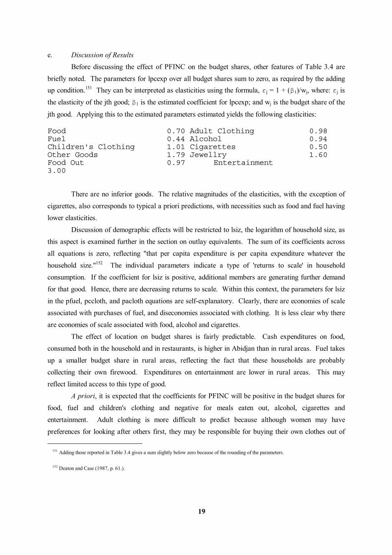
19

e. Discussion of Results Before discussing the effect of PFINC on the budget shares, other features of Table 3.4 are briefly noted. The parameters for lpcexp over all budget shares sum to zero, as required by the adding up condition.151 They can be interpreted as elasticities using the formula, εj = 1 + (β1)/wj, where: εj is the elasticity of the jth good; β1 is the estimated coefficient for lpcexp; and wj is the budget share of the

jth good. Applying this to the estimated parameters estimated yields the following elasticities: Food 0.70 Adult Clothing 0.98 Fuel 0.44 Alcohol 0.94 Children's Clothing 1.01 Cigarettes 0.50 Other Goods 1.79 Jewellry 1.60 Food Out 0.97 Entertainment 3.00

There are no inferior goods. The relative magnitudes of the elasticities, with the exception of cigarettes, also corresponds to typical a priori predictions, with necessities such as food and fuel having lower elasticities. Discussion of demographic effects will be restricted to lsiz, the logarithm of household size, as this aspect is examined further in the section on outlay equivalents. The sum of its coefficients across all equations is zero, reflecting "that per capita expenditure is per capita expenditure whatever the household size."152 The individual parameters indicate a type of 'returns to scale' in household consumption. If the coefficient for lsiz is positive, additional members are generating further demand for that good. Hence, there are decreasing returns to scale. Within this context, the parameters for lsiz in the pfuel, pccloth, and pacloth equations are self-explanatory. Clearly, there are economies of scale associated with purchases of fuel, and diseconomies associated with clothing. It is less clear why there are economies of scale associated with food, alcohol and cigarettes. The effect of location on budget shares is fairly predictable. Cash expenditures on food, consumed both in the household and in restaurants, is higher in Abidjan than in rural areas. Fuel takes up a smaller budget share in rural areas, reflecting the fact that these households are probably collecting their own firewood. Expenditures on entertainment are lower in rural areas. This may reflect limited access to this type of good. A priori, it is expected that the coefficients for PFINC will be positive in the budget shares for food, fuel and children's clothing and negative for meals eaten out, alcohol, cigarettes and entertainment. Adult clothing is more difficult to predict because although women may have preferences for looking after others first, they may be responsible for buying their own clothes out of 151 Adding those reported in Table 3.4 gives a sum slightly below zero because of the rounding of the parameters.

152 Deaton and Case (1987, p. 61.).

20

their own income and this will exert an opposite effect on the parameter sign. A similar story may hold true for jewellry, though this could reflect asset accumulation rather than consumption. The results presented in Table 3.4 are broadly consistent with these predictions. In all but the equation for children's clothing, the parameters have the sign expected if the discussion of 'maternal altruism' is correct. The coefficients of PFINC for food and fuel are positive, though the latter is not significant. They are negative and significant for two goods likely to be solely consumed by adults - alcohol and cigarettes and negative, but not significant, for meals eaten out, entertainment (which has a large number of zero observations) and adult clothing. The parameter for jewellry is positive (but not significant), possible reflecting the factors noted above. The negative coefficient on children's clothing is somewhat surprising. To investigate further, this category was disaggregated into expenditures on shoes, fabric and clothes and the budget shares of these estimated in the manner described above. PFINC was negative and significant in the regression for children's shoes and clothing and positive and significant for fabric. If certain items such as shirts and shoes are required for school, then they may be regarded as a male responsibility. This would account for the negative parameter for PFINC in the pccloth results. The magnitudes of the parameters can be used to predict the degree of change in budget shares associated with different distributions of income within the household. In Table 3.5(a), these are given where PFINC equals zero (that is, where women earn no cash income), where PFINC equals the sample mean, where women's cash income is, on average, doubled, and where all household cash income accrues to women. Table 3.5b shows the percentage changes in budget shares, relative to the mean PFINC, of doubling PFINC:

Table 3.5(a): Budget Shares at Different Levels of PFINC Budget Shares PFINC PFINC PFINC PFINC where: =0 =mean =2•mean =1 Food 0.5545 0.5670 0.5794 0.6153 Fuel 0.0349 0.0361 0.0372 0.0404 Children's 0.0195 0.0186 0.0177 0.0152 Clothing Budget Shares PFINC PFINC PFINC PFINC where: =0 =mean =2•mean =1 Other Goods 0.2452 0.2442 0.2433 0.2407 Meals Out 0.0319 0.0295 0.0272 0.0202 Adult Clothing 0.0653 0.0631 0.0609 0.0546 Alcohol 0.0213 0.0169 0.0126 0.0001 Cigarettes 0.0188 0.0165 0.0141 0.0074 Jewellry 0.0050 0.0050 0.0051 0.0051 Entertainment 0.0034 0.0029 0.0025 0.0011

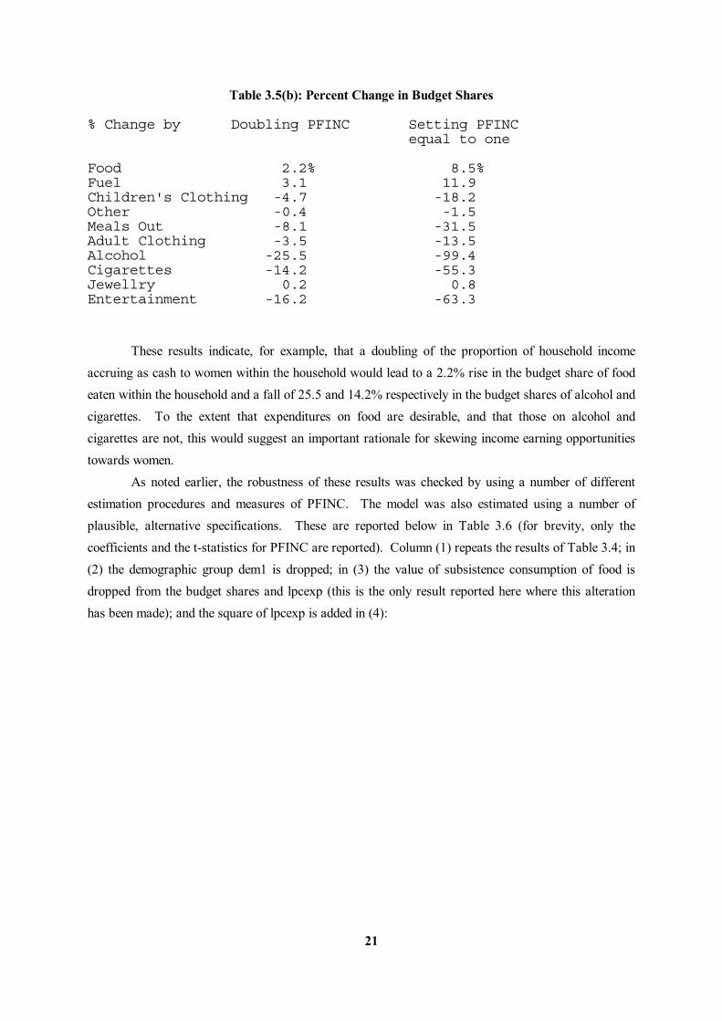
21

Table 3.5(b): Percent Change in Budget Shares % Change by Doubling PFINC Setting PFINC equal to one Food 2.2% 8.5% Fuel 3.1 11.9 Children's Clothing -4.7 -18.2 Other -0.4 -1.5 Meals Out -8.1 -31.5 Adult Clothing -3.5 -13.5 Alcohol -25.5 -99.4 Cigarettes -14.2 -55.3 Jewellry 0.2 0.8 Entertainment -16.2 -63.3 These results indicate, for example, that a doubling of the proportion of household income accruing as cash to women within the household would lead to a 2.2% rise in the budget share of food eaten within the household and a fall of 25.5 and 14.2% respectively in the budget shares of alcohol and cigarettes. To the extent that expenditures on food are desirable, and that those on alcohol and cigarettes are not, this would suggest an important rationale for skewing income earning opportunities towards women. As noted earlier, the robustness of these results was checked by using a number of different estimation procedures and measures of PFINC. The model was also estimated using a number of plausible, alternative specifications. These are reported below in Table 3.6 (for brevity, only the coefficients and the t-statistics for PFINC are reported). Column (1) repeats the results of Table 3.4; in (2) the demographic group dem1 is dropped; in (3) the value of subsistence consumption of food is dropped from the budget shares and lpcexp (this is the only result reported here where this alteration has been made); and the square of lpcexp is added in (4):

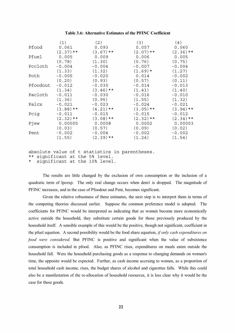
22

Table 3.6: Alternative Estimates of the PFINC Coefficient (1) (2) (3) (4) Pfood 0.061 0.093 0.057 0.060 (2.37)** (3.67)** (2.07)** (2.36)** Pfuel 0.005 0.009 0.006 0.005 (0.78) (1.30) (0.76) (0.75) Pccloth -0.004 -0.004 -0.007 -0.004 (1.33) (1.32) (1.69)* (1.27) Poth -0.005 -0.020 0.014 -0.002 (0.20) (0.93) (0.57) (0.11) Pfoodout -0.012 -0.030 -0.014 -0.013 (1.34) (3.46)** (1.41) (1.40) Pacloth -0.011 -0.030 -0.016 -0.010 (1.36) (0.95) (1.55) (1.32) Palcx -0.021 -0.023 -0.024 -0.021 (3.88)** (4.21)** (3.05)** (3.94)** Pcig -0.011 -0.015 -0.015 -0.012 (2.32)** (3.08)** (2.32)** (2.34)** Pjew 0.00005 0.0008 0.0002 0.00003 (0.03) (0.57) (0.09) (0.02) Pent -0.002 -0.004 -0.002 -0.002 (1.55) (2.39)** (1.24) (1.54) absolute value of t statistics in parentheses. ** significant at the 5% level. * significant at the 10% level.

The results are little changed by the exclusion of own consumption or the inclusion of a quadratic term of lpcexp. The only real change occurs when dem1 is dropped. The magnitude of PFINC increases, and in the case of Pfoodout and Pent, becomes significant. Given the relative robustness of these estimates, the next step is to interpret them in terms of the competing theories discussed earlier. Suppose the common preference model is adopted. The coefficients for PFINC would be interpreted as indicating that as women become more economically active outside the household, they substitute certain goods for those previously produced by the household itself. A sensible example of this would be the positive, though not significant, coefficient in the pfuel equation. A second possibility would be the food share equation, if only cash expenditures on food were considered. But PFINC is positive and significant when the value of subsistence consumption is included in pfood. Also, as PFINC rises, expenditures on meals eaten outside the household fall. Were the household purchasing goods as a response to changing demands on women's time, the opposite would be expected. Further, as cash income accruing to women, as a proportion of total household cash income, rises, the budget shares of alcohol and cigarettes falls. While this could also be a manifestation of the re-allocation of household resources, it is less clear why it would be the case for these goods.

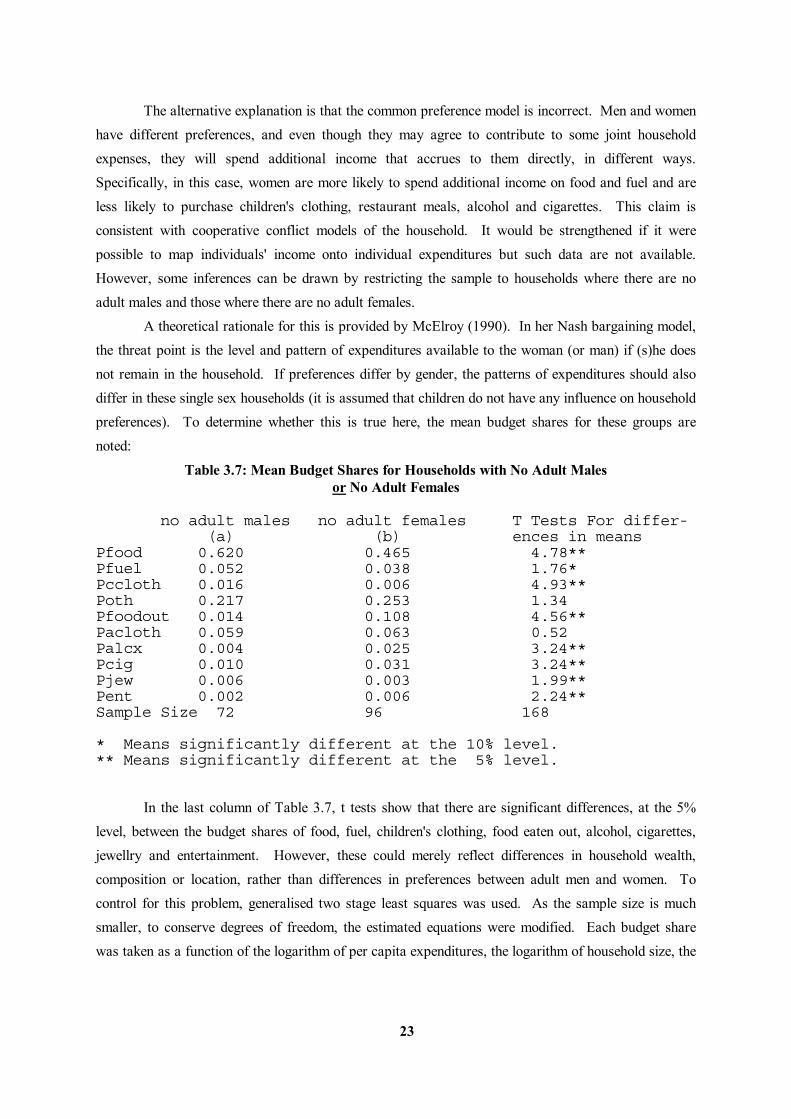
23

The alternative explanation is that the common preference model is incorrect. Men and women have different preferences, and even though they may agree to contribute to some joint household expenses, they will spend additional income that accrues to them directly, in different ways. Specifically, in this case, women are more likely to spend additional income on food and fuel and are less likely to purchase children's clothing, restaurant meals, alcohol and cigarettes. This claim is consistent with cooperative conflict models of the household. It would be strengthened if it were possible to map individuals' income onto individual expenditures but such data are not available. However, some inferences can be drawn by restricting the sample to households where there are no adult males and those where there are no adult females. A theoretical rationale for this is provided by McElroy (1990). In her Nash bargaining model, the threat point is the level and pattern of expenditures available to the woman (or man) if (s)he does not remain in the household. If preferences differ by gender, the patterns of expenditures should also differ in these single sex households (it is assumed that children do not have any influence on household preferences). To determine whether this is true here, the mean budget shares for these groups are noted:

Table 3.7: Mean Budget Shares for Households with No Adult Males or No Adult Females no adult males no adult females T Tests For differ- (a) (b) ences in means Pfood 0.620 0.465 4.78** Pfuel 0.052 0.038 1.76* Pccloth 0.016 0.006 4.93** Poth 0.217 0.253 1.34 Pfoodout 0.014 0.108 4.56** Pacloth 0.059 0.063 0.52 Palcx 0.004 0.025 3.24** Pcig 0.010 0.031 3.24** Pjew 0.006 0.003 1.99** Pent 0.002 0.006 2.24** Sample Size 72 96 168 * Means significantly different at the 10% level. ** Means significantly different at the 5% level.

In the last column of Table 3.7, t tests show that there are significant differences, at the 5% level, between the budget shares of food, fuel, children's clothing, food eaten out, alcohol, cigarettes, jewellry and entertainment. However, these could merely reflect differences in household wealth, composition or location, rather than differences in preferences between adult men and women. To control for this problem, generalised two stage least squares was used. As the sample size is much smaller, to conserve degrees of freedom, the estimated equations were modified. Each budget share was taken as a function of the logarithm of per capita expenditures, the logarithm of household size, the

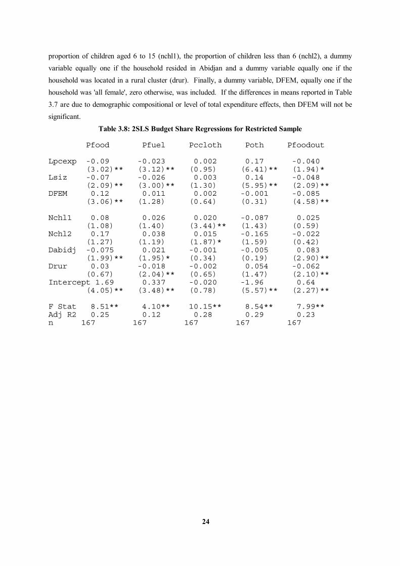
24

proportion of children aged 6 to 15 (nchl1), the proportion of children less than 6 (nchl2), a dummy variable equally one if the household resided in Abidjan and a dummy variable equally one if the household was located in a rural cluster (drur). Finally, a dummy variable, DFEM, equally one if the household was 'all female', zero otherwise, was included. If the differences in means reported in Table 3.7 are due to demographic compositional or level of total expenditure effects, then DFEM will not be significant.

Table 3.8: 2SLS Budget Share Regressions for Restricted Sample Pfood Pfuel Pccloth Poth Pfoodout Lpcexp -0.09 -0.023 0.002 0.17 -0.040 (3.02)** (3.12)** (0.95) (6.41)** (1.94)* Lsiz -0.07 -0.026 0.003 0.14 -0.048 (2.09)** (3.00)** (1.30) (5.95)** (2.09)** DFEM 0.12 0.011 0.002 -0.001 -0.085 (3.06)** (1.28) (0.64) (0.31) (4.58)** Nchl1 0.08 0.026 0.020 -0.087 0.025 (1.08) (1.40) (3.44)** (1.43) (0.59) Nchl2 0.17 0.038 0.015 -0.165 -0.022 (1.27) (1.19) (1.87)* (1.59) (0.42) Dabidj -0.075 0.021 -0.001 -0.005 0.083 (1.99)** (1.95)* (0.34) (0.19) (2.90)** Drur 0.03 -0.018 -0.002 0.054 -0.062 (0.67) (2.04)** (0.65) (1.47) (2.10)** Intercept 1.69 0.337 -0.020 -1.96 0.64 (4.05)** (3.48)** (0.78) (5.57)** (2.27)** F Stat 8.51** 4.10** 10.15** 8.54** 7.99** Adj R2 0.25 0.12 0.28 0.29 0.23 n 167 167 167 167 167

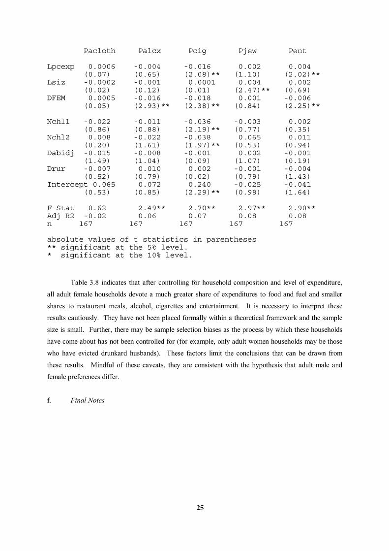
25

Pacloth Palcx Pcig Pjew Pent Lpcexp 0.0006 -0.004 -0.016 0.002 0.004 (0.07) (0.65) (2.08)** (1.10) (2.02)** Lsiz -0.0002 -0.001 0.0001 0.004 0.002 (0.02) (0.12) (0.01) (2.47)** (0.69) DFEM 0.0005 -0.016 -0.018 0.001 -0.006 (0.05) (2.93)** (2.38)** (0.84) (2.25)** Nchl1 -0.022 -0.011 -0.036 -0.003 0.002 (0.86) (0.88) (2.19)** (0.77) (0.35) Nchl2 0.008 -0.022 -0.038 0.065 0.011 (0.20) (1.61) (1.97)** (0.53) (0.94) Dabidj -0.015 -0.008 -0.001 0.002 -0.001 (1.49) (1.04) (0.09) (1.07) (0.19) Drur -0.007 0.010 0.002 -0.001 -0.004 (0.52) (0.79) (0.02) (0.79) (1.43) Intercept 0.065 0.072 0.240 -0.025 -0.041 (0.53) (0.85) (2.29)** (0.98) (1.64) F Stat 0.62 2.49** 2.70** 2.97** 2.90** Adj R2 -0.02 0.06 0.07 0.08 0.08 n 167 167 167 167 167 absolute values of t statistics in parentheses ** significant at the 5% level. * significant at the 10% level.

Table 3.8 indicates that after controlling for household composition and level of expenditure, all adult female households devote a much greater share of expenditures to food and fuel and smaller shares to restaurant meals, alcohol, cigarettes and entertainment. It is necessary to interpret these results cautiously. They have not been placed formally within a theoretical framework and the sample size is small. Further, there may be sample selection biases as the process by which these households have come about has not been controlled for (for example, only adult women households may be those who have evicted drunkard husbands). These factors limit the conclusions that can be drawn from these results. Mindful of these caveats, they are consistent with the hypothesis that adult male and female preferences differ. f. Final Notes

26

Before continuing to a discussion of outlay equivalents, it is useful to take stock of the results reported obtained thus far. In the Cote d'Ivoire, raising women's income share of household cash income causes the budget share of food to rise, and the budget shares of meals consumed outside the household, alcohol and cigarettes to fall. This result is robust to alternative specifications of the expenditure equation, different estimation procedures and takes into account the endogeneity of PFINC. Though no formal test is presented, evidence from single (adult) sex households is consistent with bargaining models of household expenditure.

4. An Outlay Equivalent Analysis of Expenditure on Adult Goods a.Introduction In this section, attention is turned to the second issue addressed in this paper: Do Ivorian households differentiate between boys and girls in the allocation of household resources? One way of measuring this is to examine how expenditure patterns on goods consumed exclusively by adults differ according to household age-gender composition. This is Deaton's (1987, 1989) 'outlay equivalent' approach and discussion here begins with a brief review of his methodology. Following a test for the adequacy of the hypothesised adult goods, attention is then turned to the possibility of gender differences in household resource allocation. Deaton, using data from the 1985-86 CILSS, found little evidence to support the hypothesis that boys are treated differently compared to girls with respect to the amount of adult goods expenditure foregone by the household. Here, his analysis is extended by refining the household demographic groups into offspring of household head and non-offspring children (who tend to be adopted or are simply residing in the family for school purposes). Of primary interest is whether a child's gender or relationship to head of household affects the magnitude of the decline in the budget shares of adult goods. b.Estimation "The basic idea [behind the 'outlay equivalent' approach] is to use expenditure on some "adult" good or goods, known not to be consumed by children, as an indicator of the extent to which parents give up their own consumption to provide the resources required by the child" (Subramanian and Deaton, 1990 p. 9). Consider two types of goods consumed by a household: food and alcohol. What affect would an additional child have on that household's demand for those goods. A priori, her effect on the consumption of food is difficult to ascertain. The cost of raising an extra child could reduce food spent on adults, but this may not be observed in a household survey because of the food's substitutability among household members. However, it is possible that alcohol consumption would also fall. This reduction is analagous to an income effect, that is, the household's budget line is

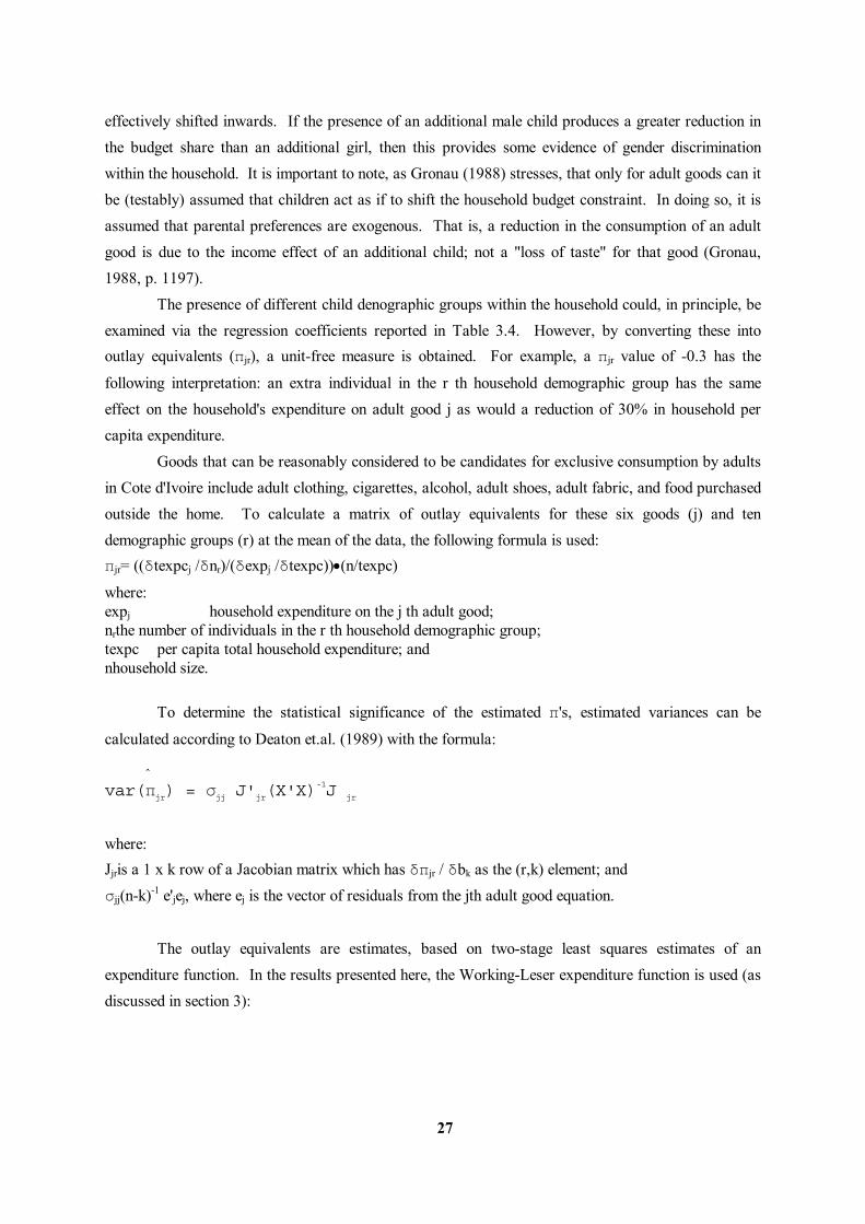
27

effectively shifted inwards. If the presence of an additional male child produces a greater reduction in the budget share than an additional girl, then this provides some evidence of gender discrimination within the household. It is important to note, as Gronau (1988) stresses, that only for adult goods can it be (testably) assumed that children act as if to shift the household budget constraint. In doing so, it is assumed that parental preferences are exogenous. That is, a reduction in the consumption of an adult good is due to the income effect of an additional child; not a "loss of taste" for that good (Gronau, 1988, p. 1197). The presence of different child denographic groups within the household could, in principle, be examined via the regression coefficients reported in Table 3.4. However, by converting these into outlay equivalents (πjr), a unit-free measure is obtained. For example, a πjr value of -0.3 has the

following interpretation: an extra individual in the r th household demographic group has the same effect on the household's expenditure on adult good j as would a reduction of 30% in household per capita expenditure. Goods that can be reasonably considered to be candidates for exclusive consumption by adults in Cote d'Ivoire include adult clothing, cigarettes, alcohol, adult shoes, adult fabric, and food purchased outside the home. To calculate a matrix of outlay equivalents for these six goods (j) and ten demographic groups (r) at the mean of the data, the following formula is used: πjr= ((δtexpcj /δnr)/(δexpj /δtexpc))•(n/texpc)

where: expj household expenditure on the j th adult good; nrthe number of individuals in the r th household demographic group; texpc per capita total household expenditure; and nhousehold size. To determine the statistical significance of the estimated π's, estimated variances can be

calculated according to Deaton et.al. (1989) with the formula:

^

var(πjr) = σjj J'jr(X'X)-1J jr

where: Jjris a 1 x k row of a Jacobian matrix which has δπjr / δbk as the (r,k) element; and σjj(n-k)-1 e'jej, where ej is the vector of residuals from the jth adult good equation.

The outlay equivalents are estimates, based on two-stage least squares estimates of an expenditure function. In the results presented here, the Working-Leser expenditure function is used (as discussed in section 3):

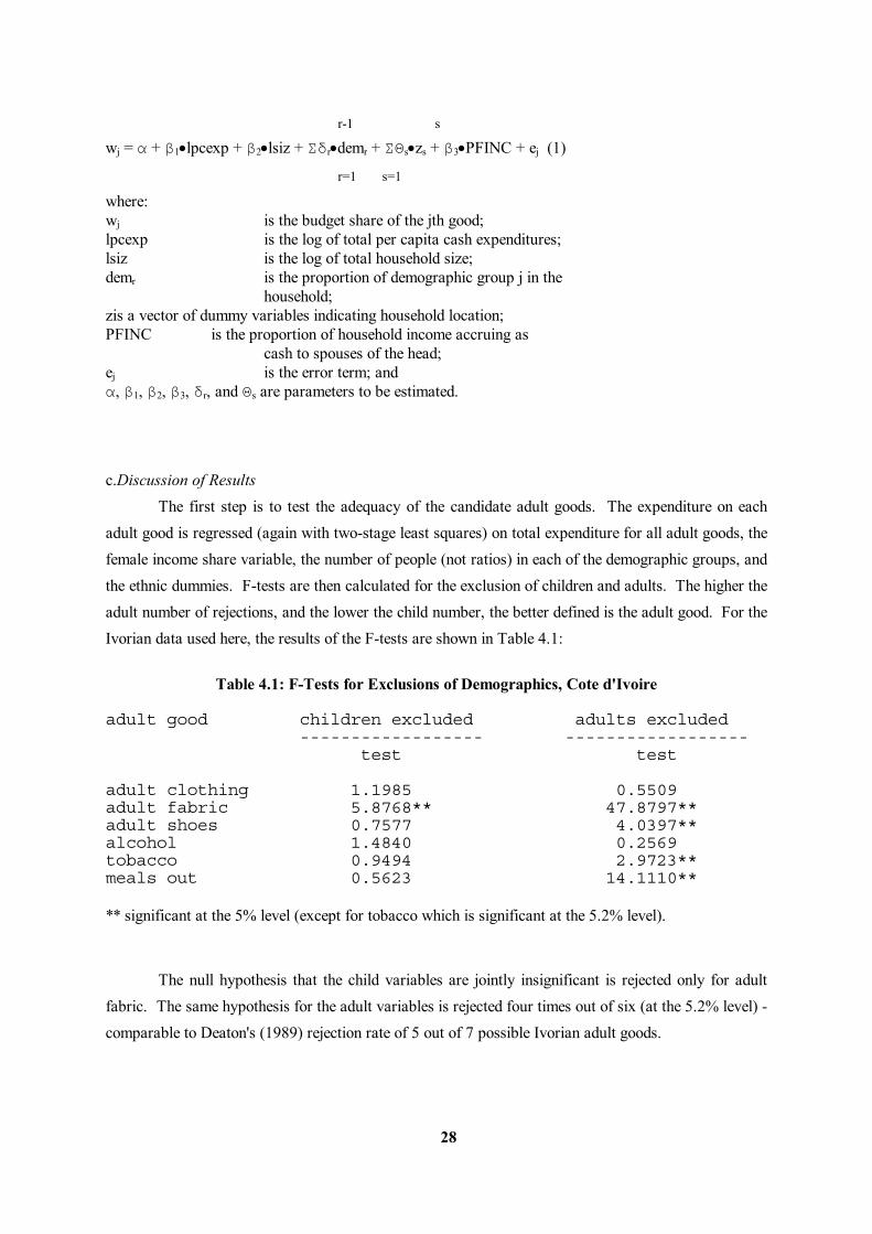
28

r-1 s wj = α + β1•lpcexp + β2•lsiz + Σδr•demr + ΣΘs•zs + β3•PFINC + ej (1)

r=1 s=1 where: wj is the budget share of the jth good; lpcexp is the log of total per capita cash expenditures; lsiz is the log of total household size; demr is the proportion of demographic group j in the household; zis a vector of dummy variables indicating household location; PFINC is the proportion of household income accruing as cash to spouses of the head; ej is the error term; and α, β1, β2, β3, δr, and Θs are parameters to be estimated.

c.Discussion of Results The first step is to test the adequacy of the candidate adult goods. The expenditure on each adult good is regressed (again with two-stage least squares) on total expenditure for all adult goods, the female income share variable, the number of people (not ratios) in each of the demographic groups, and the ethnic dummies. F-tests are then calculated for the exclusion of children and adults. The higher the adult number of rejections, and the lower the child number, the better defined is the adult good. For the Ivorian data used here, the results of the F-tests are shown in Table 4.1: Table 4.1: F-Tests for Exclusions of Demographics, Cote d'Ivoire adult good children excluded adults excluded ------------------ ------------------ test test adult clothing 1.1985 0.5509 adult fabric 5.8768** 47.8797** adult shoes 0.7577 4.0397** alcohol 1.4840 0.2569 tobacco 0.9494 2.9723** meals out 0.5623 14.1110** ** significant at the 5% level (except for tobacco which is significant at the 5.2% level). The null hypothesis that the child variables are jointly insignificant is rejected only for adult fabric. The same hypothesis for the adult variables is rejected four times out of six (at the 5.2% level) - comparable to Deaton's (1989) rejection rate of 5 out of 7 possible Ivorian adult goods.

29

Table 4.2 presents the 6 by 10 matrix of outlay equivalents for the Ivorian data. If the selection of adult goods and their measurement is accurate, all 24 coefficients on the dem3 - dem6 variables (for the 6 adult goods) for boys and girls who are offspring of the head of household (hoh) should be negative. From Table 4.2, 20 of the 24 outlay equivalents are negative as expected. For the children in the 6-15 age group who are not offspring of the household head, 10 out of 12 coefficients are negative. This is in stark contrast to the non-household head offspring children under 6 years old for whom only 1 of the 12 coefficients is negative. Using CILSS data, Strauss and Mehra (1989) report that foster children have a lower incidence of stunting than children of the household head, which they speculate could be because healthier children may be selected to be fostered in and out of households. If this is the case here, these children may have a less negative income effect on adult good expenditure. Table 4.3 presents F-tests across different gender and relationship-to-hoh groups for the six adult goods and their sum. Tests for the equality of a πjr value across demographic groups use the

estimated Engel coefficients. In general the F-statistics are small. At the 10% level only 1 null hypothesis of gender equality can be rejected (alcohol: non-hoh boys vs non-hoh girls, 6-15 years old). The results are more precise for hoh-nonhoh comparisons, but still only 7 of the 28 null hypotheses of coefficient equality are rejected.

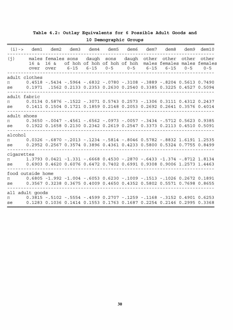
30

Table 4.2: Outlay Equivalents for 6 Possible Adult Goods and

10 Demographic Groups ════════════════════════════════════════════════════════════════════════════ (i)-> dem1 dem2 dem3 dem4 dem5 dem6 dem7 dem8 dem9 dem10 ---------------------------------------------------------------------------- (j) males females sons daugh sons daugh other other other other 16 & 16 & of hoh of hoh of hoh of hoh males females males females over over 6-15 6-15 0-5 0-5 6-15 6-15 0-5 0-5 ---------------------------------------------------------------------------- adult clothes π 0.4518 -.5434 -.5964 -.6832 -.0780 -.3108 -.3889 -.8204 0.5613 0.7490 se 0.1971 .1562 0.2133 0.2353 0.2630 0.2540 0.3385 0.3225 0.4527 0.5094 ---------------------------------------------------------------------------- adult fabric π 0.0134 0.5876 -.1522 -.3071 0.5743 0.2573 -.1306 0.3111 0.4312 0.2437 se 0.1411 0.1504 0.1721 0.1859 0.2148 0.2053 0.2692 0.2641 0.3576 0.4014 ---------------------------------------------------------------------------- adult shoes π 0.3650 -.0047 -.4561 -.6562 -.0973 -.0057 -.3434 -.5712 0.5623 0.9385 se 0.1922 0.1658 0.2130 0.2342 0.2619 0.2547 0.3373 0.2113 0.4510 0.5091 ---------------------------------------------------------------------------- alcohol π 0.0326 -.6870 -.2013 -.1234 -.5814 -.8046 0.5782 -.8832 1.6191 1.2535 se 0.2952 0.2567 0.3574 0.3896 0.4361 0.4233 0.5800 0.5324 0.7755 0.8499 ---------------------------------------------------------------------------- cigarettes π 1.3793 0.0421 -1.331 -.6668 0.4530 -.2870 -.6433 -1.374 -.8712 1.8134 se 0.6903 0.4620 0.6076 0.6472 0.7402 0.6991 0.9308 0.9006 1.2573 1.4463 ---------------------------------------------------------------------------- food outside home π 0.6805 -1.992 -1.004 -.6053 0.6230 -.1009 -.1513 -.1026 0.2672 0.1891 se 0.3567 0.3238 0.3675 0.4009 0.4650 0.4352 0.5802 0.5571 0.7698 0.8655 ---------------------------------------------------------------------------- all adult goods π 0.3815 -.5102 -.5554 -.4599 0.2707 -.1259 -.1168 -.3152 0.4901 0.6253 se 0.1283 0.1036 0.1414 0.1553 0.1763 0.1687 0.2254 0.2146 0.2995 0.3368 ════════════════════════════════════════════════════════════════════════════

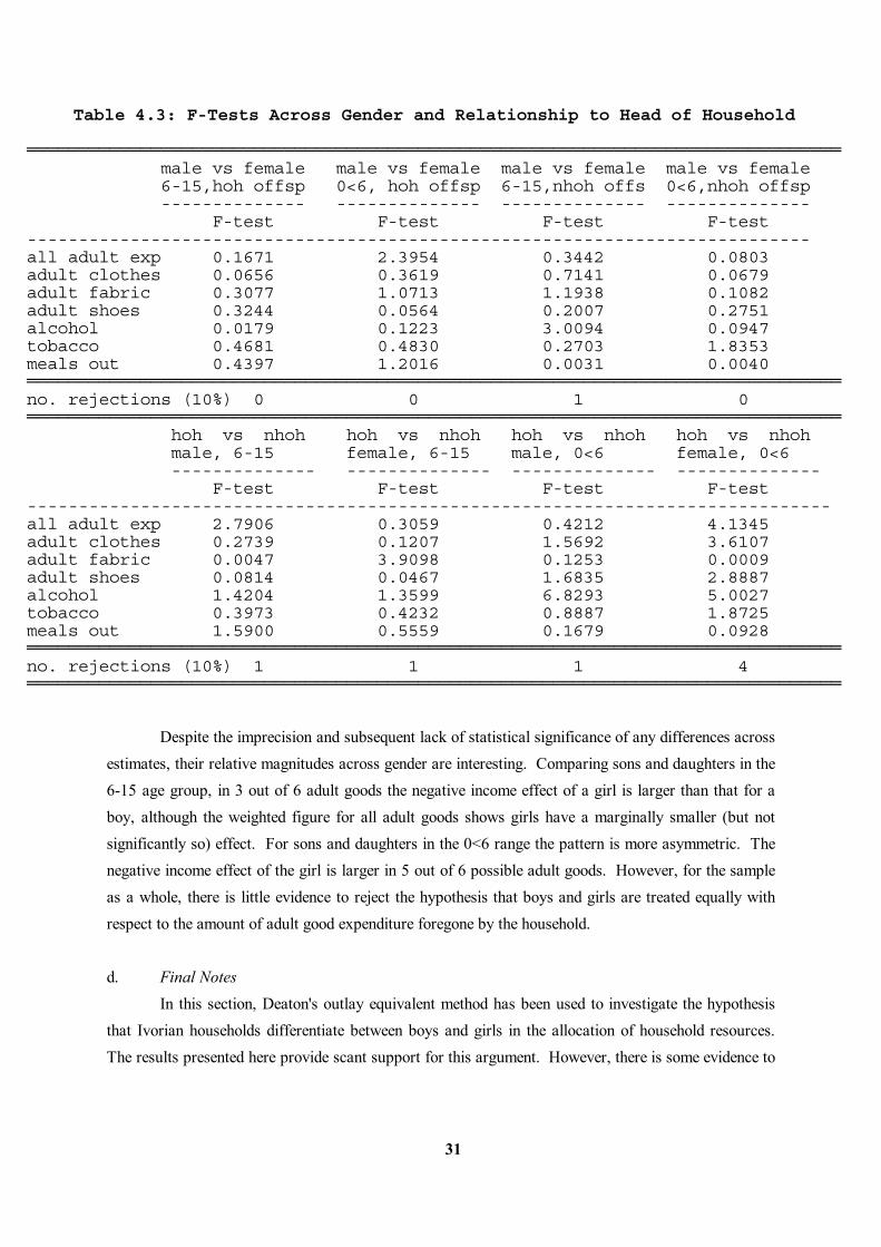
31

Table 4.3: F-Tests Across Gender and Relationship to Head of Household ═══════════════════════════════════════════════════════════════════════════════ male vs female male vs female male vs female male vs female 6-15,hoh offsp 0<6, hoh offsp 6-15,nhoh offs 0<6,nhoh offsp -------------- -------------- -------------- -------------- F-test F-test F-test F-test ---------------------------------------------------------------------------- all adult exp 0.1671 2.3954 0.3442 0.0803 adult clothes 0.0656 0.3619 0.7141 0.0679 adult fabric 0.3077 1.0713 1.1938 0.1082 adult shoes 0.3244 0.0564 0.2007 0.2751 alcohol 0.0179 0.1223 3.0094 0.0947 tobacco 0.4681 0.4830 0.2703 1.8353 meals out 0.4397 1.2016 0.0031 0.0040 ═══════════════════════════════════════════════════════════════════════════════ no. rejections (10%) 0 0 1 0 ═══════════════════════════════════════════════════════════════════════════════ hoh vs nhoh hoh vs nhoh hoh vs nhoh hoh vs nhoh male, 6-15 female, 6-15 male, 0<6 female, 0<6 -------------- -------------- -------------- -------------- F-test F-test F-test F-test ------------------------------------------------------------------------------ all adult exp 2.7906 0.3059 0.4212 4.1345 adult clothes 0.2739 0.1207 1.5692 3.6107 adult fabric 0.0047 3.9098 0.1253 0.0009 adult shoes 0.0814 0.0467 1.6835 2.8887 alcohol 1.4204 1.3599 6.8293 5.0027 tobacco 0.3973 0.4232 0.8887 1.8725 meals out 1.5900 0.5559 0.1679 0.0928 ═══════════════════════════════════════════════════════════════════════════════ no. rejections (10%) 1 1 1 4 ═══════════════════════════════════════════════════════════════════════════════

Despite the imprecision and subsequent lack of statistical significance of any differences across estimates, their relative magnitudes across gender are interesting. Comparing sons and daughters in the 6-15 age group, in 3 out of 6 adult goods the negative income effect of a girl is larger than that for a boy, although the weighted figure for all adult goods shows girls have a marginally smaller (but not significantly so) effect. For sons and daughters in the 0<6 range the pattern is more asymmetric. The negative income effect of the girl is larger in 5 out of 6 possible adult goods. However, for the sample as a whole, there is little evidence to reject the hypothesis that boys and girls are treated equally with respect to the amount of adult good expenditure foregone by the household. d. Final Notes In this section, Deaton's outlay equivalent method has been used to investigate the hypothesis that Ivorian households differentiate between boys and girls in the allocation of household resources. The results presented here provide scant support for this argument. However, there is some evidence to

32

suggest that households sacrifice fewer adult goods in the presence of boys and girls who are not offspring of the household head.

5. An Anthropometric Analysis of Gender Differentials a.Introduction In section 3, analysis focused on the role of the intrahousehold distribution of income on household expenditures. Section 4 examined the extent of gender differentials in the allocation of resources using outlay equivalents. This section combines both aspects in an examination of the determinants of anthropometric status of rural preschoolers in the Cote d'Ivoire. Specifically, it addresses two issues: (1) does the effect of the household's female income share vary across the gender of the child, and (2) are community characteristics important, and do they vary across gender of the child? Strauss' (1990) analysis of the 1985-86 CILSS anthropometric data is used to guide the approach taken here, partly to make comparisons more valid, but also because the reduced-form specification he employs minimises the substantial number of potential econometric problems. Further, his use of panel data models provides a means of accounting for unobserved household effects. The thrust of Strauss' paper is the exploitation of the community data which are available for households in the rural clusters (57 out of 100). He shows that community level variables, when interacted with mothers education, are at least as important as household and individual level information in the determination of standardized heights and weights of preschoolers. His approach is extended here, with the gender of preschooler as the disaggregation of primary interest. This makes it possible to address such questions as: would community-level improvements in health and infrastructure have a bigger impact on the health status of male or female preschoolers? In addition, the percentage share of household income earned by female household members and household total expenditure per capita, are included as extra regressors (both instrumented as in section 3). This approach risks diluting the purity of the reduced form specification by imposing some structure in order to gain further insights into the processes that generate child growth. It does not permit a distinction to be made between the common and individual preferences hypotheses of intra-household allocation (only unearned income, of which there is very little in this data set, would, under certain conditions, permit this disentanglement). Nevertheless, including these two variables makes it possible to test whether an increase in women's income share has a gender differentiated effect on the growth of her children.

33

b.Data and Variables (i) Sample size Using the 1986-87 CILSS data, mother-father-preschooler groupings were located within each household for which there are body measurements. This eliminates children from female-headed households as there are no female headed households that have a resident father who has been measured. This decision is taken because to include fathers height and education in the reduced form anthropometric equations, though as noted below, these two paternal variables do not add much to the analysis. Of the 12,912 individuals in the sample, 6,472 had their mother resident in the same household. Of these individuals, 5,109 also had resident fathers. After selecting households that contain at least two children, a sample of 559 children from 212 households remains.153 These households contain 323 mothers, and 304 children belong to households in which more than one mother is present (i.e. where the number of children in the household is greater than the number of siblings a child in that household has). The sample is restricted to children under 5 years of age as children in this age group are thought to be at greatest nutritional risk.154 (ii) Dependent variables The variables PCTHA and PCTWL represent respectively the percentage of NCHS median height-for-age and weight-for-height observed on children under 60 months of age. These two anthropometric variables represent one type of health status measure. Undoubtably, these indicators will be subject to measurement problems, and reliance on one set of measurements for a description of health status is never satisfactory. However, the data do not contain other health indicators (apart from self-recorded morbidity data), thus a latent-variable approach is not feasible. One source of comfort on the accuracy front is the close correspondence between the measurements taken two weeks apart on a subset of individuals. Of the two indicators, PCTHA is considered a measure of health status in the long run, while PCTWL is a measure that is much more sensitive to a short-run fluctuations in the levels of health inputs. Although the information contained in the questionnaire is sufficient to construct the anthropometric variables, height for age and weight for height, for 2,280 and 2,267 preschoolers respectively, the regression sample (as explained below) is necessarily much smaller. Nevertheless, it is useful, as in Tables 5.1-5.3, to examine anthropometric indicators for the larger samples in order to compare them with those constructed by Sahn (1989) for the 1985-6 CILSS data.

153 Preschoolers from two sample clusters were removed from the regression sample due to incomplete information on daily wage rates. It is not obvious whether there are any selectivity problems because of these omitted clusters.

154 The tradeoff incurred in excluding those in the 60<72 month age range is that the regression sample size may become too small to generate small estimated standard errors.

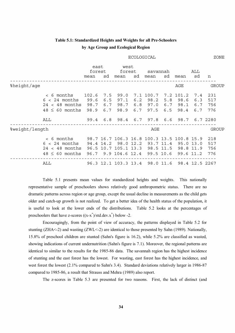
34

Table 5.1: Standardized Heights and Weights for all Pre-Schoolers by Age Group and Ecological Region ECOLOGICAL ZONE east west forest forest savannah ALL mean sd mean sd mean sd mean sd n --------------------------------------------------------------------------- %height/age AGE GROUP < 6 months 102.6 7.5 99.0 7.1 100.7 7.2 101.2 7.4 231 6 < 24 months 99.6 6.5 97.1 6.2 98.2 5.8 98.6 6.3 517 24 < 48 months 98.7 6.7 98.7 6.8 97.0 6.7 98.1 6.7 756 48 ≤ 60 months 98.9 6.7 98.9 6.7 97.5 6.5 98.4 6.7 776 ALL 99.4 6.8 98.4 6.7 97.8 6.6 98.7 6.7 2280 --------------------------------------------------------------------------- %weight/length AGE GROUP < 6 months 98.7 16.7 106.3 16.8 100.3 13.5 100.8 15.9 218 6 < 24 months 94.4 14.2 98.0 12.2 93.7 11.4 95.0 13.0 517 24 < 48 months 96.5 10.7 105.1 13.3 98.5 11.5 98.8 11.9 756 48 ≤ 60 months 96.7 9.9 104.6 12.4 99.5 10.6 99.6 11.2 776 --------------------------------------------------------------------------- ALL 96.3 12.1 103.3 13.4 98.0 11.6 98.4 12.5 2267

Table 5.1 presents mean values for standardized heights and weights. This nationally representative sample of preschoolers shows relatively good anthropometric status. There are no dramatic patterns across region or age group, except the usual decline in measurements as the child gets older and catch-up growth is not realized. To get a better idea of the health status of the population, it is useful to look at the lower ends of the distributions. Table 5.2 looks at the percentages of preschoolers that have z-scores ((x-x*)/std.dev.x*) below -2. Encouragingly, from the point of view of accuracy, the patterns displayed in Table 5.2 for stunting (ZHA<-2) and wasting (ZWL<-2) are identical to those presented by Sahn (1989). Nationally, 15.8% of preschool children are stunted (Sahn's figure is 16.2), while 5.2% are classified as wasted, showing indications of current undernutrition (Sahn's figure is 7.1). Moreover, the regional patterns are identical to similar to the results for the 1985-86 data. The savannah region has the highest incidence of stunting and the east forest has the lowest. For wasting, east forest has the highest incidence, and west forest the lowest (2.1% compared to Sahn's 3.4). Standard deviations relatively larger in 1986-87 compared to 1985-86, a result that Strauss and Mehra (1989) also report. The z-scores in Table 5.3 are presented for two reasons. First, the lack of distinct (and

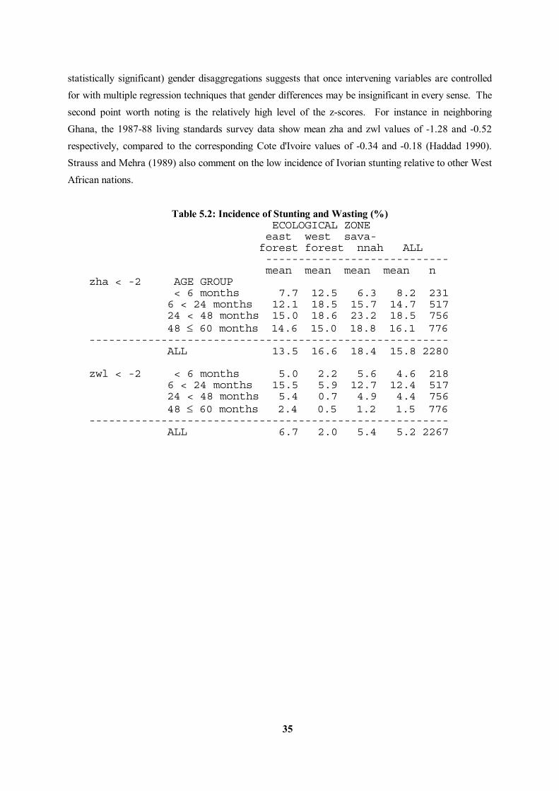
35

statistically significant) gender disaggregations suggests that once intervening variables are controlled for with multiple regression techniques that gender differences may be insignificant in every sense. The second point worth noting is the relatively high level of the z-scores. For instance in neighboring Ghana, the 1987-88 living standards survey data show mean zha and zwl values of -1.28 and -0.52 respectively, compared to the corresponding Cote d'Ivoire values of -0.34 and -0.18 (Haddad 1990). Strauss and Mehra (1989) also comment on the low incidence of Ivorian stunting relative to other West African nations.

Table 5.2: Incidence of Stunting and Wasting (%) ECOLOGICAL ZONE east west sava- forest forest nnah ALL ---------------------------- mean mean mean mean n zha < -2 AGE GROUP < 6 months 7.7 12.5 6.3 8.2 231 6 < 24 months 12.1 18.5 15.7 14.7 517 24 < 48 months 15.0 18.6 23.2 18.5 756 48 ≤ 60 months 14.6 15.0 18.8 16.1 776 ------------------------------------------------------- ALL 13.5 16.6 18.4 15.8 2280 zwl < -2 < 6 months 5.0 2.2 5.6 4.6 218 6 < 24 months 15.5 5.9 12.7 12.4 517 24 < 48 months 5.4 0.7 4.9 4.4 756 48 ≤ 60 months 2.4 0.5 1.2 1.5 776 ------------------------------------------------------- ALL 6.7 2.0 5.4 5.2 2267

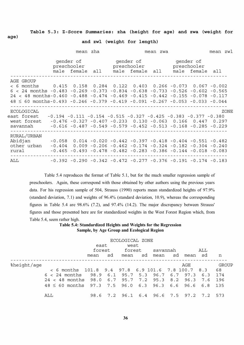
36

Table 5.3: Z-Score Summaries: zha (height for age) and zwa (weight for age) and zwl (weight for length) mean zha mean zwa mean zwl gender of gender of gender of preschooler preschooler preschooler male female all male female all male female all ---------------------------------------------------------------------------- AGE GROUP < 6 months 0.415 0.158 0.284 0.122 0.403 0.266 -0.073 0.067 -0.002 6 < 24 months -0.483 -0.269 -0.373 -0.834 -0.638 -0.733 -0.526 -0.602 -0.565 24 < 48 months-0.460 -0.488 -0.474 -0.469 -0.415 -0.442 -0.155 -0.078 -0.117 48 ≤ 60 months-0.493 -0.246 -0.379 -0.419 -0.091 -0.267 -0.053 -0.033 -0.044 ---------------------------------------------------------------------------- ECOLOGICAL ZONE east forest -0.194 -0.111 -0.154 -0.515 -0.327 -0.425 -0.383 -0.377 -0.380 west forest -0.476 -0.327 -0.407 -0.233 0.130 -0.063 0.166 0.447 0.297 savannah -0.616 -0.487 -0.549 -0.579 -0.452 -0.513 -0.168 -0.285 -0.229 ---------------------------------------------------------------------------- RURAL/URBAN Abidjan -0.058 0.014 -0.020 -0.442 -0.397 -0.418 -0.404 -0.551 -0.482 other urban -0.404 0.009 -0.206 -0.462 -0.174 -0.324 -0.182 -0.304 -0.240 rural -0.465 -0.493 -0.478 -0.482 -0.283 -0.386 -0.144 -0.018 -0.083 ---------------------------------------------------------------------------- ALL -0.392 -0.290 -0.342 -0.472 -0.277 -0.376 -0.191 -0.174 -0.183

Table 5.4 reproduces the format of Table 5.1, but for the much smaller regression sample of preschoolers. Again, these correspond with those obtained by other authors using the previous years data. For his regression sample of 504, Strauss (1990) reports mean standardized heights of 97.9% (standard deviation, 7.1) and weights of 96.4% (standard deviation, 10.9), whereas the corresponding figures in Table 5.4 are 98.6% (7.2), and 97.4% (14.2). The major discrepancy between Strauss' figures and those presented here are for standardized weights in the West Forest Region which, from Table 5.4, seem rather high.

Table 5.4: Standardized Heights and Weights for the Regression Sample, by Age Group and Ecological Region ECOLOGICAL ZONE east west forest forest savannah ALL mean sd mean sd mean sd mean sd n ---------------------------------------------------------------------------- %height/age AGE GROUP < 6 months 101.8 9.4 97.8 6.9 101.6 7.8 100.7 8.3 68 6 < 24 months 98.9 6.1 95.7 5.3 96.7 6.7 97.3 6.3 174 24 < 48 months 98.0 6.7 95.7 7.2 95.3 8.2 96.3 7.6 196 48 ≤ 60 months 97.3 7.5 96.0 6.3 96.3 6.6 96.6 6.8 135 ALL 98.6 7.2 96.1 6.4 96.6 7.5 97.2 7.2 573

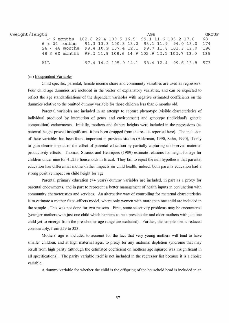
37

%weight/length AGE GROUP < 6 months 102.8 22.4 109.5 16.5 99.1 11.6 103.2 17.8 68 6 < 24 months 91.3 13.3 100.3 13.2 93.1 11.9 94.0 13.0 174 24 < 48 months 99.4 10.9 107.4 12.1 99.7 11.8 101.3 12.0 196 48 ≤ 60 months 99.2 11.9 108.6 14.9 102.9 12.1 102.7 13.0 135 ALL 97.4 14.2 105.9 14.1 98.4 12.4 99.6 13.8 573

(iii) Independent Variables Child specific, parental, female income share and community variables are used as regressors. Four child age dummies are included in the vector of explanatory variables, and can be expected to reflect the age standardisations of the dependent variables with negative estimated coefficients on the dummies relative to the omitted dummy variable for those children less than 6 months old. Parental variables are included in an attempt to capture phenotype (visible characteristics of individual produced by interaction of genes and environment) and genotype (individual's genetic composition) endowments. Initially, mothers and fathers heights were included in the regressions (as paternal height proved insignificant, it has been dropped from the results reported here). The inclusion of these variables has been found important in previous studies (Alderman, 1990, Sahn, 1990), if only to gain clearer impact of the effect of parental education by partially capturing unobserved maternal productivity effects. Thomas, Strauss and Henriques (1989) estimate relations for height-for-age for children under nine for 41,233 households in Brazil. They fail to reject the null hypothesis that parental education has differential mother-father impacts on child health; indeed, both parents education had a strong positive impact on child height for age. Parental primary education (>4 years) dummy variables are included, in part as a proxy for parental endowments, and in part to represent a better management of health inputs in conjunction with community characteristics and services. An alternative way of controlling for maternal characteristics is to estimate a mother fixed-effects model, where only women with more than one child are included in the sample. This was not done for two reasons. First, some selectivity problems may be encountered (younger mothers with just one child which happens to be a preschooler and older mothers with just one child yet to emerge from the preschooler age range are excluded). Further, the sample size is reduced considerably, from 559 to 323. Mothers' age is included to account for the fact that very young mothers will tend to have smaller children, and at high maternal ages, to proxy for any maternal depletion syndrome that may result from high parity (although the estimated coefficient on mothers age squared was insignificant in all specifications). The parity variable itself is not included in the regressor list because it is a choice variable. A dummy variable for whether the child is the offspring of the household head is included in an

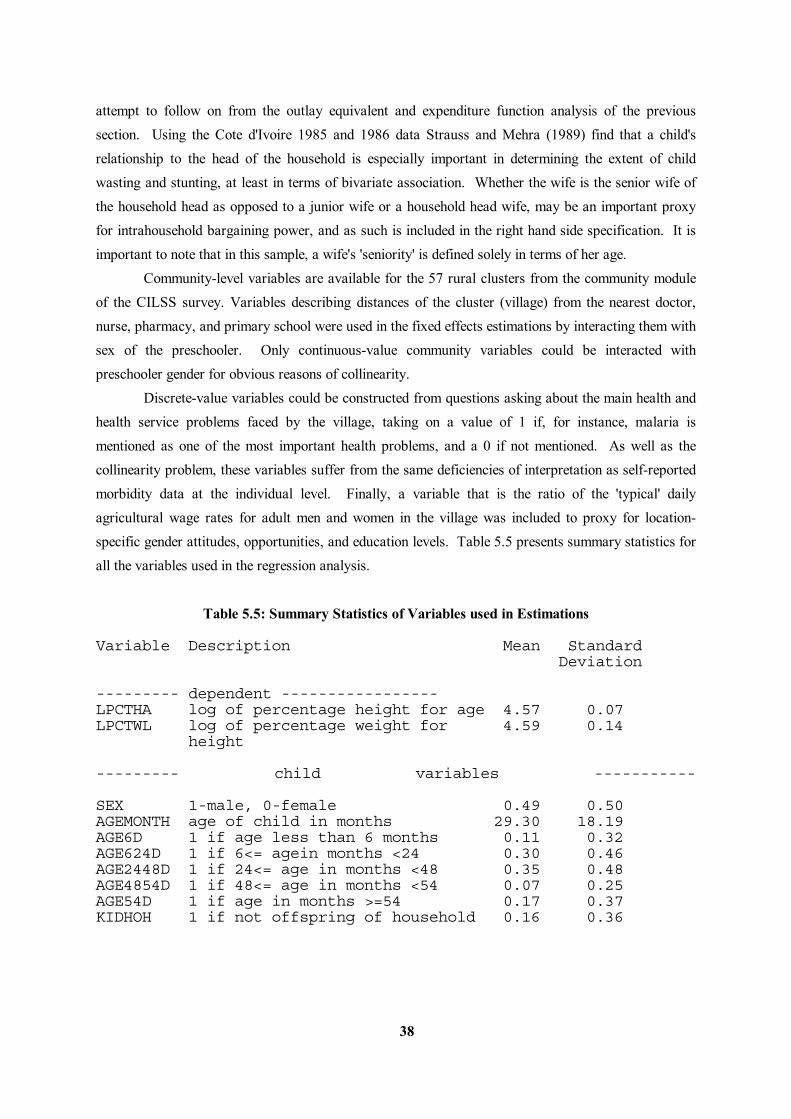
38

attempt to follow on from the outlay equivalent and expenditure function analysis of the previous section. Using the Cote d'Ivoire 1985 and 1986 data Strauss and Mehra (1989) find that a child's relationship to the head of the household is especially important in determining the extent of child wasting and stunting, at least in terms of bivariate association. Whether the wife is the senior wife of the household head as opposed to a junior wife or a household head wife, may be an important proxy for intrahousehold bargaining power, and as such is included in the right hand side specification. It is important to note that in this sample, a wife's 'seniority' is defined solely in terms of her age. Community-level variables are available for the 57 rural clusters from the community module of the CILSS survey. Variables describing distances of the cluster (village) from the nearest doctor, nurse, pharmacy, and primary school were used in the fixed effects estimations by interacting them with sex of the preschooler. Only continuous-value community variables could be interacted with preschooler gender for obvious reasons of collinearity. Discrete-value variables could be constructed from questions asking about the main health and health service problems faced by the village, taking on a value of 1 if, for instance, malaria is mentioned as one of the most important health problems, and a 0 if not mentioned. As well as the collinearity problem, these variables suffer from the same deficiencies of interpretation as self-reported morbidity data at the individual level. Finally, a variable that is the ratio of the 'typical' daily agricultural wage rates for adult men and women in the village was included to proxy for location-specific gender attitudes, opportunities, and education levels. Table 5.5 presents summary statistics for all the variables used in the regression analysis.

Table 5.5: Summary Statistics of Variables used in Estimations Variable Description Mean Standard Deviation --------- dependent ----------------- LPCTHA log of percentage height for age 4.57 0.07 LPCTWL log of percentage weight for 4.59 0.14 height --------- child variables ----------- SEX 1-male, 0-female 0.49 0.50 AGEMONTH age of child in months 29.30 18.19 AGE6D 1 if age less than 6 months 0.11 0.32 AGE624D 1 if 6<= agein months <24 0.30 0.46 AGE2448D 1 if 24<= age in months <48 0.35 0.48 AGE4854D 1 if 48<= age in months <54 0.07 0.25 AGE54D 1 if age in months >=54 0.17 0.37 KIDHOH 1 if not offspring of household 0.16 0.36

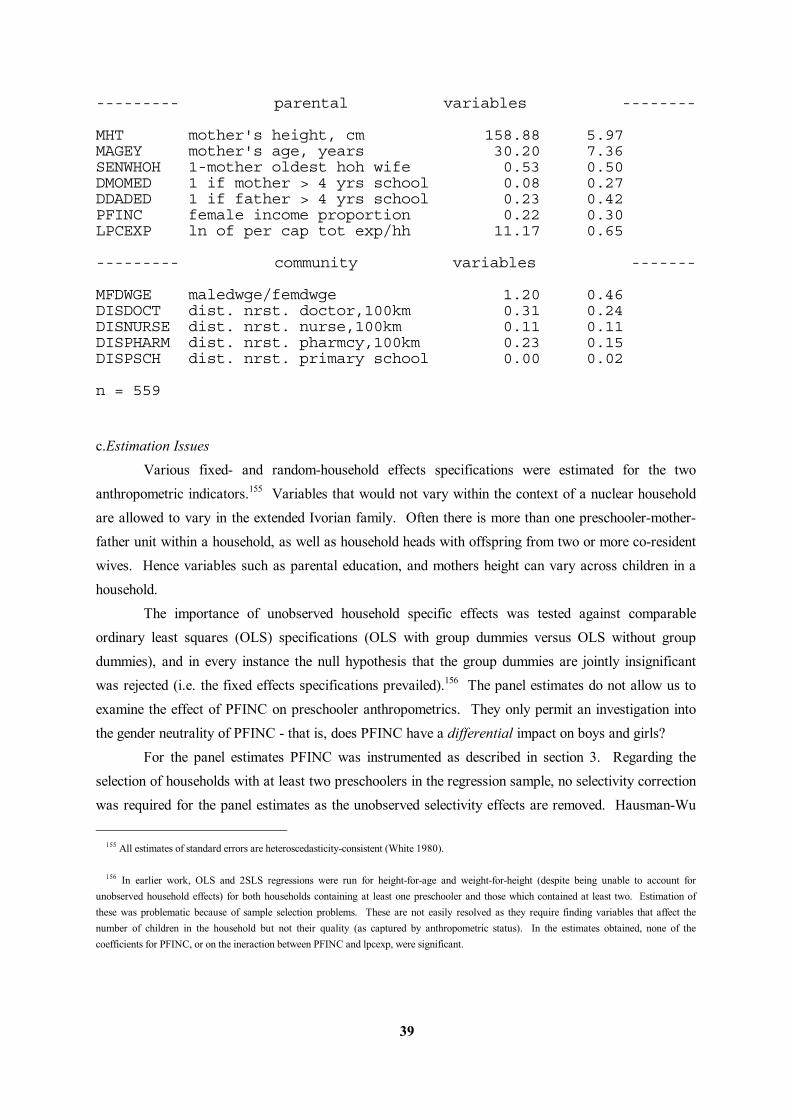
39

--------- parental variables -------- MHT mother's height, cm 158.88 5.97 MAGEY mother's age, years 30.20 7.36 SENWHOH 1-mother oldest hoh wife 0.53 0.50 DMOMED 1 if mother > 4 yrs school 0.08 0.27 DDADED 1 if father > 4 yrs school 0.23 0.42 PFINC female income proportion 0.22 0.30 LPCEXP ln of per cap tot exp/hh 11.17 0.65 --------- community variables ------- MFDWGE maledwge/femdwge 1.20 0.46 DISDOCT dist. nrst. doctor,100km 0.31 0.24 DISNURSE dist. nrst. nurse,100km 0.11 0.11 DISPHARM dist. nrst. pharmcy,100km 0.23 0.15 DISPSCH dist. nrst. primary school 0.00 0.02 n = 559

c.Estimation Issues Various fixed- and random-household effects specifications were estimated for the two anthropometric indicators.155 Variables that would not vary within the context of a nuclear household are allowed to vary in the extended Ivorian family. Often there is more than one preschooler-mother-father unit within a household, as well as household heads with offspring from two or more co-resident wives. Hence variables such as parental education, and mothers height can vary across children in a household. The importance of unobserved household specific effects was tested against comparable ordinary least squares (OLS) specifications (OLS with group dummies versus OLS without group dummies), and in every instance the null hypothesis that the group dummies are jointly insignificant was rejected (i.e. the fixed effects specifications prevailed).156 The panel estimates do not allow us to examine the effect of PFINC on preschooler anthropometrics. They only permit an investigation into the gender neutrality of PFINC - that is, does PFINC have a differential impact on boys and girls? For the panel estimates PFINC was instrumented as described in section 3. Regarding the selection of households with at least two preschoolers in the regression sample, no selectivity correction was required for the panel estimates as the unobserved selectivity effects are removed. Hausman-Wu

155 All estimates of standard errors are heteroscedasticity-consistent (White 1980).

156 In earlier work, OLS and 2SLS regressions were run for height-for-age and weight-for-height (despite being unable to account for unobserved household effects) for both households containing at least one preschooler and those which contained at least two. Estimation of these was problematic because of sample selection problems. These are not easily resolved as they require finding variables that affect the number of children in the household but not their quality (as captured by anthropometric status). In the estimates obtained, none of the coefficients for PFINC, or on the ineraction between PFINC and lpcexp, were significant.

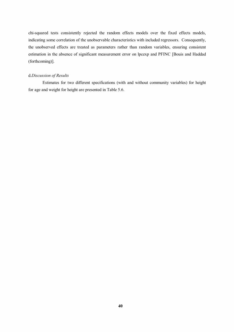
40

chi-squared tests consistently rejected the random effects models over the fixed effects models, indicating some correlation of the unobservable characteristics with included regressors. Consequently, the unobserved effects are treated as parameters rather than random variables, ensuring consistent estimation in the absence of significant measurement error on lpcexp and PFINC [Bouis and Haddad (forthcoming)]. d.Discussion of Results Estimates for two different specifications (with and without community variables) for height for age and weight for height are presented in Table 5.6.

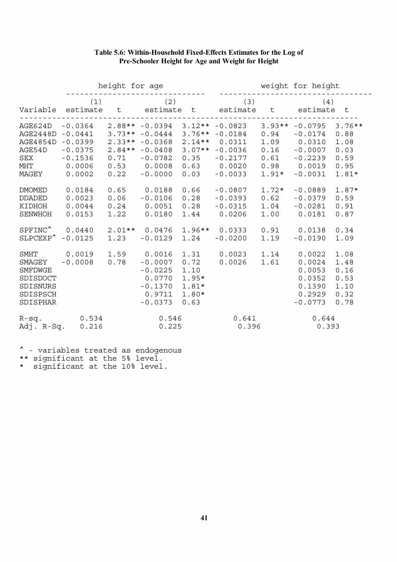
41

Table 5.6: Within-Household Fixed-Effects Estimates for the Log of Pre-Schooler Height for Age and Weight for Height

height for age weight for height ------------------------------ --------------------------------- (1) (2) (3) (4) Variable estimate t estimate t estimate t estimate t ------------------------------------------------------------------------- AGE624D -0.0364 2.88** -0.0394 3.12** -0.0823 3.93** -0.0795 3.76** AGE2448D -0.0441 3.73** -0.0444 3.76** -0.0184 0.94 -0.0174 0.88 AGE4854D -0.0399 2.33** -0.0368 2.14** 0.0311 1.09 0.0310 1.08 AGE54D -0.0375 2.84** -0.0408 3.07** -0.0036 0.16 -0.0007 0.03 SEX -0.1536 0.71 -0.0782 0.35 -0.2177 0.61 -0.2239 0.59 MHT 0.0006 0.53 0.0008 0.63 0.0020 0.98 0.0019 0.95 MAGEY 0.0002 0.22 -0.0000 0.03 -0.0033 1.91* -0.0031 1.81* DMOMED 0.0184 0.65 0.0188 0.66 -0.0807 1.72* -0.0889 1.87* DDADED 0.0023 0.06 -0.0106 0.28 -0.0393 0.62 -0.0379 0.59 KIDHOH 0.0044 0.24 0.0051 0.28 -0.0315 1.04 -0.0281 0.91 SENWHOH 0.0153 1.22 0.0180 1.44 0.0206 1.00 0.0181 0.87 SPFINC^ 0.0440 2.01** 0.0476 1.96** 0.0333 0.91 0.0138 0.34 SLPCEXP^ -0.0125 1.23 -0.0129 1.24 -0.0200 1.19 -0.0190 1.09 SMHT 0.0019 1.59 0.0016 1.31 0.0023 1.14 0.0022 1.08 SMAGEY -0.0008 0.78 -0.0007 0.72 0.0026 1.61 0.0024 1.48 SMFDWGE -0.0225 1.10 0.0053 0.16 SDISDOCT 0.0770 1.95* 0.0352 0.53 SDISNURS -0.1370 1.81* 0.1390 1.10 SDISPSCH 0.9711 1.80* 0.2929 0.32 SDISPHAR -0.0373 0.63 -0.0773 0.78 R-sq. 0.534 0.546 0.641 0.644 Adj. R-Sq. 0.216 0.225 0.396 0.393 ^ - variables treated as endogenous ** significant at the 5% level. * significant at the 10% level.

42

Tests of models (1) vs (2) and (3) vs (4) failed to reject the restricted models - introducing the community effects through the sex of the child does not add to the model. The make-up of variables representing the interactions of the sex of preschooler dummies and the distance variables was varied because of multicollinearity worries, but this did not alter the pattern or lack of strength of our results. It seems that for the Cote d'Ivoire and for the measures of community infrastructure used here, improvements in public service access would be gender neutral. This is not to say that the gender of income earner does not affect preschooler anthropometric outcomes for our sample. Unlike Strauss (1990), and Sahn (rural sample, 1989) the female income share variable has been interacted with preschooler gender (SPFINC). The estimated coefficient on this interaction variable is positive and significant for height for age (t=2.01, specification (1), and t=1.96, specification (2)), while the effect is insignificant for weight for height. At the 5% level, the null hypothesis, that the effect of increasing PFINC is gender neutral, is rejected. Boys do relatively better in terms of height for age as a result of increasing female income shares. To interpret the fixed effects results (boys do relatively better when PFINC rises), it is useful to return to the discussion of intrahousehold resource allocation. It was argued that within the common preference and bargaining frameworks, allocation amongst children could reflect efficiency, inequality aversion or efficiency-equity tradeoffs. The fixed effects results indicate how women allocate resources amongts children. Consider first the efficiency argument. A standard argument is that women favour girls over boys because daughters help with domestic tasks (whereas boys are prefered by fathers because they help with 'male' tasks such as herding cattle). But this approach is not much help here because the opposite result is obtained - increasing women's income has a larger effect on boys' height for age. It could be that mothers are responding to male-female differences in future earnings. If this effect were important, it would be captured by the variable SMFDWGE but this appears to have little impact on anthropometric status. Now consider the inequality aversion argument. Suppose women desired an equitable distribution of health amongst all children. At the outset, it would appear that boys have a poorer health endowment than girls. Svedberg (1990), using Ivorian data from the World Fertility Survey, shows there is an excess mortality of boys relative to girls amongst infants (aged less than 1 year) and toddlers (aged 1-4 years). Chapter 3, on health, found that in rural Cote d'Ivoire, the predicted probability of illness is higher in boys than in girls. Amongst very young children, the difference initially widens, then closes with girls over 13 more likely to be ill. (His results from rural Kenya show a similar pattern). Table 5.7 summarises these results:

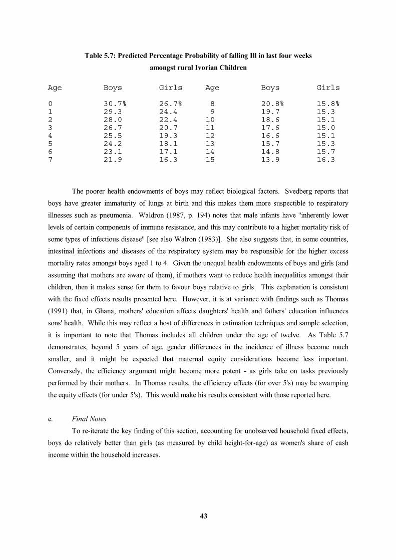
43

Table 5.7: Predicted Percentage Probability of falling Ill in last four weeks amongst rural Ivorian Children Age Boys Girls Age Boys Girls 0 30.7% 26.7% 8 20.8% 15.8% 1 29.3 24.4 9 19.7 15.3 2 28.0 22.4 10 18.6 15.1 3 26.7 20.7 11 17.6 15.0 4 25.5 19.3 12 16.6 15.1 5 24.2 18.1 13 15.7 15.3 6 23.1 17.1 14 14.8 15.7 7 21.9 16.3 15 13.9 16.3

The poorer health endowments of boys may reflect biological factors. Svedberg reports that boys have greater immaturity of lungs at birth and this makes them more suspectible to respiratory illnesses such as pneumonia. Waldron (1987, p. 194) notes that male infants have "inherently lower levels of certain components of immune resistance, and this may contribute to a higher mortality risk of some types of infectious disease" [see also Walron (1983)]. She also suggests that, in some countries, intestinal infections and diseases of the respiratory system may be responsible for the higher excess mortality rates amongst boys aged 1 to 4. Given the unequal health endowments of boys and girls (and assuming that mothers are aware of them), if mothers want to reduce health inequalities amongst their children, then it makes sense for them to favour boys relative to girls. This explanation is consistent with the fixed effects results presented here. However, it is at variance with findings such as Thomas (1991) that, in Ghana, mothers' education affects daughters' health and fathers' education influences sons' health. While this may reflect a host of differences in estimation techniques and sample selection, it is important to note that Thomas includes all children under the age of twelve. As Table 5.7 demonstrates, beyond 5 years of age, gender differences in the incidence of illness become much smaller, and it might be expected that maternal equity considerations become less important. Conversely, the efficiency argument might become more potent - as girls take on tasks previously performed by their mothers. In Thomas results, the efficiency effects (for over 5's) may be swamping the equity effects (for under 5's). This would make his results consistent with those reported here. e. Final Notes To re-iterate the key finding of this section, accounting for unobserved household fixed effects, boys do relatively better than girls (as measured by child height-for-age) as women's share of cash income within the household increases.

44

6. Conclusions In this chapter, empirical evidence has been presented on two gender aspects of household behaviour in the Cote d'Ivoire: the role of intrahousehold distribution of income on expenditures; and differentials in the allocation of household resources between boys and girls, as reflected in the consumption of adult goods and their anthropometric status. It has been shown that increases in the proportion of cash income accruing to women significantly raises the budget shares of food and lowers those of alcohol and cigarettes. The results presented here do not distinguish definitively between the common preference model and the cooperative conflict model. However, in households dominated (in both the numerical and economic senses) by women, household expenditures shift away from alcohol, restaurant meals, cigarettes and entertainment, even after controlling for household composition, total expenditure and location. The evidence on gender differentials in the allocation of household resources is far less clear-cut. At one level, it appears that there is no statistically significant difference in the change in consumption of adult goods between boys and girls. There is some evidence that children who are not offspring of the household head are discriminated against vis-a-vis children of the head, particularly amongst younger children. There is certainly no evidence to suggest that girls are discriminated against, in that gender of the child has no effect on anthropometric status. Further, improvements in public service access appear to be gender neutral. Increasing women's share of household income statistically significantly improves boys' height-for-age relative to girls. This may reflect attempts by women to equalise health status amongst offspring. Finally, if policy makers seek to increase household acquisition of food (and reduce expenditures on goods such as alcohol and cigarettes), and improve the health of boys are relatively less healthy than their female siblings, then these results provide an additional reason for policy measures to improve women's access to income-generating resources.

45

Appendix 1: Instruments for PFINC and Lpcexp As noted in the text, there are strong a priori reasons for believing that lpcexp and pfinc are not exogenous. To overcome this problem, it is necessary to include instruments for these variables that do not appear in the structural equation and are themselves exogenous. With respect to lpcexp, the following variables were used: the logarithm of the value of holdings of consumer durables expressed in per capita terms; the number of rooms in the dwelling per capita; the per capita floor area of the household dwelling; a dummy variable equalling one if the walls of the dwelling are cement, stone or brick; a dummy variable equalling one if the floor of the dwelling are cement or brick; a dummy variable equalling one if the dwelling is owned by a household residing in an urban area; the logarithm of household size; variables reflecting the age and sex composition of the household (dem1 and dem3 to dem10, as defined in the text); and locational dummy variables for households residing in Abidjan, Bete, Baoule, Guoro and Senufo areas respectively. These instruments capture the intuitive idea that wealthier households, as indicated by household location, holdings of consumer durables and quality of housing stock are likely to have higher per capita expenditures. Initially, attempts were made to predict pfinc using ordinary least squares. This produced poor results, with few variables being statistically significant and the adjusted R2 being close to zero. Examination of the data revealed that women's cash income, as a proportion of total cash income, was zero in approximately 40% of households in the sample. This suggested that the development of appropriate instruments for pfinc should account for the likelihood of it being non-zero, as well as its level. This has been resolved using a Heckman (1979) two-stage approach. It is assumed that the likelihood of a household having a non-zero pfinc is a function of certain characteristics. These include: the age of the wife of the household head (or eldest wife in polygamous households); the difference in ages between the household head and his spouse; a dummy variable equalling one if the household was female headed; a dummy variable equalling one if the spouse of the head (or eldest wife in polygamous households) has a primary school certificate; a dummy variable equalling one if the spouse of the head (or eldest wife in polygamous households) has a secondary school certificate; the amount of land operated by adult women in the household; the logarithm of the value of capital owned by adult women in the household; the number of adult women in the household; the number of boys aged 6 to 15; the number of girls aged 6 to 15; the number of girls boys aged below 6; the number of girls aged below 6; and locational dummy variables for households residing in Abidjan, Bete, Baoule, Guoro and Senufo areas respectively. This relationship was estimated using a probit, and the inverse Mill's ratio calculated. The level of pfinc is a function of the following variables: a dummy variable equalling one if the spouse of the head (or eldest wife in polygamous households) has a primary school certificate; a

46

dummy variable equalling one if the spouse of the head (or eldest wife in polygamous households) has a secondary school certificate; the difference in educational attainment between the household head and his spouse; the amount of land operated by adult women in the household; the proportion of total household land holdings operated by adult women; the proportion of household capital held by adult women (this includes the value of capital goods, machinery and inventories held as part of own business activities. It excludes the value of agricultural tools as this datum was not collected on an individual or crop specific basis); the logarithm of household size; variables reflecting the age and sex composition of the household (dem1 and dem3 to dem10, as defined in the text); locational dummy variables for households residing in Abidjan, Bete, Baoule, Guoro and Senufo areas respectively; and the inverse Mill's ratio. The method adopted here can be criticised on two grounds. A key issue to consider is whether these instruments can be considered exogenous. The existing literature suggests two approaches to this question. One, typified by Schultz (1988), is based on a model where parents maximise a single life-time utility function. As consumer durable holdings, land, capital stock and demographic variables all represent choices made by the household, they cannot be considered exogenous. Consequently, an adherent of Schultz's approach would argue that the 2SLS approach used here is invalid. They would argue that demand functions for market goods and time allocations are solely a function of market prices, life-cycle market wages, life-cycle unearned income and local public programmes. However, taken on its own terms, this view is inconsistent. If a single life-time utility function is assumed, then clearly household location is also a choice variable. Theories of migration from Todaro onwards have argued that individuals migrate in response to gains in (expected) earnings. The Tiebout hypothesis indicates that households also move in response to the provision of government services. Consequently, prices, wages and government services can no longer be considered exogenous as they have been 'chosen' (via choice of location) by households. Put another way, a consistent application of this approach would argue that there are no variables (except perhaps some components of unearned income) that can be considered purely exogenous.

47

The alternative approach is based (implicitly) on the recognition that in order to estimate a model, a choice must be made regarding the exogeneity of certain variables. An example of this is Pitt (1990). He utilises a single period utility framework in which certain variables, that change only very slowly over time, are considered fixed. These include quantities of land, housing and household capital. This method is also used when estimating agricultural production functions (see Junankar (1989)). This approach is adopted in the model presented here. As holdings of land, capital stock and major consumer durables and housing stock change slowly over time, these are assumed to be fixed.157 It could be argued that the amount (and proportion) of land available to women is endogenous. Such a view does not accord with practices in most African households where women are allocated land on marriage, or shortly thereafter, and these rarely change. A second criticism is that variables appearing in the PFINC equation could also appear in the budget share equations. An obvious candidate for this would be the education variables. This is potentially a serious problem as in their absence, educational effects on demand (such as changes in tastes) are forced to work through PFINC. In results not reported here, women's education was included in the budget shares. This did not lead to any qualitative changes in the two stage budget share results. Further, this argument does not apply to the variables representing differences in educational attainment.

157 It has been suggested that imputed values be assigned to housing and consumer durables. However, if the quantities of these goods are taken as fixed in the short term, this is no longer necessary. The budget shares estimated here are conditional on the imputed value (expenditures) on these goods.

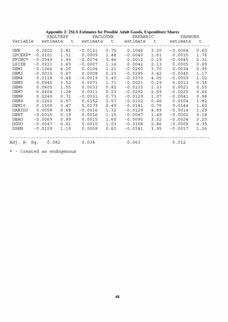
48

Appendix 2: 2SLS Estimates for Possible Adult Goods, Expenditure Shares PADLTEXP PACLOTHE PAFABRIC PASHOES Variable estimate t estimate t estimate t estimate t --------------------------------------------------------------------------- ONE 0.2602 2.81 -0.0121 0.75 0.1046 3.20 -0.0064 0.60 LPCEXP* -0.0101 1.51 0.0009 1.48 -0.0040 1.61 0.0015 1.76 PFINC* -0.0549 3.93 -0.0074 3.46 0.0012 0.19 -0.0045 2.31 LSIZE -0.0221 3.65 -0.0007 1.14 0.0042 2.13 0.0005 0.69 DEM1 0.1066 4.20 0.0104 3.21 -0.0260 3.70 0.0034 0.95 DEM3 -0.0015 0.07 0.0008 0.23 -0.0295 3.42 -0.0040 1.17 DEM4 0.0116 0.48 -0.0019 0.45 -0.0370 4.05 -0.0059 1.52 DEM5 0.0945 3.52 0.0071 1.71 -0.0021 0.19 0.0013 0.36 DEM6 0.0405 1.55 0.0033 0.82 -0.0133 1.33 0.0021 0.55 DEM7 0.0404 1.28 0.0011 0.23 -0.0292 2.59 -0.0025 0.66 DEM8 0.0249 0.71 -0.0031 0.73 -0.0129 1.07 -0.0041 0.98 DEM9 0.1262 2.97 0.0152 2.57 -0.0102 0.66 0.0104 1.82 DEM10 0.1509 3.47 0.0179 2.49 -0.0141 0.76 0.0144 1.60 DABIDJ 0.0058 0.68 -0.0016 1.32 -0.0129 4.89 -0.0014 1.29 DBET -0.0015 0.19 0.0016 1.15 -0.0047 1.49 -0.0002 0.18 DBAO -0.0069 0.99 0.0015 1.60 -0.0090 3.52 -0.0024 3.20 DGUO -0.0047 0.51 0.0015 1.03 -0.0108 2.86 -0.0005 0.35 DSEN -0.0129 1.19 0.0009 0.61 -0.0141 3.95 -0.0017 1.26 --------------------------------------------------------------------------- Adj. R- Sq. 0.082 0.034 0.063 0.012 * - treated as endogenous

49

References Adams, M. and S. Kruppenbach (1987) "Gender and Access in the African School", International Review of Education, Vol. 33, No. 4. Agarwal, B. (1986) "Women, Poverty and Agricultural Growth in India", Journal of Peasant Studies, No. 13. Ainsworth, M. and J. Munoz (1986), "The Cote d'Ivoire Living Standards Survey: Design and Implementation", Living Standards Measurement Study Working Paper no. 26, The World Bank,

Washington D.C. Ainsworth, M. (1990) "Socio-economic Determinants of Fertility in Cote d'Ivoire" Africa Tecnhnical

Department, mimeo The World Bank, Washington D.C. -----(1991a) "Economic Aspects of Child Fostering in Côte d'Ivoire", Africa Technical Department,

mimeo, World Bank, Washington D.C. Alderman, H. (1990), "Nutritional Status in Ghana and its Determinants", SDA Unit Working Paper no. 3, The World Bank, Washington D.C. Alderman, H., J. Behrman, D. Ross and R. Sabot (1991) "The Gender Gap in Human Capital Accumulation in a Poor Rural Economy", mimeo of Human Capital Accumulation in Post Green Revolution Pakistan Project, 1991. Alessie, R., P. Baker, R. Blundell, C. Heady and C. Meghir (1989) "The Working Behaviour of Young People in Rural Côte d'Ivoire: Evidence from the LSMS Panel", mimeo, University College London, for Labour Market Transitions and Structural Adjustment in the Côte d'Ivoire. Amemiya, T. (1974) "Multivariate Regression and Simultaneous Equation Models when the Dependent Variables are Truncated Normal", Econometrica, vol. 42, no. 6, pp. 999-1012. Appleton, S.M., P. Collier, and P. Horsnell (1990) "Gender Differences in Educational Attainment and in Labour Market Participation: an Analysis of the Cote d'Ivoire", S.D.A. Working Paper, The World Bank, Washington D.C. Aristophanes (411BC), Lysistrata. Armitage, J. and R. Sabot (1987) "Efficiency and Equity Implications of Subsidies to Secondary Education in Kenya" in D. Newberry and N. Stern (eds) Theory of Taxation for Developing Countries, New York: Oxford University Press. Arrow, K.J. (1973) "Higher Education as a Filter", Journal of Public Economics.

50

Bager, T. (1980) Marketing Cooperatives and Peasants in Kenya, Scandinavian Institute of African Studies, Uppsala. Banerjee, N. (1983) "Women and Poverty: Report on a Workshop", Economic and Political Weekly. Bannerjee, B. and S.M. Kanbur (1981) "On the Specification and Estimation of Macro Rural-Urban Migration Functions: with an Application to Indian Data", Oxford Bulletin of Economics and Statistics, Vol. 43, No. 1, p. 17-31. Bardhan, P.K. (1974), "On Life and Death Questions", Economic and Political Weekly. Barrera, A. (1990) "The Role of Maternal Schooling and its Interaction with Public Health Programs in Child Health Production", Journal of Development Economics, 32: 1, pp. 69-92. Bassett, T. (1988), "Breaking Up the Bottlenecks in Food Crop and Cotton Cultivation in Northern Cote d'Ivoire", Africa vol. 58 no. 2, pp. 147-173. Basu, A.M. (1987) "Is Discrimination in Food Really Necessary for Explaining Sex Differentials in Childhood Mortality", National council of Applied Economic Research, New Delhi. Becker, G. (1974), "A Theory of Social Interactions", Journal of Political Economy, vol. 82 no. 6, pp. 1063-1093. -----(1975) Human Capital (2nd Edition), Cambridge: Harvard University Press. ----- (1981), A Treatise on the Family, Harvard University Press, Cambridge Mass. Becker, G.S. and H.G.Lewis (1973) "On the Interactions between Quantity and Quality of Children" Journal of Political Economy Vol.81, No.2, Part 2, pp279-288 Behrman, J. (1984a) "Labor Force Participation and Earnings Determinants for Women in the Special Conditions of Developing Countries", Journal of Development Economics, vol. 15, pp. 259-88. -----(1984b) "Earnings and Labor Force Participation Functions in a Developing Country: Are there

Sexual Differentials?", in N. Birdsall and R. Sabot (eds) Labor market Discrimination in Developing Countries, The World Bank, Washington D.C.

-----(1988), "Intrahousehold Allocation of Nutrients in Rural India: Are Boys Favoured? Do Parents Exhibit Inequality Aversion?", Oxford Economic Papers vol. 40 no. 1, pp. 32-54. ----- (1989), "Interactions Among Human Resources and Poverty: What we Know and What we Do Not Know", mimeo, Population and Human Resources Department, The World Bank, Washington

D.C. -----(1990a) Human Resource Led Development?, New Delhi, India, ARTEP/ILO. -----(1990b) The Action of Human Resources and Poverty on One Another: What We Have Yet to

Learn, Washington D.C.: Population and Human Resources Department, World Bank.

51

-----(1990c) "Women's Schoolings and Non-Market Productivity: A Survey and a Reappraisal", Philadelphia, University of Pennsylvania, mimeo (prepared for the Women in Development Division of the Population and Human Resources Department of the World Bank).

-----(1991) "Investing in Female Education for Development: Women in Development Strategy for the

1990s in Asia and the Near East", mimeo, Williamstown, Williams College. Behrman, J.R. and A.B. Deolalikar (1988) "Health and Nutrition" Chapter 14 of H.Chenery and T.N.Srinivasan (eds) The Handbook of Development Economics North Holland, Amsterdam. -----(1990) "Are There Differential Returns to Schooling by Gender? The Case of Indonesian Labour

Markets", mimeo, Philadelphia: University of Pennsylvania. Behrman J.R., R. Pollak and P. Taubman (1982), "Parental Preferences and Provision for Progeny", Journal of Political Economy, vol. 90 no. 1, pp. 52-75. Behrman, J.R. and R. Schneider (1991) "African Educational Investments in an International Perspective", Williamstown, MA: Williams College, mimeo). Behrman, J.R. and C. Sussangkarn, (1989) "Poverty Schooling and Child Outcomes: Mother Versus Father, Schooling Quality and Interactions", mimeo, Philadelphia, University of Pennsylvania. Behrman, J.R. and P. Taubman, (1989) "Is Schooling `Mostly in the Genes'? Nature-Nurture Decomposition with Data on Relatives", Journal of Political Economy, Vol. 97, No. 6, p. 1425- 1446. Behrman, J.R. and B.L. Wolfe (1968) "Investments in Schooling in Two Generations in Pre- Revolutionary Nicaragua", Journal of Development Economics, Vol. 27, p. 395-420, North Holland. -----(1984) "The Socioeconomic Impact of Schooling in a Developing Country", Review of Eocnomics

and Statistics, 66:2 (May), pp. 296-303. -----(1989) "Does More Schooling Make Women Better Nourished and Healthier? Adult Sibling

Random and Fixed Effects Estimates for Nicaragua", Journal of Human Resources, 24:4 (Autumn), pp. 644-663.

Bergstrom, T. (1989), "A Fresh Look at the Rotten Kid Theorem - and Other Household Mysteries", Journal of Political Economy, vol. 97 no. 5, pp. 1138-1159. Bernheim, B.D. and O. Stark (1988), "Altruism within the Family Reconsidered: Do Nice Guys Finish Last", American Economic Review, vol. 78 no. 5, pp. 1034-1045. Bernheim, B.D., A. Shleifer and L. Summers (1985), "The Strategic Bequest Motive", Journal of Political Economy, vol. 93, pp. 1045-1076. Besley, T., Coate, S. and G. Loury (1990), "The Economics of Rotating Savings and Credit Associations" Discussion Paper No. 149, Research Program in Development Studies, Princeton. Bevan, D.L., P.Collier and J.Gunning (1990) Peasants and Governments Clarendon Press, Oxford

52

University. Bhuija, A. et al. (1986) "Socioeconomic Determinants of Child's Nutritional Status: Boy Versus Girl", Food and Nutrition Bulletin 8, U.N. Bigsten, A. (1984) Education and Income Determination in Kenya, Gower Publishing Company. Birdsall, N. (1980) "A Cost of Siblings: Child Schooling in Urban Colombia", in J.L. Simon and J. De Vanzo (eds) Research in Population Economies, Greenwich, Connecticut: Jai Press, 2:115-50. -----(1982) "Child Schooling and the Measurement of Living Standards", LSMS Working Paper No.

14. -----(1985) "Public Inputs and Child Schooling in Brazil", Journal of Development Economics, Vol.

18, No. 1, p. 67-86. Birdsall, N. and R.H. Sabot (1991) Labor Market Discriminaton in Developing Countries, Washington D.C.: The World Bank. Blumberg, R. (1987), "Income under Female vs. Male Control: Differential Spending Patterns and the Consequences when Women Lose Control of Returns to Labour" mimeo, The World Bank,

Washington D.C. Boissiere, M., J.B. Knight and R.H. Sabot (1975) "Earnings, Schooling Ability and Cognitive Skills", American Economic Review, Vol. 75, No. 2, p. 1016-30. Bovis, H. and L. Haddad (forthcoming) "Are Estimates of Calorie-Income Elasticities Too High? A Recalibration of the Plausible Range", Journal of Development Economics. von Braun, J. (1988), "Effects of Technological Change in Agriculture on Food Consumption and Nutrition: Rice in a West African Setting", World Development vol. 16, pp. 1083-

1098. Bray, M., P. Clarke, and D. Stephens (1986), Education and Society in Africa, Edward Arnold. Breusch, T. and A. Pagan (1979) "A Simple Test for Heteroscedasticity and Random Coefficient Variation", Econometrica, vol. 47, pp. 1287-1294. Bruce, J. (1989), "Homes Divided", World Development vol. 17 no. 7, pp. 979-992. Bruce, N. and M. Waldman (1990), "The Rotten-Kid Theorem Meets the Samaritan's Dilemma", Quarterly Journal of Economics, vol. 105 no. 1, pp. 155-166. Caces, F., F. Arnold, J.T. Fawcett and R.W. Gardner (1985) "Shadow Households and Competing Auspices: Migration Behavior in the Philippines", Journal of Development Economics, vol. 17, no. 1,

pp. 5-25 Cain, C.G. (1986) "The Economic Analysis of Labor Market Discrimination: a Survey", in O. Ashenfelter and P.R.G. Layard (eds) Handbook of Labor Economics, Elsevier.

53

Caldwell, J.W. (1977) "The Economic Rationality of High Fertility: An Investigation Illustrated with Nigerian Survey Data", Population Studies, Vol. 31, No. 1, March 1977, p.9. Cameron, A. and P.Trivedi "Econometric Models Based on Count Data: Comparisons and Applications of Some Estimators" Journal of Applied Econometrics, Vol.1, No.1 January 1986 Cassen, R.H. (1978) India: Population, Economy and Society, Macmillan Press Ltd. Chamberlain, G. (1980) "On the Use of Panel Data" mimeo, Harvard University -----(1985) "Panel Data" in Handbook of Econometrics, ed. Z.Griliches and M. Intrtiligator, vol. 2,

pp.1248-1318. Amsterdam,: North Holland Publishing Co. Chant, S. (1989) "Gender and the Urban Household", in L. Brydon and S. Chant Women in the Third World: Gender Issues in Rural and Urban Areas, Edward Elgar, Aldershot. Chatterjee (1990b) "Improving Child Nutrition through Women's Social and Economic Status", Ithaca, NY: Cornell University mimeo. Chen, L.C., E. Huq, and S. DeSouza (1981) "Sex Bias in the Family Allocation of Food and Health Care in Bangladesh", Population and Devleopment Review, Vol. 7, No. 1, p. 55-70. Chow, G. (1960), "Tests of Equality Between Sets of Coefficients in Two Linear Regressions", Econometrica, vol. 28 no. 2, pp. 591-605. Christensen, G., (1989) Determinants of Private Investment in Rural Burkina Faso, Ph.D. dissertation, Cornell University. -----(1990) "The Wary Informant Problem: Collecting Data on Credit and Livestock", paper presented

at the workshop "Locality Based Fieldwork in Developing Countries", Queen Elizabeth House, Oxford.

Clignet, R.C. and P. Foster (1966) The Fortunate Few: A Study of Secondary Schools and Students in the Ivory Coast, Northwestern University Press. Cochrane, S.H., J. Leslie, and D.J. O'Hara (1980) "The Effects of Education on Health", World Bank Staff Working Paper, No. 405. -----(1982) "Parental Education and Child Health", Health Policy and Education 2. Colclough, C. (1982) "The Impact of Primary Schooling on Economic Development: A Review of Evidence", World Development, Vol. 10, p. 167-185. Collier, P. (1986) "Allocation of Factors in Afrian Peasant Agriculture", mimeo, C.S.A.E. Oxford. Collier, P. and D. Lal (1986) Labour and Poverty in Kenya: 1900-1980 Clarendon Press, Oxford. Collier, P., S. Radwan and S. Wangwe (1986) Labour and Poverty in Rural Tanzania Clarendon Press, Oxford.

54

Cooksey, B. (1982) "Education and Sexual Inequality in Cameroon", Journal of Modern AFrican Studies, Vol. 20, No. 1, pp 167-177. Cooksey, B. and A.Ishumi (1986) A Critical Review of Policy and Practice in Tanzanian Secondary Education since 1967, Dar es Salaam, mimeo. Court, J.H. (1983) "Sex Differences in Performances on Raven's Progressive Matrices: a Review", Alberta Journal of Educational Research, Vol. 29, p. 54-74. Court, D. and K.Kinyanjui (1980) "Development Policy and Educational Opportunity: the Experience of Kenya and Tanzania" Occasional Paper No.33, Institute for Development Studies, University of

Nairobi. Cox, D.R. (1972) "Regression Models and Life Tables" Journal of Royal Statistical Society, Series B, Vol.34, pp186-220 Cox, D. and E. Jimenez (1987) "Private-public Differences in Secondary School Performance: the Role of Selection Effects in Colombia and Tanzania" Department of Economics Working Paper 104,

Washington University Cox, D.R. and D.Oakes (1984) Analysis of Survival Data, Chapman and Hall Cramer, J.S. (1986) Econometric Application of Maximum Likelihood Methods Cambridge University Press, Cambridge. David, M. and P. Wyeth (1978) "Kenya Commercial Bank Loans in Rural Areas: a Survey", IDS Working Paper 342, Nairobi. Deaton, A. (1987), "The Allocation of Goods within the Household: Adults, Children, and Gender", Living Standards Measurement Study Working Paper no. 39, The World Bank, Washington D.C. -----(1989), "Looking for boy-girl Discrimination in Household Expenditure Data", World Bank

Economic Review, vol. 3 no. 1. Deaton, A. and D. Benjamin (1988), "The Living Standards Survey and Cocoa Price Reform: A Study

of Cocoa and Coffee Producation in Cote d'Ivoire" Living Standards Measurement Study Working Paper no. 44, The World Bank, Washington D.C.

Deaton, A. and A. Case (1987), "Analysis of Household Expenditures" Living Standards Measurement Study Working Paper no. 28, The World Bank, Washington D.C. Deaton, A. and J. Muellbauer (1980), Economics and Consumer Behaviour, Cambridge University Press, Cambridge. Deaton, A., J. Ruiz-Castillo and D. Thomas (1989), "The Influence of Household Composition on Household Expenditure Patterns: Theory and Spanish Evidence", Journal of Political Economy, vol.

97 no. 1, pp. 179-200. Domencich, T. and D. McFadden (1975) Urban Travel Demand, a Behavioral Analysis, North

55

Holland, Amsterdam. Douglas, J. (1964) The Home and the School MacGibbon and Kee Douglas, J., J.Ross and W.Simpson (1968) All Our Future Peter Davies Easterlin, R.A., R.A. Pollak and M.L. Wachter (1980) "Towards a More General Model of Fertility

Determination" in R.A. Easterlin (ed) Population and Economic Change in Developing Countries Chicago: University Press p81-150

Eisemon, T.O. (1988) "The Consequences of Schooling: A Review of Research on the Outcomes of

Primary Schooling in Developing Countries" Cambridge MA. Harvard University mimeo El-Badry, M.A. (1969) "Higher Female than Male Mortality in Some Countries of South Asia" Journal of American Statistical Association Vol.64 Engle, L.E., C.Yarbrough and R.E.Klein (1983) in M.Buvinic et al "Women and Poverty in the Third

World" International Centre for Research on Women. Eshiwani, G. (1990) "Implementing Educational Policies in Kenya" World Bank Discussion Papers Africa Technical Department Series No.85 Folbre, N. (1984), "Market Opportunities, Genetic Endowments, and Intrafamily Resource Distribution: Comment", American Economic Review, vol. 74 no. 3, pp. 518-520. ----- (1986), "Hearts and Spades: Paradigms of Household Economics", World Development, vol. 14 no. 2, pp. 245-255. Foster, P. (1980) "Education and social inequality in sub-Saharan Africa" Journal of Modern African

Studies Garcia, M. (1990), "Resource Allocation and Household Welfare: A Study of the Impact of Personal Sources of Income on Food Consumption, Nutrition and Health in the Phillippines", Ph.D. dissertation,

Institute of Social Studies, The Hague, The Netherlands. Gastellu, J. (1987), "Matrilineages, Economic Groups and Differentiation in West Africa: A Note", Development and Change, vol. 18 no. 2, pp. 271-280. Glewwe, P. (1988) "Primary and Secondary School Enrollment in Cote d'Ivoire" mimeo, the World Bank, Washington D.C. ----- (1991) "Investigating the Determinants of Household Welfare in Cote d'Ivoire" Journal of Development Economics Vol.35 p307-337 Glewwe, P. and H.Jacoby (1991) "Student Achievement and Schooling Choice in Low Income Countries: Evidence from Ghana" mimeo, the World Bank, Washington D.C. Gomes, M. (1984) "Family Size and Educational Attainment in Kenya", Population and Development Review, Vol. 10, no.4, pp.647-660

56

Gould, W. (1974) "Admissions Policies in East Africa" Comparative Education Review Vol.18 No.3 Griliches, Z. (1977), "Estimating Returns to Schooling: Some Econometric Problems" Econometrica, vol. 45 no. 1, pp. 1-22. Greene, W. (1989), LIMDEP, version 5.1. Econometric Software, New York. -----(1981), "Sample Selection Bias as a Specification Error: Comment" Econometrica, vol. 49 no. 3,

pp. 795-798. -----(1990), Econometric Analysis (New York: MacMillan). Greenhalgh, C. (1980) "Male-Female Wage Differentials in Great Britain: Is Marriage an Equal Opportunity?", Economic Journal, vol.90, no. 4, pp. 751-75. Grisay, A. (1984) "Analyse des Inegalities de Rendement Liees au Sexe de l'Eleve dans l'Enseignement Primaire Ivorien" International Review of Education Gronau, R. (1974) "Wage Comparisons - A Selectivity bias", Journal of Political Economy, Vol. 82, no. 5, pp. 1119-43. ----- (1989), "Consumption Technology and the Intrafamily Distribution of Resources: Adult Equivalence Scales Reexamined", Journal of Political Economy, vol. 96 no. 6, pp. 1183-1205. Grootaert, C. (1986), "Measuring and Analysing Levels of Living in Developing Countries: An Annotated Questionnaire", Living Standards Measurement Study Working Paper no. 24, The World

Bank, Washington D.C. -----(1988) "Cote d'Ivoire's Vocational and Technical Education", Policy Planning and Research

Working Paper no. 19, The World Bank, Washington D.C. Gunderson, M. (1989) "Male-Female Wage Differentials and Policy Responses" Journal of Economic Literature, Vol. 27, pp. 46-72. Guyer, J. (1980), "Household Budgets and Women's Incomes", Boston University, African Studies Center Working Paper no. 28, Boston Mass. Guyer, J. and P. Peters (1987), "Introduction", Development and Change, vol. 18 no. 2, pp. 197-214. Haddad, L. (1990), "Gender and Poverty in Ghana: A descriptive Analysis" Social Dimensions of Adjustment Unit Working Paper, World Bank. Haddad, L. and R. Kanbur (1990a), "How serious is the neglect of intra-household inequality?" Economic Journal, vol. 100 no. 402, pp. 866-881. -----(1990b), "Is there an intra-household Kuznet's curve? Some evidence from the Philippines", Warwick University, Development Economics Research Centre Discussion Paper

Number 101.

57

Haddad, W., M.Carnoy, R.Rinaldi and O.Regel (1990) "Education and Development: Evidence for New Priorities" Washington D.C.: World Bank Discussion Paper 95

Hammond, E. (1977) "Sex Differences in Mortaility" World Health Statistics Report Han, A. and Hausman, J. (1986) "Semi-Parametric Estimation of Duration and Competing Risks Models" M.I.T. mimeo Hanushek, E. (1986) "The Economics of Schooling" Journal of Economic Literature No.3 Vol.24 p1141-77 Harriss, B. (1986), "The Intrafamily Distribution of Hunger in South Asia" London School of Hygiene and Tropical Medicine, mimeo. Hassan, N. and K.Ahmad (1984) "Intra-family distribution of food in rural Bangladesh" Food and Nutrition Bulletin 6 U.N. Hausman, J. (1978), "Specification Tests in Econometrics", Econometrica, vol. 46 no. 5, pp. 1251-1271. Hausman, J. and W. Taylor (1981) "Panel Data and Unobservable Individual Effects" Econometrica 49 (6): pp 1377-98 Heckman, J. (1976) "The Common Structure of Statistical Models of Truncation, Sample Selection and Limited Dependent Variables and Simple Estimator for Such Models", Annals of Economic and

Social Measurement, vol. 5, no. 4, pp. 475-92. -----(1978) "Dummy Endogenous Variables in a Simultaneous Equation System" Econometrica,

Vol.46, No.6 ----- (1979), "Sample Selection Bias as a Specification Error", Econometrica, vol. 47 no. 1, pp. 153-161. Hendry, D.F. (1987) "Econometric Methodology: A Personal Perspective", Ch.10 in Advantages in Econometrics Vol II, Cambridge University Press, 1987 (ed. T.Bewley) Hirshleifer, J. (1977), "Shakespeare vs. Becker on Altruism: The Importance of Having the Last Word", Journal of Economic Literature, vol. XV no. 2, pp. 500-502. Hoddinott, J. (1989), "Migration, Accumulation and Old Age Security in Western Kenya", unpublished D.Phil. thesis, University of Oxford. -----(1990), "A More General Model of Migration and Remittances Applied to Western Kenya",

mimeo, Centre for the Study of African Economies, Oxford. -----(forthcoming), "Rotten Kids and Manipulative Parents: Are Children Old Age Security in western Kenya?" Economic Development and Cultural Change.

58

Hopcraft, P. (1974) "Human Resources and Technical Skills in Agricultural Development: an Economic Evaluation of Educative Investments in Kenya's Small Farm Sector" PhD. thesis, Stanford University Horsnell, P. (1990), "Gender Inequalities in the Labour Market: Evidence from the Cote d'Ivoire", Unit for the Study of African Economies, Institute of Economics and Statistics, Oxford. Horton, S. (1985) "The Determinants of Nutrient Intake: Results from Western India", Journal of Development Economics, 19, pp. 147-167. Horton, S. and B. Miller (1987), "The Effect of Gender of Household Head on Expenditure: Evidence from Low Income Households in Jamaica", mimeo, University of Toronto. Idler, E.L. (1991) "Self-Assessed Health and Mortality: A Review of Studies", International Review of Health Psychology. Idler, E.L. and S. Kasl (1991) Health Perception and Survival: Do Global Evaluations of Health Status Really Predict Mortality?, 46: 2, pp. S55-65. Jamison, Dean T. (1986) "Child Malnutrition and School Performance in China" Journal of Developing Areas Vol.20 p299-309 Jayaweera, S. (1987) "Women and Education" International Review of Education Jiggins, J. (1989), "How Poor Women Earn Income in Sub-Saharan Africa and What Works Against

Them" World Development, vol. 17 no. 7, pp. 953-963. Johnson, M., A. McKay and J.Round (1989) "Household Income and Expenditure Aggregates from the Cote d'Ivoire Living Standards Survey 1986: Methodology and Documentation", SDA Project in

Cote d'Ivoire: Data Processing and Methodology Note Number 1, The World Bank, Washington D.C.

Joshi, H., H. Lubell, and J. Mouly (1976) Abidjan: Urban Development and Employmet in the Ivory Coast, International Labour Office, Geneva. Junankar, P.N. (1989) "The Response of Peasant Farmers to Price Incentives: The Use and MisUse of Profit Functions", Journal of Development Studies, Vol. 25, No. 2, pp. 169-182. Kakwani, N. (1986) "Is Sex Bias Significant?" W.I.D.E.R: Helsinki Kelly, G. (1987) "Setting State Policy on Female Education in the Third World" Comparative Education Vol.23 No.1 Kennedy, E. and B. Cogill (1987), "Income and Nutritional Effects of the Commercialization of Agriculture in Southwestern Kenya", International Food Policy Research Institute Research Report No.

63. Khandker, S. (1990), "Labor Market Participation, Returns to Education, and Male-Female Wage Differences in Peru", PRE Working Paper 461, World Bank.

59

King, E.M. and R. Bellew (1988) "Education Policy and Schooling Levels in Peru", Washington D.C.: The World Bank, mimeo. King, E. and M. Hill (eds)(1991) Women's Education in Developing Countries, Washington D.C. King, E. and L.Lillard (1983) "Determinants of Schooling Attainment and Enrolment Rates in the

Philippines" Rand Note N-1962-AID ----- (1987) "Education Policy and School Attainment in Malyaisa and the Philippines" Economics of Education Review Vol.6 No.2 p167-181 Kirchler, E. (1990), "Spouses' Influence Strategies in Purchase Decisions as Dependent on Conflict Type and Relationship Characteristics", Journal of Economic Psychology, vol. 11 no. 1, pp. 101-118. Knight, J. and R. Sabot (1987) "Education Policy and Labour Productivity: an Output Accounting Exercise" Economic Journal p199-214 ----- (1990) Education, Productivity, and Inequality: The East African Natural Experiment Oxford

University Press, Oxford. Kooreman, P. and A. Kapteyn (1990), "On the Empirical Implementation of Some Game Theoretic Models of Household Labor Supply" Journal of Human Resources, vol. 25 no. 4, pp. 584-598. Krueger, A. (1968) "Factor Endowments and Per Capita Income Differences Among Countries" Economic Journal, Vol.78 p641-59 Lee, L.F. (1982) "Some Approaches to the Correction of Selectivity Bias", Review of Economic Studies, vol. 49, no. 3, pp. 355-72. ----- (1983), "Generalised Econometric Models with Selectivity" Econometrica, vol. 51 no. 2, pp. 507-512. Leuthold, J. (1968), "An Empirical Study of Formula Income Transfers and the Work Decision of the Poor", Journal of Human Resources, vol. 3, pp. 312-323. Lockwood, M. and P. Collier (1988) "Maternal Education and the Vicious Circle of High Fertility and Malnutrition", Policy Planning and Research Working Paper No. 130, Washington D.C. Lockheed, M., D. Jamison and L.Jau (1984) "Farmer Education and Farm Efficiency: A Survey" Economic Development and Cultural Change Vol.29 Low, A. (1986), Agricultural Development in Southern Africa: Farm Household-Economics and the Food Crisis (London: James Currey). Maddala, G. (1983) Limited Dependent and Qualitative Variables in Economics New York: Cambridge University Press Manser, M. and M. Brown (1980), "Marriage and Household Decision-Making: A Bargaining Analysis", International Economic Review, vol. 21 no. 1, pp. 31-44.

60

Marvin, R. (1975) "'Economic Barba': is this a Satisfactory Explanation of Why African Parents Value

Schooling?" Journal of Modern African Studies Mbilinyi, M. (1973) "Education, Stratification and Sexism in Tanzania" The African Review Vol.3

No.2 Dar Es Salaam ----- (1974) "Access to Education in East Afica: an Introduction" Rural Africana (East Lansing) Vol 25 Fall McElroy, M. (1985), "The Joint Determination of Household Membership and Market Work: The Case of Young Men" Journal of Labour Economics, vol. 3 no. 3, pp. 293-316. ____ (1990), "The Empirical Content of Nash-Bargained Household Behavior", Journal of Human Resources, vol. 25 no. 4, pp. 559-583. McElroy, M. and M. Horney (1981), "Nash-Bargained Household Decisions: Toward a Generalization of the Theory of Demand", International Economic Review, vol. 22 no. 2, pp. 333-349. McKee, K. (1989), "Microlevel Strategies for Supporting Livelihoods, Employment, and Income Generation of Poor Women in the Third World: The Challenge of Significance" World

Development, vol. 17 no. 7, pp. 993-1006. McFadden,D. (1973) "Conditional Logit Analysis of Qualitative Choice Behaviour" in P.Zarembka (ed.) Frontiers in Econometrics, New York: Academic Press. Mensch, B., H. Lentzer and S.Preston (1985) "Socio-economic Differentials in Child Mortality in Developing Countries" New York, U.N. Mincer, J. (1974), Schooling, Experience and Earnings (New York: Columbia University Press). Mojekwu, V. (1976) in I.Tinker at al "Women and World Development" New York: Praeger Publishers Moock, P. (1981) "Education and Technical Efficiency in Small-Farm Production" Economic Development and Cultural Change Vol.29 Moock, P. and J. Leslie (1986) "Childhood Malnutrition and Schooling in the Terai region of Nepal"

Journal of Development Economics Mora, J. et al (1979) "Nutritional Supplementation and the Outcome of Pregnanacy, Pt. 1: Birthweight" American Journal of Clinical Nutrition No.32 Muckenhirn, E. F. (1966) "Secondary Education and Girls in Western Nigeria" Dissertation Abstracts

International June 1967 Nelson, F.D. (1975) "Estimation of Economic Relationships with Censored, Truncated and Limited Dependent Variables", University of Rochester. Olsen, W. (1990), "Longterm Fieldwork in South India: Five Mistakes I'm Glad I Made", paper

61

presented at the workshop "Locality Based Fieldwork in Developing Countries", Queen Elizabeth House, Oxford.

Pahl, J. (1983), "The Allocation of Money and the Structuring of Inequality within Marriage", Sociology Review pp. 237-262. Papanek, H. (1976) "Women in Cities: Problems and Perspectives", in I. Tinker, M.B. Bramsen, and M. Buvinic (eds) Women and World Development, Praeger, New York. Paterson, R. (1985), "Modelling the Division of Labour and Assets within Peasant Households", unpublished M.Sc. extended essay, University of Oxford. Pitt, M. (1990) Chapter 5 of An Analysis Plans for Understanding the Social Dimensions of Adjustment SDA Unit, Africa Region Report No. 8691-AFR, Washington DC, the World Bank Pitt, M., M. Rosenzweig and MD. Hassan (1990), "Productivity, Health and Inequality in the Intrahousehold Distribution of Food in Low-Income Households", American Economic Review, vol. 80 no. 5, pp. 1139-1156. Pitt, M. and M. Rosenzweig (1986) "Agricultural Prices, Food Consumption and the Health and Productivity of Farmers" in Singh et al (eds.) ----- (1990) "The Selectivity of Fertility and the Determinants of Human Capital Investments: Parametric and Semi-parametric Estimates" Living Standards Measurement Survey Working Paper No 72 Preston, S. and J.Weed (1976) "Causes of Death Responsible for International and Intertemporal Variations in Sex Mortality Differentials" World Health Statistics Report Prewitt, K. (1974) "Education and Social Equality in Kenya" Ch.9 of Court and Ghai (eds) Education,

Society and Development Psachoropoulos, G. (1985) "Returns to Education: a Further International Update and Implications", Journal of Human Resources, vol. 20, pp. 583-97. Psachoropoulos, G. (1988) "Education and Development: a Review" World Bank Research Observer

Vol.3 No.1 Jan. p99-116 Razavi, S. (1990), "Fieldwork in your Home Country", paper presented at the workshop "Locality Based Fieldwork in Developing Countries", Queen Elizabeth House, Oxford. Republique de Cote d'Ivoire (1989) "Cout de l'Education en Cote d'Ivoire" Ministere de l'Education Nationale Republic of Tanzania (1988) "Education and Training Statistics 1986" Bureau of Statistics, Ministry of Finance, Dar es Salaam Rosenzweig, M. (1986), "Program Interventions, Intrahousehold Distribution and the Welfare of Individuals: Modelling Household Behaviour", World Development, vol. 14 no. 2, pp. 233-243.

62

Rosenzweig, M. and T.P. Schultz (1982a), "Market Opportunities, Genetic Endowments, and Intrafamily Resource Distribution", American Economic Review vol. 72 no. 4, pp. 803-815. -----(1984), "Market Opportunities, Genetic Endowments, and Intrafamily Resource Distribution:

Reply", American Economic Review, vol. 74 no. 3, pp. 521-522. Rosenzweig, M. and K. Wolpin (1986) "Evaluating the Effects of Optimally Distributed Public Programs" American Economic Review Vol.76 No.3 p470-487. ----- (1989) "Migration Selectivity and the Effects of Public Programs" Journal of Public Economics, Vol. 37, p. 265-289. Sahn, D. (1989), 'The causes of malnutrition in West Africa: Evidence on the role of income'. Cornell University. Food and Nutrition Policy Program mimeo. Washington DC. -----(1990), "Malnutrition in Cote d'Ivoire", SDA Unit Working Paper no. 4, The World Bank, Washington D.C. Samuelson, P. (1956), "Social Indifference Curves", Quarterly Journal of Economics, vol. 70 no. 1, pp. 1-21. SAS version 6.03 (1988), SAS Institute Inc. Cary, North Carolina. Schaefer-Kehnert, W. (1980), "Success with Group Lending in Malawi" Quarterly Journal of International Agriculture, vol. 19 no. 4, pp. 331-337. Schultz, T.P. (1988), "Education Investments and Returns" in H. Chenery and T. Srinivasan (eds) Handbook of Development Economics Amsterdam: Elseiver Science ----- (1990a), "Women and Development: Objectives, Frameworks and Policy Interventions" New

Haven, CT: Yale University, mimeo ----- (1990b), "Testing the Neoclassical Model of Family Labor Supply and Fertility", Journal of Human Resources, vol. 25 no. 4, pp. 599-634. ----- (1991), "Returns to Women's Education" in E.King and M.Hill (eds.) Women's Education in Developing Countries Washington D.C.:World Bank Sen, A. (1966), "Peasants and Dualism with or without Surplus Labour", Journal of Political Economy, vol. 74 no. 5, pp. 425-450. -----(1981), Family and Food: Sex Bias in Poverty Oxford University -----(1985), "Women, Technology and Sexual Divisions", Trade and Development no. 6, pp. 195-223. -----(1986), "Social Choice Theory", in K. Arrow and M. Intriligator (eds) Handbook of Mathematical

Economics, vol III, North Holland, Amsterdam.

63

-----(1987), "Africa and India: What do we have to learn from each other?" All Soul's Colllege Oxford, mimeo

-----(1990) "More than 100 Million Women are Missing", New York Review of Books, 37:2, (20

December), pp. 61-66. Sen, A. and S.Sengupta (1983) "Malnutrition of Rural Children and the Sex Bias" Economic and Political Weekly Seraj, J. (1976) in I.Tinker et al Women and World Development NY: Praeger Publishers Singh, I., L. Squire and J. Strauss (eds.) (1986) Agricultural Household Models: Extensions Applications and Policy Washington D.C., World Bank Smock, A. (1977) in J.Giele and A.Smock (eds.) Women: Roles and Status in Eight Countries New

York: John Wiley and Sons Somerset, H. (1974a) "Educational Aspirations of Fourth-form Pupils in Kenya" Ch.4 in Court and

Ghai (eds) Education Society and Development ----- (1974b) "Who Goes to Secondary School? Relevance, Reliability and Equity in Secondary School Selection" Ch.7 in Court and Ghai (eds) Education Society and Development Staudt, K. (1977) "Inequities in the Delivery of Services to Female Farm Clientele: Some Implications for Policy" Discussion Paper no. 247, Institute of Development Studies, University of Nairobi. Stiglitz, J. (1976), "The Efficiency Wage Hypothesis, Surplus Labour, and the Distribution of Income in LDCs", Oxford Economic Papers, vol. 28, pp. 185-207. ----- (1975), "The Theory of Screening, Education and the Distribution of Income" American Economic Review vol. 65 pp.283-300 Strauss, J. (1986), "Does Better Nutrition Raise Farm Productivity?", Journal of Political Economy, vol. 94 no. 2, pp. 297-320. -----(1990), "Households, communities, and preschool children's nutrition outcomes: evidence from rural Cote d'Ivoire", Economic Development and Cultural Change, vol. 38 no. 2. Strauss, J. and K. Mehra (1989), "Child anthropometry in Cote d'Ivoire: Estimates from two surveys, 1985 and 1986" LSMS Working Paper no. 51. Subramanian, S. and A. Deaton (1990), "Gender effects in Indian consumption patterns" Woodrow Wilson School, DP 147, Princeton University. Svedberg, P. (1990), "Undernutrition in Sub-Saharan Africa: Is There a Gender Bias?", Journal of Development Studies, vol. 26 no. 3, pp. 469-486. Taylor, G. and R.Faruque (1983) Child and Maternal Health Services in Rural India Baltimore, John Hopkins University Press

64

Tinker, I. and Bramsen (1976) Women and Development NY: Praeger Publishers Thomas, B. (1988), "Household Strategies for Adaptation and Change: Participation in Kenyan Rural Women's Associations" Africa, vol. 58 no. 4, pp. 401-422. Thomas, D. (1990), "Intra-household resource allocation: An Inferential Approach", Journal of Human Resources, vol. 25 no. 4, pp. 635-664. -----(1991), "Like father, like son: Gender Differences in household resource allocations", mimeo, Yale University. Thomas, D., J. Strauss, and M. Henriques (1989), "Child survival, Height-for-age, and Household Characteristics in Brazil", Journal of Development Economics. -----(1990b) "How Does Mother's Education Affect Child Height?", Journal of Human Resources. Topol, R., 1991, `Bubbles and Volatility of Stock Prices: Effect of Mimetic Contagion', Economic Journal, vol. 101, pp. 786-800. Udry, C., (1990) "Rural Credit in Northern Nigeria: State Contingent Contracting in a Market for Loans", mimeo, Yale University. Ulph, D. (1988), "A General Non-Cooperative Nash Model of Household Consumption Behaviour", mimeo, University of Bristol. U.N. (1975) "Socio-cultural Determinants of Education Opportunities for Women" U.N. Economic

Commisson for Latin America Staff Paper No.3 van der Gaag, J. and W. Vijverberg (1988) "A Switching Regression Model for Wage Determinants in the Public and Private Sector of a Developing Country", Review of Economics and Statistics, vol.

70, no. 2, pp. 244-52. -----(1989) "Wage Determinants in Cote d'Ivoire: Experience, Credentials and Human Capital",

Economic Development and Cultural Change, vol. 37, no. 2, pp. 371-81. Van de Ven, W. and B. Van Praag (1981) "The Demand for Deductibles in Private Health Insurance"

Journal of Econometrics Vol.17 pp.229-252 van der Walle, E. and A. Foster (1990) "Fertility Decline in Africa: Assessment and Prospects", World Bank Technical Paper. Von Pischke, J.D. (1980), "The Pitfalls of Specialised Farm Credit Institutions in Low-Income Countries" Development Digest, vol. 18 no. 3, pp. 79-91. ----- (1977), "The Political Economy of Farm Credit in Kenya" PhD. thesis, Glasgow University Waldron, I. (1983) "Sex Differences in Human Marketing: The Role of Genetic Factors", Social Science and Medicine, Vol. 17, No. 6.

65

-----(1987) "Patterns and Causes of Excess Female Mortality Among Children in Developing Countries" World Health Statistics Quarterly, Vol. 40, pp. 194-210.

Weekes-Vagliani, W. (1985), "Actors and Institutions in the Food Chain: The Case of the Ivory Coast", Development Centre Papers, Organisation for Economic Cooperation and Development, Paris. -----(1990), "Analyse des Variables Socioculturelles et de L'Adustement en Cote d'Ivoire", Documents Techniques no. 9, Development Centre Papers, Organisation for Economic Cooperation

and Development, Paris. Woolley, F. (1988), "A Non-Cooperative Model of Family Decision-Making" Discussion Paper no. TIDI/125, London School of Economics. Wheeler, E.F. (1984) "Intra-household Food Allocation: A Review of Evidence" London School of

Hygiene and Tropical Medicine, mimeo White, E.H. (1976) "Women's Status in an Islamic Society: the Problem of Purdah" Dissertations Abstract International May 1976 Whitehead, A. (1981), "I'm hungry, mum: The Politics of Domestic Budgeting", in K. Young, C. Wolkowitz, and R. McCullagh (eds) Of Marriage and the Market: Women's Subordination in

International Perspective, Routledge, London. Wolfe, B.L. and J.R. Behrman (1986) "Child Quantity and Quality in a Developing Country: The Importance of Family Background, Endogenous Tastes and Biological Supply Factors", Economic Development and Cultural Change, 34, pp. 703-720. World Bank (1980) "Kenya: Population and Development" World Bank Country Study ------ (1981) World Development Report ------ (1988), Cotton Development Programs in Burkina Faso, Cote d'Ivoire, and Togo, Operations Evaluation Department, World Bank, Washington D.C. ----- (1989) Kenya: The Role of Women in Economic Development, Washington D.C. Yakin, N. (1976) in I.Tinker et al. Women and World Development NY: Praeger Publishers.