BOOK l: THEEVIDENCE

INTERNATIONAL PRODUCTIVITY

Ruth Sivard has for several years shown the dramatic connection between anation's productivity and military spending. Her bar chart shows clearly that as oneincreases, the other decreases, like a seesaw relationship. Others have also writtenabout this connection. What this report attempts to do is clarify the numerousimplications that come from that understanding. Most economists have convincedthemselves that all government spending stimulates the economy, and do not considerthat military spending is different, in spite of all the evidence. This report is an attemptto set the record straight, revise our mistaken "defense" policy which has dangerouslyweakenned us since 1945, and develop a new economic theory that fits all the factswithout the glaring wartime exceptions and international inconsistencies of currentmilitary Keynesianism.

Manufacturing productivity is central to all economic growth: it is as important tothe economy as an engine is to a vehicle. I have started by testing the theory that eachone percent of GNP spent on the military reduces manufacturing productivity by onepercent. I have developed several ways of proving that very point.

The "correlation coefficient" is an important statistical term because it is used byeconometricians to forecast one variable from another: according to the correlationcoefficients I have attained, anywhere from g8% to 100% of long term (1960-1978)productivity changes between nations can be explained by the difference in militaryspending rates. Similar results (99%) substantiate the trade-off between investmentand military spending amoung the four largest countries in NATO and Sweden; forthose countries, increased military spending reduced capital investment by the sameamount over the period 1960-1979.

While the world is full of economists who work in many different areas, none ofthose is as relevant, long term, as a nation's military spending plans. Military spendingis qualitatively different from all other domestic economic activity because its output isdirected external to the society. In relationship to the domestic economy, militaryspending is not productive of any good or service. lt consumes personal energy andresources without giving anything productive back to the economy. Even official U.S.government statistics stop the manufacturing productivity statistics between 1939 and1947, supporting the fact that wartime expenditures are not productive in the normaleconomic sense of the word.

Defending our society may be a necessity, but it does not normally contributeany good or service to the domestic economy. Many militarists can and do argue thatpoint, but their arguments do not explain the gaps in the statistical record created bymilitary spending. Many economists might not know the difference because only onehalf of one percent of the economic literature is basic research, and 971" is based onother people's research.

The idea that military spending creates jobs ignores the output side of theequation. On the input side, sure many people are employed in the military-industrialcomplex. But none of their activity contributes any good or service to the domesticeconomy. Their output is applied external to our economy and is destructive ratherthan constructive.

-4-

_JItI

3rlG_ol-Li --g-E--..I>e.

I

E3tr

_E{tq-

I

_-l

#.rEl)t

tGlFQ{3l€loiLiei

II

dE: .

l3lb,

=*-9:1!:--b3--CG.--i

t--- 1"* -I

-i*-I-i-I-i-

rL.*II

Ir-Ii--It-IIL-.-

L--

t

t_.

Ir-"II

f- --iIt.IIL-.-

-t-- -r'* -

I

i--r-+I-r

-F-I

One third of our engineers, our research, and our investment is siphoned off into

non-productive miliLry ictivity. one third of our scientific and engineering talent is

channelled into the military ratner than the economy. Military research represents

l2oh of Reagan's federal s-cience budget as our engineers develop such sophisticated

*""ponry tflat Oomestic spin-offs aie increasingly rare. _

And the weapons have

become so complicated they either don't work or are unreliable. Star Wars is a major

drain on our scientific talent. Some of our major universities do mostly military

research.Japan's Ministry of Industry and Trade (MlTl) is a paralle.l structure to our

pentagon. Each society makes itspriorities clear. we choose to fight the cold war and

they Jhoose to make and trade better products.. Our military burden erodes our

industrial base by competing for the limited supply of capital investment and being

instead taxed onto all our pr6ducts, making it very difficult to trade and compete with

the less militarized societies of Europe and especially Japan..The Russians have been affected too. Their military build-up in the seventies

stopped their dramatic gains in the world economy up until that time-. our best defense

is our economy. lf our economy continues to shrink while the "enemy" economy.

expands, we could indeed end up in the dust bowl of history. since world war ll

demonstrated that we can devote up to 40oh ol our economy to a major war effort' our

mutti-year war ending ability is proportional to our economic strength. lf we keep over-

preparing for war foi seveial more decades, we will eventually weaken ourselves so

much that we will indeed invite aggression. Indeed that has been happenning since

the last world war. That has hapfdned to Britain, Rome and other empires before us.

Table ol Average MilitarY and ProductivitY (1960'1978)

%GNP %Military Productivity Total Variation

Over .35%StandardDeviation

Japan 1.0 8.2Denmark 2.3 6.8Italy 2.8 6.0Sweden 3.5 5.4Germany 3.5 5.3Canada 2.3 3.9France 4.1 5.5Britain 5.3 3-2

9.2 +.2 no

9.1 +.1 no

8.8 -.2 no

8.9 -.1 no8.8 -.2 no6.2 -2.8 Yes9.6 +.6 Yes8.5 -.5 yes

U. S. 6.9 2.4 9.3 +'3 no

The data were obtained by measuring the bar chart in Ruth Sivard's work "world Military and social

Expenditures" 1980.

Because of the direct see-saw like trade-off, adding the military to the

manufacturing productivity gives a constant, 9olo. The remaining variation is similar

to the variation on. g.t. iniottege physics lab; quite precise. Thus the first building

block of the ne* ecoiomic theory is niititary spending, which is wholly nonproductive:

meaning that it reduces produitivity in basic industry because it siphons off key

resources into a nonproductive capacity.

-6-

Note that the Canadian variation is about ten times the U.S. variation. Since theU.S. has ten tirpes the economy of Canada, when these variations are converted todollars, they nearly cancel each other out. Nations trade with each other and thusintermingle their economies. People are free to travel in the free world and often workin other countries, especially neighboring countries. This is especially true of therefationship between Canada and the U.S., where 40"/"of the Canadian economy istrade with the neighbor ten times its size, and the full impact of the U.S. on Canidamay be closer lo 70T". In turn, our tiny neighbor is our biggest trading partner, evenbigger than Japan. So it is very logical to combine continental countriei together foreconomic purposes. Doing this improves my statistical connection between themilitary and manufacturing productivity to three digits of perfection (-1.00). (Thisgeographic merging of neighboring economies allows us to includeCanada and still get a correlation coefficient of -.ggz). The standarddeviation is only .21o/" of GNP, representing negligible variation. Thus militaryspending conclusively reduces manufacturing productivity, and thereby economicgrowth, dollar for dollar.

Data used for the -1.00 correlation coefficient (1960-197g)

1980 US$billions o/o oIEconomy continent

United States 2584 91.94Canada 245 8.66North America 2829 100.00

% % Mil. Gro.MiL Gro. ExL gt Total6.9 2.4 6.30 2.192.3 3.e Je s4

6.50 2.53 9.03

2.3 6.8 .06 .172.8 6.0 .43 .923.5 5.4 .16 .243.5 5.3 1.12 '1.704.1 5.5 1.04 1.405.3 3.2 1.06 .64

3.87 5.07 8.94

DenmarkItalySwedenGermanyFranceBritainEurope

Japan

64394116825654516

2569

1 048

2.4915.344.51

32.1125.4620.09

100.00

100.00 1.0 8.2 1.0 8.2 9.2

SUMMARY: Over .?1%StandardMilitary Productivity Total Variation Deviation

North America 6.50 2.S3 9.Og ;o3 noEurope 3.87 S.07 8.94 -.06 noJapan 1.0 B.Z 9.20 +.20 noThis method uses the same figures as before, but weighted averages them for eachcontinent, then is the same as the preceding chart.^ (Originally discovered Sivard's bar charton the back of a peace brochure received from AdaSanchez at a fellowship ol reconciliation meeting in Salem, Oregon, in the spring of 19g3.)

-7-

CAPTTAL INVESTMENT( 1 960- 1 e7e)

INV. MIL. TOTAL AVG. VARIATIONusA 14.0 6.5 20.5 20.5 0.0BRtrAtN 15.2 5.0 20.2 20.5 -.3

FRANCE 16.5 4.1 20.6 20.5 +.1

GERMANY 17.1 3.4 20.5 20.s 0.0SWEDEN 17.2 3.4 20.6 20.5 +.1

lNV. is the Fixed Capital Investment as % of GDPMlL. is Military Expenditures as % of GNPTOTAL is the sum of the first twoAVG. is the average TOTALVARIATION is the difference of TOTAL from the average.

This produces a correlation coefficient of -.99, meaning that about 99% of military

spending leads to a reduction in capital investment of the same amount for these

countries.

DEVELOPED VS. UNDEVELOPED WORLD (1960-80)

Do more advanced societies or less advanced societies have the highest

economic growth rates? Even though the developed world is ten times the standard of

living of th6 developing world, the eionomic grov'rth rates are the same, for this period

of time, when discounted for military and population. So there is no catching up

from behind without cutting the military.

DEVELOPED UNDEVELOPED TOTALM|L|TARY GNP % 5.89 4.65 5.68ECONOMIC GROWTH % 3.09 3.49 2.44POTENTIAL 8.98 8.14 8.12POPULATION GROWTH % .96 ?35 1.97

GROSS POTENTIAL 9.94 10.49 10.09

-8-

U.S. ECONOMIC MODEL

My findings in this report have helped me create a new economic model. Thismodel is in the best tradition of the hard sciences, based on basic empirical researchin the laboratory of the real world, and so it is unlike the dominant economic thinkingwhich is in the social science mode of thinking. Many economists cannot grasp thethought that one factor can explain most all the difference in economic growth ratesamoung nations. They think that many financial factors have been omitted from myanalysis. Reality is people's work and productivity and financial factors influence butdo not superseed that basic physical reality. They cannot see that military spending isthe prime cause of the economic disease because they are used to studying all theless reliable secondary effects. They can't see the forest for the trees. But it is easy totrace most of the "other factors" back to the one logical cause as I have done in my ownmind in case after case. My approach is based on "hard data" and theirs is usuallybased on other peoples'thinking: a house built on sand.

Military spending is the first factor. The second factor is deficit spending bygovernment. My first report "You Can Have Military Spending or Economic Growth(But Not Both)" left this factor out. With this factor in it is easy to now include World Warll successfully in the modeling period. I believe my model is unique in this respect.Classic Keynesian thinking cannot do this: it would predict absurd levels of economicgrowth during the war well beyond what actually happened. Keynes developed hismodel pre-World War ll when levels of military spending were only 1"/" of the U.S.economy in peacetime. He died in 1949 before a significant cold war record was in.Even productivity data were not kept during wartime, such as the productivity reportinggap between 1939 and 1947.

My model also works internationally and is more egalitarian, also unlike othermodels. Other economists think each country is unique: a thought that is verynationalistic but hardly scientific. All industrial market societies have similar "potential"manufacturing productivities before they reduce their productivity by spending on themilitary: in such societies, spending is the way resources are allocated. My modelalso works regardless of the starting point in terms of standard of living.

The third factor in my model is the Kondratiev weather wave. lt is very difficult tofind materials about this school of thought , but it is mentioned under "Business Cycles"in the Encyclopedia Britannica. However, my modeling becomes near perfect with theinclusion of this research on the long-term business cycle. lt also fits well with limitedinformation I have about the World and German economies after World War ll. Basedon many multi-year averaging graphs, I have estimated that the bottoms were 1g2gand 1982, and the tops were 1898 and 1952, and will be 2006. I used a sine wave tomodel between the tops and bottoms. In the science of physics, transitions aretypically modeled by differential equations and end up as sine waves, although linearregressions are typical in economics: economists have long tried to fit square pegs inround holes in this too simplistic mathematical way.

The last two factors, oil and trade war, have occurred as cataclysmic events nearthe bottoms of the sine wave. In the case of oil, there is a quantum shift of 3.7"h otGNP downward in 1974 and then the model continues nicely at the lower level, stillfollowing the long term sine wave.

Trade war is the probable cause of the Great Depression. The model fitsapproximately in the twenties, quantum shifts down 7.5% of GNP in each year of theperiod 1930-1943, returns to par in 1944 and continues to model increasingly andexceedingly well thereafter.

-21-

II

THE DATA (for manufacturing productivity):

Year Wave + Deficit - Military = Model Actual Variation Total1 9831 9821 9811 9801979197819771 97619751974

1 9731972197119701 9691 96819671 9661 965

1 9641 9631 9621 9611 9601 9591 9581 9571 956

1 9551 9541 9531 9521 9511 9501 9491 94819471 946

3.33.33.33.43.53.63.73.94.14.3

8.28.58.89.19.49.7

10.010.310.6

10.911.211.511.812.012.212.412.612.7

12.812.913.013.013.012.912.812.612.412.1

7.14.73.13.12.33.44.15.13.81.2

2.32.52.51.8

.72.5

.8

.4

.8

.81.41.91.1-.71.6.2

-2.3-4.8

5.3

6.56.15.55.24.95.05.25.55.85.8

6.17.A7.68.49.19.99.28.07.7

8.99.29.59.79.710.310.610.510.3

11.213.514.613.67.55.25.03.75.8

21.1

3.91.9

.91.3

.9

4.22.13.1

.1

.7

.3

.22.2-1.2-.2

-1 .1

-.1

1.0.8

-2.1

+1.0+1.0+2.4-2.6+.7

+1.3-1.7-1.6-.5

+2.Q+3.9

+.7+.1

-1.8+1.0-3.6

+.5-2.7

+2.4+.9

+1.2+1.5-1.4-4.0-4.0

-.2-.2

+3.7

.3

.52.71.51.3

.2

.1

1.11.9-.2

+1.0+2.0+4.4+1.8+2.5+3.8+2.1

+.5.0

+2.0+5.9+6.6+6.7+4.9+5.9+2.3+2.8

+.1

+2.5+3.4+4.6+6.1+4.7

+.7-3.3-3.5-3.7

.0

2.0 .92.6 2.53.5 4.52.1 2.9-.3 -2.4

.91.31.7

.5

.31.71.3-.5-.4

4.44.03.72.51.02.31.62.73.7

2.93.33.72.62.63.63.11.62.0

2.4.8.3.5

4.89.38.06.61.8-3.7

5.45.06.1-.1

1.73.6-.1

1.1

3.2

4.97.24.42.7

.84.6-.52.1-.7

4.81.71.52.03.45.34.06.41.6*

.0*

-22-

Year Wave + Deficit - Military = Model

1945 11.8 27.2 38.2 .81944 11.5 30.6 39.2 2.91943 11.1 33.6 37.7 7.O1942 10.8 14.9 18.5 7.2

Actual Variation Total

.0 -.8

.0 -2.9

.0 -7.0

.0 -7.2

1941 2.9 4.81940 2.5 .31939 2.1 3.61938 1.7 .91937 1.4 2.91936 1.0 6.21935 .7 2.31934 .4 6.9

1933 .1 5.51932 -.1 4.61931 -.3 .81930 -.4 -.8

5.9 1.8 2.0* +.2 +.21.7 1.1 3.5' +2.4 +2.61.2 4.5 9.S +5.0 +1.61.2 1.4 1.8 +.4 +g.01 .1 3.2 -1 .1 -4.9 +3.71.2 6.0 .2 -5.8 -2.11.0 2.0 S.O +3.6 +1.5.9 6.4 5.0 -1.4 +.1

1.1 4.5 5.9 +.8 +.91.0 3.5 €.8 -10.3 -9.5.9 -.4 4.3 +4.7 -4.9.8 -2.0 2.5 +4.5 -.9

1929 7.0 -.7 .7 5.6 4.0 -1.6 _1.61928 7.0 -.9 .7 5.4 5.3 _ .1 _1.71927 7.0 -1.2 .6 5.2 2.6 _2.6 _4.31926 7.1 -.9 .6 5.6 2.7 -2.g _7.21925 7.2 -.9 .7 S.Z 6.6 +.9 _6.91924 7.3 -t.g .B S.Z 6.7 +1.5 _4.g1923 7.4 -.7 .9 5.8 _1.8 _7.6 _12.41922 7.6 -1.4 1.9 4.9 9.6 +4.7 _7.21921 7.8 -.S g.Z 4.1 1S.O +10.9 +3.21920 8.0 -1.3 4.6 2-,1 S.9 +3.g +7.0

'Thess figures are accurats in tol1l, but guesstimates in timing due to the lapse inannual productivity figures from 1939 to 1942.Wave= Kondratieff weather wave of naturally occurring economic potential modelledby a sine wave with a 24 year up cycle and ; 30 year down cycle, except for quantumshifts.Deficit= Federal deficit as a percentage of GNp.Mllilan(= Military spending as a percent of GNP, by federat fiscat year (implies a threeto six month shift, unadjusted for)Modgl= predicted manulacturing productivity based on the formula wave + Deficit -Military.Actual= manufasturing productivity percent increase for that year.Variation= Actual - ModelT-olal= cumulative variation for each section up to that year.

-23-

HOW MANUFACTURING PRODUCTIVITY RELATES TO ECONOMIC GROWTH.There are two adjustments:1. Population or size of the workforce changes.2. Length of the average work week changes.

In the U.S. the work week dropped steadily in the early part of the century, thenlevelled off at about a 40 hour rate after the war and great Depression. Projectionsmade in this work assume that the workweek will remain constant.

Manufacturing productivity and economic growth are closely related in the postwar economy. While they may be very different year by year,long term manufacturingproductivity (2.5%) is nearly the average of two growth statistics with or withoutpopulation increases: namely the real growth rate (3.0%) and the per capita GNPg rov,rth rate (2.0"/").

Except for cataclysmic reshufflings of the basic level of economic activity like theoil crisis and the Great Depression, this model works extremely smoothly. Even then,the model works well at reduced levels. And the model works better with each passingdecade as we get away from the wild events of the first half of this century. Theamazing thing is that the variation in the model zeroes out every nine or ten years(1946-55,1956-64,1965-73,1974-83) in the post war period. Thus the model has theprecision of the laws of physics, a hard science, rather than the pseudo-science of themilitary Keynesians. What my model shows is that for every action there is an equaland opposite reaction. There is an up period after every down period, within thesenine year cycles. These resemble underdamped waves (see engineering controltheory) going through the economy after the initial shock of the World War ll overtimework stress put on the American people. There is a war boom followed by a post warbust, a Korea boom followed by an Eisenhower bust, a Kennedy boom and a Johnsonbust, then a Nixon boom followed by the oil crisis big bust. What the model shows isthat while these people take the immediate credit, they may actually be borrowing fromthe future to pay for now, and the economy may be far more deterministic thanpreviously thought. lt further verifies that deficits stimulate the economy and thatmilitary spending is wholly non-productive and reduces the economy.

Balancing the budget leads to disaster (witness Roosevelt's 1938 recession andCarte/s "lower economy each year" four years). Reagan more than made up for hismilitary buildup (+1.S%GNP) with an even bigger deficit buildup (+3.0%GNP).

The economic model needs more work with the economic growth statistics anddemographic statistics, but the uncanny accuracy of the manufacturing productivitymodel more than proves the soundness of my theory, in fact it allows me to makeaccurate long term forecasts and gives me a reliable way to expect the unexpected,such as, recessions. In fact, I predicted the productivity drop for the end of last year onJanuary 20, 1986 before the January 29th release date, and I have a VCR of that TVshow to prove it. I also suggested a recession may be on the way, and the recentincrease of unemployment may actually presage that, although the unexpected oildrop should have a positive long term impact. At best that may indicate that we areabout to return to the normal wave path (1 920-73), doubling our current potential. But I

don't think it will fully do so, thanks to conservation and adjustments the market hasfinally made to the oil crisis. New modular energy sources may be the future in energy.

-24-

What the model doesn't include is almost as important as what it does include.The fact that military spending and the federal deficit give an accurate model indicatesthat other factors are nearly insignificant or perhaps only transitory yearly parts of theeconomic system. Thus social spending by government may be economically neutraland tax changes may be transitory to be compensated for later, unless, of course,deficits are created. Deficits may be harmful long term, but I have not been able tomeasure anything but benefit short term. What is obviously true is that they are anexcellent short term fix for the economy or to mask military spending's negative impact.

Comparison with other forecasters indicates that this model is 70times better than the average forecaster and five to ten times better thaneconometricians.

Act Act Act Act Act Act Act21-29 30-33 34-41 46-55 56-64 65-73 74-83

Graph above shows the table below's Model vs. Actual , in tenths, in each time period.

SUMMARY of Model Variation:

Total Total Total TotalOverages Underages Net Model Actual

1 974-83 4.5 4.7 -0.2 18.8 18.61965-73 6.4 6.4 0.0 25.9 25.91956-64 8.2 8.1 +0.1 25.4 25.51946-55 9.7 9.8 -0.1 30.8 30.71942-45 01934-41 1 1.6 1 1.5 +0.1 26.4 26.51930-33 10.0 10.3 -0.3 5.6 5.31921-29 14.5 14.8 -0.3 46.5 46.2

Adjustoil

tradetrade(average ot 20-29and 22-29 periods)

1922-29 7.1 14.8 -7.7 43.4 35.71920-29 21.8 14.8 +7.0 49.6 56.6

The overages cancel out the underages to give an extremely low'variationin the nine year cycles.

The adjust column indicates that the normal sine wave potential has had one ofthe two special adjustments mentioned before.

-25-

r

The war years finally f inished the process begun in 1934 of reducing theunemployment rate to normal proporlions, although the first two years of the war followthe Depression era productivity modelling. Thereafter the model returns to normat.

I give two opposite reference points in the twenties. The model has two problemsin that ancient time: economic recovery from the severe postwar depression of WorldWar I and the tentativeness of the enhanced industrialization level of that era. Still thevariations are nearly equal and opposite for the average of the eight and ten yearcycles, similar to the post war preciseness of the modern era.

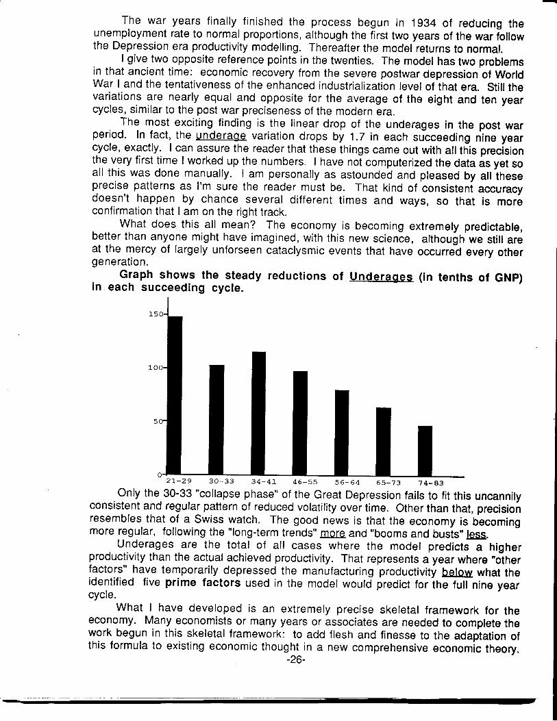
The most exciting finding is the linear drop of the underages in the post warperiod. ln fact, the underage variation drops by 1.7 in each succeeding nine yearcycle, exactly. I can assure the reader that these things came out with all this precisionthe very first time I worked up the numbers. I have not computerized the data as yet soall this was done manually. I am personally as astounded and pleased by allineseprecise patterns as I'm sure the reader must be. That kind of consisteni accuracydoesn't happen by chance several different times and ways, so that is moreconfirmation that I am on the right track.

What does this all mean? The economy is becoming extremely predictable,better than anyone might have imagined, with this new science, although we still areat the mercy of largely unforseen cataclysmic events that have occurre-d every othergeneration.

Graph shows the steady reductions of Underages (in tenths of GNp)in each succeeding cycle.

Only the 30-33 "collapse phase" of the Great Depression fails to fit this uncannilyconsistent and regular pattern of reduced volatility over time. Other than that, precisionresembles that of a Swiss watch. The good news is that the economy is becomingmore regular, following the "long-term trends" more and "booms and busis'lgss.

Underages are the total of all cases where the model predicts a higherproductivity than the actual achieved productivity. That represents ayear where "o1herfactors" have temporarily depressed the manufacturing productivity below what theidentified five prime factors used in the model would predict tor ifre tult nine yearcycle.

What I have developed is an extremely precise skeletal framework for theeconomy. Many economists or many years or associates are needed to complete thework begun in this skeletal framework: to add flesh and finesse to the adaptation ofthis formula to existing economic thought in a new comprehensive economic theory.

-26-