Profit efficiency of U.S. commercial banks: a decomposition

PROFIT EFFICIENCY OF U.S. COMMERCIAL BANKS: A DECOMPOSITION

Diego A. Restrepo Tobón

Subal C. Kumbhakar

No. 13-18

2013

Profit efficiency of U.S. commercial banks: a decomposition.I

Diego A. Restrepo-Tobon1

Department of Economics, State University of New York at Binghamton, New York, USAEAFIT University, Medellın, Colombia.

Subal C. KumbhakarDepartment of Economics, State University of New York at Binghamton, New York, USA.

Abstract

This paper presents new evidence regarding the relation between profit, revenue, and cost

efficiencies of U.S. commercial banks. Building on the widely used nonstandard profit func-

tion (NSPF) approach, we show (i) why estimation of NSPF would be wrong and (ii) how

revenue and cost efficiencies contribute to profit efficiency. Using data from U.S. commercial

banks from 2001 to 2010, we find that losses due to profit inefficiency represents about 8.2%

of banks’ equity of which 3.5% is due to revenue inefficiency and 4.7% to cost inefficiency.

Cost efficiency weighs more than revenue efficiency in estimated profit efficiency. However,

compared with cost inefficiency, revenue inefficiency affects more overall profitability.

Keywords: Profit Efficiency, Revenue efficiency, Cost efficiency, Nonstandard Profit

Function, Stochastic Frontier

JEL Classification No.: D24, G21, L13

IThe authors thank participants at the 4th International Finance and Banking Society Conference 2012, theNorth America Productivity Workshop 2012, the 38th Annual Conference of the Eastern Economic Association2012, and the 48th Annual Meeting of the Missouri Valley Economic Association 2011.

Email addresses: [email protected] (Diego A. Restrepo-Tobon ), [email protected].(Subal C. Kumbhakar)

1Corresponding author. Restrepo acknowledges financial support from the Colombian Fulbright Commission,the Colombian Administrative Department of Science, Technology and Innovation (Colciencias), and EAFITUniversity.

Preprint submitted to Elsevier June 5, 2013

1. Introduction

Over the past fifteen years, the Nonstandard Profit Function (NSPF) approach of Humphrey

and Pulley (1997) has become the dominant method to estimate profit efficiency in banking.2

In this paper, we show that the NSPF econometric model used in the empirical literature is mis-

specified and may yield misleading results. Based on Humphrey and Pulley’s framework, we

propose an alternative method that solves this misspecification problem and makes explicit the

conditions under which NSPF efficiency measures capture both revenue and cost efficiencies.

Our paper contributes to the banking literature by providing new evidence on profit effi-

ciency of U.S. commercial banks and its relation with revenue and cost efficiencies based on

our proposed alternative method. Our findings suggest that cost inefficiency weighs more than

revenue inefficiency in estimated banks’ profit efficiency. Combined annual losses for all U.S.

commercial banks due to cost and revenue inefficiencies represent about $31.5 and $23.5 bil-

lion, respectively. However, for any given efficiency level, profit efficiency responds more to

revenue efficiency changes than to cost efficiency changes. This helps explaining our finding

that, on average, banks tend to be more revenue than cost efficient.

Using our alternative method to measure banks’ profit efficiency, we find that while rev-

enue and cost efficiencies tend to be negatively correlated, both correlate positively with profit

efficiency. In contrast, using the misspecified econometric model, profit and cost efficiencies

tend to be negatively correlated, a result for which researchers have no compelling arguments

(e.g., Rogers 1998 and Berger and Mester 1997).

Since Humphrey and Pulley’s publication, more than fifty published empirical studies have

adopted the NSPF approach to investigate different issues in banking such as bank performance,

bank productivity, deregulation, competition, market power, bank size, and cross-country com-

parisons. In contrast, only one study uses the standard neoclassical profit function (Kumbhakar,

Lozano-Vivas, Lovell, and Hasan, 2001) and two others use it only for comparison purposes

(Berger and Mester, 1997 and Vivas, 1997).

Proponents of the NSPF approach argue that the neoclassical assumption of perfect compet-

2The NSPF is also known as the alternative profit function. We use the acronym NSPF to contrast it to thestandard neoclassical profit function.

2

itive markets is unsuitable for the banking industry (e.g., Berger, Humphrey, and Pulley, 1996;

Humphrey and Pulley, 1997, and Berger and Mester, 1997). In particular, Humphrey and Pul-

ley argue that banks may have more flexibility in choosing output prices than output quantities.

Further, Berger and Mester maintain that the NSPF is more appropriate for modeling banks’

maximizing behavior. The widespread use of the NSPF supports their arguments.

In the NSPF framework, banks maximize profits choosing output prices and input quantities

while taking input prices and output quantities as given. The solution of the maximization

problem yields the NSPF which is a function of input prices and output quantities. To estimate

profit efficiency, researchers append an efficiency term in an ad hoc basis to the NSPF, which

is then estimated using, mainly, the stochastic frontier technique. Building on Humphrey and

Pulley’s work, we show that such an approach, although intuitive, is algebraically incorrect and

therefore the specification of the NSPF is wrong.

Our paper is organized as follows. In Section 2, we solve the bank’s profit maximization

problem using Humphrey and Pulley’s framework. Unlike Humphrey and Pulley, we explic-

itly introduce two potential sources of profit inefficiency: input inefficiency and output price

inefficiency. Then, we show that the bank’s profit maximization problem is equivalent to solv-

ing the nonstandard revenue maximization problem (Berger et al., 1996) and the standard cost

minimization problem, separately. That is, unlike the neoclassical profit function, the correct

NSPF specification is given by the difference between the nonstandard revenue function and

the standard neoclassical cost function in which parameters are completely different. Thus the

revenue and cost functions and inefficiencies thereform can be estimated separately from each

of them. The profit efficiency measure is shown to be a composite of both cost and revenue

efficiencies, and it can be computed without estimating the profit function. In fact, it would be

wrong to estimate the profit function because of the misspecification problem which we show

explicitly. That is, the efficiency measure used in the NSPF literature is incorrect because it

is estimated using an econometric model that is not consistent with the theoretical optimizing

model.

We demonstrate that banks’ profit efficiency is an overall measure of cost and revenue effi-

ciencies only if both input and output price inefficiencies are present — price efficiency affects

3

revenues while input efficiency affects costs. Even if there is no revenue (cost) inefficiency,

profit efficiency is not the same as cost (revenue) efficiency. This result follows from the op-

timizing model used in the original NSPF framework and not from any special feature of our

modelling approach. Using the homogeneity properties of the nonstandard revenue function,

we also show that the NSPF is not linear homogeneous in input prices, contrary to the common

assumption made in the empirical literature.

We call our corrected measure the composite NSPF (CNSPF) efficiency measure to dis-

tinguish it from the traditional NSPF efficiency measure. The CNSPF decomposes profit effi-

ciency into revenue and cost efficiencies. From this decomposition, we can examine the relative

importance of improving revenue and cost efficiencies on profit efficiency.

In Section 3, we present the econometric model to estimate revenue and cost inefficien-

cies. We estimate revenue inefficiency using a nonstandard revenue function (NSRF, Berger

et al., 1996) and cost inefficiency using a standard cost function. Using revenue and cost

(in)efficiency estimates, we compute the CNSPF efficiency measure as the ratio between actual

and optimal profits without estimating a profit function.3

In Section 4, we describe the data used in the estimation and in Section 5 we present our

empirical results. We find that average revenue, cost, and profit efficiency estimates for U.S.

commercial banks are around 95%, 90%, and 80%, respectively. Forgone rents due to inef-

ficiencies amount to approximately 8% of banks’ equity. If banks were to eliminate revenue

inefficiencies, average profit efficiency would increase to 89% and forgone rents would de-

crease to 5%. On the other hand, if banks were to eliminate cost inefficiencies, average profit

efficiency would increase to 90% and forgone rents would decrease to 3%. Thus, cost effi-

ciency weighs more than revenue efficiency in estimated profit efficiencies. However, revenue

inefficiency affects more overall profitability. For example, a 1% increase in revenue (cost)

efficiency leads to a 2% (1%) increase in profit efficiency. This finding partially explains why

revenue efficiency is higher than cost efficiency.

3In addition, we can obtain estimates of the characteristics of the technology through the cost function (e.g.,returns to scale, technical change, etc.) which is not possible from the NSPF because it does not satisfy the dualityresults.

4

2. Efficiency in the NSPF Framework

In this section, we model banks’ output price and input inefficiencies and show that the

econometric model used in the NSPF literature to estimate profit efficiency is misspecified.

Using the NSPF framework, we propose an alternative method that is free from this economet-

ric problem and allows researchers to investigate the relation among profit, revenue, and cost

efficiencies.

2.1. Modelling Efficiency in the NSPF Framework

In the NSPF framework, banks maximize profits, Π=∑m pmym−∑ j w jx j, by setting output

prices (pm ; m = 1, · · · ,M) and choosing input quantities (x j ; j = 1, · · · ,J). Output quantities

(ym) and input prices (w j) are taken as given. Output and input quantities are related through

the production possibility frontier that banks face which is defined in terms of a transformation

function, A f (y,θ · x;β ) = 1 where A is a productivity parameter, f (·) is the core transforma-

tion function, 0 6 θ 6 1 captures input inefficiency (also known as input-oriented technical

inefficiency), and β represents parameters of the transformation function. Output and input

prices are related through the price possibility frontier (PPF), g(p,w,z;α) = 1, where g(·) is a

functional form, z represents factors affecting banks’ price setting strategies (e.g., output level,

risk, etc.), and α represents parameters of the PPF.

The PPF is the distinctive feature of the NSPF framework. Humphrey and Pulley (1997)

posit the existence of a price opportunity set (POS) containing all feasible combinations of in-

put and output prices and other factors. The PPF is thus the frontier of the POS and contains

the highest feasible output prices given input prices and other factors that affect it. The PPF

constrains the relation among output and input prices and other factors included in z. According

to Humphrey and Pulley (1997, p.81), the PPF reflects the bank’s assessment of their compet-

itive position, customers’ willingness to pay for the bank’s products and services, and pricing

rules that the bank may follow, among other factors influencing banks’ price setting strategies.

However, Humphrey and Pulley did not specify how failing to set optimal prices (prices lying

on the PPF) contributes to banks’ profit efficiency through lower revenue.

Unlike Berger et al. (1996) and Humphrey and Pulley, we explicitly introduce price in-

5

efficiency into the PPF.4,5 We measure output price efficiency by comparing observed output

prices with the highest feasible output prices (optimal prices) that are unobserved. We define

the optimal price vector as p∗ = η p, with η > 1. A bank is price efficient if η = 1. Price

inefficiency is the percentage shortfall of price from its optimal value (i.e., lnη = ln p∗− ln p).

Thus, price efficiency is given by 0 6 η−1 6 1 and measures how close p is to its optimal

value, p∗. The PPF becomes g(p∗,w,z,α) = 1 and the PPF frontier is g(p,w,z;α) = 1. Note

that since outputs are given, the presence of revenue inefficiency implies that observed output

prices are lower than optimal prices. This causes actual revenue to be less than optimal rev-

enue. The presence of revenue inefficiency (due to lower than optimal prices) can be tested

econometrically.

As we argued before, we explicitly model the missing connection between price and profit

efficiencies. We show below that output price efficiency (η−1) affects revenues, while input

efficiency (θ ) affects costs. Jointly, they affect profits. Without explicitly modeling output

price and input efficiency, the NSPF efficiency measure, as routinely estimated in the literature,

cannot be interpreted as an overall measure of cost and revenue efficiencies. More specifically,

the NSPF cannot be used to measure inefficiency no matter what the source of inefficiencies

are, price or input. This is shown in the next two sub-sections.

4Banks use three main pricing strategies: risk-based loan pricing, relationship-based pricing, andrelationship-lending pricing (see Berger and Udell, 2002; Edelberg, 2003; McCoy, 2007; Berger and Udell, 2006;Cowan and Cowan, 2006; Gan and Riddiough, 2008; Dick and Lehnert, 2010; and Berger and Black, 2011).However, the adoption of these strategies differ regarding banks’ characteristics (e.g., risk tolerance, geographicdiversification, bank size, loan portfolio, borrowers pool, among others.), competition, economic conditions, spe-cific demand factors, and funding costs (see the Federal Reserve’s Senior Loan Officer Opinion Survey on BankLending Practices). These pricing strategies rely on difficult to observe borrowers characteristics and other vari-ables that are outside banks’ control. The subjective nature of pricing strategies makes them complex and subjectto errors. Therefore, it is natural to assume that banks may err in setting optimal prices, and become price ineffi-cient.

5Berger et al. (1996) consider the possibility that banks may fail to set prices to maximize revenues but focuson economies of scope rather than on inefficiency. Koetter, Kolari, and Spierdijk (2012) consider a frameworkin which banks with market power fail to set prices optimally. In their model, profit inefficiency arises sincethe observed price function, or inverse demand function, is everywhere lower than the optimal price function.Nonetheless, they use the traditional NSPF and do not explicitly estimate price inefficiency as we do in this paper.

6

2.2. Solution of the Maximization Problem in the NSPF Framework

The Lagrangian associated with the profit maximization problem is:6

maxp,x

L = ∑m

pmym−∑j

w jx j +λ [A f (y,θ · x;β )−1]+µ [g(η · p,w;α)−1] (1)

Defining p∗ = p ·η and x∗ = x ·θ , the first order conditions (FOCs) for pm and x j are:

ym +µ∂g(p∗,w;α)

∂ p∗m

∂ p∗m∂ pm

= 0 ∀ m : 1, · · · ,M. (2)

−w j +λ ·A∂ f (y,x∗;β )

∂x∗j

∂x∗j∂x j

= 0 ∀ j : 1, · · · ,J. (3)

From (2) we get:

pmym

p1y1≡ p∗mym

p∗1y1=

∂ lng(p∗,w;α)

∂ ln p∗m∂ lng(p∗,w;α)

∂ ln p∗1

∀ m : 2, · · · ,M. (4)

Likewise, from (3) we get:

w jx j

w1x1≡

w jx∗jw1x∗1

=

∂ ln f (y,x∗;β )

∂ lnx∗j∂ ln f (y,x∗;β )

∂ lnx∗1

∀ j : 2, · · · ,J. (5)

Since x∗j does not appear in (4) , we can solve for p∗m from (4) together with the price opportunity

set g(p∗,w;α) = 1 in terms of w, y, and the parameters of the PPF, i.e., η pm = p∗m = φm(w, y;α)

where ym = ym/y1. This expression relates optimal prices to output quantities and input prices.

Likewise, since p∗ does not appear in (5), we can solve for θx j = x∗j from (5) together with

the transformation function A f (y,x∗;β ) = 1 in terms of w, y and the parameters of the transfor-

mation function., i.e., θx j = x∗j = ψ j(w,y;β ) where w j = w j/w1. This expression represents

6To ease the notation we drop z from the PPF. This is inessential for the results. Note that we do not requireoutput quantities to be included in the PPF. The relation between input prices and output quantities, in the spirit ofBerger et al. and Humphrey and Pulley, results naturally from the first order conditions of the profit maximizationproblem. Further, in the simple output case, if the PPF depends directly on output quantities, there is no needto solve the profit maximization problem to find out optimal prices. They could be derived directly from g(y,η ·p,w) = 1. In addition, y can be included in z, anyway.

7

the conditional factor demand functions.

These results follow from the fact that L in (1) can be written as:

maxp,x

L = maxp

L1−minx

L2 (6)

maxp

L1 = maxp ∑

mpmym +µ [g(η · p,w;α)−1] (7)

minx

L2 = minx ∑

jw jx j−λ [A f (y,θ · x;β )−1] (8)

Note that (7) does not involve x and (8) does not involve p. Consequently, the optimization

problem in (6) splits into two separate optimization problems, viz., a nonstandard revenue

maximization problem in (7) and a standard cost minimization problem in (8). Since there are

no common parameters this result is true even under the assumption of full efficiency. That is,

the above result does not depend on any special feature of our modeling strategy.

The solutions of θx and η pm from (6) - (8) can be used to define the following:

maxp

L1 gives ∑ p∗mym = ∑φm(w, y;α)ym = R(w,y;α) (9)

minx

L2 gives ∑w jx∗j = ∑w jψm(w,y;β ) =C(w,y;β ) (10)

maxp,x

L gives ∑ p∗mym−∑w jx∗j = R(w,y;α)−C(w,y;β ) (11)

The relationship in (11) is written as π(w,y;α,β ) and is labeled as the NSPF which is given

by the difference between the nonstandard maximum revenue function (NSRF) R(w,y;α) in

(9), and the standard cost function (SCF) C(w,y;β ) in (10). Unlike the neoclassical revenue

function, the NSRF depends on input prices, output quantities, and the parameters of PPF. The

function C(w,y;β ) in (10) is a SCF which depends on input prices, output quantities, and the

parameters of the technology. If one writes π(w,y;Θ) = R(w,y;α)−C(w,y;β ), and views it

as a profit function, its parameters cannot identify the α and β parameters from Θ. This is

because both the NSRF and the SCF are functions of the same variables but their parameters

are different. Consequently, the estimated parameters in the NSPF cannot be used to identify

either the transformation function or the PPF. Thus the NSPF has no economic meaning: there

are no duality results that can be drawn from it to know the features of either the transformation

8

function or the PPF. The neoclassical profit function, in contrast, does not separate additively

between the revenue and the cost functions because both are functions of the parameters of

the transformation function, β . In the neoclassical framework, going from the cost function

to the profit function requires maxy{∑m pmym−C(w,y;β )} which makes ym functions of the

same parameters β . Thus, profits are not the difference between maximum revenues R(p,x;β )

(obtained from maximizing revenue subject to the transformation function) and minimum costs

C(w,y;β ) (obtained from minimizing cost subject to the same transformation function). As we

show below, complete separability (in terms of parameters) of the NSPF explains why the

econometric model used in the literature to estimate NSPF efficiency is misspecified.7

2.3. Measuring NSPF Efficiency

Using (9) and (10), the relation among actual profit, maximum revenue, and minimum cost

is given by:

πa = Ra−Ca

= ∑ pmym−∑w jx j

= (1/η)∑η pmym− (1/θ)∑w jθx j

= (1/η)∑φm(w, y)ym− (1/θ)∑w jψm(w,y)

= (1/η)R(w,y)− (1/θ)C(w,y)

(12)

where πa, Ra, and Ca stand for actual profit, actual revenue, and actual cost while R(w,y)

and C(w,y) represent maximum revenues and minimum cost, respectively. Thus, since η > 1

and 0 6 θ 6 1, actual revenues are a fraction of maximum revenues and minimum costs are a

fraction of actual costs. Thus, 0 6 η−1 6 1 is a measure of revenue efficiency and 0 6 θ 6 1

is a measure of cost efficiency.8 Then, actual profits are lower than optimal for two reasons:

actual revenues are lower than maximum revenues due to output price inefficiency, and actual

cost are higher than minimum costs due to input inefficiency.

7From now on we drop α and β from the nonstandard revenue and the cost functions to ease notationalcomplexity.

8Consider η = 4/3, actual revenues will be 75% of maximum revenues, Ra = (3/4)R(w,y). Thus, revenueefficiency will be 75%. Now, If θ = 3/4, for example, minimum costs will be 75% of actual costs. Thus, a highervalue of θ indicates higher cost efficiency.

9

Using (11) and taking the ratio between actual (πa) and maximum profits (π∗), we get our

composite NSPF (CNSPF) efficiency measure:

γ(η ,θ) =πa

π∗=

(1/η)R(w,y)− (1/θ)C(w,y)π∗

=1η

ω1 +1θ

ω2 (13)

where ω1 = R(w,y)/π∗ > 0 and ω2 =−C(w,y)/π∗ 6 0 with ω1 +ω2 = 1. Thus, (13) makes it

clear that our CNSPF efficiency measure can be decomposed into revenue efficiency (η−1) and

(the inverse of) cost efficiency (θ ) components, viz.,1η

ω1 and1θ

ω2. Profit efficiency, γ(η ,θ),

takes values in the unit interval if πa > 0 and is nondecreasing in revenue (∂γ/∂η−1 = ω1 > 0)

and cost efficiencies (∂γ/∂θ = −ω2/θ 2 > 0) .9 The result in (13) shows that one needs to

estimate the NSRF and cost function with inefficiencies to estimate profit efficiency. It is not

necessary to estimate the profit function.

In earlier studies, researchers estimate profit efficiency using a NSPF which does not cor-

respond to its theoretical counterpart given in (11). Rather, they attach a multiplicative effi-

ciency term to the NSPF to get πa = πNSPF(w,y)× γ , where πNSPF(w,y) is an estimate of the

NSPF and 0 6 γ 6 1 is a measure of profit efficiency (πa/ πNSPF(w,y)). However, accord-

ing to (12) the NSPF with inefficiency (1/η)R(w,y)− (1/θ)C(w,y) , πNSPF(w,y)× γ , unless

γ = 1/η = 1/θ . Since η > 1 and 0 6 θ 6 1, the equality γ = 1/η = 1/θ cannot hold. That

means, it is impossible to express actual profit πa as πa = πNSPF(w,y)× γ . So, the econo-

metric model used in the NSPF literature is misspecified. If banks are fully price efficient

πa = R(w,y)−(1/θ)C(w,y) = πNSPF(w,y)+(1−1/θ)C(w,y) , πNSPF(w,y)×γ , where 0≤ γ ≤ 1

is profit efficiency which does not depend on w and y. This shows that the NSPF is misspecified,

even when banks are full price efficient.

Alternatively, if banks are fully price efficient R(w,y) = Ra and we can rewrite πa as Ra−

Ca = Ra− (1/θ)C(w,y) which implies Ca = (1/θ)C(w,y). Thus one need to estimate only the

cost function to estimate input inefficiency. Similarly, if banks are input efficient, i.e., (θ = 1),

Ca = C(w,y) which implies that πa = Ra−Ca = (1/η)R(w,y)−C(w,y). This in turn implies

9If πa < 0, γ will be ill defined. In that case, other measures of profit inefficiency can be computed using equa-tion (13). For example, we can define return on equity inefficiency as ROE∗−ROEa = (π∗−πa)/Total Equity,which measures the return on equity foregone due to both revenue and cost inefficiencies. This measure is welldefined as long as π∗ > 0, which holds by the definition of maximum profits.

10

that Ra = (1/η)R(w,y) and one needs to estimate only the NSRF to estimate price inefficiency.

In summary, there is no need to estimate a NSPF which can neither identify the sources of

inefficiency nor estimate the overall profit efficiency. If banks are only price (input) inefficient

then one needs to estimate only the NSRF (SCF) and estimate revenue (cost) efficiency.

It is clear from the above discussion that the correct approach to model inefficiency in a non-

standard profit maximizing model (as outlined in Humphrey and Pulley 1997) is to use both the

NSRF R(w,y;α) and the SCF C(w,y;β ) with inefficiencies but not the profit function as ad-

vocated in the literature. These two functions have no parameters in common and therefore,

separate estimation yields parameter estimates that are consistent with the theoretical optimiz-

ing framework underlying the NSPF. Inefficiency estimates from these two functions can be

used to estimate profit efficiency without estimating a profit function. The NSPF πNSPF(w,y;Θ)

is not consistent with the underlying optimization theory because it mixes parameters from two

different functions (the transformation function and the PPF). This problem does not arise in the

neoclassical framework since by duality theory the parameter estimates of the profit, revenue,

and cost functions are tied to a unique set of parameters of the transformation function.

One can use a misspecified model to estimate profit efficiency but as shown above, the

estimated γ from the misspecified model (πa = πNSPF(w,y)× γ) is not an estimate of profit effi-

ciency. Constraining γ to be in the interval (0,1) and interpreting it as profit efficiency might

give wrong relationship among profit, revenue, and cost efficiencies. For example, although

1/ηne1/θ , erroneously constraining γ = 1/η = 1/θ would imply that profit efficiencies are

negatively correlated with cost efficiencies but positively correlated with revenue efficiencies.

This is a common finding in the literature (e.g., Berger and Mester, 1997 and Rogers, 1998) and

it has been attributed to a negative correlation between revenue and cost efficiencies. Our em-

pirical results using the misspecified model confirm this intuition. However, using the correct

specification we show that despite a negative correlation between revenue and cost efficiencies,

profit efficiencies are positively correlated with both cost and revenue efficiencies.

In the following, we refer to the correct specification of the NSPF in (11) as the Composite

NSPF (CNSPF) because it separates into a NSRF and a cost function. We refer to its misspec-

ified version, πNSPF(w,y), as the NSPF. Further, we refer to profit efficiency estimates derived

11

from the misspecified model as NSPF efficiencies. Likewise, we refer to η−1 as the NSRF

efficiency measure and θ as the cost efficiency measure.

Our CNSPF efficiency measure is linear in revenue efficiency and nonlinear in cost effi-

ciency. It allows us to disentangle the individual effects that revenue and cost efficiencies have

on profit efficiency. In addition, to compute CNSPF efficiencies, there is no need to estimate

a profit function. Only the estimation of the NSRF and the cost frontiers is required. Finally,

one can obtain estimates of the characteristics of the technology through the cost function (e.g.,

returns to scale, technical change, etc.).

From (13), we identify five fundamental sources of profit efficiency, ceteris paribus: i)

revenue efficiency, ii) cost efficiency, iii) shifts of the cost frontier, iv) shifts of the revenue

frontier, and v) shifts in the profit frontier — a combination of iii) and iv). Increases in NSRF

efficiency (↑ η−1) or in cost efficiency (↑ θ ) increase CNSPF efficiency (↑ γ). Downward shifts

of the NSRF frontier or upward shifts of the cost frontier increase CNSPF efficiency (↑ γ).

Upward shifts of NSRF and cost frontiers lead to upward shifts of the profit frontier if revenues

increases by more than the increase in costs. All these effects may lead to different relations

between CNSPF, NSRF, and cost efficiency estimates. In general, if the shifts of the frontiers

are small, one would expect a positive correlation between CNSPF and both NSRF and cost

efficiencies, regardless of the correlation between these two.

Note that (13) constrains the range of possible values that θ and η can take in relation

with γ . In Section 5, we show that NSPF efficiency estimates using the wrong specification

of the NSPF frequently violate this constraint. In contrast, our CNSPF efficiency measure, by

construction, is free from this problem.

2.4. Relationship among Profit, Revenue, and Cost Efficiencies

Our CNSPF efficiency measure in (13) allows us to analyze profit efficiency changes due to

changes in revenue, cost efficiency, or both. The ratio between proportional changes in CNSPF

efficiency due to revenue efficiency and proportional changes in CNSPF due to cost efficiency

is:

Λ =∂ lnγ/∂ lnη−1

∂ lnγ/∂ lnθ=

Ra

Ca (14)

12

Λ > 1 if Ra > Ca, i.e., πa > 0. This result indicates that revenue and cost efficiencies affect

profit efficiency asymmetrically. A given percentage increase in revenue efficiency has a greater

impact on profit efficiency compared to the same percentage change in cost efficiency, provided

that profits are positive. If profits are negative, the opposite is true.

Using (13) we can compute the percentage change in profit efficiency due to a one percent-

age change in revenue efficiency using ∂ lnγ(η ,θ)∂η−1 = η−1

γ(η ,θ) ×ω1 > 0. Similarly, the percentage

change in profit efficiency due to a one percentage change in cost efficiency can be computed

using ∂ lnγ(η ,θ)∂θ

= − 1γ(η ,θ) ×ω2 > 0. Thus, the percentage change in profit efficiency due to a

one percentage change in both revenue and cost efficiencies is [ 1γ(η ,θ) ][η

−1×ω1−θ−1×ω2].

Since ω1 and ω2 are bank-specific and also vary over time, these effects are bank- and year-

specific.

Another way of looking at this is to think of an equiproportional change in revenue and

cost efficiencies by x%. This is equivalent to a change in revenue and cost efficiencies by

k = 1+ x%. Denoting the new profit efficiency level by γ(k ·η−1,k · θ) and the proportional

change in profit efficiency by ∆%Γ(η−1,θ) = γ(k ·η−1,k ·θ)/γ(η−1,θ)−1, we have:

1+∆%Γ(η−1,θ) =

kη

R(w,y)− 1kθ

C(w,y)

1η

R(w,y)− 1θ

C(w,y)(15)

If only revenue efficiency increases:

1+∆%Γ(η−1) =

kη

R(w,y)− 1θ

C(w,y)

1η

R(w,y)− 1θ

C(w,y)(16)

If only cost efficiency increases:

1+∆%Γ(θ) =

1η

R(w,y)− 1kθ

C(w,y)

1η

R(w,y)− 1θ

C(w,y)(17)

13

Substituting (17) in (16):

1+∆%Γ(η−1) = k [1+∆%Γ(θ)] (18)

Equation (18) is the discrete counterpart of (14). Provided that πa > 0, a x% change in revenue

(cost) efficiency has a bigger (smaller) effect on profit efficiency. To see this note that k =

1+x%. If x% ≷ 0, then k ≷ 1, implying ∆%Γ(η−1)≷ ∆%Γ(θ). This result holds for any given

level of revenue and cost efficiencies. Thus, revenue efficiency gains are more important than

cost efficiency gains for improving overall profit efficiency.

Using (15), (16), and (17), is easy to show that ∆%Γ(η−1,θ) = ∆%Γ(θ) +∆%Γ(η−1),

indicating that proportional changes in profit efficiency are the sum of proportional changes in

profit efficiency due to revenue and cost efficiency changes.

We can also compute the marginal effects of determinants of revenue and cost inefficiencies

on profit inefficiencies. Suppose that revenue and cost inefficiencies are functions of a set of

variables z j, j = 1, ..J. We denote NSRF, cost, and CNSPF inefficiencies as lnη(z), − lnθ(z),

and − lnγ(z), respectively. Then, the marginal effect of a variable z j on CNSPF inefficiency,

∂ (− lnγ)/∂ z, is given by:

∂ (− lnγ(z))∂ z j

=1

πa

[∂ (1/η(z))

∂ z jR(w,y)+

∂ (1/θ(z))∂ z j

C(w,y)]=

1π∗

[∂ lnη

∂ z jRa +

∂ (− lnθ)

∂ z jCa]

(19)

where ∂ lnη/∂ z and ∂ (− lnθ)/∂ z are the estimated marginal effects of z j on revenue and cost

inefficiencies.

2.5. Homogeneity Properties of the NSPF

In the neoclassical framework, the properties of the profit function follow solely from the

assumption of profit maximization. The reason is that the arguments of the neoclassical profit

function (input and output prices) do not enter into the transformation function. In contrast,

the arguments of the NSPF, input prices and outputs, enter into the transformation function

or the PPF. Thus, the properties of the NSPF depend crucially on the assumptions about the

14

technology and the pricing opportunity set.

From the definition of R and the assumption that y does not enter into the PPF in (1), we

can establish that the NSRF is homogeneous of degree one in outputs. To see this, note that

R/y1 = p1 +∑m=2 pmym ≡ φ(w, y) since pm = φm(w, y). Further, φ(w, y) is homogeneous of

degree zero in y which means that R = y1φ(w, y) is homogeneous of degree one in y. If y enters

into the PPF, but the PPF is homogeneous of degree zero in y, R will still be homogeneous of

degree one in y. Otherwise, the NSRF would not be homogeneous in outputs.10

The next issue is whether the NSRF is linear homogeneous in input prices or not. We

argue that it is not. The NSRF would be linear homogeneous in input prices only if φm(w, y)

in (9) is linear homogeneous in w. That is, optimal output prices have to move in unison with

input prices. However, this assumption seems unrealistic given that most empirical studies find

evidence of incomplete pass-through of market rates to banks’ lending rates, specially in bank-

based financial systems (see Cottarelli and Kourelis, 1994, Berger and Udell, 1995, Berlin

and Mester, 1999, De Bondt, 2005, and Hofmann and Mizen, 2004).11 In addition, in the

Panzar and Rosse (1987) framework of competitive structure, the assumption that revenues are

homogeneous of degree one in input prices would correspond to the case of perfect competition;

which conflicts with the key assumption of imperfect competition of the NSPF framework.

The cost function is linear homogeneous in input prices, which implies that a proportional

increase in input prices yields an equiproportional increase in total costs. Since the NSRF is

linear homogeneous in outputs quantities but not in input prices, from (11) the NSPF is neither

homogeneous in input prices nor in output quantities. Therefore, we do not see any reasons for

researchers to impose linear homogeneity conditions on the NSPF because it goes against the

theoretical framework on which the NSPF is based. In the next subsection, and in our empirical

application, we show that imposition of the linear homogeneity condition on the NSPF might

distort the dynamics between profit and cost efficiency estimates.

10Note that in the end, pm and therefore R and/or Π are functions of y and w, no matters whether y appears inthe PPF or not.

11Loan rates adjust sluggishly to changes in funding costs, specially in bank-based financial systems. Thelending rates pass-through literature shows that banks shelter customers from funding rates shocks by smoothingloan rates. For instance, Berger and Udell (1992) point out that loan interest rates may be sticky due to long-term lending relationships or recontracting with financially distress borrowers. These contractual mechanismsinduce banks to hold interest rates relatively constant over time for commitment loans which have less asymmetricinformation problems for banks.

15

3. Econometric Estimation

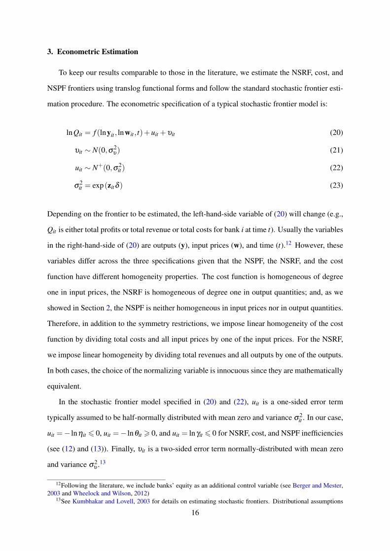
To keep our results comparable to those in the literature, we estimate the NSRF, cost, and

NSPF frontiers using translog functional forms and follow the standard stochastic frontier esti-

mation procedure. The econometric specification of a typical stochastic frontier model is:

lnQit = f (lnyit , lnwit , t)+uit +υit (20)

υit ∼ N(0,σ2υ) (21)

uit ∼ N+(0,σ2it ) (22)

σ2it = exp(zitδ ) (23)

Depending on the frontier to be estimated, the left-hand-side variable of (20) will change (e.g.,

Qit is either total profits or total revenue or total costs for bank i at time t). Usually the variables

in the right-hand-side of (20) are outputs (y), input prices (w), and time (t).12 However, these

variables differ across the three specifications given that the NSPF, the NSRF, and the cost

function have different homogeneity properties. The cost function is homogeneous of degree

one in input prices, the NSRF is homogeneous of degree one in output quantities; and, as we

showed in Section 2, the NSPF is neither homogeneous in input prices nor in output quantities.

Therefore, in addition to the symmetry restrictions, we impose linear homogeneity of the cost

function by dividing total costs and all input prices by one of the input prices. For the NSRF,

we impose linear homogeneity by dividing total revenues and all outputs by one of the outputs.

In both cases, the choice of the normalizing variable is innocuous since they are mathematically

equivalent.

In the stochastic frontier model specified in (20) and (22), uit is a one-sided error term

typically assumed to be half-normally distributed with mean zero and variance σ2it . In our case,

uit =− lnηit 6 0, uit =− lnθit > 0, and uit = lnγit 6 0 for NSRF, cost, and NSPF inefficiencies

(see (12) and (13)). Finally, υit is a two-sided error term normally-distributed with mean zero

and variance σ2υ .13

12Following the literature, we include banks’ equity as an additional control variable (see Berger and Mester,2003 and Wheelock and Wilson, 2012)

13See Kumbhakar and Lovell, 2003 for details on estimating stochastic frontiers. Distributional assumptions

16

Following Caudill, Ford, and Gropper (1995), Hadri (1999), and Wang (2002), we assume

that the variance of the inefficiencies has the functional form given in (23), where δ is a vector

of parameter to be estimated and zit is a vector of bank characteristics that are of interest to

explain bank-specific inefficiency. Specifically, we include time and time squared to capture

the inefficiency trend over time; non performing loans (NPL) as an ex-post measure of credit

risk; the ratio of fees and loan income over total operating income as a measure of core income

from loans; a proxy for off-balance sheet activities (the ratio of non interest income over total

income) to capture the effect of nontraditional activities; the fraction of real estate loans over

total assets and the ratio of total loans over total assets as a measure of output mix, and the log

of total assets to control for bank size.

The parametrization of σ2it allows us to account for time varying determinants of inef-

ficiency via the zit variables (see Wang, 2002). In this setting, E[ui] = σit [φ(0)/Φ(0)] =√2/π exp(zitδ ), where φ and Φ are the probability and cumulative density functions of a

standard normal distribution, respectively. Therefore, the marginal effects of the z variables on

the unconditional mean of inefficiency are given by:

∂E[ui]

∂ zk=

∂ (z′iδ )∂ zk

√(0.5/π)exp(z′iδ ) (24)

To accommodate possible heteroscedasticity of the error term υit , we follow Hadri (1999) and

Wang (2003) and make σ2υ = exp(hitϕ); where hit is a vector of time and bank characteristics

that may induce heteroscedasticity in υit , and ϕ is a vector of parameters to be estimated. We

include time, NPL, and leverage in h. For all stochastic frontiers we estimate, we reject the

hypothesis of homoscedasticity at the 1% level of statistical significance.

4. Data

We use data from the Report of Conditions and Income (Call Reports) from the Federal

Reserve Bank of Chicago. We include all FDIC insured commercial banks with available

data between 2001Q1 and 2010Q4. We exclude banks reporting negative values for assets,

of these one-sided errors have little impact on estimated efficiency ranks (e.g., Kumbhakar and Lovell, 2003)

17

equity, outputs and prices, standalone internet banks, commercial banks conducting primarily

credit card activities, and banks chartered outside continental U.S. territory. Our data set is an

unbalanced panel with 63,120 bank-year observations for 8,483 banks. We deflate all nominal

quantities using the 2005 Consumer Price Index for all urban consumption published by the

Bureau of Labor Statistics.

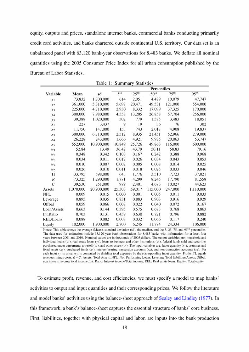
Table 1: Summary StatisticsPercentiles

Variable Mean sd 5th 25th 50th 75th 95th

y1 73,832 1,700,000 614 2,051 4,489 10,079 47,747y2 361,000 5,310,000 5,697 20,471 49,531 121,000 554,000y3 225,000 4,710,000 2,930 8,332 17,099 37,325 170,000y4 300,000 7,980,000 4,558 13,205 26,858 57,704 256,000y5 39,388 1,020,000 302 779 1,585 3,483 18,051x1 227 3,437 9 19 36 76 302x2 11,750 147,000 153 743 2,017 4,908 19,837x3 300,000 6,710,000 2,512 8,935 21,451 52,966 279,000x4 26,228 243,000 1,666 4,921 9,985 20,063 53,747x5 552,000 10,900,000 10,849 25,726 49,863 116,000 600,000w1 52.84 13.49 36.42 43.79 50.11 58.83 79.16w2 0.348 0.342 0.103 0.167 0.242 0.388 0.968w3 0.034 0.011 0.017 0.026 0.034 0.043 0.053w4 0.010 0.007 0.002 0.005 0.008 0.014 0.025w5 0.026 0.010 0.011 0.018 0.025 0.033 0.046Π 33,795 598,000 643 1,776 3,510 7,723 37,021R 73,325 1,290,000 1,771 4,299 8,245 17,790 81,558C 39,530 751,000 979 2,401 4,673 10,027 44,623

Assets 1,070,000 20,900,000 25,303 59,017 115,000 247,000 1,110,000NPL 0.009 0.015 0.000 0.001 0.005 0.011 0.033Leverage 0.895 0.035 0.831 0.883 0.903 0.916 0.929Offbal 0.059 0.066 0.008 0.022 0.040 0.072 0.167Loan/Assets 0.663 0.144 0.395 0.575 0.683 0.768 0.863Int.Ratio 0.703 0.131 0.459 0.630 0.721 0.796 0.882REL/Loans 0.088 0.082 0.008 0.032 0.066 0.117 0.240Equity 102,000 1,900,000 2,700 6,245 11,774 24,334 106,000Notes: This table shows the average (Mean), standard deviation (sd), the median, and the 5, 25, 75, and 95th percentiles.The data used for estimation include 63,120 year-bank observations for 8,483 banks with information for at least fouryears between 2001 and 2010. Nominal values are in thousands of 2005 dollars. The output variables are: household andindividual loans (y1), real estate loans (y2), loans to business and other institutions (y3), federal funds sold and securitiespurchased under agreements to resell (y4), and other assets (y5). The input variables are: labor quantity (x1), premises andfixed assets (x2), purchased funds (x3), interest-bearing transaction accounts (x4), and non-transaction accounts (x5). Foreach input x j its price, w j , is computed by dividing total expenses by the corresponding input quantity. Profits, Π, equalsrevenues minus costs, R−C. Assets: Total Assets, NPL: Non Performing Loans, Leverage:Total liabilities/Assets, Offbal:non interest income/ total income, Int. Ratio: Interest income/Total income, REL: Real estate loans, Equity: Total equity.

To estimate profit, revenue, and cost efficiencies, we must specify a model to map banks’

activities to output and input quantities and their corresponding prices. We follow the literature

and model banks’ activities using the balance-sheet approach of Sealey and Lindley (1977). In

this framework, a bank’s balance-sheet captures the essential structure of banks’ core business.

First, liabilities, together with physical capital and labor, are inputs into the bank production

18

process. Second, assets, other than physical assets, are outputs. Liabilities are composed of

core deposits and purchased funds. Assets include loans and trading securities. Therefore,

banks use labor, physical capital, and debt to produce loans, invest in financial assets, and

facilitate other financial services.

Table 1 presents summary statistics for all the variables we use. Nominal variables are in

thousands. Output and input variables for each year are computed as the quarterly average of

balance-sheet nominal (stock) values. We define five output variables: household and individ-

ual loans (y1), real estate loans (y2), business loans (y3), securities (e.g. federal funds sold and

securities purchased under agreements to resell) (y4), and other assets (y5). These outputs are

essentially the same as those used in Berger and Mester (2003).

We define five input variables: labor (number of full-time equivalent employees at the end

of each quarter) (x1), physical capital (e.g., premises and fixed assets including capitalized

leases) (x2), purchased funds (federal funds purchased and securities sold under agreements to

repurchase, total trading liabilities, other borrowed money, and subordinated notes and deben-

tures) (x3), interest-bearing transaction accounts (x4), and non-transaction accounts (x5). For

each input x j its price, w j, is computed by dividing total expenses by the corresponding input

quantity. Total costs, C, equal the sum of expenses for five inputs; total revenues, R, equal

the sum of revenues for each output category; and, profits, Π, equal total revenues minus total

costs.

On the revenue side, real estate loans account for about 42% of total banks’ revenues, loan

to business and other institutions 16% , securities 15% , and other assets 16%. Loans to individ-

uals and households only account for 7% of total revenues. On the cost side, expenditures on

non-transaction accounts represent 29%, labor 41%, premises and fixed assets 10%, purchased

funds 17%, and transaction accounts 3% of total cost.

We include the following variables as possible determinants of inefficiencies: time, time

squared, log of total assets (Assets), non performing loans (NPL), leverage (Leverage:Total

liabilities/Assets), a proxy for off-balance sheet activities (Offbal: non interest income/ total

income), the ratio between interest income and total income (Int. Ratio), the ratio of real estate

loans (REL) over total assets, and total equity.

19

5. Empirical Results

5.1. Efficiency Estimates

We summarize our main results in Table 2.14 Our proposed CNSPF efficiency measure in-

dicates that, on average, banks’ profits are 79.5% of their potential maximum. Average CNSPF

efficiency decreases with bank size. Big banks (assets > $1 billion) are more profit efficient

than medium ($100 million < assets < $1 billion), and small (assets < $100 million) banks.

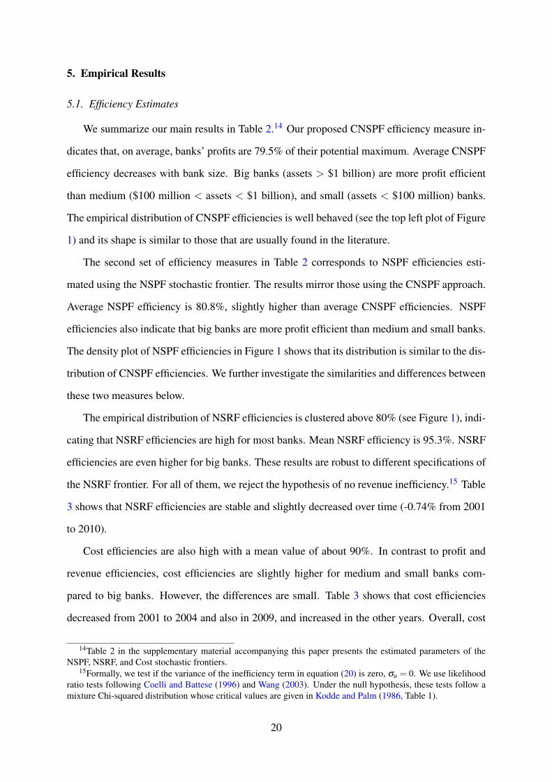
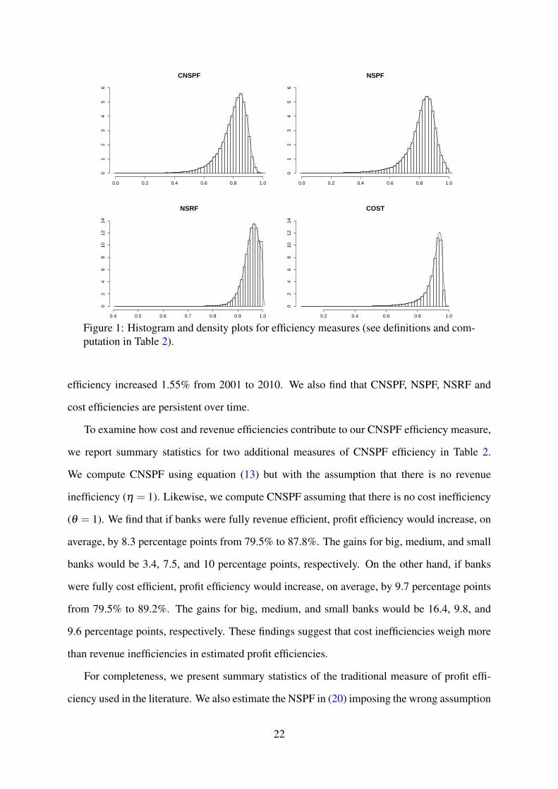
The empirical distribution of CNSPF efficiencies is well behaved (see the top left plot of Figure

1) and its shape is similar to those that are usually found in the literature.

The second set of efficiency measures in Table 2 corresponds to NSPF efficiencies esti-

mated using the NSPF stochastic frontier. The results mirror those using the CNSPF approach.

Average NSPF efficiency is 80.8%, slightly higher than average CNSPF efficiencies. NSPF

efficiencies also indicate that big banks are more profit efficient than medium and small banks.

The density plot of NSPF efficiencies in Figure 1 shows that its distribution is similar to the dis-

tribution of CNSPF efficiencies. We further investigate the similarities and differences between

these two measures below.

The empirical distribution of NSRF efficiencies is clustered above 80% (see Figure 1), indi-

cating that NSRF efficiencies are high for most banks. Mean NSRF efficiency is 95.3%. NSRF

efficiencies are even higher for big banks. These results are robust to different specifications of

the NSRF frontier. For all of them, we reject the hypothesis of no revenue inefficiency.15 Table

3 shows that NSRF efficiencies are stable and slightly decreased over time (-0.74% from 2001

to 2010).

Cost efficiencies are also high with a mean value of about 90%. In contrast to profit and

revenue efficiencies, cost efficiencies are slightly higher for medium and small banks com-

pared to big banks. However, the differences are small. Table 3 shows that cost efficiencies

decreased from 2001 to 2004 and also in 2009, and increased in the other years. Overall, cost

14Table 2 in the supplementary material accompanying this paper presents the estimated parameters of theNSPF, NSRF, and Cost stochastic frontiers.

15Formally, we test if the variance of the inefficiency term in equation (20) is zero, σu = 0. We use likelihoodratio tests following Coelli and Battese (1996) and Wang (2003). Under the null hypothesis, these tests follow amixture Chi-squared distribution whose critical values are given in Kodde and Palm (1986, Table 1).

20

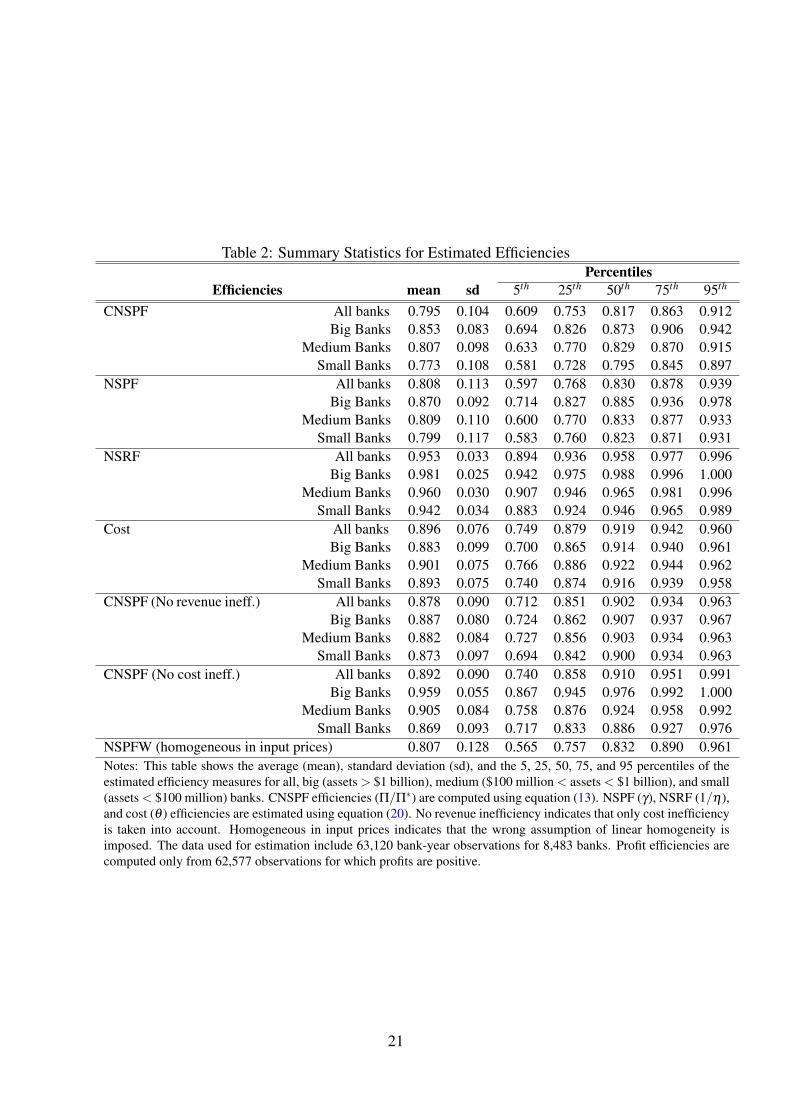
Table 2: Summary Statistics for Estimated EfficienciesPercentiles

Efficiencies mean sd 5th 25th 50th 75th 95th

CNSPF All banks 0.795 0.104 0.609 0.753 0.817 0.863 0.912Big Banks 0.853 0.083 0.694 0.826 0.873 0.906 0.942

Medium Banks 0.807 0.098 0.633 0.770 0.829 0.870 0.915Small Banks 0.773 0.108 0.581 0.728 0.795 0.845 0.897

NSPF All banks 0.808 0.113 0.597 0.768 0.830 0.878 0.939Big Banks 0.870 0.092 0.714 0.827 0.885 0.936 0.978


NSRF All banks 0.953 0.033 0.894 0.936 0.958 0.977 0.996Big Banks 0.981 0.025 0.942 0.975 0.988 0.996 1.000


Cost All banks 0.896 0.076 0.749 0.879 0.919 0.942 0.960Big Banks 0.883 0.099 0.700 0.865 0.914 0.940 0.961


CNSPF (No revenue ineff.) All banks 0.878 0.090 0.712 0.851 0.902 0.934 0.963Big Banks 0.887 0.080 0.724 0.862 0.907 0.937 0.967


CNSPF (No cost ineff.) All banks 0.892 0.090 0.740 0.858 0.910 0.951 0.991Big Banks 0.959 0.055 0.867 0.945 0.976 0.992 1.000


NSPFW (homogeneous in input prices) 0.807 0.128 0.565 0.757 0.832 0.890 0.961Notes: This table shows the average (mean), standard deviation (sd), and the 5, 25, 50, 75, and 95 percentiles of theestimated efficiency measures for all, big (assets > $1 billion), medium ($100 million < assets < $1 billion), and small(assets < $100 million) banks. CNSPF efficiencies (Π/Π∗) are computed using equation (13). NSPF (γ), NSRF (1/η),and cost (θ ) efficiencies are estimated using equation (20). No revenue inefficiency indicates that only cost inefficiencyis taken into account. Homogeneous in input prices indicates that the wrong assumption of linear homogeneity isimposed. The data used for estimation include 63,120 bank-year observations for 8,483 banks. Profit efficiencies arecomputed only from 62,577 observations for which profits are positive.

21

CNSPF

0.0 0.2 0.4 0.6 0.8 1.0

01

23

45

6

NSPF

0.0 0.2 0.4 0.6 0.8 1.0

01

23

45

6

NSRF

0.4 0.5 0.6 0.7 0.8 0.9 1.0

02

46

810

1214

COST

0.2 0.4 0.6 0.8 1.0

02

46

810

1214

Figure 1: Histogram and density plots for efficiency measures (see definitions and com-putation in Table 2).

efficiency increased 1.55% from 2001 to 2010. We also find that CNSPF, NSPF, NSRF and

cost efficiencies are persistent over time.

To examine how cost and revenue efficiencies contribute to our CNSPF efficiency measure,

we report summary statistics for two additional measures of CNSPF efficiency in Table 2.

We compute CNSPF using equation (13) but with the assumption that there is no revenue

inefficiency (η = 1). Likewise, we compute CNSPF assuming that there is no cost inefficiency

(θ = 1). We find that if banks were fully revenue efficient, profit efficiency would increase, on

average, by 8.3 percentage points from 79.5% to 87.8%. The gains for big, medium, and small

banks would be 3.4, 7.5, and 10 percentage points, respectively. On the other hand, if banks

were fully cost efficient, profit efficiency would increase, on average, by 9.7 percentage points

from 79.5% to 89.2%. The gains for big, medium, and small banks would be 16.4, 9.8, and

9.6 percentage points, respectively. These findings suggest that cost inefficiencies weigh more

than revenue inefficiencies in estimated profit efficiencies.

For completeness, we present summary statistics of the traditional measure of profit effi-

ciency used in the literature. We also estimate the NSPF in (20) imposing the wrong assumption

22

that the NSPF is linear homogeneous in input prices. We label it as NSPFW. The results are

similar to those without imposing the homogeneity restriction. However, they follow a different

pattern over time (see Table 3) and correlate differently with cost efficiencies (see Table 4).

The top right plot of Figure 1 shows that the empirical distribution of NSPF efficiencies is

similar to that of CNSPF efficiencies. The similarity between these two measures is surprising

given that they were obtained using different approaches. Common statistical tests reject that

both distributions are equal. Therefore, we further investigate if the small differences between

our CNSPF and NSPF efficiency estimates can lead to economically significant differences that

are relevant for empirical studies.

Quantile-quantile and empirical cumulative distribution plots (not reported) between NSPF

and CNSPF efficiency estimates reveals that both distributions have similar quantiles except

for those observations lying on the left tail of the distributions. Further, transition probability

matrices (not reported) show that CNSPF and NSPF efficiencies categorized by size deciles

are comparable. In summary, both efficiency estimates yield similar conclusions regarding

the efficiency level of big, medium, and small banks. However, both measures rank banks

differently.

Table 3: Mean Efficiency MeasuresYear C-NSPF %∆ NSPF %∆ NSRF %∆ COST %∆ NSPFW %∆

2001 0.776 0.857 0.951 0.903 0.8922002 0.796 2.58 0.840 -1.98 0.953 0.21 0.887 -1.77 0.870 -2.472003 0.801 0.63 0.819 -2.50 0.955 0.21 0.876 -1.24 0.848 -2.532004 0.806 0.62 0.806 -1.59 0.956 0.10 0.873 -0.34 0.831 -2.002005 0.807 0.12 0.807 0.12 0.957 0.10 0.889 1.83 0.803 -3.372006 0.794 -1.61 0.809 0.25 0.957 0.00 0.904 1.69 0.772 -3.862007 0.776 -2.27 0.797 -1.48 0.955 -0.21 0.909 0.55 0.748 -3.112008 0.779 0.39 0.775 -2.76 0.952 -0.31 0.910 0.11 0.736 -1.602009 0.798 2.44 0.773 -0.26 0.949 -0.32 0.909 -0.11 0.760 3.262010 0.817 2.38 0.780 0.91 0.944 -0.53 0.917 0.88 0.786 3.42Total 0.795 5.280 0.808 -8.980 0.953 -0.740 0.896 1.550 0.807 -11.88Notes: This table shows annual means of the estimated efficiency measures and their annual percentage changes.NSPF stands for non standard profit function (traditional method), CNSPF correspond to Composite NSPF (ourmethod) computed using equation (13). NSRF refers to efficiency estimates from the non standard revenue functionand Cost to efficiency estimates using a cost function. NSRF efficiencies are computed as 1/η and Cost efficiencyas θ (See equation (20)). CNSPF efficiencies are computed using equation (13) as Π/Π∗. No revenue inefficiencyindicates that only cost inefficiency is taken into account. The data used for estimation include 63,120 bank-yearobservations for 8,483 banks with information for at least four years between 2001 and 2010. Estimated profitefficiencies are computed only from 62,577 observations for which profits are positive.

23

The rank correlation coefficient between CNSPF and NSPF efficiency estimates is only

0.4437 with a standard error of 0.003 (see Table 4). In addition, the correlation between these

two measures and both NSRF and cost efficiency estimates differ markedly. For example,

the rank correlations of CNSPF efficiency with NSRF and cost efficiency estimates are 0.505

and 0.352, respectively. In contrast, the rank correlation between NSPF efficiency and cost

efficiency estimates is significantly negative (-0.293). Table 3 provides further evidence that

CNSPF and NSPF efficiencies are different. Overall, CNSPF efficiency increased by 5.28%

from 2001 to 2010. NSPF efficiency, in contrast, decreased by 8.98%. We think that these

differences are economically relevant for empirical studies.

Given that both CNSPF and NSPF efficiencies may lead to different conclusions, we advo-

cate using the CNSPF efficiency measure over the NSPF for two main reasons. First, the econo-

metric model used in the estimation of CNSPF efficiencies is correctly specified, as opposed

to the the one used to estimating NSPF efficiencies. Second, the CNSPF efficiency measure in

(13) clearly identifies the underlying sources of profit efficiency, which is not possible from the

NSPF. That is, one cannot identify the source of profit inefficiency from the estimated NSPF.

Equation (13) imposes constraints on the relation between cost, revenue, and cost efficien-

cies. In the NSPF approach, maximum profits (π∗) equal maximum revenues, R(w,y), minus

minimum costs, C(w,y). For given levels of cost and profit efficiency, revenue efficiency can

be computed as Ra/R(w,y) = (πa +Ca)/(π∗+C(w,y)). This relation helps in verifying the

consistency of different measures of cost, revenue, and profit efficiency. By construction, our

CNSPF efficiency measure always satisfies this relation. However, this is not the case for the

traditional NSPF efficiency measure. To show this, we compute the implicit revenue efficiency

values that are consistent with the estimated NSPF and cost efficiencies. That is, we use the

profit efficiency measures derived from the NSPF, along with the cost efficiency measures de-

rived from the cost function, and compute the implicit revenue efficiency measure. We find

that implicit revenue efficiency measures are higher than 100% for 22% of the observations.

This result implies that for some banks actual revenues are higher than the maximum possible

revenues. This exercise allows us to conclude that the traditional NSPF approach gives im-

plausible levels of revenue efficiency. In contrast, CNSPF efficiency measures are always well

24

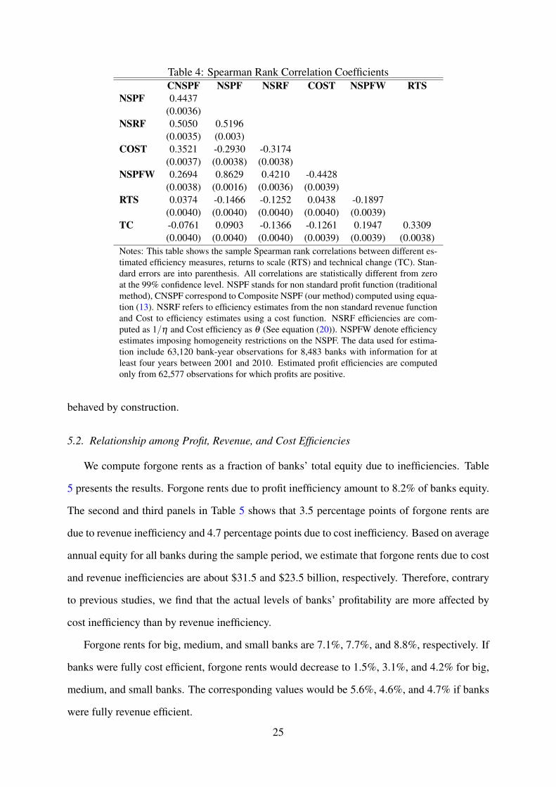
Table 4: Spearman Rank Correlation CoefficientsCNSPF NSPF NSRF COST NSPFW RTS

NSPF 0.4437(0.0036)

NSRF 0.5050 0.5196(0.0035) (0.003)

COST 0.3521 -0.2930 -0.3174(0.0037) (0.0038) (0.0038)

NSPFW 0.2694 0.8629 0.4210 -0.4428(0.0038) (0.0016) (0.0036) (0.0039)

RTS 0.0374 -0.1466 -0.1252 0.0438 -0.1897(0.0040) (0.0040) (0.0040) (0.0040) (0.0039)

TC -0.0761 0.0903 -0.1366 -0.1261 0.1947 0.3309(0.0040) (0.0040) (0.0040) (0.0039) (0.0039) (0.0038)

Notes: This table shows the sample Spearman rank correlations between different es-timated efficiency measures, returns to scale (RTS) and technical change (TC). Stan-dard errors are into parenthesis. All correlations are statistically different from zeroat the 99% confidence level. NSPF stands for non standard profit function (traditionalmethod), CNSPF correspond to Composite NSPF (our method) computed using equa-tion (13). NSRF refers to efficiency estimates from the non standard revenue functionand Cost to efficiency estimates using a cost function. NSRF efficiencies are com-puted as 1/η and Cost efficiency as θ (See equation (20)). NSPFW denote efficiencyestimates imposing homogeneity restrictions on the NSPF. The data used for estima-tion include 63,120 bank-year observations for 8,483 banks with information for atleast four years between 2001 and 2010. Estimated profit efficiencies are computedonly from 62,577 observations for which profits are positive.

behaved by construction.

5.2. Relationship among Profit, Revenue, and Cost Efficiencies

We compute forgone rents as a fraction of banks’ total equity due to inefficiencies. Table

5 presents the results. Forgone rents due to profit inefficiency amount to 8.2% of banks equity.

The second and third panels in Table 5 shows that 3.5 percentage points of forgone rents are

due to revenue inefficiency and 4.7 percentage points due to cost inefficiency. Based on average

annual equity for all banks during the sample period, we estimate that forgone rents due to cost

and revenue inefficiencies are about $31.5 and $23.5 billion, respectively. Therefore, contrary

to previous studies, we find that the actual levels of banks’ profitability are more affected by

cost inefficiency than by revenue inefficiency.

Forgone rents for big, medium, and small banks are 7.1%, 7.7%, and 8.8%, respectively. If

banks were fully cost efficient, forgone rents would decrease to 1.5%, 3.1%, and 4.2% for big,

medium, and small banks. The corresponding values would be 5.6%, 4.6%, and 4.7% if banks

were fully revenue efficient.

25

Table 5: Summary Statistics for Forgone Rents due to InefficiencyPercentiles

Forgone rents due to: mean sd 5th 25th 50th 75th 95th

Revenue and cost inefficienciesAll Banks 0.082 0.061 0.031 0.051 0.070 0.097 0.162Big Banks 0.071 0.073 0.020 0.036 0.052 0.081 0.178


Revenue inefficiencyAll Banks 0.035 0.025 0.003 0.017 0.031 0.047 0.080Big Banks 0.015 0.021 0.000 0.003 0.009 0.019 0.047


Cost inefficiencyAll Banks 0.047 0.058 0.011 0.021 0.033 0.054 0.120Big Banks 0.056 0.073 0.010 0.022 0.036 0.063 0.162


Notes: This table shows the average (mean), standard deviation (sd), and the 5, 25, 50, 75, and 95percentiles of the estimated forgone rents as a fraction of banks’ total equity due to inefficienciesfor all, big (assets > $1 billion), medium ($0.1 < assets < $1 billion), and small (assets < $0.1billion) banks. The data used for estimation include 63,120 bank-year observations for 8,483 banks.Forgone rents are computed only from 62,577 observations for which profits are positive.

Now, we estimate the effect of a 1% increase in revenue, cost, or both efficiencies on CN-

SPF efficiency. For each bank, we multiply its NSRF and cost efficiency scores by 1.01. Then,

we compute the percentage change in CNSPF efficiency due to the change in NSRF efficiency

using (16), the change in cost efficiency using (17), and changes in both NSRF and cost effi-

ciencies using (15). Table 6 reports the results.

For all banks, a 1% increase in NSRF efficiency leads to an average increase of 2.64% in

CNSPF efficiency. The same increase in cost efficiency leads to an average increase of 1.62%

in CNSPF efficiency. Thus, for any given level of efficiency, increasing revenue efficiency has

a greater impact on profit efficiency than increasing cost efficiency. This result is consistent

with our general finding that, on average, banks are highly revenue efficient. Over the years,

banks may have realized that improving revenue efficiency or avoiding revenue inefficiency

has a greater impact in overall profitability than improving cost efficiency or eliminating cost

inefficiency.

A simultaneous increase in both NSRF and cost efficiencies by 1% leads to an increase in

CNSPF efficiency by 4.26%, on average. Small banks experience bigger gains than medium

26

banks, and medium banks have bigger gains than big banks. Considering a 1% decrease, in-

stead, we find similar results.

Table 6: ∆% in CNSPF efficiency due to a 1% Change in NSRF and Cost EfficienciesPercentiles

Due to 1%∆ in: mean sd 5th 25th 50th 75th 95th

All BanksNSRF Efficiency 2.63679 5.84964 1.69016 1.98710 2.26739 2.65642 3.80156Cost Efficiency 1.62059 5.79173 0.68332 0.97733 1.25485 1.64002 2.77382Both 4.25738 11.64137 2.37348 2.96443 3.52224 4.29644 6.57537

Big BanksNSRF Efficiency 2.24624 0.89011 1.60804 1.87737 2.12209 2.45668 3.16247Cost Efficiency 1.23390 0.88130 0.60202 0.86869 1.11098 1.44225 2.14106Both 3.48015 1.77141 2.21006 2.74606 3.23307 3.89893 5.30353

Medium BanksNSRF Efficiency 2.60303 4.34329 1.71204 2.02260 2.30241 2.68706 3.80529Cost Efficiency 1.58716 4.30028 0.70499 1.01247 1.28951 1.67035 2.77752Both 4.19018 8.64357 2.41704 3.03507 3.59192 4.35741 6.58281

Small BanksNSRF Efficiency 2.72576 7.51504 1.68162 1.96570 2.24319 2.64215 3.89412Cost Efficiency 1.70867 7.44063 0.67487 0.95614 1.23088 1.62589 2.86546Both 4.43443 14.95567 2.35649 2.92185 3.47408 4.26805 6.75958Notes: This table shows the average (mean), standard deviation (sd), and the 5, 25, 50, 75, and 95 per-centiles of the percentage change in profit efficiency measures if revenue and cost efficiency estimates,or both, were shifted up by 1% for all, big (assets > $1 billion), medium ($0.1 < assets < $1 billion),and small (assets < $0.1 billion) banks. The data used for estimation include 63,120 bank-year obser-vations for 8,483 banks. Forgone rents are computed only from 62,577 observations for which profitsare positive.

We repeat the previous exercise but instead of computing the change in profit efficiencies,

we compute the change in returns on assets (ROE). The results are reported in Table 7. We

find that a 1% increase in revenue efficiencies would yield a 0.79 percentage points increase in

ROE. That is, ROE will increase from an average of 10.91% to 11.70%. From a 1% increase in

cost efficiencies, ROE will increase by 0.38 percentage points to 11.29%, on average. From a

1% increase in both revenue and cost efficiencies, ROE will increase by 1.17 percentage points

to 12.08%, on average. This effect is the sum of the two separate effects of revenue and cost

efficiencies on ROE.

Similar to the effects of cost and revenue efficiencies on profit efficiency, the effect of

revenue efficiencies on ROE is stronger than the effect of cost efficiency on ROE. The gains in

ROE from a 1% simultaneous increase in revenue and cost efficiencies are similar for big and

medium banks, but smaller for small banks.

27

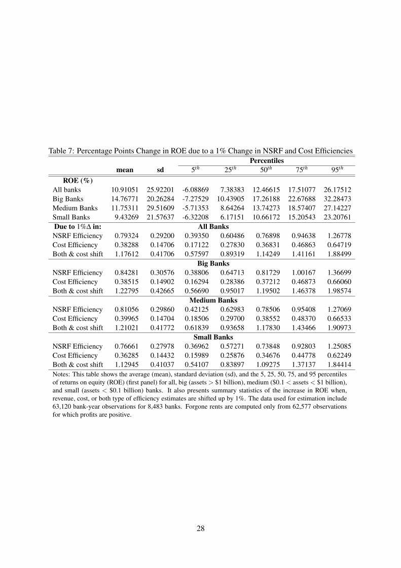
Table 7: Percentage Points Change in ROE due to a 1% Change in NSRF and Cost EfficienciesPercentiles

mean sd 5th 25th 50th 75th 95th

ROE (%)All banks 10.91051 25.92201 -6.08869 7.38383 12.46615 17.51077 26.17512Big Banks 14.76771 20.26284 -7.27529 10.43905 17.26188 22.67688 32.28473Medium Banks 11.75311 29.51609 -5.71353 8.64264 13.74273 18.57407 27.14227Small Banks 9.43269 21.57637 -6.32208 6.17151 10.66172 15.20543 23.20761Due to 1%∆ in: All BanksNSRF Efficiency 0.79324 0.29200 0.39350 0.60486 0.76898 0.94638 1.26778Cost Efficiency 0.38288 0.14706 0.17122 0.27830 0.36831 0.46863 0.64719Both & cost shift 1.17612 0.41706 0.57597 0.89319 1.14249 1.41161 1.88499

Big BanksNSRF Efficiency 0.84281 0.30576 0.38806 0.64713 0.81729 1.00167 1.36699Cost Efficiency 0.38515 0.14902 0.16294 0.28386 0.37212 0.46873 0.66060Both & cost shift 1.22795 0.42665 0.56690 0.95017 1.19502 1.46378 1.98574

Medium BanksNSRF Efficiency 0.81056 0.29860 0.42125 0.62983 0.78506 0.95408 1.27069Cost Efficiency 0.39965 0.14704 0.18506 0.29700 0.38552 0.48370 0.66533Both & cost shift 1.21021 0.41772 0.61839 0.93658 1.17830 1.43466 1.90973

Small BanksNSRF Efficiency 0.76661 0.27978 0.36962 0.57271 0.73848 0.92803 1.25085Cost Efficiency 0.36285 0.14432 0.15989 0.25876 0.34676 0.44778 0.62249Both & cost shift 1.12945 0.41037 0.54107 0.83897 1.09275 1.37137 1.84414Notes: This table shows the average (mean), standard deviation (sd), and the 5, 25, 50, 75, and 95 percentilesof returns on equity (ROE) (first panel) for all, big (assets > $1 billion), medium ($0.1 < assets < $1 billion),and small (assets < $0.1 billion) banks. It also presents summary statistics of the increase in ROE when,revenue, cost, or both type of efficiency estimates are shifted up by 1%. The data used for estimation include63,120 bank-year observations for 8,483 banks. Forgone rents are computed only from 62,577 observationsfor which profits are positive.

28

Now, we explore the effect of some bank characteristics (determinants of inefficiency) on

revenue, cost, and profit efficiencies. We parameterize the unconditional variance of the inef-

ficiency term for the NSPF, NSRF, and cost frontiers following Wang (2002) (see (23)). The

estimated parameters are presented in Table 8. The sign of each parameter gives the direction of

the marginal effects of the corresponding variable on the unconditional mean of inefficiencies.

We compute the marginal effects using (24) for each inefficiency measure. Table 9 presents the

results in elasticity form.16

Table 8: Parameter Estimates of the Variance of Inefficiency for NSPF, NSRF, and CostStochastic Frontiers

NSPF NSRF Cost FunctionVariable Parameter Std. Err. Parameter Std. Err. Parameter Std. Err.

t 0.160 0.027 -0.238 0.053 0.281 0.071t2 -0.022 0.005 0.048 0.011 -0.062 0.018NPL 12.26 0.589 11.80 1.283 15.95 1.437Int. Ratio 5.624 0.231 5.462 0.573 -5.308 0.328Offbal -3.623 0.281 -31.75 1.631 6.620 0.353RSL/Assets -12.34 0.637 -5.824 0.601 3.955 0.414Loans/Assets -5.188 0.218 -8.174 0.5767 0.427 0.281lnAssets -0.206 0.009 -0.176 0.017 -0.171 0.015Log Likelihood -15,303.679 27,730.598 28,669.082Obs. 62,579 63,120 63,120Notes: This table shows the estimated parameters of the variance of inefficiency for the three translogstochastic frontiers: NSPF, NSRF, and Cost (see (20)). NPL: Non Performing Loans. Leverage equalstotal liabilities over total assets. Int. Ratio: Interest ratio equals total interest income from loans over totalincome. Offbal: off balance-sheet activities equals total non interest income over total income. REL: Realestate loans. Assets: Total assets.

The marginal effect of time on CNSPF inefficiencies shows an average decline of 3.2% per

year from 2001 to 2010. NSRF and cost inefficiencies also decrease 1% and 0.2% per year,

respectively. In contrast, NSPF inefficiencies increase on average by 0.5% per year.

As expected, NPL has a positive effect on inefficiencies. A 10% increase in NPL contributes

to a 0.9% increase in CNSPF inefficiency, 0.57% increase in NSRF inefficiency, and 0.9%

increase in cost inefficiency.

The marginal effect of interest ratio weighs heavily on NSRF and cost inefficiencies. A

10% change in interest ratio a yields 21% decrease in cost inefficiency and a 20% increase

in NSRF inefficiency. These two effects offset each other to yield a slightly negative effect

16Although these marginal effects are observation-specific, we are reporting the mean values and their standarddeviation to conserve space. Details are available from the authors upon request.

29

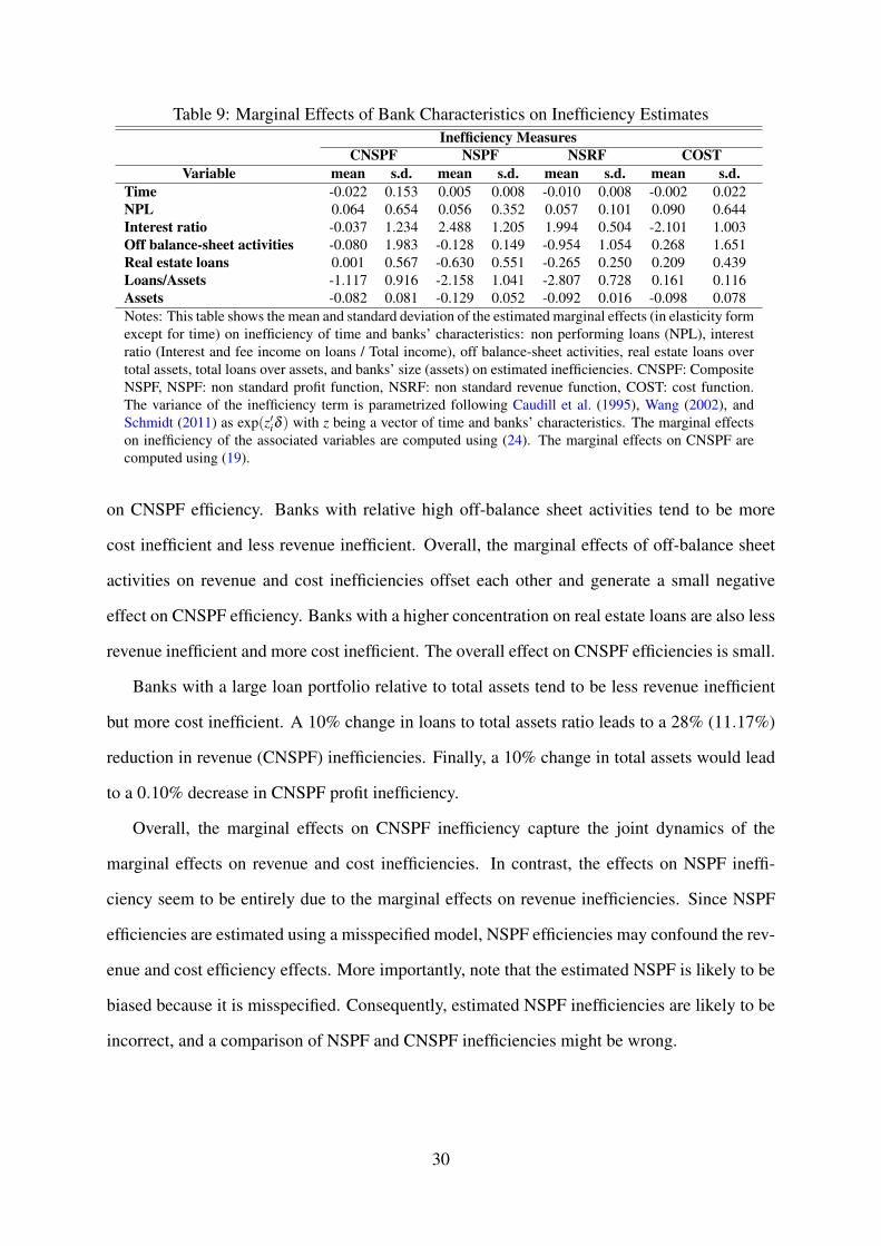
Table 9: Marginal Effects of Bank Characteristics on Inefficiency EstimatesInefficiency Measures

CNSPF NSPF NSRF COSTVariable mean s.d. mean s.d. mean s.d. mean s.d.

Time -0.022 0.153 0.005 0.008 -0.010 0.008 -0.002 0.022NPL 0.064 0.654 0.056 0.352 0.057 0.101 0.090 0.644Interest ratio -0.037 1.234 2.488 1.205 1.994 0.504 -2.101 1.003Off balance-sheet activities -0.080 1.983 -0.128 0.149 -0.954 1.054 0.268 1.651Real estate loans 0.001 0.567 -0.630 0.551 -0.265 0.250 0.209 0.439Loans/Assets -1.117 0.916 -2.158 1.041 -2.807 0.728 0.161 0.116Assets -0.082 0.081 -0.129 0.052 -0.092 0.016 -0.098 0.078Notes: This table shows the mean and standard deviation of the estimated marginal effects (in elasticity formexcept for time) on inefficiency of time and banks’ characteristics: non performing loans (NPL), interestratio (Interest and fee income on loans / Total income), off balance-sheet activities, real estate loans overtotal assets, total loans over assets, and banks’ size (assets) on estimated inefficiencies. CNSPF: CompositeNSPF, NSPF: non standard profit function, NSRF: non standard revenue function, COST: cost function.The variance of the inefficiency term is parametrized following Caudill et al. (1995), Wang (2002), andSchmidt (2011) as exp(z′iδ ) with z being a vector of time and banks’ characteristics. The marginal effectson inefficiency of the associated variables are computed using (24). The marginal effects on CNSPF arecomputed using (19).

on CNSPF efficiency. Banks with relative high off-balance sheet activities tend to be more

cost inefficient and less revenue inefficient. Overall, the marginal effects of off-balance sheet

activities on revenue and cost inefficiencies offset each other and generate a small negative

effect on CNSPF efficiency. Banks with a higher concentration on real estate loans are also less

revenue inefficient and more cost inefficient. The overall effect on CNSPF efficiencies is small.

Banks with a large loan portfolio relative to total assets tend to be less revenue inefficient

but more cost inefficient. A 10% change in loans to total assets ratio leads to a 28% (11.17%)

reduction in revenue (CNSPF) inefficiencies. Finally, a 10% change in total assets would lead

to a 0.10% decrease in CNSPF profit inefficiency.

Overall, the marginal effects on CNSPF inefficiency capture the joint dynamics of the

marginal effects on revenue and cost inefficiencies. In contrast, the effects on NSPF ineffi-

ciency seem to be entirely due to the marginal effects on revenue inefficiencies. Since NSPF

efficiencies are estimated using a misspecified model, NSPF efficiencies may confound the rev-

enue and cost efficiency effects. More importantly, note that the estimated NSPF is likely to be

biased because it is misspecified. Consequently, estimated NSPF inefficiencies are likely to be

incorrect, and a comparison of NSPF and CNSPF inefficiencies might be wrong.

30

5.3. Homogeneity Restrictions on the NSPF

For estimation, researchers often impose the restriction that the NSPF is homogeneous of

degree one in input prices (e.g. Berger and Mester, 1997, Altunbas, Evans, and Molyneux,

2001, Clark and Siems, 2002, Berger, Hasan, and Zhou, 2009, Koetter et al., 2012). In most

cases, the authors state that their results are unaffected by such restrictions. Humphrey and

Pulley (1997, p.81, 84) explicitly state that the NSPF is not linear homogeneous in input prices

and Kumbhakar (2006) formally proves this point. In Section 2, we showed that the same

results holds in our framework.

We find that imposing linear homogeneity in input prices is not innocuous. As shown in

Table 4, the rank correlation between NSPF and cost efficiencies—labeled NSPF and COST,

respectively, is −0.293. The rank correlation between NSPFW and cost efficiency is signif-

icantly lower (−0.4428). The difference between them is statistically significant and might

be economically significant in empirical studies. For example, studies usually take profit and

cost efficiencies and draw conclusions depending on how they correlate with other variables.

Imposing wrong homogeneity restrictions may lead to misleading results.

6. Conclusions

Research on bank’s profit efficiency using the nonstandard profit function sprang after the

publication of Humphrey and Pulley (1997). Since then, more than fifty published studies

have contributed significantly to the current stock of knowledge regarding some aspects of the

evolution of the banking industry over the last three decades. In this paper we show that the

econometric model used in the literature to estimate Humphrey and Pulley’s model is misspec-

ified. Using the same theoretical framework, we propose an alternative method that solves this

problem and allows researchers to study the contribution that both revenue and cost efficiencies

have on overall banks’ profit efficiency.

Our empirical results indicate that the measured levels of bank’s profit efficiency are influ-

enced more by cost inefficiencies than by revenue inefficiencies. We estimate the combined

annual losses for all U.S. commercial banks due to cost and revenue inefficiencies at about

$31.5 and $23.5 billion, respectively. We demonstrate theoretically and show empirically that

31

changes in revenue efficiency have a greater impact on profit efficiency than equivalent changes

in cost efficiency; a result consistent with the measured high levels of revenue efficiency we

present.

Our alternative method allows us to investigate the relation between profit, revenue, and

cost efficiencies across banks and over time. We find that revenue and cost efficiencies tend to

be negatively correlated, but both correlate positively with profit efficiency. As suggested by

Berger and Mester (1997), the negative correlation between revenue and cost efficiencies may

indicate that less cost efficient banks offset their related losses with higher revenue efficiency.

Perhaps because less efficient banks incur higher costs in producing higher quality outputs that

bring in higher revenues or because high revenue efficient banks exert less effort in controlling

costs. In contrast to the results obtained using the misspecified econometric model, we find that

profit and cost efficiencies tend to be positively correlated. Thus, the negative relation between

cost and profit efficiencies reported in the literature (e.g., Rogers 1998 and Berger and Mester

1997) stems from misspecification of the econometric model which, as we show, implicitly

constraints profit and cost efficiencies to be negatively correlated.

Using U.S. commercial bank data from 2001 to 2010, we find that revenue and cost effi-

ciency estimates are around 95% and 90%, respectively; leading to an overall profit efficiency

level of about 80%. Big banks are more revenue efficient than medium, and small banks. How-

ever, average cost efficiency levels are similar across the bank size distribution, except for the

very small banks. Profit inefficiency represents about 8.15% of bank equity of which 3.49% is

due to revenue inefficiencies and 4.66% due to cost inefficiencies. For big, medium, and small

banks average forgone rents are 7.1%, 7.7%, and 8.8% of banks’ equity, respectively.

If banks were fully revenue efficient, profit efficiency would increase from 79.5% to 87.8%.

If banks were fully cost efficient, profit efficiency would increase from 79.5% to 89.2%. A 1%

increase in revenue efficiency would increase profit efficiencies by 2.64%. In comparison, the

same increase in cost efficiencies would increase profit efficiencies by only 1.6%. Thus, for

any given level of cost and revenue efficiencies, revenue efficiencies weigh more than cost

efficiencies in overall profit efficiency.

32

References

Altunbas, Y., Evans, L., Molyneux, P., 2001. Bank Ownership and Efficiency. Journal of Money, Credit

& Banking (Ohio State University Press) 33 (4), 926 – 954.

Berger, A., Humphrey, D., Pulley, L., 1996. Do Consumers Pay for One-stop Banking? Evidence from

an Alternative Revenue Function. Journal of Banking & Finance 20 (9), 1601–1621.

Berger, A., Udell, G., 2006. A More Complete Conceptual Framework for SME Finance. Journal of

Banking & Finance 30 (11), 2945 – 2966.

Berger, A. N., Black, L. K., 2011. Bank Size, Lending Technologies, and Small Business Finance.

Journal of Banking & Finance 35 (3), 724 – 735, australasian Finance Conference: Global financial

crisis, international financial architecture and regulation.

Berger, A. N., Hasan, I., Zhou, M., 2009. Bank Ownership and Efficiency in China: What Will Happen

in the Worlds Largest Nation? Journal of Banking & Finance 33 (1), 113 – 130.

Berger, A. N., Mester, L. J., 1997. Inside the Black Box: What Explains Differences in the Efficiencies

of Financial Institutions? Journal of Banking & Finance 21 (7), 895 – 947.

Berger, A. N., Mester, L. J., 2003. Explaining the Dramatic Changes in Performance of US banks:

Technological Change, Deregulation, and Dynamic Changes in Competition. Journal of Financial

Intermediation 12 (1), 57 – 95.

Berger, A. N., Udell, G. F., 1992. Some Evidence on the Empirical Significance of Credit Rationing.

Journal of Political Economy 100 (5), pp. 1047–1077.

Berger, A. N., Udell, G. F., 1995. Relationship Lending and Lines of Credit in Small Firm Finance. The

Journal of Business 68 (3), pp. 351–381.

Berger, A. N., Udell, G. F., 2002. Small Business Credit Availability and relationship lending: The

Importance of Bank Organisational Structure. The Economic Journal 112 (477), F32–F53.

Berlin, M., Mester, L., 1999. Deposits and relationship lending. Review of Financial Studies 12 (3),

579–607.

Caudill, S., Ford, J., Gropper, D., 1995. Frontier Estimation and Firm-specific Inefficiency Measures in

the Presence of Heteroscedasticity. Journal of Business & Economic Statistics 13 (1), 105–111.

Clark, J. A., Siems, T. F., 2002. X-Efficiency in Banking: Looking beyond the Balance Sheet. Journal

of Money, Credit & Banking (Ohio State University Press) 34 (4), 987 – 1013.

Coelli, T., Battese, G., 1996. Identification of Factors which Influence the Technical Inefficiency of

Indian Farmers. Australian Journal of Agricultural and Resource Economics 40 (2), 103–128.

33

Cottarelli, C., Kourelis, A., 1994. Financial Structure, Bank Lending Rates, and the Transmission Mech-

anism of Monetary Policy. Staff Papers - International Monetary Fund 41 (4), pp. 587–623.

Cowan, C., Cowan, A., 2006. A Survey Based Assessment of Financial Institution Use of Credit Scoring

for Small Business Lending. Tech. rep., Small Business Administration.

De Bondt, G. J., 2005. Interest Rate Pass-Through: Empirical Results for the Euro Area. German Eco-

nomic Review 6 (1), 37–78.

Dick, A., Lehnert, A., 2010. Personal Bankruptcy and Credit Market Competition. The Journal of Fi-

nance 65 (2), 655–686.

Edelberg, W., 2003. Risk-based Pricing of Interest Rates in Household Loan Markets. Finance and

Economics Discussion Series.

Gan, J., Riddiough, T., 2008. Monopoly and Information Advantage in the Residential Mortgage Market.

The Review of Financial Studies 21 (6), pp. 2677–2703.

Hadri, K., 1999. Estimation of a Doubly Heteroscedastic Stochastic Frontier Cost Function. Journal of

Business & Economic Statistics 17 (3), pp. 359–363.

Hofmann, B., Mizen, P., 2004. Interest Rate Pass-Through and Monetary Transmission: Evidence from

Individual Financial Institutions’ Retail Rates. Economica 71 (281), 99–123.

Humphrey, D., Pulley, L., 1997. Banks’ Responses to Deregulation: Profits, Technology, and Efficiency.

Journal of Money, Credit and Banking 29 (1), 73–93.

Kodde, D. A., Palm, F. C., 1986. Wald Criteria for Jointly Testing Equality and Inequality Restrictions.

Econometrica 54 (5), pp. 1243–1248.

Koetter, M., Kolari, J., Spierdijk, L., 2012. Enjoying the Quiet Life Under Deregulation? Evidence from

Adjusted Lerner Indices for U.S. Banks. Review of Economics and Statistics.

Kumbhakar, S., 2006. Specification and Estimation of Nonstandard Profit Functions. Empirical Eco-

nomics 31 (1), 243–260.

Kumbhakar, S., Lovell, C., 2003. Stochastic Frontier Analysis. Cambridge University Press.

Kumbhakar, S., Lozano-Vivas, A., Lovell, C. A., Hasan, I., 2001. The Effects of Deregulation on the

Performance of Financial Institutions: The Case of Spanish Savings Banks. Journal of Money, Credit

& Banking (Ohio State University Press) 33 (1), 101 – 120.

McCoy, P., 2007. Rethinking Disclosure in a World of Risk-Based Pricing. Harvard Journal on Legisla-

tion 44, 123.

Panzar, J. C., Rosse, J. N., 1987. Testing For ”Monopoly” Equilibrium. The Journal of Industrial Eco-

34

nomics 35 (4), pp. 443–456.

Rogers, K., 1998. Nontraditional Activities and The Efficiency of US Commercial Banks. Journal of

Banking & Finance 22 (4), 467–482.

Schmidt, P., 2011. One-step and two-step estimation in SFA models. Journal of Productivity Analysis,

1–3.

Sealey, C., Lindley, J., 1977. Inputs, outputs, and a theory of production and cost at depository financial

institutions. Journal of Finance 32 (4), 1251–1266.

Vivas, A. L., 1997. Profit efficiency for Spanish savings banks. European Journal of Operational Re-

search 98 (2), 381 – 394.

Wang, H., 2002. Heteroscedasticity and Non-monotonic Efficiency Effects of a Stochastic Frontier

Model. Journal of Productivity Analysis 18 (3), 241–253.

Wang, H.-J., 2003. A Stochastic Frontier Analysis of Financing Constraints on Investment: The Case of

Financial Liberalization in Taiwan. Journal of Business & Economic Statistics 21 (3), pp. 406–419.

Wheelock, D., Wilson, P., 2012. Do Large Banks Have Lower Costs? New Estimates of Returns to Scale

for U.S. Banks. Journal of Money, Credit and Banking 44 (1), 171–199.

35

Profit efficiency of U.S. commercial banks: a decomposition

Documents

Transcript of Profit efficiency of U.S. commercial banks: a decomposition