Processes and continuous change in a SAT-based planner
60
Artificial Intelligence 166 (2005) 194–253 www.elsevier.com/locate/artint Processes and continuous change in a SAT-based planner Ji-Ae Shin ∗ , Ernest Davis Courant Institute, New York University,New York, NY 10012, USA Received 27 September 2004; accepted 6 April 2005 Available online 10 May 2005 Abstract The TM-LPSAT planner can construct plans in domains containing atomic actions and durative actions; events and processes; discrete, real-valued, and interval-valued fluents; reusable resources, both numeric and interval-valued; and continuous linear change to quantities. It works in three stages. In the first stage, a representation of the domain and problem in an extended version of PDDL+ is compiled into a system of Boolean combinations of propositional atoms and linear constraints over numeric variables. In the second stage, a SAT-based arithmetic constraint solver, such as LPSAT or MathSAT, is used to find a solution to the system of constraints. In the third stage, a correct plan is extracted from this solution. We discuss the structure of the planner and show how planning with time and metric quantities is compiled into a system of constraints. The proofs of soundness and completeness over a substantial subset of our extended version of PDDL+ are presented. 2005 Elsevier B.V. All rights reserved. Keywords: SAT-based planning; LPSAT; Continuous time; Metric quantities; Processes 1. Introduction Numeric and geometric entities that change continuously in time are central features of many domains, especially physical domains: the position of an object in space, the amount of gasoline in a tank, the temperature of water in a pot, and so on. Early generations of * Corresponding author. E-mail addresses: [email protected] (J. Shin), [email protected] (E. Davis). 0004-3702/$ – see front matter 2005 Elsevier B.V. All rights reserved. doi:10.1016/j.artint.2005.04.001
-
Upload
independent -
Category
Documents
-
view
2 -
download
0
Transcript of Processes and continuous change in a SAT-based planner
Artificial Intelligence 166 (2005) 194–253
www.elsevier.com/locate/artint
Processes and continuous changein a SAT-based planner
Ji-Ae Shin ∗, Ernest Davis
Courant Institute, New York University, New York, NY 10012, USA
Received 27 September 2004; accepted 6 April 2005
Available online 10 May 2005
Abstract
The TM-LPSAT planner can construct plans in domains containing atomic actions and durativeactions; events and processes; discrete, real-valued, and interval-valued fluents; reusable resources,both numeric and interval-valued; and continuous linear change to quantities. It works in three stages.In the first stage, a representation of the domain and problem in an extended version of PDDL+ iscompiled into a system of Boolean combinations of propositional atoms and linear constraints overnumeric variables. In the second stage, a SAT-based arithmetic constraint solver, such as LPSAT orMathSAT, is used to find a solution to the system of constraints. In the third stage, a correct plan isextracted from this solution. We discuss the structure of the planner and show how planning withtime and metric quantities is compiled into a system of constraints. The proofs of soundness andcompleteness over a substantial subset of our extended version of PDDL+ are presented. 2005 Elsevier B.V. All rights reserved.
Keywords: SAT-based planning; LPSAT; Continuous time; Metric quantities; Processes
1. Introduction
Numeric and geometric entities that change continuously in time are central features ofmany domains, especially physical domains: the position of an object in space, the amountof gasoline in a tank, the temperature of water in a pot, and so on. Early generations of
* Corresponding author.E-mail addresses: [email protected] (J. Shin), [email protected] (E. Davis).
0004-3702/$ – see front matter 2005 Elsevier B.V. All rights reserved.doi:10.1016/j.artint.2005.04.001
J. Shin, E. Davis / Artificial Intelligence 166 (2005) 194–253 195
domain-independent planners did not deal with numeric quantities at all, and even nowfew planners deal with continuous change. The TM-LPSAT system described in this paperis the first planner that uses the SAT-based planning methodology to deal with continuouschange, as well as many other aspects of numeric quantities.
Over the past decade, dozens of new powerful engines for propositional satisfiabilityhave become available [55] and are now being used in a broad range of applications. Onevery successful application has been the development of SAT-based propositional planning,in which a planning problem is compiled into a set of propositional constraints in such away that a solution to the constraints demarcates a valid plan [32,34,35]. Recently, a newclass of inference engines1 based on propositional satisfiability solvers has been developedfor systems of Boolean combinations of propositional atoms and linear constraints overreal-valued quantities [3,5,53].
In this paper, we show how the SAT-based planning framework can be extended, usingSAT-based arithmetic constraint solvers, to deal with domains that involve continuous time,resources, and real-valued quantities.
The TM-LPSAT planner constructs plans in domains with the following features:
• The effects and preconditions of actions can involve discrete, real-valued, and interval-valued fluents.
• An action can change the value of a real-valued fluent either continuously, as a linearfunction of time, or discretely.
• An action may be either atomic or durative (taking place over an extended time inter-val).
• An action may take real- or interval-valued parameters.• Actions may be concurrent.• Exogenous events may occur.• Autonomous processes can be defined in the language.• Processes that make a continuous change on the same fluent may be concurrent.• Reusable resources, both numeric and interval-valued, can be defined in the language.
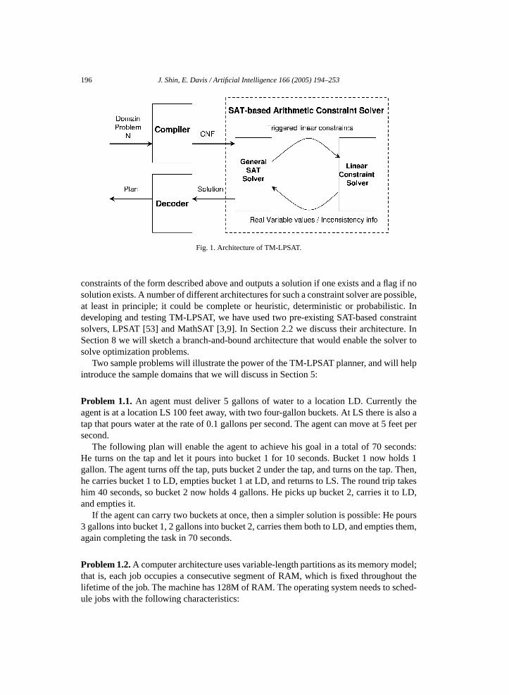
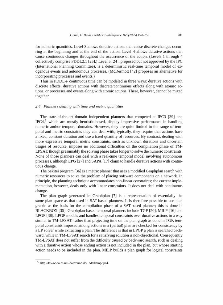
Fig. 1 shows the architecture of TM-LPSAT. The input to TM-LPSAT consists of adomain description and a problem specification represented in PDDL+ [24,25] (more pre-cisely, in a version of PDDL+ with certain restrictions and extensions as described inSection 3). The compiler compiles the planning problem into a set of constraints, eachof which is a disjunction of propositional atoms and linear (in)equalities over numericvariables. The set of constraints is passed to the SAT-based arithmetic constraint solverwhich finds a solution if one exists. From the solution, the decoder extracts a valid plan.The overall system is thus a powerful and elegant planner for a wide range of prob-lems.
Our main contribution in TM-LPSAT has been the development of the compiler. Fromour point of view, the constraint solver can be viewed a black box, that takes as input a set of
1 We will call these “SAT-based Arithmetic Constraint Solver” in this paper. They are also called “SAT-basedDecision Procedure” or “Theorem Prover” in the literature.
196 J. Shin, E. Davis / Artificial Intelligence 166 (2005) 194–253
Fig. 1. Architecture of TM-LPSAT.
constraints of the form described above and outputs a solution if one exists and a flag if nosolution exists. A number of different architectures for such a constraint solver are possible,at least in principle; it could be complete or heuristic, deterministic or probabilistic. Indeveloping and testing TM-LPSAT, we have used two pre-existing SAT-based constraintsolvers, LPSAT [53] and MathSAT [3,9]. In Section 2.2 we discuss their architecture. InSection 8 we will sketch a branch-and-bound architecture that would enable the solver tosolve optimization problems.
Two sample problems will illustrate the power of the TM-LPSAT planner, and will helpintroduce the sample domains that we will discuss in Section 5:
Problem 1.1. An agent must deliver 5 gallons of water to a location LD. Currently theagent is at a location LS 100 feet away, with two four-gallon buckets. At LS there is also atap that pours water at the rate of 0.1 gallons per second. The agent can move at 5 feet persecond.
The following plan will enable the agent to achieve his goal in a total of 70 seconds:He turns on the tap and let it pours into bucket 1 for 10 seconds. Bucket 1 now holds 1gallon. The agent turns off the tap, puts bucket 2 under the tap, and turns on the tap. Then,he carries bucket 1 to LD, empties bucket 1 at LD, and returns to LS. The round trip takeshim 40 seconds, so bucket 2 now holds 4 gallons. He picks up bucket 2, carries it to LD,and empties it.
If the agent can carry two buckets at once, then a simpler solution is possible: He pours3 gallons into bucket 1, 2 gallons into bucket 2, carries them both to LD, and empties them,again completing the task in 70 seconds.
Problem 1.2. A computer architecture uses variable-length partitions as its memory model;that is, each job occupies a consecutive segment of RAM, which is fixed throughout thelifetime of the job. The machine has 128M of RAM. The operating system needs to sched-ule jobs with the following characteristics:
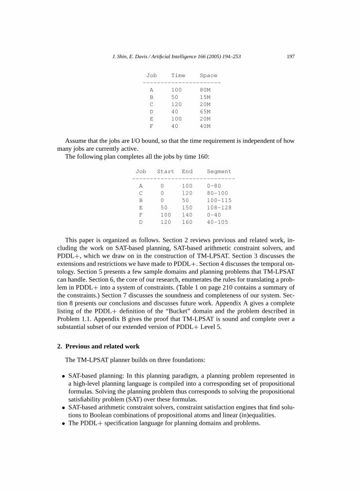
J. Shin, E. Davis / Artificial Intelligence 166 (2005) 194–253 197
Job Time Space----------------------
A 100 80MB 50 15MC 120 20MD 40 65ME 100 20MF 40 40M
Assume that the jobs are I/O bound, so that the time requirement is independent of howmany jobs are currently active.
The following plan completes all the jobs by time 160:
Job Start End Segment-----------------------------
A 0 100 0-80C 0 120 80-100B 0 50 100-115E 50 150 108-128F 100 140 0-40D 120 160 40-105
This paper is organized as follows. Section 2 reviews previous and related work, in-cluding the work on SAT-based planning, SAT-based arithmetic constraint solvers, andPDDL+, which we draw on in the construction of TM-LPSAT. Section 3 discusses theextensions and restrictions we have made to PDDL+. Section 4 discusses the temporal on-tology. Section 5 presents a few sample domains and planning problems that TM-LPSATcan handle. Section 6, the core of our research, enumerates the rules for translating a prob-lem in PDDL+ into a system of constraints. (Table 1 on page 210 contains a summary ofthe constraints.) Section 7 discusses the soundness and completeness of our system. Sec-tion 8 presents our conclusions and discusses future work. Appendix A gives a completelisting of the PDDL+ definition of the “Bucket” domain and the problem described inProblem 1.1. Appendix B gives the proof that TM-LPSAT is sound and complete over asubstantial subset of our extended version of PDDL+ Level 5.
2. Previous and related work
The TM-LPSAT planner builds on three foundations:
• SAT-based planning: In this planning paradigm, a planning problem represented ina high-level planning language is compiled into a corresponding set of propositionalformulas. Solving the planning problem thus corresponds to solving the propositionalsatisfiability problem (SAT) over these formulas.
• SAT-based arithmetic constraint solvers, constraint satisfaction engines that find solu-tions to Boolean combinations of propositional atoms and linear (in)equalities.
• The PDDL+ specification language for planning domains and problems.
198 J. Shin, E. Davis / Artificial Intelligence 166 (2005) 194–253
Also related, though not directly used in TM-LPSAT, are
• Other planning paradigms for dealing with metric time and numeric quantities.• Other automated reasoning applications that deal with continuous change.
We will discuss in turn each of these categories of previous work and their relation toTM-LPSAT.
2.1. Planning as propositional satisfiability
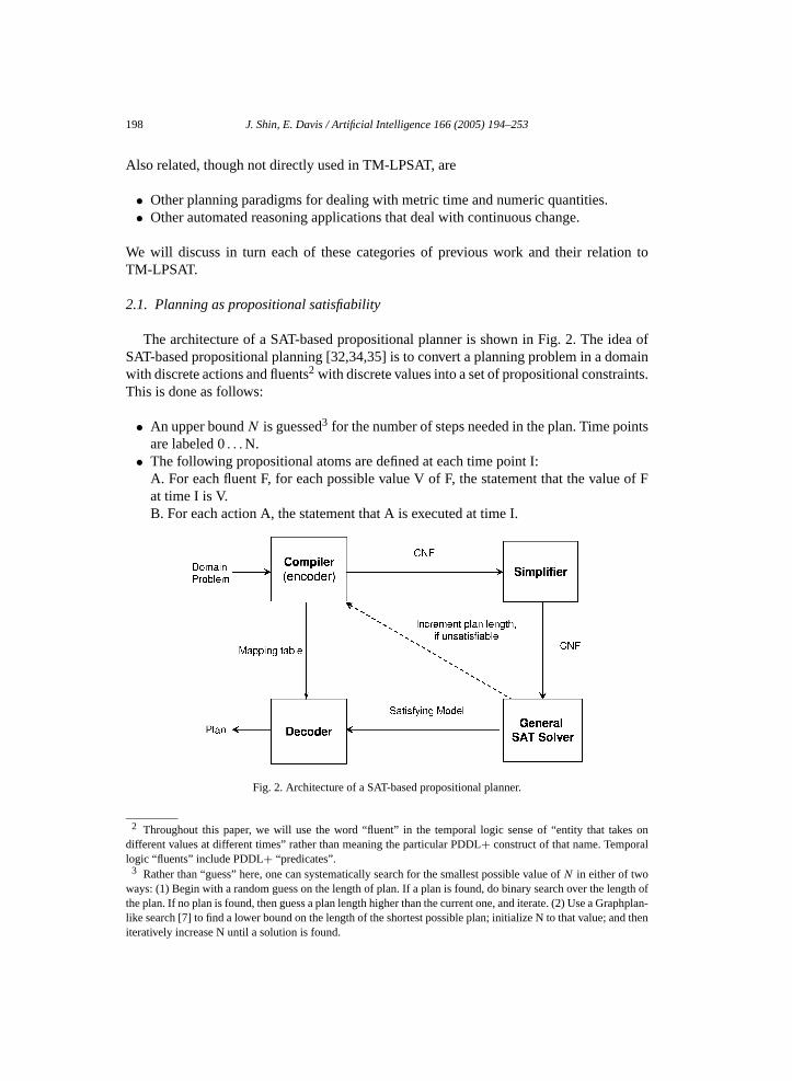
The architecture of a SAT-based propositional planner is shown in Fig. 2. The idea ofSAT-based propositional planning [32,34,35] is to convert a planning problem in a domainwith discrete actions and fluents2 with discrete values into a set of propositional constraints.This is done as follows:
• An upper bound N is guessed3 for the number of steps needed in the plan. Time pointsare labeled 0 . . .N.
• The following propositional atoms are defined at each time point I:A. For each fluent F, for each possible value V of F, the statement that the value of Fat time I is V.B. For each action A, the statement that A is executed at time I.
Fig. 2. Architecture of a SAT-based propositional planner.
2 Throughout this paper, we will use the word “fluent” in the temporal logic sense of “entity that takes ondifferent values at different times” rather than meaning the particular PDDL+ construct of that name. Temporallogic “fluents” include PDDL+ “predicates”.
3 Rather than “guess” here, one can systematically search for the smallest possible value of N in either of twoways: (1) Begin with a random guess on the length of plan. If a plan is found, do binary search over the length ofthe plan. If no plan is found, then guess a plan length higher than the current one, and iterate. (2) Use a Graphplan-like search [7] to find a lower bound on the length of the shortest possible plan; initialize N to that value; and theniteratively increase N until a solution is found.
J. Shin, E. Davis / Artificial Intelligence 166 (2005) 194–253 199
• The laws governing the domain are imposed by asserting every instance of every lawat every moment of time. In classical planning domains the major categories of lawsare: causal laws, domain constraints, and frame axioms.The paradigm, indeed, will support essentially any computable constraint; e.g., thatthe number of times action A is executed must be a prime number; a fluent will changefive time units after some particular action, etc. The main limiting factor on incorpo-rating such constraints is finding systematic ways to express them in a general domaindefinition language such as PDDL+.
• The problem instance is asserted by stating that the starting conditions hold at time 0and that the goal conditions hold at time N.
• The constraints are then fed to a propositional satisfiability solver. If a solution of theconstraints can be found, then the set of actions that are marked as occurring in thesolution constitutes a valid plan.
SAT-based propositional planners can be implemented easily and, with the current gen-eration of satisfiability solvers [55], quite effectively. The planners also have no additionaldifficulty in dealing with ADL features such as conditional effects or quantifications. Themajor drawback of SAT-based planning is that large domains can lead to enormously largesystems of constraints. Particularly dangerous are functions with many arguments; a flu-ent function or action function with k arguments generates a collection of atoms of sizeexponential in k.
Since the introduction of SATPLAN [32,34], a number of other SAT-based plannershave been developed, including BLACKBOX [35] and MEDIC [21]. Building a SAT-basedplanner involves two main types of choices. The first is the representational issue of choos-ing an encoding: What propositional atoms should be used, and how domain constraintsshould be encoded as axioms. The effectiveness of different encoding schemes has beenstudied extensively [21,33]. The second choice is the technique used to solve the satisfia-bility problem; both probabilistic methods like GSAT [32] and deterministic methods likeextensions [55] of DPLL algorithm [14] have been studied.
Temporal planning over integer time, involving constraints such as, “Action A requires3 units of time to complete”, can easily be handed in this framework, as long as the inte-gers involved are small. One defines a time point at each integer, and then encodes suchconstraints in the formulas “If A starts at T0 then it ends at T3”, “If A starts at T1 then itends at T4”, and so on [40].
The LPSAT planner [53,54] developed the LPSAT engine to extend the approach furtherto solve problems in metric planning; that is, planning with real-valued quantities, such asthe quantity of gasoline in a tank. However, the LPSAT planner could not handle problemsinvolving durative actions or continuous change.
Indeed, the claims were made that the SAT-based planning paradigm could not be ex-tended to deal with continuous time, because there would be an infinite number of groundactions, corresponding to the infinite set of choices as to when to execute an action andhow long to continue it [37,49]. The construction of TM-LPSAT has disproved the claims.The way this issue is resolved in TM-LPSAT is to encode a history in terms of a finite setof interesting time points at which something changes, rather than trying to encode all time
200 J. Shin, E. Davis / Artificial Intelligence 166 (2005) 194–253
points on the time line. The clock time of an interesting time point is a numeric variablethat is assigned a value by the constraint solver.
Many of the rules in TM-LPSAT for generating constraints come directly out of theseprevious systems. The rules that deal with effects and preconditions connecting atomicactions with discrete fluents are the same as in the SAT-based propositional planners. Therules that deal with discrete (discontinuous) effects of actions on a numerical fluent, andwith numerical preconditions of actions, are the same as in the LPSAT planner.
2.2. SAT-based arithmetic constraint solver
As shown in Fig. 1, a SAT-based arithmetic constraint solver consists primarily of twocoupled modules [1]: A DPLL-based systematic SAT solver [55], such as RelSAT [6] andMiniSAT [20], and an incremental linear programming (LP) solver, such as Cassowary [8].
A DPLL-based SAT solver does a depth-first search with backtracking through the spaceof partial truth assignments. At its deduction phase, unit resolution and propagation are ap-plied. Modern, high-powered SAT solvers enhance the basic backtracking search usingsuch techniques as conflict-driven learning, random restarts, non-chronological backtrack-ing, and branching heuristics.
The two modules are combined as follows: The input to the constraint solver is a setof generalized clauses. Each clause is a disjunction; each disjunct is either a propositionalliteral or a linear equality or inequality over numeric variables. The SAT solver first looksfor a propositional (partial) solution, treating each linear equation as a propositional atom(called a trigger), then the LP solver tries to solve the set of inequalities that have beenmarked as TRUE in the (partial) solution. If that set is inconsistent, then the SAT solverutilizes information on inconsistency detected through back-jumping or learning (addinga clause stating that these linear inequalities are not all TRUE), and it looks for a newpropositional solution. It continues going back and forth between propositional and nu-meric mode until either finding a solution, establishing that no solution exists, or reachingthe given time limit.
Since the introduction of the LPSAT architecture by Wolfman and Weld [53], Math-SAT [3,9] and more general theorem provers such as CVC Lite [5] have been developed inverification community. These solvers vary in the SAT solving techniques that they incor-porate; in their search heuristics; and in the special cases of “easy” LP categories that theyidentify.
2.3. PDDL+
PDDL (Planning Domain Definition Language) is a declarative language for the defin-ition of causal domains and planning problems. The basis of our work is PDDL+, whichwas the most recent extension4 to PDDL when we began work on TM-LPSAT. PDDL+comprises five levels. Level 1 contains discrete actions and fluents. Level 2 adds features
4 Since then, PDDL2.2 [19], extended for IPC4, was released. The features in PDDL+ remain intact; additionalfeatures included in PDDL2.2 are derived predicates and timed initial literals (sort of deterministic events). Thesefeatures could be easily incorporated in TM-LPSAT.
J. Shin, E. Davis / Artificial Intelligence 166 (2005) 194–253 201
for numeric quantities. Level 3 allows durative actions that cause discrete changes occur-ring at the beginning and at the end of the action. Level 4 allows durative actions thatcause continuous changes throughout the occurrence of the action. (Levels 1 through 4collectively comprise PDDL2.1 [25].) Level 5 [24], proposed but not approved by the IPC(International Planning Committee), is a deterministic real-time temporal model of ex-ogenous events and autonomous processes. (McDermott [42] proposes an alternative forincorporating processes and events.)
Thus in PDDL+ continuous time can be modeled in three ways: durative actions withdiscrete effects, durative actions with discrete/continuous effects along with atomic ac-tions, or processes and events along with atomic actions. These, however, cannot be mixedtogether.
2.4. Planners dealing with time and metric quantities
The state-of-the-art domain independent planners that competed at IPC3 [39] andIPC4,5 which are mostly heuristic-based, display impressive performance in handlingnumeric and/or temporal domains. However, they are quite limited in the range of tem-poral and metric constraints they can deal with; typically, they require that actions havea fixed, constant duration and use a fixed quantity of resources. By contrast, dealing withmore expressive temporal metric constraints, such as unknown durations and uncertainusages of resource, imposes no additional difficulties on the compilation phase of TM-LPSAT, though presumably the solving phase takes longer to solve the numeric constraints.None of those planners can deal with a real-time temporal model involving autonomousprocesses, although LPG [27] and SAPA [17] claim to handle durative actions with contin-uous change.
The Sekitei program [36] is a metric planner that uses a modified Graphplan search withnumeric resources to solve the problem of placing software components on a network. Inprinciple, the planning technique accommodates non-linear constraints; the current imple-mentation, however, deals only with linear constraints. It does not deal with continuouschange.
The plan graph generated in Graphplan [7] is a representation of essentially thesame plan space as that used in SAT-based planners. It is therefore possible to use plangraphs as the basis for the compilation phase of a SAT-based planner; this is done inBLACKBOX [35]. Graphplan-based temporal planners include TGP [50], MILP [16] andLPGP [38]. LPGP models and handles temporal constraints over durative actions in a waysimilar to TM-LPSAT: rather than projecting time on the plan graph as done in TGP, tem-poral constraints imposed among actions in a (partial) plan are checked for consistency bya LP solver while extracting a plan. The difference is that in LPGP a plan is searched back-ward, while in TM-LPSAT search for a satisfying solution is non-directional. ConsequentlyTM-LPSAT does not suffer from the difficulty caused by backward search, such as dealingwith a durative action whose ending action is not included in the plan, but whose startingaction needs to be included in the plan. MILP builds a plan graph for logical constraints
5 http://ls5-www.cs.uni-dortmund.de/~edelkamp/ipc4.
202 J. Shin, E. Davis / Artificial Intelligence 166 (2005) 194–253
in the same way as in LPGP, and converts the graph, together with temporal constraintsamong actions, into an integer linear programming problem.
A number of partial-order planners have dealt, to greater or lesser extent, with prob-lems involving continuous change, including Processes [29], DEVISER [51], SPIE [52],GORDIUS [48], FORBIN [15], Excalibur [18], and ZENO [44,45]. Most of these ad-dressed continuous change only in a substantially more restricted setting than TM-LPSAT.ZENO, by contrast, permitted a very general plan specification language, though its mod-els of concurrency and of processes were less general than TM-LPSAT—ZENO could nothandle concurrent continuous change of quantities. Like TM-LPSAT, ZENO was restrictedto the piecewise linear function and called a LP solver within plan refinement loop. It wasextremely slow; Wolfman and Weld [54] report that ZENO was unable to solve even thesimplest of the logistic problems that were used to test LPSAT.
McDermott [42,43] has extended his estimated-regression planner to deal with processesand continuous change. Unlike TM-LPSAT, his planner is not complete (arguably an ad-vantage, of course). It finds zero crossings using binary search, so presumably it couldeasily be extended to non-linear functions; however, the current implementation has thesame restriction as TM-LPSAT to linear functions with constant coefficients.
2.5. Formalisms for modeling continuous change
The best known study of processes in the AI literature is QP theory [22], which initi-ated a large body of research on physical reasoning with processes. This is at the extremeopposite end in terms of the language of quantities used; effects of processes are charac-terized purely in qualitative terms. A number of important ideas developed in this line ofresearch have yet to be incorporated into the planning literature, such as indirect influences.Davis [13] gives a logical analysis of QP theory.
Another formalism closely related to our work is a theory of hybrid system [30]. A hy-brid automaton combines a finite state machine undergoing a series of discrete change withreal-valued variables undergoing continuous change. A hybrid system is a collection of in-teracting hybrid automata. Fox and Long [24] have defined a semantics for PDDL+ interms of hybrid systems. The planning problem corresponds to the “reachability” problemin a theory of hybrid system. A bounded reachability problem of a linear hybrid systemwas formulated as a satisfiability problem in [4]. Their encoding is based on state tran-sitions with absolute time and clocks; on the other hand, our encoding was based on theconstraints imposed by the operators happening at the time points.
3. Extensions and restrictions to PDDL+
The input specification language for TM-LPSAT extends PDDL+ in four ways:The first extension is that actions in TM-LPSAT may have numeric parameters. For
instance, there can be actions “pour(N,BS,BD)” of pouring N gallons from bucket BSto bucket BD; “set-oven(T )” of setting the thermostat in an oven to temperature T ; or“play_key(K,V )” of playing piano key K at volume V . PDDL2.1 [25] excludes this fea-ture that existed in the original version [41], but their arguments do not strike us as cogent.
J. Shin, E. Davis / Artificial Intelligence 166 (2005) 194–253 203
Numeric parameters obviously greatly increase the expressive power of the language, and,in the TM-LPSAT approach, impose no additional computational burden.
One restriction, however, does have to be imposed on actions with numeric and in-terval parameters: There cannot be two or more concurrent actions6 with the identicalnon-numeric parameters. For instance, the actions “pour(5,b1,b2)” and “pour(2,b1,b2)”cannot be executed concurrently, though “pour(5,b1,b2)” and “pour(2,b3,b4)” can beconcurrent. The restriction is necessary because the entire SAT-based methodology restson the assumption that, once you have guessed the number of significant time points,the number of possible entities, propositions, and numeric parameters can be bounded;if an unbounded collection of simultaneous actions of the form “pour(N, c1,b1)” can begenerated, that would be a problem. The restriction is reasonable because such numericparameters are typically used in one of two ways. If the value of the parameter is assignedto a fluent—e.g., “set-dial(N,D)” results in dial D being set to value N—then two actionswith different numeric parameters would be mutually exclusive. If the value of the parame-ter is used to increment a fluent—e.g., “pour(N,BS,BD)” increases the quantity of liquidin BD by N and increases the quantity in BS by N—concurrent actions pour(5,b1,b2)and pour(2,b1,b2) can be combined into a single action pour(7,b1,b2). There are a fewexceptions; for instance, the action “sound(F, V)”, sounding a tone with frequency F andvolume V, executed by a robot with electronic speakers. It is possible for such a robot toexecute “sound(F1, V1)”, “sound(F2, V2)” . . . concurrently with different frequencies. Ourrepresentation cannot handle this case.
By virtue of this restriction, an action type is identified by the name of the func-tor and the non-numeric parameters. For example, we may speak of the action type“pour(·,b1,b2)” (pouring some amount from b1 into b2) and be sure that at most oneof these occurs at one time.
The second extension of PDDL+ is that our specification language supports reusablemetric resources, including numeric and interval-valued; that is, resources that are held byan action while the action lasts and released when the action is complete. We denote it bya “use” statement of the form “(use ?resource ?amount)”.
The motivation behind this extension is as follows: PDDL+ has no explicit provision forresources. It treats numeric resources like any other numeric quantities. Thus concurrent(shared) uses of reusable resource among atomic actions cannot be modeled in PDDL+.For example, suppose that an agent has K identical effectors, and that there is a collectionof atomic actions, such as flipping a switch, each of which requires the use of one effector.Then, clearly, it should be possible for the agent to execute K such actions concurrently.However, this can only be represented in PDDL+ by representing each effector separately.The result would be that each different assignment of actions to individual effectors wouldbe considered separately, thus multiplying the branching factor by K factorial. The useof interval resources among actions, atomic or durative, cannot be expressed in PDDL+,because there are infinitely many choices for the lower and upper bounds of the interval tobe allocated to the action.
6 The axioms in [46] allow two such durative actions to continue concurrently, though not to start simultane-ously. This requires a more complex representation, which identifies durative actions by their starting time.
204 J. Shin, E. Davis / Artificial Intelligence 166 (2005) 194–253
RAM memory in Problem 1.2 can be represented as a reusable interval resource, andits concurrent uses are disjoint subintervals of the resource. Other kinds of domains whereinterval resources are useful include the placing of books on a shelf; the assignment offrequency ranges to broadcasters; and so on.
The third extension of PDDL+ is that our language supports interval-valued fluents andquantities. We have incorporated in our language and includes Allen’s 13 binary intervalrelations [2] and several other basic useful functions on intervals.
The fourth extension is that we distinguish between numeric functions whose valuesare constant over time and given in the problem statement and numeric functions whosevalues vary over time. The former are marked as being of type float; the latter are of typefluent. For example, in the Bucket domain, “(capacity ?b - bucket)” is of sort float whereas“(level ?b – bucket)” is of sort fluent. This distinction was made in the original PDDL [41],but was removed in PDDL2.1. This feature is particularly important in TM-LPSAT fortwo reasons. First, when an entity changes its value over time, it is necessary to create aseparate variable for the value of the entity at each time point. Thus, if there are N timepoints, then each fluent F generates N numeric variables, whereas a float F generates nonumeric variables. Second, if X and Y are variables then the equation X = AY is a linearequation if the value of A is known at compilation time, but it is a non-linear equation if thevalue of A is not known. Since TM-LPSAT can only deal with linear equations, quantitieslike the flow-rate of a tap must be floats, so that equations like “change-in-quantity =flow-rate ∗ duration-of-flow” are linear equation in the variables “change-in-quantity” and“duration-of-flow”.
A few features of PDDL+ cannot be handled in the current version of TM-LPSAT.First, TM-LPSAT cannot optimize a specified plan metric, a limitation inherited from thearchitecture of the arithmetic constraint solvers we use. Second, the language must berestricted so that, in any multiplication, all but one of the terms can be statically evaluated;and, in any division, the denominator can be statically evaluated. Otherwise, the result willbe a non-linear equation, which existing SAT-based arithmetic constraint solvers cannotdeal with, and which will certainly be much more difficult for any possible constraintsolver. All other features of PDDL+ are included.
4. Temporal ontology
We use a linear, real-valued time line. The representation used in the constraint lan-guage output by TM-LPSAT characterizes the time line in terms of the states of the worldat a collection of significant time points. A significant time point is one where “some-thing changes”; roughly speaking, some action, event, or process occurs, starts, or ends.In the intervals between significant time points, fluents are either constant, or, if they arenumeric, they may undergo continuous change as a linear function of time. Every discon-tinuous change, or change in the derivative of a numeric fluent, occurs at a significant timepoint. Thus, there are two states associated with each time point T. The “state before T”consists of the values of fluents and activity levels immediately before the changes thattake place at T; the “state after T” consists of their values after the changes that take placeat T.
J. Shin, E. Davis / Artificial Intelligence 166 (2005) 194–253 205
Each time point has a clock time, which is a non-negative real value. These clock timesbecome numeric variables in the system of constraints set up by the compiler.
One tricky point arises in any theory that includes both real-valued time and atomicevents and actions: How should one deal with atomic events/actions that, intuitively, shouldoccur one immediately after another? Suppose for instance, that action A has precondi-tion P and effect Q and that event E has triggering condition Q and effects (not P) and(not Q). It should be possible for A to be executed, and then E will be triggered. Theproblem is, when do these occur? If there is a gap between A and E, then why doesn’t E
occur sooner? If A and E occur at the same time, then how can you be sure that A isoccurring before E (which is possible) and not the other way around (which is impossi-ble)?
The semantics defined by Fox and Long [24] for PDDL+ Level 5 involves an unusualmodel of the time line.7 An event that is triggered by an action or another event occurs“immediately after”, with no time gap between. To deal with this, there need to be twodistinct time points with equal clock times. Thus, we represent the situation by sayingthat A occurs at time point T5, say, and that E occurs at time point T6 and that these aredifferent time points even though clock(T5) = clock(T6) = 17.28 sec. We impose an orderon these two time points but there is no time gap between them.
Fox and Long’s semantics both for Level 4 and for Level 5 requires that a time pointwhen an action occurs be separated from the previous time point by a fixed positive con-stant ε, corresponding to the reaction time of the agent or the precision of the agent’s clock.This dependence of the theory on the arbitrary quantity ε is ugly, and in our implementa-tion of TM-LPSAT we have eliminated it in Level 5. If we can idealize events as occurringin immediate succession, why not actions as well? We have maintained the ε gap in ourimplementation of Level 4, where it applies to all time points (there are no atomic eventsin Level 4).8
Note that an event E must disable its own triggering condition; else there would have tobe additional occurrences of E at Ti+2, at Ti+3, etc.; the result would be that the system ofconstraints would have no solution with finitely many time points.
An atomic action occurs instantaneously. An action is characterized by preconditionsthat must hold before the action and effects that hold after the action. For example, theaction “turn on the faucet” has the precondition that the faucet is off and has the effect thatthe faucet is on.
In PDDL+, a durative action is conceptualized as consisting of three epochs: initial-ization, continuation, and termination. The initialization and termination resemble atomicactions; they are instantaneous and are characterized by preconditions and discrete effects.
7 Actually, this paper by Fox and Long is not at all clear on this point. Our interpretation here is our best guessas to what is intended. If this isn’t right, then it is easily changed; one of the advantages of the SAT-based planneris that making that kind of change generally affects a only few specific axioms.
8 One problematic situation is if the invariant conditions of a durative action become FALSE at a time that isless than ε after the previous time point. TM-LPSAT considers such a case to be impossible; the epsilon gapaxiom (6.1) in Section 6 requires that any two significant time points be separated by at least ε, whereas thezero-crossing axiom (10.11) requires that there be a significant time point exactly when the invariant conditionceases to hold. Hence, any plan that gives rise to such a situation is considered invalid.
206 J. Shin, E. Davis / Artificial Intelligence 166 (2005) 194–253
The continuation may take any length of time greater than ε. Its invariants must be satisfiedas long as it continues. Its effects may either take effect continuously for its entire duration,like the effects of a process, or discretely at its end.
A durative action is feasible only if it can be carried through to termination; it cannotbe begun and then abandoned.
For example, one can define “filling bucket B from tap T” as a durative action withthe following properties. The initialization has the preconditions that tap T is off; that thebucket and the agent are at the same location as the tap; and that the bucket is not full; andit has the effect that tap T is on. The continuation has the precondition that the tap is turnedon, and that the tap and the bucket are at the same location. It has the continuous effect thatthe level in the bucket rises at flow-rate(T). The termination has the precondition that thetap is on it has the effect that the tap is off.
An event is like an atomic action, except that, whereas an atomic action may occur if itspreconditions hold (if the actor so chooses), an atomic event must occur if its preconditionhold. For example, suppose that some of the buckets are fragile, with a weight limit thatis less than their volumetric capacity. If the quantity of liquid inside exceeds the weightlimit, the bottom falls out. This can be characterized in terms of an atomic event “break-Bucket(B)”. The preconditions are that B is unbroken and that level(B) � weightLimit(B).The effects are that B is broken and that level(B) = 0.
A process is active over an extended interval. It is characterized by preconditions andeffects. The preconditions must hold through the interval; if the preconditions cease tohold, the process stops. The effects of a process are, in the language of Forbus [22], directinfluences on numeric fluents. Specifically, each process has a fixed influence on somecollection of real-valued fluents; the derivative of the fluent at a given time is the sum ofits influences over all active processes and actions that influence it.
For example, the process “fillingBucket(B – bucket T – tap L – location)” has the pre-condition that tap T is currently pouring into B and that the bucket is not yet full. (Ofcourse, the tap will continue to pour even when the bucket is full, but it will cease to fillthe bucket.) The process has the effect of increasing level(B) at the rate flow(T). (We allowonly taps that are fully on or off.) There can be several co-located taps pouring simultane-ously into the same bucket; if so, the rate of increase of the level in the bucket is the sumof the flow-rates of the individual taps.
PDDL+ permits concurrent actions under fairly restrictive conditions, designed to en-sure (a) that the result of concurrent actions is meaningful; (b) that the actions do notinteract, either destructively or synergistically. However, two actions whose effect is toincrease or decrease a given numeric fluent can be executed concurrently, since the neteffect is well-defined as the sum of the separate effects. For example, one can pour intobucket b1 both from bucket b2 and from bucket b3 simultaneously. Essentially, these con-ditions amount to requiring that the actions be commutative; that is, that they can beexecuted in any order and that the result of executing them is the same in all orderings.The actual condition imposed is sufficient, though not necessary, to ensure commuta-tivity; this is in order that the conditions for concurrency can be computed easily andstatically.
J. Shin, E. Davis / Artificial Intelligence 166 (2005) 194–253 207
5. Sample domains
Let us illustrate some of the PDDL+ constructs that TM-LPSAT can deal with:
Example 5.1. The atomic action of pouring quantity Q of water from one bucket to anothercan be encoded as follows:
(:action pour:parameters (?a - agent ?bs - bucket ?bd - bucket ?q - real ?l - location):precondition (and (at ?a ?l) (carrying ?a ?bs) (at ?bd ?l)
(> ?q 0)(<= ?q (level ?bs))(<= ?q (− (capacity ?bd) (level ?bd))))
:effect (and (increase (level ?bd) ?q)(decrease (level ?bs) ?q))
)
Note the real-valued parameter ?q; the planner can choose to pour any positive amount?q as long as ?q is not more than the amount of water in the source, and not more than theamount of room in the destination.
Example 5.2 (PDDL+ Level 3). The action of filling a bucket can be characterized as adurative action with a discrete effect as follows:
(:durative-action fillBucket1:parameters (?a - agent ?b - bucket ?t - tap ?l - location):duration (at end (<= ?duration (/ (- (capacity ?b) (level ?b)) (flow-rate ?t)))):condition (and (at start (not (on ?t)))
(at start (at ?a ?l)) (at start (at ?b ?l)) (at start (at ?t ?l))(over all (on ?t)) (over all (at ?b ?l))(at end (on ?t)))
:effect (and (at start (on ?t))(at end (not (on ?t)))(at end (increase (level ?b) (* ?duration (flow-rate ?t)))))
)
The value of the duration will be set by the planner; this determines the amount of waterto fill the bucket with. It is critical, here and in Examples 5.3 and 5.4, that the quantity“(flow-rate ?t)” can be evaluated statically. If this quantity is a variable, then the equationbecomes non-linear, and the existing SAT-based arithmetic constraint solvers cannot dealwith it.
The PDDL+ semantics allow a fluent whose value changes as an effect of a durativeaction to be referable and updatable by other actions during the course of the action. Thus itis possible for one bucket to be filled by two different taps concurrently. For instance, “fill-Bucket1(a1,b1,t1,sl1)” and “fillBucket1(a2,b1,t3,sl1)” can be concurrent. However, due tothe mutex rule called no moving target on “(level ?b)”, the two actions cannot finish at thesame time.
208 J. Shin, E. Davis / Artificial Intelligence 166 (2005) 194–253
In this model, when a durative action makes a change to a numeric fluent, the changeoccurs instantaneously at the end points of the action. However, in most cases, the actualchange to a fluent occurs gradually during the course of the action. Therefore, in the middleof the occurrence of the durative action, the value given by this model is not correct. Themodel of durative actions given in Example 5.3 overcomes this limitations.
Example 5.3 (PDDL+ Level 4). The action of filling a bucket can be characterized as adurative action causing continuous change as follows:
(:durative-action fillBucket2:parameters (?a - agent ?b - bucket ?t - tap ?l - location):duration ():condition (and (at start (not (on ?t)))
(at start (at ?a ?l)) (at start (at ?b ?l)) (at start (at ?t ?l))(over all (at ?b ?l)) (over all (on ?t))(over all (<= (level ?b) (capacity ?b)))(at end (on ?t)))
:effect (and (at start (on ?t))(at end (not (on ?t)))(increase (level ?b) (* #t (flow-rate ?t)))))
In the last line above, “#t” is a special variable which, at each instant during the exe-cution of the durative action, denotes the length of time that has elapsed since the actionstarted.
Unlike the model in Example 5.2, this representation allows other actions to access thecorrect value of a continuously changing fluent at any time point over the period of theaction.
Example 5.4 (PDDL+ Level 5). The action of filling a bucket can be characterized yetagain as an atomic action of turning on the tap, followed by a process of flow from the tapinto the bucket, followed by an atomic action of turning off the tap.
(:action turnOnTap:parameters (?a - agent ?t - tap ?b - bucket ?l - location):precondition (and (at ?a ?l) (at ?b ?l) (at ?t ?l) (not (on ?t))):effect (and (on ?t) (filling ?t ?b))
)(:process fillingBucket:parameters (?b - bucket ?t - tap ?l - location):precondition (and (filling ?t ?b)
(<= (level ?b) (capacity ?b))(at ?b ?l))
:effect (increase (level ?b) (* #t (flow-rate ?t))))(:action turnOffTap:parameters (?a - agent ?t - tap ?b - bucket ?l - location):precondition (and (at ?a ?l) (at ?t ?l) (on ?t) (filling ?t ?b))
J. Shin, E. Davis / Artificial Intelligence 166 (2005) 194–253 209
:effect (and (not (on ?t)) (not (filling ?t ?b))))
Example 5.5 (Reusable metric resources). We can model the domain of filling a bucket ina different way: Assume that the taps are classified as of small capacity or of big capacity.A number of taps, either of the same capacity or not, may be at each location. Let “(flow-rate ?tot)” be the flow-rate of a tap of type ?tot; let “(no-of-taps ?tot ?l)” be the number oftaps of type ?tot in location ?l. Then “fillBucket2” shown in Example 5.3 can be representedas follows:
(:durative-action Modified-fillBucket2:parameters (?a - agent ?b - bucket ?tot - TypeOfTap ?l - location):duration ():condition (and (at start (at ?a ?l)) (at start (at ?b ?l))
(over all (at ?b ?l))(over all (<= (level ?b) (capacity ?b))))
:effect (and (increase (level ?b) (* #t (flow-rate ?tot)))(use (no-of-taps ?tot ?l) 1))
)
If there are a large number of taps of each type at a given location, then using thisrepresentation very much reduces symmetry in the search space over the previous repre-sentation in which taps are represented individually: In an individualistic representation,the search space may include every possible set of taps; here, by representing the collec-tion of a type of taps as a multiple-capacity resource, each such set is summarized by twonumeric fluents.
Also representing a resource as a numeric fluent suggests a way to deal with dynami-cally creating and destroying objects.
Example 5.6 (Partitioned interval resource). As described in Problem 1.2, in an operatingsystem that uses variable-length partitions as a memory model, each job occupies a con-secutive segment of RAM which is fixed until it finishes. “(RAM-space)” can be defined asa resource of type interval in our extended PDDL+. The consecutive segments allocatedto jobs running concurrently are disjoint subintervals of the RAM space.
(:durative-action executeJob:parameters (?j - job):duration (= ?duration (time-for ?j)):condition (and (at start (not (active ?j)))
(over all (active ?j))(at end (active ?j)))
:effect (and (at start (active ?j))(at end (not (active ?j)))(use (RAM-space) (memory-for ?j)))
)
210 J. Shin, E. Davis / Artificial Intelligence 166 (2005) 194–253
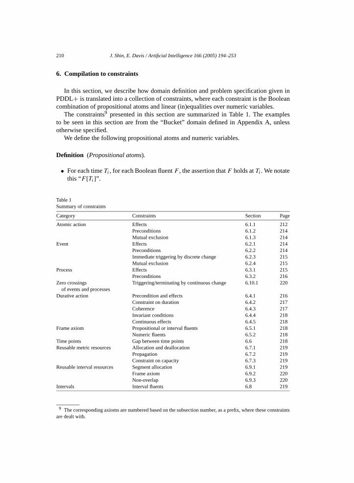
6. Compilation to constraints
In this section, we describe how domain definition and problem specification given inPDDL+ is translated into a collection of constraints, where each constraint is the Booleancombination of propositional atoms and linear (in)equalities over numeric variables.
The constraints9 presented in this section are summarized in Table 1. The examplesto be seen in this section are from the “Bucket” domain defined in Appendix A, unlessotherwise specified.
We define the following propositional atoms and numeric variables.
Definition (Propositional atoms).
• For each time Ti , for each Boolean fluent F , the assertion that F holds at Ti . We notatethis “F [Ti]”.
Table 1Summary of constraints
Category Constraints Section Page
Atomic action Effects 6.1.1 212Preconditions 6.1.2 214Mutual exclusion 6.1.3 214
Event Effects 6.2.1 214Preconditions 6.2.2 214Immediate triggering by discrete change 6.2.3 215Mutual exclusion 6.2.4 215
Process Effects 6.3.1 215Preconditions 6.3.2 216
Zero crossings Triggering/terminating by continuous change 6.10.1 220of events and processes
Durative action Precondition and effects 6.4.1 216Constraint on duration 6.4.2 217Coherence 6.4.3 217Invariant conditions 6.4.4 218Continuous effects 6.4.5 218
Frame axiom Propositional or interval fluents 6.5.1 218Numeric fluents 6.5.2 218
Time points Gap between time points 6.6 218Reusable metric resources Allocation and deallocation 6.7.1 219
Propagation 6.7.2 219Constraint on capacity 6.7.3 219
Reusable interval resources Segment allocation 6.9.1 219Frame axiom 6.9.2 220Non-overlap 6.9.3 220
Intervals Interval fluents 6.8 219
9 The corresponding axioms are numbered based on the subsection number, as a prefix, where these constraintsare dealt with.
J. Shin, E. Davis / Artificial Intelligence 166 (2005) 194–253 211
• For each time Ti , for each non-Boolean discrete fluent F , for each value V , the asser-tion that F has value V at Ti . We notate this “F [Ti] = V ”.
• For each time Ti , for each atomic action/event E, the assertion that E occurs at Ti . Wedenote it “active(E)[Ti ]”.
• For each time Ti , for each process P , the assertion “active(P )[Ti ]” assert that P isactive over the open interval (Ti, Ti+1).
• For each time Ti , for each durative action A, the assertions that A starts at Ti ;that A is continuing at Ti ; and that A ends at Ti . We denote these “starts(A)[Ti ]”,“continues(A)[Ti ]” and “ends(A)[Ti ]”, respectively.
Definition (Numeric variables).
• The clock time of every significant time point Ti , denoted “c(Ti )”.• For every time Ti , for every numeric fluent Q, the value of Q before and after Ti .
We notate these “Q[T −i ]” and “Q[T +
i ]”, respectively. These are not equal if someatomic action or event discretely changes the value of Q at time Ti . (Note that, indomains where all change is discrete, Q[T −
i ] is always equal to Q[T +i−1] whereas in
theories where all change is continuous, Q[T +i ] is always equal to Q[T −
i ]. The needfor two values at a time point therefore only arises in theories that combine discreteand continuous change, as in PDDL+ Levels 4 and 5.)
• For every time Ti , for every interval fluent Z, the lower and upper bound of Z at Ti , de-noted “left(Z,Ti )” and “right(Z,Ti )”. Note that we do not have continuously changingintervals.
• For each numeric fluent Q, for each action or event A that changes Q incrementally(i.e., executes a discrete “increase” or “decrease”), the amount of increase or decreasethat an occurrence of A makes to Q at time Ti . This is denoted “�(A,Q,Ti)”. Thisenables us to add these up over concurrent actions/events.
• For each numeric fluent Q, for each durative action or process A that changes Q
continuously, for each time Ti , the net change in Q due to A between Ti and Ti+1.This is denoted “Γ (A,Q,Ti, Ti+1)”.
• For any durative action A, “Duration(A,Ti )” is a numeric variable for the duration ofthe instance of A that starts in Ti .
• Let A(P1 . . . Pk,Q1 . . .Qm,Z1 . . .Zp) be an action where P1 . . . Pk are discrete pa-rameters; Q1 . . .Qm are numeric parameters; and Z1 . . .Zp are interval parameters.Then, by the restriction mentioned in Section 3.2.3, at any particular time Ti , for anyparticular values V1 . . . Vk of the discrete parameters, there is at most one valuation onthe Qi and the Zi for which an action of the form A(P1 . . . Pk,Q1 . . .Qm,Z1 . . .Zp)
begins at time Ti . The value of each such Qj and the values of the lower and upperbound of Zj are numeric variables; it may appear in a term on the right hand side ofan assignment statement or in a condition.For example: “pour(?a,?bs,?bd,?q,?l)” is an action with the real-valued parameter ?q.There is therefore a numeric variable “pour?q (a1,b3,b4,l3)[T5]” meaning the amountthat a1 should pour from b3 to b4 at l3 at time T5.
• For each resource R, durative action A, and time Ti , the amount of R that A uses attime Ti . This is denoted “U(R,A,Ti )”.
212 J. Shin, E. Davis / Artificial Intelligence 166 (2005) 194–253
• For any durative action A that uses interval resource R, for any time Ti , numeric vari-ables representing the lower and upper bounds of the segment of R allocated to A atTi . We denote these “lower(A,R,Ti )” and “upper(A,R,Ti )”.
Notational convention. We will use the following convention for labeling time-dependentterms:
• If a complex term α over fluents is evaluated using the values before a discrete changeis made at time Ti , we will denote this evaluation as α[T −
i ]. That is, it is evaluated withthe values of propositional fluents at Ti−1 and the values of numeric fluents before Ti ,Q[T −
i ].• If a complex term α over fluents is evaluated after a discrete change is made at time
Ti , we will denote this evaluation as α[T +i ]. That is, it is evaluated with the values of
propositional fluents at Ti , and the values of numeric fluents after Ti , Q[T +i ].
We begin by guessing at an upper bound N on the number of significant time pointsthat will be needed to solve the problem. The significant time points are then T0 . . . TN .
As discussed in Section 4, we assume throughout that there cannot be two actions,events or processes executing concurrently whose name is the same except for numericalparameters.10 For example, the actions “pour(a1,b2,b3,2,l1)” and “pour(a1,b2,b3,5,l1)”cannot be executed concurrently; there cannot be two concurrent processes of the form“fillingBucket(b1,t2,l3)” and so on.
6.1. Atomic actions
6.1.1. EffectsA: If an effect of action A is to assign term α to discrete or interval fluent F , then add
the constraint:
(1.1) active(A)[Ti] ⇒ [F [Ti] = α[T −i ]].
For example, one constraint generated by the action “turnOnTap” is
active(turnOnTap(a1,t1,b2,l3))[T5] ⇒ on(t1)[T5].
(Here the term α is just the implicit Boolean value TRUE.)B: If an effect of action A is to assign term α to numeric fluent F , then add the con-
straint:
(1.2) active(A)[Ti] ⇒ [F [T +i ] = α[T −
i ]].
10 This is slightly at variance with the PDDL+ semantics, which does allow this for durative actions. For exam-ple, it is possible that in the bucket domain given in Example 5.5, “Modified-fillBucket2(a1,b1,ST,sl1)” startingat T2 and “Modified-fillBucket2(a1,b1,ST,sl1)” starting at T4 can continue concurrently until T6, as long as thebucket b1 is not full until T6.
J. Shin, E. Davis / Artificial Intelligence 166 (2005) 194–253 213
For example, walking between two locations can be represented as a “walking” processtriggered by “go” action and “arrive” event. The “go(?a,?sl,?dl)” action sets the distancefor the agent to walk as follows:
(assign (distance-to-walk ?a ?dl) (distance ?dl ?sl)).
The constraint associated with this would be:
active(go(a1,sl1,dl1))[T5] ⇒distance-to-walk(a1,dl1)[T +
5 ] = distance(dl1,sl1).
C: If an effect of action A is to increase numeric fluent Q by the term α, then add theconstraints:
(1.3) active(A)[Ti] ⇒ [�[A,Q,Ti] = α[T −i ]].
(1.4) ¬active(A)[Ti] ⇒ [�[A,Q,Ti] = 0].For example, two constraints associated with the “pour” action are:
active(pour(a2,b2,b3,·,l1),T5) ⇒�(pour(a2,b2,b3,·,l1),level(b3),T5) = pour?q(a2,b2,b3,l1)[T5].
¬active(pour(a2,b2,b3,·,l1),T5) ⇒�(pour(a2,b2,b3,·,l1), level(b3),T5) = 0.
The first constraint above is read, “If agent a2 pours water from bucket b2 to bucket b3 atlocation l1 at time T5, then the increase in the level of water in b3 due to this action is equalto the amount that has been poured”.
D: Let A1 . . .Ak be all the action/events that can change numeric fluent Q incrementally.Let E1 . . .Ep be all the action/events that can assign to Q. Add the constraint:
(1.5) ¬active(E1)[Ti] ∧ · · · ∧ ¬active(Ep)[Ti]⇒
[Q[T +
i ] = Q[T −i ] +
∑j
�(Aj ,Q,Ti)
].
For example, suppose that there are three buckets, b1, b2, b3, one agent a1 and two loca-tions l1 and l2. Then the level in b1 can be changed either by pouring out of b1 to b2 or b3or by pouring into b1 from b2 or b3. We have therefore the following constraint:
level(b1)[T +5 ] − level(b1)[T −
5 ] =�(pour(a1,b1,b2,·,l1),level(b1),T5) +�(pour(a1,b1,b2,·,l2),level(b1),T5) +�(pour(a1,b1,b3,·,l1),level(b1),T5) +�(pour(a1,b1,b3,·,l2),level(b1),T5) +�(pour(a1,b2,b1,·,l1),level(b1),T5) +�(pour(a1,b2,b1,·,l2),level(b1),T5) +�(pour(a1,b3,b1,·,l1),level(b1),T5) +�(pour(a1,b3,b1,·,l2),level(b1),T5).
214 J. Shin, E. Davis / Artificial Intelligence 166 (2005) 194–253
Of course, in any specific scenario all but at most two of these are 0, because at most twoof these events can occur concurrently. In most instances of these constraints, all the termsend up being 0. For this reason, the actual process of solving these constraints is not nearlyas difficult as one might guess from just looking at the number and size of the constraints.
E: Conditional effects: If an effect of one of the above types is conditional on expressionβ then add β[T −
i ] as a conjunct on the left side of the above implication.
6.1.2. PreconditionsIf action A has precondition β , then add the constraint
(1.6) active(A)[Ti] ⇒ β[T −i ].
For example, one constraint generated by the action “turnOnTap” is
active(turnOnTap(a1,t2,b1,l3))[T5]⇒ ¬on(t2)[T4] ∧ at(a1,l3)[T4] ∧ at(t2,l3)[T4] ∧
at(b1,l3)[T4].
6.1.3. Mutual exclusionIf action A is mutually exclusive (mutex) with action or event E then add the constraint:
(1.7) active(A)[Ti] ⇒ ¬active(E)[Ti].As mentioned in Section 4, the PDDL+ rules [25] for mutual exclusion are complex, butstatically determined.
6.2. Events
6.2.1. EffectsThe axioms for the effects of an event have exactly the same form as those for the effects
of an action. (Section 6.1.1 above.)
6.2.2. PreconditionsWe assume that any numeric precondition of an event is a non-strict (in)equality (that is,
of the form τ � 0 where τ is a term). Otherwise, if there were a precondition τ > 0 whereτ was a term involving continuously changing fluents, there would be no first instant atwhich the precondition became TRUE, and therefore there might be no way in which theevent could be triggered at the exact moment of change. The same applies to preconditionsof processes.
Let β be the precondition of event E. Add the constraint:
(2.1) active(E)[Ti] ⇔ β[T −i ].
For example, suppose that we define the event “breakBucket” in the “Bucket” domain asfollows:
(:event breakBucket:parameters (?b - bucket):precondition (and (not (broken ?b))
J. Shin, E. Davis / Artificial Intelligence 166 (2005) 194–253 215
(>= (level ?b) (weight-limit ?b))):effect (and (broken ?b) (assign (level ?b) 0))
)
This gives the constraint:
active(breakBucket(b2))[T5] ⇔¬broken(b2)[T4] ∧ [level(b2)[T −
5 ] >= weight-limit(b2)].
6.2.3. Immediate triggering of events by discrete changeLet β be the preconditions of event E. Add the constraint:
(2.2) β[T +i ] ⇒ [c(Ti+1) = c(Ti)].
This constraint ensures that when the event E is triggered at Ti+1 by a discrete changemade by actions or events at Ti , it happens immediately, without any finite time durationbetween the change and the event.
For example, suppose that “(weight-limit b1)” is 55 gallon, that “(level b1)” is 50 gallonat Ti−1, and that the atomic action “(pour a1 b2 b1 10 l1)” occurs at Ti . Then the event“breakBucket” must occur at Ti+1, and Ti+1 and Ti must have equal clock times.
Note that the zero crossing axiom (10.7) in Section 6.10.1 assumes that the eventis triggered when a numeric precondition attains its threshold value, and therefore doesnot correctly handle a discrete change that discontinuously pushes a precondition past itsthreshold value, as in the above example.
6.2.4. Mutual exclusionAny interference between an action and an event is resolved in a way that gives priority
to the event over the action. This is enforced by axiom (2.1) and axiom (1.6): axiom (2.1)asserts that the event must occur if the preconditions hold; axiom (1.6) asserts only that theaction can be carried out only if the preconditions hold. Therefore, if the preconditions ofboth event E and action A are satisfied, but it is logically inconsistent that both the eventand the action should occur, the logical consequence is that the event does occur and thatthe action therefore does not.
It is the domain designer’s responsibility to make sure that events happening at the sametime point do not interfere each other; otherwise, the theory is inconsistent.
6.3. Processes
6.3.1. EffectsA: For each process P , for each quantity Q influenced by P , let Φ be the influence of
P on the derivative of Q. For each time Ti add the constraints:
(3.1) active(P )[Ti] ⇒ Γ (P,Q,Ti, Ti+1) = Φ · (c(Ti+1) − c(Ti)).
(3.2) ¬active(P )[Ti] ⇒ Γ (P,Q,Ti, Ti+1) = 0.
Note that Φ must be constant and statically evaluable; otherwise, the system becomes non-linear.
For example, the process “fillingBucket(b2,t3,l2)” generates the constraints:
216 J. Shin, E. Davis / Artificial Intelligence 166 (2005) 194–253
active(fillingBucket(b2,t3,l2))[T5] ⇒[ Γ (fillingBucket(b2,t3,l2),level(b2),T5, T6) =
flow-rate(t3) * (c(T6) - c(T5)) ].¬active(fillingBucket(b2,t3,l2))[T5] ⇒
[ Γ (fillingBucket(b2,t3,l2),level(b2),T5, T6) = 0 ].
B: For each quantity Q, let P1 . . . Pm be the processes that potentially affect Q. Add theconstraint:
(3.3) Q[T −i+1] = Q[T +
i ] +∑j
Γ (Pj ,Q,Ti, Ti+1).
For example, suppose there are two taps t1 and t2 and two locations l1 and l2. Thenthe four processes that might affect “level(b1)” are “fillingBucket(b1,t1,l1)”, “filling-Bucket(b1,t1,l2)”, “fillingBucket(b1,t2,l1)”, and “fillingBucket(b1,t2,l2)”. Thus we get theconstraint:
level(b1)[T −6 ] − level(b1)[T +
5 ] =Γ (fillingBucket(b1,t1,l1),level(b1),T5, T6) +Γ (fillingBucket(b1,t1,l2),level(b1),T5, T6) +Γ (fillingBucket(b1,t2,l1),level(b1),T5, T6) +Γ (fillingBucket(b1,t2,l2),level(b1),T5, T6).
6.3.2. PreconditionsLet β be the precondition for process P . Add the constraint:11
(3.4) active(P )[Ti] ⇔ β[T +i ] ∧ β[T −
i+1].The atom “active(P)[Ti ]” means that P is active over an interval starting with Ti . The
condition β must continue to hold over this entire interval. The time point when P termi-nates must be a significant time point. Hence, β holds both after Ti and before Ti+1.
If the process is triggered or terminated by a discrete change, then that change mustoccur at a significant time point, and hence this axiom will suffice to make P triggeredor terminated. If the process is triggered by a continuous change, then the zero crossingaxioms given in Section 6.10 below suffice to ensure that the exact moment of change willbe constructed as a significant time point.
For example, the process “fillingBucket(b2,t3,l2)” generates the constraint:
active(fillingBucket(b2,t3,l2))[T5] ⇔filling(t3,b2)[T5] ∧ at(b2,l2)[T5] ∧ at(t3,l2)[T5] ∧[level(b2)[T +
5 ] � capacity(b2)] ∧[level(b2)[T −
6 ] � capacity(b2)].
6.4. Durative actions
6.4.1. Conditions and effects at start and at endThe axioms for these are exactly analogous to those for atomic actions.
11 The formulation of these axioms in [47] was not quite correct.
J. Shin, E. Davis / Artificial Intelligence 166 (2005) 194–253 217
6.4.2. Constraints on durationIn PDDL+ it is possible to specify, either that the duration of a durative action is equal
to a specified term, or that it is bounded by two specified terms. One can specify that theseterms be evaluated either at the beginning of the action (time-annotated as at start) or atthe end of the action (time-annotated as at end). Each such constraint is translated directlyinto the corresponding constraint on “Duration(A,Ti )”.
If a duration constraint is given in the form “(at start β(?duration))” the correspondingaxioms have the form:
(4.1) starts(A)[Ti] ⇒ β(Duration(A,Ti))[T −i ].
That is, the instance of action A that starts in Ti has a duration that constrained by β whereβ is evaluated with values at T −
i .Similarly, if a duration constraint is given in the form “(at end β(?duration))” the corre-
sponding axioms have the form:
(4.2) [starts(A)[Ti] ∧ continues(A)[Ti+1] ∧ · · · ∧ continues(A)[Tj−1] ∧end(A)[Tj ]]
⇒ β(Duration(A,Ti))[T −j ].
(Here and in axiom (4.3) below, if j = i + 1, then there are no “continues” literals in theleft-hand side of the implication.)
For example, in the durative action “fillBucket1” given in Example 5.2, the constrainton duration is encoded as the following constraint:
starts(fillBucket1(a1,b1,t1,l2))[T2] ∧continues(fillBucket1(a1,b1,t1,l2))[T3] ∧ends(fillBucket1(a1,b1,t1,l2))[T4]
⇒ [ Duration(fillBucket1(a1,b1,t1,l2),T2) <=(capacity(b1) − level(b1)[T −
4 ]) / flow-rate(t1)].
6.4.3. CoherenceFor a durative action A, for each time Ti , 1 � i < N , add the following constraints:A: Elapsed time between the starting action and the ending action. Add the constraint
for all j , i < j � N :
(4.3) [starts(A)[Ti] ∧ continues(A)[Ti+1] ∧ · · · ∧ continues(A)[Tj−1] ∧ends(A)[Tj ]]
⇒ [c(Tj ) − c(Ti) = Duration(A,Ti)].B: A durative action does not continue before the beginning or after the end of the plan.Add the constraint:
(4.4) ¬continues(A)[T1] ∧ ¬continues(A)[TN ].C: For continuity, add the constraint:
218 J. Shin, E. Davis / Artificial Intelligence 166 (2005) 194–253
(4.5) starts(A)[Ti] ⇒ continues(A)[Ti+1] ∨ ends(A)[Ti+1].(4.6) ends(A)[Ti] ⇒ continues(A)[Ti−1] ∨ starts(A)[Ti+1].(4.7) continues(A)[Ti] ⇒ ends(A)[Ti+1] ∨ continues(A)[Ti+1].(4.8) continues(A)[Ti] ⇒ starts(A)[Ti−1] ∨ continues(A)[Ti−1].
6.4.4. Invariant conditionsLet β be the invariant conditions for a durative action A. Add the constraint:
(4.9) continues(A)[Ti] ⇒ β[T +i ].
(4.10) starts(A)[Ti] ⇒ β[T +i ].
Termination (i.e., from TRUE to FALSE) of the invariant conditions at a “continues” pointby continuously changing quantities is handled by axiom of zero crossing from TRUE toFALSE, axiom (10.11) in Section 6.10.1.
6.4.5. Continuous effects over the period of a durative actionThe axiom for continuous effects of a durative action are exactly analogous to the ax-
ioms given in Section 6.3.1 for the continuous effects of a process.“starts(A)[Ti]” and “continues(A)[Ti]” initiate a continuous change over Ti and Ti+1.
6.5. Frame axioms
6.5.1. Propositional or interval fluentsFor any fluent F let A1 . . .Ak be the actions and events that potentially change F . For
each time Ti , for each value V of F , add the constraint:
(5.1) ¬active(A1)[Ti] ∧ · · · ∧ ¬active(Ak)[Ti] ⇒ F [Ti] = F [Ti−1].
6.5.2. Numeric fluentsNo additional frame axioms are needed. If no atomic actions or events that change
quantity F are active at time Ti , then all the terms in the sum in equation of axiom (1.5)will be 0, so the equation will state that F does not change. If no processes or durativeactions that change F are continuing between Ti and Ti+1, then all the terms in the sum inEq. (3.3) will be 0, so the equation will state that F does not change.
6.6. Gap between significant time points
In Level 4, we have the constraint that, for each Ti ,
(6.1) c(Ti+1) − c(Ti) � ε.
In Level 5, we have the constraint12 that, for each Ti ,
(6.2) c(Ti+1) � c(Ti).
12 See Section 4.
J. Shin, E. Davis / Artificial Intelligence 166 (2005) 194–253 219
6.7. Reusable metric resources
The encoding we give here is for a finite resource shared among durative actions. Theencoding for sharing resources among atomic actions or in a mixed collection of atomic ac-tions and durative actions is given in [46]; the latter uses two variables for the resource levelat each time point. An example would be where a robot with multiple identical manipula-tors must use some of them for durative actions, such as carrying a tray, and concurrentlyuse others for atomic actions, such as flipping a light switch.
Recall that “U(R,A,Ti)” denotes the amount of R that A uses at time Ti .
6.7.1. Resource allocation and deallocationFor any numeric resource R, and durative action A, let β be the expression describing
the amount of R that A would use during its period. Add the constraints:
(7.1) starts(A)[Ti] ⇒ U(R,A,Ti) = β[T −i ].
(7.2) ¬starts(A)[Ti] ⇒ U(R,A,Ti) = 0.
(7.3) ends(A)[Tj ] ∧ starts(A)[Ti] ⇒ U(R,A,Tj ) = −β[T −i ].
(7.4) ¬ends(A)[Tj ] ⇒ U(R,A,Tj ) = 0.
6.7.2. PropagationFor any resource R let A1 . . .Ak be the actions that could use R; let “L(R,Ti)” be the
level of resource R at Ti . Add the constraint:
(7.5) L(R,Ti) = L(R,Ti−1) −∑j
U(R,Aj ,Ti).
6.7.3. Capacity constraintFor each time Ti , add the constraint:
(7.6) 0 � L(R,Ti) � capacity(R).
6.8. Intervals
Predicates and functions over intervals can be translated in the standard way into(in)equalities and functions over their endpoints [12,46].
6.9. Reusable interval resources
Recall that “lower(A,R,Ti )” and “upper(A,R,Ti )” be the lower and upper bounds ofthe segment of R allocated to A at Ti . Let “left(R)” and “right(R)” be the lower and upperbounds of interval resource R.
6.9.1. Segment allocation
(9.1) starts(A)[Ti] ⇒ [upper(A,R,Ti) − lower(A,R,Ti) = β[T −]].
i
220 J. Shin, E. Davis / Artificial Intelligence 166 (2005) 194–253
(9.2) lower(A,R,Ti) � left(R).
(9.3) upper(A,R,Ti) � right(R).
6.9.2. Frame axiom: Segments don’t move
(9.4) continues(A)[Ti] ⇒ [lower(A,R,Ti+1) = lower(A,R,Ti)].(9.5) continues(A)[Ti] ⇒ [upper(A,R,Ti+1) = upper(A,R,Ti)].(9.6) starts(A)[Ti] ⇒ [lower(A,R,Ti+1) = lower(A,R,Ti)].
6.9.3. Non-overlapLet A1 and A2 be two distinct durative actions that use R.
(9.7) continues(A1)[Ti] ∧ continues(A2)[Ti]⇒ [[lower(A2,R,Ti) � upper(A1,R,Ti)] ∨
[lower(A1,R,Ti) � upper(A2,R,Ti)]].
6.10. Zero crossings
6.10.1. Triggering/terminating by continuous changeOne final type of constraint is rather trickier. This has to do with an event or process
being triggered or terminated by a continuously changing numerical fluent attaining a par-ticular value.13 Suppose that process P1 is active between times Ta and Tb and is steadilyincreasing the value of fluent Q; that process P2 will be triggered when Q reaches valueV; and that this transition will occur at a time Tx between Ta and Tb . Suppose, further,that in the absence of P2, no significant change would occur between Ta and Tb, so theywould be consecutive significant time points. The problem is, how do we force the systemof constraints to recognize the time point Tx? That is, how can we prevent the system fromaccepting a solution in which Ta and Tb are consecutive time points and process P2 startsat time Tb? (Worse yet, consider a case where P2 is only triggered if Q is between V1 andV2; Q is less than V1 at time Ta and Q is greater than V2 at time Tb. Then the system ofconstraints will discover that P2 is not triggered at time Ta and not triggered at time Tb andwill conclude that it never occurs at all.)
The same thing can happen, in the reverse direction, with the numeric conditions ofprocesses and the “over all” conditions of durative actions: We must check that they con-tinue to hold throughout the interval, not just that they hold at the endpoints.
The solution rests on the fact that all numeric conditions are Boolean combinations oflinear constraints, and that, within our domains, any numeric fluent that changes continu-ously is a linear function of time. A simple solution, therefore, is as follows: Assume thatevery numerical constraint that appears as any kind of precondition for events or processeshas the form Q(t) � 0, where Q(t) is a linear function of the numerical variables and of
13 It would appear, though the point is not entirely clear, that in the definition of PDDL+ Level 5, one processcannot directly trigger another, nor can one process terminate another or itself; such an interaction must be medi-ated by an event. We do not see what purpose this restriction serves, so we have not required it.
J. Shin, E. Davis / Artificial Intelligence 166 (2005) 194–253 221
time t . We can “track” each such constraint Q(t) and make sure that we “notice” when-ever any such constraint becomes TRUE or becomes FALSE by asserting that it does notchange from positive to negative or vice versa without an intermediate “significant timepoint” where it is zero. This gives the following two constraints:
(10.1) ¬[(Q[T +i ] > 0) ∧ (Q[T −
i+1] < 0)].(10.2) ¬[(Q[T +
i ] < 0) ∧ (Q[T −i+1] > 0)].
These are respectively equivalent to
(10.3) Q[T +i ] > 0 ⇒ Q[T −
i+1] � 0.
(10.4) Q[T +i ] < 0 ⇒ Q[T −
i+1] � 0.
This is just a continuity constraint over Q of a form familiar from qualitative processtheory [22].
The problem with these constraints is that they will generate lots of spurious time points,where a constraint of this form becomes TRUE or FALSE, but no actual event or processis triggered, because the constraint is only one of a set of preconditions and the otherpreconditions are not TRUE. Generating spurious time points is extremely undesirable,of course, because the number of propositional atoms and the size of the constraint set isproportional to the number of time points.
We need, therefore, to rephrase the above constraints in such a way that they will gen-erate a significant time point only when a numerical constraint changes its truth value andthereby causes an entire set of preconditions to changes its truth value. We will first dealwith the case where a truth value changes from FALSE to TRUE and then with the casewhere it changes from TRUE to FALSE. First, we put every precondition of an event orprocess into disjunctive normal form; that is, we express it as the disjunction of a collectionof conjuncts. (This in itself can be a fairly complex manipulation of the PDDL+, especiallyin the case of conditional expression.) Now, consider any such conjunct:
F1 ∧ · · · ∧ Fk ∧ Q1 � 0 ∧ · · · ∧ Qm � 0,
where the Fi are literals and the Qi are linear functions.What we wish to assert is that, if this condition is not satisfied at Ti , then it remains
unsatisfied until Ti+1; equivalently, if it is satisfied at any time T between Ti and Ti+1 thenit is satisfied at T +
i . Symbolically,
(10.5)
[∃T ∈(Ti ,Ti+1)
∧p
Fp[T ] ∧ · · · ∧p Qp[T ] � 0
]
⇒∧p
Fp[T +i ] ∧ · · · ∧p Qp[T +
i ] � 0.
We now have to convert the quantified formula on the left hand side of this implication toan evaluable expression. This is done as follows:
• The values of the Fp do not change between two consecutive significant time points.That is, Fp[T ] = Fp[Ti].
222 J. Shin, E. Davis / Artificial Intelligence 166 (2005) 194–253
• Since between any two significant time points the Qp are all linear and hencemonotonic functions of time, we know that, if Qp[T ] � 0 then either Qp[T +
i ] > 0or Qp[T −
i+1] > 0 or Qp[T +i ] = Qp[T −
i+1] = 0.
Hence the following axiom is sufficient to achieve the above condition:
(10.6)
[∧p
Fp[Ti] ∧∧p
[Qp[T +i ] > 0 ∨ Qp[T −
i+1] > 0 ∨ Qp[T −i+1] = Qp[T +
i ] = 0]]
⇒∧p
Qp[T +i ] � 0.
The following set of axioms14 is slightly stronger, but substantially simpler: for eachQj , assert
(10.7)
[∧p
Fp[Ti] ∧ Qj [T +i ] < 0 ∧
∧p �=j
[Qp[T +i ] � 0 ∨ Qp[T −
i+1] � 0]]
⇒ Qj [T −i+1] � 0.
The logical relations between the above axioms is that [the conjunction over i of ax-ioms (10.3)] implies [the conjunction over j of axioms (10.7)] which further implies axiom(10.6). Since axiom (10.6) implies (10.5), the conjunction of (10.7) implies (10.5). Thatmeans that if we enforce (10.7), that will enforce (10.5) and ensure that no significant zerocrossing are missed. On the other hand, since (10.3) implies (10.7), that means that (10.7)can be satisfied if there are enough time points to satisfy (10.3)—i.e., there is a time pointfor every zero crossing of the constraints. That, however, is a worst-case upper bound; inpractice, (10.7) generates few if any time points that are not significant.
(The proof of the above implications is as follows. That axiom (10.3) implies axiom(10.7) is trivial, as axiom (10.7) differs from axiom (10.3) only in having additional con-ditions on the left side of the implication. That axiom (10.6) implies axiom (10.5) wasdiscussed above. That axiom (10.7) implies axiom (10.6) can be justified as follows. Ax-iom (10.7) has the form
(10.8) β ∧ Qj [T +i ] < 0 ⇒ Qj [T −
i+1] � 0.
Taking the contrapositive of the conditions on Qj we have
(10.9) β ∧ Qj [T −i+1] > 0 ⇒ Qj [T +
i ] � 0.
Now, since trivially
Qj [T +i ] = Qj [T −
i+1] = 0 ⇒ Qj [T +i ] � 0 and Qj [T +
i ] > 0 ⇒ Qj [T +i ] � 0,
14 The formulation of these axioms in [47] was not quite right.
J. Shin, E. Davis / Artificial Intelligence 166 (2005) 194–253 223
axiom (10.9) is equivalent to
(10.10) β ∧ [Qj [T −i+1] > 0 ∨ Qj [T +
i ] > 0 ∨ Qj [T +i ] = Qj [T −
i+1] = 0]⇒ Qj [T +
i ] � 0.
Now, β is the conjunction∧p
Fp[Ti]∧p �=j
[Qp[T +i ] � 0 ∨ Qp[T −
i+1] � 0].
We can weaken axiom (10.10) by strengthening the condition in β on the left-hand sideof the implication. Specifically, we replace
[Qp[T +i ] � 0 ∨ Qp[T −
i+1] � 0] by
[Qp[T −i+1] > 0 ∨ Qp[T +
i ] > 0 ∨ Qp[T +i ] = Qp[T −
i+1] = 0].Substituting these forms in the left hand side of axiom (10.10), and combining the con-straint on Qj with the same constraints on Qp where p �= j gives us axiom (10.6). End ofproof.)
The case of change from TRUE to FALSE applies in somewhat different cases. Onthe one hand, the preconditions of events do not have to be checked. As soon as the pre-condition of an event becomes TRUE, it is executed and necessarily “turns off” its ownprecondition; hence, these never become FALSE by virtue of the change to a continuousfluent. On the other hand, the invariant conditions of durative actions do have to be checked.We do not have to detect zero crossings for durative actions from FALSE to TRUE, becausea durative action is optional, and if the planner decided to execute it, then a time variablefor its starting time will be generated. On the other hand, the invariant conditions for adurative action could change from TRUE to FALSE and then back to TRUE between Ti
and Ti+1, and that should be detected and marked as impossible.15
To construct the axiom for checking for changes from TRUE to FALSE, we simply “runtime backward”; if a precondition changes from TRUE to FALSE when time is run in thepositive direction, then it changes from FALSE to TRUE when time is run backward. Itsuffices, therefore, just to exchange T −
i+1 and T +i in the numerical terms in axiom (10.7):
(10.11)
[∧p
Fp[Ti] ∧ Qj [T −i+1] < 0 ∧
∧p �=j
[Qp[T +i ] � 0 ∨ Qp[T −
i+1] � 0]]
⇒ Qj [T +i ] � 0.
The effect of these constraints is, essentially, to generate the necessary intermediate timepoints by a sort of proof by contradiction, but a logic-based system such as TM-LPSAThas no trouble with proof by contradiction.
For example: The process “fillingBucket(b1,t2,l2)” has the propositional conditions“filling(t2,b1)”, “at(t2,l2)” and “at(b1,l2)”, and the numeric condition “capacity(b1)–
15 This can happen if there is a disjunctive precondition that depends on a continuously increasing fluent, suchas ((� 2Q) ∨ (� Q 4)).
224 J. Shin, E. Davis / Artificial Intelligence 166 (2005) 194–253
level(b1) � 0”. These conditions therefore generates the two constraints:
[ filling(t2,b1)[T5] ∧ at(t2,l2)[T5] ∧ at(b1,l2)[T5] ∧[ capacity(b1)−level(b1)[T +
5 ] < 0 ] ]
⇒ [ capacity(b1)−level(b1)[T −6 ] � 0 ].
[ filling(t2,b1)[T5] ∧ at(t2,l2)[T5] ∧ at(b1,l2)[T5] ∧[ capacity(b1)−level(b1)[T −
6 ] < 0 ] ]
⇒ [ capacity(b1)−level(b1)[T +5 ] � 0 ].
Putting together the constraints from all these categories, it seems like a lot of constraints,and in many cases it is. But things are not quite as bad as they look. For any given plan,many of the numerical variables are of the form �[A,Q,Ti] where A is inactive at Ti orΓ [P,Q,Ti, Ti+1] where P is inactive between Ti and Ti+1, and are therefore equal to 0.Many of the constraints turn out to be equations between variables or between a variableand a constant; these can be eliminated by variable renaming and constant folding. Othersare difference constraints of the form Vi − Vj � C where Vi and Vj are variables and C isa constant; these are also easy to deal with [3].
6.10.2. Extended example of zero crossingLet us give an artificial example to illustrate how the above zero crossing constraints
work. Suppose that we have the following world: There is a numeric fluent N and twoBoolean fluents P and Q. Process R is always active and causes N to grow at the rate of1 unit per second. Event E is triggered if 1 � N � 2 and P is TRUE, and it causes P to beFALSE. Event F is triggered if N � 3 and P is TRUE, and it causes Q to be TRUE and Pto be FALSE. Action A has no precondition and causes P to be TRUE. Initially N = 0, P isTRUE and Q is FALSE. The goal is that Q should be TRUE.
Note that only event F can bring about Q, and that F can only occurs if P is TRUE andthe time is at least 3. Any time between 1 and 2, if P becomes TRUE, it will immediatelycause P to be FALSE. Therefore the correct plan is to wait until any time after 2 and thenexecute A to make P TRUE. F will then occur at time 3 (or immediately after A, if A wasexecuted later than time 3).
The PDDL+ representation of this world is shown in Table 2. The corresponding set ofaxioms is shown in Table 3.
Note that, if we omit the zero crossing axioms 17 and 18 in Table 3, there would be asolution with two time points16, T1 at clock time 0 and T2 at clock time 3. The remainingaxioms do not “notice” that E would be triggered in between. At clock time 3, since P is stillTRUE, F will be triggered, and will cause Q to be TRUE. Table 4 shows this “solution”symbolically. However, the zero crossing axiom 17 excludes this solution; the left handside of the implication is TRUE, and the right hand is FALSE.
Indeed, it is easily shown that there is no solution to the axioms with only two timepoints. Since ¬Q[T1] and Q[T2] by 14 we have active(F )[T2]. By 6 we have N[T −
2 ] � 3.
16 T0 denotes the initial state. A plan starts at T1.
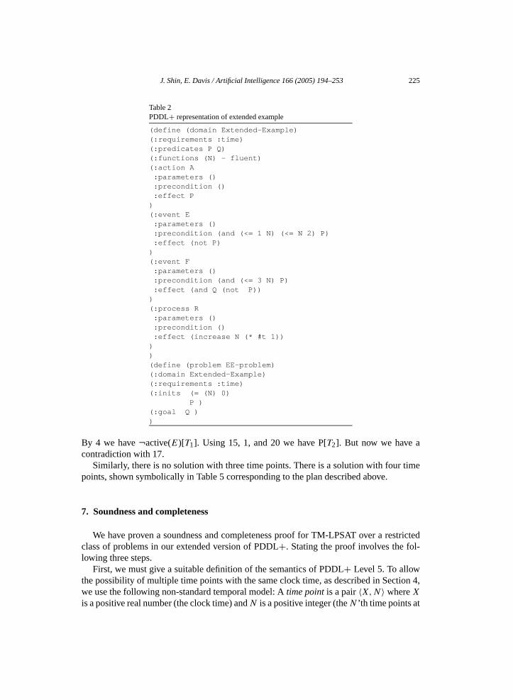
J. Shin, E. Davis / Artificial Intelligence 166 (2005) 194–253 225
Table 2PDDL+ representation of extended example
(define (domain Extended-Example)(:requirements :time)(:predicates P Q)(:functions (N) - fluent)(:action A:parameters ():precondition ():effect P
)(:event E:parameters ():precondition (and (<= 1 N) (<= N 2) P):effect (not P)
)(:event F:parameters ():precondition (and (<= 3 N) P):effect (and Q (not P))
)(:process R:parameters ():precondition ():effect (increase N (* #t 1))
))(define (problem EE-problem)(:domain Extended-Example)(:requirements :time)(:inits (= (N) 0)
P )(:goal Q ))
By 4 we have ¬active(E)[T1]. Using 15, 1, and 20 we have P[T2]. But now we have acontradiction with 17.
Similarly, there is no solution with three time points. There is a solution with four timepoints, shown symbolically in Table 5 corresponding to the plan described above.
7. Soundness and completeness
We have proven a soundness and completeness proof for TM-LPSAT over a restrictedclass of problems in our extended version of PDDL+. Stating the proof involves the fol-lowing three steps.
First, we must give a suitable definition of the semantics of PDDL+ Level 5. To allowthe possibility of multiple time points with the same clock time, as described in Section 4,we use the following non-standard temporal model: A time point is a pair 〈X,N〉 where X
is a positive real number (the clock time) and N is a positive integer (the N ’th time points at
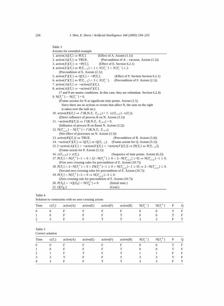
226 J. Shin, E. Davis / Artificial Intelligence 166 (2005) 194–253
Table 3Axioms for extended example1. active(A)[Ti ] ⇒ P[Ti ]. (Effect of A. Axiom (1.1))2. active(A)[Ti ] ⇒ TRUE. (Precondition of A – vacuous. Axiom (1.2))3. active(E)[Ti ] ⇒ ¬P[Ti ]. (Effect of E. Section 6.2.1)4. active(E)[Ti ] ⇔ P[Ti−1] ∧ 1 � N [T −
i] ∧ N [T −
i] � 2.
(Precondition of E. Axiom (2.1))5. active(F )[Ti ] ⇒ Q[Ti ] ∧ ¬P[Ti ]. (Effect of F. Section Section 6.2.1)6. active(F )[Ti ] ⇔ P[Ti−1] ∧ 3 � N [T −
i]. (Precondition of F. Axiom (2.1))
7. active(A)[Ti ] ⇒ ¬active(E)[Ti ].8. active(A)[Ti ] ⇒ ¬active(F )[Ti ].
(7 and 8 are mutex conditions. In this case, they are redundant. Section 6.2.4)9. N[T +
i] − N[T −
i] = 0.
(Frame axioms for N at significant time points. Axiom (1.5).Since there are no actions or events that affect N, the sum on the rightis taken over the null set.)
10. active(R)[Ti ] ⇒ Γ (R,N,Ti , Ti+1) = 1 · (c(Ti+1) - c(Ti )).(Direct influence of process R on N. Axiom (3.1))
11. ¬active(R)[Ti )] ⇒ Γ (R,N,Ti , Ti+1) = 0.(Influence of process R on fluent N. Axiom (3.2))
12. N[T −i+1] − N[T +
i] = Γ (R,N,Ti , Ti+1).
(Net effect of processes on N. Axiom (3.3))13. active(R)[Ti )] ⇔ TRUE. (Precondition of R. Axiom (3.4))14. ¬active(F )[Ti ] ⇒ Q[Ti ] ⇔ Q[Ti−1]. (Frame axiom for Q. Axiom (5.1))15. [¬active(A)[Ti ] ∧ ¬active(E)[Ti ] ∧ ¬active(F )[Ti ]] ⇒ [P[Ti ] ⇔ P[Ti−1]].
(Frame axiom for P. Axiom (5.1))16. c(Ti+1) � c(Ti ). (Sequence of time points. Axiom (6.2))17. P[Ti ] ∧ N[T +
i]−1 < 0 ∧ [2−N[T +
i] � 0 ∨ 2−N[T −
i+1] � 0] ⇒ N[T −i+1]−1 � 0.
(First zero crossing rules for precondition of E. Axiom (10.7))18. P[Ti ] ∧ 2−N[T +
i] < 0 ∧ [N[T +
i]−1 � 0 ∨ N[T −
i+1]−1 � 0] ⇒ 2−N[T −i+1] � 0.
(Second zero crossing rules for precondition of E. Axiom (10.7))19. P[Ti ] ∧ N[T +
i]−3 < 0 ⇒ N[T −
i+1]−3 � 0.(Zero crossing rule for precondition of F. Axiom (10.7))
20. P[T0] ∧ ¬Q[T0] ∧ N[T +0 ] = 0. (Initial state.)
21. Q[TK ]. (Goal.)
Table 4Solution to constraints with no zero crossing axiom
Time c(Ti ) active(A) active(E) active(F) active(R) N[T −i
] N[T +i
] P Q
0 0 F F F F 0 0 T F1 0 F F F T 0 0 T F2 3 F F T T 3 3 F T
Table 5Correct solution
Time c(Ti ) active(A) active(E) active(F) active(R) N[T −i
] N[T +i
] P Q
0 0 F F F F 0 0 T F1 0 F F F T 0 0 T F2 1 F T F T 1 1 F F3 3 T F F T 3 3 T F4 3 F F T T 3 3 F T
J. Shin, E. Davis / Artificial Intelligence 166 (2005) 194–253 227
that clock time). Time points are ordered lexicographically; that is, 〈X1,N1〉 < 〈X2,N2〉iff X1 < X2 or [X1 = X2 and N1 < N2]. A history is a mapping that maps any time pointwithin a bounded interval to the values of the fluents at that point, and the sets of actions,events, and processes that are active at that point. A history is consistent with a PDDL+domain description if it obeys the rules set forth in the description. A plan is a mappingthat maps any time point to the set of actions that are executed at that point.
History H is a projection of plan P starting in situation S0 relative to domain descriptionD if
• H and P specify the same actions at the same times.• H is consistent with D.• S0 is the starting state of H.
A goal is a property of histories. A planning problem is a specification of a starting state,a goal, and a domain description. A plan is a correct solution of a planning problem if everyprojection of the plan from the starting state relative to the domain description satisfies thegoal.
Note that constraint-based planning techniques give correct results only if the onlysource of uncertainty is the actions to be carried out; once the actions are specified, thereis only one possible projection. If there is more than one possible projection, or if thereis anything unspecified in the starting state, then a constraint-based planner will make themost optimistic assumptions about these; that is, it will set these uncontrolled parametersin the same way that it sets the actions to be carried out.
Second, we must properly delimit the class of problems. A problem is a candidate forTM-LPSAT if the following two conditions are satisfied:
• Let H be a history. We say that time point T is significant in H if either at least oneaction is executed at H(T); at least one event occurs at H(T); or at least one processbegins or ends at H(T). A planning problem is finitely solvable if there exists a historythat satisfies the problem with finitely many significant time points.
• Every arithmetic function that appears in the PDDL+ domain description is a linearfunction of the numeric fluents and non-constant numeric parameters involved withconstant coefficients.
Note that the first condition is a semantic constraint over the class of histories considered,and that the second condition is a syntactic constraint over the form of the PDDL+ de-scription. Moreover, it is in general only semi-decidable whether the semantic constraintholds. That is inelegant, but there does not seem to be any way around it.
Third, we must use the right notion of “completeness”. (There are several differentpossible notions of what it means for a planner to be complete.) TM-LPSAT is completein the following sense: Let G be any planning problem that is a candidate for TM-LPSAT.Then if TM-LPSAT is executed with a sufficient number of time points, it will return a planthat is a valid solution to the problem.
228 J. Shin, E. Davis / Artificial Intelligence 166 (2005) 194–253
In Appendix B, we give an extensive, though not fully formal, account of the semanticdefinition, of the precise statement of the theorem, and of the proof.
8. Conclusions and future work
There exist very few domain-independent planners that can handle problems involv-ing continuous change to numeric quantities. The TM-LPSAT planner demonstrates thatthe SAT-based planning framework can be extended to deal with such problems. Otherfeatures incorporated in TM-LPSAT include real-valued and interval-valued fluents, ex-ogenous events and processes, atomic and durative actions with numeric parameters, andreusable metric and interval resources. To permit the representation of some of these fea-tures, we have introduced a number of extensions into the PDDL+ description language.We have tested our encoding generated by the TM-LPSAT compiler, using different SAT-based arithmetic constraint solvers, on a number of problems of varying complexity andcharacteristics. We have proven that TM-LPSAT is sound and complete for a significantsubset of this extended description language.
The contributions of our work are:
• We have shown that the SAT-based planning framework can be used for reasoningabout continuous change. This disproves previous claims, cited in Section 2.1, thatthis would be impossible.
• The capability of TM-LPSAT for dealing with issues typical of scheduling prob-lems, such as metric quantities and reusable resources, suggests that SAT-and-LP-based planning techniques may offer a bridge spanning the divide between domain-independent planning and scheduling.
• Our approach to dealing with continuous change and continuous time—specifically,the characterization of overall behavior in terms of the values of fluents at “signifi-cant” time points—may also be applicable to other planning methodologies, such asGraphplan [7].
The current version of TM-LPSAT has the following limitations:
• The existing SAT-based arithmetic constraint solvers can only deal with Boolean com-binations of linear (in)equalities and propositional atoms. This makes it necessary torequire that all numeric terms in preconditions and in effects are linear functions offluents, and that any continuous effect of processes and durative actions is a constantinfluence on the derivative of the affected fluent.
• It is not possible in TM-LPSAT to specify a given plan metric to be optimized. Thislimitation is inherited from the architecture of the constraint solvers we used, such asLPSAT [53] or MathSAT [3,9]. (The search strategy in TM-LPSAT will return a planwith the minimum number of significant time points; but this is not even the same asthe plan with the minimum number of actions, let alone any other metric.)
• Neither the compilation process nor the encoding is optimized in the current versionof TM-LPSAT.
J. Shin, E. Davis / Artificial Intelligence 166 (2005) 194–253 229
• Scalability is certainly a concern, as in all SAT-based planners. The question is,how far can you go, using optimized encodings and heuristics for constraint solversbased on domain characteristics, before running into intractable combinatorial explo-sion.
Some thoughts on overcoming these limitations:As regards non-linear constraints: It would certainly be possible using current tech-
nology to develop an more powerful arithmetic constraint solver that could solve Booleancombinations of non-linear constraints. How effective such a solver could be made, we can-not guess. If such an engine were constructed, then that would allow two easy extensions toTM-LPSAT. First, obviously, it would make it possible to use non-linear arithmetic termsin preconditions and on the right-hand side of assignment and increment effects. Second,a little more subtly, it would allow processes whose continuous effect on a output fluentis constant, but depends on a numeric fluent set by a atomic action or event. For example,the “Bucket” domain could be modified to allow the agent to turn on a tap to any desiredlevel of flow-rate. In the Zeno domain of [53], it would be possible to set a desired constantspeed for the airplane, which would affect both the rate of motion and the rate of fuel con-sumption. Since, in such domains, all numeric fluents would be piecewise linear functionsof time, with breaks only at significant time points, the TM-LPSAT compilation rules, in-cluding the zero crossing rules, would still be valid; indeed, the proof of their soundnessand completeness would be essentially unchanged.
Extensions beyond that would involve substantially greater difficulties. If the effect ofa process depends on a fluent whose value changes continuously, then there is a differ-ential equation to be solved, particularly if the dependencies have a cycle. If numericfluents can be non-linear functions of time, then it becomes hard to guarantee that theyare monotonic functions of time; and if they are not monotonic, then the zero crossingrules of Section 6.10.1 are insufficient. The constraint solver would need to incorporate azero crossing detector.
We can think of a couple of approaches to adapt TM-LPSAT to plan optimization.17 Ifan upper bound is placed on N , the number of time points, then an objective function M
can be optimized by adding a constraint of the form M � B where B is a constant, anddoing binary search to find the smallest possible value of B . However, this strategy cannotbe used to find the overall optimal plan, where N is not bounded. In principle, of course,one could dovetail the search for B and N ; but such dovetailing is surely more suited toproofs in computation theory than to practical programming.
A more promising approach would be to modify the interaction between the SAT solverand the LP solver in the arithmetic constraint solver to use branch and bound [31]. Theproblem space consists of a collection of states. Each state is represented by two sets of
17 One difficulty about plan optimization is that, in domains as rich as these, there may not exist any optimalplan; it is easy to construct problems in which plans can be made better and better as the number of actionsincreases, as the number of significant time points increases, as the duration of the plan goes either to infinity orto a finite limit, or as the value of a numeric action parameter goes either to infinity or to a finite limit. Moreover,even if an optimal solution is known to exist—e.g., the metric is always a positive integer, and one is searchingfor a minimum—proving that a particular solution is optimal may be undecidable.
230 J. Shin, E. Davis / Artificial Intelligence 166 (2005) 194–253
constraints, one of logical constraints and the other of mixed logical linear constraints, suchthat the two sets share action variables appearing in the mixed constraints. The relaxedversion of mixed constraints is solved, only if the set of logical constraints is satisfiable;the optimal value of the relaxed constraints gives the lower bound (for a minimizationproblem) of the mixed constraints so that it can be used either to bound the optimal valueof the problem (if the values of action variables in the solution satisfy the set of logicalconstraints), to prune the search space, or to branch from the current state. This approach,we believe, may prune the search space quickly due to the action variables shared betweenthe two sets of constraints. The major challenge is to derive heuristics to decide a branchingvariable or to pick up a state to solve next. Currently we are working on this approach usingan incremental SAT solver and an LP solver.
Optimization techniques known for the propositional domains may be extended for tem-poral metric domains: adding domain axioms, such as state constraints, that are inferredthrough domain analysis [26] as preprocessing step; reducing encoding size by removingunnecessary action instantiations through type analysis [23] at compilation stage; simplify-ing binary clauses in the encoding produced by the compiler, which are generally numerousin the SAT encoding of planning [10].
In the SAT-based arithmetic constraint solver, it is known that the running time is dom-inated by the time consumed by the LP solver [1,54]. In order to reduce calls to the LPsolver, one optimization technique at the encoding (compiling) phase would be to liftarithmetic constraints mutually exclusive up to the Boolean level. In the example of Sec-tion 6.10.2, the inequalities N [Ti] � 2 in axiom 4 of Table 3 and 3 � N [Ti] in axiom 6are mutually exclusive. If we were to add this mutual exclusion as a clause, then the SATsolver could not assign them (or, more precisely, their Boolean triggers) TRUE in a partialpropositional solution. Thus, it would never be necessary to pass the two of them togetherto the LP solver to find the inconsistency. The detection of arithmetic constraints mutuallyexclusive in the encoding can generally be done as a preprocessing step in a constraintsolver, called static learning. It, however, is certainly more expensive than at the encodingphase. The layered structure adopted in MathSAT [3,9] is also an effective approach toreduce unnecessary calls to the LP solver (or, generally computationally more expensiveroutines).
It was known that a branching heuristic utilizing characteristics specific to encoding ofplanning domains (i.e. nondeterminism on choices of actions) can drastically reduce run-ning times [28]. Our preliminary experiments also show that different branching heuristicscould make a big difference in running time of a planning problem in temporal metricdomains. We, however, do not know any SAT solver or SAT-based arithmetic constraintsolver specially tailored for planning domains. Our ongoing work on branch-and-boundarchitecture built on LP and SAT solvers is to combine completeness and these heuristicscoming from planning domains.
We have done some preliminary experiments18 with IPC3 problem domains [39] and“Bucket” domain, and a number of SAT-based arithmetic solvers based on different algo-rithms. The intention of the experiments was to observe the feasibility of our encoding, the
18 The report is available at http://cs.nyu.edu/~jiae/papers/experiments.pdf.
J. Shin, E. Davis / Artificial Intelligence 166 (2005) 194–253 231
scalability of this approach in temporal metric domains, and how features of different con-straint solvers react with characteristics of constraints specific to different kinds of planning(metric planning in discrete time, temporal planning with durative actions, temporal metricplanning of real-time model).
The difficulty of solving a constraint set generally grows rapidly with its size, and showsstriking difference in performance among different constraint solvers. This is particularlyapparent in the problems of the “Bucket” domain, which are more constrained, and whichintertwine metric constraints with temporal constraints. For temporal planning problemsin which the arithmetic constraint set consists mostly of equality equations, we have foundthat the solver with a specialized routine for equality equation, a variant of Bellman–Fordalgorithm, in the layered and delayed architecture [3,9] performs considerably better thanothers. Currently the constraint solver is used as a black box and advanced analysis is leftfor future work.
Finally, we plan to explore some further applications of this type of planning. It shouldbe possible to implement some kinds of spatial reasoning by allowing region-valued fluentsand motion as a process. If regions are restricted to polygons or polyhedra, either fullyspecified, or of a specified maximum complexity, and all motions are constant-velocitytranslations, then it should be possible to compile these domains into systems of linearconstraints.
Acknowledgements
Our special thanks go to Steven Wolfman and Daniel Weld for making their LPSATprogram available for our research. The MathSAT group kindly allowed us access to theversions of MathSAT. We also would like to thank the anonymous reviewers for valuablesuggestions and comments. The research reported in this paper was supported by NSFgrant IIS-0097537.
Appendix A. The bucket domain and problem in an extended PDDL+
A.1. The bucket domain
;; ===================================================================;; "Bucket" Domain: ;;;; Deliver a specified amount of water to a specified ;;;; location(s) by a specified deadline. ;;;; ;;;; Assumptions: ;;;; - Zero or more than one tap are in each location. ;;;; - Each tap fills only one bucket at a time. ;;;; - Each bucket can be filled by more than one tap ;;;; in a location at a time, allowing concurrent continuous ;;;; change on the level of a bucket. ;;;; ===================================================================
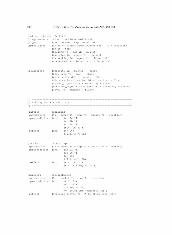
232 J. Shin, E. Davis / Artificial Intelligence 166 (2005) 194–253
(define (domain Buckets)(:requirements :time :continuous-effects)(:types agent bucket tap location)(:predicates (at ?o - (either agent bucket tap) ?l - location)
(on ?t - tap)(filling ?t - tap ?b - bucket)(carrying ?a - agent ?b - bucket)(is_walking ?a - agent ?d - location)(connected ?s - location ?d - location)
)
(:functions (capacity ?b - bucket) - float(flow_rate ?t - tap) - float(walking_speed ?a - agent) - float(distance ?s - location ?d - location) - float(amount_of_water ?l - location) - fluent(distance_to_walk ?a - agent ?d - location) - fluent(level ?b - bucket) - fluent
)
;; ==================================================================;; Filling buckets with taps ;;;; ==================================================================
(:action turnOnTap:parameters (?a - agent ?t - tap ?b - bucket ?l - location):precondition (and (at ?a ?l)
(at ?b ?l)(at ?t ?l)(not (on ?t)))
:effect (and (on ?t)(filling ?t ?b))
)
(:action turnOffTap:parameters (?a - agent ?t - tap ?b - bucket ?l - location):precondition (and (at ?a ?l)
(at ?t ?l)(on ?t)(filling ?t ?b))
:effect (and (not (on ?t))(not (filling ?t ?b)))
)
(:process fillingBucket:parameters (?b - bucket ?t - tap ?l - location):precondition (and (at ?b ?l)
(at ?t ?l)(filling ?t ?l)(<= (level ?b) (capacity ?b)))
:effect (increase (level ?b) (* #t (flow_rate ?t))))
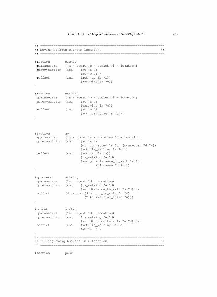
J. Shin, E. Davis / Artificial Intelligence 166 (2005) 194–253 233
;; =================================================================;; Moving buckets between locations ;;;; =================================================================
(:action pickUp:parameters (?a - agent ?b - bucket ?l - location):precondition (and (at ?a ?l)
(at ?b ?l)):effect (and (not (at ?b ?l))
(carrying ?a ?b)))
(:action putDown:parameters (?a - agent ?b - bucket ?l - location):precondition (and (at ?a ?l)
(carrying ?a ?b)):effect (and (at ?b ?l)
(not (carrying ?a ?b))))
(:action go:parameters (?a - agent ?s - location ?d - location):precondition (and (at ?a ?s)
(or (connected ?s ?d) (connected ?d ?s))(not (is_walking ?a ?d)))
:effect (and (not (at ?a ?s))(is_walking ?a ?d)(assign (distance_to_walk ?a ?d)
(distance ?d ?s))))
(:process walking:parameters (?a - agent ?d - location):precondition (and (is_walking ?a ?d)
(>= (distance_to_walk ?a ?d) 0):effect (decrease (distance_to_walk ?a ?d)
(* #t (walking_speed ?a))))
(:event arrive:parameters (?a - agent ?d - location):precondition (and (is_walking ?a ?d)
(<= (distance-to-walk ?a ?d) 0)):effect (and (not (is_walking ?a ?d))
(at ?a ?d)));; =================================================================;; Filling among buckets in a location ;;;; =================================================================
(:action pour
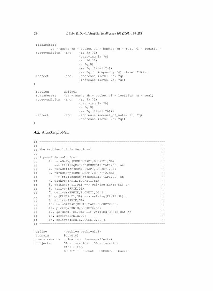
234 J. Shin, E. Davis / Artificial Intelligence 166 (2005) 194–253
:parameters(?a - agent ?s - bucket ?d - bucket ?q - real ?l - location)
:precondition (and (at ?a ?l)(carrying ?a ?s)(at ?d ?l)(> ?q 0)(<= ?q (level ?s))(<= ?q (- (capacity ?d) (level ?d))))
:effect (and (decrease (level ?s) ?q)(increase (level ?d) ?q))
)
(:action deliver:parameters (?a - agent ?b - bucket ?l - location ?q - real):precondition (and (at ?a ?l)
(carrying ?a ?b)(> ?q 0)(<= ?q (level ?b)))
:effect (and (increase (amount_of_water ?l) ?q)(decrease (level ?b) ?q))
)
A.2. A bucket problem
;; ===================================================================;; ;;;; The Problem 1.1 in Section~1 ;;;; ;;;; A possible solution: ;;;; 1. turnOnTap(ERNIE,TAP1,BUCKET1,SL) ;;;; ==> fillingBucket(BUCKET1,TAP1,SL) on ;;;; 2. turnOffTAP(ERNIE,TAP1,BUCKET1,SL) ;;;; 3. turnOnTap(ERNIE,TAP1,BUCKET2,SL) ;;;; ==> fillingBucket(BUCKET2,TAP1,SL) on ;;;; 4. pickUp(ERNIE,BUCKET1,SL) ;;;; 5. go(ERNIE,SL,DL) ==> walking(ERNIE,DL) on ;;;; 6. arrive(ERNIE,DL) ;;;; 7. deliver(ERNIE,BUCKET1,DL,1) ;;;; 8. go(ERNIE,DL,SL) ==> walking(ERNIE,SL) on ;;;; 9. arrive(ERNIE,SL) ;;;; 10. turnOffTAP(ERNIE,TAP1,BUCKET2,SL) ;;;; 11. pickUp(ERNIE,BUCKET2,SL) ;;;; 12. go(ERNIE,SL,DL) ==> walking(ERNIE,DL) on ;;;; 13. arrive(ERNIE,DL) ;;;; 14. deliver(ERNIE,BUCKET2,DL,4) ;;;; ===================================================================
(define (problem problem1.1)(:domain Buckets)(:requirements :time :continuous-effects)(:objects SL - location DL - location
TAP1 - tapBUCKET1 - bucket BUCKET2 - bucket
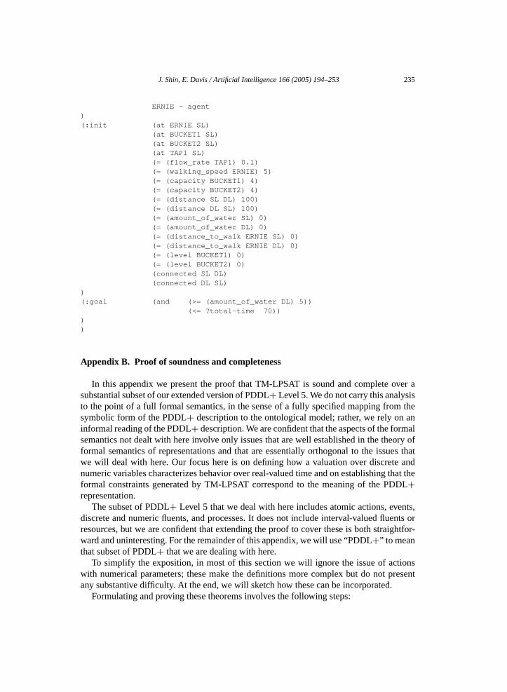
J. Shin, E. Davis / Artificial Intelligence 166 (2005) 194–253 235
ERNIE - agent)(:init (at ERNIE SL)
(at BUCKET1 SL)(at BUCKET2 SL)(at TAP1 SL)(= (flow_rate TAP1) 0.1)(= (walking_speed ERNIE) 5)(= (capacity BUCKET1) 4)(= (capacity BUCKET2) 4)(= (distance SL DL) 100)(= (distance DL SL) 100)(= (amount_of_water SL) 0)(= (amount_of_water DL) 0)(= (distance_to_walk ERNIE SL) 0)(= (distance_to_walk ERNIE DL) 0)(= (level BUCKET1) 0)(= (level BUCKET2) 0)(connected SL DL)(connected DL SL)
)(:goal (and (>= (amount_of_water DL) 5))
(<= ?total-time 70))))
Appendix B. Proof of soundness and completeness
In this appendix we present the proof that TM-LPSAT is sound and complete over asubstantial subset of our extended version of PDDL+ Level 5. We do not carry this analysisto the point of a full formal semantics, in the sense of a fully specified mapping from thesymbolic form of the PDDL+ description to the ontological model; rather, we rely on aninformal reading of the PDDL+ description. We are confident that the aspects of the formalsemantics not dealt with here involve only issues that are well established in the theory offormal semantics of representations and that are essentially orthogonal to the issues thatwe will deal with here. Our focus here is on defining how a valuation over discrete andnumeric variables characterizes behavior over real-valued time and on establishing that theformal constraints generated by TM-LPSAT correspond to the meaning of the PDDL+representation.
The subset of PDDL+ Level 5 that we deal with here includes atomic actions, events,discrete and numeric fluents, and processes. It does not include interval-valued fluents orresources, but we are confident that extending the proof to cover these is both straightfor-ward and uninteresting. For the remainder of this appendix, we will use “PDDL+” to meanthat subset of PDDL+ that we are dealing with here.
To simplify the exposition, in most of this section we will ignore the issue of actionswith numerical parameters; these make the definitions more complex but do not presentany substantive difficulty. At the end, we will sketch how these can be incorporated.
Formulating and proving these theorems involves the following steps:
236 J. Shin, E. Davis / Artificial Intelligence 166 (2005) 194–253
1. Defining the ontology of the microworld in which PDDL+ plans are executed.2. Defining the semantics of a PDDL+ problem statement in terms of this ontology.3. Defining the relation between a valuation over the variables used in TM-LPSAT and
microworld entities.4. Identifying the rare circumstances in which the physical projection of a system of
processes is underdetermined.5. Formalizing and proving the sense in which TM-LPSAT is “sound” and “complete”.
(In particular, there are several different senses in which a planner can be “complete”;only one of these applies to TM-LPSAT.)
B.1. Ontology
We assume that there are disjoint finite sets of actions, events, processes, and fluents.Each fluent F has associated with it a set of possible values, denoted vals(F ). If F isdiscrete then vals(F ) is a finite set of non-numeric values. If F is numeric, then vals(F ) isthe set of real numbers.
Definition B.1. A situation is a four-tuple 〈A,E,P,M〉 where A is a set of actions; E is aset of events; P is a set of processes, and M is a mapping over the set of fluents, such that,for any fluent F , M(F) ∈ vals(F ).
We will use a Pascal-style dot notation to denote the fields of a tuple; for example, if S
is a situation, then S.A is the set of actions in S, S.P is the set of processes, and so on.To allow the possibility of multiple time points with the same clock time, as discussed
in Section 4, we use the following non-standard temporal model:
Definition B.2. A time point is a pair 〈X,N〉 where X is a real number and N is a positiveinteger.
Intuitively, 〈X,N〉 is the N th time point (counting from 0) at clock time X. Time pointsare ordered lexicographically; that is, 〈X1,N1〉 < 〈X2,N2〉 iff X1 < X2 or [X1 = X2and N1 < N2].
Definition B.3. A time interval I is a non-empty set of time points such that, if T 1 ∈ I ,T 2 ∈ I and T 1 < T < T 2 then T ∈ I . If T 1 and T 2 are time points with T 1 < T 2 thenthe closed interval [T 1, T 2] is, as usual, the set of all time points T such T 1 � T � T 2.
Definition B.4. For any time point T = 〈X,N〉, if N > 0 then the time point preceding T
is the point 〈X,N − 1〉. If N = 0, then there is no time point preceding T .
Definition B.5. Let I = [〈X1,0〉, 〈X2,N〉] be a closed time interval. A history H over I
is a mapping from I to situations.
The following abbreviations will be convenient. Let H be a history over the time intervalI = [〈X1,0〉, 〈X2,N〉]. We will write I = dom(H) (read “the domain of H ”), and the
J. Shin, E. Davis / Artificial Intelligence 166 (2005) 194–253 237
real interval [X1,X2] = domX(H) (read “the X-domain of H ”). For any time point T ∈dom(H) and fluent F we will write H(T ,F ) as an abbreviation for [H(T ).M](F ), and wewill write ΦH,F (X) for the function over domX(H) defined by ΦH,F (X) = H(〈X,0〉,F ).Note that H(T ).A, H(T ).E, and H(T ).P are respectively the set of actions, events, andprocesses active in H at time point T .
Definition B.6. A history H over [T 0, T 1] is compact if the following holds: For anyTA,TB, if TA �= T 0, TA.X = TB.X, TA.N < TB.N and H(TA).A = H(TA).E = ∅ thenH(TB).A = H(TB).E = ∅.
That is, looking at a sequence of time points 〈X,0〉, 〈X,1〉, . . . all of the time pointswhen an action or event happens are “compacted” together at the beginning of the se-quence, with the exception of the starting time point of this history.
Definition B.7. Let H be a history and let X ∈ domX(H). We say that the processes in H
are constant around X if there exists a neighborhood (XA,XB) of X over which the activeprocesses do not change. That is, for every TC,TD if XA < TC.X < XB and XA < TD.X <
XB, then H(TC).P = H(TD).P. If the processes in H are not constant around X, then X isa time of process change in H .
Definition B.8. Let H be a history and let T be a time point in dom(H ). T is a significanttime point in H if either
• T is the starting time point of H .• T is the ending time point of H .• H(T ).A �= ∅.• H(T ).E �= ∅.• T .X is a time of process change and T .N = 0.
Definition B.9. A history H has finite complexity if it has finitely many significant timepoints. H is monotonous over real interval (XA,XB) if there is no significant time point T
such that T .X ∈ (XA,XB).
In all that follows, we will write “history” to mean “compact history of finite complex-ity”.
Definition B.10. Let H be a history, T a time point in the domain of H , and F a fluent.Assume that T is not starting time point of H . Value V is the value of F before T if thefollowing conditions are satisfied.
• If T .N > 0, then V = H(T 1,F ) where T 1 is the point preceding T .• If T .N = 0 and F is discrete, then there exists a T 0 < T such that for all T 1, if
T 0 < T 1 < T then V = H(T 1,F ).• If T .N = 0 and F is numeric, then V is the limit of ΦH,F (X) as X approaches T .X
from below.
238 J. Shin, E. Davis / Artificial Intelligence 166 (2005) 194–253
If α is a term computed over fluents, then the value of α before T is α computed overthe values of the fluents before T . If α is a Boolean expression and the value of α beforeT is TRUE, in the above sense, then we say that α holds before T .
Definition B.11. A plan P is a mapping over a bounded time interval I , such that,
• For any T ∈ I , P(T ) is a finite set of actions;• P(T ) = ∅ for all but finitely many T.
We write I = dom(P ), the domain of P .
Intuitively, P(T ) is the set of actions that the plan says should be executed at time T .
B.2. Semantics of PDDL+
Definition B.12. A PDDL+ planning problem is a triple 〈D,S,G〉 where D is a PDDL+domain representation, S is a PDDL+ representation of a starting situation, and G is aPDDL+ representation of a goal.
In Section 6 we did not describe how PDDL+ representations of a starting situationand of a goal are compiled into axioms (a) because it is obvious; (b) because it is the sameas in any SAT-based planner. We will similarly not discuss the issue here. We do, how-ever, assume that a PDDL+ representation of a starting situation uniquely determines thesituation. If S is a PDDL+ representation of a starting situation, we will write “Sit(S)”to denote the actual situation. As for goals, for our purposes here a “goal” can be essen-tially any property of a history; we assume that the translation of a PDDL+ goal into thecorresponding property is done correctly.
The following long definition contains the details of the meaning of the constructs ofPDDL+ in terms of the properties of a history. As is common in this kind of semanticdefinition, the left-hand side of the definition is an almost tautological rewording of theright-hand side. Likewise notable is the strong resemblance of the definition here to thedescription of the constraint compiler in Section 6. This resemblance (a) is to be expected;(b) means that large parts of the proof of correctness are trivial; (c) limits substantiallythe degree to which the exhibition of a soundness and correctness proof of this kind ac-tually increases the reader’s confidence in the compiler or augments her understandingof it.
Definition B.13. Let H be a history and let D be a PDDL+ domain representation. H con-forms to D if the following conditions hold:
1. If action Z ∈ H(T ).A or event Z ∈ H(T ).E and D specifies that Z assigns term τ tofluent F , then H(T ,F ) is equal to the value of τ before T .
2. If F is a numeric fluent and if there is no action Z ∈ H(T ).A nor event Z ∈ H(T ).E
such that D specifies that Z assigns a value to fluent F , then H(T ,F ) is equal to the
J. Shin, E. Davis / Artificial Intelligence 166 (2005) 194–253 239
value of F before T plus the sum over (all actions/events Z ∈ [H(T ).A ∪ H(T ).E])of the increase/decrease that Z causes in F .
3. (Frame property) Let F be a discrete fluent and let T 1, T 2 be time points suchthat T 1 < T 2. Then H(T 2,F ) = H(T 1,F ), unless there exists a time T such thatT 1 < T � T 2 and either an action Z ∈ H(T ).A or an event Z ∈ H(T ).E such that D
specifies that Z assigns a value to fluent F .4. If action Z ∈ H(T ).A, then the precondition for Z holds before T in H (in the sense
of Definition B.10).5. Event E is in H(T ).E if and only if the precondition of E holds before T in H .6. Process P is in H(T ).P if and only if the precondition of P holds before T in H .7. Suppose that H is monotonous over real interval (X1,X2). Let F be a numeric fluent.
Then:7.1 The function ΦH,F is continuous and differentiable throughout (X1,X2).7.2 For any x ∈ (X1,X2) the derivative d
dX(ΦH,F (X)) at time x is equal to the sum
over all processes P in H(〈x,0〉).P of the influence of P on F at time 〈x,0〉.7.3 For all sufficiently large N , H(〈X1,N〉,F ) is equal to the limit of ΦH,F (x) as x
approaches X1 from above.
Definition B.14. Let P be a plan; let H be a history; let S be a PDDL+ representation ofa starting situation; and let D be a PDDL+ domain description. H is a projection of planP starting in S and following D if the following conditions hold:
• dom(P ) = dom(H);• For all T ∈ dom(H), H(T ).A = P(T ).A;• Sit(S) is the starting situation of H ; and• H conforms to D.
As we shall see in Lemma B.1, for any P , S, D there exists at most one such projection,with rare exceptions to be discussed below.
Definition B.15. Let R = 〈D,S,G〉 be a PDDL+ problem. History H is a historical solu-tion of R if H starts in Sit(S), conforms to D, and achieves G. A finite plan P is a planningsolution of R if every projection of P starting in S and following D is a historical solutionof R.
Note that constraint-based planning techniques give correct results only if the onlysource of uncertainty is the actions to be carried out; once the actions are specified, thereis only one possible projection. If there is more than one possible projection, or if there isanything unspecified in the starting situation, then a constraint-based planner will make themost optimistic assumptions about these; that is, it will set these uncontrolled parametersin the same way that it sets the actions to be carried out. Note also that the definition aboveof the correctness of a plan only works for complete plan representations; partial plan rep-resentations, such as those returned by TWEAK [11], require a more complex definitionof correctness.
240 J. Shin, E. Davis / Artificial Intelligence 166 (2005) 194–253
B.3. Valuations and their interpretations
Definition B.16. Let R be a PDDL+ problem representation. Let T0 . . . Tk be a sequenceof k + 1 distinct symbols, called “time point variables”. We define the set “ATOMS[R,k]”to be the set of all the following atoms: For each time point variable Ti ,
• The atom “c(Ti )”.• For each action, event, or process Z in R, the atom “active(Z)[Ti ]”.• For each discrete fluent F in R, the atom “F [Ti]”.• For each numeric fluent F in R, the atoms “F [T −
i ]” and “F [T +i ]”.
• For each numeric fluent F and each action or event Z that potentially changes F
incrementally, the atom “�(F,Z)[Ti]”.• For each numeric fluent F and each process P that potentially influences F , the atom
“Γ (F,P,Ti, Ti+1)”.
Definition B.17. A T-valuation V is an assignment of each atom in ATOMS[R,k] to avalue of the appropriate sort, such that, for each i < j , V(“c(Ti )”) � V(“c(Tj )”).
Definition B.18. Let V be a T-valuation over ATOMS[R,k]. The time point mapping for Vis the function τ from Ti to time points defined as follows: τ(Ti) = 〈X,J 〉 where
• X = V(“c(Ti )”);• Ti is the J th time point variable such that X = V(“c(Ti)”). That is, V(“c(Ti )”) =
V(“c(Ti−1)”) = · · · = V(“c(Ti−J )”) �= V(“c(Ti−J−1)”).
Definition B.19. Let V be a T-valuation over ATOMS[R,k]. Let τ be the time point map-ping for V. Plan P is indicated by V if:
• For each Ti , P(τ(Ti)) = the set of all actions A such that V(“active(A)[Ti ]”) = TRUE.• For each T , if T �= τ(Ti) for all i, then P(T ) = ∅.
Definition B.20. Let D be a domain description, let V be a T-valuation, and let H be ahistory. Let τ be the time point mapping of V . H corresponds to V if:
1. dom(H ) = [τ(T0), τ (Tk)].2. If i < j then τ(Ti) < τ(Tj ).3. For each Ti , H (τ(Ti )).A = {A | V (“active(A)[Ti ]”) = TRUE}.4. For each Ti , H (τ(Ti )).E = {E | V (“active(E)[Ti ]”) = TRUE}.5. For any discrete fluent F , H(τ(Ti),F ) = V (“F [Ti]”).6. For any numeric fluent F , H(τ(Ti),F ) = V (“F [T +
i ]”).7. Let T be any time point in dom(H ). Let Ti be the greatest time variable such that
τ(Ti) � T .7.1. If T �= τ(Ti) then H(T ).A = H(T ).E = ∅.7.2. For any discrete fluent F , H(T ,F ) = V (“F [Ti]”).7.3. If T .X = τ(Ti).X, then
J. Shin, E. Davis / Artificial Intelligence 166 (2005) 194–253 241
7.3.1. For any numeric fluent F , H(T ,F ) = V (“F [T +i ]”).
7.3.2. For any process P , P ∈ H(T ).P if the preconditions of P , as defined in D,are satisfied before T in H .
7.4. If T .X > τ(Ti).X then7.4.1. For any numeric fluent F , let
q = (T .X − τ(T +
i ).X)/(τ(Ti+1).X − τ(Ti).X
).
Then H(T ,F ) = (1 − q)V (“F [T +i ]”) + qV (“F [T −
i+1]”).(Linear interpolation between significant points.)
7.4.2. H(T ).P = {P | V (“active(P )[Ti ]”) = TRUE}.
Note that at a significant time Ti and at all subsequent non-significant times with thesame clock time, the activity of a process in H is rather awkwardly defined in terms of thepreconditions specified in the domain description D (which is the only reason for includingD as a parameter in this definition at all). The reason for this is as follows: Recall that inour discussion of axiom (3.4) we defined “active(P )[Ti ]” to mean that P was active overan interval starting in Ti . Therefore, if P comes to an end at Ti , then in V , “active(P )[Ti ]”is FALSE. However in H , P will be active at T = τ(Ti) if its preconditions are satisfiedat Ti ; thus, P will still be active at T in H if the preconditions are becoming FALSE due toa zero crossing, which will be come negative only after T , but it will be inactive at T in H
if the preconditions have just become FALSE in T due to a discrete change. The valuationV by itself does not distinguish these two cases; one needs to know the domain definition.Of course, since the effect of a process is differential, whether or not a process is active atan instant actually makes no difference.
B.4. Indeterminate projections
As discussed above, the constraint-based approach to planning relies on the assumptionthat any plan has a unique projection; that is, once you fix the actions you are to do, that de-termines everything else that can happen. Unfortunately, in a theory that include processesof the kind in PDDL+, there are rare cases where that assumption is false.
The problem arises for the following reason: A system of processes in effect imposesa set of ordinary differential equations (ODE’s) over the numerical fluents involved. Instandard applications of ODE’s one can rely on a standard existence and uniqueness resultfor initial value problems to guarantee that, having set up the starting condition and thedifferential equation, history can develop in only one way. However, this result only holdswhen the “driving function” for the ODE is continuous. PDDL+ processes define a dis-continuous driving function, so neither existence nor uniqueness is guaranteed and indeedthere are cases where history can develop in more than one way.
Consider the following example: There is one numeric fluent F and two processes P 1and P 2. P 1 has precondition TRUE and increases F at the rate of 1 unit per second. P 2has the precondition F � 0 and decreases F at the rate of 1 unit per second. Suppose thatF = 0 at time T = 0. Then for any T 1 � 0, the following is a consistent behavior:
242 J. Shin, E. Davis / Artificial Intelligence 166 (2005) 194–253
For any time T ,
If 0 � T � T 1 then P 1 and P 2 are active at T and F = 0.If T 1 < T then only P 1 is active at T and F = T − T 1.
This corresponds to the fact that the differential equation
F ={
0 if F � 0,
1 if F > 0
has infinitely many solutions (if one allows a “solution” to have finitely many points whereit is continuous but not differentiable).
However, a history H only encounters this problem at time T if the following conditionis met: (this is a necessary condition for the problem, not a sufficient condition).
Indeterminacy condition. There is a dependency cycle between processes, numeric flu-ents, and preconditions:
P1 → F1 → Φ1 → P2 → ·· · → Φk → P1,
such that process Pi is active at T and influences fluent Fi ; Fi is involved in preconditionΦi ; and Φi is a precondition of process Pi+1 which is satisfied but just on the borderline attime T .
A history H satisfies the Unique Projection Condition (UPC) if it never satisfies theindeterminacy condition.
In principle, it would be possible to add the unique projection condition as a TM-LPSATconstraint. The theoretical advantage would be that doing so would give a slightly improvedpair of soundness and completeness results, as discussed below. We have not implementedit, however. In most actual domains where the PDDL+ representation is at all a reasonableapproximation, it is possible to determine at compilation time that no circularity can ariseamong fluents and processes; hence, no UPC axioms will be formulated. If a domain doeshave this kind of circular dependence among fluents and processes, then it is very unlikelythat it can be adequately modeled using constant-rate influences. The theoretical improve-ment to the algorithm in the rare cases where the UPC axioms do have an effect did notseem worth the programming effort.
B.5. Constraints and theorems
Finally, we introduce a notation for the set of constraints generated by TM-LPSAT, stateour soundness and completeness theorems, and prove the theorems.
Definition B.21. Let R be a planning problem and let k be a positive integer. We defineTM-LPSAT(k,R) to be the set of constraints constructed from R over ATOMS[R,k] asdefined in Sections 6.1, 6.2, 6.3, 6.5, 6.6, and 6.10, using versions (10.7) and (10.11) ofthe zero crossing axioms, but excluding the mutex axioms in Sections 6.1.3 and 6.2.4. Themutex axioms are useful for enforcing certain regularity conditions that are important inother contexts, and they are part of the standard semantics of PDDL+, but in the contextof this proof they just get in the way.
J. Shin, E. Davis / Artificial Intelligence 166 (2005) 194–253 243
Let Λ be an algorithm (the constraint solver) that achieves the following: Λ takes asinput a set of constraints C of the form produced by TM-LPSAT. If the constraints C havea solution, then Λ returns a T-valuation that is a solution of C. If the constraints C do nothave a solution, then Λ returns a flag indicating there is no solution.
Theorem B.1 (Soundness). Let R be a planning problem. If Λ(TM-LPSAT(k,R)) returnsa T-valuation V , and V satisfies the UPC then the plan indicated by V is a planningsolution to R.
Theorem B.2 (Completeness). Let R be a planning problem. If there exists a planningsolution to R, then for some value of k, Λ(TM-LPSAT(k,R)) returns a T-valuation V . ByTheorem B.1, if V satisfies the UPC then V indicates a planning solution to R.
The above pair of theorems does not close quite tight for the following reason: One canconstruct a problem R where there is a correct plan P 1 that satisfies the UPC, but wherethere is also a plan P 2 that does not satisfy the UPC, such that some but not all of theprojections of P 2 satisfy the goal. Such a plan P 2 is not a correct solution of the problem,since, if you execute it, you cannot be sure of accomplishing the goal. In this case, thereare two things that Λ(TM-LPSAT(R)) may do:
• It may return a valuation that indicates P 1. In that case, you can check that P 1 satisfiesthe UPC, and you are certain that it is a correct plan.
• It may return a valuation that indicates P 2. In that case, you can detect that P 2 violatesthe UPC. If you accept P 2, you are accepting an incorrect plan. If you reject P 2 thenyou have failed to find a plan, even though there exists a plan that satisfies the UPC.
We can tighten this, in principle, by adding the UPC to the constraints generated byTM-LPSAT. Let TM-LPSATU(k,R) be TM-LPSAT(k,R) together with the UPC. Thus, ifTM-LPSATU is applied to the above problem it will return P 1 and not P 2.
Theorem B.3. Let R be a planning problem.
• For any k, if Λ(TM-LPSATU(R, k)) returns a T-valuation V , then V indicates a plan-ning solution to R satisfying the UPC.
• If there exists a planning solution to R satisfying the UPC, then there exists k such thatΛ(TM-LPSATU(R, k)) returns a T-valuation V that indicates a planning solution toR satisfying the UPC.
B.6. Proofs
The proofs of the above three theorems follow, in a series of lemmas.
Lemma B.1. Let D be a PDDL+ domain description and let S be a PDDL+ representa-tion of a starting situation. Let P be a finite plan. Then there exists at most one history H
244 J. Shin, E. Davis / Artificial Intelligence 166 (2005) 194–253
of finite complexity that is a projection of P , starts in S, conforms to D, and satisfies theUPC.
Proof. (By contradiction.) Suppose that there exist two such histories H1 �= H2. Notethat, if TS is the starting time point of dom(P ) then Sit(S) = H1(TS) = H2(TS). Note alsothat dom(P ) = dom(H1) = dom(H2). Let interval I be the maximal initial segment ofdom(P ) such that, for all T ∈ I H1(T ) = H2(T ). (I can be constructed as the union ofall initial segments I1 of dom(P ) such that, for all T ∈ I1, H1(T ) = H2(T ).) There arethree cases to be considered:
Case 1: I has the form [TS,TE] for some ending point TE. Let TE1 be the time pointfollowing TE. Then P determines the actions in TE1. Definition B.13 parts 5 and 6 deter-mine the events and processes in TE1. Definition B.13 parts 1, 2, and 3 determine the valueof all the fluents in TE1. Hence H1(TE1) = H2(TE1).
Case 2: I has the form {T | TS � T ∧ T .X < XE} for some upper bound XE. Let TE1 =〈XE,0〉. Then the situation in TE1 is determined, by the same argument as in part (1).
Case 3: I has the form {T | TS � T ∧ T .X � XE} for some upper bound XE. In thiscase, there is no “next” situation after I , so the arguments in cases 1 and 2 do not ap-ply. Rather, we proceed as follows: Since H1 and H2 have finite complexity, there existsXF > XE and NE such that no events or actions after 〈XE,NE〉 and before 〈XF,0〉 ineither H1 or H2. That is, no actions or events occur in this interval; and the values ofdiscrete fluents does not change during this interval; and the class of active processes doesnot change in the interval {T | 〈XE,NE〉 � T < 〈XF,0〉}. Let TE = 〈XE,NE〉. By virtueof the UPC, there is a topological sorting of numerical fluents, processes that are activeat TE, and numerical preconditions of processes that are active at TE that are just on theborderline such that every process comes after its preconditions, every fluent comes af-ter the processes that influence it, and every precondition comes after the fluents that itreferences. Since numerical fluents are continuous in the absence of actions and events,there exists XG > XE such that at all time points T where XE < T.X < XG, all numeri-cal preconditions that were not on the borderline at TE remain with the same truth valueas at TE. Going through this topological sorting in order, therefore, we can predict thatthere is an interval [TE,TH] where TH.X > XE where the value of a numeric fluent isdetermined only the value at TE together with processes preceding it in the list; where thetruth of a borderline precondition is determined only by numerical fluents preceding it onthe list; and where the activities of processes is determined only by preconditions preced-ing it on the list. Thus, the history is determined for some time after I , contrary to theassumption. �Lemma B.2. For any T-valuation V and domain description D there exists a unique his-tory H that corresponds to V relative to D.
Proof. Definition B.20 gives an explicit, fully determined, construction of H from V
and D. �
J. Shin, E. Davis / Artificial Intelligence 166 (2005) 194–253 245
In all the following definitions, let R be a planning problem; let D be the domain de-scription of R; let V be a T-valuation; let H be a history; and let τ be the time pointmapping of V .
Definition B.22. A valuation V covers time point T if there exists a time point variable Ti
such that T = τ(Ti).
Lemma B.3. If H corresponds to V relative to D and either some action or event A occursin T at H , then V covers T .
Proof. Contrapositive of part 7.1 in Definition B.20. �Definition B.23. Let T be a time point in dom(H ).
• T is significant-1 if there is a precondition Φ of an event that is TRUE in T .• T is significant-2 if there is a precondition Φ of a process such that Φ is FALSE in H
before T and Φ is TRUE in H(T ).• T is significant-3 if there is a precondition Φ of a process for which one of the follow-
ing holds:– Φ is TRUE in H before T and FALSE in H(T ).– Φ is TRUE in H(T ), T .N = 0, and there exists X2 > T .X such that, for all X1,
N1, if T .X < X1 < X2 then Φ is FALSE in H(〈X1,N〉).
Lemma B.4. Let I be an initial segment of dom(H). Let Ti be a time variable such thatτ(Ti) ∈ I and such that τ(Ti).X < τ(Ti+1).X. Let time interval I1 = {T ∈ I | τ(Ti) <
T < τ(Ti+1)}. Let T 1 be any time point in I1. Let T 2 be a time point in I1 such thatT 2.X > τ(Ti).X. If V satisfies TM-LPSAT(k,R) and H corresponds to V then
A. τ(Ti+1).N = 0.B. If τ(Ti).X < T.X < τ(Ti+1).X then P is active in T if and only if V (“active(P )[Ti]”)
= TRUE.C. H is monotonous over the real interval (τ (Ti).X, T 2.X).D. If F is a discrete fluent then H(T 1,F ) = H(τ(Ti),F ).E. Let PP = H(T 2).P. Let F be a numeric fluent. Let Γ be the sum over P ∈ PP of the
influence of P on F . Then H(T 1,F ) = H(τ(Ti),F ) + Γ · (T 1.X − τ(Ti).X).F. For any numerical fluent F , the value of F before Ti+1 is equal to V (“F [T −
i+1]”).
Proof.
A. Immediate by Definition B.18 of a time point mapping.B. From Definition B.20 part 7.4.2, for all such T , the active processes are those such
that V (“active(P )[Ti ]”) = TRUE.C. By Lemma B.3, no actions or events can occur in H at uncovered points. By part B, the
set of processes remains constant; hence there are no times of process change. Hence(T 2.X,T 3.X) is monotonous.
246 J. Shin, E. Davis / Artificial Intelligence 166 (2005) 194–253
D. Immediate from Definition B.20 part 7.2.E. There are two cases to consider:
E.1. T 1.X = τ(Ti).X. In this case, the result is immediate from Definition B.20 part7.3.1.
E.2. T 1.X > τ(Ti).X. By axioms (3.1), (3.2), and (3.3) the difference V (“F [T −i+1])”−
V (“F [T +i ])” is equal to [the sum over [all processes P such that V (“active(P )[Ti ]”)
= TRUE] of the influence of P on F ] times [V (“c(Ti+1)”) − V (“c(Ti)”)]. By partB this set is PP and this sum is Γ . By Definition B.20 part 2, V(“c(Ti )”) = τ(Ti).X,so we have
V(“F [T −
i+1]”) − V
(“F [T +
i ]”) = Γ · (τ(Ti+1).X − τ(Ti).X).
By Definition B.20 part 7.4.1,
H(T ,F ) = (1 − q)V(“F [T +
i ]”) + qV(“F [T −
i+1]”), where
q = (T .X − τ(Ti).X
)/(τ(Ti+1).X − τ(Ti).X
).
By Definition B.20 part 7.3.1, H(τ(Ti),F ) = V (“F [T +i ]”). Combining the above
with some algebraic manipulation gives the desired result.F. Again there are two cases:
F.1. τ(Ti+1).N > 0. In that case the value of F before τ(Ti+1) is the value H(T 1,F )
where T 1 is the situation that precedes τ(Ti+1). Since history H is compact, someaction or event must occur in T 1. Hence, by Lemma B.3, T 1 = τ(Ti). By Def-inition B.20 part 6, H(T 1,F ) = V (“F [T +
i ]”). By axioms (3.1), (3.2), and (3.3),V (“F [T +
i ]”) = V (“F [T −i+1]”).
F.2. τ(Ti+1).N = 0. In that case the value of F before τ(Ti) is the limit of ΦH,F (X)
as X approaches τ(Ti).X from below.By part (E), ΦH,F = H(τ(Ti),F ) + Γ · (τ (Ti+1).X − τ(Ti).X).Using (E) and axioms (3.1), (3.2), and (3.3), this is equal to V (“F [T −
i+1]”). �Lemma B.5. If H corresponds to V , then there can be at most finitely many points that aresignificant-1, significant-2, or significant-3.
Proof. By Definition B.20, between any two points τ(Ti) and τ(Ti+1) every discrete fluentis constant and every numeric fluent is a linear function of time. Any numeric precondi-tions are a linear inequality over the numeric fluents, and thus a linear inequality in timeover this time interval. A time point that is significant-1, -2, or -3 must either involve achange to a discrete fluent, which do not occur at uncovered points, or a zero crossing of anumeric constraint, which can occur at most once for each such constraint between τ(Ti)
and τ(Ti+1). �Lemma B.6. If H corresponds to V and V satisfies axiom (10.6), then V covers any timepoint that is significant-1 or significant-2.
Proof. (By contradiction.) (This proof is essentially the same as the discussion in Sec-tion 6.10, but set in a specific formal context.) Let T be a time point that is significant-1
J. Shin, E. Davis / Artificial Intelligence 166 (2005) 194–253 247
or significant-2 but not covered. Let Ti be the greatest time point variable for whichτ(Ti) < T ; thus T < τ(Ti+1). Let T 1 = τ(Ti) and T 2 = τ(Ti+1). Let the preconditionof the event or process involved be put into DNF: Θ1 ∨ · · · ∨ Θz. Then all of the Θi
are FALSE before T and at least one is TRUE at T . Let Θ(T ) be a constraint that be-comes TRUE at T . Let TF be a time such that T 1 � TF < T and Θ(TF) is FALSE.Θ(T ) has the form
∧p Fp(T ) ∧ ∧
p Qp(T ) � 0. where F(p) are discrete constraints.By Definition B.20, Fp(T ) = Fp(T 1); since Θ(T ) is TRUE,
∧p Fp(T 1) must be TRUE.
Thus we must have∧
p Qp(T ) � 0 but not∧
p Qp(TF) � 0. Since each Qp is a linearfunction of time, if Qp(T ) � 0 but Qp(TF) < 0 then Qp(T 1) < 0. Also, since each Qp
is a linear function of time if Qp(T ) � 0 then either Qp(T 1) > 0 or Qp(T 2−) > 0 orQp(T 1) = Qp(T 2−) = 0. where Qp(T 2−) is the limit of Qp(T ) as T approaches T 2from below. But Qp(T 1) = V (“Qp(T +
i )”) and Qp(T 2−) = V (“Qp(T −i+1)”); so this pos-
sibility is excluded by axiom (10.6). �Let us define an additional axiom for zero crossings from TRUE to FALSE analogous
to axiom (10.6):
(10.12)
[∧p
Fp[Ti] ∧∧p
[Qp[T −i+1] > 0 ∨ Qp[T +
i ] > 0 ∨ Qp[T +i ] = Qp[T −
i+1] = 0]]
⇒[∧
p
Qp[T −i+1] � 0
].
As with axiom (10.11), we constructed this axiom by starting with axiom (10.6) and inter-changing F[T +
i ] and F[T −i+1].
Lemma B.7. If H corresponds to V and V satisfies axiom (10.12), then V covers any timepoint that is significant-3.
Proof. Exactly analogous to the proof of Lemma B.6, with the following changes: SinceΘ changes from TRUE to FALSE, choose TF such that T < TF � Ti+1 and Θ(TF) isFALSE. Since Qp is a linear function of time, Qp(T ) � 0 and Qp(TF) < 0, it follows thatQp(T 2) < 0. �Lemma B.8. Suppose that V satisfies TM-LPSAT(k,R) using axiom (10.6) and H corre-sponds to V . If the preconditions of event E are satisfied before T in H , then E occurs inH at time T .
Proof. (By contradiction.) Suppose that there is a time T when precondition Θ of event E
holds before T but event E is not active. Since E is not active, T is not a significant timepoint. We have the following case analysis:
• T .N > 0. In this case, Θ holds in T 1 where T 1 is the situation preceding T . Thiswould violate axioms (2.1) and (2.2).
248 J. Shin, E. Davis / Artificial Intelligence 166 (2005) 194–253
• T .N = 0, and T = τ(Ti) is a covered time point. By Lemma B.4, the value of β beforeT is equal to V (“β(T −
i )”). Thus, this violates axiom (2.1).• T .N = 0 and T is not a covered time point. Let T 1 be the greatest covered time point
such that T 1 < T . Let TS be the smallest value such that TS � T 1 and such thatΘ(TX) holds for all TX ∈ [TS, T ]. (Since H has finite complexity and since numer-ical preconditions are non-strict inequalities, it is easily shown that such a smallestvalue exists.) If TS = T 1 then TS is covered. If Θ(T ) comes to be TRUE in TS as aresult of a discrete change or of a discontinuous change to a numeric variable, thenTS must be covered. If Θ(T ) comes to be TRUE in TS as a result of a continuouschange in a numeric variable, then TS is significant-1 in H and hence covered. There-fore, since TS is covered, by axioms (2.1) and (2.2), E occurs in the successor toTS; hence the successor to TS must be covered. But this contradicts the definition ofT 1. �
Lemma B.9. Suppose that V satisfies TM-LPSAT(k,R) using axioms (10.6) and (10.12)
and H corresponds to V . P is active in H at time T if and only if the preconditions ofprocess P are satisfied before T in H .
Proof. Let Ti be the maximum time point such that τ(Ti) � T . If τ(Ti).X = T .X, then theresult is immediate from Definition B.20 part 7.3.2. Otherwise, note that between τ(Ti) andτ(Ti+1) there are no actions or events or time points that are significant-2 or significant-3.Since numerical precondition are all non-strict inequalities, we have the following possiblecases:
• Some precondition β of P is satisfied for all T 1 such that τ(Ti) � T 1 < τ(Ti+1). Thenβ[T +
i ] is TRUE and, by Lemma B.4 part F, β[T −i+1] is TRUE. Hence by axiom (3.4),
V (“active(P )[Ti ]”) = TRUE. Hence by Definition B.20 P is active in H(T ).• Some precondition β of P is satisfied in τ(Ti) but depends on a numerical constraint
that is on the borderline and just about to become FALSE; and no precondition of P issatisfied for any T 1 such that τ(Ti).X < T 1.X < τ(Ti+1).X. In this case, β[T −
i+1] isFALSE, so by axiom (3.4), V (“active(P )[Ti ]”) = FALSE. Hence by Definition B.20P is not active in H(T ).
• No precondition β of P is satisfied in τ(Ti). In this case, no precondition β can besatisfied for any T 1 such that τ(Ti) � T 1 < τ(Ti+1). Therefore β[T +
i ] is FALSE,so by axiom (3.4) V (“active(P )[Ti ]”) = FALSE. Hence by Definition B.20 P is notactive in H(T ). �
Lemma B.10. If V satisfies TM-LPSAT(k,R) using axioms (10.6) and (10.12) and H
corresponds to V , then H conforms to the domain description D of R.
Proof. If an action or event Z occurs in H at time T , then by Definition B.20 there isa Ti in V such that τ(Ti) = T and such that V(“active(Z)[Ti ]”). By axioms (1.1)–(1.5)for actions and the corresponding axioms for events (Section 6.2.1), the effects of theseactions will be reflected in the value of the fluents in Ti in a way that exactly matches
J. Shin, E. Davis / Artificial Intelligence 166 (2005) 194–253 249
constraints 1, 2, and 3 in Definition B.13. Thus Definition B.13 constraints 1, 2, and 3 arealways satisfied.
By axioms (1.6) and (2.1), if V(“active(Z)[Ti ]”) then β[T −] must hold. By Lemma B.4part F, this is equivalent to the condition that β must hold before Ti . So constraint 4 andthe left to right implication of constraint 5 of Definition B.13 must hold.
The right to left implication of constraint 5 is Lemma B.6. Constraint 6 is Lemma B.7.Constraint 7 follows immediately from Lemma B.4. �Corollary B.11. Lemma B.10 continues to hold if axioms (10.6) and (10.12) are replaced,either by axioms (10.3) and (10.4) or by axioms (10.7) and (10.11).
Proof. As discussed in Section 6.10, these new axioms are stronger than (10.6) and(10.12), so a T-valuation that satisfies the conditions of Corollary B.11 a fortiori also sat-isfies the conditions of Lemma B.10. �Lemma B.12. Let R be a planning problem; let V be a T-valuation that satisfies TM-LPSAT(k,R) and let H be a history that corresponds to V . Then H is a historical solutionof R.
Proof. Immediate from Corollary B.11 and Definition B.15. �Let Λ be a constraint solver, with the properties defined on p. 243.
Theorem B.1 (Soundness). Let R be a planning problem. If Λ(TM-LPSAT(k,R)) returnsa T-valuation V , and V satisfies the UPC then the plan P indicated by V is a planningsolution to R.
Proof. By Lemma B.2, there exists a unique history H corresponding to V relative to thedomain description of R. By Corollary B.11, H is a historical solution of R. By Defini-tion B.15, P is a planning solution to R. �Definition B.24. Let H be a history that conforms to domain description D. A real valueXZ is a zero crossing of H with respect to D if there is some numerical precondition β � 0of either an event or a process in D such that either
• There exists X1 < XZ such that[if X1 < X < XZ then ΦH,β(X) < 0] and limX→XZ− ΦH,β(X) = 0; or
• There exists X1 > XZ such that[if XZ < X < X1 then ΦH,β(X) < 0] and limX→XZ+ ΦH,β(X) = 0.
Lemma B.13. If history H conforms to domain description D, then H has only finitelymany zero crossings relative to D.
Proof. Using Definition B.20, the fact that H has finite complexity, and the fact that everyprecondition β is a linear function of the numeric fluents, it follows that every such β ispiecewise linear. �
250 J. Shin, E. Davis / Artificial Intelligence 166 (2005) 194–253
Definition B.25. Let H be a history that conforms to D. A time point Y is significant-4 ifeither Y is significant or Y = 〈X,0〉 where X is a zero crossing.
Definition B.26. Let H be a history that conforms to domain description D. The traceof H relative to D is the T-valuation V constructed as follows: Let Y0 . . . Yk be all thesignificant-4 time points of H in sequential order. Let T0 . . . Tk be time point variables.Then:
• V (“c(Ti )”) = Yi .X.• For any action A, V (“active(A)[Ti ]”) = TRUE iff A ∈ H(T ).A.• For any event E, V (“active(E)[Ti ]”) = TRUE iff E ∈ H(T ).E.• For any process P , V (“active(P )[Ti ]”) = TRUE iff P ∈ H(T ).P.• For any discrete fluent F , V (“F [Ti]”) = H(T ,F ).• For any numeric fluent F , V (“F [T +
i ]”) = H(T ,F ).• For any numeric fluent F , V (“F [T −
i ]”) = the value of F before T in H .• For each numeric fluent F and each action or event Z that potentially changes F
incrementally, V(“�(F,Z)[Ti]”) is the change that Z makes to F at time Yi .• For each numeric fluent F and each process P that potentially influences F , the atom
“Γ (F,Z,Ti, Ti+1)” is the change that P makes to F between Yi and Yi+1.
Lemma B.14. Let R be a planning problem. Let H be a historical solution to R. Let V bethe trace of H . Then V satisfies TM-LPSAT(k,R) and H corresponds to V .
Proof. We must establish that if H and the domain description in R satisfy the conditionsof Definition B.13 for “conform” and if V satisfies the conditions of Definition B.25 for“trace” then V satisfies each of the axioms of TM-LPSAT(k,R) and H and V satisfy eachof the conditions in Definition B.20 for “correspond”. However, this is all a straightforwardrepetition of the argumentation that we have given above in Section 6 of the paper and inthe proof of Theorem B.1. �
Note that the trace V of H will satisfy the strongest version (10.3) and (10.4) of the zerocrossing axioms, and hence satisfy the weaker forms (10.6), (10.7), (10.11) and (10.12).
Theorem B.2 (Completeness). Let Λ be a constraint solver, as in Theorem B.1 above. LetR be a planning problem. If there exists a planning solution to R, then for some value of k,Λ(TM-LPSAT(k,R)) returns a T-valuation V . By Theorem B.1, if V satisfies the UPCthen V indicates a planning solution to R.
Proof. Let P 1 be a planning solution to R. Let H1 be a projection of P 1 relative to R.Let k be the number of significant-4 time points in R. Let V 1 be the trace of H1. ByLemma B.14, V 1 satisfies TM-LPSAT(k,R), so by definition of Λ, Λ(TM-LPSAT(k,R))returns some valuation V that satisfies TM-LPSAT(k,R). By Theorem B.1, V indicates aplanning solution to R. �Theorem B.3. Let R be a planning problem.
J. Shin, E. Davis / Artificial Intelligence 166 (2005) 194–253 251
• For any k, if Λ(TM-LPSATU(R, k)) returns a T-valuation V , then V indicates a plan-ning solution to R satisfying the UPC.
• If there exists a planning solution to R satisfying the UPC, then there exists k such thatΛ(TM-LPSATU(R, k)) returns a T-valuation V that indicates a planning solution toR satisfying the UPC.
Proof. Immediate from Theorems B.1 and B.2. �B.7. Actions with numerical parameters
Finally, let us sketch how actions with numerical parameters can be fit into this frame-work. Define a symbolic action to be an atom; intuitively, this corresponds to the actionfunctor and its non-numeric parameters. Define an action to be a tuple 〈SA,P1 . . . Pk〉where S is the symbolic action and P1 . . . Pk are values of the numerical parameters. Thus,in the bucket domain, the tuple 〈POUR(A1,B1,B2,L3), 5〉 would correspond to the action“(pour a1 b1 b2 5 l3)”. Modify the definitions in this appendix as follows:
• In Definition B.1, add the constraint that in any situation S there cannot be two differ-ent actions with the same symbolic action.
• In Definition B.16, delete the word “actions” from the specification of the second cat-egory of atoms.
• In Definition B.16, add the following two categories of atoms:◦ For each symbolic action SA, the atom “active(SA)[Ti ]”.◦ For every symbolic action SA, for each numerical parameter P , the atom “SAP [Ti]”.
• Add the following definition between Definitions B.17 and B.18:For any action A = 〈SA,X1 . . .Xk〉, define V (“active(A)[Ti ]”) to be TRUE ifV (“active(SA)[Ti ]”) = TRUE and V (SAPj
[Ti]) = Xj for j = 1 . . . k.
The remainder of the definitions and the proofs of the lemmas remain unchanged. (Nothingin the other definitions or in the proofs depends on the class of actions being finite. Thenew atoms enter into the preconditions and effect constraints for the symbolic action SA inthe obvious way.)
References
[1] A. Armando, C. Castellini, E. Giunchiglia, F. Giunchiglia, A. Tacchella, SAT-based decision procedures forautomated reasoning: A unifying perspective, in: Lecture Notes in Computer Science, vol. 2605, 2003.
[2] J.F. Allen, Maintaining knowledge about temporal intervals, Comm. ACM 26 (11) (1983) 832–843.[3] G. Audemard, P. Bertoli, A. Cimatti, R. Kornilowicz, R. Sebastiani, A SAT based approach for solving
formulas over Boolean and linear mathematical propositions, in: Proceedings of the International Conferenceof Automated Deduction, in: Lecture Notes in Artificial Intelligence, vol. 2392, 2002, pp. 193–208.
[4] G. Audemard, M. Bozzano, A. Cimatti, R. Sebastiani, Verifying industrial hybrid systems with MathSAT,Electronic Notes Theoret. Comput. Sci. 89 (4) (2004).
[5] C. Barrett, S. Berezin, CVC Lite: A new implementation of the cooperating validity checker, in: Proceedingsof the International Conference on Computer Aided Verification (CAV-04), 2004, pp. 515–518.
252 J. Shin, E. Davis / Artificial Intelligence 166 (2005) 194–253
[6] R. Bayardo, R. Schrag, Using CSP Look-back techniques to solve real-world SAT instances, in: Proceedingsof the 14th National Conference on Artificial Intelligence (AAAI-97), Providence, RI, 1997, pp. 203–208.
[7] A. Blum, M. Furst, Fast planning through planning graph analysis, Artificial Intelligence 90 (1997) 281–300.[8] A. Borning, G. Badros, The cassowary linear arithmetic constraint solving algorithm: Interface and imple-
mentation, Technical Report UW-CSE-98-06-04, University of Washington, WA, 1998.[9] M. Bozzano, R. Bruttomesso, A. Cimatti, T. Junttila, P. Rossum, S. Schults, R. Sebastiani, MATHSAT:
Tight integration of SAT and mathematical decision procedures, J. Automat. Reason. (Special Issue on SAT)(2005).
[10] R. Brafman, A simplifier for propositional formulas with many binary clauses, in: Proceedings of the 19thInternational Joint Conference on Artificial Intelligence (IJCAI-01), Seattle, WA, 2001, pp. 515–522.
[11] D. Chapman, Planning for conjunctive goals, Artificial Intelligence 32 (3) (1987) 333–377.[12] E. Davis, Representations of Common Sense Knowledge, Morgan Kaufmann, San Fransisco, CA, 1990.[13] E. Davis, Axiomatizing qualitative process theory, in: Proceedings of the 3rd International Conference on
Principles of Knowledge Representation and Reasoning (KR-92), 1992, pp. 177–188.[14] M. Davis, G. Logemann, D. Loveland, A machine program for theorem proving, Comm. ACM 5 (1962)
394–397.[15] T. Dean, J. Firby, D. Miller, Hierarchical planning involving deadlines, travel times and resources, Comput.
Intelligence 4 (4) (1988) 381–398.[16] Y. Dimopoulos, A. Gerevini, Temporal planning through mixed integer programming: A preliminary report,
in: Proceedings of the 8th Conference on Principle and Practice on Constraint Programming (CP-02), 2002,pp. 47–62.
[17] M.B. Do, S. Kambhampati, Sapa: A scalable multi-objective metric temporal planner, J. Artificial Intelli-gence Res. 20 (2003) 155–194.
[18] B. Drabble, EXCALIBUR: A program for planning and reasoning with processes, Artificial Intelligence 62(1993) 1–40.
[19] S. Edelkamp, J. Hoffman, PDDL2.2: The languages for the classical part of the 4th International PlanningCompetition, Available at http://ipc.icaps-conference.org, 2004.
[20] N. Een, N. Sorensson, An extensible SAT-solver, in: Proceedings of Conference on Theory and Applicationsof Satisfiability Testing (SAT-03), 2003, pp. 502–518.
[21] M. Ernst, T. Millstein, D. Weld, Automatic SAT-compilation of planning problems, in: Proceedings of the15th International Joint Conference on Artificial Intelligence (IJCAI-97), Nagoya, Japan, 1997, pp. 1169–1176.
[22] K. Forbus, Qualitative process theory, Artificial Intelligence 24 (1984) 85–168.[23] M. Fox, D. Long, The automatic inference of state invariants in TIM, J. Artificial Intelligence Res. 9 (1998)
367–421.[24] M. Fox, D. Long, PDDL+ Level 5: An extension to PDDL2.1 for modelling planning domains continuous
time-dependent effects, Available at http://www.dur.ac.uk/d.p.long/competition.html, 2001.[25] M. Fox, D. Long, PDDL2.1: An extension to PDDL for expressing temporal planning domains, J. Artificial
Intelligence Res. 20 (2003) 61–124.[26] A. Gerevini, L. Schubert, Inferring state constraints for domain independent planning, in: Proceedings of the
15th National Conference of Artificial Intelligence (AAAI-98), St. Paul, MN, 1998, pp. 905–912.[27] A. Gerevini, A. Saetti, I. Serina, Planning through stochastic local search and temporal action, J. Artificial
Intelligence Res. 20 (2003) 239–290.[28] E. Giunchiglia, A. Massarotto, R. Sebastiani, Act and the rest will follow: Exploiting determinism in plan-
ning as satisfiability, in: Proceedings of the 15th National Conference on Artificial Intelligence (AAAI-98),St. Paul, MN, 1998, pp. 948–953.
[29] G. Hendrix, Modeling simultaneous actions and continuous changes, Artificial Intelligence 4 (1973) 145–180.
[30] T. Henzinger, The theory of hybrid automata, in: Proceedings of the 11th Annual Symposium on Logic inComputer Science, 1996, pp. 278–292.
[31] J. Hooker, Logic-Based Methods for Optimization, Wiley, New York, 2000.[32] H. Kautz, B. Selman, Planning as satisfiability, in: Proceedings of the 10th European Conference on Artifi-
cial Intelligence (ECAI-92), 1992, pp. 359–363.
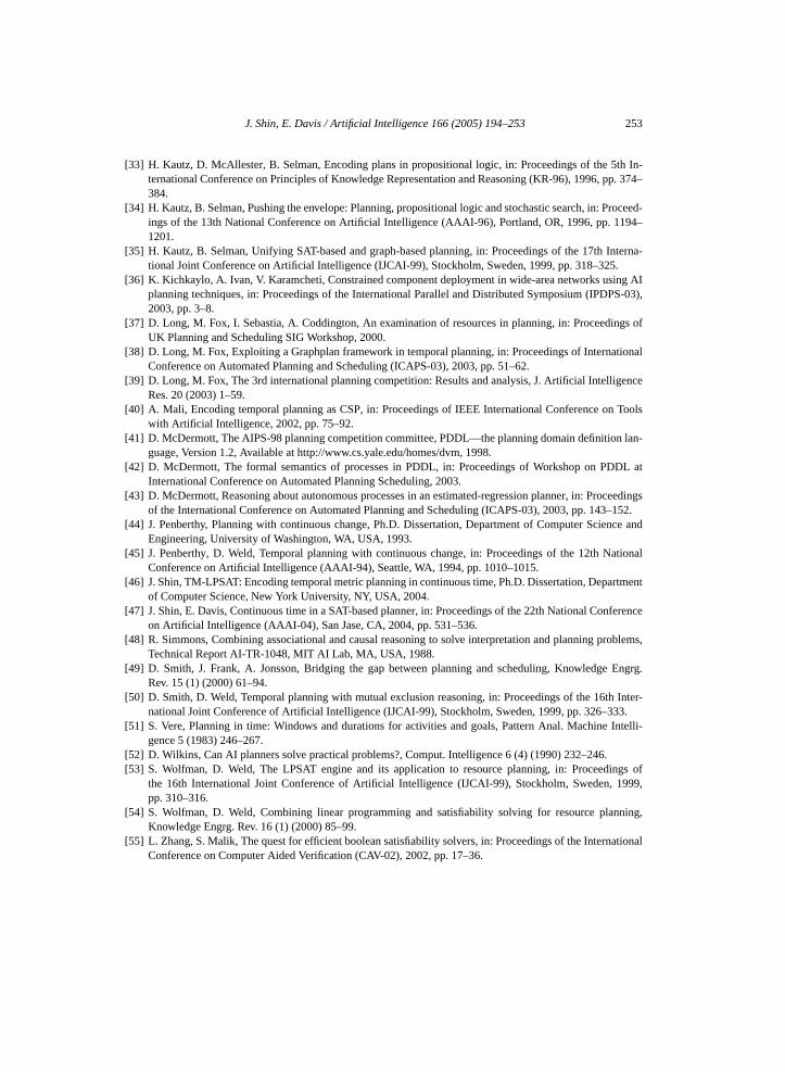
J. Shin, E. Davis / Artificial Intelligence 166 (2005) 194–253 253
[33] H. Kautz, D. McAllester, B. Selman, Encoding plans in propositional logic, in: Proceedings of the 5th In-ternational Conference on Principles of Knowledge Representation and Reasoning (KR-96), 1996, pp. 374–384.
[34] H. Kautz, B. Selman, Pushing the envelope: Planning, propositional logic and stochastic search, in: Proceed-ings of the 13th National Conference on Artificial Intelligence (AAAI-96), Portland, OR, 1996, pp. 1194–1201.
[35] H. Kautz, B. Selman, Unifying SAT-based and graph-based planning, in: Proceedings of the 17th Interna-tional Joint Conference on Artificial Intelligence (IJCAI-99), Stockholm, Sweden, 1999, pp. 318–325.
[36] K. Kichkaylo, A. Ivan, V. Karamcheti, Constrained component deployment in wide-area networks using AIplanning techniques, in: Proceedings of the International Parallel and Distributed Symposium (IPDPS-03),2003, pp. 3–8.
[37] D. Long, M. Fox, I. Sebastia, A. Coddington, An examination of resources in planning, in: Proceedings ofUK Planning and Scheduling SIG Workshop, 2000.
[38] D. Long, M. Fox, Exploiting a Graphplan framework in temporal planning, in: Proceedings of InternationalConference on Automated Planning and Scheduling (ICAPS-03), 2003, pp. 51–62.
[39] D. Long, M. Fox, The 3rd international planning competition: Results and analysis, J. Artificial IntelligenceRes. 20 (2003) 1–59.
[40] A. Mali, Encoding temporal planning as CSP, in: Proceedings of IEEE International Conference on Toolswith Artificial Intelligence, 2002, pp. 75–92.
[41] D. McDermott, The AIPS-98 planning competition committee, PDDL—the planning domain definition lan-guage, Version 1.2, Available at http://www.cs.yale.edu/homes/dvm, 1998.
[42] D. McDermott, The formal semantics of processes in PDDL, in: Proceedings of Workshop on PDDL atInternational Conference on Automated Planning Scheduling, 2003.
[43] D. McDermott, Reasoning about autonomous processes in an estimated-regression planner, in: Proceedingsof the International Conference on Automated Planning and Scheduling (ICAPS-03), 2003, pp. 143–152.
[44] J. Penberthy, Planning with continuous change, Ph.D. Dissertation, Department of Computer Science andEngineering, University of Washington, WA, USA, 1993.
[45] J. Penberthy, D. Weld, Temporal planning with continuous change, in: Proceedings of the 12th NationalConference on Artificial Intelligence (AAAI-94), Seattle, WA, 1994, pp. 1010–1015.
[46] J. Shin, TM-LPSAT: Encoding temporal metric planning in continuous time, Ph.D. Dissertation, Departmentof Computer Science, New York University, NY, USA, 2004.
[47] J. Shin, E. Davis, Continuous time in a SAT-based planner, in: Proceedings of the 22th National Conferenceon Artificial Intelligence (AAAI-04), San Jase, CA, 2004, pp. 531–536.
[48] R. Simmons, Combining associational and causal reasoning to solve interpretation and planning problems,Technical Report AI-TR-1048, MIT AI Lab, MA, USA, 1988.
[49] D. Smith, J. Frank, A. Jonsson, Bridging the gap between planning and scheduling, Knowledge Engrg.Rev. 15 (1) (2000) 61–94.
[50] D. Smith, D. Weld, Temporal planning with mutual exclusion reasoning, in: Proceedings of the 16th Inter-national Joint Conference of Artificial Intelligence (IJCAI-99), Stockholm, Sweden, 1999, pp. 326–333.
[51] S. Vere, Planning in time: Windows and durations for activities and goals, Pattern Anal. Machine Intelli-gence 5 (1983) 246–267.
[52] D. Wilkins, Can AI planners solve practical problems?, Comput. Intelligence 6 (4) (1990) 232–246.[53] S. Wolfman, D. Weld, The LPSAT engine and its application to resource planning, in: Proceedings of
the 16th International Joint Conference of Artificial Intelligence (IJCAI-99), Stockholm, Sweden, 1999,pp. 310–316.
[54] S. Wolfman, D. Weld, Combining linear programming and satisfiability solving for resource planning,Knowledge Engrg. Rev. 16 (1) (2000) 85–99.
[55] L. Zhang, S. Malik, The quest for efficient boolean satisfiability solvers, in: Proceedings of the InternationalConference on Computer Aided Verification (CAV-02), 2002, pp. 17–36.