
NorthStar Planner Feature Guide - Juniper Networks
591
NorthStar Planner Feature Guide Release Published 2019-12-17 5.1.0
-
Upload
khangminh22 -
Category
Documents
-
view
5 -
download
0
Transcript of NorthStar Planner Feature Guide - Juniper Networks
NorthStar Planner Feature Guide
ReleasePublished
2019-12-175.1.0

Juniper Networks, Inc.1133 Innovation WaySunnyvale, California 94089USA408-745-2000www.juniper.net
Juniper Networks, the Juniper Networks logo, Juniper, and Junos are registered trademarks of Juniper Networks, Inc. inthe United States and other countries. All other trademarks, service marks, registered marks, or registered service marksare the property of their respective owners.
Screenshots of VMware ESXi are used with permission.
Juniper Networks assumes no responsibility for any inaccuracies in this document. Juniper Networks reserves the rightto change, modify, transfer, or otherwise revise this publication without notice.
NorthStar Planner Feature Guide5.1.0Copyright © 2019 Juniper Networks, Inc. All rights reserved.
The information in this document is current as of the date on the title page.
YEAR 2000 NOTICE
Juniper Networks hardware and software products are Year 2000 compliant. Junos OS has no known time-relatedlimitations through the year 2038. However, the NTP application is known to have some difficulty in the year 2036.
END USER LICENSE AGREEMENT
The Juniper Networks product that is the subject of this technical documentation consists of (or is intended for use with)Juniper Networks software. Use of such software is subject to the terms and conditions of the EndUser License Agreement(“EULA”) posted at https://support.juniper.net/support/eula/. By downloading, installing or using such software, youagree to the terms and conditions of that EULA.
ii
Table of Contents
About the Documentation | xvii
Documentation and Release Notes | xvii
Documentation Conventions | xvii
Documentation Feedback | xx
Requesting Technical Support | xx
Self-Help Online Tools and Resources | xxi
Creating a Service Request with JTAC | xxi
Introduction1Router Features | 25
Interior Gateway Protocols (IGP) | 25
Equal Cost Multiple Paths (ECMP) | 25
Static Routes | 26
Policy Based Routes (PBR) | 26
Border Gateway Protocol (BGP) | 26
Virtual Private Networks (IP VPN) | 26
Class of Service (CoS) | 27
Multicast | 27
VoIP | 27
OSPF Area Design | 27
Multi-Protocol Label Switching (MPLS) Tunnels for Traffic Engineering | 28
Path Placement | 28
Modification | 28
Net Grooming | 28
Configlet Generation | 28
Path Diversity Design | 28
Fast Reroute (FRR) | 28
Inter-Area MPLS-TE | 29
DiffServ TE Tunnels | 29
Following Along with the Examples in this Manual | 29
iii
Router Data Extraction2Router Data Extraction Overview | 33
Recommended Instructions | 33
Getipconf - Router Configuration Extraction | 34
Default Inputs | 36
Bandwidth | 40
Text Mode | 52
MPLS Tunnel Extraction | 54
Delay Measurement File | 57
Updating Link Information | 58
Routing Protocols3NorthStar Planner Routing Protocols Overview | 63
Routing Protocols Recommended Instructions | 63
View Routing Protocol Details from the Map | 64
Set the IGP Routing Method | 65
Routing Protocol Details | 66
Equal Cost Multiple Paths4NorthStar Planner Equal Cost Multiple Paths Overview | 73
Equal Cost Multiple-Path Recommended Instructions | 73
Identifying Equal Cost Multiple-Paths | 74
Splitting a Flow into Sub-Flows | 78
Set ECMP Subflows Based on Bandwidth | 81
iv
Static Routes5NorthStar Planner Static Routes Overview | 85
View Static Routes | 85
Add/Modify/Delete Static Routes | 87
Static Routes Case Study | 88
Policy-Based Routes6NorthStar Planner Policy-Based Routes Overview | 97
Policy Based Routes Configuration Commands | 97
Viewing and Modifying Policy Based Routes | 98
Border Gateway Protocol7NorthStar Planner Border Gateway Protocol Overview | 105
Border Gateway Protocol Recommended Instructions | 105
BGP Data Extraction | 107
BGP Reports | 107
BGP Options | 108
BGP Map | 108
BGP Live Status Check | 114
BGP Routing Table | 115
BGP Routes Analysis | 117
BGP Information at a Node | 119
BGP Neighbor | 120
Apply, Modify, or Add BGP Polices | 125
BGP Subnets | 130
Getipconf Usage Notes | 135
BGP Report | 140
v
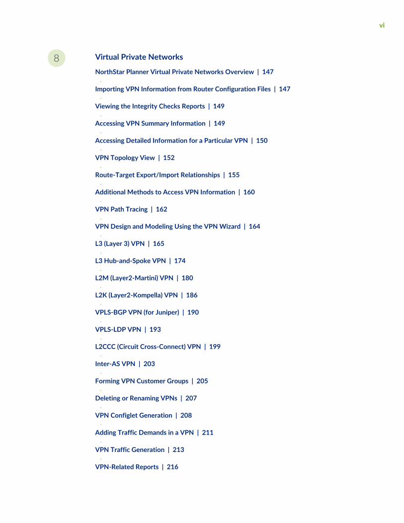
Virtual Private Networks8NorthStar Planner Virtual Private Networks Overview | 147
Importing VPN Information from Router Configuration Files | 147
Viewing the Integrity Checks Reports | 149
Accessing VPN Summary Information | 149
Accessing Detailed Information for a Particular VPN | 150
VPN Topology View | 152
Route-Target Export/Import Relationships | 155
Additional Methods to Access VPN Information | 160
VPN Path Tracing | 162
VPN Design and Modeling Using the VPNWizard | 164
L3 (Layer 3) VPN | 165
L3 Hub-and-Spoke VPN | 174
L2M (Layer2-Martini) VPN | 180
L2K (Layer2-Kompella) VPN | 186
VPLS-BGP VPN (for Juniper) | 190
VPLS-LDP VPN | 193
L2CCC (Circuit Cross-Connect) VPN | 199
Inter-AS VPN | 203
Forming VPN Customer Groups | 205
Deleting or Renaming VPNs | 207
VPN Configlet Generation | 208
Adding Traffic Demands in a VPN | 211
VPN Traffic Generation | 213
VPN-Related Reports | 216
vi
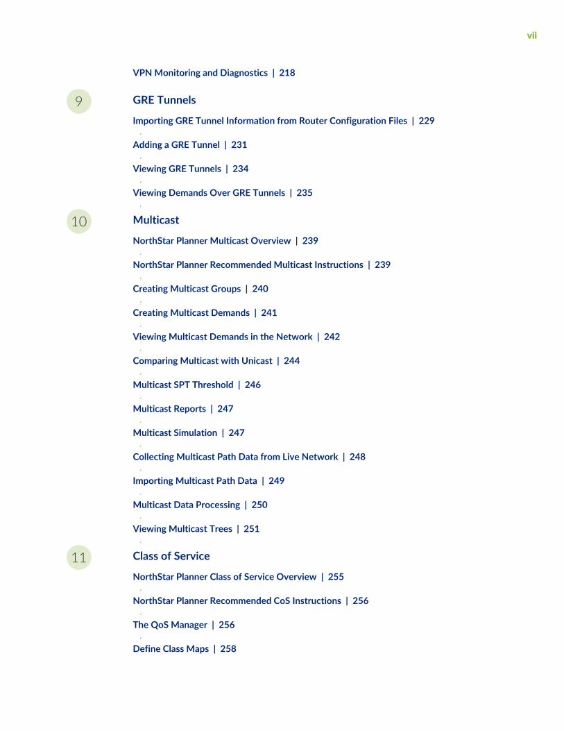
VPNMonitoring and Diagnostics | 218
GRE Tunnels9Importing GRE Tunnel Information from Router Configuration Files | 229
Adding a GRE Tunnel | 231
Viewing GRE Tunnels | 234
Viewing Demands Over GRE Tunnels | 235
Multicast10NorthStar Planner Multicast Overview | 239
NorthStar Planner Recommended Multicast Instructions | 239
Creating Multicast Groups | 240
Creating Multicast Demands | 241
Viewing Multicast Demands in the Network | 242
Comparing Multicast with Unicast | 244
Multicast SPT Threshold | 246
Multicast Reports | 247
Multicast Simulation | 247
Collecting Multicast Path Data from Live Network | 248
Importing Multicast Path Data | 249
Multicast Data Processing | 250
Viewing Multicast Trees | 251
Class of Service11NorthStar Planner Class of Service Overview | 255
NorthStar Planner Recommended CoS Instructions | 256
The QoS Manager | 256
Define Class Maps | 258
vii

Create Policies for Classes | 260
Attach Policies to Interfaces | 266
Adding Traffic Inputs | 268
Using the Text Editor | 269
Reporting Module | 269
IP Flow Information | 270
Link information | 271
Traffic Load Analysis | 272
Traffic Load by Policy Class | 273
CoS Alias File | 275
Bblink File | 275
Policymap File | 276
Demand File | 279
Traffic Load File | 279
Routing Instances12NorthStar Planner Routing Instances Overview | 283
Routing Instances Recommended Instructions | 283
Creating Routing Instances | 284
Path Analysis | 288
Traffic Matrix Solver13Traffic Matrix Solver Overview | 293
Traffic Matrix Solver Recommended Instructions | 294
Input Interface Traffic | 294
Input Seed Demands | 297
Running the Traffic Matrix Solver | 298
viii

Viewing the Results | 300
Viewing Differences Graphically | 304
Traffic Matrix Solver Troubleshooting | 305
Additional Traffic Matrix Solver Information | 306
LSP Tunnels14NorthStar Planner LSP Tunnels Overview | 311
Viewing Tunnel Info | 311
Viewing Primary and Backup Paths | 312
Viewing Tunnel Utilization Information from the Topology Map | 313
Viewing Tunnels Through a Link | 314
Viewing Demands Through a Tunnel | 315
Viewing Link Attributes/Admin-Group | 316
Viewing Tunnel-Related Reports | 317
Adding Primary Tunnels | 319
Adding Multiple Tunnels | 320
Mark MPLS-Enabled on Links Along Path | 322
Modifying Tunnels | 322
Path Configuration | 323
Specifying a Dynamic Path | 324
Specifying Alternate Routes, Secondary and Backup Tunnels | 326
Adding and Assigning Tunnel ID Groups | 330
Making Specifications for Fast Reroute | 333
Specifying Tunnel Constraints (Affinity/Mask or Include/Exclude) | 334
Adding One-Hop Tunnels | 339
Tunnel Layer and Layer 3 Routing Interaction | 342
ix
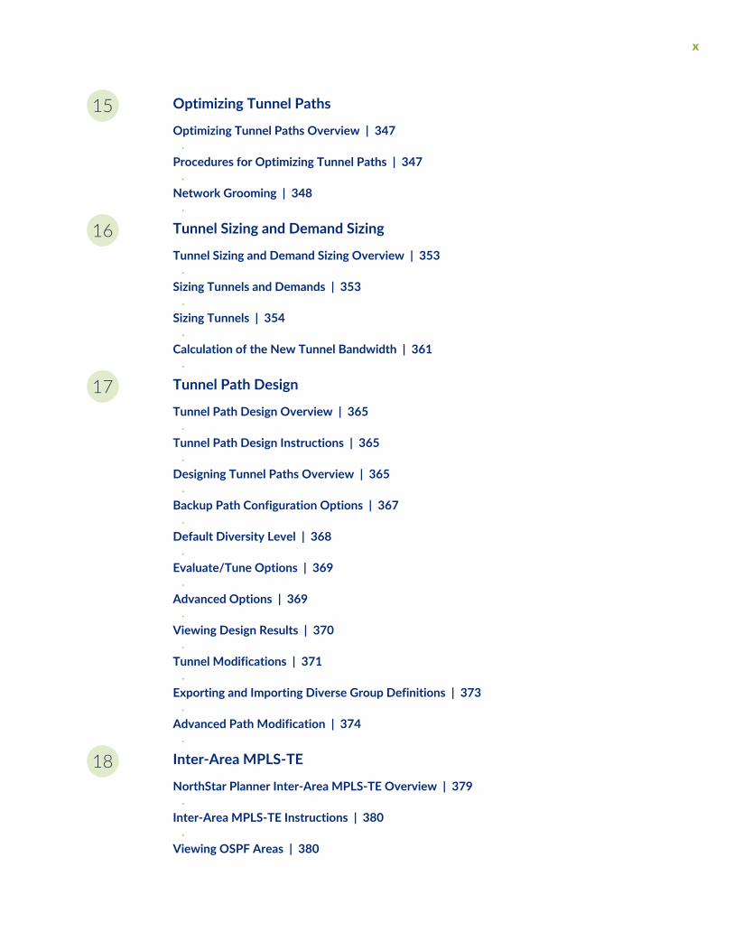
Optimizing Tunnel Paths15Optimizing Tunnel Paths Overview | 347
Procedures for Optimizing Tunnel Paths | 347
Network Grooming | 348
Tunnel Sizing and Demand Sizing16Tunnel Sizing and Demand Sizing Overview | 353
Sizing Tunnels and Demands | 353
Sizing Tunnels | 354
Calculation of the New Tunnel Bandwidth | 361
Tunnel Path Design17Tunnel Path Design Overview | 365
Tunnel Path Design Instructions | 365
Designing Tunnel Paths Overview | 365
Backup Path Configuration Options | 367
Default Diversity Level | 368
Evaluate/Tune Options | 369
Advanced Options | 369
Viewing Design Results | 370
Tunnel Modifications | 371
Exporting and Importing Diverse Group Definitions | 373
Advanced Path Modification | 374
Inter-Area MPLS-TE18NorthStar Planner Inter-Area MPLS-TE Overview | 379
Inter-Area MPLS-TE Instructions | 380
Viewing OSPF Areas | 380
x

Adding Multiple Tunnels Between Areas | 382
Tunnel Type Configuration Options Related to Areas | 382
Viewing Inter-Area Tunnels | 384
Configuring a Loose Route | 385
Point-to-Multipoint (P2MP) Traffic Engineering19NorthStar Planner P2MP Traffic Engineering Overview | 389
Point-to-Multipoint Traffic Engineering Instructions | 390
Import a Network That Already has Configured P2MP LSP Tunnels | 390
Examine the P2MP LSP Tunnels | 390
Create P2MP LSP Tunnels and Generate Corresponding LSP Configlets | 393
Examine P2MP LSP Tunnel Link Utilization | 397
Perform Failure Simulation and Assess the Impact | 398
Diverse Multicast Tree Design20Diverse Multicast Tree Design Overview | 403
Diverse Multicast Tree Instructions | 404
Open a Network That Already Has a Multicast Tree | 404
Set the Two P2MP Trees of Interest to be in the Same Diversity Group | 405
Using the Multicast Tree Design Feature to Design Diverse Multicast Trees | 407
Using the Multicast Tree Design Feature | 411
DiffServ Traffic Engineering Tunnels21DiffServ Traffic Engineering Tunnels Overview | 415
Using DS-TE LSP | 416
Hardware Support for DS-TE LSP | 416
Class Type | 417
EXP Bits | 417
Forwarding Class | 417
xi

Scheduler Map | 417
Bandwidth Model | 418
Operation | 418
NorthStar Planner Support for DS-TE LSP | 418
Class Types | 419
EXP Bits | 419
CoS Classes | 419
Cos Policies | 420
Bandwidth Model | 421
Configuring the Bandwidth Model and Default Bandwidth Partitions | 422
Forwarding Class to Class Type Mapping | 423
Link Bandwidth Reservation | 423
Creating a NewMulti-Class or Single-Class LSP | 425
Configuring a DiffServ-Aware LSP | 426
Tunnel Routing | 427
Link Utilization Analysis | 427
Fast Reroute22NorthStar Planner Fast Reroute Overview | 431
Graphical Display | 431
What-If Studies and Path Design | 431
Failure Simulation | 432
Fast Reroute Supported Vendors | 432
Juniper | 432
Cisco | 433
Import Config and Tunnel Path | 433
Viewing the FRR Configuration | 434
Viewing FRR Backup Tunnels | 436
Viewing Primary Tunnels Protected by a Bypass Tunnel | 437
xii
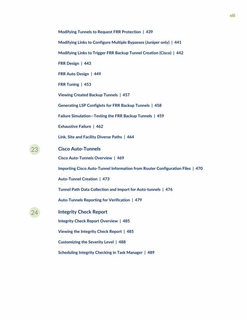
Modifying Tunnels to Request FRR Protection | 439
Modifying Links to Configure Multiple Bypasses (Juniper only) | 441
Modifying Links to Trigger FRR Backup Tunnel Creation (Cisco) | 442
FRR Design | 443
FRR Auto Design | 449
FRR Tuning | 453
Viewing Created Backup Tunnels | 457
Generating LSP Configlets for FRR Backup Tunnels | 458
Failure Simulation—Testing the FRR Backup Tunnels | 459
Exhaustive Failure | 462
Link, Site and Facility Diverse Paths | 464
Cisco Auto-Tunnels23Cisco Auto-Tunnels Overview | 469
Importing Cisco Auto-Tunnel Information from Router Configuration Files | 470
Auto-Tunnel Creation | 473
Tunnel Path Data Collection and Import for Auto-tunnels | 476
Auto-Tunnels Reporting for Verification | 479
Integrity Check Report24Integrity Check Report Overview | 485
Viewing the Integrity Check Report | 485
Customizing the Severity Level | 488
Scheduling Integrity Checking in Task Manager | 489
xiii

Integrity Check Options Tab | 490
Integrity Check Descriptions | 493
Access List and Prefix List Integrity Checks | 494
BGP Integrity Checks | 494
EIGRP/IGRP Integrity Checks | 495
IP Integrity Checks | 495
ISIS Integrity Checks | 497
RIP Integrity Checks | 497
QoS Integrity Checks | 498
LINK Integrity Checks | 499
MISCELLANEOUS Integrity Checks | 500
MPLS Integrity Checks | 502
RSVP Integrity Checks | 503
Static Routes Integrity Checks | 503
Tunnel Integrity Checks | 504
VPN Integrity Checks | 504
VLAN Integrity Checks | 505
Compliance Assessment Tool25Compliance Assessment Tool Overview | 509
Using The Compliance Assessment Tool | 510
CAT Testcase Design | 512
Creating a New Project | 513
Loading the Configuration Files | 514
Creating Conformance Templates | 517
Reviewing and Saving the Template | 521
Saving and Loading Projects | 522
Run Compliance Assessment Check | 523
Compliance Assessment Results | 526
Publishing Templates | 528
xiv

Running External Compliance Assessment Scripts | 530
Scheduling Configuration Checking in Task Manager | 531
Building Templates | 532
Special Built-In Functions | 546
NorthStar Planner Keywords For Use Within a Rule | 549
More on Regular Expressions | 555
IP Manipulation | 557
Virtual Local Area Networks26NorthStar Planner Virtual Local Area Networks Overview | 561
Importing Cisco VLAN and Spanning Tree Information | 562
Viewing VLAN Details | 562
Viewing VLAN Topology | 571
VLANModification and Design | 574
Overhead Calculation27Overhead Calculation Background | 589
Specifying the Overhead Calculation Frame Size | 590
Router Reference28Application Options | 595
NodeWindow Parameters | 596
Link Window Fields | 597
Interface Window Fields | 600
DemandWindow Fields | 602
Tunnel Window Fields | 604
xv
About the Documentation
IN THIS SECTION
Documentation and Release Notes | xvii
Documentation Conventions | xvii
Documentation Feedback | xx
Requesting Technical Support | xx
Use this guide to explore the router-specific features of the NorthStar Planner, such as those enabled byMPLS, BGP, IP VPN, and CoS.
Documentation and Release Notes
To obtain the most current version of all Juniper Networks® technical documentation, see the productdocumentation page on the Juniper Networks website at https://www.juniper.net/documentation/.
If the information in the latest release notes differs from the information in the documentation, follow theproduct Release Notes.
Juniper Networks Books publishes books by Juniper Networks engineers and subject matter experts.These books go beyond the technical documentation to explore the nuances of network architecture,deployment, and administration. The current list can be viewed at https://www.juniper.net/books.
Documentation Conventions
Table 1 on page xviii defines notice icons used in this guide.
xvii

Table 1: Notice Icons
DescriptionMeaningIcon
Indicates important features or instructions.Informational note
Indicates a situation that might result in loss of data or hardwaredamage.
Caution
Alerts you to the risk of personal injury or death.Warning
Alerts you to the risk of personal injury from a laser.Laser warning
Indicates helpful information.Tip
Alerts you to a recommended use or implementation.Best practice
Table 2 on page xviii defines the text and syntax conventions used in this guide.
Table 2: Text and Syntax Conventions
ExamplesDescriptionConvention
To enter configuration mode, typethe configure command:
user@host> configure
Represents text that you type.Bold text like this
user@host> show chassis alarms
No alarms currently active
Represents output that appears onthe terminal screen.
Fixed-width text like this
• A policy term is a named structurethat defines match conditions andactions.
• Junos OS CLI User Guide
• RFC 1997, BGP CommunitiesAttribute
• Introduces or emphasizes importantnew terms.
• Identifies guide names.
• Identifies RFC and Internet drafttitles.
Italic text like this
xviii
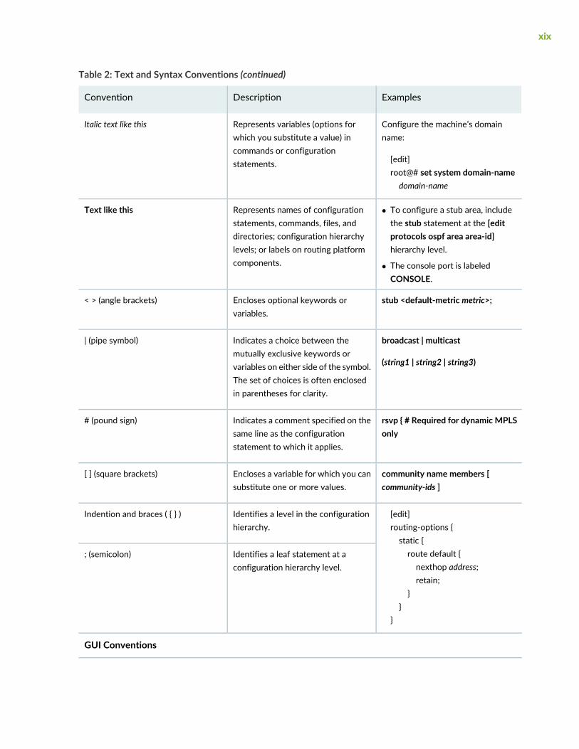
Table 2: Text and Syntax Conventions (continued)
ExamplesDescriptionConvention
Configure the machine’s domainname:
[edit]root@# set system domain-namedomain-name
Represents variables (options forwhich you substitute a value) incommands or configurationstatements.
Italic text like this
• To configure a stub area, includethe stub statement at the [editprotocols ospf area area-id]hierarchy level.
• The console port is labeledCONSOLE.
Represents names of configurationstatements, commands, files, anddirectories; configuration hierarchylevels; or labels on routing platformcomponents.
Text like this
stub <default-metric metric>;Encloses optional keywords orvariables.
< > (angle brackets)
broadcast | multicast
(string1 | string2 | string3)
Indicates a choice between themutually exclusive keywords orvariables on either side of the symbol.The set of choices is often enclosedin parentheses for clarity.
| (pipe symbol)
rsvp { # Required for dynamic MPLSonly
Indicates a comment specified on thesame line as the configurationstatement to which it applies.
# (pound sign)
community name members [community-ids ]
Encloses a variable for which you cansubstitute one or more values.
[ ] (square brackets)
[edit]routing-options {static {route default {nexthop address;retain;
}}
}
Identifies a level in the configurationhierarchy.
Indention and braces ( { } )
Identifies a leaf statement at aconfiguration hierarchy level.
; (semicolon)
GUI Conventions
xix

Table 2: Text and Syntax Conventions (continued)
ExamplesDescriptionConvention
• In the Logical Interfaces box, selectAll Interfaces.
• To cancel the configuration, clickCancel.
Represents graphical user interface(GUI) items you click or select.
Bold text like this
In the configuration editor hierarchy,select Protocols>Ospf.
Separates levels in a hierarchy ofmenu selections.
> (bold right angle bracket)
Documentation Feedback
We encourage you to provide feedback so that we can improve our documentation. You can use eitherof the following methods:
• Online feedback system—Click TechLibrary Feedback, on the lower right of any page on the JuniperNetworks TechLibrary site, and do one of the following:
• Click the thumbs-up icon if the information on the page was helpful to you.
• Click the thumbs-down icon if the information on the page was not helpful to you or if you havesuggestions for improvement, and use the pop-up form to provide feedback.
• E-mail—Send your comments to [email protected]. Include the document or topic name,URL or page number, and software version (if applicable).
Requesting Technical Support
Technical product support is available through the Juniper Networks Technical Assistance Center (JTAC).If you are a customer with an active Juniper Care or Partner Support Services support contract, or are
xx

covered under warranty, and need post-sales technical support, you can access our tools and resourcesonline or open a case with JTAC.
• JTAC policies—For a complete understanding of our JTAC procedures and policies, review the JTACUserGuide located at https://www.juniper.net/us/en/local/pdf/resource-guides/7100059-en.pdf.
• Productwarranties—For productwarranty information, visit https://www.juniper.net/support/warranty/.
• JTAC hours of operation—The JTAC centers have resources available 24 hours a day, 7 days a week,365 days a year.
Self-Help Online Tools and Resources
For quick and easy problem resolution, Juniper Networks has designed an online self-service portal calledthe Customer Support Center (CSC) that provides you with the following features:
• Find CSC offerings: https://www.juniper.net/customers/support/
• Search for known bugs: https://prsearch.juniper.net/
• Find product documentation: https://www.juniper.net/documentation/
• Find solutions and answer questions using our Knowledge Base: https://kb.juniper.net/
• Download the latest versions of software and review release notes:https://www.juniper.net/customers/csc/software/
• Search technical bulletins for relevant hardware and software notifications:https://kb.juniper.net/InfoCenter/
• Join and participate in the Juniper Networks Community Forum:https://www.juniper.net/company/communities/
• Create a service request online: https://myjuniper.juniper.net
To verify service entitlement by product serial number, use our Serial Number Entitlement (SNE) Tool:https://entitlementsearch.juniper.net/entitlementsearch/
Creating a Service Request with JTAC
You can create a service request with JTAC on the Web or by telephone.
• Visit https://myjuniper.juniper.net.
• Call 1-888-314-JTAC (1-888-314-5822 toll-free in the USA, Canada, and Mexico).
For international or direct-dial options in countries without toll-free numbers, seehttps://support.juniper.net/support/requesting-support/.
xxi

1CHAPTER
Introduction
Router Features | 25
Following Along with the Examples in this Manual | 29


Router Features
IN THIS SECTION
Interior Gateway Protocols (IGP) | 25
Equal Cost Multiple Paths (ECMP) | 25
Static Routes | 26
Policy Based Routes (PBR) | 26
Border Gateway Protocol (BGP) | 26
Virtual Private Networks (IP VPN) | 26
Class of Service (CoS) | 27
Multicast | 27
VoIP | 27
OSPF Area Design | 27
Multi-Protocol Label Switching (MPLS) Tunnels for Traffic Engineering | 28
Fast Reroute (FRR) | 28
Inter-Area MPLS-TE | 29
DiffServ TE Tunnels | 29
Interior Gateway Protocols (IGP)
• Modeling of OSPF, ISIS, EIGRP, IGRP, and RIP routing protocols
• OSPF two-layer hierarchy (backbone area and areas off of the backbone area)
• Routingmetricmodification bymodifying variables like the cost, reference bandwidth, interface bandwidth,and delay, according to each routing protocol’s metric calculation formula.
Equal Cost Multiple Paths (ECMP)
• Path analysis displaying ECMP routes between two nodes
• ECMP report listing ECMP routes in the network
25

• Load balancing by splitting flows into subflows with equal cost paths.
Static Routes
• Extraction of static route tables
• What-if studies upon adding or modifying static routes
Policy Based Routes (PBR)
• Extraction of PBR details (access list, policy route map)
• What-if analyses by modifying the policy to use on an interface
Border Gateway Protocol (BGP)
• Extraction of BGP speakers, AS numbers, Peering points for both IBGP and EBGP, Route Reflectors,BGP communities,Weight, Local preference,Multi-exit discriminator, AS_PATH, and BGP next hop fromrouter config files
• Key integrity checks are performed such as finding BGP unbalanced neighbors and checking IBGPmeshconnectivity
• Implementation of the BGP route selection rules and bottleneck analysis to troubleshoot routing failures
• BGP attribute modification for what-if studies
• BGP map logical view of EBGP and IBGP connections
Virtual Private Networks (IP VPN)
• Modeling of MPLS VPNs such as L3 VPN, L2 Kompella, L2 Martini, L2 CCC, and VPLS
• VPN extraction from router configuration files
• VPN topology display and reports
• VPN-related integrity checks
26
• Design and modeling of VPN via a VPNWizard
• Adding of VPN traffic demands
• VPN monitoring and diagnostics (when used in conjunction with the Online Module)
Class of Service (CoS)
• Extract of CoS classes and policies from router config files
• Create and modify CoS classes and policies and assign policies for link interfaces.
• View Link and Demand CoS reports and Link Load reports by CoS Policy
Multicast
• Create, view and modify multicast groups
• Create multicast demands and analyze their paths.
• PIM modes including sparse mode, dense mode, bidirectional PIM, and SSM
VoIP
• Define H.323 media gateways/gatekeepers, SIP user agents/servers, and codecs.
• Perform a call setup path analysis and view a report of call setup delays.
• Use the traffic generation wizard to generate traffic starting from Erlangs
OSPF Area Design
Design of the backbone network based on the following settings:
• Specify which nodes to use as gateways and the areas accessible to this gateway
• Specify administrative weights to be used for designed links from the Admin Weight feature
27
Multi-Protocol Label Switching (MPLS) Tunnels for Traffic Engineering
Path Placement
• Routing of LSP (label switched path) tunnels over physical links
• Routing of traffic demand flows (forwarding equivalence class, or, FEC) over LSP tunnels and links
Modification
• Modification of LSP tunnel preferred/explicit routes and media requirements (Bandwidth constraints,QoS requirements, Priority and preemption, affinity/mask and include-any/include-all/excludeadmin-groups)
• Addition of Secondary/Standby Routes
Net Grooming
• Network grooming of tunnel paths
Configlet Generation
• Configlets created based on added and modified tunnels
• Templates can be specified
Path Diversity Design
• Design primary and secondary/standby tunnel paths to be link-diverse, site-diverse, or facility-diverse.
• View or tune the resulting paths.
Fast Reroute (FRR)
• Specification of tunnels requesting FRR protection and FRR backup tunnels.
• Simulation of routing according to FRR during link failure
• Design of FRR backup tunnels for LSP tunnels requesting FRR protection according to site or facilitydiversity requirements
28

Inter-Area MPLS-TE
• Design LSP tunnels between different OSPF areas for multi-area networks.
DiffServ TE Tunnels
• Create and model Juniper Networks’ single-class and multi-class LSPs.
• Configure bandwidth model (RDM, MAM) and bandwidth partitions.
• Define scheduler maps (CoS policies) and assign them to links.
Following Along with the Examples in this Manual
1. Many of the topics in this guide use a sample network to illustrate step by step procedures that youcan follow along with. These networks are located in the $WANDL_HOME/sample folder on yourserver, where $WANDL_HOME is the directory in which the server was installed (typically /u/wandl).In the sample directory are two folders, “atm” and “router”. In the FileManager, navigate to the “router”folder and then a subdirectory, such as “fish”. Double-click on the “spec.mpls-fish” file. This opens thenetwork project.
2. At this moment, you may encounter a popup message, as shown below. This message indicates thateither you do not have an appropriate router license to open this network, or your license has expired.
NOTE: To examine your license, view the npatpw file located on your server, in$WANDL_HOME/db/sys/npatpw. If your license has expired (see the line “expire_date=”),please contact Juniper support. Otherwise, proceed to the next step.
Figure 1: Typical Missing License Warning
29

3. In this example, we will use the network in /u/wandl/sample/IP/fish to illustrate. If you see such awarning as in Figure 1, you will need to edit the sample network files slightly to accommodate thenetwork hardware types for which you do have a license to. Because the sample network files are notwritable, the following procedure is the simplest one to get your sample network up and running.
4. Log into your server machine. Then do the following at the prompt, denoted by “>” below:
> cd /u/wandl/sample/IP
> cp -r fish fish1
> cd fish1
> chmod 666 *
The above commands first makes a complete copy of the fish folder into a new folder called “fish1”,and then changes the permissions of all the files so that they are writeable, or editable, by you.
Instead of “fish1”, you may wish to specify a different location. For example:
> cp -r fish /export/home/john/myexamples/fish
5. Now, return to your client application and navigatewithin the FileManager to the newly created folder.Right-click on the “spec.mpls-fish” file and select Spec File > Modify Spec from the popup menu.
6. Within the Spec File Generation window, click on the Design Parameters tab. Within this tab, pressthe “Reset dparam File” button. Click “Yes” to any popup dialog windows that appear at this time.Notice that the Hardware Type drop-down box is now enabled. Select a type from this drop-down box.What is displayed in this list will vary, depending on the hardware types present in your license. Mostusers will probably have only one or two types listed.
7. Press the “Done” button. The Specfile Status window will appear. In the Specfile Status window, clickon the “Load Network” button. Press “Yes” to overwrite both the spec.mpls-fish and dparam.mpls-fishfiles. The sample network will now be launched successfully.
30

2CHAPTER
Router Data Extraction
Router Data Extraction Overview | 33
Recommended Instructions | 33
Getipconf - Router Configuration Extraction | 34
Default Inputs | 36
Bandwidth | 40
Text Mode | 52
MPLS Tunnel Extraction | 54
Delay Measurement File | 57
Updating Link Information | 58


Router Data Extraction Overview
In NorthStar Planner, you can construct a network model and topology by simply importing routerconfiguration files for the network. The Router Data Extraction chapter describes how the network projectspecification file can be automatically generated from a set of router configuration files both in text mode(BBDsgn) and from the graphical client interface.
NOTE: Terms such as “Import Router Configuration”, “Configuration File Import”, “ConfigurationFile Extraction” and the text mode command, “getipconf” (short for “get IP configurations”), allrefer to the same thing.
Use these procedures to create a network project specification file (see definition below) from a set ofrouter configuration files. Afterwards, you can open the network project directly from the client bydouble-clicking on the specification file from within the File Manager.
You should have access to a set of router configuration files.
For a list of supported router devices, see the Introduction chapter in the NorthStar Planner User InterfaceGuide.
RELATED DOCUMENTATION
Recommended Instructions | 33
Recommended Instructions
Following is a high-level, sequential outline of the specification file creation process from router configurationfiles and the associated, recommended procedures.
Graphical User Interface Mode
1. Select File > Create Network > From Collected Data for the Network Data Import Wizard to create anew network model with a selected set of configuration files as described in Graphical User Interface.
2. Specify the necessary directories and options for importing configuration files.
Text Mode (Alternative)
33

1. Open a console window on or a telnet window to the server that has NorthStar Planner installed.
2. Navigate to the directory containing the configuration files, andmake sure the ownership and permissionsof those files are set properly.
3. Run the command-line program, getipconf as described in “Text Mode” on page 52.
4. Open the specification file on the NorthStar Planner client and recalculate the layout.
MPLS Tunnel Path Import
Using the Import Data Wizard, extract actual MPLS tunnel path information using data input from thechosen data directory as described in “MPLS Tunnel Extraction” on page 54.
Getipconf - Router Configuration Extraction
The getipconf (“get IP configurations”) program is located in $WANDL_HOME/bin/getipconf (e.g./u/wandl/bin/getipconf).When run, this utility extracts information to create the corresponding NorthStarPlanner network model files for the network nodes, links, interfaces, tunnels, bgp, vpn and so on. Thisutility is also available through the NorthStar Planner client though running getipconf from the commandline offers a few more options not available in the graphical interface. Both methods for importingconfiguration files into NorthStar Planner, command line and NorthStar Planner client, are described inthe following sections.
Graphical User Interface
34

1. Select File > CreateNetwork > FromCollectedData to open the “Import NetworkWizard.” ClickNext.
Figure 2: Import Network Wizard - Introduction Page
2. Use the Import Type “Routers and Switches”.
35

Figure 3: Selecting the Import Type (Options vary)
3. The Default Import Directory is the default directory in which to search for network input directoriesfor config, interface, bridge, tunnel_path, equipment_cli, tunnel_path, transit_tunnel, etc. The defaultdirectory for the live network is /u/wandl/data/collection/.LiveNetwork.
4. Enter in the output directory and runcode for the new project. The output directory is where thenetwork project will be created during the import. It is recommended to use a different directory fromthe import directory. The Runcode is the file extension identifier that will be appended to all thegenerated NorthStar Planner network files. (Note that spaces are not allowed in the runcode.)
5. Click Next to continue.
Default Inputs
The next page contains tabs that allow the user to specify different options that will be applied whenimporting configuration files.
36

Figure 4: Selecting the Output Directory and Runcode
1. On the Default tab are shown the most common import directory options. The subdirectories will beautomatically populated if they have the following names: config, interface, bridge, tunnel_path,transit_tunnel, equipment_cli. Otherwise, click on the magnifying glass to browse for the directory. Toselect more than one directory, select the buttonwith twomagnifying glasses. In the advanced browser,a subfolder can be expanded or collapsed by clicking on the “+” or “-” hinges to the left of each entry.Select the desired subdirectories to be involved in the config import by clicking on the box or circle tothe left of each.
37

2. The following information can be collected via NorthStar Planner’s online module, or a third partycollection software.
CorrespondingText InterfaceOptionDescriptionOption
This directory contains your router configuration file obtained using commandslike the following:
Juniper:
show configuration | display inheritance
Cisco:
show running-config
Config Directory
-i interfaceDirThis directory contains interface bandwidth data retrieved using CLI commands.Read the CLI results of “show interface” on the router to get the bandwidth ofthe interfaces and save it to a file. The CLI commands are:
Juniper:
# show configuration | match “host-name”
# show interfaces | no-more
To extract the hostname, use the following command:
# show configuration system host-name
Cisco:
# show running | include <hostname>
# show interfaces
InterfaceDirectory
-vlandiscoveryvlandir
This directory contains the intermediate results after parsing SNMP output oflayer 2 switches collected by NorthStar Planner, usually in the “intermediates”directory. Alternatively, the raw SNMP results collected by NorthStar Plannerin the “bridge” directory can be specified here, and the parsing will be done tocreate the intermediates directory before importing it using this configextraction wizard.
VLANDiscoverydirectory
-EXSW EXSWdirThis directory contains CLI output of layer 2 switches, which can be used tostitch up the physical and Layer 2 topology. e.g., “show cdp neighbor detail”for Cisco.
Each file should be preceded with a line indicating the hostname. For example,“host-name” for Juniper and <hostname>” for Cisco.
Switch CLIdirectory
38

CorrespondingText InterfaceOptionDescriptionOption
MPLS Tunnel Extraction retrieves the actual placement of the tunnel and thestatus (up or down) of the LSP paths by parsing the output of the JuniperJUNOS command:
Juniper:
show mpls lsp statistics ingress extensive
Cisco:
show mpls traffic-eng tunnels
Each file should be preceded with a line indicating the hostname. For example,“host-name” for Juniper and <hostname>” for Cisco.
Tunnel path
This option is similar to Tunnel path, except that in addition to ingress tunnels,it also includes FRR tunnels. This directory includes the output of the JuniperJUNOS command:
Juniper:
show rsvp session ingress detail
show rsvp session transit detail
Cisco:
show mpls traffic-eng tunnels backup
Each file should be preceded with a line indicating the hostname. For example,“host-name” for Juniper and <hostname>” for Cisco.
Transit Tunnel
This directory contains the output of CLI commands related to equipmentinventory, one file per router. See /u/wandl/db/command/<vendor>.cli to seethe list of commands.
Equipment CLI
This directory contains the output of SNMP commands related to equipmentinventorywhich can be collected by the onlinemodule via Inventory >HardwareInventory, Load > Collect Inventory into/u/wandl/data/collection/.LiveNetwork/equipment.
EquipmentSNMP
39

Bandwidth
1. Click on the next tab, Bandwidth. The interface bandwidth of the network model will be derived fromany files specified here, and different options can be selected for data conversion.
2. Under Select Bandwidth Sources, there is a list of six sources from which the program can deriveinterface bandwidth. As there are multiple sources that can be supplied, the first source in the list fromwhich the bandwidth value can be retrieved for a particular interface will be used. These sources aredescribed in detail in the table below.
3. Click on “Browse” to select the appropriate file or directory for each source. Then, if you want todeselect a file or directory as a source, use the drop-down selection box and choose <none selected>.
Figure 5: Bandwidth Tab
40
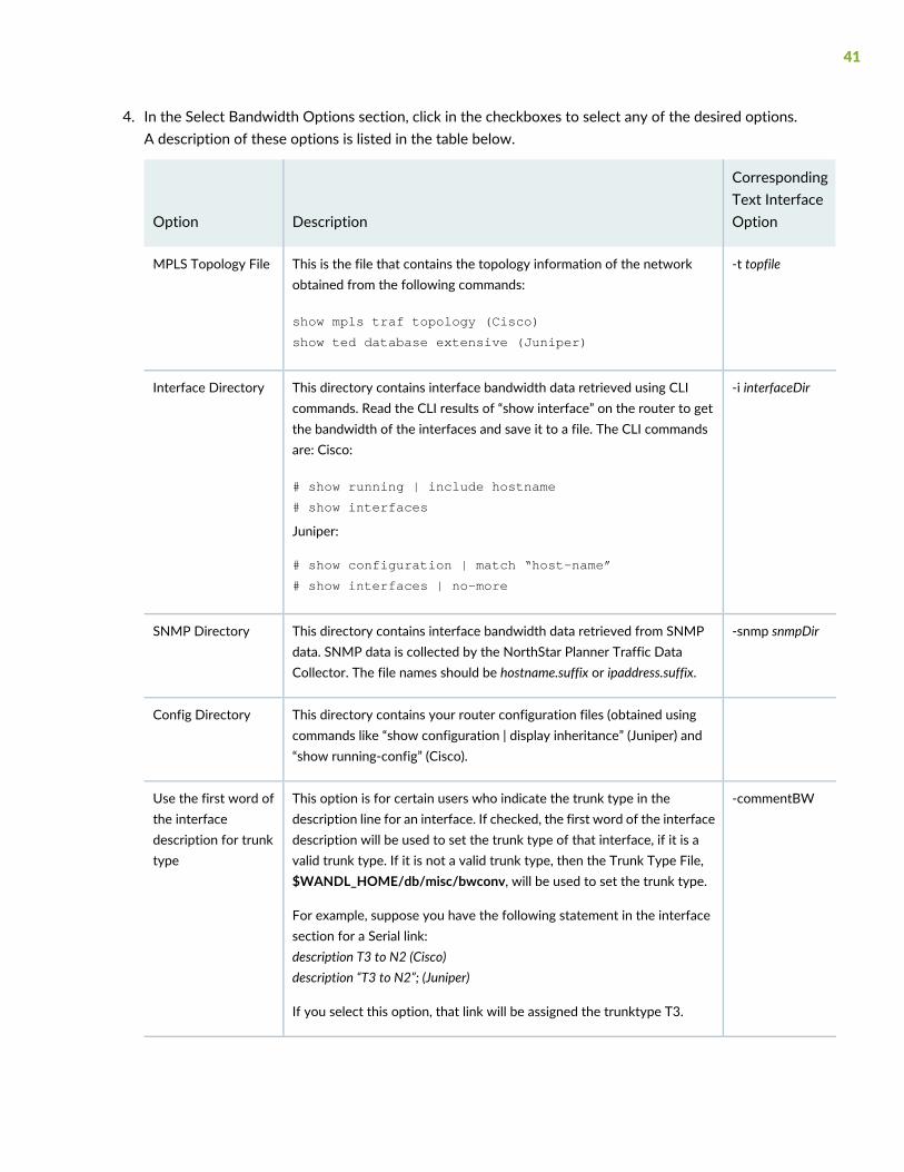
4. In the Select Bandwidth Options section, click in the checkboxes to select any of the desired options.A description of these options is listed in the table below.
CorrespondingText InterfaceOptionDescriptionOption
-t topfileThis is the file that contains the topology information of the networkobtained from the following commands:
show mpls traf topology (Cisco)
show ted database extensive (Juniper)
MPLS Topology File
-i interfaceDirThis directory contains interface bandwidth data retrieved using CLIcommands. Read the CLI results of “show interface” on the router to getthe bandwidth of the interfaces and save it to a file. The CLI commandsare: Cisco:
# show running | include hostname
# show interfaces
Juniper:
# show configuration | match “host-name”
# show interfaces | no-more
Interface Directory
-snmp snmpDirThis directory contains interface bandwidth data retrieved from SNMPdata. SNMP data is collected by the NorthStar Planner Traffic DataCollector. The file names should be hostname.suffix or ipaddress.suffix.
SNMP Directory
This directory contains your router configuration files (obtained usingcommands like “show configuration | display inheritance” (Juniper) and“show running-config” (Cisco).
Config Directory
-commentBWThis option is for certain users who indicate the trunk type in thedescription line for an interface. If checked, the first word of the interfacedescription will be used to set the trunk type of that interface, if it is avalid trunk type. If it is not a valid trunk type, then the Trunk Type File,$WANDL_HOME/db/misc/bwconv, will be used to set the trunk type.
For example, suppose you have the following statement in the interfacesection for a Serial link:description T3 to N2 (Cisco)description “T3 to N2”; (Juniper)
If you select this option, that link will be assigned the trunktype T3.
Use the first word ofthe interfacedescription for trunktype
41
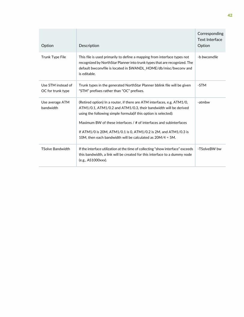
CorrespondingText InterfaceOptionDescriptionOption
-b bwconvfileThis file is used primarily to define a mapping from interface types notrecognized byNorthStar Planner into trunk types that are recognized. Thedefault bwconvfile is located in $WANDL_HOME/db/misc/bwconv andis editable.
Trunk Type File
-STMTrunk types in the generated NorthStar Planner bblink file will be given“STM” prefixes rather than “OC” prefixes.
Use STM instead ofOC for trunk type
-atmbw(Retired option) In a router, if there are ATM interfaces, e.g. ATM1/0,ATM1/0.1, ATM1/0.2 and ATM1/0.3, their bandwidth will be derivedusing the following simple formula(if this option is selected):
Maximum BW of these interfaces / # of interfaces and subinterfaces
If ATM1/0 is 20M, ATM1/0.1 is 0, ATM1/0.2 is 2M, and ATM1/0.3 is10M, then each bandwidth will be calculated as 20M/4 = 5M.
Use average ATMbandwidth
-TSolveBW bwIf the interface utilization at the time of collecting “show interface” exceedsthis bandwidth, a link will be created for this interface to a dummy node(e.g., AS1000xxx).
TSolve Bandwidth
42

Figure 6: Network Tab
5. Next, click on the Network tab. During configuration import, if you supplied a runcode that alreadyexists in the specified output directory (i.e. you are importing over an existing network model), someNorthStar Planner network files may be overwritten. To preserve or append to the original files, specifythem in the Reconcile Network Files section.
For example, you may have previously painstakingly arranged your network nodes on the topologymap. This information is saved into the Graph Coordinates (graphcoord) file. To ensure that you do notlose all your hard work from overwriting the file, specify the desired graph coordinates file in theReconcile Network Files section.
NOTE: At this time, incremental configuration import is not supported. If you import overan existing network model (i.e. you use the same runcode), you must specify the locationwhere the entire set of configuration files are located, not just a subset. Alternatively, youcan perform the new import into a newNorthStar Planner network project (correspondingto a different specification file and runcode), and then use File > Load Network Files to readin NorthStar Planner files (such as the graphcoord file) from a previous import or networkproject. After doing so, be sure to save your new network project (File > Save Network...).
43

6. There are additional options the user can select that are related to VPNs and BGPs. The description ofthese options are explained in the table below.
Corresponding Text InterfaceOptionDescriptionOption
-spec specFileThis is the file that lists, or specifies,all files related to a particular networkproject. If specified, the following filesfrom specFile will be preserved:ratedir, datadir, site, graphcoord,graphcoordaux, usercost, linkdist,fixlink, domain, and group.
Spec
-n muxlocThis is the file that contains additionallocation information of the nodessuch as NPA, NXX, latitude andlongitude. If specified, the existingmuxloc file will be preserved orappended to.
Muxloc
-p nodeparamThis is the file that specifies theparameters — node ID, hardware, IPaddress — of each node. If specified,the existing “nodeparam” file will bepreserved or appended to.
Node Parameter
-coord coordFileThis is the file that contains anyexisting graph coordinatesinformation. If specified, the existing“graphcoord” file will be preserved orappended to. This file will overwritethe graphcoord file in the Spec option,if a specification file is also specifiedin the “Reconcile Network Files”section.
Graph Coordinates
-group groupFileThis is the file that contains anyexisting grouping information. Ifspecified, the existing “group” file willbe preserved or appended to. This filewill overwrite the group file in theSpec option.
Group
44
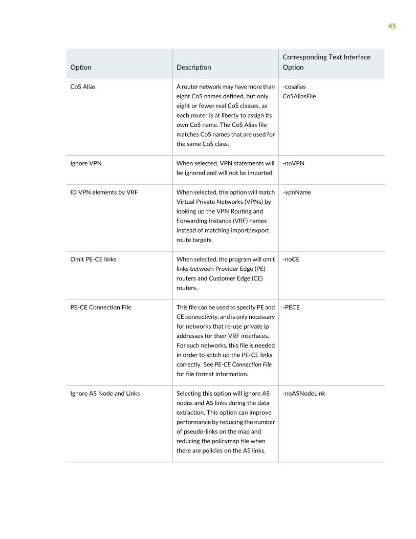
Corresponding Text InterfaceOptionDescriptionOption
-cosaliasCoSAliasFile
A router networkmay havemore thaneight CoS names defined, but onlyeight or fewer real CoS classes, aseach router is at liberty to assign itsown CoS name. The CoS Alias filematches CoS names that are used forthe same CoS class.
CoS Alias
-noVPNWhen selected, VPN statements willbe ignored and will not be imported.
Ignore VPN
-vpnNameWhen selected, this optionwill matchVirtual Private Networks (VPNs) bylooking up the VPN Routing andForwarding Instance (VRF) namesinstead of matching import/exportroute targets.
ID VPN elements by VRF
-noCEWhen selected, the programwill omitlinks between Provider Edge (PE)routers and Customer Edge (CE)routers.
Omit PE-CE links
-PECEThis file can be used to specify PE andCE connectivity, and is only necessaryfor networks that re-use private ipaddresses for their VRF interfaces.For such networks, this file is neededin order to stitch up the PE-CE linkscorrectly. See PE-CE Connection Filefor file format information.
PE-CE Connection File
-noASNodeLinkSelecting this option will ignore ASnodes and AS links during the dataextraction. This option can improveperformance by reducing the numberof pseudo-links on the map andreducing the policymap file whenthere are policies on the AS links.
Ignore AS Node and Links
45

Corresponding Text InterfaceOptionDescriptionOption
-as ASNameFileThe user can specify a differentAutonomous System (AS) name file,ASNameFile, mapping an AS name(rather than just a number) to thename of the AS nodes for display onthe topology map. If left unspecified,a default file located at/u/wandl/db/misc/ASNames is used.Note however that this file may notbe entirely up to date.
AS Name File
-bgpGroupTableThe BGP routing table object file isused by the routing engine to performBGP table lookup. To create the BGPTable Obj File from the live network,BGP routing tables are needed, withthe hostname prepended in the firstline of each file preceded by theword‘hostname’. Run the followingcommands (for Juniper BGP routingtable output ) to create the object fileoutput_object_file for this option.
/u/wandl/bin/prefixGroup
-firstAS routingtablefiles
/u/wandl/bin/routeGroup -o
output_object_file -g
group.firstAS
routingtablefiles
BGP Table Obj File*
7. Click on the next tab,Misc. Here, youmay set other desired options during the conversion of the routerconfiguration files to the NorthStar Planner network model.
46

Figure 7: Misc Tab
CorrespondingText InterfaceOptionDescriptionOption
-printDupThis option will print those links that have duplicated IPaddresses in other links. By default, these links are commentedout.
Allow duplicate address links
-secondaryFor ethernets which have secondary addresses, if their primaryaddresses do not match any subnet, the program will try tomatch their secondary addresses.
Stitch by secondary subnet
-policyOnLinkOnly the CoS policies on links in the network will be processedand saved to the policymap file. This option can be used to speedup performance by reducing the number of policies to only theones that are relevant to routing/dimensioning.
Only list policies on link
-noMedia (todisable this option)
This option will match nodes that have different media typesbut are within the same subnet.
Enable media type checking
-iptrafThis option will read in the user-specified NetFlow sample rateExtract NetFlow sample rate
47

CorrespondingText InterfaceOptionDescriptionOption
-exICThis option will cause the set of extended integrity checks tobe performed
Extended Integrity Check
-mgntBy default, management interfaces, e.g., fxp0 for Juniper, willnot be stitched together to form links. If it is desired to stitchtogether management interfaces based on IP address subnets,check this icon.
Include managementinterfaces
-dummyNodeIf youwould like to include hosts other than routers and switchesin your network model, check the option
Create dummy nodes forunrecognized files
-nodewoIntfIf this option is selected, logical nodes without any interfacesconfigured will be parsed and displayed as an isolated node. Bydefault, this option is not selected, and logical nodes lackinginterfaces will not be displayed.
Allow logical nodes withoutinterface
-IPv6If this option is selected IPv6 addresses will be used to stichlinks.
Use IPv6 addresses tostitching links
-operStatusIf this option is selected, links that are operationally down willbe marked as deleted in the bblink file.
Mark operational down linksas deleted
If this option is selected, and a config file is collected for thesame hostname twice, one of the config files will be deleted.
Delete existing data withduplicated hostname
-ignoreVRFOnLinkThe data extraction program uses various rules to stitch links,some of which are intelligent guesses based on BGP/VPNv4information. If this option is selected, those VRF-related ruleswill be ignored, and links will not be stitched based on VRFinformation.
Ignore VRF when stitchinglinks
For JUNOS dual routing engine support, by default the REextension in the router name is removed for the Node ID andNode Name, but not the hostname. To also remove it from thehostname, select this option.
Remove JUNOSRE extensionin hostname
If this option is selected, then shutdown links will be used forstitching up the backbone links. By default, these links are notused for link stitch-up.
Use shutdowninterfaces/tunnel for links
48

8. Click on the Files tab.
Figure 8: Files Tab
CorrespondingText InterfaceOptionDescriptionOption
-ICThe IC message file is the integrity check profile file that allows the user todefine the severity of a check as well as whether or not to include a particularcheck in the generated report.
IC message file
-delay delayFileA delay measurement file provides an easier method of inputting delaystatistics into the network model. (Alternatively, delay information can bespecified in the bblink link file.) Supplying the actual link delay measurementsenables the program to accurately compute delays of end-to-end paths. See“Delay Measurement File” on page 57 for file format information.
Delaymeasurementfile
-routeInstancerouteinstanceFile
A file containing routing instance definitions. Formore information about thisfeature including the file format, see “NorthStar Planner Routing InstancesOverview” on page 283.
Routinginstance file
49

CorrespondingText InterfaceOptionDescriptionOption
-srvcTypeserviceTypeFile
The service type file is used to match demands with services such as email,ftp, etc.
Service TypeFile
-srp srpTopoFileOutput of “show srp topology” used for RPR rings. For more information, seeResilient Packet Ring Overview.
SRP TopologyFile
-nodealiasnodealiasFile
This file can be used when there are devices with dual routing engines toindicate that two routing engine hostnames belong to the same device. ForJuniper, this is only needed if the names do not follow the standard namingconvention of ending with re0 or re1.
Each line of the node alias file should contain the mapping from the routingengine(s) to the corresponding AliasName that will represent the device onthe topology.
<AliasName><RoutingEngine0’sHostname><RoutingEngine1’sHostname>
Node Alias File
-ospfnbrneighborDir or-ospfnbrneighborFile
Either a directory or file can be specified for this option. If a directoryneighborDir is specified, the program will read all the files in that directory.The text files should contain the results of a Cisco IOS router’s “show ip ospfneighbor” statement or Juniper router’s “show ospf neighbor | no-more”statement. See /u/wandl/db/command for the statements for additionalvendors like Cisco CRS and Tellabs. This additional information helps connectthe devices on the topology view.
Each file should be preceded by the hostname, e.g., “hostname <hostname>”for Cisco or “host-name <hostname>;” for Juniper. In some cases, it may bepossible to extract the hostname from the prompt if the line "[hostname]>showip ospf neighbor" is included before its results. Note that the prompt can beeither “>” or “#” and that the short form, “sh ip ospf nei” is also recognized.
OSPF Neighbor
-oam oamDirOAMcan be used for connectivity checking for Juniper and Zyxel at theMACaddress layer. The OAM directory can be collected from the Scheduling LiveNetwork Task (online users), or manually via the commands in/u/wandl/db/command/*.oam.
OAM directory
Output of “show ip mroute” (Cisco IOS) or “show multicast route” (JUNOS).Each file should be begin with the router hostname information.
Multicast Path
50

CorrespondingText InterfaceOptionDescriptionOption
-isisnbr neighborDirIf a directory is specified, containing the outputs of “show isis neighbors detail”(for Cisco IOS) or “show isis adjacency detail” (for JUNOS), the program willread these files to stitch together devices on the topology view.
Each file’s command outputs should be preceded by the hostname, e.g.,“hostname <hostname>” for Cisco or “host-name <hostname>;” for Juniper.
ISIS Neighbor
-ldpnbr ldpDirIf a directory is specified, containing the outputs of “show ldp neighbor”(JUNOS) or “showmpls ldp neighbor” (Cisco IOS), the programwill read thesefiles to stitch together devices on the topology view.
Each file’s command outputs should be preceded by the hostname, e.g.,“hostname <hostname>” for Cisco or “host-name <hostname>;” for Juniper.
LDP Neighbor
Figure 9: Ignore Options Tab
51

9. Click on the final tab, the Ignore Options tab. Here, you specify the IP addresses and ERX interfacesyou want to ignore. If you select the Ignore private IP addresses checkbox, then the following blocksof IP addresses will be ignored during the import:
• 10.0.0.0 - 10.255.255.255
• 172.16.0.0 - 172.31.255.255
• 192.168.0.0 - 192.168.255.255
• 169.254.0.0 - 169.254.255.255
Corresponding TextInterface OptionDescriptionOption
-ignore ipaddrThis is the option to instruct the program that the IP addressipaddr should be ignored. The user can specify more than one IPaddress. This option is useful when the user has private IPaddresses for which it is not desirable to include in the analysis.
Ignore IP Addresses
-ignoreIntf interfaceThis is the option to instruct the program to ignore certaininterfaces. The user can specify more than one interface.Interfaces are matched based on substring.
Ignore ERXInterfaces
10.When all the options are selected as desired, click Next > to begin importing the configuration files.The generated network model will be automatically loaded if there is not already a specification fileopen. Otherwise, the program will ask if you want to close the current network.
11.When complete with the configuration import, click Finish to close the wizard.
Text Mode
1. Open a console window or a telnet window to the NorthStar Planner server. If you are not already theNorthStar Planner user, switch to the NorthStar Planner user. For example, if user ID is wandl, type in“su - wandl” and enter the password.
2. Type /u/wandl/bin/getipconf to see the command options:
usage: /u/wandl/bin/getipconf[-as asNameFile] [-b bwconvfile] [-baseIntf baseIntf] [-cat selectedcategory for report] [-checkMedia] [-commentBW] [-coord graphCoordFile] [-cosalias cosaliasFile][-delay delayFile] [-deltaIntf deltaIntf] [-dparamdparam] [-dummyNode] [-exIC] [-filter filter for report]
52

[-group groupFile] [-greTunnel] [-i interfaceDir] [-IC ICmessageList file name] [-ignore ipaddr][-ignoreIPUnnumbered] [-intf intfmap] [-iptraf] [-IPv6] [-isisnbr neighborDir] [-layer2CLI EXSWdir][-LSPDir lspDir] [-mgnt] [-nmuxloc [-pnodeparam]] [-noASNodeLink] [-noCPDNode] [-noCE] [-nodealiasnodealiasFile] [-nodewoIntf] [-noVLANLink] [-noVPN] [-oam oamDir] [-ospf ospfdatabase] [-ospfnbrneighborDir] [-PECE PECEfile] [-policyOnLink] [-printDup] [-probe probeFile] [-profile profile] [-rruncode] [-routeInstance routeInstanceFile] [-router selected router for report] [-secondary] [-snmpSNMPDir] [-spec spec] [-srp srpTopoFile] [-srvcType file] [-STM] [-t topfile] [-vlan vlanfile][-vlandiscovery vlanDir] [-hostdiscovery hostDir] [-vpnName] [-vrf vrffile] [-user username] [-dirconfigDir] [ config1 config2 ... [-tn topofiles...]
3. Run the program /u/wandl/bin/getipconf with the appropriate command-line variables. For example,if your configuration files all have the “.cfg” suffix, then type in the directory containing your configurationfiles:$ /u/wandl/bin/getipconf *.cfg
Refer to the tables above for other corresponding command-line options available. Running getipconfin the command line offers more options. These are listed in the table below.
DescriptionOption
This uses the OSPF database for topology information. The CLI command used toretrieve the OSPF database is: show ip ospf database (for Cisco) and show ospfdatabase router extensive (for Juniper).
This option is also available from File > Import Data wizard, Import Type, “OSPFDatabase”.
-ospf ospfdatabase (Cisco andJuniper)
This option is used for performance issues. This option will cause interfaces that are“ip unnumbered” to be ignored.
-ignoreIPUnnumbered
These options are used for performance issues when importing a large set of configfiles, and are normally not modified. baseIntf (default=8192) controls the base hashtable size. deltaIntf (default=2048) indicates the delta size by which the hash tableshould be increased after the hash table capacity has been reached.
-baseIntf baseIntf,-deltaIntf deltaIntf
This uses IPv6 addresses for link stitching. The default is not to use IPv6 for linkstitching.
-IPv6
4. Log onto the NorthStar Planner client and go to the directory containing the getipconf output files.
5. Open the newly created specification file and perform Layout>Recalculate Layout from the right-clickmenu of the map.
53

MPLS Tunnel Extraction
MPLS Tunnel Extraction retrieves the actual placement of the tunnel and the status (up or down) of theLSP paths by parsing the output of the tunnel_path command:
Juniper:
show mpls lsp statistics extensive
Cisco:
show mpls traffic-eng tunnels
This feature shows the exact network view of tunnel paths. This is useful if the LSPs can be dynamic (asopposed to explicit). NorthStar Planner will display the current status and routing of the LSP tunnels withinthe defined network.
1. To use this feature, you must specify a directory that contains the output of these commands, one fileper router.With your networkmodel already open, select File > Import Data to access the ImportWizard.Click Next > to go to the second page of the wizard.
2. First, under Import Type, click on the drop-down selection box to choose Tunnel Path. Then, specifythe import directory for the Tunnel Path directory. Note that there is also a directory for Transit Tunnels.This is used to collect additional information for Fast Reroute.
3. Click Browse to open up a Directory Chooser window. Navigate to the directory that contains the filesand click Select.
54
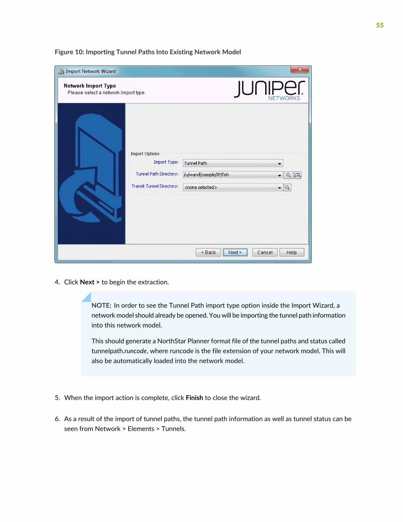
Figure 10: Importing Tunnel Paths Into Existing Network Model
4. Click Next > to begin the extraction.
NOTE: In order to see the Tunnel Path import type option inside the Import Wizard, anetworkmodel should already be opened. Youwill be importing the tunnel path informationinto this network model.
This should generate a NorthStar Planner format file of the tunnel paths and status calledtunnelpath.runcode, where runcode is the file extension of your network model. This willalso be automatically loaded into the network model.
5. When the import action is complete, click Finish to close the wizard.
6. As a result of the import of tunnel paths, the tunnel path information as well as tunnel status can beseen from Network > Elements > Tunnels.
55

Figure 11: Imported Tunnels
7. The status can be seen in the Misc field of the Properties tab:
• LIVE_STAT=UP: The tunnel is up.
• LIVE_STAT=DOWN: The tunnel is down.
• LIVE_STAT=MISSING: The status of the tunnel has not been collected. LIVE_STAT does not getupdated when importing tunnel path files, so the status is always MISSING.
The path can be seen from the Current_Route column of the Tunnels table. Select a tunnel and clickShow Path to view the tunnel graphically on the Standard Map.
Command Line Tunnel Path: rdjpath
The program /u/wandl/bin/rdjpath can be used to automate the tunnel info extraction. The command lineoptions are as follows: /u/wandl/bin/rdjpath -r runcode tunnel_path_dir
Substitute the runcodewith the same file extension used by your network project and tunnel_path_dirwiththe directory containing the tunnel path files collected from the router.
The resulting file, tunnelpath.runcode can be imported into the network via /u/wandl/bin/bbdsgn, optionM. MPLSView, 3. Read MPLS Tunnel Path. This can also be automated via input trace file.
NOTE: The tunnel path file must be in UNIX format.
56

Command Line Tunnel Traffic (Juniper only): convjtraf
The program /u/wandl/bin/convjtraf can be used to extract the tunnel traffic data from Juniper routers.The command line options are as follows:
/u/wandl/bin/convjtraf
Usage: /u/wandl/bin/convjtraf {[-start hh:mm] [-pct [avg|max|99|95|90|80]]}
runcode tunnelfile duration traf1 traf2 ...
Example1: /u/wandl/bin/convjtraf runcode tunnel.x 60 traf1
groups traffic in traf1 into 60-min periods
Example2: /u/wandl/bin/convjtraf runcode tunnel.x 5 traf1
groups traffic in traf1 into 5-min periods
If data spans more than 24 periods, the traffic
of last two hours are displayed
The resulting file can be imported into the network via File > Load Network Files > Tunnel Traffic >t_trafficload.
Delay Measurement File
A link latency file can be specified as an input to getipconf using the -delay <delayFile> option. This file isused to indicate the delay measurement from nodeA to nodeZ via a particular interface on nodeA. Thisinformation will be stored in the bblink file after the config file import via getipconf. For online users, theLink Latency Task provides one way to collect delay measurement information.
The following is an example of a link latency file with a customized header line followed by contents. Inthe example below, ATL and LDN2600 are connected.
#!NodeA,Interface,LatencyA2Z,BW
LDN2600,Ethernet0/1,50,100m
ATL,fe-0/1/3.0,50,100m
The format of the link latency file is flexible. The customizable column headers should be specified in acomma-separated list following a “#!”. The column headers on this line must be one of the followingreserved keywords in order to be recognized.
57

• NodeA, NodeZ, Interface, InterfaceZ
• LatencyA2Z: Latency from NodeA to NodeZ (ms). For microseconds, use decimals.
• LatencyZ2A: Latency from NodeZ to NodeA (ms). For microseconds, use decimals.
• RoundTripLatency: This number will be divided by two to get the latency
• BW-K: The bandwidth in K
• BW: The bandwidth in bits
• ISIS2Metric: The ISIS level 2 metric
Note that the data for one link could also be represented in one line instead of two. For example, the abovelink latency file entry for the link between LDN2600 and ATL could be shortened to one line by includingthe LatencyZ2A column, as shown below:
#!NodeA,Interface,LatencyA2Z,LatencyZ2A,BW
LDN2600,Ethernet0/1,50,50,100m
The RoundTripLatency could also be specified as an alternative to the Latency in one direction.
#!NodeA,Interface,RoundTripLatency,BW
LDN2600,Ethernet0/1,100,100m
For backwards compatibility, the following fixed format is also supported:
#RouterA,Type,RouterZ,Interface,Interface IP,Bandwidth(K),Metric,LatencyZ2A
conf1,,,Ethernet0,10.0.0.1,,,10
For the fixed format, the only attributes that are required are RouterA, Interface, and Latency, as shownin the example above. Note that the direction of Latency here is from NodeZ to NodeA.
Updating Link Information
Delay information can also be entered in interactively through the text mode version after importing theconfiguration files. This file format is also flexible and can support the following fields:NodeA, NodeZ, Node, InterfaceA, InterfaceZ, Interface, DelayAZ, DelayZA, LatencyA2Z, LatencyZ2A,Delay, IPaddrZ, IPaddr, RoundTripDelay, linkname, OSPFMetric, ISIS2Metric, ISIS1Metric, LinkName,BWType, Node, Interface, DelayAZ, DelayZA
The first line should specify the columns using a comma separated list of the above keywords, includinga column for the node and the interface or IP address at theminimum. The subsequent lines should specify
58

the Node/Interface or Node/IP pair and the other relevant columns to update. See the link latency file inthe last section for an example.
From the File > Load Network Files menu, select the file type linkdataupdate under the Network Files tab,Device Specific Files section. Click the Browse button to indicate the location of the file to use for updatingthe links.
Alternatively, in a console window, type /u/wandl/bin/bbdsgn specfilepath. Select from the Main menu:5. Modify Configuration > 4. Link Configuration > u. Update Link Properties from a File. Select ? for thehelp menu for information on the input file format. Select 2. Input File Name and enter in the location ofthe file to use for updating the links (absolute or relative path is acceptable here). Select 3. Error OutputName to enter the location of an optional file for outputting errors. Select 4. Operation to indicate whichfields to update based on the input file (the default includes all fields) and q to exit this menu. Select 5.Update link configuration to perform the actual update based on the specified input file. To save thechanges, exit until you reach the Main Menu and use the 2. Save Files menu.
PE-CE Connection File
#PE PE-interface PE-intf-address vrf CE CE-intf-address
PE1 so-0/0/1.121 10.200.138.5 aaa-251001 CE100 10.200.138.6
PE1 so-0/0/1.120 10.200.133.5 bbb-258001 CE200 10.200.133.6
59

3CHAPTER
Routing Protocols
NorthStar Planner Routing Protocols Overview | 63
Routing Protocols Recommended Instructions | 63
View Routing Protocol Details from the Map | 64
Set the IGP Routing Method | 65
Routing Protocol Details | 66


NorthStar Planner Routing Protocols Overview
The Routing Protocols chapter describes how to model routing protocols using NorthStar Planner, inparticular, interior gateway protocols such as OSPF, ISIS, EIGRP, IGRP, and RIP.
Follow these guidelines to add and modify routing protocol information.
If you wish to perform this task in the NorthStar Planner client, you should have a router specification fileopen before you begin. To follow along with this tutorial, you can open the spec.mpls-fish specificationfile located in your $WANDL_HOME/sample/IP/fish directory. ($WANDL_HOME is /u/wandl by default).
If you have an existing set of config files, use getipconf or the Import Data Wizard (via File > Import Data)to parse your config files and create a set of NorthStar Planner input files which contain router interfaces.
For an overview of NorthStar Planner or for a detailed description of each feature and the use of eachwindow, refer to the Router Reference section in this guide or the NorthStar Planner User Interface Guide.
For more information about data extraction, refer to the Router Data Extraction section in this guide.
RELATED DOCUMENTATION
Router Data Extraction Overview | 33
Routing Protocols Recommended Instructions
Following is a high-level, sequential outline of the process of viewing/modifying protocol information andthe associated, recommended detailed procedures.
• View the routing protocols and metrics in the network from the map’s Subviews > Protocols pane.
• Change the active routing method from Tools > Options > Design, Path Placement options pane.
• Modify routing protocol details from the Modify Link window’s Protocols tab and the Modify Nodewindow’s IP tab.
63

View Routing Protocol Details from the Map
1. Select the Subviews > Protocols menu from the Standard Map. The protocols enabled in the networkwill be displayed in the left pane of the map window as shown in the figure below.
Figure 12: Routing Protocols
With the ‘=’ radio button selected, clicking a checkbox next to a single protocol will display links enabledfor that protocol. When selecting the ‘&’ or ‘or’ radio buttons, logical combinations of protocols can beviewed. For example, in the above, only links that have both MPLS and OSPF enabled are displayed.
2. To view the link metrics on the map, right-click the map and select Labels>Link Labels>Show LinkDist.Note that this will display the metrics for the current routing method used. The current IGP routingmethod is displayed in the upper right of the application next to the Tunnel later/layer 3 buttons.
Figure 13: Current IGP: OSPF
Alternatively, the link metric can be labelled by selecting Labels>Link Labels>Link Labels... and thenCustomize... In addition to Metric_AZ and Metric_ZA, the following keys are also available: OSPF_AZ,OSPF_ZA, ISIS1_AZ, ISIS1_ZA, ISIS2_AZ, and ISIS2_ZA. Select the keys desired and click Add-> to addthose keys to the list of keys to display. Then select a display format and click OK.
64

Set the IGP Routing Method
1. To change the current IGP routing method , select the Applications>Options>Design, Path Placementoptions pane. For the Routing Method, the following IGPs can be selected: OSPF, IGRP, EIGRP, andISIS. To select RIP, use the Constant Distance routing method. Upon changing a routing method, therouting metrics for that routing method will be displayed on the map. (The exception to the rule is ifthe user hard-coded a metric for each link regardless of the protocol.)
2. The Max Hop parameter can also be configured from this window to indicate any hop limits for theselected protocol.
3. Note also the item for “MPLS-Enabled Mode.” If “All Links Enabled” is selected, the program will allowLSP tunnels to be routed on any link. If “User-Specified Per Link” is selected, the programwill only allowLSP tunnels to be routed on a link on which MPLS-TE (MPLS traffic engineering) is explicitly enabled.
Figure 14: Routing Method
For more information about the other Path Placement options, see the ApplicationMenu chapter in theNorthStar Planner User Interface Guide.
65

Routing Protocol Details
1. To modify protocol information on a link, select Modify > Elements > Links... in Modify mode. Selectone or more links to be modified and click the Modify button. In the resulting Modify Links window,select the Protocols tab.
Figure 15: Modify Link Protocols Tab
2. To enable a protocol, select “yes” to the right of the protocol. To enter in a metric for a particularprotocol, such as MPLS-TE, OSPF, ISIS, or ISIS2, enter it in the “A-Z Metric” and “Z-A Metric” columnsto the right of the protocol. These metrics correspond to the A and Z interfaces of the link as indicatedon the Locations tab. Note that when routing for a specific IGP, metrics should be entered in theProtocols tab rather than the Properties tab.
The following sections provide more details about configuring protocol-specific information.
RIP
No metrics need to be entered for RIP since the metrics will all be the same.
In the Tools > Options > Design, Path Placement options pane, the routing method should be set toConstant Distance and the Max Hop should be configured to 15.
66
IGRP and EIGRP
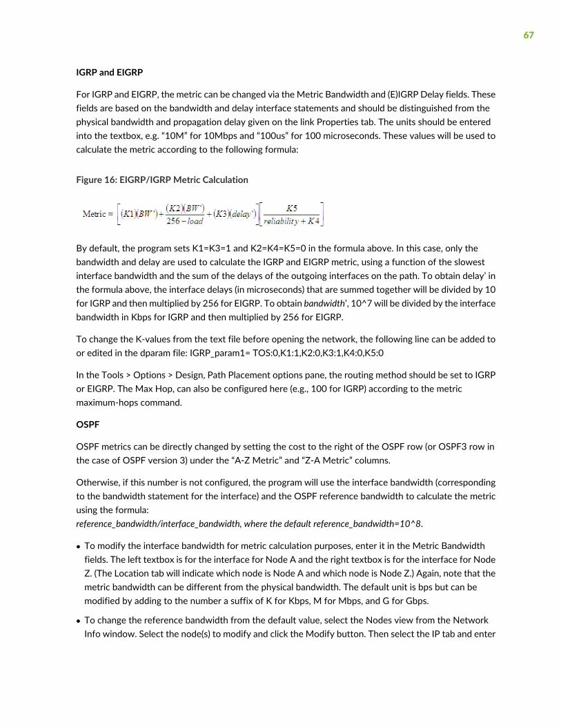
For IGRP and EIGRP, the metric can be changed via the Metric Bandwidth and (E)IGRP Delay fields. Thesefields are based on the bandwidth and delay interface statements and should be distinguished from thephysical bandwidth and propagation delay given on the link Properties tab. The units should be enteredinto the textbox, e.g. “10M” for 10Mbps and “100us” for 100 microseconds. These values will be used tocalculate the metric according to the following formula:
Figure 16: EIGRP/IGRP Metric Calculation
By default, the program sets K1=K3=1 and K2=K4=K5=0 in the formula above. In this case, only thebandwidth and delay are used to calculate the IGRP and EIGRP metric, using a function of the slowestinterface bandwidth and the sum of the delays of the outgoing interfaces on the path. To obtain delay’ inthe formula above, the interface delays (in microseconds) that are summed together will be divided by 10for IGRP and then multiplied by 256 for EIGRP. To obtain bandwidth’, 10^7 will be divided by the interfacebandwidth in Kbps for IGRP and then multiplied by 256 for EIGRP.
To change the K-values from the text file before opening the network, the following line can be added toor edited in the dparam file: IGRP_param1= TOS:0,K1:1,K2:0,K3:1,K4:0,K5:0
In the Tools > Options > Design, Path Placement options pane, the routing method should be set to IGRPor EIGRP. The Max Hop, can also be configured here (e.g., 100 for IGRP) according to the metricmaximum-hops command.
OSPF
OSPF metrics can be directly changed by setting the cost to the right of the OSPF row (or OSPF3 row inthe case of OSPF version 3) under the “A-Z Metric” and “Z-A Metric” columns.
Otherwise, if this number is not configured, the program will use the interface bandwidth (correspondingto the bandwidth statement for the interface) and the OSPF reference bandwidth to calculate the metricusing the formula:reference_bandwidth/interface_bandwidth, where the default reference_bandwidth=10^8.
• To modify the interface bandwidth for metric calculation purposes, enter it in the Metric Bandwidthfields. The left textbox is for the interface for Node A and the right textbox is for the interface for NodeZ. (The Location tab will indicate which node is Node A and which node is Node Z.) Again, note that themetric bandwidth can be different from the physical bandwidth. The default unit is bps but can bemodified by adding to the number a suffix of K for Kbps, M for Mbps, and G for Gbps.
• To change the reference bandwidth from the default value, select the Nodes view from the NetworkInfo window. Select the node(s) to modify and click the Modify button. Then select the IP tab and enter
67

in an OSPF Reference BW. The default unit is bps but can be modified by adding to the number a suffixof K for Kbps, M for Mbps, and G for Gbps.
Figure 17: Entering in the Reference BW from the Modify Nodes, IP Tab
• To specify which area the link belongs to, select it from the Area drop-down box. A secondary area canalso be specified in the Area2 drop-down box if the link belongs to more than one area. If there is noarea available in the drop-down box, an area can be first added fromModify > Protocols > OSPF Areas.Click Add. AREA0 will automatically be added. Subsequently you can enter in additional areas.
To set the OSPF overload bit, select the Nodes view from the Network Info window. Select the node(s)to modify and click the Modify button. Then select the IP tab and change the OSPF Overload Bit to true.If the OSPF overload bit is set, transit OSPF traffic will not be routed through the router.
ISIS and ISIS2
In the Modify > Elements >Links window, Protocols tab, the ISIS level 1 metrics can be changed in the“A-Z Metric” and “Z-A Metric” columns to the right of ISIS1 . ISIS level 2 metrics can be changed in the“A-Z Metric” and “Z-A Metric” columns to the right of ISIS2.
To view a node’s ISIS System ID, right-click the Nodes table header column and select Table Options...Next, select ISIS_System_ID, and add it to the columns to be displayed. Other ISIS related column optionsfor the Nodes view include ISIS_Area, ISIS_Overload_Bit, and ISIS_Ref_BW. The ISIS Area can also beviewed from the Protocols tab in the Nodes view.
To change the ISIS reference bandwidth from the default value, select the Nodes view from the NetworkInfo window. Select the node(s) to modify and click the Modify button. Then select the IP tab and enterin an ISIS Reference BW. The default unit is bps but can be modified by adding to the number a suffix ofK for Kbps, M for Mbps, and G for Gbps.
68

To set the ISIS overload bit, select the Nodes view from the Network Info window. Select the node(s) tomodify and click the Modify button. Then select the IP tab and change the ISIS Overload Bit to true. If theISIS overload bit is set, transit ISIS traffic will not be routed through the router.
MPLS-TE
The tunnel metric for MPLS-TE can be changed in the “A-Z Metric” and “Z-A Metric” columns to the rightof MPLS-TE. LSP tunnels that are not set to route according to the current IGP routing protocol will berouted according to these metrics.
Updating Link Properties from a File
Link delay and OSPF/ISIS metric information can also be modified in batch through the text mode version.This file format also flexible and can support the following fields:
NodeA, NodeZ, Node, InterfaceA, InterfaceZ, Interface, DelayAZ, DelayZA, LatencyA2Z, LatencyZ2A,Delay, IPaddrZ, IPaddr, RoundTripDelay, linkname, OSPFMetric, ISIS2Metric, ISIS1Metric, LinkName,BWType, Node, Interface, DelayAZ, DelayZA
The first line should specify the columns using a comma separated list of the above keywords, includinga column for the node and the interface or IP address at theminimum. The subsequent lines should specifythe Node/Interface or Node/IP pair and the other relevant columns to update. For example:
#!NodeA,Interface,LatencyA2Z,LatencyZ2A,OSPFMetric
LDN2600,Ethernet0/1,50,50,10
To load in this file, select Tools > Text/ASCII Mode or in a console window, type /u/wandl/bin/bbdsgnspecfilepath.
Select from the Main menu: 5. Modify Configuration > 4. Link Configuration > u. Update Link Propertiesfrom a File. Select ? for the help menu for information on the input file format.
Select 2. Input File Name and enter in the location of the file to use for updating the links (absolute orrelative path is acceptable here). Select 3. Error Output Name to enter the location of an optional file foroutputting errors. Select 4. Operation to indicate which fields to update based on the input file (the defaultincludes all fields) and q to exit this menu.
Select 5. Update link configuration to perform the actual input based on the specified input file.
After the update is finished, type ‘q’ until the Main Menu is reached. In text mode, select 2. Save Filesmenu to save the changes, or in Java graphicsmode, quit out of themenu and save via File > SaveNetwork...
69

4CHAPTER
Equal Cost Multiple Paths
NorthStar Planner Equal Cost Multiple Paths Overview | 73
Equal Cost Multiple-Path Recommended Instructions | 73
Identifying Equal Cost Multiple-Paths | 74
Splitting a Flow into Sub-Flows | 78
Set ECMP Subflows Based on Bandwidth | 81


NorthStar Planner Equal CostMultiplePathsOverview
This chapter describes several Equal Cost Multiple-Paths (ECMP) features and walks through a scenariowhere it is useful. The user will be able to display all the equal cost multiple-paths in the network as wellas view any equal cost paths between two given nodes in detail. The user can also split flows into sub-flows.Note that parallel links between two nodes do not count towards ECMPs.
Sometimes it is desirable to reduce the number of Equal Cost Multiple-Paths in order to improve thepredictability of how demands will be routed in the network. At other times it is desirable to split flowsinto sub-flows with Equal Cost Multiple-Paths in order to perform load balancing. NorthStar Planner willplace these flows on routing paths that have identical costs.
For an overview of NorthStar Planner or for a detailed description of each feature and the use of eachwindow, refer to the Router Reference section in this guide or the NorthStar Planner User Interface Guide.
Equal CostMultiple-Path Recommended Instructions
Following is a high-level, sequential outline of the Equal Cost Multiple-Paths features and the associated,recommended procedures.
• Open the Equal Cost Multi-Paths Report as described in step 3 and step 4.
• View the equivalent cost paths between two nodes as described in step 5 to step 9.
• Create sub-flows between two nodes as described in step 1 to step 4.
73

Identifying Equal Cost Multiple-Paths
1. Right-click on the topology map and select Labels > Link Labels > Show Link Metrics.
Figure 18: Show Link Distance
2. The link distances will be displayed and we can see that in this network, every metric has been set to10. This is very likely to cause numerous equal cost multiple-paths to exist.
Figure 19: Topology Map with Link Distances
3. Select Report > Report Manager to open up the Report Manager.
4. Select Network Reports > Demand Reports > Equal Cost Multi-Path Report from the left panel tobring up the report listing all of the equal cost multiple-paths of the network. As can be seen inFigure 20 on page 75, there aremany such paths. This report is also saved on the server as EQPATHRPT.runcode. Note that the ECMP paths are calculated based on IP metric only, and do not factor in theinfluence of MPLS traffic engineering tunnels on the demand routing.
74

Figure 20: Equal Cost Multiple-Paths Report
5. SelectNetwork > Path & Capacity > Equivalent Path to bring up the Demand Equivalent Path window.
Figure 21: Network > Path & Capacity > Equivalent Path
6. Select Node A and Node B, then click Show Path. The Path window will be displayed.
75

Figure 22: Demand Equivalent Path
7. All of the equivalent paths between the two selected nodes will be displayed in the Paths window.Select a path to view its detailed information and highlight it on the topology map.
Figure 23: Equivalent Cost Paths
Reducing Equal Cost Multiple Paths
8. If you choose your link metrics wisely (such as using the real distance in miles like inFigure 24 on page 77), you can increase the variability of the path costs which will make it less likelyfor equal cost multiple-paths to occur.
76

Figure 24: Topology MapWith New Link Distances
Figure 25: Routing according to Actual Mileage
9. Open up the Equal Cost Multi-Path Report again and you will see that there are no longer any equalcost multiple-paths in the network with the new link metrics.
77
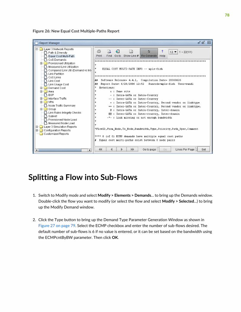
Figure 26: New Equal Cost Multiple-Paths Report
Splitting a Flow into Sub-Flows
1. Switch to Modify mode and selectModify > Elements > Demands... to bring up the Demands window.Double-click the flow you want to modify (or select the flow and selectModify > Selected...) to bringup the Modify Demand window.
2. Click the Type button to bring up the Demand Type Parameter Generation Window as shown inFigure 27 on page 79. Select the ECMP checkbox and enter the number of sub-flows desired. Thedefault number of sub-flows is 6 if no value is entered, or it can be set based on the bandwidth usingthe ECMPcntByBW parameter. Then click OK.
78

Figure 27: Demand Type Parameter Generation Window
3. Notice the new value in the Type field in Figure 28 on page 79.
Figure 28: Modify DemandWindow
4. Switch back to View mode and select Network > Elements > Demands to bring up the Demandswindow. Sub-flows are displayed differently in the Type column in View mode, as shown inFigure 29 on page 80. Rn means that n sub-flows share the same routing path. In this example, theoriginal flow called flow10was divided into 3 flows on the first ECMP and 2 flows on the second ECMP.The first entry for flow10 also says “ECMP=5”, to indicate that 5 subflows were created from theoriginal flow. The second entry for flow10 also contains a special keyword, “ECMPN” or “ECMP2”.“ECMPN” is simply a reserved keyword used by the program to identify subflows that are associatedwith another “original” flow but whose routing path is different. To elaborate, if there were threedifferent ECMP’s, then there would be three entries for flow10; the first would indicate “ECMP=n” andthe latter two would show special keyword “ECMPN”. This simply helps the program associate thesesubflows with one another.
79

Figure 29: DemandWindow in View mode
5. Open the ECMP Report again in the Report Manager. This time it will display the newly created ECMPdemands in the report.
NOTE: Although there are several discrete ECMP subflows (i.e. 5 in this example, 2 routingone way and 3 routing another), and technically the program could report an ECMPcomparing each of the 2with each of the 3, such information is not very useful. Therefore,the ECMP report only reports a single entry for flow10, comparing the two differentrouting paths.
Figure 30: Equal Cost Multiple-Paths Demand Report
80

Set ECMP Subflows Based on Bandwidth
• Users can manually define the number of subflows as defined above. Alternatively, they can use thedefault ECMPbehaviour, which is to create 6 flows for every ECMPdemandswithout count specification.
• The default number of ECMP flows to be created for an ECMP demand can also be configured basedon demand bandwidth via the ECMPcntByBW parameter in the project’s dparam file by adding in anentry with the format “ECMPcntByBW=[bandwidth:ECMPcount][|bandwidth:ECMPcount]*”
• For example, ECMPcntByBW=300M:72|100M:32|50K:6 would be interpreted as follows:
• An ECMP demand with bandwidth>=300M is split into 72 flows,
• An ECMP demand with bandwidth>=100M is split into 32 flows,
• An ECMP demand with bandwidth>=50K is split to 6 flows.
• An ECMP demand with bandwidth<50K is kept as one flow.
• This parameter can also be set in /u/wandl/db/misc/dparam.txt to change rtserver's default behaviourwhen ECMPcntByBW is not specified in the project’s dparam file.
• For the changes to the dparam file to have effect, close the network before changing the parameter,and reopen the network after changing this parameter.
81

5CHAPTER
Static Routes
NorthStar Planner Static Routes Overview | 85
View Static Routes | 85
Add/Modify/Delete Static Routes | 87
Static Routes Case Study | 88


NorthStar Planner Static Routes Overview
The Static Routes chapter describes how to view and modify static route tables. Static routes are used inIP networks and allow very precise control over traffic going through a router. By default, static routestake precedence over routing protocols such as RIP orOSPF to communicate routing information betweenrouters. Static routes are ideal for small networks with a limited number of paths and are particularly wellsuited for peripheral routers that are connected to one ormore networks via only one router. A disadvantageof static routes is its inability to adapt to router or link failures.
In Modify mode, the user may add, modify or delete any entry in any existing static route table. In all othermodes, the user is allowed to view the entries of any existing static route table. Whether or not to usestatic routes is dependent on the type of network involved and the specific situation. General guidelinesfor using static routes are described above, and more information can be found in online tutorials andnetwork design literature.
Prior to beginning this chapter, start up NorthStar Planner and open up a network (e.g., the spec.mpls-fishspecification file located in your $WANDL_HOME/sample/IP/fish directory, where $WANDL_HOME is/u/wandl by default). You should also have a general understanding of where andwhen to use static routes.
RELATED DOCUMENTATION
Add/Modify/Delete Static Routes | 87
View Static Routes
To view the static route table of a node, you must be in either View, Design, or Simulation mode.
From theMapwindow, right-click on the node of interest and selectView>Static Route Table. Alternatively,select Network > Protocols > Static Route Table.
Interpreting the Static Routing Table
A Static Routing Table window is displayed as shown here.
85

Figure 31: Viewing static routes
DescriptionField
The node from which the static route starts.Node
Virtual Routing Forwarding identification.VRF
The IP of the final destination.Dest. (IP/Mask)
The node name of the final destination.Dest. Node
The admin distance associated with the static route.Admin Distance
The next immediate link name or interface in the static route.Next Hop Link / Interface
The next node name or IP address in the static route. This may also be thefinal destination node in some cases.
Next Hop Node / IP
The next immediate tunnel in the static route.Next Hop Tunnel
Select a static route to view its details in the lower half of the window.
Click the Show Path button to highlight the static route path in the Map window.
86
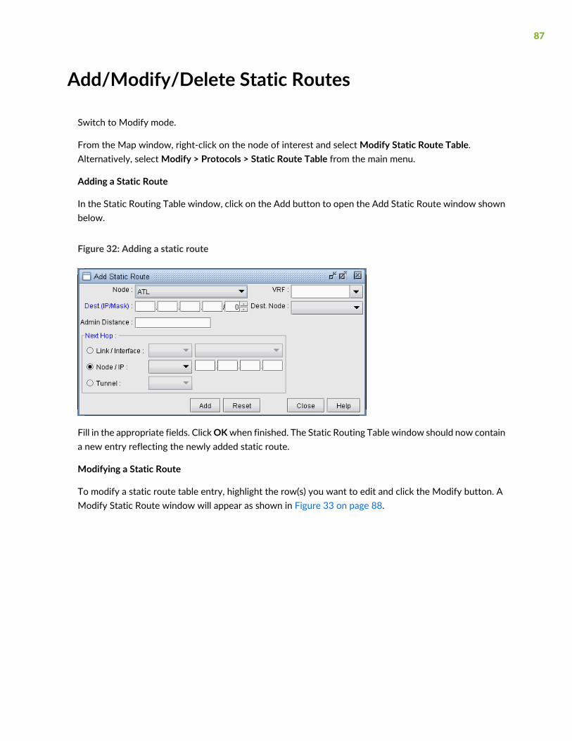
Add/Modify/Delete Static Routes
Switch to Modify mode.
From the Map window, right-click on the node of interest and selectModify Static Route Table.Alternatively, selectModify > Protocols > Static Route Table from the main menu.
Adding a Static Route
In the Static Routing Table window, click on the Add button to open the Add Static Route window shownbelow.
Figure 32: Adding a static route
Fill in the appropriate fields. ClickOKwhen finished. The Static Routing Table window should now containa new entry reflecting the newly added static route.
Modifying a Static Route
To modify a static route table entry, highlight the row(s) you want to edit and click the Modify button. AModify Static Route window will appear as shown in Figure 33 on page 88.
87

Figure 33: Modifying a static route
Edit the appropriate fields. Click OK when finished.
The modifications to the static route should be reflected in the Static Routing Table window.
Deleting a Static Route
To delete static route(s), select the desired entries from the Static Routing Table window and click theDelete button.
Static Routes Case Study
In this sectionwewill define a demandwith a destination IP and let the program route the demand accordingto the options and hardware settings present in the network. We will then define a new path for thedemand and enforce this path using a static route. After defining the static routes, the demand path willbe observed again to verify that it does indeed follow the defined static route. Note that for static routesto be successful in routing a demand, the demand must have an IP address associated with its destination,not simply a node name. This is due to the way static routes are defined in actual router configurationfiles.
Defining the Demand
1. Open the sample Fish network in /u/wandl/sample/IP/fish by double clicking the spec.mpls-fish filein the File Manager window.
2. Switch to Modify mode. In this case study we are interested in demands terminating at node NYC. Inorder for static routes to work, there must be an IP address associated with the destination node. Clickon the Modify menu and select Nodes. Scroll down until you see node NYC. Highlight it and click theModify button to bring up the Modify Node window. Type in 10.10.10.11 for the IP address as shownin Figure 34 on page 89. Click OK when finished.
88

Figure 34: Assign an IP address to node NYC
3. Go to Modify > Elements > Demands... and select the demand xflow79 between SFO and NYC.Double-click this entry or click the Modify > Selected... button to modify this demand.
4. Modify the demand by typing in the Location tab the corresponding IP address for its destination nodeas shown in Figure 35 on page 89. In this case, the IP address is 10.10.10.11 for NYC. Click “OK” tocontinue.
Figure 35: Fill in the IP address for the destination node
5. Update the network by clicking the Update button or by selecting Modify > Update Network State.Reopen the Demands window by selecting Network > Elements > Demands. Now you can display thepath of the demand xflow79 by selecting the demand and clicking the Show Path button. The currentpath will be displayed in the Map window as shown in Figure 36 on page 90 below.
89

Figure 36: Path of demand xflow79, from SFO to NYC
Creating the Static Route Table
Suppose it has been decided that the demand xflow79 and other such demands going to node NYC(10.10.10.11) are to be rerouted to go through node CHI instead of PHI. This could be due to the fact thatthe link between PHI and NYC is being heavily utilized, as indicated by the red/purple colored link. Thus,it is necessary to create a static route table at node WDC to enforce this route.
1. First, identify if there are any tunnels available starting from node WDC that go through CHI. To dothis, switch to View mode, right click on node WDC, and select View>Tunnels On/Thru Node.
2. In the new Tunnels at Node: WDC(WDC) window, notice that the tunnel RWDCBOS goes from nodeWDC to node BOS. Highlight this tunnel and click the Show Path button. The path of this tunnel willbe displayed in the Map window, as shown below in Figure 37 on page 90:
Figure 37: Path of tunnel RWDCBOS fromWDC to BOS
This is a good choice for the next hop of a static route at node WDC for the purpose of this example,since it will route all demands through nodes CHI, DET, and BOS rather than through node PHI.
3. In Modify mode, right click on the WDC node and selectModify Static Route Table.
90
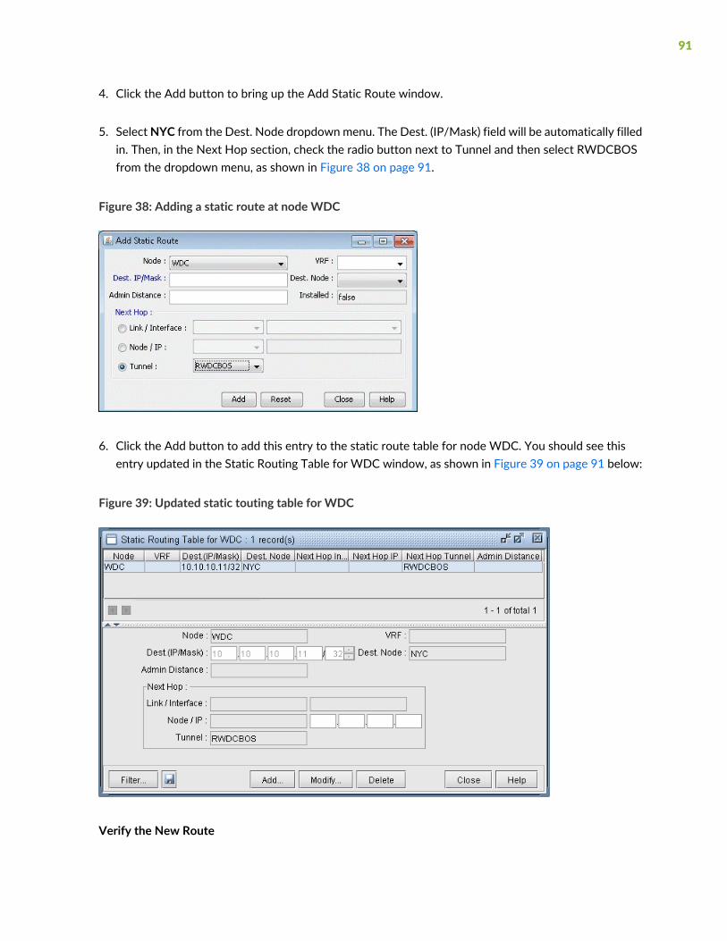
4. Click the Add button to bring up the Add Static Route window.
5. SelectNYC from the Dest. Node dropdown menu. The Dest. (IP/Mask) field will be automatically filledin. Then, in the Next Hop section, check the radio button next to Tunnel and then select RWDCBOSfrom the dropdown menu, as shown in Figure 38 on page 91.
Figure 38: Adding a static route at node WDC
6. Click the Add button to add this entry to the static route table for node WDC. You should see thisentry updated in the Static Routing Table for WDC window, as shown in Figure 39 on page 91 below:
Figure 39: Updated static touting table for WDC
Verify the New Route
91
Now that the static route has been defined, it is time to test whether or not the demands will route asplanned.
1. Switch to View mode. When it asks if you want to “Reroute demands from scratch,” click Yes.
2. Select the Network > Elements > Demands menu.
3. Locate the demand, xflow79, and highlight it. Click Show Path to display its new path in the Mapwindow. Below (Figure 40 on page 92) is a screenshot of what it should look like. Notice that the newpath takes the route specified by the static route table created at node WDC.
Figure 40: New route following static route specifications
4. Information on static routes is stored in a pathtable.runcode file. This can be verified by opening theFile Manager window, navigating to the directory where the network files are stored (i.e./u/wandl/sample/IP/fish) and opening the pathtable file (i.e. pathtable.mpls-fish). For this case study,the file will look as follows.
92

Figure 41: Static route information is stored in a pathtable file
93
6CHAPTER
Policy-Based Routes
NorthStar Planner Policy-Based Routes Overview | 97
Policy Based Routes Configuration Commands | 97
Viewing and Modifying Policy Based Routes | 98

NorthStar Planner Policy-Based Routes Overview
The Policy-Based Routes chapter explains how to view and modify policy based routes. Policy basedrouting provides additional control above that of routing protocols. A policy can be applied to an interfaceso that packets coming in through the interface meeting a given criteria will be forwarded out to a giveninterface, tunnel, or next hop. The criteria that must be met, if any, is specified in a route map statement.The information that must be matched can be specified in an access list, such as source IP address,destination IP address, port numbers, and protocol. The route map statement also sets the outgoinginterface, tunnel, or next hop.
Policy Based Routes can be used to implement QoS-specific routing, protocol-sensitive routing,source-sensitive routing, or routing based on dedicated links.
RELATED DOCUMENTATION
Policy Based Routes Configuration Commands | 97
Viewing and Modifying Policy Based Routes | 98
Policy Based Routes Configuration Commands
To use Policy Based Routes, you should have Cisco router configuration files with statements for policybased routing such as those given in the following table.
Example FormatsCommand
Sample standard access list:access-list <access-list-id> permit|deny <ip-address> <mask>
Extended access lists can be used as wellaccess-list <access-list-id> permit|deny<protocol><source-ip> <source-mask> <destination-ip><destionation-mask> [protocol parameters]
Configure for a router the access list(s)that will be referenced in the route-mapstatement(s)
ip policy route-map <route-map-name>Specify for an interface on the router, theroute-map to be applied
97

Example FormatsCommand
Specify route map name and number:
route-map <route-map-name> permit|deny <number to indicate relativeorder of application>
Specify an access list ID to match against if any:match ip address <access-list-id>
Specify the outgoing interface or else the next-hop:
set interface <interface_name>set ip next-hop <ip-address>
Define the route-map for the router
Viewing and Modifying Policy Based Routes
Following is a high-level, sequential outline of the following sections.
• Use the configuration files import to create your network.
• View policies from the link window.
• Check how the policies will affect routing by performing a path analysis.
• Modify the link PBR field to perform what-if studies.
Importing the Config Files
1. Import the config files as described in “NorthStar Planner Routing Protocols Overview” on page 63.Note that for a what-if study, you can also edit your config files to add, modify, or delete policies andthen re-import the config files.
2. Go to Tools > Options > Design. On the Path Placement option pane, set Force PBR Check (on thelower right corner of the window) to “True”.
3. Click “Yes” when asked to reroute from scratch.
Viewing PBR Details from the Link Window
1. Select the Network > Elements > Links menu. To display the PBR route map in the link table summarypane, right-click on a column header and select Table Options. Select PBR_A and PBR_Z from theAvailable items window and click “Add>” to move them to the Selected Item(s) window and then click“OK”.
98

PBR_A and PBR_Z refer to the route-map names in both directions on the link. PBR_A refers to thedirection from Node A to Node Z, while PBR_Z refers to the direction from Node Z to Node A.
2. Scroll so that you can see the PBR_A and PBR_Z headings. Click on the columns to sort the columnsand see which interfaces have policies on them.
3. Select a link row for a link that has an interface with a policy applied to it. Then click the PBR tab. Thetab is divided into a section for the interface on Node A and a section for the interface on Node Z. Eachsection contains the PBR information, including the route-map, sequence number, match criteria, andthe action to perform if there is a match.
Figure 42: PBR Tab
Path Placement
To perform a path placement, selectNetwork > Path&Capacity> Path. Optionally specify a source and/ordestination IP address (to match against the route map) that corresponds to a node’s loopback address orone of its interface addresses. Then click on the map the from-node followed by the to-node.
The Path window will be displayed. In addition, the Console window will display the relevant policy basedrouting information.
Modifying Link PBR Field
99
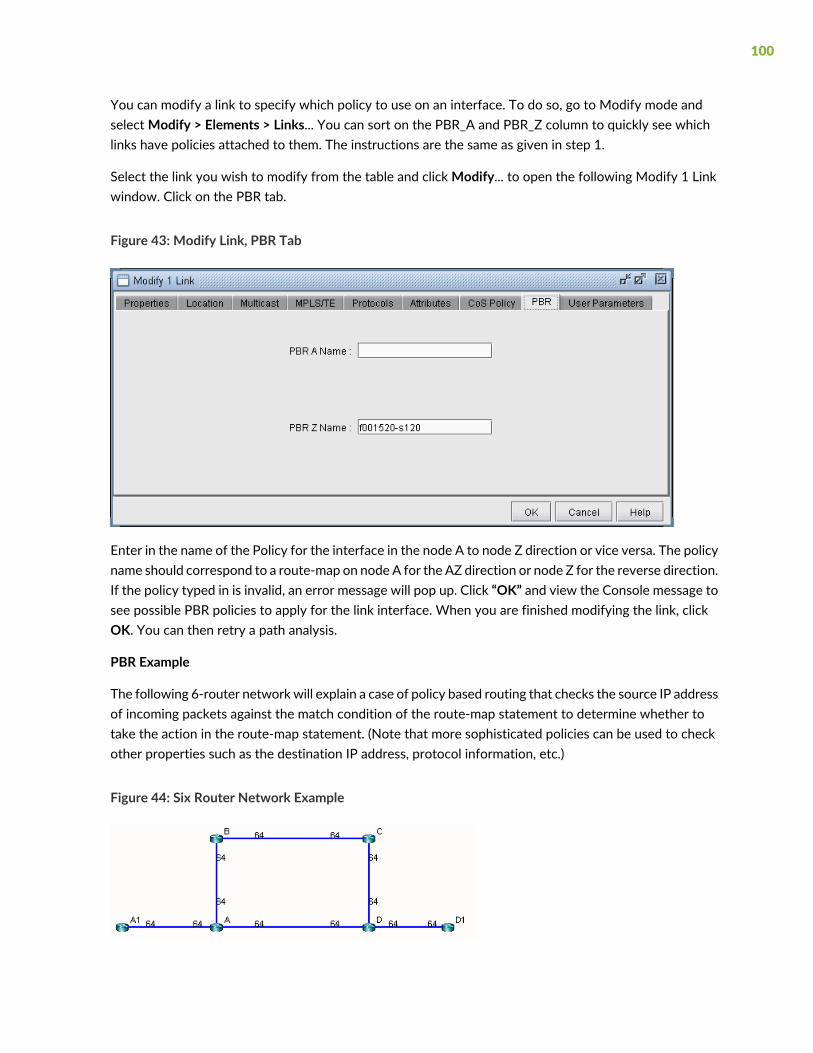
You can modify a link to specify which policy to use on an interface. To do so, go to Modify mode andselectModify > Elements > Links... You can sort on the PBR_A and PBR_Z column to quickly see whichlinks have policies attached to them. The instructions are the same as given in step 1.
Select the link you wish to modify from the table and clickModify... to open the following Modify 1 Linkwindow. Click on the PBR tab.
Figure 43: Modify Link, PBR Tab
Enter in the name of the Policy for the interface in the node A to node Z direction or vice versa. The policyname should correspond to a route-map on node A for the AZ direction or node Z for the reverse direction.If the policy typed in is invalid, an error message will pop up. Click “OK” and view the Console message tosee possible PBR policies to apply for the link interface. When you are finished modifying the link, clickOK. You can then retry a path analysis.
PBR Example
The following 6-router network will explain a case of policy based routing that checks the source IP addressof incoming packets against the match condition of the route-map statement to determine whether totake the action in the route-map statement. (Note that more sophisticated policies can be used to checkother properties such as the destination IP address, protocol information, etc.)
Figure 44: Six Router Network Example
100

In this example, router A has applied the following route-map on its interface to A1:
route-map my_route_map permit 20
match ip address 111
set interface Serial1/0/1
!
The corresponding match condition is specified in the access list (111) as follows: “access-list 111 permit11.5.5.5 0.0.0.0.” The corresponding interface to forward to in case the match condition is satisfied isSerial1/0/1, which connects A to B. As a result of the policy, router A will forward any packet coming fromA1 with a source IP address of 11.5.5.5 out the interface Serial1/0/1 toward B. A Path analysis is used toverify the routing behavior.
Suppose a path analysis is performed from A1 to D1 by selecting Network > Path & Capacity > Paths. Thesource and destination IP addresses must be entered in to simulate Policy Based Routing. In this case, weuse 11.5.5.5 as the source IP address (router A1’s IP address). The packet is then forwarded to router B.This example uses OSPF and the links have equal OSPF metric, so after the packet is forwarded to B, itmay equally well go from B to C to D to D1 as back to A and then to D to D1.
Figure 45: Results of Using an IP Address Matching the Route Map Criteria
The results are also displayed in the Console. The Console messages for the left figure above are as follows:
* * * A1(A1) - D1(D1): bw= 0 * * *
- - Find path from A1 to D1 (0.0.0.0)
- - Apply PBR my_route_map at A:
Set interface to Serial1/0/1
PBR route from A to B
101

new 11.5.5.5 D1 0 R,A2Z 02,02 A1--A--B--C--D--D1
(OSPF) Route-cost=325. Max_Path_Bw= 1.536M
Tunnels matching search criteria: 0
On the other hand, suppose a path analysis is performed from A1 to D1 using another interface IP addressat A1 such as 10.10.10.17. In this case, the source IP address no longer matches the route-map conditionand hence the routing table (OSPF in this case) is used instead:
Figure 46: Results of Using an IP Address Not Matching the Route Map Criteria
The corresponding Console message appears as follows:
* * * A1(A1) - D1(D1): bw= 0 * * *
-- Find path from A1 to D1 (0.0.0.0)
-- Apply PBR my_route_map at A:
new 10.10.10.17 D1 0 R,A2Z 02,02 A1--A--D--D1
(OSPF) Route-cost=195. Max_Path_Bw= 1.536M
102
7CHAPTER
Border Gateway Protocol
NorthStar Planner Border Gateway Protocol Overview | 105
Border Gateway Protocol Recommended Instructions | 105
BGP Data Extraction | 107
BGP Reports | 107
BGP Options | 108
BGP Map | 108
BGP Live Status Check | 114
BGP Routing Table | 115
BGP Routes Analysis | 117
BGP Information at a Node | 119
BGP Neighbor | 120
Apply, Modify, or Add BGP Polices | 125
BGP Subnets | 130
Getipconf Usage Notes | 135
BGP Report | 140

NorthStarPlannerBorderGatewayProtocolOverview
The de facto routing protocol currently used to maintain connectivity between autonomous systems (ASs) is Border Gateway Protocol (BGP) version 4 (based on RFC 1771). When BGP is used between ASs, it isrefered to as EBGP (External BGP). BGP can also be used within an AS -- known as IBGP (Internal BGP) --to primarily propagate BGP information learned from other ASs. NorthStar Planner’s Border GatewayProtocol (BGP) module allows network planners to quickly investigate various BGP routing and peeringscenarios via BGP policy and attribute modifications. After running configuration import to extract BGPinformation, the impact of changing BGP routing policies and attributes on inter-Autonomous System(inter-AS) traffic can be assessed.
RELATED DOCUMENTATION
NorthStar Planner Routing Protocols Overview | 63
BGP Data Extraction | 107
BorderGatewayProtocol Recommended Instructions
• Import your network’s configuration files as described in “BGP Data Extraction” on page 107.
• Analyse the BGP reports for integrity checks errors as described in BGP Reports.
• View BGP options as described in “BGP Options” on page 108.
• Open the BGPMap to view EBGP and IBGP peering relationships as described in “BGPMap” on page 108.
• View routing table information and perform path analyses as described in “BGP Routing Table” onpage 115 and “BGP Routes Analysis” on page 117.
• View BGP information associated with a node from the “BGP Routes Analysis” on page 117.
• View, add, or modify BGP neighbor information as described in “BGP Routing Table” on page 115.
• Apply, modify or add BGP policies as described in “Apply, Modify, or Add BGP Polices” on page 125.
• Learn how the subnet fileworks as described in “BGPSubnets” on page 130 , andwork through an examplewhere the AS_PATH attribute is used to influence routing.
• Learn about getipconf’s bgp-related usage notes and bgp-related files as described “Getipconf UsageNotes” on page 135.
105
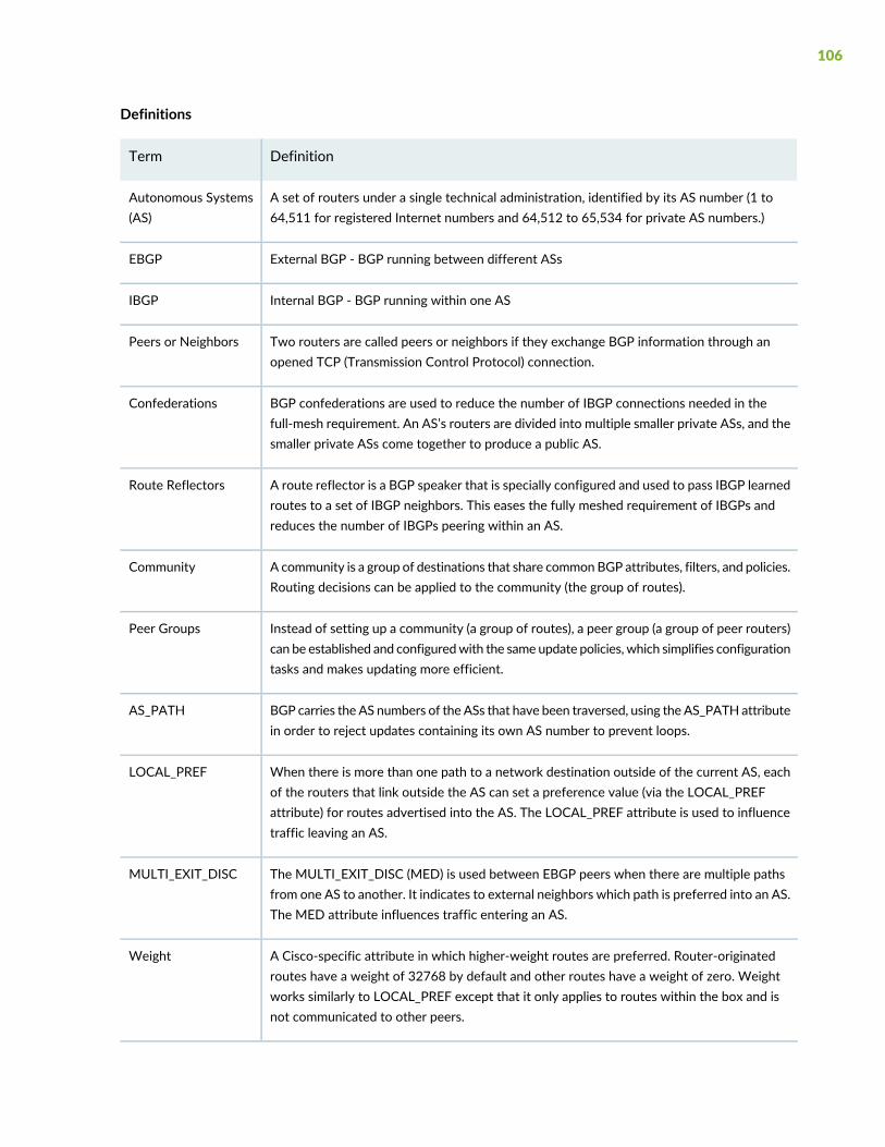
Definitions
DefinitionTerm
A set of routers under a single technical administration, identified by its AS number (1 to64,511 for registered Internet numbers and 64,512 to 65,534 for private AS numbers.)
Autonomous Systems(AS)
External BGP - BGP running between different ASsEBGP
Internal BGP - BGP running within one ASIBGP
Two routers are called peers or neighbors if they exchange BGP information through anopened TCP (Transmission Control Protocol) connection.
Peers or Neighbors
BGP confederations are used to reduce the number of IBGP connections needed in thefull-mesh requirement. An AS’s routers are divided into multiple smaller private ASs, and thesmaller private ASs come together to produce a public AS.
Confederations
A route reflector is a BGP speaker that is specially configured and used to pass IBGP learnedroutes to a set of IBGP neighbors. This eases the fully meshed requirement of IBGPs andreduces the number of IBGPs peering within an AS.
Route Reflectors
A community is a group of destinations that share commonBGP attributes, filters, and policies.Routing decisions can be applied to the community (the group of routes).
Community
Instead of setting up a community (a group of routes), a peer group (a group of peer routers)can be established and configuredwith the same update policies, which simplifies configurationtasks and makes updating more efficient.
Peer Groups
BGP carries the AS numbers of the ASs that have been traversed, using the AS_PATH attributein order to reject updates containing its own AS number to prevent loops.
AS_PATH
When there is more than one path to a network destination outside of the current AS, eachof the routers that link outside the AS can set a preference value (via the LOCAL_PREFattribute) for routes advertised into the AS. The LOCAL_PREF attribute is used to influencetraffic leaving an AS.
LOCAL_PREF
The MULTI_EXIT_DISC (MED) is used between EBGP peers when there are multiple pathsfrom one AS to another. It indicates to external neighbors which path is preferred into an AS.The MED attribute influences traffic entering an AS.
MULTI_EXIT_DISC
A Cisco-specific attribute in which higher-weight routes are preferred. Router-originatedroutes have a weight of 32768 by default and other routes have a weight of zero. Weightworks similarly to LOCAL_PREF except that it only applies to routes within the box and isnot communicated to other peers.
Weight
106

DefinitionTerm
A route reflector and its clients form a cluster. Usually a cluster has a single route reflector.For redundancy, a cluster may have more than one route reflector. When a cluster has morethan one route reflector, all of the route reflectors in the cluster need to be configured withthe same cluster ID.
Cluster ID
BGP Data Extraction
1. Select File>Import Data to import a set of configuration files. Alternatively, you may run the getipconfprogram in text mode.
2. In the Default tab, under Config Directory, click “Browse” to select a directory containing the configfiles. Notice that the Include BGP box under the Specify BGP Options section of the Network Optionstab is checked by default.
3. To ignore IP addresses with particular prefixes, such as 192.168., type in the IP addresses (partial stringallowed) under the Misc Options tab. Click “OK” to begin the extraction.
4. You can optionally modify the /u/wandl/db/misc/ASnames file used to derive the AS name labelsshown on the network map.
5. For more information about data extraction, see “Getipconf Usage Notes” on page 135 and “RouterData Extraction Overview” on page 33.
BGP Reports
After the configuration files are imported, selectReport > ReportManager and select the Network Reports> Protocols > BGP>BGPReport to check andmake sure that the network has no obvious BGP configurationerrors. The BGP report includes the following sections:
• BGP Integrity Check Report—Includes various BGP statistics, including BGP speakers, neighbors, andpolicies.
• Neighbor AS Specification Error Check Report—Shows errors related to incorrectly-specified ASs.
• Unbalanced BGP Neighbor Check Report—Reports any unbalanced neighbor relationships betweenBGP speakers.
107

• IBGPMeshConnectivity CheckReport—Reports if any AS is not fullymeshed for IPV4 or VPNV4 addressfamilies.
• Route Reflector Statistics Report—Includes route reflector related information such as hierarchy leveland redundancy for IPV4, VPNV4, and L2VPN address families.
BGP Options
Select the Tools >Options >Design, Path Placement > BGP options pane to view the BGP-related networkparameter defaults.
• The Check IBGP Policy option is also set to false by default. Setting this to true turns on hop by hopIBGP policy checking for the special case where the BGP next hop is modified as a result of IBGP policies.Because this option is a special case and involves a lot of extra processing, it is not turned on by default.However, if it is being used in your network, this option needs to be turned on.
• The IGP override option is set to false by default. This means that for external paths, BGPwill be treatedas having a higher administrative distance/preference than the IGP such as OSPF. If this is not the case,this parameter can be set to true.
• The Use Live BGP Table if Available option can be used to take advantage of routing table informationextracted from collected BGP routing tables for traffic routing.
• The Peering AS Number(s) field will be filled in when running the BGP peering analysis. It is used tospecify the AS that the network will be newly peering with. Hence, for that AS, information from thesubnet file is needed to derive the BGP routing table. For more information on the subnet file, refer to“BGP Subnets” on page 130.
BGP Map
To open the BGP map (as opposed to the standard map), select Network > Protocols > BGP > BGP Mapor Network > Maps > Map (BGP View). In the Include Which AS Values? window select which ASs youwant to view in your map. The ASs are listed in order, with the number of nodes and number of neighborsshown in parentheses. This window indicates the number of nodes, neighbors, or ASnodes for each AS.Use <Ctrl>-click and/or <Shift>-click to select multiple AS values.
The BGP map displays the network in terms of BGP speakers (routers that are running BGP) and theirpeering relationships (shown via a connection with an arrow in the middle and pointed away from thespeaker). TwoBGP routers become peers (neighbors) once they have both established a peering relationship
108

with each other (shown via two directed arrows or via a connection with a diamond in the middle if theDraw Mult. Links as Curves box is unchecked in the Tools > Options > Map Preferences window).
When the BGP map is first brought up, all routers (including BGP speakers and non-BGP speakers) areshown on the BGP map. You may wish to filter the BGP map by selecting the Filters > Advanced menu.Select Hide Isolated Points, or to look only at the BGP speakers, open up the Advanced Filter > Nodesection. Click the Set link to set BGP_Speaker = true. Then select the corresponding checkbox to turn onthe filter. The following figures show a BGP map filtered to show the BGP speakers.
Figure 47: BGP Map filtered for BGP Speakers
Logical Layout
To view the logical relationships amongst BGP neighbors more clearly, including route-reflector hierarchicalrelationships, right-click on the map and select Layout>Logical Layout.
For example, in the figure below, the network on the left shows two ASs, each with fully meshed IBGPrelationships. These ASs are connected to each other using EBGP. Meanwhile the network on the rightshows one AS with hierarchical route-reflectors. The innermost arc of routers are route reflectors for themiddle ring of routers, and some of the routers in the middle ring are route reflectors for the outermostarc of routers.
109

Figure 48: BGP Logical Views
To return back to the current view, right-click on the map and select Layout>Back to Original.(Note thatyou can use the Network > Maps > Copy Map Layout option to transfer the graphical coordinates fromthe BGP Map to the Standard Map or vice versa.)
Grouping
In the BGP map, each AS of the network is represented by a grouping disc (from the right-click menu,select Grouping > Collapse All or Grouping > Expand All to collapse or expand the disc). Each AS whichis outside of the network and has an EBGP peering relationship with BGP speakers of the network is calledan ASnode and is represented by a little square.
Note that you can change the grouping arrangement in either BGP Map or Standard Map using the mapright-clickwindow’s Grouping>Autogroup option. Here you can group byConfedAS first and then subgroupby AS.
To turn on AS group labels, choose Group Labels... from the right-click menu and select Name as shownin the following figure.
110
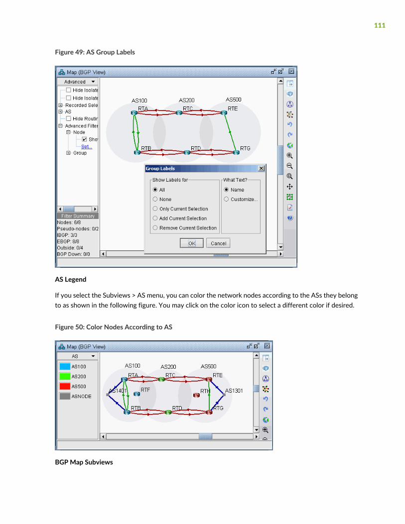
Figure 49: AS Group Labels
AS Legend
If you select the Subviews > AS menu, you can color the network nodes according to the ASs they belongto as shown in the following figure. You may click on the color icon to select a different color if desired.
Figure 50: Color Nodes According to AS
BGP Map Subviews
111

Select the Subviews > Typemenu of the BGPmap. Note the coloring of the different peering relationships:
• Gray lines denote IBGP peering relationships within the same AS hat are down
• Maroon lines denote EBGP peering relationships from one AS to another
• Green lines denote IBGP peering relationships within the same AS
• Blue lines denote EBGP peering relationships that go to ASs outside of the network, represented byASNODES because of limited information.
Figure 51: Types Subview
Select the Subviews > Protocols menu of the BGP map. The choices are as follows:
• All—This is the default subview, which shows both EBGP and IBGP types of relations.
• EBGP/Outside—This shows only EBGP relations.
• IBGP (RR client)—This shows IBGP relations that are route reflections from Route Reflectors to theirclients. Usually there is an arrow for the IBGP neighbor relations in each direction, but for this particularsubview, only one direction is shown from the route reflector to the route reflector client to make itclear which devices are the route reflectors and which devices are the route reflector clients. To see aneven clearer view of the route reflector relationships, use the Logical Layout view as described in LogicalLayout.
• IBGP (no RR)—This shows IBGP without route reflections.
• L2VPN—This shows IBGP relations related to the l2vpn address family.
• VPNv4/Inet-VPN—This shows IBGP relations related to VPNv4 or Inet-VPN address family.
• IPv4—This shows IBGP relations related to IPv4 address family.
• Symmetric Peering—This shows balanced BGP neighbor relationships
• Asymmetric Peering—This shows unbalanced BGP neighbor relationships, i.e., the neighbor relationshipis only defined on one of the two routers. For a full report of unbalanced BGP neighbor relationships,refer to the Report Manager, BGP report.
112

Figure 52: Protocols Subview
Figure 53: Different BGP Subviews (the Juniper routers are route reflectors in this example)
113
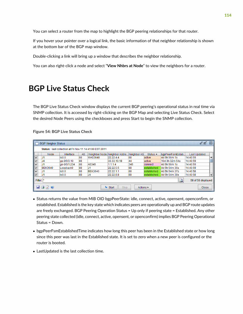
You can select a router from the map to highlight the BGP peering relationships for that router.
If you hover your pointer over a logical link, the basic information of that neighbor relationship is shownat the bottom bar of the BGP map window.
Double-clicking a link will bring up a window that describes the neighbor relationship.
You can also right-click a node and select “View Nhbrs at Node” to view the neighbors for a router.
BGP Live Status Check
The BGP Live Status Check window displays the current BGP peering’s operational status in real time viaSNMP collection. It is accessed by right-clicking on the BGP Map and selecting Live Status Check. Selectthe desired Node Peers using the checkboxes and press Start to begin the SNMP collection.
Figure 54: BGP Live Status Check
• Status returns the value from MIB OID bgpPeerState: idle, connect, active, opensent, openconfirm, orestablished. Established is the key statewhich indicates peers are operationally up and BGP route updatesare freely exchanged. BGP Peering Operation Status = Up only if peering state = Established. Any otherpeering state collected (idle, connect, active, opensent, or openconfirm) implies BGP Peering OperationalStatus = Down.
• bgpPeerFsmEstablishedTime indicates how long this peer has been in the Established state or how longsince this peer was last in the Established state. It is set to zero when a new peer is configured or therouter is booted.
• LastUpdated is the last collection time.
114

BGP Routing Table
The Find BGP Routing Table window, as shown in the following figure, will appear when the Network >Protocols > BGP > BGP Routing Table function is selected. The BGP Routing Table window is used todisplay all BGP routing from the specified source node to the specified destination node/IP address.
Figure 55: Find BGP Routing Table
Choose a source node and a destination node (and/or destination IP address) from two different autonomoussystems from the drop down lists and then click on the Show Routing Table button. Selecting the SrcASand DestAS is not required but is only used to filter the Src Node and Dest Node lists. (The Dest AS willbe ignored if it is in a different AS than the Destination IP Address entered.) Selecting a blank SrcAS andDestAS field can be done to retrieve back all source and destination nodes from the node drop down lists.
Note that different destination IP addresses may have different attributes and associated routing policies.The destination IP address can be directly entered or populated by first selecting the Dest Node. To loadadditional IP addresses at that node found in the BGP Subnet window into the drop down list (Network> Protocols > BGP > BGP Subnets...), check “List BGP Subnets.”
If you already know the IP address, you can skip selecting the matching Dest Node or Dest AS, which canbe derived from the IP address. Note also that this destination IP address should either be included in oneof the BGP subnets (see “BGP Subnets” on page 130 for more information), or defined on the destinationnode.
Another method of choosing the source and destination nodes is to use the mouse and the Standard (notBGP) map. After selecting the Network > Protocols > BGP > BGP Routing Table function, move the mouseover the map. Notice that the arrow of the mouse turns into a cross hair. Click on the first node, whichwill be the source node. Move the cross hair to another node and click on it to specify the destinationnode. Then move to the Find BGP Routing Table window and click on the OK button.
Tip: To clearly see which nodes belong to which ASs from the map, go to the Standard map’s Filter menuandmake sure that the box for Hide ASNodes/Links is unchecked. Youmight also use themap’s right-clickmenu’s Grouping>AutoGroup option and group your nodes by AS and go to the Subviews > AS menu tocolor the nodes by AS.
115
Troubleshooting: In some cases the BGP routing table search does not return any results. Make sure thatthe SrcAS and Dest AS are different. Additionally, check the EBGP neighbor relationships from the BGPmap in Network > Maps > Maps (BGP View) to verify whether two routers can communicate using EBGP.Finally, check that the destination IP address is either assigned to the destination node, or a BGP subnetoriginated from that node.
The BGP Routing Table window shows all possible routes from the specified source node to the specifieddestination node/IP address. The fields shown on the window are:
DescriptionField
The IP address of the source node.Src IP Address
The name of the source node.Src Node
The IP address of the destination node.Dest IP Address
The name of the destination node.Dest Node
This shows the router name and IP address for the last BGP speaker on the pathbefore it exits the AS of the source node.
Exit Src AS
The router name and IP address of the BGP next hop.BGP Next Hop
The corresponding mask of the destination IP address.Mask
This is not a BGP property, but is used to indicate the preferred BGP next hopchosen by the BGP route selection process when there is more than one possiblepath. Possible values are “Preferred”, “Blocked”, or blank.
Preference
The weight attributeWeight
The local preference number.Local Preference
The Multi-Exit Discriminator attributeMed
The AS path attribute, which consists of AS numbers of all ASs that the routetraverses, the most recently traversed one displayed first.
AS Path
The Community AttributeCommunity String
The origin attribute indicates how a routewas learned (e.g., IGP, EGP, or Incomplete)Origin
Total metric of the IGP route from the router to the Exit Src AS routerDistance
116
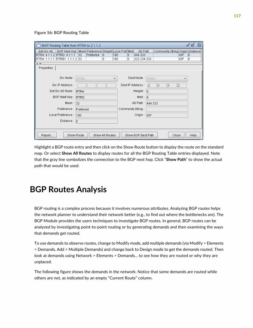
Figure 56: BGP Routing Table
Highlight a BGP route entry and then click on the Show Route button to display the route on the standardmap. Or select Show All Routes to display routes for all the BGP Routing Table entries displayed. Notethat the gray line symbolizes the connection to the BGP next hop. Click “Show Path” to show the actualpath that would be used.
BGP Routes Analysis
BGP routing is a complex process because it involves numerous attributes. Analyzing BGP routes helpsthe network planner to understand their network better (e.g., to find out where the bottlenecks are). TheBGP Module provides the users techniques to investigate BGP routes. In general, BGP routes can beanalyzed by investigating point-to-point routing or by generating demands and then examining the waysthat demands get routed.
To use demands to observe routes, change toModify mode, add multiple demands (via Modify > Elements> Demands, Add > Multiple Demands) and change back to Design mode to get the demands routed. Thenlook at demands using Network > Elements > Demands... to see how they are routed or why they areunplaced.
The following figure shows the demands in the network. Notice that some demands are routed whileothers are not, as indicated by an empty “Current Route” column.
117

Figure 57: Demands Added
Highlight a demand and click on the Show Path button in the Demands window. The routing of thehighlighted demand would be shown on the map.
Check the Consolewindow for details regarding the BGP next hops chosen along the path that are indicatedafter the arrow “->”. The sample console output below of a path analysis from RTRA to 2.1.1.2 (RTRC)indicates that RTRA chooses BGP next hop 1.1.1.2 on RTRB1 which is directly connected. RTRB1subsequently chooses BGP next hop 2.1.1.2(RTRC)which is reached via the IGP next hop of 2.1.1.1 (RTRB2)found by recursive lookup.
RTRA->1.1.1.2(RTRB1)
RTRB1->2.1.1.2(RTRC) via 2.1.1.1(RTRB2)
Looking at unplaced demands will help you to determine where the bottlenecks are and why. From theDemands window, find an unplaced demand and then click on the Bottlenecks button. Examine the maintopology map as well as the console to help you to determine the reason for the unplaced demand, e.g. amissing BGP routing table entry or being blocked by a policy.
You can investigate the originating nodes of unplaced demands to determine the reasons for the bottlenecks.For example, it may be because the status of a peering relationship is down or because a community listis denied. The console window can provide details about why a demand failed. For example, it can indicate
118

at which step the route was blocked due to out policies or in policies when troubleshooting why a BGPnext hop was not found.
BGP Information at a Node
From the nodewindow’s Protocols tab, a variety of information related to BGP is available in a table format.For instance, the following figure shows a particular node’s BGP-related properties, including AS number,BGP Speaker, Route Reflector, Confederation ID, etc.
Figure 58: BGP Information at a node
The Advanced Filter from this window contains the following keys that can be used to filter for nodes withparticular BGP properties: AS, BGP_Speaker, Cluster_ID, Confederation_ID, and Route_Reflector.
These keys can also be used to label the Standard map using Labels>Node Labels, Customize... from theStandard map’s right-click menu.
119
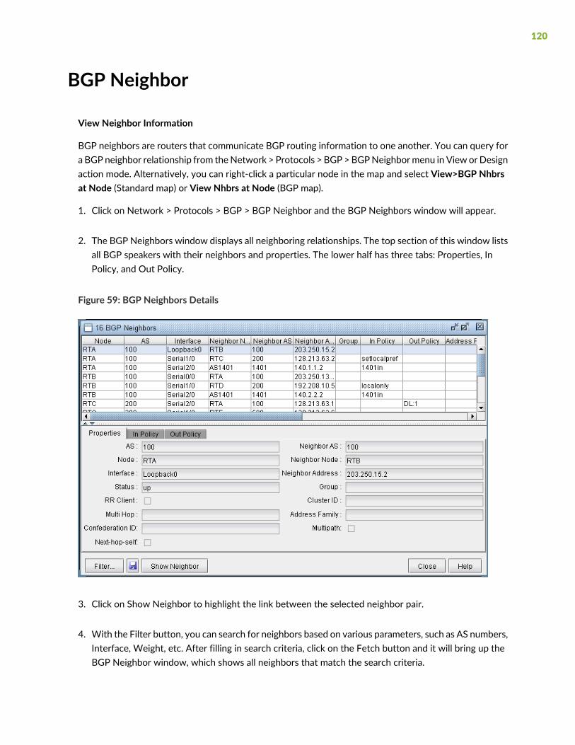
BGP Neighbor
View Neighbor Information
BGP neighbors are routers that communicate BGP routing information to one another. You can query fora BGP neighbor relationship from theNetwork > Protocols > BGP >BGPNeighbormenu in View orDesignaction mode. Alternatively, you can right-click a particular node in the map and select View>BGP Nhbrsat Node (Standard map) or View Nhbrs at Node (BGP map).
1. Click on Network > Protocols > BGP > BGP Neighbor and the BGP Neighbors window will appear.
2. The BGP Neighbors window displays all neighboring relationships. The top section of this window listsall BGP speakers with their neighbors and properties. The lower half has three tabs: Properties, InPolicy, and Out Policy.
Figure 59: BGP Neighbors Details
3. Click on Show Neighbor to highlight the link between the selected neighbor pair.
4. With the Filter button, you can search for neighbors based on various parameters, such as AS numbers,Interface, Weight, etc. After filling in search criteria, click on the Fetch button and it will bring up theBGP Neighbor window, which shows all neighbors that match the search criteria.
120

NOTE: For the Node field, you must choose a real node and not an AS (pseudo-node).To search on an AS, you can use the AS, Neighbor AS, and Neighbor Node fields. Notethat the search for AS uses exact match on the AS number. For example, you must typein 111 rather than AS111 or 1 or 1*. Wildcards are not supported in this field.
5. Right-click on an entry to see the options Show “Neighbor Address = Group” and “Show peergroupswith no members”.
• Show “Neighbor Address = Group”: These entries list the group underneath the neighbor addresscolumn. They are intended to provide information regarding the default settings of a BGP group, e.g.,configured under [edit protocols bgp group ibgp_peers] for Juniper. These default settings may beoverridden for a particular neighbor within the group.
• “Showpeergroupswith nomembers”: This optionwill display any BGP groupswhich have no neighborslisted in them.
Properties Tab
The Properties tab has the following fields:
DescriptionField
The node AS.AS
The neighbor node AS.Neighbor AS
The interface that is used to connect to the neighbor.Interface
The name of the node (BGP speaker).Node
Status of the neighbor. It is either up or down.Status
The name of the peer group if it is applicable.Group
The optional TTL (Time to Live) number from the IOS command: neighbor{ip-address | peer-group-name} ebgp-multihop [ttl]
Multihop
The virtual routing and forwarding instance name.VRF
The IP address of the neighbor.Neighbor Address
The name of the neighbor.Neighbor Node
121

DescriptionField
Indicates whether the neighbor is a route reflector client or not.RR Client
The cluster ID if it is applicable.Cluster ID
Indicates if an address family such as VPNv4 or Inet-VPN is used.Address Family
Indicates the BGP Confederation ID that the AS belongs to, if any.Confederation ID
Indicates if BGP multipath has been configured for load balancing purposes.Multipath
Indicates if the router is configured as the next hop for the BGP neighbor. “Next-hop self
In and Out Policies Tabs
The In Policy tab shows all policies that are applied to incoming routes to the node from the highlightedneighbor. The Out Policy tab shows all policies that are applied to outgoing routes from the node. (Notethat different literature may refer to in/out policy as import/export policy; they are equivalent.)
NOTE: You should have more than one AS in your network in order to see policies.
For Cisco routers, the routing policies may specify route filtering and attribute manipulation, which useroute maps, access lists, AS_path access lists, community lists, distribute lists, and filter lists.
For Juniper routers, policy statements and community lists are used. When either the In Policy tab or theOut Policy tab is selected, the policy window has the following fields:
DescriptionField
Name of the policyPolicy
The term number is used in the policy statement for Juniper. The sequencenumber is applicable to the route map for Cisco.
Term/Sequence
Permit or denyAction
122
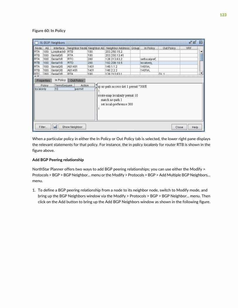
Figure 60: In Policy
When a particular policy in either the In Policy or Out Policy tab is selected, the lower right pane displaysthe relevant statements for that policy. For instance, the in policy localonly for router RTB is shown in thefigure above.
Add BGP Peering relationship
NorthStar Planner offers two ways to add BGP peering relationships; you can use either the Modify >Protocols > BGP > BGPNeighbor... menu or theModify > Protocols > BGP >AddMultiple BGPNeighbors...menu.
1. To define a BGP peering relationship from a node to its neighbor node, switch to Modify mode, andbring up the BGP Neighbors window via the Modify > Protocols > BGP > BGP Neighbor... menu. Thenclick on the Add button to bring up the Add BGP Neighbors window as shown in the following figure.
123

Figure 61: Add BGP Neighbor Window
2. Choose the AS number and Node from the AS and Node dropdown menus. Similarly, choose theNeighbor AS number and the Neighbor Node from the Neighbor AS and Neighbor Node dropdownmenus. Clicking OK results in a BGP peer being established from the Node to the Neighbor Node. Toestablish a BGP peering relationship in the opposite direction, simply perform the same steps but swapthe AS and Node selections with the Neighbor AS and the Neighbor Node selections. Note that if youare adding a bgp neighboring relationship from a route reflector to its client, be sure to check the RRClient box and specify the Cluster ID.
3. To add multiple BGP peering relationships between a node and it neighbor, use theModify > Protocols> BGP > Add Multiple BGP Neighbors... menu to bring up the Add Multiple BGP Neighbors window.The Type dropdown menu includes Intra AS and Inter AS options. The following figure shows how theAdd Multiple BGP Neighbors window with Type selected as Intra AS is used to create a full mesh ofIBGP neighboring relationships within the AS. Note that balanced neighbors (neighboring relationshipsestablished in both directions) are created.
124

Figure 62: Add Multiple BGP neighbors window
Apply, Modify, or Add BGP Polices
Applying Policies
1. BGP policies that have already been defined at a router can be applied as an in policy or as an outpolicy. To bring up the Modify BGP Neighbors window, first switch to the Modify action mode. Thenselect the Modify > Protocols > BGP > BGP Neighbors ... function to bring up the BGP Neighborswindow, from which a row can be selected. Double-click on a selected row or click on the Modifybutton to bring up the Modify BGP Neighbors window as shown in the following figure.
125

Figure 63: Modify BGP Neighbors
2. Select either the In Policy tab or the Out Policy tab to see the Available Policies at that node and theApplied Policies lists. Selected policies in the Available Policies list can bemoved to the Applied Policieslist by clicking on the Add-> button and, vice versa, selected policies in the Applied Policies list can bemoved to the Available Policies list by clicking on the <-Remove button. The following figure showsan example of a BGP policy (setlocalpref) that has been moved to the router’s Applied Policies list.
Figure 64: Applying an In Policy
In some cases, abbreviations are used to describe the policies, in the format Match Type: Match Name,where the Match types are interpreted as follows:
• AC–Access List
• AL–AS-path access list
• CL–Community List
126

• CL–Community List
• PL–Prefix List
Modify BGP Policy
1. To modify a BGP policy at the router, click on the Policy Editor... button to bring up the Routing PolicyEditor window as shown in the following figure. Then select a particular policy from the left pane todisplay corresponding policy commands in the right pane.
2. The + button expands a selection, while the - button collapses it. Dropdownmenus and text fields allowyou to modify the policy. The following figure shows an example of a BGP policy that is used to setthe local-preference to a value of 80.
Figure 65: Modifying a BGP Policy
3. To see the generated configlet for the BGP policy, click on the Configlet tab. The following figure showsthe generated configlet corresponding to a BGP policy (setlocalpref).
127

Figure 66: The Generated Configlet for a BGP Policy
4. The right-click menu or the Actions menu offers further options for modifying the routing policy. Toadd a new term to a policy, first select the policy. Then from the right pane, select New from either theAction menu or the right-click menu. Note in the following figure that after selecting New, a new itemwas added to the policy.
128
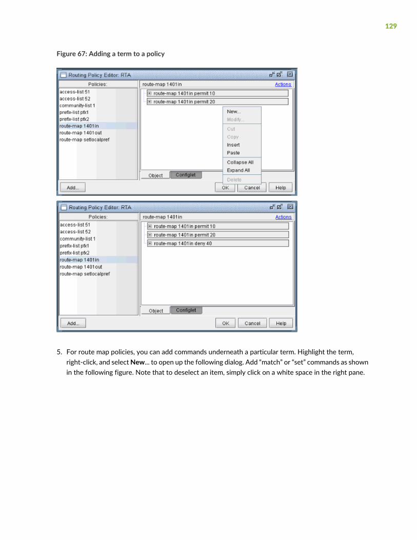
Figure 67: Adding a term to a policy
5. For route map policies, you can add commands underneath a particular term. Highlight the term,right-click, and selectNew... to open up the following dialog. Add “match” or “set” commands as shownin the following figure. Note that to deselect an item, simply click on a white space in the right pane.
129

Figure 68: Adding a match command to a term of a route-map
Adding a BGP Policy
To add a new BGP policy, click on the Add... button in the lower left hand corner of the window to bringup theNewPolicywindow (shown in the following figure), and proceed the sameway as is done inmodifyinga BGP policy. Here you have a choice of five different types of policies: route-map, access-list, as-pathaccess-list, community-list, and prefix-list. Note that the options may vary depending on the policy type.
Figure 69: New Policy Window
BGP Subnets
The BGP subnets list can be used to list prefixes, or subnetworks (whose router configuration files areunavailable) originated from a particular router or AS node. Various BGP attributes associated with thesubnetwork can be defined in the subnet file.
130
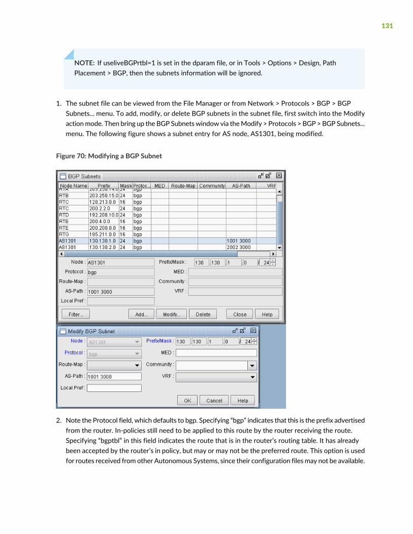
NOTE: If useliveBGPrtbl=1 is set in the dparam file, or in Tools > Options > Design, PathPlacement > BGP, then the subnets information will be ignored.
1. The subnet file can be viewed from the File Manager or from Network > Protocols > BGP > BGPSubnets... menu. To add, modify, or delete BGP subnets in the subnet file, first switch into the Modifyactionmode. Then bring up the BGP Subnetswindow via theModify > Protocols > BGP >BGP Subnets...menu. The following figure shows a subnet entry for AS node, AS1301, being modified.
Figure 70: Modifying a BGP Subnet
2. Note the Protocol field, which defaults to bgp. Specifying “bgp” indicates that this is the prefix advertisedfrom the router. In-policies still need to be applied to this route by the router receiving the route.Specifying “bgptbl” in this field indicates the route that is in the router’s routing table. It has alreadybeen accepted by the router’s in policy, but may or may not be the preferred route. This option is usedfor routes received from other Autonomous Systems, since their configuration files may not be available.
131

To illustrate how to use the BGP subnet list (accessed via Network > Protocols > BGP >BGP Subnets...),a sample network and the corresponding BGP subnet list are shown in the following two figures. Notethat within the BGP subnet list, ASnode AS1301 is declaring that it can reach subnet 130.130.1.0/24,which has an AS_PATH attribute that includes 1001. ASnode AS1301 is also declaring that it can reachsubnet 130.130.2.0/24, which has an AS_PATH attribute that includes 2002.
Figure 71: View BGP Subnets Window
Figure 72: Main View and BGP View of the network
3. To see the BGP InPolicy defined at a router RTE, bring up the BGP Neighbors table and switch to theIn Policy tab, as shown in the following figure. In this particular example, the InPolicy at router RTE is
132

defined by a Cisco route-map and says that if an incoming route has 1001 included in its AS_PATHattribute, then set the LOCAL_PREF attribute to 123; otherwise, set the LOCAL_PREF attribute to 89.The InPolicy at router RTG is the same except that 2002 is matched for instead of 1001.
Figure 73: BGP In Policy for RTE
4. Continuing with our example, we bring up our BGP routing table to verify that the LOCAL_PREFattribute got set correctly to 123 for AS1301’s subnetwork 130.130.2.0/24, which has 2002 includedin its AS_PATH attribute.
133
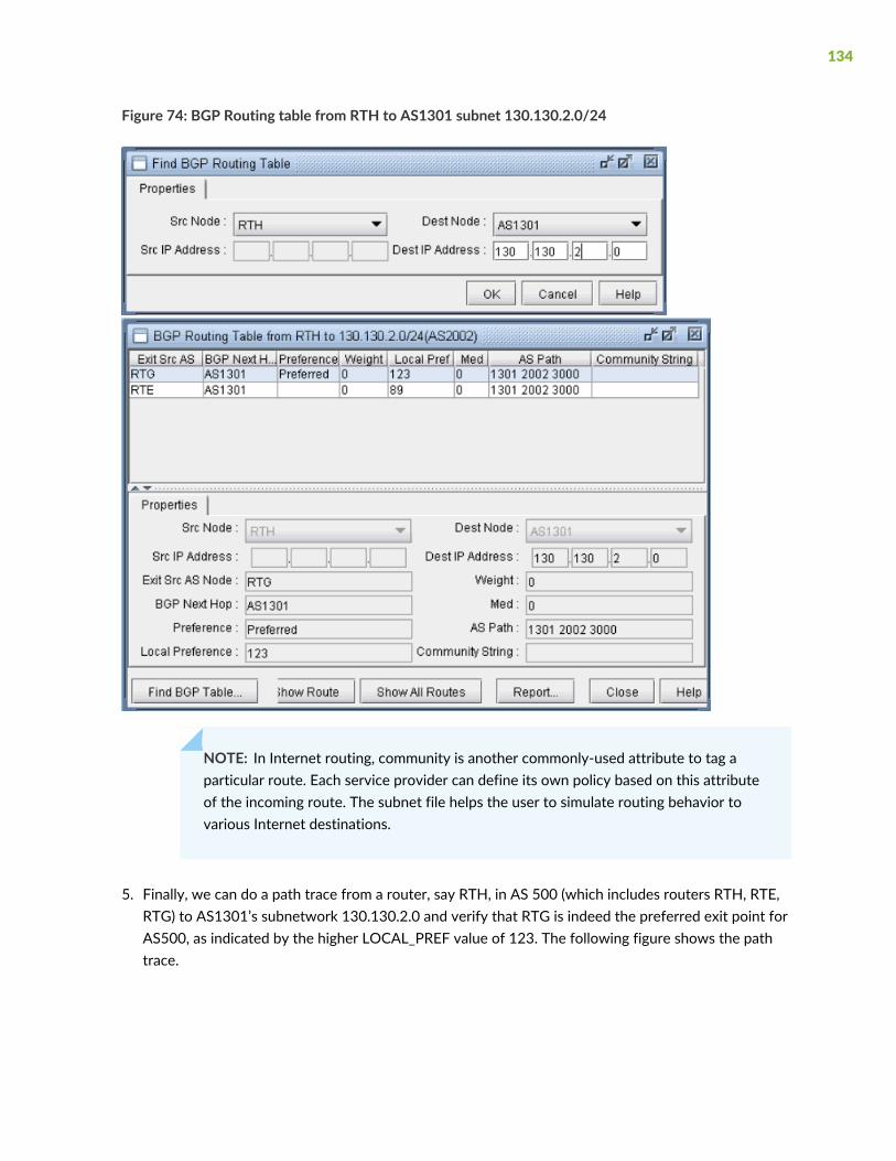
Figure 74: BGP Routing table from RTH to AS1301 subnet 130.130.2.0/24
NOTE: In Internet routing, community is another commonly-used attribute to tag aparticular route. Each service provider can define its own policy based on this attributeof the incoming route. The subnet file helps the user to simulate routing behavior tovarious Internet destinations.
5. Finally, we can do a path trace from a router, say RTH, in AS 500 (which includes routers RTH, RTE,RTG) to AS1301’s subnetwork 130.130.2.0 and verify that RTG is indeed the preferred exit point forAS500, as indicated by the higher LOCAL_PREF value of 123. The following figure shows the pathtrace.
134

Figure 75: Path trace illustrating the RTG being the preferred exit point
Getipconf Usage Notes
Syntax
getipconf [-r runcode] [-t topfile] [-b bwconvfile] [-n muxloc] [-p nodeparam]
[-noBGP] [-i interfaceDir] [-snmp SNMPDir] [-commentBW] [-ignore ipaddr] [-ospf
ospfdatabase] [-atmbw] [-cdp cdpfile1 cdpfile2 ... -conf] config1 config2 ...
BGP-related flags
DescriptionBGP-Related Flags
If this optional flag is specified, BGP information will not be generated.-noBGP
135

DescriptionBGP-Related Flags
All IP addresses of the type 10.x.x.x, 127.x.x.x, and 192.168.x.x are local addresses. Toprevent matching interfaces in one network with interfaces in another network, thisoptional ignore flag is provided. For example, if the user specifies the following:getipconf -ignore 192.168 -ignore 10. -ignore 127. *
Then all the links with addresses matching these patterns are commented out. However,if the addresses are all from the same network, this flag should not be included.
-ignore <ipaddress>
BGP Files Generated
In addition to the standard files like the spec, muxloc, and bblink files, the following are five output filesrelated to BGP that are generated by getipconf: aclist.x, controllist.x, bgpobj.x, bgpnode.x, bgplink.x,bgpnbr.x, and subnet.x (assuming the runcode is x). Below is a brief explanation of the contents of thesefiles:
• aclist.x contains information about as-path, access-list, and community-list
• controllist.x contains information about access-lists and prefix-list. The controllistobj.x file is a binaryfile.
• bgpnode.x contains information for BGP speakers
• bgplink.x contains information for BGP neighbors
• bgpnbr.x is a text file that contains all information about neighbors.
• bgpobj.x contains information about BGP neighbors shown in bgpnbr.x and route map structure. Thebgpobj file is a binary file designed to save space and to speed up performance of the software. It ispartially replaced by bgplink.x and bgpnode.x. How the program decides whether to read the bgpobj fileor the bgplink and bgpnode file is explained below.
• subnet.x is used to list those subnetworks originated by a particular router or AS node.
Corresponding Spec File Keywords
In the specification file, the keywords for the first four of these files will be listed as aclist, bgpobj, bgpnode,and bgplink. The bgpnbr file is for informational purposes only and is not included in the specification file.
For an example of the specification file entries related to BGP, see the following example:
# Files used by IP network
bgpobj= bgpobj.x
bgpnode= bgpnode.x
bgplink= bgplink.x
136

dparam= dparam.x
aclist= aclist.x
jpoBGP=jpoBGP.x
subnet= subnet.x
livebgprtblobj=livebgp.obj
controllistobj=controllistobj.x
Usage Note
Users need to comment out the specification of the bgpobj file in the specification file if they plan to editBGP attributes manually. When loading the network, the rtserver (or bbdsgn) program reads the bgpobjfile, if it is specified, ignoring the bgpnode and bgplink files. However, if the bgpobj file is not specified orit is commented out, rtserver will read the bgpnode and bgplink files instead. When saving the network,all three files: bgpobj, bgpnode and bgplink will be saved.
dparam File
The following are some of the BGP-related parameters in the dparam file that you may want to change.They can also be changed through the Tools > Options menu as described in “BGP Options” on page 108.
chkIBGPflag = 1 # 0: skip IBGP policy checking
IGPoverride= 0 # IGP over ride BGP
useliveBGPrtbl = 1
simskipAS= 1 # 1: skip AS nodes and link down simulation
• If IBGP policies are used in the network to influence routing, set the chkIBGPflag parameter to 1. Bydefault, it is set to 0 to speed up routing.
• The simskipAS parameter is set to 1 by default, meaning that AS nodes and links will not be broughtdown in an exhaustive failure simulation performed from Simulation > Predefined Scenarios. If you wishto check the impact of an AS node or AS link failure on traffic routing, change the value to 0. Note,however, that if there are a lot of AS nodes, this may greatly increase the time it takes to perform thesimulation. To indicate that only a subset of the AS nodes should be failed and the rest of the AS nodesshould be ignored, mark the AS nodes or AS links to ignore with the FAIL=0 flag. This parameter can beset in the Modify > Elements > Nodes, Design properties tab (or add it to the end of the muxloc fileentry) or Modify > Elements > Links, Properties tab (or add it to the miscellaneous field of the bblink fileentry).
137

muxloc entry: SDG SANDIEGO 760 277 US 32.883434 -117.167480 FAIL=0
bblink entry: LINK7 CHI DET DEF 1 OC3
MPLSTE,OSPF=477,FAIL=0 AREA=AREA0
• The IGPoverride option is false (0) by default, meaning that for external paths, BGP will be treated ashaving a higher administrative distance/preference than the IGP such as OSPF. If this is not the case,this parameter can be set to true (1).
bgpnode format
#Node ASno ConfedID clusterID misc
N3 222 0 0 RR
bgplink format
#lineID nodeA nodeZ Z_AS MED weight local_pref multi_hop RRclient
NBR1 N1 N2 111 0 0 0 -1 0
NOTE: Due to the complexity, peer group and policy are not defined in these two files now.
aclist format
# AS path and community lists
# column 1 - router_name separated by comma
# column 2 - AS number
# column 3 - access modifier 1-permit, 0-deny
# column 4 - type a-AS path, c-Community list
# column 5 - regular expression
router1, 9999 0 a ".*"
bgpnbr file
138

The bgpnbr file is for information purposes and is not read into the specification file. See the followingtable for a description of the fields in the bgpnbr file.
#Status,AS,Intf,Node,Z_AS,Z_intf,Z_Node,PeerGroup,RRclient,Cluster,Multihop,Loca
l Pref,Weight,Med, InPolicy,OutPolicy,VRF,Confederation_ID,MultiPath
up,111,Loopback1,S36,111,"allow_ixp",,"allow_ixp",0, ,-1,0,0,0," "," ",
DescriptionField
Status of the neighbor, either up or downStatus
The AS number of the BGP speakerAS
The IP address of the interface used to connect to the neighborIntf
The name of the BGP speakerNode
The AS number of the neighborZ_AS
The IP address of the interface on the neighbor routerZ_intf
The name of the neighborZ_Node
The peer group name if it is applicablePeerGroup
The indicator to indicate whether the neighbor is a route reflector client or notRRclient
The cluster ID if it is applicableCluster
The optional TTL (Time to Live) number from the IOS command: neighbor {ip-address| peer-group-name} ebgp-multihop [ttl]
Multihop
The Local Preference attributeLocalPref
The weight attributeWeight
The Multi-Exit Discriminator attributeMed
The names of policies for incoming routesInPolicy
The names of policies for outgoing routesOutPolicy
ASs that are outside of the network and have EBGP peering relationshipwith BGP speakers of the networkare represented by ASnodes in the muxloc file (the node file of NorthStar Planner).
139

Subnet File
A snippet of a sample subnet file is shown here. The address/mask field denotes the subnetwork originatedby the node. The misc field is used to specify any BGP attributes associated with the subnetwork.
#Node address/mask protocol misc
RTA 200.200.1.0/24 bgp
AS111 130.130.1.0/24 bgp as-path=1111 3000
AS111 130.130.2.0/24 bgp as-path=2002 3000
AS222 140.140.10.0/24 bgp community=1401:10
AS222 140.140.20.0/24 bgp community=1401:20
BGP Report
When the client session is opened for the first time, the BGP Report should be checked to make sure thatthe network has no obvious BGP configuration errors.
The output file that is written to the output directory is called “BGPRPT.runcode”.
BGP Integrity Check Report:
BGP statistics – This section shows:
• The total number of BGP speakers in the network
• The total number of neighbors
• The total number of policies
• The list of all ASs and the number of their BGP speakers
******************************************************
* BGP Integrity Check Report
******************************************************
-- 17 BGP speakers,89 neighbors,283 members,183 policies
-- 3 local AS:
ASno 222: 9 routers
ASno 111: 7 routers
ASno 555: 1 routers
Neighbor AS Specification Error Check Report
140
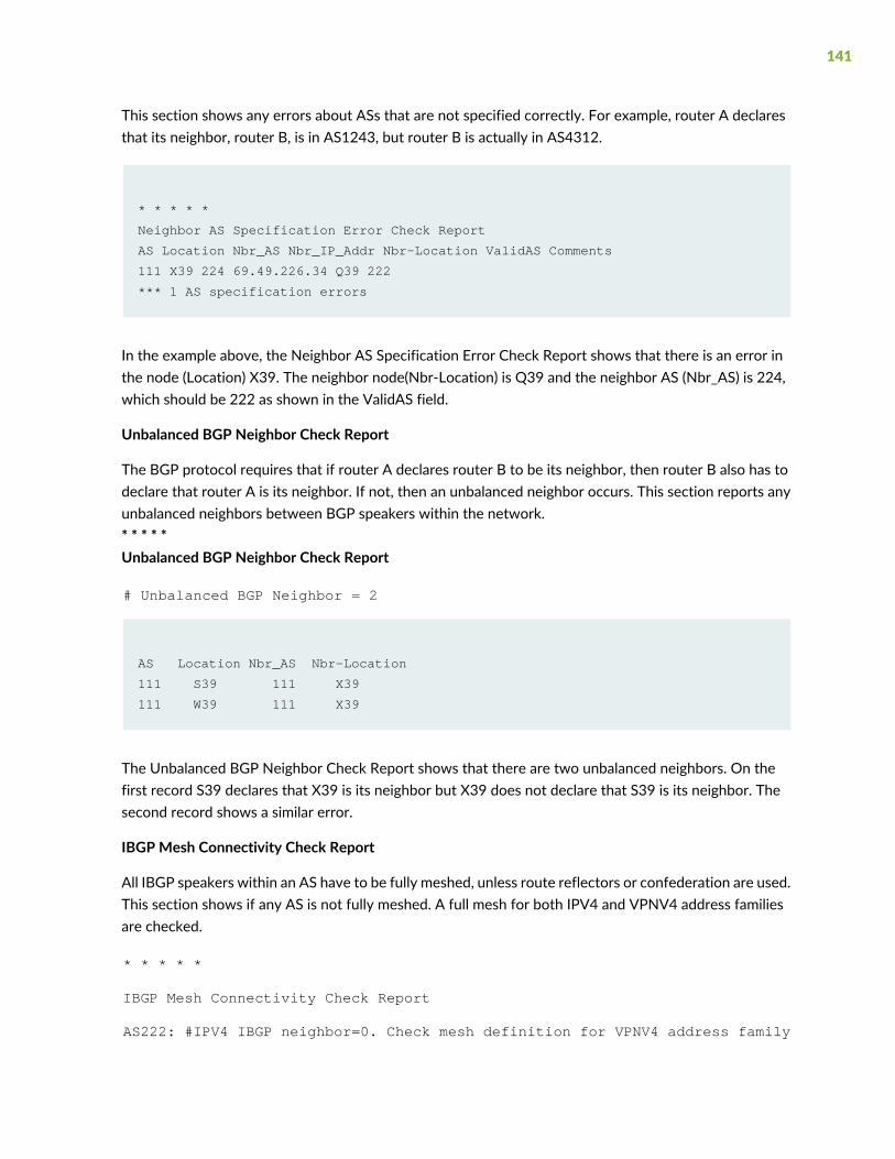
This section shows any errors about ASs that are not specified correctly. For example, router A declaresthat its neighbor, router B, is in AS1243, but router B is actually in AS4312.
* * * * *
Neighbor AS Specification Error Check Report
AS Location Nbr_AS Nbr_IP_Addr Nbr-Location ValidAS Comments
111 X39 224 69.49.226.34 Q39 222
*** 1 AS specification errors
In the example above, the Neighbor AS Specification Error Check Report shows that there is an error inthe node (Location) X39. The neighbor node(Nbr-Location) is Q39 and the neighbor AS (Nbr_AS) is 224,which should be 222 as shown in the ValidAS field.
Unbalanced BGP Neighbor Check Report
The BGP protocol requires that if router A declares router B to be its neighbor, then router B also has todeclare that router A is its neighbor. If not, then an unbalanced neighbor occurs. This section reports anyunbalanced neighbors between BGP speakers within the network.* * * * *Unbalanced BGP Neighbor Check Report
# Unbalanced BGP Neighbor = 2
AS Location Nbr_AS Nbr-Location
111 S39 111 X39
111 W39 111 X39
The Unbalanced BGP Neighbor Check Report shows that there are two unbalanced neighbors. On thefirst record S39 declares that X39 is its neighbor but X39 does not declare that S39 is its neighbor. Thesecond record shows a similar error.
IBGP Mesh Connectivity Check Report
All IBGP speakers within an AS have to be fully meshed, unless route reflectors or confederation are used.This section shows if any AS is not fully meshed. A full mesh for both IPV4 and VPNV4 address familiesare checked.
* * * * *
IBGP Mesh Connectivity Check Report
AS222: #IPV4 IBGP neighbor=0. Check mesh definition for VPNV4 address family
141

AS 222: passed mesh connectivity checking
---- VPNV4 AS111: S39 is not defined as X39's neighbor
IPV4 VPNV4 AS111: W39 is not defined as X39's neighbor
AS111: 2 neighbor definition missing
AS333: IPV4, VPNV4, L2VPN IBGP neighbors are not defined
AS 555: passed mesh connectivity checking
The IBGP Mesh Connectivity Check Report above shows the following
• AS222 is fully meshed for the VPNV4 address family but no IBGP neighbors exist for IPV4 addressfamily.
• AS111 is not fully meshed for IPV4 and VPNV4. For the VPNV4 address family, S39 and W39 are notdefined as X39’s neighbors. For the IPV4 address family, W39 is not defined as X39’s neighbor.
• AS555 passes the mesh connectivity check for both IPV4 and VPNV4.
• AS333 is missing IBGP neighbors for the IPV4, VPNV4, and L2VPN address families.
IPV4/VPNV4/L2VPN Route Reflector Statistics
These three sections indicate the route reflector statistics, including number of route reflectors, numberof route reflector clients, and hierarchical route reflector information. Route reflector clients with onlyone route reflector are listed as a warning that they do not have redundant route reflectors defined. Thefollowing is an example of the IPV4 route reflector statistics:IPV4 Route Reflector Statistics: 200 BGP Speakers, 8 Route Reflectors, 100 RouteReflector ClientsRedundant Route Reflectors are not defined at 2 RR Clients1. WDC1, RR= PHI12. WDC2, RR= PHI1
#Route Reflector Hierarchy Level= 3
Top Level: 4RR(s)
1. NYC1,
2. NYC2,
3. BOS1,
4. BOS2,
Level 2: 3RR(s)
1. PHI1, RR= NYC1 NYC2
1. PHI2, RR= NYC1 NYC2
2. BOS3, RR= BOS1 BOS2
142

Level 3: 1RR(s)
1. TRE1, RR= PHI1 PHI2
VPNV4 and L2VPN route reflector statistics are similarly provided.
It is recommended that all errors reported in the BGP Report file get fixed before carrying on furtheranalysis. One way to do it is to correct the errors on the configuration files and then run through getipconfagain.
143

8CHAPTER
Virtual Private Networks
NorthStar Planner Virtual Private Networks Overview | 147
Importing VPN Information from Router Configuration Files | 147
Viewing the Integrity Checks Reports | 149
Accessing VPN Summary Information | 149
Accessing Detailed Information for a Particular VPN | 150
VPN Topology View | 152
Route-Target Export/Import Relationships | 155
Additional Methods to Access VPN Information | 160
VPN Path Tracing | 162
VPN Design and Modeling Using the VPNWizard | 164
L3 (Layer 3) VPN | 165
L3 Hub-and-Spoke VPN | 174
L2M (Layer2-Martini) VPN | 180
L2K (Layer2-Kompella) VPN | 186
VPLS-BGP VPN (for Juniper) | 190

VPLS-LDP VPN | 193
L2CCC (Circuit Cross-Connect) VPN | 199
Inter-AS VPN | 203
Forming VPN Customer Groups | 205
Deleting or Renaming VPNs | 207
VPN Configlet Generation | 208
Adding Traffic Demands in a VPN | 211
VPN Traffic Generation | 213
VPN-Related Reports | 216
VPN Monitoring and Diagnostics | 218

NorthStar PlannerVirtual PrivateNetworksOverview
The Virtual Private Networks chapter describes NorthStar Planner’s VPNmodule (also known as VPNView)capabilities, which include VPN construction via router configuration extraction, VPN topology displayand reporting, VPN-related integrity checking, and VPN design and modeling. When used in conjunctionwith the Online module, the VPNmodule also allows the user to perform VPNmonitoring and diagnostics.
The types of VPNs supported include Layer3 (L3), Layer2 Kompella (L2K), Layer2 Martini (L2M), Layer2Circuit Cross-Connect (L2CCC), and VPLS (both LDP-based and BGP-based VPLS). VPNView supportshub-and-spoke and other complex VPNs. Depending on the type of VPN, different information is extractedfrom the router configuration files to construct the different type of VPN. For instance, the extractedinformation for L3 VPNs based on RFC 2547bis would include PE routers and CE devices (if managed),export/import route targets, route distinguisher, interfaces, protocols, etc.
Besides VPN construction via configuration import, the VPN module also offers the network planner theability to construct VPNs from scratch via a VPNWizard. Once VPNs have been constructed in the network,VPN traffic can be added (by adding traffic demands or via a gravitymodel using the VPNTraffic Generationfeature), and its effect on the network can be studied. The VPNmodule’s VPN configlet generation featurecan be used to create configuration statements that can pushed onto the router by the network engineer.
Depending on the type of VPN (e.g. for L3 VPNs, L2K VPNs, and VPLS-BGP VPNs), various rules (e.g.based on export/import route-targets) are used to determine when two routers can talk with each other;the VPN path tracing feature can be used to study the routing between two routers. NorthStar Planner’sVPNmodule features help the network engineer to understand, design, and analyze various types of VPNs.
RELATED DOCUMENTATION
Importing VPN Information from Router Configuration Files | 147
ImportingVPN Information fromRouterConfigurationFiles
To import the router configuration files, select File>Import Data and follow the Import Network Wizard.Alternatively, you may run the getipconf program in text mode. For more information, see “Router DataExtraction Overview” on page 33.
The Network tab contains the Specify VPN Options section shown in the following figure.
147

Figure 76: Configuration Import and VPN Options
• To extract VPN information from the config files, the user should leave the Ignore VPN checkboxunchecked.
• Typically, VPNs are constructed by matching import/export route targets; if the ID VPN elements byVRF checkbox is checked, then VRF names will be used for the matching instead.
• If the Omit PE-CE links checkbox is checked, then links between PE routers and CE routers will beomitted.
• The user can also specify a PE-CE Connection file that contains information used to stitch up PE-CElinks. This is useful when the network re-uses private IP subnets for PE-CE links. The format of the PE-CEConnection file is:PE_name PE_VRF_intf IP_addr_of_PE_VRF_intf VRF CE_name IP_addr_of_CE_intfpe0 serial2/1 203.55.1.65/30 vrf-a ce0 203.55.1.66/30
Once all of the options in the different tabs have been selected, click Next> to begin importing the routerconfig files. The generated network model will then be loaded into NorthStar Planner.
148

Viewing the Integrity Checks Reports
Once the network model has been loaded, the user may wish to examine the Configuration Reports(accessible via the Report > Report Manager menu) to check for any potential VPN configuration issues.The following figure shows an example of a Summary of Integrity Checks report, where certain VPNintegrity checks are reported.
Figure 77: View the Integrity Checks Reports to Check for Potential VPN Configuration Issues
Accessing VPN Summary Information
To see a summary view of all of the VPNs that are present in the current network, bring up the IP VPNSummary window (via the Network > Services > VPN menu) as shown in the following figure.
The window will provide a list of all the different types of VPNs in the network and a list of all the PErouters that make up the VPNs. The number in the parentheses following each VPN type in the tree viewon the left pane of the window describes the number of VPNs in that category. For instance, Layer2Kompella VPN (2) means that there are two L2K VPNs configured in the model. The + box can be used to
149

expand a VPN type in order to see the list of VPNs for each type. Similarly, the number in the parenthesesfollowing each PE router indicates the number of VPNs that the PE router is a part of.
You may click on a particular VPN of interest, and then more summary information for that VPN will bepresented in the Properties box of the window. For instance, the figure shows a L3VPNwith its list of fourPEs and four CEs.
Figure 78: IP VPNWindow’s Properties Box for a selected VPN
With a particular VPN selected, youmay also click on theHighlight button to see all of the routers associatedwith the VPN highlighted on the main topology map.
Accessing Detailed Information for a Particular VPN
Accessing Detailed Information for a Particular VPNTo show the detailed information for a VPN, you mayeither double-click on a particular VPN in the IP VPN Summary window, or you may navigate through theVPN tree list on the left part of the window until the particular VPN is found. The following figure showsthe detailed information for a VPN called SOMERSET. To see information for a particular node in the VPN,simply select the node from the table, and the Properties boxwill display the information. The figure shows
150
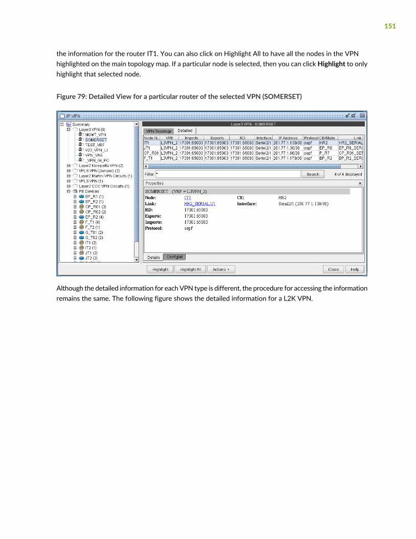
the information for the router IT1. You can also click on Highlight All to have all the nodes in the VPNhighlighted on the main topology map. If a particular node is selected, then you can clickHighlight to onlyhighlight that selected node.
Figure 79: Detailed View for a particular router of the selected VPN (SOMERSET)
Although the detailed information for eachVPN type is different, the procedure for accessing the informationremains the same. The following figure shows the detailed information for a L2K VPN.
151
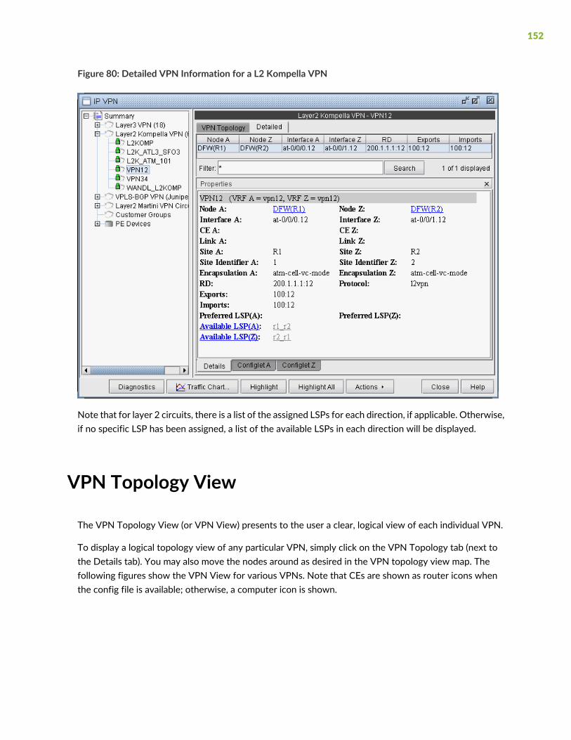
Figure 80: Detailed VPN Information for a L2 Kompella VPN
Note that for layer 2 circuits, there is a list of the assigned LSPs for each direction, if applicable. Otherwise,if no specific LSP has been assigned, a list of the available LSPs in each direction will be displayed.
VPN Topology View
The VPN Topology View (or VPN View) presents to the user a clear, logical view of each individual VPN.
To display a logical topology view of any particular VPN, simply click on the VPN Topology tab (next tothe Details tab). You may also move the nodes around as desired in the VPN topology view map. Thefollowing figures show the VPN View for various VPNs. Note that CEs are shown as router icons whenthe config file is available; otherwise, a computer icon is shown.
152

Figure 81: VPN View for a L2CCC VPN (with the selected circuit highlighted in pink)
Figure 82: VPN View for an Inter-AS VPN (called INTER-AS)
153

You may also display additional information (i.e., RD, Route Targets, interface) for a node by clicking on itfor a pop-up window to appear, as shown in the following figure.
Figure 83: Green pop-up information window for a node
There is also a right-click menu that you can use to perform basic functions to manipulate the topologyand the labels.
Figure 84: Right-click menu showing topology and label functions
154

Route-Target Export/Import Relationships
The VPN View also shows route target export/import relationships that exist between VPNs. A visualpicture helps the network planner or engineer to clearly and quickly identify relationships between VPNs(e.g. hub-and-spoke or extranet VPN relationships).When there are export/import relationships with otherVPNs, then the To Import/Export Relation View selection in the upper right-hand corner of the VPN Viewbecomes visible. The following figure shows that VPNHUB_AOhas export/import relationships with otherVPNs, since the To Import/Export Relation View selection is visible.
Figure 85: Click on To Import/Export Relation View to see import/export relationships with other VPNs
Click on To Import/Export Relation View to get to the Import/Export Relation View. The blue circle iconwith a triangle inside is a grouping icon represents the current VPN (HUB_A0), while the yellow dot iconsrepresent other VPNs (in this example, the SPOKEPPL_* VPNs) that have export/import relationships withthe current VPN.
To see how other VPNs (the yellow dots) are related to the current VPN, you can click on a yellow dot tosee the route targets that are being exported and imported. For instance the following figure shows thatVPN SPOKEPPL_7 is exporting 101:8 and importing 101:9, while HUB_A0 is exporting 101:9 and importing
155
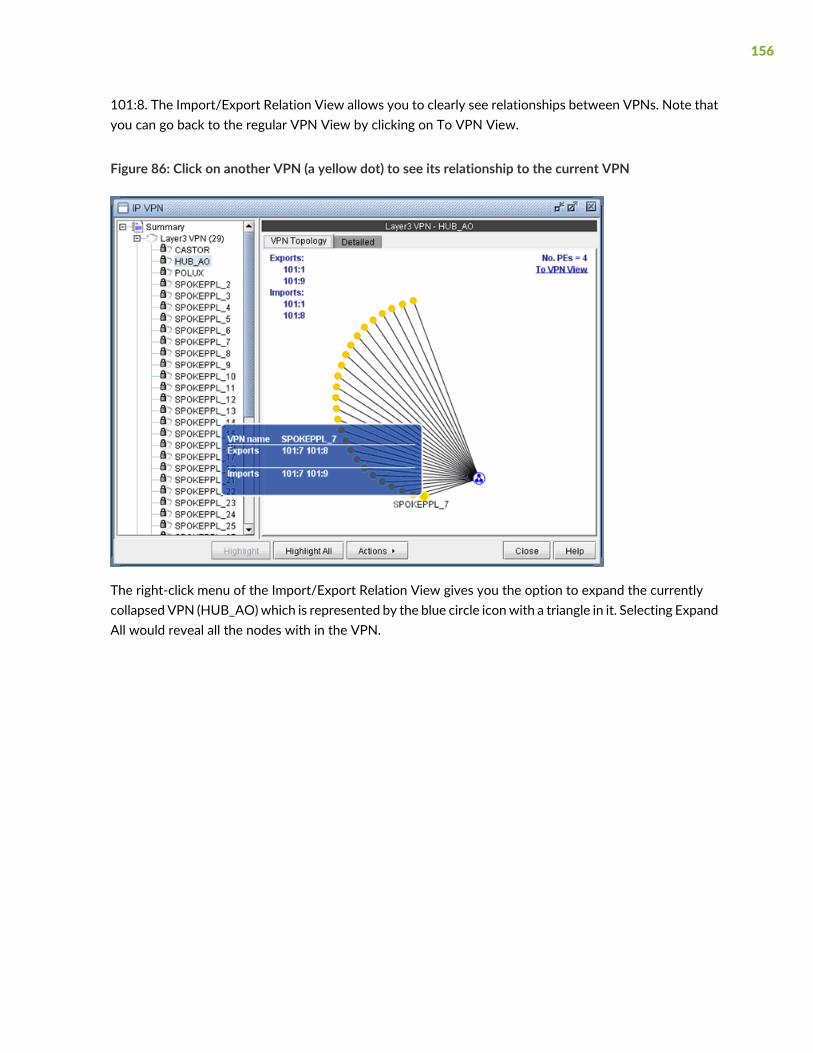
101:8. The Import/Export Relation View allows you to clearly see relationships between VPNs. Note thatyou can go back to the regular VPN View by clicking on To VPN View.
Figure 86: Click on another VPN (a yellow dot) to see its relationship to the current VPN
The right-click menu of the Import/Export Relation View gives you the option to expand the currentlycollapsed VPN (HUB_AO)which is represented by the blue circle iconwith a triangle in it. Selecting ExpandAll would reveal all the nodes with in the VPN.
156

Figure 87: Right-click menu in the Import/Export Relation View
The following figure shows you the Import/Export RelationViewwith the nodes in VPNHUB_AOexpanded.
157
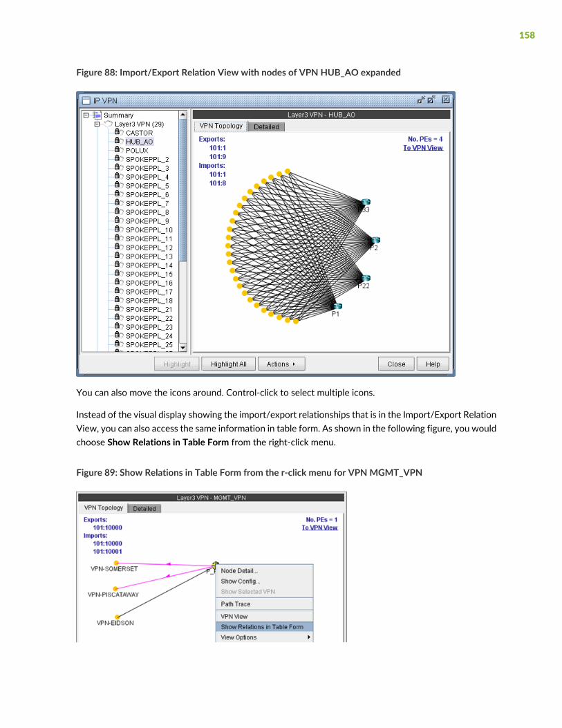
Figure 88: Import/Export Relation View with nodes of VPN HUB_AO expanded
You can also move the icons around. Control-click to select multiple icons.
Instead of the visual display showing the import/export relationships that is in the Import/Export RelationView, you can also access the same information in table form. As shown in the following figure, you wouldchoose Show Relations in Table Form from the right-click menu.
Figure 89: Show Relations in Table Form from the r-click menu for VPNMGMT_VPN
158

Once Show Relations in Table Form is chosen, the Export/Import table for the VPN is shown.
Figure 90: Export /Import table for VPNMGMT_VPN
In instances when there are a large number of export/import relations and you click on To Import/ExportRelation View, you will be prompted with the “This map could take a long time to calculate and display.”message. If you would be willing to wait and still want to see the export/import relations in graphical form,then click on “Click here if you want to proceed.” Instead, you may choose to view the import/exportrelations in table form, as described in the previous step.
Figure 91: A particular VPN could have a large number of export/import relations with other VPNs
The Report Manager includes a VPN Export-Import report under Network Reports > VPN, as shown inthe following figure, that shows all of the route target export/import relationships that exist betweenVPNs in the network.
159

Figure 92: VPN Export-Import report
Additional Methods to Access VPN Information
There are multiple ways of accessing VPN information. To access it for a specific VPN or a specific router,you can select an option from the relevant map’s right-click menu. For instance, from the IP VPN map,you can right-click on a VPN and select ViewVPN in Viewmode. From the Standardmap, you can right-clickon a router and select View>IP VPN at Node to bring up the IP VPN window, with the selected router inexpanded view. For instance, the following figure shows the window view displayed when you right-clickon the router F_T1 and then select View>IP VPN at Node.
160
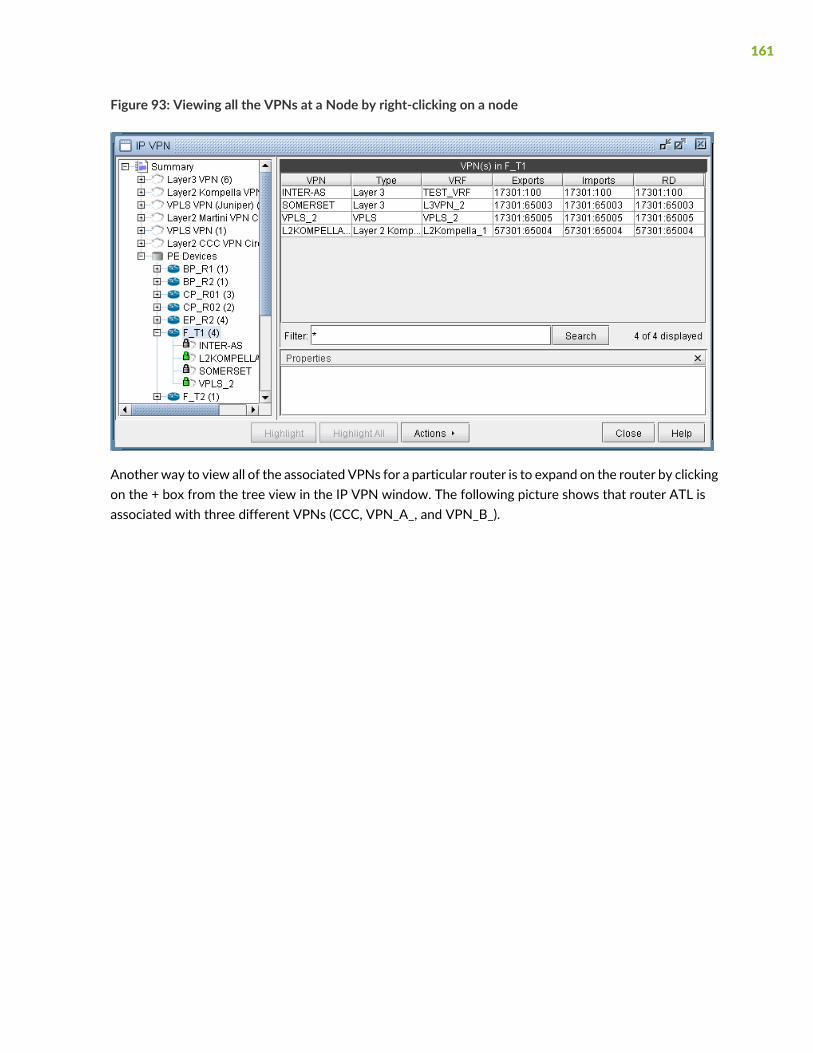
Figure 93: Viewing all the VPNs at a Node by right-clicking on a node
Another way to view all of the associated VPNs for a particular router is to expand on the router by clickingon the + box from the tree view in the IP VPN window. The following picture shows that router ATL isassociated with three different VPNs (CCC, VPN_A_, and VPN_B_).
161

Figure 94: Viewing all the VPNs at a Node by navigating the tree view
VPN Path Tracing
VPN path tracing allows you to see the routing path between two nodes belonging to a VPN. A VPN pathtrace can be performed by selecting the Path Trace option of the right-click menu in the VPN TopologyView. To use this feature, right-click over the source node, select Path Trace, and then click the destinationnode. The routing path details will then be shown on the main topology map. The following figure showsthe VPN path trace feature being performed between CE_piscataway and another node of the VPN.
162

Figure 95: VPN Path Tracing in VPN View
VPN Path Tracing in Import/Export Relations View is performed in a similar fashion. Right-click over agroup, and select Path Trace to reveal a drop-downmenu of PEs and CEs (if any), as shown in the followingfigure. Double-click to select a particular PE or CE as the source node. Then do the same to select thedestination node.
Figure 96: VPN Path Tracing in Import/Export Relations View
Alternatively, a VPN path trace can be performed between PEs (and CEs if managed) of a VPN via theNetwork > Path & Capacity > Path menu as shown in the following figure.
163

Figure 97: Demand Path window
To perform a VPN path trace instead of a regular path trace, first choose the desired VPN from the Ownerdropdown selection. Note that if the VPN is not listed in the owner selection, you should at it first fromthe VPN window as described in “Forming VPN Customer Groups” on page 205. Click on Highlight All todisplay all the nodes for the selected VPNNext, click on two of the highlighted nodes in order to see therouting being performed. PEs are highlighted yellow, and CEs (if any) are highlighted blue.
VPN Design and Modeling Using the VPNWizard
Besides the ability to derive the VPNs via network configuration import, the VPN Module allows thenetwork planner to construct and model a VPN from scratch, and to modify or add to existing VPNs. Theprocedures described below on how to add VPNs also apply for modifying existing VPNs. First switch toModify mode, and then chooseModify > Services > VPN. Then select a particular VPN and click on theModify button.
To add any VPN, click on the Add button from the VPN window. To modify a VPN, first select a particularVPN and then click on the Modify button. When you click on Add, the VPNWizard’s Add VPN window,shown in the following figure, is launched.
164

Figure 98: VPNWizard’s Add VPN window
You may choose to create different types of VPNs, including Layer 3, VPLS (both BGP and LDP flavors),Layer 2 Kompella, Layer 2 Martini, and Layer 2 CCC. Additionally, you may create inter-AS VPNs andhub-and-spoke VPNs.
The following sections will go through how a user would design andmodel several different types of VPNsusing NorthStar Planner’s VPNmodule. Successive sections will provide less detail when a particular usagescenario has already been described in an earlier section.
L3 (Layer 3) VPN
The L3 VPN is based on the IETF RFC 2547bis draft. To configure a L3 VPN (full-meshed version), theuser would perform the following sequence of steps. Additional steps that are applicable only to configuringa L3 Hub-and-Spoke VPN are described in the subsequent section.
Assign a VPN/VRF name by bringing up the Add VPN window and selecting Layer 3. Then type in a namefor the VPN (e.g. L3VPN_ph44).
165

Click on Next to bring up the window where you would choose the PEs of the VPN from the “AvailablePE Device(s)” list and add them to the right hand side “Selected PE Device(s)” list. Note that a node mustbe an iBGP speaker in order to make it into this list.
Here, you can also assign the Route Distinguisher, Route Target Exports, and Route Target Imports forthe selected AS. The program automatically recommends initial values, which you may change.
Figure 99: Adding a Full Meshed L3 VPN
Additionally, you may look up a list of Route Targets that are defined in the network by clicking on themagnifying glass icon to the right of the Import field to bring up the Route Targets Table shown below,which lists all the RTs (grouped by VPNs) in the network.
166

Figure 100: Route Targets Table
The Export Route Targets list and Import Route Targets list are populated with the route targets for theparticular VPN selected. Youmay then choose any or all of the route targets to either append to or replacethe route targets of the VPN you are currently adding. The Route Targets Table will help you to constructa VPNwith various export/import relationships (e.g. extranet or hub-and-spoke type of relationships) withother VPNs. For our current example, we will be constructing a simple full-meshed L3 VPN, so we will notneed to use the Route Targets table now.
Clicking on Next takes you to the following screen, in which you can configure a Hub-and-Spoke VPN.Since we are configuring a full-meshed L3 VPN, click Next to skip over this step.
167

Figure 101: Click Next to skip over Hub-and-Spoke configuration step
Click on Next to bring up the following window where you may add more PEs and assign the PE facingCE interfaces.
• The middle part of the window shows the topology area, where selected PE routers are placed.
• The Selected Objects area, as the name implies, lists those routers that have been selected as PEs.
• The Available Devices box lists those routers for the currently chosen AS that are eligible (i.e., they mustbe iBGP speakers) to be selected as PE routers.
• The Properties box lists all the interfaces for a particular router when it is highlighted (a router ishighlighted when it is clicked on either from the Available Devices list, the topology area of the window,or from the Selected Objects list).
Thewindow is designed to be as user-friendly as possible, with drag/drop capabilities built in. The followingfigure shows the four PEs that we have already added in the previous step.
168

Figure 102: Assigning more PEs and PE facing CE Interfaces
In more detail, you may add additional PE routers to the VPN from the Available Devices box via one oftwo methods:
• Select one or more routers (at which point the icon that has the left arrow with a circle around it willchange color from gray to blue), and then click on the blue arrow/circle icon to move it to the topologyarea part of the window (middle of the window).
• Alternatively, you could simply drag and drop PEs from the Available Devices list into the topology areaof the window.
The following figure shows you the result of adding the fifth PE router (E_V3) to the VPN.
169

Figure 103: An L3 VPN with five PEs
To assign the PE facing CE interfaces, first select a particular PE router in order to have all its interfacesshown in the Properties box. A PE is selected when it is clicked on from the Selected Objects list or fromthe topology area of the map. As shown in the following figure, the Properties box is now renamed asInterfaces in BP_R1, since the PE router BP_R1 has been selected. Another icon worth mentioning is the“–“/”+” button next to the arrow/circle button. Click on it to switch between “-“ and “+”. “-“ means to showall interfaces, while “+” means to only display interfaces that are unassigned or not shutdown.
170

Figure 104: How to assign interfaces to PEs
To assign an interface, you need to drag and drop a particular interface over to a no interface item undera particular PE. Alternatively, you can select the PE from the left hand side, and then select an interfacefrom the interface list on the bottom right hand side, and click the blue arrow in the Interfaces section.The following figure shows the window after the interfaces have been assigned to the PE routers.
171
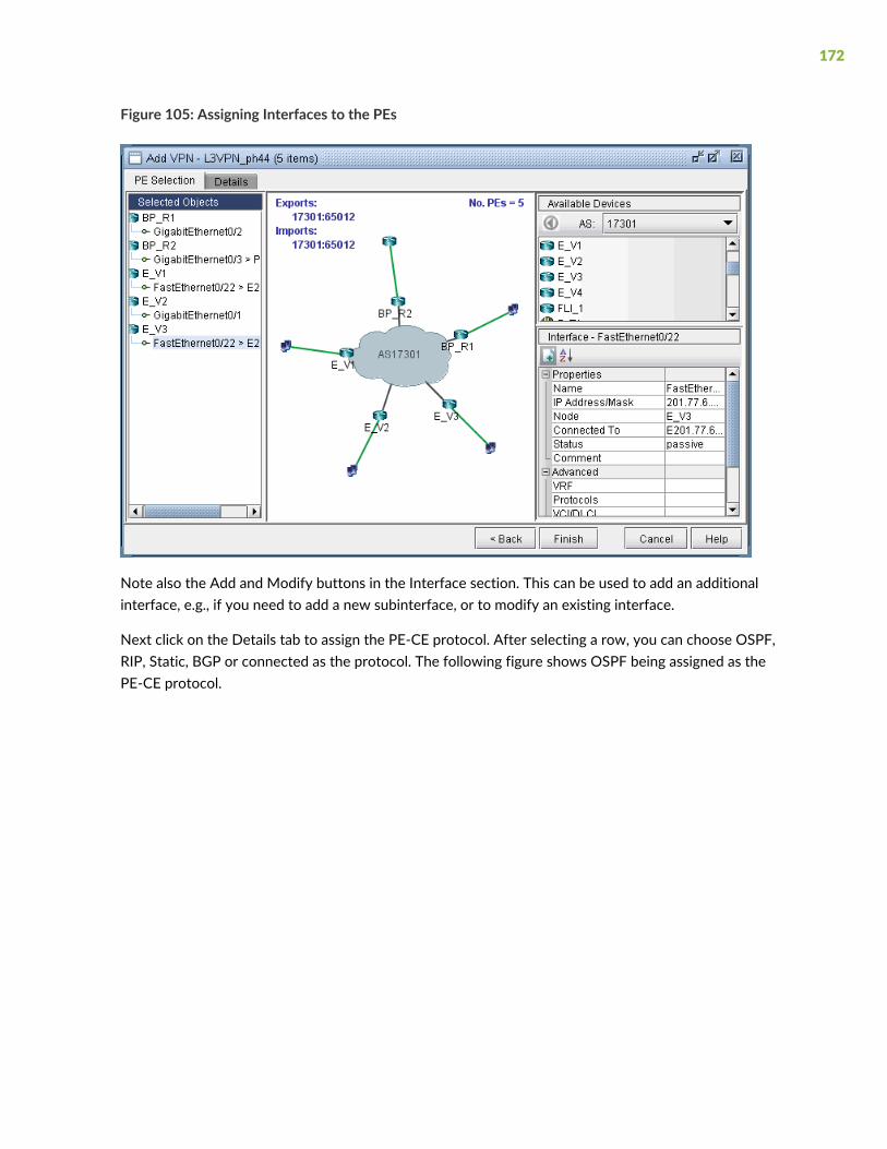
Figure 105: Assigning Interfaces to the PEs
Note also the Add and Modify buttons in the Interface section. This can be used to add an additionalinterface, e.g., if you need to add a new subinterface, or to modify an existing interface.
Next click on the Details tab to assign the PE-CE protocol. After selecting a row, you can choose OSPF,RIP, Static, BGP or connected as the protocol. The following figure shows OSPF being assigned as thePE-CE protocol.
172

Figure 106: Assigning the PE-CE Protocol in the Details tab
To assign BGP as the PE-CE protocol, first click on the BGP checkbox and then bring up the Add BGPNeighbor window (click on the icon to the left of PE->CE Neighbor IP or the icon to the left of CE->PENeighbor IP), shown in the following figure. For more information about how to create BGP neighboringrelationships, see “NorthStar Planner Border Gateway Protocol Overview” on page 105.
Figure 107: Add BGP Neighbor window
To assign Static as the PE-CE protocol, first click on the Static checkbox and then click on the icon to theright of Static to bring up the Add Static Route window.
173

To assign OSPF as the PE-CE protocol, first click on the OSPF checkbox and then click on the icon to theright of OSPF to bring up a dialog prompt, which allows you to enter in the associatedOSPF PID (Cisco-only)and OSPF Protocol. The OSPF PID should be different from that of the network core, and the area shouldmatch the CE’s area.
Finally, click Finish to complete the adding of the L3VPN. The summary window then displays the VPNthat you just added, as shown in the following figure.
Figure 108: L3VPN_ph44 has been added
With the detailed view shown (select the Detailed tab) in the upper portion of the window, click theConfiglet tab (next to the Details tab) to generate and display the configlet for the VPN that you just added.
L3 Hub-and-Spoke VPN
Merging Hub and Spokes
For the existing hub-and-spoke VPNs, NorthStar Planner does not automatically group together the vrfassociated with the hub and the vrf associated with the spoke. This should not affect routing, but forreadability purposes, users canmanually group together the hub and spoke into one VPNusing the followingprocedures.
174

1. If you are in the Online mode, click the Offline button to switch into the Offline mode.
2. Next, select the Modify mode button to switch into Modify mode.
3. SelectModify > Services > VPN, and identify the vrf’s to combine. If you select the To Import/ExportRelation View from the VPN Topology tab, it will show youwhich other instances to combine together.
Figure 109: Spoke View
Figure 110: Import/Export Relation View (Spoke -> Hub)
Since some hub-and-spoke VPN’s can have an upstream and downstream spoke, it may be best tocheck the Import/Export Relation View of the hub.
4. Select the hub-and-spoke components from the Summary > Layer 3 VPN list on the right pane and usethe Actions > Set Service menu to provide a name for the hub-and-spoke VPN.
175

Figure 111: Specifying the Hub and Spoke VPN via “Set Service”
5. Select the newly defined service from the Services category to view the VPN topology of the hub andspoke VPN.
Figure 112: Hub and Spoke VPN Topology
6. For the combined VPN, select theModify > Protocol. To identify the Hub PE node, right-click the tablecolumn header and select Table Options, and add the property “Hub” to the “Selected Items” list onthe right-hand side, to see the Hub checkbox column.
176

Figure 113: Hub Checkbox Column
7. By looking at the Exports and Imports, you can identify 2 sets of nodes with opposite imports andexports. One set of nodes should be specified as the Hub PE. For the Node which is a Hub PE, selectthe row corresponding to the outgoing interface, and then select the “Set to Hub PE” checkbox. ClickOK when you are done.
8. To update the network, selectModify > Update Network State. Then reopen the VPN window fromModify > Services > VPN.
9. If you are working on the live network (online module), you will want to preserve this setting for futureuse, so that it does not have to be repeated. To do this, first create the directory/u/wandl/data/.network_plan from the File Manager, if it does not exist.
10.Click the Design mode button to switch back to Design mode.
11. Save the network to /u/wandl/data/.network_plan via the File > SaveNetwork... menu using the defaultruncode x.
12.Now that the network is saved into the .network_plan directory, switch back to Online mode.
177

13. From Admin > Task Manager, New Task, rerun a Scheduling Live Network Collection task. Be sure toselect the checkbox option to consolidate with existing data. At this point, it is only necessary to processthe network configuration files and not to recollect the entire network, so for the “Data to Be Collectedor Processed”, you can “Deselect All” and select only the “Process” checkbox for the Configurationtype. Select Next and then Finish.
14.Once the task is complete, open Network > Services > VPN and check to ensure that the changes havebeen preserved.
Adding a New Layer 3 Hub-and-Spoke VPN
Configuring a L3 Hub-and-Spoke VPN is similar to configuring a regular L3 full-meshed VPN, except forthe following additional steps.
1. First follow the steps outlined in previous section on L3 VPN configuration until you reach theHub-and-Spoke configuration window. Click on the checkbox that says Configure Hub-and-SpokeMPLS VPN, and thenmove each PE to the appropriate list (Spoke Site Device(s) list or Hub Site Device(s)list) by using the Hub-> and <-Spoke buttons. The VPNWizard automatically suggests RT exports andimports for both the hub sites and the spoke sites in order to establish a hub-and-spoke relationship.As before, you have the option to change the RT list by editing the suggested export or import valuesor by using RTs from the Route Targets table (by clicking on the magnifying glass icon).
Figure 114: Hub-and-spoke VPN configuration
178

2. Click on Next to get to the window where you would configure PE facing CE interfaces as describedin the previous section on L3 VPN configuration. The following figure shows what the configurationlooks like after the interfaces have been assigned. Notice that GI_C2 is configured as the hub site.
Figure 115: Assigning PE facing CE interfaces in the Hub-and-Spoke VPN
3. After configuring the PE-CE protocol details under the Details tab (as described in the previous sectionon L3 VPN configuration), the resultant L3 hub-and-spoke VPN is shown in the following figure. Noticethat Import RT 17301:65016 is highlighted to indicate that it is only an import RT for the HuB site(s).
179

Figure 116: Newly created Hub and Spoke VPN
L2M (Layer2-Martini) VPN
The L2M (Layer2 Martini) VPN, based on the IETF Martini set of drafts, supports the configuration ofLayer2 Martini, AToM (Any Transport Over MPLS), and VLL (Virtual Leased Line) VPNs. The followingsteps illustrate how to configure a L2M VPN:
1. Bring up the Add VPN window by selecting Layer 2 Martini. Then type in a circuit name by filling inthe Ckt.Name box (e.g., L2Martini_1).
2. Click on Next to take you to the Common Properties window to select the two PEs. You may thenassign a VCID for the circuit. You may also optionally assign a bandwidth value for the circuit.
180
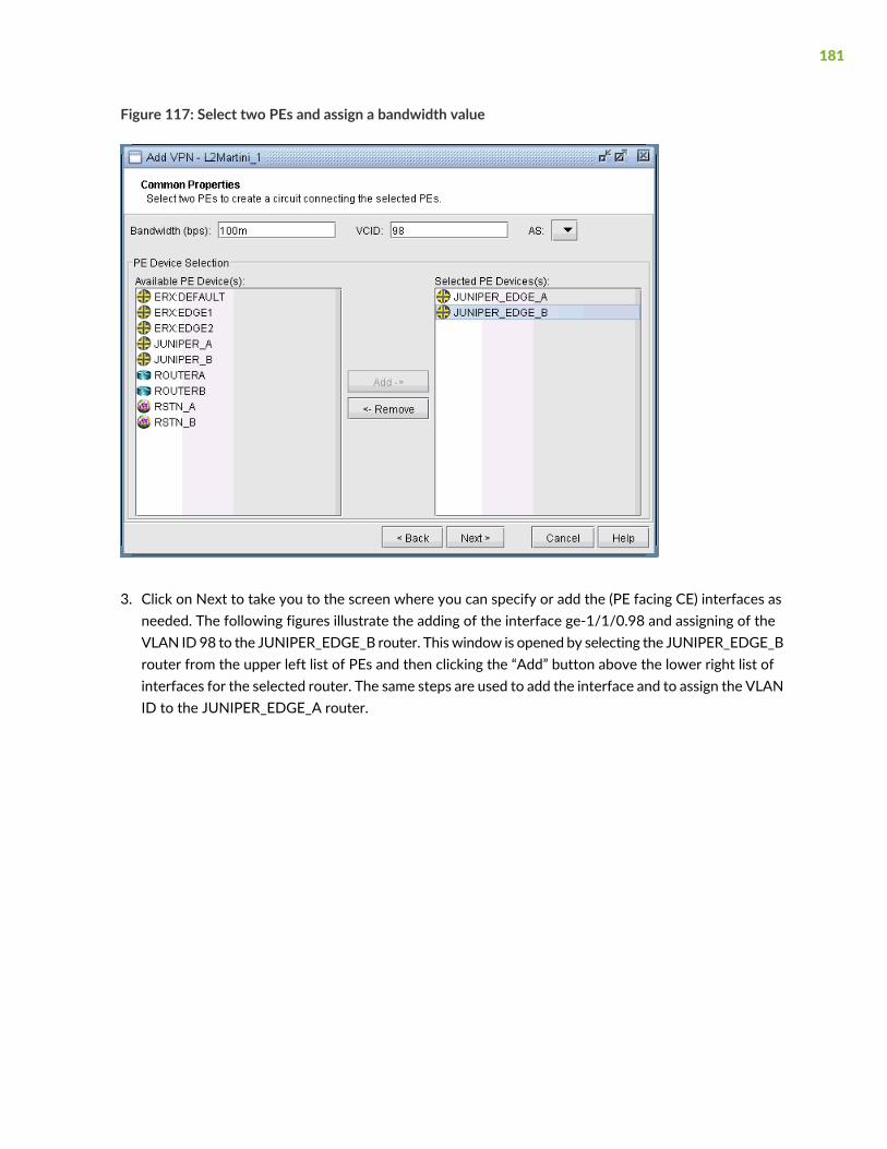
Figure 117: Select two PEs and assign a bandwidth value
3. Click on Next to take you to the screen where you can specify or add the (PE facing CE) interfaces asneeded. The following figures illustrate the adding of the interface ge-1/1/0.98 and assigning of theVLAN ID98 to the JUNIPER_EDGE_B router. This window is opened by selecting the JUNIPER_EDGE_Brouter from the upper left list of PEs and then clicking the “Add” button above the lower right list ofinterfaces for the selected router. The same steps are used to add the interface and to assign the VLANID to the JUNIPER_EDGE_A router.
181

Figure 118: Add a gigabit ethernet interface, ge-1/1/0.98
Figure 119: Assigning a VLAN ID of 98 to the interface ge-1/1/0.98
4. The following figure shows the result of both interfaces assigned, after selecting each PE router, addingthe appropriate sub-interface to the interface list in the bottom right, and then dragging and droppingthat new interface to the appropriate PE in the PE list.
182

Figure 120: Finished assigning interfaces on the PEs
5. Next, click on the Details tab to take you to the following screen, where the VCID and Encapsulationcan be assigned. Note that the VCID only needs to be assigned if it was not already done so in theCommon Properties window. The LSPs can also be assigned if necessary.
The following figure shows both the VCID and the encapsulation assigned.
183

Figure 121: Encapsulation and VCID assigned
Note that the Encapsulation drop-down can take on the values as described in the following table.
DescriptionField
For Juniper, the interface encapsulation types include: aal0, atm-aal5, atm-ccc-vc-mux, atm-cell,atm-cell-port-mode, atm-cell-vc-mode, atm-cell-vp-mode, cisco-hdlc, ethernet, ethernet-vlan,frame, frame-relay, frame-relay-ccc, interworking, and ppp.
For Cisco, the interface encapsulation types include: aal0, aal5, dot1Q, frame-relay, hdlc, andppp.
Encapsulation
6. Next click Finish to complete the adding of the L2M VPN. The following figures show both the singleand summary topology (with the added Martini circuit highlighted in pink) views for the L2M VPN justadded.
184

Figure 122: Topology view for the L2M VPN added
185

Figure 123: L2M VPN summary topology view with newly-added circuit (VCID 98) highlighted
L2K (Layer2-Kompella) VPN
The L2K (Layer2 Kompella) VPN, based on the IETF Kompella draft, is implemented by Juniper only. Toconfigure a L2K VPN, the user would perform the following sequence of steps:
1. Bring up the Add VPN window and selecting Layer 2 Kompella. Then type in a name for the VPN (e.g.L2Kompella_3).
2. Click onNext to bring up the Common Propertieswindowwhere you can assign the RouteDistinguisher,Route Target Exports, and Route Target Imports for the chosen AS and PEs. The program automaticallyrecommends values based on the chosen AS or you may provide your own.
186

Figure 124: For the chosen AS, select RD, RT, and two PEs
3. Click on Next to bring up the following window where you would identify PEs and assign the PE facingCE interfaces (in the same manner as described under the L3 (Layer 3) VPN section). The followingfigure shows the result of the assignment of the interfaces.
187

Figure 125: Interfaces have been assigned to the PEs
4. Next, click on the Details tab to specify the Encapsulation, Site, Site Identifier. Optionally, you may alsospecify the Transmit LSP and the Receive LSP. The following figure shows that Site, Site Identifier, andEncapsulation have been assigned.
188

Figure 126: Details tab showing the completed assignment of Site, Site ID, and Encapsulation
Note that the Encapsulation drop-down can take on the values as described in the following table.
DescriptionField
For Juniper, the interface encapsulation types include: aal0, atm-aal5, atm-ccc-vc-mux,atm-cell, atm-cell-port-mode, atm-cell-vc-mode, atm-cell-vp-mode, cisco-hdlc, ethernet,ethernet-vlan, frame, frame-relay, frame-relay-ccc, interworking, and ppp.
Encapsulation
5. Finally, click on Finish to complete the adding of the L2K VPN.
189

Figure 127: Newly added L2K VPN
VPLS-BGP VPN (for Juniper)
The VPLS-BGP VPN is based on the IETF Kompella/Rekher draft. To configure a VPLS-BGP VPN(implemented by Juniper only), the user would perform the following sequence of steps:
190

1. Bring up the Add VPN window and select VPLS-BGP VPN (For Juniper). Then type in a name for theVPN (e.g. VPLS_4) as shown in the following figure.
Figure 128: VPLS-BGP VPN
2. Click on Next to bring up the window where you can choose PEs and assign the Route Distinguisher,Route Target Exports, and Route Target Imports for a chosen AS as described under the L3 (Layer 3)VPN section). The program automatically recommends values or you may provide your own.
3. Click on Next to bring up the following window where you would assign the PE facing CE interfaces(in the same manner as described under the L3 (Layer 3) VPN section). The following figure shows theresult of the assignment of the interfaces.
191

Figure 129: Interfaces assigned to the PEs
4. Next, click on the Details tab to specify the Encapsulation, Site, Site Identifier. The LSPs may also bespecified, as appropriate. The following figure shows assignments completed for three nodes andin-progress for the fourth node.
192

Figure 130: Interfaces assigned to the PEs
The Encapsulation drop-down includes the following values from which you can select: ethernet-vpls,ether-vpls-over-atm-llc, extended-vlan-vpls, and vlan-vpls.
5. Finally click on Finish to complete the creation of a Juniper VPLS VPN.
VPLS-LDP VPN
The VPLS-LDP VPN, based on the IETF Lasserre/Kompella draft, is implemented by Cisco and all othervendors except Juniper. To configure a VPLS-LDP VPN, perform the following steps:
1. First identify, for the VPLS-LDP, a set of PEs with available PE-facing-CE interfaces that can be assignedas VPLS attachment circuits.
2. Next, bring up the Add VPN window and select VPLS-LDP VPN. In this example, we will configure aVPLS instance named VPLS-LDP0.
193
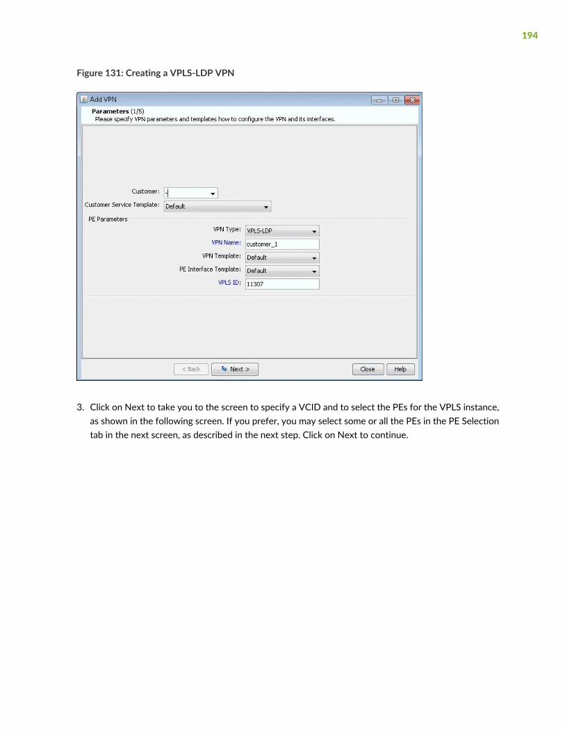
Figure 131: Creating a VPLS-LDP VPN
3. Click on Next to take you to the screen to specify a VCID and to select the PEs for the VPLS instance,as shown in the following screen. If you prefer, you may select some or all the PEs in the PE Selectiontab in the next screen, as described in the next step. Click on Next to continue.
194
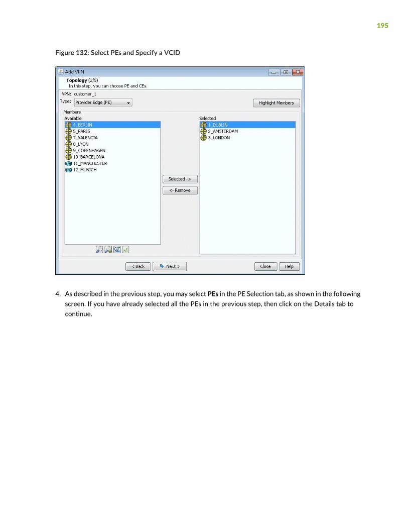
Figure 132: Select PEs and Specify a VCID
4. As described in the previous step, you may select PEs in the PE Selection tab, as shown in the followingscreen. If you have already selected all the PEs in the previous step, then click on the Details tab tocontinue.
195
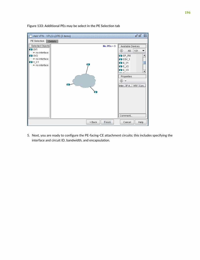
Figure 133: Additional PEs may be select in the PE Selection tab
5. Next, you are ready to configure the PE-facing-CE attachment circuits; this includes specifying theinterface and circuit ID, bandwidth, and encapsulation.
196

Figure 134: Configure VPLS-LDP Details
The encapsulation types for various vendors are:
• Cisco: dot1qaccess, dot1qtunnel, dot1qtrunk.
• Foundry: tagged, untagged.
• Tellabs, Riverstone: tagged, untagged, q-in-q.
The following figures show how an interface is assigned: First, click on the magnifying glass next toInterfaces and choose Add. Then in the Select Interface window, pick an available interface. Finally,type in the VCID for the interface
197

Figure 135: Select an interface
Figure 136: Assign the Circuit ID to the interface
6. Next, you will specify, in turn, each remote peer and the transmit LSP used to reach the peer. Click onthe magnifying glass next to Remote Peers to bring up the Add Remote Peer window, where you canchoose the remote peer and the transmit LSP from the dropdown selection menus.
Figure 137: Configure PE peers
7. The following figure shows the assignment details completed for our VPLS instance, VPLS-LDP0. Clickon Finish to add the VPLS instance to the model.
198
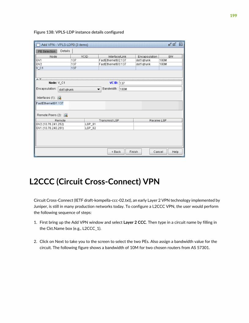
Figure 138: VPLS-LDP instance details configured
L2CCC (Circuit Cross-Connect) VPN
Circuit Cross-Connect (IETF draft-kompella-ccc-02.txt), an early Layer 2 VPN technology implemented byJuniper, is still in many production networks today. To configure a L2CCC VPN, the user would performthe following sequence of steps:
1. First bring up the Add VPN window and select Layer 2 CCC. Then type in a circuit name by filling inthe Ckt.Name box (e.g., L2CCC_1).
2. Click on Next to take you to the screen to select the two PEs. Also assign a bandwidth value for thecircuit. The following figure shows a bandwidth of 10M for two chosen routers from AS 57301.
199
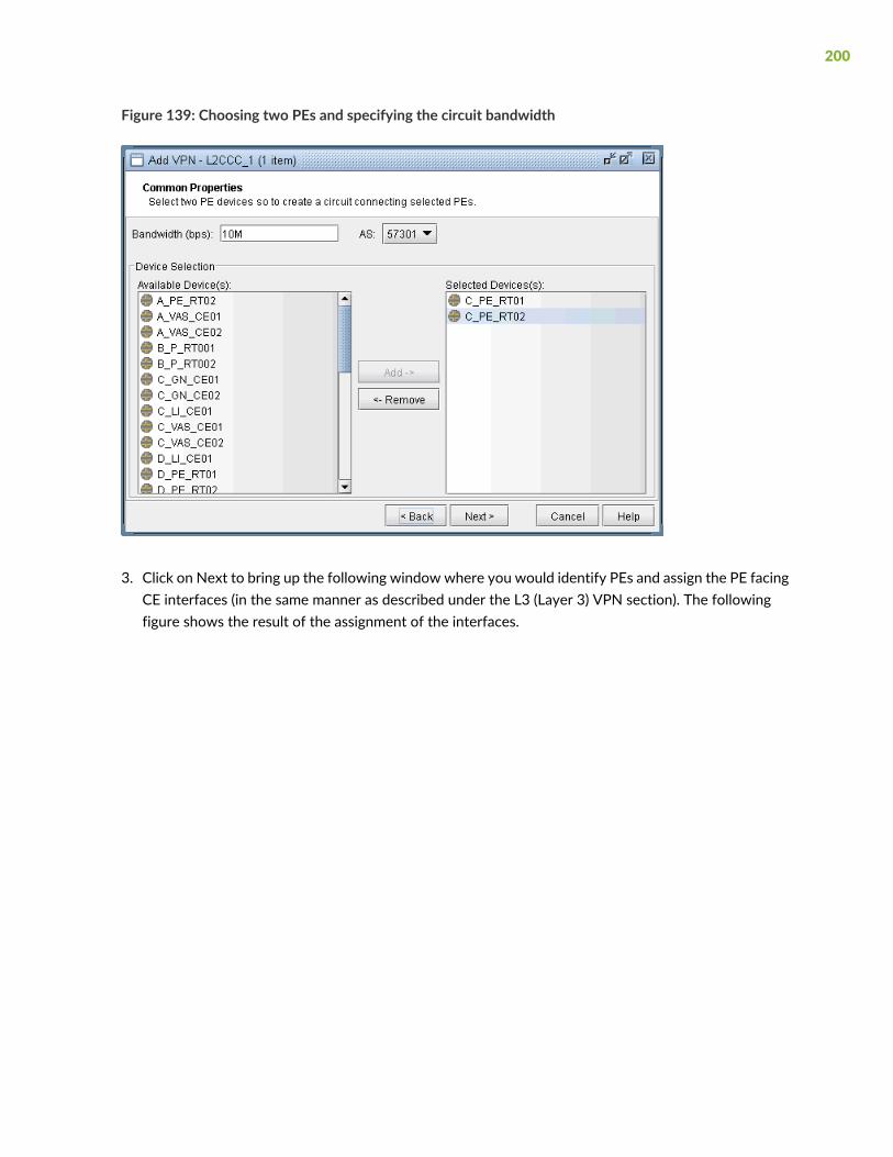
Figure 139: Choosing two PEs and specifying the circuit bandwidth
3. Click on Next to bring up the following window where you would identify PEs and assign the PE facingCE interfaces (in the same manner as described under the L3 (Layer 3) VPN section). The followingfigure shows the result of the assignment of the interfaces.
200

Figure 140: Interfaces assigned to PEs
4. Next, click on the Details tab to specify the Encapsulation, the Transmit LSP, and the Receive LSP. Formore information about how to set up LSPs, see “NorthStar Planner LSP TunnelsOverview” on page 311.The following figure shows the completed assignments.
201

Figure 141: Assigning Transmit/Receive LSPs and Encapsulation
Note that the Encapsulation drop-down can take on the values as described in the following table.
DescriptionField
For Juniper, the interface encapsulation types include: aal0, atm-aal5, atm-ccc-vc-mux,atm-cell, atm-cell-port-mode, atm-cell-vc-mode, atm-cell-vp-mode, cisco-hdlc, ethernet,ethernet-vlan, frame, frame-relay, frame-relay-ccc, interworking, and ppp.
Encapsulation
5. Finally, click on Finish to complete the creation of a L2CCC VPN.
202

Figure 142: Details of the newly-added L2CCC VPN
Inter-AS VPN
To construct an inter-AS VPN, you would follow the same steps as those used to construct a L3 VPN, withthe additional step of specifying routers from more than one AS. The following figure shows three PEs(along with completed interface assignments) from a particular AS (57301) already added.
203

Figure 143: An inter-AS VPN being constructed, with three PEs from AS 57301 already added
The next step would be to choose another AS (from the AS dropdown box under Available Devices), andthen select routers from it. As the following figure shows, two routers from AS 57222 were added to theVPN to create an inter-AS VPN. Interfaces were then assigned to the two routers to complete the process.
204
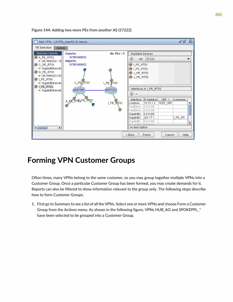
Figure 144: Adding two more PEs from another AS (57222)
Forming VPN Customer Groups
Often times, many VPNs belong to the same customer, so you may group together multiple VPNs into aCustomer Group. Once a particular Customer Group has been formed, you may create demands for it.Reports can also be filtered to show information relavant to the group only. The following steps describehow to form Customer Groups.
1. First go to Summary to see a list of all the VPNs. Select one or more VPNs and choose Form a CustomerGroup from the Actions menu. As shown in the following figure, VPNs HUB_AO and SPOKEPPL_*have been selected to be grouped into a Customer Group.
205
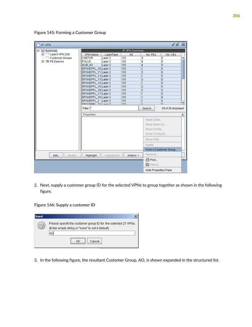
Figure 145: Forming a Customer Group
2. Next, supply a customer group ID for the selected VPNs to group together as shown in the followingfigure.
Figure 146: Supply a customer ID
3. In the following figure, the resultant Customer Group, AO, is shown expanded in the structured list.
206

Figure 147: Customer Group AO
Deleting or Renaming VPNs
In case you want to rename a particular VPN, simply select a VPN, click on Actions, and choose Rename.Then specify a new name for the VPN when prompted.
In case you want to delete a particular VPN, simply select a VPN, click on Actions, and choose Delete.
207

Figure 148: VPN Rename and Delete Actions
VPN Configlet Generation
As mentioned earlier under the sections under VPN Design andModeling using the VPNWizard, the VPNModule gives you the ability to generate VPN configlets for a particular VPN. For instance, the last stepunder the section, “L3 (Layer 3) VPN” on page 165, describes how to generate and display the configlet fora L3VPN. The following figures show configlets generated for two of the VPNs discussed earlier.
Figure 149: A Configlet Generated for a L3VPN
208

Figure 150: A Configlet Generated for a L2CCC VPN
To generate configlets in batch for several of the VPNs in a network, you may use the VPN Configletwindow (accessed via theDesign > Configlets/Delta > VPNConfiglet menu), shown in the following figure,where you can specify a particular directory (specified in the Directory box) to store the generated VPNconfiglets. In addition, you may also choose to generate configlets for particular nodes or VPNs via theNode/VPN drop-downs.
Figure 151: VPN Configlet Menu
209
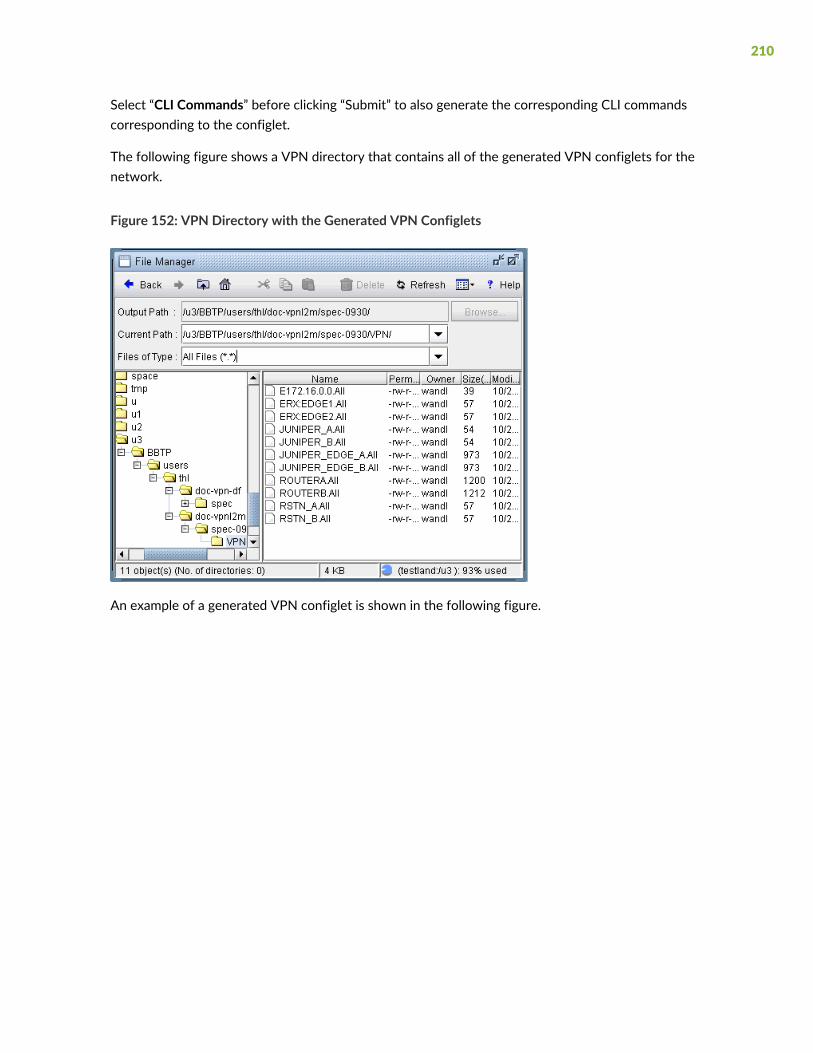
Select “CLI Commands” before clicking “Submit” to also generate the corresponding CLI commandscorresponding to the configlet.
The following figure shows a VPN directory that contains all of the generated VPN configlets for thenetwork.
Figure 152: VPN Directory with the Generated VPN Configlets
An example of a generated VPN configlet is shown in the following figure.
210

Figure 153: The Configlet Generated for JUNIPER_EDGE_A
Adding Traffic Demands in a VPN
For what-if studies, you can add multiple traffic demands between routers in the same VPN via the AddMultiple Demands window and single traffic demands via the Add Demand window.
1. To add multiple demands for a VPN, selectModify > Elements > Demands, Add > Multiple Demands.From the Type select box in the Placement (A x Z) section, choose the desired VPN type. Then selecta VPN to automatically populate the NodeA and NodeZ columns with routers from the selected VPN.
211

2. Fill out the rest of the windowwith the desired specifications and then click “Add” to add the demands.The following figure shows an example where a full-mesh of 182 1M demands are added between thePE routers in a L3 VPN called INTER-AS.
Figure 154: Adding a Full-Mesh of Demands in the VPN Called INTER-AS VPNs
3. To add a single VPN demand, bring up the Add Demandwindow and find the particular VPN of interestunder the Owner dropdown selection box. Note that if the owner is not listed, you may need to createit from the VPNwindow as explained in “Forming VPNCustomerGroups” on page 205. Once a particularVPN (Owner) has been selected, proceed to specify node A and node Z routers, and any relevantattributes, as you would for any other demand. The following figure shows a demand being added forthe VPN called L3VPN_PH44.
212

Figure 155: Adding a Single VPN Demand
VPN Traffic Generation
Alternatively, youmay add demands within the VPNs using the VPN Traffic Generation tool. Select Traffic> Demand Generation > VPN to open the window as shown in Figure 156 on page 214.
213

Figure 156: VPN Traffic Generation
1. Select, in the VPN table, one or more VPNs for which you wish to generate demands.
2. Next, specify the traffic source to use for the gravity model (either the Configured Interface BW or theInterface Traffic Load). The Interface Traffic Load corresponds to the egress/ingress files in the File >Load Network Files window, and the interfaceLoad_out and interfaceLoad_in files in the specificationfile. If selecting the Interface Traffic Load, select which period to use (Mean, Peak, or specific period.)
214

3. Specify the subscription ratio in percentages in the L3/L2K/VPLS and L2M/L2CCC textboxes. Thesubscription ratio is a percentage of the router’s PE-CE interface bandwidth utilized for VPN traffic.The formula used to calculate the demand is dependent on the type of VPN that is being applied.
gravity model is used to create a set of fully-meshed demands for this type of VPN. Theprogram takes the configured interface bandwidth of all the interfaces in the routers andcalculates a bandwidth for the circuits using a gravity formula. If the subscription ratio isnot specified, the default value is 10%.
Gravity model:
1. For each router in the VPN, add up the traffic load of all of the interfaces that areassociated with the VPN. This is the weight of the router.
2. Let Wi be the weight of router i. Then the traffic from router i to router j is Wi * Wj/ (-Wi + W1+W2...Wn), where n is the number of routers in the VPN.
3. The bandwidth of the demand is calculated by multiplying the result of the previousstep by the subscription ratio.
Layer 3 VPN, Layer 2Kompella VPN, or VPLS(Juniper) VPN
One demand is generated for each circuit that belongs in this type of VPN. The bandwidthof the demand is based on the interface bandwidthmultiplied by the percentage specifiedby the user in the subscription ratio field. If the subscription ratio is not specified, thedefault value is 10%.
Layer 2 Martini VPN orLayer 2 CCC VPN
4. “Generate demand between nodes instead of interfaces” can be selected to generate node-to-nodedemands instead of interface-to-interface demands. In this case, demands are aggregated so that onlyone demand is generated from nodeA to nodeB, instead of generating multiple demands from allinterfaces on nodeA to all interfaces on nodeB
5. Specify the demand file name. This can be an existing demand file, or the program will create the fileif it does not already exist.
6. If you are using an existing demand file, click on a radio button to select whether you wish to appendthe new demands, or overwrite the file with the new demands. Note: If the demand file specified inthe Demand file name textbox does not exist, then either one of these selections will create the filefor you.
7. Click on the Generate Demands button to generate a set of demands for the VPNs selected. Thegenerated demands will have uniquely assigned names and assigned with the owner of the VPN thatit belongs to.
215

8. Use the File Manager to view the new demands in the specified demand file.
9. To import the new demands into the network model, open the File > Load Network Files window andselect the generated demand file in the “newdemand” field.
VPN-Related Reports
To study and analyze the VPNs, as well as the impact that VPN traffic creates in your network, you mayuse the information from variety of reports that can be found in the ReportManager (accessible via Report> Report Manager).
1. You can view the Demand Route Cost Report under the Network Reports > Demand Reports folderto view demand information per VPN.
2. To view planned bandwidth and worst delay information for VPN-related demands, select the CoSDemands Report and find the VPN of interested (listed in the Owner column).
3. To view details of the particular types of VPNs in your network, select the appropriate report from theNetwork Reports > VPN folder (e.g. the Layer 3 report).
The following figures show a few VPN-related reports that can be generated.
216

Figure 157: L2 Martini VPN Report Generated in the VPN Section of the Report Manager
Figure 158: A L3 VPN Report Generated in the VPN Section of the Report Manager
217
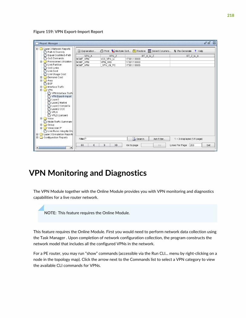
Figure 159: VPN Export-Import Report
VPNMonitoring and Diagnostics
The VPN Module together with the Online Module provides you with VPN monitoring and diagnosticscapabilities for a live router network.
NOTE: This feature requires the Online Module.
This feature requires the Online Module. First you would need to perform network data collection usingthe Task Manager . Upon completion of network configuration collection, the program constructs thenetwork model that includes all the configured VPNs in the network.
For a PE router, you may run “show” commands (accessible via the Run CLI... menu by right-clicking on anode in the topology map). Click the arrow next to the Commands list to select a VPN category to viewthe available CLI commands for VPNs.
218

To observe the network traffic condition (e.g. between PE and CE), periodic sampling of interface trafficstatistics is performed by the TaskManager. The collected interface data can then be accessed in the formor reports and charts. The following figure shows a PE->CE interface traffic chart for router SFO.
Figure 160: PE->CE Interface Traffic Chart (For PE Router SFO)
In the Report Manager, a VPN Interface Traffic report is available under Network Reports > VPN that letsyou see the interface traffic for each node of each VPN, as shown in the following figure.
219
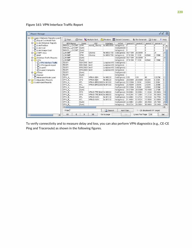
Figure 161: VPN Interface Traffic Report
To verify connectivity and to measure delay and loss, you can also perform VPN diagnostics (e.g., CE-CEPing and Traceroute) as shown in the following figures.
220

Figure 162: Ping/trace Route Between Routers from the IP VPNWindow
From the right-click menu of the VPNView topology, you can many functions (e.g. path tracing, runningCLI commands, and connect to device).
With JavaWeb Start installed, youmay also perform VPNmonitoring and diagnostic functions from awebbrowser, as well as to access VPN-related reports and charts. The following figures are meant illustratejust some of the web features available.
221

Figure 163: VPN View From the Web
222

Figure 164: View PE->CE Interface Traffic
223
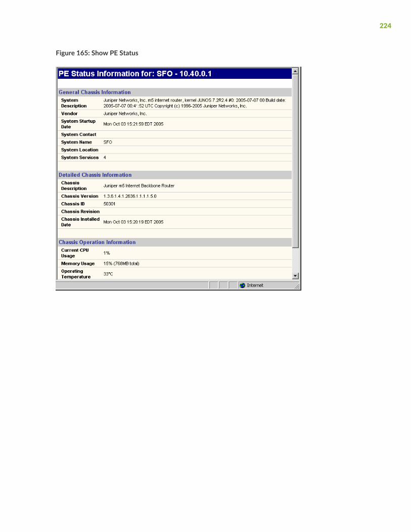
Figure 165: Show PE Status
224

Figure 166: Access VPN Summary Information
225
9CHAPTER
GRE Tunnels
Importing GRE Tunnel Information from Router Configuration Files | 229
Adding a GRE Tunnel | 231
Viewing GRE Tunnels | 234
Viewing Demands Over GRE Tunnels | 235


Importing GRE Tunnel Information from RouterConfiguration Files
Use these procedures if you have Cisco GRE tunnels configured in your network.
If you wish to perform this task, you should have a set of router configuration files with GRE tunnelsconfigured.
Generic Routing Encapsulation (GRE) Tunnels can be either imported from the router configuration files,or created from the NorthStar Planner Graphical Interface for what-if studies. Afterwards, the GRE tunnelpath and details can be viewed, as well as the details and paths of the demands routed over the GRE tunnel.The GRE tunnel can also be referenced as the next hop of a static routing table.
The following GRE statements are parsed during the config import:
Cisco
interface Tunnel<id>
ip address <ip-address> <mask>
tunnel source (ip-address|type number)
tunnel destination ip-address {hostname | ip-address}
Juniper
[edit interfaces interface-name unit logical-unit-number tunnel] level:
gr-1/2/0 {
unit 0 {
tunnel {
source <ip-address>;
destination <ip-address>;
}
}
}
NorthStar Planner maps these statements into entries in the intfmap (interface), tunnel, and bblink file.
Example intfmap entry
0.0.0.0/0,ATL,Tunnel4,active, ,,0, , , ,,,,,,,,,,,,0,,
0.0.0.0/0,BOS,Tunnel5,active, ,,0, , , ,,,,,,,,,,,,0,,
229

Example tunnel entry
#Tunnel Src Destination BW Type_Field
Tunnel4 ATL 172.16.1.2 0 R,A2Z,GRE,SOURCE=172.16.1.6,MASK=0000ffff 7,7
Tunnel5 BOS 172.16.1.6 0 R,A2Z,GRE,SOURCE=172.168.1.2,MASK=0000ffff 7,7
In the tunnel entry, note that the tunnel source of Tunnel4 matches the destination IP address of Tunnel5,and the tunnel source of Tunnel5 matches the destination IP address of Tunnel4.
Example bblink entry
#Linkname NodeA NodeZ Vendor Count TrunkType [MISC]
ATL_TUNNEL4 ATL BOS DEF 1 GRELINK C1=Tunnel4 C2=Tunnel5 # UP
#!
Each GRELINK entry references one GRE tunnel interface for the A to Z direction using C1=<interface>and one GRE tunnel interface for the Z to A direction using C2=<interface>. By default, the status of a linkof type GRELINK will be down/deleted if one of the tunnels fails to be routed. If both tunnels are routed,the GRE link is considered to be up, and traffic over a GRELINKwill then be routed over the links traversedby the GRE tunnel.
In some cases, however, the software fails to route the GRE tunnel due to incomplete information. In thosecases, the GRELINK may actually be up but there is no information to determine whether the tunnels aresuccessfully placed. For example, the the config files for the routers necessary to route the GRE tunnelmay be missing if they belong to another service provider. To avoid setting the GRELINK status to downin this scenario, set virtualgrelink=0 in the dparam file to treat GRELINKs as normal links.
To import the router configuration files, select File>Import Data and follow the Import Network Wizard.Alternatively, you may run the getipconf program in text mode.
After importing the config files, view the Integrity Checks report by selecting Report > Report Managerand then selecting the Configuration Report>Summary of Integrity Checks Report item.
The “Asymmetric GRE tunnels” integrity check will appear if there is a GRE tunnel defined at one end ofthe tunnel but not the other. Additionally, the “Inconsistent GRE tunnels protocol” integrity check willappear if the IGP protocol defined on one end of the GRE tunnel is different than the IGP protocol definedon the other end. These integrity checks are included under the TUNNEL category. To view the details ofan integrity check, right-click on the row and select Display item(s) for this msg ID/Category.
230

Adding a GRE Tunnel
If the configuration files are available, GRE tunnels can be added to the configuration files by adding twotunnel interfaces and specifying the tunnel source and destination, and then importing the configurationfiles as described in “Importing GRE Tunnel Information from Router Configuration Files” on page 229.
However, if the configuration files are not available, a what-if study can still be performed by adding theGRE tunnel interfaces, tunnels, and corresponding GRE link through the Java interface as explained below.
Assigning IP addresses to nodes/Interfaces
Before starting, IP addresses should be assigned to the nodes/interfaces that will be used as the sourceand destination of the GRE tunnel.
1. Select the Modify button to enter Modify action mode.
2. To add an IP address for a node, selectModify > Elements > Nodes and double-click a node entry. Inthe Properties tab, fill in the IP address field and click OK.
3. To add an interface, selectModify > Elements > Interfaces and click the Add button. Enter in theinterface name according to the convention of the hardware vendor of the router. Then enter therouter it resides on and the interface IP address and click OK.
Adding a GRE Tunnel Interface
1. Select the Modify button to enter Modify action mode. Then selectModify > Elements > Interfaces...
2. Next, add two interfaces for the GRE tunnels, one at each end node of the tunnel. Note thatvendor-specific naming conventions should be followed here, e.g., Tunnel1 for Cisco, or gr-1/0/2 forJuniper.
Adding a GRE Tunnel
1. SelectModify > Elements > Tunnels... and select Add > One Tunnel.
2. Use the same name for the Tunnel ID that was used for the GRE interface, and use the same case, asthis field is case-sensitive. Then select the source and destination nodes of the tunnel.
3. Add, “GRE,SOURCE=<ip-address | interface_name>” to the comma-separated Type field, using thename or IP-address of the interface or the IP-address of the node that will be the GRE tunnel source,e.g. GRE,SOURCE=172.16.1.3 or GRE,SOURCE=FastEthernet1/1. This IP address or interface nameshould either be defined on the node or interface as explained inAssigning IP addresses to nodes/Interfaceson page 163.
4. Click the Location tab and enter in the IP address of the destination node.
5. The Bandwidth (BW) field can be set to 0.
6. Create another tunnel for the reverse direction.
231

Figure 167: Adding a GRE Tunnel
Adding a GRE Link
Associated with the GRE tunnel pair should be a GRE link that can be advertised to the IGP to be used forrouting. The following steps indicate how to add a GRE link through the Java interface.
1. SelectModify > Elements > Links... and click “Add...” in the resulting window to open the Add Linkwindow.
2. Provide a name for the GRE link. For the Trunk field, select GRELINK.
3. Select the Location tab. Click the “...” button next to the Interface A field and select the GRE tunnel forthe A->Z direction. Click the “...” button next to the Interface Z field and select the GRE tunnel for theA->Z direction. If the GRE tunnel does not appear in the list, make sure that the GRE tunnel interfacesare named according to the convention of the appropriate hardware vendor.
Figure 168: Specifying the GRE Tunnels used to form the GRE Link
232
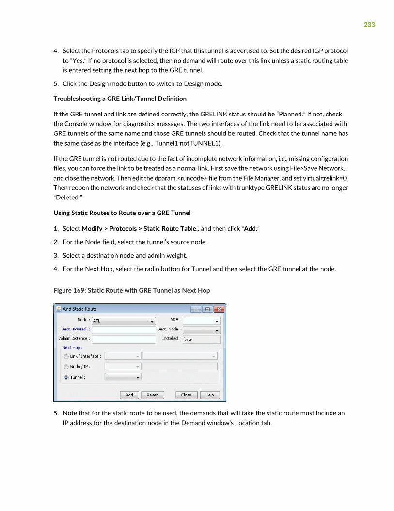
4. Select the Protocols tab to specify the IGP that this tunnel is advertised to. Set the desired IGP protocolto “Yes.” If no protocol is selected, then no demand will route over this link unless a static routing tableis entered setting the next hop to the GRE tunnel.
5. Click the Design mode button to switch to Design mode.
Troubleshooting a GRE Link/Tunnel Definition
If the GRE tunnel and link are defined correctly, the GRELINK status should be “Planned.” If not, checkthe Console window for diagnostics messages. The two interfaces of the link need to be associated withGRE tunnels of the same name and those GRE tunnels should be routed. Check that the tunnel name hasthe same case as the interface (e.g., Tunnel1 notTUNNEL1).
If the GRE tunnel is not routed due to the fact of incomplete network information, i.e., missing configurationfiles, you can force the link to be treated as a normal link. First save the network using File>SaveNetwork...and close the network. Then edit the dparam.<runcode> file from the FileManager, and set virtualgrelink=0.Then reopen the network and check that the statuses of links with trunktype GRELINK status are no longer“Deleted.”
Using Static Routes to Route over a GRE Tunnel
1. SelectModify > Protocols > Static Route Table.. and then click “Add.”
2. For the Node field, select the tunnel’s source node.
3. Select a destination node and admin weight.
4. For the Next Hop, select the radio button for Tunnel and then select the GRE tunnel at the node.
Figure 169: Static Route with GRE Tunnel as Next Hop
5. Note that for the static route to be used, the demands that will take the static route must include anIP address for the destination node in the Demand window’s Location tab.
233

Viewing GRE Tunnels
1. Select Network > Elements > Tunnels... in View or Design mode.
2. To filter for all GRE tunnels, click the Filter icon and type GRE in the Type field. (Alternatively, filter on“Type=GRE” in the Advanced Filter).
Figure 170: Filtered GRE Tunnels
3. Select the GRE tunnel to view and then click Show Path to view its path.
Figure 171: GRE Tunnel routed over LSP Tunnel
4. Note that a tunnel itself can route over a tunnel (in this case, an LSP tunnel). The portion that travelsover another tunnel is colored in purple.
234
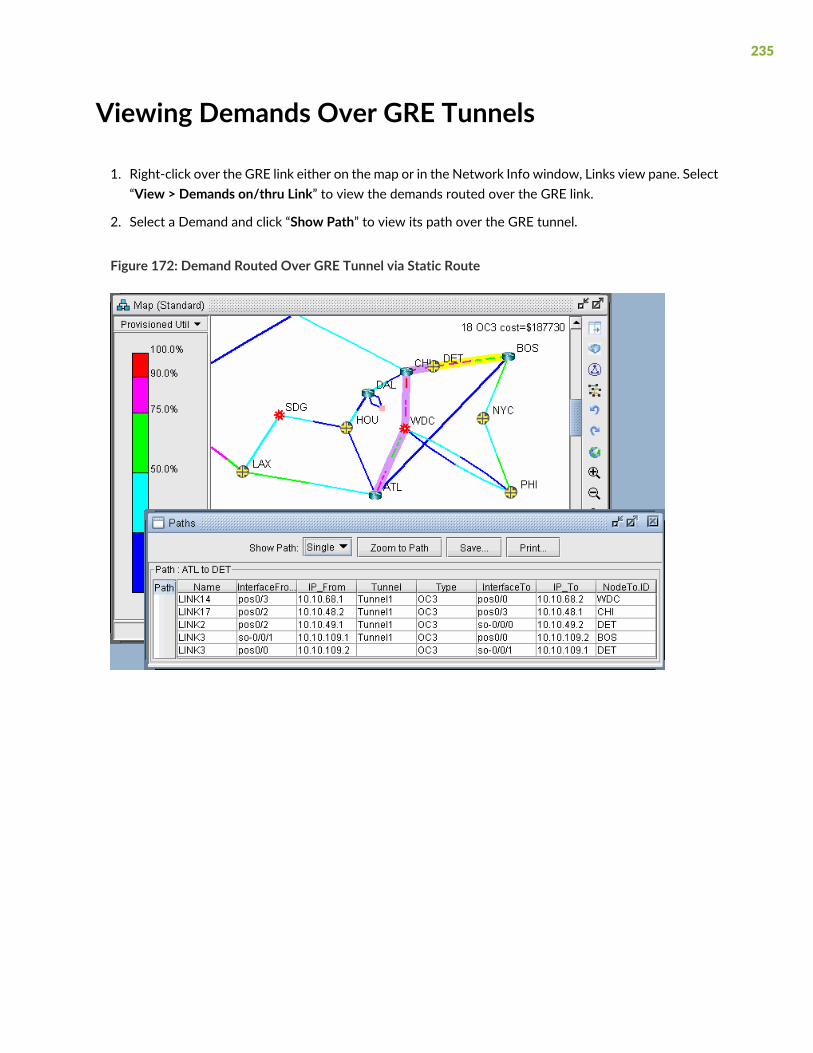
Viewing Demands Over GRE Tunnels
1. Right-click over the GRE link either on the map or in the Network Info window, Links view pane. Select“View > Demands on/thru Link” to view the demands routed over the GRE link.
2. Select a Demand and click “Show Path” to view its path over the GRE tunnel.
Figure 172: Demand Routed Over GRE Tunnel via Static Route
235

10CHAPTER
Multicast
NorthStar Planner Multicast Overview | 239
NorthStar Planner Recommended Multicast Instructions | 239
Creating Multicast Groups | 240
Creating Multicast Demands | 241
Viewing Multicast Demands in the Network | 242
Comparing Multicast with Unicast | 244
Multicast SPT Threshold | 246
Multicast Reports | 247
Multicast Simulation | 247
Collecting Multicast Path Data from Live Network | 248
Importing Multicast Path Data | 249
Multicast Data Processing | 250
Viewing Multicast Trees | 251


NorthStar Planner Multicast Overview
The Multicast chapter describes how to use the Multicast feature of NorthStar Planner. Internet Protocol(IP) multicast is a bandwidth-conserving technology that allows a single stream of data to be simultaneouslydelivered to multiple recipients, resulting in tremendous savings on server resources and efficient use ofnetwork bandwidth.
Using the Multicast feature will provide a good picture of how the network will perform under differentscenarios of multicasting as well as highlight potential problems when running multicast in the network.Since multicast offers enhanced efficiency and optimized performance, it is often used in financialapplications, streaming multimedia, enterprise resource applications, and any one-to-many data pushapplications.
Prior to beginning this task, you should have started up NorthStar Planner and opened a specification file.
RELATED DOCUMENTATION
NorthStar Planner Recommended Multicast Instructions | 239
Creating Multicast Groups | 240
Viewing Multicast Trees | 251
NorthStar Planner Recommended MulticastInstructions
Following is a high-level, sequential outline of the functionalities of the Multicast feature.
1. Open the advanced dog network in $WANDL_HOME/sample/original/router/advanced/dog.
2. Create a multicast group as described in step 1 through step 5.
3. Create multicast demands as described in step 6 through step 8.
4. View information on effects of multicast demands in the network, such as paths and link utilization, instep 1 through step 5.
5. Compare a network using multicast with one using unicast as shown in step 1 through step 7.
RELATED DOCUMENTATION
239

NorthStar Planner Multicast Overview | 239
Creating Multicast Groups
• First, for the sake of simplicity, delete all the demands in the advanced dog network. This will make iteasier to view the multicast demands that will be added later in this guide. To do this, switch to Modifymode and selectModify > Elements > Demands.... In the resulting window, click the Delete button andthen select “All Entries”.
• In Modify mode, click on Modify > Protocols > Multicast > Multicast Group to bring up the MulticastGroup window.
• Click the Add button in the Multicast Group window to bring up the AddMulticast Group window.
• Enter in a Destination IP Address, Name, and RP (Rendezvous Point) Address for the multicast group.In this example, 10.10.10.8 (WDC) will be used as the RP. If RP Addresses are already defined on Nodes,then theywill be populated in this drop-down box. Then, add the first six routers from the list of AvailableRouters to the Selected Routers list. For more information about the window display, see “ViewingDemands Over GRE Tunnels” on page 235.
Figure 173: Adding a Multicast Group
• Click the Add button when all the properties of the multicast group have been set correctly. This willadd themulticast group to the network. Close the AddMulticast Group and theMulticast Groupwindowsas they are no longer needed.
240
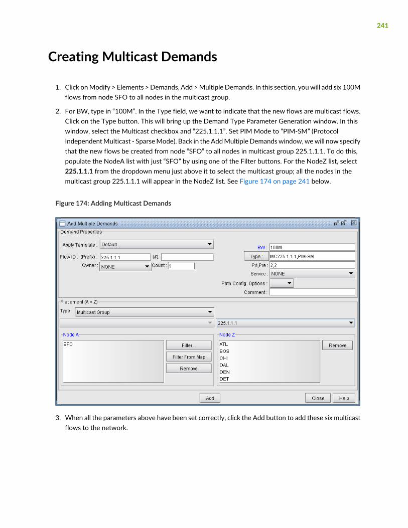
Creating Multicast Demands
1. Click onModify > Elements >Demands, Add >Multiple Demands. In this section, youwill add six 100Mflows from node SFO to all nodes in the multicast group.
2. For BW, type in “100M”. In the Type field, we want to indicate that the new flows are multicast flows.Click on the Type button. This will bring up the Demand Type Parameter Generation window. In thiswindow, select the Multicast checkbox and “225.1.1.1”. Set PIM Mode to “PIM-SM” (ProtocolIndependentMulticast - SparseMode). Back in the AddMultipleDemandswindow,wewill now specifythat the new flows be created from node “SFO” to all nodes in multicast group 225.1.1.1. To do this,populate the NodeA list with just “SFO” by using one of the Filter buttons. For the NodeZ list, select225.1.1.1 from the dropdown menu just above it to select the multicast group; all the nodes in themulticast group 225.1.1.1 will appear in the NodeZ list. See Figure 174 on page 241 below.
Figure 174: Adding Multicast Demands
3. When all the parameters above have been set correctly, click the Add button to add these six multicastflows to the network.
241

Viewing Multicast Demands in the Network
1. At this point, a multicast group has been defined and demands, or flows, to the multicast group havebeen created. Now, information on these demands and how they fit into the network can be examined.First, switch to Viewmode.When the program asks whether or not to Update Demand Routing Tables,click Yes.
2. The first thing to notice is that, even though there are multiple recipients of the 100M flows from nodeSFO, the link utilization appears uniform throughout all the utilized links, as shown inFigure 175 on page 242. This is typical of multicast networks and is a good example of the advantageof multicast over traditional unicast networks. In traditional unicast networks, one would expect “high”utilization near the source and “lower” utilization as the flows fan out to the recipients. Here, theutilization is “low” everywhere.
Figure 175: Link Utilization in a Multicast Network
3. Now, click on Network > Elements > Demands. The Demands window lists all the demands in thenetwork, which in this example should all be multicast demands.
4. Highlight any of the rows in the demands table and click the Show Path button. This will display thepath taken by the demand according to the unicast protocol being used. The default protocol is PIM-SM(Protocol Independent Multicast - Sparse Mode). This can be changed for each demand by modifyingthe demand’s Type field.
242

Figure 176: Path of a Demand from SFO to BOS
5. Detailed information on link utilization resulting from the multicast demands can be viewed throughthe Peak Link Utilization Report under Simulation Reports > Network StatisticsTo do this, click onReport > Report Manager, then select Peak Link Utilization from the list of reports in the ReportManager window. Notice in the example below that all the utilized links display a utilization of 100M.
Figure 177: Link Peak Utilization Report for a Multicast Network
243

6. Select Subviews > Multicast from the map to view the multicast tree graphically.
Figure 178: Multicast Subview
7. Note the special icons used for the source (SFO), the Rendezvous Point (WDC) and the subscribers.
8. If there are multiple trees listed, you can <Ctrl>-click to highlight multiple trees at once. Each multicasttree will have a different color, e.g., yellow, green, blue. Overlaps between trees will also have a uniquecolor, e.g., orange.
Comparing Multicast with Unicast
• It may be of interest to see what the network would look like if, instead of multicast, all the demandswere routed according to traditional unicast protocols. This can be done easily by disabling multicast onall the demands. To do this, first switch to Modify mode and click on Modify > Elements > Demands....
• In the Demands window, click the Modify button and then select “All Entries”.
• A Modify Demands window will appear. Click the Type button in this window to bring up the DemandType Parameter Generation window.
• Click the dropdown menu next to the Multicast field and select No.
244
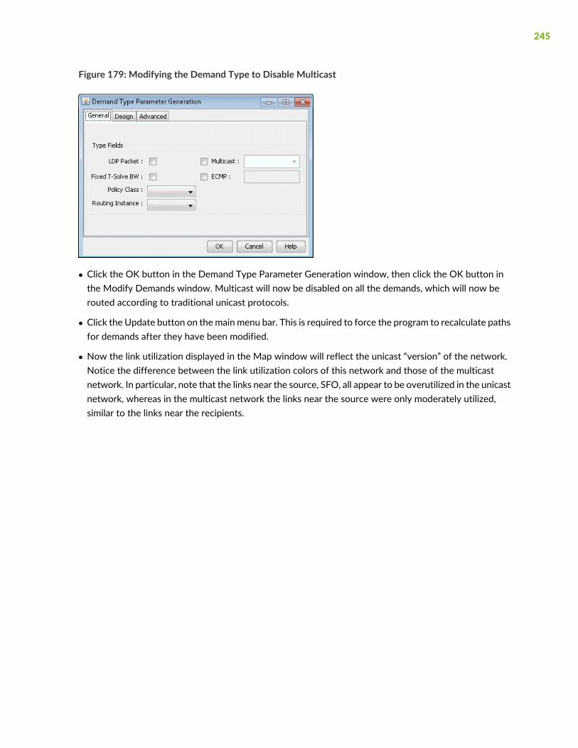
Figure 179: Modifying the Demand Type to Disable Multicast
• Click the OK button in the Demand Type Parameter Generation window, then click the OK button inthe Modify Demands window. Multicast will now be disabled on all the demands, which will now berouted according to traditional unicast protocols.
• Click the Update button on themain menu bar. This is required to force the program to recalculate pathsfor demands after they have been modified.
• Now the link utilization displayed in the Map window will reflect the unicast “version” of the network.Notice the difference between the link utilization colors of this network and those of the multicastnetwork. In particular, note that the links near the source, SFO, all appear to be overutilized in the unicastnetwork, whereas in the multicast network the links near the source were only moderately utilized,similar to the links near the recipients.
245

Figure 180: Link Utilization in a Unicast Network
Multicast SPT Threshold
When using sparse mode multicast, the SPT Threshold value can be set for a particular node to determinewhether the Rendezvous Point (RP) or the Shortest Path Tree is used for routing. If the SPT Threshold isset to 0, the RP will be ignored, and the Shortest Path Tree will always be used. If the SPT Threshold is setto “Infinity” then the RP will always be used, and the Shortest Path Tree will never be considered. To setthe SPT Threshold for a node, right click on a node in Modify mode and selectModify Nodes. Then, clickon the IP tab to display the SPT Threshold input field. Here, the user can enter “0” or “Infinity” as describedpreviously.
246

Figure 181: Modify Node: Setting the SPT Threshold
Multicast Reports
For reporting purposes, each source-destination pair is listed as one entry in the Network Reports >Demand Reports > Demand Path & Diversity report (PATHRPT) in the Report Manager.
Summary info is reported in the explanation portion of the report including the total number of multicasttrees and bandwidth information. Click the Explanation... button for this summary info. An example isshown below:
* 1 MCtrees (Tree Bandwidth=100.000M), Average # of leaves=6.00
* 1 routed(Bandwidth=100.000M, average #link/tree=13.00)
Here, the leaves refer to the destination nodes of themulticast tree. The links per tree indicate the numberof links used by the tree.
Multicast Simulation
During a simulation, each source-destination pair for the multicast tree is by default counted as a separatedemand. To count the entire tree and its bandwidth as belonging to onemulticast demand, add the followingdesign parameter in the dparam file:
247
“MCsimrptopt=1”
Collecting Multicast Path Data from Live Network
In the Schedule Live Network Collection task in the TaskManager, check theMulticast Path box as shownin the following figure. This ensures that the multicast routing table is collected. The multicast tree andsubsequent display is constructed via the olist and ilist that is contained in the collected multicast routingtable.
Figure 182: Multicast Path Collection Option
The collected data is stored in directory /u/wandl/data/collection/.LiveNetwork/multicast_path/. Thefollowing is an example for IOS of the multicast routing table that is collected.
show running | include hostname
hostname BEK3640
BEK3640#show ip mroute
IP Multicast Routing Table
248

Flags: D - Dense, S - Sparse, B - Bidir Group, s - SSM Group, C - Connected,
L - Local, P - Pruned, R - RP-bit set, F - Register flag,
T - SPT-bit set, J - Join SPT, M - MSDP created entry,
X - Proxy Join Timer Running, A - Candidate for MSDP Advertisement,
U - URD, I - Received Source Specific Host Report,
Z - Multicast Tunnel, z - MDT-data group sender,
Y - Joined MDT-data group, y - Sending to MDT-data group
Outgoing interface flags: H - Hardware switched, A - Assert winner
Timers: Uptime/Expires
Interface state: Interface, Next-Hop or VCD, State/Mode
(*, 239.1.1.1), 1w4d/00:02:43, RP 22.22.1.1, flags: S
Incoming interface: Null, RPF nbr 0.0.0.0
Outgoing interface list:
Ethernet2/1.2, Forward/Sparse, 1w4d/00:02:43
(22.22.2.2, 239.1.1.1), 1w4d/00:03:23, flags: T
Incoming interface: Ethernet2/1.6, RPF nbr 88.88.0.18
Outgoing interface list:
Ethernet2/1.2, Forward/Sparse, 1w4d/00:02:43
(22.22.3.3, 239.1.1.1), 22:10:01/00:02:57, flags: PT
Incoming interface: Ethernet2/1.2, RPF nbr 88.88.0.2
Outgoing interface list: Null(*, 224.0.55.59), 2d23h/00:03:06, RP 22.22.1.1, flags:
S
Incoming interface: Null, RPF nbr 0.0.0.0
Outgoing interface list:
Ethernet2/1.2, Forward/Sparse, 2d23h/00:03:06
(10.33.3.2, 224.0.55.59), 00:22:58/00:02:34, flags: PT
Incoming interface: Ethernet2/1.5, RPF nbr 88.88.0.6
Outgoing interface list: Null
(*, 224.0.1.40), 1w4d/00:02:59, RP 22.22.1.1, flags: SJCL
Incoming interface: Null, RPF nbr 0.0.0.0
Outgoing interface list:
Ethernet2/1.5, Forward/Sparse, 2d16h/00:02:18
Ethernet2/1.2, Forward/Sparse, 1w4d/00:02:36
Importing Multicast Path Data
If the multicast path data is available by methods other than Schedule Live Network Collection, this datacan be imported using Import NetworkWizard and selecting theMulticast Path option. This import featurecurrently supports Cisco, Juniper, and Alcatel-Lucent vendors. The data collected from themulticast routingtable should contain information about the (S,G) or (*,G) groups in the Multicast Tree (for example, forCisco the command: show ip mroute).
249

Figure 183: Import Network Wizard
Multicast Data Processing
After collecting specific multicast show commands for Cisco, Juniper and ALU, the file called mcpath.x iscreated and automatically loaded to describe the multicast flows. The names of the flows are derived fromthe multicast group IP address as follows:
source_MulticastGroupAddress for (S,G)
*_MulticastGroupAddress for (*,G)
The bandwidth of the multicast flow is derived differently depending on the vendor:
• For IOS, it is extracted from the Rate line from command “show ip mroute active”
• For IOS-XR, it is extracted from bps_in and bps_out from command "showmfib route rate". The averageof these two values is calculated as the flow bandwidth.
• For ALU, it is extracted from the Curr Fwding Rate line from command "show router pim group detail"
250

When multicast paths are imported, messages that point to errors or potential errors are written to theImport_MCTree_log.runcode file located in the Log directory of the project specification file.
This Import_MCTree_log.runcode log file contains the following columns: Lineno, Error Code, ErrorMessage,Action, LineDetail. The Lineno column references which exact line within the mcpath.runcode file that isreferenced; the line at Lineno from mcpath.runcde itself is shown in the LineDetail column.
Various values for the Error Code column may be possible. Example; Path Ignored indicates that the pathspecification is ignored; Path Error indicates that errors were encountered such as invalid IP addresses,Tunnel name specified in path specification does not exist, there's a gap in the path specification, etc.
If a Path Error is encountered, the program may take one of the following actions:
• Ignored: Error detected, path specification ignored.
• Warning: Errors detected, no action taken. Example, some of the IP addresses in an explicit pathspecification may not be defined in the network. The invalid IP addresses would still be remembered(i.e. would still be displayed and saved) and the Warning code is printed.
• Fixed: For paths imported from tunnelpath.x file, the program would try to fix the paths if possible. Thecontents of tunnelpath.x file are based on the CLI outputs of routers. The format can vary for eachvendor. There are cases where links between two different vendor nodes are not specified. If "Fixed" isprinted, that means the a link is automatically added by the program to account for the unspecified link.
For an explicit path specification, some of the IP addresses defined in the path specification may not bedefined in the network. In this case, the invalid IP addresses would be remembered (i.e. would still bedisplayed and saved) but won't have effect on the routing simulation.
Tracing through the error messagesmay require reviewing the paths hop-by-hop (IP address by IP address),and checking the rawmulticast path data used to construct the tree. The Import_MCTree_log.runcode logfile is meant to assist in the troubleshooting.
Viewing Multicast Trees
To view themulticast trees configured in the network, on themain topologymap select Subview>MulticastTree as shown in the following figure. From this subview, the (S,G) or (*,G) tree can be selected at a particularnode.
251

Figure 184: Multicast Tree
Since the mcpath.x file uses the same format as the demand file; it can be used for network planning (asknown flows) or for failure simulation. For example, links can be failed and the multicast tree (morespecifically the demands making up the multicast tree) will be rerouted.
252

11CHAPTER
Class of Service
NorthStar Planner Class of Service Overview | 255
NorthStar Planner Recommended CoS Instructions | 256
The QoS Manager | 256
Define Class Maps | 258
Create Policies for Classes | 260
Attach Policies to Interfaces | 266
Adding Traffic Inputs | 268
Using the Text Editor | 269
Reporting Module | 269
IP Flow Information | 270
Link information | 271
Traffic Load Analysis | 272
Traffic Load by Policy Class | 273
CoS Alias File | 275
Bblink File | 275

Policymap File | 276
Demand File | 279
Traffic Load File | 279
NorthStar Planner Class of Service Overview
The Class of Service chapter describes how the NorthStar Planner network design software can be usedto model Class of Service (CoS). CoS plays a key part in making sure that services can be transported overa connectionless IP network and can meet the customer Service Level Agreement.
CoS can be implemented on each interface of a router. Users define traffic classes based on “match criteria,”such as a particular protocol, access control list, or a specified input interface on which packets arrive.When a packet arrives at a router, it is classified according to the class whose criteria it successfully matches.This packet then constitutes the traffic for that class. At the router, there is a reserved queue for eachclass, and any traffic belonging to a class is directed to the corresponding queue. Users can also definecharacteristics of each class’s queue based on bandwidth and queue limit.
If you have an existing set of config files, use getipconf or the Import Data Wizard (via File > Import Data)to parse your config files and create a set of NorthStar Planner input files.
Use this feature if you want to:
• Check and validate that the current network configuration can handle customer traffic (even beforecustomer implementation).
• Identify bottlenecks and adjust the network design by performing What-if Studies
The what-if capabilities in NorthStar Planner may have to be used in order to correct the network design.For instance, if too many packets are dropped during the simulation, the following actions can beinvestigated:
• Increasing the queue size limit for a given class
• Decreasing the bandwidth of lower priority traffic classes
• Locally increasing link bandwidth
RELATED DOCUMENTATION
NorthStar Planner Recommended CoS Instructions | 256
The QoS Manager | 256
255

NorthStar Planner Recommended CoS Instructions
• Add CoS data by importing/parsing router config files via the graphical user interface, or by directlyediting the related text input files.
• Add to or modify CoS with the following steps:
• Define class maps
• Create policies for classes
• Attach policies to interfaces
• Add CoS traffic.
• Generate reports:
• Demand oriented reports which supply userswith end-to-end delay and the total bandwidth of droppedpackets.
• Link oriented reports which provide information regarding propagation, queueing delays, and the totalbandwidth of dropped packets.
• View traffic load information either via the network map color coded link utilizations or via traffic loadbar charts for statistics on a specific link.
The QoS Manager
1. To extract CoS details from a set of network configuration files, close any currently open networkbaselines and select File > Import Data. Follow the instructions in “Router Data Extraction Overview”on page 33 to import the configuration files after they have been uploaded to the NorthStar Plannerserver.
2. Once the import is finished, the network baseline will be opened.
3. Select Network > QoS... to open the QoS Manager window.
4. Select ForwardingClass to see a list of CoS classes defined on the network. NorthStar Planner supports8 classes. If there are more than 8 classes, the additional classes can be mapped to one of the 8 CoSaliases.
256

Figure 185: QoS Manager
5. Select “CoS Policy > by Policy Name” to see a summary list of the CoS policies in the network.
Figure 186: CoS Policy
257

6. The policies are organized by policy name or by node. You can select a policy under CoS Policy > byPolicy Name to see the details for the policy, and the nodes which have the given policy, or select anode under CoS Policy > by Node to see the policies configured on a given node.
7. SelectRate Limit Policy > by PolicyName to see a summary view of rate limiting policies in the network.Select a policy under Rate Limit Policy > by Policy Name to see the details for a given policy and thenodes which belong to the policy, or select a node under Rate Limit Policy > by Node to see the ratelimiting policies configured on a given node.
Figure 187: Rate Limit Policy
How to Input CoS Parameters
To input CoS parameters, you can create CoS classes and policy maps and then specify classes that belongto a particular policy together with their bandwidths and queue sizes. Finally, you need to specify whatpolicy is to be used for each interface.
Define Class Maps
1. The first thing to do is to define the names of the CoS classes. In Modify mode, selectModify > QoS> CoS Classes for the CoS Classes window.
258
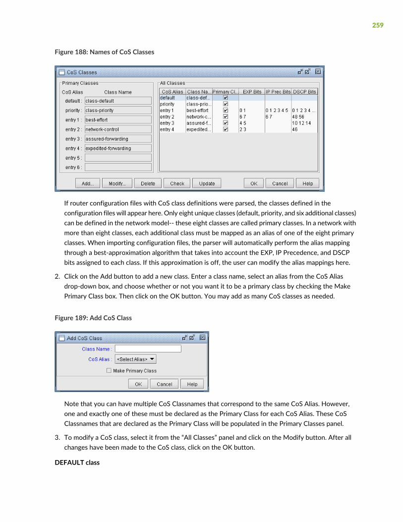
Figure 188: Names of CoS Classes
If router configuration files with CoS class definitions were parsed, the classes defined in theconfiguration files will appear here. Only eight unique classes (default, priority, and six additional classes)can be defined in the network model-- these eight classes are called primary classes. In a network withmore than eight classes, each additional class must be mapped as an alias of one of the eight primaryclasses. When importing configuration files, the parser will automatically perform the alias mappingthrough a best-approximation algorithm that takes into account the EXP, IP Precedence, and DSCPbits assigned to each class. If this approximation is off, the user can modify the alias mappings here.
2. Click on the Add button to add a new class. Enter a class name, select an alias from the CoS Aliasdrop-down box, and choose whether or not you want it to be a primary class by checking the MakePrimary Class box. Then click on the OK button. You may add as many CoS classes as needed.
Figure 189: Add CoS Class
Note that you can have multiple CoS Classnames that correspond to the same CoS Alias. However,one and exactly one of these must be declared as the Primary Class for each CoS Alias. These CoSClassnames that are declared as the Primary Class will be populated in the Primary Classes panel.
3. To modify a CoS class, select it from the “All Classes” panel and click on the Modify button. After allchanges have been made to the CoS class, click on the OK button.
DEFAULT class
259

If traffic does not satisfy the match criteria of other classes included in the policy map, then that traffic istreated as part of the “default” traffic.
PRIORITY class
The entry after “default” would be considered the “priority” class, however it may be changed. The Priorityclass is for priority queueing, which is also called Low Latency Queueing. Packets belonging to the priorityclass are sent before other packets.
You may check to see if there are any errors in the CoS class definitions or any conflicts with CoS policiesby clicking on the Check button.
When done, click OK to submit changes to the server.
DescriptionButton
This checks to verify that all CoS classes are assigned to an alias; all non-empty aliases have aprimary class defined; and that there are no “gaps” between the definition of aliases. For example,if class 3 is defined without having class 2 defined, the program will shift class 3 classes to class2.
Check
This saves the changes made to the CoS class mapping and closes the window.OK
This discards any changes made to the CoS class mapping and closes the window.Cancel
Related Cisco Commands
Router(config) # class-map class-map-name
NOTE: In NorthStar Planner’s modeling, there is no direct specification of class-map matchcriteria such as protocol type, input interface or access group. Instead, traffic modeling with CoSpolicies is accomplished by allowing the user to assign a single CoS class to particulardemands/traffic as described in “Adding Traffic Inputs” on page 268. If a demand/traffic is routedover a particular interface, then it will be treated according to the policies defined for that classin the interface’s policy map, if any.
Create Policies for Classes
SelectModify > QoS > CoS Policies to define CoS policies.
260
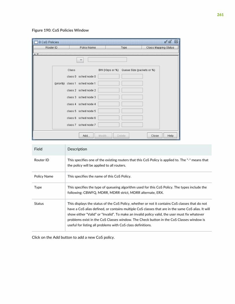
Figure 190: CoS Policies Window
DescriptionField
This specifies one of the existing routers that this CoS Policy is applied to. The "-" means thatthe policy will be applied to all routers.
Router ID
This specifies the name of this CoS Policy.Policy Name
This specifies the type of queueing algorithm used for this CoS Policy. The types include thefollowing: CBWFQ, MDRR, MDRR strict, MDRR alternate, ERX.
Type
This displays the status of the CoS Policy, whether or not it contains CoS classes that do nothave a CoS alias defined, or contains multiple CoS classes that are in the same CoS alias. It willshow either “Valid” or “Invalid”. To make an invalid policy valid, the user must fix whateverproblems exist in the CoS Classes window. The Check button in the CoS Classes window isuseful for listing all problems with CoS class definitions.
Status
Click on the Add button to add a new CoS policy.
261

Figure 191: Add CoS Policy Window
In the previous example there are four defined classes: voice, first_class_data, business_data, andeconomy_data.
This window has the following fields:
DescriptionField
This is a drop down menu that lets the user choose one of the existing routers. “[Any router]”means that the policy will be applied to all routers.
Router
CoS Policy NamePolicy Name
This is a drop down menu that lets the user select the type of queueing algorithm that this CoSpolicy uses: CBWFQ, MDRR, MDRR strict, MDRR alternate, or HWRR.
Type
For each class entry, the user can select the class name to be displayed from the drop down menu.Each drop down menu only contains the class names that have been defined for that particularCoS alias in the CoS Classes window.
Class
262
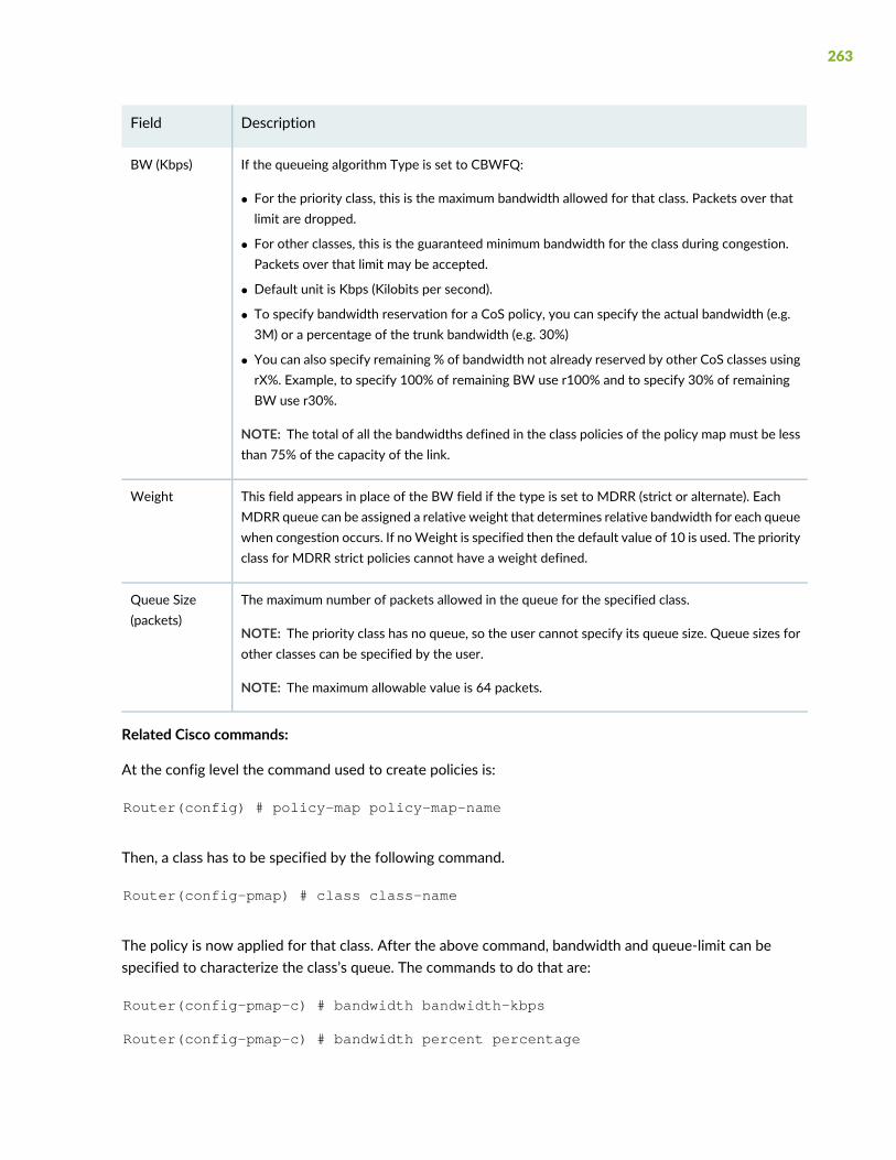
DescriptionField
If the queueing algorithm Type is set to CBWFQ:
• For the priority class, this is the maximum bandwidth allowed for that class. Packets over thatlimit are dropped.
• For other classes, this is the guaranteed minimum bandwidth for the class during congestion.Packets over that limit may be accepted.
• Default unit is Kbps (Kilobits per second).
• To specify bandwidth reservation for a CoS policy, you can specify the actual bandwidth (e.g.3M) or a percentage of the trunk bandwidth (e.g. 30%)
• You can also specify remaining % of bandwidth not already reserved by other CoS classes usingrX%. Example, to specify 100% of remaining BW use r100% and to specify 30% of remainingBW use r30%.
NOTE: The total of all the bandwidths defined in the class policies of the policy map must be lessthan 75% of the capacity of the link.
BW (Kbps)
This field appears in place of the BW field if the type is set to MDRR (strict or alternate). EachMDRR queue can be assigned a relative weight that determines relative bandwidth for each queuewhen congestion occurs. If noWeight is specified then the default value of 10 is used. The priorityclass for MDRR strict policies cannot have a weight defined.
Weight
The maximum number of packets allowed in the queue for the specified class.
NOTE: The priority class has no queue, so the user cannot specify its queue size. Queue sizes forother classes can be specified by the user.
NOTE: The maximum allowable value is 64 packets.
Queue Size(packets)
Related Cisco commands:
At the config level the command used to create policies is:
Router(config) # policy-map policy-map-name
Then, a class has to be specified by the following command.
Router(config-pmap) # class class-name
The policy is now applied for that class. After the above command, bandwidth and queue-limit can bespecified to characterize the class’s queue. The commands to do that are:
Router(config-pmap-c) # bandwidth bandwidth-kbps
Router(config-pmap-c) # bandwidth percent percentage
263

Router(config-pmap-c) # queue-limit number-of-packets
Example:
Router(config) # policy-map policy1
Router(config-pmap) # class class1
Router(config-pmap-c) # bandwidth 3000
Router(config-pmap-c) # queue-limit 30
Router(config-pmap) # class class2
Router(config-pmap-c) # bandwidth percent 10
HWRR Policies
For HWRR policies, the user is presented with a more advanced policy configuration window. BecauseERX HWRR policies can contain multiple levels of scheduler nodes, the user has the ability to define twotypes of objects in the HWRR policy editor: nodes and queues.
Figure 192: CoS HWRR Policy Window - Scheduler Nodes
To Add a Scheduler Node
1. Select the parent node in the left tree under which the new scheduler node will be added.
2. Select Scheduler Nodes from the Hierarchy Type dropdown menu.
264

3. Enter a name for the new scheduler node into the Scheduler Node column.
4. (Optional) Enter a Weight for the new scheduler node.
5. (Optional) Enter a Shaping Rate for the new scheduler node.
6. Click the Add button to add the new scheduler node.
Figure 193: CoS HWRR Policy Window - Queues
To Add a Queue
1. Select the node in the left tree under which the new queue will be added.
2. Select Queues from the Hierarchy Type dropdown menu.
3. Select a class for the new queue from the Class dropdown menu.
4. (Optional) Enter a Weight for the new queue.
5. (Optional) Enter a Queue Size for the new queue.
6. Click OK, or continue editing the policy. The queues are saved automatically.
265

Attach Policies to Interfaces
The last step is to attach policies to interfaces. A link between routers is composed of two interfaces sotwo policies can be attached per link. Click on the Modify > Elements > Links item menu to bring up thelink listing.
Figure 194: Modify Links
Click on the Modify button and select the Location tab to enter the IP addresses and interface names ofthe two end-points, if available.
266

Figure 195: Modify Link Location
Finally, click on the CoS Policy tab to attach policies to interfaces. In <Link>Figure 207 below, you canspecify policies on the Node A and Node Z endpoints of a link. Note that only the CoS Policies that areapplicable to the Node A router will be listed under the Node A Policy drop-down menu, and likewise forNode Z. Recall that in “Create Policies for Classes” on page 260 , the user can specify a particular router or“[Any Router]” for each newly created policy.
Figure 196: CoS Policy for Link Interfaces
267

Related Cisco commands:
At the interface level (config-if) the command to attach a policy to an interface is:
Router(config-if) # service-policy {input| output} policy-map
where input is to indicate the input interface, output for output interface, and policy-map is the name ofthe policy-map defined somewhere else in the config file.
Example:
Router(config) # interface e1/1
Router(config-if) # service-policy output policy1
Adding Traffic Inputs
The user can input traffic information for different classes through the NorthStar Planner client. Whencreating or modifying a particular demand, the user may assign a particular CoS Class to that demand inthe Demand Types window, as explained below. The policies for that class are then applied to thedemand/traffic.
While adding or modifying a demand, click on the Type button in the Demand window. The Demand TypeParameter Generation window will appear. From this window, choose a class from the Policy Class dropdown menu and then click the OK button.
Figure 197: Demand Type Parameter Generation Window
268

Using the Text Editor
You can also manually input CoS parameters into the NorthStar Planner format files via text editors. Thebblink file has to be modified and a new file, policymap, has to be created. For more information on fileformats refer to “CoSAlias File” on page275, “Bblink File” on page275, “PolicymapFile” on page276, “DemandFile” on page 279, and “Traffic Load File” on page 279.
Reporting Module
There are three types of reports providing interface load and queueing delays per Class of Service:
• Demand CoS
• Tunnel CoS*
• Link CoS
NOTE: To get tunnel CoS information, select the Tunnel layer button from the main menu barand then reopen the Report Manager.
• To generate these reports, go to Report > Report Manager.
• Under the Network Reports category, clicking on either the Demand Reports > CoS Demands Reportor the Link Reports > CoS Links Report will cause the following window to appear.
269

Figure 198: Query Window
Before the report is generated, you must first specify three things:
ExplanationDefinitionParameters
Normal traffic means the network does not experience anyfailure/outages. Peak means that failure simulation reports aregoing to be used.
Normal or PeakTraffic Mode
Reports can be issued for all Classes of Traffic or for a particularone (e.g. the Priority class)
All or one specific Class ofTraffic
CoS Classes
Planned means the report is generated using the interface loadcalculated based on the demand file values. Worst means that thereport is generated using the interface load calculated based onthe worst traffic load.
Planned, Worst or AllPeriod
IP Flow Information
After selecting the CoS Report Options, click the OK button and the report will appear as follows.
270

Figure 199: CoS Demands Report
Link information
After selecting parameters on the CoS Report Options window, click the OK button and the report willappear as follows.
271

Figure 200: Link CoS Report
Traffic Load Analysis
Network planners can visualize how network resources are used according to the traffic load input. InNorthStar Planner, there are twoways for the user to view network utilizationwith traffic load informationthrough the NorthStar Planner client:
• Network map color-coded link utilizations
• Traffic load bar charts
You can also supply a “trafficload” file, which specifies measured or predicted traffic loads per demandduring as many as 24 distinct periods. These periods can represent summarized daily traffic (in bits persecond), or hourly traffic, for example. NorthStar Planner can then simulate the load on the links duringeach period.More detail on the format of the traffic load file can be found in “Traffic Load File” on page 279.
Animated Traffic Load Display
To view an animation of traffic load on the network map, select the Utilization Legends > Demand CoSUtil legend. You can choose various options:
• Normal or Peak
272

• Utilization, QDelay or Drop Percentage
• All CoS classes or one particular class
Select a period to update the link colors on the map to reflect the link load that results when the demandtraffic for that period is routed over the network. Link utilization colors can bemodified on the link utilizationmap legend.
Figure 201: Demand CoS Util Legend
Alternatively, find the equivalent options from the Traffic > Traffic Load window. In this window are twoextra ticks on the slidebar for the current load and theworst load. Select Run to automatically step througheach period.
Traffic Load by Policy Class
Bar charts are used to view the traffic load on a link in more detail.
273
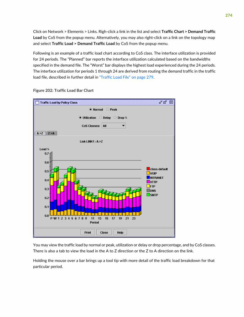
Click on Network > Elements > Links. Righ-click a link in the list and select Traffic Chart > Demand TrafficLoad by CoS from the popup menu. Alternatively, you may also right-click on a link on the topology mapand select Traffic Load > Demand Traffic Load by CoS from the popup menu.
Following is an example of a traffic load chart according to CoS class. The interface utilization is providedfor 24 periods. The “Planned” bar reports the interface utilization calculated based on the bandwidthsspecified in the demand file. The “Worst” bar displays the highest load experienced during the 24 periods.The interface utilization for periods 1 through 24 are derived from routing the demand traffic in the trafficload file, described in further detail in “Traffic Load File” on page 279.
Figure 202: Traffic Load Bar Chart
Youmay view the traffic load by normal or peak, utilization or delay or drop percentage, and by CoS classes.There is also a tab to view the load in the A to Z direction or the Z to A direction on the link.
Holding the mouse over a bar brings up a tool tip with more detail of the traffic load breakdown for thatparticular period.
274

CoS Alias File
Each line of the CoS Alias file lists an alias followed by the associated class names, with the primary classname coming first. An example is:
#Alias Class1 Class2 ...
class-default
class-priority voice
class1 first_class_data gold
class2 business_data silver
class3 economy_data
This can also be accomplished through the NorthStar Planner client in “Define Class Maps” on page 258.
After creating the CoS Alias file the user has to let the system know where that file is. Add in thespecification file the following line:
CoSAlias = CoSAlias_filename
where CoSAlias_filename is the name of the CoS Alias file just created above.
Bblink File
Policy information can be added to the bblink (link) file for a link entry by adding the following into anentry:
POLICY1=policy_name1 POLICY2=policy_name2
where policy_name1 and policy_name2 are names of the policies applied to the interfaces on both sidesof the link, interface_name1 and interface_name2, respectively. This can also be accomplished throughthe NorthStar Planner in “Attach Policies to Interfaces” on page 266. If making thesemodifications throughthe NorthStar Planner client, saving the network environment will automatically update the bblink file.
Example:
#linkname nodeA nodeZ vendor count [ C1= interface_name_1 C2=interface_name_2
] [ IP1=IP_address_1 IP2=IP_address_2 ] [ POLICY1=policy1 POLICY2=policy2 ]
275
Link345 Paris2 London4 DEF 1 C1=Serial2/0/0 C2=Serial5/0/1 IP1=192.10.20.218/30
IP2=192.10.20.217/30 POLICY1=polA1 POLICY2=polZ3
NOTE: There should be no space between the keywords, the equal sign, and the name. Also thenames should not include space.
For example, the following are incorrect specifications:
C1 = Serial2/0/0
C1=Serial 2/0/0
The following is the correct specification:
C1=Serial2/0/0
After creating the bblink file, you need to let the system know where that file is.
There are two ways of pointing to the bblink file:
• Add in the specification file the following line:
bblink = bblink_filename
where bblink_filename is the name of the bblink file just created above.
• In the Spec File Generation window of the NorthStar Planner client, click on the Network Files tab andthen click on bblink button to select or input the bblink file just created above.
Policymap File
The policymap file is used to list the mapping of classes to policies and routers. In the policymap file, thereis one line for each policy of a router. One router can have several policy maps. This policymap file isautomatically created after performing the “Create Policies for Classes” on page 260 in theNorthStar Plannerclient and then saving the network environment.
276

Each line in the policy map file contains information about the policy name, router name, defined classesand class policies (such as bandwidth and queue length). The priority class is always listed before the otherclasses. The format of each record is:
#Type|GlobalParameters|Router|Policyname|PriorityClass,Bandwidth(Kb),-{|Classname,Bandwidth,QueueLength,
bitmap,expbitmap,dscpbitmap,dscpbitmap1,bc,be,pir}
The following table provides the definition of each field (fields are separated by a vertical “|” line):
DescriptionField
The type of queueing algorithm. Valid types are “CBWFQ”, “MDRR”, “MDRR strict”,“MDRR alternate”, “ERX”.
Type
Reserved for future use. This field may be left empty for now.Global Parameters
Name of the router. This corresponds to the Node ID field in the muxloc file. A ‘-’ inthis field indicates ‘Any Router’.
Router
Name of a policy defined for the routerPolicyname
Name of the priority class. This is followed by the bandwidth in Kbps, or themaximumbandwidth of the priority class. For MDRR queueing, this field should be substitutedwith the weight value.The ‘-’ indicates that this field (typically used for queue length)is not applicable for the priority class.
PriorityClass, Bandwidth(Kbps),-
This field defines the policy for each class. It is repeatable for up to 6 classes, notincluding the priority class.
• Classname
• Bandwidth is in kbps. For MDRR queueing, this field should be substituted withthe weight value. It is not necessary to fill in all sub-fields. The dash “-“ tells thesystem to use the default values.
• QueueLength is the size of the queue of the specified class. The unit of the queuelength is the number of packets.
• bitmap and dscpbitmap are fields reserved for future use, and may be left emptyfor now.
Classname, Bandwidth,QueueLength, bitmap,dscpbitmap, expbitmap,dscpbitmap1, bc, be, pir
The priority class is for Low Latency Queueing or Priority Queueing. Packets belonging to this class havehigher priority than other classes. There is no queue limit for this class. That is why there is the dash “-“ inthe third subfield.
Examples:
277
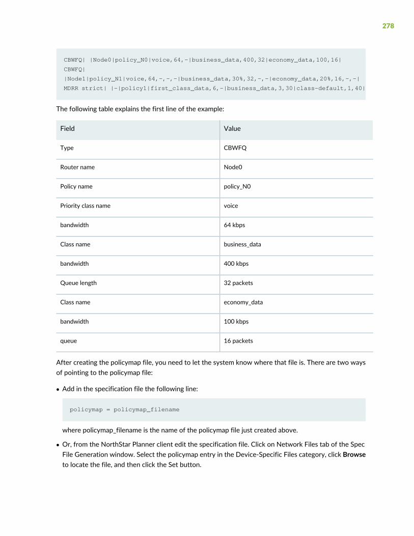
CBWFQ| |Node0|policy_N0|voice,64,-|business_data,400,32|economy_data,100,16|
CBWFQ|
|Node1|policy_N1|voice,64,-,-,-|business_data,30%,32,-,-|economy_data,20%,16,-,-|
MDRR strict| |-|policy1|first_class_data,6,-|business_data,3,30|class-default,1,40|
The following table explains the first line of the example:
ValueField
CBWFQType
Node0Router name
policy_N0Policy name
voicePriority class name
64 kbpsbandwidth
business_dataClass name
400 kbpsbandwidth
32 packetsQueue length
economy_dataClass name
100 kbpsbandwidth
16 packetsqueue
After creating the policymap file, you need to let the system know where that file is. There are two waysof pointing to the policymap file:
• Add in the specification file the following line:
policymap = policymap_filename
where policymap_filename is the name of the policymap file just created above.
• Or, from the NorthStar Planner client edit the specification file. Click on Network Files tab of the SpecFile Generation window. Select the policymap entry in the Device-Specific Files category, click Browseto locate the file, and then click the Set button.
278
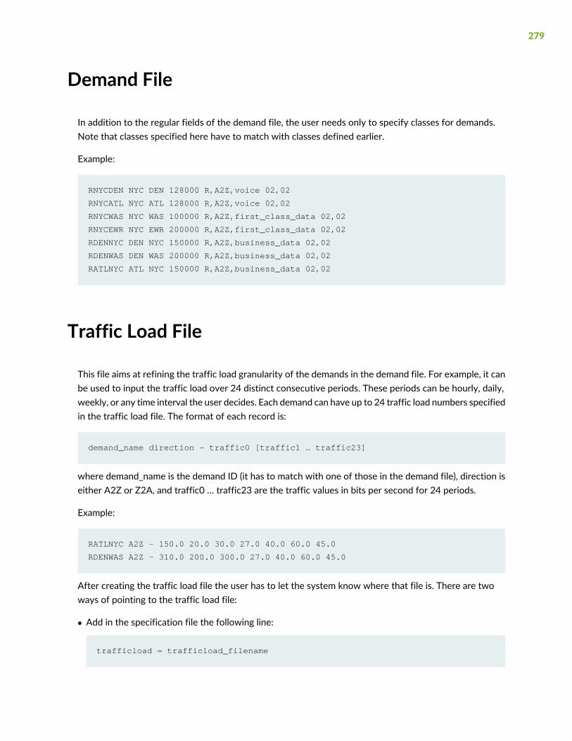
Demand File
In addition to the regular fields of the demand file, the user needs only to specify classes for demands.Note that classes specified here have to match with classes defined earlier.
Example:
RNYCDEN NYC DEN 128000 R,A2Z,voice 02,02
RNYCATL NYC ATL 128000 R,A2Z,voice 02,02
RNYCWAS NYC WAS 100000 R,A2Z,first_class_data 02,02
RNYCEWR NYC EWR 200000 R,A2Z,first_class_data 02,02
RDENNYC DEN NYC 150000 R,A2Z,business_data 02,02
RDENWAS DEN WAS 200000 R,A2Z,business_data 02,02
RATLNYC ATL NYC 150000 R,A2Z,business_data 02,02
Traffic Load File
This file aims at refining the traffic load granularity of the demands in the demand file. For example, it canbe used to input the traffic load over 24 distinct consecutive periods. These periods can be hourly, daily,weekly, or any time interval the user decides. Each demand can have up to 24 traffic load numbers specifiedin the traffic load file. The format of each record is:
demand_name direction – traffic0 [traffic1 … traffic23]
where demand_name is the demand ID (it has to match with one of those in the demand file), direction iseither A2Z or Z2A, and traffic0 … traffic23 are the traffic values in bits per second for 24 periods.
Example:
RATLNYC A2Z - 150.0 20.0 30.0 27.0 40.0 60.0 45.0
RDENWAS A2Z - 310.0 200.0 300.0 27.0 40.0 60.0 45.0
After creating the traffic load file the user has to let the system know where that file is. There are twoways of pointing to the traffic load file:
• Add in the specification file the following line:
trafficload = trafficload_filename
279

where trafficload_filename is the name of the traffic load file just created above
• Or, from the NorthStar Planner client edit the specification file. Click on the Network Files tab of theSpec File Generation window and then select the trafficload entry from the Traffic Files section. Then
click “Browse...” to select the traffic load file and then select the Load button ( ).
280

12CHAPTER
Routing Instances
NorthStar Planner Routing Instances Overview | 283
Routing Instances Recommended Instructions | 283
Creating Routing Instances | 284
Path Analysis | 288


NorthStar Planner Routing Instances Overview
This chapter describes how to use OSPF processes, or routing instances, to partition a backbone networkinto multiple networks which do not talk to each other. Because OSPF process IDs or routing instancenames can be defined per interface, multiple OSPF processes can be configured on each router. Onlyinterfaces in the same process can send packets and routing tables to each other, even if they are on thesame router. Routing Instance rules and OSPF process routing rules affect how demands are routed overthe network.
Use these procedures when you wish to model multiple logical topologies on a single physical network.
RELATED DOCUMENTATION
Routing Instances Recommended Instructions | 283
Routing Instances Recommended Instructions
Following is a high-level outline of the process of using the Routing Instance feature.
• Create, import, or open a router network.
• Create Routing Instances as described in “Creating Routing Instances” on page 284 on .
• Associated Routing Instances with demands or path traces to see how they affect the routing in thenetwork as described in “Path Analysis” on page 288 .
• View the Routing Instance integrity check report in Reports.
283
Creating Routing Instances
1. If you have configuration files for your network, you can import the configuration files to create anetwork model using the File>Import Data menu as described in “Router Data Extraction Overview”on page 33. The interfaces will automatically be associated with the routing-instance or process IDsthat they belong to.
For Juniper routers, the interfaces listed under the [edit routing-instances routing-instance-name] blockwill be assigned that routing-instance-name. Similarly, for Cisco routers, the interfaces whose addressesare advertised under the network statements of the “router ospf <processID>” block will be assignedthat processID.
Note that if an interface is not enabled for OSPF, it will be assigned to a reserved category called“NOPROT”when the network is loaded. Similarly, if the interface is enabled for OSPF but has no processID, it will be assigned to a reserved category called “NOID” when the network is loaded.
To view the associations of routing instances to interfaces, select Network > Elements > Interfaces...When selecting an interface, the bottom pane’s Advanced tabwill show the process ID/routing instancein the OSPF PID field. To view the routing instance as a column of the table, right-click on the headerrow and select Table Options... Then add OSPF PID from the Available Item(s) list to the SelectedItem(s) list.
2. OSPF process IDs (PID) or routing instance names can also be associatedwith interfaces via theModifyInterface window’s Advanced tab for what-if testing, as shown in Figure 203 on page 285. To accessthis window, click the Modify action mode button to switch to Modify mode and then selectModify> Elements > Interfaces. Then select the interfaces you want to modify and clickModify. An OSPFprocess on a Cisco router is an integer number, while an OSPF process on a Juniper router is usually aname.
284

Figure 203: Modify Interface Window
3. By default, multiprocess checking is turned off. To turn on multiprocess checking for routing instanceanalyses, select the Tools >Options >Design, Path Placement options pane and set IgnoreMultiprocessin the lower right corner to “False”. Alternatively, you can add the parameter ignoremultiprocess=0 tothe project’s dparam.runcode file. To turn on multiprocess checking by default for all new networkprojects, create or edit the file /u/wandl/db/misc/dparam.txt and add the line “ignoremultiprocess=0”.
4. To visualize Routing Instances/OSPF PIDs on the map by associating them together with a color, youcan specify a routeinstance file in the specification file as indicated in File Format on page 214 by addingthe entry “routeinst= filename” to the specification file while the network is closed, substituting filenamewith the name of the route instance definition file . This file can also be indicated during a Configurationfile Import (File>Import) by specifying the RouteInstance file on the Misc tab of the Import NetworkWizard. Alternatively, you canmake the association for the current network session by selectingModify> Protocols > OSPF/ISIS Routing Instance from the main menu while in Modify mode.
285

Figure 204: Routing Instance Window
5. Click the Add button, and a new window will appear as shown in Figure 205 on page 286.
Figure 205: Add Routing Instance Window
6. Enter in the routing instance name. Then click Add Row for each OSPF process ID (for Cisco) orrouting-instance-name (for Juniper) that should be mapped to this routing instance.
DescriptionField
The name used to identify the partitioned network.Routing Instance Name
286
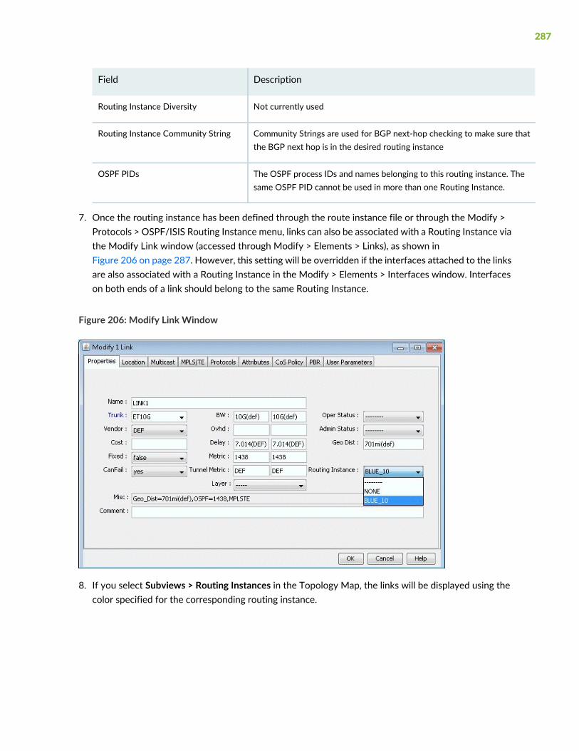
DescriptionField
Not currently usedRouting Instance Diversity
Community Strings are used for BGP next-hop checking to make sure thatthe BGP next hop is in the desired routing instance
Routing Instance Community String
The OSPF process IDs and names belonging to this routing instance. Thesame OSPF PID cannot be used in more than one Routing Instance.
OSPF PIDs
7. Once the routing instance has been defined through the route instance file or through the Modify >Protocols > OSPF/ISIS Routing Instance menu, links can also be associated with a Routing Instance viathe Modify Link window (accessed through Modify > Elements > Links), as shown inFigure 206 on page 287. However, this setting will be overridden if the interfaces attached to the linksare also associated with a Routing Instance in the Modify > Elements > Interfaces window. Interfaceson both ends of a link should belong to the same Routing Instance.
Figure 206: Modify Link Window
8. If you select Subviews > Routing Instances in the Topology Map, the links will be displayed using thecolor specified for the corresponding routing instance.
287

Figure 207: Topology Map - Routing Instance
You can toggle the checkmark next to a routing instance to turn on or off the display of links whoseinterfaces are defined to be in that routing instance. Additionally, you canmodify the color associated witha routing instance on the map by clicking the color box next to the routing instance name.
Path Analysis
To see how Routing Instances affect the routing in a network, assign a Routing Instance to the DemandType of demands (Modify > Elements > Demands) or path traces (Network > Path & Capacity > Path) asshown in Figure 224. This window is accessed by clicking on the Type button of the Modify Demand orDemand Path window. Demands with a Routing Instance assignment can only be routed over links withthe same Routing Instance setting.
288

Figure 208: Demand Type Window
Reports
While in View or Design mode, select Report > Report Manager from the main menu. Select the RouteInstance report from Network Reports > Protocols. This report (RTINSTRPT) displays several integritychecks:
• Asymmetric Route Instance Definition: Indicates links whose interfaces are associated with differentRouting Instances
• Unexpected OSPF process number: Indicates if an unexpected OSPF process number is defined
• SiteDiverse Statistics: An Isolated Site is defined as a site which has the given routing instance configuredon at least one of its routers, but that site is not accessible via this routing instance from outside thesite. A Single Link Site is defined as a site which only has one link of the given routing instance that canbe used to reach the site from outside the site. If that link goes down, there is no other way to accessthat site for this routing instance.
• BGP community definition errors: Indicates if the next-hop for any given community is in a differentRouting Instance
• Isolated colored PoP: Indicates if a Routing Instance has no outgoing link
• Note that routing instance definitions via the routeinstance file or the Modify > Protocols > OSPF/ISISRouting Instance menu are prerequisites to generating the report.
289

Figure 209: Routing Instance Integrity Check Report
File Format
ROUTEINSTANCE File
#name assigned_color OSPF_PID route-instance-name community
blue_10 color=BLUE 10 BLUE community=1234:5678
red_20 color=RED 20 RED community=2345:6789|3456:7890
white_30 color=GREEN 30 NOID
This file should be referenced in the specification file as “routeinst= filename”.
NOTE: Because OSPF process names do not need to be specified for Juniper routers, a specialkeyword “NOID” is used, as seen in the third entry. The keyword “NOID” indicates that theinterface is OSPF-enabled but is not listed in the [edit routing-instances] section for a Juniperrouter
290

13CHAPTER
Traffic Matrix Solver
Traffic Matrix Solver Overview | 293
Traffic Matrix Solver Recommended Instructions | 294
Input Interface Traffic | 294
Input Seed Demands | 297
Running the Traffic Matrix Solver | 298
Viewing the Results | 300
Viewing Differences Graphically | 304
Traffic Matrix Solver Troubleshooting | 305
Additional Traffic Matrix Solver Information | 306


Traffic Matrix Solver Overview
In your network model, a set of end-to-end demands/flows is needed to perform various design andsimulation studies. A few sources, such as Cisco’s NetFlow/TMS, Juniper’s JFlow, LDP traffic statistics,and LSP tunnel traffic statistics from SNMP, can provide end-to-end traffic information. However, this isusually CPU intensive, so the data is often partial. Most traffic collection systems, includingMRTG, Infovista,and Concord eHealth, and NorthStar Planner’s traffic collector, provide interface traffic information. Ifyou only have access to interface traffic data and/or partial end-to-end flow traffic data, you can still derivea reasonable set of end-to-end demands using the NorthStar Planner Traffic Matrix Solver.
NOTE: The NorthStar Planner Traffic Matrix Solver addresses the following problem:
Given (a) the interface traffic utilizations in the network, (b) an optional trafficload file definingthe bandwidth for a subset of the flows in the network, and (c) a set of flows indicating thesources and sinks in the network, determine the bandwidth of these flows to produce the giveninterface traffic utilization values.
This problem has no one right answer.Mathematically, it has infinitely many solutions. However,by supplying a little extra information, you can influence the NorthStar Planner Traffic Matrixsolver to choose a solution that better fits the characteristics of your network. For example, youcan indicate which nodes are sources and sinks of traffic (e.g., edge nodes). The remaining transitnodes will be limited to carrying “pass-through” traffic.
Once a possible traffic matrix solution has been derived, you can perform numerous trafficengineering studies. For example, you can run simulations to study whether the traffic flows canbe rerouted safely during network failures. Or, you can useNorthStar Planner’s design capabilitiesto determine how to optimize cost and reliability for the given traffic. You may have collectedinterface utilization data for multiple periods. For each period, you can compute a set ofend-to-end demands, especially times with heavy usage. Using this data, you can begin to builda picture of how your network traffic changes over time.
RELATED DOCUMENTATION
Traffic Matrix Solver Recommended Instructions | 294
293

Traffic Matrix Solver Recommended Instructions
1. Specify the interface traffic file against which the traffic matrix will be computed as described in “InputInterface Traffic” on page 294. The interface traffic file format is also described in “Input Interface Traffic”on page 294.
2. Optionally, specify already known flow bandwidth as described in Input TrafficLoad File .
3. Create a set of “seed” demands to identify the possible end-to-end pairs whose bandwidths must besolved for as described in “Input Seed Demands” on page 297 .
4. Run T-Solve to compute a traffic matrix that would yield interface traffic results similar to the interfacetraffic file as described in “Running the Traffic Matrix Solver” on page 298 .
5. Compare the load derived from the new traffic matrix against the interface traffic.
Input Interface Traffic
The interface traffic file can have one of the following two formats.
Interface Traffic File Format
#NodeID Interface Direction - Per1 Per2 Per3 ...
NODE3 ATM1/0.1 A2Z - 192320 204960 30263 ...
NODE4 Ethernet0 A2Z - 381 382 539 ...
#LinkName Direction - Per1 Per2 Per3 ...
LINK1 A2Z - 192320 204960 30263 ...
The period data (Per1, Per2, ... Pern) indicates the traffic measured on the interface over several consecutiveperiods. By default, the units is in bits per second. Note that the number of periods is not limited to 24.
Before running the Traffic Matrix Solver, you will be asked to choose the desired period of traffic that theTraffic Matrix tool should try to match when generating its traffic matrix solution.
294

NOTE: For your reference, the first two lines of the ingress or egress interface traffic files usuallyindicate the collection time for the first period of data and the interval (e.g. 5 minutes) betweenperiods, as shown in the following example.
Example Interface Traffic File
#Starting Time : 6/28/07 9:50 PM
#Interval : 5 minutes
NODE11 GigabitEthernet3/0/1 A2Z 0 243836792 239290424 240655400 245699408
253939296 249574480 250319920 247234760 249261400 248431176 246328192 246079952
241803032 245348992 244634288 245710200 242983256 241388720 239512760 238729992
239829624 238082232 234324288 231259912
• After opening the network project, select Traffic > Import Traffic to open the Import Traffic Wizard toconvert data from third-partymeasurements, such asMRTG, InfoVista, Concord eHealth, intoNorthStarPlanner’s format.
• Specify the interface traffic file to use for the traffic matrix computation by switching to View or Designmode. Go to File>Read, click on the “Network Files” tab, scroll down to the “Traffic Files” section of thewindow, and click on either the “egress” (outgoing interface traffic) or “ingress” (incoming interfacetraffic) entry. If both files are specified, the egress file’s value will be checked first. If the value isunspecified in the egress file, the ingress file will then be checked. Browse for the desired file on theserver, and click the blue arrow icon to load it into your network model.
• Once you have loaded the file into your network model and saved your network environment (viaFile>Save Network...), the ingress and egress traffic files will be saved and available the next time youopen that network project, or specification file.
295
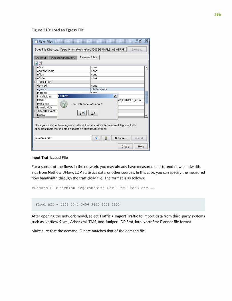
Figure 210: Load an Egress File
Input TrafficLoad File
For a subset of the flows in the network, you may already have measured end-to-end flow bandwidth,e.g., from Netflow, JFlow, LDP statistics data, or other sources. In this case, you can specify the measuredflow bandwidth through the trafficload file. The format is as follows:
#DemandID Direction AvgFrameSize Per1 Per2 Per3 etc...
Flow1 A2Z - 6852 2341 3456 3456 3568 3852
After opening the network model, select Traffic > Import Traffic to import data from third-party systemssuch as Netflow 9 xml, Arbor xml, TMS, and Juniper LDP Stat, into NorthStar Planner file format.
Make sure that the demand ID here matches that of the demand file.
296

Input Seed Demands
The seed demands are used to identify the possible source-destination pairs in the network and providesuggested bandwidth information. Given this information, the Traffic Matrix Solver will assign bandwidthvalues to the demands, such that, when routed over the network, these demands produce link utilizationsthat closely match a period of the user-specified measured interface traffic data.
Some of the flows you may already have the information for, and these can be entered into the trafficloadfile discussed in the previous section. A corresponding demand entry with the same DemandID should beincluded in the demand file.
For any other flows, for which you do not have bandwidth information for, you can also enter them intothe same demand file. Alternatively, to keep things better organized, it is recommended to separate bothsets of flows into two separate demand files, “demand” and “newdemand”, with one file for the flows withknown bandwidth, and the other file with the flows whose bandwidth are to be derived.
When defining the flows that need to be solved for, information or assumptions regarding the trafficpatterns of these demands in the network can help to provide a more accurate traffic matrix. For example,if you have a good idea which nodes are the source and sink (origination and termination) nodes of thetraffic, you can create a full mesh between only those source and sink nodes to create a more limited setof “test” demands. In this way, the traffic solver will avoid creating originating or destinating traffic attransit routers. For example, if the traffic sources and sinks are in the edge routers, but not in the corerouters, you can create a full mesh of flows between those edge routers. For VPNs, you might want touse only the Provider Edge (PE) and Customer Edge (CE) routers as sources and sinks, assuming that theProvider (P) routers are transit routers where almost all the traffic is pass-through, with very little originatingor terminating traffic. The instructions in the next section indicate how to create a full mesh of demandsbetween a set of nodes, such as the PE’s.
Additionally, if you have some idea of the relative bandwidth proportions for different demands, you canalso enter in suggested bandwidths. This bandwidth information will be used to create a “shaping” matrixagainst which possible solutions will be compared. The shaping matrix (Src x Dest) will indicate thepercentage of traffic to different destinations. If you have no assumptions to make here, you can set thebandwidths to be the same, e.g., 1k bandwidth.
Creating a Full Mesh of Demands
297

1. To create a full mesh of demands between traffic sources and sinks, switch to Modify mode and selectModify > Elements > Demands, Add > Multiple Demands.... Select the source and destination nodesfrom the Node A and Node Z boxes, respectively. You can filter on special criteria using the Adv Filter...button, e.g., using the criteria “isPE = true” to select the PE routers. Select “Populate Destination IP.”Then, enter in a bandwidth, such as 1k. Note that this will be overwritten after running the traffic solver.
2. If you want to provide different bandwidths to different demands, you can select multiple demandsfrom the Network window, Demands view pane, and selectModify > Selected... to modify theirbandwidth.
3. Note : If you have made any modifications to your currently loaded demand file during this networksession, you may wish to save a copy of your demand file before using the Traffic Matrix tool. TheTraffic Matrix tool will modify the bandwidth of demands in your network. To save your networkenvironment, go to File>Save Network.... To save just the demand file, go to File>Save NetworkFile>Demands....
4. If you have an already created demand or newdemand file, you can also read it in from File > LoadNetwork Files and save the network so that you do not have to read it in again each time you open upthe network. Alternatively, you can edit the specification file to add the line “demand = <path>”substituting <path>with the location of the demand file, or “newdemand = <path>” substituting <path>with the location of the newdemand file.
Unplaced Test Demands
If there are a significant number of demands which are unplaced, it is an indication that there may be somerouting issues that need to be resolved first before proceeding. Go to Network > Elements > Demands,press the Search (magnifying glass) icon and search for just Unplaced demands. Select one of the unplaceddemands and press the Show Path button to highlight the route. Any bottleneck information or clues willbe displayed in the Console.
Running the Traffic Matrix Solver
1. Click the Design button to switch to Design mode and then select Design > T-Solve.
298
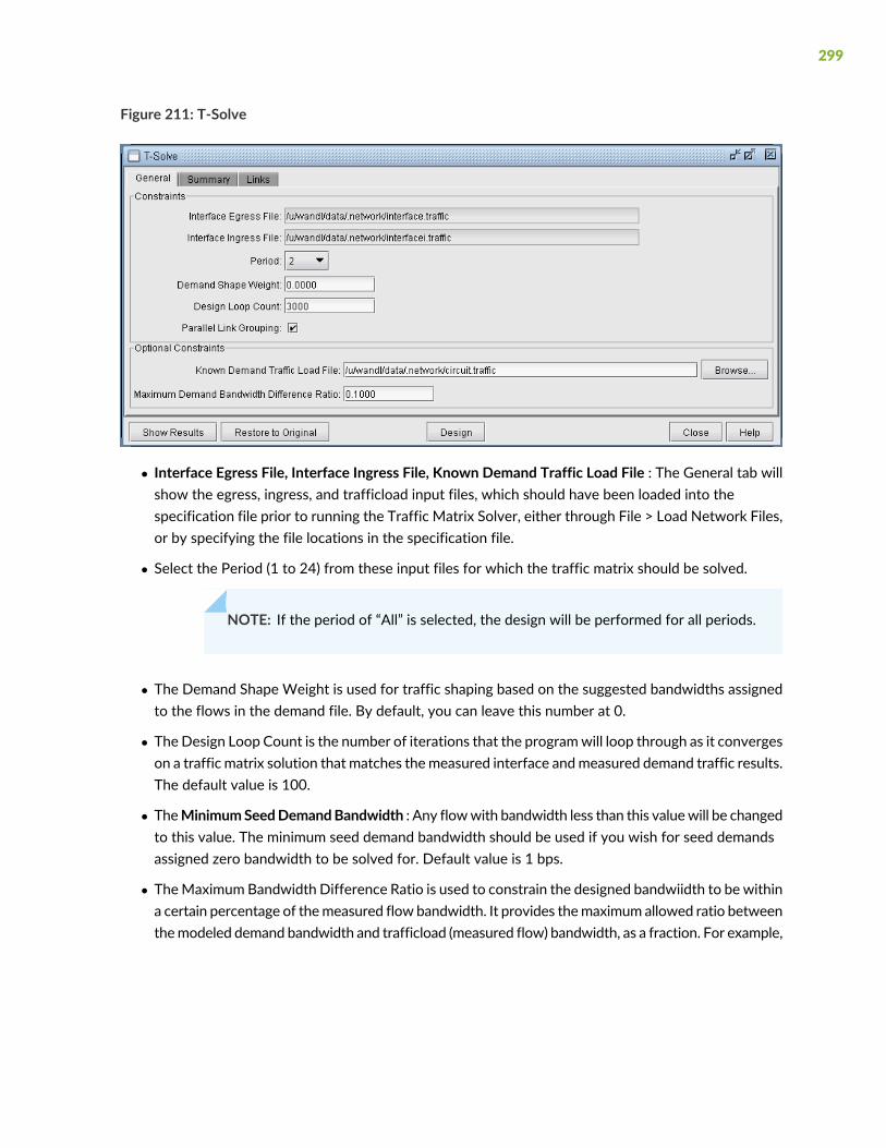
Figure 211: T-Solve
• Interface Egress File, Interface Ingress File, Known Demand Traffic Load File : The General tab willshow the egress, ingress, and trafficload input files, which should have been loaded into thespecification file prior to running the Traffic Matrix Solver, either through File > Load Network Files,or by specifying the file locations in the specification file.
• Select the Period (1 to 24) from these input files for which the traffic matrix should be solved.
NOTE: If the period of “All” is selected, the design will be performed for all periods.
• The Demand Shape Weight is used for traffic shaping based on the suggested bandwidths assignedto the flows in the demand file. By default, you can leave this number at 0.
• TheDesign Loop Count is the number of iterations that the programwill loop through as it convergeson a traffic matrix solution that matches themeasured interface andmeasured demand traffic results.The default value is 100.
• TheMinimumSeedDemandBandwidth : Any flowwith bandwidth less than this valuewill be changedto this value. The minimum seed demand bandwidth should be used if you wish for seed demandsassigned zero bandwidth to be solved for. Default value is 1 bps.
• TheMaximumBandwidth Difference Ratio is used to constrain the designed bandwiidth to be withina certain percentage of themeasured flow bandwidth. It provides themaximum allowed ratio betweenthemodeled demand bandwidth and trafficload (measured flow) bandwidth, as a fraction. For example,
299
0.1 would be used for 10% and 0.2 for 20%. You can use -1 for “don’t care” for the first iteration. Ifyou trust the measured flow bandwidth, you can set this ratio to 0.
2. After entering in the desired parameters, the TrafficMatrix tool is now ready to compute the bandwidthsto assign to the demands in the network. Click the Design button to begin.
3. If one of the provided inputs is the trafficload file, you will be prompted with a question such as thefollowing: “Set demand bandwidth to traffic load at period <n>?” Answer “Yes” if you wish to initializethe demand bandwidths to the bandwidths given by the traffic load file for the selected period. Answer“No” if you wish to use initialize the demand bandwidths to the seed demand bandwidths. For eitheranswer, the program will still take the trafficload file into account. Note that this initial demand matrixwill also be used to derive the shaping matrix.
4. After running the design, check the results as described in the following sections. If you want to laterundo the changes and restore the original state prior to running the traffic matrix solver, click the“Restore to Original” button.
Viewing the Results
Trafficload
If the period “All” was designed for, then not only will the demands be updated, but also the trafficloadfile which includes the designed bandwidth of the demand for multiple periods. The T-Solve window willonly display the results for the final period. However, the per-period results can be viewed per link afterthe design by right-clicking the link on the map and selecting Traffic Load > Interface vs Demand. SelectBar/Line to view the chart as a line chart. This chart will show howwell the utilization based on the designedtrafficload bandwidth matches with the actual interface load.
300

Figure 212: Trafficload Window
Save the network to a new directory using File > Save Network... Navigate to this directory in the FileManager and open the designed trafficload file to see the bandwidths designed for each period.
Console
Intermediate results will be displayed in the console. In each successive iteration, the program attemptstominimize the cost function, which is based on the linkDiff + shapeweight * shapeDiff, where the linkDiffis a function of the sum of the differences between measured interface traffic and an interface’s totaldemand bandwidth over the sum of the link bandwidths.
The following information is also indicated to provide warnings regarding incomplete data. The linksindicated below will not be considered into the cost function. These should be checked to see if that isthe desired behavior or not, or if additional information can be supplied.
• #link_interface without traffic and demands=n : Indicates number of links with no seed demands normeasured interface traffic.
• #link_interface without traffic=n : Indicates number of links with seed demands routed over it, but nomeasured interface traffic.
• #link_interface without demands=n : Indicates number of links with measured interface traffic, butwithout seed demands routed over it. If these are links that are important, then it may be a good ideato add the appropriate flow(s) that goes through this link into the demand file. In some cases, however,you may not worry about the link, in which case it can be ignored. For example, this might be the case
301

if you are only concerned about running designs and simulations for Area 0 traffic and link loading, butthis is a link in a different area.
Reports
After the iterations are completed, the following output files will be saved to the server:
• TMLINK.runcode : The Tomogravity Link Traffic Comparison Report provides information (per link)regarding differences between measured interface traffic and the interface’s total demand load (seeLinks Tab)
• TMShape.runcode : The Tomgravity Demand Traffic Shape Report provides information regarding theshape matrix and the traffic matrix.
• TMPATH.runcode : Provides Path Placement and bandwidth Information
• TMLOAD.runcode : The T-solve Demand Bandwidth vs Demand Load Comparison Report providesinformation (per flow) about the difference between model demand bandwidth and measured demandbandwidth from the trafficload file
Once complete, selectNetwork > Elements >Demands to view the changed demand bandwidths assignedby the Traffic Matrix Solver.
Summary Tab
Click the Summary tab to see a summary of the statistics from the links tab.
• overallFit : Sum of the absolute differences between the measured interface traffic and interface’s totaldemand load divided by the sum of the measured traffic plus geometric mean of the measured andmodeled traffic. Note that the results are independent of the link bandwidth.
• formula : overallFit = |measured traffic - demand| / [measured traffic + SQRT (measured traffic * modeledtraffic)]
• For example, a 10G link between two nodes with measured interface traffic 5G for both interfaces onthat link and 8G bidirectional demand over the link. In this example the absolute difference is |5G - 8G|= 3G. The geometric mean is SQRT(5*8) = 6.325. Thus the overallFit = absolute difference / (measuredtraffic + geometric mean) = 3/(5 + 6.325) = 0.2649 = 26.49%.
• ShapeError : The shaping error is based on a comparison the shaping matrix derived from normalizingthe seed demands’ bandwidth matrix, against the shaping matrix derived from normalizing the demands’new bandwidth matrix.
• WorstLinkDiff : Indicates the largest difference between themeasured andmodel utilization percentage,i.e., the highest value for Abs Diff Util % in the Links tab.
When evaluating the fit of the new traffic matrix to the interface traffic file, the linkDiff provides anaveraged difference, and the worst link diff provides the worst case difference for a particular link. Ideally,these two numbers should be as close to zero as possible.
Links Tab
302

Select the Links tab of the T-Solve window.
Figure 213: Links Tab
Here, you can view statistics comparing the original measured interface traffic file (Measured Traffic andMeasured Util %) with the traffic load and utilizations computed based on the set of end-to-end demands(Model Traffic and Model Util %).
• Name : Link’s name
• Direction : A2Z or Z2A direction of the link
• Node,Interface : The node and interface corresponding to the given direction on the link
• Remote Node : The other end node of the link
• Type : The link’s Trunk Type
• KnownModel Traffic : Traffic load on the link based onmeasured flow bandwidth (based on the trafficloadfile)
• Measured Traffic : Traffic load on the link according to measured interface traffic file (based on theegress/ingress files)
• Diff Traffic : The difference betweenModel Traffic andMeasured Interface Traffic. Note that the values-1, -2, -3, and -4 have special meanings here: “-4” means that there is measured interface traffic, butmodel traffic is 0, “-3” means that there is model traffic, but measured interface traffic is 0, “-2” meansthat there is model traffic but measured traffic is missing, and “-1” means the model traffic is 0, butmeasured interface traffic is missing.
• Measured Util % : Percentage Utilization of the link according to measured interface traffic file (basedon the egress/ingress files)
• Model Util % : Percentage Utilization of the link according to the sum of bandwidth of demands overthe link (based on the demand file0
• Diff Util % : Model Util % - Measured Util %
• Abs Diff Util % : The absolute value of Diff Util % (This number will always be positive)
303
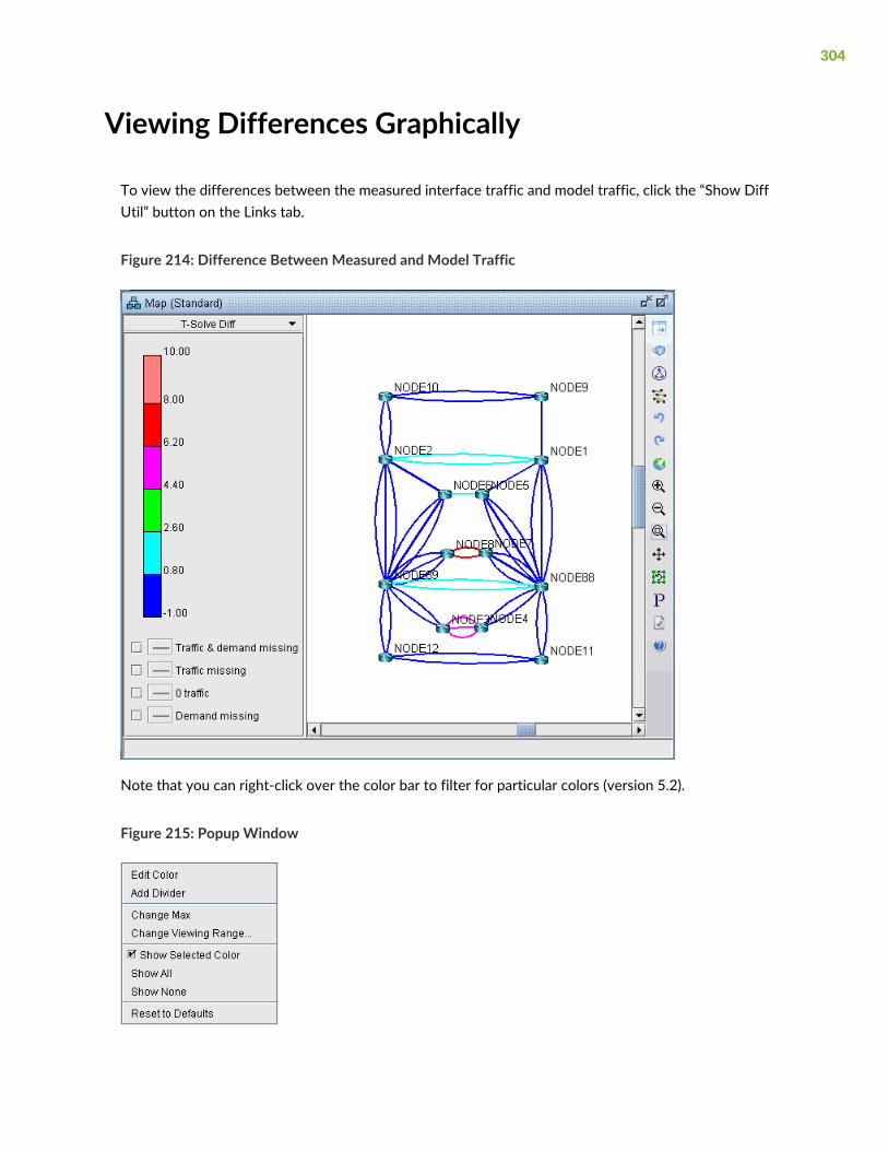
Viewing Differences Graphically
To view the differences between the measured interface traffic and model traffic, click the “Show DiffUtil” button on the Links tab.
Figure 214: Difference Between Measured and Model Traffic
Note that you can right-click over the color bar to filter for particular colors (version 5.2).
Figure 215: Popup Window
304

• Show Selected Color : Toggles the display of this color.
• Show All : Shows all colors
• Show None : Hides all original colors, showing gray instead
For example, you can first select “Show None” and then right-click the topmost color and select “ShowSelected Color” to see the links with the most differences.
The legend at the bottom also allows you to graphically view the links for which there is missing data.
• Traffic & demand missing : Both measured interface and model traffic are missing
• Traffic missing : Measured interface traffic is missing, but not model traffic
• 0 traffic : Measured interface traffic is zero
• Demand missing : Measured interface traffic is present, but no demands are routed over the link
Traffic Matrix Solver Troubleshooting
If theWorstLinkDiff is high, e.g., over 10%, you should analyze the Links tab. Sort on the Diff Util % Columnto see the links with the worst link diffs. You can select the rows for these links and click the Highlightbutton to highlight the links on the map, and to check for reasons why the difference is high.
If “Measured Traffic” (actual load) on a link is extremely high but the traffic matrix tool places 0 traffic onthat link (Model Traffic), this may be an indication of a routing scenario that needs to be resolved beforeproceeding. That is, you need to determine why the system is not routing any flow across that link. Thereare numerous possible reasons, and it varies from network to network. For example, there may be toomany parallel links in part of the network, but the ECMP value is set too low.
The typical way to troubleshoot is by using the “P” Path button on the Map window, or via Network >Path & Capacity > Path, selecting two points, and analyzing the source of the bottleneck.
In some cases, you may have supplied an inaccurate set of sources and sinks. That is, the sources and sinksyou specified for the traffic matrix flows does not match the locations where traffic is present, as indicatedby your interface traffic file. Please consider adding a larger mesh of demands.
There can also be problems if the interface traffic data that you supplied is unknown or “0” on the vastmajority of interfaces and the test demands are placed on these links. In this case, there is insufficient datato solve for a traffic matrix solution. Please check your interface traffic file.
Another problem is if you did not add seed demands to the network. You can do so either by loading inthe demand file via File>Read, or adding more demands into the network using Modify > Elements >Demands. Once this is done, restart the Traffic Matrix operation.
305
Additional Traffic Matrix Solver Information
Choosing a Period of Interface Traffic
Which period of interface traffic data should you use? Currently, it is recommended to select a few periods(for example, include one during general heavy load and one at light load), and run the Traffic Matrix toolonce for each set of traffic data to create a couple different sets of end to end flows.
Avoid choosing the period called “Worst,” as the worst/peak casemay occur at different times for differentlinks, which is not as suitable for the Traffic Matrix tool. Rather, it is better to determine a few specificperiod numbers for which the loading was heavy.
There are a few ways to load traffic data into the network model. Note that the following applies to thoseusers who use the online module / NorthStar Planner Traffic Data Collectors to collect live traffic:
• If you created your initial network project by saving it out from the live network view (File > SaveNetwork), then the last 24 samples of traffic data at the time you saved it out will already be recordedin the default interfaceTraffic.in and interfaceTraffic.out ingress and egress files associated with yournetwork project
• If you have existing ingress and egress traffic files, you can read them in via File > Load Network Files(specify them in the Traffic Files section)
• To retrieve historic traffic data, in View orDesignmode, go to Traffic > Traffic Load, and select “Interface”.Select the “Start From” time and press “Fetch”. At this point, if you do File > Save Network, thecorresponding interfaceTraffic.in and interfaceTraffic.out files will be created. Then, close and reopenthe network project, or else use File > Load Network Files to load in the interface traffic files, beforeproceeding to the Traffic Matrix tool.
If you do not have the online module or an interface traffic file, but want to generate one based on thecurrent network demands, select Traffic > Traffic Matrix > Save Interface Traffic.
Resetting Demand Bandwidth According to Demand Trafficload File
At any point in time you can reset the demand bandwidths to be the same as that of a specified period ofthemeasured demand bandwidth in the trafficload file. Any demand that does not havemeasured demandbandwidth will not be changed in this process.
To do this, first select the General tab and select the desired Period of the Traffic Load File. Then click“Show Results.” A popup window will show how many demands have a current model bandwidth that isdifferent from the measured demand bandwidth.
When asked to update the different entries, click Yes in order to update the model bandwidths to beexactly the same as the specified period of the traffic load. The Summary tab will be updated to reflectthe changes.
306

Note that during the design, if you had set theMaximumBandwidthDifference Ratio between themodeleddemand bandwidth and themeasured trafficload bandwidth to 0, then there should not be any differenceswhen clicking “Show Results” if you are using the same trafficload period.
Traffic Matrix Parameters
The following parameters can be added to your project’s dparam file to stop the TrafficMatrix Solver whenthe solution is deemed good enough or if not enough improvements can be found per iteration.
• TM_linkdiff = <ratio> : Stop earlier than the loopcount if the target LinkDiff is reached ( the differencebetween calculated demand traffic load and measured link used bandwidth.)
• TM_minimprovement = <number> : Stop earlier than the loopcount if the improvement per iteration isless than this number for 100 iterations
307
14CHAPTER
LSP Tunnels
NorthStar Planner LSP Tunnels Overview | 311
Viewing Tunnel Info | 311
Viewing Primary and Backup Paths | 312
Viewing Tunnel Utilization Information from the Topology Map | 313
Viewing Tunnels Through a Link | 314
Viewing Demands Through a Tunnel | 315
Viewing Link Attributes/Admin-Group | 316
Viewing Tunnel-Related Reports | 317
Adding Primary Tunnels | 319
Adding Multiple Tunnels | 320
Mark MPLS-Enabled on Links Along Path | 322
Modifying Tunnels | 322
Path Configuration | 323
Specifying a Dynamic Path | 324
Specifying Alternate Routes, Secondary and Backup Tunnels | 326

Adding and Assigning Tunnel ID Groups | 330
Making Specifications for Fast Reroute | 333
Specifying Tunnel Constraints (Affinity/Mask or Include/Exclude) | 334
Adding One-Hop Tunnels | 339
Tunnel Layer and Layer 3 Routing Interaction | 342

NorthStar Planner LSP Tunnels Overview
This chapter describes how to view andmodify Label Switched Path (LSP) tunnel information usingNorthStarPlanner. This includes secondary/standby and backup paths, affinity andmask. If you have aMultiprotocolLabel Switching (MPLS) network, then you should familiarize yourself with this chapter.
NOTE: If you wish to perform this task in the NorthStar Planner client, you should have a routerspecification file open before you begin. To follow along with this tutorial, you can open thespec.mpls-fish specification file located in your $WANDL_HOME/sample/IP/fish directory($WANDL_HOME is the program’s home directory. It is /u/wandl by default).
RELATED DOCUMENTATION
Viewing Tunnel Info | 311
Viewing Primary and Backup Paths | 312
Viewing Demands Through a Tunnel | 315
Adding Primary Tunnels | 319
Modifying Tunnels | 322
Viewing Tunnel Info
Load the /u/wandl/sample/IP/fish/spec.mpls-fish network example if you wish to follow along with thistutorial. When prompted, “Update demand routing tables?”, press “Yes”.
In View or Design action mode, select Network > Elements > Tunnels. Right-click a tunnel to view thevarious options available for tunnels.
311

Figure 216: All Tunnels Window
Click the “Show Path” button to see the tunnel highlighted on the map, including all defined routes.
NOTE: If more than one tunnel are selected, only their primary paths will be highlighted togetheron the map.
In the resulting path window, there will be 2 colors, including a special color for the currently highlightedtunnel in the path window.
Viewing Primary and Backup Paths
To view primary and backup tunnels together on the map, select an entry from the Tunnels window thatis a primary tunnel (not marked Standby in the Type column), right-click and select Show Path. By defaultboth tunnels are shown highlighted. To highlight only one path at a time, change from Highlight All Pathsto Highlight a Selected Path.
312

Figure 217: Tunnel Paths on Map
The diverse paths of a tunnel can also be viewed from Network > Elements > Tunnels Diverse Status orDesign > TE Tunnels > Path Design in Design mode and tunnel layer.
From the Diverse Path Design window, Check the “Div Level” column to see the current level of diversitysatisfied between primary and backup paths.
Select a tunnel and click “Show Paths” to view the primary and backup tunnels.
Select “Hide Unrelated Nodes” to display only those nodes and links which are on the primary and backuptunnels.
Figure 218: Show Primary and Backup Paths
Viewing Tunnel Utilization Information from theTopology Map
Select the Tunnel layer button from themainmenu bar. On themapwindow left pane, select the UtilizationLegends > Planned Util menu item. Because of the low planned link utilization of tunnels in this example,
313

you will need to adjust the dividers in the Planned Util legend in order to see any color differentiation onthe map.
Figure 219: Planned Tunnel Utilization (Tunnel Layer View)
• Tunnel BW / Link BW : Displays the sum of the configured bandwidths of the tunnels over the link,divided by the link bandwidth.c
• Tunnel BW / RSVP BW : Displays the sum of the configured bandwidths of the tunnels over the link,divided by the link’s configured RSVP bandwidth.
Viewing Tunnels Through a Link
Right-click on a link on the map or in the Network Info window with a planned utilization greather than 0and select View>Tunnels on/thru Link.
The example below shows tunnels through the CHI-WDC link. Select the Actionsmenu at the upper righttofurther filter the tunnels according to direction.
314
Figure 220: Tunnels through Link Window
Viewing Demands Through a Tunnel
To view all demands routed over a tunnel, right-click over the tunnel and select Show Demands Routedon Tunnel.
In theDemandswindow, examine the Current Route columnwhich indicates the path taken bythe demands.Open and closed brackets in the path indicate where a tunnel is entered and exited.
Figure 221: Demands (or Flows) Routed Through a Particular Tunnel
315

In Figure 221 on page 315, the selected demand between HOU and NYC. has the routeHOU[--DAL--CHI--]WDC--PHI--NYC, indicating that the demand traversed a tunnel fromHouston (HOU)to Washington D.C. (WDC).
Clicking on “Show Path” displays the path of the demand on the map. Notice that a purple color is usedto indicate the portion where the demand is travelling through a tunnel.
Figure 222: Path of Demand Through a Tunnel
Viewing Link Attributes/Admin-Group
Select theMap legend: Subviews > Attributes/Admin Group to view the links’ RSVP resource group/color,also known as link attributes for Cisco, and admin-group for Juniper.
The legend can be used to filter themap display to show only links that satisfy a particular criteria, comprisedof logical “all”, “or” and “not” operations.
• To display links which satisfy one specific color, select under the “all” column only the checkbox for thatcolor.
• More complicated logical combinations can also be specified. For example, selecting “red” and “yellow”under the any column and “green” for the “not” column, will filter the display to show only links thathave red or yellow color and do not have green.
316
Figure 223: Attributes/Admin Group Legend
An alternative way to input the filter criteria is via the “all”, “any”, and “not” hexadecimals in the Controlsection at the bottom of the legend. This corresponds to Juniper’s “include-all”, “include-any”, and “exclude”statements. After typing in the full hexadecimal, press the <Enter>/<Return> key to load the change onthe map.
A Cisco tunnel’s affinity/mask requirements can be translated into “all” or “not” criteria. If the mask is “1”for a bit, then an affinity of “1” for that bit would translate into an “all” for that bit and an affinity of “0”for that bit would translate into a “not” for that bit.
Viewing Tunnel-Related Reports
The following lists and describes the tunnel-related reports accessible from the Report Manager (Report> Report Manager).
DescriptionReport/Category
Displays each of the tunnel’s requirements and routed path specification.Tunnel Path & Diversity
Displays the calculated cost for each tunnel in the network based on the sum of thelink costs.
Tunnel Route Cost
Displays the values of the reserved tunnel bandwidth verses the flow bandwidthand their difference ratio.
Demand Traffic on Tunnel
317

DescriptionReport/Category
This report has to do with multiple-period traffic load on the tunnels.Tunnel Traffic
This report breaks up each tunnel into each interface segment of the tunnel path.Tunnel-Link
• Link: Displays the Amount of Link RSVP bandwidth used by tunnels per link
• Node Pair: Displays the Amount of Link RSVP bandwidth used by tunnels pernode pair
Tunnel RSVP BW on Link
Tunnel RSVP BW on Node Pair
Compares aggregate tunnel traffic load versus the measured interface traffic.Tunnel Traffic vs InterfaceTraffic
This report breaks up the link bandwidth into partitions (RSVP and GB=GuaranteedBandwidth, GlobalPool and SubPool, or CT partitions for DiffServ-TE) and showsthe tunnel bandwidth for each partition.
Link Partition
In the live network mode, this report provides the aggregate tunnel traffic load onthe link.
Per Node Pair (Measured): In the live network mode, this report provides theaggregate tunnel traffic load on the node pair.
Measured Link Util (based onT_trafficload)
Per Node Pair (Measured)
Found under Tunnel Layer Simulation Reports > Tunnel Layer Network Statistics,This report is only useful after having run a failure simulation on the network. Displaysthe peak utilization of the links that is reserved by tunnels.
Peak Tunnel Traffic on Links
• Group Tunnel Summary by Group Pair: Displays summary information for tunnelsbetween two groups.
• Group Tunnel Detail by Group Pair: Displays detailed information for each tunnelthat is between two groups or within one group.
• Group Tunnel Traffic on Link Summary: Displays summary information on tunneltraffic between two groups or within one group.
• Group Tunnel Traffic on LinkDetail: Displays detailed information for tunnel trafficthat is between two groups or within one group.
• Group Interface Load Summary: Displays summary information between interfacesof nodes in two groups or within one group.
• Group Interface LoadDetail: Displays detailed information between each interfacepair where the nodes are in two groups or within one group.
• Group Tunnel Bandwidth Distribution: View the distribution of Originating,Terminating, Transit, and Local tunnel bandwidth
Tunnel Layer Group
318
DescriptionReport/Category
Found under Tunnel Layer Network Reports >Node, this report provides informationon local, non-local and transit tunnels at each node. A local tunnel is one that startsand ends at itself, and a non-local tunnel is one that originates or terminates at thenode.
Planned Tunnel RSVP BW PerNode
Found under Tunnel Layer Network Reports > Node, this report provides measuredinbound and outbound traffic per node.
Measured Tunnel Traffic PerNode
Adding Primary Tunnels
To switch to modify mode, click on “Modify” mode button. The Modify pull-down menu gets activated.
SelectModify > Elements > Tunnels from the Modify pull-down menu. In the Tunnels window, click Addand select One Tunnel. The Add Tunnel window is displayed as shown in Figure 224 on page 319.
Figure 224: Add Tunnel Window
In the Properties tab, specify a TunnelID, the BW (bandwidth) for the tunnel, and the Pri,Pre (setuppriority/holding priority) fields. Also select the source and destination nodes (Node A and Node Z).
In the Paths tab, Note the different ways of configuring a path under the To choose paths field.
319

Figure 225: Different Methods of Choosing Paths
How to specify a configured and/or dynamic route is described later in this chapter.
After you have specified your route, click “Add” to add the tunnel. A yellow line between the source anddestination will be drawn on the map to represent the logical tunnel. Note that the routing of the tunnelhas not been performed yet.
Adding Multiple Tunnels
The Add Multiple Tunnels window can be used to add a mesh of tunnels between two sets of nodes.
SelectModify >Elements >Tunnels, Add>Multiple Tunnels from theModify pull-downmenu. Alternatively,select Add>Multiple Tunnels from the Network Info window Tunnels view. An Add Multiple Tunnelswindow should appear, similar to the one shown below.
320

Figure 226: Add Multiple Tunnel Window
The generated tunnel nameswill consist of a prefix defined in the Tunnel ID (Prefix) field and an incrementingnumber that starts with the number specified in the Tunnel ID (#) field. If no start number is specified, thetunnels will be named according to the NodeA and NodeZ endpoints.
Various options can be configured in the top right section of thewindow, including BW, Type, Affinity/Mask(Cisco) or Include-All/Exclude/Include-Any (Juniper), Pri,Pre (setup priority/holding priority), Service, Path.Config. Options, and a user definable Comment field.
A tunnel will be created for each NodeA - NodeZ pair defined in the bottom half of the window whereNodeA is the source and NodeZ is the destination. The NodeA and NodeZ boxes can populated using theFilter or Filter From Map button. The Filter button opens a Find Nodes window to specify what nodes toadd. The Filter From Map button adds the nodes highlighted on the map. The Remove button removesthe selected node(s) from the Node A or Node Z list.
The Copy A-> Z button copies the nodes that are on the Node A list to the Node Z list. As a shortcut, usersmay also select a particular category from the Type menu in the Placement (A * Z) section such as Group,Area, VPN, orMulticast Group. This will activate the drop-downmenu(s) above the the NodeA and NodeZboxeswith available entries for the selected category. Selecting an entry from the selectionwill automaticallyupdate the NodeA and NodeZ boxes.
The Create tunnels in both directions option will generate an additional full mesh of tunnels from Z to A.This option is useful when the Node A and Node Z list are not the same. Selecting the Incremental Full
321

Mesh option is recommendedwhen there is overlap between theNode A andNode Z list, to avoid creatingmore than one tunnel for the same source-destination pair.
The Incremental Full Mesh option will only generate tunnels needed for the full mesh.
Note that you can also choose to create an incremental full mesh for tunnels within a particular tunnel IDrange. To do this, first create a Tunnel user parameter and tunnel ID group based on that user parameterbefore opening the AddMultiple Tunnels window as discussed in “Adding and Assigning Tunnel IDGroups”on page 330. Then select the User Parameters tab of the Add Multiple Tunnels window and select thattunnel ID group. Tunnels will be treated as already existing in themesh if they have a source and destinationlisted in the Placement section and they are named “Tunnel<id>” where <id> is a number within the IDrange of the selected tunnel ID group.
Mark MPLS-Enabled on Links Along Path
When tunnels are placed by the routing engine, it checks the protocol on the link to determine if it ismpls-enabled to allow placement of the tunnel. Onemethod of setting a link to bempls-enabled is throughthe Modify Tunnel window. Switch to Modify mode and selectModify > Elements > Tunnels to open theModify Tunnel window. Choose a tunnel, right-click, and select “MarkMPLS-enabled on links along path.”This will set all links as mpls-enabled on the first Configured Route. If the first Configured Route is dynamic,then no links will be set as mpls-enabled.
Modifying Tunnels
To modify a tunnel, selectModify > Elements > Tunnels from the Modify pull-down menu. To modify asingle tunnel, select the tunnel from the table and click “Modify”. If multiple tunnels all require the samemodification, then select those tunnels in the table (using the <SHIFT> and <CTRL> keys for multipleselection) and click “Modify”. If all tunnels in the network require the samemodification, then click “Modify”and select “All Entries”.
In the window that is displayed, specify only those fields you wish to modify. If a field is left blank, nochanges will be made to that field.
322

Path Configuration
When adding or modifying a single tunnel, a particular path can be configured in the Paths tab of the Addor Modify Tunnel window shown below.
Figure 227: Configuring the Tunnel Path (Options may vary)
First select the desired source and destination nodes from the Node A and Node Z fields.
Next, click on the first row of the table in the Tunnels/Paths for the tunnel section to highlight it. Toconfigure a route for the tunnel, double-click on the cell in the Pathname column and remove the wordDynamic. There are various methods to add routes described below.
1. Click links/nodes on map, then right-click in table.
This method can be selected from the To choose paths dropdown box, and allows the user to choosethe links making up the path and lets the program piece them together in the right order from sourceto destination. After selecting this option, click on the links (holding down the <CTRL> key for multipleselections) making up the path from the source node to the destination in any order so that they arehighlighted.
Tips: Note that if you accidentally highlight a link, you can remove the highlighting by holding downthe <CTRL> key and clicking on it a second time. If a region is too crowded you can zoom into thatregion to facilitate selection.
When you are done selecting the links of the path, right-click on the table row and select Use MapSel’n from the popup menu.
2. Click consecutive nodes starting at Node A:
After selecting this option, select the map window. Note that your cursor will appear as a cross-hairon the topology map. Click each node of the path starting from the beginning node and proceedingsequentially to the end node. When you have reached the last node, double-click on the map to stop.
323

The path is automatically filled in for the highlighted row of the Add Tunnel window in the ConfiguredRoute column.
NOTE: If there are parallel links, this method, unlike method (a) will not specify whichparallel link to use.
3. Tunnel Path Selection window:
To open the Tunnel Path Selection window, right-click over the row for an existing path and select“Edit Route.” This option will allow users to add a route by selecting the nodes or links of the path froma list. For more information, refer to the NorthStar Planner User Interface Guide, “The Network andModify Menus” chapter section on Demands. The Tunnel Path Selection window has the samefunctionality as the Demand Path Selection window.
4. Directly typing in the path:
Another option is to directly type in the path in the Configured Route column by double-clicking thecell in that column and entering in a path with nodes delimited with the ‘-’ symbol for a strict route (or‘**’ for a loose route). To specify a specific link between two nodes, intermediate segments can bespecified using linknames. For example, SFO-LINK10-LINK6-LINK8-LINK15B could be used to specifya path from San Francisco (SFO) to Philadelphia (PHI)..
Specifying a Dynamic Path
Configuring a Dynamic Route Between Source and Destination
To add a tunnel with a dynamic route between two nodes, after you have configured the source, destination,bandwidth, priority and preempt fields, simply click the “Add” button.
NOTE: The word “Dynamic” should be displayed under the pathname column.
Configuring a Loose Route
To add in a loose route, double-click the cell under the Configured Route and type in a route. Where theroute is “loose”, enter in two asterisks as the delimiter. For example, CHI-DAL**HOU**LAX**ATL wouldbe an example of a loose route, where the only fixed portion is the path fromChicago (CHI) to Dallas (DAL).Since the exact route is not specified, it will be up to the hardware to choose a route going from DAL toHOU, HOU to LAX, and LAX to ATL.
324

Alternatively, you can specify a Loose Route through the Tunnel Path Selection window by right-clickingthe row and selecting Edit Route. In the Tunnel Path Selection window, select the Loose Route radiobutton. You will then have a wider array of options to choose from when you are adding nodes or links toyour route. Note that the nodes should still be in sequential order. When you have added the destinationrouter, the OK button will be enabled to allow you to finish adding the loose route.
Configuring an Explicit Route Based On Current Route
To cause the Current Route to be set as the Configured Route, select “Add” “Config” in the Path Config.Options explained in Path Config Options on page 252.
Excluding Network Elements from a Path (for Cisco Routers)
You can specify dynamic routes that avoid particular nodes or links. However, for accurate modeling ofyour network, you should only choose this option if your hardware supports this feature. Cisco routersimplement this with the “exclude-address” command.
• To choose nodes or links to exclude from the map, select Click links/nodes on map, then right-click intable from the To choose paths: menu.
• Next, click on the network elements you want to exclude from the route to highlight them. Note thatyou can hold down <CTRL> or <SHIFT> keys while clicking network elements to select more than one.
• After you have selected the elements to exclude, right-click on the row of the table that you want tomodify and select Use Map Sel’n as Excluded (Sel’n is an abbreviation for Selection). This will cause astatement to be entered into the Configured Route field like the following:EXCLUDE-NODEA-LINK1-LINK8-LINK14.
• Alternatively, you can double-click the Configured Route field and type in a string startingwith “EXCLUDE”and containing the IDs of the elements that are to be excluded separated by dashes ‘-’ (one dash separateseach element). After you have entered in some text, click on a different table cell in order to turn theediting mode off.
• To visualize which elements you are excluding in a particular row, click on a table cell in that row thatyou are not editing. Select ShowRoute to view the excluded elements on theMap, which will be markedwith an X as shown in Figure 228 on page 326.
325
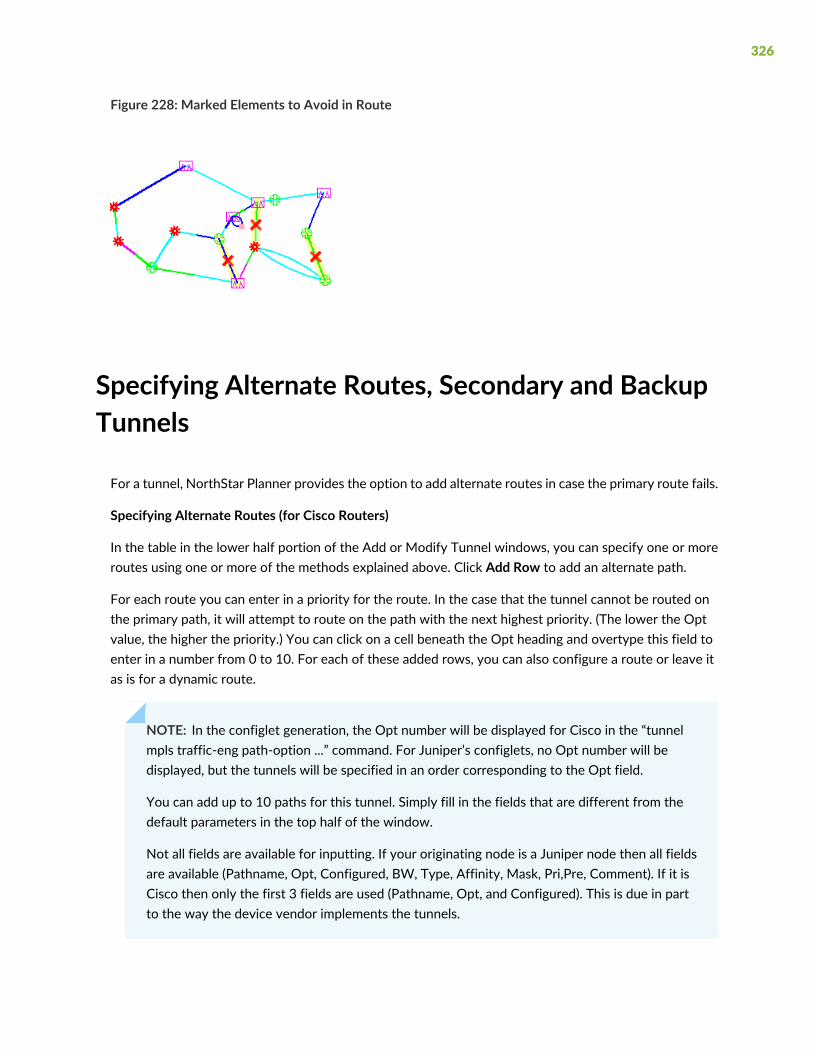
Figure 228: Marked Elements to Avoid in Route
Specifying Alternate Routes, Secondary and BackupTunnels
For a tunnel, NorthStar Planner provides the option to add alternate routes in case the primary route fails.
Specifying Alternate Routes (for Cisco Routers)
In the table in the lower half portion of the Add or Modify Tunnel windows, you can specify one or moreroutes using one or more of the methods explained above. Click Add Row to add an alternate path.
For each route you can enter in a priority for the route. In the case that the tunnel cannot be routed onthe primary path, it will attempt to route on the path with the next highest priority. (The lower the Optvalue, the higher the priority.) You can click on a cell beneath the Opt heading and overtype this field toenter in a number from 0 to 10. For each of these added rows, you can also configure a route or leave itas is for a dynamic route.
NOTE: In the configlet generation, the Opt number will be displayed for Cisco in the “tunnelmpls traffic-eng path-option ...” command. For Juniper’s configlets, no Opt number will bedisplayed, but the tunnels will be specified in an order corresponding to the Opt field.
You can add up to 10 paths for this tunnel. Simply fill in the fields that are different from thedefault parameters in the top half of the window.
Not all fields are available for inputting. If your originating node is a Juniper node then all fieldsare available (Pathname, Opt, Configured, BW, Type, Affinity, Mask, Pri,Pre, Comment). If it isCisco then only the first 3 fields are used (Pathname, Opt, and Configured). This is due in partto the way the device vendor implements the tunnels.
326

Specifying Secondary and Standby Tunnels (for Juniper Routers)
The tunnel ID, from node, to node, and IP address of the secondary/standby tunnel should be identical tothat of the primary tunnel. Thus, to add a secondary or standby tunnel, you should first have the desiredprimary tunnel open in the Add Tunnel or Modify Tunnel windows.
1. In the fish sample network, open up the Modify Tunnel window for RHOUWDC (where HOU, thesource node, is a Juniper router). In the bottom half of the window where it says Tunnels/Paths forthis tunnel, click on “Add Row.” Note that the source node should be of a type that supports secondaryor standby tunnels.
2. Right-click on the newly-added row and select the Edit Type menu option. The Tunnel Type ParameterGeneration window will appear, from which you can select Secondary or Standby instead of Primaryas shown in the Tunnel Option section of Figure 229 on page 327. Click “OK”.
Figure 229: Tunnel Type Parameter Generation Window for Juniper Routers (Options May Vary)
For more details on other type options, see the NorthStar Planner User Interface Guide, chapter on TheNetwork and Modify Menus, Tunnels, Tunnel Type Parameter Generation.
Secondary and standby tunnels are used when the primary tunnel fails. The difference is as follows:
• A secondary tunnel is not routed until the primary tunnel fails.
• A standby tunnel is routed while the primary tunnel is up.
NOTE: Secondary and standby tunnels should be listed immediately after the primarytunnel in the tunnel file. Furthermore, they should have the same tunnel ID, from node,to node and IP address.
327

3. For a secondary or standby path for Juniper, you only need to change the fields that are different fromthe primary path. You can highlight a row for a secondary or standby path by clicking on it. Afterhighlighting it, right-click and select Edit Route, Edit Type, or Edit Affinity to bring up a window whereyou can make these modifications.
4. Another option is to have the program automatically add a diverse standby or secondary tunnel byusing the Path Config. Options indicated in Path ConfigOptions on page 252. In the Add Tunnel window,after specifying the primary tunnel parameters, selectDiv.Stdby orDiv.Sec/Dynamic in the Path Config.Options drop-down menu to add a standby or secondary tunnel. Click OK to add the tunnel and itssecondary or standby tunnel.
5. If the tunnel(s) are already in the network, then select tunnels to modify and click Modify... and thenselect “Selected Entries.” In the Modify Tunnel window, select “Add” followed by Div.Stdby orDiv.Sec/Dynamic in the Path Config. Options to add a standby or secondary tunnel. Click OK to addthe secondary or standby tunnel.
NOTE: This is an Add operation, meaning that if the tunnel already had a standby tunnel andyou add a secondary tunnel, it will consequently have both a standby and secondary tunnel. Ifyou only wanted to select one of the types and not both, you should perform a subsequentmodification specifying “Remove” followed by the original type (standby or secondary) that youwant to remove and clicking “OK”.
Path Config Options
The Path Config Options and Re-routable dropdown selections can be used to specify requirements forsecondary/standby paths as described in the table below.
328
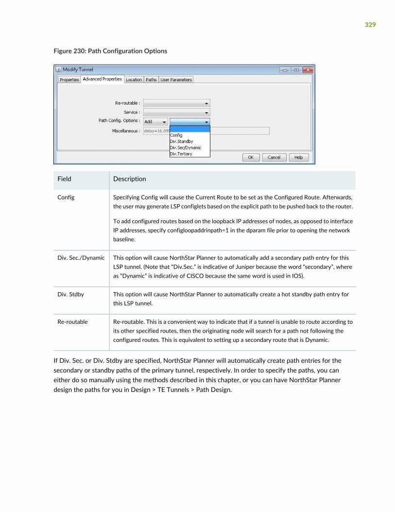
Figure 230: Path Configuration Options
DescriptionField
Specifying Config will cause the Current Route to be set as the Configured Route. Afterwards,the user may generate LSP configlets based on the explicit path to be pushed back to the router.
To add configured routes based on the loopback IP addresses of nodes, as opposed to interfaceIP addresses, specify configloopaddrinpath=1 in the dparam file prior to opening the networkbaseline.
Config
This option will cause NorthStar Planner to automatically add a secondary path entry for thisLSP tunnel. (Note that “Div.Sec.” is indicative of Juniper because the word “secondary”, whereas “Dynamic” is indicative of CISCO because the same word is used in IOS).
Div. Sec./Dynamic
This option will cause NorthStar Planner to automatically create a hot standby path entry forthis LSP tunnel.
Div. Stdby
Re-routable. This is a convenient way to indicate that if a tunnel is unable to route according toits other specified routes, then the originating node will search for a path not following theconfigured routes. This is equivalent to setting up a secondary route that is Dynamic.
Re-routable
If Div. Sec. or Div. Stdby are specified, NorthStar Planner will automatically create path entries for thesecondary or standby paths of the primary tunnel, respectively. In order to specify the paths, you caneither do so manually using the methods described in this chapter, or you can have NorthStar Plannerdesign the paths for you in Design > TE Tunnels > Path Design.
329

Adding and Assigning Tunnel ID Groups
Tunnel ID Groups are used to configure tunnel IDs that conform to Cisco’s default tunnel names whencreating LSP configlets or using the LSP Delta wizard. Cisco default tunnel IDs are of the form, Tunnel#,where the # is unique for each tunnel and is referred to as the tunnel ID. The tunnel ID assigned to an LSPtunnel is determined by the tunnel ID group to which that LSP tunnel belongs. Therefore, two items needto be configured: 1) the tunnel ID group, which contains a range of tunnel IDs, and 2) the LSP tunnel, whichneeds to be assigned to a tunnel ID group.
Once you have a tunnel ID group, it can also be used to create an incremental full mesh of tunnels for thatgroup as described in “Adding Multiple Tunnels” on page 320.
1. The first step is to create a user parameter to be used for assigning tunnel ID groups to LSP tunnels.This is done through the Modify > Elements > User Parameters menu in Modify mode, which will openthe User Parameters window. In this window, activate the Tunnel tab, then click the Add button andspecify a name for the new tunnel user parameter. In the example below, the name “Tunnel_ID_Group”is used.
Figure 231: Adding a Tunnel ID Group User Parameter
2. The next step is to create a tunnel ID group. In Modify mode, selectModify > Elements > Tunnel IDGroups.
330

Figure 232: Creating Tunnel ID Groups
3. To add a tunnel ID group, in the Tunnel ID Groups window click the Add button, then give the newgroup a name and an ID range as shown below. Also be sure to select a Tunnel User Parameter to usefor assigning tunnel ID groups to LSP tunnels.
Figure 233: Adding a Tunnel ID Group
4. Now that a tunnel ID group has been created, and a tunnel ID group user parameter has been created,the user can modify LSP tunnels to assign a tunnel ID group to that LSP tunnel’s tunnel ID group userparameter. To do this, go to Modify > Elements > Tunnels, select a LSP tunnel, and click the Modifybutton. Then in the Modify Tunnel window, select the User Parameters tab, then click the Value fieldof the tunnel ID group user parameter to activate a dropdown menu of all existing Tunnel ID Groups.Select a tunnel ID group from the list, then click OK.
331

Figure 234: Assigning a Tunnel ID Group to an LSP Tunnel
Tunnel ID groups are used in functions such as generating LSP configlets. When generating a configlet,the user will be prompted with the following window:
Figure 235: Option for Updating Tunnel Names
If Yes is selected, the tunnel name will be modified to match the Cisco naming convention, with the IDnumber selected from the tunnel ID group assigned to that tunnel. An example of a configlet with thetunnel name modified to the Cisco naming convention is shown below.
!! BOS
interface Tunnel0123
description from BOS to WDC
ip unnumbered Loopback0
tunnel destination 10.10.10.8
tunnel mode mpls traffic-eng
tunnel mpls traffic-eng autoroute announce
tunnel mpls traffic-eng priority 2 2
tunnel mpls traffic-eng bandwidth 10000
tunnel mpls traffic-eng path-option 10 explicit name Tunnel0.p0
332
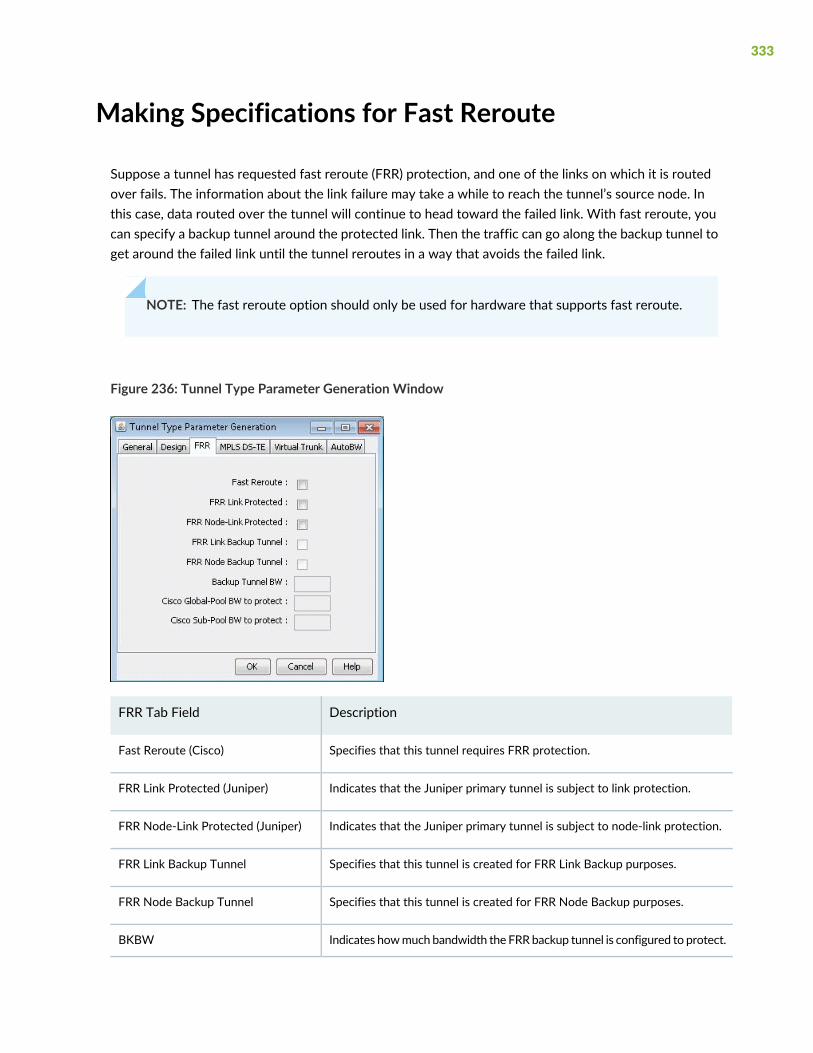
Making Specifications for Fast Reroute
Suppose a tunnel has requested fast reroute (FRR) protection, and one of the links on which it is routedover fails. The information about the link failure may take a while to reach the tunnel’s source node. Inthis case, data routed over the tunnel will continue to head toward the failed link. With fast reroute, youcan specify a backup tunnel around the protected link. Then the traffic can go along the backup tunnel toget around the failed link until the tunnel reroutes in a way that avoids the failed link.
NOTE: The fast reroute option should only be used for hardware that supports fast reroute.
Figure 236: Tunnel Type Parameter Generation Window
DescriptionFRR Tab Field
Specifies that this tunnel requires FRR protection.Fast Reroute (Cisco)
Indicates that the Juniper primary tunnel is subject to link protection.FRR Link Protected (Juniper)
Indicates that the Juniper primary tunnel is subject to node-link protection.FRR Node-Link Protected (Juniper)
Specifies that this tunnel is created for FRR Link Backup purposes.FRR Link Backup Tunnel
Specifies that this tunnel is created for FRR Node Backup purposes.FRR Node Backup Tunnel
Indicates howmuch bandwidth the FRRbackup tunnel is configured to protect.BKBW
333

DescriptionFRR Tab Field
Indicates how much Global Pool bandwidth the FRR backup tunnel isconfigured to protect. This is for Cisco only.
BKGP
Indicates howmuch Sub Pool bandwidth the FRR backup tunnel is configuredto protect. This is for Cisco only.
BKSP
To specify that a tunnel has requested for fast reroute protection, select the Fast Reroute checkbox in theTunnel Type window.
To add backup tunnels for links carrying the tunnels requesting FRR protection, see “NorthStar PlannerFast Reroute Overview” on page 431. Note that the FRR Backup Tunnel checkboxes in the Tunnel Typewindow are grayed out but will reflect changes when you successfully add the FRR_A or FRR_Z field inthe link window MPLS TE tab. .
Specifying Tunnel Constraints (Affinity/Mask orInclude/Exclude)
Constraint-based tunnel routing is implemented in Cisco and Juniper by coloring links and specifying whichlink colors a tunnel can or cannot route over. For Cisco, the links can be colored using 32 link attributes,each represented by a bit. The tunnel routing constraints are then specified per tunnel using affinity andmask. Juniper, on the other hand, uses the term admin groups to represent link colors. For Juniper, thetunnel routing constraints can be specified per tunnel using include and exclude statements. Below is abrief summary of how to specify affinity/mask for Cisco routers and include/exclude for Juniper routers.
Cisco
Link attribute contain 32 bits as the colors. A tunnel’s 32-bit mask specifies which of the tunnel’s 32 affinitybits are required to match the link attributes. If the match is successful, the tunnel is allowed to routethrough the trunk provided that the other routing requirements (such as capacity) are also satisfied. If thematch is unsuccessful, the tunnel is not allowed to route over the trunk. In other words, a tunnel can routeover a link if tunnel_affinity = (link_attribute & tunnel_mask).
Juniper
For Juniper, the terminology and options are slightly different. For Juniper, you can have up to 32administrative groups as the colors. For each link, you can assign one or more administrative groups asthe link color. Then for each tunnel, you can add groups to an “exclude” or “include” list (or, in recentversions of JUNOS, there an “include-all” and “include-any” list). For a tunnel to route over a link, that linkcannot have any of the excluded groups and must have at least one of the included groups (for include or
334

include-any) or all of the included groups (for include-all). Note that for Juniper, you can have an includeand exclude list for secondary paths as well as primary paths.
NorthStar Planner Modeling of Tunnel Constraints
In the NorthStar Planner client, the Tunnel Attributes window can be used to assign names to link attributesas described in Tunnel Attribute/Admin Group Names on page 258. For Juniper tunnels, admin-groups canbe entered here. For Cisco tunnels, the names can be left as is or changed for informational purposes.
Following this, the link attributes/admin-groups can be assigned to links from the Modify Links windowas described in Setting Link Attributes on page 258.
Finally, the tunnel routing constraints can be specified from the Modify Tunnels window by clicking theAffinity/Mask button (for Cisco) as described in Tunnel Affinity and Mask (Cisco)on page 259 orInclude-All/Exclude/Include-Any button (for Juniper) as described in Including and Excluding Admin-Groups(Juniper) on page 260.
Tunnel Attribute/Admin Group Names
If you want to give meaningful global names to one of the 32 link attributes/admin groups, you can selectTools > Options > General..., Path Placement > MPLS TE LSP Tunnel Attributes options pane for thefollowing window. For Juniper switches, enter in the admin-group names here. The default names are bit0,bit1, bit2, etc. Click “OK” to save your changes.
335

Figure 237: Tunnel Options Window
Setting Link Attributes
To change the attributes for a single link, right-click that link on the map and selectModify >Links underPointer . Then select the Attributes tab. To set the same link attribute for both directions on the link, leavethe default setting “Symmetric.” Then check off the link’s attributes. This will set the corresponding bit forthat attribute to 1.
To set different link attributes for the two directions on the link, select “Asymmetric.” Then select thedirection “A to Z” or “Z to A” that you want to modify and select the attributes for that direction.
To change the affinity attributes for multiple links at a time, selectModify > Elements > Links. In the Linkstable, select the desired rows by using the <Shift> and <Ctrl> keys. To select all rows, click “Select All” orclick in the table and press <Ctrl>-A. Then, pressModify. You will get a window like the one shown below.
Note that theMatch field appears only whenmultiple links are selected for modification. It is not a propertyof the link but is for the user to indicate which bits tomodify for the selected links. Bits that are not matchedwill not be touched in the modification.
To specify a bit that you want to change for all the selected links, click the button for that bit to activatethe checkbox for that bit. This will also turn the button text blue. Then check or uncheck the adjacent boxto turn on or off the attribute, i.e., to set the value for that attribute to 1 or 0.
336

For example, in Figure 237 on page 336, three links are being modified. For each of these links, the GOLDattribute is set to 0 and the ECONOMY attribute is set to 1. No other attributes on any of these links willbe modified.
NOTE: To customize the attribute names, refer back to Tunnel Attribute/Admin Group Names onpage 258.
Figure 238: Global Modify of Link Attributes
Tunnel Affinity and Mask (Cisco)
Affinity and mask for a tunnel can be specified through the Add Tunnel or Modify Tunnel windows. Inthese windows, there is a text field to the right of the “Affinity/Mask” button, in which you can directlyenter a hexadecimal for the affinity and mask. The affinity and mask should be separated by a comma.
Figure 239: Directly entering in Tunnel Affinity and Mask
Alternatively, if you want to specify the affinity and mask by selecting the relevant bits from which thehexadecimal number is derived, click on the “Affinity” button. The Tunnel Affinity/Mask Properties windowwill appear, as shown below.
The mask specifies which attributes a link must match in order for the tunnel to be routed over that link.The affinity specifies whether that attribute is turned on or off. For example, in Figure 239 on page 337,the tunnel is configured so that it can only route over links that have the ECONOMY attribute set to 1and the BIT8 attribute set to 0.
337

Figure 240: Tunnel Affinity/Mask Properties
The Affinity and mask are both hexadecimals. Each digit can go from 0 to F and is made up of 4 bits. Checkoff the bits that you want to set. This will change the affinity and mask listed on top. If you press “Clear”all the bits will be unchecked and the number will be reset to 00000000.
Including and Excluding Admin-Groups (Juniper)
For Juniper, include and exclude constraints can be specified through the Add Tunnel or Modify Tunnelwindows. You can directly specify these properties next to the Include-All/Exclude/Include-Any buttonin the form of hexadecimals.
Figure 241: Directly Entering in Include/Exclude Constraints
Alternatively, you can check off the attributes in the followingwindow. In the example below, the constraintis that this tunnel must route over a link with at least one of the admin-groups GOLD or SILVER but notthe admin group ECONOMY.
338

Figure 242: Tunnel Include/Exclude Constraints
Adding One-Hop Tunnels
Using the one-hop tunnel feature, users can create a pair of one-hop tunnels for each link, one for eachdirection. These tunnels are created with an explicit route that force them to use the direct link.
The following commands are the corresponding Cisco commands for creating one-hop tunnels:
mpls traffic-eng auto-tunnel primary onehop
mpls traffic-eng auto-tunnel primary tunnel-num [min num] [max num]
mpls traffic-eng auto-tunnel primary config unnumbered-interface interface
NOTE: The one-hop tunnel feature should only be used for networks where an IGP is deployedon the interfaces for which a one-hop tunnel will be created.
339

SelectModify > Elements > User Parameters. Click on the Tunnel tab. Then click “Add...” and add a userparameter to store the Tunnel Group ID, such as TunnelGroupID.
Figure 243: Adding a User Parameter for TunnelGroupID.
SelectModify > Elements > Tunnel ID Groups... In the selection menu, select the tunnel user parameterthat was just created. Then click Add... to enter in a group name and ID range. The One Hop Tunnels youcreate will be given the group name as prefix and a number in the ID range as suffix.
Figure 244: Adding a Tunnel ID Group
Note that you can only add one-hop tunnels for links that have an IGP enabled. To enable an IGP protocol,modify the links through Modify > Elements > Links... and click the Modify button. In the Protocols tabturn on either OSPF or ISIS and click OK.
340

Figure 245: Enabling OSPF or ISIS on the Links
SelectModify > Elements >Tunnels, Add > One Hop Tunnels... Select some links by filtering for them. Aneasy way is to highlight them on the map and then click Filter from Map. Select the Tunnel ID Group touse to create the one hop tunnels and add a tunnel bandwidth. Click “OK” to add the one hop tunnels.
Figure 246: Add One Hop Tunnels
SelectModify > Elements > Tunnels to view the newly added one hop tunnels. Several nodes can havetunnels with the same TunnelID but different tunnels originating from a node should have unique tunnelIDs.
341

Figure 247: Results of One Hop Tunnel Additions
Note the explicit path given in the Configured column of the following table. Double-click on a newlyadded one-hop tunnel to view the configured route. Then select the User Parameters tab. The tunnel userparameter for Tunnel ID Group is specified here.
To generate configlets for these one hop tunnels, switch to Tunnel Layer and Design mode and then selectDesign >Configlets/Delta > LSPConfiglet... Click “Submit” in the resulting window. The configlet includesin the description line the interface name used for the first hop of the tunnel.
Tunnel Layer and Layer 3 Routing Interaction
Modifications to the network model (e.g. tunnels, demands/flows, network elements, design options)usually require tunnels or flows to be rerouted. In NorthStar Planner, this rerouting occurs in the followingorder:
• If you are in Layer 3 and a reroute is triggered, tunnels will be rerouted first, followed by demands/flows.
• If you are in Tunnel Layer and a reroute is triggered, then only tunnels will be rerouted while in Tunnellayer. The moment you switch into Layer 3, however, the Layer 3 demands/flows will then be rerouted.
Additional Information
Table 3: Commands Modeled Using Affinity and Mask Feature
Corresponding Cisco Commands
mpls traffic-eng attribute-flags attributesSetting link attributes
342

Table 3: Commands Modeled Using Affinity and Mask Feature (continued)
Corresponding Cisco Commands
tunnel mpls traffic-eng affinity affinity [ mask mask ]Setting tunnel affinity and mask
Corresponding Juniper Commands for the mpls protocol
admin-groups {
group-name 1;
group-name 2;
...
}
Defining
Administrative
Groups
interface interface name {
admin-group [ group-name group-name ... ];
}
Selecting admin groups for a link
label-switched-path lsp-path-name {
to address;
...
primary path-name {
admin-group {
exclude [ group-name group-name ... ];
include [ group-name group-name ... ];
include-all [ group-name group-name ... ];
include-any [ group-name group-name ... ];
}
}
Setting admin groups for a tunnel
343
15CHAPTER
Optimizing Tunnel Paths
Optimizing Tunnel Paths Overview | 347
Procedures for Optimizing Tunnel Paths | 347
Network Grooming | 348

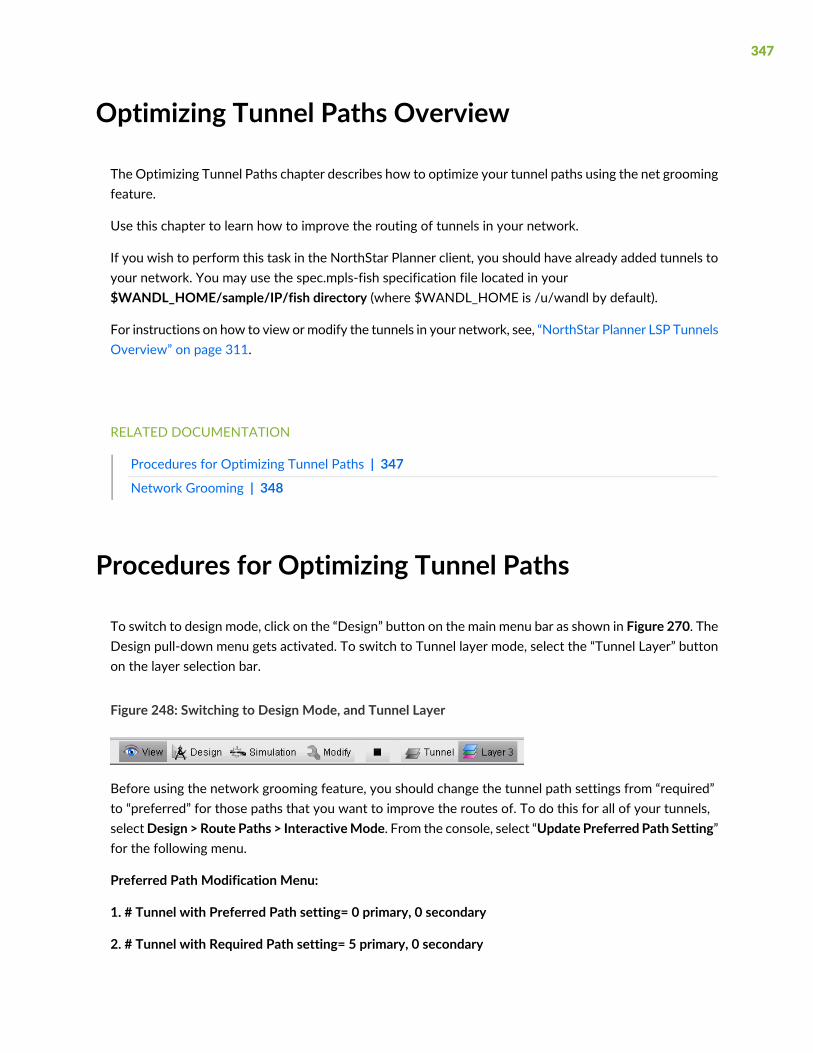
Optimizing Tunnel Paths Overview
The Optimizing Tunnel Paths chapter describes how to optimize your tunnel paths using the net groomingfeature.
Use this chapter to learn how to improve the routing of tunnels in your network.
If you wish to perform this task in the NorthStar Planner client, you should have already added tunnels toyour network. You may use the spec.mpls-fish specification file located in your$WANDL_HOME/sample/IP/fish directory (where $WANDL_HOME is /u/wandl by default).
For instructions on how to view ormodify the tunnels in your network, see, “NorthStar Planner LSP TunnelsOverview” on page 311.
RELATED DOCUMENTATION
Procedures for Optimizing Tunnel Paths | 347
Network Grooming | 348
Procedures for Optimizing Tunnel Paths
To switch to design mode, click on the “Design” button on the main menu bar as shown in Figure 270. TheDesign pull-down menu gets activated. To switch to Tunnel layer mode, select the “Tunnel Layer” buttonon the layer selection bar.
Figure 248: Switching to Design Mode, and Tunnel Layer
Before using the network grooming feature, you should change the tunnel path settings from “required”to “preferred” for those paths that you want to improve the routes of. To do this for all of your tunnels,selectDesign > Route Paths > InteractiveMode. From the console, select “Update Preferred Path Setting”for the following menu.
Preferred Path Modification Menu:
1. # Tunnel with Preferred Path setting= 0 primary, 0 secondary
2. # Tunnel with Required Path setting= 5 primary, 0 secondary
347

3. Use current routes as preferred/required paths
Select:
If any tunnels have the required setting, select 2. You will then be asked to apply changes to the primarytunnels, secondary/standby tunnels, or all. Select 3 for all.
Apply Changes to 1: Primary only, 2. Secondary/Standby only, 3. All
3
Required Paths Modification Menu:
1. Change to Preferred, 2. Remove All Required Paths, 3. No Change
Select:
Select 1 to change the paths to preferred paths. Press <Enter> repeatedly until you exit out of the console.
NOTE: You can also manually apply the changes to tunnels on an individual basis by modifyingthe tunnel file, changing the Path Required PR(path) statements to Path Select PS(path) statements.You then need to use the File>Read option to read in these changes to the tunnel file.
Network Grooming
The objective of network grooming is to reroute the paths to minimize the distance metric of the pathsusing available bandwidth in the network. Select the Design > TE Tunnels > Net Groom pull-down menu.The Net Groom window will appear:
348

Figure 249: Network Grooming Window for Tunnel Paths
Specify the Source Nodes for Tunnels to narrow down the set of tunnels to be optimized. Otherwise, bydefault, all tunnel paths will be optimized. Specify Tunnel Selection Options to further narrow down theset of tunnels.
Specify any General Options. Refer to the NorthStar Planner User Interface Guide for more information onthe Net Groom window options. To change the distance calculation method to OSPF, RIP, Delay, ISIS, orCDV, simply click on the “Set Routing Method” button and enter the desired choice in the console. Onceall options are set, click OK.
Note that AW is an abbreviation here for “Admin Weight”, which is the same thing as “Admin Cost” or“Link Metric”. Network grooming assumes that the smaller the path’s total admin weight, the better.
Figure 250: Net Groom - Potential Admin Weight (AW) Gain for Tunnel Path
By comparing the Original Admin Weight (AW) with the potential Best (smallest) AW, you can decidewhich tunnels should have their paths changed or optimized. You can click on the Best AW Gain column
349

header to sort according to the highest reduction in the total admin weight. Click on “View Paths” buttonto compare the Orig Path and Best Path using the Paths window.
SelectMultiple tunnels for optimization and click the “Optimize Selected Tunnels” button. The New AWand AW Gain columns will be populated for the selected tunnels with the actual achieved admin weight.The LSP tunnel paths are updated to the new ones discovered by NorthStar Planner.
Refer to the Design chapter in the NorthStar Planner User Interface Guide for more details about networkgrooming.
350

16CHAPTER
Tunnel Sizing and Demand Sizing
Tunnel Sizing and Demand Sizing Overview | 353
Sizing Tunnels and Demands | 353
Sizing Tunnels | 354
Calculation of the New Tunnel Bandwidth | 361


Tunnel Sizing and Demand Sizing Overview
This chapter describes how to resize a network’s LSP tunnels based upon the measured traffic on thetunnel or to resize a network’s demands based upon the traffic load.
From the Report Manager, you can identify tunnels in the network where the planned tunnel bandwidthis greater than or less than the actual transported layer 3 traffic. For such cases, you may then wish tochange those tunnels’ bandwidths to make sure that sufficient bandwidth is allocated to carry traffic tomeet Service Level Agreements (SLAs). The Tunnel Sizing feature in NorthStar Planner provides anautomated solution for resizing these tunnels.
For instructions on how to view ormodify the tunnels in your network, see “NorthStar Planner LSP TunnelsOverview” on page 311, .
RELATED DOCUMENTATION
Sizing Tunnels and Demands | 353
Sizing Tunnels and Demands
NOTE: Although the steps below are for tunnel sizing, demand sizing works the same way.
• Open a network that contains tunnels.
• Switch to Tunnel layer.
• View current tunnel utilization in the Report Manager.
• Specify Tunnel Sizing default options in the Demand/Tunnel Sizing option pane of Tools > Options >Design.
• Select Design > Tunnel Sizing to bring up the “Find Tunnels” window. Specify the search criteria fortunnels.
• Adjust the new tunnel bandwidth value if necessary by entering a new value in the tunnel’s “New BW”field or clicking on the “Recalculate Selected” button.
• Save the new bandwidth values by clicking on “Confirm Selected” or “Confirm All”. This will save thenew bandwidth values as the tunnel’s bandwidth.
353
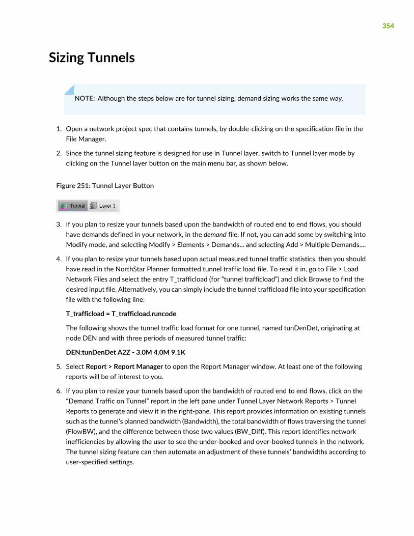
Sizing Tunnels
NOTE: Although the steps below are for tunnel sizing, demand sizing works the same way.
1. Open a network project spec that contains tunnels, by double-clicking on the specification file in theFile Manager.
2. Since the tunnel sizing feature is designed for use in Tunnel layer, switch to Tunnel layer mode byclicking on the Tunnel layer button on the main menu bar, as shown below.
Figure 251: Tunnel Layer Button
3. If you plan to resize your tunnels based upon the bandwidth of routed end to end flows, you shouldhave demands defined in your network, in the demand file. If not, you can add some by switching intoModify mode, and selecting Modify > Elements > Demands... and selecting Add >Multiple Demands....
4. If you plan to resize your tunnels based upon actual measured tunnel traffic statistics, then you shouldhave read in the NorthStar Planner formatted tunnel traffic load file. To read it in, go to File > LoadNetwork Files and select the entry T_trafficload (for “tunnel trafficload”) and click Browse to find thedesired input file. Alternatively, you can simply include the tunnel trafficload file into your specificationfile with the following line:
T_trafficload = T_trafficload.runcode
The following shows the tunnel traffic load format for one tunnel, named tunDenDet, originating atnode DEN and with three periods of measured tunnel traffic:
DEN:tunDenDet A2Z - 3.0M 4.0M 9.1K
5. Select Report > Report Manager to open the Report Manager window. At least one of the followingreports will be of interest to you.
6. If you plan to resize your tunnels based upon the bandwidth of routed end to end flows, click on the“Demand Traffic on Tunnel” report in the left pane under Tunnel Layer Network Reports > TunnelReports to generate and view it in the right-pane. This report provides information on existing tunnelssuch as the tunnel’s planned bandwidth (Bandwidth), the total bandwidth of flows traversing the tunnel(FlowBW), and the difference between those two values (BW_Diff). This report identifies networkinefficiencies by allowing the user to see the under-booked and over-booked tunnels in the network.The tunnel sizing feature can then automate an adjustment of these tunnels’ bandwidths according touser-specified settings.
354

Figure 252: Demand Traffic on Tunnel Report (formerly Planned Tunnel Util)
7. If you plan to resize your tunnels based upon actual measured tunnel traffic statistics, click on the“Measured Tunnel Traffic” report. This displays the measured tunnel traffic load numbers, as read infrom the T_trafficload file, in tabular format.
8. In Design mode, select Design > TE Tunnels > Tunnel Sizing. If you did not switch to Tunnel layerearlier, the program will ask you to switch to Tunnel layer. Click “Yes” to continue.
9. A Find Tunnels window will appear as shown in Figure 275. In addition to the regular options, thereare options specific to tunnel sizing. Those fields are described in the table below
355

Figure 253: Find Tunnels for Tunnel Sizing
DescriptionField
If the absolute value of the difference between the tunnel bandwidth and total flowbandwidth is greater than this value (expressed in kilobits), then those tunnels are fetched.
BW Diff (KB) greater than
If the absolute value of the ratio of bandwidth difference to tunnel bandwidth is greaterthan this value, then those tunnels are fetched.
BWDiff Ratio greater than
Sorts the displayed tunnels by either bandwidth difference or bandwidth difference ratio.Sort Field
Sorts the displayed tunnels according to the type in the Sort field; sorts either in decreasingorder or in decreasing order of the absolute value.
Sort Order
Specifies the source of traffic: “Layer 3 Demands” or “Traffic Load” (measured tunneltraffic). This parameter will show up as the “FlowBW” field in the Tunnel Sizing window.It is also used as the flow bandwidth of the new bandwidth calculation.
BW Source
This field specifies the time period of traffic to be used. If the BW Source is Layer 3Demands, then the Planned traffic from the demand file is used. If the BW Source isTunnel Traffic Load, then possible values are Period1 through Period24, and Peak. Peakindicates the heaviest/worst load experienced among any of these 24 traffic periods.
Traffic Period
356

DescriptionField
Specifies how many tunnels to display per page.# Tunnels Per Page
10.The next step is to check your tunnel sizing options. In the Find Tunnels window, select the “SizingParameters” tab.
NOTE: Alternatively, you can set the sizing parameters globally via Tools > Options >Design and click on the “Demand/Tunnel Sizing” options pane. When the options in theDesign Options window are set, click “OK”. A window will ask you whether to reroutethe tunnels. You can click “No” since changing the tunnel sizing options does not affecttunnel routing. (You are prompted because the program is aware that you have modifiedthe design options. Though the tunnel sizing options do not affect routing, other designoptions might.)
Figure 254: Tunnel Sizing Parameters
Set the sizing parameters to your preferred setting. The table below describes each field.
357
When the options have been selected, click “OK” to fetch tunnels that match the specified criteria.Those tunnels will then be displayed in the Tunnel Sizing window as shown in Figure 254 on page 357.
Parameter inDparamFileDescriptionField
minSizingBWThe minimum value to be assigned for any new tunnel bandwidth.If the calculated bandwidth is less than this value, then this value isused as the new bandwidth.
Minimum TunnelBW
maxSizingBWThe maximum value to be assigned for any new tunnel bandwidth.If the calculated bandwidth is greater than this value, then this valueis used as the new bandwidth.
Maximum TunnelBW
incSizingBWThe increment by which the bandwidth will be increased. Basically,the calculated bandwidth will be rounded up to the nearest multipleof this value.
Tunnel BWIncrement
sizing_growthmultiplierThis value is multiplied by the total flow bandwidth to calculate thenew bandwidth. For example, 1.00 will generate a new tunnelbandwidth assignment that is 100% of the total flow bandwidthtraversing the tunnel, and 1.5 will generate a value that is150% ofthe traffic load bandwidth.
Tunnel GrowthMultiplier
sizing_growthconstantA constant offset to add in the calculation of the new bandwidth.Tunnel GrowthConstant
sizing_standbypctIf the primary tunnel being resized has an associated standby tunnel,then use this field to indicate a percentage value of the new primarytunnel bandwidth that should be used to set the standby tunnelbandwidth. The default is 100%, or the same as the primary tunnelbandwidth.
Standby Tunnel BW%
sizing_resizeoptThe “Only Increase” option is for sizing only overbooked tunnels.When this option is set, a new bandwidth will only be calculated ifthe total flow bandwidth is greater than or equal to the currentplanned tunnel bandwidth.
When the “Fit to Traffic” option is set, a new bandwidth will alwaysbe calculated.
Resize Option
358
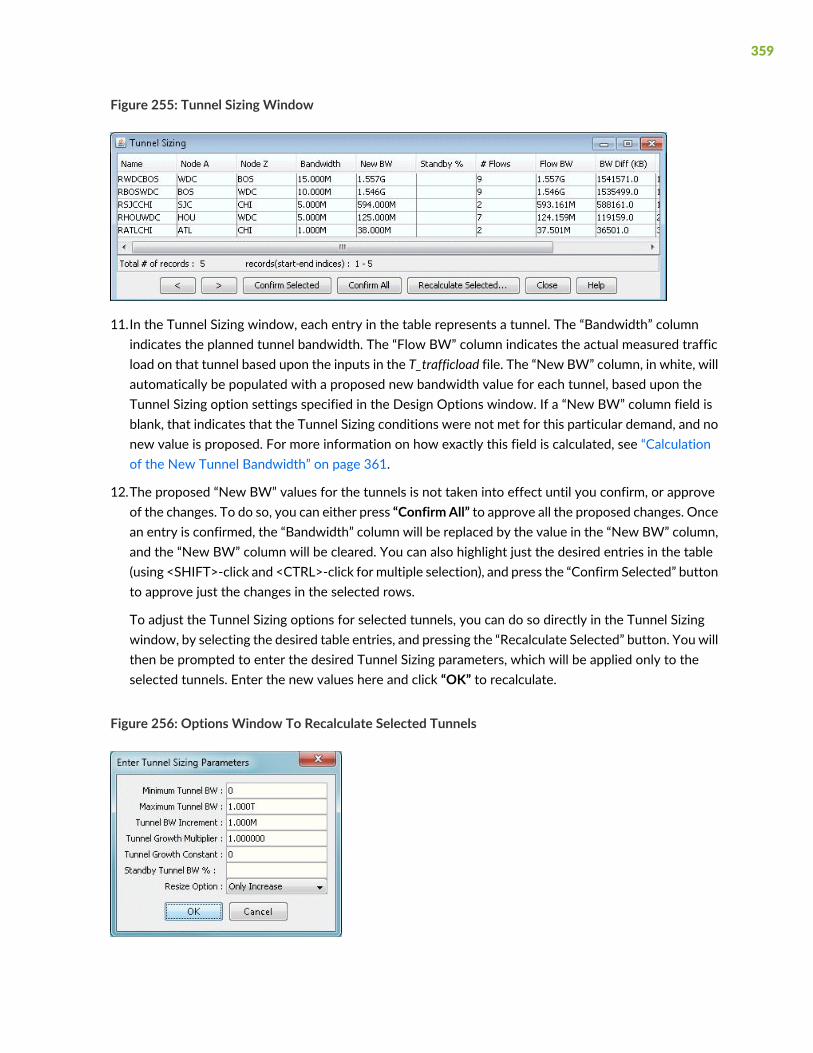
Figure 255: Tunnel Sizing Window
11.In the Tunnel Sizing window, each entry in the table represents a tunnel. The “Bandwidth” columnindicates the planned tunnel bandwidth. The “Flow BW” column indicates the actual measured trafficload on that tunnel based upon the inputs in the T_trafficload file. The “New BW” column, in white, willautomatically be populated with a proposed new bandwidth value for each tunnel, based upon theTunnel Sizing option settings specified in the Design Options window. If a “New BW” column field isblank, that indicates that the Tunnel Sizing conditions were not met for this particular demand, and nonew value is proposed. For more information on how exactly this field is calculated, see “Calculationof the New Tunnel Bandwidth” on page 361.
12.The proposed “New BW” values for the tunnels is not taken into effect until you confirm, or approveof the changes. To do so, you can either press “ConfirmAll” to approve all the proposed changes. Oncean entry is confirmed, the “Bandwidth” column will be replaced by the value in the “New BW” column,and the “New BW” column will be cleared. You can also highlight just the desired entries in the table(using <SHIFT>-click and <CTRL>-click for multiple selection), and press the “Confirm Selected” buttonto approve just the changes in the selected rows.
To adjust the Tunnel Sizing options for selected tunnels, you can do so directly in the Tunnel Sizingwindow, by selecting the desired table entries, and pressing the “Recalculate Selected” button. You willthen be prompted to enter the desired Tunnel Sizing parameters, which will be applied only to theselected tunnels. Enter the new values here and click “OK” to recalculate.
Figure 256: Options Window To Recalculate Selected Tunnels
359

13.Once you are satisfied with your changes in the Tunnel Sizing window, press the “OK” button. Anychanges that were confirmed should now be in effect. Any new bandwidth value that was not confirmedwill not be saved when the Tunnel Sizing window is closed.
During the confirmation process, the server will determine if the tunnel using the new bandwidth valuecan be placed. If it cannot be placed, the tunnel will keep its old bandwidth, and an error message willbe displayed in the console.
The following sections describe some other features available in the Tunnel Sizing window.
14.The columns in the Tunnel Sizing table can be customized to show or hide certain fields. Right-click onthe table and select “Customize Current View” from the pop-up menu (Figure 256 on page 359). Awindow will appear that allows the user to select the desired columns for display.
Figure 257: Right-click Pop-up Menu
15.The table can also be sorted by any column by clicking on the column header. This sorts the tunnelscurrently displayed in the table.
16.If there are multiple pages of tunnels, the user may wish to sort the tunnels across all the pages byeither BW diff or BW diff ratio in order to see the most overbooked tunnels on one page. This can bedone in the previous “Find Tunnels” window. If the tunnels have already been fetched, you may sortby right-clicking on the body of the table and selecting “Sort Globally”. A window will appear as shownin Figure 280 allowing you to select the sorting options.
Figure 258: Select Sort Options Window
17.You may override the suggested new bandwidth by typing in a new value directly into the table. To dothis, either double-click on the tunnel’s “New BW” field. The table cell will then become editable.
360

Alternatively, right-click on the selected tunnel(s) and choose “ReplaceNewBWValues”. You will thenbe prompted to enter a new BW value for those tunnel(s).
Calculation of the New Tunnel Bandwidth
The calculation of the new tunnel bandwidth works in the following way:
If the resize option is set to “Only Increase” (in the Design Options window) and the tunnel’s plannedbandwidth is strictly greater than the total flow or measured tunnel traffic bandwidth, then the tunnel willnot be resized. Otherwise, a new bandwidth will be calculated using the following procedure:
1. First, compute:
Temp = (Flow Bandwidth * Growth Multiplier) + Growth Constant
2. Round up the temp value to the nearest multiple of the Tunnel Bandwidth Increment, as specified inthe tunnel sizing design options.
3. If this value is less than the Minimum Tunnel Bandwidth, then the new bandwidth is set to the valueof the minimum tunnel BW.
4. If this value is greater than the Maximum Tunnel Bandwidth, then the new bandwidth is set to thevalue of the maximum tunnel BW.
5. Otherwise, simply use the new rounded up bandwidth value.
361

17CHAPTER
Tunnel Path Design
Tunnel Path Design Overview | 365
Tunnel Path Design Instructions | 365
Designing Tunnel Paths Overview | 365
Backup Path Configuration Options | 367
Default Diversity Level | 368
Evaluate/Tune Options | 369
Advanced Options | 369
Viewing Design Results | 370
Tunnel Modifications | 371
Exporting and Importing Diverse Group Definitions | 373
Advanced Path Modification | 374

Tunnel Path Design Overview
This chapter describes the Path Design feature. Tunnel Path Design lets you design tunnel paths for pathdiversity. Lsp tunnels can be designed such that their secondary/standby paths are routed in node-diverse,site-diverse, link-diverse, or facility-diverse routes from their primary path. Additionally, two differenttunnels can also be designed such that their primary paths are also on diverse paths.
Use these procedures to design primary and backup tunnel paths.
If you wish to perform this task in NorthStar Planner, you should have already added tunnels to yournetwork.You may wish to follow along by using the spec.mpls-fish specification file located in your$WANDL_HOME/sample/IP/fish directory (where $WANDL_HOME is /u/wandl by default).
For instructions on how to view ormodify the tunnels in your network, see “NorthStar Planner LSP TunnelsOverview” on page 311.
RELATED DOCUMENTATION
Tunnel Path Design Instructions | 365
Designing Tunnel Paths Overview | 365
Tunnel Path Design Instructions
Following is a high-level, sequential outline of the diversity path design feature and the associated,recommended procedures.
1. Switch to Tunnel layer and open Design > TE Tunnels > Path Design.
2. Design selected tunnels for diversity.
3. View the resulting paths graphically or generate the Path &Diversity Report from the Report Manager.
Designing Tunnel Paths Overview
1. Select the Tunnel layer button to switch to the Tunnel layer.
365

2. In Design mode, select Design > TE Tunnels > Path Design to open the Tune Paths window. Thiswindow lists all of the tunnels whose paths can be designed for. For each tunnel or group, the detailsof the first, second, and third path are provided in this window. The Div Level column indicates thecurrent level of diversity satisfied between the 2 or 3 paths that belong to this tunnel or group
Figure 259: Diverse Paths Table
3. Select the tunnels to design and select Tune > Selected Paths. Alternatively, select Tune > All Pathsto design all tunnels for diversity. This will open up the following window.
Figure 260: Tuning Options
366

Backup Path Configuration Options
The Backup Path Config Options are provided to design a tunnel’s primary and backup paths. To createbackup paths, select “Add if not existing” for the Backup Path #1 and/or Backup Path #2.
Note that it is not required to design for both backup paths. To avoid creating new backup paths, selectthe option “Change only existing backup” for Backup Path #1 and/or Backup Path #2. If the backup pathdoes not exist, no action will be taken.
Note also that backup paths cannot be removed from this window. To remove existing backup paths, usethe Tuning window option instead, Modify > Selected Paths, and set Max # Backup Paths to 0.
To avoid changing current backup path types (Standby vs. Secondary), select the option “Preservestandby/secondary settings of existing tunnels”. In this case, the backup path type settings specified willonly be usedwhen adding backup paths and not for existing backup paths. If instead you unselect “Preservethe type of existing diverse paths”, this option will be used to change the backup path type not only of theadded backup paths but also of the already existing tunnel paths.
See the examples below on some common path design scenarios:
Dynamic Primary Path
Use the following settings to configure only a dynamic primary path:
• Primary Path: “Dynamic”
• Backup Path #1 and Backup Path #2: Select “Change only existing backup” to avoid creating a backuppath
NOTE: Existing backup paths cannot be removed from this window. To remove existingbackup paths, use the Modify > Selected Paths and set Max # Backup Paths to 0.
Explicit Primary Path with Dynamic Secondary Path
Use the following settings to configure an explicit (nailed down) primary path with a dynamic secondarybackup path:
• Primary Path: “Explicit”
• Backup Path #1: “Dynamic” “Secondary” “Add if missing”
• Backup Path #2: “Change only existing backup” to avoid creating a tertiary path
367

NOTE: Existing backup paths cannot be removed from this window. To remove existingbackup paths, use the Modify > Selected Paths and set Max # Backup Paths to 0.
Explicit Primary and Explicit Standby Path
Use the following settings to configure an explicit primary and explicit standby backup path:
• Primary Path: “Explicit”
• Backup Path #1: “Explicit” “Standby” “Add if missing”
• Backup Path #2: “Change only existing backup” to avoid creating a tertiary path
NOTE: Existing backup paths cannot be removed from this window. To remove existingbackup paths, use the Modify > Selected Paths and set Max # Backup Paths to 0.
Explicit Primary and Explicit Standby Path with Dynamic Tertiary Path
Use the following settings to configure an explicit primary and standby backup path and dynamic tertiarypath.
• Primary Path: “Explicit”
• Backup Path #1: “Explicit” “Standby” “Add if missing”
• Backup Path #2: “Dynamic” “Secondary” “Add if missing”
Default Diversity Level
If you are designing for two or three configured paths, select the Default Diversity Level to target (site,link, or facility) between the paths in case it has not already been specified on a per-tunnel basis.
Site diversitymeans that the two paths do not intersect at any given site (besides the source and destination).Link diversity means that the two paths do not intersect at any given link. Site diversity is always strongerthan link diversity as site diversity implies link diversity.
SRLG/Facility can be used for SRLG-diversity. In this case, the facilities should be defined before the PathDesign. This can be done in Modify mode via the Modify > Elements > SRLG/Facilities window, or bycreating a facility file and reading it in via File > Load Network Files in Design mode.
368
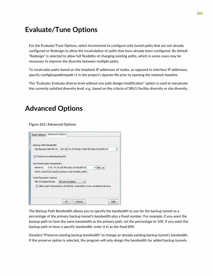
Evaluate/Tune Options
For the Evaluate/Tune Options, select Incremental to configure only tunnel paths that are not alreadyconfigured or Redesign to allow the recalculation of paths that have already been configured. By default“Redesign” is selected to allow full flexibility of changing existing paths, which in some cases may benecessary to improve the diversity between multiple paths.
To recalculate paths based on the loopback IP addresses of nodes, as opposed to interface IP addresses,specify configloopaddrinpath=1 in the project’s dparam file prior to opening the network baseline.
The “Evaluate: Evaluate diverse level without any path design/modification” option is used to reevaluatethe currently satisfied diversity level, e.g., based on the criteria of SRLG/facility-diversity or site diversity.
Advanced Options
Figure 261: Advanced Options
The Backup Path Bandwidth allows you to specify the bandwidth to use for the backup tunnel as apercentage of the primary backup tunnel’s bandwidth plus a fixed number. For example, if you want thebackup path to have the same bandwidth as the primary path, set the percentage to 100. If you want thebackup path to have a specific bandwidth, enter it in as the fixed BW.
Deselect “Preserve existing backup bandwidth” to change an already existing backup tunnel’s bandwidth.If the preserve option is selected, the program will only design the bandwidth for added backup tunnels.
369

Use the Link Reservation Parameters to reserve bandwidth on the link that cannot be used by primary andstandby paths, as a function of the percentage of the link’s bandwidth plus a fixed number. Constraintbased routing will be used to route the tunnel paths on links that do have enough available bandwidth toaccommodate both the tunnel bandwidth and this reserved bandwidth.
The Path Placement Options effects how the tunnel is placed based on MPLS protocols in the network.Selecting the User-Specified Per Link option will define the link as MPLS enabled or disabled based on theuser setting, and the tunnel can be placed only on enabled links. Selecting the All Links Enabled option willassume all links as MPLS enabled, and the tunnel can be placed on any link.
Click OK to start the design.
Viewing Design Results
After the design is complete, view the resulting Diversity Level achieved under the Div Level column.
Figure 262: Path Window After Design for Diverse Standby + Dynamic Tertiary
Scroll to the right to see the paths to see the new paths (“Current Path” columns) for the backup tunnelpaths, and the paths that have been configured (“Config Path” columns)
Click on any row and select ShowPaths to view the primary and secondary/standby paths on the topologymap. Note that the primary path is yellow, the secondary or standby path is purple, and the tertiary pathis orange. If the paths overlap, you may want to select “Highlight a Selected Path” to view one at a time.
To focus only on the selected paths, select “Hide Unrelated Nodes.”
370

Figure 263: Paths After Design for Tertiary diverse path (3DIV)
Click on View Path Details... to view the tunnel details. If you designed for standby paths, there will betwo entries for the tunnel, one for the primary path and one for the standby path marked with STANDBYin the type field. If you designed for secondary paths, the secondary path information is displayed in thesame tunnel entry as the primary path and is listed in the Paths tab.
NOTE: For secondary paths, the path name may not be specified. In that case, you may wish toenter a path name in modify mode (Modify > Elements > Tunnels) to have the name displayedfor the Secondary column.
Click Action... > Report... to save the contents of the Tune Paths window to a comma-separated file.
Tunnel Modifications
The following are some prerequisite steps that can be set up before running the Path Diversity Design, ifdesired.
SelectModify > Selected Paths or Modify > All Paths to view the following options:
371

Figure 264: Tunnel Modification Options
General Path Options
You can set up per tunnel diversity requirements, to override the default diversity level. To do so, selectthe desired tunnel(s), clickModify > Selected Paths, and select the Configured Diversity Level: FACDIV(for SRLG/facility diversity), LINKDIV, or SITEDIV.
For the primary path, select “Replace Explicit with Dynamic” to convert the primary path from beingexplicit (nailed down) to Dynamic (loose).
Diversity Group Configuration Groups
In addition to designing for diversity between a primary and backup path of the same LSP tunnel, anotherdiversity option is to establish path diversity between different tunnels, which may or may not have thesame source and destination routers. Upon grouping these tunnels together, they will be paired off, sothat each pair can be designed for diversity.
To group a set of tunnels together, select the desired tunnel(s), clickModify > Selected Paths, and enterin a name for the group under Div Group. All of the tunnels in this group will be paired off, so that eachpair can be designed for path diversity.
If you wish to group all tunnels that originate and terminate at the same sites, without creating a separategroup for each pair of sites, select the reserved Div Group “SITEPAIR”. Tunnels marked SITEPAIR will bepaired off with other tunnels marked as SITEPAIR that connect the same two sites. Each of these tunnelpairs can then be designed so that the two separate tunnels are diverse from one another.
Note that any tunnel that is added to a Div Group pair will be listed as an entry in the Tune Paths windowunder the associated group name, rather than under an entry for the tunnel name. If more than 2 tunnelsare in the same group, the different pairs will be indicated by the group name followed by a subindex. Forexample, if there are six tunnels in group “test”, they may be paired off and appear in the table as “test”,
372

“test.1” and “test.2”. The tunnels in each pair can then be designed to be diverse from each other, but theywill not be designed individually for primary/backup diversity.
To perform path design for Diversity Groups rather than tunnels’ primary/backup path design, use theselect menu in the Tune Paths window to select the group category: “ALL” versus “DivGroup” versus theregular entries for tunnel primary/backup design.
Backup Path Configuration Options
After the path design, if you do not like the current backup paths configuration, you can delete the backuppaths and redesign. To delete backup paths, select the tunnels from the Tune Paths window, click theModify > Selected Paths button, and then specify the Maximum # Backup Paths to keep. For example, ifyou enter in 0, this will remove all backup paths, leaving only the primary path. If you enter in 1, this willremove all but the first backup path, leaving only one primary path and one backup path.
You can set up per tunnel diverse path types (Standby vs. Secondary) by entering in the “Backup PathType”.
You can optionally specify that you want tertiary diverse design.
Exporting and Importing Diverse Group Definitions
To export the current diverse group definitions, select File > Save Network Files > Tunnel...
The output file, usertunneldef.runcode will be created in your output path, where runcode is substitutedby the runcode of your current network model. For example, the following is an example of a DiverseGroup Definition.
#
# Tunnel Diverse Group Definition
#
## Software Release= 5.5.1, 32 bits
## Platform=i86pc, OS=SunOS 5.10
## Report Date= 7/12/2010 04:55 Runcode=autosave User=telus
#NodeName TunnelName DivGroupName
BOS,RBOSWDC,test
WDC,RWDCBOS,test
373

ATL,RATLCHI,test
HOU,RHOUWDC,test
To import the diverse group definition, selectAction > Import DivPath Definition Filefrom the Tune Pathswindow.
Advanced Path Modification
After the path design, you may also wish to provide path names for some of the tunnel paths.
1. First, click the Modify mode button to switch to Modify mode.
2. Next, reopen Modify > Elements >Tunnels. Double-click a particular tunnel to view its details.
3. If desired you can enter unique pathnames for the backup routes under the Pathname column
4. For Cisco, the two alternate routes can be given different priorities using the “Opt” field (the defaultsare multiples of 10). For Juniper, specify for the two backup routes if they are secondary or standby inthe Type column by entering in R,STANDBY for a standby tunnel or R,SECONDARY for a secondarytunnel. Right-click an entry and select Edit Type for more options.
374

Figure 265: Designing Three Paths
To generate delta configlets for the changes made to the LSP tunnels since opening the baseline, selectAction > LSP Delta Wizard.
For more information on the LSP Delta Wizard, see Running the LSP Delta Wizard.
375

18CHAPTER
Inter-Area MPLS-TE
NorthStar Planner Inter-Area MPLS-TE Overview | 379
Inter-Area MPLS-TE Instructions | 380
Viewing OSPF Areas | 380
Adding Multiple Tunnels Between Areas | 382
Tunnel Type Configuration Options Related to Areas | 382
Viewing Inter-Area Tunnels | 384
Configuring a Loose Route | 385


NorthStar Planner Inter-Area MPLS-TE Overview
NorthStar Planner supports the design of LSP tunnels for a multiple-area network. Unlike the router whoseknowledge of the network is limited to the area to which it belongs, NorthStar Planner has a global viewof the entire network topology and can therefore design both primary and diverse inter-area LSP tunnelsmore intelligently. Once the LSP tunnels are designed, LSP configlets can be generated for loading intothe network.
NorthStar Planner supports Inter-Area MPLS-TE design for both Juniper and Cisco networks.
NOTE: Use these procedures if you have multiple OSPF areas in your network and you want toquickly generate LSP tunnels between the different areas.
If you wish to perform this task in NorthStar Planner, you should have a router specification fileopen before you begin. You should have also created multiple OSPF areas in your network andset the routing method to OSPF.
To do this, first create OSPF areas using Modify > Protocols > OSPF Areas. Then, set the areaproperty accordingly on your network links using Modify > Elements > Links (see the Locationtab). You may follow along by using any specification file with multiple OSPF areas defined inthe network.
Check that the routing method is OSPF in Tools > Options > Design, Path Placement optionpane. Additionally, check that the links have OSPF enabled usingModify > Elements > Links (seethe Protocols tab)
Review the Prerequisites to ensure that your network is configured properly.
For information about how to perform an automatic multi-area OSPF network design, se “Tunnel Sizingand Demand Sizing Overview” on page 353.
For information about LSP Tunnels and how to set their characteristics, see “NorthStar Planner LSP TunnelsOverview” on page 311.
For more information on generating LSP configlets, see LSP Configlet Generation Overview.
For information on configuring a diverse standby or secondary tunnel, see “Tunnel Path Design Overview”on page 365.
RELATED DOCUMENTATION
Inter-Area MPLS-TE Instructions | 380
379

Inter-Area MPLS-TE Instructions
• Examine the OSPF Areas in your network and AutoGroup nodes by area, as described from “ViewingOSPF Areas” on page 380.
• Add LSP tunnels between the areas, as described in “AddingMultiple Tunnels BetweenAreas” on page 382and view the tunnel options in “Tunnel Type Configuration Options Related to Areas” on page 382.
• View the newly created LSP tunnels, as described in “Viewing Inter-Area Tunnels” on page 384.
• Configure the tunnel path and generate an LSP as described in “Configuring a Loose Route” on page 385.
Viewing OSPF Areas
To illustrate one method of adding Inter-Area LSP tunnels to a network, we will use the network shownin Figure 309. There are three OSPF Areas in this network: AREA0, 1 and 2. This information can also beretrieved by going to Network > Protocols > OSPF Areas in View mode, or Modify > Protocols > OSPFAreas in Modify mode.
Figure 266: Initial Network with Area Legend
380

Figure 267: View of Areas from Modify > OSPF Areas
To facilitate the viewing of the OSPF areas, you can first group nodes by OSPF Area. Right-click on theMap window and choose Grouping > AutoGroup from the popup menu. In the AutoGroup window, firstchoose Area. Then, click Done.
The nodes are automatically grouped byArea and identified by Area ID. If you choose theNetwork Elements> Nodes legend from the top selection box to the left of the Map, you will see a tree-view structure ofthe newly created groups. Clicking on the groups in the tree view will expand the group and reveal themember nodes. Alternatively, they can be expanded by right-clicking the Map window and selectingGrouping>Expand All.
Figure 268: Grouped by OSPF Area
381

Adding Multiple Tunnels Between Areas
To add tunnels, first make sure you are in Modify mode. For this example, chooseModify > Elements >Tunnels, Add > Multiple Tunnels to add multiple tunnels between area 1 and area 2. (To add just a singletunnel, you could also use Add > One Tunnel)
In the lower half of the Add Multiple Tunnels window, select Area from the Type selection box. Then, inthe selection boxes below that, choose “2” (the name of the Area 2 group) and “1” (the name of the Area1group). The Node A and Node Z lists automatically become populated with the nodes belonging to therespective areas. Fill in a Tunnel ID prefix, bandwidth (BW), and any other desired characteristics of theLSP Tunnels using the top half of the window.
Figure 269: Adding Multiple LSP Tunnels between Groups
Tunnel Type Configuration Options Related to Areas
Select the Type button underneath the Bandwidth (BW) field to examine further options. There are twooptions for routing tunnels:
382
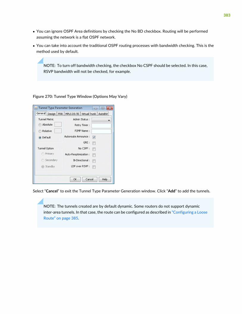
• You can ignore OSPF Area definitions by checking the No BD checkbox. Routing will be performedassuming the network is a flat OSPF network.
• You can take into account the traditional OSPF routing processes with bandwidth checking. This is themethod used by default.
NOTE: To turn off bandwidth checking, the checkbox No CSPF should be selected. In this case,RSVP bandwidth will not be checked, for example.
Figure 270: Tunnel Type Window (Options May Vary)
Select “Cancel” to exit the Tunnel Type Parameter Generation window. Click “Add” to add the tunnels.
NOTE: The tunnels created are by default dynamic. Some routers do not support dynamicinter-area tunnels. In that case, the route can be configured as described in “Configuring a LooseRoute” on page 385.
383

Viewing Inter-Area Tunnels
Once the LSP tunnels have been created, update the network state by clicking the “Update” button justbelow the main menus. Then, selectModify > Elements > Tunnels. Notice the @@ symbol in the CurrentRoute field indicating the border between two areas.
Figure 271: Current Route of Newly Created Tunnels
Click “Show Path”. On the Paths window right-click a column header and select “Table Options” and addthe Area column as shown below.
Figure 272: Path of an Inter-Area LSP Tunnel between B2 and R2
384

You can also view a detailed report of the LSP Tunnels. Go to Report > Report Manager. In the ReportManager, choose the Tunnel Path & Diversity Report under Tunnel Layer Network Reports > TunnelReports.
Configuring a Loose Route
The default setting for the tunnel is to route it dynamically. Note that for Cisco tunnels, the path shouldbe configured with loose routes to the ABR. To change the paths to configured loose routes, open the LSPTunnel window in Modify mode from Modify > Elements > Tunnels. Click Modify and then select “AllEntries” and change the Path Config. Options to “Add” “Config” to configure the route.
Notice that a loose route is now given in the Configured column, indicated by **.
Figure 273: Configured Loose Routes
A route can also be manually configured. For example, select a tunnel and click Modify and then select“Selected Entries.” In the bottom half of the window, there is a table with the route for the tunnel. Toconfigure the path, double-click the cell underneath the column “Configured Route”. Here you can enterin the path, using ** to indicate a loose route after the area border routers.
NOTE: The Exclude-IP-Address feature is not currently supported for inter-area tunnels.
385

Figure 274: Configuring a Route for a Specific LSP Tunnel
After configuring the routes as indicated in the previous step, LSP configlets can be generated for thenewly created LSP tunnels. This is accomplished in Design mode, through Design > Confligets/Delta > LSPConfiglet. For more information, see LSP Configlet Generation Overview.
Figure 275: Example of an LSP Configlet
386

19CHAPTER
Point-to-Multipoint (P2MP) TrafficEngineering
NorthStar Planner P2MP Traffic Engineering Overview | 389
Point-to-Multipoint Traffic Engineering Instructions | 390
Import a Network That Already has Configured P2MP LSP Tunnels | 390
Examine the P2MP LSP Tunnels | 390
Create P2MP LSP Tunnels and Generate Corresponding LSP Configlets | 393
Examine P2MP LSP Tunnel Link Utilization | 397
Perform Failure Simulation and Assess the Impact | 398


NorthStarPlannerP2MPTraffic EngineeringOverview
Traditionally, high-quality video transmissions have been carried over either SDH/SONET or ATM wherethe bandwidth can be guaranteed. However, the drive towards converged networks requires that thesesignals must be carried over the carrier’s IP/MPLS network. Layer-3 IP multicast using PIM is adequateonly for IP TVwhich has a low customer price and corresponding customer expectations, and is not suitablefor high-quality video transmissions which have strict SLAs for packet loss and jitter.
Point-to-multipoint (P2MP) traffic engineering solutions have been developed in the IETF and are nowdeployed commercially in production networks. P2MP traffic engineering allows for efficient trafficreplication in the network, and offers many RSVP-TE features – including explicit path specification andbandwidth specification -- available for point-to-point LSPs.
NorthStar Planner fully supports P2MP MPLS-TE tunnels for IP/MPLS networks. There’s ongoing workin the IETF in areas such as P2MP resiliency, scalability, multicast VPN integration. As new P2MP featuresbecome available in production networks, Juniper Networks will continue to enhance NorthStar Planner’sP2MP features support.
The following sections of this chapter describe the P2MP features that are currently supported byNorthStarPlanner.
Use these procedures if you have P2MP configured in your network or if you would like to use NorthStarPlanner to help you model P2MP LSP tunnels.
If you wish to perform these tasks in NorthStar Planner, you should have an IP/MPLS network routerspecification file open before you begin. Otherwise, you should have a set of router configuration filesready to be imported into the tool. The chapter assumes the user is familiar with IP, MPLS, trafficengineering, P2MP concepts and terminology, and IP multicast PIM concepts and terminology.
For information about LSP Tunnels and how to set their characteristics, see “NorthStar Planner LSP TunnelsOverview” on page 311.
For more information on generating LSP configlets, see LSP Configlet Generation Overview.
For more information about IP multicast, see “NorthStar Planner Multicast Overview” on page 239.
RELATED DOCUMENTATION
Point-to-Multipoint Traffic Engineering Instructions | 390
389

Point-to-Multipoint Traffic Engineering Instructions
• Import a network with P2MP LSPs tunnels configured in the network. Examine the sub-LSPs belongingto a particular P2MP LSP instance and visually display its path.
• Use the tool to easily create P2MP LSP tunnels and generate LSP configlets which can later be provisionedinto the router network.
• Examine P2MP LSP tunnel link utilizations to observe efficient replication.
• Perform failure simulation and assess the impact of the failure on P2MP LSPs.
Import aNetworkThatAlready hasConfiguredP2MPLSP Tunnels
Review the Prerequisites to ensure that your network is configured properly with IP, MPLS and P2MPLSP tunnels.
If you already have a specification file ready for the network, you may open it. Otherwise, if you have theset of router configuration files, then youmay follow the procedures as described in “Router Data ExtractionOverview” on page 33, in order to import the configuration files and create a NorthStar Planner specnetwork model.
Examine the P2MP LSP Tunnels
After open an existing specification file or creating a new specification file after configuration file import,you are ready to examine the P2MP LSP tunnels that are configured in your network. The tool allows youto easily examine the sub-LSPs that belong to a particular P2MP. In NorthStar Planner, P2MP LSPs areappropriately and conveniently represented as multicast trees. For instance, in the following samplenetwork, two P2MP LSPs have been defined in the network. Select the Tunnel layer button to switch intothe Tunnel layer mode, to look at P2MP multicast trees rather than IP multicast trees. Go to NetInfo >Multicast > Multicast Tree to bring up the following window.
390

Figure 276: P2MP LSP tunnels
The window presents summary information – such as source node name and number of sub-LSPs -- forall of the P2MP LSPs that are currently configured in the network.
To show the sub-LSPs that comprise the P2MP LSP, select the particular row corresponding to the P2MP2LSP of interest and then click on the Highlight button. As shown in the following figure, the P2MP LSPnamed C_BLACK is highlighted in the topology map. On the P2MP LSP tree, a circle is drawn around thenode that represents the source node (the ingress LSR) of the tree, while boxes are drawn around the leafnodes (the egress LSRs for the sub-LSPs) of the tree.
391
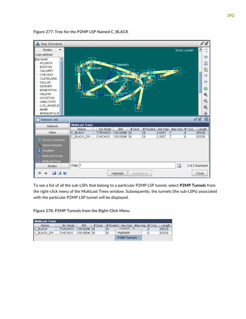
Figure 277: Tree for the P2MP LSP Named C_BLACK
To see a list of all the sub-LSPs that belong to a particular P2MP LSP tunnel, select P2MP Tunnels fromthe right-click menu of the Multicast Trees window. Subsequently, the tunnels (the sub-LSPs) associatedwith the particular P2MP LSP tunnel will be displayed.
Figure 278: P2MP Tunnels from the Right-Click Menu
392
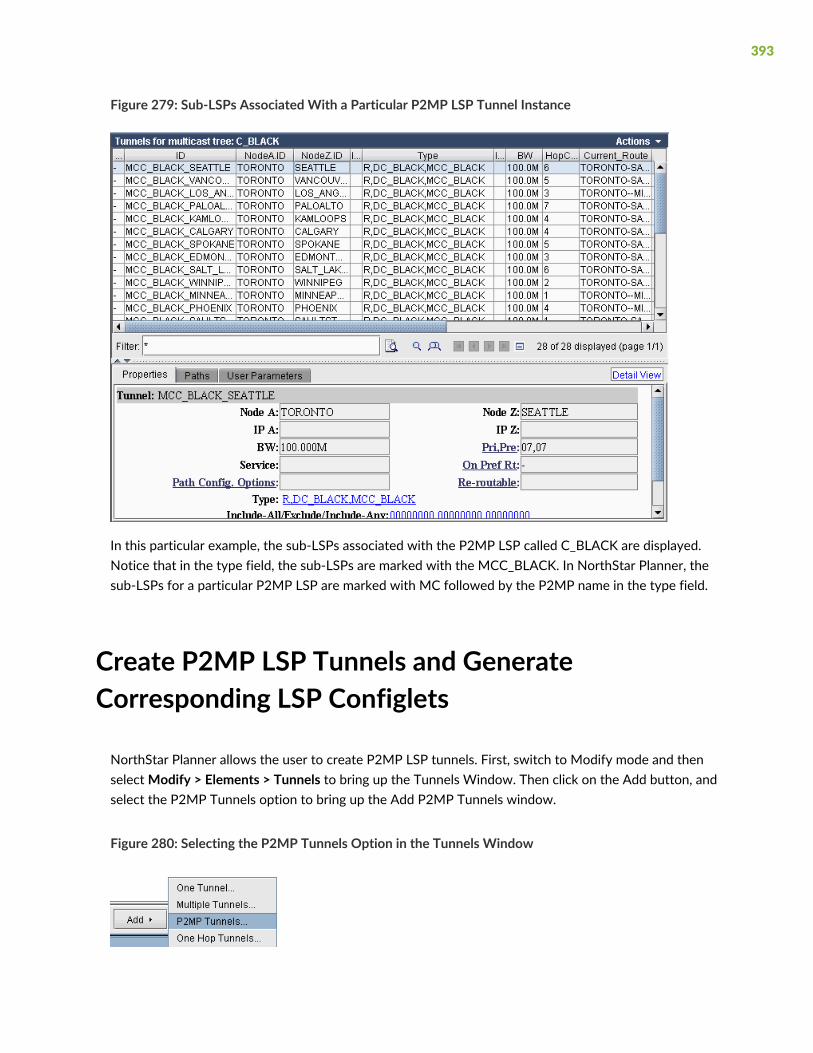
Figure 279: Sub-LSPs Associated With a Particular P2MP LSP Tunnel Instance
In this particular example, the sub-LSPs associated with the P2MP LSP called C_BLACK are displayed.Notice that in the type field, the sub-LSPs are marked with the MCC_BLACK. In NorthStar Planner, thesub-LSPs for a particular P2MP LSP are marked with MC followed by the P2MP name in the type field.
Create P2MP LSP Tunnels and GenerateCorresponding LSP Configlets
NorthStar Planner allows the user to create P2MP LSP tunnels. First, switch to Modify mode and thenselectModify > Elements > Tunnels to bring up the Tunnels Window. Then click on the Add button, andselect the P2MP Tunnels option to bring up the Add P2MP Tunnels window.
Figure 280: Selecting the P2MP Tunnels Option in the Tunnels Window
393
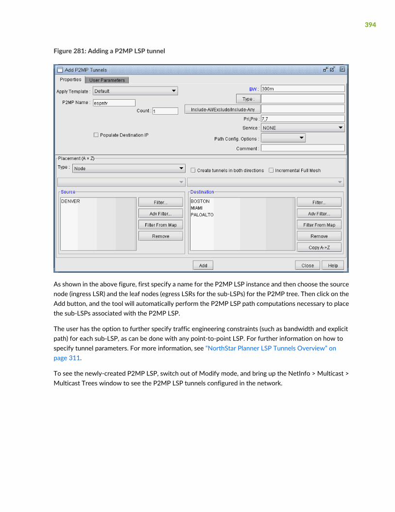
Figure 281: Adding a P2MP LSP tunnel
As shown in the above figure, first specify a name for the P2MP LSP instance and then choose the sourcenode (ingress LSR) and the leaf nodes (egress LSRs for the sub-LSPs) for the P2MP tree. Then click on theAdd button, and the tool will automatically perform the P2MP LSP path computations necessary to placethe sub-LSPs associated with the P2MP LSP.
The user has the option to further specify traffic engineering constraints (such as bandwidth and explicitpath) for each sub-LSP, as can be done with any point-to-point LSP. For further information on how tospecify tunnel parameters. For more information, see “NorthStar Planner LSP Tunnels Overview” onpage 311.
To see the newly-created P2MP LSP, switch out of Modify mode, and bring up the NetInfo > Multicast >Multicast Trees window to see the P2MP LSP tunnels configured in the network.
394

Figure 282: Newly-Added P2MP LSP Called espntv
Figure 283: The Sub-LSPs for the P2MP LSP espntv
After using the NorthStar Planner to model P2MP LSPs, the P2MP LSPs can be rolled out according tothe tool’s P2MP LSP path computation calculations. This allows the P2MP LSPs created during networkplanning to be translated into a series of actions that can be easily implemented by network operations.NorthStar Planner can be used to easily convert the outputs of the network modeling into LSP configlets.
A configlet is a small section of the router configuration file that describes all the LSP attributes: bandwidth,admin-group, primary path, etc. To generate the configlets, select Design > Confligets/Delta > LSP Configletto bring up the LSP Configlet window. After the appropriate options have been specified, click on Submitbutton to generate the configlets for the selected nodes/tunnels.
395

Figure 284: LSP Configlet Generation Window
The following figure shows the various statements listed in the configlet generated by NorthStar Plannerfor the P2MP LSP (espntv) that was created above.
396
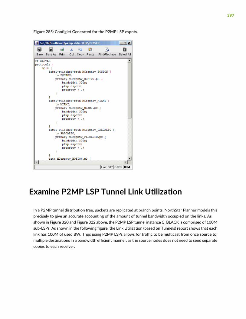
Figure 285: Configlet Generated for the P2MP LSP espntv.
Examine P2MP LSP Tunnel Link Utilization
In a P2MP tunnel distribution tree, packets are replicated at branch points. NorthStar Planner models thisprecisely to give an accurate accounting of the amount of tunnel bandwidth occupied on the links. Asshown in Figure 320 and Figure 322 above, the P2MP LSP tunnel instance C_BLACK is comprised of 100Msub-LSPs. As shown in the following figure, the Link Utilization (based on Tunnels) report shows that eachlink has 100M of used BW. Thus using P2MP LSPs allows for traffic to be multicast from once source tomultiple destinations in a bandwidth efficient manner, as the source nodes does not need to send separatecopies to each receiver.
397

Figure 286: Link Utilization Based on Tunnel Placement
Perform Failure Simulation and Assess the Impact
NorthStar Planner includes a full suite of capabilities that allow the user to perform both interactive andexhaustive failure simulation. With regards to P2MP tunnels, one could fail for instance the link on whichcertain sub-LSPs traverse in order to assess the impact of the damage on the recipients at those sub-LSPs.
For instance, the following two figures show the changes in placement of sub-LSPs after the link betweenEdmonton and Winnipeg is failed. From the result of failure simulation runs, the user may find furtherdesign for redundancy a necessity. Efforts are underway in the IETF to provide FRR support for P2MPtunnels. In addition, application-level redundancy can be provided in the form of the design of a diversemulticast P2MP tree.
398

Figure 287: Placement of Sub-LSPs Prior to Link Failure
Figure 288: Changes in Placement of Sub-LSPs After Link Failure
399
20CHAPTER
Diverse Multicast Tree Design
Diverse Multicast Tree Design Overview | 403
Diverse Multicast Tree Instructions | 404
Open a Network That Already Has a Multicast Tree | 404
Set the Two P2MP Trees of Interest to be in the Same Diversity Group | 405
Using the Multicast Tree Design Feature to Design Diverse Multicast Trees | 407
Using the Multicast Tree Design Feature | 411


Diverse Multicast Tree Design Overview
High quality video distribution (such as high-definition IP TV) with strict SLAs for packet loss and jitter arecontinuing to be rolled out bymajor broadcast service providers across the globe. Such a video distributionnetwork requires that bandwidth be reserved along a fixed pre-allocated transmission path. There arecurrently two possible solutions for protecting such a path:
1. Use pre-configured FRR LSPs to protect each LSP branch. However, the drawback to this approach isthat large spare capacity is needed for all the backup LSPs.
2. Use DiverseMulticast Trees. Here a separate multicast distribution tree is routed that is strictly diversefrom the main tree in order to achieve 1+1 protection. For two multicast trees to be diverse from eachother, the paths (i.e., the sub-LSPs of a P2MP multicast tree) to each destination from the source ofeach of the two trees have to not share any link or site or facility, depending on the diversity level.
Designing diverse multicast trees is a complex network design problem; in fact, it is NP hard(Non-deterministic Polynomial time hard) and not readily tractable for manual computation. A powerfuland heuristics-based algorithm is needed to solve the problem for large networks. NorthStar Planner hasa powerful Multicast Tree Design module that allows the user to design separate multicast trees that arestrictly diverse from each other. The design solutions are as efficient as possible and can lead to largesavings in capacity requirements for the network planner.
The following sections of this chapter describe the Multicast Tree Design features that are currentlysupported by NorthStar Planner.
Use these procedures if you have multicast trees (i.e., P2MP trees) configured in your network and if youwould like to use NorthStar Planner to help you to design diverse multicast trees.
If you wish to perform these tasks in NorthStar Planner, you should have a network router specificationfile open before you begin. Otherwise, you should have a set of router configuration files ready to beimported into the tool. The chapter assumes the user is familiar with IP, MPLS, traffic engineering, P2MP,and IP multicast.
For more information about PM2P Tunnels modeling and creation, see “NorthStar Planner P2MP TrafficEngineering Overview” on page 389.
For more information about LSP Tunnels and how to set their characteristics, see “NorthStar Planner LSPTunnels Overview” on page 311.
For more information about generating LSP configlets, see LSP Configlet Generation Overview.
For more information about IP multicast, see “NorthStar Planner Multicast Overview” on page 239.
RELATED DOCUMENTATION
403

Diverse Multicast Tree Instructions | 404
Using the Multicast Tree Design Feature to Design Diverse Multicast Trees | 407
Diverse Multicast Tree Instructions
1. Open a network with multicast trees (i.e., P2MP trees) configured in the network.
2. Mark the two multicast trees as in the same Diversity Group.
3. Use the Multicast Tree Design feature to design and route multicast distribution trees within in aDiversity Group that are strictly diverse from each other.
4. Use the Multicast Tree Design feature to tune a particular tree to reduce its cost.
Open a Network That Already Has a Multicast Tree
1. Review the Prerequisites to ensure that your network is configured properly with IP, MPLS and P2MPLSP tunnels.
2. If you already have a specification file ready for the network, you may open it. The specification fileshould already have P2MP tree configured in it. For details about P2MP trees, including how to configurethem using NorthStar Planner, see “Point-to-Multipoint Traffic Engineering Instructions” on page 390.Alternatively, if you have the set of router configuration files with P2MP trees configured in them, thenyoumay follow the procedures as described in “Router Data Extraction Overview” on page 33, in orderto import the configuration files and create a NorthStar Planner spec network model.
The following figure shows an example specification file that has two P2MP trees configured: onecalled C_BLACK (centered at TORONTO) and another called C_BLACK_DIV (centered at DENVER).The two P2MP trees have the same leaf nodes.
404

Figure 289: Two P2MP Trees Shown in Main Topology Map’s P2MP Subview
Set the Two P2MPTrees of Interest to be in the SameDiversity Group
After opening an existing specification file or creating a new specification file after configuration file import,you are ready to perform Diverse Multicast Tree design on two P2MP trees. The tool allows you to easilyselect the sub-LSPs that belong to a particular P2MP tree and then specify its Diversity Group. Two treesbelong to the same Diversity Group if all the corresponding sub-LSPs have been marked with the sameDiversity Group name.
1. To set the Diversity Group name for the sub-LSPs, first go to Modify mode and bring up the ModifyTunnels window via Modify > Elements > Tunnels.
2. Next select all the sub-LSPs for the two P2MP trees of interest and click on Modify>Selected button.
3. From the Modify Tunnels Window, click on the Type button to bring up the Tunnel Type ParameterGeneration window.
4. Next, click on the Diversity tab and fill in a name inside the Diversity Group fill-in/dropdown combobutton, as shown in the following figure.
405

Figure 290: Specify Diversity Group for Each Sub-LSP for the Two P2MP Trees
5. After clicking OK, the Type field for each tunnel modified should contain the DC_BLACK flag in it, asshown in the following figure. In NorthStar Planner, the sub-LSPs for a particular Diversity Group aremarked with D followed by the Diversity Group name in the type field.
406

Figure 291: Type Field Containing DC_BLACK.
Using the Multicast Tree Design Feature to DesignDiverse Multicast Trees
Now that the two P2MP trees of interest have been marked to be in the same Diversity Group, you areready to perform a design. For two multicast trees to be diverse from each other, the paths (i.e., thesub-LSPs of a P2MP multicast tree) to each destination from the source of each of the two trees have tonot share any link or site or facility, depending on the diversity level. By default, the algorithm tries thehighest diversity level first; so it will try to design for facility, then site, then link diversity.
To perform the design, first go to Design Mode and selectDesign >Multicast Tree Design to bring up theMulticast Tree Design window, as shown in the following figure. The top part of the window displays the
407

list of P2MP trees that are configured in the network. The bottom part of the window shows the sub-LSPsthat make up the P2MP tree selected on the top part of the window.
Figure 292: Multicast Tree Design Window Before Tuning Tree
The Div Level column indicates the current diversity level (FACILITY, SITE, LINK, or NO_DIVERSITY) forthe sub-LSP. The Show Paths button allows you to visually see two sub-LSPs that are diverse from eachother. For instance, the following figure shows that the sub-LSP from TORONTO to VANCOUVER andthe sub-LSP from DENVER to VANCOUVER are SITE-diverse from each other.
408

Figure 293: Example of Site Diverse Sub-LSPs.
Next you are ready to start the actual design run. Simply click on the Tune Tree button to bring up theTuning Options window, shown in the following figure. The Max Iterations box may be set to a highervalue in order for the design’s heuristics algorithm to perform more iteration runs, which leads to evenbetter solutions. The Remove configured paths before tuning option, which is checked by default, meansthat existing P2MP sub-LSP paths will be overwritten by the program. The Mark new paths as configuredoption, which is checked by default, means that the LSP will be explicitly routed by our optimizationprogram.
409
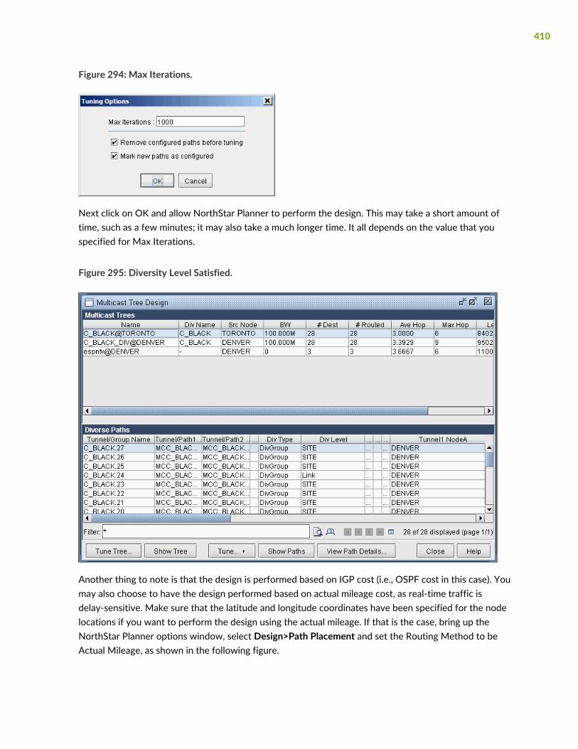
Figure 294: Max Iterations.
Next click on OK and allow NorthStar Planner to perform the design. This may take a short amount oftime, such as a few minutes; it may also take a much longer time. It all depends on the value that youspecified for Max Iterations.
Figure 295: Diversity Level Satisfied.
Another thing to note is that the design is performed based on IGP cost (i.e., OSPF cost in this case). Youmay also choose to have the design performed based on actual mileage cost, as real-time traffic isdelay-sensitive. Make sure that the latitude and longitude coordinates have been specified for the nodelocations if you want to perform the design using the actual mileage. If that is the case, bring up theNorthStar Planner options window, select Design>Path Placement and set the Routing Method to beActual Mileage, as shown in the following figure.
410

Figure 296: Setting Routing Method to use Actual Mileage
Using the Multicast Tree Design Feature
For other P2MPmulticast trees in the network that do not belong to a particular Diversity Group, you canstill select the tree and perform a tuning in order to reduce the multicast tree’s cost (which is defined thetotal length (physical or admin-cost) of the tree). For instance, the following figure shows espntv P2MPtree is not part of Diversity Group and is a candidate for tuning.
411

Figure 297: Tuning a single P2MP diverse multicast tree
412

21CHAPTER
DiffServ Traffic Engineering Tunnels
DiffServ Traffic Engineering Tunnels Overview | 415
Using DS-TE LSP | 416
Hardware Support for DS-TE LSP | 416
NorthStar Planner Support for DS-TE LSP | 418
Configuring the Bandwidth Model and Default Bandwidth Partitions | 422
Forwarding Class to Class Type Mapping | 423
Link Bandwidth Reservation | 423
Creating a New Multi-Class or Single-Class LSP | 425
Configuring a DiffServ-Aware LSP | 426
Tunnel Routing | 427
Link Utilization Analysis | 427


DiffServ Traffic Engineering Tunnels Overview
This topic discusses howDifferentiated Services Aware Traffic Engineering LSPs (DS-TE LSPs) aremodeledin NorthStar Planner. In order to provide the most value to users, NorthStar Planner’s modeling of DS-TELSPs are continually updated to reflect current vendor implementations and industry practices in this field.Therefore, it is possible that the descriptions of DS-TE LSPs may not reflect the traditional DS-TE LSPmodels (E-LSPs and L-LSPs) defined by IETF. For more information on traditional DS-TE LSP models, feelfree to peruse IETF RFC 3270. In this document, theDS-TE LSP behavior discussed is that which is currentlyimplemented by today’s hardware vendors. Currently, only Juniper Networks supports DS-TE LSPs.
Whereas standard traffic engineering works on an aggregate basis, DS-TE LSPs allow for traffic engineeringat a per-class level with different bandwidth constraints for different traffic class types. This makes itpossible to guarantee different levels of service and bandwidth to different classes across anMPLS network.Such advantages allow you to provide ATM circuit emulation over IP, Voice over IP, class based services,and guaranteed bandwidth services.
Before reading this chapter, you should have a good understanding of how standard LSPs are provisionedon a network, and you should be comfortable working with LSPs.
It should be noted that in this topic, the word “tunnel” is used in the context of traffic engineering (TE)tunnels. Also, the word “tunnel load” refers to the amount of IP traffic transported by the tunnel.
The following terms are used in this topic and related topics:
• Bandwidth Model: The bandwidth model determines the values of the available bandwidth advertisedby the interior gateway protocols (IGPs).
• Differentiated Services: Also known as DiffServ, differentiated services make it possible to give differenttreatment to traffic based on the experimental (EXP) bits in the MPLS header.
• DSCP: The Differentiated Services Code Point refers to six bits in the ToS (Type of Service) byte of apacket header that specify the particular PHB (Per Hop Behavior) to be applied to the packet.
• DS-TE LSP: Differentiated-Services-aware Traffic Engineering LSP.
• E-LSP: EXP-inferred LSP as defined in IETF RFC 3270.
• L-LSP: Label-only-inferred LSP as defined in IETF RFC 3270.
• Planned Bandwidth: The current bandwidth allotted to the tunnel.
• QoS: Quality of Service is a broad collection of networking technologies with the goal of providingguarantees on the ability of a network to deliver predictable results beyond the best-effort deliveryprovided by default.
RELATED DOCUMENTATION
415

Using DS-TE LSP | 416
Creating a New Multi-Class or Single-Class LSP | 425
Configuring a DiffServ-Aware LSP | 426
Using DS-TE LSP
Imagine a scenario where you are migrating from ATM over to IP, and you want to provision tunnels onthe IP network to support the various classes of traffic in ATM, such as CBR, VBR, RT, NRT. To useNorthStarPlanner to model this, you would follow these steps:
• Map the four types of ATM traffic to four class types.
• Partition bandwidth on your interfaces / links for these four classes.
• Create as many DS-TE LSPs as is necessary to carry the ATM traffic. Specify the class for each DS-TELSP according the type of ATM traffic it is supposed to carry.
• Route the DS-TE LSP tunnels over the network. This is done automatically by the tool.
• Examine where bottlenecks occur, where excess capacity exists, where you need to purchase morebandwidth, etc.
This is just one example of how DS-TE LSPs can be used, but it illustrates many of the steps involved insetting up and utilizing DS-TE LSPs in a network.
Hardware Support for DS-TE LSP
Juniper Networks supports two kinds of DS-TE LSPs: DiffServ-aware single-class LSPs andDiffServ-awaremulti-class LSPs. Single-class LSPs are similar to traditional L-LSPs, and support only one class per LSP.Multi-class LSPs can be thought of as L-LSPs that can handle multiple classes. Each multi-class LSP cansupport up to four classes with specific bandwidth reservation assigned to each class.WhenDiffServ-awareLSPs are routed on a network, consideration is given to the amount of bandwidth reserved on each interfacefor each class. If there is insufficient bandwidth on a particular interface for a given class on the multi-classor single-class LSP, the LSP will not be routed over that interface.
416

Class Type
A class type is a collection of traffic flows that is treated equivalently in a DiffServ domain. A class typemaps to a queue and is much like a class-of-service (CoS) forwarding class in concept. It is also known asa traffic class.EXP Bits
EXP Bits
The Experimental bits, or EXP bits, in the MPLS header are used to define the class to which a packetbelongs. A unique EXP bit pattern is associated with each class type and forwarding class defined on aDiffServ-aware router.
Forwarding Class
Forwarding classes are defined on each router and assigned to internal queues. The default forwardingclasses are: best-effort, expedited-forwarding, assured-forwarding, and network-control. Individual classtypes in DiffServ-aware LSPs aremapped to individual forwarding classes at the router. The default mappingis shown in the table below.
Forwarding Class NameClass Type
best-effortCT0
expedited-forwardingCT1
assured-forwardingCT2
network-controlCT3
Scheduler Map
The treatment given to each forwarding class on an interface is defined by the scheduler map assigned tothat interface. The scheduler map includes a list of schedulers which map specific forwarding classes tospecific scheduler configurations. These determine the per-class bandwidth allocations on each interface,which are taken into consideration when routing DiffServ-aware LSPs.
417
Bandwidth Model
A bandwidthmodel must be configured on all routers participating in the DiffServ domain. The three typesof bandwidth models supported by Juniper are MAM, Extended MAM, and RDM, which are defined inthe following table.
Defined in Internet draft draft-ietf-tewg-diff-te-mam-03.txtMAM
A proprietary bandwidth model that behaves much like standard MAM. If you configuremulticlass LSPs, you must configure the extended MAM bandwidth model.
Extended-MAM
Makes efficient use of bandwidth by allowing the class types to share bandwidth. RDM isdefined in Internet draft draft-ietf-tewg-diff-te-russian-05.txt
RDM
Operation
In order to take advantage of DiffServ aware single-class and multi-class LSPs, each class type must beconfigured consistently across the differentiated service domain. In other words, each router in the networkmust follow a consistent class type configuration. On each node router, each class type is mapped to aqueue.
The available bandwidth for a particular class type on a link is determined by the configuration of class ofservice queues for that interface. Any DiffServ-aware LSP that requires bandwidth from a particular classcannot be established through routers that do not understand the Classtype object. It is possible forDiffServ-aware LSPs and regular LSPs to be established on the same router. In this case, the regular LSPwill carry best-effort traffic by default. However, you cannot simultaneously configure multi-class LSPsand single-class LSPs on the same router.
NorthStar Planner Support for DS-TE LSP
NorthStar Planner supports both DiffServe-aware Single-Class LSPs and DiffServ-awareMulti-Class LSPs,according to the specifications in existing hardware. These LSPs can be parsed from existing routerconfiguration files, or they can be manually created from scratch using NorthStar Planner for a papernetwork design.
418

Class Types
NorthStar Planner’s class type terminology corresponds with that used in JUNOS configurations. The fourclass type names are CT0, CT1, CT2, and CT3. These class type names appear in the JUNOS configurationstatements:
Multi-class LSPSingle-class LSP
label-switched-path lsp-name {bandwidth {ct0 bandwidth;ct1 bandwidth;ct2 bandwidth;ct3 bandwidth;
}}
label-switched-path lsp-name {bandwidth {ctnumber bandwidth;
}}
EXP Bits
The Experimental bits, or EXP bits, in the MPLS header are used to define the class to which a packetbelongs. A unique EXP bit pattern is associated with each class type and forwarding class defined on aDiffServ-aware router. NorthStar Planner allows the user to define the mapping between EXP bits, classtypes, and forwarding classes.
CoS Classes
The CoS class defined in NorthStar Planner is equivalent to the forwarding class configured in JUNOS, asin the following configuration structure.
interfaces {interface-name {scheduler-map map-name;scheduler-map-chassis map-name;unit logical-unit-number {classifiers {type (classifier-name | default);}
forwarding-class class-name;
419

rewrite-rules {type (rewrite-name | default);
}}
}}
Cos Policies
NorthStar Planner’s CoS policy is equivalent to the scheduler map defined in JUNOS. A CoS policy containsinformation on how to treat each CoS class referenced by the CoS policy. The treatment given to eachCoS class at a router is determined by the CoS policy assigned to that router. Applying a CoS policy to arouter is similar to applying scheduler maps to the interfaces on that router, as in the configuration structurebelow.
interfaces {interface-name {scheduler-map map-name;scheduler-map-chassis map-name;unit logical-unit-number {classifiers {type (classifier-name | default);
}forwarding-class class-name;rewrite-rules {type (rewrite-name | default);
}}
}}
NorthStar Planner allows the user to define a robust set of Cos policies and to easily assign them to anyrouter in a network. The CoS Policy determines the amount of bandwidth reserved on a link for each trafficclass contained in the policy. The bandwidth reservation scheme for each router affects howDiffServ-awareLSPs are routed in the network.
420

Bandwidth Model
NorthStar Planner supports both MAM and RDM bandwidth models. The MAM bandwidth model usedwhen configuringDiffServ-aware LSPs in NorthStar Planner is equivalent to the extended-MAMbandwidthmodel used in JUNOS configuration, as shown below.
bandwidth-model {(extended-mam | mam | rdm);
}
The choice of whether to use MAM or RDM in NorthStar Planner affects the way in which bandwidth isassigned to a multi-class LSP, and the manner in which bandwidth is reported for a link with bandwidthpartitions for multiple classes. For example, in a situation where CT0, CT1, CT2 and CT3 are all reserved10M, the link partition will be reported differently depending on whether the bandwidth model is MAMor RDM, as shown in the table below.
RDMMAM
CT0: 40M
CT1: 30M
CT2: 20M
CT3: 10M
CT0: 10M
CT1: 10M
CT2: 10M
CT3: 10M
In the above example, for MAM, each class gets 10M. For RDM, each class also gets 10M. However, inRDM, CT2 has access to the 10M belonging to CT3, and thus has 20M total available. CT1 has its own10M plus the 20M available to CT2, and thus ends up with 30M total. Since CT0 is at the top of the stack,it receives its own 10M plus all the bandwidth available to the classes below it, for a total of 40M.
Similarly, if one were to configure a multi-class LSPwith 90M reserved for CT0 and 10M reserved for CT3,the configuration would look differently depending on the bandwidth model used. This is shown in thetable below.
RDMMAM
CT0: 100M
CT1: 0M
CT2: 0M
CT3: 10M
CT0: 90M
CT1: 0M
CT2: 0M
CT3: 10M
421
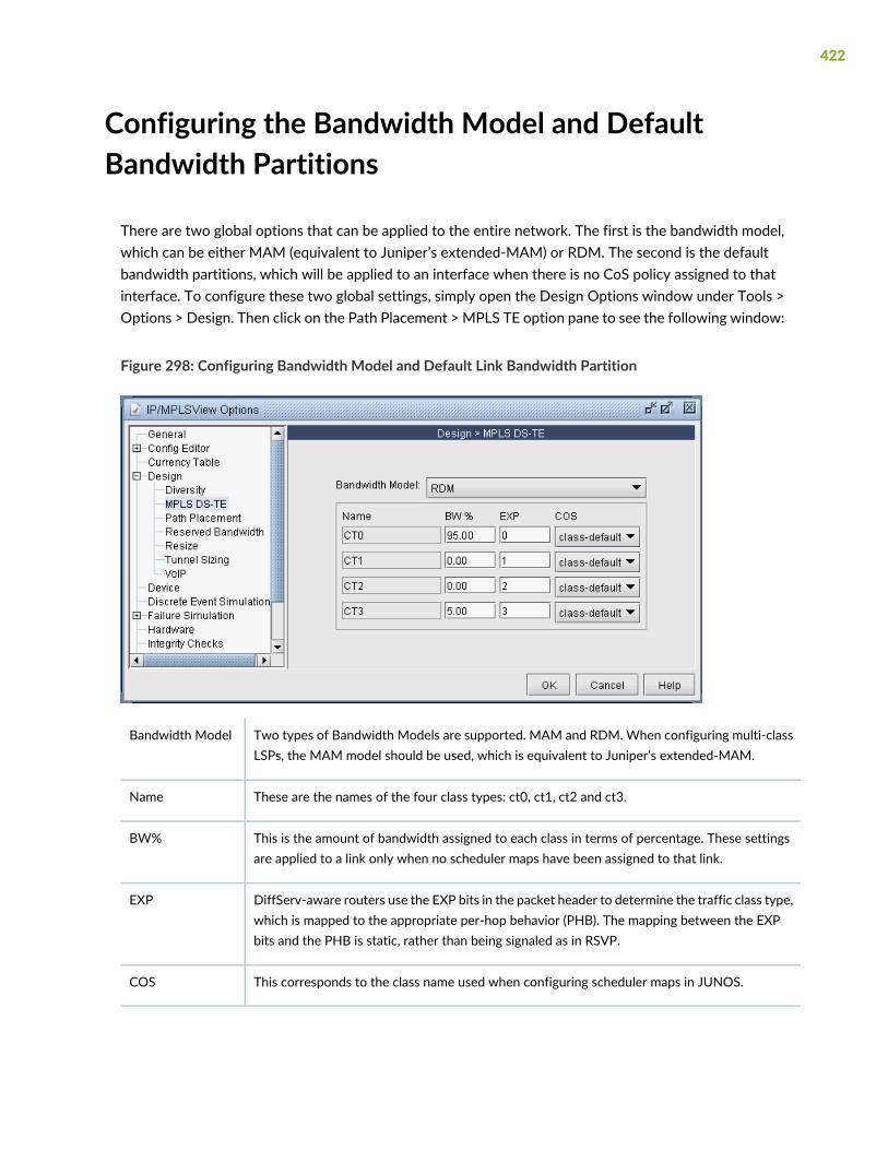
Configuring the Bandwidth Model and DefaultBandwidth Partitions
There are two global options that can be applied to the entire network. The first is the bandwidth model,which can be either MAM (equivalent to Juniper’s extended-MAM) or RDM. The second is the defaultbandwidth partitions, which will be applied to an interface when there is no CoS policy assigned to thatinterface. To configure these two global settings, simply open the Design Options window under Tools >Options > Design. Then click on the Path Placement > MPLS TE option pane to see the following window:
Figure 298: Configuring Bandwidth Model and Default Link Bandwidth Partition
Two types of Bandwidth Models are supported. MAM and RDM. When configuring multi-classLSPs, the MAM model should be used, which is equivalent to Juniper’s extended-MAM.
Bandwidth Model
These are the names of the four class types: ct0, ct1, ct2 and ct3.Name
This is the amount of bandwidth assigned to each class in terms of percentage. These settingsare applied to a link only when no scheduler maps have been assigned to that link.
BW%
DiffServ-aware routers use the EXP bits in the packet header to determine the traffic class type,which is mapped to the appropriate per-hop behavior (PHB). The mapping between the EXPbits and the PHB is static, rather than being signaled as in RSVP.
EXP
This corresponds to the class name used when configuring scheduler maps in JUNOS.COS
422

Forwarding Class to Class Type Mapping
To specify the forwarding class to class type mappings, the following parameter, cos2ctmap, needs to beincluded in the dparam file.
Example:
cos2ctmap=M-RT:CT3|1R,MC:CT2|2R,ME:CT1|4R,BE:CT0|6R
The cos2ctmap parameter takes a comma-separated list of tokens that can be specified in one of thefollowing formats:
• cosname:CTn: map demand with forwarding class cosname to CTn tunnel
• cosname:CTn|m : map demand with forwarding class cosname to tunnel with CTn and priority m
• cosname:CTn|mR : map demand with forwarding class cosname to tunnel with CTn and priority m. The"R" is restrictive, meaning that if not available don't map to the tunnel
Link Bandwidth Reservation
Individual link bandwidth reservation schemes can be assigned to a link by applying a CoS policy to thatlink. NorthStar Planner allows the user to define a robust collection of CoS policies, which can be specificto a router or generic to all routers.
423
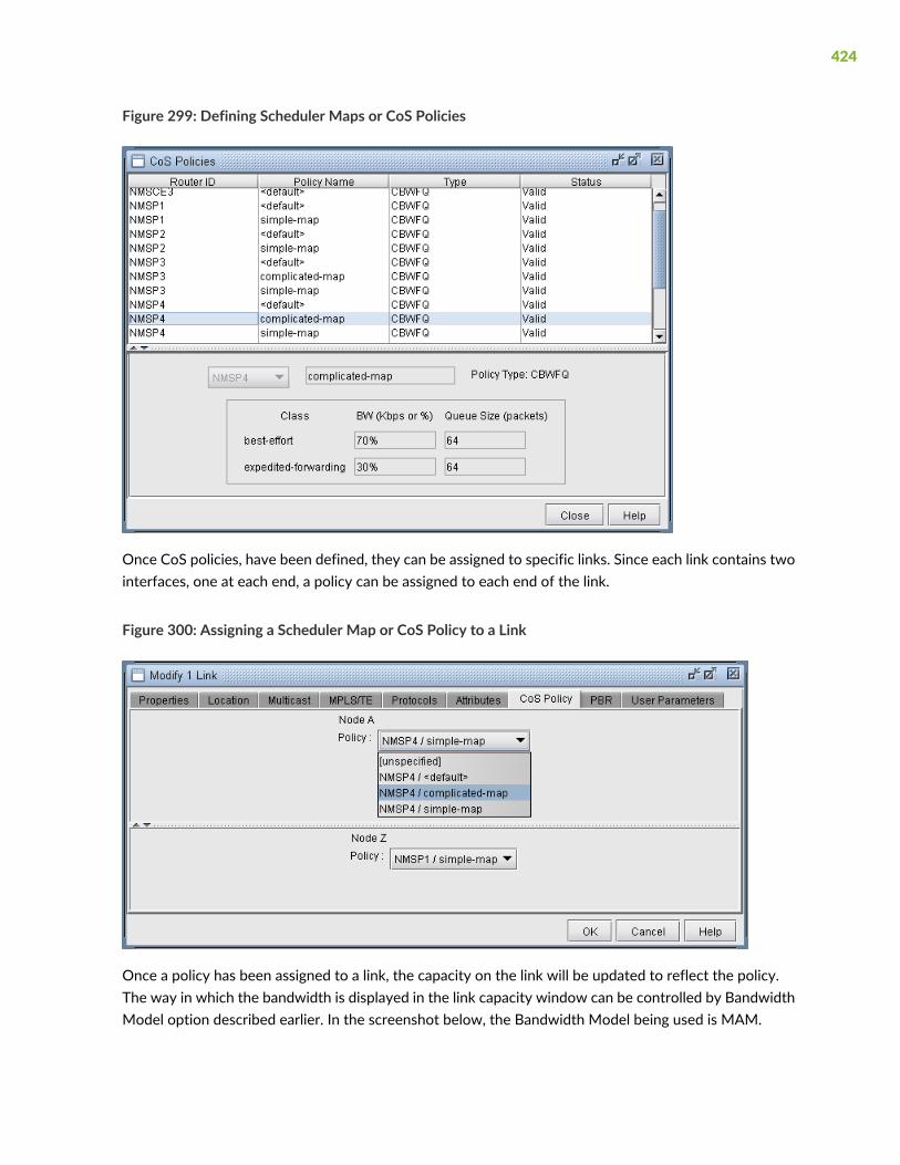
Figure 299: Defining Scheduler Maps or CoS Policies
Once CoS policies, have been defined, they can be assigned to specific links. Since each link contains twointerfaces, one at each end, a policy can be assigned to each end of the link.
Figure 300: Assigning a Scheduler Map or CoS Policy to a Link
Once a policy has been assigned to a link, the capacity on the link will be updated to reflect the policy.The way in which the bandwidth is displayed in the link capacity window can be controlled by BandwidthModel option described earlier. In the screenshot below, the Bandwidth Model being used is MAM.
424

Figure 301: Link Capacity Reflecting the Assigned Scheduler Map or CoS Policy
This corresponds to the class type associated with the policy assigned to the interface.Partition
This is the amount of bandwidth reserved for the corresponding partition, as defined bythe assigned policy.
RSVPBW
This is the amount of tunnel bandwidth currently passing through the interface.TunnelBW
This is the amount of available bandwidth remaining for the corresponding partition.AvRSVP
Creating a NewMulti-Class or Single-Class LSP
When creating a new tunnel object, there is an option to specify the type of LSP to create. The type canbe Regular (“NONE”), Single-Class LSP, or Multi-Class LSP.
425
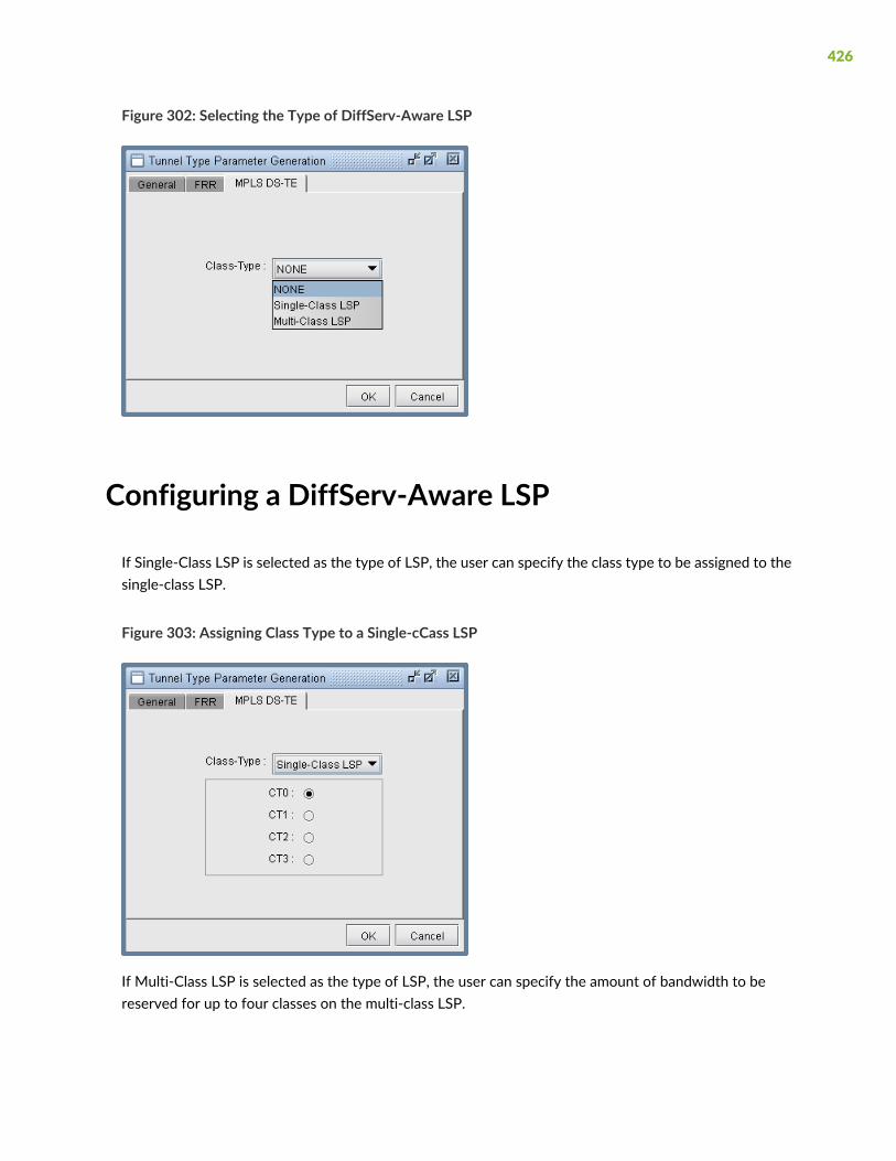
Figure 302: Selecting the Type of DiffServ-Aware LSP
Configuring a DiffServ-Aware LSP
If Single-Class LSP is selected as the type of LSP, the user can specify the class type to be assigned to thesingle-class LSP.
Figure 303: Assigning Class Type to a Single-cCass LSP
If Multi-Class LSP is selected as the type of LSP, the user can specify the amount of bandwidth to bereserved for up to four classes on the multi-class LSP.
426

Figure 304: Assigning Bandwidth per Class to a Multi-Class LSP
Tunnel Routing
NorthStar Planner’s routing engine automatically determines the optimal placement of DiffServ-awareLSPs based on the amount of bandwidth reserved per class on the LSP and the amount of bandwidthreserved per class on all available links in the network. A DiffServ-aware LSP will not be routed over anyinterface that has insufficient bandwidth allocated to any of the classes defined on the LSP.
Link Utilization Analysis
WithNorthStar Planner’s link object, it is easy to determine the amount of total bandwidth, used bandwidth,and available bandwidth for each class on the link. In the screenshot below, each class is reserved 25% ofthe bandwidth on each interface on the link. For the A-Z interface, 100 Mb of bandwidth is being usedfor DiffServ-aware LSPs that carry CT-2 and CT-3 traffic. For the Z-A interface, 5 Mb of bandwidth isbeing used from the CT-0, CT-1, and CT-2 partitions.
427

Figure 305: Link Capacity Window Showing Tunnel Traffic
It should be noted that the available bandwidth being reported in the window above is the availablebandwidth for tunnels with a pre-emption priority of seven. In other words, the model assumes that noneof the existing tunnels currently residing on the link can be bumped off the link by another tunnel.
428

22CHAPTER
Fast Reroute
NorthStar Planner Fast Reroute Overview | 431
Fast Reroute Supported Vendors | 432
Import Config and Tunnel Path | 433
Viewing the FRR Configuration | 434
Viewing FRR Backup Tunnels | 436
Viewing Primary Tunnels Protected by a Bypass Tunnel | 437
Modifying Tunnels to Request FRR Protection | 439
Modifying Links to Configure Multiple Bypasses (Juniper only) | 441
Modifying Links to Trigger FRR Backup Tunnel Creation (Cisco) | 442
FRR Design | 443
FRR Auto Design | 449
FRR Tuning | 453
Viewing Created Backup Tunnels | 457
Generating LSP Configlets for FRR Backup Tunnels | 458
Failure Simulation—Testing the FRR Backup Tunnels | 459

Exhaustive Failure | 462
Link, Site and Facility Diverse Paths | 464

NorthStar Planner Fast Reroute Overview
This topic and related topics describe how to design Fast Reroute (FRR) backup tunnels. Fast Reroute isa mechanism that can be used to protect MPLS traffic engineering LSP tunnels in the event of node orlink failures. It accomplishes this with SONET-like restoration times by locally repairing the LSPs at thepoint of failure, using backup tunnels that bypass the failure while waiting for the head-end routers toestablish a new LSP. The short restoration times are especially desirable for real-time applications such asvoice over IP, which often cannot tolerate high delays.
NorthStar Planner supports simulation and design of both FRR Node Protection and FRR Link Protection.When a tunnel that has requested FRR protection fails at a particular network element and when there isa FRR backup tunnel configured for that node or link, the packets can be diverted along the backup tunneluntil the original tunnel is able to reroute around the failed network element.
Use the NorthStar Planner Fast Reroute features to view or modify FRR configurations, to design FRRbackup tunnels for your network, and to generate configlets for primary and backup tunnels whereapplicable. You should also use this feature to simulate and analyze the impact or effectiveness of yourFRR backup tunnels on the network in the event of network element failures.
You should have LSP tunnels defined in your network model.
If you want your FRR backup tunnels to be routed over site-diverse or facility-diverse (SRLG) paths, youshould first create sites and facilities on your network.
Graphical Display
NorthStar Planner can be used to import existing tunnel path information collected through show commandsand to graphically display all the FRR backup tunnel paths protecting the links or nodes of a primary tunnel,and all the primary tunnels being protected by a given FRR backup tunnel.
What-If Studies and Path Design
Users can perform what-if studies by configuring primary tunnels to request FRR protection, and thenallow NorthStar Planner to design the FRR backup tunnels. NorthStar Planner can be used to simulate thecreation of backup tunnels in the case where it is automatically generated for what-if studies, or to helpdesign diverse backup tunnels in the case where the user wants to configure the backup tunnels to meetparticular diversity requirements. Consequently, LSP configlets can be generated to facilitate the processof updating the routers.
431

Failure Simulation
Furthermore, NorthStar Planner can also be used to perform failure analysis, showingwhether the demandsare successfully protected through FRR during node or link failure, and then indicating the rerouted pathonto the backup path, if configured, whether it be secondary (passive) or standby (active/1+1). Users canview the peak utilization when using FRR.
For instructions on how to view ormodify the tunnels in your network, see “NorthStar Planner LSP TunnelsOverview” on page 311.
Fast Reroute Supported Vendors
This document covers Cisco and Juniper implementations in particular. However, NorthStar Planner alsosupports FRR for additional router vendors, such as Alcatel and Tellabs.
Juniper
There are two methods of FRR protection for Juniper. One method is one-to-one (fast reroute) backupprotection in which case detour(s) are created to protect the nodes and links traversed by a single primaryLSP. These detours are dedicated in the sense that they can only be used for one primary LSP. To configurefor one-to-one protection, the user should configure the primary tunnel using the “fast-reroute” statement.
The other method of local protection for Juniper is many-to-one (facility) backup. In facility backup, abypass tunnel is used to route around a facility (node or link), and the bypass tunnel can be used to protectmultiple primary LSPs using the facility that are enabled for FRR. For Juniper’s facility backup, two thingsneed to be configured:
1. The primary tunnel is configured to enable link protection or node-link protection.
2. The link interface(s) are configured to enable local protection. Node protection can be turned off fora particular interface if only link protection desired.
After these configurations are made, bypass tunnels will be created for the FRR-enabled facilities alongthe paths of the FRR-enabled primary tunnels-- either next-hop bypasses to circumvent the primary tunnel’slinks in the case of link-protection or next-next-hop bypasses to circumvent the primary tunnel’s nodesin the case of node-link-protection. NorthStar Planner can be used to configure the primary tunnels forfacility backup and to simulate the creation of the bypass tunnels for each facility of the primary tunnel.
An additional feature provided by Juniper for facility backup is the option to use multiple bypass LSPs toprotect an interface. (By default, only one bypass LSP protects one interface.) In this case, the user can
432

configure additional parameters to specify the bandwidth and subscription factor of the multiple bypassesto be created. NorthStar Planner can be used to simulate the creation of multiple bypasses or to designdiverse paths for the multiple bypass tunnels and to generate the corresponding LSP configlets.
Finally, for diffserv-te, users can also configure what type of LSPs to protect (single-class, multi-class orany). In the case of single-class LSPs, the user can configure the class type (CT0, CT1, CT2, or CT3). In thecase of multi-class LSPs, users can configure a percentage for each class type.
Cisco
For Cisco’s FRR implementation, three things need to be configured:
1. The primary tunnel is configured to enable FRR
2. The backup tunnel is configured for each link of the primary tunnel, and
3. The protected link is configured to use the backup tunnel.
NorthStar Planner can be used to automate the creation of the backup tunnels given either the primarytunnel configuration (1) or the links to be protected (3). Configlets can be created for the backup tunnelsto help automate the configuration of the backup tunnels.
An additional feature provided by Cisco is the option to specify the bandwidth pool (sub-pool, global-pool,or any) the traffic must belong to in order to be protected by the backup tunnel.
Import Config and Tunnel Path
In the Live Network, configuration file and tunnel path information can be automatically collected usingthe Scheduling Live Network Collection task’s collection types “Configuration,” “Tunnel Path,” and “TransitTunnel.”
Otherwise, in offline mode, collected configuration files and tunnel path information can be importedthrough the Import Network Wizard via the File>Import Data menu.
To import configuration information in offline mode, select the import type “Router Configuration” andselect the Import Directory containing the configuration files. When performing an import of networkconfiguration data, NorthStar Planner automatically records those links that are FRR-enabled as well asthose LSP tunnels that request FRR protection. See “Router Data Extraction Overview” on page 33 formore details on importing router configuration files.
433
To import the tunnel status and path information in offline mode, select the import type “Tunnel Path”and select the Import Directory containing the tunnel path show command output. Refer to “MPLS TunnelExtraction” on page 54 for more details on the commands to collect this information.
Viewing the FRR Configuration
In offline mode, switch to Design mode by clicking on the “Design” button on the main menu bar.
Select Network > Elements > Tunnels.
The Type column can be used to determine the type of each tunnel, whether it is a primary tunnel requestingFRR protection or an FRR backup tunnel.
Cisco
For the Cisco FRR implementation, the Type field will indicate “FRR” for the primary tunnel to be protectedand “FRRLK” or “FRRND” respectively for the backup tunnels around the link or node to be protected.
Juniper
For Juniper one-to-one (fast reroute) backup, the Type field will indicate “FRR” for the primary tunnelconfigured with the “fast-reroute” statement.
For Juniper many-to-one (facility) backup, the Type field will indicate “LP” or “NLP” corresponding to the“link-protection” and “node-link-protection” statements, respectively. For the node and link bypass tunnelscreated for facility backup, the Type field will indicate “FRRLK” or “FRRND” respectively for next-hop andnext-next-hop bypass tunnels.
Click on a tunnel in the top half of the Tunnels window. In the Properties tab, click the link to the right ofthe Type field to open the Tunnel Type Parameter Generationwindow. Select the FRR tab for the followingwindow, which is populated based on the Type field.
434

Figure 306: LSP Tunnel Requesting FRR Protection
InterpretationType FieldOption
• For Juniper, this field indicates that the primary LSP is being configuredfor one-to-one (fast reroute) backup, in which case the created detourwould protect only this tunnel.
• For Cisco, this field is used to enable the primary tunnel to use a backuptunnel (configured separately) in case of node or link failure.
FRRFast Reroute
For Juniper, this field indicates the primary tunnel being configured formany-to-one (facility) backup for link protection. The resulting bypasspaths could be used to protect many LSPs.
LPFRR Link Protection
For Juniper, this field indicates the the primary tunnel being configuredfor many-to-one (facility) backup for node-link protection. The resultingbypass paths could be used to protect many LSPs.
NLPFRR Node-LinkProtection
This field indicates the next-hop bypass tunnel which can bypass a singlelink for multiple LSPs.
FRRLKFRR Link BackupTunnel
This field indicates the next-next-hop bypass tunnel which can bypass asingle node for multiple LSPs.
FRRNDFRR Node BackupTunnel
Indicates how much bandwidth the FRR backup tunnel is configured toprotect.
BKBW=<bw>BKBW
435

InterpretationType FieldOption
For Cisco only. Indicates howmuchGlobal Pool bandwidth the FRRbackuptunnel is configured to protect.
BKGP=<bw>BKGP
For Cisco only. Indicates howmuch Sub Pool bandwidth the FRR backuptunnel is configured to protect.
BKSP=<bw>BKSP
Viewing FRR Backup Tunnels
To view the FRR backup tunnels protecting a primary tunnel configured for FRR, first identify a primarytunnel marked with either FRR (for Cisco), LP (for Juniper), or NLP (for Juniper) in the Type field. To listonly the primary tunnels configured for fast reroute, you can click the “Search by Property” magnifyingglass icon on middle bar to perform a search. In the Find Tunnels window, click the “Type” button. Then,in the FRR tab of the Tunnel Type Parameter Generation window, set the Fast Reroute selection box tosay “Yes”. This will filter on all primary tunnels configured for fast reroute, including primary tunnelsconfigured for link protection , node protection, and one-to-one protection. Click “OK” to close the Typewindow and then click “OK” in the Find Tunnels window. All primary LSP tunnels requiring FRR Protectionwill be displayed in a table. Select any tunnel and click “Show Path” to view the route of the selectedtunnel.
Right-click on the primary tunnel configured for FRR to view the options “Show FRR Backup Tunnels” or“FRR Detour.”
If the head-end router is a Cisco router, select “Show FRR Backup Tunnels” to view the Cisco backuptunnel(s) protecting the primary tunnel.
If the head-end router is a Juniper router, select “ShowFRRBackup Tunnels” to view the Juniper next-hopor next-next-hop bypass tunnels created for many-to-one (facility) backup for the primary tunnel. Select“FRRDetour” to view Juniper detour tunnel(s) created for one-to-one (fast reroute) backup for the primarytunnel.
Note that for a multi-vendor network, it may be helpful to display the router vendor as a column. Right-clickon the table column header and select TableOptions... Then select “NodeA.Hardware” from the “AvailableItem(s)” list and select the right arrow to move this to the “Selected Item(s)” list. Use the up and downarrows tomove “NodeA.Hardware” column up. Click OK. Right-click on the column header again and select“AutoFit.”
After selecting “Show FRR Backup Tunnels” or “FRR Detour,” a Path window will be displayed with twosections. The top contains the primary tunnel being protected. The bottom contains the backup tunnelsprotecting each applicable link (or node) of the primary tunnel. Click on an entry to highlight it on the map.
436

Figure 307: Primary Tunnel (Yellow) and One of Three Bypass Tunnels (Green)
Figure 308: Tunnel Paths Window
If the Top and Bottom path overlap, you may want to turn off the Top path display by selecting None nextto Show Top Path.
Viewing Primary Tunnels Protected by a BypassTunnel
To view primary tunnels protected by a bypass tunnel, in Design mode, select Design > TE Tunnels > FRRDesign.
This window indicates a list of all the node pairs (Node A, Node Z) in the network for which there couldpotentially be a bypass tunnel originating from the Node A and terminating at the Node Z.
If a bypass tunnel exists, it will be displayed under the Backup Tunnel column. The Type columnwill indicatethe relevant element type being protected (node or link) and the Link Name and Protected Node fieldswill be populated accordingly.
437

Select an entry with a bypass tunnel name listed under the Backup Tunnel column and a nonzero numberof protected primary tunnels under the # Prot Prim Tun column, and click “Show Paths.”
The resulting Path window indicates the bypass tunnel, the Protected Path (e.g., the link being protected),and then the names of the primary tunnels protected by the bypass tunnel. Click on an entry in the Pathwindow to highlight the corresponding path on the map window.
Figure 309: Protected Tunnels
To view a list of Fast Reroute backup tunnels from the Tunnels window, perform a filter in the Network> Elements > Tunnels window, this time setting either the FRR Link Backup Tunnel selection box or theFRRNode Backup Tunnel selection box to “Yes”. Note that the corresponding type field for backup tunnelsis FRRLK and FRRND, respectively.
438

Figure 310: Filtering for all FRR-LK Backup Tunnels
You could also do an advanced filter (click the Advanced Search icon with the two magnifying glasses)using the string “Type = FRRND or Type = FRRLK” to filter for both FRR link and node backup tunnels.
Modifying Tunnels to Request FRR Protection
The following steps illustrate how to set up the network model before running an FRR Design, in case youwish to design for FRR using NorthStar Planner.
Switch to Modify mode by clicking on the “Modify” button on the main menu bar.
Go to Modify > Elements > Tunnels. In the Tunnels view pane,, select the tunnels for which you wouldlike to add FRR protection. You can do this by either using the “Search by Property” magnifying glass iconto retrieve a subset of tunnels, or simply by highlighting the rows of interest in the main table (using<Ctrl>-click or <Shift>-click for multiple selection).
For this example, select the tunnel(s) formodification. Then, press the “Modify” button and choose “SelectedEntries.”
TheModify Tunnel windowwill appear. Click on the “Type” button tomodify the tunnel type specification.The Tunnel Type Parameter Generation window will appear. Select the FRR tab.
439

Figure 311: LSP Tunnel Requesting FRR Protection
In the Tunnel Type Parameter Generation window, FRR tab, check off the appropriate option:
• “Fast Reroute” checkbox (for Cisco FRR or for Juniper one-to-one protection)
• “FRR Link Protected” or “FRR Node-Link Protected” (for Juniper many-to-one/facility protection)
Click “OK”. Notice that this merely populates the tunnel’s Type field with the word “FRR” (for Cisco) or“LP” or “NLP” for Juniper, indicating that this is a primary tunnel that is FRR-enabled. This tunnel is requestingFRR protection. You can also type this in directly in the comma-separated Type field rather than goingthrough the Tunnel Type Parameter Generation window.Make sure that properties listed in the Type fieldare comma-separated, and that the Type field does not contain any spaces. For example, “R,FRR” is valid.However, “R, FRR” is not.
Click OK to close the Modify Tunnel window and make the modification.
Havingmade this modification, an FRRDesign (described later in this chapter) can be used to automaticallycreate either (a) FRR-Link Protection (FRR-LP) backup tunnels for each of the links that this tunnel traverses,or (b) FRR-Node Protection (FRR-NP) backup tunnels for the intermediate nodes that this tunnel traverses,depending upon whether the user selects to design for node or link protection.
440

Modifying Links to Configure Multiple Bypasses(Juniper only)
1. To generate multiple bypass tunnels to protect an interface, switch to Modify mode.
2. SelectModify > Elements > Links.
3. Select the links to be modified and clickModify....
4. Click the MPLS/TE tab.
Figure 312: Auto Bypass Parameters
5. In theMPLS/TEParameters section, select “yes” from the FRRA and/or FRRZ selection boxes dependingupon which side of the link will be protected. This will enable the corresponding column in the AutoBypass Parameters section.
6. In the Auto Bypass Parameters section, the following fields can be configured:
441

• Max Num Bypasses: Indicates the maximum number of bypass tunnels for protecting an interface.This statement enables multiple bypasses for link protection.
• Bandwidth: Indicates the bandwidth of each of the bypass tunnels created
• Subscription: Indicates the percentage of primary tunnel bandwidth that can be protected by eachbypass tunnel. For example, setting the subscription factor to 2000 % enables a bypass tunnel ofbandwidth 50K to protect a primary tunnel of bandwidth 1M.
• Node Protection: Indicates whether the bypass tunnels created will protect a node (if on) or link (ifoff)
Modifying Links to Trigger FRR Backup TunnelCreation (Cisco)
Another way to trigger NorthStar Planner to create FRR Backup Tunnels during FRR Design (in additionto modifying tunnels as described in the previous section) is to modify the MPLS/TE parameters in theLink window. In this example, you will modify five links to require backup tunnels.
1. SelectModify > Elements > Links.
2. Select the links to be modified and clickModify....
3. Click the MPLS/TE tab.
4. In theMPLS/TEParameters section, select “yes” from the FRRA and/or FRRZ selection boxes dependingupon which side of the link will be protected. This will enable the corresponding column in the AutoBypass Parameters section.
Example
Suppose the following five links are selected, which are highlighted in the figure on the left, and that FRRA and FRR Z were set to “yes” to indicate to the NorthStar Planner FRR Design to create backup tunnelsfor these facilities.
442

Figure 313: Source-Destination Pairs for Possible FRR-LP tunnels (left) and FRR-NP Tunnels (right)
During FRR Design, if designing for link protection, ten possible backup tunnels can be created (five in theA to Z direction and five in the Z to A direction-- because both FRR A and FRR Z were set to “yes”).
If designing for node protection, ten possible backup tunnels can also be created; each originates at a NodeA and terminates at some next-next-hop. Again, five are created in the A to Z direction, and five in the Zto A direction. This results in the star pattern in the fish network on the right in Figure 356. The FRR-NP(Node Protection) tunnel will protect against a failure of the node in between the source and destinationnodes, bypassing it.
FRR Design
Once you have specified which tunnels (or links) require FRR backup tunnel protection, you can thenproceed to run the FRRDesign. The FRRDesign feature is powerful and flexible. Not only does it automatethe design, but it also allows you to specify a number of parameters to control various aspects of thedesign.
NOTE: You should have already specified which LSP tunnels require FRR protection, or haveenabled the FRR flags for the desired links as mentioned in the previous sections. As mentionedin the prerequisites, you should also have created any facilities and sites if you want site-diverseor facility-diverse paths.
Switch to Design mode by clicking on the Design mode button. This feature is only available in Tunnellayer mode. If you are not in Tunnel layer, you will automatically be switched into that layer first.
Then select Design > TE Tunnels > FRR Design to open up the Tune FRR Backup Tunnels window.
443
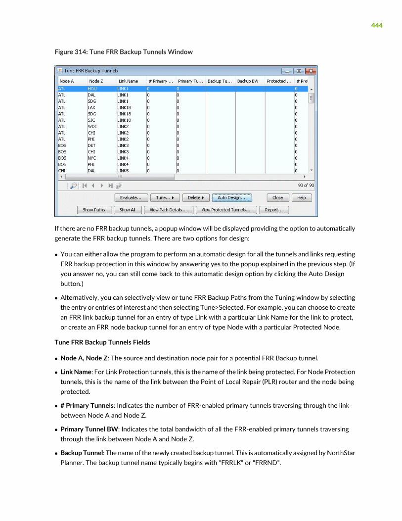
Figure 314: Tune FRR Backup Tunnels Window
If there are no FRR backup tunnels, a popupwindowwill be displayed providing the option to automaticallygenerate the FRR backup tunnels. There are two options for design:
• You can either allow the program to perform an automatic design for all the tunnels and links requestingFRR backup protection in this window by answering yes to the popup explained in the previous step. (Ifyou answer no, you can still come back to this automatic design option by clicking the Auto Designbutton.)
• Alternatively, you can selectively view or tune FRR Backup Paths from the Tuning window by selectingthe entry or entries of interest and then selecting Tune>Selected. For example, you can choose to createan FRR link backup tunnel for an entry of type Link with a particular Link Name for the link to protect,or create an FRR node backup tunnel for an entry of type Node with a particular Protected Node.
Tune FRR Backup Tunnels Fields
• Node A, Node Z: The source and destination node pair for a potential FRR Backup tunnel.
• LinkName: For Link Protection tunnels, this is the name of the link being protected. For Node Protectiontunnels, this is the name of the link between the Point of Local Repair (PLR) router and the node beingprotected.
• # Primary Tunnels: Indicates the number of FRR-enabled primary tunnels traversing through the linkbetween Node A and Node Z.
• Primary Tunnel BW: Indicates the total bandwidth of all the FRR-enabled primary tunnels traversingthrough the link between Node A and Node Z.
• BackupTunnel: The name of the newly created backup tunnel. This is automatically assigned byNorthStarPlanner. The backup tunnel name typically begins with “FRRLK” or “FRRND”.
444

• Backup BW: The amount of bandwidth the newly created backup tunnel can protect.
• Protected Pool: Indicates the type of primary tunnel that the newly created backup tunnel can protect:Sub-pool or Global-pool
• # Prot Prim Tun: Indicates the number of FRR-enabled primary tunnels actually carried/protected bythe backup tunnel.
• Type: Indicates the type of backup tunnel: Link Protected or Node Protected.
• ProtectedNode: For FRRNode Protection tunnels, this indicates the nodewhose failure is being protectedagainst.
• Prot Prim Tun BW: Indicates the total bandwidth of the FRR-enabled primary tunnels actually carriedby the backup tunnel.
• RSVP BW: The actual bandwidth reserved for the tunnel
• Design BW: The bandwidth value that is used for constraint-based routing to determine the placementof the backup tunnel during a design. This can be different from the RSVP BW actually configured onthe backup tunnel and the Backup BW.
• Div Level: Indicates whether the backup tunnel has a route that is Link-Diverse, Site-Diverse orFacility-Diverse from the protected path. Use the Evaluate button to update the diversity level for aparticular type of diversity (Facility, Link, or Site)
• Path Violation: Indicates whether there is a path violation in the backup tunnel path
• Backup Route: The route for the newly created backup tunnel, if one is found. If no route is found, thenthis field will say “Unplaced”.
Options
• Evaluate: Updates the Div Level column to show the diversity level between the protected path and itsbackup tunnel. Available diversity evaluation options are Facility, Link, or Site. For example, if you wantto see whether the protected path is on a facility-diverse path from its backup tunnel, select Facility.
• Tune>Selected: Brings up awindowwith options for tuning the selected entries by creating or modifyingthe backup tunnel for that entry
• Delete>Selected: Deletes the backup tunnel(s) listed in the selected entries
• Auto Design: Brings up a window with options for creating backup tunnels for all entries
• ShowPaths: Displays paths of backup tunnel, protected segment, and protected tunnels. Select an entrywith a Backup Tunnel and positive value for # Prot Prim Tun before clicking this button.
• Show All: Displays node to node connections of all backup tunnels on the Map window.
• View Path Details: Opens up a Tunnel window listing only the FRR backup tunnel
445

• View Protected Tunnels: Opens up a Tunnel window listing only the primary FRR-enabled tunnels thatthe selected FRR backup tunnel protects.
• Report: Saves the Tune FRR Backup Tunnels table into a comma separated report.
NOTE: The columns of the Tune FRR Backup Tunnels window can be customized. That is,you can choose just a subset of the many columns to appear. To access this feature, rightclick on a column header and choose Table Options from the popup menu.
Auto Design Parameters
Figure 315: FRR Design - Basic Options Tab
446

• Diversity Level: Select Link, Site, or Facility diversity for the link being protected and its FRR backuptunnel to be routed on link-disjoint paths, site-disjoint paths, or facility-disjoint paths, respectively. ForSite diversity, the FRR backup tunnel is to avoid, if possible, nodes that are in the same site as the linkand its endpoints. Facility and Link diversity operate similarly. If Facility diversity level is selected, thenthe link and backup tunnel route should not intersect at any of the nodes or links defined in the facility.Recall that a facility is a user-defined group of nodes and links and is commonly used to represent SharedRisk Link Groups (SRLG). For more information, refer to Link, “Link, Site and Facility Diverse Paths” onpage 464.
• Protection Type: Specify Link or Node/Node-Link to indicate whether you wish to design FRR LinkProtection or FRR Node Protection tunnels, respectively. Specify Auto Bypass to automate bypasscreation for Juniper based on the configuration parameters on the interface.
• Design Bandwidth (for Design/Placement): The Design Bandwidth is used for Design purposes only, todecide where to place the tunnel, and is not used to set the actual RSVP bandwidth. The backup tunnelswill be placed by the program using constraint-based routing assuming that it would reserve a certainbandwidth along the tunnel route for the tunnel to be placed. However, once the placement is done,the actual tunnel’s RSVP bandwidth can be set to a different value, using the following Set RSVPBandwidth option.
• The Design Bandwidth is specified as a percentage of a Reference Bandwidth Source plus a fixed value.The Reference Bandwidth Source can be the (a) Link Bandwidth:the entire link bandwidth, (b) Sub-PoolBandwidth: the subpool bandwidth allocated on the link (for Cisco only), or (c) Sum of FRR PrimaryTunnel Bandwidth: the sum of the bandwidth of all primary FRR-enabled tunnels that the backup tunnelprotects (for Juniper). By adjusting the % and fixed values (which default to the divpathbwpct anddivpathbw in the dparam file), you can perform overbooking.
NOTE: Regarding option (b), if the Reference Bandwidth Source is set to Sub-Pool and ifthe protected link has no subpool partition, then a backup tunnel will not be designed.
• Set RSVP Bandwidth to: Specifies the actual bandwidth for the backup tunnel, as a percentage of theDesign bandwidth.
• Multiple FRR Tunnel Settings: You can create multiple backup tunnels by specifying either:
• Maximum bandwidth per tunnel: This is the maximum bandwidth allowed; tunnels will be split if thedesign bandwidth exceeds this value.
• Number of tunnels per interface: You can specify directly how many backup tunnels to create on theinterface with each tunnel equally sharing the design bandwidth.
447

Figure 316: FRR Design - Advanced Options Tab
Advanced Options for Cisco
• Protect traffic of type: For the backup tunnels that are designed, you can specify the type of tunnel thatthey are to protect. If you specify Global-Pool, then the backup tunnels can only protect primary tunnelsthat are designated to carry Global-Pool traffic. If you specify Sub-Pool, then the backup tunnels designedcan only protect primary tunnels designated to carry Sub-Pool traffic. If Any is specified, then the backuptunnels designed are allowed to carry either type of primary tunnel.
Note that if Global-Pool or Sub-Pool is specified, then the newly generated backup tunnel(s) will have“BKGP” or “BKSP”, respectively, listed in the tunnels’ Type field parameters. By looking at the tunneltype parameters, the Protected Tunnel Type can be identified. If there is no indication, then the defaultprotected type is “Any”.
• Allocate Backup Bandwidth using: This selection allows you to specify whether the backup bandwidthfor the FRR backup tunnel should be allocated from the links’ Global-Pool or Sub-Pool at the time offailure.
If Sub-Pool is specified, then the newly generated backup tunnel(s) will have “GB” (Guaranteed Bandwidth)in their Type field. A backup tunnel that does not contain “GB” is by default using Global-Pool bandwidth.
• Tunnel can protect unlimited amount of BackupBandwidth: Indicates whether the amount of bandwidththe backup tunnel can protect is limited or unlimited. If checked, this option will allow all primary tunnelsto be routed over the backup tunnel. This is the default. If unchecked, the backup bandwidth will be
448

limited to the value set in the Design Bandwidth section of the Basic Options tab. This limit is effectiveat the time of failure when the backup tunnel is activated.
NOTE: Setting the Design Bandwidth to 0 is equivalent to allowing Unlimited backupbandwidth.
Advanced Options for Juniper
Protect traffic of type: For the backup tunnels that are designed, you can specify the type of tunnel thatthey are to protect. Values include Single-Class LSP,Multi-Class LSP, or Any. If Single-Class LSP is selected,you should then specify one of the resulting options: CT0, CT1, CT2, or CT3. If Multi-Class LSP is selected,enter in the percentage for each of the 4 classes. For more information about DiffServ-TE, see“DiffServTraffic Engineering Tunnels Overview” on page 415.
Other Options
Prompt to view FRR design report: Selecting this checkbox will cause the FRR Design report to beautomatically displayed once an FRR Design or View/Tune Paths operation has completed. This report issaved to the Output Path in the File Manager under the name “FRRDSGNRPT.runcode”. To access it inthe File Manager, right-click on the file and choose “Open in Report Viewer”. For more information onthe FRR design report, see FRR Design Report.
FRR Auto Design
When the FRR Design parameters are submitted for Auto Design, the program will automatically createbackup tunnels as follows:
• If the Protection Type is set to Link, then FRR Auto Design will automatically design the FRR-LP backuptunnels necessary to protect (1) Links along the paths of LSP tunnels requesting FRR protection, and (2)Individual links that have been marked to request FRR protection.
• If the Protection Type is set to Node, then FRRAutoDesignwill automatically design the FRR-NP backuptunnels necessary to protect (1) Nodes along the paths of LSP tunnels requesting FRR protection (excludingthe source and destination nodes) and (2) The destination node of links that have beenmarked to requestFRR protection.
449

NOTE: When selecting either Node Protection or Link Protection, the Auto Design willautomatically enable FRR for all the links along the paths of LSP tunnels requesting FRRprotection. If this is not desired, users should use tuning instead of auto design, or in thecase of Juniper, select “Auto Bypass” as described below.
If the Design Bandwidth Reference Bandwidth Source is set to Sub-Pool (for Cisco only)then only the links that(1) require FRR protection and (2) have subpool bandwidth allocatedwill be considered for protection in FRR Auto Design.
• If the Protection Type is set to Auto Bypass (for Juniper bypass creation), then FRR Auto Design willautomatically design the bypass tunnels for Juniper for FRR-enabled links along the paths of FRR-enabledLSP tunnels. After selecting this option, you will be prompted with the option to design paths using (a)the RSVP signaling bandwidth as the Design Bandwidth or (b) the Backup bandwidth as the DesignBandwidth. Select option (a) if you wish to simulate Juniper’s auto bypass generation. Select option (b)to help ensure there is enough bandwidth on the backup tunnel to protect the primary tunnels.
NOTE: The Auto Bypass Protection type will preserve the link’s FRR settings and avoidcreating backup tunnels for links not enabled for FRR.
Please read through the explanations of theDesign options in the previous section carefully for a completedescription of each of the FRR Design options. Though the design options may initially appear complex,understanding the function of each option will provide you with enormous flexibility. Once you havespecified the desired properties in the FRR Design window, click the “AUTO Design” button.
If you already have some existing fast reroute tunnels in the network, you may also see the followingconfirmation windows: “Routes and bandwidth for all FRR link protection backup tunnels will be adjusted.Continue?” or “Remove configured paths for 10 FRR link backup tunnels?”
In the Console window, the number of placed/unplaced/deactivated paths for the new tunnels will bedisplayed. You should see something similar to this:
Diversity Level= SITE
Tunnel Site+Link-Diversity Link-Diversity No-Diversity Notplaced
Deactivated
FRRBackup 10 0 0
0 0
FRR Design Report
450

When the design is completed, you will be asked whether you wish to view the FRR design report. Thereport is saved as FRRDSGNRPT.runcode in your File Manager Output Path. To view this report at a latertime, right-click on the report in the File Manager and choose Open in Report Viewer from the popupmenu.
NOTE: To see the FRRDSGNRPT report listed in the File Manager, you may need to refresh theFile Manager contents first, either by pressing the “Refresh” button or alternatively, the <F5>key.
Figure 317: FRR Design Report Generated from Auto Design
After the Auto Design has been performed and FRR backup tunnels created, the FRR Design Reportdisplays the result of failing each FRR-protected link or node. For example, in Figure 360, the highlightedtable entry indicates that when LINK5 is failed, there are two FRR-LP backup tunnels protecting the link.The total bandwidth of these two backup tunnels is 295.488Mbps. Of these two, one failed to be placedduring the link failure. The total bandwidth of this failed backup tunnel is 147.744Mbps, accounting for50% of the total backup tunnel bandwidth.
FRR Design Report Fields
• FailureType: Possible values are LKFAIL, NODEFAIL, and FACFAIL, indicating link, node or facility failure.
• If the Link Diversity Level was specified for the Auto Design, then the program will take down eachnode/link individually and try to find a route that is both site-diverse and link-diverse. If there is none,it will try to find a link-diverse route.
If the Site Diversity Level was specified for the Auto Design, then the program will take down eachnode/link individually and try to find a site-diverse route. If there is none, it will try to find a link-diverseroute. The rationale is that even if site diversity is not met, a link-diverse route is better than no routeat all.
451
If the Facility Diversity Level was specified for the Auto Design, then the program will take down eachnode/link individually and try to find a route that is both facility-diverse and site-diverse. If there is none,it will try to find a link-diverse route.
• Element: Indicates the failed element. If Node Protection Type (or Link Protection Type) was specifiedfor the Auto Design, then all nodes (or all the links) in the network will be failed and brought back upone at a time.
• nBKuptunnel: Indicates the number of FRR backup tunnels that are routed through the network Element.
• BKUPTunnelBW: Indicates the total backup bandwidth of all the FRR backup tunnels protecting thefailed element.
• nFail: Indicates the number of backup tunnels that failed to be placed during the element failure.
• TotalFailBW: Indicates the total bandwidth of the backup tunnels that failed to be placed during theelement failure.
• Fail%: Indicates the percentage of backup tunnel bandwidth that failed to be placed during the elementfailure.
View Created FRR Backup Tunnels
To view the newly designed FRR backup tunnels, select Network > Elements > Tunnels to display all LSPtunnels in the network. Notice that the Type field will indicate whether the FRR backup tunnels are forLink Protection (“FRRLK”) or Node Protection (“FRRND”) and that the No Autoroute Announce flag(“NOAA”) is automatically turned on.
Other possible type fields (for Cisco) are “BKSP” or “BKGP”, indicating that the backup tunnel carriesSub-Pool or Global-Pool tunnels, respectively; this corresponds to the user’s settings of the ProtectedTunnel Type field in the FRR Design parameters.
452

Figure 318: View of LSP Tunnels after FRR-LP Design
You can further examine the FRR backup tunnels created from the View/Tune Paths window as describedin “Viewing Primary Tunnels Protected by a Bypass Tunnel” on page 437.
FRR Tuning
The Tune FRR Backup Tunnels window shows a list of the possible FRR-Link Protection or Node Protectionbackup tunnels that can be created or optimized. Each entry is characterized by a source and destinationnode pair, the Protected Node (if applicable), Link Name and protection Type. This list can be customizedby using the “Filter” button, described later in this section.
NOTE: You can rearrange columns by clicking and dragging column headers. You can move theType and Protected Node columns to the front so that you can see more clearly which tunnelentries are for link protection or for node protection.
453

Each entry in the table corresponds to a potential FRR backup tunnel. Only after an FRR backup tunnelhas been designed or tuned will the rest of the columns in its table entry be filled in. To design FRR backuptunnels, select only those desired entries from the table and then press the “Tune Selected” button. Or,you can press “Tune All” to tune all the entries shown in the table. This will pop up the Tuning Optionsdialog window, allowing you to adjust the FRR design parameters that will be immediately applied to theselected entries.
Most of the parameters in the Tuning Options window are identical to those in the FRR Design window,with a few differences. For example, the following are additional options in Tuning:
Figure 319: Additional Options for Tuning (Basic Tab)
The “Create new tunnel(s) using selected tunnels as a template” option will create a new row in the Tuningwindow with the same parameters but with an additional backup tunnel protecting the given link or node.The original row will remain. The “Modify selected tunnel(s) using specific parameters” option will modifythe existing backup tunnel(s) rather than creating an additional backup tunnel.
Figure 320: Additional Options for Tuning (Advanced Tab)
The “Remove configured paths for existing backup tunnels” option is used to allow for the backup tunnels’paths to be redesigned.
Specify the desired options in the Tuning Options window and click “OK”. In this example, we tune all therows. After tuning, the remainder of each row in the Tune FRR Backup Tunnels window is filled in.
NOTE: For rows that remain blank in the Tune FRR Backup Tunnels window after tuning forthe row, this indicates that a FRR backup tunnel was not designed. This could happen, for example,if the Reference BW Source is set to Sub-Pool BW but none of the links listed in the Tune FRRBackup Tunnels table have Sub-Pool BW.
454

Figure 321: FRR Paths After Tuning is Complete
In this example, all FRR backup paths have been successfully created and are already added to the network.
NOTE: Backup tunnels created through FRR Design are automatically assigned a name of“FRRLKnum” for FRR Link Protection tunnels and “FRRNDnum” for FRRNode Protection tunnels.Notice that, in Figure 320 on page 454, there are three backup tunnels named “FRRND1”. Thereason is that tunnels are not required to have unique names unless the head-end node of thetunnel is the same.
Once a tunnel has been “tuned”, the latter columns in the table will be filled in. If an FRR path is successfullydesigned and placed, its path will show up in the Backup Route column of the Tune FRR Backup Tunnelswindow. Select a row in the table and click on the “Show Paths” button. The path for this tunnel will thenbe displayed in the Map window. A Paths window will also appear, allowing you to view either the backuppath or the path of the tunnel being protected.
The Console will also display summary information regarding the total number of placed or unplacedbackup tunnels for this tuning operation. If placed, the console window will indicate how many satisfiedSite-Diversity or Link-Diversity or whether No Diversity was satisfied. For example:
Diversity Level= SITE
Tunnel Site-Div Link-Div No-Div Unplaced Deactivated
FRRBackup 2 0 0 0
0
Filtering in the FRR Tuning Window
In the Tune FRR Backup Tunnels window, you can also use the “Filter” button to view a more selectiveset of entries for which to tune. The following window will appear:
455

Figure 322: Filter for a More Specific Set of Tuning Entries
• Node A, Node Z:The node A and node Z panels are for selecting a subset of nodes to use for filteringFRR paths. By default, all nodes in the network are used. Node A is the source, or Point of Local Repair(PLR). Node Z represents the destination, or the Next Hop / Next Next Hop node.
• FRR Backup Tunnel endpoints must match (either/both) NodeA and NodeZ: This option allows you tospecify the strictness of the endpoint match. Select “either” to match either Node A and Node Z. Select“both” to require a match of both.endpoints.
• Primary FRR-enabled Tunnel Exists: There are three options: yes, no and "---" which means “don't care”.Selecting "Yes" means a path will be displayed only if the protected path is part of a primary FRR enabledtunnel. Selecting "no" means the opposite, and selecting "---" will ignore this option during the filter.
• FRR Backup Tunnel Exists:There are three options: yes, no and "---" which means “don't care”. Selecting"Yes" means a path is displayed only if a backup tunnel exists for the protected path. Selecting no meansthe opposite, and selecting "---" will ignore this option during the filter.
• Link is FRR Enabled: There are three options: yes, no and "---" which means “don't care”. Selecting "Yes"means a path is displayed only if the link is FRR-enabled, or requests FRR protection. See “ModifyingLinks to Trigger FRRBackup Tunnel Creation (Cisco)” on page 442 for information on how to FRR-enablea link.
• FRRProtectionType: This option allows the user to fetch FRR Link Protection paths, FRRNode Protectionpaths, or both types of FRR paths if “All” is specified.
• Backup Tunnel Diversity Level:This option allows the user to fetch paths that satisfy facility, link, site,any or no diversity level.
456

• Protected Node: Located in the Protected Element Options tab, specifying a particular set of nodes willbring up only those paths that protect these nodes.
• Protected Interface: Located in the Protected Element Options tab, specifying a particular set ofinterface/link will bring up only those paths that protect these links.
• Facilities: Located in the Protected Element Options tab, specifying a particular set of facilities will bringup only those backup paths that protect any of the nodes or links defined in the facility.
Viewing Created Backup Tunnels
After performing an FRR Design as described earlier in this chapter, find the created backup tunnel in theBackup tunnel column. You can sort on this column by clicking on the column header to view existingbackup tunnels, or use the filter button.
1. Click on the “Show Paths” button in the Tune FRR Backup Tunnels window to view both the ProtectedPath and the Newly designed Path on theMapwindow as described earlier in “Viewing Primary TunnelsProtected by a Bypass Tunnel” on page 437.
2. The Paths windowwill appear. You can choose from the left-hand side of the windowwhether to viewthe path for the newly designed backup path, FRRLK1, or the path that this backup is protecting(“Protected Path”). If the protected path is part of LSP Tunnel(s) requiring FRR Protection, then youcan also view the protected LSPs tunnels’path(s). In this example, RATLCHI is the protected LSP Tunnel.
457

Figure 323: Paths Window
3. In the Tune FRR Backup Tunnels window, you can also click on the “View Path Details” button for aselected entry. This will bring up a similar window to that accessed by Network > Elements > Tunnels.In this window, click on “Details.” In the Tunnel window, select “ShowPath” or “Highlight All” to displaythe path on the map.
Generating LSP Configlets for FRR Backup Tunnels
Once you have designed the FRR backup tunnels, you may want to generate the corresponding LSPconfiglets (statements of a router configuration file) that can then be uploaded to the router. See, LSPConfiglet Generation Overview for detailed information.
458

Failure Simulation—Testing the FRR Backup Tunnels
Interactive failure simulation can be performed to fail a set of node(s), link(s), and facilities at the sametime. After the failure, users can view the use of the FRR backup tunnel, followed by the head-end rerouteif applicable, or else the usage of the diverse 1+1 backup (standby) path if configured. For information onconfiguring diverse backup paths (e.g., secondary or standby paths) see “NorthStar Planner LSP TunnelsOverview” on page 311 and “Tunnel Path Design Overview” on page 365.
Simulating Local Protection
1. To run an interactive failure, click the Simulation button to switch to Simulation mode.
2. Select the desired node(s) or link(s) to fail together by <Ctrl>-clicking the nodes or links with yourmouse.
3. Next, right-click over one of the selected node(s) and selecting “Fail Selected Nodes” or right-click overone of the selected link(s) and select “Fail Selected Links.”
4. Click the step button “>|” on the simulation tool bar to step through each tunnel to see how it is locallyrerouted. (For a faster method, but without graphical display, refer to Using the Run Button.)
Figure 324: Simulation Toolbar with Run, Step, and Stop buttons
5. On the Standard map, the old path is highlighted in red and the new path using the backup tunnel ishighlighted in yellow. In this case, the original path was from N9-N2-N1-N6. However, due to thefailure of LINK8 between N2 and N1, the new path taken is N9-N2-N7-N6.
459
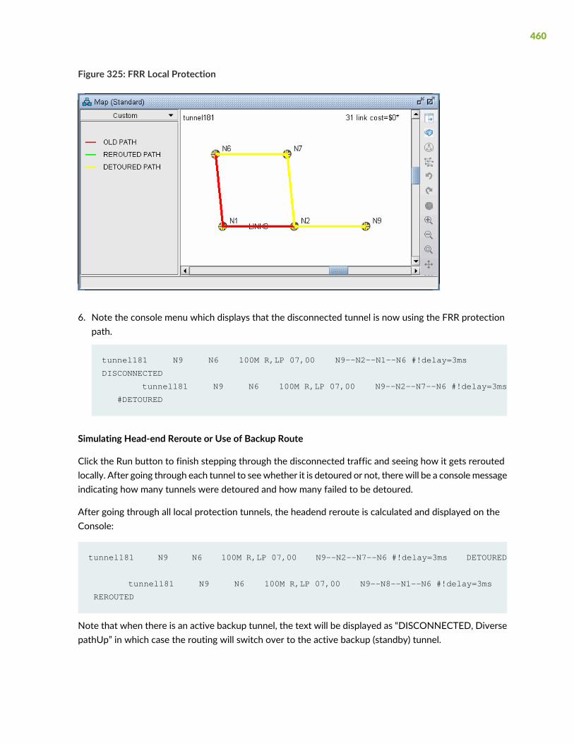
Figure 325: FRR Local Protection
6. Note the console menu which displays that the disconnected tunnel is now using the FRR protectionpath.
tunnel181 N9 N6 100M R,LP 07,00 N9--N2--N1--N6 #!delay=3ms
DISCONNECTED
tunnel181 N9 N6 100M R,LP 07,00 N9--N2--N7--N6 #!delay=3ms
#DETOURED
Simulating Head-end Reroute or Use of Backup Route
Click the Run button to finish stepping through the disconnected traffic and seeing how it gets reroutedlocally. After going through each tunnel to seewhether it is detoured or not, therewill be a consolemessageindicating how many tunnels were detoured and how many failed to be detoured.
After going through all local protection tunnels, the headend reroute is calculated and displayed on theConsole:
tunnel181 N9 N6 100M R,LP 07,00 N9--N2--N7--N6 #!delay=3ms DETOURED
tunnel181 N9 N6 100M R,LP 07,00 N9--N8--N1--N6 #!delay=3ms
REROUTED
Note that when there is an active backup tunnel, the text will be displayed as “DISCONNECTED, DiversepathUp” in which case the routing will switch over to the active backup (standby) tunnel.
460

In some cases, you may also see the word “RE-Optimized” in case the tunnel allows reoptimization and ashorter path is found during the failure simulation.
Using the Run Button
For faster performance, the interactive failure can be run without the graphical display.
1. To start a new simulation, select Simulation > Reset Simulation.
2. Before running through the simulation, selectTools >Options >Report. Under Failure Simulation>FailureReport, select Yes for Trace File and Display Paths at Failed Nodes options. This will save the rerouteinformation to a file. Otherwise, only a summary will be displayed in the Console.
3. Select the node(s) and link(s) to fail, either from themap as described earlier, or by checking the checkboxfor the corresponding element from the Simulation > Interactive Scenarios > Fail Link, Fail Node, andFail Facility windows. Click the Run button.
4. Open Report > Report Manager while in Simulation mode. Select the Interactive Failure report andscroll down to view the DETOURED and REROUTED information described earlier in a report ratherthan on the console.
Resulting Link Utilizations
After running an interactive failure simulation, you can see the resulting link utilizations after the headendreroute either through the Network > Elements > Link menu Util_AZ and Util_ZA columns and Capacitytab or through the Report > Report Manager, Planned Link Utilization report under Network Reports >Link Reports, Util column.
The Tools > Options > Failure Simulation window also contains a default FRR Mode option under theFailure Simulation > FRR option pane. The default setting is FRR + Normal. Select “FRR Only” as the FRRmode before running an interactive failure simulation to simulate only the FRR local protection and notthe headend reroute.
461

Figure 326: FRR Mode
1. After changing this setting, to start a new simulation, select Simulation > Reset Simulation. Fail thedesired nodes, links, or facilities and click the Run button.
2. To view the utilizations after the local rerouting and before the headend reroute (in the case that thereis no 1+1 backup tunnel), go to Report > Report Manager.
3. Check the Interactive Failure report. Only the DETOURED routes should be displayed and not theREROUTED tunnel routes.
Exhaustive Failure
1. To run an exhaustive failure, click the Simulation button to switch to Simulation mode.
2. Select the Simulation button and go to Simulation > Predefined Scenarios.
462

Figure 327: FRR Failure Simulation Options
During the failure simulation, NorthStar Planner keeps track of the peak, or worst utilization on eachlink. Recall that during a failure, the FRR backup tunnel provides fast restoration times by locally repairingLSPs at the point of failure, while waiting for the head-end routers to establish a new LSP. NorthStarPlanner can simulate a number of scenarios.
• Normal: Simulates the “normal” tunnel reroute. Does not consider the effect of the local repair duringthe simulation. Peak utilization reflects that during the “normal” situation.
• FRR + Normal: Simulates the FRR local repair first followed by the normal primary tunnel reroute asestablished at the head-end router. The resulting link peak utilization report identifies the worstutilization, or max value of the transient detour and normal modes.
NOTE: A primary tunnel being detoured is marked down if it cannot be rerouted.
• FRR only: Simulates only the local repair. The resulting link peak utilization report reveals just thepeak utilization experienced during the local repair.
3. Under the Options section, select FRR and “FRR+Normal.” Then select one or more exhaustivesingle-element failure scenarios under the Scripts section.
4. Next, to saved detailed reroute information including local protection and head-end rerouting to areport, select Reroute Information under the Report Options.
5. Under Options, select Peak Utilization Report.
6. Click “Run” to start the exhaustive failure simulation.
7. Summary information is indicated in the Console, with the first entry for a failed element correspondingto the tunnel layer and the second entry corresponding to the demand layer.
463

8. Go to Report > Report Manager to view the saved report file to view the detoured paths for all theprimary tunnels requiring FRR protection followed by the headend reroute.
9. Select the Peak Link Utilization report under Simulation Reports > Network Statistics to see theworst-case utilization across all the failure scenarios and the scroll to the last column to view whichelement failure the peak utilization occurred at.
10.On the StandardMap, select the Utilization Legends > Peak Util to view the peak utilizations graphically.
Link, Site and Facility Diverse Paths
From the FRR Design window, the Diversity Level parameter allows you to specify whether the routes forthe FRR-designed backup paths should be Facility-diverse, Site-diverse or Link-diverse from the primarypaths. NorthStar Planner will then try its best to satisfy the requirements. If a diverse backup path cannotbe found, the software will still attempt to route the backup tunnel if possible. In this situation, if it isrouted, this LSP tunnel will fall into the No-Diversity category. If it cannot be routed, it will fall under theUnplaced category.
Link Diversity
Link diversity is the most fundamental diversity level. Figure 371 depicts a link-diverse route in the eventof a link failure or a node failure. In the diagram on the left, the protected link is the link between A andB. A FRR-LP link-diverse route from A to B is any path that avoids the link between A and B.
The diagram at right depicts a protected node B on the path between nodes A and C. A FRR-NP link-diverseroute is technically any path that avoids both the link between A and B as well as node B.
Figure 328: Link Diverse Route for Protecting a Link (left) and Protecting a Node (right)
Site Diversity
A site is a user-defined group of nodes, specified in a site file. If no site file is specified, then by defaultsites aremappedwith individual routers listed in the node (muxloc) file. Sites are typically defined to indicatea group of nodes that are likely to fail together. Figure 372 depicts a protected node X between A and D.
464

For this example, to establish a site-diverse route, nodes B and Cmust not belong to the same site as nodeX.
Figure 329: Site Diverse Route for Protecting a Node
If no site-diverse route exists, the programwill attempt to find a link-diverse route, under the presumptionthat an alternate route is better than none.
When completing an FRR Design with the Diversity Level set to Link or Site, the Console will report asummary for all the FRR Backup tunnels, in a format similar to that below:
Diversity Level= Link or SITE
Tunnel Site-Diversity Link-Diversity No-Diversity
Unplaced
FRRBackup 34 0
54 0
The Tune FRR Backup Tunnels window, if open, will also display Site, Link, or None, accordingly, in theDiversity column.
NOTE: Site-Diversity in this context simply means Site Diversity. It does not indicate Site +Facility Diversity as is the case when the Diversity Level is set to Facility.
Facility Diversity (SRLG)
A Shared Risk Link Group (SRLG) can be represented by the concept of a facility in NorthStar Planner,,indicating a group of links that are likely to go down together in the event of a failure.
In NorthStar Planner, a facility can be defined in a special facility file as a group of links and nodes. A backuppath that is facility-diverse from its primary pathwill have a route that, aside from the source and destination,will traverse a path that does not intersect with the primary path at any of a facility’s links or nodes.
In Figure 329 on page 465, the diagram at left depicts a protected link between A and X, highlighted inyellow.
465

The alternate route depicted fromA to X is only facility-diverse if links A->B, B->C, C->X, along with nodesB and C do not belong to the same facility as link A->X. The diagram at right depicts a protected node X.The alternate FRR-NP route depicted from A to C is only facility-diverse if links A->B, B->C and node Bdo not belong to the same facility as either link A->X or node X.
If no facility-diverse route exists, the programwill attempt to find a site-diverse route, under the presumptionthat an alternate route is better than none.
NOTE: If the network model was built from the configuration files through the Import DataWizard feature described in “Router Data Extraction Overview” on page 33, then by default afacility will be set equivalent to all links associated with a router card.
Figure 330: Facility-Diverse Route for Protecting a Link (left) and Protecting a Node (right)
When completing an FRRDesignwith theDiversity Level set to Facility, the Console will report a summaryfor all the FRR Backup tunnels, in a similar format to that below:
Diversity Level= FACILITY
Tunnel Site-Diversity FAC-Diversity No-Diversity
Unplaced
FRRBackup 37 0
51 0
The Tune FRR Backup Tunnels window, if open, will also display Site, Facility, or None, accordingly, in theDiversity column.
NOTE: Site-Diversity in this context may be somewhat misleading. If the Diversity Level wasset to Facility, then Site-Diversity, both in the Console and in the Tune FRR Backup Tunnelswindow, actually indicates that Site Diversity + Facility Diversity are both satisfied. This is strongerthan simply Facility (FAC)-Diversity alone.
466

23CHAPTER
Cisco Auto-Tunnels
Cisco Auto-Tunnels Overview | 469
Importing Cisco Auto-Tunnel Information from Router Configuration Files | 470
Auto-Tunnel Creation | 473
Tunnel Path Data Collection and Import for Auto-tunnels | 476
Auto-Tunnels Reporting for Verification | 479

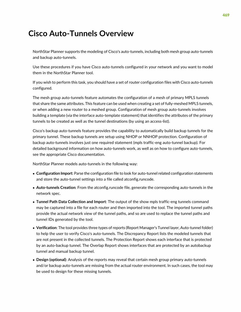
Cisco Auto-Tunnels Overview
NorthStar Planner supports the modeling of Cisco's auto-tunnels, including both mesh group auto-tunnelsand backup auto-tunnels.
Use these procedures if you have Cisco auto-tunnels configured in your network and you want to modelthem in the NorthStar Planner tool.
If you wish to perform this task, you should have a set of router configuration files with Cisco auto-tunnelsconfigured.
The mesh group auto-tunnels feature automates the configuration of a mesh of primary MPLS tunnelsthat share the same attributes. This feature can be usedwhen creating a set of fully-meshedMPLS tunnels,or when adding a new router to a meshed group. Configuration of mesh group auto-tunnels involvesbuilding a template (via the interface auto-template statement) that identifies the attributes of the primarytunnels to be created as well as the tunnel destinations (by using an access-list).
Cisco's backup auto-tunnels feature provides the capability to automatically build backup tunnels for theprimary tunnel. These backup tunnels are setup using NHOP or NNHOP protection. Configuration ofbackup auto-tunnels involves just one required statement (mpls traffic-eng auto-tunnel backup). Fordetailed background information on how auto-tunnels work, as well as on how to configure auto-tunnels,see the appropriate Cisco documentation.
NorthStar Planner models auto-tunnels in the following way:
• Configuration Import: Parse the configuration file to look for auto-tunnel related configuration statementsand store the auto-tunnel settings into a file called atconfig.runcode.
• Auto-tunnels Creation: From the atconfig.runcode file, generate the corresponding auto-tunnels in thenetwork spec.
• Tunnel Path Data Collection and Import: The output of the show mpls traffic-eng tunnels commandmay be captured into a file for each router and then imported into the tool. The imported tunnel pathsprovide the actual network view of the tunnel paths, and so are used to replace the tunnel paths andtunnel IDs generated by the tool.
• Verification: The tool provides three types of reports (ReportManager's Tunnel layer, Auto-tunnel folder)to help the user to verify Cisco's auto-tunnels. The Discrepancy Report lists the modeled tunnels thatare not present in the collected tunnels. The Protection Report shows each interface that is protectedby an auto-backup tunnel. The Overlap Report shows interfaces that are protected by an autobackuptunnel and manual backup tunnel.
• Design (optional): Analysis of the reports may reveal that certain mesh group primary auto-tunnelsand/or backup auto-tunnels are missing from the actual router environment. In such cases, the tool maybe used to design for these missing tunnels.
469

ImportingCiscoAuto-Tunnel Information fromRouterConfiguration Files
To import the router configuration files, select File>Import Data and follow the Import Network Wizard.Alternatively, you may run the getipconf program in text mode. See “Router Data Extraction Overview”on page 33 for more detailed information. The following table lists those mesh group auto-tunnel andbackup auto-tunnel related statements that are parsed during configuration import:
mesh group auto-tunnel statements
mpls traffic-eng auto-tunnel meshmpls traffic-eng auto-tunnel mesh tunnel-num min num max numinterface auto-template interface-numtunnel destination access-list num
tunnel destination access-list num
mpls traffic-eng auto-tunnel backupmpls traffic-eng auto-tunnel backup nhop-onlympls traffic-eng auto-tunnel backup tunnel-num [min num] [max num]mpls traffic-eng auto-tunnel backup config unnumbered-interface interface
mesh group auto-tunnel statements
mpls traffic-eng auto-tunnel mesh
mpls traffic-eng auto-tunnel mesh tunnel-num min num max num
interface auto-template interface-num
tunnel destination access-list num
Table 4: Cisco auto-tunnel statements parsed during configuration import
backup auto-tunnel statements
mpls traffic-eng auto-tunnel backup
mpls traffic-eng auto-tunnel backup nhop-only
mpls traffic-eng auto-tunnel backup tunnel-num [min num] [max num]
470
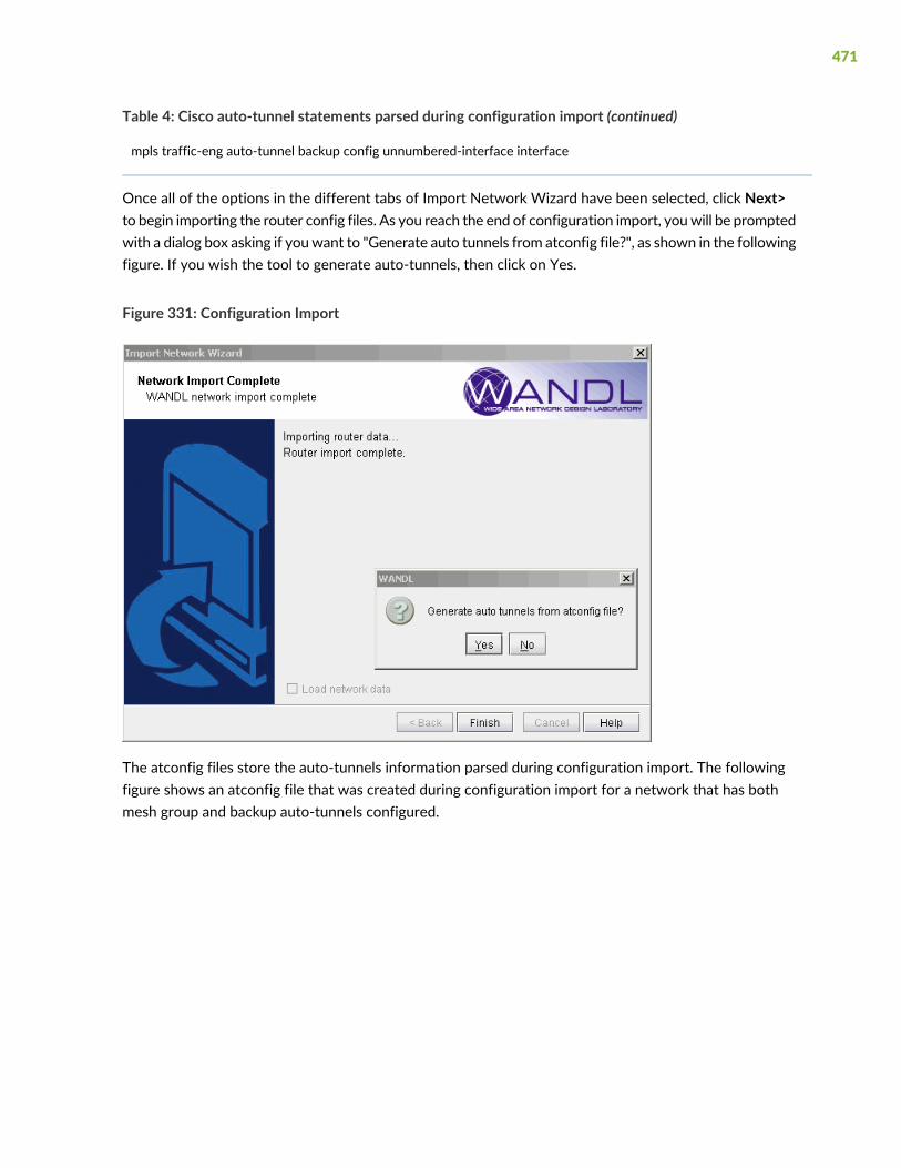
Table 4: Cisco auto-tunnel statements parsed during configuration import (continued)
mpls traffic-eng auto-tunnel backup config unnumbered-interface interface
Once all of the options in the different tabs of Import Network Wizard have been selected, click Next>to begin importing the router config files. As you reach the end of configuration import, youwill be promptedwith a dialog box asking if youwant to "Generate auto tunnels from atconfig file?", as shown in the followingfigure. If you wish the tool to generate auto-tunnels, then click on Yes.
Figure 331: Configuration Import
The atconfig files store the auto-tunnels information parsed during configuration import. The followingfigure shows an atconfig file that was created during configuration import for a network that has bothmesh group and backup auto-tunnels configured.
471

Figure 332: Atconfig File Containing Both Mesh Group and Backup Auto-Tunnels
In the above figure, the lineTunnel62000-62999 LR2 BACKUP
corresponds to the following backup auto-tunnel configuration statements:
mpls traffic-eng auto-tunnel backupmpls traffic-eng auto-tunnel backup tunnel-num min 9000 max 9099
In the above figure, the lineTunnel60000-60999 LR2 ACL-7 0 R,A2Z,LP,LDP,PATH1(NORTH),PBK10(dynamic) 7,7 #!
corresponds to the following mesh group auto-tunnel configuration statements:
mpls traffic-eng auto-tunnel meshmpls traffic-eng auto-tunnel mesh tunnel-num min 60000 max 60999…interface Auto-Template1ip unnumbered Loopback0mpls iptunnel destination access-list 7tunnel mode mpls traffic-engtunnel mpls traffic-eng autoroute announcetunnel mpls traffic-eng path-option 1 explicit name NORTHtunnel mpls traffic-eng path-option 10 dynamictunnel mpls traffic-eng fast-reroute!
472

Auto-Tunnel Creation
If you choose No when prompted with "Generate auto tunnels from atconfig file?" in the previous step,then the tool will not create any auto-tunnels. You may still generate the auto-tunnels at a later time byswitching to Designmode and then choosing one of the three options under the Auto Tunnel Designmenu(Design > TE Tunnels > Auto Tunnel Design) as shown in the following figure. Selecting Auto Mesh orBackup will cause the tool to generate mesh group auto-tunnels or backup auto-tunnels, respectively.
To generate both mesh group and backup auto-tunnels, choose the All option.
Figure 333: Auto Tunnel Design Menu
If you choose Yes when prompted with "Generate auto tunnels from atconfig file?" in the previous stepand your network configuration files have auto-tunnels configured, then the tool proceeds to createauto-tunnels using the information stored in the atconfig file. If backup auto-tunnels are configured in thenetwork, then FRR design is performed in the background to provide FRR node or FRR link protection forthe primary tunnel. To view the auto-tunnels created by the tool, bring up the Tunnels window (Network> Elements >Tunnels) as shown in the following figure:
473

Figure 334: Auto-Tunnels Tagged With “AT” in the Type fField
The figure has the Type column expanded to show that auto-tunnels have been tagged with an "AT" flag.In this example, routers LR2 & RR2 have mesh group & backup auto-tunnels configured, as indicated bythe corresponding "AT" flag.
If you wish to filter for only auto-tunnels, you may use the advanced filter. Set "Type=AT" for the Enterquery box and chooseMatch Substring as the Search Preference, as shown in the following figure.
474

Figure 335: Filtering for Auto-Tunnels
The resulting filtered tunnels window is shown in the following figure:
Figure 336: Tunnels Window Showing Only Auto-Tunnels
475

If auto-tunnels have been generated by the tool, and you exit without first saving, then youwill be promptedwith the following popup message window.
Figure 337: Click Yes to Save Auto-Tunnels
Clicking on Yes will cause the auto-tunnels to be saved and placed into an autotunnel.runcode file. Anexample is shown in the following figure
Figure 338: Auto-Tunnels Saved
Tunnel Path Data Collection and Import forAuto-tunnels
As described in the Network Data Import Wizard chapter of the NorthStar Planner User Interface Guide,the actual tunnel paths taken by tunnels can be extracted from the router and imported into the tool toprovide an exact view of the network. In addition, since auto-tunnels are generated by the routerdynamically, the exact tunnel IDs will not be known ahead of time. What is known is the tunnel ID range,so the tool creates auto-tunnels with tunnel IDs that fall into the range. To use the Tunnel Path Import
476

feature, prepare a directory that contains the output of the following Cisco show command, one file perrouter: show mpls traffic-eng tunnels.
With the specification file still open, bring up the Import NetworkWizard window (File>Import Data), andselect Tunnel Path under Select Import Type, as shown in the following figure:
Figure 339: Tunnel Path Import
Then click on Browse and navigate to the directory containing the show command output files:
477

Figure 340: Directory of Show Command Output Files
After specifying the import directory, click Next to import the tunnel paths into the model.
After tunnel path import, bring up the Tunnels window (Network > Elements >Tunnels) to examine thechanges. The following figure shows the Tunnels window up after tunnel path import.
478

Figure 341: Tunnels after Tunnel Path Import
Compared to the Tunnels window prior to tunnel path import, you can see that the tunnel IDs have beenreplaced with the actual tunnel IDs assigned by the router. The modeled tunnel paths have also beenupdated by the actual ones.
After performing tunnel path import, if there are any tunnels modeled by the tool that do not appear onthe actual router, then those tunnel IDs are renamed to atbackup_n or atmesh_n depending on theauto-tunnel type. For instance, the following figure shows that the mesh group auto-tunnel from RR2 toLR2 created by the tool did not appear in the actual router (according to the show command output fromtunnel path import). This could be an indication that the Cisco router hardware did not correctly createthe auto-tunnel.
Auto-Tunnels Reporting for Verification
There are three reports created under the Report Manager's Auto Tunnel Folder specifically for CiscoAuto Tunnel verification and analysis. Open the Report Manager (Report > Report Manager) and click onany report under the Tunnel Layer Network Reports > Auto Tunnel folder. The Discrepancy Report lists
479

the auto-tunnels modeled by the tool that are not generated by the router. In particular, an extra tunnelmodeled in the tool will have its tunnel ID set to atbackup_n or atmesh_n depending on whether it is abackup auto-tunnel ormesh group primary auto-tunnel. The following figure shows an exampleDiscrepancyReport:
Figure 342: Discrepancy Report Showing Modeled Auto-Tunnels Not Generated by Routers
The Protection Report, as shown in the following figure, shows a list of all interfaces in the network thatare being protected along with other details like the tunnel which the interface is protecting and whetherit is node protecting or link protecting the tunnel.
480

Figure 343: Protection Report Showing Protected Interfaces in the Network
481

24CHAPTER
Integrity Check Report
Integrity Check Report Overview | 485
Viewing the Integrity Check Report | 485
Customizing the Severity Level | 488
Scheduling Integrity Checking in Task Manager | 489
Integrity Check Options Tab | 490
Integrity Check Descriptions | 493


Integrity Check Report Overview
The Integrity Check Report chapter describes the use of the Integrity Check Report to flag potentialconfiguration errors found after importing a set of router configuration files.
To use the integrity check tools, you must have access to a copy of the network’s configuration files.
To create your own configuration checking rules based on a template, see Chapter 34, “Using TheCompliance Assessment Tool” on page 510.
RELATED DOCUMENTATION
Viewing the Integrity Check Report | 485
Viewing the Integrity Check Report
To view the Integrity Check Report selectReport > ReportManager, and click on the Configuration Reportsfolder, as shown in the following figure. Alternatively, the stethoscope icon located in the upper right-handcorner in the main toolbar provides for a quick shortcut to the same report.
Figure 344: Config Import Reports
Select the Integrity Checks Report to bring up the report listing all of the integrity checks that were activatedfor the network. Select the Summary of Integrity Checks Report to bring up a summary of the Integritychecks. The following figures show both reports, respectively.
485

Figure 345: Integrity Checks Report
486

Figure 346: Summary of Integrity Checks Report
Using the Report Viewer
The Integrity Check Report can also be viewed using the Report Viewer. In the File Manager, right clickon the configLog.<runcode> file and select Open in Report Viewer in the pop-up menu.
Within the Report Viewer, right-clicking on the report allows the user to save the entire report or thereport in its current view to the client, or local machine.
Figure 347: Right-Click Menu
Error Source
487
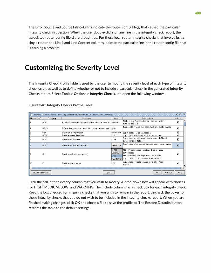
The Error Source and Source File columns indicate the router config file(s) that caused the particularintegrity check in question. When the user double-clicks on any line in the integrity check report, theassociated router config file(s) are brought up. For those local router integrity checks that involve just asingle router, the Line# and Line Content columns indicate the particular line in the router config file thatis causing a problem.
Customizing the Severity Level
The Integrity Check Profile table is used by the user to modify the severity level of each type of integritycheck error, as well as to define whether or not to include a particular check in the generated IntegrityChecks report. Select Tools > Options > Integrity Checks... to open the following window.
Figure 348: Integrity Checks Profile Table
Click the cell in the Severity column that you wish to modify. A drop-down box will appear with choicesfor HIGH, MEDIUM, LOW, and WARNING. The Include column has a check box for each integrity check.Keep the box checked for integrity checks that you wish to remain in the report. Uncheck the boxes forthose integrity checks that you do not wish to be included in the integrity checks report. When you arefinished making changes, click OK and chose a file to save the profile to. The Restore Defaults buttonrestores the table to the default settings.
488

Scheduling Integrity Checking in Task Manager
The Integrity Check Report task can be used to perform integrity checking on a set of configuration filesat a designated time interval
Integrity Check Task
1. Select Admin > Task Manager. Click the “New Task” button and select the “Integrity Check” task.
2. Enter a name for the task and click “Next”.
3. Select the “Integrity Check Options” tab. To schedule the task for the offline network, select “Useoff-line network” and specify the specification file name and the directory containing the config files.
You can also select options to filter the integrity checks by category, message, routers, topology groups,and severity.
Note that in order to select specific topology groups, the specification file that was selected shouldreference a group file. This group file can be created by saving the network after creating groups onthe topology map.
4. Additionally, select “Save the report to make it available on the web” to view the report from the webinterface. For more details on the options, refer to “Integrity Check Options Tab” on page 490.
5. When scheduling the task for an offline network, select the “ConversionOptions” tab to specify specificimport parameters. For more details on these options, see “Router Data Extraction Overview” onpage 33.
6. Finally, select the “Report Options” tab and select whether to save the Integrity Check report to a fileand/or to e-mail the report. See Report Options for more details.
7. Click “Next” and select the Schedule Type and interval parameters as necessary.
8. Then click “Finish”.
Report Options
The Report Options tab specifies how the results of the Configuration Check Task will be saved each timethe configuration check task is run.
489
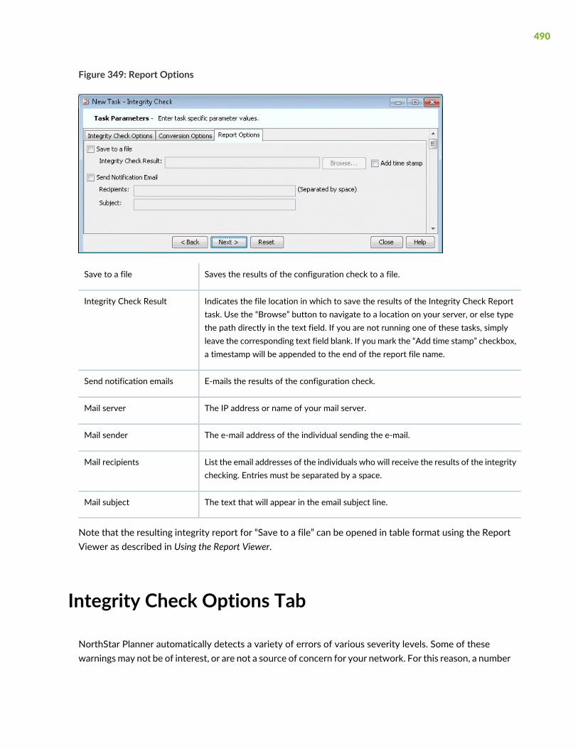
Figure 349: Report Options
Saves the results of the configuration check to a file.Save to a file
Indicates the file location in which to save the results of the Integrity Check Reporttask. Use the “Browse” button to navigate to a location on your server, or else typethe path directly in the text field. If you are not running one of these tasks, simplyleave the corresponding text field blank. If you mark the “Add time stamp” checkbox,a timestamp will be appended to the end of the report file name.
Integrity Check Result
E-mails the results of the configuration check.Send notification emails
The IP address or name of your mail server.Mail server
The e-mail address of the individual sending the e-mail.Mail sender
List the email addresses of the individuals who will receive the results of the integritychecking. Entries must be separated by a space.
Mail recipients
The text that will appear in the email subject line.Mail subject
Note that the resulting integrity report for “Save to a file” can be opened in table format using the ReportViewer as described in Using the Report Viewer.
Integrity Check Options Tab
NorthStar Planner automatically detects a variety of errors of various severity levels. Some of thesewarningsmay not be of interest, or are not a source of concern for your network. For this reason, a number
490
of options are provided in this tab to allow you to filter for just those integrity checks (ICs) that concernyou.
Network OptionsNetwork Options
TheNetwork section of thewindow is used to specify the set of configuration files to perform the integritychecking on. If you use NorthStar Planner to monitor the live network, you can select “Use live network”.Alternatively, select “Use specification file” and specify the configuration file folder and correspondingspecification file path created by importing the configuration files.
Filter by Category
IC’s are organized into different categories, as listed in thewindow. You canmark the “Include All Categories”checkbox if you wish to see IC’s belonging to all categories. Otherwise, highlight just those categories youare interested in, in the “Select From” list on the left, and move them to the “Categories to be included”list on the right via the “Add->” button. Pressing the “Add All >>” button is equivalent to selecting the“Include All Categories” checkbox.
Filter by Message
You can filter the integrity check results according to specific IC messages. There is a predefined set of ICmessages, each assigned its own msg ID (or message ID), which is the number preceding the message.These are listed in the left hand list of the Filter by Message section.
To customize the ICs to show, unselect “Include All Messages”, highlight just those categories you areinterested in, in the “Select From” list on the left, and move them to the “Messages to be included” list onthe right via the “Add->” button.
You can perform an additional filter on themessages to be included by entering text in the “And, optionallyfilter message by matching substring” text field. Only messages which include your text string will beconsidered.
Filter by Router
In the Filter by Router section, you can choose to see only those IC’s pertaining to certain routers. To doso, uncheck the “Include All Routers” checkbox, highlight the routers that you are interested in(corresponding to the routers in the network you specified), andmove them to the “Routers to be included”list on the right-hand side using the “Add->”button.
You can perform an additional filter on the desired routers to be included by entering text in the “And,optionally filter routers by matching substring” textfield. Only those router names which include your textstring as part of the name will be considered.
IC’s can also be categorized into two types:
• Router IC - an IC that pertains to a single router
• Network IC - an IC that pertains to two or more routers
491

• For example, some users may wish to see:
• All Router ICs, but only those Network ICs pertaining to the selected router(s)
• All Network ICs, but only those Router ICs pertaining to the selected router(s)
• None of the Router ICs and only those Network ICs pertaining to the selected router(s)
This explains why so many different options are provided. These options are explained below:
ExplanationRouter IC Filter
Show all router ICs, even those pertaining to routersthat are not selected.
Include All regardless of the selected routers (Show All)
Show only those router ICs pertaining to the selectedrouters.
Include if a problem occurred in selected routers (ShowOnlyfor Selected Routers)
Do not show any router ICs.Exclude if a problem occurred in selected router(s) (ShowNone)
ExplanationNetwork IC Filter
Show all network ICs pertaining to all routers in thenetwork (that is, not just those selected)
Include All regardless of the selected routers (Show All)
Show only those network ICs for which ALL involvedrouters belong to the set of selected routers.
Include if a problem occurred in selected routers (ShowOnly for Selected Routers - Strict match)
Show only those network ICs for which at least one of theinvolved routers belong to the set of selected routers.
Include if a problem occurred in any of selected routers(Show Only for Selected Routers - Loose match)
Do not show any network ICs.Exclude if a problem occurred in selected router(s) (ShowNone)
Filter by Group
In the Filter by Group section, you can choose to see only those IC’s pertaining to routers in certain topologygroups. To do so, uncheck the “Include All Groups” checkbox, highlight the groups that you are interestedin (corresponding to the routers in the network you specified), and move them to the “Groups to beincluded” list on the right-hand side using the “Add->”button.
Note that in order to select specific topology groups, the map for the selected network specification fileshould contain groups. Furthermore, these groups should be saved into the network baseline. If there aretopology groups, but they are not appearing in the list, save the network first using File > Save Network...before creating a task for the Integrity Check report.
492

Filter by Severity
ICs are assigned one of four severity levels: High, Medium, Low, Warning. You can select the severity ofintegrity check errors to display. The severity levels corresponding to individual ICs can be set within theIC Profile Table (Tools >Options > Integrity Checks). See Integrity CheckOptions Tab for more information.
Additional Report Options
Make the IC report accessible for viewing via the NorthStar Planner Web interface.Save the report to make itavailable on the web
Includes a header in the report that indicates the types of filters used to generate theparticular report. For example, the reportmight show that the user is filtering by Category(only “OSPF” was selected), Message / msg ID (only message 93 was selected), Severity(all severity levels were selected), and Router / Error Source (only router “NWK” wasselected). Note that you can look up the msg ID, or Message ID, in the Integrity ChecksProfile Table. See “Integrity Check Options Tab” on page 490 for more information.
Report with the Header
Indicate the level of detail to be used in the report: Full or compact. Both reports willdisplay the following fields: Category, Message, Detail, Severity, Error Source.
The Full report will contain some additional information to identify the source of theerror: Source File, Line #, Line Content, and msg ID.
Report Type (Full /Compact)
Integrity Check Descriptions
This section gives a description of some of the integrity checks (ICs) that are performed on the routerconfiguration files during configuration import. The IC descriptions are organized by category. For eachIC, a brief description, a msgID (corresponding to the msgID shown in the Integrity Checks reports), andthe default severity are given.
A more detailed description then follows to give more information about the particular IC check. Theseverity of the IC helps the network engineer to prioritize which ICs to look at first. High severity reportsare critical reports believed to potentially causemajor network problems.Medium and Low severity reportsdescribe problems not considered severe, but should be fixed to prevent network problems or inadvertentside effects.Warning-level reports describe potential network problems that the network engineer shouldexamine to make sure that the network is operating at its best.
493

Access List and Prefix List Integrity Checks
["Non-utilized access-list rule (Cisco)", msgID=106, High]
When access lists become long, preceding rules may be more general than subsequent rules. When thishappens, the later rules are never utilized. This check identifies situations when rules are not utilized.
["Unknown access-list (Cisco)", msgID=86, High]
This check identifies references to undefined access lists. Supported for IPv4 and IPv6.
["Unreferenced access-list (Cisco)", msgID=100, Warning]
An access-list was defined, but not referenced. Supported for IPv4 and IPv6.
["Unknown prefix-list (Cisco)", msgID=107, High]
This check identifies references to undefined prefix lists.
["Unreferenced prefix-list (Cisco)", msgID=108, Warning]
A prefix-list was defined, but not referenced.
BGP Integrity Checks
["Disabled BGP protocol (Juniper)", msgID=5, Warning]
This check identifies situations where the BGP section is defined, but the disabled statement is present.
["Ignored 'community-list' statement due to unexpected 'permit'/'deny' location (Riverstone)", msgID=18,Warning]
Because the permit/deny following the "community-list <name>" command is missing, the community-liststatement is ignored.
["BGP neighbor shutdown", msgID=51, Warning]
This check identifies situations when the BGP neighbor is shutdown.
["Unknown as-path access-list", msgID=109, High]
This check identifies references to undefined as-path access lists.
["Unreferenced as-path access-list (Cisco)", msgID=110, Warning]
An as-path access-list was defined, but not referenced.
["Unknown community-list", msgID=124, High]
494

This check identifies references to undefined community lists.
["Unreferenced community-list (Cisco)", msgID=125, Warning]
A community-list was defined, but not referenced.
["Unknown route-map action (Riverstone)", msgID=97, High]
This check identifies references to an undefined community-list in the "route-map <name> deny/match<> community-list" command.
EIGRP/IGRP Integrity Checks
["Inconsistent EIGRP definition", msgID=20, Medium]
This check finds EIGRP to be enabled on one end of a line but not the other end.
["Inconsistent IGRP definition", msgID=21, Medium]
This check finds IGRP enabled on one end of a line but not the other end.
["Invalid EIGRP inverse (wildcard) mask", msgID=61, High]
When configuring which networks EIGRP will advertise, the inverse (wildcard) mask must be correct. Thischeck identifies invalid EIGRP inverse mask values.
["Invalid IGRP inverse (wildcard) mask", msgID=62, High]
When configuring which networks IGRP will advertise, the inverse (wildcard) mask must be correct. Thischeck identifies invalid IGRP inverse masks values.
["Invalid EIGRP network address", msgID=65, High]
This check identifies invalid network addresses that EIGRP is trying to advertise.
["Unexpected IGRP network address", msgID=66, High]
This check identifies invalid network addresses that IGRP is trying to advertise.
IP Integrity Checks
["Duplicate IP address (public)", msgID=9, High]
All IP addresses assigned to router interfaces are checked for duplication since duplicate IP addresses canresult in serious problems in a network.
495

["Duplicate IP address (private)", msgID=111, Warning]
An IP address in one private address spaces can be duplicated in another (e.g., within different VPNs). Thischeck identifies duplicated IP addresses within the same private address space.
["Duplicate host name", msgID=10, High]
This check identifies duplicate config files for the same router. The duplicated config files are ignored.
["Error in address definition (Riverstone)", msgID=12, High]
This check identifies invalid IP address formats in the "interface create ip <name> address-netmask"command.
["Inconsistent media interfaces with same subnet address", msgID=19, Warning]
During configuration parsing, two interfaces are stitched up when
• Their addresses are in the same subnet
• Their media types are either Ethernet, SONET, or ATM and match on both sides.
This check identifies situations where condition 1 is true, but condition 2 is not.
["Inconsistent bandwidth", msgID=29, Low]
This check identifies the situationwhere there is a bandwidthmismatch between two terminating interfacesof a link.
["Missing host name", msgID=38, High]
This check sees that a host name was not specified after the "hostname" command.
["Multiple hostnames defined", msgID=45, High]
This check sees duplicate host names defined in the system section.
["Non-primary address matched", msgID=49, Warning]
This check alerts the user to the fact that secondary addresses were used for stitch up.
["Overlapped subnet addresses", msgID=50, High]
This check identifies overlapped subnet addresses.
["Unexpected IP address", msgID=63, High]
This check identifies invalid IP addresses in Juniper or Riverstone configs.
["Unexpected IP mask (Riverstone, Juniper)", msgID=64, High]
This check sees that the vlan specified in the "interface create ip <name> vlan" was not defined.
496
ISIS Integrity Checks
["Inconsistent ISIS definition", msgID=22, Medium]
This check sees that ISIS was enabled on one end of a line but not the other end.
["Asymmetric ISIS1 metric", msgID=114, Warning]
This check finds ISIS1 metrics to be different at the two ends of a link.
["Asymmetric ISIS2 metric", msgID=115, Warning]
This check finds ISIS2 metrics to be different at the two ends of a link.
["Overlapped network statements", msgID=164Warning]
This check flags overlapping IP address ranges related to network statements under the OSPF or BGPprotocol, for Cisco and Huawei devices.
RIP Integrity Checks
["Inconsistent RIP definition", msgID=112, Medium]
This check sees that RIP is enabled on one end of a line but not the other end. OSPF Integrity Checks
["Invalid OSPF/IGRP/EIGRP network address", msgID=69, High]
This check identifies invalid IP network prefixes in the OSPF, IGRP, or EIGRP sections.
["Duplicate area IDs defined (Riverstone)", msgID=6, High]
This check sees that duplicate non-backbone area IDs are defined.
["Inconsistent OSPF area definition", msgID=25, High]
This check sees that the two ends of an OSPF link are assigned to two different OSPF areas.
["Inconsistent OSPF definition", msgID=26, Medium]
This check sees OSPF enabled on one end of a link but not the other end.
["Multiple defined backbone areas (Riverstone)", msgID=44, High]
This check identifies situations in Riverstone configuration files where the backbone area0 is definedmorethan once.
["Invalid OSPF network address", msgID=67, High]
497

This check identifies invalid OSPF network addresses.
["Unexpected OSPF inverse (wildcard) mask", msgID=68, High]
This check indentifies invalid inverse (wildcard) masks on the network statement in the OSPF section.
["Unexpected area IP (Riverstone)", msgID=60, High]
Riverstone uses the 4-octet format for non-backbone OSPF area designation. This check identifies casesinwhich the area entered in the "ospf create area" commandwas neither "backbone" nor a valid IP address.
["Unknown OSPF area (Riverstone)", msgID=81, High]
Riverstone uses the 4-octet format for non-backbone OSPF area designation. This check identifies casesin which the area entered in the "ospf add interface to area" command was neither "backbone" nor a validIP address.
["Asymmetric OSPF metric", msgID=113, Warning]
This check identifies the situationwhere theOSPFmetrics defined on the two end interfaces are different.
["ABR not in Area 0", msgID=119, Warning]
This check finds an ABR that does not border Area 0.
["Unbalanced OSPF virtual-link", msgID=126, High]
This check sees that OSPF virtual-link is defined only in one end but not the other.
["OSPF virtual-links not in the same transit area", msgID=127, High]
OSPF virtual links can be used to establish OSPF routing in areas that can only be connected vianon-backbone (transit) areas. This check identifies the situation where the OSPF virtual-links going to andfrom the backbone area are going through a different transit area.
["Asymmetric OSPF reference bandwidth", msgID=162, Low]
This check identifies the situationwhere theOSPF reference bandwidth defined on the two end interfacesare different.
QoS Integrity Checks
["Bandwidth and priority commands cannot be used in the same classwithin the same policymap (Cisco)",msgID=3, severity=Medium]
Either the bandwidth or the priority option can be used for a particular class within a policy map to specifythe guaranteed bandwidth, but not both.
498

["Duplicate policy-Map", msgID=11, Low]
This check looks for duplicate policy-map names defined in a config file.
["Duplicate Class-Map", msgID=7, Low]
This check looks for duplicate class-map names defined in a config file.
["Duplicate CoS-Queue-Group", msgID=8, Low]
This check looks for duplicate CoS queue groups configured in a config file.
["Invalid IP precedence values", msgID=30, High]
This check identifies IP precedence values that are outside of the allowed range of 0-7.
["Invalid MPLS EXP bit value", msgID=31, High]
MPLS uses the EXP bits in the shim header to support differentiated services. Valid EXP bit values are 0-7.This check identifies invalid EXP bit values.
["Undefined class", msgID=55, Medium]
This check sees that the class referenced in a policy-map section was not configured by the class-mapcommand.
["Unknown class name in scheduler-map", msgID=90, Low]
This check sees that the class name referenced in the scheduler-map section was not defined.
["Unknown scheduler name in scheduler-map", msgID=98, Low]
This check sees that the scheduler name referenced in the scheduler-map section was not defined.
["Reference to an unknown policy-map", msgID=135, Medium]
This check identifies references to an unknown policy-map name.
LINK Integrity Checks
["Inconsistent PIM mode", msgID=27, High]
This check sees that PIM was enabled on one end of a line but not the other end.
["Undefined filter (Juniper)", msgID=56, High]
This check identifies situations where a filter is being applied to an interface, but the referenced filter isundefined.
499

["Unreferenced firewall filter", msgID=101, Warning]
This check identifies firewall filters that are never referenced
["Unknown ISIS area-tag (Cisco)", msgID=89, High]
This check identifies situations with Cisco ISIS configuration when a reference was made to an undefinedarea-tag.
["ip unnumbered command references an unknown interface (Cisco)", msgID=95, Medium]
The ip unnumbered command borrows the IP address from the specified interface to the interface onwhich the command has been configured. This check identifies situations when the specified interface isunknown.
MISCELLANEOUS Integrity Checks
["Invalid config file", msgID=33, Warning]
This check identifies those files that are not router configuration files.
["non-text file", msgID=34, Warning]
This check looks for files that contains too many unreadable characters.
["Undefined interface", msgID=77, High]
This checks finds that the interface name entered in the "isis add interface" command was not defined bythe "interface create" command.
["Undefined IP address (Riverstone)", msgID=76, High]
This check looks for undefined IP addresses in Riverstone IP address statements.
["Undefined interface IP address", msgID=78, High]
This check saw an undefined interface IP address in "isis add interface" command.
["Undefined LSP", msgID=79, Low]
This check finds that the LSP name is not defined in the LSP section.
["Unknown interface", msgID=93, Low]
This general check finds situations where the referred to interface was not defined. This could happen inmany situations.
["vlan-id defined without configuration in vlan-tagging section(Juniper)", msgID=104, Medium]
500

This checks finds that the vlan-id defined in the interface section was not configured in the vlan-taggingsection.
["Inconsistent ATM bandwidth and PVC mean value", msgID=105, Warning]
This check identifies situations in which the ATM bandwidth and PVC mean values are known, but thePVC mean value is different from the ATM bandwidth value.
["Reference to an unknown card (Alcatel)", msgID=139, High]
This check identifies cases where references were made to an undefined card name.
["Reference to an unknown port (Alcatel)", msgID=140, High]
This check identifies cases where references were made to an undefined port name.
["Reference to an unknown SDP (Alcatel)", msgID=141, High]
This check identifies cases where references were made to an undefined SDP name.
["Reference to an unknown route-map (Cisco)", msgID=130, High]
This check identifies references to an unknown route-map.
["Tunnel is configured as both autoroute announced and forwarding-adjacency", msgID=131, High]
This checks identifies the situation where a tunnel is configured as both autoroute announced andforwarding-adjacency.
["No IGP on forwarding-adjacency tunnel", msgID=132, Medium]
This checks sees that ISIS or OSPF was not configured on a forwarding-adjacency tunnel.
["bandwidth may exceed physical interface capacity", msgID=128, Low]
This check looks for situationswhere the bandwidth value configured for an interface exceeds the physicalinterface capacity. E.g., this checkwould identify the casewhere the bandwidth for a Fast Ethernet interfaceis configured as 1000000 (1G).
["Unreferenced route-map", msgID=152, Warning]
A route-map was defined, but not referenced.
["Unreferenced policy-map", msgID=153, Warning]
A policy-map was defined, but not referenced.
["Empty route-map(route-policy) statement", msgID=163, Warning]
A route-map statement was definedwithout any content. This integrity check applies to Cisco andHuaweidevices.
501

["Hostname not configured", msgID=165, Warning]
The hostname was not configured on the device. This integrity check applies to the following devices withcisco-like config: Cisco (IOS, IOS-XR), asa, casa, nxos, zte, oneaccess, adtran, hillstone, digitalchina, etc.
MPLS Integrity Checks
["Multiple group-names assigned to the same group-value (Juniper)", msgID=4, severity=High]
This check identifies situations where the same group-value (tunnel bit value) is assigned to multiplegroup-names under the admin-group statement.
["Inconsistent LDP/TDP definition", msgID=23, Medium]
This check sees that LDP/TDP was enabled on one end of a line but not the other end.
["Inconsistent MPLS-TE definition", msgID=24, Medium]
This check sees that MPLS-TE was enabled on one end of a line but not the other end.
["Invalid tunnelbit (Juniper)", msgID=32, High]
This check finds that the MPLS admin-group tunnelbit is not in the allowed range (1~31).
["Undefined admin-group", msgID=70, High]
This check finds that the admin-group referenced in the tunnel section was not configured.
["Invalid tunnel destination IP address format", msgID=72, High]
This checks identifies tunnel destination IP addresses that have an invalid format.
["Invalid hop number", msgID=73, High]
This checks sees that the hop number is out of the valid range (1~255).
["Invalid tunnel source IP address format", msgID=75, High]
This check identifies tunnel Source IP addresses that have an invalid format.
["Unknown admin-group (Juniper, Alcatel)", msgID=87, High]
This check identifies a reference to an undefined admin-group for Juniper and Alcatel routers.
["Unknown Tunnel/LSP path", msgID=96, High]
This check finds references to unknown an tunnel/LSP path.
["RSVP not defined on MPLS enabled interface", msgID=118, Warning]
502

This check warns the user that RSVP was not defined on an MPLS enabled interface.
["MPLS-TE tunnel is not enabled on the device", msgID=142, High]
Prior to configuring MPLS-TE tunnels, the mpls traffic-eng tunnels statement is configured at the globallevel. This check identifies situations where this statement is missing.
["Asymmetric MPLS-TE metric", msgID=116, Warning]
This check finds that the MPLS-TE metric to be different on the two ends.
RSVP Integrity Checks
["Inconsistent RSVP bandwidth", msgID=28, Warning]
This check identifies situations where the RSVP bandwidth is different on the two sides on a link.
["Inconsistent RSVP definition", msgID=147, Medium]
RSVP was enabled on one end of a link but not the other end.
Static Routes Integrity Checks
["Next hop not in local subnet", msgID=47, Warning]
This check sees that the next hop address defined by static route does not belong to any of the subnetsconfigured on the router.
["Shutdown interface in static route", msgID=52, Medium]
This check sees that the next hop interface for the static route was a shutdown interface on the localrouter.
["Unknown tunnel in static route", msgID=82, High]
The check finds the situation where the referenced next hop tunnel for the static route was not definedon the router.
["Unknown interface in static route", msgID=94, High]
This check finds the situation where the referenced next hop interface for the static route was not definedon the router.
["Next hop is local address", msgID=146, High]
503

This check sees that the next hop of the static route is a local address
Tunnel Integrity Checks
["Undefined Tunnel (Cisco)", msgID=80, Low]
This checks looks for a reference to an undefined tunnel in Cisco's 'mpls traffic-eng backup-path <tunnelID>' statement, where the <tunnel ID> was not defined.
["Unknown destination address in Tunnel", msgID=92, Warning]
This check any tunnel that has a destination address not in the given network.
["Asymmetric GRE tunnel", msgID=143, High]
This check sees that a GRE tunnel is defined only on one end but not the other.
["Inconsistent GRE tunnels protocol", msgID=144, High]
This check finds the GRE tunnel protocols to be defined inconsistently. If the GRE tunnel from the A endis in OSPF (ISIS) protocol section, then the GRE tunnel from the Z end also needs to be in the OSPF (ISIS)protocol section.
["autotunnel mesh groups not enabled", msgID=137, High]
To configure AutoTunnel mesh groups, you must first enable it using the 'mpls traffic-eng auto-tunnelmesh' statement. This check identifies situations in which this statement is missing.
["autotunnel backup not enabled", msgID=138, High]
To configure backup AutoTunnels, you must first enable it using the 'mpls traffic-eng auto-tunnel backup'statement. This check identifies situations in which this statement is missing.
VPN Integrity Checks
["No remote Layer 2 circuit", msgID=48, Medium]
This check finds situations where there's no remote layer2 circuit in L2M, VPLS, or L2 CCC VPNs.
["Singleton VPN", msgID=53, Warning]
This check found only one VRF statement in a particular VPN.
["VRFs with same meshed route targets", msgID=133, Warning]
504

This check lets the user know that different VRFs were found to have the mesh of route targets
["VRF without import and export route targets", msgID=134, Low]
This check saw an incomplete VRF definition, which was missing import and export route targets.
["Missing route distinguisher", msgID=120, High]
This check saw a VRF definition missing the route distinguisher statement.
["Missing export route-target", msgID=121, High]
This check saw a VRF missing the route-target export statement.
["Missing import route-target" msgID=122, High]
This check saw a VRF missing the route-target import statement.
["No interface in VRF", msgID=123, Warning]
This check sees that a particular VRF is not used in any interface.
["No interface/circuit using bridge-instance (Tellabs)", msgID=136, Warning]
This check identifies Tellabs bridging-instances that are not referenced by any interfaces/circuits.
["Unknown policy-name", msgID=129, High]
This check identifies references to an undefined policy.
["VRFs with same route targets and route distinguisher", msgID=117, Warning]
This check identifies VRFs with same route targets and route distinguisher.
["Unknown VRF", msgID=85, High]
This check identifies references to an unknown VRF.
["Duplicated RDs in different VRFs", msgID=151, Medium]
This check identifies if two different VRFs have the same RD and their route targets have no intersection.
VLAN Integrity Checks
["Undefined vlan (Riverstone)", msgID=59, High]
This check identifies in Riverstone configs references to a vlan that is undefined.
["Unknown smarttrunk", msgID=99, High]
505

This check finds that the smart trunk specified in the "smarttrunk add ports <name> to <smarttrunk>"command was not defined.
506

25CHAPTER
Compliance Assessment Tool
Compliance Assessment Tool Overview | 509
Using The Compliance Assessment Tool | 510
CAT Testcase Design | 512
Creating a New Project | 513
Loading the Configuration Files | 514
Creating Conformance Templates | 517
Reviewing and Saving the Template | 521
Saving and Loading Projects | 522
Run Compliance Assessment Check | 523
Compliance Assessment Results | 526
Publishing Templates | 528
Running External Compliance Assessment Scripts | 530
Scheduling Configuration Checking in Task Manager | 531
Building Templates | 532
Special Built-In Functions | 546

NorthStar Planner Keywords For Use Within a Rule | 549
More on Regular Expressions | 555
IP Manipulation | 557
Compliance Assessment Tool Overview
This chapter describes theNorthStar Planner Compliance Assessment Tool and how it can help an auditingor operations group check compliance of the network’s configuration files to user built customized rules.This tool can be used to provide alerts when changes to a config file break one of the user-defined rules.
Access to a copy of the network’s configuration files.
For more information on Regular Expressions, refer to the NorthStar Planner User Interface Guide appendixon Search Preferences.
The following is a high-level, sequential outline of the compliance assessment tool uses and the associated,recommended procedures.
1. Creating a New Project on page 513
2. Loading the Configuration Files on page 514
3. Creating Conformance Templates on page 517
4. Reviewing and Saving the Template on page 521
5. Saving and Loading Projects on page 522
6. Run Compliance Assessment Check on page 523
7. Publishing Templates on page 528
8. Running External Compliance Assessment Scripts on page 530
9. Scheduling Configuration Checking in Task Manager on page 531
Referred to the following for details regarding configuration rules and template syntax:
• Building Templates on page 532
• The Flow Control Syntax Table
• The Built-In Functions For Use Within a Rule Table
• NorthStar Planner Keywords For Use Within a Rule on page 549
• The Header Syntax - Conform Statements Table.
• More on Regular Expressions on page 555
• IP Manipulation on page 557
509
Using The Compliance Assessment Tool
To open the Compliance Assessment window, select Tools > Compliance Assessment. This window isused primarily by network operators to run CAT scans on the network configuration files. The CAT scansare a collection of test cases or rules that search the configuration files for keywords, strings, and statementmatches or non-matches to determine configuration compliance. These test cases are created using CATtemplate syntax by template designers. The templates syntax can use logical operators, conditionalexpressions, and variables to support more complex searches.
• The Choose screen allows for selection of the test case(s) and network for the CAT scan. Initially thisscreen will have no test cases displayed until the test cases are created and published from the CATTestcase Design window. The CAT Testcase Design window is opened by clicking Manage Templates.
Figure 350: Compliance Assessment Choose screen
• The Scan screen allows for selection of the device(s) and their configuration files for the CAT scan. Pressthe green button to start the scan.
510

Figure 351: Compliance Assessment Scan screen
• The Result screen displays the results of the CAT scan. The results can be viewed in detailed, summarizedby device, or summarized by rule name. The summary reports also calculate a Score which representsthe device’s configuration compliance to the test cases. A higher score means better compliance, and alower score means worse compliance comparatively. The ScoreWeights can be defined under Settings.
Figure 352: Compliance Assessment Result screen
• The Actions button provides options to save and open projects, manage templates, and change theResults Score Weight. Saving projects in this CAT window saves the selected test cases in the Choosescreen.
511
Figure 353: Compliance Assessment Actions options
CAT Testcase Design
To open the CAT Design window, select Tools > CAT Testcase Design. This window is used primarily bytemplate designers to create templates or test cases, create projects which are a collection of templatesand configuration files, and publish those templates or test cases for network operators to use in theCompliance Assessment window.
512

Figure 354: CAT Testcase Design window
Creating a New Project
1. To create a new CAT project, click the New Project button in the CAT Testcase Design window.
2. The project title is listed in the title bar as “Default”. Click the Save Project button to save the projectwith a name. This will open up the File Chooser window. Select a name for your project. CAT projectsare saved with file extension .prj
513

Figure 355: CAT Testcase Design creating new project
3. The next steps are to add configuration files and templates to the CAT project. It’s recommended toperiodically Save Project as you work.
Loading the Configuration Files
The following steps are to define the set of configuration files to be used in the CAT project.
514

• Select the Configurations tab and right-click in the left panel.
Figure 356: Configurations tab right-click options
• Select LoadCurrentNetworkConfigurations to load the configurations of the currently opened network.This option is only available if the current network opened has imported configuration files.
• If no network has been opened or if you want to load a different set of configuration files, select Addfrom the pop-upmenu. A file chooser will open that allows you to navigate to the directory on the serverwhere the configuration files are saved. Select the configuration file(s) to be added to the project.
515

Figure 357: Selecting Configuration Files to add to the Configurations Tab
Use <Shift>-click to select a range of items from the currently highlighted entry. Alternatively, use<Ctrl>-click to select an individual entry. The shortcut Ctrl-A can also be used to select all configurationsin the directory.
Click Select to add the configurations to the Configurations tab. A checkbox next to each file indicatesif it will be included in the compliance assessment.
• The configuration files will now be populated in the Configurations tab. Right-click and select Show Filewill display the configuration file in the right panel. Double-clicking opens the configuration file in theConfig Editor window.
516
Figure 358: Configuration File Loaded
• Configuration files that are not desired in the project can be deleted by right-clicking and selectingDelete.
• Click Save Project to save the changes to the project.
Creating Conformance Templates
The next step is to create the compliance assessment test cases or rules using the CAT template. Thetemplates will be used to load in the test cases or rules for the CAT scan.
517
1. To create a new template, select the Templates tab. Right-click in the left panel and selectNewTemplate.
Figure 359: Creating a New Template
2. A New Template window will open as shown below
518

Figure 360: New Conformance Template window
Category, Name, and Location : Are identification properties of the template.
• Category : This field is to help organize or group templates into categories.
• Name : Enter the name of the template.
• Location : Type in the location on the server where the file will be saved or use the Browse button.
• File Name : The template file extension is .tpl. You can change the default naming here.
• Types : Are device vendor properties of the template.
• Vendor/OS : Select the configuration file type: “Cisco IOS”, “Cisco IOS-XR”, “Juniper JUNOS”, “ALUTiMOS”, “Huawei”, “Redback”, “Tellabs” or “ZTE.”. Note that Cisco-IOS based templates can only beused to check compliance on Cisco configuration files, Juniper JUNOS templates on Juniperconfiguration files, and so forth.
• Hardware : The hardware type is derived from the network model. Using this field means only thespecified hardware type can be used by the template. If the field is blank, then any hardware typecan be used.
• OS Version : The OS version is derived from the configuration file. Using this field means only thespecified OS version can be used by the template. If the field is blank, then any OS version can beused. A range of OS versions can be specified using the following syntax: +, -, *
519

• 12.2+ means version newer (higher number value) than 12.2 including 12.2
• 12.2- means version older (lower number value) than 12.2 including 12.2
• 12.2* means any version starting with 12.2
• Options : Select the basic option(s) that will be applied to this template.
• Case-sensitive : If checked, upper and lower case must be matched in the compliance assessment.
• Do not use regular expression : By default regular expression syntax is supported in the template.If this option is checked, then regular expression syntax such as wildcards “*” and “?” can be notused. See <Link>“More on Regular Expressions” on page 555 for more information.
When using regular expressions, the “#conform ignore escchars” statement can be used to indicatewhich characters to be treated as is, and not as special regular expression characters. Without thisline, you would need to precede those text characters with a backslash ‘\’ to avoid interpretationof the character as a regular expression.
3. Click OK when you are done. The new template will appear in the Templates tab. A checkbox will bedisplayed to the left of each file for selecting particular configuration files/templates to be used for thecompliance assessment.
4. Double-clicking an entry will open the template file in the right panel and the template can be directlyedited.
Figure 361: Initial Template
5. The options that were selected from the previous window can be seen listed in the first few lines afterthe reserved directive, or keyword, “#conform,” and will be applied when compliance is checked. Bydefault, anything else following the pound sign “#” that does not start with “conform” denotes a commentand is ignored.
520

6. Advanced users whom are familiar with the template syntax can create the template via a text editoron the server (or the File Manager) and then import it into CAT by right-clicking the Templates leftpanel and selecting Add.
7. Once the template is created, test cases or rules must be written using template syntax.
Editing the Conformance Template
1. After loading the template file, its content can be edited directly in the right panel. Cut, Copy, Paste,and Find and Replace functions can be accessed by right-clicking or via the shortcuts <Ctrl>-x for cut,<Ctrl>-c for copy, and <Ctrl>-v for paste, and <Ctrl>-f for find.
Reviewing and Saving the Template
After you have added your rules, right-click in the right panel and select Save to save the template, or usethe shortcut <Ctrl>-s.
If the box in the upper right corner of the CAT Testcase Design window is green, it indicates that no errorshave been found in the template.
Figure 362: Template with green box indicates no errors
Otherwise, if an error has been found, the box in the upper right corner will be red. Double-click on theorange-colored segment on the right hand side bar to jump to the line with the error. For example, theerror could be related to an incomplete if statement (with no matching “end” statement).
521

Figure 363: Template with red box indicates errors
Clicking Save Project will also save any changes to the template.
Saving and Loading Projects
Once you have created a set of templates and the configurations to apply them to, this information canbe saved in a Project by clicking Save Project. A Project is defined as a set of configurations, templates,and settings. To save the project as a new name, click the Action menu and select Save Project As.
522

Figure 364: Action menu
To open a saved project, select Open from the toolbar to open the project file from the server. This willautomatically load the associated configurations and templates in the project. Most recent projects arealso displayed by clicking the Open down arrow button.
Run Compliance Assessment Check
1. Select the Configurations tab and check the configuration files on which you wish to perform acompliance assessment check.
• The right-click pop-upmenu provides shortcuts to perform selections or deselections on all or selectedconfiguration files.
• Keyboard shortcuts can select a range of rows using <Shift>-click. Individual row selection can beselected with <Ctrl>-click. All rows can be selected with <Ctrl>-a.
• The Filter field can be used to filter on the hostname, OS, or file name. To reset the filter and showall configuration files, enter wildcard * or leave the field blank and press <Enter>.
523
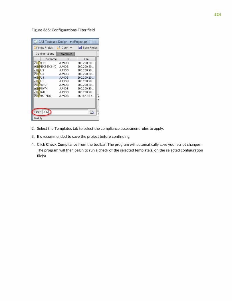
Figure 365: Configurations Filter field
2. Select the Templates tab to select the compliance assessment rules to apply.
3. It’s recommended to save the project before continuing.
4. Click Check Compliance from the toolbar. The program will automatically save your script changes.The program will then begin to run a check of the selected template(s) on the selected configurationfile(s).
524
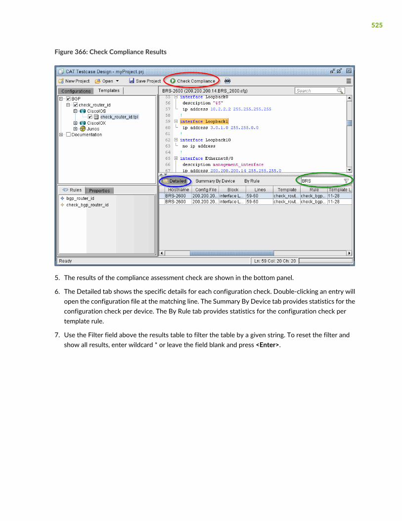
Figure 366: Check Compliance Results
5. The results of the compliance assessment check are shown in the bottom panel.
6. The Detailed tab shows the specific details for each configuration check. Double-clicking an entry willopen the configuration file at the matching line. The Summary By Device tab provides statistics for theconfiguration check per device. The By Rule tab provides statistics for the configuration check pertemplate rule.
7. Use the Filter field above the results table to filter the table by a given string. To reset the filter andshow all results, enter wildcard * or leave the field blank and press <Enter>.
525
Compliance Assessment Results
Table 5: Detailed Tab
DescriptionDetailed Tab Column
Displays information such as the general type of conformance match, mismatch, orpartial match. If there is a mismatch, the line missing from the configuration is includedin the Message. "not ordered" indicates that the lines are present in the configurationfile but their ordering is not consistent with that of the template. "hardware typemismatch" indicates that the template type (Cisco IOS or Juniper JUNOS) does notmatch the configuration file type.
Message
There are five levels. Warning shows that compliance has failed for a given line, forexample if a line is missing or failed to match. Info indicates a match or partial match.The user can also change these levels to be displayed as Minor, Major, or Critical.
Severity
Device hostnameHostname
Displays the configuration file for which this entry applies. Double-clicking on a rowwill open this configuration file in the Main Pane.
Config File
The exact block of the configuration of the messageBlock
Displays the corresponding start line and end line where the results entry applies.Lines
Displays the template that was used for this compliance assessmentTemplate
Template Rule NameRule
Range of Line numbers in which template rule occursTemplate Lines
For conform command, indicates the content of the line with violationTemplate Line
For conform command, indicates the line number with violationTemplate Line #
Template rule’s category (if specified)Category
Device vendor (e.g., Cisco, Juniper)Vendor
Device Operating SystemOS
Operating System Version, e.g., 12.2(53)SEVersion
526

Table 6: Summary By Device Tab
DescriptionSummary By Device Column
Device name converted into NorthStar Planner formatHostname
Number of template rules applied to the deviceRules Applied
Number of config blocks for which the rule was appliedConfig Blocks Applied
Number of issuesIssues
Number of critical issuesCriticals
Number of major issuesMajors
Number of minor issuesMinors
Number of warningsWarnings
Number of informational messagesInfos
Compliance score = 100 - (#criticals * 1/#rules * critical_weight) - (#majors *1/#rules * major_weight) - (#minors * 1/#rules * minor_weight) - (#warnings* 1/#rules * warning_weight) - (#infos * 1/#rules * info_weight)
Score
Table 7: By Rule Tab
DescriptionBy Rule Column
Template Rule NameFile
Template File NameRules Applied
Number of routers for which the rule was appliedRouters Applied
Number of config blocks for which the rule was appliedConfig Blocks Applied
Number of issuesIssues
Number of critical issuesCriticals
Number of major issuesMajors
Number of minor issuesMinors
527
Table 7: By Rule Tab (continued)
DescriptionBy Rule Column
Number of warningsWarnings
Number of informational messagesInfos
Compliance score = 100 - (#criticals * 1/#rules * critical_weight) - (#majors *1/#rules * major_weight) - (#minors * 1/#rules * minor_weight) - (#warnings *1/#rules * warning_weight) - (#infos * 1/#rules * info_weight)
Score
To save the contents in the results tab, select the Export to CSV icon in the toolbar to export to a CSVfile, which can be opened in Microsoft Excel. Enter in a filename. Note that 3 CSV files will be created --one for each tab.
• filename_result.csv -- Detailed tab
• filename_Result_NODE.csv -- Summary By Device tab
• filename_Result_RULE.csv. -- By Rule tab
Publishing Templates
For most network operators, their focus is monitoring the network and running compliance assessmentchecks (CAT scans). They normally do not need to learn the CAT template syntax or how to build testcases. This scope of work to build the rules is normally done by the template designers. Thus networkoperators do not need to use the CAT Testcase Design window and they can perform their work in theCompliance Assessment window.
Template designers can publish their templates from the CAT Testcase Design window to the ComplianceAssessment window. Check the templates you wish to publish, then click the Action menu and selectPublish Templates.
528

Figure 367: Publishing Templates
When templates are published, these will show up as “test cases” in the Compliance Assessment window.The details of the template syntax language and associated vendor(s) are transparent for the networkoperators.
Network operators can run compliance assessment checks using the Compliance Assessment Scan screenand view the results in the Results screen. One difference running CAT scans in this window is that all theconfiguration files are selected from the Choose screen by selecting the associated network project insteadof selecting specific individual configuration file.
529

Figure 368: Choosing Network
Running External Compliance Assessment Scripts
An external script can also be called by the conformance template. Any programming language can beused to write the script as long as it can be called from the command line. In order to display the scriptresults in the Compliance Assessment window’s Detailed Results tab, the script’s output should becomma-separated, including the following details on each line:
Message,Severity,Hostname,Config File,Block,Lines,Template,Rule,Template
Lines,Template Line,Template Line #,Category,Vendor,OS,Version
(Alternatively, the output could also be redirected to a separate file, rather than appended to the DetailedResults tab, in which case it could be in any format.)
In the following example, the perl script myscript.pl would be executed using the specification file as oneof its inputs. This perl script checks to see if links of a given trunk type have the recommended ISIS metricfor that trunk type. The perl script’s output is then appended to the Detailed Results table.
#conform type cisco ios
@define external isis_metric_check output=append
./external/edit_check_isis_metric.pl ./spec/spec.auto
530
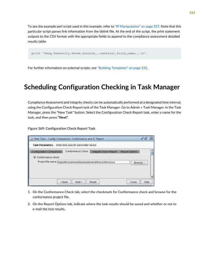
To see the example perl script used in this example, refer to “IP Manipulation” on page 557. Note that thisparticular script parses link information from the bblink file. At the end of the script, the print statementoutputs to the CSV format with the appropriate fields to append to the compliance assessment detailedresults table:
print "$msg,$severity,$node,$source,,,external,$rule_name,,,\n".
For further information on external scripts, see “Building Templates” on page 532.
Scheduling Configuration Checking in Task Manager
Compliance Assessment and integrity checks can be automatically performed at a designated time interval,using the Configuration Check Report task of the TaskManager. Go to Admin > TaskManager. In the TaskManager, press the “New Task” button. Select the Configuration Check Report task, enter a name for thetask, and then press “Next”.
Figure 369: Configuration Check Report Task
1. On the Conformance Check tab, select the checkmark for Conformance check and browse for theconformance project file.
2. On the Report Options tab, indicate where the task results should be saved and whether or not toe-mail the test results.
531

Figure 370: Compliance Assessment Report Options
3. Click “Next” and then specify the scheduling parameters, such as the interval at which to run this task.
4. Click “Finish” to submit the task.
Building Templates
A rule performs checking based upon patterns. Thus, to form a rule, you should define both pattern(s) andrule(s).
Cisco IOS Example
The following is an example Cisco IOS template made up of two patterns “hasip” and “shutdown” followedby a rule “Shutdown_or_noip” which checks the interface block based on the presence or absence of thesetwo patterns. The interface blocks (represented by keyword “interface”) are looped throughwith a “foreach”statement. If either pattern “hasip” is not matched or pattern “shutdown” is matched, a severity level of“warning” is raised. Otherwise, a severity level of “information” is raised via the print statement (equivalentof “raise info”).
#conform name ciscotemplate
#conform type cisco ios
532

@define hasip
ip address $(myip) *
@define shutdown
shutdown
@define rule Shutdown_or_noip
foreach interface do
if (!hasip || shutdown) then raise warning "$(interface.name) has no ip
address or shutdown"
else print "$(interface.name) has an ip $(myip)"
end
end
NOTE: In the pattern hasip, note that the word following “ip address” is being saved into avariable with name “myip”, so that the IP address can be printed out subsequently in theShutdown_or_noip rule.
Blank lines and white spaces in templates are ignored (except when used in regular expressions).So using blank lines to separate blocks of text in the template are not necessary
Juniper JUNOS Example
The following is a simple Juniper example to check a global variable, the OS version, and raise differentseverity levels depending upon the OS version. In this case, referencing a pattern is not necessary, since$(version) is a global variable.
#conform name junipertemplate
#conform type juniper junos
#conform use regular-expression
@define rule junosversion
if $(version) ~= "7.*" then raise critical "version $(version)"
elseif $(version) ~= "8.*" then raise major "version $(version)"
elseif $(version) ~= "9.[1-3].*" then raise minor "version $(version)"
else print "version $(version)"
end
533

Because Junos contains a well-defined hierarchical structure defined by braces, it is possible to designconfiguration compliance assessments at specific levels of the hierarchy. For example, the following rulecheck_rsvp checks for the existence of traceoptions under the protocols rsvp clause of each device:
#conform type junos
@define rsvptraceoptions
traceoptions {
file rsvp.log size 10m;
flag error;
flag resv;
flag route;
flag resvtear;
flag all;
}
@define rule check_rsvp
foreach protocols.rsvp do
if rsvptraceoptions then raise info "matched rsvp trace options"
else raise major "no match for rsvp trace options in $(hostname)"
end
end
NOTE: For Junos pattern definitions, key structural characters like ‘{‘ and ‘;’ should not besubstituted by a regular-expression, since they have special meanings to the program.
For example, if there is a section for chassis as follows, the user can use the syntax chassis.fpc.pic to loopthrough the pic’s as in “foreach chassis.fpc.pic do”:
chassis (
fpc 0 {
pic 0 {
}
}
}
If the next item in the hierarchy is an unknown name, such as for the interfaces {} block, under which arethe interface names such as ge-0/0/1, ge-0/0/2, etc. the keyword “child” can be used as follows, and itscontents can be printed using $(instance).
534

@define hasdescription
description $(intfdesc)
@define rule maindescription
foreach interfaces.child do
if (hasdescription) then print "$(instance) has description $(intfdesc)"
end
end
For more NorthStar Planner keywords, see “NorthStar Planner Keywords For Use Within a Rule” onpage 549.
Match Ordered, Unordered, or Exact
In addition to performing compliance assessments on specific blocks of code, there is a rule to check forlines within the entire configlet, using the keyword “match”, or its equivalent keyword “conform.”
Suppose the config file contains five lines:
a
b
c
d
e
Then within the template file, we can define patterns, and rules to check for an exact match of the pattern,an ordered match, or an unordered match:
@define block
a
b
d
@define block2
a
c
b
@define rule exactmatch
match exact block # not matched due to additional lines c and e
@define rule orderedmatch
match ordered block2 # not matched due to out of order lines (lines c and b)
@define rule exactmach2
match exact block2 # not matched by the same reason above (an exact match must
also be ordered)
@define rule match
match block2 # matched
535
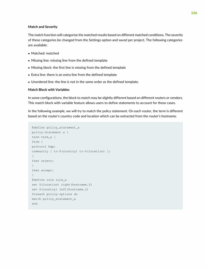
Match and Severity
Thematch functionwill categorize thematched results based on differentmatched conditions. The severityof these categories be changed from the Settings option and saved per project. The following categoriesare available:
• Matched: matched
• Missing line: missing line from the defined template
• Missing block: the first line is missing from the defined template
• Extra line: there is an extra line from the defined template
• Unordered line: the line is not in the same order as the defined template.
Match Block with Variables
In some configurations, the block to match may be slightly different based on different routers or vendors.This match block with variable feature allows users to define statements to account for these cases.
In the following example, we will try to match the policy statement. On each router, the term is differentbased on the router’s country code and location which can be extracted from the router’s hostname.
@define policy_statement_a
policy-statement a {
term term_a {
from {
protocol bgp;
community [ to-$(country) to-$(location) ];
}
then reject;
}
then accept;
}
@define rule rule_a
set $(location) right(hostname,2)
set $(country) left(hostname,2)
foreach policy-options do
match policy_statement_a
end
536
Table 8: Template Syntax
Define a pattern of a block of text. It could contain one word, one line or multiple lines.
-Wild card, *, can be used to match any text. Alternatively, regular expression can be usedif appropriate #conform use regular-expression statement is included in the header.
- Note: The wild card should not be used to hide key syntax operators on the first linesuch as braces ‘{‘ and semi-colons ‘;’
- $(<Variable Name>) can be used to capture and turn any text into a variable, which canthen be printed out in the subsequent rule.
Example: @define pattern1ip vrf $(vrf)rd $(rd)route-target export *route-target import *
@define <PatternName>
Define a compliance assessment rule used for the syntax checking.
- Multiple rules can be defined within one template.
- Rules can be assigned to different categories by adding category=<Category Name> inthe end. - Various flow control, loop, logic boolean, logic operator, print functions can usedin the rule.
- Additional flow controller keyword:
Exit : Once flow reaches exit statement, program will immediately stop checking for thecurrent rule and move on to the next rule if any.
Example :
@define rule BFD-Check category=Protocol
@define rule <RuleName>
Define a rule to execute an external program:
- A external program can be written in any language which uses stdout as result output,e.g., a perl script could be used. Make sure this program is executable from the commandline.
- The result can be either output to a file or it can be appended to wandl’s complianceassessment report if the result is in the same CSV format or can be output to anotherseparate file.
Example :
@define external rule1 output=/tmp/ls.csv /usr/bin/ls -l@define external rule2 output=append /export/home/wandl/myscript.sh
@define external <RuleName>output=[<path>|append]
537

Table 8: Template Syntax (continued)
Provide a description/explanation for the compliance assessment rule.
Example :@define descriptionThis rule checks whether the interface is shutdown or not
@define description<Rule Name>
538

Table 9: Flow Control Syntax
foreach <block> do…end
539

Table 9: Flow Control Syntax (continued)
Define a loop function to go through each pattern block matched in configuration, or to loopthrough each array element of an array. Flow controller keywords to usewithin the loop functioninclude the following:
-Next : Once flow reaches next statement, program will immediately stop the current loop andmove on to the next loop.
- Break : program will immediately leave the current foreach loop. Note that nested loops canbe used in configuration files with well-defined hierarchical structures, such as Junos.
Example for array, using reserved keyword $(element):
foreach $(your_array) do
print $(element)
done
You can get an array element by using the subscript operation. It’s syntax as follows:
$(array_name.array_index)
or
$(array_name.array_index_variable)
If $(array) is an array and $(index) is a number variable, then $(array.index), $(array.0), $(array.1),are valid syntax.
$(array.length) will return the size of the array.
The keyword in can be used to check if a variable exists in an array if $(string1) in $(array1)then...
Example for pattern block:
@define hasbandwidth
bandwidth $(bandwidth);
@define rule junosrule1 category=Interface
foreach interfaces.child.unit do
if hasbandwidth then print “$(interfaces.child)
has bw $(bandwidth)”
end
end
NOTE: Nested loops are allowed for pattern blocks only if the nested loop loops through adescendent of the parent loop. For example, the above could be written as follows:
foreach interfaces.child do
for each unit do
if hasbandwidth then print “$(interfaces.child)
has bw $(bandwidth)”
end
540
Table 9: Flow Control Syntax (continued)
end
end
Define a boolean logic condition to separate flow into different scenarios based on true or falseboolean result.
- Both elseif and else statements are optional.
- Multiple elseif statements are allowed, if necessary.
- Additional Boolean logic operator keywords include the following:
&: AND==: EQUAL||: OR!=: NOT EQUAL!: FALSE~=: WILD CARD EQUAL
Example:
if (pattern1 && !pattern2) then print “pattern1 matched and pattern2 unmatched”elseif (pattern1 && pattern2) then print "both pattern1 and pattern2 matched "elseif (pattern3 ~= “Loopback*”) then print "loopback found in pattern3"else print "none of above"end
if (<boolean logiccondition>) then…elseif (<booleanlogic condition>)then…else…end
Table 10: Built-In Functions For Use Within a Rule
To define a variable.
Example:$(x)
$(<Variable Name>)
To define a string.
Example:“This is a string”
“…”
To define a value to a variable
Example:set $(x) 1
set
541

Table 10: Built-In Functions For Use Within a Rule (continued)
Arithmetic addition between number value or number variable or concatenate between stringand string variable.
Example 1 :set $(count) $(count) + 1
Example 2 :set $(string1) $(hostname) + "," + $(interface.name)
+
To read in an external plain-text file containing multiple lines into a single degree string arrayvariable. One line per array member which can be used together with “In: function.
Example :read $(array1) "/tmp/interface-list.txt"
NOTE: Note:/tmp/interface-list.txt contains following linesRouter1,interface1Router2,interface2…RouterN,interfaceN
read
To add an element to an array. add $(your_array) $(your_element)
Example :foreach interfaces.child doif $(instance) ~= "xe*" thenadd $(full_interface_list) $(instance)endend
To copy one array to another array.add $(array1) "a"add $(array1) "b"add $(array2) $(array1)print “test case 1: $(array2)” # prints “[a, b]”add $(array2) "c"print "test case 1: $(array2)" # prints "[a, b, c]"
add
542

Table 10: Built-In Functions For Use Within a Rule (continued)
To remove an element from an array. remove $(your_array) $(your_element)
Example :foreach protocols.isis.interface doif $(interface.name) ~= "xe*" thenif isis_disable thenremove $(full_interface_list) $(interface.name)endendend
remove
To check if a string variable exists in a string array and yield true or false boolean value.
Example :fif $(string1) in $(array1) thenraise info "$(string) is in the file"end
in
To write strings into a file. This can be used to create custom reports or output file. The firstinput parameter is the file to write in. The second input parameter is the string to write in thefile. If the file already exists, it will be overwritten.
Example :@define rule test_writeset $(file) "/home/wandl/CAT/test/write_file.txt"foreach interfaces.child doprint "$(hostname),$(instance),$(description)"writeln $(file) "$(hostname),$(instance),$(description)"end
This will generate a file called write_file.txt in the directory /home/wandl/CAT/test/ withcontent similar to this sample:
J1,ge-0/0/0,management interface for J1
J1,ge-0/0/1,to 3550S2 FastEthernet0/23
J1,ge-0/0/2,to_EX1_ge-0/0/12
J1,ge-0/0/3,to_BRS_2600
J1,lo0,loop - provision by WANDL
J1,ae39,des
J1,ae40,des
writeIn
543
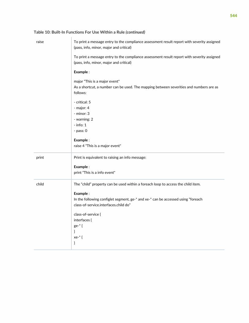
Table 10: Built-In Functions For Use Within a Rule (continued)
To print a message entry to the compliance assessment result report with severity assigned(pass, info, minor, major and critical)
To print a message entry to the compliance assessment result report with severity assigned(pass, info, minor, major and critical)
Example :
major “This is a major event"As a shortcut, a number can be used. The mapping between severities and numbers are asfollows:
- critical: 5- major: 4- minor: 3- warning: 2- info: 1- pass: 0
Example :raise 4 “This is a major event"
raise
Print is equivalent to raising an info message:
Example :print “This is a info event"
The “child” property can be used within a foreach loop to access the child item.
Example :In the following configlet segment, ge-* and xe-* can be accessed using “foreachclass-of-service.interfaces.child do”
class-of-service {interfaces {ge-* {}xe-* {}
child
544

Table 10: Built-In Functions For Use Within a Rule (continued)
To get a list of single words from config block use the keyword "line"
prefix-list list1 {10.0.0.0/8;192.168.0.0/16;10.1.1.0/24;}e.g.foreach policy-options.prefix-list doif $(prefix-list.name) == "list1" thenforeach line doprint "$(instance)"endendend
line
For arrays, a reserved variable to refer to the value of the current array object:
Example:foreach $(your_array)do print $(element)done
element
Looks for a match for the provided pattern and automatically raises a message entry into theresulting report. The Detailed Results tabwill show related line numbers and line content underTemplate Line and Template Line #.
Matches if all lines and subblocks exists in config file. These lines do not have to be in the sameorder for a match.
Example :conform myconfiglet
conform <PatternName> match<Pattern Name>
All template lines and block should be in configuration file. In addition, all the lines must beordered correctly. Note that config files may have additional lines or subblocks.
Example :conform ordered myconfiglet
conform ordered<Pattern_name>match ordered<Pattern_name>
To match, the config file must contain the exact same section as the template. In addition tohaving the lines ordered in the same way, no additional lines are allowed in that section for amatch.
Example :conform exact myconfiglet
conform exact<Pattern_name>match exact<Pattern_name>
545

Special Built-In Functions
Wildmask Conversion for Cisco
Use function called wildcardtocidr
Sample
set $(converted) wildcardtocidr(ip, wildmask)print "converting $(ip) wild mask $(wildmask) => $(converted)"
The result could be:
converting 62.179.128.0 wild mask 0.0.1.255 => 62.179.128.0/23
Convert ISIS system ID to IPv4
toipv4 (node.isis_system_id)Sample:toipv4(1921.6800.0001) will return 192.168.0.1
Match string value
Use function called getmatch
Sample:
set $(interface.name) “Bundle-Ether1”set $(number) getmatch(interface.name, “[0-9.]+”)print “$(number)”
The result of the print out is “1”
Get physical interface from sub interface
Use function called getphysicalSample:
set $(logical) “ge-0/0/1.12”set $(physical) getphysical(logical)print “$(physical)
The result of the print out is “ge-0/0/1”.
546

Arithmetic Function
Arithmetic functions supported are add, subtract, multiply, and divide
Sample:
set $(a) "5"set $(b) "2"set $(add_result) add(a,b)print "$(add_result)"
The result of the print out is “7”
set $(substract_result) subtract(a,b)print "$(substract_result)"
The result of the print out is “3”
set $(multiply_result) multiply(a,b)print "$(multiply_result)"
The result of the print out is “10”
set $(divide_result) divide(a,b)print "$(divide_result)"
The result of the print out is “2.5”
String Extraction Function
String extraction functions returns the character of properties of a string. The first character in a stringstarts at index 1. String functions includes len, right, left, mid, and find.
• len(string) # returns the length of the string
• right(string, num_char) # returns the number of characters from the right
• left(string, num_char), # returns the number of characters from the left
• mid(string, start_index, num_char) # returns the number of characters from the specified start index
• find(txt_to_find, string, [start_index]) # find the index of the character in the string, the start_index isoptional
Sample:
547

set $(host_name) "us-pe-01"set $(country) mid(host_name,1,2)print "country is $(country)"set $(role) mid(host_name,4,5)print "role is $(role)"set $(intf) "port-1/8/5:10G"set $(colon) ":"set $(res) right(intf, len(intf)- find(colon,intf,1))print "test case 1: $(intf) => $(res)"
The result of the print out is "port-1/8/5:10G => 10G"
set $(intf2) "GigabitEthernet0/7/0/36.1778"set $(res2) left(intf2, find(".",intf2,1)-1)print "test case 2: $(intf2) => $(res2)"
The result of the print out is "GigabitEthernet0/7/0/36.1778 => GigabitEthernet0/7/0/36"
set $(s) "1234567890"set $(len) len(s)print "test case 3 (a): length = $(len)"
The result of the print out is “test case 3 (a): length = 10"
Array Extraction Function
To extract an array from a string, the string syntax must have the array elements enclosed by bracket [,]and delimited by comma or white space. Then use the toarray function on the string to extract the arrayelements.
Sample:
set $(string) "protocol [ bgp direct static ]"set $(array) toarray(string)print "test case 3: $(array)" # prints [bgp, direct, static]
Data Structure Objects
Data structure objects allows the user to create an object that can have multiple attributes assigned to it.
Sample:
@define rule object_test
548

create $(interface_obj)set $(interface_obj.name) "ge-0/0/0"set $(interface_obj.isis) "yes"set $(interface_obj.disable) "no"add $(interface_obj_list) $(interface_obj)print "interface $(interface_obj)"create $(interface_obj)set $(interface_obj.name) "ge-0/0/1"set $(interface_obj.isis) "no"set $(interface_obj.disable) "no"add $(interface_obj_list) $(interface_obj)foreach $(interface_obj_list) doprint "$(element)"endset $(interface_obj) getobject(interface_obj_list, "name", "ge-0/0/0")print "$(interface_obj)"
NorthStar Planner Keywords For Use Within a Rule
The following are built-in convenient keywords available that can be used within a rule.
Description and ExampleSupportedVendorKeyword
This keyword returns node’s hostname.All$(hostname)
This keyword returns node’s operating system name.All$(os)
This keyword returns node’s operating system version
NOTE: Huawei and IOS-XR are example vendors where version cannot bedetermined from configuration files, and thus this keyword is not applicablefor them.
Vendors,whoseconfigscontainsthe version.
$(version)
This keyword returns the node’s ISIS system id.All$(node.isis_system_id)
This keyword returns the node’s hardware type.All$(node.hardware) or$(node.type)
549

Description and ExampleSupportedVendorKeyword
This keyword is used to return the name of the instance you are currentlyin. For example if your instance is family inet, $(instance) will return “familyinet”.
All$(instance)
Only applicable when your instance name has two or more words separatedby space. This keyword is used to return the name of the instance you arein minus the first word. For example if your instance is family inet,$(instance.name) will return “inet”.
NOTE: If your instance has two or more words separated by a space,$(instance.name) will only return the second word. For example, if yourinstance is interface ge-1/8/1/2 l2type vlan, $(instance.name) will return“ge-1/8/1/2”.
All$(instance.name)
Only applicable when your instance name has two or more words separatedby space. This keyword is used to return the name of the instance you arecurrently in minus the first word. For example, if your instance is “familyinet”, $(instance.value) will return “inet”
If your instance has more than two words separated by space,$(instance.value) will return everything minus the first word. For example, ifyour instance is “interface ge-1/8/1/2 l2type vlan”, $(instance.value) willreturn “ge-1/8/1/2 l2type vlan”.
All$(instance.value)
Useful when your instance name has two ormorewords separated by space,and you want to choose which word you would like to return. For exampleif your instance is “address-family ipv4 vrf SHIELD_1”, $(instance.3) willreturn “SHIELD_1”.
All$(instance.[n]) where nis 0 to unlimited.
550
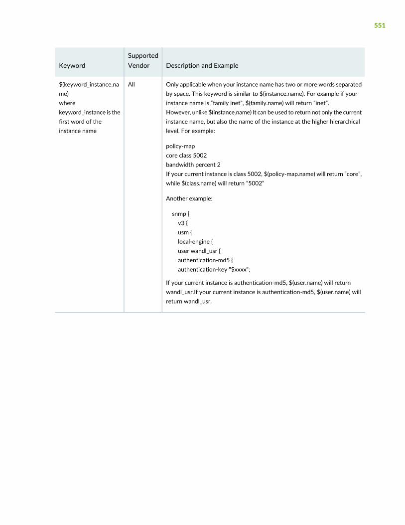
Description and ExampleSupportedVendorKeyword
Only applicable when your instance name has two or more words separatedby space. This keyword is similar to $(instance.name). For example if yourinstance name is “family inet”, $(family.name) will return “inet”.However, unlike $(instance.name) It can be used to return not only the currentinstance name, but also the name of the instance at the higher hierarchicallevel. For example:
policy-mapcore class 5002bandwidth percent 2If your current instance is class 5002, $(policy-map.name) will return “core”,while $(class.name) will return “5002”
Another example:
snmp {v3 {usm {local-engine {user wandl_usr {authentication-md5 {authentication-key "$xxxx";
If your current instance is authentication-md5, $(user.name) will returnwandl_usr.If your current instance is authentication-md5, $(user.name) willreturn wandl_usr.
All$(keyword_instance.name)wherekeyword_instance is thefirst word of theinstance name
551

Description and ExampleSupportedVendorKeyword
Only applicable when your instance name has two or more words separatedby space.
Similar to $(instance.value), for example if you instance name is “interfacege-1/8/1/2 l2type vlan”, $(interface.value) will return “ge-1/8/1/2 l2typevlan”.
However, unlike $(instance.value), this keyword can be used to return notonly the current instance name, but also the name of the instance at thehigher hierarchical level.
Example:router bgp 88address-family ipv4 vrf wandl2012redistribute ospf 919 vrf wandl2012 match internal external 1external 2no synchronizationexit-address-family!If your current instance is “address-family ipv4 vrfwandl2012”, $(router.value)will return “bgp 88”.
All$(keyword_instance.value)wherekeyword_instance is thefirst word of theinstance name.
This keyword is useful when your instance has higher hierarchical level of 2or more and you want to return instance name of the higher instance,excluding the top one.
In the following example, the “authentication-md5” instance has a hierarchicallevel of 5 (snmp -> v3 -> usm -> local-engine -> user wandl_usr).
snmp {v3 {usm {local-engine {user wandl_usr {authentication-md5 {authentication-key "$xxxx";
When your instance is authentication-md5 , $(snmp.child) will return “v3”,$(v3.child) will return usm, $(local-engine.child) will return “user wandl_usr”.
NOTE: This variable does not work when the higher instance name has twoor more words separated by space. For example $(user.child) is not valid asthe instance has twowords: “userwandl_usr”. Basically, if your higher instancehas a name (i.e user.name), then it doesn’t have a child (i.e. user.child)
Junos$(keyword_instance.child)wherekeyword_instance is theparent name of aninstance.
552

Description and ExampleSupportedVendorKeyword
Keyword is the first word of a line inside an instance. It is used to return aline inside an instance minus the keyword.
In the following example, when your instance is system, then $(host-name)will return J5, $(time-zone) will return EST, and $(authentication-order) willreturn [ tacplus password ]
system {host-name J5;time-zone EST;authentication-order [ tacplus password ];
}
$(keyword) will only return one line. If you have multiple lines with the samekeyword at the beginning of the line, only the first one will be return
$(keyword) can also be used to return a line in the instance above yourcurrent instance. For example:
firewall {policer 10m {if-exceeding {bandwidth-limit 10m;burst-size-limit 3k;
}then discard;
}}
When your instance is if-exceeding, $(then) will return “discard”. It is notrecommended to refer line in the higher instance using $(keyword) directly.See $(keyword_instance.keyword).
Junos$(keyword)
553

Description and ExampleSupportedVendorKeyword
It is used to return a line inside an instance, specified by keyword_instance,minus the keyword. For example,
interfaces {ge-0/0/0 {description “physical interface”unit 0 {description "management interface for J1";
}}
}
When your instance is unit 0, $(description) will return “managementinterface” for j1, while $(ge-0/0/0.description) will return “physical interface”.Note that $(unit.description) will also return “management interface for j1”
While it is not recommended usage, when you are not inside any instance,you can also use $(keyword_instance.instance) to return a line inside a directunderneath instance. For example:
system {host-name J1;time-zone EST;authentication-order [ tacplus password ];
}routing-options {router-id 22.22.0.5;
}
When your instance is global, $(system.host-name) will return “J1”,$(system.timezone) will return “EST”, $(system.authentication-order) willreturn “[ tacplus password ]”, $(routing-options.route r-id) will return“22.22.0.5”
Junos$(keyword_instance.keyword)wherekeyword_instance is thefirst word of aninstance, and keywordis the first word of a lineinside an instance.
The following are possible #conform statements that may appear in the template.
Table 11: Header Syntax - Conform Statements
(Required) Identifies the template name.#conform name <template_name>
(Required) Indicates the vendor and operating system of the configurationfiles for which the template will be used, e.g., Cisco IOS, IOS-XR, JuniperJunos, etc.
#conform type <cisco ios| cisco ios-xrjuniper junos|alu timos|huawei|redback|zte>
(Optional) Recognizes regular expression syntax in the template#conform use regular-expression
554
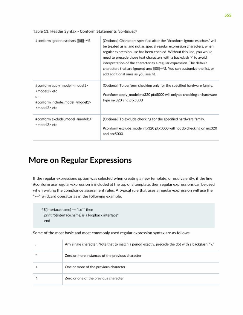
Table 11: Header Syntax - Conform Statements (continued)
(Optional) Characters specified after the “#conform ignore escchars” willbe treated as is, and not as special regular expression characters, whenregular expression use has been enabled. Without this line, you wouldneed to precede those text characters with a backslash ‘\’ to avoidinterpretation of the character as a regular expression. The defaultcharacters that are ignored are: [](){}|+^$. You can customize the list, oradd additional ones as you see fit.
#conform ignore escchars [](){}|+^$
(Optional) To perform checking only for the specified hardware family.
#conform apply_modelmx320 ptx5000will only do checking on hardwaretype mx320 and ptx5000
#conform apply_model <model1><model2> etcor#conform include_model <model1><model2> etc
(Optional) To exclude checking for the specified hardware family.
#conform exclude_model mx320 ptx5000 will not do checking on mx320and ptx5000
#conform exclude_model <model1><model2> etc
More on Regular Expressions
If the regular expressions option was selected when creating a new template, or equivalently, if the line#conform use regular-expression is included at the top of a template, then regular expressions can be usedwhen writing the compliance assessment rules. A typical rule that uses a regular-expression will use the“~=” wildcard operator as in the following example:
if $(interface.name) ~= "Lo*" thenprint "$(interface.name) is a loopback interface"end
Some of the most basic and most commonly used regular expression syntax are as follows:
Any single character. Note that to match a period exactly, precede the dot with a backslash, “\.”.
Zero or more instances of the previous character*
One or more of the previous character+
Zero or one of the previous character?
555

Any character from the set. [ch]at matches “cat” or “hat”[ ]
Any character not in the set.[^]
Groups patterns. (cat|hat) matches “cat” or “hat”( )
Any character from a through z or A through Z, inclusive[a-zA-Z]
Any integer from 0 through 9, inclusive[0-9]
Used in front of a reserved regular expression character (such as “.” or “+”), to match that particularcharacter. For example, to match “tacacs+” exactly, “tacacs\+” is required, as the plus sign has aspecial meaning in regular expression syntax.
\
Because some users may accidentally confuse wildcards with regular expressions, the ComplianceAssessment Tool automatically converts some statements, as shown in the following examples:
• “ATM*” is automatically converted to “ATM.*” - “ATM*” also matches “AT”, which is in most casesunintended by the user.
• “*ATM” is automatically converted to “.*ATM” - “*ATM” is actually illegal regular expression syntax.
NOTE: When used in regular expressions, blank spaces are respected. They are not ignored.
Some examples are shown below:
To match the ip address.ip address.*
To match the description.description.*
To match “tacacs+” exactly, instead of just “tacacs”tacacs\+
To ensure the version begins with “12.”version 12\..*
To ensure the net id ends with two zerosnet .*00
To match “router eigrp 100” or “router eigrp 299”router eigrp (100|299)
To ensure the IP address is declared 192.122.x.y where x and y areintegers.
tacacs-server host 192\.122\.[0-9]+\.[0-9]+
556
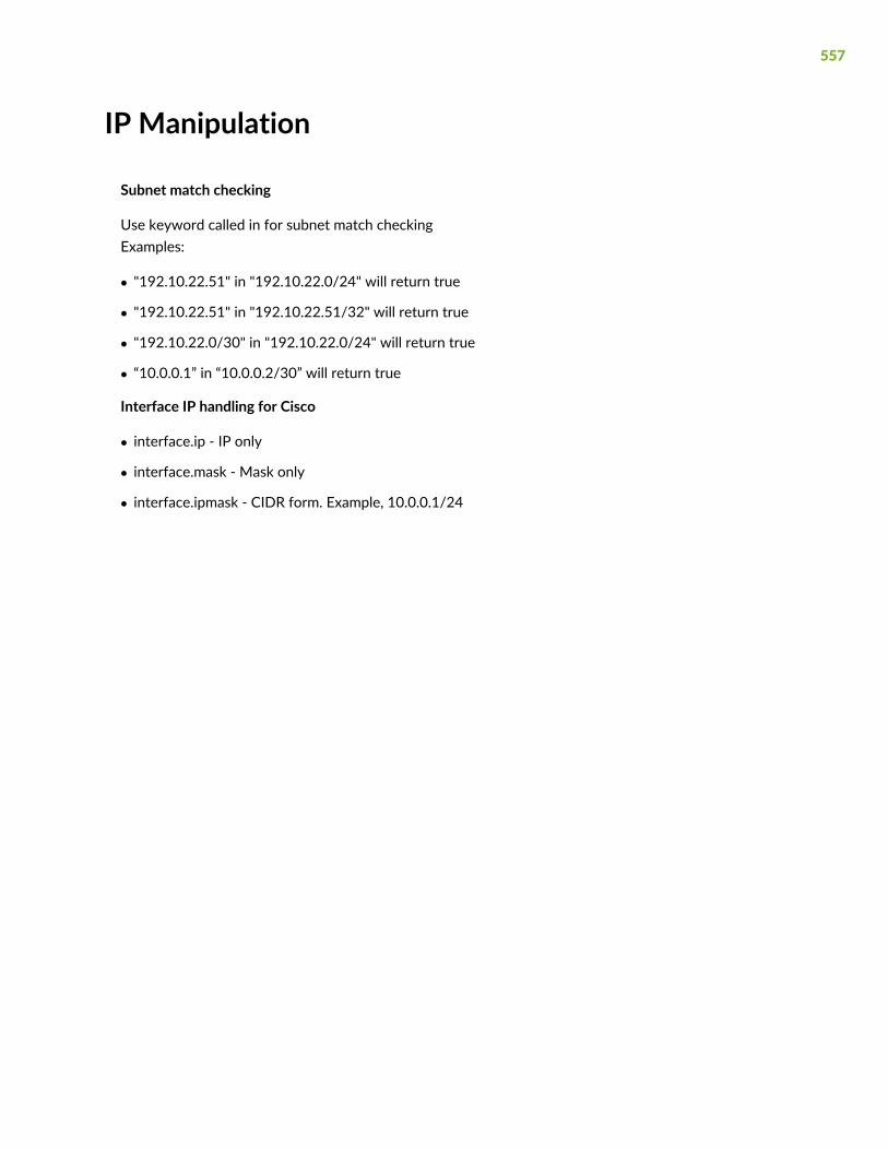
IP Manipulation
Subnet match checking
Use keyword called in for subnet match checkingExamples:
• "192.10.22.51" in "192.10.22.0/24" will return true
• "192.10.22.51" in "192.10.22.51/32" will return true
• "192.10.22.0/30" in "192.10.22.0/24" will return true
• “10.0.0.1” in “10.0.0.2/30” will return true
Interface IP handling for Cisco
• interface.ip - IP only
• interface.mask - Mask only
• interface.ipmask - CIDR form. Example, 10.0.0.1/24
557

26CHAPTER
Virtual Local Area Networks
NorthStar Planner Virtual Local Area Networks Overview | 561
Importing Cisco VLAN and Spanning Tree Information | 562
Viewing VLAN Details | 562
Viewing VLAN Topology | 571
VLAN Modification and Design | 574


NorthStar Planner Virtual Local Area NetworksOverview
NOTE: Only Juniper and Cisco devices are supported.
As modern Ethernet technologies mature and MPLS technologies such as VPLS are being used to extendLayer-2 VLANs across theMAN and theWAN, there is an increasing need for a tool that provides visibilityinto layer-2 VLANs in addition to the IP and MPLS layers. NorthStar Planner has risen to the challenge byproviding a whole suite of capabilities in support of VLANs.
NorthStar Planner automatically constructs the network's VLANs via a VLAN Discovery task that uses acombination of SNMP MIBs polling and CLI show commands. Combined with configuration file parsing,all the details related to each device, VLAN, and spanning tree are derived by the tool and easily accessedby the user. Furthermore, the VLAN View window and the L2 STP subview on the topology map allowthe user to get a clear logical view as well as status information for each individual VLAN and spanningtree. Besides gaining visibility into the VLANs in the network, NorthStar Planner also allows the networkplanner to construct VLANs from scratch via the VLANWizard. If desired, the VLAN configlet generationfeature can be used to create configuration statements that can be pushed into the router/switch by thenetwork engineer.
Apart from just displaying the nodes and links that are part of a spanning tree, STP topology uses coloringto signify the role of each node/link to make it easily understandable to the user. Devices that belong toa spanning tree can be further grouped together by defining access domains to depict the real physicalnetwork. An access domain is a group of physically connected layer 2 devices, where all the VLAN IDs areunique, i.e. devices that have the same VLAN id in an access domain belong to the same VLAN. As directphysical connectivity cannot be extracted, IPMPLSView, by default, groups all devices into the defaultdomain. For networks with multiple access domains, users should define the access domains and assignnodes into them properly as explained in the “VLAN Modification and Design” on page 574.
Layer 2 VLAN information is accessible either in online or offline mode. In online mode, you should runthe Scheduled Live Network Collection task to collect switches’ Configuration and Switch CLI output. Inaddition, you should also run the VLAN Discovery task for IPMPLSView to extract the spanning treeinformation from the switches.
For offline mode, you can collect the configuration files using any third party collector. The SNMP pollingon the other hand, is recommended to be performed using our Standalone SNMP poller, as it requires realtime interpretation of ongoing polling results to determine the entire MIBs that needed to be polled, sothat complete spanning tree information can be obtained. Please contact your Juniper representative fordetails on the Standalone SNMP poller availability.
561
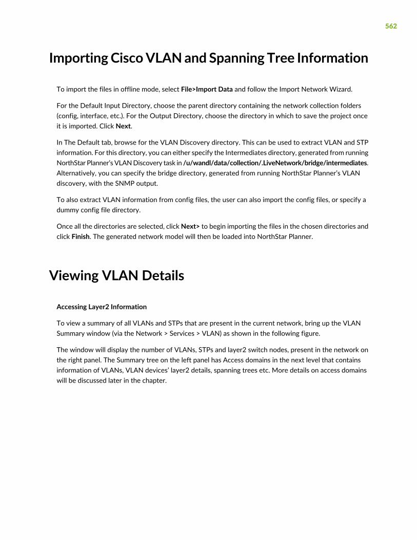
Importing CiscoVLANand Spanning Tree Information
To import the files in offline mode, select File>Import Data and follow the Import Network Wizard.
For the Default Input Directory, choose the parent directory containing the network collection folders(config, interface, etc.). For the Output Directory, choose the directory in which to save the project onceit is imported. Click Next.
In The Default tab, browse for the VLAN Discovery directory. This can be used to extract VLAN and STPinformation. For this directory, you can either specify the Intermediates directory, generated from runningNorthStar Planner’s VLANDiscovery task in /u/wandl/data/collection/.LiveNetwork/bridge/intermediates.Alternatively, you can specify the bridge directory, generated from running NorthStar Planner’s VLANdiscovery, with the SNMP output.
To also extract VLAN information from config files, the user can also import the config files, or specify adummy config file directory.
Once all the directories are selected, clickNext> to begin importing the files in the chosen directories andclick Finish. The generated network model will then be loaded into NorthStar Planner.
Viewing VLAN Details
Accessing Layer2 Information
To view a summary of all VLANs and STPs that are present in the current network, bring up the VLANSummary window (via the Network > Services > VLAN) as shown in the following figure.
The window will display the number of VLANs, STPs and layer2 switch nodes, present in the network onthe right panel. The Summary tree on the left panel has Access domains in the next level that containsinformation of VLANs, VLAN devices’ layer2 details, spanning trees etc. More details on access domainswill be discussed later in the chapter.
562
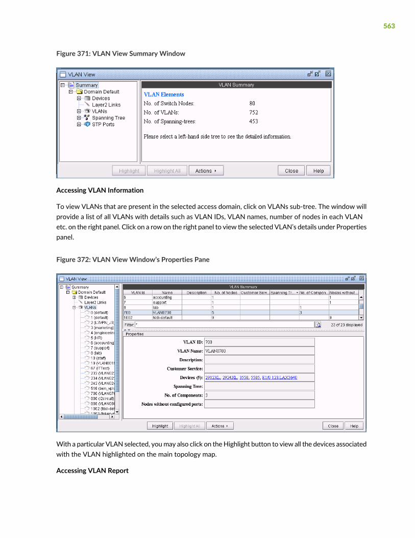
Figure 371: VLAN View Summary Window
Accessing VLAN Information
To view VLANs that are present in the selected access domain, click on VLANs sub-tree. The window willprovide a list of all VLANs with details such as VLAN IDs, VLAN names, number of nodes in each VLANetc. on the right panel. Click on a row on the right panel to view the selected VLAN’s details under Propertiespanel.
Figure 372: VLAN ViewWindow’s Properties Pane
With a particular VLAN selected, youmay also click on theHighlight button to view all the devices associatedwith the VLAN highlighted on the main topology map.
Accessing VLAN Report
563

A VLAN report is generated from running VLAN discovery task or importing intermediates directory intothe network. The generated report can be accessed from Actions > Report in VLAN View window orthrough Report > Report Manager from the main menu.
Figure 373: VLAN Report
You may double-click on VLANs sub-tree or click the (+) icon next to VLANs sub-tree to view a list of allVLANs in the selected access domain, where the VLANs are categorized by VLAN name.To view moredetailed information of a VLAN, click on a VLAN in the left panel.The Details tab, on the right panel, listsall the devices that belong to the selected VLAN and each node’s details such as bridge addresses, numberof interfaces assigned to the VLAN, in/out policies etc. Click on a row on the right panel to view the selectednode’s VLAN details under Properties panel.
564

Figure 374: Detailed View of a Selected Node=
Accessing Devices Information
The Devices sub-tree lists all the devices that belong to VLANs in the selected access domain, with theirlayer2 and layer3 address details.To view the devices, click on Devices sub-tree. Click on a row on theright panel to view the selected device’s details under Properties panel.
Figure 375: VLAN Device’s Details for a Selected Device
565
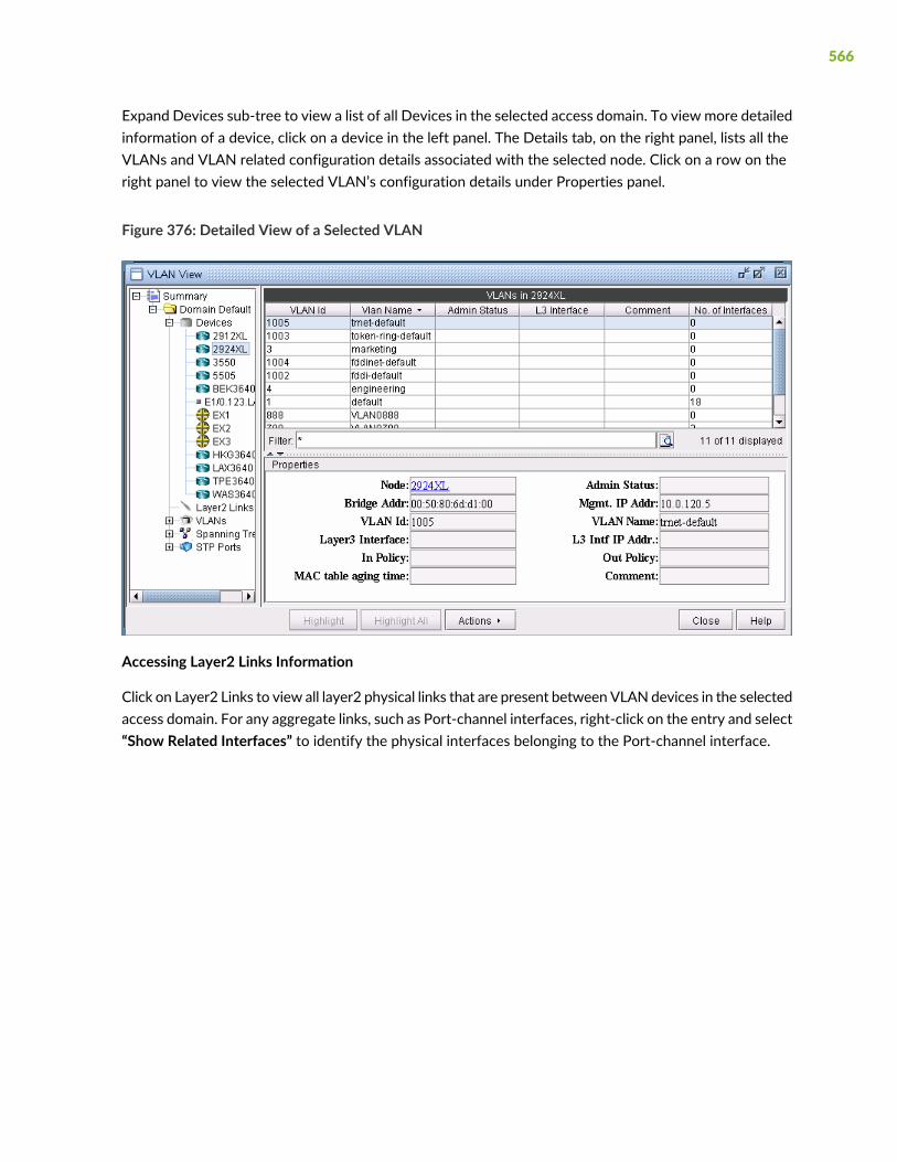
Expand Devices sub-tree to view a list of all Devices in the selected access domain. To view more detailedinformation of a device, click on a device in the left panel. The Details tab, on the right panel, lists all theVLANs and VLAN related configuration details associated with the selected node. Click on a row on theright panel to view the selected VLAN’s configuration details under Properties panel.
Figure 376: Detailed View of a Selected VLAN
Accessing Layer2 Links Information
Click on Layer2 Links to view all layer2 physical links that are present between VLAN devices in the selectedaccess domain. For any aggregate links, such as Port-channel interfaces, right-click on the entry and select“Show Related Interfaces” to identify the physical interfaces belonging to the Port-channel interface.
566

Figure 377: Layer2 Links Details
Accessing STP Information
To view spanning trees that are present in the selected access domain, click on Spanning Tree sub-tree.Thewindow will list all the spanning tree types.
567

Figure 378: Selected Spanning Tree
Expand Spanning tree and you should see a list of all the spanning trees present in the selected accessdomain with the following naming convention: STP-Type VLANID for PVSTs and STP-Type for otherspanning tree types. Select a spanning tree to view the list of nodes and spanning tree related configurationsassociated with them.
568

Figure 379: Detailed View of a Selected Node
Accessing STP Ports Information
STP Ports subtree displays all the node ports that are part of the spanning trees in the selected accessdomain, with other details such as port types, states, priority etc.
569
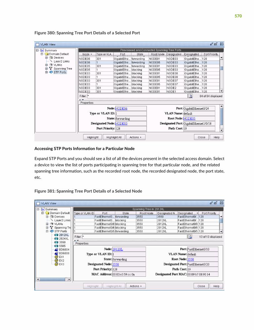
Figure 380: Spanning Tree Port Details of a Selected Port
Accessing STP Ports Information for a Particular Node
Expand STP Ports and you should see a list of all the devices present in the selected access domain. Selecta device to view the list of ports participating in spanning tree for that particular node, and the relatedspanning tree information, such as the recorded root node, the recorded designated node, the port state,etc.
Figure 381: Spanning Tree Port Details of a Selected Node
570

Viewing VLAN Topology
VLAN Topology View
The VLAN topology view (or VLAN View) presents to the user a clear, logical view of each individualVLAN.To display logical topology view of any particular VLAN, simply click on the VLAN Topology tab(next to the Details tab). You may also move the nodes around as desired in the VLAN topology view map.
Figure 382: VLAN Topology View
There is also a right-click menu that you can use to perform basic functions to manipulate the topologyand the labels. Place the cursor on a node and do a right click to view node access and topology displayoptions.
571
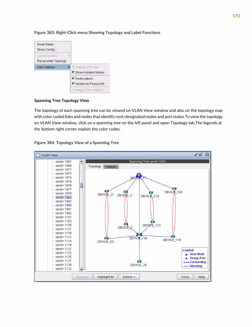
Figure 383: Right-Click menu Showing Topology and Label Functions
Spanning Tree Topology View
The topology of each spanning tree can be viewed on VLAN View window and also on the topology mapwith color coded links and nodes that identify root/designated nodes and port states.To view the topologyon VLAN View window, click on a spanning tree on the left panel and open Topology tab.The legends atthe bottom right corner explain the color codes.
Figure 384: Topology View of a Spanning Tree
572

There is also right click menu that allows you to change the spanning tree topology layout into either treeor circular shape from the original MAP (standard) standard. Place the cursor on any point inside thetopology window and do a right click to change the topology layout.
Figure 385: Right-Click Menu to Re-Layout the Spanning Tree Topology
The Spanning tree topology can also be viewed on the topology map. Choose Subviews > L2STP from thetop left drop-down menu on the Map (Standard) window.You should now view a list of all spanning treespresent in the existing network with the following naming conventions: VLANID (Root Node) for PVSTsand STP-Type (Root Node) for all other types of spanning trees. Click on a spanning tree on the left panelto view its topology on the map. The nodes and links of the selected spanning tree are colored such thateach color signifies their roles.
Figure 386: Topology View of a Spanning Tree
573

Following is a list of coloring conventions followed:
• Pink Colored Node : Root Node.
• Blue Colored Node : Designated Node.
• Green Colored Node : Non-STP Node.
• Green Colored Link : Ports on both ends of the link are in forwarding state.
• Red Colored Link : Ports on one or both ends of the link are in blocking state.
VLANModification and Design
Defining an Access Domain
An access domain is a group of physically connected layer2 devices that use spanning tree or directconnection to perform layer2 routing within the domain. Each access domain supports 4096 VLANs, thusallowing identical VLANs across multiple access domains. As direct physical connectivity informationcannot be extracted from the config files, NorthStar Planner treats all the VLANs and STPs in the networkas part of a default domain. The user should define access domains and assign the nodes to access domainsto view VLAN and STP information categorized by access domains in VLAN View window.
To define an access domain, first switch to Modify mode and then chooseModify > Services > AccessDomains...
Enter Access Domain ID & Name details and choose spanning tree running across the access domain fromthe Spanning Tree Type drop-down menu in the top panel as shown in the following figure.
574

Figure 387: Adding an Access Domain
Click the Add button on the top right panel.The middle panel displays the list of all defined access domainsand the newly added access domain should now add to the list.
To view the nodes information of a particular access domain, click on an access domain in the middle paneland the bottom panel displays the information as shown in the following figure.
575

Figure 388: Access Domains and Nodes details
Modifying an Access Domain
To modify an existing access domain, click on an access domain in the middle panel and hit Modify at thebottom. After making changes to the access domain, clickModify at the top right panel.
Deleting an Access Domain
To delete an access domain, click on an access domain in the middle panel and hit Delete. To only viewthe list of existing access domains and nodes details, click Close on the top right panel.
After adding all access domains, click Close at the bottom of Network Info window.
Assigning Nodes to Access Domain
To assign nodes to an access domain, chooseModify > Elements > Nodes...
Select a node/ multiple nodes that are located in an access domain and hit Modify.
In the Modify Nodes window, select L2SW tab. Note that the L2SW tab is only available when a node isa layer 2 device (Properties tab > L2SW is true). Choose the access domain that the selected nodes belong
576

to from the Access Domain drop-downmenu, that lists access domain IDs, and hit OK. This completes theassignment of nodes to access domain.
Figure 389: Assigning Access Domain to Nodes
Below is a VLAN View window after adding access domains.
Figure 390: VLAN ViewWindow after Defining Access Domains
Adding Layer2 Links
To add Layer 2 links between switches, chooseModify > Services > VLAN
Click on the Layer2 Links sub-tree under the access domain and then click on the Add button form theVLAN View window
577
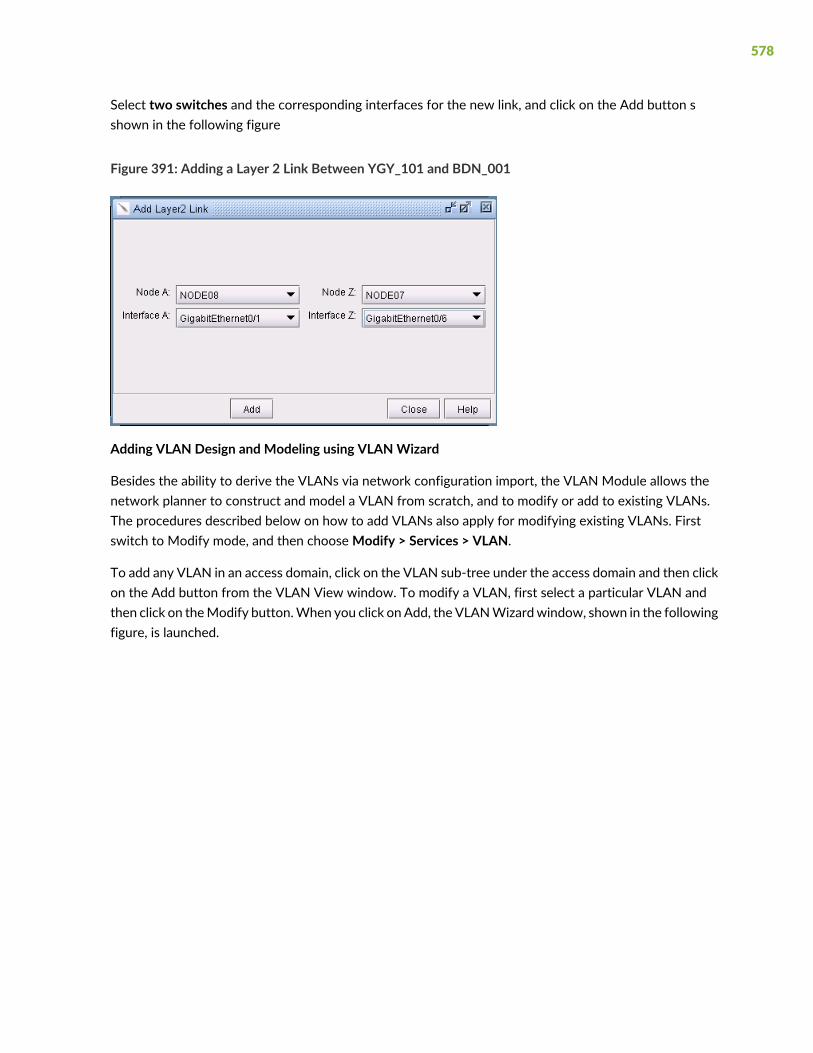
Select two switches and the corresponding interfaces for the new link, and click on the Add button sshown in the following figure
Figure 391: Adding a Layer 2 Link Between YGY_101 and BDN_001
Adding VLAN Design and Modeling using VLANWizard
Besides the ability to derive the VLANs via network configuration import, the VLAN Module allows thenetwork planner to construct and model a VLAN from scratch, and to modify or add to existing VLANs.The procedures described below on how to add VLANs also apply for modifying existing VLANs. Firstswitch to Modify mode, and then chooseModify > Services > VLAN.
To add any VLAN in an access domain, click on the VLAN sub-tree under the access domain and then clickon the Add button from the VLAN View window. To modify a VLAN, first select a particular VLAN andthen click on theModify button.When you click on Add, the VLANWizardwindow, shown in the followingfigure, is launched.
578

Figure 392: VLANWizard Window
By default, the VLANWizard sets the access domain to the one you selected in the VLAN View window.You may choose a different domain from the Access Domain drop-down menu and then enter the VLANdetails in the respective fields.In order to accommodate for multivendor non-management VLAN IDs,VLANWizard supports IDs above 2.
The Devices panel lists Layer2 Switches that belong to the selected Access domain. There is a drop-downmenu under Devices (down arrow besides Layer2 Switches) from which you can select the device typesyou want to view and then add to Devices on VLANs. Choose the device type from the drop-down anduse Add button to add the selected devices in Devices to Devices on VLANs panel. VLAN wizard adds theVLAN to the devices in Devices on VLANs.
579

Figure 393: Adding Devices to the VLAN
Click on Next to bring up the following window where you may add more devices and chosen devicesinterfaces to assign to the VLAN.
• The middle part of the window show the topology area, where selected devices are placed.
• The Selected Objects area, as the name implies, lists those devices that have been selected as VLANdevices.
• The Available Devices box lists those routers for the currently chosen access domain.
• The Properties box lists all the interfaces for a particular device when it is highlighted (a device ishighlighted when it is clicked on either from the Available Devices list, the topology area of the window,or from the Selected Objects list)
Thewindow is designed to be as user-friendly as possible, with drag/drop capabilities built in. The followingfigure shows the two devices that we have already added in the previous step.
580

Figure 394: Assigning More Devices and Device Interfaces to the VLAN
In more detail, you may add additional devices to the VLAN from the Available Devices box via one of twomethods:
Select one or more devices (at which point the icon that has the left arrow with a circle around it willchange color from gray to blue), and then click on the blue arrow/circle icon to move it to the topologyarea part of the window (middle of the window).
Alternatively, you could simply drag and drop devices from the Available Devices list into the topologyarea of the window.
To assign interfaces to the selected devices, first select a particular device in order to have all its interfacesshown in the Properties box. A device is selected when it is clicked on from the Selected Objects list orfrom the topology area of the map. As shown in the following figure, the Properties box is now renamedas Interfaces in AD101, since the device AD101 has been selected. Another icon worth mentioning is the"-"/"+" button next to the arrow/circle button. Click on it to switch between "-" and "+". "-" means to showall interfaces, while "+" means to only display interfaces that are unassigned or not shutdown.
581

Figure 395: How to Assign Interfaces to VLAN Devices
To assign an interface, you need to drag and drop a particular interface over to the device in the middlepanel. Alternatively, you can select the device from the left hand side, and then select an interface fromthe interface list on the bottom right hand side, and click the blue arrow in the Interfaces section. Thefollowing figure shows the window after the interfaces have been assigned to the devices.
582
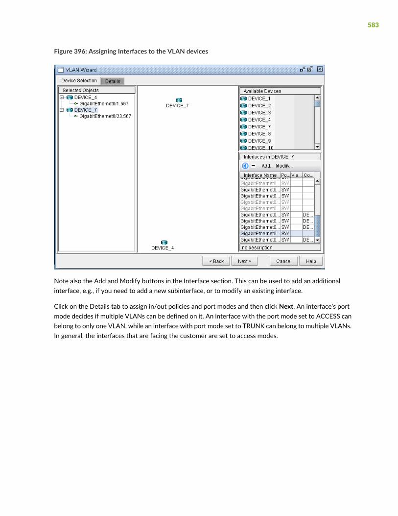
Figure 396: Assigning Interfaces to the VLAN devices
Note also the Add and Modify buttons in the Interface section. This can be used to add an additionalinterface, e.g., if you need to add a new subinterface, or to modify an existing interface.
Click on the Details tab to assign in/out policies and port modes and then click Next. An interface’s portmode decides if multiple VLANs can be defined on it. An interface with the port mode set to ACCESS canbelong to only one VLAN, while an interface with port mode set to TRUNK can belong to multiple VLANs.In general, the interfaces that are facing the customer are set to access modes.
583

Figure 397: Assigning Port Modes and In/Out Policies to Interfaces
The details entered in the final VLAN wizard window facilitates for layer3 inter-VLAN routing. Click on anode in the left panel and choose a vlan interface from Layer3 Interface drop-down menu.
Layer3 interfaces are NorthStar Planner interfaces that should be created by the user to populate layer3details in VLANWizard window. The procedure to create a vlan interface is similar to that of adding anynew interface, either from Modify > Elements > Interfaces or from the Add button in the VLAN wizardwindow. Only rule is to begin the interface name with the keyword ‘vlan’ followed by VLAN ID.
IP address and in/out policies defined on the selected vlan interfacewill now be populated in the respectivefields. L3 Interface IP Addr. field is used as node identifier while routing packets between VLANS with theapplied in/out policies.
584

Figure 398: Select Layer3 Interface for Inter-VLAN Routing
Click on Finish and you should now view the newly added VLAN to the VLANs sub-tree in the VLAN Viewwindow. The link between the two nodes signifies a direct physical connection between them. Click onthe link to view the link details.
585

Figure 399: Newly Added VLAN’s Topology View
File Format
The following are special parameters in the dparam file related to VLANs.
• keepl2stptree=1 : Setting this value to 1 will keep the spanning tree information parsed from the file.Setting this value to 0 will cause the program to be in a “smart” mode. For example, for isolated sectionsof a spanning tree without a root node, a root node will be selected.
• addroot2treename=1 : When setting this value to 1, the spanning tree name in the VLAN view will befollowed by the suffix @rootname to indicate the root node of the tree. If one tree is shown as multiplecomponents in the VLAN window’s spanning tree view, this is an indication of missing links.
The following are special parameters in the specification file related to VLANs.
• accdomain=filename : This file stores the region information for MST trees and is used to group treesby region in the VLANwindow’s spanning tree view. This file can be commented out in the specificationfile by preceding the line in the specification file with a “#”.
586

27CHAPTER
Overhead Calculation
Overhead Calculation Background | 589
Specifying the Overhead Calculation Frame Size | 590

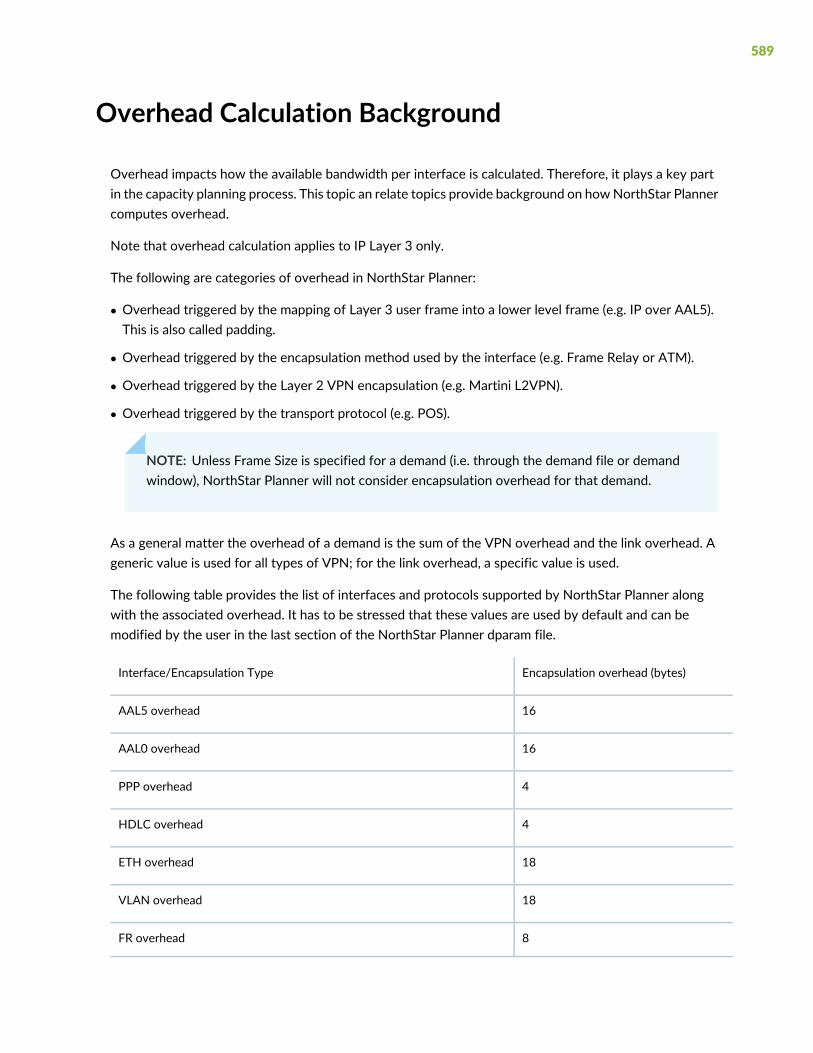
Overhead Calculation Background
Overhead impacts how the available bandwidth per interface is calculated. Therefore, it plays a key partin the capacity planning process. This topic an relate topics provide background on howNorthStar Plannercomputes overhead.
Note that overhead calculation applies to IP Layer 3 only.
The following are categories of overhead in NorthStar Planner:
• Overhead triggered by the mapping of Layer 3 user frame into a lower level frame (e.g. IP over AAL5).This is also called padding.
• Overhead triggered by the encapsulation method used by the interface (e.g. Frame Relay or ATM).
• Overhead triggered by the Layer 2 VPN encapsulation (e.g. Martini L2VPN).
• Overhead triggered by the transport protocol (e.g. POS).
NOTE: Unless Frame Size is specified for a demand (i.e. through the demand file or demandwindow), NorthStar Planner will not consider encapsulation overhead for that demand.
As a general matter the overhead of a demand is the sum of the VPN overhead and the link overhead. Ageneric value is used for all types of VPN; for the link overhead, a specific value is used.
The following table provides the list of interfaces and protocols supported by NorthStar Planner alongwith the associated overhead. It has to be stressed that these values are used by default and can bemodified by the user in the last section of the NorthStar Planner dparam file.
Encapsulation overhead (bytes)Interface/Encapsulation Type
16AAL5 overhead
16AAL0 overhead
4PPP overhead
4HDLC overhead
18ETH overhead
18VLAN overhead
8FR overhead
589

18DOT1Q overhead
9SONET overhead
Labelling overhead (bytes)
12VPN overhead
4MPLS overhead
24GRE overhead
Here are some examples of the overhead calculation:
• The overhead for a demand whose average frame size is 100 bytes using a VPN routed over an Ethernetis 12 + 18 = 30 bytes
• The overhead for a demand whose average frame size is 100 bytes using a VPN routed over a POS is12 + 9 = 21 bytes
• The overhead for a demand whose average frame size is 100 bytes using a VPN routed over a GREtunnel is 12 + 24 = 36 bytes
For IP traffic over ATM, the following specific cascading procedure is applied to determine how muchbandwidth is required to transport customer traffic :
1. VPN overhead is added to the user frame if the demand is mapped with a particular VPN.
2. MPLS overhead is added to the previous frame if a tunnel is used to transport the VPN traffic.
3. AAL5 overhead is added to the previous frame.
4. Then, the PDU is split into a number of ATM cells.
RELATED DOCUMENTATION
Specifying the Overhead Calculation Frame Size | 590
Specifying the Overhead Calculation Frame Size
The following procedures give the steps needed to specify the frame size for a demand.
590

1. InModifymode, go toModify > Elements > Demands. In the Demandswindow, double-click a demand,or select a demand from the table and press the Modify > Selected... button. The Modify Demandwindow will appear.
2. In the Modify Demand window, press the Type button to open up the Demand Type ParameterGeneration window.
Figure 400: Demand Type Parameters Window
3. In the Demand Type window, specify a number for the Frame Size. The unit is in bytes. Then, clickOK.
4. For instance, by typing 256 in the Frame Size box and open up the demand file, you would see BF256added to the type field for a demand:
RLDN2600NWK_1 LDN2600 NWK 5000000 R,A2Z,PATH10(Dynamic),BF256 02,02LDN2600_ETHERNET0/0BF256 indicates that the average frame size is 256 bytes.
591

28CHAPTER
Router Reference
Application Options | 595
Node Window Parameters | 596
Link Window Fields | 597
Interface Window Fields | 600
Demand Window Fields | 602
Tunnel Window Fields | 604


Application Options
This topic describes router-specific fields in the node, link, interface, demand, and tunnel tables as well asthe Application Options windows.
Config Editor
Refer to the NorthStar Planner User Interface Guide for details on the available options.
Design Options > BGP
Design Options > MPLS DS-TE
For more information about the available options, see “DiffServ Traffic Engineering Tunnels Overview”on page 415.
Table 12: Design Options > Path Placement
DescriptionOption
This selection specifies whether the available bandwidth of trunks will or will notbe checked during path placement. When yes is selected, it will not be checked.When no, it will be checked. Hardware default selectionwill depend on the hardwarespecification
Allow Negative AvailableCapacity
This option allows the user to enable all links as MPLS-enabled, or have them setas specified per link in the Protocols tab of the Link window.
MPLS-Enabled Mode
This number specifies the maximum number of ECMP sub-flows that can be splitfrom one original flow.
Max. ECMP Count
This bandwidth value specifies the minimum bandwidth a flow must have in orderto split it into sub-flows.
Min. ECMP Flow BW
This specifies the PIM mode for the multicast feature.PIM Mode
This option allows the user to enable or disable all links as PIM-enabled.Enable PIM
Design Options > Tunnel Sizing
For more information, see “Tunnel Sizing and Demand Sizing Overview” on page 353.
Failure Simulation > FRR
For more information, see “NorthStar Planner Fast Reroute Overview” on page 431.
Integrity Checks
595

For more information, see “Integrity Check Report Overview” on page 485.
LSP Tunnel Attributes
To display the tunnel attributes from a customized network, select Tools > Options > General, LSP TunnelAttributes. The Tunnel Options window is displayed. Type in the name for each tunnel attribute in thetextbox corresponding to the desired bit. For more information, see “NorthStar Planner LSP TunnelsOverview” on page 311,.
NodeWindow Parameters
This topic describes router-specific fields in the node, link, interface, demand, and tunnel tables as well asthe Application Options windows.
Table 13: Properties Tab
File FormatDescriptionField
nodeparam file IPADDR= ip_addressIP address of nodeIP Address
IPv6 address of nodeIPv6*
Indicates node is a layer 2 switchL2SW
Table 14: Design Properties Tab
File FormatDescriptionField
Specifies if this node is an area gateway.Gateway
domain fileOSPF Area for this node. If the node is in more than one area, selectAREA0. This field is used for design purposes only. It sets what thearea of the node should be during a design, e.g., a greenfield designstarting from zero links.
Area (for design only)
Specifies a list of areas that this node can be a gateway to. Thisparameter is a constraint used for design purposes. The areas shouldbe separated by commas.
Accessible Area List
owner fileSpecifies the virtual network that this node belongs to.Vnet
The OSPF routing instance or process ID.Routing Instance
596
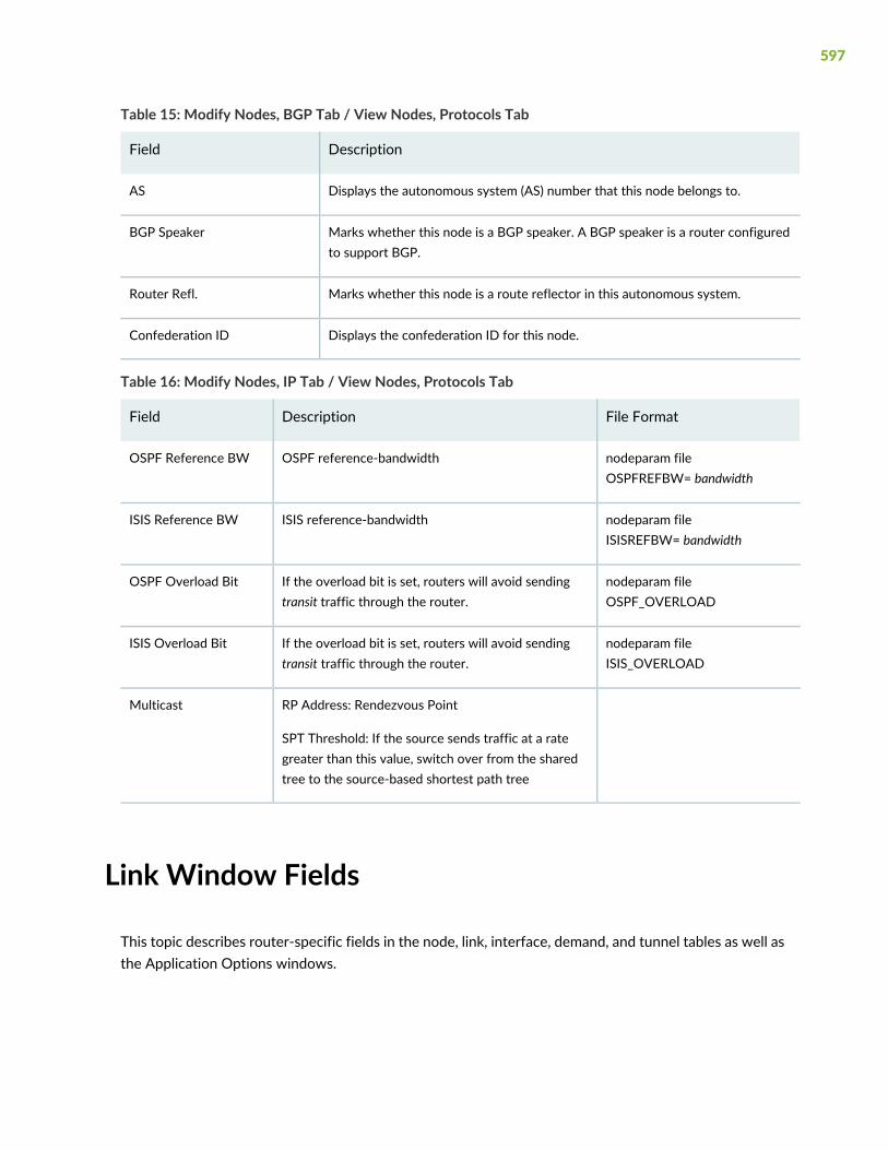
Table 15: Modify Nodes, BGP Tab / View Nodes, Protocols Tab
DescriptionField
Displays the autonomous system (AS) number that this node belongs to.AS
Marks whether this node is a BGP speaker. A BGP speaker is a router configuredto support BGP.
BGP Speaker
Marks whether this node is a route reflector in this autonomous system.Router Refl.
Displays the confederation ID for this node.Confederation ID
Table 16: Modify Nodes, IP Tab / View Nodes, Protocols Tab
File FormatDescriptionField
nodeparam fileOSPFREFBW= bandwidth
OSPF reference-bandwidthOSPF Reference BW
nodeparam fileISISREFBW= bandwidth
ISIS reference-bandwidthISIS Reference BW
nodeparam fileOSPF_OVERLOAD
If the overload bit is set, routers will avoid sendingtransit traffic through the router.
OSPF Overload Bit
nodeparam fileISIS_OVERLOAD
If the overload bit is set, routers will avoid sendingtransit traffic through the router.
ISIS Overload Bit
RP Address: Rendezvous Point
SPT Threshold: If the source sends traffic at a rategreater than this value, switch over from the sharedtree to the source-based shortest path tree
Multicast
Link Window Fields
This topic describes router-specific fields in the node, link, interface, demand, and tunnel tables as well asthe Application Options windows.
597
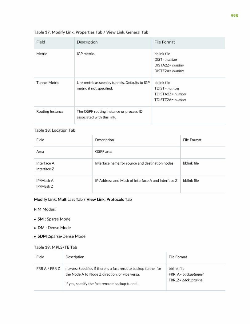
Table 17: Modify Link, Properties Tab / View Link, General Tab
File FormatDescriptionField
bblink fileDIST= numberDISTA2Z= numberDISTZ2A= number
IGP metric.Metric
bblink fileTDIST= numberTDISTA2Z= numberTDISTZ2A= number
Linkmetric as seen by tunnels. Defaults to IGPmetric if not specified.
Tunnel Metric
The OSPF routing instance or process IDassociated with this link.
Routing Instance
Table 18: Location Tab
File FormatDescriptionField
OSPF areaArea
bblink fileInterface name for source and destination nodesInterface AInterface Z
bblink fileIP Address and Mask of interface A and interface ZIP/Mask AIP/Mask Z
Modify Link, Multicast Tab / View Link, Protocols Tab
PIM Modes:
• SM : Sparse Mode
• DM : Dense Mode
• SDM :Sparse-Dense Mode
Table 19: MPLS/TE Tab
File FormatDescriptionField
bblink fileFRR_A= backuptunnelFRR_Z= backuptunnel
no/yes: Specifies if there is a fast reroute backup tunnel forthe Node A to Node Z direction, or vice versa.
If yes, specify the fast reroute backup tunnel.
FRR A / FRR Z
598
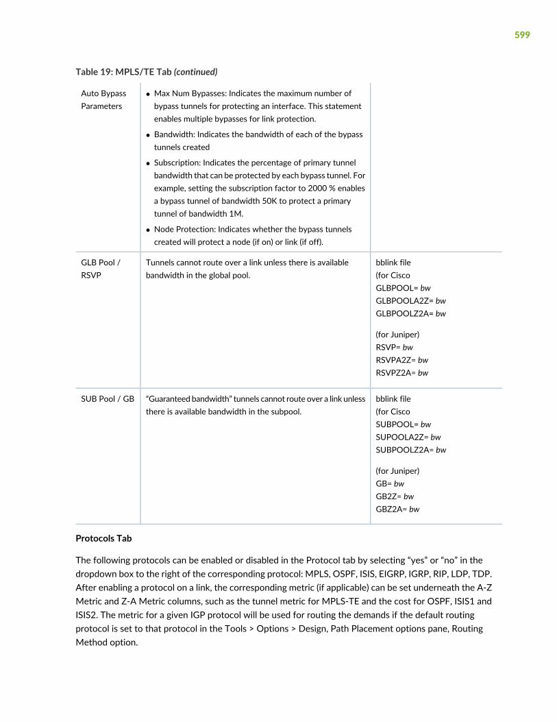
Table 19: MPLS/TE Tab (continued)
• Max Num Bypasses: Indicates the maximum number ofbypass tunnels for protecting an interface. This statementenables multiple bypasses for link protection.
• Bandwidth: Indicates the bandwidth of each of the bypasstunnels created
• Subscription: Indicates the percentage of primary tunnelbandwidth that can be protected by each bypass tunnel. Forexample, setting the subscription factor to 2000 % enablesa bypass tunnel of bandwidth 50K to protect a primarytunnel of bandwidth 1M.
• Node Protection: Indicates whether the bypass tunnelscreated will protect a node (if on) or link (if off).
Auto BypassParameters
bblink file(for CiscoGLBPOOL= bwGLBPOOLA2Z= bwGLBPOOLZ2A= bw
(for Juniper)RSVP= bwRSVPA2Z= bwRSVPZ2A= bw
Tunnels cannot route over a link unless there is availablebandwidth in the global pool.
GLB Pool /RSVP
bblink file(for CiscoSUBPOOL= bwSUPOOLA2Z= bwSUBPOOLZ2A= bw
(for Juniper)GB= bwGB2Z= bwGBZ2A= bw
“Guaranteed bandwidth” tunnels cannot route over a link unlessthere is available bandwidth in the subpool.
SUB Pool / GB
Protocols Tab
The following protocols can be enabled or disabled in the Protocol tab by selecting “yes” or “no” in thedropdown box to the right of the corresponding protocol: MPLS, OSPF, ISIS, EIGRP, IGRP, RIP, LDP, TDP.After enabling a protocol on a link, the corresponding metric (if applicable) can be set underneath the A-ZMetric and Z-A Metric columns, such as the tunnel metric for MPLS-TE and the cost for OSPF, ISIS1 andISIS2. The metric for a given IGP protocol will be used for routing the demands if the default routingprotocol is set to that protocol in the Tools > Options > Design, Path Placement options pane, RoutingMethod option.
599

Note that there are two additional entries, Metric Bandwidth and (E)IGRP delay that can also used toinfluence the routingmetric. TheMetric Bandwidth is an informational and routing parameter correspondingto the “bandwidth” statements for Cisco and Juniper interfaces. The (E)IGRP delay corresponds to the“delay” statement for Cisco interfaces.
EIGRP and IGRP metrics can be influenced by changing the Metric Bandwidth or EIGRP Delay fields.Additionally, K-values can be set from the dparam file. To change the K-values from the text file beforeopening the network, the following line can be added to or edited in the dparam file:
IGRP_param1= TOS:0,K1:1,K2:0,K3:1,K4:0,K5:0
For OSPF, the Metric Bandwidth will be used to calculate the routing metric only if no cost is specified.The reference bandwidth can be changed in Modify mode for Nodes in the IP tab.
For more details on the Protocols tab, see “NorthStar Planner Routing Protocols Overview” on page 63.
Attributes Tab
Tunnels can be prevented from routing over particular links if the link attributes, tunnel mask, and tunnelaffinity are set.
CoS Policy Tab
Specify the CoS policy attached to the interface of node A (source) or node Z (destination). .
PBR (Policy Based Routing) Tab
Lists the route maps used for policy based routing. For more details on PBR..
Modify Link, VoIP Tab / View Link, Protocols Tab
cRTP Compression: None, 2 Bytes, or 4 Bytes
Interface Window Fields
The interface window is available from Network > Elements > Interfaces. See the NorthStar Planner UserInterface Guide for more information.
Table 20: General Tab
DescriptionField
The interface nameInterface Name
The IP address and mask of the interfaceIP Address/Mask
600

Table 20: General Tab (continued)
DescriptionField
The allocated bandwidthBandwidth
Layer 3 (IP) or Layer 2 (switches)Layer
The node which contains the interfaceNode
The link which uses the interfaceLink
The operational status of the interface (active, passive, planned, down,unknown)
Oper Status
The administration status of the interface (active passive, planned, down)Admin Status
Table 21: Advanced Tab - Layer 3
DescriptionField
The virtual circuit identifier or the data link connection identifier for ATMframe relay
VCI/DLCI
The VPN being used on the interfaceVPN
The virtual routing and forwarding instance nameVRF
The virtual router nameVRouter
The hot standby routing protocolHSRP
The interface encapsulation typeEncapsulation
See “NorthStar Planner Class of Service Overview” on page 255.CoS In/Out Policy
See “NorthStar Planner Routing Instances Overview” on page 283.OSPF PID
The multipoint interfaceMultipoint
The automatic protection switching groupAPS Group
The automatic protection switching addressAPS Protected Address
The automatic protection switching nodeAPS Protected Node
601

Table 21: Advanced Tab - Layer 3 (continued)
DescriptionField
The VLAN associated with this interface, if anyVlan ID
The aggregated interface (e.g., ae0, ae1 for Juniper) associated with thisinterface.
Aggregated Interface
To associate an interface with a link, modify the link’s Location tab. Click on the ... button next to eachInterface textbox to bring up the Select Interface window. Highlight the interface you wish to associatewith that end of the link and click “OK”.
Advanced Tab - Layer 2
The interface encapsulation typeEncapsulation
The VLAN associated with this interface, if anyVlan ID
Redundant trunk groups can be configured on EX-series switches so that when theactive link in the group fails, a secondary link will start forwarding data traffic.
Redundant Trunk Group
The aggregated interface (e.g., ae0, ae1 for Juniper) associated with this interface.Aggregated Interface
Access (SW_ACCESS) or Trunk (SW_TRUNK)Port Mode
See “NorthStar Planner Class of Service Overview” on page 255.CoS In/Out Policy
Specifies the tagging type (For Juniper, VLAN_TAGGING is for single tagging,STACKED_TAGGING is for double taggin, and FLEX_TAGGING can be configuredon the physical interface to support different tagging types on different logicalinterfaces of the same physical interface).
Tagging
DemandWindow Fields
This topic describes router-specific fields in the node, link, interface, demand, and tunnel tables as well asthe Application Options windows.
File FormatDescriptionField
demand file, owner fieldVirtual Private NetworkVPN
602
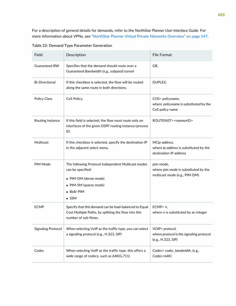
For a description of general details for demands, refer to the NorthStar Planner User Interface Guide. Formore information about VPNs, see “NorthStar Planner Virtual Private Networks Overview” on page 147.
Table 22: Demand Type Parameter Generation
File FormatDescriptionField
GB,Specifies that the demand should route over aGuaranteed Bandwidth (e.g., subpool) tunnel
Guaranteed BW
DUPLEX,If this checkbox is selected, the flow will be routedalong the same route in both directions.
Bi-Directional
COS= policyname,where policyname is substituted by theCoS policy name
CoS Policy.Policy Class
ROUTEINST=<nameorID>If this field is selected, the flow must route only oninterfaces of the given OSPF routing instance/processID.
Routing Instance
MCip-address,where ip-address is substituted by thedestination IP address
If this checkbox is selected, specify the destination IPin the adjacent select menu.
Multicast
pim-mode,where pim-mode is substituted by themulticast mode (e.g., PIM-DM)
The following Protocol Independent Multicast modescan be specified:
• PIM-DM (dense mode)
• PIM-SM (sparse mode)
• Bidir-PIM
• SSM
PIM Mode
ECMP= n,where n is substituted by an integer
Specify that this demand can be load-balanced to EqualCost Multiple Paths, by splitting the flow into thisnumber of sub-flows.
ECMP
VOIP= protocol,where protocol is the signaling protocol(e.g., H.323, SIP)
When selecting VoIP as the traffic type, you can selecta signaling protocol (e.g., H.323, SIP)
Signaling Protocol
Codec= codec_bandwidth, (e.g.,Codec=64K)
When selecting VoIP as the traffic type, this offers awide range of codecs, such as 64K(G.711)
Codec
603

Tunnel Window Fields
This topic describes router-specific fields in the node, link, interface, demand, and tunnel tables as well asthe Application Options windows.
Table 23: Tunnel Window Fields
DescriptionField
This is the user-specified name of the route for this tunnel. If “Dynamic” is specified, the routewill be chosen dynamically and the user should not configure a path in that entry. Otherwise,the user can specify a different
Pathname
This field indicates the priority of this path/route in the “Opt” field. In the “Opt” field, NorthStarPlanner will select the smallest number to be the primary route. For example, you may specifyan Opt 2 for route “Backup1” and Opt 5 for “Backup2”. NorthStar Planner will sort these tworoutes and select “Backup1” to be the primary route since its Opt is smaller.
Opt
This field displays the user-configured route/path for this tunnel.
The route consists of a sequence of node IDs or names separated by “--”. Different delimitersare used to mark the distance relationship between nodes. A listed configured route for a tunnelwould be something like “ATL--WDC--HOU--NYC”. This means the path of the tunnel beginsat node Atlanta, goes to Washington DC, Houston, and terminates at node New York City.
Configured
This is the bandwidth required by the tunnel.BW(J)
Indicates the type of the tunnel as specified in the Tunnel Attributes window. The user may editthis field by right-clicking on the table and selecting “Edit Type”.
Type(J)
Allows you to set the affinity/mask of the tunnel for Cisco, or the include all, exclude, andinclude-any settings for Juniper admin groups to prohibit particular tunnels from routing ontrunks with particular attributes (admin-groups). Trunk attributes effectively color the trunk,whereas a tunnel’s affinity/mask or include-all, exclude, and include-any settings determinewhich color trunks the tunnel is permitted to be placed upon. The user may edit this field byright-clicking on the table and selecting “Edit Affinity/Mask” for Cisco or “EditInclude-All/Exclude/Include-Any” for Juniper.
Affinity/Mask (C)IncludeAll/Exclude/IncludeAny (J)
The priority field of the circuit specification consists of two numbers separated by a comma (,),or a back-slash (/). The first number defines the setup priority of the circuit, and the secondnumber the holding priority of the circuit. The holding priority should be at the same or lowerpriority as the setup priority of the tunnel. It is assumed that this tunnel can only be bumped bya tunnel with a setup priority higher than its holding priority.
Pri,Pre(J)
604

Table 23: Tunnel Window Fields (continued)
DescriptionField
Displays any comments the user may be inclined to enter.Comment(J)
For more detail on the fields in the Table 24 on page 605, see “NorthStar Planner LSP Tunnels Overview”on page 311.
• Path Table : This button will open the Path Table window for the selected source node. The Path Tablewindow lists the primary path from the source node to every other node in the network.
• ShowRoute : This button will highlight the current path of the tunnel on the topology map with a yellowline. If you see a path displayed in gray then either the tunnel path is dynamically routed or is a looseroute. This representation is the start and finish of a loose or dynamic path. This path will be establishedby the hardware under the parameters of the path and links.
• Show All Paths : This button will highlight all paths from the path options table on the topology mapwith a yellow line. If you a path displayed in gray then either the tunnel path is dynamically routed or isa loose route. This representation is the start and finish of a loose or dynamic path. This path will beestablished by the hardware under the parameters of the path and links.
Table 24: Tunnel Type Parameter Generation
File FormatDescriptionField
ABS= absolute_metricREL= relative_metric
A tunnel metric (absolute, relative or don’t care) used by IGP ifAutoroute Announce is checked.
Absolute : Use tunnel metric as is
Relative : Set tunnel metric relative to IGP Metric (e.g., 10 wouldmean tunnel metric = IGP metric + 10)
Don’t Care : Tunnel metric defaults to IGP metric.
Tunnel Metric
Specifies whether the tunnel is primary, secondary, or standby. Thisoption can be configured for a tunnel originating at a Juniper routerby selecting Edit Type from the right-click menu of the bottom halfof the Add Tunnel or Modify Tunnel window.
Tunnel Option
MTU=<mtu>Indicates the tunnel’s Maximum Transmission Unit (default unit is inBytes).
MTU
MAXDELAY=<delay>The maximum delay allowed for this tunnel. The max delay will becalculated either from the delay inputted on the links, or else thevalue set in the Delay Parameters section of the Design Optionswindow (by default, 1ms per 100 miles).
Max Delay
605

Table 24: Tunnel Type Parameter Generation (continued)
File FormatDescriptionField
H<hopcount>The maximum number of hops allowed for this tunnel.Max Hop
MAXCOST=<value>The maximum total admin cost (sometimes referred to as “distance”or “admin weight”) allowed for this tunnel. That is, the total admincost of all the links that the tunnel traverses should not exceed thisvalue.
Max Cost
MCmulticast_nameThe tunnel belongs to this multicast group. Tunnels with the samemulticast name are members of the same P2MP tree.
Multicast Name
ROUTEINST=<inst>OSPF routing instance/process IDRouting Instance
NOAA (No AutorouteAnnounce)corresponds to notselecting thischeckbox
Announces the presence of the tunnel by the routing protocol.WhenAutoroute announce is enabled, the IGP will include the tunnel in itsshortest path calculation when the tunnel is up
Autoroute Announce
GREGeneric Router EncapsulationGRE
0BWCisco feature. During reroute, the tunnel bandwidth is 0. If this is abackup tunnel, then selecting this optionwouldmean that bandwidthwill not be reserved from the link(s) for this tunnel.
Zero BackupBandwidth
If there was a policy class established and applied to this tunnel, itwould appear here. The user can click on the down arrow and reviewall policies that apply to the tunnel.
Policy Class
GBGB Tunnels can only be routed on trunks with available bandwidthin the SubPool.
GuaranteedBandwidth-TE
Circuit cross-connect. This means that this tunnel is cross-connectingbetween two interfaces using CCC
CCC
NOBDNo Border Flag. This is an artificial parameter used for design. Whenset, routing will not follow OSPF constraints. That is, the wholenetwork will be treated like a flat network.
No BD
NOCSPFIndicates that administrative groups/link attributes will be ignoredby this tunnel.
No CSPF
606

Table 24: Tunnel Type Parameter Generation (continued)
File FormatDescriptionField
IGPIf checked, the tunnel will be routed using the current InteriorGateway Protocol’s metric rather than the tunnel metric. The currentrouting method can be found in the Design Options, Path Placementoptions pane.
IGP
REOPTIndicates that the LSP can be automatically reoptimized if the existingpath becomes suboptimal.
Auto-Reoptimization
TMLT= templatenameSpecifies a configlet template in the$WANDL_HOME/data/templates or /u/wandl/data/templatesdirectory. This option allows you to select a manually-generatedtemplate to be used for the configlet generation process. Select thedirectory in which this template file is saved.
Template
LDPFor LDP tunneling. VPN traffic can only route over LDP enabledtunnels/links. For example, this will translate to the ldp-tunneling;statement for Juniper configurations.
LDP
• Enable AutoBW: Specifies an auto-bandwidth tunnel, which will adjust according to the bandwidth overthe tunnel
• Minimum Rate/ Maximum Rate: Specifies the minimum and maximum bounds for the LSP’s bandwidth
• Threshold: (percentage) The LSP’s bandwidthwill be adjusted to the current flow bandwidth (MaxAvgBW)if the percentage difference between the current flow bandwidth and the LSP’s bandwidth is greaterthan or equal to this percentage.
• Sample interval: The adjust interval (in seconds)
• Format: AUTOBW=MinRate:MaxRate:Threshold:SampleInterval,
• Example: AUTOBW=10.000K:1.800G:40:300
The Virtual Trunk tab is used to indicate traffic engineering tunnels advertised as links in an IGP network(OSPF or ISIS) and to indicate the corresponding metric assigned. Select the Virtual Trunk checkbox inorder to configure the relevant protocol, area, and/or metric for which the virtual trunk will apply.
For Cisco, the corresponding statement would be “show mpls traffic-eng forwarding-adjacency”.
For Juniper, the corresponding statementwould be the “label-switched-path namemetricmetric” statementunder the hierarchcy level [edit protocols ospf area area-id] or “label-swiched-path name” under thehierarchy level [edit protocols isis
607

Table 25: Virtual Trunk Tab
VT orVT_areanumber
If a tunnel is marked as a virtual trunk, it is known to other routers and its metric andavailable bandwidth information will be broadcast to other routers as if it were a link.Just as a link has interfaces defined on both ends, two tunnels (one in each direction)must be defined as virtual trunks for this setting to take effect. Otherwise, the virtualtrunk will be perceived as being “down”.
VirtualTrunk
The OSPF area assigned to the Virtual Trunk. This option applies only if Virtual Trunkis selected and the network uses OSPF routing (as opposed to, say, ISIS routing). Atunnel that is marked as a virtual trunk will be advertised as a link to other routers. Ifthose routers perform OSPF area routing, they need to know what area this virtualtrunk belongs to. Select the area from the pull-down box.
Area
Table 26: Diversity Tab
DSITEDIV
Ddivgroupname wheredivgroupname is the nameof a group of tunnels forwhich diverse paths isdesired
If SITEDIV is selected, the program will pair tunnels with the sameoriginating and terminating sites. Paired tunnels are routed diversely.
This field can also be used to specify the name of a group of tunnels thistunnel belongs to. When performing diverse path design, the programwill try to design the paths of the tunnels in this group to be diverse.
Diversity
NODEDIV
LINKDIV
FACDIV
Allows users to specify path diversity requirements for tunnels withstandby or secondary paths.
Select the desired level of diversity
NODEDIV for node disjoint paths
LINKDIV for link disjoint path
FACDIV for facility/SRLG disjoint paths
DiverseLevel
3DIVIndicates that if there is a third path for this tunnel (e.g., in the case ofone primary plus two secondary paths), that all three paths should bedesigned to be diverse.
Users should add an entry for the second and third path and then designthe path using the “Design > Tunnels > PathDesign” option for NorthStarPlanner to design this path.
TertiaryDiverse
608