
Proceedings of the Third National Conference on RECENT TRENDS IN INFORMATION AND COMMUNICATION ...
516
PROCEEDINGS of THIRD NATIONAL CONFERENCE ON RECENT TRENDS IN INFORMATION AND COMMUNICATION TECHNOLOGY (RTICT 2010) 9 – 10 APRIL 2010 Editors Dr. Amitabh Wahi Mr. S. Daniel Madan Raja Mr. S. Sundaramurthy Organised by DEPARTMENT OF INFORMATION TECHNOLOGY BANNARI AMMAN INSTITUTE OF TECHNOLOGY (An Autonomous Institution Affiliated to Anna University Coimbatore | Approved by AICTE New Delhi | Accredited by NBA New Delhi and NAAC with 'A' Grade | ISO 9000:2001 Certified Institute) Sathyamangalam - 638 401 Erode District Tamil Nadu Phone: 04295-221289 Fax: 04295-226666 Email : [email protected] www.bitsathy.ac.in
Transcript of Proceedings of the Third National Conference on RECENT TRENDS IN INFORMATION AND COMMUNICATION ...

PROCEEDINGS
of
THIRD NATIONAL CONFERENCE ON
RECENT TRENDS IN INFORMATION AND COMMUNICATION
TECHNOLOGY
(RTICT 2010)
9 – 10 APRIL 2010
Editors
Dr. Amitabh Wahi
Mr. S. Daniel Madan Raja
Mr. S. Sundaramurthy
Organised by
DEPARTMENT OF INFORMATION TECHNOLOGY
BANNARI AMMAN INSTITUTE OF TECHNOLOGY (An Autonomous Institution Affiliated to Anna University Coimbatore | Approved by AICTE New Delhi |
Accredited by NBA New Delhi and NAAC with 'A' Grade | ISO 9000:2001 Certified Institute)
Sathyamangalam - 638 401 Erode District Tamil Nadu Phone: 04295-221289 Fax: 04295-226666 Email : [email protected]
www.bitsathy.ac.in

PREFACE
Almost everybody today believes that nothing in economic history has ever moved as fast
as, or had a greater impact than, the Information Revolution. Not all problems have a
technological answer, but when they do, that is the more lasting solution. Information and
communications technology unlocks the value of time, allowing and enabling multi-
tasking, multi-channels, multi-this and multi-that.
Communication has allowed the sharing of ideas, enabling human beings to work
together to build the impossible. Our greatest hopes could become reality in the future.
With the technology at our disposal, the possibilities are unbounded.
This conference acts as a platform for the blazing minds of the nation to disseminate
knowledge in their field of expertise. We are indeed at great pleasure in the response
from various researchers across the country.
We are delighted to acknowledge the sponsors of this conference. The work of the
authors and the reviewers of technical papers is commendable. We sincerely thank the
leading lights who have consented to deliver the lectures. We are grateful to our
Chairman, Dr.S.V.Balasubramaniam for his patronage. We are very much thankful to our
beloved Director, Dr.S.K.Sundararaman for his kind encouragement and support in all
our endeavors. We are indebted to our Chief Executive Dr.A.M.Natarajan for his
ebullient support in all the activities of the department. We are obliged to our Principal
Dr.A.Shanmugam, for his kind and support. We shall extend our hearty appreciation to
the members of the technical committee and the organizing committee for their zeal and
involvement.
Editors
Dr. Amitabh Wahi
Mr. S. Sundaramurthy
Mr. S. Daniel Madan Raja

latha ThiagarajanHema
ORGANISING COMMITTEE
Chief Patrons
Dr. S. V. Balasubramaniam, Chairman, BIT
Dr. S. K. Sundararaman, Director, BIT
Patron
Dr. A. M. Natarajan, CEO, BIT
Advisory Committee
Dr. S. Babusundar, King Khalid University, Saudi Arabia
Dr. P. Nagabhusan, University of Mysore, Mysore
Dr. , NIT, Tiruchirappalli
Dr. K. K. Shukla, BHU, Varanasi
Dr. Umapada Pal, Indian Statistical Institute, Kolkata
Dr. B. H. Shekar, University of Mangalore, Mangalore
Dr. R. Bhakar, GCT, Coimbatore, TN
Dr. V. P. Shukla, MITS Deemed University, Rajasthan
Dr. H. N. Upadhaya, SASTRA University, Tanjore, TN
Dr. A. K. Srivastava, NanoSonix Inc, USA
Dr. M. V. N. K. Prasad, IDRBT, Hyderabad, AP
Mr. Venugopal Kaliyannan, Sun Microsystems, Bangalore
Mr. T. R. Sridhar, Alcatel-Lucent, Bangalore
Mr. M. Karappusamy, Wipro, Bangalore
Mr. K. S. Sundar, Infosys, Mysore
Chairman
Dr. A. Shanmugam, Principal, BIT
Convener
Dr. Amitabh Wahi, Prof. & Head
Organising Secretaries
Mr. S. Sundaramurthy & Mr. S. Daniel Madan Raja
Joint Organising Secretaries
Ms. A. Valarmozhi & Mr. R. LokeshKumar
Programme Committee
Dr. C. Palanisamy, Mrs. D. Sharmila, Mrs. A. Bharathi, Mrs. O. S. Shanmugapriya,
Mrs. M. Alamelu, Ms. N. R. Gayathri, Mrs. G. Srinitya, Mr. P. Sengottuvelan, Mrs. R.
Brindha, Mr. T. Vijayakumar, Ms. K. Gandhimathi, Ms. M. Akilandeeswari, Mr. M.
Ravichandran, Mr. R. Vinoth Saravanan, Mr. T. Gopalakrishnan, Ms. S. Abirami, Ms. M.
Manimegalai, Ms. M. Priya, Mr. R. Lokesh Kumar, Mr. A. Karthikeyan, Ms. A.
Valarmozhi, Mr. S. Karthikeyan, Mr. M. S. Nagarajan

OUR SPONSORS
CSIR, New Delhi
CONTENTS
IMAGE PROCESSING
S.NO PAPER TITLE AUTHOR NAME PAGE NO
1 A Steganography Scheme for
JPEG2000
P.Krishnamoorthy
A.Vasuki.
1
2 Automatic image structure-
texture restoration with text
removal and impainting system
G.Thandavan
D.Mohana Geetha.
6
3 Optical Training Sequence and Precoding Method for MIMO
Frequency-Selective Fading
Channels
J.Jeraldroy. V.Jeyasri Arokiamary.
11
4 Face Recognition from Sparse
Representation
C.K.Shahnazeer.
Jeyavel.J.
17
5 Enhanced Ensemble Kalman
Filter for Tomographic Imaging
D.Dhanya
S.Selvadhayanithy.
24
6 Designing of Meta-Caching
Based Adaptive Transcoding for
Multimedia Streaming
N.Duraimurugan.
Sivakumar.R.
32
7 Digital image processing(dip)
Jpeg compression with client
browser plug-in approach for efficient navigation over internet
Preethy Balakrishnan
,K.Kavin prabhu.
39
8 Image Restoration Using
Regularized Multichannel Blind
Deconvolution Technique
Munia Selvan L,
Vinoth Kumar C
49
9 Text extraction in video
J.Dewakhar,
K.Prabhakaran
55
10 Information retrieval using
moment techniques
N. Anilkumar
Dr.Amitabh Wahi
66

IMAGE PROCESSING
S.NO
PAPER TITLE
AUTHOR NAME
PAGE NO
11
Intelligent face parts generation
system from
Finger prints
A.Gowri
Daniel Madan Raja.S.
73
12
A Survey on Ontology Integration
S.Varadharajan,
Sunitha.R.
83
13
An Efficient Multistage Motion
Estimation Scheme for Video
Compression Using Content Based
Adaptive Search Technique
P.Dinesh Khanna
T.SarathBabu
89
14
Framework for Adaptive
Composition and Provisioning of
Web Services
S.Thilagavathy
R.Sivaraman.
95
15
An Enhanced approach for class-
dependent feautre selection
J.Arumugam
K.Shanmugasundaram.
100
16
Design and implementation of a
multiplier
with spurious power suppression
technique
A.Jeyapraba
108
17
Robotics mobile surveillance using
zigbee
V.Suresh
H.Saravanakumar
H.Senthil kumar.
S.T.Prabhu Sowndharya.
113
18
Effective Electrocardiographic
Measurements of The Heart’s
Rhythm Using Hilbert Transform
P.Muthu
Manoj kumar Varma.
118
19
Visual Analysis for object tracking
using Filters and mean shift
Tracker
Vijayalakshmi.B.
K.Menaga.
121
20
Development of data acqusition
system using serial communication
K.Eunice, S. Smys
128

DATA MINING
S.NO
PAPER TITLE
AUTHOR NAME
PAGE NO
21
Analysis of Health care data using
different classifiers
Soby Abraham
131
22
Mining In Distributed System
Using Generic Local Algorithm
Merin Jojo
V.Venkatesh Kumar.
141
23
Province based web search
M.Gowdhaman
A.Suganthi.
147
24
Divergence Control of Data in
Replicated Database systems
P.K.Karunakaran
R.Sivaraman.
151
25
Similarity profiled spatio temporal association Mining
E.Esther Priscilla
156
26
Effective Integration anyInter
Attribute Dependancy Graphs of
Schema Matching
M.Ramkumar
V.S.Akshaya.
163
27
Designed a focused crawler using
multi-agents system with fault
tolerance involving learning
component
G.DeenaDayalan
T.Goutham,
P.Arunkumar
169
28
Secure banking using bluetooth
B. Karthika, D.
Sharmila
and R.
Neelaveni
173
29
An Artificial Device of
Neuroscience
R.Anand Raj
177
30
Issues in implementing E-learning
in Secondary Schools in Western Maharashtra
Hanmant namdeo
renushe
Abhijit S Desai.
Prasanna R .Rasal
181

BROADBAND COMMUNICATION
S.NO
PAPER TITLE
AUTHOR NAME
PAGE NO
31
Remote patient monitoring –
an
implementation in icu ward
E.Arun, V.Marimunthu,
D. Sharmila
and R. Neelaveni
188
32
An efficient search in unstructured Peer-
to-Peer networks
A.Tamilmaran
V.Vigilesh.
197
33
An Ethical Hacking Technique for
preventing malicious imposter email
Rajesh Perumal.R.
202
34
Sterling network security–
(New
dimension in computer Security)
M.Ranjith
K.Yamini
207
35
Automation of irrigation using wireless
R.Divya Priya,
R.Lavanya
217
36
Key management and distribution for
authenticating group communication
K.S.Krisshnakumar,
M.Jaisakthiraman
225
37
Comparison of cryptographic algorithms
for secure data transmission in wireless
sensor network
R.Vigneswaran,
R.Vinod mohan
232
38
Frequency synchronization in 4G wireless
communication
C.Bhuvaneshwaran,
M.Vasanthkumar
242
39
Network security (Binary level encryption)
D.Ashok
T.Arunraj
245

INFORMATION SECURITY
S.NO
PAPER TITLE
AUTHOR NAME
PAGE NO
40
Improving Broadcasting Efficiency in MANET by
Intelligent Flooding Algorithm
Madala
V.Satyanarayana
253
41
Implementation of SE Decoding Algorithm in
FPGA for MIMO Detection
S. Sharmila
Amirtham, S. Karthie
254
42
Wireless Networks Accident
Response Server “An
Automatic Accident Notification System”
S.Renuga,
R.Ramesh krishnan
257
43
Secure Dynamic Routing in Networks
M.Akilandeeswari,
G.Marimuthu,
V.Saranya, & S.Thiripurasundari
266
44
MA-MK Cryptographic Approach for Mobile Agent
Security with Mitigation of System and Information
Oriented Attacks
N.E.Vengatesh,
K.Jeykumar
271
45
New steganography method for secure data
communication
T.ThambiDurai,
K.Nagaraj
274
46
Audio steganography by reverse forward algorithm
using wavelet
based fusion
P.Arthi
G.Kavitha
281
47
Feature selection for microarray datasets using svm
& anova
Janani.G
A.Bharathi
A.M.Natrajan
288
48
Digital Fragile Watermarking using Integer Wavelet
Transform
C. Palanisamy,
Amitabh
Wahi,V.Kavitha
293
49
Testing Polymorphism in object oriented Systems at Dynamic phases for improving software Quality
Rondla vinod kumar
G.Annapoorani
299
MOBILE COMPUTING
S.NO
PAPER TITLE
AUTHOR NAME
PAGE NO
50
A paper on Efficient Reverse
Turing Test in
Artificial Intelligence
G.Geetha
305
51
Bomb detection using wireless
sensor and neural network
S.Sharon Rosy
Shakena Grace.S.
310
52
Warrior robots
A.Sandeep Kumar & S.M.Siddharth
316
53
Performance Analysis of ATM
networks using modified particle
approach
L.Nitisshish Anand
M.Sundarambal.
M.Dhivya
325
54
Curtail the cost and impact in
wireless sensor network
T.Muniraj
Vijeya kumar.K.
331
55
Data Allocation Optimization Algorithm in Mobile
P.V.Aiswarya
Sabireen.H.
337
56
Greedy Resource Allocation
Algorithm for OFDMA Based
Wireless Network
P.Subramanian
Dhanajay kumar.
346
57
Optimal power path routing in
wireless sensor networks
M.Shrilekha
Sathya priyen.V.B.
351
58
Analysis of Propagation Models
used in Wireless Communication
System Design
K.Phani Srinivas
355
59
GSM Mobile technology for
recharge systems
R.Shanthi,
G.Revathy,
J.Anandavalli
362
60
Mitigating routing misbehaviour in mobile ad hoc Networks
M.Sangeetha
,R.Vidhya prakash
M.Rajesh Babu.
368

MOBILE COMPUTING
S.NO
PAPER TITLE
AUTHOR NAME
PAGE NO
61
Automatic call transfer system Based on
location prediction using Wireless sensor
network
C.Somasudaram
Vairavamoorthy.A.
Jesvin veanc
373
62
An Energy Efficient relocation of gateway for improving Timeliness in Wireless Sensor
Networks
S.S.Rahmath ameena
Dr.B.Paramasivan
376
63
Improving stability of shortest multipath routing
algorithm in manet
S.Tamilzharasu
M.Newlin Rajkumar.
382
64
Broadcast Scheduling in wireless network
A.Grurshakthi meera
G.Prema
387
65
Performance Analysis of Security and QoS self-
Optimization in Mobile AD-Hoc Networks
R.R.Ramya
T.SreeSharmila
392
66
Security in Mobile Adhoc Network
Amit Kumar Jaiswal,
Kamal Kant
Pradeep Singh
396
67
Energy Efficient Hybrid Topology Management
Scheme for Wireless Sensor Networks
S. Vadivelan
, A.
Jawahar
400
68
Rateless Forward error correction using LDPC
for MANETS
N.Khadirkumar
406
69
Application Of Genetic Algorithm For The Design Of Circular Microstrip
Antenna
Rajendra Kumar Sethi
Nirupama Tirupathy.
411
70
Automated Water quality monitoring system
using GSM service
R.Bhaarath Vijay,
A.Kapil
416
71
U Slotted Rectangular Microstrip Antenna For
Bandwidth Enhancement
Shalet Sydney
D.Sugumar
422

MODERN DIGITAL COMMUNICATION TECHNIQUES
S.NO
PAPER TITLE
AUTHOR NAME
PAGE NO
72
Implementation of FIR filter using VEDIC Mathematics in VHDL
Arun Bhatia
427
73
Two microphone enhancement of reverberant
speech by SETA-TCLMS algorithm
M.Johnny
Manikandan.A.
Ashok.M.B
Kashi vishwanath.R.G.
434
74
A Cooperative Communication method for
noise Elimination Based on LDPC Code
S.Sasikala
439
75
Data Transmission using OFDM Cognitive
Radio under interference environment
Vinothkumar J,
Kalidoss R
446
76
Wireless communication of multi-user MIMO
system with ZFBF and sum rate analysis
K.Srinivasan
450
77
Low cost Embedded based Braille Reader
J.Raja,M.Chozhaventhar,
V.Eswaran,K.Vinothkumar
452
78
Unbiased Sampling in Ad-hoc( Peer-to-Peer)
Networks
M.Deiveegan,A.Saravanan,
S.Vinothkannan
457
79
Global chaos synchronization of identical and
different chaotic systems by nonlinear control
V. Sundarapandian,
R. Suresh
464
80
Reducing Interference by Using Synthesized
Hopping Techniques
A.Priya
B.V.Srilaxmi priya.
468
81
Real time image processing
applied to traffic
–queue detection algorithm
R.Ramya , P.Saranya
473
82
A fuzzy logic clustering technique to
analyse holy ground water
D.Anugraha,
Dharani
483
83
Image segmentation using clustering
algorithm in six color spaces
S.Venkatesh kumar
488
84
A Novel Approach for Web Service
Composition in Dynamic Environment Using
AR -based Techniques
Rebecca.R
494

Proceedings of the Third National Conference on RTICT 2010
Bannari Amman Insitute of Technology , Sathyamangalam 638 401
9-10 April 2010
A Steganography Scheme for JPEG2000
Krishnamoorthy .P
1, Vasuki .A
2
1 PG Student, 2 Asst.Professor
Department of Electronics and Communication Engineering Kumaraguru College of Technology, Coimbatore-641006
Tamilnadu India.
Email: [email protected], [email protected]
Abstract – Steganography is a technique to
hide secret information in an image. Hiding
capacity is a very important aspect in all
steganographic schemes. Hiding capacity in
JPEG2000 compressed images is very limited
due to bit stream truncation, so it is necessary
to increase the hiding capacity. In this paper,
a new steganography scheme is introduced for
JPEG2000, which uses bit plane coding and
rate distortion optimization technique.
Moreover the embedding points and their
intensity are determined using redundancy
evaluation in order to increase the hiding
capacity and the data is embedded in the
lowest bit plane to keep the message integrity.
The performance of the algorithm are
evaluated for two different images with hiding
capacity in bits and PSNR (dB) of the
reconstructed image as the parameters
Index terms – JPEG2000, bit plane coding,
steganography, data hiding
1. INTRODUCTION
Data hiding in covert communication is
possible due to the characteristics of human
visual system. The hiding technology which is
used in covert communication is named as steganography. Steganography is different from
encryption because encryption hides information
contents whereas steganography hides
information existence. The main aspects that are
considered in data hiding are: capacity, security
and robustness. Capacity means the amount of
data that can be sent secretly, security means the
inability to detect the hidden information and
robustness means the amount of data that a cover
medium can withstand before an intruder can
destroy the hidden information [1]. Robustness is
mainly considered in the digital watermarking
applications rather than steganography. The
steganography algorithms are concerned about
the hiding capacity and security.
The most widely used method is the Least
Significant Bits (LSB) method [2]. Here the
message bits are embedded in the LSB of image
pixel. This method is used because of its
simplicity and ease of implementation. The main
disadvantage is that when we go for truncation
operation then the secret message will be destroyed and thus the extraction of the secret
message is very difficult.
JPEG2000 standard is based on discrete
wavelet transform (DWT) and embedded block
coding and optimized truncation (EBCOT)
algorithms. The bit streams is rate distortion
optimized truncated after bit plane encoding. If
the secret message is embedded directly into the
lowest bit plane of the quantized wavelet
coefficients, then the secret message will be
destroyed by truncation operation [3], [4].
The spread spectrum hiding technique can be
applied in JPEG2000 without considering the bit
stream truncation problem [5]. Here the hiding
capacity is minimized by the spread spectrum pre
processing, so it is often used in digital
watermarking techniques rather than
steganography. After analyzing the challenge of
covert communication, Su and Kuo [6] presented a steganography scheme to hide high
volumetric data in JPEG2000 compressed
images. In order to avoid the bit stream
truncation, the entropy coding was completely
bypassed and is named as ―lazy mode‖. It is
limited to the simplified version of JPEG2000
and not designed for standard JPEG2000.
In this paper a steganography scheme is
proposed for the standard JPEG2000 systems,

2
the bit plane coding procedure is used twice to
solve the problem of bit stream truncation.
Moreover, the embedding points and their
intensity are determined using the redundancy
evaluation technique in order to increase the
hiding capacity. The rest of the paper is structured as follows. Section 2 describes the
details of JPEG2000 standard. Section 3
describes the procedures of proposed
steganography scheme. Section 4 shows the
simulation results. Section 5 gives the
conclusion.
2. JPEG2000 STANDARD
The JPEG2000 encoder is shown in Fig. 1.
First the source image is DC level shifted, by
subtracting all the samples of the image by , where p is the component precision.
Source image
Code stream
Fig. 1. JPEG2000 encoder
The discrete wavelet transform is applied on
the level shifted image coefficients, implemented
by Daubechies 9-tap/7-tap filter [7], which
decompose the image into different resolution
levels. After taking transform all the coefficients
are quantized using different quantization step
size for different levels.
(1)
where
(2)
where BSS is the basic step size, l is the
decomposition level, is the quantization step
size [8], is the transformed coefficient
of the sub band b, is the quantized value.
After quantization each sub band of different
resolution levels are further divided into code
blocks of size smaller than the sub bands. Then
bit plane coding is applied separately on each
code block. It operates on the bit plane in the
order of decreasing importance, to produce an
independent bit stream for each code block. Each
bit plane is encoded in a sequence of three coding passes namely, significance propagation
pass, magnitude refinement pass, clean up pass
[9].
The coefficients of each code block are
scanned as shown in Fig. 2. Starting from the top
left the first four coefficients of the first column
are scanned, then four coefficients of the second
column are scanned until the width of the code
block are scanned and so on. A similar vertical
scan is continued for any leftover rows on the
code blocks in the sub band. The scanning order is same for all the three coding passes.
Fig. 2. Scanning order
After bit plane encoding, rate distortion
optimized truncation is done on coded bit
streams. The EBCOT algorithm produces a bit
stream with many useful truncation points. The
bit stream can be truncated at the end of any
coding passes to get desired compression ratio.
The truncation point of every code block is
determined by rate-distortion optimization [9].
At the decoder side bit plane decoding,
dequantization and wavelet reconstruction is
done to reconstruct the image.
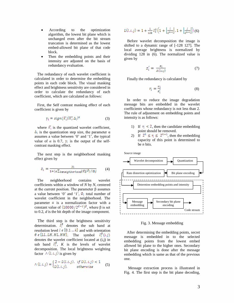
3. PROPOSED SCHEME
The block diagram of the proposed
steganography scheme is shown in Fig. 3. The
steps which are marked by dashed lines in Fig. 3 represent the proposed steganography scheme. The steps involved in the determination of the
embedding points and their intensity for a code
block are as follows:
The wavelet coefficients greater than a
certain threshold are chosen as the candidate embedding points.
Wavelet decomposition
Quantization Bit plane encoding
Rate distortion optimization
3
According to the optimization
algorithm, the lowest bit plane which is
unchanged even after the bit stream
truncation is determined as the lowest
embed-allowed bit plane of that code
block.
Then the embedding points and their
intensity are adjusted on the basis of
redundancy evaluation.
The redundancy of each wavelet coefficient is
calculated in order to determine the embedding
points in each code block. The visual masking
effect and brightness sensitivity are considered in
order to calculate the redundancy of each
coefficient, which are calculated as follows:
First, the Self contrast masking effect of each
coefficient is given by
(3)
where is the quantized wavelet coefficient,
is the quantization step size, the parameter α assumes a value between ‗0‘ and ‗1‘, the typical
value of α is 0.7, is the output of the self-contrast masking effect.
The next step is the neighborhood masking
effect given by
(4)
The neighborhood contains wavelet
coefficients within a window of N by N, centered
at the current position. The parameter β assumes
a value between ‗0‘ and ‗1‘, total number of wavelet coefficient in the neighborhood. The
parameter is a normalization factor with a
constant value of , where β is set to 0.2, d is the bit depth of the image component.
The third step is the brightness sensitivity
determination. denotes the sub band at
resolution level and with orientation
. The symbol
denotes the wavelet coefficient located at (i,j) in
sub band , K is the levels of wavelet
decomposition. The local brightness weighting
factor is given by
(5)
(6)
Before wavelet decomposition the image is
shifted to a dynamic range of [-128 127]. The
local average brightness is normalized by
dividing 128 in (6). The normalized value is
given by
(7)
Finally the redundancy is calculated by
(8)
In order to reduce the image degradation message bits are embedded in the wavelet
coefficients whose redundancy is not less than 2.
The rule of adjustment on embedding points and
intensity is as follows:
1) If , then the candidate embedding point should be removed.
2) If , then the embedding capacity of this point is determined to
be n bits.
Source image
Code stream
Fig. 3. Message embedding
After determining the embedding points, secret
message is embedded in to the selected
embedding points from the lowest embed
allowed bit plane to the higher ones. Secondary
bit plane encoding is done after the message
embedding which is same as that of the previous
one.
Message extraction process is illustrated in
Fig. 4. The first step is the bit plane decoding,
Wavelet decomposition Quantization
Bit plane encoding Rate distortion optimization
Determine embedding points and intensity
Message
embedding
Secondary bit plane
encoding

4
followed by the determination of embedding
point and intensity. Then the secret message is
extracted. Finally dequntization and IDWT is
taken to reconstruct the image.
code stream
Reconstructed image
Fig. 4. Message extraction
4. SIMULATION RESULTS
The original image is the gray scale image
―lena‖ of size 256 x 256 as shown in Fig. 5 (a).
The secret image to be embedded is the binary
image of size 64 x 64 shown in Fig. 5 (b).
The source image is decomposed using four-
level DWT. The coefficients of each sub bands
are quantized and partitioned into code blocks of
size 16 x 16. The bit plane encoding procedure is operated on each code block to produce the bit
streams. According to rate-distortion
optimization, the bit streams of each code block
should be truncated after certain coding passes in
order to get the desired compression ratio. Then
the redundancy evaluation is done to determine
the embedding points in each code block and the
secret message is embedded in those points.
After embedding the secondary bit plane coding
is done. At the receiver side the reverse process
is done to reconstruct the image and also the
secret message is retrieved.
In order to test the performance of the
proposed algorithm, two methods are evaluated.
Method 1: with redundancy evaluation
Method 2: without redundancy
evaluation
The two methods are tested for two different
images with same size. For a threshold of 8, the
hiding capacities of the image ―lena‖, for
different compression ratios are compared in Table 1. Hiding capacity is the total number of
bits that can be embedded in the image. The
embedded secret image is shown in Fig. 5 (b).
The reconstructed image and the retrieved logo is
shown in Fig. 6. After reconstructing the image
the PSNR is calculated between the original and
the reconstructed image.
(9)
where
MSE = (original image—reconst.image)2 (10)
TABLE 1
COMPARISON OF HIDING CAPACITY OF IMAGE
―LENA‖ FOR THRESHOLD ‗8‘
Bits per
pixel
Capacity(bits) PSNR
(dB) Method 1 Method 2
0.4 5381 2117 30.3819
0.6 6270 2502 32.3748
0.8 6576 2640 35.2095
(a) (b)
Fig. 5 (a) Original image (b) logo image
(a) (b)
Fig. 6 (a) Reconstructed image (b) retrieved logo
For the same threshold value the hiding
capacity of the image ―Goldhill‖, for different
compression ratios are compared in Table 2. The
secret message is the same logo image. The
PSNR value of the reconstructed image is also
Bit plane Decoding
Determine embedding points and intensity
Message extraction Dequantization
Wavelet reconstruction

5
calculated. The original and the reconstructed
image is shown in Fig. 7
TABLE 2
COMPARISON OF HIDING CAPACITY OF IMAGE
―GOLDHILL‖ FOR THRESHOLD ‗8‘
Bits per
pixel
Capacity(bits) PSNR
(dB) Method 1 Method 2
0.4 9175 3542 26.9621
0.6 13636 5423 28.1836
0.8 14264 5701 28.9238
(a) (b)
Fig. 7 (a) original image (b) reconstructed image
Thus it is clear from the Table 1 and Table 2
that the hiding capacity of the proposed
algorithm is higher and also the PSNR value of
the reconstructed image will vary.
5. CONCLUSION
In this paper a new steganography scheme is
proposed for the standard JPEG2000 systems,
which uses redundancy evaluation technique to
embed the secret message and thus the hiding
capacity of the JPEG2000 compressed images is
increased. But the bit plane coding procedure is
used twice, which will not have much effect on
the computational complexity.
REFERENCES
[1] N. Provos and P. Honeyman, ―Hide and seek: An introduction to steganography,‖
IEEE Security and Privacy Mag., vol. 1, no.
3, pp.32–44, 2003
[2] C. K. Chan and L. M. Cheng, ―Hiding data
in images by simple LSB substitution,‖
Pattern Recognit., vol. 37, no. 3, pp. 469–
474, 2004.
[3] JPEG2000 Part 1: Final Committee Draft
Version 1.0, ISO/IEC. FCD 15444-1, 2000.
[4] JPEG2000 Part 2: Final Committee Draft,
ISO/IEC FCD 15444-2, 2000.
[5]R. Grosbois and T. Ebrahimi, ―Watermarking in the JPEG2000 domain,‖ in Proc. IEEE
4th Workshop on Multimedia Signal, 2001,
pp.339–344
[6] P. C. Su and C. C. J. Kuo, ―Steganography
in JPEG2000 compressed images,‖ IEEE
Trans. Consum. Electron., vol. 49, no. 4, pp.
824–832, Apr. 2003.
[7] C. Christopoulos, A. Skodas, T. Ebrahimi,
―The JPEG-2000 Still Image Coding
System: An Overview,‖ IEEE Trans.
Consumer Electronics, vol. 46, no. 4, pp. 1103-1127, Nov. 2000.
[8] B.E. Usevitch, ―A tutorial on modern lossy
wavelet image compression: Foundations of
JPEG 2000,‖ IEEE Signal Processing Mag.,
vol. 18, pp.22-35, Sept. 2001.
[9] D. Taubman, ―High performance scalable
image compression with EBCOT,‖ IEEE
Trans. Image Processing, vol. 9, pp. 1158-
1170, July 2000.

Proceedings of the Third National Conference on RTICT 2010
Bannari Amman Insitute of Technology , Sathyamangalam 638 401
9-10 April 2010
6
AUTOMATIC IMAGE STRUCTURE-TEXTURE RESTORATION WITH TEXT
REMOVAL AND INPAINTING SYSTEM
G. Thandavan, Mrs. D. Mohana Geetha
PG Scholor, Assistant professor
Department of Electronics and Communicaton Engineering
Kumaraguru College of technology, Coimbatore
[email protected] , [email protected]
ABSTRACT - This paper deal with the problem of
finding text in images and with the inpainting
problem. Many of the methods are used for structure
and texture inpaintings. Here we used Field Of
Experts (FOE) method. This new approach provides
a practical method for learning higher-order Makov
Random Field (MRF) models with potential function
that extend over large pixels neighborhoods. These
cliques potential are modeled using the Product of
Experts framework that uses non-linear filter
responses. In contrast to the previous approaches all
parameter, including linear filters themselves, are
learned from training data. Field Of Experts model
mainly used two applications, image denoising and
image inpainting. The novel contribution of this
paper is the combination of the inpainting techniques
with the techniques of finding text in images and a
simple morphing algorithm links them. This
combination of results in a automatic system for text
removal and image restoration that requires no user
interface at all.
Key words: Inpainting, Field of Experts, Text
detection, mathematical morphology.
1. INTRODUCTION
Inpainting is the process of filling in missing
or damaged image information. Its applications
involve include the removal of scratches in a
photograph, repairing damaged areas in ancient
paintings, recovering lost blocks caused by wireless
image transmission, image zooming and super
resolution , removing undesired objects from an
image, even perceptual filtering. Text extraction from
an images and video sequences finds many useful
applications in document processing , detection of
vehicle license plate, analyses of technical papers
with tables, maps, charts, and electric circuits and
content based image/video data base. Educational
training and TV programs such as news contains
mixed text-picture-graphics region. In the inpainting
problem, the user has to select the area to be filled in,
inpainting region, since the area missing or damaged
in an image cannot be easily classified in an objective
way. However, there are some occasions where this
can be done. One such a example detecting and
recognizing these characters can be very important in bi-model search of internet data (image and text), and
removing these is important in the context of
removing indirect advertisement, and for aesthetic
reasons.
This paper deal with a problem of automatic
inpainting- based image restoration after text
detection and removal from `images that require no user interaction. This system is important because the
selection of the area to be inpainted has been done
manually by previous inpainting systems.
2.BACKGROUND AND REVIEW OF
INPAINTING
For the in painting problem it is essential to
proceed to the discrimination between the structure
and the texture of an image. Structure define the main
parts - objects of an image, whose surface is
homogeneous without having any details. Texture
defines the details on the surface of the objects which
make the images more realistic.
2.1. Structure Inpainting
The term inpainting was first used by Bertalmio
et al .The idea is to propagate the isophotes (lines
with the same intensity) that arrive at the boundary of
the inpainting region, smoothly inside the region
while preserving the arrival angle. In the same
context of mimicking a natural process, Bertalmioet al. suggested another similar model, where the
evolution of the isophotes is based on the Navier

7
Stokes equations that govern the evolution of fluid
dynamics.
Apart from physical processes, images can also be
modeled as elements of certain function spaces. An
early related work under the word ”disocclusion”
rather than inpainting was done by Masnou and
Morel . In Chan and Shenderived an inpainting model
by considering the image as an element of the space
of Bounded Variation (BV) images, endowed with
the Total Variation (TV) norm .
2.2. Texture Inpainting
The problem of texture inpainting is highly connected with the problem of texture synthesis. A
very simple and highly effective algorithm was
presented by Efros and Leung . In this algorithm the
image is modeled as a Markov Random Field and
texture is synthesized in a pixel by pixel way, by
picking existing pixels with similar neighborhoods in
a randomized fashion. This algorithm performs very
well but it is very slow since the filling-in is being
done pixel by pixel. In the speed was greatly
improved by using a similar and Simpler algorithm,
which filled in the image in a block by block of pixels way.
2.3. Fields of Experts Model Inpainting
To overcome the limitations of pair wise
MRFs and patch-based models we define a high-
order Markov random field for entire images X using
a neighborhood system that connects all nodes in an
m×m square region. This is done for all overlapping
m×m regions of x, which now denotes an entire
image rather than a small image patch. Every such
neighborhood centered on a node (pixel) k = 1… k defines a maximal clique x (k) in the graph. Without
loss of generality we usually assume that the
maximal cliques in the MRF are square pixel patches
of a fixed size. Other, non-square, neighborhoods can
be used.
(1)
where
This equation (1) that the potentials are defined
with a set of expert functions that model filter
responses to a bank of linear filters. This global prior
for low-level vision is a Markov random field of
“experts", or more concisely a Field of Experts
(FoE).More formally, Eq. (1) is used to define the
potential function (written as factor):
(2)
Each Ji is a linear filter that defines the direction (in
the vector space of the pixel values in x(k)) that the
corresponding expert Ф(.;.) Is modeling, and αi is
its corresponding (set of) expert parameter(s). θ =
Ji,αi | i=1,..N is the set of all model parameters. The
number of experts and associated filters, N, is not
prescribed in a particular way. Since each factor can
be unnormalized, we neglect the normalization
component of Eq. (1) for simplicity. Overall, the Field-of-Experts model is thus
defined as
(3)
All components retain their definitions from
above. It is very important to note here that this
definition does not imply that we take a trained PoE
model with fixed parameters θ and use it directly to
model the potential function. This would be incorrect,
because the PoE model described was trained on
independent patches. In case of the FoE, the pixel
regions x(k) that correspond to the maximal cliques
are overlapping and thus not independent. Instead, we
use the untrained PoE model to define the potentials,
and learn the parameters θ in the context of the full MRF Model. What distinguishes this model is that it
explicitly models the overlap of image patches and
the resulting statistical dependence.
The filters Ji, as well as the expert
parameters αi must account for this dependence (to
the extent they can). It is also important to note that
the FoE parameters θ = Ji,αi | i=1,..N are shared
between all maximal cliques and their associated
factors.The model applies to images of an arbitrary
size and is translation invariant because of the homogeneity of the potential functions. This means
that the FoE model can be thought of as a translation-
invariant PoE model.
3 . NEW SYSTEMS
This system aims in the automatic detection of
text and its removal from images. First we make an

8
initial detection of the text characters in the image.
The algorithm assumes that the intensity of the text
characters is different by their background by at least
a certain threshold, for example 30 in an image with
8-bit intensity, i.e., the characters correspond to the
strong edges of the image. After that a morphological closing operator is being applied and the connected
components that represent regions with text are
derived. The character positions are then derived by a
second thresholding of each connected component
Here need to dilate the text region that was derived
from the algorithm in order to cover all the text
character pixels and only those. This goal leads us to
two morphological operators: Conditional dilation
and reconstruction opening.
Conditional dilation is defined as:
where X is the reference frame inside which
the dilations are allowed, and M plays the role of a
marker to be expanded inside the frame. The
reconstruction opening is the limit of iterative
conditional dilation with the same reference frame
and it is defined as the operator Here apply iterative
conditional dilation but with an adaptive reference
frame
Fig. 1. A new system for automatic text removal and image inpainting
Fig. 2. FOE Model Filters
To calculate the reference frame at each iteration of
the algorithm, the hypothesis that the intensity of the pixels in the characters is different is different by at
least a certain threshold γ than their background and
the hypothesis that the all the pixels that correspond
to characters have similar intensity.
The algorithm is as follows: Let M the binary
picture that represents the initial guess of the text
position, and let u be the original image.
1. Initialization: M1=M
2. Calculation of reference frame Xn:
Calculation of the mean value of the original
image in the mask area:
Dilation with unitary disk B , of the image
Mn
Where γ is the threshold mentioned above (eg. γ=30).
3. Conditional dilation for the new prediction:
Mn+1 = δB(Mn|Xn).
4. Repeat step 2-3 until Mn+1=Mn
Experimentally found that a good empirical value for
the threshold is γ = 30 and that the algorithm
converges quickly, e.g. in less than 10 repetitions.
After the termination of this algorithm we have the
exact positions of

9
Fig3(a) Original image
Fig3(b)Initial Text guess
Fig3(c) Final Text guess
Fig3(d) Reconstructed image
Fig4(a) Original image
Fig4 (b) initial text guess
Fig4 (c) Final Text guess
Fig4(d) Reconstructed image

10
the text characters in the image. We can also apply an
unconditional morphological dilation operation with
a unitary disk, to ensure that we have captured all the
pixels that correspond to text characters In image
inpainting the goal is to remove certain parts of an image, for example scratches on a photograph or
unwanted occluding objects, without disturbing the
overall visual appearance. Typically, the user
supplies a mask, M, of pixels that are to be filled in
by the algorithm.
To perform inpainting, we use a simple
gradient ascent procedure, in which we leave the
unmasked pixels untouched, while modifying the
masked pixels only based on the FoE prior. We can
do this by defining a mask matrix M that sets the
gradient to zero for all pixels outside of the masked region M:
(5)
Here, η is the step size of the gradient ascent
procedure. In contrast to other algorithms, we make
no explicit use of the local image gradient direction;
local structure information only comes from the responses to the learned filter bank. The filter bank as
well as the αi are the same as in the denoising
experiments. A schematic representation of our
system is given in Fig. 1.
4. EXPERIMENTAL RESULTS
This paper present a results of the system that
we described above. It is important to note that, the
system requires no user interaction, since both the
text detection (inpainting region) and the inpainting process are being done automatically. In Fig. 3 we
used texture inpainting and the algorithm area around
the text characters is an area with texture and no
structure at all. In Fig. 4 the image contains both
structure and texture; thus, both the decomposition of
the image in the two components and the separate
processing of each one are needed. In general, an
automatic system is needed to decide about the
appropriate inpainting method In Fig. 3(b) we can
easily recognize the text, but this area does not
contain all the character pixels. After applying the simple recursive algorithm we can see that the final
guess contains all the pixels, and thus the inpainting
algorithms can be applied effectively. When we
apply the inpainting over the initial textguess area,
we see that the whole area is not restored because the
text has not been captured completely. However the
text area that has been captured is restored
satisfactory.
This is not the case in Fig. 4. As we can see,
the image inpainting, when the inpainting area is the initial text gives very poor results. The reason is that
in this example we applied simultaneous structure
and texture inpainting. Structure inpainting uses the
neighboring pixels to generate new information.
Since the initial text guess has not captured all the
text-pixels, the neighboring pixels are still text-pixels
and thus they don’t generate the appropriate
information characters, and therefore this area
vanished gradually from the reference frame
5. CONCLUSION
This paper dealt with the combined
problems of inpainting and finding text in images.
Have proposed a new simple morphological
algorithm inspired from the reconstruction opening
operation. This algorithm captures all the pixels that
correspond to text characters and thus its output can
be considered as the inpainting region. By applying
then an appropriate inpainting method, have
developed a system for automatic text removal and
image inpainting.
6. REFERENCES
1. A.Pnevmatikakis and Petros Maragros “An
Inpainting system for Image structure-
texture restortion with text removal” IEE
.Trans.Im.Proc-2008.
2. Stefan Roth and Michael J. Black “ Field of
Experts”. Int.J.Comput.Vision, Nov-2008
3. Y. Hasan and L. Karam, “Morphological
text extraction from images,” IEEE
Trans.Im. Proc., vol. 9, no. 11, pp. 1978–
1983,2000. 4. M. Dimmiccoli and P. Salembier,
“Perceptual filtering with connected
operators and image inpainting,” in Proc.
ISMM,2007.
5. M. Bertalmio, L. Vese, G. Sapiro, and S.
Osher, “Simultaneous structure and texture
image inpainting,” IEEE Trans. Im.
Proc.,vol. 12, no. 8, pp. 882–889, 2003..
6. A. Criminisi, P. Perez, and K. Toyama,
“Object removal by exemplar based
inpainting,” in Proc. IEEE-CVPR, 2003.

Proceedings of the Third National Conference on RTICT 2010
Bannari Amman Insitute of Technology , Sathyamangalam 638 401
9-10 April 2010
11
Optimal Training Sequence and Precoding Method for
MIMO Frequency-Selective Fading Channels
V.JEYASRI AROKIAMARY1,
J.JERALDROY
2
1 Asst. Professor, 2 PG Scholar
Kumarguru College of Technology Department of Electronics and Communication Engineering
Coimbatore-641006, Tamilnadu,India.
E-mail: [email protected], [email protected]
Abstract—A new affine precoding and decoding
method for multiple-input multiple-output (MIMO)
frequency-selective fading channels is proposed.The
affine precoder consists of a linear precoder and a
training sequence, which is superimposed on the
linearly precoded data in an orthogonal manner and the
optimal power allocation between the data and training
signals is also analytically derived.This method is better
compared to other affine precoding methods with
regard to source detection performance and
computational complexity.
Index Terms—Affine precoding, decoding, MIMO
channel estimation, source detection, training Sequence.
I. INTRODUCTION
Multi-input and multiple-output wireless
communications systems is used to achieve the very
high data rates over the wireless links . A major
challenge is how to effectively recover the data trans-
mitted over an unknown frequency-selective fading
channel. Then the training sequence is used for
identifying the unknown channel . But it cannot be
used to guard against the effects of frequency
distortion caused by multi-paths. To avoid these
effects, Redundancy is introduced (Redundancy is
introduced to avoid the probability error) by linearly precoding the source data prior to transmission over
the channel .But the linear precoder can guard against
channel spectral nulls [1], [2], it can be inefficient in
identifying the channel . Therefore both the training
sequence and linear precoder are simultaneously
needed.
In this paper, we propose a new affine precoding method for MIMO frequency-selective fading
channels, Prior to the channel estimation, the
proposed method completely eliminates the linearly
precoded data from the received signal in a simple
manner, so that the channel is effectively estimated.
In contrast to the conventional approaches where the
source data vector s is precoded by a “tall” matrix F
to obtain the precoded dataFs, in our approach a
source data matrix S is first built from the source data
vector and then is postmultiplied by a “fat” pre-coder
matrix P. This yields the precoded data matrix SP,
which is later decoded by postmultiplying with a
decoder matrix QE, designed such that PQE=0. As a
result, the unwanted interference from the unknown
precoded data in the channel estimation process is
easily eliminated. Then, in the source detection
process, the presence of the introduced training
sequence C is completely nulled out by postmultiplying the received signal by another
decoder matrix QD, designed such that CQD=0. This
proposed “postmultiplying”-based decoder is much
more flexible than the previously developed “pre-
multiplying”-based decoders.To further improve the
performances of the channel estimation and source
detection, the optimal power allocation between the
training sequence and data signal is also addressed.
Notation:
Superscript T and H means transposition and the
Hermitian adjoint operators, respectively,while
A-H = (A-1)H .
The symbol ⊗ stands for the Kronecker product.
IN is the N x N identity matrix and the 0N x M
zero matrix.
E is the expectation operation.
tr is the trace of matrix A .
The vectorization operator on a matrix to form a
column vector by vertically stacking the matrix’s
columns is denoted by vec(⋅) .
II. SYSTEM MODEL
Consider the frequency selective block-fading
channel with t transmit antenna and r receive
antennas. The equivalent baseband channel can be
described by the channel coefficients that are constant
during each transmission block and may change from
one block to the next. Let L be the channel order and
the vector hji=[hji(0),…,hji(L)]T
represent the
12
I/P Bit stream
(A). Transmitter
O/P Bit stream
(B). Receiver
Fig.1. System Model
transmission link between the jth receive antenna and
the ith transmit antenna, j=1,2,…,r; i=1,2,…,t. Under
the previous precoding methods , the source symbol
s is pre-multiplied by a “tall” precoder matrix F
before being superimposed with a training vector t.
The received signal is y=HFs+Ht+w, where
represents the effect of additive white Gaussian noise
(AWGN) and is the so-called channel matrix, which
is created from hji . As the precoder matrix F is
Located between the matrix H and the source s, it is
not easy to eliminate the undesired interference of the
superimposed training during in the symbol detection
process. Moreover, as the training sequence and the
precoded data together share a limited power budget,
the tradeoff in power allocation between the data and
the training signals is very important. An increase of
the training power leads to a better channel
estimation but may degrade the source detection due
to the decreased power for the data transmission.
Such a trade]. For a SISO channel, the approximation
AAH=cs I for a “tall” orthogonal matrix and the
assumption that the to-be-estimated matrix H must be
invertible and well conditioned.
In our method, all of the above disadvantages are
overcome, i.e., the unknown data is easily eliminated
in the channel estimation, while the training signal is
completely nulled out in the symbol detection
process. The optimal power allocation between data
and training signals is also derived to enhance the
data detection performance. The key novelty in our
method is that precoding the source data is carried
out by postmultiplying it with a precoder matrix,
which then offers a greater flexibility for channel
estimation and source detection.Our proposed
method is now described by referring to Fig. 1. In
each transmission block, the source sequence is
divided into k vectors of fixed length p, each is
denoted by si, i=1,…,k. The k source vectors si are
gathered to form the following source data matrix:
S=[s1,s2,…,sk]p*k.This source data matrix is
precoded by postmultiplying it with a precoder
matrix
P= k*(k+n), s p (1)
Form the
source
data
matrix
(pp x k)
Precoding
by post-
multiplying
wi th matrix
(Pk x (k+n))
Transmit
Antennas
Adding
Training
matrix
(Cp x(k+n))
Receive
Antennas
Decoupling
for
channel
estimation
Decoupling
for
Data
detection
Channel
detection
Data
detection
+

13
to obtain the precoded data
X=SP=[x1,x2,…,kk+n]p*(k+n).
Here p1,p2,…,pk1*(k+n). are row vectors and n is the
number of redundant vectors introduced by the
precoder. The training matrix is given by
C=[c1,c2,…,ck+n]p*(k+n).
Is added to X to form the transmitted signal
U=C+X=[u1,u2,…,uk+n]p*(k+n).
As the transmitted signal is U is a sum of the training
signal C and the precoded data X, the orthogonality
between C and P is desirable for effectively decoupling them in channel estimation and data
detection. To avoid inter-block interference
(IBI),each p-dimensional transmitted signal vector ui
is divided into t sub-vectors of length m=p/t >=1.
Each sub-vector is then appended with a sequence of
zeros before being transmitted over one of the
transmit antennas.
W=[w1,w2,…,wk+n]p(L+m)r*(k+n).
Be the matrix that represents the effect of AWGN.
Define
Hji=(L+m)m (2)
Which is a Toeplitz matrix constructed from hji . The
overall channel matrix H p(L+m)r*p can be
represented as
H=
It follows that the received signal matrix
Y (L+m)r*(k+n). The transmitted signal U, the noise
W and the channel H are related by the following
equation:
Y=HU+W=HC+HSP+W
A. The channel estimation problem
At the receiver , the matrix Y is postmultiplied
by an estimator matrix QE (k+n)*p, designed such
that
PQE=0kxp (5)
and QE
HQE=Ipxp (6)
i.e., the columns of QE from an orthogonal basis for
the null space of P. The result of this
postmultiplication is
YQE=HCQE+HSPQE+WQE
=HCQE+WQE. (7)
Condition (5) is to ensure that the channel can be
estimated without the presence of the interference
from the data, while condition (6) ensures that the
noise is not amplified with the multiplication operation. Based on the observation YQE in (7), the
problem is now how to design the training matrix and
the estimator matrix QE such that the channel
estimation error is minimized under the mean-
squared error (MSE) criterion.
B. The source detection process
For data detection, consider the system model in
(4).By postmultiplying both sides of (4) by a decoder
matrix
QD(k+n)*k such that
CQD=0pxk and PQD=Ik (8)
the superimposed training signal is easily eliminated
from the received signal. In particular, the equivalent
system for data detection is given by
YQD=HS+WQD (9)
As can be seen from (8), the decoder matrix QD is
the postpseudoinverse of P and it is contained in the
null-space of C. It is given as
QD=PH(PPH)-1 (10)
With P k*(k+n) designed such that
CPH=0pxk
PCH=0kxp (11)
i.e.,CH is contained in the null-space of P.

14
Equation (9) then becomes
YPH(PPH)-1=HS+WPH(PPH)-1 (12)
Define
Y=YPH(PPH)-1, W=WPH(PPH)-1. (13) (12) is written as
Y=HS+H (14)
A popular measure of the detection performance is
the meansquared error of the source symbol, defined
as
ɛS(QD)=trE(S-S)(S-S)H (15)
where S is the estimate of S. The objective is to find
QD to minimize ɛS(QD)..
Another measure is the effective SNR of the system
(14), defined as
SNR= (16)
One is then interested in finding QD to maximize the
above SNR.It will be shown in Section IV
performance indexes lead to the same design of the
optimal precoder P matrix .
C .The power allocation problem
Let denote the estimate of H . Then the channel
estimation error is
=H- .
Rewrite (14) as
=( + )S + = S + S + . (17)
Since the channel is estimated by the MMSE
estimator, H and H are statistically uncorrelated, and
so are HS and HS [4]. The term Z = HS +W is thus
considered as noise and it is statistically uncorrelated
with the signal HS . It follows that the effective SNR
of the system in (17) can be defined as
SNReff= (18)
As will be seen shortly, this effective SNR depends
on the power allocation between the source data S
and the training signal C. This implies that the
detection performance of the source data S can be
improved by maximizing this effective SNR as a
function of the training power.
III. TRAINING DESIGN AND ALGORITHM FOR
CHANNEL ESTIMATION
This section solves the problem of designing the training matrix C and the estimator matrix QE
that minimize the meansquared error between the
channel vector
h = [ , ,…, , ,…, ,…, ,…, ]T (19)
and its linear estimate . The minimization is under
the constraints
(5) and (6). Define
YQ = YQE (L+m)r*p
CQ = CQE
p*p
WQ = WQE (L+m)r*p
the system model in (7) for channel estimation can be
written as
YQE = HCQ +WQ (20)
Observe from (2) and (3) that the matrix H is sparse
and it is linearly dependent on the channel vector h.
Let p be the jth column of
CQ , j=1,….,p. Divide each vector into t sub-
vectors = = [ , ,…, ]T m,
i=1,2,…,t. Tthen construct a Toeplitz matrix from
as follows:
ji=(L+m)*(L+1) (21)
Equation (20) can now be rewritten as
y = h + (22)
where
= vec(YQ) (L+m)r*p
15
= vec(WQ) (L+m)r*p
Let
j = [ j1 j2 … jt ] (L+m)*(L+1)*t
(23)
= (L+m)pr*(L+1)rt (24)
Equation (22) becomes
h + (25)
On the other hand, with w = vec(W) is given by
= vec(WQ) = ( I(L+m)r) w.
The linear MMSE estimate of h is the solution of the
following optimization problem:
=
= tr
= (26)
Accordingly, in our design the matrices C and QE
are chosen through an arbitrary orthogonal matrix
O (k+n)*(k+n)
by the following expressions:
C = c O (1:p,:) p*(k+n)
(27)
QE = O (1:p,:)H (k+n)*p
(28)
Where O (1:p,:) denotes the 1st to pth rows of O.
With the above designs of C and QE , the equality
CQE CH = CCH
holds true (although QE generally is not the
identity matrix). This means that .
tr = tr = p(k+n) .
Condition (6) is obviously satisfied, while condition
(5) is also satisfied by the design of the optimal
precoder matrix P in Section IV.
Furthermore, since CQE = c , it is clear
that the matrix ji defined by (21) satisfies the
equation shown at the bottom of the previous page.
Therefore, for the matrix defined by (24), one can
readily verify that
H = Ir
= Ir
= m(k+n) I(L+1)rt
which is a scaled identity matrix
Conditions (5) and (11) are automatically satisfied
with the design of the precoder matrix p in Section
IV. LINEAR PRECODER DESIGH FOR DATA
DETECTION
We now address the problem of designing
the precoder matrix P that satisfies conditions (5) and (11) and minimizes the MMSE in (15).
With the same orthogonal matrix
O ∊ as in the definition (26) of the
training matrix C,
let O((p+1):(p+k),:) denote the (p+1)th to (p+k)th rows of O. It is clear that
P=
Finally, it should be pointed out that, as C in (27)
contains p rows of O , while P in (29) contains k rows of O, the size (k+n) of O must be greater than or
equal to (k+p) . This results in the condition that n ≥ p
in (1) required in our method.
V. POWER ALLOCATION FOR DATA
DETECTION ENHANCEMENT
In this section, we derive the optimal power
allocation between the training sequence and the
source data such that SNR in (18) is maximized.
eff =

16
VI.SIMULATION RESULTS:
0 0.1 0.2 0.3 0.4 0.5 0.6 0.7 0.8 0.9 130
32
34
36
38
40
42
44
46
48
50
sigma C
Eff
ecti
ve S
NR
Eff SNR Vs Sigc
SNR=20dB
Fig. 2. Impact of the power allocation in the proposed design on the S Reff performance at different channel SNR
values (SNR = 5,10,and 15 dB): 2 x 2 MIMO frequency-selective fading channel with L=2, p = k = n = 4.
= , where
(30)
eff is actually a quadratic function in :
eff ( ) (31)
Where is given by
(32)
VII. CONCLUSION
We have presented a new method of designing an
affine precoder for MIMO frequency-selective fading
channels based on the concept of orthogonal
superimposed training and linear precoding.In the
proposed design method, the channel is estimated
independently of the affine precoded data while the
interference of the superimposed training signal in
data detection is completely eliminated. Simulation
results show that the proposed method outperforms
the other recently-proposed method in source data detection while its computational complexity is much
reduced.
REFERENCES
[1] G. D. Forney and M. V. Eyuboglu, “Combined
equalization and coding using precoding,” IEEE
Commun. Mag., vol. 29, no. 12, pp. 25–34,Dec. 1991.
[2] G. B. Giannakis, “Filterbanks for blind channel
identification and equalization,” IEEE Signal
Process. Lett., vol. 4, no. 6, pp. 184–187,Jun. 1997. [3] B. Hassibi and B. M. Hochwald, “How much
training is needed in multiple-antenna wireless
links?,” IEEE Trans. Inf. Theory, vol. 49, no. 4, pp.
951–963, Apr. 2003.
[4] X. Ma, L. Yang, and G. B. Giannakis, “Optimal
training for MIMO frequency-selective fading
channels,” IEEE Trans. Wireless Commun., vol. 4,
no. 2, pp. 453–466, Mar. 2005.
[5] J. H. Manton, I. V. Mareels, and Y. Hua, “Affine
precoders for reliable communications,” in Proc.
IEEE Int. Conf. Acoustics, Speech, Signal Processing, Jun. 2000, pp. 2749–2752.
[6] J. H. Manton, “Design and analysis of linear
precoders under a mean square error criterion, Part I:
Foundations and worst case design,” Syst.Control
Lett., vol. 49, pp. 121–130, 2003.
[7] J. H. Manton, “Design and analysis of linear
precoders under a meansquare error criterion, Part II:
MMSE design and conclusions,” Syst.Control Lett.,
vol. 49, pp. 131–140, 2003.
[8] S. Ohno and G. B. Giannakis, “Superimposed
training on redundant precoding for low-complexity
[9] S. Ohno and G. B. Giannakis, “Optimal training and redundant precoding for block transmissions with
application to wireless OFDM,”IEEE Trans.
Commun., vol. 50, no. 12, pp. 2113–2123, Dec. 2002.
[10] D. H. Pham and J. H. Manton, “Orthogonal
superimposed training on linear precoding: A new
affine precoder design,” in Proc. IEEE 6th Workshop
Signal Processing Advance inWireless
Communication, Jun.2005, pp. 445–449.
Proceedings of the Third National Conference on RTICT 2010
Bannari Amman Insitute of Technology , Sathyamangalam 638 401
9-10 April 2010
17
FACE RECOGNITION FROM SPARSE REPRESENTATION
1Shahnazeer C K
2Jayavel J
1 PG scholar, Dept of IT, Anna University, Coimbatore-47, Tamilnadu, India.
Email:[email protected] 2Lecturer, Dept of IT, Anna University, Coimbatore-47, Tamilnadu, India,
Email: [email protected]
Abstract - This paper provides a problem of automatically recognizing human faces from frontal views with
various facial expressions, occlusion, illumination and pose. There are two underlying motivations for us to write
this paper: the first is to provide an occlusion and various expressions of the existing face recognition and the
second is to offer some insights into the studies of pose and illumination of face recognition. We present a
mathematical formulation and an algorithmic framework to achieve these goals. The existing framework offers a
sparse representation of the test image with respect to the training image. The sparse representation can be
accurately and efficiently computed by the l1
minimization. The proposed framework offers a local translational
model for deformation due to pose with a linear subspace model for lighting variations and also gives competitive
performance for moderate variations in both pose and illumination. Extensive experiments on publicly available
databases verify the efficacy of the proposed method and support the above claims. Index Terms- Face Recognition, Occlusion, Illumination, Pose, Sparse representation, l1-minimization
I INTRODUCTION
Real-world automatic face recognition systems
are confronted with a number of sources of
within-class variation, including pose, expression, and illumination, as well as
occlusion or disguise. Several decades of intense
study within the pattern recognition community have produced numerous methods for handling
each of these factors individually.
In this paper, we exploit the discriminative
nature of sparse representation[2] to perform classification. We represent the test sample in an
over-complete dictionary whose base elements
are the training samples themselves. If sufficient training samples are available from each class, it
will be possible to represent the test samples as a
linear combination of just those training samples from the same class. This representation is
naturally sparse, involving only a small fraction
of the overall training database. We argue that in
many problems of interest, it is actually the sparsest linear representation of the test sample
in terms of this dictionary and can be recovered
efficiently via l1-minimization [3]. Seeking the
sparsest representation therefore automatically
discriminates between the various classes
present in the training set. Sparse representation also provides a simple and surprisingly effective
means of rejecting invalid test samples not
arising from any class in the training database:
these samples sparsest representations tend to
involve many dictionary elements, spanning
multiple classes. We investigate to what extent accurate
recognition are possible using only 2D frontal
images. More specifically, we address the following problem: Given only frontal images
taken under several illuminations recognize
faces despite large variation in both pose and
illumination. Our algorithm will apply to test images with
significantly different illumination conditions,
and pose variations upto ±45. In this setting, a typical test image would have an arbitrary pose
in the given range and also an illumination not
present in the training. Our approach is simple but effective: for each small patch of the test
image, we find a corresponding location and
illumination condition that best approximate it.
The quality of this match is used directly as a statistic for classification, and results from
multiple patches are aggregated by voting. For
comparison, we also propose a second scheme that performs pose-invariant recognition
between the test image and a training image
synthesized from the recovered illumination conditions, by matching deformation-resistant
features such as SIFT keys. We will motivate
and study this new approach to classification

18
within the context of automatic face recognition.
Human faces are arguably the most extensively studied object in image-based recognition. This
is partly due to the remarkable face recognition
capability of the human visual system [4] and
partly due to numerous important applications for face recognition technology [5]. In addition,
technical issues associated with face recognition
are representative of object recognition and even data classification in general.
II REVIEW OF EXISTING SYSTEM
A basic problem in object recognition is to use
labeled training samples from k distinct object classes to correctly determine the class to which
a new test sample belongs. We arrange the given
ni training samples from the ith class as columns
of a matrix Ai= [vi,1,vi,2,……,vi,n]εIRmxn
i . In the context of face recognition, we will identify a w
x h grayscale image with the vector vεIRm
(m=wh) given by stacking its columns; the columns of Ai are then the training face images
of the ith
subject.
A Sparse Representation of training samples
In this section, the training images were
presented in matrices form. It performed a linear feature transform. Given sufficient training
samples of the ith
object class, Ai
=[vi,1,vi,2,….,vi,ni]ε IRmxni
, any new (test) sample yε IR
m from the same class will approximately
lie in the linear span of the training samples
associated with object i: y= αi,1vi,1+αi,2vi,2+….+αi,nivi,ni for some
scalars,αi,jεIR, j = 1, 2, . . . , ni. Since the
membership i of the test sample was initially
unknown, and defined a new matrix A for the entire training set as the concatenation of the n
training samples of all k object classes:
A=[A1,A2,….,Ak]=[v1,1,v1,2,…..,vk,nk]. Then, the linear representation of y can be rewritten in
terms of all training samples as y =Ax0 ε IRm,
where x0=[0,….,0,αi,1,αi,n,0,….,0]T
ε IRn is a
coefficient vector whose entries were zero except those associated with the i
th class.
B Recognition with facial features
In this section, the role of feature extraction
within the new sparse representation framework
for face recognition was reexamined. One
benefit of feature extraction, which carried over to the proposed sparse representation
framework, was reduced data dimension and
computational cost. Our SRC algorithm tested
using several conventional holistic face features, namely, Eigenfaces [6], Laplacianfaces [7], and
Fisher faces, and compares their performance
with two unconventional features: random faces and down-sampled images. In this section, the
stable version of SRC in various lower
dimensional feature spaces were used for solving the reduced optimization problem with
the error tolerance ε=0.05. The Mat lab
implementation of the reduced (feature space)
version of Algorithm 1 took only a few seconds per test image on a typical 3-GHz PC.
C Handling corruption and occlusion.
Occlusion poses a significant obstacle to robust
real-world face recognition. This difficulty is mainly due to the unpredictable nature of the
error incurred by occlusion: it may affect any
part of the image and may be arbitrarily large in
magnitude.
Now, to show how the proposed sparse
representation classification framework can be extended to deal with occlusion. Assume that the
corrupted pixels are a relatively small portion of
the image. The error vector e0, like the vector x0, then has sparse nonzero entries. Since y0= Ax0,
we can rewrite y = y0 +e0 =Ax0+e0 as
Y= [A, I]
0
0
e
x= Bw0.
Here, B= [A, I]ε IR mx(n+m)
, so the system y =Bw
is always underdetermined and does not have a unique solution for w. However, from the above
discussion about the sparsity of x0 and e0, the
correct generating w0=[x0, e0] has at most ni +ρm nonzeros. We might therefore hope to recover
w0 as the sparsest solution to the system y =Bw.
In fact, if the matrix B is in general position, then as long as y =Bŵ for some ŵ with less than
m/2 nonzeros, ŵ is the unique sparsest solution.
Thus, if the occlusion e covers less than (m- ni
)/2 pixels, ≈50 percent of the image, the sparsest

19
solution ŵ to y =Bw is the true generator,
w0=[x0, e0]. More generally, one can assume that the corrupting error e0 has a sparse
representation with respect to some basis Ae ε
IRmxn
e . That is, e0 =Aeu0 for some sparse vector
u0 ε IRm. Here, choosing the special case Ae =I ε
IRmxm
as e0 is assumed to be sparse with respect
to the natural pixel coordinates. If the error e0 is
instead sparser with respect to another basis, the matrix B can simply redefine by appending Ae
(instead of the identity I) to A and instead seek
the sparsest solution w0 to the equation: y =Bw with B =[A, Ae] ε IR
mx(n+ni).
In this way, the same formulation can handle
more general classes of (sparse) corruption. As before, to recover the sparsest solution w0 from
solving the following extended 11-minimization
problem: (l1e ) :ŵ1 =arg min||w||1 subject to Bw=
y. That is, in Algorithm 1, now replace the
image matrix A with the extended matrix B =[A,
I] and x with w =[x, e].
Clearly, whether the sparse solution w0 can be
recovered from the above 11-minimization
depends on the neighborliness of the new polytope P =B (P1)=[A, I](P1). This polytope
contains vertices from both the training images
A and the identity matrix I. The bounds given in imply that if y is an image of subject i, the 1
1-
minimization cannot guarantee to correctly
recover w0 = [x0, e0] if ni +|support(e0)| > d/3. Generally, d » ni, so, c .m < t < [(m+1)/3]
implies that the largest fraction of occlusion.
Algorithm 1 below summarizes the complete recognition procedure. Our implementation
minimizes the l1-norm via a primal-dual
algorithm for linear programming.
Algorithm1. Sparse Representation-based
Classification (SRC)
1. Input: a matrix of training samples A =
[A1,A2, . . .,Ak ]εIRmxn
for k classes, a test sample xεIR
m, (and an optional error
tolerance ε> 0.)
2. Normalize the columns of A to have unit l2-norm.
3. Solve the l1-minimization problem:
ŷ1=arg miny ||y||1 subject to Ay=x (Or alternatively, solve ŷ1=arg miny ||y||1
subject to ||Ay-x||2 <= ε.)
4. Compute the residuals ri(x)=||x-Aδi
(ŷ1)||2 for i = 1, . . . ,k.
5. Output: identity(x)= arg mini ri(x).
III PROPOSED SYSTEM
In this section, we discuss the difficulties
associated with variations in pose and
illumination, and why state-of-the-art methods that are quite effective at handling one of these
modes of variability tend to fail when both are
present simultaneously [8].
We assume that the face is well-localized in the test image, i.e., any gross misalignment or
scaling has already been compensated for. In
practice, this is accomplished by applying an affine or projective transformation to
approximately map eye and mouth corners of the
test image to eye and mouth corners of training image. We will denote the so-aligned test image
by . We will assume access to a
gallery of registered frontal training images
for each subject i, taken at k
distinct illuminations.
The figure 1 represents the system architecture
of face recognition. It has two phases: (i) Training Phase (ii) Testing Phase. In training
phase there can be four or more input face
images. These inputs extract the features that are expression, occlusion, illumination and pose.
These details were stored in a database. Put one
image in the testing phase and it will compare features on the database. If the feature matches
with the test image then it will display the
identified face. Otherwise it will not display any
image, because there is no corresponding image in the database.

20
Fig 1: System Architecture
A Matching Image Patches
We first select a set of feature point locations
in the test image for matching. In
Section , we will see that the choice of feature points is not essential – a sufficient number of
randomly selected or evenly distributed feature
points work as well as the scale-space extrema
popular in the image matching literature [9].
Around each feature point in the test
image, we select a square window
of pixels for matching. If this feature is also visible in the training frontal view, there is a
corresponding point in each training
image . If all images were taken under
ambient illumination, we would expect the
corresponding patches to be quite similar in
appearance: .
However, if the test image is taken at more extreme illumination, it is more appropriate to
approximate the patch by a linear
combination of training patches:
Now, since gross misalignments and scalings
have already been compensated for, we may
assume that the corresponding point lies in a
small neighborhood of .
For each training subject i, we search for the
best match within this neighborhood, seeking a
point where the subspace spanned by the
training patches offers the best approximation to
:
Thus, for each feature denotes the
location of the best match to a linear
combination of training patches for subject i,
while denotes the corresponding best
coefficients.
B Classification Based On Nearest Subspace
Matching We compare two methods for determining the identity of the test image from the
correspondences obtained from (1). The first,
which we refer to as Nearest Subspace Patch Matching (NSPM), uses the approximation error
in (1) as a statistic for classification. The m-th
test patch is classified to the subject
i whose coefficients best approximate it.
The classifications of these patches are then
aggregated into a single classification of the test
image by voting. This process is summarized as
Algorithm 2. The algorithm is computationally efficient and scalable – the complexity is linear
in the number of subjects. A similar scheme has
achieved state-of-the-art performance for recognizing handwritten digits [10]. In this
Section, we will see that this simple approach
also performs quite well for face recognition with moderate variations in pose and
illumination.
C Classification Based On SIFT Matching
For purposes of comparison, we also outline a
second approach which uses the computed α to compensate for global illumination variations,
and then applies standard matching techniques.
This approach finds for each training subject i, a single illumination condition (expressed as
Input image1
Input imageN
Input image
Feature Extractor
Feature Extractor
Feature Extractor
Features of
Faces
(Various
expression,
Occlusion, Illuminatio
n and
poses) TESTING PHASE
TRAINING PHASE
Data base Comparison
using SRC
and NSPM algorithm
Correctly Identified
Found

21
coefficients ) that best reproduces the test
illumination. These coefficients are used to synthesize a set of “equivalent” frontal training
images . In the next paragraph, we describe
how the can be robustly computed from
noisy data. With illumination compensated for in
this manner, classical deformation-invariant
matching algorithms can then be applied. In practice, we find that once illumination has been
corrected, the SIFT (Scale-invariant feature
transform) algorithm[11] performs quite
successfully in matching the test image to the
synthetic image for the correct subject. The
number of SIFT correspondences between and
each of the provides a simple statistic for
classification. Equation (1) gives, for each training subject i, a set of putative
correspondences and
coefficient vectors . For each subject
i, we will synthesize a frontal training image
whose illumination best approximates the
illumination in the test image. That is, from each
set of coefficient vectors we
will compute a single and set
. If the correspondences
were perfect, and there were no deviations from
linearity, one could simply set to be the
average of . Here we use clustering to
remove outliers in fitting a single, global
illumination model. With illumination compensated for, conventional feature matching
techniques can be effectively applied to the test
image and the synthesized training image.
Algorithm 2.Nearest-Subspace Patch
Matching (NSPM)
1. Input: test image , frontal training
images taken at k
different illuminations, for each
subject i.
2. Select feature points in
3. for each feature point do
4. for each subject i, compute the
corresponding location and
coefficients from (1);
5. set Identity( ) to be:
6. end for
7. Output: class i that maximizes the
number of with Identity ( ) =
i.
IV SIMULATION RESULTS
In this work, we have used the ORL database, a
set of pictures taken at Olivetti Research
Laboratory. There are ten different images of each of 40 distinct subjects. For some subjects,
the images were taken at different times, varying
the lighting, facial expressions and facial details. All the images were taken against a dark
homogeneous background with the subjects in
an upright, frontal position. The images are 256
gray levels with a resolution of 92x112 pixels. This database includes the manually made
occluted images.
Output Screen
Fig 2: Form
The figure 2 represents the output screen of the
recognition system. This form contains training,
input image and testing buttons.

22
Training
Fig 3: Training Images
The figure 3 represents the training images of
the ORL database. By clicking training, the message “training is done” appears in the
command window.
Input Image
Fig 4: Input Image
The figure 4 represents the input image of the
recognition system. Clicking input image will display the ORL database, from this select the
input image.
Various Expressions
Fig 5: Various Expressions
The figure 5 represents the output of the various expression face image. Click testing, then
recognized image will display in the screen and
a message box also appeared that is “Correctly
Recognized”.
Occlusion Images
Fig 6: Occluted facial image
The figure 6 represents the output of an occluted
face image. Click testing, then recognized image will display in the screen and a message box also
appeared that is “Correctly Recognized”.
Illumination
Fig 7: Illumination
The figure 7 represents the output of an
illumination face image. Click testing, then
recognized image will display in the screen.
Pose Detection
Fig 8: Pose Detection
The figure 8 represents the output of a pose face image. Click testing, then recognized image will
display in the screen.

23
Incorrectly recognized image
Fig 9: Incorrectly recognized image
The figure 9 represents the output of the
incorrectly recognized image. Select an image
which is not in the database. Then image not
found will display in the screen. Images only
recognized in the database.
V CONCLUSION AND FUTURE WORK
We have presented here a method of computing
sparse representations of facial images that preserve the information required to estimate
expression, occlusion, pose and illumination
with SRC and NSPM. These both reduce the computation required to compute SRC, NSPM
and improves the accuracy of the results.
An intriguing question for future work is
whether this framework can be useful for object
detection, in addition to recognition. The
usefulness of sparsity in detection has been
noticed in the work in [12]. We believe that the
full potential of sparsity in robust object
detection and recognition together is yet to be
uncovered. From a practical standpoint, it would
also be useful to extend the algorithm to less
constrained conditions, especially variations in
object pose. Robustness to occlusion allows the
algorithm to tolerate small pose variation or
misalignment.
REFERENCES
[1] John Wright, Allen Y Yang, Arvind Ganesh, and S Shankar Sastry,”Robust Face
Recognition Via Sparse Representation “, IEEE
Transaction on Pattern Analysis And Machine
Intelligence, February 2009.
[2] K. Huang and S. Aviyente, “Sparse
Representation for Signal Classification,” Neural Information Processing Systems, 2006
[3] D.Donoho, “For Most Large
Underdetermined Systems of Linear Equations
the Minimal l1-Norm Solution Is Also the
Sparsest Solution,” Comm. Pure and Applied
Math., vol. 59, no. 6, pp. 797 829, 2006
[4] P. Sinha, B. Balas, Y. Ostrovsky, and R. Russell, “Face Recognition by Humans:
Nineteen Results All Computer Vision
Researchers Should Know about,” Proc. IEEE, vol. 94, no. 11, pp. 1948-1962,2006.
[5] W. Zhao, R. Chellappa, J. Phillips, and A.
Rosenfeld, “Face Recognition: A Literature
Survey,” ACM Computing Surveys, pp. 399-458, 2003.
[6] M. Turk and A. Pentland, “Eigenfaces for
Recognition,” Proc. IEEE Int’l Conf. Computer Vision and Pattern Recognition, 1991.
[7] X. He, S. Yan, Y. Hu, P. Niyogi, and H.
Zhang, “Face Recognition Using Laplacianfaces,” IEEE Trans. Pattern Analysis
and Machine Intelli, Mar.2005
[8] D. Lowe. Distinctive image features from
scale-invariant keypoints. IJCV, 2004. [9] Nearest-Subspace Patch Matching for Face
Recognition Under Varying Pose and
Illumination, Zihan Zhou, Arvind Ganesh and Yi Ma, 2007
[10] D. Keysers, T. Deselaers, C. Gollan, and H.
Ney. Deformation models for image recog.
PAMI, 2007. [11] J. Luo, Y. Ma, E. Takikawa, S. Lao, M.
Kawade, and B. Lu. Person-specific SIFT
features for face recognition. In proc. ICASSP, volume 2, 2007.
[12] D. Geiger, T. Liu, and M. Donahue,
“Sparse Representations for Image Decompositions,” Int’l J. Computer Vision, vol.
33, no. 2, 1999.

Proceedings of the Third National Conference on RTICT 2010
Bannari Amman Insitute of Technology , Sathyamangalam 638 401
9-10 April 2010
24
ENHANCED ENSEMBLE KALMAN FILTER FOR TOMOGRAPHIC IMAGING
D.Dhanya Second year M.E( CSE), Mr.S.Selva Dhayanithy,Lecturer(CSE).
Jerusalem College of Engineering Chennaii.
Abstract-This addresses the problem of
dynamic tomography by formulating it
under the linear state-space model. The
main theoretical contribution is a new
theorem that addresses the convergence
of the EnKF.The main idea behind the
paper“ENHANCED ENSEMBLE KALMAN
FILTER FOR TOMOGRAPHIC IMAGING” is to
formulate the state estimation problem of
a dynamic image and thereby
reconstructing the original image. This can
be done by a filter known as Ensemble
Kalman Filter, a Monte Carlo algorithm
that is computationally tractable when the
state dimension is large. Since it is based
on mathematical procedure it is called
tomographic reconstruction. The Kalman
Filter, a time dependent construction
method is used in this application. In
medical tomography state may change by
a small amount during the measurement
interval and is considered to be static,
hence estimation becomes cumbersome
process. In Existing a high resolution with a
spatial resolution of 128x128 pixels are
used to get the clarity of the image. The
problem is solved by Ensemble Kalman
Filter which is used to get the result of
unfeasible or impossible task and is
tractable when the state dimension is
large. Frequency domain is used in this
application’s. A high resolution with a
spatial resolution of 256x256 pixels is used
in this application. The results of the
algorithm will be presented and
discussed.
Index Terms-Imageprocessing,Kalman
filtering,stateestimation,Ensemble
Kalman Filter,tomography.
I. Introduction
The Ensemble Kalman Filter has been
examined and applied in a number of
studies since it was first introduced by
Evensen(1994b)[3,5].It has gained
popularity Because of its simple conceptual
formulation and relative ease of
implementation, e.g., it requires no
derivation of a tangent linear operator or
adjoint equations, and no integrations
backward in time.The problem of
estimating the properties of a hidden
Markov random process is encountered in
many applications, including radar tracking
of multiple targets time-dependent
tomography and interferometric imaging,
geophysical data assimilation and economic
forecasting[2].Tomography is one of the
most important processes which involve

25
gathering projections of data from multiple
directions and feeding the data into a
tomographic reconstruction software
algorithm processed by a computer[8,6]. It
is a method of producing a image of the
internal structures of a solid object (as the
human body or the earth) by the
observation and recording the differences
in the effects on the passage of waves of
energy impinging on those structures
.Different types of signal acquisition can be
used in similar calculation algorithms in
order to create a tomographic
image[1].There are various types of
tomography such as
Neutron tomography, Optical
projection tomography, Optical coherence
tomography, Ultrasound transmission
tomography, X-ray tomography[6]etc. The
Dynamic tomography problem can be
solved by modeling the unknown object as
Markov random process and then
estimating its properties. The filters used in
this dynamic tomography is Kalman
Filter(KF) and Ensemble Kalman
Filter(EnKF).The Kalman Filter is a set of
mathematical equations that provides an
efficient computational recursive means to
estimate the state of a process, in a way
that minimizes the mean of the squared
error. The Kalman Filter operates on Hidden
Markov model(HMM).If the dynamic
tomography problem can be posed under
the linear state-space model,then the
kalman filter may be used to recursively
compute linear MMSE state estimates.
2 Methodology and System Architecture
This section represents the design
requirements and system architecture of
Ensemble Kalman Filter. The design phase
mainly depends on the detailed
specification in the feasibility study. The
design phase acts as a bridge between the
required specification and implementation
phase. It is the process or art of defining the
architecture, components, modules,
interfaces, and data for a system to satisfy
specified requirements.
2.1 System Architecture
This section presents an overview
of the system architecture. System
architecture is the conceptual design that
defines the structure or behavior of a
system. An architecture description is a
formal description of a system, organized in
a way that supports reasoning about the
structural properties of the system.
In this paper Ensemble Kalman
Filter is used for the reconstruction of
Dynamic images. It is a Monte-Carlo
algorithm which makes computation ease
when the state dimension of the image is
large. This framework explains the overall
process of the Ensemble Kalman Filter and
how the images are converged and how it is
been reconstructed.
The blurred images can be
reconstructed using Ensemble Kalman filter,
the images are been converged and these
images are given priority based on image
resolution, using Linear Minimum Mean
square error technique the noises and
errors are removed. The error freed images
are been sharpened using a tool known as
covariance tapering. The boundaries of the

26
images are identified using covariance
matrix, once these boundaries are
identified they are sharpened. Covariance
tapering improves sample size covariance
and introduces a systematic bias into the
estimator and reduces its variance.
The covariance matrix is otherwise
known as dispersion matrix which is a
matrix of covariances between elements of
a random vector. It is a generalization to
the higher dimensions of variance.
Frequency domain is mainly concerned. It is
a common image and signal processing
technique. The reason for doing filtering in
frequency domain is generally it is
computationally faster to perform and it
can smooth, sharpen, and restore the
images.
The Kalman Filter are used to
compute Minimum Mean Square Error and
is computationally intractable for large
dimension problems. The Ensemble Kalman
Filter is demonstrated to give dynamic
tomographic reconstruction of large
dimension image. A high resolution with a
spatial resolution of 256 * 256 pixels can be
used to get the high quality of large
dimension images.
III. Theoretical Development
A. Treat the problem of Dynamic
Tomography
This module covers the problem of dynamic
tomographic by developing it under linear
state space model. Under this model, the
unknown is the Markov random process
where the unknown state is a random
vector with real components and the time
index is a positive integer. Lowercase
boldfaced symbols denote vectors and
ordinary type symbols denote scalars. The
observable measurements are denoted by
the random process, each a random vector
with M real components. The state and
measurement processes are fully described
by the probability density functions (PDFs).
B. Designing the Kalman Filter
The Kalman filter is an efficient
recursive filter that estimates the state of a
linear dynamic system from a series of
Blurred
images
Convergence of
ensemble
kalman
filter
Prior estimation
Linear minimum mean
square error-LMMSE
Covariance tapering-
sharpening the image
Performance measures
using
EnKF
Reconstructed image
-
256X256 pixels

27
noisy measurements. It is used in a wide
range of engineering applications from a
radar to computer vision. The Kalman filter
exploits the trusted model of the dynamics
of the target, which describes the kind of
the movement possibly by the target to
remove the effects of the noise and get a
good estimate of the location of the target
at the present time (filtering),at a future
time(prediction),or at a time in the
past(interpolation or smoothing).
The Kalman filter is a minimum
mean square error estimator. The Kalman
filter in Dynamic Tomography works under
Hidden Markov Model, under this model
the unknown is the markov random
process. Observable measurements are
denoted by random process each random
vector with M real components. Using
Probability density function state and
measurements, processes are fully
described. Under hidden markov model,
dynamic tomography problems are solved
using minimum mean square error
standard. High dimensional state estimation
is computationally intractable under the
general HMM.Kalman Filter starts with
initial prior estimate and estimate error
covariance.
High-dimensionalstate estimation is
computationally intractable under the
general HMM and the remainder of the
paper focuses on the linear state-space
model. Linear state space model is matched
for many applications in remote sensing
and other fields. Kalman filter is recursive
algorithm for linear minimum mean square
error (LMMSE) calculates of state under
linear space model. The Kalman gain is a
function of the prior estimate error
covariance, a symmetric positive definite
matrix with unique components. In this
module we find out kalman filter.
C. Determine the Ensemble Kalman Filter
The EnKF is a Monte Carlo
approximation to the KF developed to find
approximate LMMSE estimates when the
state dimension N is large enough that the
storage of the KF estimate error covariance
becomes computationally intractable.
Initial state x1 (left) and the initial prior estimate µ1 (right)
given by the backprojected estimate at low resolution. The
error between x1
and µ1 is 0.49.
Log-lin comparison of the error for the three
filters

28
Initial state x1 (left) and the initial prior estimate µ1 (right)
given by the backprojected estimate at highresolution. The
error between x1
and µ1 is 0.49
The end result of EnKF is set of
approximate linear minimum mean square
error estimate for each time index i.The
advantage of EnKF results from the use of
sample error covariance where as Kalman
Filter requires the storage of N*N matrix to
calculate Kalman gain.
Theorem 1: The EnKF estimates xbi|i
converge in probability to the LKF estimates
xbi|i
1, i.e.,
in the limit as the ensemble size L→∞.
The LKF is initialized with
and
The LKF measurement update is given by
The LKF time update is given by
The general idea is to efficiently update an
ensemble of samples such that the
ensemble sample mean approximates the
LMMSE state estimate. The end result of
the EnKF is the set of approximate LMMSE
estimates for each time index i. The
computational advantage of the EnKF
results from the use of the sample error
covariance.To minimize storage and
processing requirements,a small ensemble
size L is desirable.
When no covariance taper is
applied,the LKF and KF are equivalent.The
EnKF estimates converge in probability to
the estimates given by the localized kalman
filter.LKF is computationally expensive as
the KF and is not intended for use in large
scale state estimation.The EnKF with the
taper matrix Ci,may process the
measurements sequentially and inherits the
same benefits as the KF with sequential
processing.
D. Test Cases

29
Test cases are used to develop the
test data, both input and the expected
output, based on the domain of the data
and the expected behaviors that must be
tested. Test data are the inputs which have
been devised to test the system.
3.4.1 Kalman Filter
1. Ensure that the two blurred
images of dynamic objects are
converged.
2. Frequency is applied for each
image.
Expected Result
Two Images are made to meet at
one point.
Frequency is filtered.
3.4.2 Ensemble Kalman Filter
Convergence
1. Ensure the two images of
dynamic object are converged.
Expected result
Two images are made to
meet at one point.
2. Ensure that better viewed images
are given priority respectively.
Expected result
Images are given priority.
3. Ensure that the noise is removed
form the image which is given fist
priority.
Expected result
Noise is removed and the
image is clear.
IV. Summary and Conclusion
This paper addresses the problem
of dynamic tomography by formulating it
under linear state space model.The Kalman
Filter, is implemented in frequency domain
rather than time domain. It is a set of
mathematical equations that provides an
efficient computational means to estimate
the state of a process. The results
demonstrate that the Kalman Filter is
computationally intractable for the large
dimension problems.The Ensemble Kalman
Filter was demonstrated to give dynamic
tomographic reconstructions of almost
equal quality as the optimal KF at a fraction
of computational expense. In Further
computational developments, Ensemble
Kalman Filter can be applied to full remote
sensing problems where the state may have
in excess of one million components.

30
REFERENCES
[1] R. A. Frazin,1 M. D. Butala,1 A. Kemball,2 and F.
Kamalabadi “Time-Dependent Reconstruction Of
Nonstationary Objects with Tomographic or Interferometric
Measurements” The Astrophysical Journal,Vol 635 pp.L197-
L200,2005.
[2] Geir Evensen ,“Sequential Data Assimilation with a
Nonlinear Quasi-Geostrophic model using Monte Carlo
methods to forecast error statistics” Nansen ,Environmental
and Remote Sensing Center, Bergen, Norway, “Vol .3,P.e
1994.
[3] P. L. Houtekamer, Herschel L. Mitchell, Gérard Pellerin,
Mark Buehner, Martin Charron,Lubos Spacek, and Bjarne
Hansen “Atmospheric Data Assimilation with an Ensemble
Kalman Filter: Results with Real Observations”Vol 133,2004 .
[4] Hussein El Dib, Andrew Tizzard and Richard Bayford,
Middlesex University, Department of Natural Sciences,
Hendon, London, UK” Dynamic Electrical Impedance
Tomography for Neonate Lung Function Monitoring using
Linear Kalman Filter”.
[5] L.Scherliess, R. W. Schunk, J. J. Sojka,andD. C.
Thompson“Development of a Physics-Based Kalman Filter
for the Ionosphere in GAIM” Schunk et al., 2002.
[6]Bonnet,A.Koenig,S.Roux,P.Hugonnard,R.Guillemaud,and
P.Grangeat,”Dynamic X-ray Computed
Tomography”Proc.IEEE,Vol 91,pp.1574-1587,2003.
[7] N. Gordon, D. Salmond, and C. Ewing, “Bayesian state
estimation for
tracking and guidance using the bootstrap filter,” J. Guid.
Control Dyn.,
vol. 18, pp. 1434–1443, 1995.
[8] J. Geweke, “Bayesian inference in econometric models
using Monte
Carlo integration,” Econometrica, vol. 57, pp. 1317–1339,
1989
[9] N. P. Willis and Y. Bresler, “Optimal scan for time
varying tomographic
imaging I: Theoretical analysis and fundamental limitations,”
IEEE Trans. Image Process., vol. 4, pp. 642–653, 1995.
[10] N. P. Willis and Y. Bresler, “Optimal scan for time
varying tomographic imaging II: Efficient design and
experimental validation,” IEEE
Trans. Image Process., vol. 4, pp. 654–666, 1995.
[11] N. Aggarwal and Y. Bresler, “Spatio-temporal modeling
and adaptive
acquisition for free-breathing cardiac magnetic resonance
imaging,”
presented at the 2nd SIAM Conf. Imag. Sci.,
2004.
[12] M. Vahkonen, P. A. Karjalainen, and J. P. Kaipio, “A
Kalman filterapproach to track fast impedance changes in
electrical impedance tomography,”
IEEE Trans. Biomed. Eng., vol. 45, pp. 486–493, 1998.

Proceedings of the Third National Conference on RTICT 2010
Bannari Amman Insitute of Technology , Sathyamangalam 638 401
9-10 April 2010
32
Designing of Meta-Caching Based Adaptive
Transcoding for Multimedia Streaming
Mr.R.Siva Koumar, Mr.N.Durai Murugan, Lecturer Investigator, M.Tech Student,
Department of Information Technology,
Madras Institute of Technology, Anna University, Chennai 44.
Abstract - Internet access rates are heterogeneous and
many Multimedia content providers today are made up of
different versions of the videos, transcoding is a technique
employed by media proxies which is dynamically
personalized the multimedia objects for individual client
characteristics and respective device profile. The proposed
Meta-caching Based Adaptive Transcoding will always cache
certain selectively adaptive transcoded versions and identifies
some versions from which certain intermediate objects would
cached so that it can easily maximizes the CPU utilization
and minimizes the storage memory at media proxy. Both the
network and the media proxy CPU are potentially narrow
congested for streaming media delivery. The simulated
results show that the proposed system can rapidly improves
the system throughput over previous results.
Keywords – Streaming Media, CPU Intensive
Computing, Content Adaptation, Caching, Transcoding
1. INTRODUCTION
In expansion of multimedia applications and present
communication infrastructure comprised of different
underlying network bandwidth and there has been a
growing need for inter-network multimedia
communications over heterogeneous networks. With
aggregate increase of internet bandwidth and the rapid
development of wireless networks efficient delivery of
multimedia objects to all types of wireless devices, internet
accesses from portable devices, such as PDAs and cell
phones, are also growing rapidly. For example, in
transmitting a video bit stream over a heterogeneous
network, the connection from the video source to the end
user may established through links of different
characteristics and capacities. In this case, the bandwidth
required by the compressed video was usually adjusted by
the source in order to match the available capacity of the
most structural network link are used in the connection.
Media transcoder converts previously compressed
video signal into another one with different format, such as
different bit rate, frame rate, frame size, or even
compression standard. If real-time video is used, the
encoder will adjust its coding parameters. The PDAs and
mobile phones are having different screen sizes than the
personal computer and these devices requires significant
bandwidth as compared to the desktop computers, the
multimedia file formats which are supported by personal
computers (such as, movies, audio/video files, images,
texts, etc..) cannot be delivered directly on a mobile phone.
It must personalize appropriately before it is delivering to
the client or it has to done during the runtime. This can
supports the Quality of Services and is often refer to as
content adaptation. Two approaches are used for providing
this type of QoS support in the context of multimedia
content delivery.
I. Pre-encoding provides the multiple provisioned
translations and physically encodes the different media
objects. All the media object details are worked out before
they delivered to the client. For example, see [1], many
content hosts encodes their video clips at different bit rate
versions, 28/56 Kbps for dial-up clients and 100-plus Kbps
for broadband clients. If considering all possible
requirements of client devices (not limited to various
network speeds), pre-encoding demands a huge amount of
storage for different versions. Scalably coded content
requires less space than multiple individual versions, but it
is still not efficient in compression of this media content. In
addition, content created by this way can only satisfy
certain rough granular QoS requests. It is less adaptable
when QoS is required. More importantly, pre-encoding
does not scale to the vast variety of media adaptation
applications. It may be easy to show the possible bit rate
versions that are required for a streaming application, but it
would be difficult to pre-encoded content for more generic
adaptation tasks such as personalization. When pre-

33
encoded video need to distribute to users with different
connections, the implementation is difficult because the
target transmission channel conditions are generally
unknown when the video is originally encoded. Besides the
problem of characteristics and capacities, different client
devices used today’s communication also make some
problems.
II. Transcoding - However, gives us a second chance for
dynamically adjust the video format according to channel
bandwidth and users devices. Transcoding enables re-
compression of multimedia content, i.e. reduction in the
content's byte size, so that the delay for downloading
multimedia content can be reduced, here transcoding
provides the real-time content adaptation support. Media
transcoding is not mostly restricted for QoS support while
doing the personalization of media objects. This is
particularly useful when there are time variations in the
channel characteristics; it has more flexibility and scales
well with the variety of the applications. However,
transcoding is often computing intensive, especially for
multimedia content. Research on developing efficient real-
time transcoding algorithms has received much attention,
particularly on video transcoding.
The common motivation for applying adaptive
transcoding is to reduce the delay experienced when
downloading multimedia content over Internet access links
of limited bandwidth, the transcoding function has
typically placed within an HTTP proxy (media proxy
server) that resides between the content provider’s Web
server and the client Web browser. The transcoding proxy
reduces the size in bytes of the multimedia content via loss
compression techniques (e.g. video, audio and images are
more aggressively compressed). The media proxy then
sends the re-compressed multimedia content over the
modem/wireless access link down to the client. The
reduction in byte size over the access link, typically a
bottleneck, enables an often-significant reduction in the
perceived response time. Transcoding has also been
applied to continuous media to reduce a video’s bit rate and
thereby enable clients connected over bandwidth-
constrained links to receive the modified video streaming
2 ADAPTIVE TRANSCODING
Fig. 1 illustrates the processing flow of the adaptive
transcoding, media server gets request from the client and it
checks for the availability of the object, if the object is
available in the server then the object is serve to the client
and that object is cached in the media proxy. If the requested
object is not available in media server then it will checks in
media proxy, each requested object by client is cached in
media proxy, so that for frequently requesting objects can
accessed easily by the client. Those objects which are caching
from the media server are transcoded (full transcoder) and
this transcoded objects is also cached (regular-full or no
cache). These objects are even transcoded adaptively
(Adaptive Transcoder), when this media content is cached
(meta-cache). Since the media content are cached the
transcoding process can be reduced in future and the media
objects would deliver to client easily.
Fig1. Block Diagram for Adaptive Transcoding.
2.1. META-CACHING SCHEME
Caching is a feasible technique for achieve computing load
reduction. The results of transcoded versions for a client
request can be cached so that in future if same media content
is requested then it can be served without transcoding. The
design of adaptive transcoding for meta-caching scheme has
systematically examined. But now the focus is on efficient
utilization of different resources (Processing, Memory and
Bandwidth) for rapid development of throughput of the
transcoding in media proxy. The cached data may be the
input or output of the transcoder.
Specifically, if a transcoded version is fully cached full-
caching scheme, identical future requests can be directly
served without additional transcoding. However, to cache
each transcoded version may quickly exhaust the cache
space, if a transcoded version is not cached no-caching
scheme, identical requests will result in repetitive
transcoding, consuming extensive CPU cycles. If nothing is
cached, e.g., there is no cache at the transcoding proxy;
we call it the “no-caching” method. In this case, the
service proxy always starts a new session upon request
34
arrival and the per-session computing load is 100%. In
another extreme, if the system caches the final results,
we call it the “full-caching” method. In this case, no
computing is required for a future identical session
assuming unlimited cache space.
This paper revokes the meta-caching scheme; here
transcoding movements are deliberated and identified so that
appropriate intermediate results (called metadata) can be
cached. With the cached metadata, the fully transcoded object
can be easily produced with a small amount of CPU cycles.
The resource balancer makes the decision based on the cache
space and computing cycles available, since metadata only
cached, the required cache space is considerably reduced.
The saved cache space can be used to store metadata for
other transcoding sessions so that, the overall computing load
can be reduced. Thus the meta-caching scheme allows the
system to achieve a joint control of the CPU and storage
resources. It contributes a balanced position between the full-
caching and no-caching schemes. The contents are
transcoded according to client requests before transmitted
through the Internet. This setup is often found in many
server-side proxies. The cache space on the proxy is
partitioned into two sections. Considering a transcoding
proxy that performs transcoding on compressed MPEG
video objects, the transcoding flow may produce
metadata, Regular cache is used to store the final results of
transcoding sessions. Meta cache is used to store the
metadata which is defined as the intermediate result produced
during a transcoding session.
3. DESIGN ARCHITECTURE
The modules and features of a media transcoding system
are illustrated in Fig 2. In this system, pre-encoded, high
quality, high bit-rate videos are stored at the media source.
The media transcoding proxy has two components, a
transcoder and a control module. The transcoder is an actual
conversion engine of streaming media content. On the other
hand, different user clients maintain the client’s profile.
The media transcoding proxy can be implemented on the
media server where the pre-encoded media content are
stored, or on an intermediate node along the transmission
path. The basic function of the media transcoding proxy
includes, Frame Size: Change the frame size according to
the client profile. Such as most handheld devices can only
display small size video (176x144 pixel) When the pre-
encoded video is in big video size, it needs to be
transcoded to small frame size. Frame Rate: Change the
video frame rate. Since some handheld devices can only
play video at a low frame rate, such as 5, or 10 fps (frames
per second), the high quality video (30 fps) needs to be
transcoded to low frame rate one. Frame rate conversion
can also reduce the bit rate. Bit Rate Adaptation: Convert
the video bit rate according to the channel conditions.
Since the pre-encoded video is encoded at high quality and
bit rate. For low bandwidth connections, the video bit rate
needs to be converted to low bit rate. Frame format: The
control method determines frame format by estimating
both the display size and processing power of the client
device. First, the control module derives the frame format
for a video stream to be fit to the client display size, the
control module derives the largest frame format for which
both width and height are within the client display size, the
control module calculates the maximum frame rate at
which the client device can reproduce a video stream in
real time on the frame format. Under the condition of
constant encoding bit rate and the same frame format, the
more the quality value increases, the more the frame rate
decreases, that is to say there is a trade-off relationship
between quality and frame rate.
Basically transcoder will decodes media content and
then it will convert the size of media content and re-
encoding. Change the compression standards, such as from
MPEG1 to H.263, etc the transcoding process can be
synchronized with time, and it is possible to execute media
transcoding in real time. While consider the size
conversion it is need to specify the frame format. The
frame format indicates both width and height of the media
content, the encoding method, quality value, and encoding
bit rate must be specified. The encoding method is a
compression method such as MPEG-4. The quality value is
used for quantization of the video frame, the quality value
is dependent on applications that are a greater quality value
indicates high quality and the lesser the quality value, the
lower the quality. The encoding bit rate is the data rate at
which the transcoder looks for and the frame rate is
adjusted in the transcoder automatically so that the data
rate may become the specified rate. Then the control
module, based on profiles sent from the client proxy, the
client proxy relays the data between the media proxy and
the media client. It keeps data size relayed to the video
client; by adding up the data size in a specified interval, the
download throughput can be measured.
The client proxy notifies the media proxy of its result.
Further-more, the client proxy collects the responsibility of
transmission profile for monitoring the dynamic condition

35
of the transmission channel, such as effective channel
bandwidth, channel error rate, etc. Device profile describes
the capability of the device, such as display size,
processing power and decoder information, etc.

36
Fig2. Design Architecture of Transcoding Media Server .
User profile describes the user preference. Which enables
the mobile user to control the transcoding process, and
notifies the video? In implementation, the client proxy
may be integrated with the video client or separated from
it; say, the video client is located on a note-book PC or
PDA, and the client proxy on a mobile phone.
4. PERFOMANCE AND SIMULATIONS
On analyzing meta-cache, the simulated result shows
that the three type of caching schemes is achieved model-
driven analytical result, the proposed system is
reproducing a maximize throughput, thus adaptively use
different schemes upon dynamic client access patterns
and resource availability, on considering the performance
of the Adaptive transcoding, let we move on to the
calculation that are discussed in [1]. Based on the
available storage space the number transcoding sessions
are taken; the average storage requirement for full cache
will be Sf, here we consider K is most popular media
object requested by client v is transcoding versions N is
total no of access to object in transcoding proxy server.
- Eq. 4.1
For meta-caching Sm we consider -storage
requirement for meta-cache which relate to full cache,
- Eq. 4.2
For no caching Sn, it’s no need for the requirement of
transcoding versions v,
- Eq. 4.3
After considering the storage space, now we consider
the CPU load for full, meta and no caching. The
available CPU capacity for full caching Zfc, here we
consider C as total computing cycle
- Eq. 4.4
Where A= , M is total no of media objects in
media proxy server and is a skew factor and is
always set to be between 0.47 and 0.73. For meta-cache
the CPU capacity is Zfm
- Eq. 4.5
For no-caching Znc,
- Eq. 4.6
With reference to the parameter defined above the
Simulated Throughput can be conciseness on basis of
α and β values it may consider that α as 0.5 and β as
0.3. Fig 3 is simulated for 10000 objects; the
throughput is measured on an application layer at user
clients so that accurate throughput can be measured.
Fig 4. Consider the workload of 20000 objects. Each
one would contain around 1000 requests from different
clients. The framework made here would calculate the
ratio of the active storage size over the total Storage
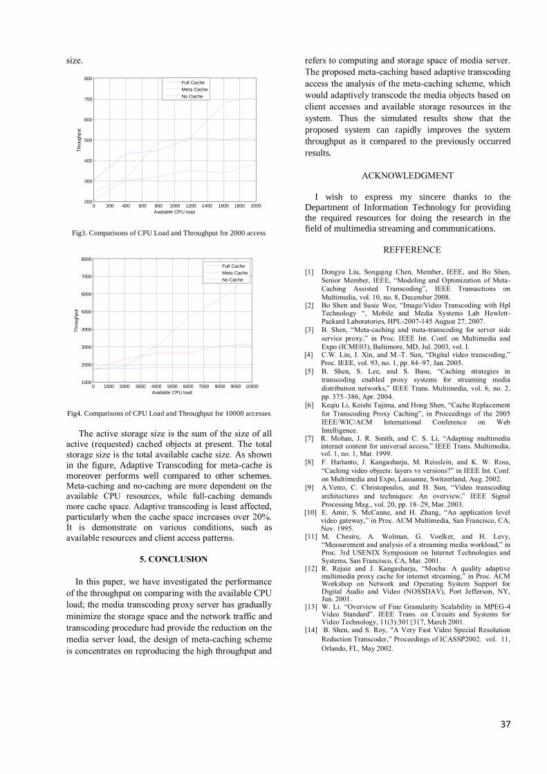
37
size.
0 200 400 600 800 1000 1200 1400 1600 1800 2000200
300
400
500
600
700
800
Available CPU load
Thro
ughput
Full Cache
Meta Cache
No Cache
Fig3. Comparisons of CPU Load and Throughput for 2000 access
0 1000 2000 3000 4000 5000 6000 7000 8000 9000 100001000
2000
3000
4000
5000
6000
7000
8000
Available CPU load
Thro
ughput
Full Cache
Meta Cache
No Cache
Fig4. Comparisons of CPU Load and Throughput for 10000 accesses
The active storage size is the sum of the size of all active (requested) cached objects at present. The total
storage size is the total available cache size. As shown
in the figure, Adaptive Transcoding for meta-cache is
moreover performs well compared to other schemes. Meta-caching and no-caching are more dependent on the
available CPU resources, while full-caching demands
more cache space. Adaptive transcoding is least affected,
particularly when the cache space increases over 20%. It is demonstrate on various conditions, such as
available resources and client access patterns.
5. CONCLUSION
In this paper, we have investigated the performance
of the throughput on comparing with the available CPU
load; the media transcoding proxy server has gradually
minimize the storage space and the network traffic and
transcoding procedure had provide the reduction on the
media server load, the design of meta-caching scheme
is concentrates on reproducing the high throughput and
refers to computing and storage space of media server.
The proposed meta-caching based adaptive transcoding
access the analysis of the meta-caching scheme, which
would adaptively transcode the media objects based on
client accesses and available storage resources in the
system. Thus the simulated results show that the
proposed system can rapidly improves the system
throughput as it compared to the previously occurred
results.
ACKNOWLEDGMENT
I wish to express my sincere thanks to the Department of Information Technology for providing
the required resources for doing the research in the
field of multimedia streaming and communications.
REFFERENCE
[1] Dongyu Liu, Songqing Chen, Member, IEEE, and Bo Shen,
Senior Member, IEEE, “Modeling and Optimization of Meta-
Caching Assisted Transcoding”, IEEE Transactions on
Multimedia, vol. 10, no. 8, December 2008. [2] Bo Shen and Susie Wee, “Image/Video Transcoding with Hpl
Technology “, Mobile and Media Systems Lab Hewlett-Packard Laboratories, HPL-2007-145 August 27, 2007.
[3] B. Shen, “Meta-caching and meta-transcoding for server side
service proxy,” in Proc. IEEE Int. Conf. on Multimedia and
Expo (ICME03), Baltimore, MD, Jul. 2003, vol. I. [4] C.W. Lin, J. Xin, and M.-T. Sun, “Digital video transcoding,”
Proc. IEEE, vol. 93, no. 1, pp. 84–97, Jan. 2005.
[5] B. Shen, S. Lee, and S. Basu, “Caching strategies in
transcoding enabled proxy systems for streaming media
distribution networks,” IEEE Trans. Multimedia, vol. 6, no. 2,
pp. 375–386, Apr. 2004.
[6] Keqiu Li, Keishi Tajima, and Hong Shen, “Cache Replacement
for Transcoding Proxy Caching”, in Proceedings of the 2005
IEEE/WIC/ACM International Conference on Web
Intelligence. [7] R. Mohan, J. R. Smith, and C. S. Li, “Adapting multimedia
internet content for universal access,” IEEE Trans. Multimedia, vol. 1, no. 1, Mar. 1999.
[8] F. Hartanto, J. Kangasharju, M. Reisslein, and K. W. Ross,
“Caching video objects: layers vs versions?” in IEEE Int. Conf.
on Multimedia and Expo, Lausanne, Switzerland, Aug. 2002.
[9] A.Vetro, C. Christopoulos, and H. Sun, “Video transcoding
architectures and techniques: An overview,” IEEE Signal
Processing Mag., vol. 20, pp. 18–29, Mar. 2003. [10] E. Amir, S. McCanne, and H. Zhang, “An application level
video gateway,” in Proc. ACM Multimedia, San Francisco, CA, Nov. 1995.
[11] M. Chesire, A. Wolman, G. Voelker, and H. Levy, “Measurement and analysis of a streaming media workload,” in Proc. 3rd USENIX Symposium on Internet Technologies and Systems, San Francisco, CA, Mar. 2001.
[12] R. Rejaie and J. Kangasharju, “Mocha: A quality adaptive multimedia proxy cache for internet streaming,” in Proc. ACM Workshop on Network and Operating System Support for Digital Audio and Video (NOSSDAV), Port Jefferson, NY, Jun. 2001.
[13] W. Li. “Overview of Fine Granularity Scalability in MPEG-4 Video Standard”. IEEE Trans. on Circuits and Systems for Video Technology, 11(3):301317, March 2001.
[14] B. Shen, and S. Roy, "A Very Fast Video Special Resolution
Reduction Transcoder,” Proceedings of ICASSP2002. vol. 11,
Orlando, FL, May 2002.

38
[15] S. Ota et al., “Architecture of Multimedia Data Transcoding
System for Mobile Computing,” 2000 IEICE General Conf., B-
5-174, Mar. 2000, (in Japanese), pp. 559.

Proceedings of the Third National Conference on RTICT 2010
Bannari Amman Insitute of Technology , Sathyamangalam 638 401
9-10 April 2010
39
DIGITAL IMAGE PROCESSING (DIP)
JPEG COMPRESSION WITH CLIENT BROWSER PLUG-IN APPROACH FOR
EFFICIENT NAVIGATION OVER INTERNET
K.Kavin Prabhu, Preethy Balakrishnan
Students, II-M.Sc Software Engineering
P.G. Department of Software Engineering
M.Kumarasamy College of Engineering
Thalavapalayam,Karur-639113,Tamilnadu,India
ABSTRACT
Image compression and
transmission has been steadily gaining in
importance with the increasing
prevalence of visual digital media. In this
work we present an application of the
latest image compression standard JPEG
in managing and browsing image
databases. Focusing on the image
transmission aspect, we combine the
technologies of JPEG image compression
with client-server socket connections and
client browser plug-in, as to provide with
an all-in-one package for remote browsing
of JPEG compressed image databases,
suitable for the effective dissemination of
cultural heritage. The main features of
JPEG, in which our implementation is
based upon, is progressiveness and
embedded bit stream syntax, which
implies the ability to extract from one
compressed file many different
resolutions or quality levels of an image,
depending on the user’s request.Our goal
was to achieve a more efficient way of
navigation. Particularly, in HTTP the
proposed system consists mainly of an
application specifically developed for
browsing JPEG images over the Internet
using JPIK (JPeg Interactive with Kakadu)
protocol rather than the World Wide Web
standard HTTP. On the other hand, in
wide spread browser, the system is based
on the implementation of a helper
application, which is a third-party piece of
software. The helper application has to be
distributed and is executed on the client
side whenever a request from a browser
activates it. In this case, the actual image
data are displayed in a separate window
and they cannot be manipulated from
within the browser. To overcome these
disadvantages, we decided to develop a
browser plug-in which is an approach
frequently used for displaying content
with in today’s internet browsers, which
increases the transmission rate.
1.INTRODUCTION
One of the major technical
problems that the Internet experiences
today is its data transmission rate
capability. The prohibitive transmission
rates for large images combined with
the need for enormous storage spaces
lead to the development of new coding
schemes to compress image
information. An example of such a
compression scheme with wide

40
acceptance on the Internet is JPEG . By
using JPEG on an image 10 * 15 cm at
600 dpi, we reduce the transmission
time through the modem line from 1 h
to about 30 s, while preserving a
moderate image quality (about 32 dB
PSNR).JPEG employs wavelet transform
to achieve energy compaction into a
small number of transform coefficients
and a highly sophisticated embedded
coding, combined with a binary
arithmetic encoder and rate control
mechanisms, packing data into a
meaningful, flexible and easily
parseable code stream. This new
standard shows great potential in aiding
the management and transmission of
images over the Internet and thus is one
of the most useful tools to adapt to a
cultural heritage database.
JPEG compression example:
JPEG compression example, (a) original image, 24 bpp, and transmission time about 1 h
and (b) compressed at 0.19 bpp, quality 32 dB PSNR and transmission time about 30 s.
The transmission of data is
done in a differential way, so that the
user accepts only the information
needed to move on to a next step in the
scenario. The interaction between the
user and the database server is
controlled by a socket connection, while
41
JPEG decoding and display is
accomplished by a client browser plug-
in. This means that the original image
code stream has to be structured in
such away as to include many different
resolutions and quality levels of itself.
At each request for one of these
resolutions or quality levels, the server
is responsible for extracting the
appropriate data from the original file
and for transmitting it to the client
where the final merging with the data
already existing from previous requests
would be accomplished.
2.JPEG CODING STEPS:
The key part for achieving
progressive image transmission in our
work is the use of JPEG, which provides
with a wide set of tools for image
compression. The main features of
JPEG, in which our implementation is
based upon, is progressiveness and
embedded bit stream syntax, which
implies the ability to extract from one
compressed file many different
resolutions or quality levels of an image,
depending on the user’s request. The
basic building blocks of the encoder are
shown.
3.SYNTAX OF JPEG CODESTREAM
The code stream syntax specifies such
fundamental quantities as image size, tile
size, number of components, and their
associated sub-sampling factors. It also
specifies all parameters related to
quantization and coding .most coding
parameters can be chosen on a tile by tile
basis. In the simplest case, a JPEG code
stream is structured as a main header
followed by a sequence of tile-streams.
The extension of such a JPEG file, as
proposed by the JPEG standard is noted
as “jpc” (JPEG Code stream).The main
header contains global information
Forward
Transform
Quantization Entrophy
Encoding
Compressed image data
Inverse
Transform
De-
Quantization
Entrophy
Decoding
Compressed image data
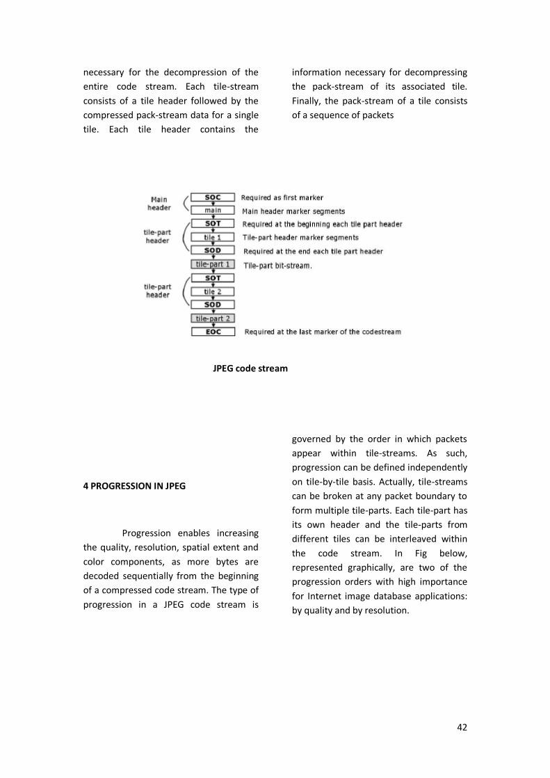
42
necessary for the decompression of the
entire code stream. Each tile-stream
consists of a tile header followed by the
compressed pack-stream data for a single
tile. Each tile header contains the
information necessary for decompressing
the pack-stream of its associated tile.
Finally, the pack-stream of a tile consists
of a sequence of packets
JPEG code stream
4 PROGRESSION IN JPEG
Progression enables increasing
the quality, resolution, spatial extent and
color components, as more bytes are
decoded sequentially from the beginning
of a compressed code stream. The type of
progression in a JPEG code stream is
governed by the order in which packets
appear within tile-streams. As such,
progression can be defined independently
on tile-by-tile basis. Actually, tile-streams
can be broken at any packet boundary to
form multiple tile-parts. Each tile-part has
its own header and the tile-parts from
different tiles can be interleaved within
the code stream. In Fig below,
represented graphically, are two of the
progression orders with high importance
for Internet image database applications:
by quality and by resolution.

43
5.CLIENT-SERVER TECHNOLOGY
Client-Server technology is based on
creating sockets to achieve the
communication between two or more
remote computers. A socket works much
like a telephone. It’s the end point of a
two way communication channel .By
connecting two sockets we can pass data
between processes, even processes
running on different computers, just as
we can talk over the telephone. Programs
written to use the TCP protocol are
developed using the client-server model.
When two programs use TCP to exchange
data, one of the programs must assume
the role of the client and the other the
role of the server. The client application
initiates what is called an active open. It
creates a socket and actively attempts to
connect to a server. On the other
hand,the server application creates a
socket and listens for incoming
connections from clients, performing
what is called a passive open . When the
client initiates a connection, the server is
notified that some process is attempting
to connect with it. By accepting the
connection, the server completes what is
called a virtual circuit, a logical
communication pathway between the
two programs
6.IMPLEMENTATION
For the purposes of our application
all of the aforementioned technologies
were combined in order to achieve a
progressive and dynamic way of accessing
the images in a database. Our
implementation includes a server and a
client application
6.1 PREPARATION OF DATABASE
IMAGES: To be able to extract from a
single image code stream multiple
segments that correspond to user
requests, a specific way of encoding
should be followed. Code stream data
must be arranged in resolution level
blocks, so that each sequential resolution
level added to the previous would
produce a greater resolution and
specifically of double width and height,
due to the nature of the wavelet
transform in JPEG. In order to have
images encoded in a way that the first
resolution level has maximum
dimensions, say 64*64 pixels, we have to
estimate the number of decomposition
levels needed for each image in order to
achieve the thumbnail resolution of

44
64*64 pixels, and to compress each image
using lossless JPEG coding.
nw ≤ log2 w/w′, nh ≤ log2 h/h′
n = [maxnw,nh]
where w and h are the width and height
of the original image, w’ and h’ are the
desired width and height, and ‘nw ‘and ‘nh
‘ stand for how many times the image
must be divided by 2 across the width and
height resolutions respectively, to
produce a desired resolution. In our case
the values of w’ and h’ are preset to 64
pixels. Thus, the number of wavelet
decomposition levels ‘n’ must be the
immediate greater integer of the
maximum value between ‘nw ‘and ‘nh ‘
Code stream structure of data base image
This way images will be encoded with
resolution levels (there will be n+1 SOT’
markers in the code stream), ensuring
that the image thumbnail will be of 64*64
pixels maximum resolution. A
representation of the code stream
structure of such an image is illustrated in
Fig above. Hereafter, the database
compressed images are ready to be used
by the server for code stream processing
and progressive transmission to any
remote user through the Internet.
6.2 THE SERVER
The server must be working in
multithreaded mode, so that it can
process many client connections at the
same time, something mandatory for our
application. The server has the ability to
send an image of any resolution by
parsing the image code stream and
selecting the required segments.
Additionally, it can automatically create
the respective HTML files through which
the clients can view the desired images in

45
desired resolutions. Each time a client
requests the thumbnail resolution of an
image, the server sends the respective
code stream segment, including the main
header. When the client has a specific
resolution already available and requests
for a greater one, the server sends the
appropriate differential information:
those tile-parts that correspond to the
requested resolution, not including the
main header and the already sent tile-
parts. The client should be able to merge
them into one single meaningful code
stream. For automation of the
process, the HTML pages in which the
images of each resolution are being
displayed are created on the server side,
always a step ahead of the next greater
resolution.
6.3 THE CLIENT:
The client consists of a browser
plug-in application. The plug-in is
responsible for receiving the coded JPEG
code stream from the server, decoding it,
and then displaying the resulting image
inside user’s browser. After the browser
locates, from the MIME type of the
EMBED tag, the suitable plug-in that must
be executed, it calls it and the whole
control of receiving and sending data is
passed to the plug-in. Particularly, when
the browser starts, all available plug-ins
are loaded into memory. Then the plug-in
follows the below logical flow chart.
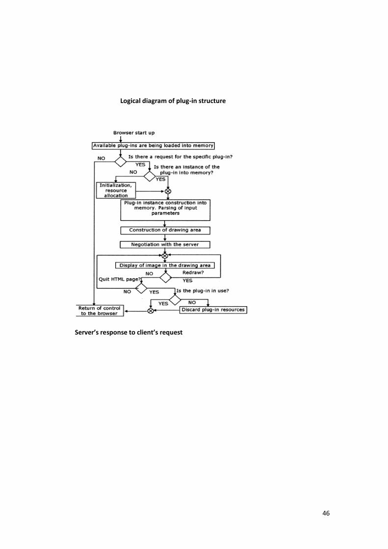
46
Logical diagram of plug-in structure
Server’s response to client’s request
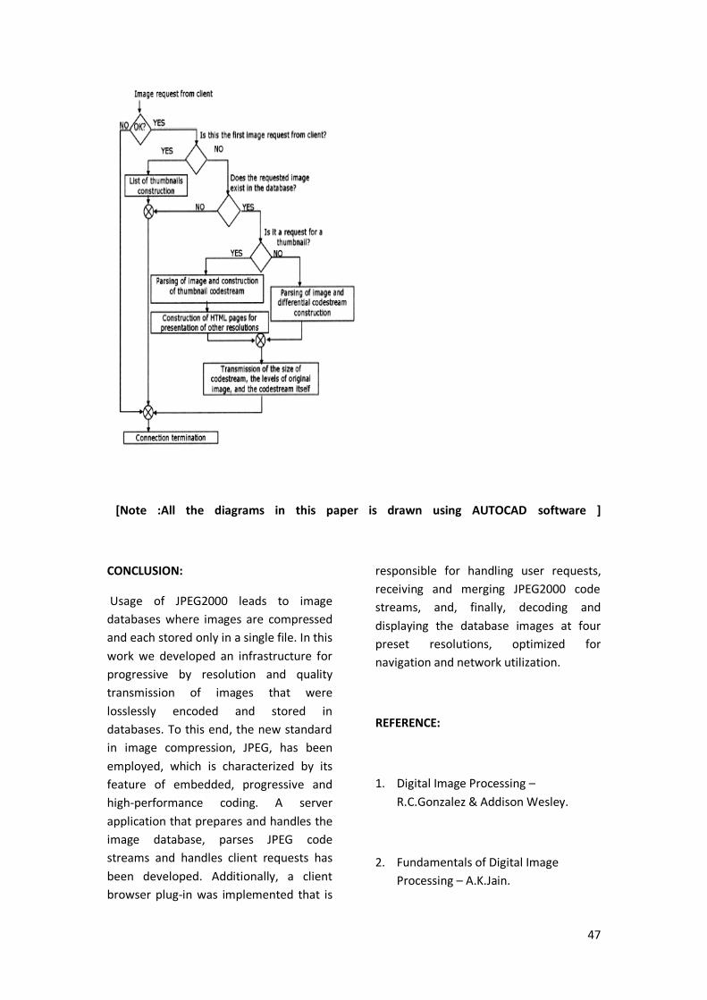
47
[Note :All the diagrams in this paper is drawn using AUTOCAD software ]
CONCLUSION:
Usage of JPEG2000 leads to image
databases where images are compressed
and each stored only in a single file. In this
work we developed an infrastructure for
progressive by resolution and quality
transmission of images that were
losslessly encoded and stored in
databases. To this end, the new standard
in image compression, JPEG, has been
employed, which is characterized by its
feature of embedded, progressive and
high-performance coding. A server
application that prepares and handles the
image database, parses JPEG code
streams and handles client requests has
been developed. Additionally, a client
browser plug-in was implemented that is
responsible for handling user requests,
receiving and merging JPEG2000 code
streams, and, finally, decoding and
displaying the database images at four
preset resolutions, optimized for
navigation and network utilization.
REFERENCE:
1. Digital Image Processing –
R.C.Gonzalez & Addison Wesley.
2. Fundamentals of Digital Image
Processing – A.K.Jain.

48
3. www.sigmedia.com
4.D.Artz. Digital Steganography; hiding
Data within Data, IEEE Internet
Computing, Vol.5
5.N.F. Johnson, S. Jajodia, Steganalysis :
The Investigation of Hidden Information
Proc. IEEE Information Technology Conf.

Abstract — In this paper, we propose the Multichannel
blind image deconvolution technique to restore the input image
from blurred and noisy images. The direct image restoration
methods are: Mutually Referenced Equalizer (MRE) and
Regularized Mutually Referenced Equalizer (RMRE). The MRE
method based on inverse filtering works only in noiseless case for
perfect image restoration. In noisy environment regularization
method (R-MRE) is used. The objective function of R-MRE
method is to avoid noise amplification. Another restoration
method is identification of PSF for Multichannel blind
deconvolution method. We determine the degradation filter.
Next, using the degradation filter, original image is restored.
Finally, the performance of the two restoration method can be
analyzed using quality of the image.
I. INTRODUCTION
OWADAYS, Multichannel(MC) image processing is
relatively active field of research. Normally MC method
is used in signal case, now it is extended to the image.
Because of increasing number of application where several
directions of the captured image are available, In Multichannel
framework, in a single scene observed by several images and
it passes through different channels. The multispectral images
are used in frequency band channel. In different time slots, we
captured different images are provided at different resolution.
This is also treated as Multichannel representation. The
advantages of MC processing is to exploit the diversity and
redundancy of information in the different images. Hence, the
set of observed images are considered as one entity based on
it‘s worth.
Image deconvolution/restoration solutions can be divided
into two classes: stochastic and deterministic. Stochastic
methods consider observed images as random fields and
estimate the original image as the most probable realization of
a certain random process. These methods are, mainly, the
linear minimum mean squares error (LMMSE) [13], the
maximum likelihood (ML) [11], and the maximum a
posteriori (MAP) [3]. These methods have two major
drawbacks: i) they are very sensitive to perturbations and
modeling errors, ii) strong statistical hypothesis are made on
the image and the noise which are considered as uncorrelated
homogeneous random processes. On the other hand,
deterministic methods do not rely on such hypothesis and
estimate the original image by minimizing a norm of a certain
residuum. These methods include among others: constrained
least square (CLS) methods which incorporate a regularization
term [12], the iterative blind deconvolution technique [5] and
the non-negativity and support constraint—recursive inverse
filtering (NAS-RIF) algorithm [10]. The latter methods are
based on minimizing a certain criterion under some constraints
like non-negativity of the original image, finite support of the
convolution masks, smoothness of the estimate, etc.
Blind MC image deconvolution can be performed in two
restoration method. The original image is directly using
equalization or inverse filtering technique called Mutually
Referenced Equalizers (MRE). The MRE method is not a
perfect restoration method at the noise environment. Then the
regularization term is incorporated in order to perfect from
noise amplification. In PSF Identification method, first
identify the filter then it will restore the original image using
the identified filter. We compared these techniques in terms of
estimation accuracy (restored image quality). More precisely,
our contributions consist of i) a new blind restoration method
using the mutually referenced equalizers technique in
conjunction with a regularization method that truncates the
greatest singular values of the inverse filter matrix; ii) a new
robust Multichannel restoration method based on a total
variation technique; and iii) a performance evaluation and
comparative study of the different blind restoration methods
using some objective image quality metrics.
II. MOTIVATION FOR MC PROCESSING
The motivations behind the use of MC framework as
compared to the standard mono-channel one are first the
increasing number of applications in this field, but more
importantly, the potential diversity gain that may lead to
significant improvements in the restored image quality. And
another method based on the iterative Richardson–Lucy
scheme. Clearly, this example highlights the performance
gain that can be obtained by MC processing. This gain is due
to the inherent diversity of Multichannel systems where
multiple replica of the same image is observed through
different (independent) channels. In that case, if a part of the
original information is lost (degraded) in one of the observed
images, it can be retrieved from the other observed images
upon certain diversity conditions. More precisely, this is
possible when the same image distortion does not occur on all
the observed images simultaneously. Mathematically, this is
expressed in the condition that the spectral transforms of the
PSF’s do not share common zeros. Indeed, a PSF’s zero
represents roughly a “fading” around a particular frequency
point, and, hence, common zeros represent the situation where
the same fading occurs on all channels simultaneously. In the
presence of noise, perfect reconstruction is not possible but the
Image Restoration Using Regularized
Multichannel Blind Deconvolution Technique
Munia Selvan L, Vinoth Kumar C
Department of ECE, SSN College of Engineering Mail id: [email protected], [email protected]
N
Proceedings of the third National conference on RTICT 2010Bannari Amman Insitute of Technology , Sathyamangalam 638 401
9-10 April 2010
49

diversity gain provides significant improvement in the restored
image quality. For the MC case, we use the restoration method
with the PSF identification approach (Section VI). One can
observe that the gain increases in terms of image restoration
quality when using the MC processing. Furthermore, this gain
is obtained with a relatively small number of independent
PSFs (3 to 4 depending on the SNR level), which limits the
extra computational burden of MC processing.
III. PROBLEM STATEMENT
A. Notations
It is assumed that a single image passes through K>2
independent channels and, hence, K different noisy blurred
images are observed. Each channel corresponds to a degrading
filter. The PSF functions are assumed to have no common
zeros, i.e., the polynomials are strongly co-prime.
KkzzjiHkzzHj
m
i
n
j
i
k
h h
,,,,1,).(),( 2
1
0
1
0
121 == −−
=
−
=
−∑∑ ….(1)
Then the system model can be written as
),(),(),(),(1
0
21
1
0
21 nmNlnlmFllHnmG k
m
i
n
j
kk
h h
+−−×= ∑∑−
=
−
=
….(2)
In the above eqn, F (m, n) is the original image of size (mf,
nf). Hk is the point spread function (PSF) of Kth image and its
size is (mh, nh). The Kth channel degraded images Gk of its size
is (mg, ng). In the sequel, the images and impulse responses
will be processed in a vectorized, windowed form of size (mw,
nw). Hence, we denote Gk (m, n) by the data vector
corresponding to a window of the Kth image where the last
pixel is indexed by (m,n), i.e., the right bottom pixel.
T
wwk
wkkk
nnmmG
nnmGnmGnmg
)]1,1(,,,,,
)1,(,,,),,([),(
+−+−
+−= ….(3)
In order to exploit the diversity and the redundancy offered
by the multiple observations of F, we deal simultaneously with
all observed images by merging them into a single observation
vector
[ ]TT
k
Tgnmgnmg ,,,,,,,),,(),( 1=
),(),( nmnnmHf +=
….(4)
B. Objectives
The ultimate goal is to restore the original image in a
satisfactory way even in “severe” observation conditions. In
practice, the original image as well as the degrading filters is
totally unknown, so that our restoration procedure is totally
blind. To tackle this problem two types of solutions are
proposed. The direct image restoration technique [2] and the
indirect one, that first estimates the unknown PSFs and then
restores the original image in a nonblind way (i.e., using the
previously estimated PSFs) [1]. 1) Direct Restoration:
Our objective here is to directly restore the original image
using only its degraded observed versions. More precisely, we
search for a unique equalizer or inverse filter which, applied to
the set of observations, allows us to restore the original image.
We pay a particular attention to the robustness against additive
noise by including in the estimation criterion of the inverse
filter an additional term that controls and limits the noise
effect.
2) Restoration via PSF Identification:
Our objective here is to, first identify the PSF function and
then inverse it in order to restore the original image. In the
noisy case, the filter response inversion leads to noise
amplification, and, hence, we propose to add a regularization
term in order to reduce this undesired effect.
IV. MUTUALLY REFERENCED EQUALIZERS (MRE)
In this section, we introduce our first image restoration
method using the direct estimation of the inverse filters. These
filters are estimated by MRE method in [9]. The proposed
method builds on the concept of the mutually referenced
equalizers (MRE), which were first introduced in which a set
of K (K>1) filters are considered, the outputs of which act as
training signals for each other. A multidimensional mean-
square error MRE criterion for blind MC equalization is
derived, and certain minimization procedures are discussed.
The obtained algorithm is shown to meet several conditions of
important practical concern:
1) The MRE criterion is unimodal; hence, the algorithm
exhibits global convergence.
2) The MRE criterion is a mean-square error. Full flexibility is
gained for the implementation. In contrast, flexibility of
design is difficult to obtain with subspace decomposition
methods as well as with adaptive BE methods relying on a
high-order nonlinear cost.
3) The method directly provides channel inverses with all
possible delays, hence, yielding robustness with respect to the
noise amplification problems that may be related to a specific
delay (typically the minimum and maximum delays yield poor
results if the channel has coefficients that taper off at the
ends).
4) Finally, the MRE method shows empirical robustness in the
presence of channel length mismatch. We investigate the
theoretical properties of the MRE criterion in the noise-free
case and show that its minimization is necessary and sufficient
for linear MC equalization. We show that the MRE criterion is
a multidimensional MSE that has to be constrained in order to
avoid the convergence toward undesirable solutions.
We search, here, for the restoration filter denoted η which,
applied to the Κ observed images, provides us with an
estimate of the original image. This η is a Multichannel 2-D
filter of size (Kme, Kne) filter exists under the following
assumptions: i) the PSFs have no common zeros [2] and ii) the
filter matrix has full column-rank [9].
)1)(1( −+−+≥Κ ehehee nnmmnm ….(5)
When both conditions are satisfied, there exists a set of
equalizers η1,…ηd each of them allowing us to restore the
original image with a specific spatial shift (md,nd). Note that
there exists an infinity of equalizers of different sizes (an
infinity of couple (me,ne) that satisfy the condition. Hence,
when is fixed, the original image is estimated up to a certain
constant factor and a certain spatial shift. The principle of
50

mutually referenced equalizers is as follows: suppose we have
computed two equalizers ηi and ηj inducing the spatial shift
(mi , mj) and (ni , nj) respectively
),(),,(),(1
, nmnnmmFnmG iik
k
ki ∀−−=∗∑Κ
=
αη ….(6)
),(,),(),(1
, nmnnmmFnmGk
jjkkj ∀−−=∗∑Κ
=
αη ….(7)
where αis a given positive scalar
kiiii ,,1, ],......,[ ηηηη Κ∆ ….(8)
being the 2-D filter of size (me, ne) applied to the Kth observed
image.
In the noiseless case, if we apply the equalizer ηi to G(m-mj ,
n-nj) and the equalizer ηj to G(m-mi , n-ni), we obtain exactly
the same windowed area of the original image.
∑∑Κ
=
Κ
=
−−∗=−−∗1
,
1
, ),(),(k
jjkki
k
iikkj nnmmGnnmmG ηη
….(9)
This solution presents a major drawback: it requires the
computation of a large number of equalizers and, hence, it is
computationally expensive. We can reduce the number of
equalizers to be estimated it is shown in [9] and [7],
consequently, the computational cost of this solution. More
precisely, it was proved that only 2 extremal equalizers taken
from the Kth observed image. The two equalizers are in
boundary of observed image are like (0,0) and (me+mh-1,
ne+nh-1) are sufficient perfect image restoration In practice,
these shifts do not appear to perform good restoration quality
due to the artifacts appearing in the boundaries of the restored
image. Therefore, we propose to use a third equalizer
corresponding to the median shift
))2/()2/(()3,3( 22 nmnm ⋅= ….(10)
where . the integer part. Solving the equalizers η1, η2 and
η3 consists in solving the following set of linear equations
∑∑
∑∑
∑∑
Κ
=
Κ
=
Κ
=
Κ
=
Κ
=
Κ
=
−−∗=−−∗
−−∗=−−∗
−−∗=−−∗
1
11,3
1
33,1
1
33,2
1
22,3
1
22,1
1
11,2
),(),(
),(),(
),(),(
k
kk
k
kk
k
kk
k
kk
k
kk
k
kk
nnmmGnnmmG
nnmmGnnmmG
nnmmGnnmmG
ηη
ηη
ηη
….(11)
V. REGULARIZED MUTUALLY REFERENCED
EQULAIZER
In the noisy case, the MRE algorithm fails in restoring
efficiently the image. This is due to the ill-conditioned filter
matrix whose inversion leads to noise amplification. In order
to come through this difficulty, we propose, here, to combine
the MRE criterion with a regularization technique [8] and
adapted to the multichannel framework. In fact, the noise
amplification is due to the largest singular values of the
Inverse Filter Matrix. Therefore, our regularization technique
simply consists in the truncation of the largest singular values
of the IFM. This truncation is realized through an adaptive
thresholding technique, which is explained below. Now, to
reduce the computational cost of the desired eigenvalues, we
exploit the Toeplitz structure and the large dimension of the
inverse filter matrix in such a way to approximate it by a block
circulant matrix [14] whose eigenvalues can be computed by
means of Fourier transform [4].
In this paper, we choose η3 among the MRE equalizers to
restore the original image as it provides the best restoration
performance compared to external shift equalizers η1 and η2
as mentioned previously. Let us write this equalizer as
]......,[ ,31,33 Κ∆ ηηη ….(12)
Let Ek be the IFM associated with γ3,K . Since Ek is a
large block Toeplitz matrix with Toeplitz blocks, a large block
circulant matrix with Ek circulant blocks can approximate it.
This approximation leads to the following estimation
=−
132
11
21
:
EEE
EEE
EEE
EEKK
K
k
L
M
L
L
….(13)
Then the above equation becomes,
∗
∗≈
31 f
g
g
E
k
M
….(14)
We propose to truncate the largest eigenvalues of E to avoid
noise amplification when restoring the original image. A well-
known property of circulant matrices is that their eigenvalues
can be expressed as a function of the elements of the first
column. This property can be extended to block circulant
matrices by considering the first column of each column
block. Since E is a block circulant matrix with circulant blocks
Ek [14]
MeuuuT
n == Κ ][ 1L . ….(15)
where u is a vector containing the eigenvalues of E, M is a
known sparse matrix and n is the number of pixels in the
restored image.
VI. IMAGE RESTORATION USING PSF
IDENTIFICATION METHOD
a) Image restoration algorithm using Wiener filter
If the image and the noise are assumed to be generalized
stationary process, image may be restored through Wiener
filter. When the discrete Fourier transform (DFT) method is
51

used to estimate the restored image, the Wiener filter may be
expressed as follows:
+
=
xx
nn
SS
H
YHZ
2
2
….(16)
where, X, Y and H are the DFT of the real image (x), the
blurred image (y) and the blur function (h) respectively; *
denotes the conjugate operation; Snn and Sxx denote the
power spectrum of the noise and the real image. As it is
usually very difficult to estimate Snn and Sxx, the Wiener
filter is usually approximated by the following formula:
( )Γ+=
2
2
H
YHZ ….(17)
where, Γ is a positive constant. The best value of Γ is the
reciprocal of the SNR of the observed image.
b) SNR estimation of image
The estimated signal-to-noise ratio (SNR) may be a reference
to select the regularized parameters in the Wiener filtering
restoration algorithm. The SNR of a blurred image is usually
defined as follows:
= 2
2
10log10n
xSNRδ
δ ….(18)
where 2
xδ is the variance of the blurred image, and 2
nδ is the
variance of the noise.
The local variances between the flat region and the edge are
different from each other in an image. Places with large local
variance shows that there are much detail information, and
places with small local variance means that it is relatively flat
in this region. If the quality of the observed image is good (for
example, the SNR is above 30dB), it is reasonable to take the
region with the maximum local variance as the edge, and to
take the area with the minimum local variance as the flat
region. Thus, the variance of the image (δ) is taken as the
maximum local variance, and the variance of the noise (δn) is
approximated as the minimum local variance. The local
variance of the observed image (y) at position (i,j) is defined
as follows:
[ ]
( ))12)(12(
),(),(2
2
++
−++
=
∑ ∑−= −=
qp
jiljkiyp
pk
q
ql
y
yl
µ
δ ….(19)
where, p and q are the sizes of the local area; µ y denotes
the local mean value which is defined as follows:
[ ]
( ))12)(12(
),(
++
++
=
∑ ∑−= −=
qp
ljkiyp
pk
q
ql
yµ ….(20)
Generally, the local variance is taken as p=q=2, and the
template may be expressed as:
++=
11111
11111
11111
11111
11111
)12)(12[(
1
qpe
….(21)
So, the local mean value may be denoted as:
[ ]
( )
[ ]
cy
lksljkiy
qp
ljkiy
p
pk
q
ql
p
pk
q
ql
y
*
),(.),(
)12)(12(
),(
=
++=
++
++
=
∑ ∑
∑ ∑
−= −=
−= −=µ
….(22)
The local variance may be written as:
( )[ ]
( )( )( )
( )[ ] [ ][ ]
( ) cy
lkejiljkiy
qp
jiljkiy
ji
y
p
pk
q
ql
y
p
pk
q
ql
y
yk
*
),(),(,
1212
),(,
),(
2
2
2
2
µ
µ
µ
δ
==
−−++=
++
−++
=
∑∑
∑∑
−= −=
−= −=
….(23)
Thus, the SNR of image y may be estimated as the ratio of
the maximum local variance and the minimum local variance,
namely:
( ))min()max(log10 22
10 ylylSNR δδ= ….(24)
c) Estimation of Gaussian PSF
Gaussian point spread function (PSF) is the most common
blur function of many optical measurements and imaging
systems. Generally, the Gaussian PSF may be expressed as
follows:
( ) ( )
∈
+−
=
others
Rnmnmnmh
,0
,2
1exp
2
1
),(
22
2δπδ ….(25)
where, δ is the standard deviation; R is a supporting region.
Commonly, R is denoted by a matrix with size of K×K, and K
is often an odd number. Thus, two parameters that are the size
(K) and the standard deviation (δ) need to be identified for the
Gaussian PSF. Because the Fourier transformation of a
Gaussian function is still a Gaussian function, it is impossible
to identify the parameters by the zero- crossing point in the
frequency domain. But in many cases, the isolated point and
the intensity edges in the observed image may provide the
necessary information to identify the blurring function.
In Wiener filtering algorithm, in order to restrain the parasitic
ripple induced by the boundary cutoff, the image needs to
have circular boundary. For the observed image (y) with size
of M × N, reflection symmetric extension is performed on it,
52

and the size of the extended image becomes 2M×2N. Then,
calculate the Fourier transformation of the extended image
(Y). Given a size (K) of the PSF, the error-parameter curve is
generated at different standard deviations (δ). According to
error-parameter the curves at different sizes, we can estimate
these two parameters approximately. The identification
process is expressed as follows:
Step 1: Select a standard deviation range given by the
minimum value (δmin) and the maximum value (δmax)
Step 2: Set a searching number (S), and we will get:
∆δ=(δmax-δmin) /S
Step 3: Set different sizes (K) of the PSF, repeating Step 4
Step 4: For i=1:S, repeat Step 4.1~ Step 4
Step 4.1: Compute the current standard deviation:
si ∆−+= )1(minδδ
Step 4.2: Generate the Gaussian blurring function h according
to K and δ
Step 4.3: Add zeroes to h and make it to be the size of
2M×2N, and compute its DFT (H)
Step 4.4: According to equation (24), estimate the Fourier
transformation of the real image (X)
Step 4.5: Compute the estimation error: K=||Y-ZH||2, and
normalize it
Step 5: Plot the error-parameter curves at different sizes
Step 6: Give an estimation error (e), calculate the distance
between curves, the curve once the distance (d) is smaller than
threshold T1 represent the real parameters, from which the
size (K) of the PSF is estimated
Step 7: Calculate the increment at different standard
deviations on this curve, once the increment is greater than
threshold T2, the deviation (δ) of the PSF is estimated
VII. SIMULATION RESULTS
In the following, we test the image restoration performance
using regularized MRE and identification of PSF based
restoration. Experiments were carried out for an image: the
cameraman one which has a homogeneous background with a
man in the middle. These images are adequate to measure the
ability of the developed algorithms to restore the image details
and edges as well as the homogeneous area. In all
experiments, the degraded images are altered by a set of PSFs,
which simulate a camera motion, a motion, average and a
gaussian filtering. The number of observed images
corresponding to the number of independent PSFs is K=4 and
the PSFs’ size is 3x3. We first propose to the regularized
version of the MRE algorithm and the nonregularized one for
a set of degraded images.
(a) (b)
Fig.1 (a) Original image. (b) Blurred image with motion filter
(a) (b)
Fig.2 (a) Blurred image with average filter (b) Gaussian filter
(a) (b)
(c)
Fig.3. Restoration using MRE method, the equalizer obtained
by different spatial shifts
(a) (b)
(c) (d)
Fig.4.Restored image using PSF identification of Multichannel
(a) Channel 1 (b) Channel 1 &2 (c) Channel 1,2 & 3 (d)
Channel 1,2,3 & 4.
53
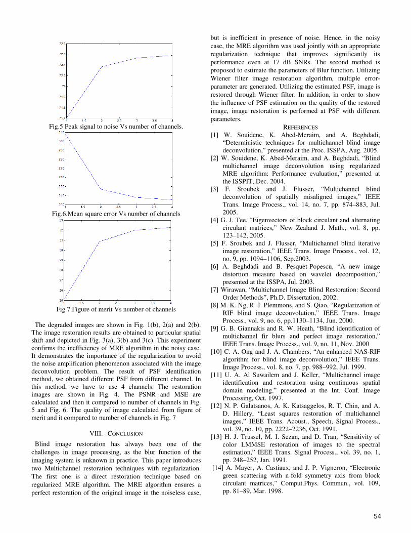
Fig.5 Peak signal to noise Vs number of channels.
Fig.6.Mean square error Vs number of channels
Fig.7.Figure of merit Vs number of channels
The degraded images are shown in Fig. 1(b), 2(a) and 2(b).
The image restoration results are obtained to particular spatial
shift and depicted in Fig. 3(a), 3(b) and 3(c). This experiment
confirms the inefficiency of MRE algorithm in the noisy case.
It demonstrates the importance of the regularization to avoid
the noise amplification phenomenon associated with the image
deconvolution problem. The result of PSF identification
method, we obtained different PSF from different channel. In
this method, we have to use 4 channels. The restoration
images are shown in Fig. 4. The PSNR and MSE are
calculated and then it compared to number of channels in Fig.
5 and Fig. 6. The quality of image calculated from figure of
merit and it compared to number of channels in Fig. 7
VIII. CONCLUSION
Blind image restoration has always been one of the
challenges in image processing, as the blur function of the
imaging system is unknown in practice. This paper introduces
two Multichannel restoration techniques with regularization.
The first one is a direct restoration technique based on
regularized MRE algorithm. The MRE algorithm ensures a
perfect restoration of the original image in the noiseless case,
but is inefficient in presence of noise. Hence, in the noisy
case, the MRE algorithm was used jointly with an appropriate
regularization technique that improves significantly its
performance even at 17 dB SNRs. The second method is
proposed to estimate the parameters of Blur function. Utilizing
Wiener filter image restoration algorithm, multiple error-
parameter are generated. Utilizing the estimated PSF, image is
restored through Wiener filter. In addition, in order to show
the influence of PSF estimation on the quality of the restored
image, image restoration is performed at PSF with different
parameters.
REFERENCES
[1] W. Souidene, K. Abed-Meraim, and A. Beghdadi,
“Deterministic techniques for multichannel blind image
deconvolution,” presented at the Proc. ISSPA, Aug. 2005.
[2] W. Souidene, K. Abed-Meraim, and A. Beghdadi, “Blind
multichannel image deconvolution using regularized
MRE algorithm: Performance evaluation,” presented at
the ISSPIT, Dec. 2004.
[3] F. Sroubek and J. Flusser, “Multichannel blind
deconvolution of spatially misaligned images,” IEEE
Trans. Image Process., vol. 14, no. 7, pp. 874–883, Jul.
2005.
[4] G. J. Tee, “Eigenvectors of block circulant and alternating
circulant matrices,” New Zealand J. Math., vol. 8, pp.
123–142, 2005.
[5] F. Sroubek and J. Flusser, “Multichannel blind iterative
image restoration,” IEEE Trans. Image Process., vol. 12,
no. 9, pp. 1094–1106, Sep.2003.
[6] A. Beghdadi and B. Pesquet-Popescu, “A new image
distortion measure based on wavelet decomposition,”
presented at the ISSPA, Jul. 2003.
[7] Wirawan, “Multichannel Image Blind Restoration: Second
Order Methods”, Ph.D. Dissertation, 2002.
[8] M. K. Ng, R. J. Plemmons, and S. Qiao, “Regularization of
RIF blind image deconvolution,” IEEE Trans. Image
Process., vol. 9, no. 6, pp.1130–1134, Jun. 2000.
[9] G. B. Giannakis and R. W. Heath, “Blind identification of
multichannel fir blurs and perfect image restoration,”
IEEE Trans. Image Process., vol. 9, no. 11, Nov. 2000
[10] C. A. Ong and J. A. Chambers, “An enhanced NAS-RIF
algorithm for blind image deconvolution,” IEEE Trans.
Image Process., vol. 8, no. 7, pp. 988–992, Jul. 1999.
[11] U. A. Al Suwailem and J. Keller, “Multichannel image
identification and restoration using continuous spatial
domain modeling,” presented at the Int. Conf. Image
Processing, Oct. 1997.
[12] N. P. Galatsanos, A. K. Katsaggelos, R. T. Chin, and A.
D. Hillery, “Least squares restoration of multichannel
images,” IEEE Trans. Acoust., Speech, Signal Process.,
vol. 39, no. 10, pp. 2222–2236, Oct. 1991.
[13] H. J. Trussel, M. I. Sezan, and D. Tran, “Sensitivity of
color LMMSE restoration of images to the spectral
estimation,” IEEE Trans. Signal Process., vol. 39, no. 1,
pp. 248–252, Jan. 1991.
[14] A. Mayer, A. Castiaux, and J. P. Vigneron, “Electronic
green scattering with n-fold symmetry axis from block
circulant matrices,” Comput.Phys. Commun., vol. 109,
pp. 81–89, Mar. 1998.
54

Proceedings of the Third National Conference on RTICT 2010
Bannari Amman Insitute of Technology , Sathyamangalam 638 401
9-10 April 2010
55
TEXT EXTRACTION IN VIDEO
J.Dewakhar
Student, II- M.Sc- information Technology
P.G. Department of Information Technology
M.KumarasamyCollege of Engineering,
ThalavapalayamKarur-639113,Tamilnadu,India
E-Mail: [email protected], Contact No: 9789258879
K.Prabhakaran
Student, II- M.Sc- information Technology
P.G. Department of Information Technology
M.KumarasamyCollege of Engineering,
ThalavapalayamKarur-639113,Tamilnadu,India
E-Mail: mit816prabu@yahoo., Contact No: 978696921
Abstract
Text data present in images and video contain useful information for automatic
annotation, indexing, and structuring of
images. Extraction of this information involves detection, localization, tracking,
extraction, enhancement, and recognition of
the text from a given image. However,
variations of text due to differences in size, style, orientation, and alignment, as well as
low image contrast and complex background
make the problem of automatic text
extraction extremely challenging. Most work so far has made restrictive
assumptions about the nature of text
occurring in video. Such work is therefore not applicable to unconstrained, general-
purpose video.
In this paper we present methods for
automatic segmentation of caption text in digital videos. The output is directly passed

56
to a standard OCR software package in
order to translate the segmented text into ASCII. The algorithms we propose make
use of typical characteristics of text in
videos in order to enable and enhance
segmentation performance. Especially the inter-frame dependencies of the characters
provide new possibilities for their
refinement. Keywords-segmentation, caption text, OCR,
text extraction, general-purpose video
1 Introduction Nowadays the volume of data contained in
video format makes necessary to create useful tools, which allow extracting
information from these video sequences in
order to classify (e.g. indexation) or to analyse (e.g. CBIR) them without human
supervision. Contents can be perceptual,
such as colour, shapes, textures, etc., or semantic, such as objects, text or events and
its relationships. The perceptual ones are
easier to analyse automatically while the
semantic are easier to handle linguistically. Caption or superimposed text is a semantic
content whose computational cost is lower
than the cost of others semantic contents. Due to the fact that usually text is
synchronized and related to the scene, its
extraction becomes a useful feature
providing very relevant information for the semantic analysis.
Although text is easily detectable for
humans, even in the case of a foreign language, up to our knowledge, there are no
methods allowing its extraction in any kind
of video sequence. This is due to the fact that there is a wide range of text formats
(size, style, orientation), the low resolution
of the images (quality) and the complexity
of the background. Despite these facts, text lines present some
homogeneity features, which make it
detectable such as contrast, spatial cohesion, textured appearance, colour homogeneity,
stroke thickness, temporal uniformity,
movement on the sequences, position on the frame, etc.
Therefore, the aim of this paper is to
introduce our methods for automatic text segmentation in digital videos. Text features
are presented in Section 2,followed by
description of our segmentation algorithms
in Section 3, which are based on the features stated in Section 2. Information about the
text recognition step is given in Section 4.
Section 5 reviews the related work. Section 6concludes the paper.
2 Text Features Text may appear anywhere in the video and in different contexts. We discriminate
between two kinds of text: scene text and
artificial text. Scene text appears as a part of
and was recorded with the scene, whereas artificial text was produced separately from
the video shooting and is laid over the scene
in a post-processing stage, e.g. by video title machines.The following features
characterize the mainstream of artificial text
appearances: Characters are in the foreground. They are
never partially occluded. Characters are
monochrome. Characters are rigid. They do
not change their shapeframe. Characters have size restrictions. A letter is not as large
as the whole screen, nor are letters smaller
than a certain number of pixels as they would otherwise be illegible to viewers.
Character are mostly upright. Characters are
either stationary or linearly moving. Moving
characters also have a dominant translation direction: horizontally from right to left or
vertically from bottom to top. Characters
contrast with their background since artificial text is designed to be read easily.
The same characters appear in multiple
consecutive frames. Characters appear in clusters at a limited distance aligned to a
horizontal line, since that is the natural
method of writing down words and word
groups. Our text segmentation algorithms are based on these features.
3 Text Segmentation The objective of text segmentation is to produce a binary image that depicts the text
appearing in the video. Hence, standard
OCR software packages can be used to recognize the segmented text. All the
processing steps are performed on color

57
images in the RGB color space and not on
grayscale images.
3.1 Color Segmentation First each frame is segmented into suitable
objects. The monochromaticity character feature is taken as grouping criterion for
pixels and contrast with the local
environment is taken as the separation
criterion for pixels. Together with a segmentation procedure, which is capable of
extracting monochrome regions that contrast
highly to their environment under significant noise, suitable objects can be constructed.
Such a segmentation procedure preserves
the characters of artificial text occurrences. Its effect on multicolored objects and/or
objects lacking contrast to their local
environment is insignificant here.
Subsequent segmentation steps identify the regions of such objects as non-character
regions and thus eliminate them.
As a starting point we over-segment each frame by a region-growing algorithm
[15](see Figure 2). The threshold value for
the color distance is selected by the criterion to preclude that occurring characters merge
with their surroundings.
Figure 1. Original video frame
Hence, the objective of the region growing is to strictly avoid any under-segmentation
of characters. The output after the split and
merge algorithm is shown in Figure 3. Then, regions are merged to remove the over-
segmentation of characters while at the same
time avoiding their under-segmentation. Given a monochrome object in the frame
under high additive noise, these
segmentation algorithms would always split
up the object randomly into different regions. It is the objective of the merger
process to detect and merge such random
split-ups of objects. We identify random split-ups via a frame’s edge and orientation
map. If the border between two regions does
not coincident with a roughly perpendicular edge or local orientation in the close
neighborhood, the separation of the regions
is regarded as incidentally due to noise, and
they are merged. Let f be an image for which
regions are to be grown
Define a set of regions, R1,R2,….Rn, each consisting
repeat
for i=1 to n do for each
pixel,p,at the
border of Ri do
for all neighbours of p
do
Let x,y be the neighbour’s
coordinates
Let μi be the
mean grey level of pixels in Ri
if the neighbour
is unassigned and
| f(x,y) - μi | ≤ Δ
then
Add neighbour
to Ri Update μi
endif endfor
endfor
endfor until no more pixels are being
assigned to regions.
Figure 2. Region Growing Algorithm, size or
orientation from frame to

58
Orientation and Localization together allow
to detect most random split-ups of objects. Edges are localized by means of the Canny
edge detector extended to color images, i.e.
the standard Canny edge detector is applied
to each image band. Then, the results are integrated by vector addition. Edge detection
is completed by non-maximum suppression
and contrast enhancement. Figure 3.
Applying split and merge algorithm to
Figure 1. Merging regions of similar colors completes
the color segmentation. This segmentation
algorithm yields an excellent segmentation of a video with respect to the artificial
characters. Usually most of them will now
consist of one region.
3.2 Contrast Segmentation Video frame can also be segmented properly
by means of the high contrast of the
character contours to their surroundings and by the fact that the strength of the stroke of a
character is considerably less than the
maximum character size. For each video frame a binary contrast image is derived in
which set pixels mark locations of
sufficiently high absolute local contrast.
Figure 4:
Image Result after contrast analysis
The absolute local color contrast at position
I(x,y) is measured by where || || color metric employed
G k,l Gaussian filter mask
r size of the local neighborhood Then, each set pixel is dilated by half the
maximum expected strength of the stroke of
a character.
As a result, all character pixels as well as some non-character pixels, which also show
high local color contrast, are registered in
the binary contrast image. Likewise for color segmentation, the contrast threshold is
selected in such a way that, under normal
conditions, all character-pixels are captured by binary contrast image. Finally, all regions
that overlap by less than 80% with the set
pixels in the binary contrast image are
discarded. Figure 4 gives the result after applying contrast analysis to Figure 3.
3.3 Geometry Analysis

59
Characters are subjected to certain
geometric restrictions. Their height, width, width-to-height ratio and compactness do
not take on any value, but usually fall into
specific ranges of values. If a region’s
geometric features do not fall into these ranges of values the region does not meet
the requirements of a character region and is
thus discarded. The precise values of these restrictions depend on the range of the
character sizes selected for segmentation. In
our work, the geometric restrictions have been determined empirically based on the
bold and bold italic versions of the four
TrueType fonts Arial, Courier, Courier New
and Times New Roman at the sizes of 12pt,
24pt, and 36 pt (4*3*4 = 24 fonts in total).
The measured ranges of width, height, width-to-height ratio and compactness are
listed in Table 1 below.
Since we have assumed that each character consists of exactly one region after the color
segmentation step, the empirical values can
be used directly to rule out non-character regions. All regions, which do not comply
with the measured geometric restrictions, are
discarded. The resulting image after
applying size restriction is given in Figure 5.
3.4 Motion Analysis Another feature of artificial text occurrences
is that they either appear statically at a fixed
position on the screen or move linearly
across the screen. More complicated motion
paths are extremely improbable between the on- and disassembly of text on the screen.
Figure 5:
Applying size restrictions to Figure 3
Any other, more complex motion would
make it much harder to track and thus read
the text, and this would contradict the intention of artificial text occurrences.
This feature applies both to individual
characters and whole words. It is the
objective of motion analysis to identify regions which cannot be tracked or which do
not move linearly, in order to reject them as
non-character regions. The object here is to track the characters not
only over a short period of time but also
over the entire duration of their appearance
Geometri
c
Restriction
M
in
Max
Width 1 31
Height 4 29
Width-to-
height-ratio
0.
56
7.00
Compactn
ess
0.
2
1
1.00
60
in the video sequence. This enables us to
extract exactly one bitmap of every text occurring in the video.
Motion analysis can also be used to
summarize the multiple recognition results
for each character to improve the overall recognition performance. In addition, a
secondary objective of motion analysis is
that the output should be suitable for standard OCR software packages.
Essentially this means that a binary image
must be created.
Character Objects Formation A central term in motion analysis is the
character object C. It gradually collects from contiguous frames all those regions,
which belong to one individual character.
Since we assume that a character consists of exactly one region per image after the color
segmentation step, at most one region per
image can be contained in a character object. A character object C is described formally
by the triple (A, [a, e],v) where, A feature
values of the regions, which were assigned
to the character object and which are employed for comparison with ther regions,
[a,e] the frame number interval of the
regions’ ppearance, v the estimated and constant speed of the
character in pixels/ frame.
In a first step, each region ri in frame n is
compared against each character object Cj,j
∈ 1,....,J constructed from the frames 1 to
n-1. To this are compared the mean color, size and position of the region ri and the
character objects Cj,j ∈ 1,....,J.
.
If a region is sufficiently similar to the best-
matching character object, a copy of that character object will be created, and the
region added to the initial character object.
We need to copy the character object before
assigning a region to it since; at most, one region ought to be assigned to each
character object per frame. Due to necessary
tolerances in the matching procedure, however, it is easy to assign the wrong
region to a character object. The falsely
assigned region would block that character
object for the correct region. By means of
the copy, however, the correct region can still be matched to its character object. It is
decided at a later stage in motion analysis,
whether the original character object or one
of its copies is to be eliminated If a region does not match to any character
object existing so far, a new character object
will be created and initialized with the region. Also, if a region best fits to a
character object that consists of fewer than
three regions, a new character object is created and initialized with the region. This
prevents a possible starting region of a new
character object from being sucked up by a
still shorter and thus unstable character object. Finally upon the processing of frame
n, all character objects, which offend against
the features of characters, are eliminated. In detail all copies of a character object are
discarded which were created in frame n-1
but not continued in frame n as well as all character objects, which could not be
continued during the last 6 frames or whose
forecasted location lies outside the frame
and whose regions do not fit well to each other, which are shorter than 5 frames,
which consist of fewer than 4 regions or
whose regions move faster than 9 pixels/frame.Figure 6 gives the resulting
image after applying motion analysis to two
consecutive frames of Figure 5.
Text Objects Formation In order to, firstly, eliminate character
objects standing alone which either represents no character or a character of
doubtful importance, and secondly, to group
character objects into words and lines of text, character objects are merged into so-
called text objects. A valid text object Ti =
Ci1,…,C
i n (i) is formed by at least three
character objects which approximately
1. occur in the same frames, 2. show the same (linear) motion,
3. are the same mean color,
4. lie on a straight line and 5. are neighbors.
These grouping conditions result directly
from the features of Roman letters. We use a

61
fast heuristics to construct text objects: At
the beginning all character objects belong to the set of the character objects to be
considered. Then, combinations of three
character objects are built until they
represent a valid text object. These character objects are moved from the set of the
character objects into the new text object.
Next, all character objects remaining in the set, which fit well to the new text object, are
moved from the set to the text object. This
process of finding the next valid text object and adding all fitting character objects is
carried out until no more valid text objects
can be formed or until all character objects
are grouped to text objects. To avoid splintering multi-line horizontal
text into vertical groups, this basic grouping
algorithm must be altered slightly. In a first run, only text objects are constructed whose
characters lie roughly on a horizontal line.
The magnitude of the gradient of the line must be less than 0.25. In a second run,
character groups are allowed to run into any
direction.
The text objects constructed so far are still incomplete. The precise temporal range
[ai,e
i] of occurrence of each character object
C i of a text object are likely to differ
somewhat. In addition, some character
objects have gaps at frames in which, for various reasons, no appropriate region was
found. The missing characters are now
interpolated.
Figure 6:
After applying motion analysis to Figure 5
At first, all character objects are extended to
the maximum length over all character
objects of a text object, represented by [mina
i1,….,a
im(1),maxb
i1,…,b
in(i)]. The
missing regions are interpolated in two passes: a forward and a backward pass. The
backward pass is necessary in order to
predict the regions missing at the beginning of a character object.
The procedure is given in Figure 7.
4 Text Recognition
For text recognition, the OCR-Software
Development Kit Recognita V3.0 for Windows can be used. Two recognition
modules are offered: one for typed and one
for handwritten text. Since most artificial text occurrences appear in block letters, the
OCR module for typed text was used to
translate the rearranged binary text images
into ASCII text. The recognized ASCII text in each frame was written out into a
database file. The recognition result can be
improved by taking advantage of the multiple instances of the same text over
consecutive frames, because each character
in the text often appears somewhat altered from frame to frame due to noise, and
changes in background and/or position.
Combining their recognition results into one
final character result might improve the overall recognition performance.
Character Object

62
region region no region no in frame in frame region in frame region
n+1 n+2 n+4
Character Object after extension
no region region no region region no
region frame frame region frame frame region
n+1 n+2 n+4
Character Object after forward interpolation
no region region inter- region region inter- region frame
frame polated frame frame polated. n+1 n+2 n+4 n+5

63
inter- region region inter- region region inter-
polated frame frame polated frame framepolated.
5 Related Works
Numerous reports have been published about text extraction in digital video
sequences, each concentrating on different
aspects. Some employ manual annotation
[4][1], others compute indices automatically. Automatic video indexing generally uses
indices based on the color, texture, motion,
or shape of objects or whole images [2][8][13]. Sometimes the audio track is
analyzed, too, or external information such
as storyboards and closed captions is used[5]. Other systems are restricted to
specific domains such as newscasts [13],
football, or soccer [3]. None of them tries to
extract and recognize automatically the text appearing in digital videos.
Existing work on text recognition has
focused primarily on optical recognition of characters in printed and handwritten
documents in answer to the great demand
and market for document readers for office
automation systems. These systems have attained a high degree of maturity [6].
Further text recognition work can be found
in industrial applications, most of which focus on a very narrow application field. An
example is the automatic recognition of car
license plates [10]. The proposed system works only for characters/ numbers whose
background is mainly monochrome and
whose position is restricted.
There exist some proposals regarding text detection in and text extraction drom
complex images and video. In [9], Smith
and Kanade briefly propose a method to detect text in video frames and cut it out.
However, they do not deal with the
preparation of the detected text for standard
optical character recognition software. In
particular, they do not try to determine
character outlines or segment the individual characters. They keep the bitmaps
containing text as they are. Human beings
have to parse them. They characterize text as
a “horizontal rectangular structure of clustered sharp edges” [9] and use this
feature to identify text segments. Their
approach is completely intra-frame and does not utilize the multiple instances of the same
text over successive frames to enhance
segmentation and recognition performance. Yeo and Liu propose a scheme of caption
detection and extraction based on a
generalization of their shot boundary
detection technique for abrupt and gradual transitions to locally restricted areas in the
video [12]. According to them, the
appearance and disappearance of captions are defined as a localized cut or dissolve.
Thus, their approach is inherently inter-
frame. It is also very cheap computationally
since it operates on compressed MPEG videos. However, captions are only a small
subset of text appearances in video.
Yeo and Liu’s approach seems to fail when confronted with general text appearance

64
produced by video title machine, such as
scroll titles, since these text appearances cannot just be classified by their sudden
appearance and disappearance. In addition,
Yeo and Liu do not try to determine the
characters’ outline, segment the individual characters and translate these bitmaps into
text.
Zhong et. al. propose a simple method to locate text in complex images [14]. Their
first approach is mainly based on finding
connected monochrome color regions of certain size, while the second locates text
based on its specific spatial variance. Both
approaches are combined into a single
hybrid approach. Wu et. al. propose a four-step system that
automatically detects text in and extracts it
from images such as photographs [11]. First, text is treated as a distinctive texture.
Potential text locations are found by using 3
second-order derivatives of Gaussians on three different scales. Second, vertical
strokes coming from horizontally aligned
text regions are extracted. Based on several
heuristics, strokes are grouped into tight rectangular bounding boxes.
These steps are then applied to a pyramid of
images generated from the input images in order to detect text over a wide range of font
sizes. The boxes are then fused at the
original resolution. In a third step, the
background is cleaned up and binarized. In the fourth and final step, the text boxes are
refined by repeating steps 2 and 3 with the
text boxes detected thus far. The final output produces two binary images for each text
box and can be passed by any standard OCR
software. Another interesting approach to text
recognition in scene images is that of Ohya,
Shio, and Akamatsu [7]. Text in scene
images exists in 3-D space, so it can be rotated, tilted, slanted, partially hidden,
partially shadowed, and it can appear under
uncontrolled illumination. In view of the many possible degrees of freedom of text
characters, Ohya et al. restricted characters
to being almost upright, monochrome and not connected, in order to facilitate their
detection.
6 Conclusion
We have presented our new approach to text
segmentation and text recognition in digital
video. The text segmentation algorithms operate on uncompressed frames and make
use of intra- and inter-frame features of text
appearances in digital video. The algorithm can be been tested on title sequences of
feature films, newscasts and commercials
References
[1] Marc Davis. Media Streams:
Representing Video for Retrieval and Repurposing. Proc. ACM Multimedia 94,
pp. 478-479, San Francisco, CA, USA,
October 15-20, 1994. [2] M. Flickner, H. Sawney, et al. Query by
Image and Video Content: The QBIC
System. IEEE Computer, Vol. 28, No. 9, pp.
23-32, September 1995. [3] Y. Gong, L. T. Sin, C. H. Chuan, H. J.
Zhang, and M. Sakauchi. Automatic Parsing
of TV Soccer Programs. In Proc. International Conference of Multimedia
Computing and Systems, pp. 167-174, May
1995. [4] R. Hjelsvold, S. Langørgen, R.
Midstraum, and O. Sandstå. Integrated
Video Archive Tools. Proc. ACM
Multimedia 95, San Francisco, CA, Nov. 1995, pp. 283-293.

65
[5] C. J. Lindblad, D. J. Wetherall, and W.
Stasior. View- Station Applications: Implications for Network Traffic.IEEE
Journal on Selected Areas in
Communications, Vol. 13, 1995.
[6] S. Mori, C. Y. Suen, and K. Yamamoto. Historical Review of OCR Research and
Development. Proceedings of the IEEE,
Vol. 80, No. 7, pp. 1029-1058, July 1992. [7] J. Ohya, A. Shio, and S. Akamatsu.
Recognizing Characters in Scene Images.
IEEE Transactions on Pattern Analysis and Machine Intelligence, Vol. 16, No. 2, pp.
214-220, 1994.
[8] J. R. Smith and S. F. Chang. Visualseek:
A Fully Automated Content-based Image Query System. In ACM Multimedia, pp. 87-
98, November 1996.
[9] M. A. Smith and T. Kanade. Video Skimming for Quick Browsing Based on
Audio and Image Characterization. Carnegie
Mellon University, Technical Report CMU-CS-95-186, July 1995.
[10] M. Takatoo et al., Gray Scale Image
Processing Technology Applied to Vehicle
License Number Recognition System. In Proc. Int. Workshop Industrial Applications
of Machine Vision and Machine
Intelligence, pp. 76-79, 1987. [11] V. Wu, R. Manmatha and E. M.
Riseman. Finding Text in Images. In
Proceedings of Second ACM International
conference on Digital Libraries, Philadelphia, PA, S. 23-26, July 1997.
[12] B.-L. Yeo and B. Liu. Visual Content
Highlighting via Automatic Extraction of Embedded Captions on MPEG compressed
Video. In Digital Video Compression:
Algorithms and Technologies, Proc. SPIE 2668-07 (1996).
[13] H.J. Zhang, Y. Gong, S. W. Smoliar,
and S. Y. Tan. Automatic Parsing of News
Video. Proc. IEEE Conf.on Multimedia Computing and Systems, pp. 45-54, 1994.
[14] Y. Zhong, K. Karu and A. K. Jain.
Locating Text in Complex Color Images. Pattern Recognition, Vol. 28, Nr. 10, S.
1523-1535, October 1995.
[15] S. Zucker. Region Growing: Childhood
and Adolescence. Computer Graphics and
Image Processing, Vol. 5, pp. 382-399, 1976.

Proceedings of the Third National Conference on RTICT 2010
Bannari Amman Insitute of Technology , Sathyamangalam 638 401
9-10 April 2010
66
Information Retrieval using Moment techniques
N.Anilkumar1,Dr Amitabh wahi2
1ME (software engineering)
2Professor and Head of the Department
Department of Information Technology
Bannari Amman Institute of Technology, Sathyamangalam
E-mail id: [email protected]
Abstract:
Moment technique provides a valuable
method for detecting various information
from the images. The image features we
investigate in this study are a set of
combinations of geometric image moments
which are invariant to translation, scale,
rotation and contrast. Moments and
functions of moments have been
extensively employed as invariant global
features of images in pattern recognition.
While earlier the representation of objects
using two dimensional images that are
taken from different angles for objective. In
this study, after preprocessing divide the
image in to four similar non overlapping
datasets and apply any moment technique
to obtain the accurate value. This will
increase the strength of the value and find
the exact image from the database or pool
of images.
Keywords: Thermal medical images,
medical infrared images, content- based
image retrieval, moment invariants.
1 Introduction
While image analysis and pattern
recognition techniques have been applied
to infrared (thermal) images for many years
in astronomy and military applications,
relatively little work has been conducted on
the automatic processing of thermal
medical images. Furthermore, those few
approaches that have been presented in

67
the literature are all specific to a certain
application or disease such as the detection
of breast cancer as in [6]. In this paper we
consider the application of content-based
image retrieval (CBIR) for thermal medical
images as a more generic approach for the
analysis and interpretation of medical
infrared images. CBIR allows the retrieval of
visually similar and hence usually relevant
images based on a pre-defined similarity
measure between image features derived
directly from the image data. In terms of
medical infrared imaging, images that are
similar to a sample exhibiting symptoms of
a certain disease or other disorder will be
likely to show the same or similar
manifestations of the disease. These known
cases together with their medical reports
should then provide a valuable asset for the
diagnosis of the unknown case.
1.1 Thermal medical imaging
Advances in camera technologies
and reduced equipment costs have lead to
an increased interest in the application of
infrared imaging in the medical fields [2].
Medical infrared imaging uses a camera
with sensitivities in the infrared to provide a
picture of the temperature distribution of
the human body or parts thereof. It is a
non-invasive, radiation-free technique that
is often being used in combination with
anatomical investigations based on x-rays
and three-dimensional scanning techniques
such as CT and MRI and often reveals
problems when the anatomy is otherwise
normal. It is well known that the radiance
from human skin is an exponential function
of the surface temperature which in term is
incensed by the level of blood perfusion in
the skin. Thermal imaging is hence well
suited to pick up changes in blood perfusion
which might occur due to animation,
angiogenesis or other causes. Asymmetrical
temperature distributions as well as the
presence of hot and cold are known to be
strong indicators of an underlying
dysfunction [8]. Computerized image
processing and pattern recognition
techniques have been used in acquiring and
evaluating medical thermal images [5, 9]
and proved to be important tools for clinical
diagnostics.
1.2 Content-based image retrieval
Content-based image retrieval has
been an active research area for more than
a decade. The principal aim is to retrieve
digital images based not on textual
annotations but on features derived directly
from image data. These features are then
stored alongside the image and serve as an
index. Retrieval is often performed in a
query by example fashion where a query
image is provided by the user. The retrieval
system is then searching through all images
in order to
Find those with the most similar indices
which are returned as the candidates most
alike to the query. A large variety of
features have been proposed in the CBIR
literature [7]. In general, they can be
grouped into several categories: color
features, texture features, shape features,
sketch features, and spatial features. Often

68
one or more feature types are combined in
order to improve retrieval performance.
2 Existing systems
2.1 Retrieving thermal medical
images
In this paper we report on an initial
investigation on the use of CBIR for thermal
medical images. One main advantage of
using this concept is that it represents a
generic approach to the automatic
processing of such images. Rather than
employing specialized techniques which will
capture only one kind of disease or defect,
image retrieval when supported by a
sufficiently large medical image database of
both 'healthy' and 'sick' examples will
provide those cases that are
Most similar to a given one, the query by
example method is perfectly suited for this
task with the thermal image of an
'unknown' case as the query image. The
features we propose to store as an index for
each thermal image are invariant
combinations of moments of an image. Two
dimensional geometric moments Mpq of
order p + q of a density distribution function
f(x; y) are defined as
In terms of a digital image g(x; y) of size N
_M the calculation of Mpq becomes
discredited and the integrals are hence
replaced by sums leading to
Rather than Mpq often central moments
With
are used, i.e. moments where the centre of
gravity has been moved to the origin
(i.e. _10 = _01 = 0). Central moments have
the advantage of being invariant to
translation.
It is well known that a small number of
moments can characterize an image fairly
well; it is equally known that moments can

69
be used to reconstruct the original image
[1]. In order to achieve invariance to
common factors and operations such as
scale, rotation and contrast, rather than
using the moments themselves algebraic
combinations thereof known as moment
invariants are used that are independent of
these transformations. It is a set of such
moment invariants that we use for the
retrieval of thermal medical images. In
particular the descriptors we use are based
on Hu's original moment invariants given by
[1]
M1=µ20+µ02
M2= (µ20-µ02)2+4µ211
M3= (µ30-3µ12)2+3(µ21+µ03)2
M4= (µ30+µ12)2+ (µ21+µ03)2
M5= (µ30+µ12) (µ30-µ12) [(µ30+µ12)2-
3(µ21+µ03)2] +
(3µ21-µ03) (µ21+µ03) [3(µ30+µ12)2-
3(µ21+µ03)2]
M6= (µ20-µ02) [(µ30+µ12)2- (µ21+µ03)2]
+ 4µ11 (µ30+µ12) (µ21+µ03)
M7= (3µ21-µ03) (µ30-µ12+) [(µ30+µ12)2-
3(µ21+µ03)2] + (µ30+µ12)
[3(µ30+µ12)2-3(µ21+µ03)2]
Combinations of Hu's invariants can be
found to achieve invariance not only to
translation and rotation but also to scale
and contrast [4]
The distance between two invariant vectors
computed from two thermal images I1 and
I2 is defined as
where C is the covariance matrix of the
distribution.
2.2 Experimental results

70
The moment invariant descriptors
described above were used to index an
image database of 530 thermal medical
images provided by the University of
Glamorgan [3]. An example of an image of
an arm was used to perform image retrieval
on the whole dataset. The result of this
query is given in Figure 1 which shows those
20 images that were found to be closest to
the query (sorted according to descending
similarity from left to right, top to bottom).
It can be seen that all retrieved images
contain an arm of a subject. Unfortunately,
due to the lack of enough samples of cases
of known diseases, such retrieval as
outlined earlier cannot be performed at the
moment. We are in the processes of
collecting a large number of thermo grams,
both images of 'normal' people [3] and
cases of known symptoms of diseases. This
documented dataset will then provide a
tested for the evaluating of our method
proposed in this paper as well as future
approaches.
3 Proposed systems:
In this proposal we are doing the
invariant feature extraction for object
classification. After finding edge of the
image then calculating the moment using
Hu moment technique. It is similar to the
existing approach; here we are dividing the
image in to similar parts and applying the
Hu moments technique. By this method we
can get the accurate moment value and
with that we can compare the image with
database. The database had related images
of specific application. Which image we
want to compare take it as input image and
compare that with database. Main aim of
the proposal is giving single input and
getting single output. For this we divide the
input image in to similar parts and apply the
Hu moments to all separately. We will get
the fractional value after finding the
moment invariants. Related work of the
proposed system is shown below.
3.1 Related work
Dividing the image in to similar
none overlapping blocks and apply the Hu
moment technique.

71
Fig2. Divide image in to similar block .
4 Conclusions:
We have investigated the
application of content-based image
retrieval to the domain of medical infrared
images. Each image is characterized by a set
of moment invariants which are
independent to translation, scale, rotation
and contrast. Retrieval is performed by
returning those images whose moments are
most similar to the ones of a given query
image. The aim is that to give single input
and obtain single output from the database.
5 References:
1. M.K. Hu. Visual pattern recognition by
moment invariants. IRE Transactions on
Information Theory, 2002
2. B.F. Jones. A re-appraisal of infrared
thermal image analysis for medicine. IEEE
Trans. Medical Imaging, 2000
3. B.F. Jones. EPSRC Grant GR/R50134/01
Report, 2001.
4. S. Maitra. Moment invariants.
Proceedings of the IEEE, 1979.
5. P. Plassmann and B.F. Jones. An open
system for the acquisition and evaluation of
medical thermo logical images. European
Journal on Thermology,1997
6. H. Qi and J. F. Head. Asymmetry analysis
using automatic segmentation and
Classification for breast cancer detection in
thermo grams. In 23rd Int. Conference IEEE
Engineering in Medicine and Biology, 2001.
7. A.W.M. Smeulders, M. Worring, S.
Santini, A. Gupta, and R.C. Jain. Content-
based image retrieval at the end of the
early years. IEEE Trans. Pattern Analysis and
Machine Intelligence, December 2000.
8. S. Uematsu. Symmetry of skin
temperature comparing one side of the
body to the Other. Thermology, 1985.
9. B. Wiecek, S. Zwolenik, A. Jung, and J.
Zuber. Advanced thermal, visual and

72
Radiological image processing for clinical
diagnostics. In 21st Int. Conference IEEE
Engineering in Medicine and Biology, 1999.

Proceedings of the Third National Conference on RTICT 2010
Bannari Amman Insitute of Technology , Sathyamangalam 638 401
9-10 April 2010
73
INTELLIGENT FACE PARTS GENERATION SYSTEM FROM
FINGER PRINTS
A.Gowri, II ME
Department of Information Technology
Bannari Amman Institute of Technology
Mr.S.Daniel Madhan Raja
Senior lecture in Department of Information Technology
Bannari Amman Institute of Technology
Sathyamangalm
ABSTRACT
Biometric dashed person identification systems are used to provide alternative solutions for security.
Although many approaches and algorithm for biometric recognition techniques have been developed
and proposed in the literature. I have tried to generate the face of a person using only fingerprint
biometric feature of the same person without any information about his or her face. Biometric based
person identification systems are used to provide alternative solutions for security. Although many
approaches and algorithms for biometric recognition techniques among biometric features have not
been studied in the field so far. In this study, we have analyzed the existence of any relationship
between biometric features and we have tried to obtain a biometric feature of a person from another
biometric feature of the same person .consequently, we have designed and introduced a new and
intelligent system using a novel approach based on artificial neural network for generating face masks
including eyes, nose and mouth from finger print. In addition it is shown that fingerprints and faces are
related to each other closely. In spite of the proposed system is initial study and it is still under
development, the results are very encouraging and promising. Also proposed work is very important
from view of the point that it is a new research area in biometrics.

74
1. INTRODUCTION
Biometrics is automated methods of
recognizing a person based on a
physiological or behavioral characteristic.
Among the features measured are; face
fingerprints, hand geometry, handwriting,
iris, retinal, vein, and voice. Biometric
technologies are becoming the foundation
of an extensive array of highly secure
identification and personal verification
solutions. As the level of security breaches
and transaction fraud increases, the need
for highly secure identification and personal
verification technologies is becoming
apparent.
Biometric-based solutions are able to
provide for confidential financial
transactions and personal data privacy. The
need for biometrics can be found in federal,
state and local governments, in the military,
and in commercial applications. Enterprise-
wide network security infrastructures,
government IDs, secure electronic banking,
investing and other financial transactions,
retail sales, law enforcement, and health
and social services are already benefiting
from these technologies. Figure 1 illustrates
a general biometric system
Figure 1. The basic block diagram of a
biometric system
2. RELATED WORKS
2.1 Neural network
A biological neural network is composed of
a group or groups of chemically connected
or functionally associated neurons. A single
neuron may be connected to many other
neurons and the total number of neurons
and connections in a network may be
extensive. Connections, called synapses, are
usually formed from axons to dendrites,
though dendrodendritic microcircuits and
other connections are possible. Apart from
the electrical signaling, there are other
forms of signaling that arise from
neurotransmitter diffusion, which have an
effect on electrical signaling. As such, neural
networks are extremely complex.
Artificial intelligence and cognitive
modeling try to simulate some properties of
neural networks. While similar in their
techniques, the former has the aim of

75
solving particular tasks, while the latter
aims to build mathematical models of
biological neural systems.
The artificial intelligence field, artificial
neural networks have been applied
successfully to speech recognition, image
analysis and adaptive control, in order to
construct software agents (in computer and
video games) or autonomous robots. Most
of the currently employed artificial neural
networks for artificial intelligence are based
on statistical estimation, optimization and
control theory.
The cognitive modeling field involves the
physical or mathematical modeling of the
behavior of neural systems; ranging from
the individual neural level (e.g. modelling
the spike response curves of neurons to a
stimulus), through the neural cluster level
(e.g. modelling the release and effects of
dopamine in the basal ganglia) to the
complete organism (e.g. behavioral
modelling of the organism's response to
stimuli).
Automatic fingerprint recognition system
Automated fingerprint verification is a
closely-related technique used in
applications such as attendance and access
control systems. On a technical level,
verification systems verify a claimed
identity (a user might claim to be John by
presenting his PIN or ID card and verify his
identity using his fingerprint), whereas
identification systems determine identity
based solely on fingerprints.
With greater frequency in recent years,
automated fingerprint identification
systems have been used in large scale civil
identification projects. The chief purpose of
a civil fingerprint identifications system is to
prevent multiple enrollments in an
electoral, welfare, driver licensing, or
similar system. Another benefit of a civil
fingerprint identifications system is its use
in background checks for job applicants for
highly sensitive posts and educational
personnel who have close contact with
children.
The fingerprint recognition problem can
be grouped into two sub-domains: one is
fingerprint verification and the other is
fingerprint identification (Figure 2). In
addition, different from the manual
approach for fingerprint recognition by
experts, the fingerprint recognition here is
referred as AFRS (Automatic Fingerprint
Recognition System), which is program-
based.
Figure 2 Verification vs. Identification
Fingerprint verification is to verify the
authenticity of one person by his
fingerprint. The user provides his fingerprint
together with his identity information like
his ID number. The fingerprint verification
system retrieves the fingerprint template
76
according to the ID number and matches
the template with the real-time acquired
fingerprint from the user. Usually it is the
underlying design principle of AFAS
(Automatic Fingerprint Authentication
System).
Fingerprint identification is to specify one
person’s identity by his fingerprint(s).
Without knowledge of the person’s identity,
the fingerprint identification system tries to
match his fingerprint(s) with those in the
whole fingerprint database. It is especially
useful for criminal investigation cases. And
it is the design principle of AFIS (Automatic
Fingerprint Identification System).
However, all fingerprint recognition
problems, either verification or
identification, are ultimately based on a
well-defined representation of a fingerprint.
As long as the representation of fingerprints
remains the uniqueness and keeps simple,
the fingerprint matching, either for the 1-
to-1 verification case or 1-to-m
identification case, is straightforward and
easy.
Face recognition system
Face recognition process is defined as the
identification or verification of individuals
from still images or video images of their
face using a stored database of faces. This
recognition process is really complex and
difficult due to numerous factors affecting
the appearance of an individual’s facial
features such as 3D pose, facial expression,
hair style, make up, etc.[9]. In addition to
these varying factors, lighting, background,
scale, noise and face occlusion and many
other possible factors make these tasks
even more challenging [9]. In general, a face
recognition system (FRS) consists of three
main steps. These steps cover detection of
the faces in a complicated background,
localization of the faces followed by
extraction of the features from the faces
regions and finally identification or
verification tasks.
Many effective and robust methods have
been proposed for the face recognition
[10].Knowledge-based methods encode
human knowledge of what constitutes a
typical face. In general the rules capture the
relationships between facial features.
Feature invariant methods aim to find
structural features that exit even when the
pose, viewpoint or lighting conditions vary
to locate faces. Theses two methods are
designed mainly for face localization.
Template matching based methods are
from the face recognition techniques which
in several standard patterns of a face were
stored to describe the face as a whole or
the facial features separately. The
correlations between an input image and
the stored patterns are computed for
detection and recognition. Theses methods
have been used for both face localization
and detection. The last main group of
techniques is appearance –based methods
that operate directly on images or
appearances of face objects and process the
images as tow dimensional holistic patterns.
In theses approaches, models or templates
are learned from a set of training images
capturing the representative variability of
facial appearance. Theses learned models
are used for detection and recognition.
Appearance- based methods are designed
mainly for face detection [11]. Face part
generating system from
fingerprint:

77
As briefly expressed in the previous
sections, fingerprint verification and face
recognition topics have been received
significantly more attention. The aims of
this study are to establish a relationship
among fingerprints and faces (Fs&Fs), to
analyze this relationship and to generate
the face features from fingerprints,
requiring no priori knowledge about faces,
using a system equipped with the best
parameter settings. The majority of these
aims were achieved in this work.
Our motivation in this study arises from
biological and physiological conditions, as
briefly reviewed below. It is known that the
phenotype of the biological organism is
uniquely determined by the interaction of a
specific genotype and a specific
environment [12]. Physical appearances of
faces and fingerprints are also a part of an
individual’s phenotype. In the case of
fingerprints, the genes determine the
general characteristics of the pattern [12].
In dermatoglyphics studies, the maximum
generic difference between fingerprints has
been found among individuals of different
races. Unrelated persons of the same race
have very little generic similarity in their
fingerprints, parent and child have some
generic similarity as they share half of the
genes, siblings have more similarity and the
maximum generic similarity is observed in
the identical twins, which have the closest
genetic relationship [13]. Some scientists in
biometrics field have focused on analyzing
the similarities in fingerprint minutiae
patterns in identical twin fingers [13], and
have confirmed the claim that the
fingerprints of identical twins have a large
class correlation. In addition to this class
correlation, other correlations based on
generic attributes of the fingerprints such
as ridge count, ridge width, ridge separation
and ridge depth were also found to be
significant in identical twins. In the case of
faces, the situation is very similar with the
fingerprints. The general characteristics of
the face patterns were determined by the
genes and the maximum generic difference
between faces has been found among
individuals of different races. Very little
generic similarity was found in the faces of
unrelated persons of the same race. Parent
and child have some generic similarity as
they share half of the genes, siblings have
more similarity and the maximum generic
similarity is observed in the identical twins,
which bear the closest
genetic relationship. A number of studies
have especially focused on analyzing the
significant correlation among faces and
fingerprints of the identical twins. The large
correlation among biometrics of identical
twins was repeatedly indicated in the
literature by declaring that identical twins
would cause vulnerability problems in
biometrics based security applications. For
example, the similarity measure of identical
twin fingerprints is reported as much as
95%. In the case of faces of identical twins,
the situation is very similar. The reason of
this high degree similarity measure was
explained in some studies as: identical twins
have identical DNA except for the generally
undetectable micro mutations that begin as
soon as the cell starts dividing. Fingerprints
and faces of identical twins start their
development from the same DNA, so they
show considerable generic similarity.
Generally, it is a simple process for an
individual to distinguish the fingerprints or
faces of different people. However,

78
distinguishing the fingerprints or faces of
identical twins is a very difficult and
complicated process, not only for the eyes
and brain of a human being but also for
biometric based recognition systems. The
high degree of similarity in fingerprints and
faces of identical twins, of examples are
shown in Figure 4, converts this simple
recognition process to a hard task.
Face part generating system
The intelligent face parts generation system
from fingerprints (IFPGSF) system was
designed to generate face border of a
person using only one fingerprint of the
same person without having any
information about his or her face. The
architecture of the IFPGSF system is given in
figure 4.1
The IFPGSF system to establish a
relationship among Fs&Fs can be
summarized as follows: A multimodal
database having Fs&Fs of 120 people was
established. Fingerprint feature sets were
obtained from the fingerprints.
Enhancements, binarization, thinning, and
feature extraction processes were applied
to the acquired fingerprint to achieve this
process. Face feature sets were obtained
from the faces. 22 points were used to
represent for a face border. Training and
test data sets were established to train and
test the ANN predicators in the IFPGSF
system.
Feature invariant methods aim to find
structural features that exist even when the
pose, viewpoint or lighting conditions vary
to locate faces. The features sets of the
faces a feature based approach has been
preferred from the face recognition. A
minutiae-based approach to get the feature
sets of the fingerprints. Actually minutiae-
based approaches rely on the physical
features of the fingerprint. Therefore it is
reasonable that the feature sets of both
face and fingerprint should be obtained in
the same way. The template that was
shaped from manually extracted 35 points
to represent a face. In comparison to the
approach proposed, increasing the number
Data Enrollment:
(Fs&Fs)
Feature Extraction:
(Fs&Fs)
ANN module:
(Train &test)
Test & Evaluation:
(Minimize the error in
training evaluate the results
in test)

79
of reference points helped to represent the
faces more accurately and sensitively
Experimentation Results
A fingerprint database from the FVC2000
(Fingerprint Verification Competition 2000)
is used to test the experiment performance.
My program tests all the images without
any fine-tuning for the database. The
experiments show my program can
differentiate imposturous minutia pairs
from genuine minutia pairs in a certain
confidence level. Furthermore, good
experiment designs can surely improve the
accuracy as declared by [10]. Further
studies on good designs of training and
testing are expected to improve the result.
Here is the diagram for Correct Score and
Incorrect Score distribution:
Figure6 Distribution of Correct Scores and
Incorrect Scores
Red line: Incorrect Score
Green line: Correct Scores
It can be seen from the above figure that
there exist two partially overlapped
distributions. The Red curve whose peaks
are mainly located at the left part means
the average incorrect match score is 25. The
green curve whose peaks are mainly
located on the right side of red curve means
the average correct match score is 35. This
indicates the algorithm is capable of
differentiate fingerprints at a good correct
rate by setting an appropriate threshold
value.
The above diagram shows the FRR
and FAR curves. At the equal error rate
25%, the separating score 33 will falsely
reject 25% genuine minutia pairs and falsely
accept 25% imposturous minutia pairs and
has 75% verification rate. The high incorrect
acceptance and false rejection are due to
some fingerprint images with bad quality
and the vulnerable minutia match algorithm

80
Figure 7 FAR and FRR curve
Blue dot line: FRR curve
Red dot line: FAR curve
Conclusion
In this study generate the face parts from
fingerprint is successfully achieved and
introduced. In addition the relationship
among biometrics are also experimentally
shown in order to do the experiments
easily and effectively, an IFPGSF is designed,
implemented and introduced for
generating the face parts from fingerprint
without having any information about his or
her face .
REFERENCE
[1] Zhang, Q., Yan, H., Fingerprint
classification based on extraction and
analysis of singularities and pseudo
ridges, Pattern Recognition, no. 11, pp.
2233-2243 (2004)
[2] Ozkaya, N., Sagiroglu, S., Wani, A., An
intelligent automatic fingerprint recognition
system design, 5th International Conference
on Machine Learning and Applications, pp:
231 – 238 (2006).
[3] Haykin, S., Neural Networks: A
Comprehensive Foundation, Macmillan
College Publishing Company, New
York,(1994).
[4] Maio, D., Maltoni D., Neural network
based minutiae filtering in fingerprints, 14th
International Conference on Pattern
Recognition, pp. 1654 -1658 (1998)
[5] A. Jain and L. Hong, On-line Fingerprint
Verification, Proc. 13th ICPR, Vienna, pp.
596-600, 1996.
[6] N.Ozkaya, S.Sagiroglu, Intelligent face
border generation system from fingerprint.
2008 IEEE International Conference on fuzzy
systems (FUZZY2008)
[7] Jain, A., Prabhakar, S., Pankanti, S., on
the similarity of identical twin fingerprints,
Pattern Recognition 35 (11), 2653–2663
(2002).
[8] Anil Jain, Lin Hong and Yatin Kulkarni
F2ID: A Personal Identification System Using
Faces and Fingerprints, proc. 14th
International Conference on Pattern
Recognition, (1998), Brisbane
pp.1373_1375.
[9] D.Boucha and A. Amira, structural
hidden Markov Models for Biometrics:
Fusion of face and fingerprint “, In special
issue of pattern recognition, Journal,
feature Extraction and Machine Learning for

81
Robust Multimodal Biometrics(2007),Article
in press, available.
[10] N.Ozkaya, S.Sagiroglu, “Intelligent
Mask prediction system”. 2008
International Joint Conference on Neural
Networks (IJCNN 2008)
[11] Jain, A., Prabhakar, S., Pankanti, S., on
the similarity of identical twin fingerprints,
Pattern Recognition 35 (11), 2653–2663
(2002).
[12] Cummins, H., Midlo, C., Fingerprints,
Palms and Soles: An Introduction to
Dermatoglyphics, Dover Publications Inc.,
New York, 1961.

Proceedings of the Third National Conference on RTICT 2010
Bannari Amman Insitute of Technology , Sathyamangalam 638 401
9-10 April 2010
83
Abstract— The Semantic Web brings structure and meaningful
content to the Web; The Semantic Web is specifically a web of
machine-readable information whose meaning is well defined by
standards. Ontologies are at the heart of semantic web, which
define concepts and relationships and make global semantic
interoperability possible. This is assisting the ontology engineers
and domain experts in operating ontology integration. One of
the main hurdles towards a wide endorsement of ontologies is
the high cost of constructing them. Reuse of existing ontologies
offers a much cheaper alternative than building new ones from
scratch. The main advantage of Ontology integration helps
reduce end user effort and produce better quality ontology. The
above issues pertaining to ontology integration has become the
subject matter for this survey and has been exhaustively
presented.
Index Terms — Semantic Web, Ontology Integration, Ontology
Reuse.
I. INTRODUCTION
The proliferation of information on the World Wide Web
(WWW) has made it necessary to make all this information
not only available to people, but also to machines. The
Semantic Web is a web of data. The Semantic Web can bring
structure and meaningful content to the Web. This involves
moving the Web from a repository of data without logic to a
level where it is possible to express logic through knowledge
representation systems. The vision for the Semantic Web is to
augment the existing Web with resources more easily
interpreted by programs and intelligent agents.
The term “ontology” has been introduced to computer
science as a means to formalize the kinds of things that can
be talked about in a system or a context. With a long-standing
tradition in philosophy, where “Ontology” denotes “the study
of being or existence”, ontologies provide knowledge
engineering and artificial intelligence support for modeling
some domain of the world in terms of labeled concepts,
attributes and relationships, usually classified in
specialization/generalization hierarchies.
Ontologies are widely being used to enrich the semantics of
the web, and the corresponding technology is being developed
to take advantage of them [1]. An ontology is defined as “a
formal, explicit specification of a shared conceptualization”
[2], where formal refers to the meaning of the specification
which is encoded in a logic-based language, explicit means
concepts, properties, and axioms are explicitly defined,
shared indicates that the specification is machine readable,
and conceptualization models how people think about things
of a particular subject area.
Ontologies are likely to be everywhere, and constitute the
core of many emerging applications in database integration,
peer-to-peer systems, e-commerce, semantic web services, and
social networks [3]. With the infrastructure of the semantics
web, we witness a continuous growth in both the number and
size of available ontologies developed to annotate knowledge
on the web through semantics markups to facilitate sharing
and reuse by machines. This, on the other hand, has resulted
in an increased heterogeneity in the available information as
different parties adopt different ontologies. The ontologies are
developed with different purpose in mind; therefore the
ontologies are modeled in different ways. For example, the
same entity could be given different names in different
ontologies or it could be modeled or described in different
ways.
Despite advances in physical and syntactic connectivity, the
goal of having networks of seamlessly connected people,
software agents and IT systems remains elusive and
ontologies together with semantics based technologies could
be the key in resolving semantic issues [4]. Semantic
interoperability may be achieved through semantic processing
to provide means to address the heterogeneity gap between
ontologies.
Nowadays, the increasing amount of semantic data
available on the Web leads to a new stage in the potential of
Semantic Web applications. However, it also introduces new
issues due to the heterogeneity of the available semantic
resources. One of the most remarkable is redundancy, that is,
the excess of different semantic descriptions, coming from
different sources, to describe the same intended meaning.
Ontology integration is the process of creating a new
ontology from two or more existing ontologies with
overlapping parts. Ontology matching is the process of
discovering similarities between two source ontologies.
Ontology matching is carried out through the application of
match operator, similarity measures, In ontology integration,
a new ontology is created which is the union of source
ontologies in order to capture all the knowledge from the
original ontologies.
The rest of the paper is structured as follows. Section 2
presents existing approaches of ontology integration. A
A Survey on Ontology Integration
S.Varadharajan
Department of Computer Science,
Pondicherry University, Puducherry, India.
R. Sunitha, Lecturer,
Department of Computer Science,
Pondicherry University, Puducherry, India.

84
section 3 presents basic concepts of ontology integration,
ontology integration approaches and ontology matching
techniques. Section 4 discusses the ontology integration tools.
Section 5 depicts the challenges in ontology integration.
Section 6 presents the research issues in ontology integration.
Finally Section 7 concludes the work.
II. EXISTING APPROACHES
The hybrid approach [5] of ontology integration is
combination of materialized (data warehouse) and virtual
views. The author‟s claim that, while much work is still
ahead, their experiments so far indicate that the ideas used in
this work are promising which may result in significant
theoretical as well as practical contributions. The
materialized and virtual views are needed to improve the
performance and complexity of reasoning.
The HCONE [6] project is the design and implementation
of a human-centered and collaborative workbench for the
engineering of ontologies. The workbench aims to support the
HCOME methodology for ontology engineering developed by
members of the AI-Lab and to follow up the prototype version
of Human Centered Ontology Engineering Environment
(HCONE). In addition to the implementation of the proposed
tool, It is further to develop and conduct research on subjects
such as the support and integration of new semantic web
standards, the integration of an ontology library, ontology
versioning and discussion facilities, and effective ontology
mapping/merging techniques. This approach is semi-
automated and requires human involvement for defining
semantics for information and for analysis of relationships
between concepts, in case there are some conflicts.
Ontology composition algebra [7] is a set of basic operators
to manipulate ontologies. The algebraic operators can be used
to declaratively specify how to compose new, derived
ontologies from the existing source ontologies. The algebraic
operators use the articulation rules to compose the source
ontologies. Articulation rule generation functions can be
implemented as semi-automatic subroutines that deploy
heuristic algorithms to articulate ontologies. The ontology
composition algebra has unary and binary operations that
enable an ontology composer to select interesting portions of
ontologies and compose them.
Schema-based alignment algorithm [8] compares each pair
of ontology terms by, firstly, extracting their ontological
contexts up to a certain depth (enriched by using transitive
entailment) and, secondly, combining different elementary
ontology matching techniques. Benchmark results show a
very good behavior in terms of precision, while preserving an
acceptable recall. The Benchmark test can only consider the
positive matching. The human behavior is requiring the
mapping the ontology terms.
Another approach for ontology mapping is Quick Ontology
Mapping [9]. The Quick Ontology Mapping first calculates
various similarities based on expert encoded rules, and then it
use neural network to integrate all these similarity measures.
In the contrast, the features are not limited to the variety of
similarities. It will not produce good result in large size
ontologies. It requires the evaluation steps to check the
syntactic errors.
III. ONTOLOGY INTEGRATION
Ontologies are increasingly used to represent the intended
real-world semantics of data and services in information
systems. One of the main hurdles towards a wide
endorsement of ontologies is the high cost of constructing
them. Reuse of existing ontologies offers a much cheaper
alternative than building new ones from scratch, yet tools to
support such reuse are still in their infancy.
Fig.1. Graphical representations of Pinto et al (1999)‟s
definitions on ontology integration D=Domain O=Ontology.
Ontology integration is the process of creating a new
ontology from two or more existing ontologies with
overlapping parts. Ontology Integration is building a new
ontology reusing other available ontologies and evaluate.
Ontology Integration is the process of finding
commonalities between two different ontologies A and B
and deriving a new ontology C. The Figure 1 shows the
Pinto et al approach of ontology definitions of ontology
Integration. Ontology Integration requires the ontology
matching for matching the concepts. Ontology matching can
be defined as the process of discovering similarities between
two ontologies, and it can be processed by exploiting a
number of different techniques
The task of integrating heterogeneous information sources
put ontologies in context. They cannot be perceived as
standalone models of the world. Consequently, the relation of
ontology to its environment plays an essential role in
information integration. The term mappings are referring to
the connection of ontology to other parts of the application
system.
A. ONTOLOGY INTEGRATION APPROACHES
The main approaches to ontology integration are including
ontology reusing, merging, and mapping. The term “ontology
integration” designates the operations and the process of
building ontologies from other ontologies, available in some
ontology development environments. This involves following
O D
O1 D1
O2
D2
O3 D3
O1
O2
O4 O3
integrate
85
methodologies that specify how to build ontologies using
other, publicly available, ontologies [10].
Ontology integration is motivated by the following three
factors. First, the use of multiple ontologies. For example,
suppose we want to build ontology about tourism in Montreal
that contains information about transportation, hotels,
restaurants, etc. This requires a lot of effort, especially since
ontologies are huge and complex. A more reasonable
approach is to reuse available ontologies on the topics, such
as transportation, restaurants, and hotels in Montreal, to build
a desired “integrated” ontology.
The second motivation is the use of an integrated view.
Suppose the company has branches, dealers, etc, distributed
around the world. The main branch needs information from
the other, such as customers, sellers, and some statistics about
the employees, sales, etc. In this case, user can query the
ontologies at various branches through proper mappings and
wrappers, thus providing a unified view in the main branch.
The third motivation for ontology integration is the merge
of source ontologies. Suppose there is much ontology on the
same topic, such as medicine, covering different aspects of
the field, which may contain overlapping information. We
might want to build a new, single ontology about the medical
field, which “unifies” the various concepts, terminologies,
definitions, constraints, etc., from the existing ontologies. For
instance, among many existing medical ontologies.
1) Ontology Reuse
The use of existing ontologies can be considered as a
„lower‟ level integration, because it does not modify the
ontologies, but merely uses the existing concepts. Since the
survey in [10], there have been some developments in
using/reusing ontologies, such as the On-To-Knowledge
project [11]. This project resulted in a software toolkit for
ontology development, maintenance, and (re)use. In [14],
they proposed to combine ontology reuse and merging,
consisting of merging local (federated) ontologies at some
stage. These “federated ontologies” are analogous to federated
databases. Another interpretation of reusing existing
ontologies, in conjunction with formal integration, is the
architecture of Fisheries ontology [12].
2) Ontology Mapping
Ontology mapping methods [13] into three categories:
mapping ontology, mapping revisions, and intersection
ontology. In mapping ontologies, a created ontology OM
contains the rules that map concepts between ontologies O1
and O2. In the mapping revisions method contains rules that
map objects in O2 to terminologies in O1 and vice versa. In
an intersection ontology, where the created ontology ON
includes the intersection of concepts common to O1 and O2,
and renames terms where necessary.
3) Ontology Merging
Ontology Merging defines the act of bringing together two
conceptually divergent ontologies or the instance data
associated to two ontologies. This is similar to work in
database merging. The ontology merging [10] defines
merging as combining different ontologies with the same
subject domain to create a unified ontology. Synonymous with
this definition, [11] defines the unification process. Moreover,
the proposal in [12] defines the merger of two ontologies as
their intersection, and the knowledge engineer is in charge of
making merger decisions. Their intention is to create a
massive governmental knowledge base. While the process of
ontology merging defined in [12] yields a merged ontology
from input ontologies, it is not clear how the performance is
affected by various assumptions about the input ontologies
when their subjects are the same, similar, or complementary.
B. ONTOLOGY MATCHING TECHNIQUES
The ontology matching process [15] aims at finding a
similarity between two ontologies which express
correspondences between their entities. This section reviews
techniques currently used for ontology matching. These
techniques are classified into element level and structure level
techniques.
1) Element-level techniques
These techniques view ontology entities or their instances
as isolated from other entities or instances. This technique is
classified into string-based, language-based, and constraints-
based.
a) String-based techniques
These techniques are used to match names of the entities in
ontologies. Such techniques are based on the similarity of the
names of entities, considered strings. The more similar the
strings, the more likely denote the same concepts. There are
numerous methods introduced for string similarity matching.
The most frequently used methods are:
Edit distance: In this method of matching two entities,
a minimal cost of operations to be applied on one entity
in order to obtain the other entity is considered.
Examples of such well-known measures are Levenshtein
distance, Needleman-Wunch distance, Smith-
Waterman, Gotoh, Monge-Elkan, Jaro measure, and
Smoa .
Normalization: To improve the matching results
between strings, a normalization operation is performed
in before matching. In particular, these operations are
case normalization, diacritics suppression, blank
normalization, link stripping, digital suppression, and
punctuation elimination.
String equality: The string equality method basically
returns 0 if the input strings compared are not identical,
and 1 if they are. An example of such a method is the
Hamming distance.
Substring test: This identifies the ratio of common
subparts between two strings. Also, it is used to compute
if a string is a substring of another string. i.e., a prefix
or suffix.

86
Token-based distances: This method considers a string
as a set of words. These methods are used to split long
strings (strings that are composed of many words) into
independent tokens.
b) Language-based techniques
These techniques measure the relatedness of concepts, for
which consider names as words in some natural language,
e.g. English. They use Natural Language Processing (NLP)
techniques to extract meaningful terms from the text. Usually,
they are applied to words (names) of entities. The matching
similarity is determined based on linguistic relations between
words, such as synonyms and hyponyms. Many language-
based methods have been implemented in the WordNet [4].
c) Constraints-based techniques
In order to calculate the similarity between entities, these
techniques are mainly applied to the definitions of entities,
such as their types, attributes, cardinality and ranges, and the
transitivity or symmetry of their properties.
There are different methods proposed based on constraints,
which compare the properties, data types, and domains of
entities.
Property comparison: When the properties of two
classes are similar (similar names and types), it is more
likely that these two classes are similar.
Data type comparison: This compares the way in
which the values are represented, e.g. integer, float,
string.
Domain comparison: Depending on the entities to be
considered, what can be reached from a property can be
different: in classes, these are domains, while in
individuals, these are values.
2) Structure-level techniques
In contrast to element-based techniques, structure-based
techniques compare the two entities from two ontologies with
regards to the relations of these entities with other entities in
the ontologies: the more similar the two entities are the more
alike their relation would be. Mainly, there are two well-
known structure level techniques: graph-based techniques and
taxonomy-based techniques.
a) Graph-based techniques
This technique considers the ontologies to be
matched as labeled graphs. The basic idea here is that, if two
nodes from two ontologies are similar, their neighbors should
also somehow be similar.
b) Taxonomy-based techniques
These techniques are basically graph-based techniques
which consider only the specialization relation. The basic
idea they focus on is that an is-a relationship links terms that
are already similar; therefore their neighbors may also be
similar. Matching ontologies using their structure
information is important as it allows all the relations between
entities to be taken into account.
The most common techniques used for ontology matching
are taxonomy-based, since taxonomies play a pivotal role in
describing ontologies.
IV. ONTOLOGY INTEGRATION TOOLS
A. ONION
ONION (ONtology compositION) [7] is a framework
for ontology integration that uses a graph-oriented model for
the representation of ontologies. In ONION, there are two
types of ontologies, individual ontologies, referred as source
ontologies and articulation ontologies, which contain the
concepts and relationships expressed as articulation rules.
The mapping between ontologies is executed by ontology
algebra. It consists of three operations namely, intersection,
union and difference.
B. MAFRA
MAFRA [16] is part of a multi-ontology system, and
it aims to automatically detect similarities of entities
contained in two different ontologies. Both ontologies must be
normalized to a uniform representation; it is eliminating
syntax differences and making semantic differences between
the source and the target ontology more apparent. This
normalization process is done by a tool, LIFT, which brings
DTDs, XML Schema and relational databases to the
structural level of the ontology. Another interesting
contribution of the MAFRA framework is the definition of a
semantic bridge. This is a module that establishes
correspondences between entities from the source and target
ontology based on similarities found between them. All the
information regarding the mapping process is accumulated,
and populates ontology of mapping constructs; this technique
is so called Semantic Bridge Ontology (SBO).
C. PROMPT
Prompt [17] is an algorithm for ontology merging and
alignment embedded in Protege. It starts with the
identification of matching class names. Based on this initial
step an iterative approach is carried out for performing
automatic updates, finding resulting conflicts, and making
suggestions to remove these conflicts. The tools are offer
extensive merging functionalities, most of them based on
syntactic and semantic matching heuristics, which is derived
from the behavior of ontology engineers when confronted
with the task of merging ontologies. It is not a complete
automation tool. Prompt Algorithm is matching only concept
names.
D. CHIMAERA
Chimaera [18] is an ontology integration merging
and diagnosis tool developed by the Stanford University
Knowledge System Laboratory (KSL). It deals with
lightweight ontologies. The two major tasks in merging
ontologies that Chimaera support are (1) coalesce two

87
semantically identical terms from different ontologies so that
they are referred to by the same name in the resulting
ontology, and (2) identify terms that should be related by
subsumption, disjointness or instance relationships and
provide support for introducing those relationships. Chimaera
also has diagnostic support for verifying, validating and
critiquing ontologies. Chimaera can be used to solve
mismatches at the terminological level. It is also able to find
some similar concepts that have a different description at the
model level. Further, Chimaera does a great job in helping
the user to find possible edit point. The diagnostic functions
are difficult to evaluate, because their description is very
brief.
V. CHALLEGES IN ONTOLOGY INTEGRATION
The Ontology integration system is reusing existing
ontologies; the quality of those ontologies will certainly affect
the quality of the output ontology. Users might want to
restrict the system to only those ontologies that pass certain
quality tests, or are provided by specific organizations or
authors.
Some of the specific challenges in ontology integration that
we must address in the near future are:
• Finding similarities and differences between ontologies in
automatic and semi-automatic way
• Defining mappings between ontologies
• Developing an ontology-integration architecture
• Composing mappings across different ontologies
• Representing uncertainty and imprecision in mappings
One of the crucial factors when building new ontologies
from existing ones is obviously the availability of ontologies
to reuse, in terms of numbers and domain variety. Many of
the ontologies constructed by semantic web researchers and
developers are never put on the web.
This will hopefully change once ontology search engines
become more popular, and the benefits of making ontologies
available for others become more apparent. The system may
make some changes to ontologies they are reusing, declare
equivalence between their terms and terms in other
ontologies, and so on.
There is a challenge to find similarities and differences
between the ontologies in automatic or semi-automatic way.
Differences could be as simple as the use of synonyms for the
same concept.
VI. RESEARCH ISSUES
Ontology Integration application provides a partially
automated solution to a specific aspect of ontology integration
within their chosen implementation language. Automation on
the system and syntactic level is relatively straightforward
and achieved. No such tools are currently available for
rendering ontology from web [19].
Ontology Matching is a challenging problem in many
applications, and is a major issue for interoperability in
information systems. It is major issue of finding semantic
correspondences between a pair of input ontologies.
These existing approaches are not performing ontology
evaluation and human intervention is there.
VII. ONTOLOGY ALIGNMENT EVALUATION
INITIATIVE
Ontology Alignment Evaluation Initiative [20] is popular
organization to contact the ontology engineering events. The
increasing number of methods available for schema
matching/ontology integration suggests the need to establish a
consensus for evaluation of these methods. The Ontology
Alignment Evaluation Initiative is a coordinated international
initiative to forge this consensus.
The goals of the Ontology Alignment Evaluation Initiative
are:
Assessing strength and weakness of alignment/matching
systems;
Comparing performance of techniques;
Increase communication among algorithm developers;
Improve evaluation techniques;
Most of all, helping improving the work on ontology
alignment/matching.
The organization of a yearly evaluation event.
The publication of the tests and results of the event for
further analysis.
The names "Ontology Alignment Evaluation Initiative",
"OAEI", or the name of the tool and/or method that was used
to generate the results must not be used to endorse or promote
products derived from the use of these data without prior
permission of their respective owners.
VIII. CONCLUSION
The Semantic Web is a promising research topic that will
allow the construction of intelligent applications capable of
understanding the contents on the web. The power of such
applications will rely on metadata expressed as ontologies.
This ontology integration helps to reduce end-user effort
and produce good quality ontology. The ontology integration
is an effective approach rather than building a new one.
Future works of ontology integration may include
developing a prototype for efficient and effective ontology
integration with less human intervention, less conflicts and
less suggestions and try to contribute in automating ontology
integration.
REFERENCES
[1] John Davies, Dieter Fensel , Frank Van Harmelen , Towards The Semantic
Web , John Wiley & Sons LTD , 2003
[2] Gruber, T. A Translation Approach to Portable Ontology Specification,
Knowledge Acquisition, 5(2): 199-220,1993.
[3] T. Berners-Lee, J.Hendler, and O. Lassila, “Semantic Web,” Scientific
American, May 2001.
[4] Dr.S.A.M.Rizvi, Nadia Imdadi, Jamia Millia, Ontology Integration
Paradigms for Automatic Semantic Integration Incorporating Semantic
Repositories, Proceedings of second National conference on challenges

Proceedings of the Third National Conference on RTICT 2010
Bannari Amman Insitute of Technology , Sathyamangalam 638 401
9-10 April 2010
89
An Efficient Multistage Motion Estimation Scheme for
Video Compression Using Content Based Adaptive
Search Technique First Author Second Author
P.DINESH KHANNA T.SARATH BABU P.G. Student (C&SP) Associate Professor
ECE Dept., G.Pulla Reddy Engineering College, ECE Dept., G.Pulla Reddy Engineering College ,
Kurnool (dt), Andhra Pradesh. Kurnool (dt), Andhra Pradesh. [email protected] [email protected]
Abstract—This paper describes about a multistage motion
estimation scheme that encompasses technique such as motion
vector prediction, determination of search range and search
patterns, and identification of termination criteria. Each of
these techniques has several diversions that may suit a
particular set of video characteristics. The proposed algorithm,
called content adaptive search technique (CAST), is a multistage
approach that first performs an online motion analysis. Motion
characteristics are extracted and passed on to the next stage that
includes a mathematical model of block distortion surface to
estimate the distance from the current search point to the global
optimal position. The MV search is performed on a precise search
area adaptive to the statistical properties of the MV prediction
error, separately for foreground and background regions. The
proposed algorithm, including the pre-stage, is fast and, therefore, is
suitable for online and real-time encoding. Due to its self-tuning
property, not only does the proposed scheme adapt to scenes
by yielding better visual quality but it also yields a lower
computational complexity, compared with the other predictive
motion estimation algorithms.
Keywords-video compression, motion vector prediction, adaptive,
block matching motion estimation.
I. INTRODUCTION
Video Compression makes it possible to use, transmit, or
manipulate videos easier and faster. Many applications
benefits from video compression. Compression is the process of converting data to a format that requires fewer bits. If there
exists a loss of information along this process, the
compression is lossy. Lossless compression is a manner in
which no data is lost. The compression ratio obtained is
usually not sufficient and lossy compression is required.
Video encoder includes a number of components, out of
which motion estimation (ME) carries a greater significance
because it can consume more than 80% of the overall
processing power and also because it has a high impact on video
quality. The goal of an ME algorithm is to find the most accurate
motion vectors (MVs) with the minimum processing cost. This paper proposes an ME algorithm that performs
self-adjustment to suit the video sequence in order to achieve the best possible video quality while minimizing the complexity. we introduce a ME scheme for a new paradigm of video compression that we call content adaptive video compression. The notion of content adaptive is that the
encoder is aware of the content (e.g., objectivity and scene complexity) that it is encoding and the context in which it is being used (e.g., a certain performance measure). The aim is to provide adaptability and self-adjustment to the environment that the compression is being used for. The proposed algorithm, called content adaptive search technique (CAST), is a multistage approach that first performs an on-line motion analysis. Motion characteristics are extracted and passed on to the next stage that includes a mathematical model of block distortion surface to estimate the distance from the cur-rent search point to the global optimal position. The MV search is performed on a precise search area adaptive to the statistical properties of the MV prediction error, separately for foreground and background regions. Fast ME algorithms have been proposed as alterna-
tives to the exhaustive full search technique. Some of these al-
gorithms have been widely utilized in video coding applica-
tions. Examples include the three step search (TSS) [4], the new
three step search (NTSS) [5], the four step search (4SS) [9],
the diamond search (DS) [13], the gradient search [6], [7], hi-
erarchical search [10], and the cross search (CS) [2]. Due to
their uniform search strategy without differentiating the types of
motion, these algorithms perform well only for certain video
sequences. A representative algorithm is the motion vector field
adaptive search technique (MVFAST) [3], which has been
adopted by MPEG-4 Part 2 as the core technology for fast ME
algorithm. MVFAST selects the MVs from the region of
support (ROS) as the predictors. It classifies motion types based
on local motion activity. The predictor that yields the
minimum distortion is selected as the initial search center for
high motion activity MB. MVFAST uses different search
patterns (small diamond and large diamond) based on the local
motion activity. FAME [1] is another ME algorithm based on
MV prediction. In addition to the spatial predictors, it includes a temporal predictor obtained from motion inertia prediction.
FAME adaptively selects different motion search patters: large
diamond pattern and elastic diamond pattern are used for a
coarse search with a range, while small diamond pattern is
used for fine tuning an MV. However, the performance of
these algorithms highly depends on the characteristics of the
video contents. In contrast, the proposed algorithm aims to per-
form well for diverse types of videos by flexibly adjusting its
search strategies. The rest of this paper is organized as follows

90
Fig.1. Block diagram for the content adaptive search technique Section II describes the CAST algorithm. Section III presents
the evaluation results and performance comparisons with other
MV prediction ME algorithms. Section IV provides some
concluding remarks.
II.PROPOSED TECHNIQUE
MV prediction, determination of search range and
search patterns, and identification of termination criteria are
basic techniques used in ME. Each of these techniques has several diversions that are suitable for different video
characteristics. As opposed to pre-deciding these strategies, the
proposed MV algorithm analyzes and extracts the
characteristics from the video contents and adapts its
strategies to the video contents. Fig. 1 shows the block
diagram of the proposed scheme. The CAST algorithm
consists of three stages: MV field prediction, motion analysis
and motion estimation. They are described as follows:
Stage 1) Motion Vector Field (MVF) Prediction: This stage
predicts the MVF from the previous coded frame using the
proposed Weighted Mean Inertia prediction technique.
Stage 2) Motion Analysis: This stage clusters MBs into back-
ground and foreground regions based on the predicted MVF and
extract motion characteristics of each region. Parameters
indicating motion characteristics are delivered to the next
stage.
Stage 3) Motion Estimation: This stage performs motion es-
timation which is fine tuned by the regional motion
parameters. The subsequent subsections introduce the details
of these three stages.
A. Motion Vector Field Prediction
A MVF is a rich source for motion analysis. It can be
predicted from the coded MBs by exploiting the spatial and
temporal correlations between MVs. Several MV prediction
techniques have been proposed [3], [11], [12], [9]. However, due
to the dependency, it is difficult to construct the whole MVF
using the spatial prediction before the encoding of a frame.
Temporal prediction works well only for slow motion videos due to the small correlation in fast motion. To deal with these
problems, a few methods exploiting the motion inertia property
have been proposed to increase the temporal prediction
accuracy [1], [8]. Because a natural object has the inertia to stay
in the state of rest or uniform motion unless acted upon by an
external force, the underlying assumption of inertia prediction
is that the motion of an object tends to stay unchanged during a
short period between frames. The inertia prediction can be
formulated as follows:
arg min x v x y v yc rx r c ry rinertiar R
Where (xc, yc) is the coordinate of the current MB, R is the set of MBs in the reference frame, (xr, yr) is the coordinate of a
MB r , rR, vrx, and vry are the MVs of MB r in horizontal
and vertical directions.
Although the inertia prediction increases temporal
prediction accuracy in fast motion, the MVF obtained by
inertia prediction is not smooth due to its block based
inherence. To solve this problem, we propose to average the
surrounding inertia MVs with weighting. This method, called
weighted mean inertia (WMI) prediction, can increase the
smoothness as well as the accuracy of the predicted MVF. The
WMI prediction is described in the following and illustrated in
Fig. 2.
Fig. 2. Example of WMI MV prediction.
Let MBi,t-1 denote MB i in frame t -1, as shown in white
blocks. Denote the MV of MBi ,t-1as MV i,t-1.Due to the mo-
tion inertia, MB i ,t-i intends to maintain its motion and
move to Pi,t in frame t , as shown in gray blocks.
TABLE I
CORRELATION BETWEEN THE PREDICTED MVF AND THE TRUE MVF
The prediction accuracy can be evaluated by the correlation
coefficients between the predicted MVF and the true MVF
obtained by exhaustive search. Table I shows the correlation
coefficients comparison between WMI and the inertia method
proposed in [1]. The experimental results verify that WMI has
higher prediction accuracy.

91
B. Motion Analysis
In this stage, the predicted MVF is decomposed into
foreground and background MVFs. Based on this
decomposition, a frame is segmented into different regions. For
each type of region, motion parameters characterizing the
regional motion are computed. 1) Motion Based Region Segmentation:
Motion in video contents usually consists of foreground
motion and background motion. Generally, background motion
is dominated by camera motion, which may be still, panning,
tilting, zooming or their combinations. Motion of foreground
MBs is typically homogeneous because foreground objects are
often correlated.
Motions in a local region generally exhibit similar
properties. The second stage of the CAST algorithm clusters
the MBs into three regions based on the MVF predicted from
the reference frame. Fig. 3 illustrates three regions: foreground,
background, and uncovered background. The uncovered background is a region initially covered by an object in the
reference frame but uncovered in the current frame due to the
object movement.
Fig. 3. Demonstration of foreground, background, and uncovered
background regions.
The foreground and background region can be
segmented as follows:
1) reconstruct the background MVF
1
1
u
v
, with the estimated
affine parameters '
1a to '
6a ;
2) compute the error (E) between the predicted MVF and the
reconstructed MVF ' '
, , , , ,x y x y x y x y x yE u u v v (2)
3) threshold T is set to be
,
0 ,0
1x y
x N y m
T E EN
(3)
Where E is the average of E in a frame;
4) for each MB, if the sum of its overlaps is less than 128, we mark it as uncovered background. Otherwise, its type is
determined as follows:
foreground ,MBtype=
background ,
E x y T
E x y T
(4)
An example of the motion-based region segmentation is
presented in Fig. 4. Fig. 4(a) is the original MVF of a frame
in "Foreman." Fig. 4(b) and (c) are the background MVF
and foreground MVF obtained with the above approach. The
background MVF consists of affine motion. The foreground
MVF captures the object motions.
Fig. 4.(a) Original MVF.(b) Background MVF.(c) Foreground MVF.
2) Motion Parameters: We define two parameters to model
the regional motion characteristics as follows.
Motion Velocity: This is the average length of MVs in a
region. MBvel and MFvel denote the background motion
velocity and foreground motion velocity, respectively.
Motion Complexity: This is the standard derivation of MVs in a region, which indicates the degree of the motion disorder. The
motion complexity of background and foreground are denoted
by MBcomp and MFcomp. R e s p e c t i v e l y
C. Motion Estimation
The motion parameters charactering the regional
motions are employed to optimize the search technique. In this

92
section, we present a search technique that adapts to the
motion parameters obtained through the first two stages. The
CAST technique encompasses several techniques, which are
described in the following.
Fig. 5. Average block distortion surface of test sequence Stefan.
1) Modeling the Block Distortion Surface: Block distortion
surface (BDS) is a 2-D array of distortion values at all points in
the search window. Although almost all fast ME algorithms are
based on the assumption that the BDS is unimodal, no mathe-
matical model for the BDS has been reported. Here, we present
a model of block distortion that is a function of distance, mo-
tion and texture. Based on this function, we estimate the dis-
tance from the current search point to the global minimum point
(GMP) given the motion parameters, texture complexity and the
block distortion at the search point. We start by considering a
BDS. Fig. 5 illustrates the average BDS of the test sequence
Stefan. Note that we center the (x, y) plane at the GMP. The
block distortion increases as the search position moving
further to the GMP.
To simplify the problem, we transform this 2-D
function to 1-D. r is defined as the chess-board distance of
vector (x, y)
r x y (5) D(r) denotes the block distortion of the search point having a
distance r to the GMP. D(O) is the global minimum distortion
value. Generally, the distortion in a block depends on the
complexity of the texture. It is because when a block contains
complex textures, it is less likely to find a matching block with
similar texture structure. Therefore, the value of D(O) will be
large if the texture is complex, and vice versa. We use D(O) to
represent the texture complexity.
By exploring the relation between D(r) and , we
observe that is ((D(r) - D(0)/D(0)))2 closely linear related to
the distance , as shown in Fig. 6. The solid lines in Fig. 6 are the
fitting curves of the measured data. 2.
D r Dg r
D
(6)
Where g is a factor.
2) Tight Search Area: To avoid checking the unnecessary
area, a tight search area derived from the statistics of MV
Fig. 6. Linear relation between ((D(r)-D(0)/D(0)))2 and r
prediction errors are proposed. It is well known that the
distribution of the MV prediction error is highly concentrated.
Here, we define the MV prediction error as the distance
between the predicted MV and the true MV. Shown in Fig. 7 is
the MV prediction error distribution using MV prediction
technique proposed in [3], that is, using best MV of the left,
upper, upper-right coded MB in the current frame and the
colocated MB in the reference frame.
Fig. 7. MV prediction error distribution of “Stefan” using MV
prediction technique in [3].
TABLE II
TIGHT SEARCH AREA FOR VARIOUS MOTION COMPLEXITY LEVELS
Table II includes the search area radius for various
motion complexity levels. Note that for high complexity
motion, we do not restrict the search area in order to increase
search accuracy. 3) Initial Search Point: The intention is to select an initial
search point as close to the GMP as possible. Therefore, a set of MV predictors (denoted by PSET) is evaluated, and the one
producing the minimum SAD is set to be the initial MV. Often,
increasing the number of MV predictors obtains more accurate
initial MVs and accordingly reduces the complexity in the sub-
sequent search. However, in a chaotic MVF where the predicted
MVs are disordered and inaccurate, increasing the number of
predictors may not help. Moreover, using more MV predictors
creases the computational cost in the initial step. Thus, the
choice of the MV predictors is critical.

93
TABLE III PERFORMANCE COMPARISON (RESOLUTION 176 x 144)
TABLE IV PERFORMANCE COMPARISON (RESOLUTION 720 x 480)
4) Search Strategy: We propose an exponentially expanding search process starting from the initial search point and restricted
by the search area. Two search modes are used in the search
process: cross search mode and exponential search mode.
The search process has the following steps.
Step 1) Let the current search point P be the initial search
point. If SAD(P) < T , stop search.
Step 2) Switch to cross search mode. Check the cross pattern
centered at P. Mark the point with minimum
SAD as the current best point (CBP). If P=CBP go
to Step 3). Otherwise, go to Step 4).
Step 3) If s = 1 stop the search process. Otherwise, set s =
1 and go to Step 2).
Step 4) Switch to exponential mode. Compute the expo-
nential step size V = CBP — P = (dx,dy),
where dx and dy are the displacement in horizontal and
vertical direction. Compute expanded search
ESP=P+2V=P+2 x (dx,dy).If
SAD(ESP)<SAD(CBP),mark ESP as the
new CBP and repeat Step 4).Otherwise, mark
the CBP as new P and go to Step 2).
T is an early stop threshold, which is defined as follows.
1) If all the MV predictors in PSET are identical, T is
set to the maximum SAD of the spatial adjacent
MBs.
2) Otherwise, T is set to the minimum SAD of the
spatial adjacent MBs.
III. PERFORMANCE EVALUATION
A. Complexity Analysis: The computational complexity of the
motion analysis is dominated by the computation of the affine
model parameter and motion segmentation. The complexity of

94
obtaining affine parameters and motion segmentation is
negligible. The SAD is dominant computation in the ME
process.
B. Experimental Results
This section includes the performance of CAST as
well as a comparison with MVFAST and FAME. We used the
Microsoft MPEG-4 Verification Model software encoder in the
simulation with 17 most popular test sequences containing low
and fast motion. We encoded 150 frames of each sequence with
constant bit rate (384 kbps for the 176 x 144 format and 1
Mbps for 720 x 480 format).
Tables III -IV show the objective quality and
complexity comparisons among MVFAST, FAME, and CAST.
The objective quality is measured by the peak signal-to-noise
ratio (PSNR), which is commonly used in the objective quality
comparison. Since the SAD operation dominates the
complexity of the ME algorithm, we can measure the
algorithm complexity by the number of SAD operations,
which is identical to the number of search points (NSP). This
metric is also commonly used for fair inter-platform
comparison.
The speedup column in these tables shows the
reduction in complexity as compared to MVFAST. It can be
observed that CAST yields the lowest complexity among the
algorithms being compared. CAST exhibits considerable
speedup for sequences with ordered background motion field,
irrespective of whether the background motion is still, slow or
fast. For example, for the sequence containing still or slow
background motion, such as News, Hall monitor and Container,
CAST achieved speedups of 2.86,4.31, and 12.68 in CIF format
and 7.22, 3.49, and 11.79 in QCIF format. An advantage of CAST compared to other ME
algorithms is that it drastically reduces the complexity in the
background. When the background motion is very slow and
smooth, the algorithm terminates without SAD computation
and the WMI predicted MV is the final MV. We observe that
"News" sequence shows a large difference in speedup in
different resolutions (2.86 at 176 x 144). In higher resolution,
MVBevel usually is larger. Thus, fewer MBs satisfy this
condition in high resolution than in low resolution, especially
for the sequences where most of the MBs are located in slow
motion background, such as "News." Further improvement can
be obtained by fine tuning the early termination threshold for
different resolutions.
The average complexity comparison is shown in
Table V. CAST achieved 3.83, 3.05, and 2.44 times speedup
compared to the MVFAST for the 176 x 144 and 720 x 480 for-
mats, respectively. On the other hand, FAME gained only 1.44,
1.44, and 1.37 speedups for the same test. CAST outperformed
both MVFAST and FAME.
TABLE V
AVERAGE SPEED UP OF PSNR GAINS
IV CONCLUSION
This paper presented a multistage algorithm for
block matching motion estimation, encompassing a motion
analysis stage to assist the motion vector search. The
analysis stage helps the search technique to adapt to the
motion characteristics. The experimental results show that the proposed algorithm outscores the other predictive ME
algorithms in terms of computational cost and visual quality,
while showing the adaptability to various types of scenes. The
proposed scheme has the best overall performance among the
compared algorithms. Motion characteristics and their
utilization on motion estimation can be further studied.
REFERENCES
[1] I. Ahmad, W. Zheng, J. Luo, and M. Liu, "A fast adaptive motion estimation algorithm," IEEE Trans. Circuits Syst. Video Technol., vol. 16, no. 3, pp. 439-446, Mar. 2006. [2] M. Ghanbari, "The cross-search algorithm for motion estimation," IEEE Trans. Commun., vol. 38, no. 7, pp. 950-953, Jul. 1990. [3] P. I. Hosur and K. K. Ma, "Motion vector field adaptive fast motion estimation," presented at the 2nd Int. Conf. Info., Commun. Signal Process. (ICICS), Singapore, Dec. 1999. [4] J. R. Jain and A. K. Jain, "Displacement measurement and its application in interframe image coding," IEEE Trans. Commun., vol. 29, no. 12, pp. 1799-1808, Dec. 1981. [5] R. Li, B. Zeng, and M. Liou, "A new three-step search algorithm for block motion estimation," IEEE Trans. Circuits Syst. Video Technol., vol. 4, no. 4, pp. 438-442, Aug. 1994. [6] B. Liu and A. Zaccartin, "New fast algorithms for estimation of block motion vectors," IEEE Trans. Circuits Syst. Video Technol., vol. 3, no2,pp. 148-157, Apr. 1993. [7] L. K. Liu and E. Feig, "A block-based gradient descent search algorithm for block motion estimation in video coding," IEEE Trans. Circuits Syst. Video Technol., vol. 6, no. 4, pp. 419^22, Aug. 1996. [8] T. Liu, K.-T. Lo, J. Feng, and X. Zhang, "Frame interpolation scheme using inertia motion prediction," Signal Process.: Image Commun., vol. 18, pp. 221-229, 2003. [9] J. Luo, I. Ahmad, Y. Liang, and Y. Sun, "Motion estimation for content adaptive video compression," in Proc. ICME, Taiwan, Jun. 2004, pp. 1427-1430. [10] X. Song, T. Chiang, and Y.-Q. Zhang, "A scalable hierarchical motion estimation algorithm for MPEG-2," in Proc. IEEE Int. Conf. Image Process. (ICIP), 1998, pp. IV126-IV129. [11] A. M. Tourapis, O. C. Au, and M. L. Liou, "Fast block-matching motion estimation using predictive motion vector field adaptive search technique (PMVFAST)," presented at the ISO/IEC JTC1/SC29/WG11 MPEG99/m5866, Noordwijkerhout, The Netherlands, Mar. 2000. [12] A. Tourapis, G. Shen, M. Liou, O. Au, and I. Ahmad, "New predictive diamond search algorithm for block-based motion estimation," in Proc. VCIP, 2000, pp. 1365-1373. [13] S. Zhu and K. K. Ma, "A new diamond search algorithm for fast block-matching motion estimation," IEEE Trans. Image Process., vol. 9, no. 2, pp. 287-290, Feb. 2000.
SPEED UP PSNR GAIN
176X144 720X480 176X144 720X480
MVFAST 1.00 1.00 0 0
FAME 1.48 1.37 -0.010 +0.070
CAST 4.27 2.23 +0.015 +0.046

88
& opportunities in information technology(COIT-2008),
MandiGobindgarh, March 29, 2008.
[5] Alasoud, A., Haarslev, V., And Shiri, N. A Hybrid Approach for Ontology
Integration. In VLDB Workshop on Ontologies-based techniques for Data-
Bases and Information Systems (ODBIS) Trondheim, Norway, 2005.
[6] The HCONE Approach to Ontology Merging Konstantinos Kotis1, George
A. Vouros1, In Proceedings of the 21st International Symposium on
Computer Architecture (ESWS), Vol. 3053,Springer (2004), p. 137-151.
[7] Mitra, P. and Wiederhold, G. (2001) “An Algebra for Semantic
Interoperability of Information Sources,” 2nd. IEEE Symposium on
BioInformatics and Bioengineering (BIBE), Bethesda, MD, IEEE
Computer Society Press, 174-182.
[8] J. Gracia and E. Mena. Ontology Matching with CIDER: Evaluation
report for the OAEI 2008. In Proc. of 3rd Ontology Matching Workshop
(OM'08) at ISWC'08, Karlsruhe, Germany, October 2008
[9] M. Ehrig, S. Staab. QOM - Quick Ontology Mapping. In: Proceedings of
the 3rd International Semantic Web Conference (ISWC2004), November,
2004, Hiroshima, Japan. LNCS, Springer, 2004
[10] Pinto, H. Some issues on ontology integration. In: Proceedings of the
IJCAI-99 Workshop on Ontologies and Problem-Solving methods
(KRR5), Stockholm, Sweden, pp. 7-1 – 7-12, 1999.
[11] Fensel, D., Harmelen, F., Ding, Y., Klein, M., Akkermans, H., Broekstra,
J., Kampman, A., Meer, J., Sure, Y., Studer, R., Krohn, U., Davies, J.,
Engels, R., Iosif, V., Kiryakov, A., Lau, T., Reimer, U., and Horrocks, I.
On-To-Knowledge in a Nutshell. Special Issue of IEEE Computer on Web
Intelligence (WI). 2002
[12] Gangemi, A., Fisseha, F., Pettman, I., Pisanelli, D., Taconet, M.,Keizer, J.
A Formal Ontological Framework for Semantic Interoperability in the
Fishery Domain. Proceedings of the ECAI-02 Workshop on Ontologies
and Semantic Interoperability, pp. 16-30, Lyon, France. 2002.
[13] Heflin, J. and Hendler, J. Dynamic ontologies on the Web. Proceedings of
17th National Conference on Artificial Intelligence (AAAI-2000).
[14] Stumme, G. and A. Maedche, FCA-Merge: Bottom-up Merging of
Ontologies, In seventh international Conference on Artificial Intelligence
(IJCAI’01), seattle, WA, USA, 200, pp: 225-230
[15] Ahmed Khalifa Alasoud, A Multi-Matching Technique for Combining
Similarity Measures in Ontology Integration, Department of Computer
Science and Software Engineering, Concordia University,
Montréal,Canada,February 2009.
[16] Silva, N. and Rocha, J. MAFRA - An Ontology MApping FRAmework for
the Semantic Web, Proceedings of the 6th International Conference on
Business Information Systems, Colorado Springs (CO), USA, 2003.
[17] Noy N.F. and M.A. Muser, The PROMPT suite: Interactive tools for
Ontology merging and mapping, Int. J. Human Comput. Stud, 59: 983–
1024,2003
[18] D.McGuinnes, R.Fikes,J. Rice, and S.Wilder, An Environment for
Merging and Testing Large Ontologies, In Proceedings of the 17th
International conference on Principles of Knowledge Representation
and Reasoning (KR-2000),USA,April 2000.
[19] H. Alani. Position paper: Ontology construction from online ontologies. In
Proc. of 15th International World Wide Web Conference (WWW2006),
Edinburgh, UK, May 2006.
[20] http://oaei.ontologymatching.org/, Ontology Alignment Evaluation
Initiative.
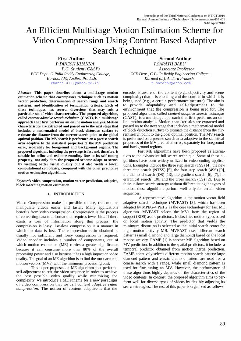
Proceedings of the Third National Conference on RTICT 2010
Bannari Amman Insitute of Technology , Sathyamangalam 638 401
9-10 April 2010
89
An Efficient Multistage Motion Estimation Scheme for
Video Compression Using Content Based Adaptive
Search Technique First Author Second Author
P.DINESH KHANNA T.SARATH BABU P.G. Student (C&SP) Associate Professor
ECE Dept., G.Pulla Reddy Engineering College, ECE Dept., G.Pulla Reddy Engineering College ,
Kurnool (dt), Andhra Pradesh. Kurnool (dt), Andhra Pradesh. [email protected] [email protected]
Abstract—This paper describes about a multistage motion
estimation scheme that encompasses technique such as motion
vector prediction, determination of search range and search
patterns, and identification of termination criteria. Each of
these techniques has several diversions that may suit a
particular set of video characteristics. The proposed algorithm,
called content adaptive search technique (CAST), is a multistage
approach that first performs an online motion analysis. Motion
characteristics are extracted and passed on to the next stage that
includes a mathematical model of block distortion surface to
estimate the distance from the current search point to the global
optimal position. The MV search is performed on a precise search
area adaptive to the statistical properties of the MV prediction
error, separately for foreground and background regions. The
proposed algorithm, including the pre-stage, is fast and, therefore, is
suitable for online and real-time encoding. Due to its self-tuning
property, not only does the proposed scheme adapt to scenes
by yielding better visual quality but it also yields a lower
computational complexity, compared with the other predictive
motion estimation algorithms.
Keywords-video compression, motion vector prediction, adaptive,
block matching motion estimation.
I. INTRODUCTION
Video Compression makes it possible to use, transmit, or
manipulate videos easier and faster. Many applications
benefits from video compression. Compression is the process of converting data to a format that requires fewer bits. If there
exists a loss of information along this process, the
compression is lossy. Lossless compression is a manner in
which no data is lost. The compression ratio obtained is
usually not sufficient and lossy compression is required.
Video encoder includes a number of components, out of
which motion estimation (ME) carries a greater significance
because it can consume more than 80% of the overall
processing power and also because it has a high impact on video
quality. The goal of an ME algorithm is to find the most accurate
motion vectors (MVs) with the minimum processing cost. This paper proposes an ME algorithm that performs
self-adjustment to suit the video sequence in order to achieve the best possible video quality while minimizing the complexity. we introduce a ME scheme for a new paradigm of video compression that we call content adaptive video compression. The notion of content adaptive is that the
encoder is aware of the content (e.g., objectivity and scene complexity) that it is encoding and the context in which it is being used (e.g., a certain performance measure). The aim is to provide adaptability and self-adjustment to the environment that the compression is being used for. The proposed algorithm, called content adaptive search technique (CAST), is a multistage approach that first performs an on-line motion analysis. Motion characteristics are extracted and passed on to the next stage that includes a mathematical model of block distortion surface to estimate the distance from the cur-rent search point to the global optimal position. The MV search is performed on a precise search area adaptive to the statistical properties of the MV prediction error, separately for foreground and background regions. Fast ME algorithms have been proposed as alterna-
tives to the exhaustive full search technique. Some of these al-
gorithms have been widely utilized in video coding applica-
tions. Examples include the three step search (TSS) [4], the new
three step search (NTSS) [5], the four step search (4SS) [9],
the diamond search (DS) [13], the gradient search [6], [7], hi-
erarchical search [10], and the cross search (CS) [2]. Due to
their uniform search strategy without differentiating the types of
motion, these algorithms perform well only for certain video
sequences. A representative algorithm is the motion vector field
adaptive search technique (MVFAST) [3], which has been
adopted by MPEG-4 Part 2 as the core technology for fast ME
algorithm. MVFAST selects the MVs from the region of
support (ROS) as the predictors. It classifies motion types based
on local motion activity. The predictor that yields the
minimum distortion is selected as the initial search center for
high motion activity MB. MVFAST uses different search
patterns (small diamond and large diamond) based on the local
motion activity. FAME [1] is another ME algorithm based on
MV prediction. In addition to the spatial predictors, it includes a temporal predictor obtained from motion inertia prediction.
FAME adaptively selects different motion search patters: large
diamond pattern and elastic diamond pattern are used for a
coarse search with a range, while small diamond pattern is
used for fine tuning an MV. However, the performance of
these algorithms highly depends on the characteristics of the
video contents. In contrast, the proposed algorithm aims to per-
form well for diverse types of videos by flexibly adjusting its
search strategies. The rest of this paper is organized as follows

90
Fig.1. Block diagram for the content adaptive search technique Section II describes the CAST algorithm. Section III presents
the evaluation results and performance comparisons with other
MV prediction ME algorithms. Section IV provides some
concluding remarks.
II.PROPOSED TECHNIQUE
MV prediction, determination of search range and
search patterns, and identification of termination criteria are
basic techniques used in ME. Each of these techniques has several diversions that are suitable for different video
characteristics. As opposed to pre-deciding these strategies, the
proposed MV algorithm analyzes and extracts the
characteristics from the video contents and adapts its
strategies to the video contents. Fig. 1 shows the block
diagram of the proposed scheme. The CAST algorithm
consists of three stages: MV field prediction, motion analysis
and motion estimation. They are described as follows:
Stage 1) Motion Vector Field (MVF) Prediction: This stage
predicts the MVF from the previous coded frame using the
proposed Weighted Mean Inertia prediction technique.
Stage 2) Motion Analysis: This stage clusters MBs into back-
ground and foreground regions based on the predicted MVF and
extract motion characteristics of each region. Parameters
indicating motion characteristics are delivered to the next
stage.
Stage 3) Motion Estimation: This stage performs motion es-
timation which is fine tuned by the regional motion
parameters. The subsequent subsections introduce the details
of these three stages.
A. Motion Vector Field Prediction
A MVF is a rich source for motion analysis. It can be
predicted from the coded MBs by exploiting the spatial and
temporal correlations between MVs. Several MV prediction
techniques have been proposed [3], [11], [12], [9]. However, due
to the dependency, it is difficult to construct the whole MVF
using the spatial prediction before the encoding of a frame.
Temporal prediction works well only for slow motion videos due to the small correlation in fast motion. To deal with these
problems, a few methods exploiting the motion inertia property
have been proposed to increase the temporal prediction
accuracy [1], [8]. Because a natural object has the inertia to stay
in the state of rest or uniform motion unless acted upon by an
external force, the underlying assumption of inertia prediction
is that the motion of an object tends to stay unchanged during a
short period between frames. The inertia prediction can be
formulated as follows:
arg min x v x y v yc rx r c ry rinertiar R
Where (xc, yc) is the coordinate of the current MB, R is the set of MBs in the reference frame, (xr, yr) is the coordinate of a
MB r , rR, vrx, and vry are the MVs of MB r in horizontal
and vertical directions.
Although the inertia prediction increases temporal
prediction accuracy in fast motion, the MVF obtained by
inertia prediction is not smooth due to its block based
inherence. To solve this problem, we propose to average the
surrounding inertia MVs with weighting. This method, called
weighted mean inertia (WMI) prediction, can increase the
smoothness as well as the accuracy of the predicted MVF. The
WMI prediction is described in the following and illustrated in
Fig. 2.
Fig. 2. Example of WMI MV prediction.
Let MBi,t-1 denote MB i in frame t -1, as shown in white
blocks. Denote the MV of MBi ,t-1as MV i,t-1.Due to the mo-
tion inertia, MB i ,t-i intends to maintain its motion and
move to Pi,t in frame t , as shown in gray blocks.
TABLE I
CORRELATION BETWEEN THE PREDICTED MVF AND THE TRUE MVF
The prediction accuracy can be evaluated by the correlation
coefficients between the predicted MVF and the true MVF
obtained by exhaustive search. Table I shows the correlation
coefficients comparison between WMI and the inertia method
proposed in [1]. The experimental results verify that WMI has
higher prediction accuracy.

91
B. Motion Analysis
In this stage, the predicted MVF is decomposed into
foreground and background MVFs. Based on this
decomposition, a frame is segmented into different regions. For
each type of region, motion parameters characterizing the
regional motion are computed. 1) Motion Based Region Segmentation:
Motion in video contents usually consists of foreground
motion and background motion. Generally, background motion
is dominated by camera motion, which may be still, panning,
tilting, zooming or their combinations. Motion of foreground
MBs is typically homogeneous because foreground objects are
often correlated.
Motions in a local region generally exhibit similar
properties. The second stage of the CAST algorithm clusters
the MBs into three regions based on the MVF predicted from
the reference frame. Fig. 3 illustrates three regions: foreground,
background, and uncovered background. The uncovered background is a region initially covered by an object in the
reference frame but uncovered in the current frame due to the
object movement.
Fig. 3. Demonstration of foreground, background, and uncovered
background regions.
The foreground and background region can be
segmented as follows:
1) reconstruct the background MVF
1
1
u
v
, with the estimated
affine parameters '
1a to '
6a ;
2) compute the error (E) between the predicted MVF and the
reconstructed MVF ' '
, , , , ,x y x y x y x y x yE u u v v (2)
3) threshold T is set to be
,
0 ,0
1x y
x N y m
T E EN
(3)
Where E is the average of E in a frame;
4) for each MB, if the sum of its overlaps is less than 128, we mark it as uncovered background. Otherwise, its type is
determined as follows:
foreground ,MBtype=
background ,
E x y T
E x y T
(4)
An example of the motion-based region segmentation is
presented in Fig. 4. Fig. 4(a) is the original MVF of a frame
in "Foreman." Fig. 4(b) and (c) are the background MVF
and foreground MVF obtained with the above approach. The
background MVF consists of affine motion. The foreground
MVF captures the object motions.
Fig. 4.(a) Original MVF.(b) Background MVF.(c) Foreground MVF.
2) Motion Parameters: We define two parameters to model
the regional motion characteristics as follows.
Motion Velocity: This is the average length of MVs in a
region. MBvel and MFvel denote the background motion
velocity and foreground motion velocity, respectively.
Motion Complexity: This is the standard derivation of MVs in a region, which indicates the degree of the motion disorder. The
motion complexity of background and foreground are denoted
by MBcomp and MFcomp. R e s p e c t i v e l y
C. Motion Estimation
The motion parameters charactering the regional
motions are employed to optimize the search technique. In this

92
section, we present a search technique that adapts to the
motion parameters obtained through the first two stages. The
CAST technique encompasses several techniques, which are
described in the following.
Fig. 5. Average block distortion surface of test sequence Stefan.
1) Modeling the Block Distortion Surface: Block distortion
surface (BDS) is a 2-D array of distortion values at all points in
the search window. Although almost all fast ME algorithms are
based on the assumption that the BDS is unimodal, no mathe-
matical model for the BDS has been reported. Here, we present
a model of block distortion that is a function of distance, mo-
tion and texture. Based on this function, we estimate the dis-
tance from the current search point to the global minimum point
(GMP) given the motion parameters, texture complexity and the
block distortion at the search point. We start by considering a
BDS. Fig. 5 illustrates the average BDS of the test sequence
Stefan. Note that we center the (x, y) plane at the GMP. The
block distortion increases as the search position moving
further to the GMP.
To simplify the problem, we transform this 2-D
function to 1-D. r is defined as the chess-board distance of
vector (x, y)
r x y (5) D(r) denotes the block distortion of the search point having a
distance r to the GMP. D(O) is the global minimum distortion
value. Generally, the distortion in a block depends on the
complexity of the texture. It is because when a block contains
complex textures, it is less likely to find a matching block with
similar texture structure. Therefore, the value of D(O) will be
large if the texture is complex, and vice versa. We use D(O) to
represent the texture complexity.
By exploring the relation between D(r) and , we
observe that is ((D(r) - D(0)/D(0)))2 closely linear related to
the distance , as shown in Fig. 6. The solid lines in Fig. 6 are the
fitting curves of the measured data. 2.
D r Dg r
D
(6)
Where g is a factor.
2) Tight Search Area: To avoid checking the unnecessary
area, a tight search area derived from the statistics of MV
Fig. 6. Linear relation between ((D(r)-D(0)/D(0)))2 and r
prediction errors are proposed. It is well known that the
distribution of the MV prediction error is highly concentrated.
Here, we define the MV prediction error as the distance
between the predicted MV and the true MV. Shown in Fig. 7 is
the MV prediction error distribution using MV prediction
technique proposed in [3], that is, using best MV of the left,
upper, upper-right coded MB in the current frame and the
colocated MB in the reference frame.
Fig. 7. MV prediction error distribution of “Stefan” using MV
prediction technique in [3].
TABLE II
TIGHT SEARCH AREA FOR VARIOUS MOTION COMPLEXITY LEVELS
Table II includes the search area radius for various
motion complexity levels. Note that for high complexity
motion, we do not restrict the search area in order to increase
search accuracy. 3) Initial Search Point: The intention is to select an initial
search point as close to the GMP as possible. Therefore, a set of MV predictors (denoted by PSET) is evaluated, and the one
producing the minimum SAD is set to be the initial MV. Often,
increasing the number of MV predictors obtains more accurate
initial MVs and accordingly reduces the complexity in the sub-
sequent search. However, in a chaotic MVF where the predicted
MVs are disordered and inaccurate, increasing the number of
predictors may not help. Moreover, using more MV predictors
creases the computational cost in the initial step. Thus, the
choice of the MV predictors is critical.
93
TABLE III PERFORMANCE COMPARISON (RESOLUTION 176 x 144)
TABLE IV PERFORMANCE COMPARISON (RESOLUTION 720 x 480)
4) Search Strategy: We propose an exponentially expanding search process starting from the initial search point and restricted
by the search area. Two search modes are used in the search
process: cross search mode and exponential search mode.
The search process has the following steps.
Step 1) Let the current search point P be the initial search
point. If SAD(P) < T , stop search.
Step 2) Switch to cross search mode. Check the cross pattern
centered at P. Mark the point with minimum
SAD as the current best point (CBP). If P=CBP go
to Step 3). Otherwise, go to Step 4).
Step 3) If s = 1 stop the search process. Otherwise, set s =
1 and go to Step 2).
Step 4) Switch to exponential mode. Compute the expo-
nential step size V = CBP — P = (dx,dy),
where dx and dy are the displacement in horizontal and
vertical direction. Compute expanded search
ESP=P+2V=P+2 x (dx,dy).If
SAD(ESP)<SAD(CBP),mark ESP as the
new CBP and repeat Step 4).Otherwise, mark
the CBP as new P and go to Step 2).
T is an early stop threshold, which is defined as follows.
1) If all the MV predictors in PSET are identical, T is
set to the maximum SAD of the spatial adjacent
MBs.
2) Otherwise, T is set to the minimum SAD of the
spatial adjacent MBs.
III. PERFORMANCE EVALUATION
A. Complexity Analysis: The computational complexity of the
motion analysis is dominated by the computation of the affine
model parameter and motion segmentation. The complexity of

94
obtaining affine parameters and motion segmentation is
negligible. The SAD is dominant computation in the ME
process.
B. Experimental Results
This section includes the performance of CAST as
well as a comparison with MVFAST and FAME. We used the
Microsoft MPEG-4 Verification Model software encoder in the
simulation with 17 most popular test sequences containing low
and fast motion. We encoded 150 frames of each sequence with
constant bit rate (384 kbps for the 176 x 144 format and 1
Mbps for 720 x 480 format).
Tables III -IV show the objective quality and
complexity comparisons among MVFAST, FAME, and CAST.
The objective quality is measured by the peak signal-to-noise
ratio (PSNR), which is commonly used in the objective quality
comparison. Since the SAD operation dominates the
complexity of the ME algorithm, we can measure the
algorithm complexity by the number of SAD operations,
which is identical to the number of search points (NSP). This
metric is also commonly used for fair inter-platform
comparison.
The speedup column in these tables shows the
reduction in complexity as compared to MVFAST. It can be
observed that CAST yields the lowest complexity among the
algorithms being compared. CAST exhibits considerable
speedup for sequences with ordered background motion field,
irrespective of whether the background motion is still, slow or
fast. For example, for the sequence containing still or slow
background motion, such as News, Hall monitor and Container,
CAST achieved speedups of 2.86,4.31, and 12.68 in CIF format
and 7.22, 3.49, and 11.79 in QCIF format. An advantage of CAST compared to other ME
algorithms is that it drastically reduces the complexity in the
background. When the background motion is very slow and
smooth, the algorithm terminates without SAD computation
and the WMI predicted MV is the final MV. We observe that
"News" sequence shows a large difference in speedup in
different resolutions (2.86 at 176 x 144). In higher resolution,
MVBevel usually is larger. Thus, fewer MBs satisfy this
condition in high resolution than in low resolution, especially
for the sequences where most of the MBs are located in slow
motion background, such as "News." Further improvement can
be obtained by fine tuning the early termination threshold for
different resolutions.
The average complexity comparison is shown in
Table V. CAST achieved 3.83, 3.05, and 2.44 times speedup
compared to the MVFAST for the 176 x 144 and 720 x 480 for-
mats, respectively. On the other hand, FAME gained only 1.44,
1.44, and 1.37 speedups for the same test. CAST outperformed
both MVFAST and FAME.
TABLE V
AVERAGE SPEED UP OF PSNR GAINS
IV CONCLUSION
This paper presented a multistage algorithm for
block matching motion estimation, encompassing a motion
analysis stage to assist the motion vector search. The
analysis stage helps the search technique to adapt to the
motion characteristics. The experimental results show that the proposed algorithm outscores the other predictive ME
algorithms in terms of computational cost and visual quality,
while showing the adaptability to various types of scenes. The
proposed scheme has the best overall performance among the
compared algorithms. Motion characteristics and their
utilization on motion estimation can be further studied.
REFERENCES
[1] I. Ahmad, W. Zheng, J. Luo, and M. Liu, "A fast adaptive motion estimation algorithm," IEEE Trans. Circuits Syst. Video Technol., vol. 16, no. 3, pp. 439-446, Mar. 2006. [2] M. Ghanbari, "The cross-search algorithm for motion estimation," IEEE Trans. Commun., vol. 38, no. 7, pp. 950-953, Jul. 1990. [3] P. I. Hosur and K. K. Ma, "Motion vector field adaptive fast motion estimation," presented at the 2nd Int. Conf. Info., Commun. Signal Process. (ICICS), Singapore, Dec. 1999. [4] J. R. Jain and A. K. Jain, "Displacement measurement and its application in interframe image coding," IEEE Trans. Commun., vol. 29, no. 12, pp. 1799-1808, Dec. 1981. [5] R. Li, B. Zeng, and M. Liou, "A new three-step search algorithm for block motion estimation," IEEE Trans. Circuits Syst. Video Technol., vol. 4, no. 4, pp. 438-442, Aug. 1994. [6] B. Liu and A. Zaccartin, "New fast algorithms for estimation of block motion vectors," IEEE Trans. Circuits Syst. Video Technol., vol. 3, no2,pp. 148-157, Apr. 1993. [7] L. K. Liu and E. Feig, "A block-based gradient descent search algorithm for block motion estimation in video coding," IEEE Trans. Circuits Syst. Video Technol., vol. 6, no. 4, pp. 419^22, Aug. 1996. [8] T. Liu, K.-T. Lo, J. Feng, and X. Zhang, "Frame interpolation scheme using inertia motion prediction," Signal Process.: Image Commun., vol. 18, pp. 221-229, 2003. [9] J. Luo, I. Ahmad, Y. Liang, and Y. Sun, "Motion estimation for content adaptive video compression," in Proc. ICME, Taiwan, Jun. 2004, pp. 1427-1430. [10] X. Song, T. Chiang, and Y.-Q. Zhang, "A scalable hierarchical motion estimation algorithm for MPEG-2," in Proc. IEEE Int. Conf. Image Process. (ICIP), 1998, pp. IV126-IV129. [11] A. M. Tourapis, O. C. Au, and M. L. Liou, "Fast block-matching motion estimation using predictive motion vector field adaptive search technique (PMVFAST)," presented at the ISO/IEC JTC1/SC29/WG11 MPEG99/m5866, Noordwijkerhout, The Netherlands, Mar. 2000. [12] A. Tourapis, G. Shen, M. Liou, O. Au, and I. Ahmad, "New predictive diamond search algorithm for block-based motion estimation," in Proc. VCIP, 2000, pp. 1365-1373. [13] S. Zhu and K. K. Ma, "A new diamond search algorithm for fast block-matching motion estimation," IEEE Trans. Image Process., vol. 9, no. 2, pp. 287-290, Feb. 2000.
SPEED UP PSNR GAIN
176X144 720X480 176X144 720X480
MVFAST 1.00 1.00 0 0
FAME 1.48 1.37 -0.010 +0.070
CAST 4.27 2.23 +0.015 +0.046

Proceedings of the Third National Conference on RTICT 2010
Bannari Amman Insitute of Technology , Sathyamangalam 638 401
9-10 April 2010
95
Framework for Adaptive Composition and
Provisioning of Web Services M.S.Thilagavathy
#1, R.SivaRaman
*2
# 1 Department of Computer Science and Engineering, Anna University Tiruchirappalli
Tiruchirappalli ,Tamil Nadu, India, 2Lecturer, Anna University , Tiruchirappalli [email protected]
Abstract— Web service composition allows developers
to create applications on top of service oriented computing’s
native paradigm of description, discovery, and communication
capabilities. Such applications are rapidly deployable and offer
developers reuse possibilities and provide users a seamless access
to a variety of complex services. This paper describes the design
of a framework for adaptive composition of web services. In the
composition model service context and exceptions are configured
to accommodate needs of different users. Services selection is
made dynamically identifying the best set of services available at
runtime. This allows for reusability of a service in different
contexts and achieves a level of adaptiveness and
contextualization without recoding and recompiling of the
overall composed services. The execution model is adaptive in the
sense that the runtime environment is able to detect exceptions
and react to them according to a set of rules. The single
centralized repository is being substituted by dedicated
repositories that cooperate and exchange information about
stored services on demand. Aspect oriented approach is used to
provide support for service adaptation. Three core services,
coordination service, context service, and event service, are
implemented to automatically schedule and execute the
component services, and adapt to user configured exceptions and
contexts at run time. The various parts of the framework are
explained with a common case study taken from E-learning
domain.
Keywords— Web service, service composition, service-oriented
architecture, exception handling, aspect-oriented programming,
event-based service execution.
I. INTRODUCTION
In service-oriented computing (SOC), developers use
services as fundamental elements in their application
development processes. Services are platform and network
independent operations that clients or other services invoke
[1]. Web services are typical example of SOC. Definition
published by the World Wide Web consortium W3C, in the
web services Architecture document states that a web service
is a software system identified by a URL, whose public
interfaces and bindings are defined and described using XML.
Its definition can be discovered by other software systems. These systems may then interact with the web service in a
manner prescribed by its definition, using XML-based
messages given by internet protocols.
Nowadays, an increasing amount of companies and
organizations only implement their core business and
outsource other application services over Internet. Service
composition is a process of combining existing services in
order to satisfy the functionality required by the user. Service
composition accelerates rapid application development,
service reuse, and complex service consummation. Every
composition approach must guarantee connectivity, non-
functional QoS properties, such as timeliness, security, and
dependability, correctness and scalability. To make service composition dynamic selection of Web services composition
focus on context aware business processes.
A current trend is to provide adaptive service
composition and provisioning solutions that offer better
quality of composite Web services[2],[3]. The pervasiveness
of the Internet and the proliferation of interconnected
computing devices (e.g., laptops, PDAs, 3G mobile phones)
offer the technical possibilities to interact with services
anytime and anywhere. Service adaptation refers to the
problem of modifying a service so that it can correctly interact
with another service, overcoming functional and non-functional mismatches and incompatibilities. While the
service functionality remains to a large extent the same, a
service needs to adapt to existing one. To simplify adaptation,
it is important to separate the adaptation logic from the
business logic. Such separation helps to avoid the need of
developing and maintaining several versions of a service
implementation and isolates the adaptation logic in a single
place [4].
Adaptive Composition of web services with
Distributed Registries provides a system infrastructure for
distributed, adaptive, context-aware provisioning of composite
Web services. This allows service designers to focus more on specifying service composition requirements at a high level of
abstraction such as business logic of applications, generic
exception handling policies, and contextual constraints, rather
than on low-level deployment and coordination concerns [5].
The salient features of our approach are:
Adaptable service composition model decouples the
contextual and exceptions specification from the business
logic of the actual service. The concept of process schema is
used for modeling the business logic of the composite service.
End users can then customize this process schema by
assigning users’ contextual constraints to the process schema. Generic exception behaviours (e.g., service failures, network
errors) that may happen during the service provisioning are
specified as policies that can be reused across different
process schemas. By adopting AOP approach for modeling
96
exceptions, end users can dynamically add, remove, and
modify tuples of aspects on how exceptions can be handled
without changing functionalities of composite service.
DIstributed REgistry (DIRE), which is devoted to service
publication and exploits a publish/subscribe middleware to
support the dynamic federation of heterogeneous registries
and the flexible distribution of service descriptions based on
explicit subscriptions.
An event-driven service execution model provides the
execution semantics of adaptive composite services. We
propose the use of an aspect-oriented programming (AOP) approach to weave adaptation solutions into the different
composite services that need to be modified. The execution
semantics is enforced by means of three core generic services:
coordination service, context service, and event service. These
basic infrastructure form the backbone of a middleware that
provides deployment and automatic execution of the adaptive
composite service in a robust and scalable manner.
II. RELATED WORK
Recently, automatic service composition approaches
typically exploit the Semantic Web and artificial intelligence
(AI) planning techniques. By giving a set of component services and a specified requirement (e.g., user’s request), a
composite service specification can be generated
automatically [4]. However, realizing a fully automatic
service composition is still very difficult and presents several
open issues [1], [6], [8]. The basic weakness of most research
efforts proposed so far is that Web services do not share a full
understanding of their semantics, which largely affects the
automatic selection of services. The work in [11] proposes a
trade-off between planning and optimization approaches. In a
first semiautomatic logical composition step, the goal is
translated into a workflow-based specification that introduces abstract tasks. A second physical composition step maps
abstract tasks to concrete services and is supervisioned by the
composed service designer.
Composite services orchestration is a very active area of
research and development. Our work’s distributed
orchestration model has some similarities with the work
presented in [7], which proposes a decentralized orchestration
approach. The approach, however, differs from our work, in
that it is only applicable when the assignment of activities to
their executing entities is known during the deployment of the
workflow, which is a restrictive assumption In the context of
service composition where providers can leave and join a community or alter the characteristics of their offers (e.g., the
QoS or the price) after the composite service has been defined
and deployed. Several techniques have been proposed to deal
with adaptability of composite Web services. In the effort
reported in [10], a platform has been developed where BPEL
processes can be extended with policies and constraints for
runtime configuration. The other two recent efforts for
adaptive Web services composition, reported in [2], focus on
dynamic service selection for context-aware business
processes.
III. ADAPTABLE COMPOSITION MODEL
The service composition encompasses roles and
functionality for aggregating multiple services into a single
composite service. Resulting composite services can be used
as basic services in further service compositions or offered as
complete applications and solutions to service clients. The
basic weakness of most of the service composition models
proposed so far is that Web Services do not share a full
understanding of their behaviour. Though some approaches to Web Service description consider behaviour, but it is not
publicly available. Therefore, it is not exploited in
composition, discovery, etc. All traditional service
composition model depends on process modeling notations to
choreograph the component services. This mode of
composition should know the context that the service will be
executed before composing the component services. For
adaptive service composition, Web service invocation is based
on the dynamic selection of concrete services at runtime. The
user or front-end application which invokes a Web service
may specify only its abstract interface requirements and quality of service constraints. The environments that users
interact with are dynamic by nature. Therefore it is not
possible to enumerate all the possible contexts and exceptions
at service design time.
A. Process Specification
A composed service is specified at an abstract level as a
high-level business process. We assume that a composed
service is characterized by a single initial task and a single end
task. The operational language for process implementation is BPEL . A set of semantic annotations are associated to the
process specification to specify requirements by the user of
the composed service. Some annotations specified are
Global and local constraints on quality dimensions.
Web service dependency constraints.
A process schema is a reusable and extensible business
process template devised to reach a particular goal . A process
schema can be configured by assigning a number of user
contexts to the process schema’s tasks and the schema itself.
Individual users can customize process schemas to meet their
particular requirements by assigning contexts to schema as parameters. A process schema can also be configured to
handle particular type of exceptions. Exception handling
Policies are assigned to the process schema and its tasks by
the relation policy Assignment. These policies prescribe the
knowledge on the appropriate response to a particular
exception.
A statechart is made up of states and transitions. States can
be initial, end, basic, or compound. A basic state corresponds
to an invocation of a service operation, whether an atomic
service, a composite service, or a community. The concept of
Web service community [6] is proposed to handle the large number and dynamic nature of Web services in a flexible way.

97
The statechart of a simplified process schema of the E-
learning class assistant is given in section VII. E-learning
class assistant helps students to manage their class activities.
B. Configuration of composite service
Process schemas that correspond to recurrent user needs
(e.g., booking rooms, travel planning) are defined by service
designers based on common usage patterns, and are stored in
schema repositories. The configuration is done by specifying a number of user contexts and exception handling policies and
assigning them to the process. Two abstractions for modeling
user contexts are execution contexts and data supply and
delivery contexts.
1) Execution Context: An execution context specifies that
certain conditions must be met in order to perform a particular
operation. Two constraints considered in our service
composition model are temporal and spatial constraints. These
constraints specify the time and location in which the task has
to be executed. Temporal and spatial constraints can be empty,
meaning that the corresponding task can be executed anytime and anywhere.
2) Data Supply and delivery Context: The value of a task’s
input parameter may be: 1) requested from user during task
execution. 2) obtained from user profile, or 3) obtained as an
output of another task, they are expressed as queries. Similarly,
the value of a task’s output parameter may be: 1) sent to other
tasks as input parameters and/or 2) sent to an end user.
IV. SERVICE ADAPTATION
If the invoked service changes the interface or protocol,
then all the composite services invoking it will have to
undergo analogous changes to interact with the new version of
the invoked service. Taxonomy of mismatches that can occur
between two services are Signature mismatch, Parameter
constraint, ordering mismatch, Extra message, Message split.
For each mismatch a template is provided in the AOP
approach to adaptation.Template contains a set of <pointcut,
advice> pairs that define where the adaptation logic is to be
applied, and what this logic is. An example of template for the signature mismatch is presented in table 1.
V. ARCHITECTURE OF OUR APPROACH
Fig.1 provides architecture of our framework for adaptable
web service composition. We propose DIstributed REgistries
(DIRE) instead of single UDDI registry. It provides support
for the cooperation among heterogeneous registries. It exploits
a Service Publication Bus to connect a set of registries and
allow them to share their services. The service builder, the
service discovery engine, the proxy service, and the service
deployer compose the service development and deployment
environment, which provide a service composition
environment where service designers and users can compose and invoke Web services. The runtime environment consists
of a set of generic services (coordination, context, and event)
that provide mechanisms for enacting the execution of
composite Web services.
TABLE I
TEMPLATE FOR SIGNATURE MISMATCH
Signature Template
Query Generic Adaptation Advice
query (<inputType>)
executes before receive when typebp = <inputType>
Signaturepart1 (<Ti>) Receive msgOes ; Assign msgObp .inParabp . typebp
<Ti> (msgOes .inParaes .typees); Reply msgObp;
query (<outputType>)
executes before reply when typebp = <outputType>
Signaturepart2 (<To>) Receive msgObp; Assign msgOes .outParaes . typees
<To> mgObp .outParabp .typebp);
Reply msgOes;
A. Service Development/Deployment Environment
The service discovery engine facilitates the advertisement
and location of services. Service registration, discovery, and
invocation are implemented by SOAP calls. When a service
registers with a discovery engine, a SOAP request containing
the service description in WSDL is sent to the DIRE registry.
After a service is registered in the DIRE registry, service designers and end users can locate the service by sending the
SOAP request (e.g., business name, service type) to the DIRE
registry. The service builder assists service designers in the
creation and maintenance of composite services. It provides
an editor for describing the statechart diagram of a composite
service operation and for importing operations from existing
services into composite services and communities. It should
be noted that the service builder also supports the
specification of process schemas.
The service deployer is responsible for generating
Aspect templates and control tuples of every task of a composite service. Once the control tuples and templates are
generated, the service deployer assists the service designer in
the process of uploading these tuples into the tuple spaces of
the corresponding component services and the composite
service. Coordination services communicate asynchronously
through the shared spaces by writing, reading, and taking
control tuples.
DIRE (DIstributed REgistry) fosters the seamless
cooperation among heterogeneous registries since it does not
require modifications to the publication and discovery
processes adopted by the organizations behind the registries. DIRE exploits the publish/subscribe (P/S) paradigm. Special-
purpose element, called dispatcher is used for both to
subscribe and publish. DIRE exploits both content-based and
subject-based subscriptions.
B. Runtime Environment
This layer contains the three core generic service that
provides the execution semantics for the adaptive composite
services. The coordination service provides an operation
called coordinate for receiving messages, managing service
instances (i.e., creating and deleting instances), registering

98
events to the event service, triggering actions, tracing service
invocations and communicating with other coordination
services. The coordination service relies on tuple space of the
associated service to manage service activities. The context
service detects, collects, and disseminates context information
while the event service fires and distributes events. Finally,
the event service provides operations for receiving messages,
including subscribing messages from the coordination service
of a service and context information from the context service,
and notifying the fired events to the coordination services.
.
Fig.1 Frame work for adaptable web service composition.
VI. EXECUTION MODEL
Existing service provisioning systems are centralized and
service orchestration is ensured by a single process which acts
as a central scheduler. Centralized execution models suffer
from permanent connectivity, availability and scalability
problems [7]. Accordingly, to achieve adaptive and scalable
execution of composite services in dynamic environments, the
participating services should be self-managed: they should be
capable of coordinating their actions in an autonomous way.
This leads to Decentralized Orchestration of composite web services. In Decentralized Orchestration, data and control
dependences between the components are analyzed and the
code can be partitioned into smaller components that execute
at distributed locations. We refer to this mode of execution as
decentralized orchestration. There are multiple engines, each
executing a composite web service specification at distributed
locations. The engines communicate directly with each other
to transfer data and control when an asynchronous manner.
Performance benefits of Decentralized Orchestration are
There is no centralized coordinator which can be a
potential bottleneck.
Distributing the data reduces network traffic and
improves transfer time.
A. Orchestration Enabling
The model consists of three core services, namely the
coordination service, the context service, and the event service. These three elements form orchestration enabling
services. When executing a composite service, orchestration
enabling services automatically schedule and execute the
component services, and adapt to user configured exceptions
and contexts. Each participating Web service is associated
with a coordination service that monitors and controls the
service execution. The coordination service determines when
should a component service be executed, and what should be
done after the execution is completed. The knowledge needed
by a coordination service in order to answer these questions at
runtime is statically extracted from the description of the
composite service (e.g., statecharts, user contexts), and placed in the corresponding tuple space. A coordination service
enforces the control tuples with the help of an event service
and a context service. The event service is responsible for
disseminating events registered by the coordination service,
and the context service is responsible for collecting context
information from context providers.
VII. IMPLEMENTATION
In our implementation, we design an E-Learning service.
We offer some courses. User has to register for a course. Once
they have registered, their username and password will be
stored. When the user accesses the service, first authentication of the user is performed. Then he is given the information
about his subjects lecture time and place. The service that
delivers lecture notes will take input from attendance
remainder service. Lecture notes are provided to the user
only during that particular lecture time. Lecture notes will be
delivered in an adaptive way. By analyzing the time required
by the users to view the pages and understand its contents, we
find an average time. If the user views the page beyond the
critical time limit, he is provided with a page that describes its
contents in a simpler form (e.g. diagrams, flowcharts etc.). If
the student has any doubts he can either post or vote his
queries based on the questions already raised. All these implementations are made in java with Apache Tomcat6 as a
Web server where Apache Axis is deployed. Apache Axis
provides not only a server-side infrastructure for deploying
and managing services, but a client-side API for invoking
these services. Each service has a deployment descriptor that
includes the unique identifier of the Java class to be invoked,
session scope of the class, and operations in the class available
for the clients. Each service is deployed using the service
management client by providing its descriptor and the URL of
the Axis servlet rpcrouter.
Service Builder
Proxy Service Service Discovery Engine
Service
Deployer
DIRE
Registry
Registry
Service Publication Bus
Registry
Registry
Tuple Space
Coordination service
Context
Context service
Event Service
Web Services
Composite Services
Development/
Deployment
Environment
Run time
Environment

99
Fig .2 class assistant process schema
VIII. CONCLUSION AND FUTURE WORK
The paper presented the framework for the deployment of
adaptable Web service compositions. First, we introduced a
adaptable service composition model. The innovative aspect
of our model is to provide distinct abstractions for service context and exceptions, which can be embedded or plugged
into the process schemas through simple interaction with end
users. It comprises DIRE for the user-controlled replication of
services onto distributed registries. We proposed the use of
AOP for service adaptation to interface and protocol
mismatches. The notion of template also promotes reusability
of adaptation logic that occurs repetitively across different
locations in an implementation of a service. In the future, we
plan to extend the Development Environment to offer a semi-
automated identification of mismatches and a graphical
interface that allows the user to create queries over process
specifications and navigate through the results
REFERENCES
[1] N. Milanovic and M. Malek, “Current Solutions for Web Service
Composition,” IEEE Internet Computing, vol. 8, no. 6,
pp. 51- 59 , Nov./Dec. 2004 [2] D. Ardagna and B. Pernici, “Adaptive Service Composition in
Flexible Processes,” IEEE Trans. Software Eng., vol. 33, no. 6,
pp. 369-384, June 2007.
[3] L. Baresi, E. Di Nitto, C. Ghezzi, and S. Guinea, “A Framework
for the Deployment of Adaptable Web Service Compositions,”
Service Oriented Computing and Applications, vol. 1, no. 1, pp.
75-91, 2007.
[4] W. Kongdenfha, R. Saint-Paul, B. Benatallah, and F. Casati, “An
Aspect-Oriented Framework for Service Adaptation,” Proc. Fourth
Int’l Conf. Service-Oriented Computing (ICSOC ’06), Dec. 2006. [5] Q. Z. Sheng, B. Benatallah, Z. Maamar, and A. H. H.
Ngu,“Configurable composition and adaptive provisioning of web
services”, IEEE Services Computing, vol. 2, NO. 1, pp.34- 49,
Mar. 2009.
[6] D. Berardi, G.D. Giacomo, and D. Calvanese, “Automatic
Composition of Process-Based Web Services: A Challenge,” Proc.
14th Int’l World Wide Web Conf. (WWW ’05), May 2005.
[7] G.B. Chafle, S. Chandra, V. Mann, and M.G. Nanda,
“Decentralied Orchestration of Composite Web Services,” Proc.
13th Int’l World Wide Web Conf. (WWW ’04), May 2004.
[8] Q. Yu, X. Liu, A. Bouguettaya, and B. Medjahed, “Deploying and
Managing Web Services: Issues, Solutions, and Directions,” The
VLDB J., vol. 17, no. 3, pp. 537-572, 2008.
[9] M.P. Papazoglou, P. Traverso, S. Dustdar, and F. Leymann,
“Service-Oriented Computing: State of the Art and Research
Challenges,” Computer, vol. 40, no. 11, pp. 38-45, Nov. 2007. [10] B. Srivastava and J. Koehler, “Web Service Composition—
Current Solutions and Open Problems, Proc. Int’l Conf.
Automated Planning and Scheduling (ICAPS ’03), 2003. [11] V. Agarwal, K. Dasgupta, N. Karnik, A. Kumar, A. Kundu,
S. Mittal, and B. Srivastava, “A Service Creation Environment
Based on End to End Composition of Web Services,” Proc. 14th
Int’l Conf. World Wide Web (WWW ’05), May 2005.
Course registration
User login
Attendance remainder
Attendance guide
Lecture notes
Browse
question
s
Vote question
Post question
consultation
feedback
Proceedings of the Third National Conference on RTICT 2010 Bannari Amman Insitute of Technology , Sathyamangalam 638 401
9-10 April 2010
100
AN ENHANCED APPROACH FOR CLASS-DEPENDENT FEAUTRE SELECTION
K. Shanmuga Sundaram . B.E., J. Arumugam.M.E
Lecturer of Computer Science & Engg. Lecturer of Computer Science & Engg.
Hindustan University Hindustan University
Chennai-603 103 Chennai-603 103
[email protected] [email protected]
Abstract
Today data sets that we process are
becoming increasingly larger, not only in terms
of the number of patterns (instances), but also
the dimension of features (attributes), which may
degrade the efficiency of most learning
algorithms, especially when there exist irrelevant
or redundant features. The predictive accuracy
of the learning algorithms are reduced in the
presence of irrelevant features. The distribution
of truly relevant features for the main task are
blurred by irrelevant or redundant features.
Deleting those irrelevant features cannot only
improve the classification accuracy, but also
reduce the structural complexity of the radial
basis function (RBF) neural network and
facilitate rule extraction. All these reasons urge
us to carry out data dimensionality reduction
(DDR).
1. Literature Review
There are numerous techniques for
DDR. Depending on whether the original
features are transformed to new features, one
may categorize these techniques into feature
extraction or feature selection techniques,
respectively. Depending on whether a classifier
is used to evaluate the performance of the new
feature set, these DDR techniques can be
categorized into wrapper or filter methods,
respectively. Feature extraction methods, e.g.,
principal component analysis (PCA) and linear
discriminant analysis (LDA) transform the
original set of features into a new set of features.
Because the new features are different from the
original features, it may be difficult to interpret
the meaning of the new features. Feature
selection selects a desirable subset of the
original features while maintaining or increasing
acceptable classification accuracy. Feature
selection eliminates unimportant features, e.g.,
redundant and irrelevant features, and obtains
the best subset of features that discriminates
well among classes. Thus how to decide which
features are important so as to form the
desirable feature subset is the main objective of
feature selection.
Many factors affect the success of machine
learning on a given task. The representation and
quality of the instance data is first and foremost.
If there is much irrelevant and redundant
information present or noisy and unreliable data,
then knowledge discovery during the training

101
phase is more difficult. In real-world data, the
representation of data often uses too many
features, but only a few of them may be related
to the target concept. There may be
redundancy, where certain features are
correlated so that is not necessary to include all
of them in modeling; and interdependence,
where two or more features between them
convey important information that is obscure if
any of them is included on its own.
2.Proposed System
The general wrapper approach to
selection of class-dependent features consists of
the following three steps (Fig. 3.1).
1. In the first step, a C-class
classification problem has been converted into
two-class classification problems, i.e., problem
1, problem 2,…,and problem C. The goal of
problem c is to correctly separate the original
class c from the other patterns, where
c=1,2,……..,C. For problem c , All training
patterns have been into two classes: class A is
the original class c, and class B consists of all
the other training patterns.
2. The second step is to search for
a desirable feature subset for each binary
classification problem. In this paper, a forward
search has been adapted as follows. We rank
the attribute importance using a ranking
measure, such as RELIEF weight measure,
CSM, information-theoretic measure, and the
minimal-redundancy–maximal-relevancy
(mRMR) measure based on mutual information
(MI).
In this project, RELIEF weight measure
has been adapted, CSM, and the mRMR to
evaluate the importance of the features for each
class (in each of the C sub-problems). Three
feature ranking measures are briefly reviewed in
the next section. The attribute importance
ranking has been regarded thus obtained class-
dependent attribute importance ranking. After
obtaining the attribute importance ranking of
each class, choose a desirable feature subset
for each class through a classifier, e.g., the
support vector machine (SVM), for a given
feature subset search algorithm.
For each class, forward selection search
(or bottom-up search) has been used to form
different attribute subsets, that is, it has been
started with the most important feature as the
first feature subset, and then each time add one
attribute into the previous subset in the order of
importance ranking to form a new feature
subset, until a stopping condition is satisfied,
e.g., the validation accuracy starts to decrease
or all the attributes in this class have been
added. For high-dimensional data sets, it will be
computationally expensive to incrementally form
all feature subsets and evaluate them through a
classifier. Therefore, first select certain number
of features, e.g., the top 70 from 649 ranked
features for the handwritten digits
recognition(HDR) multi feature (or HDR) data
set from the LIBSVM data, and then
incrementally form different feature subsets. In-
putting each feature subset into the classifier,
we can obtain different classification accuracy
for different feature subsets. Then choose the
attribute combination with the highest
classification accuracy or lowest error rate as
the desirable feature subset for a given feature

102
subset search algorithm.
A feature mask has been used to
represent a feature subset, i.e., a “0” or “1” in a
feature mask indicates the absence or presence
of a particular feature, respectively. For
example, if originally there are five features,
i.e., x1, x2, x3, x4, x5, and the desirable
feature subset turns out to be x1,x2,x3 with the
fourth and fifth features deleted, the feature
mask will be 1,1,1,0,0.
In the testing stage after training, the
input test pattern has been classified according
to the classifier (Fig. 3.2) with the maximum
response. The classifier in Fig. 3.2 includes
several models. When using those class-
dependent feature subsets to train and test
models, each model has an output, which
provides the probability that each sample
belongs to the current class in terms of the
current class’ feature subset. If we use SVM in
all models, we have the probability estimate, of
each cur-rent class as the output of each model.
In SVM models, each class has a probability
estimate which indicates the probability the
testing sample belongs to each class. A
common way to generate an overall output from
individual outputs of all models is to choose the
maximum individual as the overall output of the
class-dependent classifier. However, it is not fair
to directly compare outputs produced from
different feature spaces proposed the pdf
projection theorem and utilized it to project those
class-specific features pdfs back into the original
space where a fair comparison is possible. In
our paper, we propose a heuristic method, i.e., a
weight measure, to deal with the problem of
unfair comparisons on outputs from different
feature spaces.
3. Feature Ranking Measures
3.1 Relief Weight Measure
Relief is a relevance-based function
selection algorithm inspired by instance based
learning, techniques. It defines relevance in
terms of consistency. It assumes that samples
belonging to the same class should be closer, in
terms of their feature values, than samples
from different classes. As a result, if two
instances (samples) belong to the same class
and are generally similar, the similar features
for the two instances are rewarded and the
different ones are punished. When the samples
belong to different classes the opposite occurs .
One important question addressed
here is whether Relief is able to identify
relevance when the learning task is function
approximation. Medications have been
proposed to deal with function approximation.
Some modifications proposed by Kononenko
have been used that generalize the algorithm to
multiple classes and reduce its sensitive to
noise. As part of this process, different versions
of modified algorithm has to be tested and tune
its parameters to best perform in out context.
The basic Relief algorithm selects
samples randomly from the sample space. For
each sample, it finds the closest sample of the
same class (hit) and the closest sample of a
different class (miss). The difference in feature
values between the sample and the hit and
between the sample and the miss are then used
to update the weights of each feature. If the hit

103
difference is smaller than the miss difference the
weight will increase, indicating that the feature is
a good one. The relief algorithm is given below:
1. Introduce a weight vector and
initialize it to zero:
w1,…,wi,…,wD=0. D is the number of
features.
2. Randomly select an instance X from
training instances S and find its nearest hit Xh
and nearest miss Xm
3. Calculate and update the weight wi of
the ith feature xi:wi=wi+(xi-xmi)2-(xi-xhi)
2,
i=1,2,….,D. Where xmi is the ith element of Xm
and xhi is the ith element of Xh. Each feature’s
weight is updated by the differences ( Euclidean
distance) and between the samples and the
hits(hit differences). The weight is increased if
the miss differences are greater than the hit
differences, which means that the feature is
relevant.
4. Repeat steps 2 and 3 over all training
instances. In our approach to class-dependent
feature selection, multi-class problems are
already converted into multiple two class
problems, and therefore we can use the original
RELIEF algorithm to rank the features.
However, for class-independent feature
selection method, it is multi-class problem so
that we will use the extended version RELIEF to
rank the features importance. Each sample will
have one hit and more than one miss, and the
differences between the misses and the sample
are weight averaged. The weight adopted here
is the a priori probability of the miss class.
After obtaining the weight of each
feature, the importance of the features has been
ranked according to rationale: the larger the
weights, the more important the features.
3.2 Class Separability Measure
The CSM evaluates how well two classes
are separated by a feature vector. The greater
the distance is between different classes, the
easier the classification task. Therefore, the
feature subset that can maximize the distances
between different classes may also maximize
classification accuracy and is therefore
considered more important. The jth sample is
represented as Xj,tj, where Xj= xj1,xj2,….,xjDs
the input data and tj=1,2,…..,C is the class
label of Xj. Class separability consists of two
elements, i.e., the distance between patterns
with each class Sw
C
c
nc
j
/TmcXcjmcXcjPcSw1 1
21]))([(
and the distance between patterns among
different classes Sb
C
c
/TmmcmmcPcSb1
21]))([(
Here Pc is the probability of the cth class
and nc is the number of samples in the cth class.
Xcj is the jth sample in the cth class, mc is the
mean vector of the cth class, and m is the mean
vector of all samples in the data set.

104
The ratio Sw/Sb can be used to measure
the separability of the classes: the smaller the
value, i.e., the smaller the distances within each
class and the greater the distance among
different classes, the better the separability. The
importance of a feature may be evaluated by
ratio Sw/Sb calculated after the feature is
removed from the data set, i.e., The greater
S’w/Sb’ is, the more important the removed
attribute is. For example, if removing attribute 1
from the data set leads to greater S’w/Sb’,
compared with removing attribute 2, we may
consider attribute 1 more important compared to
attribute 2 for classifying the data set, and vice
versa. Hence, we may evaluate the importance
level of the attributes according to ratio Sw/Sb
with an attribute deleted each time in turn.
3.3 The Minimal-Redundancy Maximal-
Relevance Measure:
The mRMR feature selection method was
proposed by Peng et al.. It is based on the MI
theory to select features in terms of their
relevancy and redundancy. Let FD=xi |
i=1,2,…,D denote a feature set. According to
the definition of MI, the MI value of two features
xi and xj is denoted as I(xi; xj) (i, j = 1,2,…,D),
which describes statistical dependence between
the two features. In the same manner, the MI
value I(xi; xj) (c is one of C classes) is used to
denote the statistical dependency of the feature
xi to the class c. Peng et al. used the
incremental search strategy to sequentially
select features with the maximal relevancy and
minimal redundancy. The sequence in which
features are included corresponds to the ranking
order of features. Suppose Fm -1 denote the
feature subset consisting of m-1 top ranked
features, the mth ranked feature xm should be
selected according to the following:
Although RELIEF cannot detect redundancy in
features, RELIEF was often adopted due to its
efficiency in computation. The CSM is used to
detect feature’s relevancy in classification
problems by many authors, e.g., Fu et al., even
as a linear ranking measure. Compared with
these two feature importance ranking
measures, the mRMR measure may be more
effective since it is a nonlinear method and it
evaluates features in terms of both
relevancy
Fig. 3.2. Architecture of the general classifier
with class-dependent feature subsets
(after training and during testing).

105
redundancy.
Fig. 3.1. Schematic diagram for general wrapper
approach to class-dependentfeature selection.
.
Suppose the output of the cth model is
denoted as Oc (c = 1, 2, …,C), which is the
probability that one sample belongs to the cth
model to classify the sample between two
classes, i.e., class A (the cth class) and class B (
all other classes except the cth class). For C
models, we have C outputs, i.e., O1,
O2,…..,O
c,…O
c, each representing the
probability that the sample belongs to the
current class, respectively. Instead of
comparing the C outputs obtained from different
feature spaces, we assign a weight to each
output and compare the weighted outputs, e.g.,
pc.O
c in Fig 3.2. These weights are obtained
feature space. That is, we first combine all
class-dependent feature subsets together to
form one union set, Xc. Then we classify
the sample using the union set, as the feature
subset with C classes as target classes,
together with a classifier, such as an SVM. The
classifier produces outputs p1,…..,p
c,…..,p
C
each representing the probability that the
sample belong to each of C class, respectively.
We assign these probabilities obtained from the
common feature space to the corresponding
O1,…..,O
c,…..,O
C for a fair comparison. Since
class-dependent feature subsets vary with
different training samples in the training process,
those weights model in Fig 3.2. has C outputs,
i.e., probability estimates for all classes.
4.Implementation Result
We train and test the artificial data sets
, then to select feature subset as optimum from
binary classifier using class-dependent feature
selection method. It is outperform compared to
class-independent feature selection method.
The figure 5.1 shows the class
dependent feature set input to the MATLAB
program. The figure 5.2 shows the feature
subsets output obtained from the MATLAB
program using class dependent feature
selection.

106
Fig. 5.1 Feature set (Input)
Fig. 5.2 Feature subsets (Output)
5.Conclusion and Future work
In this project, a general wrapper
approach to class-dependent feature selection is
proposed. In order to demonstrate the scenario
mentioned in the Introduction, two data sets A
and B have been generated. The experimental
results for the two artificial data show that our
class-dependent feature selection method can
select those specific feature subset for each
class, i.e., class-dependent feature subsets, so
that the number of noise features or redundant
features can be greatly reduced and the
classification accuracy is substantially
increased.
Future work is to decrease the
computational cost which may be worthwhile in
certain applications where improvements of
accuracy or reduction of data dimensionality are
very important and meaningful.
6.Reference
1. Lipo Wang, Nina Zhou, and Feng Chu
“A General Wrapper Approach to Selection of
Class-Dependent Features” IEEE Transactions
on neural networks vol. 19. No.7, July 2008
2. P. M. Baggenstoss, “Class-specific
classifier: Avoiding the curse of
dimensionality,” IEEE Aerosp. Electron.
Syst. Mag., vol. 19, no. 1, pt. 2, pp. 37–
52, Jan. 2004.
3. P. M. Baggenstoss, “The PDF projection
theorem and the class-specific method,”
IEEE Trans. Signal Process., vol. 51,
no. 3, pp. 672–685, Mar. 2003.
4. P. M. Baggenstoss, “Class-specific
features in classification,” IEEE Trans.
Signal Process., vol. 50, no. 12, pp.
3428–3432, Dec. 2002
5. J. Bins and B. Draper, “Feature
selection from huge feature sets,” in
Proc. Int. Conf. Comput. Vis.,
Vancouver, BC, Canada, 2001, pp.
159–165 [Online]. Available:

107
http://citeseer.ist.psu.edu/bins01feature.
html
6. A. L. Blum and P. Langley, “Selection of
relevant features and examples in
machine learning,” Proc. Nat. Acad. Sci.
USA, vol. 95, pp. 933–942, 1998.

Proceedings of the Third National Conference on RTICT 2010 Bannari Amman Insitute of Technology , Sathyamangalam 638 401
9-10 April 2010
108
DESIGN AND IMPLEMENTATION OF A MULTIPLIER
WITH SPURIOUS POWER SUPPRESSION TECHNIQUE
(SPST)
JEYAPRABA.A
ABSTRACT
This project provides the
experience of applying an advanced
version of Spurious Power
Suppression Technique (SPST) on
multipliers for high speed and low
power purposes. When a portion of
data does not affect the final
computing results, the data controlling
circuits of SPST latch this portion to
avoid useless data transition occurring
inside the arithmetic units, so that the
useless spurious signals of arithmetic
units are filter out.
Modified Booth Algorithm is
used in this project for multiplication
which reduces the number of partial
product to n/2. To filter out the
useless switching power, there are
two approaches, i.e. using registers
and using AND gates, to assert the
data signals of multipliers after data
transition.
The simulation result shows
that the SPST implementation with
AND gates owns an extremely high
flexibility on adjusting the data
asserting time which not only
facilitates the robustness of SPST but
also leads to a speed improvement
and power reduction.
MODIFIEDBOOTH
ENCODER ALGORITHM
A generator that creates a
smaller number of partial products
will allow the partial product
summation to be faster and use less
hardware. A method known as
Modified Booth’s Algorithm reduces
the number of partial products by
about a factor of two, without
requiring a pre add to produce the
partial products.
The multiplier is partitioned
into overlapping groups of 3 bits, and
each group is decoded to select a
single partial product as per the
selection table. In general the there
will be n/2 products, where n is the
operand length.
The encoding of the multiplier
Y, using the modified booth
algorithm, generates the following

109
five signed digits, -2, -1, 0, +1, +2.
Each encoded digit in the multiplier
performs a certain operation on the
multiplicand, X, as illustrated in
figure 2.
Figure 1: Multiplication using
Modified Booth encoding
Figure 2 – 16 bit Booth 2 Example
Fig. 2 shows a computing example of
Booth multiplying two numbers
“2AC9”and “006A,” where the
shadow denotes that the numbers in
this part of Booth multiplication are
all zero so that this part of the
computations can be neglected.
Saving those computations can
significantly reduce the power
consumption caused by the transient
signals.
DETECTION LOGIC
The first implementing
approach of the control signal
assertion circuits is using registers as
shown in figure 3. The registers may
latch the wrong values because of
delay problem. To solve this problem,
we adopt the other implementing
approach of the control signal
assertion circuits illustrated in the
shadow area in Fig. 4, using an AND
gate in place of the registers to control
the signal assertion. Efficient timing
control and power consumption
achieved through this implementation.
Figure 3 - Detection Logic using
Register

110
Figure 4 – Detection Logic using
AND gate
SPSTADDER
The SPST is illustrated through
a low-power adder/subtractor design
example. The adder/subtractor is
divided into two parts, i.e., the most
significant part (MSP) and the least
significant part (LSP). The MSP of
the original adder/subtractor is
modified include detection logic
circuits, data controlling circuits,
denoted as latch-A and latch-B in Fig.
5, sign extension circuits, and some
glue logics for calculating the carry in
and carry out signals.
Figure 5 – Low Power SPST
ADDER
LOW POWER MULTIPLIER
DESIGN USING SPST
APPLYING SPST ON MODIFIED
BOOTH ENCODER
We already discussed the
computing example of Booth
Multiplying of two numbers “2AC9”
and “006A” in figure 2, where the
shadow denotes that the numbers in
this part of Booth multiplication are
all zero so that this part of the
computations can be neglected. We
propose the SPST-equipped modified-
Booth encoder, which is controlled by
a detection unit. The detection unit
has one of the two operands as its
input to decide whether the Booth
encoder calculates redundant
computations. As shown in figure 6,
the latches can, respectively, freeze
the inputs of MUX-4 to MUX-7 or
only those of MUX-6 to MUX-7
when the PP4 to PP7 or the PP6 to
PP7 are zero, to reduce the transition
power dissipation. Such cases occur
frequently in e.g., FFT/IFFT,
DCT/IDCT, and Q/IQ which are
adopted in encoding or decoding
multimedia data.

111
Figure 6 – SPST equipped Modified
Booth Encoder
APPLYING THE SPST ON
COMPRESSION TREE
The proposed SPST-equipped
multiplier is illustrated in Fig. 7. The
PP generator generates the five
candidates of the partial products, i.e.,
2A, A, 0, +A, +2A, which are then
selected according to the Booth
encoding results of the operand B.
Moreover, when the operand besides
the Booth encoded one has a small
absolute value, there are opportunities
to reduce the spurious power
dissipated in the compression tree.
According to the redundancy
analysis of the additions, we replace
some of the adders in compression
tree of the multiplier with the SPST-
equipped adders, which are marked
with oblique lines in Fig. 7.
The bit-widths of the MSP and
LSP of each SPST-equipped adder are
also indicated in fraction values
nearing the corresponding adder in
Fig. 7.
Figure 7 – Proposed High
Performance and Low Power
Multiplier
SIMULATION RESULT OF
PARTIALPRODUCT
GENERATOR USING MODIFIED
BOOTH ENCODER
112
CONCLUSION
The high speed low
power multiplier adopting the new
SPST is designed. The Multiplier is
designed by equipping SPST on a
modified Booth encoder which is
controlled by a detection unit using
AND gate. The modified Booth
encoder will reduce the number of
partial products generated by a factor
two. The SPST adder will avoid the
unwanted addition and thus minimize
the switching power dissipation. The
SPST implementation with AND gate
have an extremely high flexibility on
adjusting the data asserting time. This
facilitates the robustness of SPST can
attain significant speed improvement
and power reduction when compared
with the conventional tree multipliers.
This design verified using Xilinx 9.1
using Verilog HDL coding.
REFERENCES
Kuan-Hung Chen and
Yuan-sun Chu “Low
Power Multiplier with
Spurious Power
Suppression Technique”
IEEE Trans on VLSI
Systems, VOL 15, July
2007.
O. Chen, R. Sheen, and
S. Wang, “A low power
adder operating on
effective dynamic data
ranges,” IEEE Trans.
Very Large Scale Integr.
(VLSI) Syst., vol. 10, no.
4, pp. 435–453, Aug.
2002
S. Henzler, G.
Georgakos, J. Berthold,
and D. Schmitt-
Landsiedel, “Fast power-
efficient circuit-block
switch-off scheme,”
Electron. Lett., vol. 40,
no. 2, pp. 103–104, Jan.
2004

Proceedings of the Third National Conference on RTICT 2010 Bannari Amman Insitute of Technology , Sathyamangalam 638 401
9-10 April 2010
113
ROBOTICS MOBILE SURVEILLANCE USING ZIGBEE
H.Senthil Kumar1 H.Saravanakumar
2 V.Suresh
3 S.T.Prabhu Sowndharya
4
1Assistant Professor, Mepco Schlenk Engineering College, Sivakasi.
2,3,4Final ECE, Mepco Schlenk Engineering College, Sivakasi.
ABSTRACT
Recently, increasing research attention
has been directed toward wireless
technology,Collections of small, low power
nodes, that can intelligently deliver high level
sensing results to the user. Mobile sensor provide
an inexpensive and more convenient way to
monitor physical environments. Mobile sensor
system can enrich human life in applications
such as home security, building monitoring, and
healthcare.
Our robotics mobile surveillance system
uses numerous sensors, zigbee, line follower
robot, web cam etc. to monitor the physical
environment. Conventional approaches in the
implementation of surveillance systems
continuously capture events, which require huge
computation or manpower to analyze. Robotics
mobile surveillance system can reduce such
overhead while providing more advanced
services.
Key word: Zigbee, Line follower robot,
wireless camera, sprinklers
1.INTRODUCTION
Robotics mobile surveillance system
consists of zigbee, line follower robot, wireless
web cam, microcontroller and various sensors
which monitors human intrusion, temperature,
smoke, fire, flood, gas leakage. When any
unwanted events happening in the environment,
the corresponding sensor indicates the
microcontroller which transmits the
corresponding data to the remote place via
zigbee module. If necessary the web cam
capture that events and transmits the snapshot
wirelessly. So this eliminates the continues
monitoring of camera and greatly reduce the
memory storage.Also if fire occurs in that
environment zigbee switch on the sprinklers via
wirelessly to cut off fire.
114
BLOCK DIAGRAM
Figure 1: Block diagram of our project
2.DESCRIPTION
2.1ZIGBEE
Zigbee is a technological standard
created for control and sensor networks. It is
based on IEEE 802.15.4 standard which is
created by zigbee alliance which aims low data
rate, low power consumption, small packet
devices. Zigbee network is a self-organizing and
supports peer-to-peer and mesh networks.
Bandwidth: 20-250KB/s
Transmission Range: 1-100+ meters
System Resources: 4KB-32KB
Network size: 2^64
Battery life: 100-1000 days
Figure 2: IEEE 802.15.4
2.1.1 ZIGBEE NETWORK FORMATION
Zigbee networks are called personal area
networks (PAN). Each network contains a 16-
bit identifier called a PAN ID. ZigBee defines
three different device types – coordinator,
router, and end device.An example of such a
network is shown below.
Figure 3: Node Types / Sample of a Basic
ZigBee Network Topology
Coordinator – Responsible for selecting the
channel and PAN ID. The coordinator starts a
new PAN. Once it has started a PAN, the
coordinator can allow routers and end devices to
join the PAN. The coordinator can transmit and
receive RF data transmissions, and it can assist
in routing data through the mesh network.
Router – A router must join a ZigBee PAN
before it can operate. After joining a PAN, the
router can allow other routers and end devices to
join the PAN. The router can also transmit and
receive RF data transmissions, and it can route
data packets through the network
115
End Device – An end device must join a
ZigBee PAN, similar to a router. The end
device, however, cannot allow other devices to
join the PAN, nor can it assist in routing data
through the network. An end device can
transmit or receive RF data transmissions. Since
the end device may sleep, the router or
coordinator that allows the end device to join
must collect all data packets intended for the
end device, and buffer them until the end device
wakes and is able to receive them.
In our project zigbee is used to transmit digital
output data from microcontroller to remote
place.For example if any gas leakage occurs in
the environment it will indicate to the remote
place which is either computer or lcd
display.And if fire is detected by the
corresponding sensor, zigbee automatically
switch on the sprinklers attached in the wall.
3. LINE FOLLOWER ROBOT
Line follower robot is a machine that can follow
a path. The path can be visible like a black line
on a white surface (or vice-versa) or it can be
invisible like a magnetic field.In our project we
are using differential drive line follower.
Differential drive means the wheel gets the
power from separate source respectively. And
the sensor we are using is white line sensor.
White line sensor is the most critical part of the
robot. It is basically a light intensity sensor. It
consists of infrared LED and photo diode.
Infrared LED illuminates the surface and photo
diode senses the reflected light from the surface.
We are using Infrared LED because ir LED
emits light at 940 nanometer and photo diode
shows maximum sensitivity at 940 nanometer
wavelength. Based on the output from the white
line sensor, the power to each wheel differs.So
the speed of each wheel can vary. The power
applied to the wheel is based on principle of
pulse width modulation (PWM).The
microcontroller we are used is P89V51RD2.
Figure 4: Line Follower Block Diagram
Figure 5:Assembled Line Sensor
SENSORS
In our project the following sensors are
used:

116
PIR module
LM35(Temperature)
SY-HS-220(Humidity) MQ5(Gas Sensor)
4.RESULTS AND DISCUSSION
4.1 HUMAN DETECTION
The PIR (Passive Infra-Red) Sensor is a
pyroelectric device that detects motion by
measuring changes in the infrared levels emitted
by surrounding objects. This motion can be
detected by checking for a high signal on a
single I/O pin. Pyroelectric devices, such as the
PIR sensor, have elements made of a crystalline
material that generates an electric charge when
exposed to infrared radiation. The changes in
the amount of infrared striking the element
change the voltages generated, which are
measured by an on-board amplifier. The device
contains a special filter called a Fresnel lens,
which focuses the infrared signals onto the
element. As the ambient infrared signals change
rapidly, the on-board amplifier trips the output
to indicate motion.
4.2 TEMPERATURE DETECTION
The LM35 series are precision
integrated-circuit temperature sensors, whose
output voltage is linearly proportional to the
Celsius (Centigrade) temperature
4.3 GAS LEAKAGE SENSOR
The gas sensor we are used is MQ5.
They are used in gas leakage detecting
equipments in family and industry, are suitable
for detecting of LPG, natural gas , town gas,
avoid the noise of alcohol and cooking fumes
and cigarette smoke
5. CONCLUSION
The sensor network community has
moved out of its infancy and is now embarking
on more serious design efforts—large-scale,
long-lived systems that truly require self-
organization and adaptivity.In this project we
developed zigbee based robotics mobile
surveillance.This can greatly reduce the
manpower and enhance secutity.
6. FUTURE WORK
Our project can be extended to send the
information to users via GSM modem.So the
user can get the information from anywhere in
the world.
7. REFERENCES
[1].A zigbeebased home automation syste
m,Gill, K.; Shuang-Hua Yang; Fang Yao; Xin
Lu; Consumer Electronics, IEEE
Transactions on Volume: 55 , Issue: 2 ,2009

117
[2].Wireless Home Securityand Automation
System Utilizing ZigBee based Multi-hop
Communication,Sarijari, M.A.B.; Rashid,
R.A.; Rahim, M.R.A.; Mahalin, N.H.; Telecommunication Technologies 2008 and 2008 2nd Malaysia Conference on Photonics. NCTT-MCP 2008.
[3]. Realization of Home Remote Control
Network Based on ZigBee,ZhangShunyang
XuDu,JiangYongping,WangRiming. Electr
onic Measurement and Instruments, 2007. ICEMI'07.
[4]. D. Johnson et al., “Mobile Emulab: A
Robotic Wireless and Sensor Network Testbed,” Proc. 25th Ann. IEEE Conf. Computer Comm. (Infocom 06), IEEE Press, 2006.

Proceedings of the Third National Conference on RTICT 2010
Bannari Amman Insitute of Technology , Sathyamangalam 638 401
9-10 April 2010
118
Abstract - Many people have irregular heartbeats from time
to time. Some heart problems occur during certain activities,
such as eating, exercise or even sleeping. Sometimes the
irregular heartbeats don’t influence life style and are usually
harmless in normal hearts. But it is also possible that these
irregular heartbeats with pre-existing illness can cause heart
attacks that lead to death. Holter monitoring system records
continuous electrocardiographic measurements of the
heart’s rhythm. Usually the recording time is around 24 to
48 hours. That means even when the heartbeat is normal, the
Holter monitor also works as well. The system discussed
here can automatically record the ECG wave when the user
is not feeling good or the heartbeats are not regular. The
recording algorithm is not continuous any more. This
increases the recording time up to 72 hour or more. The R-
Peak detection is used for ECG analysis. The Hilbert
transform of ECG signal is used for efficient R-Peak
detection and is simulated using Matlab.
Keywords - Electrocardiogram (ECG), Holter Monitor, Irregular
Heartbeats, R-Peak, Hilbert transform.
I. INTRODUCTION
The standard ECG is a representation of the
heart’s electrical activities recorded from electrodes that
are placed on different parts of patient’s body. The
electrocardiogram is composed of complexes and waves.
In normal sinus rhythm, waves and complexes are the P
wave, QRS complex, ST Segment, T wave and U wave.
Measurements are PR interval, QRS duration, QT
interval, RR interval and PP interval.
Since the development of medical science, many
instruments for improving people’s health have been developed. The electrocardiogram (ECG) monitoring
system is one of them. The most common type of ECG
monitoring is Holter monitoring. Holter monitoring is a
portable recording tool and can help doctors make a
precise diagnosis[1].
The system discussed here can automatically
record the ECG wave when the user is not feeling good or
the heartbeats are not regular. The recording algorithm is
not continuous any more. It also can record the heartbeats
manually; the wearers can record the heartbeat if wanted
when the heart rhythms are ordinary.
II. BASICS OF ELECTROCARDIOGRAM (ECG) AND
HOLTER MONITOR
A. Electro cardiogram
The standard ECG is a representation of the
heart’s electrical activities recorded from electrodes that
are placed on different parts of patient’s body. The
electrocardiogram is composed of complexes and waves.
In normal sinus rhythm, waves and complexes are the P
wave, QRS complex, ST Segment, T wave and U wave.
Measurements are PR interval, QRS duration, QT interval, RR interval and PP interval[2,3]. Figure 1
illustrates a typical waveform of normal heartbeats and
intervals as well as standard time and voltage measures.
Figure 1. ECG signal
B. Advantanges of Holter Monitoring System The Holter monitoring system records the
electrical activity of heart during usual daily activities.
The system discussed here can automatically record the
ECG wave when the user is not feeling good or the
heartbeats are not regular[4]. Comparison with New
system is shown in Table 1. TABLE 1
COMPARISON BETWEEN GENERAL HOLTER MONITOR WITH
NEW SYSTEM DEVELOPED HERE
General
Holter
Monitor
New system
Continuity Continuous Intermittent
Saving time 24-48
hours
More than 48 hours
Operation Manually
operated
Automatic/Manually
operated
Effective Electrocardiographic Measurements of The Heart’s Rhythm Using
Hilbert Transform
Manoj Kumar Verma1, P. Muthu
2
1P.G Scholar, Karunya University. Coimbatore,India
2Assistant Professor, Karunya University, Coimbatore,India
119
C.Structure of The Holter Monitoring System
The structure of Holter monitoring system is shown in
Figure 2.
Figure 2. The structure of the Holter Monitoring System
1) Differentiation: The differentiation of ECG data is to
remove the baseline drift and to minimize other
artifacts.
2) Hilbert transform: One of the properties of the
Hilbert transform is that it is an odd function. Similarly a crossing of the zero between consecutive
positive and negative inflexion points in the original
waveform will be represented as a peak in its Hilbert
transformed conjugate[5,6]. This interesting property
can be used to develop an elegant and much easier
way to find the peak of the QRS complex in the ECG
waveform corresponding to a zero crossing in its first
differential waveform d/dt (ECG).
3) R-Peak Detection: R-Peaks are detected using an
adaptive thresholding and maximum value in the
sequence. The second stage detector uses the
information provided by the first approximation. A defined width window subset (i.e., ±10 samples from
the location of the peak found in the corresponding
h(n) sequence) is selected in the original ECG
waveform to locate the real R peak[7]. Once again a
simple maximum peak locator in the values of this
subset sequence is used.
D.Holter Monitoring Review
The Holter monitor is battery-powered and can
continuously record the electrical activities of the heart over a specified period of time, normally 24 to 48 hours.
Usually the patient will undergo Holter monitoring as an
outpatient, meaning that the monitor will be placed on the
body of the patient by a technician in a cardiologist’s
office. Then the patient will go home and do normal
activities[8,9]. With the development of technology, the
Holter monitor is greatly reduced in size. It is now very
compact and combined with digital recording and used to
record ECGs.
As Figure 3 shows, the Holter monitor is a
small-size recording device. The monitor has wires called
leads. The leads attach to metal disks called electrodes, which the user wears on his chest. These electrodes are
very sensitive, and they can pick up the electrical
impulses of the heart. The impulses are recorded by the
Holter monitor record the heart’s electrical activity.
Figure 3. A man with the Holter monitor
Advanced Holter monitors have been developed
that employ digital electrocardiographic recordings,
extended memory for more than 24 hours recording, pacemaker pulse detection and analysis, software for
analysis of digital ECG recordings that are downloaded
and stored on a computer, and capability of transmission
of results over the internet.
E. Hilbert Transform Review
In 1893, the physicist Arthur E. Kennelly (1861-
1939) and the scientist Charles P. Steinmetz (1865-1923)
first used the Euler formula
e jz = cos (z) + j sin (z) (1)
which was derived by a famous Swiss
mathematician Lenonard Euler (1707-1783) to introduce
the complex notation of harmonic wave forms in
electrical engineering, that is:
e jwt = cos (ωt) + j sin (ωt) , (2)
Where j is the imaginary unit.
In the beginning of the 20th century, the German
scientist David Hilbert (1862-1943) proved that the
Hilbert transform of the function cos (ωt) is sin (ωt). This
is the one of properties of the Hilbert transform, i.e., basic ± π/2 phase-shift[10].
III. IMPLEMENTATION AND SIMULATION
RESULTS
A. R-Peak Detection Using Adaptive Thresholding
Since this algorithm for Hilbert transformation
works well with short sequences, a moving 1024 points
window is used to subdivide the input sequence y(n)
before obtaining its Hilbert transform. In this work, the
sample frequency used is 360 Hz. To optimize accuracy,
the starting point of the next window should match the last R point located in the previous ECG subset. Because
the P and T waves are minimized in relation to the relative
peak corresponding to QRS complex in the Hilbert
sequence, simple threshold detection is used to locate the
peaks in the h (n) sequence[11]. The threshold must be
adaptive in order to guarantee accurate detection of the R
peaks.
Raw ECG
Data
Differentiation
of ECG signal
Hilbert
transform of
differentiated
ECG signal
R-Peak
detection algorithm
Second stage detection
Recording in flash memory
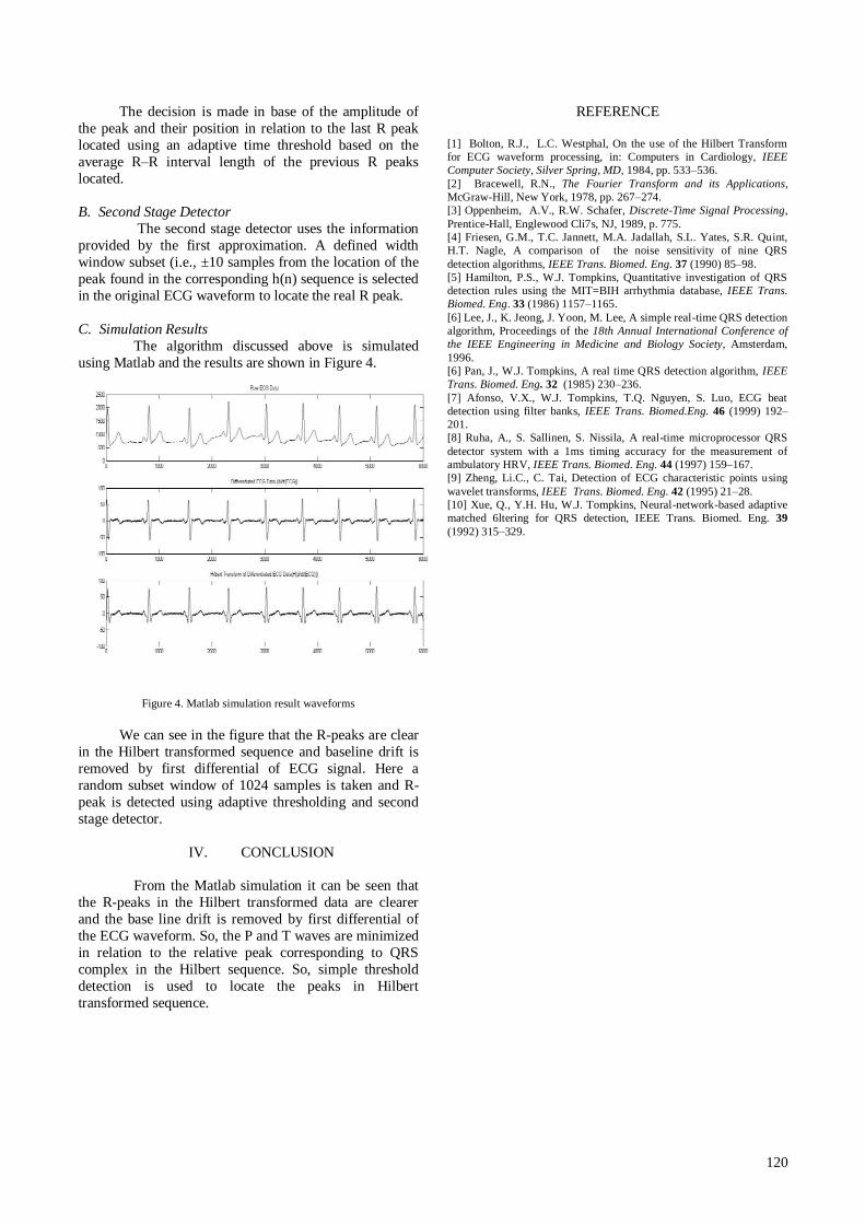
120
The decision is made in base of the amplitude of
the peak and their position in relation to the last R peak
located using an adaptive time threshold based on the
average R–R interval length of the previous R peaks
located.
B. Second Stage Detector
The second stage detector uses the information
provided by the first approximation. A defined width
window subset (i.e., ±10 samples from the location of the
peak found in the corresponding h(n) sequence is selected
in the original ECG waveform to locate the real R peak.
C. Simulation Results
The algorithm discussed above is simulated
using Matlab and the results are shown in Figure 4.
Figure 4. Matlab simulation result waveforms
We can see in the figure that the R-peaks are clear
in the Hilbert transformed sequence and baseline drift is
removed by first differential of ECG signal. Here a
random subset window of 1024 samples is taken and R-
peak is detected using adaptive thresholding and second
stage detector.
IV. CONCLUSION
From the Matlab simulation it can be seen that
the R-peaks in the Hilbert transformed data are clearer
and the base line drift is removed by first differential of
the ECG waveform. So, the P and T waves are minimized
in relation to the relative peak corresponding to QRS
complex in the Hilbert sequence. So, simple threshold
detection is used to locate the peaks in Hilbert
transformed sequence.
REFERENCE
[1] Bolton, R.J., L.C. Westphal, On the use of the Hilbert Transform
for ECG waveform processing, in: Computers in Cardiology, IEEE
Computer Society, Silver Spring, MD, 1984, pp. 533–536.
[2] Bracewell, R.N., The Fourier Transform and its Applications,
McGraw-Hill, New York, 1978, pp. 267–274.
[3] Oppenheim, A.V., R.W. Schafer, Discrete-Time Signal Processing,
Prentice-Hall, Englewood Cli7s, NJ, 1989, p. 775.
[4] Friesen, G.M., T.C. Jannett, M.A. Jadallah, S.L. Yates, S.R. Quint,
H.T. Nagle, A comparison of the noise sensitivity of nine QRS
detection algorithms, IEEE Trans. Biomed. Eng. 37 (1990) 85–98.
[5] Hamilton, P.S., W.J. Tompkins, Quantitative investigation of QRS
detection rules using the MIT=BIH arrhythmia database, IEEE Trans.
Biomed. Eng. 33 (1986) 1157–1165.
[6] Lee, J., K. Jeong, J. Yoon, M. Lee, A simple real-time QRS detection
algorithm, Proceedings of the 18th Annual International Conference of
the IEEE Engineering in Medicine and Biology Society, Amsterdam,
1996.
[6] Pan, J., W.J. Tompkins, A real time QRS detection algorithm, IEEE
Trans. Biomed. Eng. 32 (1985) 230–236.
[7] Afonso, V.X., W.J. Tompkins, T.Q. Nguyen, S. Luo, ECG beat
detection using filter banks, IEEE Trans. Biomed.Eng. 46 (1999) 192–
201.
[8] Ruha, A., S. Sallinen, S. Nissila, A real-time microprocessor QRS
detector system with a 1ms timing accuracy for the measurement of
ambulatory HRV, IEEE Trans. Biomed. Eng. 44 (1997) 159–167.
[9] Zheng, Li.C., C. Tai, Detection of ECG characteristic points using
wavelet transforms, IEEE Trans. Biomed. Eng. 42 (1995) 21–28.
[10] Xue, Q., Y.H. Hu, W.J. Tompkins, Neural-network-based adaptive
matched 6ltering for QRS detection, IEEE Trans. Biomed. Eng. 39
(1992) 315–329.

Proceedings of the Third National Conference on RTICT 2010 Bannari Amman Insitute of Technology , Sathyamangalam 638 401
9-10 April 2010
121
Visual Analysis for Object Tracking Using Filters
and Mean Shift Tracker B.Vijayalakshmi
#1, K.Menaka
#2,
#1 Assistant professor, KLN College of Information Technology, Madurai #2M.E Student, KLN College of Engineering(2) , Madurai.
[email protected],[email protected]
Abstract
This paper represents a technique for the
target representation and localization, the
central component in visual tracking of
objects is proposed. Colour histogram is used
as a reliable feature to model object and its
adaptation handles with elimination changes.
Tracking plays a key role in an effective
analysis of an object. Many experimental
results demonstrate the successful tracking of
targets whose visible colors change drastically
and rapidly during the sequence, where the
basic Mean Shift tracker obviously fails.
Definite measure minimization during
tracking enhances the guarantees of
convergence. . Proposed method extends the
traditional mean shift tracking, which is
performed in the image coordinates, by
including the scale and orientation as
additional dimensions and simultaneously
estimates all the unknowns in a few number of
Asymmetric mean shift iterations. We
describe only few of the potential applications:
exploitation of background information,
Kalman tracking using motion models, and
face tracking. The object tracking using
Gaussian approach is revealed by Kalman
Filter whereas the non Gaussian approach is
by means of condensation algorithm. The
retrieval of an image during its motion is
revealed by Mean Shift Tracker. The
extension of this paper can be revealed in
features of stable convergence and speed.
Keywords: Object tracking, Filters, Mean shift
tracker.
I. INTRODUCTION
Tracking is the propagation of shape and motion
estimates over time, driven by a temporal stream
of observations. The noisy observations that arise
realistic problems demand a robust approach
involving propagation of probability distribution
122
over time. Modest levels of noise may be treated
satisfactorily using Gaussian densities, and this is
achieved effectively by Kalman Filtering. More
pervasive noise distributions as commonly arise
in visual background clutter, demand a more
powerful, a non –Gaussian approach. The
condensation algorithm described, combines
random sampling with learned dynamical model
to propagate an entire probability distribution for
object position and shape over time. Mean Shift
tracker works by searching in each frame for the
location of an image region whose color
histogram is closest to the reference color
histogram of the target. The distance between
two histograms is measured using their
Bhattacharyya coefficient, and the search is
performed by seeking the target location via
Mean Shift iterations. Traditional mean shift
method requires a symmetric kernel, such as a
circle or an ellipse, and assumes constancy of the
object scale and orientation during the course of
tracking.
1.1 Object Tracking Filters
1.1.1 Kalman Filter
When the noise sequences are Gaussian and are
linear functions, the optimal solution is provided
by the Kalman filter which yields the posterior
being also Gaussian. When the functions are
nonlinear, by linearization the Extended Kalman
Filter (EKF) the posterior density being still
modeled as Gaussian. A recent alternative to the
EKF is the Unscented Kalman Filter (UKF)
which uses a set of discretely sampled points to
parameterize the mean and covariance of the
posterior density. The most general class of
filters is represented by particle filters also called
bootstrap filters. The filtering and association
techniques discussed above were applied in
computer vision for various tracking scenarios.
Boykov and Huttenlocher [1] employed the
Kalman filter to track vehicles in an adaptive
framework. Rosales and Sclaroff [2] used the
Extended Kalman Filter to estimate a 3D object
trajectory from 2D image motion. Particle
filtering was first introduced in vision as the
Condensation algorithm by Isard and Blake [3].
Probabilistic exclusion for tracking multiple
objects was discussed in [4]. Wu and Huang
developed an algorithm to integrate multiple
target clues [5]. Li and Chellappa [6] proposed
simultaneous tracking and verification based on
particle filters applied to vehicles and faces.
Applications are smoothness of the similarity
function allows application of a gradient
optimization method which yields much faster
target localization compared with the (optimized)
exhaustive search. In our case the Bhattacharyya
coefficient has the meaning of a correlation
score. The new target representation and
localization method can be integrated with
various motion filters and data association
techniques.
1.1.2 Condensation Filtering Algorithm

123
The Condensation algorithm is based on factored
sampling but extended to apply iteratively to
successive images in a sequence. Given that the
estimation process at each time-step is a self-
contained iteration of factored sampling, the
output of an iteration will be a weighted, time-
stamped sample-set, denoted St(n), , n = 1, ... ,
N with weights ∏t(n), representing
approximately the conditional state-density
p(xt/Zt) at time t, where Zt = (Z1……..Zt). How
this is sample-set obtained? Clearly the process
must begin with a prior density and the effective
prior for time-step t should be p(xt/Zt-1).
This prior is of course multi-modal in general and
no functional representation of it is available. It is
derived from the sample set representation (S t-1
(n)), ∏ (t-1) (n) ), n. = 1, ... , N of (x t-1(n) ,Z t-1n),
the output from the previous time-step, to which
prediction must then be applied. The iterative
process applied to the sample-sets is depicted in
Figure 1.
At the top of the diagram, the output from time-
step t - 1 is the weighted sample-set (S t-1 (n) ,∏
t-1 (n)), n = 1, ...N the aim is to maintain at
successive time steps, sample sets of fixed size
N, so that the algorithm can be guaranteed to run
within a given computational resource. The first
operation therefore is to sample (with
replacement) N times from the set St-1(n)
choosing a given element with probability ∏t-
1(n) .Some elements, especially those with high
weights, may be chosen several times, leading to
identical copies of elements in the new set.
Others with relatively low weights may not be
chosen at all.
Each element chosen from the new set is now
subjected to a predictive step. The dynamical
model we generally use for prediction is a linear
stochastic differential equation (s.d.e.) learned
from training sets of sample object motion (Blake
et al., 1995). The predictive step includes a
random component, so identical elements may
now split as each undergoes its own independent
random motion step. At this stage, the sample set
St(n), for the new time-step has been generated
but, as yet, without its weights; it is
approximately a fair random sample from the
effective prior density p(x t /Z t-1) for time-step t.
Finally, the observation step from factored
sampling is applied, generating weights from the
observation density p(Zt/xt) to obtain the sample-
set representation S t (n), ∏ t (n) of state-
density for time t.
Figure 1.1 One time step in the condensation algorithm. Blob centers
represent the sample values and sizes depict the sample weights
The algorithm is specified in detail in Figure 1.1.
The process for a single time-step consists of N
iterations to generate the N elements of the new

124
sample set. Each iteration has three steps,
detailed in the figure, and explained as follows.
1. Select nth new sample St(n)
to be some
St-1(j)
from the old sample set, sampled
with replacement with probability ∏t-
1(j)
This is achieved efficiently by using
cumulative weights Ct-1(j)
(constructed
in step 3).
2. Predict by sampling randomly from
the conditional density for the dy-
namical model to generate a sample
for the new sample-set.
3. Measure in order to generate weights
∏t(n)
for the new sample.
1.2 Mean Shift Tracker
Recently, Mean-Shift Tracking [2] has attracted
much attention because of its efficiency and
robustness to track non-rigid objects with partial
occlusions, significant clutter, and variations of
object scale. As pointed out by Yang and
Duraiswami [7], the computational complexity of
traditional Mean-Shift Tracking is quadratic in
the number of samples, making real-time
performance difficult. Although the complexity
can be made linear with the application of a
recently proposed fast Gauss transform [7],
tracking in real-time remains a problem when
large or multiple objects are involved. The main
focus on the advantage enhancing high quality
edge preserving filtering and image segmentation
can be obtained by means of applying the mean
shift in the combined spatial-range domain. The
method we developed is conceptually very
simple being based on the same idea of
iteratively shifting a fixed size window to the
average of the data points within. Details in the
image are preserved due to the non parametric
character of the analysis which does not assume a
priori any particular structure for the data.
1.2.1 Asymmetric kernel mean shift
The asymmetric kernel mean shift, in which the
scale and orientation of the kernel adaptively
change depending on the observations at each
iteration. Proposed method extends the
traditional mean shift tracking, which is
performed in the image coordinates, by including
the scale and orientation as additional dimensions
and simultaneously estimates all the unknowns in
a few number of mean shift iterations.
Asymmetric kernels [7] have been used in the
area of statistics for over a decade and have been
shown to improve the density estimation. The
main advantage of anisotropic symmetric kernels
is that most of the non-object region resides
outside of the kernel. These kernels, however, do
not represent the object shape and still contain
non-object regions as part of the object. An ideal
kernel has the shape of the tracked object which
may be asymmetric as shown in Figure 1.2.
Asymmetric kernels, however, may not have an
analytical form. This observation suggests the

125
use of implicit functions for defining the profile
of arbitrarily shaped kernels.
Figure 1.2 Asymmetric kernel mean shift tracker image
II EXPERIMENTAL RESULTS
The following tracking ball picture represents the
various results obtained using Kalman and
condensation filters as well as Mean Shift
Tracker.
Figure 2.1 Input Tracking Ball
Figure 2.2 Removed Background
Figure 2.3 Erosion
Figure 2.4 Detected Ball
Figure 2.5 Kalman Filtered Ball
Figure 2.6 Condensed Filtered ball
Moving objects are characterized by their color-
histograms. Therefore the key operation of the
object tracking algorithm is histogram estimation.
Mean-shift tracking algorithm is an iterative

126
scheme based on comparing the histogram of the
original object in the current image frame and
histogram of candidate regions in the next image
frame. The aim is to maximize the correlation
between two histograms.
Figure 2.8. Moving object tracking results; frame 1, 10, 20, 30, 60 and 70.
III CONCLUSION
Thus the object is tracked visually using Kalman
Filter, a parametric and a Gaussian approach. The
existing pervasive in the visual of Kalman Filter
is enhanced and overcome by non Gaussian
approach involved condensation Filter algorithm.
The retrieval of an image during its motion is
revealed by Mean Shift Tracker. The extension of
this paper can be revealed in features of stable
convergence and speed.
REFERENCES
[1]Y. Boykov and D. Huttenlocher. A new Bayesian
approach to object recognition. In Proc. of IEEE CVPR,
1999.
[2] R. Rosales, S. Sclaroff, Learning body pose using
specialized maps, in: T.G. Dietterich et al. (Eds.),
Advances in Neural Information Processing Systems 14,
MIT Press, 2002, pp. 1263-1270.
[3] Blake,A. and Israd, M. (1997). Condensation-
conditional density propagation for visual tracking.,
International Journal of Computer Vision, v.29 n.1, p.5-28,
Aug. 1998.
[4] MacCormick, J. Blake, A. A probabilistic exclusion
principle for tracking multiple objects. The Proceedings of
the Seventh IEEE International Conference on Computer
Vision 1999.
[5] Y.Wu and T. Huang, “A co-inference approach to
robust tracking,” in Proc. 8th Intl. Conf. on
ComputerVision, Vancouver, Canada, volume II, 2001, pp.
26–33.
[6] B. Li and R. Chellappa, “Simultaneous tracking and
verification via sequential posterior estimation,” in Proc.
IEEE Conf. on Computer Vision and Pattern Recognition,
Hilton Head, SC, volume II, 2000, pp. 110–117.
[7] Yilmaz, A “Object Tracking by Asymmetric Kernel
Mean Shift with Automatic Scale and Orientation
Selection” . IEEE Conference on Computer Vision and
Pattern Recognition, 2007. CVPR '07

Proceedings of the Third National Conference on RTICT 2010 Bannari Amman Insitute of Technology , Sathyamangalam 638 401
9-10 April 2010
128
DEVELOPMENT OF DATA ACQUSITION SYSTEM USING
SERIAL COMMUNICATION
1K.Eunice, S. Smys
2
1Student of ECE Department,
2 Assistant professor, ECE Department, Karunya university, Coimbatore.
Eunicekarasala, smys @karunya.edu
Abstract: This system is used for real time capture
and display of parameters of precision optical
instrument. The processing, capture and display can
be accomplished by three blocks; they are optical
sensor package, digital processing and display. The
sensor package contains optical sensor, FPGA
(Field Programmable Gate Array) card etc. The sensor measures the angular rotation with great
accuracy and precision. All the parameters that are
required by the sensor are processed in FPGA and
DSP, later these parameters are communicated
through the serial port. The various parameters
obtained from sensor are communicated through
the RS232 serial port through dedicated FPGA.
Introduction:
The basic principle of operation is, a
simple optical sensor that measures any rotation
about its sensitive axis. This implies that the orientation in inertial space will be known at all
times. A sensor converts a physical property or
phenomenon into a corresponding measurable
electrical signal, such as voltage, current, frequency
etc. These electrical parameters has to be known to
the external world. Hence, a data acquisition
system is required. The components of data
acquisition system include appropriate sensors that
convert any measurement parameter to an electrical
signal, which is acquired by data acquisition
hardware. Here, an RS232 serial port of a PC is used to send a command and receive the data from
the sensor package. Hence a software and GUI has
to be developed using LabVIEW.The project is
undertaken basically for designing a software
system for real time capture and display of
parameters of precision optical instrument. This is
based on modelling and simulation of FPGA based
data acquisition software scheme for precision
angle measurement. The document has been
proposed to provide an over view of the data that
has been acquired through the sensor all the
parameters that are required by the sensor are processed in FPGA and DSP, later these parameters
are communicated through the serial port.
2. Laser based rotation sensor:
Fig 1 – block diagram of Laser based rotation
sensor A Sensor is a device that responds to physical
stimuli (such as heat, light, sound, pressure,
magnetism, motion) and transmits the resulting
signal or data for providing measurement,
operating a control or both. From the sensor get the
data to be measure
The sensor electronics can be classified into the
following parts depending on their function:
Now the data obtained from the sensor is connected
to the FPGA to program and control using serial
communication. Data acquisition systems, as the name implies, are products and/or processes used to
collect information to document or analyze some
phenomenon. In the simplest form, a technician
logging the temperature of an oven on a piece of
paper is performing data acquisition. As technology
has progressed, this type of process has been
simplified and made more accurate, versatile, and
reliable through electronic equipment. Equipment
ranges from simple recorders to sophisticated
computer systems. Data acquisition products serve
as a focal point in a system, tying together a wide
variety of products, such as sensors that indicate temperature, flow, level, or pressure. Some
common data acquisition terms are shown below.
Data acquisition (abbreviated DAQ) is the
process of sampling of real world physical
conditions and conversion of the resulting samples

Proceedings of the Third National Conference on RTICT 2010
Bannari Amman Insitute of Technology , Sathyamangalam 638 401
9-10 April 2010
129
into digital numeric values that can be manipulated
by a computer.
3.Data acquisition system:
Data acquisition and data acquisition systems
(abbreviated with the acronym DAS) typically involves the conversion of analogy waveforms into
digital values for processing. The components of
data acquisition systems include:
Sensors that convert physical parameters
to electrical signals.
Signal conditioning circuitry to convert
sensor signals into a form that can be
converted to digital values.
Analog-to-digital converters, which
convert conditioned sensor signals to
digital values. When defining a Data Acquisition System, this
can be can be accurately described by explaining
what a Data Acquisition System does – not what it
―is.‖ A Data Acquisition System catches or
captures data about an actual system and stores that
information in a format that can be easily
retrievable for purposes of engineering or scientific
review and analysis. Another requirement of a Data
Acquisition System should be that it captures
information programmatically or automatically – in
other words, without any hands-on human
intervention or guidance. Generally speaking, there are seven elements or functions in a Data
Acquisition System. The seven elements/functions
are (in no particular order) data collection,
measurement, timing and triggering, a real-time
clock, system control, data communication and data
archiving. All seven elements must be in place for a
structure to be considered a Data Acquisition
System. If only a number of these elements are part
of the system, the module could be defined as a
component of a Data Acquisition System. If a
system has all seven elements along with additional features, it is probably a larger system with a Data
Acquisition System being part of the larger
structure.The actual components or elements of a
Data Acquisition System to perform the seven
essential functions are critical to the efficiency of
the system. There must be a series of sensors as
inputs to a Data Acquisition Board; in addition,
there must be a trigger to synchronize the sensor
inputs (the data stream), as well as a control for the
Data Acquisition Board. Between the Data
Acquisition Board and the processor of the system and system clock, a data communications bus (I/O)
is also required. While the data is being stored real-
time, the analysis and review of the information is
performed after data is gathered. By definition,
information cannot be analyzed in real-time,
otherwise data events will be missed or overlooked.
The Data Acquisition System must collect, sort,
catalog and store data to be reviewed and analyzed
in a meticulous manner.
The purpose of data acquisition is to measure an
electrical or physical phenomenon such as voltage,
current, temperature, pressure, or sound. PC-based data acquisition uses a combination of modular
hardware, application software, and a computer to
take measurements. While each data acquisition
system is defined by its application requirements,
every system shares a common goal of acquiring,
analyzing, and presenting information. Data
acquisition systems incorporate signals, sensors,
actuators, signal conditioning, data acquisition
devices, and application software.
Serial Communication Data Acquisition
Systems:
Serial communication data acquisition
systems are a good choice when the
measurement needs to be made at a location
which is distant from the computer. There are
several different communication standards,
RS232 is the most common but only supports
transmission distances up to 50 feet. RS485 is superior to RS485 and supports
transmission distances to 5,000 feet.
Fig
3
Figure 2 data acquisition system
RS232
A standard for serial communications found in many data acquistion systems.
RS232 is the most common serial

Proceedings of the Third National Conference on RTICT 2010
Bannari Amman Insitute of Technology , Sathyamangalam 638 401
9-10 April 2010
130
communication, however, it is somewhat
limited in that it only supports
communication to one device connected to
the bus at a time and it only supports
transmission distances up to 50 feet.
RS485 A standard for serial communications
found in many data acquistion systems.
RS485 is not as popular as RS232,
however, it is more flexible in that it
supports communication to more than one
device on the bus at a time and supports
transmission distances of approximately
5,000 feet.
RS232 is a popular communications protocol for
connecting modems and data acquisition devices to computers. RS232 devices can be plugged straight
into the computer's serial port (also known as the
COM or Comms port). Examples of data
acquisition devices include GPS receivers,
electronic balances, data loggers, temperature
interfaces and other measurement instruments.
RS232 Software:
To obtain data from your RS232 instruments and
display it on your PC you need some software.
Version 4.3 of the Windmill RS232 software is
now free from their web site. They also offer free
serial trouble-shooting software. The RS232 Standard:
RS stands for recommended standard. In the 60's a
standards committee now known as the Electronic
Industries Association developed an interface to
connect computer terminals to modems. Over the
years this has been updated: the most commonly
used version of the standard is RS232C (sometimes
known as EIA232); the most recent is RS232E. The
standard defines the electrical and mechanical
characteristics of the connection - including the
function of the signals and handshake pins, the voltage levels and maximum bit.RS232 standard
was created for just one specific situation and the
difficulties come when it is used for something
else. The standard was defined to connect
computers to modems. Any other use is outside of
the standard. The authors of the standard had in
mind the situation below:
The standard defines how computers ( it calls them
Data Terminal Equipment or DTEs) connect to
modems ( it calls them Data Communication
Equipment or DCEs). The standard says that
computers should be fitted with a 25 way plug
whilst modems should have a 25 way D socket. The interconnecting lead between a computer and a
modem should be simply pin1—pin1, pin2—pin2,
etc. The main signals and their direction of flow are
described below. It is important to note that a signal
which is an output from a computer is an input to a
modem and vice versa. This means that you can
never tell from the signal name alone whether it is an input or an output from a particular piece of
equipment. Also, instead of being a DCE device, a
data acquisition device might be configured as
DTE. In this case you need an adaptor or the
RS232 cable wired differently to normal. When the
PC is connected to a DTE instrument, some of the
cable wires must cross over.
TXD Transmitted Data, Pin 2 of 25 way D
This is the serial encoded data sent from a
computer to a modem to be transmitted over the telephone line.
RXD Received Data, Pin 3 of 25 way D
This is the serial encoded data received by a
computer from a modem which has in turn received
it over the telephone line.
DSR Data Set Ready, Pin 6 of 25 way D
This should be set true by a modem whenever it is
powered on. It can be read by the computer to
determine that the modem is on line.
DTR Data Terminal Ready, Pin 20 of 25 way D
This should be set true by a computer whenever it
is powered on. It can be read by the modem to determine that the computer is on line.
RTS Request to Send, Pin 4 of 25 way D
This is set true by a computer when it wishes to
transmit data.
CTS Clear To Send, Pin 5 of 25 Way D
This is set true by a modem to allow the computer
to transmit data. The standard envisaged that when
a computer wished to transmit data it would set its
RTS. The local modem would then arbitrate with
the distant modem for use of the telephone line. If
it succeeded it would set CTS and the computer would transmit data. The distant modem would use
its CTS to prevent any transmission by the distant
computer.
DCD Data Carrier Detect, Pin 8 of 25 Way D
This is set true by a modem when it detects the data
carrier signal on the telephone line..
PC Serial Ports
A nine pin D plug has become the standard fitting
for the serial ports of PCs, although it's nothing to
do with the RS232 standard. The pin connections
used are: Pin Direction Signal

Proceedings of the Third National Conference on RTICT 2010
Bannari Amman Insitute of Technology , Sathyamangalam 638 401
9-10 April 2010
131
1 Input DCD Data Carrier Detect
2 Input RXD Received Data
3 Output TXD Transmitted Data
4 Output DTR Data Terminal Ready
5 Signal Ground 6 Input DSR Data Set Ready
7 Output RTS Request To Send
8 Input CTS Clear To Send
9 Input RI Ring Indicator
Conclusion:
The speed of RS232 communications is expressed
in Baud. The unit is named after Jean Maurice-
Emile Baudot (1845-1903), a French telegraph
engineer and the inventor of the first teleprompter. It was proposed at the International Telegraph
Conference of 1927. The maximum speed,
according to the standard, is 20000 Baud. The
length of the cable also plays a part in maximum
speed. The longer the cable, the greater the cable's
capacitance and the slower the speed at which you
can obtain accurate results. A large capacitance
means voltage changes on one signal wire may be
transmitted to an adjacent signal wire. Fifty feet is
commonly quoted as the maximum distance, but
this is not specified in the standard. We generally
recommend a maximum distance of 50 metres, but this depends on the type of hardware connecting
and characteristics of the cable.
References:
[1] A. Deshpande, M. Garofalakis, and R. Rastogi.
Independence is Good: Dependency-Based
Histogram Synopses for High-Dimensional Data.
In SIGMOD, May 2001.
[2] A. Desphande, C. Guestrin, W. Hong, and S.
Madden. Exploiting correlated attributes in
acquisitional query processing. Technical report, Intel-Research, Berkeley, 2004.
[3] L. Getoor, B. Taskar, and D. Koller. Selectivity
estimation using probabilistic models. In SIGMOD,
May 2001.
[4] P. B. Gibbons. Distinct sampling for highly-
accurate answers to distinct
values queries and event reports. In Proc. of VLDB,
Sept 2001.
[5] P. B. Gibbons and M. Garofalakis.
Approximate query processing: Taming the
terabytes (tutorial), September 2001.
[6] P. B. Gibbons and Y. Matias. New sampling-based summary statistics for improving
approximate query answers. In SIGMOD, 1998.
[7] J. M. Hellerstein, R. Avnur, A. Chou, C.
Hidber, C. Olston, V. Raman, T. Roth, and P. J.
Haas. Interactive data analysis with CONTROL.
IEEE Computer, 32(8), August 1999.
Proceedings of the Third National Conference on RTICT 2010 Bannari Amman Insitute of Technology , Sathyamangalam 638 401
9-10 April 2010
131
Analysis of Health Care Data Using Different
Classifiers.
Soby Abraham,
M.Tech.–CSE IVth Sem, University School of Information Technology, GGS Indraprastha University, Delhi
Abstract- Data mining is an interesting field of
research whose major objective is to acquire
knowledge from large amounts of data. With
advances in heath care related research, there is a
wealth of data available. However, there is a lack of
effective analytical tools to discover hidden and
meaningful patterns and trends in data, which is
essential for any research.
Data mining is used in fields like business, science,
engineering etc. the various data mining
functionalities that can be applied in these fields
include characterization and discrimination,
frequent pattern mining, classification and
prediction.
In recent years, human immune-deficiency virus
(HIV) related illnesses have become a threat to the
modern world. Researchers all over world, including
India, are trying hard to find suitable answer to this
and this led to lots of research in the field.
Therefore, a tool which can process data in
meaningful way is the need the time.
In this study, we briefly examine the potential use
of classification based data mining techniques such
as Naive Bayesian classifier, J48 and Zeror classifier
to massive volume of health care data. Data mining
fondly called patterns analysis on large sets of data.
Keywords- decision tree, classification, Human
immunodeficiency virus, antiretroviral therapy
I. INTRODUCTION
Data mining is the analysis of (often large)
observational data sets to find unsuspected
relationships and to summarize the data in
novel ways that are both understandable and
useful
to the data owner.
Data mining, also known as knowledge
discovery in databases [1] is defined as the
extraction of implicit, previously unknown and

132
potentially useful information from data. Data
mining starts with the raw data, which usually
takes the form of simulation data, observed
signals, or images. These data are preprocessed
using various techniques such as sampling,
analysis, feature extraction, and normalization.
It is an interactive and iterative process
involving data pre-processing, search for
patterns, knowledge evaluation, and possible
refinement of the process based on input from
domain experts. Data mining tools can answer
business questions that traditionally were too
time consuming to resolve [2]. Data mining is
the next step in the process of analyzing data.
Instead of getting queries on standard or user
specified relationships, data mining goes a step
farther by finding meaningful relationships in
data.
There are several data mining techniques, such
as, Decision Trees, Artificial Neural Networks
(ANNs), Clustering, Naïve Bayes, Association
Rules, Time series etc[2] but decision tree is one
of the more powerful technique that produce
interpretable result and thus widely used in
clinical purpose.
Hence, decision tree may be considered mining
knowledge from large amounts of data since it
involves knowledge extraction, as well as
data/pattern analysis in tree diagrams [4].
Considering decision trees, classification is the
most common data mining task and it consists
of examining the features of a newly presented
object in order to assign it to one of a
predefined set of classes. Classification deals
with discrete outcomes, estimation deals with
continuously-valued outcomes.
In this study, our objective are to: (1) present an
evaluation of techniques such as Naive Bayes
classifier, Zeror and J48 classifiers which are
used to predict the occurrence of route of
transmission based on treatment history of HIV
patients. (2) demonstrate that data mining
method can yield valuable new knowledge and
pattern related to the HIV patient; (3) assesses
the utilization of healthcare resources and
demonstrate the socioeconomic, demographic
and medical histories of patient.
Organization of paper is as follows; in section II
we give a brief explanation of the data mining
and knowledge discovery. In section III we give a
brief explanation of the data mining techniques.
In section IV we analyze of HIV patients using
decision trees as well as different classifiers.
Result and conclusion are discussed in Section V
and section VI.
II. DATA MINING AND KNOWLEDGE DISCOVERY
Knowledge plays a vital role in the lives of all
human beings and important pieces of
knowledge hold the key to our future on this
planet. With out knowledge it is not feasible to
proceed further and gain success in any
discipline. In today’s world, there is a
continuous search for data from which
important pieces of knowledge can be
extracted. Such pieces of knowledge are
required by both users and non-users of data.
With the enormous amount of data stored in
files, databases, and other repositories, it is
increasingly important, if not necessary, to
develop powerful means for analysis and
perhaps interpretation of such data and for the
extraction of interesting knowledge that could
help in decision-making.
Data mining is also known as Knowledge
Discovery in Databases refers to the nontrivial
extraction of implicit, previously unknown and
potentially useful information from data in
databases. While data mining and knowledge
discovery in databases are frequently treated as
synonyms, data mining is actually part of the
knowledge discovery process [6].
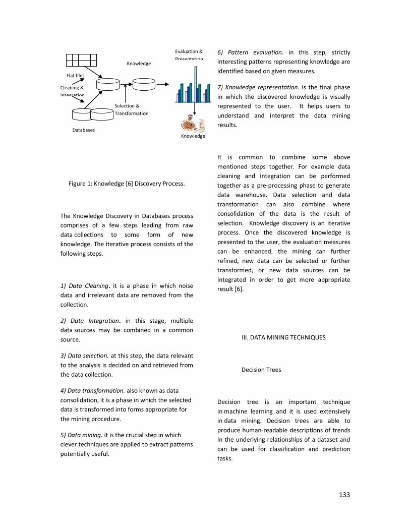
133
Figure 1: Knowledge [6] Discovery Process.
The Knowledge Discovery in Databases process
comprises of a few steps leading from raw
data collections to some form of new
knowledge. The iterative process consists of the
following steps.
1) Data Cleaning. it is a phase in which noise
data and irrelevant data are removed from the
collection.
2) Data Integration. in this stage, multiple
data sources may be combined in a common
source.
3) Data selection. at this step, the data relevant
to the analysis is decided on and retrieved from
the data collection.
4) Data transformation. also known as data
consolidation, it is a phase in which the selected
data is transformed into forms appropriate for
the mining procedure.
5) Data mining. it is the crucial step in which
clever techniques are applied to extract patterns
potentially useful.
6) Pattern evaluation. in this step, strictly
interesting patterns representing knowledge are
identified based on given measures.
7) Knowledge representation. is the final phase
in which the discovered knowledge is visually
represented to the user. It helps users to
understand and interpret the data mining
results.
It is common to combine some above
mentioned steps together. For example data
cleaning and integration can be performed
together as a pre-processing phase to generate
data warehouse. Data selection and data
transformation can also combine where
consolidation of the data is the result of
selection. Knowledge discovery is an iterative
process. Once the discovered knowledge is
presented to the user, the evaluation measures
can be enhanced, the mining can further
refined, new data can be selected or further
transformed, or new data sources can be
integrated in order to get more appropriate
result [6].
III. DATA MINING TECHNIQUES
Decision Trees
Decision tree is an important technique
in machine learning and it is used extensively
in data mining. Decision trees are able to
produce human-readable descriptions of trends
in the underlying relationships of a dataset and
can be used for classification and prediction
tasks.
Flat files
Databases
Cleaning &
Integration
Evaluation &
Presentation
Knowledge
Knowledge
Discovery
Selection &
Transformation

134
This technique has been used successfully in
many different areas, such as medical diagnosis,
plant classification, and customer marketing
strategies etc.
A decision tree is a predictive machine-learning
model that decides the target value of a new
sample based on various attribute values of the
available data. The internal nodes of a decision
tree denote the different attributes, the
branches between the nodes tell us the possible
values that these attributes can have in the
observed samples, while the terminal nodes tell
us the final value (classification) of the
dependent variable.
The principle idea of a decision tree is to split
data recursively into subsets so that each subset
contains more or less homogeneous states of
target variable (predictable attribute). At each
split in the tree, all input attributes are
evaluated for their impact on the predictable
attribute. When this recursive process is
completed, a decision tree is formed.
There are few advantages of using decision
trees over using other data mining algorithms,
for example , decision trees are quick to build
and easy to interpret.
A. Naive Bayes Classifier
Naive Bayes classifier is based [7] on Bayes’
theorem and the theorem of total probability. A
classifier that suffers relatively little from high
dimensionality is the Naive Bayes classifier.
These classifiers require an optimization
procedure that is computationally unacceptable
in settings in which the training data changes
continuously. In simple terms, a Naive Bayes
classifier assumes the presence or absence of a
feature of a class is unrelated to the presence or
absence of any other feature.
The probability model for a classifier is a
conditional model is P(C/F1,…,Fn) over a
dependent class variable C with a small number
of outcomes or classes, conditional on several
feature variables F1 through Fn. Using Bayes’
theorem , we write
p(C/F1,…,Fn) =
Depending on the nature of the probability
model, Naive Bayes classifiers can be trained
very efficiently in a supervised learning setting.
Naïve bayes method uses the method of
maximum likely hood.
An advantage of the Naive Bayes classifier is
that it requires a small amount of training data
to estimate the parameters necessary for
classification. Because independent variables
are assumed, only the variances of the variables
for each class need to be determined and not
the entire covariance matrix.
B. J48 Classifier
J48 classifier is [8] a simple C4.5 decision tree used
for classification. It creates a binary tree. This is a
standard algorithm that is widely used in
machine learning. In order to classify a new item
using J48, firstly create a decision tree based on
the attribute values of the available training
data. So, whenever it encounters a set of items,
it identifies the attribute that discriminates the
various instances most clearly. These features
tell us about the data instances so that we can
p(C) p(F1,…,Fn/C)
p(F1,…,Fn)

135
classify them the best which have the highest
information gain. If there is any value for which
there is no ambiguity, that is, for which the data
instances falling within its category have the
same value for the target variable, then we
terminate that branch and assign to it the target
value that we have obtained.
For the other cases, we then look for another
attribute that gives us the highest information
gain. Hence we continue in this manner until we
either get a clear decision of what combination
of attributes gives us a particular target value, or
we run out of attributes.
C. ZeroR Classifier
ZeroR classifier [8] simply predicts the majority
class in the training data. Although it makes
little sense to use this scheme for prediction, it
can be useful for determining a baseline
performance as a benchmark for other learning
schemes. ZeroR classifier is also used to
compare the performances. ZeroR is frequently
used as a baseline for evaluating other machine
learning algorithms. ZeroR always predict the
most common classification. For example, if
most of training data got low coverage, ZeroR
will predict low coverage on all inputs. ZeroR
provides a useful indication of a predictor’s
worst performance, since a nonrandom
prediction scheme should do better.
IV. ANALYSIS
In this study, data gathered from ART Clinic, was
analyzed using different classifiers such as Naive
Bayesian classifier, J48 classifier and ZeroR
classifier. Significant [9] research efforts have
been undertaken in investigating the association
between HIV and ART. HIV database is
considered as one of the deadly disease all over
the world.
Following tests and procedures may be used:
Physical exam and history.
Complete blood count
Stages of infection.
Chest X-ray.
A. Methods of Data Collection.
We collected the data from different
ART systems.
We derived a dataset from HIV
database that include 1054 enrolled patient out
of which we have considered only 672 unique
patients because rest of patients is defaulter.
B. Data Cleaning
Real world data, like data acquired
from ART Clinic tend to incomplete, inconsistent
and noisy. Data cleaning routine attempt to fill
missing values, smooth out noise and correct
inconsistencies in the data.
C. Missing Values.
Most datasets contain missing values.
There are number of causes for missing

136
data. Many methods were applied to solve
this,
Fill the missing values manually.
Replace the missing values with
the most popular value.
Use a global consistent.
Figure 2: Missing values.
D. Noisy Data
Noise is a random error or variance in a
measured variable. Many methods for data
smoothing are also methods for data reduction
involving discretization.
E. Data Integration.
Data integration is the merging of data
from multiple data sources. The data may also
need to be transformed into forms appropriate
for mining. Careful integration of data from
multiple sources can help reduce and avoid
redundancies and inconsistencies. It helps to
improve the accuracy and speed of the mining
process.
F. Data Selection.
Attribute selection reduces the data set
size by removing irrelevant or redundant
attributes. The goal is to find a minimum set of
attributes such that the resulting probability
distribution is close to the original distribution
obtained using all the attributes. In this paper,
HIV care was the main aim, so data concerning
the diagnosis of HIV was carefully selected from
the over all data sets.
Main focus on following data.
Figure 3: Attribute selection.
V. RESULTS.
In this study, we analyze data on Route of
transmission in the HIV database and investigate
their association with patient’s history of ART.
Classifiers like Naïve Bayes, J48 and applied to
the database for identifying the patterns.
In HIV database we have used certain codes for
route of transmission and the code is given
table1.
TABLE I

137
Code for Route of Transmission
Type of transmission Value
Heterosexual 1
Mother-to-Child 2
Blood Transfusion 3
IVD 4
Surgical Instrument 5
Unsafe Injection 6
Professional needle
stick Injury
7
Professional needle
stick Injury
8
Unknown 9
A. Analysis using Naive Bayes Classifier
When we analyzed the data using Naive Bayes
classifier, output is as shown below.
Figure 4: Naive Bayes Classifier.
Receiver Operator Characteristic areas are
commonly used to present results for binary
decision problems in machine learning. It is used
to find out the accuracy of the test. ROC areas
can also be calculated from clinical prediction
rules. Using Naive Bayes ROC area = 0.991, is
high for class2 compared to other classes, which
is mother to child. Mean absolute error in this
case is 0.0491.
B. Analysis using J48 Classifier.
When we analyzed the data using J48 Classifier,
output is as shown below.

138
Figure 5: J48 Classifier.
Using J48 Classifier, ROC area = 0.5 for all
classes. Mean absolute error in this case is
0.0728.
C. Analysis using Zeror Classifier.
ZeroR is a simple classifier that always returns a
predefined answer regardless of the test
instance; it assigns a new instance to the most
frequent class of training instances. The ZeroR
model simply classifies every data item in the
same class.
When we analyzed the data using J48 Classifier,
output is as shown below.
Figure 6: ZeroR Classifier.
Using ZeroR Classifier, ROC area = 0.5 for all
classes, which is same that we have obtained
from J48 classifier, but the mean absolute error
is lower in this case. Mean absolute error in this
case is 0.0744.
VI. CONCLUSION
In this paper we have described classification
techniques for healthcare datasets. We have
used different data mining classifiers such as
Naive Bayes, J48 and ZeroR to find out ROC area
and mean absolute error. Mean absolute error
is low in the case of Naive Bayes classifier. This
paper leads the study of data mining in health
care datasets.

139
VII. ACKNOWLEDGMENTS
The author will like to thank Dr. Anjana Gosain,
University School of Information Technology,
Guru Gobind Singh Indraprastha University for
the guidance during the course of study.
VIII. REFERENCES
[1] J. Han and M. Kamber – Data Mining: Concepts
and techniques; Second Edition; Morgan
Kaufmann, 2006.
[2] I.H. Witten, and E. Frank – Data Mining: Practical
Machine Learning Tools and Techniques; Second
Edition; Morgan Kaufmann, 2005.
[3] Lindsay, Clark. "Data Mining." Online. Internet. 3
Oct. 1997.
[4] http://www.twocrows.com.
[5] Osmar R. Zaļane- Principles of Knowledge
Discovery in Databases, 1999.
[6] A. Kumar, “Applications of data mining”, In
proceedings of National Conference on
Information Technology: Present Practices and
challenges, 2007.
[7] P.Bhargavi and Dr.S.Jyothi- Applying Naive
Bayes Data Mining Technique for Classification
of Agricultural Land Soils.
[8] http://wikipedia.org/
[9] Harleen Kaur and Siri Krishan Wasan: Empirical
Study on Applications of Data Mining Techniques
in Healthcare.
[10] Mark Hall, Eibe Frank, Geoffrey Holmes, Bernhard
Pfahringer, Peter Reutemann, Ian H.
Witten: The WEKA Data Mining Software: An
Update

Proceedings of the Third National Conference on RTICT 2010
Bannari Amman Institute of Technology ,Sathyamangalam- 638401
9-10 April 2010
141
Merin Jojo (M.E Computer Science and Engineering) 1,
V.Venkatesakumar M.E., 2
1Student, Department
of CSE, Anna University Coimbatore.
Lecturer, Department of CSE, Anna University Coimbatore.
Abstract- In this paper, we deals with distributed data mining
in peer-to-peer networks with the help of generic local
algorithm. For large networks of computers or wireless
sensors, each of the components or peers has some data about
the overall state of the system. System’s functionalities are
based on modeling the global state. The state of the system is
constantly changing, so it is necessary to keep the models up-
to-date. The data modeling and communication cost may be
very costly due to the scale of the system. In this paper we
describe a two step approach for dealing with these costs.
First, we describe a highly efficient local algorithm which can be used to monitor a wide class of data mining models. Then,
we use this algorithm as a feedback loop for the monitoring of
complex functions.
Keywords- Distributed data mining, Local Algorithm, Peer-
to-peer, Mean monitoring.
1. INTRODUCTON
Large distributed systems or in wireless sensor networks, produce, store and process huge amounts of status
data as a main part of their daily operation and often the need
to model the data that is distributed over the entire system. But
centralizing the data is a costly approach. The internets,
intranets, local area networks, ad-hoc wireless networks and
sensor networks are some of the examples .Mining in such
environments naturally calls for proper utilization of these
distributed resources. When data and system changes are
frequent, designers should update the model frequently and
risk wasting resources on insignificant changes, causes
inaccuracy and resulting in system degradation.
At least three algorithmic approaches can be
followed in order to address this situation. The periodic
approach is to simply rebuild the model from time to time but
waste the resources. The incremental approach is to update the
model with every change of the data and it might be
inaccurate. Last, the reactive approach is to monitor the
change and rebuild the model only when it no longer suits the
data. The benefit of the incremental approach is that its
accuracy can be optimal. If monitoring is done efficiently and
accurately, then the reactive approach can be applied to many
different data mining algorithm at low costs.
A local algorithm is one in which the complexity of
computing the result does not directly depend on the number
of participants and mainly based on distributed systems.
Instead, each processor usually computes the result using
information gathered from just a few nearby neighbors. Local
algorithms are in-network algorithms in which data is
decentralized but rather computation is performed by the peers of the network. At the heart of a local algorithm there is a data
dependent criteria dictating when nodes can avoid sending
updates to their neighbors. In a local algorithm, it often
happens that the overhead is independent of the size of the
system. Because of this reason, local algorithms exhibit high
scalability. The dependence on the criteria for avoiding
sending messages also makes local algorithms inherently
incremental. Specifically, if the data changes in a way that
does not violate the criteria, then the algorithm adjusts to the
change without sending any message. These local algorithms
were developed, for a large selection of data modeling problems. Problems such as association rule mining, facility
location, outlier detection, L2 norm monitoring classification
and multivariate regression etc can be solved.
In this work first, we generalize a common theorem
underlying the local algorithms. Next, we describe a generic
algorithm, relying on the said generalized theorem, which can
be used to compute arbitrarily complex functions of the
average of the data in a distributed system. Then, we describe
a general framework for monitoring, and consequent reactive
updating of any model of horizontally distributed data.
Finally, we describe the application of this framework for the problem of providing a mean monitoring which is a good
approximation of the k-means clustering of data distributed
over a large distributed system. Some simulation results are
also added at the last section. The last section deals with
conclusion and future works.
2. NOTATIONS AND ASSUMPTIONS
Mining In Distributed System Using Generic
Local Algorithm

142
In this section we discuss the notations, assumptions
and problem definition which will be used throughout the
paper. The main idea of the algorithm is to have peers
accumulate sets of input vectors from their neighbors. We
show that under certain conditions on the accumulated vectors
a peer can stop sending vectors to its neighbors long before it collects all input vectors.
2.1 Notations
Let V = p1. . . pn be a set of peers connected to
one another via an underlying communication infrastructure.
The set of peers with which pi can directly communicate, Ni, and is known to pi. Ni contains pi and at least one more peer. pi
is given a time varying set of input vectors in IRd. Peers
communicate with one another by sending sets of input
vectors X i,j the latest set of vectors sent by peer pi to pj . We
further define four sets of vectors that are central to our
algorithm.
Definition 2.1: The knowledge of pi, is Ki =∪pj ε Ni Xi,j
Definition 2.2: The agreement of pi and any neighbor pj ∈ Ni
is A i,j = X i,j ∪ Xj,i.
Definition 2.3: The withheld knowledge of pi with respect to a
neighbor pj is the subtraction of the agreement from the
knowledge Wi,j = Ki \ A i,j .
Definition 2.4: The global input is the set of all inputs
G = ∪ pj ∈ V X i,i
We are interested in inducing functions defined on G.
Since G is not available at any peer, we derive conditions on
K, A and W which will allow us to learn the function on G. We
denote a given cover RF respective of F if all regions except
the tie region, F is constant.
2.2 Assumptions
We make the following assumptions:
Assumption 2.1.Communication is reliable.
Assumption 2.2.Communication takes place over a spanning
communication tree.
Assumption 2.3. Peers are notified on changes in their own
data xi, and in the set of their neighbors Ni.
Assumption 2.4. Input vectors are unique.
Assumption 2.5. A respective cover RF can be precomputed
for F.
Simple approaches such as piggybacking message
acknowledgement can be implemented in even the most
demanding scenarios mainly for wireless sensor networks.
3. PROBLEM DEFINITION
Problem definition: Given a function F, a spanning network
tree G (V, E) which might change with time, and a set of time
varying input vectors X i,i at every pi ε V , the problem is to
compute the value of F over the average of the input vectors
G. While the problem definition is limited to averages of data
it can be extended to weighted averages by simulation. If a
certain input vector needs to be given an integer weight ω then
ω peers can be simulated inside the peer that has that vector
and each be given that input vector. Likewise, if it is desired
that the average be taken only over those inputs which comply
with some selection criteria then each peer can apply that
criteria to X i,i apriori and then start off with the filtered data. Thus, the definition is quite conclusive.
4. MAIN THEOREM
The main theorem of this paper lay the background
for a local algorithm which guarantees eventual correctness in
the computation of a wide range of ordinal functions. The
theorem generalizes the local stopping rule described in [1] by
describing a condition which bounds the whereabouts of the
global average vector in Rd depending on the Ki, Ai,j and Wi,j
of each peer pi.
Theorem 3.1: [Main Theorem] Let G(V,E) be a spanning
tree in which V is a set of peers and let X i,i be the input of pi,
Ki be its knowledge, and A i,j and Wi,j be its agreement and
withheld knowledge with respect to a neighbor pj ∈ Ni as
defined in the previous section. Let R ⊆ IRd be any convex
region. If at a given time no messages traverse the network
and for all pi and pj ∈ Ni Ki, A i,j ∈ R and either W i,j = Ø or
W i,j ∈ R as well, then G ∈ R.
Proof: Consider a communication graph G(V,E) in which for
some convex R and every pi and pj such that pj ∈ Ni ,it holds
that Ki, Ai.j∈ R and either Wi,j = Ø or W i,j ∈ R as well.
Assume an arbitrary leaf pi is eliminated and all of the vectors
in W i,j are added to its sole neighbor pj . The new knowledge
of pj is K’j = Kj ∪ W i,j . Since by definition Kj ∩ Wi,j = Ø ,
the average vector of the new knowledge of pj , K′ j , can be
rewritten as Kj∪ Wi,j = α·Kj+(1−α)·W i,j for some α ∈ [0, 1].
Since R is convex, it follows from Kj ,W i,j ∈ R that K′ j ∈ R
too. Now, consider the change in the withheld knowledge of pj
with respect to any other neighbor pk ∈ Nj resulting from
sending such a message. The new W′ j,k = W i,j ∪ W j,k.
Again, since Wi,j ∩ W j,k = Ø and since R is convex it
follows from Wi,,j ,W j,k ∈ R that W′ j,k ∈ R as well. Finally,
notice the agreements of pj with any neighbor pk except pi do
not change as a result of such message. Hence, following

143
elimination of pi we have a communication tree with one less
peer in which the same conditions still apply to every
remaining peer and its neighbors. Proceeding with elimination
we can reach a tree with just one peer p1, still assured that K1
∈ R. Moreover, since no input vector was lost at any step of
the elimination K1 = G. Thus, we have that under the said
conditions G ∈ R.
Figure 1: The graphical allignment of three peers having
weight, agreement and withheld knowledge are gven in
figure
The above theorem is exemplified in Figure 1. Three peers are
shown, each with a drawing of its knowledge, it agreement
with its neighbor or neighbors, and the withheld knowledge.
Notice the agreement A 1, 2 drawn for p1 is identical to A2, 1 at
p2. For graphical simplicity we assume all of the vectors have
the same weight and avoid expressing it. We also depict the
withheld knowledge vectors twice once as a subtraction of the
agreement from the knowledge by using a dotted line . If the
position of the three peers’ data is considered vis-à-vis the
circular region then the conditions of Theorem 3.1 hold. Now, assume what would happen when peer p1 is eliminated. This
would mean that all of the knowledge it withholds from p2 is
added to K2 and to W2,3. Since we assumed |W1,2| = |K2| = 1 the
result is simply the averaging of the previous K2 and W1,2.
Notice both these vectors remain in the circular region. Lastly,
as p2 is eliminated as well, W2,3 which now also includes W1,2
is blended into the knowledge of p3. Thus, K3 becomes equal
to G. However, the same argument, as applied in the
elimination of p1, assures the new K3 is in the circular region
as well
To see the relation of Theorem 3.1 to the previous the
Majority-Rule algorithm [1], one can restate the majority
voting problem as deciding whether the average of zero-one
votes is in the segment [0, λ) or the segment [λ, 1]. Both
segments are convex, and the algorithm only stops if for all
peers the knowledge is further away from λ than the agreement – which is another way to say the knowledge, the
agreement, and the withheld data are all in the same convex
region. Therefore, Theorem 3.1 generalizes the basic stopping
rule of Majority-Rule to any convex region in Rd. Two more
theorems are used for the proper working explanation of the
generic algorithm.
5. GENERIC ALGORITHM AND ITS USAGE
The generic algorithm, depicted in Algorithm 1,
receives as input the function F, a respective cover RF, and a
constant, L, whose function is explained below. Each peer pi
outputs, at every given time, the value of F based on its
knowledge Ki.
Algorithm 1 Generic Local Algorithm
Input of peer pi: F, RF = R1,R2, . . . , T , L, Xi,i, and Ni
Ad hoc output of peer pi: F (Ki)
Data structure for pi : For each pj ∈ Ni X i,j , |X i,j |, Xj,i |Xi,j |,
last_ message
Initialization: last message ← −∞
On receiving a message X, |X| from pj
– X j,i ← X, |X, j i| ← | X |
On change in Xi,i, Ni, Ki or |Ki|: call OnChange()
OnChange( )
For each pj ∈ Ni:
If one of the following conditions occurs:
1. RF (Ki)= T and either Ai,j ≠ Ki or |Ai,j | ≠ |Ki|
2. |Wi,j | = 0 and Ai,j ≠ Ki
3. Ai,j ∈ RF (Ki) or Wi,j ∈ RF (Ki)
then call SendMessage(pj)
SendMessage(pj):
If time ( ) – last_ message ≥ L If RF( Ki) = T then the new Xi,j and |Xi,j | are Wi,j and |Wi,j |,
respectively
Otherwise compute new Xi,j and |Xi,j | such that Ai,j ∈ RF
(Ki) and either Wi,j ∈ RF( Ki) or |Wi,j | = 0
last message ← time ( )
Send Xi,j , |Xi,j | to pj
Else Wait L − (time ( ) − last message) time units and then
call OnChange( )
The algorithm is event driven. Events could be one of
the following: a message from a neighbor peer, a change in the
set of neighbors due to failure or recovery, a change in the
local data, or the expiry of a timer which is always set to no
more than L. On any such event pi calls the OnChange
method. When the event is a message X, |X| received from a
neighbor pj, pi would update Xi,j to X and |Xi,j | to |X | before it
calls OnChange.

144
The objective of the OnChange method is to make
certain that the conditions are maintained for the peer that runs
it. These conditions require Ki, Ai,j , and Wi,j to all be in RF
(Ki), which is not the tie region T . Of the three, Ki cannot be
manipulated by the peer. The peer thus manipulates both Ai,j , and Wi,j by sending a message to pj , and subsequently
updating Xi,j .However, this solution is one of the many
possible changes to Ai,j and Wi,j , and not necessarily the
optimal one. We leave the method of finding a value for the
next message Xi,j which should be sent by pi unspecified at
this stage, as it may depend on characteristics of the specific
RF. The other possible case is that RF (Ki) = T. Since T is
always the last region of RF, this means Ki is outside any other
region R ∈ RF. Since T is not necessarily convex, the only
option which will guarantee eventual correctness in this case
is if pi sends the entire withheld knowledge to every neighbor
it has. Lastly, we need to address the possibility that although
|Wi,j | = 0 we will have Ai,j which is different from Ki. This
can happen, e.g., when the withheld knowledge is sent in its
entirety and subsequently the local data changes.
Had we used sets of vectors, Wi,j would not have
been empty, and would fall into one of the two cases above.
As it stands, we interpret the case of non-empty Wi,j with zero
|Wi,j | as if Wi,j is in T .According to the above theorem, the
peer send withheld knowledge and local data changes. The
peer can rely on the correctness of the general results from the
previous section which assure that if F (Ki) is not the correct
answer then eventually one of its neighbors will send it new
data and change Ki. If, one the other hand, one of the
aforementioned cases do occur, then pi sends a message. This is performed by the SendMessage method. If Ki is in T then pi
simply sends all of the withheld data. Otherwise, a message is
computed which will assure Ai,j and Wi,j are in RF (Ki).
One last mechanism employed in the algorithm is a
“leaky bucket” mechanism. This mechanism makes certain no
two messages are sent in a period shorter than a constant L.
Leaky bucket is often used in asynchronous, event-based
systems to prevent event inflation. Every time a message
needs to be sent, the algorithm checks how long has it been
since the last one was sent. If that time is less than L, the
algorithm sets a timer for the reminder of the period and calls OnChange again when the timer expires. Note that this
mechanism does not enforce any kind of synchronization on
the system. It also does not affect correctness: at most it can
delay convergence because information would propagate more
slowly.
6. REACTIVE ALGORITHMS
The above section described an efficient generic local
algorithm, capable of computing any function even when the
data and system are constantly changing. Here, we leverage
this powerful tool to create a framework for producing and maintaining various data mining models. This framework is
simpler than the current methodology of inventing a specific
distributed algorithm for each problem and may be as efficient
as its counterparts. In this section we describe the mean
monitoring application. The basic idea of this framework is
used in order to monitor the quality of the model with the help
of algorithm. Here we discuss about the mean monitoring.
A. Mean Monitoring
The problem of monitoring the mean of the input
vectors has direct applications to many data analysis tasks.
The objective in this problem is to compute a vector μ which
is a good approximation for G. Formally, we require that
||G − μ ||≤ ∈ for a desired value of ∈. For any given estimate
μ, monitoring whether ||G – μ|| ≤ ∈ is possible via direct
application of the L2 thresholding algorithm .Every peer pi
subtracts μ from every input vector in Xi,i. Then, the peers
jointly execute L2 Norm Thresholding over the modified data.
If the resulting average is inside the ∈-circle then μ is a
sufficiently accurate approximation of G not otherwise.
The basic idea of the mean monitoring algorithm is to
employ a convergecast-broadcast process in which the
convergecast part computes the average of the input vectors
and the broadcast part delivers the new average to all the
peers. The trick is that, before a peer sends the data it collected
up the convergecast tree, it waits for an indication that the
current μ is not a good approximation of the current data.
Thus, when the current μ is a good approximation,
convergecast is slow and only progresses as a result of false alerts. During this time, the cost of the convergecast process is
negligible compared to that of the L2 thresholding algorithm.
When, on the other hand, the data does change, all peers alert
almost immediately. Thus, convergecast progresses very fast,
reaches the root, and initiates the broadcast phase. Hence, a
new μ is delivered to every peer, which is a more updated
estimate of G. The details of the mean monitoring algorithm
are given persist for a given period of time before the
convergecast advances. Experimental evidence suggests that
setting τ to even a fraction of the average edge delay greatly
reduces the number of convergecast without incurring a significant delay in the updating of μ. The second step is the
separation of the data used for alerting the input of the L2
thresholding algorithm from that which is used for computing
the new average. If the two are the same then the new average
may be biased. This is because an alert, and consequently
advancement in the convergecast, is bound to be more
frequent when the local data is extreme. Thus, the initial data,
and later every new data, is randomly associated with one of
two buffers: Ri, which is used by the L2 Thresholding
algorithm, and Ti, on whom the average is computed when
convergecast advances. In third step of implementation is the converge cast
process. First, every peer tracks changes in the knowledge of
the underlying L2 thresholding algorithm. When it moves
from inside the ∈-circle to outside the ∈-circle the peer takes
note of the time, and sets a timer to τ time units. When a timer
expires or when a data message is received from one of its
neighbors pi checks if currently there is an alert and if it was

145
recorded τ or more time units ago. If so, it counts the number
of its neighbors from whom it received a data message. If it
received data messages from all of its neighbors, the peer
moves to the broadcast phase, computes the average of its own
data and of the received data and sends it to itself. If it has
received data messages from all but one of the neighbors then this one neighbor becomes the peer’s parent in the
convergecast tree; the peer computes the average of its own
and its other neighbors’ data, and sends the average with its
cumulative weight to the parent. Then, it moves to the
broadcast phase. If two or more of its neighbors have not yet
sent a data messages pi keeps waiting.
Next deals with broadcast process. Every peer which
receives the new μ vector, updates its data by subtracting it
from every vector in Ri and transfers those vectors to the
underlying L2 thresholding algorithm. Then, it re-initializes
the buffers for the data messages and sends the new μ vector to its other neighbors and changes the status to convergecast.
There could be one situation in which a peer receives a new μ
vector even though it is already in the convergecast phase.
This happens when two neighbor peers concurrently become
roots of the convergecast tree (i.e., when each of them
concurrently sends the last convergecast message to the other).
To break the tie, a root peer pi which receives μ from a
neighbor pj while in the convergecast phase ignores the
message if i > j it ignores the message. Otherwise if i < j pi
treats the message just as it would in the broadcast phase.
7. SIMULATION RESULTS
The following are required simulations for analyzing
the performance of the algorithm. The dependency of cost and
quality of mean monitoring is based on many factors such as
alert mitigation period, alert threshold and length of epoch.
The below simulation gives the information about the
dependency of quality and cost on mean monitoring on the
alert mitigation period τ.
(a)Quality versus τ
(b)Quality versus τ
Some of the implementation results are given below.
(c) One Client side output for viewing events
(d) One server side output. This using incremental
algorithmic approach.
8. CONCLUSION
In this paper we present a generic algorithm which can
compute many function of the average data in large
distributed system. We present a number of interesting
applications for this generic algorithm. Besides direct

146
contributions to the calculation of L2 norm, the mean, and k-
means in peer-to-peer networks, we also suggest a new
reactive approach in which data mining models are computed
by an approximate or heuristic method and are then efficiently
judged by an efficient local algorithm. The future work is
based on the usage of local algorithm in network topology and the limitations of lcal computation.
REFERENCES
[1] R. Wolff and A. Schuster, “Association Rule Mining in Peer-to-Peer
Systems,” in Proceedings of ICDM’03, Melbourne, Florida, 2003, pp.
363–370.
[2]R. Wolff, K. Bhaduri, and H. Kargupta, “Local L2 Thresholding based
Data Mining in Peer-to-Peer Systems,” in Proceedings of SDM’06,
Bethesda, Maryland, 2006, pp. 428–439.
[3].D. Krivitski, A. Schuster, and R. Wolff, “A Local Facility Location
Algorithm for Sensor Networks,” in Proceedings of DCOSS’05, Marina
del Rey, California, 2005, pp. 368–375.
[4].Y. Birk, L. Liss, A. Schuster, and R. Wolff, “A Local Algorithm for Ad
Hoc Majority Voting Via Charge Fusion,” in Proceedings of DISC’04,
Amsterdam, Netherlands, 2004, pp. 275–289.
[5]. K. Bhaduri, “Efficient Local Algorithms for Distributed Data Mining in
Large Scale Peer to Peer Environments: A Deterministic Approach,”
Ph.D. dissertation, University of Maryland, Baltimore County, Baltimore,
Maryland, USA, May 2008.
[6].K. Das, K. Bhaduri, K. Liu, and H. Kargupta, “Distributed Identification
of Top-l Inner Product Elements and its Application in a Peer-to-Peer
Network,” IEEE Transactions on Knowledge and Data Engineering
(TKDE), vol. 20, no. 4, pp. 475–488, 2008.
[7]. S. Bandyopadhyay, C. Giannella, U. Maulik, H. Kargupta, K. Liu,
and S. Datta, “Clustering Distributed Data Streams in Peer-to-Peer
Environments,” Information Science, vol. 176, no. 14, pp. 1952–1985,
2006.
[8]. W. Kowalczyk, M. Jelasity, and A. E. Eiben, “Towards Data Mining
in Large and Fully Distributed Peer-to-Peer Overlay Networks,” in
Proceedings of BNAIC’03, Nijmegen, Netherlands, 2003, pp. 203–210.
[9].S. Datta, C. Giannella, and H. Kargupta, “K-Means Clustering over
Large, Dynamic Networks,” in Proceedings of SDM’06, Maryland, 2006,
pp. 153–164.
[10].M. Rabbat and R. Nowak, “Distributed Optimization in Sensor
Networks,”
in Proceedings of IPSN’04, California, 2004, pp. 20–27.
[11].N. Jain, D. Kit, P. Mahajan, P. Yalagandula, M. Dahlin, and Y. Zhang,
“STAR: Self-tuning aggregation for scalable monitoring,” in Proceedings
of VLDB’07, Sept. 2007, pp. 962–973.
[12]. R. van Renesse, K. P. Birman, and W. Vogels, “Astrolabe: A robust and
scalable technology for distributed system monitoring, management, and
data mining,” ACM Transactions on Computer Systems (TOCS), vol. 21,
no. 2, pp. 164–206, 2003.
[13].D. Kempe, A. Dobra, and J. Gehrke, “Computing Aggregate Information
using Gossip,” in Proceedings of FOCS’03, Cambridge, Massachusetts,
2003, pp. 482–491.
[14].Y. Afek, S. Kutten, and M. Yung, “Local Detection for Global Self
Stabilization,” Theoretical Computer Science, vol. 186, no. 1-2, pp. 199–
230, 1997.
[15].N. Linial, “Locality in Distributed Graph Algorithms,” SIAM Journal of
Computing, vol. 21, no. 1, pp. 193–2010, 1992.

Proceedings of the Third National Conference on RTICT 2010
Bannari Amman Institute of Technology ,Sathyamangalam- 638401
9-10 April 2010
147
PROVINCE BASED WEB SEARCH
A.Suganthi1, M.Gowdhaman
2
1Lecturer,
2 Post Graduate Student
Department of Computer Science And Engineering,
PSG College of Technology,
Coimbatore.. [email protected] ,
Abstract
In this project, we search a given set of
keywords in categorized documents. Searching is
done after the categorization is completed and
categories of given documents are available.
Here we do two separate operations. First we
generate the categories and its related
categories. After that we give required web site
links to find categories of those links. Here each
website contents are parsed into keywords list
and using those keys the corresponding category
is determined. Now the documents and its
categories are computed to search using keys.
Second, we give keywords to search engine to
search the document and its corresponding
category. If keyword is composite of multiple
keywords then all keys are searched and its
corresponding document and its corresponding
category will be retrieved. The category contains
name, keys, and weights for corresponding keys.
Category is sorted using those weights and key
occurrences.
Keywords: Category, Search, Weights.
I. INTRODUCTION
IN the last 10 years, content-based document
management tasks have gained a prominent status in
the information system field, due to the increased
availability of documents in digital form and the ensuring need to access them in flexible ways.
Among such tasks, Text Categorization assigns
predefined categories to natural language text
according to its content. Text categorization has
attracted more and more attention from researchers
due to its wide applicability. Since this task can be
naturally modeled as a supervised learning problem.
Support Vector Machines (SVM) is the machine
learning algorithm introduced by Vapnik. SVM was
first applied for text categorization task by Jaochim. SVM is based on the Structural Risk Minimization
principle with the error-bound analysis. The method
is defined over a vector space where the problem is to
find a decision surface that “best” separates the data
points in two classes. While a wide range of classifiers have been used,
virtually all of them were based on the same text
representation, “bag of words,” where a document is represented as a set of words appearing in this
document. Values assigned to each word usually
express whether the word appears in a document or
how frequently this word appears. These values are
indeed useful for text categorization. However, are
these values enough?
Considering the following example, “Here you are”
and “You are here” are two sentences corresponding
to the same vector using the frequency-related values,
but their meanings are totally different. Although this is a somewhat extreme example, it clearly illustrates
that besides the appearance and the frequency of
appearances of a word, the distribution of a word is also
important.
Searching a given keyword set in a given document
set and categorizes the documents. If a keyword set
is given then it will determine the documents which are most relevant to that keyword set and also the
category which it belongs to that keyword set.
Most of the users are interested in the website
contents of their desired information. Also users want
the information location where that info is found. So
this project gives a solution for user that user can

148
search where a particular text paragraph is found in a
given set of websites and corresponding category.
With the enormous growth in information on the
Internet, there is a corresponding need for tools that
enable fast and efficient searching, browsing and
delivery of textual data. The concurrent execution
will greatly simplify the complexity of the search.
II. RELATED WORK
When the features for text categorization are
mentioned, the word “feature” usually have two
different but closely related meanings. One refers to
which unit is used to represent a document or to
index a document, while the other focuses on how to
assign an appropriate weight to a given feature.
Consider “bag of words” as an example. Using the former meaning, the feature is a single word, while
tf-idf weighting is the feature given the latter
meaning. This section will focus on previous
researches about the features used for text
categorization based on these two meanings. Other
topics about text categorization can be found in a
review .
Weights for keywords in different words are
calculated using modified tf.idf -method,
Weight(i,j)= tfi,j . idfi,j.
. where i is keyword, j is document and term
frequency tfi;j is ”normalized” by dividing it by the
total number of words in the corresponding
document. We take the logarithm of the document frequency to
nullify keywords that occur in all documents:
The contribution of this paper are the following:
.1.Distributional features for text categorization are
design.. Using these features can help improve the
performance, while requiring only a little additional
cost.
.2.How to use the distributional features is answered. Combine traditional term frequency with the
distributional features results in improved
performance.
.3.The factors affecting the performance of the
distributional features are discussed. The benefit of
the distributional features is closely related to the
length of documents in a corpus and the writing style
of documents.
Text categorization is a process of automatically
assigning text documents into some predefined
categories. Text categorization adopts classification
algorithms for building the models. For text domain,
features are a set of terms extracted from the document corpus. There are many previous works
which proposed and compared among different
algorithms for categorizing texts. Yang and Liu
(1999) presented a comparative study on many
different text categorization algorithms including
Support Vector Machines(SVM), k-Nearest Neighbor
(kNN), Neural Network(NNet), Linear Least-Squares
Fit (LLSF) and Naive Bayes(NB) . Based on the
thorough valuation, SVM yieldedthe best
performance, allowed by kNN, LLSF, NNet and NB,
respectively.
The main problem issue for text categorization is the
high dimensionality of feature space. The feature set
for text documents is a set of unique terms or words
which occur in all documents. In general, the number
of terms in a document corpus can be in the range of
tens or hundreds of thousands. To construct a model
for text categorization algorithms efficiently and effectively, feature selection technique is usually
applied. Yang and Pedersen (1997) presented a
comparative study on feature selection in text
categorization.
study on text categorization algorithms with various
feature Text categorization can be considered as a
classification approach in machine learning in which
features are words or terms extracted from a given
text corpus. The size of these features can be in the
range of tens or hundreds of thousands. To effectively and efficiently train the classification
model, we need to reduce the set of terms to a scale
of few thousands. Therefore, we applied feature
selection technique by comparing among several
well-known methods including document frequency
threshold (DF), information gain (IG) and χ2 (CHI).
Although, there were some previous works
performing comparative selection methods, most of
them focused on English text collection.
.we adopt three feature selection methods as follows.
• Document Frequency (DF) threshold: Document
frequency is the number of documents in which a
term occurs. DF value can be calculated for each
term from a training document corpus. The terms
whose DF values are less than some predefined
threshold are removed from the feature set.

149
• Information Gain (IG): IG is based on the concept
of information theory. It measures the amount of
information obtained for category prediction by
knowing the presence or absence of a term in a
document. We compute the IG value for each term
and move the term whose IG value is less than some predefined threshold.
• χ2 (CHI): CHI is based on the statistical theory. It
measures the lack of independence between the term
and the category. CHI is a normalized value and can
be compared across the terms in the same category.
III. EXISTING SYSTEM MODEL
In the existing system the search is based on the
category of the keyword which is given as input. The
categorization is done by some method without using
neural network. The main disadvantage is more
number of keywords are to be predefined and new
keywords are to be added frequently. So to avoid this problem proposed system uses neural network to
develop the procedure.
IV. PROPOSED SYSTEM MODEL
In our project, we search a given set
of keywords in categorized documents. Searching is done after the categorization is completed and
categories of given documents are available. Here we
do two separate operations. First we generate the
categories and its related categories. After that we
give required web site links to find categories of
those links. Here each website contents are parsed
into keywords list and using those keys the
corresponding category is determined. Now the
documents and its categories are computed to search
using keys. Second, we give keywords to search
engine to search the document and its corresponding
category. If keyword is composite of multiple keywords then all keys are searched and its
corresponding document and its corresponding
category will be retrieved. The category contains
name, keys, and weights for corresponding keys.
Category is sorted using those weights and key
occurrences.
V. PROPOSED SYSTEM DESIGN
The proposed system consist two kinds of
process:
1. Categorizer. 2. Searching.
Categorizer
Figure.1 Categorization Process.
First store all the keywords and its
corresponding weights in one file. We feed collection
of websites and keywords file to categorizer. It process the request and store the websites into
corresponding category.
Searching
The searching process accept the query and the
selected category from user, search the given query in
the selected category documents. Finally display the
URL of the documents that are mostly corresponding
to user needs.
Keywords Websites
Categorizer
Documents +
Categories

150
Figure.2 Searching Process
V. CONCLUSION Thus the analysis, design and
implementation of text categorization and searching
are done successfully. So that the user can able to do searching of a set of keywords in a list of websites
and the user can able to view the each keyword count
for a particular website. This searching is very useful
for crawl the websites with particular perspective
view of specific content. Also the search is running
concurrently, so we can get higher performance.
.
REFERENCES
1. T. Joachims. Text categorization with
support vector machines: Learning with
many relevant features. Proc. of the10th
European Conf. on Machine Learning,
pages 137–142,1998.
2. D.Lewis ,Y.Yang and F.Li.Revi: A new
benchmark collection for text categorization research.
J.of Machine Learning Research, 5:361-397,2004.
3. J.R.Quinlan. Induction of decision trees. Machine
Learning, 1(1):81-106, 1986.
4. T.Joachims, Text categorization with support
vector machines: Learning with many relevant
features,” proc. 10th European conf. Machine
Learning,1998.
5.D.Lewis,reuters-21578 Text Categorization test
collection, Dist. 1.0,1999.
6.M.Sauban and B.Pfahringer,”Text Categorization
using documents profiling,” Proc. Seventh European
conf. Priniciples and practice of knowledge discovery
in databases(PKDD’03),pp, 616-623,2003.
User query and
category
Search
Documents

Proceedings of the Third National Conference on RTICT 2010
Bannari Amman Institute of Technology ,Sathyamangalam- 638401
9-10 April 2010
151
Divergence Control of Data in Replicated
Database System P.K.Karunakaran, R.Sivaraman
Department of Computer Science and Engineering,
Anna University Tiruchirappalli, Tiruchirappalli,
Tamilnadu, India.
Abstract— To provide high availability for services such as mail
or bulletin boards, data must be replicated. One way to
guarantee consistency of replicated data is to force service
operations to occur in the same order at all sites, but this
approach is expanse. For some applications a weaker causal
operation order can preserve consistency while providing better
performance. This paper describes a distributed method to
control the view divergence of data freshness for clients in
replicated database systems whose facilitating or administrative
roles are equal. Our method provides data with statistically
defined freshness to clients when updates are initially accepted
by any of the replicas, and then, asynchronously propagated
among the replicas that are connected in a tree structure a new
way of implementing causal operations. Our technique also
supports two other kinds of operations: operations that are
totally ordered with respect to one another and operations that
are totally ordered with respect to all other operations. To
provide data with freshness specified by clients, our method
selects multiple replicas using a distributed algorithm so that
they statistically receive all updates issued up to a specified time
before the present time. We evaluated by simulation the
distributed algorithm to select replicas for the view divergence
control in terms of controlled data freshness, time, message, and
computation complexity. The method performs well in terms of
response time, operation-processing capacity, amount of stored
state, and number and size of messages: it does better than
replication methods based on reliable multicast techniques.
Keywords— Data replication, weak consistency, freshness, delay,
asynchronous update.
1. INTRODUCTION
Many computer based services must be highly available: they
should be accessible with high probability despite site crashes
and network failures. To achieve availability, the server’s state must be replicated. Consistency of replicated state can be
guaranteed by forcing service operations to occur in the same
order at all sites. However, some applications can preserve
consistency with a weaker, causal ordering, leading to better
performance. This paper describes a new technique that
supports causal order. An operation call is executed at just one
replica; updating of other replicas happens by lazy exchange
of ―gossip‖ messages—hence the name ―lazy replication‖.
The replicated service continues to provide service in spite of
node failures and network partitions. We have applied the
method to a number of applications, including distributed
garbage collection, deadlock detection [6], orphan detection [12], locating movable objects in a distributed system [9], and
deletion of unused versions in a hybrid concurrency control
scheme. Another system that can benefit from causally
ordered operations is the familiar electronic mail system.
Normally, the delivery order of mail messages sent by
different clients to different recipients, or even to the same
recipient, is unimportant, as is the delivery order of messages
sent by a single client to different recipients. However
suppose client c1 sends a message to client c2 and then a
later message to c3 that refers to information in the earlier
message.
If, as a result of reading class message, c3 sends an
inquiry message to c2, c3 would expect its message to be
delivered to c2 after c1’s message. Therefore, read and send
mail operations need to be causally ordered. Applications that use causally ordered operations may occasionally require a
stronger ordering. Our method allows this. Each operation has
an ordering type; in addition to the causal operations, there are
forced and immediate operations. Forced operations are
performed in the same order (relative to one another) at all
replicas. Their ordering relative to causal operations may
differ at different replicas but is consistent with the causal
order at all replicas. They would be useful in the mail system
to guarantee that if two clients are attempting to add the same
user-name on behalf of two different users simultaneously,
only one would succeed. Immediate operations are performed at all replicas in the same order relative to all other operations.
They have the effect of being performed immediately when
the operation returns, and are ordered consistently with
external events [7].

152
Fig.1. Need for data freshness in data warehousing.
They would be useful to remove an individual from a
classified mailing-list ―at once,‖ so that no messages
addressed to that list would be delivered to that user after the
remove operation returns. It is easy to construct and use
highly-available applications with our method. The user of a
replicated application just invokes operations and can ignore
replication and distribution, and also the ordering types of the
operations. The application programmer supplies a non
replicated implementation, ignoring complications due to
distribution and replication, and defines the category of each operation (e.g., for a mail service the designer would indicate
that send-mail and read-mail are causal, add–user and delete–
user are forced, and delete at once is immediate). To
determine the operation categories, the programmer can use
techniques developed for determining permissible
concurrency [8].
Our method does not delay update operations (such as
send-mail), and typically provides the response to a query
(such as read_ mail) in one message round trip. It will perform
well in terms of response time, amount of stored state, number
of messages, and availability in the presence of node and communication failures provided most update operations are
causal. Forced operations require more messages than causal
operations; immediate operations require even more messages
and can temporarily slow responses to queries. However,
these operations will have little impact on overall system
performance provided they are used infrequently. This is the
case in the mail system where sending and reading mail is
much more frequent than adding or removing a user. Our
system can be instantiated with only forced operations. In this
case it provides the same order for all updates at all replicas,
and will perform similarly to other replication techniques that
guarantee this property (e.g., voting or primary copy ). Our method generalizes these other techniques because it allows
queries to be performed on stale data while ensuring that the
information observed respects causality. The idea of allowing
an application to make use of operations with differing
ordering requirements appears in the work on ISIS [2] and
Psync , and in fact we support the same three orders as ISIS.
These systems provide a reliable multicast mechanism that
allows processes within a process group consisting of both
clients and servers to communicate; a possible application of
the mechanism is a replicated service. Our technique is a
replication method. It is less general than a reliable multicast mechanism, but is better suited to providing replicated
services that are distinct from clients and as a result provides
better performance: it requires many fewer messages than the
process-group approach; the messages are smaller, and it can
tolerate network partitions.
Our technique is based on the gossip approach first
introduced by Fischer and Michael , and later enhanced by
Wuu and Bernstein and our own earlier work [10]. We have
extended the earlier work in two important ways: by
supporting causal ordering for updates as well as queries and
by incorporating forced and immediate operations to make a
more generally applicable method. The implementation of
causal operations is novel and so is the method for combining
the three types of operations. The rest of the paper is
organized as follows. Section 2 describes the implementation
technique. The following sections discuss system
performance, scalability, and related work. We conclude with
a discussion of what we have accomplished.
2. MOTIVATION
Lazy-group replication is most suitable for large-scale data
processing systems, as described in Section 1. In lazy-group
replication, data freshness depends on replicas.The goal of an application will often affect the type of clustering algorithms
being used. For example, when trying to discover some good
locations for setting up the stores, a supermarket chain may
like to cluster their customers such that the sum of the
distance to the cluster center is minimized. For such
applications where the distance to the cluster centre is desired
to be short, partitioning algorithms like k-means and k-
mediods are often used. On the other hand, in applications
like finger print and facial recognition .In such case, clusters
discovered should have certain uniformity in density, colors,
etc. and can be of arbitrary shape and size. Since algorithms like k-means and k-mediods tend to discover clusters with
spherical shape and similar size, density-based algorithms will
be more suitable for these applications.
Fig. 2. System architecture used in divergence control for lazy-group replication.
3. CENTRALIZED VIEW DIVERGENCE CONTROL
3.1 System Architecture
The system architecture used in our method is shown in Fig.2.
This system processes two types of transactions: refer and
update. To process them, there are three types of nodes: client,
front-end, and replica nodes. Each replica node is composed of
more than one database server for fault tolerance, as
described in [8]. Replicas are connected by logical links.
As described in Section 1, our system is designed for
enterprise and cross-enterprise systems. A system architecture
for enterprise use must be simple for easy administration
and operation. For example, when update propagation
troubles occur in complicated systems, tracing where and how they occurred is difficult. Cross- enterprise systems in
particular require simple interfaces between enterprises for
troubleshooting. In addition, simple system architecture
leads to simple estimation of update delays for controlling

153
data freshness. From the viewpoint of fault tolerance, the
system architecture should have redundancy of processing
nodes and update propagation paths. To solve the
disadvantage of a tree-topology network, where there is only
one path between replicas, every replica is composed of
multiple database servers for node failures in our system.
An update to change data in replicated database systems
is propagated through the links of a tree as a refresh
transaction to which some updates are aggregated. How to
aggregate updates to one refresh transaction depends on
the application. For example, in mobile host tracking, old data are overwritten by the newest data. As a result, old
updates are omitted. For decision - support systems to
handle the sales of a product in an area, a refresh
transaction includes the update of totaled sales included
in all updates.
In our system, a replica may join and leave a tree-topology
network. When a replica joins a tree-topology network, the
replica’s administrator determines how it should be connected
based on the distances between replicas.
A client retrieves and changes the values of data objects
stored in replicated database systems through a front-end node. The functions of a client are to send refer and update
requests to a front-end node to retrieve and change data,
respectively, and to receive in reply processing results from
a front-end node. A refer request includes the degree of
freshness that is required by a client. The degree of
freshness, called read data freshness (RDF), is statistically
defined in this system. The RDF is formally described in
Section 3.3. When clients request the same RDF, our method
restricts the differences in RDF accordingly. We call this
difference in RDF among clients view divergence.
A front-end node is a proxy for clients to refer and update data in replicas. When a front-end node receives an
update from a client, it simply transmits the update to a
replica. In Fig. 2, when an update from client c1 is received
by front-end f1, it is forwarded to replica r3. When a
frontend node receives a refer request from a client, it
calculates data values satisfying the degree of freshness
required by the client after it retrieved data values and transaction processing logs of one or more replicas. We call
this set of replicas accessed by a front-end node a read
replica set. In Fig. 2, when front-end f3 receives a refer
request from client c3, it retrieves data values and
transaction processing logs from replicas r3; r9, and r12.
To process refer and update transactions, a replica has
five functions:
1. processing refer and update requests to its local
database;
2. processing asynchronously propagated updates in refresh transactions;
3. propagating update and refresh transactions to other
replicas;
4. calculating read replica sets for multiple degrees of
freshness by cooperating with other replicas; and
5. informing all front-end nodes about whether or not
it is a read replica for a degree of freshness.
3.2 Available Transactions
In lazy-group replication, any node can initially process
an update. Updates are then asynchronously propagated
among replicas. Because the orders of transactions processed
by replicas can vary, updates may conflict with each
other. Conflicts between updates cause inconsistent states
of data objects. To eliminate inconsistency, various ways are
used to process updates and record deletions in lazy-group
replication. For update processing, attributes associated
with update requests and data objects such as time stamps
and version numbers are used [4]. For eliminating inconsistent
states caused by the difference in the order of updates and record deletions among replicas, a method called
death certificate or tombstone is used.
Timestamped replace a value replaces a value with a newer
value. If the current value of the object already has a
timestamp greater than this update’s timestamp, the incoming
update is discarded.
3.3 Read Data Freshness As a measure of data freshness, there are two options:
the probabilistic degree and the worst boundary of data
freshness. When we use the probabilistic degree of freshness,
updates issued before a particular time are reflected in obtained data with some probability. On the other hand, data
reflect all updates issued before a particular time when data
freshness is defined by its worst boundary. There are a
number of applications whose users are tolerant to some
degree of errors inherent in the data. Therefore, we use the
probabilistic degree of data freshness as its measure, referring
to this measure as RDF. The degree of RDF represents a
client’s requirements in terms of the view divergence. The
formal definition of RDF, or Tp, is Tp= tc - te, where time
te is such that all updates issued before te in the network are
reflected in the data acquired by a client with probability p,
and tc is the present time. If the last update reflected in the
acquired data was at tl (<te), there is no update request
between tl and te with probability p.
3.4 Centralized Algorithm
3.4.1 Assumptions To determine a read replica set so that the client’s required
RDF is satisfied, we use the delay in update propagation
between replicas and assume three conditions.
1. The node clocks are synchronized.
2. The delay in update propagation can be statistically estimated.
3. The time it takes a client to obtain data, Tr, is less
than the degree of RDF required by the client, Tp.
Condition 1 means that the clocks on a client, front-end
node, and replica nodes are synchronized with each other.
Condition 2 means that we can estimate the upper confidence limit of the delay between replicas with some
probability by using samples of the measured delay time.
For obtaining data, we need the time for communication
between a client and a front-end node and for communication
between the front-end node and replica nodes. Therefore,
when a client requires data with a degree of RDF, Tp, it
can request only data that satisfy condition 3.
3.4.2 Terminology
154
We define four terms for explaining our algorithm: a range
originator, a read replica (set), a classified replica, and a mandatory replica. Table 1 describes their formal definitions.
A range originator for replica r is a replica from which a
refresh transaction can reach replica r within time Tp with
probability p, where Tp is the degree of RDF required by a
client.
TABLE 1
Formal Definition of Terminology
3.4.3 Calculating a Minimum Read Replica Set In our method, we have to choose a read replica set such that
For any replica r, at least one element of the set can receive
updates from replica r within Tp with probability p. This
means that the sum of the range originator sets of all read
replicas is the set of all replicas. The flow of the centralized
algorithm to calculate a minimum read replica set is shown in
Fig. 3a. The main part of the algorithm is composed of three
processes: classified-replica, mandatory-replica, and minimum-
subtree determination. The three processes are iterated until one
replica covers all replicas in a tree.
4 DISTRIBUTED VIEW DIVERGENCE CONTROL
4.1 Assumptions for Distributed View Divergence Control In addition to the assumptions for the centralized view
divergence control described in Section 3.4.1, we assume the
following conditions: 1. A replica can directly communicate with only its
adjacent replicas.
2. A replica knows the adjacent replica to which it
should send a message destined for a particular
replica. This can be achieved by various routing
protocols .
3. A front-end node knows the set of all replicas. This
can be accomplished using diffusing computation
and the termination detection for it .
4. Every replica knows the set of all front-end nodes.
On termination of the distributed algorithm, all replicas inform all front-end nodes about whether or not they are
read replicas. A front-end node can determine whether it
learns the set of all read replicas because it knows the set of
all replicas and every replica informs front-end nodes
whether or not it is a read replica.
Fig. 3. Flow of centralized and distributed algorithms to calculate a minimum read replica set.
4.2 Overview A distributed view divergence control method needs a
distributed algorithm to calculate a minimum read replica
set, which includes classified-replica, mandatory-replica, and
minimum-subtree determination. For efficiency, distributed view divergence control achieves low time and computation
complexity of the algorithm to calculate a minimum read
replica set. When the centralized algorithm to calculate a
minimum read replica set is executed in a distributed manner,
classified-replica, mandatory-replica, and minimum-subtree
determination are iterated a number of times. Therefore, each
replica needs to detect the termination of a current process to
determine when it should start the next process.
4.3 Classified-Replica Determination In the classified-replica determination of the centralized
algorithm, the range originator set of every replica is
compared with those of all the other replicas. If a replica
interacts with all the other replicas in distributed classified-
replica determination, it takes time D(bp + bc) + bp in
the worst case that a replica receives information from the
furthest replica, where D is the diameter of a tree for update
propagation. However, when new data are required, the range
originator set of a replica tends to include only replicas close
to it. Therefore, the time complexity of classified-replica
determination in the distributed algorithm can be improved
by eliminating comparisons between the range originator sets of replicas far from each other.
4.4 Mandatory-Replica Determination As is described in the centralized algorithm to calculate a
minimum read replica set, a classified replica is selected as
a mandatory replica when its range originator set has one or
more elements that are not included in the range originator
set of any other classified replica. In mandatory-replica
determination, we can also decrease its time and computation
complexity for the same reason as in classified-replica

155
determination because the range originator sets of replicas
far from each other tend to have no intersection.
4.5 Minimum-Subtree Determination Minimum - subtree determination in the distributed algorithm
consists of three functions: 1) calculating the minimum subtree for the next iteration as the centralized algorithm does;
2) removing replicas covered by mandatory replicas from the
range originator sets of replicas in the current subtree; and
3) detecting the termination of the distributed algorithm that
calculates a minimum read replica set. A replica in the
minimum subtree for the next iteration satisfies at least one of
the following two conditions: 1) it is not included in the range
originator set of any mandatory replica or 2) it is along the
path between replicas satisfying condition 1).
4.6 Time, Message, and Computation Complexity In each iteration, the time and message complexity of our
distributed algorithm to calculate a minimum read replica set
are the sums of those of the above processes. The computation
complexity of our distributed algorithm to calculate a
minimum read replica set is decreased from the centralized
algorithm by using the information of topology that connects
all replicas and the properties of probabilistic delay.
4.7 Dynamic Addition and Deletion of Replicas Dynamic addition and deletion of replicas cause the change
in paths along which refresh transactions are propagated
among replicas, which leads to the recalculation of range
originator sets in replicas. We divide replicas deleted from
replicated database systems into two types: leaf and nonleaf
replicas. When a leaf replica leaves replicated database
systems, our distributed algorithm works by deleting it from
the range originator sets of all replicas. When a nonleaf
replica leaves replicated database systems, a tree-topology
network for update propagation in our system is divided into two or more subtrees.
5 EVALUATION
5.1 Controlled Data Freshness Data freshness controlled by our algorithm depends on the
delay of update propagation and topology that connects
replicas. When our method is practically used, topology that
connects replicas should have a minimum diameter in order
to improve data freshness because the number of hop counts
for message propagation has the minimum value in a tree
with a minimum diameter.
5.2 Efficiency of Distributed Algorithm We evaluated the efficiency of our distributed algorithm in
Terms of time, message, and computation complexity. For
evaluation, we used 50 randomly generated tree-topology networks. They satisfied only the condition that the degrees
of nodes are in the range from 1 to 5. The numbers of
replicas in the evaluation were 100, 500, and 1,000.
6 RELATED WORK
Data freshness is one of the most important attributes of
data quality in a number of applications, To guarantee and
improve data freshness, various methods have been proposed.
When using lazy-group replication, a replica with the most
up-to-date data does not always exist as a source database.
Therefore, the aforementioned methods are not available in
lazy-group replication.
7 CONCLUSION
We have proposed a distributed method to control the view
divergence of data freshness for clients in replicated
database systems. We evaluated by simulation the
distributed algorithm to calculate a minimum read replica set
in terms of controlled data freshness time, message, and
computation complexity.
REFERENCES
[1] P.A. BERNSTEIN, V. HADZILACOS, AND N. GOODMAN, CONCURRENCY
Control and Recovery in Database Systems. Addison-Wesley, 1987.
[2] R . Ladin, B. Liskov, and S. Ghemawat, ―Providing High
Availability Using Lazy Replication, ‖ ACM Trans. Computer
Systems, vol. 10, no. 4, pp. 360-391, 1992.
[3] C. Pu and A. Leff, ―Replica Control in Distributed Systems: An
Asynchronous Approach,‖ Proc. ACM SIGMOD ’91, pp. 377-386,
May 1991.
[4] J. Gray, P. Helland, P. O’Neil, and D. Shasha, ―The Dangers of
Replication and a Solution,‖ Proc. ACM SIGMOD ’96, pp. 173-182,
June 1996.
[5] J.J. Fischer and A. Michael, ―Sacrificing Serializability to Attain
High Availability of Data in an Unreliable Network,‖ Proc. First
ACM Symp. Principles of Database Systems, pp. 70-75, May
1982.
[6] P. Cox and B.D. Noble, ―Fast Reconciliations in Fluid Replication,‖
Proc. Int’l Conf. Distributed Computing Systems, pp. 449-458, 2001
[7] M. Bouzeghoub and V. Peralta, ―A Framework for Analysis of
Data Freshness, ‖ Proc. Int’l Workshop Information Quality in
Information Systems, pp. 59-67, 2004.
[8] T. Yamashita and S. Ono, ―Controlling View Divergence of Data
Freshness in a Replicated Database System Using Statistical
Update Delay Estimation, ‖ IEICE Trans. Information and Systems,
vol. E88-D, no. 4, pp. 739-749, 2005.
[9] J. Han and M. Kamber, Data Mining, second ed. Morgan
Kaufmann, 2006.
[10] L.P. English, Improving Data Warehouse and Business Information
Quality. John Wiley & Sons, 1999.
[11] Distributed Systems , S. Mullender, ed. ACM Press, 1989.
[12] A. Demers, D. Greene, C. Hauser, W. Irish, J. Larson, S. Shenker,
H. Sturgis, D. Swinehart, and D. Terry, ―Epidemic Algorithm for
Replicated Database Maintenance, ‖ Proc. Sixth Ann. ACM Symp.
Principles of Distributed Computing, pp. 1-12, 1987.
[13] J. Gray and A. Reuter, Transaction Processing: Concepts and
Techniques. Morgan Kaufmann Publishers, 1993.
[14] E. Pacitti, E. Simon, and R. Melo, ―Improving Data Freshness in
Lazy Master Schemes, ‖ Proc. 18th IEEE Int’l Conf. Distributed
Computing Systems, pp. 164 - 171, May 1998.

Proceedings of the Third National Conference on RTICT 2010
Bannari Amman Institute of Technology ,Sathyamangalam- 638401
9-10 April 2010
156
INTRODUCTION
Overview:
Similarity profiled temporal association
mining can reveal interesting relationships
of data items that co-occur with a particular
event over time. For example, the
fluctuation of consumer retail sales is
closely tied to changes in weather and
climate. While bottled water and generator
sales might not show any correlation on
normal days,a sales association between the
two items may develop with the increasing
strength of a hurricane in a particular region.
Retail decision makers may be interested in
such an association pattern to improve their
decisions regarding how changes in weather
affect consumer needs.Recent advances in
data collection and storage technology have
made it possible to collect vast amounts of
data every day in many areas of business
and science. Common examples are
recordings of sales of products, stock
exchanges, web logs, climate measures, and
Similarity-Profiled SpatioTemporal Association Mining
Esther Priscilla.E under the guidance of Ms.J.Preethi H.O.D(i/c) Dept of CSE
Anna University Coimbatore
Abstract—Given a time stamped transaction database and a user-defined reference sequence of interest over time,
similarity-profiled temporal association mining discovers all associated item sets whose prevalence variations over
time are similar to the reference sequence. The similar temporal association patterns can reveal interesting
relationships of data items which co-occur with a particular event over time.Most works in temporal association
mining have focused on capturing special temporal regulation patterns such as cyclic patternsand calendar scheme-
based patterns. The dissimilarity degree of the sequence of support values of an item set to the reference sequence is
used to capture how well its temporal prevalence variation matches the reference pattern. By exploiting interesting
properties such as an envelope of support time sequence and a lower bounding distance for early pruning candidate
item sets,an algorithm for effectively mining similarity-profiled temporal association patterns is developed..Mining
based on space is also included in our work referring spatio temporal mining

157
so on. One major area of data mining from
these data is association pattern analysis.
Association rules discover interrelationships
among various data items in transactional
data. However, most works in temporal
association mining have focused on special
temporal regulation patterns of associated
item sets such as cyclic patterns and
calendar-based patterns. For example, it may
be found that beer and chips are sold
together primarily in evening time on week
days. The temporal regulation patterns can
be explained with binary sequences where
the 1’s correspond to the time units in which
the pattern is prevalent (i.e., its support
value is greater than a minimum prevalence
threshold), and the 0’s correspond to the
time units in which the pattern is not
prevalent. For instance, when the unit of
time is day, a repetitive temporal pattern
on Monday is defined as 10000001000000. .
Fig. 1a illustrates an example of temporal
regulation patterns. It shows the prevalence
values of three item sets I1, I2, and I3 over
time, and the binary temporal sequences of
I1 and I2 under a fixed prevalence threshold
(e.g., support threshold ). It can be noticed
that item sets I1 and I2 show the same .Fig.
1b illustrates an example of temporal
similarity patterns. The prevalence values of
item sets I2 and I3 show a very similar
variation with a user guided reference
sequence R. The reference sequence can
represent the change of prevalence of an
item of interest (e.g., a product sale in
market basket data, a stock exchange in the
stock market, a climate measure such as
temperature or precipitation, and a scientific
phenomenon), or a user guided prevalence
sequence pattern showing special shapes
(e.g., a seasonal, emerging, or diminishing
pattern over time). Current methods for
temporal regulation pattern mining cannot
reveal these types of temporal patterns that
are based on actual prevalence similarity.
Application examples. similarity-profiled
temporal association patterns can give

158
important insight into many application
domains such as business, agriculture, earth
science, ecology, and biology. They can also
be used as filtered information for further
analysis of market trends, prediction, and
factors showing strong connections with a
certain scientific event. For example, the
weather-to-sales relationship is a very
interesting problem in retail analysis.
Managers in the merchandise and food sales
division of Walt Disney World are hoping to
find correlations between daily temperatures
and sales. Wal-Mart discovered a surprising
customer buying pattern during hurricane
season in one of its sales regions. Not only
did survival kits (e.g., flashlights,
generators, tarps) show similar selling
patterns with bottled water, but also did the
sales of Strawberry Pop-Tarts (a snack item)
Our method can help in finding such item
sets whose sales similarly change to that of a
specific item (event) for a period of time.
The mining results can improve supply
chain planning and retail decision making
for maximizing the visibility of items most
likely to be in high demand during special
time periods. Another example in the
business domain from the online website
Weather.com, which offers weather-related
lifestyle information including travel,
driving, home and garden, and sporting
events, as well as weather information. The
website reports that almost 40 percent of
weather.com visitors shop home
improvement products when temperatures
rise . The website may attract more
advertisers if it can analyze the relationships
of visited websites through weather.com
with changes of weather. Our temporal
patterns may be used for finding such
weather-related sponsor sites.
OBJECTIVE:
In this project, similarity-profiled temporal
association pattern is formalized. The
problem of mining the temporal pattern is
formulated with a similarity-profiled subset
specification, which consists of a reference
time sequence, a similarity function, and a
dissimilarity threshold. The subset
specification is used to define a user interest
temporal pattern and guide the degree of
approximate matching of prevalence values
of associated item sets for it. Similarity-
profiled temporal association mining
presents challenges during computation. The
straight-forward approach is to divide the
mining process into two separate phrases.
The first phrase computes the support values
of all possible item sets at each time point
and generates their support sequences. The

159
second phrase compares the generated
support time sequences with a given
reference sequence and finds similar item
sets. In this step, a multidimensional access
method such as an R-tree family can be used
for a fast sequence search. However, the
computational costs of first generating the
support time sequences of all combinatorial
candidate item sets and then doing the
similarity search become prohibitively
expensive with increase of items. Thus, it is
crucial to devise schemes to reduce the item
set search space effectively for efficient
computation. It is explored that interesting
properties for similarity-profiled association
mining. First, to estimate support sequences
without examining an input data set, we
define tight upper and lower bounds of true
support sequences. For early pruning of
candidate item sets, the concept of a lower
bounding distance, which is often used for
indexing schemes in the time series
literature and define the lower bounding
distance with the upper and lower bounds of
support sequences is utilized. upper lower
bounding distance is especially noteworthy
because it is monotonically nondecreasing
with the size of the item set. This property is
used for further reducing the item set search
space. A Similarity-Profiled temporal
Association Mining method (SPAMINE)
algorithm is developed on our algorithmic
design concept. For comparison, an
alternative algorithm, a sequential method
using a traditional support-pruning scheme,
is also presented. It is analytically shown
that the SPAMINE algorithm is complete
and correct, i.e., there is no false dropping or
false admission for similarity-profiled
associated item sets.
PROBLEM DEFINITION:
Problem Statement Given:
1. a finite set of items I;
2. an interest time period T t1 tn, where
ti is a time slot by a time granularity, ti tj
,i j
3. a time-stamped transaction database
DD1 Dn, Di Dj ,i j
, wherein each transaction d D is a tuple
<timestamp; itemset>, where timestamp is a
time T that the transaction is executed,
and itemset I. Di is a set of transaction
included in time slot ti; and
4. a subset specification:
4a. a reference sequence R <r1; . . . rn>
over time slots t1; . . . ; tn,
4b. a similarity function
similarityf ( ,x y
) I RN where x
and y
are
numeric sequences, and

160
4c. a dissimilarity threshold
Find. A set of item sets I I that satisfy the
given subset specification, i.e.,
similarityf (
,IS
R
)≤ where
IS
= <s1; . . . ; sn> is the sequence of
support values of an item set I over time
slots t1. . . tn.
Objective. Find the complete and correct
result set while reducing the computational
cost.
SYSTEM ANALYSIS
EXISTING SYSTEM:
The system used for mining just takes the
transaction no time.
Comparison of two standard can only be
done individually
Either manual or system input is been given.
PROPOSED SYSTEM:
For the first time both transaction and time
are taken under consideration
More than two standard can be compared at
the same transaction
Both manual and system input is been given
Systemflow diagram
yes
yes
Username
&
Password
Authenticatio
n
Load the
data
Data Input
path
Threshold
value
Apply
association
Final
Result
Exit
no

161
CONCLUSION AND FUTURE WORK
It is formulated that the problem of mining
similarity-profiled temporal association
patterns and proposed a novel algorithm to
discover them. The proposed SPAMINE
algorithm substantially reduced the search
space by pruning candidate item sets using
the lower bounding distance of the bounds
of support sequences, and the monotonicity
property of the upper lower bounding
dist
anc
e
wit
hout compromising the
correctness and completeness of the mining
results. Experimental results on synthetic
and real data sets showed that the
SPAMINE algorithm is computationally
An example of similarity-profiled temporal association mining: (a) input data,
(b) generated prevalence (support) time sequences and sequence search, and (c)
output item sets.

162
efficient and can produce meaningful results
from real data. However, our pruning
scheme effect depends on data distribution,
dissimilarity threshold, and type of reference
sequence. In the future, It is explored that
different similarity models for our temporal
patterns. The current similarity model using
a Lp norm-based similarity function is a
little rigid in finding similar temporal
patterns. It may be interesting to consider
not only a relaxed similarity model to catch
temporal patterns that show similar trends
but also phase shifts in time. For example,
the sale of items for cleanup such as chain
saws and mops would increase after a storm
rather than during the storm

Proceedings of the Third National Conference on RTICT 2010
Bannari Amman Institute of Technology ,Sathyamangalam- 638401
9-10 April 2010
Effective Integration any Inter Attribute Dependency Graphs of Schema
Matching M. Ramkumar, M.E (Computer science and Engineering)
Email:[email protected] Mrs. V.S. Akshaya, Senior Lecturer
Department of Computer Science and Engineering Kumaraguru College of Technology, Coimbatore
163
Abstract—Schema matching is one of the key challenges in information integration. It is a
labor-intensive and time-consuming process. To
alleviate the problem, many automated solutions
have been proposed. Most of the existing solutions mainly rely upon textual similarity of
the data to be matched. However, there exist
instances of the schema-matching problem for which they do not even apply. Such problem
instances typically arise when the column names
in the schemas and the data in the columns are opaque or very difficult to interpret. In our
previous work, we proposed a two-step
technique to address this problem. In the first
step, we measure the dependencies between attributes within tables using an information-
theoretic measure and construct a dependency
graph for each table capturing the dependencies among attributes. In the second step, we find
matching node pairs across the dependency
graphs by running a graph-matching algorithm.
Index Terms—Schema matching, attribute
dependency, graph matching.
1 INTRODUCTION
The schema-matching problem at the most basic
level refers to the problem of mapping schema elements (for example, columns in a relational
database schema) in one information repository
to corresponding elements in a second
repository. While schema matching has always been a problematic and interesting aspect of
information integration, the problem is
exacerbated as the number of information sources to be integrated, and hence, the number
of integration problems that must be solved,
grows. Such schema-matching problems arise both in “classical” scenarios such as company
mergers and in “new” scenarios such as the
integration of diverse sets of queriable
information sources over the web.
To clarify our aims and provide some context, consider a classical schema mapping
problem where two employee tables are
integrated. How should we determine which
attributes in one table should be mapped to which attributes in the other table? First, one
logical approach is to compare attribute names
across the tables. Some of the attribute names will be clear candidates for matching, due to
common names or common parts of names.
Using the classification given in such an approach is an example of schema-based
matching. However, for many columns, schema-
based matching will not be effective because
different institutions may use different names for semantically identical attributes, or use similar
names for unrelated attributes.
To gain insight into our approach,
consider the example tables in Table 1. Suppose
these tables are from two automobile plants in
different companies. Imagine that the column
names of the second table and data instances in
columns B and C are some incomprehensible
values to the schema-matching tools.
Conventional instance-based matchers may find
correspondence between the columns Model and
A due to their syntactic similarity. However, no
further matches are likely to be found because
the two columns B and C cannot be interpreted,
and they share exactly same statistical
characteristics; that is, they have the same
number of unique values, similar distributions,
and so forth
When schema-based matching fails, the
next logical approach is to look at the data
values stored in the schemas. Again referring to
the classification from this approach is called
instance-based matching [18], [32], [39].

[Type text]
164
Instancebased matching also will work in many
cases. For example, if we are deciding whether
to match Dept in one schema to either
DeptName or DeptID in the other, by looking at
the column instances, one may easily find the
mapping because DeptName and DeptID are
likely to be drawn from different domains.
Unfortunately, however, instance-based
matching is also not always successful.
When instance-based mapping fails, it is
often because of its inability to distinguish
different columns over the same data domain and, similarly, its inability to find matching
columns using values drawn from different
domains. For example, EmployeeID and CustomerID columns in a tableare unlikely to be
distinguished if both the columns use similar
IDs. By the same token, if the two tables use different types of IDs for the same column, the
traditional
TABLE 1 Two Tables from Car Part Databases
To make progress in such a difficult
situation, our technique exploits dependency
relationships between the attributes in each table. For instance, in the first table in Table 1,
there will exist some degree of dependency
between Model and Tire if model partially determines the kinds of tires a car can use. On
the other hand, perhaps Model and Color are
likely to have very little interdependency. If we can measure the dependency between columns
A and B and columns A and C, and compare
them with the dependency measured from the
first table, it may be possible to find the remaining correspondences.
2 UNINTERPRETED MATCHING
In this section, we describe in detail our uninterpreted structure-matching technique. The
algorithm takes two table instances as input and
produces a set of matching node pairs. Our
approach works in two main steps as shown below:
1. G1 <- Table2DepGraph(S1);
G2 <- Table2DepGraph(S2) and
2. ( G1(a) , G2(b ) ) GraphMatch(G1,G2),
where Si = input table, Gi = dependency graph, ( G1(a), G2(b) ) = matching node pair.
The function Table2DepGraph( ) in the first step
transforms an input table like the one shown in Fig. 1a into a dependency graph shown in Fig.
1c. The function GraphMatch( ) in the second
step takes as input the two dependency graphs
generated in the first step and produces a mapping between corresponding nodes in the
two graphs.
The two steps are described in detail later in this section
Fig 1 Two input table examples and their dependency graphs. A weight on an edge represents mutual information between the two adjacent attributes and a weight on a node
represents entropy of the attribute (or equivalently, self-information MI(A;A)).
3 WEIGHTEDGRAPH-MATCHING
ALGORITHMS FOR SCHEMA
MATCHING
In this section, we investigate efficient
approximation algorithms for the graph-matching problem in the second step of our
approach. We focus our discussion particularly
on the bijective mapping problem for two
reasons. 1) The solution to this problem can be used as an integral part of the general solutions
for the other two problems because the other

[Type text]
165
problems can be formulated with multiple
bijective mappings. For example, an injective mapping between graphs S (m nodes) and T (n
nodes, where m > n) can be solved by finding an
n node subgraph of S that minimizes the
bijective mapping distance to T. The partial mapping problems can be formulated similarly.
Of course, this may not be an ideal solution for
them. Evaluating this approach versus approaches specifically tailored to the injective
and partial mapping problems is an interesting
area for future work. 2) The problem can be formulated in a clean mathematical optimization
framework and because of that a large number
of approximation algorithms have been
developed. We will investigate a spectrum of the solutions covering a wide range of optimization
techniques that can work for our problem
context.
The bijective mapping problem between
two dependency graphs S and T is essentially the problem of finding a permutation matrix P
that minimizes the euclidean distance between
the two dependency graphs’ adjacency matrices
AS and AT , respectively, and can be formulated as
MinPЄ || AS - PTATP||
2 F
where minx f(x) is a function that finds
an x that minimizes the f(x),|| . ||2 F is a square of
a euclidean norm (or Frobenius norm, ||A||2 F
= a2
i j
and is the set of all permutation matrices.
The above problem is known as a
weighted graphmatching problem (WGMP). WGMP is a purely combinatorial problem, and
it is generally very difficult to find an exact 0-1
integral solution. The complexity of the problem is largely dependent on the choice of metric
being optimized. However, we can show that, at
the least, the general WGMP includes the graph
isomorphism problem, for which no polynomial time algorithm has yet been found . This leads
us to focus on finding an efficient approximate
algorithm that can produce a “nearly optimum” solution, rather than finding an exact search
algorithm.
In what follows, we introduce five weighted graphmatching algorithms:
1. Umeyama’s eigen-decomposition (ED)
approach, 2. linear programming (LP),
3. convex quadratic programming (QP),
4. hill climbing (HC), and, finally, 5. branch and bound.
4 Hill-Climbing Approach So far, we have considered three deterministic
approximation algorithms for WGMP. All of
them are based on the relaxation of the original
problem to an algebraic optimization framework. We now introduce a simple
nondeterministic, iterative improvement
algorithm. The HC algorithm is simply a loop that moves, in each state transition, to a state
where the most improvement can be achieved. A
state represents a permutation that corresponds to a mapping between the two graphs. We limit
the set of all states reachable from one state in a
state transition, to a set of all permutations
obtained by one swapping of any two nodes in the permutation corresponding to the current
state. The algorithm stops when there is no next
state available that is better than the current state. As we can see, it is nondeterministic;
depending on where it starts, even for the same
problem, the final states may differ. To avoid
being stuck in a local minimum after an unfortunate run, the usual practice is to perform
some number of random restarts.
Hill Climbing Algorithm
currentNode = startNode;
loop do L = NEIGHBORS(currentNode);
nextEval = -INF;
nextNode = NULL;
for all x in L if (EVAL(x) > nextEval)
nextNode = x;
nextEval = EVAL(x); if nextEval <= EVAL(currentNode)
//Return current node since no better
neighbors exist return currentNode;
currentNode = nextNode;

[Type text]
166
Modeling new Dependency Relation The dependency graph function produces such
dependency graphs by calculating the pair wise
mutual information over all pairs of attributes in
a table and structuring them in an undirected labeled graph. For instance, each edge in the
dependency graph G1 has a label indicating
mutual information between the two adjacent nodes; for example, the mutual information
between nodes A and B is 1.5, and so on. The
label on a node represents the entropy of the attribute, which is equivalent to its mutual
information with itself or self-information.
Hence, we can model our dependency graph in a
simple symmetric square matrix of mutual information, which is defined as follows:
Let S be a schema instance with n attributes and
(1 )ia i n be its ith attribute. We define
dependency graph of schema S using square
matrix M by
( ),ijM m where
( ; ),1 ,ij i jm MI a a i j n
The intuition behind using mutual information as a dependency measure is twofold: It is value
independent; hence, it can be used in
uninterpreted matching. It captures complex correlations between two probability
distributions in single number, which simplifies
the matching task in the second stage of our
algorithm.
Enhanced Weighted Graph-Matching
Algorithms For Schema Matching. Hill climbing is a simple nondeterministic,
iterative improvement algorithm. The HC
algorithm is simply a loop that moves, in each state transition, to a state where the most
improvement can be achieved. A state represents
a permutation that corresponds to a mapping
between the two graphs. We limit the set of all states reachable from one state in a state
transition, to a set of all permutations obtained
by one swapping of any two nodes in the permutation corresponding to the current state.
The algorithm stops when there is no next state
available that is better than the current state. As we can see, it is nondeterministic; depending on
where it starts, even for the same problem, the
final states may differ. To avoid being stuck in a
local minimum after an unfortunate run, the usual practice is to perform some number of
random restarts.
proposed new Graph-Matching Algorithms
For Schema Matching
The given database of known objects and a query, the task is to retrieve one or several objects from the database that are similar to query. If graphs are use for object representation this problem turns into determining the similarity of graphs, which is generally referred to as graph matching. Standard concepts in graph matching include graph isomorphism, subgraph isomorphism, and maximum common subgraph. The graph matching algorithms
I) Direct Tree Search
Searches all subgraph isomorphs between
two graph GA and GB
1. pA and qA are the number of nodes and
edges of GA
and pB and qB are likewise for GB
2. mij=1 if the degree of GB ’s j th node is
higher or equal to degree of GA ’s i th node, 0 otherwise
3. M=[mij] 4. M’= pA x pB whose elements are either
0 or 1
5. C=[cij]=M’(M’B)T
6. If (i j) (aij=1) (cij=1) 1 i pA
1 j pA
then matrix M’ results subgraph
isomorph between GA and GB

[Type text]
167
Fig 2. Entrophy each item.
Fig 3. Inter attribute mutual information.
Fig 4. Conditional entrophy.
In this project, we have proposed a two-step schema-matching technique that works even in the presence of opaque column names and data values. In the first step, we measure the pairwise attribute correlations in the tables to be matched and construct a dependency graph using mutual information as a measure of the dependency between attributes. In the second stage, we find matching node pairs across the dependency graphs by running a graph-matching algorithm. Our work is the first to introduce an uninterpreted matching technique utilizing interattribute dependency relations. We have shown that while a single column uninterpreted matching such as entropyonly matching can be somewhat effective alone, further improvement was possible by exploiting interattribute correlations.
5 CONCLUSION
We have proposed a two-step schema-matching techniquethat works even in the presence of
opaque column namesand data values. In the
first step, we measure the pairwise

[Type text]
168
attribute correlations in the tables to be matched
and construct a dependency graph using mutual information as a measure of the dependency
between attributes. In the second stage, we find
matching node pairs across the dependency
graphs by running a graph-matching algorithm. To our knowledge, our work is the first to
introduce an uninterpreted matching technique
utilizing interattribute dependency relations. We have shown that while a single column
uninterpreted matching such as entropyonly
matching can be somewhat effective alone, further improvement was possible by exploiting
interattribute correlations. In this work, we also
investigated approximation algorithms for the
matching problem and showed that an efficient implementation can be possible for our
approach. Among the algorithms we evaluated,
the HC approach showed the most promising results. It found close to optimal solutions very
quickly, suggesting that the graphmatching
problems arising in our schema-matching domain are amenable to HC. A good deal of
room for future work exists. In our work, we
have only tested two simple distance metrics—
euclidean and normal. It is possible that more sophisticated distance metrics could produce
better results. It would also be interesting to
evaluate other dependency models using different uninterpreted methods.
6 REFERENCES
1. E.D. Andersen and K.D. Andersen, “The
Mosek Interior Point Optimizer for Linear Programming: An Implementation of the
Homogeneous Algorithm,” Proc. High
Performance Optimization Techniques (HPOPT), 1997.
2. K.M. Anstreicher and N.W. Brixius, “A
New Bound for the Quadratic Assignment
Problem Based on Convex Quadratic Programming,” Math. Programming, vol.
89, pp. 341-357, 2001.
3. P. Atzeni, G. Ausiello, C. Batini, and M. Moscarini, “Inclusion and Equivalence
between Relational Database Schemata,”
Theoretical Computer Science, vol. 19, pp. 267-285, 1982.
4. P. Atzeni, P. Cappellari, and P.A. Bernstein,
“Modelgen: Model Independent Schema
Translation,” Proc. 21st Int’l Conf. Data
Eng. (ICDE ’05), pp. 1111-1112, 2005. 5. C. Beeri, A.O. Mendelzon, Y. Sagiv, and
J.D. Ullman, “Equivalence of Relational
Database Schemes,” SIAM J. Computing,
vol. 10, no. 2, pp. 352-370, 1981. 6. J. Albert, Y.E. Ioannidis, and R.
Ramakrishnan, “Conjunctive Query
Equivalence of Keyed Relational Schemas,” Proc. 16th ACM SIGACT-SIGMOD-
SIGART Symp. Principles of Database
Systems (PODS ’97), pp. 44-50, 1997 7. H.A. Almohamad and S.O. Duffuaa, “A
Linear Programming Approach for the
Weighted Graph Matching Problem,” IEEE
Trans. Pattern Analysis and Machine Intelligence, vol. 15, no. 5, pp. 522-525,
May 1993.
M. Ramkumar received B.E degrees in Computer Science
and Engineering from the Anna
University in 2008 and pursuing ME degree in Computer Science
and Engineering from the Anna
University Coimbatore in 2010. His research
interests include Data mining.

Designed a focused crawler using multi-agents system with fault tolerance involving learning component
M.Balaji Prasath, Lecturer/IT
Sona College of Technology Department of Information
Technology, Salem.
ArulPrakash,Student/IT
Sona College of Technology Department of Information
Technology, Salem
DeenaDayalan,Student/IT [email protected]
Sona College of Technology Department of Information
Technology, Salem
ABSTRACT:-
Internet has become an important source for collecting useful information. There are various search engines that indexes only the static collections of web and lack in filtering the duplicate web results and also, web search engines typically provide search results without considering user interests or context. This scenario leads to a development of more sophisticated search tool with built-in intelligence using user personalized interest. The proposed system describes the design of such an intelligent web crawling system with multiple agents mining the web online at query time. The intelligence is incorporated into agents using neural networks with reinforcement learning. To provide search results correspond to user relevance, user interest are mapped with ODP taxonomy.
Keyword: Focused Crawler, Personalized Crawler, Multi –agent Systems
Proceedings of the Third National Conference on RTICT 2010 Bannari Amman Institute of Technology ,Sathyamangalam- 638401
9-10 April 2010
169

Introduction:
The web creates new challenges for information retrieval. The amount of information on the web is growing rapidly, as well as the number of new users inexperienced in the art of web research. People are likely to surf the web using its link graph, often starting with high quality human maintained indices such as Yahoo!
Human maintained lists cover popular topics effectively but are subjective, expensive to build and maintain, slow to improve, and can’t cover all esoteric topics. Automated search engines that rely on keyword matching usually return too many low quality matches .To make matters worse; some advertisers attempt to gain people’s attention by taking measures meant to mislead automated search engines.
The term “search engines” is often used generically to describe both crawler-based search engines and human-powered directories. These two types of search engines gather their listings in radically different ways.
Search engines use indexing algorithms to index web pages using a program called web crawler or robot that visit web pages regularly and index them. They can be distinguished on two aspects: crawling and ranking strategy. Crawling strategy decides which page to download next and the ranking strategy contributes to the retrieval of search results based on rank. The above two strategies decides the parameters like recall (fraction of relevant pages that are retrieved), recency (fraction of retrieved pages that are current) of a search engine and precision (fraction of retrieved pages that are relevant) of a search engine.
Information Retrieval algorithms support thecomputerized search of large document collections (millions of documents) to retrieval small subsets of documents relevant to a user's information need. Such algorithms are the basis for Internet search engines and digital library catalogues. This paper attempts to find a solution for scalability problem by incorporating
agent based systems for mining the hyperlinks on a web page to find more quality web pages. The solution is designed in such a way that it narrows down the gap between the current web content and the one found at the previous crawls. A significant characteristic of a web page is “quality”, which is the relevance of web pagesthat is to be retrieved as per the user’s request. In all other agent based information retrieval systems, the agent is made to crawl according to specified predefined information. The prototype system called LACrawler mines the hyperlink information and learns itself from the previous crawls and enhances the quality of web pagesduring retrieval.
This paper presents an architectural framework for locating relevant Web documents for a specific user or group of users. The personalization is incorporated in the input and crawling modules. The input module consists of a topic suggestion component that extracts search query terms from different sources. The crawle module is realized with two types of agents: retrieval agents and coordinator agent. The coordinator agent is built with multi-level frontier queue to achieve tunneling and the URLs stored there are disseminated to retrieval agents. The retrieval agents download and classify Web pages as relevant or irrelevant using personalized relevance score.
2. Research Issues
Every search engine has its own crawling and ranking algorithms that influence the parameterslike recall, recency, and precision. It is to be noted that the success of Google is attributed to its ranking algorithms.
The following are the issues which influence thedesign of intelligent agent based crawlers:
I. Incorporating a technique to calculate the relevance of a page.
II. Automatic extraction of information from unfamiliar web sites.
III. Incorporating learning ability.
170

IV. To make agents share their experience.V. To make agents fault tolerant.
When employing multiple agents, care should betaken to make the overall system manageable,flexible and robust. The main question is how toincorporate scalability and in what terms. In thisarticle, scalability is defined as the number ofrelevant pages downloaded per second. Anotherdesign issue is employing the learning capability in the system. It is known that feed-forward neural network is best suited for pattern identification problem.
As per the definition, the autonomous agents act continuously until it is eaten or otherwise dies automatically.To incorporate graceful degradation, the workload of the dead agent should be transferred to newly spanned agent. To identify the agent that is destroyed due to system crash or network interruptions, either timeout or message passing scheme or a combination of both may be employed.
3. Architecture:
The inputs to the system are: seed URLs, query terms or keyword list, and maximum number of pages to crawl. The seed URLs serve as the starting point of search. They can be obtained either from a domain expert or from a trusted search engine like Google. As the complete
information regarding relevant pages is not known apriori, getting input from domain expert is a tedious task, if not impossible. Due to this difficulty,the input is obtained from the Google. The starting documents are pre-fetched and each agent is positioned at one of these documents and given an initial amount of energy to crawl.
initial query term
topic taxonomy
User profile
Suggested list Of query terms
The main functionality of this module is to drive the crawler with appropriate query terms and an example set of URLs. This feature makes the crawler to decide whether a Web page is relevant or not apart from exploiting information available in link structures. This step is considered crucial since the user may not exactly know the keyword describing the topic of search. If these terms are extracted from other sources and suggested, the user may very well be able to guide the crawler to the correct direction. The user has to specify the initial search terms which are stored in the user profile, to query term evaluator. This component integrates topic taxonomy like Yahoo! and user profile, to extract keywords from example set of documents available in the taxonomy. The query term evaluator suggests a list of keywords and URLs of example Web documents to the user. He/she has to select one or more of them which is given as input to the crawler module. While picking the search terms, the user has to provide a weight measure which is the indicator of how important is the presence of that term in the Web document.
4. Implementation details
The web crawler design exploits computational parallelism to achieve efficiency. Hence,
Query term evaluator
User interface
171

multithreading is expected to provide betterutilization of resources. The distributed agent isimplemented using java as it has built-in support for threads. To keep the interface as simple as possible, the users are kept transparent about the parameters used. The query terms and maximum number of pages to be crawled are given as input. Once the search is started, the system obtains the seed URLs from a trusted search engine like Google and initiates crawlers. A crawled page is displayed to the user if and only if its probability of estimated relevance is above a given threshold.
LACrawler Algorithm:
User_input(query_terms, MAX); Seed_URLs = search-engine(query_terms);Prefetch_document(seed_URLsInitialize_dagent ( query_terms, MAX); for each dagent position (dagent, document); dagent_energy=initial value; for each dagent while visited < MAX get_the_hyperlink( );for each hyperlink dagent_doc := fetch_new_document( );estimate_link_relevance(query_terms, dagent_doc);estimate_prob(link_relevance); learning (dagent, link_relevance);if estimate_prob>thresholddisplay();store();dagent_energy+= link_relevance – latency( ); reproduce( );elseSend (“killed”);Kill;
5 Conclusions:
Several issues of designing a personalized crawler are discussed in this paper. A new
architecture is proposed to locate relevant information with respect to particular user. A novel strategy is proposed to compute personalized relevance score. The input module integrated in the system improves the effectiveness of the retrieval task. Experimental results suggest that the system proposedperforms well in terms of harvest rate, and coverage. This work can be extended to apply dynamic data fusion algorithm in the coordinator module allowing the retrieval agents to download duplicate pages in order to reduce the time taken on coordinating them by a centralagent.
References
[1] Aktas,M. S., Nacar,M. A., andMenzcer, F. Using hyperlinks features to personalizeweb search. Advances in Web Mining and Web Usage Analysis, LNCS, pages 104–115, 2006.[2] Altingövde, I. S. and Özgür Ulusoy. Exploiting inter-class rules for focussed crawling. IEEE Intelligent Systems, 19:66–73, 2004.[3] Bar-Yossef, Z. and Gurevich, M. Random sampling from a search engine’s index. In Proceedings of 15th International conference on WWW, pages 367–376, 2006.[4] Barfouroushi, A., Anderson, M., Nezhad, H. M., and Perlis, D. Information retrieval on the world wide web and active logic: A survey and problem definition. Technical Report, pages 1–45, 2002.[5] Bra, P. D., Houben, G.-J., Kornatzky, Y., and Post, R. Information retrieval in distributed hypertexts. In Proceedings of 4th International Conference on Intelligent Multimedia Information Retrieval Systems and Management (RIAO 94), Center of High International Studies of Documentary Information Retrieval (CID), pages 481–491, 1994.[6] Brin, S. and Page, L. The anatomy of large scale hypertextual web search engine. In Proceedings of 7thWorldWideWeb Conference, Elsevier Science, pages 107–117, 1998.
172

Proceedings of the Third National Conference on RTICT 2010
Bannari Amman Institute of Technology ,Sathyamangalam- 638401
9-10 April 2010
173
SECURE BANKING USING BLUETOOTH
B.Karthika D. Sharmila R.Neelaveni
II Year M.E.,(S.E) Professor Asst Professor
Bannari Aman Institute Bannari Amman Institute PSG college of
of Technology of Technology Technology
Sathyamnaglam. Sathyamangalam. Coimbatore.
[email protected] [email protected] [email protected]
ABSTRACT
Now a days mobile device are the
most popular payment mechanism for mobile payment system. Mobile devices are a pocket
sized computing device typically having a
display screen with touch input. Even though
mobile devices offer many advantages, it has been subjected to many security threats.
Bluetooth is an open wireless protocol for
exchanging data over short distances between the mobile devices. In the proposed m-
payment mechanism, Bluetooth is used as a
tool for transactions. The existing system provides a framework for m-transaction. In the
existing system, the transactions are done for
payments through using elliptic curve
cryptography algorithm. Instead of using the existing algorithm, in the proposed system
modified SAFER plus algorithm is used. It
provides very high speed, less encryption time and high data throughput. In the proposed
system, a secure m-cheque payment system
for macro payments is to be developed. In the
proposed system, the replacement of the existing elliptic curve cryptography (ECC)
algorithm with the modified SAFER plus
algorithm are to be done. Comparison of both existing algorithm and proposed algorithm is
to be done.
Key words: PDA, ECC, Modified SAFER+,
Bluetooth
1. INTRODUCTION
Bluetooth is an open wireless protocol for
exchanging data over short distances from
fixed and mobile devices. This allows users to
form ad hoc networks between a variety of devices to transfer voice and data. When two
or more Bluetooth devices, sharing the same
profile(s), come in range of one another, they establish a connection automatically. Once
Bluetooth devices are all connected, a network
is created. Bluetooth devices create a personal
area network (PAN), or commonly called a piconet. Bluetooth piconets are designed to
link up to eight different devices. A piconet
can be as small as a two foot connection between a keyboard and computer, or it can
encompass several devices over an entire
room. In order to regulate communications one of the participating devices is assigned the
role of master of the piconet, while all other
units become slaves. Masters have the duty of
directing and controlling communications, even between two slave devices. Under the
current Bluetooth specification, up to seven
slaves and one master can actively communicate. Furthermore, in order to extend
these networks, several piconets can be joined
together in what is known as a scatternet.
Today, all communication
technologies are facing the issue of privacy
and identity theft. Bluetooth technology is no exception. The information and data share
through these communication technologies
should be private and secure. Everyone knows that email services, company networks, and
home networks all require security measures.
Likewise Bluetooth communication too needs
some security mechanism where security is a major concern for example military, banking
and so on. Mobile payment is a new and
rapidly adopting alternative payment method. Instead of paying with cash, cheque, credit
174
cards and so on, a consumer can use a mobile
phone to pay for wide range of services. In the proposed system, we are going to combine
mobile payments through Bluetooth
technology. Here we are going to concentrate
in providing security when performing large amount of transactions
2. RELATED WORK
The study was made to examine
various factors for the acceptance of mobile technology model. This also includes
exploratory research on external factors
convenience, security, new technology that
affects mobile payment acceptance and use [2]. The payroll cards can serve as an
introductory financial product for consumers
who do not want to manage a checking account, but want the combined benefits of
direct deposit and a nationally branded debit
card.[4]. The document is all about a state of the art review of mobile payment technologies
[5]. It covers all of the technologies involved
in a mobile payment solution, including
mobile networks, mobile services, mobile platforms, mobile commerce and different
mobile payment solutions.
An electronic payment provides a new
payment technique which is represented and
transferable in electronic form. Book money
provided by the central bank and credit institutions has been represented digitally and
transferable through electronic networks for a
long time already[3].Don Johnson et al proposed the Elliptic Curve Digital Signature
Algorithm (ECDSA). The paper deals with
asymmetric digital signatures schemes where Asymmetric means that each entity selects a
key pair consisting of a private key and a
related public key This is all about digital
signatures integrated with elliptic curve cryptography. The author proposed a
framework for discussion of electronic
payment schemes. A comprehensive index of such schemes and a brief overview of their
relationship to the framework is provided. The
framework consists of two axes, the levels of abstraction at which the protocol is analyzed
and the payment model considered.
3. PROPOSED SYSTEM
In the proposed system, categorization
of an electronic payment according to the
amount of money conveyed from the payer (customer) to the payee (merchant) [1] is done
as
Pico payments for transaction volumes of less than Rs 1000
Micro payments for amounts between
Rs 1000 and Rs 100000 Macro payments for amounts
exceeding Rs 100000
Figure 1 depicts the block diagram of
the proposed system. All steps performed
in the proposed system are clearly
explained. In the proposed system, modified SAFER+ algorithm is used for
encryption and decryption of cheque. The
system provides high data throughput. Before the user initiates transaction, it
encrypts the bank to PDA and merchant to
PDA by invoking the authentication and
key exchange mechanisms. A principal must possess a valid digital certificate
signed by a trusted Certificate Authority
(CA).
The principals exchange certificates to
authenticate the customer identity to the merchant and bank.After the PDA
receives an invoice from the merchant, it
initiates a conversation with the bank. The
bank issues the cheque, signs it with its digital signature key, and sends it to the
PDA. Next, the PDA transfers the cheque
to the merchant, who verifies the bank’s signature and other information. Finally,
after the process’s successful completion,
the user receives a confirmation, and the merchant can subsequently clear the
cheque[1].In this system, all actors use a
Bluetooth enabled mobile device for
transaction. The laboratory setup has been made for all the actors which create
personal area networks.

175
Figure 1. Block diagram of the process
3.1 Steps in Proposed System:
The proposed system comprises of three communication sessions
PDA to merchant(via Bluetooth)
PDA to bank (via GPRS) Merchant to bank (via the Internet)
In the existing system, the elliptic
curve cryptography algorithm is used for generating the key. The key is used for the
authentication purposes. In the proposed
system, encryption and decryption are done using the modified SAFER plus algorithm.
Instead of using the existing algorithm, the
modified SAFER+ algorithm is used. It is efficient against some Bluetooth attacks
namely Blue jacking, Blue snarfing, man in
the middle attack and eavesdropping.
3.2 System Specification
JAVA is a programming language originally developed by James Gosling at Sun
Microsystems and released in 1995. The
language derives much of its syntax from C and C++ but has a simpler object model and
fewer low level facilities. My SQL is used as
a back end to store the data
3.3 Work Done
Figure 2 Invoice
Invoice from payee to payer is
depicted in Figure 2. The cheque validation
time and encryption algorithm is mentioned.
After the completion
of purchase, Invoice is
being issued to user
Invoice is being sent to
the bank
The cheque is verified
at the merchant side
using the same
The cheque is
encrypted using modified SAFER plus
algorithm
Once the bank verifies
the data, issues cheque
to the user
Confirmation is being
sent to the user

176
The amount requested as invoice to the payer
is also displayed. The payee is then asked for the amount of the purchased products by the
payer. It is then sent to the payer. In this the
process is started from the payee. Based on the
invoice only the cheque is requested. It is then encrypted at the bank and sent to the payer.
Then payer forwards cheque to the payee. At
the payee side, decryption of the cheque is done.
Figure 3. Cheque Request
Based on the invoice amount, the
cheque request is made by the payer to FSP
and is shown in Figure 3.The account number
and the amount is mentioned.
3.4 Conclusion and Future Work
In this system, the process of
implementing the Modified SAFER+
algorithm in Bluetooth networks is implemented. Yet to compare the performance
of ECC and modified SAFER plus algorithm,
REFERENCES
[1] Gianluigi Me, Maurizio Adriano
Strangio and Alexander Schuster (2006) “Mobile Local Macro
payments Security and Prototyping”,
Proceedings of IEEE Computer society.
[2] Dennis Viehland and Roslyn Siu
Yoong Leong (2007) “Acceptance and Use of Mobile Payments”,
www.acis2007.usq.edu.au/assets/pape
rs/108.pdf.
[3] K. Soramaki and B. Hanssens (2003) “E-Payments: What Are They and
What Makes Them Different?”,
www.e-pso.info/epso/papers/ePSO-DS-no1.pdf .
[4] S. Frumkin, W. Reeves, and B. Wides
(2005) “Payroll Cards: An Innovative Product for Reaching the Unbanked
and Underbanked”,
www.occ.treas.gov/cdd/payrollcards.p
df [5] David McKitterick and Jim Dowling
(2004) “State of the Art Review of
Mobile Payment Technology.” https://www.cs.tcd.ie/publications/tec
h...03/TCD-CS-2003-24.pdf

Proceedings of the Third National Conference on RTICT 2010
Bannari Amman Institute of Technology ,Sathyamangalam- 638401
9-10 April 2010
177
Issues in implementing E-learning in Secondary
Schools in Western Maharashtra
#1Hanmant N. Renushe,
#2Abhijit S. Desai,
#3 Prasanna R. Rasal
#1, 2,3 Bharati Vidyapeeth University, Y.M. Institute of Management Karad
#[email protected], #[email protected], #[email protected]
Abstract— this research paper highlights issues in implementing
E-learning in secondary schools in western Maharashtra. Today
enterprise networks are distributed to different geographical
locations and applications are more centrally located. This
enhancement offers new flexible opportunities and subsequently
increases efficiency of organisation’s performance. But
educational sector, especially primary and secondary level
schools are lagging behind in implementation of Information
technology in teaching- learning process. The Government of
India has formulated mission on education through ICT
[information and communication technology]. Still the focus of
this mission is to develop infrastructure and creation of the e-
content. Therefore researcher like to focuses on various issues in
implementation of E-learning methodology in secondary schools.
Keywords— E-learning, Asynchronous E-learning, Synchronous
E-learning, Internet, Radio, Cell phone, ICT
I. INTRODUCTION
In order to measure the performance of individual,
organization, state or country the key parameters are to be
considered such as Knowledge and adoption of new changing
scenario, and today world demands for teaching and learning
process as E-learning. Many organizations have been adopted
E-learning but Educational sector is still in budding stage. Govt. of India has formulated mission on education through
ICT, this program is designed to develop basic skills for
computer operations and focused on developing the
infrastructure. E-learning can be defined as learning by
making use of information technology, Communication
technology and network technology, the network
communication devices such as Radio, Television , Internet
tools , Mobile Phones can be used to in teaching learning
process. As on today in western Maharashtra every secondary
school is well equipped with computer peripherals and use of
these computer peripherals are limited to basic operations. In
every secondary school teacher uses traditional teaching methodologies [Blackboard-Chock]. E-Learning is a
combination of learning services and technology to provide
high value integrated learning; anytime, anyplace. It is being
resented in the marketplace as the next evolution of the
training and the education industry and the next phase in the
digital revolution.
II. CURRENT SCENARIO
It is noticed that most of the teachers are conscious about
the quality of their teaching. To enhance the quality, some
teachers use teaching aids, like, charts, models – static &
working, specimen, projection slides, etc. because teachers are
given training both in preparation and use of Audio-visual
Aids, but most of them do not have appropriate teaching aids.
The information technology is influencing in major area of human life and educational sector is not exception of
information technology. Therefore the Govt. of Maharastra
has taken a step forward by implementing ICT enabled
education. The focus of the ICT enabled Mission is to develop
infrastructure and creation e-content. Instead of all such
efforts, still the methodology remains as the traditional one.
Presently in various schools of Western Maharashtra, some
measures are being taken for creating awareness of
information technology amongst the students by starting
Computer education from secondary level in the curriculum.
Despite of these efforts initiated by Government of
Maharashtra, there is immense need of implementing an E-learning Framework in Secondary School Education System.
For which some following issues are need to be resolved, so
that an effective E-learning framework can be implemented
for the utmost benefit of the students.
A. Issues in implementing E-learning
1) Infrastructure Unavailability
Presently most of the schools in urban area are having
computer laboratories with sufficient computers along with printers, but in rural area most of the schools are not having
well equipped computer laboratories. In addition, these
laboratories are not maintained properly on regular basis.
One more aspect is unavailability of internet connectivity in
schools, creates gap between a Information Warehouse and
students of schools. [1]
2) Teachers Participation
There is an ongoing debate as to whether teachers are
becoming redundant as a consequence of the use of ICT in
education or whether an e-classroom is just a myth. The role
of teachers has changed and continues to change from being

178
an instructor to becoming a constructor, facilitator, coach, and
creator of learning environments. Most of teachers goes with
conventional methods for teaching, resulting an obstacle in e-
learning implementation.[2] This unchanging attitude of
teachers is affecting in adoption of e-learning process.[3]
3) Students Attitude
There have been studies undertaken to understand the
factors of the students in acceptance of e-learning, which
emphasizes the importance of learning style of students in
teaching learning process. Lack of interest to use
technological advancements in learning process by students is
the key issue in e-learning implementation
4) Absence of a unique ICT portal for specific area
Presently, there is absence of a unique ICT portal, through
which a common platform of education would have been
provided to all students in the languages widely spoken.
5) Policy Implementation
Government of Maharashtra has taken adequate steps to
frame the educational policies for Secondary education, but
the necessary actions are being taken for effective
implantation of the same.
There are other several issues needed to be addressed, such
as lack of involvement of parents,
III. NEW EDGE METHODOLGY
Information and Communication Technology [ICT] uses
the hardware and software for efficient management of
information, i.e. storage, retrieval, processing, communication,
and sharing of information. The ICT leads to development of Websites of Government, Industries, Educational sector, etc.
The information in audio, video or textual format can be
transmitted to the users and it created opportunities like,
Online learning, e-learning, online movie. The 3G Mobiles are
also part of ICT. 3G Mobile phone provides e-mail facility,
Compact Application, and compact web browsers. Therefore
these 3G mobiles can be accessed anywhere. The ICT brings
more rich material in the classrooms and libraries for the
teachers and students. It has provided opportunity for the
learner to use maximum senses to get the information. Here
we are specifying some digital equipment for teaching and learning programs
A. Television
Now a days the children’s are spending most of the time in
watching television programs, broadcasting the educational
material on specific channel at prime time can beneficial to
the students. Some channels such as National Geographic,
Discovery, Animal Planet and TATA Sky’s Learner Kit
broadcasting educational material. IGNOU, New Delhi
conducts online classes for their various classes at GYANDARSHAN channel. On this channel, various lectures
are conducted online and students can acquire knowledge
irrespective of location.
B. 3G Mobile
The mobile phones are becoming an important commodity
nowadays. It can be taken away to anywhere and it leads to
opportunity to make use of mobiles teaching and learning
process. The 3G mobile phones can process audio and video
data at very high speed and high quality. They are having
multiple applications such as word, excel PowerPoint, and
slide share and adobe reader so the user can listen, watch or
read the e-content related to education circulated by the school
online.
C. Internet2
it is well known that one can get maximum knowledge
using internet, therefore it is better to introduce to all students.
This can be done by introducing IT related tools in school
education. The Web Based Learning has the potential to meet
the perceived need for flexible pace, place. The web allows
education to go to the learner rather than the learner to their
education.
IV. FRAMEWORK OF E-LEARNING IN SCHOOL
Every industry in India trying to use the digital revolution, and as the part most of the organization adopted the new edge
scenario i.e. information and communication technology
[ICT]. To use the ICT in Education especially in secondary
school we proposed the given model.
Fig1. E-learning Framework for Secondary School
This framework is formed using database server, web
server and the students as E-learner user.
A. Database server.
The server component provides a function or service to one
or many clients, and A Database server is a server that
provides database services to other computer programs. There
are several kinds of database server available such as Flat File
Database Server, Relational Database Server, Object Database
Server, and Object Relational Database Server, Spatial
database Server, Temporal Database Server etc. The Learning
Content can be stored on database server viz Photograph,
Animated lessons, Audio speeches, Video lessons, Question
179
banks, frequently Asked Questions Laboratory Manuals, and
e-books etc.
B. Web Server
Web server is the computer on the internet which serves
web pages on the request of internet users. Every web server
has the unique IP address and other devices such as Computer,
3G Mobiles, IP Television, and PDA can communicate with
web server using IP addresses. The E-learning web portal resides on this web server and provides access to various
schools who likes to get benefitted by this e-learning project.
C. School MIS
An 'MIS' is a planned system of the collecting, processing,
storing and disseminating data in the form of information
needed to carry out the functions of management. In a way it
is a documented report of the activities those were planned
and executed.[5] In schools, a uniform Management Information systems[ MIS ] can be implemented in each
school, which will provide access to the necessary multimedia
information from the central database server through web
server. This MIS also will play role in establishing
communication between students and e-learning system.
D. 3G Mobile
The services offered in 3G mobile has ability to make voice
call, download information, and email processing and IM
(Instant Messaging) anytime and anywhere. These mobiles are supporting for IP calling and IP Connectivity with the
computer. E-content can be taken from web server by using
school MIS.
E. Web Sites
The E-content can be accessed by the student in the form
of web pages. The well formed web pages such as content of
textbook in the form animation, Video or text format class
wise can be accessed from database server using web server.
F. IP Television
Now as days most of the television set supports to IP
address. Reliance Communication has launched IPTV in
Mumbai, which includes services such as Internet, telephone
and TV Channels. The well prepared E-content which has
been stored with database server can be broadcasted to
television. The learning ability increases with audio-visual
aids. So this can be achieved using IP TV.
G. IPOD
One can use IPOD as a drive to store and transfer data files.
As it is handheld device stored data can read the content in
textual format, hear the audio or watch the content in the form
of Video or animated film.
H. Web Radio
E-radio can be used to update students about school activities and latest happening in education. In this context
Ramnarian Ruia College in central Mumbai has launched
campus e-radio station to keep update of their students
regarding college update and latest happing in the city [4]
V. CONCLUSIONS
In the nutshell, it is observed that there are various issues in
implementation of E-learning in secondary schools in western
Maharashtra. These issues can be addressed by using various
new edge methodologies in practice. [6]The Government of Maharashtra has already taken the
initiative, but the school managements can be motivated by
allocating special grants, financial aid, to build the necessary
infrastructure such as well equipped computer laboratory,
videoconferencing, broadband internet connectivity, net
meeting setup, setting up web radios and IP Television
channels etc. In addition to this, The Government can motivate to NGO’s [Non Government Organisation],
Charitable Trusts, And Voluntary bodies in building necessary
state-of-art infrastructure. Again one more way is to build
infrastructure is to introduce Build-Operate-Transfer [BOT]
schemes in this project. So that private firms can come into
play and they will bring the necessary speed in development
of infrastructure with world class quality.
Change is the universal law of nature. Every object used to
change over the time. And resistance to change is the
phenomenon which always goes along with this change. Same
thing happens with the teachers of secondary schools. Most of them are reluctant to change or enhance their teaching
methodologies. An integrated programme can be organized
by Education Department of Government of Maharashtra to
increase the level of interest of teachers in teaching learning
process selected for E-learning project. In such programme,
teacher’s participation about new edge methodologies /
technologies can be increased by reducing their resistance to
changes in teaching methods of E-learning Framework. It can
be achieved by increasing teacher’s awareness about new edge
technologies, ease of usage, and increase in effectiveness of
teaching methodologies.
The most important object, Student for whom everybody is concerned, is required to be motivated to actively participate
in effective implementation of E-learning Framework.
Various activities can be undertaken to increase the interest
amongst the student, so that they can be really benefitted by
the implementation of E-learning framework.
There must be uniqueness in E-learning portal should be
developed and updated on regular basis. For this perpetual
activity, there is necessity of an integrated information Cell,
which can lead to regular revision and updating the E-content
such as study material in the form of multimedia, tutorials,
quiz’s, online tests, etc. Last but not the least, a firm policy should be framed and
strictly implemented with the goals and objectives of the
E-learning Project. Again Progress of the E-learning Project
should be continuously tracked and necessary changes can be
made.

180
ACKNOWLEDGMENT
The researchers are grateful to the authors, writers
and editors of the book and articles, which have been referred for preparing the presented research paper.
It is the duty of the researchers to remember their
parents whose blessings are always with them.
REFERENCES
[1] http://home.nic.in/nicportal/projects.html
[2] http://learningonlineinfo.org/2006/07/02/teachers-role-and-ict-in-
education/
[3] Farida Umrani-Khan, shridhar Ayyar, ‘ELAM: A Model of Acceptance
and Use of E-learning by Teachers and Students.
[4] http://www.ruiacollegeradio.com/
[5] http://en.wikipedia.org/wiki/Management_information_system
[6] E-World-Book by Arpita Gopal, E-Learning

Proceedings of the Third National Conference on RTICT 2010
Bannari Amman Institute of Technology ,Sathyamangalam- 638401
9-10 April 2010
181
AN ARTIFICIAL DEVICE OF NEUROSCIENCE
ANANDRAJ.R
SAKTHI MARIAMMAN ENGINEEERING COLLEGE DEPARTMENT OF COMPUTER SCIENCE ENGINEERING
E-MAIL ID: [email protected] MOBILE NO: 9884107283
ABSTRACT:
It is a ―device which implements the brain
through the system‖. It is designed to help those
who have lost the control of their limbs, or other
bodily functions. ―The goal of the device is to
program to develop a fast, reliable and unobtrusive
connection between the brain of a severely disabled
person and a personal computer and with bionic
hands‖.
A ‗brain-computer‘ interface that uses
internal neural signal sensor and external processors
to convert neural signals into an output signal under
the users own control. It is direct communication
between the human brain and an external device (say
computer). This system is based on Cyber kinetics'
platform technology to sense, transmit, analyze and
apply the language of neurons. The System consists
of a sensor that is implanted on the motor cortex of
the human brain and a device that analyzes brain
signals. The principle of operation behind this is that
with intact brain function, brain signals are generated
even though they are not sent to the arms, hands and
legs. This device can provide paralyzed or motor-
impaired patients a mode of communication through
the translation of thought into direct computer
control to the bionic hands.
At last we conclude that the invention of this
system hopped ―to provide paralyzed individuals
with a gateway through which they can access the
broad capabilities of computers, control devices in
the surrounding environment, and even move their
own limbs‖.
INTRODUCTION:
• The device is a brain implant system.
• Designed to help those who have lost
control of their limbs, or other bodily
functions.
It consists of a surgically implanted sensor that
records the activity of dozens of brain cells
simultaneously. The system also decodes these
signals in real time to control a computer or other
external devices.
CHIP SENSOR PROCESS:
The sensor consists of a tiny chip (smaller
than a baby aspirin) with one hundred electrode
sensors each thinner than a hair that detect brain
cell electrical activity. Sensors, or electrodes, on
the silicone chip detect signals from surrounding
neurons in the brain‘s motor cortex. This area is
highly saturated with neurons, but each sensor only
needs to detect signals from 10 to 50 neurons to
trigger the system to move the computer cursor.
The sensors act as facilitators for the message,
which is carried out by the computer.

182
The electrode translates brain activity and
sends the information to the computer in a format it
can understand. The System is based on Cyber
kinetics platform technology to sense, transmit,
analyze and apply the language of neurons. The
System consists of a sensor that is implanted on the
motor cortex of the brain and a device that
analyzes brain signals. The principle of operation
behind the System is that with intact brain
function, brain signals are generated even though
they are not sent to the arms, hands and legs.
The signals are interpreted and translated into
cursor movements, offering the user an alternate to
control a computer with thought, just as individuals
who have the ability to move their hands use a
mouse.
THE DESIGN OF A DEVICE:
It focusing on motor neuroprosthetics
aim to either restore movement in paralysed
individuals or provide devices to assist them, such
as interfaces with computers or robot arms.
Researchers at Emory University in Atlanta
led by Philip Kennedy and Roy Bakay were first to
install a brain implant in a human that produced
signals of high enough quality to simulate
movement. Their patient, Johnny Ray, suffered
from ‗locked-in syndrome‘ after suffering a brain-
stem stroke.
MOTOR CORTEX:
The motor cortex appears to be par
excellence a synthetic organ for motor acts the
motor cortex seems to possess, or to be in touch
with, the small localized movements as separable
units, and to supply great numbers of connecting
processes between these, so as to associate them
together in extremely varied combinations. The
acquirement of skilled movements, though
certainly a process involving far wider areas of the
cortex than the excitable zone itself, may be
presumed to find in the motor cortex an organ
whose synthetic properties are part of the
physiological basis that renders that acquirement
possible‖.
THE INTERFACE:
It sometimes called a direct neural interface
or a brain-machine interface is a direct
communication pathway between a human or
animal brain (brain cell culture) and an external
device. In one-way, computers either accept
commands from the brain or send signals to it (for
example, to restore vision) but not both. Two-way,
would allow brains and external devices to
exchange information in both directions but have
yet to be successfully implanted in animals or
humans. In this definition, the word brain means
the brain or nervous system of an organic life form
rather than the mind. Computer means any
processing or computational device, from simple
circuits to silicon chips (including hypothetical
future technologies such as quantum computing).
EXISTING VERSUS PROPOSED:
Neuroprosthetics is an area of neuroscience
concerned with neural prostheses—using artificial
devices to replace the function of impaired nervous
systems or sensory organs. The most widely used
neuroprosthetic device is the cochlear implant,
which was implanted in approximately 100,000
people worldwide as of 2006. There are also
several neuroprosthetic devices that aim to restore

183
vision, including retinal implants, although this
article only discusses implants directly into the
brain. The differences between Neuro and
neuroprosthetics are mostly in the ways the terms
are used: neuroprosthetics typically connect the
nervous system, to a device, whereas ―My system‖
usually connects the brain (or nervous system) with
a computer system. Practical neuroprosthetics can
be linked to any part of the nervous system, for
example peripheral nerves, while the term "Neuro"
usually designates a narrower class of systems
which interface with the central nervous system.
The terms are sometimes used interchangeably and
for good reason. Neuroprosthetics and Neuros seek
to achieve the same aims, such as restoring sight,
hearing, movement, ability to communicate, and
even cognitive function. Both use similar
experimental methods and surgical techniques.
NON-INVASIVE NEURO’S:
As well as invasive experiments, there have
also been experiments in humans using non-
invasive neuro imaging technologies as interfaces.
Signals recorded in this way have been used to
power muscle implants and restore partial
movement in an experimental volunteer. Although
they are easy to wear, non-invasive implants
produce poor signal resolution because the skull
dampens signals, dispersing and blurring the
electromagnetic waves created by the neurons.
Although the waves can still be detected it is more
difficult to determine the area of the brain that
created them or the actions of individual neurons.
Recordings of brainwaves produced by an
electroencephalogram
PARTIALLY-INVASIVE NEUROS:
Partially invasive Neuro devices are
implanted inside the skull but rest outside the brain
rather than amidst the grey matter. They produce
better resolution signals than non-invasive Neuros
where the bone tissue of the cranium deflects and
deforms signals and have a lower risk of forming
scar-tissue in the brain than fully-invasive Neuros.
Electrocorticography (ECoG) measures the
electrical activity of the brain taken from beneath
the skull in a similar way to non-invasive
electroencephalography, but the electrodes are
embedded in a thin plastic pad that is placed above
the cortex, beneath the dura mater. ECoG
technologies were first trialed in humans in 2004.
ECoG is a very promising intermediate Neuro
modality because it has higher spatial resolution,
better signal-to-noise ratio, wider frequency range,
and lesser training requirements than scalp-
recorded EEG, and at the same time has lower
technical difficulty, lower clinical risk, and
probably superior long-term stability than
intracortical single-neuron recording. This feature
profile and recent evidence of the high level of
control with minimal training requirements shows
potential for real world application for people with
motor disabilities.
Electroencephalography (EEG) is the most
studied potential non-invasive interface, mainly
due to its fine temporal resolution, ease of use,
portability and low set-up cost. But as well as the
technology's susceptibility to noise, another
substantial barrier to using EEG as a brain-
computer interface is the extensive training
required before users can work the technology. For
example, in experiments beginning in the mid-
1990s, Niels Birbaumer of the University of
Tübingen in Germany used EEG recordings of

184
slow cortical potential to give paralysed patients
limited control over a computer cursor.
Magnetoencephalography (MEG) and functional
magnetic resonance imaging (fMRI) have both
been used successfully as non-invasive BCIs. In a
widely reported experiment, fMRI allowed two
users being scanned to play Pong in real-time by
altering their haemodynamic response or brain
blood flow through biofeedback techniques. fMRI
measurements of haemodynamic responses in real
time have also been used to control robot arms
with a seven second delay between thought and
movement.
ABOUT NEURO DEVICE:
The Neural Interface Device is a
proprietary brain-computer interface that consists
of an internal neural signal sensor and external
processors that convert neural signals into an
output signal under the users own control. The
sensor consists of a tiny chip smaller than a baby
aspirin, with one hundred electrode sensors each
thinner than a hair that detect brain cell electrical
activity. Neuro consists of a surgically implanted
sensor that records the activity of dozens of brain
cells simultaneously. The system also decodes
these signals in real time to control a computer or
other external devices. In the future, Neuro could
control wheelchairs or prosthetic limbs. The long-
term goal: Pairing Neuro with a muscle stimulator
system – which would allow people with paralysis
to move their limbs again.
The Neuro technology platform was
designed to take advantage of the fact that many
patients with motor impairment have an intact
brain that can produce movement commands. This
may allow the Neuro system to create an output
signal directly from the brain, bypassing the route
through the nerves to the muscles that cannot be
used in paralyzed people.
NEURONEXUS’ CORE ADVANTAGES: NeuroNexus Technologies offers a variety
of probe designs. The extensive design freedom
offered by the micromachining technology has
resulted in a variety of different probes which
satisfy the needs of most investigators.
NeuroNexus's probes have the following
advantages over conventional microelectrodes:
One shank, with multiple sites, that is about
the size of a conventional wire electrode
Batch fabricated
High reproducibility of geometrical shape,
electrical properties and mechanical
properties
Easy customization of site placement and
substrate shape
Small size, resulting in minimal
displacement of the neural tissue
High spatial resolution at various depths up
to 1cm
Multiple parallel shanks, providing
horizontal spatial sampling
Independent recording/stimulation among
sites
Higher data output with fewer animals
TRACT OF IMPLEMENTATION:
By overcoming the cons of robotic arms
used in robotic technology and to sophistication
use of paralyzed people in individual.
Movement signals persist in the primary
motor cortex, the area of the brain
responsible for movement, long after a
spinal cord injury.
spiking from many neurons – the language
of the brain – can be recorded and routed
outside the human brain and decoded into
command signals;

185
Paralyzed humans can directly and
successfully control external devices, such
as a computer cursor and robotic limb,
using these neural command signals.
NEURON MOVEMENTS:
EARLY WORK:
ROBOTIC TECHNOLOGY:
DRAWBACKS FOUNDED:
Additional device.
Movement inaccuracy.
Environmental uncertainty.
Sensor inaccuracy.
Monkeys have navigated computer cursors
on screen and commanded robotic arms to perform
simple tasks simply by thinking about the task and
without any motor output. Other research on cats
has decoded visual signals.
NEURO NEURAL INTERFACE SYSTEM:
Neuro Neural Interface Device- a ‗BRAIN-
MACHINE‘ interface that uses internal neural
signal sensor and external processors to convert
neural signals into an output signal under the users
own control.
HOW IT WORKS:
The chip is implanted on the surface of the
brain in the motor cortex area that controls
movement. In the pilot version of the
device, a cable connects the sensor to an
external signal processor in a cart that
contains computers. The computers
translate brain activity and create the
communication output using custom
decoding software. Importantly, the entire
Neuro system was specifically designed for
clinical use in humans and thus, its
manufacture; assembly and testing are
intended to meet human safety
requirements.
• Operation behind the Neuro System is that
with intact brain function, brain signals are
generated even though they are not sent to
the arms, hands and legs.
• The signals are interpreted and translated
into cursor movements, offering the user an
alternate "Neuro pathway" to control a
computer with thought, just as individuals
who have the ability to move their hands
use a mouse.
Neuron 1 Neuron 3 Neuron 6 Neuron 8 Neuron 9 Neuron 15 Neuron 19 Neuron 20 Neuron 27
Neuron 29 Neuron 30 Neuron 31 Neuron 32 Neuron 36 Neuron 37 Neuron 38 Neuron 39 Neuron 40
Neuron 41 Neuron 45 Neuron 47 Neuron 48 Neuron 49 Neuron 50 Neuron 51 Neuron 52 Neuron 53

186
THE BRAINS BEHIND NEURO DEVICE:
1. The person thinks about moving the
computer cursor. Electrodes on a silicone chip
implanted into the person‘s brain detect neural.
Activity from an array of neural impulses in the
brain‘s motor cortex.
2 .The impulses transfer from the chip to a
pedestal protruding from the scalp through
connection wires.
3. The pedestal filters out unwanted signals or
noise, and then transfers the signal to an amplifier.
4. The signal is captured by an acquisition
system and is sent through a fiber-optic cable to a
computer. The computer then translates the signal
into action, causing the cursor to move.
BENEFITS:
Can provide paralyzed or motor-impaired
patients a mode of
Communication through the translation of thought
into direct computer control. ―The goal of the
Neuro program is to develop a fast, reliable and
unobtrusive connection between the brain of a
severely disabled person and a personal computer‖.
APPLICATIONS:
Navigate Internet.
Play Computer Games.
Turn Lights On and Off.
Control Television.
FUTURE APPLICATIONS:
Future implications are mind blowing.
We can have a robot completely
controlled by the thoughts which can do
any work and obviously very much
effectively.
There won’t be any masterminds like
astrophysics “stephen hawkings”
paralysed.
It can be a boon not only to the paralysed
persons but also to the entire humanity.
CONCLUSION:
Depending on patient‘s condition and
disability, a remedy is available and by the years
end it will be commercialized. On the other side, it
might be interesting to contact company and offer
assistance with development and testing as they are
actually working in the dark, without proper user
feedback they are limited. At last we conclude that
the invention of brain gate is been hopped ―to
provide paralyzed individuals with a gateway
through which they can access the broad
capabilities of computers, control devices in the
surrounding environment, and even move their
own limbs".
REFERENCES:

187
1. Monkey Moves Robot Using Mind Control,
Sky News, July 13, 2009
2. [http:/www.braingate2.org]
3. J. Vidal, "Real-Time Detection of Brain Events
in EEG", in IEEE Proceedings, May 1977, 65-
5:633-641.
4. S. P. Levine, J. E. Huggins, S. L. BeMent, R.
K. Kushwaha, L. A. Schuh, M. M. Rohde, E.
A. Passaro, D. A. Ross, K. V. Elisevich, and B.
J. Smith, "A direct brain interface based on
event-related potentials," IEEE Trans Rehabil
Eng, vol. 8, pp. 180-5, 2000.
5. Weymouth man, a volunteer in experiments,
dies at 27 July 25,
2007.[http://www.boston.com/news/globe/city_
region/breaking_news/2007/07/weymouth_ma
n_a.html]
6. Mind Control March 2005.
[http://www.wired.com/wired/archive/13.03/br
ain.html]
7. "Brain chip reads man's thoughts". BBC News
[http://news.bbc.co.uk/2/hi/health/4396387.stm
].
8. News about matt nagle.
[http://en.wikipedia.org/wiki/Matt_Nagle#cite_
ref-0].
9. News about Jens Naumann.
[http://www.seeingwithsound.com/etumble.htm
].
Proceedings of the Third National Conference on RTICT 2010
Bannari Amman Institute of Technology ,Sathyamangalam- 638401
9-10 April 2010
188
REMOTE PATIENT MONITORING
E.Arun1 ,V.Marimunthu
2 ,D.Sharmila
3 and R.Neelaveni
4
IV Year, B.Tech, Information Technology,
Bannari Amman Institute of Technology, Sathyamangalam.
Email: [email protected] 1 and [email protected]
2
Contact no: +91 99768 356911
ABSTRACT
The problem found in most hospitals
is that the physician has to frequently visit
the patient and asses his/her condition by
measuring the parameters such as
temperature, blood pressure, drip level etc.
In case of emergencies, the nurse intimates
the doctor through some means of
communication like mobile phone. A
growing selection of innovative electronic
monitoring devices is available, but
meaningful communication and decision
supports are also needed for both patients
and clinicians.
The aim is to develop a reliable,
efficient and easily deployable remote
patient monitoring system that can play a
vital role in providing basic health services
to the patients. This system enables expert
doctors to monitor patients in remote areas
of hospital. Mobile phones or personal
digital assistants (PDAs) with wireless
networking capabilities may serve as
gateways that process, store, and transfer
measured parameters to clinicians for further
analysis or diagnosis. The timely manner of
conveying the real time monitored
parameter to the doctor is given high priority
which is very much needed.
1 INTRODUCTION
Telecommunications has the
potential to provide a solution to medical
services to improve quality and access to
health care regardless of geography. The
advances in information and communication
technologies enable technically, the
continuous monitoring of health related
parameters with wireless sensors, wherever
the user happens to be. They provide
valuable real time information enabling the
physicians to monitor and analyze a
patient‟s current and previous state of
health. To remove or minimize cables, a
robust wireless link with low power
capabilities is required. Although many
wireless standards can be used, there are
important considerations such as range,

189
throughput, security, ease of implementation
and cost. Bluetooth is quickly becoming the
preferred technology for wireless patient
monitoring (Noel Baisa, 2005). A major
motivation for reducing the number of cable
or for doing away with the cables
completely is to eliminate the potentially
harmful currents to the patient. The patient
monitoring involves handling of sensitive
data. These data should be transmitted
securely without any intrusion. Even a
Bluetooth enabled gadget can try to
participate in the network which introduces
risk.
3.1 Objective
The objective of this work is to
create an automated patient monitoring
system for the patient in hospital. Presently,
the care is being provided by nurse, who
performs all the steps of patient care
manually. They take readings of patient‟s
physiological data using instruments which
are difficult to handle and require manual
tuning etc. Then, they record this data into
printed forms manually. Finally, the
collected forms are sent to a doctor who
goes through them looking for any symptom
of abnormality. The doctor then takes
decision regarding the patient‟s treatment.
The automated system that replaces all this
hectic activity, should be able to gather the
physiological data, transmit it, record it, find
any abnormality and then assist the doctor in
the decision making process.
3.2 Mode of monitoring
The mode of monitoring the patient
is determined by the nature and seriousness
of disease. A patient with mild problems
needs to be monitored only at periodic
intervals, whereas a critical patient must be
under constant monitoring. Remote
monitoring systems in general, are divided
into two basic modes of operations namely
periodic checkup mode and continuous
monitoring mode.
3.2.1 Periodic checkup mode
A typical patient under normal
circumstances can be monitored at periodic
intervals. The periodic checkups will be
performed by the health worker. In this
mode, it is rather easy to establish a reliable
and error free communication channel that
can preserve all relevant characteristics of
the transferred medical signals, regardless of
the communication service.
3.2.2 Continuous monitoring mode
Continuous monitoring mode is
required for critical patients. In this mode,

190
the patient‟s physiological data is under
constant surveillance. However, the doctors
suggest that the patients in critical condition
are admitted to the hospital instead of being
provided with remote monitoring. This
mode is particularly useful in emergency
scenarios.
3.3 Infrastructure Requirement
A rapidly increasing number of
health care professionals now believe that
wireless technology will provide accurate
data with improved patient care. A wireless
telecare system is needed along the patient
bedside to provide good health care. The
system must be interactive. The physician is
needed to send the suggestion back about
the patient to the nurse so that nurse can take
immediate action. The proposed system
consists of three main blocks. They are
mentioned in the block diagram shown in
Figure 1
The system is constructed such that it
measures the biomedical parameters at the
patient end without any intervention and
then transmits the data acquired to the
remote station. Sensors play an important
role in monitoring the parameters. The
precision at which the handheld device is to
be operated is decided by the sensor that is
used. Vital parameters such as temperature,
glucose level, ECG, drip level, pulse rate
can also be measured. The measured value is
then transmitted to the base station via
Bluetooth. The Temperature sensor is used
for sensing the temperature. This system is
constructed with low power consumption so
that it would not cause much hindrance to
the patient. The device is constructed such
that it transmits the vital information
periodically say 2 minute.
3.4 Working Model
Each patient is connected with a
temperature sensor. Measured parameters of
patients are interfaced with the system at the
patient end. The patient end system is
connected with server and doctor mobile via
Bluetooth. The server stores the central
database of all the patients. The status of the
parameter is decided in the patient end
system. If the status is normal, the parameter
is transmitted to the server and entered in the
database. If the status is abnormal, then the
parameter is immediately intimated to the
doctor end and also the data is stored in the
database of the server and is depicted in
Figure 1
.

191
Figure 1 Working Model
3.4.1 Temperature Sensor
The LM35 series are a precision
integrated circuit temperature sensor, whose
output voltage is linearly proportional to the
Celsius (Centigrade) temperature. The
LM35 has an advantage over linear
temperature sensors calibrated in ° Kelvin,
as the user is not required to subtract a large
constant voltage from its output to obtain
convenient centigrade scaling.
Figure 2 shows the block diagram of
temperature sensor module. The measured
temperature is in analog. The analog value is
converted into digital value for further
processing using 8051 microcontroller. The
digital data is transmitted to the PC through
MAX 232 driver and RS 232 serial
interface. The recorded temperature is saved
in a database.
Figure 2 Block Diagram of Temperature
Sensor Module
Temperature
Sensor
8051
Microcontroller
MAX 232
Driver
RS 232 Interface
of Computer
Temperature
Sensor
Patient end
System
Central Server
Doctor’s Mobile

192
Figure 3 Recording Setup
Figure 3 shows the recording setup.
The LM35 sensor is attached to the patient.
The data is received from the patient end in
ASCII form. The „Bluetooth Hospital
Client‟ does the conversion of ASCII values
into decimal values. The application reads
from the serial communication (COM) port.
3.4.2. Patient End System
Each patient at the Intensive Care
Unit (ICU) is provided with a computer
system, that has ‟Bluetooth Hospital Client‟
application. This application reads the
temperature sensor through the interface.
The patient parameters like patient
identification number (PID), temperature,
heart beat, sugar, inhale, exhale and blood
pressure can be transmitted to the server
from the patient end system. The user
interface of the patient end system is
inferred in Figure 4
Figure 4 Patient End System
The Bluetooth Hospital Client
application has two menus: File and Client.
The File Menu has a sub menu „Exit‟. Exit
submenu is used to close the application.
Client has two submenus: „ServerIP‟ and
„Start‟. „ServerIP‟ submenu is used to
connect with the central server and „Start‟
submenu initializes the connection.
Authentication is done after clicking the
start submenu and entering a valid pass key.
This pass key is a secret shared between
client and the server. This process is needed
to pair the client with the server. The various
patient parameters are given in the user

193
interface. The status of the patient is
displayed in the user interface.
Figure 5 Status Window
Figure 5 shows the various
parameters of the patients with the status
displayed as normal or abnormal. The
unique ID of the patient is displayed in PID
field. The temperature of the patient is
displayed in Fahrenheit. If the temperature
of the patient is less than or equal to 99 o
F,
then the status of the patient is normal. If the
temperature of the patient is greater than 99
o F, then the status of the patient is abnormal.
The readings recorded at 2 minute intervals
is displayed in Figure 6
Figure 6 Database in Patient System
This work can be extended to
measure other parameters by interfacing the
respective sensor .The work in this thesis is
done only for temperature so other fields are
displayed as NA. The data collected for a
period is stored in client database. The
database consists of patient ID, patient
name, time, temperature and the status
3.4.3 Server
Bluetooth enabled server is the
centralized system. An application
„Bluetooth Hospital Server‟ is present in the
server. This application is used to store the
various details of the patients. The server is
always active. Server updates the patient
details from each patient end system and

194
provides authentication for each patient end
system.
The server application has two
menus namely „File‟ and „Bluetooth‟. „File‟
has a submenu „Exit‟. Exit submenu is used
to close the application. „Bluetooth‟ menu
has a submenu „start‟. This start menu is
used to begin the application. A passkey is
provided to disable the unauthorized access.
The same pass key is used in the patient end
system in order to participate in the network.
After authentication, the server displays the
details of any received patient data and the
attack list.
The server displays as „Bluetooth
Started‟ when server become active. The
data is encrypted in the patient end system
(client system). The encrypted information
is transmitted to the server via Bluetooth.
Server decrypts the data and the decrypted
information is stored in the server. The
message is displayed in the server window
as shown in Figure 7.
Figure 7 Server Interface
The display consists of a block that
displays the received patient information.
IP24342 is the Identification number of the
patient. 100 o F
is the measured temperature
of the patient. NAs are other patient
parameters which are not applicable in this
work.
The server database stores the
parameters of all patients in ICU as shown
in Figure 8. It displays the recent updates of
each patient

195
Figure 8 Server Database
3.4.4 Mobile of Doctor
An application „Bluetooth Hospital
Mobile‟ is present in the Bluetooth enabled
mobile of the doctor. This application
presents the critical information of the
patient as shown in Figure 9. This mobile
application has two menus, namely „File‟
and „Client‟. „File‟ is used to close the
application. „Client‟ has two sub menus:
Server IP and Start. The server IP submenu
is used to connect with the server. Start
submenu is enabled after providing server IP
address, and now the mobile is connected
with the server. Start menu starts the
application and the details of the patient
with unique ID are displayed. Search option
is also provided in this application. Doctor
can use the search option to know the details
of the patients.
Figure 9 Mobile Interface
The mobile displays the PID and the
monitored parameters. Temp is the

196
temperature of the patient measured in
Fahrenheit. The analysis is made at the
patient end system. If abnormal, the doctor
receives the patient information in his
mobile.
4 CONCLUSION
The field of telemedicine has seen a
tremendous technical development in the
developed countries. Sustained efforts are
also underway in the developing countries
like China, Egypt and India in this field. The
timely manner of conveying the real time
monitored parameter to the doctor and
Providing 24 hours per day supervision
increases the costs of treatment. A real time
patient monitoring system is implemented
for transmission of patient data to doctor‟s
mobile
REFERENCES
V.Thulasi Bai et al, “Design and
implementation of mobile telecardiac
system” in the Journal of Scientific &
Industrial Research Vol. 67, December
2008, pp. 1059-1063 , 2008.
V.Thulasi Bai et al, “Wireless Tele Care
System for Intensive Care Unit of Hospitals
Using Bluetooth and Embedded
Technology” in Information technology
Journal at Asian Network for Scientific
Information, 2006.
K. E. B. Wallin et al, from the Department
of Anesthesiology and Intensive Care,
Karolinska Hospital, Sweden, “Evaluation
of Bluetooth as a Replacement for Cables in
Intensive Care and Surgery”, 2004.
M. Schwaibold, “A Wireless, Bluetooth-
Based Medical Communication Platform”,
2003.
Michaël Setton et al, "“Bluetooth sensors for
wireless home and hospital healthcare
monitoring paper”, 2006.
Emil Jovanov et al, Electrical and Computer
Engineering Department, University of
Alabama, “Patient Monitoring Using
Personal Area Networks of Wireless
Intelligent Sensors” 2004.
Proceedings of the Third National Conference on RTICT 2010
Bannari Amman Institute of Technology ,Sathyamangalam- 638401
9-10 April 2010
197
An Efficient Search in
Unstructured Peer - to - Peer Networks
1A.TAMILMARAN,
PG Scholar,
Department of CSE,
Kumaraguru College of Technology,
Coimbatore – 641 006
Email: [email protected]
2Mr.V.VIGILESH,
Senior Lecturer,
Department of IT,
Kumaraguru College of Technology,
Coimbatore – 641 006
Email: [email protected]
Abstract
Peer-to-peer (P2P) networks
establish loosely coupled application-level
overlays on top of the Internet to facilitate
efficient sharing of resources. They can be
roughly classified as either structured or
unstructured networks. Without stringent
constraints over the network topology,
unstructured P2P networks can be
constructed very efficiently and are therefore
considered suitable to the Internet environment. However, the random search
strategies adopted by these networks usually
perform poorly with a large network size. In
this paper, we seek to enhance the search
performance in unstructured P2P networks
through exploiting users’ common interest
patterns captured within a probability-
theoretic framework termed the user interest
model (UIM). A search protocol and a routing
table updating protocol are further proposed
in order to expedite the search process
through self organizing the P2P network into a small world.
Index Terms - Unstructured peer - to - peer
network, self organization, user interest model
1 INTRODUCTION
(P2P) networks establish loosely coupled
application-level overlays on top of the Internet
to facilitate efficient sharing of vast amount of
resources. One fundamental challenge of P2P networks is to achieve efficient resources
discovery. In the literature, many P2P networks
have been proposed in an attempt to overcome
this challenge. Those networks can be largely
classified into two categories, namely, structured
P2P networks based on a distributed hash table
(DHT) and unstructured P2P networks based on
diverse random search strategies (e.g., flooding) .
Without imposing any stringent constraints over
the network topology, unstructured P2P
networks can be constructed very efficiently and
have therefore attracted far more practical use in
the Internet than the structured networks. Peers
in unstructured networks are often termed blind, since they are usually incapable of determining
the possibility that their neighbor peers can
satisfy any resource queries. An undesirable
consequence of this is that the efficiency of
distributed resource discovery techniques will
have to be compromised.
In practice, resources shared by a peer often
exhibit some statistical patterns. The
fundamental idea of this paper is that the
statistical patterns over locally shared resources
of a peer can be explored to guide the distributed resource discovery process and therefore
enhance the overall resource discovery
performance in unstructured P2P networks.
Three essential research issues have been
identified and studied in this paper in order to
save peers from their blindness [1], [2]. For ease
of discussion, only one important type of
resources, namely, data files will be considered
in this paper. The first research issue questions
the practicality of modeling users’ diverse
interests. To solve this problem, we have
introduced the user interest model (UIM) based on a general

198
probabilistic modeling tool termed Condition
Random Fields (CRFs) . With UIM, we are able
to estimate the probability of any peer sharing a certain resource (file) upon given the fact that it
shares another resource (file) fi. This estimation
further gives rise to an interest distance between
any two peers [3].
The second research issue considers the actual
exploration of users’ interests as embodied by
UIM. To address this concern, a greedy file
search protocol is presented in this paper for fast
resource discovery. Whenever a peer receives a
query for a certain file that is not available
locally, it will forward the query to one of its
neighbors that have the highest probability of actually sharing that file.
The third research issue has been highlighted
with the insight that the search protocol alone is
not sufficient to achieve high resource discovery
performance [5], [6]. This paper proposes a
routing table updating protocol to support our
search protocol through self organizing the
whole P2P network into a small world. Different
from closely related research works that are also
inspired by the small-world model , in order to
reduce the overall communication and processing cost, in this paper, the updating of
routing tables are driven by the queries received
by each peer.
In a P2P network, queries handled by a peer
may be satisfied by any peer in the network with
uneven probability.
This uneven distribution has a significant
impact on our routing table updating protocol
and is demonstrated in this paper. To ensure the
effectiveness of our protocol, a filtering
mechanism is further introduced to mitigate the
impact of uneven updating. To support our discussion in this paper,
theoretical analysis has been performed with two
major outcomes:
1) Using deterministic limiting models (DLMs),
we analytically compared four routing table
updating strategies, with the strong indication
that our protocol is most suitable for managing
neighbor peers.
2) It is shown in this paper that the expected
number of search for any query, provided that
each peer can maintain at least log n routing entries. n stands for the total number of files
shared by the P2P network [7]. Although several
assumptions have been utilized to make our
analysis applicable, these two results clearly
justify the effectiveness of our protocols in
unstructured P2P networks.
Finally, to evaluate all the proposed protocols
and algorithms. We have specifically compared
four protocols for updating routing tables via
experiments. The experiment results suggest that our protocol outperforms the rest three protocols,
including least recently used (LRU) and
enhanced clustering cache replacement (ECCR).
Experiments under varied network conditions are
reported, including different network sizes,
different routing table sizes, and inaccurate
UIMs[4],[9]. The robustness of our protocols is
further evaluated in a dynamic environment,
where peers continuously join and leave the
network. Our experiment results indicate that the
protocols presented in this paper are effective.
2 RELATED WORK
A variety of techniques for locating resources
(files) in P2P networks have been devised over
the last few years. Initial approaches such as
Napster [13], emphasize on a centralized
architecture with designated indexing peers. Due
to the single point of failure problem and the
lack of scalability, recent research in P2P
networks focuses more on distributed search
technologies. Two basic categories of P2P
networks have been proposed to support
distributed search, namely, structured P2P
networks and unstructured P2P networks.
Peers in unstructured P2P networks enjoy more
freedom to choose their neighbors and locally
shared files. In purely unstructured P2P networks
such as Gnutella [12], blind search through
flooding mechanisms is usually explored for
resource discovery. To find a file, a peer sends
out a query to its neighbors on the overlay. These
neighbors, in turn, will forward the query to all
of their neighbors until the query has traveled a certain radius. Despite its simplicity and
robustness, flooding techniques, in general, do
not scale. In large networks, the probability of a
successful search may decrease dramatically
without significantly enlarging the flooding
radius.
Different from semantic-based measurement, this
paper introduces a probability-theoretic
framework for capturing Users’ common
interests. Our UIM does not rely on any
predetermined semantic structure and is flexible to change in response to new evidence regarding

199
the files shared by peers [10]. Moreover, UIM
does not restrict the type of features employed
for describing a file, and it works well with
features that assume symbolic values. Another
prominent strength of UIM is due to its
encapsulation of users’ common interests statistically based on real file sharing patterns.
During the process of searching for a certain file,
all files discovered along the search path can be
evaluated using UIM to identify their degree of
matching the user’s interests.
Those files with a matching degree (or
probability) above a certain level can be returned
to the user as a useful supplement to the file
being searched for Inspired by the seminal
work on small-world networks, methods have
been proposed recently to improve the overall
resource discovery performance by forming a loosely structured P2P network that exhibits the
small-world property (i.e., peers are only a few
steps away from each other). For example, in,
Zhang et al. introduced an ECCR scheme to
obtain small-world networks through self
organization [11]. ECCR requires every peer in
the network to store some files that are not to the
interest of its users. As a result, the locality of
files is essentially destroyed, resulting in the
same problem as in structured P2P networks.
In comparison, we are able to achieve similar search performance, without restricting peers to
store files that they do not want. Both theoretical
and experimental analyses will be performed in
this paper to further compare ECCR and our
protocols.
3 GUIDED SEARCH BASED ON USERS
COMMON INTEREST
3.1 P2P Network Architecture
This paper considers a loosely connected P2P network. We use p to denote a single peer in
the network. P is further utilized to denote the set
of all peers in the network. The main type of
resource, namely, a data file, is represented by f.
For every peer p, Fp is used to represent the
group of files shared by p. In order to conduct
distributed search over the P2P network, every
peer p maintains locally a list of neighbor peers.
3.2 USER INTEREST MODEL
For many Internet applications, users’ diverse
interests often exhibit important statistical
patterns, which can be effectively exploited to
improve the quality of service of these
applications. This section deals with one
essential problem as to how user’s interests can
be modeled properly.
3.3 Learning User Interest Model
To actually apply our model in practice
domain-specific UIMs have to be established and
maintained based on observed file sharing
patterns across the whole P2P network [8]. The
primary concern of this paper is to manage
network topology and to enhance resource
discovery performance with the help of UIM.
However, to make our discussion complete, this
section will briefly introduce the process through
which UIM can be learned and updated
3.4 The Search Protocol
A file search protocol is presented to regulate
the activities of every peer p in a P2P network
upon receiving a query. The local decision
involved in the search protocol demands three
main types of information:
1) The search history hq stored in the query q,
2) The routing table Rp of the peer p that handles
the query q, and
3) The UIM, which are readily available in many
P2P networks.
Fig. 1. The guided search protocol.
4 PROTOCOL FOR UPDATING ROUTING
TABLES
4.1 Routing Table Updating Protocol
The details of our protocol for up dating.
routing table are described in Fig.2

200
Fig. 2. The protocol for updating routing tables.
Whenever the search process driven by any
query q is completed successfully, a new routing
entry, indicating that peer pi shares the queried
file fq, will be temporarily added into the routing
table Rp of every peer p recorded in the search
history hq. If Rp is not full, no entries of Rp will
be removed. Otherwise, the size of Rp will be
reduced to below Br by deleting one or more
selected entries.
5 DESIGN METHODOLOGY
5.1 Network construction
Construct the dynamic network topology. We
can add any number of Peers dynamically and
construct the connections dynamically. Peer can
easily leave from the network, and share the
resources dynamically. Uploading process can
do the dynamic resource sharing.
5.2 Resource Search
Search the need resource by using the resource
name. Peer search the resource using guided
search method. It check the routing table if any
address is available it directly go to that peer else
it search throughout the network. It takes the
resource from the available peer at the same time
it takes address of that particular Peer and other
sharing resource names.
5.3 Routing Table Updating
Routing table contains the information about the
past successful search results. It contains name
of the peer, address, resource name, and count of
the search. Routing table will update every
possible search result. It also has the other
sharing resource names. It could help for future
reference. It leads the guided search.
5.4 UIM
The search based on the user’s common interest.
It will estimate the user’s interest between two
peers. It gives the priority for the user’s interest
resources. It maintains the details about the particular resource in the memory in certain
time. Memory is cleared at the certain time
intervals.
6. CONCLUSION
In this paper, we have shown that the search
performance in unstructured P2P networks can
be effectively improved through exploiting the
statistical patterns over users’ common interests.
Our solution toward enhancing search
performance was presented in three steps:
1. A UIM has been introduced in order to capture
users’ diverse interests within a probability-
theoretic framework. It leads us to further
introduce a concept of interest distance between
any two peers.
2. Guided by UIM, a greedy protocol has been
proposed to drive the distributed search of
queried files through peers’ local interactions.
3. Finally, a routing table updating protocol has
been proposed to manage peers’ neighbor lists.
With the help of a newly introduced filtering
mechanism, the whole P2P network will
gradually self organize into a small world.
Theoretical analysis has also been performed
to facilitate our discussion in this paper.
Specifically, the search protocol was shown to be
quite efficient in small-world networks.
Succeeding analysis further justifies that by
using our routing table updating protocol, the P2P network will self organize into a small
world that guarantees search efficiency.
The search performance in unstructured P2P
networks can be effectively improved through
exploiting the statistical patterns over users’
common interests.

201
To conclude, it is noticed that our solution
presented can be extended from several aspects.
For example, UIM can include extra attributes
that characterize a network user (e.g., gender,
age, and occupation). Meanwhile, live data from
real P2P networks are expected to be collected and applied to further test the effectiveness of
our protocols.
7. REFERENCES
[1] V. Cholvi, P.A. Felber, and E.W. Bier
sack, “Efficient Search in Unstructured Peer-to-
Peer Networks”, European Trans. Telecomm.,
vol. 15, no. 6, 2004.
[2] S. Tewari and L. Kleinrock, “Optimal Search Performance in Unstructured Peer-to-Peer
Networks with Clustered Demands”, IEEE J.
Selected Areas in Comm., vol. 25, no. 1, 2007.
[3] E. Cohen, A. Fiat, and H. Kaplan,
“Associative Search in Peer-to-Peer Networks:
Harnessing Latent semantics”, Proc.IEEE
INFOCOM, 2003.
[4] H. Jin, X. Ning, and H. Chen, “Efficient
Search for Peer-to-Peer Information Retrieval Using Semantic Small World”, Proc. Int’l Conf.
World Wide Web (WWW ’06), pp. 1003-1004,
2006.
[5] T.M. Adami, E. Best, and J.J. Zhu, “Stability
Assessment Using Lyapunov’s First Method”,
Proc. 34th Southeastern Symp. System Theory
(SSST ’02), pp. 297-301, 2002.
[6] S. Androutsellis-Theotokis and D. Spinellis,
“A Survey of Peer-to-Peer Content Distribution
Technologies”, ACM Computing Surveys, vol. 36, no. 4, pp. 335-371, 2004
[7] Cohen, E. and Shenker, S., "Replication
Strategies in Unstructured Peerto- Peer
Networks", in Proc. of ACM SIGCOMM,
August 2002.
[8] Tewari, S., Kleinrock, L. "On Fairness,
Optimal Download Performance and
Proportional Replication in Peer-to-Peer
Networks", in Proc. of IFIP Networking, May 2005.
[9] Sarshar, N., Oscar Boykin., Roy
chowdhury, V. P., "Percolation Search in Power
Law Networks: Making Unstructured Peer-To-
Peer Networks Scalable", in Proc. of IEEE Peer-
to-Peer Computing, September 2003.
[10] B. Y. Zhao, L. Huang, J. Stribling, A. D.
Joseph, and J. D.Kubiatowicz, “Exploiting routing redundancy via structured peer-to-peer
overlays”, in Proceedings of ICNP, Atlanta, GA,
Nov 2003, pp. 246–257.
[11] A. Rowstron and P. Druschel, “Storage management and caching in PAST, a large-scale,
persistent peer-to-peer storage utility”, in
Proceedings of SOSP, Banff, Canada, Oct 2001,
pp. 188–201.
[12]TheGnutellaWebsite,
http://gnutella.wego.com, 2003.
[13]TheNapsterWebsite,
http://www.napster.com/, 2007.
Proceedings of the Third National Conference on RTICT 2010
Bannari Amman Institute of Technology ,Sathyamangalam- 638401
9-10 April 2010
202
AN ETHICAL HACKING TECHNIQUE FOR PREVENTING
MALICIOUS IMPOSTER EMAIL
R.Rajesh Perumal
Department of Information Technology
Ponjesly College of Engineering
Nagercoil.
Abstract - Active hacking methods are easily
identifiable with the analysis of firewall and
intrusion detection/prevention device (IDS or
IPS) log files. However too Many
organizations & individuals fail to identify the
potential threats from the Malicious Impostor
Emails (the next generation attack), and not
normally identifiable from software or human
beings. In this paper, we see about a next
generation attack, much more powerful than
previous ones, called malicious impostor
emails. A malicious impostor email looks
perfectly legitimate in every way (e.g., it can
pass any statistical filter and human
inspection).There are 3 major defenses, such
as Prevention, Containment and Detection.
We are focusing on prevention. Prevention
can be obtained by Encrypted Address Book
(EAB). EAB can significantly slow down
malicious email spreading. Encrypting those
email addresses may theoretically defeat their
self-spreading.
I.INTRODUCTION
Ethical hacking is essentially the act of
unearthing vulnerabilities in a web based application before going live so that they can be
fixed before being accessed by anyone. People
who do it are IT professionals, not by hackers
with darker intentions. Many companies use
different third party providers for ethical hacking
services. For example, one large bank or large
internet vendor might utilize outside professional
services yearly to test their major applications
yearly, using a different firm each time. The idea
is to get a different perspective, because
methodologies differ from firm to firm, not to mention the different habits of the people
performing the test. R.Rajesh Perumal, Department of
Information Technology, Ponjesly College of
Engineering, Nagercoil.
Email: [email protected]
Active hacking methods are easily identifiable with the analysis of firewall and
intrusion detection/prevention device (IDS or
IPS) log files. However too Many organizations
& individuals fail to identify the potential threats
from the Malicious Impostor Email Problem (the
next generation attack), and not normally
identifiable from software or human beings. In
this paper, we see about a next generation attack,
much more powerful than previous ones, called
malicious impostor emails.
II.SCOPE OF THE PAPER Email has become an indispensable part
of most people’s daily routines, but abuses such
as spam, worms, and viruses have undermined
its utility. In this paper, we focused on a next
generation attack, much more powerful than
previous ones, called malicious impostor emails.
A malicious impostor email looks perfectly
legitimate in every way (e.g., it can pass any
statistical filter and human inspection). It has a
harmful executable as an attachment, which is
dangerous because it appears so authentic that the recipient would have no qualms with opening
its attachment.
There are 3 major defenses, such as
Prevention, Containment and Detection. Always
prevention is better than cure, so in our proposed
approach, we are focusing on prevention. This
prevention can be obtained by Encrypted
Address Book (EAB). EAB can significantly
slow down malicious email spreading. Many
email viruses and malicious impostor emails
proliferate by exploiting the email address books on the infected hosts. Thus, encrypting those
email addresses may theoretically defeat their
self-spreading.
III. PROBLEM DESCRIPTION
SMTP is a “push” protocol, allowing a
client to send an email to its server, which in turn

203
sends it to the recipient’s server. There are some
commands in SMTP to process it. They are
given below
Each received email contains a header
with the email ID, sender, recipient,
time, subject, and path it took from
server to server.
They are easy to create and falsify by
the sender or a relay.
Due to a lack of security safeguards,
SMTP headers are a security
vulnerability that are simple for
adversaries to exploit.
A. Existing Threats to Email: Less Harmful
1) Spam
o unsolicited advertising emails
o commercially-motivated o mass-produced and distributed
2) Phishing
o social engineering attack by
impersonating an authority
o Gleans passwords, account numbers,
cryptographic keys.
B. Existing Threats to Email: More Harmful
1) Email Viruses
o malevolent program sent by email as
an attachment
o inserts itself into other executables and corrupts files
2) Email Worms
o self-replicating, self-propagating
program
o Harms the network and consumes
bandwidth.
Malicious Impostor Email
Problem will do both the less harmful as well as
more harmful threats. Now we can see the
solution for this problem.
C. Malicious Impostor Email Definition-A malicious impostor email is an
email sent to a recipient U with mechanisms
White List U, Filter U, and Scanner U such that
Pr [sender (email) Є White List U] = 1, meaning
that the email possesses a sender address that is
on U’s white list.
Pr [Filter U (email) outputs “suspicious”] = 0,
meaning that the nonattachment content cannot
be detected as malicious, even by a human being.
Pr [Scanner U (email) outputs “suspicious”] =
θ for some 0 ≤ θ < 1.
Consequences of these attacks are severe. They are as follows
The attachment payload could exploit
any system vulnerability.
A PKI could be rendered ineffective.
They may go unnoticed for long periods
of time.
IV.COMMON ATTACK PHASES
Figure 1 The basic phases used to attack are shown in the
figure shown above.
Penetrate perimeter: bypassing the
firewalls and scanning the target
Acquire target : It is referred to the set
of activities undertaken where the tester
subjects the suspect machine to more intrusive challenges such as
vulnerability scans and security
assessment

204
Escalate privileges: once the target has
been acquired, the tester attempts to
exploit the system and gain greater
access to protected resources.
V. OUR PROPOSED APPROACH
We have used four building
blocks to achieve this encrypted address book.
They are as follows
Building-block I: Embedding
passphrases onto pictures
Building-block II: Encryption scheme
and its security requirement
Building-block III: How to encrypt so as to avoid offline dictionary attack
(e.g., @ etc.) Our mechanism for
encrypting email addresses in address
books and folders is called EAB.
• Each address book entry is encrypted with a
unique key.
• The users are relieved of memorizing any
passwords.
• There is no need for any special purpose
hardware.
EAB takes advantage of current hard AI
problems such as and image recognition puzzles.
A. EAB under the Hood
An address book consists of records A
= (A0, A1, A2), where A0 is the
address, A1 is the username, and A2 are
other attributes.
EAB substitutes A0 with several new
attributes, but keeps A1 and A2 intact.
EAB uses symmetric key encryption to
encrypt each A0 (RC4 stream cipher in
practice) with a unique passphrase as
the key.
B.. Securely Encrypting an Email Address
Email addresses are well-formed and
follow a specified format.
EAB encrypts each address, although
top-level domains, the first character,
and “@” and “.” characters are not
encrypted.
EAB maps valid email characters (A-Z,
a-z, 0-9, “-” and “_”) to the first six bits
per character, with the remaining set to
“0”.
C. An Entry in an Address Book
An icon is associated with a contact,
with the passphrase (RC4’s key)
embedded in the icon.
Correctly typing the passphrase
decrypts the email address.
To avoid typos, a second encrypted image may be used, with the passphrase
as its key. If the image is consistent
with the icon the passphrase was
correctly typed
D. Functionalities of the Prototype System
eab.setup(ces.ab)
eabØ
for each(a0,a1,a2) Є ces.ab
Select a random string r0
user picks a passphrase pa
user picks a picture image
icon embed(pa,image)
c0 Ench (r0 , pa) ( a0 )
eab eab U (icon, r0 ,c0 , a1,a2)
eab.modifyaddr(eab)
User clicks an icon Є eab
User enters passphrase pa from icon
User enters new address newaddr
c0 Ench (r0 , pa) ( newaddr )
update(icon, r0 ,c0 , a1,a2 ) in eab
eab.deleteaddr(eab,icon)
If(icon, r0 ,c0 , a1,a2 ) Є eab
eab eab (icon, r0 ,c0 , a1,a2 )
Initialize(ces.ab,ces.folders)
eab.setup(ces.ab)
For each folder Є ces.folders
For each email Є folders
For each u Є email
u.addr eab.geticon(eab,u.name)

205
erase ces.ab
receive(eab)
EMAILS ces.receive() Table projection (eab,icon,c1)
For each em Є EMAILS
For each u Є EMAILS
If (icon,u,name) Є Table
u.addr icon
Else
User picks an icon for u.name
eab.addaddr(eab,u.addr,u.name)
u.addr eab.geticon(eab,u.name)
eab.addaddr(eab,addr,user)
Select a random string r0
user picks a passphrase pa
user picks a picture image
icon embed(pa,image)
c0 Ench (r0 , pa) ( addr )
c1 user c2 info
eab eab U (icon, r0 ,c0 , c1,c2 )
eab.getaddr(eab,icon)
If(icon, r0 ,c0 , c1,c2 ) Є eab
User enters pa from icon
return Dech (r0 , pa) (c0)
Else return NULL
eab.geticon(eab,user)
If(icon, r0 ,c0 , user,c2 ) Є eab
return icon
Else return NULL
deleteaddr(eab,new.folder, icon)
For each folder Є new.folders
For each email Є folder
If icon = email.addr
eab.deleteaddr(eab,icon)
return
insertaddr(eab,email)
If user clicks “insert address” button
User clicks on an icon Є eab
addr eab.getaddr(eab,icon)
ces.insertaddr(addr)
If user types in an email address addr User enters a username user
If eab.geticon(eab,user) = NULL
eab.addaddr(eab,addr,user)
E. Security Assumptions
Image recognition is a difficult
problem. Specifically, given two images, do they correspond to the same
person or not?
CAPTCHAs are hard for programs to
decipher; conversely, CAPTCHAs are
easy for a human to decipher.
Users will type low-entropy
passphrases.
VI. OUR EXPERIMENTS
Example Email Address Book Entry is shown in
the diagram below
Example Email in the Inbox shown in the

206
diagram below
A. Verifying the CAPTCHA
These are the captcha verifying screenshots.
B. Related Prior Works
Actually some commercial software,
which however “encrypts all addresses
with a single password”
But can be integrated with our so that we get “two layers of encryption”
(EAB for the email addresses you care
most)
VII. Conclusions
We systematically explored the feasibility of
encrypting email address books so that malicious
impostor emails and email viruses cannot
automatically spread themselves within a short
period of time.
Beyond: Email folders are also protected
VIII. References
1) How to Secure Your Email Address Books -
Erhan J Kartaltepe, Paul Parker, and Shouhuai
Xu Department of Computer Science
University of Texas at San Antonio
2) SMTP Information gathering –Liuis
Mora,Neutralbit
3) Web Application Hacking -Matthew Fisher,
SPI Dynamics
4) Gray Hat Hacking The Ethical Hacker’s Handbook -Shon Harris, Allen Harper, Chris
Eagle, Jonathan Ness, and Michael Lester
5) Passive Information Gathering The Analysis of Leaked Network Security Information -Gunter
Ollmann, Professional Services Director

Proceedings of the Third National Conference on RTICT 2010
Bannari Amman Institute of Technology ,Sathyamangalam- 638401
9-10 April 2010
207
STERLING NETWORK SECURITY
– (New dimension in computer Security)
K.YAMINI (3rd
year )
Department of computer science and
engineering
Anand institute of higher technology
ABSTRACT:
Network security is a complicated
subject, historically only tackled by well-
trained and experienced experts.
However, as more and more people
become ``wired'', the number of security
threats have increased exponentially in
recent times. In spite of so many security
services provided, still the hackers find it
possible to break the code.
The security function of the
system is divided into two equal partitions
and rests equally on both firewalls and
VPN. Virtual Private Network is a
method of providing secure data and
voice communication across a public
network, usually the Internet.
Virtual Private Network should basically
possess
Encryption
Authentication
Access control
M.RANJITH (3rd
year )
Department of computer science and
engineering
Anand institute of higher technology
Virtual Private Network security is
established by tunneling.
Tunneling would establish a set of
protocols legs which complaint Internet
components could create their own
channel inside the Internet. This channel
would be protected by authentication and
encryption counter-measures
Here is our effort to provide a stern
resistance to the hackers by combining
already existing features like firewall and
VPN. The two security measures though
proved already, do contain certain flaws
of their own. Here we have tried to
combine the merits of the two systems
and exclude the demerits.
1. INTRODUCTION:
People choose a variety of security
models, the commonly referred model is

208
“Security Through Obscurity” this
model, a system is presumed to be
secure simply because nobody knows
about it-its existence, measure or
anything else.
Probably the most for computer security
is “Host Security”
A firewall is a system or a group of
systems that enforces an access control
policy between two networks. It is
basically a protective device. Firewall is
a set of hardware components –a router,
a host computer or some combination of
routers, computers and networks with
appropriate software. Packet filtering
proves to provide insufficient security.
And also the advanced types of firewalls
have some security holes for hackers.
Therefore using encryption,
authentication and stegnography along
with Firewalls can strengthen security.
1.1 EFFECTIVE BORDER
SECURITY:
To maintain the absolute minimum level
of effective Internet security, we must
control our border security using
firewalls that perform all the three of the
basic firewall functions.
Packet filtering
Network address translation
High level service proxy
1.2 COMMENTS:
Many services contain logon banners or
automatically generated error pages that
identify the firewall product we are
using. This could be dangerous if
hackers have found a weakness in your
specific firewall.
1.3 PACKET FILTERING:
KEY: Rejects TCP/IP packets from
unauthorized access hosts and rejects
connection attempts to unauthorized
services.
The main feature of packet filtering is
that it rejects the unauthorized access to
the TCP/IP packets. Filtering operations
are based on set of rules encoded in the
software running in the firewall. The
most common type of packet filtering is
done on IP datagrams. Datagrams are

209
the packets that are transferred through
the datalink layer.
1.4 NETWORK ADDRESS
TRANSLATION:
It translates the IP address of the internal
hosts to hide them from outside
monitoring. Network Address
Translation is also called as IP
masquerading.
1.5 PROXY SERVICES:
Makes high-level application
connections on behalf of internal hosts to
completely break the network layer
connection between internal and external
hosts. The proxy services provide or
establish a connection between the high-
level applications on behalf of the
internal hosts to break the connection
between the internal and external hosts
in the network layer completely.
ADVANTAGES OF USING
FIREWALLS:
The firewall plays a very important role
in the case of security and secures the
system .The basic advantages of the
firewall are listed below.
1. A firewall is a focus for security
decisions
2. A firewall can enforce a security
policy
3. A firewall can log Internet
activity efficiently
4. A firewall limits your exposure
5. A firewall can’t fully protect
against viruses out of a network.
PROBLEMS FIREWALLS
CAN’T SOLVE:
The problem with all proprietary
firewalls is the lack of support for third-
party security software like content
filters and virus scanners.
2. Virtual Private Networks:
With the Point-to-Point Tunneling
Protocol (PPTP) or Layer Two
Tunneling Protocol (L2TP), which are
automatically installed on your
computer, you can securely access
resources on a network by connecting to
a remote access server through the
Internet or other network. The use of
both private and public networks to
create a network connection is called a
virtual private network. Now, after these
initial security works performed by
firewall, VPN performs equally
important functions
2.1 VPN:-

210
Virtual Private Network is a method of
providing secure data and voice
communication across a public network,
usually the Internet.
Virtual Private Network should basically
possess
Encryption
Authentication
Access control
Virtual Private Network security is
established by tunneling.
Tunneling would establish a set of
protocols legs which complaint Internet
components could create their own
channel inside the Internet. This channel
would be protected by authentication
and encryption counter-measures.
2.2 ENCRYPTED
AUTHENTICATION:
Allows users on the public network to
prove their identity to the firewall in
order to gain access to the private
network from external locations.
2.3 ENCRYPTED TUNNELS:
It is used to establish a secure
connection between two private
networks over a public medium like the
Internet. This method allows physically
separated networks to use to the Internet
rather than a leased-line connection to
communicate. Tunneling is also called as
VPN.
VPN (CONNECTION
OVERVIEW)
Advantages of VPN:-
1. Cost advantages:
The Internet is used as a connection
instead of a long distance telephone
number or 1-800 service. Because an
ISP maintains communications hardware
such as modems and ISDN adapters,
your network requires less hardware to
purchase and manage.
2. Outsourcing dial-up networks
You can make a local call to the
Telephone Company or Internet service
provider (ISP), which then connects you
to a remote access server and your
corporate network. It is the telephone
company or ISP that manages the
modems and telephone lines required for
dial-up access.
3. Enhanced security
The connection over the Internet is
encrypted and secure. New
authentication and encryption protocols
are enforced by the remote access server.

211
Sensitive data is hidden from Internet
users, but made securely accessible to
appropriate users through a VPN
5. IP address security
Because the VPN is encrypted, the
addresses you specify are protected, and
the Internet only sees the external IP
address. For organizations with
nonconforming internal IP addresses, the
repercussions of this are substantial, as
no administrative costs are associated
with having to change IP addresses for
remote access via the Internet.
3. INTEGRATING FIREWALL
& VPN:-
(OUR PROPOSED MODEL)
Here is the list of actions occurring, once
VPN and firewall have been integrated.
SECURITY SERVICES:
Firewall use codes and ciphers for two
virtually important purposes.
3.1 Authentication
3.2 Encryption
3.1. AUTHENTICATION:
To provide the identity of the user.
3.1.1. HTTP
AUTHENTICATIONTH
THROUGH A FIREWALL:
The HTTP authentication is done by the
following 4 steps:
Step 1: The user from the Internet
initiates an HTTP request to a specified
Corporate web server.
Step 2: The firewall intercepts the
connection and initiates the
authentication process.
Step 3: If the user authenticates
successfully the firewall completes the
HTTP connection to the corporate web
server.
Step 4: Firewall forwards requests and
response without further intervention.
3.2. ENCRYPTION:
Encryption is a technique by which the
text in the readable format is converted
into an unreadable format. This process
involves with the three things. That is
the input which is nothing but the
plaintext and the key is used to perform
some calculations on the plaintext then
the cipher text is the output which is
obtained by the operation performed on
the plaintext by using the key. To hide
the contents of the data stream.
Encryption is performed using
cryptography.
3.3 FIREWALLS to be used:
The various firewalls which can be used
in our work are as follows

212
WINDOWS NT:
This is an excellent firewall because it is
configured on existing Operating
Systems. Thus it acts as a double-edged
sword.
ALTAVISTA FIREWALL98:
AltaVista firewall is a high-end security
proxy. Their software runs on both
Windows NT and UNIX. The Alta Vista
provides a similar interface to
administrators of either system of
Windows NT and UNIX.
DEDICATED FIREWALLS:
Dedicated firewalls include built in
operating system and firewall software.
These devices consist of have network
interfaces, plenty of RAM and a fast
microprocessor.
With this firewall, we don’t need a
firewall to run on a same operating
system as we use for file on application
services.
3.4 CONNECTING THE VPN:-
There are two ways to create a
connection: By dialing an ISP, or by
connecting directly to the Internet, as
shown in the following examples.
1. In the first method, the VPN
connection first makes a call to an ISP.
After the connection is established, the
connection then makes another call to
the remote access server that establishes
the PPTP or L2TP tunnel. After
authentication, you can access the
corporate network, as shown in the
following illustration.
2. In the second method, a user who is
already connected to the Internet uses a
VPN connection to dial the number for
the remote access server. Examples of
this type of user include a person whose
computer is connected to a local area
network, a cable modem user, or a
subscriber of a service such as ADSL,
where IP connectivity is established
immediately after the user's computer is
turned on.

213
Connecting directly to the
Internet means direct IP access
without going through an ISP.
(For example, some hotels allow
you to use an Ethernet cable to
connect to the Internet.)
If you have an active Winsock
Proxy client, you cannot create a
VPN. A Winsock Proxy client
immediately redirects data to a
configured proxy server before
the data can be processed in the
fashion required by a VPN. To
establish a VPN, you should
disable the Winsock Proxy client.
3.5 INTEGRATION OF VPN
AND FIREWALLS:
Below is the diagrammatic
representation of our proposed model.
Now the question arises as to how the
functions of firewalls and VPN can be
integrated,
Firewall has its own flaws and
VPN has its own drawbacks.
By their integration of VPN and
firewalls all flaws can be
truncated.
VPN fails to provide security if
the operating system of the
machine is not secure. Thus,
PN is mainly based on the O.S.
Thus it is clear that platform for
VPN to perform well is the
operating system.
The firewalls protect the base
operating system from attack.
Thus VPN and firewall
combination is the best security
solution for all intrusions
available.
3.6 FUNCTIONING OF OUR
MODEL:
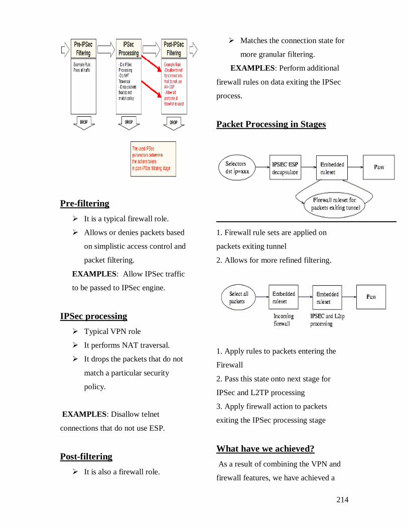
214
Pre-filtering
It is a typical firewall role.
Allows or denies packets based
on simplistic access control and
packet filtering.
EXAMPLES: Allow IPSec traffic
to be passed to IPSec engine.
IPSec processing
Typical VPN role
It performs NAT traversal.
It drops the packets that do not
match a particular security
policy.
EXAMPLES: Disallow telnet
connections that do not use ESP.
Post-filtering
It is also a firewall role.
Matches the connection state for
more granular filtering.
EXAMPLES: Perform additional
firewall rules on data exiting the IPSec
process.
Packet Processing in Stages
1. Firewall rule sets are applied on
packets exiting tunnel
2. Allows for more refined filtering.
1. Apply rules to packets entering the
Firewall
2. Pass this state onto next stage for
IPSec and L2TP processing
3. Apply firewall action to packets
exiting the IPSec processing stage
What have we achieved?
As a result of combining the VPN and
firewall features, we have achieved a

215
dual protection feature in our new
security system.
1. The OS, which is the base for the
performance of VPN and the protection
for the OS is brought about by firewall,
thus mutually benefiting from each of
their features.
2. We have utilized the basic resources
available for us and have come up with a
trustable yet simple feature. The basic
flaws of the proposed systems have been
discarded by just combining them and
with no other major change.
3. A firewall is different from VPN, but
the two of them work together to help
protect your computer. You might say
that a firewall guards the windows and
doors against strangers or unwanted
programs trying to get in, while VPN
protects against viruses or other security
threats that can try to sneak in through
the front door.
MERITS:-
Most simple method.
Based completely on the
available resources (the system is
modularized).
IPSec security parameters can be
used as filtering criteria.
The features of the new system
are based on proved concepts and
hence, probability of flaws is
minimal.
DEMERITS:-
In spite of all the security
features enhanced, still virus
protection isn’t achieved entirely
and we may have to seek a virus
protection system to achieve this.
Combination firewall/VPN
appliances are not the best
solution in some environments,
such as in companies that
generate revenue from high-
traffic Web sites and rely heavily
on VPN for branch office and
remote access connectivity
because VPN eats a lot of
processing power, potentially
slowing down Web-traffic
response-time.
FUTURE ENHANCEMENTS:-
(What we have to achieve in the
upcoming years)
All the firewalls don’t offer very good
virus protection. Thus Virtual Private
Networks and firewall combination is
the best security solution for all
intrusions available but not for viruses.
The best way to provide solutions for all
the security problems related to the
viruses is given below.
216
Security logs
System logs
Traffic logs
Packet logs
The most practical way to address the
virus problem is through host based
virus protection software. Hence the
combination of Virtual Private Networks
and firewalls with some virus protection
software embedded in it will provide the
best secure network. Most anti-virus
software offer options such as automatic
cleaning, prompt for response, delete if
the virus cannot be repaired. If this is
configured it works in background
without disturbing.
CONCLUSION:
No VPN solution provides effective
security if the operating system of the
machine is not secure. The firewall will
protect the base operating system from
attack. But our proposed system will
truncate the flaws of both VPN and
firewalls. Thus the security can be
strengthened by the combination of VPN
and firewall hence become truculent in
terminating any type of intrusion.
Though the combination will work out
effectively, it will be inefficient in
preventing the intrusion of few viruses.
Thus virus protection software can be
built to enhance the security and build
perfect security.
BIBLIOGRAPHY
E-security and You-Sundeep Oberoi.
Firewalls a complete Guide-
Goncalves,Marcus
Building Internet firewalls-
Elizabeth.d.Zwick
Firewalls-Strebe,Mathe

Proceedings of the Third National Conference on RTICT 2010
Bannari Amman Institute of Technology ,Sathyamangalam- 638401
9-10 April 2010
217
Authors:
R.Divya Priya ([email protected])
R.Lavanya ([email protected])
Thiagarajar College of Engineering
Madurai-15.
“AUTOMATIONOF IRRIGATION
USING WIRELESS”
Abstract:
The aim of the present paper is to
review the technical and scientific state
of the art of wireless sensor technologies
and standards for wireless
communications in the Agric-Food
sector. These technologies are very
promising in several fields such as
environmental monitoring, precision
agriculture, cold chain control or
traceability. . The paper focuses on WSN
(Wireless Sensor Networks) and data
acquisition system Presenting the
different systems available, recent
developments and examples of
applications of cultivation.
Today in India inclination towards
automization of irrigation is gaining
momentum due to :
• Automation eliminates manual
operation to open or close valves,
especially in intensive Irrigation process.
• Possibility to change frequency of
irrigation and festination process and
also to optimize these processes.
• Adoption of advanced crop systems
and new technologies, especially new
crops system. That are complex and
difficult to operate manually.
• Use of water from different sources
and increased water and fertilizer use
efficiency.
• System can be operated at night, thus
the day time can be utilized for other
agricultural activities.
• Pump starts and stops exactly when
required, thus optimizing energy
requirements.
Automation:
Automation of irrigation system
refers to operation of the system with no
or minimum manual interventions.
Irrigation automation is well justified
where a large area to be irrigated is

218
divided into small segments called
irrigation blocks and segments are
irrigated in sequence to match the flow
or water available from the water source.
SYSTEMS OF AUTOMATION:
1. Closed Loop Systems:
This type of system requires feedback
from one or more sensors. The
operator develops a general control
strategy. Once the general strategy is
defined, the control system takes over
and makes detailed decisions of when to
apply water and how much water to
apply. Irrigation decisions are made and
actions are carried out based on data
from sensors. In this type of system, the
feedback and control of the system are
done continuously.Closed loop
controllers require data acquisition of
environmental parameters (such as soil
moisture, temperature, radiation, wind-
speed, etc) as well as system parameters
(pressure,
flow, etc.).
2. Real Time Feedback System
Real time feedback is the application if
irrigation based on actual dynamic
demand of the plant itself, plant root
zone effectively reflecting all
environmental factors acting upon the
plant. Operating within controlled
parameters, the plant itself determines
the degree of irrigation required. Various
sensors viz., tensiometers, relative
humidity sensors, rain sensors,
temperature sensors etc control the
irrigation scheduling. These sensors
provide feedback to the controller to
control its operation.
Automatic Systems:
In fully automated systems the human
factor is eliminated and replaced by a
computer specifically programmed to
react appropriately to any changes in the
parameters monitored
by sensors. The automatic functions are
activated by feedback from field units

219
and corrections in the flow parameters
by control of devices in the irrigation
system until the desired performance
level is attained. Automatic systems can
also perform auxiliary functions such as
stopping irrigation in case of rain,
injecting acid to control pH, sounding
alarms, etc. Most control systems
include protection in emergencies such
as loss of the handled liquid due to pipe
burst. They close the main valve of the
whole system or of a branching, when an
unusually high flow rate or an unusual
pressure drop is reported by the
sensors.
System Component Of An Automatic
Irrigation System
Controllers:
This device is the heart of the
automation, which coordinates
operations of the entire system. The
controller is programmed to run various
zones of an area for their required
duration or volume. In some cases
sensors are used to provide feedback to
the controller. In the simplest form,
irrigation controllers are devices which
combine an electronic calendar and
clock and are housed in suitable
enclosure for protection from the
elements.The PLC’s, microprocessors
and computers are now available and
being used extensively.
(PLC-Programmable Logic Controllers).
Electromechanical Controllers:
These types of controllers are
generally very reliable and not very
sensitive to the quality of the power
available. However, because of the
mechanically-based components, they
are limited in the features they provide.
The picture shows the controller for
opening and closing of irrigating pipes.
Electronic Controllers:
These types of systems are more
sensitive to power-line quality than
electromechanical
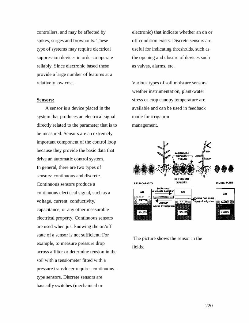
220
controllers, and may be affected by
spikes, surges and brownouts. These
type of systems may require electrical
suppression devices in order to operate
reliably. Since electronic based these
provide a large number of features at a
relatively low cost.
Sensors:
A sensor is a device placed in the
system that produces an electrical signal
directly related to the parameter that is to
be measured. Sensors are an extremely
important component of the control loop
because they provide the basic data that
drive an automatic control system.
In general, there are two types of
sensors: continuous and discrete.
Continuous sensors produce a
continuous electrical signal, such as a
voltage, current, conductivity,
capacitance, or any other measurable
electrical property. Continuous sensors
are used when just knowing the on/off
state of a sensor is not sufficient. For
example, to measure pressure drop
across a filter or determine tension in the
soil with a tensiometer fitted with a
pressure transducer requires continuous-
type sensors. Discrete sensors are
basically switches (mechanical or
electronic) that indicate whether an on or
off condition exists. Discrete sensors are
useful for indicating thresholds, such as
the opening and closure of devices such
as valves, alarms, etc.
Various types of soil moisture sensors,
weather instrumentation, plant-water
stress or crop canopy temperature are
available and can be used in feedback
mode for irrigation
management.
The picture shows the sensor in the
fields.

221

222
This flowchart explains about the
requirements needed for the irrigation
and the abnormal conditions of the
climatic environment such as drought,
climatic changes, seasonal rainfall,
and many more.
The chart is explained as follows:
First and foremost step is the
analysis of soil condition by
sensors such as tensiometer
to measure the water
percolation, moisture in soil.
Then, the crop requirements
are taken into account and the
analysis is done for the crop.
If suppose the crop is paddy,
we need an adequate supply
of water.
After the analysis, the
climatic condition is taken
into account such as monsoon
season, summer and winter.
The data acquired from the
above analysis are processed
and finally using the wireless
network the operation is
done.
Automatic Metering Valve:
These valves are required only in
volume based irrigation system. The
volume of water
required for the irrigation can be
adjusted in these automatic metering
valves. These valves
can be simple metering valve which
shuts off after delivering preset quantity
of water or
automatic metering valve with pulse
output which provides pulses to the
controller to count
the volume of water.
Valves:
Automated valves are activated either
electrically, hydraulically or
pneumatically and used to switch water
on or off, flush filters, mains and
laterals, sequence water from one field
or segment to other.
Metering pumps:
These pumps are suitable for feeding of
known quantity of fertilizers/chemicals.

223
The capacity of pumps varies from 1.5 to
3.5 litres / hour
APPLICATION OF WIRELESS:
Using wireless sensor networks
within the agricultural industry is
increasingly common. Gravity fed water
systems can be monitored using pressure
transmitters to monitor water tank levels,
pumps can be controlled using wireless
I/O devices, and water use can be
measured and wirelessly transmitted
back to a central control center for
billing. Irrigation automation enables
more efficient water use and reduces
waste.
The above picture shows the root and
nodes of the wireless network.
Wireless sensor networks (WSN)
technologies are increasingly being
implemented for modern precision
agriculture monitoring. The advantages
of WSN in agriculture are for several
reasons; these includes suitability for
distributed data collecting and
monitoring in tough environments,
capable to control an economical way of
climate, irrigation and
nutrient supply to produce the best crop
condition, increase the production
efficiency while decreasing cost and
provide the real time information of the
fields that enable the farmers to adjust
strategies at any time. This paper
presents the preliminary design on the
development of WSN for paddy rice
cropping monitoring application. The
propose WSN system will be able to
communicates each other with lower
power consumption in order to deliver
their real data collection. The main
objective of the new design architecture
is to cater the most important and critical
issue in WSN, that is power
consumption. The design will attempt a
sensor node board systems consist of a
low power microcontroller so called
nano-Watt technology, low-power
semiconductor based sensors, Zigbee™

224
IEEE 802.15.4 wireless transceiver and
solar energy source with optimal power
management
system. The all information’s are
processed using data acquisition system.
Conclusion:
Environmental monitoring in agriculture
is essential for controlling in economical
way of climate, irrigation and nutrient
supply to produce the best crop
condition, increase the production
efficiency while decreasing cost . The
real time information of the fields will
provide a solid base for farmers to adjust
strategies at any time. WSN will
revolutionize the data collection in
agricultural research. However, there
have been few researches on the
applications of WSN for agriculture.
“ Innovation is the mothering for the
Future Technology”

Proceedings of the Third National Conference on RTICT 2010
Bannari Amman Institute of Technology ,Sathyamangalam- 638401
9-10 April 2010
225
Key management and distribution for
Authenticating group communication
Krisshnakumar K.S., Department of computer science and engineering,
Jaisakthiraman M., Department of computer science and engineering,
Velammal college of engineering and technology, Madurai-9.
Abstract – In network communication,
security is important to prevent intruder’s
attack, where authentication plays a very
important role in ensuring the
communication with the right participant.
To authenticate a group of users and to
hold confidentiality between them a new
approach of key management is handled in
this paper. This key management is a
group key management used for
cryptography process that provides security
with less computation complexity, which
leads to fast and easy authentication. Here
a tree based key management scheme has
been designed through which key
distribution among the user involves
authentication with less storage complexity
too. here dynamic membership
authentication is described which talks
about communication or transaction
among user and server with a new different
instant key that is formed from a group of
members who are currently participating in
transaction or communication. Releasing
or joining a user from or to the group is
possible here by which the keys get
changed instantly whenever there is an
alteration in the current participation in
transaction or communication. With the
help of users hidden key an ‘Instant key
can be computed As the entire users’
hidden keys is used for the generation of
the instant key we can ensure the
communication between a valid set of
authenticated users. So an intruder cannot
interrupt any communication between the
users as their keys get vied often. Thus we
can provide a very reliable system for the
communication of the people. Keywords: - Authentication, Instant key,
Hidden key, Dynamic membership,
Group key.
I Introduction To strengthen the communication security,
authentication is preferred to authenticate the
users to ensure their validly and hold their
confidentiality. This is based on cryptography
which has many advantages over the other
schemes [4].This paper describes a group key
management that is used for cryptography
process that provides authentication for
providing identification. Here the group key is an instantly generated
key, which is as a function of all the current
group members, termed as an instant key.
This is for group communication over
particular servers‟ access. It is formed by a
virtual tree based approach where each leaf
node denotes a user (who wishes to access the
same server) and each intermediate node
value is evaluated from its subordinate node.
Each user holds a pair of keys namely „short-
term secret key‟ and „hidden key‟.

226
The „instant key is generated from the
collection of the entire user‟s value that
remains valid from the time when the user
joins and until he leaves the tree structure. In this group key management scheme,
releasing a user from the group is possible
which is described in section III.B. Similarly
a member can also join the existing group
which is described in III.C. In this situation
the key gets changed instantly whenever there
is an alteration in current participation of
users for communication. Only after receiving the group key, a user
can further communicate with other
servers. It‟s explained in the section III of
this paper. By ensuring the correctness of
the user, the server will abduct all its
communication information by
encrypting using the group key. Hence only valid users are supported by the
server for the further communication. This method involves less storage space
complexity and less computation
complexity that leads to fast up the process.
II Subset Tree Structure There is some tree structure based scheme
that is used for group communication [2]
[3] [5] [7] as shown in figure: 1. here all the
nodes will be allotted with a value. The leaf
nodes are members M1, M2……Mn. A
member‟s value is obtained from the root
node to its member leaf node. By evaluating
the members in the root nodes, group key is
formed for communication. Then the key is
broadcasted across the tree structure to all
its nodes. In a proposed scheme called Group key
Management Protocol (GKMP) [5] [7], the
entire group shares the same key called as
session-encrypting key (SEK). In some of
the tree-based key distribution scheme [6]
[7], the root value is used as the session key
as well as group key. In these schemes, to
our knowledge, the storage detail about the
user occupies more space [8]. In some techniques [5] [7], it is stated that
at the depth two or more from the root, the
key values are duplicated across the tree
twice. For example, L1 and L2 in figure: 1.
Also it is stated that the deletion of more
than one member may bring the scheme to
halt. This paper proposes the scheme
through which it highlights the
enhancement of this tree based group
communication for authenticating user with
less storage and computation complexity.
III Proposed Tree Based Group Key Generation In this Group key generation each user is
denoted as a leaf node .Each key „u‟
represents secret key „Ku‟(i.e. own key
and a hidden key „Hku‟ as shown in the
figure 2 that remain valid from the time
user joins and until he leaves.

227
A Hidden Key Generation Hidden Key can calculated as Every intermediate node holds a secret
key obtained from its leaf user (parent‟s
value is evaluated from the user). The secret key of the intermediate node
can be generated as
With the help of each users hidden key,
group key can be computed .for example
as in figure: 2 from the user „M1‟ a group
key can be generated.
Using K7 and HK8 the node „3‟
can calculate its‟ key value(i.e. K3)
Then using K3 and HK4, the key
value of K1 can be obtained. Similarly K1 and Hk2 provide a
computed value K0, which is the
group key. A binary tree with „n‟ leaves will have
(2n-1) nodes. i.e. (2n-1) HKs are
considered for the evaluation. From the authorized users „Mi‟ those who
require service will be collected and
formed as a tree structure. Then the key
calculation takes place to compute the
group key, say „K‟. If a new user joins the
group dynamically the key gets changed
as K‟. If a user leaves the group then
instantly it becomes K‟‟.
B Member joins Consider a binary tree that has a valid
members M1, M2, Mn.Among these n
valid users only those who request for a
service on a particular server will be
formed as an individual group. A new
member Mn+1 indicate the service request
message that contains its own HKey
(hidden key) i.e.HK [Mn+1].This message is
distinct from any join messages generated
by the underlying communication system.
The authentication server first determines
the insertion point in the tree. The insertion
point is the shallowest rightmost node,
where the join doesn‟t increase the height
of the key tree. Otherwise if the key tree is
fully balanced, the new member joins to the
root node.

228
Suppose a user M8 wished to access a
particular server the newly requested
user M8 has to be added to the existing
list of users as shown in the fig3. Here, the
insertion point in the tree is node5 where
M4 exists.
Now a binary node is
created from node5, in turn it becomes
the intermediate node where M4 is shifted
to its left most node (seen in the above
figure) and the newly requested user is
joined in the rightmost node i.e. M8.The
server proceeds to update its share and
compute the group key; it can do this
since it‟s know all the necessary HKey.
While addition of a new user the
server has to perform n+ 1 computation [7].
Infact in obtaining the HK[8] the server
starts computations and then it rekeys the
nodes‟5‟,‟2‟ and „0‟ and then process further .All other members update their new
instantly generated group key.
C Member Leaves Once again, we start with n members and
assume that member Mn leaves the group.
The sponsor in this case is the server which
instantly updates the generated keys.
Suppose a user wants to leave from this
group all the keys from the leaf node to the
root most must be updated in order to
prevent the access to the future data. If member M7 wants to departure from
the service, then intermediate node 6 will
have a change and shuffle with 13 and 14
as shown in the figure 5. The server has to perform (n-1)
computations under deletion of an existing
user [7]. Now the key S of the intermediate
nodes „6‟,‟2‟ and „0‟ must be renewed as
shown in the figure 6 after the release of
M7 from the current group. Hence the key
gets dynamically convert, due to the
changes in the participation of user access,
with less computation. The server uses
instant key whenever there is an alteration
in the group key communication.

229
IV Instant Key Communication
The dynamically generated instant
key from the group of valid users is used to
encrypt the authentication details for
further communications in figure 7.
Consider a user „U‟ with identity
‟IDu‟ and an authenticating server „AS‟
with the identity „IDas‟ shares a secret
codeword „cw‟.consider two large prime
numbers p and q, where p=2q+1, and
perform a secure one way hash function „h‟ In the proposed scheme following
procedure takes place:
a. Initial phase
Initially the user requests the AS by
sending its H value.
After receiving H, AS checks the „cw‟.
Then it generates a random number „R1‟
sends to U where („i‟
already obtained from U)
b. Middle phase U checks the received message
whether it equals the sent content
which is i. Then U sends its HK along
with R1 to AS encrypted as Kas. After receiving the HK of every valid
user, AS will form the tree structure
for grouping the key (GK) as per
request for „Srv‟. Also it creates identification content
„id-msg‟ comprises of the following
Where „Ku,srv‟ denotes the key used
for cryptography, process of user and
data server communication and
„Kas,srv‟ denotes the key for
communicating AS and server.
c. Main phase AS constructs and sends the
confirmation message to individual U
by encrypting through the newly
generated group key.

230
„TS‟ denotes”Time Sampling” at
which the key was issued. Here the entire content was encrypted
using GK, which can be decrypted
only by the authorized users. The
detail content can only decrypt by the
respective user because a distinct key
(Kuj, AS) for each user encrypts it. Now, the user passes the „id-msg‟ to the
server. It is obtained from AS that cannot
be revealed even by the user. The server
decrypts its (Server-User) Key using [id-msg].
V Discussion The discussions and comparisons
emphasize the benefits of the proposed
group key scheme as given below: In the group key management protocol
(GKMP)[5][7],the entire group shares
the same key called session-encrypting
key (SEK), where as in the proposed
Instant key method, the instant key is
common to all users for initial stage but
a distinct key for each user is provided. In some of the tree-based key
distribution scheme [6] [7], the root
value is used as the session key as well
as the group key. But here the
computation of the hidden key forms
the group key, through which the
session key for individual user is sent. The instant key gets varied all the
time when a node arrives or leaves the
group. It keeps on changing the key so
that an intruder cannot enter into the
communication of the group. So it
leads to high security.
As the instant key is new for all changes
in the tree path, impersonation of the
authorized user is avoided so it confirms
only the valid user‟s transmission. As the newly generated key is obtained
from current user‟s hidden key, the
valid currently operating users only can
access it. Hence authentication is
successfully ensured. It leads to assure
secure communication. Whenever a node joins/leaves, the server
has to perform (n+1)/ (n-1) computations
respectively [7].Also in some tree-based
communications, all other members
update their tree accordingly and
compute the new group key. It n=might
appear wasteful to broadcast the entire
tree to all members [2] [3] [6]. But in this
proposed scheme, only a particular part
of the tree is necessary for computation
whenever the tree structure is altered.
Consequently it minimizes the storage
requirements for the user information on
server. In some authentication scheme (like
certification scheme), verifiers spend
more time to extract a certificate path
from network of certificates and do
repeated process to verify and
authenticate a user. In this scheme
verification time is very less. As a unique session key is provided to
the individual user, impersonation is
also not possible. In certain tree-based group key scheme,
the intermediated nodes are duplicated
across tree several times (at least
twice)[7].where as in this scheme, even
while generating the instant key, the
required path alone chosen without
disturbing the other intermediate nodes
so the duplication is avoided.
231
VI Conclusion The proposed scheme is a tree based key
management where an instantly generated
key is computed as a function of all current
group members present in communication.
Thus only valid users can communicate with
each other and the presence of users is
ensured without much difficulty.
Authentication is successfully processed
during communication. The time and storage
complexity is reduced. Hence the proposed
tree based key management scheme ensures
the right participant in communication with
less time and authenticates the users to
maintain confidentiality. REFERENCES
[1] David A. McGrew and Alan T.
Sherman, “Key Establishment in
Large Dynamic Groups Using
One- Way Function Trees"
Cryptographic Technologies
Group, TIS Labs at Network
Associates, May 20, 1998.
[2] Yongdae, Perrig and Tsudik,
"Group Key Agreement efficient in
communication", IEEE transactions
on computers, Oct 2003.
[3] Sang won Leel, Yongdae Kim2,
Kwangjo Kiml "An Efficient Tree-
based Group Key Agreement using
Bilinear Map", Information and
Communications University (ICU),
58-4, Hwaam-Dong, Yuseong-gu,
Daej eon, 305-732, Korea.
Proceedings of the Third National Conference on RTICT 2010
Bannari Amman Institute of Technology ,Sathyamangalam- 638401
9-10 April 2010
232
COMPARISON OF CRYPTOGRAPHIC ALGORITHMS FOR SECURE
DATA TRANSMISSION IN WIRELESS SENSOR NETWORK
R.Vigneswaran
R.Vinod Mogan
Pre-Final B.Tech(It)
Abstract:
This paper proposes an secure data
transmission over the wireless sensor network
environment using various symmetric
cryptographic algorithms which provides a
guarantee to the transmitted data to be secure, no
encryption and decryption take place at cluster
head and comparison is made based on the
performance of different (AES, DES & Blowfish)
cryptographic algorithms.
Security is a critical requirement in data
transmission over the wireless sensor network
environment. A dishonest intermediate node can
read, modify or drop the data as well as send false
values to mislead the base station. Generally data
transmitted by the sensor node should be
decrypted at cluster head .The aggregated data is
then encrypted before being transmitted to the
base station. This technique is vulnerable from
security perspective because decryption of data
requires the cluster head to obtain the symmetric
key that may result in insecure data transmission.
Therefore sensor node sends encrypted data to the
cluster head and cluster head just forward the
encryption data from the sensor nodes to base
station and base station can decrypt the
transmitted data and obtain the plaintext.
Keywords: wireless sensor network,
encryption, decryptions and security.
Introduction:
Sensor network are dense wireless
network of small, and low cost sensors, which
collects, and disseminate (spread widely) the data

233
from remote location. It facilitate monitoring [4]
and controlling of physical environment from
remote location with better accuracy, sensor
network can be described as a collection of sensor
nodes which co-ordinate to perform some specific
function.
Sensor nodes are small, inexpensive low
power distributed devices that are capable of
processing the sensed data locally and
communicated them through wireless network.
Each sensor node is capable with only a limited
amount of processing but when co-ordinate with
the information from a large number of other
nodes, they have the ability to measure a physical
environment. Such sensor network are expected to
be widely deployed in a vast variety of
environment for commercial, civil and military
application such as surveillance, vehicle tracking,
climate and habitat monitoring, intelligence,
medical and acoustic data gathering The key
limitation of wireless sensor network are the
storage, power and processing. These limitations
and the specific architecture of sensor nodes call
for energy efficient and secure communication
protocol. The foremost challenge in sensor
networks is to maximize the lifetime of sensor
nodes due to the fact that it is not feasible to
replace the batteries of thousand of sensor nodes.
To obtain the estimated location
information of sensors, deployment of the sensor
nodes over the network area must be done by
following a procedure. Assume the sensor
network area is a square; the following is the
deployment procedure of our key distribution
scheme.
Sensor nodes are divided equally in to an
„n‟deployment groups
Sensor deployment area is divided equally
into „n‟deployment grids.
The center points of these „n‟grids is
determined as deployment points.
A group of sensor is dropped from each
deployment point
Figure1. Represent the sensor network area with
deployment pints, each deployment point is
represented by small circle while gray shaded
square represent a deployment grid. Deployment
grids are denoted by notation n (i, j).
Figure (1) also has neighboring grids that are
represented by White Square (si, j). This
neighboring area of shaded deployment grids

234
Figure No. 1 Sensor network area with sub-
square and deployment points
Sensor network is hierarchical architecture
where data is routed from sensor nodes to base
station through cluster heads. Base station
interface sensor network to the outside network.
Sensor nodes are assumed to immobile and also
they do not have a specific architecture when
deployed over a specific geographic area.
However, these nodes organize themselves into
clusters, based on self-organizing cluster to
handle the communication between the cluster to
handle the communication between the cluster
nodes and the base station.
Sensor nodes are battery powered and
their lifetime is limited. Therefore, cluster heads
are dynamically chosen initially. In order to have
uniform power consumption among all the sensor
nodes, cluster heads are then selected based on the
remaining battery power. To maximize the
lifetime, sensor nodes are in active mode when
they are put to sleep mode. Base station is
assumed to have sufficient power and memory to
communicate securely with all sensor nodes and
also with the external wired network.
Sensor nodes are assigned a secret key (ki)
and a unique ID number that identifies itself in the
network. As wireless transmission is not
completely trustable, assigning secret keys to
sensor nodes in wireless environment is not
secure. Hence Ki and sensor IDs are assigned
during the manufacturing phase. Base station is
then given all the ID numbers and Ki used in the
network before the deployment of network.
Having a complete list of sensors in the base
station protect sensor network from malicious
sensor nodes. Whenever base station broadcasts a
new Kb all the sensor nodes have to re-generate
their new secret session keys (Kt, b). The built in
keys in sensor nodes avoid the distribution if
secret keys in the wireless environment as well as
providing substantial security.
SECURE DATA TRANSMISSION
ALGORITHM FOR WIRELESS
SENSOR NETWORKS
The security protocol achieves secure data
transmission on wireless sensor network by
implementing the following five phases in two
algorithms: Algorithm A and B are implemented
in the sensor nodes and in the base station
respectively,
1) Broadcasting session key by base station is
performed in algorithm B.

235
2) Generation of cryptographic key in sensor
nodes is performed in algorithm A.
3) Transmission of encrypted data from sensor
nodes to cluster heads is performed in algorithm
A.
4) Appending the ID# to data and then forwarding
it to higher level cluster heads are performed in
algorithm A
5) Decryption and authentication of data by the
base station is performed in algorithm B.
The base station, periodically
broadcasts new session key to maintain data
freshness. Sensor nodes receive broadcasted
session key Kb and computes their nodes –
specific secret session key (Ki, b) by XORing
with Ki with Kb.Ki, b is used for all the
consequent data encryption and decryption during
that session by both algorithms. Since each sensor
node calculates Ki,b using its unique built in key,
encryption data with Ki,b also provides data
authentication in the proposed architecture.
Changing encryption keys time-to –time
guarantees data freshness in the sensor network,
moreover it helps to maintain confidentiality of
transmitted data by preventing the use of the same
secret key at all times. During the data
transmission, each sensor nodes appends its ID#
and time stamp to the messages to verify data
freshness. Additional security in the data
communication is obtained by sending the
encrypted data .The cluster head, when receives
the data from the nodes, appends its own ID#
before forwarding the data to the base station.
This helps the station in locating the origin of the
data.
Algorithm A: Implemented in sensor nodes
1). If sensor node I want to send data to its cluster
head, go to next step, and otherwise exit the
algorithm.
2). Sensor node I requests the cluster head to send
the current session key Kb.
3). Sensor node I XORs the current session key
(Kb) with it‟s built in key Ki to compute the
encryption key Ki, b.
4). Sensor node I encrypts the data with Ki, b and
appends its ID# and the time stamp to the
encrypted data and then sends them to the cluster
head.
5). Cluster head receives the data, appends its own
ID#, and then sends them to the higher –level
cluster head or the base station. Go to step 1.

236
Note: Cluster head appends its own ID# to the
data in order to help the base station to locate the
originating sensor node.
Algorithm B: Implemented in base station
1. Check if there is any need to broadcast the
session key Kb all the sensor nodes. If so,
broadcast Kb to all sensor nodes.
2. If there is no need for a new session key then
check if there is any incoming data from the
cluster heads. If there is no data being sent to the
base station, then go to step 1.
3.If there is any data coming to the base station
then compute the encryption key Ki,b using the
ID# of the node and the time stamp within there
data .base station ten uses the Ki,b to decrypt the
data.
4.Check if the current encryption key Ki,b has
decrypted the data perfectly .This leads to check
the creditability of the time stamp and the ID# .If
the decrypted data is not perfect discard the data
and go to step 6.
5. Process the decrypted data and obtain the
message sent by the sensor nodes.
6. Decides whether to request to all sensor nodes
for retransmission of data .If not necessary then
go back to step 1.
7. If a request is necessary the request to the
sensor nodes to retransmit the data. When this
session is finished go back to step 1.
In the above algorithms A and B we use prototype
sensor nodes of smart Dust .As shown table 1
these sensor nodes are resources constraint in
every sense.
IMPLEMENTATION
Considering restricted resource the cry to
graphic primitives used in sensor networks must
chosen carefully in term of their code size and
energy consumption therefore, we evaluated
several cryptographic algorithms to use for
encryption and decryption. It is observed from the
analysis that code space can be saved by using
same cipher for both encryption and decryption.
TABLE 1.CHARACTERISTICS OF
SMART DUST SENSORS
CPU 8-bit, 4 MHz
Storage 8K instruction flash
512 byte RAM
512 bytes
EEPROM
Communication 916 MHz radio

237
Bandwidth 10 kilobits per
second
Operating system TinyOS
OS code space 3500 bytes
Available code space 4500 bytes
The number of clock needed by the
processor to compute the security function
primarily determines the amount of computational
energy consumed by a security function on a
given microprocessor. The number of clocks
necessary to perform the security function mainly
depends on the efficiency of the cryptographic
algorithms.
In the above methods of data transmission the
security algorithms faces the some disadvantages.
This is Limited number of Storage available and it
takes additional memory space and takes more
delay time. In base station we get less number of
throughputs. Security function determined in
microprocessor needs more of clock signal. Due
to this disadvantage we cannot get secure data in
base station correctly .In order to overcome these
shortcomings and to reduce interference in data
transmission we introduce various cryptographic
algorithms implemented using “Network
simulator (NS-2)”and find the performance results
such as throughput, delay time
Network security:
Security is a critical requirement in data
transmission [3] over the wireless sensor network
environment. A dishonest inter mediate node can
read, modify or drop the data as well as send false
values to mislead base station. Asymmetric
cryptographic algorithms are not suitable to
provide security on wireless sensor network since
they require high computation power, and storage
resources. Therefore symmetric key cryptographic
algorithms are employed to support security
because of limited key length and memory
available on the sensor nodes. In symmetric key
encryption or secret key encryption, only one key
is used to encrypt and decrypt data and the key
should be distributed before transmission between
two entities. It is also known to be very efficient
since the key size can be small. Generally data
transmitted by the sensor nodes should be
decrypted at cluster head.
The data was encrypted before being
transmitted to the base station. This technique is
vulnerable from security perspective because
decryption of data requires the cluster head to
obtain the symmetric key that may result in
insecure data transmission.

238
Figure No. 2 Encryption Model
Therefore sensor node send encrypted data
to the cluster head and cluster head just forward
the encrypted data from the sensor nodes to base
station and base station can decrypt the
transmitted data and obtain the plaintext.
Performance between symmetric cryptography
algorithms are proposed based on throughput as
well as end-to-end delay using „Network
simulator (NS-2)‟.
Throughput is the amount of information that is
successfully transmitted from the transmitting end
to receiving end at the instant of time taken to
receive the last packet.
Cryptographic Algorithms:
1. Blow fish:
a) Blowfish is a symmetric block cipher that can
be used as drop in replacement for DES or IDEA
[4].
b). It takes variable length key, from 32 bits to
128 bits. The block size is 64 bits.
c). It is ideal for both domestic and exportable
use.
d) It is much faster than DES and IDEA,
unpatebted and royalty free, no license are
required.
e). It iterates a simple encryption function by 16
times.
f). In DES, 56 bits key size is vulnerable to brute
force attack, and recent advance in differential
cryptanalysis and linear cryptanalysis indicate that
DES is vulnerable to other attacks as well.
g). Data encryption occurs via a 16round each
round consist of key dependent permutation and a
key and data dependent substitution .All operation
are xores and addition on 32 bit word. The only
additional operation is fore indexed array data
lookups per round.
2. Data Encryption Standard (DES)
In data encryption standard key [4 consists of 64
binary digits („0‟s or 1‟s) of which 56 bits are
randomly generated and used directly by the
algorithms .The others 8‟bits, which are not used
by the algorithms, are used for error detection.

239
The algorithm is designed to encrypt and decrypt
blocks of data consisting of 64 bits under control
of 64-bit key. The unique key chosen for use in a
particular application makes the results of
encrypting data using the algorithm unique.
Selection of a different key causes the cipher that
is produced for any given set of inputs to be
different. The cryptographic security of the data
depends on the security provided for the key used
to encipher and decipher the data. The algorithm
is designed to encipher and decipher blocks of
data consisting of 64 bits under control of a64–bit
key**. Deciphering must be accomplished by
using the same key used for enciphering, but with
the schedule of addressing the key bits altered so
that the deciphering process is the reverse of the
enciphering process. A block to be enciphered is
subjected to an initial permutation IP, then to a
complex key- dependent computation and finally
to a permutation which is the inverse of the initial
permutation IP inverse. The key –dependent
computation can be simply defined in terms of a
function f called the cipher function, and a
function Ks called the schedule.
3. Advance encryption standard (AES):
AES [9] must be symmetric block cipher with a
block length of 128 bits and support for key
lengths of 128,192,256, bits. AES must have high
computational efficiency, so as to be usable in
high-speed application links. Analysis of AES
compared to DES the amount of time requirement
for the operation is limited. The input to the
encryption and decryption algorithm is a single
128 –bit block. This block is copied into the state
array, which is modified at each stage of
encryption and decryption. After the final stage,
state is copied to an output matrix. Similarly 128-
bit key is depicted as a square matrix of bytes.
This key is then expanded into an array of key
schedule is 44 words for the 128 bit key, ordering
the bytes within a matrix is by column for
example, the first four bytes of a 128-bit plaintext
input encryption cipher occupy the first column
and the second four byte occupy second column,
and so as on.
Overall AES structure:
1. AES do not use a festal structure but process
the entire data block in parallel during each round
using substitution and permutation.
2. The key that is provided as input is expanded
into an array of forty-four 32-bit worlds [i]. Four
distinct words serve as each round.
3. Four different stages are used, one of
permutation and three of substitution.
Substitution bytes: Uses an S-Box to perform a
byte-by-byte substitution of the block.
Shift rows: A simple permutation

240
Mix columns: A substitution that makes use of
arithmetic over GF (2^8)
Add round key: A simple bit wise XOR of the
current block with apportion of the expanded key.
4. For both encryption and decryption, the cipher
begins with an add round key stage, followed by
nine rounds that each includes all four stages.
5. Only the Add Round Key stage makes use of
the key. For this reason, the cipher begins ends
with an Add Round Key stage.
6. Cipher as the alternating operation of XOR
encryption (Add Round Key) of the block,
followed by scrambling of the block (the other
three stages), and followed by XOR encryption,
and so on. This scheme is efficient highly secure.
7. Each stage is easily reversible .for the substitute
byte, shift Row, and Mix columns a stage, an
inverse function is used in the decryption
algorithm. For the Add round key stage, the
inverse is achieved by XORing the same round
key to the block, using the result that A XORs A
XORs B = B.
8. As with most block ciphers, the decryption
algorithm makes use of the expanded key in
reverse order. However the decryption algorithm
is not identical to the encryption algorithm.
9. The final round of the both encryption and
decryption consists of only three stages again.
Again, this is a consequence of the particular
structure of AES and is required to make the
cipher reversible.
Rijndael (AES) was designed to have the
following characteristics:
Resistance against all attacks.
Speed and code compactness on a wide
range of platforms.
Design simplicity.
Simulation Results:
Fig 3.Load Vs Throughput graph for
cryptographic algorithms
From the above three curves red co lour curve
is load versus throughput graph of AES algorithm,
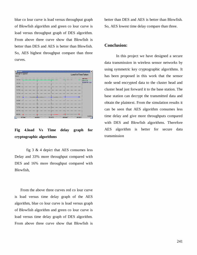
241
blue co lour curve is load versus throughput graph
of Blowfish algorithm and green co lour curve is
load versus throughput graph of DES algorithm.
From above three curve show that Blowfish is
better than DES and AES is better than Blowfish.
So, AES highest throughput compare than three
curves.
Fig 4.load Vs Time delay graph for
cryptographic algorithms
fig 3 & 4 depict that AES consumes less
Delay and 33% more throughput compared with
DES and 16% more throughput compared with
Blowfish,
From the above three curves red co lour curve
is load versus time delay graph of the AES
algorithm, blue co lour curve is load versus graph
of Blowfish algorithm and green co lour curve is
load versus time delay graph of DES algorithm.
From above three curve show that Blowfish is
better than DES and AES is better than Blowfish.
So, AES lowest time delay compare than three.
Conclusion:
In this project we have designed a secure
data transmission in wireless sensor networks by
using symmetric key cryptographic algorithms. It
has been proposed in this work that the sensor
node send encrypted data to the cluster head and
cluster head just forward it to the base station. The
base station can decrypt the transmitted data and
obtain the plaintext. From the simulation results it
can be seen that AES algorithm consumes less
time delay and give more throughputs compared
with DES and Blowfish algorithms. Therefore
AES algorithm is better for secure data
transmission

Proceedings of the Third National Conference on RTICT 2010
Bannari Amman Institute of Technology ,Sathyamangalam- 638401
9-10 April 2010
242
FREQUENCY SYNCHRONIZATON IN 4G WIRELESS COMMUNICATION
BHUVANESHWARAN.C , VASANTH KUMAR.M
III Year UG students, Department of Electrical and Electronics Engineering
Thiagarajar College of Engineering, Madurai-625015
Ph.no:9791249011, 9043844059
Email id: [email protected] , [email protected]
Abstract
Third Generation Partner Project
(3GPP) is considering Long Term
Evolution for both radio interface and
network characteristics. These systems
support reliable high data communication
over time dispersive channels with limited
spectrum and Inter Symbol Interference
(ISI). Orthogonal Frequency Division
Multiple Access (OFDMA) is used as a
multiple access technology in the
downlink of LTI systems and OFDM as
data transmission technology. The OFDM
is highly sensitive to timing and frequency
synchronization errors causing loss of
orthogonality among sub-carriers, because
orthogonality allows simultaneous
transmission on a lot of sub-carriers in a
tight frequency space without interference
with each other. This paper addresses
algorithm for frequency synchronization
for downlink LTE using defined
synchronization sequence. The detection
algorithm along with simulation is
presented.
Introduction
Long Term Evolution (LTE) is the
fourth generation of radio technologies
designed to increase the capacity and
speed of the mobile telephone network. It
is standard being specified by 3GPP within
release 8. In Orthogonal Frequency
Division Multiple Access (OFDMA) used
for downlink transmission and for uplink
Single Carrier Frequency Division
Multiple Access (SC-FDMA) has been
specified by 3GPP. It offers favourable
features such as high spectral efficiency,
robust performance in frequency selective
channel conditions, simple receiver
architecture , etc
However it is well known that
OFDM systems are more prone to time
and frequency synchronization errors,
hence accurate synchronization is needed
for interference free data reception.
Furthermore, when an user equipment
(UE) operates in a cellular system, it needs
to establish connection as fast as possible
with the best serving base station. So time
and frequency synchronization is the
primary criterion to be considered for any
LTE systems.
The frequency synchronization for
3GPP LTE has been investigated in this
paper and also a detection algorithm for
frequency offset is described.
LTE frame structure
Fig.1. LTE FRAME STRUCURE

243
LTE radio frames are 10ms in
duration. Each frame has ten sub-frames
and each sub-frame consists of two slots
each of 0.5ms duration.Each slots consists
of six or seven OFDM symbols depending
on whether normal or extended cyclic
prefix used.
The number of sub-carriers allocated
depends on the available bandwidth of the
system. The LTE specification defines
bandwidth from 1.25MHZ to 20MHZ. The
physical resource block (PRB) is defined
as time-frequency grid consisting of 12
sub-carriers in each slot (0.5ms). Resource
element is the smallest element in the time
frequency grid.
Fig.2.DOWNLINK RESOURCE GRID
0FDM system model
OFDM is a combination of
modulation and multiplexing.
Multiplexing generally refers to
independent signals, those produced by
different sources. In OFDM the signal
itself is first split into independent
channels, modulated by data and then re-
multiplexed to create OFDM carrier. The
modulation scheme may be any of the
following method, BPSK,QPSK,8PSK,32-
QAM or whatever.
Fig.3.OFDM system model
The OFDM signal is generated at
baseband by taking Inverse Fast Fourier
Transform (IFFT) of Binary Phase Shift
Keying (BPSK) modulated signal. The
data x(k) are modulated on N sub-carriers
by IFFT and last L samples are copied and
put as a preamble (cyclic prefix) to form
OFDM frame s(k). This data is transmitted
over the channel. The reason for addition
of cyclic prefix is to mitigate the effects of
fading, inter symbol interference and
increase bandwidth.
The transmitted signal s(k) is
affected by complex, Additive White
Gaussian Noise (AWGN) n(k). The
uncertainty in carrier frequency occurs in
the receiver that may affect the s(k) is due

244
to difference in the local oscillator in the
transmitter and the receiver, and is
modelled as a complex multiplicative
distortion with a factor of the
received data. Where ε denotes the
difference in the transmitter and receiver
oscillators relative to the inter-carrier
spacing known as the frequency offset.
Hence the received data is given by
r(k)= [s(k)+n(k)]
(we considered only frequency offset)
The data y(k) is obtained from r(k)
by discarding last L samples (cyclic prefix)
and demodulating the n remaining samples
of each frame by means of a FFT. Since
the symbol error mainly depends on ε, our
aim is to estimate this parameter from the
received data r(k).
Effect of frequency offset
Frequency synchronization is
necessary to preserve orthogonality
between the sub-carriers. OFDM are more
susceptible to frequency offset errors. So a
robust frequency algorithm is to be
developed. The estimation of frequency is
done by the synchronization signals.
LTE synchronization signals
A dedicated synchronization signal
is specified for LTE by 3GPP. The
sequence d(n) used for the primary
synchronization signal is generated from a
frequency domain ZADOFF-CHU
sequence
Where the Zadoff-CHU root index u can
take the values:25,29,34.
The synchronization sequence is
mapped on to 62 sub-carriers located
symmetrically around the DC-carrier.
Frequency Synchronization Algorithm
The objective of synchronization is to
estimate carrier frequency offset (CFO).
Since ε denotes the frequency offset.
Let s(n) will be obtained after taking
IFFT,
r(n)= s(n)* exp((j*2*Pi* ε)/N)
To calculate frequency offset,multiply
the received signal with conjugate of ifft of
the sequence and sum the product which is
given as
y=r(n) * [conj(d(n))]
Let θ be the angle of y,
.
The frequency offset can be derived as
ε= [y*N] / [(N+1 )*pi]
Simulations
Here we used Monte Carlo
simulations for evaluating the performance
of the presented algorithm. The 1.25 MHZ
system is considered with 128 point
FFT/IFFT, 9 sample Cyclic Prefix (CP)
and a 15 KHZ sub-carrier spacing.
Simulations were performed over
sufficient number of sub-frame based
transmissions over independent channel
realization for SNR = 0 to 10 dB.
In figure the root mean square error
(RMSE) of the OFDM symbol frequency
estimation is plotted against SNR.
Conclusion
By using the proposed algorithm
the frequency offset for the LTE systems
can be determined easily. In this algorithm
the estimation of frequency offset is
performed with the primary
synchronization signal.

Proceedings of the Third National Conference on RTICT 2010 Bannari Amman Institute of Technology ,Sathyamangalam- 638401
9-10 April 2010
245
NETWORK SECURITY (BINARY LEVEL ENCRYPTION)
D.Ashok, T.Arunraj,
B-Tech Information Technology, K.S.RANGASAMY COLLEGE OF TECHNOLOGY K.S.R. KALVI NAGAR, TIRUCHENGODE
ABSTRACT
Cryptography – The art of converting the
data to unintelligible form (Encryption) to make it
secure to be transferred over the network and
retrieves the data back (Decryption), only if the
receiver is the intended one i.e., the one who knows
the key. One of the main principle’s of
cryptography is the Principle of Weakest Link
which states that “Security can be no stronger than
its weakest link”.
Kerckhoff’s principle is that “All
algorithms must be public; only the keys are
secret”. This shows the vitality of the encryption
algorithm. In all encryption algorithms, the plain
text is modified based on the key. This gives room
for intruders to break the key. Conventional
Encryption Algorithms suffer from various
problems making them susceptible to various forms
of attack including Frequency analysis, Brute force
attack, etc.
Using keys in English may appear to have
some inherent pattern and is hence possible to break
such a code. Using random numbers provides an
increased level of security during transmission. Key
tables are popularly used for encryption. Once the
key table has been identified by any of the
cryptanalytic means, all the messages being sent
between the source and the destination can be easily
decrypted by the intruder. In our proposed
algorithm, we use binary random numbers as keys
for encryption. The use of binary random numbers
makes cracking the code virtually impossible. We
also propose to use a different encryption table each
time the messages are encoded and sent. The use of
binary digits and a varying encryption table
provides an increased level of security in message
transfer. We also created software for our proposed
algorithm.

246
CRYPTOGRAPHY:
The messages to be encrypted, known as
plain text, are transformed to cipher text by a
function that is parameterized by a key. This art of
devising ciphers is called as cryptography.
CRYPTANALYSIS:
This deals with the breaking of a cipher to
recover information or forging encrypted
information that will be accepted as authentic.
There are two approaches to attack a conventional
encryption scheme.
Cryptanalysis: Cryptanalytic attacks rely
on the nature of the algorithm plus the
general knowledge of the characteristics of
the plain text. This type of attack exploits
characteristics of the algorithm to attempt to
deduce a specific plain text or to deduce the
key being used. If the attack succeeds in
deducing the key, the effect is catastrophic.
All future and past messages encrypted with
that key are compromised.
Brute Force Attack: The intruder tries
every possible key on a piece of cipher text
until an intelligible translation into plain text
is obtained.
GENERAL PLAINTEXT – KEY RELATION:
The key is a value independent of the
plaintext.
C = E (P, K)
P = D (C, K)
C - Cipher P - Plaintext K – Key
E - Encryption algorithm D - Decryption
algorithm
SECURITY GOALS:
The basic goals to be ensured for a secure
communication are as mentioned below
Confidentiality – protection of transmitted
data from passive attacks.
Integrity – assurance that the data received
are exactly as sent by an authorized entity
Availability – the property of a system or
resource being accessible and usable upon
demand by an authorized entity.
RANDOM NUMBER GENERATION:
Random numbers play an important role in
encryption. The random numbers are combined
with the plain text before transmission. But the
generation of random numbers is a daunting task.
The generation of random numbers cannot be truly
random and follow some well-defined statistical
sense. They are also highly unpredictable. Sources
of true random number generators are few and far
between. The decoding procedure is also highly
complex.
RSA ALGORITHM:

247
The RSA scheme is a block cipher
developed by Rivest, Shamir and Adelman. The
plain text and the cipher text values are less than
some value n. The Encryption and Decryption are
of the following form:
C = Pe mod n
P = Cd mod n
C – cipher text P – plain text n – a
large number
e – encryption key d – decryption key
In our proposed algorithm, we use this
method to transmit the key and encryption table.
DES ALGORITHM:
This is a scheme based on the Data
Encryption Standard adopted by the National
Bureau of Standards in 1977. It is one of the best
algorithms proposed so far. The DES algorithm
follows the following five steps: an initial
permutation, a complex permutation and
substitution, a simple permutation that switches the
two halves of the data, a complex permutation –
substitution again and finally a permutation that is
the inverse of the first permutation.
Our algorithm is based on this principle of
permutation and substitution and incorporates the
additional security of binary manipulations.
KEYWORDS USED:
Plain text – Text to be encrypted
Cipher text – Encrypted text
Cryptanalysis –The process used by a
cryptanalyst or cryptographer to break an
algorithm.
Cryptanalyst – One who tries to retrieve the
information illegitimately.
CORE OF THE PROPOSED METHOD:
A key table and an encryption table contain
codes to convert the English alphabet to binary.
First, convert the entire plain text and key to binary.
Reverse the every alphabet of the key. Add the
plain text to the reversed key using the ex-or
mechanism. Take the binary value of every letter of
the key, divide it into two, reverse the left half alone
and perform ex-or addition with the plain text.
Finally, reverse the right half of the original key
alone and perform ex-or addition with the plain
text. Repeat the above process 26 times to ensure
maximum security.
PROCEDURE:
AT THE TRANSMITTING ENDS:
Build an encryption table:
Choose any random number less
than 512(since we have assumed 8 bit
codes). Assign it to the first alphabet (i.e.
A). Assume any other random number
considerably less than the first. Generate the
next number by adding the above mentioned
random numbers. This is assigned to the
next alphabet (i.e., B). Add the latter to the
last generated number to generate the next

248
alphabet (i.e. C). This procedure is followed
till all the alphabets have binary numbers.
Building a key table:
The key table is generated in a
manner similar to the encryption table.
Ensure that the random number chosen for
the key table and the encryption table are
different.
The following steps should
be repeated 26 times
Reverse the binary value of
every alphabet of the key
Add the plain text and the
reversed key using ex-or
addition.
Consider the binary value of
every letter of the key. Split the
key into two halves. Reverse the
left half of the key.
Add that value to the text
resulting after the first step.
Consider the initially taken key.
Split the key into two halves.
Reverse the right half of the key
this time around.
Add that value to the text
resulting after that third step.
Once the above procedure is
complete, the key table must be
rotated.
Transmitting the cipher:
The first number of the
encryption table and the key
table are concatenated together.
This results in a large number.
This number is encoded using
the RSA algorithm.
This number is sent first,
followed by the encrypted key
and then the resulting cipher text
in binary.
IMPLEMENTATION OF ENCRYPTION:
Encryption table:
A 00000101 K 01001011 U 10010001 B 00001100 L 01010010 V 10011000 C 00010011 M 01011001 W 10011111 D 00011010 N 01100000 X 10100110 E 00100001 O 01100111 Y 10101101 F 00101000 P 01101110 Z 10110100 G 00101111 Q 01110101 H 00110110 R 01111100 I 00111101 S 10000011 J 01000100 T 10001010
Key table:
A 00001011 K 01010001 U 10010111 B 00010010 L 01011000 V 10011110 C 00011001 M 01011111 W 10100101 D 00100000 N 01100110 X 10101100 E 00100111 O 01101101 Y 10110011 F 00101110 P 01110100 Z 10111010 G 00110101 Q 01111011 H 00111100 R 10000010 I 01000011 S 10001001 J 01001010 T 10010000
The plain text is BEANS and the key used is
SNAKE
P: 0000 1100 0010 0001 0000 0101 0110 0000
1000 0011
K: 1000 1001 0110 0110 0000 1011 0101 0001
0010 0111

249
Step 1:
i. Reverse the key
K: 1001 0001 0110 0110 1101 0000 1000
1010 1110 0100
ii. Add it to the plain text
P: 0000 1100 0010 0001 0000 0101 0110
0000 1000 0011
K: 1001 0001 0110 0110 1101 0000 1000
1010 1110 0100
1001 1101 0100 0111 1101 0101
1110 1010 0110 0111
iii. Reverse the left half of the
original key
K: 0001 1001 0110 0110 0000 1011 1010
0001 0100 0111
iv. Add it to the P resulting from
ii.
P: 1001 1101 0100 0111 1101 0101 1110
1010 0110 0111
K: 0001 1001 0110 0110 0000 1011 1010
0001 0100 0111
1001 0100 0010 0001 1101 1110
0100 1011 0010 0000
v. Reverse the right half of the
original key
K: 1000 1001 0110 0110 0000 1011 0101
0001 0010 0111
vi. Add it to the P resulting from
iv.
P: 1001 0100 0010 0001 1101 1110 0100
1011 0010 0000
K: 1000 1001 0110 0110 0000 1011 0101
0001 0010 0111
0001 1101 0100 0111 1101 0101
0001 1010 0000 0111
vii. Rotate the entire key table
such that a = b, b = c, and so on till
z = a.
Resulting key table:
A 00010010 K 01011000 U 10011110 B 00011001 L 01011111 V 10100101 C 00100000 M 01100110 W 10101100 D 00100111 N 01101101 X 10110011 E 00101110 O 01110100 Y 10111010 F 00110101 P 01111011 Z 00001011 G 00111100 Q 10000010 H 01000011 R 10001001 I 01001010 S 10010000 J 01010001 T 10010111
The above steps are repeated 25 times. The
resulting binary sequence is,
0001 1101 1101 1000 0110 0001
1001 0111 0010 1010
The above binary sequence is transmitted
without any of the spaces.
AT THE RECIEVER ENDS:
The RSA encoded number is received.
Decode the number and retrieve the
numbers used.

250
Generate the encryption and the key tables
appropriately.
The encrypted key is received next.
Decrypt the received key.
Use the same procedure to decipher the
received cipher text.
IMPLEMENTATION OF DECRYPTION:
The steps that are followed for encryption
are followed for the decryption process as well.
Since we use ex-or operations on the binary
numbers, the key table and the encryption table
used at the transmitter can be used at the receiver.
Step 1:
i. Reverse the key
K: 1001 0001 0110 0110 1101 0000 1000
1010 1110 0100
ii. Add it to the plain text
C: 0001 1101 1101 1000 0110 0001 1001
0111 0010 1010
K: 1001 0001 0110 0110 1101 0000 1000
1010 1110 0100
1000 1100 1011 1110 1011
0001 0001 1101 1100 1110
iii. Reverse the left half of the
original key
K: 0001 1001 0110 0110 0000 1011 1010
0001 0100 0111
iv. Add it to the C resulting from
ii.
C: 1000 1100 1011 1110 1011 0001 0001
1101 1100 1110
K: 0001 1001 0110 0110 0000 1011 1010
0001 0100 0111
1001 0101 1101 1000 1011
1010 1011 1100 1000 1001
v. Reverse the right half of the
original key
K: 1000 1001 0110 0110 0000 1011 0101
0001 0010 0111
vi. Add it to the C resulting from
iv.
C: 1001 0101 1101 1000 1011 1010 1011
1100 1000 1001
K: 1000 1001 0110 0110 0000 1011 0101
0001 0010 0111
0001 1101 1011 1110 1011
0001 1110 1101 1010 1110
vii. Rotate the entire key table
such that a = b, b = c, and so on till
z = a.
The following steps are repeated and at step
26 we end up with the plain text value
P: 0000 1100 0010 0001 0000 0101 0110 0000
1000 0011
Referring to the table we get the plain text message
BEANS
STRENGTHS:
The following are the strengths of our
proposed algorithm:

251
Binary manipulations are
performed and hence can be
easily done using hardware.
Two levels of keys used, hence
increased level of security.
Dynamically generated tables.
Algorithm can be extended to 16/
24/ 32 bits depending on the
amount of security required.
Both encryption and decryption
use the same algorithm
SOFTWARE IMPLEMENTATION:
P1 := binary_ptext(P);
for i := 1 to 26 do
K1 := binary_key(K);
for j:= 1 to m do
K2 := reverse binary value of
every alphabet of the key
K1;
end for
P2 := P1 (+) K2;
for j:= 1 to m do
K3 := reverse left half of
binary value of every alphabet
of the key K1;
end for
P3 := P2 (+) K3;
for j:= 1 to m do
K4 := reverse right half of
binary value of every
alphabet of the key K1;
end for
P4 := P3 (+) K4;
rotate the key table once;
P1 := P4;
end for
Note: - (+) denotes Ex-or addition
HARDWARE IMPLEMENTATION:
COMPLEXITY OF THE ALGORITHM:
On using software techniques for the
encryption and decryption process, we have found
the complexity of our algorithm to be of the order
of m*n.
This can be further reduced by the use of
rapidly developing hardware. The complexity in
this case is of the order of m.
Where, m indicates the number of alphabets and n
indicates the number of bits used.

252
NOTE:
The transfer of the key is by using any
existing key transfer mechanism. The transfer of
keys should be effective to ensure that
confidentiality is maintained. Cipher cannot be
converted back to English alphabets. This is
because the resulting binary values are not part of
the encryption table. To ensure an error free
transmission, some error checking and correcting
mechanisms are appended to the cipher.
FUTURE DEVELOPMENTS:
To devise our own key transfer mechanism.
To convert our algorithm to an asymmetric
mode of encryption for increased security.
REFERNCES:
1. Stallings, W. Cryptography and Network
Security: Principles and Practice, Third
edition. Upper Saddle River, NJ: Prentice
Hall, 1999.
2. Scheneier, B. Applied Cryptography. New
York: Wiley, 1996.
3. Stallings, W. Network Security Essentials:
Applications and Standards. Delhi, India:
Pearson Education Asia, Reprint 2001.
4. Pfleeger, Charles and Pfleeger, Shari. P., Elementary
Cryptography, Third edition. Delhi, India: Pearson
Education Asia.

Proceedings of the Third National Conference on RTICT 2010
Bannari Amman Institute of Technology ,Sathyamangalam- 638401
9-10 April 2010
253
Improving Broadcasting Efficiency in MANET by
Intelligent Flooding Algorithm
Madala V Satyanaryanaya (M.Tech C.S.E)
Guide:
Dr. M.A. DoraiRanga Swamy,
QIS College of Engg. & Tech.
Abstract:
Broadcasting is a common operation in a network to resolve many issues in
Mobile Ad hoc Networks (MANET) in particular due to host mobility. Such operations
are expected more frequently, eg. such as finding a route to particular host, and sending
alert signals, etc. In this paper we mainly consider the three factors - bandwidth
utilization, computational and space complexity, and power utilization in the network as
low as possible. We consider sender-based broad casting algorithms, specified by Liu et
al and Mojid Khabbazian. In both sender-based broadcasting algorithms, they maintained
list of forwarding nodes attached in the message and selection of subset of neighbors. In
each host it improves space and computational complexity. To overcome these factors,
we proposed a simple and efficient algorithm, Intelligent Flooding Algorithm (IFA),
which efficiently utilizes bandwidth as low as possible and reduces space and
computational complexity by reducing the number of broadcasting host, and redundant
rebroadcast in the network. Using simulation, we confirm these results and show that the
number of broadcasts in our proposed IFA can be even less than one of the best known
approximations for the minimum number of required broadcasts.
* * *
Key words: Mobile Ad hoc Networks, wireless networks, broadcasting, and
flooding.

Proceedings of the Third National Conference on RTICT 2010
Bannari Amman Institute of Technology ,Sathyamangalam- 638401
9-10 April 2010
254
Implementation of SE Decoding Algorithm in
FPGA for MIMO Detection
S. Sharmila Amirtham1, S. Karthie
2
1 M.E. (Applied Electronics) Dept of ECE, SSN College of Engineering, Kalavakkam, (TN) 2Assistant Professor Dept. of ECE, SSN College of Engineering, kalavakkam, (TN)
Abstract
Multiple-Input-Multiple-Output (MIMO) systems use
multiple antennas in both transmitter and receiver ends for
higher spectrum efficiency. The hardware implementation of
MIMO detection becomes a challenging task as the
computational complexity increases. MIMO sphere decoding
algorithm, the Schnorr-Euchner (SE) algorithm is taken for
analysis. The SE decoding algorithm is implemented on an
FPGA platform and are evaluated for decoding rates, BER
performance, Power consumptions, and area utilizations. FPGA
based implementation of this algorithm is advantageous
compared to DSP based sphere decoding algorithm
implementation.
Key Words: FPGA, MIMO detection, lattice point search,
sphere decoding.
I. INTRODUCTION
The use of multiple input-multiple output (MIMO)
technology in wireless communication systems enables
high-rate data transfers and improved link quality through
the use of multiple antennas at both transmitter and
receiver. It has become a key technology to achieve the bit rates that will be available in next-generation wireless
communication systems, combining spatial multiplexing
and space-time coding techniques. In addition, the
prototyping of those MIMO systems has become
increasingly important in recent years to validate the
enhancements advanced by analytical results. For that
purpose, field-programmable gate arrays (FPGAs), with
their high level of parallelism and embedded multipliers,
represent a suitable prototyping platform.
The information theory for MIMO systems has been
well studied on performance parameters such as data rate and bit error rate (BER). The layered space-time receiver
structures and coding schemes have allowed the MIMO
systems to approach the theoretical capacities on a
multiantenna channel. On the receiver end, one of the key
functions is to perform channel decoding to recover the
original data stream corresponding to each of the
transmitted antennas from the receiving signal vector and
estimated channel information. Both lattice theory and
coding theory are applied in the design of MIMO detection
algorithms. In a multiple antenna channel environment,
each of the transmitted signal vectors is aligned on the
modulated constellation points. Therefore, a multilayered lattice is formed with a set of finite points and the MIMO
detection is essentially an algorithm to search for the
closest lattice point to the received vector. There are two
typical classes of comprehensive search algorithms for a
lattice without an exploitable structure. One is the Pohst
strategy that examines lattice points lying inside a
hypersphere. The lattice decoding algorithm developed by
Viterbo and Boutros is based on the Pohst strategy.
Another class of lattice search strategy is suggested by
Schnorr and Euchner, based on examining the points inside
the aforementioned hypersphere in zig zag order of lattice layers with nondecreasing distance from the received
signal vector. A representative lattice decoding algorithm
based on Schnorr–Euchner (SE) strategy is applied by
Agrell et al. Both lattice search algorithms solve the
maximum-likelihood (ML) detection problem. Both
algorithms are considered the most promising approaches
for MIMO detection, and are also commonly referred as
sphere decoders since the algorithms search for the closest
lattice point within a hypersphere.
While it would require more operations on a standard
DSP it is much more suitable for a VLSI implementation.
It completely avoids the numerically critical operation of analytically finding an initial branch for the enumeration
procedure. Instead, it examines all branches that originate
from the current node in parallel and finds the smallest
one. This allows to operate directly on arbitrary complex
constellations without increasing the dimension of the
problem (i.e. the depth of the tree). The architecture is
designed to visit one node in each clock cycle. Its main
advantage in terms of throughput results from the fact that
no node is ever visited twice. The basic principle of SDA
is to avoid the exponentially complex exhaustive search in
the signal constellations, by applying a sphere constraint (only the constellation points within the sphere would be
considered) and transform the ML detection problem into a
tree search and pruning process. Regular SDA conducts a
depth-first search in the tree while the K-Best lattice
decoding algorithm, a variant of SDA, does a breadth-first
tree search. The latter approach, however, has performance
degradation unless K is sufficiently large.
Field-programmable gate-array (FPGA) devices are
widely used in signal processing, communications, and
network applications because of their reconfigurability and
support of parallelism. FPGA has at least three advantages
over a DSP processor; the inherent parallelism of an FPGA is equipped for vector processing; it has reduced
instruction overhead; the processing capacity is scalable if
the FPGA resource is available. The development cycle of
the FPGA design is usually longer than the DSP
implementation. But once an efficient architecture is
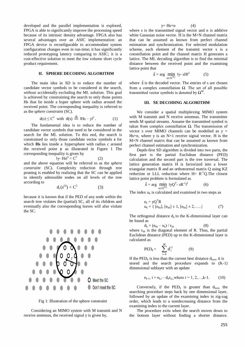
255
developed and the parallel implementation is explored,
FPGA is able to significantly improve the processing speed
because of its intrinsic density advantage. FPGA also has
several advantages over an ASIC implementation: an
FPGA device is reconfigurable to accommodate system
configuration changes even in run-time; it has significantly reduced prototyping latency comparing to ASIC; it is a
cost-effective solution to meet the low volume short cycle
product requirement.
II. SPHERE DECODING ALGORITHM
The main idea in SD is to reduce the number of
candidate vector symbols to be considered in the search,
without accidentally excluding the ML solution. This goal is achieved by constraining the search to only those points
Hs that lie inside a hyper sphere with radius around the
received point. The corresponding inequality is referred to
as the sphere constraint (SC).
d(s) ≤ C2 with d(s) ‖Hs – y‖
2 . (1)
The fundamental idea is to reduce the number of
candidate vector symbols that need to be considered in the
search for the ML solution. To this end, the search is constrained to only those candidate vector symbols s for
which Hs lies inside a hypersphere with radius c around
the received point y as illustrated in Figure 1 The
corresponding inequality is given by
‖y- Hs‖2 < C2 (2)
and the above equation will be referred to as the sphere
constraint (SC). Complexity reduction through tree
pruning is enabled by realizing that the SC can be applied
to identify admissible nodes on all levels of the tree
according to
di (s(i)
) < C2 (3)
because it is known that if the PED of any node within the
search tree violates the (partial) SC, all of its children and
eventually also the corresponding leaves will also violate
the SC.
Fig 1: Illustration of the sphere constraint
Considering an MIMO system with M transmit and N
receive antennas, the received signal y is given by,
y= Hs+n (4)
where s is the transmitted signal vector and n is additive
white Gaussian noise vector. H is the M×N channel matrix
that can be assumed as known from perfect channel
estimation and synchronization. For selected modulation
scheme, each element of the transmit vector s is a constellation point and the channel matrix H generates a
lattice. The ML decoding algorithm is to find the minimal
distance between the received point and the examining
lattice point that
s = arg TM
u min ‖y- sH‖2 (5)
where s is the decoded vector. The entries of s are chosen
from a complex constellation Ω. The set of all possible
transmitted vector symbols is denoted by ΩM.
III. SE DECODING ALGORITHM
We consider a spatial multiplexing MIMO system
with M transmit and N receive antennas. The transmitter
sends M spatial streams. Assume the transmitted symbol is
taken from complex constellation Ω. The transmission of
vector s over MIMO channels can be modelled as y =
Hs+n, where y is an N×1 receive signal vector. H is the
M×N channel matrix that can be assumed as known from
perfect channel estimation and synchronization.
Depth-first SD algorithm is divided into two parts, the first part is the partial Euclidean distance (PED)
calculation and the second part is the tree traversal. The
lattice generation matrix H is factorized into a lower
triangular matrix R and an orthonormal matrix Q using KZ
reduction or LLL reduction where H= R-1Q.The closest
lattice point problem is formulated as
s = arg TM
u min ‖yQT- sR-1‖2 (6)
The index uk is calculated and examined in two steps as
ek = yQTR
uk = [ekk], [ekk] ± 1, [ekk] ± 2,….. (7)
The orthogonal distance dk to the K-dimensional layer can
be found as
dk = (ekk – uk) / rkk (8)
where rkk is the diagonal element of R. Thus, the partial
Euclidean distance (PED) up to the K-dimensional layer is
calculated as
PEDk =
M
ki
id 2 (9)
If the PEDk is less than the current best distance dbest, it is
stored and the search procedure expands to (K-1)
dimensional sublayer with an update
ek-1, i = ek,i – dkrk,i, where i = 1, 2,…,k-1. (10)
Conversely, if the PEDk is greater than dbest, the
searching procedure steps back by one dimensional layer,
followed by an update of the examining index in zig-zag
order, which leads to a nondecreasing distance from the examining index to the current layer.
The procedure exits when the search moves down to
the bottom layer without finding a shorter distance.
256
Therefore, the best lattice point found so far becomes the
output.
The step-by-step procedures of the SE algorithm are
illustrated in the following.
1) Preprocessing: Perform QR factorization on channel
matrix H and inversion of the triangular matrix R. Initialize dimensional index K = M find the bounded index uk and
the distance dk from y to the current sublayer M , and set
dbest = ∞.
2) FSM: Updates PEDk using dk ; let dnew = PEDk.
if dnew < dbest and k > 1, go to state A;
if dnew < dbest and k = 1, go to state B;
if dnew ≥ dbest and k > 1, go to state C;
3) State A: Expand the search into K-1 sublayer, find
bounded uk and distance dk, and go to FSM.
4) State B: Record current best distance dbest = dnew and the
lattice point u ; set k = 2 find bounded uk and distance dk
and go to FSM.
5) State C:Exit if K = MT Otherwise, move the search into
K-1 sublayer, find bounded uk and distance dk , and go to
FSM.
Because there is no bound constraint in the SE algorithm, it
does not need to calculate and to update the bound in each
layer, thus the time-consuming square root operations are
avoided. Second, the chance of early identifying the correct
layer is maximized using the nondecreasing order of
investigation. Furthermore, the lattice point search starts from the Babai point, so no initial radius is required.
IV. EXPERIMENTAL RESULTS
The DSP implementation of MIMO sphere decoding
SE algorithm is discussed below.
A. Decoding Rate Performance
The data rate for the MIMO sphere decoder with M
transmit and N receive antennas is determined by
R =
stateavgc
fMb
dim
(11)
where is the system frequency of the circuits in megahertz,
bits per dimension bdim is determined by the modulation
scheme, and ηstate is the number of state visits required to
decode a receive vector at certain SNR. cavg is the average
number of clock cycles per state visit that is calculated as
cavg = stateistatei CP ,,( ) (12)
where Pi, state denotes the statistic percentage for visiting
state i, which can be obtained from high-level simulation.
Ci,state is the number of clock cycles used for state i
captured from the FPGA circuit simulation. A DSP
processor TMS320C6201 is chosen which requires 94
cycles, the decoding rate is around 3.66 Mbps. The number of state visits of the DSP implementation is significantly
larger than that of the FPGA implementation because DSP
does not support the state level parallelism. Similarly, the
DSP-based decoders cannot implement the current
execution of preprocessing and decoding It does not
support the parallel processing of real/image parts of
decoding algorithms either
A. B. BER Performance
The BER performance is evaluated using different
lattice generation matrices with Gaussian distribution and a
large number of source data at different SNRs with
additive white Gaussian noise (AWGN). The FPGA
implementations apply the proposed complex
transformation method and decode the real and imaginary
parts seperately. The software simulations directly conduct
the lattice search using complex numbers. The BER
performance of the FPGA implementations is then compared to the software simulation.
B. C. Power and Area Estimation
The power consumption of the TMS320C6201 DSP is
based on the typical values for high activity operations
(75% high and 25% low). The area of the DSP is larger
than the FPGA design. One obvious reason is the
difference in process technology. The most important
reason is that the area of FPGA is calculated based on the
number of slices mapped for a particular algorithm. But the
die size of the entire DSP is counted as the silicon area,
which is application- independent. In particular, some elements on the DSP device may not actively used for the
MIMO decoding algorithm, such as phase-locked loop
(PLL) and direct memory access (DMA) controller.
FPGA implementation differ from implementations on
DSPs through their potential for massively parallel
processing and the availability of customized operations
and operation sequences that can be executed in a single
cycle. The potential of an algorithm to exploit these
properties is crucial to guarantee an efficient high-
throughput implementation. The FPGA implementation of SE algorithm is expected to get a decoding rate above 50
Mbps and upto 80 Mbps which is about 20 times faster
than DSP implementation. The power consumption is
comparable for both FPGA and DSP implementation. The
area utilization in case of DSP implementation is about
95mm2 and for FPGA implementation we expect this to be
around 25-35mm2 which is very less compared to that of
DSP implementation.
The simulation result of the SE algorithm is as shown
in fig 2. First the pre processing unit of sphere decoding
algorithm is considered that is generation of channel matrix and then the best distance is calculated from the
received vector y and the examining lattice plane. The
algorithm proceeds following the steps in SE decoding
algorithm as explained above. Finally the closest lattice
point to the received vector y is calculated.

CONCLUSION
The system architecture and analysis of sphere
decoding SE algorithm for MIMO detection is presented
in this paper. The SE algorithm has lower circuit
complexity, smaller silicon area, and fewer lattice search
iterations.The MIMO sphere decoder which is of great
attraction towards the Wireless communication based
applications, its implementation in FPGA and
optimization of its architecture gains more interest in the
field of research. Power consumptions of the FPGA and DSP implementations are comparable, but the areas of
the FPGA designs are smaller. The throughput
advantage of the FPGA is due to its rich computational
resources and the parallel processing. This work can be
extended towards reducing the power and area utilization
and to achieve faster area throughput.
REFERENCES
[1]. B. M. Hochwald and S. Ten Brink, “Achieving near-capacity on a
multiple-antenna channel,” IEEE Trans. Commun., vol. 51, no. 3, pp.
389–399, Mar. 2003.
[2]. M. O. Damen, A. Chkeif, and J.-C. Belfiore, “Lattice code decoder
for space-time codes,” IEEE Comm. Let., pp. 161–163, May 2000.
[3]. D. Gesbert, M. Shafi, S. Da-shan, P. J. Smith, and A. Naguib,
“From theory to practice: An overview of mimo space-time coded
wireless systems,” IEEE J. Sel. Areas Commun., vol. 21, no. 3, pp.
281–302, Mar. 2003.
[4]. M. O. Damen, H. El Gamal, and G. Caire, “On maximum-
likelihood detection and the search for the closest lattice point,” IEEE
Trans. Inf.Theory, vol. 49, no. 10, pp. 2389–2402, Oct. 2003.
[5]. E. Viterbo and J. Boutros, “A universal lattice code decoder for
fading channels,” IEEE Trans. Inf. Theory, vol. 45, no. 5, pp. 1639–
1642, May 1999.
[6]. M.V. Clark, M. Shafi, W.K. Kennedy and L.J. Greenstein,
“Optimum Linear Diversity Receivers for Mobile Communications”,
IEEE Trans. Veh. Technol., Vol. 43, No. 1, pp. 47–56, 1994.
[7]. E. Agrell, T. Eriksson, A. Vardy, and K. Zeger, “Closest point
search in lattices,” IEEE Trans. Inf. Theory, vol. 48, no. 8, pp. 2201–
2214, Aug. 2002.
[8]. D. Garrett, L. Davis, S. ten Brink, B. Hochwald, and G. Knagge,
“Silicon complexity for maximum likelihood MIMO detection using
spherical decoding,” IEEE J. Solid-State Circuits, vol. 39, no. 9, pp.
1544–1552, Sep. 2004.
Fig 2: Simulation Result of SE Decoding Algorithm
Proceedings of the Third National Conference on RTICT 2010
Bannari Amman Institute of Technology ,Sathyamangalam- 638401
9-10 April 2010
257
Wireless Networks
Accident Response Server
“An Automatic Accident Notification System” NOORUL IRFANA.S
Department of Computer Science and
Engineering (3rd
year)
Anand Institute of Higher Technology
Abstract
“Technology does not drive change, it
Enables change.” The primary purpose of Technology is its
implementation in day-to-day life where in it
could enhance the lifestyle as well as provide better safety and performance to its end users.As
it may be understood, it is thus required to
provide systems that would cater to the unforeseen and unfortunate events that happen
in the modern day world. Providing timely and
accurate information is another key aspect in
reacting to situations of that would be catastrophic. With the number of vehicle users
in the country going manifold and with statistics
of accidents increasing at an alarming rate, systems should be devised that would call for
attention instantaneously reducing the severity
of any such calamities. It is sometimes referred
to as the golden first hour after any accident that takes place and is very precious in savings lives
of the victims. Another important factor to be
considered is accidents at highways are completely isolated from nearby hospitals,
rescue sites, etc. It is therefore required to
Provide an automated system that will help provide assistance in a minimal time. This
project, titled, Accident response server provides
an effective and reliable method that could be
used in highways to monitor and report location of accidents and take necessary action further.
The first and foremost requirement is to
accurately locate and pinpoint the accident so that help could be called for. For this purpose, a
database server is maintained online that stores
the list of area names with nearby help-centers contact numbers that should be alerted.
An electronic system would be installed in the
vehicle connected to the centralized system. The
RAMESH KRISHNAN.R
Department of Computer Science and
Engineering (3rd
year)
Anand Institute of Higher Technology
[email protected] electronic system has GPS and GSM to
communicate with the centralized database
system. When an accident occurs, the sensor
senses the vibration then sends a pulse to the system which is in vehicle side. Then the same
system passing the coordinates and vehicle
details to it. The centralized system then identifies the corresponding telephone number
and mail id and automatically sends the
screenshot of the accident to alert the area help-centers about the vehicle details , location and
notifies by call or SMS.
Keywords :- Accident detection, GPS based vehicle
Tracking, Vibration Sensors, GSM Modem,
Information Transfer to local help center.
1.Introduction
An accident is a disaster which is specific,
identifiable, unexpected, unusual and unintended external event which occurs in a particular time
and place, without apparent or deliberate cause
but with marked effects. It implies a generally negative probabilistic outcome which may have
been avoided or prevented had circumstances
leading up to the accident been recognized, and acted upon, prior to its occurrence. The first one
hour is the golden hour and that can make all the
difference. The aim is to reach out quickly to the
victims with help, upping the chances of their survival after an accident. Serious injuries can
result in disability, fatalities and life-long
psychological, emotional and economic damage to loved ones.Our system provides the
automatics response to such accidents. The
working of our project is divided in to the following sections:
1.1. GSM communication
GSM modem receives vehicle details and coordinate position of vehicle from GPS

258
module. It transmits messages to centralized
server for accident alerting. It is controlled by micro controller by interfacing with RS-232
1.2. GPS tracking
The GPS module calculates the geographical position of the vehicle. This helps in detecting
the location/position, velocity of our system.The
module output data like global positioning system fixed data, geographic position–
latitude/longitude are passed to GSM modem.
1.3.Microcontroller interfacing - RS- 232
It acts as an interface to GSM modem and micro
controller and to centralized server and GSM
Modem.
1.4 Vibration Sensing
The sensor used to sense the accident and sends as pulse to the microcontroller .The pulse is
transmitted as data to the GSM modem.
1.5. Accident notification
PC uses RS-232 protocol to forward call to
nearest help center using GSM Modem.
2. General Terminologies [1]Control Room: A control room is a room
serving as an operations centre where a facility
or service can be monitored and controlled. [2]Microcontroller: microcontroller (also MCU
or μC) is a functional computer system-on-
achip. It contains a processor core, memory, and
programmable input/output peripherals. [3]Google Earth: Google Earth displays satellite
images of varying resolution of the Earth's
surface, allowing users to visually see things like cities and houses from a bird's eye view.
[4]SMS: Short Message Service (SMS) is a
communications protocol allowing the interchange of short text messages between
mobile telephone devices.
[5]GSM: GSM (Global System for Mobile
communications: originally from Groupe Special Mobile) is the most popular standard for
mobile phones in the world.
. [6]GPS: Global Positioning System: a
navigational system involving satellites and
computers that can determine the latitude and longitude of a receiver.
[7]Vibration Sensor: It is a type of device
which can be activated by vibrations in a pre determined zone.
[8]AT Commands: AT commands are
instructions used to control a modem. AT is the
abbreviation of Attention.
3. Existing system
The following are the approaches followed
today, regarding accident reporting. They are, D Initially people used to make a call to the
help center. Anyone can save a life, but
people are not taking the initiative at the right time.
Accident reporting system with instant
messaging to default caller. This takes a
long time and it is of no use. Accident reporting system with default calling. This
system makes the situation worse and confusing.
4. Proposed system
Architecture of the Accident Response
Server
The architecture of the accident response server
is shown,
Fig 1 – The Architecture of the Accident
Response Server
Accident monitoring system with a database server maintained online that stores the list of
area names with nearby help-centers contact
numbers that should be alerted. The GPS- GSM
based accident notification system is such a state of the art automobile accessory. In case of any
accident, the accident notification subsystem
automatically makes a call to the police control room and also to some predefined telephone
numbers such as ambulance service; highway
security team etc.The whole system must be installed in the vehicle system with caution.
The main board of the system must be installed
in the middle position of the vehicle in a secure
location.

259
It provides us with the following advantages
It enables us to respond immediately when an accident occurs.
It provides the screenshot of the accident
captured and send to the help center.
The help centers are notified by call or SMS. It has an enhancement of blocking the
notification by engaging a button for minor
vibrations. We have our system designed with four
modules and the following components.
Module 1: GSM Communication
Module 2: GPS Tracking
Module 3: Vibration sensing
Module 4: Accident notification
4.1.Microcontroller The AT89C51 is a low-power, highperformance
CMOS 8-bit microcomputer with 4 Kbytes of
Flash Programmable and Erasable Read Only Memory (PEROM). The device is manufactured
using Atmel’s high density nonvolatile memory
technology and is compatible with the industry standard MCS- 51O instruction set and pinout.
The on-chip Flash allows the program memory
to be reprogrammed in-system or by a
conventional nonvolatile memory programmer. By combining a versatile 8-bit CPU with Flash
on a monolithic chip, the Atmel AT89C51 is a
powerful microcomputer which provides a highly flexible and cost effective solution to
many embedded control applications.The
AT89C51 provides the following standard
features: 4 Kbytes of Flash, 128 bytes of RAM, 32 I/O lines, two 16-bit timer/counters, a five
vector two-level interrupt architecture, a full
duplex serial port, on-chip oscillator and clock circuitry.
4.1.1 AT89C51 Instruction Set
ACALL:ACALL unconditionally calls a subroutine at the indicated code address.
ACALL pushes the address of the instruction
that follows ACALL onto the stack, least
significant- byte first, most-significant-byte second. The Program Counter is then updated so
that program execution continues at the
indicated address. The new value for the Program Counter is calculated by replacing the
least significant-byte of the Program Counter
with the second byte of the ACALL instruction, and replacing bits 0-2 of the most significant-
byte of the Program Counter with 3 bits that
indicate the page. Bits 3-7 of the most-
significant-byte of the Program Counter remain unchanged. Since only 11 bits of the
Program Counter are affected by ACALL, calls
may only be made to routines located within the
same 2k block as the first byte that follows ACALL.
CJNE:CJNE compares the value of operand1
and operand2 and branches to the indicated relative address if operand1 and operand2 are
not equal. If the two operands.
DJNZ:DJNZ decrements the value of register by 1. If the initial value of register is 0,
decrementing the value will cause it to reset to
255 (0xFF Hex). If the new value of register is
not 0 the program will branch to the address indicated by relative addr. If the new value of
register is 0 program flow continues with the
instruction following the DJNZ instruction the value "rolls over" from 0 to 255.
JNB:JNB will branch to the address indicated
by reladdress if the indicated bit is not set. If the bit is set program execution continues with the
instruction following the JNB instruction.
MOV:MOV copies the value of operand2 into
operand1. The value of operand2 is not affected. Both operand1 and operand2 must be in Internal
RAM. No flags are affected unless the
instruction is moving the value of a bit into the carry bit in which case the carry bit is affected or
unless the instruction is moving a value into the
PSW register (which contains all the program
flags. RET:RET is used to return from a subroutine
previously called by LCALL or ACALL.
Program execution continues at the address that is calculated by popping the topmost 2 bytes off
the stack. The mostsignificant- byte is popped
off the stack first, followed by the least-significant-byte.
SETB:Sets the specified bit.
4.2. GSM Modem
A GSM modem is a wireless modem that works with a GSM wireless network. A wireless
modem behaves like a dial-up modem. The main
difference between them is that a dial-up modem sends and receives data through a fixed
telephone line while a wireless modem sends
and receives data through radio waves. A GSM modem can be an external device or a
PC Card / PCMCIA Card. Typically, an external

260
GSM modem is connected to a computer
through a serial cable or a USB cable. A GSM modem in the form of a PC Card / PCMCIA
Card is designed for use with a laptop computer.
It should be inserted into one of the
PC Card / PCMCIA Card slots of a laptop computer. Like a GSM mobile phone, a GSM
modem requires a SIM card from a wireless
carrier in order to operate. Both GSM modems and dial-up modems support a common set of
standard AT commands. You can use a GSM
modem just like a dial-up modem. In addition to the standard AT commands, GSM modems
support an extended set of AT commands. These
extended AT commands are defined in the GSM
standards.
4.3.AT commands
AT commands are instructions used to control a
modem. AT is the abbreviation of ATtention. Every command line starts with "AT" or "at".
That's why modem commands are called AT
commands. Many of the commands that are used to control wired dialup modems, such as ATD
(Dial), ATA (Answer), ATH (Hook control) and
ATO (Return to online data state), are also
supported by GSM/GPRS modems and mobile phones. Besides this common AT command set,
GSM/GPRS modems and mobile phones
support an AT command set that is specific to the GSM technology, which includes SMS-
related commands like AT+CMGS (Send SMS
message), AT+CMSS (Send SMS message from
storage), AT+CMGL (List SMS messages) and AT+CMGR (Read SMS messages).Note that the
starting "AT" is the prefix that informs the
modem about the start of a command line. It is not part of the AT command name. For example,
D is the actual AT command name in ATD and
+CMGS is the actual AT command name in AT+CMGS. However, some books and web
sites use them interchangeably as the name of an
AT command.
4.4.GPS The global positioning system (GPS) was
developed by the U.S government for the
department of Defense. It is essentially a U.S military system, it offers navigation services to
civilians; however, at present, there is no law
which mandates the service to be made available for commercial application. Position fix is
obtained through passive receivers by the
triangulation method; where in estimated ranges from four satellites are used to derive the
position of a point. Ranges from three satellites
can provide the latitude and longitude of a point
on the earth; the addition of a fourth satellite can provide a user’s altitude and correct receiver
clock error. It is possible to derive the velocity
of the user and precise time information originating from onboard atomic clocks, which
have a drift rate of 1sec per 70,000 years
There are cesium atomic clocks aboard each satellite.
4.5.GPS Receivers
In 1980, only one commercial GPS receiver was
available on the market, at a price of several hundred thousand U.S. dollars. This, however,
has changed considerably as more than 500
different GPS receivers are available in today’s market.Commercial GPS receivers may be
divided into four types, according to their
receiving capabilities. These are: singlefrequency code receivers, single-frequency
carrier-smoothed code receivers,
singlefrequency
code and carrier receivers, and dualfrequency receivers. Single-frequency receivers access the
L1
frequency only, while dualfrequency receivers access
both the L1 and the L2 frequencies. GPS
receivers
can also be categorized according to their number of
tracking channels, which varies from 1 to 12
channels. A good GPS receiver would be multi channel, with each channel dedicated to
continuously
tracking a particular satellite. Presently, most GPS
receivers have 9 to 12 independent (or parallel)
channels. Features such as cost, ease of use,
power consumption, size and weight, internal and/or
external datastorage capabilities, interfacing
capabilities are to be considered when selecting a
GPS receiver.
4.6.GPS Antennas The antenna receives the GPS satellite signals
and

261
passes them to the receiver. The GPS signals are
spread spectrum signals in the 1575 MHz range and
do not penetrate conductive or opaque surfaces.
Therefore, the antenna must be located outdoors
with a clear view of the sky. The Lassen SQ GPS
receiver
requires an active antenna. The received GPS signals
are very low power, approximately -130 dBm, at
the surface of the earth. Trimble's active antennas
include
a preamplifier that filters and amplifies the GPS
signals before delivery to the receiver.
5.Working Of the system
5.1.Module 1: GSM Communication
GSM modem sends the message as “ACCIDENT OCCURRED” to the centralized
server using AT commands as AT commands
+CMGS can be used to send SMS messages from a computer / PC
AT+CMGS="91234567"<CR> Sending text
messages is easy.<Ctrl+z> GSM modem is
controlled by using microcontroller which is interfaced with RS- 232.RS-232 and
microcontroller is interfaced using MAX-232.
5.2.Module 2: GPS Tracking Each GPS satellite transmits radio signals that
enable the GPS receivers to calculate where its
(or your vehicles) location on the Earth and convert the calculations into geodetic latitude,
longitude and velocity. A receiver needs signals
from at least three GPS satellites to pinpoint
your vehicle’s position. GPS Receivers commonly used in most Vehicle tracking
systems can only receive data from GPS
Satellites. They cannot communicate back with
GPS or any other satellite. A system based on GPS can only calculate its location but cannot
send it to central control room. In order to do
this they normally use GSM-GPRS Cellular
networks connectivity using additional GSM modem/module. GPS Receiver can only Receive
data and cannot send data to Satellite (s). GPS
satellites do not know the position of a GPS Receiver. GPS Receiver calculate its position
using data from 3-4 satellites and no single
satellite know the calculations done by GPS receiver or its position. GPS Satellite service is
freely available throughout the world, anyone
anywhere can receive GPS data by buying any
off-the-shelf GPS receivers. GPS satellites are different satellites and can only send small and
week radio signals to earth.GPS Satellite signals
are weak and can be received normally with GPS antenna (external or integrated with GPS
receiver) facing open sky. GPS signals cannot be
received inside the home, building, garage, bridges. Even clouds and Trees can prevent GPS
signals from reaching GPS receiver. Hence no
GPS receiver can guarantee performance.
Certain advanced and sensitive GPS receivers can receive signals in above situations but
performance is still not satisfactory. GPS
receiver only gives Latitude, Longitude and Velocity calculated. To know your location you
need highly accurate map. If maps are not
accurate you will have much high error in
location. Normally accuracy of Maps is considered more important then accuracy of
GPS Receiver. GSM-GPRS is most suitable two
way communication system available to complement GPS receiver and send location
information to Mobile phone, Office or Internet.
GSM-GPRS Modem/Receiver can allow you to receive GPS position by SMS or Data.
5.3.Module 3: Vibration sensing
Vibration sensors are sensors for measuring,
displaying and analyzing linear velocity, displacement and proximity, or else acceleration.
They can be used on a stand-alone basis, or in
conjunction with a data acquisition system. Vibration sensors are available in many forms.
They can be raw sensing elements, packaged
transducers, or as a sensor system or instrument, incorporating features such as totalizing, local or
remote display and data recording. When the

262
vibration occurs it is sensed as pulse and send to
the micro-controller which is taken as the input to it.
5.4.Module 4: Accident notification
The control room maintains a centralized server.
The server maintains a database of names of cities all over the world and the rescue and the
help center number with the mail-id of those
centers.. MySql database is used to store the data. JDBC connectivity is used to retrieve the
data from the server and forward the call or sms
to the help centers. With the received vehicle details, the screen shot of vehicle location is
captured and sent to the help center from the
centralized server.
5.5. Reason for utilizing MySQL
5.5.1.MySQL is Cross-Platform
One great advantage of using MySQL is its
crossplatform capabilities. You can develop your database on a Windows laptop and deploy
on Windows Server 2003, a Linux server, a IBM
mainframe, or an Apple XServe, just to name a few potential platforms. This gives you a lot of
versatility when choosing server hardware. You
can even set up replication using a master on a
Windows platform with Linux slaves. It's incredibly easy to move between platforms: on
most platforms you can simply copy the data
and configuration files between servers and you are ready to go.
5.5.2.MySQL is Fast
An independent study by Ziff Davis found
MySQL to be one of the top performers in a group that included DB2, Oracle, ASE, and SQL
Server 2000. MySQL is used by a variety of
corporations that demand performance and stability including Yahoo!, Slashdot, Cisco, and
Sabre. MySQL can help achieve the highest
performance possible with your available hardware, helping to cut costs by increasing time
between server upgrades.
5.5.3.MySQL is Free
MySQL is Open Source software.As per its GPL license, you are free to redistribute those
changes as long as your software is also Open
Source. If you do not wish to make your software Open Source, you are free to do so as
long as you do not distribute your application
externally. If you adhere to the requirements of the GPL, MySQL is free for you to use at no
cost. If you wish to distribute your closed source
application externally, you will find that the cost
of a MySQL commercial license is extremely low (MySQL licenses start at only $249 US).
MySQL AB also offers well priced commercial
support that is significantly less expensive than
some of its counterparts.
6. Component Details (Hardware and
Software Requirements)
Table 1 – Table depicting the various hardware
and software requirements of Accident Response Server
7.Implementation – Approach and
Details
7.1.Module 1: GSM Communication
Microcontroller embedded with assembly
language program is interfaced with the GSM
modem using the RS-232. RS232 data is bi-polar.... +3 TO +12 volts indicates an "ON or 0-
state (SPACE) condition" while A -3 to -12 volts
indicates an "OFF" 1- state (MARK) condition.... Modern computer equipment
ignores the negative level and accepts a zero
voltage level as the "OFF" state. In fact, the "ON" state may be achieved with lesser positive
potential. This means circuits powered by 5
VDC are capable of driving RS232 circuits
directly, however, the overall range that the RS232 signal may be transmitted/ received
may be dramatically reduced. To make RS-232
TTL compatible, MAX-232 is used to interface Microcontroller and RS-232. The MAX232
device is a dual driver/receiver that includes a
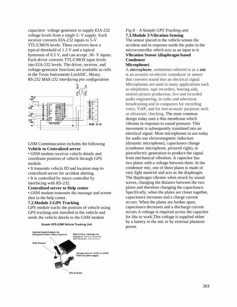
263
capacitive voltage generator to supply EIA-232
voltage levels from a single 5- V supply. Each receiver converts EIA-232 inputs to 5-V
TTL/CMOS levels. These receivers have a
typical threshold of 1.3 V and a typical
hysteresis of 0.5 V, and can accept .30- V inputs. Each driver converts TTL/CMOS input levels
into EIA-232 levels. The driver, receiver, and
voltage-generator functions are available as cells in the Texas Instruments LinASIC. library.
RS-232 MAX-232 interfacing pin configuration
GSM Comminucation includes the following
Vehicle to Centralized server
• GSM modem receives vehicle details and coordinate position of vehicle through GPS
module.
• It transmits vehicle ID and location map to centralized server for accident alerting.
• It is controlled by micro controller by
interfacing with RS-232.
Centralized server to Help center
• GSM modem transmits the message and screen
shot to the help center.
7.2.Module 2:GPS Tracking GPS module tracks the position of vehicle using
GPS tracking unit installed in the vehicle and
sends the vehicle details to the GSM modem
Fig 8 – A Sample GPS Tracking unit
7.3.Module 3:Vibration Sensing The sensor placed in the vehicle senses the
accident and in response sends the pulse to the
microcontroller which acts as an input to it.
Vibration Sensor (diaphragm based
Condenser
Microphone)
A microphone, sometimes referred to as a mic
is an acoustic-to-electric transducer or sensor
that converts sound into an electrical signal.
Microphones are used in many applications such as telephones, tape recorders, hearing aids,
motion picture production, live and recorded
audio engineering, in radio and television
broadcasting and in computers for recording voice, VoIP, and for non-acoustic purposes such
as ultrasonic checking. The most common
design today uses a thin membrane which vibrates in response to sound pressure. This
movement is subsequently translated into an
electrical signal. Most microphones in use today for audio use electromagnetic induction
(dynamic microphone), capacitance change
(condenser microphone, pictured right), or
piezoelectric generation to produce the signal from mechanical vibration. A capacitor has
two plates with a voltage between them. In the
condenser mic, one of these plates is made of very light material and acts as the diaphragm.
The diaphragm vibrates when struck by sound
waves, changing the distance between the two
plates and therefore changing the capacitance. Specifically, when the plates are closer together,
capacitance increases and a charge current
occurs. When the plates are further apart, capacitance decreases and a discharge current
occurs.A voltage is required across the capacitor
for this to work.This voltage is supplied either by a battery in the mic or by external phantom
power.

264
7.4.Module 4:Call forwarding
The server placed in the control room stores the details of millions of help centers and the rescue
centers. JDBC connectivity is used to retrieve
the data and the server forwards the call to centers. The snapshot of the accident is taken
and it is mailed to the police station to get the
exact view of the accident.
Compilation of java file:
Snapshot:
Mail sending:
8. Conclusion
Thus the Accident Response Server would act as a benchmark rendering effective and quick
responses for reporting accidents. Also, it could
be fitted onto existing vehicles, requiring no
special setups. . Being Students of Technology we strongly feel that the Accident Response
Server would be a landmark of both
Technological as well as Social excellence .If our project could help to save precious human
lives by reporting accidents faster ,then the
success of our project would have been
achieved.
9. Future Research
In future, introducing a still faster responding
system would increase the efficiency. Till now GSM is the best known communication.GSM
could be replaced by some other technology. As
it is very costly. The sensors used in the system could be replaced by better detecting devices for
increasing the capability of sensing We are
working in this project to implement it as a best
real time project. Various steps are taken to use this system in forest areas where the possibility
of signal coverage is very less.
10. References
[1] Accident Prevention Stratergies : Causation
Model and Research directions Panagiotis Mitropoulos , Gregory A. Howell, and Tariq S.
Abdelhamid

265
[2] Accident notification system for vehicle,
Yamagishi, Junichi (Tokyo 111-0034, JP) [3]http://www.gsm-modem.de/gsmfaq.Html
[4]http://www.econsystems.com/gpscomm
module.asp
[5]http://www.java2s.com [6]http://www.developershome.com/sms/at
CommandsIntro.asp
[7] http://www.mysql.com/

Proceedings of the Third National Conference on RTICT 2010
Bannari Amman Institute of Technology ,Sathyamangalam- 638401
9-10 April 2010
266
SECURE DYNAMIC ROUTING IN NETWORKS
Marimuthu G,Saranya V,Thiripurasundari S & Akilandeeswari M
B.Tech, Information Technology,
Bannari Amman Institute of Technology, Sathyamangalam.
Email: [email protected] and [email protected]
Contact no: +91 9597100912
ABSTRACT
Security has become one of the
major issues for data communication over
wired and wireless networks. Different from
the past work on the designs of
cryptography algorithms and system
infrastructures, we propose a “Secure
Dynamic Routing Algorithm” that could
randomize delivery paths for data
transmission. It adopts the method of
multiple paths between source and
destination to increase the throughput of the
data transmission. It provides considerably a
minimum path similarity of two consecutive
transmitted packets. The algorithm is easy to
implement and compatible with popular
routing protocols. It could be used in
cryptography-based system designs to
further improve the data transmission over
networks. Thus it focuses on the security of
data transmission with very minimal
interception in multiple paths.
1. EXISTING SYSTEM
In the past decades, various security-
enhanced measures have been proposed to
improve the security of data transmission
over public networks. Existing work on
security-enhanced data transmission
includes the designs of cryptography
algorithms and system infrastructures and
security-enhanced routing methods. Their
common objectives are o ften to defeat
various threats over the Internet, including
eavesdropping, spoofing, session hijacking,
etc.
Among many well-known designs
for cryptography based systems, the IP
Security (IPSec) and the Secure Socket
Layer (SSL) are popularly supported and
implemented in many systems and
platforms. Although IPSec and SSL do
greatly improve the security level for data
transmission, they unavoidably introduce
substantial overheads especially on
gateway/host performance and effective
network bandwidth.
For example, the data transmission
overhead is 5 cycles/byte over an Intel

267
Pentium II with the Linux IP stack alone,
and the overhead increases to 58 cycles/byte
when Advanced Encryption Standard (AES)
is adopted for encryption/decryption for
IPSec .
1.1 Limitations of Existing System
Number of Retransmission is high
Cost is high to implement a
cryptographic technique
Eavesdropping is easily occur
2. PROPOSED SYSTEM
The security-enhanced data
transmission is to dynamically route packets
between each source and its destination so
that the chance for system break-in, due to
successful interception of consecutive
packets for a session, is slim. The intention
of security-enhanced routing is different
from the adopting of multiple paths between
a source and a destination to increase the
throughput of data transmission. The
proposed system is a secure routing protocol
to improve the security of end-to-end data
transmission based on multiple path
deliveries.
The set of multiple paths between
each source and its destination is determined
in an online fashion, and extra control
message exchanging is needed. A set of
paths is discovered for each source and its
destination based on message flooding.
Thus, a mass of control messages is needed.
The system proposed a traffic
dispersion scheme to reduce the probability
of eavesdropped information along the used
paths provided that the set of data delivery
paths is discovered in advance. Although
excellent research results have been
proposed for security-enhanced dynamic
routing, many of them rely on the discovery
of multiple paths either in an online or
offline fashion. For those online path
searching approaches, the discovery of
multiple paths involves a significant number
of control signals over the Internet.
On the other hand, the discovery of
paths in an offline fashion might not be
suitable to networks with a dynamic
changing configuration. Therefore, we will
propose a dynamic routing algorithm to
provide security enhanced data delivery
without introducing any extra control
messages. Let us discuss about the DDRA
algorithm which we used.
2.1 DDRA ALGORITHM
Consider the delivery of a packet
with the destination „t‟ at a node „N‟. In
order to minimize the probability that
packets are eavesdropped over a specific
link, a randomization process for packet
deliveries shown in Procedure 1 is adopted.

268
In this process, the previous next hop „B‟ for
the source node „S‟ is identified in the first
step of the process. Then, the process
randomly picks up a neighboring node in N
excluding B as the nexthop for the current
packet transmission. The exclusion of B for
the nexthop selection avoids transmitting
two consecutive packets in the same link,
and the randomized pickup prevents
attackers from easily predicting routing
paths for the coming transmitted packets.
Procedure 1:
Randomizedselector(S,t,pkt)
1: Let H be the used nexthop for the
previous packet delivery for
the source node S.
2: if H belongs to Candidate nodes(C) then
3: if |C|>1 then
4: Randomly choose a node x from |C-H| as
a nexthop, and send the packet pkt to the
node x.
5: H x, and update the routing table of N.
6: else
Send the packet pkt to H.
7: end if
8: else
Randomly choose a node y from C
as a nexthop,
and send the packet pkt to the node
y.
9: H y, and update the routing table of N.
10: end if
Before the current packet is sent to
its destination node, we must randomly pick
up a neighboring node excluding the used
node for the previous packet.
Once a neighboring node is selected, we
need to determine whether the selected
neighboring node for the current packet is
the same as the one used by the previous
packet. If the path is same as that of the
previous one, we should select the
alternative path.
3. MODULES
The following are the modules used ,
Network Structure Formation
Random Path Selection
Message Transmission
3.1Network Structure Formation
In this module, topology structure is
constructed using the existing nodes. The
nodes are connected to form a network. The
connection is made through sockets. Here
we use mesh topology because of its
unstructured nature.

269
The input is to be given as number of
nodes. And each node details such as IP
address, and port no are given. The link
information between the nodes obtained and
checked with existing network in the
database. If the link is already available, we
go for other links. Otherwise the link is
made between the nodes.
3.2 Random Path Selection
Random path algorithm is applied to
select a random path between the nodes
from the routing table. New route is found
using secure dynamic routing algorithm.
Routing history is updated in order to select
the path for message transmission.
The node details are given in the
login form. Then the destination is selected.
The nexthops are chosen from the database.
Once a neighboring node is selected,
we need to determine whether the selected
neighboring node for the current packet is
the same as the one used by the previous
packet. If the path is same as that of the
previous one, we should select the alternate
path.
3.3 Message Transmission
Random path is selected using the
routing table. Then the message is
Yes
No
Data Store
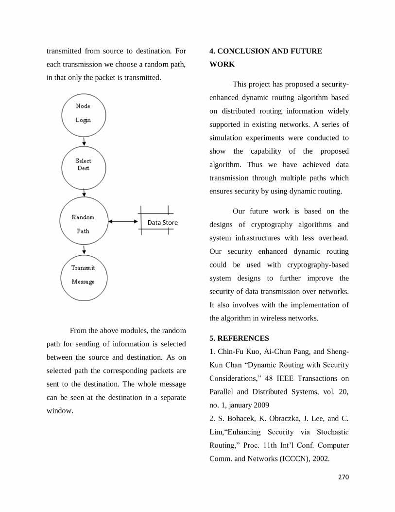
270
transmitted from source to destination. For
each transmission we choose a random path,
in that only the packet is transmitted.
From the above modules, the random
path for sending of information is selected
between the source and destination. As on
selected path the corresponding packets are
sent to the destination. The whole message
can be seen at the destination in a separate
window.
4. CONCLUSION AND FUTURE
WORK
This project has proposed a security-
enhanced dynamic routing algorithm based
on distributed routing information widely
supported in existing networks. A series of
simulation experiments were conducted to
show the capability of the proposed
algorithm. Thus we have achieved data
transmission through multiple paths which
ensures security by using dynamic routing.
Our future work is based on the
designs of cryptography algorithms and
system infrastructures with less overhead.
Our security enhanced dynamic routing
could be used with cryptography-based
system designs to further improve the
security of data transmission over networks.
It also involves with the implementation of
the algorithm in wireless networks.
5. REFERENCES
1. Chin-Fu Kuo, Ai-Chun Pang, and Sheng-
Kun Chan “Dynamic Routing with Security
Considerations,” 48 IEEE Transactions on
Parallel and Distributed Systems, vol. 20,
no. 1, january 2009
2. S. Bohacek, K. Obraczka, J. Lee, and C.
Lim,“Enhancing Security via Stochastic
Routing,” Proc. 11th Int‟l Conf. Computer
Comm. and Networks (ICCCN), 2002.
Data Store

Proceedings of the Third National Conference on RTICT 2010
Bannari Amman Institute of Technology ,Sathyamangalam- 638401
9-10 April 2010
271
Abstract – Considering the problem of keeping all types of
sensitive data and algorithms contained in a mobile agent from
discovery and exploitation by a malicious host. The paper
illustrates a novel distributed protocol for multi agent
environments to improve the communication security in packet-
switched networks. To enrich the overall system security the
approach makes use of distribution and varieties of available
encryption and some other traditional methods such as digital
signature. In this approach the encrypted private key and the
message are broken into different parts and is then encrypted
carrying by different agents which makes it difficult for
malicious entities to mine the private key for message
encryption, while the private key for the encrypted key is
allocated on the predetermined destination nodes. On the other
hand, all of the previously proposed encryption algorithms can
be applied in the proposed approach that deteriorates the key
discovery process. To improve the overall system security, the
paper makes use of Advanced Encryption Standard (AES) as
the encryption base for message encryption. The paper also
presents some evaluation discussions presenting time overhead
analysis and crack probability. And the destination address is
divided into two agents for carrying the network and host
identification. Thus the paper ensures the security policies not
only for the source and its information but the destination host
also.
Keywords- Mobile Agents; Distributed Cryptography;
Cryptographic Protocols; MA-MK (Multi Agent – Multi Key);
Multi Agent Environment; Double Cryptography Approach;
Internet Security; Communication Security;
I. INTRODUCTION
Because of dispersed number of system users, security is one of
the most challenging issues particularly in networked
environments. In traditional security methods, discovering the
determined private key is enough for message decryption that can
be done through malicious attacks to the network nodes or listening
to communication links.
1 K. Jeyakumar, is currently pursuing his Final year B.Tech - Information
Technology in Anna University Coimbatore. ([email protected]).
2
N.E.Vengatesh, is currently pursuing his Final year B.Tech - Information
Technology in Anna University Coimbatore. ([email protected]).
Since mobile agents have the features like self-learning and
mobility, we enable it as a carrier wave for the information
transmission. For a surprise, still there is no killer application for
mobile agents, even though we should consider the security issues
like masquerading, denial of service, unauthorized access,
eavesdropping, alteration and repudiation. Our proposed solution
avoids all kinds of security issues related to the mobile agents.
In traditional way, it is not possible to transfer the code and the
execution state. The most advantage of agent based communication
is that it can transfer the data, code and as well as the execution
state. The transfer of state together with data and code is based on
its mobility whether the strong mobility or weak mobility
respectively.
The paper is organized as follows:
Since we are using AES algorithm, the next section explains this
algorithm. Then we will talk about basic concepts of multi-key and
multi agent cryptography. The proposed multi agent-multi key
(MA-MK) protocol is then explained and the related simulation
results are presented. Finally, the conclusion section ends the paper.
II. ADVANCED ENCRYPTION STANDARD
According to malicious view, cryptography can be discussed
according to the following points:
How to access to the system.
How to recognize the encryption algorithm.
How to access to the private key.
Accessing to the private key can be considered as the end point of
a malicious process. The proposed approach provides the system
security, and makes the masquerader not to recognize the
encryption algorithm easily but not in the existing concepts and
improves private key security using the following strategies:
Encrypting the private key and data using an encryption
algorithm (AES algorithm is used in this paper).
Breaking the encrypted private key and data into different
units.
Encrypting the different parts carrying by the mobile
agents.
Breaking the destination address into two agents for the
identification of network and host.
K.Jeyakumar 1, N.E.Vengatesh
2
MA-MK Cryptographic Approach for Mobile Agent Security with
Mitigation of System and Information Oriented Attacks
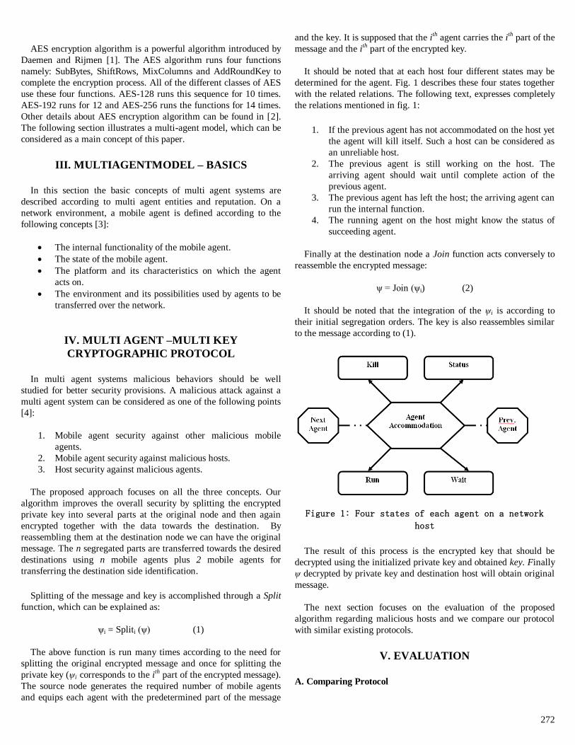
272
AES encryption algorithm is a powerful algorithm introduced by
Daemen and Rijmen [1]. The AES algorithm runs four functions
namely: SubBytes, ShiftRows, MixColumns and AddRoundKey to
complete the encryption process. All of the different classes of AES
use these four functions. AES-128 runs this sequence for 10 times.
AES-192 runs for 12 and AES-256 runs the functions for 14 times.
Other details about AES encryption algorithm can be found in [2].
The following section illustrates a multi-agent model, which can be
considered as a main concept of this paper.
III. MULTIAGENTMODEL – BASICS
In this section the basic concepts of multi agent systems are
described according to multi agent entities and reputation. On a
network environment, a mobile agent is defined according to the
following concepts [3]:
The internal functionality of the mobile agent.
The state of the mobile agent.
The platform and its characteristics on which the agent
acts on.
The environment and its possibilities used by agents to be
transferred over the network.
IV. MULTI AGENT –MULTI KEY
CRYPTOGRAPHIC PROTOCOL
In multi agent systems malicious behaviors should be well
studied for better security provisions. A malicious attack against a
multi agent system can be considered as one of the following points
[4]:
1. Mobile agent security against other malicious mobile
agents.
2. Mobile agent security against malicious hosts.
3. Host security against malicious agents.
The proposed approach focuses on all the three concepts. Our
algorithm improves the overall security by splitting the encrypted
private key into several parts at the original node and then again
encrypted together with the data towards the destination. By
reassembling them at the destination node we can have the original
message. The n segregated parts are transferred towards the desired
destinations using n mobile agents plus 2 mobile agents for
transferring the destination side identification.
Splitting of the message and key is accomplished through a Split
function, which can be explained as:
ψi = Spliti (ψ) (1)
The above function is run many times according to the need for
splitting the original encrypted message and once for splitting the
private key (ψi corresponds to the ith part of the encrypted message).
The source node generates the required number of mobile agents
and equips each agent with the predetermined part of the message
and the key. It is supposed that the ith agent carries the ith part of the
message and the ith part of the encrypted key.
It should be noted that at each host four different states may be
determined for the agent. Fig. 1 describes these four states together
with the related relations. The following text, expresses completely
the relations mentioned in fig. 1:
1. If the previous agent has not accommodated on the host yet
the agent will kill itself. Such a host can be considered as
an unreliable host.
2. The previous agent is still working on the host. The
arriving agent should wait until complete action of the
previous agent.
3. The previous agent has left the host; the arriving agent can
run the internal function.
4. The running agent on the host might know the status of
succeeding agent.
Finally at the destination node a Join function acts conversely to
reassemble the encrypted message:
ψ = Join (ψi) (2)
It should be noted that the integration of the ψi is according to
their initial segregation orders. The key is also reassembles similar
to the message according to (1).
Figure 1: Four states of each agent on a network
host
The result of this process is the encrypted key that should be
decrypted using the initialized private key and obtained key. Finally
ψ decrypted by private key and destination host will obtain original
message.
The next section focuses on the evaluation of the proposed
algorithm regarding malicious hosts and we compare our protocol
with similar existing protocols.
V. EVALUATION
A. Comparing Protocol
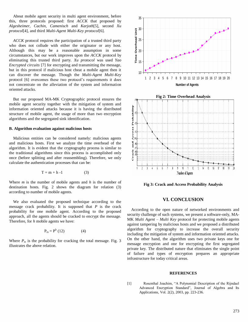
273
About mobile agent security in multi agent environment, before
this, three protocols proposed: first ACCK that proposed by
Algesheimer, Cachin, Camenisch and Karjoth[5], second Xu
protocol[4], and third Multi-Agent Multi-Key protocol[6].
ACCK protocol requires the participation of a trusted third party
who does not collude with either the originator or any host.
Although this may be a reasonable assumption in some
circumstances, but our work improves upon the ACCK protocol by
eliminating this trusted third party. Xu protocol was used Yao
Encrypted circuits [7] for encrypting and transmitting the message,
but in this protocol if malicious host cheat a mobile agent then it
can discover the message. Though the Multi-Agent Multi-Key
protocol [6] overcomes these two protocol’s requirements it does
not concentrate on the alleviation of the system and information
oriented attacks.
But our proposed MA-MK Cryptographic protocol ensures the
mobile agent security together with the mitigation of system and
information oriented attacks because it is having the distributed
structure of mobile agent, the usage of more than two encryption
algorithms and the segregated sink identification.
B. Algorithm evaluation against malicious hosts
Malicious entities can be considered namely: malicious agents
and malicious hosts. First we analyze the time overhead of the
algorithm. It is evident that the cryptography process is similar to
the traditional algorithms since this process is accomplished only
once (before splitting and after reassembling). Therefore, we only
calculate the authentication processes that can be:
T = m + h -1 (3)
Where m is the number of mobile agents and h is the number of
destination hosts. Fig. 2 shows the diagram for relation (3)
according to number of mobile agents.
We also evaluated the proposed technique according to the
message crack probability. It is supposed that P is the crack
probability for one mobile agent. According to the proposed
approach, all the agents should be cracked to encrypt the message.
Therefore, for h mobile agents we have:
Pm = Ph (12) (4)
Where Pm is the probability for cracking the total message. Fig. 3
illustrates the above relation.
Fig 2: Time Overhead Analysis
10
15
20
25
30
35
1 2 3 4 5 6 7 8 9 10 11 12 13 14 15 16 17 18 19 20
Number of Agents
Tim
e O
verh
ead
Un
it
Fig 2: Time Overhead Analysis
Fig 3: Crack and Access Probability Analysis
VI. CONCLUSION
According to the open nature of networked environments and
security challenge of such systems, we present a software-only, MA-
MK Multi Agent – Multi Key protocol for protecting mobile agents
against tampering by malicious hosts and we proposed a distributed
algorithm for cryptography to increase the overall security
including the mitigation of system and information oriented attacks.
On the other hand, the algorithm uses two private keys one for
message encryption and one for encrypting the first segregated
private key. The distributed nature that eliminates the single point
of failure and types of encryption prepares an appropriate
infrastructure for today critical areas.
REFERENCES
[1] Rosenthal Joachim, “A Polynomial Description of the Rijndael
Advanced Encryption Standard”, Journal of Algebra and Its
Applications, Vol. 2(2), 2003, pp. 223-236.

[2] National Institute of Standards and Technology, “Announcing
the ADVANCED ENCRYPTION STANDARD (AES),” Federal
Information Processing Standards Publication, no. 197, Nov. 2001.
[3] Dasgupta Dipankar and Brian Hal, “Mobile Security Agents for
Network Traffic Analysis”, in Proc. proceedings of DARPA
Information Survivability Conference, Anaheim California, June
2001.
[4] Xu Ke, “Mobile Agent Security Through Multi-Agent
Cryptographic Protocols”, PhD Thesis, Department of Computer
Science and Engineering, University of North Texas, May 2004.
[5] Joy Algesheimer, Christian Cachin, Jan Camenisch, and G Unter
Karjoth, “Cryptographic security for mobile code”, in Proc. IEEE
Symposium on Security and Privacy, May 2001, pp. 2-11.
[6] Abolfazl Esfandi, and Ali Movaghar Rahimabadi, “Mobile Agent
Security in Multi agent Environments Using a Multi agent-Multi
key Approach”, in Proc. IEEE, 2009, pp. 438-441.
[7] Andrew Chi-Chih Yao, "How to generate and exchange secrets",
in Proc. 27th IEEE Symposium on Foundations of Computer
Science (FOCS), 1986, pp. 162-167.

Proceedings of the Third National Conference on RTICT 2010
Bannari Amman Institute of Technology ,Sathyamangalam- 638401
9-10 April 2010
274
NEW STEGANOGRAPHY METHOD FOR SECURE DATA
COMMUNICATION
T.Thambidurai
Demonstrator, P.G. Department of Software Engineering
M.Kumarasamy College of Engineering
Thalavapalayam,Karur-639113,Tamilnadu,India E-Mail: [email protected], Contact No:9444851747
K.Nagaraj
Student, II-M.Sc Software Engineering
P.G. Department of Software Engineering
M.Kumarasamy College of Engineering
Thalavapalayam,Karur-639113,Tamilnadu,India E-Mail: [email protected], Contact No:9688628175
1.Abstract :
Steganography is the art of passing
information in a manner that the very
existence of the message is unknown. The
goal of steganography is to avoid drawing
suspicion to the transmission of a hidden
message. If suspicion is raised, then this goal
is defeated. Steganalysis is the art of
discovering and rendering useless such
covert messages. In this paper,we identify
characteristics in current steganography
software that direct the steganalyst to the
existence of a hidden message and introduce
the ground work of a tool for automatically
detecting the existence of hidden messages in
images. Today sending information through
internet is very difficult and somebody can
hack the secret information and send secret
information to the receiver with some
modifications and receiver can receive and
understand the secret information wrongly,
so inorder to avoid this problem we
introduced a new method to send our secret
information through internet(send
information from sender to receiver).During
our research work we find out this new
method using steganography and we also
discussed about our new algorithm and we
explained our new method with example.
2.Introduction :
An overview of current steganography
software and methods applied to digital
images . Hiding information, where
electronic media are used as such carriers,
requires alterations of the media properties
which may introduce some form of
degradation. If applied to images that
degradation, at times, may be visible to the

275
human eye and point to signatures of the
steganographic methods and tools used.
These signatures may actually broadcast the
existence of the embedded message, thus
defeating the purpose of steganography,
which is hiding the existence of a message.
Two aspects of attacks on steganography are
detection and destruction of the embedded
message. Any image can be manipulated
with the intent of destroying some hidden
information whether an embedded message
exists or not.
3.Detecting Hidden Information :
Steganography tools typically hide relatively
large blocks of information where
watermarking tools place less information in
an image, but the watermark is distributed
redundantly throughout the entire image . In
any case, these methods insert information
and manipulate the images in ways as to
remain invisible to the human eye. However,
any manipulation to the image introduces
some amount of distortion and degradation
of some aspect in the "original" image's
properties. The tools vary in their approaches
for hiding information. Without knowing
which tool is used and which, if any,
stegokey is used, detecting the hidden
information may become quite complex.
However, some of the tools produce stego-
images with characteristics that act as
signatures for the steganography method or
tool used.
4.History & Importance
Steganography was first used by the
Greeks to send secret message. One of the
first documents mentioning steganography is
from Histories of Herodotus. The Greek
historian, Herodotus wrote how documents
with strategic information were transferred
during a battle. Text was written on tablets
that were then covered with wax to hide the
original message. The messenger could
transport the undetectable information
hidden on the tablets. Upon delivery the wax
would be melted and the message would
appear. Other stories documented by
Herodotus indicated it was a common
practice to shave the heads of slaves and
tattoo messages. After the hair had grown
back, the slave would sent on their way with
the message that was undetectable until their
hair was shaved off. This worked was long as
the non-intended recipient did not have the
key; which was the clue to shave the heads of
message carrier. Before the tragic event of
September 11,2001 USA Today reported that
terrorists were using the internet to transmit
hidden communications. During the recent
U.S Embassy bombing case in Africa,
several documents came to light in the media
that suggest Osama bin Laden and his
associates have been using steganography to
hide terrorist target plans inside pornography
and MP3 other files that are freely distributed
over the internet. These claims proved to be
false according to research done by Nives
proves, using the web crawler that
downloaded over two million images from
Ebay’s auction site, not a single message was
acquired. Even there has been a major shift
of focus toward identifying the use of this
technology because of the ability to conceal
strategic and demanding information on the

276
internet . Since September 11,the emphasis
on detecting hidden communications has
again become a hot interest area to law
enforcement and counter intelligence
agencies. They are interested in
understanding these technologies and their
weakness , so as to detect and trace allegedly
hidden messages in communications that the
al-Qaeda terrorist cell could use to continue
their terrorist attack on the united states. No
evidence was found so far but
acknowledgment was given in the public
media that this kind of information hiding
could be used. There are still frequent reports
in the new media that the same tactics are
being used. Such is the importance of
steganography in the today’s world. So we
have to develop tools, which could counter
the technologies used improperly.
5.Algorithm Based Stegnography
5.1 Proposed Algorithm For Encryption
Most Steganographic methods also encrypt
the message so even if the presence of the
message is detected, deciphering the message
will still be required. Steganography to
complementary to cryptography because it
adds an extra Maximum capacity = entropy
of PXb Xa:
H(X/X=Xa)=-PX/X( X/X)*log2P
X/X( X/X)layer of security. Therefore
both Steganography and cryptography were
used in this study. The proposed algorithm
explained step by step below:
1.Select a numeric key (This key may be
equal to MxN. where M and N denote the
total number of the pixels in the horizontal
and the vertical dimensions of the image)
2.Initialize the random permutation of the
integers algorithm (RIP) by using the
selected numeric key. The RIP (m:n)
corresponds to random permutations of
integers between m and n (m and n are both
integers)
3.Obtain a message scattering matrix by
using the RIP (1;MxN)
4.Replace the positions of the pixels of the
message by using the elements of RIP
(1;MxN) in order to obtain the scattered
message matrix (SM).
5.Run step-2 and Step-3 in order to obtain
pixel data scattering in binary bits matrix.
(PC), PC =RIP (K:8)
6.Take the ith pixel from the Cover Image
and convert its gray value to 8-bit binary (P)
Take that ith clement of PC corresponding
to the position of the bit which will be
replaced in P with the binary value of the
ith pixel of the SM.
7. Repeat step 6 for each pixel of the
scattered message.
5.2 Proposed Algorithm for the Decryption.
The proposed Algorithm for the Decryption
of the encrypted steganography algorithm is
given below step by step.

277
1. Select the numeric key used at
encryption phase.
2. Initialize the random permutation of
the integers algorithm (RIP) by using the
selected numeric key.
3. Obtain the message scattering
matrix by using the RIP (1;M x N).
4. Take the pixel data scattering in
binary bits matrix (PC), PC = RIP (k; 8).
5. Take the ith pixel from the
encrypted image and convert its gray value to 8 bit binary (P). Take the ith element
of PC corresponding to the position of the
bit which will be taken as the
6.ith pixel of the original binary converted
message (T) in P.
7.Replace the position of the ith pixel in T
with the ith element of PC.
The above algorithm is implemented
in MATLAB. The output of the
encrypting program is the PNG file
containing the embedded secret text. We
go in for PNG format with the view
of reducing the size of the image for
easy and efficient transmission. The
decryption program outputs the text file
filtering the image from text.
6.Implementation
The algorithm has been implemented in
MATLAB. Here is the procedure involved
in hiding a text file.
1) Give finger print to the system
2) Give finger print to the system(for
authentication &signature
3) Select the first source Image
4) Apply the above source image to hide
and seek method
5) Embed the First source image
6) Select the second source image
7) Apply the above source image to hide
and seek method
8) Embed the second source image
9) Give relation ship to person which you
want to send message
10) Embed these two source image into
one single source image.
11) connect your image with neural
network
12) Apply the above source image to hide
and seek method
13) Select the text file.
14) Set a password for the file.
15) The program outputs a PNG image with the hidden text.
The program outputs a PNG image Here is
the procedure for recovering the hidden
text files.
Here is the procedure for recovering the
hidden text files.
1)Select the PNG file to be recovered.
2) Give finger print to the system
3)Give finger print to the system(for
authentication &signature)
4)Select the first source Image
5)Apply the above source image to hide and
seek method
6) Find the Embedded the First source
image
7)Select the second source image

278
8)Apply the above source image to hide and
seek method
9)Find the Embedded the second source
image
10)connect your image with neural network
11)Give relation ship to person which the
want sender already send’s
message
12)Select the text file.
13)Set a password for the file.
14)The program outputs the hidden text
file in the same directory.
15)If the password is incorrect, the user
gets only an gets only an encrypted file,
which he can not understand.
For Example :
1. For example I have the following(this is
the password for the system)
2. Again give the same finger print to the
system
3) Select the first source Image
Imagesource:http://images.wikio.com/ima
ges/s/562/super-hind.jpg
4) Apply the above source image to hide and
seek method
5)Embed the first source image
6)Select the Second source image
Imagesource:https://newsline.llnl.gov/artic
les/2008/aug/images/super_earth_planet.jp
g&imgrefurl=https://newsline.llnl.gov/arti
cles/2008/aug/08.22.08_super.php&usg=__
nqaQ3NfYAencIcMdWqlnPq4vt9Y=&h=
342&w=528&sz=19&hl=en&start=13&um
=1&itbs=1&tbnid=ELEG7XXdR7slOM:
&tbnh=86&tbnw=132&prev=/images%3F
q%3Dsuper%2Bimages%26um%3D1%2
6hl%3Den%26rls%3DGAPB,GAPB:2005
-09,GAPB:en%26tbs%3Disch:1

279
7)Apply the above source image to hide and
seek method
8)Embed the Second source image
9)Give relation ship to person which you want to send message .For example if we are
three members in the system named
dines,dur, KrishIf I want to send send
message(i.e dur) to dinesh .just give the arrow mark to the persion (dinesh)which you
want to send.
10)Embed these two source image into one
single source image.
The following source image is taken as final
source image and it is used for processing .
11)connect your image with neural network
12)Apply the above source image to hide and
seek method
13)select text file:
D:du.doc
type the contents
Hi how are u.
14)set the password
15)The program outputs a PNG image with
the hidden text.
The reverse process can be done for receiver
side
7)Related Work
This paper provided an introduction to
steganalysis and identified weaknesses and
visible signs of steganography. This work is
but a fraction of the steganalysis approach.
To date a general detection technique as
applied to digital image steganography has
not been devised and methods beyond visual
analysis are being explored. Too many
images exist to be reviewed manually for
hidden messages. We have introduced some
weaknesses of steganographic software that
point to the possible existence of hidden
messages. Detection of these "signatures"
can be automated into tools for detecting
steganography .
8.Comments and Conclusion
Steganography transmits secrets through
apparently innocuous covers in an effort to
conceal the existence of a secret. Digital
image steganography and its derivatives are
XXXXXX

280
growing in use and application. In areas
where cryptography and strong encryption
are being outlawed, citizens are looking at
steganography to circumvent such policies
and pass messages covertly. Commercial
applications of steganography in the form of
digital watermarks and a stego-image which
seems innocent enough may, upon further
investigation, actually broadcast the
existence of embedded information digital
fingerprinting are currently being used to
track the copyright and ownership of
electronic media .This system will definitely
give more security and unbreakable method
9.References
[1].Anderson, R., : Information hiding: first
international workshop, Cambridge, UK.
Lecture Notes in Computer Science, Vol.
1174. Springer-Verlag, Berlin Heidelberg
New York (1996)
[2].Anderson, R., Petitcolas, F.: On the
Limits of Steganography, IEEE Journal on
Selected Areas in Communications, Vol. 16,
No. 4, May (1998) 474-481.
[3]. D.Artz. Digital Steganography; hiding
Data within Data, IEEE Internet Computing,
Vol.5
[4]. N.F. Johnson, S. Jajodia, Steganalysis :
The Investigation of Hidden Information
Proc. IEEE Information Technology Conf.
[5]. R.J. Anderson, F.A.P. Petit Colas, on
the Limits of Steganography. IEEE
Journal of Selected Areas in
Communications, Vol.16.

Proceedings of the Third National Conference on RTICT 2010
Bannari Amman Institute of Technology ,Sathyamangalam- 638401
9-10 April 2010
281
AUDIO STEGANOGRAPHY BY REVERSE FORWARD
ALGORITHM USING WAVELET BASED FUSION
P.Arthi G.Kavitha
B.Tech-IT, III Year, B.Tech-IT, III Year,
[email protected] [email protected]
Abstract: Digital Audio
Steganography exploits the use of a host
audio to hide another audio of same size
into it in such a way that it becomes
invisible to a human observer. This
paper presents a Reverse Forward
algorithm based on the wavelet based
fusion technique. In this method the
wavelet decomposition of both the cover
audio and the secret audio are merged
into a single fused result using an
embedding factor containing the
concatenation of the dimensions of the
secret audio coefficient matrix.
Experimental results showed the high
invisibility of the proposed algorithm as
well as the large hiding capacity it
provides.
Keywords, steganography, cover audio,
stego audio, forward reverse scheme,
integer wavelets.
1. Introduction
The existence of the Internet has been
considered to be one of the major events
of the past years; information became
available on-line, all users who have a
computer can easily connect to the
Internet and search for the information
they want to find. This increasing
dependency on digital media has created
a strong need to create new techniques
for protecting these materials from
illegal usage. One of those techniques
that have been in practical use for a very
long time is Encryption. The basic
service that cryptography offers is the
ability of transmitting information
between persons in a way that prevents a
third party from reading it correctly.
Although, encryption protects content
during the transmission of the data from
the sender to receiver, after receipt and
282
subsequent decryption, the data is no
longer protected and is in the clear. That
is what makes steganography to
compliment encryption. Digital
Steganography exploits the use of a
host(container) data to hide or embed a
piece of information that is hidden
directly in media content, in such a way
that it is imperceptible to a human
observer, but easily detected by a
computer. The principal advantage of
this is that the content is inseparable
from the hidden message .
2. Earlier work on Steganography
The scientific study of steganography
began in 1983 when Simmons stated the
prisoner's
Problem. Some techniques are more
suited while dealing with small amounts
of data, while others to large amounts.
Some techniques are highly resistant to
geometric modifications, while others
are more resistant to non-geometric
modifications, e.g., filtering. Current
methods for the embedding of messages
fall into two main categories: High bit-
rate data hiding and low bit-rate data
hiding, where bit-rate means the amount
of data that can be embedded as a
portion of the size of the cover. High bit-
rate methods are usually designed to
have minimal impact upon the
perception of the host audio, but they do
not tend to be immune to audio
modifications. In return, there is an
expectation that relatively large amounts
of data can be encoded. All high bit-rate
methods can be made more robust
through the use of error-correction
coding, at the expense of data rate. So,
high bit-rate codes are only appropriate
where it is reasonable to expect that a
great deal of control will be maintained
over the audios. The most common and
simplest form of high bit-rate encoding
is the least significant bit insertion
(LSB). The advantages of the LSB
method include the ease of
implementation and high message
payload.
Other techniques include embedding the
message by modulating coefficients in a
transform domain, such as the Discrete-
Cosine Transform (DCT), Discrete
Fourier Transform, or Wavelet
Transform. The transformation can be
applied to the entire audio or to its
subparts. The embedding process is done
by modifying some coefficients that are
selected according to the type of
protection needed. If we want the
message to be imperceptible then the

283
high range of frequency spectrum is
Chosen, but if we want the message to
be robust then the low range of
frequency spectrum is selected. Usually,
the coefficients to be modified belong to
the medium range of frequency
spectrum, so that a tradeoff between
perceptual invisibility and robustness is
achieved.
3. Integer-to-Integer Wavelet
Transforms
The wavelet domain is growing up very
quickly. Wavelets have been effectively
utilized as a powerful tool in many
diverse fields, including approximation
theory; signal processing, physics,
astronomy, and image processing .A one
dimensional discrete wavelet transform
is a repeated filter bank algorithm . The
input is convolved with a high pass filter
and a low pass filter. The result of the
latter convolution is a smoothed version
of the input, while the high frequency
part is captured by the first convolution.
The reconstruction involves a
convolution with the syntheses filters
and the results of these convolutions are
added. In two dimensions, we first apply
one step of the one dimensional
transform to all rows. Then, we repeat
the same for all columns. In the next
step, we proceed with the coefficients
that result from a convolution in both
directions. These steps result in four
classes of coefficients: the (HH)
coefficients represent diagonal features
of the audio, whereas (HG and GH)
reflect vertical and horizontal
information. At the coarsest level, we
also keep low pass coefficients (LL). We
can do the same decomposition on the
LL quadrant up to log2(min (height,
width)).
Since the discrete wavelet transform
allows independent processing of the
resulting components without significant
perceptible interaction between them,
hence it is expected to make the process
of imperceptible embedding more
effective. However, the used wavelet
filters have floating point coefficients.
Thus, when the input data consist of
sequences of integers (as in the case for
images), the resulting filtered outputs no
longer consist of integers, which doesn't
allow perfect reconstruction of the
original audio. However, with the
introduction of Wavelet transforms that
map integers to integers we are able to
characterize the output completely with
integers.
One example of wavelet transforms that

284
map integers to integers is the S-
transform. Its smooth (s) and detail (d)
outputs for an index n are given. Note
that the smooth and the detail outputs are
the results of the application of the high-
pass and the low-pass filters
respectively. At the first sight it seems
that the rounding-off in this definition of
s(n) discards some information.
However, the sum and the difference of
two integers are either both odd or both
even. We can thus safely omit the last bit
of the sum since it equals to the last bit
of the difference. The S-transform is
thus reversible..
Note that the transforms are not
computed using integer arithmetic, since
the
Computations are still done with floating
point numbers. However, the result is
guaranteed to be integer due to the use of
the floor function and hence the
invertetibility is preserved.
4. The Proposed Algorithm
The proposed algorithm
employs the concept of wavelet based
fusion. It involves merging of the
wavelet decomposition of the
normalized versions of both the cover
audio and the secret audio into a single
fused result. In a normalized audio the
pixel components take on values that
span a range between 0.0 and 1.0 instead
of the integer range of [0,255]. Hence,
the corresponding wavelet coefficients
will also range between 0.0 and
1.0.Before the embedding process takes
place we need first to apply a pre-
processing step on the cover audio. This
step actually ensures that the embedded
message will be recovered correctly. The
extraction process involves subtracting
the original cover audio from the stego
audio in the wavelet domain to get the
coefficients of the secret audio. Then the
embedded audio. Then the embedded
audio is retrieved by applying IIWT.
4.1 The Embedding Module
The main idea of the proposed algorithm
is the reverse forward technique
employing wavelet based fusion. Fusion
or more specifically, data fusion refers to
the processing and synergistic
combination of information from various
knowledge sources and sensors to
provide better understanding of the
situation under consideration. As we can
see in figure1, the fusion process takes
place in the wavelet domain between the
IWT of the cover audio and the IWT of
the secret data. To be more specific we
mean by the “secret data” another audio.

285
That is, the proposed algorithm takes
advantage of the format similarity
between the cover and the secret.
However, we know that the ordinary
wavelet filters have floating point
coefficients i.e, when the input data
consist of sequences of integers, the
resulting filtered outputs no longer
consist of integers. We applied a
normalization operation on the cover
audio, i.e, to make the corresponding
wavelet coefficients to range between
0.0 and 1.0. This normalization
operation applies on the cover audio as
well as the secret audio. The step
concerning the wavelet-based fusion,
actually merges the wavelet
decomposition of both the cover audio
and secret audio into a single fused using
the following equation:
f’(x,y)= f(x,y) + α g(x,y)
where f’ is the modified IWT
coefficient, f is the original IWT
coefficient, g is the message coefficient,
and α is the embedding strength.
As you can notice, this operation may
cause the resultant embedded
coefficients to go out of the original
normalized range. That is, according to
the above equation, if it happens that the
value of f is 1, then the value of f’ will
go out of range depending on the sign of
the coefficient g and vice versa. Hence,
we first need to perform cover
adjustment before the embedding
process takes place. Then we apply the
2D IWT on the normalized versions of
the audio. We also propose a new idea
for the computation of the secret key
used to extract the stego audio. That is
instead of handling the key as an input
parameter, the key is derived from the
concatenation of the dimensions from
the secret audio coefficient matrices.
And hence in the extraction process the
key would be used instead of embedding
a header in the stego audio. Then the
technique of reverse forward
algorithm is employed to fuse the
normalized coefficients of both the cover
audio and the secret audio to obtain the
stego audio that need to be transmitted to
preserve the secret audio data. As per
this algorithm, the normalized
coefficients of the secret audio is merged
with that of the host audio in the reverse
order i.e. the normalized wavelet
transformed coefficients of the secret
audio in the reverse order is merged with
that of the host audio coefficients in the
forward (original) order so that the stego
audio thus obtained becomes highly

286
imperceptible for a casual observer thus
avoiding the attack or an attempt to
discover the presence of any secret data
or information.
4.2 The Extraction Module
As shown in figure 2(b), the extraction
process reverses the embedding
operation starting from applying the
IWT on the stego audio, then selecting
the embedded coefficients using the
reverse forward scheme as in the
embedding process.The next step
involves extracting the embedded
message coefficients from fused
normalized coefficients by subtracting
the original cover audio from the stego
audio in the wavelet domain.
Furthermore, the extracted normalized
coefficients are transformed into audio
format by applying IIWT. Obviously,
the algorithm discussed above is a cover
screw scheme since the extraction
process requires the cover audio to get
the message coefficients by subtracting
the original IWT coefficients from the
modified stego coefficients
.
5. Hiding capacity
In high bit-rate data hiding we have two
primary objectives: the technique should
provide the maximum possible payload
and the embedded data must be
imperceptible to the observer. We stress
on the fact that steganography is not
meant to be robust. Any modifications to
the file, such as conversions between file
types is expected to remove the hidden
data from the file. Fundamentally, data
payload of a steganographic scheme can
be defined as the amount of information
[3] it can hide within the cover media.
As with any method of storing data, this
can be expressed as a number of
wavelets, which indicates the max
message size that might be inserted into

287
an audio.
PAYLOAD PERCENTAGE = 100%
6. Experimental Results
Usually the invisibility of the hidden
message is measured in terms of the
Signal-to-Noise Ratio (SNR).
Fig: Experimental result of the proposed method
on audios.
(a) Cover audio entitled cover.wav.
(b) Secret audio entitled secret.wav (c) Stego
audio entitled stego.wav
7. Conclusions
This paper presents a reverse forward
steganographic scheme that is based on
the idea of merging wavelet
decomposition of both the cover audio
and the secret audio are merged into a
single fused result using an embedding
strength factor. Experimental results
showed that applying the idea of the
wavelet based fusion provides a better
performance than any existing method.
8. References
1) “High capacity image steganography
using wavelet based fusion ” by
M.Fahmy Tolba,M, Al-Said Ghonemy,
Ismail Abdoul-Hameed Taha, Ain
Shams university, Cairo ,Egypt.
2) Neil F.Johnson and Sushil Jajodia,
“Steganography:Seeing the unseen”,
IEEE computer, February 1998,pp 26-
34.
3) “Image adaptive steganography using
wavelets” by K.B.Raja, S.Akshatha,
Lalit patnaik, University Visvesvaraya
college of engg., bangalore.
4)
www.watermarkingworld.org/WMMLA
rchive/0509/msg00004.html - 22k

FEATURE SELECTION FOR MICROARRAY DATASETS USING SVM &
ANOVA
Janani.G1
A.Bharathi2
A.M.Natrajan3
PG Scholar1, Research Scholar
2, Supervisor
3
Bannari Amman Institute of Technology,
Sathyamangalam, Tamil Nadu
[email protected], [email protected]
3
Abstract: This project highlights the work in
making use of an accurate classifier and
feature selection approach for improved
cancer dataset classification. Developing an
accurate classifier for high dimensional
microarray datasets is a challenging task
due to availability of small sample size.
Therefore, it is important to determine a set
of relevant genes that classify the data well.
Traditionally, gene selection method often
selects the top ranked genes according to
their discriminatory power. Often these
genes will be correlated with each other
resulting in redundancy. In this work,
ANOVA with SVM has been proposed to
identify a set of relevant genes that classify
the data more accurately and along with
these two methods K-NN is used for filling
the missing values. The proposed method is
expected to provide better results in
comparison to the results found in the
literature in terms of both classification
accuracy and number of genes selected.
Keywords-- Cancer classification, Gene
Selection, Support Vector Machine , Genetic
Algorithm, Analysis of Variance.
I. INTRODUCTION
Data mining is defined as the
process of extracting information or
knowledge from large amount of data. It is
widely being used in a number of fields like
Bioinformatics, retail industry, finance,
telecommunication, etc. In recent year’s
bioinformatics is becoming one of the more
and more notable areas in research field
since it allows us to analyze data of an
organism in order to diagnose various
diseases like cancer. All human diseases are
accompanied by specific changes in gene
expression in the gene expression.
Bioinformatics community has generated
much interest in classification of patient
samples based on gene expression for
disease diagnosis and treatment. Cancer is
the second leading cause of death.
Classification is one of the data mining tasks
which allow arranging the data in a
predefined group. Classification of human
sample is a crucial aspect for the diagnosis
and treatment of cancer. Cancer
classification plays an important role in
cancer treatment.
From the classification
point of view it is well known that when the
number of samples is much smaller than the
Proceedings of the Third National Conference on RTICT 2010Bannari Amman Insitute of Technology , Sathyamangalam 638 401
9-10 April 2010
288

number of features, classification methods
may lead to over fitting. Moreover high
dimensional data requires inevitably large
processing time. So for analyzing
microarray data, it is necessary to reduce the
data dimensionality by selecting a subset of
genes (features) that are relevant for
classification. In order to deal with these
challenges there is necessity to select the top
most genes for better classification accuracy.
The main challenges in using microarray
data are
1) Overfitting, which occurs when the
number of samples is much smaller than the
number of features;
2) Redundant data, since microarray data
are generally highly multidimensional that
leads to noisy data.
Alon[2] et al used two
way clustering for analyzing the analyzing
a data set consisting of the expression
patterns of different cell types identify
families of genes and tissues based on
expression patterns in the data set. Chris
et al [3] proposed a minimum
redundancy – maximum relevance
(MRMR) feature selection framework.
Genes selected via MRMR provide a
more balanced coverage of the space and
capture broader characteristics of
phenotypes. They lead to significantly
improved class predictions in extensive
experiments on 5 gene expression data
sets. Edmundo [6] made use of hybrid
approach of SVM and GA with LOOCV
validation for better accuracy but the
computation time taken was high and it did
not give small set of genes. Jaeger [8] used a
gene informative technique in which the top
k genes are selected using a t statistics
method the problem here is correlation was
high. Jin [9] proposed SGANN which is a
speciated GA with ANN, this system used a
small sized set of gene and obtained better
performance. Mohd [12] used a hybrid
approach of GA+SVM I and GA+SVM II it
yielded better accuracy but did not avoid
over fitting.
In this proposed system, the
number of genes selected, M is set by
human intuition with trial-and-error. There
are also studies on setting M based on
certain assumption on data distributions.
These M genes may be correlated among
themselves, which may lead to redundancy
in the feature set. Also certain genes may be
noisy which may decrease classification
accuracy. So this set of selected genes is
further reduced with the help of genetic
algorithm combined with SVM. ANOVA is
proposed which selects the smallest
important set of genes that provides
maximum accuracy. The proposed method is
experimentally assessed on two well known
datasets (Lymphoma and SRBCT).
II.METHODOLOGY
Each micro array is a
silicon chip on which gene probes are
aligned in a grid pattern. One microarray can
be used to measure all the human genes.
However, the amount of data in each
microarray is too overwhelming for manual
analysis, since a single sample contains
measurement for around 10,000 genes. Due
to this excessive amount of information,
efficiently producing result is done. By
using machine learning techniques the
computer can be trained to recognize
patterns that classify the microarray. One of
the goals of microarray data analysis is
cancer classification. Cancer classification
plays an important role in cancer treatment
and drug discovery. Cancer Classification,
given a new tissue, predict if it is healthy or
not; or categorize it into a correct class.
There are two tasks in cancer classification.
They are class prediction and class
discovery. Class discovery refers to the
process of dividing samples into groups with
similar behavior or properties. Class
prediction refers to the assignment of
particular tumor sample to already-defined
classes, which could reflect current states or
future outcomes. Given a set of known
classes, determine the correct class for a new
patient.
289

In order to deal with
microarray data set which are highly
redundant and to classify the data sets more
accurately there are two steps to be
followed. They are to select the top most
genes from entire gene subsets and then
apply the classifier to selected set of top
most genes and finally obtain the selected
set of genes.
In the proposed system the
entire dataset is taken to that the gene
ranking method is applied. Entropy based
gene ranking is used from which the
Topmost M genes are obtained. The number
of genes selected, M, is set by human
intuition with trial and error. These M genes
maybe correlated among themselves which
may lead to redundancy in the feature set.
Also certain genes maybe noisy which may
lead to decreased classification accuracy. So
this set of gene is further reduced with help
of ANOVA with SVM.
SVM was originally designed
for binary classification. Since SVM is a
binary classifier it cannot be effectively used
for more than two classes in order to solve
this problem the Multi-class SVM is used.
The most common way to build a Multi-
class SVM is by constructing and combining
several binary classifiers. The representative
ensemble schemes are One-Against-All and
One-Versus-One. The outputs of the
classifier are aggregated to make a final
decision. Error correcting output code is a
general representation of One-Against-All or
One-Versus-One formulation, which uses
error-correcting codes for encoding outputs.
Radial basis function (RBF)
and Cross-validation is a way to predict the
fit of a model to a hypothetical validation set
when an explicit validation set is not
available. The five fold cross validation is
used for calculating the classification
accuracy. The 5 fold cross validation was
carried out in the training data set. The CV
was used for all of the data sets and selects
the smallest CV error.
Figure 1: Gene Selection in Proposed
System
ANOVA is a powerful
statistical technique that is used to compare
the means of more than two groups. One
way ANOVA is a part of the ANOVA
family. When we are comparing the means
of more than two populations based on a
single treatment factor, then it said to be one
way ANOVA. The equation used for one
way ANOVA is as follows: yij = m + ai + eij,
where this equation indicates that the jth
data value, from level i, is the sum of three
components: the common value (grand
mean), the level effect (the deviation of each
level mean from the grand mean), and the
residual.
III EXPERIMENTAL RESULTS
The topmost genes were
selected using the ranking method called
Entropy based ranking scheme. SVM
classifier is also implemented using
Entire gene
set
Gene
Ranking
Method
Topmost M
genes
ANOVA
with SVM
Selected set of
genes
290

MATLAB 7.4. Kernel chosen here is RBF
kernel (K (x→,
y→)
= exp(-γ||x→
-y→
|| 2) in the
multi-class SVM classifier. The data sets
that were taken are Lymphoma, SRBCT.
The number of genes used for lymphoma
dataset is 4026 and he number of samples
used are 62 with 3 classes that is 42 samples
from DLBCL, 9 samples from FL and 11
samples from CLL. For that of SRBCT
dataset the number of genes used are 2308
and number of samples used are 83 with 4
classes NB, RMS, NHL and EWS. ANOVA
is to be implemented for feature selection. In
the experiments the original partition of the
datasets into training and test sets is used
whenever information about the data split is
available. In the absence of separate test set,
cross validation is used for calculating the
classification accuracy.
IV CONCLUSION
In the proposed system one
way ANOVA in conjunction with the SVM
with entropy gene ranking method produced
92.75% accuracy for lymphoma dataset and
99.32% accuracy for SRBCT dataset with 5
fold cross validation. ANOVA and CV are
highly effective ranking schemes, along with
these SVM is used which is a good
classifier.
5 13 21 29 37 450
10
20
30
40
50
60
70
80
90
100
No of Features
Accura
cy
All parameters
Genetic + SVM
Anova + SVM
Figure 1: Classification accuracy - SRBCT
5 13 21 29 37 450
10
20
30
40
50
60
70
80
90
100
No of Features
Accura
cy
All parameters
Genetic + SVM
Anova + SVM
Figure2:Classification accuracy- Lymphoma
REFERENCE
[1] R. K. Agrawal, and Rajni Bala (2007) ‘A
Hybrid Approach for Selection of Relevant
Features for Microarray Datasets’ World
Academy of Science, Engineering and
Technology 29 2007. pp. 281-288.
[2] Alon, U. (1999) ‘Broad patterns of
gene expression revealed by clustering
analysis of tumor and normal colon tissues
probed by oligonucleotide arrays’
Proceedings. of National. Academy of
Science. Vol. 96, pp. 6745–6750.
[4] Chris, D. and Hanchuan, P. (2004)
‘Minimum redundancy feature selection
from microarray gene expression data’ IEEE
Computer Society Bioinformatics Conf
pp.1-8.
[5] Donna, K S. and Tamayo, P (2000)
‘Class prediction and discovery using gene
expression data’ ACM pp 263-271.
[6] Edmundo, B H. (2006) ‘A hybrid
GA/SVM approach for gene selection and
classification of microarray data’
EvoWorkshops 2006, LNCS 3907, pp. 34–
291

44, 2006. Springer-Verlag Berlin
Heidelberg.
[7] Golub, T R. and Slonim, D K. (1999),
‘Molecular classification of cancer: class
discovery and class prediction by gene
expression monitoring’ SCIENCE VOL 286
15 pp. 531-537.
[8] J. Jaeger, J. and Sengupta, P. (2003)
‘Improved gene selection for classification
of microarrays’ Proceedings of Pacific
Symposium on Biocomputing, vol 8, pp53-
64.
[9] Jin, H H. Sung, B C. (2005) ’Efficient
huge-scale feature selection with speciated
genetic algorithm’ Science direct Pattern
Recognition Letters 143–150.
[10] Lei, X. (2004) ‘Is cross-validation valid
for small-sample microarray classification?’
Topics in Bioinformatics.
[11] Momiao, X. and Wuju, Li. (2001)
‘Feature (Gene) selection in gene
expression-based tumor classification’
Molecular Genetics and Metabolism 73, pp
239–247.
[12] Mohd, S M. and Safaai, D. (2008) ‘An
approach using hybrid methods to select
informative genes from microarray data for
cancer classification’ Second Asia
International Conference on Modelling &
Simulation, IEEE Computer Society, pp
603-608.
[13] Mohammed, L A. (2005) ’Feature
selection of DNA microarray data’
Proceedings of the tenth ACM SIGKDD
international conference on Knowledge
discovery and data mining, pp.737 – 742.
[14] Sridhar, R. and Tamayo, P (2001)
’Multiclass cancer diagnosis using tumor
gene expression signatures’ PNAS, vol. 98,
no. 26, pp 15149–15154.
292

9-10 April 2010
Digital Fragile Watermarking using Integer Wavelet Transform V. Kavitha, C. Palanisamy,and Amitabh Wahi
Department of Information Technology
Bannari Amman Institute of Technology, Sathyamangalam- 638 401
[email protected], [email protected] and [email protected]
ABSTRACT
A new method for speeding up the integer wavelet transforms constructed by the lifting scheme
is proposed. This work describes the fragile watermarking technique using wavelets. In our
approach we change a few wavelet coefficients to achieve fragile watermarking. This lifting
algorithm hides data into one or more middle bit-plane(s) of the integer wavelet transform
coefficients in the LH, HL and HH frequency sub bands. It can embed more data into the bit
planes and also has the necessary imperceptibility requirement. As a result, our method can save
the decomposition/reconstruction time and experiments are carried out using Mat lab.
Keywords: Watermarking, Wavelets, lifting, LH, HL, HH.
1. INTRODUCTION
Recently, some distortion less
watermarking techniques have reported
in the literature. The first method [1] is
carried out in the image spatial domain.
With the focus on the space domain,
several fragile watermarking methods
that utilize the least significant bit (LSB)
of image data were developed. For
example, a technique that inserts a
checksum determined by the seven most
significant bits into the LSBs of selected
pixels was proposed in [2].
Authentication techniques are required
in applications where verification of
integrity and authenticity of an image is
essential [3], [4]. A watermark is said to
be fragile if the watermark hidden within
the host signal is destroyed as soon as
the watermarked signal undergoes any
manipulation. When a fragile watermark
is present in a signal, we can infer, with
a high probability, that the signal has not
been altered. The attacker is no longer
interested in making the watermarks
unreadable.
The lifting scheme is new method for
constructing integer wavelet transform
[5]. Recently, biorthogonal wavelets
constructed by the lifting scheme have
been identified as very promising filters
for lossless/lossy image compression
applications [6]. By making use of
similarities between the high- and low-
pass filters, the lifting scheme reduces
the computation complexity by a factor
of two compared with traditional
wavelet transform algorithms. Actually,
disturbing this type of watermark is easy
because of its fragility. So the
researchers developed a hybrid
authentication watermarking consisting
of a fragile and a robust watermark [7].
The goal of the attackers is, conversely,
producing a fake but legally
watermarked signal. This host media
forgery can be reached by either making
undetectable modifications on the
watermarked signal or inserting a fake
watermark into a desirable signal.
In our paper we used the integer wavelet
based fragile watermarking. The main
aim of our approach is to reduce
distortion in the watermarked image and
can split the very small watermarked
block size can embed the information.
The integer wavelet based fragile
Proceedings of the Third National Conference on RTICT 2010Bannari Amman Insitute of Technology , Sathyamangalam 638 401
293

watermarking also improves the
robustness of the message. Fragile
watermarking authentication has an
interesting variety of functionalities
including tampering localization and
discrimination between malicious and
non-malicious manipulations.
The rest of the paper is organized as
follows. Section 2 discusses the exiting
Data hiding approaches. The proposed
method is presented in section 3.
Experiments and results are presented in
Section 4. Section 5 concludes the paper.
2. EXISTING APPROACH
When we transform an image block
consisting of integer-valued pixels into
wavelet domain using a floating point
wavelet transform and the values of the
wavelet coefficients are changed during
watermark embedding, the
corresponding watermarked image block
will not have integer values. The original
image cannot be reconstructed from the
watermarked image.
The horizontal and vertical and detailed
bands are to embed the watermark data.
These bands are separated out and used
to embed the watermark data. The
watermark data is embedded directly in
bytes as the difference between the
neighboring pixels pairs in [8].
The expandable pixel pairs are only
selected for embedding. If a pair is not
suitable then the next two pixels are
checked and so on till all bytes are
embedded. But still this method is
having the problem of overflow.
3. PROPOSED APPROACH
Lifting scheme is an effective
method to improve the processing speed
of DWT. Integer wavelet transform
allows to construct lossless wavelet
transform which is important for fragile
watermarking. By lifting scheme, we can
construct integer wavelet transform.
Wavelet transform is a time domain
localized analysis method with the
window’s size fixed and forms
convertible. Also there is quite good
frequency differentiated rate in its low
frequency part. It can distill the
information from signal effectively. The
basic idea of discrete wavelet transform
(DWT) in image process is to multi-
differentiated decompose the image into
sub-image of different spatial domain
and independent frequency component.
Then transform the coefficient of sub-
image.
A two-dimensional image after three-
times DWT decomposed can be shown
as Fig.1. Here L represents low-pass
filter, H represents high-pass filter. An
original image can be decomposed of
frequency components of HL1, LH1,
and HH1. The low-frequency component
information also can be decomposed into
sub-level frequency component
information of LL2, HL2, LH2 and
HH2. By doing this the original image
can be decomposed for n level wavelet
transformation.
The lossless watermarking processed in
the wavelet domain is attracted. The
high compression rate obtained by de-
correlation in wavelet domain is for
embedding high-capacity data. The
watermarked image with suitable
embedding data obtained by multi-
resolution is for imperceptible in vision.
Origina
l Image
Original
Image 294
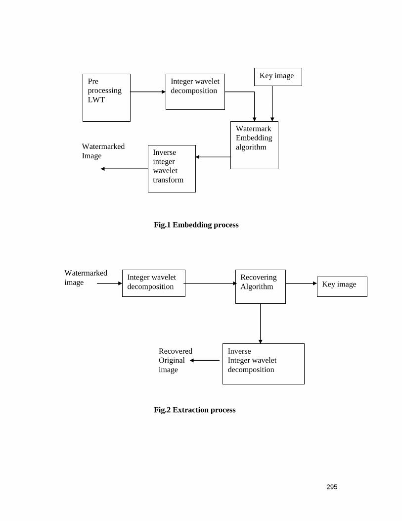
Fig.1 Embedding process
Fig.2 Extraction process
Watermarked
image Integer wavelet
decomposition
Recovering
Algorithm Key image
Inverse
Integer wavelet
decomposition
Recovered
Original
image
Pre
processing
LWT
Integer wavelet
decomposition
Watermark
Embedding
algorithm Inverse
integer
wavelet
transform
Key image
Watermarked
Image
295

Steps in Embedding
1. Let R= P1 , P2 ,......Pn represent the set of all
neighboring pixel pairs in one
direction and Pi be a single pair
for all i=1 to n.
2. let W = W1 ,W2 ,......Wm represent the watermark data
where each 0,1,2,.....,9
Wi are used to represent ASCII
characters. The same digits can
represent Text or image
watermark.
In this above steps are indicating the
embedding process for watermarking
image.
P is represented as each pixel for
original image. Where W is represented
as each pixel for key image. The
information of low frequency component
is an image close to the original image.
Most signal information of Original
image is in this frequency component.
The frequency components of LH, HL
and HH respectively, represent the level
detail, the upright detail and the diagonal
detail of the original image. For testing
the performance of this algorithm, the
experiments are simulated with the
MATLAB. In the following
experiments, the gray-level image with
size of 256 * 256 “Lena” is used as host
image to embed watermark.
3. EXPERIMENTS AND RESULTS
4.1 DWT Based Watermarking
Fig.3 Before watermarking Lena
image
Watermarked Image
Fig.4 DWT based watermarked
image
Fig.5 DWT based recovered image
Here the standard Lena image is used to
hide the information. When the
embedding message is used in the
transformed domain, the robustness is
high and the distortion is very low.
Compare with other methods,
embedding technique using wavelets
performs better. This is because the
resolution is very high and compared the
Recovered Watermark
296

image distortion is very low. Here the
key is represented as the text which to be
embedded with the image. The Lena
image before and after watermarking are
as shown in figures 4 and 5 respectively.
4.2 IWT Based Watermarking
Fig.6 IWT based watermarked image
Fig.7 IWT based recovered image
Table 1: PSNR values of the embedded
watermarked image
The above Table1 shows the different
types of transforms embedding and it
shows the peak signal to noise ratio
(PSNR) and that will take the time for
embedding an image. So the above
analysis, final result is achieved by
integer wavelet transform by using
lifting scheme. In addition, the security
can be enhanced by incorporating a
private embedding key to code the map
associating the embedded bits to the
selected wavelet watermarking blocks.
By using the integer wavelet
transformation it is avoid the overflow of
the data compared with the existing
method. The result shows the distortion
less watermarked image. The results are
presented in Table.1 Indicates the types
of transformation like LSB, DCT, DWT,
and IWT this compares the results of
peak signal to noise ratio value.
As a result finally we got good PSNR
value in integer wavelet transform. To
verify the advantage of the packed
integer wavelet transform, we compared
its performance with that of the original
integer wavelet transform for image
compression. It produces many small
high-frequency coefficients by the high-
pass filter. On the other hand, the minor
errors are generated by the computation.
In the integer computation, the
magnitude does not even increase
Consequently, overflow of the
magnitude is not a concern in our
applications. In general, multiple
coefficients can be packed into one
integer provided that the width of the
data-path is sufficient.
Transforms PSNR value in
db
Elapsed
time in (s)
LSB 1.2212e+005 10.5625
DCT 2.4061e+003 11.6563
DWT 3.1402e+003 10.6563
LWT 33.153037 35.5625
Retrieved Watermark
Watermarked Image
297
5. CONCLUSION
In this paper, we analyze the security of
fragile image authentication schemes
based on watermarking that can
accurately localize modifications. We
start with a comparison of PSNR Values
and Elapsed time using DWT based
algorithm and proposed algorithm. The
experiments are carried out using
Matlab. In Future work we are going to
use the moments for rotation and
cropping for watermarked image.
REFERENCES
1. C. W. Honsinger, P. Jones, M.
Rabbani, and J. C. Stoffel,
“Lossless recovery of an original
image containing embedded
data,” US Patent application,
Docket No: 77102/E−D (1999).
2. S. Walton, “Information
authentication for a slippery new
age,” Dr.Dobbs J., vol. 20, no. 4,
pp. 18–26, Apr. 1995.
3. B. B. Zhu, M. D. Swanson, and
A. H. Tewfik, “When seeing isn’t
believing,” IEEE Signal Proces.
Mag., vol. 21, no. 2, pp. 40–49,
Mar. 2004.
4. M. U. Celik, G. Sharma, E.
Saber, and A. M. Tekalp, “A
hierarchical image authentication
watermark with improved
localization and security,” in
Proc. IEEE Int. Conf. Image
Processing, Oct. 2001, vol. 2, pp.
502–505.
5. W. Sweldens, “The lifting
scheme: a custom-design
construction of biorthogonal
wavelets,” Appl. Comput.
Harmon. Anal., vol. 3, no. 2, pp.
186–200, 1996.
6. I. Daubechies and W. Sweldens,
“Factoring Wavelet Transforms
into Lifting Steps,” Tech. Rep.,
Lucent Technologies, Bell Labs.,
Holmdel, NJ, 1996.
7. E. Koch and J. Zhao, “Towards
robust and hidden image
copyright labeling,” in Proc.
IEEE Workshop on Nonlinear
Signal and Image Processing,
Jun. 1995, pp. 452–455.
8. S. Kurshid Jinna1, Dr. L.
Ganesan , “Lossless Image
Watermarking using Lifting
Wavelet Transform” ,
International Journal of Recent
Trends in Engineering, Vol 2,
No. 1, November 2009.
298

Proceedings of the Third National Conference on RTICT 2010
Bannari Amman Institute of Technology ,Sathyamangalam- 638401
9-10 April 2010
299
Testing Polymorphism in Object Oriented Systems
at Dynamic Phases for Improving Software Quality
R.VinodKumar, G.Annapoorani
Department of Computer Science Engineering
Anna University Tiruchirappalli,Tamilnadu, India [email protected]
Abstract— With object-oriented testing should centre on object
class, generic classes and super classes, inheritance and
polymorphism, instead of subprograms. In object-oriented
software test, the feature of inheritance and polymorphism
produces the new obstacle during dynamic testing.
Polymorphism becomes a problem in dealing with object-
oriented software testing. Although program faults are widely
studied, there are many aspects of faults that still do not
understand, particularly about object-oriented software. The
important goal during testing is to cause failures and there by
detect faults, a full understanding of the characteristics of faults
is crucial to several research areas. The power of inheritance and
polymorphism brings to the expressiveness of programming
languages also brings a number of new anomalies and fault
types. In this application various issues and problems that are
associated with testing polymorphic behaviour of objects in
object oriented systems is discussed. The application of these
techniques can result in an increased ability to find faults and to
create overall higher quality software.
Keywords—Polymorphism, Inheritance, Software Testing,
Software Quality, Method Overriding, Metrics, Overloading and Object Orientated Systems.
I. INTRODUCTION
Testing of object-oriented software presents a variety of
new challenges due to features such as inheritance,
polymorphism, dynamic binding and object state. Programs
contain complex interactions among sets of collaborating
objects from different classes. These interactions are greatly complicated by object-oriented features such as polymorphism,
which allows the binding of an object reference to objects of
different classes. While this is a powerful mechanism for
producing compact and extensible code, it creates numerous
fault opportunities.
Polymorphism is common in object-oriented software for
example; polymorphic bindings are often used instead of case
statements. However, code that uses polymorphism can be
hard to understand and therefore fault-prone. For example,
understanding all possible interactions between a message
sender object and a message receiver object under all possible
bindings for these objects can be challenging for programmers.
The sender object of a message may fail to meet all
preconditions for all possible bindings of the receiver object.
A subclass in an inheritance hierarchy may violate the
contract of its super class’s clients that send polymorphic
messages to this hierarchy may experience inconsistent
behaviour. For example, an inherited method may be incorrect
in the context of the subclass or an overriding method may
have pre conditions and post conditions different from the
ones for the overridden method. In deep inheritance
hierarchies, it is easy to forget to override methods for lower-
level subclasses.
There are a number of testing issues that are unique to object-oriented software. Several researchers have asserted
that some traditional testing techniques are not effective for
object-oriented software and that traditional software testing
methods test the wrong things. Specifically, methods tend to
be smaller and less complex, so path-based testing techniques
are less applicable [1][3][5]. Additionally, inheritance and
polymorphism brings undesirability to the software. The
execution path is no longer a function of the class's static
declared type, but a Intra-method testing, in which tests are
constructed for individual methods.
Inter-method testing, in which multiple methods within a class are tested in concert. Intra-class testing, in which tests
are constructed for a single class, usually as sequences of calls
to methods within the class. Inter-class function of the
dynamic type that is not known until run-time. A class is
usually regarded as the basic unit of OO testing. There are
three levels of testing. Testing in which more than one class is
tested at the same time. Gallagher and Offutt had added this
level.
Polymorphism is an important feature of object oriented
software which allows an object reference to bind with the
objects of other classes. Method overriding is a way of giving a method one name that is shared up and down in a class
hierarchy, with each class in the hierarchy implementing the
method in a way appropriate to itself.
The decision as to which method is to be used is left till
run time using a technique called Dynamic method lookup. If
the subclass includes a method with the same "signature" as a
method in the super class the super class will not be inherited.

300
It is observed that the subclass method overrides the super
class methods.
Dynamic binding allows the same statement to execute
different method bodies. Which one is executed depends on
the current type of the object that is used in the method call.
These features make testing more difficult because the exact data type and implementation cannot be determined statically
and the control flow of the object oriented program is less
transparent.
Various techniques can be found in testing literature for
testing of polymorphic relationships. Most approaches require
testing that exercises all possible bindings of certain
polymorphic references. Each possible binding of a
polymorphic component requires a separate test. It may be
hard to find all such bindings, increasing the chance of errors
and posing an obstacle to reaching coverage goals. This may
also complicate integration planning, in that many server
classes may need to be integrated before a client class can be tested.
II. COVERAGE CRITERIA FOR POLYMORPHISM
Various techniques for testing of polymorphic interactions
have been proposed in previous work. These approaches
require testing that exercises all possible polymorphic
bindings for certain elements of the tested software. Binder [4]
points out that “just as we would not have high confidence in
code for which only a small fraction of the statements or
branches have been exercised, high confidence is not
warranted for a client of a polymorphic server unless all the
message bindings generated by the client are exercised”. These requirements can be encoded as coverage criteria for
testing of polymorphism. There is existing evidence that such
criteria are better suited for detecting object-oriented faults
than the traditional statement and branch coverage criteria.
A program-based coverage criterion is a structural test
adequacy criterion that defines testing requirements in terms
of the coverage of particular elements in the structure of the
tested software. Such coverage criteria can be used to evaluate
the adequacy of the performed testing and can also provide
valuable guidelines for additional testing. In this paper, we
focus on two program-based coverage criteria for testing of
polymorphism [4][6]. The all-receiver-classes criterion requires exercising of all possible classes of the receiver
object at a call site. The all-target-methods criterion requires
exercising of all possible bindings between a call site and the
methods that may be invoked by that site. Some existing
approaches explicitly define coverage requirements based on
these criteria, while, in other approaches, the coverage of
receiver classes and/or target methods is part of more general
coverage requirements that take into account polymorphism .
For example, in addition to all-receiver-classes, proposes
coverage of all possible classes for the senders and the
parameters of a message.
III. CLASS ANALYSIS FOR COVERAGE TOOLS
The use of coverage criteria is essentially impossible
without tools that automatically measure the coverage
achieved during testing. A coverage tool analyses the tested
software to determine which elements need to be covered,
inserts instrumentation for runtime tracking, executes the test
suite, And reports the degree of coverage and the elements
that have not been covered.
To determine which software elements need to be covered, a coverage tool has to use some form of source code
analysis. Such an analysis computes the elements for which
coverage should be tracked and determines the kind and
location of the necessary code instrumentation. For simple
criteria such as statement and branch coverage, the necessary
source code analysis is trivial; however, the all-receiver-
classes and all-target-methods criteria require more complex
analysis [2][4]. To compute the all-receiver-classes and all-
target-methods coverage requirements, a tool needs to
determine the possible classes of the receiver object and the
possible target methods for each call site. In the simplest case,
this can be done by examining the class hierarchy i.e., by considering all classes in the sub tree rooted at the declared
type of the receiver object. It appears that previous work on
testing of polymorphism uses this approach (or minor
variations of it) to determine the possible receiver classes and
target methods at polymorphic calls.
Some of the existing work on static analysis for object-
oriented languages shows that using the class hierarchy to
determine possible receiver classes may be overly
conservative i.e., not all subclasses may be actually feasible.
Such imprecision has serious consequences for coverage tools
because the reported coverage metrics become hard to interpret, is the low coverage due to inadequate testing or is it
due to infeasible coverage requirements. This problem
seriously compromises the usefulness of the coverage metrics.
In addition, the person who creates new test cases may spend
significant time and effort trying to determine the appropriate
test cases before realizing that it is impossible to achieve the
required coverage.
This situation is unacceptable because the time and
attention of a human tester can be very costly compared to
computing time. To address above mentioned short comes,
propose using class analysis to compute the coverage
requirements. Class analysis is a static analysis that determines an overestimate of the classes of all objects to
which a given reference variable may point. While initially
developed in the context of optimizing compilers for object-
oriented languages, class analysis also has a variety of
applications in software engineering tools. In a coverage tool
for testing of polymorphism, class analysis can be used to
determine which are the classes of objects that variable x may
refer to at call site x.m(),from this information, it is trivial to
compute the all-receiver-classes and all-target-methods
criteria for the call site. There is a large body of work on
various class analyses with different tradeoffs between cost and precision. However, there has been no previous work on
using these analyses for the purposes of testing of
polymorphism.
IV.DYNAMIC METRICS

301
Dynamic polymorphic metrics measure the various aspect
of the polymorphism behavior in the programs [7].
a) Call Site Polymorphic Value (CSPV) metric count total
number of different call sites executed. This measurement
does not include static invoke instructions, but does count virtual method calls with a single receiver.
b) Invoke Density Polymorphic Value (IDVP) metric count
number of invoke Virtual and invoke Interface calls per kbc
executed. This metric estimates the importance of invoke byte
codes relative to other instructions in the program, indicating
the relevance of optimizing invokes.
c) Receiver Polymorphic Bin (RPB) metric shows the
percentage of all call sites that have one, two and more than
two different receiver types. The metric is dynamic, since we
measure the number of different types that actually occur in the execution of the program.
d) Receiver Call Polymorphic Bin (RCPB) metric shows the
percentage of all calls that occur from a call site with one, two
and more than two different receiver types. This metric
measures the importance of polymorphic calls.
e) Receiver Cache Miss Rate polymorphic Value (RCMRV)
metric shows as a percentage how often a call site switches
between receiver types. This is the most dynamic
measurement of receiver polymorphism, and it represents the miss rate of a true inline cache.
f) Target Polymorphic Bin (TPB) metric shows the percentage
of all call sites that have one, two and more than two different
target methods. This metric is dynamic, but does not reflect
the run time importance of call sites.
g) Target Call Polymorphic Bin (TCPB) metric shows the
percentage of all calls that occur from a call site with one, two
and more than two different target methods.
h) Target Cache Miss Rate polymorphic Value (TCMRV) metric shows as a percentage how often a call site switches
between target methods. It represents the miss rate of an
idealized branch target buffer. It is always lower than the
corresponding inline cache miss rate since targets can be equal
for different receiver types. Accordingly, this metric can also
be heavily influenced by the order in which target methods
occur.
i) Dynamic polymorphism in ancestors (DPA) is the sum of
number of dynamic polymorphism function members in
ancestor that appears in the different classes.
j) Dynamic Polymorphism in Descendants (DPD) is the sum
of number of dynamic polymorphism function members in
descendant that appears in the different classes.
k) Average Changing Rate of Virtual methods (ACRV) are
used to check the efficiency by using run time method
resolution.
IV. MODELING POLYMORPHISM: THE YOYO GRAPH
One of the major difficulties with using polymorphism
and dynamic binding is that of modeling and visualizing the complicated interactions. The essential problems are that of
understanding which version of a method will be executed and
which versions can be executed. The fact that execution can
sometimes “bounce” up and down among levels of inheritance
has been called the yo-yo effect by Binder and he introduced a
preliminary graph [8]. We have extended this notion as a basis
for a graphical representation that we call the “yo-yo graph” to
show all possible actual executions in the presence of dynamic
binding.
A
t u v w
D() G() H() I() J() L()
B
x
H() I()
K()
C
I() J() L()
Fig1. Data Flow anomalies with polymorphism
Consider the inheritance hierarchy shown in Figure 1.
Assume that in A’s implementation, d() calls g(), g() calls h(),
h() calls i(), and i() calls j(). Further, assume that in B’s
implementation, h() calls i(), i() calls its parent’s (that is, A’s)
Methods Defines Users
A..h A..u, A..w
A..i A..u
A..j A..v A..w
A..l A..v
B..h A..x
B..i B..x
C..i A..y
C..j C..v
C..l A..v
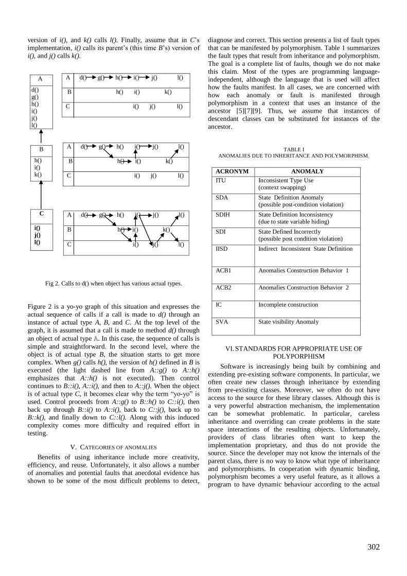
302
version of i(), and k() calls l(). Finally, assume that in C’s
implementation, i() calls its parent’s (this time B’s) version of
i(), and j() calls k().
A
d() g() h() i() j() l()
Fig 2. Calls to d() when object has various actual types.
Figure 2 is a yo-yo graph of this situation and expresses the
actual sequence of calls if a call is made to d() through an
instance of actual type A, B, and C. At the top level of the
graph, it is assumed that a call is made to method d() through
an object of actual type A. In this case, the sequence of calls is
simple and straightforward. In the second level, where the
object is of actual type B, the situation starts to get more
complex. When g() calls h(), the version of h() defined in B is
executed (the light dashed line from A::g() to A::h()
emphasizes that A::h() is not executed). Then control
continues to B::i(), A::i(), and then to A::j(). When the object
is of actual type C, it becomes clear why the term “yo-yo” is
used. Control proceeds from A::g() to B::h() to C::i(), then
back up through B::i() to A::i(), back to C::j(), back up to B::k(), and finally down to C::l(). Along with this induced
complexity comes more difficulty and required effort in
testing.
V. CATEGORIES OF ANOMALIES
Benefits of using inheritance include more creativity,
efficiency, and reuse. Unfortunately, it also allows a number
of anomalies and potential faults that anecdotal evidence has
shown to be some of the most difficult problems to detect,
diagnose and correct. This section presents a list of fault types
that can be manifested by polymorphism. Table 1 summarizes
the fault types that result from inheritance and polymorphism.
The goal is a complete list of faults, though we do not make
this claim. Most of the types are programming language-
independent, although the language that is used will affect how the faults manifest. In all cases, we are concerned with
how each anomaly or fault is manifested through
polymorphism in a context that uses an instance of the
ancestor [5][7][9]. Thus, we assume that instances of
descendant classes can be substituted for instances of the
ancestor.
TABLE I
ANOMALIES DUE TO INHERITANCE AND POLYMORPHISM.
VI. STANDARDS FOR APPROPRIATE USE OF
POLYPORPHISM
Software is increasingly being built by combining and
extending pre-existing software components. In particular, we often create new classes through inheritance by extending
from pre-existing classes. Moreover, we often do not have
access to the source for these library classes. Although this is
a very powerful abstraction mechanism, the implementation
can be somewhat problematic. In particular, careless
inheritance and overriding can create problems in the state
space interactions of the resulting objects. Unfortunately,
providers of class libraries often want to keep the
implementation proprietary, and thus do not provide the
source. Since the developer may not know the internals of the
parent class, there is no way to know what type of inheritance
and polymorphisms. In cooperation with dynamic binding, polymorphism becomes a very useful feature, as it allows a
program to have dynamic behaviour according to the actual
A d() g() h() i() j() l()
B h() i() k()
C i() j() l()
B
h() i() k()
A d() g() h() i() j() l()
B h() i() k()
C i() j() l()
C
i()
j()
l()
A d() g() h() i() j() l()
B h() i() k()
C i() j() l()
ACRONYM ANOMALY
ITU Inconsistent Type Use (context swapping)
SDA State Definition Anomaly (possible post-condition violation)
SDIH State Definition Inconsistency (due to state variable hiding)
SDI State Defined Incorrectly (possible post condition violation)
IISD Indirect Inconsistent State Definition
ACB1 Anomalies Construction Behavior 1
ACB2 Anomalies Construction Behavior 2
IC Incomplete construction
SVA State visibility Anomaly

303
type of object under execution. A number of design patterns
are formalized based on this concept. Although it is a very
useful feature many researchers address that polymorphism
does not prevent software from defects [2][3][8][9]. Barbey
and Strohmeier state that to gain confidence in an operation a
statement of which is a call to a dynamically invoked operation, it becomes necessary to make assumptions
regarding the nature of the polymorphic parameters, i.e. a
“hierarchy specification” must be provided for each of their
operations, which specifies the expected minimal behaviour of
their operation and all their possible redefinitions. Therefore
whenever methods are inherited by a derived class some
further testing is necessary which must be in context to the
derived class. This is true both for those methods which have
been inherited unchanged and those which have been
overridden.
VII. EXPERIMENTAL RESULTS
A polymorphic call in object oriented system takes the form of invoke virtual or invoke interface.
TABLE II
ANALYSIS OF RESULTS
METRIC I II III IV V
CSPV 1 2 3 4 5
IDVP 6 19 13 11 23
RPB 22% 7.14% 8.09% 9.09% 4.35%
RCPB 20% 57.14% 54.55% 63.64% 60.67%
RCMRV 0% 28.57% 27.27% 36.36% 17.36%
TPB 20% 85.71% 75% 99% 76.92%
TCPB
20% 80% 75% 100% 78.78%
TCMRV 0% 16.67% 16.67% 0.14% 0.1%
DPA 2 1 2 1 2
DPD 1 1 1 1 1
ACRV 0.38% 0.43% 0.5% 0.39% 0.53%
This paper is presenting eleven dynamic metrics as a means of
assessing the actual run time behavior of a program by providing a high-level overview of several of its key aspects.
This dynamic information can be more relevant than the more
common static measures. These metrics are designed with the
goals of being unambiguous, dynamic, robust, discriminating,
and platform-independent. These metrics are also classified in
four categories value, percentile, bin and continuous. The
utility of the metrics is evaluating by applying them to five
specific dynamic polymorphic problems and determining to
which extent they provided useful information for each task.
We furthermore want to establish the preciseness of using
dynamic metrics as helping tools for exploratory program understanding in object oriented system. Implementation of
dynamic metrics is given in this section on the set of five
different polymorphic programs. The results are mentioned in
Table II.
VIII.CONCLUSIONS AND FUTHERWORK
We have shown the types of faults are likely to be
encountered in object-oriented programs. The results of our
empirical study suggest that traditional testing techniques,
such as functional testing and white-box approaches that
utilize the statement and branch coverage criteria, are not
adequate for detecting object-oriented faults. The object flow
based testing strategy, however, takes object-oriented features
into account and is reliable with respect to most OO faults.
Therefore, to have confidence in testing object oriented
programs, it is important to incorporate traditional testing
techniques with the object-flow based testing strategy. Nevertheless, with a few feasible efforts the reliability of the
program can be improved effectively and the maintenance
cost can be reduced significantly. Much work remains to be
done in this research area. We are currently investigating the
correlation of Object Oriented design metrics with fault
population and distribution. It is expected that such a
relationship can be used to select effective testing techniques
and to prioritize these selected techniques, so that most faults
can be detected with an affordable cost. Meanwhile, we are
studying the granularity of the object flow based testing
strategy to compare the strengths and the cost of this strategy with the data flow testing strategy which is a further
refinement of the object-flow strategy.
REFERENCES
[1] M.D. Smith and D.J. Robson, “Object-Oriented Programming: The
Problems of Validation”, Proc. IEEE Conf. Software Maintenance, IEEE
Computer Society Press, Los Alamitos, Calif., pp. 272-281, 1990.
[2] M.H. Ghai and M. H.Kao,”Testing Object-Oriented Programs an
Integrated Approach. In Proceedings of the 10th international
Symposium on Software Reliability Engineering”, ISSRE.IEEE
Computer Society, Washington, DC, pp.73-83, November 01-04, 1999.
[3] R. Alexander and J. Offutt.,“Criteria for Testing Polymorphic
Relationships”, In Proceedings of the 11th international Symposium on
Software Reliability Engineering (Issre'00). ISSRE. IEEE Computer
Society, Washington, DC, pp.15-23, October 08 - 11, 2000.
[4] Atanas Rountev, Ana Milanova and Barbara G. Ryder, “Fragment Class
Analysis for Testing of Polymorphism in Java Software”, IEEE Trans.
Software Engineering, vol. 30, no.6, pp.372-387, Jun. 2004.
[5] S. Barbey and A. Strohmeier, “The Problematic of Testing Object-
Oriented Software”, Proceedings of SQM '94 Second Conference on
Software Quality Management, Edinburgh, Scotland, UK, vol.2, pp.
411-426, 1994.
[6] Stephane Barbey and Alfred Strohmeier,”The problematic of testing
object-oriented software”, In SQM'94 Second Conference on Software
Quality Management, Edinburgh, Scotland, UK, July 26-28, vol. 2,
pp.411-426, 1994.
[7] Parvinder Singh Sandhu, and Gurdev Singh,”Dynamic Metrics for
Polymorphism in Object Oriented Systems”, In World Academy of
Science, Engineering and Technology , vol. 39, no.3, pp.412-121, 2008.
[8] Jeff Offutt and Roger Alexander, “A Fault Model for Subtype
Inheritance and Polymorphism”, The Twelfth IEEE International
Symposium on Software Reliability Engineering (ISSRE ’01), Hong
Kong, PRC, November 2001.

304
[9] Mei-Hwa Chen and Howard M. Kao,”Testing Object-Oriented
Programs - An Integrated Approach”, ISSRE. IEEE Computer Society,
Los Alamitos, 2007.
Proceedings of the Third National Conference on RTICT 2010
Bannari Amman Institute of Technology ,Sathyamangalam- 638401
9-10 April 2010
305
A paper on Efficient Reverse Turing Test in
Artificial Intelligence
G. Geetha
PG Computer Science,
Sree Saraswathy Thyagaraja College, Pollachi
Abstract— This paper presents an introduction to
Artificial intelligence (AI). Artificial intelligence is
exhibited by artificial entity, a system is generally
assumed to be a human intelligence of computer.
This paper takes into the consideration of the
relationship between the two independent lines of
research into user modelling activities in human-
computer interaction (HCI) and artificial intelligence
(AI). The user modelling research conducted in HCI
and AI respectively is then discussed along with the
goals of HCI and AI. In addition a view of how the
various Turing Testing Techniques are employing AI
user models including the Reverse Turing Tests is
evaluated. The paper begins by considering the AI
techniques and the field of HCI with the later
sections discussing the historical evolution of AI,
various Turing Test Techniques involved. The
remaining paper focuses on presenting the Reverse
Turing Test involved with AI its applications.
Finally, we bring up the Enhanced methodology
using CAPTCHA as a contributed work which is
more efficient Reverse Turing Test than the existing
method. This Enhanced methodology, EPIX is
discussed with its technical work clearly projected
out along with its advantages and future work.
Keywords— Artificial Intelligence (AI), CAPTCHA
(Completely Automated Public Turing test to tell Computers and Humans Apart), Human Computer
Interaction (HCI)
I. INTRODUCTION
The scientific and engineering discipline that makes up or is closely allied with AI is relatively recent origin.
They date back to the 1950s at the earliest, with the first
encyclopaedia article on AI appearing in 1967. AI have been rapidly changing and expanding both in intellectual
content and in application, especially in the last decade.
The recent accelerated pace of change has been due in no small part to the almost breathtaking innovations and
product developments in the supporting microelectronics,
electro optics, and display technologies—all hardware-intensive areas. Growth in the amount of new
terminology and technical jargon always accompanies
such changes and advances in technology. Recognizing
the futility of attempts to craft comprehensive definitions in light of these rapid changes, the panel has
opted to provide brief descriptions of four frequently
used terms: artificial intelligence, human-computer interface, virtual worlds, and synthetic environments.
A. Artificial intelligence (AI)
Artificial intelligence (AI) is defined as intelligence
exhibited by an artificial entity. Such a system is
generally assumed to be a computer [3]. Although AI
has a strong science fiction connotation, it forms a vital branch of computer science, dealing with intelligent
behaviour, learning and adaptation in machines.
Research in AI is concerned with producing machines to automate tasks requiring intelligent behaviour. Examples
include control, planning and scheduling, the ability to
answer diagnostic and consumer questions, handwriting,
speech, and facial recognition. As such, it has become a scientific discipline, focused on providing solutions to
real life problems. AI systems are now in routine use in
economics, medicine, engineering and the military, as well as being built into many common home computer
software applications, traditional strategy games like
computer chess and other video games. Artificial intelligence is the collection of
computations that at any time make it possible to assist
users to perceive, reason, and act. Since it is
computations that make up AI, the functions of perceiving, reasoning, and acting can be accomplished
under the control of the computational device (e.g.,
computers or robotics) in question. AI at a minimum includes representations of "reality,"
cognition, and information, along with associated
methods of representation, Machine learning, representations of vision and language, Robotics and
Virtual reality.
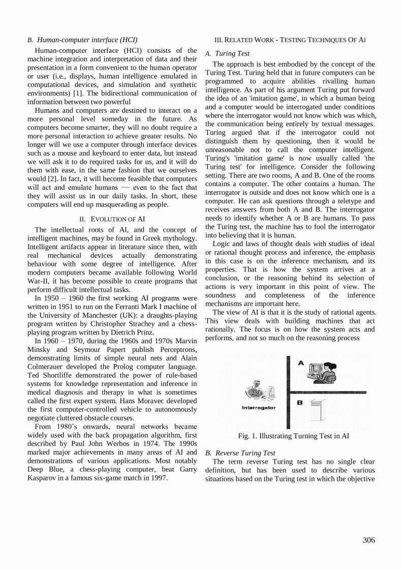
306
B. Human-computer interface (HCI)
Human-computer interface (HCI) consists of the machine integration and interpretation of data and their
presentation in a form convenient to the human operator
or user (i.e., displays, human intelligence emulated in computational devices, and simulation and synthetic
environments) [1]. The bidirectional communication of
information between two powerful
Humans and computers are destined to interact on a more personal level someday in the future. As
computers become smarter, they will no doubt require a
more personal interaction to achieve greater results. No longer will we use a computer through interface devices
such as a mouse and keyboard to enter data, but instead
we will ask it to do required tasks for us, and it will do them with ease, in the same fashion that we ourselves
would [2]. In fact, it will become feasible that computers
will act and emulate humans −− even to the fact that
they will assist us in our daily tasks. In short, these computers will end up masquerading as people.
II. EVOLUTION OF AI
The intellectual roots of AI, and the concept of intelligent machines, may be found in Greek mythology.
Intelligent artifacts appear in literature since then, with
real mechanical devices actually demonstrating behaviour with some degree of intelligence. After
modern computers became available following World
War-II, it has become possible to create programs that
perform difficult intellectual tasks. In 1950 – 1960 the first working AI programs were
written in 1951 to run on the Ferranti Mark I machine of
the University of Manchester (UK): a draughts-playing program written by Christopher Strachey and a chess-
playing program written by Dietrich Prinz.
In 1960 – 1970, during the 1960s and 1970s Marvin
Minsky and Seymour Papert publish Perceptrons, demonstrating limits of simple neural nets and Alain
Colmerauer developed the Prolog computer language.
Ted Shortliffe demonstrated the power of rule-based systems for knowledge representation and inference in
medical diagnosis and therapy in what is sometimes
called the first expert system. Hans Moravec developed the first computer-controlled vehicle to autonomously
negotiate cluttered obstacle courses.
From 1980’s onwards, neural networks became
widely used with the back propagation algorithm, first described by Paul John Werbos in 1974. The 1990s
marked major achievements in many areas of AI and
demonstrations of various applications. Most notably Deep Blue, a chess-playing computer, beat Garry
Kasparov in a famous six-game match in 1997.
III. RELATED WORK - TESTING TECHNIQUES OF AI
A. Turing Test
The approach is best embodied by the concept of the Turing Test. Turing held that in future computers can be
programmed to acquire abilities rivalling human
intelligence. As part of his argument Turing put forward the idea of an 'imitation game', in which a human being
and a computer would be interrogated under conditions
where the interrogator would not know which was which, the communication being entirely by textual messages.
Turing argued that if the interrogator could not
distinguish them by questioning, then it would be
unreasonable not to call the computer intelligent. Turing's 'imitation game' is now usually called 'the
Turing test' for intelligence. Consider the following
setting. There are two rooms, A and B. One of the rooms contains a computer. The other contains a human. The
interrogator is outside and does not know which one is a
computer. He can ask questions through a teletype and receives answers from both A and B. The interrogator
needs to identify whether A or B are humans. To pass
the Turing test, the machine has to fool the interrogator
into believing that it is human. Logic and laws of thought deals with studies of ideal
or rational thought process and inference, the emphasis
in this case is on the inference mechanism, and its properties. That is how the system arrives at a
conclusion, or the reasoning behind its selection of
actions is very important in this point of view. The
soundness and completeness of the inference mechanisms are important here.
The view of AI is that it is the study of rational agents.
This view deals with building machines that act rationally. The focus is on how the system acts and
performs, and not so much on the reasoning process
Fig. 1. Illustrating Turning Test in AI
B. Reverse Turing Test
The term reverse Turing test has no single clear
definition, but has been used to describe various
situations based on the Turing test in which the objective

307
and/or one or more of the roles have been reversed
between computers and humans.
Conventionally, the Turing test is conceived as having a human judge and a computer subject which attempts to
appear human. Critical to the concept is the parallel
situation of a human judge and a human subject, who
also attempts to appear human. The intent of the test is for the judge to attempt to distinguish which of these
two situations is actually occurring. It is presumed that a
human subject will always be judged human, and a computer is then said to "pass the Turing test" if it too is
judged human. Any of these roles may be changed to
form a "Reverse Turing test".
Arguably the standard form of reverse Turing test is one in which the subjects attempt to appear to be a
computer rather than a human.
A formal reverse Turing test follows the same format as a Turing test. Human subjects attempt to imitate the
conversational style of a conversation program such as
ELIZA. Doing this well involves deliberately ignoring, to some degree, the meaning of the conversation that is
immediately apparent to a human, and the simulation of
the kinds of errors that conversational programs
typically make. Arguably unlike the conventional Turing test, this is most interesting when the judges are very
familiar with the art of conversation programs, meaning
that in the regular Turing test they can very rapidly tell the difference between a computer program and a human
acting normally.
The humans that perform best (some would say worst) in the reverse Turing test are those that know computers
best, and so know the types of errors that computers can
be expected to make in conversation. There is much
shared ground between the skill of the reverse Turing test and the skill of mentally simulating a program's
operation in the course of programming and especially
debugging. As a result, programmers (especially hackers) will sometimes indulge in an informal reverse Turing
test for recreation.
An informal reverse Turing test involves an attempt to
simulate a computer without the formal structure of the Turing test. The judges of the test are typically not
aware in advance that a reverse Turing test is occurring
and the test subject attempts to elicit from the 'judges' (who, correctly, think they are speaking to a human) a
response along the lines of "is this really a human?‖
Describing such a situation as a "reverse Turing test" typically occurs retroactively.
C. Design of a Reverse Turing Test
We propose what we call a ―reverse Turing test‖ of the following kind. When a user — human or machine —
chooses to take the test (e.g. in order to enter a protected
Web site), a program challenges the user with one
synthetically generated image of text; the user must type back the text correctly in order to enter. This differs
from Turing’s proposal in at least four ways:
The judge is a machine, rather than human;
There is only one user, rather than two;
The design goal is to distinguish, rather than to
fail to
Distinguish, between human and machine; and
The test poses only one challenge – or very
few—rather than an indefinitely long sequence
of challenges.
The challenges must be substantially different almost every time, else they might be recorded exhaustively,
answered off-line by humans, and then used to answer
future challenges. Thus we propose that they be generated pseudo randomly from a potentially very large
space of distinct challenges.
"CAPTCHA" is an acronym for "Completely
Automated Public Turing test to tell Computers and Humans Apart" so that the original designers of the test
regard the test as a Turing test.
The term "reverse Turing test" has also been applied to a Turing test (test of humanity) that is administered by
a computer. In other words, a computer administers a
test to determine if the subject is or is not human.
CAPTCHA are used in some anti-spam systems to prevent automated bulk use of communications systems.
CAPTCHA is cropping up everywhere as it is used to
defend against:
Skewing search-engine rankings (Altavista,
1999)
Infesting chat rooms, etc (Yahoo!, 2000)
Gaming financial accounts (PayPal, 2001)
Robot spamming (MailBlocks, SpamArrest
2002)
In the last two years: Overture, Chinese
website, HotMail,
CD-rebate, TicketMaster, MailFrontier, Qurb,
Madonnarama, Gay.com, …
On the horizon it is being covered out at all ballot
stuffing, password guessing, denial-of-service attacks
`blunt force’ attacks (e.g. UT Austin break-in, Mar ’03). The use of CAPTCHA is controversial.
Circumvention methods exist that reduce their
effectiveness. Also, many implementations of CAPTCHA (particularly ones desired to counter
circumvention) are inaccessible to humans with

308
disabilities, and/or are difficult for humans to pass.
Types of CAPTCHA are
Text based i. Gimpy, ez-gimpy
ii. Gimpy-r, Google CAPTCHA
iii. Simard’s HIP (MSN)
Graphic based i. Bongo
ii. Pix
Audio based
D. Text Based CAPTCHA
In Text Based CAPTCHA the methodologies like
Gimpy, ez-gimpy a word or words from a small dictionary is picked up and they are distort them and add
noise and background
In Gimpy-r, Google’s CAPTCHA methodology we pick random letters and distort them, then add noise and
background
In Simard’s HIP methodology we pick random letters and numbers and distort them and then finally add arcs
Fig. 2. Illustrating Text Based CAPTCHA
E. Graphic Based CAPTCHA
In graphics based CAPTCHA the Bongo methodology is used which displays two series of blocks and the user
must find the characteristic that sets the two series apart
user is asked to determine which series each of four single blocks belongs to.
Fig. 3. Illustrating Graphics Based CAPTCHA
F. Audio Based CAPTCHA
In Audio Based CAPTCHA, the general
methodologies is to pick a word or a sequence of numbers at random then render them into an audio clip
using TTS software and distort the audio clip then ask
the user to identify and type the word or numbers
G. Related work in Reverse Turing Test
• Gimpy
Gimpy picks seven random words out of a dictionary,
distorts them, and renders them to users. The user needs
to recognize three out of the seven words to prove that he or she is a human user. Because words in Gimpy
overlap and undergo nonlinear transformations, they
pose serious challenges to existing OCR systems.
However, they also place a burden on human users. The burden is so great that Yahoo pulled Gimpy off its Web
site. The CMU team later developed an easier version,
EZ Gimpy. It shows a single word over a cluttered background and is currently used on Yahoo’s Web site.
• Bongo
Bongo explores human ability in visual pattern
recognition. It presents to a user two groups of visual patterns (e.g., lines, circles, and squares), named LEFT
and RIGHT. It then shows new visual patterns and asks
the user to decide if the new patterns belong to LEFT or RIGHT.
• Pix
Pix rely on a large database of labelled images. It first randomly picks an object label (e.g., flower, baby, lion,
etc.) from the label list and then randomly selects six
images containing that object from the database and
shows the images to a user. The user needs to enter the correct object label to prove he or she is a human user.
Fig. 4. Illustrating the Image for the object Dog
IV. THE EPIX -CONTRIBUTION WORK
EPIX is the Enhanced methodology of the PIX which the reverse Turing test techniques. It is very similar to
PIX in which we pick a concrete object then get 6
images at random from images.google.com that match
the object and then distort the images. Then a list of 100 words is built in which 90 is taken from a full dictionary,
10 from the objects dictionary. Then the user is
prompted to pick the object from the list of words
A. EPIX – Technical Issues
Make an HTTP call to images.google.com and
search for the object
309
Screen scrape the result of 2-3 pages to get the
list of images
Pick 6 images at random
Randomly distort both the images and their
URLs before displaying them
Expire the CAPTCHA in 30-45 seconds
B. EPIX – Advantages
The database already exists and is public
The database is constantly being updated and
maintained
Adding ―concrete objects‖ to the dictionary is
virtually instantaneous
Distortion prevents caching hacks
Quick expiration limits streaming hacks
V. CONCLUSIONS
We tried to explain with brief ideas the fundamentals
of AI. The paper then discusses the human computer
interaction and they both are significantly linked to each other. Then the historical evolutions of over years of AI
are projected. The Turing test Techniques are discussed
in detail along with Reverse Turing Test and its
categories are brought out. The related works of Reverse Turing test are studied and a proficient methodology of
Enhanced PIX, EPIX has been contributed through this
paper which can perform more efficient then the existing methodologies.
We conclude this paper by contributing a new
methodology by making enhancements in the existing system which could bring out a tremendous and
effective performance ratio when compared to the
existing methodologies
REFERENCES
[1] M. Schmitz, J. Baus, and S. Schmidt.
Anthropomorphized objects: A novel interaction
metaphor for instrumented spaces. In A. Q. Thomas Strang, Vinny Cahill, editor, Pervasive 2006
Workshop Proceedings. Deutsches Zentrum f¨ur
Luftund Raumfahrt. ISBN 978-3-00-018411-6, 2006.
[2] Schmidhuber, J. 2003. Goedel machines: self-
referential universal problem solvers making
provably optimal self-improvements. In Artificial General Intelligence, eds. B. Goertzel and C.
Pennachin. Forthcoming. New York: Springer-
Verlag. [3] Advances in Artificial Intelligence subject of
conference 23rd AAAI Conference on AI (AAAI-
08) July 13-17, 2008 Hyatt Regency McCormick
Place, Chicago, Illinois.
[4] F. O. Karray, C. de Silva. Soft Computing and
Intelligent Systems Design. Addison Wesley, 2004.
Concepts of Artificial Intelligence. [5] Artificial Intelligence – An Introduction to
Robotics Tim Niemueller and Sumedha
Widyadharma July 8, 2003.
[6] J. Hawkins, S. Blakeslee. On Intelligence. Times Books, 2004.An interesting book on a
comprehensive theory of intelligence based on the
human brain and neuro-science. [7] GregWelch and Gary Bishop. An Introduction to
the Kalman Filter. Technical report, Department of
Computer Science – University of North Carolina
at Chapel Hill, 2003. [8] RWTH Aachen Robocup Team. AllemaniACs.
http://robocup.rwth-aachen.de, 2003.
[9] Sebastian Thrun. Robotic Mapping: A Survey. Technical report, School of Computer Science –
Carnegie Mellon University, 2003.
[10] Stuart Russel and Peter Norvig. Artificial Intelligence. A Modern Approach, 2nd Edition.
Prentice Hall, 2003

Proceedings of the Third National Conference on RTICT 2010
Bannari Amman Institute of Technology ,Sathyamangalam- 638401
9-10 April 2010
310
BOMB DETECTION USING WIRELESS SENSOR AND
NEURAL NETWORK
Sharon Rosy S, M.E- Power System (PT) Doing, Anna University, Trichy
Shakena Grace S, M.E- Computer Science.
ABSTRACT : Today, if we want to
know where a terrorist attack will
happen, then we need to think like a
terrorist. Terrorists want to kill as many
people as possible.
At present bombs are detected
by using different machines like x-ray
machines, handheld detectors etc..In case
of x-ray machine the pictures are
captured and transmitted to experts.
They will analyze the presence and type
of bomb. Other detectors also used only
with the presences of experts. But this
way of analyzing takes more time and
make risk to life of experts
Solution for this problem is
provided in this paper using neural
network technology and GPS tracking
system. Kalman‟s filter algorithm is
used to train the network for automatic
recognition of bomb.
The wireless sensor network is
used to connect all the sensors which are
present at different locations and it is
used to produce the result to the
controller. This the static part of finding
the bomb
GPS tracking system is used to
position the exact place of bomb .This is
the dynamic part of the operation.
Index terms—Sensor networks, bomb,
neural network, GPS, KF
I. INTRODUCTION
Terrorists have a huge economic
advantage over law enforcement because it
is, many times, more expensive to detect
terrorist threats than it is to deploy terrorist
threats. The fundamental concept behind
explosives is very simple. At the most basic
level, an explosive is just something that
burns or decomposes very quickly,
producing a lot of heat and gas in a short
amount of time.
A bomb is a weapon designed to
explode when thrown, dropped or detonated
by some form of signal. A bomb is a hollow
case filled with explosives or other
destructive chemicals and exploded by
percussion or a timing device. The outer
case may be metal, plastic, concrete or glass
and the shape, size and contents of a bomb
311
depends on its application. Explosives used
for peaceful purposes such as mining and
heavy construction, are referred to as
explosive charges, but when used to maim
or destroy persons or property, they are
called "bombs".
Problem observed in the existing
work:
At present the bomb are detected
using different instruments. In all the cases
the human expert presences is necessary to
analysis the presences of bomb. In this
situation, we may lose very good analyst
when bomb gets explode. In case of x-ray
machine the pictures are captured and
transmitted to experts. They will analyze the
presence and type of bomb but they take
more time to analyze and 24 hours manual
work is necessary to get a proper result.
Training should be provided to x-ray
operators as well as security personnel and
supervisors. It takes long time to make them
expert.
Some of the drawbacks in existing system
are
Fault in suspension
Impossible to continue work
Takes long time to analyze
May miss the sensed object before
analyzing
Dog is also exiting method but there
concentration can be distracted
The main aim to propose this
concept.
To produce immediate result
To reduce manual power
To avoid manual error
To collect information from different
node at a time
To locate a exact position
II SENSING
Sensors are used here to sense the
explosive materials which are also called as
bomb detecting devices or sensors. Wireless
Sensor Network (WSN) is a network
designed with bomb sensor nodes and
deployed in different locations to sense the
bombs. WSN is scattered in a region where
it is meant to collect data through bomb
sensor nodes. Sensor networks involve three
areas:
Sensing (hardware)
Communications (software)
Computation (Algorithm).
The main architectural components
of a sensor network: Data acquisition
(Achievement) by sensors, Data transport to
system, Data analysis by the trained
network.
Bomb detecting device is taken as
sensor node. This sensor can be placed in
one static place and information can be
continuously gathered .Based on coverage
capacity of sensors, the number of sensors is
used in particular region. We can use any
kind of trustworthy bomb sensors and
portioning of area depends on these sensors.
For understanding, we can name the sensors
as S1, S2, S3…..These sensors will sense
the bomb when it enters their sensing area.
In case of joining different nodes in
different place to the controller through
wired mean is expensive, at the same time it
alerts the terrorist to damage the sensor. So
sensors are connected to the controller room
through wireless means. These sensors sense
and transmit the information trough
transmitter to the receiver at the controller
room. Here the wireless sensor is chosen to

312
change the position or to replace sensors
when their life span ends.
III TRAINED NETWORK
Neural networks are based on the
parallel architecture Neural networks are a
form of multiprocessor computer system,
with
simple processing elements
a high degree of interconnection
Interacting with noisy data or data
from the environment
Massive parallelism
Fault tolerance
Adapting to circumstances
Based on various approaches, several
different learning algorithms have been
given in the literature for neural networks.
Almost all algorithms have constant learning
rates or constant accelerative parameters,
though they have been shown to be effective
for some practical applications. The learning
procedure of neural networks can be
regarded as a problem of estimating (or
identifying) constant parameters (i.e.
connection weights of network) with a
nonlinear or linear observation equation.
The Kalman filter purpose is to use
measurements that are observed over time
that contain noise (random variations) and
other inaccuracies, and produce values that
tend to be closer to the true values of the
measurements and their associated
calculated values. The Kalman filter has
many applications in technology, and is an
essential part of the development of space
and military technology.
The Kalman filter produces estimates
of the true values of measurements and their
associated calculated values by predicting a
value, estimating the uncertainty of the
predicted value, and computing a weighted
average of the predicted value and the
measured value. The most weight is given to
the value with the least uncertainty.
The Kalman filter uses a system's
dynamics model (i.e. physical laws of
motion), known control inputs to that
system, and measurements (such as from
sensors) to form an estimate of the system's
varying quantities (its state) that is better
than the estimate obtained by using any one
measurement alone. As such, it is a common
sensor fusion algorithm.
All measurements and calculations
based on models are estimates to some
degree. Noisy sensor data, approximations
in the equations that describe how a system
changes, and external factors that are not
accounted for introduce some uncertainty
about the inferred values for a system's state.
Here, consider the problem of
determining the precise location of a moving
vehicle, say helicopter. The vehicle can be
equipped with a GPS unit that provides an
estimate of the position within a few meters.
The GPS estimate is likely to be very noisy
and jump around at a high frequency, though
always remaining relatively close to the real
position. The vehicle's position can also be
estimated by integrating its velocity and
direction over time, determined by keeping
track of the amount the accelerator is
depressed and how much the steering wheel
is turned. This is a technique known as dead
reckoning. Typically, dead reckoning will
provide a very smooth estimate of the
helicopter's position,
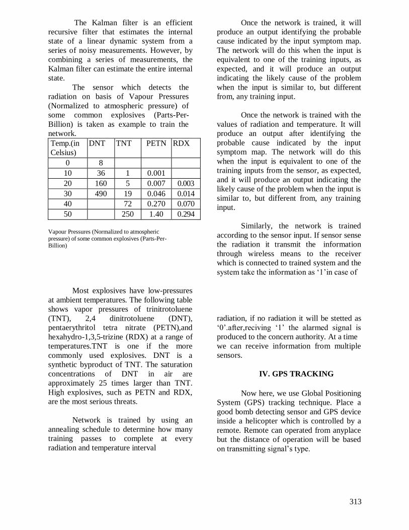
313
The Kalman filter is an efficient
recursive filter that estimates the internal
state of a linear dynamic system from a
series of noisy measurements. However, by
combining a series of measurements, the
Kalman filter can estimate the entire internal
state.
The sensor which detects the
radiation on basis of Vapour Pressures
(Normalized to atmospheric pressure) of
some common explosives (Parts-Per-
Billion) is taken as example to train the
network.
Temp.(in
Celsius)
DNT TNT PETN RDX
0 8
10 36 1 0.001
20 160 5 0.007 0.003
30 490 19 0.046 0.014
40 72 0.270 0.070
50 250 1.40 0.294
Vapour Pressures (Normalized to atmospheric pressure) of some common explosives (Parts-Per-Billion)
Most explosives have low-pressures
at ambient temperatures. The following table
shows vapor pressures of trinitrotoluene
(TNT), 2,4 dinitrotoluene (DNT),
pentaerythritol tetra nitrate (PETN),and
hexahydro-1,3,5-trizine (RDX) at a range of
temperatures.TNT is one if the more
commonly used explosives. DNT is a
synthetic byproduct of TNT. The saturation
concentrations of DNT in air are
approximately 25 times larger than TNT.
High explosives, such as PETN and RDX,
are the most serious threats.
Network is trained by using an
annealing schedule to determine how many
training passes to complete at every
radiation and temperature interval
Once the network is trained, it will
produce an output identifying the probable
cause indicated by the input symptom map.
The network will do this when the input is
equivalent to one of the training inputs, as
expected, and it will produce an output
indicating the likely cause of the problem
when the input is similar to, but different
from, any training input.
Once the network is trained with the
values of radiation and temperature. It will
produce an output after identifying the
probable cause indicated by the input
symptom map. The network will do this
when the input is equivalent to one of the
training inputs from the sensor, as expected,
and it will produce an output indicating the
likely cause of the problem when the input is
similar to, but different from, any training
input.
Similarly, the network is trained
according to the sensor input. If sensor sense
the radiation it transmit the information
through wireless means to the receiver
which is connected to trained system and the
system take the information as „1‟in case of
radiation, if no radiation it will be stetted as
„0‟.after,reciving „1‟ the alarmed signal is
produced to the concern authority. At a time
we can receive information from multiple
sensors.
IV. GPS TRACKING
Now here, we use Global Positioning
System (GPS) tracking technique. Place a
good bomb detecting sensor and GPS device
inside a helicopter which is controlled by a
remote. Remote can operated from anyplace
but the distance of operation will be based
on transmitting signal‟s type.

314
The principle behind GPS is that
receivers are able to use the technique of
“trilateration” to calculate their coordinates
on Earth by measuring the time taken for
signals from various satellites to reach them.
The GPS software will account for any
irregularities in the signal strength and clock
differences between itself and the GPS
satellite network by using signals from four
separate satellites to improve accuracy.
Usually the coordinates are then used
to locate the GPS device on a map, which is
either displayed to the user or used as a basis
for calculating routes, navigation, or as input
into mapping programs.
In fact, it is this use which
represents the simplest form of GPS
tracking. The user is able, using a portable
GPS device, to keep a track of where they
have been, in order to be able to either
retrace their steps, or follow the same path
again in the future. For example, Say,
Helicopter is designed as Light weight
By visualizing through GPS, we can
monitor position, and control the movement
of helicopter carrying GPS device and
sensor.GPS device is the transmitter here to
show the map of that particular region,
receiver receives the signals and visualize it
to the computer. From control room, the
authorized person can control the sensor. If,
the bomb is detected by the sensor, the
intensity of the LED at sensor gets increase,
when, it goes nearby to the bomb placed
from the respective sensor .Now, process
gets easy. Sensor senses the bomb and GPS
shows the path to search. Applying any
process to remove the bomb, the process of
removing bombs may be done faster and
easier.
V.CONCLUSION
There may be many varieties of
sensors and so many types of bombs. But
selecting precise sensor and removing bomb
earlier by analyzing easier is important.
By using technologies which is in
our hand, trust we can make developments
in technologies and do everything effective
and save our precious life from dangers. Let
the small thing may make great change with
many ideas in future.
REFERENCES
1. James A. Freeman and David M.
Skapura (2002) “Neural network
2. Algorithms, Application and
Programming Techniques”, Low
price edition. Page 189-211.
3. Simon Haykins (2001) “Neural
network, A Comprehensive
foundation”, Low price edition,2nd
ed. Page 1-5.
4. Sean M. Brennan, Angela M.
Mielke, and David C. Torney (2004)
“Radiation Detection with
Distributed Sensor Networks”
5. Edward J. Seuter, “Understanding
the strengths and limitations of each
bomb detection technology is the key
to a good protection strategy”
6. James Dunnigan (2004) “The Truth
about Dirty Bombs
7. Dr. Frank Barna (2005) “Dirty
Bombs and Primitive Nuclear
Weapons”
8. M. W. Siegel and A. M. Guzman,

315
“Robotic Systems for Deployment of
Explosive Detection Sensors and
Instruments”
9. “FAS Public Interest Report: The
Journal of the Federation of
American Scientists”
10. Lisa Thiesan, David Hannum, Dale
W. Murray, John E. Parmeter (2004)
“Survey of Commercially Available
Explosives, Detection techn. And
Equipment
11. Journal of lntelligent and Robotic
Systems 3: 305-319, 1990. Kluwer
Academic Publishers. Printed in
the Netherlands
12. Dan Simon (2001) “Kalman
Filtering”
13. Jianguo Jack Wang a*,Jinling Wang,
David Sinclair, Leo Watts “Neural
Network Aided Kalman Filtering
For Integrated Gps/Ins Geo-
Referencing Platform”
14. Greg Welch and Gary Bishop “An
Introduction to the Kalman Filter”

Proceedings of the Third National Conference on RTICT 2010
Bannari Amman Institute of Technology ,Sathyamangalam- 638401
9-10 April 2010
316
WARRIOR ROBOTS
A.Sandeep Kumar & S.M.Siddharth
ABSTRACT:
Robotics is the science that makes the
Robot as agent to move around, react to
their environment in pursuit of our goals.
Any electronic system that uses a computer
chip, but that is not a general-purpose
workstation, desktop or laptop computer is
called an embedded system. Such systems
use microcontrollers or microprocessors.
In this paper we discussed about the
implementation of embedded system based
robot in security field. The robots are used
in many real world applications such as in
military sensing, rescuing operations during
disaster management etc. We have analyzed
and worked on this topic and came out with
a project of MILITARY SECURITY
APPLICATION. It holds the capability of
detecting and conveying the information of
presence of human being (including the
image of the person) to the controller. The
controller can decide whether the person is
allowable inside our border or not. The
detection is performed by Pyroelectric Infra
red sensor and it was conveyed using wired
network. The strange person can be allowed
or shot by passing the respective command
to the Robot which is placed along with the
sensor in the border end.
BENEFICIAL IMPROVEMENTS:
The same project can be
implemented with the help of wireless
communication technologies so that it may
enable the control from distant place. More
over, when the project’s size is reduced and
with more improved features such as sensing
and rescuing facility etc., it may be also
employed in disaster management
applications. The size can be reduced with
the help of advance technology such as
NANOTECHNOLOGY.
INTRODUCTION:
EMBEDDED SYSTEM:
An embedded system is some combination
of computer hardware and software that is
specifically designed for a particular kind of
application device. Industrial machines,

317
automobiles, medical equipment, cameras,
household appliances, airplanes, and toys
are among the possible hosts of an
embedded system.
DEFINITION OF ROBOTICS:
The science and technology that deals with
robots are called robotics (or) Robotics is
the science or study of the technology
associated with the design, fabrication,
theory, and application of robots.
Robots and robotic technologies have an
intellectual and emotional appeal that
surpasses any other type of engineered
product. This appeal has attracted the
inquisitive minds of children and young
adults.
ROBOTS:
Robots are mechanical devices that operate
automatically. They can perform a wide
variety of tasks; jobs that are repetitious and
boring, difficult, or too dangerous for people
to perform. Industrial robots efficiently
complete routine tasks such as drilling,
welding, assembly, painting, and packaging.
They are used in manufacturing, electronics
assembly, and food processing.
A typical robot completes its task by
following a set of specific instructions that
tell it what and how the job is to be
completed. These instructions are
programmed and stored in the robot's
control center, a computer or partial
computer.
These new generation robots are controlled
by both their stored instructions (software
programs) and by feedback that they receive
from the sensors. Such robots might be used
on the ocean floor at depths man is unable to
reach and in planetary exploration and other
scientific research.
TYPES OF ROBOTICS:
Analog Robotics:
Analog robotics indulges the analog
robots.
Analog robot is a type of robot which uses
analog circuitry to go toward a simple goal
such as finding more light or responding to
sound. The first real analog robot was
invented in 1940.
Autonomous robotics:
A fully autonomous robot has the ability to
Gain information about the
environment.
Work for an extended period without
human intervention.

318
Move either all or part of itself
throughout its operating environment
without human assistance.
Avoid situations that are harmful to
people, property, or itself unless
those are part of its design
specifications.
NANOROBOTICS:
Nanorobotics is the technology of creating
machines or robots at or close to the
microscopic scale of nanometers (10-9
meters). More specifically, nanorobotics
refers to the still largely hypothetical
nanotechnology engineering discipline of
designing and building nanorobots.
Nanorobots (nanobots, nanoids or nanites)
would be typically devices ranging in size
from 0.1-10 micrometers and constructed of
nanoscale or molecular components. As no
artificial non-biological nanorobots have yet
been created, they remain a hypothetical
concept.
OUR PROJECT:
Our project titled “warrior Robot”
is equipped with PIR sensor, which is
capable of sensing live human being alone.
Once live person is detected nearby, robot
sends a logic 1 signal to Microcontroller
which in turns activates the weapon.
Parallely the video camera fixed at
head of robot captures the video information
and transmits to remote controller.
EMBEDDED SYSTEM:
Embedded systems are the computing
systems embedded within electronic
devices.
AIM OF THIS PROJECT:
o To replace the armed men in the
country border.
o So that the precious human life may
be prevented from death.
o To withstand extreme climatic
conditions or so intensive
environment.
o Implementing the advanced
technology for proper security
purpose.
319
BLOCK DIAGRAM OF WARRIOR
ROBOT:

320
PIR SENSOR:
Pyroelectric infrared sensor to detect
infrared energy radiation from human body.
It can detect the human presence (like
security alarm) in the range up to 500cm.
THEORY OF OPERATION:
Infrared radiation exists in the
electromagnetic spectrum at the wave length
that is longer than visible light .objects that
generate infrared radiation includes animals
and the human body, the infrared radiation
generated by human is strongest
This PIR sensor is designed specifically to
sense the infrared radiation emitted from
human body.
FEATURES OF PIR SENSOR:
Human infrared radiation detection
Human presence detection up to 5 meters
Human motion direction up to 1.5 meters
APPLICATIONS OF PIR SENSOR:
Human moving direction measurement
Human-following device
Human avoidance and security robot
MICROCONTROLLER
CONTROLLER FEATURES:
4K Bytes of In-System Reprogrammable
Flash Memory-
Endurance: 1,000 Write/Erase Cycles
Fully Static Operation: 0 Hz to 24 MHz
Three-Level Program Memory Lock
128 x 8-Bit Internal RAM
32 Programmable I/O Lines
Two 16-Bit Timer/Counters

321
Six Interrupt Sources
Programmable Serial Channel
MOTOR DRIVERS:
The dc motors are used for the wheel
movement
Four relay circuits drive the motors
The relay circuits are activated with
respect to the command from the
controller.
CONTROL FOR WHEELS
ROBOT MOVEMENT:
To move the robot left, the left motor is
not powered and the right motor is
made to rotate
To move the robot right the right motor
is not powered and the left motor is
made to rotate.
The motor rotation is governed by the
control from the processor (computer)
through the controller and the relay
circuit.
WEAPON DRIVER:
The firing gun is fixed at the robot
terminal
The control to the weapon is given from
the processor through the separate relay
circuit
RELAY CIRCUIT
CONTROL TO WEAPON DRIVER:
At the robot terminal a camera is fixed,
which sends the image of the
surrounding environment
The visuals from the camera is directly
sent to the processor(computer)
If any person is identified, the weapon
is fired depending on the respective
command from the processor through
the controller and the relay circuit.
HARDWARE REQUIREMENT:
1. Robot Chassis
2. AT89s8252 – 8 bit Microcontroller
3. Stepper motor driver
4. Video Transmitter
5. Computer with windows 9(x) OS
SOFTWARE REQUIREMENT:

322
1. Visual basic 6.0
WORKING:
1. The PIR sensors detect the human
being and send the signal to the
controller.
2. The controller transmits the signal to
the computer.
3. The computer also receives the video
signal from camera.
4. By using the computer we can make
the firing equipment to fire or to
move front, back, to the left or right
through relay circuit.
ADVANTAGES OF THIS ROBOT:
It fulfills the necessity of
presence of human warrior
(the human can’t be alert for
all 24 hours)
It can be implemented at low
cost
It is smaller in size.
PHOTO FLIPS OF OUR PROJECT EMBEDDED ROBO:
VISUAL EQUIPMENT (CAMERA)
323
OVERVIEW OF THE ROBOT:

324
CONCLUSION:
Using robots in defence prevents
precious Human life from death
By using Artificial Intelligence ,we can
develop robots which can be used for
different purposes in defence
“NECESSITY IS THE MOTHER OF
INNOVATION!!!”
We need more. So innovate more
REFERENCES:
1. WWW.ATMAL.COM
2. WWW.KEIL.COM
SSOOFFTTWWAARREE--FFRROONNTT EENNDD

Proceedings of the Third National Conference on RTICT 2010
Bannari Amman Institute of Technology ,Sathyamangalam- 638401
9-10 April 2010
325
PERFORMANCE ANALYSIS OF ATM NETWORKS USING
MODIFIED PARTICLE APPROACH
M.Sundarambal
#1, M.Dhivya
#2, L.Nitisshish Anand
#3,
#1 Department of Electrical and Electronics Engineering,
Coimbatore Institute of Technology, Coimbarore-641014.INDIA.
#2
Department of Electrical and Electronics Engineering,
#3
Department of Mechanical Engineering
Anna University Coimbatore, Coimbatore-641047.INDIA.
Abstract:
This paper presents generalized particle approach
to optimize the bandwidth allocation and QoS parameters
in ATM networks. The generalized particle approach
algorithm (GPAA) transforms the network bandwidth
allocation problem into dynamics and kinematics of
numerous particles in a force-field. In ATM networks
optimization, the GPA deals with a variety of random and
emergent phenomena, like congestion, failure, and
interaction. The bandwidth allocated, success rate and the
shortest path determined by GPAA are compared with the
same parameters determined using Max-Min fairness
(MMF) algorithm. The comparison among the algorithms gives the effective performance analysis of ATM networks.
1. INTRODUCTION
ATM network is to support multiple classes of traffic
(e.g. video, audio, and data) with widely different
characteristics and Quality of Service (QoS) requirements. The
major challenges are guaranteeing the QoS required for all the
admitted users and dynamically allocating appropriate
resources to maximize the resource utilization. Many
algorithms and evaluation criteria for the bandwidth allocation
have been proposed are based on maximizing an aggregate
utility function of users, an average priority or average
reliability of traffics; minimizing the overhead of data transmission and the highest call blocking Probability of all
source-destination pairs. In some duality models the network's
optimization problem can be solved by a primal Parallel
algorithm for allotted rates and a dual parallel algorithm for
shadow prices or congestion signals [1].
In this paper GPAA is used to determine bandwidth to
be allocated based on pricing and shortest path. MMF is used
to determine bandwidth to be allocated based on fairness and
pricing. The success rate, shortest path are also calculated
using both methods separately and compared.
2. GENERALIZED PARTICLE APPROACH
The GP model consists of numerous particles and forces,
with each particle having its own dynamic equations to
represent the network entities and force having its own time-
varying properties to represent various social interactions
among the network entities. Each particle in GP has four main
characteristics [2]:
1. Each particle in GP has an autonomous self-
driving force, to embody its own autonomy and the personality of network entity.
2. The dynamic state of every particle in GP is a
piecewise linear function of its stimulus, to guarantee a stable
equilibrium state.
3. The stimulus of a particle in GP is related to its own
objective, utility and intention, and to realize the multiple
objective optimizations.
4. There is variety of interactive forces among particles,
including unilateral forces, to embody various
social interactions in networks.
The bandwidth allocation policy of a network link depends on the payment policy of a network path. It changes
dynamically according to the situation of the demands and
supplies of bandwidths and influences the kinematics and
dynamics of the link particles and path particles in their force-
fields. The link particles move in resource force-field FR and
the path particles that require bandwidth assignment move in
demand force-field FD as shown in figure1. Normally a
network path pays less amount under the condition that its
bandwidth requirement is satisfied. It is embodied in the
proposed model by the corresponding path particle. Similarly
to maximize the price benefit a link tries to assign its own
bandwidth to the path that pays maximal price.
3. MODEL FOR BANDWIDTH ALLOCATION
3.1 EVOLUTION OF GP:
The mathematical model based on GP [1] for dynamic
bandwidth allocation that involves m links, n paths and p
channels is defined with following notations:
ri : The maximum bandwidth of link Ai.
d j : The bandwidth that channel T j requires.
q j : The maximum payoff that channel T j can afford for its d j. Ai : The ith physical link in the network.
Tk : The kth path of the jth channel T j.
a ik : The bandwidth that link Ai allots to path Tk.
P ik : The price per unit bandwidth that path Tk tries to
Pay link Ai.

326
3.1.1Total Utility: u k(t) is the distance from the current position of the
path particle T k to the upper boundary of the demand force-
field FD at time t, and let JD(t) be the total utility of all the path
particles in FD. uk(t) and JD(t) are defined respectively as stated
below;
m
u k(t) =δ 1 exp[- ∑ a ik(t) / p ik(t) ] (1) i=1
p n
J D (t) = α1 ∑ ∑ u k(t) (2) j=1 k=1
u i (t) is the distance from the current position of the link particle Ai to the upper boundary of the resource Force-field
FR at time t, and let JR(t) be the total utility of all the link
particles in FR. ui(t) and JR(t)are defined respectively as stated
below;
p n
u i(t) =δ 2 exp [- ∑ ∑ p ik(t) / a ik(t) ] (3) j=1 k=1
m
J R (t) = α2 ∑ u i(t) (4)
i=1 δ 1, δ 2 >1,and 0< α1, α2 <1.
3.1.2 Potential Energy: At time t, the potential energy functions, PD(t) and
PR(t), that are caused by the upward gravitational forces of the
force-fields, FD and FR, are defined respectively as stated
below;
p n
PD(t) = ε 2 ln[- ∑ ∑ exp [( u k(t))2 / 2 ε 2] - ε 2 ln(n) (5)
j=1 k=1
m
PR(t) = ε 2 ln ∑ exp [( ui (t))2 / 2 ε 2] - ε 2 ln(m) (6)
i=1
At time t, the potential energy functions, QD(t) and QR(t),
that are caused by the interactive forces among the particles in
FD and FR are defined respectively as stated below;
p n
Q D (t)= β1 ∑ [∑ a ik(t) – d j(t)]2 + E D(t) j=1 k=1
p n m
+ ρ∑ [ ∑ ∑ a ik(t) p ik(t) – q j(t)]2 (7) j=1 k=1 i=1
m n p
Q R (t) = β2 ∑ [∑ ∑ a ik(t) – r j(t)]2 + ER(t) (8) i=1 k=1 j=1
0< ε<1, 0< β1 β2, ρ<1;
ED(t) and ER(t) are the potential energy functions that involve
other kinds of the interactive forces among the particles in
FD and FR, respectively.
3.1.3 Stability:
Dynamic equations for path particle T k and
link particle Ai are defined respectively as stated below;
du k (t)/dt =φ1(t)+φ2(t) (9)
φ1(t) = - u k(t) + γ1 v1 (t) (9a)
φ2(t) =-[ε1 +ε2 dJ D(t)/d u k(t) + ε3dPD(t)/du k(t)
+ ε4 dQD(t)/d u k(t)] *
m
∑ [d u k(t) / dp ik(t)]2 (9b)
i=1
(OR)
du i (t)/dt = ψ1(t)+ ψ 2(t) (10)
ψ 1(t) = - u i(t) + γ2 v2(t) (10 a)
ψ 2(t) = -[ λ 1 + λ 2 dJ R(t)/d u i(t)+ λ 3 dPR(t)/d ui (t)
+ λ 4 dQR(t)/d u k(t) ] *
n p ∑ ∑ [d u i (t) / da ik(t)]
2 (10 b)
k=1 j=1
v1(t) and v2(t) is a piecewise linear function. γ1, γ2 >1; 0< λ 1, λ 2, λ 3 ,λ 4, ε1, ε2, ε3 ,ε4,<1
dp ik(t)/dt = - ε1[ d u k(t) / dp ik(t)] - ε2[dJ D(t)/dp ik(t)]
-ε3[dPD(t)/dp ik(t)] - ε4[dQD (t)/dp ik(t)]
(11)
da ik(t)/dt = - λ 1[ d u i(t) / da ik(t) - λ 2[dJ R(t)/da ik(t)]
-λ 3[dPR(t)/ da ik(t)] - λ 4[dQR (t)/da ik(t)]
Figure1: GPAA to optimize bandwidth allocation- a) Demand force- field FD for path particles.
b) Resource force-field FR for link particles.

327
(12)
3.1 GP ALGORITHM:
Based on the above mathematical model the algorithm is
written as given below.
Input:
Maximum bandwidth ri , required bandwidth d j ,
Maximum payoff q j
Output:
1. Initialization:
At time t=0;
Initiate bandwidth a ik(t) and price p ik(t)
2. calculate utility, potential energy functions as per the
Equations (1) to (8).
3. If
du k (t)/dt =0; (Or) du i (t)/dt =0;
hold for every particle ,finish with success;
Else goto step 4.
4. Calculate du k(t)/dt and update u k(t)
calculate dui (t)/dt and update ui(t)
calculate da ik(t)/dt ,
a ik(t) = a ik(t -1) + da ik(t)/dt
calculate dp ik(t)/dt,
p ik(t) = p ik(t -1)+ dp ik(t)/dt
goto step 2.
A network with 7 nodes and 11 edges as exhibited in
Figure 2: is considered with the set of node pairs:
V =(v1,v7),(v2,v6),(v4,v6),(v1,v3),(v1,v5)
Figure 2: A network with 7 nodes and 11 edges
The communication bandwidth bij requested between given
set of (v=vi,vj) network node pairs are:
B =15,25,21,20,17
The virtual path sets are:
T18 =(e8,e9),(e1,e2,e3),(e1,e11,e9),(e1,e2,e12,e9)
T27 = (e2, e3,e4),(e11,e10,e5),(e11,e9,e4),
(e2, e12,e10,e5), (e2,e12,e9,e4)
T47 =(e10,e5),(e9,e4)
T16 =(e7,e6),(e8,e10),(e1,e11,e10)
T26 =(e11,e10),(e2,e12,e10)
And the set of links with maximum allowable bandwidths are
e1=10 ;e2=8; e3=3; e4=18; e5=19; e6=8; e7=12; e8=15;
e9=4; e10=6;e11=15;e12=20
The minimal price, bandwidth requested, maximal price,
maximum bandwidths of link are given as input, to the GPA
algorithm. The QOS index required by every virtual path
connection (VPC) is generated randomly within 0.5 to 1.5.
4. MAX-MIN FAIRNESS ALGORITHM:
The Max-Min fairness is computed via an iterative
procedure. The algorithm classifies every virtual session as
either completely utilized or not[3].
The allocated rate for session P is denoted by rp and
the allocated flow on network is[4];
Fa= ∑ δp(a) r p
pεP
δp(a)=1 if a is on path P and 0 otherwise.
r p>=0, for all p ε Pk
Fa<=Ca, for all a ε A.
Ca is capacity of arc a and r is vector of allocated rates.
4.1 MMF ALGORITHM :
Initial Conditions:
K=1,where k is the iterative index.
Capacity Fa =0; rate r p=0; P1=P; A1=A;
1. nk =number of paths ; p ε Pk with δp(a)=1
2. rate vector r- k = min(Ca-Fa(k-1))/nk
3. r p = r p(k-1)+ r- k for p ε Pk
Else
r p = r p(k-1)
4. Fa = ∑ δp(a) r p
pεP
5. A(k+1) = a|Ca-Fa > 0
6. P(k+1) = p| δp(a)=0,for all ¢ A(k+1)
7. k = k+1
8. If P k is empty, then stop; else goto 1.
The above algorithm terminates and finds the max-
min fairness vector r, if it exists, within k steps.
Initially all sessions are unsaturated, and their status
change from unsaturation to saturation. A session is allocated
a rate r p equal to minimum of the link bandwidth on its path.
Initially bandwidth allocated to the link is one third of the
minimum bandwidth of link on its session P. The algorithm
checks the saturation condition and updates the bandwidth till
the session is saturated. The algorithm terminates if all the
sessions are saturated.
For the network in figure 2: the bandwidth requested,
minimal price (rp) and the allowable bandwidth of link (Ca)
are given as input to MMF algorithm.
5. PERFORMANCE ANALYSIS:
The Generalized particle approach (GPAA) and Max-
Min fairness algorithm is implemented with MATLAB 7.0.1.
The solution obtained is given below.
TABLE 1: BANDWIDTH ALLOCATION
Path
path set
Bandwidth allocation
GPAA MMF
12
2
1 8 4
5
3 6 7
10
8
8 19
18 6
14 4
20
15 3
328
T18
e8,e9 8.2500 4
e1,e2,e3
3.7125 3
e1,e11,e9 1.6706 4
e1,e2,e12,e9 1.3669 4
T27
e2,e3,e4
13.7500
3
e11,e9,e4
6.1875
4
e11,e10,e5 2.7844 6
e2,e12,e9,e4 1.2530 4
e2,e12,e10,e5 1.0252 6
T47
e9,e4 11.5500 4
e10,e5 9.4500 6
T26 e11,e10 9.3500 6
e2,e12,e10 7.6500 6
T16
e7,e6 11.0000 8
e8,e10 4.9500 6
e1,e11,e10 4.0500 6
In Table1: the performance comparisons of
bandwidth allocation for paths are given. Every path set in a path is analyzed separately using both algorithms.. The
amount of bandwidth allocated is tabulated respectively. The
requested bandwidth is distributed among the path sets
according to the respective algorithms.
In figure 3: and 4: the bandwidth allocation for path 1
and path2 are given. For path1 the bandwidth allocation using
Max-Min fairness algorithm gives fair allocation. For path 2
the bandwidth allocation using Max-Min fairness algorithm
doesn’t meet the requirement. The GPAA exhibits much better
performance than the MMF in terms of bandwidth allocation
for path2.
In figure 5: the success rates of both the algorithms are compared. The success rate is computed as the difference
between requested bandwidth and allocated bandwidth. The
success rate of GPAA is better compared to Max-Min fairness
algorithm. For path 2 and 3 the success rate is very less in
Max-Min fairness algorithm.
Figure 3: Illustrates bandwidth allocation for path1, where fairness is
obtained in MMF and priority analysis is seen in GPAA.
1 2 3 4 50
2
4
6
8
10
12
14
path set no
bandw
idth
allocation (
Mbps)
bandwidth allocation for path 2
MMF
GPAA
Figure 4: Illustrates bandwidth allocation for path 2; where in GPAA the need
is met and in MMA the allocation is not satisfied.
1 2 3 4 50.4
0.5
0.6
0.7
0.8
0.9
1
path no
success r
ate
(%)
path no VS success rate
MMF
GPAA
Figure5: the comparison of GPAA and MMF algorithm with success rate.
In figure 6: the price allocation for every path set of path 3 is
analyzed. For shortest path the price allocated is low.
1 2 3 4 50.5
0.55
0.6
0.65
0.7
0.75
0.8
0.85
0.9
path set no
price b
oundary
PRICE ALLOCATION FOR PATH 2
Figure 6: The satisfactory degree of path 2 through GPAA.
Taking 100 no of particles of size 10*10; price distribution
and utility distribution are computed as shown in figure 7: and
8: respectively.

329
0
5
10
0
5
100.5
1
1.5
resource no
Price distribution of 10 * 10 particles
user no
pric
e di
strib
utio
n
Figure 7: The particles distribution within the price boundary.
0
5
10
0
5
101
2
3
utilit
y d
istr
ibution
Utility distribution of 10 *10 particles
resource nouser no
Figure 8: The total utility value for 10*10 particles
In figure 8: the utility distribution of all the particles at
the final stage of GPAA execution is illustrated.
The routing optimality can be determined with the shortest
path and the feasible bandwidth allocated for that.
In Table 2: The performance comparisons of shortest path, success rate, net bandwidth allotted are given. It
illustrates that the algorithm GPAA exhibit better performance
than the MMF algorithm in terms of bandwidth allocation and
success rate, whereas they have approximately same shortest
paths.
TABLE 2: OPTIMAL ANALYSIS OF PARAMETERS
Path
Requested
Bandwidth
Network
Bandwidth
Utilization
Success rate Shortest path
GPAA MMF GPAA MMF GPAA MMF
T18 15 15 15 100% 100% e8,
e9
e8,
e9
T27 25 25 23 100% 92%
e2,
e3,
e4
e11,
e9,
e4
T47
21
21
10
100%
47%%
e9,
e4
e10,
e5
T2 6
17
17
12
100%
70%
e11,
e10
e11,
e10
T16
20
20
20
100%
100%
e7,
e6
e7,
e6
6.CONCLUSION: In this paper a generalized particle approach
algorithm is used to estimate the bandwidth allocation in ATM
networks. The performance evaluation using GPAA is
compared with MMF algorithm and found better in terms of
success rate, network bandwidth utilization, price allocation
and quality of service. In future, congestion factor, breakdown
factor, fairness factor can be incorporated in GPA model to
optimize the bandwidth allocation.
REFERENCES:
[1] Dianxun Shuai, Xiang Feng, Francis C.M.Lau, A new generalized
Particle approach to parallel bandwidth allocation. Computer
Communications July 2006 3933-3945.
[2] Dianxun Shuai, Yuming Dong, Qing Shuai, Optimal control of
Network services based on Generalised particle model.
[3] Saswati Sarkar, Leandros Tassiulas,Fair Distributed congestion control
in multirate multicast networks IEEE/ACM Transactions on
Networking vol.13.no1, February 2005
[4] Dimitri Bertsekas, Robert Gallager, Data Networks. Englewood cliffs
NJ: Prentice Hall,1987
[5] Ammar W.Mohammed and Nirod Chandra sahoo,
Efficient computation of shortest paths in networks using Particle
Swarm optimization and Noising metaheuristics ,Hindawi publishing
Corporation ,volume 2007,Article Id 27383,
[6] Bozidar Radunovic,A unified framework for Max-Min and Min-max
Fairness with applications,july2002.
[7] Chang Wook Ahn,R.S.Ramakrishna, A Genetic Algorithm for Shortest
Path routing problem and the sizing of populations.
IEEE/ Transactions on Evolutionary Computation, vol, 6, N0:6,
December
2002.
[8] Particle Swarm optimization Tutorial
www.swarmintelligence.org/tutorials

Proceedings of the Third National Conference on RTICT 2010
Bannari Amman Institute of Technology,Sathyamangalam- 638401
9-10 April 2010
331
CURTAIL THE COST AND IMPACT IN WIRELESS SENSOR
NETWORK
T.MUNIRAJ
M.E, Communication Systems
Anna University Coimbatore.
K.N.VIJEYAKUMAR
Lecturer, Dept of ECE,
Anna University Coimbatore.
ABSTRACT The paper presents an original integrated MAC and
routing scheme for wireless sensor networks The design objective is to elect the next hop for data
forwarding by jointly minimizing the amount of
signaling to complete a contention and maximizing
the probability of electing the best candidate node.
Toward this aim, to represent the suitability of a
node to be the relay by means of locally calculated
and generic cost metrics. Based on these costs, and
analytically model the access selection problem
through dynamic programming techniques, which
we use to find the optimal access policy. Hence, the
paper proposes a contention-based MAC and
forwarding technique, called Cost- and Collision-Minimizing Routing (CCMR). This scheme is then
thoroughly validated and characterized through
analysis, simulation, and experimental results.
Index Terms—Routing protocols, distributed
applications, algorithm/protocol design and
analysis, dynamic programming, wireless sensor
networks
1. INTRODUCTION
FORWARDING algorithms for Wireless Sensor
Networks (WSNs) should be simple, as sensor nodes
are inherently resource constrained. Moreover, they
should also be efficient in terms of energy
consumption and quality of the paths that are used to
route packets toward the data gathering point
(referred to here as sink). A trend in recent research
is to select the next hop for data forwarding locally
and without using routing tables. Such a localized
neighbor election is aimed at minimizing the
overhead incurred in creating and maintaining the
routing paths. Often, nodes are assumed to know
their geographical location. Such a knowledge can be
exploited to implement online routing solutions
where the next hop is chosen depending on the
advancement toward the sink. However, in addition
to the maximization of the advancement, other
objectives such as the maximization of residual
energies should be taken into account. The schemes
in are localized MAC/routing algorithms (LRAs),
where nodes only exchange information with their
one-hop neighbors (i.e., the nodes within
transmission range). This local information exchange
is essential to achieve scalability, while avoiding the
substantial communication costs incurred in
propagating path discovery/update messages.
GeRaF is an example of a geographical
integrated MAC and routing scheme where the
forwarding area (whose nodes offer geographical
advancement toward the sink) is subdivided into a
number of priority regions. The next hop is elected
by means of a channel contention mechanism, where
the nodes with the highest priority (i.e., closest to the
sink) contend first. This has the effect of reducing
the number of nodes that simultaneously transmit
within a single contention, while increasing the
probability of electing a relay node with a good
geographical advancement. The authors in propose
Contention-Based Forwarding (CBF). In their
scheme, the next hop is elected by means of a
distributed contention. CBF makes use of biased
timers, i.e., nodes with higher advancements respond
first to contention requests. The value of the timers is
determined based on heuristics. A similar approach is
exploited in [3], where the authors propose Implicit
Geographic Forwarding (IGF). This technique
accounts for biased timers as well. Response times
are calculated by also considering the node’s residual

332
energy and a further random term. Advancements,
energies, and random components are encoded into
cost metrics. The random term improves the
performance when multiple nodes have similar costs.
To improve the performance of LRAs by presenting
the concept of partial topology knowledge
forwarding. Sensors are assumed to know the state of
the nodes within their communication range (called
knowledge range in [4]) only. Their goal is to
optimally tune, based on the local topology, the
communication range (local view) at each sensor in
order to approach globally optimal routing. Reference
[5] proposes the MACRO integrated MAC/ routing
protocol. This is a localized approach relying on
priority regions as [1] by, in addition, exploiting
power control features for improved energy
efficiency. A common denominator among these
forwarding schemes is that they are all based on some
sort of cost metrics, which are locally computed, and
take into consideration the goodness of a node to be
elected as the relay
To analytically characterize the
joint routing and relay election problem,
finding optimal online
policies.
To use these results for the design
of a practical solution for WSNs, which
we call CCMR.
CCMR is compared against state-
of-the-art solutions belonging to the
same class of protocols, showing its
effectiveness.
To describe the software
implementation of our algorithm and
present experimental results to
demonstrate the feasibility of our
approach.
The algorithm can be seen as a generalization of
[1], [5], and [6], as contentions are carried out by
considering cost-dependent access probabilities
instead of geographical [1] or transmission power-
aware [5] priority regions. Moreover, the
optimization performed in the present work is a
nontrivial extension of the approaches in [6] and in
[12]. In particular, the channel contention follows an
optimization process over multiple access slots and,
for each slot, over a two- dimensional cost-token
space (justified and formally presented in Section 2.1
this considerably improves the performance of the
forwarding scheme. In addition, the contention
strategy we devise here is optimal rather than
heuristic, and we add a new dimension to carry out
the optimization (i.e., the node “cost,” to be defined
shortly). Also, as our solution provides a method to
locally and optimally elect the next hop for a given
knowledge range (transmission power), we note that
it can be readily coupled with previous work [4].
Finally, our technique can be used in conjunction
with advanced sleeping behavior algorithms [10],
[11]. This is possible due to the stateless nature of
our scheme, which makes it well adaptable to system
dynamics. More specifically, we present an original
forwarding technique coupling the desirable features
of previous work, such as the local nature of the next-
hop election and the definition of suitable cost
metrics, with optimal access policies
2. ANALYTICAL FRAMEWORK
2.1 Cost Model
In this section, we introduce a simple analytical cost
model that we adopt to design our scheme. In doing
so, we explicitly account for the correlation among
costs, as this parameter affects the optimal channel
access behavior the most. In the next sections, such a
cost model is used to derive the optimal access policy
and to design an integrated channel access/routing
protocol. In Section 4, simulation results are given to
demonstrate the validity of the approach in the
presence of realistic costs, depending on
geographical advancements and energy levels.
Further, in Section 5, we show experimental results
where the cost is associated with geographical
advancements and is used to implement a greedy
geographical routing scheme. Let us consider a
generic set SN of N nodes, where we refer to ck as
the cost associated with node k 2 SN. In order to
model the cost correlation, we assume that ck is
given by ck ¼ c þ _k, where c is a cost component
common to all nodes, whereas _k is an additive
random displacement uniformly distributed in ½__c;
_ð1 _ cÞ_, _ 2 ½0; 1_, and independently picked for
every node k. c is drawn from a random variable with
domain in [0, 1] and whose exact statistics depends
on the specific environment where the sensors
operate. With the above model, _ ¼ 0 corresponds to
the fully correlated case as all node costs collapse to
c. Conversely, _ ¼ 1 gives the i.i.d. case ð_ ¼ 0Þ as
333
the costs of every pair of nodes in SN are
independent. Intermediate values of lead to a
correlation _ 2 ð0; 1Þ. The (linear) correlation
coefficient between the costs of any two nodes r; s 2
SN is defined as _r;s ¼ ðE½crcs_ _
E½cr_E½cs_Þ=ð_r_sÞ, where _2s ¼ E½ðcs _
E½cs_Þ2_, cr ¼ c þ _r, and cs ¼ c þ _s. Hence, the
correlation coefficient is given by
As an example, if c is drawn from a uniform distribution in [0, 1] (E½c2_ ¼ 1=3 and E½c_2 ¼ 1=4), (1) becomes
Note that as long as E½c2_ > E½c_2, the correlation can be tuned by varying the parameter _, and as anticipated
above, _ ¼ 0 and _ ¼ 1 lead to the fully correlated and to the i.i.d. case, respectively. Also, there is a one-to-one
mapping between _ and _ as (1) is invertible.
2.2 State Space Representation and Problem
Formulation
Let us consider the next-hop election
problem for a given node in the network. Such an
election is performed by means of MAC contentions,
which usually consume resources in terms of both time and energy. Broadly speaking, our goal is to let
the relay node by maximizing the joint probability
that a node wins the contention and it has the smallest
cost (or a sufficiently small cost) among all active
neighbors. The formal problem statement is given at
the end of this section. Here, we refer to this election
strategy as optimal. According to our scheme, the
node sends a request (REQ) addressed to all nodes in
its active (or forwarding) set, which is composed of
all active neighbors providing a positive
advancement toward the sink. Upon receiving the
REQ, the active nodes in this set transmit a reply (REP) by considering a slotted time frame of W slots.
Specifically, each node picks one of these slots
according to its cost and uses it to transmit a REP to
the inquiring node. The first node to send a REP
captures the channel so that the nodes choosing a
later slot refrain from transmitting their REPs
.
To model the above scheme and find the
optimal slot election strategy under any cost
correlation value, we proceed as follows: For each
node, we account for a cost and a token, the latter being a random number that is uniformly picked in
[0, 1] at every contention round. Tokens are used to
model cost-unaware access probabilities [13]. In
more detail, when costs are fully correlated ð_ ¼ 1Þ,
the nodes should pick the access slots by only
considering their tokens, as their costs are all
equivalent by definition. In this case, the aim of the
algorithm is to select any node in the forwarding set
by maximizing he probability of having a successful
contention, and the solution reduces to the one in
[12]. On the other hand, when costs are completely uncorrelated ð_ ¼ 0Þ, tokens must be disregarded,
and the slot selection should be made on the basis of
the node costs only. Finally, if the cost correlation is
in (0, 1), both costs and tokens should be taken into
account in the selection of the access slot. In addition,
in order to simplify the problem formulation, access
probabilities can be expressed in terms of access
intervals as we explain next. For illustration, consider
the case where _ ¼ 1, i.e., only tokens are accounted
for in making access decisions. In this case, at any
given node and for a given slot, accessing the channel
with a given probability p is equivalent to accessing the channel if the token is within the interval ½0; p_.
When _ ¼ 0, the same rationale can be used for the
costs, by defining intervals in the cost space. In the
most general case ð_ 2 ð0; 1ÞÞ, we can define
rectangular access regions spanning over both costs
and tokens. For the sake of explanation, we illustrate
the concept by means of Fig. 1, where we plot an
access slot selection example for W ¼ 4 slots.
Fig. 1. Example of access region and node
representation for W ¼ 4.
A formal treatment is given in Section 2.3 The active
set is composed of the three nodes n1, n2, and n3,
which are plotted in the token-cost space by means of
white-filled circles. We associate the access regions
R1, R2, R3, and R4 with the access slots 1, 2, 3, and
4, respectively Note that R1 _ R2 _ R3 _ R4; this

334
Fig. 2. cifor N ¼ 10, W ¼ 10, and c ¼ 0:5.
property holds in the general case; see
Section 2.3. For the slot selection, each node picks
the access slot corresponding to the smallest region
containing its (cost, token) pair. Specifically, node n1
cannot transmit in any of the slots as it is not within a valid access region. Moreover, in the first slot, none
of the remaining nodes can access the channel. In
fact, R3 is the first region containing a node, n2 in
our example, which therefore sends its REP in the
third slot. Note that according to our slot selection
strategy, n3 would be allowed to transmit its REP in
slot 4. However, it refrains from transmitting the REP
In this slot as it senses the ongoing communication
of node n2. In this example, a single node (n2)
accesses the channel, and this is the node with the minimum cost in the active set. We observe that
collisions (multiple nodes select the same slot) are
possible. Moreover, although it could also be possible
that the winner of the contention is not the node with
the minimum cost, our solution is aimed at
minimizing the probability of occurrence of this
event.
Optimal Access Schedules: Discussion of Results
As a first result, in Fig. 2, we show the probability
’ð1;R0Þ of having a successful contention round
using the optimal policy, by averaging over c (uniformly distributed in [0, 1]). The parameters for
this figure are " ¼ 0 and _ ¼ 0:5. Perfect knowledge
is assumed at the transmitter for the number of
contenders N, the cost correlation _, and c. As
expected, ’ð1;R0Þ increases with an increasing
number of access slots W: increasing W from 2 to 10
almost doubles the performance, whereas further
increasing it (10 ! 20) only provides marginal
improvements. Also, for a given W, the success
Probability quickly stabilizes ðN _ 10Þ to its
asymptotic value. obtain a reasonable trade-off between complexity and effectiveness
Fig. 3. cifor N ¼ W ¼ 10, c ¼ 0:5, and " ¼ 0:1
. In Figs. 3 and 4, we plot the optimal access regions
for costs and tokens, respectively. Notably, the value
of _ does have an impact on the shape of the regions.
In practice, the case _ ¼ 0 is the most selective in the
sense that high costs, for any given slot, are penalized
the most. Also, we observe that for _ ¼ 1, all costs are equal by construction, and hence, they should not
affect the slot selection process. This is in fact
verified in Fig. 3, where cost regions are all equal to
one for _ ¼ 1. This concept can be remarked by
looking at Fig. 4, where we plot the token regions t i
for the same system parameters. In this case, t i are
equal to one for _ 2 ½0; 1Þ. This means that for these
values of _, the tokens do not influence the slot
selection, which is only driven by the costs. On the
other hand, for _ ¼ 1, costs are no longer relevant to
3. COST-AND COLLISION-
MINIMIZING ROUTING
In this section, based on the previously
discussed results, we present an integrated channel
access and routing scheme that we name as CCMR.
Our cross-layer design relies on the definition of the
costs, which are used in the channel access to
discriminate among nodes. This is achieved by
accounting for routing metrics such as the
geographical advancement, right in the cost
calculation. Realistic cost models are presented in
Section 4, where we report extensive simulation results to validate our approach. Next, we outline our
integrated scheme by considering the costs as give
Consider a generic node n. When the node has a
packet to send, it first senses the channel according to
a CSMA policy, as done in, e.g., IEEE 802.15.4. If
the channel is sensed idle for a predetermined
interval, the contention starts. The contention to elect
the next hop works in rounds and ends as soon as a
round is successful. At the generic round r _ 1, node
n sends a request (REQ) including its identifier and
an estimate for the number of contenders N and specifies a cost interval ½cmin;r; cmax;r_, where
cmin;1 ¼ 0, and cmax;1 ¼ 1. We detail how this
interval is modified for r > 1 in point 3 belo All
active devices providing a positive advancement

335
toward the sink contend for the channel. Upon
receiving the REQ, at round r _ 1, every node
considers W access slots and calculates cost and
token regions as follows: The node first computes a
decay function dðrÞ ¼ r_=ðr_ þ 1Þ depending on the
round number r and on a constant _ > 0. If ðcmax;r _ cmin;rÞ > dðrÞ, the c i s are calculated by means of
(15) and t i ¼ 1 8 i; otherwise, c i ¼ 1 8 I and t i ¼ t
i_1 þ p i ðt 0 ¼ 0Þ, where p i are as in (14) and i 2 f1;
2; . . .;Wg. In other words, dðrÞ is used to estimate
when costs can be assumed to be equal, and
therefore, the corresponding theory for _ ¼ 1 should
be used. We refer to the cost region associated with
the last slot W as c W;r. Subsequently, using these
access regions and its own cost, the node picks a slot
in f1; 2; . . .;Wg according to the scheme in Section 2
and schedules a reply (REP) in this slot.
4. RESULTS
All sensors generate traffic according to a
Poisson arrival process. The network generation rate
net is varied from 0.2 to 1.5 packets per second to
respect the capacity limits we found in the previous
section. The generation rate for a single node is ¼
net=Nu. We repeated at least 10 experiments for each
value of net, where each node generates 100 packets
for each experiment. For the transmission of RTS
messages, we adopted an IEEE 802.11-like CSMA
technique. In particular, in case of a busy medium, we set the bakeoff timer so that new RTSs cannot
interfere with ongoing contentions. Costs are
Fig 4 Nodes Creation.
Packets are transferred by constructing only
three nodes which is shown in NAM output. Packet
receiving output shows the data transferring from
source node to sink node (Destination node) only in a
single path direction. Cost function denotes the
distance between the two nodes. Time function denotes the time taken by packets to reach from one
node to another node.
Packet Receiving
During each experiment, the packets
received at the sink are collected, storing the source
and the number of hops traversed. Also, each node
saves statistics about all its (one-hop) contentions.
The performance metrics we show here are the
delivery rate, defined as the average number of
packets delivered to the sink over the total number of
packets generated, the fraction of duplicate packets reaching the sink, and the distribution of the
contention outcome. This last metric represents the
statistics of the number of contention rounds for the
election of the next hop. Fig.5 shows the delivery
rate, averaged over all nodes, as a function of net.
Both simulation and experimental points are shown
in the plot. To this end, we used the simulator
presented in Section 4, which was configured to
reproduce, as closely as possible, our experimental
setting. Two types of simulations were run. In the
former, nodes are in a real multi hop scenario (referred to as MH in the figure)
Fig 5 Packet Received
336
5.CONCLUSIONS
In this paper, we presented an original
integrated channel access and routing technique for
WSNs. Our design objectives were to minimize the
energy consumption (the number of packets sent for each channel contention), while maximizing the
probability of picking the best (lowest cost) node in
the forwarding set. By analysis, we found an online
algorithm that we called CCMR. We tested this
scheme via simulation, by comparing its performance
against that of state-of-the-art solutions. Besides
proving the effectiveness of the scheme, our results
show its robustness against critical network
parameters. Finally, we demonstrated the feasibility
of implementing CCMR as a lightweight software
module for TinyOS and validated the protocol
experimentally.
6. FUTURE WORK:
Further optimizations of the software implementing
CCMR are possible, including the possibility of using
the protocol as a basis for data aggregation and
distributed network coding techniques.
REFERENCE
[1] M. Zorzi and R.R. Rao, “Geographic Random
Forwarding (GeRaF)
for Ad Hoc and Sensor Networks: Multihop Performance,” IEEE
Trans. Mobile Computing, vol. 2, no. 4, pp. 337-348,
Oct.-Dec. 2003.
[2] H. Fu¨ ßler, J. Widmer, M. Ka¨semann, M.
Mauve, and
H. Hartenstein, “Contention-Based Forwarding for
Mobile
Ad-Hoc Networks,” Elsevier’s Ad Hoc Networks,
vol. 1, no. 4,
pp. 351-569, Nov. 2003.
[3] T. He, B.M. Blum, Q. Cao, J.A. Stankovic, S.H.
Son, and T.F. Abdelzaher, “Robust and Timely
Communication over
Highly Dynamic Sensor Networks,” Real-Time
Systems, vol. 37,
no. 3, pp. 261-289, Dec. 2007.
[4] T. Melodia, D. Pompili, and I.F. Akyildiz,
“Optimal Local
Topology Knowledge for Energy Efficient
Geographical Routing
in Sensor Networks,” Proc. IEEE INFOCOM ’04,
Mar. 2004. [5] D. Ferrara, L. Galluccio, A. Leonardi, G.
Morabito, and S. Palazzo,
“MACRO: An Integrated MAC/ROuting Protocol for
Geographical
Forwarding in Wireless Sensor Networks,” Proc.
IEEE
INFOCOM ’05, Mar. 2005.
[6] M. Rossi and M. Zorzi, “Integrated Cost-Based
MAC and
Routing Techniques for Hop Count Forwarding in Wireless
Sensor Networks,” IEEE Trans. Mobile Computing,
vol. 6, no. 4,
pp. 434-448, Apr. 2007.
[7] M.C. Vuran and I.F. Akyildiz, “Spatial
Correlation-Based Collaborative
Medium Access Control in Wireless Sensor
Networks,”
IEEE/ACM Trans. Networking, vol. 14, no. 2, pp.
316-329, Apr. 2006.
[8] S. Lee, B. Bhattacharjee, and S. Banerjee,
“Efficient Geographic Routing in Multihop Wireless Networks,” Proc.
ACM MobiHoc ’05,
May 2005.
[9] W. Ye, J. Heidemann, and D. Estrin, “An Energy-
Efficient
MAC Protocol for Wireless Sensor Networks,” Proc.
IEEE
INFOCOM ’02, June 2002.
[10] A. Keshavarzian, H. Lee, L. Venkatraman, D.
Lal, K. Chintalapudi,
and B. Srinivasan, “Wakeup Scheduling in Wireless Sensor
Networks,” Proc. ACM MobiHoc ’06, May 2006.
[11] S. Du, A.K. Saha, and D.B. Johnson, “RMAC: A
Routing-Enhanced
Duty-Cycle MAC Protocol for Wireless Sensor
Networks,” Proc.
IEEE INFOCOM ’07, May 2007.
[12] Y.C. Tay, K. Jamieson, and H. Balakrishnan,
“Collision-
Minimizing CSMA and Its Applications to Wireless
Sensor
Networks,” IEEE J. Selected Areas in Comm., vol. 22, no. 6,
pp. 1048-1057, Aug. 2004.
[13] P. Popovski, F.H. Fitzek, and R. Prasad, “Batch
Conflict
Resolution Algorithm with Progressively Accurate
Multiplicity
Estimation,” Proc. Joint Workshop Foundations of
Mobile Computing
(DIAL M-POMC ’04), Oct. 2004.
[14] E.V. Denardo, Dynamic Programming: Models
and Applications, second ed. Dover Publications, 2003.
[15] S. Ghosh and S.G. Henderson, “Behavior of the
NORTA Method.
Proceedings of the Third National Conference on RTICT 2010 Bannari Amman Institute of Technology ,Sathyamangalam- 638401
9-10 April 2010
337
DATA ALLOCATION OPTIMIZATION ALGORITHM IN
MOBILE COMPUTING
AISWARYA.P.V, SABIREEN.H
PANIMALAR ENGINEERING COLLEGE
MAIL-ID:[email protected],[email protected]
Abstract-In this paper, we devise data allocation
algorithms that can utilize the knowledge of user
moving patterns for proper allocation of shared
data in a mobile computing system. By employing
the data allocation algorithms devised, the
occurrences of costly remote accesses can be
minimized and the performance of a mobile
computing system is thus improved. The data
allocation algorithms for shared data, which are
able to achieve local optimization and global
optimization, are developed. Local optimization
refers to the optimization that the likelihood of local
data access by an individual mobile user is
maximized whereas global optimization refers to
the optimization that the likelihood of local data
access by all mobile users is maximized.
Specifically, by exploring the features of local
optimization and global optimization, we devise
algorithm SD-local and algorithm SD-global to
achieve local optimization and global optimization,
respectively. In general, the mobile users are
divided into two types, namely, frequently moving
users and infrequently moving users. A
measurement, called closeness measure which
corresponds to the amount of the intersection
between the set of frequently moving user patterns
and that of infrequently moving user patterns, is
derived to assess the quality of solutions provided
by SD-local and SD-global. Performance of these
data allocation algorithms is comparatively
analyzed. From the analysis of SD-local and SD-
global, it is shown that SD-local favors infrequently
moving users whereas SD-global is good for
frequently moving users. The simulation results
show that the knowledge obtained from the user
moving patterns is very important in devising
effective data allocation algorithms which can lead
to prominent performance improvement in a mobile
computing system.
1. INTRODUCTION
Due to recent technology advances, an
increasing number of users are accessing various
information systems via wireless communication.
Such information systems as stock trading, banking,
and wireless conferencing, are being provided by
information services and application providers and
mobile users are able to access such information via
wireless communication from anywhere at any
time. For cost-performance reasons, a mobile

338
computing system is usually of a distributed server
architecture. In general, mobile users tend to submit
transactions to servers nearby for execution so as to
minimize the communication overhead incurred [1],
[2]. Data objects are assumed to be stored at servers
to facilitate coherency control and also for memory
saving at mobile units. Data replication is helpful
because it is able to improve the execution
performance of servers and facilitate the location
lookup of mobile users [3], [4]. The replication
scheme of a data object involves how many replicas
of that object to be created and to which servers
those replicas are allocated. Clearly, though
avoiding many costly remote accesses, the
approach of data replication increases the cost of
data storage and update. Thus, it has been
recognized as an important issue to strike a
compromise between access efficiency and storage
cost when a data allocation scheme is devised. The
data allocation schemes for traditional distributed
databases are mostly designed in static manners,
and the user moving patterns, which are particularly
relevant to a mobile computing system where users
travel between service areas frequently, were not
fully explored. The server is expected to take over
the transactions submitted by mobile users and
static data allocation schemes may suffer severe
performance problems in a mobile computing
system.
For example consider the network topology given
in fig,1 . There are 12 servers and 4 replicated
servers which are shown by slant lines. Suppose
that the shared data are replicated statically at sites
A, F, J, and L under the data allocation schemes for
traditional distributed databases. Assume that the
mobile user U1 is found to frequently travel in
service areas of A and E (i.e., A,E is called the
moving pattern of mobile user U1) and the mobile
user U2 frequently moves in the service areas of A,
B, C, and D. It can be seen that the advantage of
having replicas on F, J and L cannot be fully taken
by mobile users U1 and U2, and the extra cost of
maintaining those replicas is not justified by the
moving patterns of users U1 and U2.
A B C D
E F G H
I J K L
Fig 1. an example network scenario
The extra cost of maintaining those replicas is not
justified by the moving patterns of users U1 and U2.
Similarly to the calling patterns of users, it is
envisioned that most users tend to have their own
user moving patterns since the behaviors of users
are likely to be regular [5]. Since each mobile user
has his / her own moving pattern, in this paper, we
devise data allocation algorithms that can utilize the
knowledge of user moving patterns for proper
allocation of shared data. Explicitly, the data
allocation schemes for shared data, which are able
to achieve local optimization and global
optimization, are developed. Local optimization
refers to the likelihood of local data access by an
individual mobile user is maximized whereas global
optimization refers to the likelihood of local data
access by all mobile users is maximized based on

339
which we devise algorithm SD-local and algorithm
SD-global to achieve local optimization and global
optimization, respectively.
It is assumed that the mobile users who have
regular moving behaviors can be further divided
into two types, namely, frequently moving users
and infrequently moving users.
A measurement, called closeness measure which
corresponds to the amount of the intersection
between the set of frequently moving user patterns
and that of infrequently moving user patterns, is
derived to assess the quality of solutions resulted by
SD-local and SD-global. From the analysis of SD-
local and SD-global, it is shown that SD-local
favors infrequently moving users and SD-global is
good for frequently moving users.
There is a proposed data distribution scheme that is
based on the read/write patterns of the data objects.
Given some user calling patterns, the proposed
algorithm in [6] employed the concept of
minimum-cost maximum-flow to compute the set
of sites where user profiles should be replicated.
The attention of the study in [6] was mainly paid to
the distribution of location data for mobile users.
Schemes for personal data allocation were explored
in [7], whose attention was mainly paid to
developing mining procedure to cope with personal
data allocation, but not for the shared data
allocation explored in this paper.The contributions
of this paper are twofold. We not only devise data
allocation for shared data in a mobile computing
system, but also in light of user moving patterns
obtained, optimize the data allocation schemes
devised.
This paper is organized as follows: Preliminaries
are given in Section 2. Shared data allocation
algorithms based on user moving patterns are
developed in Section 3. Analysis results are
presented in Section 4. This paper concludes with
Section 5.
2. PROBLEM FORMULATION
In this paper, we devise data allocation algorithms
that can utilize user moving patterns to determine
the set of replicated servers for proper shared data
allocation. Since each mobile user has his / her own
moving pattern, how to select proper sites for
shared data allocation is the very problem we shall
deal with in this paper. The problem that we study
in this paper can be formally defined as follows:
Problem of shared data allocation based on user
moving patterns: Given the number of mobile
users with their moving patterns, the number of
servers and the number of replicated servers, we
shall determine the proper set of sites to which
shared data are allocated with the purpose of
maximizing the number of local access of shared
data. In this paper, with the proper allocation of
shared data, the number of local access of shared
data is improved and the properties of data objects
are read-only in order to fully focus our problem on
design the shared data allocation based on user
moving patterns. Table 1 shows the description of
symbols used in modeling the problem.

340
Table 1: Descriptions of symbols used
fig2. Sharing data where number of users are 3
Fig. 2 shows the problem formulation of allocating
shared data where the number of mobile users is 3.
The set of total servers is expressed by S, where |S|
is the total number of servers. Denote the set of
replicated sites for shared data as R. The union set
of moving patterns for mobile user Ui is expressed
by FSi (standing for frequent set), where |FSi| is the
number of distinct sites within the set FSi. The
number of moving paths for mobile user Ui is
denoted by ni, where a moving path is a sequence
of servers accessed by a mobile user.
Clearly, the probability of local access of mobile
user Ui, denoted by
L(Ui) is proportional to | R FSi |
|FSi|
which is formulated as follows:
L(Ui)=f* | R FSi | (1)
|FSi|
where f is a hit coefficient and 0<f<1
Consider the mobile user U1 in Table 2, where the
network topology is shown in Fig. 1. Assume that
without exploring user moving patterns, the set of
replicated sites R = A, F, J, L and the value
f=0.8. From Table 2, the set of FS1 can be obtained
by unifying two moving patterns of mobile user U1
into one set, i.e., FS1= AEABC=ABCE. It
can be verified that the set of R FS1 is A. Then,
we have the estimated probability of local access of
mobile user U1 is 0.8*1/4-=0.2. Since each mobile
user has his/her own moving patterns, how to select
proper sites for shared data allocation, i.e., R, is a
very important issue which will be dealt with in this
paper. To facilitate the presentation, we denote PT
as the threshold to determine whether the mobile
user belongs to the group of frequently moving
users or not.
Table 2: example for data allocation patterns for
users Ui
Frequent set of mobile users Ui FSi
Probability of local access hit for mobile
user Ui
L(Ui)
Set of total servers S
Set of replicated servers R
No. of moving paths for mobile user Ui ni
No. of mobile users N
Threshold value to identify frequent
moving mobile users
PT
Ui Moving
patterns
Frequent
set FSi
No. of
moving
paths
1 AE,ABC ABCE 1500
2 BC,GJ BCGJ 350
3 BCD BCD 300
4 CGF CGF 200

341
The union set of frequent sets of frequently moving
users is defined as
FFS= i,1 i N and ni PT FSi.
The union set of frequent sets of infrequently
moving users is defined as
UFS = i,1 i N and ni < PT FSi.
To quantify how closely FFS approximates UFS, we
use a closeness measure, denoted by C(FFS, UFS
that returns normalized value in [0, 1] to indicate
the closeness between FFS and UFS. The larger the
value of C(FFS, UFS) is, the more closely FFS
approximates to UFS. C(FFS, UFS) is formulated as
follows:
C(FFS, UFS)= |FFS UFS|
|FFS UFS|
For the example profile in Table 2, assuming the
value of PT is 500. U1 is the frequently moving user
(with n1 = 1, 500 movements), and U2, U3, and U4
are infrequently moving users (with n2 = 350, n3 =
300, and n4 = 200 movements, respectively). Also,
the set of FFS is ABCE (i.e., FS1) and the set of
UFS is BCDFGJ (i.e., FS2 FS3 FS4). It can be
verified that the value of C(FFS, UFS) is 0.25 (i.e.,
2/8).As can be seen later, the closeness measure
between FFS and UFS influences the solution quality
resulted by shared data allocation algorithms.
3.SHARED DATA ALLOCATION
ALGORITHMS BASED ON MOVING
PATTERNS
In Section 3.1, we develop two shared data
allocation algorithms, SD-local and SD- global, to
improve the performance of a mobile computing
system. An analysis of Algorithms SD-local and
SD-global is given in Section 3.2.
L2 User
occurrence
count for
sd-local
Movement
Occurrence
count
for sd-global
AB 1 n AB (U1)=800
BC 3 nBC (U1)+ nBC (U2)+ and nBC
(U3)=600
CD 1 nCD (U3)=200
CG 2 nCG (U2)+ nCG (U4)=400
GJ 2 nGJ (U2)+ nGJ (U4)=350
AE 1 nAE (U1)=500
CF 1 nCF (U3)=500
Table 3: Occurrence rating of the paths
3.1.1 Data Allocation Scheme in a Fixed Pattern
In the scheme which allocates data in a fixed
pattern (referred to as DF), the replication sites are
determined when the database is created. Explicitly,
the number of replicated sites and the sites at which
the shared data can be replicated are predetermined.
Though being adopted in some traditional
distributed database systems due to its ease of
implementation, DF is not suitable for mobile
computing environments where mobile users move
frequently. DF suffers from poor performance since
it does not take user moving patterns into
consideration.
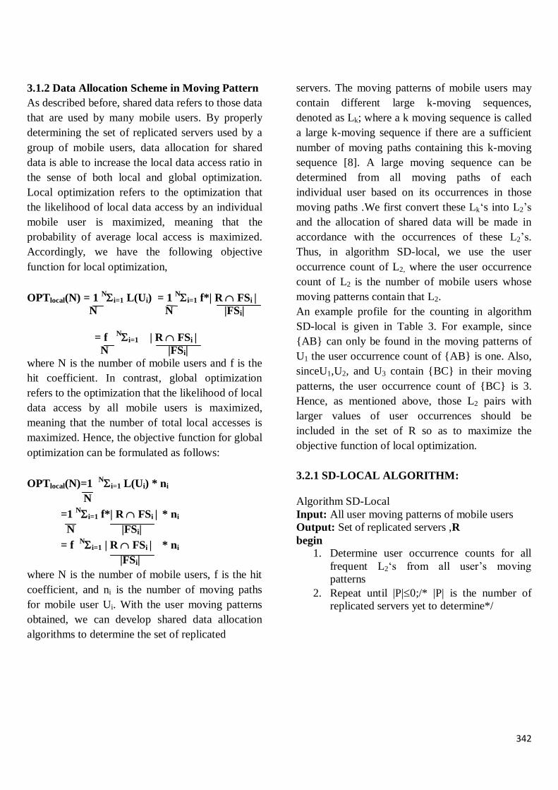
342
3.1.2 Data Allocation Scheme in Moving Pattern
As described before, shared data refers to those data
that are used by many mobile users. By properly
determining the set of replicated servers used by a
group of mobile users, data allocation for shared
data is able to increase the local data access ratio in
the sense of both local and global optimization.
Local optimization refers to the optimization that
the likelihood of local data access by an individual
mobile user is maximized, meaning that the
probability of average local access is maximized.
Accordingly, we have the following objective
function for local optimization,
OPTlocal(N) = 1 Ni=1 L(Ui) = 1
Ni=1 f*| R FSi |
N N |FSi|
= f Ni=1 | R FSi |
N |FSi|
where N is the number of mobile users and f is the
hit coefficient. In contrast, global optimization
refers to the optimization that the likelihood of local
data access by all mobile users is maximized,
meaning that the number of total local accesses is
maximized. Hence, the objective function for global
optimization can be formulated as follows:
OPTlocal(N)=1 Ni=1 L(Ui) * ni
N
=1 Ni=1 f*| R FSi | * ni
N |FSi|
= f Ni=1 | R FSi | * ni
|FSi|
where N is the number of mobile users, f is the hit
coefficient, and ni is the number of moving paths
for mobile user Ui. With the user moving patterns
obtained, we can develop shared data allocation
algorithms to determine the set of replicated
servers. The moving patterns of mobile users may
contain different large k-moving sequences,
denoted as Lk; where a k moving sequence is called
a large k-moving sequence if there are a sufficient
number of moving paths containing this k-moving
sequence [8]. A large moving sequence can be
determined from all moving paths of each
individual user based on its occurrences in those
moving paths .We first convert these Lk„s into L2‟s
and the allocation of shared data will be made in
accordance with the occurrences of these L2‟s.
Thus, in algorithm SD-local, we use the user
occurrence count of L2, where the user occurrence
count of L2 is the number of mobile users whose
moving patterns contain that L2.
An example profile for the counting in algorithm
SD-local is given in Table 3. For example, since
AB can only be found in the moving patterns of
U1 the user occurrence count of AB is one. Also,
sinceU1,U2, and U3 contain BC in their moving
patterns, the user occurrence count of BC is 3.
Hence, as mentioned above, those L2 pairs with
larger values of user occurrences should be
included in the set of R so as to maximize the
objective function of local optimization.
3.2.1 SD-LOCAL ALGORITHM:
Algorithm SD-Local
Input: All user moving patterns of mobile users
Output: Set of replicated servers ,R
begin
1. Determine user occurrence counts for all
frequent L2„s from all user‟s moving
patterns
2. Repeat until |P|0;/* |P| is the number of
replicated servers yet to determine*/
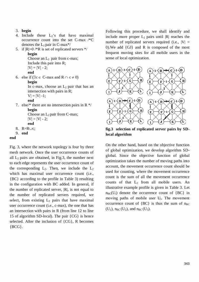
343
3. begin
4. Include those L2„s that have maximal
occurrence count into the set C-max /*C
denotes the L2 pair in C-max*/
5. if |R|=0 /*R is set of replicated servers */
begin
Choose an L2 pair from c-max;
Include this pair into R;
|V| = |V| - 2;
end
6. else if (c C-max and R c 0)
begin
In c-max, choose an L2 pair that has an
intersection with pairs in R;
V| = |V| -1;
end
7. else/* there are no intersection pairs in R */
begin
Choose an L2 pair from C-max;
|V| = |V| - 2;
end
8. R=Rc;
9. end
end
Fig. 3, where the network topology is four by three
mesh network. Once the user occurrence counts of
all L2 pairs are obtained, in Fig.3, the number next
to each edge represents the user occurrence count of
the corresponding L2. Then, we include the L2
which has maximal user occurrence count (i.e.,
BC according to the profile in Table 3) resulting
in the configuration with BC added. In general, if
the number of replicated server, |R|, is not equal to
the number of replicated servers required, we
select, from existing L2 pairs that have maximal
user occurrence count (i.e., c-max), the one that has
an intersection with pairs in R (from line 12 to line
15 of algorithm SD-local). The pair CG is hence
selected. After the inclusion of CG, R becomes
BCG.
Following this procedure, we shall identify and
include more proper L2 pairs until |R| reaches the
number of replicated servers required (i.e., |V| =
0).We add GJ and R is composed of the most
frequent moving sites for all mobile users in the
sense of local optimization.
fig.3 selection of replicated server pairs by SD-
local algorithm
On the other hand, based on the objective function
of global optimization, we develop algorithm SD-
global. Since the objective function of global
optimization takes the number of moving paths into
account, the movement occurrence count should be
used for counting, where the movement occurrence
count is the sum of all the movement occurrence
counts of that L2 from all mobile users. An
illustrative example profile is given in Table 3. Let
nBC(Ui) denote the occurrence count of BC in
moving paths of mobile user Ui. The movement
occurrence count of BC is thus the sum of nBC
(U1), nBC (U2), and nBC (U3).
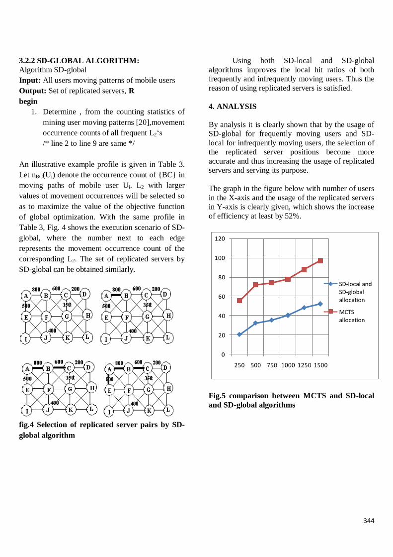
344
3.2.2 SD-GLOBAL ALGORITHM:
Algorithm SD-global
Input: All users moving patterns of mobile users
Output: Set of replicated servers, R
begin
1. Determine , from the counting statistics of
mining user moving patterns [20],movement
occurrence counts of all frequent L2„s
/* line 2 to line 9 are same */
An illustrative example profile is given in Table 3.
Let nBC(Ui) denote the occurrence count of BC in
moving paths of mobile user Ui. L2 with larger
values of movement occurrences will be selected so
as to maximize the value of the objective function
of global optimization. With the same profile in
Table 3, Fig. 4 shows the execution scenario of SD-
global, where the number next to each edge
represents the movement occurrence count of the
corresponding L2. The set of replicated servers by
SD-global can be obtained similarly.
fig.4 Selection of replicated server pairs by SD-
global algorithm
Using both SD-local and SD-global
algorithms improves the local hit ratios of both
frequently and infrequently moving users. Thus the
reason of using replicated servers is satisfied.
4. ANALYSIS
By analysis it is clearly shown that by the usage of
SD-global for frequently moving users and SD-
local for infrequently moving users, the selection of
the replicated server positions become more
accurate and thus increasing the usage of replicated
servers and serving its purpose.
The graph in the figure below with number of users
in the X-axis and the usage of the replicated servers
in Y-axis is clearly given, which shows the increase
of efficiency at least by 52%.
0
20
40
60
80
100
120
250 500 750 1000 1250 1500
SD-local and SD-global allocation
MCTS allocation
Fig.5 comparison between MCTS and SD-local
and SD-global algorithms

345
5. CONCLUSION
In this paper, we devised data allocation schemes
that utilize the knowledge of user moving patterns
for proper allocation of shared data in a mobile
computing system. Specifically, by exploring the
features of local optimization and global
optimization, we derived the objective functions of
local optimization and global optimization. With
the objective functions, we devised algorithm SD-
local and algorithm SD-global to achieve local
optimization and global optimization, respectively.
A measurement, called closeness measure which
corresponds to the amount of the intersection
between the set of frequently moving user patterns
and that of infrequently moving user patterns, was
derived to assess the quality of solutions resulted by
SD-local and SD-global. It was shown by our
analysis that the knowledge obtained from the user
moving patterns is very important in devising
effective shared data allocation algorithms which
can lead to prominent performance improvement in
a mobile computing system.
6. REFERENCES:
[1] J. Jing, A. Helal, and A. Elmagarmid, “Client-
Server Computing in Mobile Environments,” ACM
Computing Surveys, vol. 31, no. 2, pp. 117-157,
June 1999.
[2]N. Krishnakumar and R. Jain, “Escrow
Techniques for Mobile Sales and Inventory
Applications,” ACM J. Wireless Network, vol.
3,no. 3, pp. 235-246, July 1997.
[3]J. Jannink, D. Lam, N. Shivakumar, J. Widom,
and D. Cox,“Efficient and Flexible Location
Management Techniques for
Wireless Communication Systems,” ACM J.
Wireless Networks,vol. 3, no. 5, pp. 361-374, 1997.
[4]O. Wolfson, S. Jajodia, and Y. Huang, “An
Adaptive DataReplication Algorithm,” ACM Trans.
Database Systems, vol. 22,no. 4, pp. 255-314, June
1997.
[5]H.-K. Wu, M.-H. Jin, J.-T. Horng, and C.-Y. Ke,
“Personal Paging Area Design Based on Mobile‟s
Moving Behaviors,” Proc. IEEE Infocom 2001, pp.
21-30, Apr. 2001.
[6]N. Shivakumar, J. Jannink, and J. Widom, “Per-
User Profile Replication in Mobile Environments:
Algorithms, Analysis and Simulation Results,”
ACM J. Mobile Networks and Applications, vol. 2,
pp. 129-140, 1997.
[7]E. Pitoura and G. Samaras, “Locating Objects in
Mobile Computing,”IEEE Trans. Knowledge and
Data Eng., vol. 13, no. 4, pp. 571- 592, July/Aug.
2001.
[8]W.-C. Peng and M.-S. Chen, “Mining User
Moving Patterns for Personal Data Allocation in a
Mobile Computing System,” Proc. 29th Int‟l Conf.
Parallel Processing (ICPP 2000), Aug. 2000.
[9]M.H. Dunham, A. Helal, and S. Balakrishnan,
“A MobileTransaction Model That Captures Both
the Data and MovementBehavior,” ACM J. Mobile
Networks and Applications, vol. 2, pp. 149-
162,1997.
[10] EIA/TIA, Cellular Radio Telecomm.
Intersystem Operations,1991.
[11] T. Imielinski and B.R. Badrinath, “Mobile
Wireless Computing,”Comm. ACM, vol. 37, no.
10, pp. 18-28, Oct. 1994.
[12] Intelligent Transportation Systems,
http://www.artimis.org/,2004.
Proceedings of the Third National Conference on RTICT 2010
Bannari Amman Institute of Technology ,Sathyamangalam- 638401
9-10 April 2010
346
Greedy Resource Allocation Algorithm for OFDMA
Based Wireless Network Dhananjay Kumar P. Subramanian
Sr. Lecturer M. Tech. Student
Department of Information Technology, Anna University, Madras Institute of Technology Campus,
Chennai-600 044
[email protected], [email protected]
Abstract — A dynamic channel allocation algorithm for an
Orthogonal Frequency Division Multiple Access (OFDMA)
network is presented in this paper. The main objective is to
perform variable resource allocation based on channel gain and
channel state information. Base stations will know the channel
gain based on the feedback given by the mobile station. An
algorithm based on the greedy approach is used to allocate the
resources such as power, bit rate and sub channels. The sub-
carrier allocation algorithm (SAA) consists of two stages. The first
stage determines the number of subcarriers that a user needs and
the second stage deals with the assignment of the subcarriers to
satisfy their rate requirements. The SAA helps to utilize the
available spectrum efficiently. The snap shot of average
transmitted power and observed average Signal to Noise Ratio
(SNR) is presented to predict the system behaviour. Bit Error
Rate (BER) and the transmitting power is measured. The
simulation result shows that with an SNR of 12dB, the average
un-coded BER falls below 10-3
.
Keywords— Adaptive modulation, Resource allocation,
Multiuser channel, OFDM, SNR values
I. INTRODUCTION
The demands for high speed wireless networks are
increasing day by day. The higher throughput per bandwidth
to accommodate more users with higher data rates while
retaining a guaranteed quality of service becomes the main goal of system design. A dynamic multi user resource
allocation strategy is needed achieve this. This requirement is
explored here in the context of an OFDM based multiple
access technique called OFDMA. An OFDMA system is
defined as one in which each user is assigned a subset of the
subcarriers for use, and each carrier is assigned exclusively to
one user [1]. In OFDMA systems the power control and
bandwidth allocation for mobile station is still largely
unexplored that maximizes the system performance. The
OFDMA system performs well because instead of
transmitting over a single channel, users are allowed to choose best sub-channels as per the prevailing conditions [5]. An
adaptation in the frequency domain requires a large amount
of feedback, which makes the channel variation tracking
difficult in mobile applications. To reduce the feedback
overhead, it is often preferred to allow frequency diversity in
each subchannel (SCH) and then SCH wise link adaptation
is performed. In Code Division Multiplexing (CDM), data
symbols of same user are multiplexed and hence the
interference is reduced [2]. Higher data rates can be achieved
by higher levels of modulation techniques.But this may lead to
inter symbol interference(ISI) among the subchannels.This ISI can be mitigated easily by using multi user OFDM.In general
the subcarriers with high channel gain usually employ higher
levels of modulation to carry more bits per OFDM
symbol[3].While those sub carriers that are having low
channel gain are in deep fades and they may or may not carry
bits.The transmission power is distributed across all sub
channels to maximize the throughput..
In typical mobile communication scenario, different sub-carriers experience different channel gain, various data rates
and fade with respect to time and distance. At any instance all
the users may not see the channels that are in deep fade. The
static allocation for the OFDMA system is the simplest one in
which once the sub carriers are assigned to users, they remain
the same through out that session irrespective of their fading
characteristics. This motivates us to consider an adaptive
multiuser subcarrier allocation scheme where the subcarriers are assigned to the users based on instantaneous channel
information. This approach will allow all the subcarriers to be
used more effectively because a subcarrier will be left unused
only if it appears to be in deep fade to all users.
The objective of the proposed algorithm is to maximize the
sum data rate of the system by selecting the channel that
requires minimum transmitting power.Bit loading is done
based on the instantaneous fading characteristics of each sub
channel. An iterative algorithm based on the greedy approach
is used to allocate the subcarriers to multi users in the system. A base station will have some overhead while transmitting the
information about the allocated sub carriers and the number of
bits assigned to each carrier to the users via a dedicated
control channel in the downlink. But this overhead can be
slightly reduced if channel fading is slow and this information
is sent once every OFDM symbols.
The organisation of paper is as follows. In Section II, the
description of the system model and the problem formulation
of the minimum overall transmit power is presented. In
Section III, the bit and power allocation algorithm based on
the greedy approach is studied. The simulation result has been provided in Section IV, followed by conclusions in Section V.
II. SYSTEM MODEL
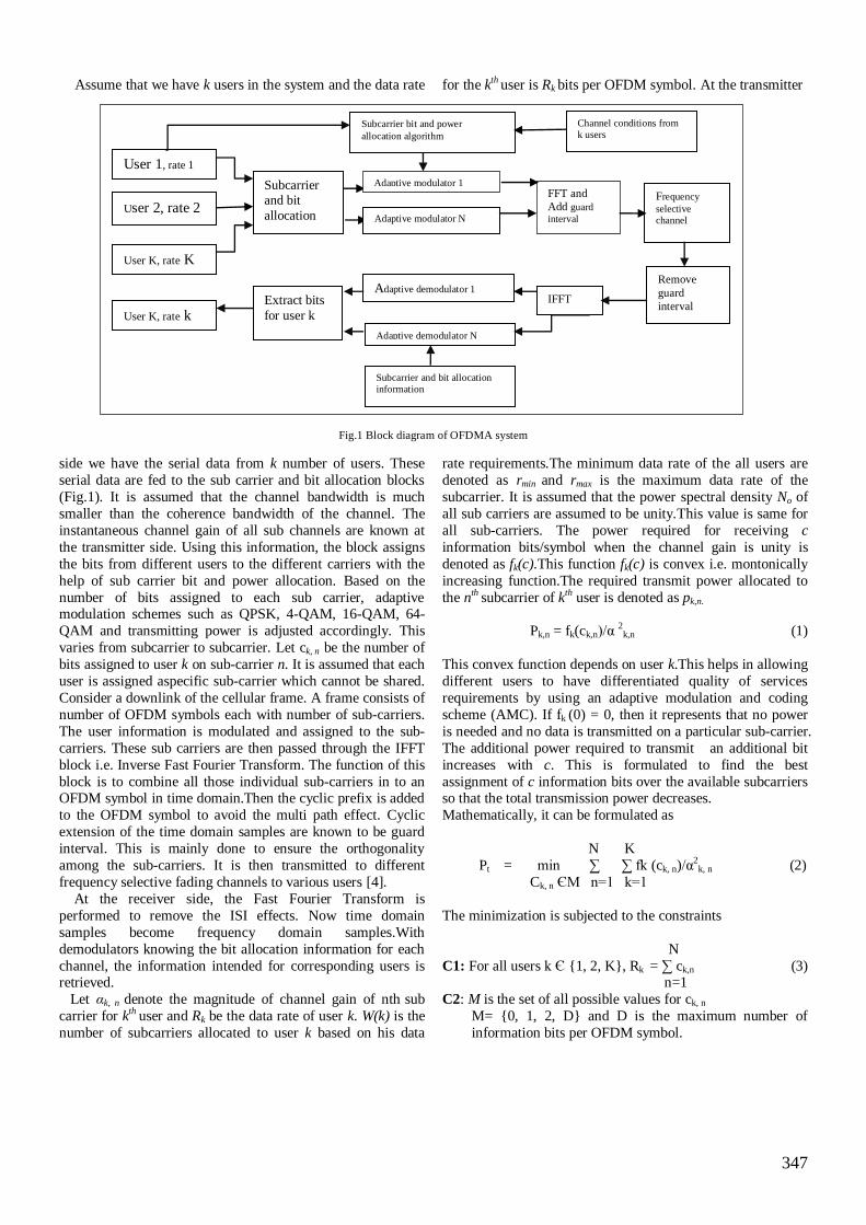
347
Assume that we have k users in the system and the data rate for the kth user is Rk bits per OFDM symbol. At the transmitter
Fig.1 Block diagram of OFDMA system
side we have the serial data from k number of users. These
serial data are fed to the sub carrier and bit allocation blocks
(Fig.1). It is assumed that the channel bandwidth is much
smaller than the coherence bandwidth of the channel. The
instantaneous channel gain of all sub channels are known at
the transmitter side. Using this information, the block assigns
the bits from different users to the different carriers with the
help of sub carrier bit and power allocation. Based on the
number of bits assigned to each sub carrier, adaptive modulation schemes such as QPSK, 4-QAM, 16-QAM, 64-
QAM and transmitting power is adjusted accordingly. This
varies from subcarrier to subcarrier. Let ck, n be the number of
bits assigned to user k on sub-carrier n. It is assumed that each
user is assigned aspecific sub-carrier which cannot be shared.
Consider a downlink of the cellular frame. A frame consists of
number of OFDM symbols each with number of sub-carriers.
The user information is modulated and assigned to the sub-
carriers. These sub carriers are then passed through the IFFT
block i.e. Inverse Fast Fourier Transform. The function of this
block is to combine all those individual sub-carriers in to an OFDM symbol in time domain.Then the cyclic prefix is added
to the OFDM symbol to avoid the multi path effect. Cyclic
extension of the time domain samples are known to be guard
interval. This is mainly done to ensure the orthogonality
among the sub-carriers. It is then transmitted to different
frequency selective fading channels to various users [4].
At the receiver side, the Fast Fourier Transform is
performed to remove the ISI effects. Now time domain
samples become frequency domain samples.With
demodulators knowing the bit allocation information for each
channel, the information intended for corresponding users is retrieved.
Let αk, n denote the magnitude of channel gain of nth sub
carrier for kth user and Rk be the data rate of user k. W(k) is the
number of subcarriers allocated to user k based on his data
rate requirements.The minimum data rate of the all users are
denoted as rmin and rmax is the maximum data rate of the
subcarrier. It is assumed that the power spectral density No of
all sub carriers are assumed to be unity.This value is same for
all sub-carriers. The power required for receiving c
information bits/symbol when the channel gain is unity is
denoted as fk(c).This function fk(c) is convex i.e. montonically
increasing function.The required transmit power allocated to
the nth subcarrier of kth user is denoted as pk,n.
Pk,n = fk(ck,n)/α 2k,n (1)
This convex function depends on user k.This helps in allowing
different users to have differentiated quality of services
requirements by using an adaptive modulation and coding
scheme (AMC). If fk (0) = 0, then it represents that no power
is needed and no data is transmitted on a particular sub-carrier.
The additional power required to transmit an additional bit
increases with c. This is formulated to find the best
assignment of c information bits over the available subcarriers so that the total transmission power decreases.
Mathematically, it can be formulated as
N K
Pt = min ∑ ∑ fk (ck, n)/α2
k, n (2)
Ck, n ЄM n=1 k=1
The minimization is subjected to the constraints
N
C1: For all users k Є 1, 2, K, Rk = ∑ ck,n (3) n=1
C2: M is the set of all possible values for ck, n
M= 0, 1, 2, D and D is the maximum number of
information bits per OFDM symbol.
Adaptive demodulator N
User 1, rate 1
User 2, rate 2
User K, rate K
User K, rate k
Subcarrier and bit
allocation
Extract bits
for user k
Subcarrier bit and power
allocation algorithm
Adaptive modulator 1
Adaptive modulator N
Adaptive demodulator 1 IFFT
FFT and
Add guard
interval
Frequency
selective
channel
Remove
guard
interval
Subcarrier and bit allocation
information
Channel conditions from
k users

348
C3: W (k) = rmin/rmax, for all users. (4)
C4: Rk ≥ rmin, for all users.
C5: ∑w (k) ≤ N, for all users
III GREEDY ALGORITHM
Initially the problem of resource allocation is divided in to
two stages.
A) Subcarrier Estimation: In this stage we find out the
number of subcarrier that each user needs based on their data rate requirements.
B) Bit Allocation: Based on the channel state
information of all subcarriers, the subcarriers are
allocated to the users.
A) Subcarrier Estimation
The number of subcarrier that each user needs is
determined by using (4).
W (k) = rmin / rmax
The SNR of all the sub-carriers at any instance will not be
same. Hence in a wireless environment some users will have very less SNR values compared to other users. As per LR
algorithm once users have sufficient subcarriers to satisfy their
minimum rate requirements, giving more subcarriers to users
with lower average SNR helps to reduce the total transmission
power.In this way the fairness among the users can be
maintained.
B) Bit Allocation Algorithm
The SAA as shown in Fig.2 assigns bits to the subcarriers
one bit at a time and in each assignment the subcarrier that
requires least transmission is selected. The selected greedy approach is optimal because the power needed to transmit
certain number of bits in a subcarrier is independent of the
number of bits allocated to other subcarriers.
Initialization:
Cn = 0 for all n and ∆pn= [f (1)-f (0)]/α2n;
For each user k:
Repeat the following until all the bits are assigned.
Step1: Select the subchannel that requires the least
transmission power.
n = arg Minn ∆pn;
Cn, k = Cn, k +1;
Step2: Increase the data rate of the selected subchannel and power proportionally based on the values in table 1 given
below.
Step3: After assignment of the bits, calculate the power
needed for assigniing each additional bit.
∆pn= [f (Cn, k +1)-f (Cn, k)]/ α2n
Step4: Repeat the same procedure for selecting the other
subcarriers until data rate requirements of the user is satisfied.
The Table I provide information about data rates of the
various modulation schemes being used. If the channel gain
of any particular subcarrier is very less then a lower order
modulation will be employed. For those that are having good
channel gain, data rates are increased.
TABLE I
ADAPTIVE MODULATION SCHEMES
S. No Data rate in bps
Modulation Schemes
1 1 BPSK
2 2 QPSK
3 4 4-QAM
4 6 16-QAM
Fig.2 Flow chart of the subcarrier allocation algorithm
IV.SIMULATIONS
The main system parameter under consideration is listed in
Table II. The channel model is based on the Rayleigh fading
model with Rician absolute value. The system is simulated
using Matlab version 7.8.0. The single-sided power spectral
density level is taken to unity. The average required transmit

349
power (Fig.3) in defined here is the ratio of the overall
transmit energy per OFDM symbol including all subcarriers
and all users to the total number of bits transmitted per OFDM
symbol. The average SNR is computed as the ratio of average
transmit power to the noise power spectral density level No.
The overall transmit power is proportional to the average SNR
(Fig.4). TABLE III
SYSTEM PARAMETERS
No. of users
1 - 5
Bandwidth 4 MHz
No. of sub-carriers
128
Modulation BPSK, QPSK, 16,64-QAM
Convolution codes Rate
½, 2/3, 3/4
1 2 3 4 50
5
10
15
20
25
Number of users
Tra
nsm
itte
d P
ow
er
in d
b
Fig.3 Transmitted power in db versus Number of users
1 2 3 4 50
5
10
15
20
25
Number of users
SN
R in d
b
Fig.4 SNR in db versus Number of users
It is also observed during simulation that the transmitting
power requirement for each user depends on their data rate
requirements. In other words the SNR requirement is dictated
by the band width requirement of the mobile user. The BER
depends on the SNR and the order of modulation (M) used in
M-QAM. The average BER plot in Fig.5 corresponds to an
un-coded channel.
10 12 14 16 18 20 22 2410
-6
10-5
10-4
10-3
10-2
10-1
100
Average signal to noise ratio
Avera
ge B
it E
rror
Rate
Fig.5 Average BER versus Average SNR
V CONCLUSIONS
The dynamic resource allocation in OFDMA allows
efficient use of system resources in terms of power and
bandwidth. The feasibility of the algorithm is influenced by
the factors such as the channel variation, and the accuracy and
overhead of the channel estimation.The transmission power and bit error rate observed here represents a practical OFDMA
systems.
ACKNOWLEDGMENT
We wish to express our sincere thanks to the Department of
Information Technology, Anna University, MIT Campus,
Chennai for providing the required hardware and software
tools to carry out simulation.
REFERENCES
[1] Kwang soon kimVariable, Yuu hee Kim, ―Power and Rate Allocation
using simple CQI for Multiuser OFDMA-CDM systems,‖IEEE
Trans.Wireless Comm, Vol.8, no.6, june2009.
[2] E. S. Lo, P. W. C. Chan, V. K. N. Lau, R. S. Cheng, K. B. Letaief, R. D.
Murch, and W. H. Mow, “Adaptive resource allocation and capacity com-
parison of downlink multiuser MIMO-MC-CDMA and MIMO-OFDMA,"
IEEE Trans. Wireless Common., vol. 6, no. 3, pp. 1083-1093, Mar. 2007.
[3] K. S. Kim, Y. H. Kim, and J. Y. Ann, “An efficient adaptive transmission technique for LDPC coded OFDM cellular systems using multiple antennas," IEE Electron. Let. vol. 40, no. 6, pp. 396-397, Mar. 2004.
[4] D. Ivan, G. Li, and H. Liu, “Computationally efficient bandwidth
allocation and power control for OFDMA," IEEE Trans. Wireless Common., vol. 2, no. 6, pp. 1150-1158, Oct. 2003.
[5] D. Test and P. Viswanath, Fundamentals of Wireless Communication.
New York: Cambridge University Press, 2005.

Proceedings of the Third National Conference on RTICT 2010
Bannari Amman Institute of Technology ,Sathyamangalam- 638401
9-10 April 2010
351
Optimal power path routing in wireless sensor
networks Sathiyapriyen.V.B
#1, Shrilekha.M
# 2
#Electronics and Communication Engineering Department, Easwari Engineering College
Ramapuram, Chennai- 600089, India
Abstract—this paper aims to design an optimal power path routing
protocol for IEEE802.15.4 based LRWPAN. IEEE802.15.4 LR-
WPAN has a challenge that power consumption has to be reduced to
maximize the lifetime. The current strategy being used is variable
range transmission power control. Here the coordinator is made to
radiate power depending on the distance and other several
parameters between itself and the end devices and the concepts have
been applied to only data packets. This idea is further stretched to
include the low power route paths also. We will initially simulate the
scenario by incorporating the changes specified, using Network
Simulator 2 (NS2) and then implement it using real time wireless
sensors and compare the results of the original with the modified
analysis
Keywords— wireless sensor networks, AODV, Ns2
1. INTRODUCTION
Wireless Sensor Network (WSN) is an interconnection
of spatially distributed autonomous devices that are used to
monitor a particular physical or environmental condition. It is a
well known fact that in WSN the major constraint is energy
conservation and battery-power consumption, since the sensor is
required to operate under remote conditions without fresh supply
of power to replenish themselves. This paper aims to design a routing protocol at network layer with optimal power as a
primary routing metric.
WSN falls under the category of Low Range Wireless
Personal Area Network (LR-WPAN). The nodes consist of
sensors, a radio transceiver, battery and an embedded processor.
The main applications of sensor networks include industrial
control, asset tracking and supply chain management,
environmental sensing, health monitoring and traffic control.
WSN is different from traditional ad hoc networks in certain
aspects such as being highly energy efficient, having low traffic
rate, low mobility and predefined traffic patterns [1]. Energy conservation is a critical factor for the design of these networks.
Energy conservation involves optimizing protocols at various
layers of the protocol stack. Optimal placement of nodes in
sensor field also contributes to energy conservation but typically
the philosophy in WSN is to have a large number of cheap nodes
which could fail and thus resilience in the distributed protocols is
preferred over strategies such as an optimal placement of nodes.
The major constraint in WSN is energy conservation since the
sensor is required to operate under remote conditions without
fresh supply of power to replenish itself.
2. WSN ARCHITECHTURE
A WSN device can be configured as one of the three types of
nodes namely, a coordinator (PANCOORD), a router (RTR) or
an end device (ED). The end device will sense the environmental
conditions and will communicate the data to the co-ordinator.
The router in addition to its normal routing operations can also
act as an end device. The co-ordinator will collect the data from
end devices and router and process them accordingly. A LR-
WPAN normally consists of one coordinator, several routers and
many end devices. All the nodes operate at a given transmit power irrespective of their location.[2] Some of the
characteristics are Sensors are of :
• Low cost
• Low processing capability System strength based on sensor collaboration
• Large scale networks Multihop communication
• Sensors are battery operated for long unattended period: Saving energy is a primary objective
Some of the applications of WSN are
Remote area monitoring
Object location
Industry machinery monitoring
Disaster prevention
Wireless medical systems
2.1 ENERGY CONSERVATION IN WSN
According to IEEE standard 802.15.4 MAC protocol
[3], energy conservation is accomplished through idle modes and
sleep modes in a sensor node. The node switches between active
and sleep states based on the operations. During sleep states, all
the blocks of the sensor mode are switched off, saving
considerable power. The node wakes up at the time when it wants to transmit or when it expects information from the coordinator.
352
The extent of sleep periods and active periods depends on the
configuration of the network, namely, beacon-enabled mode and
non-beacon-enabled mode.
Although this saves power considerably, there is a
possibility of control over transmit power which can further bring
down the energy spent on transmissions.
3. AODV ROUTING PROTOCOL
AODV [4] is an on-demand routing protocol, only when
the source has data to send, a short route request (RREQ)
message will be initiated and broadcast by the source, with an estimated and pre-defined lifetime (TTL). This RREQ is
rebroadcast until the TTL reaches zero or a valid route is
detected. The nodes receiving the RREQ will add a valid route
entry to its routing table to reach the RREQ source, called reverse
route formation. When the RREQ reaches the destination or a
node that has a valid route to the destination, a route reply
(RREP) message is uni-cast by this node to the source. If one
round of route discovery fails (the RREQ TTL decreases to zero),
the source will re-initiate a new RREQ with a larger initial TTL
after time-out. If several rounds of route request all fail, it means
no valid route can be found. The RREP message will go to the source, following the reverse route formed by the RREQ. For
every hop the RREP is forwarded, intermediate nodes will add a
valid route pointing to the destination, called forward route
formation, until the RREP reaches the source. If the RREP is
generated by an intermediate node that already has a valid route
to the destination, a special message called gratuitous route reply
(G-RREP) is uni-cast to the destination, notifying it that the
source has route request and then a bi-directional route is formed.
By then, both the data source and destination have routes to each
other, and all the intermediate nodes have routes to the source
and destination. In the original AODV, source node will choose
the shortest path if there are multi-routes discovered (with several route replies).
3.1 ROUTE MAINTANANCE IN AODV
Hello messages in AODV are used in the route
maintenance part of the AODV protocol. Hello messages are enabled so that every node knows entire details about its
neighboring nodes. When a node receives a hello message from
its neighbor, it creates or refreshes the neighbor table entry to the
neighbor. Hello message is not enabled by default. You need to
comment the following 2 lines in aodv.h file
#defineAODV_LINK_LAYER_DETECTION
#define AODV_USE_LL_METRIC
hello hello hello
hello hello hello hello hello
Fig 1 Hello messages
3.2 POWER CALCULATION AND UPDATING NEIGHBOUR TABLE
Power calculation is done using Distance and LQI values.
Distance and LQI are split up into five regions: Low, Medium
and High. Transmitting power values are decided using the nine
combinations. LQI is inversely proportional to power. Distance is
directly proportional to power
Only neighbor address and expiry time are available in
the neighbor table initially. Program is altered to include power
values in the neighbor table. After this alteration, when a node
refreshes the neighbor table while receiving a hello message,
power values also get refreshed along with it.
4. ANALYSIS OF WSN UNDER CONTROLLED CONDITIONS
The required transmit power levels are obtained by
observing the parameters under consideration for an ideal
network scenario. The simulation environment is created with the
parameters as given in Table 1.
Table 1: Parameters used to create Simulation Environment
Sl. No. Parameters Values
Fixed Parameters
1 Frequency of
operation
914 MHz
2 Receiver
Threshold
-82 dBm
3 Carrier Sense
Threshold
-92 dBm
4 MAC Protocol IEEE 802.15.4
5 Network
Routing Protocol
AODV
6 Traffic CBR 512
bytes/pkt
7 Simulation
Time
200 seconds
Variable Parameters
1 No. of nodes 2 / 4 / 6 / 25
(Four scenarios)
2 Mobility Induced Mobility in
selected nodes
3 Transmit Power Varied from 0.2
W to 0.2818W
4 Propagation
Model
Two Ray
Ground
Reflection /
Free space
In order to minimise transmit power, we propose a
protocol to be implemented in devices that follow the IEEE
802.15.4 standard such that the transmit power varies with
respect to LQI, distance in between the communicating nodes and
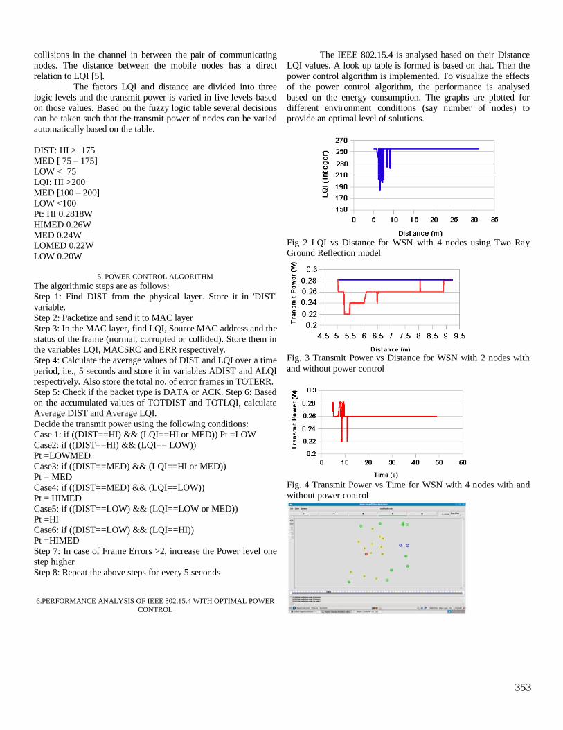
353
collisions in the channel in between the pair of communicating
nodes. The distance between the mobile nodes has a direct
relation to LQI [5].
The factors LQI and distance are divided into three
logic levels and the transmit power is varied in five levels based
on those values. Based on the fuzzy logic table several decisions can be taken such that the transmit power of nodes can be varied
automatically based on the table.
DIST: HI > 175
MED [ 75 – 175]
LOW < 75
LQI: HI >200
MED [100 – 200]
LOW <100
Pt: HI 0.2818W
HIMED 0.26W
MED 0.24W LOMED 0.22W
LOW 0.20W
5. POWER CONTROL ALGORITHM
The algorithmic steps are as follows:
Step 1: Find DIST from the physical layer. Store it in 'DIST'
variable.
Step 2: Packetize and send it to MAC layer
Step 3: In the MAC layer, find LQI, Source MAC address and the
status of the frame (normal, corrupted or collided). Store them in
the variables LQI, MACSRC and ERR respectively.
Step 4: Calculate the average values of DIST and LQI over a time
period, i.e., 5 seconds and store it in variables ADIST and ALQI
respectively. Also store the total no. of error frames in TOTERR.
Step 5: Check if the packet type is DATA or ACK. Step 6: Based
on the accumulated values of TOTDIST and TOTLQI, calculate Average DIST and Average LQI.
Decide the transmit power using the following conditions:
Case 1: if ((DIST==HI) && (LQI==HI or MED)) Pt =LOW
Case2: if ((DIST==HI) && (LQI== LOW))
Pt =LOWMED
Case3: if ((DIST==MED) && (LQI==HI or MED))
Pt = MED
Case4: if ((DIST==MED) && (LQI==LOW))
Pt = HIMED
Case5: if ((DIST==LOW) && (LQI==LOW or MED))
Pt =HI Case6: if ((DIST==LOW) && (LQI==HI))
Pt =HIMED
Step 7: In case of Frame Errors >2, increase the Power level one
step higher
Step 8: Repeat the above steps for every 5 seconds
6.PERFORMANCE ANALYSIS OF IEEE 802.15.4 WITH OPTIMAL POWER
CONTROL
The IEEE 802.15.4 is analysed based on their Distance
LQI values. A look up table is formed is based on that. Then the
power control algorithm is implemented. To visualize the effects
of the power control algorithm, the performance is analysed
based on the energy consumption. The graphs are plotted for
different environment conditions (say number of nodes) to provide an optimal level of solutions.
Fig 2 LQI vs Distance for WSN with 4 nodes using Two Ray Ground Reflection model
Fig. 3 Transmit Power vs Distance for WSN with 2 nodes with
and without power control
Fig. 4 Transmit Power vs Time for WSN with 4 nodes with and
without power control

354
Fig. 5 NAM screenshot of WSN with 25 nodes
The analysis done are collected as a group and then formatted as
a tabular column containing power conserved by implementing
the algorithm and the energy conservation done. The tabular column is given for 2nodes, 4nodes, 6nodes and 25nodes with
two ray model as propagation model. The tabular column is given
as follows:
Table 2: Energy consumption for different number of nodes
Condition Energy consumed(mJ)
2nodes two ray model 36.89(without power
control)
34.036(with power control)
4nodes two ray model 35.23(without power
control)
34.23(with power
control)
6nodes two ray model 37.23(without power
control)
34.394(with power
control)
25 nodes two ray
model
43.23(without power
control)
42.62(with power
control)
Using the table 2 a graph is plotted for number of nodes vs
energy consumed. The line in red color indicates the plot without
power control and the line in green indicates the plot with power
control.
Thus from the graph it can be clearly viewed that the energy has
been successfully conserved thereby increasing the life time of
the sensors used.
7. CONCLUSION
Energy efficient protocol design is the need of the hour
because of increasing dependence on independent systems that
could operate without utilizing much power. Through this paper
we plan to upgrade the existing technique with optimal usage of
power. This technique is being worked out currently in Network
Simulator 2 (NS 2).
8.REFERENCES
[1] Holger Karl and Andreas Willig, ―Protocols and
Architectures for Wireless Sensor Networks‖, First Edition,
Wiley and sons, 2007 .
[2] Energy Efficient Medium Access Control for Wireless Sensor
Networks, Sabitha Ramakrishnan,
T.Thyagarajan, IJCSNS International Journal of Computer
Science and Network Security, VOL.9 No.6, June 2009.
[3] IEEE 802.15.4a: Wireless Medium Access Control (MAC)
and Physical Layer (PHY) Specifications for Low-Rate Wireless
Personal Area Networks (WPANs), Internet draft.
[4] Energy-Aware Algorithms for AODV in Ad Hoc Networks, Xiangpeng Jing and Myung J. Lee
[5] Variable-Range Transmission power control in Wireless Ad
Hoc Networks, IEEE transactions on mobile computing, vol 6,
no.1, January 2007
[6]Energy efficient traffic scheduling in IEEE 802.15.4 for home
automation networks, IEEE Transactions on consumer
electronics, Volume 53, No.2, May 2007.
[7] Variable-Range Transmission Power Control in Wireless Ad
Hoc Networks, IEEE transactions on mobile computing, vol. 6,
no. 1, January 2007
[8] Power Saving Algorithms for Wireless Sensor Networks on IEEE 802.15.4, IEEE Communications Magazine, June 2008.

Proceedings of the Third National Conference on RTICT 2010
Bannari Amman Institute of Technology ,Sathyamangalam- 638401
9-10 April 2010
355
Analysis of Propagation Models used in
Wireless Communication System Design K.PHANI SRINIVAS Asst Professor KL University
Email: [email protected] Cell: 9849462633
ABSTRACT---The communication path between the transmitter
and the receiver in wireless communication can vary from simple
line of sight (LOS) to one that is rigorously obstructed by buildings,
mountains and shrubbery. Unlike wired channel that are
motionless and predictable, radio channels are extremely random
and do not offer simple analysis. Even the speed of motion impacts
how rapidly the signal level fades as a mobile terminal moving in
space. The radio propagation model has previously been one of the
most complex parts of mobile system design, and is usually done in
a statistical fashion, based on measurements made specifically for
an intended communication system or spectrum allocation. Various
propagation models exist in the open literature. These models are
basically divided into two distinct classes namely physical and
analytical models. Physical models focus on the location of
transmitter and receiver without taking the antenna design into
account. Analytical models capture physical wave propagation and
antenna configuration simultaneously by describing the transfer
function between the antenna arrays at both link ends. This paper
deals with various propagation models and studies their application
to wireless communications system design. The advantages and
disadvantages of each model are given where applicable. Keywords— Quality of service (QoS),Radio frequency(RF), .
Multiple Input Multiple Output (MIMO), Angle of Arrival (AOA),
Angle of Departure (AOD),Line of sight(LOS),Multiple path
components(MPCs)
I. INTRODUCTION Wireless communications is, by any measure, the fastest
growing segment of the communications Industry. As such, it
has captured the attention of the media and the imagination of
the public. Cellular phones have experienced exponential
growth over the last decade, and this growth continues unabated
worldwide, with more than a billion worldwide cell phone users
projected in the near future. Indeed, cellular phones have
become a critical business tool and part of everyday life in most
developed countries, and are rapidly supplanting antiquated wire
line systems in many developing countries. This development is
being driven primarily by the transformation of what has been
largely a medium for supporting voice telephony into a medium for supporting other services, such as the transmission of video,
images, text, and data. Many new applications, including
wireless sensor networks, automated highways and factories,
smart homes and appliances, and remote telemedicine, are
emerging from research ideas to concrete systems. The
explosive growth of wireless systems coupled with the
proliferation of laptop and palmtop computers indicate a bright future for wireless networks, both as stand-alone systems and as
part of the larger networking infrastructure. Thus, similar to the
developments in wire line capacity in the 1990s, the demand for
new wireless capacity is growing at a very rapid pace. Although
there are, of course, still a great many technical problems to be
solved in wire line communications, demands for additional
wire line capacity can be fulfilled largely with the addition of
new private infrastructure, such as additional optical fiber,
routers, switches, and so on. On the other hand, the traditional
resources that have been used to add capacity to wireless
systems are radio bandwidth and transmitter power.
Unfortunately, these two resources are among the most severely limited in the deployment of modern wireless networks: radio
bandwidth because of the very tight situation with regard to
useful radio spectrum, and transmitter power because mobile
and other portable services require the use of battery power,
which is limited. These two resources are simply not growing or
improving at rates that can support anticipated demands for
wireless capacity. many technical challenges remain in
designing robust wireless networks that deliver the performance
necessary to support emerging applications. On the other hand,
one resource that is growing at a very rapid rate is that of
processing power. The term "wireless" has become a generic and all-encompassing word used to describe communications in
which electromagnetic waves or RF (rather than some form of
wire) carries a signal over part or the entire communication path
Like in Fig 1. Wireless operations permits services, such as long
range communications, that are impossible or impractical to
implement with the use of wires. The term is commonly used in
the telecommunications industry to refer to telecommunications
systems (e.g. radio transmitters and receivers, remote controls,
computer networks, network terminals, etc.) which use some
form of energy to transfer information without the use of wires.
Information is transferred in this manner over both short and
long distances. Electromagnetic waves propagate through
356
environments where they are reflected, scattered, and diffracted
by walls, terrain, buildings, and other objects. The ultimate
details of this propagation can be obtained by solving Maxwell’s
equations with boundary conditions that express the physical
Figure 1.Basic wireless communication system
characteristics of these obstructing objects. The two most
important requirements for a modern day wireless
communication system are to support high data rates within the
limited available bandwidth and to offer the maximum
reliability. Multiple Input Multiple Output (MIMO) technology,
which exploits the spatial dimension, has shown potential in
providing enormous capacity gains and improvements in the
quality of service (QoS) [1-5]. in any communication system,
the capacity is dependent on the propagation channel conditions, which in turn are dependent on the environment. Propagation
Modeling is an area of active research and several models have
been developed to predict, simulate and design a high
performance communication system. Propagation models can be
classified into two broad categories, namely physical models
and analytical models as shown in Table 1. Site specific physical
models help in network deployment and planning, while site
independent models are mostly used for system design and
testing. The physical models may be further classified into
deterministic and stochastic models. Deterministic models
characterize the physical propagation parameters in a completely deterministic manner (examples are ray tracing and
stored measurement data). With geometry-based stochastic
propagation models (GSPM), the impulse response is
characterized by the laws of wave propagation applied to
specific Tx, Rx, and scattered geometries, which are chosen in a
stochastic (random) manner. A deterministic model tries to
reproduce / repeat the actual physical radio propagation process
for a given environment along with the reflection, diffraction,
shadowing by discrete obstacles, and the wave guiding in street
canyons. Recorded impulse response and ray tracing
techniques are some of the examples of deterministic
channel modeling techniques. The stochastic models are
based on the fact that the wireless propagation channels are
unpredictable and time varying in nature but its parameters, like
the Angle of Arrival (AOA), Angle of Departure (AOD), time
delay profiles etc., follow a defined stochastic/ statistical
behavior, depending on the environment. The stochastic channel
models are generally computationally efficient. Most stochastic
models have a geometrical basis; In the realm of geometrically
based stochastic models, large variants of the model have been
proposed, but the basic philosophy remains the same. Different
geometrically based stochastic models reproduce different sets of environments like indoor or outdoor scenarios, and narrow
band or wide band environments. Usually, the models are
validated by comparing the values or distributions of certain
physical parameters like AOA, AOD, Time of arrival (TOA),
and power spectrum etc., obtained through the model with those
acquired through measurements under specific conditions. In
contrast, non-geometric stochastic models describe and
determine physical parameters (the direction of departure
(DoD), and the direction of arrival (DoA) delay, etc.) in a
completely stochastic way by prescribing underlying probability
distribution functions without assuming an underlying geometry
(examples are the extensions of the Saleh-Valenzuela model, Zwick model [14], [15]).
Table 1.
Physical models: Analtical models 1. Deterministic : -Ray tracing -Stored measurements
2. Geometry –based Stochastic: -GSPM 3 .Non-Geometrical Stochastic: -Saleh-Valenzula type -Zwick model
1.Correlation-based: - canonical model
-Kronecker model -weichselberger Model 2. Propagation -motivated: -Finite scatterer
model -Maximum entropy model -Virtual channel representation
II. PHYSICAL MODELS
A. Deterministic Physical Models
Physical propagation models are termed “deterministic” if they
plan to reproduce the actual physical radio propagation process
for a given atmosphere. The deterministic channel modeling
techniques try to repeat the actual physical scenario between the
transmit and the receive arrays. In urban environments, the
geometric and electromagnetic characteristics of the
environment and of the radio link can be easily stored in files (environment databases) and the corresponding propagation
process can be simulated through computer programs. Most
often, the antenna parameters like the antenna patterns, array
size and geometry, the effects of mutual coupling between the
array elements, polarization etc. are not accounted for [6].
Although electromagnetic models such as the method of
moments (MoM) or the finite-difference in time domain

357
(FDTD) model may be useful to study near field problems in the
vicinity of the Transmitter or Receiver antennas.
Ray tracing softwares and techniques are one of the most
accepted ways for modeling the channel deterministically. In ray
tracing software’s, the geometry and the electromagnetic
characteristics of any particular situation/ environment is stored in files. The ray tracing Software’s are basically based on the
phenomenon of geometrical optics like reflection, refraction,
diffraction etc. These files are later used for simulating the
electromagnetic propagation process between the transmitter
and the receiver. These models are fairly accurate and may be
used in place of measurement campaigns, when time is at
premium. In ray tracing techniques, flat top polygons of
different sizes and shapes are generally used to represent
buildings as shown in fig.2 Geometrical optics is based on the
so-called ray approximation, which assumes that the wavelength
is sufficiently small compared to the dimensions of the obstacles
in the environment. This assumption is usually valid in urban radio propagation and allows to express the electromagnetic
field in terms of a set of rays, each one of them corresponding to
a piece-wise linear path connecting two terminals. Each
“corner” in a path corresponds to an “interaction” with an
obstacle (e.g. wall reflection, edge diffraction). Rays have a null
transverse dimension and therefore can in principle describe the
field with infinite resolution. If beams with a finite transverse
dimension are used instead of rays, then the resulting model is
called beam launching, or ray splitting. Beam launching models
allow faster field strength prediction but are less accurate in
characterizing the radio channel between two SISO or MIMO terminals.
Fig. 2 propagation scenario (Rectangular blocks shows buildings) B. Geometry-Based Stochastic Physical Models
Any geometry-based model is resolute by the scatterer locations.
In deterministic geometrical approaches (like RT discussed in
the previous subsection), the scatterer locations are prescribed in
a database. In contrast, geometry-based stochastic propagation
models (GSPM) choose the scatterer locations in a random style
according to a certain probability distribution. The actual
channel impulse response is then found by a simplified RT
procedure. 1).Single-Bounce Scattering The antecedent of the GSPM in [7] placed scatterers in a
deterministic mode on a circle around the mobile station, and
assumed that only single scattering occurs. approximately
twenty years later, several groups simultaneously suggested to
augment this single-scattering model by using randomly placed
scatterers [10], [11], [12], This random assignment reflects
physical reality much better. The single-scattering assumption
makes RT extremely simple: apart of the LoS, all paths consist
of two sub paths connecting the scatterer to the Tx and Rx,
respectively. [13], [14], [15]. These sub paths characterize the
DoD, DoA, and propagation time (which in turn determines the overall attenuation, usually according to a power law). The
scatterer interaction itself can be taken into account via an
additional random phase shift. Different types of the GSPM differ mainly in the proposed
scatterer distributions. The simplest GSPM is obtained by
assuming that the scatterers are spatially uniformly distributed.
Contributions from far scatterers carry less power since they
propagate over longer distances and are thus attenuated more
strongly; this model is also often called single-bounce
geometrical model. An alternative approach suggests to place
the scatterers randomly around the MS [12], [14]. Various other scatterer distributions around the MS were analyzed; a one-sided
Gaussian distribution w.r.t. distance from the MS resulted in an
approximately exponential PDP, which is in good agreement
with many measurement results[16]. To make the density or
strength of the scatterers depend on distance, two
implementations are possible. In the ”classical” approach, the
probability density function of the scatterers is adjusted such
that scatterers occur less likely at large distances from the MS.
Alternatively, the“non-uniform scattering cross section” method
places scatterers with uniform density in the considered area, but
down-weights their contributions with increasing distance from
the MS [17]. For very high scatterer density, the two approaches are equivalent. However, non-uniform scattering cross section
can have numerical advantages, in particular less statistical
fluctuations of the power-delay profile when the number of
scatterers is finite. Another important propagation effect arises
from the existence of clusters of far scatterers (e.g. large
buildings, mountains . . .). Far scatterers lead to increased
temporal and angular dispersion and can thus significantly
influence the performance of MIMO systems. In a GSPM, they
can be accounted for by placing clusters of far scatterers at
random locations in the cell.
2) Multiple-Bounce Scattering
358
The single bounce scattering based on the theory that only
single-bounce scattering is present. This is limiting insofar as
the position of a scatterer completely determines DoD, DoA,
and delay, i.e., only two of these parameters can be chosen
independently. However, many environments (e.g., micro- and
Pico cells) feature .multiple-bounce scattering for which DoD, DoA, and delay are completely decoupled. In microcells, the BS
is below rooftop height, so that propagation mostly consists of
wave guiding through street canyons, which involves multiple
reflections and diffractions (this effect can be significant even in
macro cells[18,19]For Pico cells, propagation within a single
large room is mainly determined by LoS propagation and single-
bounce reflections. However, if the Tx and Rx are in different
rooms, then the radio waves either propagate through the walls
or they leave the Tx room e.g. through a window or door, are
waveguide through a corridor, and be diffracted into the room
with the Rx [20]. If the directional channel properties need to be
reproduced only for one link end (i.e., multiple antennas only at the Tx or Rx), multiple-bounce scattering can be incorporated
into a GSPM via the concept of equivalent scatterers. These are
virtual single-bounce scatterers whose position is chosen such
that they mimic multiple bounce contributions in terms of their
delay and DoA. This is always possible since the delay,
azimuth, and elevation of a single-bounce scatterer are in one-
to-one correspondence with its Cartesian coordinates.
C. Non-geometrical Stochastic Physical Models Non-geometrical stochastic(random) models tell paths from Tx
to Rx by statistical parameters only, without indication to the geometry of a physical surroundings. There are two classes of
stochastic non-geometrical models reported in the literature. The
first one uses clusters of MPCs and is generally called the
extended Saleh-Valenzuela model since it generalizes the
temporal cluster model developed in [21]. The second one
Zwick model, treats MPCs individually.[22]
1) Saleh-Valenzuela Model:
Saleh and Valenzuela projected to model clusters of MPCs in
the delay domain via a doubly exponential decay process . The
Saleh-Valenzuela model uses one exponentially decaying
profile to control the power of a multipath cluster.[21] The MPCs within the individual clusters are then characterized by a
second exponential profile with a steeper slope.The Saleh-
Valenzuela model has been extended to the spatial domain in
[23]. In particular, the extended Saleh-Valenzuela MIMO
model in is based on the assumptions that the DoD and DoA
statistics are self-sufficient and identical. Usually, the mean
cluster angle is assume to be uniformly distributed within
0,2 and the angle ' of the MPCs in the cluster are
Laplacian distributed, i.e., their probability density function
equals
(1)
where characterizes the cluster’s angular spread. The mean
delay for each cluster is characterized by a Poisson process, and
the individual delays of the MPCs within the cluster are
characterized by a second Poisson process relative to the mean
delay.[24]
2) Zwick Model: It is argued that for indoor channels clustering and multipath
fading do not occur when the sampling rate is sufficiently large
. Thus, in the Zwick model, MPCs are generated independently
(no clustering) and without amplitude fading. However, phase
changes of MPCs are incorporated into the model via geometric
considerations describing Tx, Rx, and scatterer motion[24]. The
geometry of the scenario of course also determines the existence
of a specific MPC, which thus appear and disappear as the
channel impulse response evolves with time. For non-line of
sight (NLoS) MPCs, this effect is modeled using a marked
Poisson process. If a line-of-sight (LoS) component shall be included, it is simply added in a separate step. This allows to use
the same basic procedure for both LoS and NLoS
environments.[22]
III. ANALYTICAL MODELS
A. Correlation-based Analytical Models
Various narrowband analytical models are based on a
multivariate complex Gaussian distribution of the MIMO
channel coefficients. The channel matrix can be split into a zero-mean stochastic part Hs and a purely deterministic part Hd
[9,26]
(2)
Where K 0 denotes the Rice factor. The matrix Hd refers for LoS components and other non-fading contributions. In the
following, we focus on the NLoS components characterized by
the Gaussian matrix Hs.
For simplicity, we thus assume K = 0, i.e., H = Hs. In its most
general form, the zero-mean multivariate complex Gaussian
distribution of h = vecH is given by
(3)
The nm × nm matrix
(4)

359
is known as full correlation matrix and describes the spatial
MIMO channel statistics. It contains the correlations of all
channel matrix elements. Realizations of MIMO channels with
distribution (3) can be obtained by
(5)
Here, denotes an arbitrary matrix square root and g is an
nm × 1 vector with i.i.d. Gaussian elements with zero mean and
unit variance.[30]
1) canonical model
canonical model is also called the i.i.d. model. Here
i.e., all elements of the MIMO channel matrix H are
uncorrelated (and hence statistically independent) and have
equal variance . Physically, this corresponds to a spatially
white MIMO channel which occurs only in rich scattering
environments characterized by independent MPCs uniformly
distributed in all directions. The i.i.d. model consists just of a
single parameter (the channel power ) and is often used for
theoretical considerations like the information theoretic analysis
of MIMO systems [27].
2) The Kronecker Model: The Kronecker model became popular because of its simple
analytic treatment. However, the main drawback of this model
is that it forces both link ends to be separable , irrespective of
whether the channel supports this or not. Kronecker model was
used in for capacity analysis before being proposed by [30] in
the framework of the European Union SATURN project. It
assumes that spatial Tx and Rx correlation are separable, which
is equivalent to restricting to correlation matrices that can be
written as Kronecker product[28,29,31]
(6)
With the Tx and Rx correlation matrices
(7) Respectively. It can be shown that under the above assumption,
(14) simplifies to the Kronecker model
(8)
With G = unvec(g) an i.i.d. unit-variance MIMO channel matrix. The model requires specification of the Tx and Rx correlation
matrices, which amounts to n2 + m2 real parameters. _ _ _
_ _ _ _ _ _ _
_ _ _ _ _ _ _
_ _ _ _ _ _ _
3) The Weichselberger Model:
The idea of Weichselberger was to relax the separability
Restriction of the Kronecker model and t o allow for any
arbitrary coupling between the transmit and receive Eigen base,
i.e. to model the correlation properties at the receiver and
transmitter jointly. Its definition is based on the eigen value
decomposition of the Tx and Rx correlation matrices,
x, (9)
(10)
Here, UTx and URx are unitary matrices whose columns are the
eigenvectors of RTx and RRx, respectively,[31] and and
are diagonal matrices with the corresponding eigen values. The model itself is given by
(11)
where G is again an n × m i.i.d. MIMO matrix, denotes the
Schur-Hadamard product (element-wise multiplication), and is an n×m coupling matrix whose (real-valued and nonnegative)
elements determine the average power coupling between the Tx
and Rx eigen modes. This coupling matrix allows for joint
modeling of the Tx and Rx channel correlations. We note that
the Kronecker model is a special case of the Weichselberger
model obtained with the rank-one coupling matrix
where and are vectors containing the eigen values of the
Tx and Rx correlation matrix, respectively. [22,24]
B. Propagation-motivated Analytical Models
1) Finite Scatterer Model:
The fundamental assumption of the finite scatterer model is that
propagation can be modeled in terms of a finite number P of
multipath components as shown in Fig. 3. For each of the
components (indexed by p), a DoD , DoA , complex
amplitude , and delay is specified.[24]
Fig. 3 finite scatterer model with single-bounce scattering (solid line), multiple-bounce scattering (dashed line), and a “split” component (dotted line)
The model allows for single-bounce and multiple-bounce
scattering, which is in contrast to GSPMs that usually only
incorporate single-bounce and double-bounce scattering. Given
the parameters of all MPCs, the MIMO channel matrix H for the
narrowband case (i.e., neglecting the delays ) is given by
(12) where
and are the Tx and Rx steering vectors Corresponding to the pth MPC, and is a diagonal matrix
360
consisting of the multipath amplitudes. For wideband systems,
also the delays must be taken into account. Including the band
limitation to the system bandwidth B = 1/Ts into the channel, the
resulting tapped delay line representation of the channel reads
(13) with
where and Tl is a diagonal matrix with diagonal elements
. For example, the
measurements in [71] suggest that in an urban environment all
multipath parameters are statistically independent and the
DoAs and DoDs are approximately uniformly distributed,the complex amplitudes »p have a log-normally
distributed magnitude and uniform phase, and the delays are
exponentially distributed.[24,31,32]
2) Maximum Entropy Model:
Analytically wireless propagation models are derived from the
maximum entropy principle,when only limited information about the environment is available. These models are useful in
situations where analytical models of the fading characteristics
of a multiple-antennas wireless channel are needed,and where
the classical Rayleigh fading model is too coarse. In scrupulous, the maximum entropy principle was proposed to
conclude the distribution of the MIMO channel matrix based on
a priori information that is existing. This a priori information
might include properties of the propagation environment and
system parameters (e.g., bandwidth, DoAs, etc.). The maximum
entropy principle was justified by the objective to avoid any
model assumptions not supported by the prior information. As
far as consistency is concerned, shows that the target application for which the model has to be consistent can influence the
proper choice of the model. Hence, one may obtain different
channels models for capacity calculations than for bit error rate
simulations. Since this is obviously undesirable, it was proposed
ignore information about any target application when
constructing practically useful models. Then, the maximum
entropy channel model was shown to equal [24,31]
(14)
where G is an sRx × sTx Gaussian matrix with i.i.d. elements. We note that this model is consistent in the sense that less detailed
models (for which parts of the prior information are not
available) can be obtained by “marginalizing” (14) with respect
to the unknown parameters9. Examples include the i.i.d.
Gaussian model where only the channel energy is known
(obtained with = Fm where Fm is the length-m DFT matrix,
= Fn, PTx = I, and PRx = I), the DoA model where steering
vectors and powers are known only for the Rx side (obtained
with = Fm, PTx = I), and the DoD model where steering vectors and powers are known only for the Tx side. (obtained
with = Fn, PRx = I). We conclude that a useful feature of the
maximum entropy approach is the simplicity of translating an
increase or decrease of (physical) prior information into the
channel distribution model in a consistent fashion.
3) Virtual Channel Representation: In contrast to the two prior models , the virtual channel
Representation (VCR) models the MIMO channel in the
beamspace instead of the eigenspace. In particular, the
eigenvectors are replaced by fixed and predefined steering
vectors. A MIMO model called virtual channel representation
was proposed as follows:
Here, the DFT matrices Fm and Fn contain the steering vectors
for m virtual Tx and n virtual Rx scatterers, G is an n × m i.i.d.
zero-mean Gaussian matrix, and is an n × m matrix whose elements characterize the coupling of each pair of virtual
scatterers, i.e. represents the “inner” propagation
environment between virtual Tx and Rx scatterers. We note that
the virtual channel model can be viewed as a special case of the
Weichselberger model with Tx and Rx eigen modes equal to the
columns of the DFT matrices.[33] In the case where = 1, the virtual channel model reduces to the i.i.d. channel model,
i.e., rich scattering with full connection of (virtual) Tx and Rx
scatterer clusters. Due to its simplicity, the virtual channel
model is mostly useful for theoretical considerations like the
analysing the capacity scaling behavior of MIMO channels. It
was also shown to be capacity complying in However, one has
to keep in mind that the virtual representation in terms of DFT
steering matrices is appropriate only for uniform linear arrays at
Tx and Rx.[34,35]
IV. CONCLUSIONS
The tremendous development in wireless communications Leads to the emergence of new ideas and techniques to increase
Capacity and improve the QoS. Smaller cell sizes higher
frequencies, and more complex environments need to be more
accurately modeled and site- specific propagation prediction
models need to be developed to achieve optimum design of
Next-generation wireless communication systems. This paper
provided a survey of the most important concepts in radio
propagation modeling for wireless systems. We advocated an
intuitive classification into physical models that focus on double
directional propagation and analytical models that concentrate
on the channel impulse response (including antenna properties). For both types, we take the examples that are widely used for
the design and evaluation of MIMO wireless systems.

361
REFERENCES
1. D.-S. Shiu, G. J. Foschini, M. J. Gans, and J. M. Kahn, “Fading
correlation and its effect on the capacity of multielement antenna
systems,” IEEE Transactions on Communication., vol. 48, no. 3,
pp. 502-513, March 2000.
2. I. E. Telatar, “Capacity of multi-antenna Gaussian channels,” European
Trans. Telecommun. Related Technol., vol. 10, pp. 585-595, 1999.
3. Volker Kuhn, Wireless Communications over MIMO Channels,
John Wiley and sons, 2006.
4. Claude Oesteges, and Bruno Clerckx, MIMO Wireless Communications:
Real-World Propagation to Space-TimeCode Design, Academic Press, 2007.
5. George Tsoulos, MIMO System Technology for Wireless
Communications, CRC Press, 2006.
6. A. F. Molisch, Wireless Communications. IEEE Press – Wiley, 2005. 7. W. Lee, “Effects on Correlations between Two Mobile Base-Station Antennas,” IEEE Trans. Comm., vol. 21, pp. 1214–1224, 1973.
8. J. Wallace and M. Jensen, “Statistical Characteristics of Measured MIMO Wireless Channel Data and Comparison to Conventional Models,” in Proc. IEEE Vehicular Technology Conference, VTC 2001
Fall, vol. 2, Sidney, Australia, Oct. 2001, pp. 1078–1082. 9. J. Wallace and M. Jensen “Modeling the Indoor MIMO Wireless Channel,” IEEE Trans. on Antennas and Propagation, vol. 50, no. 5
, pp. 591–599, May2002. 10. P. Petrus, J. Reed, and T. Rappaport, “Geometrical-based Statistical Macrocell Channel Model for Mobile Environments,” IEEE Trans.
Comm., vol. 50, no. 3, pp. 495–502, Mar. 2002. 11. J. C. Liberti and T. Rappaport, “A Geometrically Based Model for Line-Of-Sight Multipath Radio Channels,” in Proc. IEEE Vehicular
Technology Conf., Apr.May 1996, pp. 844–848. 12. J. Blanz and P. Jung, “A Flexibly Configurable Spatial Model for Mobile Radio Channels,” IEEE Trans. Comm., vol. 46, no. 3, pp.
367–371, Mar. 1998. 13. O. Norklit and J. Andersen, “Diffuse Channel Model and Experimental Results for Array Antennas in Mobile Environments,”
IEEETrans. on Antennas and Propagation, vol. 46, no. 6, pp. 834– 843, June 1998. 14. J. Fuhl, A. F. Molisch, and E. Bonek, “Unified Channel Model for
Mobile Radio Systems with Smart Antennas,” IEEE Proc. - Radar, Sonar and Navigation: Special Issue on Antenna Array Processing Techniques, vol. 145, no. 1, pp. 32–41, Feb. 1998.
15. C. Oestges, V. Erceg, and A. Paulraj, “A physical scattering model for MIMO macrocellular broadband wireless channels,” IEEE Journal on Selected Areas in Communications, vol. 21, no. 5, pp.
721–729, June 2003. 16. J. Laurila, A. F. Molisch, and E. Bonek, “Influence of the Scatter Distribution on Power Delay Profiles and Azimuthal Power Spectra
of Mobile Radio Channels,” in Proc. ISSSTA’98, Sept. 1998, pp. 267– 271. 17. [56] A. F. Molisch, A. Kuchar, J. Laurila, K. Hugl, and R.
Schmalenberger, “Geometry-based Directional Model for Mobile Radio Channels – Principles and Implementation,” European Trans. Telecomm., vol. 14, pp. 351–359, 2003.
18. M. Toeltsch, J. Laurila, A. F. Molisch, K. Kalliola, P. Vainikainen, and E. Bonek, “Statistical Characterization of Urban Mobile Radio Channels,” IEEE J. Sel. Areas Comm., vol. 20, no. 3, pp. 539–549,
Apr. 2002. 19.] A. Kuchar, J.-P. Rossi, and E. Bonek, “Directional Macro-Cell Channel Characterization from Urban Measurements,” IEEE Trans.
on Antennas and Propagation, vol. 48, no. 2, pp. 137–146, Feb.2000 20. C. Bergljung and P. Karlsson, “Propagation Characteristics for
Indoor Broadband Radio Access Networks in the 5 GHz Band,” in Proc. PIMRC’99, Sept. 1998, pp. 612–616. 21. A. Saleh and R. Valenzuela, “A Statistical Model for Indoor Multipath
Propagation,” IEEE J. Sel. Areas Comm., vol. 5, no. 2, pp.128–137,
Feb. 1987. 22. T. Zwick, C. Fischer, and W. Wiesbeck, “A Stochastic Multipath
Channel Model Including Path Directions for Indoor Environments,” IEEE J. Sel. Areas Comm., vol. 20, no. 6, pp. 1178–1192, Aug. 2002.
23. C. Chong, C. Tan, D. Laurenson, M. Beach, and A. Nix, “A New Statistical Wideband Spatio-temporal Channel Model for 5-GHz Band WLAN Systems,” IEEE J. Sel. Areas Comm., vol. 21, no. 2, pp.
139–150, Feb. 2003. 24. P. Almers, E. Bonek, A. Burr, N. Czink, M. Debbah, V. Degli-
Esposti, et al, “Survey of Channel and Radio Propagation Models
for Wireless MIMO Systems.” EURASIP Journal on Wireless
Communications and Networking. 2007.
26. P. Soma, D. Baum, V. Erceg, R. Krishnamoorthy, and A. Paulraj,
“Analysis and Modeling of Multiple-Input Multiple-Output (MIMO) Radio Channel Based on Outdoor Measurements Conducted at 2.5 GHz for Fixed BWA Applications,” in Proc. IEEE Intern. Conf. on
Comm., ICC 2002, vol. 1, Apr./May 2002, pp. 272–276. 27. I. Telatar, “Capacity of Multi-Antenna Gaussian Channels,” Technical Memorandum, Bell Laboratories, Lucent Technologies, Oct.
1998, published in European Transactions on Telecommunications, vol. 10, no. 6, pp. 585–595, Nov./Dec. 1999. 28. C.-N. Chuah, J. Kahn, and D. Tse, “Capacity of Multi-Antenna Array
Systems in Indoor Wireless Environment,” in Proc. IEEE Global Telecommunications Conf., vol. 4, Sidney, Australia, 1998, pp. 1894– 1899.
29. D. Chizhik, F. Rashid-Farrokhi, J. Ling, and A. Lozano, “Effect of Antenna Separation on the Capacity of BLAST in Correlated Channels,” IEEE Comm. Letters, vol. 4, no. 11, pp. 337–339, Nov.
2000. 30. J. Kermoal, L. Schumacher, K. Pedersen, P. Mogensen, and F. Frederiksen, “A Stochastic MIMO Radio Channel Model with
Experimental Validation,” IEEE J. Sel. Areas Comm., vol. 20, no. 6, pp. 1211–1226, Aug. 2002. 31. Babu Sena Paul and Ratnajit Bhattacharjee: MIMO Channel
Modeling: A Review; IETE TECHNICAL REVIEW , Vol
25 , ISSUE 6, NOV-DEC 2008
32. Li-Chun Wang, Senior Member, IEEE, Wei-Cheng Liu,
Student Member, IEEE, and Yun-Huai Statistical Analysis
of a Mobile-to-Mobile Rician Fading Channel Model; IEEE
TRANSACTIONS ON VEHICULAR TECHNOLOGY, VOL. 58, NO. 1,
JANUARY 2009.
33. A. Sayeed, “Deconstructing Multiantenna Fading Channels,” IEEE Trans. on Signal Proc., vol. 50, no. 10, pp. 2563–2579, Oct. 2002.
34. M. Debbah, R. M¨uller, H. Hofstetter, and P. Lehne, “Validation of Mutual Information Complying MIMO Models,” submitted to IEEE Transactions on Wireless Communications, can be downloaded at
http://www.eurecom.fr/»debbah, 2004. 35. M. Debbah and R. M¨uller, “Capacity Complying MIMO Channel Models,” in Proc. the 37th Annual Asilomar Conference on Signals,
Systems and Computers, Pacific Grove, California, USA, 2003, November 2003.

Proceedings of the Third National Conference on RTICT 2010
Bannari Amman Institute of Technology ,Sathyamangalam- 638401
9-10 April 2010
362
GSM MOBILE TECHNOLOGY FOR RECHARGE SYSTEM
R.shanthi1
, G.Revathy2
, J.Anandhavalli3
M.phil(computer science) E-mail : [email protected], [email protected] , [email protected]
Periyar Maniammai University , Vallam, Thanjavur.
Mr.K.Sethurajan, Asst.Prof(MCA Dept)
E-mail : [email protected]
Periyar Maniammai University , Vallam, Thanjavur.
Abstract
Global system for mobile
communication system (GSM) provided
the efficient services and technologies
for mobile networks. Now a days
wireless communication technologies
providing a new innovation technologies
as well as challenges to tele
communications. The use of handheld
Devices such as mobile handsets that
charged by a Global system for mobile
communication network is increasing.
but Gsm services are faced the problem
like challenges of inefficient bandwidth
utilization and congestion in the
transmission control. One of the main
reason for this congestion that on the
network by need to reload/recharge
phone credit in order to enable calls.
quality of services(QoS) Demands that
wireless services be readily available to
end users without limitations occasioned
by congested highways, inefficient
bandwidth utilization and remote
location challenges in signal coverage
areas. Here we proposes a GSM
networks on mobile agent recharge
system.the main goal of this system is to
provide a bandwidth utilization and
remote challenges in signal coverage
areas. This paper explained a mobile
agent based recharging system for GSM
networks. And also improving a
bandwidth utilization by using a method
of query processing and report
feedbacks.
Keywords
GSM system, Mobile agents,
telecommunication networks, wireless
networks and software agents
1. Introduction
Wireless networks are complex
multidisciplinary systems, and a
description of their standards is often
very long and tedious. The Global
system for Mobile (GSM) is an ETSI
(European telecommunications standards
Institute) standard for 2G Pan-European
digital cellular with international
roaming. The original goal of the GSM
could be met only by defining a new air-
interface, the group went beyond just the
air-interface and defined a system that
compiled with emerging ISDN
(Integrated services digital networks)
like services and other emerging fixed
network features.
GSM is the most widely used
mobile network in the world. It
providing of good speech quality, low
terminal and service cost, support for
international roaming , support for
handheld terminals, spectral efficiency
and ISDN compatibility. Now a days
mobile phone networks are increasingly
used for much more than voice calls. As
a result of that mobile handsets can

363
offer access to email, sms , gps, mms ,
wap(wireless application protocol) based
on increasing technological
advancement in their operations.
GSM services is a multipurpose
system to identify the services that are
provided by that network because the
entire network is designed to support
these services. GSM is an integrated
voice data service that provides a
number of services beyond cellular
telephone. These services are divided
into three categories: Teleservices ,
Bearer services , Supplementary
Services.
2.Summary of the paper: In this paper
we defines the objectives and
architecture of the GSM. Then the
mechanisms that are designed to support
mobility to the GSM services. we give a
presentation of GSM networks model
with mobile agent areas of applications
and suitability for recharge systems and
describe the operational framework and
the proposed model and mobile agent
based recharging , retrieval ,and request
forwarding to their destinations.
2.1 Reference Architecture
Description of a wireless network
standard is a complex process that
involves detailed specification of the
terminal , fixed hardware backbone and
software data based that are need to
support the operation. To describe such a
complex a reference model or overall
architecture is divided into two
subsystems.
1.Mobile station(MS)
Base station subsystem(BSS)
2. Network and switching
subsystem(NSS)
2.2 Mechanisms to support Mobile
Environment
Four mechanisms are embedded
in all voice oriented wireless networks
that allow a mobile to establish and
maintain a connection with the network.
These mechanisms are
Registration
Call establishment
Handover(or handoff) and
Security
Registration take place as soon as on
turns the mobile unit on, Call
establishment occurs when the user
initiates or receives a call , handover
helps the MS to change its connection
point to the network and security
protects the user from fraud via
authentication , avoid revealing the
subscriber number over the air and
encrypt conversation where possible. All
these are achieved using proprietary
algorithms in GSM
3.0 Networks Models For GSM
In order to accommodate the
diversity of network components,
management applications incorporate
large numbers of interfaces and tools.
Mobile phone network management
systems are usually huge monoliths that
are difficult to maintain. In this section,
we review a number of application areas
aimed at illustrating the suitability of
mobile agents in the management of
mobile phone networks. The OSI
management model identifies distinct
functional areas based on the
requirement of each category.
These include:
Fault management
Configuration management
Performance management
364
Network monitoring and
accounting management
Security management
There exist several potential applications
in each of these areas. However, our
focus in this paper is on network
monitoring and accounting management.
3.1 Model Presentation The Agent model can be viewed as a
composition of the following
infrastructures:
(a) Agents
(b) Mobility
(c) Communication
(d) Servers and
(e) Security The simulated model consists of three
basic components.
• Mobile client/unit model
• Communication network and
• The server model
Agents
A mobile agent in this regard is a
composed object with ability to visit
agent-enabled environments(server(s)) in
a telecommunication network.
Generally, a mobile agent consists of its
code (completely or partially) and its
persistent state. The code is said to be
complete if all the instruction and
materials needed for its operation is
provided at the point of
composition/generation. However, due
to the task of some agents involving
several activities as it traverse a network,
large volume of codes usually slow
down the operation and migration
potentials of such agent. To this end,
such agents are provided with minimal
amount of code necessary for the
commencement of its operation while
other codes are downloaded in the
course of the operation. This special
compiled version of mobile agent is
necessitated by the fact that cellular
phones now operates by their own
operating system. The rapid growth of
Java-based mobile units/devices and
subsequent portability on mobile phones
provides execution environment with no
additional software except for the mobile
agent’s code that is expected to be
transferred once alongside the agent’s
state
Mobility
A clear distinguishing factor
proposed in this research is the migration
ability incorporated into its agents. Not
all agents are mobile, thus it behooves to
say that mobility is an important feature
in this research in other to allow
utilization of other attributes of an agent.
The ability of an agent to move from one
location to the other embedded with the
list of expected operation and places
(servers) to be visited cum flexible query
issuance and processing is a major
advantage to be employed to achieve
mobility. Java’s provision for the above
operation is known as Remote Method
Invocation (RMI) while OMG provides
mobile system agent interoperability
facility.
Communication
The notion of communication becomes
important as the need arise for an agent
to request (communicate) with other
agents in its environment or even the
database (server). Several prototypes
available for this operation.Standard
University providing support for
knowledge Query and Manipulation
Language (KQKL), language known for
Knowledge Representation (KR) or
Knowledge Interchange Format (KIF).
After their operation in the migrated
environment, it is also

365
expected that the same mode is
employed by the agent to communicate
with their owner and vice-versa by either
a status mail or SMS message to the
originator. Our approach employs
message passing through the Short Mail
Service (SMS), which is not costly to
process and compose.
Servers
Server in this regard refers to any
network environment supporting agent
operation for query issuance and
processing. The agent server is
responsible for service provision to the
mobile agents based on their requests.
Each server has a network
communicator employed for transferring
and receiving agents on one hand, and
processing of agents’ requests to/from
the owner or other collaborating agents.
The network communicator also
monitors agents’ attributes like resource
requirements, security issues e.t.c.
.
Security
The concepts of communication
and mobility would have been totally
rubbished if security were not involved.
Security is thus one of the most
important issues that can make or mar
the functionality and acceptability of a
mobile agent system. Imagine an agent
trying to interfere with the server host or
gaining unauthorized access to another
territory. There should be strict control
of sensitive information pullout. The
server is/and must be fully equipped to
authenticate the ownership of an agent,
its assigned level of access/permission
and also audit the agents’ execution.
This is achievable through the Java
Programming high security model.
3.2 Model Interactions and Notational
Representation
A large number of the mobile
agents will have their originating point
from the Mobile Client Model (MCM).
These not being unconnected with the
fact that most requests are queries
usually emanating from the mobile unit.
This is transported in the form of short
message services (SMS) having 5 tuples.
A typical example is given below.
Passcode#Pin#Rchg#Networkname#V
alue##
The tuple above depict 5
different values. The passcode among
other things consists of the user account
number in the database upon which this
MA architecture is ported. The PIN
(Personal Identification Number) is the
actual value that authenticates the owner
of the account so that even if somebody
else now owns the account number, the
PIN is still expected to be a private
(personal) value.
The admittance or non-
admittance thus rests solely on the
validity of both the PASSCODE and the
PIN. On confirmation of the above, the
mobile agent checks for the operation
required in the RCHG (recharge) value,
in this case, if the holder/user intend to
recharge its account, then it informs it of
how much (monetary value) the user is
intending to recharge with (purchase).
The NETWORKNAME informs the MA
of the type of network the user operates.
The VALUE now confirms the
presentation of the RCHG and then the
MA completes other required operation
leading to account recharge or denial or
other query processing .
Messages passing between the

366
mobile clients and the server must go
through the cloud of communication
network. Each tuple is assumed to take
insignificant time in passing through the
network. It is also expected that once the
message composition and onward
transmission is completed, bandwidth
can be released for other users until the
response to the request is ready before
another connection is ensured.
Once the message has
successfully gotten to the server, the
event monitor of the intelligent agent
structure picks the packet (SMS) and
logs it in the event database. The
housekeeping module gets hold of all
event packets and passed it to the
manager’s module. The manager module
after proper understanding of the request
of the agent’s packet thus pass it down to
the task interface that interconnects the
database where the mobile agent actually
complete its operation.
The following sequence of
operation is performed to facilitate the
agent admittance and performance of
any operation on the database.
Pass the SMS for conformity
Pick the passcode and pin to
authenticate (verify) the user
Collect the user information
from the database (compare with
the SMS)
Confirm the type of recharge
required by the user and value
Confirm that client’s account is
funded enough for transaction
Process vouchers type and
forward voucher number to the
client
Update database accordingly.
4.0 Algorithm For Query
Confirmation And Request Processing
Pass the SMS for conformity
If passcode and pin is valid then
Obtain user information
Confirm type of recharge required and
value
If client’s account balances >RCHG &
Minbal required then
Process voucher type and forward
voucher number to client
Update database accordingly
Else
Generate an invalid passcode or pin
message
End
5.Conclusion
In this paper , we have discussed
about the Global System for mobile
technologies and the architecture and
mechanisms that are supported a mobile
environment.
Mobile Agent technology
provided the increased bandwidth over a
telecommunication networks and how
the sms provided to the server without
any data missing through the networks
after checking the authentication details.
And proceed the algorithm for
query confirmation and request
processing. The objective is to depict the
effectiveness of mobile agent for
intermittent connectivity based queries.
In future work the proposed
system as comprising the of the client
side and facilitates the minimum power
consumption through MA
implementation.

367
REFERENCES
1. Baldi, M. and G.P. Picco (1998).:
Evaluating the Tradeoffs of
Mobile Code Paradigms in
Network Management
Application, in Proceedings of
the 20th International Conference
on Software (ICSE’98), April,
Kyoto, Japan, pp 146 – 155.
2. Adhicandra, I and C. Pattinson,
(2002): Performance Evaluation
of Network Management
Operations, in Proceedings of 3rd
Annual Symposium of
Postgraduate Networking
Conference (PGNET), Liverpool,
UK, pp 210 – 214.
3. Bieszczad, A., S.K. Raza, B.
Pagurek and T. White (1998a).:
Agent-Based Schemes for Plug
and Play Network Components,
in Proceedings of the Third
International Workshop on
Agents in Telecommunications
Applications (IATA ‘98), July 4-
7, Paris, France, pp 89 – 101.
4. Bates, J (1994).: The Role of
Emotion in Believable
Characters, Communications of
ACM, 37(7): pp 122 – 125.
5. Bieszczad, A., S.K. Raza, B.
Pagurek and T. White (1998b).:
Mobile Agent for Network
Management, IEEE
Communications Survey, 1(1) pp
2 – 9.
6. Bieszczad, A. and B. Pagurek
(1998).: Network Management
Application-Oriented Taxonomy
of Mobile Code, in Proceedings
of the EEE/IFIP Network
Operations and Management
Symposium (NOMS’98), Feb. 15
– 20, New Orleans, Louisiana, pp
659 – 669.
7. Baldi, M., S. Gai and G.P. Picco
(1997): Exploiting Code
Mobility in Decentralized and
Flexible Network Management,
in Proceedings of First
International Workshop on
Mobile Agents (MA’97), April,
Berlin, Germany, pp 13 – 26.
8. Appleby, S. and S. Steward
(1994): Mobile Agents for
Control in Telecommunications
Networks, British Technology
Journal, 12(2): pp 104 – 113.
9. Adhicandra, I., C. Pattinson, and
E. Shaghouei (2003): Using
Mobile Agents to Improve
Performance of Network
Management Operations. in
Proceedings of 4th Annual
Symposium of Postgraduate
Networking Conference
(PGNET).
10. Kaveh pahlavan and Prashant
Krishnamurthy - Principles of
wireless networks.
11. http://www.javasoft.com/security
- Java Security, Java Soft (1998)
12. Chess, D., B. Grosof, C.
Harrison, D. Levine, and C.
Parris (1995),: Itinerant Agents
for Mobile Computing, IEEE
Personal Communications, 2(5):
pp 34 – 49.

Proceedings of the Third National Conference on RTICT 2010
Bannari Amman Institute of Technology ,Sathyamangalam- 638401
9-10 April 2010
368
MITIGATING ROUTING
MISBEHAVIOUR IN MOBILE AD HOC
NETWORKS
M. Rajesh Babu
1 M. Sangeetha
2 R. Vidhya Prakash
3
1 Senior Lecturer, Department of CSE, PSG College of Technology, Coimbatore, [email protected]
2 PG Student, Department of CSE, PSG College of Technology, Coimbatore, [email protected] 3 PG Student, Department of CSE, PSG College of Technology, Coimbatore,
ABSTRACT
Security in MANETs is of prime
importance in several scenarios of deployment
such as battlefield, event coverage, etc. The
traditional non-secure routing protocols for
MANETs fail to prevent against attacks such as
DoS, spoofing and cache poisoning. One of the
primary goals of designing secure routing
protocols is to prevent the compromised nodes in
the network from disrupting the route discovery
and maintenance mechanisms. In this paper, we
describe a new authentication service for securing
MANET routing protocols. The focus of this work
is on securing the route discovery process in DSR.
Our goal is to explore a range of suitable
cryptographic techniques with varying flavors of
security, efficiency and robustness. This approach
allows the source to securely discover an
authenticated route to the destination using
message authentication codes (MAC) and
signatures.
Key words: AODV, DSR, Mobile Ad hoc Networks, Routing Protocols, Selfish Nodes, Security.
1. INTRODUCTION
Mobile ad hoc networks (MANETs) have
become a prevalent research area over the last couple
of years. Many research teams develop new ideas for
protocols, services, and security, due to the specific
challenges and requirements MANETs have. They
require new
concepts and approaches to solve the networking challenges. MANETs consist of mobile nodes which
can act as sender, receiver, and forwarder for
messages. They communicate using a wireless
communication link. These networks are subject to
frequent link breaks which also lead to a constantly
changing network topology. Due to the specific
characteristics of the wireless channel, the network
capacity is relatively small. Hence, very effective and
resource efficient protocols are needed to use MANETs with many nodes.
Since many nodes communicate over an air
interface, security becomes a very important issue.
Compared to a wired link, the wireless link can be
intercepted or disrupted by an attacker much more
easily, since it is freely accessible and not protected
at all. In addition, the constantly changing topology
makes it hard to determine which node really left the
network, just changed the location, or has been
intercepted or blocked. Due to numerous proposed attack scenarios, mechanisms and protocols have to
be developed to secure MANETs and utilize them,
e.g. in a commercial scenario.
Because of the changing topology special
routing protocols have been proposed to face the
routing problem in MANETs. Since routing is a basic
service in such a network, which is a prerequisite for
other services, it has to be reliable and trustworthy.
Otherwise dependable applications cannot be
provided over MANETs. This brings up the need for
secure routing protocols. A secure routing protocol has to be able to identify trustworthy nodes and find a
reliable and trustworthy route from sender to
destination node. This has to be realized within a few
second or better tenths of seconds, depending on the
mobility of the nodes and the number of hops in the
route.
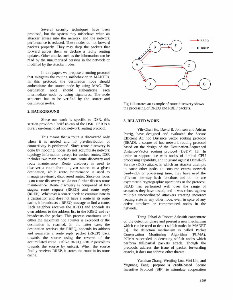
369
Several security techniques have been
proposed, but the system may misbehave when an
attacker enters into the network and the network
performance is reduced. These nodes do not forward
packets properly. They may drop the packets that
forward across them or declare a faulty routing updates. Other attacks such as the information can be
read by the unauthorized persons in the network or
modified by the attacker nodes.
In this paper, we propose a routing protocol
that mitigates the routing misbehavior in MANETs.
In this protocol, the destination node should
authenticate the source node by using MAC. The
destination node should authenticate each intermediate node by using signatures. The node
sequence has to be verified by the source and
destination nodes.
2. BACKGROUND
Since our work is specific to DSR, this
section provides a brief re-cap of the DSR. DSR is a
purely on-demand ad hoc network routing protocol.
This means that a route is discovered only
when it is needed and no pre-distribution of
connectivity is performed. Since route discovery is
done by flooding, nodes do not accumulate network
topology information except for cached routes. DSR
includes two main mechanisms: route discovery and
route maintenance. Route discovery is used to discover a route from a given source to a given
destination, while route maintenance is used to
manage previously discovered routes. Since our focus
is on route discovery, we do not further discuss route
maintenance. Route discovery is composed of two
stages: route request (RREQ) and route reply
(RREP). Whenever a source needs to communicate to
a destination and does not have a route in its route
cache, it broadcasts a RREQ message to find a route.
Each neighbor receives the RREQ and appends its
own address to the address list in the RREQ and re-
broadcasts the packet. This process continues until either the maximum hop counter is exceeded or the
destination is reached. In the latter case, the
destination receives the RREQ, appends its address
and generates a route reply packet (RREP) back
towards the source using the reverse of the
accumulated route. Unlike RREQ, RREP percolates
towards the source by unicast. When the source
finally receives RREP, it stores the route in its route
cache.
Fig.1illustrates an example of route discovery shows the processing of RREQ and RREP packets.
3. RELATED WORK
Yih-Chun Hu, David B. Johnson and Adrian
Perrig, have designed and evaluated the Secure
Efficient Ad hoc Distance vector routing protocol (SEAD), a secure ad hoc network routing protocol
based on the design of the Destination-Sequenced
Distance-Vector routing protocol (DSDV) [1]. In
order to support use with nodes of limited CPU
processing capability, and to guard against Denial-of-
Service (DoS) attacks in which an attacker attempts
to cause other nodes to consume excess network
bandwidth or processing time, they have used the
efficient one-way hash functions and do not use
asymmetric cryptographic operations in the protocol.
SEAD has performed well over the range of
scenarios they have tested, and it was robust against multiple uncoordinated attackers creating incorrect
routing state in any other node, even in spite of any
active attackers or compromised nodes in the
network.
Tarag Fahad & Robert Askwith concentrate
on the detection phase and present a new mechanism
which can be used to detect selfish nodes in MANET
[3]. The detection mechanism is called Packet
Conservation Monitoring Algorithm (PCMA).
PCMA succeeded in detecting selfish nodes which perform full/partial packets attack. Though the
protocols address the issue of packet forwarding
attacks, it does not address other threats.
Yanchao Zhang, Wenjing Lou, Wei Liu, and
Yuguang Fang, propose a credit-based Secure
Incentive Protocol (SIP) to stimulate cooperation
C A
D F G
E B
RREQ
RREP

370
among mobile nodes with individual interests [4].
SIP can be implemented in a fully distributed way
and does not require any pre-deployed infrastructure.
In addition, SIP is immune to a wide range of attacks
and is of low communication overhead by using a
Bloom filter. Though the protocol addresses the issue of packet forwarding attacks, it does not address
other threats.
Liu, Kejun Deng, Jing Varshney, Pramod K.
Balakrishnan, Kashyap propose the 2ACK scheme
that serves as an add-on technique for routing
schemes to detect routing misbehavior and to
mitigate their adverse effect [5]. The main idea of the
2ACK scheme is to send two-hop acknowledgment packets in the opposite direction of the routing path.
In order to reduce additional routing overhead, only a
fraction of the received data packets are
acknowledged in the 2ACK scheme. But, the
acknowledgement packets are sent even though there
is no misbehavior, which results in unnecessary
overhead.
A. Patwardhan,J. Parker, M. Iorga, A.
Joshi,T. Karygiannis and Y. Yesha, present an
approach of securing a MANET using a threshold
based intrusion detection system and securing routing
protocol [6]. Their implementation of IDS deployed
on hand held devices and in a MANET test bed
connected by a secure version of AODV over IPV6.
While the IDS help detect attacks on data traffic, Sec
AODV incorporates security features of non-
repudiation and authentication, without relaying on
the availability of a Certificate Authority (CA) or a
Key Distribution Center (KDC). They have presented the design and implementation details of their
system, the practical considerations involved, and
how these mechanisms are used to detect and thwart
malicious attacks.
4. SYSTEM DESIGN AND ALGORITHM
OVERFLOW
We begin by stating some
environmental assumptions and summarizing our
notation. We assume bidirectional communication on
each link: if node S is able to send a message to node
D, then node D is able to send to node S. This
assumption is justified, since many wireless MAC-
layer protocols, including IEEE 802.11, require
bidirectional communication.
We assume that a node is aware of the exact
set of its current immediate neighbors.
The cryptographic techniques that we
propose further below fall into two categories:
shared-key MACs and public key signatures.
Although sometimes implemented with the aid of
conventional ciphers, MAC functions are often
constructed using cryptographically suitable keyed hash functions. The most common MAC construct is
the HMAC. For schemes based on MACs, we assume
the existence of a secure key distribution mechanism.
In our approach, each node will keep track
of number of packets forwards to the neighboring
nodes, and number of acknowledgements received
for the forwarded packets. When packet drop is more
in neighboring node, then it assumes that node as
misbehaving node.
In DSR, a route is accumulated incrementally through flooding until the destination
is reached, at which point the route is confirmed by
re-visiting it by unicast in reverse order.
Each node generates the Secret key and
public key, and then it distributes the public key to all
other nodes.
When a node wants to transfer a packet, it
first looks at its cache for the route. If any route is
found, it forwards the packet. If there is no pre-existing route, then the sender constructs the Route
Request.
The sender generates the Route Request
(RREQ) packet. In RREQ, it includes the source id,
destination id and route id. The sender computes
MAC over the route id and adds it in the packet
header and floods the RREQ to its neighboring nodes
except misbehaving nodes.
The intermediate node receives the RREQ
checks for the destination id. If it does not match with its id, then it adds its id and signature with RREQ and
then floods to its neighbors.
When the destination node receives the
RREQ packet, it checks for the identity of source by
computing the MAC over the route id by using the
key shared with the source. If the computed MAC is
same as that in the RREQ packet, then the destination
will verify the integrity of RREQ by using the public
key of each intermediate node. If the verification of
any intermediate node fails, then it discards the RREQ.
371
When the MAC computed over route id
does not matches with the MAC in destination then it
discards the RREQ.
The RREQ process is illustrated below:
SN1 : RREQ[S, D, MAC (Rid)]
N1N2 : RREQ[S, D, MAC (Rid), (N1),
(signn1)]
N2N3 : RREQ[S, D, MAC (Rid), (N1,N2),
(signn1,signn2)]
NM-1D: RREQ[S, D, MAC(Rid),(N1,N2,Nm-1),
(signn1,signn2,signm-1)]
The destination node then constructs the
Route Reply (RREP) by adding its id, source id, route
id and id of all the intermediate nodes. Then it forwards RREP to its neighbor node.
When the sender receives the RREP packet,
it repeats the same steps as the destination node. It
checks for authentication of the destination system by
checking with the MAC computed over route id, then
integrity of the intermediate nodes by using the
public key of intermediate nodes.
The RREP process is illustrated below:
DNM-1: RREP[S, D, MAC (Rid), (N1,N2,NM-1), (signD)]
N2N1: RREP[S, D, MAC (Rid), (N1,N2,NM-1),
(signD,signm-1,signn2)]
N1S : RREP[S, D, MAC (Rid), (N1,N2,NM-1),
(signD,signm-1,signn2,signn1)]
5. CONCLUSION
Mobile Ad Hoc Networks
(MANETs) have been an active area over the past
few years, due to their potentially widespread
application in military and civilian communications. Such a network is highly dependent on the
cooperation of all its members to perform networking
functions. This makes it highly vulnerable to selfish
nodes. One such misbehavior is related to routing.
When such misbehaving nodes participate in the
Route Discovery phase but refuse to forward the data
packets, routing performance may be degraded
severely. For robust performance in an untrusted
environment, it is necessary to resist such routing
misbehavior. A possible extension to DSR to mitigate
the effects of routing misbehavior in ad hoc networks has been proposed. It provides security against
routing misbehavior and attacks. It relies on
cryptographic techniques for authentication. The
security mechanism which is developed is highly
efficient. It also prevents a variety of DoS attacks.
REFERENCES
1. Farooq Anjum and Dhanant
Subhadrabandhu and Saswati Sarkar
“Signature based Intrusion Detection for
Wireless Ad-Hoc Networks: A
Comparative study of various routing
protocols” Vehicular Technology
Conference, 2003. VTC 2003-Fall. 2003 IEEE 58th, Oct. 2003.
2. M.Rajesh Babu and S.Selvan,”A Secure
Authenticated Routing Protocol for Mobile
Ad-Hoc Networks”, CIIT Journal, July
2009.
3. Yih-Chun Hu, David B. Johnson and Adrian
Perrig, "SEAD: Secure Efficient Distance
Vector Routing for MobileWireless Ad Hoc
Networks", in proceedings of IEEE
Workshop on Mobile Computing Systems
and Applications, pp.3-13, 2002.
4. Tarag Fahad & Robert Askwith “A Node
Misbehaviour Detection Mechanism for
Mobile Ad-hoc Networks” The 7th Annual
PostGraduate Symposium on The
Convergence of Telecommunications,
Networking and Broadcasting, 26-27 June
2006.
5. YihChun Hu, Adrian Perrig and David B. Johnson," Ariadne: A Secure On Demand
Routing Protocol for Ad Hoc Networks",
Technical Report, Rice university 2001
6. Yanchao Zhang, Wenjing Lou, Wei Liu, and
Yuguang Fang, “A secure incentive
protocol for mobile ad hoc networks”,
Wireless Networks (WINET), vol 13, issue
5, October 2007.
7. Liu, Kejun Deng, Jing Varshney, Pramod K.
Balakrishnan, Kashyap “An
Acknowledgment-based Approach for the
Detection of Routing Misbehavior in
MANETs” Mobile Computing, IEEE
Transactions on May 2007.
8. A. Patwardhan,J. Parker, M. Iorga, A.
Joshi,T. Karygiannis and Y. Yesha,

372
"Threshold-based intrusion detection in ad
hoc networks and secure AODV", Vol.6,
No.4, pp.578-599, 2008.
9. Katrin Hoeper and Guang Gong,
"Bootstrapping Security in Mobile Ad Hoc
Networks Using Identity-Based Schemes
with Key Revocation", Technical
Report CACR 2006-04, Centre for Applied
Cryptographic Research, January 2006.
10. Gergely Acs, Levente Buttya, and Istvan Vajda, "Provably Secure On- Demand
Source Routing in Mobile Ad Hoc
Networks", IEEE Transactions On
Mobile Computing, Vol. 5, No. 11, pp.1533-
1546, November 2006.
11. Syed Rehan Afzal, Subir Biswas, Jong-bin
Koh, Taqi Raza, Gunhee Lee, and Dong-
kyoo Kim, "RSRP: A Robust Secure Routing Protocol for Mobile Ad hoc
Networks", IEEE Conference on Wireless
Communications and Networking, pp.2313-
2318, April 2008.

AUTOMATIC CALL TRANSFER SYSTEM BASED ON LOCATION PREDICTION USING
WIRELESS SENSOR NETWORK
Vairavamoorthy.A#1, Somasundaram.C#2, Jesvin Veancy#
Department of Electronics and Communication Engineering, Easwari Engineering College
Approved by AICTE Accredited by NBA, Affiliated to Anna University, Chennai and ISO 9001-2000 Certified [email protected]
Abstract—The Public Switched Telephone Network
(PSTN) is the oldest and largest tele-communications
network in existence. The auto call-transfer function
is one of the basic services supported by PSTN that
switches incoming calls to the subscriber. It is likely
for the subscribers to lose incoming calls when they
leave the room. Therefore, we propose a ZigBee
location-awareness and tag identification technique
for the traditional phone system. Our technique
identifies a person’s location as he/she moves around
the office building. Whenever there is an incoming
call, the call will be transferred to the office phone
nearest the person. As a result, the overall service
quality would be enhanced to practical effect.
I. INTRODUCTION
The current telephone systems can be grouped into
PSTN, GSM and the new digital technology SIP
(VOIP) and Skype systems. These systems
intercommunicate through different gateway
interfaces. PSTN has been around for hundreds of
years and remains high in market shares. Therefore,
integration into PSTN is a common goal for the rest
of the systems. PSTN provides an important
function: the auto call-transfer service. This service
switches unanswered incoming calls to a back-up
position after a pre-determined interval of time. (If
a call is not answered at phone X after a set time,
the call will be transferred to Y). Currently, the
GSM system can automatically transfer a PSTN
call to a predestined cell phone line. However, the
service charges an additional fee from the cell
phone customers. A number of studies have sprung
to study RFID (Radio Frequency Identification)
and Zigbee technology and aimed to reach the goal
of positioning. RFID is an auto-identification
technology using radio to identify objects. Its
principal operation theory is to use a reader for
transmitting radio signals and reading the tag
embedded or posted on the objects. RFID uses the
radio data to trace its objects using the reader as a
positioning reference. It has become a common
practice to include these indoor positioning devices
in both wired and wireless networks. However,
because the wireless network is built upon the
backbone network of the wired, the infrastructure
of the wireless cannot be established without the
wired network. The other auto identification
system, Zigbee, has a self-built network that can be
constantly updated. It also has low power
consumption. Zigbee uses the intensity of the
received signals from the laidout sensors to identify
the position of the mobile devices. In this study, we
propose a location-awareness technique in the
traditional phone system that offers a call-transfer
service by locating the person moving around with
an RFID and Zigbee. Our system also supports
Mesh and provides Multi-path functionality to
enhance network stability. The rest of the paper is
organized as follows. In Section II gives a
description of the system architecture. Section III
presents the experiment environment and the
simulation result. Finally, Section IV concludes
this work.
II. SYSTEM ARCHITECTURE The functional block diagram of the cabin side and
system side are shown in the fig. 1 and fig. 2
respectively.
Fig.1 Cabin side
Proceedings of the third National conference on RTICT 2010Bannari Amman Insitute of Technology , Sathyamangalam 638 401
9-10 April 2010
373

Fig. 2 System side
In cabin side, RFID is used to monitor the
position of person. If person in Cabin1 then system
sends that corresponding information about that
person to system. In the system side decision will
be taken for call. It monitors all persons where they
are present using zigbee communication.
Our system consists of a user’s hand-held
Zigbee tag. It is moved in a pre-defined area, when
the set reference point detects the tag. After the
positioning system concludes its correct position,
the detected position is sent by the Application
System to the DataBase for cross comparison to
acquire the extension number of the position, the
application system sends out transfer instruction by
way of communication interface to PABX for auto-
transfer service. The system architecture is
illustrated in Fig.3.
Fig. 3: System Architecture
A. Location-Awareness
Our system adopts a signal intensity ranging
algorithm. The signal intensity received by the tags
set up at different reference points is used to do
position analysis. The measured data of single
signal intensity could only lock the mobile stations
on a track which will take the reference point as
center position. The radius of a circle could be
confirmed by signal strength, when there are three
reference points, the received signal could
accurately tell the position of the mobile device.
B. Application Systems
We use the SCADA (Supervisory Control And
Data Acquisition) as the main screen in this study.
It monitors both the real time moving status of
different devices and the RSSI value received by
each reference point. With the calculation
positioning system, the position of the tag will be
accurately shown on the graphic interface, and the
tag number will be displayed. At the same time, the
new data of each mobile device are recorded (Tag,
Time and Position). When a “moving event” takes
place, the system will inquire DB (DataBase). This
inquiry begins with the tag. The tag gets the local
phone number and the phone number of the new
position, and then sends out the instructions to the
PABX system by passing through the transfer
service. Every step of the transfer process can be
monitored in real time through the screen.
C. PABX Transfer Services
The telephone system used in this study is Phillip’s
traditional enterprise-type PABX with 60 outbound
lines and 1500 inbound lines. The system provides
Command Line instruction that can be connected
through RS-232. The transmission interface is set
to 9600 bps (bits per second), 8 bits, and non-
parity. The instruction of ChFoME (Change Follow
Me) is used as the phone transfer setup.
Change follow me relation
CHFLME: <FM-TYPE>, <ORIG-DNR> [,<DEST-
NUMBER>];
<FM-TYPE>: 0: when has Ring starts transfer
<ORIG-DNR>:Original telephone number
<DEST-NUMBER>:Destination telephone
number
<;>:Execution
Example:
chflme: 0,503300,503201;
When have dial telephone number is 503300 will
be transfered to 503201.
III. EXPERIMENTAL RESULTS This section evaluates the automatic phone transfer
service based on the location-awareness technology
by setting up actual calls. The parameters of the
test environment are shown in Fig. 4. An additional
phone is used to call into these people’s offices.
Ten calls have been used to connect each of the
five telephones, and each call is unmistakenly
transferred to the correct person in his/her new
location. For example, the person with the tag ID
101 gets the call at the destination office with the
new phone number 503201 that has been
transferred from the original phone line.
374
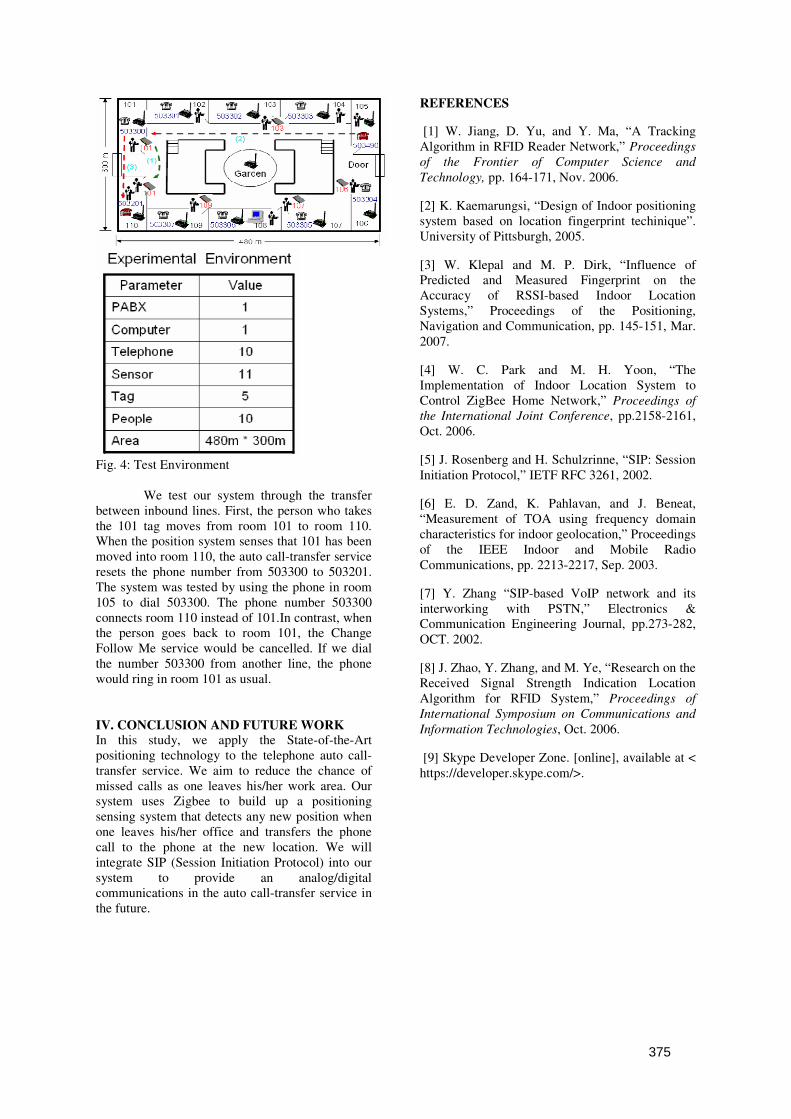
Fig. 4: Test Environment
We test our system through the transfer
between inbound lines. First, the person who takes
the 101 tag moves from room 101 to room 110.
When the position system senses that 101 has been
moved into room 110, the auto call-transfer service
resets the phone number from 503300 to 503201.
The system was tested by using the phone in room
105 to dial 503300. The phone number 503300
connects room 110 instead of 101.In contrast, when
the person goes back to room 101, the Change
Follow Me service would be cancelled. If we dial
the number 503300 from another line, the phone
would ring in room 101 as usual.
IV. CONCLUSION AND FUTURE WORK In this study, we apply the State-of-the-Art
positioning technology to the telephone auto call-
transfer service. We aim to reduce the chance of
missed calls as one leaves his/her work area. Our
system uses Zigbee to build up a positioning
sensing system that detects any new position when
one leaves his/her office and transfers the phone
call to the phone at the new location. We will
integrate SIP (Session Initiation Protocol) into our
system to provide an analog/digital
communications in the auto call-transfer service in
the future.
REFERENCES
[1] W. Jiang, D. Yu, and Y. Ma, “A Tracking
Algorithm in RFID Reader Network,” Proceedings
of the Frontier of Computer Science and
Technology, pp. 164-171, Nov. 2006.
[2] K. Kaemarungsi, “Design of Indoor positioning
system based on location fingerprint techinique”.
University of Pittsburgh, 2005.
[3] W. Klepal and M. P. Dirk, “Influence of
Predicted and Measured Fingerprint on the
Accuracy of RSSI-based Indoor Location
Systems,” Proceedings of the Positioning,
Navigation and Communication, pp. 145-151, Mar.
2007.
[4] W. C. Park and M. H. Yoon, “The
Implementation of Indoor Location System to
Control ZigBee Home Network,” Proceedings of
the International Joint Conference, pp.2158-2161,
Oct. 2006.
[5] J. Rosenberg and H. Schulzrinne, “SIP: Session
Initiation Protocol,” IETF RFC 3261, 2002.
[6] E. D. Zand, K. Pahlavan, and J. Beneat,
“Measurement of TOA using frequency domain
characteristics for indoor geolocation,” Proceedings
of the IEEE Indoor and Mobile Radio
Communications, pp. 2213-2217, Sep. 2003.
[7] Y. Zhang “SIP-based VoIP network and its
interworking with PSTN,” Electronics &
Communication Engineering Journal, pp.273-282,
OCT. 2002.
[8] J. Zhao, Y. Zhang, and M. Ye, “Research on the
Received Signal Strength Indication Location
Algorithm for RFID System,” Proceedings of
International Symposium on Communications and
Information Technologies, Oct. 2006.
[9] Skype Developer Zone. [online], available at <
https://developer.skype.com/>.
375
Proceedings of the Third National Conference on RTICT 2010
Bannari Amman Institute of Technology, Sathyamangalam-638401
9-10 April 2010
376
An Energy Efficient relocation of gateway
for improving Timeliness in Wireless Sensor
Networks
S.S.Rahmath Ameena* Dr.B.Paramasivan
**
* Student, Dept. of CSE, National Engineering College, Kovilpatti.
E-Mail: [email protected] **Professor, Dept.of CSE, National Engineering College, Kovilpatti.
E-Mail: [email protected]
ABSTRACT:
In Wireless Sensor Networks (WSN) collected
data are routed to multiple gateway nodes for processing.
Based on the gathered reports the gateways may also
work collaboratively on a set of actions to serve
application level requirements or to better manage the
resource constrained WSN. In this paper an efficient
algorithm of AQM (Active Queue Management) is
presented. AQM strives to maintain buffer management
among the gateways while repositioning individual
gateway to better manage the sensors in their vicinity.
Simulation results have demonstrated the effectiveness of
AQM and positive effect on network longevity.
Keywords: Wireless Sensor Networks, AQM, Timeliness, End
to End delay.
1. INTRODUCTION
Wireless sensor networks(WSN) have
numerous applications in a variety of disciplines, both
military and civilian [1] [2].The ability to remotely
measure ambient conditions and track dynamic events become valuable especially in harsh environments
where human intervention is risky or infeasible.
Sensors are usually battery-operated and have a limited
transmission and processing capacity. Such constraints
have motivated lots of research on data fidelity, latency,
and coverage so that the network can stay functional for
the longest duration.
A typical WSN architecture involves large
numbers of sensor nodes that report their measurements
to locally deployed data collection centers often
referred to as gateway node. Gateway is usually more capable in terms of their energy supply, radio range and
computational resources.
Gateway relocation [3] is one of the
approaches pursued to improve the performance of the
network. By relocating the gateway towards highly
active sensors, the packet will be routed to the gateway
through fewer sensors. The shortened data paths help in
preserving sensors energy, lowering the packet loss rate
and reducing delivery latency. In general, most gateway
relocation techniques identify bottlenecks in the current
network topology and tend to move the gateway close
to the bottleneck positions. However, such
performance-centric relocation may move the gateway
dangerously close to one or multiple targets/events in the environment and thus may expose the gateway to
the risk of getting damaged, captured etc.
In this paper we propose a AQM (Active Queue
Management) algorithm solution to the gateway
relocation problem .The idea is to identify a position for
the gateway to better serve wireless sensor network
which consists of a large number of sensor nodes and
one or more sink nodes scattered over a region of
interest where data gathering and reporting tasks are
performed. A sensor node often has limited power
resources. Therefore it is very crucial to reduce the
energy consumption in certain real-time applications such as fire alarm monitoring, traffic monitoring
information collected is valid only for a limited amount
of time after that it become irrelevant information.
Hence all the packets need to be conveyed to the sink
within a certain deadline period and packet timeliness
requirement also becomes an important issue for such
real-time applications in wireless sensor network.
Sensor networks data are routed towards a
single sink the gateway in our model hops close to that
gateway become heavily involved in packet forwarding
and thus their energy resource gets depleted rather quickly. Such scenario increases total transmission
power and gradually limits sensor coverage in the
network and eventually makes the networks useless. If
the gateway has limited motion capability it will be
desirable to relocate the gateway close to an area of
heavy traffic or near loaded hops in order to decrease
the total transmission power and extend the life of
nodes on the path of heavy packet traffic.
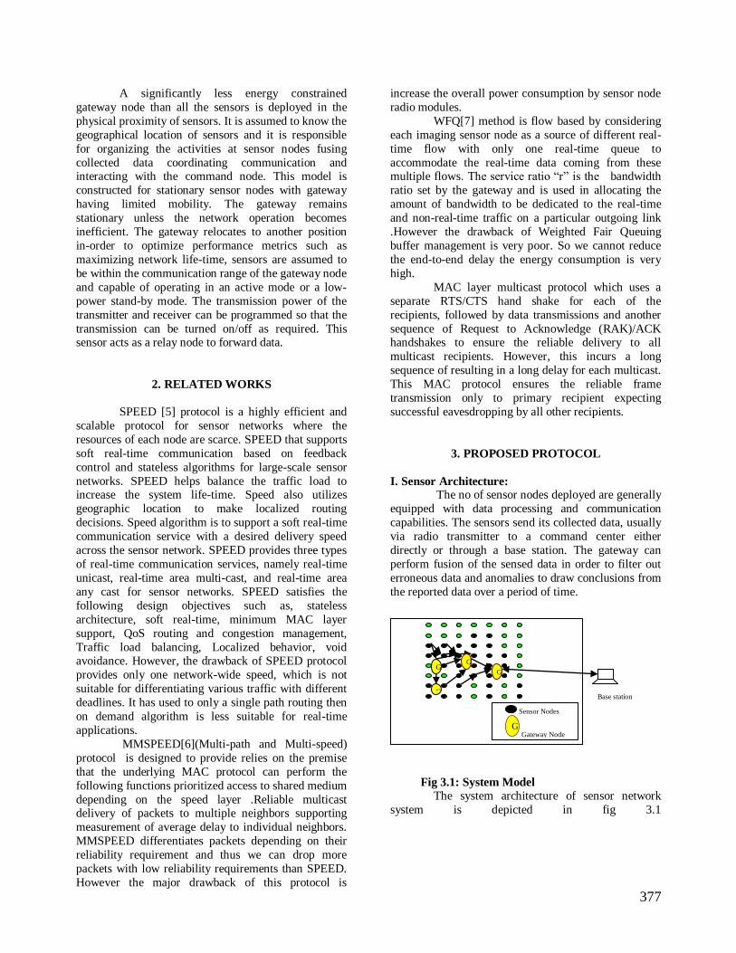
377
A significantly less energy constrained
gateway node than all the sensors is deployed in the
physical proximity of sensors. It is assumed to know the
geographical location of sensors and it is responsible
for organizing the activities at sensor nodes fusing
collected data coordinating communication and interacting with the command node. This model is
constructed for stationary sensor nodes with gateway
having limited mobility. The gateway remains
stationary unless the network operation becomes
inefficient. The gateway relocates to another position
in-order to optimize performance metrics such as
maximizing network life-time, sensors are assumed to
be within the communication range of the gateway node
and capable of operating in an active mode or a low-
power stand-by mode. The transmission power of the
transmitter and receiver can be programmed so that the
transmission can be turned on/off as required. This sensor acts as a relay node to forward data.
2. RELATED WORKS
SPEED [5] protocol is a highly efficient and
scalable protocol for sensor networks where the
resources of each node are scarce. SPEED that supports
soft real-time communication based on feedback
control and stateless algorithms for large-scale sensor
networks. SPEED helps balance the traffic load to increase the system life-time. Speed also utilizes
geographic location to make localized routing
decisions. Speed algorithm is to support a soft real-time
communication service with a desired delivery speed
across the sensor network. SPEED provides three types
of real-time communication services, namely real-time
unicast, real-time area multi-cast, and real-time area
any cast for sensor networks. SPEED satisfies the
following design objectives such as, stateless
architecture, soft real-time, minimum MAC layer
support, QoS routing and congestion management,
Traffic load balancing, Localized behavior, void avoidance. However, the drawback of SPEED protocol
provides only one network-wide speed, which is not
suitable for differentiating various traffic with different
deadlines. It has used to only a single path routing then
on demand algorithm is less suitable for real-time
applications.
MMSPEED[6](Multi-path and Multi-speed)
protocol is designed to provide relies on the premise
that the underlying MAC protocol can perform the
following functions prioritized access to shared medium
depending on the speed layer .Reliable multicast delivery of packets to multiple neighbors supporting
measurement of average delay to individual neighbors.
MMSPEED differentiates packets depending on their
reliability requirement and thus we can drop more
packets with low reliability requirements than SPEED.
However the major drawback of this protocol is
increase the overall power consumption by sensor node
radio modules.
WFQ[7] method is flow based by considering
each imaging sensor node as a source of different real-
time flow with only one real-time queue to
accommodate the real-time data coming from these multiple flows. The service ratio “r” is the bandwidth
ratio set by the gateway and is used in allocating the
amount of bandwidth to be dedicated to the real-time
and non-real-time traffic on a particular outgoing link
.However the drawback of Weighted Fair Queuing
buffer management is very poor. So we cannot reduce
the end-to-end delay the energy consumption is very
high.
MAC layer multicast protocol which uses a
separate RTS/CTS hand shake for each of the
recipients, followed by data transmissions and another
sequence of Request to Acknowledge (RAK)/ACK handshakes to ensure the reliable delivery to all
multicast recipients. However, this incurs a long
sequence of resulting in a long delay for each multicast.
This MAC protocol ensures the reliable frame
transmission only to primary recipient expecting
successful eavesdropping by all other recipients.
3. PROPOSED PROTOCOL
I. Sensor Architecture: The no of sensor nodes deployed are generally
equipped with data processing and communication
capabilities. The sensors send its collected data, usually
via radio transmitter to a command center either
directly or through a base station. The gateway can
perform fusion of the sensed data in order to filter out
erroneous data and anomalies to draw conclusions from
the reported data over a period of time.
Fig 3.1: System Model
The system architecture of sensor network
system is depicted in fig 3.1
Sensor Nodes
G
Gateway Node
Base station
G
G
G
G

378
Fig 3.2: Process flow diagram of gateway
relocation
II. Cluster Formation:
The sensors are uniformly deployed and the
cluster is formed using the location based clustering
algorithm. This algorithm fully utilizes the location
information of routing to reuse the routing cost. The
cluster is formed by following equation
Fns1rs1
snT
))/mod(()(
0 Others
Where s - Percentage of cluster heads
over all nodes in the network
r - The number of rounds of
selection
F - The set of nodes that are not
selected in round 1/s
III. Gateway Election:
Gateway election is more important in wireless
sensor networks. Gateway is also called as cluster head.
Gateway is elected for the context information of all the
sensor nodes which is based on all the sensor node energy and bandwidth coverage.
IV. AQM Implementation:
In order to solve the buffer management
problem and then decrease the end-to-end delay we
propose a Active Queue Management (AQM) based
phenom routing protocol for sensor networks. Active
Queue Management provides congestion signal for flow
control not only based on the queue length but also the
channel condition and the transmission rate. It uses
priority based queue management to improve
performance in congested area. Once the nodes are
deployed the sensor nodes form the cluster members
and elect a cluster head using location based clustering
algorithm. Next elect a cluster head as the gateway and
apply the AQM method where the buffer management is high by comparing the weighted fair queuing method
.Hence avoids more no of packet loss.
v. Relocation Approach to Enhance Performance :
There are three phases in gateway relocation
depicted in fig 3.2. These are when to relocate the
gateway, where to put it and how to handle its motion
without disrupting data traffic and negative effect.
Phase I: The time when gateway should be relocated Step 1: Always relocation is decided based on the
missed ratio.
Step 2: The missed ratio is indirectly related to finding proper r-value in the above equation.
Step 3: Real time routing finds the r-value by
considering all the paths from the source of real time
traffic to the gateway.
Step 4: In cases where a proper r-value between 0 and
1 cannot be found, the connection is simply rejected
and the path is not established
Step 5: Even where proper r-values are found, the miss
ratio may start to decrease.
Step 6: The gateway sets a threshold value for the
maximum level of miss ratio and maintains such statistics periodically when such threshold is reached
the gateway is to a better location.
Step 7: The gateway can be relocated more than once
whenever necessary during the data traffic cycles in fig
3.3
Phase II: The position to which the gateway should
be located
Initially Sensor nodes
are deployed
Last hop node are
assuming gateway
Gateway relocation
should be decided
Based on performance miss ratio.
Gateway can be
relocated more than once
During data traffic cycles
Fig 3.3: When to relocate the gateway
Nodes are connected multihop
path
Sensor Architecture
Cluster Formation
Cluster Head Election
AQM Implementation
Cluster Head Mobility
Find Relocation
Performance Analysis
Context
Information
Traffic
Monitoring

379
Step 1: After deciding that the gateway is to be
relocated then a new location is searched for it.
Step 2: Next the gateway is moved towards the loaded
nodes interms of real time traffic so that the end-to-end
delay can be decreased.
Step 3: Then next searches the last hop nodes. Step 4: The biggest r-value are considered for
relocating the gateway at the position of that hop.
Step 5: Decrease the average end-to-end delay since the
number of hops for data packets to travel will be
decreased.
Step 6: Breaking the ties when multiple alternative
nodes with the same r-value are found
Step 7: If the gateway is still reachable by the nodes Y
and Z they just increase their transmission range of
uninterrupted data delivery.
Phase III: How to relocate the gateway Step 1: After determined the new location, the gateway
explores two options based on the information of
whether it will be out of range at the new location or
not.
Step 2: If the gateway detects that it would go out of
the transmission range of last hop nodes and cannot
receive the data from other relay nodes at the new
location.
Step 3: Then explores the option of employing sensor
nodes to forward the packets.
Step 4: The miss ratio for real time data periodically to detect situations where there is need for relocation.
Step 5: Then final gateway are communicating to
command node.
Step 6: Next gateway checks whether it can still be
reachable by by the last hopes while traveling on the
next stride and inform yht last hop nodes about its
situation.
Step 7: Once,it detects that forwarder nodes are needed,
the routes are extended by those nodes and that
information is sent to relevant nodes.
4. PERFORMANCE RESULTS
In this section the performance results were
shown from fig5.1 to 5.4 with and without repositioning
the gateway. In order to see the effect of repositioning
the gateway on energy consumption, we looked at the
average lifetime of a node, time for first and last node
to die and average energy consumed per packet. The results depicted in fig1 have shown that our approach of
repositioning the gateway decreases energy
consumption significantly especially by increasing the
average lifetime of the node and time for first node to
die. In this approach, since the gateway is relocated
close to heavily loaded nodes, less energy is consumed
for communication thus leading significant amount of
energy savings. On the other hand, the latency of the
packets from those nodes to the gateway will be
decreased, causing the decrease delay per packet to
decrease drastically. There is also a slight increase on
the throughput due to smaller packet drop probability since packets travel shorter distances.
Table1: Simulation Environment Settings
Terrain 500mx500m
Node number 50
Node placement Uniform
Bandwidth 100 kbps
Inter-column spacing 82m
Inter-row spacing 70m
Simulation duration 10s
Transmission rate 10ms/pkt
Table 2: Movable Gateway
ST TRE ARE PDR AE2E
D
10 1069 106.9 98.03 0.157
20 2120 212 98.69 0.109
30 3180 318 99.02 0.085
40 4230 423 99.22 0.071
50 5281 528.1 99.35 0.062
60 6331 633.1 99.44 0.056
70 7390 739 99.51 0.051
80 8435 843.5 99.57 0.047
90 9486 948.6 99.61 0.044
Table 3: Fixed Gateway
ST TRE ARE PDR AE2ED
10 1070 107 97.69 0.1563
20 2129 212.9 97.30 0.1227
30 3179 317.9 97.17 0.1122
40 4230 423 97.5 0.1072
50 5275 527.5 97.69 0.1041
60 6340 634 97.82 0.1017
After increasing packet losses on some
data path
Next continuing packet delivery to
gateway node
Then gateway motion handling
Next involving data transfer
Fig 3.4 :How to relocate the
gateway
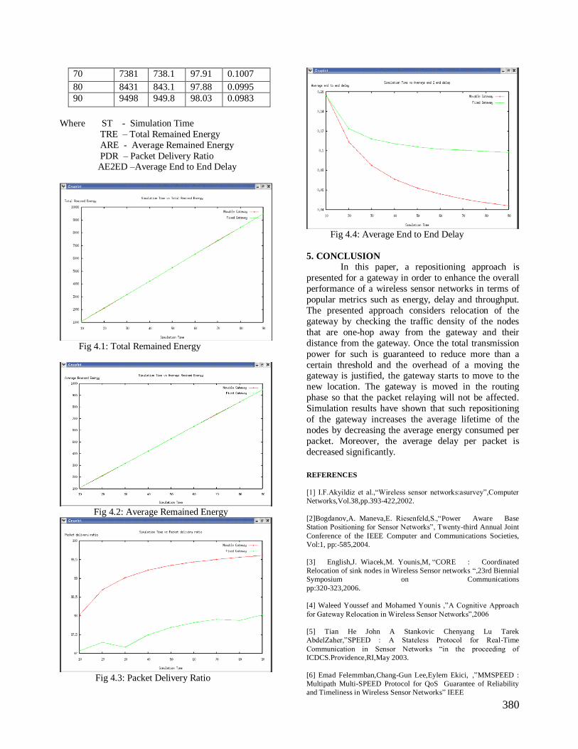
380
70 7381 738.1 97.91 0.1007
80 8431 843.1 97.88 0.0995
90 9498 949.8 98.03 0.0983
Where ST - Simulation Time
TRE – Total Remained Energy
ARE - Average Remained Energy
PDR – Packet Delivery Ratio AE2ED –Average End to End Delay
Fig 4.1: Total Remained Energy
Fig 4.2: Average Remained Energy
Fig 4.3: Packet Delivery Ratio
Fig 4.4: Average End to End Delay
5. CONCLUSION In this paper, a repositioning approach is
presented for a gateway in order to enhance the overall
performance of a wireless sensor networks in terms of
popular metrics such as energy, delay and throughput.
The presented approach considers relocation of the
gateway by checking the traffic density of the nodes
that are one-hop away from the gateway and their
distance from the gateway. Once the total transmission
power for such is guaranteed to reduce more than a
certain threshold and the overhead of a moving the gateway is justified, the gateway starts to move to the
new location. The gateway is moved in the routing
phase so that the packet relaying will not be affected.
Simulation results have shown that such repositioning
of the gateway increases the average lifetime of the
nodes by decreasing the average energy consumed per
packet. Moreover, the average delay per packet is
decreased significantly.
REFERENCES
[1] I.F.Akyildiz et al.,“Wireless sensor networks:asurvey”,Computer
Networks,Vol.38,pp.393-422,2002.
[2]Bogdanov,A. Maneva,E. Riesenfeld,S.,“Power Aware Base
Station Positioning for Sensor Networks”, Twenty-third Annual Joint
Conference of the IEEE Computer and Communications Societies,
Vol:1, pp:-585,2004.
[3] English,J. Wiacek,M. Younis,M, “CORE : Coordinated
Relocation of sink nodes in Wireless Sensor networks “,23rd Biennial
Symposium on Communications
pp:320-323,2006.
[4] Waleed Youssef and Mohamed Younis ,”A Cognitive Approach
for Gateway Relocation in Wireless Sensor Networks”,2006
[5] Tian He John A Stankovic Chenyang Lu Tarek
AbdelZaher,”SPEED : A Stateless Protocol for Real-Time
Communication in Sensor Networks “in the proceeding of
ICDCS.Providence,RI,May 2003.
[6] Emad Felemmban,Chang-Gun Lee,Eylem Ekici, ,”MMSPEED :
Multipath Multi-SPEED Protocol for QoS Guarantee of Reliability
and Timeliness in Wireless Sensor Networks” IEEE

381
TRANSACTIONS ON MOBILECOMPUTING,volume:5,No.6,
2006.
[7] Ramon Serna Oliver and Gerhard Fohler,” A Proposal for a
Notion of Timeliness in Wireless Sensor Networks”,2004
[8]Boonma,P. Suzuki,J.,”LeveragingBiologically-inspired Mobile
Agents Supporting Composite Needs of Reliability and Timeliness in
Sensor Applications”, FBIT 2007 Frotiers in the Convergence of
Bioscience and Information Technologies.Pp:851-860,2007.
[9] Tian He Stankovic, J.A. Chenyang Lu Abdelzaher, T,”
SPEED: a stateless protocol for real-time communication in sensor
networks”, 23 rd International Conference on
DistributedComputingSystems,2003,19-22May2003, On page(s):46-5
[10] Kamal Akkaya Mohamed Younis and Meenakshi Bangad,”Sink
Repositioning for Enhanced Performance in Wireless Sensor
Networks”, 2006.

Proceedings of the Third National Conference on RTICT 2010
Bannari Amman Institute of Technology, Sathyamangalam-638401
9-10 April 2010
382
IMPROVING STABILITY OF SHORTEST MULTIPATH
ROUTING ALGORITHM IN MANET
S.Tamizharasu
M.E. Software Engineering
Anna University
Jothipuram, Coimbatore
ABSTRACT
To propose multipath routing
scheme, referred to as shortest multipath
source (SMS) routing based on dynamic source
routing (DSR) is proposed here. To avoid the
root flop by identify the node weight and
transfer the data from source to destination.
The mechanism that compare AOMDV
routing schemes with DSR routing schemes
along with the performance metrics viz:
throughput, end-to-end delay, delivery ratio,
and distance calculation.
The SMS achieves shorter multiple
partial-disjoint paths and allows more rapid
recovery from route breaks. The performance
differentials are investigated using NS-2 under
conditions of varying mobility, offered load
and network size. Results reveal that SMS
provides a better solution than existing source-
based approaches in a truly mobile ad-hoc
environment.
M.Newlin rajkumar M.E.
Lecturer
Dept. of Computer Science and Engineering
Anna University
Jothipuram, Coimbatore
1. AN INTRODUCTION TO MOBILE AD
HOC NETWORK
Mobile ad-hoc networks (MANETs)
are a key part of the ongoing evolution of wireless
communications. MANETs are defined as the
category of wireless networks that utilize multi-
hop radio relaying and are generally capable of
operating without the support of any fixed-line
infrastructure. Each node has the capability to
communicate directly with other nodes, acting not
only as a mobile wireless host but also as a router,
forwarding data packets to other nodes. In other
words, such networks are self-creating, self-
organizing and self-administrating. Key
application areas for these types of networks
include: conference networking, disaster relief,
military networks and sensor networks.The
network topology may be subject to numerous,
frequent and random changes. In a network
consisting of mobile nodes, the connection
between a source–destination pair may break and
require to be updated regularly. Routing should
adapt to such dynamics and continue to maintain
connections between the communication nodes in
the presence of path breaks caused by mobility
and/or node failures. A variety of routing
protocols for MANETs have been previously
proposed.

383
2 SHORTEST MULTIPATH SOURCE
Shortest Multipath Source SMS
computes multiple partial-disjoint paths that will
bypass at least one intermediate node on the
primary path. An example that illustrates the
computation of partial-disjoint paths is shown in
Figure 1. In case of a link failure between A and
B (Figure 2), the source node will search for an
alternate route that does not contain node B. In
this case, an alternative route between source and
destination is S-A-G-C-D. The major advantage
of such a protocol is that the shortest alternative
routes by contrast to the routes computed using
either link-disjoint or node-disjoint paths are
selected.
Figure 1 Partial disjoint multiple paths
Figure 2 Selection of alternative
path in case of link failure
Route Discovery
Route Discovery has two basic phases;
route request propagation and route reply.
Route Request Propagation
When a node seeks to communicate with
another node, it searches its cache to find any
known routes to the destination. If no routes are
available, the node initiates route discovery by
flooding route-request packet, containing an ID
which, along with source address, uniquely
identifies the current discovery. The SMS scheme
introduces a novel approach to reduce broadcast
overhead. Each node records the ID of route-
request packet and the number of hops the route
request traversed from the source node. Nodes use
this information to rebroadcast duplicate route-
request packets only if: number of hops ≤ last
hop-count recorded.
Route Reply Propagation
When the node receives the route
request, it generates a route reply to the source
using the reverse path identified within the route
request. In addition, the node records the reverse
path within its internal cache. Upon receiving
multiple copies of route-request packets of the
same session, the node sends limited replies to
avoid a reply storm. These new paths are also
appended to the internal cache. In SMS, the
source is responsible for selecting and recording
multiple partial disjoint route paths.
Route Maintenance
In the event of a link failure or an
intermediate node moving out of range, a route-
error packet is transmitted. The reception of a
route-error packet will invalidate the route via that
link to that destination and will switch to an
alternative path if available. The source node will
select an alternative path that does not contain the
next node of the one that sent a route-error packet.
When all routes in the cache are marked as
invalid, the node will delete the invalid routes and
a new route discovery is instigated.

384
3. ROUTING OVER HEAD DETAILS
DSDV-SQ are plotted on a the same
scale as each other, but AODVLL and TORA are
each plotted on different scales to best show the
effect of pause time and offered load on overhead.
TORA, DSR, and AODV-LL are on-demand
routing protocols, so as the number of sources
increases, to expect the number of routing packets
sent to increase because there are more
destinations to which the network must maintain
working routes. DSR and AODV-LL, which use
only on-demand packets and very similar basic
mechanisms, have almost identically shaped
curves. Both protocols exhibit the desirable
property that the incremental cost of additional
sources decreases as sources are added, since the
protocol can use information learned from one
route discovery to complete a subsequent route
discovery. However, the absolute overhead
required by DSR andAODV-LLare very different,
with AODV-LL requiring about 5 times the
overhead of DSRwhen there is constant node
motion (pause time 0). This dramatic increase in
AODV-LL‟s overhead occurs because each of its
route discoveries typically propagates to every
node in the ad hoc network.
3. 1 PACKET DELIVERY RATIO DETAILS
The fraction of the originated application
data packets each protocol was able to deliver, as
a function of both node mobility rate (pause time)
and network load (number of sources). For DSR
and AODV-LL, packet delivery ratio is
independent of offered trafficload; with both
protocols delivering between 95% and 100% of
the packets in all cases.DSDV-SQ fails to
converge below pause time 300, where it delivers
about 92% of its packets. At higher rates of
mobility (lower pause times), DSDV-SQ does
poorly, dropping to a 70% packet delivery ratio.
Nearly all of the dropped packets are lost because
a stale routing table entry directed them to be
forwarded over a broken link. The DSDV-SQ
maintains only one route per destination and
consequently, each packet that the MAC layer is
unable to deliver is dropped since there are no
alternate routes.
3.2 SHORTEST MULTIPATH ROUTING
Shortest Multipath Routing (SMR) is an on-
demand routing protocol that builds multiple
routes using request/reply cycles. When the
source needs a route to the destination but no
route information is known, it floods the ROUTE
REQUEST (RREQ) message to the entire
network. Because this packet is flooded, several
duplicates that traversed through different routes
reach the destination. The destination node selects
multiple disjoint routes and sends ROUTE
REPLY (RREP) packets back to the source via
the chosen routes.RREQ Propagation The main
goal of SMR is to build maximally disjoint
multiple paths.To construct maximally disjoint
routes to prevent certain nodes from being
congested, and to utilize the available network
resources efficiently. To achieve this goal in on-
demand routing schemes, the destination must
know the entire path of all available routes so that
it can select the routes. Therefore, by use the
source routing approach where the information of
the nodes that consist the route is included in the
RREQ packet. Additionally, Intermediate nodes
are not allowed to send RREPs back to the source
even when they have route information to the
destination. If nodes reply from cache as in DSR
and AODV it is difficult to establish maximally
disjoint multiple routes because not enough
RREQ packets will reach the destination and the
destination node will not know the information of
the route that is formed from the cache of
intermediate nodes.
3. 3 FINDING LINK DISJOINT PATHS
Path disjointness has the nice property
that paths fail independently. There are two types
of disjoint paths: node-disjoint and link-disjoint.
Node-disjoint paths do not have any nodes in
common, except the source and destination. In
contrast, link-disjoint paths do not have any
common link. Note that link-disjoint paths may
have common nodes. After investigated the issue
of node- vs. linkdisjointness carefully. Generally
speaking, using linkdisjointness is fine as long as
links do fail independently. This is often the case,
except in situations where multiple links from/to a
node fail together as the node moves out of range.

385
4 RELATED WORKS
AOMDV
AOMDV is a multipath routing
protocol which is based on AODV. When each
node receives duplicate copies of RREQ, it checks
whether the packets‟ hop counts are less than the
hop count already in a routing table. This check
avoids routing loops. Also, if this check is passed,
additional route information is added to the
routing table.
Multiple Routes Establishment by RREQ/RREP
Enhancement
To extend RREQ/RREP messages by
forcing source routing information in order to
establish valid multiple routes. Note that, unlike
other source routing protocols like DSR, to use
source routing information only in the case of
RREQ/RREP messages. Any data packets are
forwarded in a hop-by-hop manner without source
routing option similar to AODV.
RREQ Extension
In this extension, each node which
forwards RREQ packets inserts its own IP address
into a packet header. After receiving a RREQ
packet, it also checks source routing information
field in the packet. If there exists its own address,
it detects routing loop and discards the RREQ
packet. Otherwise, it updates its routing table with
the RREQ information. Unlike AODV, duplicate
copies of RREQ are not discarded immediately. If
the second path information of the routing table is
empty, and loop check is passed, the RREQ
information is adopted as the second reverse path.
RREP Extension
Similar to the RREQ extension, each
node that forwards RREP packets inserts source
routing information and updates its routing table
accordingly. The RREP packets are forwarded
along reverse routes. If there are multiple (two)
reverse routes, the node bicasts RREP packets to
each of them. The call direction going to a
destination “upstream”, and direction returning to
a source node “downstream”. When a node
receives a RREP packet, it checks that next hop (1
or 2) of the reverse route (to the node S) exists in
an address information field in the RREP packet.
If the next hop is found, this means that the RREP
packet was forwarded from the downstream nodes
and routing loop occurred. In this case, the node
discards the RREP packet immediately.
5 PROPOSED SYSTEM
To avoid the root flop by use the Link
Score value to identify the node weight and
transmission success rate to transfer the data‟s
from source to destination. The mechanism that
compare AOMDV routing schemes with SMR
routing schemes along with the performance
metrics viz: throughput, end-to-end delay,
delivery ratio, and distance calculation. A metric,
LinkScore,is defined as LinkScore = (PE ラ WE
+PT ラ WT ), where PE – energy level of the next
hop node (0.0 to 100.0), WE– assigned weight for
PE (0.0 to 1.0), PT – transmission success rate
(0.0 to 100.0) and WT – assigned weight for PT
(0.0 to 1.0). Weights, WE and WT, may be
determined empirically but their sum must equal
1. For example, in a low noise environment, the
probability of successful transmission is higher. In
this scenario, WE = 0.7 and WT = 0.3may be
chosen allowing routing decisions to focus more
on energy conservation in path selection.
Conversely, in a noisy environment, WT = 0.7 and
WE = 0.3 could be chosen instead, giving higher
emphasis to the selection of high reliability paths
over energy conservation. LinkScore then takes on
a value from 0 to 100 and a higher value indicates
a better link. An arbitrary value is initially
assigned to PT as the link performance is
unknown. PT rises (or drops) when subsequent
packet transmissions succeed (or fail). PE starts at
100 and drops as a node consumes its energy
resources.

386
LinkScore is used when there are two
links of different routes with the same hub
distance competing to be admitted to the routing
table. When a new link is received and the routing
table is full, link replacement is initiated. The
search ignores blacklisted links and targets the
link with the lowest LinkScore to be replaced.
When there is more than one entry with the same
LinkScore, the entry with the longest length is
chosen to be replaced. This worst route is then
compared against the incoming route and the
shorter route is admitted into the routing table. If
there is a tie in route length, then the route with
the higher LinkScore is admitted. Since each node
stores and maintains the best available RF links in
its routing table, packets travel on the best route
from a node to a hub at the given time. Since the
routing table contains only one entry to the next
hop node, its size scales slowly with network size
and multiple hubs.
Figure 6 Illustration of forwarding based
on link score metric
CONCLUSION
The SMS model is also implemented within
the NS-2 simulator environment and SMS
performance is compared with SMR, which uses
node-disjoint secondary paths for correcting route
breaks. The SMS model is compared with
AOMDV and route flops are reduced by using the
Link score values. With an increase in mobility,
offered load and network size.
REFERENCES
1. BROCH J., MALTZ D.A., JOHNSON
D.B., HU Y., JETCHEVA J.: „A
performance comparison of multi-hop
wireless ad-hoc network routing
protocols‟. Proc. 4th Annual ACM/IEEE
Int. Conf. on Mobile Computing and
Networking, Dallas, October 1998, pp.
85–97
2. JOHNSON D.B., HU Y., MALTZ D.A.:
„Dynamic source routing in ad-hoc
wireless networks‟, IETF RFC 4728,
February2007,http://www.ietf.org/rfc/rfc4
728.txt
3. LEE S., GERLA M.: „Split multipath
routing with maximally disjoint paths in
ad-hoc networks‟. Proc. IEEE Int. Conf.
On Commun. (ICC), Helsinki, June 2001,
pp. 3201–3205
4. LI X., CUTHBERT L.: „A reliable node-
disjoint multipath routing with low
overhead in wireless ad-hoc
networks‟.Proc. 7th ACM/IEEE Int.
Symp. on Modeling, Analysis and
Simulation of Wireless and Mobile
Systems, Venezia, 2004,pp. 230–233
5. MARINA M., DAS S.: „On-demand
multipath distance vector routing in ad-
hoc networks‟. Proc. 9th IEEE Int.Conf.
on Network Protocols, California, 2001,
pp. 14–23
6. NASIPURI A., CASTANEDA R., DAS
S.: „Performance of multipath routing for
on-demand protocols in mobile adhoc
networks‟, ACM/Kluwer Mobile Netw.
Appl. J., 2001, 6, (4), pp. 339–349
7. Performance evaluation of shortest
multipath source routing scheme H.
Zafar1, 2 D. Harle1 I. Andonovic1 Y.
Khawaja2

Proceedings of the Third National Conference on RTICT 2010
Bannari Amman Institute of Technology, Sathyamangalam-638401
9-10 April 2010
387
BRODCAST SCHEDULING IN WIRELESS NETWORK
Ms.A.Gurushakthi Meera, PG Student, Mrs.G.Prema, M.S, Professor
Electronics and Communication Engineering, Mepco Schlenk Engineering College, sivakasi,virudhunagar dist
[email protected], [email protected]
Abstract – The paper broadcast scheduling in
wireless networks is designed to avoid the
problem of broadcast storm. The broadcast
storm problem tells us that naive flooding is not
practical because it causes severe contention,
collision and congestion. In this paper the
broadcast storm problem is investigated using
two new models. They are 2-disk model and
SINR model.In 2 Disk model, 2 disks are
employed to represent the transmission and the
interference range. The signal to interference
model plus noise ratio model is more realistic
where many far-away nodes could still have the
effect of interfering some nodes if they are
transmitting simultaneously. The 2-disk model
is extended to SINR model because in SINR
model the accumulative interference range of
many nodes outside the interference range will
not be neglected.
Keywords— Broadcast, Scheduling, SINR,
2-Disk, TDMA.
I.INTRODUCTION
Broadcast is a task initiated by a single processor,
called the source, transmitting a single message.
The goal is to have the message reach all processors
in the network. Broadcast is the task initiated by
any of the nodes of a network, called source, whose
goal is to send a message to all other network
nodes. In addition to disseminating data, a
broadcast mechanism represents the starting point
for the implementation of group communication
primitives and various system services in
distributed environments. With the renewed interest
in ad hoc networks, combined with the need to
support multimedia and real-time applications, the
need arises to have in the mobile network a
mechanism for reliable dissemination of control and
data. It is necessary to have broadcast protocols that
meet the combined requirements of these
networks—delivery-guarantee and mobility
transparency. The broadcast problem has been
extensively studied for multi-hop networks. In
particular, several solutions have been presented in
which the broadcast time complexity is
investigated. In detail optimal solutions were
obtained for the case when each node knows the
topology of the entire network.
Broadcast is an important operation in wireless
networks. However, broadcasting by naive flooding
cause severe contention, collision, and congestion,
which is named as the broadcast storm problem.
Many protocols have been proposed to solve this
problem, with some investigations focusing on
collision avoidance yet neglecting the reduction of
redundant rebroadcasts and broadcasting latency;
while other studies have focused on reducing
redundant rebroadcasts yet have paid little attention
to collision avoidance. Due to advances in wireless
communication technology and portable devices,
wireless communication systems have recently
become increasingly widespread. A wireless
388
network is a collection of hosts that communicate
with each other via radio channels. The hosts can be
static such as base stations in packet radio
networks, or mobile, such as notebook computers in
mobile ad hoc networks (MANETs). If all hosts in a
wireless network can communicate directly, the
network is single hop, otherwise it is multi-hop.
Broadcast is an important operation in all kinds of
networks. However, due to the limited transmission
range and bandwidth of a radio channel, the
broadcast protocol must be designed carefully to
avoid serious contention, collision, and congestion,
known as the broadcast storm problem.
References [1, 2, 3, 4, 5, 6, 7, and 8] attempt to
design collision-free neighbouring broadcast
protocols, and model the broadcast scheduling
problem as a graph-colouring problem. The colours
in the graphs represent the channels assigned to the
hosts(which could be slots, frequencies or codes).
Since no host can be assigned the same colour
(channel) as any of its neighbours within two-hop,
collisions can be avoided. The research goal of the
protocols presented in [6, 7] is to minimize the
assigned colours (channels), while the protocols
Presented in [2, 8] aim to increase total through-put.
Using a different approach, two collision-free
protocols for one-to-all broadcast are proposed in
[9], one centralized and the other distributed. In the
centralized scheme, the source host schedules the
transmission sequence using knowledge of global
network topology. Unlike the graph-colouring
problem, a host can simultaneously use the same
channel as its neighbours within two hops, provided
no collisions occur among the receiving hosts.
However, in the distributed scheme, the source host
follows the depth first search tree to pass a token to
every host in the network. After receiving the
token, the host realizes which time slots are
collision-free and can then decide its transmission
sequence based on this information. The above
broadcast protocols are aimed to alleviate the
broadcast storm problem: some works [1, 9, 2, 3, 4,
5, 6, 7, 8] focus on avoiding collisions but pay little
attention to reducing redundant rebroadcasts and
broadcasting latency. Other studies [10and 11] try
to reduce redundant rebroadcasts, but cannot
guarantee a collision-free broadcast.
Our work uses the SINR model, so it is also related
to those who used this model. Moschibroda et al.
[25].They considered the problem of scheduling a
given topology by using the SINR model. In a
network, for any given topology, we may not be
able to realize this topology in one time slot if
interference is considered. In other words, we need
to do scheduling in order to make a topology
feasible, and Moscibroda et al. [12] focused on the
latency issue. This problem is not directly related to
our work, as scheduling a topology is always a one-
hop concept, in which there is no relay. In
broadcast, a non source node cannot transmit a
message, unless it has already received from
another node. This property makes our work
fundamentally different from [12].
II.INTERFERENCE MODELS
In this section, we introduce two interference
models, namely, the 2-Disk and SINR models.
A.2-Disk Model
A wireless network is modelled as a set of nodes
V arbitrarily located in a 2D Euclidean space. Each
node is associated with two radii: the transmission
radius rT and the interference radius rI (where rI
greater than or equal to rT). The transmission
range of a node v is a disk of radius r T centred at
v, and the interference range of v is a disk of radius
rI centred at v. However, the transmission range is
a concept with respect to the transmitting nodes,
while the interference range is a concept with
respect to the receiving nodes. A node u receives a
message successfully from v if and only if u is
within the ―v‖ transmission range and no other
nodes are within ―u‖ interference range. For
simplicity, we assume that all nodes have the same
rT and rI in the 2-Disk model throughout this
paper.
B.SINR MODEL

389
In the SINR model, a wireless network is also
regarded as a set V in a 2D Euclidean space. Each
node is associated with a transmission power P. For
simplicity, we assume that all nodes have the same
P. A node v receives a message successfully in a
time slot from another node u if and only if the
SINR at v is at least a given constant Beta, where
Beta is called the minimum SINR.
III.BROADCAST SCHEDULING
The broadcast scheduling consists of three steps.
A.MIS CONSTRUCTION
We consider the transmission graph G =(V ,ET )
generated by rT and V . To define the broadcast
schedule, we first need to construct a virtual
backbone as follows: We look at G and its Breadth
First Search (BFS) tree and then divide V into
layers L0; L1; L2; . . . ; LR. All nodes of layer i are
thus i hop away from the root. Then, we construct a
layered maximal independent2 set, called BLACK,
as follows: Starting from the zero-th layer, which
contains only s, we pick up a maximal independent
set (MIS), which contains only s as well. Then, at
the first layer, we pick up an MIS in which each
node is independent of each other and those nodes
at the zero-th layer. Note that this is empty, because
all nodes in L1 (layer 1) must be adjacent to s.
Then, we move on to the second layer, pick up an
MIS, and mark these nodes black again. Note that
the black nodes of the second layer also need to be
independent of those of the first layer. We repeat
this process until all layers have been worked on.
Nodes that are not marked black are marked white
at last. Those black nodes are also called the
dominators, and we will use these two terms
interchangeably throughout this paper. The pseudo
code of layered MIS construction is given as
follows.
1 .Construct an MIS in G layer by layer.
2. Input the value of set of nodes, Source node,
Graph
3. Set the value of BLACK is equal to NULL.
4. Find an MIS such that the value of value of
BLACKi is the subset of Li.
5. Set BLACK as Combination of independent Set
and Maximum Independent set.
B.VIRTUAL BACKBONE CONSTRUCTION
Now, we construct the virtual backbone as follows:
We pick some of the white nodes and colour them
blue to interconnect all black nodes. Note that
L0=s and all nodes in L1 must be white. We
simply connect s to all nodes in L1. To connect L1
and L2, we look at L2’s black nodes. Each black
node must have a parent on L1, and this parent
node must be white, since black nodes are
independent of each other. We colour this white
node blue and add an edge between them.
Moreover, we know that this blue node must be
dominated by a black node either on L1 or L0 (in
this case, L0). We then add an edge between this
blue node and its dominator. We repeat this process
layer by layer and finally obtain the desired virtual
backbone (which is a tree) in this manner. Note that
in this tree, each black node has a blue parent at the
upper layer and each blue node has a black parent at
the same layer or the layer right next to it above.
C.SCHEDULING THE BROADCAST
The broadcast scheduling algorithm based on the
virtual backbone in the 2-Disk model is described
as follows: Starting from the zero layer containing
Only the source s, the s is scheduled to transmit in
the first time slot, and obviously, this transmission
causes no collision. After the first time slot, all
nodes of the first layer will receive successfully. A
schedule is designed such that all nodes of the (i+1)
layer receive from the ith layer successfully for i
=1, 2….R. We partition the plane into half-open
half-closed hexagons. Then, the distance between
two hexagons of the same colour is at least r t+ r1,
which guarantees the validity of the proposed
schedule. This schedule has two parts, and in the
first part, each blue node of layer I is scheduled to
transmit in the time slot according to its targeted
black nodes colours. If there is more than one
targeted black node with the same colour, those
blue nodes will need to transmit multiple times.
Transmission
Graph
Tessellation of
layers

390
Figure 1: Block Diagram of Proposed System
IV.RESULT
In Figure2 the transmission latencies remain
almost the same when the number of nodes in
network n is larger than 1,000 for each set of X and
Y. This is actually expected: the increase in n does
not change the transmission tessellation and its
depth significantly (as discussed in Section 7). As
the network size increases, the transmission latency
becomes longer. This is because of the increased
depth of the virtual backbone.
Figure 2: Transmission Latency for different
network sizes
Figure 3: Transmission Latency for different
number of nodes.
V.CONCLUSION
Many highly theoretical models were used in all
previous works on broadcast scheduling. Instead, in
these paper two more practical models for
reinvestigating this problem has been used. It has
been found that the same method can be applied to
Both models and obtain low-latency schedules.
Although the proposed algorithms used in this
paper are centralized, the minimum latency problem
could not be solved. The main reason for that is the
difficulty of representing the condition that ―a node
can only transmit if it has successfully received
from another node.‖ So far, there is still no good
formulation for representing this condition, even in
the general graph model, so we believe that it is
more difficult to represent it in our more
complicated 2-Disk and SINR models.
IV.REFERENCES
[1] S. Basagni, D. Bruschi, and I. Chlamtac. A
mobility transparent deterministic broadcast
mechanism for ad hoc networks. IEEE/ACM
Transactions on Networking, 7:799–807, December
1999.
[2] A. Ephremides and T. V. Truong. Scheduling
broadcasts in multihop radio networks. IEEE
Virtual
backbone
networks
Broadcast
Scheduling

391
Transactions on Communications, 38:456 –460,
April 1990.
[3] M. L. Huson and A. Sen. Broadcast scheduling
algorithms for radio networks. In IEEE Military
Communications Conference, pages 647–651, July
1995.
[4] J. H. Ju and V. O. K. Li. An optimal topology-
transparent scheduling method in multihop packet
radio networks.IEEE/ACM Transactions on
Networking, 6:298 –306,June 1998.
[5] C. K. Lee, J. E. Burns, and M. H. Ammar.
Improved randomized broadcast protocols in multi-
hop radio networks.In Proceedings of International
Conference on Network Protocols, pages 234–241,
October 1993.
[6] S. Ramanathan and E. L. Lloyd. Scheduling
algorithms for multihop radio networks.IEEE/ACM
Transactions on Networking, 1:166 –177, April
1993.
[7] R. Ramaswami and K. K. Parhi. Distributed
scheduling of broadcasts in a radio network. In
INFOCOM, volume 2, pages 497–504, 1989.
[8] A. Sen and J. M. Capone. Scheduling In Packet
Radio Networks - A New Approach. In Proceedings
of Global Telecommunications Conference, pages
650–654,1999.
[9] I. Chlamtac and S. Kutten. Tree-based
broadcasting in multihop radio networks. IEEE
Transaction on Computers, pages 1209–1225,
October 1987
[10] S. Y. Ni, Y. C. Tseng, Y. S. Chen, and J. P.
Sheu. TheBroadcast Storm Problem in a Mobile Ad
Hoc Network.In Proceedings of the fifth annual
ACM/IEEE international conference on Mobile
computing and networking, pages 151–162, August
1999.
[11] W. Peng and X.-C. Lu. On the reduction of
broadcast redundancy in mobile ad hoc networks.
In Proceedings of Mobile and Ad Hoc Networking
and Computing, pages 129–130, 2000.
[12] T. Moscibroda, R. Wattenhofer, and A.
Zollinger, ―Topology Control Meets SINR: The
Scheduling Complexity of Arbitrary Topologies,‖
Proc. ACM MobiHoc ’06, pp. 310-321, 2006.

Proceedings of the Third National Conference on RTICT 2010
Bannari Amman Institute of Technology, Sathyamangalam-638401
9-10 April 2010
392
Abstract— Quality of Service (QoS) is the important parameter
to achieve the better performance of the network. In Previous
work increase the security that decreases the QoS. No solution
has been provided when changing available network resources
due to traffic, mobility etc., which results in security features
producing too much overhead such that it significantly impacts
routing QoS performance. To achieve the objective of this
project proposes the three routing protocols like Destination
Sequenced Distance Vector (DSDV), Dynamic Source Routing
(DSR) and Ad Hoc On-Demand Distance Vector Routing
(AODV) and the performance have been implemented. This
project aims to propose a security and QoS self- optimization for
mobile ad hoc network which can automatically adapt the
network security level and QoS with minimum requirements
while aiming to provide more than the minimum security and
QoS. A simulation model describes DSR perform better than the
DSDV and AODV protocol. A variety of parameters, as
characterized by mobility, and size of the ad hoc network were
simulated. The performance differentials are analyzed using
varying mobility, and network size. These simulations are
carried out based on the ns -2 network simulator to run ad hoc
simulations.
Index Terms— MANET, AODV, DSR, DSDV, NS2.
I. INTRODUCTION
A mobile Ad-hoc network (MANET) is a kind of
wireless ad-hoc network, and is the collection of mobile nodes
where the nodes will self configure and self optimize
themselves of mobile routers (and associated hosts)
connected by wireless links. The routers are free to move
randomly and organize themselves arbitrarily; thus, the
network's wireless topology may change rapidly and
unpredictably. Such a network may operate in a standalone
fashion, or may be connected to the larger Internet. It is also
expected to play an important role in civilian forums such as
campus recreation, conferences, and electronic classrooms,
military, earthquake etc. Due to the mobility of nodes, the
topology of the network may changes. In MANETs, the nodes
must be able to relay traffic since communicating nodes
might be out of range. The inherent feature of
communications quality in a MANET makes it difficult to
offer fixed guarantees on the services offered to a device.
Providing different quality of service levels in changing
environment will be a challenging issue. One of the main
factors in Ad-hoc network is to develop a routing protocol
which must be capable of handling large number of nodes in
the network with secure communication among the nodes and
improving the quality of service in the network. The existing
routing techniques for network services, and poses a number
of challenges ensuring the security of communication. Many
ad hoc routing protocols have been proposed to solve the
security issues to route packets among participating nodes. In
this paper we mainly discuss the performance analysis of
security and quality of service of three wireless multi-hop
routing protocols; reactive protocols like DSR and AODV,
and proactive protocol, DSDV. We focus on the performance
of both proactive and reactive protocols specifically AODV,
DSR (reactive) and DSDV (proactive) protocols in dynamic
environment. By this motive, we intend to compare Ad Hoc
routing protocols and analyze results of these protocols. We
need this work to study the behaviour of each protocol and
how they performing in different scenarios and to find, which
protocol performs better under a particular simulation.
The rest of this paper is organized as follows, System
model is given in Section 2. In Section 3, we present our
routing protocol. Simulation results are presented in Section
4. Section 5 concludes this System Model
II. SYSTEM MODEL
Mobile Ad Hoc Networks are wireless networks which do
not need any infrastructure support for transferring data
between nodes. In these networks, nodes also work as a
router, which means that they also route packets for other
nodes. Thus a node can be a host or router at different times
depending upon the situation i.e. if the node wants to send or
receive data, then it will act as a host and if it has to just
transfer some data packet to other node, then it will act as a
router. Nodes are free to move, independent of each other.
Topology of such networks keeps on changing dynamically
which makes routing much difficult. Therefore routing is one
of
Performance Analysis of Security and QoS
Self-Optimization in Mobile Ad Hoc Networks. R.R.Ramya, [email protected] T. Sree Sharmila
Dept of Information technology
SSN COLLEGE OF ENGINEERING,
KALAVAKKAM, CHENNAI.

393
the most concerned areas in these networks. Normal routing
protocols which work well in fixed networks do not show the
same performance in Mobile Ad Hoc Networks because the
requirements differ in the two scenarios. In wireless
networks, routing protocols should be more dynamic so that
they quickly respond to topological changes which occur
frequently in these networks.
The dynamic nature of MANETs is attributed to several
inherent characteristics, such as variable link behaviour, node
movements, changing network topology and variable
application demands. Providing QoS in such a dynamic
environment is very difficult. The routing protocols fall into
two categories:
1. Reactive
2. Pro-active
In Re-active routing protocol does not use bandwidth
except when needed. It establishes routes “on demand” by
flooding a query. Much network overhead is present in the
flooding process when querying for routes. In Pro-active routing protocols, consistent and up-t o-date routing
information to all nodes is maintained at each n ode.
III. AD-HOC ROUTING PROTOCOLS DESCRIPTION
Many QoS routing algorithms represent an extension of
existing classic best-effort routing algorithms. Many routing
protocols have been developed which support establishing and
maintaining multi-hop routes between nodes in MANETs.
These algorithms can be classified into two different
categories: on-demand (reactive) such as DSR and AODV
and table-driven (proactive) such as Destination Sequenced
Distance Vector protocol (DSDV).
Table-driven routing protocols (DSDV) attempt to
maintain up-to-date routing information from each node to
every other node in the network. Every node in this network
maintains the route table to store route information. On the
other hand, on-demand routing protocols create route only
when needs araise. When a source needs a route to a
destination, it starts route discovery and maintenance.
For our performance analysis study, we pick up two on
demand protocols (AODV, DSR) and one table-driven
protocol, DSDV.
A. DSR- Dynamic Source Routing Protocol
DSR is one of the most well known routing algorithms for
ad hoc wireless networks. DSR uses source routing, which
allows packet routing to be loop free. It increases its
efficiency by allowing nodes that are either forwarding route
discovery requests or overhearing packets through
promiscuous listening mode to cache the routing information
for future use. DSR is also on demand, which reduces the
bandwidth use especially in situations where the mobility is
low. It is a simple and efficient routing protocol for use in ad
hoc networks. It has two important phases, route discovery
and route maintenance
The main algorithm works in the following manner. A node
that desires communication with another node first searches
its route cache to see if it already has a route to the
destination. If it does not, it then initiates a route discovery
mechanism. This is done by sending a Route Request
message. When the node gets this route request message, it
searches its own cache to see if it has a route to the
destination. If it does not, it then appends its id to the packet
and forwards the packet to the next
node; this continues until either a node with a route to the
destination is encountered (i.e. has a route in its own cache)
or the destination receives the packet. In that case, the node
sends a route reply packet which has a list of all of the nodes
that forwarded the packet to reach the destination. This
constitutes the routing information needed by the source,
which can then send its data packets to the destination using
this newly discovered route. Although DSR can support
relatively rapid rates of mobility, it is assumed that the
mobility is not so high as to make flooding the only possible
way to exchange packets between nodes.
B. AODV - The Ad Hoc On-demand Distance-Vector
Protocol
AODV is another routing algorithm used in ad hoc
networks. Unlike DSR, it does not use source routing, but like
DSR it is on-demand. In AODV, to initiate a route discovery
process a node creates a route request (RREQ) packet. The
packet contains the source node’s IP address as well as the
destination’s IP address. The RREQ contains a broadcast ID,
which is incremented each time the source node initiates a
RREQ. The broadcast ID and the IP address of the source
node form a unique identifier for the RREQ. The source node
then broadcasts the packet and waits for a reply. When an
intermediate node receives a RREQ, it checks to see if it has
seen it before using the source and broadcast ID’s of the
packet. If it has seen the packet previously, it discards it.
Otherwise it processes the RREQ packet.
To process the packet the node sets up a reverse route entry
for the source node in its route table which contains the ID of
the neighbour through which it received the RREQ packet. In
this way, the node knows how to forward a route reply packet
(RREP) to the source if it receives one later. When a node
receives the RREQ, it determines if indeed it is the indicated
destination and, if not, if it has a route to respond to the
RREQ. If either of those conditions is true, then it unicasts a
route reply (RREP) message back to the source. If both
conditions are false, i.e. if it does not have a route and it is
not the indicated destination, it then broadcasts the packet to
its neighbours. Ultimately, the destination node will always
be able to respond to the RREQ message. When an
intermediate node receives the RREP, it sets up a forward
path entry to the destination in its routing table. This entry
contains the IP address of the destination, the IP address of
the neighbour from which the RREP arrived, and the hop
count or distance to the destination. After processing the
RREP packet, the node forwards it toward the source. The
node can later update its routing information if it discovers a
better route. This could be used for QoS routing support to
choose between routes based on different criteria such as
reliability and delay. To provide

394
such support additional QoS attributes would need to be
created, maintained, and stored for each route in the routing
table to allow the selection of the appropriate route among
multiple routes to the destination.
C. DSDV - The Destination Sequenced Distance Vector
Protocol
DSDV is one of the most well known table-driven routing
algorithms for MANETs. It is a distance vector protocol. In
distance vector protocols, every node maintains for
each destination a set of distances for each node j that is a
neighbor of node i treats neighbor k as a next hop for a
packet. The succession of next hops chosen in this manner
leads along the shortest path. In order to keep the distance
estimates up to date, each node monitors the cost of its
outgoing links and periodically broadcasts to all of its
neighbors its current estimate of the shortest distance to every
other node in the network. The distance vector which is
periodically broadcasted contains one entry for each node in
the network. DSDV is a distance vector algorithm which uses
sequence numbers originated and updated by the destination,
to avoid the looping problem caused by stale routing
information. In DSDV, each node maintains a routing table
which is constantly and periodically updated (not on-demand)
and advertised to each of the node’s current neighbors. Each
entry in the routing table has the last known destination
sequence number. Each node periodically transmits updates,
and it does so immediately when significant new information
is available. The data broadcasted by each node will contain
its new sequence number and the following information for
each new route: the destination’s address, the number of hops
to reach the destination and the sequence number of the
information received regarding that destination, as originally
stamped by the destination. No assumptions about mobile
hosts maintaining any sort of time synchronization or about
the phase relationship of the update periods between the
mobile nodes are made. Following the traditional distance-
vector routing algorithms, these update packets contain
information about which nodes are accessible from each node
and the number of hops necessary to reach them. Routes with
more recent sequence numbers are always the preferred basis
for forwarding decisions. Of the paths with the same sequence
number, those with the smallest metric (number of hops to the
destination) will be used. The addresses stored in the route
tables will correspond to the layer at which the DSDV
protocol is operated.
IV. SIMULATION RESULTS
Simulations have been conducted with varying the node
density and Source-Destination pairs. Following metrics
are used for evaluation.
1. Routing overhead: The total number of routing
packets transmitted by sending or receiving node
which involved in the session during the simulation.
2. Throughput: It is the amount of data moved
successfully from one place to another in a given
time period.
3. Packet Drop ratio: It describes how many packets
were lost in transmit between the source (or input)
and destination (or output).
4. Packet Received ratio: It describes that no. Of
packets received and no. Of packets sent.
Routing Overhead is an important metric for comparing
these protocols. The degree to which congested and low
bandwidth environments which should be secure transmits
the packets and maintains the quality of service. The
protocols which send large number of routing packets can
increase with minimum delay time and minimize the
dropping of packets.
Fig.1 shows overhead of routing protocols, where it
contains AODV, DSR, DSDV plots. And it desides that DSR
is having less overhead than others. Fig 2 shows the
comparision of Throughput analysis, whereas DSR
Throughput is increased to that of AODV.Fig 3 Received
ratio of AODV,DSR.DSDV, and it clearly shows that DSR
have high receiving packets. Fig 4 Drop ratio of
AODV,DSR,DSDV where DSR shows less drop ratio thn
others.
Fig 1:Comparision of Routing Protocols overheads
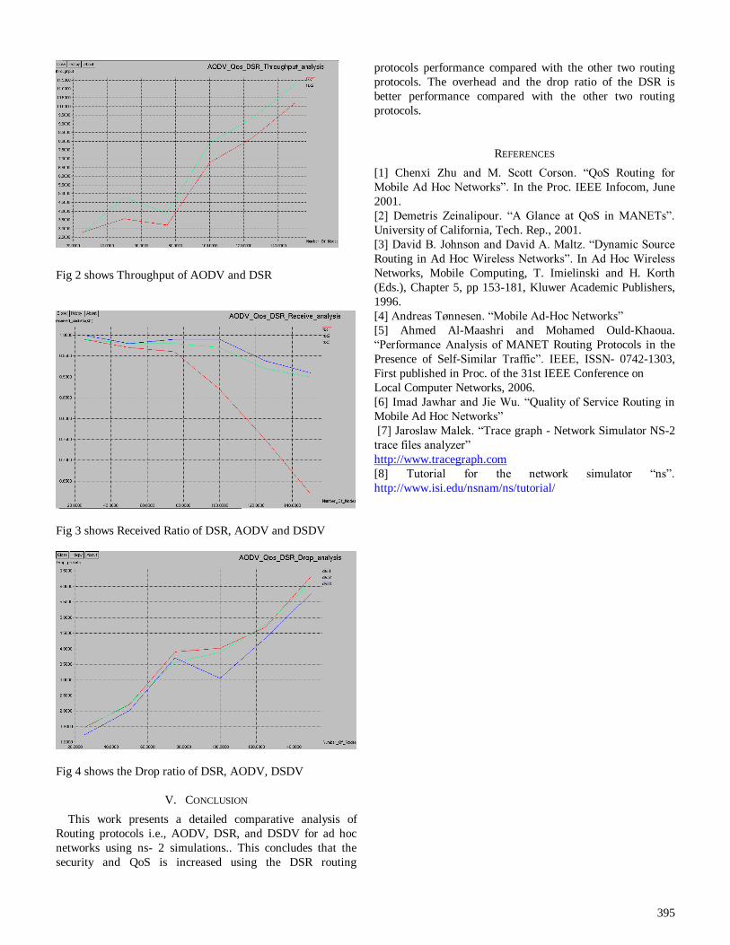
395
Fig 2 shows Throughput of AODV and DSR
Fig 3 shows Received Ratio of DSR, AODV and DSDV
Fig 4 shows the Drop ratio of DSR, AODV, DSDV
V. CONCLUSION
This work presents a detailed comparative analysis of
Routing protocols i.e., AODV, DSR, and DSDV for ad hoc
networks using ns- 2 simulations.. This concludes that the
security and QoS is increased using the DSR routing
protocols performance compared with the other two routing
protocols. The overhead and the drop ratio of the DSR is
better performance compared with the other two routing
protocols.
REFERENCES
[1] Chenxi Zhu and M. Scott Corson. “QoS Routing for
Mobile Ad Hoc Networks”. In the Proc. IEEE Infocom, June
2001.
[2] Demetris Zeinalipour. “A Glance at QoS in MANETs”.
University of California, Tech. Rep., 2001.
[3] David B. Johnson and David A. Maltz. “Dynamic Source
Routing in Ad Hoc Wireless Networks”. In Ad Hoc Wireless
Networks, Mobile Computing, T. Imielinski and H. Korth
(Eds.), Chapter 5, pp 153-181, Kluwer Academic Publishers,
1996.
[4] Andreas Tønnesen. “Mobile Ad-Hoc Networks”
[5] Ahmed Al-Maashri and Mohamed Ould-Khaoua.
“Performance Analysis of MANET Routing Protocols in the
Presence of Self-Similar Traffic”. IEEE, ISSN- 0742-1303,
First published in Proc. of the 31st IEEE Conference on
Local Computer Networks, 2006.
[6] Imad Jawhar and Jie Wu. “Quality of Service Routing in
Mobile Ad Hoc Networks”
[7] Jaroslaw Malek. “Trace graph - Network Simulator NS-2
trace files analyzer”
http://www.tracegraph.com
[8] Tutorial for the network simulator “ns”.
http://www.isi.edu/nsnam/ns/tutorial/
Proceedings of the Third National Conference on RTICT 2010 Bannari Amman Institute of Technology, Sathyamangalam-638401
9-10 April 2010
396
Security in Mobile Adhoc Network
Amit Kumar Jaiswal Kamal Kant Pardeep Singh
[email protected] [email protected] [email protected]
Department of Computer Science and Engineering
National Institute of Technology, Hamirpur (H.P)
Abstract: In this paper, we discuss security issues and
their current solutions in the mobile ad hoc network. Due
to the vulnerable nature of the mobile ad hoc network,
there are numerous security threats that disturb the
development of it. We first analyze the main
vulnerabilities in the mobile ad hoc networks, which have
made it much easier to suffer from attacks than the
traditional wired network. Then we discuss the security
criteria of the mobile ad hoc network and present the
main attack types that exist in it. Finally we survey the
current security solutions for the mobile ad hoc network.
I. INTRODUCTION
The Mobile Ad Hoc Network is one of the wireless
networks that have attracted most concentrations
from many researchers. A Mobile Ad hoc NETwork (MANET) is a system of wireless mobile nodes that
dynamically self-organize in arbitrary and temporary
network topologies. People and vehicles can thus be
internetworked in areas without a preexisting
communication infrastructure or when the use of such
infrastructure requires wireless extension [1]. In the
mobile ad hoc network, nodes can directly
communicate with all the other nodes within their
radio ranges; whereas nodes that not in the direct
communication range use intermediate node(s) to
communicate with each other. In these two situations,
all the nodes that have participated in the communication automatically form a wireless
network, therefore this kind of wireless network can
be viewed as mobile ad hoc network. The mobile ad
hoc network has the following typical features [2]:
Unreliability of wireless links between nodes.
Because of the limited energy supply for the wireless
nodes and the mobility of the nodes, the wireless
links between mobile nodes in the ad hoc network are
not consistent for the communication participants.
The rest of the paper is organized as follows: In
Section 2, we discuss the main challenges that make the mobile ad hoc networks unsecure. In Section 3,
we discuss security goals for the mobile ad hoc
networks, in Section 4 and 5 we will discuss the few
existing solution for security in Adhoc network and
at last we have given some open challenges for
mobile adhoc network.
II. CHALLENGES
Lack of secure boundaries makes the mobile ad hoc
network susceptible to the attacks. The mobile ad hoc
network suffers from all-weather attacks, which can
come from any node that is in the radio range of any
node in the network, at any time, and target to any
other node(s) in the network. The attacks mainly
include passive eavesdropping, active interfering,
leakage of secret information, data tampering,
message replay, message contamination, and denial
of service Secondly, in many situations the nodes may be left unattended in a hostile environment. This
enables adversaries to capture them and physically
attack them. Proper precautions (tamper resistance)
are required to prevent attackers from extracting
secret information from them. Even with these
precautions, we cannot exclude that a fraction of the
nodes may become compromised. This enables
attacks launched from within the network. Thirdly, an
ad hoc network is dynamic because of frequent
changes in both its topology and its membership (i.e.,
nodes frequently join and leave the network). Trust relationship among nodes also changes, Fourthly,
many wireless nodes will have a limited energy
resource (battery, solar panel, etc.). This is
particularly true in the case of ad hoc sensor
networks. Security solutions should be designed with
this limited energy budget in mind. lack of
centralized management machinery will impede the
trust management for the nodes in the ad hoc network
[2]. In mobile ad hoc network, all the nodes are
required to cooperate in the network operation, while
no security association (SA2) can be assumed for all
the network nodes. Thus, it is not practical to perform an a priori classification, and as a result, the usual
practice of establishing a line of defense, which
distinguishes nodes as trusted and nontrusted, cannot
be achieved here in the mobile ad hoc network.
III. SECURITY GOALS
To secure an adhoc network, we consider the
following attributes: availability, confidentiality,
integrity, authentication, and non-repudiation.
397
Availability ensures the survivability of network
services despite denial of service attacks. A denial of
service attack could be launched at any layer of an ad
hoc network.
Confidentiality ensures that certain information is
never disclosed to unauthorized entities. Network transmission of sensitive information, such as
strategic or tactical military information, requires
confidentiality. Leakage of such information to
enemies could have devastating consequences.
Integrity guarantees that a message being transferred
is never corrupted. A message could be corrupted
because of benign failures, such as radio propagation
impairment, or because of malicious attacks on the
network.
Authentication enables a node to ensure the identity
of the peer node it is communicating with. Without
authentication, an adversary could masquerade a node, thus gaining unauthorized access to resource
and sensitive information and interfering with the
operation of other nodes.
Non-repudiation ensures that the origin of a message
cannot deny having sent the message. Non-
repudiation is useful for detection and isolation of
compromised nodes. When a node A receives an
erroneous message from a node B, non-repudiation
allows A to accuse B using this message and to
convince other nodes that B is compromised.
IV. SECURE ADHOC ROUTING PROTOCOLS
The secure adhoc routing protocols enhance the
existing ad hoc routing protocols, such as DSR and
AODV with security extensions. In these protocols,
one node signs its routing messages using some
cryptographic authentication method like digital
signature so that each node can authenticate the legal
traffic efficiently and distinguish the unauthenticated message packets from attackers and correct packets.
However, there are still chances that an authenticated
node has been compromised and controlled by the
malicious attacker. Therefore, we have to further
ensure that a node obeys the routing protocols
properly even it is an authenticated node. In the
following, we describe how different types of routing
protocols are secured.
A. Source Routing
For source routing protocols such as DSR, the main
challenge is to ensure that none of intermediate
nodes can remove already existing nodes from or add
extra nodes into the route. The basic idea is to attach
a per-hop authenticator for the source routing
forwarder list so that any altering of the list can be
detected right away. A secure extension of DSR is
Ariadne, which is described in [3].
B. Distance Vector Routing
For distance vector routing protocols such as
AODV, the main challenge is that the information
about the routing metric has to be advertised
correctly by each intermediate node. For example, if we use hop count as the routing metric, each node has
to increase the hop count only by one exactly. A hop
count hash chain is used so that none of the
intermediate nodes can decrease the hop count in a
routing update to achieve benefits, which is described
in [4].
C. Secure Packet Forwarding
The routing message exchange is only one part of the
network-layer protocol which needs to be protected.
It is still possible that malicious nodes deny
forwarding packages correctly even they have acted
correctly during the routing discovery phase. The basic idea to solve this issue is to ensure that each
node indeed forwards packages according to the
protocol. Reactive methods should be used instead of
proactive methods since attacks on package
forwarding cannot be prevented.
V. MULTICAST SECURITY IN MANET
Integrity plays an important role in ad-hoc
networks. To overcome man-in-the-middle attack in
mobile-ad-hoc networks, SHA-1 algorithm is used. Normally, hop count field is mutable in nature. To
protect this hop count value, hash values are found by
using SHA-1 algorithm for those fields. Here, the
packets are sent along with the hashed values of hop
count field. Now, the malicious nodes, which
forwards the false routing information, can be
effectively defended [5].This algorithm takes input as
source address, destination address and hop count
with a maximum length of less than 264 bits and
produces output as a 160-bits message digest. The
input is processed in 512-bits blocks. This algorithm
includes the following steps [6]. Padding —The purpose of message padding is to
make the total length of a padded message congruent
to 448 modulo 512 (length = 448 mod 512). The
number of padding bits should he between 1 and 512.
Padding consists of a single 1-bit followed by the
necessary number of 0-bits.
Appending Length— The 64-bit binary representation
of the original length of the message is appended to
the end of the message.
Initialize the SHA-1 buffer —The 160-bit buffer is
represented by five four-word buffers (A, B, C, D, E) used to store the middle or finally results of the
message digests for SHA-I functions and they are
initialized to the following values in hexadecimal.
Low-order bytes are put first:

398
Word A: 67 45 23 01
Word B: EF CD AB 89
Word C: 98 BA DC EF
Word D: 10 32 54 16
Word E: C3 D2 El FO
Process message in 16-word blocks The heart of the algorithm is a module that consists of four rounds
of processing 20 steps each. The four rounds have a
similar structure, but each uses a different primitive
logical function. These logical functions are defined
as follows:
Initialize hash value :
a := A
b := B
c := C
d := D
e := E
Main loop: for i from 0 to 79
if 0 ≤ i ≤ 19 then
f := (b and c) or ((not b) and d)
k := 0x5A827999
else if 20 ≤ i ≤ 39
f := b xor c xor d
k := 0x6ED9EBA1
else if 40 ≤ i ≤ 59
f := (b and c) or (b and d) or (c and d)
k := 0x8F1BBCDC
else if 60 ≤ i ≤ 79 f := b xor c xor d
k := 0xCA62C1D6
The output of the fourth round is added to the input
of the first round, and then the addition is modulo 232
produce the ABCDE value that calculate next 5l2-
bits block.
Output After all 512-bits blocks have been processed,
the output of the last block is the 160-bits message
digest. These message digest values are sent along
with the packets .So, the packets which are sent by
malicious nodes are suppressed. Thus, the integrity is
ensured.
VI. OPEN CHALLENGES
The research on MANET security is still in its early
stage. The existing proposals are typically attack-
oriented in that they first identify several security
threats and then enhance the existing protocol or
propose a new protocol to thwart such threats.
Because the solutions are designed explicitly with
certain attack models in mind, they work well in the
presence of designated attacks but may collapse under unanticipated attacks. Therefore, a more
ambitious goal for d hoc network security is to
develop a multifence security solution that is
embedded into possibly every component in the
network, resulting in in-depth protection that offers
multiple lines of defense against many both known
and unknown security threats. This new design
perspective is what we call resiliency-oriented
security design. We envision the resiliency-oriented
security solution as possessing several features. First, the solution seeks to attack a bigger problem space. It
attempts not only to thwart malicious attacks, but also
to cope with other network faults due to node
misconfiguration, extreme network overload, or
operational failures. In some sense, all such faults,
whether incurred by attacks or misconfigurations,
share some common symptoms from both the
network and end-user perspectives, and should be
handled by the system. Second, resiliency-oriented
design takes a paradigm shift from conventional
intrusion precertain degrees of intrusions or
compromised/captured nodes are the reality to face, not the problem to get rid of, in MANET security.
The overall system has to be robust against the
breakdown of any individual fence, and its
performance does not critically depend on a single
fence. Even though attackers intrude through an
individual fence, the system still functions, but
possibly with graceful performance degradation.
Third, as far as the solution space is concerned,
cryptography-based techniques just offer a subset of
toolkits in a resiliency-oriented design. The solution
also uses other noncrypto-based schemes to ensure resiliency. For example, it may piggyback more
“protocol invariant” information in the protocol
messages, so that all nodes participating in the
message exchanges can verify such information. The
system may also exploit the rich connectivity of the
network topology to detect inconsistency of the
protocol operations. In many cases, routing messages
are typically propagated through multiple paths and
redundant copies of such messages can be used by
downstream nodes. Fourth, the solution should be
able to handle unexpected faults to some extent. One
possible approach worth exploring is to strengthen the correct operation mode of the network by
enhancing more redundancy at the protocol and
system levels. At each step of the protocol operation,
the design makes sure what it has done is completely
along the right track. Anything deviating from valid
operations is treated with caution. Whenever an
inconsistent operation is detected, the system can
raise a suspicion flag and query the identified source
for further verification. This way, the protocol tells
right from wrong because it knows right with higher
confidence, not necessarily knowing what is exactly wrong. The design strengthens the correct operations
and may handle even unanticipated threats in runtime
operations. Next, the solution may also take a
collaborative security approach, which relies on

399
multiple nodes in a MANET to provide any security
primitives. Therefore, no single node is fully trusted.
Instead, only a group of nodes will be trusted
collectively. The group of nodes can be nodes in a
local network neighborhood or all nodes along the
forwarding path. Finally, the solution relies on multiple fences, spanning different devices, different
layers in the protocol stack, and different solution
techniques, to guard the entire system. Each fence
has all functional elements of prevention,
detection/verification, and reaction. The above
mentioned resiliency-oriented MANET security
olution poses grand yet exciting research challenges.
How to build an efficient fence that accommodates
each device’s resource constraint poses an interesting
challenge. Device heterogeneity is one important
concern that has been largely neglected in the urgent
security design process. However, multifence security protection is deployed throughout the
network, and each individual fence adopted by a
single node may have different security strength due
to its resource constraints. A node has to properly
select security mechanisms that fit well into its own
available resources, deployment cost, and other
complexity concerns. The security solution should
not stipulate the minimum requirement a component
must have. Instead, it expects best effort from each
component. The more powerful a component is, the
higher degree of security it has. Next, identifying the system principles of how to build such a new-
generation of network protocols remains unexplored.
The state-of-the-art network protocols are all
designed for functionality only. The protocol
specification fundamentally assumes a fully rusted
and well-behaved network setting for all message
exchanges and protocol operations. It does not
anticipate any faulty signals or ill behaved nodes. We
need to identify new principles to build the next-
generation network protocols that are resilient to
faults. There only exist a few piecemeal individual
efforts. Finally, evaluating the multifence security design also offers new research opportunities. The
effectiveness of each fence and the minimal number
of fences the system has to possess to ensure some
degree of security assurances should be evaluated
through a combination of analysis, simulations, and
measurements in principle. However, it is recognized
that the current evaluation for state-of-the-art
wireless security solutions is quite ad hoc. The
community still lacks effective analytical tools,
particularly in a large scale wireless network setting.
The multidimensional trade-offs among security strength, communication overhead, computation
complexity, energy consumption, and scalability still
remain largely unexplored. Developing effective
evaluation methodology and toolkits will probably
need interdisciplinary efforts from research
communities working in wireless networking, mobile
systems, and cryptography.
VII. CONCLUSION
In this paper we have discussed the several security
issues in Mobile Adhoc Network. We have also given
some existing solution to these security problem but
the solutions available are not enough to cover all the
security threats. At last we have also given the open
challenges that exists in the field of Mobile Adhoc
Network and need to be solved.
REFERENCES
[1] M.S. Corson, J.P. Maker, and J.H. Cernicione,
Internet-based Mobile Ad Hoc Networking, IEEE Internet Computing, pages 63–70, July-August 1999.
[2] Amitabh Mishra and Ketan M. Nadkarni, Security
in Wireless Ad Hoc Networks, in Book The
Handbook of Ad Hoc Wireless Networks (Chapter
30), CRC Press LLC, 2003.
[3] Y. Hu, A. Perrig, and D. Johnson, Ariadne: A
Secure On-demand Routing Protocol for AdHoc
Networks, ACM MOBICOM, 2002.
[4] M. Zapata, and N. Asokan: Securing Ad Hoc
Routing Protocols, ACM WiSe, 2002.
[5] Junaid Arshad and Mohammad Ajmal Azad,“ Performance Evaluation of Secure on Demand
Routing Protocols for Mobile Adhoc Networks”,
IEEE Network, 2006, pp 971-975.
[6] Dai Zibin and Zhou Ning, “FPGA
Implementation of SHA-1 Algorithm”, IEEE 2003,
pp 1321-1324 .
[7] Yongguang Zhang and Wenke Lee, Security in
Mobile Ad-Hoc Networks, in Book AdHoc Networks
Technologies and Protocols (Chapter 9), Springer,
2005.
[8] Panagiotis Papadimitraos and Zygmunt J. Hass,
Securing Mobile Ad Hoc Networks, in Book The Handbook of Ad Hoc Wireless Networks (Chapter
31), CRC Press LLC, 2003.
[9] Yi-an Huang and Wenke Lee, A Cooperative
Intrusion Detection System for Ad Hoc Networks, in
Proceedings of the 1st ACM Workshop on Security of
Ad hoc and Sensor Networks, Fairfax, Virginia, 2003,
pp. 135 – 147.
[10] Data Integrity, from Wikipedia, the free
encyclopedia,http://en.wikipedia.org/wiki/Data_integ
rity.
[11] P. Papadimitratos and Z. J. Hass, Secure Routing for Mobile Ad Hoc Networks, in Proceedings of SCS
Communication Networks and Distributed Systems
Modeling and Simulation Conference (CNDS), San
Antonio, TX, January 2002
Proceedings of the Third National Conference on RTICT 2010
Bannari Amman Institute of Technology, Sathyamangalam-638401
9-10 April 2010
400
Abstract—Sensor networks consist of large number of tiny
nodes. Each node is operated by battery of limited energy.
Hence the major design challenge in sensor network is to
increase their operational lifetime as much as possible. The
existing topology management schemes improve the lifetime at
the cost of either latency or packet loss. The aim of our work is
to improve the energy efficiency of the sensor network without
packet loss. The STEM (Sparse Topology and Energy
Management) reduces energy consumption in the monitoring
state, by switching the radio off when they are not in use.
Geographic Adaptive Fidelity (GAF) reduces the energy
consumption of the sensor nodes by dividing the sensor
network into small virtual square grids and keeps only one
node in active state in each grid which will take part in the
traffic forwarding process. Since STEM and GAF are
orthogonal to each other, more energy can be saved by
integrating these two schemes but the packet loss due to
unreachable corner arises. To overcome this problem we have
replaced the square grids in GAF by hexagonal grids (GAF-h)
and integrate STEM with GAF-h. Our proposed work has
improved the energy efficiency of the sensor network without packet loss.
Keywords— sensor networks, topology management, energy efficiency and network lifetime
I. INTRODUCTION
sensor network is composed of a large number of sensor nodes that are densely deployed either inside the area to be monitored or very close to it. The position of
sensor nodes need not be predetermined. Hence random deployment in inaccessible terrains or disaster relief operations is possible. On the other hand, this also means that sensor network protocols and algorithms must possess self-organizing capabilities. Sensor nodes consist of sensing unit, processing unit, transceiver unit and power unit. The sensing unit consists of sensors which will sense the interested parameter. The output data of the sensor unit is partially processed by the onboard processor in the sensing unit. The partially processed data is then transmitted to the sink through multi hop wireless path. The power unit consists of a battery source of limited energy, which will supply power to all other units in the node. Such sensor network has the application in wildlife observation and office
buildings. The sensor networks are used in battlefield and disaster area monitoring.
The major design challenge in sensor network is to increase the operational lifetime of the sensor node as much as possible, because the sensor nodes are powered by the battery of limited energy. The available energy should be utilized efficiently. In terms of energy consumption, the wireless exchange of data between the nodes will strongly dominates the other node functions such as sensing and processing. The radio in transceiver unit consume almost the same energy in receive and idle states. Most of the time, the sensor network is in monitoring state and the radio is being idle. Since the significant energy saving can be obtained by switch off the radio when it is idle.
The aim of the topology management scheme is to maintain the sufficient network connectivity between the nodes such that the data can be forwarded efficiently to the sink. The existing topology management scheme called Geographic Adaptive Fidelity (GAF) reduces the energy consumption of the sensor node at the cost of packet loss. GAF divides the sensor field into number of virtual square grids and kept only one node in active state in each grid. All other nodes in each grid are kept in sleep mode and hence it will reduce the energy consumption of the sensor nodes.
Sparse Topology and Energy Management (STEM) is a topology management scheme which will reduce the energy consumption of the sensor node at the cost of latency. STEM turns off the radio and it will wakes up its radio when it is needed to transmit data to the sink. Now, the problem is that the radio of the next hop in the path to the data sink is still turned off. To overcome this problem, each node periodically turns on its radio for a short time to check whether any other nodes want to communicate with it. In order to avoid the interference between the wake up protocol and the data packet transmission, dual radio with separate radios operating at different frequency bands are used.
GAF controls the node density to save energy without affecting the data forwarding capacity. STEM saves energy by putting the radio of the sensor node into the sleep mode when they are not in use. We can get better result by utilizing the advantages of both schemes. Fortunately STEM and GAF are orthogonal to each other and hence the resulting energy gain will be the full potential of both schemes.
In GAF-h, the sensor field is divided into number of virtual grids and in each grid only one node is kept in active
Energy Efficient Hybrid Topology Management
Scheme for Wireless Sensor Networks
S. Vadivelan #1
, A. Jawahar #2
#Electronics and Communication Engineering, SSN College of Engineering, Chennai, TamilNadu, India 603110
[email protected] [email protected]
A

401
state. The node in active state will act as the grid head and takes part in the routing function. In combined scheme, the GAF-h manages one of the nodes in each grid as grid head based on its available energy. STEM controls grid head between the sleep mode and the active mode.
II. GEOGRAPHIC ADAPTIVE FIDELITY (GAF)
Geographic Adaptive Fidelity (GAF) [3] divides the sensor field into number of virtual square grids of side r. The size of the square grid r is chosen such that all the nodes in a grid can be reached by all the nodes in its horizontal and vertical adjacent grids.
Figure 1. GAF grid size.
In order to make all the nodes in the adjacent grid can be
reachable for all the nodes in the grid the size of the grid is
set as shown in Figure 1. By applying Pythagoras theorem, the value of R is given
by
25rR
To make all the nodes in the adjacent grids are reachable, the sides of the virtual square grid r must be
5
Rr
Where R is radio range and r is the sides of the virtual square grid.
Since all the nodes in a grid can be reached by all the nodes in its adjacent grids, it is possible to perform routing function with single node in each grid. GAF keeps only one node in active mode in each grid and all other nodes in the sleep mode. In sleep mode the sensing and processing units are kept on and the radio unit is switched off. Whenever the node has data to send, it will turn on its radio unit. The active node in each grid will act as the grid head and take part in the data forwarding process. In order to balance the energy consumption of the nodes, the responsibility of grid head is rotating among the nodes in the grid. The grid head is elected based on the remaining energy available in the battery source. Therefore the energy consumption of the node is shared equally by all the nodes in the grid. If we have ns nodes in the square grid, the nodes in the grid will be in active mode for only 1/ns
th of the time. Therefore the energy
consumed by the node is reduced by ns times and hence the lifetime of the node is increased by ns times.
The average number of nodes in each grid is given by
2
2r
L
Nns
Where, ns is the average number of nodes in the grid, N is the total number of nodes deployed, L2 is the area of the sensor field and r2 is the area of a square grid.
A. Unreachable Corner Problem
GAF sizes its virtual grid based on the radio range R such that the nodes in any adjacent grids must be able to reach each other with single hop. To evaluate the upper bound of life time, r is set such that
5
Rr
In GAF, nodes in a grid is reachable to all the nodes in the vertical and horizontal grids using single hop and considered as neighbors but not all the nodes in the diagonal grid are reachable [5] as shown in Figure 2.
Figure 2. Unreachable corner in GAF.
In order to reach the nodes in the diagonal grid, the transmission range can be increased. But if we increase the transmission range, the transceiver consumes more energy. If we keep the transmission range constant and reduce the grid size to overcome the unreachable corner node problem, the number of grid increases and hence the number of active node increases. This leads to more energy consumption and decreases the lifetime of the network.
The Probability of a node is not reachable by another node
is the probability of distance between the nodes is greater
than R.
Punreach=Pdistance between nodes >R (5)
r r
r R

402
B. Diagonal Forwarding Probability
Consider a packet originated from a node and its destinations are evenly distributed through the space. The choice of the next hop cell depends on the position of the destination. When the next hop node falls into a diagonal grid, it may be unreachable.
Figure 3. Adjacent grids in GAF.
The probability that a packet is routed via diagonal grid is
Pgridsadjacent ofnumber Total
gridsadjacent diagonal ofNumber diagonal via
5.08
4 diagonal Pvia
C. Loss Probability in GAF
When the node is not reachable to the node in the adjacent diagonal grid, then the data packets send to that node will be lost or dropped. So the retransmission of the lost packets will be required which will take alternate path to the destination. The alternate path may have more number of hops and hence more number of nodes spends their energy to forward the packets to the sink. It also causes congestion in traffic flow and hence the throughput of the network is reduced.
The probability of packet loss due to unreachable nodes
can be written as
P packet loss = P un reach × P via diagonal
To overcome the problem of packet loss due to unreachable nodes, we have replaced the square virtual grid in GAF by the hexagonal virtual grid [5]. In hexagonal virtual mesh each hexagonal grid has six neighbor grids. The GAF with hexagonal grids is called as GAF-h. The size of the hexagon is based on the radio range of the transmitter. The size of the hexagon is chosen such that a node in the hexagonal grid can communicate with all nodes in its six adjacent hexagonal grids within single hop.
The virtual hexagonal grid is formed such that all the nodes in a grid can reach all the nodes in the neighbor grids
within the single hop. To evaluate the upper bound of life time of the sensor nodes, the side r of the hexagon is set to
13
Rr
Where r is the side of the hexagonal grid and R is the transmission range.
Figure 4. Adjacent grids in GAF-h.
Therefore the area a of one hexagonal grid is
2
2
33ra
The area of hexagonal grid in terms of radio transmission range is obtained by applying (9) in (10).
2
26
33Ra (11)
The average number of nodes in a hexagonal grid is
aL
Nnh 2
Where, nh is the average number of nodes in a hexagonal grid and a is the area of one hexagonal grid.
The cell placement of GAF-h topology management scheme is shown in the figure 5.
The horizontal distance between the centers of the hexagonal grid to one half of the side of the hexagon along the straight line is
O
D D
D D
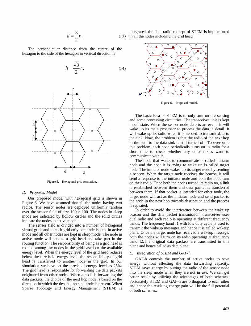
403
rd2
3
The perpendicular distance from the centre of the hexagon to the side of the hexagon in vertical direction is
rh2
3
Figure 5. Hexagonal grid formation.
D. Proposed Model
Our proposed model with hexagonal grid is shown in Figure 6. We have assumed that all the nodes having two radios. The sensor nodes are deployed uniformly random over the sensor field of size 100 × 100. The nodes in sleep mode are indicated by hollow circles and the solid circles indicate the nodes in active mode.
The sensor field is divided into a number of hexagonal virtual grids and in each grid only one node is kept in active mode and all other nodes are kept in sleep mode. The node in active mode will acts as a grid head and take part in the routing function. The responsibility of being as a grid head is rotated among the nodes in the grid based on the available energy level. When the energy level of the grid head reduces below the threshold energy level, the responsibility of grid head is transferred to another node in the grid. In our simulation we have set the threshold energy level as 25%. The grid head is responsible for forwarding the data packets originated from other nodes. When a node is forwarding the data packets, the choice of the next hop node is based on the direction in which the destination sink node is present. When Sparse Topology and Energy Management (STEM) is
integrated, the dual radio concept of STEM is implemented in all the nodes including the grid head.
Figure 6. Proposed model.
The basic idea of STEM is to only turn on the sensing
and some processing circuitries. The transceiver unit is kept in off state. When the sensor node detects an event, it will wake up its main processor to process the data in detail. It will wake up its radio when it is needed to transmit data to the sink. Now, the problem is that the radio of the next hop in the path to the data sink is still turned off. To overcome this problem, each node periodically turns on its radio for a short time to check whether any other nodes want to communicate with it.
The node that wants to communicate is called initiator node and the node it is trying to wake up is called target node. The initiator node wakes up its target node by sending a beacon. When the target node receives the beacon, it will send a response to the initiator node and both the node turn on their radio. Once both the nodes turned its radio on, a link is established between them and data packet is transferred between them. If that packet is intended for other node, the target node will act as the initiator node and send packet to the node in the next hop towards destination and the process is repeated.
In order to avoid the interference between the wake up beacon and the data packet transmission, transceiver uses dual radio and each radio is operating at different frequency bands. The frequency band f1 with low duty cycle is used to transmit the wakeup messages and hence it is called wakeup plane. Once the target node has received a wakeup message, both the nodes will turn on its radio operating at frequency band f2.The original data packets are transmitted in this plane and hence called as data plane.
E. Integration of STEM and GAF-h
GAF-h controls the number of active nodes to save energy without affecting the data forwarding capacity. STEM saves energy by putting the radio of the sensor node into the sleep mode when they are not in use. We can get better result by utilizing the advantages of both schemes. Fortunately STEM and GAF-h are orthogonal to each other and hence the resulting energy gain will be the full potential of both schemes.
h
h
d d
r

404
In GAF-h, the sensor field is divided into number of virtual hexagonal grids and in each grid only one node is kept in active state. The node in active state will act as the grid head and takes part in the routing function. In combined scheme, the GAF-h manages one of the nodes in each grid as grid head based on its available energy. STEM controls grid head between the sleep mode and the active mode.
In GAF-h, the energy consumption of a sensor node is
hn
EE 0
Where, E0 is the energy consumption of a node at normal condition and nh is the number of nodes in that grid. .
When the STEM is interacted with GAF-h, the power
consumption of the node become
h
wakeupdata
n
EEE
Where E is the energy consumption of a node with
hybrid scheme, Edata is the energy consumption of a node in
data plane, Ewakeup is the energy consumption of a node in
wakeup plane and nh is the number of nodes in the grid.
III. PERFORMANCE EVALUATION
We verify our algorithm through simulations. We deploy N number of nodes in an uniformly random fashion over the square field of size L × L and each node has transmission range R. For a network having large number of deployed nodes N, the probability for a node to have n neighbor is approximated by Poisson distribution.
x
n
en
xnP
!)(
The average number of neighbors of a node is denoted by the parameter x.
2
2R
L
Nx
Where, x is the average number of neighbor which
denotes the average number of nodes within the coverage
area of node and R2 is the coverage area of the transmitter of a node.
A. Simulation Setup
In our simulation we have chosen the transmission
range R = 20 m, which has the radio characteristics as
shown in the table 1.
TABLE I. RADIO CHARECTERISTICS
Radio mode Power consumption (mW)
Transmit (Tx) 14.88
Receive (Rx) 12.50
Idle 12.36
Sleep 0.016
We divide the square field of size 100 × 100 into number of square grids of size r × r. We have simulated the
GAF scheme and found out the number of unreachable
corner nodes and the percentage of packets lost. The
simulation is repeated by increasing the number of deployed
nodes of the order of 100.
B. Simulation Results
Figure 7 shows the number of unreachable corner nodes as the function of number of the number of nodes deployed. In GAF the number of unreachable corner nodes increases as the number of deployed nodes increases but in GAF-h the number of unreachable corner nodes is zero. In our simulation the number of unreachable corner nodes is 78 when the total number of deployed nodes is 1000.
Figure 7. Unreachable corners nodes.
Figure 8 shows the percentage of packet lost due to unreachable corners as the function of number of nodes deployed. In GAF the percentage of packet lost increases as the number of nodes deployed increases but in GAF-h, the percentage of packets lost is zero.
Figure 9 shows the normalized energy consumption of sensor node as the function of average number of neighbors in GAF-h, STEM, our proposed scheme and the normalized energy consumption of a sensor node without any schemes. We have plotted the energy consumption of node in STEM

405
scheme with the wake up interval of 600 ms over the observation time of 1000 ms.
Figure 8. Packet loss.
Figure 9. Energy Consumption of a node.
In STEM, the energy consumption of the node is constant with respect to the average number of neighbors,
because STEM works on the time domain. The energy
consumption of a node in GAF-h decreases with average
number of neighbors increases, because the GAF-h
algorithm is related to the density domain. When STEM is
integrated with GAF-h, we got further reduction in the
energy consumption of the sensor node. When the average
number of neighbors is 130, the normalized energy
consumption of a node is 0.16 in GAF-h, 0.38 in STEM and
the normalized energy consumption of a node is 0.06 in the
hybrid scheme of GAF-h and STEM.
IV. CONCLUSION
In this paper we have analyzed the GAF, a topology
management scheme that reduces the energy consumption
of the sensor node by using the node density. But in GAF
the diagonal adjacent grids are not taken into the
consideration. Hence there is the possibility of packet loss
due to unreachable corner nodes. In our work we replace the
square virtual grids by hexagonal virtual grids to overcome
the packet loss due to unreachable corner nodes and hence it
is called as GAF-h. GAF-h reduces the energy consumption of the sensor node by six.
On the other hand, STEM reduces the energy
consumption of the sensor node by switching its radio off
when they are idle. In this work we simulate STEM with
wakeup interval of 600 ms which reduce the energy
consumption of the node by the factor of about 2.5
We have integrated STEM with GAF-h and the hybrid
scheme reduces the energy consumption of the sensor node
by 18 times when the average number of neighbor is 130.
In our proposed scheme the energy conservation of about 18
times is achieved at the cost of latency. So it is worth
investigating how the energy efficiency can be improved with reduced latency.
REFERENCES
[1] I. F. Akyildiz, W. Su, Y. Sankarasubramaniam and E. Cayirci, “A
Survey on Sensor Networks,” IEEE Communications Magazine, vol. 40, pp. 102 - 114, 2002.
[2] I Mo Li, Baijian Yang, “A A Survey on Topology issues in Wireless
Sensor Network,” SPIE – The International Society for Optical Engineering, Orlando, FL, pp. 229-237, April 1999.
[3] Y. Xu, J. Heidemann, D. Estrin, “Geography-informed energy conservation for ad hoc routing,” MobiCom 2001, Rome, Italy, pp.
70-84, July 2001.
[4] Curt Schurgers, Vlasios Tsiatsis, Mani B. Srivastava, “STEM: Topology Management for Energy Efficient Sensor Networks,”
IEEEAC paper #260, Updated Sept 24, 2001.
[5] Ren Ping Liu*, Glynn Rogers, Sihui Zhou, John Zic, “Topology Control with Hexagonal Tessellation,” Feb 16, 2003.
[6] Curt Schurgers, Vlasios Tsiatsis, Saurabh Ganeriwal, Mani B.
Srivastava, “Optmimizing Sensor Networks in the Energy-Latency-Density Design Space,” IEEE Transactions on mobile computing,
vol. 1, No. 1, January-March 2002.
[7] Susumu Matsumae, Vlasios Tsiatsis, Mani B. Srivastava, “Energy-Efficient Cell Partition for Sensor Networks with Location
Information,” Network Protocols and Algorithms, Vol. 1, No. 2., 2009.
[8] Majid I. Khan,Wilfried N. Gansterer, Günter Haring, “Congestion
Avoidance and Energy Efficient Routing Protocol for Wireless Sensor Networks with a Mobile sink,” Journal of Networks, vol. 2,
No. 6, December 2007.
[9] Ya Xu, Solomon Bien, Yutaka Mori, John Heidemann, Deborah
Estrin “Topology Control Protocols to Conserve Energy in Wireless Adhoc Networks,” , January 23, 2003.
[10] Sankalpa Gamwarige, Chulantha Kulasekere, “A Cluster Based
Energy Balancing Strategy to Improve Wireless Sensor Network Lifetime,” Second International Conference on Industrial and
Information Systems, ICIIS 2007, Sri Lanka, 8 – 11 August 2007.
[11] Chuan-Yu Cho, Cheng-Wei Lin and Jia-Shung Wang, “Reliable Grouping GAF Algorithm using Hexagonal Virtual Cell Structure,”
3rd International Conference on Sensing Technology, Tainan, Nov. 30 – Dec. 3, 2008.
[12] Annette Bohm, “State of Art on Energy-Efficient and Latency-
Constrained Networking Protocol for Wireless Sensor Networks ,” Technical Report, IDE0749, June 2007.
Proceedings of the Third National Conference on RTICT 2010
Bannari Amman Institute of Technology, Sathyamangalam-638401
9-10 April 2010
406
RATE LESS FORWARD ERROR CORRECTION USING LDPC
FOR MANETS
N.Khadirkumar
Student, IInd
M.tech(IT Department), Anna University Coimbatore, Coimbatore-22. [email protected]
Abstract The Topology-transparent scheduling for mobile wireless ad hoc networks has been treated as a theoretical
curiosity. This makes two contributions towards its practical deployment. One is cover-free family and another one is rateless forward error correction. As a result from cover free family, a much wider number and variety of constructions for schedules exist to match network conditions. In simulation, I closely match the theoretical bound on expected throughput by using rateless forward error correction (RFEC). Since the wireless medium is inherently unreliable, RFEC also offers some measure of
automatic adaptation to channel load. These contributions renew interest in topology-transparent scheduling when delay is a principal objective.
Index Terms:
Mobile ad hoc Networks, rateless forward error correction, Topology-transparent scheduling
Introduction
Mobile ad hoc Networks is a collection of mobile
nodes that are dynamically communicating without
centralized supervision. It is self-creating, self-
organizing and self-administrating network. Absence
of the base station from the network necessitates the
functionality of the network nodes to include routing
as well. This task becomes more complex as the network nodes change randomly their positions. An
efficient routing protocol that minimizes the access
delay and power consumption while maximizing
utilization of resources remains a challenge for the
ad-hoc network design.
For these reasons we have considered efficient
routing protocols and we have evaluated their
performances on a different MAC layers.
Each device in a MANET is free to move
independently in any direction, and will therefore
change its links to other devices frequent. The
medium access protocol attempts to order to
minimum delay and maximum throughput on a per
hop basis on each nodes
A Vehicular Ad-Hoc Network, or VANET, is a
form of Mobile ad-hoc network, to provide
communications among nearby vehicles and between vehicles and nearby fixed equipment, usually
described as roadside equipment
Intelligent vehicular ad hoc networks
(InVANETs) are a kind of artificial intelligence that
helps vehicles to behave in intelligent manners during
vehicle-to-vehicle collisions, accidents, drunken
driving etc.
Scheduled approaches to channel access provide
deterministic rather than probabilistic delay
guarantees. This is important for applications
sensitive to maximum delay. Furthermore, the control overhead and carrier sensing associated with
contention MAC protocols can be considerable in
terms of time and energy [1].
Two approaches have emerged in response to
topology changes. Topology-dependent protocols
alternate between a contention phase in which
neighbor information is collected, and a scheduled
phase in which nodes follow a schedule constructed
using the neighbor information [2],[3]. Topology-
transparent protocols are to design schedules that are
independent of the detailed network topology. The
schedules do not depend on the identity of a node’s neighbors, but rather on how many of them are
transmitting. Even if a node’s neighbors change its
schedule does not change. The schedule is still
succeeds when the number of neighbors does not
exceed the designed bound.

407
The main objective of this paper is to reduce
delay and maximum throughput for mobile nodes.
Part 2, defines a cover-free family and examines time
division multiplexing and as I also derive the bound
on expected throughput. Part 3, discusses
acknowledgment schemes including RFEC for this purpose and overviews the LDPC process. In part 4,
the simulation environment is explained and in part 5,
the conclusion is stated.
RELATED WORK
The extensive work related to this paper can be
categorized into cover-free family and rateless
forward error correction
Cover Free Family
In designing a topology-transparent
transmission schedule with parameters N and D we
are interested in the following combinatorial property. For each node, we must guarantee that if a
node ʋi has at most D neighbors its schedule Si
guarantees a collision-free transmission to each
neighbor.
This is precisely a D cover-free family. These are
equivalent to D disjoint matrices and to superimposed
codes of order. As a result, there is also equivalence
between the no-tation used for cover-free families,
disjunct matrices, and superimposed codes. Such
combinatorial designs arise in many other
applications in networking. As we showed existing constructions for
topology- transparent schedules correspond to, time
division multiple access giving cover-free families.
Since this is essential to the provision of topology-
transparent schemes of sufficient variety and number
for practical applications, we outline this connection
in more detail.
TDMA-based MAC protocol developed for low
rate and reliable data transportation with the view of
prolonging the network lifetime,
Adapted from LMAC protocol. Compared to conventional -based protocols, which depend on
central node manager to allocate the time slot for
nodes within the cluster, our protocol uses distributed
technique where node selects its own time slot by
collecting its neighborhood information. The protocol
uses the supplied energy efficiently by applying a
scheduled power down mode when there is no data
transmission activity.
The protocol is structured into several frames,
where each frame consists of several time slots. As
shown in each node transmits a message at the beginning of its time slot, which is used for two
purposes; as synchronization signal and neighbor
information exchanges.
By using this message, the controlled node
informs which of its neighboring nodes will be
participating in the next data session. The intended
nodes need to stay in listening mode in order to be
able to receive the intended packet, while other nodes
turn to power down mode until the end of the current time. TDMA calculates collision frequency for each
nodes and automatically send packets from the source
to destination. By allocating time we can easily find
collision and thus it reduces time and the throughput
increases.
The operation of time slot assignment in A-MAC
is divided into four states; initial, wait, discover, and
active. As illustrated in the Fig. 4 below, a new node
that enters a network starts its operation in initial
state where node listens to the channel for its
neighbor’s beacon message in order to synchronize
with the network. Node starts synchronization when it receives a beacon message from one of its
neighbors and adjusts its timer by subtracting the
beacon received time with beacon transmission time.
Node remains in this state for a Listen frames in
order to find the strongest beacon signal. This is
important as to continuously receive the signal from
the synchronized node.
Else, a potential synchronization problem with
the rest of neighboring nodes might arise due to the
resulted drift problem caused by imprecision of
microcontroller’s timer. analyze the effects of MAC protocols, four ad hoc routing protocols are selected
for study. First, the Dynamic Source Routing (DSR)
and Ad hoc On-Demand Distance Vector Routing
protocol are included as examples of on demand
protocols. On-demand protocols only establish routes
when they are needed by a source node, and only
maintain these routes as long as the source node
requires them.
Structure of A-MAC frame
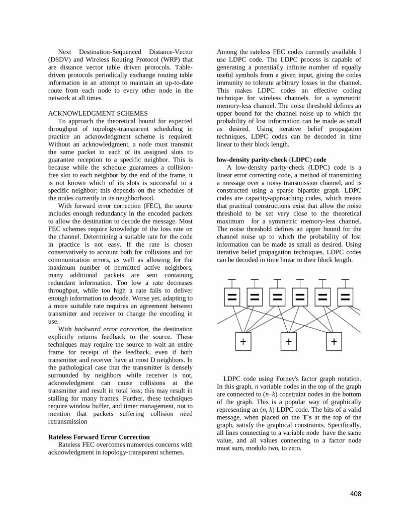
408
Next Destination-Sequenced Distance-Vector
(DSDV) and Wireless Routing Protocol (WRP) that
are distance vector table driven protocols. Table-
driven protocols periodically exchange routing table
information in an attempt to maintain an up-to-date
route from each node to every other node in the network at all times.
ACKNOWLEDGMENT SCHEMES
To approach the theoretical bound for expected
throughput of topology-transparent scheduling in
practice an acknowledgment scheme is required.
Without an acknowledgment, a node must transmit
the same packet in each of its assigned slots to
guarantee reception to a specific neighbor. This is
because while the schedule guarantees a collision-
free slot to each neighbor by the end of the frame, it
is not known which of its slots is successful to a specific neighbor; this depends on the schedules of
the nodes currently in its neighborhood.
With forward error correction (FEC), the source
includes enough redundancy in the encoded packets
to allow the destination to decode the message. Most
FEC schemes require knowledge of the loss rate on
the channel. Determining a suitable rate for the code
in practice is not easy. If the rate is chosen
conservatively to account both for collisions and for
communication errors, as well as allowing for the
maximum number of permitted active neighbors, many additional packets are sent containing
redundant information. Too low a rate decreases
throughput, while too high a rate fails to deliver
enough information to decode. Worse yet, adapting to
a more suitable rate requires an agreement between
transmitter and receiver to change the encoding in
use.
With backward error correction, the destination
explicitly returns feedback to the source. These
techniques may require the source to wait an entire
frame for receipt of the feedback, even if both
transmitter and receiver have at most D neighbors. In the pathological case that the transmitter is densely
surrounded by neighbors while receiver is not,
acknowledgment can cause collisions at the
transmitter and result in total loss; this may result in
stalling for many frames. Further, these techniques
require window buffer, and timer management, not to
mention that packets suffering collision need
retransmission
Rateless Forward Error Correction
Rateless FEC overcomes numerous concerns with acknowledgment in topology-transparent schemes.
Among the rateless FEC codes currently available I
use LDPC code. The LDPC process is capable of
generating a potentially infinite number of equally
useful symbols from a given input, giving the codes
immunity to tolerate arbitrary losses in the channel.
This makes LDPC codes an effective coding technique for wireless channels. for a symmetric
memory-less channel. The noise threshold defines an
upper bound for the channel noise up to which the
probability of lost information can be made as small
as desired. Using iterative belief propagation
techniques, LDPC codes can be decoded in time
linear to their block length.
low-density parity-check (LDPC) code
A low-density parity-check (LDPC) code is a
linear error correcting code, a method of transmitting
a message over a noisy transmission channel, and is constructed using a sparse bipartite graph. LDPC
codes are capacity-approaching codes, which means
that practical constructions exist that allow the noise
threshold to be set very close to the theoretical
maximum for a symmetric memory-less channel.
The noise threshold defines an upper bound for the
channel noise up to which the probability of lost
information can be made as small as desired. Using
iterative belief propagation techniques, LDPC codes
can be decoded in time linear to their block length.
LDPC code using Forney's factor graph notation.
In this graph, n variable nodes in the top of the graph
are connected to (n–k) constraint nodes in the bottom
of the graph. This is a popular way of graphically
representing an (n, k) LDPC code. The bits of a valid
message, when placed on the T's at the top of the
graph, satisfy the graphical constraints. Specifically,
all lines connecting to a variable node have the same
value, and all values connecting to a factor node must sum, modulo two, to zero.
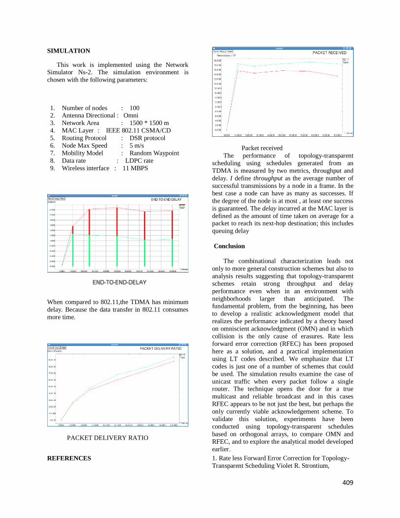
409
SIMULATION
This work is implemented using the Network Simulator Ns-2. The simulation environment is
chosen with the following parameters:
1. Number of nodes : 100 2. Antenna Directional : Omni
3. Network Area : 1500 * 1500 m
4. MAC Layer : IEEE 802.11 CSMA/CD
5. Routing Protocol : DSR protocol
6. Node Max Speed : 5 m/s
7. Mobility Model : Random Waypoint
8. Data rate : LDPC rate
9. Wireless interface : 11 MBPS
When compared to 802.11,the TDMA has minimum
delay. Because the data transfer in 802.11 consumes
more time.
PACKET DELIVERY RATIO
Packet received
The performance of topology-transparent
scheduling using schedules generated from an
TDMA is measured by two metrics, throughput and
delay. I define throughput as the average number of
successful transmissions by a node in a frame. In the
best case a node can have as many as successes. If
the degree of the node is at most , at least one success
is guaranteed. The delay incurred at the MAC layer is
defined as the amount of time taken on average for a packet to reach its next-hop destination; this includes
queuing delay
Conclusion
The combinational characterization leads not
only to more general construction schemes but also to
analysis results suggesting that topology-transparent
schemes retain strong throughput and delay
performance even when in an environment with
neighborhoods larger than anticipated. The fundamental problem, from the beginning, has been
to develop a realistic acknowledgment model that
realizes the performance indicated by a theory based
on omniscient acknowledgment (OMN) and in which
collision is the only cause of erasures. Rate less
forward error correction (RFEC) has been proposed
here as a solution, and a practical implementation
using LT codes described. We emphasize that LT
codes is just one of a number of schemes that could
be used. The simulation results examine the case of
unicast traffic when every packet follow a single router. The technique opens the door for a true
multicast and reliable broadcast and in this cases
RFEC appears to be not just the best, but perhaps the
only currently viable acknowledgement scheme. To
validate this solution, experiments have been
conducted using topology-transparent schedules
based on orthogonal arrays, to compare OMN and
RFEC, and to explore the analytical model developed
earlier.
REFERENCES 1. Rate less Forward Error Correction for Topology-
Transparent Scheduling Violet R. Strontium,

410
Member, IEEE, Charles J. Coburn, and South
Yellamraju
2. J.-H. Ju and V. O. K. Li, “An optimal topology-
transparent scheduling method in multihop packet
radio networks,” IEEE/ACM Trans. Networking, vol.
6, no. 3, pp. 298–306, Jun. 1998.
3. C. J. Colbourn, A. C. H. Ling, and V. R. Syrotiuk,
“Cover-free families and topology-transparent
scheduling for MANETs,” Designs, Codes, and
Cryptography, vol. 32, no. 1–3, pp. 35–65, May 2004.
4. V. R. Syrotiuk, C. J. Colbourn, and A. C. H. Ling,
“Topology-transparent scheduling for MANETs
using orthogonal arrays,” in Proc. DIAL-M/POMC
JointWorkshop on Foundations of Mobile
Computing, Sep. 2003, pp. 43–49.
5. D. R. Stinson, R. Wei, and L. Zhu, “Some new
bounds for cover-free families,” J. Combinatorial
Theory, ser. A, vol. 90, pp. 224–234, 2000.
6. M. Ruszinkó, “On the upper bound of the size of
the -cover-free families,” J. Combinatorial Theory,
ser. A, vol. 66, pp. 302–310, 1994.
7. D.-Z. Du and F. K. Hwang, Combinatorial Group
Testing and Its Applications,
ser. Series on Applied Mathematics, 2nd ed.
Singapore:World Scientific, 2000, vol. 12.
8. A. D’yachkov, V. Rykov, and A. M. Rashad,
“Superimposed distance
codes,” Problems Control and Information Theory,
vol. 18, pp.
237–250, 1989.
9.C. J. Colbourn, J. H. Dinitz, and D. R. Stinson,
“Applications of combinatorial designs to
communications, cryptography, and networking,” in
Surveys in Combinatorics, ser. Lecture Note Series
267, J. D. Lamb
and D. A. Preece, Eds. London, U.K.: London
Mathematical Society,
1999, pp. 37–100.

Proceedings of the Third National Conference on RTICT 2010
Bannari Amman Institute of Technology, Sathyamangalam-638401
9-10 April 2010
411
APPLICATION OF GENETIC ALGORITHM FOR THE DESIGN OF CIRCULAR MICROSTRIP ANTENNA
Mr. Rajendra Kumar Sethi,Sr. Lect,GIET,Gunupur,Orissa,[email protected] Ms. Nirupama Tripathy,Lect.,GIET,Gunupur,Orissa,[email protected]
Abstract
Microstrip antennas are widely used
in the telecommunication field. It has
advantages like low profile, low cost, ease
of construction, conformal geometry and
flexibility in terms of radiation pattern, gain
and polarization etc. The MoM based
Zealand IE3D software has been opted as an
efficient tool for microstrip antenna design
and analysis. On the other hand evolutionary
techniques like Genetic Algorithm, Particle
Swarm Optimization, Bacterial Foraging
Optimization and Artificial Neural Networks
etc have gained a great importance in the
field of antenna application. These are all
based on biological concepts. In this paper
we have applied Genetic Algorithm for
optimization of Circular microstrip antenna.
A genetic algorithm is natural selection
procedure, i.e survival of the fittest or
Darwinian principle. It is a population to
population global search technique based on
statistics.
Keywords
MoM, GA, IE3D, Crossover, Mutation
Introduction
Microstrip antenna has very low
bandwidth. Hence it is very important to
find an accurate dimension and its feed
position to efficiently operate such antenna.
There are many empirical formulae for
different regular structure microstrip patch
antenna for calculating the resonant
frequency. However, resonant frequency
being a non-linear function of parameters
like the physical dimensions and material
property of the antenna, it is quite difficult
to adjust all these parameters simultaneously
to design a microstrip patch antenna for a
particular operating frequency. Therefore,
Genetic Algorithm is applied in this thesis to
optimize such problems. Genetic Algorithm
performs its searching process through
population to population instead of point-to-
point search. The most favorite advantage of
Genetic Algorithm is its parallel architecture.
They use probabilistic and deterministic
rules.
Genetic Algorithm Overview

412
Generate initial population G(0) at random, i=0
Determine fitness of every individual in population G(i)
Select parents from G(i), based on
their fitness, and a genetic operator.
Apply genetic operator on selected parents to create one or more
individuals for G(i+1)
G(i+1) is filled up?
i=i+1
Termination criteria satisfied?
Yes
NO
Yes NO
Find the fittest individual in G(i), And Quit
Yes
a) A Genetic Algorithm is a global search
technique based on Darwinian principle,
i.e., survival of the fittest.
Figure. 1 Flow Chart of Genetic Algorithm
It performs following six basic
tasks:-
b) Encode the solution parameters as
genes,
c) Create a string of genes to form a
chromosome,
d) Initialize a starting population,
e) Evaluate and assign fitness values to
individuals in the population,
f) Perform reproduction through the
fitness-weighted selection of individuals
from the population, and
g) Perform crossover and mutation to
produce members of new generation
Design of Circular Microstrip Patch
Antenna using Genetic Algorithm
Circular microstrip antenna, due to
its simple design features is popular in
industrial and commercial applications.
However, due to inherent narrow bandwidth,
the resonant frequency or the dimension of
the patch antenna must be predicted
accurately.
Genetic Algorithm (GA) has been
applied to calculate the optimized radius of
Circular Microstrip Antennae. Resonant
frequency (f) in the dominant TM11 mode,
dielectric constant (r) and thickness of the
substrate (h) are taken as inputs to GA,
which gives the optimized radii (a) of the
antennae. We have applied Method of
Moment (MOM) based IE3D software of the
Zealand Inc., USA to validate experimental
results with that of GA outputs. It is shown
in the table that the GA results are more
accurate while taking less computational

413
time. The results are in good agreement with
experimental findings.
The circular patch antenna with its
design parameters i.e. thickness of substrate
„h‟ and radius of circular patch „a‟, is shown
in figure 2.
Fig. 2 Circular Patch Antenna
The resonant frequency of circular
microstrip antenna is expressed as:
2/1
0
))]65.1268.0()77.144.1()2
(ln(2
1[2
84118.1
rr
r
eff
r
a
h
h
a
a
ha
cf
[1]
Where, the effective dielectric constant
( eff), is given by
2/112
12
1
2
1
a
hrr
eff
[2]
And c0 is the velocity of light.
Equation (1) is used as the fitness
function of GA to optimize radius of the
patch of the antennae. The population size is
taken 20 individuals, and 200 generations
are produced. The probability of crossover is
set at 0.25, while the probability of mutation
was equal to 0.01. Resonant frequency (fr),
dielectric constant (r) and thickness of the
substrate (h) are given as inputs to GA,
which gives the optimized radii (a) of the
antennae. The comparisons of GA and
results obtained by IE3D software are listed
in table 1 for nine different fabricated
circular microstrip antennae. The optimized
radii (a) obtained using GA are in good
agreement with the experimental results as
listed in column „VII‟ of table 1.
Using these calculated radius (a) in
IE3D simulation software, resonant
frequencies are calculated which almost
match with the input resonant frequencies
used as input, thus, validating the results of
GA. The percentage of error in calculation
of radius using GA, are listed in column VI.
Average error obtained using GA is only
0.65.
Table 1 Comparison of Genetic Algorithm Result
with Experimental Result
I II III IV V VI VII
a A
n te
nna
No. rf
In
GHz
r
h
In
mm
a
In
mm
By GA
Error
In %
DIEf 3
In
GHz
1 4.945 4.55 2.35 7.6742 0.306234 4.94
2 3.75 4.55 2.35 10.3837 0.156731 3.735
3 2.003 4.55 2.35 20.0659 0.3295 2.02
4 1.03 4.55 2.35 39.5602 0.477484 1.05
5 0.825 4.55 2.35 49.502 0.0040404 0.82
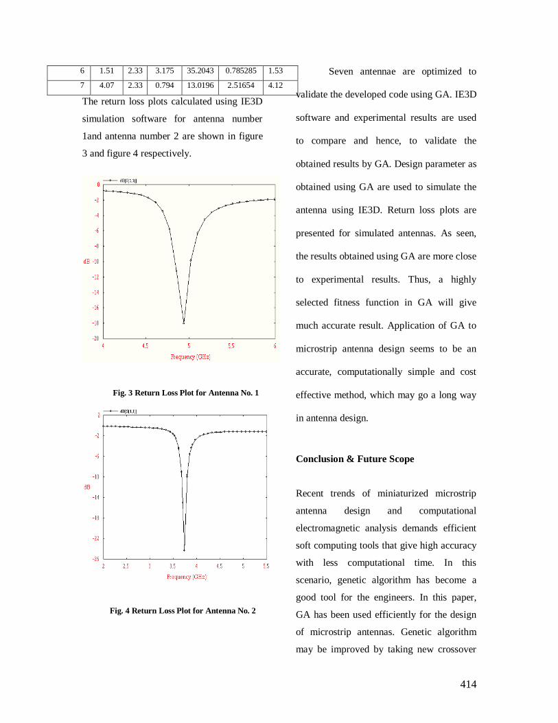
414
6 1.51 2.33 3.175 35.2043 0.785285 1.53
7 4.07 2.33 0.794 13.0196 2.51654 4.12
The return loss plots calculated using IE3D
simulation software for antenna number
1and antenna number 2 are shown in figure
3 and figure 4 respectively.
Fig. 3 Return Loss Plot for Antenna No. 1
Fig. 4 Return Loss Plot for Antenna No. 2
Seven antennae are optimized to
validate the developed code using GA. IE3D
software and experimental results are used
to compare and hence, to validate the
obtained results by GA. Design parameter as
obtained using GA are used to simulate the
antenna using IE3D. Return loss plots are
presented for simulated antennas. As seen,
the results obtained using GA are more close
to experimental results. Thus, a highly
selected fitness function in GA will give
much accurate result. Application of GA to
microstrip antenna design seems to be an
accurate, computationally simple and cost
effective method, which may go a long way
in antenna design.
Conclusion & Future Scope
Recent trends of miniaturized microstrip
antenna design and computational
electromagnetic analysis demands efficient
soft computing tools that give high accuracy
with less computational time. In this
scenario, genetic algorithm has become a
good tool for the engineers. In this paper,
GA has been used efficiently for the design
of microstrip antennas. Genetic algorithm
may be improved by taking new crossover

415
and mutation operators in continuous micro-
genetic algorithms. The proposed methods
may be applied in wide range applications
like calculation of radiation pattern, gain
array factor correction etc. of microstrip
antennas.
References
1. J. Watkins, “Circular Resonant
Structures in Microstrip,” Electronic
Letters, Vol. 5, No. 21, Oct. 1969, p.
524.
2. R. K. Mishra and A. Patnaik,
“Design of Circular Microstrip
Antenna using Neural Networks,”
IETE Journal of Research, vol. 44,
pp. 35-39, Jan-Apr 1998.
3. X. Gang, “On the resonant
frequencies of microstrip antennas,”
IEEE Trans. Antennas Propagat., pp.
245-247, Feb. 1989.
4. G. A. Deschamps, “Microstrip
Microwave Antennas,” The Third
Symposium on The USAF Antenna
Research and Development
Program, University of Illinois,
Monticello, Illinois, October 18-22,
1953.
5. R. Garg, P. Bhartia, I. Bahl and A.
Ittipiboon, “Microstrip Antenna
Design Handbook,” Artech House,
Inc, 2001.
6. Pozar DM, Schaubert DH.
Microstrip Antennas: The Analysis
and Design of Microstrip Antennas
and Arrays. IEEE Press: New York,
1995.
7. G. Derneryd, “New Technologies
for Lightweight, Low Cost
Antennas,” Workshop on
lightweight antennas, 18th European
Microwave Conference, Stockholm,
Sweden, 1988.
8. G. Kumar and K. P. Ray,
“Broadband Microstrip Antennas,”
Artech House, Inc, 2003.
9. D. S. Weile and E. Michielssen,
“Genetic algorithm optimization
applied to electromagnetics: A
review,” IEEE Trans. Antennas
propagat., vol. 45, Mar. 1997, pp.
343-353.
10. J. M. Johnson and Y. Rahmat-Samii,
“Genetic algorithms in engineering
electromagnetics,” IEEE Antennas
Propagat. Mag., vol. 39, Aug. 1997,
pp. 7-21.
11. Goldberg, D. E., "Genetic
Algorithms in Search, Optimization
and Machine Learning," Addison-
Wesley, 1989.
12. IE3D Software with its
manual(student version) from
www.Zealand.com

Bhaarath Ramesh Vijay
Department of Electronics and Communication
Sri Venkateswara College of Engineering
Pennalur, Sriperumbudur, India.
E-Mail id: [email protected]
Abstract:
This is a research paper proposes a design of Water
Quality monitoring System Using GSM Service for the
Aqua - Culture based Industries. This design, if
implemented, helps in monitoring the water quality
remotely, via GSM (by SMS). It is compulsory for an every
officer from his industry to visit the ponds at a designated
time and perform manual testing on finding the purity
level of the water. But it is also known, that these kind of
technique will consume lot time and effort. This research
project focuses on developing a prototype that can
evaluate data collected through three bases: Oxygen
dissolved in the water, Level of pH in water,
Temperature level of the water. This design also has the
capability conducting the tests automatically with a timer
present in it. It also sends the degra- adation of water
quality in the pond via SMS (Short Messaging Service).
1. Introduction
During the country’s fresh water resources consist
of 195210 kilometers of rivers and canals, 2.9 million hectares
of Minor and major reservoirs, 2.4 million hectares of ponds
and Lakes and about 0.8 million hectares of flood plain lakes
and derelict water bodies. During the ten-year period of 1995-
2004 inland capture production grew from 600,000 tons to
800,000 tones and at present contributes to 13% of total fish
production of the country [1].
Among issues faced by industry is monitoring
by conducting water quality for their ponds. Maintaining
water quality is important in farming aquaculture organisms, as
they are sensitive to water condition.
In the past, aqua farmers monitor quality of water by
conducting colorimetric test. The test is conducted to measure
ammonia level, pH level and dissolved oxygen (DO) level in
the water. The test is conducted by trained and skilled staff
Kapil Adhikesavalu Department of Electronics and Communication
Sri Venkateswara College of Engineering
Pennalur, Sriperumbudur, India.
E-Mail id: [email protected]
Furthermore, the process is very tedious to execute. To solve
the problem, water quality monitoring system was introduced to
farm [2].
The aims of the research project are to implement an
automated remote water quality monitoring system via SMS as
well as an alert system to inform the degradation of water
quality.
The objectives of this paper are to disclose why the three
criteria namely Dissolved Oxygen level, pH level and
temperature level are used as the parameters to monitor water
conditions, to describe the development process that will take
place in implementing this system and lastly to explain the
architecture of the remote automated water monitoring system.
2. Literature Review
2.1 Importance of Quality in water for aquaculture.
Water is a ‘Universal Solvent’ where various chemical
dissolved in the water, as well as all physical attributes affecting
them combines to form water quality. Good water quality level
determined by all attribute present in the water at an appropriate
level and often aquaculture water quality does not equal to
environmental water quality criteria differ from species to
species [3].
Physical, chemical, and biological properties are
interrelated and it affects survival, growth and reproduction of
aquaculture. Aquaculture also can have reverse effect to the
environment as aquatic organism, consume oxygen and
produce and ammonia. Important water quality parameters to
be considered are; temperature, salinity, pH, dissolved
oxygen, ammonia, nitrite/nitrate, hardness, alkalinity, and
turbidity.
Proceedings of the third National conference on RTICT 2010Bannari Amman Insitute of Technology , Sathyamangalam 638 401
9-10 April 2010
416

2.2 Water Quality Parameter
P. Fowler, et al. [4] in their study recommended that
temperature, DO, and pH be monitored directly on a
continuous basis since they tend to change rapidly and have a
significant adverse effect on the system if allowed to operate
out-of- range.
Temperature refers to degree of hotness or coldness and
it can be measured in degree Celsius. Temperature of water
needs to be monitored regularly as outside tolerable temperature
range, disease and stress become more prevalent. Among effect
of temperature changes are; photosynthetic activity, diffusion
rate or gases, amount of oxygen that can be dissolved, and
physiological process of the prawn and level of other
parameters [5].
pH refers to the hydrogen ion concentration or how acidic
or basic as water is pH is defines as log[H+]. pH value range
form 0-14; pH = 7 is neutral, ph < 7 is acidic, pH > 7 is basic.
Fig.1 explains the effects of pH to prawn.
Figure 1: Effect of pH to Prawn
Dissolved oxygen describes the concentration of oxygen
molecular in the water and it dependent on the temperature of
the water and the biological demand of the system [3].
Dissolved oxygen is used in aerobic decomposition of organic
matter, respiration of aquatic organism, and chemical oxidation
of mineral. As many organisms in the water use dissolved
oxygen, therefore it tends to change rapidly. Dissolved oxygen
is supplied to water through several method direct diffusion of
oxygen from the atmosphere, wind and wave action; and
photosynthesis [3].
2.3 Automated Water Quality Monitoring System
Aquaculture is the farming of aquatic organism in natural
or controlled marine or freshwater environments [4].
Aquaculture history has started during 19th century in Tonle Sap
Lake, Kampuchea and Indonesia. Farmers used cages made by
bamboo and later the technique was improved by using steel
tubes and later the technique was improved by using steel tubes
and floating drums t o act as cage. Since 20 years ago,
aquaculture industry is blooming rapidly and it is most popular
method in fishery sector [5].
‘Intelligent Aqua Farm System via SMS’ is an example
of remote monitoring and maintaining water quality system of
aquaculture ponds. The system automatically monitors and
records real-time data of two parameters; pH level and DO
level, which are reported through Short Messaging Service [5].
2.4 Evaluating Water Quality Degradation
A study has been done by Faculty of Engineering, Akdeniz
University using fuzzy logic to assess ground water pollutions
levels below agriculture field. The study was conducted by
taking into consideration four inputs; nitrite, nitrate,
orthophosphate, and seepage index value. Water quality index
is then determined using fuzzy logic. Water quality index was
originally designed to make an integrated assessment of water
quality conditions to meet utilization goals. In the study, a fuzzy
logic system was developed to assess the ground water pollution
of Kumluca plain at previously selected nine sampling stations.
The applied water pollution evaluation system involves the
selection of water quality parameters and index values to form
Water Pollution Index (WPI) [7].
Other example of research project using fuzzy logic is a
case study by Virgili University. The study used fuzzy logic
due to limitation of current water quality index. The study
indicated the need for more appropriated techniques to manage
the importance of water quality variables, the interpretation of
an acceptable range for each parameter, and the method used to
integrate dissimilar parameters involved in the evaluation
process is clearly recognized. Therefore they propose fuzzy
logic inference to solve the problem. The study proposed
dissolve oxygen and organic matters as input for the evaluation.
Several sets of rule were define to help them with the evaluation
[8].
Meanwhile, a study conducted by et al [6] used for
model; Dissolved Oxygen predicting model, unilinear
temperature model, BOD-DO multi linear model, and one
dimension zoology model in evaluating and predicting water
quality of ponds [6].
2.5 Relationship among the Water Quality Parameters
P.Fowler, et al in their study recommended that temperature,
DO, and pH be monitored directly on a continuous basis since
they tend to change rapidly and have a significantly adverse
effect on the system if allowed to operate out of range [12].
417

During day, aquatic organism respiration uses oxygen
and produces carbon dioxide. The carbon dioxide is then used
by aquatic plant through photosynthesis and it produces oxygen
as it by product. The cycle continues during daytime. However,
during nighttime, aquatic organisms keeps using oxygen but
carbon dioxide produced dissolve in water as photosynthesis do
not occurs during night. As for that, concentration of oxygen in
water reduces [13].
Table 1 and Table 2 below describe relation of dissolved
oxygen, carbon dioxide and pH in ponds over 24 hours, as well
as summarized tolerable range of water quality parameter for
prawn farming [14].
2.6 Data Telemetry
Remote monitoring system is an important technology in
today’s life. Our society for instance is pervaded by computer-
controlled devices. Everything from Digital Clock to Hi-fi
Robot can have one or often several microcomputer devices and
can be controlled remotely [9]. Remote monitoring system
employs a technology called data telemetry. It allows remote
measurement and reporting information of interest to the system
designer or operator [5].
The most wide spread, wide area, wireless, digital network is
the GSM network. GSM is a digital cellular network,
originally intended for voice telephony [9]. SMS (Short
messaging service) is an application that can be utilized from
GSM network. Message sent, which is in text only, from the
sending mobile is stored in a central short message centre
(SMC) which will then be forwarded to the destination mobile
[5].
3. Research Project Development
Figure 2 depicts the development flow of the
research project. Development of the research project starts
with preliminary research to obtain adequate
information regarding the problem was identified and agreed,
design phase takes place.
After that, development of the research project
starts by configuring hardware to be used, followed by
developing the software required. After both hardware and
software are completed, the system is then tested. The
development of the research project follows the figure above
where at each phases; evaluation will be done to determine
whether the design/system developed fulfills the requirement.
Figure 2
Flowchart Diagram for Development of Research project
418

4. System Architecture
The system architecture, which represents skeleton of the
research project, consists of four components; data acquisition
System, data telemetry, data processing and output and is
depicted in Figure 3.
4.1 Power supply and UPS
This block helps the monitoring system to be in activation
mode 24×7. In case of any power failure, the UPS which can
withstand for long hours can help in continuing the activation of
the monitoring system.
4.2 Timer Count down
This equipment controls the device regularly. It has a timer
in it. When the count is done the test is done and the acquired
information is transmitted. The tests can be performed regularly
without any manual help. They are programmed that the test
can be performed once in a day and send the details. Also the
staff in-charge can also program the timing for the tests to be
conducted.
4.3 Data Acquisition System
Data Acquisition system is consists of two components;
sensors and data acquisition kit. Sensors are needed to pick
particular reading from the pond and the reading would be
gathered by data acquisition kit. Data acquisition kit is
responsible to convert analog signal received and converts it
into digital signal. The kit is also responsible to prepare
message for data telemetry purposes.
4.4 Data Telemetry
Data telemetry is consisting of GSM modem. The modem
is connected to the data acquisition kit. The modem will receive
prepared messages by the kit and send the message to data
processing component.
4.5 Data Processing
Data processing component would be the heart of the
system. The component consists of four sub-component; data-
base, knowledge base, inference, and evaluation. The first sub-
component stores the message received from data acquisition kit
through short message service. Knowledge base, meanwhile,
stores data related to water quality level for inference purpose.
Inference component would use Mamdani fuzzy logic style.
Real time data received would be fed into the inference to
determine water quality of the pond. Evaluation will be done
using the inference result. This sub-system enables proactive
measure in the monitoring system. Monitored data would not
have to be in intolerable range before it could trigger the
system.
4.6 Output
Result of the water quality evaluation would be used by this
component. Two type of output would be produced; first, the
data received and the output of the evaluation would be
displayed on central computer screen, second, alert message
would be sent to farmers upon detecting degradation of the
water quality.
4.7 Data flow Diagram
Data flow diagram (DFD) is a tool that depicts the flow of
data through as system and the work or processing performed
by the system [11]. Figure 4 shows the data flow diagram for
the project.
419
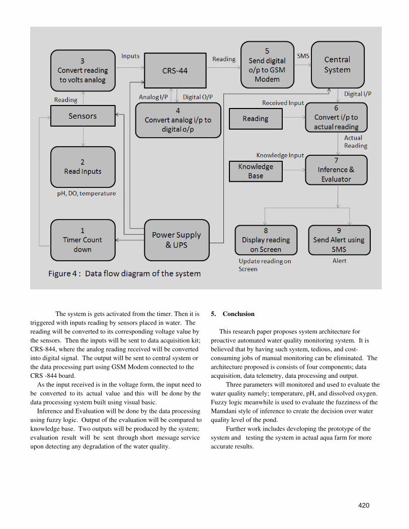
The system is gets activated from the timer. Then it is
triggered with inputs reading by sensors placed in water. The
reading will be converted to its corresponding voltage value by
the sensors. Then the inputs will be sent to data acquisition kit;
CRS-844, where the analog reading received will be converted
into digital signal. The output will be sent to central system or
the data processing part using GSM Modem connected to the
CRS -844 board.
As the input received is in the voltage form, the input need to
be converted to its actual value and this will be done by the
data processing system built using visual basic.
Inference and Evaluation will be done by the data processing
using fuzzy logic. Output of the evaluation will be compared to
knowledge base. Two outputs will be produced by the system;
evaluation result will be sent through short message service
upon detecting any degradation of the water quality.
5. Conclusion
This research paper proposes system architecture for
proactive automated water quality monitoring system. It is
believed that by having such system, tedious, and cost-
consuming jobs of manual monitoring can be eliminated. The
architecture proposed is consists of four components; data
acquisition, data telemetry, data processing and output.
Three parameters will monitored and used to evaluate the
water quality namely; temperature, pH, and dissolved oxygen.
Fuzzy logic meanwhile is used to evaluate the fuzziness of the
Mamdani style of inference to create the decision over water
quality level of the pond.
Further work includes developing the prototype of the
system and testing the system in actual aqua farm for more
accurate results.
420

6. Reference
[1] FAO fisheries and aquaculture of INDIA
http://www.fao.org/fishery/countrysector/naso_india/en
[2] Handheld Professional Plus Instrument Saves
Time When There’s No Time To Spare. : YSI
Environmental, 2007.
[3] "Water Quality Management and Treatment for
Prawn Hatchery." Marine Aquaculture Institute, Kota
Kuala Muda, Kedah. 13 Jun. 2005.
[4] C. S. Hollingsworth, R. Baldwin, K. Wilda, R.
Ellis, S. Soares, , et al. "Best Management Practices
For Finfish Aquaculture in Massachusetts." UMass
Extension Publication AG-BPFA (2006)
[5] Sharudin, Mohd Shahrul Zharif . "Intelligent
Aqua-Farm System via SMS." Diss. Universiti
Teknologi PETRONAS, 2007.
[6] W. Ruimei, H. Youyuan, F. Zetian., "Evaluation
of the Water Quality of Aquaculture Pond Expert
System." Institute of Agriculture Engineering, Beijing
(2004): 390-397.
[7] A. Muhammetoglu, and A. Yardimci .
"Evaluation of the A Fuzzy Logic Approach to
Assess Groundwater Pollution Level Below
agricultural Fields." Environmental Monitoring and
Assessment, Springer 118 (2005): 337-354.
[8] W. O. Duque, N. F. Huguet, J. L. Domingo, M.
Schuhmacher, , et al. "Assessing Water Quality in
Rivers with Fuzzy Inference Systems: A Case Study."
Environment International 32.6 (2006): 733-742.
[9] Mikael , Sj¨odin. "Remote Monitoring and
Control Using Mobile Phones." Newline Information
(2001)
[10] D. E. Avison, and G. Fitzgerald . "Where now
for development methodologies?." Communications
of the ACM 46.1 (2003): 78-82.
[11] J. L. Whitten, L. D. Bentley, K. C. Dittman,
“System Analysis and Design Methods 5th Edition”,
McGraw Hill, 2001
[12] P. Fowler, D. Baird, R. Bucklin, S. Yerlan, C. Watson &
F. Chapman2, , et al. "Microcontrollers in
Recirculating Aquaculture Systems1." EES 326
(1994): 1-7.
[13] N. Hashim, M. Ibrahim, T. Murugan, . Personal
Interview. 9 Apr. 2008.
[14] . Cadangan Perniagaan Projek Ternakan Udang
Galah. Kuala Lumpur: Department of Fisheries,
Ministry of Agriculture and Agro-Based Industry,
2004.
421

Proceedings of the Third National Conference on RTICT 2010
Bannari Amman Institute of Technology, Sathyamangalam-638401
9-10 April 2010
422
U Slotted Rectangular Microstrip Antenna for Bandwidth
Enhancement
D.Sugumar 1, Shalet sydney
2
1 & 2Department of Electronics and Communication
Karunya University, Coimbatore 641114, Tamil Nadu, India
Abstract: - A new design technique of microstrip patch antenna is presented in this paper. The
proposed antenna design consists of direct coaxial probe feed technique and the novel u
slotted shaped patch.The composite effect of integrating these techniques and by introducing
the new slotted patch, offer a low profile, high gain, broadband, and compact antenna
element. Parameters like return loss, radiation pattern and bandwidth are analysed using
FDTD algorithm in MATLAB and compared for a non slotted microstrip patch antenna , a
rectangular slotted microstrip patch antenna and a u slotted microstrip patch antenna.
Bandwidth for the u slot design is found to be as large as about 1.785 times that of a
corresponding unslotted rectangular microstrip antenna and also better directivity is achieved.
Details of the antenna design and simulated results are presented and discussed.
Key-Words: -Microstrip Patch Antenna, Bandwidth Enhancement, FDTD Algorithm,MATLAB.
1.Introduction
With the wide spread proliferation of
wireless communication technology in
recent years, the demand for compact, low
profile and broadband antennas has
increased significantly. A number of new
developed techniques to support high data
rate wireless communication for the next
generation technologies have been rapidly
increasing. Basically, the maximum
achievable data rate or capacity for the
ideal band-limited additive white Gaussian
noise (AWGN) channel is related to the
bandwidth and the signal-to-noise ratio
through Shannon-Nyquist criterion :
C=Blog2(1+SNR) (1)
where C denotes the maximum transmit
data rate, B stands for the channel
bandwidth, and SNR is the signal-to-noise
ratio. From this principle, the transmit data
rate can be enhanced by increasing either
the bandwidth occupation or the
transmission power. However, the
transmission power cannot be readily
increased since many portable devices are
battery powered and the potential
interference should also be avoided. Thus,
a large frequency bandwidth seems to be
the proper solution to achieve a high data
rate. To meet the requirement, the
microstrip patch antenna has been
proposed because of its low profile, light
weight and low cost . However,
conventional microstrip patch antenna
suffers from very narrow bandwidth. This
poses a design challenge for the microstrip
antenna designer to meet the broadband
techniques.
There are several well-known methods to
increase the bandwidth of patch antennas,
such as the use of thick substrate, cutting a
resonant slot inside the patch, the use of a
low dielectric substrate, multi- resonator
stack configurations, the use of various
impedance matching and feeding

423
techniques, and the use of slot antenna
geometry. However, the bandwidth and the
size of an antenna are generally mutually
conflicting properties, that is,
improvement of one of the characteristics
normally results in degradation of the
other.
Several techniques have been proposed to
enhance the bandwidth in the state-of-the
art antenna research. A novel single layer
wide-band U slotted rectangular patch
antenna with improved impedance
bandwidth has been demonstrated. By
using a U-slot patch, and coaxial feed
patch antennas, wideband which is
electrically small in size have been
reported .
2.FDTD analysis
Fig. 1. The 3-D FDTD unit cell.
The FDTD algorithm solves Maxwell’s
time-dependent curl equations by first
filling up the computation space by a
number of “Yee cells”. The relative spatial
arrangements of the E fields and the H
fields on the “Yee cell” enables the
conversion of Maxwell’s equations into
finite-difference equations. These
equations are then solved in a time
matching sequence by alternatively
calculating the electric and magnetic fields
in an interlaced spatial field.
The first step in designing an antenna with
an FDTD code is to grid up the object. A
number of parameters must be considered
in order for the code to work successfully.
The grid size must be small enough so that
the fields are sampled sufficiently to
ensure accuracy. Once the grid size is
chosen, the time step is determined such
that numerical instabilities are avoided,
according to the courant stability
condition.
A Gaussian pulse voltage with unit
amplitude, given by
V (t)=exp(−(t−t0)2/T2) (2)
where T denotes the period and t0
identifies the center time, is excited in the
probe feed.In this case, the frequency
domain FDTD near to far field
transformation are used because it is both
memory efficient and time efficient.
3.Design considerations of the
proposed antenna
The geometries of the proposed antennas
are given below:
Fig. 2. Geometry of a broad-band rectangular microstrip antenna
without a slot and having coaxial feed. The dimensions given in
thefigure are in millimeters.
Fig. 3. Geometry of a broad-band rectangular microstrip antenna
with a rectangular slot and coaxial feed. The dimensions given
in thefigure are in millimeters.

424
Fig. 4. Geometry of a broad-band rectangular microstrip antenna
with modified U-shaped slot and coaxial feed. The dimensions
given in the figure are in millimeters.
Fig. 2, shows the geometry of a
rectangular patch antenna without any slot
in it and Fig. 3, shows Geometry of a
broad-band rectangular microstrip antenna
with a rectangular slot. As shown in Fig. 4,
a U shaped slot is placed on the patch. The
rectangular patch has dimensions of
57.5055 mm 47.6975 mm and is printed on
a grounded substrate of thickness(h) 1.6
mm, relative permittivity(ᵋ) 3.2 and size 60
mm ×50 mm. The values of thickness(h) ,
relative permittivity (ᵋ) and resonant
frequency are fixed previously and patch
length and width are determined using
transmission line model. The patch is fed
by a coaxial probe along the centreline(x
axis) at a distance of L6 from the edge of
the patch as shown in figures 2,3, and 4.
TABLE 1
Parameter Value[mm]
L 47.6975
W 57.5055
L1 3.97479
L2 11.924375
L3 3.179839
L4 19.07900
L5 11.92437
L6 26.233625
L7 4.76975
W1 18.68928
W2 21.56457
W3 11.5011
W4 6.46936875
W5 10.06347
d(relative
permitivity)
3.2
4.Results and conclusions
Coding is done in matlab and radiation
patterns for a non slotted microstrip patch
antenna, a rectangular slot microstrip
patch antenna and a u slot microstrip patch
antenna is obtained as follows. It is
observed that for the U slot design , the
side lobes are reduced and the major lobe
has become more prominent increasing the
directivity of the patch antenna.
0
20
40
60
80
0
20
40
60-60
-40
-20
0
20
40
60
Position (microns)Ex
Fig. 5. Radiation pattern of rectangular microstrip patch antenna
without a slot.
0
20
40
60
80
0
20
40
60-40
-20
0
20
40
60
Position (microns)Ex
Fig. 6. Radiation pattern of rectangular microstrip patch antenna
with a rectangular slot.

425
0
20
40
60
80
0
20
40
60-40
-20
0
20
40
60
80
Position (microns)Ex
Fig. 7. Radiation pattern of rectangular microstrip patch antenna
with a U-slot.
Fig. 8. Simulated return loss against frequency for proposed
antennas. Parameters for antennas 1–3 are described in Table
I.and Table 2.
Bandwidth can be said as the frequencies
on both the sides of the centre frequency in
which the characteristics of antenna such
as the input impedance, polarization, beam
width, radiation pattern etc are almost
close to that of this value. It can be
defined as the range of suitable frequencies
within which the performance of the
antenna, w.r.t some characteristic,
conforms to a specific standard.
The bandwidth is the ratio of the upper and
lower frequencies of an operation. It can
be obtained as:
Using equations (2) and (3) bandwidth for
each of the three considered antennas are
calculated .
(3)
(4)
TABLE 2
PERFORMANCES OF THE PROPOSED BROAD-BAND ANTENNAS; Fc IS THE CENTER FREQUENCY , FL AND FH ARE THE
LOWER AND HIGHER FREQUENCIES WITH 10-dB RETURN LOSS IN THE OPERATING
BANDWIDTH, AND THE ANTENNA BANDWIDTH IS DETERMINED FROM FH-FL
FL (MHz)
Fc (MHz)
FH (MHz)
Bandwidth (MHz,%)
Antenna 1 (antenna
without slot)
1636
1666
1721
85,5.1020
Antenna 2 (antenna
with rectangular slot)
1661
1789
1822
161,8.99
Antenna 3 (antenna
with u slot)
1677
1800
1841
164,9.1111

426
The fundamental resonant frequency
of the unslotted rectangular patch
antenna is at about 1.66 GHz, with
an operating bandwidth of 5.102 %.
Since the obtained antenna
bandwidths are as large as 8.99–9.11
%, the proposed antennas show a
much greater operating bandwidth,
more than 1.7 times that of an
unslotted rectangular patch
antenna.Thus a new technique for
enhancing the gain and bandwidth
of a microstrip patch antenna has
been developed and implemented
successfully. The experimental
results demonstrate that it has a
better impedance bandwidth of
9.1111% at 10 dB return loss,
covering from 1.67 to 1.84 GHz
frequency. Techniques for
microstrip broadbanding, size
reduction and stable radiation
pattern are applied with significant
improvement in the design by
employing the proposed u-slotted
patch shaped design and coaxial
probe.
4.References [1]Mohammad Tariqul Islam., Mohammed Nazmus Shakib.,
Norbahiah Misran., Baharudin
Yatim, Aug. 2000,” Analysis of L-Probe Fed Slotted Microstrip Patch
Antenna” IEEE Transactions on
Antennas and Propagation, Volume 48, Issue 8, Page(s):1149 – 1152
[2] Mohammad Tariqul Islam.,
Mohammed Nazmus Shakib., Norbahiah Misran., 2009,” multi-slotted
microstrip patch antenna for wireless
communication” Progress In Electromagnetics Research Letters,
Vol. 10, Page(s):11-18
[3] Mohammad Tariqul Islam., Mohammed Nazmus Shakib.,
Norbahiah Misran., Baharudin Yatim,
25-27 December, 2008, Khulna, Bangladesh 2008,” Analysis of
Broadband Slotted Microstrip Patch
Antenna” Proceedings of 11th
International Conference on Computer
and Information Technology (ICCIT 2008), Vol. 32, Page(s):121-148
[4] Jia-Yi Sze., Kin-Lu Wong, Aug.
2000,”Slotted rectangular microstrip antenna for bandwidth enhancement”
IEEE Transactions on Antennas and
Propagation, Volume 48, Issue 8, Page(s):1149 – 1152
[5] Jeun-Wen Wu., Jui-Han Lu, June
2003,” Slotted circular microstrip antenna for bandwidth enhancement”
IEEE Antennas and Propagation
Society International Symposium,Volume 2, Page(s):272 –
275.
[6] Jui-Han Lu , May 2003,”
Bandwidth enhancement design of
single-layer slotted circular microstrip
antennas” IEEE Transactions on Antennas and Propagation, Volume:
51, Issue:5, page(s): 1126- 1129
[7] J. A. Ansari ., R. B. Ram, May
2008,” Broadband stacked U-slot microstrip patch antenna”, Progress In
Electromagnetics Research Letters,
Vol. 4, Page(s):17–24. [8] Baharudin Yatim ., Mohammed N.
Shakib., Mohammad T. Isla.,
Norbahiah Misran , 2009,” Design Analysis of a Slotted Microstrip
Antenna for Wireless Communication”
World Academy of Science,
Engineering and Technology,Page: 49 . [9] Balanis constantine,Antenna theory,
wiley-india, 2008.

Abstract— Finite impulse response (FIR) filter is the key
functional block in the field of digital signal processing. But in the VHDL implementation, the hardware complexity of the FIR
filter is directly proportional to the tap length and the bit-width of input signal. But in Digital signal processing (DSP) is the fastest growing technology this century and, therefore, it poses tremendous challenges to the engineering community. Faster additions and multiplications are of extreme importance in DSP for convolution, discrete Fourier transforms digital filters, etc. The core computing process is always a multiplication routine; therefore, DSP engineers are
constantly looking for new algorithms and hardware to implement them. The whole of Vedic mathematics is based on 16 sutras (word formulae) and manifests a unified structure of mathematics. The exploration of Vedic algorithms in the DSP domain may prove to be extremely advantageous. Engineering institutions now seek to incorporate research-based studies in Vedic mathematics for its applications in various engineering processes. Further research prospects may include the design
and development of a Vedic DSP chip using VHDL technology.
Keywords—VHDL, FPGA, FIR, CAD
I. INTRODUCTION
A finite impulse response (FIR) filter is a type of a
digital filter. The impulse response is finite because it
settles to zero in a finite number of sample intervals.
This is in contrast to infinite impulse response (IIR)
filters, which have internal feedback and may continue
to respond indefinitely. The impulse response of an Nth-
order FIR filter lasts for N+ 1 sample, and then dies to
zero. Firstly Time Domain input data is transformed into the Frequency Domain using a Fast Fourier Transform
(FFT), filtered directly in the Frequency Domain by
passing or amplifying desired frequencies and zeroing
out unwanted ones, and inverse transformed back into
Arun Bhatia is with the Department of Electronics and
Communication Engineering, Mharishi Markandeshwar Engineering
College,Mullana,Ambala, Haryana, India (e-mail:
[email protected] Contact No: 09996820693).
the Time Domain using an Inverse Fast Fourier Transform (IFFT). The outputs of the IFFT are then
concatenated together if necessary as shown in the fig 1.
[1]
Figure 1 Block diagram Of Basic filter
FIR filters have some basic properties:
FIR Filters are inherently stable. This is
due to the fact that all the poles are located at the origin and thus are located within the
unit circle.
They require no feedback. This means that
any rounding errors are not compounded
by summed iterations. The same relative
error occurs in each calculation. This also
makes implementation simpler.
They can easily be designed to be linear
phase by making the coefficient sequence symmetric; linear phase, or phase change
proportional to frequency, corresponds to
equal delay at all frequencies.
II. INTRODUCTION
TO VEDIC MATHEMATICS
Vedic mathematics is the name given to the system of
mathematics to be precise, a unique technique of
calculations based on simple rules and principles with
which any mathematical problem can be solved it
arithmetic, algebra, geometry or trigonometry. The
system is based on 16 Vedic sutras or aphorisms, which
Arun Bhatia, Student, Electronics & Communication Engineering Department Of M.M
Univerisity,Mullana(AMBALA). E-Mail Id: - [email protected] OR
[email protected] Contact NO:09996820693
Implementation of FIR filter using VEDIC Mathematics in VHDL
Proceedings of the Third National Conference on RTICT 2010Bannari Amman Institute of Technology, Sathyamangalam-638401
9-10 April 2010
427

are actually word formulae describing natural ways of
solving a whole range of mathematical problems. Vedic
mathematics was rediscovered from the ancient Indian
scriptures between 1911 and 1918 by Sri Bharati
Krishna Tirthaji (1884-1960), a scholar of Sanskrit,
mathematics, Vedic mathematics is the name given to the ancient system of mathematics, or, to be precise, a
unique technique of calculations based on simple rules
and principles with which any mathematical problem
can be solved – be it arithmetic, algebra, geometry or
trigonometry. The system is based on 16 Vedic sutras or
aphorisms, which are actually word formulae describing
natural ways of solving a whole range of mathematical
problems. Vedic mathematics was rediscovered from the
ancient Indian scriptures between 1911 and 1918 by Sri
Bharati Krishna Tirthaji (1884-1960), a scholar of
Sanskrit, mathematics, renewed interest in Vedic
mathematics, and scholars and teachers in India started taking it seriously. According to Mahesh Yogi, The
sutras of Vedic Mathematics are the software for the
cosmic computer that runs this universe. A great deal of
research is also being carried out on how to develop
more powerful and easy applications of the Vedic sutras
in geometry, calculus and computing. Conventional
mathematics is an integral part of engineering education
since most engineering system designs are based on
various mathematical approaches. All the leading
manufacturers of microprocessors have developed their
architectures to be suitable for conventional binary arithmetic methods. The need for faster processing
speed is continuously driving major improvements in
processor technologies, as well as the search for new
algorithms. The Vedic mathematics approach is totally
different and considered very close to the way a human
mind works. [2]
III. FPGA IMPLIMENTATION
OF FIR FILTERS
FPGAs are being used for a variety of computationally
intensive applications, mainly in Digital Signal
Processing (DSP) and communications [3]. Due to rapid
increases in the technology, current generation of
FPGAs contain a very high number of Configurable
Logic Blocks (CLBs), and are becoming more feasible
for implementing a wide range of applications. The high non-recurring engineering (NRE) costs and long
development time for ASICs are making FPGAs more
attractive for application specific DSP solutions. DSP
functions such as FIR filters and transforms are used in a
number of applications such as communication and
multimedia. These functions are major determinants of
the performance and power consumption of the whole
system. Therefore it is important to have good tools for
optimizing these functions. Equation (1) represents the
output of an L tap FIR filter, which is the convolution of
the latest L input samples. L is the number of
coefficients h(k) of the filter, and x(n) represents the input time series.
y[n] = Σ h[k] x[n-k] k= 0, 1, ..., L-1 --- (1)
The conventional tapped delay line realization of this
inner product is shown in Figure 2. This implementation
translates to L multiplications and L-1 additions per
sample to compute the result. This can be implemented
using a single Multiply Accumulate (MAC) engine, but
it would require L MAC cycles, before the next input sample can be processed. Using a parallel
implementation with L MACs can speed up the
performance L times. A general purpose multiplier
occupies a large area on FPGAs. Since all the
multiplications are with constants, the full flexibility of
a general purpose multiplier is not required, and the area
can be vastly reduced using techniques developed for
constant multiplication. Though most of the current
generation FPGAs have embedded multipliers to handle
these multiplications, the number of these multipliers is
typically limited. Furthermore, the size of these multipliers is limited to only 18 bits, which limits the
precision of the computations for high speed
requirements. The ideal implementation would involve a
sharing of the Combinational Logic Blocks (CLBs) and
these multipliers. In this paper, we present a technique
that is better than conventional techniques for
implementation on the CLBs.
Figure 2. A MAC FIR filter block diagram
The coefficients in most of DSP applications for the
multiply accumulate operation are constants. The partial
products are obtained by multiplying the coefficients by
multiplying one bit of data at a time in AND operation. These partial products should be added and the result
depends only on the outputs of the input shift registers.
The AND functions and adders can be replaced by Look
Up Tables (LUTs) that gives the partial product. This is
shown in Figure 3.
428

Figure 3. A serial DA FIR filter block diagram
Input sequence is fed into the shift register at the input sample rate. The serial output presented to the RAM
based shift registers (registers are not shown in Figure
for simplicity) at the bit clock rate which is n+1 times (n
is number of bits in a data input sample) the sample rate.
The RAM based shift register stores the data in a
particular address. The outputs of registered LUTs are
added and loaded to the scaling accumulator from LSB
to MSB and the result which is the filter output will be
accumulated over the time. For an n bit input, n+1 clock
cycles are needed for a symmetrical filter to generate the
output. In conventional MAC method with a limited number of MAC engines, as the filter length is
increased, the system sample rate is decreased. This is
not the case with serial DA architectures since the filter
sample rate is decoupled from the filter length. As the
filter length is increased, the throughput is maintained
but more logic resources are consumed. Though the
serial DA architecture is efficient by construction, its
performance is limited by the fact that the next input
sample can be processed only after every bit of the
current input samples is processed. Each bit of the
current input samples takes one clock cycle to process.
Therefore, if the input bit width is 12, then a new input can be sampled every 12 clock cycles. The performance
of the circuit can be improved by modifying the
architecture to a parallel architecture which processes
the data bits in groups. Figure 4 shows the block
diagram of a 2 bit parallel DA FIR filter. The tradeoff
here is performance for area since increasing the number
of bits sampled has a significant effect on resource
utilization on FPGA. For instance, doubling the number
of bits sampled, doubles the throughput and results in
the half the number of clock cycles. This change doubles
the number of LUTs as well as the size of the scaling accumulator. The number of bits being processed can be
increased to its maximum size which is the input length
n. This gives the maximum throughput to the filter. For
a fully parallel implementation of the DA filter (PDA),
the number of LUTs required would be enormous. In
this work we show an alternative to the PDA method for
implementing high speed FIR filters that consumes
significantly lesser area and power.
Figure 4. A 2 bit parallel DA FIR filter block diagram
A popular technique for implementing the transposed
form of FIR filters is the use of a multiplier block,
instead of using multipliers for each constant as shown
in Figure 5. The multiplications with the set of constants
hk are replaced by an optimized set of additions and
shift operations, involving computation sharing. Further
optimization can be done by factorizing the expression
and finding common subexpressions. The performance
of this filter architecture is limited by the latency of the
biggest adder and is the same as that of the PDA.
Common sub expression elimination algorithm that minimizes the number of adders as well as the number
of latches. [4-7]
Figure 5. Replacing constant multiplication by multiplier block
Multiplications with constants have to be performed in many signal processing and communication applications
such as FIR filters, audio, video and image processing.
Using a general purpose multiplier for performing
constant multiplication is expensive in terms of area.
Though embedded multipliers are very popular in
modern FPGAs, the size (18x18) and the number of
these multipliers is a limitation. The partial product
429
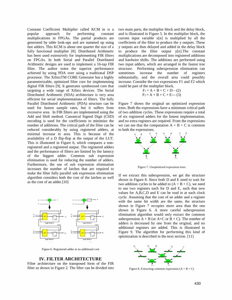
Constant Coefficient Multiplier called KCM in is a
popular approach for performing constant
multiplications in FPGAs. The partial products are
generated by table look-ups and are summed up using
fast adders. This KCM is about one quarter the size of a
fully functional multiplier [8]. Distributed Arithmetic has been used extensively for implementing FIR filters
on FPGAs. In both Serial and Parallel Distributed
Arithmetic designs are used to implement a 16-tap FIR
filter. The author notes the superior performance
achieved by using PDA over using a traditional DSP
processor. The XilinxTM CORE Generator has a highly
parameterizable, optimized filter core for implementing
digital FIR filters [9]. It generates synthesized core that
targeting a wide range of Xilinx devices. The Serial
Distributed Arithmetic (SDA) architecture is very area
efficient for serial implementations of filters. The fully
Parallel Distributed Arithmetic (PDA) structure can be used for fastest sample rates, but it suffers from
excessive area. In FIR filters are implemented using the
Add and Shift method. Canonical Signed Digit (CSD)
encoding is used for the coefficients to minimize the
number of additions. The critical path of the filter can be
reduced considerably by using registered adders, at
minimal increase in area. This is because of the
availability of a D flip-flop at the output of the LUT.
This is illustrated in Figure 6, which compares a non-
registered and a registered output. The registered adders
and the performance of filters are limited by the latency of the biggest adder. Common sub expression
elimination is used for reducing the number of adders.
Furthermore, the use of sub expression elimination
increases the number of latches that are required to
make the filter fully parallel sub expression elimination
algorithm considers both the cost of the latches as well
as the cost of an adder.[10]
Figure 6. Registered adder at no additional cost
IV. FILTER ARCHITECTURE Filter architecture on the transposed form of the FIR
filter as shown in Figure 2. The filter can be divided into
two main parts, the multiplier block and the delay block,
and is illustrated in Figure 5. In the multiplier block, the
current input variable x[n] is multiplied by all the
coefficients of the filter to produce the y outputs. These
y outputs are then delayed and added in the delay block
to produce the filter output y[n].The constant multiplications are decomposed into registered additions
and hardwire shifts. The additions are performed using
two input adders, which are arranged in the fastest tree
structure. Performing subexpression elimination can
sometimes increase the number of registers
substantially, and the overall area could possibly
increase. Consider the two expressions F1 and F2 which
could be part of the multiplier block.
F1 = A + B + C + D—(2)
F2 = A + B + C + E--- (3)
Figure 7 shows the original un optimized expression trees. Both the expressions have a minimum critical path
of two addition cycles. These expressions require a total
of six registered adders for the fastest implementation,
and no extra registers are required. From the expressions
we can see that the computation A + B + C is common
to both the expressions.
Figure 7. Unoptimized expression trees
If we extract this subexpression, we get the structure
shown in Figure 8. Since both D and E need to wait for
two addition cycles to be added to (A + B + C), we need
to use two registers each for D and E, such that new
values for A,B,C,D and E can be read in at each clock
cycle. Assuming that the cost of an adder and a register with the same bit width are the same, the structure
shown in Figure 7 occupies more area than the one
shown in Figure 6. A more careful subexpression
elimination algorithm would only extract the common
subexpression A + B (or A+C or B + C). The number of
adders is decreased by one from the original, and no
additional registers are added. This is illustrated in
Figure 9. The algorithm for performing this kind of
optimization is described in the next section. [11]
Figure 8. Extracting common expression (A + B + C)
430

Figure 9. Extracting common subexpression (A+B)
V. OPTIMIZATION ALGORITHM
Optimization is to reduce the area of the multiplier block
by reducing the number of adders and any additional
registers required for the fastest implementation of the
FIR filter. In the common sub expression elimination
methods polynomial transformation of constant
multiplications. Given a representation for the constant
C, and the variable X, the multiplication C*X can be
represented as a summation of terms denoting the
decomposition of the multiplication into shifts and additions as
C*X= Σ+XL—(4)
The terms can be either positive or negative when the
constants are represented using signed digit
representations such as the Canonical Signed Digit
(CSD) representation. The exponent of L represents the
magnitude of the left shift. In this method minimum
number of registers required the fastest tree structure
with three addition steps, and one register to
synchronize the intermediate values, such that new values for A,B,C,D,E,F can be read in every clock cycle.
This is illustrated in Figure 10. [12]
Figure 10. Calculating registers required for fastest evaluation
VI. CAD SYSTEM FOR FIR FILTERS
To design FIR filters with the CAD tool that generates various optimum architectures for FIR filters needed in
different applications in terms of speed, power and area
in the IC implementation. CAD system for filter
generation in VHDL. The CAD methodology for this
filter compiler tool centers around a VHDL-based
functional compiler which accepts functional parameters
and automatically generates optimized IC
implementation for FIR filters. Previous functional compilers are extremely rigid in architecture generation
and technology retargeting because of their dependence
on specific low-level layout/floor plan generation tools.
In contrast, our approach generates a VHDL solution
which feeds into logic synthesis tools and achieves
technology independence. The design flow achieved
with the functional compiler is shown in Figure 11. This
design flow leverages advances made in high level
synthesis tools and provides multiple levels of
simulations from VHDL to layout. User specifies
parameters for a design to the functional compiler which
produces an optimum architecture in VHDL format. Logic synthesis tools accept the generated VHDL and
target the design to different IC technologies. Design
verification may be performed at system, VHDL and
layout levels. [13]
Figure 11 CAD tool design flow with Functional Compilers
VII. FIR FILTER ARCHITECTURE
DERIVATION An FIR filter implements the following non-recursive
difference equation:
N-1
Y[n] = ∑ h[k]x [n-k] --- (5)
k = 0
where h[k] are the coefficients of the FIR filter and N is
the order of the filter. This algorithm can be expressed
as a DG shown in Figure 12. The DG of the FIR shows
the dependence of the computations in the FIR filtering
algorithm. The diagonal arcs in the DG intersect the DG
nodes needed to compute a given output sample. The
horizontal arcs pass the current input sample to DG nodes where it is required for computation and the
vertical arcs pass the coefficients to the appropriate DG
nodes. A detailed DG node consists of an adder and a
multiplier. Each node in the DG adds a partial sum
along its input diagonal to the product of the coefficient
431

and the current input sample and outputs the resulting
sum along its output diagonal. Based on different
mappings of the DG onto an array structure, a number of
SFGs (signal $ow graphs) can be derived from the DG.
An SFG is closer to the architecturehardware
implementation of the algorithm and is obtained by PE (processor element) allocation followed by operation
scheduling [14].
Figure.12 Transpose-form architecture derivation using the DG-SFG
technique
A. Architecture Derivation for Decimation Filters
The decimation FIR filter is described by the following
equation:
N-1
y[m] = ∑ h[k]x[mD-k]--- (6)
k = O
where D is the decimation factor. Two approaches have been used to implement decimation FIRS. The first
approach uses a decimator immediately following a full
fledged FIR filters. The second approach computes
decimation FIR output as sum of outputs of D polyphase
filters. These implementations do not exploit decimation
to reduce complexity and as a result can be highly non-
optimal for high decimation factors.
B. Impact of decimation on the DG of an FIR
filter
Figure. 13 show the effect of decimation on the DG of
an FIR filter. The DG nodes are shown shaded on the
diagonal arcs which produce the decimated output
samples. For an FIR filter with N = 4 and D = 2 (Figure
13), computations for every alternate output sample
need to be performed. For D = 2, only half of the DG nodes, which are shown shaded, need to be computed in
each cycle. An alternative interpretation is the division
of the DG into 2 sections as shown in Figure.13. Only
one of the 2 DG nodes from each section is computed
every clock cycle This can be generalized to any
arbitrary filter order, N and decimation factor D. For a
given N and D, the number of nodes to be computed per
clock cycle is [N / D] , where (r) represents the largest
integer contained in r. In other words, decimation
divides the DG into [N/D] each containing D DG nodes,
of which only one is computed every cycle.[15]
Figure.13 Effect of decimation on the DG of the FIR filter
VIII. CONCLUSION
FPGA architecture is proposed that is tailored for FIR
filters realization. The novelty of this architecture lies in
several fields that are associated with the
interconnection scheme of the 169 CALUs within a fine-grained architecture and the way the coefficients are
retrieved from the same output, using paths with
different delay time based on a certain configuration.
Additionally, by using the POF technique and designing
heterogeneous, configurable blocks, the power
calculation of our design has been proved to be
competitive compared with general purpose FPGAs,
although the associated built-in flexibility that implies
high degree of robustness and the additional logic
circuitry, which is introduced in order the system to
cope efficiently with overflow. The primary results,
which have been obtained, are related with the hardware realization and power consumption of this architecture.
Finally, our future research is going to be focused on the
efficient realization of medium and high order FIR
filters on this architecture by using evolutionary
technique.
432

IX. REFRENCES
[1]. http://en.wikipedia.org/wiki/Finite_impulse_response
[2].Jagadguru Swami Sri Bharati Krisna Tirthaji Maharaja, Vedic
Mathematics: Sixteen Simple Mathematical Formulae from the Veda.
Delhi (1965).
[3] K.D.Underwood and K.S.Hemmert, "Closing the Gap: CPU and
FPGA Trends in Sustainable Floating- Point BLAS Performance",
International Symposium on Field-Programmable Custom Computing
Machines, California, USA, 2004.
[4] Y.Meng, A.P.Brown, R.A.Iltis, T.Sherwood, H.Lee, and
R.Kastner, "MP Core: Algorithm and Design Techniques for Efficient
Channel Estimation in Wireless Applications", Design Automation
Conference (DAC), Anaheim, CA, 2005.
[5] B. L. Hutchings and B. E. Nelson, "Gigaop DSP on FPGA",
Acoustics, Speech, and Signal Processing, 2001. Proceedings.
(ICASSP '01). 2001 IEEE International Conference on, 2001.
[6] A.Alsolaim, J.Becker, M.Glesner, and J.Starzyk, "Architecture and
Application of a Dynamically Reconfigurable Hardware Array for
Future Mobile Communication Systems", International Symposium on
Field Programmable Custom Computing
[7] S.J.Melnikoff, S.F.Quigley, and M.J.Russell, "Implementing a
Simple Continuous Speech Recognition System on an FPGA",
International Symposium on Field-Programmable Custom Computing
Machines (FCCM), 2002.
[8] K.Chapman, "Constant Coefficient Multipliers for the XC4000E,"
Xilinx Technical Report 1996.
[9] "Distributed Arithmetic FIR Filter v9.0," Xilinx Product
Specification 2004.
[10] M. Yamada and A. Nishihara, "High-speed FIR digital filter with
CSD coefficients implemented on FPGA", Design Automation
Conference, 2001. Proceedings of the ASP-DAC 2001. Asia and South
Pacific, 2001.
[11] K. Wiatr and E. Jamro, "Constant coefficient multiplication in
FPGA structures", Euromicro Conference, 2000. Proceedings of the
26th, 2000.
[12] G.R.Goslin, "A Guide to Using Field Programmable Gate Arrays
(FPGAs) for Application-Specific Digital Signal Processing
Performance," Xilinx Application Note, San Jose 1995.
[13]R.Jain, P.Yang, and T. Yoshino, FIRGEN: A Computer-Aided
Design System for High Performance FIR Integrated Circuits, IEEE
trans. on Signal Processing, vol. 39, no. 7, pp. 1655-1658
[14]S.Y. Kung, VLSIArray Processors, Prentice Hall, 1988 J.
Laskowski, A Silicon Compiler for Linear-Phase FIR Digital jilters,
M.S. Thesis, UCLA, 1991
[15]Thu-Ji Lin and Henry Samueli, A 200-MHz CMOS x/sin(x)
Digital filter for Compensating D/A Comerter Frequency Response
Distorrion, IEEE JSSC, vol. 26, no. 9, Sept. 1991 Robert Hawley, A
Silicon Compiler for High-speed CMOS Multirate FIR Digital Filters,
M.S. Thesis, UCLA, 1991
X. BIOGRAPHIES
Arun Bhatia born at 4, Dayal Bagh, Bharat Nagar Ambala
Cantt (HARYANA) on June 11, 1984 received B. Tech. in
(Instrumentation and Control Engineering) from Haryana
Engineering College Jagadhri, affiliated to Krukshetra
University krukshetra in the year 2007. Pursuing M.TECH in
the field of Electronics & Communication Engg from M.M
Engineering College Affiliated to M.M University Mullana
(AMBALA).
433

Proceedings of the Third National Conference on RTICT 2010
Bannari Amman Institute of Technology, Sathyamangalam-638401
9-10 April 2010
434
TWO MICROPHONE ENHANCEMENT OF
REVERBERANT SPEECH BY SETA-TCLMS
ALGORITHM
Authors: Manikandan A1, Ashok MB2, Johnny M3, Kashi Vishwanath RG4
1-Lecturer, KLN College of Information Technology
2, 3, 4-Students, KLN College of Information Technology
Mail id: [email protected]
Abstract- In this letter we propose a novel approach for
implementing two microphone enhancement of
reverberant speech using Selective Tap filtering. Our
approach involves capturing the reverberant speech using
two microphones in the proposed SIMO model and then to
restore the corrupted speech by computing essential filter
tap coefficients which impacts on the corrupted
reverberant speech and updating the tap coefficients
further on each subsequent iteration based on SETA-
TCLMS. Experimental results show that the results are in
correspondence with theoretical results and better than its
full update counterpart (MCLMS algorithm).
Index Terms – Multi Channel Least Mean Square
(MCLMS), Selective Tap Two Channel Least Mean Square
(SETA-TCLMS), Single Input Multiple Output model
(SIMO), Perceptual Evaluation of Speech Quality (PESQ)
I. INTRODUCTION
The speech is subjected to distortion by acoustic
reverberation especially when a speaker is distant from a
microphone such as in hands-free telephony environment and teleconferencing. Reverberation is harmful to speech
intelligibility since it blurs temporal and spectral cues,
flattens formant transitions, reduces amplitude
modulations associated with the fundamental frequency
of speech and increases low-frequency energy, which in
turn results in masking of higher speech frequencies [1].
In that case, dereverberation techniques should be applied
to corrupted speech to restore clean speech. Thus,
dereverberation has become an important topic because
of its high potential for wide applications including
speech enhancement and recognition. Since clean speech
and reverberant environments are usually unknown, blind dereverberation methods have been proposed to
estimate an inverse filter of the reverberation from
microphone speech signal.
In this paper, we derive a novel blind single-
input two-output reverberant speech enhancement
strategy, which stems from the multichannel least-mean-
square (MCLMS) algorithm. The proposed method uses
second-order statistics to identify the acoustic paths in
the time-domain and relies on a novel selective-tap
criterion to update only a subset of the total number of filter coefficients in every iteration. Therefore, it
substantially reduces computational requirements with
only minimal degradation in dereverberation
performance. The potential of the proposed low-
complexity algorithm is verified and assessed through
numerical simulations in realistic acoustical scenarios.
II. PROBLEM FORMULATION
Consider the paradigm shown in Fig. (A)
Where the speech is picked up by two
microphones of a hearing aid device. Let )(ks
represents clean speech signal, )(1 kh and
)(2 kh represents the impulse response of the two
acoustic paths modeled using finite impulse
response (FIR) filters. And )(1 kx and )(2 kx be
the reverberant signals captured by the two microphones of the device such that one
microphone is directional front microphone and
the other is Omni directional microphone
respectively. In the noiseless two-microphone
scenario, we exploit the correlation between the
output signals of each microphone
)()()( kskhkx ii and )()()( kskhkx jj (1)
Where * denotes linear convolution and i, j=1, 2. From (1) and for all i ≠ j, follows that
)()()()()( kskhkhkxkh ijij
)()( kxkh ji (2)

435
Fig (A) -The above mentioned model is an SIMO system, i.e., Single input with Two Microphone system
III. ALGORITHM
A. MULTICHANNEL Least Mean Square
ALGORITHM (MCLMS)
As shown in [10], an intuitive way to ’blindly’ calculate
the unknown acoustic paths is to minimize a cost
function that penalizes correlated output signals between
the th and jth sensors, such that
1
1 1
2)1(minarg)1(
M
i
M
ijijh kkJ e (3)
After rewriting (2) in vector notation, the error function
eij (k+1) in (3) can be further expanded to
)()1()()1()1(~~
khkxkhkxke i
T
jjT
iij (4)
Defined for all i, j = 1, 2 and i ≠ j, where ( . )T denotes
vector transpose.
Then
Tiiii Lkxkxkxkx )1(),...,1(),()( (5)
is the corrupted (reverberant) speech picked up by the ith
microphone . Accordingly, the update equation of the
time-domain multichannel least-mean-square
(MCLMS) algorithm is given by [10]
)1()()1(~~
kJkhkh (6)
)(
)1()1(
~
kh
kJkJ
(7)
2~
~~~~
)(
)()1()()1(2
kh
khkJkhkR x
(8)
Where 0< µ < 1 is the learning parameter controlling the
rate of convergence and speed of adaptation.
The channel coefficient vectors are such that
TTTkhkhkh )](),([)( 2
~
1
~~
(9)
The autocorrelation of the microphone signals is equal to
)()(
)()()(
1121
1222
~~
~~~
kRkR
kRkRkR
xxxx
xxxxx (10)
with )]()([)(~
kxkxEkRT
jxxx ji valid for all i,j =1,2
B. SELECTIVE-TAP TWO-CHANNEL Least Mean
Square ALGORITHM (SETA-TCLMS)
We formulate the new selective-tap approach
based on the two-microphone configuration
depicted in Fig(A).By inspecting (6)-(8) we can
see that as the adaptive algorithm approaches
convergence, the cost function J(k+1) diminishes and its gradient with respect to estimated filter
coefficients which becomes
)()1(2)(~~~
khkRkh x (11)
After removing the unit-norm constraint from
(8). From the above equation, it readily becomes
evident that the convergence behavior of the
MCLMS algorithm depends solely on the
magnitude (element-wise) of the
autocorrelation matrix estimated at each iteration . The computational complexity and
slow convergence of the MCLMS algorithm can
be therefore reduced substantially by employing
a simple tap-selection criterion to update only M
out of L coefficients containing the largest
values of the autocorrelation matrix [11]. The
subset of the filter coefficients updated at
iteration can be determined from the M x M
matrix Q(k), which is coined the tap-selection
matrix
)1(000
0
)1(0
0...0)0(
)(
Mq
q
q
kQ
ij
ij
ij
(12)
Where each element is given by
T
ijijijij Mkqkqkqkq )]1(),...,1(),([)(
(13)
Such that
otherwise
RMlkRlkq xxij
||max|)(|
,0
,1)(
~~
(14)
Where in a two-channel setup (12)-(14) are defined for
i,j =1, 2 and for all lags l = 0,1,2 …. M-1 and the
operator | . | denotes absolute value. In order to calculate
the different filter coefficients that are to be updated at

436
different time instants, a fast sorting routine (e.g., see
SORTLINE [12]) is executed at every iteration. After
sorting, each block of the tap-selection matrix contains
coefficients equal to one in the positions (or indices)
calculated from (14) and zeros elsewhere, such that M <
L , with M = tr | Q(k)| where tr | . | denotes the sum of the diagonal elements of matrix Q(k). To update only M
taps of the equalizer, we write the selective-tap two-
channel least-mean-square (SETA-TCLMS) algorithm as
follows:
)()1(2)()1(~~~~
khlkRkhkh lxll (15)
Where the update is carried out with learning rate λ
only if L corresponds to one of the first M maxima of
autocorrelation, whereas when qi,j ( k-l ) = 0, then (15) becomes
)()1(~~
khkh ll (16)
Note that for M = L, the SETA-TCLMS reduces to the
full-update algorithm described in (6)-(8).
IV. EXPERIMENTAL RESULTS
The performance of the Algorithm is evaluated using
sentences which are phonetically balanced each
consisting of seven to twelve words. These speech
sources are 10s in duration and sampled at 8 kHz.
This algorithm is executed with L=128, whereas the tap
selection length is set to 128, 64, 32.also these
phonetically balanced sentences are pre-recorded and
collected in an IEEE database.
A. PERFORMANCE EVALUATION:
NORMALISED PROJECTION MISALIGNMENT
(NPM):
Since, in our experimental setup the acoustic channel
impulse responses are known a priori the channel
identification accuracy is calculated using the
normalized projection misalignment (NPM) metric.
h
kkNPM
)(log20)( 10
(17)
With h = [h1T, h2
T]T and the projection misalignment ε(k)
)(
)()(
)()(
~
~~
~
kh
khkh
khhhk
T
T
(18)
Where for perfectly identified acoustic paths ε (k) tends
to 0.
Learning Curve as per SETA-TCLMS for L=128 and
M=128
0 50 100 150 200 250 300-0.2
0
0.2
0.4
0.6
0.8
1
1.2
Learning curve as per SETA-TCLMS for L=128 and
M=64
0 20 40 60 80 100 120 140 160 180 200-0.2
0
0.2
0.4
0.6
0.8
1
1.2
Learning Curve as per SETA-TCLMS for L=128 and
M=32
0 20 40 60 80 100 120 140 160 180-0.2
0
0.2
0.4
0.6
0.8
1
1.2
TABLE-I
NPM computed after Convergence of SETA-TCLMS
algorithm
L | M Speaker NPM(dB) PESQ

437
128|128
A
B
C
-11.47
-10.21
-14.32
4.22
4.09
4.35
128|64
A
B C
-10.83
- 9.55 -12.09
3.83
3.62 3.92
128|32
A
B
C
- 8.26
- 9.21
-8.07
3.29
3.48
3.12
Where A, B, C are three different speakers pronouncing
phonetically balanced sentences as per the IEEE
subcommittee database.
PERCEPTUAL EVALUATION OF SPEECH QUALITY
(PESQ):
Although the NPM metric can measure channel
identification accuracy reasonably well, it might not
always reflect the output speech quality. For that reason,
we also assess the performance of the proposed
algorithm using the PESQ [15]. The PESQ employs a
sensory model to compare the original (unprocessed) with
the processed signal, which is the output from the
Dereverberation algorithm, by relying on a perceptual model of the human auditory system. In the context of
additive noise suppression, PESQ scores have been
shown to exhibit a high Pearson’s correlation
coefficient of ρ = 0.92 with subjective listening quality
tests [16]. The PESQ measures the subjective
assessment quality of the dereverberated speech rated as a
value between 1 and 5 according to the five grade mean
opinion score (MOS) scale. Here we use a modified
PESQ measure [16], referred to as mPESQ, with
parameters optimized towards assessing speech signal
distortion, calculated as a linear combination of the average disturbance value Dind and the average
asymmetrical disturbance values Aind [15], [16].
indAaaamPESQ 210 (19)
Such that
191.0,959.4 10 aa and 006.02 a (20)
By definition, a high value of mPESQ indicates low
speech signal distortion, whereas a low value suggests
high distortion with considerable degradation present.
In effect, the mPESQ score is inversely proportional to
reverberation time and is expected to increase as
reverberant energy decreases.
A. DISCUSSION
Table I contrasts the performance of the SETA-
TCLMS algorithm relative to the performance of its
full-update counterpart (MCLMS algorithm). As it can
be seen in Table I, the full-update TCLMS yields the
best NPM performance and the highest mPESQ scores.
Still, the degree of Dereverberation remains largely
unchanged when updating with the SETA-TCLMS using only M = 128 filter coefficients. In fact, even
when employing just M = 32taps, which accounts for a
75% reduction in the total equalizer length (with a
processing delay of just 64 ms at 8 kHz) the algorithm
can estimate the room impulse responses with
reasonable accuracy.In terms of overall speech quality
and speech distortion, the mPESQ score for the
reverberant (unprocessed) speech signals, averaged
across all five speakers and in both microphones, is
equal to 2.72, which suggests that a relatively high
amount of degradation is present in the microphone
inputs. In contrast, after processing the two-microphone reverberant input signals with the SETA-
TCLMS algorithm, the average mPESQ scores
increase to 4.17, 3.62 and 3.40 when using, M=128,
64 and 32 taps, respectively. The estimated mPESQ
values suggest that the proposed SETA-TCLMS
algorithm can improve the speech quality of the
microphone signals considerably, while keeping signal
distortion to a minimum.
V. CONCLUSION
We have developed a selective-tap blind identification
scheme for reverberant speech enhancement using a
two-microphone model. Numerical experiments
carried out on MATLAB with speech signals in a
reverberant setup, indicate that the proposed two-
channel Dereverberation technique is capable of
equalizing fairly long acoustic echo paths with
sufficient accuracy and no degradation. The
proposed adaptive algorithm exhibits a low
computational overhead and therefore is amenable to
real-time implementation in portable devices like
Mobile phones, Hearing aids.
REFERENCES
[1] A. K. Nabelek and J. M. Picket, “Monaural and
binaural speech perception through hearing aids under
noise and reverberation with normal and hearing-
impaired listeners,” J. Speech Hear. Res., vol. 17, pp.
724-739, 1974.
[2] S. Haykin, Ed., Unsupervised Adaptive Filtering
New York, Wiley, 2000, vol. II, Blind Deconvolution. [3] S. Gannot and M. Moonen, “Subspace methods for
multi-microphone speech dereverberation,” EURASIP
J. Appl. Signal Process., vol. 11, pp. 1074-1090, 2003.
[4] T. Nakatani and M. Miyoshi, “Blind dereverberation
of single channel speech signal based on harmonic
structure,” in Proc. ICASSP, 2003, vol. 1, pp. 92-95.

438
[5] M. Wu and D. L. Wang, “A two-stage algorithm for
one-microphone reverberant speech enhancement,”
IEEE Trans. Audio, Speech, Lang. Process., vol. 14, no.
3, pp. 774-784, May 2006.
[6] J.-H. Lee, S.-H. Oh, and S.-Y. Lee, “Binaural semi-blind dereverberation of noisy convoluted speech
signals,” Neurocomputing, vol. 72, pp. 636-642, 2008.
[7] E.A.P.Habets,“Multi-channel speech dereverberation
based on a statistical model of late reverberation,” in
Proc. ICASSP, 2005, vol. 4, pp.173-176.
[8] H. W. Löllmann and P. Vary, “A blind speech
enhancement algorithm for the suppression of late
reverberation and noise,” in Proc. ICASSP, 2009, pp.
3989-3992.
[9] T. Yoshioka, T. Nakatani, T. Hikichi, and M. Miyoshi,
“Maximum like lihood approach to speech enhancement
for noisy reverberant signals,” in Proc. ICASSP, 2008,
pp. 4585-4588.
[10] Y. Huang and J. Benesty, “Adaptive multi-channel
least mean square and Newton algorithms for blind
channel Identification,”Signal Processing, vol. 82, pp.
1127-1138, 2002.
[11] T. Aboulnasr and K. Mayyas, “Complexity
reduction of the NLMS algorithm via selective
coefficient update,” IEEE Trans. Signal Processing., vol.
47, pp. 1421-1424, 1999.
[12] I. Pitas, “Fast algorithms for running ordering and max/min calculation,” IEEE Trans. Circuits Systems.,
vol. 36, no. 6, pp. 795-804, Jun. 1989
[13] IEEE Subcommittee, “IEEE recommended
practice speech quality measurements”,” IEEE
Trans. Audio Electroacoustics., vol. 17, no. 3, pp.
225-246, Sep. 1969.
[14] B. G. Shinn-Cunningham, N. Kopco, and T. J.
Martin, “Localizing nearby sound sources in a
classroom: binaural room impulse responses,” J. Acoust. Soc. Amer., vol. 117, pp. 3100-3115, 2005.
[15] Perceptual Evaluation of Speech Quality
(PESQ), an Objective Method for End-To-End
Speech Quality Assessment of Narrow-Band
Telephone Networks and Speech Coders
ITU-T Recommendation, 2001, ITU-T
Recommendation P.862.
[16] Y. Hu and P. C. Loizou, “Evaluation of objective
quality measures for speech enhancement,” IEEE Trans.
Audio, Speech, Lang. Process., vol. 16, no. 1, pp. 229-238, Jan. 2008.
[17] J.Benesty , S.Makino and J.Chen , “Seperation and
dereverberation of speech signals with Multiple
Microphones, Springer series on Signals and
Communication Technology , ISBN 3-540-24039-X
Springer Berlin Heidelberg NewYork.
[18] Kostas Kokkinakis and Philipos C. Loizou , “ Selective Tap Blind signal Processing for Speech
Seperation ,” 31st Annual International Conference of
the IEEE EMBS Minneapolis , Minnesota , USA ,
September 2-6, 2009.
[19] John G Proakis, Dimitris G Manolakis, Digital
Signal Processing, Principles, Algorithms and
Applications, 4th edition, PHI Pvt Ltd. 2007
[20] John G Proakis, Masoud Salehi, Digital
Communications, 5thedition, McGraw Hill International
Edition 2008.

A Cooperative Communication method for noise
Elimination Based on LDPC Code
Abstract:
In telecommunication, intersymbol interference (ISI)
is a form of distortion of a signal in which one symbol interferes
with subsequent symbols. This is an unwanted phenomenon as
the previous symbols have similar effect as noise, thus making
the communication less reliable. ISI is usually caused by
multipath propagation or the inherent non-linear frequency
response of a channel causing successive symbols to "blur"
together. The presence of ISI in the system introduces errors in
the decision device at the receiver output. Therefore, in the
design of the transmitting and receiving filters, the objective is
to minimize the effects of ISI, and thereby deliver the digital
data to its destination with the smallest error rate possible.
Ways to fight intersymbol interference include adaptive
equalization and error correcting codes.
Index Terms—RA-Type LDPC codes, splitting, rate
compatibility, convergence, HARQ.
Introduction:
In the simplest case, transmitted messages consist of
strings of 0's and 1's, and errors introduced by the channel consist of
bit inversions: 0 to 1 and 1 to 0. The essential idea of forward error
control coding is to augment messages to produce codeword
containing deliberately introduced redundancy, or check bits. With
care, these check bits can be added in such a way that codeword are
sufficiently distinct from one another so that the transmitted
message can be correctly inferred at the receiver, even when some
bits in the codeword are corrupted or lost during transmission over
the channel.
In this thesis, we consider code design and decoding for a
family of error correction codes known as low-density parity-check
(LDPC) block codes. In the simplest form of a parity-check code, a
single parity-check equation provides for the detection, but not
correction, of a single bit inversion in a received codeword.
To permit correction of errors induced by channel noise,
additional parity checks can be added at the expense of a decrease in
the rate of transmission. Low-density parity-check codes are a special
case of such codes.
Drawback of Existing Parity-check codes
The simplest possible error detection scheme is the single
parity check, which involves the addition of a single extra bit to a
binary message. Whether this parity bit should be a 0 or a 1 depends
on whether even or odd parity is being used. In even parity, the
additional bit added to each message ensures an even number of 1s in
each transmitted codeword. For example, since the 7-bit ASCII code
for the letter S is 1010011, a parity bit is added as the eighth bit. If
even parity is being used, the value of the parity bit is 0 to form the
codeword 10100110.
More formally, for the 7-bit ASCII plus even parity code we
define a codeword c to have the following structure:
c = c1 c2 c3 c4 c5 c6 c7 c8
Where each ci is either 0 or 1, and every codeword satisfies the constraint
c1 c2 c3 c4 c5 c6 c7 c8 0
Here the symbol represents modulo-2 addition, which is
equal to 1 if the ordinary sum is odd and 0 if the ordinary sum is even.
Proceedings of the Third National Conference on RTICT 2010Bannari Amman Institute of Technology, Sathyamangalam-638401
9-10 April 2010
439

While the inversion of a single bit due to channel noise can
easily be detected with a single parity check as this code is not
sufficiently powerful to indicate which bit, or bits, were inverted.
Moreover, since any even number of bit inversions produces a word
satisfying the constraint (1), any even numbers of errors go undetected
by this simple code.
Detecting more than a single bit error calls for increased
redundancy in the form of additional parity checks. To illustrate,
suppose we define a codeword c to have the following structure:
c = c1 c2 c3 c4 c5 c6 where each ci is either 0 or 1, and c is constrained by three parity-
check equations
In matrix form we have that c = [c1 c2 c3 c4 c5 c6] is a codeword if
and only if it satisfies the constraint
THc
where the parity-check matrix, H, contains the set of parity-check
equations which define the code. To generate the codeword for a given
message, the code constraints can be rewritten in the form
where bits c1, c2, and c3 contain the 3-bit message, and parity-check
bits c4, c5 and c6 are calculated from the message. Thus, for example,
the message 110 produces parity check bits
c4 = 1 1 = 0,
c5 = 1 0 = 1
and c6 = 1 1 0 = 0,
and hence the codeword 110010. The matrix G is the generator matrix
of the code. Substituting each of the 32 = 8 distinct messages c1c2c3
= 000, 001,…..111 into equation yields the following set of code
words:
440

The minimum distance of this code is 3, so a single bit error always
results in a word closer to the codeword which was sent than any other
codeword, and hence can always be corrected. In general, for a code
with minimum distance dmin, e bit errors can always be corrected by
choosing the closest codeword
whenever
min 1/ 2e d
where (x) is the largest integer that is at most x.
In this method Error correction by direct search is feasible only when
the number of distinct code words is small. For codes with thousands
of bits in a codeword, it becomes far too computationally expensive to
directly compare the received word with every codeword in the code
Introduction to LDPC: One of the causes of intersymbol interference is what is known as
multipath propagation in which a wireless signal from a transmitter
reaches the receiver via many different paths. The causes of this
include reflection (for instance, the signal may bounce off buildings),
refraction (such as through the foliage of a tree) and atmospheric
effects such as atmospheric ducting and ionospheric reflection. Since
all of these paths are different lengths - plus some of these effects will
also slow the signal down - this results in the different versions of the
signal arriving at different times.
000000 001011 010111 011100
100101 101110 110010 111001:
The reception of a word which is not in this set of code words can
be detected using the parity-check constraint equation THc .
Suppose for example that the word r = 101011 is received from the
channel. Substitution into equation THc gives
which is nonzero and so the word 101011 is not a codeword of our
code. To go further and correct the error requires that the decoder
determine the codeword most likely to have been sent. Since it is
reasonable to assume that a small number of errors is more likely to
occur than a large number, the required codeword is the one closest
in Hamming distance to the received word. By comparison of the
received word r = 101011 with each of the code words in above
matrix, the closest codeword is c = 001011, which is at Hamming
distance 1 from r.
441

This delay means that part or all of a given symbol will be
spread into the subsequent symbols, thereby interfering with the
correct detection of those symbols. Additionally, the various paths
often distort the amplitude and/or phase of the signal thereby causing
further interference with the received signal.
There are several techniques in telecommunication and data storage
that try to work around the problem of intersymbol interference.
One technique is to design symbols that are more robust
against intersymbol interference. Decreasing the symbol rate
(the "baud rate"), and keeping the data bit rate constant (by
coding more bits per symbol), reduces intersymbol
interference.
Other techniques try to compensate for intersymbol
interference. For example, hard drive manufacturers found
they could pack much more data on a disk platter when they
switched from Modified Frequency Modulation MFM to
Partial Response Maximum Likelihood (PRML). Even
though it's impossible to tell the difference between a "1" bit
and a "0" bit if you only look at the signal during that bit,
you can still tell them apart by looking at a cluster of bits at
once and figuring out which binary sequence,
Implementation of LDPC in error correction:
Low-density parity-check (LDPC) codes are a class of
linear block LDPC codes. The name comes from the characteristic of
their parity-check matrix which contains only a few 1’s in comparison
to the amount of 0’s. Their main advantage is that they provide a
performance which is very close to the capacity for a lot of different
channels and linear time complex algorithms for decoding.
Furthermore are they suited for implementations that make heavy use
of parallelism.
Representations for LDPC codes
Basically there are two different possibilities to represent
LDPC codes. Like all linear block codes they can be described via
matrices. The second possibility is a graphical representation.
(i) Matrix Representation
Lets look at an example for a low-density parity-check
matrix first. The matrix defined in below equation is a parity check
matrix with dimension n ×m for a (8, 4) code. We can now define two
numbers describing these matrixes. wr for the number of 1’s in each
row and wc for the columns. For a matrix to be called low-density the
two conditions wc n and wr m must be satisfied. In order to
do this, the parity check matrix should usually be very large.
442

(ii) Graphical Representation
Bit – flipping (BF) in LDPC
Bit-Flipping algorithm is presented, based on an initial hard
decision (0 or 1) assessment of each received bit. An essential part of
iterative decoding is the passing of messages between the nodes of the
Tanner graph of the code. For the bit-Flipping algorithm the messages
are simple: a bit node sends a message to each of the check nodes to
which it is connected declaring if it is a 1 or a 0, and each check node
sends a message to each of the bit nodes to which it is connected,
declaring whether the parity check is satisfied or not.
The sum-product algorithm for LDPC codes operates
similarly but with more complicated messages.
The bit-Flipping decoding algorithm is as follows:
Step 1.
Initialization: Each bit node is assigned the bit value
received from the channel, and sends messages to the check nodes to
which it is connected indicating this value.
Step 2.
Parity update: Using the messages from the bit nodes, each
check node calculates whether or not its parity-check equation is
satisfied. If all parity-check equations are satisfied the algorithm
terminates, otherwise each check node sends messages to the bit nodes
to which it is connected indicating whether or not the parity-check
equation is satisfied.
Step 3.
Bit update: If the majority of the messages received by each
bit node are not satisfied," the bit node ips its current value, otherwise
the value is retained. If the maximum number of allowed iterations is
reached the algorithm terminates and a failure to converge is reported,
otherwise each bit node sends new messages to the check nodes to
which it is connected, indicating its value and the algorithm returns to
Step 2.
443

To illustrate the operation of the bit-flipping decoder, that the
codeword c = 001011 is sent, and the word r = 101011 is received
from the channel.
The steps required to decode this received word are
In Step 1 the bit values are initialized to be 1, 0,1,0,1, and 1,
respectively, and messages are sent to the check nodes indicating these
values.
In Step 2 each parity-check equation is satisfied only if an even
number of the bits included in the parity-check equation is 1. For the
first and third check nodes this is not the case, and so they send “not
satisfied" messages to the bits to which they are connected.
In Step 3 the first bit has the majority of its messages indicating “not
satisfied" and so flips its value from 1 to 0. Step 2 is repeated and
since now all four parity-check equations are satisfied, the algorithm
halts and returns c = 001011 as the decoded codeword. The received
word has therefore been correctly decoded without requiring an
explicit search over all possible code words.
In this type of algorithm when neither of the parity-check equations
are satisfied, it is not possible to determine which bit is causing the
error.
Proposed Algorithm: Bit-flipping (BF) decoding algorithm is a hard-decision
decoding algorithm which is much simpler than SPA or its
modifications but does not perform as well. To reduce the
performance gap between SPA and BF based decoders, variants of the
latter such as weighted bit-flipping (WBF), modified weighted bit-
flipping (MWBF) and improved modified bit- flipping (IMWBF)
algorithms have been proposed. They provide tradeoffs between
computational complexity and error performance. The reliability ratio
based weighted bit-flipping (RRWBF) decoding algorithm needs not
to find optimal parameters as variants of the WBF algorithm do but
yields better performance.
(I) Weighted bit Flipping (WBF):
The standard belief-propagation (BP) decoding can achieve
excellent performance but often with heavy implementation
complexity. Bit-flipping (BF) decoding is simple, but it often incurs
considerable performance loss compared to the BP decoding. To
bridge the performance gap between BF decoding and BP decoding,
weighted BF (WBF) decoding and its variants were proposed.
For some high-rate low-density parity-check (LDPC) codes of large
row weight, it is shown that the WBF algorithm proposed performs
extraordinarily well.
Let C be a regular ( , ) LDPC code of block length N and dimension K, which has a parity check matrix H of M rows, and N columns with exactly “ones” in each row and “ones” in each column.
444

Let Rc = K/N denote its code rate.
Consider now that the LDPC coded bits are BPSK modulated, and
further transmitted over an additive white Gaussian noise (AWGN)
channel.
Let c = (c1, c2,……, cN) denote a codeword of C.
It is mapped to x = (x1, x2,……, xN) by xn = 2cn – 1 before
transmission.
At the receiver, we get the received vector y = (y1,y2,……; yN),
where yn = xn + vn
n = 1, 2,…..,N, vn is the zero-mean additive Gaussian noise
with variance of 2 = 10(2 / )c bR E N .
Let z = (z1, z2,……, zN) be the binary hard-decision vector
from y
i.e., zn = sgn(yn), where
sgn(y) = 1 if y 0 and sgn(y) = 0 if y < 0.
We denote the set of bits that participate check
m,nm by N(m) = n, h =1
Similarly, we denote the set of checks in which bit n participates as m,n M(n) = m, h =1
Conclusion:
In this project , a rate-control scheme called WBF , MWBF and
IMWBF has been proposed. These splitting methods can be a good
candidate for the next generation communication system which
requires high system throughput.
References:
[1] T. J. Richardson and R. L. Urbanke, “Efficient encoding of low-
density
parity-check codes,” IEEE Trans. Inf. Theory, pp. 638-656, Feb. 2001.
[2] H. Jin, A. Khandekar, and R. J. McEliece, “Irregular repeat-
accumulate
codes,” in Proc. 2nd Int. Symp. Turbo Codes Related Topics, Sep.
2000, pp. 1-8.
[3] IEEE 802.16 Broadband Wireless Access Project, “IEEE
C802.16e- 05/066r3,” Jan. 2005.
[4] IEEE TRANSACTIONS ON COMMUNICATIONS, VOL. 57,
NO. 1, JANUARY 2009 Low-Density Parity-Check Codes with 2-
State Trellis Decoding
445

Proceedings of the Third National Conference on RTICT 2010
Bannari Amman Institute of Technology, Sathyamangalam-638401
9-10 April 2010
446
DATA TRANSMISSION USING OFDM COGNITIVE RADIO
UNDER INTERFERENCE ENVIRONMENT Vinothkumar J
1,Kalidoss R
2
1Student,
2Assistant Professor, Department of Electronics and Communication, SSN College of
Engineering, Kalavakkam, (TN) [email protected]
Abstract—A cognitive radio-based wireless mesh network is
considered. We consider a cognitive radio (CR) network that
makes opportunistic use of a set of channels licensed to a
primary network. During operation, the CR network is required
to carry out spectrum sensing to detect active primary users,
thereby avoiding interfering with them. Interference
temperature model is used to define the occupancy and
availability of a channel. The interference temperature (IT)
model offers a novel way to perform spectrum allocation and
management. Efficient and reliable subcarrier power allocation
in orthogonal frequency-division multiplexing (OFDM)-based
cognitive radio networks is a challenging problem.
Keywords— Cognitive radio, Interference temperature, Sensing
techniques, OFDM-CR.
I. INTRODUCTION:
THE traditional approach of fixed spectrum allocation to
licensed networks leads to spectrum under-utilization. In
recent studies by the FCC, it is reported that there are vast
temporal and spatial variations in the usage of allocated
spectrum.This motivates the concepts of opportunistic
spectrum access that allows cognitive radio (CR) networks to
opportunistically exploit under-utilized spectrum. On the one
hand, opportunistic spectrum access can improve the overall
spectrum utilization. On the other hand, transmission from CR networks can cause harmful interference to primary users of
the spectrum. To mitigate such a problem, CR networks can
frequently carry out spectrum sensing to detect active primary
users. Upon detecting an active cochannel primary user, a CR
network can either change its operating parameters, e.g.,
reduce its transmit powers, or move to another channel to
avoid interfering with the primary user . In most cases, to
achieve reliable spectrum sensing for a particular channel, a
CR network has to postpone all of its transmissions on that
channel, i.e., quiet sensing periods must be scheduled. Note
that scheduling quiet sensing periods results in negative
impacts to various performance metrics of CR networks, such as throughput and latency. One approach to reduce these
negative impacts is to design efficient spectrum sensing
algorithms that require short sensing time. One of the criteria,
proposed by the Interference Protection Working Group of
Spectrum Policy Task Force (set up by FCC) to
opportunistically share the licensed spectrum bands and to
quantify and manage the interference is interference
temperature. Interference temperature is a measure of the RF
power available at a receiving antenna to be delivered to
receiver – power that is generated by other emitters and noise
sources. FCC in its Notice for Proposed Rule Making
(NPRM) has suggested that unlicensed devices can be allowed to use licensed spectrum bands in a geographical region
provided the interference temperature at each licensed
receiver in the region does not exceed an interference
temperature threshold.
II. GENERAL CR SYSTEM MODEL:
We consider a CR deployment on licensed band, as
depicted in Fig. 1. Each CR network consists of a set of nodes
that are supported by a base station (BS). Each CR network
operates based on making opportunistic use of the channels
Fig.1.General system model
that belong to a primary network. This is one of the CR
network architectures similar to the future deployment of
IEEE802.22 technologies.
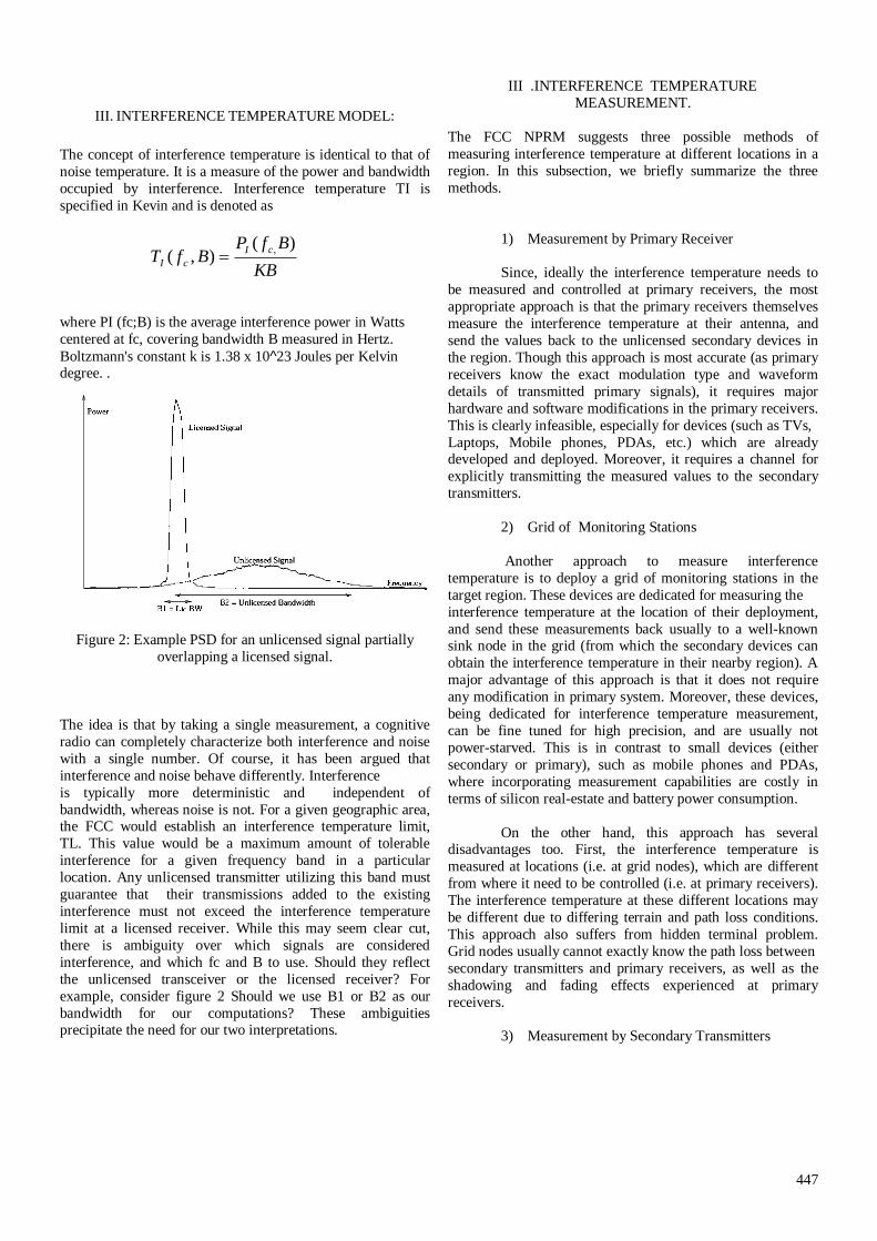
447
III. INTERFERENCE TEMPERATURE MODEL:
The concept of interference temperature is identical to that of
noise temperature. It is a measure of the power and bandwidth
occupied by interference. Interference temperature TI is
specified in Kevin and is denoted as
KB
BfPBfT
cI
cI
)(),(
,
where PI (fc;B) is the average interference power in Watts
centered at fc, covering bandwidth B measured in Hertz.
Boltzmann's constant k is 1.38 x 10^23 Joules per Kelvin degree. .
Figure 2: Example PSD for an unlicensed signal partially
overlapping a licensed signal.
The idea is that by taking a single measurement, a cognitive
radio can completely characterize both interference and noise
with a single number. Of course, it has been argued that
interference and noise behave differently. Interference
is typically more deterministic and independent of
bandwidth, whereas noise is not. For a given geographic area, the FCC would establish an interference temperature limit,
TL. This value would be a maximum amount of tolerable
interference for a given frequency band in a particular
location. Any unlicensed transmitter utilizing this band must
guarantee that their transmissions added to the existing
interference must not exceed the interference temperature
limit at a licensed receiver. While this may seem clear cut,
there is ambiguity over which signals are considered
interference, and which fc and B to use. Should they reflect
the unlicensed transceiver or the licensed receiver? For
example, consider figure 2 Should we use B1 or B2 as our
bandwidth for our computations? These ambiguities precipitate the need for our two interpretations.
III .INTERFERENCE TEMPERATURE
MEASUREMENT.
The FCC NPRM suggests three possible methods of
measuring interference temperature at different locations in a
region. In this subsection, we briefly summarize the three
methods.
1) Measurement by Primary Receiver
Since, ideally the interference temperature needs to
be measured and controlled at primary receivers, the most
appropriate approach is that the primary receivers themselves
measure the interference temperature at their antenna, and
send the values back to the unlicensed secondary devices in
the region. Though this approach is most accurate (as primary
receivers know the exact modulation type and waveform
details of transmitted primary signals), it requires major
hardware and software modifications in the primary receivers.
This is clearly infeasible, especially for devices (such as TVs,
Laptops, Mobile phones, PDAs, etc.) which are already developed and deployed. Moreover, it requires a channel for
explicitly transmitting the measured values to the secondary
transmitters.
2) Grid of Monitoring Stations
Another approach to measure interference
temperature is to deploy a grid of monitoring stations in the
target region. These devices are dedicated for measuring the
interference temperature at the location of their deployment,
and send these measurements back usually to a well-known sink node in the grid (from which the secondary devices can
obtain the interference temperature in their nearby region). A
major advantage of this approach is that it does not require
any modification in primary system. Moreover, these devices,
being dedicated for interference temperature measurement,
can be fine tuned for high precision, and are usually not
power-starved. This is in contrast to small devices (either
secondary or primary), such as mobile phones and PDAs,
where incorporating measurement capabilities are costly in
terms of silicon real-estate and battery power consumption.
On the other hand, this approach has several disadvantages too. First, the interference temperature is
measured at locations (i.e. at grid nodes), which are different
from where it need to be controlled (i.e. at primary receivers).
The interference temperature at these different locations may
be different due to differing terrain and path loss conditions.
This approach also suffers from hidden terminal problem.
Grid nodes usually cannot exactly know the path loss between
secondary transmitters and primary receivers, as well as the
shadowing and fading effects experienced at primary
receivers.
3) Measurement by Secondary Transmitters

448
The simplest but somewhat inaccurate method to
measure the interference temperature is to let a secondary
device itself measure the interference temperature locally.
This approach neither requires any modification in primary
system, nor any additional deployment of measuring services.
But the interference temperature that the secondary device
measures locally and the one that is present at a primary
receiver may differ significantly (unless both the devices are
very near to each other), due to location and terrain-dependent
multipath interference and shadowing affects. Moreover, secondary devices need to be equipped with interference
temperature measurement capabilities.
IV SPECTRUM SENSING IN CR NETWORKS:
Spectrum sensing is crucial for CR networks to
detect active primary users and avoid causing interference. Let
us briefly go through important parameters that characterize
spectrum sensing in CR networks.
1) Signal to Noise Ratio (SNR): When a primary user is active, the higher the SNR of the primary user’s signal at
the receiver of a CR device, the easier it is to detect. We
denote this SNR by 𝛾.
2) Probability of Detection 𝑃𝑑: This is the
probability that a CR network accurately detects the presence
of an active primary user. The higher the value of 𝑃𝑑, the
better the protection for primary operation.
3) Probability of False Alarm 𝑃𝑓 : This is the
probability that a CR network falsely detects the presence of
primary users when in fact none of them are active at the
sensing time. From the CR network point of view, the lower
the value of 𝑃𝑓, the higher the spectrum utilization.
4) Detection Time 𝑇𝑑: This is the time taken to detect
a primary user since it first turns on.
V OFDM- COGNITIVE RADIO:
Orthogonal-Frequency-Division Multiplexing
(OFDM) is the best physical layer candidate for a CR system
since it allows easy generation of spectral signal waveforms
that can fit into discontinuous and arbitrary-sized spectrum
segments. Besides, OFDM is optimal from the viewpoint of
capacity as it allows achieving the Shannon channel capacity
in a fragmented spectrum. Owing to these reasons, in this
paper, we consider the problem of Data Transmission in an
OFDM based CR system. When we transmit data in OFDM, BER decreases, when signal-to-noise ratio increases.
Simulation result is shown in the fig.3.
VI SIMULATION RESULT:
FIGURE.3.BER Vs SNR
VII CONCLUSION:
In this paper we have considered how to use both interference
temperature and the regulatory interference temperature limit
to select an optimal radio bandwidth for a particular
interference environment.Also we discussed both spectrum
sensing parameters and the effect of data transmission in
OFDM.
REFERENCES
[1] T. Charles Clancy, William A. Arbaugh, “Measuring
Interference Temperature” Dept of Computer science,
University of Maryland, college park, Labouratory for
telecommunication sciences, Dept of Defence,Vol 43,2009.
[2] Anh Tuan Hoang, , Ying-Chang Liang, and Yonghong
Zeng, “Adaptive Joint Scheduling of Spectrum Sensing and
Data Transmission in Cognitive Radio Networks”IEEE
Transactions on communications, Vol 58,No.1,Jan 2010.
[3] Ziaul Hasan, Gaurav Bansal. Ekram Hossain, Vijay K. Bhargava, “ Energy Efficient Power allocation in OFDM-
Based Cognitive Radio Systems: A Risk Return Model”IEEE
Transactions on Wireless Communications, Vol 8, No 12,
DEC 2009.

449
[4] Manuj Sharma, Anirudha Sahoo, K.D. Nayak, “channel
Selection Under IT Model in Multi-hop Cognitive Radio
Mesh Networks”, IEEE transactions on communication, Vol
6,2009.

Wireless Communication of Multi-User MIMO System with ZFBF and Sum Rate Analysis
k.srinivasan Department of Communication System
Dhanalakshmi Srinivasan Engineering College, Perambalur. [email protected]
Abstract-We present the exact sum-rate analysis of the multi-user multiple-input multiple-output (MIMO) systems with zero-forcing transmit beam forming (ZFBF). ZERO-FORCING transmit beam forming (ZFBF) is a practical multi-user transmission strategy for multi-user MIMO systems. We develop the analytical expressions of the ergodic sum-rate for two low-complexity user selection strategies for the dual-transmit antenna scenario. Based on the analytical results, we examine the parameter optimization problem to properly tradeoff between channel power gain and directional gain in term of maximizing the ergodic sum rate. Proper user selection scheme is essential for ZFBF-based multi-user MIMO system to fully benefit from multi-user diversity gain. The optimum ZFBF user selection strategy involves the exhaustive search of all possible user subsets, which becomes prohibitive to implement when the number of users is large.
Index TermsMIMO broadcast channel, zero-forcing beam forming, multi-user diversity, sum-rate analysis, and wireless communications.
I.INTRODUCTION
Zero-forcing transmit beam forming (ZFBF) is a practical Multi-user transmission strategy [1], [2] for multi-user MIMO systems. By designing one users beam forming vector to be orthogonal to other selected users channel vectors, ZFBF can completely eliminate multi-user interference. It has been shown that ZFBF can achieve the same sum-rate scale law of log log(), where is the number of users in the system, as the optimal DPC scheme [3][5] . Proper user selection scheme is essential for ZFBF-based multi-user MIMO system to fully benefit from multi-user diversity gain [6]. The optimum ZFBF user selection strategy involves the exhaustive search of all possible user subsets, which becomes prohibitive to implement when the number of users is large. Several low-complexity user selection strategies have been proposed and studied in the literature [6], [7], [9], [10]. Among them, two greedy search algorithms, the successive projection ZFBF (SUP-ZFBF)[6] and greedy weight clique ZFBF (GWC-ZFBF) [7], are attractive for implementation simplicity and their ability to achieve the same scale rate of double log as the DPC scheme. Most previous work on multi-user MIMO transmission schemes have been based on either simulation study or asymptotic analysis, which have limited applicability to accurate tradeoff analysis and design parameter optimization. In this paper, we adopt a different approach and
study multi-user ZFBF transmission schemes through statistical performance analysis. II. SYSTEM AND CHANNEL MODELS We consider a multiuser MIMO system with two transmit antennas at the base station. There are totally K≥2 single antenna users in the system. The channel gains from transmit antennas to users are assumed to be independent and identically distributed (i.i.d.) zero mean complex Gaussian random variable with unitary variance. As such, the norm square of the k-th users channel vector (termed as channel power gain in this paper) is a Chi-square distributed random variable with four degrees of freedom, with probability density function (PDF) and cumulative distribution function (CDF). III. SUM-RATE ANALYSIS In this section, we analyze the ergodic sum rate of ZFBF Based multi-user MIMO system with SUP-ZFBF and GWCZFBF schemes. For that purpose, we first derive the statistics of channel power gains of selected users.
analytical sum-rate expression derived in this paper, we can easily find the optimal value by using one-dimensional Optimization algorithms. We can also observe that the optimal
Proceedings of the Third National Conference on RTICT 2010Bannari Amman Institute of Technology, Sathyamangalam-638401
9-10 April 2010
450

Value of increases with the number of users , which Indicates that when more users are in the system we should trade channel power diversity for directional diversity gain. EXISTING SYSTEM
Most previous work on multi-user MIMO
transmission schemes have been based on either simulation study or asymptotic analysis, which have limited applicability to accurate tradeoff analysis and design parameter optimization. Several low-complexity user selection strategies have been proposed. Among them, two greedy search algorithms, the successive projection ZFBF (SUP-ZFBF) and greedy weight clique ZFBF (GWC-ZFBF), are attractive for implementation simplicity and their ability to achieve the same scale rate of double log as the DPC scheme. This is based on additive white Gaussian noise channel (AWGN).
PROPOSED SYSTEM In this paper, we adopt a different approach and study multi-user inter symbol interference (ISI) transmission schemes through statistical performance analysis. Specifically, we derive the exact analytical expressions for the ergodic sum rate of the SUP-ZFBF and GWC-ZFBF schemes for the important dual-transmit-antenna scenario. We then apply these analytical results to the parameter optimization for each scheme. We show that while the sum rate performance of GWC-ZFBF scheme is sensitive to the channel direction constraint that of SUP-ZFBF scheme is affected little as long as the constraint is not very strict. By using fading channel transmission and reception is performed without noise. APPLICATION This system has enormous application in wireless communication. Such as transmission of signal without affecting additive white Gaussian noise. This system has various applications in signal transmission and reception. FUTURE ENCHANCEMENT
Hardware implementation of the system will give better results than simulation.
ADVANTAGES
This system uses a noiseless channel transmission. The transmission time duration is less compared to
existing systems. The system does not use AWGN this is the main
advantage of this system Complexity is less. More than companies are occupied in this processing.
Conclusion:
Opportunistic beam forming with clustered OFDM promises throughput on par with a smart antenna solution, with little feedback and possibly a lower complexity base station.
REFERENCES [1] P. Viswanath, D. N. C. Tse, and R. Laroia, Opportunistic beamforming using dumb antennas," IEEE Trans. Inform. Theory, vol. 48, no. 6, pp.1277-1294, June 2002. [2] W. Rhee, W. Yu, and J. M. Cioffi, The optimality of beamforming in uplink multiuser wireless systems," IEEE Trans. Wireless Commun.,vol. 3, no. 1, pp. 86-96, Jan. 2004. [3] N. Jindal and A. Goldsmith, Dirty paper coding vs. TDMA for MIMO broadcast channels," in Proc. IEEE Int. Conf. Commun. (ICC2004), Paris, France, vol. 2, pp. 682-686, June 2004. [4] M. Sharif and B. Hassibi, A comparison of time-sharing, DPC, and beamforming for MIMO broadcast channels with many users," IEEE Trans. Commun., vol. 55, no. 1, pp. 11-15, Jan. 2007. [5] M. Costa, Writing on dirty paper," IEEE Trans. Inform. Theory, vol. 29, pp. 439-441, May 1983. [6] T. Yoo and A. Goldsmith, On the optimality of multiantenna broadcast
451
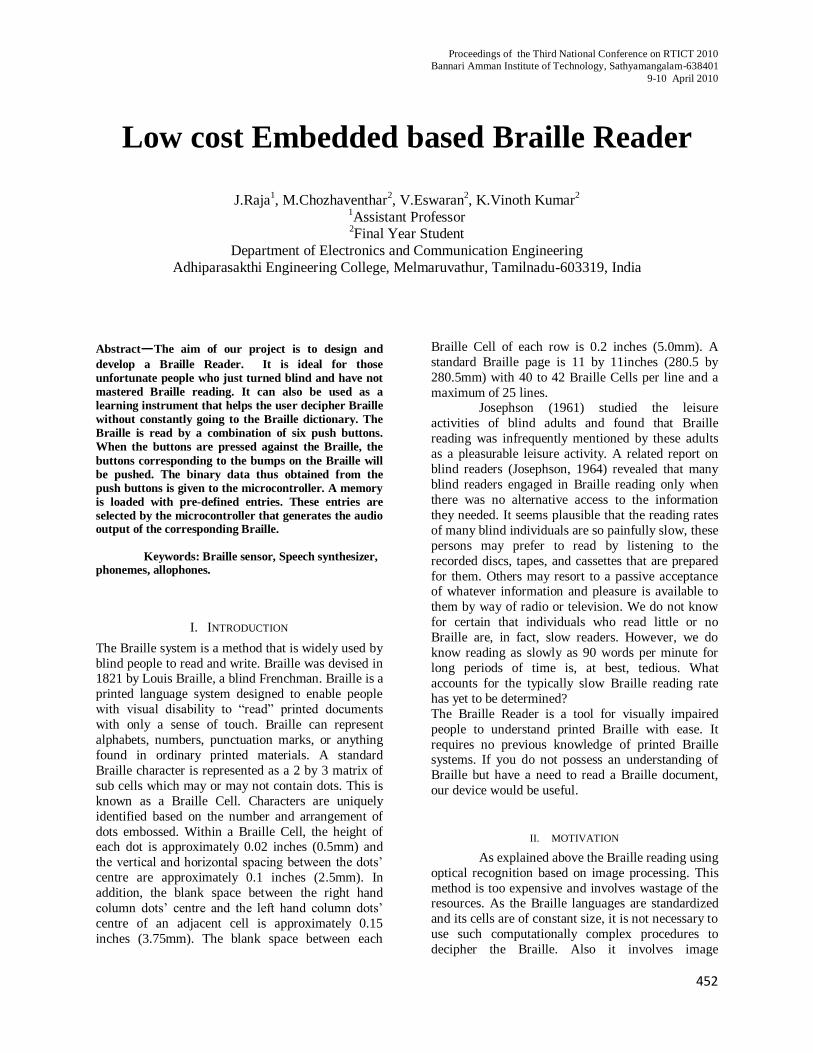
Proceedings of the Third National Conference on RTICT 2010
Bannari Amman Institute of Technology, Sathyamangalam-638401
9-10 April 2010
452
Low cost Embedded based Braille Reader
J.Raja
1, M.Chozhaventhar
2, V.Eswaran
2, K.Vinoth Kumar
2
1Assistant Professor
2Final Year Student
Department of Electronics and Communication Engineering
Adhiparasakthi Engineering College, Melmaruvathur, Tamilnadu-603319, India
Abstract—The aim of our project is to design and
develop a Braille Reader. It is ideal for those
unfortunate people who just turned blind and have not
mastered Braille reading. It can also be used as a
learning instrument that helps the user decipher Braille
without constantly going to the Braille dictionary. The
Braille is read by a combination of six push buttons.
When the buttons are pressed against the Braille, the
buttons corresponding to the bumps on the Braille will
be pushed. The binary data thus obtained from the
push buttons is given to the microcontroller. A memory
is loaded with pre-defined entries. These entries are
selected by the microcontroller that generates the audio output of the corresponding Braille.
Keywords: Braille sensor, Speech synthesizer, phonemes, allophones.
I. INTRODUCTION
The Braille system is a method that is widely used by
blind people to read and write. Braille was devised in 1821 by Louis Braille, a blind Frenchman. Braille is a
printed language system designed to enable people
with visual disability to “read” printed documents
with only a sense of touch. Braille can represent
alphabets, numbers, punctuation marks, or anything
found in ordinary printed materials. A standard
Braille character is represented as a 2 by 3 matrix of
sub cells which may or may not contain dots. This is
known as a Braille Cell. Characters are uniquely
identified based on the number and arrangement of
dots embossed. Within a Braille Cell, the height of each dot is approximately 0.02 inches (0.5mm) and
the vertical and horizontal spacing between the dots’
centre are approximately 0.1 inches (2.5mm). In
addition, the blank space between the right hand
column dots’ centre and the left hand column dots’
centre of an adjacent cell is approximately 0.15
inches (3.75mm). The blank space between each
Braille Cell of each row is 0.2 inches (5.0mm). A
standard Braille page is 11 by 11inches (280.5 by
280.5mm) with 40 to 42 Braille Cells per line and a
maximum of 25 lines. Josephson (1961) studied the leisure
activities of blind adults and found that Braille
reading was infrequently mentioned by these adults
as a pleasurable leisure activity. A related report on
blind readers (Josephson, 1964) revealed that many
blind readers engaged in Braille reading only when
there was no alternative access to the information
they needed. It seems plausible that the reading rates
of many blind individuals are so painfully slow, these
persons may prefer to read by listening to the
recorded discs, tapes, and cassettes that are prepared
for them. Others may resort to a passive acceptance of whatever information and pleasure is available to
them by way of radio or television. We do not know
for certain that individuals who read little or no
Braille are, in fact, slow readers. However, we do
know reading as slowly as 90 words per minute for
long periods of time is, at best, tedious. What
accounts for the typically slow Braille reading rate
has yet to be determined?
The Braille Reader is a tool for visually impaired
people to understand printed Braille with ease. It
requires no previous knowledge of printed Braille systems. If you do not possess an understanding of
Braille but have a need to read a Braille document,
our device would be useful.
II. MOTIVATION
As explained above the Braille reading using
optical recognition based on image processing. This
method is too expensive and involves wastage of the resources. As the Braille languages are standardized
and its cells are of constant size, it is not necessary to
use such computationally complex procedures to
decipher the Braille. Also it involves image

453
processing that obviates need of digital camera which
incur additional cost on the device.
Hence in order to provide cost effective
solution and easy to handle device to such visually
challenged people we proposed our system in that
Instead of image sensing, we decided to use 6 push buttons in a 2x3 matrix. When the buttons are
pressed against the Braille, the buttons corresponding
to the bumps on the Braille will be pushed.
Depending upon this combination corresponding
audio output will be generated with the help of
microcontroller and speech synthesizer.
III. PROPOSED SYSTEM
Our proposed system involves three main
components .they are i) Braille sensor ii)
microcontroller and iii) speech synthesizer.
Fig.1.Braille Sensor
Braille sensor is the physical part that acts as an
interface between the blind people and Braille book.
Braille sensor can be realized with the help of six
push buttons as shown. When this Braille sensor are
pressed against Braille, combination of bumps
present in the Braille cell produce unique binary
pattern as shown above. On obtaining binary input, it
is given as an input to the microcontroller which is
programmed in such a way as to recognize it and obtain its corresponding text output.
Thus overall block diagram of our proposed system
can be represented as shown in fig.1.
Once the text of the Braille was obtained, speech
synthesizers enter into play. It contains the phoneme
sets that are previously stored. In order to retrieve the
phonemes that corresponds to the input
microcontroller outputs the sequence of commands
required via its serial port.
Normally speech synthesizers are self contained, single chip that produces complex sounds
depends on the input commands. Hence when
connected it on speaker it produces audio of the
corresponding input.
Fig.2.Braille Reader
IV. HARDWARE REQUIREMENTS
After analyzing the various requirements we have proposed to use the following
hardware components
Protoboard – This is the skeleton of the Braille
reader. It holds the Atmel 8352 microcontroller and
supports links to other components.
Braille Sensor – A combination of 6 NKK buttons.
This is like user’s eye. It converts Braille to Binary
data. (B2B) So the MegaL32 can process the data.
ATMega8535 – The heart of Braille Reader. This
microcontroller receives data from Braille sensor and
generates the sound output at amazing speed. (16
MHz) It also controls different parameters of the
Braille Reader such as Volume.
SpeakJet –This speech synthesizer can acts as the messenger between the microcontroller and the user.
Whenever a button is pushed or a Braille is read, the
SpeakJet will generate a robotic voice and deliver a
message to the user to make sure the user is updated
with his/her surrounding.
CHARACTERER
VOICE
BRAILLE SENSOR
MICROCONTROLLER
SPEECH SYNTHESIZER PHONEME SET
BINARY
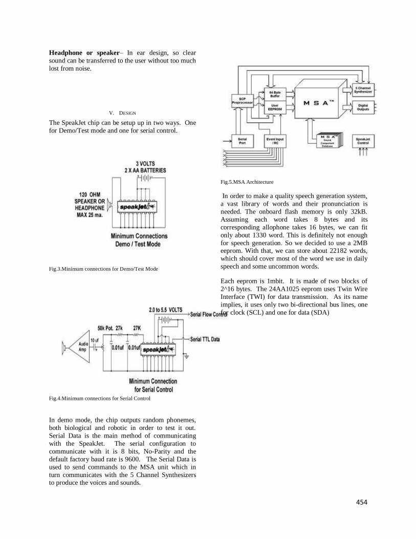
454
Headphone or speaker– In ear design, so clear
sound can be transferred to the user without too much
lost from noise.
V. DESIGN
The SpeakJet chip can be setup up in two ways. One
for Demo/Test mode and one for serial control.
Fig.3.Minimum connections for Demo/Test Mode
Fig.4.Minimum connections for Serial Control
In demo mode, the chip outputs random phonemes,
both biological and robotic in order to test it out.
Serial Data is the main method of communicating
with the SpeakJet. The serial configuration to
communicate with it is 8 bits, No-Parity and the
default factory baud rate is 9600. The Serial Data is
used to send commands to the MSA unit which in
turn communicates with the 5 Channel Synthesizers to produce the voices and sounds.
Fig.5.MSA Architecture
In order to make a quality speech generation system,
a vast library of words and their pronunciation is
needed. The onboard flash memory is only 32kB.
Assuming each word takes 8 bytes and its
corresponding allophone takes 16 bytes, we can fit
only about 1330 word. This is definitely not enough
for speech generation. So we decided to use a 2MB eeprom. With that, we can store about 22182 words,
which should cover most of the word we use in daily
speech and some uncommon words.
Each eeprom is 1mbit. It is made of two blocks of
2^16 bytes. The 24AA1025 eeprom uses Twin Wire
Interface (TWI) for data transmission. As its name
implies, it uses only two bi-directional bus lines, one
for clock (SCL) and one for data (SDA)

455
VI. SOFTWARE
In order to pronounce the words that are not in the
library, the MCU will divide the input word into
existing words. It would break the unknown word
down by finding the longest existing word from our
library that matches with the prefix of the unknown
word.
For example:
Input Word: “appletree”
The Braille reader will pronounce: “apple”
+ “tree”
For data storage, all words can be put in a single
character array with “*” between words to indicate
where words start and stop. This design can be
picked over double character array because double
character array requires same length for each word.
So the shortest word “a” will have to take the same
amount of space as the longest word in the
dictionary. However, the single array made binary
search impossible. So linear search can be used.
In order to save time with searching, the words in the
dictionary are arranged in alphabetical order and
recorded the position for each of the 26 letters in the
alphabet. So instead of traverse through the entire
library for searching, it will only search words that
match the first letter.
The CMU dictionary provided by Carnegie Mellon
University for research purposes can be used. The
dictionary contains over 125,000 North American
English words with their transcriptions. The
dictionary uses 39 phonemes in its transcriptions.
Phoneme Set
Phoneme Example Translation
------- ------- -----------
AA odd AA D
AE at AE T
AH hut HH AH T
AO ought AO T
AW cow K AW
AY hide HH AY D B be B IY
CH cheese CH IY Z
D dee D IY
DH thee DH IY
EH Ed EH D
ER hurt HH ER T
EY ate EY T
F fee F IY
G green G R IY N
HH he HH IY
IH it IH T IY eat IY T
JH gee JH IY
K key K IY
L lee L IY
M me M IY
N knee N IY
NG ping P IH NG
OW oat OW T

456
OY toy T OY
P pee P IY
R read R IY D
S sea S IY
SH she SH IY
T tea T IY
TH theta TH EY T AH
UH hood HH UH D
UW two T UW V vee V IY
W we W IY
Y yield Y IY L D
Z zee Z IY
ZH seizure S IY ZH ER
VII. CONCLUSION
This paper makes an attempt to provide a
low cost solution to the visually impaired people. The
paper is based on microcontroller and can also be
used by dumb blind people to communicate freely
with the external world. This device can also be
designed at much lower price without synthesizer by
storing the required allophones on a memory. . This
would also have saved a lot more money than buying
a retail Braille reader which costs $1,400.Thus this
would definitely assist the visually challenged to decipher the Braille with less burden at affordable
cost.
REFERENCES
[1] y. Matsuda, et al., “analysis of emotional expression of finger
braille,” ifmbe proc. Vol. 19, 7th asian-pacific conference on
medical and biological engineering, china, pp.484-487, april 2008.
[2] y. Matsuda, et al., “finger braille teaching system for people
who communicate with deaf blind people,” proc. Of the 2007 ieee
international conference on mechatronics and automation, china,
pp.3202-3207, august 2007.
[3] i/o terminal for finger braille,” proc. Of the human interface
symposium 2000, japan, pp.37-40, september 2000.
[4] m. Fukumoto, et al., “body coupled fingering: wireless
wearable keyboard,” proc. Of the acm conference on human
factors in computing systems, france, pp.147-154, march 1997.
[5] bouraoui a., extending an existing tool to create non visual
interfaces. Proceedings of csun 2006, centre on disabilities 21st
annual international technology and persons with disabilities
conference, california state university northridge, 2006.
[6] information about braille and other reading codes for the blind
http://www.brailler.com/braillehx.htm
http://www.nyise.org/blind/
http://www.duxburysystems.com/braille.asp
http://en.wikipedia.org/wiki/braille
[7] cmu dictionary
http://www.speech.cs.cmu.edu/cgi-bin/cmudict
[8]speakjet datasheet
http://www.magnevation.com/pdfs/speakjetusermanual.pdf
[9]phrase-a-lator software and phonetic dictionary
http://magnevation.com/software.htm

Unbiased Sampling in Ad-hoc (Peer-to-Peer) Networks
M.Deiveegan,A.Saravanan,S.Vinothkannan
Department of Information Technology,Anna university [email protected]
[email protected] [email protected]
Abstract—This paper presents a detailed examination of how the dynamic and heterogeneous nature of real-world peer-to-peer systems can introduce bias into the selection of representative samples of peer properties (e.g., degree, link bandwidth, number of files shared). We propose the Metropolized Random Walk with Backtracking and Linking (MRWBL) technique for collecting nearly unbiased samples and conduct an extensive simulation study to demonstrate that our technique works well for a wide variety of commonly-encountered peer-to-peer net work conditions. We have implemented the MRWBL algorithm for selecting peer addresses uniformly at random. Using the Gnutella network, we empirically show that ion-sampler yields more accurate samples than tools that rely on commonly-used sampling techniques and results in dramatic improvements in efficiency and scalability compared to performing earlier algorithms.
Index Terms—Peer-to-peer, sampling.
I. INTRODUCTION
HE popularity and wide-spread use of peer-to-peer sys-tems has motivated numerous empirical studies aimed at
providing a better understanding of the properties of deployed peer-to-peer systems. However, due to the large scale and highly dynamic nature of many of these systems, directly measuring the quantities of interest on every peer is prohibitively expen-sive. Sampling is a natural approach for learning about these systems using light-weight data collection, but commonly-used sampling techniques for measuring peer-to-peer systems tend to introduce considerable bias for two reasons. First, the dy-namic nature of peers can bias results towards short-lived peers, much as naively sampling flows in a router can lead to bias to-wards short-lived flows. Second, the heterogeneous nature of the overlay topology can lead to bias towards high-degree peers.
In this paper, we are concerned with the basic objective of devising an unbiased sampling method, i.e., one which selects any of the present peers with equal probability. The addresses of the resulting peers may then be used as input to another mea-surement tool to collect data on particular peer properties (e.g., degree, link bandwidth, number of files shared). The focus of our work is on unstructured P2P systems, where peers select neighbors through a predominantly random process. Most pop-ular P2P systems in use today belong to this unstructured cate-gory. For structured P2P systems such as Chord [1] and CAN [2], knowledge of the structure significantly facilitates unbiased sampling as we discuss in Section VII.
Achieving the basic objective of selecting any of the peers present with equal probability is non-trivial when the structure of the peer-to-peer system changes during the measurements. First-generation measurement studies of P2P systems typically
relied on ad-hoc sampling techniques (e.g., [3], [4]) and pro-vided valuable information concerning basic system behavior. However, lacking any critical assessment of the quality of these sampling techniques, the measurements resulting from these studies may be biased and consequently our understanding of P2P systems may be incorrect or misleading. The main contri-butions of this paper are (i) a detailed examination of the ways that the topological and temporal qualities of peer-to-peer sys-tems (e.g., Churn [5]) can introduce bias, (ii) an in-depth ex-ploration of the applicability of a sampling technique called the Metropolized Random Walk with Backtracking (MRWB), repre-senting a variation of the Metropolis-Hastings method [6]-[8], and (iii) an implementation of the MRWB algorithm into a tool called -. While sampling techniques based on the original Metropolis-Hastings method have been considered ear-lier (e.g., see Awanet al. [9] andBar-YossefandGurevich [10]), we show that in the context of unstructured P2P systems, our modification of the basic Metropolis-Hastings method results in nearly unbiased samples under a wide variety of commonly encountered peer-to-peer network conditions.
The proposed MRWB algorithm assumes that the P2P system provides some mechanism to query a peer for a list of its neighbors—a capability provided by most widely deployed P2P systems. Our evaluat ions of the - tool shows that the MRWB algorithm yields more accurate samples than previously considered sampling techniques. We quantify the observed differences, explore underlying causes, address the tool's efficiency and scalability, and discuss the implications on accurate inference of P2P properties and high-fidelity modeling of P2P systems. While our focus is on P2P networks, many of our results apply to any large, dynamic, undirected graph where nodes may be queried for a list of their neighbors.
After discussing related work and alternative sampling tech-niques in Section II, we build on our earlier formulation in [11] and focus on sampling techniques that select a set of peers uni-formly at random from all the peers present in the overlay and then gather data about the desired properties from those peers. While it is relatively straightforward to choose peers uniformly at random in a static and known environment, it poses consid-erable problems in a highly dynamic setting like P2P systems, which can easily lead to significant measurement bias for two reasons.
The first cause of sampling bias derives from the temporal dynamics of these systems, whereby new peers can arrive and existing peers can depart at any time. Locating a set of peers and measuring their properties takes time, and during that time the peer constituency is likely to change. In Section III, we show
T
Proceedings of the Third National Conference on RTICT 2010Bannari Amman Institute of Technology, Sathyamangalam-638401
9-10 April 2010
457

how this often leads to bias towards short-lived peers and ex-plain how to overcome this difficulty.
The second significant cause of bias relates to the connectivity structure of P2P systems. As a sampling program explores a given topological structure, each traversed link is more likely to lead to a high-degree peer than a low-degree peer, significantly biasing peer selection. We describe and evaluate different tech-niques for traversing static overlays to select peers in Section IV and find that the Metropolized Random Walk (MRW) collects unbiased samples.
In Section V, we adapt MRW for dynamic overlays by adding backtracking and demonstrate its viability and effectiveness when the causes for both temporal and topological bias are present. We show via simulations that the MRWB technique works well and produces nearly unbiased samples under a variety of circumstances commonly encountered in actual P2P systems.
Finally, in Section VI we describe the implementation of the tool based on the proposed MRWBL algorithm and
empirically evaluate its accuracy and efficiency through com-parison with complete snapshots of Gnutella taken with Cruiser [12], as well as with results obtained from previously used, more ad-hoc, sampling techniques. Section VII concludes the paper by summarizing our findings and plans for future work.
II. RELATED WORK
A. Graph Sampling
The phrase "graph sampling" means different things in dif-ferent contexts. For example, sampling from a class of graphs has been well studied in the graph theory literature [13], [14], where the main objective is to prove that for a class of graphs sharing some property (e.g., same node degree distribution), a given random algorithm is capable of generating all graphs in the class. Cooper et al. [15] used this approach to show that their algorithm for overlay construction generates graphs with good properties. Our objective is quite different; instead of sam-pling a graph from a class of graphs our concern is sampling peers (i.e., vertices) from a largely unknown and dynamically changing graph. Others have used sampling to extract informa-tion about graphs (e.g., selecting representative subgraphs from a large, intractable graph) while maintaining properties of the original structure [16]—[18]. Sampling is also frequently used as a component of efficient, randomized algorithms [19]. How-ever, these studies assume complete knowledge of the graphs in question. Our problem is quite different in that we do not know the graphs in advance.
A closely related problem to ours is sampling Internet routers by running traceroute from a few hosts to many destinations for the purpose of discovering the Internet's router-level topology. Using simulation [20] and analysis [21], research has shown that traceroute measurements can result in measurement bias in the sense that the obtained samples support the inference of power law-type degree distributions irrespective of the true na-ture of the underlying degree distribution. A common feature of our work and the study of the traceroute technique [20], [21] is that both efforts require an evaluation of sampling techniques without complete knowledge of the true nature of the underlying connectivity structure. However, exploring the router topology and P2P topologies differ in their basic operations for graph-ex-ploration. In the case of traceroute, the basic operation is "What is the path to this destination?" In P2P networks, the basic oper-ation is "What are the neighbors of this peer?" In addition, the
Internet's router-level topology changes at a much slower rate than the overlay topology of P2P networks.
Another closely related problem is selecting Web pages uni-formly at random from the set of all Web pages [22], [23]. Web pages naturally form a graph, with hyper-links forming edges between pages. Unlike unstructured peer-to-peer networks, the Web graph is directed and only outgoing links are easily dis-covered. Much of the work on sampling Web pages therefore focuses on estimating the number of incoming links, to facili-tate degree correction. Unlike peers in peer-to-peer systems, not much is known about the temporal stability of Web pages, and temporal causes of sampling bias have received little attention in past measurement studies of the Web.
B. Random Walk-Based Sampling of Graphs
A popular technique for exploring connectivity structures consists of performing random walks on graphs. Several properties of random walks on graphs have been extensively studied analytically [24], such as the access time, cover time, and mixing time. While these properties have many useful applications, they are, in general, only well-defined for static graphs. To our knowledge the application of random walks as a method of selecting nodes uniformly at random from a dynamically changing graph has not been studied. A number of papers [25]-[28] have made use of random walks as a basis for searching unstructured P2P networks. However, searching simply requires locating a certain piece of data anywhere along the walk, and is not particularly concerned if some nodes are preferred over others. Some studies [27], [28] additionally use random walks as a component of their overlay-construction algorithm. Two papers that are closely related to our random walk-based sampling approach are by Awan et al. [9] and Bar-Yossef and Gurevich [10]. While the former also address the problem of gathering uniform samples from peer-to-peer networks, the latter are concerned with uniform sampling from a search engine's index. Both works examine several random walk tech-niques, including the Metropolis-Hastings method, but assume an underlying graph structure that is not dynamically changing. In addition to evaluating their techniques empirically for static power-law graphs, the approach proposed by Awan et al. [9] also requires special underlying support from the peer-to-peer application. In contrast, we implement the Metropolis-Hast-ings method in such a way that it relies only on the ability to discover a peer's neighbors, a simple primitive operation commonly found in existing peer-to-peer networks. Moreover, we introduce backtracking to cope with departed peers and con-duct a much more extensive evaluation of the proposed MRWB method. Specifically, we generalize our formulation reported in [11] by evaluating MRWB over dynamically changing graphs with a variety of topological properties. We also perform empirical validations over an actual P2P network.
C. Sampling in Hidden Populations
The problem of obtaining accurate estimates of the number of peers in an unstructured P2P network that have a certain prop-erty can also be viewed as a problem in studying the sizes of hidden populations. Following Salganik [29], a population is called "hidden" if there is no central directory of all population members, such that samples may only be gathered through re-ferrals from existing samples. This situation often arises when
458

public acknowledgment of membership has repercussions (e.g., injection drug users [30]), but also arises if the target population is difficult to distinguish from the population as a whole (e.g., jazz musicians [29]). Peers in P2P networks are hidden because there is no central repository we can query for a list of all peers. Peers must be discovered by querying other peers for a list of neighbors.
Proposed methods in the social and statistical sciences for studying hidden populations include snowball sampling [31], key informant sampling [32], and targeted sampling [33]. While these methods gather an adequate number of samples, they are notoriously biased. More recently, Heckathorn [30] (see also [29], [34]) proposed respondent-driven sampling, a snowball-type method for sampling and estimation in hidden populations. Respondent-driven sampling first uses the sample to make infer-ences about the underlying network structure. In a second step, these network-related estimates are used to derive the propor-tions of the various subpopulations of interest. Salganik et al. [29], [34] show that under quite general assumptions, respon-dent-driven sampling yields estimates for the sizes of subpop-ulations that are asymptotically unbiased, no matter how the seeds were chosen.
Unfortunately, respondent-driven sampling has only been studied in the context where the social network is static and does not change with time. To the best of our knowledge, the accuracy of respondent-driven sampling in situations where the underlying network structure is changing dynamically (e.g., unstructured P2P systems) has not been considered in the existing sampling literature
III. SAMPLING WITH DYNAMICS
We develop a formal and general model of a P2P system as follows. If we take an instantaneous snapshot of the system at time , we can view the overlay as a graph G(V, E) with the peers as vertices and connections between the peers as edges. Extending this notion, we incorporate the dynamic aspect by viewing the system as an infinite set of time-indexed graphs, Gt = . The mo st co mmon approach fo r samp l ing from this set of graphs is to define a measurement window, [to, to + , and select peers uniformly at random from the set of peers who are present at any time during the window: Vto,to+A = UtLt Vt- Thus, it does not distinguish between occurrences of the same peer at different times.
This approach is appropriate if peer session lengths are expo-nentially distributed (i.e., memoryless). However, existing mea-surement studies [3], [5], [37], [38] show session lengths are heavily skewed, with many peers being present for just a short time (a few minutes) while other peers remain in the system for a very long time (i.e., longer than ). As a consequence, as A increases, the set Vtotto+A includes an increasingly large fraction of short-lived peers.
A simple example may be illustrative. Suppose we wish to observe the number of files shared by peers. In this example system, half the peers are up all the time and have many files, while the other peers remain for around 1 minute and are imme-diately replaced by new short-lived peers who have few files. The technique used by most studies would observe the system for a long time (A) and incorrectly conclude that most of the peers in the system have very few files. Moreover, their results will depend on how long they observe the system. The longer the
measurement window, the larger the fraction of observed peers with few files.
One fundamental problem of this approach is that it focuses on sampling peers instead of peer properties. It selects each sampled vertex at most once. However, the property at the vertex may change with time. Our goal should not be to select a vertex Vi e Ut=t , but rather to sample the property at Vi at a par-ticular instant . Thus, we distinguish between occurrences of the same peer at different times: samples vi>t and vitt> gathered at distinct times t ^ t' are viewed as distinct, even when they come from the same peer. The key difference is that it must be possible to sample from the same peer more than once, at different points in time. Using the formulation ui;t e , t £ [to, to + , the sampling technique will not be biased by the dynamics of peer behavior, because the sample set is decoupled from peer session lengths. To our knowledge, no prior P2P measurement studies relying on sampling make this distinction.
Returning to our simple example, our approach will correctly select long-lived peers half the time and short-lived peers half the time. When the samples are examined, they will show that half of the peers in the system at any given moment have many files while half of the peers have few files, which is exactly cor-rect.
If the measurement window (A) is sufficiently small, such that the distribution of the property under consideration does not change significantly during the measurement window, then we may relax the constraint of choosing t uniformly at random from [t0, t0 + A].
We still have the significant problem of selecting a peer uni-formly at random from those present at a particular time. We begin to address this problem in Section IV.
IV. SAMPLING FROM STATIC GRAPHS
We now turn our attention to topological causes of bias. Towards this end, we momentarily set aside the temporal issues by assuming a static, unchanging graph. The selection process begins with knowledge of one peer (vertex) and progressively queries peers for a list of neighbors. The goal is to select peers uniformly at random. In any graph-exploration problem, we have a set of visited peers (vertices) and a front of unexplored neighboring peers. There are two ways in which algorithms differ: (i) how to chose the next peer to explore, and (ii) which subset of the explored peers to select as samples. Prior studies use simple breadth-first or depth-first approaches to explore the graph and select all explored peers. These approaches suffer from several problems:
• The discovered peers are correlated by their neighbor rela tionship.
• Peers with higher degree are more likely to be selected. • Because they never visit the same peer twice, they will
introduce bias when used in a dynamic setting as described in Section III.
1) Random Walks: A better candidate solution is the random walk, which has been extensively studied in the graph theory
literature (for an excellent survey see [24]). We briefly summarize the key terminology and results relevant to sampling. The transition matrix P(x. y) describes the
459
probability of transitioning to peer y if the walk is currently at peer :
If the vector v describes the probability of currently being at each peer, then the vector v' = vP describes the probability
In other words, if we select a peer as a sample every r steps, for sufficiently large , we have the following good properties:
• The information stored in the starting vector, , is lost, through the repeated selection of random neighbors. There fore, there is no correlation between selected peers. Alter nately, we may start many walks in parallel. In either cases, afte r steps, the selection is independent of the origin.
• While the stationary distribution, , is biased towards peers with high degree, the bias is precisely known, al lowing us to correct it.
• Random walks may visit the same peer twice, which lends itself better to a dynamic setting as described in Section III.
In practice, r need not be exceptionally large. For graphs where the edges have a strong random component (e.g., small-world graphs such as peer-to-peer networks), it is sufficient that the number of steps exceed the log of the population size, i.e., r>O(\og\V\). 2) Adjusting for Degree Bias: To correct for the bias towards
high degree peers, we make use of the Metropolis-Hastings method for Markov Chains. Random walks on a graph are a spe cial case of Markov Chains. In a regular random walk, the tran sition matrix P(x,y) leads to the stationary distribution , as described above. We would like to choose a new transition matrix, , to produce a different stationary distribution,
. Specifically, we desire /J,(X) to be the uniform distribution so that all peers are equally likely to be at the end of the walk. Metropolis-Hastings [6]-[8] provides us with the
desired Equivalently, to take a step from peer , select a neighbor y of x as normal (i.e., with probability ) . T h e n , w i t h probability min (^^1^Z'X\, 1), accept the move. Otherwise, return to x (i.e., with probability 1 - YJZ^X Qix-).
To collect uniform samples, we have ijA = , so the move-acceptance probability becomes:
.
Therefore, our algorithm for selecting the next step from some peer x is as follows:
• Select a neighbor y of x uniformly at random. Quer y for a list of its neighbors, to determine its degree. • Generate a random value, , uniformly between 0 and 1.
• If V < degree^) ' V iS me DeXt SteP'
• Otherwise, remain at x as the next step. We call this the Metropolized Random Walk (MRW).
Qualitatively, the effect is to suppress the rate of transition to peers of higher degree, resulting in selecting each peer with equal probability. 3) Evaluation: Although [6] provides a proof of
correctness for the Metropolis-Hastings method, to ensure the correctness of our implementation we conduct evaluations through simulation over static graphs. This additionally provides the opportunity to compare MRW with conventional techniques such as Breadth-First Search (BFS) or naive random walks (RW) with no adjustments for degree bias.
To evaluate a technique, we use it to collect a large number of sample vertices from a graph, then perform a goodness-of-fit test against the uniform distribution. For Breadth-First Search, we simulate typical usage by running it to gather a batch of 1,000 peers. When one batch of samples is collected, the process is reset and begins anew at a different starting point. To ensure robustness with respect to different kinds of connectivity structures, we examine each technique over several types of graphs as follows:
• Erdös-Rényi: The simplest variety of random graphs • Watts-Strogatz: "Small world" graphs with high
clus tering and low path lengths
• Barabási-Albert: Graphs with extreme degree distribu tions, also known as power-law or scale-free graphs
• Gnutella: Snapshots of the Gnutella ultrapeer topology, captured in our earlier work [39]
To make the results more comparable, the number of vertices (\V\ = 161.680) and edges (\E\ = 1.946,596) in each graph are approximately the same.1Table I presents the results of the goodness-of-fit tests after collecting 1000-|F| samples, showing that Metropolis-Hastings appears to generate uniform samples over each type of graph, while the other techniques fail to do so by a wide margin. typical node should be selected k times, with other nodes being selected close to k times approximately following a normal dis tribution with variance .2 We used k = 1,000 samples. We also include an "Oracle" technique, which selects peers uniformly at random using global information. The Metropolis-Hastings results are virtually identical to the Oracle, while the other techniques select many peers much more and much less than k times. In the Gnutella, Watts-Strogatz, and Barabási-Albert graphs, Breadth-First Search exhibits a few vertices that are selected a large number of times (> . T h e ( n o t -a d - justed) Random Walk (RW) method has similarly selected a few vertices an exceptionally large number of times in the Gnutella and Barabási-Albert models. The Oracle and MRW, by contrast, did not select any vertex more than
=
otherwise ,0
x,ofneighbor a isy ,)(deg
1),( xreeyxP
460

around 1,300 times. In summary, the Metropolis-Hastings method selects peers
uniformly at random from a static graph. The Section V exam-ines the additional complexities when selecting from a dynamic graph, introduces appropriate modifications, and evaluates the algorithm's performance.
V. Metropolised Random Walk with Backtracking and Linking algorithm.
In this paper we propose a new algorithm called Metropolised Random Walk with Backtracking and Linking. The major drawback of the Metropolised Random walk With backtracking algorithm is there is a lot of chances for failure of the algorithm because they use the stack for storing the samples .Stack works on the principle LIFO(Last In First Out).If we want to pop or remove a sample from the stack means we have to remove all its neibhours list then only we can pop a single element from the stack. So if a node fails to respond then we have to remove even the nodes that responds. In order to avoid this problem we propose a new method that is MRWBL for collecting the samples.In this algorithm we use the linked list for storing the samples. The nodes will get the information about the neer node that was connected to it . If any node does not responds in the list then the previous node will directly get connected with the new node which is connected to the earlier node. So there is no chance of failure of the whole algorithm .So in this way this algorithm will help the nodes to transfer the datas over the path that is senced or discovered by using the ion-sampler tool and saved in the linked list.
VI. DISCUSSION
A. How Many Samples are Required?
An important consideration when collecting samples is to know how many samples are needed for statistically significant results. This is principally a property of the distribution being sampled. Consider the problem of estimating the underlying fre-
quency / of an event, e.g., that the peer degree takes a particular value. Give n unbiased samples, an unbiased estimate of / is / = M/N where M is the number of samples for which the event occurs. / has root mean square (RMS) relative error
From this expression, we derive the following observations: • Estimation error does not depend on the population size;
in particular the estimation properties of unbiased sampling scale independently of the size of the system under
study. • The above expression can be inverted to derive the
number of samples Nfj(J required to estimate an outcome of frequency / up to an error . A simple bound is Nf „ <
• Unsurprisingly, smaller frequency outcomes have a larger relative error. For example, gathering 1,000 unbiased samples gives us very little useful information about events which only occur one time in 10,000; the associated a value is approximately 3: the likely error dominates the value to be estimated. This motivates using biased sampling .
The presence of sampling bias complicates the picture. If an event with underlying frequency / is actually sampled with fre- quency , then the RMS relative error acquires an additional term (1 - /o//)2 which does not reduce as the number of samples N grows. In other words, when sampling from a biased distribution, increasing the number of samples only increases the accuracy with which we estimate the biased distribution.
B. Unbiased Versus Biased Sampling
At the beginning of this paper, we set the goal of collecting unbiased samples. However, there are circumstances where unbiased samples are inefficient. For example, while unbiased samples provide accurate information about the body of a distribution, they provide very little information about the tails: the pitfall of estimating rare events we discussed in the previous subsection.
In circumstances such as studying infrequent events, it may be desirable to gather samples with a known sampling bias, i.e., with non-uniform sampling probabilities. By deliberately introducing a sampling bias towards the area of interest, more relevant samples can be gathered. During analysis of the data, each sample is weighted inversely to the probability that it is sampled. This yields unbiased estimates of the quantities of interest, even though the selection of the samples is biased. This approach is known as importance sampling [50].
A known bias can be introduced by choosing an appropriate definition of fix) in the Metropolis-Hastings equations presented in Section IV and altering the walk accordingly. Because the desired type of known bias depends on the focus of the research, we cannot exhaustively demonstrate through simulation that Metropolis-Hastings will operate correctly in a dynamic
461

environment for any . Our results show that it works well in the common case where unbiased samples are desired (i.e., fi(x) = fj,(y) for all x and y).
C. Sampling From Structured Systems
Throughout this paper, we have assumed an unstructured peer-to-peer network. Structured systems (also known as Dis-tributed Hash Tables or DHTs) should work just as well with random walks, provided links are still bidirectional. However, the structure of these systems often allows a more efficient technique.
In a typical DHT scheme, each peer has a randomly generated identifier. Peers form an overlay that actively maintains certain properties such that messages are efficiently routed to the peer "closest" to a target identifier. The exact properties and the defi-nition of "closest" vary, but the theme remains the same. In these systems, to select a peer at random, we may simply generate an identifier uniformly at random and find the peer closest to the identifier. Because peer identifiers are generated uniformly at random, we know they are uncorrelated with any other prop-erty. This technique is simple and effective, as long as there is little variation in the amount of identifier space that each peer is responsible for. We made use of this sampling technique in our study of the widely-deployed Kad DHT [51].
VII. CONCLUSIONS AND FUTURE WORK
This paper explores the problem of sampling representative peer properties in large and dynamic unstructured P2P systems. We show that the topological and temporal properties of P2P systems can lead to significant bias in collected samples. To collect unbiased samples, we present the Metropolized Random Walk with Backtracking and linking (MRWBL), a modification of the Metropolis-Hastings technique, which we developed into t h e - tool. Using both simulation and empirical evaluation, we show that MRWB can collect approximately unbiased samples of peer properties over a wide range of realistic peer dynamics and topological structures.
We are pursuing this work in the following directions. First, we are exploring improving sampling efficiency for uncommon events (such as in the tail of distributions) by introducing known bias, Second, we are studying the behavior of MRWBL under flash-crowd scenarios, where not only the properties of individual peers are changing, but the distribution of those properties is also rapidly evolving. Finally, we are developing additional plug-ins for -and using it in conjunction with other measurement tools to accurately characterize several properties of widely-deployed P2P systems.
REFERENCES
[1] I. Stoica, R. Morris, D. Liben-Nowell, D. R. Karger, M. F. Kaashoek, F. Dabek, and H. Balakrishnan, "Chord: A scalable peer-to-peer lookup protocol for Internet applications," IEEE/ACM Trans. Networking, vol. 11, no. 1, pp. 17-32, Feb. 2002.
[2] S. Ratnasamy, P. Francis, M. Handley, R. Karp, and S. Shenker, "A scalable content-addressable network," presented at the ACM SIGCOMM 2001, San Diego, CA.
[3] S. Saroiu, P. K. Gummadi, and S. D. Gribble, "Measuring and ana-lyzing the characteristics of Napster and Gnutella hosts," Multimedia Syst. J., vol. 9, no. 2, pp. 170-184, Aug. 2003.
[4] R. Bhagwan, S. Savage, and G. Voelker, "Understanding availability," presented at the 2003 Int. Workshop on Peer-to-Peer Systems, Berkeley, CA.
[5] D. Stutzbach and R. Rejaie, "Understanding churn in peer-to-peer net-
works," presented at the 2006 Internet Measurement Conf., Rio de Janeiro, Brazil.
[6] S. Chib and E. Greenberg, "Understanding the Metropolis-Hastings algorithm," The Americian Statistician, vol. 49, no. 4, pp. 327-335, Nov. 1995.
[7] W. Hastings, "Monte carlo sampling methods using Markov chains and their applications," Biometrika, vol. 57, pp. 97-109, 1970.
[8] N. Metropolis, A. Rosenbluth, M. Rosenbluth, A. Teller, and E. Teller, "Equations of state calculations by fast computing machines," J. Chem. Phys., vol. 21, pp. 1087-1092, 1953.
[9] A. Awan, R. A. Ferreira, S. Jagannathan, and A. Grama, "Distributed uniform sampling in unstructured peer-to-peer networks," presented at the 2006 Hawaii Int. Conf. System Sciences, Kauai, HI, Jan. 2006.
[10] Z. Bar-Yossef and M. Gurevich, "Random sampling from a search engine's index," presented at the 2006 WWW Conf., Edinburgh, Scotland.
[11] D. Stutzbach, R. Rejaie, N. Duffield, S. Sen, and W. Willinger, "Sampling techniques for large, dynamic graphs," presented at the 2006 Global Internet Symp., Barcelona, Spain, Apr. 2006. [12] D. Stutzbach and R. Rejaie, "Capturing accurate snapshots of the Gnutella network," in Proc. 2005 Global Internet Symp., Miami, FL, Mar. 2005, pp. 127-132. [13] B. Bollobás, "A probabilistic proof of an asymptotic formula for
the number of labelled regular graphs," Eur. J. Combinator., vol. 1, pp. 311-316, 1980.
[14] M. JerrumandA. Sinclair, "Fast uniform generation of regular graphs," Theoret. Comput. Sci., vol. 73, pp. 91-100, 1990.
[15] C. Cooper, M. Dyer, and C. Greenhill, "Sampling regular graphs and a peer-to-peer network," in Proc. Symp. Discrete Algorithms, 2005, pp. 980-988.
[16] V. Krishnamurthy, J. Sun, M. Faloutsos, and S. Tauro, "Sampling In-ternet topologies: How small can we go?," in Proc. 2003 Int. Conf. Internet Computing, Las Vegas, NV, Jun. 2003, pp. 577-580.
[17] V. Krishnamurthy, M. Faloutsos, M. Chrobak, L. Lao, and J.-H. C. G. Percus, "Reducing large Internet topologies for faster simulations," presented at the 2005 IFIP Networking Conf., Waterloo, Ontario, Canada, May 2005.
[18] M. P. H. Stumpf, C. Wiuf, and R. M. May, "Subnets of scale-free networks are not scale-free: Sampling properties of networks," Proc. National Academy of Sciences, vol. 102, no. 12, pp. 4221-4224, Mar. 2005.
[19] A. A. Tsay, W. S. Lovejoy, and D. R. Karger, "Random sampling in cut, flow, and network design problems," Math. Oper. Res., vol. 24, no. 2, pp. 383-413, Feb. 1999.
[20] A. Lakhina, J. W. Byers, M. Crovella, and P. Xie, "Sampling biases in IP topology measurements," presented at the IEEE INFOCOM 2003, San Francisco, CA.
[21] D. Achlioptas, A. Clauset, D. Kempe, and C. Moore, "On the bias of traceroute sampling; or, power-law degree distributions in regular graphs," presented at the 2005 Symp. Theory of Computing, Baltimore, MD, May 2005.
[22] P. Rusmevichientong, D. M. Pennock, S. Lawrence, and C. L. Giles, "Methods for sampling pages uniformly from the World Wide Web," in Proc. AAAI Fall Symp. Using Uncertainty Within Computation, 2001, pp. 121-128.
[23] M. Henzinger, A. Heydon, M. Mitzenmacher, and M. Najork, "On near-uniform URL sampling," in Proc. Int. World Wide Web Conf., May 2001, pp. 295-308.
[24] L. Lovász, "Random walks on graphs: A survey," Combinatorics: Paul Erdös is Eighty, vol. 2, pp. 1^6, 1993.
[25] Q. Lv, P. Cao, E. Cohen, K. Li, and S. Shenker, "Search and replication in unstructured peer-to-peer networks," presented at the 2002 Int. Conf. Supercomputing, New York, NY.
[26] Y. Chawathe, S. Ratnasamy, and L. Breslau, "Making Gnutella-like P2P systems scalable," presented at the ACM SIGCOMM 2003, Karl-sruhe, Germany.
[27] C. Gkantsidis, M. Mihail, and A. Saberi, "Random walks in peer-to-peer networks," presented at the IEEE INFOCOM 2004, Hong Kong.
[28] V. Vishnumurthy and P. Francis, "On heterogeneous overlay construc-tion and random node selection in unstructured P2P networks," pre-sented at the IEEE INFOCOM 2006, Barcelona, Spain, Apr. 2006.
[29] M. Salganik and D. Heckathorn, "Sampling and estimation in hidden populations using respondent-driven sampling," Sociological Method-ology, vol. 34, pp. 193-239, 2004.
[30] D. Heckathorn, "Respondent-driven sampling: a new approach to the study of hidden populations," Social Problems, vol. 44, no. 2, pp. 174-199, 1997.
[31] L. Goodman, "Snowball sampling," Ann. Math. Statist., vol. 32, pp. 148-170, 1961.
[32] E. Deaux and J. Callaghan, "Key informant versus self-report estimates of health behavior," Eval. Rev., vol. 9, pp. 365-368, 1985.
[33] J. Watters and P. Biernack, "Targeted sampling: Options for the study
462

of hidden populations," Annu. Rev. Sociol., vol. 12, pp. 401^129, 1989. [34] M. Salganik, "Variance estimation, design effects, and sample size cal-
culation for respondent-driven sampling,"J. Urban Health, vol. 83, pp. 98-112, 2006, Suppl. 1.
[35] J. Leskovec, J. Kleinberg, and C. Faloutsos, "Graphs over time: Den-sification laws, shrinking diameters and possible explanations," presented at the ACM SIGKDD Int. Conf. Knowledge Discovery and Data Mining, Chicago, IL, Aug. 2005.
[36] A. Bonato, "A survey of models of the web graph," Combinatorial and Algorithmic Aspects of Networking, pp. 159-172, 2004.
[37] J. Pouwelse, P. Garbacki, D. Epema, and H. Sips, "The BitTorrent P2P file-sharing system: Measurements and analysis," presented at the 2005 Int. Workshop on Peer-to-Peer Systems (IPTPS), Ithaca, NY.
[38] M. Izal, G. Urvoy-Keller, E. W. Biersack, P. A. Felber, A. A. Hamra, and L. Garces-Erice, "Dissecting BitTorrent: Five months in atorrent's lifetime," presented at the Passive and Active Measurement Conf. (PAM), Antibes Juan-les-Pins, France, Apr. 2004.
[39] D. Stutzbach, R. Rejaie, and S. Sen, "Characterizing unstructured overlay topologies in modern P2P file-sharing systems," in Proc. Internet Measurement Conf., Berkeley, CA, Oct. 2005, pp. 49-62.
[40] K. P. Gummadi, S. Saroiu, and S. D. Gribble, "King: Estimating la-
tency between arbitrary Internet end hosts," presented at the Internet Measurement Workshop, Marseille, France, Nov. 2002.
[41] D. Liben-Nowell, H. Balakrishnan, and D. Karger, "Analysis of the evolution of peer-to-peer systems," in Principles of Distributed Com-puting, Monterey, CA, Jul. 2002.
[42] S. Rhea, D. Geels, and J. Kubiatowicz, "Handling Churn in a DHT," in Proc. USENIX, 2004, pp. 127-140.
[43] J. Li, J. Stribling, F. Kaashoek, R. Morris, and T. Gil, "A performance vs. cost framework for evaluating DHT design tradeoffs under churn," presented at the IEEE INFOCOM 2005, Miami, FL.
[44] F. E. Bustamante and Y. Qiao, "Friendships that last: Peer lifespan and its role in P2P protocols," in Proc. Int. Workshop on Web Content Caching and Distribution, 2003, p. 2.
[45] S. Sen and J. Wang, "Analyzing peer-to-peer traffic across large networks," IEEE/ACM Trans. Networking, vol. 12, pp. 219-232, Apr. 2004.
[46] K. P. Gummadi, R. J. Dunn, S. Saroiu, S. D. Gribble, H. M. Levy, and J. Zahorjan, "Measurement, modeling, and analysis of a peer-to-peer file-sharing workload," in Proc. 19th ACM Symp. Operating Systems Principles (SOSP 2003), Bolton Landing, NY, 2003, pp. 314-329.
[47] D. Leonard, V. Rai, and D. Loguinov, "On lifetime-based node failure and stochastic resilience of decentralized peer-to-peer networks," pre-sented at the 2005 ACM SIGMETRICS, Banff, Alberta, Canada.
[48] H. Dämpfling, Gnutella Web Caching System: Version 2 Specifications Client Developers' Guide. Jun. 2003 [Online]. Available: http://www. gnucleus.com/gwebcache/newgwc.html
[49] P. Karbhari, M. Ammar, A. Dhamdhere, H. Raj, G. Riley, and E. Ze-gura, "Bootstrapping in Gnutella: A measurement study," presented at the 2004 Passive and Active Measurement Conf. (PAM) Antibes Juan-les-Pins, France, Apr. 2004.
[50] R. Srinivasan, Importance Sampling—Application in Communications and Detection. Berlin, Germany: Springer-Verlag, 2002.
[51] D. Stutzbach and R. Rejaie, "Improving lookup performance over a widely-deployed DHT," presented at the IEEE INFOCOM 2006, Barcelona, Spain, Apr. 2006.
463

Proceedings of the Third National Conference on RTICT 2010
Bannari Amman Institute of Technology, Sathyamangalam-638401
9-10 April 2010
464
Global Chaos Synchronization of Identical and
Different Chaotic Systems by Nonlinear Control V. Sundarapandian
#, R. Suresh
*
#R & D Department, Vel Tech Dr. RR & Dr. SR Technical University, Avadi, Chennai-600 062, Tamil Nadu [email protected]
* Department of Mathematics, Vel Tech Dr. RR & Dr. SR Technical University, Avadi, Chennai-600 062, Tamil Nadu [email protected]
Abstract— This paper investigates the global synchronization of
two identical and two different chaotic systems. The proposed
method by nonlinear control and Lyapunov functions is very
effective and convenient to synchronize two identical and two
different chaotic systems. The nonlinear control method has been
successfully applied to synchronize two identical Duffing
attractors and then to synchronize two different chaotic sytems,
namely Duffing attractor and Murali-Lakshmanan-Chua circuit.
Numerical simulations have been provided to illustrate the
validity of theoretical results.
Keywords— Chaos synchronization, Duffing attractor, Murali-
Lakshmanan-Chua circuit, nonlinear control, Lyapunov
function.
I. INTRODUCTION
Chaos synchronization is an important topic in the
nonlinear control systems and this has been developed and
studied extensively over the last few years [1-12]. Chaos
synchronization can be applied in the vast areas of physics,
engineering and biological science. The idea of synchronizing two identical chaotic systems was first introduced by Carroll
and Pecora [1-2]. Murali and Lakshmanan [3] derived
important results in secure communication using chaos
synchronization.
In most of the synchronization approaches, the master-slave
or drive-response formalism is used. If a particular chaotic
system is called the master or drive system and another
chaotic system is called the slave or response system, then the
idea of synchronization is to use the output of the master
system to control the slave system so that the output of the
response system tracks the output of the master system asymptotically. Since the seminal work by Carroll Pecora
[1,2], a variety of impressive approaches have been proposed
for the synchronization for the chaotic systems such as PC
method [1,2], sampled-data feedback synchronization method
[4], OGY method [5], adaptive design method [6,7], time-
delay feedback approach [8], backstepping design method
[9,10], sliding mode control method [11], active control
method [12], etc.
We organize this paper as follows. In Section 2, we give the
methodology of chaotic synchronization by nonlinear control
method. In Section 3, we discuss chaos synchronization of
two identical Duffing chaotic attractors. In Section 4, we
discuss the chaos synchronization of two different chaotic
systems with Murali-Chua circuit system as the master system
and Duffing attractor as the slave system. Finally,
conclusions and references close the paper.
II. THE PROBLEM STATEMENT AND OUR METHODOLOGY
Consider the chaotic system described by the dynamics
( )x Ax f x (1)
where nxR is the state of the system, A is the n n
matrix of the system parameter and : n nf R R is the
nonlinear part of the system. We consider the system (1) as
the master or drive system. As the slave or response system, we consider the following
chaotic system described by the dynamics
( )y By g y u (2)
where nyR is the state vector of the response system, B is
the n n matrix of the system parameter, : n ng R R is
the nonlinear part of the response system and nuR is the
controller of the response system. If A B and ,f g then
x and y are the states of two identical chaotic systems. If
A B and ,f g then x and y are the states of two
different chaotic systems.
The synchronization problem is to design a controller
,u which synchronizes the states of the drive system (1) and
the response system (2). If we define the synchronization error
as
,e y x (3)
then the synchronization error dynamics is obtained as
( ) ( ) .e By Ax g y f x u (4)
Thus, the synchronization problem is essentially to find a
controller u so as to stabilize the error dynamics (4), i.e.
lim ( ) 0.t
e t
(5)
We use Lyapunov function technique as our methodology.
We take as Lyapunov function

465
( ) TV e e Pe (6)
where P is a positive definite matrix. Note that ( )V e is a
positive definite function by construction.
We assume that the parameters of the master and response
systems are known and the states of both systems (1) and (2)
are measurable.
If we find a controller u such that
,TdVV e Qe
dt (7)
where Q is a negative definite matrix, then V is a negative
definite function.
Hence, by Lyapunov stability theory [13], the error
dynamics (4) is globally asymptotically stable and hence the
condition (5) will be satisfied for all initial conditions
(0) ne R .
III. SYNCHRONIZATION OF TWO IDENTICAL DUFFING SYSTEMS
In this section, we apply the nonlinear control technique for
the synchronization of two identical Duffing chaotic systems
described by
1 2
3
2 2 1 1 cos
x x
x x x x a t
(8)
which is the master or drive system and
1 2 1
3
2 2 1 1 2
( )
cos ( )
y y u t
y y y y a t u t
(9)
which is the slave or response system, where 1 2[ , ]Tu u u is
the nonlinear controller to be designed.
Our goal is to design the controller u for the global
synchronization of the two identical Duffing chaotic systems
(8) and (9).
The synchronization error e is defined by
1 1 1 2 2 2, e y x e y x (10)
The error dynamics is obtained as
1 2 1
3 3
2 2 1 1 1 2
e e u
e e e y x u
(11)
We choose the controller u defined by
1 2 1
3 3
2 1 1 1 2( )
u e e
u e y x e
(12)
where 0.
Then the error dynamics (11) simplifies to
1 1
2 2
e e
e e
(13)
Consider the candidate Lyapunov function
2 2
1 2
1( )
2V e e e (14)
which is clearly a positive definite function.
We find that
2 2
1 1 2 2 1 2( )V e e e e e e e
which is clearly a negative definite function.
Thus, by Lyapunov stability theory, the error dynamics (13) is
globally asumptotically stable.
3.1 Numerical Results:
The Matlab-simulink method is used to solve the systems of
differential equations.The initial state of the drive system are x1(0) = 2 and x2(0) = 2 and the initial state of the response
system are y1(0) = 5and y2(0) = 5.The results of the two
identical systems with active control are as shown in figures.
Figure:1 Chaotic Portrait-Duffing System
Figure:2 Time History of Duffing System

466
Figure:3 Controlled Unified Chaotic System
Figure:4 Controlled Unified Chaotic System
IV. SYNCHRONIZATION OF TWO DIFFERENT CHAOTIC SYSTEMS
In this section, we apply the nonlinear control technique for the synchronization of two different chaotic systems described
by Murali-Lakshmanan cha circuit as drive system and
duffing system as response system.
Consider the Murali-Lakshmanan Chua circuit
(14)
Where
x1, x2 are the state variables. From equation (8) and (12), the
following error system equation can be obtained,
1 1 1 2 2 2, e y x e y x
The error dynamics is obtained as
(15)
We choose the controller u defined by
+
(16)
where 0.
Consider the candidate Lyapunov function
2 2
1 2
1( )
2V e e e
which is clearly a positive definite function.
We find that
2 2
1 1 2 2 1 2( )V e e e e e e e
which is clearly a negative definite function.
Thus, by Lyapunov stability theory, the error dynamics (15) is
globally asumptotically stable.
4.1 Numerical Results:
The Matlab-simulink method is used to solve the systems of
differential equations.The initial state of the drive system are
x1(0) = 2 and x2(0) = 2 and the initial state of the response
system are y1(0) = 5and y2(0) = 5.The results of the two identical systems with active control are as shown in figures.
Figure:5 Chaotic Portrait-Murali-Lakshmanan
Circuit
Figure:6 Time History of Murali-Lakshmanan
Circuit

467
Figure:7 Controlled Two different Chaotic
System
Figure:8 Controlled Two different Chaotic
System
V. CONCLUSIONS
In this paper, modification based on Lyapunov stability theory
to design a non linear to design a non linear controller is
proposed to synchronize two identical chaotic system and two
different chaotic systems. Numerical simulations are also
given to validate the proposed synchronization approach.
The simulation results show that the states of two identical
duffing system are globally exponentially synchronized. For two different chaotic systems, the Murali -Lakshmanan chua
circuit system is forced to trace the duffing system and the
states of two systems become ultimately the same. Since the
Lyapunov exponents are not required for the calculation, this
method is effective and convenient to synchronize two
identical systems and two different chaotic systems.
References:
[1].L.M.Pecora, T.L.Carroll, Synchronization in chaotic
system Physics Review Letter, 64 (1990) 821–824.
[2].G.Chen,X.Dong,Form Chaos to Order: Methodologies,
Perspective and Application World Scientifics,
Singapore,(1998)
[3] .J.A.Lu, J.Xie, J.Lu,S.H. Chen, Control chaos in transition
system using sampled-data feedback, Applied Mathe-
matics and Mechanics 24, 11 (2003) 1309–1315.
[4].M.Itoh, T.Yang, L.O.Chua, Conditions for impulsive
synchronization of chaotic and hyper chaotic system,
International journal of Bifurcation and Chaos 11, 2 (2000). [5].K.Y.Lian, P.Liu,T-S.Chiang, C-S.Chiu, Adaptive
synchronization for chaotic system via a scalar signal IEEE
Transaction on circuit and system-I, 49 (2002)17–27.
[6] Z.M.Ge,Y.S.Chen, Adaptive synchronization of
unidirectional and mutual coupled chaotic system Chaos,
Solitons and Fractals, 26 (2005)881–888.
[7] J.Q.Fang,Y.Hong,G.Chen, A switching manifold approach
to chaos synchronization, Physical Review E, 59(1999)2523.
[8] X.Tan,J.Zhang, Y.Yang, Synchronizing chaotic system
using back stepping design Chaos, Solitons and Fractals,16
(2003)37–45. [9] H.T.Yau, Design of adaptive sliding mode controller for
chaos synchronization with uncertainties Chaos, Solitons and
Fractals, 22 (2004) 341–347.
[10] C.C.Wang, J.P.Su, A new adaptive variable structure
control for chaotic synchronization and secure
communication, Chaos, Solitons and Fractals, 20 (2004) 967–
977.
[11] X.Yu,Y.Song, Chaos synchronization via controlling
partial state of chaotic system International journal of
Bifurcation and Chaos , 11 (2001),1737–1741.
[12] X.F.Wang,Z.Q.Wang, G.R.Chen, A new criterion for synchronization of coupled chaotic oscillators with application
to chua’s circuits, International journal of Bifurcation and
Chaos , 9 (1999),1285–1298.

Proceedings of the Third National Conference on RTICT 2010
Bannari Amman Institute of Technology ,Sathyamangalam- 638401
9-10 April 2010
468
Reducing Interference by Using Synthesized Hopping Techniques By
A.Priya, B.V.Sri Laxmi Priya
[email protected], [email protected]
ELECTRONICS AND COMMUNICATION ENGINEERING
K.L.N.COLLEGE OF ENGINEERING
ABSTRACT:
Synthesized frequency hopping allows the
mobile station to change its operating frequency
from a time slot to another in a GSM network. This
technique cannot be applicable to BCCH
(Broadcast Control Channels) which must transmit
on a fixed frequency in order to improve RX quality
level. Synthesized frequency hopping can be used to
improve the quality of the network. It also is used to
increase the capacity of the network thereby
reducing the number of sites required for capacity.
Both simulation and measurements reveals for the
better results.
Keywords: RX quality, Drop call rate, call
successful rate.
1. INTRODUCTION
GSM introduced antenna diversity and slow
frequency hopping to improve the transmission quality,
as described in GSM .while antenna diversity combats
multipath fading only, frequency hopping additionally
averages the effects of interference. This allows a
tighter frequency reuse, thus, increasing network
capacity through carrier updating while maintaining a
given quality of service (QoS).Alternatively if no
carrier upgrading is performed, frequency hopping
allows for QoS and network performance to be
improved while maintaining capacity.
Frequency hopping was introduced in GSM
specifications in order to make use of the two features
it provides for the transmission quality improvement,
namely frequency diversity and interference diversity.
In urban environments, especially, but not
only, radio signals reach the receiver on different paths
after multiple reflections and diffraction resulting in
fading effects. The received signals levels vary as a
function of time, operation frequency and receiver
location. Slow MSs may stay in a fading notch for a
long period of time and suffer from a severe loss of
information. Frequency hopping combats multipath
fading because different frequencies experience
different fading and, thus, MSs experience different
fadings at each burst and do not stay in a deep
minimum for a long period of time over which the
codeword is spread with interleaving. Therefore SFH
improves the transmission quality because too long
fading periods are avoided. Since fast moving mobiles
do not stay long periods in deep fading holes, they do
not suffer severely from this type of fading.

469
The improvement results in increased average
power density under fading conditions at the receiver
site and therefore in improved quality both in uplink
and downlink direction as compared to the non-
hopping configuration. This is called frequency
diversity.
Without SFH some receivers (be they MS or
BTS) experience strong interference, while receivers
operating on other frequencies, experience light
interference or not interfered at all. Some interference
could last a long period of time when sources are fixed
interferes incorrectly radiating in the GSM band or
could be permanent such as those produced by BCCH
frequencies on the downlink. With random SFH the
interfering scenario changes from a time slot to
another, due to its own hopping and to the uncorrelated
hopping of potential interferers. Thus all receivers
experience an averaged level of interference. This is
called interference averaging or interference diversity.
Frequency diversity and interference diversity
result in an improved network quality. Thus, the
implementation of SFH in a mature network is a means
to improve the network service quality. Network
capacity increase can be performed in a second step,
after the introduction of SFH. Due to the fact that the
same QoS level can be reached with a lower carrier-to-
interference(C/I) ratio, a SFH network can be planned
with a tighter reuse cluster size. Therefore more
carriers per site can be used.
This paper presents principles and practical
results of SFH implantation in the most congested area
of a specific GSM network covering an urban
environment.
This paper is organized as follows. Then the
network topology and its quality parameters before the
SFH introduction. Then analyze the effects of SFH and
the QoS improvement as revealed by the simulation
and checked through measurements. Also, we present
the necessary tuning of some network parameters after
the SFH introduction. Finally we summarize our
results.
2. NETWORK TOPOLOGY
The above mentioned area is located in a flat
region surrounded by hilly terrain. Because of this no
regular frequency pattern could be used. The base
transceiver stations (BTS) are equipped with minimum
of two transceivers (TRX) and two-sector antennas,
while some of them-with three-sector antennas. The
network is assigned 22 GSM radio channels in two
disjoint frequency bands.
The existing QoS in the network is particularly
good and does not require
Immediate action. For instance call drop rate is
1.54%,call setup successful rate is 98.59%,and the
MOS (mean opinion score) for the voice transmissions
is on average 4.09 and 4.13 on the uplink and the
downlink, respectively. But the forecasted offered
traffic is 20% greater than the present one. This value
was obtained from the traffic history by using a long-
term forecasting technique based on linear regression
without seasonal pattern. Repeated simulations
revealed that the increase in network capacity by using
traditional methods of antenna tilting, and radio

470
planning optimization could not cope with the
forecasted offered traffic increase.
The chosen solution was to introduce the
Synthesized Frequency Hopping in the existing GSM
network in order to face the forecasted increase in the
needed capacity as well as to obtain a better QoS. The
new frequency plan had to offer flexibility in the near
future for network reconfigurations and, also, to take
into account the enlargement of the assigned frequency
band with two new radio channels.
Special care has been taken in the BCCH
channels distribution among network cells in order to
advantageously use the existence of the two disjoint
frequency bands and keep as big as possible guard
between their band and the hopping sequences as one
(at least one radio channel).
Another important issue in the design is the selection
of reuse pattern (cluster size) as it dramatically
influences the maximum allowable limit for the RF
load factor (defined as the ratio between the number of
hopping TRXs and the number of frequencies in a
hopping sequence).By maintaining the RF load factor
under the maximum allowable limit one fulfills the
intra-site constraint: no collision among the same site
sectors for synchronized hopping sequences. The
maximum limit is 50% for a reuse pattern of 1/3 and
only 16.6%for a reuse pattern of 1.
By using 12 radio channels for BCCH, the remaining
10 channels as traffic channels (mobile allocation-MA)
yield an RF load factor of 10% for an all 3-TRX-cell
site network and of 20% for an all 2-TRX-cell site
network, respectively. For the network topology under
consideration with only several 3-TRX cell site this
means that the introduction of SHF is only possible by
upgrading all the sites to 3-TRX (an expensive
solution) or by using a reuse pattern of 1/3 (with
penalties on the network capacity).Considering the two
new radio channels the RF load factor becomes 16.6%
even for an all 2-TRX-cell site network. So the reuse
pattern of 1 is possible and this pattern was chosen.
With the reuse pattern of 1 the percentage of
overlapping areas of neighboring cells become a very
important issue, as collisions are possible in these
regions. By extensive simulations and drive tests
measurements the total overlapping area was reduced
to a minimum through appropriate tilting of the
antennas.
3. SIMULATION RESULTS AND
MEASUREMENTS
Table 1 comparatively shows the main QoS
parameters of the network before and after SFH
introduction, respectively. The data were obtained after
extensive simulations with a professional simulation
tool, also used for the network initial planning.
QUALITY INDICATOR NO SFH SFH
CALL DROP RATE (%) 1.54 1.04
CALL SETUP RATE (%) 98.59 98.8
HANDOVER EXTERN (%) 99.53 97.95
RX QUAL FULL
STD
+/-1.25
+/-1.16
MIN 0 0
MAX 7 7

471
Due to frequency diversity, a noticeable gain
in the call drop rate was obtained. Further decrease of
the call drop rate and bad quality Erlang was obtained
by upgrading of 2TRX cells with 1TRX.Voice quality
(average value, standard deviation, minimum and
maximum values) is better in the case of SFH for the
Uplink, and undesired result is proved by the data
measurements, which offered an explanation too. A
solution to counteract this behavior is presented later in
this section.
The simulated result was checked against the measured
data reports obtained by extensive drive tests.
So, it was noted that the percentage of the RX quality
Rate and call success rate significantly increased after
the introduction of SFH.Fig represents the call setup
successful rate for 10 successive days, day no.4 being
the starting date of SFH.Similary; Fig represents the
distribution of Call Drop Rate and reveals a decrease of
this indicator value. Both of these parameters are main
components of the perceived QoS, so it is very clear
that SFH brings a significant improvement in the QoS
value and the network capacity increases, as well.
DLQ
75.0
80.0
85.0
90.0
95.0
100.0
1/3/2
010
1/5/2
010
1/7/2
010
1/9/2
010
1/11/2
010
1/13/2
010
1/15/2
010
1/17/2
010
1/19/2
010
Date
DLQ
Impr
ovem
ent
DLQ
An impact of SFH on the Handovers Reasons
Distribution was also noticed, with the increased
importance of both the Uplink and Downlink Level,
and quite the same importance of the acquisition of the
Better cell.
Drop call
90.091.092.093.094.095.096.097.098.099.0
1/3/2
010
1/5/2
010
1/7/2
010
1/9/2
010
1/11/2
010
1/13/2
010
1/15/2
010
1/17/2
010
1/19/2
010
Date
Dro
p ca
ll Im
prov
emen
t
Drop call
The drive tests confirmed the simulation results of the
Downlink quality decrease after the SFH introduction
and, also, revealed that the downlink quality
significantly decreases just before handover triggering
in the overlapping regions of the neighboring cells
where the probability of collision is very high.
In order to maintain a good average quality of
the link the handover margin between cells was
reduced from 5 dB to 0.This reduction is made only for
a short period of time (15 to 30 seconds) just before the
handover triggering in order to avoid the ping-pong
effect. Thus, the handover is triggered by the
acquisition of a Better Cell process and the decrease of
the link quality is avoided.
Statistics of the measured data reveal, also,
another positive effect of SFH implementation (as a
result of congestion decreasing): the increase of
Handover Outgoing Successful Rate (Outgoing Inter
BSC/Outgoing Intra BSC Handover Rate) and
Handover Incoming Successful Rate (Incoming Inter
BSC/Incoming Intra BSC Handover Rate).

472
After a power control mechanism optimization
the call drop rate further decreased from 1.04% to
0.8%.
SUMMARY
The benefits of implementing the slow frequency
Hopping in an existing GSM network are underlined, they
are proved through simulation, and, finally, checked by
measurements with protocol analyzers and by extensive
drive tests. Practical solutions to combat adverse side effects
are presented; too.It was proved that calls drop rate
decreases and call setup successful rate and the RX quality
level increases and hence overall network capacity increases.
REFERENCES
1. GSM, GPRS and EDGE performance by Timo Halonen.
2. GSM switching, services and protocols by J.Eberspacher.
3. Multiple access protocols for mobile communications by
Alex Brand.
4. Performance enhancements in a frequency hopping GSM
network by Thomas Toftegaard Nielsen and Jeroen Wigard.

Proceedings of the Third National Conference on RTICT 2010
Bannari Amman Institute of Technology ,Sathyamangalam- 638401
9-10 April 2010
473
`
`ABSTRACT:
This paper primarily aims at the new
technique of video image processing used
to solve problems associated with the real-
time road traffic control systems. There is
a growing demand for road traffic data of
all kinds. Increasing congestion problems
and problems associated with existing
detectors spawned an interest in such new
vehicle detection technologies. But the
systems have difficulties with congestion,
shadows and lighting transitions.
Problem concerning any practical
image processing application to road
traffic is the fact that real world images are
to be processed in real time. Various
algorithms, mainly based on back ground
techniques, have been developed for this
purposes since back ground based
algorithms are very sensitive to ambient
lighting conditions, they have not yielded
the expected results. So a real-time image
tracking approach using edged detection
techniques was developed for detecting
vehicles under these trouble-posing
conditions.
This paper will give a general
overview of the image processing
technique used in analysis of video
images, problems associated with it,
methods of vehicle detection and tracking,
pre-processing techniques and the paper
also presents the real-time image
processing technique used to measure
traffic queue parameters.
Finally, general comments will be
made regarding the extensibility of the
method and the scope of the new queue
detection algorithm will be discussed.
Real Time Image Processing
Applied To Traffic –Queue Detection Algorithm
r.ramya, p.saranya

474
AIM:
Fig 1
In normal traffic light system, the
traffic signals are changed in the
predetermined time. This method is
suitable when the no of vehicles in all
sides of a junction are same (fig 1). But
when there is an unequal no of vehicles in
the queues (fig 2) this method is
inefficient. So we go for the image
processing techniques using queue
detection algorithm to change the traffic
signals.
Fig 2
1. INTRODUCTION
Increasing demand for road traffic
data of all sorts
Variation of parameters in real-world
traffic
Aimed to measure queue parameters
accurately
Algorithm has two operations :
vehicle detection and motion detection
Operations applied to profiles
consisting sub-profiles to detect queue
Motion detection is based on applying
a differencing technique on the profiles of
the images along the road
The vehicle detection is based on
applying edge detection on these profiles
2. IMAGE PROCESSING APPLIED
TO TRAFFIC
2.1 NEED FOR PROCESSING OF
TRAFFIC DATA
Traffic surveillance and control, traffic
management, road safety and development
of transport policy.
2.2 TRAFFIC PARAMETERS
MEASURABLE
Traffic volumes, Speed, Headways, Inter-
vehicle gaps, Vehicle classification, Origin
and destination of traffic, Junction turning.
3. STAGES OF IMAGE ANALYSIS

475
Image sensors used: Improved
vision cameras: automatic gain control,
low SNR
ADC Conversion: Analog video
signal received from video camera is
converted to digital/binary form for
processing
Pre-processing: High SNR of the
camera output reduces the quantity of
processing enormous data flow.
To cope with this, two methods are
proposed:
1. Analyze data in real time -
uneconomical
2. Stores all data and analyses off-line at
low speed.
Pipeline Preprocessing does this job
3.1 STAGES IN PIPELINE
PREPROCESSING
(1) Spatial Averaging – contiguous pixels
are averaged (convolution)
(2) Subtraction of background scene from
incoming picture.
(3) Threshold – Large diff.s are true „1‟,
small diff.s are false „0‟
(4) Data Compression – reduces
resulting data.
(5) Block buffering – collects data into
blocks.
(6) Tape Interface – blocks are loaded onto
a digital cassette recorder
Preprocessed picture is submitted to
processor as 2-D array of no.s.
4. METHODS OF VEHICLE
DETECTION:
Background frame differencing: -
grey-value intensity reference image
Inter-frame differencing: -
incoming frame itself becomes the
background for the following frame
Segmentation and classification: -
Sub division of an image into its
constituent parts depending on the context
4.1 QUEUE DETECTION
ALGORITHM
Approach described here is a spatial-
domain technique to detect queue -
implemented in real-time using low-cost
system
For this purpose two different
algorithms have been used,
Motion detection operation, Vehicle
detection operation
Motion detection is first – as in this
case vehicle detection mostly gives
positive result, while in reality, there may
not be any queue at all.
Applying this scheme further reduces
computation time.
5. MOTION DETECTION
OPERATION BLOCK DIAGRAM:

476
a) Differencing two consecutive frames.
b) Histogram of the key region parts of the
frames is analyzed by comparing with the
threshold value.
c) Key region should be at least 3-pixel-
wide profile of the image along the road.
d) A median filtering operation is firstly
applied to the key region (profile) of each
frame and one-pixel-wide profile is
extracted.
e) Difference of two profiles is compared
to detect for motion.
f) When there is motion, the differences of
the profiles are larger than the case when
there is no motion. The motion can be
detected by selecting a threshold value.
5.1 MOTION DETECTION
ALGORITHM THEORY BEHIND
The profile along the road is
divided into a number of smaller profiles
(sub-profiles)
The sizes of the sub-profiles are
reduced by the distance from the front of
the camera.
Transformation causes the equal
physical distances to unequal distances
according to the camera parameters.
Knowing coordinates of any 6
reference points of the real-world
condition and the coordinates of their
corresponding images, the camera
parameters (a11, a12…a33) are calculated.
The operations are simplified for flat plane
traffic scene - (Zo=0).
Solving matrix equation for camera parameters
Above equation is used to reduce
the sizes of the sub-profiles - each sub
profile represents an equal physical
distance.
No. of sub profiles depend on the
resolution and accuracy required
6. VEHICLE DETECTION
ALGORITHM
Following the application of the
motion detection operation, a vehicle
detection operation is applied on the
profile of the unprocessed image.
To implement the algorithm in real
time, two strategies are often applied: key
region processing and simple algorithms.

477
Most of the vehicle detection
algorithms developed so far are based on a
background differencing technique, which
is sensitive to variations of ambient
lighting.
The method used here is based on
applying edge detector operators to a
profile of the image – Edges are less
sensitive to the variation of ambient
lighting and are used in full frame
applications (detection).
Edge detectors consisting of separable
medium filtering and morphological
operators, SMED (Separable
Morphological Edge Detector) are applied
to the key regions of the image. (The
SMED approach is applied (f) to each sub-
profile of the image and the histogram of
each sub-profile is processed by selecting
Dynamic left-limit value and a threshold
value to detect vehicles.
SMED has lower computational
requirement while having comparable
performance to other morphological
operators
SMED can detect edges at different
angles, while other morphological
operators are unable to detect all kinds of
edges.
7. LEFT-LIMIT SELECTION
PROGRAM
This program selects a grey value
from the histogram of the window, where
there are approx. zero edge points above
this grey value.
When the window contains an
object, the left-limit of the histogram shifts
towards the maximum grey value,
otherwise it shifts towards the origin.
This process is repeated for a large
no. of frames(100),and the minimum of
the left-limit of these frames is selected as
the left-limit for the next frame
8. THRESHOLD SELECTION
PROGRAM
The no. of edge points greater than
the left limit grey value of each window is
extracted for a large no. of frames (200) to
get enough parameters below and above a
proper threshold value.
This nos. are used to create a
histogram where it‟s horizontal and
vertical axes correspond to the no. of edge
points greater than left limit and the
frequency of repetition of these numbers
for a period of operation of the algorithm
(200 frames).
This histogram is smoothed using a
median filter and we expect to get two
peaks in the resulted diagram, one peak
related to the frames passing a vehicle and
the other related to the frames without
vehicles for that window.
We use statistical approach based
on selecting a point on the horizontal axis,
where the sum of the entropy of the points

478
above and below this point is maximum.
This point is selected as the threshold
value for the next period.
9. TRAFFIC MOVEMENTS AT
JUNCTIONS (TMJ)
Measuring traffic movements of
vehicles at junctions such as number of
vehicles turning in a different direction
(left, right, and straight) is very important
for the analysis of cross-section traffic
conditions and adjusting traffic lights.
Previous research work for the
TMJ parameter is based on a full-frame
approach, which requires more computing
power and, thus, is not suitable for real-
time applications.
We use a method based on counting
vehicles at the key regions of the junctions
by using the vehicle-detection method.
The first step to measure the TMJ
parameters using the key region method is
to cover the boundary of the junction by a
polygon in such a way that all the entry
and exit paths of the junction cross the
polygon. However, the polygon should not
cover the pedestrian marked lines. This
step is shown in the figure given below.
The second step of the algorithm is to
define a minimum numbers of key regions
inside the boundary of the polygon,
covering the junction.
These key regions are used for
detecting vehicles entering and exiting the
junction, based on first vehicle –in first-
vehicle-out logic.
Following the application of the
vehicle detection on each profile, a status
vector is created for each window in each
frame.
If a vehicle is detected in a window, a
“one” is inserted on its corresponding
status vector, otherwise, a “Zero” is
inserted.
Now by analyzing the status vector of each
window, the TMJ parameters are
calculated for each path of the junction
10. RESULTS AND DISCUSSIONS
The main queue parameters we
were interested in identifying were the
length of the queue, the period of
occurrence and the slope of the occurrence
of the queue behind the traffic lights.
To implement the algorithm in
real-time, it was decided that the vehicle
detection operation should only be used in
a sub-profile where we expect the queue
will be extended. The procedure is as
follows:

479
11. OUTPUT:
SOFTWARE USED: MATLAB
TRAFFIC IN A ROAD:
SIDE 1:
SIDE 2:
SIDE 3:

480
SIDE 4:
BACKGROUND:
IMAGE IS CONVERTED INTO RGB
TO GRAY:
The photos of all the four sides are
taken at regular intervals ( depending upon
traffic say 5 sec), and these are stored in
the computers, which is placed in the
signal and these images are processed
using the following code..
MATLAB CODE:
clc;
clear all;
close all;
i1=imread('D:\DINESH\DINESH
WORK\car1.png');
i1=rgb2gray(i);
i1=imresize(i1,[256 256]);
i2=imread('D:\DINESH\DINESH
WORK\back.png');
i2=rgb2gray(i2);
i2=imresize(i2,[256 256]);
i3=imsubtract(i1,i2);i3=rgb2gray(i3);
% these lines are used to read the
background pictures
s1=imread('D:\GI\GI WORK\back1.png');
s2=imread('D:\GI\GI WORK\back2.png');
s3=imread('D:\GI\GI WORK\back3.png');
s4=imread('D:\GI\GI WORK\back4.png');
% these lines are used to read the taken
traffic pictures
t1=imread('D:\GI\GI
WORK\image1.png');
t2=imread('D:\GI\GI
WORK\image2.png');
t3=imread('D:\GI\GI
WORK\image3.png');
t4=imread('D:\GI\GI
WORK\image4.png');
Figuire,imshow(i1);
figure,imshow(i2);
figure,imshow(i3);
side1=imsubtract(t1-s1);

481
side2=imsubtract(t2-s2);
side3=imsubtract(t3-s3);
side4=imsubtract(t4-s4);
w1=imwhite(side1);
w2=imwhite(side1);
w3=imwhite(side1);
w4=imwhite(side1);
whitebox=[w1 w2 w3 w4];
time=[];
ontime=[];
% we assume that a vehicle takes 10 sec to
move
for i=1:4
time(i)=time(i-1)+10*whitebox(i);
ontime(i)=10*whitebox(i)%it counts the
time for four sides and it is stored in an
array.we give it to the traffic light through
output ports.
end
%function for converint it into white
boxes
function k=imwhite(image)
for i=1:256
for j=1:256
if(image(i,j)>0)
image(i,j)=255;
end
end
end
k=count(image,white);
IMAGE AFTER SUBTRACTION
OUTPUT
Whitebox=[5 3 1 0]
Time=[ 50 80 90 90]
Ontime=[ 50 30 10 0]
EXPLANATION
Side1=5 vehicles
Side1=3 vehicles
Side1=1 vehicles
Side1=0 vehicles
Each takes 10 seconds (assume)
12. CONCLUSIONS
Algorithm measuring basic queue
parameters such as period of occurrence
between queues, the length and slope of
occurrence has been discussed. The
algorithm uses a recent technique by
applying simple but effective operations.
In order to reduce computation
time motion detection operation is applied
on all sub-profiles while the vehicle
detection operation is only used when it is
necessary.

482
The vehicle detection operation is a less
sensitive edge-based technique. The
threshold selection is done
dynamically to reduce the effects
of variations of lighting.
The measurement algorithm has
been applied to traffic scenes with
different lighting conditions.
Queue length measurement showed
95% accuracy at maximum. Error is due to
objects located far from camera and can be
reduced to some extent by reducing the
size of the sub-profiles.
13. REFERENCES
Digital Image Processing by Rafael
C.Gonzalez and Richard Elwood‟s.
Hose, N.: „Computer Image
Processing in Traffic Engineering‟.
Bourke, A., and Bell, M.G.H.: „Queue
detection and congestion monitoring using
mage processing‟, Traffic Egg. And
Control.
Traffic Queue Length Measurement
Using an Image Processing Sensor by
Misacts Higashikobo, Toshio Honeoye and
Kowhai Takeout.
A Real-time Computer Vision System for
Vehicle Tracking and Traffic Surveillance
by Benjamin Coffman (corresponding
author).
Proceedings of the Third National Conference on RTICT 2010
Bannari Amman Institute of Technology ,Sathyamangalam- 638401
9-10 April 2010
483
A FUZZY LOGIC CLUSTERING
TECHNIQUE TO ANALYSE HOLY
GROUND WATER
Abstract-- A fuzzy set theoretic approach
has been developed to study the potable nature of
the holy groundwater samples in summer and
winter by clustering method using equivalence
relation. The physico-chemical parameters viz.,
pH, Salinity, TDS, CH, MH, TH, Chloride and
Fluoride are considered as attributes to develop the
clusters. Based on the WHO recommendations for
the water quality parameters, the linguistic
approach has been developed for the 22 holy
groundwater samples in this study. Normalized
eucilidean distance chosen for this study, measures
the deviation of the determined quality parameters
for any two holy groundwater samples. In the
present paper, the seasonal changes in the quality
of the water samples among the clusters at various
rational alpha cuts are derived. Key words: fuzzy set, potable nature,
groundwater, fuzzy cluster, alpha cuts
1.Introduction
The physico-chemical quality of
drinking water becomes as important as its
availability. The water quality parameters with
desirable, acceptable and not acceptable values,
recommended by World Health Organization
(WHO) create awareness among the public,
which enroot them towards the removal
techniques []. From the WHO guideline values,
the groundwater samples are categorized for
quality with respect to each water quality
parameter. This may lead to a decision but with ambiguity, because it is derived out of only one
parameter. So far, numerous research works
have been carried out in the determination of
water quality using fuzzy synthetic evaluation
(Lu et al., 1999; Jiahhua et al., 2008; Singh et al.,
2008), fuzzy process capability (Kahraman and
Kaya, 2009), fuzzy clustering and pattern
recognition method (Chuntao et al., 2008; Yuan
et al., 2006) and fuzzy logic approach
(Muhammetoglu and Yardimici, 2006). In the
present work, a new focus has been attempted
using fuzzy equivalence relation to arrive at non-
overlapping clusters of 22 groundwater samples by considering various agreement levels (alpha
cuts).
2 Study objectives and methods
The objective of the present study is to
obtain non-overlapping clusters of twenty two holy groundwater samples (Table 1) of Rameswaram
temple in the summer and winter seasons based on the water quality parameters viz., pH, Salinity, Total Dissolved Solids (TDS), Calcium Hardness(CH), Magnesium Hardness(MH), Total Hardness(TH), Chloride(Cl) and Fluoride(F).
2.1 Study area
Rameswaram is located around an
intersection of the 9º28’North Latitude and 79º3’East Longitude with an average elevation of 10 meters above the MSL, covering an area of 61.8 sq.kms and bearing a population of about 38,000, as on September 2007. 120 This Indian Island having connection with main land assumes a shape of conch, is a Taluk with 1 Firka, 2 Revenue villages and 31 Hamlets. Climate prevails with a minimum temperature of 25ºC in
winter and a maximum of 36ºC in summer. The average rainfall is 813mm.
S.Dharani, Student, Department of Information Technology, Thiagarajar College of Engineering, Madurai-625015, [email protected]
D.Anugraha, Student, Department of Computer Science and Engineering, Thiagarajar College of Engineering, Madurai-625015, [email protected]

484
Table 1 Name of the holy groundwater samples
Sample No.
Name of the holy groundwater
1 Mahalakshmi
2 Savithri
3 Gayathri
4 Saraswathi
5 Sangu
6 Sarkarai
7 Sethumadhava
8 Nala
9 Neela
10 Kavaya
11 Kavacha
12 Kandhamadhana
13 Bramahathi
14 Ganga
15 Yamuna
16 Gaya
17 Sarwa
18 Siva
19 Sathyamrudham
20 Surya
21 Chandra
22 Kodi
2.2 Clustering of groundwater samples
Let S1, S2 ......S22 were the twenty two groundwater samples of Rameswaram temple are considered for clustering based on the criteria C1, C2..........C8 viz., pH, Salinity, TDS, CH, MH, TH, Cl and F. Linguistic terms such as Excellent, Fairly Excellent, Good, Fairly Good and Poor were assigned
to the chosen water samples with respect to the recommendations of the World Health Organization (WHO).
2.3 Membership functions and fuzzy relations Membership function (µ) is a critical measure which represents numerically the degrees of elements belonging to a set. Distance measure is a
term that describes a difference between fuzzy sets and can be considered as a dual concept of similarity measure. The linguistic terms (Table 2) were converted into fuzzy numbers (membership functions) using probability technique. Using the fuzzy numbers, the Normalized Euclidean distance (eqn.1)
was used to obtain similarity measures, which was found by subtracting the distance measure from 1 using MATLAB (version 7). The obtained similarity measure possesses tolerance relation (R) between the undertaken groundwater samples (Tables 3 and 4). A fuzzy relation (R) is said to be fuzzy tolerance relation if R is reflexive [if µR(x,x)=1, for every x Є X] and
symmetric [if µR[x,y)=µR(y,x) for every x,y Є X]. A fuzzy relation, R is said to be fuzzy equivalence relation RE, if R is fuzzy tolerance relation and transitive closure [if µR satisfies µR(x,z)≥ minµR(x,y), µR(y,z)for every x,y,z Є X. An equivalence relation (RE) in Tables 5 and 6 was
determined from the computed tolerance relation by the following algorithm using Visual C + + on windows platform.
Step 1: R’ =R o (RR)
Step 2: If R’ ≠R, make R=R’ and go to step 1.
Step 3: Stop: R’ = RE
In the above o is the max-min composition and min-
max composition of fuzzy relations and is the
standard fuzzy union. By the consideration of reasonable alpha cuts (x/µ(x) > α, for some x ЄX), the groundwater samples were clustered in the non-overlapping nature. 3. Results and discussion
Clusters starts forming at the AL of.925in sum&.930in win(max-min). Similarly clusters starts forming at the AL of.905in sum&.910in win(min-max).
Samples which groups in sum 10,4 & 20,21 hav similar characteristics in both the algor.
Samples 10,12 &20,21 hav similar characteristics in both the algor.
Sample “7” sethumadha have Unique
characteristics in all the algor in all seasons. Sample “8” have also 80% unique
characteristics when we starts increasing the AL.
From these results, it is observed that, even at 0.05%
difference in AL reveal some changes in the water quality characteristics.

485
The seasonal influence can also be witnessed from the merging of different clusters at 90% AL.
The above cluster separation from summer to winter indicates the change in the water quality parameters with respect to dilution influenced by seasons. Entry of foreign substances in winter seasons have changed the properties of water in season Also it was observed that the samples 10 and 12 from two different clusters in summer grouped into a
particular cluster in winter. This shows that the water quality parameters of both the samples falls within the standards fixed in this study as per WHO even after the seasonal influence. In winter, the number of clusters at 0.9 AL and 0.85 AL were computed to be 6 and 3 respectively and this
highlights the reduction of clusters indicates the role of dilution which causes recharging of groundwater and setting the water quality parameters with respect to the fixed standards as per WHO. This reflects that these two samples possess the quality characteristics within a particular limit, fixed in the study in accordance with WHO recommendations.
The identity of a single membered cluster containing a groundwater sample No. 7 (Sethumadhava) at both the agreement levels in two different seasons, ascertains the distinct quality of the water sample.
Evidently, the present observation was in
agreement with our earlier work (Sivasankar and
Ramachandramoorthy, 2008).
EQUIVALENCE MATRIX IN WINTER
EQUIVALENCE MATRIX IN SUMMER

486
NON OVERLAPPING CLUSTERS FOR SUITABLE ALPHA CUTS IN SUMMER AND WINTER (MAX_MIN)
Max-Min(ror final)
Alph
a
cuts
SUMMER WINTER
samp
les
7 (10,4)
(20,21)
8 7 (10,12)
(20,21)
8
0.900 * * * * * * * *
0.905 * * * * * * * *
0.910 * * * * * * * *
0.915 * * * * * * * *
0.920 * * * * * * * *
0.925 & * * * * * * *
0.930 & * * * & * * *
0.935 & * * * & * * *
0.940 & * * * & * * *
0.945 & * * * & * * *
0.950 & * * * & * * *
0.955 & * * * & & * *
0.960 & * * & & & * *
0.965 & & & & & & & *
0.970 & & & & & & & &
NON OVERLAPPING CLUSTERS FOR SUITABLE ALPHA CUTS IN SUMMER AND WINTER(MIN_MAX)
* represents absence of sample
& represents presence of the sample
4.Membership values assigned for the water quality parameters
5.ADVANTANTAGES
In this methodology we proposed a sys of forming clusters with the samples which
Min-Max(dhar_ror)
Alpha cuts
SUMMER WINTER
samples
7 (10,4)
(20,21)
8 7 (12,10)
(20,21)
8
0.900 * * * * * * * *
0.905 & * * & * * * *
0.910 & *` & & & * * *
0.915 & * & & & * * *
0.920 & * & & & * * *
0.925 & * & & & * * *
0.930 & * & & & * * *
0.935 & * & & & * * *
0.940 & * & & & * * *
0.945 & * & & & * * &
0.950 & * & & & * * &
0.955 & * & & & * * &
0.960 & * & & & * * &
0.965 & & & & & & * &
0.970 & & & & & & & &

487
proves to be more efficient than the chemistry aspect of comparing each and
every parameters . We provide an automated software which
reduces the time consumption and provides
a more clear understanding about the properties of water
From each appreciable cluster, containing a group of water samples, the similarity of ground water quality among the samples
with respect to the chosen parameters, was identified.
6. FUTURE WORK:
Various data mining algorithms(clustering) are analyzing to improve the efficiency and to find out the nature of these samples
A wide range of samples can be analyzed so
that quality of the water can be increased and unique samples may be preserved .
7. References
1. R.-S,Lu,S.-L Lo, J.-Y.Hu,1999. Analysis of reservoir water quality using fuzzy
synthetic evaluation. Stochastic
Environmental Research and Risk Assessment
13
327-336.
2. WANG Jianhua, LU Xianguo, TIAN Jinghan ,
JIANG Ming, 2008. Fuzzy Synthetic
Evaluation of Water Quality of Naoli River
Using Parameter Correlation Analysis.
Chin. Geogra. Sci. 18(4) 361-368. DOI: 10.1007/s1179-008-0361-5.
3. Bhupinder Singh . Sudhir Dahiya . Sandeep
Jain. Use of fuzzy synthetic evaluation for
Assessment of groundwater quality for
drinking usage: a case study of Southern
Haryana, India. Environ Geol 54: 249 –
255.DOI: 10.1007/s00254-007-0812-9
4. Cengiz Kahraman . Ihsan Kaya, 2009. Fuzzy
process capability indices for quality control of irrigation water. Stoch Environ
Res Risk Assess 23: 451-462. DOI:
10.1007/s00477-008-0232-8.
5. MAO Yuan-yuan, AHANg Xue-gang,
WANG Lian-Sheng, 2006. Fuzzy pattern
recognition method for assessing ground
vulnerability to pollution in the Zhangji area.
Journal of Zhejiang University Science A ,
ISSN 1009-3095(Print); ISSN 1862-
1775(Online).
6. REN Chuntao, LI Changyou, JIA Keli,
ZHANG Sheng, LI Weiping, CAO Youling .
Water quality assessment for Ulansuhai Lake
using fuzzy clustering and pattern Recognition. Chinese Journal of Oceanology
and Limnology, Vol. 26 No.3, P.339-
344,2008.
7. AYSE MUHAMMETOGLU and AHMET
YARDIMCI,2006. A fuzzy logic approach
to asses groundwater pollution levels below
agricultural fields. Environmental
Monitoring and Assessment 118: 337-354.
DOI: 10.1007/s10661-006-1497-3.

Proceedings of the third national conference on RTICT 2010
Bannari Amman Institute of Technology,Sathyamangalam-638401
9-10 April 2010
IMAGE SEGMENTATION USING CLUSTERING ALGORITHM IN
SIX COLOR SPACES
S.Venkatesh Kumar, [email protected],9025895717
S.Thiruvenkadam M.E, Sr.Lecturer
Dr.Mahalingam College of Engineering and Technology, pollachi. .
Abstract
Image segmentation is an subdivides of an
image into constituent parts or objects of natural
image. It is a very efficient segmentation
approach method mainly it is based on fusion
and blending process which aims at combining
relevant information from two or more images
into a single image. The resulting image will be
more informative than any of the input images in order to finally get a good, reliable, accuracy
and high performance quality of the image. In
our applications, we use simple k-means
clustering algorithm technique on an input
image is expressed in different color spaces. This
fusion process is to combine overall
segmentation images and also perform fastly to
improve the quality of the image. The fused
image can have complementary spatial and
spectral resolution characteristics. This fusion
framework process remains simple to implement, fast, easily parallelizable general enough to be
applied to various computer vision applications
such as aerial and satellite imaging, motion
detection, robot vision. Finally a significant
improvement of subjective quality of image will
be achieved reliable and accuracy.
Key terms: Image Segmentation, Image
Fusion, Color Spaces, K-means Algorithm.
I INTRODUCTION
In computer vision, segmentation refers to the
process of partitioning a digital image into
multiple segments (sets of pixels) (Also known
as super pixels). The goal of segmentation is to
simplify and/or change the representation of an
image into something that is more meaningful
and easier to analyze. Segmentation of nontrivial
images is one of the most difficult task in image
processing. Segmentation accuracy determines
the eventual success or failure of computerized
analysis procedures. The goal of image
segmentation is to cluster pixels into salient image regions, i.e., regions corresponding to the
individual surfaces, objects, or natural parts of
objects.
A segmentation could be used for object
recognition, occlusion boundary estimation
within motion or stereo systems, image
compression, image editing, or image database
look-up. Because of its simplicity and efficiency,
clustering approaches were one of the first techniques used for the segmentation of
(textured) natural images. The set of connected
pixels belonging to each estimated class thus
defined the different regions of the image. The
most common algorithm uses an iterative
refinement technique. Due to its ubiquity it is
often called as the k-means algorithm; it is also
referred to as Lloyd’s algorithm particularly in
the computer science community. Many other
methods have been proposed previously to solve
the texture of image segmentation problem such as efficient graph based image segmentation,
contrary to clustering algorithm, mean-shift-
based techniques, Markov random field (MRF)-
based statistical models [4].
In recent years research work has been
focused on color image segmentation, since grey
scale images can not satisfy the needs in many
situations. Color is perceived by humans as a
combination of tristimuli Red(R), Green(G), and
Blue(B) which form RGB color space. Other kinds of color representation can be driven from
RGB color space by using either linear or non
linear transformation. Hence, several color
spaces such as HSV, YIQ, XYZ, LAB, LUV are
used in color image segmentation.
Often an object that is not extracted in gray
levels can be extracted while using the color
information. Generally monochromatic
segmentation techniques are extended to color
images however all these techniques have
advantages and inconvenient. Most method of segmentation are combination of classic
488

techniques and/or fuzzy logic notations, neural
network, genetic algorithms etc complete.
Clustering is the search for distinct groups in
the feature space. It is expected that these groups
have different structures and that can be clearly differentiated. The clustering task separates the
data into number of partitions, which are
volumes in the n-dimensional feature space.
These partitions define a hard limit between the
different groups and depend on the functions
used to model the data distribution.
It’s a new strategy for segmentation approach
method and better designed segmentation model
of natural image. In our technique it explores
the possible alternative of fusing several
segmentation images combining to a simple segmentation models in order to get a reliable,
accuracy and high performance quality of the
image. Mainly this work proposes a fusion
framework which aims at fusing several k-means
clustering result applied on input image
expressed by different color spaces. Among them
k-means clustering is often applied as an
essential step in the segmentation process.
As a traditional clustering algorithm, K-Means
is popular or its simplicity for implementation, and it is commonly applied for grouping pixels
in images or video sequences. Therefore, a fast
and efficient algorithm for K-Means image
segmentation is proposed to handle these
problems. K-Means algorithm is an unsupervised
clustering algorithm that classifies the input data
points into multiple classes based on their
inherent distance from each other. The algorithm
assumes that the data features form a vector
space and tries to find natural clustering in them. These different label fields are fused together by
a simple K-means clustering techniques using as input features, the local histogram of the class
labels, previously estimated and associated to
each initial clustering result.
It demonstrates that the proposed fusion
method, while being simple and fast performs
competitively and often better in terms of visual
evaluations and quantitative performance
measures than the best existing state-of-the-art
recent segmentation methods. to be classified.
Most of the works in color image segmentation can be roughly classified into several categories:
Histogram thresholding, clustering methods,
region growing, edge based approaches and
fuzzy methods. A combination of these
approaches is often used for color image
segmentation. Finally used fusion procedure to
combine several segmentation maps in order to
get a high performance quality of the image.
II PRIMARY SEGMENTATIONS
The initial segmentation maps which will then
be fused together by our fusion framework are
simply given, in our application, by a K -means
[2] clustering technique, applied on an input
image is expressed by different color spaces, and
using as simple cues (i.e., as input
multidimensional feature descriptor) the set of
values of the re-quantized color histogram (with
equidistant binning) estimated around the pixel
to be classified. Several algorithms have been
proposed in the literature for clustering: P-CLUSTER, CLARANS, CLARA, focusing
techniques, Ejcluster and GRIDCLUS. The k-
means method has been shown to be effective in
producing good clustering results for many
practical applications.
In k-means clustering we are given a set of n
data points in d-dimensional space and an integer
k, and the problem is tom determine a set of k-
points in d-space, called centers, so as to minimize the mean squared distance from each
data points to its nearest center. A popular
heuristic for k-means clustering is Lloyd’s
algorithm.
Mathematically, let b(x) 0,1,….,Nb-1 denote
the bin index associated with the color vector
y(x) at pixel location (lying on a pixel grid) and
be the set of pixel locations x and N(x) within
the squared neighborhood region (of fixed-size
Nw X Nw ) centered at pixel location x (in which
local color information will be gathered). H(x) = h (n;x)n=0,1,….,Nb-1 is estimate of 125 bins
descriptor. Its characterizes the color distribution
for each pixel to be classified, is given by the
following standard bin counting procedure:
489
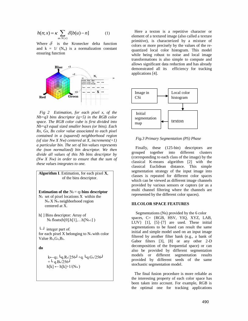
( )
( ; ) [ ( ) ]u N x
h n x b u n
(1)
Where is the Kronecker delta function
and k = 1/ (Nw) is a normalization constant
ensuring function
Fig 2 Estimation, for each pixel x, of the
Nb=q3 bins descriptor (q=5) in the RGB color space. The RGB color cube is first divided into
Nb=q3 equal sized smaller boxes (or bins). Each
Rx, Gx, Bx color value associated to each pixel
contained in a (squared) neighborhood region
(of size Nw X Nw) centered at X, increments(+1)
a particular bin. The set of bin values represents
the (non normalized) bin descriptor. We then
divide all values of this Nb bins descriptor by
(Nw X Nw) in order to ensure that the sum of
these values integrates to one.
Algorithm I. Estimation, for each pixel X,
of the bins descriptor.
Estimation of the Nb = q3 bins descriptor
Nx set of pixel locations X within the
Nw X Nw neighborhood region
centered at X.
h[ ] Bins descriptor: Array of
Nb floats(h[0].h[1],…h[Nb-1] )
integer part of. for each pixel X belonging to Nx with color
Value Rx,Gx,Bx.
do
k←q2.q.Rx/256+q.q.Gx/256
+ q.Bx/256
h[k] ← h[k]+1/(Nw )
Here a texton is a repetitive character or
element of a textured image (also called a texture
primitive), is characterized by a mixture of
colors or more precisely by the values of the re-
quantized local color histogram. This model
while being robust to noise and local image transformations is also simple to compute and
allows significant data reduction and has already
demonstrated all its efficiency for tracking
applications [4].
Fig.3 Primary Segmentation (PS) Phase
Finally, these (125-bin) descriptors are
grouped together into different clusters
(corresponding to each class of the image) by the
classical K-means algorithm [2] with the
classical Euclidean distance. This simple
segmentation strategy of the input image into
classes is repeated for different color spaces
which can be viewed as different image channels
provided by various sensors or captors (or as a
multi channel filtering where the channels are
represented by the different color spaces).
III.COLOR SPACE FEATURES
Segmentations (Ns) provided by the 6 color
spaces, C= RGB, HSV, YIQ, XYZ, LAB,
LUV [1], [5]–[7] are used. These initial
segmentations to be fused can result the same
initial and simple model used on an input image
filtered by another filter bank (e.g., a bank of
Gabor filters [3], [8] or any other 2-D
decomposition of the frequential space) or can
also be provided by different segmentation models or different segmentation results
provided by different seeds of the same
stochastic segmentation model.
The final fusion procedure is more reliable as
the interesting property of each color space has
been taken into account. For example, RGB is
the optimal one for tracking applications
Image in
CSi
Local color
histogram
Initial
segmentation
map
texton
490

[18].due to it being an additive color system
based on trichromatic theory and nonlinear with
visual perception. The HSV is more apt to
decouple chromatic information from shading
effect [4]. The YIQ color channels have the
property to code the luminance and chrominance information which are useful in compression
applications (both digital and analogue). Also
this system is intended to take advantage of
human color characteristics.
XYZ although are nonlinear in terms of linear
component color mixing, has the advantage of
being more psychovisually linear. The LAB
color system approximates human vision, and its
component closely matches human perception of
lightness [1]. The LUV components provide a
Euclidean color space yielding a perceptually uniform spacing of color approximating a
Riemannian space [8]. To measure four image
segmentation indices for each color spaces
finally using fusion process is to combine several
segmented images into a single image inorder to
get a high performance quality of the image.
The complete specification of an RGB color
space also requires a white point chromaticity
and a gamma correction curve. HSV - defines a
type of color space. It is similar to the modern
RGB and CMYK models. The HSV color space has three components: hue, saturation and value. The Y component represents the luma
information, and is the only component used by
black-and-white television receivers. I and Q
represent the chrominance information. A Lab
color space is a color opponent space with
dimension L for lightness and a and b for the
color-opponent dimensions, based on
nonlinearly-compressed CIEXYZ color space
coordinates. LUV color space is extensively used
for applications such as computer graphics which
deal with colored lights.
RGB YIQ XYZ
HSV LUV LAB
Fig 4 Characteristics of Six Color Spaces
IV. IMAGE SEGMENTATION TO BE
FUSED
The key idea of the proposed fusion process
using k-means algorithm as simply consists of
considering, for each site (or pixel to be
classified), the local histogram of the class (or
texton) labels of each segmentation to be fused,
computed on a squared fixed size Nw
neighborhood centered around the pixel, as input
feature vector of a final clustering procedure. For
a fusion of Ns segmentation with K1 classes into
a segmentation with K2 classes, the preliminary feature extraction step of this fusion procedure
thus yields to Ns (K1-bin) histograms which are
then gathered together in order to form, K1 X Ns
dimensional feature vector or a final bin
histogram which is then normalized to sum to
one, so that it is also a probability distribution
function.
In computer vision, Multisensor Image fusion
is the process of combining relevant information
from two or more images into a single image. The resulting image will be more informative
than any of the input images. Image fusion
methods can be broadly classified into two -
spatial domain fusion and transform domain
fusion. The fusion methods such as averaging,
Brovey method, principal component analysis
(PCA) and IHS based methods fall under
spatial domain approaches.
The proposed fusion process and k-means
algorithm is then herein simply considered as a
problem of clustering local histograms of (preliminary estimated) class labels computed
around and associated to each site. To this end,
we use, once again, a K-means clustering
procedure exploiting, for this fusion step, a
histogram based similarity measure derived from
the Bhattacharya similarity coefficient. (Fig 5)
Bhattacharya distance between a normalized
histogram and a reference histogram is given by
1
* * 1/2[ , ( )] 1 ( ) ( ; )( )bN
B
n o
D h h x h n h n x
Fig.5 shows an example of the clustering
segmentation model (into classes) of an input
image expressed in the RGB, HSV, YTQ, XYZ,
LAB, and LUV color spaces and the final
segmentation map (into classes) which results of
the fusion of these clustering. We can find that
491
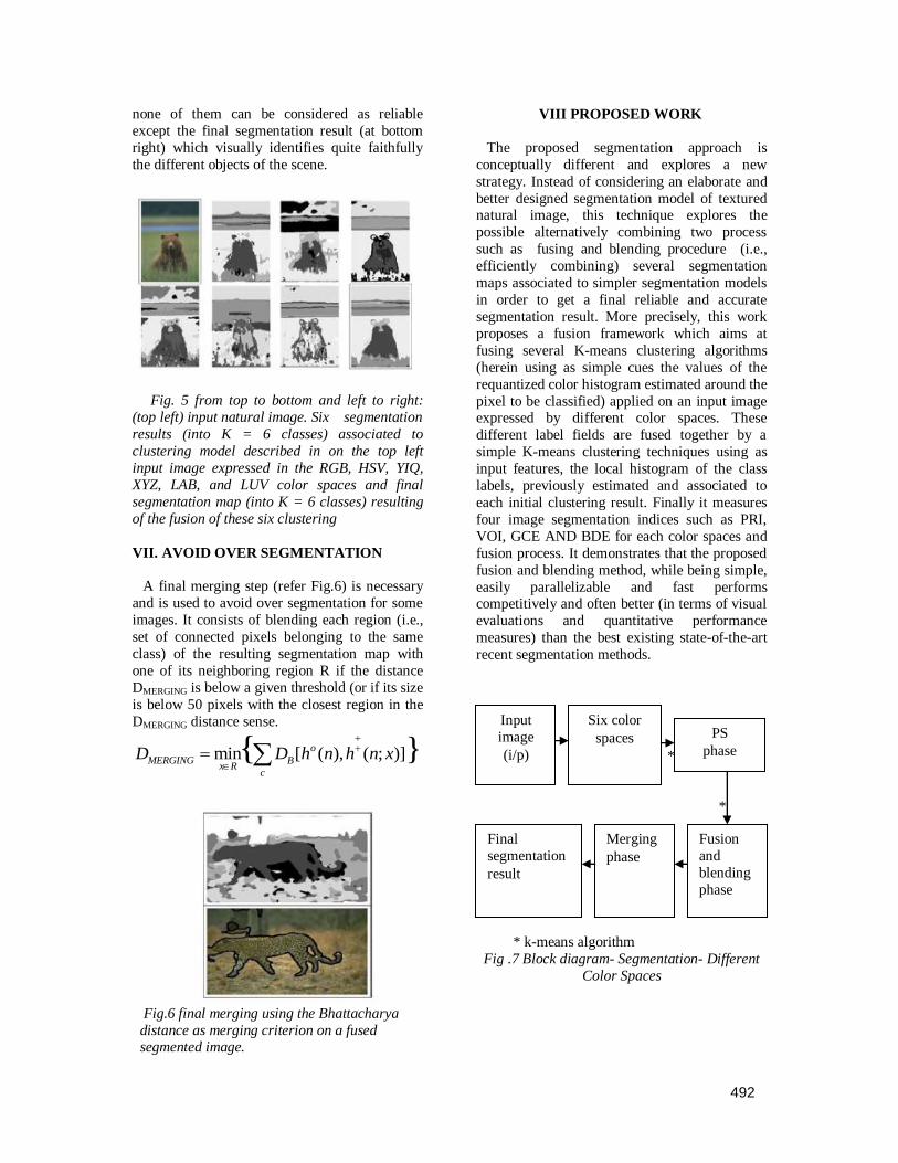
none of them can be considered as reliable
except the final segmentation result (at bottom
right) which visually identifies quite faithfully
the different objects of the scene.
Fig. 5 from top to bottom and left to right:
(top left) input natural image. Six segmentation
results (into K = 6 classes) associated to
clustering model described in on the top left
input image expressed in the RGB, HSV, YIQ,
XYZ, LAB, and LUV color spaces and final
segmentation map (into K = 6 classes) resulting
of the fusion of these six clustering
VII. AVOID OVER SEGMENTATION
A final merging step (refer Fig.6) is necessary
and is used to avoid over segmentation for some
images. It consists of blending each region (i.e.,
set of connected pixels belonging to the same
class) of the resulting segmentation map with
one of its neighboring region R if the distance
DMERGING is below a given threshold (or if its size
is below 50 pixels with the closest region in the
DMERGING distance sense.
min [ ( ), ( ; )] o
MERGING Bx R
c
D D h n h n x
Fig.6 final merging using the Bhattacharya
distance as merging criterion on a fused segmented image.
VIII PROPOSED WORK
The proposed segmentation approach is
conceptually different and explores a new
strategy. Instead of considering an elaborate and
better designed segmentation model of textured natural image, this technique explores the
possible alternatively combining two process
such as fusing and blending procedure (i.e.,
efficiently combining) several segmentation
maps associated to simpler segmentation models
in order to get a final reliable and accurate
segmentation result. More precisely, this work
proposes a fusion framework which aims at
fusing several K-means clustering algorithms
(herein using as simple cues the values of the
requantized color histogram estimated around the
pixel to be classified) applied on an input image expressed by different color spaces. These
different label fields are fused together by a
simple K-means clustering techniques using as
input features, the local histogram of the class
labels, previously estimated and associated to
each initial clustering result. Finally it measures
four image segmentation indices such as PRI,
VOI, GCE AND BDE for each color spaces and
fusion process. It demonstrates that the proposed
fusion and blending method, while being simple,
easily parallelizable and fast performs competitively and often better (in terms of visual
evaluations and quantitative performance
measures) than the best existing state-of-the-art
recent segmentation methods.
*
*
* k-means algorithm
Fig .7 Block diagram- Segmentation- Different
Color Spaces
Input
image
(i/p)
Six color
spaces PS
phase
Final
segmentation
result
Merging
phase
Fusion
and
blending
phase
492

493
IX CONCLUSION
This paper have presented a new, simple, and
efficient segmentation approach, based on a
fusion procedure which aims at combining
several segmentation maps associated to simpler partition models in order to finally get a more
reliable and accurate segmentation result and
also we get good and high performance quality
of the image . The primary segmentations to be
fused can also be provided by different
segmentation models or different segmentation
results provided by different seeds of the same
stochastic segmentation model.
REFERENCES
[1] Bo Zhau, Zhongxiang Zhu, Enrong Mao and
Zhenghe Song, “Image segmentation based on ant colony optimization and K-means
clustering,” Proc. IEEE International Conference
on Automation and Logistics, August 18-21,
2007.
[2]H.Stokman and T.Gevers, “Selection and
fusion of color models for image feature
detection,” IEEE Tans. Pattern Anal. Mach.
Intell., vol.29, no.3, pp.371-381, mar.2007.
[3] Charles kervrann and Fabrice Heitz, “A MRF
model –based approach to unsupervised texture
segmentation using global spatial statistics,” IEEE Trans. on image processing, vol.4, no.6,
june1995.
[4] Ming Zhang and Reda Alhajj, “Improving the
graph based image segmentation method,” Proc.
IEEE International Conference on tools with
Artificial Intelligence pp.0-7695-2728, Nov
2006.
[5] Mustafa Ozden and Ediz Polat, “image
segmentation using color and texture features,”
Proc. IEEE International Conference on tools
with Artificial Intelligence pp.0-2145-2728, Nov
2005. [6] K.Blekas, A.Likas, N.P.Galatsonas, and
I.E.Lagaris, “A spatially constrained mixture
model for image segmentation,” IEEE Trans. on
neural network, vol.16, no.2, march2005.
[7] Priyam chatterjee and Peyman milanfar,
“Clustering based denoising with locally learned
dictionaries,” IEEE Trans. on Image Processing,
vol.18, no.7, July 2006.
[8] J.P. Braquelaire and L. Brun, “Comparison
and optimization of the methods of color
image quantization,” IEEE Trans. image process., vol. 6, no. 7, pp. 1048–1952, Jul. 1997.
[9] H.Essaqote, N.Zahid, I.Haddaoui and
A.Ettouhami, “Color image segmentation based
on new clustering algorithm,” IEEE journal on
applied sciences 2(8):853-858, May 2007.
[10] Tse-Wei Chen, Yi-Ling Chen and Shao-Yi
chien, “Fast image segmentation based on K-
means clustering on HSV color spaces,” IEEE
Int. Conf. on Image Proc. April 2008. [11] D. Comaniciu and P. Meer, “Mean shift: A
robust approach toward feature space analysis,”
IEEE Trans. Pattern Anal. Mach. Intell., vol.24,
no. 5, pp. 603–619, May 2002.
[12] E. Maggio and A. Cavallaro, “Multi-part
target representation for color tracking,” in Proc.
Int. Conf. Image Processing, Italy, Genova, Sep
2005, pp. 729–732.

Proceedings of the third national conference on RTICT 2010
Bannari Amman Institute of Technology,Sathyamangalam-638401
9-10 April 2010
A Novel Approach for Web Service Composition in Dynamic Environment Using
AR -based Techniques
R.Rebecca, Department of CSE, Anna University Tiruchirappalli,[email protected] I.Shahanaz Begum, Lecturer, Anna UniversityTiruchirappalli,[email protected]
Abstract— Web service compositions are receiving significant amount of interest as a important strategy to allow
enterprise collaboration. Dynamic web service selection refers to determining a subset of component web services to be
invoked so as to orchestrate a composite web service. We observe that both the composite and constituent Web services
often constrain the sequences of invoking their operations. We therefore propose to use finite state machine (FSM) to
model the invocation order of web service operations. We define a measure, called aggregated reliability, to measure the
probability that a given state in the composite web service will lead to successful execution in the context where each
component web service may fail with some probability. In orchestrating a composite web service, we propose a strategy
to select component web services that are likely to successfully complete the execution of a given sequence of operations.
A prototype that implements the proposed approach using BPEL for specifying the invocation order of a Web service is
developed
Index Terms: Web services, reliability, service composition, web service selection, BPEL.
1 INTRODUCTION:
The web service today has radically changed how
businesses interact with applications distributed within and
across organizational boundaries. However a WS may run in
highly dynamic environment: business rules may change to fit new requirement and existing services may become
temporarily unavailable, etc. Such a highly dynamic
environment increases the probability to lead to unsuccessful
execution. So simply choosing a WS for execution an
incoming operation may not be the best strategy because it
may lead to the violation of some constraints. Therefore it is
important to effectively integrate several available WSs into
composite WS to lead successful execution. The composition of WSs involves using an
orchestration model to 1) define the possible orders of calling
WSs at design time and 2) dynamically select WSs to be invoked at runtime. To address the former, several theoretical
orchestration models have been proposed in the literature,
including finite state machine (FSM), Petri net, -calculus,
activity hierarchies, and rule-based orchestration [1]. Practical
service composition languages, such as BPEL, WS-
Choreography, WSCL, XPDL, and OWL-S have also been
proposed, and many commercial service platforms or products
that implement the available standards and composition
languages are available in the market, including the Sun ONE
framework based on J2EE, Microsoft.NET, the Oracle BPEL
Process Manager, the HP WSs Management Platform, and the
IBM Web Sphere Application Server.
However, none of the above works provide strategies
or mechanisms to dynamically select WSs to be invoked when
executing a series of operations in a composite WS. Dynamic WS selection refers to choosing the available WSs
to be invoked so as to realize the functionality of a composite
WS constructed using an orchestration model at runtime.
However, a WS may comprise multiple operations such that
their invocation sequence is constrained. Typical constraints
are separation of duties and binding of duties. It is imperative
that the dynamic WS selection Procedure takes all these
constraints into account. When choosing the operations of
WSs to compose a (composite) WS, the atomicity of each WS,
which requires either none of its operations to be invoked or
some final state to be reached, has to hold at the end of WS composition.
The network (intranet, extranet, or even the Internet)
where WSs operate is a failure-prone environment partly due
to the autonomous requirement of each participating service
provider. A WS may become malfunctioned or unavailable at
runtime, causing failure to the execution of a composite WS.
The WS reliability can be measured from various
perspectives, including correctness, fault tolerance, testability,
interoperability, and timeliness [3]. We define the reliability
of a WS operation as the probability that it successful
responds within a reasonable period of time and the proposed approach is not restricted to any WS modeling language and
employs a generic formalism FSM to define the order of
operations in a WS.
2 RELATED WORKS:
Self-Adaptation by late binding service calls: Bianculli et al. [8] propose architecture for self-adaptive Web service
compositions in which each service has an associated
repudiation. During service calls, the engine monitors QoS
and pushes repudiation data to a registry. For each
service call, a specialized service calls mechanism first checks
for a low repudiation of the called partner. In case the
494

repudiation is low another partner is selected from a registry.
In comparison, this work can monitor/adapt only service calls
and not other BPEL activities. Further, new self-adaptation
features cannot be added.
Karastoyanova et al. Propose to extend BPEL by the “find and bind” mechanism. By adding a new construct <find
bind> to BPEL, they enable the dynamic binding of explicitly
component web services at run time. Another similar work [7]
presents an approach for improving the adaptability by
extending the composition engine. A proper repository before
a web service is invoked. Some other utilizes Aspect-Oriented
Programming (AOP) to improve the flexibility of web service
composition. Charfi [6] proposes an extension to the BPEL
language, which is the service works, oriented BPEL
(AO4BPEL).
Several different QoS models have been proposed in
literature (e.g., [8, 12] ). However, most approaches do not
discuss how QoS can be monitored. An overview of QoS
monitoring approaches for web services is presented by Thio
et al. [12]. The authors discuss various techniques such as
low-level suing or proxy-based solutions. QoS monitoring has
been an active research area for years which is not only
focused on web service technology.
3 PROPOSED WORK:
Each (composite or candidate) WS is associated with a
formal model FSM that constrains the order of its operations.
The objective of automatic WS composition is to determine a
composition that satisfies all the given constraints. The reliability of a composite WS can be derived by aggregating the
reliabilities of constituent WSs based on the occurrence rate of each flow pattern.
Definition 1: A WS W is composed of a set of operations Σ and an FSM that prescribes the legal executions of these
operations. W is a tuple (Σ,S ,s0, δ, F) where
Σ is a set of operations,
S is a finite set of states,
s0 is a state in S, representing the initial state of W,
δ: S×Σ—>S is the transition function of an FSM,
F S represents the set of final states, i.e., the states where the interactions with W can be terminated.
The FSM of a WS prescribes legal executions of its
operations so as to realize the control flow, data flow, and/or
object flow supported by the WS.
Definition2: A target WS, denoted Wt, and is a WS whose
operations are interfaces to operations in other WSs also known as the component WSs. In general, when a client
application invokes operations in a target WS, the target WS
does not execute these operations itself, but delegates them to
the component WSs instead. The set of component WSs to be
delegated is called the WS community.It is possible that all
operations on the target WS can be handled by one single
Fig1: Invoking relationships between components WSs, the
composite WS, and the application
component WS, the more general scenario is to involve
multiple component WSs to complete the entire series of
operations on the target WS.
In this work, we consider a target WS Wt and a WS
community W1, W2… ,Wn. As an invocation of an operation in Wt can be in fact executed by more than one
component WSs.
As an example, suppose that one is planning a trip to
attend an event. The trip planning can be regarded as a target
WS (Wt), as shown in Figure 2. Also assume that there are
five WSs available on the Internet, each capable of
accomplishing only a subset of operations required by the
entire trip planning.W1 provides a package for booking both a
flight and a car.W2 offers the users to book a flight and a car
or a limo. W3 provides hotel booking and shuttle booking
services. W4 is used to register an event. W5 allows the user to book either a flight or a cruise, followed by the booking of
a car or a limo.
Fig 2: Target WS for Trip Planning
495
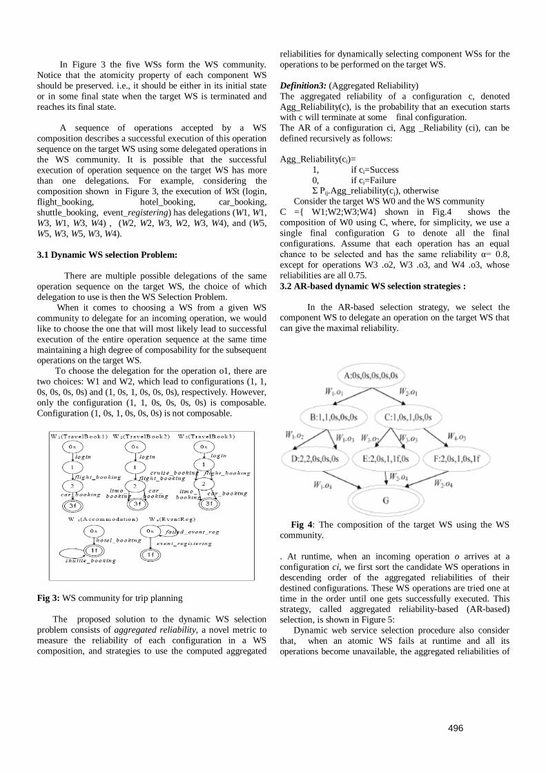
In Figure 3 the five WSs form the WS community.
Notice that the atomicity property of each component WS
should be preserved. i.e., it should be either in its initial state
or in some final state when the target WS is terminated and
reaches its final state.
A sequence of operations accepted by a WS
composition describes a successful execution of this operation
sequence on the target WS using some delegated operations in
the WS community. It is possible that the successful
execution of operation sequence on the target WS has more
than one delegations. For example, considering the
composition shown in Figure 3, the execution of WSt (login,
flight_booking, hotel_booking, car_booking,
shuttle_booking, event_registering) has delegations (W1, W1,
W3, W1, W3, W4) , (W2, W2, W3, W2, W3, W4), and (W5,
W5, W3, W5, W3, W4).
3.1 Dynamic WS selection Problem:
There are multiple possible delegations of the same
operation sequence on the target WS, the choice of which
delegation to use is then the WS Selection Problem.
When it comes to choosing a WS from a given WS
community to delegate for an incoming operation, we would
like to choose the one that will most likely lead to successful
execution of the entire operation sequence at the same time
maintaining a high degree of composability for the subsequent operations on the target WS.
To choose the delegation for the operation o1, there are
two choices: W1 and W2, which lead to configurations (1, 1,
0s, 0s, 0s, 0s) and (1, 0s, 1, 0s, 0s, 0s), respectively. However,
only the configuration (1, 1, 0s, 0s, 0s, 0s) is composable.
Configuration (1, 0s, 1, 0s, 0s, 0s) is not composable.
Fig 3: WS community for trip planning
The proposed solution to the dynamic WS selection
problem consists of aggregated reliability, a novel metric to
measure the reliability of each configuration in a WS
composition, and strategies to use the computed aggregated
reliabilities for dynamically selecting component WSs for the
operations to be performed on the target WS.
Definition3: (Aggregated Reliability)
The aggregated reliability of a configuration c, denoted
Agg_Reliability(c), is the probability that an execution starts with c will terminate at some final configuration.
The AR of a configuration ci, Agg _Reliability (ci), can be
defined recursively as follows:
Agg_Reliability(ci)=
1, if ci=Success
0, if ci=Failure Σ Pij.Agg_reliability(cj), otherwise
Consider the target WS W0 and the WS community
C = W1;W2;W3;W4 shown in Fig.4 shows the
composition of W0 using C, where, for simplicity, we use a
single final configuration G to denote all the final
configurations. Assume that each operation has an equal
chance to be selected and has the same reliability α= 0.8,
except for operations W3 .o2, W3 .o3, and W4 .o3, whose
reliabilities are all 0.75.
3.2 AR-based dynamic WS selection strategies :
In the AR-based selection strategy, we select the component WS to delegate an operation on the target WS that
can give the maximal reliability.
Fig 4: The composition of the target WS using the WS
community.
. At runtime, when an incoming operation o arrives at a
configuration ci, we first sort the candidate WS operations in
descending order of the aggregated reliabilities of their
destined configurations. These WS operations are tried one at
time in the order until one gets successfully executed. This strategy, called aggregated reliability-based (AR-based)
selection, is shown in Figure 5:
Dynamic web service selection procedure also consider
that, when an atomic WS fails at runtime and all its
operations become unavailable, the aggregated reliabilities of
496
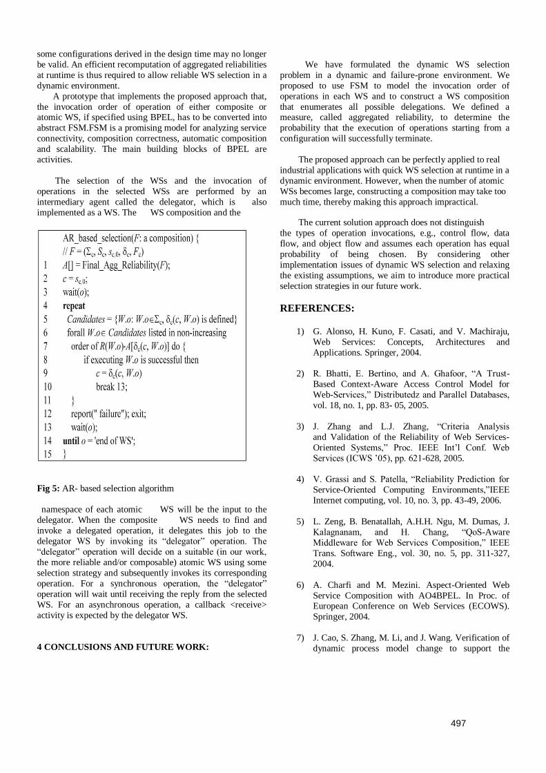
some configurations derived in the design time may no longer
be valid. An efficient recomputation of aggregated reliabilities
at runtime is thus required to allow reliable WS selection in a
dynamic environment.
A prototype that implements the proposed approach that,
the invocation order of operation of either composite or atomic WS, if specified using BPEL, has to be converted into
abstract FSM.FSM is a promising model for analyzing service
connectivity, composition correctness, automatic composition
and scalability. The main building blocks of BPEL are
activities.
The selection of the WSs and the invocation of
operations in the selected WSs are performed by an
intermediary agent called the delegator, which is also
implemented as a WS. The WS composition and the
Fig 5: AR- based selection algorithm
namespace of each atomic WS will be the input to the
delegator. When the composite WS needs to find and
invoke a delegated operation, it delegates this job to the
delegator WS by invoking its “delegator” operation. The
“delegator” operation will decide on a suitable (in our work,
the more reliable and/or composable) atomic WS using some
selection strategy and subsequently invokes its corresponding
operation. For a synchronous operation, the “delegator”
operation will wait until receiving the reply from the selected
WS. For an asynchronous operation, a callback <receive>
activity is expected by the delegator WS.
4 CONCLUSIONS AND FUTURE WORK:
We have formulated the dynamic WS selection
problem in a dynamic and failure-prone environment. We
proposed to use FSM to model the invocation order of
operations in each WS and to construct a WS composition
that enumerates all possible delegations. We defined a measure, called aggregated reliability, to determine the
probability that the execution of operations starting from a
configuration will successfully terminate.
The proposed approach can be perfectly applied to real
industrial applications with quick WS selection at runtime in a
dynamic environment. However, when the number of atomic
WSs becomes large, constructing a composition may take too
much time, thereby making this approach impractical.
The current solution approach does not distinguish
the types of operation invocations, e.g., control flow, data
flow, and object flow and assumes each operation has equal
probability of being chosen. By considering other
implementation issues of dynamic WS selection and relaxing
the existing assumptions, we aim to introduce more practical
selection strategies in our future work.
REFERENCES:
1) G. Alonso, H. Kuno, F. Casati, and V. Machiraju,
Web Services: Concepts, Architectures and
Applications. Springer, 2004.
2) R. Bhatti, E. Bertino, and A. Ghafoor, “A Trust-
Based Context-Aware Access Control Model for
Web-Services,” Distributedz and Parallel Databases,
vol. 18, no. 1, pp. 83- 05, 2005.
3) J. Zhang and L.J. Zhang, “Criteria Analysis
and Validation of the Reliability of Web Services-
Oriented Systems,” Proc. IEEE Int’l Conf. Web
Services (ICWS ’05), pp. 621-628, 2005.
4) V. Grassi and S. Patella, “Reliability Prediction for
Service-Oriented Computing Environments,”IEEE
Internet computing, vol. 10, no. 3, pp. 43-49, 2006.
5) L. Zeng, B. Benatallah, A.H.H. Ngu, M. Dumas, J.
Kalagnanam, and H. Chang, “QoS-Aware
Middleware for Web Services Composition,” IEEE
Trans. Software Eng., vol. 30, no. 5, pp. 311-327,
2004.
6) A. Charfi and M. Mezini. Aspect-Oriented Web
Service Composition with AO4BPEL. In Proc. of European Conference on Web Services (ECOWS).
Springer, 2004.
7) J. Cao, S. Zhang, M. Li, and J. Wang. Verification of
dynamic process model change to support the
497

adaptive workflow. In Proc. of 2004 IEEE
International Conference on- Services Computing
(SCC), 2004.
8) Comprehensive QoS Monitoring of Web Services
and Event-Based SLA Violation Detection Anton Michlmayr, Florian Rosenberg, Philipp Leitner,
Schahram DustdarDistributed Systems Group,
Vienna University of Technology Argentinierstrasse
8/184-1, 1040 Wien, Austria
9) P. Chan, M. Lyu, and M. Malek. Reliable web
services: Methodology, experiment and modeling. In
Proc. of IEEE International Conference on Web
Services, Salt Lake City, Utah, USA, 9-13 Jul 2007.
10) P. P. W. Chan. Building Reliable Web Services: Methodology, Composition, Modeling and
Experiment. PhD thesis, The Chinese University of
Hong Kong, Hong Kong, Dec 2007.
11) Arias-Fisteus, J., Fernandez, L.S., Kloos, C.D.:
Formal Veri¯cation of BPEL4WS Business
Collaborations. In Bauknecht, K., Bichler, M.,
PrÄoll, B., eds.: EC-Web. Volume 3182 of LNCS.
Springer (2004).
12) Comprehensive QoS Monitoring of Web Services and Event-Based SLA Violation Detection Anton
Michlmayr, Florian Rosenberg, Philipp Leitner,
Schahram DustdarDistributed Systems Group,
Vienna University of Technology Argentinierstrasse
8/184-1, 1040 Wien, Austria
498

Our Special Thanks to

To ADVERTISERS, DONORS AND SPONSORS
Compiled and Edited by
Convener
Dr. Amitabh Wahi, Professor & Head, Dept. of Information Technology, BIT
Organizing Secretaries
Mr. S. Sundaramurthy and Mr. S. Daniel Madan Raja,
Dept. of Information Technology, BIT