NAACL HLT 2018

The 2018 Conference of theNorth American Chapter of the

Association for Computational Linguistics:Human Language Technologies

Proceedings of the Student Research Workshop

June 2 - June 4, 2018New Orleans, Louisiana

This material is based upon work supported by the National Science Foundation under Grants No. 1803423 and1714855. Any opinions, findings, and conclusions or recommendations expressed in this material are those of theauthors and do not necessarily reflect the views of the National Science Foundation.

c©2018 The Association for Computational Linguistics

Order copies of this and other ACL proceedings from:

Association for Computational Linguistics (ACL)209 N. Eighth StreetStroudsburg, PA 18360USATel: +1-570-476-8006Fax: +1-570-476-0860acl@aclweb.org

ISBN 978-1-948087-26-1

ii

Introduction

Welcome to the NAACL-HLT 2018 Student Research Workshop!

This year’s submissions were organized in two tracks: research papers and thesis proposals.

• Research papers may describe completed work, or work in progress with preliminary results. Forthese papers, the first author must be a current graduate or undergraduate student.

• Thesis proposals are geared towards PhD students who have decided on a thesis topic and wish toget feedback on their proposal and broader ideas for their continuing work.

This year, we received a total of 51 submissions: 43 of these were research papers, and 8 were thesisproposals. We accepted 16 research papers and 4 thesis proposals, resulting in an overall acceptancerate of 39%. The main author of the accepted papers represent a variety of countries: Canada, Estonia,France, Germany, India, Japan (2 papers), Switzerland, UK, USA (11 papers).

Accepted research papers will be presented as posters within the NAACL main conference postersessions. We will have oral presentations at our SRW oral session on June 2 for all 4 thesis papers to allowstudents to get feedback about their thesis work, along with 2 research papers selected as outstandingpapers.

Following previous editions of the Student Research Workshop, we have offered students the opportunityto get mentoring feedback before submitting their work for review. Each student that requested pre-submission mentorship was assigned to an experienced researcher who read the paper and providedsome comments on how to improve the quality of writing and presentation of the student’s work. A totalof 21 students participated in the mentorship program. During the workshop itself, we will also providean in-site mentorship program. Each mentor will meet with their assigned students to provide feedbackon their poster or oral presentation, and to discuss their research careers.

We would like to express our gratitude for the financial support from the National Science Foundation(NSF) and the Computing Research Association Computing Community Consortium (CRA-CCC).Thanks to their support, this year’s SRW is able to assist students with their registration, travel, andlodging expenses.

We would like to thank the mentors for dedicating their time to help students improve their papers priorto submission, and we thank the members of the program committee for the constructive feedback theyhave provided for each submitted paper.

This workshop would not have been possible without the help from our faculty advisors, and we thankthem for their guidance along this year of workshop preparation. We also thank the organizers ofNAACL-HLT 2018 for their continuous support.

Finally, we would like to thank all students who have submitted their work to this edition of the StudentResearch Workshop. We hope our collective effort will be rewarded in the form of an excellent workshop!

iii

Organizers:

Silvio Ricardo Cordeiro (Aix-Marseille Université)Shereen Oraby (University of California, Santa Cruz)Umashanthi Pavalanathan (Georgia Institute of Technology)Kyeongmin Rim (Brandeis University)

Faculty Advisors:

Swapna Somasundaran (ETS Princeton)Sam Bowman (New York University)

Program Committee:

Bharat Ram Ambati (Apple Inc)Rachel Bawden (Université Paris-Sud)Yonatan Bisk (University of Washington)Dallas Card (Carnegie Mellon University)Wanxiang Che (Harbin Institute of Technology)Monojit Choudhury (Microsoft Research)Mona Diab (George Washington University)Jesse Dodge (Carnegie Mellon University)Bonnie Dorr (Florida Institute for Human-Machine Cognition)Ahmed Elgohary (University of Maryland, College Park)Micha Elsner (The Ohio State University)Noura Farra (Columbia University)Thomas François (Université catholique de Louvain)Daniel Fried (University of California, Berkeley)Debanjan Ghosh (Rutgers University)Kevin Gimpel (Toyota Technological Institute at Chicago)Ralph Grishman (New York University)Alvin Grissom II (Ursinus College)Jiang Guo (Massachusetts Institute of Technology)Luheng He (University of Washington)Jack Hessel (Cornell University)Dirk Hovy (Bocconi University)Mohit Iyyer (Allen Institute for Artificial Intelligence)Yacine Jernite (New York University)Yangfeng Ji (University of Washington)Kristiina Jokinen (University of Helsinki)Daisuke Kawahara (Kyoto University)Chris Kedzie (Columbia University)Philipp Koehn (Johns Hopkins University)Jonathan K. Kummerfeld (University of Michigan)Maximilian Köper (University of Stuttgart)

v

Éric Laporte (Université Paris-Est Marne-la-Vallée)Sarah Ita Levitan (Columbia University)Jasy Suet Yan Liew (Universiti Sains Malaysia)Diane Litman (University of Pittsburgh)Stephanie M. Lukin (US Army Research Laboratory)Shervin Malmasi (Harvard Medical School)Diego Marcheggiani (University of Amsterdam)Daniel Marcu (University of Southern California)Mitchell Marcus (University of Pennsylvania)Prashant Mathur (eBay)Kathy McKeown (Columbia University)Julie Medero (Harvey Mudd College)Amita Misra (University of California,Santa Cruz)Saif M. Mohammad (National Research Council Canada)Taesun Moon (IBM Research)Smaranda Muresan (Columbia University)Karthik Narasimhan (Massachusetts Institute of Technology)Shashi Narayan (University of Edinburgh)Graham Neubig (Carnegie Mellon University)Avinesh P.V.S. (Technische Universität Darmstadt)Yannick Parmentier (University of Lorraine)Gerald Penn (University of Toronto)Massimo Poesio (Queen Mary University of London)Christopher Potts (Stanford University)Daniel Preotiuc-Pietro (University of Pennsylvania)Emily Prud’hommeaux (Boston College)Sudha Rao (University Of Maryland, College Park)Mohammad Sadegh Rasooli (Columbia University)Michael Roth (Saarland University)Markus Saers (Hong Kong University of Science and Technology)David Schlangen (Bielefeld University)Minjoon Seo (University of Washington)Kevin Small (Amazon)Sandeep Soni (Georgia Institute of Technology)Ian Stewart (Georgia Institute of Technology)Alane Suhr (Cornell University)Shyam Upadhyay (University of Pennsylvania)Sowmya Vajjala (Iowa State University)Bonnie Webber (University of Edinburgh)John Wieting (Carnegie Mellon University)Adina Williams (New York University)Diyi Yang (Carnegie Mellon University)Justine Zhang (Cornell University)Meishan Zhang (Heilongjiang University)Ran Zhao (Carnegie Mellon University)

vi

Table of Contents

Alignment, Acceptance, and Rejection of Group Identities in Online Political DiscourseHagyeong Shin and Gabriel Doyle . . . . . . . . . . . . . . . . . . . . . . . . . . . . . . . . . . . . . . . . . . . . . . . . . . . . . . . . . 1

Combining Abstractness and Language-specific Theoretical Indicators for Detecting Non-Literal Usageof Estonian Particle Verbs

Eleri Aedmaa, Maximilian Köper and Sabine Schulte im Walde . . . . . . . . . . . . . . . . . . . . . . . . . . . . . . 9

Verb Alternations and Their Impact on Frame InductionEsther Seyffarth . . . . . . . . . . . . . . . . . . . . . . . . . . . . . . . . . . . . . . . . . . . . . . . . . . . . . . . . . . . . . . . . . . . . . . . . 17

A Generalized Knowledge Hunting Framework for the Winograd Schema ChallengeAli Emami, Adam Trischler, Kaheer Suleman and Jackie Chi Kit Cheung . . . . . . . . . . . . . . . . . . . . 25

Towards Qualitative Word Embeddings Evaluation: Measuring Neighbors VariationBenedicte Pierrejean and Ludovic Tanguy . . . . . . . . . . . . . . . . . . . . . . . . . . . . . . . . . . . . . . . . . . . . . . . . . 32

A Deeper Look into Dependency-Based Word EmbeddingsSean MacAvaney and Amir Zeldes . . . . . . . . . . . . . . . . . . . . . . . . . . . . . . . . . . . . . . . . . . . . . . . . . . . . . . . 40

Learning Word Embeddings for Data Sparse and Sentiment Rich Data SetsPrathusha Kameswara Sarma . . . . . . . . . . . . . . . . . . . . . . . . . . . . . . . . . . . . . . . . . . . . . . . . . . . . . . . . . . . . 46

Igbo Diacritic Restoration using Embedding ModelsIgnatius Ezeani, Mark Hepple, Ikechukwu Onyenwe and Enemouh Chioma . . . . . . . . . . . . . . . . . . 54

Using Classifier Features to Determine Language Transfer on MorphemesAlexandra Lavrentovich . . . . . . . . . . . . . . . . . . . . . . . . . . . . . . . . . . . . . . . . . . . . . . . . . . . . . . . . . . . . . . . . . 61

End-to-End Learning of Task-Oriented DialogsBing Liu and Ian Lane . . . . . . . . . . . . . . . . . . . . . . . . . . . . . . . . . . . . . . . . . . . . . . . . . . . . . . . . . . . . . . . . . . 67

Towards Generating Personalized Hospitalization SummariesSabita Acharya, Barbara Di Eugenio, Andrew Boyd, Richard Cameron, Karen Dunn Lopez, Pamela

Martyn-Nemeth, Carolyn Dickens and Amer Ardati . . . . . . . . . . . . . . . . . . . . . . . . . . . . . . . . . . . . . . . . . . . . . 74

Read and Comprehend by Gated-Attention Reader with More BeliefHaohui Deng and Yik-Cheung Tam . . . . . . . . . . . . . . . . . . . . . . . . . . . . . . . . . . . . . . . . . . . . . . . . . . . . . . . 83

ListOps: A Diagnostic Dataset for Latent Tree LearningNikita Nangia and Samuel Bowman . . . . . . . . . . . . . . . . . . . . . . . . . . . . . . . . . . . . . . . . . . . . . . . . . . . . . . 92

Japanese Predicate Conjugation for Neural Machine TranslationMichiki Kurosawa, Yukio Matsumura, Hayahide Yamagishi and Mamoru Komachi . . . . . . . . . . 100

Metric for Automatic Machine Translation Evaluation based on Universal Sentence RepresentationsHiroki Shimanaka, Tomoyuki Kajiwara and Mamoru Komachi . . . . . . . . . . . . . . . . . . . . . . . . . . . . . 106

Neural Machine Translation for Low Resource Languages using Bilingual Lexicon Induced from Com-parable Corpora

Sree Harsha Ramesh and Krishna Prasad Sankaranarayanan . . . . . . . . . . . . . . . . . . . . . . . . . . . . . . . 112

Training a Ranking Function for Open-Domain Question AnsweringPhu Mon Htut, Samuel Bowman and Kyunghyun Cho . . . . . . . . . . . . . . . . . . . . . . . . . . . . . . . . . . . . . 120

vii

Corpus Creation and Emotion Prediction for Hindi-English Code-Mixed Social Media TextDeepanshu Vijay, Aditya Bohra, Vinay Singh, Syed Sarfaraz Akhtar and Manish Shrivastava . . 128

Sensing and Learning Human Annotators Engaged in Narrative SensemakingMcKenna Tornblad, Luke Lapresi, Christopher Homan, Raymond Ptucha and Cecilia Ovesdotter

Alm. . . . . . . . . . . . . . . . . . . . . . . . . . . . . . . . . . . . . . . . . . . . . . . . . . . . . . . . . . . . . . . . . . . . . . . . . . . . . . . . . . . . . . .136

Generating Image Captions in Arabic using Root-Word Based Recurrent Neural Networks and DeepNeural Networks

Vasu Jindal . . . . . . . . . . . . . . . . . . . . . . . . . . . . . . . . . . . . . . . . . . . . . . . . . . . . . . . . . . . . . . . . . . . . . . . . . . . 144

viii

Conference Program

Saturday, June 2

10:30–12:00 Posters and Demos: Discourse and Pragmatics

Alignment, Acceptance, and Rejection of Group Identities in Online Political Dis-courseHagyeong Shin and Gabriel Doyle

15:30–17:00 Posters and Demos: Semantics

Combining Abstractness and Language-specific Theoretical Indicators for Detect-ing Non-Literal Usage of Estonian Particle VerbsEleri Aedmaa, Maximilian Köper and Sabine Schulte im Walde

Verb Alternations and Their Impact on Frame InductionEsther Seyffarth

A Generalized Knowledge Hunting Framework for the Winograd Schema ChallengeAli Emami, Adam Trischler, Kaheer Suleman and Jackie Chi Kit Cheung

Towards Qualitative Word Embeddings Evaluation: Measuring Neighbors Varia-tionBenedicte Pierrejean and Ludovic Tanguy

A Deeper Look into Dependency-Based Word EmbeddingsSean MacAvaney and Amir Zeldes

15:30–17:00 Posters and Demos: Sentiment Analysis

Learning Word Embeddings for Data Sparse and Sentiment Rich Data SetsPrathusha Kameswara Sarma

ix

Saturday, June 2 (continued)

17:00–18:30 Oral Presentations: Student Research Workshop Highlight Papers

17:00–17:14Igbo Diacritic Restoration using Embedding ModelsIgnatius Ezeani, Mark Hepple, Ikechukwu Onyenwe and Enemouh Chioma

17:15–17:29Using Classifier Features to Determine Language Transfer on MorphemesAlexandra Lavrentovich

17:30–17:44End-to-End Learning of Task-Oriented DialogsBing Liu

17:45–17:59Towards Generating Personalized Hospitalization SummariesSabita Acharya, Barbara Di Eugenio, Andrew Boyd, Richard Cameron, Karen DunnLopez, Pamela Martyn-Nemeth, Carolyn Dickens and Amer Ardati

18:00–18:14A Generalized Knowledge Hunting Framework for the Winograd Schema ChallengeAli Emami, Adam Trischler, Kaheer Suleman and Jackie Chi Kit Cheung

18:15–18:30Alignment, Acceptance, and Rejection of Group Identities in Online Political Dis-courseHagyeong Shin and Gabriel Doyle

x

Sunday, June 3

10:30–12:00 Posters and Demos: Information Extraction

Read and Comprehend by Gated-Attention Reader with More BeliefHaohui Deng and Yik-Cheung Tam

15:30–17:00 Posters and Demos: Machine Learning

ListOps: A Diagnostic Dataset for Latent Tree LearningNikita Nangia and Samuel Bowman

15:30–17:00 Posters and Demos: Machine Translation

Japanese Predicate Conjugation for Neural Machine TranslationMichiki Kurosawa, Yukio Matsumura, Hayahide Yamagishi and Mamoru Komachi

Metric for Automatic Machine Translation Evaluation based on Universal SentenceRepresentationsHiroki Shimanaka, Tomoyuki Kajiwara and Mamoru Komachi

Neural Machine Translation for Low Resource Languages using Bilingual LexiconInduced from Comparable CorporaSree Harsha Ramesh and Krishna Prasad Sankaranarayanan

xi

Monday, June 4

10:30–12:00 Posters and Demos: Question Answering

Training a Ranking Function for Open-Domain Question AnsweringPhu Mon Htut, Samuel Bowman and Kyunghyun Cho

10:30–12:00 Posters and Demos: Social Media and Computational Social Science

Corpus Creation and Emotion Prediction for Hindi-English Code-Mixed Social Me-dia TextDeepanshu Vijay, Aditya Bohra, Vinay Singh, Syed Sarfaraz Akhtar and ManishShrivastava

14:00–15:30 Posters and Demos: Cognitive Modeling and Psycholinguistics

Sensing and Learning Human Annotators Engaged in Narrative SensemakingMcKenna Tornblad, Luke Lapresi, Christopher Homan, Raymond Ptucha and Ce-cilia Ovesdotter Alm

14:00–15:30 Posters and Demos: Vision, Robotics and Other Grounding

Generating Image Captions in Arabic using Root-Word Based Recurrent NeuralNetworks and Deep Neural NetworksVasu Jindal

xii

Proceedings of NAACL-HLT 2018: Student Research Workshop, pages 1–8New Orleans, Louisiana, June 2 - 4, 2018. c©2017 Association for Computational Linguistics

Alignment, Acceptance, and Rejection of Group Identities in OnlinePolitical Discourse

Hagyeong ShinDept. of Linguistics

San Diego State UniversitySan Diego, CA, USA, 92182

hshin@sdsu.edu

Gabriel DoyleDept. of Linguistics

San Diego State UniversitySan Diego, CA, USA, 92182

gdoyle@sdsu.edu

Abstract

Conversation is a joint social process, withparticipants cooperating to exchange informa-tion. This process is helped along throughlinguistic alignment: participants’ adoption ofeach other’s word use. This alignment is ro-bust, appearing many settings, and is nearly al-ways positive. We create an alignment modelfor examining alignment in Twitter conversa-tions across antagonistic groups. This modelfinds that some word categories, specificallypronouns used to establish group identity andcommon ground, are negatively aligned. Thisnegative alignment is observed despite othercategories, which are less related to the groupdynamics, showing the standard positive align-ment. This suggests that alignment is stronglybiased toward cooperative alignment, but thatdifferent linguistic features can show substan-tially different behaviors.

1 Introduction

Conversation, whether friendly chit-chat or heateddebate, is a jointly negotiated social process, inwhich interlocutors balance the assertion of one’sown identity and ideas against a receptivity to theothers. Work in Communication Accommoda-tion Theory has demonstrated that speakers tend toconverge their communicative behavior in order toachieve social approval from their in-group mem-bers, while they tend to diverge their behavior in aconversation with out-group members, especiallywhen the group dynamics are strained (Giles et al.,1991, 1973).

Linguistic alignment, the use of similar wordsto one’s conversational partner, is one prominentand robust form of this accommodation, and hasbeen detected in a variety of linguistic interac-tions, ranging from speed dates to the SupremeCourt (Danescu-Niculescu-Mizil et al., 2011; Guoet al., 2015; Ireland et al., 2011; Niederhoffer and

Pennebaker, 2002). In particular, this alignmentis usually positive, reflecting a widespread will-ingness to accept and build off of the linguisticstructure provided by one’s interlocutor; the differ-ences in alignment have generally been of degree,not direction, subtly reflecting group differencesin power and interest.

The present work proposes a new model ofalignment, SWAM, which adapts the WHAMalignment model (Doyle and Frank, 2016). We ex-amine alignment behaviors in a setting with cleargroup identities and enmity between the groupsbut with uncertainty on which group is majority orminority: conversations between supporters of thetwo major candidates in the 2016 U.S. Presidentialelection. Unlike previous alignment work, we findsome cases of substantial negative alignment, es-pecially on personal pronouns that play a key rolein assigning group identity and establishing com-mon ground in the discourse. In addition, within-versus cross-group conversations show divergentpatterns of both overall frequency and alignmentbehaviors on pronouns even when the alignment ispositive. These differences contrast with the rel-atively stable (though still occasionally negative)alignment on word categories that reflect possiblerhetorical approaches within the discussions, sug-gesting that group dynamics within the argumentare, in a sense, more contentious than the argu-ment itself.

2 Previous Studies

2.1 Linguistic Alignment

Accommodation in communication happens atmany levels, from mimicking a conversation part-ner’s paralinguistic features to choosing whichlanguage to use in multilingual societies (Gileset al., 1991). One established approach to as-sess accommodation in linguistic representation

1

is to look at the usage of function word cate-gories, such as pronouns, prepositions, and articles(Danescu-Niculescu-Mizil et al., 2011; Niederhof-fer and Pennebaker, 2002). This approach arguesthat function words provide the syntactic struc-ture, which can vary somewhat independently ofthe content words being used. Speakers can ex-press the same thought through different speechstyles and reflect their own personality, identity,and emotions (Chung and Pennebaker, 2007).

In this context, we view limit our analysis toconvergence in lexical category choices, whichcan be the consequence of both social and cogni-tive processes. We call this specific quantificationof accommodation “linguistic alignment”, but it isclosely related to general concepts such as primingand entrainment. This alignment behavior may bethe result of social or cognitive processes, or both,though we focus on the social influences here.

2.2 Linguistic Alignment between Groups

Recent models of linguistic alignment have at-tempted to separate homophily, an inherent sim-ilarity in speakers’ language use, from adaptivealignment in response to a partner’s recent worduse (Danescu-Niculescu-Mizil et al., 2011; Doyleet al., 2017). If homophily is not separated fromalignment, it is impossible to compare within-and cross-group alignment, since the groups them-selves are likely to have different overall word dis-tributions. Both alignment and homophily can bemeaningful; Doyle et al. (2017) combine the twoto estimate employees’ level of inclusion in theworkplace.

Separating these factors opens the door to in-vestigate alignment behaviors even in cases wheredifferent groups speak in different ways; if ho-mophily is not factored out, cross-group dif-ferences will produce alignment underestimates.Thus far, these models of alignment been appliedmostly in cases where there is a single salientgroup that speakers wish to join (Doyle et al.,2017), or where group identities are less salientthan dyadic social roles or relationships, suchas social power (Danescu-Niculescu-Mizil et al.,2012), engagement (Niederhoffer and Pennebaker,2002), or attraction (Ireland et al., 2011).

There is some evidence and an intuition thatalignment can cross group boundaries, but it hasnot been measured using such models of adap-tive linguistic alignment. Niederhoffer and Pen-

nebaker (2002) pointed out that speakers with neg-ative feelings are likely to coordinate their linguis-tic style to each other, while speakers who are notengaged to each other at all are less likely to aligntheir linguistic style. Speakers also might activelycoordinate their speech to their opponents’ in or-der to persuade them more effectively (Burlesonand Fennelly, 1981; Duran and Fusaroli, 2017). Iftwo people with different opinions are talking toeach other, they may also align their speech styleas a good-faith effort to understand the other’s po-sition (Pickering and Garrod, 2004).

However, it is also reasonable to expect thatspeakers with enmity would diverge their speechstyle as a way to express their disagreement toeach other, especially if they feel disrespected orslighted (Giles et al., 1991). At the same time, ifthe function word usage can reflect speakers’ psy-chological state (Chung and Pennebaker, 2007),then negative alignment to opponents would beobserved as a fair representation of the disagree-ment between speakers. Supporting this idea,Rosenthal and McKeown (2015) showed that ac-commodation in word usage could be a feature toimprove their model detecting agreement and dis-agreement between speakers.

In the present work, we consider cross-groupalignment on personal pronouns, which can ex-press group identity, as well as on word cate-gories that may indicate different rhetorical ap-proaches to the argument (Pennebaker et al.,2003). Van Swol and Carlson (2017) suggeststhat the pronoun category can be useful markers ofgroup dynamics in a debate setting, and Schwartzet al. (2013) suggests that it is reasonable to expectthe different word usage from different groups. Infact, although we find mostly positive alignment,we do see negative alignment in some cross-groupuses, suggesting strong group identities can over-rule the general desire to align.

3 Data

3.1 Word categories

This study examines alignment and baseline worduse on 8 word categories from Linguistic In-quiry and Word Count (LIWC; Pennebaker et al.(2007)), a common categorization method inalignment research. Details on word categoriesand example words for each category can be foundin Table 1. For example, the first person singularpronoun I category counted 12 different forms of

2

Category Example Size1st singular (I) I, me, mine 122nd person (You) you, your, thou 201st plural (We) we, us, our 123rd plural (They) they, their, they’d 10Social processes talk, they, child 455Cognitive processes cause, know, ought 730Positive emotion love, nice, sweet 406Negative emotion hurt, ugly, nasty 499

Table 1: Word categories for linguistic alignment withexamples and the number of word tokens in the cate-gory.

the I pronoun, such as I, me, mine, myself, I’m, andI’d.

We choose four pronoun categories (I, you, we,they) to investigate the relationship between groupdynamics and linguistic alignment. We expectthat in a conversation between in-group mem-bers, I, we, they will be observed often. Whenthese pronouns are initially spoken by a speaker,repliers can express their in-group membershipwhile aligning to their usage of the words at thesame time. In the conversation with out-groupmembers, you usage will be observed more of-ten because it will allow repliers to refer to thespeaker while excluding themselves as a part ofthe speaker’s group. In the cross-group conver-sation, alignment on inclusive we indicates thatrepliers acknowledged and expressed themselvesas a member of speakers’ in-group. However,alignment on exclusive they in cross-group conver-sation should be interpreted with much more atten-tion. When a replier is aligning their usage of theyto their out-group member, it likely indicates thatboth groups are referring to a shared referent, im-plying enough cooperation to enter an object intocommon ground (Clark, 1996).

Additionally, four rhetorical word categories areconsidered. In LIWC, psychological processes arecategorized into social processes, cognitive pro-cesses, and affective processes, the last of whichcovers positive and negative emotions. Social andaffective process categories are, as their names in-dicate, the markers of social behavior and emo-tions. Cognitive process markers include wordsthat reflect causation (because, hence), discrep-ancy (should, would), certainty (always, never),and inclusion (and, with), to name a few. Aspeaker’s baseline usage of rhetorical categories

will present the group-specific speech styles thatmay be dependent on group identity, reflectingpreferred styles of argument. The degree of align-ment on rhetorical categories indicates whetherspeakers maintain their group’s discussion style oradapt to the other group.

3.2 Twitter ConversationThe corpus data was built specifically for this re-search. The population of the data was Twit-ter conversations about the 2016 presidential elec-tion dated from July 27th, 2016 (a day after bothparties announced their candidates) to November7th, 2016 (a day before the election day). Twit-ter users were divided into two different groupsaccording to their supporting candidates, basedon the assumption that all speakers included inthe data were partisans and had a single support-ing candidate. When the users’ supporting can-didate was not explicitly shown in their speech,additional information was considered, includingprevious Tweets, profile statements, and profilepictures. Speakers’ political affiliation was firstcoded by the researcher and the coder’s reliabil-ity was tested. Two other coders agreed on theresearcher’s coding of 50 users (25 were codedas Trump supporters and 25 were coded as Clin-ton supporters) with Fleiss’ Kappa score 0.87 (κ =0.86, p < 0.001) with average 94.4% confidencein their answers.

3.3 Sampling MethodThe corpus data was built by a snowball methodfrom seed accounts. Seed accounts spanned majormedia channels (@cnnbrk; @FoxNews; @NBC-News; @ABC) and the candidates’ Twitter ac-counts (@realDonaldTrump; @HillaryClinton).The original Twitter messages from the seed ac-counts were not considered as a part of the data,but replies and replies to replies were. The mini-mal unit of the data was a paired conversation ex-tracted from the comment section. An initial mes-sage a (single Twitter message, known as a tweet)and the following reply b created a pair of the con-versation.

3.4 DatasetsIn total, four sets of Twitter data were gath-ered. The first two datasets (TT, CC) consistedof conversations between members of the samegroup (within-group conversation). The othertwo datasets (TC, CT) consisted of conversations

3

Dataset Message ReplyTT I saw a poll where she was up by 8 here and

people say that they hate her so who knowsI’m not sure what’s going on with that, but#Reality tells a different story. Someone’slying.

Dems spreading lies again. They are pro-jecting Trump as stupid but voters knowshe is not!!

Dems running out of ways to get rid ofTrump, so now they will push this BS thathe is CRAZY and out of control!!

CC Jill Stein is more concerned about Hillarythan she is about Trump. That tells you allyou need to know about this loon. #Green-TownHall

You make a lot of sense. I’m sick of Hillarybashing.

TC#Libtard you are in for the shock of yourlife #TRUMPTRAIN

You are if you think he has a chance; haveyou any idea what the Electoral U maplooks like?... Hillary!

Unbelievable that #TeamHillary thinksAmerica is so stupid we won’t notice thatmoderator is a close Clinton pal

Not America. Just folks like you.#Trumpsuneducated

CT Fight - not a fight - he was told Mexicowon’t pay for it. Why should they?

Never expected Mex 2 write us a check.Other ways 2 make them pay for wall.Trump knows how 2 negotiate.

Table 2: Examples of conversation pairs from each dataset (First letter indicates initiator’s group, second indicatesreplier’s)

across the groups (cross-group conversation). Inthe dataset references, Trump supporters’ mes-sage is represented with T, and Clinton supporters’message is represented with C. The first letter indi-cates the initiator’s group; the second indicates thereplier’s group. There is an average of 266 uniquerepliers in each group.

4 SWAM Model

This study adapts the Word-Based HierarchicalAlignment Model (WHAM; Doyle and Frank(2016)) to estimate alignment on different wordcategories in the Twitter conversations. WHAMdefines two key quantities: baseline word use, therate at which someone uses a given word categoryW when it has not been used in the preceding mes-sage, and alignment, the relative increase in theprobability of words from W being used when thepreceding message used a word from W .

Both quantities have been argued to be psy-chologically meaningful, with baseline usage re-flecting internalization of in-group identity, ho-mophily, and enculturation, and alignment reflect-ing a willingness to adjust one’s own behaviorto fit another’s expectations and framing (Doyleet al., 2017; Giles et al., 1991).

The WHAM framework uses a hierarchy of nor-

mal distributions to tie together observations fromrelated messages (e.g., multiple repliers with sim-ilar demographics) to improve its robustness whendata is sparse or the sociological factors are sub-tle. This requires the researcher to make statis-tical assumptions about the structure’s effect onalignment behaviors, but can improve signal de-tection when group dynamics are subtle or groupmembership is difficult to determine (Doyle et al.,2016).

However, when the group identities are strongand unambiguous, this inference can be exces-sive, and may even lead to inaccurate estimates, asthe more complex optimization process may cre-ate a non-convex learning problem. The Bayesianhierarchy in WHAM also aggregates informationacross groups to improve alignment estimates; incases where the groups are opposed, one group’sbehavior may not be predictive of the other’s.We propose the Simplified Word-Based Align-ment Model (SWAM) for such cases, where groupdynamics are expected to provide robust and pos-sibly distinct signals.

WHAM infers two key parameters: ηalign andηbase, the logit-space alignment and baseline val-ues, conditioned on a hierarchy of Gaussian priors.

4

ηalign µalign Calign

ηbase µbase Cbaselogit−1

Binom

logit−1

Binom

Nalign

N base

Figure 1: Generative schematic of the Simplified Word-Based Alignment Model (SWAM) used in this study.Hierarchical parameter chains from the WHAM modelare eliminated; alignment values are fit independentlyby word category and conversation group.

SWAM estimates the two parameters directly as:

ηbase = log p(B|notA) (1)

ηalign = logp(B|A)

p(B|notA) , (2)

where p(B|A) is the probability of a replier us-ing a word category when the initial message con-tained it, and p(B|notA) is the probability of thereplier using it when the initial message did not.

SWAM treats alignment as a change in thelog-odds of a given word in the reply belong-ing to W , depending on whether W appeared inthe preceding message. SWAM can be thoughtof as a midpoint between WHAM and the sub-tractive alignment model of Danescu-Niculescu-Mizil et al. (2011), with three main differencesfrom the latter model. First, SWAM’s baseline isp(B|notA), as opposed to unconditioned p(B) forDanescu-Niculescu-Mizil et al. (2011). Second,SWAM places alignment on log-odds rather thanprobability, avoiding floor effects in alignment forrare word categories. Third, SWAM calculatesby-word alignment rather than by-message, con-trolling for the effect of varying message/replylengths. These three differences allow SWAM toretain the improved fit of WHAM (Doyle et al.,2016), while gaining the computational simplic-ity and group-dynamic agnosticism of Danescu-Niculescu-Mizil et al. (2011).

5 Results

5.1 PronounsThe results of baseline frequency and alignmentvalues for the four conversation types are pre-sented in Figure 2 and 3, respectively. We analyzeeach pronoun set in turn.

First of all, baseline usage of you shows that youwas used more often among repliers in the cross-group conversations. However, the alignment pat-tern for you was much stronger in within-groupconversations. That is, repliers are generally morelikely to use you in cross-group settings to refer toout-group members overall, but within the group,one member using you encourages the other to useit as well.

You alignment in within-group conversationcould reflect rapport-building, a sense that speak-ers understand each other well enough to talkabout each other, and an acceptance of the other’scommon ground (as in the example for CC inTable 2). On the other hand, you alignmentin between-group conversations should be inter-preted as the result of disagreement to each other(See examples for TC in Table 2). You alignmentin this case is the action of pointing fingers at eachother, which happens at an overall elevated level,regardless of whether the other person has alreadydone so.

Baseline usage of they shows the opposite pat-tern from you usage, with higher they usage in thein-group conversations. This type of they usagecan be a reference to out-group members (see thesecond example for TT in Table 2). By using they,repliers can express their membership as a part ofthe in-group and make assertions about the out-group. It also can reflect acceptance of the inter-locutor placing objects in common ground, whichcan be referred to by pronouns.

They alignment patterns were comparableacross the conversation types, except that Trumpsupporters showed divergence when responding toClinton supporters. The CT conversation in Table2 reflects this divergence, with Mexico being re-peated rather than being replaced by they, suggest-ing Trump supporters reject the elements Clintonsupporters attempt to put into common ground.

Moving on to baseline usage of we, Trump sup-porters were most likely to use this pronoun, espe-cially in their in-group conversations, suggesting astrong awareness of and desire for group identity.Contrary to the alignment patterns of they, Clin-

5

pronounsrhetorical

−5 −4 −3 −2 −1

they

we

you

i

negativeemotion

positiveemotion

cognitiveprocesses

socialprocesses

baseline (log−frequency)

TTCCTCCT

Figure 2: Repliers’ baseline usage of category markersis the probability of usage of the word when it has notbeen said by the initial speaker.

ton supporters were actively diverging their usageof we from Trump supporters. Meanwhile, Trumpsupporters were not actively diverging on we asthey did for the they usage.

Claiming in-group membership by using in-group identity marker can be one way of claim-ing common ground, which indicates that speak-ers belong to the group who shares specific goalsand values (Brown and Levinson, 1987). There-fore, Trump supporters’ baseline use and align-ment of we and they suggest that they were ac-cepting and reinforcing common ground with in-group members by using we, but rejecting com-mon ground with out-group members by not align-ing to they. Clinton supporters showed a differentway of reflecting their acceptance and rejection.They chose to reject common ground by not align-ing to their out-group members’ in-group markerwe, but seemed to accept the common groundwithin the conversation built by out-group mem-bers’ use of they.

Interestingly, I showed the least variability, bothin baseline and alignment, across the groups.However, I is also the only one of these pronoungroups that does not refer to someone else, andthus should be least affected by group dynamics.In fact, we see Chung and Pennebaker (2007)’sgeneral finding of solid I-alignment, even in cross-group communication.

pronounsrhetorical

−1 0 1

they

we

you

i

negativeemotion

positiveemotion

cognitiveprocesses

socialprocesses

alignment

TTCCTCCT

Figure 3: Repliers’ alignment on category markers rep-resents the probability of repliers’ usage of the wordwhen it has been said by the initial speaker.

Overall, we see effects both in the baseline andalignment values that are consistent with a stronggroup-identity construction process. Furthermore,we see strong negative alignment in cross-groupcommunication on pronouns tied to group iden-tity and grounding, showing that cross-group an-imosity can overrule the general pattern of pos-itive alignment in certain dimensions. However,the overall alignment is still positive; even the re-jection of certain aspects of the conversation donot lead to across-the-board divergence.

5.2 Rhetorical CategoriesDespite our hypothesis that the rhetorical cate-gories of words could indicate different groups’preferred style of argumentation, these categoriesshowed limited variation compared to the pro-nouns. The baseline values only varied a smallamount between groups, with Clinton supportershaving slightly elevated baseline use of social andcognitive words, and slightly less positive emo-tion.

The alignment values were mostly small posi-tive values, much as has been observed in stylis-tic alignment in previous work. However, cross-group Trump-Clinton conversations did have neg-ative alignment on cognitive processes. This cate-gory spans markers of certainty, discrepancy, andinclusion, and has been argued to reflect argumen-tation framing that appeals to rationality. This may

6

be a sign of rejecting or dismissing their interlocu-tors’ argument framing. But overall, there is nostrong evidence of differences in alignment in ar-gumentative style in this data, and the bulk of theeffect remains on group identification.

A possible reason for the lack of differencesin argumentation style may be uncertainty aboutthe setting of the cross-group communication. El-evated causation word usage has been argued tobe employed by the minority position within a de-bate, to provide convincing evidence against thestatus quo (Pennebaker et al., 2003; Van Swol andCarlson, 2017). The datasets consist of conversa-tions from the middle of the election campaign,when it was uncertain which group was in the ma-jority or minority (as seen in the first TT conver-sation in Table 2). This uncertainty may have ledboth groups to adopt more similar argumentationstyles than if they believed themselves to occupydifferent points in the power continuum.

6 Discussion

From our results, we see that social context af-fected pronoun use and alignment, which fits intothe Communication Accommodation Theory ac-count (Giles et al., 1991). Meanwhile, rhetoricalword use and alignment was independent of so-cial context between speakers, though it is unclearwhether this reflects a perception of equal foot-ing in their power dynamics or is driven primar-ily by automatic alignment influences rather thansocial factors (Pickering and Garrod, 2004). Toexpand the scope of this argument, we can fur-ther test if the negative alignment can be foundin other LIWC categories as well, which have noclear group-dynamic predictions.

One thing to point out is that even though pro-nouns and some rhetorical words are categorizedas function words, which have been hypothesizedto reflect structural rather than semantic alignment(Chung and Pennebaker, 2007), these categorywords are still somewhat context- and content-oriented. That is, use and alignment of some func-tion words is inevitable for speakers to stay withinthe topic of conversation or to mention the entitywhose referential term is already set in the com-mon ground. From Trump supporters’ negativealignment on they, we could see that speakers werein fact able to actively reject the reference methodby not using the content-oriented function words.In the future work, it will be meaningful to sepa-

rate the alignment motivated by active acceptanceand agreement from the alignment that must haveoccurred in order to stay within the conversation.

Testing our hypotheses in different settings canhelp to resolve this issue. One possibility is toseparate the election debate into small sets of con-versations with different topics, and then comparethe alignment patterns between sets. Because ofthe lexical coherence that each topic of conver-sations have, we will be able to better separatethe effect of context- and content-oriented wordsfrom the linguistic alignment result. As a result,we might be able to see negative alignment onrhetorical category between subset of conversa-tions. We can also test our hypotheses with dif-ferent languages. Investigating alignment in lan-guages that do not use pronouns heavily for refer-ence can be useful to see how the group dynamicsare expressed through different word categories.Particles in some languages, such as Japanese andKorean, can mark specific argument roles, and thislinguistic structure can allow us to detect syntacticalignment without looking much into the context-and content-oriented function words. Lastly, theSWAM model is an adaptation of the WHAMmodel, and while the basic patterns look similar tothose found by WHAM, a more precise compari-son of the models’ estimates with a larger datasetis an important step to ensure that the SWAM es-timates are accurate.

7 Conclusion

Pronoun usage and alignment reflect the groupdynamics between Trump supporters and Clin-ton supporters, and observations of negative align-ment are consistent with a battle over who definesthe groups and common ground. However, theuse and alignment of rhetorical words were notsubstantially affected by the group dynamics butrather reflected that there was an uncertainty aboutwho belongs to the majority or minority group.In a political debate or conversation between op-ponents, speakers are likely to project their groupidentity with the usage of pronouns but are likelyto maintain their rhetorical style as a way to main-tain their group identity.

ReferencesPenelope Brown and Stephen C. Levinson. 1987. Po-

liteness: Some universals in language usage, vol-ume 4. Cambridge university press.

7

Brant R. Burleson and Deborah A. Fennelly. 1981. Theeffects of persuasive appeal form and cognitive com-plexity on children’s sharing behavior. Child StudyJournal, 11:75–90.

Cindy Chung and James W Pennebaker. 2007. Thepsychological functions of function words. Socialcommunication, 1:343–359.

Herbert H. Clark. 1996. Using Language. CambridgeUniversity Press, Cambridge.

Cristian Danescu-Niculescu-Mizil, Michael Gamon,and Susan Dumais. 2011. Mark my words!: lin-guistic style accommodation in social media. InProceedings of the 20th international conference onWorld Wide Web, pages 745–754.

Cristian Danescu-Niculescu-Mizil, Lillian Lee,Bo Pang, and Jon Kleinberg. 2012. Echoes ofpower: Language effects and power differencesin social interaction. In Proceedings of the 21stinternational conference on World Wide Web, pages699–708.

Gabriel Doyle and Michael C. Frank. 2016. Investigat-ing the sources of linguistic alignment in conversa-tion. In Proceedings of the 54th Annual Meeting ofthe Association for Computational Linguistics (Vol-ume 1: Long Papers), volume 1, pages 526–536.

Gabriel Doyle, Amir Goldberg, Sameer Srivastava, andMichael Frank. 2017. Alignment at work: Usinglanguage to distinguish the internalization and self-regulation components of cultural fit in organiza-tions. In Proceedings of the 55th Annual Meeting ofthe Association for Computational Linguistics (Vol-ume 1: Long Papers), volume 1, pages 603–612.

Gabriel Doyle, Dan Yurovsky, and Michael C. Frank.2016. A robust framework for estimating linguisticalignment in Twitter conversations. In Proceedingsof the 25th international conference on World WideWeb, pages 637–648.

Nicholas D. Duran and Riccardo Fusaroli. 2017. Con-versing with a devils advocate: Interpersonal coor-dination in deception and disagreement. PloS one,12(6):e0178140.

Howard Giles, Nikolas Coupland, and Justine Coup-land. 1991. Accommodation theory: Communica-tion, context, and consequences. In Howard Giles,Justine Coupland, and Nikolas Coupland, editors,Contexts of accommodation: Developments in ap-plied sociolinguistics, pages 1–68. Cambridge Uni-versity Press, Cambridge.

Howard Giles, Donald M. Taylor, and Richard Bourhis.1973. Towards a theory of interpersonal accommo-dation through language: Some canadian data. Lan-guage in society, 2(2):177–192.

Fangjian Guo, Charles Blundell, Hanna Wallach, andKatherine Heller. 2015. The Bayesian Echo Cham-ber: Modeling Social Influence via Linguistic Ac-commodation. In Proceedings of the 18th Inter-national Conference on Artificial Intelligence andStatistics, pages 315–323.

Molly E. Ireland, Richard B. Slatcher, Paul W. East-wick, Lauren E. Scissors, Eli J. Finkel, and James W.Pennebaker. 2011. Language style matching pre-dicts relationship initiation and stability. Psycholog-ical Science, 22:39–44.

Kate G. Niederhoffer and James W. Pennebaker. 2002.Linguistic style matching in social interaction. Jour-nal of Language and Social Psychology, 21(4):337–360.

James W. Pennebaker, Roger J. Booth, and Martha E.Francis. 2007. Linguistic Inquiry and Word Count:LIWC. Austin, TX: liwc.net.

James W. Pennebaker, Matthias R. Mehl, and Kate G.Niederhoffer. 2003. Psychological aspects of nat-ural language use: Our words, our selves. Annualreview of psychology, 54(1):547–577.

Martin J. Pickering and Simon Garrod. 2004. Towarda mechanistic psychology of dialogue. Behavioraland brain sciences, 27(2):169–190.

Sara Rosenthal and Kathy McKeown. 2015. I couldntagree more: The role of conversational structure inagreement and disagreement detection in online dis-cussions. In Proceedings of the 16th Annual Meet-ing of the Special Interest Group on Discourse andDialogue, pages 168–177.

H. Andrew Schwartz, Johannes C. Eichstaedt, Mar-garet L. Kern, Lukasz Dziurzynski, Stephanie M.Ramones, Megha Agrawal, Achal Shah, MichalKosinski, David Stillwell, Martin E.P. Seligman, andLyle H. Ungar. 2013. Personality, gender, and age inthe language of social media: The open-vocabularyapproach. PloS one, 8(9):e73791.

Lyn M. Van Swol and Cassandra L. Carlson. 2017.Language use and influence among minority, major-ity, and homogeneous group members. Communi-cation Research, 44(4):512–529.

8

Proceedings of NAACL-HLT 2018: Student Research Workshop, pages 9–16New Orleans, Louisiana, June 2 - 4, 2018. c©2017 Association for Computational Linguistics

Combining Abstractness and Language-specific Theoretical Indicators forDetecting Non-Literal Usage of Estonian Particle Verbs

Eleri Aedmaa1, Maximilian Koper2 and Sabine Schulte im Walde21 Institute of Estonian and General Linguistics, University of Tartu, Estonia

2 Institut fur Maschinelle Sprachverarbeitung, Universitat Stuttgart, Germanyeleri.aedmaa@ut.ee

maximilian.koeper,schulte@ims.uni-stuttgart.de

Abstract

This paper presents two novel datasets and arandom-forest classifier to automatically pre-dict literal vs. non-literal language usage fora highly frequent type of multi-word expres-sion in a low-resource language, i.e., Estonian.We demonstrate the value of language-specificindicators induced from theoretical linguis-tic research, which outperform a high major-ity baseline when combined with language-independent features of non-literal language(such as abstractness).

1 Introduction

Estonian particle verbs (PVs) are multi-word ex-pressions combining an adverbial particle with abase verb (BV), cf. Erelt et al. (1993). Theyare challenging for automatic processing becausetheir components do not always appear adjacentto each other, and the particles are homonymouswith adpositions. In addition, as illustrated in ex-amples (1a) vs. (1b), the same PV type can be usedin literal vs. non-literal language.

(1) a. Tahe

astu-sstep-PST.3SG

kakstwo

sammustep.PRT

tagasi.back

‘He took two steps back.’b. Ta

heastu-sstep-PST.3SG

ameti-stjob-ELA

tagasi.back

‘He resigned from his job.’

Given that the automatic detection of non-literal expressions (including metaphors and id-ioms) is critical for many NLP tasks, the lastdecade has seen an increase in research on dis-tinguishing literal vs. non-literal meaning (Birkeand Sarkar, 2006, 2007; Sporleder and Li, 2009;Turney et al., 2011; Shutova et al., 2013; Tsvetkovet al., 2014; Koper and Schulte im Walde, 2016).

Most research up to date has, however, focused onresource-rich languages (mainly English and Ger-man), and elaborated on general indicators – suchas contextual abstractness – to identify non-literallanguage. As to our knowledge, only Tsvetkovet al. (2014) and Koper and Schulte im Walde(2016) explored language-specific features.

The aim of this work is to automatically pre-dict literal vs. non-literal language usage for avery frequent type of multi-word expression in alow-resource language, i.e., Estonian. The pred-icate is the center of grammatical and usuallysemantic structure of the sentence, and it deter-mines the meaning and the form of its arguments,cf. Erelt et al. (1993). Hence, the surroundingwords (i.e., the context), their meanings and gram-matical forms could help to decide whether thePV should be classified as compositional or non-compositional.

In addition to applying language-independentfeatures of non-literal language, we demonstratethe value of indicators induced from theoreticallinguistic research, that have so far not been ex-plored in the context of compositionality. For thispurpose, this paper introduces two novel datasetsand a random-forest classifier with standard andlanguage-specific features.

The remainder of this paper is structured as fol-lows. We give a brief overview of previous studieson Estonian PVs in Section 2, and Section 3 intro-duces the target dataset. All features are describedin Section 4. Section 5 lays out the experimentsand evaluation of the model, and we conclude ourwork in Section 6.

2 Related Work

The compositionality of Estonian PVs has beenunder discussion in the theoretical literature for

9

decades but still lacks a comprehensive study.Tragel and Veismann (2008) studied six verbalparticles and their aspectual meanings, and de-scribed how horizontal and vertical dimensionsare represented. Veismann and Sahkai (2016) in-vestigated the prosody of Estonian PVs, findingPVs expressing perfectivity the most problematicto classify.

Recent computational studies on Estonian PVsinvolve their automatic acquisition (Kaalep andMuischnek, 2002; Uiboaed, 2010; Aedmaa, 2014),and predicting their degrees of compositionality(Aedmaa, 2017). Muischnek et al. (2013) inves-tigated the role of Estonian PVs in computationalsyntax, focusing on Constraint Grammar. Most re-search on automatically detecting non-literal lan-guage has been done on English and German (asmentioned above), and elaborated on general indi-cators to identify non-literal language. Our workis the first attempt to automatically distinguish lit-eral and non-literal usage of Estonian PVs, and tospecify on theory- and language-specific features.

3 Target PV Dataset

For creating a dataset of literal and non-literal lan-guage usage for Estonian PVs, we selected 210PVs across 34 particles: we started with a list of1,676 PVs that occurred at least once in a 170-million token newspaper subcorpus of the Esto-nian Reference Corpus1 (ERC) and removed PVswith a frequency ≤9. Then we sorted the PVs ac-cording to their frequency and selected PVs acrossdifferent frequency ranges for the dataset. In ad-dition, we included the 20 most frequent PVs. Weplan to analyse the influence of frequency on thecompositionality of PVs in future work, thus it wasnecessary to collect evaluations for PVs with dif-ferent frequencies.

For each of the 210 target PVs, we then auto-matically extracted 16 sentences from the ERC.The sentences were manually double-checked tomake sure that verb and adverb formed a PV anddid not appear as independent word units in aclause. The choice of the numbers of PVs andsentences relied on the fact of limited time andother resources that allowed us to evaluate approx-imately 200 PVs and 2,000 sentences.

1www.cl.ut.ee/korpused/segakorpus/

The resulting set of sentences was evaluatedby three annotators with a linguistic background.They were asked to assess each sentence by an-swering the question: ”What is the usage of thePV in the sentence on a 6-point scale ranging fromclearly literal (0) to clearly non-literal (5) languageusage?” In case of multiple PVs in the same sen-tence, the information of which PV to evaluate wasprovided for the annotators. Although we use bi-nary division of PVs in this study, it was reason-able to collect evaluations on a larger than binaryscale because of the following reasons: first, it isa well-known fact that multi-word expressions donot fall into the binary classes of compositionalvs. non-compositional expressions (Bannard et al.,2003), and second, it was important to create adataset that would be applicable to multiple tasks.Thus our dataset can be used to investigate the de-grees of compositionality of PVs in the future.

The agreement among 3 annotators on all 6 cat-egories is fair (Fleiss’ κ = 0.36). A binary dis-tinction based on the average sentence scores intoliteral (average ≤ 2.4) and non-literal (average ≥2.5) resulted in substantial agreement (κ = 0.73).Our experiments below use the binary-class set-ting, disregarding all cases of disagreement.

This final dataset2 includes 1,490 sentences:1,102 non-literal and 388 literal usages across 184PVs with 120 different base verbs and 32 parti-cle types. 63 PVs occur only in non-literal sen-tences, 15 only in literal sentences and 106 PVs innon-literal and literal sentences. From 120 verbs50 appear only in non-literal sentences, 15 only inliteral sentences, and 55 verbs in both literal andnon-literal sentences. The distribution of (non-)literal sentences across particle types is shown inFigure 1. While many particles appear mostly innon-literal language (and esile, alt, uhte, ara areexclusively used in their non-literal meanings inour dataset), they all have literal correspondences.No particle types appear only in literal sentences.

4 Features

In this section we introduce standard, language-independent features (unigrams and abstractness)as well as language-specific features (case and an-imacy) that we will use to distinguish literal andnon-literal language usage of Estonian PVs.

2The dataset is accessible from https://github.com/eleriaedmaa/compositionality.

10

0

50

100

150

200

välja ette üle läbi

vastu

mahaüles

kokk

usis

setagasi

ümber

järelealla kin

nipeale

kaasa

juurdelahti

tagava

helekü

lgeedasi

esileeemale

kõrva

le

tagantalt

möödaühte

otsa ära ligi

particle

coun

tclass

literal

non−literal

Figure 1: (Non-)literal language usage across particles.

Unigrams Our simplest language-independentfeatures are unigrams, i.e., lemmas of contentwords that occur in the same sentences with ourtarget PVs. More precisely, unigrams are the listof lemmas of all words that we induced from allour target sentences (there is at least one PV ineach sentence), after excluding lemmas that oc-curred ≤5 times in total.

Abstractness Abstractness has previously beenused in the automatic detection of non-literal lan-guage usage (Turney et al., 2011; Tsvetkov et al.,2014; Koper and Schulte im Walde, 2016), asabstract words tend to appear in non-literal sen-tences. Since there were no ratings for Estonian,we followed Koper and Schulte im Walde (2016)to automatically generate abstractness ratings forEstonian lemmas: we translated 24,915 Englishlemmas from Brysbaert et al. (2014) to Estonianrelying on the English-Estonian Machine Trans-lation dictionary3. We then lemmatized the 170-million token ERC subcorpus and created a vec-tor space model. To learn word representations,we relied on the skip-gram model from Mikolovet al. (2013). Finally, we applied the algorithmfrom Turney et al. (2011) using the 29,915 trans-lated ratings from Brysbaert et al. (2014) as seeds.

3http://www.eki.ee/dict/ies/

This algorithm relies on the hypothesis that the de-gree of abstractness of a word’s context is predic-tive of whether the word is used in a metaphoricalor literal sense. The algorithm learns to assign ab-stractness scores to every word representation inour vector space, resulting in a novel resource4 ofautomatically created ratings for 243,675 Estonianlemmas.

Unfortunately we can not provide an evaluationfor this dataset at the moment, because Estonianis lacking a suitable human-judgement-based goldstandard. In addition, the creation would requireextensive psycholinguistic research which falls farfrom the authors’ specialization.

We adopted the following abstractness featuresfrom Turney et al. (2011) and Koper and Schulteim Walde (2016): average rating of all words in asentence, average rating of all nouns in a sentence(including proper names), rating of the PV subject,and rating of the PV object.

The ratings of PV subject and object express theabstractness score of the head of the noun phrase.For example, the average score of the object (i.e.,oma koera) in the sentence (2c) is the rating of thehead of the noun phrase (i.e., koer), not the aver-age of the ratings of the determiner and the head.

4The dataset is accessible from https://github.com/eleriaedmaa/compositionality.

11

We assume that the subjects and objects are moreconcrete in literal sentences. For example, the sub-ject (sober) and the object (koer) in the literal sen-tences (2a) and (2c) are more concrete than thesubject (surm) and object (viha) in the non-literalsentences (2b) and (2d).

(2) a. Soberfriend

jooks-i-srun-PST-3SG

mu-lleI-ALL

jarele.after

‘A friend ran after me.’b. Surm

deathjooks-i-srun-PST-3SG

ta-llehe-ALL

jarele.after

‘The death ran after him.’c. Mees

mansuru-spush-PST.3SG

koeradog.GEN

maha.down

‘The man pushed the dog down.’d. Mees

mansuru-spush-PST.3SG

vihaanger.GEN

maha.down

‘The man suppressed his anger.’

Figure 2 illustrates the abstractness scores forliteral vs. non-literal sentences. In general, lit-eral sentences are clearly more concrete, espe-cially when looking at nouns only, and even moreso when looking at the nouns in specific subjectand object functions.

0.0

2.5

5.0

7.5

10.0

all nouns subjects objects

conc

rete

ness

literal non−literal

Figure 2: Abstractness scores across literal and non-literal sentences.

Subject and object case Estonian distinguishesbetween “total” subjects in the nominative caseand “partial” subjects in the partitive case. Par-tial subjects are not in subject-predicate agree-ment (Erelt et al., 1993). For example, the subjectkulaline receives nominative case in sentence (3b)and partitive case in sentence (3a). We observedthat subject case assignment often correlates with(non-)literal readings; in the examples, sentence(3a) is literal, and sentence (3b) is non-literal.

(3) a. Kulalineguest.NOM

tule-bcome-3SG

juurde.near

‘The guest approaches.’

b. Kulali-siguest.PL.PRT

tule-bcome-3SG

juurde.up

‘The number of guests is increasing.’

Similarly, a “total” object in Estonian receivesnominative or genitive case, and a “partial” objectreceives partitive case. For example, the objectsupi in sentence (4a) is assigned genitive case, andthe object mida in sentence (4b) partitive case. Insentence (4a), the meaning of the PV ette votma isliteral; in sentence (4b) the meaning is non-literal.

(4) a. Tudrukgirl

vot-tistake-PST.3SG

ettefront

supi.soup.GEN

‘The girl took the soup in front ofher.’

b. Midawhat.SG.PRT

koostogether

ettefront

vot-ta?take-INF

‘What should we do together?’

Figure 3 illustrates that the distribution of sub-ject and object cases across literal and non-literalsentences does not provide clear indicators. In ad-dition, the correlation between subject/object caseand (non-)literalness has not been examined thor-oughly in theoretical linguistics. But based on cor-pus analyses as exemplified by the sentences (3b)–(4b), we hypothesize that the case distributionmight provide useful indicators for (non-)literallanguage usage.

73%

26%70%

29%

0

300

600

900

literal non−literal

Case of subjectpartitive

no subject

nominative

14%16%

53%

17%

12%

15%

49%

24%

0

300

600

900

literal non−literal

Case of objectpartitive

no object

nominative

genitive

Figure 3: Distribution of subject/object case across lit-eral and non-literal sentences.

12

Subject and object animacy According to Es-tonian Grammar (Erelt et al., 1993) the meaning ofthe predicate might determine (among other fea-tures) the animacy of its arguments in a sentence.If the verb requires an animate subject, but the sub-ject is inanimate, the meaning of the sentence isnon-literal. For example, the PV in the sentences(5a) and (5b) is the same (sisse kutsuma ’to invitein’), but in the first sentence the subject sober isanimate and the sentence is literal, while the sub-ject maja in sentence (5b) is inanimate and the sen-tence is non-literal. Similarly, the subject naine insentence (5c) is animate and the sentence is literal,while the subject valimus in sentence (5d) is inan-imate and the sentence is non-literal.

As before, the correlation between subject ani-macy and (non-)literalness has not been examinedthoroughly in theoretical linguistics, but the ani-macy of the subject seems to correlate with the(non-)literalness of the sentences.

(5) a. Soberfriend

kutsu-sinvite-PST.3SG

muI.GEN

sisse.in

‘A friend invited me in.’

b. Majahouse

eiNEG

kutsuinvite.CONNEG

sisse.in

‘The house doesn’t look inviting.’

c. Nainewoman

touka-spush-PST.3SG

meheman.GEN

eemale.away

‘A woman pushed a man away.’

d. Poeshop.GEN

valimusappearance

touka-spush-PST.3SG

meheman.GEN

eemale.away

‘The appearance of the shop made theman go away.’

The impact of the object animacy on the mean-ing of the PVs is less intuitive, but still the ob-ject in sentence (6a) is inanimate and the meaningof the PV is literal, while the object in sentence(6b) is animate and the meaning of the PV is non-literal.

(6) a. Meesman

poleta-sburn-PST.3SG

kaitsmefuse.GEN

labi.out

‘The man burned the fuse.’

b. Meesman

poleta-sburn-PST.3SG

enesehimself.GEN

labi.out

‘The man had a burnout.’

There are no explicit connections between thesubject animacy pointed out in the literature. Fig-ure 4 shows the distribution of animacy acrosssubjects and objects across the literal and non-literal usage. The differences in numbers are notremarkable, but based on the examples, we assumethat the animacy of the subject might have an im-pact on the literal and non-literal usage of PVs.Thus, we include animacy into our feature space.

21%

25%

54%

26%

28%

46%

0

300

600

900

literal non−literal

Animate subjectyes

no subject

no

37%

53%

10%

40%

49%

11%

0

300

600

900

literal non−literal

Animate objectyes

no object

no

Figure 4: Distribution of subject/object animacy acrossliteral and non-literal language.

Sentences (6a) and (6b) demonstrate that theabstractness/concreteness scores may already in-dicate the (non-)literal usage of the PV and thefeature of animacy does not add any information:the concrete words are inanimate and they appearin the literal sentences, and the animate (and ab-stract) words in non-literal sentences. Still, asshown in sentences (5a)–(5d), the concrete subjectof literal sentence can be also animate (i.e., sober,naine), the concrete subject of non-literal sentencecan be inanimate (i.e., maja), and the inanimatesubject of non-literal sentence might be abstract(i.e., valimus). Thus, we argue that the abstract-ness ratings are not sufficient to express the ani-macy of the words and animacy can be useful asfeature for the detection of (non-)literal usage ofEstonian PV.

Case government Case government is a phe-nomenon where the lexical meaning of the baseverb influences the grammatical form of the argu-ment, e.g., the predicate determines the case of the

13

argument (Erelt et al., 1993). Thus, argument casedepends on the meaning of the PV. For example, insentence (7a) the PV labi minema ’to go through’5

is literal and requires an argument that answers thequestion from where? Hence, the argument hasto receive elative case. In sentence (7b) the PVprovides a non-literal meaning (’to succeed’) anddoes not require any additional arguments. We hy-pothesize that the case of the argument is helpfulto predict (non-)literal usage of PVs.

(7) a. Tashe

laksgo.PST.3SG

metsa-stforest-SG.EL

labi.through

‘She went through the forest.’

b. MuI.GEN

ettepanekproposal

laksgo.PST.3SG

labi.through

‘My proposal was successful.’

Note that the cases of the subject and objectare individual features in our experiments, the fea-ture of case government includes the cases of othertypes of arguments, i.e., adverbials and modifiers.

In addition, Figure 5 introduces the distributionof the argument case across the literal and non-literal sentences, and shows that not all cases (e.g.,inessive, translative) appear in both types of sen-tences.

0

300

600

900

no govern

ment

elative

allativ

e

comita

tive

ablativ

e

inessive

illativ

e

additive

transla

tive

case

classliteral

non−literal

Figure 5: Distribution of argument case across literaland non-literal sentences.

Compared to all other features described in thissection, animacy is the most problematic becausethe information is not obtained automatically. For

5The verb minema ’to go’ is irregular and the stem is notderivable from the infinitive.

the abstractness scores we use the previously de-scribed dataset, and the cases of subjects, objectsand other arguments are accessible with the helpof the morphological analyser6 and the part-of-speech tagger7. At the moment, the animacy in-formation about the subject and object are addedmanually by the authors.

5 Experiments and Results

The classification experiments to distinguish be-tween literal and non-literal language usage of Es-tonian PVs rely on the sentence features definedabove. They were carried out using a randomforest classifier (Breiman, 2001) that constructs anumber of randomized decision trees during thetraining phase and makes prediction by averagingthe results. For our experiments, we used 100 ran-dom decision trees. The random forest classifierperforms better in comparison of other classifica-tion methods that we have applied in the Wekatoolkit (Witten et al., 2016). For the evaluation weperform 10-fold cross validation, hence we use thepreviously described data for training and testing.

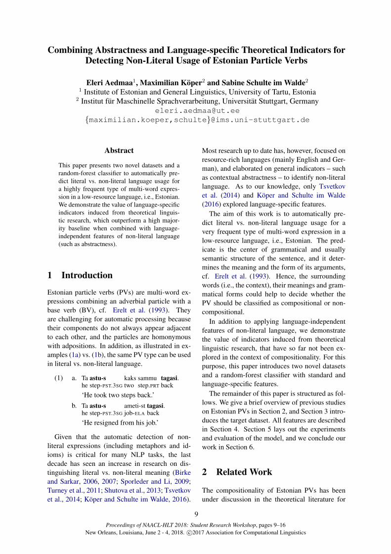
The classification results across features andcombinations of features are presented in Table 1.We report accuracy as well as F1 for literal andnon-literal sentences.

Table 1 shows that the best single feature typesare the unigrams (acc: 82.3%) and the base verbs(81.2%). Combining the two, the accuracy reaches84.2%. No other single feature type goes beyondthe high majority baseline (74.0%), but the combi-nations in the Table 1 significantly outperform thebaseline, according to χ2 with p<0.01.

Adding the particle type to the base verb infor-mation (1–2) correctly classifies 85.2% of the sen-tences. Further adding unigrams (1–3), however,does not help. Regarding abstractness, adding theratings for all but objects to the particle-verb infor-mation (1–2, 4–6) is best and reaches an accuracyof 86.3%. Subject case information, animacy andcase government in combination with 1–2 reachsimilar values (85.3–86.3%). The overall best re-sult (87.9%) is reached when combining particleand base verb information with all-noun and sub-ject abstractness ratings, subject case, subject ani-macy, and case government.

6http://www.filosoft.ee/html_morf_et/7http://kodu.ut.ee/˜kaili/parser/

14

feature type acc F1

n-lit litmajority baseline 74.0% 85.0 0.001 particle (p) 73.6% 84.4 13.62 base verb (v) 81.2% 87.9 58.03 unigrams, f>5 (uni) 82.3% 89.0 54.64 average rating of words (abs) 68.1% 79.8 24.55 average rating of nouns (abs) 68.5% 79.7 30.16 rating of the PV subject (abs) 72.3% 83.1 23.77 rating of the PV object (abs) 73.0% 83.5 25.28 subject case (case) 74.0% 85.0 0.009 object case (case) 74.0% 85.0 0.0010 subject animacy (animacy) 74.0% 85.0 0.0011 object animacy (animacy) 74.0% 85.0 0.0012 case government (govern) 73.8% 84.6 10.1p+v, 1–2 85.2% 90.3 68.7v+uni, 2–3 84.2% 89.6 66.4p+v+uni, 1–3 85.0% 90.1 68.5p+v+abs, 1–2, 4–6 86.3% 90.9 72.3p+v+abs, 1–2, 4–7 86.0% 90.7 71.3p+v+abs, 1–2, 5–6 86.0% 90.7 71.9p+v+case, 1–2, 8 85.3% 90.4 68.9p+v+case, 1–2, 8–9 84.6% 89.7 69.3p+v+animacy, 1–2, 10–11 86.2% 90.8 72.3p+v+govern, 1–2, 12 86.2% 90.9 71.6p+v+abs+lang, 1–2, 4–6, 10-12 87.3% 91.6 73.8p+v+abs+lang, 1–2, 4–12 87.5% 91.8 73.8p+v+abs+lang, 1–2, 5–6, 8, 10, 12 87.9% 92.0 75.0

Table 1: Overview of classification results.

While Table 1 only lists a selection of all pos-sible combinations of features to present the mostinteresting cases, it illustrates that the combinationof language-independent features and language-specific features is able to outperform the high ma-jority baseline. Although the difference betweenthe best combination without language-specificfeatures (86.3%) and the best combination withlanguage-specific features (87.9%) is not statis-tically significant, the best-performing combina-tion provides F1=92.0 for non-literal sentencesand F1=75.0 for literal sentences.

6 Conclusion

This paper introduced a new dataset with 1,490sentences of literal and non-literal language usagefor Estonian particle verbs, a new dataset of ab-stractness ratings for >240,000 Estonian lemmasacross word classes, and a random-forest classifierthat distinguishes between literal and non-literalsentences with an accuracy of 87.9%.

The most salient feature selection confirms ourtheory-based hypotheses that subject case, subjectanimacy and case government play a role in non-

literal Estonian language usage. Combined withabstractness ratings as language-independent in-dicators of non-literal language as well as verband particle information, the language-specificfeatures significantly outperform a high majoritybaseline of 74.0%.

Acknowledgements

This research was supported by the University ofTartu ASTRA Project PER ASPERA, financedby the European Regional Development Fund(Eleri Aedmaa), and by the Collaborative Re-search Center SFB 732, financed by the GermanResearch Foundation DFG (Maximilian Koper,Sabine Schulte im Walde).

ReferencesEleri Aedmaa. 2014. Statistical methods for Estonian

particle verb extraction from text corpus. In Pro-ceedings of the ESSLLI 2014 Workshop: Compu-tational, Cognitive, and Linguistic Approaches tothe Analysis of Complex Words and Collocations.Tubingen, Germany, pages 17–22.

Eleri Aedmaa. 2017. Exploring compositionality ofEstonian particle verbs. In Proceedings of the ESS-LLI 2017 Student Session. Toulouse, France, pages197–208.

Colin Bannard, Timothy Baldwin, and Alex Las-carides. 2003. A statistical approach to the seman-tics of verb-particles. In Proceedings of the ACLWorkshop on Multiword Expressions: Analysis, Ac-quisition and Treatment. Sapporo, Japan, pages 65–72.

Julia Birke and Anoop Sarkar. 2006. A clustering ap-proach for the nearly unsupervised recognition ofnonliteral language. In Proceedings of the 11th Con-ference of the European Chapter of the ACL. Trento,Italy, pages 329–336.

Julia Birke and Anoop Sarkar. 2007. Active learn-ing for the identification of nonliteral language. InProceedings of the Workshop on Computational Ap-proaches to Figurative Language. Rochester, NY,pages 21–28.

Leo Breiman. 2001. Random forests. Machine learn-ing 45(1):5–32.

Marc Brysbaert, Amy Beth Warriner, and Victor Ku-perman. 2014. Concreteness ratings for 40 thousandgenerally known English word lemmas. BehaviorResearch Methods 64:904–911.

15

Tiiu Erelt, Ulle Viks, Mati Erelt, Reet Kasik, HelleMetslang, Henno Rajandi, Kristiina Ross, HennSaari, Kaja Tael, and Silvi Vare. 1993. Eesti keelegrammatika II. Suntaks. Lisa: kiri [The Grammar ofthe Estonian Language II: Syntax]. Tallinn: EestiTA Keele ja Kirjanduse Instituut.

Heiki-Jaan Kaalep and Kadri Muischnek. 2002. Us-ing the text corpus to create a comprehensive list ofphrasal verbs. In Proceedings of the 3rd Interna-tional Conference on Language Resources and Eval-uation. Las Palmas de Gran Canaria, Spain, pages101–105.

Maximilian Koper and Sabine Schulte im Walde. 2016.Automatically generated affective norms of abstract-ness, arousal, imageability and valence for 350 000German lemmas. In Proceedings of the 10th In-ternational Conference on Language Resources andEvaluation. Portoroz, Slovenia, pages 2595–2598.

Maximilian Koper and Sabine Schulte im Walde. 2016.Distinguishing literal and non-literal usage of Ger-man particle verbs. In Proceedings of the Confer-ence of the North American Chapter of the Associ-ation for Computational Linguistics: Human Lan-guage Technologies. San Diego, California, USA,pages 353–362.

Tomas Mikolov, Ilya Sutskever, Kai Chen, Greg S. Cor-rado, and Jeff Dean. 2013. Distributed representa-tions of words and phrases and their compositional-ity. In Advances in Neural Information ProcessingSystems 26. Lake Tahoe, Nevada, USA, pages 3111–3119.

Kadri Muischnek, Kaili Muurisep, and Tiina Puo-lakainen. 2013. Estonian particle verbs and theirsyntactic analysis. In Proceedings of Human Lan-guage Technologies as a Challenge for ComputerScience and Linguistics: 6th Language & Technol-ogy Conference. Poznan, Poland, pages 7–11.

Ekaterina Shutova, Simone Teufel, and Anna Korho-nen. 2013. Statistical Metaphor Processing. Com-putational Linguistics 39(2):301–353.

Caroline Sporleder and Linlin Li. 2009. Unsupervisedrecognition of literal and non-literal use of idiomaticexpressions. In Proceedings of the 12th Conferenceof the European Chapter of the Association for Com-putational Linguistics. Athens, Greece, pages 754–762.

Ilona Tragel and Ann Veismann. 2008. Kuidas horison-taalne ja vertikaalne liikumissuund eesti keeles as-pektiks kehastuvad? [Embodiment of the horizontaland vertical dimensions in Estonian aspect]. Keel jaKirjandus 7:515–530.

Yulia Tsvetkov, Leonid Boytsov, Anatole Gershman,Eric Nyberg, and Chris Dyer. 2014. Metaphor de-tection with cross-lingual model transfer. In Pro-ceedings of the 52nd Annual Meeting of the As-sociation for Computational Linguistics. Baltimore,Maryland, pages 248–258.

Peter Turney, Yair Neuman, Dan Assaf, and Yohai Co-hen. 2011. Literal and metaphorical sense identifi-cation through concrete and abstract context. In Pro-ceedings of the Conference on Empirical Methodsin Natural Language Processing. Edinburgh, UK,pages 680–690.

Kristel Uiboaed. 2010. Statistilised meetodid mur-dekorpuse uhendverbide tuvastamisel [Statisticalmethods for phrasal verb detection in Estonian di-alects]. Eesti Rakenduslingvistika Uhingu aastaraa-mat 6:307–326.

Ann Veismann and Heete Sahkai. 2016.Uhendverbidest labi prosoodia prisma [Particleverbs and prosody]. Eesti RakenduslingvistikaUhingu aastaraamat 12:269–285.

Ian H. Witten, Eibe Frank, Mark A. Hall, and Christo-pher J. Pal. 2016. Data Mining: Practical MachineLearning Tools and Techniques. Morgan Kaufmann.

16

Proceedings of NAACL-HLT 2018: Student Research Workshop, pages 17–24New Orleans, Louisiana, June 2 - 4, 2018. c©2017 Association for Computational Linguistics

Verb Alternations and Their Impact on Frame Induction

Esther SeyffarthDept. of Computational Linguistics

Heinrich Heine UniversityDusseldorf, Germany

Esther.Seyffarth@hhu.de

Abstract

Frame induction is the automatic creation offrame-semantic resources similar to FrameNetor PropBank, which map lexical units of a lan-guage to frame representations of each lexicalunit’s semantics. For verbs, these representa-tions usually include a specification of their ar-gument slots and of the selectional restrictionsthat apply to each slot. Verbs that participatein diathesis alternations have different syntac-tic realizations whose semantics are closely re-lated, but not identical. We discuss the influ-ence that such alternations have on frame in-duction, compare several possible frame struc-tures for verbs in the causative alternation, andpropose a systematic analysis of alternatingverbs that encodes their similarities as well astheir differences.

1 Introduction

One of the aims of natural language processing isto access and process the meaning of texts auto-matically. For tasks like question answering, auto-matic summarization, or paraphrase detection, an-notating the text with semantic representations is auseful first step. A good annotation represents thesemantics of each element in the text as well as therelations that exist between the elements, such asthe relations between a verb and its arguments andadjuncts.

Frame semantics, founded on work by Fillmore(1968), Minsky (1974), Barsalou (1992), and oth-ers, provides a powerful method for the creationof such representations. A frame-semantic repre-sentation of a concept expresses the attributes thatcontribute to its semantics as functional relationsin a recursive attribute-value structure. Frame-semantic lexical resources, such as FrameNet(Ruppenhofer et al., 2006) or PropBank (Palmeret al., 2005), map lexical units of a language to

frames, which are described in terms of the frameelements, or roles, that are central to the concept.

Since the manual compilation of such resourcesis time-consuming, costly, and error-prone, muchcan be gained from the use of semi-supervised orunsupervised methods. The process of creating aframe lexicon automatically is known as frame in-duction.

Unsupervised frame induction draws on obser-vations about each lexical item’s behavior in a cor-pus to create a frame lexicon. If two different lex-ical units can evoke the same frame, they sharecertain semantic properties, and the frame inducerhas to determine the amount of semantic overlapbetween them based on observable and latent fea-tures of each of the lexical items. In this paper, wediscuss some of the problems that occur in frameinduction when lexical units have a relatively largesemantic overlap, but are not close enough to eachother to be treated as total synonyms.

While there are several types of frame-evokingpredicates, we focus here on verbs and the framesthey evoke. We assume that the meaning of a sen-tence can be expressed using the frame represen-tation of the sentence’s root verb. The semanticcontribution of all other elements in the sentenceis then specified with respect to their relation tothe root verb. Therefore, it is crucial to assign thecorrect semantic frame to the root verb.

Diathesis alternations are a phenomenon thatis observed when verbs can occur with morethan one valency pattern. In some alternations,the different uses of the participating verbs in-troduce changes in the semantics as well (Levin,1993). This is particularly relevant for alternationsthat change the Aktionsart of the verb, such asthe causative-inchoative alternation (Levin, 1993,Chapter 1.1.2). Verbs in this alternation can beused either transitively or intransitively, where thetransitive use adds a causative meaning to the sen-

17

tence that is not present in the intransitive use, asin the sentences in (1).

(1) a. Mary opened the door.b. The door opened.

In this paper, we argue that sentence pairs likethis differ in their semantics to a degree that war-rants their annotation with different frames, but ina way that still expresses their semantic relation toeach other. We compare different possible framerepresentations for verbs in the causative alterna-tion and propose some guidelines for the way aframe inducer should analyze alternating verbs.

2 The Causative Alternation

The causative alternation is characterized by a roleswitch (McCarthy, 2001) between transitive andintransitive uses of participating verbs, as shownin the sentences in (2). The role switch determinesthe position of the semantic THEME, the rent, assyntactic object (in (2-a)) or subject (in (2-b)). AnAGENT is only present in the transitive sentence.

(2) a. They have increased my rent.b. My rent has increased.

Both sentences describe a situation which resultsin the rent being higher than before.

Transitive uses of verbs in the causative alter-nation can be paraphrased as “cause to [verb]-intransitive” (see Levin, 1993, p. 27). For in-stance, sentence (2-a) can be paraphrased as “Theyhave caused my rent to increase.”

In some cases, this type of paraphrase is notcompletely synonymous with the causative use ofthe verb; for a discussion of such cases, see e.g.Dowty (1991, pp. 96-99) and Cruse (1972). Theseauthors claim that a difference between scenariosof direct and indirect causation renders some para-phrases ungrammatical or different in meaningfrom the original sentences with causative verbs.However, for the purposes of this paper, we focuson the regular cases, where the causative use andthe paraphrased form do express the same mean-ing.

Dowty (1991) decomposes causative verbs as[x CAUSE [BECOME y]], where an inchoativeevent [BECOME y] is embedded in a causativeone. Thus, for verbs in the causative alternation,the transitive sentence has a more complex seman-tic structure. This is not the case for verbs outsidethe alternation: Sentences (3-a) and (3-b) below

have the same semantic complexity, and one doesnot describe something that causes the other.

(3) a. I’m eating an apple.b. I’m eating.

If (3-a) is true, then (3-b) must necessarily alsobe true, but there is no causation relationship be-tween the sentences. Instead, (3-b) is a less spe-cific description of the same situation that is alsodescribed by (3-a).

Like Rappaport Hovav (2014), we assume thata causative sentence entails its inchoative counter-part. In both sentences in (2), the verb increase de-scribes an event that affects the semantic THEME;if it is true that a CAUSE is responsible for theevent that increases the rent, then a statement thatdoes not contain a CAUSE, but otherwise describesthe same event, is necessarily also true. In otherwords, it is impossible for (2-a) to be true without(2-b) also being true.

2.1 Possible Frame Representations

A frame representation of the sentences in (2) thatfocuses on their shared semantics is given in Fig-ure 1. A similar structure could also be used torepresent the sentences in (3).

increaseCAUSE they / ∅THEME my rent

Figure 1: Frame representation that is agnostic towardsthe question of causativity or inchoativity.

This analysis assigns an increase frame, inde-pendent of the syntactic realization and observedarguments. If a cause is given, it is included; oth-erwise, it is not, and the CAUSE slot is unfilled.

A disadvantage of this choice is that the struc-ture does not differentiate between causative andinchoative uses of alternating verbs, except by thepresence and absence of the CAUSE slot. As dis-cussed in the previous section, this is acceptablefor sentences like (3), but undesirable for sen-tences like (2).

The representation in Figure 1 is similar to thestructure used in PropBank (see Palmer et al.,2005, p. 77). There, both uses of an alternat-ing verb are associated with one shared frameset.The PropBank annotation makes no difference be-tween the sentences in (2) and the sentences in (3).

18

The FrameNet frame hierarchy includes amechanism to connect frames with an “is causativeof” relation and its inverse, “is inchoative of”(Ruppenhofer et al., 2006, p. 85). Different framesfor alternating verbs are stored in the database andconnected by these relations. Figure 2 gives theFrameNet representations for the sentences in (2).For a discussion of these representations, see Rup-penhofer et al. (2006, p. 12 and pp. 15-16).

cause change position on a scaleCAUSE theyITEM my rent

[change position on a scaleITEM my rent

]

Figure 2: FrameNet representations for the sentencesin (2).

These frames show a clear conceptual separa-tion between the causative meaning of increaseand its inchoative counterpart. The two frames arelinked by the relations mentioned above, and theirnames hint at the semantic connection that existsbetween them.

However, it is not obvious from the separateframes that the two sentences are connected by anentailment relationship. If a sentence like (2-a) isobserved, the first representation will be chosen; ifa sentence like (2-b) is observed, the second repre-sentation will be chosen. Without referring to theFrameNet frame hierarchy, it will not be possibleto recognize that sentence (2-a) necessarily entailssentence (2-b).

A frame representation that encodes this rela-tionship more visibly is presented in Figure 3.That representation is analogous to the decompo-sition for causative verbs given by Dowty (1991),which is [x CAUSE [BECOME y]]. The specificsentence (2-a) is represented as [[they do some-thing] CAUSE [BECOME [my rent is higher]]].

Figure 3 represents the event as a causationframe. The EFFECT slot of that frame is linkedto the content of the [BECOME y] part of the de-composition, which is an inchoation frame. TheRESULT of the inchoation is the formula’s y.

These representations are inspired by Osswaldand Van Valin Jr (2014). They visibly express therelationship between the frames and are consistentwith the decompositional event structures used byRappaport Hovav and Levin (1998) in their dis-

cussion of alternating verbs. The frame in Fig-ure 3 provides a slot for the result state of the in-choation frame, here expressed as a frame of thetype higher. Osswald and Van Valin Jr (2014)suggest that the semantics of verbs that expressa gradual change of state should be representedin terms of the initial and final state and a spec-ification of the relation between them. Thus, theframe should state that the rent had an initial andfinal amount, and the meaning of “They have in-creased my rent” is that the states are connectedby a GREATER THAN relation.

causation

CAUSE

[activityAGENT they

]

EFFECT

inchoation

RESULT

[increaseTHEME my rent

]

inchoation

RESULT

[increaseTHEME my rent

]

[increaseTHEME my rent

]

Figure 3: Decompositional frame representation of thesentences in (2), inspired by Osswald and Van Valin Jr(2014).

While the decompositional approach has advan-tages over the other representations shown above,it is difficult to use in a computational setting,where this level of detail in the expression of grad-ual changes is often neither attainable nor desir-able. Additionally, only a subset of the alternatingverbs specify a change of state that can be repre-sented like this. Other verbs (roll, fly, . . . ) describemovement or induced action, and we aim at a rep-resentation that works universally for alternatingverbs.

This is why we prefer the frame representationsin Figure 4. They are related to the decomposi-tional frames in Figure 3, but do not make use ofthe innermost embedding layer.

19

causation

CAUSE

[activityAGENT they

]

EFFECT

[increaseTHEME my rent

]

Figure 4: Frame representation for (2-a)

Compared to the frames in Figure 3, this struc-ture is more compact. Like them, it acknowledgesthat the transitive use of increase adds not onlyan additional argument slot, but also a causativemeaning that “wraps around” the increase frame.

This analysis is consistent with that of Rappa-port Hovav (2014), who supports an analysis ofalternating verbs that assumes they are lexicallyassociated with their internal arguments only.

A question that is often discussed in researchon diathesis alternations is that of underlying andderived forms; for an overview of perspectives onthis question that are discussed in the literature,see e.g. Pinon (2001). The assumption is thatknowledge of the derivation processes involvedin diathesis alternations can inform the semanticanalysis. Here, we do not claim that one use ofalternating verbs is derived from the other. Wedo however note that inchoative sentences spec-ify fewer participants of the event they describe,since they do not contain an argument slot for theentity that has causative control over the situation– unlike causative sentences, where these entitiesare part of the frame.

3 Frame Induction

Verbs that participate in diathesis alternations arelikely to be observed in different syntactic config-urations in a corpus. For a frame inducer, it is im-portant to distinguish between these cases on theone hand, and homographs whose semantics arenot (or less closely) related on the other hand. Forinstance, the system should recognize that the verbrun in the sentences in (4) has two meanings thatare less closely related than the transitive and in-transitive meanings of open or increase.

(4) a. I ran ten miles this morning.b. I started the program two days ago,

but it’s still running.

A frame induction system that uses the observedsyntactic subjects and objects as indicators for the

correct frame will initially treat both run and in-crease in the same way: It notices that the (syn-tactic) slot fillers in the observed sentences are nothomogeneous enough to assign a single frame forboth uses, and therefore assumes different frames.In the case of run, this is desirable, but in the caseof verbs that participate in diathesis alternations, itresults in an unnecessarily large number of framesin the lexicon, and the relationship between the se-mantics of transitive and intransitive uses of theverbs would not be represented.

The architecture we propose is one that com-bines existing probabilistic approaches to frameinduction with an additional level of analysis thatmakes sure the learned frames are distinguishedwith regard to their participation in the alternation.

Thus, the system will be able to make an in-formed decision whether different uses of a verbare due to non-obligatory arguments, as in the sen-tences in (3); due to polysemy, as in the sentencesin (4); or due to a diathesis alternation, as in thesentences in (2). In the first case, a single framemust be assigned to all uses of the verb, with op-tional arguments as observed in the data. In thesecond case, different semantic frames need to beassigned, because the meanings of the differentuses of the verb do not have a large enough over-lap to be subsumed into the same frame. Finally, ifthe frame inducer has correctly identified the verbas one which does participate in a diathesis alter-nation, the alternating frame structure of that alter-nation can be used to create frames for the partic-ular verb in a way that relates the meanings of thedifferent uses to each other.

In order to distinguish between alternatingverbs and non-alternating verbs, the frame inducercan employ one of the methods for alternationidentification that have been proposed in the liter-ature. Early approaches to this relied on WordNetor similar resources to identify the slot overlap ofdifferent subcategorization frames (McCarthy andKorhonen, 1998; Schulte im Walde, 2000; Mc-Carthy, 2001) or on the evaluation of latent seman-tic properties of the slot fillers, approximated us-ing manually-defined rules (Stevenson and Merlo,1999). More recently, distributional representa-tions of slot fillers have been used to create clusterswhose overlap can be used for the distinction (Ba-roni and Lenci, 2009; Sun and Korhonen, 2009;Sun et al., 2013). We propose that distributionalmethods be used by the frame inducer, in order to

20

minimize the dependence on manually-created re-sources.

The frame inducer can store the different frameswith cross-references between the alternating vari-ants. This ensures that the core semantics that de-scribes the event and its result state is stored in oneplace only – the inchoative frame –, while the lex-icon entry for the causative frame can access theinchoative frame to build the causative semanticsaround it.

Frame induction is notoriously difficult to eval-uate quantitatively. Since the structure of seman-tic frames depends on a number of factors, includ-ing the perspective on the event, the desired levelof granularity of the description, and the applica-tion context in which the frame representation isto be used, there is no single, objectively correctframe structure for a given event. However, to geta general indicator for the performance of the sys-tem, one can evaluate the induced frames againstresources like SemLink (Bonial et al., 2013) tocalculate the amount of overlap between the in-duced frame hierarchy and manually-created hier-archies. Note that among other data sources, Sem-Link contains annotations from FrameNet, wherecausative and inchoative uses of alternating verbsare associated with different frames, but also an-notations from PropBank, where no distinction isbeing made. We leave a detailed specification ofan optimal evaluation setup to future work.

4 Discussion

The frame representation we propose has a num-ber of advantages in the context of the semantictasks mentioned in the introduction.

First, it expresses overtly the fact that the maindifference between the semantics of the causativeand inchoative use of each verb is the addedcausative meaning in the transitive form. Thishelps because inferences about the result state ofthe event should be consistent across both tran-sitive and intransitive uses, and the structure wepropose that embeds the inchoative frame into thecausative one means that all relevant informationabout the result state can be derived from the em-bedded frame as needed.

A similar point applies to the question of en-tailment. As mentioned in Section 2, a transitivesentence with a verb in the causative alternation asthe root entails the intransitive version of that sen-tence. With our frame structure, this entailment

is expressed in the frame already, since the truthof the embedded frame contributes directly to thetruth of the whole frame.

We also look to frame-semantic parsing inchoosing this frame structure. The paraphrase ofsentence (2-a) as “They have caused my rent toincrease” is an illustration of the benefit of ouranalysis: A frame-semantic annotation of the para-phrased sentence should include a structure that islike the one we propose for the causative use ofincrease.

Contrast this with the way a parser that relies onFrameNet frames (see Figure 2 above) would an-alyze the paraphrase: FrameNet will assign a cau-sation frame to the verb cause, with the increasingof the rent being specified in the EFFECT slot ofthe causation frame. The resulting mismatch doesnot encode the fact that the paraphrase carries thesame meaning as the causative use of the verb.

4.1 Productivity of the Causative Alternation

We view the causative alternation as an open class.Levin (1993) lists verbs that regularly participatein the alternation and verbs that cannot alternate,but we assume that there are also verbs that canbe used in an alternating way to produce a novelcausative construction. An example is given in (5).

(5) The bad weather decided him to take thecar.1

Sentences like this are indicative of a certain pro-ductivity of the causative alternation. When a verbthat usually only occurs in intransitive forms isused transitively, we can assume that this changeadds a causative dimension. Our frame structureallows us to embed any verb frame into a causativeframe to create the frame in Figure 5 for sentence(5). Note that the role of AGENT is being filledby different entities in the subframes CAUSE andEFFECT. This is different from the frame given inFigure 4 because decide does not usually select aTHEME.

1This sentence is a heavily adapted version of a passagefrom Chapter 4 of David Lodge’s novel The British Museumis Falling Down (1965).

21

causation

CAUSE

[activityAGENT the bad weather

]

EFFECT

decideAGENT heDECISION to take the car

Figure 5: Frame representation for (5)

Separating the core semantics of each verb fromthe alternating mechanism results in a frame lex-icon that is more flexible and therefore betterequipped to deal with unseen constructions thanthe alternative analyses we have discussed.

4.2 Extending the Analysis to OtherAlternations

So far, we have focussed on the causative alter-nation, but similar analyses are also conceivablefor other alternations. In the conative alternation(Levin, 1993, p. 41), one of the syntactic envi-ronments in which the alternating verb can occurdescribes an attempted action and lacks entailmentof success or completion of the action described.A representation that uses embedded frames, anal-ogous to the ones described above, may look likethe frame in Figure 6. The frame represents thesemantics of the sentence in (6).

(6) Mary cut at the rope.

attemptAGENT Mary

ACTION

cutAGENT MaryTHEME the rope

Figure 6: Frame representation for (6)

As in the causative alternation, a preconditionfor such an analysis is knowledge of the alternata-bility of a sentence’s root verb and access to rulesthat control the creation of the embedding frames.Having access to rules that govern the creation ofsuch complex frames allows the frame inducer torepresent the conative meaning by combining theattempt part of the meaning with a reference to thecut frame stored in the lexicon.

5 Future Work

We will employ the strategies outlined here to de-velop a frame inducer that is sensitive to slight dif-ferences in semantics, such as the ones observed indiathesis alternations, and that is equipped to han-dle these differences in a systematic way.

The resulting system will be semi-supervised,since the productive rules for complex frames likethe ones presented above can be created manually.The frame inducer then has the task of identifyingverbs that participate in the alternations to whichthe pre-defined rules apply, and of storing the dif-ferent uses of the alternating verbs in an appropri-ate way. Using cross-references to link a causativeframe to the inchoative frame embedded in it willensure that the lexicon can be kept to a small sizewhile providing as much expressive power as nec-essary for the semantic distinctions at hand.

While we are optimistic about the system sug-gested here for the treatment of alternating verbs,we are aware that frame induction is not a trivialtask. Particularly, we note that it is difficult, if notimpossible, to argue that one specific frame rep-resentation of a concept is correct while anotheris incorrect. The way frames are being formed torepresent semantics is highly subjective, and thedecisions one makes always have to depend on thepurpose for which the frame lexicon is being cre-ated.

However, we find it important to identify waysin which the induction of frames may be system-atized. We are convinced that the idea of storingcomplex frames in the lexicon that embed seman-tically related frames is useful for the analysis ofdiathesis alternations as well as similar phenom-ena.

An important part of working on frame induc-tion is the exploration of different ways to evaluatethe induced frame hierarchy. In addition to the ap-proach mentioned in Section 3, where the overlapof the new hierarchy and some manually-built re-source is being determined, we are also interestedin the possibility of extrinsic evaluation. For in-stance, a question-answering task may be set upand tested using the output of versions of the frameinducer with and without alternation-specific func-tions, in order to enable a comparison of each sys-tem’s success in this type of application context.

22

6 Conclusion

Diathesis alternations pose a challenge to the cre-ation of frame-semantic resources, because theylicense verb uses that are closely related, but notsimilar enough to be treated as synonyms. In thispaper, we argued that alternating verbs should berepresented with frames that highlight this rela-tionship while also specifying the differences be-tween the alternating verb uses.

Unlike the frames defined in PropBank andFrameNet for alternating verbs, our proposed anal-ysis involves the embedding of one frame (the“core meaning” of the verb) into another (the cau-sation frame that “wraps around” the core mean-ing in transitive uses). We find that this anal-ysis is consistent with the appropriate analysiswhen parsing a sentence like (5), where a verbthat may not be stored in the lexicon as having acausative property (here, the verb decide) is usedexactly like verbs that participate in the alterna-tion. We wish to minimize the difference betweensuch analyses that are conducted at parsing timeand the entries in the frame lexicon.

The successful induction of frames of the typedescribed here depends on the successful identi-fication of the alternation. If the frame inducermistakes a verb that has several unrelated mean-ings for a verb that participates in the alternation,the system will create frames that are inappropri-ate for that verb. For instance, the sentences in(4) should not be analyzed with frames that em-bed one another, since the meanings of their rootverbs are too dissimilar and there is no entailmentrelation between the different uses of run.

A frame induction system that follows the sug-gestions outlined in this paper will be able to rep-resent the semantics of alternating verbs (and phe-nomena that exhibit similar behaviors) in a waythat not only clarifies the semantic relations thatexist between the different uses of the verbs, but isalso consistent with annotations that are created inthe context of frame-semantic parsing.

Acknowledgments

The work presented in this paper was financedby the Deutsche Forschungsgemeinschaft (DFG)within the CRC 991 “The Structure of Represen-tations in Language, Cognition, and Science”. Iwould like to thank Laura Kallmeyer and all re-viewers of this work for their valuable commentsand suggestions.

ReferencesMarco Baroni and Alessandro Lenci. 2009. One Distri-

butional Memory, Many Semantic Spaces. In Pro-ceedings of the Workshop on Geometrical Modelsof Natural Language Semantics, pages 1–8, Athens,Greece. Association for Computational Linguistics.

Lawrence W. Barsalou. 1992. Frames, concepts, andconceptual fields. In A. Lehrer and E. Kittay, ed-itors, Frames, Fields, and Contrasts: New Essaysin Semantic and Lexical Organization, pages 21–74.Lawrence Erlbaum Associates, Hillsdale, N.J.

Claire Bonial, Kevin Stowe, and Martha Palmer. 2013.Renewing and Revising SemLink. In Proceedingsof the 2nd Workshop on Linked Data in Linguistics(LDL-2013): Representing and linking lexicons, ter-minologies and other language data, pages 9–17.Association for Computational Linguistics.

Donald A. Cruse. 1972. A Note on English Causatives.Linguistic Inquiry, 3(4):520–528.

David R. Dowty. 1991. The semantics of aspectualclasses of verbs in English. In Word meaning andMontague grammar, pages 37–132. Springer.

Charles J. Fillmore. 1968. The Case for Case. InE. Bach and R. T. Harms, editors, Universals in Lin-guistic Theory, pages 1–88. Holt, Rinehart and Win-ston.

Beth Levin. 1993. English Verb Classes and Alterna-tions: A Preliminary Investigation. University ofChicago press.

Diana McCarthy. 2001. Lexical Acquisition at theSyntax-Semantics Interface: Diathesis Alternations,Subcategorization Frames and Selectional Prefer-ences. Ph.D. thesis, University of Sussex, UK.

Diana McCarthy and Anna Korhonen. 1998. Detect-ing Verbal Participation in Diathesis Alternations.In COLING 1998 Volume 2: The 17th InternationalConference on Computational Linguistics.

Marvin Minsky. 1974. A Framework for RepresentingKnowledge. Technical report, Massachusetts Insti-tute of Technology, Cambridge, MA, USA.

Rainer Osswald and Robert D. Van Valin Jr. 2014.FrameNet, Frame Structure, and the Syntax-Semantics Interface. In Thomas Gamerschlag,Doris Gerland, Rainer Osswald, and Wiebke Pe-tersen, editors, Frames and Concept Types, pages125–156. Springer.

Martha Palmer, Daniel Gildea, and Paul Kingsbury.2005. The Proposition Bank: An Annotated Cor-pus of Semantic Roles. Computational Linguistics,31(1):71–106.

Christopher Pinon. 2001. A Finer Look at theCausative-Inchoative Alternation. Semantics andLinguistic Theory, 11:346–364.

23

Malka Rappaport Hovav. 2014. Lexical content andcontext: The causative alternation in English revis-ited. Lingua, 141:8–29.

Malka Rappaport Hovav and Beth Levin. 1998. Build-ing Verb Meanings. In The projection of arguments:Lexical and compositional factors, pages 97–134.University of Chicago Press.

Josef Ruppenhofer, Michael Ellsworth, Miriam R.L.Petruck, Christopher R. Johnson, and Jan Schef-fczyk. 2006. FrameNet II: Extended Theory andPractice. International Computer Science Institute,Berkeley, California. Distributed with the FrameNetdata.

Suzanne Stevenson and Paola Merlo. 1999. AutomaticVerb Classification Using Distributions of Gram-matical Features. In Ninth Conference of the Euro-pean Chapter of the Association for ComputationalLinguistics, pages 45–52. Association for Computa-tional Linguistics.

Lin Sun and Anna Korhonen. 2009. Improving VerbClustering with Automatically Acquired SelectionalPreferences. In Proceedings of the 2009 Conferenceon Empirical Methods in Natural Language Pro-cessing, pages 638–647. Association for Computa-tional Linguistics.

Lin Sun, Diana McCarthy, and Anna Korhonen. 2013.Diathesis alternation approximation for verb cluster-ing. In Proceedings of the 51st Annual Meeting ofthe Association for Computational Linguistics (Vol-ume 2: Short Papers), pages 736–741. Associationfor Computational Linguistics.

Sabine Schulte im Walde. 2000. Clustering VerbsSemantically According to their Alternation Be-haviour. In COLING 2000 Volume 2: The 18th In-ternational Conference on Computational Linguis-tics, pages 747–753. Association for ComputationalLinguistics.

24

Proceedings of NAACL-HLT 2018: Student Research Workshop, pages 25–31New Orleans, Louisiana, June 2 - 4, 2018. c©2017 Association for Computational Linguistics

A Generalized Knowledge Hunting Framework forthe Winograd Schema Challenge

Ali Emami1, Adam Trischler2, Kaheer Suleman2, and Jackie Chi Kit Cheung1

1School of Computer Science, McGill University2Maluuba Research, Montreal, Quebec

ali.emami@mail.mcgill.caadam.trischler, kasulema@microsoft.com

jcheung@cs.mcgill.ca

Abstract

The Winograd Schema Challenge is a popularalternative Turing test, comprising a binary-choice coreference-resolution task that re-quires significant common-sense and worldknowledge to solve. In this paper, we pro-pose a novel framework that successfully re-solves many Winograd questions while im-posing minimal restrictions on their form anddifficulty. Our method works by (i) gen-erating queries from a parsed representationof a Winograd question, (ii) acquiring rele-vant knowledge using Information Retrieval,and (iii) reasoning on the gathered knowledge.Our approach improves the F1 performanceby 0.16 over previous works, without task-specific supervised training.

1 Introduction

The Winograd Schema Challenge (WSC) hasemerged as a popular alternative to the Turing testas a means to measure progress towards human-like artificial intelligence (Levesque et al., 2011).WSC problems are short passages containing a tar-get pronoun that must be correctly resolved to oneof two possible antecedents. They come in pairswhich differ slightly and result in different correctresolutions. As an example:

(1) a. Jim yelled at Kevin because he was soupset. (Answer: Jim)

b. Jim comforted Kevin because he wasso upset. (Answer: Kevin)

WSC problem pairs (“twins,” using the termi-nology of Hirst (1988)) are carefully controlledsuch that heuristics involving syntactic salience,the number and gender of the antecedent, or othersimple syntactic and semantic cues are ineffec-tive. This distinguishes the task from the standardcoreference resolution problem. Performant sys-tems must make common-sense inferences; i.e.,

that someone who yells is likely to be upset, andthat someone who is upset tends to be comforted.Additional examples are shown in Table 1.

WSC problems are simple for people tosolve but difficult for automatic systems becausecommon-sense reasoning encompasses manytypes of reasoning (causal, spatio-temporal, etc.)and requires a wide breadth of knowledge. Therehave been efforts to encode such knowledge di-rectly, using logical formalisms (Bailey et al.,2015) or by using deep learning models (Liu et al.,2016a); however, these approaches have so farsolved only restricted subsets of WSC questionswith high precision, and show limited ability togeneralize to new instances. Other work aimsto develop a repository of common-sense knowl-edge (e.g., Cyc (Lenat, 1995), ConceptNet (Liuand Singh, 2004)) using semi-automatic methods.These knowledge bases are necessarily incompleteand further processing is required to retrieve theentries relevant to a given WSC context. Evengiven the appropriate entries, further reasoning op-erations must usually be performed as in Liu et al.(2016b); Huang and Luo (2017).

In this work we propose a three-stage knowl-edge hunting method for solving the WSC. We hy-pothesize that on-the-fly, large-scale processing oftextual data can complement knowledge engineer-ing efforts to automate common-sense reasoning.In this view, information that appears in naturaltext can act as implicit or explicit evidence for thetruth of candidate WSC resolutions.

There are several challenges inherent to such anapproach. First, WSC instances are explicitly de-signed to be robust to the type of statistical corre-lations that underpin modern distributional lexicalsemantics. In the example above, yelled at andcomforted are both similar to upset, so it is diffi-cult to distinguish the two cases by lexical simi-larity. Also, common sense involves background

25

1 a) The man couldn’t lift his son because he was so weak. (Answer: the man)1 b) The man couldn’t lift his son because he was so heavy. (Answer: son)2 a) The older students were bullying the younger ones, so we punished them. (Answer: the older students)2 a) The older students were bullying the younger ones, so we rescued them. (Answer: the younger ones)

3 a) Sam tried to paint a picture of shepherds with sheep, but they ended up looking more like golfers.(Answer: shepherds)

3 b) Sam tried to paint a picture of shepherds with sheep, but they ended up looking more like dogs.(Answer: sheep)

Table 1: Examples of Winograd Questions.

knowledge that is, by definition, shared by mostreaders. Common sense is thus assumed knowl-edge that is rarely stated explicitly in naturallyoccurring text. As such, even modern NLP cor-pora composed of billions of word tokens, likeGigaword (Graff and Cieri, 2003) and GoogleNews (http://news.google.com), are unlikely to of-fer good coverage – or if they do, instances of spe-cific knowledge are likely to be diffuse and rare(“long tail”).

Information Retrieval (IR) techniques cansidestep some of these issues by using the entireindexed Internet as an input corpus. In particu-lar, our method of knowledge hunting aims to re-trieve scenarios that are similar to a given WSCquestion but where the ambiguities built into thequestion are absent. For example, to solve (1a),the following search result contains the relevantknowledge without the matching ambiguity:

(2) I got really upset with her and I started toyell at her because...

Here, the same entity I is the subject of both upsetand yell at, which is strong evidence for resolv-ing the original ambiguity. This information canbe extracted from a syntactic parse of the passageusing standard NLP tools.

Previous work on end-to-end knowledge-hunting mechanisms for the WSC includes a re-cent framework that compares query counts ofevidence retrieved online for the competing an-tecedents (Sharma et al., 2015). That frame-work’s coverage is restricted to a small subset ofthe Winograd instances based on knowledge con-straints. In contrast, our approach covers a muchlarger subset of WSC passages and is impartial toknowledge constraints. Our framework adopts anovel representation schema that achieves signifi-cant coverage on Winograd instances, as well as anantecedent selection process that considers the evi-dence strength of the knowledge retrieved to makea more precise coreference decision.

Our method achieves a balanced F1 of 0.46 on

the WSC, which significantly improves over theprevious state-of-the-art of 0.3. We will also dis-cuss the importance of F1 as a basis for comparingsystems on the WSC, since it prevents overspeci-fying systems to perform well on certain WSC in-stances (boosting precision at the cost of recall).

2 Knowledge Hunting Framework

Our framework takes as input a Winograd sen-tence and processes it through three stages thatculminate in the final coreference decision. First,it fits the sentence to a semantic representationschema and generates a set of queries that capturethe predicates in the sentence’s clauses. The queryset is then sent to a search engine to retrieve textsnippets that closely match the schema. Finally,returned snippets are resolved to their respectiveantecedents and the results are mapped to a bestguess for the original Winograd question’s resolu-tion. We detail these stages below.

2.1 Semantic Representation SchemaThe first step of our system is to perform a par-tial parse of each sentence into a shallow semanticrepresentation; that is, a general skeleton of eachof the important semantic components in the orderthat they appear.

In general, Winograd questions can be sepa-rated into a context clause, which introduces thetwo competing antecedents, and a query clause,which contains the target pronoun to be resolved.We use the following notation to define the com-ponents in our representation schema:

E1, E2 the candidate antecedents

PredC the context predicate

+ discourse connective

P the target pronoun

PredQ the query predicate

E1 and E2 are noun phrases in the sentence.In the WSC, these two are specified and can be

26

identified without ambiguity. PredC is the con-text predicate composed of the verb phrase relat-ing both antecedents to some event. The contextcontains E1, E2, and the context predicate PredC .The context and the query clauses are often con-nected by a discourse connective +. The querycontains the target pronoun, P , which is also spec-ified unambiguously. In addition, preceding orsucceeding P is the query predicate, PredQ, averb phrase involving the target pronoun. Table 2shows sentence pairs in terms of each of thesecomponents.

2.2 Query Generation

In query generation, we aim to generate queriesto send to a search engine in order to extract textsnippets that resemble the original Winograd sen-tence. Queries are of the form:+TermC +TermQ −“Winograd”−E1

We assume here that the search queries are com-posed of two fundamental components, TermC

and TermQ, which are strings that represent theevents occurring in the first (context) and second(query) clause of the sentence, respectively. In ad-dition, by excluding search results that may con-tain Winograd or E1, we ensure that we do notretrieve some rewording of the original Winogradsentence itself.

The task then is to construct the two querysets, C and Q, whose elements are possible en-tries for TermC and TermQ, respectively. Weachieve this by identifying the root verbs alongwith any modifying adjective in the context andquery clauses, using Stanford CoreNLP’s depen-dency parse of the sentence. We then add theroot verbs and adjectives into the sets C and Qalong with their broader verb phrases (again iden-tified directly using the dependency tree). Theseextracted queries serve as event information thatwill be used in the subsequent modules. Beanand Riloff (2004) also learn extraction patterns tosupport coreference, but unlike our method, theirmethod relies on a static domain and constructs anexplicit probabilistic model of the narrative chainslearned.

Augmenting the query set with WordNet Weuse WordNet (Kilgarriff, 2000) to construct anaugmented query set that contains synonyms forthe verbs or adjectives involved in a representa-tion. In particular, we include the synonyms listedfor the top synset of the same part of speech as the

extracted verb or adjective.

Manual query construction To understand theimpact of the query generation step, we also man-ually extracted representations for all Winogradquestions. We limited the size of these sets tofive to prevent a blowing-up of search space duringknowledge extraction.

In Table 3 we show examples of generatedqueries for C and Q using the various techniques.

2.3 Extracting Knowledge from SearchResults

From the search results, we obtain a set of textsnippets that sufficiently resemble the originalWinograd sentence, as follows. First, TermC

and TermQ are restricted to occur in the samesnippet, but are allowed to occur in any order. Wefilter the resulting sentences further to ensure thatthey contain at least two entities that corefer toone another. These sentences may be structuredas follows:

E′1 Pred′C E′

2 + E′3 Pred′Q

E′1 Pred′C E′

2 + Pred′Q E′3

E′1 Pred′C + E′

3 Pred′QE′

1 Pred′C + Pred′Q E′3

We call these evidence sentences. They exhibita structure similar to the corresponding Winogradquestion, but with different entities and event or-der. In particular, Pred′C and Pred′Q (result-ing from the queries TermC and TermQ, resp.)should ideally be similar if not identical to PredCand PredQ from the original Winograd sentence.Note, however, that E′

1, E′2, and E′

3 may not allhave the same semantic type, potentially simplify-ing their coreference resolution and implying thecorrect resolution of their Winograd counterpart.

A sentence for which E′3 refers to E′

1 is sub-sequently called an evidence-agent, and one forwhich E′

3 refers to E′2 an evidence-patient. The

exception to this rule is when an event occurs inthe passive voice (e.g., was called), which reversesthe conventional order of the agent and patient:where in active voice, the agent precedes the pred-icate, in passive voice, it succeeds it. Anotherexception is in the case of causative alternation,where a verb can be used both transitively and in-transitively. The latter case can also reverse theconventional order of the agent and patient (e.g.,he opened the door versus the door opened).

As an example of the previously mentioned

27

Pair PredC E1 E2 PredQ P Alternating Word (POS)

1 couldn’t lift the man his son was so heavy he weak/heavy (adjective)2 were bullying the older students the younger ones punished them punished/rescued (verb)3 tried to paint shepherds sheep ended up .. like they golfers/dogs (noun)

Table 2: Winograd sentence pairs from Table 1.

Sentence: The trophy doesn’t fit into the brown suitcase because it is too large.

Query Generation Method C Q

Automatic “doesn’t fit into”, “brown”, “fit” “large”, “is too large”Automatic, with synonyms “doesn’t fit into”, “brown”, “accommodate”, “fit”, “suit” “large”, “big”, “is too large” Manual “doesn’t fit into”, “fit into”,“doesn’t fit” “is too large”, “too large”

Table 3: Query generation techniques on an example Winograd sentences, where C and Q represent thesets of queries that capture the context and query clauses of the sentence, respectively.

coreference simplification, a valid evidence sen-tence is: He tried to call her but she wasn’t avail-able. Here, the sentence can be resolved simplyon the basis of the gender of the antecedents; E′

3

– in this case, the pronoun she – refers to the pa-tient, E′

2. Accordingly, the sentence is consideredan evidence-patient.

2.4 Antecedent Selection

We collect and reason about the set of sentencesacquired through knowledge extraction using a se-lection process that a) resolves E′

3 in each of thesesentences to either E′

1 or E′2 (rendering them ei-

ther evidence-agent or evidence-patient), by directuse of CoreNLP’s coreference resolution module;and b) uses both the count and individual fea-tures of the evidence sentences to resolve a givenWinograd sentence. For example, the more simi-lar evidence-agents there are for the sentence Paultried to call George on the phone, but he wasn’tsuccessful, the more likely it is that the processwould guess Paul, the agent, to be the correct ref-erent of the target pronoun.

To map each sentence to either an evidence-agent or evidence-patient, we developed a rule-based algorithm that uses the syntactic parse ofan input sentence. This algorithm outputs an ev-idence label along with a list of features.

The features indicate: which two entities co-refer according to Stanford CoreNLP’s resolver,and to which category of E′

1, E′2, or E′

3 each be-long; the token length of the sentence’s searchterms, TermC and TermQ; the order of the sen-tence’s search terms; whether the sentence is in ac-

tive or passive voice; and whether or not the verbis causative alternating. Some of these features arestraightforward to extract (like token length andorder, and coreferring entities given by CoreNLP),while others require various heuristics. To mapeach coreferring entity in the snippet to E′

1, E′2,

or E′3 (corresponding loosely to context subject,

context object, and query entity, respectively), weconsider their position relative to the predicatesin the original Winograd question. That is, E′

1

precedes TermC , E′2 succeeds TermC , and E′

3

may precede or succeed TermQ depending onthe Winograd question. To determine the voice,we use a list of auxiliary verbs and verb phrases(e.g., was, had been, is, are being) that switch thevoice from active to passive (e.g., “they are beingbullied” vs “they bullied”) whenever one of theseprecedes TermC or TermQ (if they are verbs).Similarly, to identify causative alternation, we usea list of causative alternating verbs (e.g., break,open, shut) to identify the phenomenon wheneverTermC or TermQ is used intransitively.

These features determine the evidence label,evidence-agent (EA) or evidence-patient (EP), ac-cording to the following rules:

Label(e) =

EA, if E′3 refers to E′

1, active (1)EA, if E′

3 refers to E′2, passive (2)

EP, if E′3 refers to E′

2, active (3)EP, if E′

3 refers to E′1, passive (4)

EP, if E′1 refers to E′

3, causative (5)

The exceptions, (2), (4), and (5), can be illus-trated with the following examples:

28

• The weight couldn’t be lifted by me, becauseI was so weak. Here, because of the passivevoice, E′

2 plays the agent role, while syntacti-cally being the object. Using rule (2), the sen-tence is correctly reversed to evidence-agent.

• The weight couldn’t be lifted by me, becauseit was so heavy. For similar reasons, the sen-tence is correctly reversed to evidence-patientby rule (4).

• The weight lifted. It was heavy. This is re-versed to evidence-patient, since ’lift’ is acausative alternating verb by rule (5).

In addition to determining the evidence label,the features are also used in a heuristic that gen-erates scores we call evidence strengths for eachevidence sentence, as follows:

Strength(e) = LengthScore(e)+OrderScore(e)

LengthScore(e) =

2, if len(TermQ) > 1

2, if len(TermC) > 1

1, otherwise

OrderScore(e) =

2, if TermC ≺ TermQ

1, if TermQ ≺ TermC

The final stage of our framework runs the aboveprocesses on all snippets retrieved for a Winogradsentence. The sum of strengths for the evidence-agents are compared to that of the evidence-patients to make a resolution decision.

3 Experiments

We tested three versions of our framework (vary-ing in the method of query generation: automaticvs. automatic with synonyms vs. manual) on theoriginal 273 Winograd sentences (135 pairs andone triple). We compared these systems with pre-vious work on the basis of Precision (P), Recall(R), and F1, where precision is the fraction ofcorrectly answered instances among answered in-stances, recall is the fraction of correctly answeredinstances among all instances, and

F1 = 2 ∗ P ∗R/(P +R).

We used Stanford CoreNLP’s coreference re-solver (Raghunathan et al., 2010) during querygeneration to identify the predicates from the syn-tactic parse, as well as during antecedent selection

to retrieve the coreference chain of a candidate ev-idence sentence. Python’s Selenium package wasused for web-scraping and Bing-USA and Google(top two pages per result) were the search engines(we unioned all results). The search results com-prise a list of document snippets that contain thequeries (for example, “yelled at” and “upset”). Wethen extract the sentence/s within each snippet thatcontain the query terms (with the added restrictionthat the terms should be within 70 characters ofeach other to ensure relevance). For example, forthe queries “yelled at” and “upset”, one snippet is:“Once the football players left the car, she testifiedthat she yelled at the girl because she was upsetwith her actions from the night before.”

In the next section we compare the performanceof our framework with the most recent automaticsystem that tackles the original WSC (Sharmaet al., 2015) (S2015). In addition to P/R/F1,we also compare systems’ evidence coverage, bywhich we mean the number of Winograd questionsfor which evidence sentences are retrieved by thesearch engine. This should not be conflated withthe schemal coverage of our system, by whichwe mean the number of Winograd questions thatsyntactically obey Class A (85% of the Winogradquestions). Our system is designed specifically toresolve these Class A questions. We neverthelesstest on the remaining 15% in our experiments.

Although other systems for the WSC exist out-side of S2015, their results are not directly com-parable to ours for one or more of the followingreasons: a) they are directed towards solving thelarger, easier dataset; b) they are not entirely auto-matic; or c) they are designed for a much smaller,author-selected subset of the WSC. We elaborateon this point in Section 5.

4 Results

Table 4 shows the precision, recall, and F1 ofour framework’s variants, automatically generatedqueries (AGQ), automatically generated querieswith synonyms (AGQS), and manually generatedqueries (MGQ), and compares these to the sys-tems of Sharma et al. (2015) (S2015) and Liu et al.(2016b) (L2016). The system developed by Liuet al. (2016b) uses elements extracted manuallyfrom the problem instances, so is most closelycomparable to our MGQ method. Our best au-tomated framework, AGQS, outperforms S2015by 0.16 F1, achieving much higher recall (0.39 vs

29

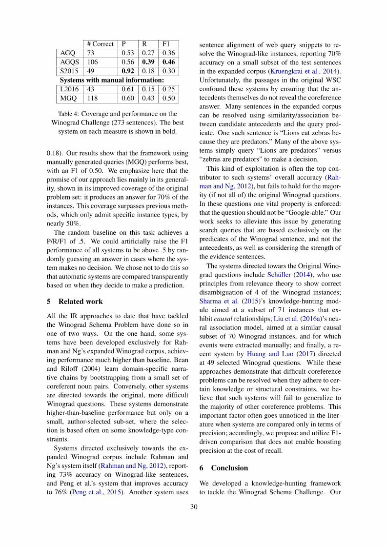
# Correct P R F1AGQ 73 0.53 0.27 0.36AGQS 106 0.56 0.39 0.46S2015 49 0.92 0.18 0.30Systems with manual information:L2016 43 0.61 0.15 0.25MGQ 118 0.60 0.43 0.50

Table 4: Coverage and performance on theWinograd Challenge (273 sentences). The best

system on each measure is shown in bold.

0.18). Our results show that the framework usingmanually generated queries (MGQ) performs best,with an F1 of 0.50. We emphasize here that thepromise of our approach lies mainly in its general-ity, shown in its improved coverage of the originalproblem set: it produces an answer for 70% of theinstances. This coverage surpasses previous meth-ods, which only admit specific instance types, bynearly 50%.

The random baseline on this task achieves aP/R/F1 of .5. We could artificially raise the F1performance of all systems to be above .5 by ran-domly guessing an answer in cases where the sys-tem makes no decision. We chose not to do this sothat automatic systems are compared transparentlybased on when they decide to make a prediction.

5 Related work

All the IR approaches to date that have tackledthe Winograd Schema Problem have done so inone of two ways. On the one hand, some sys-tems have been developed exclusively for Rah-man and Ng’s expanded Winograd corpus, achiev-ing performance much higher than baseline. Beanand Riloff (2004) learn domain-specific narra-tive chains by bootstrapping from a small set ofcoreferent noun pairs. Conversely, other systemsare directed towards the original, more difficultWinograd questions. These systems demonstratehigher-than-baseline performance but only on asmall, author-selected sub-set, where the selec-tion is based often on some knowledge-type con-straints.

Systems directed exclusively towards the ex-panded Winograd corpus include Rahman andNg’s system itself (Rahman and Ng, 2012), report-ing 73% accuracy on Winograd-like sentences,and Peng et al.’s system that improves accuracyto 76% (Peng et al., 2015). Another system uses

sentence alignment of web query snippets to re-solve the Winograd-like instances, reporting 70%accuracy on a small subset of the test sentencesin the expanded corpus (Kruengkrai et al., 2014).Unfortunately, the passages in the original WSCconfound these systems by ensuring that the an-tecedents themselves do not reveal the coreferenceanswer. Many sentences in the expanded corpuscan be resolved using similarity/association be-tween candidate antecedents and the query pred-icate. One such sentence is “Lions eat zebras be-cause they are predators.” Many of the above sys-tems simply query “Lions are predators” versus“zebras are predators” to make a decision.

This kind of exploitation is often the top con-tributor to such systems’ overall accuracy (Rah-man and Ng, 2012), but fails to hold for the major-ity (if not all of) the original Winograd questions.In these questions one vital property is enforced:that the question should not be “Google-able.” Ourwork seeks to alleviate this issue by generatingsearch queries that are based exclusively on thepredicates of the Winograd sentence, and not theantecedents, as well as considering the strength ofthe evidence sentences.

The systems directed towars the Original Wino-grad questions include Schuller (2014), who useprinciples from relevance theory to show correctdisambiguation of 4 of the Winograd instances;Sharma et al. (2015)’s knowledge-hunting mod-ule aimed at a subset of 71 instances that ex-hibit causal relationships; Liu et al. (2016a)’s neu-ral association model, aimed at a similar causalsubset of 70 Winograd instances, and for whichevents were extracted manually; and finally, a re-cent system by Huang and Luo (2017) directedat 49 selected Winograd questions. While theseapproaches demonstrate that difficult coreferenceproblems can be resolved when they adhere to cer-tain knowledge or structural constraints, we be-lieve that such systems will fail to generalize tothe majority of other coreference problems. Thisimportant factor often goes unnoticed in the liter-ature when systems are compared only in terms ofprecision; accordingly, we propose and utilize F1-driven comparison that does not enable boostingprecision at the cost of recall.

6 Conclusion

We developed a knowledge-hunting frameworkto tackle the Winograd Schema Challenge. Our

30

system involves a novel semantic representationschema and an antecedent selection process actingon web-search results. We evaluated the perfor-mance of our framework on the original problemset, demonstrating performance competitive withthe state-of-the-art. Through analysis, we deter-mined our query generation module to be a criticalcomponent of the framework.

Our query generation and antecedent selectionprocesses could likely be enhanced by various Ma-chine Learning approaches. This would requiredeveloping datasets that involve schema identifi-cation, query extraction, and knowledge acquisi-tion for the purpose of training. As future work,we consider using the extensive set of sentencesextracted by our knowledge hunting framework inorder to develop a large-scale, Winograd-like cor-pus. In addition, we are currently working to de-velop deep neural network models that performboth knowledge acquisition and antecedent selec-tion procedures in an end-to-end fashion.

ReferencesDan Bailey, Amelia Harrison, Yuliya Lierler, Vladimir

Lifschitz, and Julian Michael. 2015. The winogradschema challenge and reasoning about correlation.In In Working Notes of the Symposium on LogicalFormalizations of Commonsense Reasoning.

David Bean and Ellen Riloff. 2004. Unsupervisedlearning of contextual role knowledge for corefer-ence resolution. In Proceedings of the Human Lan-guage Technology Conference of the North Ameri-can Chapter of the Association for ComputationalLinguistics: HLT-NAACL 2004.

David Graff and C Cieri. 2003. English gigaword cor-pus. Linguistic Data Consortium .

Graeme Hirst. 1988. Semantic interpretation and am-biguity. Artificial intelligence 34(2):131–177.

Wenguan Huang and Xudong Luo. 2017. Common-sense reasoning in a deeper way: By discovering re-lations between predicates. In ICAART (2). pages407–414.

Adam Kilgarriff. 2000. Wordnet: An electronic lexicaldatabase.

Canasai Kruengkrai, Naoya Inoue, Jun Sugiura, andKentaro Inui. 2014. An example-based approach todifficult pronoun resolution. In PACLIC. pages 358–367.

Douglas B Lenat. 1995. Cyc: A large-scale investmentin knowledge infrastructure. Communications of theACM 38(11):33–38.

Hector J Levesque, Ernest Davis, and Leora Morgen-stern. 2011. The winograd schema challenge. InAAAI Spring Symposium: Logical Formalizations ofCommonsense Reasoning. volume 46, page 47.

Hugo Liu and Push Singh. 2004. Conceptnet—a prac-tical commonsense reasoning tool-kit. BT technol-ogy journal 22(4):211–226.

Quan Liu, Hui Jiang, Andrew Evdokimov, Zhen-HuaLing, Xiaodan Zhu, Si Wei, and Yu Hu. 2016a.Probabilistic reasoning via deep learning: Neural as-sociation models. arXiv preprint arXiv:1603.07704.

Quan Liu, Hui Jiang, Zhen-Hua Ling, Xiaodan Zhu,Si Wei, and Yu Hu. 2016b. Combing context andcommonsense knowledge through neural networksfor solving winograd schema problems. arXivpreprint arXiv:1611.04146 .

Haoruo Peng, Daniel Khashabi, and Dan Roth.2015. Solving hard coreference problems. Urbana51:61801.

Karthik Raghunathan, Heeyoung Lee, Sudarshan Ran-garajan, Nathanael Chambers, Mihai Surdeanu, DanJurafsky, and Christopher Manning. 2010. A multi-pass sieve for coreference resolution. In Proceed-ings of the 2010 Conference on Empirical Meth-ods in Natural Language Processing. Associationfor Computational Linguistics, pages 492–501.

Altaf Rahman and Vincent Ng. 2012. Resolvingcomplex cases of definite pronouns: the winogradschema challenge. In Proceedings of the 2012Joint Conference on Empirical Methods in NaturalLanguage Processing and Computational NaturalLanguage Learning. Association for ComputationalLinguistics, pages 777–789.

Peter Schuller. 2014. Tackling winograd schemas byformalizing relevance theory in knowledge graphs.In Fourteenth International Conference on the Prin-ciples of Knowledge Representation and Reasoning.

Arpit Sharma, Nguyen Ha Vo, Somak Aditya, andChitta Baral. 2015. Towards addressing the wino-grad schema challenge-building and using a seman-tic parser and a knowledge hunting module. In IJ-CAI. pages 1319–1325.

31

Proceedings of NAACL-HLT 2018: Student Research Workshop, pages 32–39New Orleans, Louisiana, June 2 - 4, 2018. c©2017 Association for Computational Linguistics

Towards Qualitative Word Embeddings Evaluation: MeasuringNeighbors Variation

Benedicte Pierrejean and Ludovic TanguyCLLE: CNRS & Universite de Toulouse

Toulouse, Francebenedicte.pierrejean,ludovic.tanguy@univ-tlse2.fr

Abstract

We propose a method to study the variation ly-ing between different word embeddings mod-els trained with different parameters. We ex-plore the variation between models trainedwith only one varying parameter by observingthe distributional neighbors variation and showhow changing only one parameter can havea massive impact on a given semantic space.We show that the variation is not affecting allwords of the semantic space equally. Variationis influenced by parameters such as setting aparameter to its minimum or maximum valuebut it also depends on the corpus intrinsic fea-tures such as the frequency of a word. Weidentify semantic classes of words remainingstable across the models trained and specificwords having high variation.

1 Introduction

Word embeddings are widely used nowadays inDistributional Semantics and for a variety of tasksin NLP. Embeddings can be evaluated using ex-trinsic evaluation methods, i.e. the trained em-beddings are evaluated on a specific task such aspart-of-speech tagging or named-entity recogni-tion (Schnabel et al., 2015). Because this type ofevaluation is expensive, time consuming and dif-ficult to interpret, embeddings are often evaluatedusing intrinsic evaluation methods such as wordsimilarity or analogy (Nayak et al., 2016). Suchmethods of evaluation are a good way to get aquick insight of the quality of a model. Many dif-ferent techniques and parameters can be used totrain embeddings and benchmarks are used to se-lect and tune embeddings parameters.

Benchmarks used to evaluate embeddings onlyfocus on a subset of the trained model by onlyevaluating selected pairs of words. Thus, they lackinformation about the overall structure of the se-mantic space and do not provide enough informa-

tion to understand the impact of changing one pa-rameter when training a model.

We want to know if some parameters have moreinfluence than others on the global structure ofembeddings models and get a better idea of whatvaries from one model to another. We specificallyinvestigate the impact of the architecture, the cor-pus, the window size, the vectors dimensions andthe context type when training embeddings. Weanalyze to what extent training models by chang-ing only one of these parameters has an impact onthe models created and if the different areas of thelexicon are impacted the same by this change.

To do so, we provide a qualitative methodol-ogy focusing on the global comparison of seman-tic spaces based on the overlap of the N nearestneighbors for a given word. The proposed methodis not bound to the subjectivity of benchmarks andgives a global yet precise vision of the variationbetween different models by evaluating each wordfrom the model. It provides a way to easily inves-tigate selected areas, by observing the variation ofa word or of selected subsets of words.

We compare 19 word embedding models to adefault model. All models are trained using thewell-known word2vec. Using the parameters ofthe default model, we train the other models bychanging the value of only one parameter at a time.We first get some insights by performing a quan-titative evaluation using benchmark test sets. Wethen proceed to a qualitative evaluation by observ-ing the differences between the default model andevery other model. This allows us to measurethe impact of each parameter on the global vari-ation as well as to detect phenomena that were notvisible when evaluating only with benchmark testsets. We also identify some preliminary featuresfor words remaining stable independently of theparameters used for training.

32

2 Related Work

The problems raised for the evaluation of Distri-butional Semantic Models (henceforth DSMs) isnot specific to word embeddings and have beengiven attention for a long time. Benchmarks onlyfocus on a limited subset of the corpus. For ex-ample, WordSim-353 (Finkelstein et al., 2002) istesting the behaviour of only 353 pairs of wordsmeaning we only get a partial representation ofthe model performance. To get a better idea ofthe semantic structure of DSMs and of the type ofsemantic relations they encode, some alternativedatasets were designed specifically for the evalu-ation of DSMs (Baroni and Lenci, 2011; Santuset al., 2015). Although these datasets provide adeeper evaluation, they focus on specific aspectsof the model and we still need a better way to un-derstand the global impact of changing a parame-ter when training DSMs.

Some extensive studies have been made com-paring a large number of configurations gener-ated by systematic variation of several parameters.Lapesa and Evert (2014) evaluated 537600 mod-els trained using combinations of different param-eters. Other studies focused on a specific param-eter when training embeddings such as the cor-pus size (Asr et al., 2016; Sahlgren and Lenci,2016), the type of corpus used (Bernier-Colborneand Drouin, 2016; Chiu et al., 2016) or the typeof contexts used (Levy and Goldberg, 2014; Mela-mud et al., 2016; Li et al., 2017). Results showedthat choosing the right parameters when trainingDSMs improve the performance for both intrinsicand extrinsic evaluation tasks and can also influ-ence the type of semantic information captured bythe model. Levy et al. (2015) even found that tun-ing hyperparameters carefully could prove betterin certain cases than adding more data when train-ing a model.

Chiu et al. (2016) showed that the performanceof DSMs is influenced by different factors includ-ing corpora, preprocessing performed on the cor-pora, architecture chosen and the choice of sev-eral hyperparameters. However they also noticedthat the effects of some parameters are mixed andcounterintuitive.

Hamilton et al. (2016) measured the variationbetween models by observing semantic change us-ing diachronic corpora. Hellrich and Hahn (2016)also used diachronic corpora to assess the reliabil-ity of word embeddings neighborhoods. Antoniak

and Mimno (2018) showed how the corpus influ-ences the word embeddings generated.

We relate to these studies but rather than find-ing the best combination of parameters or focus-ing on a single parameter, we assess the individualimpact of selected parameters when training wordembeddings. We intent to investigate those effectsby getting a global vision of the change from onemodel to another. Unlike benchmarks test sets, wewill not focus on evaluating only selected wordpairs from the different models but we will eval-uate the variation for each word from one modelto the other.

3 Measuring neighbors variation

To evaluate the different models trained, we fo-cus on the study of neighbors variation betweentwo models. This type of approach was proposedby Sahlgren (2006) who globally compared syn-tagmatic and paradigmatic word space models bymeasuring their overlap. We go further by apply-ing this method to a new type of models and by ob-serving variation for words individually. We alsoidentify zones with different degrees of variation.

The nearest neighbors of a given target word arewords having the closest cosine similarity scorewith the target word. To compute the variationbetween models, we propose to compute the de-gree of nearest neighbors variation between twomodels. For two models M1 and M2, we first getthe common vocabulary. We then compute thevariation var by getting the common neighborsamongst the n nearest neighbors for each word inthe two models such as:

varnM1,M2(w) = 1− |neighb

nM1

(w) ∩ neighbnM2(w)|

n

The value of n is important. To choose the mostrepresentative value, we selected a number of can-didate values (1, 5, 10, 15, 25, 50 and 100). Wefound that for most pairs of models compared withthis method, 25 was the value for which the varia-tion scores had the highest correlation scores com-pared with other values of n across the entire vo-cabulary. In this work all comparisons use thisvalue. We computed the variation for open-classparts of speech (henceforth POS) only i.e. nouns,verbs, adjectives and adverbs.

33

Parameters Default Values testedArchitecture SG CBOW

Corpus BNC ACLWindow size 5 1 to 10

Vectors dim. 10050, 200, 300,400, 500, 600

Context type window deps, deps+

Table 1. Parameters values used to train embed-dings that are compared.

4 Experiments

4.1 Experiment setupIn this work, we use a DEFAULT model as a ba-sis of comparison. Starting from this model, wetrained new models by changing only one param-eter at a time among the following parameters: ar-chitecture, corpus, window size, vectors dimen-sions, context type. We thus trained 19 mod-els which will all be compared to the DEFAULTmodel. Although we compare less models and lessparameters than other studies conducted on theevaluation of hyperparameters, we provide botha global and precise evaluation by computing thevariation for each word of the model rather thanevaluating selected pairs of words.

4.1.1 Default modelWe trained our DEFAULT model using the widelyused tool word2vec (Mikolov et al., 2013) withthe default parameters values on the BNC corpus1.The parameters used were the following:

• architecture: Skip-gram,• algorithm: negative sampling,• corpus: BNC (written part only, made of

about 90 million words),• window size: 5,• vector size: 100,• negative sampling rate: 5,• subsampling: 1e-3,• iterations: 5.

The min-count parameter was set to a value of 100.

4.1.2 Variant models5 different parameters are evaluated in this work:architecture, corpus, window size, vectors dimen-sions and context type. Using the default config-uration, we then trained one model per possibleparameter value stated in Table 1, e.g. we changed

1http://www.natcorp.ox.ac.uk/

the value of the window size or the number of di-mensions. We did not change more than one pa-rameter when training the models since this workaims at evaluating the influence of a single param-eter when training word embeddings. We chosethe parameters to be investigated as well as theirvalues based on selected studies that analyze theinfluence of parameters used when training DSMs(Baroni et al., 2014; Levy and Goldberg, 2014;Li et al., 2017; Melamud et al., 2016; Bernier-Colborne and Drouin, 2016; Sahlgren and Lenci,2016; Chiu et al., 2016).

Models were trained on the BNC except for theACL model which was trained on the ACL An-thology Reference corpus (Bird et al., 2008), acorpus made of about 100 million words. Bothcorpora were parsed using Talismane, a depen-dency parser developed by Urieli (2013). Wetrained models with dimensions ranging from 50to 600 (DIM50 to DIM600 models). We usedtwo different types of contexts: window-based anddependency-based contexts. For window-basedmodels we used a window size from 1 to 10(WIN1 to WIN10 models). For dependency-basedmodels (DEPS and DEPS+) we used word2vecf,a tool developed by Levy and Goldberg (2014).This tool is an extension of word2vec’s Skip-gram. Word2vecf uses syntactic triples as con-texts. We extracted the triples from the corpususing the scripts provided by Levy and Goldberg(2014)2 and obtained triples such as head modi-fier#reltype. Prepositions were “collapsed” as de-scribed in Levy and Goldberg (2014). To investi-gate the influence of the triples used for trainingon the embeddings generated we decided to trainwith selected syntactic relations triples (DEPS+model). We based our selection on Pado and La-pata (2007) work and chose to keep the follow-ing dependency relations: subject, noun modifier,object, adjectival modifier, coordination, apposi-tion, prepositional modifier, predicate, verb com-plement. Prepositions were still collapsed a laLevy and Goldberg (2014) and the same was donefor conjuctions.

4.2 Quantitative evaluation

To get an overview of the different models per-formance we first ran a partial quantitative evalu-

2https://bitbucket.org/yoavgo/word2vecf

34

Figure 1. Evaluation results for all models on WordSim-353 and SimLex-999 with 95% confidenceinterval span computed from DEFAULT model (DEFAULT model is shown in bold).

ation. We used the toolkit3 provided by Faruquiand Dyer (2014). This toolkit provides severalbenchmarks to test against the trained vectors. Theevaluation is computed by ranking the differentcosine scores obtained for each pair of the cho-sen dataset. The evaluation was run on WordSim-353 and Simlex-999 (Hill et al., 2015), two bench-marks commonly used for DSMs evaluation (e.g.see Levy and Goldberg (2014); Melamud et al.(2016)).

Figure 1 shows the performance of the differentmodels on both test sets as well as the confidenceinterval for the DEFAULT model. We see thatchanging parameters creates differences in mod-els performance and that this difference is gen-erally not significant. Changing the architecturefrom Skip-gram to CBOW yields worse resultsfor WordSim-353 than changing the corpus usedfor training. However, when testing on SimLex-999, performance is similar for the DEFAULT andCBOW models, while the ACL model performedworse. In a similar way, changing the training cor-pus gives better result on WordSim-353 than us-ing a different type of contexts, as shown per theresults of DEPS and DEPS+.

Performance is not consistent between the twobenchmarks. DEPS and DEPS+ both yields theworst performance on WordSim-353 but at thesame time their performance on SimLex-999 isbetter than most other models. The same is true forthe WIN1 and WIN10 models. Increasing the vec-tor dimensions gets slightly better performance,independently of the benchmark used. Increas-ing the window size gives better performance re-sults for WordSim-353 but worse for SimLex-999.Dependency-based models performs the worst on

3https://github.com/mfaruqui/eval-word-vectors

Figure 2. Mean variation value with standard de-viation interval for all trained models compared toDEFAULT model. The dashed line corresponds tothe mean variation value for the DEFAULT modeltrained 5 times with the exact same parameters.

WordSim-353.This kind of evaluation is only performed on se-

lected pairs of words and despite small differencesin performance scores, larger differences may ex-ist. In the next section we introduce a method thatquantifies the variation between the different mod-els trained by evaluating the distributional neigh-bors variation for every word in the corpus.

4.3 Qualitative evaluation4.3.1 Exploring the variationFigure 2 shows the mean variation score with thestandard deviation span between the DEFAULTmodel and the 19 other models4. Since it is known

4For models trained on the BNC, 27437 words were eval-uated. When comparing DEFAULT to ACL the vocabularysize was smaller (10274) since the models were not trainedon the same corpus.

35

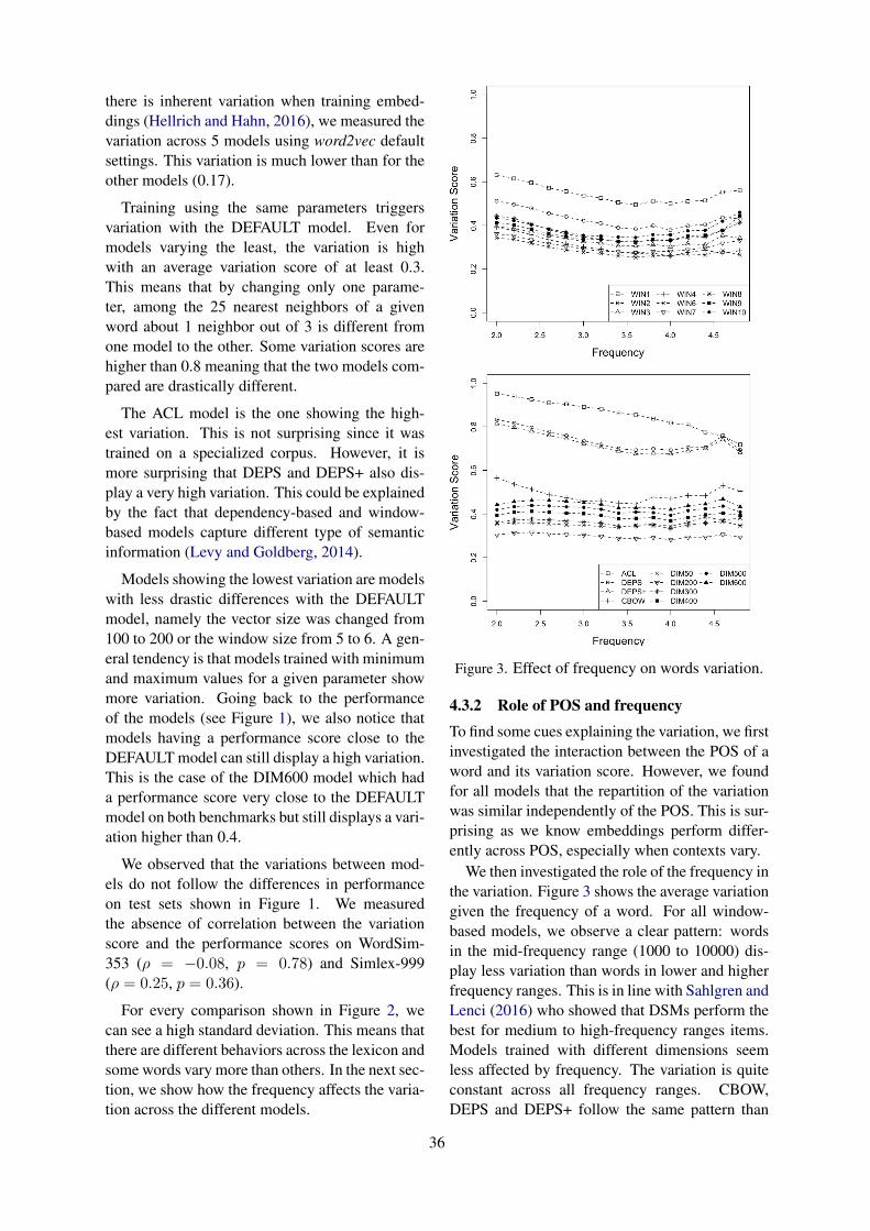
there is inherent variation when training embed-dings (Hellrich and Hahn, 2016), we measured thevariation across 5 models using word2vec defaultsettings. This variation is much lower than for theother models (0.17).

Training using the same parameters triggersvariation with the DEFAULT model. Even formodels varying the least, the variation is highwith an average variation score of at least 0.3.This means that by changing only one parame-ter, among the 25 nearest neighbors of a givenword about 1 neighbor out of 3 is different fromone model to the other. Some variation scores arehigher than 0.8 meaning that the two models com-pared are drastically different.

The ACL model is the one showing the high-est variation. This is not surprising since it wastrained on a specialized corpus. However, it ismore surprising that DEPS and DEPS+ also dis-play a very high variation. This could be explainedby the fact that dependency-based and window-based models capture different type of semanticinformation (Levy and Goldberg, 2014).

Models showing the lowest variation are modelswith less drastic differences with the DEFAULTmodel, namely the vector size was changed from100 to 200 or the window size from 5 to 6. A gen-eral tendency is that models trained with minimumand maximum values for a given parameter showmore variation. Going back to the performanceof the models (see Figure 1), we also notice thatmodels having a performance score close to theDEFAULT model can still display a high variation.This is the case of the DIM600 model which hada performance score very close to the DEFAULTmodel on both benchmarks but still displays a vari-ation higher than 0.4.

We observed that the variations between mod-els do not follow the differences in performanceon test sets shown in Figure 1. We measuredthe absence of correlation between the variationscore and the performance scores on WordSim-353 (ρ = −0.08, p = 0.78) and Simlex-999(ρ = 0.25, p = 0.36).

For every comparison shown in Figure 2, wecan see a high standard deviation. This means thatthere are different behaviors across the lexicon andsome words vary more than others. In the next sec-tion, we show how the frequency affects the varia-tion across the different models.

Figure 3. Effect of frequency on words variation.

4.3.2 Role of POS and frequency

To find some cues explaining the variation, we firstinvestigated the interaction between the POS of aword and its variation score. However, we foundfor all models that the repartition of the variationwas similar independently of the POS. This is sur-prising as we know embeddings perform differ-ently across POS, especially when contexts vary.

We then investigated the role of the frequency inthe variation. Figure 3 shows the average variationgiven the frequency of a word. For all window-based models, we observe a clear pattern: wordsin the mid-frequency range (1000 to 10000) dis-play less variation than words in lower and higherfrequency ranges. This is in line with Sahlgren andLenci (2016) who showed that DSMs perform thebest for medium to high-frequency ranges items.Models trained with different dimensions seemless affected by frequency. The variation is quiteconstant across all frequency ranges. CBOW,DEPS and DEPS+ follow the same pattern than

36

Model Var. Identified semantic classesACL Low numerals (2nd, 14th, 10th...)

nationalities (hungarian, french, danish, spanish...)time nouns (afternoon, week, evening...)

Highspecialized lexicon (embedded, differential, nominal, probabilistic, patch, spell,string, graph...)

DIM200 Low numerals (40th, 15th...)nationalities (hungarian, dutch, french, spanish...)family nouns (grandparent, sister, son, father...)

High generic adjectives (all, near, very, real...)polysemic nouns (field, marker, turn, position...)

Table 2. Words showing lowest and highest variation for ACL and DIM200 compared to DEFAULT.

the window models, with a variation less high formedium frequency words. ACL5 display a veryhigh variation for low frequency words but thevariation decreases with frequency.

4.3.3 Getting a preview of the variationThe variation measure can also be used to ex-amine more local differences. For example, forgiven pairs of models we can easily identify whichwords show the most extreme variation values. Wedid this for two of our models: ACL which showsthe highest variation and DIM200 which showsthe lowest variation. Table 2 shows a few of themost stable and unstable words. It appears thatdifferent semantic classes emerge in each case. Itseems that these classes correspond to dense clus-ters, each word having all others as close neighbor.Some of these clusters remain the same across thetwo pairs of models (e.g. nationality adjectives)while other clusters are different. In the ACLmodel, we find a cluster of time nouns while in theDIM200 model we find family nouns. We see thatwords varying the most for the specialized corpusare words carrying a specific meaning (e.g. nomi-nal, graph). We also find that words with a highvariation score are highly polysemic or generic inthe DIM200 model (e.g. field, marker). In the fu-ture we want to analyze the impact of the degree ofpolysemy on the variation score along with othercharacteristics of words.

5 Conclusion

This work compared 19 models trained using onedifferent parameter to a default model. We mea-sured the differences between these models with

5The variation for ACL was measured on a smaller vocab-ulary set. The frequency used in Figure 3 is the one from theBNC.

benchmark test sets and a methodology whichdoes not depend on the subjectivity and limitedscope of benchmark test sets. Test sets showmarginal differences while neighbors variation re-vealed that at least one third of the nearest 25neighbors of a word are different from one modelto the other. In addition it appears that the parame-ters have a different impact depending on the waydifferences are measured.

We saw that the variation is not affecting allwords of the semantic space equally and wefound features which help identify some areas of(in)stability in the semantic space. Words havinga low and high frequency range have a tendency todisplay more variation. Words in the medium fre-quency range show more stability. We also foundword features that could play a role in the varia-tion (polysemy, genericity, semantic clusters etc.).These features can help understanding what reallychanges when tuning the parameters of word em-beddings and give us more control over those ef-fects.

In further work, we want to extend our analysisto more parameters. We especially want to see ifthe observations made in this study apply to mod-els trained with specialized corpora or corpora ofdifferent sizes. We also want to distinguish fea-tures that will help classify words displaying moreor less variation and qualify the variations them-selves.

Acknowledgments

We would like to thank the Student ResearchWorkshop for setting up the mentoring programthat we benefited from. We especially thank ourmentor, Shashi Narayan, for his very helpful com-ments. We are also thankful to the anonymous re-viewers for their suggestions and comments.

37

Experiments presented in this paper werecarried out using the OSIRIM platformthat is administered by IRIT and sup-ported by CNRS, the Region Midi-Pyrenees,the French Government, and ERDF (seehttp://osirim.irit.fr/site/en).

ReferencesMaria Antoniak and David Mimno. 2018. Evaluating

the Stability of Embedding-based Word Similarities.Transactions of the Association for ComputationalLinguistics, 6:107–119.

Fatemeh Torabi Asr, Jon A. Willits, and Michael N.Jones. 2016. Comparing Predictive and Co-occurrence Based Models of Lexical SemanticsTrained on Child-directed Speech. In Proceedingsof the 37th Meeting of the Cognitive Science Soci-ety.

Marco Baroni, Georgiana Dinu, and GermanKruszewski. 2014. Don’t count, predict! Asystematic comparison of context-counting vs.context-predicting semantic vectors. In Proceedingsof the 52nd Annual Meeting of the Associationfor Computational Linguistics, pages 238–247,Baltimore, Maryland, USA.

Marco Baroni and Alessandro Lenci. 2011. How weBLESSed distributional semantic evaluation. InProceedings of the GEMS 2011 Workshop on Ge-ometrical Models of Natural Language Semantics,EMNLP 2011, pages 1–10, Edinburgh, Scotland,UK.

Gabriel Bernier-Colborne and Patrick Drouin. 2016.Evaluation of distributional semantic models: aholistic approach. In Proceedings of the 5th Inter-national Workshop on Computational Terminology,pages 52–61, Osaka, Japan.

Steven Bird, Robert Dale, Bonnie Dorr, Bryan Gibson,Mark Joseph, Min-Yen Kan, Dongwon Lee, BrettPowley, Dragomir Radev, and Yee Fan Tan. 2008.The ACL Anthology Reference Corpus: A Refer-ence Dataset for Bibliographic Research in Compu-tational Linguistics. In Proceedings of LanguageResources and Evaluation Conference (LREC 08),Marrakesh, Morrocco.

Billy Chiu, Gamal Crichton, Anna Korhonen, andSampo Pyysalo. 2016. How to Train Good WordEmbeddings for Biomedical NLP. In Proceedings ofthe 15th Workshop on Biomedical Natural LanguageProcessing, pages 166–174, Berlin, Germany.

Manaal Faruqui and Chris Dyer. 2014. CommunityEvaluation and Exchange of Word Vectors at word-vectors.org. In Proceedings of the 52nd AnnualMeeting of the Association for Computational Lin-guistics: System Demonstrations, pages 19–24, Bal-timore, Maryland, USA.

Lev Finkelstein, Evgeniy Gabrilovich, Yossi Matias,Ehud Rivlin, Zach Solan, Gadi Wolfman, and Ey-tan Ruppin. 2002. Placing Search in Context: TheConcept Revisited. In ACM Transactions on Infor-mation Systems, volume 20, page 116:131.

William L. Hamilton, Jure Leskovec, and Dan Juraf-sky. 2016. Diachronic Word Embeddings RevealStatistical Laws of Semantic Change. In Proceed-ings of the 54th Annual Meeting of the Associationfor Computational Linguistics, pages 1489–1501,Berlin, Germany.

Johannes Hellrich and Udo Hahn. 2016. Bad Com-pany - Neighborhoods in Neural Embedding SpacesConsidered Harmful. In Proceedings of COLING2016, the 26th International Conference on Compu-tational Linguistics: Technical Papers, pages 2785–2796, Osaka, Japan.

Felix Hill, Roi Reichart, and Anna Korhonen. 2015.SimLex-999: Evaluating Semantic Models with(Genuine) Similarity Estimation. ComputationalLinguistics, 41:665–695.

Gabriella Lapesa and Stefan Evert. 2014. A LargeScale Evaluation of Distributional Semantic Mod-els: Parameters, Interactions and Model Selection.Transactions of the Association for ComputationalLinguistics, 2:531–545.

Omer Levy and Yoav Goldberg. 2014. Dependency-Based Word Embeddings. In Proceedings of the52nd Annual Meeting of the Association for Com-putational Linguistics, pages 302–308, Baltimore,Maryland, USA.

Omer Levy, Yoav Goldberg, and Ido Dagan. 2015.Improving Distributional Similarity with LessonsLearned from Word Embeddings. Transactionsof the Association for Computational Linguistics,3:211–225.

Bofang Li, Tao Liu, Zhe Zhao, Buzhou Tang, Alek-sandr Drozd, Anna Rogers, and Xiaoyong Du. 2017.Investigating Different Syntactic Context Types andContext Representations for Learning Word Embed-dings. In Proceedings of the 2017 Conference onEmpirical Methods in Natural Language Process-ing, pages 2411–2421.

Oren Melamud, David McClosky, Siddharth Patward-han, and Mohit Bansal. 2016. The Role of ContextTypes and Dimensionality in Learning Word Em-beddings. In Proceedings of NAACL-HLT 2016, SanDiego, California.

Tomas Mikolov, Kai Chen, Greg Corrado, and JeffreyDean. 2013. Efficient Estimation of Word Represen-tations in Vector Space. CoRR, abs/1301.3781.

Neha Nayak, Gabor Angeli, and Christopher D. Man-ning. 2016. Evaluating Word Embeddings Using aRepresentative Suite of Practical Tasks. In Proceed-ings of the 1st Workshop on Evaluating Vector SpaceRepresentations for NLP, pages 19–23, Berlin, Ger-many.

38

Sebastian Pado and Mirella Lapata. 2007.Dependency-Based Construction of Seman-tic Space Models. Computational Linguistics,33(2):161–199.

Magnus Sahlgren. 2006. The Word-Space Model.Ph.D. thesis, Stockholm University, Sweden.

Magnus Sahlgren and Alessandro Lenci. 2016. The Ef-fects of Data Size and Frequency Range on Distribu-tional Semantic Models. In Proceedings of the 2016Conference on Empirical Methods in Natural Lan-guage Processing, pages 975–980, Austin, Texas.

Enrico Santus, Frances Yung, Alessandro Lenci, andChu-Ren Huang. 2015. EVALution1.0: an Evolv-ing Semantic Dataset for Training and Evaluationof Distributional Semantic Models. In Proceedingsof the 4th Workshop on Linked Data in Linguistics(LDL-2015), pages 64–69, Beijing, China.

Tobias Schnabel, Igor Labutov, David Mimno, andThorsten Joachims. 2015. Evaluation methods forunsupervised word embeddings. In Proceedings ofthe 2015 Conference on Empirical Methods in Nat-ural Language Processing, pages 298–307.

Assaf Urieli. 2013. Robust French syntax analysis:reconciling statistical methods and linguistic knowl-edge in the Talismane toolkit. Ph.D. thesis, Univer-sity of Toulouse, France.

39

Proceedings of NAACL-HLT 2018: Student Research Workshop, pages 40–45New Orleans, Louisiana, June 2 - 4, 2018. c©2017 Association for Computational Linguistics

A Deeper Look into Dependency-Based Word Embeddings

Sean MacAvaneyInformation Retrieval Lab

Department of Computer ScienceGeorgetown UniversityWashington, DC, USA

sean@ir.cs.georgetown.edu

Amir ZeldesDepartment of Linguistics

Georgetown UniversityWashington, DC, USA

amir.zeldes@georgetown.edu

Abstract

We investigate the effect of variousdependency-based word embeddings ondistinguishing between functional and domainsimilarity, word similarity rankings, and twodownstream tasks in English. Variationsinclude word embeddings trained usingcontext windows from Stanford and Universaldependencies at several levels of enhancement(ranging from unlabeled, to Enhanced++dependencies). Results are compared tobasic linear contexts and evaluated on sev-eral datasets. We found that embeddingstrained with Universal and Stanford depen-dency contexts excel at different tasks, andthat enhanced dependencies often improveperformance.

1 Introduction

For many natural language processing applica-tions, it is important to understand word-level se-mantics. Recently, word embeddings trained withneural networks have gained popularity (Mikolovet al., 2013; Pennington et al., 2014), and havebeen successfully used for various tasks, such asmachine translation (Zou et al., 2013) and infor-mation retrieval (Hui et al., 2017).

Word embeddings are usually trained using lin-ear bag-of-words contexts, i.e. tokens positionedaround a word are used to learn a dense representa-tion of that word. Levy and Goldberg (2014) chal-lenged the use of linear contexts, proposing in-stead to use contexts based on dependency parses.(This is akin to prior work that found that depen-dency contexts are useful for vector models (Padoand Lapata, 2007; Baroni and Lenci, 2010).) Theyfound that embeddings trained this way are bet-ter at capturing semantic similarity, rather than re-latedness. For instance, embeddings trained us-ing linear contexts place Hogwarts (the fictional

setting of the Harry Potter series) near Dumble-dore (a character from the series), whereas em-beddings trained with dependency contexts placeHogwarts near Sunnydale (fictional setting of theseries Buffy the Vampire Slayer). The former isrelatedness, whereas the latter is similarity.

Work since Levy and Goldberg (2014) exam-ined the use of dependency contexts and sen-tence feature representations for sentence classifi-cation (Komninos and Manandhar, 2016). Li et al.(2017) filled in research gaps relating to modeltype (e.g., CBOW, Skip-Gram, GloVe) and depen-dency labeling. Interestingly, Abnar et al. (2018)recently found that dependency-based word em-beddings excel at predicting brain activation pat-terns. The best model to date for distinguishingbetween similarity and relatedness combines wordembeddings, WordNet, and dictionaries (Recskiet al., 2016).

One limitation of existing work is that ithas only explored one dependency scheme:the English-tailored Stanford Dependen-cies (De Marneffe and Manning, 2008b). Weprovide further analysis using the cross-lingualUniversal Dependencies (Nivre et al., 2016). Al-though we do not compare cross-lingual embed-dings in our study, we will address one importantquestion for English: are Universal Dependencies,which are less tailored to English, actually betteror worse than the English-specific labels andgraphs? Furthermore, we investigate approachesto simplifying and extending dependencies, in-cluding Enhanced dependencies and Enhanced++dependencies (Schuster and Manning, 2016), aswell as two levels of relation simplification. Wehypothesize that the cross-lingual generalizationsfrom universal dependencies and the additionalcontext from enhanced dependencies shouldimprove the performance of word embeddingsat distinguishing between functional and domain

40

Enhanced + +

Enhanced

Basic

Simplified

Stanford Universal++

CBOW

k = 2 k = 5

Linear Contexts Dependency Contexts

Unlabeled

Skip-Gram

Subword

+

Figure 1: Visual relationship between types of embed-ding contexts. Each layer of enhancement adds moreinformation to the dependency context (e.g., simpli-fied adds dependency labels to the unlabeled context).We investigate CBOW using both a context window ofk = 2 and k = 5, and we use the SkipGram model bothwith and without subword information.

similarity. We also investigate how these differ-ences impact word embedding performance atword similarity rankings and two downstreamtasks: question-type classification and namedentity recognition.

2 Method

In this work, we explore the effect of two depen-dency annotation schemes on the resulting embed-dings. Each scheme is evaluated in five levels ofenhancement. These embeddings are compared toembeddings trained with linear contexts using thecontinuous bag of words (CBOW) with a contextwindow of k = 2 and k = 5, and Skip-Gramcontexts with and without subword information.These configurations are summarized in Figure 1.

Two dependency annotation schemes for En-glish are Stanford dependencies (De Marneffeand Manning, 2008b) and Universal dependen-cies (Nivre et al., 2016). Stanford dependen-cies are tailored to English text, including de-pendencies that are not necessarily relevant cross-lingually (e.g. a label prt for particles like up inpick up). Universal dependencies are more gener-alized and designed to work cross-lingually. Manystructures are similar between the two schemes,but important differences exist. For instance,in Stanford dependencies, prepositions head theirphrase and depend on the modified word (in is the

Simp. Basic

Stanford dependenciesmod poss, prt, predet, det, amod, tmod, npadvmod,

possessive, advmod, quantmod, preconj, mark,vmod, nn, num, prep, appos, mwe, mod, num-ber, neg, advcl, rcmod

arg agent, iobj, dobj, acomp, pcomp, pobj, ccomp,arg, subj, csubj, obj, xcomp, nsubj

aux aux, copsdep xsubj, sdep

Universal dependenciescore iobj, dobj, ccomp, csubj, obj, xcomp, nsubjncore discourse, cop, advmod, dislocated, vocative,

aux, advcl, mark, obl, explnom case, nmod, acl, neg, appos, det, amod, num-

modcoord cc, conjspecial goeswith, reparandum, orphanloose parataxis, listmwe compound, mwe, flatother punct, dep, root

Table 1: Simplified Stanford and Universal dependencylabels. For simplified dependencies, basic labels arecollapsed into the simplified label shown in this table.(Relations not found in this table were left as is.)

head of in Kansas), whereas in universal depen-dencies, prepositions depend on the prepositionalobject (Kansas dominates in). Intuitively, thesedifferences should have a moderate effect on theresulting embeddings because different words willbe in a given word’s context.

We also investigate five levels of enhancementfor each dependency scheme. Basic dependenciesare the core dependency structure provided by thescheme. Simplified dependencies are more coarsebasic dependencies, collapsing similar labels intorough classes. The categories are based off of theStanford Typed Dependencies Manual (De Marn-effe and Manning, 2008a) and the Universal De-pendency Typology (De Marneffe et al., 2014),and are listed in Table 1. Note that the two depen-dency schemes organize the relations in differentways, and thus the two types of simplified depen-dencies represent slightly different structures. Theunlabeled dependency context removes all labels,and just captures syntactically adjacent tokens.

Enhanced and Enhanced++ dependen-cies (Schuster and Manning, 2016) addresssome practical dependency distance issues byextending basic dependency edges. Enhanceddependencies augment modifiers and conjunctswith their parents’ labels, propagate governorsand dependents for indirectly governed argu-ments, and add subjects to controlled verbs.

41

Enhanced++ dependencies allow for the deletionof edges to better capture English phenomena,including partitives and light noun constructions,multi-word prepositions, conjoined prepositions,and relative pronouns.

3 Experimental Setup

We use the Stanford CoreNLP parser1 to parsebasic, Enhanced, and Enhanced++ dependencies.We use the Stanford english SD model to parseStanford dependencies (trained on the Penn Tree-bank) and english UD model to parse Universaldependencies (trained on the Universal Dependen-cies Corpus for English). We acknowledge thatdifferences in both the size of the training data(Penn Treebank is larger than the Universal De-pendency Corpus for English), and the accuracyof the parse can have an effect on our overall per-formance. We used our own converter to generatesimple dependencies based on the rules shown inTable 1. We use the modified word2vecf soft-ware2 Levy and Goldberg (2014) that works witharbitrary embedding contexts to train dependency-based word embeddings.

As baselines, we train the followinglinear-context embeddings using the originalword2vec software:3 CBOW with k = 2,CBOW with k = 5, and Skip-Gram. We alsotrain enriched Skip-Gram embeddings includingsubword information (Bojanowski et al., 2016)using fastText.4

For all embeddings, we use a cleaned recentdump of English Wikipedia (November 2017,4.3B tokens) as training data. We evaluate eachon the following tasks:

Similarity over Relatedness Akin to the quanti-tative analysis done by Levy and Goldberg (2014),we test to see how well each approach ranks sim-ilar items above related items. Given pairs ofsimilar and related words, we rank each wordpair by the cosine similarity of the correspondingword embeddings, and report the area-under-curve(AUC) of the resulting precision-recall curve.We use the labeled WordSim-353 (Agirre et al.,2009; Finkelstein et al., 2001) and the Chiarellodataset (Chiarello et al., 1990) as a source of sim-ilar and related word pairs. For WordSim-353,1stanfordnlp.github.io/CoreNLP/2bitbucket.org/yoavgo/word2vecf3code.google.com/p/word2vec/4github.com/facebookresearch/fastText

we only consider pairs with similarity/relatednessscores of at least 5/10, yielding 90 similar pairsand 147 related pairs. For Chiarello, we disregardpairs that are marked as both similar and related,yielding 48 similar pairs and 48 related pairs.

Ranked Similarity This evaluation uses a list ofword pairs that are ranked by degree of functionalsimilarity. For each word pair, we calculate the co-sine similarity, and compare the ranking to that ofthe human-annotated list using the Spearman cor-relation. We use SimLex-999 (Hill et al., 2016)as a ranking of functional similarity. Since thisdataset distinguishes between nouns, adjectives,and verbs, we report individual correlations in ad-dition to the overall correlation.

Question-type Classification (QC) We use anexisting QC implementation5 that uses a bidirec-tional LSTM. We train the model with 20 epochs,and report the average accuracy over 10 runs foreach set of embeddings. We train and evaluate us-ing the TREC QC dataset (Li and Roth, 2002). Wemodified the approach to use fixed (non-trainable)embeddings, allowing us to compare the impact ofeach embedding type.

Named Entity Recognition (NER) We use theDernoncourt et al. (2017) NER implementation6

that uses a bidirectional LSTM. Training con-sists of a maximum of 100 epochs, with earlystopping after 10 consecutive epochs with no im-provement to validation performance. We evalu-ate NER using the F1 score on the CoNLL NERdataset (Tjong Kim Sang and De Meulder, 2003).Like the QC task, we use a non-trainable embed-ding layer.

4 Results

4.1 Similarity over Relatedness

The results for the WordSim-353 (WS353) andChiarello datasets are given in Table 2a. For theWS353 evaluation, notice that the Enhanced de-pendencies for both Universal and Stanford de-pendencies outperform the others in each scheme.Even the poorest-performing level of enhancement(unlabeled), however, yields a considerable gainover the linear contexts. Both Skip-Gram variantsyield the worst performance, indicating that they

5github.com/zhegan27/sentence_classification

6github.com/Franck-Dernoncourt/NeuroNER

42

(a) Sim/rel (AUC) (b) Ranked sim (Spearman) (c) Downstream

Embeddings WS353 Chiarello Overall Noun Adj. Verb QC (Acc) NER (F1)

Universal embeddingsUnlabeled 0.786 0.711 0.370 0.408 0.484 0.252 0.915 0.877Simplified 0.805 0.774 0.394 0.420 0.475 0.309 0.913 0.870Basic 0.801 0.761 0.391 0.421 0.451 0.331 0.920 0.876Enhanced 0.823 0.792 0.398 0.416 0.473 0.350 0.915 0.875Enhanced++ 0.820 0.791 0.396 0.416 0.461 0.348 0.917 0.882

Stanford embeddingsUnlabeled 0.790 0.741 0.382 0.414 0.507 0.256 0.911 0.870Simplified 0.793 0.748 0.393 0.416 0.501 0.297 0.923 0.873Basic 0.808 0.769 0.402 0.422 0.494 0.341 0.910 0.865Enhanced 0.817 0.755 0.399 0.420 0.482 0.338 0.911 0.871Enhanced++ 0.810 0.764 0.398 0.417 0.496 0.346 0.918 0.878

Baselines (linear contexts)CBOW, k=2 0.696 0.537 0.311 0.355 0.338 0.252 0.913 0.885CBOW, k=5 0.701 0.524 0.309 0.353 0.358 0.258 0.899 0.893Skip-Gram 0.617 0.543 0.264 0.304 0.368 0.135 0.898 0.881SG + Subword 0.615 0.456 0.324 0.358 0.451 0.166 0.897 0.887

Table 2: Results of various dependency-based word embeddings, and baseline linear contexts at (a) similarity overrelatedness, (b) ranked similarity, and (c) downstream tasks of question classification and named entity recognition.

capture relatedness better than similarity. For theChiarello evaluation, the linear contexts performeven worse, while the Enhanced Universal embed-dings again outperform the other approaches.

These results reinforce the Levy and Goldberg(2014) findings that dependency-based word em-beddings do a better job at distinguishing simi-larity rather than relatedness because it holds formultiple dependency schemes and levels of en-hancement. The Enhanced universal embeddingsoutperformed the other settings for both datasets.For Chiarello, the margin between the two is sta-tistically significant, whereas for WS353 it is not.This might be due to the fact that the the Chiarellodataset consists of manually-selected pairs that ex-hibit similarity or relatedness, whereas the set-tings for WS353 allow for some marginally re-lated or similar terms through (e.g., size is relatedto prominence, and monk is similar to oracle).

4.2 Ranked SimilaritySpearman correlation results for ranked similar-ity on the SimLex-999 dataset are reported in Ta-ble 2b. Overall results indicate the performanceon the entire collection. In this environment, ba-sic Stanford embeddings outperform all other em-beddings explored. This is an interesting result

because it shows that the additional dependencylabels added for Enhanced embeddings (e.g. forconjunction) do not improve the ranking perfor-mance. This trend does not hold for Universal em-beddings, with the enhanced versions outperform-ing the basic embeddings.

All dependency-based word embeddings signif-icantly outperform the baseline methods (10 folds,paired t-test, p < 0.05). Furthermore, the un-labeled Universal embeddings performed signif-icantly worse than the simplified Universal, andthe simplified, basic, and Enhanced Stanford de-pendencies, indicating that dependency labels areimportant for ranking.

Table 2b also includes results for word pairs bypart of speech individually. As the majority cat-egory, Noun-Noun scores (n = 666) mimic thebehavior of the overall scores, with basic Stanfordembeddings outperforming other approaches. In-terestingly, Adjective-Adjective pairs (n = 111)performed best with unlabeled Stanford dependen-cies. Since unlabeled also performs best amonguniversal embeddings, this indicates that depen-dency labels are not useful for adjective simi-larity, possibly because adjectives have compara-tively few ambiguous functions. Verb-Verb pairs

43

Embeddings QC (Acc) NER (F1)

Universal embeddingsUnbound 0.921 (+0.007) 0.887 (+0.000)Simplified 0.929 (+0.016) 0.883 (+0.013)Basic 0.920 (+0.000) 0.891 (+0.015)Enhanced 0.923 (+0.008) 0.886 (+0.010)Enhanced++ 0.927 (+0.010) 0.890 (+0.008)

Stanford embeddingsUnbound 0.926 (+0.015) 0.879 (+0.009)Simplified 0.933 (+0.010) 0.877 (+0.004)Basic 0.927 (+0.017) 0.885 (+0.020)Enhanced 0.923 (+0.013) 0.885 (+0.014)Enhanced++ 0.929 (+0.011) 0.884 (+0.006)

Baselines (linear contexts)CBOW, k=2 0.921 (+0.008) 0.892 (+0.007)CBOW, k=5 0.925 (+0.026) 0.892 (+0.001)Skip-Gram 0.914 (+0.016) 0.887 (+0.006)SG + Subword 0.919 (+0.022) 0.896 (+0.009)

Table 3: Performance results when embeddings arefurther trained for the particular task. The number inparentheses gives the performance improvement com-pared to when embeddings are not trainable (Table 2c).

(n = 222) performed best with Enhanced uni-versal embeddings. This indicates that the aug-mentation of governors, dependents, and subjectsof controlled verbs is particularly useful giventhe universal dependency scheme, and less so forthe English-specific Stanford dependency scheme.Both Stanford and universal unlabeled dependen-cies performed significantly worse compared to allbasic, Enhanced, and Enhanced++ dependencies(5 folds, paired t-test, p < 0.05). This indicatesthat dependency labels are particularly importantfor verb similarity.

4.3 Downstream Tasks

We present results for question-type classifica-tion and named entity recognition in Table 2c.Neither task appears to greatly benefit from em-beddings that favor similarity over relatedness orthat can rank based on functional similarity ef-fectively without the enhanced sentence featurerepresentations explored by Komninos and Man-andhar (2016). We compare the results using tothe performance of models with embedding train-ing enabled in Table 3. As expected, this im-proves the results because the training capturestask-specific information in the embeddings. Gen-erally, the worst-performing embeddings gainedthe most (e.g., CBOW k = 5 for QC, and basicStanford for NER). However, the simplified Stan-ford embeddings and the embeddings with sub-word information still outperform the other ap-

proaches for QC and NER, respectively. This in-dicates that the initial state of the embeddings isstill important to an extent, and cannot be learnedfully for a given task.

5 Conclusion

In this work, we expanded previous work by Levyand Goldberg (2014) by looking into variations ofdependency-based word embeddings. We inves-tigated two dependency schemes: Stanford andUniversal embeddings. Each scheme was ex-plored at various levels of enhancement, rang-ing from unlabeled contexts to Enhanced++ de-pendencies. All variations yielded significant im-provements over linear contexts in most circum-stances. For certain subtasks (e.g. Verb-Verbsimilarity), enhanced dependencies improved re-sults more strongly, supporting current trends inthe universal dependency community to promoteenhanced representations. Given the disparate re-sults across POS tags, future work could also eval-uate ways of using a hybrid approach with differ-ent contexts for different parts of speech, or usingconcatenated embeddings.

ReferencesSamira Abnar, Rasyan Ahmed, Max Mijnheer, and

Willem Zuidema. 2018. Experiential, distributionaland dependency-based word embeddings have com-plementary roles in decoding brain activity. In Pro-ceedings of the 8th Workshop on Cognitive Modelingand Computational Linguistics (CMCL 2018). SaltLake City, UT, pages 57–66.

Eneko Agirre, Enrique Alfonseca, Keith Hall, JanaKravalova, Marius Pasca, and Aitor Soroa. 2009. Astudy on similarity and relatedness using distribu-tional and wordnet-based approaches. In Proceed-ings of HLT-NAACL 2009. Boulder, CO, pages 19–27.

Marco Baroni and Alessandro Lenci. 2010. Distribu-tional memory: A general framework for corpus-based semantics. Comput. Linguist. 36(4).

Piotr Bojanowski, Edouard Grave, Armand Joulin,and Tomas Mikolov. 2016. Enriching word vec-tors with subword information. arXiv preprintarXiv:1607.04606 .

Christine Chiarello, Curt Burgess, Lorie Richards, andAlma Pollock. 1990. Semantic and associativepriming in the cerebral hemispheres: Some wordsdo, some words don’t sometimes, some places.Brain and language 38(1):75–104.

44

Marie-Catherine De Marneffe, Timothy Dozat, Na-talia Silveira, Katri Haverinen, Filip Ginter, JoakimNivre, and Christopher D Manning. 2014. Univer-sal Stanford dependencies: A cross-linguistic typol-ogy. In Proceedings of LREC 2014. Reykjavik, vol-ume 14, pages 4585–4592.

Marie-Catherine De Marneffe and Christopher D Man-ning. 2008a. Stanford typed dependencies manual.Technical report, Stanford University.

Marie-Catherine De Marneffe and Christopher D Man-ning. 2008b. The Stanford typed dependenciesrepresentation. In Coling 2008: proceedings ofthe workshop on cross-framework and cross-domainparser evaluation. pages 1–8.

Franck Dernoncourt, Ji Young Lee, and PeterSzolovits. 2017. NeuroNER: an easy-to-use pro-gram for named-entity recognition based on neuralnetworks. In Proceedings of EMNLP 2017. Copen-hagen.

Lev Finkelstein, Evgeniy Gabrilovich, Yossi Matias,Ehud Rivlin, Zach Solan, Gadi Wolfman, and Ey-tan Ruppin. 2001. Placing search in context: Theconcept revisited. In Proceedings of the 10th inter-national conference on World Wide Web. pages 406–414.

Felix Hill, Roi Reichart, and Anna Korhonen. 2016.Simlex-999: Evaluating semantic models with (gen-uine) similarity estimation. Computational Linguis-tics 41(4).

Kai Hui, Andrew Yates, Klaus Berberich, and Gerardde Melo. 2017. PACRR: A position-aware neuralIR model for relevance matching. In Proceedings ofEMNLP 2017. Copenhagen.

Alexandros Komninos and Suresh Manandhar. 2016.Dependency based embeddings for sentence classi-fication tasks. In Proceedings of HLT-NAACL. SanDiego, CA, pages 1490–1500.

Omer Levy and Yoav Goldberg. 2014. Dependency-based word embeddings. In Proceedings of ACL2014. Baltimore, MD, pages 302–308.

Bofang Li, Tao Liu, Zhe Zhao, Buzhou Tang, Alek-sandr Drozd, Anna Rogers, and Xiaoyong Du. 2017.Investigating different syntactic context types andcontext representations for learning word embed-dings. In Proceedings of EMNLP 2017. Copen-hagen, pages 2411–2421.

Xin Li and Dan Roth. 2002. Learning question clas-sifiers. In Proceedings of COLING 2002. Taipei,pages 1–7.

Tomas Mikolov, Kai Chen, Greg Corrado, and JeffreyDean. 2013. Efficient estimation of word represen-tations in vector space. CoRR abs/1301.3781 .

Joakim Nivre, Marie-Catherine de Marneffe, FilipGinter, Yoav Goldberg, Jan Hajic, Christopher DManning, Ryan T McDonald, Slav Petrov, SampoPyysalo, Natalia Silveira, et al. 2016. Universal de-pendencies v1: A multilingual treebank collection.In Proceedings of LREC 2016. Portoroz, Slovenia.

Sebastian Pado and Mirella Lapata. 2007.Dependency-based construction of semanticspace models. Computational Linguistics .

Jeffrey Pennington, Richard Socher, and ChristopherManning. 2014. Glove: Global vectors for wordrepresentation. In Proceedings of EMNLP 2014.Doha, Qatar, pages 1532–1543.

Gabor Recski, Eszter Iklodi, Katalin Pajkossy, and An-dras Kornai. 2016. Measuring semantic similarityof words using concept networks. In Proceedingsof the 1st Workshop on Representation Learning forNLP. Berlin, Germany, pages 193–200.

Sebastian Schuster and Christopher D Manning. 2016.Enhanced English universal dependencies: An im-proved representation for natural language under-standing tasks. In Proceedings of LREC 2016.

Erik F Tjong Kim Sang and Fien De Meulder.2003. Introduction to the CoNLL-2003 shared task:Language-independent named entity recognition. InProceedings of HLT-NAACL 2003. volume 4, pages142–147.

Will Y Zou, Richard Socher, Daniel Cer, and Christo-pher D Manning. 2013. Bilingual word embeddingsfor phrase-based machine translation. In Proceed-ings of EMNLP 2013. Seattle, WA, pages 1393–1398.

45

Proceedings of NAACL-HLT 2018: Student Research Workshop, pages 46–53New Orleans, Louisiana, June 2 - 4, 2018. c©2017 Association for Computational Linguistics

Learning Word Embeddings for Data Sparse and Sentiment Rich DataSets

Prathusha Kameswara SarmaElectrical and Computer Engineering

UW - Madison

Abstract

This research proposal describes two al-gorithms that are aimed at learning wordembeddings for data sparse and senti-ment rich data sets. The goal is touse word embeddings adapted for domainspecific data sets in downstream appli-cations such as sentiment classification.The first approach learns word embed-dings in a supervised fashion via SWESA(Supervised Word Embeddings for Sen-timent Analysis), an algorithm for senti-ment analysis on data sets that are of mod-est size. SWESA leverages document la-bels to jointly learn polarity-aware wordembeddings and a classifier to classify un-seen documents. In the second approachdomain adapted (DA) word embeddingsare learned by exploiting the specificity ofdomain specific data sets and the breadthof generic word embeddings. The newembeddings are formed by aligning cor-responding word vectors using Canoni-cal Correlation Analysis (CCA) or the re-lated nonlinear Kernel CCA. Experimentalresults on binary sentiment classificationtasks using both approaches for standarddata sets are presented.

1 Introduction

Generic word embeddings such as Glove andword2vec (Pennington et al., 2014; Mikolov et al.,2013) which are pre-trained on large sets of rawtext, in addition to having desirable structuralproperties have demonstrated remarkable successwhen used as features to a supervised learner invarious applications such as the sentiment classi-fication of text documents. There are, however,many applications with domain specific vocabu-

laries and relatively small amounts of data. Theperformance of word embedding approaches insuch applications is limited, since word embed-dings pre-trained on generic corpora do not cap-ture domain specific semantics/knowledge, whileembeddings trained on small data sets are of lowquality. Since word embeddings are used to ini-tialize most algorithms for sentiment analysis etc,generic word embeddings further make for poorinitialization of algorithms for tasks on domainspecific data sets.

A concrete example of a small-sized domainspecific corpus is the Substances User Disorders(SUDs) data set (Quanbeck et al., 2014; Litvinet al., 2013), which contains messages from dis-cussion forums for people with substance addic-tions. These forums are part of mobile health in-tervention treatments that encourages participantsto engage in sobriety-related discussions. Theaim with digital intervention treatments is to an-alyze the daily content of participants’ messagesand predicit relapse risk. This data is both do-main specific and limited in size. Other examplesinclude customer support tickets reporting issueswith taxi-cab services, reviews of restaurants andmovies, discussions by special interest groups, andpolitical surveys. In general they are common infields where words have different sentiments fromwhat they would have elsewhere.

Such data sets present significant challenges foralgorithms based on word embeddings. First, thedata is on specific topics and has a very differentdistribution from generic corpora, so pre-trainedgeneric word embeddings such as those trained onCommon Crawl or Wikipedia are unlikely to yieldaccurate results in downstream tasks. When per-forming sentiment classification using pre-trainedword embeddings, differences in domains of train-ing and test data sets limit the applicability of theembedding algorithm. For example, in SUDs, dis-

46

cussions are focused on topics related to recov-ery and addiction; the sentiment behind the word‘party’ may be very different in a dating contextthan in a substance abuse context. Similarly seem-ingly neutral words such as ‘holidays’, ‘alcohol’etc are indicative of stronger negative sentiment inthese domains, while words like ‘clean’ are indica-tive of stronger positive sentiment. Thus domainspecific vocabularies and word semantics may bea problem for pre-trained sentiment classificationmodels (Blitzer et al., 2007).

Second, there is insufficient data to completelytrain a word embedding. The SUD data set con-sists of a few hundred people and only a fractionof these are active (Firth et al., 2017) and (Naslundet al., 2015). This results in a small data set oftext messages available for analysis. Furthermore,the content is generated spontaneously on a day today basis, and language use is informal and un-structured. Running the generic word embeddingconstructions algorithms on such a data set leadsto very noisy outputs that are not suitable as inputfor downstream applications like sentiment classi-fication. Fine-tuning the generic word embeddingalso leads to noisy outputs due to the highly non-convex training objective and the small amount ofthe data.

This proposal briefly describes two possible so-lutions to address this problem. Section 3 de-scribes a Canonical Correlation Analysis (CCA)based approach to obtain domain adapted wordembeddings. Section 2 describes an biconvex op-timization algorithm that jointly learns polarityaware word embeddings and a classifier. Section 4discusses results from both approaches and out-lines potential future work.

2 Supervised Word Embeddings forSentiment Analysis on Small SizedData Sets

Supervised Word Embedding for Sentiment Anal-ysis (SWESA) algorithm is an iterative algorithmthat minimizes a cost function for both a classifierand word embeddings under unit norm constrainton the word vectors. SWESA incorporates doc-ument label information while learning word em-beddings from small sized data sets.

2.1 Mathematical model and optimization

Text documents di in this framework are repre-sented as a weighted linear combination of words

in a given vocabulary. Weights φi used are termfrequencies. SWESA aims to find vector repre-sentations for words, and by extension of text doc-uments such that applying a nonlinear transforma-tion f to the product (θ>Wφ) results in a binarylabel y indicating the polarity of the document.Mathematically we assume that,

P[Y = 1|d = Wφ,θ] = f(θ>Wφ) (1)

for some function f The optimization problemin (1) can be solved as the following minimizationproblem,

J(θ,W)def=−1

N

[C+

∑

yi=+1

logP(Y = yi|Wφi,θ)

+ C−∑

yi=−1logP(Y = yi|Wφi,θ)

]

+λθ||θ ||22.This optimization problem can now be written

as

minθ∈Rk,

W∈Rk×V

J(θ,W) (2)

s.t. ||wj ||2 = 1 ∀j = 1, . . . V.

Class imbalance is accounted for by using mis-classification costs C−,C+ as in (Lin et al., 2002).The unit norm constraint in the optimization prob-lem shown in (2) is enforced on word embeddingsto discourage degenerate solutions of wj . Thisoptimization problem is bi-convex. Algorithm 1shows the algorithm that we use to solve the op-timization problem in (2). This algorithm is analternating minimization procedure that initializesthe word embedding matrix W with W0 and thenalternates between minimizing the objective func-tion w.r.t. the weight vector θ and the word em-beddings W.

The probability model used in this work is lo-gistic regression. Under this assumption the min-imization problem in Step 3 of Algorithm 1 isa standard logistic regression problem. In orderto solve the optimization problem in line 4 ofAlgorithm 1 a projected stochastic gradient de-scent (SGD) with suffix averaging (Rakhlin et al.,2011). Algorithm 2 implements the SGD algo-rithm (with stochastic gradients instead of full gra-dients) for solving the optimization problem instep 4 of Algorithm 1. W0 is initialized via pre-trained word2vec embeddings and Latent Seman-tic Analysis (LSA) (Dumais, 2004) based word

47

Algorithm 1 Supervised Word Embeddings forSentiment Analysis (SWESA)Require: W0, Φ, C+, C−, λθ, 0 < k < V , La-

bels: y = [y1, . . . , yN ], Iterations: T > 0,

1: Initialize W = W0.2: for t = 1, . . . , T do3: Solve θt ← arg minθ J(θ,Wt−1).4: Solve Wt ← arg minW J(θt,W).5: end for6: Return θT ,WT

Algorithm 2 Stochastic Gradient Descent for W

Require: θ, γ,W0, Labels: y = [y1, . . . , yN ], It-erations: N, step size: η > 0, and suffix pa-rameter: 0 < τ ≤ N .

1: Randomly shuffle the dataset.2: for t = 1, . . . , N do3: Set Ct = C+ if yt = +1, Ct = C− if

yt = −1.4: Wt+1 = Wt− ηCt

1+eyi(θ>Wφi)

×(−yi θ φ>i )

5: Wt+1,j = Wt+1,j /||Wt+1,j ||2 ∀j =1, 2, . . . , V

6: η ← ηt

7: end for8: Return W = 1

τ

∑Nt=N−τ Wt

embeddings obtained form a matrix of term fre-quencies from the given data. Dimension k ofword vectors is determined empirically by select-ing the dimension that provides the best perfor-mance across all pairs of training and test data sets.

2.2 Experiment evaluation and results

SWESA is evaluated against the following base-lines and data sets,Datasets: 3 balanced data sets (Kotzias et al.,2015) of 1000 reviews from Amazon, IMDB andYelp with binary ‘positive’ and ‘negative’ senti-ment labels are considered. One imbalanced dataset with 2500 text messages obtained from a studyinvolving subjects with alcohol addiction is con-sidered. Only 8% of the messages are indicative of‘relapse risk’ while the rest are ‘benign’. Note thatthis imbalance influences the performance metricsand can be seen by comparing against the scoresachieved by the balanced data sets. Additional in-formation such as number of word tokens etc can

Data Set Method Avg Precision Avg AUC

Yelp

SWESA (LSA)SWESA (word2vec)

TS (LSA)TS (word2vec)

NBRNTN (pre-trained)RNTN (re-trained)

78.09±2.8478.35±4.6276.27±3.065.22±4.470.31±5.683.31±1.151.15±4.3

86.06±2.486.03±3.583.05±5.069.08±3.557.07±3.3

--

Amazon

SWESA (LSA)SWESA (word2vec)

TS (LSA)TS (word2vec)

NBRNTN (pre-trained)RNTN (re-trained)

80.31±3.380.36±2.877.32±4.671.09±6.272.54±6.482.84±0.649.15±2.1

87.54±4.287.19±3.385.00±6.277.09±5.361.16±4.5

--

IMDB

SWESA (LSA)SWESA (word2vec)

TS (LSA)TS (word2vec)

NBRNTN (pre-trained)RNTN (re-trained)

76.40±5.277.27±5.470.36±5.556.87±7.673.31±5.680.88±0.753.95±1.9

81.08±7.681.04±6.877.54±6.859.34±8.948.40±2.9

--

A-CHESS

SWESA (LSA)SWESA (word2vec)

TS (LSA)TS (word2vec)

NBRNTN (pre-trained)RNTN (re-trained)

35.80±2.535.40±2.032.20±3.223.60±2.430.30±3.8

--

83.80±3.183.40±2.683.80±3.168.00±1.245.23±3.3

--

Table 1: This table shows results from a standardsentiment classification task on all four data sets.Results from SWESA are in boldface and resultsfrom pre-trained RNTN are in blue.

be found in the supplemental section.

• Naive Bayes: This is a standard baseline thatis best suited for classification in small sizeddata sets.

• Recursive Neural Tensor Network: RNTNis a dependency parser based sentiment anal-ysis algorithm. Both pre-trained RNTN andthe RNTN algorithm retrained on the datasets considered here are used to obtain clas-sification accuracy. Note that with the RNTNwe do not get probabilities for classes hencewe do not compute AUC.

• Two-Step (TS): In this set up, embeddingsobtained via word2vec on the test data setsand LSA are used to obtain document rep-resentation via weighted averaging. Docu-ments are then classified using a Logistic Re-gressor.

Hyperparameters: Parameters such as dimen-sion of word embeddings, regularization on thelogistic regressor etc are determined via 10-foldcross validation.

48

Figure 1: This figure depicts word embeddings ona unit circle. Cosine angle between embeddingsis used to show dissimilar word pairs learned viaSWESA and word2vec.

Results: Average Precision and AUC are re-ported in table 2. Note that, the word2vec em-beddings used in TS are obtained by retrainingthe word2vec algorithm on the test data sets. Toreinforce the point that retraining neural networkbased algorithms on sparse data sets depreciatestheir performance, results from pre-trained and re-trained RNTN are presented to further support thisfact. Since SWESA makes use of document labelswhen learning word embeddings, resulting wordembeddings are polarity aware. Using cosine sim-ilarity, word antonym pairs are observed. Givenwords ‘Good,’‘fair’ and ‘Awful,’ the antonym pair‘Good/Awful’ is determined via cosine similaritybetween wGood and wAwful. Figure 1 shows asmall sample of word embeddings learned on theAmazon data set by SWESA and word2vec. Thecosine similarity (angle) between the most dissim-ilar words is calculated and words are depicted aspoints on the unit circle. These examples illustratethat SWESA captures sentiment polarity at wordembedding level despite limited data.

3 Domain Adapted Word Embeddingsfor Improved Sentiment Classification

While SWESA learns embeddings from do-main specific data alone, this approach proposesa method for obtaining high quality DomainAdapted (DA) embeddings by combining genericembeddings and Domain Specific (DS) embed-dings via CCA/KCCA. Generic embeddings aretrained on large corpora and do not capture do-main specific semantics, while DS embeddings areobtained from the domain specific data set via al-gorithms such as Latent Semantic Analysis (LSA)or other embedding methods. Thus DA embed-

dings exploit the breath of generic embeddingsand the specificity of DS embeddings. The twosets of embeddings are combined using a linearCCA (Hotelling, 1936) or a nonlinear kernel CCA(KCCA) (Hardoon et al., 2004). They are pro-jected along the directions of maximum correla-tion, and a new (DA) embedding is formed by av-eraging the projections of the generic embeddingsand DS embeddings. The DA embeddings are thenevaluated in a sentiment classification setting. Em-pirically, it is shown that the combined DA em-beddings improve substantially over the genericembeddings, DS embeddings and a concatenation-SVD (conc-SVD) based baseline.

3.1 Brief description of CCA/KCCALet WDS ∈ R|VDS |×d1 be the matrix whosecolumns are the domain specific word embeddings(obtained by, e.g., running the LSA algorithm onthe domain specific data set), where VDS is itsvocabulary and d1 is the dimension of the em-beddings. Similarly, let WG ∈ R|VG|×d2 be thematrix of generic word embeddings (obtained by,e.g., running the GloVe algorithm on the Com-mon Crawl data), where VG is the vocabularyand d2 is the dimension of the embeddings. LetV∩ = VDS∩VG. Let wi,DS be the domain specificembedding of the word i ∈ V∩, and wi,G be itsgeneric embedding. For one dimensional CCA, letφDS and φG be the projection directions of wi,DS

and wi,G respectively. Then the projected valuesare,

wi,DS = wi,DS φDS

wi,G = wi,G φG. (3)

CCA maximizes the correlation ρ between wi,DSand wi,G to obtain φDS and φG such that

ρ(φDS , φG) = maxφDS ,φG

E[wi,DSwi,G]√E[w2

i,DS ]E[w2i,G]

(4)

where the expectation is over all words i ∈ V∩.The d-dimensional CCA with d > 1 can be de-

fined recursively. Suppose the first d − 1 pairsof canonical variables are defined. Then the dth

pair is defined by seeking vectors maximizing thesame correlation function subject to the constraintthat they be uncorrelated with the first d − 1pairs. Equivalently, matrices of projection vec-tors ΦDS ∈ Rd1×d and ΦG ∈ Rd2×d are ob-tained for all vectors in WDS and WG where d ≤

49

Data Set Embedding Avg Precision Avg F-score Avg AUC

Yelp

WDA

WG

WDS

KCCA(Glv, LSA)CCA(Glv, LSA)

KCCA(w2v, LSA)CCA(w2v, LSA)

KCCA(GlvCC, LSA)CCA(GlvCC, LSA)

KCCA(w2v, DSw2v)CCA(w2v, DSw2v)concSVD(Glv, LSA)concSVD(w2v, LSA)

concSVD(GlvCC, LSA)GloVe

GloVe-CCword2vec

LSAword2vec

85.36± 2.883.69± 4.787.45± 1.284.52± 2.388.11± 3.083.69± 3.578.09± 1.786.22± 3.580.14± 2.685.11± 2.384.20± 3.777.13± 4.282.10± 3.582.80± 3.575.36± 5.473.08± 2.2

81.89±2.879.48±2.483.36±1.280.02±2.685.35±2.778.99±4.276.04±1.784.35±2.478.50±3.083.51±2.280.39±3.772.32±7.976.74±3.478.28±3.571.17±4.370.97±2.4

82.57±1.380.33±2.984.10±0.981.04±2.185.80±2.480.03±3.776.66±1.584.65±2.278.92±2.783.80±2.080.83±3.974.17±5.078.17±2.779.35±3.172.57±4.371.76±2.1

Amazon

WDA

WG

WDS

KCCA(Glv, LSA)CCA(Glv, LSA)

KCCA(w2v, LSA)CCA(w2v, LSA)

KCCA(GlvCC, LSA)CCA(GlvCC, LSA)

KCCA(w2v, DSw2v)CCA(w2v, DSw2v)concSVD(Glv, LSA)concSVD(w2v, LSA)

concSVD(GlvCC, LSA)GloVe

GloVe-CCword2vec

LSAword2vec

86.30±1.984.68±2.487.09±1.884.80±1.589.73±2.485.67±2.385.68±3.283.50±3.482.36±2.087.28±2.984.93±1.681.58±2.579.91±2.784.55±1.982.65±4.474.20±5.8

83.00±2.982.27±2.282.63±2.681.42±1.985.47±2.483.83±2.381.23±3.281.31±4.081.30±3.586.17±2.577.81±2.377.62±2.781.63±2.880.52±2.573.92±3.872.49±5.0

83.39±3.282.78±1.783.50±2.082.12±1.385.56±2.684.21±2.182.20±2.981.86±3.781.51±2.586.42±2.079.52±1.778.72±2.781.46±2.681.45±2.076.40±3.273.11±4.8

IMDB

DA

WG

WDS

KCCA(Glv, LSA)CCA(Glv, LSA)

KCCA(w2v, LSA)CCA(w2v, LSA)

KCCA(GlvCC, LSA)CCA(GlvCC, LSA)

KCCA(w2v, DSw2v)CCA(w2v, DSw2v)concSVD(Glv, LSA)concSVD(w2v, LSA)

concSVD(GlvCC, LSA)GloVe

GloVe-CCword2vec

LSAword2vec

73.84±1.373.35±2.082.36±4.480.66±4.554.50±2.554.08±2.060.65±3.558.47±2.773.25±3.753.87±2.278.28±3.264.44±2.650.53±1.878.92±3.767.92±1.756.87±3.6

73.07±3.673.00±3.278.95±2.775.95±4.554.42±2.953.03±3.558.95±3.257.62±3.074.55±3.251.77±5.877.67±3.765.18±3.562.39±3.574.88±3.169.79±5.356.04±3.1

73.17±2.473.06±2.079.66±2.677.23±3.853.91±2.054.90±2.158.95±3.758.03±3.973.02±4.753.54±1.974.55±2.964.62±2.649.96±2.375.60±2.469.71±3.859.53±8.9

A-CHESS

DA

WG

WDS

KCCA(Glv, LSA)CCA(Glv, LSA)

KCCA(w2v, LSA)CCA(w2v, LSA)

KCCA(GlvCC, LSA)CCA(GlvCC, LSA)

KCCA(w2v, DSw2v)CCA(w2v, DSw2v)concSVD(Glv, LSA)concSVD(w2v, LSA)

concSVD(GlvCC, LSA)GloVe

GloVe-CCword2vec

LSAword2vec

32.07±1.332.70±1.533.45±1.333.06±3.236.38±1.232.11±2.925.59±1.224.88±1.427.27±2.929.84±2.328.09±1.930.82±2.038.13±0.832.67±2.927.42±1.624.48±0.8

39.32±2.535.48±4.239.81±1.034.02±1.134.71±4.836.85±4.428.27±3.129.17±3.134.45±3.036.32±3.335.06±1.433.67±3.427.45±3.131.72±1.634.38±2.327.97±3.7

65.96±1.362.15±2.965.92±0.660.91±0.961.36±2.662.99±3.157.25±1.757.76±2.061.59±2.362.94±1.162.13±2.660.80±2.357.49±1.259.64±0.561.56±1.957.08±2.5

Table 2: This table shows results from the classi-fication task using sentence embeddings obtainedfrom weighted averaging of word embeddings.Metrics reported are average Precision, F-scoreand AUC and the corresponding standard devia-tions (STD). Best results are attained by KCCA(GlvCC, LSA) and are highlighted in boldface.

min d1, d2. Embeddings obtained by wi,DS =wi,DS ΦDS and wi,G = wi,G ΦG are projectionsalong the directions of maximum correlation.

The final domain adapted embedding for word iis given by wi,DA = αwi,DS + βwi,G, where theparameters α and β can be obtained by solving the

Data Set Embedding Avg Precision Avg F-score Avg AUC

Yelp

GlvCCKCCA(GlvCC, LSA)

CCA(GlvCC, LSA)concSVD(GlvCC,LSA)

RNTN

86.47±1.991.06±0.886.26±1.485.53±2.183.11±1.1

83.51±2.688.66±2.482.61±1.184.90±1.7

-

83.83±2.288.76±2.483.99±0.884.96±1.5

-

Amazon

GlvCCKCCA(GlvCC, LSA)

CCA(GlvCC, LSA)concSVD(GlvCC, LSA)

RNTN

87.93±2.790.56±2.187.12±2.685.73±1.982.84±0.6

82.41±3.386.52±2.083.18±2.285.19±2.4

-

83.24±2.886.74±1.983.78±2.185.17±2.6

-

IMDB

GlvCCKCCA(GlvCC, LSA)

CCA(GlvCC, LSA)concSVD(GlvCC, LSA)

RNTN

54.02±3.259.76±7.353.62±1.652.75±2.380.88±0.7

53.03±5.253.26±6.150.62±5.153.05±6.0

-

53.01±2.056.46±3.458.75±3.753.54±2.5

-

A-CHESS

GlvCCKCCA(GlvCC, LSA)

CCA(GlvCC, LSA)concSVD(GlvCC, LSA)

RNTN

52.21±5.155.37±5.554.34±3.640.41±4.2

-

55.26±5.650.67±5.048.76±2.944.75±5.2

-

74.28±3.669.89±3.168.78±2.468.13±3.8

-

Table 3: This table shows results obtained by us-ing sentence embeddings from the InferSent en-coder in the sentiment classification task. Met-rics reported are average Precision, F-score andAUC along with the corresponding standard devi-ations (STD). Best results are obtained by KCCA(GlvCC, LSA) and are highlighted in boldface.

following optimization,

minα,β‖wi,DS − (αwi,DS + βwi,G)‖22+

‖wi,G − (αwi,DS + βwi,G)‖22. (5)

Solving (5) gives a weighted combination withα = β = 1

2 , i.e., the new vector is equal to theaverage of the two projections:

wi,DA =1

2wi,DS +

1

2wi,G. (6)

Because of its linear structure, the CCA in (4)may not always capture the best relationships be-tween the two matrices. To account for nonlinear-ities, a kernel function, which implicitly maps thedata into a high dimensional feature space, can beapplied. For example, given a vector w ∈ Rd, akernel function K is written in the form of a fea-ture map ϕ defined by ϕ : w = (w1, . . . ,wd) 7→ϕ(w) = (ϕ1(w), . . . , ϕm(w))(d < m) such thatgiven wa and wb

K(wa,wb) = 〈ϕ(wa), ϕ(wb)〉.In kernel CCA, data is first projected onto ahigh dimensional feature space before performingCCA. In this work the kernel function used is aGaussian kernel, i.e.,

K(wa,wb) = exp(− ||wa−wb ||2

2σ2

).

The implementation of kernel CCA follows thestandard algorithm described in several texts suchas (Hardoon et al., 2004); see reference for details.

50

3.2 Experimental evaluation and results

DA embeddings are evaluated in binary sentimentclassification tasks on four data sets describedin Section 2.2. Document embeddings are ob-tained via i)a standard framework that expressesdocuments as weighted combination of their con-stituent word embeddings and ii) by initializing astate of the art sentence encoding algorithm In-ferSent (Conneau et al., 2017) with word embed-dings to obtain sentence embeddings. Encodedsentences are then classified using a Logistic Re-gressor.Word embeddings and baselines:

• Generic word embeddings: Generic wordembeddings used are GloVe1 from bothWikipedia and common crawl and theword2vec (Skip-gram) embeddings2. Thesegeneric embeddings will be denoted as Glv,GlvCC and w2v.

• DS word embeddings: DS embeddings areobtained via Latent Semantic Analysis (LSA)and via retraining word2vec on the test datasets using the implementation in gensim3.DS embeddings via LSA are denoted by LSAand DS embeddings via word2vec are de-noted by DSw2v.

• concatenation-SVD baseline: Generic andDS embeddings are concatenated to form asingle embeddings matrix. SVD is performedon this matrix and the resulting singular vec-tors are projected onto the d largest singularvalues to form resultant word embeddings.These meta-embeddings proposed by (Yinand Schutze, 2016) have demonstrated con-siderable success in intrinsic tasks such assimilarities, analogies etc.

Details about dimensions of the word embeddingsand kernel hyperparameter tuning are found in thesupplemental material.

Note that InferSent is fine-tuned with a combi-nation of GloVe common crawl embeddings andDA embeddings, and concSVD. Since the datasets at hand do not contain all the tokens re-quired to retrain InferSent, we replace word tokens

1https://nlp.stanford.edu/projects/glove/

2https://code.google.com/archive/p/word2vec/

3https://radimrehurek.com/gensim/

that are common across our test data sets and In-ferSent training data with the DA embeddings andconcSVD.

3.2.1 Discussion of resultsFrom tables 2 and 3 we see that DA embed-dings perform better than concSVD as well as thegeneric and DS word embeddings, when used in astandard classification task as well as when usedto initialize a sentence encoding algorithm. Asexpected LSA DS embeddings provide better re-sults than word2vec DS embeddings. Also sincethe A-CHESS dataset is imbalanced, we look atprecision closely over the other metric since thepositive class is in minority. These results are be-cause i) CCA/KCCA provides an intuitively bet-ter technique to preserve information from boththe generic and DS embeddings. On the otherhand the concSVD based embeddings do not ex-ploit information in both the generic and DS em-beddings. ii) Furthermore, in their work (Yinand Schutze, 2016) propose to learn an ‘ensem-ble’ of meta-embeddings by learning weights tocombine different generic word embeddings via asimple neural network. Via the simple optimiza-tion problem we propose in equation (5), we de-termine the proper weight for combination of DSand generic embeddings in the CCA/KCCA space.Thus, task specific DA embeddings formed by aproper weighted combination of DS and genericword embeddings are expected to do better thanthe concSVD and other embeddings and this isverified empirically. Also note that the LSA DSembeddings do better than the word2vec DS em-beddings. This is expected due to the size of thetest sets and the nature of the word2vec algorithm.We expect similar observations when using GloVeDS embeddings owing to the similarities betweenword2vec and GloVe.

4 Future work and Conclusions

From these initial preliminary results we can seethat while SWESA learns embeddings from thedomain specific data sets along, DA embeddingscombine both generic and domain specific embed-dings thereby achieving better performance met-rics than SWESA or DS embeddings alone. How-ever, SWESA imparts potentially desirable struc-tural properties to its word embeddings. As anext step we would like to infer from both theseapproaches to learn better polarized and domainadapted word embeddings.

51

ReferencesJohn Blitzer, Mark Dredze, Fernando Pereira, et al.

2007. Biographies, bollywood, boom-boxes andblenders: Domain adaptation for sentiment classi-fication. In ACL. volume 7, pages 440–447.

Alexis Conneau, Douwe Kiela, Holger Schwenk, LoicBarrault, and Antoine Bordes. 2017. Supervisedlearning of universal sentence representations fromnatural language inference data. arXiv preprintarXiv:1705.02364 .

Susan T Dumais. 2004. Latent semantic analysis. An-nual review of information science and technology38(1):188–230.

Joseph Firth, John Torous, Jennifer Nicholas, Re-bekah Carney, Simon Rosenbaum, and Jerome Sar-ris. 2017. Can smartphone mental health interven-tions reduce symptoms of anxiety? a meta-analysisof randomized controlled trials. Journal of AffectiveDisorders .

David R Hardoon, Sandor Szedmak, and John Shawe-Taylor. 2004. Canonical correlation analysis: Anoverview with application to learning methods.Neural computation 16(12):2639–2664.

Harold Hotelling. 1936. Relations between two sets ofvariates. Biometrika 28(3/4):321–377.

Dimitrios Kotzias, Misha Denil, Nando De Freitas, andPadhraic Smyth. 2015. From group to individual la-bels using deep features. In Proceedings of the 21thACM SIGKDD International Conference on Knowl-edge Discovery and Data Mining. ACM, pages 597–606.

Yi Lin, Yoonkyung Lee, and Grace Wahba. 2002. Sup-port vector machines for classification in nonstan-dard situations. Machine learning 46(1-3):191–202.

Erika B Litvin, Ana M Abrantes, and Richard ABrown. 2013. Computer and mobile technology-based interventions for substance use disorders:An organizing framework. Addictive behaviors38(3):1747–1756.

Tomas Mikolov, Ilya Sutskever, Kai Chen, Greg S Cor-rado, and Jeff Dean. 2013. Distributed representa-tions of words and phrases and their compositional-ity. In Advances in neural information processingsystems. pages 3111–3119.

John A Naslund, Lisa A Marsch, Gregory J McHugo,and Stephen J Bartels. 2015. Emerging mhealth andehealth interventions for serious mental illness: areview of the literature. Journal of mental health24(5):321–332.

Jeffrey Pennington, Richard Socher, and ChristopherManning. 2014. Glove: Global vectors for wordrepresentation. In Proceedings of the 2014 confer-ence on empirical methods in natural language pro-cessing (EMNLP). pages 1532–1543.

Andrew Quanbeck, Ming-Yuan Chih, Andrew Isham,Roberta Johnson, and David Gustafson. 2014. Mo-bile delivery of treatment for alcohol use disorders:A review of the literature. Alcohol research: currentreviews 36(1):111.

Alexander Rakhlin, Ohad Shamir, and Karthik Srid-haran. 2011. Making gradient descent optimalfor strongly convex stochastic optimization. arXivpreprint arXiv:1109.5647 .

Wenpeng Yin and Hinrich Schutze. 2016. Learningword meta-embeddings. In Proceedings of the 54thAnnual Meeting of the Association for Computa-tional Linguistics (Volume 1: Long Papers). vol-ume 1, pages 1351–1360.

A Supplemental Material

Dimensions of CCA and KCCA projections.Using both KCCA and CCA, generic embeddingsand DS embeddings are projected onto their dlargest correlated dimensions. By construction,d ≤ min (d1, d2). The best d for each data setis obtained via 10 fold cross validation on thesentiment classification task. Table 2 providesdimensions of all word embeddings considered.Note that for LSA and DA, average word embed-ding dimension across all four data sets are re-ported. Generic word embeddings such as GloVeand word2vec are of fixed dimensions across allfour data sets.

Kernel parameter estimation. Parameter σ ofthe Gaussian kernel used in KCCA is obtained em-pirically from the data. The median (µ) of pair-wise distances between data points mapped by thekernel function is used to determine σ. Typicallyσ = µ or σ = 2µ. In this section both values areconsidered for σ and results with the best perform-ing σ are reported.

Word tokens and word embeddings dimen-sions:

Table 4 provide the number of unique word to-kens in all four data sets used in SWESA as wellas in learning DA embeddings.

Data Set Word TokensYelp 2049

Amazon 1865IMDB 3075

A-CHESS 3400

Table 4: This table presents the unique tokenspresent in each of the four data sets considered inthe experiments.

52

Table 5 presents the dimensions of DS andgeneric word embeddings used to obtain DA em-beddings.

Word embedding DimensionGloVe 100

word2vec 300LSA 70

CCA-DA 68KCCA-DA 68

GloVe common crawl 300AdaptGloVe 300

Table 5: This table presents the average dimen-sions of LSA, generic and DA word embeddings.

53

Proceedings of NAACL-HLT 2018: Student Research Workshop, pages 54–60New Orleans, Louisiana, June 2 - 4, 2018. c©2017 Association for Computational Linguistics

Igbo Diacritic Restoration using Embedding Models

Ignatius Ezeani Mark Hepple Ikechukwu Onyenwe Chioma EnemuoDepartment of Computer Science,

The University of Sheffield, United Kingdom.https://www.sheffield.ac.uk/dcs

ignatius.ezeani, m.r.hepple, i.onyenwe, clenemuo1@sheffield.ac.uk

Abstract

Igbo is a low-resource language spoken byapproximately 30 million people world-wide.It is the native language of the Igbo peopleof south-eastern Nigeria. In Igbo language,diacritics - orthographic and tonal - play ahuge role in the distinction of the meaningand pronunciation of words. Omitting dia-critics in texts often leads to lexical ambigu-ity. Diacritic restoration is a pre-processingtask that replaces missing diacritics on wordsfrom which they have been removed. In thiswork, we applied embedding models to thediacritic restoration task and compared theirperformances to those of n-gram models. Al-though word embedding models have beensuccessfully applied to various NLP tasks, ithas not been used, to our knowledge, for di-acritic restoration. Two classes of word em-beddings models were used: those projectedfrom the English embedding space; and thosetrained with Igbo bible corpus (≈ 1m). Ourbest result, 82.49%, is an improvement on thebaseline n-gram models.

1 Introduction

Lexical disambiguation is at the heart of a varietyof NLP tasks and systems, ranging from grammarand spelling checkers to machine translation sys-tems. In Igbo language, diacritics - orthographicand tonal - play a huge role in the distinction ofthe meaning and pronunciation of words (Ezeaniet al., 2017, 2016). Therefore, effective restorationof diacritics not only improves the quality of cor-pora for training NLP systems but often improvesthe performance of existing ones (De Pauw et al.,2007; Mihalcea, 2002).

1.1 Diacritic Ambiguities in Igbo

There is a wide range of ambiguity classes in Igbo(Thecla-Obiora, 2012). In this paper, we focus on

diacritic ambiguities. Besides orthographic dia-critics (i.e. dots below and above), tone marks alsoimpose the actual pronunciation and meaning ondifferent words with the same latinized spelling.Table 1 shows Igbo diacritic complexity which im-pacts on word meanings and pronunciations1.

Char Ortho Tonal

a – a,a, ae – e,e, ei i. ı, ı, i, ı., ı., i.o o. o, o, o, o. , o. , o.u u. u, u, u, u. , u. , u.m – m,m, mn n n,n, n

Table 1: Igbo diacritic complexity

An example of lexical ambiguity caused bythe absence of tonal diacritics is the word akwawhich could mean akwa (cry), akwa (bed/bridge),akwa (cloth) and akwa (egg). Another exam-ple of ambiguity due to lack of orthographic di-acritics is the word ugbo which could mean u. gbo.(craft:car|boat|plane); ugbo (farm).

1.2 Proposed Approach

As shown in section 2, previous approaches todiacritic restoration techniques depend mostly onexisting human annotated resources (e.g. POS-tagged corpora, lexicon, morphological informa-tion). In this work, embedding models were usedto restore diacritics in Igbo. For our experiments,models are created by training or projection. Theevaluation method is a simple accuracy measurei.e. the average percentage of correctly restoredinstances over all instance keys. An accuracy of

1In Igbo, m and n are nasal consonants which are in somecases treated as tone marked vowels.

54

82.49% is achieved with the IgboBible model us-ing Tweak3 confirming our hypothesis that the se-mantic relationships captured in embedding mod-els could be exploited in the restoration of diacrit-ics.

2 Related Works

Some of the key studies in diacritic restoration in-volve word-, grapheme-, and tag-based techniques(Francom and Hulden, 2013). Some examples ofword-based approaches are the works of Yarowsky(Yarowsky, 1994., 1999) which combined deci-sion list with morphological and collocational in-formation.

Grapheme-based models tend to support low re-source languages better by using character collo-cations. Mihalcea et al (2002) proposed an ap-proach that used character based instances withclassification algorithms for Romanian. This laterinspired the works of Wagacha et al (2006), DePauw et al (2011) and Scannell (2011) on a vari-ety of relatively low resourced languages. How-ever, it is a common position that the word-basedapproach is superior to character-based approachfor well resourced languages.

POS-tags and language models have also beenapplied by Simard (1998) to well resourced lan-guages (French and Spanish) which generally in-volved pre-processing, candidate generation anddisambiguation. Hybrid techniques are commonwith this task e.g. Yarowsky (1999) used deci-sion list, Bayesian classification and Viterbi de-coding while Crandall (2005) applied Bayesian-and HMM-based methods. Tufis and Chitu(1999) used a hybrid approach that backs off tocharacter-based method when dealing with “un-known words”.

Electronic dictionaries, where available, oftenaugment the substitution schemes used (Santicet al., 2009). On Maori, Cocks and Keegan (2011)used naıve Bayes algorithms with word n-grams toimprove on the character based approach by Scan-nell (2011).

For Igbo, however, one major challenge to ap-plying most of the techniques mentioned abovethat depend on annotated datasets is the lack ofthese datasets for Igbo e.g tagged corpora, mor-phologically segmented corpora or dictionaries.This work aims at using a resource-light approachthat is based on a more generalisable state-of-the-art representation model like word-embeddings

which could be tested on other tasks.

2.1 Igbo Diacritic Restoration

Igbo was among the languages in a previous work(Scannell, 2011) with 89.5% accuracy on web-crawled Igbo data (31k tokens with a vocabularysize of 4.3k). Their lexicon lookup methods, LLand LL2 used the most frequent word and a bi-gram model to determine the right replacement.However, their training corpus was too little to berepresentative and there was no language speakerin their team to validate their results.

Ezeani et al (2016) implemented a more com-plex set of n–gram models with similar techniqueson a larger corpus and reported better results buttheir evaluation method assumed a closed-worldby training and testing on the same dataset. Bet-ter results were achieved with the approach re-ported in (Ezeani et al., 2017) but it used a non-standard data representation model which assignsa sequence of real values to the words in the vo-cabulary. This method is not only inefficient butdoes not capture any relationship that may existbetween words in the vocabulary.

Also, for Igbo, diacritic restoration does not al-ways eliminate the need for sense disambiguation.For example, the restored word akwa could be re-ferring to either bed or bridge. Ezeani et al (2017)had earlier shown that with proper diacritics onambiguous wordkeys2(e.g. akwa), a translationsystem like Google Translate may perform betterat translating Igbo sentences to other languages.This strategy, therefore, could be more easily ex-tended to sense disambiguation in future.

Table 2: Disambiguation challenge for Google Trans-late

2A wordkey is a “latinized” form of a word i.e. a wordstripped of its diacritics if it has any. Wordkeys could havemultiple diacritic variants, one of which could be the same asthe wordkey itself.

55

3 Embedding Projection

Embedding models are very generalisable andtherefore will be a good resource for Igbo whichhas limited resources. We intend to use bothtrained and projected embeddings for the task.The intuition for embedding projection, illustratedin Figure 1, is hinged on the concept of the univer-sality of meaning and representation.

Figure 1: Embedding Projection

We adopt an alignment-based projectionmethod similar to the one described in (Guoet al., 2015). It uses an Igbo-English alignmentdictionary AI|E with a function f(wI

i ) that mapseach Igbo word wI

i to all its co-aligned Englishwords wE

i,j and their counts ci,j as defined inEquation 1. |V I | is the vocabulary size of Igboand n is the number of co-aligned English words.

AI|E = wIi , f(wI

i ); i = 1..|V I |f(wI

i ) = wEi,j , ci,j; j = 1..n

(1)

The projection is formalised as assigning theweighted average of the embeddings of the co-aligned English words wE

i,j to the Igbo word em-beddings vec(wI

i ) (Guo et al., 2015):

vec(wIi )←

1

C

∑

wEi,j),ci,j∈f(wI

i )

vec(wEi,j) · ci,j (2)

where C ←∑

ci,j∈f(wIi )

ci,j

4 Experimental Setup

4.1 Experimental Data

We used the English-Igbo parallel bible corpora,available from the Jehova Witness website3, for

3jw.org

our experiments. The basic statistics are presentedin Table 34.

Item Igbo EnglishLines 32416 32416Words+puncs 1,070,708 1,048,268Words only 902,429 881,771Unique words 16,084 15,000Diacritized words 595,221 –Unique diacritized words 8,750 –All wordkeys 15,476 –Unique wordkeys 14,926 –

Ambiguous wordkeys: 550– 2 variants 516 –– 3 variants 19 –– 4 variants 9 –– 5 variants 3 –– 6 variants 3 –

Table 3: Corpus statistics

Table 3 shows that both the total corpus wordsand its word types constitute over 50% diacriticwords i.e. words with at least one diacritic charac-ter. Over 97% of the ambiguous wordkeys have 2or 3 variants.

4.2 Experimental Datasets

We chose 29 wordkeys which have several vari-ants occurring in our corpus, the wordkey itself oc-curring too5. For each wordkey, we keep a list ofsentences (excluding punctuations and numbers),each with a blank (see Table 5) to be filled withthe correct variant of the wordkey.

4.3 Experimental Procedure

The experimental pipeline, as illustrated in Figure2, follows three fundamental stages:

4.3.1 Creating embedding modelFour embedding models, two trained and two pro-jected, were created for Igbo in the first stage ofthe pipeline:

Trained: The first model, IgboBible, is pro-duced from the data described in Table3 using the Gensim word2vec Python li-braries (Rehurek and Sojka, 2010). Default

4In these counts, the case of words is preserved e.g. O. tu. tu.and o. tu. tu. have different counts

5Highly dominant variants or very rarely occurring word-keys were generally excluded from the datasets.

56

Figure 2: Pipeline for Igbo Diacritic Restoration usingWord Embedding

configurations were used apart from opti-mizing dimension(default = 100) andwindow size(default = 5) parameters to140 and 2 respectively on the Basic restora-tion method described in section 4.3.3.

We also used IgboWiki, a pre-trained Igbomodel from fastText Wiki word vectors6

project (Bojanowski et al., 2016).

Projected Using the projection method definedabove, we created the IgboGNews modelfrom the pre-trained Google News7word2vecmodel while the IgboEnBbl is projectedfrom a model we trained on the English bible.

Table 4 shows the vocabulary sizes (#|V |L) forembedding models of each language L, as well asthe dimensions (#vecs) of each of the models usedin our experiments. While the pre-trained modelsand their projections have vector sizes of 300, ourtrained IgboBible performed best with vector sizeof 140 and so we trained the IgboEnBbl with thesame dimension.

6Pre-trained on 294 different languages of Wikipedia7https://code.google.com/archive/p/word2vec/

Model #|V |I #vecs #|V |E #dataIgboBible 4968 140 – 902.5kIgboWiki 3111 300 – (unknown)IgboGNews 3046 300 3m 100bnIgboEnBbl 4057 140 6.3k 881.8k

Table 4: Igbo and English models: vocabulary, vectorand training data sizes

IgboGNews has a lot of holes i.e. 1101 out of4057, (24.92%) entries in the alignment dictionarywords were not represented in the Google Newsembedding model. A quick look at the list re-vealed that they are mostly bible names that donot exist in the Google News model and so haveno vectors for their Igbo equivalents e.g. ko. ri.nt,nimshai., manase, peletai.t, go. g, pileg, abi.shag,aro. na, franki.nsens.

The projection process removes8 these wordsthereby stripping the model of a quarter of itsvocabulary with any linguistic information fromthem.

4.3.2 Deriving diacritic embedding modelsIn both training and projection of the embeddingmodel, vectors are assigned to each word in thedictionary, and that includes each diacritic variantof a wordkey. The Basic restoration process (sec-tion 4.3.3) uses this initial embedding model as-is. The models are then refined by “tweaking” thevariant vectors to get new ones that correlate morewith context embeddings.

For example, let mcwv contain the top n of themost co-occurring words of a certain variant, vand their counts, c. The following three tweakingmethods are applied:

• Tweak1: adds to each diacritic variant vec-tor the weighted average of the vectors of itsmost co-occurring words (see Equation (3)).At restoration time, all the words in the sen-tence are used to build the context vector.

• Tweak2: updates each variant vector as inTweak1 but its restoration process uses onlythe vectors of co-occurring words with eachof the contesting variants excluding commonwords.

• Tweak3: is similar to the previous methodsbut replaces (not updates) each of the variant

8Other variants of this process assign zero vectors to thesewords or remove the same words from the other models.

57

Variant Left context Placeholder Right context Meaningakwa ka okwa nke kpokotara o na-eyighi eyi otu eggakwa a kpara akpa mee ngebichi nke onye na-ekwe clothakwa ozugbo m nuru mkpu ha na ihe ndi a cry

Table 5: Instances of the wordkey akwa in context

vectors (see Equation (4)).

diacvec ← diacvec+1

|mcwv|∑

w∈mcwv

wvec∗wc

(3)

diacvec ←1

|mcwv|∑

w∈mcwv

wvec ∗ wc (4)

where wc is the ‘weight’ of w i.e. the proba-bility distribution of the count of w in mcwv.

4.3.3 Diacritic restoration processAlgorithm 1 sketches the steps followed to ap-ply the diacritic embedding vectors to the diacriticrestoration task. This algorithm is based on the as-sumption that combining the vectors of words incontext is likely to yield a vector that is more sim-ilar to the correct diacritic variant. In this process,a set of candidate vectors, Dwk = d1, ..., dn foreach wordkey, wk, are extracted from the embed-ding model. C is defined as the list of the contextwords of a sentence containing a placeholder (ex-amples are shown in Table 5) to be filled and vecCis the context vector of C (Equation (5)).

Algorithm 1 Diacritic Restoration ProcessRequire: Embedding & instances with blanksEnsure: Blanks filled with variants

1: load embeddings and instances2: for each instance do3: Get candidate vectors:Dwk

4: vecC ← 1|C|

∑

w∈Cembed[w] (5)

5: diacbest ← argmaxdi∈Dwk

sim(vecC, di) (6)

6: end for

5 Evaluation Strategies

A major subtask of this project is building thedataset for training the embedding and other lan-

guage models. For all of the 29 wordkeys9 usedin the project, we extracted 38,911 instances eachwith the correct variant and no diacritics on allwords in context. The dataset was used to optimisethe parameters in the training of the Basic embed-ding model. Simple unigram and bigram methodswere were used as the baseline for the restorationtask. 10-fold cross-validation was applied in theevaluation of each of the models.

6 Results and Discussion

Our results (Table 6) indicate that with respectto the n-gram models, the embedding based di-acritic restoration techniques perform compar-atively well. Though the projected models(IgboGNews and IgboEnBbl) appear to havestruggled a bit compared to the IgboBible, one caninfer that having been trained originally with thesame dataset and language of the task may havegiven the latter some advantage. It also capturesall the necessary linguistic information for Igbobetter than the projected models.

Again, IgboEnBbl did better than IgboGNewspossibly because it was trained on a corpus thatdirectly aligns with the Igbo data used in the ex-periment. The pre-trained IgboWiki model wasabysmally poor possibly because, out of the 3111entries in its vocabulary, 1,930 (62.04%) were En-glish words while only 345 (11.09%) were foundin our Igbo dictionary10 used. It is not clear yetwhy all the results are the same across the meth-ods. The best restoration technique across themodels is the Tweak3 which suggests that very fre-quent common words may have introduced somenoise in the training process.

9The average number of instances is 1341 with the min-imum and maximum numbers being 38 and 14,157 respec-tively.

10We note however that our Igbo dictionary was built fromonly the Igbo bible data and therefore is by no means com-plete. Igbo words and misspellings in IgboWiki that are notfound in IgboBible vocabulary were simply dropped

58

Baselines: n-gram modelsUnigram Bigram72.25% 80.84%

Embedding modelsTrained Projected

IgboBible IgboWiki IgboGNews IgboEnBblBasic 69.28 18.94 57.57 64.72Tweak1 74.11 18.94 61.10 69.88Tweak2 78.75 18.94 67.28 74.84Tweak3 82.49 18.94 72.98 76.34

Table 6: Accuracy Scores for the Baselines, Trained and Projected embedding models [Bolds indicate best tweak-ing method].

7 Conclusion and Future ResearchDirection

This work contributes to the IgboNLP11

(Onyenwe et al., 2018) project with the ulti-mately goal to build a framework that can adapt,in an effective and efficient way, existing NLPtools to support the development of Igbo. This pa-per addresses the issue of building and projectingembedding models for Igbo as well as applyingthe models to diacritic restoration.

We have shown that word embeddings can beused to restore diacritics. However, there is stillroom for further exploration of the techniques pre-sented here. For instance, we can investigate howgeneralizable the models produced are with re-gards to other tasks e.g. sense disambiguation,word similarity and analogy tasks. On the restora-tion task, the design here appear to be more sim-plistic than in real life as one may want to restorean entire sentence, and by extension a document,and not just fill a blank. Also, with Igbo being amorphologically rich language, the impact of char-acter and sub-word embeddings as compared toword embeddings could be investigated.

ReferencesPiotr Bojanowski, Edouard Grave, Armand Joulin, and

Tomas Mikolov. 2016. Enriching word vectors withsubword information. CoRR, abs/1607.04606.

John Cocks and Te-Taka Keegan. 2011. A Word-based Approach for Diacritic Restoration inMaori. In Proceedings of the Australasian Lan-guage Technology Association Workshop 2011,pages 126–130, Canberra, Australia. Url =http://www.aclweb.org/anthology/U/U11/U11-2016.11See igbonlp.org

David Crandall. 2005. Automatic Accent Restorationin Spanish text. [Online; accessed 7-January-2016].

Guy De Pauw, Gilles-Maurice De Schryver, L. Preto-rius, and L. Levin. 2011. Introduction to the SpecialIssue on African Language Technology. LanguageResources and Evaluation, 45:263–269.

Guy De Pauw, Peter W Wagacha, and Gilles-MauriceDe Schryver. 2007. Automatic Diacritic Restorationfor Resource-Scarce Language. In InternationalConference on Text, Speech and Dialogue, pages170–179. Springer.

Ignatius Ezeani, Mark Hepple, and IkechukwuOnyenwe. 2016. Automatic Restoration of Diacrit-ics for Igbo Language. In Text, Speech, and Dia-logue: 19th International Conference, TSD 2016,Brno , Czech Republic, September 12-16, 2016, Pro-ceedings, pages 198–205, Cham. Springer Interna-tional Publishing.

Ignatius Ezeani, Mark Hepple, and IkechukwuOnyenwe. 2017. Lexical Disambiguation of Igbousing Diacritic Restoration. SENSE 2017, page 53.

Jerid Francom and Mans Hulden. 2013. Diacritic er-ror detection and restoration via part-of-speech tags.Proceedings of the 6th Language and TechnologyConference.

Jiang Guo, Wanxiang Che, David Yarowsky, HaifengWang, and Ting Liu. 2015. Cross-lingual depen-dency parsing based on distributed representations.In Proceedings of the 53rd Annual Meeting of theAssociation for Computational Linguistics and the7th International Joint Conference on Natural Lan-guage Processing (Volume 1: Long Papers), vol-ume 1, pages 1234–1244.

Rada Mihalcea. 2002. Diacritics restoration: Learn-ing from letters versus learning from words. In Pro-ceedings of the Third International Conference onComputational Linguistics and Intelligent Text Pro-cessing, CICLing ’02, pages 339–348, London, UK,UK. Springer-Verlag.

59

Ikechukwu E Onyenwe, Mark Hepple, UchechukwuChinedu, and Ignatius Ezeani. 2018. A Basic Lan-guage Resource Kit Implementation for the IgbonlpProject. ACM Trans. Asian Low-Resour. Lang. Inf.Process., 17(2):10:1–10:23.

Radim Rehurek and Petr Sojka. 2010. Software Frame-work for Topic Modelling with Large Corpora. InProceedings of the LREC 2010 Workshop on NewChallenges for NLP Frameworks, pages 45–50, Val-letta, Malta. ELRA. http://is.muni.cz/publication/884893/en.

Kevin P. Scannell. 2011. Statistical unicodification ofafrican languages. Language Resource Evaluation,45(3):375–386.

Michel Simard. 1998. Automatic Insertion of Accentsin French texts. Proceedings of the Third Confer-ence on Empirical Methods in Natural LanguageProcessing, pages 27–35.

Udemmadu Thecla-Obiora. 2012. The issue of ambi-guity in the igbo language. AFRREV LALIGENS:An International Journal of Language, Literatureand Gender Studies, 1(1):109–123.

Dan Tufis and Adrian Chitu. 1999. Automatic Dia-critics Insertion in Romanian Texts. Proceedings ofthe International Conference on Computational Lex-icography, pages 185–194.

Nikola Santic, Jan Snajder, and Bojana Dalbelo Basic.2009. Automatic Diacritics Restoration in CroatianTexts. In The Future of Information Sciences, Dig-ital Resources and Knowledge Sharing, pages 126–130. Dept of Info Sci, Faculty of Humanities andSocial Sciences, University of Zagreb , 2009. ISBN:978-953-175-355-5.

Peter W. Wagacha, Guy De Pauw, and Pauline W.Githinji. 2006. A Grapheme-based Approach to Ac-cent Restoration in Gikuyu. In In Proceedings of thefifth international conference on language resourcesand evaluation.

David Yarowsky. 1994. A Comparison of Corpus-based Techniques for Restoring Accents in Spanishand French Text. In Proceedings, 2nd Annual Work-shop on Very Large Corpora, pages 19–32, Kyoto.

David Yarowsky. 1999. Corpus-based techniques forrestoring accents in spanish and french text. In Nat-ural Language Processing Using Very Large Cor-pora, pages 99–120. Kluwer Academic Publishers.

60

Proceedings of NAACL-HLT 2018: Student Research Workshop, pages 61–66New Orleans, Louisiana, June 2 - 4, 2018. c©2017 Association for Computational Linguistics

Using Classifier Features to Determine Language Transfer on Morphemes

Alexandra LavrentovichDepartment of Linguistics, University of Florida

Gainesville, FL 32601 USAalavrent@ufl.edu

Abstract

The aim of this thesis is to perform a NativeLanguage Identification (NLI) task where weidentify an English learner’s native languagebackground based only on the learner’s En-glish writing samples. We focus on the use ofEnglish grammatical morphemes across fourproficiency levels. The outcome of the compu-tational task is connected to a position in sec-ond language acquisition research that holdsall learners acquire English grammatical mor-phemes in the same order, regardless of na-tive language background. We use the NLItask as a tool to uncover cross-linguistic influ-ence on the developmental trajectory of mor-phemes. We perform a cross-corpus evalua-tion across proficiency levels to increase thereliability and validity of the linguistic featuresthat predict the native language background.We include native English data to determinethe different morpheme patterns used by na-tive versus non-native English speakers. Fur-thermore, we conduct a human NLI task to de-termine the type and magnitude of languagetransfer cues used by human judges versus theclassifier.

1 Introduction

Native Language Identification (NLI) is a textclassification task that determines the native lan-guage background (L1) of a writer based solelyon the writer’s second language (L2) production.Within computational linguistics, there is a flurryof activity as researchers test the best classifiermodels with a wide range of linguistic and stylis-tic features to reach the highest classification ac-curacy scores. NLI is pursued in a variety of writ-ten genres such as argumentative essays (Cross-ley and McNamara, 2012), online journal entries(Brooke and Hirst, 2012), scientific articles (Ste-hwien and Pado, 2015) as well as transcribed spo-ken language (Zampieri et al., 2017), and even eye

fixation data while reading (Berzak et al., 2017).Although the majority of NLI studies have usedEnglish as the L2, recent work expands the NLItask to other L2 languages including Arabic, Chi-nese, and Spanish (Malmasi, 2016).

These forays illustrate that computational meth-ods are robust for identifying the first languagebackground of the language learner. This taskhas interesting implications for exploring how theL1 permeates into the L2. Specifically, by se-lecting and analyzing the most informative lin-guistic features that predict the L1 background,we can generate testable hypotheses about lan-guage transfer that would be of value to secondlanguage acquisition (SLA) researchers and prac-titioners. One such application would be to deter-mine if grammatical morphemes are susceptible tocross-linguistic influence (CLI) throughout devel-opment, which have previously been described tobe learned in the same order, regardless of the L1.

The thesis consists of four main studies. First,we conduct the NLI task and feature analysis forten L1 backgrounds across four proficiency lev-els to determine the nature and extent of CLI onthe developmental trajectory of morpheme pro-duction. Second, we include native English datain a second iteration of the NLI task to determinethe linguistic patterns that vary between native andnon-native English writers. Third, we conduct across-corpus evaluation across proficiency levelsto determine which features are more reliable andcorpus-independent. Fourth, we conduct a humanNLI task to determine the linguistic cues used byhumans versus machines in detecting a writer’sL1. Taking these studies together, the thesis usesNLI to support and inform topics in SLA, and con-versely, we connect principles in SLA to NLI byexpanding and building new NLI models.

61

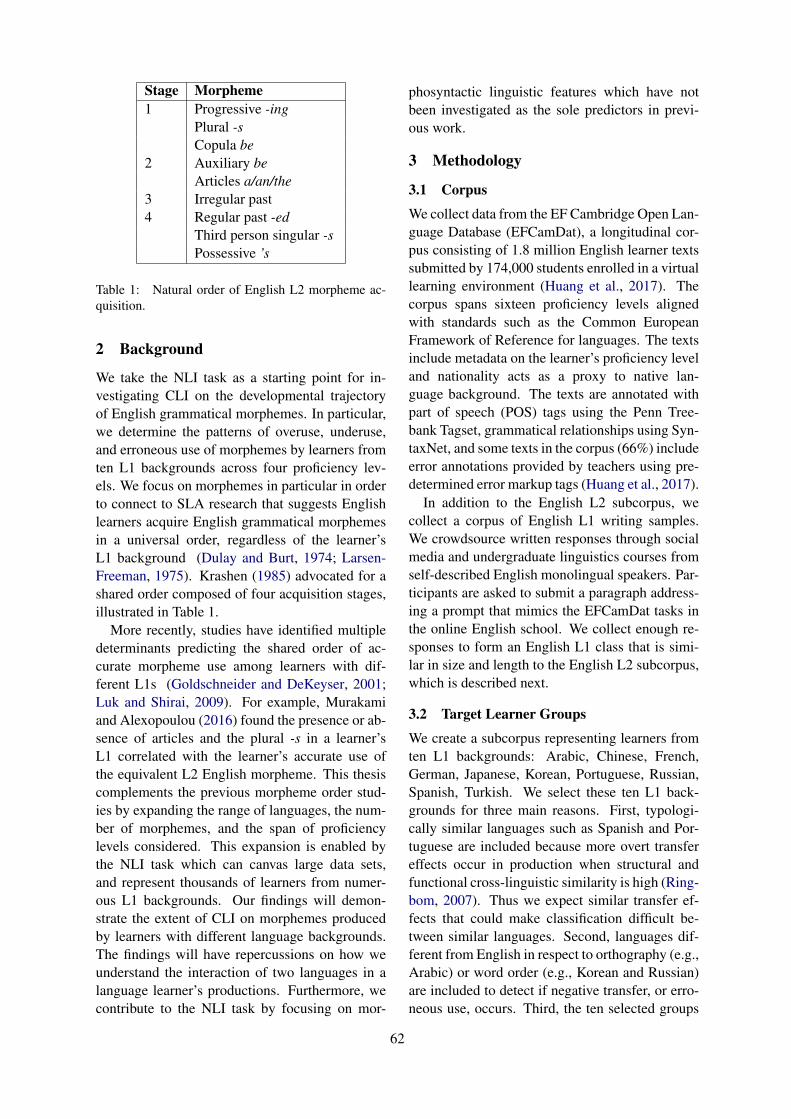
Stage Morpheme1 Progressive -ing

Plural -sCopula be

2 Auxiliary beArticles a/an/the

3 Irregular past4 Regular past -ed

Third person singular -sPossessive ’s

Table 1: Natural order of English L2 morpheme ac-quisition.

2 Background

We take the NLI task as a starting point for in-vestigating CLI on the developmental trajectoryof English grammatical morphemes. In particular,we determine the patterns of overuse, underuse,and erroneous use of morphemes by learners fromten L1 backgrounds across four proficiency lev-els. We focus on morphemes in particular in orderto connect to SLA research that suggests Englishlearners acquire English grammatical morphemesin a universal order, regardless of the learner’sL1 background (Dulay and Burt, 1974; Larsen-Freeman, 1975). Krashen (1985) advocated for ashared order composed of four acquisition stages,illustrated in Table 1.

More recently, studies have identified multipledeterminants predicting the shared order of ac-curate morpheme use among learners with dif-ferent L1s (Goldschneider and DeKeyser, 2001;Luk and Shirai, 2009). For example, Murakamiand Alexopoulou (2016) found the presence or ab-sence of articles and the plural -s in a learner’sL1 correlated with the learner’s accurate use ofthe equivalent L2 English morpheme. This thesiscomplements the previous morpheme order stud-ies by expanding the range of languages, the num-ber of morphemes, and the span of proficiencylevels considered. This expansion is enabled bythe NLI task which can canvas large data sets,and represent thousands of learners from numer-ous L1 backgrounds. Our findings will demon-strate the extent of CLI on morphemes producedby learners with different language backgrounds.The findings will have repercussions on how weunderstand the interaction of two languages in alanguage learner’s productions. Furthermore, wecontribute to the NLI task by focusing on mor-

phosyntactic linguistic features which have notbeen investigated as the sole predictors in previ-ous work.

3 Methodology

3.1 Corpus

We collect data from the EF Cambridge Open Lan-guage Database (EFCamDat), a longitudinal cor-pus consisting of 1.8 million English learner textssubmitted by 174,000 students enrolled in a virtuallearning environment (Huang et al., 2017). Thecorpus spans sixteen proficiency levels alignedwith standards such as the Common EuropeanFramework of Reference for languages. The textsinclude metadata on the learner’s proficiency leveland nationality acts as a proxy to native lan-guage background. The texts are annotated withpart of speech (POS) tags using the Penn Tree-bank Tagset, grammatical relationships using Syn-taxNet, and some texts in the corpus (66%) includeerror annotations provided by teachers using pre-determined error markup tags (Huang et al., 2017).

In addition to the English L2 subcorpus, wecollect a corpus of English L1 writing samples.We crowdsource written responses through socialmedia and undergraduate linguistics courses fromself-described English monolingual speakers. Par-ticipants are asked to submit a paragraph address-ing a prompt that mimics the EFCamDat tasks inthe online English school. We collect enough re-sponses to form an English L1 class that is simi-lar in size and length to the English L2 subcorpus,which is described next.

3.2 Target Learner Groups

We create a subcorpus representing learners fromten L1 backgrounds: Arabic, Chinese, French,German, Japanese, Korean, Portuguese, Russian,Spanish, Turkish. We select these ten L1 back-grounds for three main reasons. First, typologi-cally similar languages such as Spanish and Por-tuguese are included because more overt transfereffects occur in production when structural andfunctional cross-linguistic similarity is high (Ring-bom, 2007). Thus we expect similar transfer ef-fects that could make classification difficult be-tween similar languages. Second, languages dif-ferent from English in respect to orthography (e.g.,Arabic) or word order (e.g., Korean and Russian)are included to detect if negative transfer, or erro-neous use, occurs. Third, the ten selected groups

62

are represented in the TOEFL11 corpus which willbe used for a cross-corpus evaluation.

The individual learner texts from each languagebackground will be grouped by proficiency level.Since not all learners progress through all six-teen instructional units and some proficiency lev-els are overrepresented, the proficiency levels willbe merged into four groups covering Levels 1-3, 4-7, 8-11, 12-16. Previous research shows clusteringthese proficiency levels has been useful for identi-fying the native language of learners (Jiang et al.,2014). We ensure text size is homogeneous bymerging texts into 1,000 word tokens and compil-ing texts into equally-sized sets for each languagebackground at each proficiency level. The texts re-tain information on individual identification num-bers and writing topics.

3.3 Target Morphemes and Feature Set

The target morphemes include nine morphemesthat frequently appear in the morpheme order stud-ies: articles a/an/the, auxiliary be, copula be, plu-ral -s, possessive ’s, progressive -ing, irregularpast, regular past tense -ed, and third person singu-lar -s. We include short plural -s (e.g., boot/boots)and long plural -es (e.g., hoof/hooves) and ex-clude irregular plurals (e.g., foot/feet). The cop-ula and auxiliary will include the first, second,and third person present and progressive forms,respectively. We make a distinction between thedefinite (the) and indefinite (a/an) articles becauseprevious research suggests learners acquire defi-nite and indefinite articles at different rates de-pending on their L1 background (Crosthwaite,2016; Dıez-Bedmar and Papp, 2008). The irreg-ular and regular past tense forms will be limitedto lexical verbs (e.g., went, walked) and will ex-clude modals (e.g., would) and passive voice (e.g.,stolen). The third person singular form -s will in-clude the allomorphs -s and -es (e.g., she waits andwatches). The possessive ’s will include forms at-tached to a noun phrase (e.g., cat’s tail or cats’tails).

We use features that capture morphemes andmorphosyntactic relationships. The feature setincludes function words, lexical n-grams, POSn-grams, dependency features, and error correc-tions. Function words include topic-independentgrammatical lexical items, and will capture def-inite/indefinite articles and auxiliary verbs. Weuse lexical words to capture regular and irregular

past tense verbs. To avoid some topic bias, weremove proper nouns from the texts. We use POS1-3grams and dependency features to capture mor-phosyntactic relationships such as possession, pro-gressive -ing, plural -s, and third person singular-s. Error corrections provided by the EFCamDatmetadata capture morpheme errors such as articlemisuse and incorrect plurals. We evaluate the pre-dictive power of the features through a step-wiseprocedure.

4 Native Language Identification Task

We use a Support Vector Machine (SVM) clas-sifier to evaluate the data, and obtain the follow-ing metrics: precision, recall, accuracy, and theF-measure. We use a one-vs-all approach, andevaluate each feature type using 10-fold cross-validation. The linear SVM classifier is selectedgiven its sustained success in NLI work, as seen inthe recent 2017 NLI shared task (Malmasi et al.,2017).

To evaluate feature information as it relates tomorpheme acquisition, we compare the overuse,underuse, and erroneous use of the linguistic fea-tures within the ten L1 groups and native Englishgroup. Following a methodology proposed by(Malmasi and Dras, 2014), we use SVM weightsto identify the most predictive features that areunique to each L1 class. We compare if the samebest-performing features appear for each profi-ciency band. If the features are different in eachproficiency band, then we suspect these may beproficiency related effects and we follow with posthoc analysis.

Post hoc analysis is conducted to compare themorphemes appearing more or less regularly givena specific L1 background, and across proficiencylevels. This method allows us to piece togethera diachronic view of morpheme use. We deter-mine if the linguistic features show evidence oflanguage transfer based on statistical evidence ofbetween-group differences and within-group sim-ilarities. We expect to see differential use of mor-phemes between L1 groups that may or may nothave equivalent morphemes between the L1 andL2. For example, Russian L1 learners may un-deruse English articles because they are absent inthe L1. On the other hand, Spanish L1 learnersmay overuse articles because Spanish articles fol-low a different semantic scheme, thus English ar-ticles may be oversupplied to inappropriate con-

63

texts.We also determine how well the classifier per-

forms with native English data to each L1 foreach proficiency level. We expect the classifierwill show more confusion for typologically simi-lar languages to English, especially at higher profi-ciency levels where written productions may con-tain fewer L1 idiosyncrasies.

5 Cross-Corpus Evaluation

In this section, we address the following ques-tions: (1) How well do the most discriminatorylinguistic features used in the EFCamDat corpusperform on an independent corpus? (2) Whichfeatures are corpus-specific? (3) Which featuresbest predict the L1 class when trained on the EF-CamDat and tested on an independent corpus, andvice versa. The classifier trained on the EFCam-Dat subcorpus will be used in a cross-corpus eval-uation to increase the reliability of the linguisticpredictors as evidence for language transfer.

We train on the EFCamDat subcorpus and teston an independent corpus, the TOEFL11, and viceversa. The TOEFL11 corpus consists of 12,100English essays written during high-stakes collegeentrance exams from learners across eleven L1backgrounds (Arabic, Chinese, French, German,Hindi, Italian, Japanese, Korean, Spanish, Telugu,and Turkish) and distributed across eight promptsand three essay score levels (low/medium/high).The TOEFL11 corpus was designed with a nativelanguage identification task in mind and used inthe first NLI shared task (Blanchard et al., 2013).

We match a subset of the learner groups fromthe TOEFL11 data with classes in the EFCam-Dat, use comparable text lengths for each lan-guage background, and match the proficiency lev-els between the two corpora. Success is mea-sured by NLI accuracy that is higher than a chancebaseline when the SVM is trained with the EF-CamDat and tested on the TOEFL11, and viceversa. Most importantly, the corpus comparisondetermines which specific features serve as thestrongest determiners of L1 background acrossproficiency levels, despite genre differences be-tween the two corpora.

A cross-corpus methodology has the advantageof providing robust results that bolster the argu-ment for CLI in the course of L2 morpheme de-velopment. The features that successfully distin-guish between L1 groups will be analyzed to in-

form SLA research as to how certain morphemesmay be more susceptible to language transferthan others, and how different L1 groups mayfollow unique trajectories of morpheme acquisi-tion. Previous research has found some corpus-independent L1 transfer features that generalizeacross the different task requirements representedin the EFCamDat and TOEFL11 corpora (Mal-masi and Dras, 2015). However, it is unknown ifthis generalizability will hold between proficiencybands. Thus, we test the classifier on different pro-ficiency levels across EFCamDat and TOEFL11 todetermine the features that are corpus-independentacross proficiency levels. These findings will thenbe connected to formulating hypotheses on lan-guage transfer during the developmental trajectoryof morpheme acquisition.

6 Human Cross-Validation

In this section, we address the following ques-tions: (1) How does the performance of the clas-sifier compare to humans performing the sametask? (2) What linguistic predictors do humans usein classifying texts? To address these questions,we recruit native and non-native English speakerswith a background in language instruction and/orself-reported linguistic training to perform a sim-plified online NLI task. We follow a similar pro-cedure from Malmasi et al. (2015). The ratersdeal with five L1 classes representing the most dis-parate L1s from the EfCamDat subcorpus in orderto facilitate classification. We split the texts intoequal distributions of low and high proficiency es-says for each L1 group. Raters perform the NLItask on roughly 50 essays and indicate the lin-guistic features that led to their decision and theirconfidence in that decision. We determine accu-racy scores for the L1 groups across proficiencylevels, and if the raters use morphemes and mor-phosyntactic relationships as indicators of the L1.The results of the study will indicate the qualita-tive and quantitative differences in detecting cross-linguistic influence based on human evaluationsversus computational measures.

7 Conclusion

This thesis expands on NLI methodology andconnects computational linguistics with SLA re-search. In terms of methodology, we investigateNLI using only grammatical morphemes, whichhave not been singled out in previous NLI re-

64

search. English is considered a morphologicallyweak language with comparatively few require-ments for agreement and declensions. Achiev-ing an accuracy score higher than chance indi-cates that morphemes, however ubiquitous in writ-ing, can reveal a significant distribution that cor-rectly identifies a writer’s L1 background. Thethesis may provide motivation to perform NLI onmorphologically rich languages such as Slavic orBantu, to identify if a classifier can use a wider setof morphemes as the sole feature. Furthermore,we expand the methodology to cross-corpus eval-uations on four proficiency levels. This line of re-search shows how robust a model may be for lowerto higher proficiency English learners.

In terms of combining computational linguisticswith SLA, we use the NLI task as a tool for uncov-ering cross-linguistic influence that may otherwisego unseen by a human researcher. We test if thatis indeed the case in the human cross-validationstudy. The NLI task increases the number and typeof comparisons we can make between languages,which can lead to new insights in the underuse,overuse, and erroneous use of morphemes. We de-termine how learner groups develop the capacityto use morphemes through development. The au-tomatic detection of transfer is especially valuablefor higher proficiency learners, where transfer isharder to discern because the effects may not beobviously visible as errors (Ringbom, 2007). Theability to detect subtle CLI effects holds the poten-tial to generate new hypotheses about where andwhy language transfer occurs, so that understand-ing can be transferred to L2 education. This the-sis accounts for these transfer effects and providestestable hypotheses.

Acknowledgements

I am grateful to Dr. Stefanie Wulff for constantsupport and helpful discussions, and thank theanonymous reviewers for comments and sugges-tions on improving the thesis proposal.

ReferencesYevgeni Berzak, Chie Nakamura, Suzanne Flynn, and

Boris Katz. 2017. Predicting native language fromgaze. arXiv preprint arXiv:1704.07398.

Daniel Blanchard, Joel Tetreault, Derrick Higgins,Aoife Cahill, and Martin Chodorow. 2013. Toefl11:A corpus of non-native english. ETS Research Re-port Series, 2013(2).

Julian Brooke and Graeme Hirst. 2012. Robust, lexi-calized native language identification. Proceedingsof COLING 2012, pages 391–408.

Scott Crossley and Danielle McNamara. 2012. Detect-ing the first language of second language writers us-ing automated indices of cohesion, lexical sophisti-cation, syntactic complexity and conceptual knowl-edge. Approaching language transfer through textclassification: Explorations in the detection-basedapproach, pages 106–126.

Peter Crosthwaite. 2016. L2 english article use byl1 speakers of article-less languages. InternationalJournal of Learner Corpus Research, 2(1):68–100.

Marıa Belen Dıez-Bedmar and Szilvia Papp. 2008. Theuse of the english article system by chinese andspanish learners. Language and Computers Studiesin Practical Linguistics, 66:147.

Heidi Dulay and Marina Burt. 1974. Natural sequencesin child second language acquisition. LanguageLearning, 24(1):37–53.

Jennifer M Goldschneider and Robert M DeKeyser.2001. Explaining the natural order of l2 morphemeacquisition in english: A meta-analysis of multipledeterminants. Language Learning, 51(1):1–50.

Yan Huang, Akira Murakami, Theodora Alexopoulou,and Anna Korhonen. 2017. Dependency parsing oflearner english.

Xiao Jiang, Yufan Guo, Jeroen Geertzen, Dora Alex-opoulou, Lin Sun, and Anna Korhonen. 2014. Na-tive language identification using large, longitudi-nal data. In Proceedings of the 9th InternationalConference on Language Resources and Evaluation,pages 3309–3312.

Stephen Krashen. 1985. The input hypothesis: Issuesand implications. Addison-Wesley Longman Ltd.

Diane Larsen-Freeman. 1975. The acquisition ofgrammatical morphemes by adult esl students.TESOL Quarterly, pages 409–419.

Zoe Pei-sui Luk and Yasuhiro Shirai. 2009. Is the ac-quisition order of grammatical morphemes impervi-ous to l1 knowledge? evidence from the acquisitionof plural -s, articles, and possessive ’s. LanguageLearning, 59(4):721–754.

Shervin Malmasi. 2016. Native language identifica-tion: explorations and applications. Ph.D. thesis,Macquarie University.

Shervin Malmasi and Mark Dras. 2014. Languagetransfer hypotheses with linear svm weights. In Pro-ceedings of the 2014 Conference on Empirical Meth-ods in Natural Language Processing, pages 1385–1390.

65

Shervin Malmasi and Mark Dras. 2015. Large-scalenative language identification with cross-corpusevaluation. In Proceedings of the 2015 Conferenceof the North American Chapter of the Associationfor Computational Linguistics: Human LanguageTechnologies, pages 1403–1409.

Shervin Malmasi, Keelan Evanini, Aoife Cahill, JoelTetreault, Robert Pugh, Christopher Hamill, DianeNapolitano, and Yao Qian. 2017. A Report on the2017 Native Language Identification Shared Task.In Proceedings of the 12th Workshop on BuildingEducational Applications Using NLP, Copenhagen,Denmark. Association for Computational Linguis-tics.

Shervin Malmasi, Joel Tetreault, and Mark Dras. 2015.Oracle and human baselines for native languageidentification. In Proceedings of the 10th Workshopon Innovative Use of NLP for Building EducationalApplications, pages 172–178.

Akira Murakami and Theodora Alexopoulou. 2016. L1influence on the acquisition order of english gram-matical morphemes: A learner corpus study. Studiesin Second Language Acquisition, 38(3):365–401.

Hakan Ringbom. 2007. Cross-linguistic similarity inforeign language learning. Multilingual Matters.

Sabrina Stehwien and Sebastian Pado. 2015. Nativelanguage identification across text types: how spe-cial are scientists? Italian Journal of ComputationalLinguistics, 1(1).

Marcos Zampieri, Alina Maria Ciobanu, and Liviu PDinu. 2017. Native language identification on textand speech. arXiv preprint arXiv:1707.07182.

66

Proceedings of NAACL-HLT 2018: Student Research Workshop, pages 67–73New Orleans, Louisiana, June 2 - 4, 2018. c©2017 Association for Computational Linguistics

End-to-End Learning of Task-Oriented Dialogs

Bing Liu, Ian LaneCarnegie Mellon University

5000 Forbes Avenue, Pittsburgh, PA 15213, USAliubing@cmu.edu, lane@cmu.edu

Abstract

In this thesis proposal, we address the limita-tions of conventional pipeline design of task-oriented dialog systems and propose end-to-end learning solutions. We design neural net-work based dialog system that is able to ro-bustly track dialog state, interface with knowl-edge bases, and incorporate structured queryresults into system responses to successfullycomplete task-oriented dialog. In learningsuch neural network based dialog systems, wepropose hybrid offline training and online in-teractive learning methods. We introduce amulti-task learning method in pre-training thedialog agent in a supervised manner usingtask-oriented dialog corpora. The supervisedtraining agent can further be improved via in-teracting with users and learning online fromuser demonstration and feedback with imita-tion and reinforcement learning. In addressingthe sample efficiency issue with online policylearning, we further propose a method by com-bining the learning-from-user and learning-from-simulation approaches to improve theonline interactive learning efficiency.

1 Introduction

Dialog systems, also known as conversationalagents or chatbots, are playing an increasingly im-portant role in today’s business and social life.People communicate with a dialog system in nat-ural language form, via either textual or audi-tory input, for entertainment and for completingdaily tasks. Dialog systems can be generally di-vided into chit-chat systems and task-oriented di-alog systems based on the nature of conversation.Comparing to chit-chat systems that are designedto engage users and provide mental support, task-oriented dialog systems are designed to assist userto complete a particular task by understanding re-quests from users and providing relevant informa-tion. Such systems usually involve retrieving in-

formation from external resources and reasoningover multiple dialog turns. This thesis work fo-cuses on task-oriented dialog systems.

Conventional task-oriented dialog systems havea complex pipeline (Raux et al., 2005; Younget al., 2013) consisting of independently devel-oped and modularly connected components forspoken language understanding (SLU) (Sarikayaet al., 2014; Mesnil et al., 2015; Chen et al., 2016),dialog state tracking (DST) (Henderson et al.,2014; Mrksic et al., 2016; Lee and Stent, 2016),and dialog policy learning (Gasic and Young,2014; Su et al., 2016). Such pipeline system de-sign has a number of limitations. Firstly, creditassignment in such pipeline systems can be chal-lenging, as errors made in upper stream modulesmay propagate and be amplified in downstreamcomponents. Moreover, each component in thepipeline is ideally re-trained as preceding compo-nents are updated, so that we have inputs similarto the training examples at run-time. This dominoeffect causes several issues in practice.

We address the limitations of pipeline dialogsystems and propose end-to-end learning solu-tions. The proposed model is capable of robustlytracking dialog state, interfacing with knowledgebases, and incorporating structured query resultsinto system responses to successfully completetask-oriented dialog. With each functioning unitbeing modeled by a neural network and connectedvia differentiable operations, the entire system canbe optimized end-to-end.

In learning such neural network based dialogmodel, we propose hybrid offline training and on-line interactive learning methods. We first let theagent to learn from human-human conversationswith offline supervised training. We then improvethe agent further by letting it to interact with usersand learn from user demonstrations and feedbackwith imitation and reinforcement learning. In ad-

67

dressing the sample efficiency issue with onlinepolicy learning via interacting with real users, wefurther propose a learning method by combininglearning-from-user and learning-from-simulationapproaches. We conduct empirical study with bothautomatic system evaluation and human user eval-uation. Experimental results show that our pro-posed model can robustly track dialog state andproduce reasonable system responses. Our pro-posed learning methods also lead to promising im-provement on dialog task success rate and humanuser ratings.

2 Related Work

2.1 Task-Oriented Dialog Systems

User

AutomaticSpeech

Recognition(ASR)

Spoken Language

Understanding(SLU)

DialogState

Tracking(DST)

DialogPolicy

NaturalLanguageGeneration

(NLG)

TextTo

Speech(TTS)

DB/KB

InputSpeech

ASRHypothesis

Domain / Intents /

Slot Values

BeliefState

DialogAct

SystemResponse

VoiceOutput

Figure 1: Pipeline architecture for spoken dialog systems

Figure 1 shows a typical pipeline architectureof task-oriented spoken dialog system. Transcrip-tions of user’s speech are firstly passed to the SLUmodule, where the user’s intention and other keyinformation are extracted. This information is thenformatted as the input to DST, which maintainsthe current state of the dialog. Outputs of DSTare passed to the dialog policy module, which pro-duces a dialog act based on the facts or entities re-trieved from external resources (such as a databaseor a knowledge base). The dialog act emitted bythe dialog policy module serves as the input tothe NLG, through which a natural language for-mat system response is generated. In this thesiswork, we propose end-to-end solutions that focuson three core components of task-oriented dialogsystem: SLU, DST, and dialog policy.

2.2 End-to-End Dialog ModelsConventional task-oriented dialog systems use apipeline design by connecting the above core sys-tem components together. Such pipeline systemdesign makes it hard to track source of errorsand align system optimization targets. To ame-liorate these limitations, researchers have recently

started exploring end-to-end solutions for task-oriented dialogs. Wen et al. (Wen et al., 2017) pro-posed an end-to-end trainable neural dialog modelwith modularly connected system components forSLU, DST, and dialog policy. Although these sys-tem components are end-to-end connected, theyare trained separately. It is not clear whethercommon features and representations for differenttasks can be effectively shared during the dialogmodel training. Moreover, the system is trainedwith supervised learning on fixed dialog corpora,and thus may not generalize well to unseen dialogstates when interacting with users.

Bordes and Weston (Bordes and Weston, 2017)proposed a task-oriented dialog model from amachine reading and reasoning approach. Theyused an RNN to encode the dialog state and ap-plied end-to-end memory networks to learn it. Inthe same line of research, people explored us-ing query-regression networks (Seo et al., 2016),gated memory networks (Liu and Perez, 2017),and copy-augmented networks (Eric and Man-ning, 2017) to learn the dialog state RNN. Similarto (Wen et al., 2017), these systems are trained onfixed sets of simulated and human-machine dialogcorpora, and thus are not capable to learn inter-actively from users. The knowledge base infor-mation is pulled offline based on existing dialogcorpus. It is unknown whether the reasoning capa-bility achieved in offline model training can gen-eralize well to online user interactions.

Williams et al. (Williams et al., 2017) proposeda hybrid code network for task-oriented dialog thatcan be trained with supervised and reinforcementlearning (RL). Li et al. (Li et al., 2017) and Dhin-gra et al. (Dhingra et al., 2017) also proposedend-to-end task-oriented dialog models that can betrained with hybrid supervised learning and RL.These systems apply RL directly on supervisedpre-training models, without discussing the poten-tial issue with dialog state distribution mismatchbetween supervised training and interactive learn-ing. Moreover, current end-to-end dialog modelsare mostly trained and evaluated against user sim-ulators. Ideally, RL based dialog learning shouldbe performed with human users by collecting realuser feedback. In interactive learning with humanusers, online learning efficiency becomes a criti-cal factor. This sample efficiency issue with onlinepolicy learning is not addressed in these works.

68

3 End-to-End Dialog Learning

3.1 Proposed Dialog Learning Framework

Task-oriented dialog system assists human user tocomplete tasks by conducting multi-turn conver-sations. From a learning point of view, the dia-log agent learns to act by interacting with usersand trying to maximize long-term success or anexpected reward. Ideally, the dialog agent shouldnot only be able to passively receive signals fromthe environment (i.e. the user) and learn to act onit, but also to be able to understand the dynamicsof the environment and predict the changes of theenvironment state. This is also how we human be-ings learn from the world. We design our dialoglearning system following the same philosophy.

DialogAgent

HumanUser

Observation /User Input

Action /Sys OutputReward/

Feedback

Agent

Modeled User(in agent’s mind)

EvaluatorDialogAgent

ActionProposal

PredictedObservation

Inferred User State

AgentState

PredictedReward

Knowledge Base

Figure 2: Proposed task-oriented dialog learning framework

Figure 2 shows our proposed learning frame-work for task-oriented dialog. The dialog agentinteracts with user in natural language format andimproves itself with the received user feedback.The dialog agent also learns to interface with ex-ternal resources, such as a knowledge base or adatabase, so as to be able to provide responses touser that are based on the facts in the real world.Inside the dialog agent, the agent learns to modelthe user dynamics by predicting their behaviors inconversations. Such modeled user or simulateduser in the agent’s mind can help the agent tosimulate dialogs that mimic the conversations be-tween the agent and a real user. By “imagining”such conversations and learning from it, the agentcan potentially learn more effectively and reducethe number of learning cycles with real users.

3.2 End-to-End System Architecture

Figure 3 shows the architecture of our proposedend-to-end task-oriented dialog system (Liu et al.,2017). We use a hierarchical LSTM to model a di-alog with multiple turns. The lower level LSTM,which we refer to as the utterance-level LSTM,

is used to encode the user utterance. The higher-level LSTM, which we refer to as the dialog-levelLSTM, is used to model a dialog over a sequenceof turns. User input to the system in natural lan-guage format is encoded in a continuous vectorform via the utterance-level LSTM. The LSTMoutputs can be fed to SLU decoders such as an in-tent classifier and a slot filler. We may use suchSLU module outputs as input to the state tracker.Alternatively, we may directly use the continuousrepresentation of user’s utterance without passingit through a semantic decoder. The encoded userutterance, together with the encoding of the pre-vious system turn, is connected to the dialog-levelLSTM. State of this dialog-level LSTM maintainsa continuous representation of the dialog state.Based on this state, the belief tracker generates aprobability distribution over candidate values foreach of the tracked goal slots. A query commandcan then be formulated with the belief trackingoutputs and sent to a database to retrieve requestedinformation. Finally, the system produces an ac-tion by combining information from the dialogstate, the belief tracking outputs, and the encod-ing of the query results. This system dialog ac-tion, together with the belief tracking output andthe query results, is used to generate the final nat-ural language system response via a natural lan-guage generator. All system components are con-nected via differentiable operations, and the entiresystem (SLU, DST, and policy) can thus be opti-mized end-to-end.

4 Learning from Dialog Corpora

In this section, we describe our proposed corpus-based supervised training methods for task-oriented dialog. We first explain our supervisedlearning models for SLU, and then explain howthese models are extended for dialog modeling.

4.1 SLU and Utterance Modeling

We first describe our proposed utterance represen-tation learning method by jointly optimizing thetwo core SLU tasks, intent detection and slot fill-ing. Intent detection and slot filling are usuallyhandled separately by different models, withouteffectively utilizing features and representationsthat can be shared between the two tasks. We pro-pose to jointly optimize the two SLU tasks withrecurrent neural networks. A bidirectional LSTMreader is used to encode the user utterance. LSTM

69

Agent

Modeled User(in agent’s mind)

EvaluatorDialogAgent

ActionProposal

PredictedObservation

Inferred User State

AgentState

PredictedReward

Figure 3: End-to-end task-oriented dialog system architecture

state output at each time step is used for slot la-bel prediction for each word in the utterance. Aweighted average of these LSTM state outputsis further used as the representation of the utter-ance for user intent prediction. The model objec-tive function is a linear interpolation of the cross-entropy losses for intent and slot label predictions.Experiment results (Liu and Lane, 2016a,b) onATIS SLU corpus show that the proposed jointtraining model achieves state-of-the-art intent de-tection accuracy and slot filling F1 scores. Thejoint training model also outperforms the indepen-dent training models on both tasks.

4.2 Dialog Modeling with HierarchicalLSTM

The above described SLU models operate on ut-terance or turn level. In dialog learning, we expectthe system to be able to reason over the dialog con-text, which covers information over a sequence ofpast dialog turns. We extend the LSTM based SLUmodels by adding a higher level LSTM on top tomodel dialog context over multiple turns (Liu andLane, 2017a). The lower level LSTM uses thesame bidirectional LSTM design as in section 4.1to encode natural language utterance. These en-coded utterance representation at each turn serveas the input to the upper level LSTM that mod-els dialog context. Based on the dialog state en-coded in the dialog-level LSTM, the model pro-duces a probability distribution over candidate val-ues for each of the tracked goal slots. This servesthe functionality of a dialog state tracker. Further-more, the model predicts the system dialog act or

a delexicalised system response based on the cur-rent dialog state. This can be seen as learning asupervised dialog policy by following the expertactions via behavior cloning.

In supervised model training, we optimize theparameter set θ to minimize the cross-entropylosses for dialog state tracking and system actionprediction:

minθ

K∑

k=1

−[ M∑

m=1

λlm logP (lmk∗|U≤k,A<k,E<k; θ)

+λa logP (a∗k|U≤k,A<k,E≤k; θ)

]

(1)

where λs are the linear interpolation weights forthe cost of each system output. lmk

∗ and a∗k are theground truth labels for goal slots and system actionat the kth turn. In the evaluation (Liu and Lane,2017b) on DSTC2 dialog datset, the proposedmodel achieves near state-of-the-art performancein dialog goal tracking accuracy. Moreover, theproposed model demonstrates promising results inproducing appropriate system responses, outper-forming prior end-to-end neural network modelsusing per-response accuracy evaluation metric.

5 Learning from Human Demonstration

The supervised training dialog model described insection 4 performs well in offline evaluation set-ting on fixed dialog corpora. The same model per-formance may not generalize well to unseen dialogstates when the system interacts with users. Wepropose interactive dialog learning methods withimitation learning to address this issue.

70

5.1 Imitation Learning with HumanTeaching

Supervised learning succeeds when training andtest data distributions match. During dialog inter-action with users, any mistake made by the systemor any deviation in the user’s behavior may lead itto a different state distribution that the supervisedtraining agent has seen in the training corpus. Thesupervised training agent thus may fail due to thecompounding errors and dialog state distributionmismatch between offline training and user inter-action. To address this issue, we propose a dialogimitation learning method and let the dialog agentto learn interactively from user teaching. After ob-taining a supervised training model, we deploy theagent to let it interact with users using its learneddialog policy. The agent may make errors duringuser interactions. We then ask expert users to cor-rect the agent’s mistakes and demonstrate the rightactions for the agent to take (Ross et al., 2011). Inthis manner, we collect additional dialog samplesthat are guided by the agent’s own policy. Learn-ing on these samples directly addresses the limita-tion of the currently learned model. With exper-iments (Liu et al., 2018) in a movie booking do-main, we show that the agent can efficiently learnfrom the expert demonstrations and improve dia-log task success rate with the proposed imitationdialog learning method.

5.2 Dialog Reward Learning withAdversarial Training

Supervised learning models that imitate expert be-havior in conducting task-oriented dialogs usuallyrequire a large amount of training samples to suc-ceed due to the compounding errors from covari-ate shift as discussed in 5.1. A potential resolutionto this problem is to infer a dialog reward functionfrom expert demonstrations and use it to guide di-alog policy learning. Task-oriented dialog systemsare mainly designed to maximize overall user sat-isfaction, which can be seen as a reward, in assist-ing users with tasks. As claimed by Ng et al. (Nget al., 2000), reward function as opposed to policycan usually provide the most succinct and robustdefinition of a task.

We propose a generative adversarial trainingmethod in recovering the dialog reward functionin the expert’s mind. The generator is the learneddialog agent, who interacts with users to gener-ate dialog samples. The discriminator is a neu-

ral network model whose job is to distinguish be-tween the agent’s behavior and an expert’s behav-ior. Specifically, we present two dialog samples,one from the human agent and one from the ma-chine agent, to the discriminator. We let the dis-criminator to maximize the likelihood of the sam-ple from the human agent and minimize that fromthe machine agent. The likelihood of the samplegenerated by the machine agent can be used as thereward to the agent. Gradient of the discriminatorin optimization can be written as:

∇θD[Ed∼θdemo

[log(D(d))]+Ed∼θG [log(1−D(d))]]

(2)where θG is the learned policy of the machineagent and θdemo is the human agent policy. θDis the parameters of the discriminator model.

6 Learning from Human Feedback

In this section, we describe our proposed meth-ods in learning task-oriented dialog model inter-actively from human feedback with reinforcementlearning (RL).

6.1 End-to-End Dialog Learning with RLAfter the supervised and imitation training stage,we propose to further optimize the dialog modelwith RL by letting the agent to interact with usersand collecting simple form of user feedback. Thefeedback is only collected at the end of a dialog. Apositive reward is assigned for success tasks, anda zero reward is assigned for failure tasks. A smallstep penalty is applied to each dialog turn to en-courage the agent to complete the task in fewersteps. We propose to use policy gradient basedmethods for dialog policy learning. With likeli-hood ratio gradient estimator, the gradient of theobjective function can be derived as:

∇θJk(θ) = ∇θEθ [Rk]= Eθa [∇θ log πθ(ak|sk)Rk]

(3)

This last expression above gives us an unbiasedgradient estimator. We sample the agent actionbased on the currently learned policy at each di-alog turn and compute the gradient. In the ex-periments (Liu et al., 2017) on a movie bookingtask domain, we show that the proposed RL basedoptimization leads to significant improvement ontask success rate and reduction of dialog turn sizecomparing to supervised training model. RL afterimitation learning with human teaching not only

71

improves dialog policy, but also improves the un-derlying system components (e.g. state tracking)in the end-to-end training framework.

6.2 Co-Training of Dialog Agent andSimulated User

We aim to design a dialog agent that can not onlylearn from user feedback, but also to understandthe user dynamics and predict the change of userstates. Thus, we need to build a user model, whichcan be used to simulate conversation between anagent and a user to help the agent to learn betterpolicies. Similar to how a dialog agent acts intask-oriented dialogs, a simulated user picks ac-tions based on the dialog state. In addition, theuser policy also depends on the user’s goal. Inmodeling the user (Liu and Lane, 2017c), we de-sign a hierarchical LSTM model, similar to thedesign of dialog agent described in section 3.2,with additional user goal encoding as the modelinput. The simulated user is firstly trained in asupervised manner using task-oriented dialog cor-pora, similar to how we train the dialog agent asdescribed in section 4.2. After bootstrapping a di-alog agent and a simulated user with supervisedtraining, we improve them further by simulatingtask-oriented dialogs between the two agents anditeratively optimizing their policies with deep RL.The reward for RL can either be obtained from thelearned reward function described in section 5.2or given by the human users. The intuition be-hind the co-training framework is that we modeltask-oriented dialog as a goal fulfilling process, inwhich we let the dialog agent and the modeled userto positively collaborate to achieve the goal. Themodeled user is given a goal to complete, and it isexpected to demonstrate coherent but diverse userbehavior. The agent, on the other hand, attemptsto estimate the user’s goal and fulfill his request.

6.3 Learning from Simulation andInteraction with RL

Learning dialog model from user interaction bycollecting user feedback (as in section 6.1) is ef-fective but can be very sample inefficient. Onemight have to employ a large number of usersto interact with the agent before the system canreach a satisfactory performance level. On theother hand, learning from dialog simulation in-ternally to the dialog agent (as in section 6.2) isrelatively cheap to conduct, but the performanceis limited to the modeling capacity learned from

the limited labeled dialog samples. In this sec-tion, we describe our proposed method in combin-ing the learning-from-user approach and learning-from-simulation approach, with expectation to im-prove the online interactive dialog learning effi-ciency with real users.

We let the dialog agent to conduct dialog withreal users using its learned policy and collect feed-back (reward) from the user. The newly collecteddialog sample and reward are then used to updatethe dialog agent with the RL algorithm describedin section 6.1. Before letting the agent to starta new session of interactive learning with users,we perform a number of learning-from-simulationtraining cycles. We let the updated dialog agent to“imagine” its conversation with the modeled user,and fine-tune both of them with RL using the re-ward obtained from the learned reward function(section 5.2). The intuition behind this proposedintegrated learning method is that we want to en-force the dialog agent to fully digest the knowl-edge learned from the interaction with real userby simulating similar dialogs internally. Such in-tegrated learning method may effectively improvedialog learning efficiency and reduce the numberof interactive learning attempts with real users.

7 Conclusions

In this thesis proposal, we design an end-to-endlearning framework for task-oriented dialog sys-tem. We present our proposed neural networkbased end-to-end dialog model architecture anddiscuss the proposed learning methods using of-fline training with dialog corpora and interactivelearning with users. The proposed end-to-end di-alog learning framework addresses the limitationsof the popular pipeline design of task-oriented di-alog systems. We show that the proposed modelis able to robustly track dialog state, retrieve in-formation from external resources, and produceappropriate system responses to complete task-oriented dialogs. The proposed learning meth-ods achieve promising dialog task success rate anduser satisfaction scores. We will further studythe effectiveness of the proposed hybrid learningmethod in improving sample efficiency in onlineRL policy learning. We believe the work proposedin this thesis will pioneer a new class of end-to-end learning systems for task-oriented dialog andmake a significant step towards intelligent conver-sational human-computer interactions.

72

ReferencesAntoine Bordes and Jason Weston. 2017. Learning

end-to-end goal-oriented dialog. In ICLR.

Yun-Nung Chen, Dilek Hakkani-Tur, Gokhan Tur,Jianfeng Gao, and Li Deng. 2016. End-to-end mem-ory networks with knowledge carryover for multi-turn spoken language understanding. In INTER-SPEECH, pages 3245–3249.

Bhuwan Dhingra, Lihong Li, Xiujun Li, Jianfeng Gao,Yun-Nung Chen, Faisal Ahmed, and Li Deng. 2017.Towards end-to-end reinforcement learning of dia-logue agents for information access. In ACL.

Mihail Eric and Christopher D Manning. 2017. Acopy-augmented sequence-to-sequence architecturegives good performance on task-oriented dialogue.In EACL.

Milica Gasic and Steve Young. 2014. Gaussian pro-cesses for pomdp-based dialogue manager optimiza-tion. IEEE/ACM Transactions on Audio, Speech,and Language Processing.

Matthew Henderson, Blaise Thomson, and SteveYoung. 2014. Word-based dialog state tracking withrecurrent neural networks. In SIGDIAL.

Sungjin Lee and Amanda Stent. 2016. Task lineages:Dialog state tracking for flexible interaction. In SIG-DIAL.

Xuijun Li, Yun-Nung Chen, Lihong Li, and JianfengGao. 2017. End-to-end task-completion neural dia-logue systems. In IJCNLP.

Bing Liu and Ian Lane. 2016a. Attention-based recur-rent neural network models for joint intent detectionand slot filling. In Interspeech.

Bing Liu and Ian Lane. 2016b. Joint online spoken lan-guage understanding and language modeling withrecurrent neural networks. In SIGDIAL.

Bing Liu and Ian Lane. 2017a. Dialog context lan-guage modeling with recurrent neural networks. InAcoustics, Speech and Signal Processing (ICASSP),2017 IEEE International Conference on. IEEE.

Bing Liu and Ian Lane. 2017b. An end-to-end trainableneural network model with belief tracking for task-oriented dialog. In Interspeech.

Bing Liu and Ian Lane. 2017c. Iterative policy learningin end-to-end trainable task-oriented neural dialogmodels. In IEEE ASRU.

Bing Liu, Gokhan Tur, Dilek Hakkani-Tur, PararthShah, and Larry Heck. 2017. End-to-end optimiza-tion of task-oriented dialogue model with deep rein-forcement learning. In NIPS Workshop on Conver-sational AI.

Bing Liu, Gokhan Tur, Dilek Hakkani-Tur, PararthShah, and Larry Heck. 2018. Dialogue learning withhuman teaching and feedback in end-to-end train-able task-oriented dialogue systems. In NAACL.

Fei Liu and Julien Perez. 2017. Gated end-to-endmemory networks. In EACL.

Gregoire Mesnil, Yann Dauphin, Kaisheng Yao,Yoshua Bengio, Li Deng, Dilek Hakkani-Tur, Xi-aodong He, Larry Heck, Gokhan Tur, Dong Yu,et al. 2015. Using recurrent neural networks forslot filling in spoken language understanding. Au-dio, Speech, and Language Processing, IEEE/ACMTransactions on, 23(3):530–539.

Nikola Mrksic, Diarmuid O Seaghdha, Tsung-HsienWen, Blaise Thomson, and Steve Young. 2016.Neural belief tracker: Data-driven dialogue statetracking. arXiv preprint arXiv:1606.03777.

Andrew Y Ng, Stuart J Russell, et al. 2000. Algorithmsfor inverse reinforcement learning. In ICML.

Antoine Raux, Brian Langner, Dan Bohus, Alan WBlack, and Maxine Eskenazi. 2005. Lets go pub-lic! taking a spoken dialog system to the real world.In in Proc. of Interspeech 2005.

Stephane Ross, Geoffrey J Gordon, and Drew Bagnell.2011. A reduction of imitation learning and struc-tured prediction to no-regret online learning. In In-ternational Conference on Artificial Intelligence andStatistics, pages 627–635.

Ruhi Sarikaya, Geoffrey E Hinton, and Anoop Deoras.2014. Application of deep belief networks for nat-ural language understanding. IEEE/ACM Transac-tions on Audio, Speech, and Language Processing.

Minjoon Seo, Ali Farhadi, and Hannaneh Hajishirzi.2016. Query-regression networks for machine com-prehension. arXiv preprint arXiv:1606.04582.

Pei-Hao Su, Milica Gasic, Nikola Mrksic, Lina Rojas-Barahona, Stefan Ultes, David Vandyke, Tsung-Hsien Wen, and Steve Young. 2016. On-line activereward learning for policy optimisation in spoken di-alogue systems. In ACL.

Tsung-Hsien Wen, David Vandyke, Nikola Mrksic,Milica Gasic, Lina M. Rojas-Barahona, Pei-Hao Su,Stefan Ultes, and Steve Young. 2017. A network-based end-to-end trainable task-oriented dialoguesystem. In EACL.

Jason D Williams, Kavosh Asadi, and Geoffrey Zweig.2017. Hybrid code networks: practical and efficientend-to-end dialog control with supervised and rein-forcement learning. In ACL.

Steve Young, Milica Gasic, Blaise Thomson, and Ja-son D Williams. 2013. Pomdp-based statistical spo-ken dialog systems: A review. Proceedings of theIEEE.

73

Proceedings of NAACL-HLT 2018: Student Research Workshop, pages 74–82New Orleans, Louisiana, June 2 - 4, 2018. c©2017 Association for Computational Linguistics

Towards Generating Personalized Hospitalization Summaries

Sabita Acharya, Barbara Di Eugenio, Andrew Boyd, Richard Cameron, Karen Dunn Lopez,Pamela Martyn-Nemeth, Carolyn Dickens, Amer Ardati

University of Illinois at ChicagoChicago, Illinois

sachar4,bdieugen,boyda,rcameron,kdunnl2,pmartyn,cdickens,aardati@uic.edu

Abstract

Most of the health documents, including pa-tient education materials and discharge notes,are usually flooded with medical jargons andcontain a lot of generic information about thehealth issue. In addition, patients are only pro-vided with the doctor’s perspective of whathappened to them in the hospital while the careprocedure performed by nurses during theirentire hospital stay is nowhere included. Themain focus of this research is to generate per-sonalized hospital-stay summaries for patientsby combining information from physician dis-charge notes and nursing plan of care. It usesa metric to identify medical concepts that areComplex, extracts definitions for the conceptfrom three external knowledge sources, andprovides the simplest definition to the patient.It also takes various features of the patientinto account, like their concerns and strengths,ability to understand basic health information,level of engagement in taking care of theirhealth, and familiarity with the health issueand personalizes the content of the summariesaccordingly. Our evaluation showed that thesummaries contain 80% of the medical con-cepts that are considered as being important byboth doctor and nurses. Three patient advisors(i.e individuals who are trained in understand-ing patient experience extensively) verified theusability of our summaries and mentioned thatthey would like to get such summaries whenthey are discharged from hospital.

1 Introduction

In the current hospital scenario, when a patient isdischarged, s/he is provided with a discharge notealong with the patient education materials, whichcontain more information about the health issue aswell as the measures that need to be taken by thepatient or the care-taker to continue with the muchneeded care. However, with statistics showing that

over a third of US adults have difficulty with com-mon health tasks like adhering to medical instruc-tions (Kutner et al., 2006), not many people willbe able to understand basic health information andservices needed to make appropriate health deci-sions. More often, patients end up discarding thehealth documents that are provided to them, eitherbecause they get overwhelmed with a lot of infor-mation, or because they find it hard to comprehendthe medical jargons that such documents are usu-ally flooded with (Choudhry et al., 2016).

Our solution is to generate concise and compre-hensible summaries of what happened to a patientin the hospital. Since patients with chronic healthconditions such as heart failure (as is our case)need to continue much of the care that is providedby nurses in the hospital even after they are dis-charged, we integrate the information from boththe physician and nursing documents into a sum-mary. We also develop a metric for determiningwhether a medical concept (a single word or muli-word term) is Simple or Complex and provide def-initions for Complex terms. Unlike the “one sizefits all” approach that is used for creating healthdocuments, we generate summaries that are per-sonalized according to the patient’s preferences,interests, motivation level, and ability to compre-hend health information. In this proposal, we willbriefly explain our work on summarizing informa-tion and simplifying medical concepts. We willalso describe our ongoing efforts on personalizingcontent and our plans for future evaluations.

2 Related Work

Most of the existing approaches on using naturallanguage generation (NLG) for multi-documentsummarization work only for homogeneous doc-uments (Yang et al., 2015; Banerjee et al., 2015),unlike our case where the physician and nursing

74

documentation contain different type of content(free text vs concepts). As concerns identifyingterms that are Complex, some applications assumethat all the terms that appear in specific vocabu-laries or corpora are difficult to understand (Onget al., 2007; Kandula et al., 2010). These methodsare unreliable because none of the currently avail-able vocabularies are exhaustive. For providingexplanations to terms that are identified as diffi-cult, Horn et al. (2014) and Biran et al. (2011) usethe replacement that was provided to terms fromWikipedia in the Simple Wikipedia parallel cor-pus. Elhadad (2006) supplements the selected ter-minologies with definitions obtained from Google“define”. In medical domain, some work has beendone in obtaining pairs of medical terms and ex-planations: Elhadad and Sutaria (2007) preparepairs of complex medical terms by using a paral-lel corpus of abstracts of clinical studies and cor-responding news stories; Stilo et al. (2013) mapmedical jargon and everyday language by search-ing for their occurrence in Wikipedia and Googlesnippets. Our simplification metric is similar tothat of (Shardlow, 2013) but we use five times asmany features and a different approach for dis-tinguishing between Simple and Complex terms.We provide definitions to terms similar to Rameshet al. (2013), but we are not restricted to singleword terms only. Unlike Klavans and Muresan(2000), we refer to multiple knowledge sources fordefinitions of medical concepts.

There are several existing systems that producepersonalized content in biomedical domain (Jimi-son et al., 1992; DiMarco et al., 1995) as wellas in non-medical domains (Paris, 1988; Moraeset al., 2014). However, only a few of the existingbiomedical systems generate personalized contentfor the patients (Buchanan et al., 1995; Williamset al., 2007). PERSIVAL system takes in a natu-ral language query and provides customized sum-maries of medical literature for patients or doc-tors (Elhadad et al., 2005). BabyTalk system (Ma-hamood and Reiter, 2011) generates customizeddescriptions of patient status for people occupy-ing different roles in Neonatal Intensive Care Unit.However, this system relies on handcrafted ontolo-gies, which are very time intensive to create. Ourapproach to personalization uses several parame-ters that determine the content to be included inour summary, similarly to the PERSONAGE sys-tem (Mairesse and Walker, 2011), a parameteriz-

Attending: Dr. PHYSICIAN.Admission diagnosis: acute subcortical CVA.Secondary diagnosis: hypertension.Discharge diagnosis: Right sided weakness of unknown eti-ology.Consultations:. Physical Medicine Rehabilitation.Physical Therapy.Occupational Therapy.General Medicine.Nutrition.HPI (per chart):. The patient is a AGE y/o AAF with H/oHTN, DM, CVA in past transferred from MRH for evalua-tion for possible stroke. per patient, she was ne until saturdayat around 700 pm, while attempting to go to bathroom, shefell down as her body below chest suddenly gave away.[...]

Figure 1: Portion of the doctor’s discharge note forPatient 149.

Figure 2: Part of HANDS POC for Patient 149.

able language generator that takes the user’s lin-guistic style into account and generates restaurantrecommendations. To the best of our knowledge,there are no existing systems that generate com-prehensible and personalized hospital-stay sum-maries for patients. Moreover, the combinationof the four different factors (patient health liter-acy, motivation to self-care, strengths and con-cerns, and the patient’s familiarity with the healthissue) that guide our personalization process hasnot been explored before.

3 Dataset

Our dataset consists of the doctor’s discharge noteand shift-by-shift update of the nursing care planfor 60 patients. Discharge note is an unstruc-tured plain text document that usually containsdetails about the patient, along with other infor-mation like the diagnosis, findings, medications,and follow-up information. However, no uniformstructure of discharge note is known to be fol-lowed by all physicians (Doyle, 2011). Figure 1shows around 5% of our discharge note for Pa-tient 149. On the other hand, nurses record thedetails in a standardized electric platform called

75

Figure 3: The inputs, output, and workflow of ourpersonalized summary generation system.

HANDS(Keenan et al., 2002), which uses struc-tured nursing taxonomies: NANDA-I for nursingdiagnosis (Herdman, 2011), NIC for nursing inter-vention (Butcher et al., 2013), and NOC for out-comes (Strandell, 2000). Figure 2 shows 15% of aHANDS plan of care (POC) for Patient 149.

4 Approach

The workflow of our presonalized summary gener-ation system is shown in Figure 3. The Extractionmodule is responsible for extracting concepts fromphysician and nursing documentation and explor-ing relationship between them. The functioning ofthis module is explained in Section 4.1. Simplifi-cation module distinguishes Complex terms fromSimple terms and provides simple explanations toComplex terms. This module is explained in Sec-tion 4.2. Most of the remaining components ofthe workflow play a role in producing personal-ized content and are explained in Section 4.3.

4.1 Exploring relationship between physicianand nursing terms

We use MedLEE (Friedman et al., 2004), a medi-cal information extraction tool for extracting med-ical concepts from the discharge notes and nurs-ing POC. MedLEE maps the concepts to the Uni-fied Medical Language System (UMLS) vocabu-lary (NIH, 2011). UMLS is a resource that in-cludes more than 3 million concepts from over 200health and biomedical vocabularies. The knowl-edge sources provided by UMLS allow us to queryabout different concepts, their Concept UniqueIdentifier (CUI), meaning, definitions, along withthe relationships between concepts. We begin with

Category FeaturesLexical features Number of vowels, consonants, prefixes,

suffixes,letters, syllables per wordCounts of each Number of nouns, verbs, adjectives,POS type prepositions, conjunctions, determiners,

adverbs, numerals (using Stanford parser)Vocabulary based Normalized frequency of the term in

Google n-gram corpus, presence of theterm in Wordnet

UMLS derived Number of semantic types, synonyms,features CUIs that are identified for the term;

if the term is present in CHV; if the entireterm has a CUI; if the semantic type ofthe term is one of the 16 semantic typesfrom (Ramesh et al., 2013)

Table 1: Features that are extracted for modelingcomplexity

the nursing concepts (because they are lesser innumber as compared to physician concepts) andexplore UMLS to identify the physician conceptsthat are either directly related to the nursing con-cept or are related through one intermediate node.We restrict ourself to only one intermediate nodebecause going beyond that will lead to reaching upto around 1 million terms in the UMLS graph (Pa-tel et al., 2007), which is not useful for our study.Hence, as shown in Figure 3, the input to thismodule are all the medical concepts present in thephysician and nursing documentation and the out-put is a list of medical concepts, which comprisesof all the concepts from the nursing POC, conceptsfrom the discharge note that are either directly re-lated to a nursing concept or are related throughan intermediate concept, and the intermediate con-cepts themselves. All the concepts that have beenexplored in this step are candidates for inclusion inour summary. These concepts are then sent to theSimplification module, which is briefly describedin Section 4.2. For more details on the Extractionmodule, please refer to (Di Eugenio et al., 2014).

4.2 Simplification

The Simplification module functions in two steps:1) it determines whether a concept is Simple orComplex, and 2) it provides the simplest availabledefinition to a Complex concept. Since the exist-ing metrics for assessing health literacy (REALM,TOFHLA, NAALS) and reading level (Felsch, FryGraph, SMOG) work only on sentences and noton terms (that might consist of a single word ormultiple words like arrhythmia, heart failure), weset out to develop a new metric for determin-ing term complexity. Our training dataset con-sists of 600 terms; 300 of which were randomly

76

Given: i) term T

ii) linear regression function LR from Section 4.2

1) Assign variable D=0

2) Extract all the features for T

3) Supply feature values to LR to obtain a score Z

4) If Z<0.4, D=0

If Z>0.66, D=1

If Z>=0.4 and Z<=0.66:

If semantic type of T falls in our shortlisted types, D=1

Else D=0

5) If D=1:

i) Obtain definitions for T from UMLS, Wikipedia, Google

ii) Extract the medical terms in each definition

iii) For each term, repeat step 1, 2, and 3 and get a score.

iv) Add scores of the terms in each definition

v) Append the definition with the least score to T

vi) Return T

Else return T with no definition attached

Figure 4: Algorithm for simplifying a term T .

selected from the Dale-Chall list1, while the re-maining 300 terms were randomly chosen fromour database of 3164 terms that were explored inSection 4.1. We labeled all the terms from theDale-Chall list as Simple and the terms from ourdatabase were annotated as Simple or Complexby two non-native English speaking undergradu-ate students who have never had any medical con-ditions (Cohen’s Kappa k=0.786). We assume thatnon-native English speakers without medical con-ditions are less familiar with any kind of medicalterm as compared to native English speakers with-out medical conditions. Disagreements betweenthe annotators were resolved via mutual consulta-tion. The remaining 2564 terms from our databasewere used as the testing data.

We extracted all the features enlisted in Table 1for our terms in training and test dataset. We thenused a two step approach for developing our met-ric. In the first step, we performed linear regres-sion on the training dataset with Complexity as thedependent variable. This helped us to identify thefeatures that do not contribute to the complexity ofa term. It also provided us with a linear regressionfunction (which we will call as LR) that includesonly the important features. In the second step,we performed clustering on the test dataset, using

1This list consists of 3000 terms that are known to beunderstood by 80% of 4th grade students

You were admitted for acute subcorticalcerebrovascular accident. During your hospitaliza-tion, you were monitored for chances of ineffec-tive cerebral tissue perfusion, risk for falls, problemin verbal communication and walking. We treateddifficulty walking related to nervous system disorderwith body mechanics promotion. Mobility as a findinghas improved appreciably. We provided treatmentfor risk for ineffective cerebral tissue perfusion withmedication management and medication administration. Asa result, risk related to cardio-vascular health has reducedslightly. We worked to improve verbal impairment related tocommunication impairment with speech therapy.[...] Withyour nurse and doctors, you learned about disease processand medication.

Follow-up: Can follow-up with General Neurology clinic andMedicine clinic as outpatient if desired.

Figure 5: Part of the summary for Patient 149

the 600 terms from our training dataset as clusterseeds. This process resulted in 3 clusters. Out ofthe 600 cluster seeds, 70% of those in Cluster1 hadSimple label; 58% of those in Cluster2 had Sim-ple label and 42% had Complex label; while 79%of those in Cluster3 had Complex label. This in-dicates the presence of three categories of terms:some that can be identified as Simple (Cluster1),some that are Complex (Cluster3), and the rest forwhich there is no clear distinction between Simpleand Complex (Cluster2). For the terms in each ofthese clusters, we further supplied feature valuesto LR and analyzed the corresponding scores. Wefound that across all clusters, 88% of the terms la-beled as Simple have scores below 0.4 while 96%of the terms whose score was above 0.66 were la-beled Complex. For the terms whose score wasbetween 0.4 and 0.66, no clear majority of Simpleor Complex labeled terms was observed in any ofthe clusters. These observations led to the devel-opment of our metric, whose functioning is sum-marized in Figure 4 and is explained in detail in(Acharya et al., 2016). Hence, the Simplificationmodule takes a medical concept as input and de-termines whether it is Simple or Complex. For theconcepts that are identified as being Complex, thesimplest definition is extracted from the knowl-edge sources and is appended to the concept, whilethe Simple concepts are directly sent to the lan-guage generator.

4.3 Personalized summary generation

4.3.1 Summarizing hospital-stay informationWe summarize the information from the dischargenote and HANDS POC by using a language gen-

77

eration approach. We use a Java based API calledSimpleNLG (Gatt and Reiter, 2009), which usesthe supplied constituents like the subject, verb,object, tense, and produces a grammatically cor-rect sentence. It can also compute inflected formsof the content and can aggregate syntactic con-stituents like phrases and sentences together. Themedical concepts with or without definitions ap-pended to them (i.e the output of the Simplifica-tion module), along with suitable verbs are our in-put to SimpleNLG. The group of NANDA-I, NIC,and NOC terms are explained in exactly the sameorder as they are present in the HANDS note. Foreach group, we begin by explaining the diagno-sis (NANDA-I), followed by the treatment that wasprovided (NIC term), and the outcome of the treat-ment (NOC) i.e how effective the intervention wasin treating the problem. The NANDA-I term isused as the subject of the sentence, followed bythe physician terms that are directly connected toit or the intermediate concepts that were extractedwhile exploring the relationship in Section 4.1.The NIC intervention is supplied as the object forthe diagnosis and a verb ”treat” is used for thispurpose. We use the current and expected ratingvalues that are associated with each NOC conceptand use the percentage improvement to decide onthe adverb for the sentence. Some portion of thesummary generated for Patient 149 is shown inFigure 5. The terms that are underlined in Fig-ure 5 were determined as being Complex by ourmetric and have a definition appended to them.The definitions can be displayed in different forms(like tool-tip text or footnote) depending upon themedium in which the summary will be presented.

We also provide the follow-up information thatwas mentioned by the physician in the dischargenote, if any. Since the patient follow-up informa-tion may appear as a separate section or may bespread across various other sections, we use 67keywords and 15 regular expressions to algorith-mically recognize such information. The last para-graph in Figure 5 shows the follow-up informationthat was obtained for Patient 149.

4.3.2 Personalizing the summarySo far, we have a reasonable summary that con-tains the important content from both the physi-cian and nursing documentations. However, oursummaries still do not include the patient’s per-spective. Studies have shown that patients’ per-spective is essential for patient education (Shapiro,

Dear Patient 149, we are sorry to know that you wereadmitted for acute subcortical cerebrovascular accident.Cerebrovascular accident is a medical condition in whichpoor blood flow to the brain results in cell death. Dealingwith this issue must have been tough for you, we hope youare feeling much better now.

During your hospitalization, we provided treatment fordifficulty walking related to nervous system disorder andrisk for ineffective cerebral tissue perfusion. We worked toimprove verbal impairment and risk for falls.

We can understand that you have to make changes in yourway of living, diet and physical activity as a result of yourhealth condition. You have said that you are concerned aboutyour family and friends. We are very glad to know that youhave sources to support you and it is really good that you areworking on this. Being committed to solving this problem isso important.

Follow-up: Can follow-up with General Neurology clinic andMedicine clinic as outpatient if desired.

Figure 6: Version of a summary for a patient withlow PAM score and low level of health literacy.

1993) and that engaging the patients in their owncare reduces hospitalizations and improves thequality of life (Riegel et al., 2011). Our workon personalizing patient summary is motivated bythese studies. We expect that including patient-specific information such as social-emotional sta-tus, preferences, and needs in a summary will en-courage patients to read and understand its con-tent, and will make them more informed and activein understand and improving their health status.

There are four different factors that guide ourpersonalization process: health literacy, patientengagement level, patient’s familiarity with thehealth issue, and their strength/concerns. We alsointroduce several parameters, whose values de-pend upon the response given by the patient tothese four factors.A) Health literacy: Health literacy is the mea-sure of an individual’s ability to gain access toand use information in ways that promote andmaintain good health (Nutbeam, 1998). We usethe Rapid Estimate of Adult Literacy (REALM)(Davis et al., 1993) test for assessing the healthliteracy of the patients. REALM consists of 66-itemed word recognition and pronunciation test.Depending upon how correctly a participant pro-nounces the words in the list, a score is provided.This score tells us whether the health literacy levelof the patient is of third grade or below, fourthto sixth grade, seventh to eighth grade, or of highschool level.

78

Dear Patient 149, you were admitted for acute subcorticalcerebrovascular accident. Cerebrovascular accident is amedical condition in which poor blood flow to the brainresults in cell death. During your hospitalization, youwere monitored for chances of ineffective cerebral tissueperfusion, risk for falls, problem in verbal communicationand walking.

We treated difficulty walking related to nervous systemdisorder with body mechanics promotion. We providedtreatment for risk for ineffective cerebral tissue perfusionwith medication management and medication administra-tion. We worked to improve verbal impairment related tocommunication impairment with speech therapy. We treatedrisk for falls by managing environment to provide safety.

As a result of these interventions, mobility has improvedappreciably. Risk related to cardiovascular health hasreduced slightly. On the other hand, communication and fallprevention behavior have improved slightly. With your nurseand doctors, you learned about disease process, medicationand fall prevention.

We appreciate your efforts in making changes in your way ofliving, diet and physical activity for maintaining your health.Keep up the good work. We are very glad to know that youhave sources to support you. We hope that you feel better sothat you can spend time with your family and friends andreturn back to your work.

Follow-up: Can follow-up with General Neurology clinicand Medicine clinic as outpatient if desired.

For more information on cerebrovascular ac-cident, please refer to the following website:https://www.healthline.com/health/cerebrovascular-accident

Figure 7: Version of a summary for patient withhigh PAM score and high level of health literacy.

B) Patient engagement level: In order to deter-mine how motivated a patient is in taking careof his/her health, we use a metric called PatientActivation Measure (PAM) (Hibbard et al., 2005).PAM consists of 13 questions that can be used todetermine the patient’s stage of activation. Werepresent patients at stage 1 or 2 as having lowPAM and those at stage 3 or 4 as having high PAM.C) Strengths/concerns of the patient: We arealso interested in identifying the patient’s sourcesof strength and how the disease has affected theirlives. For this purpose, we have conducted in-terviews of 21 patients with heart issues. Theseinterviews are open-ended and the patients areasked to talk about their experiences since theywere first diagnosed. We used a pure induc-tive, grounded theory method for coding the inter-views of 9 patients. We found several categoriesof strength/concern that most of the patients fre-quently mention, such as: a) priorities in life, b)changes in lifestyle because of the health issue, c)

means of support, and d) ability to cope up withhealth issues. These topics as well as the possibleresponses that were collected from the interviewswill be phrased as multiple choice questions andwill be used for eliciting the strengths and con-cerns of the patients in real time.D) Patient’s familiarity with the health issue:We are also interested in capturing the patient’sdisease-specific knowledge. After thoroughly an-alyzing all the patient interviews, we noticed thatpatients who have either been having the health is-sue for some time, or have a history of the healthissue in the family, use more disease-specific ter-minologies during their conversation. Based onthis observation, we introduced two parameters:number of years since first diagnosis, and historyof the health issue in the family.

Hence, before a patient gets discharged, s/hewill take the health literacy test and answer thefollowing: 1)13 questions from PAM, 2) ques-tions regarding their strengths and concerns, and3) questions that will assess the patient’s famil-iarity with the health issue. We also introduce aparameter called health proficiency, whose valuedepends upon 4 other parameters: health literacy,number of years since first diagnosis, history of thehealth issue in the family, and self-efficacy score(i.e. an average of the scores for questions 4, 8, 9from PAM). Currently, these 4 constituent param-eters are combined in such a way that health pro-ficiency can have a value of 1, 2, or 3. We providemaximum weightage to health literacy, while theremaining three features are equally weighted. Wehave developed several rules that take the scoresfor all the four parameters into account and assigna value to health proficiency. Based on the value ofhealth proficiency, we make decisions on whetherto include more or less details about the medicalprocedures in the patient summary. Similarly, de-pending upon whether a patient has high PAM orlow PAM, we decide on whether more or less em-pathy should be included in the summary.

The phrases that have been used for expressingempathy and encouragement, and the statementsfor reinforcing patient participation have been de-rived from the literature on physician-patient andnurse-patient communication (Keller, 1989; Cas-sell, 1985), as well as some online sources.2,3,4

2www.thedoctors.com/KnowledgeCenter/PatientSafety/Appendix-2-Examples-Empathetic-Statements-to-Use

3myheartsisters.org/2013/02/ 24/empathy-1014www.kevinmd.com/empathy-patient-interactions.html

79

We have also collected samples of statements fromworking nursing professionals. Figure 6 showsthe personalized version of the summary in Fig-ure 5 for a patient with low health literacy and lowPAM. Similarly, Figure 7 shows the high healthliteracy and high PAM version of the same sum-mary. As seen from the two samples, the lowhealth literacy version provides information aboutthe health issues of the patient (see second para-graph in Figure 6) and does not include further de-tails about the interventions, while the high liter-acy version includes details of the health issues,interventions that were done, and the outcomesof the interventions (see second and third para-graph in Figure 7). The patient’s response to thequestions on their strengths and concerns (as dis-cussed in Section 4.3.2) are described in the thirdand fourth paragraph of Figure 6 and Figure 7 re-spectively. For patients with low PAM (see Fig-ure 6), we include empathetic phrases like “weare sorry to know that”, “we can understand that”and highlight the importance of patient participa-tion with sentences like “Being committed to solv-ing this problem is so important”. For high PAMpatients, we appreciate their efforts in taking careof themselves and include encouraging sentenceslike “Keep up the good work”.

5 Evaluation and Results

We have performed two qualitative evaluations ofour summaries, where we measured the coverageof medical terminologies, and obtained feedbackon the content and organization of information inthe personalized summaries.

5.1 Coverage of medical terminologies

In order to determine whether our summaries haveproper representation of the important informa-tion from the physician and nursing notes, weasked a nursing student to read both the physicianand nursing notes and generate hand-written sum-maries for 35 patients. A doctor and a nurse high-lighted the important contents from 5 out of the35 handwritten summaries, which were then com-pared with the corresponding computer generatedversions. This evaluation showed that on average,our summaries contain 80% of the concepts thatwere considered as important by both the doctorand nurse. Similarly, 70% of the concepts fromthe entire handwritten summary are present in ourautomatically generated summaries.

5.2 Feedback on the personalized summaries

We asked three patient advisors for their feed-back on our attempts for personalization. Patientadvisors are a good representative of the patientviews because their job role is to communicatewith patients first hand. The main aspect that wereevaluated are the appearance of our personalizedsummaries in terms of their feasibility, readability,consistency of style and formatting, and the clarityof the language used.

All the patient advisors liked the personalizedsummaries as compared to the original ones be-cause they thought that it had a better flow of in-formation. They were able to distinguish betweenthe low literacy and high literacy version of oursummaries. All of them said that they would liketo get such a summary when they are dischargedfrom the hospital. One interesting thing that weobserved is that even within such a small group ofevaluators that have almost similar medical knowl-edge and experiences, we found that there was nouniformity in the sample of summary they pre-ferred, nor were their reasons behind choosing theparticular sample alike. This further demonstratesthe need for producing personalized summaries,because the preferences and interests of individ-uals vary from each other.

6 Conclusion and Future Work

In this paper, we described our efforts on sum-marizing information from physician and nursingdocumentation and simplifying medical terms. Weexplored different factors that can guide a per-sonalization system for producing adaptive healthcontent for patients. We also proposed a person-alization system that can incorporate the beliefs,interests, and preferences of different patients intothe same text.

Our next immediate goal is to further improveour personalization algorithm by performing sev-eral iterations of evaluations with nurses and pa-tient advisors. We are also in the process of con-ducting a more thorough analysis of our patientinterviews to identify other features that can beuseful for improving the content and quality ofour personalized summaries. We also plan to con-duct an evaluation on a fairly large population sothat we can get insights into whether the decisionstaken by our algorithm on the kind of content toinclude/exclude in different situations aligns withthat of a more general population.

80

ReferencesSabita Acharya, Barbara Di Eugenio, Andrew D Boyd,

Karen Dunn Lopez, Richard Cameron, and Gail MKeenan. 2016. Generating summaries of hospital-izations: A new metric to assess the complexity ofmedical terms and their definitions. In The 9th Inter-national Natural Language Generation conference,page 26.

Siddhartha Banerjee, Prasenjit Mitra, and KazunariSugiyama. 2015. Multi-document abstractive sum-marization using ilp based multi-sentence compres-sion. In IJCAI, pages 1208–1214.

Or Biran, Samuel Brody, and Noemie Elhadad. 2011.Putting it simply: a context-aware approach to lex-ical simplification. In Proceedings of the 49th An-nual Meeting of the Association for ComputationalLinguistics: Human Language Technologies: shortpapers-Volume 2, pages 496–501. Association forComputational Linguistics.

Bruce G Buchanan, Johanna D Moore, Diana EForsythe, Giuseppe Carenini, Stellan Ohlsson, andGordon Banks. 1995. An intelligent interactive sys-tem for delivering individualized information to pa-tients. Artificial intelligence in medicine, 7(2):117–154.

Howard K Butcher, Gloria M Bulechek, Joanne M Mc-Closkey Dochterman, and Cheryl Wagner. 2013.Nursing interventions classification (NIC). ElsevierHealth Sciences.

Eric J Cassell. 1985. Talking with patients: The theoryof doctor-patient communication.(vol. 1).

Asad J Choudhry, Yaser MK Baghdadi, Amy E Wagie,Elizabeth B Habermann, Stephanie F Heller, Don-ald H Jenkins, Daniel C Cullinane, and Martin DZielinski. 2016. Readability of discharge sum-maries: with what level of information are we dis-missing our patients? The American Journal ofSurgery, 211(3):631–636.

Terry C Davis, Sandra W Long, Robert H Jackson,EJ Mayeaux, Ronald B George, Peggy W Murphy,and Michael A Crouch. 1993. Rapid estimate ofadult literacy in medicine: a shortened screening in-strument. Family medicine, 25(6):391–395.

Barbara Di Eugenio, Andrew D Boyd, CamilloLugaresi, Abhinaya Balasubramanian, Gail MKeenan, Mike Burton, Tamara G Rezende Macieira,Karen Dunn Lopez, Carol Friedman, Jianrong Li,et al. 2014. Patientnarr: Towards generating patient-centric summaries of hospital stays. INLG 2014,page 6.

Chrysanne DiMarco, Graeme Hirst, Leo Wanner, andJohn Wilkinson. 1995. Healthdoc: Customizing pa-tient information and health education by medicalcondition and personal characteristics. In Workshopon Artificial Intelligence in Patient Education.

Edward Doyle. 2011. The wrong stuff: big gaps indischarge communications.

Noemie Elhadad. 2006. Comprehending technicaltexts: predicting and defining unfamiliar terms. InAMIA.

Noemie Elhadad, M-Y Kan, Judith L Klavans, andKR McKeown. 2005. Customization in a unifiedframework for summarizing medical literature. Ar-tificial intelligence in medicine, 33(2):179–198.

Noemie Elhadad and Komal Sutaria. 2007. Mininga lexicon of technical terms and lay equivalents.In Proceedings of the Workshop on BioNLP 2007:Biological, Translational, and Clinical LanguageProcessing, pages 49–56. Association for Compu-tational Linguistics.

Carol Friedman, Lyudmila Shagina, Yves Lussier, andGeorge Hripcsak. 2004. Automated encoding ofclinical documents based on natural language pro-cessing. Journal of the American Medical Informat-ics Association, 11(5):392–402.

Albert Gatt and Ehud Reiter. 2009. Simplenlg: A re-alisation engine for practical applications. In Pro-ceedings of the 12th European Workshop on NaturalLanguage Generation, pages 90–93. Association forComputational Linguistics.

T Heather Herdman. 2011. Nursing Diagnoses 2012-14: Definitions and Classification. John Wiley &Sons.

Judith H Hibbard, Eldon R Mahoney, Jean Stockard,and Martin Tusler. 2005. Development and testingof a short form of the patient activation measure.Health services research, 40(6p1):1918–1930.

Colby Horn, Cathryn Manduca, and David Kauchak.2014. Learning a lexical simplifier using wikipedia.In ACL (2), pages 458–463.

Holly B Jimison, Lawrence M Fagan, RD Shachter, andEdward H Shortliffe. 1992. Patient-specific expla-nation in models of chronic disease. Artificial Intel-ligence in Medicine, 4(3):191–205.

Sasikiran Kandula, Dorothy Curtis, and Qing Zeng-Treitler. 2010. A semantic and syntactic text sim-plification tool for health content. In AMIA annualsymposium proceedings, volume 2010, page 366.American Medical Informatics Association.

Gail M Keenan, Julia R Stocker, Annie T Geo-Thomas,Nandit R Soparkar, Violet H Barkauskas, and Jan LLee. 2002. The hands project: studying and refiningthe automated collection of a cross-setting clinicaldata set. Computers Informatics Nursing, 20(3):89–100.

Mary L Keller. 1989. Interpersonal relationships: Pro-fessional communication skills for nurses.

81

Judith L Klavans and Smaranda Muresan. 2000.Definder: Rule-based methods for the extraction ofmedical terminology and their associated definitionsfrom on-line text. In Proceedings of the AMIA Sym-posium, page 1049. American Medical InformaticsAssociation.

Mark Kutner, Elizabeth Greenburg, Ying Jin, andChristine Paulsen. 2006. The health literacy ofamerica’s adults: Results from the 2003 national as-sessment of adult literacy. nces 2006-483. NationalCenter for Education Statistics.

Saad Mahamood and Ehud Reiter. 2011. Generatingaffective natural language for parents of neonatal in-fants. In Proceedings of the 13th European Work-shop on Natural Language Generation, pages 12–21. Association for Computational Linguistics.

Francois Mairesse and Marilyn A Walker. 2011. Con-trolling user perceptions of linguistic style: Train-able generation of personality traits. ComputationalLinguistics, 37(3):455–488.

Priscilla Moraes, Kathleen McCoy, and Sandra Car-berry. 2014. Adapting graph summaries to the usersreading levels. INLG 2014, page 64.

NIH. 2011. Umls quick start guide.Unified Medical Language System,https://www.nlm.nih.gov/research/umls/quickstart.html.Last accessed on 10/10/2016.

D Nutbeam. 1998. Health promotion glossary1.Health promotion international, 13(4):349–64.

Ethel Ong, Jerwin Damay, Gerard Lojico, KimberlyLu, and Dex Tarantan. 2007. Simplifying text inmedical literature. Journal of Research in Science,Computing and Engineering, 4(1).

Cecile L Paris. 1988. Tailoring object descriptions to auser’s level of expertise. Computational Linguistics,14(3):64–78.

Chintan O Patel, James J Cimino, et al. 2007. A scale-free network view of the umls to learn terminologytranslations. In Medinfo 2007: Proceedings of the12th World Congress on Health (Medical) Informat-ics; Building Sustainable Health Systems, page 689.IOS Press.

Balaji Polepalli Ramesh, Thomas K Houston, CynthiaBrandt, Hua Fang, and Hong Yu. 2013. Improv-ing patients’ electronic health record comprehensionwith noteaid. In MedInfo, pages 714–718.

Barbara Riegel, Christopher S Lee, Nancy Albert,Terry Lennie, Misook Chung, Eun Kyeung Song,Brooke Bentley, Seongkum Heo, Linda Worrall-Carter, and Debra K Moser. 2011. From noviceto expert: confidence and activity status determineheart failure self-care performance. Nursing re-search, 60(2):132–138.

Johanna Shapiro. 1993. The use of narrative in thedoctor-patient encounter. Family Systems Medicine,11(1):47.

Matthew Shardlow. 2013. A comparison of techniquesto automatically identify complex words. In ACL(Student Research Workshop), pages 103–109.

Giovanni Stilo, Moreno De Vincenzi, Alberto E Tozzi,and Paola Velardi. 2013. Automated learning of ev-eryday patients’ language for medical blogs analyt-ics. In RANLP, pages 640–648.

Corrine Strandell. 2000. Nursing outcomes classifica-tion. Rehabilitation Nursing, 25(6):236.

Sandra Williams, Paul Piwek, and Richard Power.2007. Generating monologue and dialogue topresent personalised medical information to pa-tients. In Proceedings of the Eleventh EuropeanWorkshop on Natural Language Generation, pages167–170. Association for Computational Linguis-tics.

Guangbing Yang, Dunwei Wen, Nian-Shing Chen,Erkki Sutinen, et al. 2015. A novel contextual topicmodel for multi-document summarization. ExpertSystems with Applications, 42(3):1340–1352.

82

Proceedings of NAACL-HLT 2018: Student Research Workshop, pages 83–91New Orleans, Louisiana, June 2 - 4, 2018. c©2017 Association for Computational Linguistics

Read and Comprehend by Gated-Attention Reader with More Belief

Haohui Deng∗Department of Computer Science

ETH Zurich8092 Zurich, Switzerland

hadeng@student.ethz.ch

Yik-Cheung Tam∗WeChat AI

Tencent200234 Shanghai, China

wilsontam@tencent.com

Abstract

Gated-Attention (GA) Reader has been effec-tive for reading comprehension. GA Readermakes two assumptions: (1) a uni-directionalattention that uses an input query to gate to-ken encodings of a document; (2) encoding atthe cloze position of an input query is con-sidered for answer prediction. In this paper,we propose Collaborative Gating (CG) andSelf-Belief Aggregation (SBA) to address theabove assumptions respectively. In CG, wefirst use an input document to gate token en-codings of an input query so that the influ-ence of irrelevant query tokens may be re-duced. Then the filtered query is used to gatetoken encodings of an document in a collab-orative fashion. In SBA, we conjecture thatquery tokens other than the cloze token maybe informative for answer prediction. We ap-ply self-attention to link the cloze token withother tokens in a query so that the importanceof query tokens with respect to the cloze po-sition are weighted. Then their evidences areweighted, propagated and aggregated for bet-ter reading comprehension. Experiments showthat our approaches advance the state-of-the-art results in CNN, Daily Mail, and Who DidWhat public test sets.

1 Introduction

Recently, machine reading has received a lot of at-tention in the research community. Several large-scale datasets of cloze-style query-document pairshave been introduced to measure machine readingcapability. Deep leaning has been used for tex-t comprehension with state-of-the-art approach-es using attention mechanism. One simple andeffective approach is based on Gated Attention(GA) (Dhingra et al., 2017). Viewing the at-tention mechanism as word alignment, GA usesdocument-to-query attention to align each word

∗ indicates equal contribution

position of a document with a word token in aquery in a “soft” manner. Then the expected en-coding of the query, which can be viewed as amasking vector, is computed for each word po-sition of a document. Through a gating functionsuch as the element-wise product, each dimensionof a token encoding in a document is interact-ed with the query for information filtering. Intu-itively, each token of a document becomes query-aware. Through the gating mechanism, only rele-vant information in the document is kept for fur-ther processing. Moreover, multi-hop reasoning isapplied that performs layer-wise information fil-tering to improve machine reading performance.

In this paper, we propose Collaborative Gat-ing (CG) that attempts to model bi-directional in-formation filtering between query-document pairs.We first apply query-to-document attention sothat each token encoding of a query becomesdocument-aware. Then we use the filtered queryand apply usual document-to-query attention tofilter the document. Bi-directional attention mech-anisms are performed in a collaborative manner.Multi-hop reasoning is then applied like in theGA Reader. Intuitively, bi-directional attentionmay capture complementary information for bet-ter machine comprehension (Seo et al., 2017; Cuiet al., 2017). By filtering query-document pairs,we hope that feature representation at the final lay-er will be more precise for answer prediction. Ourexperiments have shown that CG can yield furtherimprovement compared to GA Reader.

Another contribution is the introduction of self-attention mechanism in GA Reader. One assump-tion made by GA Reader is that at the final lay-er for answer prediction, only the cloze positionof a query is considered for computing the evi-dence scores of entity candidates. We conjecturethat surrounding words in a query may be relat-ed to the cloze position and thus provide addition-

83

al evidence for answer prediction. Therefore, weemploy self-attention to weight each token of thequery with respect to the cloze token. Our pro-posed Self-Belief Aggregation (SBA) amounts tocompute the expected encoding at the cloze po-sition which can be viewed as evidence propaga-tion from other word positions. Then similarityscores between the expected cloze token and thecandidate entities of the document are computedand aggregated at the final layer. Our experimentshave shown that SBA can improve machine read-ing performance over GA Reader.

This paper is organized as follows: In Section 2,we briefly describe related work. Section 3 givesour proposed approaches to improve GA Reader.We present experimental results in Section 4. InSection 5, we summarize and conclude with futurework.

2 Related Work

The cloze-style reading comprehension task canbe formulated as: Given a document-query pair(d, q), select c∈C that answers the cloze positionin q where C is the candidate set. Each candidateanswer c appears at least once in the document d.Below are related approaches to address readingcomprehension problem.

Hermann et al. (2015) employed AttentiveReader that computes a document vector via at-tention using q, giving a joint representationg(d(q), q). In some sense, d(q) becomes a query-aware representation of a document. ImpatientReader was proposed in the same paper to modelthe joint representation but in a incremental fash-ion. Stanford Reader (Chen et al., 2016) furthersimplified Attentive Reader with shallower recur-rent units and a bilinear attention. Attention-Sum(AS) Reader introduced a bias towards frequentlyoccurred entity candidates via summation of theprobabilities of the same entity instances in a doc-ument (Kadlec et al., 2016). Cui et al. (2017) pro-posed Attention-over-Attention (AoA) Reader thatemployed a two-way attention for reading compre-hension. Multi-hop architecture for text compre-hension was also investigated in (Hill et al., 2016;Sordoni et al., 2016; Shen et al., 2017; Munkhdalaiand Yu, 2017; Dhingra et al., 2017). Kobayashi etal. (2016) and Trischler et al. (2016) built dynamicrepresentations for candidate answers while read-ing the document, sharing the same spirit to GAReader (Dhingra et al., 2017) where token encod-

ings of a document become query-aware. Brar-da et al. (2017) proposed sequential attention tomake the alignment of query and document to-kens context-aware. Wang et al. (2017a) showedthat additional linguistic features improve readingcomprehension.

Self-attention has been successfully applied invarious NLP applications including neural ma-chine translation (Vaswani et al., 2017), abstrac-tive summarization (Paulus et al., 2017) and sen-tence embedding (Lin et al., 2017). Self-attentionlinks different positions of a sequence to gener-ate a structural representation for the sequence.In reading comprehension literature, self-attentionhas been investigated. (Wang et al., 2017b) pro-posed a Gated Self-Matching mechanism whichproduced context-enhanced token encodings in adocument. In this paper, we have a different an-gle for applying self-attention. We employ self-attention to weight and propagate evidences fromdifferent positions of a query to the cloze positionto enhance reading comprehension performance.

3 Proposed Approaches

To enhance the performance of GA Reader, wepropose: (1) Collaborative Gating and (2) Self-Belief Aggregation described in Section 3.1 andSection 3.2 respectively. The notations are con-sistent to which in original GA Reader paper (seeAppendix A).

3.1 Collaborative Gating

In GA Reader, document-to-query attention isapplied to obtain query-aware token encodingsof a document. The attention flow is thusuni-directional. Seo et al. (2017) and Cui etal. (2017) showed that bi-directional attentioncan be helpful for reading comprehension. In-spired by their idea, we propose a CollaborativeGating (CG) approach under GA Reader, wherequery-to-document and document-to-query atten-tion are applied in a collaborative manner. Wefirst use query-to-document attention to generatedocument-aware query token encodings. Intu-itively, we use the document to create a mask foreach query token. In this step, the query is saidto be “filtered” by the document. Then we use thefiltered query to gate document tokens like in GAReader. The document is said to be “filtered” bythe filtered query in the previous step. The outputdocument token encodings are fed into the nex-

84

Bi-GRUBi-GRU

Embedding

Y

)1(X

GA(Q(1), D

(1))

)1(Q

GA(D(1), Z

(1))

)1(D

)1(Z

Bi-GRUBi-GRU

Y

)2(X

GA(Q(2), D

(2))

)2(Q

GA(D(2), Z

(2))

)2(D

)2(Z

CG Module CG Module

Bi-GRUBi-GRU

Y

...

...

GA(Q(K), D

(K))

)(KQ

)(KD <,>

)(Klz

Softmax

Attention Sum

s ),|Pr( qdc

(document)

(query)

Figure 1: Collaborative Gating with a multi-hop architecture.

t computation layer. Figure 1 illustrates CG un-der a multi-hop architecture, showing that CG fitsnaturally into GA Reader. The mathematical no-tations are consistent to GA Reader described inAppendix A. Dashed lines represent dropout con-nections. CG modules are circled. At each layer,document tokens X and query tokens Y are fedinto Bi-GRUs to obtain token encodings Q and D.Then we apply query-to-document attention to ob-tain a document-aware query representation usingGA(Q,D):

βj = softmax(DT qj) (1)

dj = Dβj (2)

zj = qj dj (3)

Upon this, we get the filtered query tokens Z =[z1, z2, ..., z|Q|]. Then we apply document-to-query attention using Z to obtain a query-awaredocument representation using GA(D,Z):

αi = softmax(ZTdi) (4)

zi = Zαi (5)

xi = di zi (6)

The resulting sequence X = [x1, x2, ..., x|D|] arefed into the next layer. We also explore anotherway to compute the term z in equation 5. In par-ticular, we may replace Z byQ in equation 5 since

Q is in the unmodified encoding space comparedto Z. We will study this effect in detail in Sec-tion 4.

At the final layer of GA Reader, encoding at thecloze position is used to calculate similarity scorefor each word token in a document. We evaluatewhether applying the query-to-document attentionto filter the query is crucial before computing thesimilarity scores. In other words, we use D(K) tofilter the query producing Z(K). Then the scorevector of document positions s is calculated as:

s = softmax((z(K)l )TD(K)) (7)

where index l is the cloze position. Similar to GAReader, the prediction then can be obtained usingequation 19 and equation 20 in Appendix A. Wewill study the effect of this final filtering in detailin Section 4.

3.2 Self Belief AggregationIn this section, we introduce self-attention for GAReader to aggregate beliefs from positions otherthan the cloze position. The motivation is that sur-rounding words other than the cloze position of aquery may be informative so that beliefs from thesurrounding positions can be propagated into thecloze position in a weighted manner. We employself-attention to measure the weight between thecloze and surrounding positions. Figure 2 shows

85

Bi-GRU Bi-GRU

Bi-GRU

... ... ... ...

)(1Kq )(K

lq)(||KQq

SBA Module

Y

weighting

<,>

][ )(KlqE

)(KD

Softmax

Attention Sum

),|Pr( qdcs)(KX

1b lb ||Qb

Figure 2: Self Belief Aggregation.

the Self-Belief Aggregation module at the finallayer of GA Reader. Query Y is fed into the S-BA module that uses another Bi-directional GRUto obtain token encodings B = [b1, b2, ..., b|Q|].Then attention weights are computed using:

B =←−−→GRU(Y ) (8)

λ = softmax(BT bl) (9)

where l is the cloze position. λ measures theimportance of each query word with respect tothe cloze position. We compute weighted-sumE[q

(K)l ] using λ so that beliefs from surround-

ing words can be propagated and aggregated up-on similarity score computation. Finally, scores atword positions of a document are calculated using:

s = softmax((E[q(K)l ])TD(K)) (10)

When CG is applied jointly with SBA, the filteredquery Z(K) is used instead of Q(K). Namely,E[q

(K)l ]) is replaced by E[z

(K)l ]) in equation 10.

Note that self-attention can also be applied ondocuments to model correlation among words indocuments. Considering a document sentence“Those efforts helped him earn the 2013 CNNHero of the Year” and query “@placeholder wasthe 2013 CNN Hero of the Year”. Obviously, theentity co-referenced by him is the answer. So wehope that self-attention may have the co-referenceresolution effect for “him”. We will provide em-pirical results in Section 4.

4 Experiments

We provide experimental evaluation on our pro-posed approaches on public datasets in this sec-tion.

4.1 Datasets

News stories from CNN and Daily Mail (Hermannet al., 2015)1 were used to evaluate our approach-es. In particular, a query was generated by re-placing an entity in the summary with @place-holder. Furthermore, entities in the news articleswere anonymized to erase the world knowledgeand co-occurrence effect for reading comprehen-sion. Word embeddings of these anonymized enti-ties are thus less informative.

Another dataset was Who Did What2 (WD-W) (Onishi et al., 2016), constructed from the LD-C English Gigaword newswire corpus. Documentpairs appeared around the same time period andwith shared entities were chosen. Then, one ar-ticle was selected as document and another arti-cle formed a cloze-style query. Queries that wereanswered easily by the baseline were removed tomake the task more challenging. Two versionsof the WDW datasets were considered for experi-ments: a smaller “strict” version and a larger butnoisy “relaxed” version. Both shared the same val-idation and test sets.

4.2 Collaborative Gating Results

We evaluated Collaborative Gating under varioussettings. Recall from Section 3.1, we proposed t-wo schemes for calculating the gates: Using Q orZ in equation 5. When using Z for computation,the semantics of the query are altered. When usingthe original Q, the semantics of the query are notaltered. Moreover, we also investigate whether toapply query filtering at the final layer (denoted as“+final filtering” in Table 2).

Results show that CG helps compared to thebaseline GA Reader. This may be due to the effectof query-to-document attention which makes thetoken encodings of a query more discriminable.Moreover, it is crucial to apply query filtering atthe final layer. Using the original Q to computethe gates brought us the best results with an abso-lute gain of 0.7% compared to GA Reader on boththe validation and test sets. Empirically, we found

1https://github.com/deepmind/rc-data2https://tticnlp.github.io/who_did_

what/

86

Model CNN Daily Mail WDW Strict WDW RelaxedVal Test Val Test Val Test Val Test

Deep LSTM Reader † 55.0 57.0 63.3 62.2 - - - -Attentive Reader † 61.6 63.0 70.5 69.0 - 53 - 55Impatient Reader † 61.8 63.8 69.0 68.0 - - - -MemNets † 63.4 66.8 - - - - - -AS Reader † 68.6 69.5 75.0 73.9 - 57 - 59DER Network † 71.3 72.9 - - - - - -Stanford AR † 73.8 73.6 77.6 76.6 - 64 - 65Iterative AR † 72.6 73.3 - - - - - -EpiReader † 73.4 74.0 - - - - - -AoA Reader † 73.1 74.4 - - - - - -ReasoNet † 72.9 74.7 77.6 76.6 - - - -NSE † - - - - 66.5 66.2 67.0 66.7BiDAF † 76.3 76.9 80.3 79.6 - - - -GA Reader † 77.9 77.9 81.5 80.9 71.6 71.2 72.6 72.6MemNets (ensemble) † 66.2 69.4 - - - - - -AS Reader (ensemble) † 73.9 75.4 78.7 77.7 - - - -Stanford AR (ensemble) † 77.2 77.6 80.2 79.2 - - - -Iterative AR (ensemble) † 75.2 76.1 - - - - - -CG 78.6 78.6 81.9 81.4 72.4 71.9 73.0 72.6SBA 78.5 78.9 82.0 81.2 71.5 71.5 72.3 71.3CG + SBA 78.5 78.2 81.9 81.2 72.4 72.0 73.1 72.8

Table 1: Validation and test accuracies on CNN, Daily Mail and WDW. Results marked with † are previouslypublished results.

Model AccuracyVal Test

GA Reader 77.9 77.9CG (by Z) 78.4 78.1CG (by Q) 77.9 78.1CG (by Z, +final filtering) 78.7 77.9CG (by Q, +final filtering) 78.6 78.6

Table 2: Performance of Collaborative Gating underdifferent settings on the CNN corpus.

that CG usingZ for gate computation seems easierto overfit. Therefore, we use CG with the setting“by Q, +final filtering” for further comparison.

4.3 Self-Belief Aggregation ResultsTo study the effect of SBA, we disabled CG in thereported experiments of this section. Furthermore,we compare the attention functions using dot prod-uct and a feed forward neural network with tanh()activation (Wang et al., 2017b). Results are shownin Table 3.

SBA yielded performance gain on all settingswhen the attention function was dot product. Onthe other hand, attention function using feed-

Model AccuracyVal Test

GA Reader 77.9 77.9SBA on Q(K) (tanh) 77.1 77.1SBA on Q(K) 78.5 78.9SBA on D(K) 78.1 78.3SBA on D(K)&Q(K) 78.1 78.2

Table 3: Performance of Self-Belief Aggregation underdifferent settings on the CNN corpus.

forward neural network degraded accuracy com-pared to the baseline GA Reader which was sur-prising to us. Although SBA on Q(K) and D(K)

individually yielded performance gain, combiningthem together did not bring further improvement.Even a slight drop in test accuracy was observed.Applying SBA on both query and document maymake the training more difficult. From the empir-ical results, it seems that the learning process wasled solely by document self-attention. In futurework, we will consider a stepwise approach wherethe previous best model of a simplier network ar-chitecture will be used for initialization to avoid

87

Query: in a video , @placeholder says he is sick of @entity3 being discriminated against in@entity5 (Correct Answer: @entity18)GA Reader (Prediction: @entity4):@entity4 , the leader of the @entity5 @entity9 ( @entity9 ) , complains that @entity5

’s membership of the @entity11 means it is powerless to stop a flow of foreign immigrants

, many from impoverished @entity15 , into his ” small island ” nation . in a video posted

on @entity20 , prince @entity18 said he was fed up with discrimination against @entity3

living in @entity5 .Collaborative Gating (Prediction: @entity18):@entity4 , the leader of the @entity5 @entity9 ( @entity9 ) , complains that @entity5

’s membership of the @entity11 means it is powerless to stop a flow of foreign immigrants

, many from impoverished @entity15 , into his ” small island ” nation . in a video posted

on @entity20 , prince @entity18 said he was fed up with discrimination against @entity3

living in @entity5 .Self Belief Aggregation (Prediction: @entity18):@entity4 , the leader of the @entity5 @entity9 ( @entity9 ) , complains that @entity5

’s membership of the @entity11 means it is powerless to stop a flow of foreign immigrants

, many from impoverished @entity15 , into his ” small island ” nation . in a video posted

on @entity20 , prince @entity18 said he was fed up with discrimination against @entity3

living in @entity5 .

Figure 3: Comparison between GA Reader and our proposed approaches. Entities with more red color receiveshigher softmax scores.

joint training from scratch. Self-attention over along document may be difficult. Constraints suchas locality may be imposed to restrict the numberof word candidates in self-attention. We conjec-ture that modeling co-reference between entitiesand pronouns may be helpful compared to the full-blown self-attention over all word tokens in a doc-ument.

Figure 4 shows self-attention on two samplequeries using a trained model. Surprisingly, theattention weight at the cloze position is almost

Query: in a video , @placeholder sayshe is sick of @entity3 being discriminatedagainst in @entity5

Query: @placeholder @entity0 built avast business empire

Figure 4: Self beliefs on each query positions with re-spect to @placeholder.

equal to unity. As a result, the weighted-sum ofencodings at the cloze position reduces to encod-ing at the cloze position, that is the assumption ofGA Reader. This may imply that SBA somehow

contributes to better GA Reader training. Since theattention weight at the cloze position is almost uni-ty, SBA can be removed during test. On the otherhand, SBA did not work well on smaller datasetssuch as WDW.

4.4 Overall Results

We compare our approaches with previous pub-lished models as shown in Table 1. Note that CGand SBA are under the best settings reported inprevious sections. CG+SBA denotes the combina-tion of the best settings of our proposed approach-es described in earlier sections. Overall, our ap-proaches achieved the best validation and test ac-curacies on all datasets. On CNN and Daily Mail,CG or SBA performed similarly. But the combi-nation of them did not always yield additional gainon all datasets. CG exploited information fromquery and document while SBA only used query.Although these two approaches are quite differen-t, CG and SBA may not have strong complemen-tary relationship for combination from the empiri-cal results.

88

4.5 Significance TestingWe conducted McNemar’s test on the best resultswe achieved using sclite toolkit 3. The test showedthe gains we achieved were all significant at 95%confidence level. To complete the test, we repeat-ed the baseline GA Reader. Our repetition of GAReader yielded almost the same accuracies report-ed by the original GA Reader paper.

5 Conclusion

We presented Collaborative Gating and Self-Belief Aggregation to optimize Gated-AttentionReader. Collaborative Gating employs document-to-query and query-to-document attentions in acollaborative and multi-hop manner. With gatingmechanism, both document and query are filteredto achieve more fine-grained feature representa-tion for machine reading. Self-Belief Aggregationattempts to propagate encodings of other querywords into the cloze position using self-attentionto relax the assumption of GA Reader. We e-valuated our approaches on standard datasets andachieved state-of-the-art results compared to thepreviously published results. Collaborative Gatingperformed well on all datasets while SBA seems towork better on large datasets. The combination ofCollaborative Gating and Self-Belief Aggregationdid not bring significant additive improvements,which may imply that they are not complementary.We hope that self-attention mechnism may cap-ture the effect of co-reference among words. Sofar, experimental results did not bring gain morethan we hope for. Perhaps more constraints in self-attention should be imposed to learn a better mod-el for future work. Another future investigationwould be to apply SBA at each layer of GA Readerand further investigate better interaction with Col-laborative Gating.

ReferencesRami Al-Rfou, Guillaume Alain, Amjad Almahairi,

Christof Angermueller, Dzmitry Bahdanau, NicolasBallas, Frederic Bastien, Justin Bayer, Anatoly Be-likov, Alexander Belopolsky, et al. 2016. Theano:A python framework for fast computation of mathe-matical expressions. arXiv preprint .

Dzmitry Bahdanau, Kyunghyun Cho, and Yoshua Ben-gio. 2015. Neural machine translation by jointlylearning to align and translate. In Proceedings of

3http://www1.icsi.berkeley.edu/Speech/docs/sctk-1.2/sclite.htm

the International Conference on Learning Represen-tations.

Sebastian Brarda, Philip Yeres, and Samuel R. Bow-man. 2017. Sequential attention: A context-awarealignment function for machine reading. In ACL2017 2nd Workshop on Representation Learning forNLP.

Danqi Chen, Jason Bolton, and Christopher D Man-ning. 2016. A thorough examination of the cn-n/daily mail reading comprehension task. In Pro-ceedings of the 54th Annual Meeting of the Associa-tion for Computational Linguistics.

Kyunghyun Cho, Bart Van Merrienboer, Caglar Gul-cehre, Dzmitry Bahdanau, Fethi Bougares, HolgerSchwenk, and Yoshua Bengio. 2014. Learningphrase representations using rnn encoder-decoderfor statistical machine translation. In Proceedingsof the Empirical Methods in Natural Language Pro-cessing.

Yiming Cui, Zhipeng Chen, Si Wei, Shijin Wang, T-ing Liu, and Guoping Hu. 2017. Attention-over-attention neural networks for reading comprehen-sion. In Proceedings of the 55th Annual Meetingof the Association for Computational Linguistics.

Bhuwan Dhingra, Hanxiao Liu, Zhilin Yang,William W Cohen, and Ruslan Salakhutdinov.2017. Gated-attention readers for text comprehen-sion. In Proceedings of the 55th Annual Meeting ofthe Association for Computational Linguistics.

Bhuwan Dhingra, Zhong Zhou, Dylan Fitzpatrick,Michael Muehl, and William W Cohen. 2016.Tweet2vec: Character-based distributed representa-tions for social media. In Proceedings of the 54thAnnual Meeting of the Association for Computation-al Linguistics.

Karl Moritz Hermann, Tomas Kocisky, EdwardGrefenstette, Lasse Espeholt, Will Kay, Mustafa Su-leyman, and Phil Blunsom. 2015. Teaching ma-chines to read and comprehend. In Advances in Neu-ral Information Processing Systems. pages 1693–1701.

Felix Hill, Antoine Bordes, Sumit Chopra, and JasonWeston. 2016. The goldilocks principle: Readingchildren’s books with explicit memory representa-tions. In Proceedings of the 4th International Con-ference on Learning Representations.

Rudolf Kadlec, Martin Schmid, Ondrej Bajgar, and JanKleindienst. 2016. Text understanding with the at-tention sum reader network. In Proceedings of the54th Annual Meeting of the Association for Compu-tational Linguistics.

Diederik Kingma and Jimmy Ba. 2015. Adam: Amethod for stochastic optimization. In Proceedingsof the International Conference on Learning Repre-sentations.

89

Sosuke Kobayashi, Ran Tian, Naoaki Okazaki, andKentaro Inui. 2016. Dynamic entity representationwith max-pooling improves machine reading. InHLT-NAACL. pages 850–855.

Peng Li, Wei Li, Zhengyan He, Xuguang Wang, Y-ing Cao, Jie Zhou, and Wei Xu. 2016. Dataset andneural recurrent sequence labeling model for open-domain factoid question answering. arXiv preprintarXiv:1607.06275 .

Zhouhan Lin, Minwei Feng, Cicero Nogueira dos San-tos, Mo Yu, Bing Xiang, Bowen Zhou, and YoshuaBengio. 2017. A structured self-attentive sentenceembedding. In Proceedings of the InternationalConference on Learning Representations.

Tsendsuren Munkhdalai and Hong Yu. 2017. Reason-ing with memory augmented neural networks forlanguage comprehension. In Proceedings of the 5thInternational Conference on Learning Representa-tions.

Takeshi Onishi, Hai Wang, Mohit Bansal, Kevin Gim-pel, and David McAllester. 2016. Who did what:A large-scale person-centered cloze dataset. In Pro-ceedings of the Empirical Methods in Natural Lan-guage Processing.

Razvan Pascanu, Tomas Mikolov, and Yoshua Bengio.2013. On the difficulty of training recurrent neuralnetworks. In International Conference on MachineLearning. pages 1310–1318.

Romain Paulus, Caiming Xiong, and Richard Socher.2017. A deep reinforced model for abstractive sum-marization. arXiv preprint arXiv:1705.04304 .

Jeffrey Pennington, Richard Socher, and ChristopherManning. 2014. Glove: Global vectors for wordrepresentation. In Proceedings of the empiri-cal methods in natural language processing. pages1532–1543.

Minjoon Seo, Aniruddha Kembhavi, Ali Farhadi, andHannaneh Hajishirzi. 2017. Bidirectional attentionflow for machine comprehension. In Proceedings ofthe International Conference on Learning Represen-tations.

Yelong Shen, Po-Sen Huang, Jianfeng Gao, andWeizhu Chen. 2017. Reasonet: Learning to stopreading in machine comprehension. In Proceedingsof the 23rd ACM SIGKDD International Conferenceon Knowledge Discovery and Data Mining. ACM,pages 1047–1055.

Alessandro Sordoni, Philip Bachman, Adam Trischler,and Yoshua Bengio. 2016. Iterative alternating neu-ral attention for machine reading. arXiv preprintarXiv:1606.02245 .

Sainbayar Sukhbaatar, Jason Weston, Rob Fergus, et al.2015. End-to-end memory networks. In Advancesin neural information processing systems. pages2440–2448.

Adam Trischler, Zheng Ye, Xingdi Yuan, and KaheerSuleman. 2016. Natural language comprehensionwith the epireader. In Proceedings of the EmpiricalMethods in Natural Language Processing.

Ashish Vaswani, Noam Shazeer, Niki Parmar, JakobUszkoreit, Llion Jones, Aidan N. Gomez, LukaszKaiser, and Illia Polosukhin. 2017. Attention is allyou need. In Advances in neural information pro-cessing systems.

Hai Wang, Takeshi Onishi, Kevin Gimpel, and M-cAllester David. 2017a. Emergent predication struc-ture in hidden state vectors of neural readers. In Pro-ceedings of the 55th Annual Meeting of the Associa-tion for Computational Linguistics.

Wenhui Wang, Nan Yang, Furu Wei, Baobao Chang,and Ming Zhou. 2017b. Gated self-matching net-works for reading comprehension and question an-swering. In Proceedings of the 55th Annual Meet-ing of the Association for Computational Linguistic-s. volume 1, pages 189–198.

Jason Weston, Sumit Chopra, and Antoine Bordes.2014. Memory networks. arXiv preprint arX-iv:1410.3916 .

A Gated-Attention Reader

Dhingra et al. (2017) proposed Gated-AttentionReader that combined two successful factors fortext comprehension: Multi-hop architecture (We-ston et al., 2014; Sukhbaatar et al., 2015) and at-tention mechanism (Bahdanau et al., 2015; Choet al., 2014). At each layer, the Gated-Attentionmodule applies attention to interact with each di-mension of token encodings of a document, gener-ating query-aware token encodings. The gated to-ken encodings were then fed as inputs to the nextlayer. After a multi-hop representation learning,dot product was applied to measure the relevancebetween each word position in a document and thecloze position of a query. The score of each candi-date entity token was calculated and summed likein the Attention-Sum Reader. Below are the de-tails describing GA Reader computation.

Gated Recurrent Units (GRU) are used fortext encoding. For an input sequence X =[x1, x2, ..., xT ], the output sequence H =[h1, h2, ..., hT ] can be computed as follows:

rt = σ(Wrxt + Urht−1 + br)

zt = σ(Wzxt + Uzht−1 + bz)

ht = tanh(Whxt + Uh(rt ht−1) + bh)

ht = (1− zt) ht−1 + zt ht

90

where denotes the element-wise multiplication.rt and zt are reset and update gates respective-ly. A Bi-directional GRU (Bi-GRU) is used toprocess the sequence in both forward and back-ward directions. The produced output sequences[hf1 , h

f2 , ..., h

fT ] and [hb1, h

b2, ..., h

bT ] are concate-

nated as output encodings:←−−→GRU(X) = [hf1 ||hbT , ..., hfT ||hb1] (11)

Let X(1) = [x(1)1 , x

(1)2 , ..., x

(1)|D|] denote token em-

beddings of a document, and Y = [y1, y2, ..., y|Q|]denote token embeddings of a query. |D| and |Q|are the length of a document and a query respec-tively. The multi-hop architecture can be formu-lated as follows:

D(k) =←−−→GRU

(k)D (X(k)) (12)

Q(k) =←−−→GRU

(k)Q (Y ) (13)

X(k+1) = GA(D(k), Q(k)) (14)

where GA(D,Q) is a Gated-Attention module.Mathematically, it is defined as:

αi = softmax(QTdi) (15)

qi = Qαi (16)

xi = di qi (17)

where di is the i-th token inD. LetK be the indexof the final layer, GA Reader predicts an answerusing:

s = softmax((q(K)l )TD(K)) (18)

Pr(c|d, q) ∝∑

i∈I(c,d)si (19)

c∗ = argmaxc∈CPr(c|d, q) (20)

where l is the cloze position, c is a candidate andI(c, d) is the set of positions where a token c ap-pears in document d. c∗ is the predicted answer.

B Implementation Details

We used the optimal configurations for CNN, Dai-ly Mail and WDW datasets provided by (Dhin-gra et al., 2017) for our experiments. Our codewas implemented based on the source code 4 usingTheano (Al-Rfou et al., 2016). Character embed-ding (Dhingra et al., 2016) and the token-level in-dicator feature (Li et al., 2016) were used for WD-W. For CNN and Daily Mail, GloVe vectors (Pen-nington et al., 2014) were used for word embed-ding initialization. We employed gradient clipping

4https://github.com/bdhingra/ga-reader

to stabilize GRU training (Pascanu et al., 2013).ADAM (Kingma and Ba, 2015) optimizer wasused in all of our experiments.

91

Proceedings of NAACL-HLT 2018: Student Research Workshop, pages 92–99New Orleans, Louisiana, June 2 - 4, 2018. c©2017 Association for Computational Linguistics

ListOps: A Diagnostic Dataset for Latent Tree Learning

Nikita Nangia1

nikitanangia@nyu.edu

Samuel R. Bowman1,2,3

bowman@nyu.edu

1Center for Data ScienceNew York University

60 Fifth AvenueNew York, NY 10011

2Dept. of LinguisticsNew York University10 Washington PlaceNew York, NY 10003

3Dept. of Computer ScienceNew York University

60 Fifth AvenueNew York, NY 10011

Abstract

Latent tree learning models learn to parse asentence without syntactic supervision, anduse that parse to build the sentence representa-tion. Existing work on such models has shownthat, while they perform well on tasks like sen-tence classification, they do not learn gram-mars that conform to any plausible semantic orsyntactic formalism (Williams et al., 2018a).Studying the parsing ability of such models innatural language can be challenging due to theinherent complexities of natural language, likehaving several valid parses for a single sen-tence. In this paper we introduce ListOps, atoy dataset created to study the parsing abilityof latent tree models. ListOps sequences are inthe style of prefix arithmetic. The dataset is de-signed to have a single correct parsing strategythat a system needs to learn to succeed at thetask. We show that the current leading latenttree models are unable to learn to parse andsucceed at ListOps. These models achieve ac-curacies worse than purely sequential RNNs.

1 Introduction

Recent work on latent tree learning models (Yo-gatama et al., 2017; Maillard et al., 2017; Choiet al., 2018; Williams et al., 2018a) has introducednew methods of training tree-structured recurrentneural networks (TreeRNNs; Socher et al., 2011)without ground-truth parses. These latent treemodels learn to parse with indirect supervisionfrom a downstream semantic task, like sentenceclassification. They have been shown to performwell at sentence understanding tasks, like textualentailment and sentiment analysis, and they gen-erally outperform their TreeRNN counterparts thatuse parses from conventional parsers.

Latent tree learning models lack direct syntac-tic supervision, so they are not being pushed toconform to expert-designed grammars, like the

[MAX 2 9 [MIN 4 7 ] 0 ]

Figure 1: Example of a parsed ListOps sequence.The parse is left-branching within each list, andeach constituent is either a partial list, an integer,or the final closing bracket.

Penn Treebank (PTB; Marcus et al., 1999). The-oretically then, they have the freedom to learnwhichever grammar is best suited for the task athand. However, Williams et al. (2018a) show thatcurrent latent tree learning models do not learngrammars that follow recognizable semantic orsyntactic principles when trained on natural lan-guage inference. Additionally, the learned gram-mars are not consistent across random restarts.This begs the question, do these models fail tolearn useful grammars because it is unnecessaryfor the task? Or do they fail because they are in-capable of learning to parse? In this paper we in-troduce the ListOps datasets which is designed toaddress this second question.

Since natural language is complex, there areoften multiple valid parses for a single sentence.Furthermore, as was shown in Williams et al.(2018a), using sensible grammars is not neces-sary to do well at some existing natural languagedatasets. Since our primary objective is to studya system’s ability to learn a correct parsing strat-egy, we build a toy dataset, ListOps, that primar-ily tests a system’s parsing ability. ListOps is inthe style of prefix arithmetic; it is comprised ofdeeply nested lists of mathematical operations anda list of single-digit integers.

The ListOps sequences are generated with a ref-erence parse, and this parse corresponds to the

92

[MAX [MED [MED 1 [SM 3 1 3 ] 9 ] 6 ] 5 ] [MAX [MED [MED 1 [SM 3 1 3 ] 9 ] 6 ] 5 ]

Truth: 6; Pred: 5 Truth: 6; Pred: 5

[SM [SM [SM [MAX 5 6 ] 2 ] 0 ] 5 0 8 6 ] [SM [SM [SM [MAX 5 6 ] 2 ] 0 ] 5 0 8 6 ]

Truth: 7; Pred: 7 Truth: 7; Pred: 2

[MED 6 [MED 3 2 2 ] 8 5 [MED 8 6 2 ] ] [MED 6 [MED 3 2 2 ] 8 5 [MED 8 6 2 ] ]

Truth: 6; Pred: 6 Truth: 6; Pred: 5

Figure 2: Left: Parses from RL-SPINN model. Right: Parses from ST-Gumbel model. For the first set ofexamples in the top row, both each models predict the wrong value (truth: 6, pred: 5). In the second row,RL-SPINN predicts the correct value (truth: 7) while ST-Gumbel does not (pred: 2). In the third row,RL-SPINN predicts the correct value (truth: 6) and generates the same parse as the ground-truth tree;ST-Gumbel predicts the wrong value (pred: 5).

simplest available strategy for interpretation. Weare unaware of reasonably effective strategies thatdiffer dramatically from our reference parses. If asystem is given the ground-truth parses, it is triv-ially easy to succeed at the task. However, if thesystem does not have the reference parses, or isunable to learn to parse, doing well on ListOpsbecomes dramatically more difficult. Therefore,we can use ListOps as a litmus test and diagnos-tic tool for studying latent tree learning models.ListOps is an environment where parsing is essen-tial to success. So if a latent tree model is able toachieve high accuracy in this rigid environment, itindicates that the model is able to learn a sensibleparsing strategy. Conversely, if it fails on ListOps,it may suggest that the model is simply incapableof learning to parse.

2 Related Work

To the best of our knowledge, all existing workon latent tree models studies them in a naturallanguage setting. Williams et al. (2018a) experi-ment with two leading latent tree models on thetextual entailment task, using the SNLI (Bow-man et al., 2015) and MultiNLI corpora (Williamset al., 2018b). The Williams et al. (2018a) anal-ysis studies the models proposed by Yogatamaet al. (2017) (which they call RL-SPINN) andChoi et al. (2018) (which they call ST-Gumbel). Athird latent tree learning model, which is closelyrelated to ST-Gumbel, is presented by Maillardet al. (2017).

All three models make use of TreeLSTMs (Taiet al., 2015) and learn to parse with distant super-vision from a downstream semantic objective. TheRL-SPINN model uses the REINFORCE algo-rithm (Williams, 1992) to train the model’s parser.

93

The parser makes discrete decisions and cannot betrained with backpropogation.

The model Maillard et al. (2017) present uses aCYK-style (Cocke, 1969; Younger, 1967; Kasami,1965) chart parser to compute a soft combinationof all valid binary parse trees. This model com-putes O(N2) possible tree nodes for N words,making it computationally intensive, particularlyon ListOps which has very long sequences.

The ST-Gumbel model uses a similar datastructure to Maillard et al., but instead utilizesthe Straight-Through Gumbel-Softmax estimator(Jang et al., 2016) to make discrete decisions inthe forward pass and select a single binary parse.

Our work, while on latent tree learning models,is with a toy dataset designed to study parsing abil-ity. There has been some previous work on the useof toy datasets to closely study the performanceof systems on natural language processing tasks.For instance, Weston et al. (2015) present bAbI, aset of toy tasks for to testing Question-Answeringsystems. The tasks are designed to be prerequi-sites for any system that aims to succeed at lan-guage understanding. The bAbI tasks have influ-enced the development of new learning algorithms(Sukhbaatar et al., 2015; Kumar et al., 2016; Penget al., 2015).

3 Dataset

Description The ListOps examples are com-prised of summary operations on lists of single-digit integers, written in prefix notation. The fullsequence has a corresponding solution which isalso a single-digit integer, thus making it a ten-way balanced classification problem. For exam-ple, [MAX 2 9 [MIN 4 7 ] 0 ] has the solution 9.Each operation has a corresponding closing squarebracket that defines the list of numbers for the op-eration. In this example, MIN operates on 4, 7,while MAX operates on 2, 9, 4, 0. The correctparse for this example is shown in Figure 1. Aswith this example, the reference parses in ListOpsare left-branching within each list. If they wereright-branching, the model would always have tomaintain the entire list in memory. This is becausethe summary statistic for each list is dependent onthe type of operation, and the operation token ap-pears first in prefix notation.

Furthermore, we select a small and easy opera-tion space to lower output set difficulty. The oper-ations that appear in ListOps are:

• MAX: the largest value of the given list. Forthe list 8, 12, 6, 3, 12 is the MAX.

• MIN: the smallest value of the given list. Forthe list 8, 12, 6, 3, 3 is the MIN.

• MED: the median value of the given list. Forthe list 8, 12, 6, 3, 7 is the MED.

• SUM MOD (SM): the sum of the items inthe list, constrained to a single digit by theuse of the modulo-10 operator. For the list8, 12, 6, 3, 9 is the SM.

ListOps is constructed such that it is triviallyeasy to solve if a model has access to the ground-truth parses. However, if a model does not havethe parses, or is unable to learn to parse correctly,it may have to maintain a large stack of informa-tion to arrive at the correct solution. This is partic-ularly true as the sequences become long and havemany nested lists.

Efficacy We take an empirical approach to de-termine the efficacy of the ListOps dataset to testparsing capability. ListOps should be trivial tosolve if a model is given the ground-truth parses.Therefore, a tree-structured model that is providedwith the parses should be able to achieve near100% accuracy on the task. So, to establish theupper-bound and solvability of the dataset, we usea TreeLSTM as one of our baselines.

Conversely, if the ListOps dataset is adequatelydifficult, then a strong sequential model should notperform well on the dataset. We use an LSTM(Hochreiter and Schmidhuber, 1997) as our se-quential baseline.

We run extensive experiments on the ListOpsdataset to ensure that the TreeLSTM does consis-tently succeed while the LSTM fails. We tune themodel size, learning rate, L2 regularization, anddecay of learning rate (the learning rate is low-ered at every epoch when there has been no gain).We require that the TreeLSTM model does wellat a relatively low model size. We further ensurethat the LSTM, at an order of magnitude greatermodel size, is still unable to solve ListOps. There-fore, we build the dataset and establish its effec-tiveness as a diagnostic task by maximizing thisRNN–TreeRNN gap.

Theoretically, this RNN–TreeRNN gap arisesbecause an RNN of fixed size does not have the ca-pacity to store all the necessary information. More

94

concretely, we know that each of the operationsin ListOps can be computed by passing over thelist of integers with a constant amount of mem-ory. For example, to compute the MAX, the systemonly needs to remember the largest number it hasseen in the operation’s list. As an RNN reads a se-quence, if it is in the middle of the sequence, it willhave read many operations without closed paren-theses, i.e. without terminating the lists. There-fore, it has to maintain the state of all the openoperations it has read. So the amount of informa-tion the RNN has to maintain grows linearly withtree depth. As a result, once the trees are deepenough, an RNN with a fixed-size memory can-not effectively store and retrieve all the necessaryinformation.

For a TreeRNN, every constituent in ListOps iseither a partial list, an integer, or the final clos-ing bracket. For example, in Figure 1, the firstconstituent, ([MAX, 2, 9), is a partial list. So, theamount of information the TreeLSTM has to storeat any given node is no greater than the smallamount needed to process one list. Unlike withan RNN, this small amount of information at eachnode does not grow with tree depth. Consequently,TreeRNNs can achieve high accuracy at ListOpswith very low model size, while RNNs requirehigher capacity to do well.

Generation The two primary variables that de-termine the difficulty of the ListOps dataset aretree depth and the function space of mathematicaloperations. We found tree depth to be an essen-tial variable in stressing model performance, andin maximizing the RNN–TreeRNN gap. Whilecreating ListOps, we clearly observe that with in-creasing recursion in the dataset the performanceof sequential models falls. Figure 3 shows the dis-tribution of tree depths in the ListOps dataset; theaverage tree depth is 9.6.

As discussed previously, since we are con-cerned with a model’s ability to learn to parse, andnot its ability to approximate mathematical opera-tions, we choose a minimal number of operations(MAX, MIN, MED, SM). In our explorations, wefind that these easy-to-compute operations yieldbigger RNN–TreeRNN gaps than operations likemultiplication.

The ListOps dataset used in this paper has 90ktraining examples and 10k test examples. Duringdata generation, the operations are selected at ran-dom, and their frequency is balanced in the final

Figure 3: Distribution of average tree depth in theListOps training dataset.

dataset. We wrote a simple Python script to gen-erate the ListOps data. Variables such as maxi-mum tree-depth, as well as number and kind ofoperations, can be changed to generate variationson ListOps. One might want to increase the aver-age tree depth if a model with much larger hiddenstates is being tested. With a very large model size,an RNN, in principle, can succeed at the ListOpsdataset presented in this paper. The dataset anddata generation script are available on GitHub.1

4 Models

We use an LSTM for our sequential baseline, anda TreeLSTM for our tree-structured baseline. Forthe latent tree learning models, we use two leadingmodels discussed in Section 2: RL-SPINN (Yo-gatama et al., 2017) and ST-Gumbel (Choi et al.,2018). We are borrowing the model names fromWilliams et al. (2018a).

Training details All models are implemented ina shared codebase in PyTorch 0.3, and the codeis available on GitHub.1 We do extensive hyper-parameter tuning for all baselines and latent treemodels. We tune the learning rate, L2 regular-ization, and rate of learning rate decay. We tunethe model size for the baselines in our endeavorto establish the RNN–TreeRNN gap, wanting toensure that the TreeLSTM, with reference parses,can solve ListOps at a low hidden dimension size,while the LSTM can not solve the dataset at sig-nificantly larger hidden sizes. We test model sizesfrom 32D to 1024D for the baselines. The model

1https://github.com/NYU-MLL/spinn/tree/listops-release

95

Model ListOps SNLI

Prior Work: Baselines

100D LSTM (Yogatama) – 80.2300D BiLSTM (Williams) – 81.5300D TreeLSTM (Bowman) – 80.9

Prior Work: Latent Tree Learning

300D RL-SPINN (Williams) – 83.3300D ST-Gumbel (Choi) – 84.6100D Soft-Gating (Maillard) – 81.6

This Work: Baselines

128D LSTM 73.3 –1024D LSTM 74.4 –48D TreeLSTM 94.7 –128D TreeLSTM 98.7 –

This Work: Latent Tree Learning

48D RL-SPINN 62.3 –128D RL-SPINN 64.8 –48D ST-Gumbel 58.5 –128D ST-Gumbel 61.0 –

Table 1: SNLI shows test set results of modelson the Stanford Natural Language Inference Cor-pus, a sentence classification task. We see that thelatent tree learning models outperform the super-vised TreeLSTM model. However, on ListOps,RL-SPINN and ST-Gumbel have worse perfor-mance accuracy than the LSTM baseline.

size for latent tree models is tuned to a lesser ex-tent, since a model with parsing ability shouldhave adequate representational power at lower di-mensions. We choose the narrower range of modelsizes based on how well the TreeLSTM baselineperforms at those sizes. We consider latent treemodel sizes from 32D to 256D. Note that the la-tent tree models we train with sizes greater than128D do not show significant improvement in per-formance accuracy.

For all models, we pass the representationthrough a 2-layer MLP, followed by a ten-waysoftmax classifier. We use the Adam optimizer(Kingma and Ba, 2014) with default values for thebeta and epsilon parameters.

5 ListOps Results

Baseline models The results for the LSTM andTreeLSTM baseline models are shown in Table 1.We clearly see the RNN–TreeRNN gap. TheTreeLSTM model does well on ListOps at embed-ding dimensions as low as 48D, while the LSTMmodel shows low performance even at 1024D,and with heavy hyperparameter tuning. With this

large performance gap (∼25%) between our tree-based and sequential baselines, we conclude thatListOps is an ideal setting to test the parsing abil-ity of latent-tree learning models that are deprivedof syntactic supervision.

Latent tree models Prior work (Yogatama et al.,2017; Choi et al., 2018; Maillard et al., 2017;Williams et al., 2018a) has established that la-tent tree learning models often outperform stan-dard TreeLSTMs at natural language tasks. InTable 1 we summarize results for baseline mod-els and latent tree models on SNLI, a textual en-tailment corpus. We see that all latent tree mod-els outperform the TreeLSTM baseline, and ST-Gumbel does so with a sizable margin. However,the same models do very poorly on the ListOpsdataset. A TreeLSTM model, with its access toground truth parses, can essentially solve ListOps,achieving an accuracy of 98.7% with 128D modelsize. The RL-SPINN and ST-Gumbel models ex-hibit very poor performance, achieving 64.8% and61.0% accuracy with 128D model size. These la-tent tree models are designed to learn to parse, anduse the generated parses to build sentence repre-sentations. Theoretically then, they should be ableto find a parsing strategy that enables them to suc-ceed at ListOps. However, their poor performancein this setting indicates that they can not learn asensible parsing strategy.

Interestingly, the latent tree models performsubstantially worse than the LSTM baseline. Wetheorize that this may be because the latent treemodels do not settle on a single parsing strategy.The LSTM can thoroughly optimize given its fullysequential approach. If the latent tree models keepchanging their parsing strategy, they will not beable to optimize nearly as well as the LSTM.

To test repeatability and each model’s robust-ness to random initializations, we do four runs ofeach 128D model (using the best hyperparametersettings); we report the results in Table 2. Wefind that the LSTM maintains the highest accuracywith an average of 71.5. Both latent tree learningmodels have relatively high standard deviation, in-dicating that they may be more susceptible to badinitializations.

Ultimately, ListOps is a setting in which parsingcorrectly is strongly encouraged, and doing so en-sures success. The failure of both latent tree mod-els suggests that, in-spite their architectures, theymay be incapable of learning to parse.

96

Accuracy SelfModel µ(σ)µ(σ)µ(σ) max F1

LSTM 71.5 (1.5) 74.4 -RL-SPINN 60.7 (2.6) 64.8 30.8ST-Gumbel 57.6 (2.9) 61.0 32.3

Random Trees - - 30.1

Table 2: Accuracy shows accuracy across four runsof the models (expressed as mean, standard devia-tion, and maximum). Self F1 shows how well eachof these four model runs agrees in its parsing de-cisions with the other three.

F1 wrt. Avg.Model LB RB GT Depth

48D RL-SPINN 64.5 16.0 32.1 14.6128D RL-SPINN 43.5 13.0 71.1 10.448D ST-Gumbel 52.2 15.3 55.3 11.1128D ST-Gumbel 56.5 9.8 57.3 12.7

Ground-Truth Trees 41.6 8.8 100.0 9.6Random Trees 24.0 24.0 24.2 5.2

Table 3: F1 wrt. shows F1 scores on ListOps withrespect to left-branching (LB), right-branching(RB), and ground-truth (GT) trees. Avg. Depthshows the average across sentences of the averagedepth of each token in its tree.

6 Analysis

Given that the latent tree models perform poorlyon ListOps, we take a look at what kinds of parsesthese models produce.

F1 scores In Table 3, we show the F1 scoresbetween each model’s predicted parses and fullyleft-branching, right-branching, and ground-truthtrees. We use the best run for each model in thereported statistics.

Overall, the RL-SPINN model produces parsesthat are most consistent with the ground-truthtrees. The ListOps ground-truth trees have a highF1 of 41.6 with left-branching trees, comparedto 9.8 with right-branching trees. Williams et al.(2018a) show that RL-SPINN tends to settle on aleft-branching strategy when trained on MultiNLI.We observe a similar phenomena here at 48D.Since ListOps is more left-branching, this ten-dency of RL-SPINN’s could offer it an advan-tage. Furthermore, as might be expected, increas-ing model size from 48D to 128D helps improveRL-SPINN’s parsing quality. At 128D, it has a

high F1 score of 71.1 with ground-truth trees. The128D model also produces parses with an aver-age tree depth (10.4) closer to that of ground-truthtrees (9.6).

The parses from the 128D ST-Gumbel havea significantly lower F1 score with ground-truthtrees than the parses from RL-SPINN. This resultcorresponds with the performance on the ListOpstask where RL-SPINN outperforms ST-Gumbelby∼4%. Even though the trees ST-Gumbel gener-ates are of a worse quality than RL-SPINN’s, thetrees are consistently better than random trees onF1 with ground-truth trees.

It’s important to note that the F1 scores havevery high variance from one run to the next. Ta-ble 2 shows the self F1 scores across randomrestarts of both models. Both have very pooragreement in parsing decisions across restarts,their self F1 is comparable to that of randomlygenerated trees. For RL-SPINN, the F1 withground-truth trees ranges from 18.5 to 71.1, withan average of 39.8 and standard deviation of 19.4.While ST-Gumbel has an average of 44.5, and astandard deviation of 11.8. This high variance inF1 scores is reflective of the high variance in ac-curacy across random restarts, and it supports ourhypothesis that these latent tree models do not findand settle on a single parsing strategy.

Parse trees In Figure 2, we show some exam-ples of trees generated by both models. We usethe best runs for the 128D versions of the models.Parses generated by RL-SPINN are in the left col-umn, and those generated by ST-Gumbel are onthe right.

For the pair of examples in the top row of Fig-ure 2, both models incorrectly predict 5 as the so-lution. Both parses compose the first three opera-tions together, and it is not clear how these modelsarrive at that solutions given their chosen parses.

In the second pair of examples, RL-SPINN pre-dicts the correct value of 7, while ST-Gumbelwrongly predicts 2. The parse generated by RL-SPINN is not the same as the ground-truth tree butit finds some of the correct constituent boundaries:([MAX 5 6

)are composed with a right-branching

tree, and(2 ]

)are composed together. Since

the first three operations are all SUM MOD, theirstrange composition does not prevent the modelfrom correctly predicting 7.

For the third pair of examples, the RL-SPINNmodel generates the same parse as the ground-

97

Figure 4: Model accuracy on ListOps test set bysize of training dataset.

truth reference and rightly predicts 6. WhileST-Gumbel gets some of the correct constituentboundaries, it produces a fairly balanced tree, andfalters by predicting 5. Overall, the generatedparses are not always interpretable, particularlywhen the model composes several operations to-gether.

Dataset size ListOps is intended to be a simpledataset that can be easily solved with the correctparsing strategy. One constraint on ListOps is thedataset size. With a large enough dataset, in prin-ciple an RNN with enough capacity should be ableto solve ListOps. As we stated in Section 3, arequirement for ListOps is having a large RNN–TreeRNN gap to ensure the efficacy of the dataset.

However, it is possible that the latent tree mod-els we discuss in this paper could greatly benefitfrom a larger dataset size, and may indeed be ableto learn to parse given more data. To test this hy-pothesis, and to ensure that data volume is not crit-ical to solving ListOps, we generate three expan-sions on the training data, keeping the original testset. The new training datasets have 240k, 540k,and 990k examples, with each dataset being a sub-set of the next larger one. We train and tune the128D LSTM, RL-SPINN, and ST-Gumbel modelson these datasets. Model accuracies for all train-ing sets are plotted in Figure 4. We see that whileaccuracy does go up for the latent tree models, it’snot at a rate comparable to the LSTM. Even withan order of magnitude more data, the two mod-els are unable to learn how to parse successfully,and remain thoroughly outstripped by the LSTM.Clearly then, data volume is not a critical issue

keeping these latent tree models from success.

7 Conclusion

In this paper we introduce ListOps, a new toydataset that can be used as a diagnostic tool tostudy the parsing ability of latent tree learningmodels. ListOps is an ideal setting for testing asystem’s parsing ability since it is explicitly de-signed to have a large RNN–TreeRNN perfor-mance gap. While ListOps may not be the sim-plest type of dataset to test a system’s parsing ca-pability, it is certainly simpler than natural lan-guage, and it fits our criteria.

The experiments conducted on ListOps withleading latent tree learning models show that thesemodels are unable to learn to parse, even in asetting that strongly encourages it. We only testtwo latent tree models, and are unable to train andanalyse some other leading models, like Maillardet al.’s (2017) due to its high computational com-plexity. In the future, we would like to develop aversion of ListOps with shorter sequence lengths,while maintaining the RNN–TreeRNN gap. Withsuch a version, we can experiment with more com-putationally intensive models.

Ultimately, we aim to develop a latent treelearning model that is able to succeed at ListOps.If the model can succeed in this setting, thenperhaps it will discover interesting grammars innatural language that differ from expert designedgrammars. If those discovered grammars are prin-cipled and systematic, they may lead to improvedsentence representations. We hope that this workwill inspire more research on latent tree learningand lead to rigorous testing of such models’ pars-ing abilities.

Acknowledgments

This project has benefited from financial supportto Sam Bowman by Google, Tencent Holdings,and Samsung Research. We thank Andrew Droz-dov, who contributed to early discussions that mo-tivated this work.

ReferencesSamuel R. Bowman, Gabor Angeli, Christopher Potts,

and Christopher D. Manning. 2015. A large an-notated corpus for learning natural language infer-ence. In Proceedings of the 2015 Conference onEmpirical Methods in Natural Language Processing(EMNLP).

98

Jihun Choi, Kang Min Yoo, and Sang-goo Lee. 2018.Learning to compose task-specific tree structures.In Proceedings of the 2018 Association for the Ad-vancement of Artificial Intelligence (AAAI).

John Cocke. 1969. Programming Languages and TheirCompilers: Preliminary Notes. Courant Institute ofMathematical Sciences, New York University.

Sepp Hochreiter and Jurgen Schmidhuber. 1997.Long short-term memory. Neural computation,9(8):1735–1780.

Eric Jang, Shixiang Gu, and Ben Poole. 2016. Cat-egorical reparameterization with gumbel-softmax.In Proceedings of the International Conference onLearning Representations (ICLR).

Tadao Kasami. 1965. An efficient recognition and syn-tax analysis algorithm for context-free languages.Air Force Cambridge Research Laboratory, Bed-ford, MA.

Diederik P. Kingma and Jimmy Ba. 2014. Adam: Amethod for stochastic optimization. In Proceedingsof the International Conference for Learning Repre-sentations (ICLR).

Ankit Kumar, Ozan Irsoy, Peter Ondruska, MohitIyyer, James Bradbury, Ishaan Gulrajani, VictorZhong, Romain Paulus, and Richard Socher. 2016.Ask me anything: Dynamic memory networks fornatural language processing. In Proceedings of the33rd International Conference on Machine Learning(ICML).

Jean Maillard, Stephen Clark, and Dani Yogatama.2017. Jointly learning sentence embeddings andsyntax with unsupervised tree-lstms. arXiv preprint1705.09189.

Mitchell P. Marcus, Beatrice Santorini, Mary AnnMarcinkiewicz, and Ann Taylor. 1999. Treebank-3.LDC99T42. Linguistic Data Consortium.

Baolin Peng, Zhengdong Lu, Hang Li, and Kam-FaiWong. 2015. Towards neural network-based reason-ing. arXiv preprint 1508.05508.

Richard Socher, Jeffrey Pennington, Eric H. Huang,Andrew Y. Ng, and Christopher D. Manning. 2011.Semi-supervised recursive autoencoders for predict-ing sentiment distributions. In Proceedings of the2011 Conference on Empirical Methods in NaturalLanguage Processing (EMNLP).

Sainbayar Sukhbaatar, Arthur Szlam, Jason Weston,and Rob Fergus. 2015. End-to-end memory net-works. In Proceedings of the 2015 Conference onAdvances in Neural Information Processing Systems(NIPS).

Kai Sheng Tai, Richard Socher, and Christopher D.Manning. 2015. Improved semantic representationsfrom tree-structured long short-term memory net-works. In Proceedings of the 53rd Annual Meet-ing of the Association for Computational Linguistics

and the 7th International Joint Conference on Natu-ral Language Processing (ACL-IJCNLP).

Jason Weston, Antoine Bordes, Sumit Chopra, andTomas Mikolov. 2015. Towards AI-complete ques-tion answering: A set of prerequisite toy tasks.arXiv preprint 1502.05698.

Adina Williams, Andrew Drozdov, and Samuel R.Bowman. 2018a. Learning to parse from a seman-tic objective: It works. is it syntax? In Proceedingsof the Transactions of the Association for Computa-tional Linguistics (TACL).

Adina Williams, Nikita Nangia, and Samuel R Bow-man. 2018b. A broad-coverage challenge corpus forsentence understanding through inference. In Pro-ceedings of the 2018 Conference of the North Amer-ican Chapter of the Association for ComputationalLinguistics (NAACL).

Ronald J. Williams. 1992. Simple statistical gradient-following algorithms for connectionist reinforce-ment learning. Machine learning, 8(3-4):229–256.

Dani Yogatama, Phil Blunsom, Chris Dyer, EdwardGrefenstette, and Wang Ling. 2017. Learning tocompose words into sentences with reinforcementlearning. In Proceedings of the International Con-ference on Learning Representations (ICLR).

Daniel H. Younger. 1967. Recognition and parsing ofcontext-free languages in time n3. Information andControl, 10:10:189–208.

99

Proceedings of NAACL-HLT 2018: Student Research Workshop, pages 100–105New Orleans, Louisiana, June 2 - 4, 2018. c©2017 Association for Computational Linguistics

Japanese Predicate Conjugation for Neural Machine Translation

Michiki Kurosawa, Yukio Matsumura, Hayahide Yamagishi and Mamoru KomachiTokyo Metropolitan University

Hino city, Tokyo, Japankurosawa-michiki, matsumura-yukio, yamagishi-hayahide@ed.tmu.ac.jp

komachi@tmu.ac.jp

Abstract

Neural machine translation (NMT) has a draw-back in that can generate only high-frequencywords owing to the computational costs of thesoftmax function in the output layer.In Japanese-English NMT, Japanese predicateconjugation causes an increase in vocabularysize. For example, one verb can have asmany as 19 surface varieties. In this re-search, we focus on predicate conjugation forcompressing the vocabulary size in Japanese.The vocabulary list is filled with the variousforms of verbs. We propose methods usingpredicate conjugation information without dis-carding linguistic information. The proposedmethods can generate low-frequency wordsand deal with unknown words. Two meth-ods were considered to introduce conjugationinformation: the first considers it as a token(conjugation token) and the second consid-ers it as an embedded vector (conjugation fea-ture).The results using these methods demonstratethat the vocabulary size can be compressedby approximately 86.1% (Tanaka corpus) andthe NMT models can output the words notin the training data set. Furthermore, BLEUscores improved by 0.91 points in Japanese-to-English translation, and 0.32 points in English-to-Japanese translation with ASPEC.

1 Introduction

Neural machine translation (NMT) is gainingsignificant attention in machine translation re-search because it produces high-quality transla-tion (Bahdanau et al., 2015; Luong et al., 2015a).However, because NMT requires massive compu-tational time to select output words, it is neces-sary to reduce the vocabulary in practice by us-ing only high-frequency words in the training cor-pus. Therefore, NMT treated not only unknown

words, which do not exist in the training corpus,but also OOV, which can not consider words toNMT’s computational ability, as unknown wordtoken1.

Two approaches were proposed to address thisproblem: backoff dictionary (Luong et al., 2015b)and byte pair encoding, or BPE (Sennrich et al.,2016). However, because the backoff dictionaryis a post-processing method to replace OOV, it isnot a fundamental solution. BPE can eliminateunknown words by dividing a word into partialstrings; however, there is a possibility of loss oflinguistic information such as loss of the meaningof words.

In Japanese grammar, the surfaces of verb,adjective, and auxiliary verb change into differ-ent forms by the neighboring words. This phe-nomenon is called “conjugation,” and 18 conju-gation patterns can be formed at maximum foreach word. We consider the conjugation forms asthe vocabulary of NMT using Japanese languagebecause the Japanese morphological analyzer di-vides a sentence into words based on conjugationforms. The vocabulary set in the NMT model musthave all conjugation forms for generating fluentsentences.

In this research, we propose two methods us-ing predicate conjugation information without dis-carding linguistic information. These methodscan not only reduce OOV words, but also dealwith unknown words. In addition, we consider amethod to introduce part-of-speech (POS) infor-mation other than predicate. We found this methodis related to source head information.The main contributions of this paper are as fol-lows:

1In this paper, we denote a word not appearing in the train-ing corpus as “unknown word,” and a word treated as an un-known low-frequency word as “OOV.”

100

語幹 未然形 連用形 終止形 連体形 仮定形 命令形Stem Irrealis Continuative Terminal Attributive Hypothetical Imperative走る 走ら (hashi-ra) 走り 走る 走る 走れ 走れ

(hashi-ru; run) 走ろ (hashi-ro) (hashi-ri) (hashi-ru) (hashi-ru) (hashi-re) (hashi-re)歩く 歩か (aru-ka) 歩き 歩く 歩く 歩け 歩け

(aru-ku; walk) 歩こ (aru-ko) (aru-ki) (aru-ku) (aru-ku) (aru-ke) (aru-ke)する せ (se) し する する すれ しろ (shi-ro)

(su-ru; do) し (shi) (shi) (su-ru) (su-ru) (su-re) せよ (se-yo)

Table 1: Leverage table of verb.

• The proposed NMT reduced the vocabularysize and improved BLEU scores particularlyin small- and medium-sized corpora.

• We found that conjugation features are bestexploited as tokens rather than embeddingsand suggested the connection between theposition of the token and linguistic proper-ties.

2 Related work

Backoff dictionary. Luong et al. (2015b) pro-posed a method of rewriting an unknown word to-ken in the output into an appropriate word using adictionary. This method determines a correspond-ing word using alignment information between anoutput sentence and an input sentence and rewritesthe unknown word token in the output using thedictionary. Therefore, it does not allow NMT toconsider the meaning of OOVs. However, thismethod can be used together with the proposedmethod, which results in the further reduction ofunknown words.

Byte pair encoding. Sennrich et al. (2016) pro-posed a method to construct vocabulary by split-ting all the words into characters and re-combiningthem based on their frequencies to make sub-word unit. Because all words can be split intoknown words based on characters, this methodhas an advantage in that OOV words disappear.However, because coupling of subwords dependson frequency, grammatical and semantic informa-tion is not taken into consideration. Incidentally,Japanese has many characters especially kanji;therefore, there might exist unknown charactersthat do not exist in the training corpus even afterapplying BPE.

Input feature. Sennrich and Haddow (2016)proposed a method to add POS information anddependency structure as embeddings with the aimof explicitly learning syntax information in NMT.However, it can only be applied to the input side.

3 Japanese predicate conjugation

Japanese predicates consist of stems and conjuga-tion suffixes. In the vocabulary set obtained byconventional word segmentation, they are treatedas different words. Therefore, the vocabulary setis occupied with predicates which have similarmeaning but different conjugation.

As an example, a three-type conjugation tableis shown in Table 1. In this way, conjugation rep-resents many expressions with only a subtle dif-ference in meaning. Due to the Japanese writingsystem, most of the predicates do not share con-jugation suffixes even though they share the sameconjugation patterns. Comparing “走る (run)” and“歩く (walk)”, if one wants to share the conjuga-tion suffixes using BPE, it is necessary to repre-sent these words using Latin alphabets instead ofphonetic characters, or kana. In addition, a specialverb “する (do)” cannot share the conjugation suf-fixes with these words even using BPE. Therefore,we cannot divide the predicates into the stems andshared conjugation suffixes using BPE.

In the proposed method, we handle them collec-tively. Since types of conjugation are limited, wecan deal with every types. All conjugation formscan be consolidated into one lemma, and OOV canbe reduced2. Furthermore, by treating a lemmaand conjugation forms as independent words, it ispossible to represent the predicates which we wereobserved a few times on the training corpus bycombining lemmas and conjugation forms foundin the training corpus.

In this research, MeCab3 is used as a Japanesemorphological analyzer, and the morpheme infor-mation adopts the standard of IPADic. Specif-ically, “surface form”, “POS (coarse-grained)”,“POS (fine-grained)”, “conjugation type”, “conju-

2Derivational grammar (Ogawa et al., 1998) to unify mul-tiple conjugation forms, but it cannot distinguish betweenplain and attributive forms and imperfective and continuativeforms if they have the same surface.

3https://github.com/taku910/mecab

101

gation form”, and “lemma” are used. Hereafter,predicates represent verbs, adjectives, and auxil-iary verbs.

4 Introducing Japanese predicateconjugation for NMT

We propose two methods to introduce conjuga-tion information: in the first method, it is treatedas a token (conjugation token) and in the sec-ond, it is treated as concatenation of embeddings(conjugation feature). Moreover we considere tointroduce POS information into all words (POStoken).

4.1 Conjugation tokenIn this method, lemmas and conjugation forms aretreated as tokens. A conjugation form is intro-duced as a special token with which its POS canbe distinguished from other tokens.

In this method, the special token also occupies apart of the vocabulary. However, as there are only55 tokens4 at maximum in the IPADic standard,the influence is negligible compared to the vocab-ulary size that can be reduced. Moreover, becausethe stem and its conjugation suffix are explicitlyretrieved, the output can be restored at any time.For example, these are converted as follows.

走る → 走る <動詞・基本形>(run) (verb–plain)

走れ → 走る <動詞・命令形>(run) (verb–imperative)

だ → だ <助動詞・体言接続>(COPULA) (aux.verb–attributive)

4.2 Conjugation featureIn this method, we use a conjugation form as afeature of input side. Specifically, “POS (coarse-grained)”, “POS (fine-grained)”, and “conjuga-tion forms” are used in addition to the lemma.Moreover, this information is added to words otherthan predicates. These features are first repre-sented as one-hot vectors, and the learned embed-ding vectors are concatenated and used.

This method has an advantage in that it does notwaste vocabulary size; however, because it is nottrivial to restore a word from embeddings, it canbe adopted to the source side only.

4.3 POS tokenAs a natural extension to Conjugation token, weintroduce POS information into all words in ad-dition to conjugation information. We use POS

4Verb: 18, Adjective: 14, Auxiliary verb: 22

Corpus train dev test Max lengthNTCIR 1,638,742 2,741 2,300 60ASPEC 827,503 1,790 1,812 40Tanaka 50,000 500 500 16

Table 2: Details of each corpus.

information and conjugation information in thesame manner to Conjugation token. We proposethree methods to incorporate POS information asspecial tokens.

Suffix token. This method introduces POS andconjugation information behind each word as a to-ken.

Prefix token. This method introduces POS andconjugation information in front of each word as atoken.

Circumfix token. This method introduces POSinformation in front of each word and conjugationinformation behind each word as a token.

Example sentences are shown below:

Baseline私は走る。(I run .)

Suffix token私 <noun>は <particle>走る <verb-plain>

<verb>。 <symbol>

Prefix token<noun> 私 <particle> は <verb>

<verb-plain>走る <symbol>。

Circumfix token<noun> 私 <particle> は <verb> 走る

<verb-plain> <symbol>。

5 Experiment

We experimented two baseline methods (with andwithout BPE) and two proposed methods. Eachexperiment was conducted four times with differ-ent initializations. We report the average perfor-mance over all experiments.

We used three data sets: NTCIR PatentMTParallel Corpus - 10 (Goto et al., 2013), AsianScientific Paper Excerpt Corpus (Nakazawa et al.,2016), and Tanaka Corpus (Excerpt, Prepro-cessed)5. The details of each corpus are shown inTable 2. Only in Tanaka, English sentences were

5http://github.com/odashi/small_parallel_enja

102

Method Japanese - English English - JapaneseNTCIR ASPEC Tanaka NTCIR ASPEC Tanaka

Baseline

w/o BPE 33.87 20.98 30.23 36.41 29.57 30.25BPE only Japanese 34.17 21.10 30.43 35.96 28.96 28.66BPE both sides - 21.43 30.45 - 30.93 29.27BPE only English - 20.55 30.13 - 30.59 29.15

Only predicateconjugation information

(4.1) Conjugation token 33.96 21.47 32.47 36.48 29.89 30.46(4.2) Conjugation feature 33.84 21.33 30.35 N/A N/A N/A

Using predicateconjugation informationand all POS information

(4.3) Suffix token - 21.49 31.82 - 29.77 31.47(4.3) Prefix token - 21.61 32.16 - 29.02 30.36(4.3) Circumfix token - 21.89 32.96 - 28.89 31.07

Table 3: BLEU scores of each experiment (average of four runs). The best score in each corpus is made bold(expect for BPE “both” and “only English”).

already lowercased; hence, truecase was not used.As for ASPEC, we used only the first one mil-lion sentences sorted by sentence alignment con-fidence. Japanese sentences were tokenized bythe morphological analyzer MeCab (IPADic), andEnglish sentences were preprocessed by Moses6

(tokenizer, truecaser). As for the training corpus,we deleted sentences that exceeded the maximumnumber of tokens each sentence shown in Table 2.

We used our implementation7 based onLuong et al. (2015a) as the baseline. Hyper-parameters are as follows. If the setting differs inthe corpus, it is written in the order of NTCIR /ASPEC / Tanaka.

Optimization: AdaGrad, Learning rate: 0.01,Embed size: 512, Hidden size: 1,024,Batch size: 128, Maximum epoch: 15 / 15 / 30,Vocab size: 30,000 / 30,000 / 5,000,Output limit: 100 / 100 / 40

The setting of each experiment except the baselineis shown below. We used the same setting as thebaseline unless otherwise specified.

Byte pair encoding. We conducted an experi-ment using BPE as the comparative method. BPEwas applied to the Japanese side only for makinga fair comparison with the proposed method.

The number of merge operations in both NTCIRand ASPEC was set to 16,000 and in Tanaka, thenumber was set to 2,000. As a result, OOV did notexist in all corpora because the size of Japanesevocabulary is smaller than that of BPE.

Conjugation token. Because the output ofEnglish–Japanese translation includes special to-kens, we evaluate it by restoring the results withrules using IPADic. The restoration accuracy is

6http://www.statmt.org/moses/7http://github.com/yukio326/nmt-chainer

100%. If the output has only a lemma, it is con-verted into the plain form, and if it has a conju-gation token only, the token is deleted from theoutput.

Conjugation feature. Because this method cansolely be adopted to the source side, onlyJapanese-to-English translation was performed.To restrict the embed size to 512, the size of eachfeature was set to POS (coarse-grained): 4, POS(fine-grained): 8, conjugation form: 8, lemma:492.

POS token. We increased the output limit by 2.5times in English-to-Japanese translation becauseof additional POS tokens attached to all words.

We used the same restoration rules as for Con-jugation token to treat special tokens.

We evaluated POS features in only ASPEC andTanaka owing to time constraints.

6 Discussion

6.1 Translation qualityThe results of BLEU score (Papineni et al., 2002)are shown in Table 3. Compared to the base-line without BPE, Conjugation token improvedin BLEU score on all corpora and in both trans-lation directions. In addition, Conjugation to-ken outperformed the baselines with BPE with anexception on NTCIR in Japanese-to-English di-rection. When the POS token was introduced,BLEU scores improved by 1.82 points on averagefrom the baseline in Japanese-to-English transla-tion. (ASPEC : 0.91, Tanaka : 2.73)

Furthermore, we compared proposed methodswith the baseline that adopted BPE to the Japaneseside only8. Table 3 shows the results of baseline

8Owing to time limitations, we performed comparisonwith ASPEC and Tanaka corpora only, and experimentedonly once on each corpus.

103

Corpus BaselineConjugation

tokenConjugation

featureNTCIR 26.48% 27.43% 27.46%ASPEC 18.56% 18.96% 18.96%Tanaka 46.46% 53.95% 54.41%

Table 4: Vocabulary coverage.

with BPE to both English and Japanese sides. Ac-cording to the results, Japanese-only BPE was in-ferior to the baseline without BPE.

6.2 Vocabulary coverage

The proposed method is effective in reducing thevocabulary size. The coverage of each trainingcorpus is shown in Table 4. As for Conjugationfeature, we evaluate only the number of lemmas.

It can be seen that OOV is reduced in all cor-pora. In particular, a significant improvement wasfound in the small Tanaka corpus. It can partly ac-count for the improvement in BLEU scores in theproposed methods.

6.3 Effect of conjugation information

Experimental results showed that Conjugation to-ken improved the BLEU score. However, Con-jugation feature exhibited little or no improve-ment over the baselines with and without BPE. Itwas shown that conjugation information consistsof useful features, but we should exploit the infor-mation as Conjugation token.

In the Conjugation token method, we found thatthe scores are influenced by the corpus size. Inparticular, the largest improvement was seen in asmall Tanaka corpus. Conversely, Conjugation to-ken had a small effect in a large NTCIR corpus,where both proposed methods were inferior com-pared to the baseline using BPE in Japanese-to-English translation. This is because the size ofthe corpus was sufficient to learn frequent wordsto produce fluent translations. Also, our methodis superior to BPE in small corpus because it cancompress the vocabulary without relying on fre-quency.

6.4 Output example

Tables 5 and 6 show the output examples inJapanese-to-English translation results.

Table 5 depicts the handling of OOV. The base-line without BPE treated “古来” (ever lived) in thissource sentence as OOV, so it could not translatethe word. However, BPE and Conjugation token

src 彼は古来10 まれな大政治家である。ref he is as great a statesman as ever lived .

w/o BPE he is as great a statesman as any .BPE he is as great a statesman as ever lived .

C token9 he is as great a statesman as ever lived .

Table 5: Output example 1.

src これを下ろす10 のてつだってください。ref please give me help in taking this down .

w/o BPE please take this for me .BPE please take this to me .

C token9 please take this down .

Table 6: Output example 2.

could translate it because it was included in eachvocabulary.

Table 6 shows the handling of an unknownword. In the baseline without BPE, “下ろす” (takedown) in the source sentence was represented asan unknown word token because it did not ap-pear on the training corpus, and therefore, it failedto generate “take down” correctly. However, theconjugation token could successfully translate itbecause the lemma (“下ろす”) which appears onthe training corpus as the conditional form (“下ろせ”), continuative form (“下ろし”), and plain form(“下ろす”) could be used to generate the plainform (“下ろす”).

6.5 Effect of POS information

Experimental results showed that the Circumfixtoken (4.3) achieved the best score in Japanese-to-English translation, whereas the Conjugationtoken (4.1) or suffix token (4.3) was the best inEnglish-to-Japanese translation.

We suppose that the reason for this tendency de-rives from the head-directionality of the target lan-guage. Because the target language in English-to-Japanese translation is Japanese, which is a head-final language, the POS token as the suffix seemsto improve the translation accuracy more than theothers.

However, experimental results in Japanese-to-English translation contradict this hypothesis. Weassume that it is because of the right-hand headrule (Ziering and van der Plas, 2016) in English.According to this rule, basic linguistic informa-tion should be introduced before a word whereasinflection information should be placed after theword. This accounts for the different tendency in

9Abbreviation for Conjugation token.10OOV or unknown word in the baseline.

104

the performance of the POS token.

7 Conclusion

In this paper, we proposed two methods usingpredicate conjugation information for compress-ing Japanese vocabulary size. The experimentalresults confirmed improvements in both vocabu-lary coverage and translation performance by us-ing Japanese predicate conjugation information. Itis important for the NMT systems to retain thegrammatical property of the target language wheninjecting linguistic information as a special to-ken. Moreover, it was confirmed that the proposedmethod is effective not only for OOV but also forunknown words.

ReferencesDzmitry Bahdanau, Kyunghyun Cho, and Yoshua Ben-

gio. 2015. Neural machine translation by jointlylearning to align and translate. In Proc. of ICLR.

Isao Goto, Ka Po Chow, Bin Lu, Eiichiro Sumita, andBenjamin K. Tsou. 2013. Overview of the patentmachine translation task at the NTCIR-10 work-shop. In Proc. of NTCIR, pages 260–286.

Thang Luong, Hieu Pham, and Christopher D. Man-ning. 2015a. Effective approaches to attention-based neural machine translation. In Proc. ofEMNLP, pages 1412–1421.

Thang Luong, Ilya Sutskever, Quoc Le, Oriol Vinyals,and Wojciech Zaremba. 2015b. Addressing the rareword problem in neural machine translation. InProc. of ACL, pages 11–19.

Toshiaki Nakazawa, Manabu Yaguchi, Kiyotaka Uchi-moto, Masao Utiyama, Eiichiro Sumita, SadaoKurohashi, and Hitoshi Isahara. 2016. ASPEC:Asian scientific paper excerpt corpus. In Proc. ofLREC, pages 2204–2208.

Yasuhiro Ogawa, Mahsut Muhtar, Katsuhiko Toyama,and Yasuyoshi Inagaki. 1998. Derivational grammarapproach to morphological analysis of Japanese sen-tences. In Proc. of PRICAI, pages 424–435.

Kishore Papineni, Salim Roukos, Todd Ward, and Wei-Jing Zhu. 2002. BLEU: a method for automaticevaluation of machine translation. In Proc. of ACL,pages 311–318.

Rico Sennrich and Barry Haddow. 2016. Linguistic in-put features improve neural machine translation. InProc. of WMT, pages 83–91.

Rico Sennrich, Barry Haddow, and Alexandra Birch.2016. Neural machine translation of rare words withsubword units. In Proc. of ACL, pages 1715–1725.

Patrick Ziering and Lonneke van der Plas. 2016. To-wards unsupervised and language-independent com-pound splitting using inflectional morphologicaltransformations. In Proc. of NAACL, pages 644–653.

105

Proceedings of NAACL-HLT 2018: Student Research Workshop, pages 106–111New Orleans, Louisiana, June 2 - 4, 2018. c©2017 Association for Computational Linguistics

Metric for Automatic Machine Translation Evaluationbased on Universal Sentence Representations

Hiroki Shimanaka† Tomoyuki Kajiwara†‡†Graduate School of Systems Design, Tokyo Metropolitan University, Tokyo, Japan

shimanaka-hiroki@ed.tmu.ac.jp, komachi@tmu.ac.jp‡Institute for Datability Science, Osaka University, Osaka, Japan

kajiwara@ids.osaka-u.ac.jp

Mamoru Komachi†

Abstract

Sentence representations can capture a widerange of information that cannot be capturedby local features based on character or wordN-grams. This paper examines the usefulnessof universal sentence representations for eval-uating the quality of machine translation. Al-though it is difficult to train sentence represen-tations using small-scale translation datasetswith manual evaluation, sentence representa-tions trained from large-scale data in othertasks can improve the automatic evaluation ofmachine translation. Experimental results ofthe WMT-2016 dataset show that the proposedmethod achieves state-of-the-art performancewith sentence representation features only.

1 Introduction

This paper describes a segment-level metric forautomatic machine translation evaluation (MTE).MTE metrics having a high correlation with hu-man evaluation enable the continuous integrationand deployment of a machine translation (MT)system. Various MTE metrics have been pro-posed in the metrics task of the Workshops onStatistical Machine Translation (WMT) that wasstarted in 2008. However, most MTE metricsare obtained by computing the similarity betweenan MT hypothesis and a reference translationbased on character N-grams or word N-grams,such as SentBLEU (Lin and Och, 2004), whichis a smoothed version of BLEU (Papineni et al.,2002), Blend (Ma et al., 2017), MEANT 2.0 (Lo,2017), and chrF++ (Popovic, 2017), whichachieved excellent results in the WMT-2017 Met-rics task (Bojar et al., 2017). Therefore, they canexploit only limited information for segment-levelMTE. In other words, MTE metrics based on char-acter N-grams or word N-grams cannot make fulluse of sentence representations; they only checkfor word matches.

We propose a segment-level MTE metric byusing universal sentence representations capableof capturing information that cannot be capturedby local features based on character or word N-grams. The results of an experiment in segment-level MTE conducted using the datasets for to-English language pairs on WMT-2016 indicatedthat the proposed regression model using sentencerepresentations achieves the best performance.

The main contributions of the study are summa-rized below:

• We propose a novel supervised regressionmodel for segment-level MTE based on uni-versal sentence representations.

• We achieved state-of-the-art performance onthe WMT-2016 dataset for to-English lan-guage pairs without using any complex fea-tures and models.

2 Related Work

DPMFcomb (Yu et al., 2015a) achieved thebest performance in the WMT-2016 Metricstask (Bojar et al., 2016). It incorporates 55default metrics provided by the Asiya MTevaluation toolkit1 (Gimenez and Marquez,2010), as well as three other metrics, namely,DPMF (Yu et al., 2015b), REDp (Yu et al.,2015a), and ENTFp (Yu et al., 2015a), using rank-ing SVM to train parameters of each metric score.DPMF evaluates the syntactic similarity betweenan MT hypothesis and a reference translation.REDp evaluates an MT hypothesis based on thedependency tree of the reference translation thatcomprises both lexical and syntactic information.ENTFp (Yu et al., 2015a) evaluates the fluency ofan MT hypothesis.

1http://asiya.lsi.upc.edu/

106

Figure 1: Outline of Skip-Thought. Figure 2: Outline of InferSent. Figure 3: Outline of our metric.

After the success of DPMFcomb,Blend2 (Ma et al., 2017) achieved the bestperformance in the WMT-2017 Metricstask (Bojar et al., 2017). Similar to DPMFcomb,Blend is essentially an SVR (RBF kernel) modelthat uses the scores of various metrics as features.It incorporates 25 lexical metrics provided by theAsiya MT evaluation toolkit, as well as four othermetrics, namely, BEER (Stanojevic and Sima’an,2015), CharacTER (Wang et al., 2016), DPMFand ENTFp. BEER (Stanojevic and Sima’an,2015) is a linear model based on characterN-grams and replacement trees. Charac-TER (Wang et al., 2016) evaluates an MThypothesis based on character-level edit distance.

DPMFcomb is trained through relative rankingof human evaluation data in terms of relative rank-ing (RR). The quality of five MT hypotheses ofthe same source segment are ranked from 1 to 5via comparison with the reference translation. Incontrast, Blend is trained through direct assess-ment (DA) of human evaluation data. DA providesthe absolute quality scores of hypotheses, by mea-suring to what extent a hypothesis adequately ex-presses the meaning of the reference translation.The results of the experiments in segment-levelMTE conducted using the datasets for to-Englishlanguage pairs on WMT-2016 showed that Blendachieved a better performance than DPMFcomb

(Table 2). In this study, we use Blend and pro-pose a supervised regression model trained usingDA human evaluation data.

Instead of using local and lexical features,

2http://github.com/qingsongma/blend

ReVal3 (Gupta et al., 2015a,b) proposes usingsentence-level features. It is a metric using Tree-LSTM (Tai et al., 2015) for training and captur-ing the holistic information of sentences. It istrained using datasets of pseudo similarity scores,which is generated by translating RR data, andout-domain datasets of similarity scores of SICK4.However, the training dataset used in this metricconsists of approximately 21,000 sentences; thus,the learning of Tree-LSTM is unstable and accu-rate learning is difficult (Table 2). The proposedmetric uses sentence representations trained usingLSTM as sentence information. Further, we ap-ply universal sentence representations to this task;these representations were trained using large-scale data obtained in other tasks. Therefore, theproposed approach avoids the problem of using asmall dataset for training sentence representations.

3 Regression Model for MTE UsingUniversal Sentence Representations

The proposed metric evaluates MT results withuniversal sentence representations trained usinglarge-scale data obtained in other tasks. First, weexplain two types of sentence representations usedin the proposed metric in Section 3.1. Then, weexplain the proposed regression model and featureextraction for MTE in Section 3.2.

3.1 Universal Sentence Representations

Several approaches have been proposed to learnsentence representations. These sentence repre-sentations are learned through large-scale data so

3https://github.com/rohitguptacs/ReVal4http://clic.cimec.unitn.it/composes/sick.html

107

cs-en de-en fi-en ro-en ru-en tr-enWMT-2015 500 500 500 - 500 -WMT-2016 560 560 560 560 560 560

Table 1: Number of DA human evaluation datasets for to-English language pairs8 in WMT-2015 (Stanojevic et al.,2015) and WMT-2016 (Bojar et al., 2016).

that they constitute potentially useful features forMTE. These have been proved effective in vari-ous NLP tasks such as document classification andmeasurement of semantic textual similarity, andwe call them universal sentence representations.

First, Skip-Thought5 (Kiros et al., 2015) buildsan unsupervised model of universal sentence rep-resentations trained using three consecutive sen-tences, such as si−1, si, and si+1. It is an encoder-decoder model that encodes sentence si and pre-dicts previous and next sentences si−1 and si+1

from its sentence representation si (Figure 1). Asa result of training, this encoder can produce sen-tence representations. Skip-Thought demonstrateshigh performance, especially when applied to doc-ument classification tasks.

Second, InferSent6 (Conneau et al., 2017) con-structs a supervised model computing uni-versal sentence representations trained usingStanford Natural Language Inference (SNLI)datasets7 (Bowman et al., 2015). The NaturalLanguage Inference task is a classification task ofsentence pairs with three labels, entailment, con-tradiction and neutral; thus, InferSent can trainsentence representations that are sensitive to dif-ferences in meaning. This model encodes sen-tence pairs u and v and generates features by sen-tence representations u and v with a bi-directionalLSTM architecture with max pooling (Figure 2).InferSent demonstrates high performance acrossvarious document classification and semantic tex-tual similarity tasks.

3.2 Regression Model for MTE

In this paper, we propose a segment-level MTEmetric for to-English language pairs. This prob-lem can be treated as a regression problem that es-timates translation quality as a real number froman MT hypothesis t and a reference translation r.Once d-dimensional sentence vectors t and r aregenerated, the proposed model applies the follow-

5https://github.com/ryankiros/skip-thoughts6https://github.com/facebookresearch/InferSent7https://nlp.stanford.edu/projects/snli/

ing three matching methods to extract relations be-tween t and r (Figure 3).

• Concatenation: (t, r)

• Element-wise product: t ∗ r

• Absolute element-wise difference: |t − r|

Thus, we perform regression using 4d-dimensional features of t, r, t ∗ r and |t − r|.

4 Experiments of Segment-Level MTEfor To-English Language Pairs

We performed experiments using evaluationdatasets of the WMT Metrics task to verify theperformance of the proposed metric.

4.1 Setups

Datasets. We used datasets for to-Englishlanguage pairs from the WMT-2016 Metricstask (Bojar et al., 2016) as summarized in Table 1.Following Ma et al. (2017), we employed all otherto-English DA data as training data (4,800 sen-tences) for testing on each to-English languagepair (560 sentences) in WMT-2016.

Features. Publicly available pre-trained sen-tence representations such as Skip-Thought5 andInferSent6 were used as the features mentionedin Section 3. Skip-Thought is a collectionof 4,800-dimensional sentence representationstrained on 74 million sentences of the BookCor-pus dataset (Zhu et al., 2015). InferSent is a col-lection of 4,096-dimensional sentence represen-tations trained on both 560,000 sentences of theSNLI dataset (Bowman et al., 2015) and 433,000sentences of the MultiNLI dataset (Williams et al.,2017).

Model. Our regression model used SVR withthe RBF kernel from scikit-learn9. Hyper-parameters were determined through 10-fold cross

8en: English, cs: Czech, de: German, fi: Finnish, ro: Ro-manian, ru: Russian, tr: Turkish

9http://scikit-learn.org/stable/

108

cs-en de-en fi-en ro-en ru-en tr-en Avg.SentBLEU (Bojar et al., 2016) 0.557 0.448 0.484 0.499 0.502 0.532 0.504Blend (Ma et al., 2017) 0.709 0.601 0.584 0.636 0.633 0.675 0.640DPMFcomb (Bojar et al., 2016) 0.713 0.584 0.598 0.627 0.615 0.663 0.633ReVal (Bojar et al., 2016) 0.577 0.528 0.471 0.547 0.528 0.531 0.530SVR with Skip-Thought 0.665 0.571 0.609 0.677 0.608 0.599 0.622SVR with InferSent 0.679 0.604 0.617 0.640 0.644 0.630 0.636SVR with InferSent + Skip-Thought 0.686 0.611 0.633 0.660 0.649 0.646 0.648

Table 2: Segment-level Pearson correlation of metric scores and DA human evaluations scores for to-Englishlanguage pairs in WMT-2016 (newstest2016).

validation using the training data. We examinedall combinations of hyper-parameters among C ∈0.01, 0.1, 1.0, 10, ϵ ∈ 0.01, 0.1, 1.0, 10, andγ ∈ 0.01, 0.1, 1.0, 10.

There are three comparison methods:Blend (Ma et al., 2017), DPMFcomb (Yu et al.,2015a), and ReVal (Gupta et al., 2015a,b), asdescribed in Section 2. Blend and DPMFcomb areMTE metrics that exhibited the best performancein the WMT-2017 Metrics task (Bojar et al., 2017)and WMT-2016 Metrics task, respectively. Wecompared the Pearson correlation of each metricscore and DA human evaluation scores.

4.2 Result

As can be seen in Table 2, the proposed met-ric, which combines InferSent and Skip-Thoughtrepresentations, surpasses the best performance inthree out of six to-English languages pairs andachieves state-of-the-art performance on average.

4.3 Discussion

These results indicate that it is possible to adoptuniversal sentence representations in MTE bytraining a regression model using DA humanevaluation data. Since Blend is an ensemblemethod using combinations of various MTE met-rics as features, our results show that universalsentence representations can consider informationmore abundantly than a complex model. SinceReVal is also based on sentence representations,we conclude that universal sentence representa-tions trained on a large-scale dataset are moreeffective for MTE tasks than sentence represen-tations trained on a small or limited in-domaindataset.

4.4 Error Analysis

We re-implemented Blend10 (Ma et al., 2017) andcompared the evaluation results with the proposedmetric.11

We analyzed 20% of the pairs of MT hypothe-ses and reference translations (112 sentence pairs× 6 languages = 672 sentence pairs) in descend-ing order of DA human score in each languagepair. In other words, the top 20% of MT hypothe-ses that were close to the meaning of the referencetranslations for each language pair were analyzed.Among these, only Blend estimates the translationquality as high for 70 sentence pairs, and only ourmetric estimates the translation quality as high for88 sentence pairs.

Surface. Among pairs estimated to have hightranslation quality by each method, there were 26pairs in Blend and 42 pairs in the proposed methodwith a low word surface matching rate betweenMT hypotheses and reference translations. Thisresult shows that the proposed metric can evaluatea wide range of sentence information that cannotbe captured by Blend.

Unknown words. There were 26 MT hypothe-ses consisting of words that were treated as un-known words in Skip-Thought or InferSent thatwere correctly evaluated in Blend. On the otherhand, there were 26 MT hypotheses that were cor-rectly evaluated in the proposed metric. This re-sult shows that the proposed metric is affectedby unknown words. However, it is also truethat there are some MT hypotheses containingunknown words that can be correctly evaluated.

10http://github.com/qingsongma/blend11The average Pearson correlation of all language pairs af-

ter re-implementing Blend was 0.636, which is a little lowerthan the value reported in their paper. However, we judgedthat the following discussion will not be affected by this dif-ference.

109

Therefore, we analyzed further by focusing onsentence length. There were 17 MT hypothesesconsisting of words that were treated as unknownwords by either Skip-Thought or InferSent with ashort length (15 words or less) that were correctlyevaluated in Blend. However, in the proposed met-ric, there were only two MT hypotheses that werecorrectly evaluated. This result indicates that theshorter the sentence, the more likely is the pro-posed metric to be affected by unknown words.

5 Conclusions

In this study, we tried to apply universal sentencerepresentation to MTE based on the DA of humanevaluation data. Our segment-level MTE metricachieved the best performance on the WMT-2016dataset. We conclude that:

• Universal sentence representations can con-sider information more comprehensively thanan ensemble metric using combinations ofvarious MTE metrics based on features ofcharacter or word N-grams.

• Universal sentence representations trained ona large-scale dataset are more effective thansentence representations trained on a small orlimited in-domain dataset.

• Although a metric based on SVR with uni-versal sentence representations is not goodat handling unknown words, it correctly esti-mates the translation quality of MT hypothe-ses with a low word matching rate with refer-ence translations.

Following the success of In-ferSent (Conneau et al., 2017), manyworks (Wieting and Gimpel, 2017; Cer et al.,2018; Subramanian et al., 2018) on universalsentence representations have been published.Based on the results of our work, we expect thatthe MTE metric will be further improved usingthese better universal sentence representations.

ReferencesOndrej Bojar, Yvette Graham, and Amir Kamran.

2017. Results of the WMT17 Metrics Shared Task.In Proceedings of the Second Conference on Ma-chine Translation, pages 489–513.

Ondrej Bojar, Yvette Graham, Amir Kamran, andMilos Stanojevic. 2016. Results of the WMT16

Metrics Shared Task. In Proceedings of the FirstConference on Machine Translation, pages 199–231.

Samuel R. Bowman, Gabor Angeli, Christopher Potts,and Christopher D. Manning. 2015. A Large An-notated Corpus for Learning Natural Language In-ference. In Proceedings of the 2015 Conference onEmpirical Methods in Natural Language Process-ing, pages 632–642.

Daniel Cer, Yinfei Yang, Sheng yi Kong, Nan Hua,Nicole Limtiaco, Rhomni St. John, Noah Constant,Mario Guajardo-Cespedes, Steve Yuan, Chris Tar,Yun-Hsuan Sung, Brian Strope, and Ray Kurzweil.2018. Universal Sentence Encoder. arXiv preprintarXiv:1803.11175.

Alexis Conneau, Douwe Kiela, Holger Schwenk, LoıcBarrault, and Antoine Bordes. 2017. SupervisedLearning of Universal Sentence Representationsfrom Natural Language Inference Data. In Proceed-ings of the 2017 Conference on Empirical Methodsin Natural Language Processing, pages 670–680.

Jesus Gimenez and Lluıs Marquez. 2010. Asiya: AnOpen Toolkit for Automatic Machine Translation(Meta-) Evaluation. The Prague Bulletin of Math-ematical Linguistics, (94):77–86.

Rohit Gupta, Constantin Orasan, and Josef van Gen-abith. 2015a. ReVal: A Simple and Effective Ma-chine Translation Evaluation Metric Based on Re-current Neural Networks. In Proceedings of the2015 Conference on Empirical Methods in NaturalLanguage Processing, pages 1066–1072.

Rohit Gupta, Constantin Orasan, and Josef van Gen-abith. 2015b. Machine Translation Evaluation usingRecurrent Neural Networks. In Proceedings of theTenth Workshop on Statistical Machine Translation,pages 380–384.

Ryan Kiros, Yukun Zhu, Ruslan R Salakhutdinov,Richard Zemel, Raquel Urtasun, Antonio Torralba,and Sanja Fidler. 2015. Skip-Thought Vectors. InAdvances in Neural Information Processing Systems28, pages 3294–3302.

Chin-Yew Lin and Franz Josef Och. 2004. OR-ANGE: a Method for Evaluating Automatic Evalu-ation Metrics for Machine Translation. In Proceed-ings of the 20th International Conference on Com-putational Linguistics, pages 501–507.

Chi-Kiu Lo. 2017. MEANT 2.0: Accurate semanticMT evaluation for any output language. In Proceed-ings of the Second Conference on Machine Transla-tion, pages 589–597.

Qingsong Ma, Yvette Graham, Shugen Wang, and QunLiu. 2017. Blend: a Novel Combined MT MetricBased on Direct Assessment ―CASICT-DCU sub-mission to WMT17 Metrics Task. In Proceedingsof the Second Conference on Machine Translation,pages 598–603.

110

Kishore Papineni, Salim Roukos, Todd Ward, and Wei-Jing Zhu. 2002. BLEU: a Method for AutomaticEvaluation of Machine Translation. In Proceedingsof 40th Annual Meeting of the Association for Com-putational Linguistics, pages 311–318.

Maja Popovic. 2017. chrF++: words helping charactern-grams. In Proceedings of the Second Conferenceon Machine Translation, pages 612–618.

Milos Stanojevic, Philipp Koehn, and Ondrej Bojar.2015. Results of the WMT15 Metrics Shared Task.In Proceedings of the Tenth Workshop on StatisticalMachine Translation, pages 256–273.

Milos Stanojevic and Khalil Sima’an. 2015.BEER 1.1: ILLC UvA submission to metricsand tuning task. In Proceedings of the TenthWorkshop on Statistical Machine Translation, pages396–401.

Sandeep Subramanian, Adam Trischler, Yoshua Ben-gio, and Christopher J Pal. 2018. Learning Gen-eral Purpose Distributed Sentence Representationsvia Large Scale Multi-task Learning. In Proceed-ings of the 6th International Conference on Learn-ing Representations, pages 1–16.

Weiyue Wang, Jan-Thorsten Peter, Hendrik Rosendahl,and Hermann Ney. 2016. CharacTER: TranslationEdit Rate on Character Level. In Proceedings ofthe First Conference on Machine Translation, pages505–510.

John Wieting and Kevin Gimpel. 2017. Pushing theLimits of Paraphrastic Sentence Embeddings withMillions of Machine Translations. arXiv preprintarXiv:1711.05732.

Adina Williams, Nikita Nangia, and Samuel R. Bow-man. 2017. A Broad-Coverage Challenge Cor-pus for Sentence Understanding through Inference.arXiv preprint arXiv:1704.05426.

Hui Yu, Qingsong Ma, Xiaofeng Wu, and Qun Liu.2015a. CASICT-DCU Participation in WMT2015Metrics Task. In Proceedings of the Tenth Workshopon Statistical Machine Translation, pages 417–421.

Hui Yu, Xiaofeng Wu, Wenbin Jiang, Qun Liu, andShouxun Lin. 2015b. An Automatic Machine Trans-lation Evaluation Metric Based on DependencyParsing Model. arXiv preprint arXiv:1508.01996.

Yukun Zhu, Ryan Kiros, Richard Zemel, RuslanSalakhutdinov, Raquel Urtasun, Antonio Torralba,and Sanja Fidler. 2015. Aligning Books andMovies: Towards Story-like Visual Explanationsby Watching Movies and Reading Books. arXivpreprint arXiv:1506.06724.

111

Proceedings of NAACL-HLT 2018: Student Research Workshop, pages 112–119New Orleans, Louisiana, June 2 - 4, 2018. c©2017 Association for Computational Linguistics

Neural Machine Translation for Low Resource Languages using BilingualLexicon Induced from Comparable Corpora

Sree Harsha Ramesh and Krishna Prasad SankaranarayananCollege of Information and Computer Sciences

University of Massachusetts Amherstshramesh, ksankaranara@cs.umass.edu

Abstract

Resources for the non-English languages arescarce and this paper addresses this problemin the context of machine translation, by au-tomatically extracting parallel sentence pairsfrom the multilingual articles available on theInternet. In this paper, we have used an end-to-end Siamese bidirectional recurrent neuralnetwork to generate parallel sentences fromcomparable multilingual articles in Wikipedia.Subsequently, we have showed that using theharvested dataset improved BLEU scores onboth NMT and phrase-based SMT systemsfor the low-resource language pairs: English–Hindi and English–Tamil, when compared totraining exclusively on the limited bilingualcorpora collected for these language pairs.

1 Introduction

Both neural and statistical machine translation ap-proaches are highly reliant on the availability oflarge amounts of data and are known to performpoorly in low resource settings. Recent crowd-sourcing efforts and workshops on machine trans-lation have resulted in small amounts of paralleltexts for building viable machine translation sys-tems for low-resource pairs (Post et al., 2012).But, they have been shown to suffer from lowaccuracy (incorrect translation) and low coverage(high out-of-vocabulary rates), due to insufficienttraining data. In this project, we try to address thehigh OOV rates in low-resource machine transla-tion systems by leveraging the increasing amountof multilingual content available on the Internetfor enriching the bilingual lexicon.

Comparable corpora such as Wikipedia, are col-lections of topic-aligned but non-sentence-alignedmultilingual documents which are rich resourcesfor extracting parallel sentences from. For exam-ple, Figure 1 shows that there are equivalent sen-tences on the page about Donald Trump in Tamil

Language(ISO 639-1)

# BilingualWiki articles

# Curateden–xxsent. pairs

Urdu (ur) 124,078 35,916Hindi (hi) 121,234 1,495,854Tamil (ta) 113,197 169,871Telugu (te) 67,508 46,264Bengali (bn) 52,518 23,610Malayalam (ml) 52,224 33,248

Table 1: Number of bilingual articles in Wikipediaagainst the number of parallel sentences in thelargest xx–en corpora available.

and English, and the phrase alignment for an ex-ample sentence is shown in Table 2.

Table 1 shows that there are at least tens ofthousands of bilingual articles on Wikipedia whichcould potentially have at least as many paral-lel sentences that could be mined to address thescarcity of parallel sentences as indicated in col-umn 2 which shows the number of sentence-pairs in the largest available bilingual corporafor xx-en1. As shown by Irvine and Callison-Burch (2013), the illustrated data sparsity canbe addressed by extending the scarce parallelsentence-pairs with those automatically extractedfrom Wikipedia and thereby improving the perfor-mance of statistical machine translation systems.

In this paper, we will propose a neural approachto parallel sentence extraction and compare theBLEU scores of machine translation systems withand without the use of the extracted sentence pairsto justify the effectiveness of this method. Com-pared to previous approaches which require spe-

1en–ta : http://ufal.mff.cuni.cz/˜ramasamy/parallel/html/en–hi: http://www.cfilt.iitb.ac.in/iitb parallel/en–others:https://github.com/joshua-decoder/indian-parallel-corpora

112

Figure 1: A side-by-side comparison of nearly parallel sentences from bilingual Wikipedia articles aboutDonald Trump in English and Tamil.

Table 2: Phrase-aligned en–ta pairs from Fig 1

cialized meta-data from document structure or sig-nificant amount of hand-engineered features, theneural model for extracting parallel sentences islearned end-to-end using only a small bootstrap setof parallel sentence pairs.

2 Related Work

A lot of work has been done on the problem of au-tomatic sentence alignment from comparable cor-pora, but a majority of them (Abdul-Rauf andSchwenk, 2009; Irvine and Callison-Burch, 2013;Yasuda and Sumita, 2008) use a pre-existing trans-lation system as a precursor to ranking the candi-date sentence pairs, which the low resource lan-guage pairs are not at the luxury of having; oruse statistical machine learning approaches, wherea Maximum Entropy classifier is used that relieson surface level features such as word overlap in

order to obtain parallel sentence pairs (Munteanuand Marcu, 2005). However, the deep neural net-work model used in our paper is probably the firstof its kind, which does not need any feature en-gineering and also does not need a pre-existingtranslation system.

Munteanu and Marcu (2005) proposed a paral-lel sentence extraction system which used com-parable corpora from newspaper articles to ex-tract the parallel sentence pairs. In this procedure,a maximum entropy classifier is designed for allsentence pairs possible from the Cartesian prod-uct of a pair of documents and passed through asentence-length ratio filter in order to obtain can-didate sentence pairs. SMT systems were trainedon the extracted sentence pairs using the additionalfeatures from the comparable corpora like distor-tion and position of current and previously alignedsentences. This resulted in a state of the art ap-proach with respect to the translation performanceof low resource languages.

Similar to our proposed approach, Barron-Cedeno et al. (2015) showed how using paral-lel documents from Wikipedia for domain specificalignment would improve translation quality ofSMT systems on in-domain data. In this method,

113

similarity between all pairs of cross-language sen-tences with different text similarity measures areestimated. The issue of domain definition is over-come by the use of IR techniques which use thecharacteristic vocabulary of the domain to query aLucene search engine over the entire corpus. Thecandidate sentences are defined based on wordoverlap and the decision whether a sentence pairis parallel or not using the maximum entropy clas-sifier. The difference in the BLEU scores betweenout of domain and domain-specific translation isproved clearly using the word embeddings fromcharacteristic vocabulary extracted using the ex-tracted additional bitexts.

Abdul-Rauf and Schwenk (2009) extract paral-lel sentences without the use of a classifier. Tar-get language candidate sentences are found us-ing the translation of source side comparable cor-pora. Sentence tail removal is used to strip the tailparts of sentence pairs which differ only at the end.This, along with the use of parallel sentences en-hanced the BLEU score and helped to determineif the translated source sentence and candidate tar-get sentence are parallel by measuring the wordand translation error rate. This method succeedsin eliminating the need for domain specific text byusing the target side as a source of candidate sen-tences. However, this approach is not feasible ifthere isn’t a good source side translation system tobegin with, like in our case.

Yet another approach which uses an existingtranslation system to extract parallel sentencesfrom comparable documents was proposed by Ya-suda and Sumita (2008). They describe a frame-work for machine translation using multilingualWikipedia articles. The parallel corpus is as-sembled iteratively, by using a statistical ma-chine translation system trained on a preliminarysentence-aligned corpus, to score sentence-levelen–jp BLEU scores. After filtering out the un-aligned pairs based on the MT evaluation metric,the SMT is retrained on the filtered pairs.

3 Approach

In this section, we will describe the entire pipeline,depicted in Figure 2, which is involved in train-ing a parallel sentence extraction system, and alsoto infer and decode high-precision nearly-parallelsentence-pairs from bilingual article pages col-lected from Wikipedia.

3.1 Bootstrap Dataset

The parallel sentence extraction system needs asentence aligned corpus which has been curated.These sentences were used as the ground truthpairs when we trained the model to classify par-allel sentence pair from non-parallel pairs.

3.2 Negative Sampling

The binary classifier described in the next sec-tion, assigns a translation probability score to agiven sentence pair, after learning from exam-ples of translations and negative examples of non-translation pairs. For, this we make a simplisticassumption that the parallel sentence pairs foundin the bootstrap dataset are unique combinations,which fail being translations of each other, whenwe randomly pick a sentence from both the sets.Thus, there might be cases of false negatives dueto the reliance on unsupervised random samplingfor generation of negative labels.

Therefore at the beginning of every epoch, werandomly sample m negative sentences of the tar-get language for every source sentence. From afew experiments and also from the literature, weconverged on m = 7 to be performing the best,given our compute constraints.

3.3 Model

Here, we describe the neural network architectureas shown in Gregoire and Langlais (2017), wherethe network learns to estimate the probability thatthe sentences in a given sentence pair, are transla-tions of each other, p(yi = 1|sSi , sTi ), where sSiis the candidate source sentence in the given pair,and sTi is the candidate target sentence.

3.3.1 TrainingAs illustrated in Figure 2 (d), the architecture usesa siamese network (Bromley et al., 1994), con-sisting of a bidirectional RNN (Schuster and Pali-wal, 1997) sentence encoder with recurrent unitssuch as long short-term memory units, or LSTMs(Hochreiter and Schmidhuber, 1997) and gated re-current units, or GRUs (Cho et al., 2014) learn-ing a vector representation for the source and tar-get sentences and the probability of any given pairof sentences being translations of each other. Forseq2seq architectures, especially in translation, wehave found the that the recommended recurrentunit is GRU, and all our experiments use this overLSTM.

114

Figure 2: Architecture for the parallel sentence extraction system showing training and inferencepipelines. EN - English, TA - Tamil

The forward RNN reads the variable-length sen-tence and updates its recurrent state from the firsttoken until the last one to create a fixed-size con-tinuous vector representation of the sentence. Thebackward RNN processes the sentence in reverse.In our experiments, we use the concatenation ofthe last recurrent state in both directions as a finalrepresentation hS

i = [−→h S

i,N ;←−h S

i,1]

wSi,t = ES>

wk (1)−→h S

i,t = φ(−→h S

i,t−1,wSi,t) (2)

←−h S

i,t = φ(←−h S

i,t+1,wSi,t) (3)

where φ is the gated recurrent unit (GRU). Af-ter both source and target sentences have beenencoded, we capture their matching informationby using their element-wise product and absoluteelement-wise difference. We estimate the proba-bility that the sentences are translations of eachother by feeding the matching vectors into fully

connected layers:

h(1)i = hS

i hTi (4)

h(2)i = |hS

i − hTi | (5)

hi = tanh(W(1)h(1)i +W(2)h

(2)i + b) (6)

p(yi = 1|hi) = σ(W(3)hi + c) (7)

where σ is the sigmoid function, W(1), W(2),W(3), b and c are model parameters. The modelis trained by minimizing the cross entropy of ourlabeled sentence pairs:

L =−n(1+m)∑

i=1

yi log σ(W(3)hi + c)

− (1− yi) log(1− σ(W(3)hi + c))

(8)

where n is the number of source sentences and mis the number of candidate target sentences beingconsidered.

3.3.2 InferenceFor prediction, a sentence pair is classified as par-allel if the probability score is greater than or equalto a decision threshold ρ that we need to fix. Wefound that to get high precision sentence pairs, we

115

Table 3: A sample of parallel sentences extracted from Wiki en–ta articles. The translation of the extractedTamil sentence in English is also provided. Translation probability corresponds to our model’s score ofhow likely the sentences are translations of each other, as calculated in Equation 8.

had to use ρ = 0.99, and if we were able to sac-rifice some precision for recall, a lower ρ = 0.80of 0.80 would work in the favor of reducing OOVrates.

yi =

1 if p(yi = 1|hi) ≥ ρ0 otherwise

(9)

4 Experiments

4.1 DatasetWe experimented with two language pairs: En-glish – Hindi (en–hi) and English – Tamil (en–ta).The parallel sentence extraction systems for bothen–ta and en–hi were trained using the architecturedescribed in 3.2 on the following bootstrap set ofparallel corpora:

• An English-Tamil parallel corpus (Ra-masamy et al., 2014) containing a totalof 169, 871 sentence pairs, composed of3, 984, 038 English Tokens and 2, 776, 397Tamil Tokens.

• An English-Hindi parallel corpus(Kunchukuttan et al., 2017) containinga total of 1, 492, 827 sentence pairs, fromwhich a set of 200, 000 sentence pairs werepicked randomly.

Subsequently, we extracted parallel sentences us-ing the trained model, and parallel articles col-lected from Wikipedia2. There were 67, 449 bilin-

2Tamil: dumps.wikimedia.org/tawiki/latest/Hindi: dumps.wikimedia.org/hiwiki/latest/

gual English-Tamil and 58, 802 English-Hindi ti-tles on the Wikimedia dumps collected in Decem-ber 2017.

4.2 Evaluation Metrics

For the evaluation of the performance of our sen-tence extraction models, we looked at a few sen-tences manually, and have done a qualitative anal-ysis, as there was no gold standard evaluation setfor sentences extracted from Wikipedia. In Table3, we can see the qualitative accuracy for someparallel sentences extracted from Tamil. The sen-tences extracted from Tamil, have been translatedto English using Google Translate, so as to fa-cilitate a comparison with the sentences extractedfrom English.

For the statistical machine translation and neu-ral machine translation evaluation we use theBLEU score (Papineni et al., 2002) as an evalu-ation metric, computed using the multi-bleu scriptfrom Moses (Koehn et al., 2007).

4.3 Sentence Alignment

Figures 3a shows the number of high precisionsentences that were extracted at ρ = 0.99 with-out greedy decoding. Greedy decoding couldbe thought of as sampling without replacement,where a sentence that’s already been extracted onone side of the extraction system, is precludedfrom being considered again. Hence, the numberof sentences without greedy decoding, are of anorder of magnitude higher than with decoding, ascan be seen in Figure 3b.

116

(a) Without greedy decoding (b) With greedy decoding

Figure 3: Number of parallel sentences extracted from 10,000 parallel Wikipedia article pairs using dif-ferent thresholds and decoding methods

Training Data Model BLEU #SentsIIT Bombay en–hi SMT 2.96 200,000

+ Wiki Extracted =0.99 SMT 3.57(+0.61) +77,988IIT Bombay en–hi NMT 3.46 200,000

+ Wiki Extracted =0.99 NMT 3.97(+0.51) +77,988Ramasamy et.al en–ta SMT 4.02 169,871

+ Wiki Extracted =0.99 SMT 4.57(+0.55) +75,970Ramasamy et.al en–ta NMT 4.53 169,871

+ Wiki Extracted =0.99 NMT 5.03(+0.50) +75,970

Table 4: BLEU score results for en–hi and en–ta

4.4 Machine Translation

We evaluated the quality of the extracted parallelsentence pairs, by performing machine translationexperiments on the augmented parallel corpus.

4.4.1 SMTAs the dataset for training the machine transla-tion systems, we used high precision sentencesextracted with greedy decoding, by ranking thesentence-pairs on their translation probabilities.Phrase-Based SMT systems were trained usingMoses (Koehn et al., 2007). We used the grow-diag-final-and heuristic for extracting phrases,lexicalised reordering and Batch MIRA (Cherryand Foster, 2012) for tuning (the default param-eters on Moses). We trained 5-gram languagemodels with Kneser-Ney smoothing using KenLM(Heafield et al., 2013). With these parameters, wetrained SMT systems for en–ta and en–hi languagepairs, with and without the use of extracted paral-lel sentence pairs.

4.4.2 NMTFor training neural machine translation models,we used the TensorFlow (Abadi et al., 2016) im-

plementation of OpenNMT (Klein et al.) withattention-based transformer architecture (Vaswaniet al., 2017). The BLEU scores for the NMT mod-els were higher than for SMT models, for both en–ta and en–hi pairs, as can be seen in Table 4.

5 Conclusion

In this paper, we evaluated the benefits of us-ing a neural network procedure to extract parallelsentences. Unlike traditional translation systemswhich make use of multi-step classification proce-dures, this method requires just a parallel corpusto extract parallel sentence pairs using a SiameseBiRNN encoder using GRU as the activation func-tion.

This method is extremely beneficial for trans-lating language pairs with very little parallel cor-pora. These parallel sentences facilitate significantimprovement in machine translation quality whencompared to a generic system as has been shownin our results.

The experiments are shown for English-Tamiland English-Hindi language pairs. Our modelachieved a marked percentage increase in theBLEU score for both en–ta and en–hi language

117

pairs. We demonstrated a percentage increase inBLEU scores of 11.03% and 14.7% for en–ta anden–hi pairs respectively, due to the use of parallel-sentence pairs extracted from comparable corporausing the neural architecture.

As a follow-up to this work, we would becomparing our framework against other sentencealignment methods described in (Resnik andSmith, 2003), (Ayan and Dorr, 2006), (Rosti et al.,2007) and (Smith et al., 2010). It has also been in-teresting to note that the 2018 edition of the Work-shop on Machine Translation (WMT) has releaseda new shared task called Parallel Corpus Filter-ing 3 where participants develop methods to fil-ter a given noisy parallel corpus (crawled from theweb), to a smaller size of high quality sentencepairs. This would be the perfect avenue to test theefficacy of our neural network based approach ofextracting parallel sentences from unaligned cor-pora.

ReferencesMartın Abadi, Ashish Agarwal, Paul Barham, Eugene

Brevdo, Zhifeng Chen, Craig Citro, Greg S Corrado,Andy Davis, Jeffrey Dean, Matthieu Devin, et al.2016. Tensorflow: Large-scale machine learning onheterogeneous distributed systems. arXiv preprintarXiv:1603.04467.

Sadaf Abdul-Rauf and Holger Schwenk. 2009. On theuse of comparable corpora to improve smt perfor-mance. In Proceedings of the 12th Conference ofthe European Chapter of the Association for Com-putational Linguistics, pages 16–23. Association forComputational Linguistics.

Necip Fazil Ayan and Bonnie J. Dorr. 2006. Goingbeyond aer: An extensive analysis of word align-ments and their impact on mt. In Proceedings ofthe 21st International Conference on ComputationalLinguistics and the 44th Annual Meeting of the As-sociation for Computational Linguistics, ACL-44,pages 9–16, Stroudsburg, PA, USA. Association forComputational Linguistics.

Alberto Barron-Cedeno, Cristina Espana Bonet, JosuBoldoba Trapote, and Luıs Marquez Villodre. 2015.A factory of comparable corpora from wikipedia.In Proceedings of the Eighth Workshop on Buildingand Using Comparable Corpora, pages 3–13. Asso-ciation for Computational Linguistics.

Jane Bromley, Isabelle Guyon, Yann LeCun, EduardSackinger, and Roopak Shah. 1994. Signature ver-ification using a” siamese” time delay neural net-work. In Advances in Neural Information Process-ing Systems, pages 737–744.3http://statmt.org/wmt18/parallel-corpus-filtering.html

Colin Cherry and George Foster. 2012. Batch tuningstrategies for statistical machine translation. In Pro-ceedings of the 2012 Conference of the North Amer-ican Chapter of the Association for ComputationalLinguistics: Human Language Technologies, pages427–436. Association for Computational Linguis-tics.

Kyunghyun Cho, Bart Van Merrienboer, Caglar Gul-cehre, Dzmitry Bahdanau, Fethi Bougares, HolgerSchwenk, and Yoshua Bengio. 2014. Learningphrase representations using rnn encoder-decoderfor statistical machine translation. arXiv preprintarXiv:1406.1078.

Francis Gregoire and Philippe Langlais. 2017. A deepneural network approach to parallel sentence extrac-tion. arXiv preprint arXiv:1709.09783.

Kenneth Heafield, Ivan Pouzyrevsky, Jonathan HClark, and Philipp Koehn. 2013. Scalable modifiedkneser-ney language model estimation. In ACL (2),pages 690–696.

Sepp Hochreiter and Jurgen Schmidhuber. 1997.Long short-term memory. Neural computation,9(8):1735–1780.

Ann Irvine and Chris Callison-Burch. 2013. Combin-ing bilingual and comparable corpora for low re-source machine translation. In WMT@ ACL, pages262–270.

G. Klein, Y. Kim, Y. Deng, J. Senellart, and A. M.Rush. OpenNMT: Open-Source Toolkit for NeuralMachine Translation. ArXiv e-prints.

Philipp Koehn, Hieu Hoang, Alexandra Birch, ChrisCallison-Burch, Marcello Federico, Nicola Bertoldi,Brooke Cowan, Wade Shen, Christine Moran,Richard Zens, et al. 2007. Moses: Open sourcetoolkit for statistical machine translation. In Pro-ceedings of the 45th annual meeting of the ACL oninteractive poster and demonstration sessions, pages177–180. Association for Computational Linguis-tics.

Anoop Kunchukuttan, Pratik Mehta, and PushpakBhattacharyya. 2017. The iit bombay english-hindiparallel corpus. arXiv preprint arXiv:1710.02855.

Dragos Stefan Munteanu and Daniel Marcu. 2005. Im-proving machine translation performance by exploit-ing non-parallel corpora. Computational Linguis-tics, 31(4):477–504.

Kishore Papineni, Salim Roukos, Todd Ward, and Wei-Jing Zhu. 2002. Bleu: a method for automatic eval-uation of machine translation. In Proceedings ofthe 40th annual meeting on association for compu-tational linguistics, pages 311–318. Association forComputational Linguistics.

Matt Post, Chris Callison-Burch, and Miles Osborne.2012. Constructing parallel corpora for six indianlanguages via crowdsourcing. In Proceedings of the

118

Seventh Workshop on Statistical Machine Transla-tion, pages 401–409. Association for ComputationalLinguistics.

Loganathan Ramasamy, Ondrej Bojar, and ZdenekZabokrtsky. 2014. Entam: An english-tamil paral-lel corpus (entam v2. 0).

Philip Resnik and Noah A Smith. 2003. The webas a parallel corpus. Computational Linguistics,29(3):349–380.

Antti-Veikko Rosti, Necip Fazil Ayan, Bing Xiang,Spyros Matsoukas, Richard Schwartz, and BonnieDorr. 2007. Combining outputs from multiple ma-chine translation systems. In Human LanguageTechnologies 2007: The Conference of the NorthAmerican Chapter of the Association for Computa-tional Linguistics; Proceedings of the Main Confer-ence, pages 228–235.

Mike Schuster and Kuldip K Paliwal. 1997. Bidirec-tional recurrent neural networks. IEEE Transactionson Signal Processing, 45(11):2673–2681.

Jason R Smith, Chris Quirk, and Kristina Toutanova.2010. Extracting parallel sentences from compa-rable corpora using document level alignment. InHuman Language Technologies: The 2010 AnnualConference of the North American Chapter of theAssociation for Computational Linguistics, pages403–411. Association for Computational Linguis-tics.

Ashish Vaswani, Noam Shazeer, Niki Parmar, JakobUszkoreit, Llion Jones, Aidan N Gomez, LukaszKaiser, and Illia Polosukhin. 2017. Attention is allyou need. arXiv preprint arXiv:1706.03762.

Keiji Yasuda and Eiichiro Sumita. 2008. Method forbuilding sentence-aligned corpus from wikipedia. In2008 AAAI Workshop on Wikipedia and Artificial In-telligence (WikiAI08), pages 263–268.

119

Proceedings of NAACL-HLT 2018: Student Research Workshop, pages 120–127New Orleans, Louisiana, June 2 - 4, 2018. c©2017 Association for Computational Linguistics

Training a Ranking Function for Open-Domain Question Answering

Phu Mon Htut1pmh330@nyu.edu

Samuel R. Bowman1,2,3

bowman@nyu.eduKyunghyun Cho1,3

kyunghyun.cho@nyu.edu

1Center for Data ScienceNew York University

60 Fifth AvenueNew York, NY 10011

2Dept. of LinguisticsNew York University10 Washington PlaceNew York, NY 10003

3Dept. of Computer ScienceNew York University

60 Fifth AvenueNew York, NY 10011

Abstract

In recent years, there have been amazing ad-vances in deep learning methods for machinereading. In machine reading, the machinereader has to extract the answer from the givenground truth paragraph. Recently, the state-of-the-art machine reading models achieve hu-man level performance in SQuAD which isa reading comprehension-style question an-swering (QA) task. The success of machinereading has inspired researchers to combineinformation retrieval with machine readingto tackle open-domain QA. However, thesesystems perform poorly compared to readingcomprehension-style QA because it is difficultto retrieve the pieces of paragraphs that con-tain the answer to the question. In this study,we propose two neural network rankers thatassign scores to different passages based ontheir likelihood of containing the answer to agiven question. Additionally, we analyze therelative importance of semantic similarity andword level relevance matching in open-domainQA.

1 Introduction

The goal of a question answering (QA) systemis to provide a relevant answer to a natural lan-guage question. In reading comprehension-styleQA, the ground truth paragraph that contains theanswer is given to the system whereas no such in-formation is available in open-domain QA setting.Open-domain QA systems have generally beenbuilt upon large-scale structured knowledge bases,such as Freebase or DBpedia. The drawback ofthis approach is that these knowledge bases are notcomplete (West et al., 2014), and are expensive toconstruct and maintain.

Another method for open-domain QA is acorpus-based approach where the QA system

looks for the answer in the unstructured text cor-pus (Brill et al., 2001). This approach eliminatesthe need to build and update knowledge bases bytaking advantage of the large amount of text dataavailable on the web. Complex parsing rules andinformation extraction methods are required to ex-tract answers from unstructured text. As machinereaders are excellent at this task, there have beenattempts to combine search engines with machinereading for corpus-based open-domain QA (Chenet al., 2017; Wang et al., 2017). To achieve highaccuracy in this setting, the top documents re-trieved by the search engine must be relevant tothe question. As the top ranked documents re-turned from search engine might not contain theanswer that the machine reader is looking for, re-ranking the documents based on the likelihood ofcontaining answer will improve the overall QAperformance. Our focus is on building a neuralnetwork ranker to re-rank the documents retrievedby a search engine to improve overall QA perfor-mance.

Semantic similarity is crucial in QA as the pas-sage containing the answer may be semanticallysimilar to the question but may not contain the ex-act same words in the question. For example, theanswer to “What country did world cup 1998 takeplace in?” can be found in “World cup 1998 washeld in France.” Therefore, we evaluate the perfor-mance of the fixed size distributed representationsthat encode the general meaning of the whole sen-tence on ranking. We use a simple feed-forwardneural network with fixed size question and para-graph representations for this purpose.

In ad-hoc retrieval, the system aims to returna list of documents that satisfies the user’s in-formation need described in the query.1 Guoet al. (2017) show that, in ad-hoc retrieval, rele-

1Information Retrieval Glossary:http://people.ischool.berkeley.edu/ hearst/irbook/glossary.html

120

Figure 1: The overall pipeline of the open-domain QA model

vance matching—identifying whether a documentis relevant to a given query—matters more thansemantic similarity. Unlike semantic similarity,that measures the overall similarity in meaningbetween a question and a document, relevancematching measures the word or phrase level localinteractions between pieces of texts in a questionand a document. As fixed size representations en-code the general meaning of the whole sentence ordocument, they lose some distinctions about thekeywords that are crucial for retrieval and ques-tion answering. To analyze the importance of rel-evance matching in QA, we build another rankermodel that focuses on local interactions betweenwords in the question and words in the docu-ment. We evaluate and analyze the performance ofthe two rankers on QUASAR-T dataset (Dhingraet al., 2017b). We observe that the ranker modelthat focuses on relevance matching (Relation-Networks ranker) achieves significantly higher re-trieval recall but the ranker model that focuses onsemantic similarity (InferSent ranker) has betteroverall QA performance. We achieve 11.6 percentimprovement in overall QA performance by inte-grating InferSent ranker (6.4 percent improvementby Relation-Networks ranker).

2 Related Work

With the introduction of large-scale datasets formachine reading such as CNN/DailyMail (Her-mann et al., 2015) and The Stanford Question An-swering Dataset (SQuAD; Rajpurkar et al., 2016),the machine readers have become increasingly ac-curate at extracting the answer from a given para-graph. In machine reading-style question answer-ing datasets like SQuAD, the system has to locate

the answer to a question in the given ground truthparagraph. Neural network based models excel atthis task and have recently achieved human levelaccuracy in SQuAD.2

Following the advances in machine reading,researchers have begun to apply Deep Learn-ing in corpus-based open-domain QA approachby incorporating information retrieval and ma-chine reading. Chen et al. (2017) propose a QApipeline named DrQA that consists of a Docu-ment Retriever and a Document Reader. TheDocument Retriever is a TF-IDF retrieval sys-tem built upon Wikipedia corpus. The DocumentReader is a neural network machine reader trainedon SQuAD. Although DrQA’s Document Readerachieves the exact match accuracy of 69.5 in read-ing comprehension-style QA setting of SQuAD,their accuracy drops to 27.1 in the open-domainsetting, when the paragraph containing the answeris not given to the reader. In order to extract thecorrect answer, the system should have an effec-tive retrieval system that can retrieve highly rele-vant paragraphs. Therefore, retrieval plays an im-portant role in open-domain QA and current sys-tems are not good at it.

To improve the performance of the overallpipeline, Wang et al. (2017) propose ReinforcedRanker-Reader (R3) model. The pipeline of R3

includes a Lucene-based search engine, and a neu-ral network ranker that re-ranks the documents re-trieved by the search engine, followed by a ma-chine reader. The ranker and reader are trainedjointly using reinforcement learning. Qualitativeanalysis of top ranked documents by the ranker ofR3 shows that the neural network ranker can learn

2SQuAD leaderboard:https://rajpurkar.github.io/SQuAD-explorer/

121

to rank the documents based on semantic similar-ity with the question as well as the likelihood ofextracting the correct answer by the reader.

We follow a similar pipeline as Wang et al.(2017). Our system consists of a neural networkranker and a machine reader as shown in Fig-ure 1. The focus of our work is to improve theranker for QA performance. We use DrQA’s Doc-ument Reader as our reader. We train our rankerand reader models on QUASAR-T (Dhingra et al.,2017b) dataset. QUASAR-T provides a collectiontop 100 short paragraphs returned by search en-gine for each question in the dataset. Our goal isto find the correct answer span for a given ques-tion.

3 Model Architecture

3.1 Overall Setup

The overall pipeline consists of a search engine,ranker and reader. We do not build our own searchengine as QUASAR-T provides 100 short pas-sages already retrieved by the search engine foreach question. We build two different rankers: In-ferSent ranker to evaluate the performance of se-mantic similarity in ranking for QA, and Relation-Networks ranker to evaluate the performance ofrelevance matching in ranking for QA. We use theDocument Reader of DrQA (Chen et al., 2017) asour machine reader.

3.2 Ranker

Given a question and a paragraph, the rankermodel acts as a scoring function that calculatesthe similarity between them. In our experi-ment, we explore two neural network models asthe scoring functions of our rankers: a feed-forward neural network that uses InferSent sen-tence representations (Conneau et al., 2017), andRelation-Networks (Santoro et al., 2017). Wetrain the rankers by minimizing the margin rank-ing loss (Bai et al., 2010):

k∑

i=1

max(0, 1− f(q, ppos) + f(q, pineg)) (1)

where f is the scoring function, ppos is a para-graph that contains the ground truth answer, pnegis a negative paragraph that does not contain theground truth answer, and k is the number of neg-ative paragraphs. We declare paragraphs that con-tain the exact ground truth answer string provided

in the dataset as positive paragraphs. For everyquestion, we sample one positive paragraph andfive negative paragraphs. Given a question and alist of paragraphs, the ranker will return the simi-larity scores between the question and each of theparagraphs.

3.2.1 InferSent RankerInferSent (Conneau et al., 2017) provides dis-tributed representations for sentences.3 It istrained on Stanford Natural Language InferenceDataset (SNLI; Bowman et al., 2015) and Multi-Genre NLI Corpus (MultiNLI; Williams et al.,2017) using supervised learning. It generalizeswell and outperforms unsupervised sentence rep-resentations such as Skip-Thought Vectors (Kiroset al., 2015) in a variety of tasks.

As InferSent representation captures the generalsemantics of a sentence, we use it to implement theranker that ranks based on semantic similarity. Tocompose sentence representations into a paragraphrepresentation, we simply sum the InferSent rep-resentations of all the sentences in the paragraph.This approach is inspired by the sum of word rep-resentations as composition function for formingsentence representations (Iyyer et al., 2015).

We implement a feed-forward neural network asour scoring function. The input feature vector isconstructed by concatenating the question embed-ding, paragraph embedding, their difference, andtheir element-wise product (Mou et al., 2016):

xclassifier =

qp

q − pq⊙

p

(2)

z = W (1)xclassifier + b(1) (3)

score = W (2)ReLU(z) + b(2) (4)

The neural network consists of a linear layer fol-lowed by a ReLU activation function, and anotherscalar-valued linear layer that provides the similar-ity score between a question and a paragraph.

3.2.2 Relation-Networks (RN) RankerWe use Relation-Networks (Santoro et al., 2017)as the ranker model that focuses on measuringthe relevance between words in the question andwords in the paragraph. Relation-Networks aredesigned to infer the relation between object pairs.

3https://github.com/facebookresearch/InferSent

122

In our model, the object pairs are the questionword and context word pairs as we want to capturethe local interactions between words in the ques-tion and words in the paragraph. The word pairswill be used as input to the Relation-Networks:

RN(q, p) = fφ

(∑

i,j

gθ([E(qi);E(pj)])

)(5)

where q = q1, q2, ..., qn is the question that con-tains n words and p = p1, p2, ..., pm is the para-graph that contains m words; E(qi) is a 300 di-mensional GloVe embedding (Pennington et al.,2014) of word qi, and [·; ·] is the concatenation op-erator. fφ and gθ are 3 layer feed-forward neuralnetworks with ReLU activation function.

The role of gθ is to infer the relation betweentwo words while fφ serves as the scoring function.As we directly compare the word embeddings, thismodel will lose the contextual information andword order, which can provide us some semanticinformation. We do not fine-tune the word embed-dings during training as we want to preserve thegeneralized meaning of GloVe embeddings. Wehypothesize that this ranker will achieve a high re-trieval recall as relevance matching is importantfor information retrieval (Guo et al., 2017).

3.3 Machine ReaderThe Document Reader of DrQA (Chen et al.,2017) is a multi-layer recurrent neural networkmodel that is designed to extract an answer spanto a question from a given document (or para-graphs). We refer readers to the original workfor details. We apply the default configurationused in the original work, and train the DrQA onQUASAR-T dataset.4 As QUASAR-T does notprovide the ground truth paragraph for each ques-tion, we randomly select 10 paragraphs that con-tain the ground truth answer span for each ques-tion, and use them to train the DrQA reader.

3.4 Paragraph SelectionThe ranker provides the similarity score between aquestion and each paragraph in the article. We se-lect the top 5 paragraphs based on the scores pro-vided by the ranker. We use soft-max over the top5 scores to find P (pij), the model’s estimate of theprobability that the passage is the most relevantone from among the top 5.

4DrQA code available at:https://github.com/facebookresearch/DrQA .

Furthermore, the machine reader provides theprobability of each answer span given a para-graph P (answerj |pij), where answerj stands forthe answer span of jth question in dataset andpij indicates the corresponding top 5 paragraphs.We can thus calculate the overall confidence ofeach answer span and corresponding paragraphP (pij , answerj) by multiplying P (answerj |pij)with P (pij). We then choose the answer span withthe highest P (answerj , pij) as the output of ourmodel.

4 Experimental Setup

4.1 QUASAR Dataset

The QUestion Answering by Search And Read-ing (QUASAR) dataset (Dhingra et al., 2017b)includes QUASAR-S and QUASAR-T, each de-signed to address the combination of retrieval andmachine reading. QUASAR-S consists of fill-in-the-gaps questions collected from Stackoverflowusing software entity tags. As our model is notdesigned for fill-in-the-gaps questions, we do notuse QUASAR-S. QUASAR-T, which we use, con-sists of 43,013 open-domain questions based ontrivia, collected from various internet sources. Thecandidate passages in this dataset are collectedfrom a Lucene based search engine built uponClueWeb09.5,6

4.2 Baselines

We consider four models with publicly availableresults for QUASAR-T dataset. GA: Gated Atten-tion Reader (Dhingra et al., 2017a), BiDAF: Bidi-rectional Attention Flow (Seo et al., 2016), R3:Reinforced Ranker-Reader (Wang et al., 2017) andSR2: Simple Ranker-Reader (Wang et al., 2017)which is a variant of R3 that jointly trains theranker and reader using supervised learning.

4.3 Implementation Details

Each InferSent embedding has 4096 dimensions.Therefore, the input feature vector to our InferSentranker has 16384 dimensions. The dimensions ofthe two linear layers are 500 and 1.

As for Relation-Networks (RN), gθ and fφ arethree layer feed-forward neural networks with(300, 300, 5) and (5, 5, 1) units respectively.

5https://lucene.apache.org/6https://lemurproject.org/clueweb09/

123

Question: Which country’s name means “equator”? Answer: Ecuador

InferSent ranker RN ranker

Ecuador : “Equator” in Spanish , as the countrylies on the Equator.

Salinas, is considered the best tourist beach re-sort in Ecuador’s Pacific Coastline.. Quito,Ecuador Ecuador’s capital and the country’s sec-ond largest city.

The equator crosses just north of Ecuador’s cap-ital, Quito, and the country gets its name fromthis hemispheric crossroads.

Quito is the capital of Ecuador and of Pichincha,the country’s most populous Andean province, issituated 116 miles from the Pacific coast at analtitude of 9,350 feet, just south of the equator.

The country that comes closest to the equatorwithout actually touching it is Peru.

The location of the Republic of EcuadorEcuador, known officially as the Republic ofEcuador -LRB- which literally means “Republicof the equator” -RRB- , is a representative demo-cratic republic

The name of the country is derived from its posi-tion on the Equator.

The name of the country is derived from its posi-tion on the Equator.

Table 1: An example question from the QUASAR-T test set with the top passages returned by the two rankers.

We use NLTK to tokenize words for the RNranker. 7 We lower-case the words, and removepunctuations and infrequent words that occur lessthan 5 times in the corpus. We pass untokenizedsentence string as input directly to InferSent en-coder as expected by it.

We train both the InferSent ranker and the RNranker using Stochastic Gradient Descent with theAdam optimizer (Kingma and Ba, 2014).8 Adropout (Srivastava et al., 2014) of p=0.5 is ap-plied to all hidden layers for training both In-ferSent and RN rankers.

5 Results and Analysis

First, we evaluate the two ranker models based onthe recall@K, which measures whether the groundtruth answer span is in the top K ranked docu-ments. We then evaluate the performance of ma-chine reader on the top K ranked documents ofeach ranker by feeding them to DrQA reader andmeasuring the exact match accuracy and F-1 scoreproduced by the reader. Finally, we do qualita-tive analysis of top-5 documents produced by eachranker.

5.1 Recall of Rankers

The performance of the rankers is shown in Table2. Although the recall of the InferSent ranker is

7https://www.nltk.org/8Learning rate is set to 0.001.

somewhat lower than that of the R3 ranker at top-1, it still improves upon the recall of search engineprovided by raw dataset. In addition, it performsslightly better than the ranker from R3 for recallat top-3 and top-5. We can conclude that using In-ferSent as paragraph representation improves therecall in re-ranking the paragraphs for machinereading.

The RN ranker achieves significantly higherrecall than R3 and InferSent rankers. Thisproves our hypothesis that word by word rele-vance matching improves retrieval recall. Doeshigh recall mean high question answering accu-racy? We further analyze the documents retrievedby the rankers to answer this.

5.2 Machine Reading Performance

For each question, we feed the top five docu-ments retrieved by each ranker to DrQA trainedon QUASAR-T to produce an answer. The over-all QA performance improves from exact matchaccuracy of 19.7 to 31.2 when InferSent rankeris used (Table 3). We can also observe that In-ferSent ranker is much better than RN ranker interms of overall QA performance despite its lowrecall for retrieval. InferSent ranker with DrQAprovides comparable result to SR2 despite being asimpler model.

124

Top-1 Top-3 Top-5

IR 19.7 36.3 44.3Ranker from R3 40.3 51.3 54.5

InferSent ranker 36.1 52.8 56.7RN ranker 51.4 68.2 70.3

Table 2: Recall of ranker on QUASAR-T test dataset.The recall is calculated by checking whether the groundtruth answer appears in top-N paragraphs. IR is thesearch engine ranking given in QUASAR-T dataset.

EM F1

No ranker + DrQA 19.6 24.43InferSent + DrQA 31.2 37.6RN + DrQA 26.0 30.7

GA (Dhingra et al., 2017a) 26.4 26.4BiDAF (Seo et al., 2016) 25.9 28.5R3 (Wang et al., 2017) 35.3 41.7SR2 (Wang et al., 2017) 31.9 38.7

Table 3: Exact Match(EM) and F-1 scores of differentmodels on QUASAR-T test dataset. Our InferSent +DrQA model is as competitive as SR2 which is a su-pervised variant of the state-of-the-art model, R3

5.3 Analysis of paragraphs retrieved by therankers

The top paragraphs ranked by InferSent are gener-ally semantically similar to the question (Table 1).However, we find that there is a significant numberof cases where proper noun ground truth answer ismissing in the paragraph. An example of such asentence would be “The name of the country is de-rived from its position on the Equator”. Thoughthis sentence is semantically similar to the ques-tion, it does not contain the proper noun answer.As InferSent encodes the general meaning of thewhole sentence in a distributed representation, it isdifficult for the ranker to decide whether the repre-sentation contains the important keywords for QA.

Although the top paragraphs ranked by RNranker contain the ground truth answer, they arenot semantically similar to the question. This be-havior is expected as RN ranker only performsmatching of words in question with words in theparagraph, and does not have information aboutthe context and word order that is important forlearning semantics. However, it is interesting toobserve that RN ranker can retrieve the paragraph

that contains the ground truth answer span evenwhen the paragraph has little similarity with thequestion.

In Table 1, the top paragraph retrieved by RNranker is not semantically similar to the ques-tion. Moreover, the only word overlap betweenthe question and paragraph is “country’s” whichis not an important keyword. The fourth paragraphretrieved by RN ranker not only contains the word“country” but also has more word overlap withthe question. Despite this, RN ranker gives a lowerscore to the fourth paragraph as it does not containthe ground truth answer span. As RN ranker is de-signed to give higher ranking score to sentences orparagraphs that has the highest word overlap withthe question, this behavior is not intuitive. We no-tice many similar cases in test dataset which sug-gests that RN ranker might be learning to predictthe possible answer span on its own. As RN rankercompares every word in question with every wordin the paragraph, it might learn to give a high scoreto the word in the paragraph that often co-occurswith all the words in the question. For example, itmight learn that Equador is the word that has high-est co-occurence with country, name, means andequator, and gives very high scores to the para-graphs that contain Equador.

Nevertheless, it is difficult for machine reader tofind answer in such paragraphs that have little orno meaningful overlap with the question. This ex-plains the poor performance of machine reader ondocuments ranked by RN ranker despite its highrecall.

6 Conclusion

We find that word level relevance matching signif-icantly improves retrieval performance. We alsoshow that the ranker with very high retrieval re-call may not achieve high overall performance inopen-domain QA. Although both semantic simi-larity and relevance scores are important for open-domain QA, we find that semantic similarity con-tributes more for a better overall performance ofopen-domain QA. For the future work, we wouldlike to explore new ranking models that considerboth overall semantic similarity and weighted lo-cal interactions between words in the question andthe document. Moreover, as Relation-Networksare very good at predicting the answer on theirown, we would like to implement a model that cando both ranking and answer extraction based on

125

Relation-Networks.

Acknowledgments

PMH is funded as an AdeptMind Scholar. Thisproject has benefited from financial support toSB by Google, Tencent Holdings, and SamsungResearch. KC thanks support by AdeptMind,eBay, TenCent, NVIDIA and CIFAR. This work ispartly funded by the Defense Advanced ResearchProjects Agency (DARPA) D3M program. Anyopinions, findings, and conclusions or recommen-dations expressed in this material are those of theauthors and do not necessarily reflect the views ofDARPA.

ReferencesBing Bai, Jason Weston, David Grangier, Ronan Col-

lobert, Kunihiko Sadamasa, Yanjun Qi, OlivierChapelle, and Kilian Q. Weinberger. 2010. Learn-ing to rank with (a lot of) word features. Inf. Retr.,13(3):291–314.

Samuel R. Bowman, Gabor Angeli, Christopher Potts,and Christopher D. Manning. 2015. A large an-notated corpus for learning natural language infer-ence. In Proceedings of the 2015 Conference onEmpirical Methods in Natural Language Processing(EMNLP). Association for Computational Linguis-tics.

Eric Brill, Jimmy J. Lin, Michele Banko, Susan T.Dumais, and Andrew Y. Ng. 2001. Data-intensivequestion answering. In Proceedings of The TenthText REtrieval Conference, TREC 2001, Gaithers-burg, Maryland, USA, November 13-16, 2001.

Danqi Chen, Adam Fisch, Jason Weston, and AntoineBordes. 2017. Reading wikipedia to answer open-domain questions. In Proceedings of the 55th An-nual Meeting of the Association for ComputationalLinguistics, ACL 2017, Vancouver, Canada, July 30- August 4, Volume 1: Long Papers, pages 1870–1879.

Alexis Conneau, Douwe Kiela, Holger Schwenk, LoıcBarrault, and Antoine Bordes. 2017. Supervisedlearning of universal sentence representations fromnatural language inference data. In Proceedings ofthe 2017 Conference on Empirical Methods in Nat-ural Language Processing, EMNLP 2017, Copen-hagen, Denmark, September 9-11, 2017, pages 670–680.

Bhuwan Dhingra, Hanxiao Liu, Zhilin Yang,William W. Cohen, and Ruslan Salakhutdinov.2017a. Gated-attention readers for text comprehen-sion. In Proceedings of the 55th Annual Meetingof the Association for Computational Linguistics,ACL 2017, Vancouver, Canada, July 30 - August 4,Volume 1: Long Papers, pages 1832–1846.

Bhuwan Dhingra, Kathryn Mazaitis, and William WCohen. 2017b. Quasar: Datasets for question an-swering by search and reading. arXiv preprintarXiv:1707.03904.

Jiafeng Guo, Yixing Fan, Qingyao Ai, and W. BruceCroft. 2017. A deep relevance matching model forad-hoc retrieval. CoRR, abs/1711.08611.

Karl Moritz Hermann, Tomas Kocisky, EdwardGrefenstette, Lasse Espeholt, Will Kay, Mustafa Su-leyman, and Phil Blunsom. 2015. Teaching ma-chines to read and comprehend. In Advances inNeural Information Processing Systems 28: AnnualConference on Neural Information Processing Sys-tems 2015, December 7-12, 2015, Montreal, Que-bec, Canada, pages 1693–1701.

Mohit Iyyer, Varun Manjunatha, Jordan L. Boyd-Graber, and Hal Daume III. 2015. Deep unorderedcomposition rivals syntactic methods for text clas-sification. In Proceedings of the 53rd Annual Meet-ing of the Association for Computational Linguisticsand the 7th International Joint Conference on Natu-ral Language Processing of the Asian Federation ofNatural Language Processing, ACL 2015, July 26-31, 2015, Beijing, China, Volume 1: Long Papers,pages 1681–1691.

Diederik P. Kingma and Jimmy Ba. 2014. Adam:A method for stochastic optimization. CoRR,abs/1412.6980.

Ryan Kiros, Yukun Zhu, Ruslan Salakhutdinov,Richard S. Zemel, Raquel Urtasun, Antonio Tor-ralba, and Sanja Fidler. 2015. Skip-thought vec-tors. In Advances in Neural Information Process-ing Systems 28: Annual Conference on Neural In-formation Processing Systems 2015, December 7-12, 2015, Montreal, Quebec, Canada, pages 3294–3302.

Lili Mou, Rui Men, Ge Li, Yan Xu, Lu Zhang, RuiYan, and Zhi Jin. 2016. Natural language inferenceby tree-based convolution and heuristic matching.ACLWeb, (P16-2022).

Jeffrey Pennington, Richard Socher, and Christo-pher D. Manning. 2014. Glove: Global vectors forword representation. In Proceedings of the 2014Conference on Empirical Methods in Natural Lan-guage Processing, EMNLP 2014, October 25-29,2014, Doha, Qatar, A meeting of SIGDAT, a SpecialInterest Group of the ACL, pages 1532–1543.

Pranav Rajpurkar, Jian Zhang, Konstantin Lopyrev, andPercy Liang. 2016. Squad: 100, 000+ questions formachine comprehension of text. In Proceedings ofthe 2016 Conference on Empirical Methods in Nat-ural Language Processing, EMNLP 2016, Austin,Texas, USA, November 1-4, 2016, pages 2383–2392.

Adam Santoro, David Raposo, David G. T. Bar-rett, Mateusz Malinowski, Razvan Pascanu, Peter

126

Battaglia, and Tim Lillicrap. 2017. A simple neu-ral network module for relational reasoning. In Ad-vances in Neural Information Processing Systems30: Annual Conference on Neural Information Pro-cessing Systems 2017, 4-9 December 2017, LongBeach, CA, USA, pages 4974–4983.

Min Joon Seo, Aniruddha Kembhavi, Ali Farhadi,and Hannaneh Hajishirzi. 2016. Bidirectional at-tention flow for machine comprehension. CoRR,abs/1611.01603.

Nitish Srivastava, Geoffrey E. Hinton, AlexKrizhevsky, Ilya Sutskever, and Ruslan Salakhutdi-nov. 2014. Dropout: a simple way to prevent neuralnetworks from overfitting. Journal of MachineLearning Research, 15(1):1929–1958.

Shuohang Wang, Mo Yu, Xiaoxiao Guo, Zhiguo Wang,Tim Klinger, Wei Zhang, Shiyu Chang, GeraldTesauro, Bowen Zhou, and Jing Jiang. 2017. R$ˆ3$:Reinforced reader-ranker for open-domain questionanswering. CoRR, abs/1709.00023.

Robert West, Evgeniy Gabrilovich, Kevin Murphy,Shaohua Sun, Rahul Gupta, and Dekang Lin. 2014.Knowledge base completion via search-based ques-tion answering. In 23rd International World WideWeb Conference, WWW ’14, Seoul, Republic of Ko-rea, April 7-11, 2014, pages 515–526.

Adina Williams, Nikita Nangia, and Samuel R. Bow-man. 2017. A broad-coverage challenge corpus forsentence understanding through inference. CoRR,abs/1704.05426.

127

Proceedings of NAACL-HLT 2018: Student Research Workshop, pages 128–135New Orleans, Louisiana, June 2 - 4, 2018. c©2017 Association for Computational Linguistics

Corpus Creation and Emotion Prediction for Hindi-English Code-MixedSocial Media Text

Deepanshu Vijay*, Aditya Bohra*, Vinay Singh, Syed S. Akhtar, Manish ShrivastavaInternational Institute of Information Technology

Hyderabad, Telangana, Indiadeepanshu.vijay, aditya.bohra, vinay.singh, syed.akhtar@research.iiit.ac.in

m.shrivastava@iiit.ac.in

Abstract

Emotion Prediction is a Natural Language Pro-cessing (NLP) task dealing with detection andclassification of emotions in various monolin-gual and bilingual texts. While some workhas been done on code-mixed social media textand in emotion prediction separately, our workis the first attempt which aims at identify-ing the emotion associated with Hindi-Englishcode-mixed social media text. In this pa-per, we analyze the problem of emotion iden-tification in code-mixed content and presenta Hindi-English code-mixed corpus extractedfrom twitter and annotated with the associatedemotion. For every tweet in the dataset, weannotate the source language of all the wordspresent, and also the causal language of the ex-pressed emotion. Finally, we propose a super-vised classification system which uses variousmachine learning techniques for detecting theemotion associated with the text using a vari-ety of character level, word level, and lexiconbased features.

1 Introduction

Micro-blogging sites like Twitter and Facebookencourage users to express their daily thoughtsin real time, which often result in millions ofemotional statements being posted online, ev-eryday. Identification and analysis of emotionsin social-media texts are of great significance inunderstanding the trends, reviews, events andhuman behaviour. Emotion prediction aims toidentify fine-grained emotions, i.e., Happy, Anger,Fear, Sadness, Surprise, Disgust, if any present inthe text. Previous research related to this task hasmainly been focused only on the monolingual text(Chen et al., 2010; Alm et al., 2005) due to theavailability of large-scale monolingual resources.However, usage of code mixed language in onlineposts is very common, especially in multilingualsocieties like India, for expressing one’s emotions

* These authors contributed equally to this work.

and thoughts, particularly when the communica-tion is informal.Code-Mixing (CM) is a natural phenomenon ofembedding linguistic units such as phrases, wordsor morphemes of one language into an utteranceof another (Myers-Scotton, 1993; Muysken, 2000;Duran, 1994; Gysels, 1992). Following are someinstances from a Twitter corpus of Hindi-Englishcode-mixed texts also transliterated in English.

T1 : “I don’t want to go to school today,teacher se dar lagta hai mujhe.”Translation : “I don’t want to go to school today,I am afraid of teacher.”

T2 : “Finally India away series jeetne meinsuccessful ho hi gayi :D”Translation : “Finally India got success inwinning the away series :D”

T3 : “This is a big surprise that Rahul Gandhicongress ke naye president hain.”Translation : “This is a big surprise that RahulGandhi is the new president of Congress.”

The above examples contain both Englishand Hindi texts. T1 expresses fear throughHindi phrase “dar lagta hai mujhe”, happiness isexpressed in T2 through a Hindi-English mixedphrase “jeetne mein successful ho hi gayi”, whilein T3, surprise is expressed through Englishphrase “This is a big surprise”.Since very few resources are available for Hindi-English code-mixed text, in this paper we presentour initial efforts in constructing the corpus andannotating the code-mixed tweets with associatedemotion and the causal language for that emotion.We strongly believe that our initial efforts inconstructing the annotated code-mixed emotioncorpus will prove to be extremely valuable forresearchers working on various natural processing

128

tasks on social media.The structure of the paper is as follows. In Section2, we review related research in the area of codemixing and emotion prediction. In Section 3,we describe the corpus creation and annotationscheme. In Section 4, we discuss the data statis-tics. In Section 5, we summarize our classificationsystem which includes the pre-processing stepsand construction of feature vector. In Section 6,we present the results of experiments conductedusing various character-level, word-level andlexicon features. In the last section, we concludeour paper, followed by future work and thereferences.

2 Background and Related Work

(Bali et al., 2014) performed analysis of data fromFacebook posts generated by English-Hindi bilin-gual users. They created the corpus using postsfrom Facebook pages in which En-Hin bilingualsare highly active. They also collected the datafrom BBC Hindi News page. Their final cor-pus consisted of 6983 posts and 113,578 words.Among the 6983 posts 206 posts were in Devana-gari Script, 6544 posts in Roman Script, 246 inMixed Scripta and 28 in Other Script. After an-notating the data with the Named Entities, POSTags, Word Origin and deleting all such postswhich had less than 5 words, they performed anal-ysis on data. Their analysis showed that atleast4.2% of the data is code-switched. Analysis de-picted that significant amount of code-mixing waspresent in the posts. (Vyas et al., 2014) formalizedthe problem, created a POS tag annotated Hindi-English code-mixed corpus and reported the chal-lenges and problems in the Hindi-English code-mixed text. They also performed experiments onlanguage identification, transliteration, normaliza-tion and POS tagging of the dataset. Their POStagger accuracy fell by 14% to 65% without us-ing gold language labels and normalization. Thus,language identification and normalization are crit-ical for POS tagging. (Sharma et al., 2016) ad-dressed the problem of shallow parsing of Hindi-English code-mixed social media text and devel-oped a system for Hindi-English code-mixed textthat can identify the language of the words, nor-malize them to their standard forms, assign themtheir POS tag and segment into chunks. (Barmanet al., 2014) addressed the problem of languageidentification on Bengali-Hindi-English Facebook

comments. They annotated a corpus and achievedan accuracy of 95.76% using statistical modelswith monolingual dictionaries. (Raghavi et al.,2015) developed a Question Classification sys-tem for Hindi-English code-mixed language usingword level resources such as language identifica-tion, transliteration, and lexical translation.In addition to information, text also contains someemotional content. (Alm et al., 2005) addressedthe problem of text-based emotion prediction inthe domain of children’s fairy tales using super-vised machine learning. (Das and Bandyopad-hyay, 2010) deals with the extraction of emotionalexpressions and tagging of English blog sentenceswith Ekman’s six basic emotion tags and any ofthe three intensities: low, medium and high. (Xuet al., 2010) built a Chinese emotion lexicon forpublic use. They adopted a graph-based algorithmwhich rank words according to a few seed emo-tion words. (Wang et al., 2016) performed emo-tion analysis on Chinese-English code-mixed textsusing a BAN network. (Joshi et al., 2016; Ghoshet al., 2017) performed Sentiment Identification inHindi-English code-mixed social media text.

3 Corpus Creation and Annotation

We created the Hindi-English code-mixed cor-pus using tweets posted online in last 8 years.Tweets were scrapped from Twitter using the Twit-ter Python API1 which uses the advanced searchoption of twitter. We have mined the tweetsby selecting certain hashtags from politics, socialevents, and sports, so that the dataset is not lim-ited to a particular domain. The hashtags usedcan be found in the appendix section. Tweets re-trieved are in the json format which consists all theinformation such as timestamp, URL, text, user,retweets, replies, full name, id and likes. An ex-tensive semi-automated processing was carried outto remove all the noisy tweets. Noisy tweets arethe ones which comprise only of hashtags or urls.Also, tweets in which language other than Hindi orEnglish is used were also considered as noisy andhence removed from the corpus. Furthermore, allthose tweets which were written either in pure En-glish or pure Hindi language were removed, andthus, keeping only the code-mixed tweets. In theannotation phase, we further removed all thosetweets which were not expressing any emotion.

1https://pypi.python.org/pypi/twitterscraper/0.2.7

129

Figure 1: Annotated Instance for tweet “@sachin rtsab cheezo ke bare main tweet kartey ho toh #delhiAir-pollution kaise bhol gaye jo national emergency hai,play a fair game sirji”

3.1 Annotation

The annotation step was carried out in followingtwo phases:

Language Annotation : For each word, atag was assigned to its source language. Threekinds of tags namely, ‘eng’, ‘hin’ and ‘other’were assigned to the words by bilingual speakers.‘eng’ tag was assigned to words which are presentin English vocabulary, such as “successful”,“series” used in T2. ‘hin’ tag was assigned towords which are present in the Hindi vocabularysuch as “naye”(new), “hain”(is) used in T3. Thetag ‘other’ was given to symbols, emoticons,punctuations, named entities, acronyms, andURLs.

Emotion and Causal Language Annota-tion : We annotated the tweets with six standardemotions, namely, Happiness, Sadness, Anger,Fear, Disgust and Surprise (Ekman, 1992, 1993).Hindi and English were annotated as the twocausal languages. Since emotion in a statementcan be expressed through the two languagesseparately, and also through mixed phrases like:

“mujhe fear hai”, it is thus essential to annotatethe data with four kinds of causal situations (Leeand Wang, 2015), i.e. Hindi, English, Mixed andBoth. Next, we further discuss these situations indetail.

Hindi means the emotion of the given postis solely expressed through Hindi text. In theexample, T4 happiness is expressed through Hinditext.

T4 : “Bahut badiya, ab sab okay hai surgi-cal strike ke baad.”Translation : “Very good, now everything is okayafter the surgical strike.”

English means the emotion of the given postis solely expressed through English text. T5 is anexample that expresses surprise through Englishtext.

T5 : “He is in complete shock, itni propertywaste ho gayi uski.”Translation : “He is in complete shock that somuch of his property has been wasted.”

Both means the emotion of the given tweetis expressed through both Hindi and English text.Since a user can express a kind of emotion usingmultiple phrases, it is essential to incorporate thecase when same emotion is expressed throughboth the languages. T6 is an example wheresadness is expressed through both Hindi andEnglish texts.

T6 : “Demonetisation ko Saal hogaye hai..abtoh chod do..these are the people jo har post ko@narendramodi NoteBandi aur Desh ki Sena sejod dete hai.. grow up man..have a life for Godssake.”Translation : “It has been one year of Demoneti-sation. Please Leave it now. These are the peoplewho relates every post with @narendramodi,NoteBandi and Army of this country. Grow upman. Have a life for Gods sake.”

Mixed means the emotion of the given tweetis expressed through one or multiple Hindi-English mixed phrases. T7 is an example whichexpresses sadness through the mixed phrase‘dekhke sad lagta hai’.

130

T7 : “In this country gareeb logo ki haalatdekhke sad lagta hai.”Translation : “It is sad to see the condition ofpoor people in this country.”

Annotation of this dataset is performed bytwo of the co-authors who are native Hindispeakers and have proficiency in both Hindi andEnglish. Figure 1 shows an instance of anno-tation, where both the emotion and the causedlanguage is annotated. In a given tweet, for eachemotion, annotator marked whether it expressesthat emotion along with it’s caused language. Theannotated dataset with the classification system ismade available online2.

3.2 Inter Annotator Agreement

Annotation of the dataset to identify emotion inthe tweets was carried out by two human annota-tors having linguistic background and proficiencyin both Hindi and English. In order to validatethe quality of annotation, we calculated the inter-annotator agreement (IAA) between the two anno-tation sets of 2866 code-mixed tweets using Co-hen’s Kappa coefficient. Table 1 shows the resultsof agreement analysis. We find that the agreementis significantly high. This indicates that the qualityof the annotation and presented schema is produc-tive. Furthermore, the agreement of emotion anno-tation is lower than that of caused language, whichprobably is due to the fact that in some tweets,emotions are expressed indirectly.

Cohen KappaEmotion 0.902Caused Language 0.945

Table 1: Inter Annotator Agreement.

4 Data Statistics

We retrieved 3,55,448 tweets from Twitter. Aftermanually filtering the tweets as described in Sec-tion 3, we found that only 5546 tweets were code-mixed tweets. Table 2 shows the distribution ofdata across different emotion categories. Out of5546 code-mixed tweets, only 2866 tweets wereexpressing any emotion. The remaining tweetswere removed from our dataset, thus keeping only

2https://github.com/deepanshu1995/Emotion-Prediction

Emotion SentencesHappiness 595Sadness 878Anger 667Fear 85Disgust 291Surprise 182Multiple Emotions 168Total sentences 2866

Table 2: Data Distribution.

Caused Language SentencesEnglish 113 (3.7%)Hindi 1301 (43%)Mixed 1483 (49%)Both 127 (4.1%)

Table 3: Caused Language Distribution.

those code-mixed tweets which were expressingany of the six emotions. Also, it is vital to note thatsome of the tweets contained multiple phrases de-picting different emotions. These emotions couldbe caused by any of the four causal languages. Asa result, total number of causal language anno-tations is more than the number of tweets in thedataset. Usually, a user while posting a tweet feelsonly one kind of emotion. Hence all such tweetsare neglected to avoid any conflict between the lit-eral depiction and the implicit conveyance of emo-tions in the tweets. This resulted in 2698 emo-tional code-mixed tweets. Table 3 shows the countof sentences in which emotion was expressed inEnglish, Hindi, Both and Mixed. It clearly showsthat in most of the sentences emotion is expressedthrough a mixed Hindi-English phrase.

5 System Architecture

After developing the annotated corpus, we try todetect emotion in the code-mixed tweets. Webreak down the process of emotion detection intothree sub-processes: pre-processing of raw tweets,feature identification and extraction and finally,the classification of emotion as happiness, sad-ness, and anger. It is important to note that clas-sification is carried out only for three classes i.e.,‘happiness’, ‘sadness’ and ‘anger’, as number oftweets which express ‘fear’, ‘disgust’ and ‘sur-prise’ are extremely limited. The steps have beendiscussed in sequential order.

131

5.1 Pre-processing of the code-mixed tweetsFollowing are the steps which were performed inorder to pre-process the data prior to feature ex-traction.

1. Removal of URLs: All the links and URLsin the tweets are stored and replaced with“URL”, as these do not contribute towardsemotion of the text.

2. Replacing User Names: Tweets often con-tain mentions which are directed towards cer-tain users. We replaced all such mentionswith ”USER.”

3. Replacing Emoticons : All the emoticonsused in the tweets are replaced with “Emoti-con”. Before replacing, the emoticons alongwith their respective counts are stored sincewe use them as one of the features for classi-fication.

4. Removal of Punctuations: All the punctua-tion marks in a tweet are removed. However,before removing them we store the count ofeach punctuation mark since we use them asone of the features in classification.

5.2 Feature Identification and Extraction :In our work, we have used the following featurevectors to train our supervised machine learningmodel.

1. Character N-Grams (C): Character N-Grams are language independent and haveproven to be very efficient for classifyingtext. These are also useful in situationswhen the text suffers from errors such asmisspellings (Cavnar et al., 1994; Huffman,1995; Lodhi et al., 2002). Groups of charac-ters can help in capturing semantic meaning,especially in the code-mixed language wherethere is an informal use of words, which varysignificantly from the standard Hindi and En-glish words. We use character n-grams as oneof the features, where n varies from 1 to 3.

2. Word N-Grams (W) : Bag of word featureshave been widely used to capture emotion ina text (Purver and Battersby, 2012) and in de-tecting hate speech (Warner and Hirschberg,2012). Thus we use word n-grams, where nvaries from 1 to 3 as a feature to train ourclassification models.

3. Emoticons (E) : We also use emoticons asa feature for emotion classification since theyoften represent textual portrayals of a writer’semotion in the form of symbols. For exam-ple, ‘:o(’and ‘:(’ express sadness, ‘:)’and ‘;)’express happiness. We use a list of WesternEmoticons from Wikipedia.3

4. Punctuations (P): Punctuation marks canalso be useful for emotion classification.Users often use exclamation marks when theywant to express strong feelings. Multiplequestion marks in the text can denote sur-prise, excitement, and anger. Usage of anexclamation mark in conjunction with thequestion mark indicates astonishment and an-noyed feeling. We count the occurrence ofeach punctuation mark in a sentence and usethem as a feature.

5. Repetitive Characters (R) : Users on so-cial media often repeat some characters in aword to stress upon particular emotion. Forexample, ‘lol’ (abbreviated form of laughingout loud) can be written as ‘loool’, ‘looool’.‘Happy’ can be written as ‘happppyyyy,’‘haaappyy’. We stored the count of all suchwords in a tweet in which a particular charac-ter is repeated more than two times in a rowand use them as one of the features.

6. Uppercase Words (U) : Users often writesome words in a text in capital letters torepresent shouting and anger (Dadvar et al.,2013). Hence for every tweet, we count allsuch words which are completely written incapital letters and contain more than 4 lettersand use it as a feature.

7. Intensifiers (I): Users often tend to use inten-sifiers for laying emphasis on sentiment andemotion. For example in the following code-mixed text,“Wo kisi se baat nahi karega because he istoo sad”,Translation : “He will not talk to anyone be-cause he is too sad”.“too” is used to emphasize on the sadnessof the boy. A list of English intensifiers wastaken from wikipedia4. For creating the list ofHindi intensifiers, English intensifiers were

3https://en.wikipedia.org/wiki/List of emoticons4https://en.wikipedia.org/wiki/Intensifier

132

Class WeightHappiness 4Sadness 2Anger 1

Table 4: Weights assigned to classes

transliterated to Hindi. Also Hindi wordsfound in the corpus which are usually usedas intensifiers were incorporated in the list.We count the number of intensifiers in a tweetand use the count as a feature.

8. Negation Words (N) : We select nega-tion words to address variance from the de-sired emotion caused by negated phrases like“not sad” or “not happy”. For example thetweet “It’s diwali today and subah jaldi uthnapadega!! Not happy” should be classifiedas a sad tweet, even though it has a happyunigram. To tackle this problem we definenegation as a separate feature. A list of En-glish negation words was taken from Christo-pher Pott’s sentiment tutorial5. Hindi nega-tion words were manually selected from thecorpus. We count the number of negations ina tweet and use the count as a feature.

9. Lexicon (L) : It has been demonstrated in(Mohammad, 2012) that emotion lexicon fea-tures provide a significant gain in classifica-tion accuracy when combined with corpus-based features, if training and testing sets aredrawn from the same domain. We used the(Mohammad and Turney, 2010, 2013) emo-tion lexicon containing 14182 unigrams bothof English and Hindi. The words in Hindiemotion lexicon were written in the Devana-gri6 script and had to be transliterated intoRoman Script by the authors. Each word inthe lexicon is given a association score of 1 ifit is related to a emotion otherwise the associ-ation score is 0. A weight was given to eachword in a lexicon. The exact weight valuesare mentioned in the Table 4. This assign-ment of weight ensured that if a word is re-lated to more than one emotion then we don’tlose any information.

5http://sentiment.christopherpotts.net/lingstruc.html6https://en.wikipedia.org/wiki/Devanagari

Feature Eliminated AccuracyNone 58.2Emoticons 58.1Char N-Grams 42.9Word N-Grams 57.6Repetitive Characters 58.2Punctuation Marks 57.4Upper Case Words 58.2Intensifiers 58.2Negation Words 58.2Lexicon 57.9

Table 5: Impact of each feature on the classificationaccuracy of emotion in the text calculated by eliminat-ing one feature at a time.

6 Results and Discussions

This section presents the results for various featureexperimentation.

6.1 Feature Experiments

In order to determine the effect of each feature onclassification, we performed several experimentsby elimination one feature at a time. In all the ex-periments, we carried out 10-fold cross-validation.We performed experiments using SVM classifierwith radial basis function. The results of the ex-periments performed after eliminating one featureat a time (i.e., Ablation test to test interaction offeature sets) and using the above-mentioned clas-sifier are mentioned in Table 5. Since the size offeature vectors formed are very large, we appliedchi-square feature selection algorithm which re-duces the size of our feature vector to 16007. Inour system, we have used SVM with RBF ker-nel as they perform efficiently in case of high di-mensional feature vectors. For training our systemclassifier, we have used Scikit-learn(Pedregosaet al., 2011). The results from Table 5 shows thatCharacter N-Grams, Punctuation Marks, Word N-Grams, Emoticons and Upper Case Words are thefeatures which affect the accuracy most. We wereable to achieve the best accuracy of 58.2% usingthe Character N-Grams, Word N-grams, Punctua-tion Marks and Emoticons as features trained withSVM classifier.

7The size of feature vector was decided after empiricalfine tuning

133

7 Conclusion and Future Work

In this paper, we present a freely available corpusof Hindi-English code-mixed text, consistingof tweet ids and the corresponding annotations.We also present the supervised system used forclassifying the emotion of the tweets. The corpusconsists of 2866 code-mixed tweets annotatedwith 6 emotions namely happiness, sadness,anger, surprise and sadness and with the causedlanguage, i.e., English, Hindi, Mixed and Both.The words in the tweets are also annotated withthe source language of the words. Experimentsclearly show that usage of punctuation marksand emoticons result in better accuracy. CharN-Grams feature vector is also important forclassification. As it is clear from the results, inthe absence of char n-grams, the classificationaccuracy drops nearly by 16%. This paperdescribes the initial efforts in emotion predictionin Hindi-English code-mixed social media texts.

As a part of future work, the corpus can beannotated with part-of-speech tags at word levelwhich may yield better results. Moreover, thedataset contains very limited tweets expressingfear, disgust, and surprise as emotion. Thus itcan be extended to include more tweets havingthese emotions. The annotations and experimentsdescribed in this paper can also be carried outfor code-mixed texts containing more than twolanguages from multilingual societies, in future.

ReferencesCecilia Ovesdotter Alm, Dan Roth, and Richard

Sproat. 2005. Emotions from text: machine learningfor text-based emotion prediction. In Proceedings ofthe conference on human language technology andempirical methods in natural language processing,pages 579–586. Association for Computational Lin-guistics.

Kalika Bali, Jatin Sharma, Monojit Choudhury, andYogarshi Vyas. 2014. ” i am borrowing ya mix-ing?” an analysis of english-hindi code mixing infacebook. In Proceedings of the First Workshopon Computational Approaches to Code Switching,pages 116–126.

Utsab Barman, Amitava Das, Joachim Wagner, andJennifer Foster. 2014. Code mixing: A challengefor language identification in the language of socialmedia. In Proceedings of the first workshop on com-putational approaches to code switching, pages 13–23.

William B Cavnar, John M Trenkle, et al. 1994. N-gram-based text categorization. Ann arbor mi,48113(2):161–175.

Ying Chen, Sophia Yat Mei Lee, Shoushan Li, andChu-Ren Huang. 2010. Emotion cause detectionwith linguistic constructions. In Proceedings of the23rd International Conference on ComputationalLinguistics, pages 179–187. Association for Com-putational Linguistics.

Maral Dadvar, Dolf Trieschnigg, Roeland Ordelman,and Franciska de Jong. 2013. Improving cyberbul-lying detection with user context. In European Con-ference on Information Retrieval, pages 693–696.Springer.

Dipankar Das and Sivaji Bandyopadhyay. 2010. Iden-tifying emotional expressions, intensities and sen-tence level emotion tags using a supervised frame-work. In Proceedings of the 24th Pacific Asia Con-ference on Language, Information and Computa-tion.

Luisa Duran. 1994. Toward a better understandingof code switching and interlanguage in bilingual-ity: Implications for bilingual instruction. The Jour-nal of Educational Issues of Language Minority Stu-dents, 14(2):69–88.

Paul Ekman. 1992. An argument for basic emotions.Cognition & emotion, 6(3-4):169–200.

Paul Ekman. 1993. Facial expression and emotion.American psychologist, 48(4):384.

Souvick Ghosh, Satanu Ghosh, and Dipankar Das.2017. Sentiment identification in code-mixed socialmedia text. arXiv preprint arXiv:1707.01184.

Marjolein Gysels. 1992. French in urban lubumbashiswahili: Codeswitching, borrowing, or both? Jour-nal of Multilingual & Multicultural Development,13(1-2):41–55.

Stephen Huffman. 1995. Acquaintance: Language-independent document categorization by n-grams.Technical report, DEPARTMENT OF DEFENSEFORT GEORGE G MEADE MD.

Aditya Joshi, Ameya Prabhu, Manish Shrivastava, andVasudeva Varma. 2016. Towards sub-word levelcompositions for sentiment analysis of hindi-englishcode mixed text. In Proceedings of COLING 2016,the 26th International Conference on ComputationalLinguistics: Technical Papers, pages 2482–2491.

Sophia Lee and Zhongqing Wang. 2015. Emotion incode-switching texts: Corpus construction and anal-ysis. In Proceedings of the Eighth SIGHAN Work-shop on Chinese Language Processing, pages 91–99.

Huma Lodhi, Craig Saunders, John Shawe-Taylor,Nello Cristianini, and Chris Watkins. 2002. Textclassification using string kernels. Journal of Ma-chine Learning Research, 2(Feb):419–444.

134

Saif Mohammad. 2012. Portable features for classify-ing emotional text. In Proceedings of the 2012 Con-ference of the North American Chapter of the Asso-ciation for Computational Linguistics: Human Lan-guage Technologies, pages 587–591. Association forComputational Linguistics.

Saif M Mohammad and Peter D Turney. 2010. Emo-tions evoked by common words and phrases: Us-ing mechanical turk to create an emotion lexicon. InProceedings of the NAACL HLT 2010 workshop oncomputational approaches to analysis and genera-tion of emotion in text, pages 26–34. Association forComputational Linguistics.

Saif M. Mohammad and Peter D. Turney. 2013.Crowdsourcing a word-emotion association lexicon.29(3):436–465.

Pieter Muysken. 2000. Bilingual speech: A typologyof code-mixing, volume 11. Cambridge UniversityPress.

Carol Myers-Scotton. 1993. Dueling languages:Grammatical structure in code-switching. claredon.

Fabian Pedregosa, Gael Varoquaux, Alexandre Gram-fort, Vincent Michel, Bertrand Thirion, OlivierGrisel, Mathieu Blondel, Peter Prettenhofer, RonWeiss, Vincent Dubourg, et al. 2011. Scikit-learn:Machine learning in python. Journal of machinelearning research, 12(Oct):2825–2830.

Matthew Purver and Stuart Battersby. 2012. Experi-menting with distant supervision for emotion classi-fication. In Proceedings of the 13th Conference ofthe European Chapter of the Association for Com-putational Linguistics, pages 482–491. Associationfor Computational Linguistics.

Khyathi Chandu Raghavi, Manoj Kumar Chinnakotla,and Manish Shrivastava. 2015. Answer ka type kyahe?: Learning to classify questions in code-mixedlanguage. In Proceedings of the 24th InternationalConference on World Wide Web, pages 853–858.ACM.

Arnav Sharma, Sakshi Gupta, Raveesh Motlani, PiyushBansal, Manish Srivastava, Radhika Mamidi, andDipti M Sharma. 2016. Shallow parsing pipeline forhindi-english code-mixed social media text. arXivpreprint arXiv:1604.03136.

Yogarshi Vyas, Spandana Gella, Jatin Sharma, Ka-lika Bali, and Monojit Choudhury. 2014. Pos tag-ging of english-hindi code-mixed social media con-tent. In Proceedings of the 2014 Conference onEmpirical Methods in Natural Language Processing(EMNLP), pages 974–979.

Zhongqing Wang, Yue Zhang, Sophia Lee, ShoushanLi, and Guodong Zhou. 2016. A bilingual atten-tion network for code-switched emotion prediction.In Proceedings of COLING 2016, the 26th Inter-national Conference on Computational Linguistics:Technical Papers, pages 1624–1634.

William Warner and Julia Hirschberg. 2012. Detectinghate speech on the world wide web. In Proceed-ings of the Second Workshop on Language in SocialMedia, pages 19–26. Association for ComputationalLinguistics.

Ge Xu, Xinfan Meng, and Houfeng Wang. 2010. Buildchinese emotion lexicons using a graph-based algo-rithm and multiple resources. In Proceedings of the23rd international conference on computational lin-guistics, pages 1209–1217. Association for Compu-tational Linguistics.

A Appendix

A.1 HashTags

Category Hash TagsPolitics #budget, #Trump,

#swachhbharat,#makeinindia,

#SupremeCourt,#RightToPrivacy,

#RahulGandhi,#MannKiBaat,

#ManmohanSingh,#MakeInIndia,

#SurgicalStrikeSports #CWCU19, #U19CWC,

#icc, #srt,#pvsindhu, #IndvsSA,

#kohli, #dhoniSocial Events #Festivals, #Holi,

#DiwaliOthers #bitcoin, #Jio,

#Fraud, #PNBScam,#MoneyLaundering, #Scam

Table 6: List of Hashtags used for mining the tweets.

135

Proceedings of NAACL-HLT 2018: Student Research Workshop, pages 136–143New Orleans, Louisiana, June 2 - 4, 2018. c©2017 Association for Computational Linguistics

Sensing and Learning Human AnnotatorsEngaged in Narrative Sensemaking

McKenna K. Tornblad,1 Luke Lapresi,2 Christopher M. Homan,2Raymond W. Ptucha3 and Cecilia Ovesdotter Alm4

1College of Behavioral and Health Sciences, George Fox University2Golisano College of Computing and Information Sciences, Rochester Institute of Technology

3Kate Gleason College of Engineering, Rochester Institute of Technology4College of Liberal Arts, Rochester Institute of Technology

mtornblad14@georgefox.edu, lxl6996@rit.edu, cmh@cs.rit.edu,rwpeec@rit.edu, coagla@rit.edu

Abstract

While labor issues and quality assurance incrowdwork are increasingly studied, how an-notators make sense of texts and how they arepersonally impacted by doing so are not. Westudy these questions via a narrative-sortingannotation task, where carefully selected (bysequentiality, topic, emotional content, andlength) collections of tweets serve as exam-ples of everyday storytelling. As readers pro-cess these narratives, we measure their facialexpressions, galvanic skin response, and self-reported reactions. From the perspective of an-notator well-being, a reassuring outcome wasthat the sorting task did not cause a mea-surable stress response, however readers re-acted to humor. In terms of sensemaking,readers were more confident when sorting se-quential, target-topical, and highly emotionaltweets. As crowdsourcing becomes more com-mon, this research sheds light onto the percep-tive capabilities and emotional impact of hu-man readers.

1 Introduction

A substantial sector of the gig economy is theuse of crowdworkers to annotate data for machinelearning and analysis. For instance, storytellingis an essential human activity, especially for in-formation sharing (Bluvshtein et al., 2015), mak-ing it the subject of many data annotation tasks.Microblogging sites such as Twitter have reshapedthe narrative format, especially through characterrestrictions and nonstandard language, elementswhich contribute to a relatively unexplored modeof narrative construction; yet, little is known aboutreader responses to such narrative content.

We explore reader reactions to narrative sense-making using a new sorting task that varies thepresumed cognitive complexity of the task and

elicits readers’ interpretations of a target topic andits emotional tone. We carefully and systemati-cally extracted 60 sets of tweets from a 1M-tweetdataset and presented them to participants via aninterface that mimicks the appearance of Twitter(Figure 1). We asked subjects to sort chronolog-ically the tweets in each set, half with true narra-tive sequence and half without. Each set consistedof 3–4 tweets from a previously collected corpus,where each tweet was labeled using a frameworkby Liu et al. (2016) as work-related or not. Inaddition to sequentiality and job-relatedness, setswere evenly distributed across two other variableswith two levels each, of interest for understand-ing narrative sensemaking (Table 1). We recordedreaders’ spoken responses to four questions (Fig-ure 2) about each set, which involved the sort-ing task, reader confidence, topical content (job-relatedness), and emotional tone. We used gal-vanic skin response (GSR) and facial expressionanalysis to explore potentially quantifiable met-rics for stress-based reactions and other aspects ofreader-annotator response. Our results add under-standing of how annotators react to and processeveryday microblog narratives.

This study makes these contributions:1) Opens a dialogue on annotator well-being;2) Presents a method to study annotator reactions;3) Indicates that narrative sorting (task with de-grees of complexity) does not cause an increasedstress response as task complexity increases;4) Studies the role of topic saliency and emotionaltone in narrative sense-making; and5) Probes how features model annotator reactions.

2 Related Work

That annotation tasks cause fatigue is widely rec-ognized (Medero et al., 2006), and crowdsourcing

136

Figure 1: The experimental setup showing the experi-menter’s screen, a view of the participant on a secondmonitor, and a closeup view of the participant’s screen.A fictional tweet set is shown to maintain privacy.

1. What is the correct chronological order ofthese tweets?

2. How confident are you that your sorted se-quence is correct?

3. Are these tweets about work? [Target topic]If so, are they about starting or leaving a job?

4. What is the dominant emotion conveyed inthis tweet set?

Figure 2: The four study questions that participants an-swered for each tweet set in both trials.

annotations has been critiqued for labor market is-sues, etc. (Fort et al., 2011). Another importantconcern is how stressful or cognitively demandingannotation tasks may adversely impact annotatorsthemselves, a subject matter that has not yet beenprominently discussed, despite its obvious ethicalimplications for the NLP community and machinelearning research.

Microblogging sites raise unique issues aroundsharing information and interacting socially.Compared to traditional published writing, Twitterusers must choose language that conveys meaningwhile adhering to brevity requirements (Barnard,2016). This leads to new narrative practices, suchas more abbreviations and nonstandard phraseol-ogy, which convey meaning and emotion differ-ently (Mohammad, 2012). Tweets are also pub-lished in real time and the majority of users maketheir tweets publicly available, even when theirsubject matter is personal (Marwick and Boyd,

2011). Stories are shared among—and everydaynarrative topics are explored by—communities,providing a window into the health and well-beingof both online and offline networks at communitylevels.

We selected job-relatedness as our Target Topicvariable. Employment plays a prominent rolein the daily lives and well-being of adults andis a popular theme in the stories microbloggersshare of their lives. One study reported thatslightly more than a third of a sample of nearly40,000 tweets by employed people were work-related (van Zoonen et al., 2015). Employees canuse social media to communicate with coworkersor independently to share their experiences (Mad-sen, 2016; van Zoonen et al., 2014), providingmany interesting job-related narratives. Because itis so common in on- and off-line storytelling, an-notators can relate to narratives about work. Workis also a less stressful topic, compared to otherones (Calderwood et al., 2017). Tweets with highor low emotional content in general may also af-fect readers in ways that change how they under-stand texts (Bohn-Gettler and Rapp, 2011). Weused the sentiment functionality of TextBlob1 todistinguish high- and low-emotion tweets in thestudy.

Variable Lvl 1 Abbr. Lvl 2 Abbr.

Narrative Seq. yes seq+ no seq-Target Topic yes job+ no job-

Emo. Content high emo+ low emo-Num. Tweets 3 4

Table 1: Overview of the four study variables that char-acterize each tweet set. Lvl 1 indicates the first condi-tion for a variable, and Lvl 2 indicates the second. Theprimary distinction is between sets in Trial 1 (all seq+)and 2 (all seq-).

3 Study Design

The study involved 60 total tweet sets across twotrials, reflecting a presumed increase in the cog-nitive complexity of the narrative sorting task.Trial 1 consisted of sets with a true narrative or-der (seq+) and Trial 2 of sets without (seq-); withthe assumption that the latter is more cognitivelydemanding. The tweets were evenly distributedacross the other three study variables (Table 1).

1https://textblob.readthedocs.io

137

For selecting job+ sets in Trial 1, queries ofthe corpus combined with keywords (such ascoworker, interview, fired and other employment-related terms) identified job-related seed tweetswhile additional querying expanded the set for thesame narrator. For example, a 3-item narrativecould involve interviewing for a job, being hired,and then starting the job. For the job- sets in Trial1, queries for seed tweets focused on keywords forother life events that had the potential to containnarratives (such as birthday, driver’s license, andchild), continuing with the same method used forjob+ sets. For each Trial 2 set, we conducted simi-lar keyword queries, except that we chose the seedtweet without regard to its role in any larger nar-rative. We selected the rest of the tweets in theset to match and be congruent with the same userand job+/job- and emo+/emo- classes as the seedtweet. The final selection of 60 tweet sets wasbased on careful manual inspection.

4 Methods

Participants: Participants were nineteen individ-uals (21% women) in the Northeastern U.S. whoranged in age from 18 to 49 years (M = 25.3).58% were native English speakers, and activeTwitter users made up 42% of the sample.Measures: Galvanic Skin Response (GSR): Weused a Shimmer3 GSR sensor with a sampling rateof 128 Hz to measure participants’ skin conduc-tance in microsiemens (µS). More cognitively dif-ficult tasks may induce more sweating, and higherµS, corresponding to a decrease in resistance andindicating cognitive load (Shi et al., 2007). Weused GSR peaks, as measured by iMotions soft-ware (iMotions, 2016), to estimate periods of in-creased cognitive arousal.

Facial Expression: To also differentiate be-tween positive and negative emotional arousal,we captured and analyzed readers’ expressed fa-cial emotions while interacting with the task usingAffectiva’s facial expression analysis in iMotions(McDuff et al., 2016; iMotions, 2016).Procedure: Participants sat in front of a monitorwith a Logitech C920 HD Pro webcam and werefitted with a Shimmer3 GSR sensor worn on theirnon-dominant hand. They then completed a de-mographic pre-survey while the webcam and GSRsensor were calibrated within the iMotions soft-ware. Next, participants completed a practice trialwith an unsorted tweet set on the left-hand side of

the screen and questions on the right (Figure 1).Participants answered each question aloud,

minimizing movement, and continued to the nextquestion by pressing a key. We provided a visualof Plutchik’s wheel of emotions (Plutchik, 2001) ifthe participant needed assistance in deciding on anemotion for Question 4 (Figure 2), although theywere free to say any emotion word. After the prac-tice trial, the participant completed Trial 1 (seq+),followed by a short break, then Trial 2 (seq-). Fi-nally, we gave each participant a post-study sur-vey on their self-reported levels of comfort withthe equipment and of cognitive fatigue during eachtrial.

One experimenter was seated behind the partic-ipant in the experiment room with a separate videoscreen to monitor the sensor data and answer anyquestions. A second experimenter was in anotherroom recording the participants’ answers as theywere spoken via remote voice and screen sharing.Classifier: Pairing each tweet set with each partic-ipant’s response data as a single item yields 1140data items (19 subjects * 60 sets). We used theLIBSVM (Chang and Lin, 2011) support vectormachine (SVM) classifier library, with a radial ba-sis function kernel and 10-fold cross-validation, topredict variables of interest in narrative sensemak-ing. Table 2 lists observed and predicted features.When a feature served as a prediction target it wasnot used as an observed one. The mean valueof the feature was used in cases of missing datapoints.

Study Self-Report Sensing

Narrative Seq. Kendall τ Dist. Facial ExpressionEmo. Content Confidence Average GSRTarget Topic Topic Judgment Num. GSR PeaksNum. Tweets . Dom. Emotion Time

Twitter UserSoc. Media Use

Table 2: Features used for a SVM classifier were putinto three groups: 1) Study variables; 2) Subject self-reported measures from participants’ answers to studyquestions and pre-survey responses related to socialmedia use; and 3) Sensing attributes relating to col-lected sensor and time data.

5 Results and Discussion

Trial Question 1: Tweet Sorting To quantify howclose participants’ sorted orders were to the cor-

138

rect narrative sequence for each tweet set in Trial1, we used the Kendall τ rank distance betweenthe two, or the total number of pairwise swaps ofadjacent items needed to transform one sequenceinto the other. An ANOVA revealed that partici-pants were significantly closer to the correct nar-rative order when tweets were job-related (job+),compared to not job-related (job-), regardless ofemotional content, F (1, 566) = 13.30, p < .001(Figure 3a). This result indicates that the targettopic was useful for temporally organizing partsof stories. Without this topic’s frame to start from,readers were less accurate in the sorting task.

Figure 3: The four panels show: (a) Average Kendallτ rank distance between participants’ orders and thecorrect order by job-relatedness (target topic) and emo-tional content in Trial 1 only. Participants were signif-icantly more accurate with sets about the target topic,regardless of emotional content. (b) Average Kendallτ rank distance between participants’ sorted orders andthe correct order by confidence level in Trial 1. 0 =No Confidence and 3 = High Confidence. Participantstended to be closer to the correct order as their confi-dence increased. (c) Average confidence ratings acrossboth trials by job-relatedness and emotional content.The only non-significant difference was between Job-Related (job+) x High Emotional Content (emo+), andJob-Related (job+) x Low Emotional Content (emo-)groups (see Table 3), indicating an interaction betweentarget topic and emotional content. (d) Average timespent (ms) per tweet set by confidence and trial. Par-ticipants spent overall less time on sets in Trial 2 thanTrial 1, and less time for sets in both trials as confidenceincreased.

Trial Question 2: Confidence An ANOVAshowed that as participants became more confident

Grp 1 Grp 2 t p SE d

Y × H Y × L 1.646 .101 0.066 0.097Y × H N × H 4.378 <.001* 0.062 0.259Y × H N × L 10.040 <.001* 0.063 0.595Y × L N × H 2.541 .012† 0.064 0.151Y × L N × L 8.030 <.001* 0.065 0.476N × H N × L 5.750 <.001* 0.063 0.341

Table 3: Student’s t-test indicates differences in con-fidence by job-relatedness and emotional content (vi-sualized in Figure 3c) with df=284 for all conditions.Groups are named with the following convention: Job-Relatedness x Emotional Content. Y = Yes (job+), N= No (job-), H = High (emo+), and L = Low (emo-).(* p < .001 † p < .05).

in Trial 1, their sorted tweet orders were closer tothe correct order, F (3, 566) = 14.72, p < .001.This demonstrated that readers are able to accu-rately estimate their correctness in the sorting taskwhen tweets had a true narrative sequence (Fig-ure 3b). This is an interesting result suggestingthat participants were not under- or overconfidentbut self-aware of their ability to complete the sort-ing task. An ANOVA also showed that partici-pants were significantly more confident in Trial1 (M = 2.20, SD = 0.79) than Trial 2 (M =1.50, SD = 0.92), F (1, 1138) = 188.00, p <.001, regardless of other study variables (Fig-ure 4). This indicates that it was more difficultfor participants to assign a sorted order when thetweets did not have one.

Figure 4: Total instances of each confidence level bytrial (0 = No Confidence and 3 = High Confidence).

Because each participant’s confidence scoresfor tweet sets in Trial 1 were not related to scoresin Trial 2, we used an independent samples t-testand found that confidence was significantly higherfor job+ tweets (M = 2.05, SD = 0.84) than

139

job- tweets (M = 1.65, SD = 0.97), t(1138) =−7.38, p < .001. By including emotional con-tent in an ANOVA, we also found that partic-ipants were significantly more confident aboutemo+ tweets compared to emo-, but only whenthe topic was not job-related (job-), F (1, 1136) =5.65, p = .018. Comparisons among groups thesegroups can be seen in Table 3 and Figure 3c.

These findings suggest that the target topic, hav-ing a known narrative frame, was the most usefulpiece of information for participants in orderingtweets. When there was no job narrative to guideinterpretation, emotional context was instead usedas the primary sorting cue. This result agrees withprevious work (Liu et al., 2016) by suggesting thatthe job life cycle involves a well-known narrativesequence that is used as a reference point for sort-ing tweets chronologically.

Confidence level could indicate cognitive load,which is supported by the ANOVA result thatparticipants spent less time for each tweet setas their confidence increased, regardless of trial,F (3, 1103) = 16.71, p < .001 (Figure 3d).This suggests that participants spent less time onsets that appeared to be easier to sort and moretime on sets that were perceived as more diffi-cult. This could be a promising factor to predicthow straightforward sorting different texts will bebased on readers’ confidence and time spent.

However, participants also spent significantlymore time for each tweet set in Trial 1 than Trial2 regardless of confidence level, F (1, 1103) =29.53, p < .001 (Figure 3d), even though Trial 2was expected to be more difficult and thus time-consuming. This contrary result could be for sev-eral reasons. First, participants may have simplygot faster through practice. Second, they may havebeen fatigued from the task and sped up to finish.Lastly, participants could have given up on the taskmore quickly because it was more difficult, an in-dicator of cognitive fatigue.

Trial Question 3: Target Topic Participants cor-rectly inferred the topic as job-related 97.5% of thetime (true positive rate) and not job-related 96.3%(true negative rate) of the time. For more ambigu-ous sets, we observed that participants added qual-ifiers to their answers more often, such as “thesetweets could be about starting a job,” but were stillable to determine the topic. These observations in-dicate that readers perform well when determiningthe topical context of tweets despite the format pe-

culiarities that accompany the text.

Trial Question 4: Dominant Emotion If partic-ipants gave more than one word to answer thisquestion, we used only the first to capture theparticipant’s initial reaction to the text. We cate-gorized words according to Plutchick’s wheel ofemotions (2001), and used the fundamental emo-tion in each section of the wheel (such as joy andsadness) as the category label. Emotion words inbetween each section were also used as labels anda neutral category was added, resulting in 17 cate-gories explored in classification (below).

Sensor Data Analysis We averaged GSR read-ings across all four study questions for each tweetset. Because participants spent minutes answeringquestions 1 and 4 compared to mere seconds on 2and 3, we chose to examine overall readings foreach set instead of individual questions. An ex-tremely short timeframe yields fewer data pointsand more impact in the event of poor measure-ment. We were also more interested in differencesbetween the study variables of the tweet sets (Ta-ble 1) rather than differences by question, althoughthis could be a direction for future data analysisand research.

Interestingly, an ANOVA indicated no differ-ences in overall normalized GSR levels or num-ber of peaks across any of the four study variables,which leads to important insights. First, it suggeststhat annotators may not feel more stressed whentrying to sort texts that have no true narrative se-quence. This could be because piecing togethernarratives is so fundamental and natural in humaninteraction and cognition. Second, when the focusis the sorting task, it appears that engaging withtweet sets with high emotional content—whetherabout or not about the target topic—did not elicit agreater stress response in readers. This adds moreunderstanding to previous research (Calderwoodet al., 2017) on emotional and physiological re-sponses to texts.

We analyzed facial expressions using Affec-tiva (McDuff et al., 2016), obtaining the total num-ber of instances per minute of each facial expres-sion (anger, contempt, disgust, fear, joy, sadness,and surprise) for each tweet set by participant. Werecorded the emotion that was displayed most of-ten by a participant for a given tweet set (neutralif no emotion registered over Affectiva’s thresh-old of 50). Disgust and contempt appeared to bethe primary emotions displayed across all narra-

140

tives regardless of topic or emotional content.Weobserved that participants’ neutral resting facestended to be falsely registered as disgust and con-tempt. Other factors such as skin tone and glassesinfluenced facial marker tracking.

By observation it was clear that participants hadreactions (Figure 5) to tweet sets that were funny,including complex forms of humor such as ironyand sarcasm. This is an important finding becauseannotating humor is a task that human readers arevery good at compared to machines. The facial re-sponse to humor when reading texts could be usedin a machine learning-based model to identify andclassify humorous content.

Figure 5: Participant displaying a neutral facial expres-sion followed by a joy reaction to a humorous tweet.

Classification Results To further study the col-lected human data and explore patterns of inter-est in the data, we used SVMs to model a tweetset’s Emotional Content (emo+/-) and Narra-tive Sequence (seq+/-); and a participant’s Confi-dence and self-reported Dominant Emotion (Dom.Emo.) (see Table 4). The label set differed foreach classification problem, ranging from binary(emo+/- and seq+/-) to multiple, less balancedclasses (4 for confidence and 17 for dominantemotion). When the label being predicted was alsopart of the observed feature group used to build theclassifier, it was excluded from the feature set.

Table 4 displays the accuracy for these classi-fiers, using various combinations of the featuressets from Table 2. It also shows, for each variablemodeled, results from a Good-3 selection of fea-tures. This approach uses top-performing featuresvia exhaustive search over all valid combinationsof three. The same Good-3 features (Table 5) wereused for all trials for a classification problem in Ta-ble 4.

Often, either All or Good-3 sets result in higherperformance. Confidence and emo+/- classifica-tion improves performance with Trial 1 classifica-tion; however, since the dataset is modest in size,

Feat. Conf. Emo+/- Dom. Emo. Seq+/-

T1 T2 C T1 T2 C T1 T2 C C

Leave 1-subject out cross-validation

Study 49 41 45 53 53 53 32 34 33 53Rep. 48 35 43 65 62 59 28 28 26 67Sens. 43 39 37 54 56 52 26 22 25 49All 46 38 42 62 64 62 35 32 34 68

Good-3 49 42 45 71 62 66 34 30 32 70Leave 1-question out cross-validation

Study 46 41 44 27 27 53 23 19 21 53Rep. 47 40 42 63 58 43 21 22 20 64Sens. 45 43 39 45 52 44 24 21 25 51All 47 41 45 39 44 42 26 19 23 63

Good-3 50 41 46 55 31 57 34 25 30 67Leave 1-subject-and-question out cross-validation

Study 49 45 47 27 27 27 35 36 34 27Rep. 46 41 43 64 57 56 24 27 25 68Sens. 46 42 39 52 55 50 26 24 25 59All 50 42 47 57 61 60 35 31 34 74

Good-3 51 42 46 71 62 66 34 33 33 70

Table 4: Classification accuracies rounded to nearestpercent for Trial 1 (T1), Trial 2 (T2) and both trialscombined (C). Bold values indicate the most accuratefeature set’s prediction percentage per trial or com-bined. Because trials 1 and 2 differed in having a truenarrative sequence, no seq+/- prediction is reported bytrial.

it is difficult to make a judgment as to whether ornot presenting users with chronologically orderedtweets yield better classifiers for narrative content.As expected, regardless of which set of features isbeing used, simpler boolean problems outperformthe more difficult multiclass ones.

6 Conclusion and Future Work

This study adds understanding of how annotatorsmake sense of microblog narratives and on the im-portance of considering how readers may be im-pacted by engaging with text annotation tasks.

The narrative sorting task—and the self-evaluated confidence rating—appears useful forunderstanding how a reader may frame and inter-pret a microblog narrative. Confidence displayed astrong relationship with several factors, includingtarget topic, time spent, Kendall τ distance, andcognitive complexity between trials. This pointsto the importance of considering confidence in an-

141

Confidence Emo+/- Dom. Emo. Seq+/-

Seq+/- # of Tweets # of Tweets Job+/-Kendall τ dist. Job+/- Emo+/- K. τ dist.Soc. Med. use Dom. Emo. Seq+/- Confid.

Table 5: Good-3 features used for each SVM classifier.

notation. Confidence ratings can also help iden-tify outlier narratives that are more challenging toprocess and interpret. The increase in cognitivecomplexity in Trial 2 did not appear to cause a po-tentially unhealthy stress response in annotators.

Despite generating interesting results, this studyhad limitations. For example, the sample size wasmodest and trial order was not randomized. Ad-ditionally, the topics of tweets were not overlystressful, and we avoided including tweets wethought could trigger discomfort. As an ex-ploratory study, the quantitative results presentedrepresent preliminary findings. More nuanced andadvanced statistical analysis is left for future work.

Future work could benefit from developing clas-sifiers for predicting whether a microblog post ispart of a narrative; a useful filtering task completedby careful manual inspection in this study. Ad-ditional development of classifiers will focus onfurther aspects related to how readers are likely tointerpret and annotate microblog narratives.

Acknowledgments

This material is based upon work supported bythe National Science Foundation under Award No.IIS-1559889. Any opinions, findings, and conclu-sions or recommendations expressed in this ma-terial are those of the author(s) and do not nec-essarily reflect the views of the National ScienceFoundation.

ReferencesJosie Barnard. 2016. Tweets as microfiction: On Twit-

ter’s live nature and 140-character limit as tools fordeveloping storytelling skills. New Writing: The In-ternational Journal for the Practice and Theory ofCreative Writing, 13(1):3–16.

Marina Bluvshtein, Melody Kruzic, and Victor Mas-saglia. 2015. From netthinking to networking to net-feeling: Using social media to help people in jobtransitions. The Journal of Individual Psychology,71(2):143–154.

Catherine M Bohn-Gettler and David N Rapp. 2011.Depending on my mood: Mood-driven influences

on text comprehension. Journal of Educational Psy-chology, 103(3):562.

Alexander Calderwood, Elizabeth A Pruett, RaymondPtucha, Christopher Homan, and Cecilia O Alm.2017. Understanding the semantics of narrativesof interpersonal violence through reader annota-tions and physiological reactions. In Proceedings ofthe Workshop on Computational Semantics beyondEvents and Roles, pages 1–9.

Chih-Chung Chang and Chih-Jen Lin. 2011. LIB-SVM: A library for support vector machines. ACMTransactions on Intelligent Systems and Technology,2:27:1–27:27.

Karen Fort, Gilles Adda, and K Bretonnel Cohen.2011. Amazon Mechanical Turk: Gold mine or coalmine? Computational Linguistics, 37(2):413–420.

iMotions. 2016. iMotions Biometric Research Plat-form 6.0.

Tong Liu, Christopher Homan, Cecilia OvesdotterAlm, Megan C Lytle, Ann Marie White, andHenry A Kautz. 2016. Understanding discourse onwork and job-related well-being in public social me-dia. In Proceedings of the 54th Annual Meetingof the Association for Computational Linguistics,pages 1044–1053.

Vibeke Thøis Madsen. 2016. Constructing organi-zational identity on internal social media: A casestudy of coworker communication in Jyske Bank.International Journal of Business Communication,53(2):200–223.

Alice E Marwick and Danah Boyd. 2011. I tweet hon-estly, I tweet passionately: Twitter users, contextcollapse, and the imagined audience. New Media& Society, 13(1):114–133.

Daniel McDuff, Abdelrahman Mahmoud, Moham-mad Mavadati, May Amr, Jay Turcot, and Rana elKaliouby. 2016. AFFDEX SDK: A cross-platformreal-time multi-face expression recognition toolkit.In Proceedings of the 2016 CHI Conference Ex-tended Abstracts on Human Factors in ComputingSystems, CHI EA ’16, pages 3723–3726, New York,NY, USA. ACM.

Julie Medero, Kazuaki Maeda, Stephanie Strassel, andChristopher Walker. 2006. An efficient approach togold-standard annotation: Decision points for com-plex tasks. In Proceedings of the Fifth InternationalConference on Language Resources and Evaluation,volume 6, pages 2463–2466.

Saif M Mohammad. 2012. #Emotional tweets. In Pro-ceedings of the First Joint Conference on Lexicaland Computational Semantics, pages 246–255. As-sociation for Computational Linguistics.

Robert Plutchik. 2001. The Nature of Emotions.American Scientist, 89:344.

142

Yu Shi, Natalie Ruiz, Ronnie Taib, Eric Choi, and FangChen. 2007. Galvanic skin response (GSR) as an in-dex of cognitive load. In Proceedings of CHI ’07Extended Abstracts on Human Factors in Comput-ing Systems, CHI EA ’07, pages 2651–2656, NewYork, NY, USA. ACM.

Ward van Zoonen, Toni GLA van der Meer, andJoost WM Verhoeven. 2014. Employees work-related social-media use: His master’s voice. PublicRelations Review, 40(5):850–852.

Ward van Zoonen, Joost WM Verhoeven, and RensVliegenthart. 2015. How employees use Twitter totalk about work: A typology of work-related tweets.Computers in Human Behavior, 55:329–339.

143

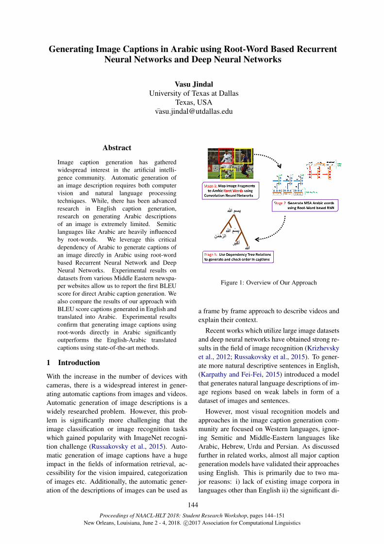
Proceedings of NAACL-HLT 2018: Student Research Workshop, pages 144–151New Orleans, Louisiana, June 2 - 4, 2018. c©2017 Association for Computational Linguistics

Generating Image Captions in Arabic using Root-Word Based RecurrentNeural Networks and Deep Neural Networks

Vasu JindalUniversity of Texas at Dallas

Texas, USAvasu.jindal@utdallas.edu

Abstract

Image caption generation has gatheredwidespread interest in the artificial intelli-gence community. Automatic generation ofan image description requires both computervision and natural language processingtechniques. While, there has been advancedresearch in English caption generation,research on generating Arabic descriptionsof an image is extremely limited. Semiticlanguages like Arabic are heavily influencedby root-words. We leverage this criticaldependency of Arabic to generate captions ofan image directly in Arabic using root-wordbased Recurrent Neural Network and DeepNeural Networks. Experimental results ondatasets from various Middle Eastern newspa-per websites allow us to report the first BLEUscore for direct Arabic caption generation. Wealso compare the results of our approach withBLEU score captions generated in English andtranslated into Arabic. Experimental resultsconfirm that generating image captions usingroot-words directly in Arabic significantlyoutperforms the English-Arabic translatedcaptions using state-of-the-art methods.

1 Introduction

With the increase in the number of devices withcameras, there is a widespread interest in gener-ating automatic captions from images and videos.Automatic generation of image descriptions is awidely researched problem. However, this prob-lem is significantly more challenging that theimage classification or image recognition taskswhich gained popularity with ImageNet recogni-tion challenge (Russakovsky et al., 2015). Auto-matic generation of image captions have a hugeimpact in the fields of information retrieval, ac-cessibility for the vision impaired, categorizationof images etc. Additionally, the automatic gener-ation of the descriptions of images can be used as

بسم هللا

حمن الرب سم هللا

أكبرهللا

Figure 1: Overview of Our Approach

a frame by frame approach to describe videos andexplain their context.

Recent works which utilize large image datasetsand deep neural networks have obtained strong re-sults in the field of image recognition (Krizhevskyet al., 2012; Russakovsky et al., 2015). To gener-ate more natural descriptive sentences in English,(Karpathy and Fei-Fei, 2015) introduced a modelthat generates natural language descriptions of im-age regions based on weak labels in form of adataset of images and sentences.

However, most visual recognition models andapproaches in the image caption generation com-munity are focused on Western languages, ignor-ing Semitic and Middle-Eastern languages likeArabic, Hebrew, Urdu and Persian. As discussedfurther in related works, almost all major captiongeneration models have validated their approachesusing English. This is primarily due to two ma-jor reasons: i) lack of existing image corpora inlanguages other than English ii) the significant di-

144

(book)

(subscription)(writer)

(clerk) (library)

(postal letter)

ك ت ب

Figure 2: Leveraging Root-Word in Arabic, Constantsand Vowels are filled using Recurrent Neural Network

Root Word K-T-B(Writer)

Full Caption

كاتب

كتابة كتاب رجل

Root Word K-T-B(Book)

كتاب

Root Word K-T-B(he writes) يكتب

Figure 3: State-of-the-Art: Man studying with booksOurs (translated from Arabic for reader’s readability):Writer writing on notebook

alects of Arabic and the challenges in translatingimages to natural sounding sentences. Translationof English generated captions to Arabic captionsmay not always be efficient due to the various Ara-bic morphologies, dialects and phonologies whichresults in losing the descriptive nature of the gen-erated captions. A cross-lingual image captiongeneration approach in Japanese concluded thata bilingual comparable corpus has better perfor-mance than a monolingual corpus in image captiongeneration (Miyazaki and Shimizu, 2016).

Arabic is ranked as the fifth most widely spokennative language among the population. Further-more, Arabic has tremendous impact on the socialand political aspects in the current community andis listed as one of the six official languages of theUnited Nations. Given the high influence of Ara-bic, it is necessary for a robust approach for Arabiccaption generation.

1.1 Novel Contributions

Semitic languages like Arabic are significantly in-fluenced by their original root-word. Figure 2 ex-

plains how simple root-words can form new wordswith similar context. We leverage this criticalaspect of Arabic to formalize a three stage ap-proach integrating root-word based Deep NeuralNetworks and root-word based Recurrent NeuralNetwork and dependency relations between theseroot words to generate Arabic captions. Frag-ments of images are extracted using pre-traineddeep neural network on ImageNet, however, un-like other published approaches for English cap-tion generation (Socher et al., 2014; Karpathy andFei-Fei, 2015; Vinyals et al., 2015), we map thesefragments to a set of root words in Arabic ratherthan actual words or sentences in English. Ourmain contribution in this paper is three-fold:

• Mapping of image fragments onto root wordsin Arabic rather than actual sentences orwords/fragments of sentences as suggested inpreviously proposed approaches.• Finding the most appropriate words for an

image by using a root-word based RecurrentNeural Network.• Finally, using dependency tree relations of

these obtained words to check order in sen-tences in Arabic

To the best of our knowledge, this is the firstwork that leverage root words to generate captionsin Arabic (Jindal, 2017). We also report the firstBLEU scores for Arabic caption generation. Ad-ditionally, this opens a new field of research touse root-words to generate captions from imagesin Semitic languages. For the purpose of clarity,we use the term ”root-words” throughout this pa-per to represent the roots of an Arabic word.

2 Background

2.1 Previous Works

The adoption of deep neural networks (Krizhevskyet al., 2012; Jia et al., 2014; Sharif Razavianet al., 2014) has tremendously improved both im-age recognition and natural language processingtasks. Furthermore, machine translation using re-current neural networks have gained attention withsequence-to-sequence training approaches (Choet al., 2014; Bahdanau et al., 2014; Kalchbrennerand Blunsom, 2013).

Recently, many researchers, have started tocombine both a convolutional neural network anda recurrent neural network. Vinyals et al. used

145

a convolutional neural network (CNN) with in-ception modules for visual recognition and longshort-term memory (LSTM) for language model-ing (Vinyals et al., 2015).

However, to the best of our knowledge mostcaption generation approaches were performedon English. Recently, authors in (Miyazaki andShimizu, 2016) presented results on the first cross-lingual image caption generation on the Japaneselanguage. (Peng and Li, 2016) generated Chinesecaptions on the Flickr30 dataset. There has beenno single work addressing to the generation of cap-tions in Semitic languages like Arabic. Further-more, all previously proposed approaches map im-age fragments to actual words/phrases. We ratherpropose to leverage the significance of root-wordsin Semitic languages and map image fragmentsto root-words and use these root-words in a root-word based recurrent neural network.

2.2 Arabic Morphology and Challenges

Arabic belongs to the family of Semitic languagesand has significant morphological, syntactical andsemantical differences from other languages. Itconsists of 28 letters and can be extended to 90by adding shapes, marks, and vowels. Arabic iswritten from right to left and letters have differentstyles based on the position in the word. The basewords of Arabic inflect to express eight main fea-tures. Verbs inflect for aspect, mood, person andvoice. Nouns and adjectives inflect for case andstate. Verbs, nouns and adjectives inflect for bothgender and number.

Furthermore, Arabic is widely categorized asa diglossia (Ferguson, 1959). A diglossia refersto a language where the formal usage of speechin written communication is significantly differ-ent in grammatical properties from the informalusage in verbal day to day communication. Ara-bic morphology consists of a bare root verb formthat is trilateral, quadrilateral, or pentalateral. Thederivational morphology can be lexeme = Root +Pattern or inflection morphology (word = Lexeme+ Features) where features are noun specific, verbspecific or single letter conjunctions. In contrast,in most European languages words are formed byconcatenating morphemes.

Stem pattern are often difficult to parse in Ara-bic as they interlock with root consonants (Al Bar-rag, 2014). Arabic is also influenced by infixeswhich may be consonants and vowels and can be

misinterpreted as root-words. One of the majorproblem is the use of a consonant, hamza. Hamzais not always pronounced and can be a vowel. Thiscreates a severe orthographic problem as wordsmay have differently positioned hamzas makingthem different strings yet having similar meaning.

Furthermore, diacritics are critical in Arabic.For example, two words formed from ”zhb” mean-ing ”to go” and ”gold” differ by just one diacritic.The two words can only be distinguished using di-acritics. The word ”go” may appear in a variety ofimages involving movement while ”gold” is morelikely to appear in images containing jewelry.

3 Methodology

Our methodology is divided into three mainstages. Figure 1 gives an overview of our ap-proach. In Stage 1, we map image fragments ontoroot words in Arabic. Then, in Stage 2, we usedroot word based Recurrent Neural Networks withLSTM memory cell to generate the most appropri-ate words for an image in Modern Standard Ara-bic (MSA). Finally, in Stage 3, we use dependencytree relations of these obtained words to check theword order of the RNN formed sentences in Ara-bic. Each step is described in detail in followingsubsections.

3.1 Image Fragments to Root-Words usingDNN

We extract fragments from images using the state-of-the-art deep neural networks. According to(Kulkarni et al., 2011; Karpathy et al., 2014), ob-jects and their attributes are critical in generatingsentence descriptions. Therefore, it is importantto efficiently detect as many objects as possible inthe image.

We apply the approach given in (Jia et al., 2014;Girshick et al., 2014) to detect objects in everyimage with a Region Convolutional Neural Net-work (RCNN). The CNN is pre-trained on Ima-geNet (Deng et al., 2009) and fine-tuned on the200 classes of the ImageNet Detection Challenge.We also use the top 19 detected locations as givenby Karpathy et al in addition to the whole im-age and compute the representations based on thepixels inside each bounding box as suggested in(Karpathy and Fei-Fei, 2015). It should be notedthat the output of the convolutional neural networkare Arabic root-words. To achieve this, at anygiven time when English labels of objects were

146

ك ت ب درسع ل م

ادرس علم

(book) (study) (knowledge)

h1 h2 h3

x1 x2 x3

y1 y2 y3

W W

Arabic Root Words

Arabic Words

LSTM LSTM LSTM

Figure 4: Our Root-Word based Recurrent Neural Network

used in training of the convolution neural net-work, Arabic root-words of the object were alsogiven as input in the training phase. (Yaseen andHmeidi, 2014; Yousef et al., 2014) proposed thewell-known transducer based algorithm for Arabicroot extraction which is used to extract root-wordsfrom an Arabic word in the training stage. Giventhe Arabic influence on root-words and the lim-ited 4 verb prefixes, 12 noun prefixes and 20 com-mon suffixes, the approach is optimized for initialtraining. Briefly, the algorithm has following stepsgiven the morphology of Arabic.1. Construct all noun/verb transducer2. Construct all noun/verb patterns transducer3. Construct all noun/verb suffixes transducer4. Concatenate noun transducers/verb transducersobtained in steps 1, 2 and 3.5. Sum the two transducers obtained in step 4.

Similar to (Vinyals et al., 2015), we used a dis-criminative model to maximize the probability ofthe correct description given the image. Formally,this can be represented using:

θ? = arg maxθ

∑

(I,S)

N∑

t=0

log p(St|I, S0, . . . , St−1; θ)

(1)where θ are the parameters of our model, I isan image, and S its correct transcription andN is a particular length of a caption. Thisp(St|I, S0, . . . , St−1; θ) is modeled using a root-word based Recurrent Neural Network (RNN).

3.2 Root-Word Based Recurrent NeuralNetwork and Dependency Relations

We propose a root-word based recurrent neuralnetwork (rwRNN). The model takes different root-words extracted from text, and predicts the mostappropriate words for captions in Arabic, essen-tially also learning the context and environment ofthe image. The structure of the rwRNN is basedon a standard many-to-many recurrent neural net-work, where current input (x) and previous infor-mation is connected through hidden states (h) byapplying a certain (e.g. sigmoid) function (g) withlinear transformation parameters (W ) at each timestep (t). Each hidden state is a long short-termmemory (LSTM) (Hochreiter and Schmidhuber,1997) cell to solve the vanishing gradient issue ofvanilla recurrent neural networks and inefficiencyin learning long distance dependencies.

While a standard input vector for RNN derivesfrom either a word or a character, the input vectorin rwRNN consists of a root-word specified with 3letters (r1n, r2n, r3n) that correspond to the char-acters in root-words’ position. Most root-words inArabic are trilateral very few being quadilateral orpentalateral. If a particular root-word is quadilat-eral (pentalateral) then the r2n represents the mid-dle three (four) letters of the root-word. Formally:

xn =

r1nr2nr3n

(2)

The final output (i.e. the predicted actual Ara-bic word yn), the hidden state vector (hn) of the

147

Root Word: KURA(Ball)

Playing with

Root Word K-L-B(Dog)

Full Caption

كرة معيلعب

كلب

كلب يلعب مع الكرة

Figure 5: Arabic-English: Dog playing withballOurs: Dog plays with a ball

Root Word: J-M-L(Camel)

Man sitting

R-M-L (Sand/DesertSahra’)

Full Caption

Figure 6: Arabic-English: Man sitting on camelOurs: Man moving on camel in desert

Crown

Woman

Full Captionتاج

مرأة

نساء مع تاج يقف أمام ناطحات السحاب

Skyscraper

ناطحات السحاب

Figure 7: Arabic-English: Woman standing incityOurs: Woman with crown standing in front ofskysrapers

Palm Tree/Island

Sea

Full Caption

جزيرة النخيل في البحر

البحر

شجرة النخل /جزيرة

Figure 8: Arabic-English: Island in SeaOurs: Palm Shaped Islands in the Sea

LSTM is taken as input to the following softmaxfunction layer with a fixed vocabulary size (v).

yn =exp (Wh · hn)∑v exp (Wh · hn)

(3)

Cross-entropy training criterion is applied to theoutput layer to make the model learn the weightmatrices (W ) to maximize the likelihood of thetraining data. Figure 4 gives an overview of ourroot-word based Recurrent Neural Network. Thedependency tree relations are used to check if theorder of Recurrent Neural Network is correct.

Dependency tree constraints (Kuznetsova et al.,2013) checks the caption generated from RNN tobe grammatically valid in Modern Standard Ara-bic and robust to different diacritics in Arabic.The model also ensures that the relations betweenimage-text pair and verbs generated from RNN arestill maintained. Formally, the following objectivefunction is maximized:

Maximize F (y;x) = Φ(y;x, v) + Ψ(y;x)

subject to Ω(y;x, v)(4)

where x = xi is the input caption from RNN (asentence), v is the accompanying image, y = yi isthe output sentence, Φ(y;x, v) is the content selec-tion score, Φ(y;x) is the linguistic fluency score,and Ω(y;x, v) is the set of hard dependency treeconstraints. The most popular Prague Arabic De-pendency Treebank (PADT) consisting of multi-level linguistic annotations over Modern StandardArabic is used for the dependency tree constraints(Hajic et al., 2004).

4 Experimental Results

Figure 3, 5-8 gives a sample of our approach in ac-tion. For the convenience of our readers who arenot familiar with Arabic, Figure 5, 6, 7, 8 have theEnglish caption generated using (Xu et al., 2015)denoted as ”Arabic-English” and ”Ours” denotea professional English translation of the Arabiccaption generated from our approach. We eval-uate our technique using two datasets: Flickr8kdataset with manually written captions in Arabicby professional Arabic translators and 405,000 im-

148

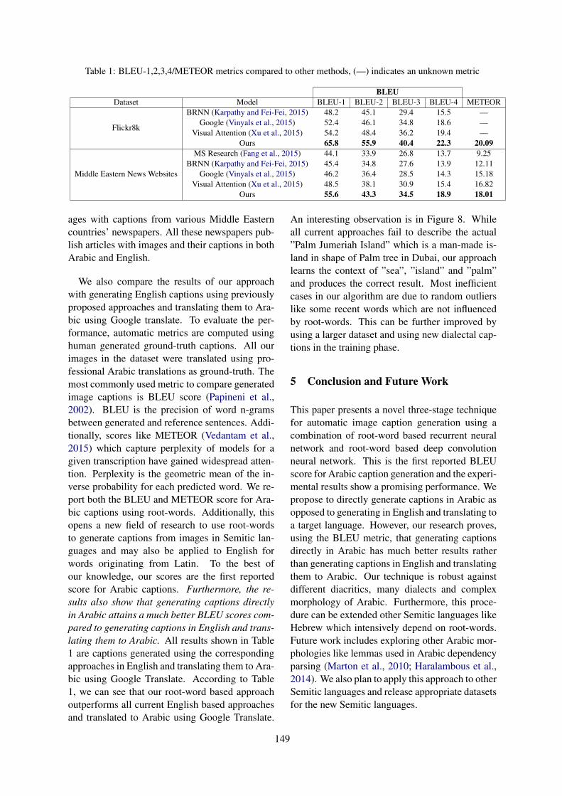
Table 1: BLEU-1,2,3,4/METEOR metrics compared to other methods, (—) indicates an unknown metric

BLEUDataset Model BLEU-1 BLEU-2 BLEU-3 BLEU-4 METEOR

Flickr8k

BRNN (Karpathy and Fei-Fei, 2015)Google (Vinyals et al., 2015)

Visual Attention (Xu et al., 2015)Ours

48.252.454.265.8

45.146.148.455.9

29.434.836.240.4

15.518.619.422.3

———

20.09

Middle Eastern News Websites

MS Research (Fang et al., 2015)BRNN (Karpathy and Fei-Fei, 2015)

Google (Vinyals et al., 2015)Visual Attention (Xu et al., 2015)

Ours

44.145.446.248.555.6

33.934.836.438.143.3

26.827.628.530.934.5

13.713.914.315.418.9

9.2512.1115.1816.8218.01

ages with captions from various Middle Easterncountries’ newspapers. All these newspapers pub-lish articles with images and their captions in bothArabic and English.

We also compare the results of our approachwith generating English captions using previouslyproposed approaches and translating them to Ara-bic using Google translate. To evaluate the per-formance, automatic metrics are computed usinghuman generated ground-truth captions. All ourimages in the dataset were translated using pro-fessional Arabic translations as ground-truth. Themost commonly used metric to compare generatedimage captions is BLEU score (Papineni et al.,2002). BLEU is the precision of word n-gramsbetween generated and reference sentences. Addi-tionally, scores like METEOR (Vedantam et al.,2015) which capture perplexity of models for agiven transcription have gained widespread atten-tion. Perplexity is the geometric mean of the in-verse probability for each predicted word. We re-port both the BLEU and METEOR score for Ara-bic captions using root-words. Additionally, thisopens a new field of research to use root-wordsto generate captions from images in Semitic lan-guages and may also be applied to English forwords originating from Latin. To the best ofour knowledge, our scores are the first reportedscore for Arabic captions. Furthermore, the re-sults also show that generating captions directlyin Arabic attains a much better BLEU scores com-pared to generating captions in English and trans-lating them to Arabic. All results shown in Table1 are captions generated using the correspondingapproaches in English and translating them to Ara-bic using Google Translate. According to Table1, we can see that our root-word based approachoutperforms all current English based approachesand translated to Arabic using Google Translate.

An interesting observation is in Figure 8. Whileall current approaches fail to describe the actual”Palm Jumeriah Island” which is a man-made is-land in shape of Palm tree in Dubai, our approachlearns the context of ”sea”, ”island” and ”palm”and produces the correct result. Most inefficientcases in our algorithm are due to random outlierslike some recent words which are not influencedby root-words. This can be further improved byusing a larger dataset and using new dialectal cap-tions in the training phase.

5 Conclusion and Future Work

This paper presents a novel three-stage techniquefor automatic image caption generation using acombination of root-word based recurrent neuralnetwork and root-word based deep convolutionneural network. This is the first reported BLEUscore for Arabic caption generation and the experi-mental results show a promising performance. Wepropose to directly generate captions in Arabic asopposed to generating in English and translating toa target language. However, our research proves,using the BLEU metric, that generating captionsdirectly in Arabic has much better results ratherthan generating captions in English and translatingthem to Arabic. Our technique is robust againstdifferent diacritics, many dialects and complexmorphology of Arabic. Furthermore, this proce-dure can be extended other Semitic languages likeHebrew which intensively depend on root-words.Future work includes exploring other Arabic mor-phologies like lemmas used in Arabic dependencyparsing (Marton et al., 2010; Haralambous et al.,2014). We also plan to apply this approach to otherSemitic languages and release appropriate datasetsfor the new Semitic languages.

149

ReferencesThamir Al Barrag. 2014. Noun phrases in urban hijazi

arabic: A distributed morphology approach.

Dzmitry Bahdanau, Kyunghyun Cho, and Yoshua Ben-gio. 2014. Neural machine translation by jointlylearning to align and translate. arXiv preprintarXiv:1409.0473.

Kyunghyun Cho, Bart Van Merrienboer, Dzmitry Bah-danau, and Yoshua Bengio. 2014. On the propertiesof neural machine translation: Encoder-decoder ap-proaches. arXiv preprint arXiv:1409.1259.

Jia Deng, Wei Dong, Richard Socher, Li-Jia Li, Kai Li,and Li Fei-Fei. 2009. Imagenet: A large-scale hi-erarchical image database. In Computer Vision andPattern Recognition, 2009. CVPR 2009. IEEE Con-ference on, pages 248–255. IEEE.

Hao Fang, Saurabh Gupta, Forrest Iandola, Rupesh KSrivastava, Li Deng, Piotr Dollar, Jianfeng Gao, Xi-aodong He, Margaret Mitchell, John C Platt, et al.2015. From captions to visual concepts and back. InProceedings of the IEEE Conference on ComputerVision and Pattern Recognition, pages 1473–1482.

Charles A Ferguson. 1959. Diglossia. word,15(2):325–340.

Ross Girshick, Jeff Donahue, Trevor Darrell, and Ji-tendra Malik. 2014. Rich feature hierarchies for ac-curate object detection and semantic segmentation.In Proceedings of the IEEE conference on computervision and pattern recognition, pages 580–587.

Jan Hajic, Otakar Smrz, Petr Zemanek, Jan Snaidauf,and Emanuel Beska. 2004. Prague arabic depen-dency treebank: Development in data and tools. InProc. of the NEMLAR Intern. Conf. on Arabic Lan-guage Resources and Tools, pages 110–117.

Yannis Haralambous, Yassir Elidrissi, and PhilippeLenca. 2014. Arabic language text classificationusing dependency syntax-based feature selection.arXiv preprint arXiv:1410.4863.

Sepp Hochreiter and Jurgen Schmidhuber. 1997.Long short-term memory. Neural computation,9(8):1735–1780.

Yangqing Jia, Evan Shelhamer, Jeff Donahue, SergeyKarayev, Jonathan Long, Ross Girshick, SergioGuadarrama, and Trevor Darrell. 2014. Caffe: Con-volutional architecture for fast feature embedding.In Proceedings of the 22nd ACM international con-ference on Multimedia, pages 675–678. ACM.

Vasu Jindal. 2017. A deep learning approach for ara-bic caption generation using roots-words. In AAAI,pages 4941–4942.

Nal Kalchbrenner and Phil Blunsom. 2013. Recurrentcontinuous translation models. In EMNLP, 39, page413.

Andrej Karpathy and Li Fei-Fei. 2015. Deep visual-semantic alignments for generating image descrip-tions. In Proceedings of the IEEE Conference onComputer Vision and Pattern Recognition, pages3128–3137.

Andrej Karpathy, Armand Joulin, and Fei Fei F Li.2014. Deep fragment embeddings for bidirectionalimage sentence mapping. In Advances in neural in-formation processing systems, pages 1889–1897.

Alex Krizhevsky, Ilya Sutskever, and Geoffrey E Hin-ton. 2012. Imagenet classification with deep con-volutional neural networks. In Advances in neuralinformation processing systems, pages 1097–1105.

Girish Kulkarni, Visruth Premraj, Sagnik Dhar, Sim-ing Li, Yejin Choi, Alexander C Berg, and Tamara LBerg. 2011. Baby talk: Understanding and generat-ing image descriptions. In Proceedings of the 24thCVPR.

Polina Kuznetsova, Vicente Ordonez, Alexander CBerg, Tamara L Berg, and Yejin Choi. 2013. Gen-eralizing image captions for image-text parallel cor-pus. In ACL (2), pages 790–796.

Yuval Marton, Nizar Habash, and Owen Rambow.2010. Improving arabic dependency parsing withlexical and inflectional morphological features. InProceedings of the NAACL HLT 2010 First Work-shop on Statistical Parsing of Morphologically-RichLanguages, pages 13–21. Association for Computa-tional Linguistics.

Takashi Miyazaki and Nobuyuki Shimizu. 2016.Cross-lingual image caption generation. In Pro-ceedings of the 54th Annual Meeting of the Associa-tion for Computational Linguistics, volume 1, pages1780–1790.

Kishore Papineni, Salim Roukos, Todd Ward, and Wei-Jing Zhu. 2002. Bleu: a method for automatic eval-uation of machine translation. In Proceedings ofthe 40th annual meeting on association for compu-tational linguistics, pages 311–318. Association forComputational Linguistics.

Hao Peng and Nianhen Li. 2016. Generating chinesecaptions for flickr30k images.

Olga Russakovsky, Jia Deng, Hao Su, Jonathan Krause,Sanjeev Satheesh, Sean Ma, Zhiheng Huang, AndrejKarpathy, Aditya Khosla, Michael Bernstein, et al.2015. Imagenet large scale visual recognition chal-lenge. International Journal of Computer Vision,115(3):211–252.

Ali Sharif Razavian, Hossein Azizpour, Josephine Sul-livan, and Stefan Carlsson. 2014. Cnn features off-the-shelf: an astounding baseline for recognition. InProceedings of the IEEE Conference on ComputerVision and Pattern Recognition Workshops, pages806–813.

150

Richard Socher, Andrej Karpathy, Quoc V Le, Christo-pher D Manning, and Andrew Y Ng. 2014.Grounded compositional semantics for finding anddescribing images with sentences. Transactionsof the Association for Computational Linguistics,2:207–218.

Ramakrishna Vedantam, C Lawrence Zitnick, and DeviParikh. 2015. Cider: Consensus-based image de-scription evaluation. In Proceedings of the IEEEConference on Computer Vision and Pattern Recog-nition, pages 4566–4575.

Oriol Vinyals, Alexander Toshev, Samy Bengio, andDumitru Erhan. 2015. Show and tell: A neural im-age caption generator. In Proceedings of the IEEEConference on Computer Vision and Pattern Recog-nition, pages 3156–3164.

Kelvin Xu, Jimmy Ba, Ryan Kiros, Kyunghyun Cho,Aaron C Courville, Ruslan Salakhutdinov, Richard SZemel, and Yoshua Bengio. 2015. Show, attend andtell: Neural image caption generation with visual at-tention. In ICML, volume 14, pages 77–81.

Qussai Yaseen and Ismail Hmeidi. 2014. Extractingthe roots of arabic words without removing affixes.Journal of Information Science, 40(3):376–385.

Nidal Yousef, Aymen Abu-Errub, Ashraf Odeh, andHayel Khafajeh. 2014. An improved arabic word’sroots extraction method using n-gram technique.Journal of Computer Science, 10(4):716.

151

Author Index

Acharya, Sabita, 74Aedmaa, Eleri, 9Akhtar, Syed Sarfaraz, 128Ardati, Amer, 74

Bohra, Aditya, 128Bowman, Samuel, 92, 120Boyd, Andrew, 74

Cameron, Richard, 74Cheung, Jackie Chi Kit, 25Chioma, Enemouh, 54Cho, Kyunghyun, 120

Deng, Haohui, 83Di Eugenio, Barbara, 74Dickens, Carolyn, 74Doyle, Gabriel, 1Dunn Lopez, Karen, 74

Emami, Ali, 25Ezeani, Ignatius, 54

Hepple, Mark, 54Homan, Christopher, 136Htut, Phu Mon, 120

Jindal, Vasu, 144

Köper, Maximilian, 9Kajiwara, Tomoyuki, 106Kameswara Sarma, Prathusha, 46Komachi, Mamoru, 100, 106Kurosawa, Michiki, 100

Lane, Ian, 67Lapresi, Luke, 136Lavrentovich, Alexandra, 61Liu, Bing, 67

MacAvaney, Sean, 40Martyn-Nemeth, Pamela, 74Matsumura, Yukio, 100

Nangia, Nikita, 92

Onyenwe, Ikechukwu, 54

Ovesdotter Alm, Cecilia, 136

Pierrejean, Benedicte, 32Ptucha, Raymond, 136

Ramesh, Sree Harsha, 112

Sankaranarayanan, Krishna Prasad, 112Schulte im Walde, Sabine, 9Seyffarth, Esther, 17Shimanaka, Hiroki, 106Shin, Hagyeong, 1Shrivastava, Manish, 128Singh, Vinay, 128Suleman, Kaheer, 25

Tam, Yik-Cheung, 83Tanguy, Ludovic, 32Tornblad, McKenna, 136Trischler, Adam, 25

Vijay, Deepanshu, 128

Yamagishi, Hayahide, 100

Zeldes, Amir, 40

153