AADDMM0033

Proceedings Australasian Data Mining Workshop

8th December, 2003, Canberra, Australia

Edited by Simeon J. Simoff, Graham J. Williams and

Markus Hegland

in conjunction with The 2003 Congress on

Evolutionary Computation Canberra – Australia,

8th – 12th December, 2003

University of Technology Sydney 2003

© Copyright 2003. The copyright of these papers belongs to the paper's authors. Permission to copy without fee all or part of this material is granted provided that the copies are not made or distributed for direct commercial advantage.

Proceedings of the 2nd Australasian Data Mining Workshop – ADM03, in conjunction with the 2003 Congress on Evolutionary Computation, 8th – 12th December, 2003, Canberra, Australia.

S. J. Simoff, G. J. Williams and M. Hegland (eds).

Workshop Web Site: http://datamining.csiro.au/adm03/

Published by the University of Technology Sydney

ISBN 0-9751724-1-7

i

Foreword

The Australasian Data Mining Workshop is a flagship event in the area of discovering meaningful insights in large data sets. The art and science of analytics and data mining have always attracted researchers and industry practitioners in the region. Data mining projects involve both the utilisation of established algorithms from machine learning, statistics, and database systems, and the development of new methods and algorithms, targeted at large data mining problems. Nowadays data mining efforts have gone beyond crunching databases of credit card usage or retail transaction records. The progress in computing technology affects all aspects of human existence. The data mining technologies are becoming the core part of the so-called “embedded intelligence” in business, health care, drug design, biology, design and other areas of human endeavour.

The first edition of the Australasian Data Mining Workshop was a successful event, conducted in conjunction with the 15th Australian Joint Conference on Artificial Intelligence, 2nd - 6th December 2002, Canberra, Australia. The workshop attracted a number of participants from Australian industry, academia, research institutions and centers, in particular, researchers from the ANU Data Mining Group, CSIRO Enterprise Data Mining, and UTS Smart e-Business Systems Lab. The workshop facilitated the links between different research groups in Australia and industry, evidenced by the initiative in the creation of an Australian Research Council Research Network on Improving Australia's Data Mining and Knowledge Discovery Research, and the Institute of Analytic Professionals of Australia. It also strengthened the interconnections between researchers in academic and research organisations, and industry practitioners, who utilise data mining techniques in various business case studies.

This year the workshop builds on these trends. The workshop is expected to broaden and strengthen the links within the analytics community, offering a forum for presenting and discussing latest research and practical experience in the area. The workshop follows a rigid blind peer-review process and ranking-based paper selection process. All papers were extensively reviewed by two to three referees drawn from the program committee. Papers that present comprehensive, completed (or near completion) research work have been allocated larger presentation time slots. The works that present research work in progress or “green house” ideas have been allocated shorter time slots, with more time left for discussion. The organisers have reserved a special presentation session for an overview of on-going initiatives.

Once again, we would like to thank all those, who supported this year’s efforts on all stages – from the development and submission of the workshop proposal to the preparation of the final program and proceedings. We would like to thank all those who submitted their work to the workshop. Special thanks go to the program committee members and other reviewers, for the final quality of selected papers depends on their efforts.

Simeon, J. Simoff, Graham J. Williams and Markus Hegland

November 2003

ii

Workshop Chairs

Simeon J Simoff University of Technology, Sydney Graham J Williams CSIRO Canberra Markus Hegland Australian National University

Program Committee

Mihael Ankerst Boeing Corp., USA Michael Böhlen University of Bolzano, Italy Doug Campbell SAS Australian and New Zealand Jie Chen CSIRO, Canberra, Australia Peter Christen Australian National University, Australia Vladimir Estivill-Castro Giffith University, Australia Warwick Graco Australian Taxation Office Weiqiang Lin Australian Taxation Office Warren Jin CSIRO, Canberra, Australia Paul Kennedy University of Technology, Sydney, Australia Inna Kolyshkina Pricewaterhouse Coopers Actuarial, Sydney, Austrlia Tom Osborn NUIX Pty Ltd, Australia Francois Poilet Parc Universitaire de Laval-Change, France Chris Rainsford DSTO Canberra, Australia David Skillicorn University of Queens, Canada Marcel van Rooyen Hutchison Communications, Australia John Yearwood University of Ballarat, Australia Osmar Zaiane University of Alberta, Canada

iii

Program for ADM03 Workshop

Monday, 8 December, 2003, Canberra, Australia

9:00 - 9:15 Opening and Welcome

9:15 - 10:30 Session 1

• 09:15 - 09:40 STOCHASTIC PRELIMINARY INVESTIGATIONS INTO STATISTICALLY VALID EXPLORATORY RULE DISCOVERY Geoffrey I. Webb

• 09:40 - 10:05 TWO PHASE CLASSIFICATION BY EMERGING PATTERNS Ming Fan, Weimei Zhi, Hongjian Fan and Yigui Sun

• 10:05 - 10:30 FEATURE PREPARATION IN TEXT CATEGORIZATION Ciya Liao, Shamim Alpha and Paul Dixon

10:30 - 11:00 Coffee break

11:00 - 12:30 Session 2

• 11:00 - 11:25 LEARNING QUANTITATIVE GENE INTERACTIONS FROM MICROARRAY DATA Michael Bain and Bruno Gaëta

• 11:25 - 11:50 AN MINING APPROACH USING MOUCLAS PATTERNS Yalei Hao, Markus Stumptner and Gerald Quirchmayr

• 11:50 - 12:15 FROM RULE VISUALISATION TO GUIDED KNOWLEDGE DISCOVERY Aaron Ceglar, John F. Roddick, Carl H. Mooney and Paul Calder

• 12:15 - 12:30 TEXTURE ANALYSIS VIA DATA MINING Martin Heckel

12:30 - 13:30 Lunch

13:30 - 14:50 Session 3

• 13:30 - 13:45 CLUSTERING TIME SERIES FROM MIXTURE POLYNOMIAL MODELS WITH DISCRETISED DATA A. J. Bagnall, G. Janacek, B. de la Iglesia and M. Zhang

• 13:45 - 14:00 RELATIVE TEMPORAL ASSOCIATION RULE MINING Edi Winarko and John F. Roddick

• 14:00 - 14:25 A STUDY OF DRUG-REACTION RELATIONS IN AUSTRALIAN DRUG SAFETY DATA M. A. Mamedov, G. W. Saunders and E. Dekker

• 14:25 - 14:50 MINING GEOGRAPHICAL DATA WITH SPARSE GRIDS Markus Hegland and Shawn W. Laffan

14:50 - 15:20 Coffee break

15:20 - 16:40 Session 4

• 15:20 - 15:45 CONGO: Clustering on the Gene Ontology Paul J. Kennedy and Simeon J. Simoff

• 15:45 - 16:00 ADAPTIVE MINING TECHNIQUES FOR DATA STREAMS USING ALGORITHM OUTPUT GRANULARITY Mohamed Medhat Gaber, Shonali Krishnaswamy and Arkady Zaslavsky

• 16:00 - 16:15 An Analytical Approach for Handling Association Rule Mining Results Rodrigo Salvador Monteiro, Geraldo Zimbrão and Jano Moreira de Souza

• 16:15 - 16:40 Modelling Insurance Risk: A Comparison of Data Mining and Logistic Regression Approaches Inna Kolyshkina, Peter Petocz and Ingrid Rylander

16:40 - 17:00 Closing Session

• 16:40 - 16:50 AUSTRALIAN RESEARCH COUNCIL RESEARCH NETWORK ON IMPROVING AUSTRALIA'S DATA MINING AND KNOWLEDGE DISCOVERY RESEARCH John F. Roddick

• 16:50 - 17:00 INSTITUTE OF ANALYTIC PROFESSIONALS OF AUSTRALIA Inna Kolyshkina

iv

v

Table of Contents

Stochastic Preliminary Investigations Into Statistically Valid Exploratory Rule Discovery Geoffrey I. Webb …………………………………………………………………………… 001

Two Phase Classification By Emerging Patterns Ming Fan, Weimei Zhi, Hongjian Fan and Yigui Sun ……………………………………………… 011

Feature Preparation In Text Categorization Ciya Liao, Shamim Alpha and Paul Dixon ……………………………………………………… 023

Learning Quantitative Gene Interactions from Microarray Data Michael Bain and Bruno Gaëta ……………………………………………………………… 035

An Mining Approach Using MOUCLAS Patterns Yalei Hao, Markus Stumptner and Gerald Quirchmayr …………………………………………… 051

From Rule Visualisation to Guided Knowledge Discovery Aaron Ceglar, John F. Roddick, Carl H. Mooney and Paul Calder ………………………………… 059

Texture Analysis via Data Mining Martin Heckel ……………………………………………………………………………… 095

Clustering Time Series from Mixture Polynomial Models with Discretised Data A. J. Bagnall, G. Janacek, B. de la Iglesia and M. Zhang ………………………………………… 105

Relative Temporal Association Rule Mining Edi Winarko and John F. Roddick …………………………………………………………… 121

A Study of Drug-Reaction Relations in Australian Drug Safety Data M. A. Mamedov, G. W. Saunders and E. Dekker ………………………………………………… 143

Mining Geographical Data with Sparse Grids Markus Hegland and Shawn W. Laffan ………………………………………………………… 163

CONGO: Clustering on the Gene Ontology Paul J. Kennedy and Simeon J. Simoff ………………………………………………………… 181

Adaptive Mining Techniques for Data Streams using Algorithm Output Granularity Mohamed Medhat Gaber, Shonali Krishnaswamy and Arkady Zaslavsky …………………………… 199

An Analytical Approach for Handling Association Rule Mining Results Rodrigo Salvador Monteiro, Geraldo Zimbrão and Jano Moreira de Souza ………………………… 217

Modelling Insurance Risk: A Comparison of Data Mining and Logistic Regression Approaches Inna Kolyshkina, Peter Petocz and Ingrid Rylander ……………………………………………… 227

Author Index …………………………………………………………………………… 239

Preliminary Investigations into Statistically

Valid Exploratory Rule Discovery

Geoffrey I. Webb

School of Computer Science and Software Engineering, Monash University,Melbourne, Vic 3800, Australiawebb@infotech.monash.edu

Abstract. Exploratory rule discovery, as exemplified by association rulediscovery, is has proven very popular. In this paper I investigate issuessurrounding the statistical validity of rules found using this approachand methods that might be employed to deliver statistically sound ex-ploratory rule discovery.

1 Introduction

Association rule discovery has proven very popular. However, it is plagued bythe problem that it often delivers unmanageably large numbers of rules. As thecurrent work reveals, not only are the rules numerous, but in at least some casesthe vast majority are spurious or unproductive specialisations of more generalrules. This paper discusses the issues of spurious and unproductive rules andpresents preliminary approaches to address them. Experimental results confirmthe practical realisation of the concerns and suggests that the preliminary tech-niques presented are effective.

2 Exploratory rule discovery

I use the term exploratory rule discovery to encompass data mining techniquesthat seek multiple rather than single models, with the objective of allowing theend-user to select between those models. It is distinguished from predictive data

mining that seeks a single model that can be used for making predictions.Exploratory data mining is often applicable when there are factors that can

affect the usefulness of a model but it is difficult to quantify those factors in amanner that may be used by an automated data mining system. By deliveringmultiple alternative models to the end-user they are empowered to evaluatethe available models and to select those that best suit their business or otherobjectives.

Three prominent frameworks for exploratory rule discovery on which I herefocus are association rule discovery [1], k-most-interesting rule discovery [2] andcontrast or emerging pattern discovery [3, 4] as it is variously known. These tech-niques all discover qualitative rules, rules that represent relationships betweennominal-valued variables.

Each such rule A → C represents the presence of a (potentially) interestingrelationship between the antecedent A and the consequent C, where A is aconjunction of nominal-valued terms and C is a single nominal valued term1. Therules are usually presented together with statistics that describe the relationshipbetween A and C.

2.1 Association Rule Discovery

Association rule discovery [1] is the most widely deployed exploratory rule discov-ery approach. It grew out of market-basket analysis, the analysis of transactiondata for combinations of products that are purchased in a single transaction.Association rule discovery uses the so called support-confidence framework. Itfinds all rules that satisfy a user-specified minimum support constraint togetherwith whatever further constraints the user may specify. Essentially, the approachgenerates all rules that satisfy the minimum support constraint but discards atthe final stage any rules that fail the further constraints.

Support is the proportion of records in the training data that satisfy boththe antecedent and consequent of the rule.

Initial approaches used a further constraint on minimum confidence. To avoidpotential confusion with the statistical concept of confidence I will hereafter referto this metric as strength.

strength = support/coverage (1)

where coverage is the proportion of records that satisfy the antecedent.More recent approaches typically use a constraint on minimum lift in prefer-

ence to a constraint on strength:

lift = strength/prior (2)

where prior is the proportion of records that satisfy the consequent.The main mechanism available to control the number of rules that are dis-

covered is the value that is specified for minimum support. However, it is usuallydifficult to anticipate which values of minimum support will result in manage-able numbers of rules. Too large a value will result in no rules. Too small a valuewill result in literally millions of rules. In practice there may be a very narrowrange of values of support below which there are extremely few rules discoveredand above which there are too many rules discovered [5].

2.2 K-Most-Interesting Rule Discovery

K-most-interesting rule discovery [2] addresses this problem by empowering theuser to specify both a metric of interestingness and a constraint on the maximum

1 While association rules are often described in terms of allowing C to be an arbitraryconjunction of terms, in many implementations C is restricted to a single term. Inthe current work I follow this practice as it greatly reduces the complexity of therule discovery task while satisfying many rule discovery needs.

number of rules to by discovered. In place of a minimum support constraint, k -most-interesting rule discovery uses these two pieces of information to prune thesearch space. They return the k rules that optimise the interestingness metricwithin whatever other constraints the user might specify. It is left up to the userto specify the interestingness metric, the only constraint on the metric beingthat it must define a partial order on a set of rules given a set of data by whichthe interestingness of those rules is to be scored.

2.3 Contrast Discovery

Contrast discovery [4] (initially developed under the name emerging pattern dis-

covery [3]) seeks rules that identify conditions whose frequency differs betweengroups of interest. It has been shown that this is equivalent to a form of rulediscovery restricted to a consequent that signifies group membership [6].

3 Spurious Rules

A problem for all three of these forms of exploratory rule discovery is that theysuffer a high risk of discovering spurious rules. These are rules that appearinteresting on the sample data but which would not be interesting if the truepopulation probabilities were used to assess their level interestingness in placeof the observed sample frequencies.

For example, suppose that there is a rule with coverage of one record and alift of 2.0. This provides very little evidence that the lift that would be obtainedby substituting population probabilities for sample frequencies would have highlift as a rule with one record coverage must have either a support of zero or onerecord and hence, irrespective of the population lift, the observed lift must eitherbe 0.0 or 1.0/prior. In other words, when the rule coverage is low, the statis-tical confidence will be low that the observed relative frequencies are stronglyindicative of the population probabilities.

The support-confidence framework of association rule discovery attempts tocounter this problem by enforcing a minimum support constraint in the expec-tation that considering only rules with high support will lead to the observedfrequencies being strongly representative of the population frequencies.

4 The Multiple Comparisons Problem

However, this ignores the problem of multiple comparisons [7]. If many obser-vations are made then one can have high confidence that some events that areunlikely in the context of a single observation are likely to occur in some of themany observations that are made. For example, suppose a hypothesis test isapplied to evaluate whether a rule is spurious with a significance level of 0.05.Consider a spurious rule A → C for which A and C are independent. The proba-bility that this spurious rule will be accepted as not spurious is 5%. If this process

were applied to 1,000,000 rules in a context where all rules were spurious (forexample, the data were generated stochastically using uniform probabilities) wecould reasonably expect that 5% or 50,000 would be accepted as non-spuriousdespite all being spurious. In practice the rule spaces explored by rule discov-ery systems are many magnitudes greater than 1,000,000, and hence we shouldexpect many spurious rules to be generated even if we apply a significance testbefore accepting each one.

5 Filters for Spurious Rules

One response to this problem is to apply a correction for multiple comparisons,such as the Bonferroni adjustment that divides the critical value α by the numberof rules evaluated. This is the approach adopted in the contrast discovery contextby STUCCO [4]. A problem with this approach is that the search process mayrequire the evaluation of very large numbers of rules and hence α may be drivento extremely low values. The lower the value of α the higher the probability oftype-2 error, that is, of rejecting rules that are not spurious.

What is required is an approach that minimises the risk of type-1 error,that is, of accepting spurious rules, without in the process discarding the mostinteresting non-spurious rules.

6 Unproductive Rules

A further problem for rule discovery is that of unproductive rules. A rule A →

C is unproductive if it has a generalisation B → C such that strength(A →

C) ≤ strength(B → C). An unproductive rule will arise when a variable that isunrelated to either B or C is added to B. As the strength is unaltered, the liftof the unproductive rule will equal that of the generalisation. In practice datasets often involve many variables that do not impact upon the rules of interestand hence very large numbers of unproductive rules are generated.

The problem of unproductive rules interacts with the problem of spuriousrules. It is straightforward to add a filter to the rule discovery process thatdiscards any rule for which the observed strength is not greater than the observedstrength of all its generalisations. However, random variations in the data samplewill lead to almost half the unproductive rules appearing to be productive (albeitin many cases only very slightly). A statistical test of significance may be applied,as supported by the Magnum Opus rule discovery system [8], but we again facethe multiple comparisons problem.

7 A New Approach

Hypothesis testing is designed for controlling the risk of type-1 error in thecontext of evaluating a prior hypothesis against previously unsighted data. It is

inadequate to the task of both generating hypotheses and evaluating them fromthe same set of data.

An approach that has been used in other data mining contexts is to use aholdout set for hypothesis testing. Models are inferred from a training set andthen evaluated against a holdout set. My proposal is to utilise this framework inan exploratory rule discovery context. The available data will be divided into anexploratory data set from which rules will be discovered. This will be treated asa hypothesis generation process. The rules discovered are treated as hypothesesthat are then evaluated against the holdout set. As the holdout data is parti-tioned from the exploratory data, the huge number of rules considered duringrule discovery does not affect the subsequent evaluation. A simple multiple com-parisons adjustment need only divide the selected alpha value by the number ofrules delivered by the rule discovery phase. Thus the α value need not be setprohibitively low, minimising the problem of type-2 error.

Note that re-sampling methods, such as cross-validation, that serve to eval-uate the power of a method for a given set of data are not adequate to thistask. Unlike the case where we wish to predict the likely predictive accuracy ofa single model produced by a system, here we wish to produce many rules. Wewant to control the risk of any of these rules being spurious.

I propose the use of k -most-interesting rule discovery for the rule discoveryphase rather than association rule discovery, because it is desirable to find aconstrained number of rules during the rule discovery phase. If too many rulesare discovered the necessary multiple comparisons adjustment will result in araised risk of type-2 error. If too few rules are discovered then there is a raisedrisk of failing to discover sufficient interesting rules to satisfy the user. Standardassociation rule discovery provides only very imprecise control over the numberof rules discovered. Tightening or weakening each of the constraints will respec-tively decrease or increase the number of rules discovered, but typically it is notpossible to predict by exactly how much a particular alteration to the constraintswill affect the number of rules discovered. In contrast, k -most interesting rulediscovery always returns k rules, except in the unusual circumstance that theother constraints applied are satisfied by fewer than k rules.

7.1 Selection of Holdout Data

The proposed generic holdout technique is applicable to two different contexts.In the first context there is a single set of data available, and this data needsto be partitioned. In this context, it would be appropriate for the data to berandomly partitioned, a process that can be readily automated. It is probablydesirable that the partitions be of similar sizes. It is important to have as muchdata as possible for exploratory rule discovery, so as to generate as powerfulhypotheses as possible. It is also important to have as much holdout data aspossible so as to maximise the power of the statistical tests that are applied.

The second context is one in which there are natural partitions of the data.For example, data may be obtained over time. In such a context it might bevaluable to utilise the natural partitions so as to evaluate whether the regularities

apparent in the exploratory partition (such as the data from one year) generaliseacross partitions (such as to the next year).

7.2 Holdout Evaluation Tests

For each rule A → C we wish to assess whether the observed strength(A → C) issignificantly higher than would be expected if there were no relationship betweenthe antecedent and consequent and also whether it is significantly higher thanthe strength of all its generalisations2. I use a binomial test to assess whether anobserved strength is signficantly higher than a comparator strength. The largenumber of subsets of an antecedent containing many conditions would make test-ing against all generalisations infeasible. In consequence I test strength(A → C)against the sample frequency of C (which equals strength(∅ → C)) and againstthe strength of all its immediate generalisations (rules formed by removing asingle condition from A). While it is theoretically possible for a rule to havehigher strength than all of its immediate generalisations but lower strength thana further generalisation, to do so requires a very specific type of interactionbetween four or more variables of a form that might make the resulting ruleinteresting in its own right despite being unproductive with respect to one of itsgeneralisations.

8 Evaluation

The Magnum Opus [8] k -most interesting rule discovery system was extended tosupport the form of holdout evaluation described above.

I first sought to evaluate what proportion of rules discovered by a traditionalassociation rule approach to rule discovery might be either spurious or unpro-ductive. To this end I investigated rule discovery performance on two large datasets from the UCI repository [9], covtype (581012 records, 10 numeric fields,41 categorical fields) and census-income (199,523 records, 7 numeric fields, 34categorical fields). Numeric fields are discretised into three bins, each containingequal numbers of records.

Each data set was randomly divided into two equal sized subsets, the ex-ploratory data used to discover rules and the holdout data used for holdoutevaluation.

I started by seeking to find values of minimum support and minimum lift thatresulted in constrained numbers of rules (less than 10,000). After a number oftrials I found for the covtype data that a minimum support of 0.25 and minimumlift of 2.75 resulted in 1997 rules of which 1936 (96.9%) were rejected by holdoutevaluation. For the census-income data minimum support of 0.4 and minimumlift of 2.0 resulted in 7502 rules of which 7462 (99.4%) were rejected as spuriousor unproductive when assessed against the holdout data. These figures provide a

2 Actually, as ∅ → C is a generalisation of A → C, the latter condition subsumes thefirst.

dramatic illustration of the degree to which traditional association rule discoveryresults may be dominated by rules that are effectively noise.

To separate the issues of unproductiveness from spuriousness, I applied afilter to discard unproductive rules during the rule discovery phase. That is,during rule discovery a rule was discarded if it was unproductive as assessedusing the observed strength on the exploratory data without application of asignificance test.

With the same support and lift constraints, for covtype 433 rules were foundof which 377 (87.1%) were rejected by holdout evaluation. Whereas only 40rules passed the holdout evaluation when the support confidence framework wasemployed, when filtering of unproductive rules is added this is raised to 63 rules,as the number of multiple comparisons is reduced and hence the adjusted α valueused in holdout evaluation is raised.

When a binomial test was applied during rule discovery to evaluate whethera rule was significantly productive (on the exploratory data), using α = 0.05,the number of rules found was further reduced to 73 of which 45 (61.6%) wererejected by holdout evaluation. Note that the number of rules that have passedthe holdout test (18) has decreased. This illustrates the problem of filtering soas to adequately balance the risks of type-1 and type-2 error. The filter appliedduring rule discovery has discarded 45 rules that were found with a weaker filterand then accepted after holdout evaluation.

Applying yet stronger filters, for example by adjusting for multiple compar-isons the α used in the statistical test applied during rule discovery, can beexpected to improve the proportion of rules that pass holdout evaluation, butto decrease the absolute number of rules that pass.

For census-income when unproductive rules were discarded during the rulediscovery phase, 48 rules were discovered of which 8 were rejected by holdoutevaluation. This resulted in the same 40 rules passing holdout evaluation as whenunproductive rules were not discarded during the rule discovery phase. Tighten-ing the filter applied during rule discovery by adding a significance test resultedin the discovery of 45 rules of which 5 were discarded by holdout evaluation,leaving the same 40 rules.

As a final test, I applied k-most-interesting rule discovery in place of thesupport-confidence framework. As a measure of interestingness I used leverage,

leverage(A → C) = support/coverage(A) × coverage(C) . (3)

This represents the difference between the observed joint frequency and thejoint frequency that would be expected if the antecedent and consequent wereindependent. I sought the 100 rules that maximised this value without any otherconstraints other than that all rules had to be significantly productive at the 0.05level, that is that they had to pass a binomial test at the 0.05 level indicatingthat they had higher strength than any immediate generalisation. Note thatthis process did not require the time consuming and error prone business ofidentifying a suitable minimum support constraint.

For covtype all 100 rules passed the holdout evaluation. All rules found hadextremely high support, the lowest being 0.436. The lowest lift was 2.19. It is

interesting that the search for the 100 most interesting rules found quite a differ-ent trade-off between support and lift than I found during my manual attemptto find a set of constraints that provided sufficiently few rules for consideration,resulting in rules with higher support but lower lift. It is also notable that allrules so found passed holdout evaluation, as the search explicitly sought rulesthat were most exceptional on the exploratory data and hence the most valuableto evaluate on the holdout data.

For census-income, of the 100 rules found 13 were discarded by holdout eval-uation. All rules found had high support, the lowest being 0.413. The lowest liftof a rule was 1.91. This illustrates the difficulty of finding appropriate constraintsto apply within the traditional association rule framework, as it lay just outsidethe minimum lift that I had found after some experimentation in the attemptto return only a constrained number of rules.

For each data set, the k -most-interesting approach to rule discovery deliveredhigher numbers of statistically sound rules without need for manual determina-tion of appropriate support and other constraints.

9 Conclusion

I have presented an approach to addressing the problems of spurious and un-productive rules in exploratory rule discovery. Two examples have demonstratedthat over 99% of rules discovered using the support-lift framework can be spuri-ous or unproductive. I have shown that the use of k -most-interesting rule discov-ery with holdout evaluation can overcome this problem, delivering for the firsttime statistically sound exploratory discovery of potentially interesting rulesfrom data.

References

1. Agrawal, R., Imielinski, T., Swami, A.: Mining associations between sets of itemsin massive databases. In: Proceedings of the 1993 ACM-SIGMOD InternationalConference on Management of Data, Washington, DC (1993) 207–216

2. Webb, G.I.: Efficient search for association rules. In: The Sixth ACM SIGKDDInternational Conference on Knowledge Discovery and Data Mining, New York,NY, The Association for Computing Machinery (2000) 99–107

3. Dong, G., Li, J.: Efficient mining of emerging patterns: Discovering trends and dif-ferences. In: ACM SIGKDD 1999 International Conference on Knowledge Discoveryand Data Mining, ACM (1999) 15–18

4. Bay, S.D., Pazzani, M.J.: Detecting group differences: Mining contrast sets. DataMining and Knowledge Discovery 5 (2001) 213–246

5. Zheng, Z., Kohavi, R., Mason, L.: Real world performance of association rule al-gorithms. In: KDD-2001: Proceedings of the Seventh International Conference onKnowledge Discovery and Data Mining, New York, NY, ACM (2001) 401–406

6. Webb, G.I., Butler, S., Douglas, N.: On detecting differences between groups. In:Proceedings of The Ninth ACM SIGKDD International Conference on KnowledgeDiscovery and Data Mining (KDD’03). (2003) 256–265

7. Jensen, D.D., Cohen, P.R.: Multiple comparisons in induction algorithms. MachineLearning 38 (2000) 309–338

8. Webb, G.I.: Magnum Opus version 1.3. Computer software, Distributed by Rule-quest Research, http://www.rulequest.com (2001)

9. Blake, C., Merz, C.J.: UCI repository of machine learning databases. [Machine-readable data repository]. University of California, Department of Information andComputer Science, Irvine, CA. (2001)

Two Phase Classification By Emerging Patterns∗

Ming Fan1, Weimei Zhi1, Hongjian Fan2, Yigui Sun1,

1 Department of Computer Science, Zhengzhou University Zhengzhou Henan 450052, P.R.China

{mfan,iewmzhi}@zzu.edu.cn 2 Department of CSSE, The University of Melbourne

Parkville, Vic 3052, Australia hfan@cs.mu.oz.au

Abstract. Emerging Patterns (EPs) are itemsets whose supports change significantly from one data class to another. It has been shown that they are useful for constructing accurate classifiers. Existing EP-based classifiers try to use high support-ratio EPs, which may leads to poor generalization capability when applied to unseen instances. PNrule is a new two-phase framework for learning classifier models in data mining. The first phase detects the presence of the target class, while the second detects the absence of the target class. This work proposes a novel classification method, called Two-Phase Classification by Emerging Patterns (TPCEP), to combine the idea of two-phase induction and classification by emerging patterns. Our experiment study carried on benchmark datasets from the UCI Machine Learning Repository shows that TPCEP performs comparably with other state-of-the-art classification methods such as CBA, CMAR, C5.0, NB, and CAEP in terms of overall predictive accuracy.

Keyword ： Data mining, classification, emerging pattern, two-phase classification

1 Introduction

Classification is an important data mining problem, and has also been studied substantially in statistics, machine learning, neural networks and expert systems over decades. In general, given a training dataset, the task of classification is to build a concise mode from the training dataset such that it can be used to predict class labels of unknown objects. Classification is also known as supervised learning as the learning of the model is “supervised” in that it is told which class each training example belongs to.

Classification has a wide range of applications in business, finance, DNA analysis, telecommunication, science research and so on. There are many classification models proposed by researchers in machine learning, expert systems, statistics, and neural networks. Most of these algorithms are memory-based, typically assuming a small ∗ This joint work is supported in part by the Nature Science Foundation of Henan Province of

China under Grant No. 0211050100.

2 M. Fan, W. Zhi, H. Fan, Y. Sun

datasets. With the growth of data in volume and dimensionality, it has become a challenge to build efficient classifiers for large datasets. Recent data mining research focuses on developing scalable classification techniques capable of handing large disk-resident data [9].

1.1 Background

The traditional rule-based classifier models are popular in the domain of data mining, because humans can easily interpret the rules and the accuracy of the resulting classifiers is competitive to other state-of-the-arts. A general rule-based model includes a disjunction (union) of rules, where each rule is a conjunction of conditions imposed on different attributes. The goal of learning rule-based models directly from the training data is to discover a small number of rules to cover most of the positive examples of the target class (high coverage or recall) and very few of the negative examples (high accuracy or precision) [1].

Existing methods of general-to-specific learning techniques, such as C4.5 and Ripper, usually follow a sequential covering strategy. Their aim is to build a DNF (disjunct normal form) model. Initially, the model contains only the most general rule, an empty rule. Specific conditions are added to it progressively. In each iteration, a conjunctive rule that can predict the target class with a high accuracy is discovered. Then the instances covered by this rule are removed. Only the remaining instances will be used in the next iteration. The sequential covering technique works fine but may fail in the following two possible scenarios. The first one is when the target class signature is composed of the two components, presence of the target class and absence of the non-target-class, and the later component is not correctly or completely learned. It is referred to as the problem of splintered false positives. The second one is the problem of small disjuncts [11], in which rules that cover a small number of target class examples are more prone to generalization error than rules covering larger number of such examples.

PN-rule is a new two stage general-to-specific framework for learning classifier models in data mining [2]. It is based on both rules that predict presence of the target class (P-rules) and rules that predict absence of the target class (N-rules). In the first stage, a set of P-rules is learned. They together cover most of the positive training instances and each rule covers enough number of instances to maintain its statistical significance. The set of P-rules will also cover some negative training instances (called false positives) because of the relaxation of accuracy, e.g., accuracy is compromised in favour of support. In the second stage, the whole dataset is reduced to the union of all true positives and those false positives. On the reduced dataset, N-rules are learned to remove the false positives. The two-phase technique makes the resulting classifier less sensitive to the problem of small disjuncts. A case study on a real-life network intrusion-detection dataset shows that the two-phase method achieves comparable results with other state-of-the-art classification methods such as C4.5 and Ripper and it performs significantly better for rare classes.

Two Phase Classification by Emerging Patterns 3

1.2 Motivation

Emerging Pattern (EP) is a new kind of knowledge patterns [5], which represents the knowledge of sharp differences between data classes. Emerging Patterns are basically conjunctions of simple conditions imposed on different attributes. EPs are defined as multivariate features (i.e., itemsets) whose supports (or frequencies) change significantly from one class to another. The concept of EPs is very suitable for serving as a classification model. By aggregating the differentiating power of EPs, the constructed classification systems are usually more accurate than other existing state-of-the-art classifiers. EPs-based classifiers are effective for large datasets with high dimensionality because the learning phrase uses efficient algorithms such as border-based algorithms and tree-based algorithms to discover EPs. EPs-based classifiers differ from the rule-based classifiers in that they aggregate the power of many EPs, i.e., they consider many combinations of attributes for classification of a test, whereas the rule-based classifiers usually use only one rule for one test, i.e., they consider one group of attributes.

The number of EPs present in large datasets may be exponential in the worst case. It has been recognized that only a small fraction of the large number of EPs are very useful for classification purpose. Recently, a special kind of EPs, called essential emerging patterns (eEP), is suggested to be excellent candidates for building accurate classifiers [7]. Essential emerging patterns are the most general hypotheses that fit the training examples, that is, they are the most minimal itemsets satisfying the conditions. Any proper subset of an eEP does not satisfy the conditions. Super sets of eEPs are not regarded as essential because Ockham’s razor states that the simplest hypothesis consistent with the data is preferred. The set of eEPs is not only high quality patterns for classification, but also orders of magnitude smaller than that of all EPs.

1.3 Our Work

In the paper we propose a novel classification method, called Two-Phase Classification by Emerging Patterns (TPCEP), which takes advantage of two-phase technique and the aggregation strength of EP-based classifiers.

TPCEP distinguishes itself from other EPs-based classifiers by two-phase induction of EPs and a new scoring mechanism. Existing EP-based classifiers such as JEP-C [12] usually use EPs with large growth rate because those EPs have very sharp discriminating power. However, high growth-rate EPs tend to have low supports and even they together cannot cover enough of the training data. This may leads to poor generalization capability when applied to unseen instances, i.e., the classifier cannot find any EP to classify some tests and it has to “guess” using the majority class, which is very unreliable. By two-phase induction of EPs, TPCEP has better generalization ability. In the first phase, it finds the set of EPs (called P-eEPs) that have high supports and high coverage on the training data. Initially large growth-rate EPs are

4 M. Fan, W. Zhi, H. Fan, Y. Sun

selected, but later high support EPs are preferred to satisfy the coverage requirement. So we relax the strict requirement of large growth-rate EPs. The use of moderate growth-rate EPs makes the set of P-eEPs also cover some negative training instances (called false positives). The second phase will then try to mine another set of EPs (N-eEPs), which can remove false positives in the collection of the instances covered by the first phase EPs. Here we correct the errors due to the use of EPs whose discriminating power are not so sharp.

Our experiment study carried on 10 benchmark datasets from the UCI Machine Learning Repository shows that TPCEP performs comparably with other state-of-the-art classification methods such as CBA, CMAR, C5.0, NB and CAEP in terms of overall predictive accuracy, Organization: An outline of the remainder of this paper is as follows. Section 2 defines the basic conceptions. Section 3 details our TPCEP to use eEPs for classification. Section 4 presents an extensive experimental evaluation of TPCEP on popular benchmark datasets from the UCI Machine Learning Repository and compares its performance with CBA, CMAR, C5.0, NB, CAEP and BCEP. Finally, in section 5 we provide a summary and discuss future research issues.

2. Preliminary

Suppose a dataset consists of a number of data objects (instances, or examples) of the form (a1, a2, …, an) following the schema (A1, A2,…, An), where A1, A2,…, An are called attributes. Attributes can be categorical or quantitative. Quantitative attributes are discretized by dividing the range of the attribute into intervals and the real data values are replaced by interval labels. Each data object in the dataset is also labelled by a class label C ∈ {C1, C2,…, Ck} to indicate which class the data object belongs to.

An item is a pair of the form (attribute-name, attribute-value). Let I be the set of all items appearing in the raw dataset. A set X of items is also called an itemset, which is defined as a subset of I. Each object in the raw dataset can be represented by an itemset. In the association rule context, such an itemset is called a transaction. Emerging patterns are defined on the discretized transaction database. We say any instance S contains an itemset X, if X ⊆ S.

Definition 1: The support of an itemset X in a dataset D of datasets, supD(X), is countD(X)/|D|, where countD (X) is the number of instances in D containing X, and |D| is the total number of instances in D.

Definition 2:Given two different datasets D’ and D, the growth rate of an itemset X from D’ to D is defined as

≠=∞==

=→ )(/)(

0 0, 0 0

)('

'otherwiseXsupXsup

(X)sup(X)supif(X)sup(X)supif

XGRDD

DD'

DD'

DD

Two Phase Classification by Emerging Patterns 5

Emerging patterns are itemsets whose supports change significantly from one data class to another.

Definition 3: Given a growth rate threshold ρ >1, an itemset X is said to be an ρ-emerging pattern (ρ-EP or simply EP) from D’ to D if GRD’→D (X) ≥ ρ.

When D’ and D are clear from context, an EP X from D’ to D is simply called an EP of D. The support of X in D, denoted as sup(X), is called the support of the EP X.

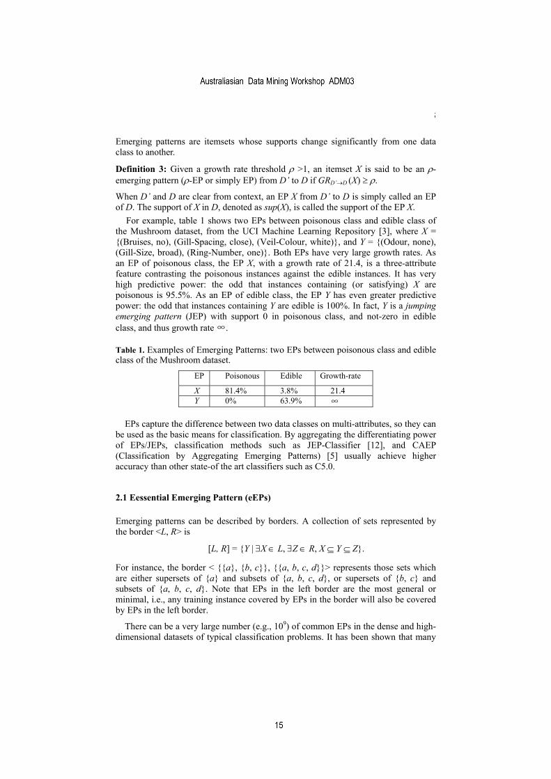
For example, table 1 shows two EPs between poisonous class and edible class of the Mushroom dataset, from the UCI Machine Learning Repository [3], where X = {(Bruises, no), (Gill-Spacing, close), (Veil-Colour, white)}, and Y = {(Odour, none), (Gill-Size, broad), (Ring-Number, one)}. Both EPs have very large growth rates. As an EP of poisonous class, the EP X, with a growth rate of 21.4, is a three-attribute feature contrasting the poisonous instances against the edible instances. It has very high predictive power: the odd that instances containing (or satisfying) X are poisonous is 95.5%. As an EP of edible class, the EP Y has even greater predictive power: the odd that instances containing Y are edible is 100%. In fact, Y is a jumping emerging pattern (JEP) with support 0 in poisonous class, and not-zero in edible class, and thus growth rate ∞.

Table 1. Examples of Emerging Patterns: two EPs between poisonous class and edible class of the Mushroom dataset.

EP Poisonous Edible Growth-rate

X 81.4% 3.8% 21.4 Y 0% 63.9% ∞

EPs capture the difference between two data classes on multi-attributes, so they can be used as the basic means for classification. By aggregating the differentiating power of EPs/JEPs, classification methods such as JEP-Classifier [12], and CAEP (Classification by Aggregating Emerging Patterns) [5] usually achieve higher accuracy than other state-of the art classifiers such as C5.0.

2.1 Eessential Emerging Pattern (eEPs)

Emerging patterns can be described by borders. A collection of sets represented by the border <L, R> is

[L, R] = {Y | ∃X ∈ L, ∃Z ∈ R, X ⊆ Y ⊆ Z}.

For instance, the border < {{a}, {b, c}}, {{a, b, c, d}}> represents those sets which are either supersets of {a} and subsets of {a, b, c, d}, or supersets of {b, c} and subsets of {a, b, c, d}. Note that EPs in the left border are the most general or minimal, i.e., any training instance covered by EPs in the border will also be covered by EPs in the left border.

There can be a very large number (e.g., 109) of common EPs in the dense and high-dimensional datasets of typical classification problems. It has been shown that many

6 M. Fan, W. Zhi, H. Fan, Y. Sun

of them are not so useful in classification [7]. Suppose that X1 and X2 are two EPs, and X1 ⊂ X2. X2 is less useful than X1 for classification because every example covered by X2 must also be covered by X1. Shorter EPs contains fewer attributes, and tend to have larger supports. If we can use a few attributes to distinguish two data classes, adding more attributes will not contribute to classification, and in some worse cases, bring noise.

Previous works show that essential emerging patterns are sufficient for building accurate classifiers.

Definition 4: An itemset X is called an essential emerging pattern (eEP) of the target class C if it satisfies the following conditions:

(1) X is an EP of class C with high growth rate ρ, and

(2) any proper subset of X is not an EP of class C, and

(3) the support of X in class C is not less than ξ, where ξ is a predefined min-support threshold.

eEPs are believed to be the most expressive patterns for classification because of the following reasons:

Large or even infinite growth rates ensure that each eEP has significant level of discrimination. The minimum support threshold makes every eEP cover at least a certain

number of training instances, because itemsets with too low supports are regarded as noise. Supersets of eEPs are not useful for classification because of the following

reason. Suppose E1 ⊂ E2, where E1 is an eEP. E1 covers more (at least equal) training instances than E2, because sup(E1) >= sup(E2). By the definition of eEP, both E1 and E2 have large growth rate. So E2 does not provide any more information for classification than E1.

In fact, eEPs are the shortest EPs contained in the left bound of the border representing the EP collections, and have at least a certain coverage rate on the training dataset. The set of eEPs is much smaller than the set of all common EPs. The classifiers based on eEPs is not only more efficient, but also more effective.

2.2 Tree Based Algorithms for Efficiently Mining eEPs

Efficient tree based algorithms have been developed to mine essential emerging pattern [7]. The tree data structure is called P-tree. Like FP-tree [10], P-tree stores compressed all the item information of the training data. Unlike FP-tree, P-tree keeps the class attributes information in order to mine EPs. The algorithm adopts the pattern fragment growth mining method: it recursively partitions the database into sub-database according to the patterns found and search for local patterns to assemble longer global one. It searches the tree in the depth-first manner; it operates directly on the data contained in the tree, i.e., no new nodes are inserted into the original tree and no nodes are removed from it during the mining process. The major operations of

Two Phase Classification by Emerging Patterns 7

mining are counting and link adjusting, which are usually less expensive than the previous Apriori level-wise, candidate generation-and-test approach.

The details of these algorithms are omitted here. They can be found in [6,7].

3. Two Phase Classification By Emerging Patterns (TPCEP)

3.1 Basic Ideas

We use two-class problem to show the basic idea of TPCEP classifier. Suppose the two classes are C1 and C2. TPCEP mines eEPs of C1 and C2 in two phases and uses these eEPs and their supports to construct classifier of each phase. In the first phase, we use all of the training instances to mine eEPs. In the second phase, we focus on those instances that are covered by eEPs of the wrong class. For example, eEPs of C1 from the first phase also cover some instances of C2. Our aim is to mine another set of eEPs to identify these “false positives” or “true negatives”.

When the growth rate threshold ρ is high enough, eEPs of C will cover many training instances of C (cover-rate = ξ) and few training instances of non-C.

3.2 Mine P-eEPs and N-eEPs

In the first phase, we use all the training instances to generate eEPs of C1 and C2. By adjusting min-growth-rate threshold η and min-support threshold ξ, we make the eEPs of C1 cover a certain percentage (e.g. 90% or more) of C1. Here we don’t care these eEPs’ coverage on C2. Figure 1 (a) expresses the process, where the two rectangles show the training instances of C1 and C2 respectively, the instances in the light-grey area are those instances that eEPs of C1 covered. The eEPs cover most of the instances of C1 and part of instances of C2. Similarly, eEPs of C2 cover many instances of C2 while only a few instances of C1.

The eEPs of C1 (or C2) mined in the first phase are called P-eEPs of C1 (or C2). Using the P-eEPs of C1 and C2 mined in the first phase, we can build a single-phase classifier. Suppose S is a test instance. Suppose S contains P-eEPs of C1: X11, …, X1m, with supports s11,…,s1m respectively; S also contains P-eEPs of C2: X21, …, X2k, with supports s21,…,s2k respectively. We use formula (1) (see section 3.3) to calculate the similarity rate of C1 and C2 for S, denoted as SR1(S, C1) and SR1(S, C2). The classifier of single-phase uses the following rules to classify S:

If SR1(S,C1) > SR1(S,C2) or ( SR1(S,C1) = SR1(S,C2) and | C1 | ≥ | C2 | ), the class label of S will be C1, else be C2.

Although the single-phase classifier is simple, it achieves good accuracy for classification. However, there is much room to improve it by adding the second phrase. (See experiment result and analysis)

8 M. Fan, W. Zhi, H. Fan, Y. Sun

(b) (a)

Instances of C1

Instances of C2

Instances of C1

Instances of C2

Fig. 1. The training instances used in mining eEPs in two phases. (a) In the first phase, we use all the training instances to generate P-eEPs of C1; (b) in the second phase, we only use the instances that covered by P-eEPs of C1 mined in the first phase to generate N-eEPs of C1.

In the second phase, to generate eEPs of C2 (or C1), we only use the instances that covered by P-eEPs of C1 (or C2) mined in the first phase. Take mining eEPs of C2 for example. Fig.1 (b) shows those instances used in the second phase. Here, we use all the instances of C1 and the instances of C2 covered by P-eEPs of C1 to mine eEPs of C2. The eEPs of C2 mined here in the second phase are also called N-eEPs of C1, because they are “negative” eEPs of C1. Similarly, the eEPs of C1 mined in the second phase are also called N-eEPs of C2.

Now we have P-eEPs (the first phrase) and N-eEPs (the second phrase) for each class. In the second phase we pay more attention on the possible misclassification than the first phase. Since we have additional EPs mined in the second phrase, we need to design a new scoring method to use eEPs of both phases and their supports to make a better classification.

3.3 Scoring function (Calculation of Similarity Rate)

To classify an unseen instance S, TPCEP needs to calculate a score for each class. The class with the highest score is then returned as the classification. The idea behind the scoring function is that if the unknown instance S belongs to class Ci, S will be “similar” to the instances of Ci. The similarity can be measured using the eEPs of Ci that are contained in S. Suppose S contains an eEP of Ci, denoted as E1. E1 has enough support, which suggests S is consistent to a reasonable number of instances of Ci on a group of attributes. E1 also has large growth rate, which means S is very unlike the classes other than Ci. Intuitively, the more percentage eEPs of S cover the instances of Ci, the more similar S is to Ci.

Definition 5: Given a test instance S and a set E(C) of EPs of a class C discovered from the training data, the similarity rate of S for C, denoted as SR(S,C), can be calculated using the following steps:

1. Find the EPs from E(C) which are contained by S, denoted as X1 ,…, Xm.

2. set count = 0;

3. for each instance in C, if it contains one EP from X1 ,…, Xm, then count++;

Two Phase Classification by Emerging Patterns 9

4. SR(S,C) = count / the total number of instances of C

Step 3 counts how many instances of C are covered by the set of EPs X1 ,…, Xm collectively. Here we say an instance is covered by the EP set if the instance contains one EP from that set.

We can use the eEPs and their supports to calculate SR(S,C) approximately. Suppose S is a test instance and it contains eEPs X1 ,…, Xm, of Ci, where the supports are s1 ,…, sm, respectively. Let Ai be the event “Xi appears in the instances of C”. The calculation of SR(S,C) is equivalent to the calculation of probability P(A1∪…∪Am). So, we have:

)...()1(...)()()(

)...(),(

211

111

1

mm

mkjikjiji

mji

m

ii

m

AAAPAAAPAAPAP

AAPCSSR−

≤<<≤≤<≤=−+++−=

∪∪=

∑∑∑

where P(Ai) = si. Assuming that eEPs are independent, we have the following approximation:

mm

mkjikji

mjiji

m

ii sssssssssCSSR ...)1(...),( 21

1

111

−

≤<<≤≤<≤=−+++−= ∑∑∑ (1)

3.4 TPCEP Classification

In training phase, the task of TPCEP classification is to mine eEPs with their supports in two phases. eEPs and their supports construct the basis of TPCEP classification.

Definition 6: Suppose S is an unclassified instances, SR1(S, Ci) is the similarity rate of Ci for S using eEPs of Ci mined in the first phase (i.e., P-eEPs of Ci), and SR2(S, Cj) (j ≠ i) are the similarity rate of Cj for S using eEPs mined in the second phase (i.e., N-eEPs of Ci). The score of S for Ci is defined as score(S, Ci) = SR1(S, Ci) - SR2(S, Cj), where i, j = 1 or 2, i ≠ j.

The scoring method considers to use the second phase to correct the errors made in the first phrase.

Given a test instance S, S will be classified as the class with the highest score. That is, after TPCEP calculates score(S,C1) and score(S, C2), it uses the following rules to decide the class label for S:

If score(S,C1) > score(S,C2) or score(S,C1) = score(S,C2) and | C1 | ≥ | C2 |, the class label of S will be C1, else be C2.

3.5 Multiple Classes Problem

TPCEP can be easily extended to k (>2) classes. For a k-class problem, we build k classifiers: G1 ,…, Gk. Firstly, we use all the training data and partition it into two classes: C1 and non-C1. We build classifier G1 in the first step. Then the whole training data is regarded as another two classes: C2 and non-C2 (including C1). In the

10 M. Fan, W. Zhi, H. Fan, Y. Sun

second step we build the classifier G2. Generally, to build Gi, we divide the whole training dataset into two classes: Ci and non-Ci.

To classify a test S, we use G1 ,…, Gk to decide the class label of S. After computing all the scores of S for Ci, we compare the scores and assign S to the class with the highest score.

4. Experiment Result and Analysis

In order to investigate TPCEP’s performance compared with that of other classifiers, we carry experiments on 10 datasets from UCI Machine Learning Repository. We compare TPCEP with other state-of-the-art classifiers: Naive Bayes (NB), the two important classifiers based on association rules CBA [14] and CMAR [13], the widely known decision tree induction C5.0; an EP-based classifier CAEP; and BCEP, a novel Bayes classifier based on emerging patterns.

Our experiments were performed on a 900Mhz Pentium III PC with 128Mb of memory. The programming environment is Microsoft Visual C++. The accuracy was obtained by using the methodology of ten-fold cross-validation. We use the Entropy method in [8] to discretize datasets containing continuous attributes. Experiment results of the competitive classifiers are taken from their original papers.

Table 2. Summary of the predictive accuracy of of classifiers.

Dataset Accuracy (%) CBA CMAR NB C5.0 CAEP BCEP TPCEP One-phase

Adult --- --- 84.12 85.54 83.09 85.00 80.30 78.60 Australia 84.90 86.10 85.65 84.93 85.51 86.40 89.30 86.97

Cleve 82.80 82.20 82.78 77.16 82.13 82.41 91.30 86.30 Diabete 74.50 75.80 75.13 73.03 67.30 76.80 77.30 71.78 German 73.40 74.90 74.10 71.90 74.50 74.50 73.30 72.08

Heart 81.90 82.20 88.22 76.30 82.22 81.85 88.93 76.70 Mushroom --- --- 99.68 100.00 93.91 100.00 99.20 98.70

Pima 72.90 75.10 75.90 75.39 77.60 75.66 77.70 71.82 Tic-tac 99.60 99.20 70.15 85.91 85.91 99.37 85.80 77.40

Vehicle 68.70 68.80 61.12 73.68 68.80 68.05 66.30 --- Average 79.69 80.38 80.10 83.00 82.94

Table 2 summarizes the accuracy results. From the table, we can see that TPCEP achieves the best accuracy on 5 datasets and also performs well on the other datasets. The average accuracy of TPCEP is higher than that of NB, C5.0, and CAEP; and it is almost the same as BCEP. The advantage of TPCEP over BCEP is that TPCEP is much faster. BCEP is slow because it has to calculate probability approximation using many itemsets in a chain of product. TPCEP is fast due to a relatively simple scoring function. TPCEP dose not degrade accuracy because two-phrase mechanism can correct the errors made by simple scoring to some extend.

Two Phase Classification by Emerging Patterns 11

Comparing to the CBA and CMAR, two classifiers based on association rules, we can see that TPCEP wins on five datasets, Australia, Cleve, Diabete, Heart, Pima, but loses on the three datasets, namely, German, Tic-tac and Vehicle.

In the last column, we give the results obtained by EP-based single-phase classification that uses the same scoring function as TPCEP. We can see that single-phase classifier is fairly good. Further more, we can see that TPCEP wins its single-phase counterpart on most of the datasets. These experimental results confirm our belief that two-phase classification has advantages over one-phase.

5. Conclusion

In the paper, we have proposed a new novel classifier, i.e., Two-Phase Classification by Emerging Patterns (TPCEP). TPCEP combines the benefits of two-phase classification method and classification by emerging patterns. The first phase of TPCEP aims to find the EPs that have high supports and high coverage on the training data. Here we alleviate the strict requirement of high support-ratio EPs. The second phase will then tries to mine another set of EPs which can remove false positives in the collection of the instances covered by the first phase EPs. Here we correct the errors due to the use of moderate support-ratio EPs whose discriminating power are not so sharp. Our experiment study carried on 10 benchmark datasets from the UCI Machine Learning Repository shows that TPCEP performs comparably with other state-of-the-art classification methods such as CBA, CMAR, C5.0, NB, CAEP LB and BCEP in terms of overall predictive accuracy.

The factors that can affect the accuracy of TPCEP are the differentiation power of EPs and their coverage on data. These factors are represented by two interrelated parameters: min-support threshold and min-growth rate threshold. Generally, fixing min-support threshold, higher growth rate will result in more discriminating EPs, but can reduce coverage on the training data (does not generalize well). Fixing growth rate, higher min-support threshold may lead to lower coverage; but when min-support is too low, EPs may be not statistically significant and thus the classifier built upon them tends to overfit. To select the right values for these thresholds is the art of human, guided by trial and error. As the future work, we will go deeper on the problem of automatic optimization of the two parameters.

References

1. R. Agarwal, and M. V. Joshi. PNrule: A new Framework for Learning Classifier Models in Data Mining (A Case-Study in Network Intrusion Detection). In Proc. of the First SIAM Conference on Data Mining. Chicago, USA, April 2001.

2. R. Agarwal, M. V. Joshi, and V. Kumar. Mining Needles in a Haystack: Classifying Rare Classes via Two-Phase Rule Induction. In Proc. of the 2001 ACM SIGMOD, pp 91-102, Santa Barbara, California, USA, May 2001.

12 M. Fan, W. Zhi, H. Fan, Y. Sun

3. C. Blake, and C. Merz. UCI repository of machine learning databases. [http://www.ics.uci.edu/~mlearn/MLRepository.html]. Irvine, CA: University of California, Department of Information and Computer Science.

4. G. Dong and J. Li. Efficient mining of emerging patterns: Discovering trends and differences. In Proc. of KDD’99, pp 15-18, San Diego, USA, Sep. 1999.

5. G. Dong, X. Zhang, L. Wong and J. Li. CAEP: Classification by Aggregating emerging patterns. In Proc. of the 2nd Int’l Conf. On Discovery Science (DS’99), pp 30-42, Tokyo, Japan, Dec 1999.

6. H. Fan and K. Ramamohanarao. An Efficient Single-Scan Algorithm for Mining Essential Jumping Emerging Patterns for Classification. In Proc. of 2002 Pacific-Asia Conf. on Knowledge Discovery and Data Mining (PAKDD'02), pp455-562, Taipei, Taiwan, China, May 6-8, 2002.

7. H. Fan and K. Ramamohanarao. A Bayesian Approach to use Emerging Patterns for Classification. In Proc of the 14th Australasian Database Conference. pp 39-48 Feb 2003.

8. U. M. Fayyad and K. B. Irani. Multi-interval Discretization of Continuous-valued Attributes for Classification learning. In Proc. the 13 International Joint Conference on Artificial Intelligence (IJCAI), pp.1022-1029, San Francisco, USA.

9. J. Han and M. Kamber. Data Mining: Concepts and Techniques. Morgan Kaufmann Publishers, 2000.

10. J. Han, J. Pei, J. and Y. Yin. Mining frequent patterns without candidate generation. In Proc. of the 2000 ACM-SIGMOD Intl. Conf. on Management of Data, pp 1-12, May 2000.

11. Holte, R. C., Acker, L. E. and Porter, B. W. (1989). Concept Learning and the Problem of Small Disjuncts. In Proc. of Eleventh International Joint Conference on Artificial Intelligence (IJCAI-89), 1989, pp 813-818.

12. J. Li, G. Dong and K. Ramamohanarao. Making Use of the Most expressive Jumping Emerging Patterns for Classification. In Proc. of 2000 Pacific-Asia Conf. Knowledge Discovery and Data Mining (PAKDD’00), pp 220-232.

13. W. Li, J. Han, and J. Pei. CMAR: Accurate and efficient classification based on multiple class-association rules. In ICDM’01, pp. 369-376, San Jose, CA, Nov. 2001.

14. B. Liu, W. Hsu, and Y. Ma. Integrating classification and association rule mining. In KDD’98, pp. 80-86, New York, NY, Aug. 1998.

Feature Preparation in Text Categorization

Ciya Liao1, Shamim Alpha

1, Paul Dixon

1

1Oracle Corporation,

{david.liao, shamim.alpha, paul.dixon}@oracle.com

Abstract. Text categorization is an important application of machine learning

to the field of document information retrieval. Most machine learning methodstreat text documents as a feature vectors. We report text categorization accuracyfor different types of features and different types of feature weights. We reportthe classification result for neural network classification and Support VectorMachine by using Reuters and Ohsumed collections. We found that SVM is su-perior to neural network classification in both effectiveness and efficiency. Inour experiments, we did not see any significant improvement for classificationaccuracy by using noun-phrase features. The comparison of those classifiersshows surprisingly that the simply stemmed or un-stemmed single words as fea-tures give a better classifier compared to other type of features.

1 Introduction

Text categorization is a conventional classification problem applied to the textual do-

main. It solves the problem of assigning text content to predefined categories. As thevolume of text content grows continuously on-line and in corporate domains, textcategorization, acting as a way to organize the text content, becomes interesting notonly from an academic but also from an industrial point of view. A growing numberof statistical classification methods have been applied to text categorization, such asNaive Bayesian (Joachims,1997), Bayesian Network (Sahami,1996), Decision Tree(Quinlan,1993;Weiss,1999), Neural Network(Wiener,1995), Linear Regres-sion(Yang,1992), k-NN (Yang,1999), Support Vector Machines (Dumais,1998;

Joachims, 1998), and Boosting (Schapire,2000; Weiss,1999). A comprehensive com-parative evaluation of a wide-range of text categorization methods is reported inref.(Yang,1999; Dumais,1998) against the Reuters corpus.

Most of the statistical classification methods mentioned above are borrowed fromthe field of machine learning, where a classified item is treated as a feature vector. Asimple way to transform a text document into a feature vector is using a “bag-of-words” representation, where each feature is a single token. There are two problems

associated with this representation.

The first problem to be raised when using a feature vector representation is to an-swer the question, “what is a feature?”. In general, a feature can be either local or

global. In text categorization, local features are always used but in different-length

scales of locality. A feature can be as simple as a single token, or a linguistic phrase,or a much more complicated syntax template. A feature can be a characteristic quan-tity at different linguistic levels. To transform a document, which can be regarded as astring of tokens, into another set of tokens will lose some linguistic information suchas word sequence. Word sequence is crucial for a human being to understand a docu-ment and should be also crucial for a computer. Using phrases as features is a partialsolution for incorporating word sequence information into text categorization. Thispaper will investigate the effectiveness of different classifiers by using single tokens,phrases, stemmed tokens, etc. as features.

The second problem is how to quantify a feature. A feature weight should show thedegree of information represented by local feature occurrences in a document, at aminimum. A slightly more complicated feature weight scheme may also represent sta-

tistical information of the feature’s occurrence within the whole training set or in apre-existing knowledge base (taxonomy or ontology). A yet more complicated featureweight may also include information about feature distribution among different

classes. This paper will only investigate the first two types of feature weights.

2 From Text to Features

In order to transform a document into a feature vector, preprocessing is needed. Thisincludes feature formation (tokenization, phrase formation, or higher level feature ex-

traction), feature selection, and feature score calculations. Tokenization is a trivialproblem for white-spaced languages like English.

Feature formation must be performed with reference to the definition of the fea-tures. Different linguistic components of a document can form different types of fea-

tures. Features such as single tokens or single stemmed tokens are most frequently

used in text categorization. In this bag-of-words representation, information about de-pendencies and the relative positions of different tokens are not used. Phrasal features

consisting of more than one token are one possible way to make use of the dependen-

cies and relative positions of component tokens. Previous experiments (Sahami,1996;Dumais,1998) show that introducing some degree of term dependence in the Bayesian

network method will achieve undoubtably higher accuracy in text categorizationcompared to the independence assumption in the Naive Bayesian method. However,

whether the introduction of phrases will improve the accuracy of text categorizationhas been debated for a long time. Lewis (Lewis,1992) was the first to study the effectsof syntactic phrases in text categorization. In his study, a naive Bayesian classifier

with only noun phrases yielded significantly lower effectiveness than a standard clas-sifier using bag-of-single-words. More reports on inclusion of syntactic phrases show

no significant improvement on rule-based classifiers (Scott,1999) and naive Bayesianand SVM classifiers (Dumais,1998). For statistical phrases like n-grams, one report(Caropreso,2001) shows that certain term selection methods such as document fre-

quency, information gain and chi-square give high selection scores to a considerable

number of statistical phrases, which indicates they have important predictive value. In

the same report, directly using selected uni-grams or bigrams during text categoriza-tion with the Rocchio classifier yields a slightly higher effectiveness compared to

only using uni-grams in the case that the classifier chooses an adequate but equal

number of terms as features. A significant drop in effectiveness was observed when

the classifier chose fewer terms. The report then commented that inclusion of somebigrams may only duplicate information of existing uni-grams but force other impor-tant uni-grams out. However, other reports on statistical phrases show that the addi-tion of n-grams to the single words model can improve performance in the shorter-length n-grams case(Furnkranz, 1998; Mladenic,1998).

One type of a higher level feature has been studied in text categorization (Furnk-ranz,1998), where linguistic patterns were extracted automatically and input as fea-tures to naive Bayesian and rule-based classifiers. A consistent improvement in preci-sion was observed in the naive Bayesian classifier and at low recall level in the rule-based classifier. Adding linguistic patterns to the single word representation yieldsconsistent improvement of precision except at a very high recall level.

Feature selection has been studied by (Yang,1997), where information gain and

chi-square methods are found most effective for k-NN and linear regression learningmethods. Term selection based on document frequency in the training set as a wholeis simple but has similar performance to information gain and chi-square methods.

Selected features must be associated with a numerical value to evaluate the impactof the feature to the classification problem. Most types of feature weighting schemesin text categorization are borrowed from the field of information retrieval. The mostfrequently used weight is TFIDF (Salton, 1988). The original TFIDF is:

f

fdfddf

Dlogtf=ω

(1)

where ωfd

is the weight of feature f in document d, tffd

the occurrence frequency offeature f in document d, D the total number of documents in the training set, and df

fis

the number of documents containing the feature f.

In this paper, we will compare text categorization using different types of features,and different types of feature weighting schemes. The feature types will include singletokens, single stemmed tokens, and phrases. Weighting schemes will include binaryfeature (BI), term frequency (TF), TFIDF(eq.1), logTFIDF(eq.2), etc.

f

fdfddf

Dlog)5.0tflog( +=ω

(2)

We note that the logarithm of the TF part is to amend unfavorable linearity. Themachine learning algorithms we report in this paper include SVM (Joachims, 1998)and Neural Network. Feature selection in Neural Networks and Support Vector Ma-chine classifiers is based on document frequency. Only features (single words orphrases) occurring in an adequate number of training documents will be selected. Thecorpus includes reuters-21578 and ohsumed.

3 Phrase Features

We only use training set documents to find valid phrases. We first scan the documentsin the training set and detect phrases based on linguistic and statistical conditions. We

only use noun phrases as valid phrases. Valid phrases are inserted into a phrase data-base which is specific to the training set. The phrase database is used to replace thephrases in the training documents and test documents with specific tokens. For exam-ple, the phrase "information retrieval" in the document will be changed to the token"information_retrieval". After phrases in the documents are marked, the documentscan be input into tokenization program in training or classification processes for per-formance testing.

To detect valid noun phrase chunking, Brill’s transformation-based part of speechtagger (Brill, 1995) was used to mark parts-of-speech in the training documents.Training documents with POS tags are input into Ramshaw&Marcus’s noun phrasechunking detector (Ramshaw,1995) for noun phrase detection. The resultant nounphrase chunks are output to a file, which is input to a statistical chi-square test pro-

gram. This program tests the statistical significance of co-occurrences of the compo-nent tokens in n-gram noun phrases. In particular, we choose the noun phrases(ngrams, up to 4-grams) such that the null hypothesis that its component tokens areindependent of each other can be proved not true.

4 Machine Learning Algorithms

We test two different type of machine learning algorithms: Neural Networks andSupport Vector Machines. We use the SVM_light package (Joachims, 1998) with de-

fault parameter settings, which results in a linear SVM classifier.For Neural Network, we use a home-made program. The Neural Network has no

hidden layer and therefore is equivalent to a linear classifier. Text document classifi-cation has high dimensional data characteristics because of the large size of naturallanguage vocabulary. Documents in one class usually can be linearly separated fromother classes due to high dimensionality (Joachims,1998;Schutze,1995). A prior ex-periment (Schutze, 1995) shows that linear neural networks can achieve the same ac-curacy as non-linear neural networks with hidden layers.

During the learning process, a sequential back propagation algorithm is used tominimize training error. We use cross-entropy error, thus making our learning methodequivalent to logistic regression learning (Schutze, 1995). We tried to use weightregularization methods (Zhang, 2001) to deal with overfitting, but the accuracy was

not improved and convergence is hard to achieve by using back propagation learning.The results we present in this paper do not use regularization.

5 Corpus

The evaluation experiments are done on two text collections. The first is Reuters-

21578 with ModApte split. Many text categorization methods have been tested

against this corpus (Yang,1999; Dumais,1998; Joachims,1998). This is a collection of

newswire stories from 1987 compiled by David Lewis. The number of distinct tokensin the training set is 39189, of which 18586 tokens occur more than once, 12951 to-kens occur more than twice, 10328 tokens occur more than three times, 8789 tokensoccur more than four times, and 3262 tokens occur more than 20 times in the trainingset.

The second collection is taken from Ohsumed corpus used in the Filtering Track inTREC-9 (Robertson,2000). The Ohsumed collection consists of Medline documentsfrom the years 1987-1991 and a set of topics and relevance judgments. In order to re-duce the size of the problem, we chose MESH categories in which the number of Oh-sumed documents in 1991 is larger than 300 (which results 98 categories). The train-ing/testing split is across the document series number 91250000. Training documentshave the document series number less than 91250000. This split results in 14655

training documents and 6698 test documents. The resultant training set and testing sethave more homogenous distribution across different categories than the Reuters col-lection. The minimum (maximum) number of training documents in one category is65 (465). The minimum (maximum) number of testing documents in one category is29(214). In the training set, there are 52162 distinct tokens, of which 28857 tokensoccur more than once, 22128 tokens occur more than twice, 18493 tokens occur morethan three times, 9224 tokens occur more than 12 times, and 3458 tokens occur morethan 60 times.

6 Experiment Results and Discussion

We first compare the impact of different feature types. The meaning of the followinglegends in the figure denote feature types: “single words” means only single tokens as

features, “noun phrases” uses detected noun phrases as features without using compo-

nent tokens, “stem words” uses Porter-stemmer-determined stems for each token asfeatures, “noun phrases and words” uses detected noun phrases and their component

tokens.

Fig.1 and Fig.2 show the micro-average breakeven points (BEP) with differentnumbers of features using the SVM classifier to classify the Reuters and ohsumed

corpora, respectively. Breakeven accuracies increase with the number of features.There is no overfitting observed in the experimental range as the number of features

increases. The maximum number of features in Fig.1 is 16000 for Reuters. This num-ber of single tokens is roughly the number of tokens occurring twice or above in thetraining set. The maximum number of features in Fig.2 is 20000 for ohsumed. This

number of single tokens is roughly the number of tokens occurring three times orabove in the training set.

The maximum BEPs are achieved at the maximum number of features. For reuters,the best BEP is 0.88, which is slightly higher than the reported microAvg. BEP in(Joachims, 1998) (0.860). For ohsumed, the best BEP is 0.602, achieved by using

stem words.

The effect of stemming can be easily seen in Fig. 1 and 2. When the number of fea-

tures is small, the coverage of selected features is poor but stemming of words can in-crease the feature coverage, thus giving the best breakeven accuracy compared to

other types of features. However, as the number of chosen features increases, and

coverage of the chosen features becomes large enough, the accuracy of the features in

conveying the information becomes more important. This can be seen in Fig.1 wherethe BEPs of other types of features are as good as stem words at large number of fea-tures.

0.75

0.77

0.79

0.81

0.83

0.85

0.87

0.89

0 2000 4000 6000 8000 10000 12000 14000 16000

number of features

bre

ake

ve

np

oin

ts

single words

noun phrases

stem words

noun phrases and words

Fig. 1. Breakeven points for the Reuters collection using SVM. The feature vector

is normalized to have unity sum. The feature weight is LOGTFIDF.

0.3

0.35

0.4

0.45

0.5

0.55

0.6

0.65

0 5000 10000 15000 20000

number of features

bre

akeven

poin

ts

single words

noun phrases

stem words

Fig. 2. Breakeven points for the ohsumed collection using SVM. The feature vector is normal-

ized to have unity sum. The feature weight is LOGTFIDF.

It is interesting to see how well the automatically determined noun phrase features

perform. The Fig.1 and Fig. 2 show that noun phrases classifiers give the worst BEP.This is disappointing. It was expected that good phrase features provide more accurateinformation by constraining the meaning of component words. One example is thephrase “consumer price index”, where the combination of the three token means a

specific index. However, this result is consistent with the findings of the previous lit-

erature (Lewis,1992; Scott,1999; Dumais,1998). This can be partially explained bydecreased feature coverage due to replacement of original tokens by phrases. For ex-

ample, if the two words “oracle database” are replaced by one phrase “ora-

cle_database”, this phrase feature will only match itself and can not convey any simi-larity with its individual word components “oracle” and “database”. However, we

know that an article discussing enterprise software may only mention “oracle” or “da-tabase” separately. Another example is replacing the two phrases “Oracle database”

and “DB2 database” with two separate features makes it impossible to map the simi-larity existing between them. Thus each phrase will have narrower coverage. Thecoverage problem is caused by replacing a number of token features with a single fea-

ture which is more accurate but finer. This problem can be partially reduced by not

eliminating the phrase’s component words. In fig.1, we see a significant increase of

BEP for noun phrases including component words.The single words are natural linguistic units and are employed by many text classi-

fication systems. From Fig.1 and Fig.2, one can see that this natural and simple fea-

ture unit performs fairly well compared with other complicated types of features.

0.7

0.75

0.8

0.85

0.9

0 2000 4000 6000 8000 10000

number of features

bre

akeven

poin

ts

single words

noun phrases

stem words

noun phrases and words

Fig. 3. Breakeven points for the Reuters collection using Neural Network. The feature vector is

normalized to have unity sum. The feature weight is LOGTFIDF

The above results and discussion about types of features are not just applied to a

single machine learning algorithm (SVM in Fig.1, Fig.2). We performed the same ex-periments with a Neural Network classifier. The results are shown in Fig.3 and Fig.4.The BEPs using Neural Network are not as good as those using SVM. The maximumBEP using Neural Network is 0.871 for Reuters using single words and 0.568 for oh-sumed using stem words. It is worthwhile to mention that the training time for theneural network is much longer than SVM (>10 times in this experiment’s problemscale).

0

0.1

0.2

0.3

0.4

0.5

0.6

0 2000 4000 6000 8000 10000

number of features

bre

akeven

poin

ts

single words

noun phrases

stem words

Fig. 4. Breakeven points for the ohsumed collection using Neural Network. The feature vector

is normalized to have unity sum. The feature weight is LOGTFIDF

So far, the discussed results all use one feature weighting scheme: LOGTFIDF (eq.2). In Fig.5, Fig.6, we employed different feature weighting schemes. They are:

− IDF: log(D/dff)

− TF: tffd

− TFIDF: eq. 1

− LOGTFIDF: eq. 2

− LOGTF: log(tffd)

− BINARY: 1 or 0

Although the BEP ranking sequence for different weighting schemes is different

for Fig.5 and Fig.6, we still can find some common characteristics for weightingmethods based on the results vs. the Reuters and ohsumed collections. One can ob-serve that the BEPs using LOGTF weight are always larger than those using TFweight. This shows that non-linear weighting of term frequency is better than conven-tional linear weighting. We think that this observation also holds in the field of infor-mation retrieval for relevance ranking.

Fig.5 and Fig.6 show that IDF weighting is better than BINARY weighting. Be-cause IDF weight is only assigned to a feature occurring in the concerned document,IDF weight is actually BINARY weight multiplying an IDF score which contains thestatistical information of the feature inside the whole corpus. Considering the fact thatTFIDF is better than TF, LOGTFIDF better than LOGTF, one can than conclude thatintroducing the corpus information helps improve the accuracy of text categorization.

It is seen from Fig.5 and Fig.6 that LOGTFIDF, which is the multiplication of theLOGTF and IDF weights, performs the best in both collections.

0.74

0.76

0.78

0.8

0.82

0.84

0.86

0.88

0.9

0 2000 4000 6000 8000 10000 12000 14000 16000

number of features

bre

ake

ve

np

oin

ts

IDFTFIDFLOGTFIDFTFLOGTFBINARY

Fig. 5. Breakeven points for the Reuters collection using SVM. The feature vector

is normalized to have unity length. The features are single words.

0.3

0.35

0.4

0.45

0.5

0.55

0.6

0.65

0 5000 10000 15000 20000

number of features

bre

ak

ev

en

po

ints

IDF

TFIDF

LOGTFIDF

TF

LOGTF

BINARY

Fig. 6. Breakeven points for the ohsumed collection using SVM. The feature vector is normal-

ized to have unity length. The features are single words.

7 Conclusions

We have compared text classifiers using different types of features and differentweighting schemes. In order to achieve a generic conclusion regarding the featurepreparation independent with machine learning algorithms, we employed SupportVector Machines and a Neural Network algorithm as two machine learning classifi-ers. We tested these classifiers on the Reuters and ohsumed collections. Based on thiscomparison, we find that SVM algorithm is superior to the linearized neural networkboth in accuracy and training speed. Stem words, which normalize different featureforms to one stem form, show significant advantages in the case where a small num-ber of features are used because of the larger coverage of the stems. Replacing con-tiguous tokens with detected noun phrases as features gains accuracy but loses cover-

age due to the problem of normalization. One may surmise that if a similarity matchbetween different features is introduced to replace the current binary match betweentwo features, the feature normalization problem will be eliminated. Single words asfeatures perform fairly well. The comparison of different weighting schemes showsLOGTFIDF as the preferred feature weighting method.

References

1. Joachims T.(1998), Text categorization with support vector machines: learningwith many relevant features. Proceedings of ECML-98, 10th European Conference

on Machine Learning.2. Yang Y., Pederson J.O.(1997), A comparative study on feature selection in text

categorization, International Conference on Machine Learning (ICML).3. Yang Y.(1999), An evaluation of statistical approaches to text categorization.

Journal of Information Retrieval, Vol.1, No.1/2.4. Weiss S.W.,Apte C.,Damerau F.J., Johnson D.E.,Oles F.J.,Goetz T.,Hampp

T.(1999), Maximizing text-mining performance,IEEE Intelligent systems.5. Quinlan J.R.(1993), C4.5: Programs for machine learning, Morgan Kaufmann.6. Joachims T.(1997), A probabilistic analysis of the Rocchio algorithm with TFIDF

for text categorization, Proceedings of ICML-97, 14th International Conference onMachine Learning.

7. Wiener E.(1995), J.O.Pederson, A.S.Weigend, A neural network approach to topic

spotting. Proceedings of SDAIR-95, 4th Annual Symposium on Document Analy-sis and Information Retrieval.

8. Dumais S., Platt J., Heckerman D., Sahami M.(1998), Inductive learning algo-rithms and representations for text categorization. Proceedings of the 7th Interna-tional Conference on Information and Knowledge Management (CIKM 98).

9. Sahami M. (1996),Learning limited dependence Bayesian classifier. In KDD-96:Proceedings of the second international Conference on Knowledge Discovery andData Mining, 335-338. AAAI press.

10.Yang Y., Chute C.G.(1992), A linear least squares fit mapping method for infor-mation retrieval from natural language texts. Proceedings of the 14th InternationalConference on Computational Linguistics (COLING 92).

11.Schapire R.E., Singer Y.(2000),Boostexter: A boosting-based system for text cate-

gorization. Machine Learning, 39(2/3).12.D.D.Lewis D.D.(1992), Feature selection and feature extraction for text

categorization, Proceedings of Speech and Natural Language Workshop.13.Scott S., Matwin S.(1999), Feature engineering for text classification, Proceedings

of ICML-99, 16th International Conference on Machine Learning.14.Caropreso M.F., Matwin S., Sebastiani F.(2001), A learner-independent evaluation

of the usefulness of statistical phrases in automated text categorization, Text data-base and Document Management: Theory and Practice.

15.Furnkranz J.(1998), A study using n-gram features for text categorization. Techni-cal Report OEFAITR-98-30.

16.Mladenic D., Grobelnik M.(1998), Word sequences as features in text-learning.Proceedings of ERK-98, the Seventh Electrotechnical and Computer Science Con-ferences.

17.Furnkranz J., Mitchell T., Riloff E., A case study of using linguistic phrases fortext categorization on the WWW, Proceedings of the 1st AAAI Workshop onLearning for Text Categorization.

18.Brill E.(1995),Transformation-based error-driven learning and natural languageprocessing: a case study in part of speech tagging, Computational Linguistics,21(4).

19.Ramshaw L.A., Marcus M.P.(1995), Text chunking using transformation-based

learning, Proceedings of third Workshop on Very Large Corpora.20.Salton G., Buckley C.(1988), Term Weighting Approaches in Automatic Text Re-

trieval, Information Processing and Management, Vol. 24, No.5, P513.21.Schutze H., Hull D.A. (1995), J.O.Pederson, A Comparison of Classifiers and

Document Representations for the Routing Problem, in Proceedings of SIGIR95.22.Zhang T., Oles F.J.(2001), Text Categorization Based on Regularized Linear Clas-

sification Methods, Information Retrieval, vol.4.23.Robertson S., Hull D.A.(2000), The TREC-9 Filter Track Final report, Proceedings

of the Ninth Text Retrieval Conference (TREC-9).

Learning Quantitative Gene Interactions from

Microarray Data

Michael Bain1,3 and Bruno Gaeta1,2,3

1 School of Computer Science and Engineering, University of New South Wales,Sydney, Australia 2052

{mike,bgaeta}@cse.unsw.edu.au2 School of Biotechnology and Biomolecular Sciences, University of New South

Wales, Sydney, Australia 20523 The Clive & Vera Ramaciotti Centre for Gene Function Analysis

Abstract. The development of microarray technology has enabled thestates of entire genomes comprising tens or hundreds of thousands ofgenes to be measured in controlled experiments. The computational in-ference of genetic regulatory networks is a rapidly emerging area of bioin-formatics which requires the application of techniques from statistics anddata-mining to microarray data. A key problem is that the underlyingbiological systems are believed to be quite complex, and may incorpo-rate many genes at various times, although often there are relatively fewsamples in each experiment. This paper describes recent experimentsin automatically constructing quantitative gene interaction models frommicroarray data. The approach is based on earlier work on behaviouralcloning, where reactive agents are learned from the logged data of skilledhuman operators controlling a complex dynamic system. In behaviouralcloning the task of controlling the system is decomposed into that oflearning individual agents for the the control of a particular variable.Combining the agents results in a strategy for the successful control ofthe overall system. In this paper selected target genes are treated asagents and tree-structured models are applied to learn regulatory depen-dencies from a benchmark data set. We describe some interesting aspectsof the approach and outline directions for extending the work, includingthe design of an interactive system for biologists to use these machinelearning methods in exploratory data analysis.

1 Introduction

The increasing availability of technology to accomplish large scale assays israpidly moving biological data analysis requirements into the area of experi-mental “systems” biology. This presents a challenge to devise methods suitablefor discovery of biological knowledge from such data resources. It also makesavailable a role for the practice of data mining and machine learning alongsidemore traditional hypothesis testing methodologies in biology.

Genome-wide measurement of the activity of regulatory networks in cells isnow possible using the technology of DNA microarrays [2]. Such snapshots can

2

be combined to enable inference from data of the causal relationships betweengenes controlling the processes in living cells. Knowledge of such properties holdstremendous promise. For example, it may aid in understanding fundamental bio-logical processes such as the cell life cycle. The effect on genes of drug treatmentsor environmental factors, or the role of genes in diseases such as cancer can alsobe investigated by these methods.

2 Biological background

This section provides a brief review of the general problem of the underlyingbiological systems of interest, how they might be modelled, and how such modelsmight be learned.

2.1 Regulation in biological systems

Microarray technology allows experimental evaluation not of what constitutesthe genome (the full complement of genetic information of the organism) or eventhe proteome (the protein-coding regions of the genome) but the transcriptome(the population of mRNA transcripts in the cell weighted by their expressionlevels) [7]. The complexity of biological systems arises from the differential ex-pression of genes which results in the variation of gene products (such as pro-teins) available to participate in cell function. Typically only a small fractionof genes in a genome are expressed at any one time. Protein synthesis incursan energy cost, so unnecessary gene expression is inefficient. The main stages ingene expression and their points of regulation are shown in Figure 1.

So far our description of gene expression has left out many important de-tails. The key point, however, is that the process is regulated to maintain therequired concentrations of proteins (and other biochemical compounds) in thecell. Regulation of the initiation of transcription in particular allows the syn-chronised expression of multiple gene products on which the control of cellularprocesses depends. The relationships involved in such regulatory dependenciesare typically very complex. The interaction between protein and DNA involves aregion called a promoter to which regulatory proteins bind. Once the appropri-ate proteins, called transcription factors, are bound as a transcription complex,the transcription of the gene can begin, shown in Figure 2

Biological activity in cells can thus be viewed in terms of systems of inter-related molecular compounds undergoing self-regulation. Control is achieved bypathways of regulatory dependencies. The effect of transcription regulation canbe positive, to activate transcription, or negative, to suppress it. Through evo-lution these systems have developed to sustain the cell in an environment, soregulation must not only control the internal operation but also the movementof compounds in and out from the extracellular region. These metabolic andsignalling processes also have an effect on the expression of genes.

3

Fig. 1. Gene expression. In this example two genes (dark regions on the DNA) aretranscribed into RNAs then translated into proteins. These gene products contributeto cellular effects, including possible regulation of transcription and translation

2.2 Microarray technology

The basis of microarray technology is in the ability of DNA and RNA to bindtogether in complementary strands (for example in the well-known double he-lix). Essentially, microarrays are constructed for a set of probes, complementaryto a set of genes, such as the genome of an organism. These probes are boundto the surface of the array. When a sample containing genetic material (DNAor RNA) is introduced, the probes on the array will bind to the complementarynucleotide chain by a process called hybridization. With suitable marking, usu-ally a fluorescent chemical, the intensity of the binding of the different probescan be measured.

The expression level as measured by this intensity (actually derived by pro-cessing an image of the entire array) is taken to indicate the amount of transcrip-tion of the corresponding genes in the biological system from which the samplewas extracted. In turn, this is taken to indicate the protein concentration. Afurther complication is that expression levels can be estimated as ratios of twomeasurements, for example from two samples under different conditions.

2.3 Modelling cellular systems

As noted above, the advent of microarrays and other “high-throughput” formsof technology for biological analyses is leading to a shift of approach in exper-imentation. In the past a typical focus would be to test hypotheses applyingto a single gene or gene product at a time. A picture of the underlying system

4

would have to be built up step-by-step. Now it is possible to test all of the genesfor their activity as part of entire biological systems. In terms of computationalbiology, this leads ultimately to the modelling in silico of cells or even complete“virtual organisms” [5, 10].

Fig. 2. Transcription factors bind to promoter regions singly or as a complex of severalproteins to initiate transcription of a gene.

It is possible to separate the goals of simulation and identification in mod-elling. By simulation is meant running a computational model of some physicalsystem, such as a cell or an oil refinery, with some given inputs to generate somebehaviour of interest, such as a prediction of the chance of an explosion, or theresponse to a particular drug. In contrast identification is in some sense the in-verse of simulation. It is less common and usually much harder; given some dataabout the behaviour of some physical system, e.g. inputs and outputs, generatea model to explain this behaviour and accurately predict other new behavioursof interest.

However, at the systems level such models become extremely complex. Bothsimulation and identification are required. Simulation models the entire systemto generate predictions for empirical testing. Identification enables the automa-tion of model construction given empirical data from the system. The domainspecialist’s understanding of the system is thus encoded in the model. In order

5

to ensure confidence in the model, the formalism must be adequate with respectto both simulation and identification.

Fig. 3. Schematic diagram of the yeast cell cycle (modified from [3]). Actively dividingyeast cells must undergo DNA synthesis/replication (S phase) before mitosis/cell divi-sion (M phase). The S and M phases are separated by two “gap” phases (G1 and G2).Four different methods (cdc28, cdc15, alpha factor and elutriation) were used to arrestthe cell cycle and synchronise yeast cell cultures at specific points of the cell cycle. Thecells were then released from arrest and mRNA levels were measured at multiple timepoints for each group of synchronised cells [17]. The time-series data used in the presentstudy was generated by sampling mRNA levels every 10 minutes for 300 minutes aftercdc15 synchronisation.

Take an organism like E. coli where considerable knowledge has been accu-mulated on its molecular biology. This knowledge can be expressed in the formof a metabolic network, i.e. a labelled graph, where the vertices represent chem-ical compounds and the edges biochemical reactions. At a more abstract level,with a knowledge of the complete genome of E. coli, and data on proteins whichhave an effect on, say, the transcription of other proteins, we again constructa graphical representation of this biological system. In both cases, the dynamicnature of the underlying systems to be modelled leads to graphs being a naturalformalism for the modelling task [9].

2.4 Learning system models

The task of inferring complete models of biological systems from data becomesoverwhelming in the sample complexity due to the number of parameters. To dealwith this problem a number of strategies have been adopted, such as restrictingthe class of models which can be learned [11], learning features common to sets

6

of models [6] and learning with background knowledge containing known path-ways [4]. In this paper we adopt an approach developed for learning to controldynamical systems, such as flight simulators, known as behavioural cloning.

Behavioural cloning is a machine learning technique which has been suc-cessfully used to construct control systems in a number of domains [12, 15, 18].Clones are built by recording the performance of a skilled human operator andthen running an induction algorithm over the traces of the behaviour. The mostbasic form of behavioural cloning results in a set of situation-action rules thatmap the current state of the process being controlled to a set of actions thatachieve some desired goal.

In [1] this was generalised to include a method of learning goals, or referencevalues, which hold in a particular context, in addition to causal effects whichresult from applying certain control actions. This allows learning feedback controlmodels from data. Recently this approach has been used to learn PID controlrules directly from data [8].

Behavioural cloning is an appropriate framework for learning from microarraydata since the cells from which the data are obtained can be viewed as dynamicalsystems under self-regulatory control. This is the same situation which holdswhen learning from behavioural traces in which one agent controls a plant orsystem. In the case of a human pilot controlling a flight simulator, the agentis external to the system being controlled. However, viewing the genome as insome sense the controller of the cellular system, clearly the controller is integralto the environment.

Experience with machine learning applications to behavioural cloning hasdemonstrated some advantages when dealing with data from complex systems.First, in behavioural cloning the task of controlling the system is broken down byselecting target variables to be controlled. Predictive models are learned for thebehaviour of these variables. Second, the models are then embedded in agentsdedicated to the control of a particular variable. Combining the agents results ina strategy for the successful control of the overall system. These points shouldenable modelling the combined activity of transcriptional regulation in the cellfor a given set of experimental data. Third, using symbolic machine learningmethods has the advantage that models mapping states to actions can be read-able, allowing a degree of user insight into the dynamics of system control. Thisproperty is an advantage for biologists wishing to avoid “black-box” models.

3 Learning from microarray data

In this paper we adopt the behavioural cloning approach to learning causaldependencies within a complex system, namely the relationships in expressionlevels detected in a microarray experiment.

3.1 Learning models for individual genes

The approach taken is to decompose the problem of learning models of systemsbehaviour into learning models of individual “agent” behaviour given that of

7

other relevant agents. In this paper we consider as relevant agents all genes inthe genome, although in fact there will only be data on those in the transcriptomeunder any given set of experimental conditions.

YAL002W <= 0.015 :

| YBR002C <= 0.015 : YDR054C = 0.368

| YBR002C > 0.015 : YDR054C = 0.772

YAL002W > 0.015 :

| YAL041W <= -0.035 : YDR054C = -0.392

| YAL041W > -0.035 : YDR054C = -1.04

YAL002W (VPS8): membrane-associated hydrophilic protein which contains a C-terminal cysteine-rich region that conforms to the H2 variant of the RING fingerZn2+ binding motif

YBR002C (RER2): cis-prenyltransferaseYAL041W (CDC24): guanine nucleotide exchange factor (a.k.a. GDP-release factor)

for cdc42

Fig. 4. Regression tree for YDR054C (CDC34): E2 ubiquitin-conjugating enzyme.

Following from recent work on behavioural cloning [8] we select model treesas our representation. Tree-structured classifiers are efficient algorithms with astrong but effective bias, namely to prefer small trees. In the microarray appli-cation this means preferring to minimise the number of genes in a tree.

Regression or model trees are suitable for numerical prediction. This meansthere is no pre-discretisation required. They give a piecewise linear approxi-mation to the unknown gene expression function. This means that non-linearregulation effects can be modelled. Since this approach is intended as a tool forexploratory data analysis, using tree-structured models is appropriate since theyamenable to inspection and straightforward interpretation, i.e., not a “black-box”.

3.2 An experiment on yeast expression data

The method adopted was to select a subset of genes of interest and try to predicttheir expression from the expression levels of the other genes.

A benchmark time series data set [17] and subset of genes of interest wasselected [16]. The sample was taken from asynchronous cultures of the samecells growing exponentially at the same temperature in the same medium. Adiagram of the cell-cycle is in Figure 3.

This data set contains measurements from four different experiments. Each isreferred to by the name of the method used to synchronise the cycles of all cells

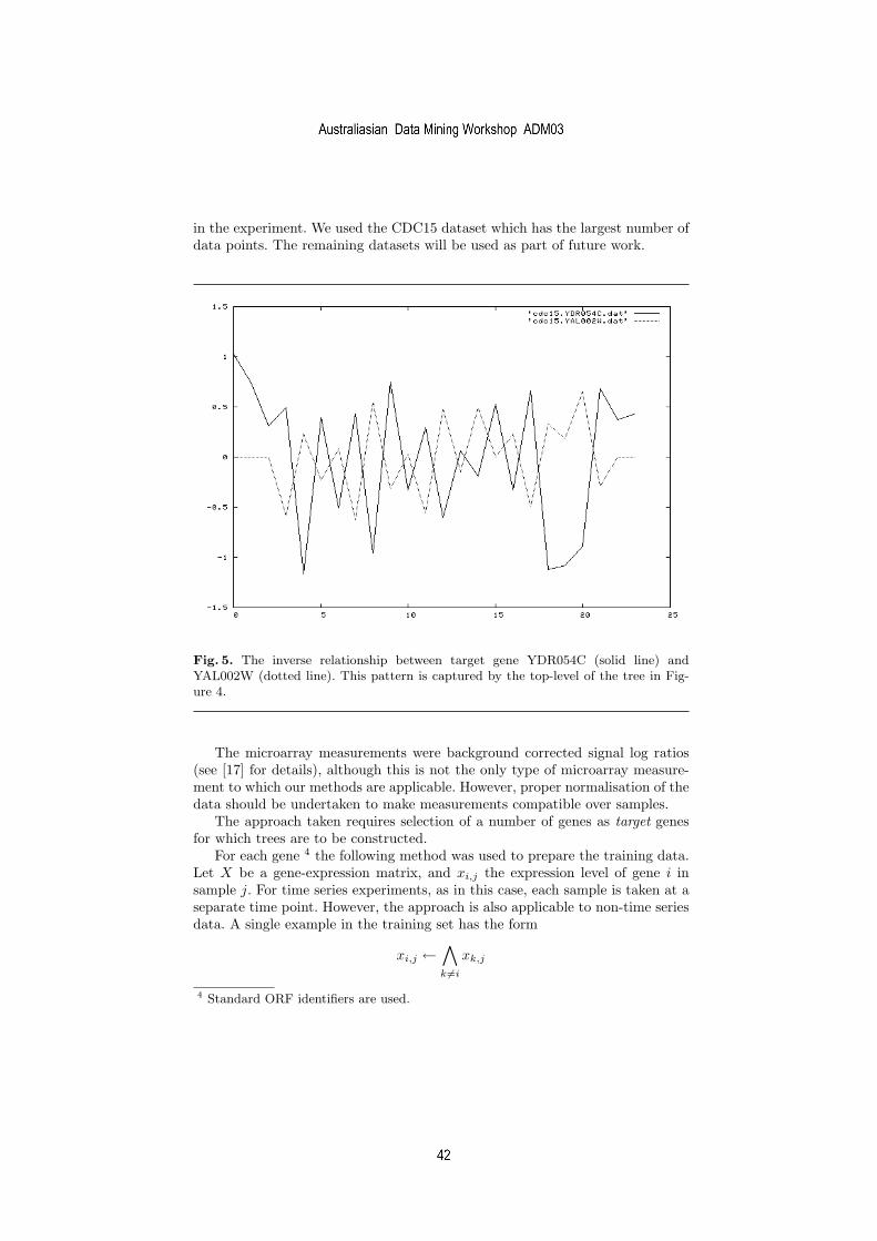
8

in the experiment. We used the CDC15 dataset which has the largest number ofdata points. The remaining datasets will be used as part of future work.

Fig. 5. The inverse relationship between target gene YDR054C (solid line) andYAL002W (dotted line). This pattern is captured by the top-level of the tree in Fig-ure 4.

The microarray measurements were background corrected signal log ratios(see [17] for details), although this is not the only type of microarray measure-ment to which our methods are applicable. However, proper normalisation of thedata should be undertaken to make measurements compatible over samples.

The approach taken requires selection of a number of genes as target genesfor which trees are to be constructed.

For each gene 4 the following method was used to prepare the training data.Let X be a gene-expression matrix, and xi,j the expression level of gene i insample j. For time series experiments, as in this case, each sample is taken at aseparate time point. However, the approach is also applicable to non-time seriesdata. A single example in the training set has the form

xi,j ←

∧

k 6=i

xk,j

4 Standard ORF identifiers are used.

9

That is, the expression level of the target gene i in sample j depends on theconjunction of the expression levels of all other genes in sample j.

Examples in this format consist of an output variable (the expression levelof the target gene) and a set of input variables (the expression levels of theremaining genes). An example in this format is generated for each sample inthe experiment. A different set of examples if generated for each of the selectedtarget genes.

Following the framework of [16] a set of twenty target genes selected knownto be involved in cell cycle regulation was selected. It is worth noting that thewhole genome could be taken as the set of target genes, although this wouldobviously generate a large number of trees.

For each of the target genes a tree-structured classifier was induced. Wegenerated both regression trees and model trees [14] using the Weka machinelearning toolkit [19]. Regression and model trees fit the data as decision trees butwith a continuous “class” or output variable at the leaves of the tree. They differas follows. Regression trees contain a single value at each leaf node, typically themean of the output variable for all examples in that leaf. Model trees contain alinear regression model at each leaf node, fitted to the examples in that leaf.

Decision trees were also generated, using the binary classification ‘up-’ or‘down-regulated’. Default parameter setting were used throughout. All runs wereof 10-fold cross-validation on the entire training set.

3.3 Results and discussion

Correlation of actual and predicted values for each 10-fold cross-validation wereobtained for model and regression trees. Predictive accuracy (1 - classificationerror) for decision trees was also obtained. These results are summarised inTable 1.

The results in terms of predictive accuracy are quite mixed. Some of thepredictions appear to be quite accurate. These may also be showing interestingcausal relationships, although this has yet to be evaluated. For other target genes,it is unlikely that any significant regulatory relationships have been uncovered.

Model trees seem to be the most accurate method. Decision trees are themost compact, often with only a single node. Regression trees are positionedin the middle; without the linear regression models in the leaves they are morecompact than the model trees, and they contain more dependencies between thetarget and other genes than the decision trees. However, the data set is verysmall, particularly considering the number of genes. Further experiments withmore data are necessary, since the methods may well be overfitting.

In terms of exploratory data analysis, the results are encouraging. Althoughwe have not been able to verify any of the relationships appearing in the trees,some of the interactions are plausible. More work is needed for this.

As expected, the tree methods seem to be picking out a small number of genesfor each target gene to predict its expression level. An example is the regressiontree in Figure 4. This expresses a simple putative regulatory relationship whichcan be summarised as follows. If the gene YAL002W is down-regulated then

10

Table 1. Cross-validation results for target gene prediction (N = 20).

Decision Trees Regression Trees Model TreesAccuracy No. of trees Correlation No. of trees Correlation No. of trees

≥ 90% 3 ≥ 0.9 0 ≥ 0.9 1≥ 80% 4 ≥ 0.8 2 ≥ 0.8 2≥ 70% 12 ≥ 0.7 5 ≥ 0.7 8≥ 60% 15 ≥ 0.6 8 ≥ 0.6 11≥ 50% 20 ≥ 0.5 10 ≥ 0.5 13

≥ 0.4 16 ≥ 0.4 17≥ 0.3 16 ≥ 0.3 17≥ 0.2 16 ≥ 0.2 18≥ 0.1 17 ≥ 0.1 19≥ 0.0 18 ≥ 0.0 19· · · · · · · · · · · ·

≥ -0.3 20 ≥ -0.3 20

Mean = 72.29% Mean = 0.46 Mean = 0.57

(in general) the target gene YDR054C is up-regulated, and vice-versa. Thereis a further level of refinement, however, which is that gene YBR002C will up-regulate YDR054C if it is itself up-regulated; also gene YAL041W will down-regulate gene YDR054C if it is itself up-regulated. This example illustrates howpositive and negative conditional dependencies can be encapsulated in a simpletree. The top level inverse regulatory relationship between genes YAL002W andYDR054C is shown by plotting the raw data in Figure 5.

A combination of using tree representations and simple plots provides asource of information on the behaviour of the underlying system. This wouldnot be the case with simply clustering genes.

An additional feature of the approach is that model trees for each of thetarget genes can be combined to provide a simulation of the subsystem definedby those genes, as outlined in Section 2.4. Causal dependencies between targetgenes occur when one target gene appears as an attribute in the tree for anothertarget gene. This situation is shown in Figure 6.

In our experiment this was observed for the gene SKP1 which was includedas an attribute in regression and model trees for target gene SWI4. It is likelythat other such dependencies would be uncovered with a larger set of targetgenes. This will be investigated as part of further work.

3.4 Related work

There has been a significant amount of work on applications of machine learn-ing to microarray data (see [13] for an overview). Many applications are of apreliminary nature. It is not yet apparent that any single technique has a clearadvantage on microarray data.

11

Fig. 6. The target gene D of the tree on the left appears as an attribute in the tree fortarget gene E on the right. Trees combined in a network showing only gene interactions.

The most common technique is still clustering, such as hierarchical clustering.With appropriate transformations of the data, such as a Fourier-type analysis todetect periodicities in time series data [17], clustering can be extremely useful.However, it is still restricted to grouping together similar examples in terms of apre-defined similarity measure. For example, the disjunctive structure of context-dependent relationships found in tree-structured classifiers evident in Figure 4may be a better fit for certain regulatory interactions. Although more complexdistance functions may be defined for clustering, this places a burden on theuser, and it may be difficult to know ahead of time what the “correct” distancefunction might be.

A well-known problem is dealing with the large number of genes in microarraydata, particularly since the number of samples is usually small. As costs reduceover time, data sets may include many more samples. However, the main problemto be solved by machine learning algorithms on such data is to select the geneswith important relationships and eliminate the redundant genes from the model.

In learning Bayes nets from expression data [6] this selection is on the basisof a statistical score which ranks genes for inclusion in the network. At each stepin an iterative procedure the number of possible genes which can be added tothe network is limited to a threshold k ≪ n, where n is the number of genes.

Our work is more closely related to that of [16] in which decision-tree learningwas applied to expression data for a number of selected target genes. Here theproblem is similar to that of learning Bayes nets; for a given gene, how to selecta subset of genes from the entire genome to be included in the tree. This isachieved by the tree-construction algorithm, which greedily selects a gene forinclusion in the tree by ranking each candidate in terms of its relationship to thetarget gene (by information gain, or standard deviation reduction, etc.) withoutthe requirement of a threshold k.

12

Fig. 7. Bioinformatics tool to support biologists in exploratory microarray data analy-sis. Annotation is used to extend the representation and formulate new learning tasks.

In contrast to [16] we avoid pre-discretisation of the expression levels of thegenes by using regression and model trees. Thus the learned model includesquantitative values for the output variable, which can be important in showingthe relation between expression levels at different nodes of a tree.

Lastly, it is interesting to note that with such tree-based methods the set oftarget genes could be all of the genes in the genome. Although this would leadto a large number of trees being learned, this could be done in parallel. Sincetree construction is efficient, this may not require excessive computation. Wemay assume therefore that the approach may be quite scalable (given suitableparallel processing resources), although this has not been tested. However, thequestion of interpretability for such a large set of models is likely to becomemuch more important.

4 Bioinformatics tools for biologists

A major advantage of our approach over currently used clustering methods is theextraction of explicit rules from the data, that can be further investigated andverified by domain experts. The techniques described in this paper can thereforebe incorporated into a tool for biologists to explore the results from microarrayexperiments in an interactive fashion. We are currently developing such a toolin collaboration with a group of experimental biologists. The goal is to providethe user with an easy way to select target genes, launch analyses, and identify“interesting” relationships in the resulting trees.

13

In order to facilitate this exploration, the user interface should display notonly the relationships in terms of gene names, but also annotate these resultswith relevant known attributes for the genes. These attributes include attributesof the gene itself (location on the chromosomes, relevant patterns in the sur-rounding DNA sequences) as well as attributes of its encoded protein (functionalcategory, cellular localisation, known interaction partners etc). Combining therelationships predicted by the data mining techniques with an integrated viewof these attributes should greatly facilitate the examination of the results andtheir evaluation and exploration by domain experts.

The exploration tool (see Figure 7) therefore incorporates a series of agentsfor retrieving the relevant attributes from various Internet data sources as re-quired, and integrating these attributes with the data mining output. The explo-ration tool should also allow the user to combine multiple classifiers to constructa gene network, using both computational predictions and their own domainexpertise. The exploration tool (see Figure 7) should include the following com-ponents:

– Database for storing microarray data– Data mining tools– Graphical user interface for– Browsing through the microarray experiments– Selecting target genes– Launching analyses– Displaying “annotated” trees– Combining trees into networks– Agents for querying local and external annotation sources and collating and

formatting the retrieved annotations

The exploration tool should allow the domain experts to make immediate usedomain experts to make immediate use of the classification methods for generat-ing scientific hypotheses that can be validated experimentally. It will also allowa direct, subjective evaluation of the predictions by the domain experts. Furtherdevelopments of this tool can include the automatic capture of the biologist’spatterns of use, which could be used as the basis for the development of a moreautomated expert system for exploring microarray data.

5 Conclusions and further work

This is preliminary work and it is too soon to draw firm conclusions. Never-theless there seem to be some promising aspects to our initial results. First, theapproach of treating the problem as one of learning control rules for an unknownsystem is appealing. This allows a simple decomposition of the overall system,which makes learning models more efficient. These individual predictive modelscan be combined for system-level behaviour. The approach has been extensivelyinvestigated in the area of behavioural cloning, and this has resulted in many

14

refinements such as learning feedback control rules, learning reference values forsteady-state systems and a wide range of representations and learning methods.

Second, the use of symbolic machine learning methods which can fit quitecomplex, non-linear functions using simple structures has many advantages. Themodels are not black-boxes, which is important for biologists. They can be usedfor prediction and explanation. Overall, they have much more to offer thanclustering, which has been the most commonly used method for applicationsto microarray data.

Third, as more information sources are available to include in training setsfor model construction, both in the form of additional microarray data andother data such as sequence and interaction data, it should be straightforwardto extend this approach. It is likely that more interactive stages in the learningwill help to guide this process.

On the other side of the balance sheet there are a number of drawbacks.There is currently no way to obtain estimates of the statistical significance ofthe models learned by our methods. Although ultimately biological significanceis more important than statistical significance, and it is well-known that statis-tical significance does not always imply biological significance, and vice versa,nonetheless it is important for data mining and machine learning practitionersto address this requirement. Possible directions include both theoretical devel-opments based on the algorithms used, and empirical methods of significanceestimation.

Much more work needs to be done to apply these approaches to more data.This includes: running these methods on many more target genes in a data setand comparing the output models; testing the predictive accuracy of the modelson several data sets; applying the methods on microarray datasets other than thebenchmark sets; validation of the predictions in terms of biological significance.

In summary, we fully expect the challenges of microarray data mining tolead to extensions to or new developments of machine learning methods, and togreatly improve our understanding of what is required for them to be successfulon these large-scale biological data sets.

Acknowledgements. Thanks to Claude Sammut, Andrew Isaac, Ian Dawes,Geoff Kornfeld and Rohan Williams for helpful discussions on these topics.

References

1. M. Bain and C. Sammut. A Framework for Behavioural Cloning. In K. Furukawa,D. Michie, and S. Muggleton, editors, Machine Intelligence 15, pages 103–129.Clarendon Press, Oxford, 1999.

2. P. Baldi and W. Hatfield. DNA Microarrays and Gene Expression. CambridgeUniversity Press, Cambridge, UK, 2002.

3. J.M. Berg, J.L. Tymoczo, and L. Stryer. Biochemistry (5th Edition). W. H.Freeman and Company, New York, NY, 2002.

15

4. C. Bryant, S. Muggleton, S. Oliver, D. Kell, P. Reiser, and R. King. Combin-ing Inductive Logic Programming, Active Learning, and Robotics to Discover theFunction of Genes. Linkoping Electronic Articles in Computer and InformationScience, 6(12), 2001.

5. D. Endy and R. Brent. Modelling cellular behaviour. Nature, 409:391–395, 2001.6. N. Friedman, M. Linial, I. Nachman, and D. Pe’er. Using Bayesian Networks to

Analyze Expression Data. Journal of Computational Biology, 7:601 – 620, 2000.7. D. Greenbaum, N. Luscombe, R. Jansen, J. Qian, and M. Gerstein. Interrelating

Different Types of Genomic Data, from Proteome to Secretome: ’Oming in onFunction. Genome Research, 11:1463–1468, 2001.

8. A. Isaac and C. Sammut. Goal-directed learning to fly. In Proc. of the Interna-tional Conference on Machine Learning, pages 258–265, Los Altos, 2003. MorganKaufmann.

9. P. Karp. Pathway Databases: A Case Study in Computational Symbolic Theories.Science, 293:2040, 2001.

10. H. Kitano. Computational systems biology. Nature, 420:206–210, 2002.11. S. Liang, S. Fuhrman, and R. Somogyi. REVEAL, A General Reverse Engineer-

ing Algorithm for Inference of Genetic Network Architectures. In Third PacificSymposium on Biocomputing, pages 18 – 29, 1998.

12. D. Michie, M. Bain, and J. Hayes-Michie. Cognitive models from subcognitiveskills. In M. Grimble, S. McGhee, and P. Mowforth, editors, Knowledge-basedSystems in Industrial Control. Peter Peregrinus, IEEE Press, 1990.

13. M. Molla, M. Waddell, D. Page, and J. Shavlik. Using Machine Learning to De-sign and Interpret Gene-Expression Microarrays. AI Magazine (special issue onBioinformatics), 2003.

14. J. R. Quinlan. Learning with Continuous Classes. In Proc. 5th Australian JointConference on Artificial Intelligence, pages 343–348, 1992.

15. C. Sammut, S. Hurst, D. Kedzier, and D. Michie. Learning to fly. In D. Sleemanand P. Edwards, editors, Proceedings of the Ninth International Conference onMachine Learning, San Mateo, CA, 1992. Morgan Kaufmann.

16. L. Soinov, M. Krestyaninova, and A. Brazma. Towards reconstruction of genenetworks from expression data by supervised learning. Genome Biology, 4(1),2003.

17. P. Spellman, G. Sherlock, M. Zhang, V. Iyer, K. Anders, M. Eisen, P. Brown,D. Botstein, and B. Futcher. Comprehensive Identification of Cell Cycle-regulatedGenes of the Yeast Saccharomyces cerevisiae by Microarray Hybridization. Molec-ular Biology of the Cell, 9:3273–3297, 1998.

18. T. Urbancic and I. Bratko. Reconstructing human skill with machine learning. InProceedings of the 11th European Conference on Artificial Intelligence. John Wiley& Sons, 1994.

19. I. Witten and E. Frank. Data Mining. Morgan Kaufmann, San Francisco, Califor-nia, 2000.

simeon

Australiasian Data Mining Workshop ADM03

An Mining Approach Using MOUCLAS Patterns

Yalei Hao1 Markus Stumptner1 Gerald Quirchmayr1 2

1 Advanced Computing Research Centre, University of South Australia, SA5095, Australia Yalei.Hao@postgrads.unisa.edu.au, mst@cs.unisa.edu.au, Gerald.Quirchmayr@unisa.edu.au

2

Institut für Informatik und Wirtschaftsinformatik, Universität Wien, Liebiggasse 4, A-1010 Wien, Austria

Abstract. The integration of data mining techniques with classification problems relies on the success in the mining of interesting knowledge patterns during the learning phase of the classifiers. This paper proposes a new kind of patterns for the classification over quantitative data in high dimensional database, which is called MOUCLAS (MOUntain function based CLASsification) Patterns, based on the concept of the fuzzy set membership function which gives the new approach a solid mathematical foundation and compact mathematical description of classifiers, and integrating classification and clustering and association rules mining to identify interesting knowledge in the databases. The framework of the paper is formed by concentrating on three major issues of classification: the definition of the new MOUCLAS patterns, the algorithm for the discovery of the MOUCLAS patterns, and the construction of new classifiers.

1 Introduction and Motivation An increasing part of research in the data mining communities focuses on the task of classification, in addition to three other tasks: generation of association rules, clustering, and concept description. Data mining based classification aims to build accurate and efficient classifiers not only on small data sets but more importantly also on large and high dimensional data sets, while the widely used traditional statistical data analysis techniques are not sufficiently powerful for this task [12], [13]. The use of association rules to discover dependencies among data [2] has been extensively studied in both the database and data mining communities for a long time, with major studies in [3], [4], [5], [15], [17], [21], [23], [25], [27], [29], [30], and [33]. With the development of new data mining techniques on association rules, new classification approaches based on concepts from association rule mining are emerging. These include such classifiers as ARCS [20], CBA [18], LB [22], CAEP [10], etc., which are different from the classic decision tree based classifier C4.5 [24] and k-nearest neighbor [6] in both the learning and testing phases. ARCS [20] demonstrated the successful application of concepts of clustering for the purpose of classification. However, ARCS is limited to 2D-rules based classifiers of the format A ∧ B ⇒ Classi, where A and B are two predicates. It uses the method of “Binning” to discretize the value of quantitative attributes.

Consequently, the accuracy of ARCS is strongly related to the degree of discretization used. A non-grid-

based technique [26] has been proposed to find quantitative association rules that can have more than two

predicates in the antecedent. The authors noticed that the information loss caused by partitioning could not

be ignored and have tried to employ a measure of partial completeness to quantify the information lost, but

the measure is still constrained by the framework of binning. Though there are several excellent

discretization algorithms [11], [8], a standard approach to discretization has not yet been developed.

Different approaches could lead to different collections of large itemsets even with respect to the same

support threshold in a given data set. ARCS and the non-grid-based technique lead to research question 1

being addressed: “Is it possible that an association rule based classifier can be developed for quantitative

attributes by the concepts of clustering which can overcome the limitation caused by the discretization

method? ” CBA [18] gives us an interesting indication that the idea of apriori property can be applied to a set

of predicates (itemsets) for classification. Suppose an association rule based classifier in the form of A1 ∧ A2

∧ … ∧ Al ⇒ Ci, where Aj (j=1, …, l) are predicate variables, Ci is the class label, the antecedent of the rule is

a frequent itemset. This raises question 2: “If an association rule based classifier can be built based on the

concept of clustering, is it possible that a link between CBA and ARCS can be found so that an association

rule based classifier with any number of predicates in the antecedent can be setup by clustering? ”

The above research issues establish a challenge that comes within our research focus. In this paper, we

present a new approach to the classification over quantitative data in high dimensional databases, called

MOUCLAS (MOUntain function based CLASsification), based on the concept of the fuzzy set membership

function. It aims at integrating the advantages of classification, clustering and association rules mining to

identify interesting patterns in selected sample data sets.

2 Problem Statement We now give a formal statement of the problem of MOUCLAS Patterns (called MPs) and introduce some definitions. The MOUCLAS algorithm, similar to ARCS, assumes that the initial association rules can be agglomerated into clustering regions, while obeying the anti-monotone rule constraint. Our proposed framework assumes that the training dataset D is a normal relational set, where transaction d ∈ D. Each transaction d is described by attributes Aj, j = 1 to l. The dimension of D is l, the number of attributes used in D. This allows us to describe a database in terms of volume and dimension. D can be classified into a set of known classes Y, y ∈ Y. The value of an attribute must be quantitative. In this work, we treat all the attributes uniformly. We can treat a transaction as a set of (attributes, value) pairs and a class label. We call each (attribute, value) pair an item. A set of items is simply called an itemset. Since CBA indicates the feasibility of setting up a link between association rule and classification and ARCS proves that the idea of designing a classification pattern based on clustering can work effectively and efficiently, we design a MOUCLAS Pattern (so called MP) as an implication of the form:

Cluster(D)t → y, where Cluster(D)t is a cluster of D, t = 1 to m, and y is a class label. The definitions of frequency and accuracy of MOUCLAS Patterns are defined as following: The MP satisfying minimum support is frequent, where MP has support s if s% of the transactions in D belong to Cluster(D)t and are labeled with class y. The MP that satisfies a pre-specified minimum confidence is called accurate, where MP has confidence c if c% of the transactions belonging to Cluster(D)t are labeled with class y. Though framework of support – confidence is used in most of the applications of association rule mining, it

may be misleading by identifying a rule A ⇒ B as interesting, even though the occurrence of A may not

imply the occurrence of B. This requires a complementary framework for finding interesting relations.

Correlation [15] is one of the most efficient interestingness measures other than support and confidence. Here

we adopt the concept of reliability [34] to describe the correlation. The measure of reliability of the

association rule A ⇒ B can be defined as:

reliability R(A ⇒ B) = )(

)(AP

BAP ∧− ( )BP

Since R is the difference between the conditional probability of B given A and the unconditional of B, it

measures the effect of available information of A on the probability of the association rule. Correspondingly,

the greater R is, the stronger MOUCLAS patterns are, which means the occurrence of Cluster(D)t more

strongly implies the occurrence of y. Therefore, we can utilize reliability to further prune the selected

frequent and accurate and reliable MOUCLAS patterns (MPs) to identify the truly interesting MPs and make

the discovered MPs more understandable. The MP satisfying minimum reliability is reliable, where MP has

reliability defined by the above formula.

Given a set of transactions, D, the problems of MOUCLAS are to discover MPs that have support and

confidence greater than the user-specified minimum support threshold (called minsup) [4], and minimum

confidence threshold (call minconf) [4] and minimum reliability threshold (call minR) respectively, and to

construct a classifier based upon MPs.

3 The MOUCLAS Algorithm

The classification technique, MOUCLAS, consists of two steps:

1. Discovery of frequent, accurate and reliable MPs.

2. Construction of a classifier, called De-MP, based on MPs.

The core of the first step in the MOUCLAS algorithm is to find all cluster_rules that have support above

minsup. Let C denote the dataset D after dimensionality reduction processing. A cluster_rule represents a

MP, namely a rule:

cluset → y,

where cluset is a set of itemsets from a cluster Cluster(C)t, y is a class label, y ∈ Y. The support count of the

cluset (called clusupCount) is the number of transactions in C that belong to the cluset. The support count of

the cluster_rule (called cisupCount) is the number of transactions in D that belong to the cluset and are

labeled with class y. The confidence of a cluster_rule is (cisupCount / clusupCount) × 100%. The support

count of the class y (called clasupCount) is the number of transactions in C that belong to the class y. The

support of a class (called clasup) is (clasupCount / |C |) × 100%, where | C | is the size of the dataset C.

Given an MP, the reliability R can be defined as:

R(cluset → y) = (cisupCount / clusupCount) - (clasupCount / |C |) × 100%

The traditional association rule mining only uses a single minsup in rule generation, which is inadequate for many practical datasets with uneven class frequency distributions. As a result, it may happen that the rules found for infrequent classes are insufficient and too many may be found for frequent classes, inducing useless or over-fitting rules, if the single minsup value is too high or too low. To overcome this drawback, we apply the theory of mining with multiple minimum supports [32] in the step of discovering the frequent MPs as following. Suppose the total support is t-minsup, the different minimum class support for each class y, denoted as minsupi can be defined by the formula:

minsupi = t-minsup × freqDistr(y) where, freqDistr(y) is the function of class distributions. Cluster_rules that satisfy minsupi are called frequent cluster_rules, while the rest are called infrequent cluster_rules. If the confidence is greater than minconf, we say the MP is accurate. The first step of the MOUCLAS algorithm works in three sub-steps, by which the problem of discovering a set of MPs is solved:

Algorithm: Mining frequent and accurate and reliable MOUCLAS patterns (MPs)

Input: A training transaction database, D; minimum support threshold (minsupi); minimum confidence threshold (minconf)

Output: A set of frequent, accurate and reliable MOUCLAS patterns (MPs)

Methods: (1) Reduce the dimensionality of transactions d, which efficiently reduces the data size by removing

irrelevant or redundant attributes (or dimensions) from the training data, and

(2) Identify the clusters of database C for all transactions d after dimensionality reduction on attributes Aj in database C, based on the Mountain function, which is a fuzzy set membership function, and specially capable of transforming quantitative values of attributes in transactions into linguistic terms, and

(3) Generate a set of MPs that are both frequent, accurate and reliable, namely, which satisfy the user-specified minimum support (called minsupi), minimum confidence (called minconf) and minimum reliability (called minR) constraints.

In the first sub-step, we reduce the dimensionality of transactions in order to enhance the quality of data mining and decrease the computational cost of the MOUCLAS algorithm. Since, for attributes Aj, j = 1 to l in database, D, an exhaustive search for the optimal subset of attributes within 2l possible subsets can be prohibitively expensive, especially in high dimensional databases, we use heuristic methods to reduce the search space. Such greedy methods are effective in practice, and include such techniques as stepwise forward selection, stepwise backward elimination, combination of forwards selection and backward elimination, etc. The first sub-step is particularly important when dealing with raw data sets. Detailed methods concerning dimensionality reduction can be found in [9], [19], [28], [16]. Fuzzy based clustering is performed in the second sub-step to find the clusters of quantitative data. The Mountain-climb technique proposed by R. R. Yager and D. P. Filev [31] employed the concept of a mountain function, a fuzzy set membership function, in determining cluster centers used to initialize a Neuro-Fuzzy system. The substractive clustering technique [7] was defined as an improvement of Mountain-climb clustering. A similar approach is provided by the DENCLUE algorithm [14], which is especially efficient for clustering on high dimensional databases with noise. The techniques of Mountain-climb clustering, Substractive clustering and Denclue provide an effective way of dealing with quantitative attributes by mountain functions (or influence functions), which has a solid mathematical foundation and compact mathematical description and is totally different from the traditional processing method of binning. It offers us an opportunity of mining the patterns of data from an innovative angle. As a result, question 1 presented in the introduction can now be favorably answered.

The observation that, a region which is dense in a particular subspace must create dense regions when projected onto lower dimensional subspaces, has been proved by R. Agrawal and his research cooperators in CLIQUE [1]. In other words, the observation follows the concepts of the apriori property. Hence, we may employ prior knowledge of items in the search space based on the property so that portions of the space can be pruned. The successful performance of CLIQUE has again proved the feasibility of applying the concept of apriori property to clustering. It brings us a step further towards the solution of problem 2, that is, if the

initial association rules can be agglomerated into clustering regions, just like the condition in ARCS, we may be able to design a new classifier for the purpose of classification, which confines its search for the classifier to the cluster of dense units of high dimensional space. The answer to question 2 can contribute to the third sub-step of the MOUCLAS algorithm, i.e., the forming of the antecedents of cluster_rules, with any number of predicates in the antecedent. In the third sub-step, we identify the candidate cluster_rules which are actually frequent and accurate and reliable. From this set of frequent and accurate and reliable cluster_rules, we produce a set of MPs. Let I be the set of all items in D, C be the dataset D after dimensionality reduction, where transaction d ∈ C contains X ⊆ I, a k-itemset. Let E denote the set of candidates of cluster_rules, where e ∈ E, and F denote the set of frequent cluster_rules. The first step of the MOUCLAS algorithm is given in Figure 1 as follows. 1 X = reduceDim (I); // reduce the dimensionality on the set of all items I of in D 2 Cluster(C)t = genCluster (C); // identify the complete clusters of C 3 for each Cluster(C)t do E = genClusterrules(cluset, class); // generate a set of candidate cluster_rules 4 for each transaction d ∈ C do 5 Ed = genSubClusterrules (E, d); // find all the cluster_rules in E whose cluset are supported by d 6 for each e ∈ Ed do 7 e. clusupCount++; // accumulate the clusupCount of the cluset of cluster_rule e 8 if d.class = e.class then e.cisupCount++ // accumulate the cisupCount of cluster_rule e supported

by d 9 end 10 end 11 F = {e ∈ E | e.cisupCount ≥ minsupi }; // construct the set of frequent cluster_rules 12 MP = genRules (F); //generate MP using the genRules function by minconf and minR 13 end

14 MPs = MP; // discover the final set of MPs

Figure 1: The First Step of the MOUCLAS Algorithm The task of the second step in MOUCLAS algorithm is to use a heuristic method to generate a classifier, named De-MP, where the discovered MPs can cover D and are organized according to a decreasing precedence based on their confidence and support. Suppose R be the set of frequent, accurate and reliable MPs which are generated in the past step, and MPdefault_class denotes the default class, which has the lowest precedence. We can then present the De-MP classifier in the form of

<MP1, MP2, …, MPn, MPdefault_class>,

where MPi ∈ R, i = 1 to n, MPa MPb if n ≥ b > a ≥ 1 and a, b∈ i, C ⊆ cluset of MPi,.

The second step of the MOUCLAS algorithm also consists of three sub-steps, by which the De-MP classifier

is formed:

Algorithm: Constructing De-MP Classifier

Input: A training database after dimensionality reduction, C; The set of frequent and accurate and reliable

MOUCLAS patterns (MPs)

Output: De-MP Classifier

Methods: (1) Identify the order of all discovered MPs based on the definition of precedence and sequence them

according to decreasing precedence order.

(2) Determine possible MPs for De-MP classifier from R following the descending sequence of MPs.

(3) Discard the MPs which cannot contribute to the improvement of the accuracy of the De-MP classifier

and keep the final set of MPs to construct the De-MP classifier.

In the first sub-step, the MPs are sorted in descending order, which has the training transactions surely

covered by the MPs with the highest precedence when possible in the next sub-step. The sort of the whole set

of MPs is performed following the definition of precedence as in CBA:

Given two MPs, we say that MPa has a higher precedence than MPb, denoted as MPa �MPb,

if ∀ MPa, MPb ∈ MPs, it holds that: the confidence of MPa is greater than that of MPb, or if their confidences

are the same, but the support of MPa is greater than that of MPb, or if both the confidences and supports of

MPa and MPb are the same, but MPa is generated earlier than MPb.

In the second sub-step, we test the MPs following decreasing precedence and stop the sub-step when there is no rule or no training transaction. For each MP, we scan C to find those transactions satisfying the cluset of the MP. If the MP can correctly classify one transaction, we store it in a set denoted as L. Those transactions satisfying the cluset of the MP will be removed from C at each pass. Each transaction can be identified by a unique ID. The next pass will be performed on the remaining data. A default class is defined at each scan, which is the majority class in the remaining data. At the end of each pass, the total number of errors that are made by the current L and the default class are also stored. When there is no rule or no training transaction left, we terminate this sub-step. After this sub-step, every MP in L can correctly classify at least one training transaction in C. In the third sub-step, though we would like to find as many MPs as possible to give good coverage of the training transactions in the second sub-step, we prefer strong MPs which have relatively high support and confidence, due to their characteristics of corresponding to larger coverage and stronger differentiating power. Meanwhile, we hope that the De-MP classifier, consisting of a combination of strong MPs, has a relatively smaller number of classification errors, because of greedy strategy. In addition, the reduction of MPs can increase the understandability of the classifier. Therefore, in this sub-step, we identify the first MP with the least number of errors in L and discard all the MPs after it because these MPs produce more errors. The undiscarded MPs and the default class corresponding to the first MP with the least number of errors in L form our De-MP classifier. The second step of the MOUCLAS algorithm is shown in Figure 2. 1 R = sort(R); // sort MPs based on their precedence 2 for each MP∈ R in sequence do 3 temp = ∅ ; 4 for each transaction d ∈ C do 5 if d satisfies the cluset of MP then 6 store d.ID in temp; 7 if MP correctly classifies d then 8 insert MP at the end of L; 9 delete the transaction who has ID in temp from C; 10 selecting a default class for the current L; // determine the default class based on majority class of remaining transactions in C 11 end 12 compute the total number of errors of L; // compute the total number of errors that are made by the current L and the default class 13 end 14 Find the first MP in L with the lowest total number of errors and discard all the MPs after the MP in L; 15 Add the default class associated with the above mentioned first MP to end of L; 16 De-MP classifier = L

Figure 2: The Second Step of the MOUCLAS Algorithm

In the testing phase, when we classify a new transaction, the first MP in De-MP satisfying the transaction is used to classify it. In De-MP classifier, default_class, having the lowest precedence, is used to specify a default class for any new sample that is not satisfied by any other MPs as in C4.5[24], CBA[18]. 4 Example of MOUCLAS Application Oil/gas formation identification is a vital task in the petroleum industry, where the petroleum database contains such records (or attributes) as seismic data, various types of well logging data (e.g. GR, DEN, CNL, Resistivity, BCSL, etc.), and physical propertiy data (e.g. porosity, permeability, etc.), whose values are all quantitative. An illustration of using well logging date for purpose of oil/gas formation identification is illustrated in figure 3. One transaction of the database can be treated as a set of the items corresponding to the same depth and a class label (oil/gas formation or not). A hypothetically useful MP may suggest a relation between petroleum data at a certain depth and the class label of oil/gas formation. In this sense, a selected set of such MPs can be a useful guide to petroleum engineers to identify possible drilling targets and their depth and thickness at the stage of exploration and exploitation. The notable advantage of MOUCLAS over more traditional processing techniques such as seismic inversion is that a physical model to describe the relationship between the seismic data and the property of interest is not needed; nor is an very precise understanding of the phases of the seismic data. From this point of view,

MOUCLAS provides a complementary and useful technical approach towards the interpretation of petroleum data and benefits petroleum discovery.

Figure 3: Quantitative Petroleum Data Suitable for MOUCLAS Mining

(note: the dashed lines indicate the location of oil formations) 5 Conclusion We have introduced a new type of classification patterns, the MOUCLAS Pattern (MP), for quantitative data in high dimensional databases. We have also proposed an algorithm for discovering the interesting MPs and construct a new classifier called De-MP. As a hybrid of classification, clustering, and association rules mining, our approach may have several advantages which are that (1) it has a solid mathematical foundation and compact mathematical description of classifiers, (2) it does not require discretization, as opposed to other, otherwise quite similar methods such as ARCS, (3) it is robust when handling noisy or incomplete data in high dimensional data space, regardless of the database size, due to its grid-based characteristics, (4) it is not sensitive to the order of input items and it scales linearly with the size of the input. 6 Acknowledgement This work was partially supported by the Australia-China Special Fund for Scientific and Technological Cooperation under grant CH030086. We would like to thank Dr. Dan Corbett for many fruitful discussions that helped to further refine our approach. References 1. R. Agrawal, J. Gehrke, D. Gunopulos, and P. Raghavan. Automatic subspace clustering of high

dimensional data for data mining applications. SIGMOD’98. (1998)

2. Agrawal, R., Imielinski, T., & Swami, A. Mining association rules between sets of items in large databases. Proc. of the 1993 ACM­SIGMOD ACM Press. (1993) 207--216

3. Agrawal, R., Mannila, H., Srikant, R., Toivonen, H., & Verkamo, A. I. Fast discovery of association

rules. Advances in knowledge discovery and data mining. AAAI/MIT Press. (1996) 1-34

4. Agrawal, R., Srikant, R. Fast algorithms for mining association rules. Proc. of the 20th VLDB (1994)

487- 499

5. Bayardo, R. J. Efficiently mining long patterns from databases. Proc. of the 1998 ACM­SIGMOD. ACM

Press. (1998) 85-93

6. Cover, T. M., & Hart, P. E. Nearest neighbor pattern classification. IEEE Transactions on Information

Theory, 13. (1967) 21-27

7. Chiu, S. L. Fuzzy model identification based on cluster estimation. Journal of Intelligent and Fuzzy

System, 2(3), (1994)

8. Dougherty, J., Kohavi, R., & Sahami, M. Supervised and unsupervised discretization of continuous features. Proc. of the Twelfth Int’l Conf. on Machine Learning pp. 94--202. Morgan Kaufmann. (1995)

9. Dong, G., & Li, J. Feature selection methods for classification. Intelligent Data Analysis: An

International Journal, 1, (1997)

10. Dong, G., & Li, J. Efficient mining of emerging patterns: Discovering trends and differences. Proc. of

the Fifth ACM SIGKDD. (1999)

11. Fayyad, U., & Irani, K. Multi­interval discretization of continuous­valued attributes for classification

learning. Proc. of the 13th Int’l Conf. on Artificial Intelligence. Morgan Kaufmann. (1993) 1022--1029

12. Fayyad, U. M., Piatetsky­Shapiro, G., & Smyth, P. From data mining to knowledge discovery: An

overview. Advances in knowledge discovery and data mining. AAAI/MIT Press. (1996) 1-34

13. Han, J., & M. Kamber. Data mining: concepts and techniques. Morgan Kaufmann Publishers. (2000)

14. A. Hinneburg and D. Keim. An efficient approach to clustering in large Multimedia dataset with noise.

KDD’98, (1998) 58-65

15. Han, J., Pei, J., & Yin, Y. Mining frequent patterns without candidates generation. Proc. of the 2000

ACM­SIGMOD. ACM Press. (2000) 1-12

16. R. Kohavi and G. John. Wrappers for feature subset selection. Artificial Intelligence, (1997) 273-324

17. Lee, S. D., Cheung, D. W., & Kao, B. Is sampling useful in data mining? a case in the maintenance of

discovered association rules. Data Mining and Knowledge Discovery, 2. (1998) 233-262.

18. B. Liu, W.Hsu, and Y.Ma. Integrating classification and association rule mining. KDD’98. (1998) 80-86

19. H. Liu and H. Motoda, editors. Feature Selection for Knowledge Discovery and Data Mining. Boston:

Kluwer Academic Publishers, (1998)

20. B. Lent, A. Swami, and J. Widom. Clustering association rules. ICDE'97, (1997) 220-231

21. Mannila, H., Toivonen, H., & Verkamo, A. I. Efficient algorithms for discovering association rules.

Proc. of AAAI'94 Workshop KDD'94. AAAI Press. (1994) 181-192.

22. Meretakis, D., & Wuthrich, B. Extending naive Bayes classifiers using long itemsets. Proc. of the Fifth

ACM SIGKDD. ACM Press. (1999) 165-174

23. R.J. Miller and Y. Yang. Association rules over interval data. SIGMOD'97, (1997) 452-461

24. Quinlan, J. R. C4.5: Programs for machine learning. San Mateo, CA: Morgan Kaufmann. (1993)

25. Srikant, R., & Agrawal, R. Mining generalized association rules. Proc. of the 21st Int’l. Conf. on VLDB.

Morgan Kaufmann. (1995) 407-419

26. R. Skikant and R. Agrawal. Mining quantitative association rules in large relational tables. SIG-

MOD’96, (1996) 1-12.

27. Savasere, A., Omiecinski, E., & Navathe, S. An efficient algorithm for mining association rules in large

databases. Proc. of the 21st VLDB. Morgan Kaufmann. (1995) 432-443

28. W.Sarawagi and M. Stonebraker. On automatic feature selection. Int’l J. of Pattern Recognition and

Artificial Intelligence, 2, (1988) 197-220.

29. Toivonen, H. Sampling large databases for association rules. Proc. of the 22rd VLDB. Bombay, India:

Morgan Kaufmann. (1996) 134-145

30. Wijsen, J., & Meersman, R. On the complexity of mining quantitative association rules. Data Mining and

Knowledge Discovery, 2, 1998 263-282

31. Yager, R. and D. Filev, "Generation of Fuzzy Rules by Mountain Clustering," Journal of Intelligent &

Fuzzy Systems, Vol. 2, No. 3, (1994) 209-219

32. Bing Liu, Wynne Hsu, Yiming Ma, "Mining Association Rules with Multiple Minimum Supports"

Proceedings of the ACM SIGKDD International Conference on Knowledge Discovery & Data Mining

(KDD-99), August 15-18, San Diego, CA, USA (1999)

33. Zhang, T. Association rules. Proc. of the Fourth Pacific­Asia Conf. on Knowledge Discovery and Data

Mining (2000) 245-256

34. Khalil M. Ahmed, Nagwa M. El-Makky, Yousry Taha: A note on "Beyond Market Baskets:

Generalizing Association Rules to Correlations". In The Proceedings of SIGKDD Explorations

Volume1, Issue 2, (2000) 46-48

simeon

Australiasian Data Mining Workshop ADM03

From Rule Visualisation to Guided Knowledge

Discovery

Aaron Ceglar, John F. Roddick, Carl H. Mooney and Paul Calder

School of Informatics and EngineeringFlinders University

PO Box 2100, Adelaide 5001, South Australia.Email: {aaron.ceglar, john.roddick, carl.mooney,

paul.calder}@infoeng.flinders.edu.au

Abstract. As a result of the inability of computer systems to under-stand abstract concepts, data mining algorithms do not generally con-strain the generation of rules to those that are of interest to the useradequately. Interactive knowledge discovery techniques aim to alleviatethis problem by involving the user in the mining process, so that theuser’s broader understanding of abstract semantic concepts and domainknowledge can guide the discovery process, resulting in accelerated min-ing with improved results. At present this is done largely through datavisualisation techniques and to a lesser degree through rule visualisation.This paper discusses some of the current research in interactive data min-ing research and argues that the next stage after rule visualisation is theinteractive user manipulation of the mining process - Guided KnowledgeDiscovery. The paper also introduces two unique visualisation tools –the CARV hierarchical association rule mining visualisation tool and theINTEM sequential pattern rule visualisation tool.

Additional Keywords: Interactive data mining.

1 Introduction

Although computer based, the knowledge discovery process is human-centric be-cause of its reliance upon the user’s involvement in both mechanistic aspects suchas data selection and preparation, and in aspects involving quantitative judge-ment such as analysis and interpretation of the results. Using current techniques,the user is involved within all stages of the discovery process, with the excep-tion of the analysis1 stage, which remains a ‘black box’. This analysis stage usesdata mining algorithms to explore a dataset and discover patterns or structures,which are influenced by user specified constraints and objective measures of in-terestingness. To date, data mining research has focused mainly upon heuristiccorrectness and efficiency. In interactive data mining, the process is extended to

1 For convenience we use the CRISP nomenclature (Chapman, Kerber, Clinton,Khabaza, Reinartz & Wirth 1999)

investigate ways in which the user can become an integral part of the miningprocess. The need for user inclusion is based on the premise that the concept ofinterestingness is subjective, and cannot therefore be fully defined in heuristicterms. This suggests that by extending data mining algorithms to incorporatesubjective measures of interestingness (through user participation), more usefulresults will be produced. The collaboration between computer and human willresult in a symbiosis; the computer will provide processing power and storagefacilities, and the user will contribute such capabilities as understanding andperception.

This paper investigates interaction techniques that allow the user to activelyguide the knowledge discovery process, in effect overcoming the computer’s in-ability to incorporate knowledge about intangible subjective measures such asdomain knowledge and data semantics. In addition to producing more interest-ing results, guidance of the mining process implies that the algorithm can bedynamically constrained during processing (to reduce the breadth or depth ofanalysis), hence reducing both mining time and result set size.

There are two classes of data mining tasks: directed and undirected. Directedmining, also known as supervised learning or predictive analysis, refers to a groupof methods that build a model based upon a set of data and make predictionsabout new items based on this model. Undirected mining, also known as unsu-pervised learning or explorative analysis, employs techniques that are used todiscover patterns, unknown or theorised by the user. Interactive mining can onlybe applied to the explorative tasks such as clustering and association mining;as directed mining tasks such as classification and characterisation are guidedthrough training sets of data.

This paper explores the techniques available for visualisation of and inter-action with undirected knowledge discovery systems. Section 2 builds toward adiscussion on interactive data mining by outlining the need for human participa-tion within the knowledge discovery process. This is followed by a discussion ofpresentation paradigms in Section 3, highlighting both the strengths and weak-nesses of textual and graphical methods. Section 4 contains a comprehensivetaxonomy of undirected mining presentations, including the presentation of hi-erarchical, temporal and spatial semantics. Section 5 looks at interaction and,more specifically, direct manipulation techniques and the creation of interactionmappings. The section also provides a discussion about interactive views and dis-tortion, which are two common interaction-based methods used to alleviate someof the problems incurred through the presentation of large complex datasets incoordinate space. Finally Section 6 discusses the current state of interactive datamining and the few relevant tools that are available, and Section 7 provides abrief look at the future directions of interactive data mining research.

2 User Participation

Computers process data at a syntactic level only. For example, a computer haslittle understanding of the semantics behind the string book and therefore which

is the correct interpretation for a particular instance. For the correct semanticinterpretation the computer needs to understand the context in which the term ispresented. An accurate comprehension of complex context is beyond the ability ofcomputers at present. The inability of the computer to understand is significantto data mining and the knowledge discovery process, as the objective is to findpatterns of interest.

Identifying what is of interest is non-trivial and much research has been donewithin this field (Hilderman & Hamilton 1999, Piatetsky-Shapiro 1991, Silber-schatz & Tuzhilin 1996). There are two classes of measures of interestingness:objective and subjective. Objective measures are based upon heuristics, wherethe interestingness of the pattern is defined objectively based upon a function ofthe discovered pattern and its associated data. Piatetsky-Shapiro (1991) formallydescribes this function as follows.

Definition 1 The objective interestingness of a rule X → Y is defined as a

function of f(X), f(Y ) and f(XY ), where f(k) is the probability that k is true.

However, objective measures fail to capture all the characteristics of patterninterestingness as heuristic measures are logically constrained (Silberschatz &Tuzhilin 1996). An item of interest is one that incorporates characteristics ofnovelty, complexity, focus and usefulness. From this definition it is apparentthat patterns cannot be classed as interesting through an analysis of a pattern’sstructure alone, but must also incorporate subjective measures.

Subjective measures of interestingness depend not only upon the structure ofthe rule and the underlying data but also upon the user’s interpretation of thepattern’s representation. For example, one characteristic of an interesting ruleis that it must be goal-oriented; satisfaction of this characteristic is based uponan understanding of the mining task goals. For example, if a user is trying tojustify additional department funding, a pattern indicating a trend in increasingemployee height would not be useful. Subjective interpretation provides semanticunderstanding of patterns because users have the ability to comprehend datasemantics and relate them to the problem domain. This builds upon the conceptof knowledge-based architectures for Human Computer Interaction (HCI), whichhave explored the possibility of an implicit communication channel that, in anabstract sense, provides the computer with knowledge of the problem domainand objectives (see Figure 1) (Dix, Finlay, Abowd & Beale 1998).

Data mining algorithms can generate a large number of patterns, most ofwhich are of no interest to the user. It is therefore essential to incorporate bothsubjective and objective measures of interestingness into the mining process,constraining the algorithm to an extent where only the most interesting pat-terns are generated. The inclusion of subjective measures requires the user toactively participate in the data mining process, creating synergy through anunderstanding of the data, that will result in the discovery of a more conciseset of interesting rules and probably decrease mining time. Participation mayalso promote better work ethics due to what is known as the Hawthorne Effect,which states that people tend to work harder when they sense that they are par-

ticipating in something new or in something in which they have more control

Fig. 1: Knowledge Based HCI

(Mayo 1945). In order for the user to participate in the mining process theremust be mechanisms in place to provide for this functionality. Such mechanismsinclude:

– One or more interfaces between the user and the mining process.– A cause and effect mapping between interaction primitives and mining pro-

cess manipulation.– Mining algorithm extensions allowing for guidance of the processing through

human interaction.

3 Presentation

The acquisition of knowledge derived from a set of data requires a presentationof the data’s underlying structure to the user. The most common method isvisual presentation, which is the focus of this section. However there is currentresearch into the auditory presentation of data and the benefits of combiningauditory with visual presentations (Barass 1995). There are two classes of visualpresentation: textual and graphical. Textual presentation methods are simplerbut more constrained. Graphical techniques are more difficult to implement butshow more promise as they facilitate discovery through incorporating humanperception in a less constrained manner.

Textual presentations are constrained to a set of well defined primitives (char-acters, symbols and mathematical operators), which are interpreted by the userin a sequential manner at a fine-grained level of detail, with each primitive exam-ined in turn. For example, reading is a sequential low level interpretation of thesymbols on a page. The benefit of this presentation style is that it is recognisedand perceived in the same way by different users and is relatively quick and easy

to produce. A drawback for textual presentations is that they are not conduciveto the analysis of patterns, complex data or large data sets, all of which are keycharacteristics of useful data mining results.

Graphical methods or visualisations of mining results provide more powerfulforms of presentation as they are not constrained to a pre-specified set of primi-tives. Graphical presentations take many different forms, as the underlying datacan be mapped to many different types of graphical primitives such as position,shape, colour and size. Such diversity leads to individual visualisations beingable to present many dimensions of data in a concise manner by mapping datadimensions to varied graphical primitives. By contrast, in textual presentationsthe data dimensions are mapped to the same textual primitive type.

Human Perception and Information Theory (Miller 1956) indicates that graph-ical presentation facilitates the search for patterns by harnessing the capabilitiesof the human visual system to elicit information, through visualisation, multi-dimensional perception, recoding, and relative judgement. Many experimentswithin the field of cognitive psychology have identified that regardless of sen-sory type (eg. sight, taste, and smell), humans can accurately perceive differ-ences in the stimuli to a greater extent when many parameters of that stimuliare presented. For example, in experiments by Garner et al. (Garner, Hake &Erikson 1956), participants were presented with a series of single dimension stim-uli in the form of images each showing a point at a different position on a line.Participants were asked to label each image either from a list of possibilitiesor with a number from 0 to 100 indicating where to the best of their judge-ment the point lay on the line. Results showed that on average humans couldaccurately perceive approximately 10 different placements. However in experi-ments where the visual stimulus was increased to two dimensions (Klemmer &Frick 1953) by the presentation of a point within a square, the level of percep-tion rose to approximately 25 different placements. Multi-dimension perceptionthus suggests that graphical presentations will improve user perception due totheir multi-dimensional nature. However, the relationship between dimensional-ity and perception has been found to be asymptotic. Above ten or so dimensions,addition of further dimensions does not improve perception (Miller 1956).

Recoding is the process of reorganising information into fewer chunks withmore information within each chunk. This process is the means by which hu-mans extend short-term memory. The concept of recoding suggests that it ismore difficult to perceive patterns within textual presentations because of thefine-grained sequential interpretation required. This is not conducive to patternperception as the logical units remain small, resulting in the inability to under-stand the underlying structure of the result set. Visual presentations present amore contiguous representation of the data that can often be interpreted as asingle logical unit, providing a conducive means by which the overall structureof the data set may be examined.

Weber’s Law states that the likelihood of detection [of a change] is propor-tional to the relative change, not the absolute change of a graphical attribute.This law indicates that a user’s perception will be superior when relative judge-

ment instead of absolute measurement is made. For example, it is easier toperceive the change in a graphical object if its original form is displayed withthe newly modified representation because we can compare the difference or rel-ative change between the two objects, whereas it is more difficult to perceivechanges when the original object is replaced by the new because no comparisonis available and reliance is instead placed upon the knowledge of the object’sabsolute measures.

Relative judgement is a graphical capability and is a major strength of graph-ical presentations as it allows the users to obtain a holistic qualitative view ofthe result set where relative differences between items can be recognised. Thisqualitative view is then used to focus attention, with subsequently more focusedand quantitative analysis (absolute measurement) following. This process wasdubbed the Visual Information Seeking Mantra by Shneiderman (1996) and isconducive to pattern discovery as it allows the user to analyse a picture at dif-ferent levels.

Although more powerful and flexible than textual presentations, graphicalpresentations are more difficult to create and are open to subjective interpre-tation, whereas textual primitives have in general a more stable interpretation.Subjective interpretation is due to the abstraction of the underlying results intographical primitives through defined mappings. This allows the results to bepresented in ways that facilitate perception of patterns and structure within theresult set, but if non-intuitive mappings are used then the perception of patternswill be less predictable.

4 Presentation of Mining Results

The variance in subjective interpretations of a presentation can be reducedthrough good design. This includes ensuring that presentation styles reflect thedata-mining task, and that the mapping between mining and graphical prim-itives is intuitive, takes into consideration the user’s objectives and facilitatesinteraction techniques. Clearly there is no single best presentation technique fora data-mining task as there are too many factors that depend upon both theuser and the problem domain. The solution is therefore to create a flexible setof presentation formats for each mining task that can satisfactorily be appliedto a wide range of problems.

4.1 Clustering

Clustering refers to a group of automated techniques that objectively groupitems into classes based upon selected item attributes, maximising intra-classsimilarity and inter-class dissimilarity. These techniques are used to discover at-tribute correlations and overall distribution patterns within sets of data, helpingthe user understand the natural grouping structure of the data (see (Fasulo 1999,Hartigan 1975, Jain & Dubes 1988, Rasmussen 1992) for detailed discussions onclustering algorithms).

Clustering algorithms are based upon calculating the similarity measure ofselected attributes between items. This requires the participating attributes tobe in numeric form. Hence clustering visualisations are usually presented incoordinate space within which the items coordinates are directly mapped to theenvironment’s coordinates. The base criterion for a clustering visualisation is anunderstandable representation of both the participating items and the clustersto which they belong. However the visualisation of these criteria are subjective.The choice of mapping depends upon the type of clustering algorithm used, theobjectives of the clustering task and the users perception of how this informationis best represented.

We present here an overview of clustering visualisations that facilitate per-ception. The visualisations are divided into partition-based and density-basedpresentations. Grid-based techniques are incorporated within the density-basedsection due to their common grounding. This is followed by discussions on vol-ume rendering and projection, which deals with clustering visualisation issues.The section concludes with discussions on the inclusion of hierarchical, spatialand temporal semantics into clustering presentations.

Partition-based Presentations Partition-based methods analytically subdi-vide items into a number of clusters such that items in a cluster are more similarto each other than they are to items in other clusters.

(a) H-Blob: 3D clustering presenta-tion

(b) 3D centroid clustering withmembership mapping

Fig. 2: Centroid based 3D clustering presentations

Figure 2 presents two types of 3D partitioning visualisation. Figure 2a is asnapshot of the tool H-Blob created by Sprenger, Brunella and Gross (2000).The figure indicates the item-points and represents their cluster membershipas a translucent encasing. Figure 2b presents the same elements and althoughless informative than H-Blob with respect to item membership, provides more

information regarding cluster membership by correlating centroid size with mem-bership.

A general problem with partition-based clustering methods is that the shapeof all discovered clusters are convex because a partition is equivalent to a VoronoiDiagram and each cluster is contained within one of the Voronoi polygons(Sander, Ester, Kriegel & Xu 1998). To overcome this limitation, density-basedalgorithms were devised.

Density-based Presentations Density-based algorithms regard clusters asdense regions of items which are separated by regions of low density. This groupof algorithms relies upon point-density functions and a density threshold pa-rameter to discover clusters of arbitrary shape. The first presentations of thesealgorithms were planar, as illustrated by Figure 3. The figure shows a DBSCAN(Ester, Kriegel, Sander & Xu 1996) presentation that illustrates the discovery ofarbitrarily shaped clusters, each represented by a different colour.

Fig. 3: Density based clusteringpresentation

Fig. 4: Partition based density presentation

Figure 4 represents a more informative visualisation from the University ofHalle’s DENCLUE system (Hinneburg & Keim 1999), which illustrates clusteringover two attributes. The left image extends into 3D space indicating item-pointdensity within the planar coordinate space. The selected density threshold isrepresented as a slice parallel to the image base. The right image reflects theidentified clusters as though looking down upon the threshold slice as it cutsthrough the 3D space.

Grid based clustering is a density-based method that optimises processingthrough the summarisation of point data. This is accomplished by mapping thedata points to a grid of like dimensionality. Where the number of points within aparticular cell exceed a density threshold, the cell is classed as dense and includedas part of the cluster. This type of clustering differs from other density-basedpresentations, as the visualisation is of the cells not the data-points. As indicatedin Figure 5 the clustering can be performed at different levels of resolution byvarying the grid cell size. This variance results in a tradeoff between clusteringaccuracy and processing time (Hinneburg, Keim & Wawryniuk 1999).

(a) (b) (c)

Fig. 5: Grid based clustering presentation with resolution variance

Projection techniques To this point we have assumed that clustering hasinvolved only two or three item attributes, the results of which can be mappeddirectly onto coordinate-space presentations2. Presentation of clustering involv-ing more than three item attributes is more difficult because projections of higherdimensional space are unfamiliar. There are two solutions to this problem: thereduction of attributes through non-linear dimension reduction techniques priorto the clustering process, and the viewing of high dimensional results throughprojecting the data onto lower dimension sub-spaces.

Central to non-linear dimension reduction techniques is the concept that,regardless of the dimensionality, a relative distance can be calculated betweenall item pairs (Li, Vel & Coomans 1995). Calculation of this distance providesa basis for defining topology-preserving transformations that project each itemfrom n-dimensional space to two or three dimensional space whilst preservingthe relative distances between each item. Several different techniques exist forperforming these transformations including, multidimensional scaling (Young1987) and spring-embedding systems (Bruss & Frick 1996, Gross, Sprenger &Finger 1997). Once the transformation has occurred the clustering is performedon two or three attributes which can then be directly mapped to viewing space.

Subspace projection techniques can be presented either statically or throughanimation. Static presentations appear as scatterplot matrices (Carr, LittleField,Nicholson & Littlefield 1987, Ward 1994), each of which contains a differentpaired combination of the clustered attributes. Figure 6 illustrates this methodwith colours used to differentiate clusters. Animated subspace presentation isbased upon the grand-tour concept devised by Asimov (1985). This concept isan extension of data-rotation for multidimensional datasets, whereby a tour ofthe high dimensional space is created by iterating through subspace projectionsvia interpolation along a geodesic path, creating the illusion of smooth motion.

Brushing techniques (Ward 1994) can be used within both the static andanimated techniques to track items in separate subspace visualisations. For ex-ample, within scatterplot matrices the brushing of an item will result in it beinghighlighted in each matrix. Within animated projections such as GrandTour,brushing of an item will allow the user to track its movement from one subspace

2 Single attribute clustering is presented using common techniques like pie-charts andhistograms, which are not discussed within this paper.

Fig. 6: Scatterplot matrix projection

presentation to another. The way in which the point moves may elicit furtherinformation about the item and its relationships.

Tour paths can be selected in different ways including random, statistical andcluster-separation techniques. Random tours arbitrarily iterate through everyset of different attributes. Statistical tours use explorative statistical techniquessuch as principal component analysis (Faloutsos, & Lin 1995) and projectionpursuit indices (Asimov & Buja 1995) to examine the statistical significance ofvariables and to decide which should be included in further analysis. Cluster-separation techniques (Yang 2000) use cluster-centroid positions to facilitateprojection selection, each one based upon the mapping of the item to a threedimensional subspace determined by the centroids of four clusters whereby thedistance between these centroids is maximised.

Volume rendering It is often the case in large datasets that multiple items mapto the same visualisation coordinate, which ultimately leads to misinterpretationof the visualisation as many items appears as one. The presentation of largenumbers of items can result in a cluttered environment, making it difficult tocomprehend. To alleviate these issues the results can be presented as an item-density map instead of a item-point map using volume rendering techniques. Thistechnique promotes the perception of density at each location in the respectiveenvironment. Although not as accurate as item-point representations due to theuse of binning techniques to calculate the voxelised data to be rendered, it is auseful overview technique that can be used as the starting point for explorationof the results. A detail threshold can be defined within this type of presentation,at which point the representation could change to a item-point map to give amore accurate, detailed representation.

Hierarchical clustering presentations Cluster algorithms that result in theidentification of hierarchical clusters or clusters of differing strengths are basedupon extensions to either partition or density-based algorithms. The associatedpresentations reflect the underlying nature of the algorithm and incorporatehierarchical semantics or structure as illustrated in Figure 7.

Fig. 7: Partition-based hierarchical clustering

Partition-hierarchy presentations are based upon the result of a sequenceof partitioning operations, whereby different levels of clusters are discovered bysplitting or merging currently discovered clusters. Figure 8 presents two differentrepresentations of the same clustered dataset. Figure 8a presents a planar circlebounded set of text item-points positioned in accordance with selected featurevalues and represented as black points. The dissecting lines represent the hier-archical clustering of the dataset. Each area (numerically labelled) relates to aleaf-item in an associated dendogram shown in Figure 8b, which clearly indicatesthe hierarchical nature of the clustering (Fox 2001).

(a) (b)

Fig. 8: Hierarchical clustering planar presentation, comprised of a hierarchically parti-tioned space and associated dendogram (Fox,2001)

Three dimensional presentations of partition-based hierarchical clustering aretypified in Figure 9, which shows a visualisation of the H-Blob system thatuses smooth translucent shapes (blobs) to indicate cluster boundaries (Sprenger,Brunella & Gross 2000). In sequence, these separate visualisations representinstances of an agglomerative H-blob session where the clusters are built upfrom individual data points. The different levels of clustering are representedseparately to help perception, as the superimposition of all blobs upon a singleimage would result in a cluttered and occluded environment.

(a) (b) (c)

Fig. 9: H-BLOB: Hierarchical clustering presentation

Density-hierarchy clustering methods are based upon the selection of a se-quence of density threshold levels as illustrated in Figure 10, Figure 10a is thesame as that presented in Figure 4. By varying the density-threshold level, differ-ent clusters are apparent. In this instance the thresholds have been arbitrarily se-lected. However more intelligent techniques such as OPTICS’s reachability-plotshave been developed (Ankherst, Breunig, Kriegel & Sander 1999). Figure 11illustrates an OPTICS visualisation of both the reachability plot and the resul-tant hierarchical clustering with arrows super imposed to illustrate the mappingbetween the two images.

(a) (b) (c)

Fig. 10: DENCLUE - Density presentation of same dataset with different thresholdsindicating possible hierarchical extension

Fig. 11: OPTICS - hierarchical clustering using reachability plot

Conglomerative hierarchical visualisations exist within planar space (Figures10, 11, 13, and 14). 3D space presentations commonly avoid conglomerative visu-alisations (Figure 9) and instead represent hierarchical clustering as a sequenceof separate visualisations. This techniques reduces occlusion, whereby the lowerlevel clusters will be difficult to see because the higher level clusters will in effecthide them from view. For example, H-Blob (Figure 9) does not use conglomera-tive presentation because although the membranes representing the clusters aretranslucent, lower level cluster membranes would remain unclear, especially inscenario’s involving many levels.

Spatial clustering presentations In general the same techniques can be usedto present spatial and non-spatial clustering results because of the commongrounding of all clustering algorithms in distance metrics. The only difference iswhether the coordinate-space mapping is direct or abstract, where a direct map-ping refers to spatial semantics. However there are two techniques related tospatial clustering that are of interest from a presentation perspective: spatiallyextended objects, and spatial obstacles.

Within many different application areas items occupy an area instead of a sin-gle point. The clustering of these spatially extended objects or polygons requiresspecialisation of the density-based method whereby each object is considered tohave a bounding area instead of occupying a particular point. The results arethen presented in a typical coordinate-space as illustrated by Figure 12.

The incorporation of real-world physical constraints such as the presence oflakes and highways can effect clustering results. For example, Figure 13 showshow COD (Tung, Hou & Han 2001) tackles this problem. The underlying algo-rithm incorporates knowledge of the spatial location of obstacles that constrainthe clustering, such that a cluster cannot cross an obstacle.

Temporal clustering presentations Clustering can incorporate temporal se-mantics through either incremental or instance-based techniques. Incrementaltechniques involve the real-time incorporation of new or modified data into the

Fig. 12: Clustering of spatially extended objects

(a) Preliminary presen-tation of the data pointsand obstacles

(b) Presentation of re-sults using an obstacleignorant clustering algo-rithm

(c) COD result

Fig. 13: COD - Clustering with obstructed distance

clustered result set. Instance-based techniques require the data set to be clus-tered in its entirety at specific instances in time. The presentation of temporalclustering may be either static as a sequence of static images, each of whichrepresents the clustering at a particular time, or the temporal semantics canbe incorporated through the use of animation. However, the actual presentationforms do not differ from those already presented.

Presentation difficulties may arise when trying to incorporate both hierarchi-cal and temporal semantics in a clustering presentation, especially in 3D space.Hierarchical inclusion requires sequencing of images to avoid occlusion. If tem-poral semantics were also to be included as a sequence of images, a matrix ofimages would be required, each one representing a level of the hierarchy at aparticular point in time. The most efficient way of presenting these semanticstogether would be in a single planar partition-based hierarchical presentation,using interpolation along an intuitive path to incorporate time.

4.2 Association Presentations

Association mining, or group affiliation, refers to a group of techniques thatdiscover relationships between items based on frequency metrics (see (Agrawal,Imielinski & Swami 1993, Han, Kamber & Tung 2001, Srikant, Vu & Agrawal1997) for further discussion). Associated presentations incorporate representa-tions of the items and their relationships. These presentations fall into twoclasses: matrix-based and graph-based methods.

Matrix-based Presentations Two types of matrix structure used in the pre-sentation of association rules are 2D matrices and mosaic plots. 2D matricesmap the antecedent and consequent to separate axes with the third axis indi-cating the relationship strength, as illustrated by Figure 14a. Figure 14b is avisualisation from SGI’s MINESET tool, which follows the same matrix design.Matrix-based visualisations are useful when small numbers of itemsets are to bepresented. However they degenerate as the underlying result set increases in sizeand complexity as every new combination of valid antecedents or consequentsis appended to each axis in the presentation resulting in an order of n2 rateof matrix growth. This may lead to large presentations that are cumbersome,occluded and hence difficult to understand.

(a) 2D matrix illustrating therule A + B → C with supportindicated by the third dimen-sion

(b) SGI Mineset Visualisation of AssociationRules

Fig. 14: Matrix based Association Presentations

Wong et al. (Wong, Whitney & Thomas 1999) have tried to minimise someof these matrix problems through the implementation of a rule-to-item basedmatrix shown in Figure 15, which is based upon the premise that an item can onlyoccur once in a rule. The technique improves upon previous matrix presentationsin that the matrix growth is linear when new rules are appended and the matrixis less sparse. Occlusion is also improved by displaying the associated supportand confidence data as wall plates.

Fig. 15: Rule vs item association matrix

Hofman et al. (2000) created an alternative form of matrix visualisation -Interactive Mosaic Plots. This visualisation technique (shown in Figure 16) al-lows the investigation of the associations between a set of antecedents (and allpermutations thereof) and a consequent. Within mosaic plots individual an-tecedents are represented as horizontal bars along the x-axis and the strengthof an association is represented by the height of the vertical column above thespecified antecedent permutation (inclusion denoted by black bar). Figure 16illustrates the associations between the antecedent set heineken&coke&chicken

and the consequent sardines, the vertical columns indicate both the strength ofthe positive-association (dark grey) and its negation notsardines (light grey).

Consequent

Antecedents

Fig. 16: Interactive Mosaic Plot (Hofman, Siebes & Wilhelm 2000)

Interactive mosaic plots allow the user to arbitrarily specify sets of an-tecedents and consequents. However the technique is designed for focused dis-covery where the set of attributes under consideration is small and becomesincreasingly difficult to interpret as the number of items increase.

Figure 16 indicates that a potential rule of interest may exist in the form ofheineken&coke&chicken⇒ sardines as there is a significant difference betweenits confidence and that of all other permutations. The example highlights thecontribution of the mosaic plots technique visualisation technique as although itis constrained in terms of volume of information presented, it allows a detailedanalysis of the participants.

Graph-based presentations Graph based techniques present items as nodesand associations as the linking of nodes. Presentations vary in the placement ofthe nodes and the representation of metadata, including direction, confidenceand support. This presentation type displays association rules in a more concisemanner than that of matrix-based techniques. However as the number of itemsincrease, graph based visualisations become cluttered and hence also hard tointerpret.

Fig. 17: Rule Graph

Rule Graph (Klemettinen, Mannila, Ronkainen & Verkano 1994) illustratedin Figure 17, is a comprehensive directed graph presentation. In this presentationinstance items are represented by alpha-labelled nodes, with the arc thicknessand label representing the association’s confidence and support. Rule Graph usesrule templates to reduce the complexity of the presentation by allowing usersto create display filters through template manipulation. This is indicated in thefigure by items E through J, which have been removed from the display andappear to the right of the image. This allows the user to focus on rule subsetsaiding in presentation comprehension.

Rainsford and Roddick (2000) (Figure 18) developed a circular visualisationin which the items are evenly spaced around the circumference and L2 associ-

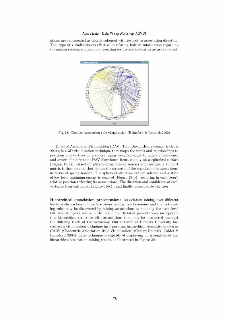
ations are represented as chords coloured with respect to association direction.This type of visualisation is effective in relating holistic information regardingthe mining session, concisely representing results and indicating areas of interest.

Fig. 18: Circular association rule visualisation (Rainsford & Roddick 2000)

Directed Associated Visualisation (DAV) (Hao, Dayal, Hsu, Sprenger & Gross2001), is a 3D visualisation technique that maps the items and relationships topositions and vertices on a sphere, using weighted edges to indicate confidenceand arrows for direction. DAV distributes items equally on a spherical surface(Figure 19(a)). Based on physics principles of masses and springs, a supportmatrix is then created that relates the strength of the association between itemsin terms of spring tension. The spherical structure is then relaxed and a stateof low local minimum energy is reached (Figure 19(b)), resulting in each item’srelative position reflecting its associations. The direction and confidence of eachvertex is then calculated (Figure 19(c)), and finally presented to the user.

Hierarchical association presentations Association mining over differentlevels of abstraction implies that items belong to a taxonomy and that interest-ing rules may be discovered by mining associations at not only the item levelbut also at higher levels in the taxonomy. Related presentations incorporatethis hierarchical structure with associations that may be discovered amongstthe differing levels of the taxonomy. Our research at Flinders University hascreated a visualisation technique incorporating hierarchical semantics known asCARV (Concentric Association Rule Visualisation) (Ceglar, Roddick, Calder &Rainsford 2003). This technique is capable of displaying both single-level andhierarchical association mining results as illustrated in Figure 20.

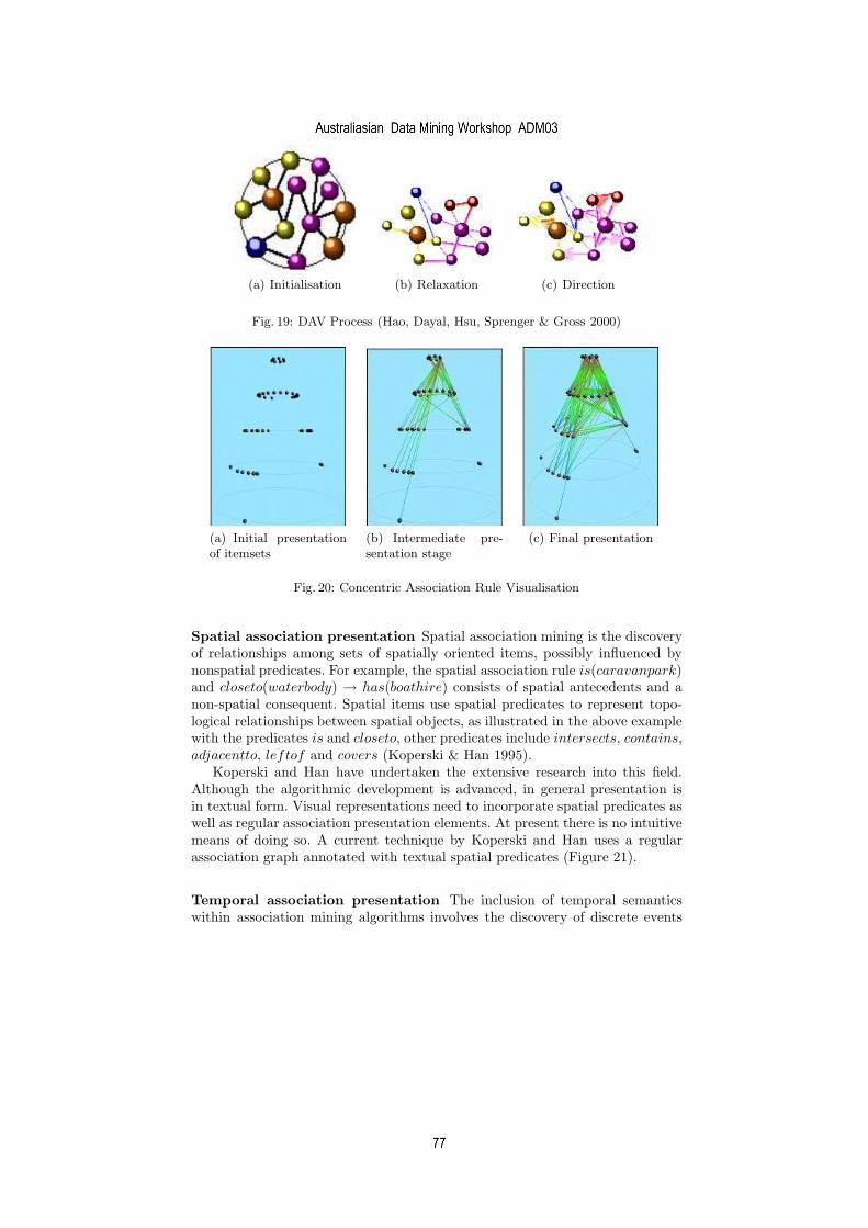
(a) Initialisation (b) Relaxation (c) Direction

Fig. 19: DAV Process (Hao, Dayal, Hsu, Sprenger & Gross 2000)

(a) Initial presentationof itemsets

(b) Intermediate pre-sentation stage

(c) Final presentation

Fig. 20: Concentric Association Rule Visualisation

Spatial association presentation Spatial association mining is the discoveryof relationships among sets of spatially oriented items, possibly influenced bynonspatial predicates. For example, the spatial association rule is(caravanpark)and closeto(waterbody) → has(boathire) consists of spatial antecedents and anon-spatial consequent. Spatial items use spatial predicates to represent topo-logical relationships between spatial objects, as illustrated in the above examplewith the predicates is and closeto, other predicates include intersects, contains,adjacentto, leftof and covers (Koperski & Han 1995).

Koperski and Han have undertaken the extensive research into this field.Although the algorithmic development is advanced, in general presentation isin textual form. Visual representations need to incorporate spatial predicates aswell as regular association presentation elements. At present there is no intuitivemeans of doing so. A current technique by Koperski and Han uses a regularassociation graph annotated with textual spatial predicates (Figure 21).

Temporal association presentation The inclusion of temporal semanticswithin association mining algorithms involves the discovery of discrete events

Fig. 21: Geominer - Spatial association rule visualisation

that frequently occur in the same arrangement along a time line. Thereforetemporal mining is the study of the temporal element arrangement, whereasassociation mining is the study of item relationships. Like spatial mining, tem-poral mining requires the incorporation of a set of defined temporal predicates.

For example, teaafter→ cinema consists of two events tea and cinema with the

predicateafter→ indicating their temporal arrangement.

Fig. 22: Temporal Association Mining

Figure 22 shows a temporal presentation designed by Rainsford and Roddick(1999), that incorporates temporality, by representing the temporal predicates(centre column) through which each rule (line) passes. In this way the temporalrelationships between the antecedent (left) and consequent (right) can be seen,with colour representing each rule’s confidence. Although restricted to simplerules (single antecedent and consequent), this visualisation technique efficientlypresents rules with diverse temporal predicates.

Fig. 23: Sequence Mining Presentation

Closely related to temporal mining is sequence mining, in which the patternsbeing discovered are constrained to sequentially discrete events. This focus on aparticular temporal aspect facilitates visualisation design as only a single tem-poral predicate is to be represented. Research by Wong et al. (Wong, Cowley,Foote, Jurrus & Thomas 2000) focus on sequential mining and to this end theyhave developed a visualisation for the presentation of temporal patterns discov-ered from newspaper article topics over a period of time. This is illustrated inFigure 23, where the topics are listed on the y-axis and the timeline along thex-axis. The patterns found at various times are displayed in a colour representinglevel of support. The four dashed circles highlight the presence of the same twopatterns within the time period.

The technique by Wong et al. provides a mixture of qualitative and quanti-tative information, showing the patterns while providing information regardingthe times at which they occurred. A more qualitative and concise presentationof the interesting information (the two re-occurring patterns) might have beenachieved through the use of Rainsford’s presentation method. However this wouldbe dependent upon the underlying algorithm.

Advances in sequence mining has resulted in a need to incorporate moremeaning within the generated rules, resulting in the inclusion of temporal logicsemantics (Allen 1983) within sequential mining algorithms (Hoppner 2002, Pad-manabhan & Tuzhilin 1996). This enables rules such as the following to be de-tected and reported.

Legend

Node Colour Description

Green Root Node for the interaction (E)

Blue Enclosing sub-episode (G, L, I, H)

Orange Enclosed sub-episode (C, A, T, O)

Purple Shared node of both enclosing andenclosed sub-episodes (N, S)

Edge Colour

Red Relationship between two Nodesand their supports

Gray The point(s) at which the enclosedsub-episode begins/ends within theenclosing sub-episode

Fig. 24: INTEM interaction of CANTONESE during ENGLISH

((Alarm Abefore−→ Alarm B)

during←→ Alarm C)

starts←→ Alarm D

These types of rules can become quite complex and to the authors’ knowl-edge have to date only been presented textually. In an attempt to present therules in a more meaningful manner, we at Flinders have developed the INTEM(INTeracting Episode Miner) visualization technique. The technique is simi-lar to mosaic plots 16 in that it allows the detailed investigation of particularsequence interactions that are of interest to the user, as illustrated in Figure 24.

5 Human Computer Interaction

Visualisation facilitates the perception of patterns and structure within datamining results. However, a static presentation in itself is often inadequate andinteractive capabilities are required to allow effective exploration of the visuali-sation. This relates to Shneiderman’s Visual Information Seeking Mantra, whichstated that the initial view is qualitative and of an overview nature and thatthrough interaction the user can proceed to focus upon interesting sub-areas formore quantitative analysis.

Interaction occurs at many different levels, as illustrated by the Layered Inter-action Model, shown in Figure 25. This model identifies a sequence of interactionlevels that build upon each other, illustrating that a interaction requirement canbe broken into different levels of abstraction, ranging from the subjective goals ofthe interaction through to the physical I/O of the interaction. There is however adefinite shift between the concept-based upper levels and the activity-based lowerlevels, indicating a transition between what is required and how it is done. Themapping or transformation between the concept and activity levels of interactionis known as direct manipulation and occurs at the junction of the syntactic andsemantic levels. This section discusses the exploration of presentations throughdirect manipulation and the use of views to facilitate understanding in largecomplex visualisations.

Level Name Exchanged Information Example

7 Goal Real World Concepts Remove letter section

6 Task Computer oriented actions Delete 6 lines of edited text

5 Semantics Specific operations Delete selected lines

4 Syntax Sentences of tokens Click at left of first char.,whilst holding down leftmouse button, click to theright of the last character

3 Lexical Tokens (smallest info carrying units) Click at left of first char.

2 Alphabetic Lexemes (primitive symbols) Click at (200,150)

1 Physical Hard I/O (movement,click) Click

Fig. 25: Layered Interaction Model

5.1 Direct manipulation

Direct manipulation can be defined as the mapping between the semantic andsyntactic levels of the layered interaction model (refer to Figure 25). The ob-jective in constructing this mapping is to create as close a match as possiblebetween the structure of how users think about a task and the activity used insolving it, while attempting to maximise problem domain compatibility (John,Rosenbloom & Newell 1985). Direct manipulation design effects the interactivequality of the system, including error frequency, speed of task performance, anduser skill retention (Buxton 1986).

There is not always a single best set of interaction capabilities for a particularvisualisation. Not all users have the same mental model, and even for a singleuser the mental model may differ depending upon the user’s current goals. There-fore the optimal solution is an intuitive set of mappings that mimic real worldactivities. For example, the task of moving a file in a paper-based office involvesgoing to the relevant filing cabinet, removing the required file and carrying it toits new location. Intuitively the same task on a computer system should followthe same steps. Graphical interfaces provide this capability by representing dataas graphical icons and encapsulating activities within interaction mappings. Sothe movement of a piece of data within the computer system will generally in-volve selecting the relevant icon and dragging it to its new location. Importantly,the syntax of operations in an interaction command should closely correspondto the data’s required semantic changes, and the screen representation shouldreflect these changes.

Graphical level interaction is based upon selection and navigation activitiesthat are specified to the computer by the user through pointing devices. Selectionis the designation of a point of interest within the graphical interface, signifiedthrough an action such as clicking a mouse button or pressing a key. Navigationis the movement of the interest focus, which is generally accomplished througha continuous activity such as moving the mouse or holding down specific keys.

These primitives work together within different environments to provide themeans by which any presentation may be explored in a detailed manner.

As there are an arbitrary number of semantic tasks that can be undertakenwithin a presentation, the overloading of an activity primitive such as selec-tion is achieved by varying the graphical primitive specification. For example,the functionality required within a presentation environment might include theability to delete items and to display item details in a pop-up dialog, both ofwhich involve item selection. Overloading of the selection primitive is achievedby either varying the selection action for each semantic task or requiring a com-bination action either in sequence or parallel. Another technique used to combatoverloading, (especially in navigation) is indirect manipulation, whereby the pre-sentation is manipulated through interaction with associated graphic artefacts.A common example is the use of scroll-bars within presentation environmentsto provide navigation at both the screen and document levels. However, indirectmanipulation techniques require that the user’s focus be drawn away from theactual presentation and lessen the interactive experience (Koedinger 1992). Micewith scroll-wheels overcome this by providing an additional form of vertical nav-igation, hence providing a means for direct navigation at both the screen anddocument levels.

3D presentations commonly provide more freedom but increase input over-loading and hence the variation of actions required to effectively explore theenvironment. Alternatively the use of immersive presentation devices such asheadsets, and pointing devices that allow further degrees of freedom such as fly-ing mice and gloves can increase the user’s experience of direct interaction andreduce the mapping overload.

The provision of a succinct set of direct manipulation mappings is critical foreffective presentation exploration. The level of interactive functionality providedis important as too little will constrain the exploration process and too muchwill result in interactive quality degradation. This degradation reflects the provi-sion of too many functional alternatives, resulting in non-intuitive mappings andhence longer task times and less skill retention. Therefore good direct manip-ulation design involves the specification of a succinct intuitive set of mappingsbased upon selection and navigation primitives to facilitate the comprehensiveexploration of a presentation.

5.2 Interactive Views

Mining result sets are often large and complex, typically tens of thousands ofitems. Their size makes them difficult to entirely represent in a form conduciveto understanding by the user. Large result sets produce cluttered presentationsbecause of the larger number of graphical objects required to represent the un-derlying data and their discovered relationships. Additional problems occur inthe presentation of hierarchical clustering semantics where separate presenta-tions are required to display different hierarchical instances of the clustering.

Interactive views use direct and indirect manipulation methods to enhanceuser perception of a result through user-specified filtering of the result set so

that only a subset are presented (Klemettinen, Mannila & Toivonen 1997, Rib-arsky, Katz, Jiang & Holland 1999, Wills 1998). Filter parameters are generallyspecified through indirect manipulation via interface controls and can involvethreshold, parameter, and template specification and also control the partici-pation of individual items and discovered relations. Threshold specification canbe used in association rules to constrain the confidence and support parametersthat provide heuristics as to the strength of the association and the importanceof the item within the data set. By raising the required confidence threshold,the weaker rules will no longer be displayed. Templates can constrain the ruleform. For example, the presentation can be limited to those rules that have onlya single antecedent.

(a) 7 clusters (b) 12 clusters

(c) 24 clusters (d) 76 clusters

Fig. 26: Interactive Views of hierarchical clustering

Clustering based presentations are different in that the discovered relation-ships are global in nature unlike association mining where each relationshipeffects only a few items, therefore constraint of the presentation to a subset ofclustered items is generally unwarranted. However Figure 26 shows how inter-active views can be useful in presenting hierarchical clustering results. The usercan change the number and hence levels of clustering viewed through the use ofan associated slide bar.

6 Guided Knowledge Discovery and Interactive Data

Mining

Interactive data mining is a process whereby the user can guide the knowledgediscovery. It is achieved by dynamically presenting the results of the data miningprocess and incorporating interactive capabilities within the presentation envi-ronment. This allows the user to interact with the underlying mining process.Through such interaction the user is able to guide the mining process and steerthe discovery process to areas of user interest.

Fig. 27: Knowledge Discovery Process

The iterative knowledge discovery process is illustrated in Figure 27. Thisprocess is controlled by user specification of data sources, tools, and associatedparameters. The process includes data collection (possibly from multiple het-erogenous sources), pre-processing (which massages the data into a form requiredfor analysis), analysis (mining), presentation, and finally interpretation by theuser. This widely accepted model of the knowledge discovery process shows eachstage as being independent, with the interaction between stages constrained tothe piping of the output of one stage to the input of the next stage. Dependingupon the extent to which the results satisfy the user’s goals, the user may refinethe specification of tools and parameters and re-cook the results. This re-cooking

or iteration of the knowledge discovery process or portions thereof can be atime expensive exercise, with the stages of collection, preprocessing and analysisrequiring many hours of work for large or complex data sets.

Some researchers report that the initial specification of the collection andpreprocessing stages can take up to 60% of the processing time. However becausethe user has a high degree of control over these processes and can specify exactlywhat is required, refinement is typically unnecessary. The analysis or miningstage, however, is generally batch oriented, so the user has no control over theprocess. User refinement and re-cooking generally occur at the analysis stage,with the user tweaking the mining algorithm’s parameters in an attempt toproduce results of greater interest. It is this lack of user control within theanalysis process that is rectified by incorporating interactive capabilities withinthe mining process.

Involving the user in the mining process requires an interface whereby theuser can see and guide the mining. In this way, the coupling between the analy-sis and presentation stages is strengthened by providing real-time streaming ofanalysis results to the presentation tool for user interpretation and by allowingthe subsequent guidance of the mining algorithm through user interaction withthe presentation.

Fig. 28: Guided Knowledge Discovery Process

Figure 28 shows the changes to the process. The change results in the mergingof the analysis and presentation stages, although current research is focused onmaintaining stage independence and increasing the coupling through the speci-fication of a generic set of interface methods that capture the required interac-tive functionality. This technology will provide flexibility by allowing the userto select the presentation technique that best suits their current needs. Ex-amples of this technology are the FIDO project currently being undertaken atFlinders University (Roddick & Ceglar 2001) and the KESO project at the Uni-versity of Helsinki (Wrobel, Wettschereck, Verkamo, Siebes, Mannila, Kwakkel& Klosgen 1996).

Increased coupling between the analysis and presentation stages is illustratedin Figure 29 and Figure 30, which differentiate between a batch and interactivemining run. The four images comprising these figures represent data mining runsas a tree structure with each level implying a point in time. The time interval isnot constant but indicates a point at which the mining algorithm reaches a stagewhere intermediate results may be produced. The production of intermediateresults is algorithm dependant, however most exploratory mining algorithms, forexample Apriori and k-means, involve multiple iterations over the dataset, whichprovide natural processing stages. Where the algorithm requires only a singlepass, techniques such as sampling can be used to provide intermediate results.Within Figures 32 and 33, the nodes within each tree level indicate the discoveredinformation at that point in time; the blue nodes represent intermediate resultsand the red nodes represent terminal results.

Fig. 29: Batch Data Mining Run

Figure 29 presents a regular batch mining run where the terminal results arepresented only at completion. If refinement is required, the entire mining runmust be repeated. Figure 30 illustrates the guidance of the knowledge discoveryprocess through interactive mining. These three diagrams show the productionor update of the presentation at different stages during the analysis process, thusproviding the user with insight into the process.

The initial presentation (Figure 30a) is generated based upon the availableintermediate results. The user is then able to interact with this presentation toguide further processing, represented in Figure 30b by the green coloured nodesthat indicate the users interest in these intermediate results. Further processing isthen constrained to the intermediate results indicated by these nodes. Figure 30cillustrates the completed state of the exploration process, within which can beseen the inclusion of further guidance.

Comparing Figure 29 and Figure 30c highlights the advantages of interactivedata mining. In particular the terminal result set is smaller, with less inter-

(a) Initial presentation (b) Intermediate Presen-tation

(c) Completed presenta-tion

Fig. 30: Interactive data mining

mediate results being processed. This reduces mining time and produces lesscluttered presentations. In addition the incorporation of subjective as well asobjective measures of interest within guided knowledge discovery ensures thatthis smaller, more quickly produced result set will be of greater interest to theuser. It is therefore also likely that less refinement and reprocessing will be re-quired, further reducing mining time.

Other techniques used to reduce mining time, particularly in the case ofassociation mining, are cache-based and constraint-based mining. Cache-basedmining or dynamic mining involves the storage of the results of frequently re-quested queries for fast retrieval of mining over common sets (Nag, Deshpande &DeWitt 1999, Raghavan & Hafez 2000). Constraint-based mining includes tech-niques such as subset mining and the prior specification of constraints. Subsetmining involves the mining of a subset of the data, the rules of which are thenverified against the whole set (Toivonen 1996). However, this method is proba-bilistic and may not discover some rules of interest. Prior constraint techniquesinvolve the specification of boolean expressions to constrain the mining process(Srikant et al. 1997). However it is often the case in explorative tasks the userdoes not know beforehand what is of interest; only through the presentation ofoptions can the user focus on what is of greater interest. Although these meth-ods may reduce mining time, they do not pre-empt guided discovery throughinteraction, and are not associated with the benefits it offers.

The granularity and types of interaction possible are dependent upon boththe presentation type and mining task. The user may manipulate the miningprocess either in terms of its focus, its parameters or its constituent dataset byinteracting with the associated real-time presentation. Figure 30 is indicative ofan exclusion form of interaction whereby the user eliminates a node from furtherprocessing. A more advanced technique is that of priority interaction whereby theuser selects the nodes of interest, which are processed first and hence presentedfirst. This doesn’t exclude the further processing of the other nodes; it simplyputs off this processing until the prioritised work has been completed. Thisensures that eventually all elements will be processed, so all possibly interestingresults are discovered, while arranging for those of most interest (as specified bythe user) to be processed first (Wrobel et al. 1996).

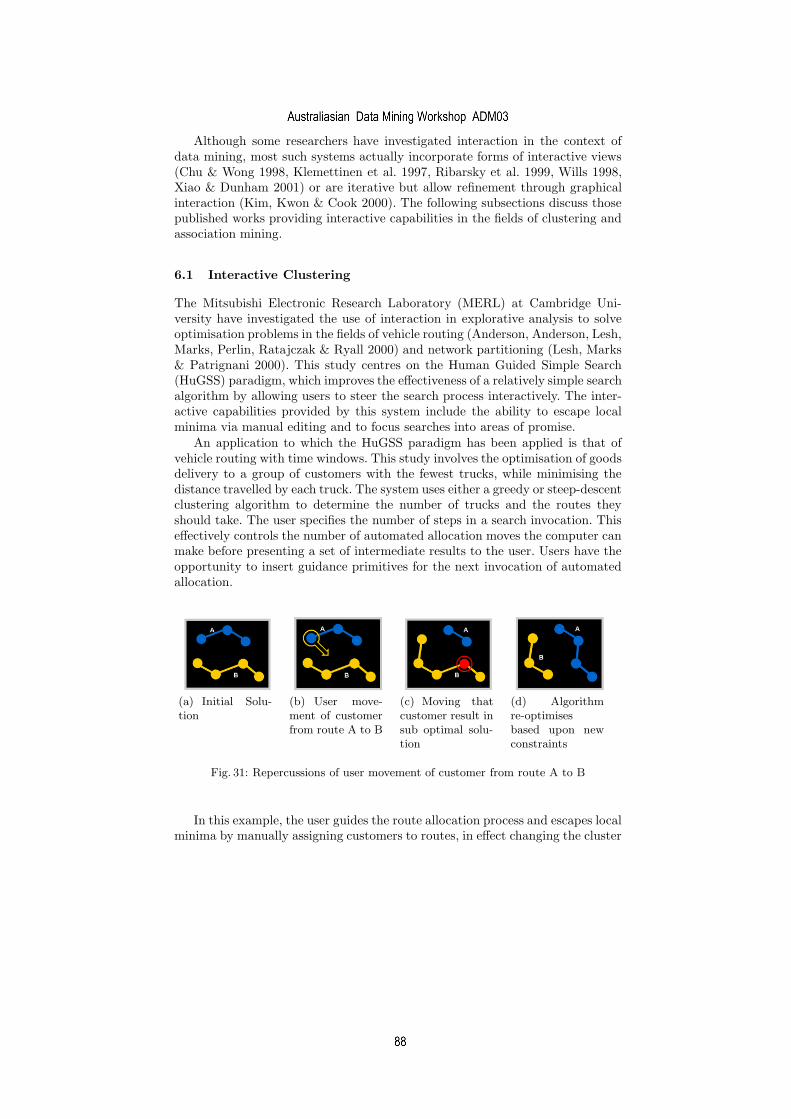
Although some researchers have investigated interaction in the context ofdata mining, most such systems actually incorporate forms of interactive views(Chu & Wong 1998, Klemettinen et al. 1997, Ribarsky et al. 1999, Wills 1998,Xiao & Dunham 2001) or are iterative but allow refinement through graphicalinteraction (Kim, Kwon & Cook 2000). The following subsections discuss thosepublished works providing interactive capabilities in the fields of clustering andassociation mining.

6.1 Interactive Clustering

The Mitsubishi Electronic Research Laboratory (MERL) at Cambridge Uni-versity have investigated the use of interaction in explorative analysis to solveoptimisation problems in the fields of vehicle routing (Anderson, Anderson, Lesh,Marks, Perlin, Ratajczak & Ryall 2000) and network partitioning (Lesh, Marks& Patrignani 2000). This study centres on the Human Guided Simple Search(HuGSS) paradigm, which improves the effectiveness of a relatively simple searchalgorithm by allowing users to steer the search process interactively. The inter-active capabilities provided by this system include the ability to escape localminima via manual editing and to focus searches into areas of promise.

An application to which the HuGSS paradigm has been applied is that ofvehicle routing with time windows. This study involves the optimisation of goodsdelivery to a group of customers with the fewest trucks, while minimising thedistance travelled by each truck. The system uses either a greedy or steep-descentclustering algorithm to determine the number of trucks and the routes theyshould take. The user specifies the number of steps in a search invocation. Thiseffectively controls the number of automated allocation moves the computer canmake before presenting a set of intermediate results to the user. Users have theopportunity to insert guidance primitives for the next invocation of automatedallocation.

(a) Initial Solu-tion

(b) User move-ment of customerfrom route A to B

(c) Moving thatcustomer result insub optimal solu-tion

(d) Algorithmre-optimisesbased upon newconstraints

Fig. 31: Repercussions of user movement of customer from route A to B

In this example, the user guides the route allocation process and escapes localminima by manually assigning customers to routes, in effect changing the cluster

to which the item belongs. This automatically invokes a route optimisation algo-rithm on the effected routes only, ensuring that under these new constraints thesystem still provides the best possible solution, as illustrated in Figure 31. Theuser can additionally change a customer’s priority, which effects when the cus-tomer is considered for movement by the algorithm, and changes the algorithm’sassociated objective measures and mode before invocating another sequence ofautomated route allocations.

The MERL group has also applied the HuGSS paradigm to the area of k-way network partitioning, a NP-hard problem arising from VLSI design andelsewhere. This application has required the development of a different set ofpresentation techniques that visualise the required relevant aspects. The workconsequently led to the development of a new set of interaction mappings thateffectively provide the same types of interactive guidance as the route discoveryapplication (Lesh et al. 2000). Other work (Nascimento & Eades 2001) allowthe user to interactively change clusters number and size however the crucialelement in MERL’s research is the ability to guide the cluster membership ofparticular items. This research by MERL is the most significant published workin the field to date.

6.2 Interactive Association Mining

Research undertaken by Brin and Page at the Stanford University (Brin &Page 1998) appears to be the only piece of research that satisfies our crite-ria for guided association mining. Known as Dynamic Data Mining (DDM),their work attempts to produce more interesting rules by foregoing traditionalsupport-based algorithms (that use a single deterministic run) and instead usea method that continuously explores more of the search space. This is accom-plished through the incorporation of a user-defined measure of interest, Weight,which can be redefined dynamically and a heuristic, HeavyEdgeProperty, whichguides the exploration process.

Rather than the mining process being a single deterministic run (producinga well-defined set of itemsets and rules), DDM invokes a process that continu-ally generates improving itemsets, based upon the Dynamic Itemset Countingalgorithm (DIC) (Brin, Motwani, Ullman & Tsur 1997). This allows the DDMto take advantage of intermediate counts to form an estimate of an itemset’soccurrence or weight, which results in the presentation of intermediate results tothe user. The user is then able to dynamically adjust individual item weights, ineffect prioritising them. User interaction is indirect and textual, with refinementoccurring through an associated text box within which the user can adjust globalmining parameters and individual item weights via a simple language.

This research provides a means of prioritising the mining of particular itemsand in effect allows the user to insert a subjective measure of interestingness intothe algorithm. The technique will produce a more interesting and smaller set ofresults than traditional batch processing methods.

7 Conclusion

Guided knowledge discovery through interactive data mining as a discrete fieldof research is still in its infancy and as such there are few published works ofrelevance. This leaves open broad and diverse areas of further research in the ar-eas of algorithmic development, interaction, and presentations and in associatedareas such as collaborative guidance.

Future algorithmic research in the field will focus upon methods by whichguidance can be incorporated into new or existing explorative algorithms at dif-ferent levels of granularity. Preliminary areas that show promise include prioritybased algorithms (Brin & Page 1998), incremental computation (Sundaresh &Hudak 1991) and state based processing, which uses the concept of rollback toreturn to a previous intermediate state instead of re-instigating a new analysis.An associated area is the investigation of supporting frameworks that provideflexible interactive knowledge discovery environments.

It seems likely that the majority of these techniques will remain domain-specific (if not task- specific), because of associated subjective interpretation.The challenge lies in the creation of generic sets of interaction mappings betweenthe graphical interface and the underlying mining process. The development ofsuch mappings was indicated by the research of the MERL team (Andersonet al. 2000, Lesh et al. 2000) where a single set of interaction functions wereeffectively incorporated within two different problems domains, using differentdomain specific presentations.

Existing knowledge discovery tools do not adequately provide the capabilitiesto incorporate subjective measures of interestingness into the analysis process.Current analysis results in ineffective discovery processes, as heuristic measurescannot accurately portray what is potentially of interest to the user. As shownby the MERL team (Anderson et al. 2000, Lesh et al. 2000), and Brin andPage (1998), subjective judgement can be incorporated by actively engaging theuser in the mining process. Benefits include an accelerated knowledge discoveryprocess and improved results. User participation in the mining process results ingreater confidence in the correctness of the discovered patterns, due to the senseof control that guidance capabilities provide.

References

Agrawal, R., Imielinski, T. & Swami, A. (1993), Mining association rules between setsof items in large databases, in ‘1993 ACM SIGMOD Int. Conf. Management ofData’, Washington D.C. U.S.A, pp. 207–216.

Allen, J. F. (1983), ‘Maintaining knowledge about temporal intervals’, Communicationsof the ACM 26(11), 832–843.

Anderson, D., Anderson, E., Lesh, N., Marks, J., Perlin, K., Ratajczak, D. & Ryall,K. (2000), Human guided simple search: combining information visualization andheuristic search, in ‘Proc. of the workshop on new paradigms in information vi-sualization and manipulation. In conjunction with the eighth ACM internationalconference on Information and Knowledge Management’, ACM Press, Kansas City,MO, pp. 21–25.

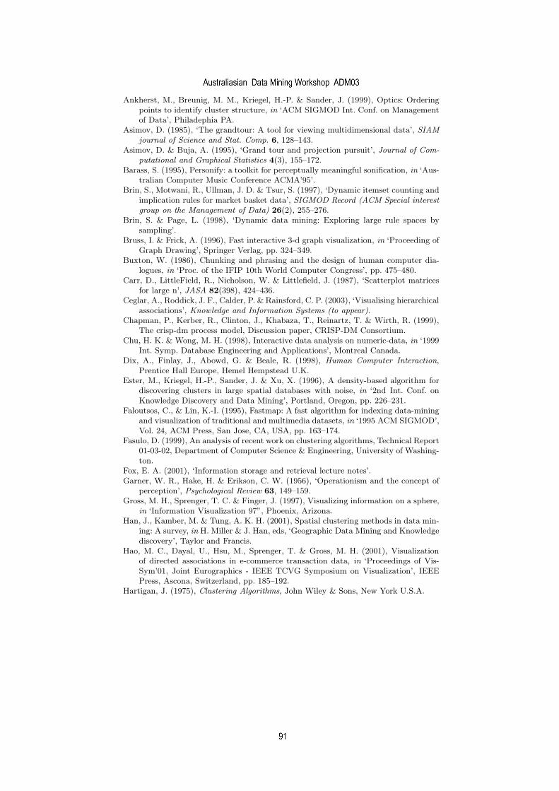
Ankherst, M., Breunig, M. M., Kriegel, H.-P. & Sander, J. (1999), Optics: Orderingpoints to identify cluster structure, in ‘ACM SIGMOD Int. Conf. on Managementof Data’, Philadephia PA.

Asimov, D. (1985), ‘The grandtour: A tool for viewing multidimensional data’, SIAMjournal of Science and Stat. Comp. 6, 128–143.

Asimov, D. & Buja, A. (1995), ‘Grand tour and projection pursuit’, Journal of Com-putational and Graphical Statistics 4(3), 155–172.

Barass, S. (1995), Personify: a toolkit for perceptually meaningful sonification, in ‘Aus-tralian Computer Music Conference ACMA’95’.

Brin, S., Motwani, R., Ullman, J. D. & Tsur, S. (1997), ‘Dynamic itemset counting andimplication rules for market basket data’, SIGMOD Record (ACM Special interestgroup on the Management of Data) 26(2), 255–276.

Brin, S. & Page, L. (1998), ‘Dynamic data mining: Exploring large rule spaces bysampling’.

Bruss, I. & Frick, A. (1996), Fast interactive 3-d graph visualization, in ‘Proceeding ofGraph Drawing’, Springer Verlag, pp. 324–349.

Buxton, W. (1986), Chunking and phrasing and the design of human computer dia-logues, in ‘Proc. of the IFIP 10th World Computer Congress’, pp. 475–480.

Carr, D., LittleField, R., Nicholson, W. & Littlefield, J. (1987), ‘Scatterplot matricesfor large n’, JASA 82(398), 424–436.

Ceglar, A., Roddick, J. F., Calder, P. & Rainsford, C. P. (2003), ‘Visualising hierarchicalassociations’, Knowledge and Information Systems (to appear).

Chapman, P., Kerber, R., Clinton, J., Khabaza, T., Reinartz, T. & Wirth, R. (1999),The crisp-dm process model, Discussion paper, CRISP-DM Consortium.

Chu, H. K. & Wong, M. H. (1998), Interactive data analysis on numeric-data, in ‘1999Int. Symp. Database Engineering and Applications’, Montreal Canada.

Dix, A., Finlay, J., Abowd, G. & Beale, R. (1998), Human Computer Interaction,Prentice Hall Europe, Hemel Hempstead U.K.

Ester, M., Kriegel, H.-P., Sander, J. & Xu, X. (1996), A density-based algorithm fordiscovering clusters in large spatial databases with noise, in ‘2nd Int. Conf. onKnowledge Discovery and Data Mining’, Portland, Oregon, pp. 226–231.

Faloutsos, C., & Lin, K.-I. (1995), Fastmap: A fast algorithm for indexing data-miningand visualization of traditional and multimedia datasets, in ‘1995 ACM SIGMOD’,Vol. 24, ACM Press, San Jose, CA, USA, pp. 163–174.

Fasulo, D. (1999), An analysis of recent work on clustering algorithms, Technical Report01-03-02, Department of Computer Science & Engineering, University of Washing-ton.

Fox, E. A. (2001), ‘Information storage and retrieval lecture notes’.Garner, W. R., Hake, H. & Erikson, C. W. (1956), ‘Operationism and the concept of

perception’, Psychological Review 63, 149–159.Gross, M. H., Sprenger, T. C. & Finger, J. (1997), Visualizing information on a sphere,

in ‘Information Visualization 97”, Phoenix, Arizona.Han, J., Kamber, M. & Tung, A. K. H. (2001), Spatial clustering methods in data min-

ing: A survey, in H. Miller & J. Han, eds, ‘Geographic Data Mining and Knowledgediscovery’, Taylor and Francis.

Hao, M. C., Dayal, U., Hsu, M., Sprenger, T. & Gross, M. H. (2001), Visualizationof directed associations in e-commerce transaction data, in ‘Proceedings of Vis-Sym’01, Joint Eurographics - IEEE TCVG Symposium on Visualization’, IEEEPress, Ascona, Switzerland, pp. 185–192.

Hartigan, J. (1975), Clustering Algorithms, John Wiley & Sons, New York U.S.A.

Hilderman, R. J. & Hamilton, H. J. (1999), Knowledge discovery and interestingnessmeasures: A survey, Technical Report CS 99-04, Department of Computer Science,University of Regina.

Hinneburg, A. & Keim, D. A. (1999), A:(tutorial) clustering techniques for large datasets: From the past to the future, in ‘SIGMOD Conference’, Philadelphia.

Hinneburg, A., Keim, D. A. & Wawryniuk, M. (1999), ‘Hd eye: Visual mining of highdimensional data’, IEEE Computer Graphics and Applications 19(5), 22–31.

Hofman, H., Siebes, A. P. & Wilhelm, A. F. (2000), Visualizing association rules withinteractive mosaic plots, in ‘KDD 2000’, ACM, Boston, MA USA, pp. 227–235.

Hoppner, F. (2002), Discovery of core episodes from sequences – using generalization fordefragmentation of rule sets, in ‘Pattern Detection and Discovery in Data Mining,LNAI’, Vol. 2447, Springer, London, England, pp. 199–213.

Jain, A. K. & Dubes, R. C. (1988), Algorithms for Clustering Data, Prentice Hall,Englewood Cliffs New Jersey U.S.A.

John, Rosenbloom, P. & Newell, A. (1985), A theory of stimulus-response compatibilityapplied to human computer interaction, in ‘Proceedings of CHI’85’, pp. 213–230.

Kim, S.-S., Kwon, S. & Cook, D. (2000), ‘Interactive visualization of hierarchical clus-ters using mds and mst’, Metrika 51(1), 39–51.

Klemettinen, M., Mannila, H., Ronkainen, T. & Verkano, A. (1994), Finding interestingrules from large sets of discovered association rules, in N. R. Adam, B. K. Bhargava& Y. Yesha, eds, ‘Third International Conference on Information and KnowledgeManagement (CIKM’94)’, ACM Press, Gaitherburg Maryland USA, pp. 401–407.

Klemettinen, M., Mannila, H. & Toivonen, H. (1997), A data mining methodologyand its application to semi-automatic knowledge acquisition, in ‘Proceedings ofthe 8th International Workshop on Database and Expert Systems Applications’,IEEE Press, pp. 67–677.

Klemmer, E. T. & Frick, F. C. (1953), ‘Assimilation of information from dot and matrixpatterns’, Experimental Psychology 45, 15–19.

Koedinger, K. R. (1992), Emergent properties and structural constraints: Advantagesof diagrammatic representations for reasoning and learning, in ‘AAAI Spring Sym-posia on Reasoning with Diagrammatic Representations’, Stanford University.

Koperski, K. & Han, J. (1995), Discovery of spatial association rules in geographicinformation databases, in ‘4th Int’l Symp. on Large Spatial Databases (SSD’95)’,Portland, Maine, pp. 47–66.

Lesh, N., Marks, J. & Patrignani, M. (2000), Interactive partitioning, Technical report,Mitsubishi Electronic Research Laboratory.

Li, S., Vel, O. d. & Coomans, D. (1995), Comparative performance analysis of non-linear dimensionality reduction methods, Technical report, James Cook University.

Mayo, E. (1945), The Social Problems of an Industrialized Society, Harvard UniversityPress, Boston.

Miller, G. A. (1956), ‘The magic number seven,plus or minus two: Some limits on ourcapacity for processing information’, Psychological Review 63, 81–97.

Nag, B., Deshpande, P. M. & DeWitt, D. J. (1999), Using a knowledge cache forinteractive discovery of association rules, in ‘KDD-99’, ACM Press, San Deigo CaUSA, pp. 244–253.

Nascimento, H. A. & Eades, P. (2001), Interactive graph clustering based upon userhints, in ‘Proc. of the Second Int. Workshop on Soft Computing Applied to Soft-ware Engineering’, Enschede, The Netherlands, p. 7.

Padmanabhan, B. & Tuzhilin, A. (1996), Pattern discovery in temporal databases: atemporal logic approach, in E. Simoudis, J. Han & U. Fayyad, eds, ‘Proceedings

of the 2nd International Conference on Knowledge Discovery and Data Mining’,AAAI Press, Portland, Oregon, pp. 351–354.

Piatetsky-Shapiro, G. (1991), Discovery, analysis and presentation of strong rules, inW. J. Frawley & G. Piatetsky-Shapiro, eds, ‘Knowledge Discovery in Databases’,AAAI - MIT Press.

Raghavan, V. & Hafez, A. (2000), Dynamic data mining, in ‘Industrial and Engineer-ing Applications of Artificial Intelligence and Expert Systems’, Lecture Notes inComputer Science, Springer-Verlag, pp. 220–229.

Rainsford, C. P. & Roddick, J. F. (1999), Adding temporal semantics to associationrules, in J. Zytkow & J. Rauch, eds, ‘Proceedings of the 3rd European Confer-ence on Principles and Practice of Knowledge Discovery in Databases, PKDD’99’,Springer Verlag, Prague, Czech Republic, pp. 504–509.

Rainsford, C. & Roddick, J. (2000), Visualisation of temporal interval association rules,in ‘Proc 2nd International Conference on Intelligent Data Engineering and Auto-mated Learning’, Shatin, N.T. Hong Kong.

Rasmussen, E. (1992), Clustering algorithms, in W. Frakes & R. Baeze-Yates, eds, ‘In-formation Retrieval: Data Structures and Algorithms’, Prentice-Hall, EnglewoodCliffs, New Jersey U.S.A.

Ribarsky, W., Katz, J., Jiang, F. & Holland, A. (1999), ‘Discovery visualization usingfast clustering’, IEEE Computer Graphics and Applications 19(5), 32–39.

Roddick, J. & Ceglar, A. (2001), ‘Fido’.Sander, J., Ester, M., Kriegel, H.-P. & Xu, X. (1998), ‘Density-based clustering in

spatial databases: The algorithm gdbscan and its applications’, Data Mining andKnowledge Discovery 2(2), 169–194.

Shneiderman, B. (1996), The eyes have it: A task by data type taxonomy for informa-tion visualization, in ‘1996 IEEE Symp. on Visual Languages’, Boulder Colorado,pp. 336–343.

Silberschatz, A. & Tuzhilin, A. (1996), ‘What makes patterns interesting in knowl-edge discovery systems?’, IEEE Transactions on Knowledge and Data Engineering8(6), 970–974.

Sprenger, T. C., Brunella, R. & Gross, M. H. (2000), H-blob: A hierarchical visualclustering method using implicit surfaces, in ‘IEEE Visualisation 2000’, Salt LakeCity, UTAH, USA.

Srikant, R., Vu, Q. & Agrawal, R. (1997), Mining association rules with item con-straints, in D. Eckerman, H. Mannila, D. Pregibon & R. Uthursamy, eds, ‘3rd Int.Conf. on Knowledge Discovery and Data Mining’, AAAI Press, Newport Beach,C.A., U.S.A., pp. 67–73.

Sundaresh, R. S. & Hudak, P. (1991), Incremental computation via partial evaluation,in ‘18th Annual ACM Symp. on POPL’, ACM Press, New York, pp. 1–13.

Toivonen, H. (1996), Sampling large databases for association rules, in T. Vijayara-man, Alejandro, P.Buchmann, C. Mohan & N. Sarda, eds, ‘Proceedings of the22nd International Conference on Very Large Data Bases’, Morgan Kaufman,Mumbia(Bombay), India, pp. 134–145.

Tung, A. K. H., Hou, J. & Han, J. (2001), Spatial clustering in the presence of obstacles,in ‘Int. Conf. on Data Engineering’, Heidelberg, Germany.

Ward, M. O. (1994), Xmdvtool : Integrating multiple methods for visualising multi-variate data, in R. D. Bergeron & A. E. Kaufman, eds, ‘IEEE Visualization ’94’,pp. 326–333.

Wills, G. (1998), An interactive view for hierarchical clustering, in ‘Information Visu-alization ’98’, Raleigh, North Carolina, USA.

Wong, P. C., Cowley, W., Foote, H., Jurrus, E. & Thomas, J. (2000), Visualizingsequential patterns for text mining, in ‘IEEE Sym. on Information Visualization2000’, IEEE Press, Salt Lake City, Utah.

Wong, P. C., Whitney, P. & Thomas, J. (1999), Visualizing association rules for textmining, in ‘Proceedings of IEEE Symposium on Information Visualization’99’,IEEE Computer Society Press, Los Alamitos, California,USA, pp. 120–124.

Wrobel, S., Wettschereck, D., Verkamo, I., Siebes, A., Mannila, H., Kwakkel, F. &Klosgen, W. (1996), User interactivity in very large scale data mining, in W. Dilger,M. Schlosser, J. Zeidler & A. Ittner, eds, ‘FGML-96 Annual Workshop of the GISpecial Interest Group Machine Learning’, TU Chemnitz-Zwickau, pp. 125–130.

Xiao, Y. & Dunham, M. H. (2001), Interactive clustering for transaction data, inY. Kambayashi, W. Winiwarter & M. Arikawa, eds, ‘Third Int. Conf. Data Ware-housing and Knowledge Discovery’, Springer Verlag, Munich, Germany, pp. 121–130.

Yang, L. (2000), n23tool: A tool for exploring large relational datasets trough dynamicprojections, in ‘9th Int. Conf. on Information and Knowledge Management CIKM2000’, ACM Press, pp. 322–327.

Young, F. (1987), Multidimensional Scaling: history, theory and applications, LawrenceErlbaum Associates, Hillsdale New Jersey U.S.A.

Texture Analysis via Data Mining

Martin Heckel

Brno University of Technology, Faculty of Information Technology, Bozetechova 2, 612 66 Brno, Czech Republic heckel@fit.vutbr.cz

Abstract. This paper deals with an idea of the use of data mining approach in texture analysis. A new method based on association rules is proposed. This approach extracts texture primitives from an image texture and describes mutual relationships between these primitives. Within this method, a technique for feature vector construction without a priori knowledge of textures different from the analyzed one is presented. The Fisher criterion was used to measure an ability of the proposed method for successful discrimination of pairs of textures. This work provides also comparison of the proposed technique with a wide-used wavelet texture features.

1 Introduction

Texture is one of the most important property of image data used in many application domains, for instance medical image processing, industrial inspection, remote sensing, document processing etc. Texture description usually as a part of feature vector has also appeared in the area of content based image retrieval for image browsing, searching and retrieval [1], [2], [3].

In the last thirty years, many texture analysis techniques have been developed. They can be divided into four main classes [4]: statistical methods, signal processing methods, model based approaches and geometrical approaches. Currently, signal processing methods, mainly wavelet decomposition (e.g. [5], [3]) and Gabor filters (e.g. [1], [2]) belong to the most popular techniques.

This work focuses on the other class, on geometrical properties of image texture. Herein, a texture is considered as being composed of texture primitives and an arrangement of these primitives is described by certain rules.

We attempt to capture texture arrangement properties by data mining approach, particularly by association rules. The best-known application domain, where association rules have been successfully used, is market basket analysis. Here, the goal is to identify items frequently purchased together. We utilize association rules to determine texture primitives occurring together in a texture.

The idea of using association rules during texture analysis was published by J. A. Rushing et al. in [6]. We extended this idea by the processing of image texture at the primitive level. We also developed a technique of the feature vector construction without a priori knowledge of textures different from the analyzed one.

The paper is organized as follows. The next section describes a proposed texture analysis method. Section 3 deals with separability measurements on pairs formed from some Brodatz textures [7]. Section 4 summarizes the results of the proposed approach.

2 Texture Description Method

We developed a new method of texture image description based on association rules for analyzing grey level texture images. This approach consists of three following steps:

1. Extraction and description of texture primitives – The goal is to extract and describe texture primitives in an image texture (Section 2.1).

2. Mining of association rules – In this step, the transaction databases are constructed and association rules are mined (Section 2.2).

3. Feature vector construction – The goal is to compute a feature vector without a priori knowledge of a set of textures, different from the analyzed one (Section 2.3).

In this method, the image texture is not analyzed at the pixel level (as in [6]), but at

higher one, at the image primitive level. Obtained association rules describe texture primitive arrangement in a non-deterministic way. This data mining approach finds frequently occurring local structures at the primitive level in an analyzed image.

2.1 Extraction and Description of Texture Primitives

In this stage, we extract texture primitives from the analyzed image texture. As a texture primitive, we understand a connected region composed of pixels at the same grey level. Thus, the number and the size of extracted primitives depend on a texture type. For instance, we obtain a big number of small primitives in case of a microtexture.

Once the primitives are identified, we describe them by their own grey levels and the geometrical properties. Then, the set of primitive descriptions is the output of this stage.

In order to extract texture primitives, it is necessary to quantize every image to a certain number of grey levels. We chose the well-known statistical clustering algorithm k-means [8] to perform an adaptive quantization to a certain small number of levels.

It remains texture primitive identification. For this task, we use connected component analysis. The connected component is a set of image pixels, which share a certain property. In this component, there exists a path between every pair of pixels. Every connected component represents one texture primitive, whereby a grey level of pixels is used as a shared property. We use a row-by-row labeling algorithm proposed by A. Rosenfeld and J. L. Phaltz [9].

Every identified primitive is described by its properties: 1. The grey level. 2. The area of primitive (number of pixels)

( ) .,00 ∑∑=x y

yxfm (1)

3. The centroid ( ): tt yx ,

( ),

,

00m

yxxfx x y

t

∑∑= (2)

( ),

,

00m

yxyfy x y

t

∑∑= (3)

where denotes the analyzed image texture. This function returns 1, if a pixel ) belongs to the primitive, otherwise 0.

( yxf ,( y,

)x

2.2 Mining of Association Rule

This part of a proposed method focuses on the mining of association rules, which characterize mutual relationships between texture primitives. The set of primitive descriptions together with the primitive adjacency information are the input of this stage. For the set of primitive descriptions, a transaction database is constructed based on primitive adjacency (Subsection Transaction Database Construction). In order to mine the association rules from a transaction database, we used the well-known Apriori algorithm (SubSection Association Rule Discovery). Thus, the set of association rules form the output of this stage. SubSection Association Rules provides brief introduction to association rules.

Association Rules. Association Rules was introduced by R. Agrawal et al. [10] as one knowledge type, which can be discovered in databases. Association rules are non-deterministic rules, which capture mutual relationship between data stored in a database. Initially, these rules are designed for transaction databases. Such a database consists of transactions, where a transaction is a set of items related together.

An association rule is an implication of the form A ⇒ B, where A, B are disjoint sets of items. This rule has two probability values: support s and confidence c.

Support s of the rule expresses the percentage of transactions in the whole database, which contain both the sets A and B. Confidence c means the percentage of transactions containing both A and B from all transaction containing A. This can be written as follows:

,)()( BAPBAs ∪=⇒ (4)

. )(

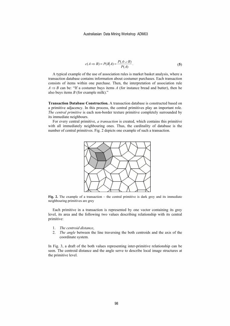
)()()(AP

BAPABPBAc ∪==⇒ (5)

A typical example of the use of association rules is market basket analysis, where a transaction database contains information about costumer purchases. Each transaction consists of items within one purchase. Then, the interpretation of association rule A ⇒ B can be: “If a costumer buys items A (for instance bread and butter), then he also buys items B (for example milk).”

Transaction Database Construction. A transaction database is constructed based on a primitive adjacency. In this process, the central primitives play an important role. The central primitive is each non-border texture primitive completely surrounded by its immediate neighbours.

For every central primitive, a transaction is created, which contains this primitive with all immediately neighbouring ones. Thus, the cardinality of database is the number of central primitives. Fig. 2 depicts one example of such a transaction.

Fig. 2. The example of a transaction – the central primitive is dark grey and its immediate neighbouring primitives are grey

Each primitive in a transaction is represented by one vector containing its grey level, its area and the following two values describing relationship with its central primitive:

1. The centroid distance, 2. The angle between the line traversing the both centroids and the axis of the

coordinate system.

In Fig. 3, a draft of the both values representing inter-primitive relationship can be seen. The centroid distance and the angle serve to describe local image structures at the primitive level.

Because of the numeral nature of information stored in the transaction, it is necessary to quantize these values in the whole transaction database. For instance, the angle can be quantized to 4, 8 or 16 levels etc.

Fig. 3. A relationship between central (dark grey) and neighbouring primitive (grey)

Association Rule Discovery. We selected the well-known Apriori algorithm [10] to process a transaction database (for further details of this algorithm see e.g. [11]). The output of this algorithm is the set of frequent itemsets, which are sets of items satisfying the condition of minimum support value.

From this set of frequent itemsets, association rules, which fulfill the minimum confidence condition, are generated according to the following widely used algorithm:

1. For each frequent itemset l, all its non-empty subsets are generated.

2. For every generated subset A, create a rule A ⇒ (l - A), if its confidence )()(

Asls

is equal or greater than the minimum confidence value. Note, that the itemset l of cardinality k generates 2k candidate association rules. Based on the number of generated rules for tested texture images, we limited the right and the left side cardinalities of rules to the following rule cardinality types:

1. ( ) ⇒ ( ), 2. ( )( ) ⇒ ( ), 3. ( )( ) ⇒ ( )( ), 4. ( )( )( ) ⇒ ( ),

where the symbol ( ) denotes one item.

2.3 Feature Vector Construction

In this stage, a feature vector representing an analyzed image texture is computed. The set of association rules is the input and one feature vector is the output. The feature vector is constructed in the following steps:

1. Input set of association rules is divided into four groups of the same

cardinality type (see Section 2.2). 2. The rules in every group are sorted by the support and by the confidence. 3. In every sorted group, only a certain number of first rules is kept. We used

only the first two rules from every group. 4. The length of the feature vector is divided into four partitions for every

association rule groups. 5. Each association rule is stored to the feature vector in this way: First, the

values of the items on the right side and second, the values of the items of the left side (items of both sides of the rule are presorted in lexicographic order).

6. If some rule group has less than two rules, the space for this rule in the feature vector is completed by zeros.

Using this algorithm, a 104-dimensional feature vector is composed (4 values per one item). The feature vector is constructed without a priori knowledge of textures different from analyzed one (in contrast with [6]) and it has a fixed size and form. Such a form of the feature vector is suitable e.g. for content based image retrieval or for the data mining tasks performed over the entire image database.

3 Discriminatory Ability of the Method

In order to analyze properties of the proposed method, the Fisher criterion (Section 3.1) which determine a discriminatory ability for a pair of textures is used. We performed a number of experiments over textures from the Brodatz album [7] and provide a comparison with wide-used wavelet texture features (Section 3.2).

3.1 Fisher criterion

In this work, the Fisher criterion is utilized to measure of proposed method ability to discriminate one texture from the other. The Fisher criterion expresses a separability of two clusters containing feature vectors, which characterize an analyzed pair of textures. In the area of texture analysis, this method was first proposed by P. Kruizinga and N. Petkov [12]. More details of the Fisher criterion can be found e.g. in [15], [16].

The Fisher linear discriminant function can be written in the following form:

,)( 121 xSy T rrr −−= µµ (6)

where xr is feature vector obtained from an analyzed texture, y is its projection, 21 , µµ rr are the means of the two clusters and S is a pooled covariance matrix

( ) ( ) ( ) ( .2

1 21

12;22;2

11;11;1

21

−−+−−

−+= ∑∑

==

N

jj

Tj

N

jj

Tj xxxx

NNS µµµµ rrrrrrrr ) (7)

N1 is the number of selected (e.g. randomly) feature vectors jx ;1r from the first cluster

and N2 is the number of selected vectors jx ;2r from the second one.

The Fisher linear discriminant function (6) realizes the projection of the n-dimensional feature space on one-dimensional space (on a line). The dimensionality of a feature space is given by the number of features, contained in feature vectors. This projection maximizes the Fisher criterion

,22

21

21

σσ

ηη

+

−=f (8)

where η1, η2 and , are the means and the variances characterizing the distribution of the projected feature vectors of the two clusters. The means η1, η2 are yielded by the projections:

21σ

22σ

.)(

,)(

21

212

11

211

µµµη

µµµηrrr

rrr

−

−

−=

−=

S

ST

T (9)

The Fisher criterion measures the distance between the means of the both clusters relative to the sum of their variances, thus to their compactness. That is why, it is suitable to measure separability of two clusters and also to express the capability of texture description methods for successful discrimination of pairs of different textures.

3.2 Experimental schema and results

We performed a number of experiments with the proposed method over textures from the Brodatz album [7] under following conditions:

Six textures D34, D49, D75, D84, D95, D104 that were used are shown in Fig. 4. From every texture, one thousand of feature vectors were extracted by analysing texture in a 128 × 128 pixel window moving through the analysed image texture. All positions of this moving window cover the whole analysed texture uniformly. Thus, these thousand vectors for every given texture form a respective cluster.

The texture analysis method was configured as follows: An input image (128 × 128) – content of the moving window is quantized into 4 levels. Transaction database is quantized: 1. the grey level into 16 levels, 2. the area into 5 levels, 3. the distance into 5 levels and 4. the angle into 8 levels. For association rule mining, the support is set to 0.02 and the confidence to 0.2.

We measured the Fisher criterion for every possible pair of the selected textures. The obtained results can be seen in Table 1. There are also the results of a wavelet

features there to provide a comparison between this new approach and one of the wide-used texture features.

Fig. 4. Textures from the Brodatz album [7] used in experiments: D34, D49, D75, D84, D95, D104 (left to right, top to bottom)

For this task, wavelet features similar to one mentioned in [5] were utilized. The manner of obtaining the cluster of feature vectors stays the same as for the association rule features, only the moving window size is changed to 32 × 32 pixel. Over input image (content of the moving window), three-level tree-structured wavelet decomposition using Haar filters is constructed (for further details see e.g. [13], [14]). From every of the ten obtained subbands, mean and standard deviation is computed. These values form a 20-dimensional feature vector.

Table 1. The Fisher criterion values computed from wavelet features (WT) and association rule features (AR)

Texture D34 D49 D75 D84 D95 D104 - AR: 17.53 AR: 7.25 AR: 115.09 AR: 27.08 AR: 4.20 D34 - WT: 27.16 WT: 12.30 WT: 9.08 WT: 11.10 WT: 26.45

- AR: 3.38 AR: 45.78 AR: 15.07 AR: 50.01 D49 - WT: 13.17 WT: 18.19 WT: 10.51 WT: 16.85

- AR: 1.26 AR: 2.09 AR: 2.31 D75 - WT: 8.29 WT: 4.55 WT: 8.71

- AR: 1.37 AR: 2.16 D84 - WT: 5.69 WT: 10.51

- AR: 2.08 D95 - WT: 10.81

- D104 -

Many results of the proposed method are a little worse than wavelet feature, but some results overcome them significantly. It is important to notice that this new method is still at the beginning of its development and after some modification (e.g. better extraction of primitives) it could yield much better results.

4 Conclusion

In this paper, a new method of a texture analysis based on the association rules has been proposed. This approach processes an image texture at primitive level. Within this new method, a technique for the feature vector construction without a priori knowledge of textures different from analyzed one (in contrast with [6]) was pre-sented. Such a feature vector is suitable e.g. for content based image retrieval or for the data mining tasks performed over the entire image database. The discriminatory capability of the method was tested on some textures selected from the Brodatz album [7].

Currently, we try to extend this approach by the multiresolution analysis, thus an image texture processing in several resolution levels. Our future work will focus on the research on the influence of an adjacency level extension upon the rule discovery process. The adjacency level extension means that a transaction will not only contain immediate neighbours of a central primitive, but even neighbours of these neighbours etc. We would also like to define the texture primitive description with more precision by using its shape properties.

Acknowledgements

This research has been supported by the Ministry of Education, Youth and Sports, grant No. FR830/2003/G1 and by the Czech Grant Agency grant No. GA102/02/0507.

References

1. Manjunath, B. S., Ma, W. Y.: Texture Features for Browsing and Retrieval of Image Data. IEEE Transactions on Pattern Analysis and Machine Intelligence, Vol. 18, 1996, pp. 837-842

2. Wu, P., Manjunath, B. S., Newsam, S., Shin, H. D.: A Texture Descriptor for Browsing and Similarity Retrieval. Journal of Signal Processing: Image Communication, Vol. 16, Issue 1-2, 2000, pp. 33-43

3. Wang, J. Z., Wiederhold, G., Firschein, O., Wei, S. X.: Wavelet-based image indexing techniques with partial sketch retrieval capability. Proceedings IEEE Forum on Research and Technology Advances in Digital Libraries (ADL'97), Washington D.C., IEEE, 1997, pp. 13-24

4. Tuceryan, M., Jain, A. K.: Texture Analysis, In: Handbook of Pattern Recognition and Computer Vision (2nd edition), World Scientific Publishing Co., 1998, pp. 207-248

5. Smith, J. R., Chang, S.: Transform Features For Texture Classification and Discrimination in Large Image Databases. Proceedings of the IEEE International Conference on Image Processing, 1994, pp. 407-411

6. Rushing, J. A., Ranganath, H. S., Hinke, T. H., Graves, S. J.: Using Association Rules as Texture Features. IEEE Transactions on Pattern Analysis and Machine Intelligence, Vol. 23, No 8, 2001, pp. 845-858

7. Brodatz, P.: Textures: A Photographic Album for Artists and Designers. New York, Dover Publication, 1966

8. Hartigan, J. A., Wong, M. A.: A k-means Clustering Algorithm. Applied Statistics, 28, 1979, pp. 100-108

9. Rosenfeld, A., Pfaltz, J. L.: Sequential Operations in Digital Image Processing. Journal of the Association for Computing Machinery, Vol. 13, 1966, pp. 471-494

10. Agrawal, R., Imielinski, T., Swami, A.: Mining Association Rules Between Sets of Items in Large Databases. Proceedings of the ACM SIGMOD International Conference on Management of Data, Washington, USA, 1993

11. Han, J., Kamber, M.: Data Mining Techniques And Concepts. Morgan Kaufmann Publishers, 2000

12. Kruizinga, P., Petkov, N.: Nonlinear Operator for Oriented Texture. IEEE Transactions on Image Processing, Vol. 8, No 10, 1999, pp. 1395-1407

13. Fournier, A.: Wavelets and their Applications in Computer Graphics. SIGGRAPH'95 Course Notes, 1995

14. Heckel, M.: Texture Analysis for Content Based Image Retrieval, In: Proceedings of 5th International Conference ISM, Ostrava, CZ, MARQ, 2002, pp. 37-44

15. Duda, R. O., Hart, P. E., Stork, D. G.: Pattern Classification (second edition). John Wiley and Sons, 2001

16. Theodoridis, S., Koutroumbas, K.: Pattern Recognition, Academic Press, 1999

Clustering Time Series from Mixture Polynomial

Models with Discretised Data

A. J. Bagnall, G. Janacek, B. de la Iglesia and M. Zhang

University of East AngliaNorwich

England NR4 7TJContact email: ajb@cmp.uea.ac.uk

Abstract. Clustering time series is an active research area with appli-cations in many fields. One common feature of time series is the likelypresence of outliers. These uncharacteristic data can significantly effectthe quality of clusters formed. This paper evaluates a method of over-coming the detrimental effects of outliers. We describe some of the al-ternative approaches to clustering time series, then specify a particularclass of model for experimentation with k-means clustering and a corre-lation based distance metric. For data derived from this class of model wedemonstrate that discretising the data into a binary series of above andbelow the median improves the clustering when the data has outliers.More specifically, we show that firstly, discretisation does not signifi-cantly effect the accuracy of the clusters when there are no outliers andsecondly it significantly increases the accuracy in the presence of outliers,even when the probability of outliers is very low.

1 Introduction

The clustering of time series has attracted the interest of researchers from a widerange of fields, particularly from statistics [37], signal processing [17] and datamining [12]. This has resulted in the development of a wide variety of techniquesdesigned to detect common underlying structural similarities in time dependentdata. A review of some of the work in the field is given in Section 2. Thesetechniques have been applied to data arising from many areas, for example:web mining [13, 5]; finance and economics [43, 20]; medicine [23]; meterology [8];speech recognition [17, 28]; gene expression analysis [18, 6] and robotics [45].Our interest is primarily motivated by the desire to be able to detect commonpatterns of behaviour in bidding strategies of agents competing in markets inorder to quantify adaptive agent performance [4].

Clustering is an unsupervised learning task, in that the learning algorithmis not informed whether the assignment of a data to a cluster is correct or not.For background into clustering see [25]. There are two main ways clustering hasbeen used with time series. Firstly, clustering can be applied to a single timeseries, frequently using a windowing system, to form different generating modelsof the single series [15]. Note that there is some controversy over the usefulness

of this approach (see [27]). The second problem involves forming k clusters form time series rather than from a single series. We are interested in the latterproblem, which can be described as follows:

Given m time series, S = {s1, . . . , sm} of length n1, . . . nm, the problemis to form k clusters or sets of time series, C = {C1, . . . , Ck}, so that the most“similar” time series are in the same cluster. k may or may not be known a priori.Also, cluster membership may be deterministic or probabilistic. To encompassboth we can generalise the clustering task to assigning a probability distributionps(j), to each time series which defines the probability that series s is in clusterCj .

The obvious crucial question is what is meant by most “similar” time series.This is usually model and problem dependent, but can be generalised as follows.Suppose a distance function d(a, b) is defined on the space of all possible series,D. A distance function d(si, sj) : D × D → ℜ is a metric if it satisfies the fourconditions

d(a, b) > 0 if a 6= b

d(a, a) = 0d(a, b) = d(b, a)

d(a, c) ≤ d(a, b) + d(b, c) ∀ a, b, c ∈ A.

The distance function may have a domain that is the space of all time seriesor it may be embedded in a lower dimensional space formed through, for exam-ple, fitting a parameterised model to each series. Given a distance metric, theclustering task is to find the clusters that minimize the distance between theelements within each cluster and maximize the distance between clusters. Thiscan be described by the introduction of a cost function. Suppose the cost for acluster Cj is defined as

cj =∑

a,b∈S

pa(j) · pb(j) · d(a, b).

The clustering problem for a given k is to find the partition that minimizes thetotal cost, c =

∑m

j=1cj . If k is not given, then some weighting function has to

be included to encourage parsimonious clustering.Clustering algorithms can be classified as two types, hierarchical methods

and partitioning methods. Hierarchical methods involve calculating all distancesthen forming a dendrogram by using a linkage method such as nearest or fur-thest neighbour. The second approach involves partitioning using an iterativealgorithm that attempts to optimize cluster assignation based on minimizing acost function.

The most commonly used partitioning method is the k-means algorithm [35].This is an iterative local search method that attempts to minimize the distancewithin the clusters. The EM (Expectation Maximizing) algorithm is a gener-alisation of k-means [16]. Instead of assigning a data to a particular cluster, aprobability of membership of all clusters is maintained. In addition to a centroidrecording the means of the cluster, the EM algorithm also records a covariance

matrix. Both k-means and EM have been used for clustering time series. Acomprehensive description of clustering algorithms can be found in [25].

The aim of this research is to demonstrate that discretizing the data canmake clustering time series more robust to the presence of outliers without sig-nificantly decreasing accuracy when outliers are not present or highly unlikely.Our initial approach to this is to define a simple class of underlying model sim-ilar to that used by other researchers, then measure the effect on performanceof the introduction of outliers. Section 2 provides background into some of theresearch into clustering time series. Section 3 describes experimentation on simu-lated data with a standard clustering technique (k-means) and a simple distancemetric based on correlation and provides evidence of a scenario under which clip-ping allows the optimal clusters to be found. Section 4 summarises the resultsand describes the next stages of this research.

2 Related Research

Most research assumes some underlying form of the model and performs the clus-tering based on this assumption. [12] makes the case for a model based, or gener-

ative approach, which can be classified into three broad categories, discussed inSection 2.1: AutoRegressive Moving Average (ARIMA) models, Markov Chain(MC) and Hidden Markov models (HMM) and polynomial mixture models. Ap-proaches that do not assume a model form, often called similarity based ap-proaches, are summarised in Section 2.2. Focardi [20] provides good backgroundmaterial on clustering time series.

2.1 Model Based Approaches

ARIMA Models: The main approach of statistics researchers to the problemof clustering time series is to assume the underlying models are generated by anARIMA process [10]. The clustering procedure usually involves:

1. fitting a model to each time series;2. measuring distance between fitted models;3. clustering based on these distances.

This approach is adopted by Piccolo [44], Maharaj [36, 37] and Baragona [7].Tong and Dabas [48] cluster different ARIMA models that have been fitted tothe same data set, but the techniques used are also relevant to clustering modelsfrom different data sets.

Fitting the model requires the estimation of the structure and parameters ofan ARIMA model. Structure is either assumed to be given or estimated using,for example, Akaike’s Information Criterion or Schwartz’s Bayesian Imforma-tion Criterion [10]. Parameters are commonly fitted using the generalised leastsquares estimators. An order m ARIMA model can be fully specified by a set ofparameters

π = {π1, π2, . . . πm}.

Some of the research based on assuming an ARIMA model derives the dis-tance function from the differences between the estimates of these parameters.Piccolo [44] uses the Euclidean distance between the parameters,

d(πa, πb) =

(

∞∑

i=1

(πi,a − πi,b)2

)1

2

.

Maharaj [36, 37] adjusts her measure of distance between parameter sets by thecorrelation matrix estimated by the least squares to allow for dependent timeseries. She uses the resulting statistic as a test forH0: πa = πb vsH1: πa 6= πb

A function of the p-value of this test is used as a similarity mesasure (low p-values making common cluster membership unlikely). An alternative approachto forming a distance function, used in [48, 7], is to base distance on the residualsof the model. Let ea be the residuals for model πa and ρa,b(i) be the correlationbetween the residuals ea and eb. Tong [48] uses the sample correlation coefficientwith lag 0, denoted ρ(0),

d(a, b) = 1 − |ρ(a, b)(0)|

Baragona [7] uses a distance function that scales the zero lag correlation bythe sum of the lagged correlations,

d(a, b) =

√

(1 − ρ2

a,b(0))∑m

i=1(ρ2

a,b(i))

This function was proposed in [9], although in this case it was used on the timeseries rather than the residuals of the models. A variety of clustering techniqueshave been employed. For example, principle coordinates and multidimensionalscaling were used in [48, 44], hierarchical clustering with average linkage was usedin [36] and with single linkage, complete linkage and Ward’s method in [48] andheuristic search techniques (genetic algorithms, simulated annealing and tabusearch) were employed in [7].

Hidden Markov Models (HMM): An alternative approach to the problemhas been adopted by researchers in speech recognition and machine learning.Instead of an ARMA model, it is common to assume that the underlying gen-erating models for each cluster can be accurately described as a markov chain(MC) or hidden markov model (HMM). A HMM is a set of unobserved states,each of which has an associated probability distribution for the random variablebeing observed, and a transition matrix that specifies the probability of movingfrom one state to another on any time step. A first-order HMM is an HMMwhere T is dependent only on the previous state. A MC also involves a set ofstates, except that the states correspond to the set of observable values of therandom variable (and hence are not hidden).

For both approaches, the clustering algorithm generally involves the followingsteps:

1. form an initial estimate of cluster membership;2. form HMM models based on membership;3. while there is some improvement in models

(a) adjust cluster membership;(b) reform models;

The clustering may be hierarchical or partitional. One key difference in tech-nique between the ARIMA and the MC/HMM methods is that the ARIMAapproach is to fit a model to each data before clustering, whereas most researchinto HMMs involves forming the cluster models on each iteration of the clusteringalgorithm.

MC models have been adopted by Ramoni et al [45] to model and clusterdiscrete series. Each state is associated with each value a data can take, andthe problem becomes one of finding k transition matrices and identifying whichseries originates from which matrix. Their algorithm, called Bayesian Clusteringby Dynamics (BCD), is a bottom up hierarchical agglomerative method, wheredistance between models is measured using the Kullback-Leiber distance.

Cadez et al [12] also use a MC model in the context of a generalised proba-bilistic EM-based framework for clustering. In [13] they apply the technique toweb mining. Ridgeway [46] compares using EM against Gibbs resampling whenclustering Markov processes.

Smyth [47] clusters using HMM by fitting a model to each series, then usesthe log-likelihood as a distance for a hierarchical furthest neighbour technique.Parameters for a given model structure are estimated with the Baum-Welchprocedure.

Oates et al [40, 39, 42, 41] fit k HMMs using the Viterbi algorithm to trainHMM on greedily selected subsets of series. In [41] they set the initial clusteringusing Dynamic Time Warping. HMM are fitted to each cluster, a Monte Carlosimulation is conducted on each model and series that are empirically unlikelyto have been observed from a model are removed from the cluster. The model isthen retrained and the process repeated until no more series can be removed. Itis then tested whether unassigned series can be placed into other clusters. If not,they form their own new clustering. They find that the hybridization of DTWand HMM forms better clusters than either approach alone on simulated data(which is also discretised) from models used in [47].

Zhong and Ghosh [53, 50–52, 49] use a model-based k-means clustering al-gorithm and a version of the EM algorithm. The also use a hierarchical modelsimilar to that of [45], using HMM instead of MC models. Li and Biswas [32, 33,30, 31, 34] propose a Bayesian HMM clustering methodology that includes deter-mining the number of clusters and the structure of the HMM. Cadez, Gaffneyand Smyth [12, 13] use HMM within the context of a generalised probabilisticframework. Alon et al [2] use the EM algorithm in HMM based clustering andassess the performance of EM in relation to k-means.

Polynomial Models Another approach is to assume the underlying model isa mixture of Polynomial functions. Gaffney and Smyth [21, 22] assume a mix-ture regression model. The EM algorithm with Maximum A Posteriori (MAP)estimates is used to estimate the cluster membership probabilities and weightedleast squares used to fit the models. The technique is applied to simulated data,environmental data and video streaming data.

Bar-Joseph et al [6] adopt a mixture spline model for gene expression data,again using the EM algorithm in conjunction with least squares.

2.2 Model Free Approaches

Rather than assume a model form and base similarity on fitted parameter es-timates, an alternative approach is to measure distance with the original ortransformed data.

The simplest approach is to treat the time series as an N -dimensional vectorand use the Lq Minkowsky distances, most commonly the Euclidean distancemetric, L2,

L2 = (

N∑

i=1

|ai − bi|2)

1

2 (1)

This measure is used by [1] in conjunction with fast fourier transforms. Themain problem with using an Lq measure for time series similarity is that theyare effected by the scale of the two time series, thus shape characteristics canbe lost, (a further problem is that it is required that data be available for thesame time steps, and this may not always be the case). [29] use a distancemetric based on the Euclidean distance but introduces an extra set of shapeparameters. An alternative is to use a metric that does capture the similarityin shape, for example one based on the correlation between the series. If welet C(a, b) be the correlation between the series a and b, then Equation 2 is ametric, as demonstrated by Ormerod and Mounfield [43]. Similar metrics wereused in [9].

d(a, b) =√

2(1 − C(a, b)) (2)

Other researchers look for commonality measures based on common subse-quences. For example [14] and [19] define measures based on common subse-quences.

An alternative approach is to transform the data then use an associatedmetric. Approaches used include: time warping [41]; fast fourier transforms [1];wavelet transforms [38] and piecewise constant approximation [26].

3 Experimentation

The results presented in this paper demonstrate that, for a certain class of un-derlying clustering model (described in Section 3.1), and with a particular exper-imental set up and clustering algorithm (outlined in Section 3.2), transformingthe continuous time series into a discrete binary series

– does not significantly degrade clustering performance when there are no out-liers; and

– significantly improves the quality of the final clusters found when there areoutliers, even when the probability of an outlier is very low.

3.1 Experimental Model

We generate time series data from polynomial models of the form

m(t) = p(t) + ǫ (3)

where ǫ is N(0, σ) and σ is constant. We assume the polynomial is order 1, i.e.

p(t) = a + b · t

The purpose of these experiments is to demonstrate the robustness in the pres-ence of outliers of using a discretised time series rather than the the continuousdata for clustering. Hence, we add a further term to Equation 3 to model theeffect of outliers. A continuous time series is assumed to be generated by a se-quence of observations from the model

m(t) = a + b · t + ǫ + r (4)

wherer = s · x · y.

s is a constant, x ∈ {0, 1} and y ∈ {−1, 1} are observations of independentrandom variables, X and Y , where X has density

f(x) = px(1 − p)1−x

and Y has density

f(y) =1

2.

r is a random shock effect that can occur with probability p, and if it occursit has the effect of either adding or subtracting a constant s to the data (withequal probability). A continuous time series is a sequence of observations froma model, now defined as

y(t) = p(t) + ǫ + r t = 1 . . . n (5)

A binary data series is generated by transforming a continuous series into seriesof above and below the median. If φy is the sample median of the data seriesy(t), t = 1, . . . , n, then the associated discretised time series, z, is defined as

z(t) =

{

1 if y(t) > φy

0 otherwise(6)

A data set is parameterised as follows: there are k models of the form given inEquation 5, each of which generates l time series; each of the l ·k time series is of

length n and is sampled at the same points t = 1, 2, . . . , n; σ defines the variabil-ity of static noise, s the level of random shocks and p the probability of shocks.From a data mining perspective, the clustering problem we are attempting tosolve has the following properties:

– learning is unsupervised since cluster membership is not known a priori;

– cluster sizes are equal (l is the same for all clusters k);

– there is no missing data (each series sampled at the same points);

– the number of clusters, k, is known a priori; and

– the distribution of ǫ is constant for all observations and all series.

3.2 Experimental Procedure

We use the k-means algorithm with the correlation based distance metric givenin Equation 2 for experimentation. We choose k-means as it is one of the mostpopular and simple clustering algorithms. Further experimentation will involveassessment of the clustering using alterative algorithms and distance metrics.

We initialise the centroids for k-means to a random data series. It is wellknown that k-means is sensitive to initial conditions [11], hence we repeat theclassification algorithm with random initial conditions and then average over theruns. For any data set D of l · k time series derived from a particular set of k

models, the clustering algorithm is run u times. For any particular parametervalues, v different sets of k models are generated.

Clustering performance is measured by the classification accuracy, i.e. theratio of the percentage of the data in the final clustering that is in the correctcluster. Note we are measuring accuracy on the training data rather than ap-plying the data to a separate testing data set. We do this because we wish tomeasure the effects of outliers in the training data rather than assess the algo-rithm’s ability to solve the clustering problem. We use this measure rather thansome of the alternatives (see [24]) since we know the correct clustering.

For a given clustering we measure the accuracy by forming a k×k contingencymatrix. Since the clustering label may not coincide with the actual labelling(e.g. all those series in cluster 1 may be labelled cluster 2 by the clusteringalgorithm) we evaluate the accuracy (number correctly classified divided by thetotal number of series) for all possible k! permutations of the columns of thecontingency table. The achieved accuracy is the maximum accuracy over allpermutations.

We average the accuracy over the u repetitions to find the average accuracyfor a set of particular models, and average this data over the v different modelsets to find the average performance for a particular set of parameter values.This average of averages we term the average correct classification.

All the parameters are given in Figure 1. Unless otherwise stated, the pa-rameter values used in all experimentation is given in brackets.

Parameters Meaning Default valueexperiment parametersk Number of clusters k = 2n Time series length n = 100l Series per cluster l = 10u Clusterings per model u = 20v Number of models v = 20D Data set consisting of l · k seriesmi A generating modelmodel parametersai, bi, i = 1 . . . k Linear parametersσ Model noise σ = 10p Outlier probabilitys Random shock value s = 100

Fig. 1. List of experimental parameters

3.3 Experimental Sequence

We demonstrate that the discretised data results in significantly better clusterswhen there are outliers in the data by conducting two experiments.

– Experiment 1 shows that discretising the data does not significantly reducethe clustering accuracy when there are no outliers or outliers are very unlikely(Section 3.4).

– Experiment 2 shows that discretising the data does significantly increase theclustering accuracy when outliers are more likely (Section 3.5).

3.4 Experiment 1: Showing that using z does not significantlydecrease accuracy

The objective of this experiment is to determine whether discretising the datasignificantly reduces the accuracy of the classification of the k-means algorithmusing a correlation based distance metric. We perform this experiment witha sample from a wider class of models than used in Experiments 1 and 2. Theformat of the models is as given in Equations 5 and 6 and the default parametersare used (Figure 1). For each cluster, bi is selected randomly on the interval[−0.5, 0.5] and a1 and a2 are uniformly sampled in the range [100, 200] for eachtime series. The justification for these parameters is given in [3].

Let M be the set of all models considered in the experiment, with an instancedenoted mi. M contains all linear models with constants in the range [100, 200]and gradient in the range [−0.5, 0.5]. Let C be the set M × M of generators ofthe two cluster model. φy is the population median of the average classificationaccuracy of the k-means algorithm (k known, random initial centroids) over the

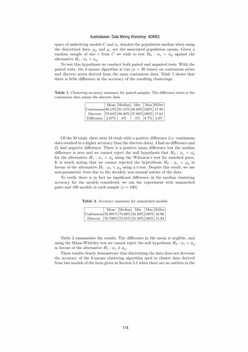
space of underlying models C and φz denotes the population median when usingthe discretised data. µy and µz are the associated population means. Given arandom sample of size v from C we wish to test H0 : φz = φy against thealternative H1 : φz < φy.

To test this hypothesis we conduct both paired and unpaired tests. With thepaired tests, the k-means algorithm is run (u = 20 times) on continuous seriesand discrete series derived from the same continuous data. Table 1 shows thatthere is little difference in the accuracy of the resulting clusterings.

Table 1. Clustering accuracy summary for paired samples. The difference series is thecontinuous data minus the discrete data

Mean Median Min Max StDevContinuous 80.13% 91.15% 56.60% 100% 17.80

Discrete 79.84% 86.30% 57.80% 100% 17.64Difference 2.67% 0% -5% 8.7% 2.67

Of the 50 trials, there were 24 trials with a positive difference (i.e. continuousdata resulted in a higher accuracy than the discrete data), 4 had no difference and21 had negative difference. There is a positive mean difference but the mediandifference is zero and we cannot reject the null hypothesis that H0 : φz = φy

for the alternative H1 : φz < φy using the Wilcoxon’s test for matched pairs.It is worth noting that we cannot rejected the hyptothesis H0 : µz = µy infavour of the alternative H1 : µz < µy using a t-test. Despite this result, we usenon-parametric tests due to the decidely non normal nature of the data.

To verify there is in fact no significant difference in the median clusteringaccuracy for the models considered, we ran the experiment with unmatchedpairs and 100 models in each sample (v = 100).

Table 2. Accuracy summary for unmatched models

Mean Median Min Max StDevContinuous 76.801% 73.00% 56.20% 100% 16.96

Discrete 76.798% 72.85% 55.50% 100% 15.83

Table 2 summarises the results. The difference in the mean is neglible, andusing the Mann-Whittley test we cannot reject the null hypothesis H0 : φz = φy

in favour of the alternative H1 : φz 6= φy.

These results clearly demonstrate that discretising the data does not decreasethe accuracy of the k-means clustering algorithm used to cluster data derivedfrom two models of the form given in Section 3.1 when there are no outliers in the

data. The next experiment shows that the accuracy of the clustering significantlyimproves even when the probability of an outlier is very small.

3.5 Experiment 2: Using a discretised series increases accuracy

Fig. 2. Difference in clustering accuracy for probability of an outlier between 0 and 0.5with paired samples

To demonstrate the desirability of discretising, we repeat experiment 3 forvarious values of p with both paired and unpaired samples. All other parametersare identical to those used in results presented in Section 3.4 (v = 50, x = 0.5).Figure 3.5 shows how the accuracy difference changes as the probability of anoutlier increases. Each data represents the median of 50 evaluations, where eachevaluation consists of 20 runs of the k-means algorithm. There is an initial dra-matic decrease in accuracy of clustering using the continuous data. As the prob-ability of an outlier increases the accuracy difference between using discretisedand continuous data decreases. This is because the noise eventually overwhelmsthe algorithms ability to cluster correctly. To illustrate the effect of outliersmore clearly, Figure 3 shows the results for the same experiment using a smallerrange of p. Clearly the clustering algorithm is performing much better with thediscretised data even when the probability of outlier is very low.

Figure 4 shows a repeat of the experiment described by Figure 3 with un-paired samples. For contrast with Figure 3, the mean values rather than the

Fig. 3. Difference in clustering accuracy for probability of an outlier between 0 and0.05 with paired data

Fig. 4. Difference in clustering accuracy for probability of an outlier between 0 and0.05 with unpaired data

medians are shown, but the pattern in both averages is the same. A very smallprobability of outliers results in a much improved performance when the discre-tised data is used. Finally, to emphasise the point further, we fixed the number

of outliers so that each series of 100 data had exactly one outlier and repeatedthe paired experiment. Of the 50 trials, 9 resulted in the continuous data havinghigher accuracy, in 1 trial the accuracy was the same and in the remaining 40the accuracy was greater when the discrete data was used.

Using Wilcoxon’s signed-rank test for matched pairs, the null hypothesisH0 : φd = 0 can be rejected in favour of the alternative H1 : φd < 0 at the 1%level

4 Conclusions and Future Direction

The clustering of time series is a field that has attracted the interest of researchersfrom a wide range of disciplines. This report has provided a brief review of thetechniques used, including a description of the types of models assumed, thedistance metrics employed and the clustering techniques used. Many real worldtime series have the unfortunate property that they contain outliers, and theaim of this research is to demonstrate that if discretised series are used insteadof the continuous data then the effect of outliers can be lessened significantly.

We have demonstrated how, for a certain class of model, distance metric andclustering algorithm, discretising the series into binary series of above and belowthe median can improve the clustering accuracy when there are outliers in thedata, even when the probability of an outlier is very small.

Although there are benefits from using the binary series of above and belowthe median when there are outliers, it obviously means some of the informationin the original data is discarded. It is worthwhile discovering how much thiseffects the quality of clusters formed.

The obvious way of extending this work would be to assess the effect ofdiscretisation when the data arises from other models and when alternativedistance metrics and/or clustering algorithms are employed. It is also a logicalextension to apply the technique to real world data.

Working with binary series can often allow for significant speed improvementswith model fitting and clustering techniques, and this could be another benefitof discretisation.

References

1. Rakesh Agrawal, Christos Faloutsos, and Arun N. Swami. Efficient SimilaritySearch In Sequence Databases. In D. Lomet, editor, Proceedings of the 4th Inter-national Conference of Foundations of Data Organization and Algorithms (FODO),pages 69–84, Chicago, Illinois, 1993. Springer Verlag.

2. Jonathan Alon, Stan Sclaroff, George Kollios, and Vladimir Pavlovic. Discover-ing clusters in motion time-series data. In IEEE Computer Vision and PatternRecognition Conference (CVPR), 2003.

3. A. J. Bagnall, G. Janakec, and M. Zhang. Clustering time series from mixturepolynomial models with discretised data. Technical Report CMP-C03-17, Schoolof Computing Sciences, University of East Anglia, 2003.

4. A. J. Bagnall and I. Toft. An agent model for first price and second price privatevalue auctions. In Proceedings of the 6th International Conference on ArtificialEvolution, 2003.

5. A. Banerjee and J. Ghosh. Clickstream clustering using weighted longest com-mon subsequences. In Proceedings of the Web Mining Workshop at the 1st SIAMConference on Data Mining, Chicago, April 2001., 2001.

6. Z. Bar-Joseph, G. Gerber, D. Gifford, T. Jaakkola, and I. Simon. A new approachto analyzing gene expression time series data. In Proceedings of The Sixth An-nual International Conference on Research in Computational Molecular Biology(RECOMB), pages 39–48, 2002.

7. Roberto Baragona. A simulation study on clustering time series with metaheuristicmethods. Quaderni di Statistica, 3, 2001.

8. R. Blender, K. Fraedrich, and F. Lunkeit. Identification of cyclone-track regimesin the north atlantic. Quart J. Royal Meteor. Soc., (123):727–741, 1997.

9. Z. Bohte, D. Cepar, and K. Kosmelj. Clustering of time series. In Proceedings inComputational Statistics. Physica-Verlag, 1980.

10. G. E. P. Box, G. M. Jenkins, and G. C. Reinsel. Time Series Analysis: Forecastingand Control, 3rd Edition. Prentice Hall, 1994.

11. Paul S. Bradley and Usama M. Fayyad. Refining initial points for K-Means cluster-ing. In Proc. 15th International Conf. on Machine Learning, pages 91–99. MorganKaufmann, San Francisco, CA, 1998.

12. Igor V. Cadez, Scott Gaffney, and Padhraic Smyth. A general probabilistic frame-work for clustering individuals and objects. In Knowledge Discovery and DataMining, pages 140–149, 2000.

13. Igor V. Cadez, David Heckerman, Christopher Meek, Padhraic Smyth, and StevenWhite. Visualization of navigation patterns on a web site using model-based clus-tering. In Knowledge Discovery and Data Mining, pages 280–284, 2000.

14. Gautam Das, Dimitrios Gunopulos, and Heikki Mannila. Finding similar timeseries. In Principles of Data Mining and Knowledge Discovery, pages 88–100,1997.

15. Gautam Das, King-Ip Lin, Heikki Mannila, Gopal Renganathan, and PadhraicSmyth. Rule discovery from time series. In Knowledge Discovery and Data Mining,pages 16–22, 1998.

16. A. P. Dempster, N. M. Laird, and D. B. Rubin. Maximum likelihood from incom-plete data. J. R. Stat. Soc. B, 39:1–38, 1972.

17. Evangelos Dermatas and George Kokkinakis. Algorithm for clustering continuousdensity HMM by recognition error. IEEE Tr. On Speech and Audio Processing,4(3):231–234, 1996.

18. Michael B. Eisen, Paul T. Spellman, Patrick O. Brown, and David Botstein. Clus-ter analysis and display of genome-wide expression patterns. Proceedings of theNational Academy of Sciences, 95(25):14863–14868, 1998.

19. Christos Faloutsos, M. Ranganathan, and Yannis Manolopoulos. Fast subsequencematching in time-series databases. In Proceedings 1994 ACM SIGMOD Conference,Mineapolis, MN, pages 419–429, 1994.

20. Sergio M. Focardi. Clustering economic and financial time series: exploring theexistence of stable correlation conditions. Technical Report 2001-04, The IntertekGroup, 2001.

21. Scott Gaffney and Padhraic Smyth. Trajectory clustering with mixtures of regres-sion models. Technical Report 99-15, Department of Information and ComputerScience, University of California, 1999.

22. Scott Gaffney and Padhraic Smyth. Curve clustering with random effects regres-sion mixtures. In C. M. Bishop and B. J. Frey, editors, Proceedings of the NinthInternational Workshop on Artificial Intelligence and Statistics, 2003.

23. Amir B. Geva and Dan H. Kerem. Fuzzy and Neuro-Fuzzy Systems in Medicine,chapter 3. Brain state identification and forecasting of acute pathology using un-supervised fuzzy clustering of EEG temporal patterns. CRC Press, 1998.

24. Maria Halkidi, Yannis Batistakis, and Michalis Vazirgiannis. On clustering val-idation techniques. Journal of Intelligent Information Systems, 17(2-3):107–145,2001.

25. A. K. Jain and R. C. Dubes. Algorithms for Clustering Data. Prentice Hall, NewJersey, 1988.

26. E. J. Keogh and M. J. Pazzani. A simple dimensionality reduction technique forfast similarity search in large time series databases. In T. Terano, H. Liu, andA. Chen, editors, Knowledge Discovery and Data Mining, Current Issues and NewApplications, 4th Pacific-Asia Conference, PAKDD 2000, volume 1805, pages 122–133, Kyoto, Japan, 2000. Springer.

27. Eamonn Keogh, Jessica Lin, and Wagner Truppel. Clustering of streaming time se-ries is meaningless. In Proceedings of the 8th ACM SIGMOD workshop on Researchissues in data mining and knowledge discovery, 2003.

28. Filipp Korkmazskiy, Biing-Hwang Juang, and Frank Soong. Generalized mixtureof HMMs for continuous speech recognition. In Proceedings IEEE Int. Conf. onAcoustics, Speech and Signal Processing, volume 2, pages 1443–1446, 1997.

29. K. Kosmelj and V. Batagelj. Cross-sectional approach for clustering time varyingdata. Journal of Classification, 7:99–109, 1990.

30. Cen Li and Gautam Biswas. Clustering sequence data using hidden markov modelrepresentation. In SPIE’99 Conference on Data Mining and Knowledge Discovery:Theory, Tools, and Technology, pages 14–21, 1999.

31. Cin Li. A Bayesian approach to temporal data clustering using the hidden Markovmodel methodology. PhD thesis, Vanderbilt University, Nashville, 2000.

32. Cin Li and Gautam Biswas. Profiling of dynamic system behaviors using hiddenmarkov model representation. In Proceedings of the ICSC’99 Advances in Intelli-gent Data Analysis(AIDA’99), 1999.

33. Cin Li and Gautam Biswas. Temporal pattern generation using hidden markovmodel based unsupervised classification. In D. Hand, K. Kok, , and M. Berthold,editors, Advances in Intelligent Data Analysis, Lecture Notes in Computer Sciencevol. 1642. Springer, 1999.

34. Cin Li and Gautam Biswas. Bayesian clustering for temporal data using hid-den markov model representation. In proceedings of the Seventeenth InternationalConference on Machine Learning, pages 543–550, 2000.

35. J. MacQueen. Some methods for classification and analysis of multivariate ob-servations. In Lucien M. Le Cam and Jerzy Neyman, editors, Proceedings ofthe Fifth Berkeley Symposium on Mathematical Statistics and Probability. VolumeI,Statistics. University of California Press, 1967.

36. Elizabeth Ann Maharaj. A significance test for classifying arma models. Journalof Statistical Computation and Simulation, 54:305–331, 1996.

37. Elizabeth Ann Maharaj. Clusters of time series. Journal of Classification, 17:297–314, 2000.

38. Eamonn Keogh Michail Vlachos, Jessica Lin and Dimitrios Gunopulos. A wavelet-based anytime algorithm for k-means clustering of time series, 2003.

39. Tim Oates. Identifying distinctive subsequences in multivariate time series by clus-tering. In S. Chaudhuri and D. Madigan, editors, Fifth International Conferenceon Knowledge Discovery and Data Mining, pages 322–326, San Diego, CA, USA,1999. ACM Press.

40. Tim Oates, Laura Firoiu, and Paul Cohen. Clustering time series with hiddenmarkov models and dynamic time warping. In Proceedings of the IJCAI-99 Work-shop on Neural, Symbolic and Reinforcement Learning Methods for Sequence Learn-ing, pages 17–21, 1999.

41. Tim Oates, Laura Firoiu, and Paul R. Cohen. Using dynamic time warping tobootstrap HMM-based clustering of time series. Lecture Notes in Computer Sci-ence, 1828:35–52, 2001.

42. Tim Oates, Matthew D. Schmill, and Paul R. Cohen. Identifying qualitatively dif-ferent outcomes of actions: Gaining autonomy through learning. In Carles Sierra,Maria Gini, and Jeffrey S. Rosenschein, editors, Proceedings of the Fourth Inter-national Conference on Autonomous Agents, pages 110–111, Barcelona, Catalonia,Spain, 2000. ACM Press.

43. Paul Ormerod and Craig Mounfield. Localised structures in the temporal evolutionof asset prices. In New Approaches to Financial Economics. Santa Fe Conference,2000.

44. Domenico Piccolo. A distance measure for classifying ARIMA models. Journal ofTime Series Analysis, 11(2):153–164, 1990.

45. Marco Ramoni, Paola Sebastiani, and Paul Cohen. Bayesian clustering by dynam-ics. Machine Learning, 47(1):91–121, 2002.

46. Greg Ridgeway. Finite discrete Markov processes. Technical Report MSR-TR-97-24, Microsoft Research, 1997.

47. Padhraic Smyth. Clustering sequences with hidden markov models. In Michael C.Mozer, Michael I. Jordan, and Thomas Petsche, editors, Advances in Neural In-formation Processing Systems, volume 9, page 648. The MIT Press, 1997.

48. P. Tong and H. Dabas. Cluster of time series models: An example. Journal ofApplied Statistics, 17:187–198, 1990.

49. Shi Zhong. Probabilistic model-based clustering of complex data. PhD thesis, Uni-versity of Texas at Austin, 2002.

50. Shi Zhong and Joydeep Ghosh. HMMs and coupled HMMs for multi-channel EEGclassification. In Proc. IEEE Int. Joint Conf. on Neural Networks, 2002.

51. Shi Zhong and Joydeep Ghosh. A unified framework for model-based clustering.In Intelligent Engineering Systems Through Artificial Neural Networks (ANNIE),2002.

52. Shi Zhong and Joydeep Ghosh. A unified framework for model-based clusteringand its application to clustering time sequences. Technical report, Department ofElectrical and Computer Engineering, University of Texas, 2002.

53. Shi Zhong and Joydeep Ghosh. Scalable, balanced model-based clustering. InProceedings of SIAM Int. Conf. on Data Mining, 2003.

Relative Temporal Association Rule Mining

Edi Winarko and John F. Roddick

School of Informatics and EngineeringFlinders University,

PO Box 2100, Adelaide,South Australia 5001,

Email: {edi.winarko, john.roddick}@infoeng.flinders.edu.au

Abstract. A temporal association rule is one that has a specified tem-poral constraint on its validity, for example, it may hold only during aspecific time interval. A relative temporal rule is one that is further qual-ified according to a temporal relationship with other events or intervalsas opposed to an absolute point in time. Due to their potential appli-cation, the problem of finding temporal association rules has recentlybecome an important research topic and is receiving great interest fromresearchers. Several models of temporal association rules and algorithmsfor discovering such rules have been proposed, although the discoveryof relative temporal rules has received less attention. In this paper, wesurvey the work to date in temporal association rule mining and presenta taxonomy of research to date. We also present a new mechanism fordiscovering relative temporal association rules.

Keywords: Temporal Data Mining, Relative Temporal Association Rules.

1 Introduction

The problem of finding association rules was originally proposed in 1993 (Agrawal,Imielinski & Swami 1993) and has been investigated widely for a number ofyears. In general, however, this work does not consider any temporal aspectwhich might be inherent in the data and thus important information may re-main undiscovered. While association rule mining can only ever reliably reporton useful knowledge in the dataset under examination, and therefore for the timeperiod for which the dataset corresponds, there is often an implicit assumptionthat the discovered rules are valid universally in time. Moreover, the dataset itselfmay contain useful time-dependant observations and thus temporal correlations,trends and changes may be contained in the data.

As a result, the information that can be conveyed by non-temporal rules canoften be less valuable as their applicability is generalised – there is no way ofknowing when the rules are strongest, or the manner in which they occur intime. As stated by Chen and Petrounias (2000), the association rule - customerswho buy bread and butter also buy milk during the summer - may be more useful

than the non-temporal equivalent - customers who buy bread and butter also buymilk.

Because of this richer rule semantics, the problem of finding temporal asso-ciation rules has recently become an important research topic and is receiving agreat deal of research interest. A number of temporal association rule models andalgorithms to discover such rules have been proposed (Ale & Rossi 2000, Chen& Petrounias 2000, Lee, Lin & Chen 2001, Li, Ning, Wang & Jajodia 2001, Oz-den, Ramaswamy & Silberschatz 1998, Ramaswamy, Mahajan & Silberschatz1998, Rainsford & Roddick 1999, Wang, Yang & Muntz 1999, Wang, Yang &Muntz 2001, Zimbrao, de Souza, de Almeida & da Silva 2002) and a survey oftemporal data mining methods and paradigms in general is given in (Roddick &Spiliopoulou 2002).

The paper is structured in two major parts. The first part presents a surveyof work in temporal association rule mining and discusses a taxonomy for thisresearch. The second part presents a new method for discovering relative tem-poral association rules including a discussion of the problems of applying theApriori principle to temporally augmented itemsets.

2 Current Research in Temporal Association Rule

Mining

Ozden et al. (1998) discuss the problem of mining cyclic association rules, i.e.,the association rules that occur periodically over time. Two algorithms and op-timization techniques to discover cyclic association rules are proposed, although,this work is limited because it cannot describe real-life concepts such as the firstbusiness day of every month in which the distance between two consecutive suchbusiness days are not always the same. Ramasmamy et al. (1998) extend thiswork by considering the discovery of association rules that hold during the timeintervals described by a user-defined calendar algebra expression. The calendaralgebra adopted is considered more powerful in defining temporal patterns, butto give such expressions the users need to know what temporal patterns theyare interested in.

To provide more flexibility to the user Li et al. (2001) propose a temporalassociation rule model that uses calendar schemas as a framework for temporalpatterns, instead of using user-defined calendar algebra expressions. Their workconsiders all possible temporal patterns in the calendar schema as opposed tosimply complying with user-supplied temporal expressions.

Ale and Rossi (2000) studied the discovery of association rules that holdfor transactions during the lifetime (lifespan) of items involved in the rules. Thelifetime is intrinsic to the data, so that the users are not required to define it. Thelifetime of items is a period between the first and the last time the items appearsin transactions in the dataset. Similar to this work is the work proposed by Lee etal. (2001) who studied the problem of mining general temporal association rulesin publication database. A publication database refers to a set of transactionswhere each transaction contains an individual exhibition period. Zimbrao et

al. (2002) extend this work by proposing a new approach to discover calendar-based association rules with item’s lifespan restriction.

The discovery of the longest interval and the longest periodicity of associ-ation rules was presented in (Chen & Petrounias 2000) and in (Rainsford &Roddick 1999), it was proposed to add temporal features to association rulesby associating a conjunction of binary temporal predicates that specify the rela-tionships between the timestamps of transactions. Visualisation techniques forviewing these temporal predicate association rules were provided in (Rainsford& Roddick 2000).

All the above work assumed that each transaction is associated with a tempo-ral attribute that records the time for which the attributes of the transaction arevalid in the modeled domain. They also assumed that all non-temporal attributeshave binary (boolean) domain. Unlike these work, (Wang et al. 1999, Wanget al. 2001) has proposed another model by introducing the mining of temporalassociation rules for evolving numerical attributes.

Despite this work, to the best of our knowledge, there has not been specificsurvey available on the topic of temporal association rule discovery although(Antunes & Oliveira 2001) provide a survey on the most significant techniquesto deal with temporal sequences while (Roddick & Spiliopoulou 2002) provide abroad survey of temporal data mining research. In order to fill this gap, in thispaper we first survey the research area.

2.1 Taxonomy of Temporal Association Rules

A number of temporal association models has been proposed, each with differ-ent reasons and goals. Each model has its own characteristics, differences andsimilarities. In this section, we classify the models by looking at them from fourdifferent aspects: the domain in which the models applied, measures of interest-ingness used, temporal feature associated with the rules, and algorithms used todiscover the rules.

Domain of Attributes It can be seen in Table 1 that most of temporal asso-ciation rule models discussed here has assumed that all non-temporal attributeshave binary (boolean) domain. It means that the generated temporal associationrules only deal with the association between the presence or absence of itemsor attributes. The transaction dataset of these models is normally defined asfollows:Let I = {i1, i2, . . . , im} be a set of literals, called items. D is a dataset of trans-actions, where each transaction s consists of a set of items such that s ⊆ I.Associated with each transaction s is a timestamp ts which represents validtime of transaction s.

Wang et al. (1999, 2001) studied the mining of temporal association rulesover evolving numerical attributes, instead of binary attributes. This work isdifferent from the model of quantitative association rules introduced in (Srikant& Agrawal 1996). In this model, the dataset consists of a set of objects, each ofwhich has a unique ID and a set of time varying numerical attributes.

Measures In association rules mining, two measures of rule interestingness thatare commonly used are support and confidence. Both reflect the usefulness andcertainty of discovered rules (Han & Kamber 2001). However, for some of tempo-ral association rule models, these two measures are considered insufficient and anadditional measure is considered necessary in their proposed model, for exampletemporal support (Ale & Rossi 2000), frequency (Chen & Petrounias 2000), tem-poral confidence (Rainsford & Roddick 1999), and strength and density (Wanget al. 1999, Wang et al. 2001), as shown in Table 1.

Ale and Rossi (2000) introduce the notion of temporal support to filter theitems with high support but short life. The combination of support and temporalsupport is used to determine if an itemset is large. Ie., an itemset is large if itsatisfies the user-specified minimum support and minimum temporal support.

Chen and Petrounias (2000) propose using frequency to measure the pro-portion of the intervals, during which the rules satisfy minimum support andminimum confidence, to the intervals in φ(TF ). φ(TF ) represents a set of timeintervals, i.e., φ(TF ) = {P1, P2, . . . , Pn}, where Pi is a time interval. The as-sociation rules should satisfy the minimum frequency in addition to minimumsupport and minimum confidence.

In (Rainsford & Roddick 1999), temporal confidence is used to determinehow strong the temporal relationship between temporal items in the rule. Sincethe temporal relationship between items is represented as a binary predicate,each predicate in the rule must satisfy the minimum temporal confidence.

Wang et al. (2001) propose two new measures, strength and density, to qualifythe validity of rules on evolving numerical attributes. The support, strength,and density of the rules indicates the frequency of occurrences, concentrationof population, and the degree of non-independence represented by the rules,respectively.

Temporal Association Rule Types According to (Chen & Petrounias 2000),a temporal association rule can be represented as a pair < AR, TF >, whereAR is an association rule and TF is temporal feature belongs to AR. Dependingon the interpretation of the temporal feature TF , a temporal association rules< AR, TF > can be classified as:

– a universal association rule if φ(TF ) = {T}, where T represents the timedomain;

– an interval association rule if φ(TF ) = {itvl}, where itvl ⊂ T is a specifictime interval;

– a periodic association rule if φ(TF ) = {p1, p2, . . . , pn}, where pi ⊂ T is aperiodic interval in cycles;

– a calendric association rule if φ(TF ) = {cal1, cal2, . . . , calm}, where calj ⊂ Tis a calendric interval in a specific calendar.

This classification method is used to classify the temporal association rulemodels presented in this paper. However, since certain models cannot be in-cluded in these classes we have to create two new classes – binary predicate and

numerical attribute evolution. The universal association rule class is excludedfrom our classification because it represents a class of classical association rules(non-temporal association rules). Table 1 shows five classes in our classification,namely interval, cyclic, calendric, binary predicate, and numerical attribute evo-lution. Using this classification, a model can be classified into more than oneclass, depending on the temporal feature associated with association rules. Eachtemporal association model with its temporal feature is presented in Table 2.

Author Measures Type of Association Rule AttributeDomain

Supp. Conf. Extra Interval Cyclic Calendric Binary Attr.Measure Pred. Evol.

Ale & Rossi (200) X X Temporal X Binarysupport

Ozden et al. (1998) X X X BinaryChen & Petrounias (2000) X X Frequency X X BinaryRamaswamy et al. (1998) X X X BinaryLi et al. (2001) X X X BinaryRainsford & Roddick(1999)

X X Temporal X Binary

confidenceLee et al. (2001) X X X BinaryZimbrao et al. (2002) X X X X BinaryWang et al. (1999,2001) X Strength & X Numeric

Density

Table 1. Temporal association rule classification

Author Algorithms Temporal AR Models

Apriori-based Other

Ale & Rossi (2000) X (X ⇒ Y, [t1, t2])[t1, t2] is a lifespan of X ∪ Y

Ozden et al. (1998) X (X ⇒ Y, c = (l, o))c is a cycle with length l and offset o

Chen & Petrounias (2000) X (X ⇒ Y, TF )φ(TF ) = {P1, P2, . . . , Pn}

Ramaswamy et al. (1998) X (X ⇒ Y, C)C is a calendar expression

Li et al. (2001) X (X ⇒ Y, e)e is a calendar pattern

Rainsford & Roddick (1999) X X ⇒ Y ∧ P1 ∧ P2 . . . Pn

Pi is a binary temporal predicateLee et al. (2001) X PPM (X ⇒ Y, (t, n))

(t, n) is the max. common exhibition periodZimbrao et al. (2002) X (X ⇒ Y, e, [t1, t2])

e is a calendar pattern[t1, t2] is a lifespan of X ∪ Y

Wang et al. (1999,2001) X TAR X ⇐⇒ YX and Y are conjunctions of att. evolution

Table 2. Temporal association rule models and algorithms

From the four models in the interval association rule class, each model pro-vides different meaning to the time interval. In (Ale & Rossi 2000, Zimbraoet al. 2002), a time interval represents the lifespan of items in the rules, in (Leeet al. 2001), it represents the maximum common exhibition period of items inthe rules, while in (Chen & Petrounias 2000), it represents any specific timeinterval.

We classify the works of Ramaswamy et al. (1998) and Li et al. (2001) intothe calendric association class. (Ramaswamy et al. 1998) introduced the notionof calendar algebra to describe phenomena of interest in association rules. It isbased on the work reported in (Allen 1983, Leban, McDonald & Forster 1986)and the implementation reported in (Chandra, Segev & Stonebraker 1994). Thecalendar algebra expression defines a set of time intervals that the algorithmconsiders in discovering the association rules. The association rules are calledcalendric if they have the minimum support and confidence in every time unitcontained in the calendar. The algorithms proposed to discover such rules aresimilar to the ones discussed in (Ozden et al. 1998), but they were modifiedto deal with calendars, instead of cycles. Li et al. (2001) use calendar schemasinstead of calendar algebra expressions.

Algorithms The algorithms so far proposed to discover temporal associationrules can be divided into two categories, i.e., Apriori-based and non Apriori-based algorithms. Table 2 shows that all models discussed here can be categorisedas using the Apriori-based algorithms. Two models also proposed new algo-rithms which are not based on Apriori (Lee et al. 2001, Wang et al. 1999, Wanget al. 2001). In (Lee et al. 2001) the algorithm Progressive-Partition-Miner(PPM) is proposed to discover general temporal association rules in a publi-cation database, while Wang et al. (1999,2001) discuss the TAR algorithm todiscover the temporal association rules on evolving numerical attributes.

In the following sections, we discuss in more detail the Apriori-based algo-rithms to discover interval association rules, cyclic association rules, calendricassociation rules, and temporal predicate association rules. In addition, we alsodiscuss the optimized algorithms to discover cyclic and calendric associationrules.

2.2 Interval Association Rules

The interval association rule model discovers association rules that hold duringthe lifetime of items involved in the rules (Ale & Rossi 2000). The model ismotivated by the observation that it is possible to have association rules witha high confidence but with little support. During the mining process such rulesmay not be discovered as their support is less than the minimum support. asthe denominator in the support calculation is the total number of transactionsin dataset. If the denominator is limited to the total number of transactionsbelonging only to the lifetime of items, these rules could be discovered. Therefore,in this model the search for large itemsets is limited to the lifetime of the itemset’s

members and each generated rule has an associated time frame, correspondingto the lifetime of the items participating in the rule.

We will use the following transaction dataset, found in (Ale & Rossi 2000),to describe how the model works.Example 3.1: Let I = {A,B, C, D, E, F,G, H, I} and D contain six transac-tions:

s1 = {A,C, F, H, I}, t: 1s2 = {A,B,C, G}, t: 2s3 = {B,C,D,G, I}, t: 3s4 = {A,C, I}, t: 4s5 = {C,D,E,H, I}, t: 5s6 = {A,D, F, G}, t: 6

The lifespan of an item A is represented by a closed interval [ti, tj ], whereti <T tj , and is denoted by lA. If D is the transaction dataset, then DlA is thesubset of D whose timestamps ti ∈ lA, and |DlA | is the number of transactionswhose timestamps ti ∈ lA. As an example, from the transaction dataset above,the lifespan of A, B and C is lA = [1, 6], lB = [2, 3] and lC = [1, 5], respectively.The lifespan of an itemset X is calculated as an intersection of the items’ lifespanin the itemset. If X = {I1, I2, . . . , In} then its lifespan is lX = lI1

∩ lI2∩ . . .∩ lIn

.In the case X = {A,C} then its lifespan is lX = lA ∩ lC = [1, 6] ∩ [1, 5] = [1, 5].

The calculation of support of an itemset X is modified by taking into consid-eration the itemset’s lifespan. The denominator is not the number of transactionsof the entire dataset |D|, but |DlX |, that is the number of transactions whosetimestamp ti ∈ lX . The support of X in D over its lifespan lX is denoted assup(X, lX , D). Thus, the support of X = {A} and Y = {H} is sup(X, lX , D) =4/6 = 0.67 and sup(Y, lY , D) = 2/5 = 0.40, respectively.

It is possible for the itemset to have high support but short life. As anexample, an item E has support of 100% but its lifespan is short, i.e., |lE | = 1.The temporal support can be used to filter such items. Therefore, to determine ifan itemset X is large or not the combination of support and temporal support isused. Given the minimum support σ ∈ [0, 1] and the minimum temporal supportτ , an itemset X is large in its lifespan lX if sup(X, lX , D) ≥ σ and |lX | ≥ τ .

This model proposed the concept of item’s obsolescence. It is used to filterout the items or itemsets that are considered obsolete. An item whose lifespanis [ti, tj ] is obsolete at a specified time instant to if t2 < to. It is not necessaryto check for obsolete k-itemsets, for k > 1, because a k-itemset is obsolete if itcontains an obsolete item.

The confidence of a rule X ⇒ Y in [t1, t2], where [t1, t2] is a time framecorresponding to the lifespan of X ∪ Y , is denoted by conf(X ⇒ Y, lX∪Y , D)and defined as

conf(X ⇒ Y, lX∪Y , D) = sup(X ∪ Y, lX∪Y , D)/sup(X, lX∪Y , D)

Let T = {. . . , to, t1, t2, . . .} be a set of time instants, countably infinite, overwhich a linier order <T is defined, where t1 <T t2 means that t1 occurs before

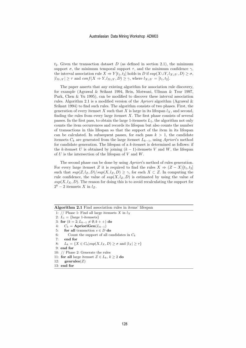
t2. Given the transaction dataset D (as defined in section 2.1), the minimumsupport σ, the minimum temporal support τ , and the minimum confidence γ,the interval association rule X ⇒ Y [t1, t2] holds in D if sup(X∪Y, lX∪Y , D) ≥ σ,|lX∪Y | ≥ τ and conf(X ⇒ Y, lX∪Y , D) ≥ γ, where lX∪Y = [t1, t2].

The paper asserts that any existing algorithm for association rule discovery,for example (Agrawal & Srikant 1994, Brin, Motwani, Ullman & Tsur 1997,Park, Chen & Yu 1995), can be modified to discover these interval associationrules. Algorithm 2.1 is a modified version of the Apriori algorithm (Agrawal &Srikant 1994) to find such rules. The algorithm consists of two phases. First, thegeneration of every itemset X such that X is large in its lifespan lX , and second,finding the rules from every large itemset X. The first phase consists of severalpasses. In the first pass, to obtain the large 1-itemsets L1, the algorithm not onlycounts the item occurrences and records its lifespan but also counts the numberof transactions in this lifespan so that the support of the item in its lifespancan be calculated. In subsequent passes, for each pass k > 1, the candidateitemsets Ck are generated from the large itemset Lk−1, using Apriori’s methodfor candidate generation. The lifespan of a k-itemset is determined as follows: ifthe k-itemset U is obtained by joining (k − 1)-itemsets V and W , the lifespanof U is the intersection of the lifespan of V and W .

The second phase can be done by using Apriori’s method of rules generation.For every large itemset Z it is required to find the rules X ⇒ (Z − X)[t1, t2]such that sup(Z, lZ , D)/sup(X, lZ , D) ≥ γ, for each X ⊂ Z. In computing therule confidence, the value of sup(X, lZ , D) is estimated by using the value ofsup(X, lX , D). The reason for doing this is to avoid recalculating the support for2k − 2 itemsets X in lZ .

Algorithm 2.1 Find association rules in items’ lifespan

1: // Phase 1: Find all large itemsets X in lX2: L1 = {large 1-itemsets}3: for (k = 2; Lk−1 6= ∅; k + +) do

4: Ck = AprioriGen(Lk−1)5: for all transaction s ∈ D do

6: Count the support of all candidates in Ck

7: end for

8: Lk = {X ∈ Ck|sup(X, lX , D) ≥ σ and |lX | ≥ τ}9: end for

10: // Phase 2: Generate the rules11: for all large itemset Z ∈ Lk, k ≥ 2 do

12: genrules(Z)13: end for

2.3 Cyclic Association Rules

The concept of cyclic (periodic) association rules and the mining tasks for dis-covering such rules was described in (Ozden et al. 1998). An association rule iscalled cyclic if the rule has the minimum confidence and support at regular timeintervals. Such a rule is not required to hold for the entire transactional dataset,but rather only for transactional data in a particular periodic time interval.

In order to discover cyclic association rules, the model assumes that the unitof time (hour, day, week, month, etc.) is given by the user. The ith time unit isdenoted by ti, i ≥ 0, and corresponds to the time interval [i.t, (i + 1).t]. Given atransaction dataset D, a set of transactions executed in ti is denoted by D[i].

A cycle c is a tuple (l, o) consisting of length l (multiples of the time unit)and an offset o (the first time unit in which the cycle occurs), 0 ≤ o ≤ l. A timeunit ti is part of a cycle c = (l, o) if o = i mod l holds. For example, if the unitof time is an hour, every fourth hour starting from the 3rd hour (3rd, 7th,. . .) ispart of cycle c = (4, 3).

The support of an itemset X in D[i] is the fraction of transactions in D[i] thatcontain X. The confidence of a rule X ⇒ Y in D[i] is the fraction of transactionsin D[i] containing X that also contain Y . Given the minimum support σ andthe minimum confidence γ, an association rule X ⇒ Y holds in time unit ti ifthe support of X ∪ Y in D[i] exceeds σ and the confidence of X ⇒ Y in D[i]exceeds γ.

An association rule has a cycle c = (l, o) if the association rule holds in everyith time unit starting with time unit to. Thus, if the unit of time is an hour and arule X ⇒ Y holds during the interval 8am-9am every day (i.e., every 24 hours),then X ⇒ Y has a cycle c = (24, 8). An association rule can have more than onecycle. For example, if X ⇒ Y holds during the interval 8am-9am and 4pm-5pmevery day, then X ⇒ Y has two cycles c1 = (24, 8) and c2 = (24, 16).

A cycle can be a multiple of other cycles. A cycle (li, oi) is a multiple ofanother cycle (lj , oj) if lj divide li and (oj = oi mod lj). From this definition,a cycle (24, 15) is a multiple of a cycle (12, 3). Therefore, it is only interestingto discover cyclic association rules with ‘large’ cycles, i.e., the cycle that is notmultiple of any other cycle.

Two algorithms are proposed to discover cyclic association rules. The first al-gorithm, called sequential algorithm, is the extension of non temporal associationrule mining techniques which treats association rules and cycles independently.The second algorithm, which is called interleaved algorithm, uses optimizationtechniques for discovering cyclic association rules. This section discusses the se-quential algorithm. The interleaved algorithm will be discussed in Section 2.6.

The sequential algorithm consists of two phases. First, the generation of theassociation rules that hold in each time unit. Second, the discovery of cyclicassociation rules using the cycle detection procedure as shown in Algorithm 2.2.

The first phase can be done using one of the existing methods (Agrawal &Srikant 1994, Savasere, Omiecinski & Navathe 1995). In (Ozden et al. 1998),the implementation is based on the Apriori algorithm from (Agrawal & Srikant1994). In the second phase, it is required to represent each association rule as

Algorithm 2.2 Find cyclic association rules

1: // Phase 1: Generate rules for each time unit2: for all time unit ti do

3: Generate large itemsets in ti

4: Generate the rules from the large itemsets in ti

5: end for

6: // Phase 2: Detect large cycles7: Convert each rule into binary sequence8: for all binary sequence do

9: Generate the set of cycles for each rule10: Discover the large cycles from the set of cycles11: end for

a binary sequence. In this representation, ones correspond to the time unitsin which the rule holds and zeros correspond to the time units in which therule does not hold. For example, the binary sequence 001100010101 representsthe association rule X ⇒ Y holds in D[2], D[3], D[7], D[9], and D[11]. Aftereach association rule is represented in a binary sequence, the cycle detectionprocedure can be started to discover cyclic association rules. From the aboveexample the cycle detection procedure will discover a rule X ⇒ Y has a cyclec = (4, 3) because the rule holds in every fourth time unit starting from timeunit t3, followed by t7 and t11.

The cycle detection procedure is composed of two steps. In the first step, thesequence is scanned. Each time a zero is encountered at a sequence position i,candidate cycles (j, i mod j), 1 ≤ j ≤ m, where m is the maximum cycle lengthof interest, are eliminated from the set of candidate cycles. Initially, the set ofcandidate cycles contains all possible cycles. This step completes whenever thelast bit of the sequence is scanned or the set of candidate cycles becomes empty,whichever is first. In the second step, large cycles (cycles that are not multiples ofany existing cycles) are detected. This can be done by eliminating cycles that arenot large as follows: starting from the shortest cycle, for each cycle ci = (li, oi)eliminate each other cycle cj = (lj , oj) from the set of cycles if lj is a multipleof li and oi = oj mod li) holds.

2.4 Calendric Association Rules

In this section, we discuss the calendric association rules as described in (Liet al. 2001). In order to discover calendric association rules, the user needs onlyto give a simple calendar patterns belonging to a calendar schema. A calendarschema is a relational schema R = (fn : Dn, fn−1 : Dn−1, . . . , f1 : D1). Eachattribute fi is a calendar unit name such as year, month, and week etc. Eachdomain Di is a finite subset of the positive integers. Given a calendar schemaR = (fn : Dn, fn−1 : Dn−1, . . . , f1 : D1), a calendar pattern on the calendarschema R is a tuple on R of the form 〈dn, dn−1, . . . , d1〉, where di is in Di orthe wild-card symbol ”*”. Each calendar pattern represents the time interval

given by a set of tuples in Dn x Dn−1 x . . . x D1. As an example, found in (Liet al. 2001), a calendar schema may be (year:{1995, 1996, . . ., 1999}), month:{1,2, . . ., 12}, day:{1, 2, . . ., 31}). The calendar pattern (1999, 12, *) representsevery day in December, 1999.

A calendric association rule over calendar schema R is a pair (r, e), where ris an association rule and e is a calendar pattern on R. The paper defines twoclasses of calendric association rules: precise-match association rules and fuzzy-match association rules. Precise-match association rules require the rules to holdduring every interval while fuzzy-match association rules require the rules tohold during a significant fraction of these intervals. More formal definition ofprecise-match and fuzzy-match association rules can be stated as follows.

1. (Precise match) Given a calendar schema R and a set of timestamped trans-actions T , a precise-match association rule (r, e) holds in T if and only if theassociation rule r holds in T [t] for each basic time interval t covered by e.

2. (Fuzzy match) Given a calendar schema R, a set of timestamped transactionsT , and a real number m (match ratio), where 0 < m < 1, a fuzzy-matchassociation rule (r, e) holds in T if and only if the association rule r holdsin T [t] for at least 100m% of the basic time intervals t covered by e.

Similar to the problem of finding non-temporal association rules, the problemof finding calendric association rules can also be divided into two subproblems.First, finding all large itemsets for all calendar patterns, and second, generatingcalendric association rules using the large itemsets and their calendar patterns.The work in (Li et al. 2001) only focuses on finding calendric large itemsets. Twotypes of algorithms for finding calendric large itemsets are proposed and bothare based on Apriori algorithm (Agrawal & Srikant 1994): direct-Apriori algo-rithms that treat each basic time interval individually and directly apply Apriorimethod (Agrawal & Srikant 1994) for candidate generation and temporal-Apriorialgorithms that are optimized by exploiting the relationship among calendar pat-terns. In this section we only discuss the direct-Apriori algorithms to find bothclasses of calendric association rules. The temporal-Apriori algorithms will bediscussed in section 2.6.

Algorithm 2.3 shows the direct-Apriori algorithm to generate precise-matchand fuzzy-match large itemsets. In pass k of the algorithm, where k > 1, theprocessing of each basic time interval eo consists of three phases. The first phasegenerates candidate k-itemsets for each basic time interval from large (k − 1)-itemsets. This can be done by using Apriori’s method for candidate generationas follows: Ck(eo) = AprioriGen(Lk−1(eo)). The second phase scans the trans-actions whose timestamps are covered by the basic time interval, and discoverslarge k-itemsets for this basic time interval. These two phases are the same forboth precise-match and fuzzy-match. In the third phase, the discovered largek-itemsets for the basic interval, Lk(eo), are used to update the large k-itemsetsfor each star calendar pattern e that covers the basic time interval. The up-date procedure for precise-match and fuzzy-match is different. For precise-match,the update is performed by intersecting the set of large k-itemsets for the ba-

sic interval eo with the set of large k-itemsets for the calendar pattern e, i.e.,Lk(e) = Lk(e) ∩ Lk(eo). In the first update, Lk(e) = Lk(eo).

Algorithm 2.3 Find precise-match and fuzzy-match large itemsets

1: for all basic time interval eo do

2: L1(eo) = {large 1-itemsets in T [eo]}3: for all star patterns e that covers eo do

4: update L1(e) using L1(eo);5: end for

6: end for

7: for (k = 2; ∃ a star calendar pattern e such that Lk−1(e) 6= ∅;k + +) do

8: for all basic time interval eo do

9: // Phase 1: Generate candidates10: generate candidate Ck(eo);11: // Phase 2: Scan the transactions12: for all transactions T ∈ T [eo] do

13: // increment the count of c ∈ Ck(eo) contained in T

14: subset (Ck(eo), T )15: end for

16: Lk(eo) ={c ∈ Ck(eo)|sup(c) ≥ σ}17: // Phase 3: Update star calendar patterns18: for all star patterns e that covers eo do

19: update Lk(e) using Lk(eo);20: end for

21: end for

22: return 〈Lk(e), e〉 for all star calendar pattern e

23: end for

The update procedure for fuzzy-match is more complex than that for precise-match. The procedure is presented in Algorithm 2.4. Each large itemset l ∈ Lk(e)is associated with the counter updatecounter which is initially set to 1.

Algorithm 2.4 Fuzzy-match Update

1: N = the number of basic time interval covered by e

2: n = the n-th update to Lk(e)3: m = match ratio4: if Lk(e) has never been updated then

5: Lk(e) = Lk(eo)6: l.updatecount = 1 for each l ∈ Lk(e)7: else

8: l.updatecount = 1 for each l ∈ Lk(eo) − Lk(e)9: l.updatecount + + for each l ∈ Lk(eo) ∩ Lk(e)

10: Lk(e) = {l ∈ Lk(e) ∪ Lk(eo)|l.updatecount + (N − n) ≥ m.N}11: end if

2.5 Temporal Predicate Association Rules

The temporal predicate association rule was first proposed by (Rainsford &Roddick 1999). It extended the association rules by adding to the rules a con-junction of binary temporal predicates that specify the relationships betweenthe timestamps of transactions. Binary temporal predicates are defined usingthirteen interval based relations proposed by Allen (1983) and the neighbor-hood relationships defined by Freksa that allow generalisation of relationships(Freksa 1992).

Let I = {i1, i2, . . . , im} be a set of items. Let D be a dataset of transactions,where each transaction s consists of a set of items such that s ⊆ I. Given anitemset X ⊆ I, a transaction s contains X if and only if X ⊆ s. Associatedwith each transaction is temporal attributes that record the time for which theitem is valid. Let P1∧P2 . . .∧Pn be a conjunction of binary temporal predicatesdefined on attributes contained in either X or Y , where n ≥ 0. The temporalpredicate association rule is a rule of the form X ⇒ Y ∧ P1 ∧ P2 . . .∧ Pn, whereX ⊆ I, Y ⊆ I and X ∩ Y = ∅.

The temporal confidence is used to determine how strong the temporal rela-tionship between temporal items in the rule. The rule X ⇒ Y ∧P1 ∧P2 . . .∧Pn

holds in a dataset D with the confidence c if and only if at least c% of transac-tions in D that contain X also contain Y . Likewise, each predicate Pi holds witha temporal confidence tcpi if and only if at least tc% of transactions in D thatcontain X and Y also satisfy Pi. Following is an example of temporal predicateassociation rule found in (Rainsford & Roddick 1999):

policyC ⇒ investA, productB | 0.87 ∧during(investA,policyC) | 0.79 ∧before(productB,investA)|0.91

An interpretation for this rule is:

The purchase of investment A and product B are associated with insur-ance policy C with a confidence factor 0.87. The investment A occursduring the period of policy C with a temporal confidence factor 0.79 andthe purchase of product B occurs before investment A with a temporalconfidence factor of 0.91.

The algorithm to discover temporal predicate association rules consists of fourphases. The first phase of the algorithm can be performed using any associationrule algorithm. During this phase the temporal attributes associated with theitems are not considered. In the second phase all of possible pairings of temporalitems in each generated rule are generated. For example, if the association ruleis AB ⇒ C then there are three possible pairings, AB, AC, and BC. In thethird phase, the dataset is scanned and each tuple is checked to see if it supportsa given rule. Finally, the aggregation of temporal relationships found in thisphase is then concatenated with the original rule to generate temporal predicateassociation rules.

2.6 Improving Efficiency of the Algorithms

In mining non-temporal association rules, many variations of the Apriori algo-rithm that focus on improving the efficiency of the original algorithm have beenproposed. One of the goals is to reduce the search space for large itemsets. In tem-poral mining the search space will be even larger than in non-temporal miningand thus optimization is required. This section discusses optimization techniquesemployed in discovering cyclic association rules and calendric association rules.

Cycle Pruning, Cycle Skipping and Cycle Elimination In the sequentialalgorithm (as discussed in Section 2.3), the cycle detection procedure has to scanand process every bit position of binary sequence sequentially. By exploiting therelationship between cycles and large itemsets this procedure can be optimizedso that the sequence position that cannot be part of any of the candidate cycles isskipped. In order to do this the interleaved algorithm employs three optimizationtechniques: cycle-pruning, cycle-skipping, and cycle-elimination.

An itemset, in the same way an association rule, can be represented as abinary sequence where ones correspond to the time units in which the itemsetis large and zeros correspond to the time units in which the itemset is notlarge. A cycle can also be represented as a binary sequence. A cycle c = (l, o) isrepresented as a binary sequence with length l and the value of bit position oone. For example, a cycle c = (4, 3) is represented as a binary sequence 0001.

Cycle-pruning is based on the property that if an itemset X has a cycle (l, o),then any subset of X has the cycle (l, o). It implies that, any cycle of itemset Xmust be a multiple of a cycle of an itemset that is subset of X and the numberof cycles of an itemset X is less than or equal to the number of cycles of anysubset of X. For example, if 010 is the only large cycle of A, and 010 is also theonly large cycle of item B, then cycle-pruning implies that the itemset AB canhave only the cycle 010 or its multiples.

Cycle-elimination is based on the property that if an itemset X is not largein time D[i], then X cannot have the cycle (j, i mod j), lmin ≤ j ≤ lmax. Cycle-elimination can be used to discard cycles that an itemset X cannot have assoon as possible. So if lmax is the maximum cycle length and the support for anitemset A is not large for the first lmax time units, then cycle-elimination impliesthat A cannot have any cycles.

Cycle-skipping is based on the property that if time unit ti is not part of acycle of an itemset X then there is no need to calculate the support of X in timesegment D[i].

The interleaved algorithm consists of two phases. In the first phase, the algo-rithm generates the cyclic large itemsets. In the second phase, cyclic associationrules are generated from cyclic large itemsets. The first phase of the algorithm isshown in Algorithm 2.5. IHTk contains candidate k-itemsets and their potentialcycles, and THT contains the itemsets that are active in time unit t. An itemsetis active in time unit t if it has a cycle that t participates in. Cycle-skipping de-termines, from the set of candidate cycles for k-itemsets, the set of k-itemsets forwhich support will be calculated in time segment D[i]. For a candidate itemset

X, if X is not large at time segment ti then by applying cycle-elimination eachcycle c = (l, o), where (o = i mod l) holds, is removed from the set of potentialcycles of X.

Algorithm 2.5 Find cyclic large itemsets

1: k = 12: while there are still candidate in IHTk with potential cycles do

3: for all time unit ti do

4: // apply cycle-skipping5: insert active itemsets from IHTk into THT

6: count support of each itemset in THT in ti

7: for all X ∈ THT do

8: if sup(X) < σ then

9: // apply cycle-elimination10: delete corresponding cycles of itemset X

11: end if

12: end for

13: empty THT

14: end for

15: verify actual cycles of each member of IHTk

16: // apply cycle-pruning17: IHTk+1 = generate new candidate of size k + 118: k = k + 119: end while

Temporal AprioriGen and Horizontal Pruning Two optimization tech-niques discussed in this section focus on improving the candidate generationphase (phase 1) of the direct-Apriori algorithm shown in Algorithm 2.3. It canbe seen that during the processing of each basic time interval eo, the algorithmhas to count the support of all the potentially large k-itemsets generated byCk(eo) = AprioriGen(Lk−1(eo)). It is considered as inefficient because even if acandidate k-itemset could be large for eo, it can be ignored if it cannot be largefor any of the star calendar patterns that cover eo.

Therefore, in order to optimize the candidate generation, the computation ofCk(eo) is based on Lk−1(e1)), where e1 is 1-star pattern that covers eo, insteadof Lk−1(eo)). The optimized candidate generation procedure, called temporalAprioriGen, is shown in Algorithm 2.6.

As an example, let the calendar schema R = (week : {1, . . . , 5}, day :{1, . . . , 7}). Let large 2-itemsets L2(〈3, 2〉) = {AB,AC,AD,AE,BC,BD, CD,CE},L2(〈∗, 2〉) = {AB,AC,AD,BC,BD, CE}, and L2(〈3, ∗〉) = {AB,AC,AD,BD,CD}.The direct-Apriori algorithm generates the set of candidate large 3-itemsetsC3(〈3, 2〉) from L2(〈3, 2〉). The result is C3(〈3, 2〉) = {ABC, ABD,ACD, ACE,BCD}.On the other hand, if the temporal AprioriGen is used, it first generates C3(〈∗, 2〉) =

Algorithm 2.6 Temporal AprioriGen

1: Ck(eo) = ∅2: for all 1-star patterns e1 that covers eo do

3: Ck(eo) = Ck(eo) ∪ AprioriGen(Lk−1(e1))4: end for

{ABC, ABD} and C3(〈3, ∗〉) = {ABD, ACD}, then followed by C3(〈3, 2〉) =C3(〈∗, 2〉) ∪ C3(〈3, ∗〉) = {ABC, ABD,ACD}.

Even though the temporal AprioriGen procedure has been able to reduce thenumber of candidate k-itemsets generated, this number can be further reduced byusing the second optimization technique, horizontal pruning, shown in Algorithm2.7.

Algorithm 2.7 Horizontal Pruning

1: if ∃ 1-star pattern e1 that covers eo such that Lk(e1) has not been updated evenonce then

2: return Ck(eo)3: end if

4: P = ∅5: for all 1-star patterns e1 that covers eo do

6: P = P ∪ Lk(e1)7: end for

8: return (Ck(eo) ∩ P )

Continuing from an example above, suppose when the basic interval 〈3, 2〉is being processed, we already have L3(〈∗, 2〉) = {ABD} and L3(〈3, ∗〉) ={ABD, ACD}. Given the generated set of candidate large 3-itemsets C3(〈3, 2〉) ={ABC, ABD,ACD}, it can be further pruned by C3(〈3, 2〉) = C3(〈3, 2〉) ∩(L3(〈3, ∗〉) ∪ L3(〈3, ∗〉)) = {ABD, ACD}.

3 A New Method for Relative Temporal Association

Rule Mining

We now discuss a new method for mining relative temporal association rules andin particular some issues that pose problems in the process.

A relative temporal association rule, for the purposes of this work, is onestructured as follows:

antecedentstemprel=⇒ consequents, quals (1)

where temprel is a temporal relationship taken from, for example, those sug-gested by Allen, Freksa and others, and quals is some rule quality qualifications(such as support).

In our current work, we propose here a new relative temporal associationrule mining model. The model is proposed to discover an important form oftemporal association rules which are useful but cannot be discovered with theexisting temporal association rule mining framework. Taking medical data as anexample, our rule can have the following form:

A,B,C<

=⇒ D,E (2)

which is equivalent to an assertion that patients who have attributes (such assymptoms) A, B and C are also likely to later have recorded attributes D andE. Ie. in this rule, the < annotation means that A, B and C occur before D andE.

Unlike temporal association rule models discussed above, the proposed modeltakes into account transaction-id and transaction timestamp. For example, con-sider a scenario in which a patient is admitted to hospital at time ti with symp-tom A. Later, at time tj , the patient is readmitted with symptoms B and C.Other models consider this scenario as two different transactions. However, theproposed model offers the user the ability to view it as one (temporal) trans-action. It means that each transaction-id can have more than one timestamp.Even though our transaction dataset is similar to the one used for mining se-quential patterns discussed in (Agrawal & Srikant 1995), the rules generated bythe proposed model are different.

Note that the temporal nature of the rule means that, unlike static rules,the same attribute can occur on both sides of the rule. Ie., in this model, it ispossible to have the following rules:

A,B<

=⇒ A (3)

which means that attribute A and B implies the continuation or reoccurrenceof A in later periods, while

D>

=⇒ CD (4)

means that attribute C and D were probably preceded by D in earlier timeperiods.

The algorithm consists of four phases: Sort phase, Litemset phase, Transfor-mation phase, and Relative litemset phase.1. Sort Phase. In this phase, the original transaction dataset is sorted, withcustomer-id as the primary key and transaction-time as the secondary key, asshown in Table 3.

2. Litemset Phase. In this phase, we find the set of all large itemsets (Litem-sets) by using Apriori algorithm. In doing so, the definition of support is modi-fied. Originally, the support of an itemset is defined as the fraction of transactionsin which an itemset is present. Here, the support an itemset is defined as thefraction of transactions in which an item appears (at any time). For example,

CustID Timestamp Items1 25-Jun-03 H1 30-Jun-03 C2 10-Jun-03 A B D2 15-Jun-03 C2 20-Jun-03 D F G2 25-Jun-03 B3 25-Jun-03 C E G4 25-Jun-03 C4 30-Jun-03 D G4 25-Jul-03 D4 30-Jul-03 B

Table 3. Sorted dataset

even though the item B appears three times in the transaction dataset, its sup-port is 2 as it appears for only the second and fourth transaction. By taking aminimum support of 2, the large itemsets that can be generated from transactiondataset above is shown in table 4.

Large Itemsets Support Mapped To{B} 2 1{C} 4 2{D} 2 3{G} 3 4{DG} 2 5Table 4. Large Itemsets

3. Transformation Phase. Before the transformation phase takes place, theset of large itemsets generated in previous phase is first mapped into a set of in-tegers, as shown in Table 4, column three. The result of transformation phase isshown in table 5. Each transaction is replaced by the set of all litemsets containedin that transaction. As an example, the first transaction of the second customer(A B D H) is transformed into a set of litemset {(D), (H)}. If a transaction doesnot contain any litemset, it is not retained in the transformed sequence. The firsttransaction of the first customer does not contain any litemset, thus it is dropfrom the transformed customer sequence, as shown in table 5. If a transformedcustomer sequence only contains one set of litemsets, this sequence is drop fromthe transformed sequence. The customer sequence that has only one set of litem-set will not produce relative itemsets. Therefore, customer sequence of the firstand the third customer are drop from the transformed sequence. However, theyare still being used to the count of total number of customers.

4. Relative Itemset Phase. This phase is used to generate large relativeitemsets. The algorithm is based on the Apriori algorithm and is shown in Al-gorithm 3.1.

1-Litemset

(1)

(2)

(3)

(4)

(5)

L1 C2

2-Litemset

(1 1)

(1 2)

(1 3)

(1 4)

(1 5)

(2 1)

(2 2)

(2 3)

(2 4)

(2 5)

(3 1)

(3 2)

(3 3)

(3 4)

(3 5)

(4 1)

(4 2)

(4 3)

(4 4)

(4 5)

(5 1)

(5 2)

(5 3)

(5 4)

(5 5)

2-Litemset Sup 2-Litemset Sup 2-Litemset Sup

(1 1)

(1 2)

(1 3)

(1 4)

(1 5)

(2 1)

(2 2)

(2 3)

(2 4)

(2 5)

0

0

0

0

0

2

0

2

2

2

(3 1)

(3 2)

(3 3)

(3 4)

(3 5)

(4 1)

(4 2)

(4 3)

(4 4)

(4 5)

2

1

2

1

1

2

0

1

0

0

(5 1)

(5 2)

(5 3)

(5 4)

(5 5)

2

0

1

0

0

C2

Candidate

Generate

Scan Database

Relative Litemset Phase: to generate large relative itemsets

2-Litemset

(2 1)

(2 3)

(2 4)

(2 5)

(3 1)

(3 3)

(4 1)

(5 1)

3-Litemset

(2 1 1)

(2 1 3)

(2 1 4)

(2 1 5)

(2 3 3)

(2 3 1)

(2 3 4)

(2 3 5)

(2 4 4)

(2 4 1)

(2 4 3)

(2 4 5)

(2 5 5)

(2 5 1)

(2 5 3)

(2 5 4)

(3 1 1)

(3 1 3)

(3 3 3)

(3 3 1)

3-Litemset

(2 3 3)

(2 3 1)

(2 4 1)

(2 5 1)

(3 3 3)

(3 3 1)

3-Litemset Support

(2 3 3)

(2 3 1)

(2 4 1)

(2 5 1)

(3 3 3)

(3 3 1)

1

2

2

2

0

2

3-Litemset

(2 3 1)

(2 4 1)

(2 5 1)

(3 3 1)

L2C3 (after joining) C3 (after pruning)

C3 L3

Generate

Litemset

Generate

Candidate

Pruning

Scan

Database

Generate

Litemset

Fig. 1. Generation of candidate and large relative itemsets

Cust ID Original Transformed AfterCustomer Sequence Customer Sequence Mapping

1 (H) (C) {(C)}2 (A B D H) (C) (D F G) {(B), (D)} {(C)} {(D), (G), (DG)} {B} {1, 3} {2} {3, 4, 5} {1}3 (C E G) {(C), (G)}4 (C) (D G) (D H) {(C)} {D), (G), (DG)} {(D)} {B} {2} {3, 4, 5} {3} {1}

Table 5. Transformed dataset

Algorithm 3.1 Generate Large Relative Itemset

1: L1 = {Large relative 1-itemset};2: for (k = 2; Lk−1 6= ∅; k + +) do

3: Ck = Candidate generation from Lk−1;4: for each customer sequence s in the dataset do

5: Increment the count of all candidate in Ck that are contained in s;6: end for

7: Lk = Candidate in Ck with minimum support;8: end for

In the algorithm, Lk is a set of large relative k-itemsets. The set of largerelative 1-itemset L1 is initialized by using the the set of large itemsets generatedin the litemset phase. The candidate generation to obtain Ck is generated byjoining Lk−1. Let p and q be large relative k − 1-itemsets in Lk−1. In Apriori, pand q are joinable if their first (k − 2) items are in common, and the resultingitemset is p[1]p[2] . . . p[k−1]q[k−1], where p[k−1] < q[k−1]. In this algorithm,the requirement that p[k − 1] < q[k − 1] is removed, thus the itemset p can bejoined to itself. The join procedure is shown below:

insert into Ck

select p[1], p[2], . . . , p[k − 1], q[k − 1]from Lk−1 p, Lk−1 qwhere p[1] = q[1], . . . , p[k − 2] = q[k − 2]

The pruning procedure will delete all candidate c ∈ Ck if some k− 1-itemsetof c is not in Lk−1.

Using the transformed dataset in Table 5, the generation of candidate andlarge relative itemsets is shown in Figure 1. In this figure, the k-itemset (I1I2 . . . Ik)represents the relationship I1 < I2 < . . . < Ik. Therefore, the large relative 3-itemset (2 5 1) represents the relationship 2 < 5 < 1, which has the interpreta-tion that C occurs before DG and DG occurs before B.

4 Conclusions and Future Work

In this paper, we have surveyed temporal association rule models. In order todo that, we have classified the models based on four different aspects of themodels: attribute domains, measures, temporal features, and algorithms. Thisis followed by the discussion of the algorithms to discover interval association

rules, cyclic association rules, calendric association rules, and binary predicateassociation rules. We also discuss how the algorithms to discover cyclic andcalendric association rules can be optimized.

We also discuss a new method to generate relative temporal association rules.At this stage the basic algorithm is complete but substantial further work isrequired in order to optimise and operationalise the ideas. Nevertheless, thealgorithm looks promising and all indications are that this will be a useful newmethod.

References

Agrawal, R., Imielinski, T. & Swami, A. (1993), Mining association rules between setsof items in large databases, in ‘Proceedings of ACM Conference on Managementof Data’, pp. 207–216.

Agrawal, R. & Srikant, R. (1994), Fast algorithms for mining association rules, in

J. B. Bocca, M. Jarke & C. Zaniolo, eds, ‘Proceedings of the 20th InternationalConference on Very Large Data Bases’, Morgan Kaufmann, pp. 487–499.

Agrawal, R. & Srikant, R. (1995), Mining sequential patterns, in P. S. Yu & A. S. P.Chen, eds, ‘Proceedings of 11th International Conference on Data Engineering’,pp. 3–14.

Ale, J. M. & Rossi, G. H. (2000), An approach to discovering temporal association rules,in ‘Proceedings of the 2000 ACM Symposium on Applied Computing’, pp. 294–300.

Allen, J. F. (1983), ‘Maintaining knowledge about temporal intervals’, Communications

of the ACM 26(11), 832–843.Antunes, C. M. & Oliveira, A. L. (2001), Temporal data mining: An overview, in

‘Proceedings of the Knowledge Discovery and Data Mining (KDD2001) Workshopon Temporal Data Mining’, San Francisco, EUA.

Brin, S., Motwani, R., Ullman, J. D. & Tsur, S. (1997), Dynamic itemset countingand implication rules for market basket data, in J. Peckham, ed., ‘ProceedingsACM SIGMOD International Conference on Management of Data, Tucson, Ari-zona, USA’, ACM Press, pp. 255–264.

Chandra, R., Segev, A. & Stonebraker, M. (1994), Implementing calendars and tem-poral rules in next generation databases, in ‘Proceedings of the 10th InternationalConference on Data Engineering (ICDE)’, Houston, TX, pp. 264–273.

Chen, X. & Petrounias, I. (2000), An integrated query and mining system for tem-poral association rules, in Y. Kambayashi, M. K. Mohania & A. M. Tjoa, eds,‘Proceedings of the Second International Conference, DaWaK 2000’, London, UK,pp. 327–336.

Freksa, C. (1992), ‘Temporal reasoning based on semi-intervals’, Artificial Intelligence

54(1), 199–227.Han, J. & Kamber, M. (2001), Data Mining : Concepts and Techniques, Academic

Press, San Diego.Leban, B., McDonald, D. & Forster, D. (1986), A representation for collections of

temporal intervals, in ‘Proceedings of the AAAI-1986 5th Int. Conf. on ArtificialIntelligence’, pp. 367–371.

Lee, C.-H., Lin, C.-R. & Chen, M.-S. (2001), On mining general temporal associationrules in a publication database, in ‘Proceedings of the First IEEE InternationalConference on Data Mining’.

Li, Y., Ning, P., Wang, X. S. & Jajodia, S. (2001), Discovering calendar-based temporalassociation rules, in ‘Proceedings of the 8th International Symposium on TemporalRepresentation and Reasoning’, pp. 111–118.

Ozden, B., Ramaswamy, S. & Silberschatz, A. (1998), Cyclic association rules, in ‘Pro-ceedings of the 14th International Conference on Data Engineering’, pp. 412–421.

Park, J. S., Chen, M.-S. & Yu, P. S. (1995), An effective hash based algorithm formining association rules, in M. J. Carey & D. A. Schneider, eds, ‘Proceedings ofthe 1995 ACM SIGMOD International Conference on Management of Data’, SanJose, California, pp. 175–186.

Rainsford, C. P. & Roddick, J. F. (1999), Adding temporal semantics to associationrules, in J. M. Zytkow & J. Rauch, eds, ‘Proceedings of the 3rd European Confer-ence on Principles and Practice of Knowledge Discovery in Databases (PKDD’99)’,pp. 504–509.

Rainsford, C. P. & Roddick, J. F. (2000), Visualisation of temporal interval associationrules, in ‘Proceedings of 2nd International Conference on Intelligent Data Engi-neering and Automated Learning, (IDEAL 2000), Shatin, N.T., Hong Kong’, Vol.1983 of Lecture Notes in Computer Science, Springer, pp. 91–96.

Ramaswamy, S., Mahajan, S. & Silberschatz, A. (1998), On the discovery of interestingpatterns in association rules, in ‘Proceedings of the 24th International Conferenceon Very Large Data Bases’, pp. 368–379.

Roddick, J. F. & Spiliopoulou, M. (2002), ‘A survey of temporal knowledge discoveryparadigms and methods’, IEEE Transactions on Knowledge and Data Engineering

14(4), 750–767.Savasere, A., Omiecinski, E. & Navathe, S. B. (1995), An efficient algorithm for min-

ing association rules in large databases, in ‘Proceedings of the 21th InternationalConference on Very Large Data Bases’, pp. 432–444.

Srikant, R. & Agrawal, R. (1996), Mining quantitative association rules in large re-lational tables, in ‘Proceedings of ACM SIGMOD International Conference onManagement of Data’, pp. 1–12.

Wang, W., Yang, J. & Muntz, R. (1999), Temporal association rules with numericalattributes, Technical Report 980031, UCLA CSD.

Wang, W., Yang, J. & Muntz, R. R. (2001), TAR: Temporal association rules onevolving numerical attributes, in ‘Proceedings of the Seventeenth InternationalConference on Data Engineering, ICDE 2001’, IEEE Computer Society, Heidelberg,Germany, pp. 283–292.

Zimbrao, G., de Souza, J. M., de Almeida, V. T. & da Silva, W. A. (2002), An algo-rithm to discover calendar-based temporal association rules with item’s lifespanrestriction, in ‘Proceedings of The Second Workshop on Temporal Data MiningThe Eighth ACM SIGKDD International Conference on Knowledge Discovery andData Mining’.

1

A Study of Drug-Reaction Relations in Australian Drug Safety

Data

M. A. Mamedov G. W. Saunders and E. Dekker

School of Information Technology and Mathematical Sciences, University of Ballarat, Victoria,3353, Australia

Contact: G. W Saunders, PhD Student ITMS University of BallaratUniversity Drive Mount Helen 3353 Victoria Australiaphone: 613 5327 9376email: g.saunders@ballarat.edu.aufax: 613 5327 9289M. A. MammadovPostdoctoral Fellowphone: 613 5327 9336email: m.mammadov@ballarat.edu.auE. DekkerResearch Assistantphone: 613 5327 9336email: e.dekker@ballarat.edu.au

Keywords: knowledge representation, adverse drug reaction, text categorization, multi-labelclasses, suspected drugs.

Abstract

This paper studies drug-reaction relationships using the system organ classgrouping of reactions from Australian drug safety data. For each drug we definea vector of weights which indicates the “probability” of occurrence of reactions.Such a representation of drug-reaction associations and the accuracy of establishedrepresentations are evaluated applying two algorithms: the well-known text cat-egorization algorithm BoosTexter and a new algorithm introduced in this paper.We use different evaluation measures. The ways of developing reasonable distancemeasures is investigated and discussed. This novel use of text categorization typealgorithms provides a broader perspective for the development of new algorithmsto study drug-reaction relationships.

2

1 Introduction

An Adverse Drug Reaction (ADR) is defined by the World Health Organization (WHO) as:“a response to a drug that is noxious and unintended and occurs at doses normally used inman for the prophylaxis, diagnosis or therapy of disease, or for modification of physiologicalfunction” [34]. ADRs are estimated to be the fourth leading cause of death in the USA [26],and the amount of published literature on the subject is vast [1]. Some of the problems con-cerning ADRs are discussed in our research report [19]. Many approaches have been tried forthe analysis of adverse reaction data, such as: Fisher’s Exact Test and matched pair designs(McNemar’s test) [30], Reporting Odds Ratio (ROR), and Yule’s Q [32]. One approach thathas had some success is the Proportional Reporting Ratios (PRR) for generating signals fromdata in the United Kingdom. One problem with this method is that very striking signalsfor a particular drug will reduce the magnitude of the PRR for other signals with that drugdue to inflation of the denominator [12]. The Norwood-Sampson Model has been applied todata in the United States of America and approved by the Food and Drug Administration(FDA), despite some bias inherent in the model – Hillson et al. propose a modification of theNorwood-Sampson method to adjust for this [17]. A common approach to the assessment ofADRs uses the Bayesian method [8]. For example, the Bayesian confidence propagation neuralnetwork (BCPNN) [2], and an empirical Bayesian statistical data mining program called aGamma Poisson Shrinker (GPS) [10], and the Multi-item Gamma Poisson Shrinker (MGPS)[28], which have been applied to the United Sates Food and Drug Administration (FDA)Spontaneous Reporting System database. The Bayesian method has met with success, butis very exacting regarding the quantification of expectations [18]. Each method has its ownadvantages and disadvantages in respect of applicability in different situations and possibilitiesfor implementation [32]. However, these methods are still prone to problems of interpretationsuch as Simpson’s paradox, when two variables appear to be related because of their mutualassociation with a third variable [10]. The relative merits of these methods is difficult to assessdue to the lack of a ‘gold standard’.

One of the main problems of ADR is the following: given a patient (the set of drugs takenand reactions reported) to identify drug(s) which are responsible for these reactions. Suchdrugs are termed, in the ADRAC database, “suspected” drugs. The accurate definition ofsuspected drugs for each report has a very important effect on the quality of the database forfuture study of drug-reaction relationships.

The authors of this paper are developing an alternative approach to the ADR problem [19],[20], [21]. We formulate the main goal of our ADR study as follows: Given a patient havingtaken some drug(s), to be able to predict what kind of reaction(s) can occur. This problemrelys on the availability of suitable data from a sufficient number of reports of ADR cases usingwell developed methods [1], [3], [4], [15], [23], [26], [29].

In general, the necessary information can be divided into two groups: individual patientinformation including “reason for use”, “history” and so on, and information about drug(s)including dosage, duration and so on.

We simplify the main ADR problem assuming that the main goal can be achieved by solvingthe following problems separately:

P1. To study drug-reaction relationships not involving any other patient information;

3

that is, for each drug to define all the possible reactions that can occur (with correspondingweights).

P2. To predict the possible reaction(s) for a particular patient using both the patientinformation and the drug-reaction relationships, which requires data mining techniques.

The study of useful information about patients and the collection of such kinds of informa-tion are important problems [15], [22] and there is an initiative to add consumer ADR reporting[7], [9], [13], [31]. In ADRAC data that we consider in this paper, some data fields are verypoorly presented for easy analysis. This is particularly the case with drug dosage informationas well as other important fields having many records with missing values (see [19]), whichhighlights the advantage of studying the problems P1 and P2 separately.

In this paper we will consider the first problem P1. There are some issues which complicatethe study of this problem: dosages, frequency and duration of drugs taken. The use of dosageinformation is difficult because in the ADRAC data different units (liters, grams, and so on),which makes standardization and scaling a significant problem. At this stage of investigationwe decided to neglect the dosage information and to apply two different values: “Yes” – ifdrug was taken and “No” if not. This is, a common assumption used by many researchers(because of the assumption of normal dose in the definition of an ADR – see above), althoughnot explicitly stated (for example see – [11], [14], [25], [33], [36]).

By understanding the drug-reaction relationship in the absence of information about otherfactors influencing this relationship we expect to be able to establish a clearer relationshipbetween drugs and reactions. When these relationships become characterized more clearly,this knowledge can be applied to the more general study of the total dataset. Another reasonfor focussing primarily on drugs and reactions relates to the inconsistent quality and quantityof relevant data on factors which also play a role in the drug-reaction association.

1.1 ADRAC Data

The Australian Adverse Drug Reaction Advisory Committee (ADRAC) database has beendeveloped and maintained by the Therapeutic Goods Administration (TGA) with the aim todetect signals from adverse drug reactions as early as possible. The ADRAC data contains137,297 voluntarily reported adverse drug reaction records involving 5057 different drugs, basedon the ‘drug dictionary’ used by ADRAC of 7416 different drug terms, and 1224 differentreactions, based on 1392 different reaction terms. A more detailed account of the ADRACdatabase is given in [19]. Much of this data on ADRs is derived from voluntary reporting,some of the problems and advantages of such a reporting system are discussed in [3], [23], [29],[33], [5], [16], [24].

The biggest challenge in summarizing safety data is the need to consolidate the massiveamount of data into a manageable format. One way is to group the safety data into K classescharacterized by body systems and determined in conjunction with underlying disease andtreatments involved. Such pooling of data through coding is especially helpful for rare events[6], [23]. ADRAC uses 18 systems organ class (SOC) reaction term classes, which we use togroup the 1224 different reaction terms in the ADRAC data collected from 1971–2001 andcalled this dataset Mallreac. The number of reaction terms and number of occurrences foreach class is shown in Table 1, where the occurrence is a cumulative count for each reactionclass.

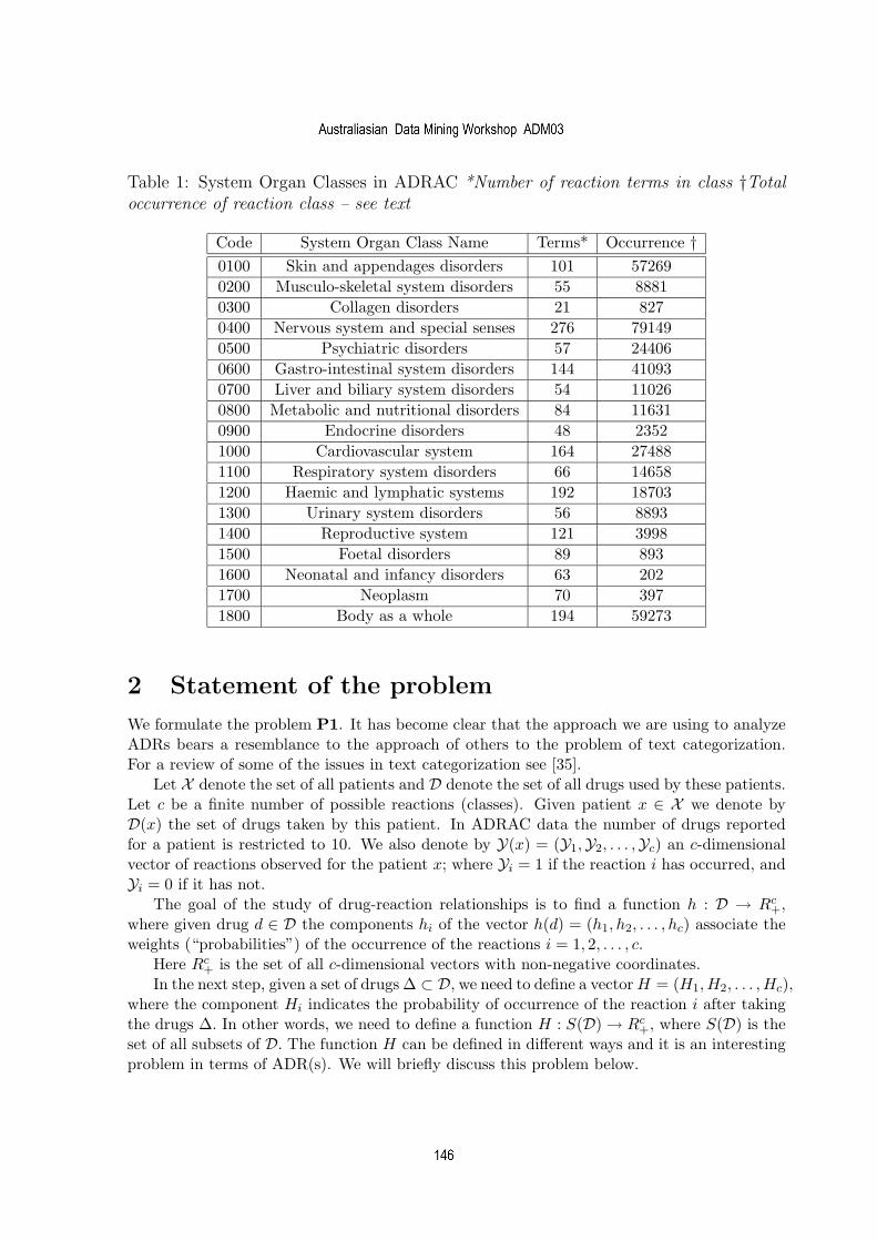
4

Table 1: System Organ Classes in ADRAC *Number of reaction terms in class †Totaloccurrence of reaction class – see text

Code System Organ Class Name Terms* Occurrence †

0100 Skin and appendages disorders 101 57269

0200 Musculo-skeletal system disorders 55 8881

0300 Collagen disorders 21 827

0400 Nervous system and special senses 276 79149

0500 Psychiatric disorders 57 24406

0600 Gastro-intestinal system disorders 144 41093

0700 Liver and biliary system disorders 54 11026

0800 Metabolic and nutritional disorders 84 11631

0900 Endocrine disorders 48 2352

1000 Cardiovascular system 164 27488

1100 Respiratory system disorders 66 14658

1200 Haemic and lymphatic systems 192 18703

1300 Urinary system disorders 56 8893

1400 Reproductive system 121 3998

1500 Foetal disorders 89 893

1600 Neonatal and infancy disorders 63 202

1700 Neoplasm 70 397

1800 Body as a whole 194 59273

2 Statement of the problem

We formulate the problem P1. It has become clear that the approach we are using to analyzeADRs bears a resemblance to the approach of others to the problem of text categorization.For a review of some of the issues in text categorization see [35].

Let X denote the set of all patients and D denote the set of all drugs used by these patients.Let c be a finite number of possible reactions (classes). Given patient x ∈ X we denote byD(x) the set of drugs taken by this patient. In ADRAC data the number of drugs reportedfor a patient is restricted to 10. We also denote by Y(x) = (Y1,Y2, . . . ,Yc) an c-dimensionalvector of reactions observed for the patient x; where Yi = 1 if the reaction i has occurred, andYi = 0 if it has not.

The goal of the study of drug-reaction relationships is to find a function h : D → Rc+,

where given drug d ∈ D the components hi of the vector h(d) = (h1, h2, . . . , hc) associate theweights (“probabilities”) of the occurrence of the reactions i = 1, 2, . . . , c.

Here Rc+ is the set of all c-dimensional vectors with non-negative coordinates.

In the next step, given a set of drugs ∆ ⊂ D, we need to define a vector H = (H1, H2, . . . , Hc),where the component Hi indicates the probability of occurrence of the reaction i after takingthe drugs ∆. In other words, we need to define a function H : S(D) → Rc

+, where S(D) is theset of all subsets of D. The function H can be defined in different ways and it is an interestingproblem in terms of ADR(s). We will briefly discuss this problem below.

5

Given patient x ∈ X and a set of drugs D(x), we will use the notation H(x) = H(D(x)).Therefore, we will denote a classifier as the couple (h, H). To evaluate the performance

of different classifiers we need to measure the closeness of the two vectors H(x) and Y(x).In this work we will use different evaluation measures presented in the Section on EvaluationMeasures.

In this statement, the problem P1 is a multi-class, multi-label text categorization problem,but there are some interesting points that should be mentioned in relation to P1. One of themain characteristics of ADRs is that the number of drugs (that is, words in the context of textcategorization) for each patient is restricted to 10 in the ADRAC data, and for majority ofpatients just one drug was used. This complicates learning and classification, but on the otherhand, this allows us to introduce simple and fast algorithms.

It also should be noted that, at this stage of our investigation, the classification of reactionsis not the major aim. Here we aim to establish drug-reaction relations h(d) such that rep-resentations H(x), x ∈ X , are close to Y(x). This makes the problem P1 more than justa classification problem. Thus, we mainly concentrate on drug-reaction relations. Some othercharacteristics of the problem P1 which are of interest in terms of ADRs will be discussedbelow.

2.1 Potential Reactions

The vectors h(d) show what kind of reactions are caused by the drugs d ∈ D(x). Therefore thevector H(x) can be considered as potential reactions which could occur with patient x. Butwhat kind of reactions will occur? This will depend upon the individual characteristics of thepatient as well as external factors [6]. Different patients can have different predispositions fordifferent reactions. Some reactions which have potentially high degrees may not be observedbecause of the strong resistance of the patient to developing these reactions. But the existenceof these potential reactions could have an influence on the patient somehow. The resultsobtained in [19] show that the information about the existence of potential reactions (butwhich were not reported to ADRAC) helps to make prediction of reaction outcomes (bad andgood) more precise.

The function H can be defined in different ways. The study of more sensible definitions ofthe function H is an interesting problem for future investigations. This problem is also relatedto the study of Interaction of Drugs [19]. In the calculation below we will use the following linearfunction H, which provided more accurate classification in [19]: H = (H1, . . . , Hc); wherefor each subset ∆ ⊂ D the components Hi are defined as follows: Hi =

∑

d∈∆ hi(d), i =1, . . . , c. In this case, for each patient x ∈ X , we have H(x) = (H1(x), . . . , Hc(x)), where

Hi(x) =∑

d∈D(x)

hi(d), i = 1, . . . , c. (2.1)

The use of this function means that, we accumulate the effects from different drugs. Forexample, if hi(dn) = 0.2 (n=1,2) for some reaction i, then there exists a potential of 0.4 forthis reaction; that is, the two small effects (i.e. 0.2) become a greater effect (i.e. 0.4). This

6

method seems a more natural one, because physically both drugs are taken by the patient, andthe outcome could even be worse if there were drug-drug interaction(s).

The other important issue that is related to the definition of H, is the time factor; thatis, the time when the administration of each drug d ∈ D(x) ceases and the decay function ofthe drug. In a simple case we can describe this decay by the function exp (td − t), wheret ≥ td and td is the time of cessation of drug d. Then we can use the following formula for thedefinition of H :

Hi(x) =∑

d∈D(x)

f(td − t∗)hi(d), i = 1, . . . , c; (2.2)

where t∗ is the time of onset of reaction(s) and f(td − t) = exp (td − t) if t ≥ td, andf(td − t) = 0 if t < td. The application of the formula (2.2) is a very interesting problem forfuture investigations which also needs to take into account many other factors such as themetabolism and elimination of drugs. Drug exposure time is another important factor to takeinto consideration [6].

3 Evaluation measures

To evaluate the accuracy of established drug-reaction relations by a given classifier (h, H),we will use different measures.

3.1 Average Distance

This measure evaluates the closeness of the two vectors H(x) (predicted reactions) andY(x) (observed reactions). In this case, we define a distance dist(H(x),Y(x)) between thesevectors. The better classifier should provide the minimal sum of all distances. Therefore, weare looking for a classifier (h, H) which minimizes the total sum of distances.

A common evaluation measure used in multi-label problems is the Hamming distance. Butit is not reasonable to use this distance here, because we deal with real valued weights H(x).

In this paper we will examine the following distance functions:

distp (H(x),Y(x)) =c

∑

i=1

(‖Y(x)‖)−p (Hi − Yi)2, p = 0, 1, 2; (3.3)

where H(x) = (H1(x), . . . , Hc(x)), Y(x) = (Y1(x), . . . ,Yc(x)), ‖Y(x)‖ =∑

j=1,...,c Yj(x) isthe number of reactions for the patient x, and the sign “bar” indicates a normalization:

Hi(x) =‖Y(x)‖

∑

j=1,...,c Hj(x)Hi(x).

7

The role of number p can be explained as follows. Clearly

distp (H(x),Y(x)) =c

∑

i=1

(

(‖Y(x)‖)−p

2 Hi(x) − ‖Y(x)‖)−p

2 Yi(x))2

,

and therefore, potential reactions are normalized such that the sum of these normalized po-tential reactions can be represented as

c∑

i=1

(‖Y(x)‖)−p

2 Hi(x) = (‖Y(x)‖)1−p

2 .

In the distance dist0 this sum is equal to the number of reactions ‖Y(x)‖. In dist2 weget the corresponding sum is equal to 1. dist1 can be considered as a middle version wherethis sum is

√

‖Y(x)‖, and 1 ≤√

‖Y(x)‖ ≤ ‖Y(x)‖.It would be interesting to consider the Euclidian distance. But some preliminary analysis

showed that this distance does not provide us a reasonable evaluation.Therefore, we will examine only the measures 3.3. Given a classifier (h, H), the average

distance error will be calculated as

Epav =

1

|X |

∑

x∈X

distp (H(x),Y(x)) (3.4)

Here |X | stands for the cardinality of the set X .Now we formulate the problem P1 as the following optimization problem:

Epav → min; (3.5)

subject to : hi(d) ≥ 0, i = 1, ..., c, d ∈ D. (3.6)

In this paper we will describe an algorithm which aims to minimize the average distance errorEp

av. This aim changes by taking different numbers p = 0, 1, 2. A discussion of the mostreasonable choice of distance measures is one of the main goals of this paper.

3.2 Other evaluation measures

We will also consider the following measures used in [27].

1. One-error. This measure evaluates how many times the reaction, (say i) havingthe maximal weight in the vector H(x), has not occurred (that is, Yi(x) = 0). In the case

8

where there is more than one reaction, having the same maximal weight in H(x), we needto precisely define this measure.

Denote H∗(x) = {i ∈ {1, . . . , c} : Hi(x) = max{H1(x), . . . , Hc(x)}}, and Y ∗(x) = {i ∈{1, . . . , c} : i ∈ H∗(x) and Yi(x) = 1}. Then we define the one-error as

Eone−error =1

|X |

∑

x∈X

(

1 −|Y ∗(x)|

|H∗(x)|

)

.

The meaning of this measure can be clarified using a simple example. Assume that thereare two reactions having the maximal weight. If both of them have occurred then the error iszero, if just one of them has occurred then error is 0.5, if none have occurred then the error is 1.

2. Coverage. This measure evaluates the performance of a classifier for all the reactionsthat have been observed.

Given x ∈ X , we denote by T (x) the set of all ordered reactions τ = {i1, . . . , ic} ={1, . . . , c} satisfying Hi1(x) ≥ . . . ≥ Hic(x). Then according to a reaction vector (Y1(x), . . . ,Yc(x)),we define the rank and the error as:

rankτ (x) = max{n : Yin(x) = 1, n = 1, . . . , c}; errorτ (x) =rankτ (x)

‖Y(x)‖− 1.

Obviously, the number rankτ (x) and errorτ (x) depend on the order τ. One way to avoidthe dependence on ordering is to take the middle value of maximal and minimal ranks. In thispaper we will use this approach. We define the rank as

rank (x) =1

2(rankmax (x) + rankmin (x));

whererankmax (x) = max

τ∈T (x)rankτ (x), and rankmin (x) = min

τ∈T (x)rankτ (x).

The numbers rankmax (x) and rankmin (x) associated to the “worst” and “best” ordering,respectively.

To define the average error - coverage, we will use the formula:

Ecov =1

|X |

∑

x∈X

(

rank (x)

‖Y(x)‖− 1

)

.

9

Note that, Ecov = 0 if a classifier makes a prediction such that for all x ∈ X the observedreactions are placed at the top of the ordering list of weights Hi(x).

3. Average Precision.

One-error and coverage do not completely describe multi-label classification problems. In[27] the average precision was used to achieve evaluation more completely. We also will usethis measure. Similar to the average error, the average precision depends on a given orderτ = {τ1, . . . , τc} ∈ T (x). So we define the average precision as a middle value of averageprecisions obtained by the “worst” and “best” ordering.

Let Y (x) = {l ∈ {1, . . . , c} : Yl(x) = 1} be a set of reactions that have been observed forthe patient x. Given order τ = {τ1, . . . , τc} ∈ T (x), (that is, Hτ1(x) ≥ . . . ≥ Hτc(x) ), wedefine the rank for each reaction l ∈ Y (x) as rankτ (x; l) = k, where τk = l. Then, AveragePrecision will be defined as:

Pav =1

|X |

∑

x∈X

1

2|Y (x)|(Pworst(x) + Pbest(x)) ;

where

Pworst(x) = minτ∈T (x)

∑

l∈Y (x)

|{k ∈ Y (x) : rankτ (x; k) ≤ rankτ (x; l)}|

rankτ (x; l);

Pbest(x) = maxτ∈T (x)

∑

l∈Y (x)

|{k ∈ Y (x) : rankτ (x; k) ≤ rankτ (x; l)}|

rankτ (x; l).

4 A solution to the optimization

problem (3.5),(3.6)

The function in (3.4) is non-convex and non-linear, and therefore may have many local min-imum points. We need to find the global optimum point. The number of variables is |D| · c.For the data Mallreac, that we will consider, |D| = 5057 and c = 18. Thus we have a globaloptimization problem with 91026 variables, which is very hard to handle using existing globaloptimization methods. Note that, we also tried to use local minimization methods which wereunsuccessful. This means that there is a clear need to develop new optimization algorithmsfor solving problem (3.5),(3.6), taking into account some peculiarities of the problem.

In this paper we suggest one heuristic method for finding a “good” solution to the problem(3.5),(3.6). This method is based on the proposition given below.

10

We denote by S the unit simplex in Rc; that is,

S = {h = (h1, . . . , hc) : hi ≥ 0, h1 + . . . hc = 1}.

In this case for each h(d) ∈ S the component hi(d) indicates simply the probability of theoccurrence of the reaction i.

Given drug d we denote by X(d) the set of all records in X , which used just one drug– d. Simply, the set X(d) combines all records where the drug d was used alone.

Consider the problem:

∑

x∈X(d)

c∑

j=1

‖Y(x)‖−p · (Yj(x) − ‖Y(x)‖hj(d))2 → min, (4.7)

h(d) = (h1(d), . . . , hc(d)) ∈ S. (4.8)

Proposition 4.1 A point h∗(d) = (h∗1(d), . . . , h∗

c(d)), where

h∗j (d) =

∑

x∈X(d)

‖Y(x)‖2−p

−1

·∑

x∈X(d)

‖Y(x)‖1−p Yj(x), j = 1, . . . , c, (4.9)

is the global minimum point for the problem (4.7),(4.8).

Now, given drug d, we consider the set Xall(d) which combines all records that used thedrug d. Clearly X(d) ⊂ Xall(d). The involvement of other drugs makes it impossible to solvethe corresponding optimization problem similar to (4.7), (4.8). In this case, we will use thefollowing heuristic approach to find a “good” solution.

We denote by Ndrug(x) the number of drugs taken by the patient x. Then, we set:

h∗∗j (d) =

∑

x∈Xall(d)

‖Y(x)‖2−p

−1

·∑

x∈Xall(d)

‖Y(x)‖1−p Yj(x)

Ndrug(x), j = 1, . . . , c. (4.10)

This formula has the following meaning. If Ndrug(x) = 1 for all x ∈ Xall(d), then (4.10)provides global minimum solution. Let Ndrug(x) > 1 for some record x ∈ Xall(d). In thiscase, we assume that all drugs are responsible to the same degree; so we associate only thepart 1/Ndrug(x) of the reactions Yj(x) to this drug.

11

4.1 The calculation of weights for each drug

For each drug d we define the sets X(d) – the set of all cases where drug d was used alone andXall(d) – the set of all cases where drug d was used. The set X(d) carries very important infor-mation, because here the drug d and reactions are observed in a pure relationship. Therefore,if the set X(d) contains a “sufficiently large” number of records, then it will be reasonable todefine the weights hj(d), (j = 1, . . . , c) by this set.

We consider two numbers: |X(d)| – the number of cases where the drug is used alone,and P (d) = 100|X(d)|/|Xall(d)| – the percentage of these cases. To determine whether the setX(d) contains enough records we need to use the both numbers. We will consider a functionφ(d) = a|X(d)| + bP (d) to describe how large the set X(d) is.

Therefore, we define h(d) = (h1(d), . . . hc(d)) as follows:

h(d) =

{

h∗(d) if φ(d) ≥ φ∗;h∗∗(d) otherwise;

(4.11)

where h∗(d) and h∗∗(d) are defined by (4.9) and (4.10), respectively.

Remark 4.1 We note that the weight hi(d) is not exactly a probability of the occurrence ofthe reaction i; that is, the sum

∑ci=1 hi(d) does not need to be equal to 1.

Remark 4.2 We have the situation where, for some new (test) examples, new drugs wereinvolved. For each such new drug d we set hi(d) = 0, i = 1, . . . , c.

5 The algorithms

For our analysis we use two algorithms. The first algorithm A(p) which is introduced inthis paper is described below. The second algorithm that we use is BoosTexter (version Ad-aBoost.MH with real-valued predictions, [27]) which has a high performance in text catego-rization problems and seems to be suitable for representing drug-reaction associations.

These two algorithms produce the weighted vector H(x) for each patient x which makesit suitable for the applying distance evaluation measures. But the methods of calculating thevectors H(x) are quite different: the algorithm A(p) uses only drugs that have been takenby the patient x, in contrast, BoosTexter uses all drugs in the list of attributes defined (thatis, even drugs that have not been taken by patient x, are used for the calculation of the vectorH(x)). Our hope is that, we can make more accurate conclusions by applying both quitedifferent methods.

The algorithm A(p) determines a classifier (h, H), where the weights h(d), d ∈ D, aredefined by (4.11), and the function H(x) is defined by (2.1). We will consider three versions:A(0), A(1), A(2), corresponding to the distance functions distp, p = 0, 1, 2, respectively. Eachof these algorithms tends to minimize the average distance calculated by its own measure.

12

The second algorithm BoosTexter [27] produces predictions in the form H(x) = (H1(x), . . . ,Hc(x)),where the numbers Hi(x) are real values which can be positive or negative. In other words,this algorithm defines potential reactions that we are interested in.

To apply the distance measures described above, we need to make all weights calculatedby BoosTexter non-negative. Let Hmin(x) = mini=1,...,c Hi(x). Then we set H(x) = H(x), ifHmin(x) ≥ 0; and

H(x) = (H1(x) −Hmin(x), . . . ,Hc(x) −Hmin(x), if Hmin(x) < 0.

Therefore, we will apply two quite different algorithms – A(p) and BoosTexter. It would beinteresting to compare the drug-reaction relations (that is, h(d)), produced by these algorithms.For this aim we consider one example.

Example 5.1 Assume that, the drug d, which was used alone in 4 cases: in one case thefirst and second reactions and in the all other cases just the first reaction have been observed.We have the following representations h(d). The results for BoosTexter are normalized.

A(0): h(d) = (0.714, 0.286, 0, 0, 0, 0, 0, 0, 0, 0, 0, 0, 0, 0, 0, 0, 0, 0);A(1): h(d) = (0.800, 0.200, 0, 0, 0, 0, 0, 0, 0, 0, 0, 0, 0, 0, 0, 0, 0, 0);A(2): h(d) = (0.875, 0.125, 0, 0, 0, 0, 0, 0, 0, 0, 0, 0, 0, 0, 0, 0, 0, 0);BoosTexter (round=500): h(d) = (0.673, 0.327, 0, 0, 0, 0, 0, 0, 0, 0, 0, 0, 0, 0, 0, 0, 0, 0);BoosTexter (round=2000): h(d) = (0.675, 0.325, 0, 0, 0, 0, 0, 0, 0, 0, 0, 0, 0, 0, 0, 0, 0, 0).In this example the first reaction occurred 4 times and the second once. We see that,

BoosTexter produces weights such that the weight for the first reaction is just 2 times greaterthan for the second reaction, whereas, this difference is greatest for algorithm A(2). Theinteresting question is: which drug-reaction representation is “better” – one which offers a bigdifference in weights or one which offers a slight difference in weights in spite of big differencesin distribution.

For this purpose we use different evaluation measures. Note that, in terms of One-error,Coverage and Average Precision all the representations in Example 5.1 work similarly; that is,the rank for the first reaction is 1 and for the second is 2. The effect of different drug-reactionrepresentations can be observed considering the cases where more than one drug was used.

New events

One of the main difficulties that arises in the study of drug-reaction relationships is thelow level of repeating cases (events) in spite of the large number of records. We considereighteen groups of reactions (out of 1224 reactions) in order to have a sufficient number ofrepeating cases. However, in the dataset Mallreac this problem still exists (for the drugs).One way to avoid this problem is to combine similar drugs as one meta-drug (as it has beendone for reactions), but to achieve this requires a more complete classification of drugs byADRAC, which has partially implemented the Nordic anatomical therapeutic chemical (ATC)classification [23].

We define a new event as a case where, for some test example, all drugs used are notpresented in the training set; in other words, all drugs have been taken by this patient are“new”. This situation relates to the fact that, new drugs are constantly appearing on themarket. Obviously, to make prediction for such examples does not make sense. Therefore, inthe calculations below, we will remove all new events from test sets.

13

6 The results of numerical experiments

In the calculations below we take as a test set records sequentially from each year, startingfrom 1996 until 2001. For example, if records from 1999 are taken as a test set, then all recordsfrom years 1972–1998 form a training set. In the Table 2 we summarized the number of recordsin test and training sets, and, also, the number of new events removed.

Table 2: The Training and Test Sets *“Removed” means how many records were removedfrom test set.

Year Number of Records

Training Test Removed*

1996 79660 7734 410

1997 87804 8090 715

1998 96609 9361 774

1999 106744 11216 840

2000 118880 11244 671

2001 130795 6186 191

First we made calculations by the algorithm BoosTexter. We ran this algorithm choosingdifferent numbers of training rounds. The results obtained for 6000 rounds are presented inTables 3 and 4. In Table 4 we present the results obtained for One-error, Coverage and AveragePrecision.

Next we applied the algorithms A(0), A(1) and A(2), corresponding to the distance func-tions distp, p = 0, 1, 2, respectively. We used a function φ(d) = |X(d)| + P (d) to describethe informativeness of the set X(d). We also need to set a number φ∗. The calculations showthat the results are not essentially changed for different values of φ∗ in the region φ∗ ≥ 50. Weset a large number φ∗ = 1000 in the calculations which means that for the majority of drugsweights are caculated by formula (4.10). The results are presented in Tables 5 and 6.

In Table 3 we present the results for the average distance errors comparing algorithmA(p) to BoosTexter for average error. On the basis of this measure algorithm A(p) performsconsitently better than BoosTexter. This means that the formulae (4.11) for definition ofweights h(d) provides a “good” approximation for the minimal solution to the Problem (3.5),(3.6).

The results for the other measures (one-error, coverage and average precision) for Boos-Texter are given in Table 4, and for A(p) in Tables 5 and 6. It can be seen that, for alldrugs, comparing Tables 4 and 5, the performance of A(p) and BoosTexter are very similar.When the suspected drugs are compared (Tables 4 and 6), algorithm A(1) performs betterthan BoosTexter. The comparison of results obtained for other evaluation measures (Tables5 and 6) reveals differences in the performance of these three versions. We observe that byOne-error measure A(1) performs better than the others, by Coverage A(2) performs betterand by Average Precision both A(1) and A(2) perform better. In all cases A(0) has a worseperformance. Therefore, we can conclude that, the definition of distance measure, taking p =1or 2, is preferable than p=0.

14

Table 3: The Results Obtained by A(0), A(1), A(2) and BoosTexter for Average Errorfor Distance Measure p = 1 The algorithm BoosTexter2 1 [27] was set to run for 6000training rounds. ‘all drugs” means that the drug-reaction weights are calculated assumingall drug(s), suspected “sus. drugs” means that we use only suspected drug(s) reported inADRAC data

Year Drugs A(0) A(1) A(2) BoosTexter

Training Test Training Test Training Test Training Test

1996 all drugs 0.695 0.740 0.678 0.731 0.693 0.751 0.817 0.820

sus. drugs 0.679 0.740 0.661 0.732 0.681 0.759 0.816 0.820

1997 all drugs 0.696 0.740 0.679 0.734 0.694 0.755 0.817 0.824

sus. drugs 0.680 0.743 0.663 0.737 0.683 0.762 0.817 0.825

1998 all drugs 0.697 0.737 0.680 0.731 0.694 0.751 0.818 0.818

sus. drugs 0.681 0.748 0.664 0.742 0.684 0.767 0.817 0.818

1999 all drugs 0.697 0.726 0.680 0.722 0.694 0.751 0.817 0.820

sus. drugs 0.681 0.722 0.665 0.718 0.683 0.749 0.816 0.820

2000 all drugs 0.696 0.756 0.680 0.752 0.693 0.783 0.817 0.815

sus. drugs 0.681 0.755 0.665 0.753 0.683 0.787 0.817 0.815

2001 all drugs 0.697 0.749 0.682 0.747 0.695 0.781 0.817 0.809

sus. drugs 0.684 0.749 0.668 0.748 0.687 0.787 0.817 0.809

As we have shown in Example 5.1, the algorithm A(2), in comparison with A(1), gen-erates drug-reaction representations with greater differences in weights. The results presentedin Table 5, for One-error and Coverage, obtained by the algorithms A(1) and A(2), allowus to make very interesting conclusions:

– if we are interested in One-error (that is, simply saying, the probability of occurrence ofthe reaction which has the greatest weight) then it is better to use drug-reaction representationswith small differences in weights;

– if we are interested in Coverage then it is better to use drug-reaction representationswith big differences in weights. We note that, in all cases, the results are improved if onlysuspected drugs are used.

Below we will only concentrate on the results obtained by A(1) and BoosTexter.The comparison of the training errors in Tables 3, 4, 5 and 6 shows that A(1) performs

generally better than BoosTexter. We can decrease training errors for BoosTexter by increas-ing the number of training rounds (results not presented), but in this case test errors increase.This should be expected, because the algorithm BoosTexter is not designed to minimize somedistance measures, instead it tends to achieve good performance for the other evaluation mea-sures.

There are two important points that make using the algorithm A(1) preferable for thestudy drug-reaction associations.

1. BoosTexter does not calculate weights for each drug. For example, until the year 2000,where 5057 drugs were used. BoosTexter running for 6000 rounds defines weights only for 4521

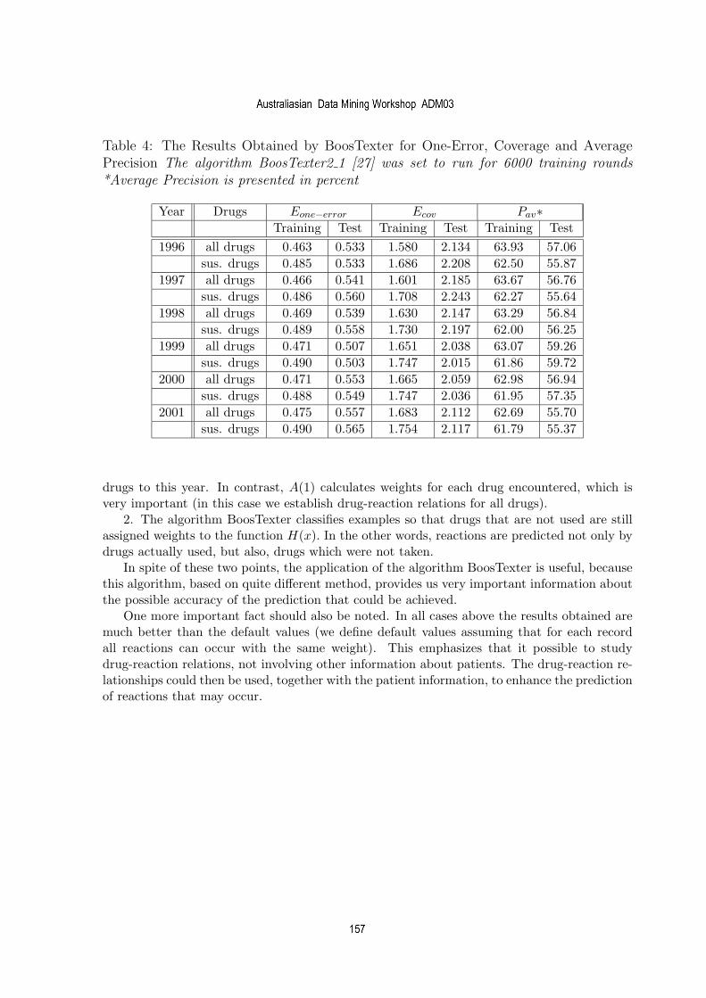
15

Table 4: The Results Obtained by BoosTexter for One-Error, Coverage and AveragePrecision The algorithm BoosTexter2 1 [27] was set to run for 6000 training rounds*Average Precision is presented in percent

Year Drugs Eone−error Ecov Pav∗

Training Test Training Test Training Test

1996 all drugs 0.463 0.533 1.580 2.134 63.93 57.06

sus. drugs 0.485 0.533 1.686 2.208 62.50 55.87

1997 all drugs 0.466 0.541 1.601 2.185 63.67 56.76

sus. drugs 0.486 0.560 1.708 2.243 62.27 55.64

1998 all drugs 0.469 0.539 1.630 2.147 63.29 56.84

sus. drugs 0.489 0.558 1.730 2.197 62.00 56.25

1999 all drugs 0.471 0.507 1.651 2.038 63.07 59.26

sus. drugs 0.490 0.503 1.747 2.015 61.86 59.72

2000 all drugs 0.471 0.553 1.665 2.059 62.98 56.94

sus. drugs 0.488 0.549 1.747 2.036 61.95 57.35

2001 all drugs 0.475 0.557 1.683 2.112 62.69 55.70

sus. drugs 0.490 0.565 1.754 2.117 61.79 55.37

drugs to this year. In contrast, A(1) calculates weights for each drug encountered, which isvery important (in this case we establish drug-reaction relations for all drugs).

2. The algorithm BoosTexter classifies examples so that drugs that are not used are stillassigned weights to the function H(x). In the other words, reactions are predicted not only bydrugs actually used, but also, drugs which were not taken.

In spite of these two points, the application of the algorithm BoosTexter is useful, becausethis algorithm, based on quite different method, provides us very important information aboutthe possible accuracy of the prediction that could be achieved.

One more important fact should also be noted. In all cases above the results obtained aremuch better than the default values (we define default values assuming that for each recordall reactions can occur with the same weight). This emphasizes that it possible to studydrug-reaction relations, not involving other information about patients. The drug-reaction re-lationships could then be used, together with the patient information, to enhance the predictionof reactions that may occur.

16

Table 5: The Results Obtained by A(0), A(1) and A(2) for Different Evaluation Measures– using all drugs *Average Precision is presented in percent

Year Algorithms Eone−error Ecov Pav*

Train Test Train Test Train Test

1996 A(0) 0.494 0.538 1.930 2.304 60.03 55.70

A(1) 0.471 0.526 1.655 2.112 63.10 57.72

A(2) 0.497 0.538 1.512 2.013 63.46 58.30

1997 A(0) 0.496 0.542 1.949 2.355 59.73 55.41

A(1) 0.473 0.534 1.676 2.193 62.88 57.22

A(2) 0.498 0.551 1.532 2.102 63.26 57.24

1998 A(0) 0.497 0.536 1.971 2.288 59.54 56.45

A(1) 0.475 0.525 1.701 2.146 62.60 57.81

A(2) 0.501 0.562 1.556 2.068 62.99 56.96

1999 A(0) 0.497 0.515 1.980 2.185 59.52 58.42

A(1) 0.474 0.504 1.720 2.043 62.49 59.81

A(2) 0.501 0.532 1.578 1.979 62.84 59.28

2000 A(0) 0.498 0.568 1.982 2.365 59.45 53.74

A(1) 0.474 0.559 1.724 2.180 62.47 55.49

A(2) 0.499 0.575 1.584 2.061 62.87 56.67

2001 A(0) 0.502 0.563 1.998 2.288 59.15 54.04

A(1) 0.478 0.550 1.735 2.125 62.22 56.11

A(2) 0.502 0.571 1.595 2.043 62.64 56.68

7 Conclusion

In this paper we have studied drug-reaction relations using the system organ class grouping ofreactions from ADRAC data. These relations are presented in the form of a vector of weights.To determine these vectors we applied two algorithms based on quite different methods. Theresults show the possibility of studying drug-reaction relations, not involving other informationabout patients. In all cases above the results obtained are much better than the default values.For instance, the results for test sets (that is, for new patients) in terms of One-error werearound 0.270 which should be considered sufficiently low error rate. This error rate means thatfor 73 percent of new patients, the reaction having the greatest weight has occurred.

To develop new algorithms taking into account the peculiarities of ADRs is an importantproblem. The development of these algorithms should help us to extract more useful infor-mation from ADRAC data. In particular, the study of drug-reaction associations, drug-druginteractions and the influence of other data fields contained in the ADRAC data are interestingproblems for future investigation.

17

Table 6: The Results Obtained by A(0), A(1) and A(2) for Different Evaluation Measures– using only suspected drugs *Average Precision is presented in percent

Year Algorithms Eone−error Ecov Pav*

Train Test Train Test Train Test

1996 A(0) 0.472 0.520 1.806 2.236 61.98 57.28

A(1) 0.453 0.510 1.547 2.057 64.76 59.14

A(2) 0.469 0.518 1.410 1.984 65.13 59.38

1997 A(0) 0.474 0.531 1.827 2.303 61.70 56.75

A(1) 0.454 0.519 1.566 2.156 64.56 58.29

A(2) 0.470 0.532 1.429 2.071 64.93 58.38

1998 A(0) 0.474 0.520 1.840 2.238 61.61 57.80

A(1) 0.456 0.516 1.586 2.106 64.33 58.86

A(2) 0.471 0.549 1.451 2.038 64.71 57.96

1999 A(0) 0.473 0.503 1.847 2.141 61.61 59.37

A(1) 0.456 0.492 1.599 2.010 64.26 60.66

A(2) 0.472 0.518 1.469 1.955 64.57 60.08

2000 A(0) 0.476 0.566 1.855 2.343 61.43 54.15

A(1) 0.456 0.558 1.611 2.135 64.16 56.38

A(2) 0.473 0.564 1.482 2.041 64.48 57.24

2001 A(0) 0.481 0.554 1.878 2.271 60.99 54.43

A(1) 0.462 0.542 1.631 2.090 63.80 56.91

A(2) 0.478 0.562 1.502 2.022 64.11 57.36

8 Acknowledgements

The work reported in this paper has been supported by The Australian Research Council,the TGA (Therapeutic Goods Administration), the Ballarat Division of General Practice, theMedical Software Industry Association, the Therapeutic Guidelines Pty. Ltd. We are indebtedto Patrick Purcell from the TGA for providing expert comments. We also thank Rob Schapirefor his helpful advice in using BoosTexter.

References

[1] Aronson J.K., Derry S., Loke Y.K. Adverse drug reactions: keeping up to date. FundamClin Pharmacol 2002;16:49–56.

[2] Bate A, Lindquist M, Edwards IR, Olsson S, Orre O, Lansner A, De Freitas R. A Bayesianneural network method for adverse drug reaction signal generation. Eur J Clin Pharmacol1998;54(4):315–321.

18

[3] Bates D.W., Evans R.S., Murff H., Stetson P.D., Pizziferri L., Hripcsak G. DetectingAdverse Events Using Information Technology. J Am Med Inform Assoc 2003;10:115–128.

[4] Bates D.W., Gawande A.A. Improving Safety with Information Technology. N Engl J Med2003;348:2526–34.

[5] Brown Jr Stephen D., Landry Frank J. Recognizing, Reporting, and Reducing AdverseDrug Reactions. South Med J 2001;94(4):454–462.

[6] Chuang-Stein C. Statistics for Safety Data. In: Stephens M.D.B., Talbot J.C.C., Rout-ledge P.A., editors. Detection of New Adverse Drug Reactions. 4th ed. London: MacmillanReference Ltd 1998. p. 271–79.

[7] Consumer Reports on Medicines. Consensus Document adopted at the FirstConference on CRM. 2000 Sep 29–Oct 1; Sigtuna, Sweden. Available at:http://www.kilen.org/kilen/htm/crm.htm

[8] Coulter David M., Bate Andrew, Meyboom Ronald H. B., Lindquist Marie, Edwards I.Ralph. Antipsychotic drugs and heart muscle disorder in international pharmacovigilance:data mining. BMJ 2001;322(7296):1207–1209.

[9] Dormann H., Criegee-Rieck M., Neubert A., Egger T., Geise A., Krebs S., et al. Lack ofAwareness of Community-Aquired Adverse Drug Reactions Upon Hospital Admission –Dimensions and Consequences of a Dilemma. Drug Saf 2003;26(5):353–362.

[10] DuMouchel W. Bayesian data mining in large frequency tables, with an application to theFDA spontaneous reporting system. Am Statistician 1999;53(3):177–190.

[11] Egberts A.C.G., Meyboom R.H.B., von Puijenbrock E.P. Use of Measures of Dispropor-tionality in Pharmacovigilance. Drug Saf 2002;25(6):453–458.

[12] Evans S.J.W., Waller P.C., Davis S. Use of proportional reporting ratios (PRRs) for signalgeneration from spontaneous adverse drug reaction reports. Pharmacoepidemiol Drug Saf2001;10:1–4.

[13] Fernanopulle R.B.M., Weerasuriya K. What Can Consumer Adverse Drug Reaction Re-porting Add to Health Professional-Based Systems? Drug Saf 2003;26(4):219–225.

[14] Harvey J.T., Turville C., Barty S.M. Bayesian Data Mining of the Australian AdverseDrug Reactions Database. International Trans Operational Research 2002. In press

[15] Hartmann K., Doser A.K., Kuhn M. Postmarketing Safety Information: How Useful areSpontaneous Reports? Pharmacoepidemiol Drug Saf 1999;8:S65–S71.

[16] Heely Emma, Riley Jane, Layton Deborah, Wilton Lynda V., Shakir, Saad A.W. Prescription-event monitoring and reporting of adverse drug reactions. Lancet2001;358(9296):182–184.

[17] Hillson Eric M., Reeves Jaxk H., McMillan Charlotte A. A statistical signalling model foruse in surveillance of adverse drug reaction data. J Appl Statistics 1998;25(1):23–41.

19

[18] Hutchinson Tom A. Bayesian assessment of adverse drug reactions. Can Med Assoc J2000;163(11):1463–1466.

[19] Mamedov M.A., Saunders G.W. AnAnalysis of Adverse Drug Reactions from the ADRAC Database. Part1: Cardiovascu-lar group. University of Ballarat School of Information Technology and MathematicalSciences, Research Report 02/01, Ballarat, Australia, February 2002;1–48. Available at:http://www.ballarat.edu.au/itms/research-papers/paper2002.shtml

[20] Mamedov M.A., Saunders G.W. A Fuzzy Derivative Approach to Classification of out-comes from the ADRAC database. International Trans Operational Research 2002. Inpress

[21] Mamedov M.A., Saunders G.W. Analysis of Cardiovascular Adverse Drug Reactions fromthe ADRAC Database. Proceedings of the APAC Conference and Exibition on AdvancedComputing, Grid Applications and eResearch 2003. Royal Pines Resort, Gold Coast,Queensland, 29 September – 2 October 2003 http://www.apac.edu.au/apac03/

[22] Orsini M., Funk P.A. An ADR Surveillance Program: Increasing Quality, Number ofIncidence Reports. Formulary 1995;30(8):454–461.

[23] Pinkston V., Swain E.J. Management of Adverse Drug Reaction and Adverse Event Datathrough Collection, Storage and Retrieval. In: Stephens MDB, Talbot JCC, Routledge PA,editors. Detection of New Adverse Drug Reactions. 4th ed. London: Macmillan ReferenceLtd 1998. p. 281–96.

[24] Pirmohamed Munir, Breckenridge Alasdair M., Kitteringham Neil R., Park B. Kevin.Adverse drug reactions. BMJ 1998;316(7140):1294–1299.

[25] Purcell P., Barty S. Statistical Techniques for Signal Generation – The Australian Expe-rience. Drug Saf 2002;25(6):415–421.

[26] Redfern W.S., Wakefield I.D., Prior H., Pollard C.E., Hammond T.G., Valentin J-P. Safetypharmacology – a progressive approach. Fundam Clin Pharmacol 2002;16:161–173.

[27] Schapire Robert E., Singer Yoran. Boostexter: A boosting-based system for text catego-rization. Machine Learning 2000;39: 135–168.BoosTexter software available at:http://www.cs.princeton.edu/ ∼ schapire/boostexter.html

[28] Szarfmann Ana, Machado Stella G., O’Neill Robert T. Use of Screening Algorithms andComputer Systems to Efficiently Signal Higher-Than-Expected Combinations of Drugsand Events in the US FDA’s Spontaneous Reports Database. Drug Saf 2002;25(6):381–392.

[29] Troutman W.G., Doherty K.M. Comparison of voluntary adverse drug reaction reportsand corresponding medical records. Am. J Health-Syst Pharm 2003;60(6):572–575.

[30] Tubert-Bitter P., Begaud B. Comparing Safety of Drugs. Post Marketing Surveillance1993;7:119–137.

20

[31] van Groothees K., de Graaf L., de Jong-van den Berg T.W. Consumer Adverse DrugReaction Reporting – A New Step in Pharmacovigilance? Drug Saf 2003;26(4):211–217.

[32] van Puijenbroek Eugne P., Bate Andrew, Leufkens Hubert G. M., Lindquist Marie, OrreRoland, Egberts Antoine C. G. A comparison of measures of disproportionality for signaldetection in spontaneous reporting systems for adverse drug reactions. PharmacoepidemiolDrug Saf 2002;11(1):3–10.

[33] van Puijenbroek Eugne P., Diemount Willem L., van Grootheest Kees. Application ofQuanitative Signal Detection in the Dutch Spontaneous Reporting System for AdverseDrug Reactions. Drug Saf 2003;26(5):293–301.

[34] World Health Organization. WHO Technical Report No 498, and Note for Guidance onClinical Safety Data Management: Definitions and Standards for Expedited Reporting(CPMP/ICH/377/95) 1972.

[35] Yang Yimming, Liu Xin. A re-examination of text categorization methods. Proceedingsof SIGIR-99, 22nd ACM International Conference on Research and Development in In-formation Retrieval 1999;39:42–49.

[36] Zapater Pedro, Such Jos, Prez-Mateo Miguel, Horga Jos Francisco. A New Poisson andBayesian-Based Method to Assign Risk and Causuality in Patiens with Suspected HepaticAdverse Drug Reactions. Drug Saf 2002;25(10):735–750.

Mining Geographical Data with Sparse Grids

Markus Hegland1, and Shawn W. Laffan2,1

1 Mathematical Sciences Institute, Australian National University, Canberra,Australia, 0200.

Markus.Hegland@anu.edu.au2 School of Biological, Earth and Environmental Sciences, University of New South

Wales, Sydney, Australia, 2052.Shawn.Laffan@unsw.edu.au

Abstract. Predictive modelling tools combined with spatial data min-ing techniques can be used to discover relationships among geographicphenomena. Mining geographical data requires very flexible and simplefunction classes for data fitting, highly efficient methods to be able to fita large number of models locally to vast amounts of data. The modelsneed to have structure which allows collections of models to be mined. Itappears that sparse grids do satisfy these requirements of geographicaldata mining.After a discussion of requirements of geographical data, mining sparsegrids will be reviewed and their suitability for mining geographical datawill be discussed. Some results are presented and some further ideas formining of large collections of local sparse grid models are discussed.

Keywords: Spatial analysis, geographic data mining, predictive modelling,sparse grids

1 What do geographers want from data mining?

One can describe geography as being the study of where things are, where thingsare not, and how these things interact with one another through space and time.“Things” in this sense are any phenomena that have some spatial component,and might be discrete objects or continuous surfaces (fields) [25]. Examples in-clude individual trees and animals, or populations of such trees and animals.Alternately, one might investigate spatial processes such as the flow of waterthrough a catchment and the associated flux of sediment, nutrients and pol-lutants [30]. From this, one can see that geographers are interested in a widevariety of problems from many different fields of research.

The sparse grids technique one means of analysing geographic phenomena,and we describe its potential for geographic data mining in this paper.

1.1 The problems of geographic data

There is now an enormous amount of information collected that has spatial at-tributes, including from remote sensing satellites, national censuses, mobile tele-phone records, crime statistics, land use change in agriculture, health records,

epidemiological data, and consumer purchasing records. The challenge for geog-raphers is to make sense of these data to derive an understanding of the under-lying spatial phenomena. The problem we face is that there is an overwhelmingvolume of data.

As an example of the volume of data, the 2001 census of the Australian pop-ulation has over 17,000 sample areas for the state of New South Wales at thefinest aggregate unit (census collection district). For each of these collection dis-tricts there are thirty-three categories containing over 4000 attribute fields intowhich the population is divided. Each person in the collection district at thetime of the census will fall into at least one field within each category, and some-times more. When one extends the analysis to include temporal relationshipsamong the population over several censuses then the amount of data increasesconsiderably. This is despite each earlier census being of slightly lower detail.

As another example, consider the amount of data generated by remote sens-ing satellites. A commonly used data source is the Landsat Enhanced ThematicMapper, which collects data in six visible and infra-red bands (30 m resolution),one thermal band (with high and low spatial resolution versions (120 m and60 m), and one panchromatic band (across visible and near infra-red spectra,15 m resolution). The data are divided into scenes for distribution, with eachscene approximately 185 km along each side. This translates to approximately6000 by 6000 cells for the visible and infra-red bands. This is normally a reason-able data set to deal with. However, when one includes the temporal componentthen, once again, the amount of data increases rapidly. The Landsat satelliterepeats its polar orbit cycle every sixteen days, so a location at the equator issampled every sixteen days, and more frequently near the poles due to spatialoverlap of the sample swaths. The result is that, if there is no cloud to obscurethe ground, one would have twenty-two scenes to analyse for each year of a study.While this is very simple example, as many locations are obscured by cloud forat least some portion of the scenes each year, there are other satellites carryingradar sensors that are not affected by cloud, hyperspectral sensors which recordspectral response in tens to hundreds of bands, and sensors with very high spa-tial resolutions (eg. 0.6 m). This is a major issue given that each of these sensorsprovides complementary information and so they could all be used in a singleanalysis.

A second consideration is spatial and temporal non-stationarity, which canhave serious effects on analysis results. This is related to Tobler’s First Law ofGeography “that everything is related to everything else; but that near thingsare more related than those far apart” [29].

If a model is applied to a data set and is assumed to apply equally over theentire study area, study period, or both, then one is assuming that the processesare spatially and temporally stationary. This means that the landscape studiedis in some form of equilibrium between the phenomenon of interest (responsevariable) and the phenomena it is being related to (correlate variables). This isoften not the case [18–20]. Spatial phenomena are often the result of a series ofsuperimposed processes, all operating at different spatial and temporal scales [3].

Some of these processes may be in equilibrium with the phenomenon of interest,but many may not be. The end result is that the response variable will havea good relationship with some of the correlate variables, and little relationshipwith others. If the analysis is conducted at a geographically local scale (by usinga geographically local sample) then many of these problems may be reducedbecause the effects of non-stationarity will be less over smaller regions.

A third major problem that arises from these geographic data are that theyare all highly correlated, both through space and time. Any analysis applied tothe data must be able to operate in the presence of such correlation withoutviolating the assumptions of the method.

Finally, there are issues with the treatment of geographic and temporalspaces. Geographic processes are often complex and non-Euclidean [19], meaningthat the treatment of the geographic relationships will impact on the validity ofthe results of the mining exercise. In addition to this, time cannot be treated asmerely an extension of the spatial domain [27]. The nature of time is very dif-ferent in that it is unidirectional in the flow of effects, whereas spatial processesoperate in three dimensions.

The above issues are just a sample of those that affect geographic analyses(see [24] and [23]), and there is a clear need for data mining tools that canapproach geographical problems involving such complexity and sheer volumes ofdata. Sparse grids provide one approach that may be able to cope with some ofthese issues.

2 Predictive modelling with sparse grids

2.1 Sparse grid functions

The sparse grid idea was known for some time, it appears in the modern liter-ature in [28] and sparse grids were applied to the solution of engineering prob-lems by Zenger [31]. The first data mining applications of sparse grids appearedin [16] and [9] and geographical applications were first considered in [21]. Sparsegrids can also be viewed as a special variant of multivariate regression splines(MARS) [8]. The theory of sparse grids has been developed considerably, espe-cially for the case of the classical sparse grids, starting with [31] and the “Munichschool”.

In the following we provide a short introduction into sparse grid functionsand contrast them with regular grid functions.

Sparse grid functions are multivariate real functions f(x1, . . . , xd). They com-bine many features of linear models, regression trees [2], wavelets [4], MARS [8],finite elements [1], additive models [13], and splines [5].

In the univariate case, d = 1 the sparse grids are piecewise linear functions [5],defined on a regular grid, i.e. a grid with equidistant grid points. The number ofgridpoints is nk where n0 = 1 corresponds to constant functions, n1 = 1 to linearfunctions. For k > 1 one has nk = 2k−1 + 1. Piecewise linear functions providea good compromise between computational efficiency and continuity and form

the basis for MARS [8, 13, 5]. Adaptivity is obtained through the choice of thelevel parameter k.

In the case of of bivariate functions, d = 2 regular grids define piecewisebilinear functions. In each cell defined by four grid lines the functions are bilinear,i.e., have the form a0+a1x1+a2x2+a3x1x2. Such function spaces are commonlyused in finite element analysis, for example, in finite element fitting and for theapproximation of smoothing splines [26]. The number of grid points is now theproduct nk1

nk2of the numbers of gridpoints in each dimension. The simplest

spaces of functions defined in this way contain the constant functions with onegrid point, the functions which are linear in one variable with two grid points,and the bilinear functions with 4 grid points.

These are the simplest four spaces defined by two-dimensional regular grids.Note that in particular the space of linear functions, while a subspace of bilinearfunctions, does not correspond to a regular grid. As the functions are representedby the values at the grid points it is not totally obvious unless one computesa difference of the type y1 − y2 − y3 + y4 of the values of the four grid pointsif the bilinear function is actually linear or not. This is a slight computationaldisadvantage for data mining if one would like to generate many models andextract the linear ones.

This situation is even worse in the case of more than 2 variables. The sim-plest regular grid which involves all d variables has 2d grid points and defines amultilinear function which is defined by the values in the grid points and thusrequires 2d coefficients for their representation. Linear functions, which can berepresented with d+1 parameters, are thus not economically described by regu-lar grid functions which use 2d parameters. Moreover, the determination of thelinearity of a multilinear function is much more complicated than in the previouscase. Note that the simplest function defined by a regular grid and involving alld variables is multilinear and needs 2d coefficients. This is an aspect of the curseof dimensionality. Regular grid function approximations are thus not suitable formost data mining applications.

Sparse grid functions address these shortcomings. The grids are unions ofregular (and typically small) grids and a sparse grid function is the sum ofthe corresponding regular grid functions. For example, a sparse grid functionf(x1, . . . , xd) could have the form

f(x1, . . . , xd) = f1(x1) + f2(x4) + f3(x2, x4, x5) + f4(x2, x4, x5) + · · ·

where each component fi is defined by a regular grid. Note that the same vari-ables, e.g., x2, x4, x5, can occur in different components which relate to differentgrid sizes, e.g., a grid with 5 × 5 × 3 grid points and a grid with 2 × 3 × 9 gridpoints. Note that there is some redundancy in this representation, for exampleone could add a constant to any component and subtract it from any otherwithout changing the function.

Any regular grid is also a sparse grid. For example, the space of constantfunctions is a sparse grid function space. More generally, if one takes the union ofthe linear functions in one variable (all of which are regular grids) one obtains the

space of linear functions which is thus a sparse grid space. For the representationone requires two coefficients for each component function and so, in the case of d

variables, one requires 2d coefficients for the representation of linear functions asa sparse grid as the constant part is represented redundantly in each component.While slightly redundant, this compares very favourably with the case whereone represents a linear function by a regular grid, i.e., as a multilinear functionwith 2d coefficients. With sparse grids one can now directly search for linearfunctions and in collections of large numbers of models recognise a linear functionimmediately. More generally, if one considers the union of regular grids withfunctions which only depend on one variable one obtains additive functions.Like in the case of the linear functions one avoids the curse of dimensionality(the exponential dependence of the number of coefficients) and has the samesmall redundancy as the constants are represented in all components. If onenow considers the union of regular grids where the functions only depend on 2variables, i.e., where the grids are planar, one obtains a sparse grid which includeinteractions between variables. Higher order interactions can also be obtainedwhen one uses regular grid functions which depend on more than 2 variables. Asimple example of a construction of a sparse grid from a couple of regular gridsis given in figure 1.

= + +

Fig. 1. Construction of a sparse grid from regular components

Sparse grids provide an efficient tool to investigate multiscale effects in addi-tion to the interaction effects discussed previously. In the case of one dimensionthe width of the grid cells defines the scale. Very fine grids allow the representa-tion of highly oscillating functions and coarser grids are used for more smoothvariations. In higher dimensions one may have different scales for the differentvariables. Moreover, the scales of the interactions, in particular, high-order in-teractions are typically lower than the ones for additive components as theyintroduce a higher degree of singularity. For a grid with one variable and nk

grid points one defines the level or scale as k. This can be generalised for twodimensions where the grid with nk by nj grid points has now an overall level ofk + j. The so defined level is approximately the logarithm of the total numberof grid points and thus a reasonable complexity measure. It is used to define the“classical” sparse grids [31] which contain components which all have the samelevel. It was demonstrated that these classical sparse grids have very similarapproximation performance as the regular grid which contains the sparse grid.

The classical sparse grids are computationally feasible up to around ten di-mensions. This is substantially higher than the regular grids which are pre-dominantly used in two and three dimensions and are maybe feasible for fourdimensions. In data mining applications, however, one does encounter regularlybetween 10 and 100 variables and in many applications in bioinformatics, bank-ing, spectroscopy and others thousands of variables are common. Sparse gridsare able to represent functions with close to arbitrary numbers of variables.

2.2 Why sparse grids are suitable for mining geographical data

While sparse grid functions have not been widely used so far in geographical dataanalysis, it appears that they provide an efficient tool for predictive modelling-based data mining and, in particular, compare favourably with other methodsused like artificial neural nets and regression networks.

1. Sparse grids define a collection of function spaces which include the space oflinear functions, spaces of additive models, ANOVA decomposition spacesand multilevel decomposition spaces. A function space selection procedure isan important part of the sparse grid mining routines and the type of spacefitted provides valuable information about the data.

2. Sparse grids are flexible enough to approximate arbitrary functions. In par-ticular, sparse grid functions provide good approximations of functions fromreproducing kernel Hilbert spaces, radial basis functions or regularisationnetworks. There is some literature on sparse grid approximation propertiesbut no systematic review, see, e.g., http://bibliothek.iam.uni-bonn.de/duennbib.html for some earlier references.

3. Sparse grids are additive and sparse grid fitting amounts to solving a pe-nalised least squares problem. The regularisation parameter can be chosenusing crossvaliation or test data sets, see [13]

4. There are powerful computational techniques akin to backfitting and usingpreconditioned conjugate gradient methods which reduce the solution of thesparse grid fitting problem to the iterated solution of multiple regular grid fit-ting problems for which efficient iterative and direct solvers are available [11,17].

5. Sparse grid functions can be readily compared in terms of their componentspaces and the actual functions and thus lend themselves to mining thecollection of models obtained (see last section).

6. Sparse grid functions are similar to ANOVA decompositions and have thesame interpretative power in terms of additive effects and interactions. Thisfeature is shared with methods like MARS [8], additive models [14] andANOVA splines [22].

7. Sparse grids allow the identification of linear trends, curvatures, and higherorder fluctuations and permit multiresolution analysis.

8. Sparse grid fitting and evaluation can be done efficiently using parallel andhigh performance computers and exhibit both coarse and fine grain paral-lelism. Sparse grid algorithms use finite element technology developed for

engineering problems and tested in many applications and commercial pack-ages. The algorithms scale linearly in the data size and allow scalable paral-lel execution over the data records. Consequently, the sparse grid algorithmshave the capacity required to analyse very large data sets and fit complexmodels [10, 16, 17].

9. Open source software is available, see http://datamining.anu.edu.au.10. The sparse grid model can be interpreted as a linear model using features

which are defined by the regular grid basis functions. Thus any methodsbased on linear models can be applied. In particular, one may take intoaccount the autocorrelation postulated in Tobler’s law using sparse grid au-

toregressive models which are models of the form

y(p) = f(x(p), y(pN ), y(pS), y(pE), y(pW ))

where p denotes the position of the prediction and pN etc etc are the positionsof neighbouring points. After such a model has been learnt the prediction atany new point requires an iterative process which will predict the values ina neighbourhood of points as well. The sparse grids are again just a flexiblegeneralisation of ordinary autoregressive models. Alternatively, sparse gridsallow the introduction of models using differential equations of the form

y(p) = f(x(p),∆py(p))

where ∆p is a differential operator in the position.

In summary, sparse grids provide a computationally efficient tool to modelfunctions of very many variables, fitting vast amounts of data, and they canbe used to extract and identify additive components, interactions and effects atmultiple scales. In geographical applications all these properties are seen to beuseful, one often has many variables, and would like to find components, and inparticular, compare various models. This is further expanded in the following.

2.3 Fitting sparse grids to data

Predictive modelling addresses the problem of learning from data, i.e. givenn data points x1, . . . , xn corresponding to n objects or observations which allhave labels or features y1, . . . , yn one would like to find a function f such thatyi ≈ f(xi) so that the function f can be used to predict the labels or featuresfor future observations. Typically this prediction will not be ideal as the modelwill be limited and the data is usually not sufficient to explain every variationof the labels or features. In order to identify a “best possible” function f oneintroduces a loss function which depends on both the observed data and thefunction and f is chosen as the minimum of the loss function. Much has beenwritten about this both in the statistical and machine learning literature andshall not be discussed any further here. Instead the focus of this discussion is oncomputational issues relating to sparse grid learning. For a good recent referenceon the topic of statistical learning in general, see [13].

First consider learning a function from a given sparse grid function space bya least squares fit such that f is determined as minimiser of the functional:

J(f) =∑

i=1

(yi − f(xi))2.

The sparse grid is represented as a sum of regular grid functions fj such that:

f(x) =

m∑

j=1

fj(x).

If one expands the functions fj in terms of any basis functions a linear systemof equations for the coefficient vectors cj of the functions fj is obtained of theform:

A11 A12 · · · A1m

......

...Am1 Am2 · · · Amm

c1

...cm

=

b1

...bm

.

It turns out that this system of equations does pose two computational chal-lenges. First, it can be seen that in most cases the off-diagonal blocks Aij (i 6= j)are fairly dense and only the diagonal blocks are sparse and second the matrixis typically large and singular. The singularity of the matrix can be addressedby regularisation.

The size and density of the matrix is dealt with by a backfitting approachwhere a sequence of approximations is constructed by

f (k) =

m∑

j=1

f(k)j

and

f(k+1)j = argminfj

J(

j−1∑

s=1

f (k+1)s + fj +

m∑

s=j+1

f (k)s ).

In this way, at each step a sequence of regular grids have to be determined andthus a collection of small sparse linear systems of equations are solved insteadof the one big dense system.

While this algorithm, and, in particular, an acceleration using conjugate gra-dients, converges reasonably quickly, the small sparse linear systems cannot besolved concurrently. However, there is an alternative algorithm which allows theconcurrent determination of components where:

f(k+1)j = argminfj

J(

j−1∑

s=1

f (k)s + fj +

m∑

s=j+1

f (k)s ).

This approach is basically a block Jacobi method and converges considerablyslower than the original backfitting which is a block Gauss-Seidel method.

In [17] a method has been introduced which combines advantages of theadditive approach with fast convergence. The idea of this algorithm is based onthe combination technique [12, 15]. In order to be able to apply the combinationtechnique one requires that

1. The regular spaces which define the sparse grid also contain all the intersec-tions of any two generating grids (which is regular as well).

2. If one first fits any of the component grids to the data, then evaluates onthe data and then fits these values to a different component grid one getsexactly the fit onto the intersection of the two components.

In this case it can be seen that there are coefficients γj which do not depend onthe data such that sparse grid f which fits the data is given by

f =

m∑

j=1

γjfj

where the fj are the fits of the components onto the data.In general, this formula would not hold but one can define an iterative tech-

nique where f(0)j = 0 and

f(k+1)j = f

(k)j + argmingj

J(f (k) + gj)

where gj is in the j-th component space, where

f (k) =m

∑

j=1

γ(k)j f

(k)j

and where the coefficients γ(k)j are chosen such that for the given f

(k)j the func-

tional J(f (k)) is minimised. This algorithm allows the parallel determination ofall the components fj . It can be seen that the algorithm has similar performanceto the backfitting approach, see [17].

The most difficult part of learning with sparse grids is the determinationof the sparse grid space from the data. Only a heuristic, greedy approach isavailable here. The algorithm uses the natural ordering of the sparse grids givenby the subgrid relation. It starts with a grid with one point and considers all nextlarger grids, the so-called covering grids. The covering sparse grid with the bestperformance is selected as the next candidate space in the iteration. This greedyalgorithm is similar to the one used in the MARS method [8]. After a relativelyfine grid is obtained crossvalidation or test data is used to prune the grid. Notethat the procedure used is closely related to subspace or variable selection.

2.4 A sparse grid web service

For ease of use, the sparse grid predictive modelling capacity is delivered by aweb server using forms to select the type of analysis and data sets required. A

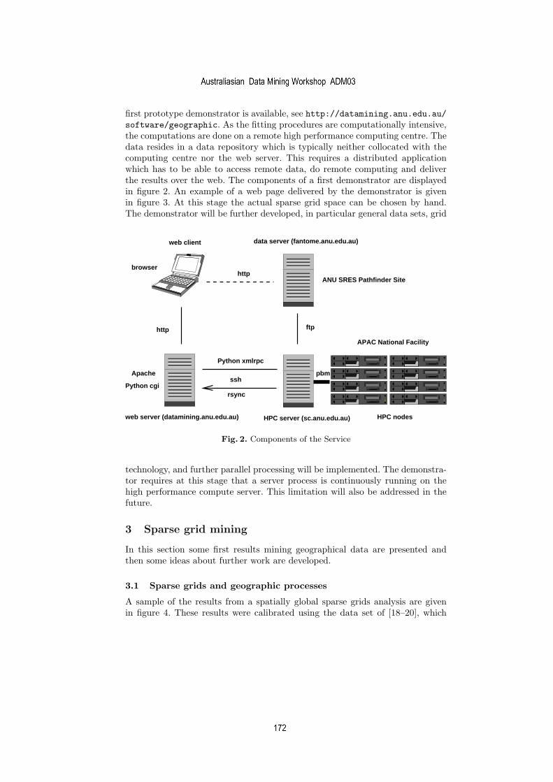
first prototype demonstrator is available, see http://datamining.anu.edu.au/software/geographic. As the fitting procedures are computationally intensive,the computations are done on a remote high performance computing centre. Thedata resides in a data repository which is typically neither collocated with thecomputing centre nor the web server. This requires a distributed applicationwhich has to be able to access remote data, do remote computing and deliverthe results over the web. The components of a first demonstrator are displayedin figure 2. An example of a web page delivered by the demonstrator is givenin figure 3. At this stage the actual sparse grid space can be chosen by hand.The demonstrator will be further developed, in particular general data sets, grid

browser

web client

http

web server (datamining.anu.edu.au)

ftp

http

HPC server (sc.anu.edu.au) HPC nodes

pbm

data server (fantome.anu.edu.au)

ssh

APAC National Facility

Apache

Python xmlrpc

Python cgi

ANU SRES Pathfinder Site

rsync

Fig. 2. Components of the Service

technology, and further parallel processing will be implemented. The demonstra-tor requires at this stage that a server process is continuously running on thehigh performance compute server. This limitation will also be addressed in thefuture.

3 Sparse grid mining

In this section some first results mining geographical data are presented andthen some ideas about further work are developed.

3.1 Sparse grids and geographic processes

A sample of the results from a spatially global sparse grids analysis are givenin figure 4. These results were calibrated using the data set of [18–20], which

Fig. 3. Web page of the Sparse Grid Web service

contains sample records for regolith properties as well as continuous surfaces oftopographic and hydrological indices and Landsat spectral response. They usedsparse grids with seventeen grid points in each dimension, with eight variablesand 28 first order interaction grids. From these results it is clear that not all of thevariables are good predictors of silica abundance, and one can easily determinewhich is useful.

These results are just a sample of what can be generated, and there are manypotential avenues for data mining of sparse grids. We consider here only threeof the possible approaches that can be used to gain a greater understanding ofgeographic patterns and processes.

1. The first consideration is an understanding of where there is a relationshipbetween the predictor variable and the correlates. As noted above, this islikely to be in geographically local areas. The approach one can take to anal-yse this is to use geographically local sample regions and fit a sparse gridsmodel within them. This is analogous to kernel methods, but the weightingsare calculated using only the geographical coordinates. In the case of sparsegrids, we have devised such a system of analysing geographically local sam-ples, where a sparse grids model is generated for each of these local samples.The results are a general improvement over the global model, and are betterthan the results of [19, 20] who used an artificial neural network and movingwindow regression analyses applied to the same data.

2. However, the above approach can be limiting in that each sample locationuses a different model, ignoring those used elsewhere in the study area. Fol-lowing from this, one might be interested in where similar processes occuracross a landscape. For example, similar processes controlling a relationshipmay occur in several regions across a landscape, but these regions may beseparated by some distance. When a model is generated for a local sample itcan readily be applied to any other location in the study area where there aresufficient data. By mapping the locations where errors for such a predictionare low, one might be able to generate interesting hypotheses concerning therelationships between the response and correlate variables. This is describedfurther in the next section.

3. The local analyses are very useful approaches to understanding geographicphenomena. However, one still needs to interpret the underlying relationshipsrepresented by the sparse grid models to understand what relationships thereare. We now consider a sample of these.

One method of interpreting the sparse grids system is an analysis of theaccuracies of each of the input grids. While this can be implemented as astandard step-wise procedure for model selection (§2.3), the interpretationof the relationship between each of the different correlates is very valuableinformation (fig 4). When it is mapped as a geographic surface then onecan gain even greater insight into the strength of the relationships betweenvariables throughout a study area. With this information one can begin tobetter understand the system of relationships as they vary through space.

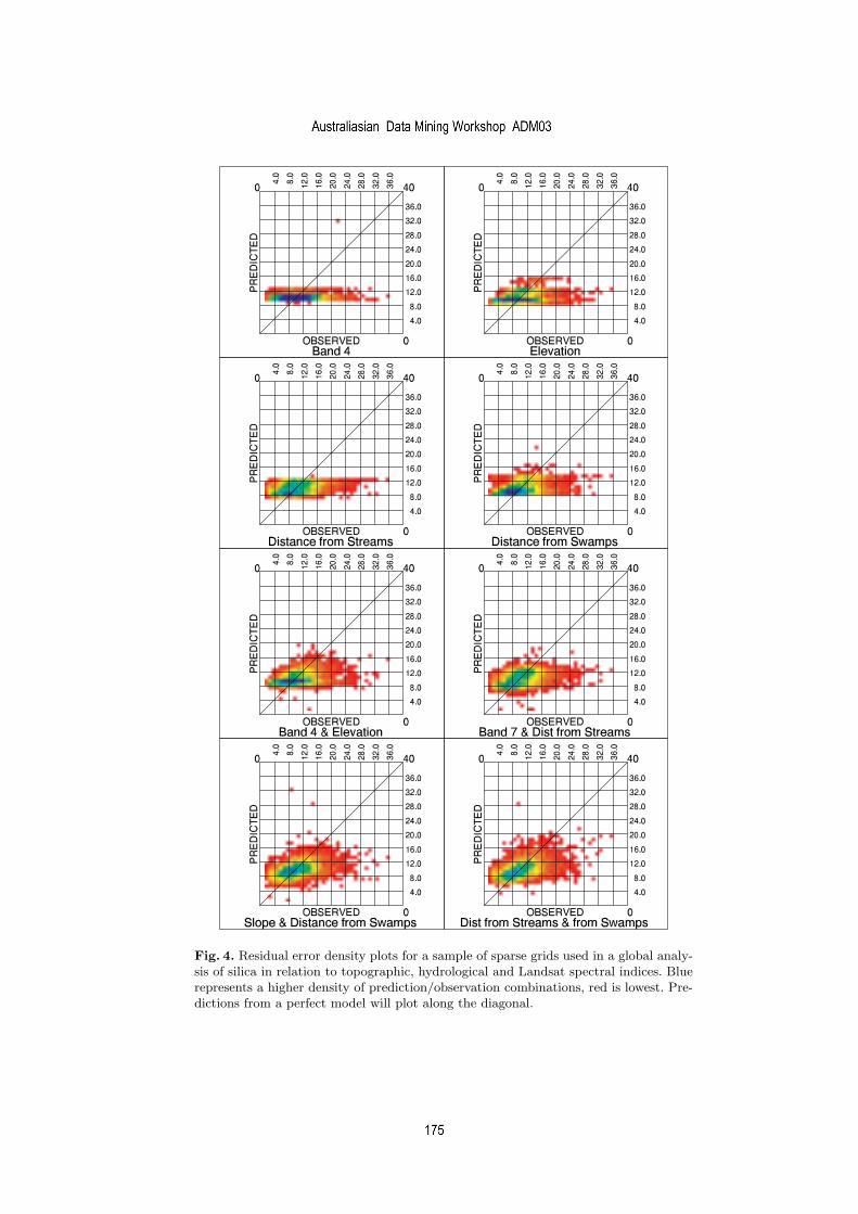
Fig. 4. Residual error density plots for a sample of sparse grids used in a global analy-sis of silica in relation to topographic, hydrological and Landsat spectral indices. Bluerepresents a higher density of prediction/observation combinations, red is lowest. Pre-dictions from a perfect model will plot along the diagonal.

The above approach is not particular to sparse grids, as it can be applied toany predictive model where one can derive the relationships between vari-ables. What sparse grids also allow one to do is analyse the number of gridpoints (and thus model complexity) used for each grid (see §2.1). If theanalysis is conducted such that the number of grid points is optimised tothe data, then some understanding of the nature of the relationship maybe obtained. For example, if the relationship between the correlate and onepredictor variable is consistently represented using few grid points, and hasa reasonably good accuracy, then there is a broad relationship. If many gridpoints are used, then the relationship is one of fine detail. This should, ofcourse, be corrected to allow for the variability of the original data. Theseindices can be readily extracted from the sparse grids system.

3.2 Mining sparse grid collections

In addition to the analysis using local predictive models sparse grids allow furtheranalysis due to the fact that different sparse grids can be readily compared atvarious levels. How this can be done is discussed in the following. To focus thediscussion one can consider the fitting problem. As above, one determines afamily of predictive models f(x; z) where z represents the local area. In ourexample, the models are determined as the minimisers of a family of functionals

J(f ; p) =n

∑

i=1

w(‖pi − p‖)(yi − f(xi))2

where pi are the spatial locations of the observations and p the location of thelocal model found. Here the weight functions are given, for example

w(s) = exp(−λs2)

where λ is a given coefficient. Possible centres z used could include a large subsetof the data points xi. Models are then fitted in a greedy way for each of the z. Ofcourse, the computational requirements are considerably increased in this way.The difference to the approach considered so far and discussed above is, however,what is done after all the models have been determined.

After this first step a large number of local sparse grid functions have beendetermined which model local data and they all have a spatial attribute. Thiscollection of spatial models can now be mined using spatial mining tools. As-pects of spatial mining include the detection of interesting regions, i.e., regionswhere certain models are prevalent, e.g., where particular types of correlationscan be found. Another aspect is the detection of spatial trends, i.e., the analysisof change of the models in space. The underlying ideas are very similar to tradi-tional spatial data mining, see, e.g. [6] where tools are provided for the detectionof interesting regions which either have concentrations of high values of certainfeatures [7] or have trends of feature values. The application of this analysisbenefits from the fact that the sparse grid spaces are fairly simple linear spaces.

Basically, the functions are grouped into classes of similar functions andthe support in the data (similar to association rule mining) and geographicaldistribution for each of these classes is determined. Classes can be either given apriori, or they may be found by clustering. The a priori given classes are obtainedby comparing various features of the locally found models:

– A simple analysis could consider only the set of variables selected for thesparse grids at different locations. These selected variables are the ones whichjointly provide a best explanation of the variation of the response. The co-incidence of gradients of the response with gradients in other variables andpossibly higher level variations may be detected. In this case two models are“the same” if they use the same variables.

– The location and feasibility of linear models can be investigated.– A slightly more sophisticated analysis would consider the types of interac-

tions used in any one model– Finally, one can discretise model space and investigate support and location

of specific models.

A challenge of some these approaches is that one needs to introduce a metric onthe sparse grid space in order to find similar models. However, once the metrichas been selected and once the collections of models have been found one mayfurther mine these collections using methods related to frequent itemset mining.In addition the geographical distribution of certain classes of models may provideinformation about underlying processes.

References

1. Dietrich Braess. Finite elements. Cambridge University Press, Cambridge, secondedition, 2001.

2. Leo Breiman, J. H. Friedman, R. A. Olshen, and C. J. Stone. Classification andRegression Trees. Wadsworth Publishing Company, Belmont, California, U.S.A.,1984.

3. P. A. Burrough. Soil variability: A late 20th century view. Soils and Fertilizers,56:529–562, 1993.

4. Ingrid Daubechies. Ten lectures on wavelets, volume 61 of CBMS-NSF RegionalConference Series in Applied Mathematics. Society for Industrial and AppliedMathematics (SIAM), Philadelphia, PA, 1992.

5. Carl de Boor. A Practical Guide to Splines. Springer, 1978.

6. M. Ester, H.-P. Kriegel, and J. Sander. Knowledge discovery in spatial databases.In 23rd German Conf. on Artificial Intelligence (KI ’99), volume 1701 of LectureNotes in Computer Science, pages 61–74. Springer Verlag, 1999.

7. V. Estivill-Castro and I. Lee. Data mining techniques for autonomous explorationof large volumes of geo-referenced crime data. In D. Pullar, editor, Proceedings ofthe 6th International Conference on GeoComputation, University of Queensland,Brisbane, September 2001.

8. Jerome H. Friedman. Multivariate adaptive regression splines. Ann. Statist.,19(1):1–141, 1991. With Discussion and A Rejoinder By The Author.

9. J. Garcke and M. Griebel. Classification with sparse grids using simplicial basisfunctions. Intelligent Data Analysis, 6(6):483–502, 2002.

10. J. Garcke, M. Griebel, and M. Thess. Data mining with sparse grids. Computing,67(3):225–253, 2001.

11. M. Griebel, M. Schneider, and C. Zenger. A combination technique for the solutionof sparse grid problems. In P. de Groen and R. Beauwens, editors, Iterative Methodsin Linear Algebra, pages 263–281. IMACS, Elsevier, North Holland, 1992.

12. Michael Griebel, Michael Schneider, and Christoph Zenger. A combination tech-nique for the solution of sparse grid problems. In Iterative methods in linear algebra(Brussels, 1991), pages 263–281. North-Holland, Amsterdam, 1992.

13. T. Hastie, R. Tibshirani, and J. Friedman. The Elements of Statistical Learning:Data Mining, Inference and Prediction. Springer, 2001.

14. T. J. Hastie and R. J. Tibshirani. Generalized additive models, volume 43 of Mono-graphs on Statistics and Applied Probability. Chapman and Hall Ltd., London,1990.

15. M. Hegland. Adaptive sparse grids. In K. Burrage and Roger B. Sidje, editors,Proc. of 10th Computational Techniques and Applications Conference CTAC-2001,volume 44, pages C335–C353, April 2003. [Online] http://anziamj.austms.org.au/V44/CTAC2001/Hegl [April 1, 2003].

16. M. Hegland, O. Nielsen, and Z. Shen. High dimensional smoothing based on multi-level analysis, 2000.

17. Markus Hegland. Additive sparse grid fitting. In Curve and Surface Fitting: StMalo 2002, pages 209–218, 2002.

18. S. W. Laffan. Inferring the Spatial Distribution of Regolith Properties Using SurfaceMeasurable Features. PhD thesis, Australian National University, 2001.

19. S. W. Laffan. Using process models to improve spatial analysis. InternationalJournal of Geographical Information Science, 16:245–257, 2002.

20. S. W. Laffan and B. G. Lees. Predicting regolith properties using environmen-tal correlation: a comparison of spatially global and spatially local approaches.Geoderma, in press.

21. S. W. Laffan, H. Silcock, O. Nielsen, and M. Hegland. A new approach to analysingspatial data using sparse grids. In MODSIM 2003, Integrative Modelling of Bio-physical, Social and Economic Systems for Resource Management Solutions, 2003.

22. Z. Luo, G. Wahba, and D. R. Johnson. Spatial-temporal analysis of temperatureusing smoothing spline ANOVA. Journal of Climate, 11:18–28, 1998.

23. H. J. Miller and J. Han. Geographic data mining and knowledge discovery. Taylorand Francis, London, UK, 2001.

24. S Openshaw. Geographical data mining: key design issues. In Proceedings ofthe 4th International Conference on GeoComputation, Geocomputation99, MaryWashington College, Virginia, USA, July 1999.

25. D. J. Peuquet. Representations of space and time. Guilford, 2002.26. Stephen Roberts, Markus Hegland, and Irfan Altas. Approximation of a thin plate

spline smoother using continuous piecewise polynomial functions. SIAM J. Numer.Anal., 41(1):208–234 (electronic), 2003.

27. J. F. Roddick and B. G. Lees. Paradigms for spoatial and spatio-temporal datamining. In H. J. Miller and J. Han, editors, Geographic data mining and knowledgediscovery, chapter 2, pages 33–49. Taylor and Francis, 2001.

28. S. A. Smolyak. Quadrature and interpolation formulas for tensor products ofcertain classes of functions. Dokl. Akad. Nauk SSSR, 148:1042–1043, 1963. Russian,Engl. Transl.: Soviet Math. Dokl. 4:240–243, 1963.

29. W. R. Tobler. A computer movie simulating urban growth in the Detroit region.Economic Geography, 46 (supplement):234–240, 1970.

30. T. G. Whiteway, S. W. Laffan, and R. J. Wasson. Using sediment budgets toinvestigate the pathogen flux through catchments. Environmental Management,submitted.

31. C. Zenger. Sparse grids. In W. Hackbusch, editor, Parallel Algorithms for Par-tial Differential Equations, Proceedings of the Sixth GAMM-Seminar, Kiel, 1990,volume 31 of Notes on Num. Fluid Mech., pages 241–251. Vieweg, 1991.

simeon

Australiasian Data Mining Workshop ADM03

CONGO: Clustering on the Gene Ontology

Paul J. Kennedy⋆ and Simeon J. Simoff⋆⋆

Faculty of Information Technology, University of Technology, Sydney, PO Box 123,Broadway, NSW 2007, AUSTRALIA

Abstract. Rapid development of technologies for the collection of bi-ological data have led to large increases in the amount of informationavailable for understanding diseases and biological mechanisms. How-ever, progress has not been as fast in comprehending the data. Devel-opments in understanding diseases and biological mechanisms governingthem may come from combining data from different sources. We describea method of clustering lists of genes identified as important to the un-derstanding of a childhood cancer using functional information aboutthe genes from the Gene Ontology. The measure of distance used in theclustering algorithm is notable for considering the relationship betweenterms in the ontology. Meaningful descriptions of clusters are automati-cally generated from the Gene Ontology terms.

1 Introduction

Rapid developments in bio–technology, measurement and collection of diversebiological and clinical data have led to revolutionary changes in bio–medicineand biomedical research. The data collected in bio–medical experiments or as aresult of medical examination ranges from gene expression levels measured usingmicroarray technologies to data collected in therapy research. Researchers arelooking at discovering relations between patterns of genes (sequences, interac-tions between specific genes, dependencies between changes in gene expressionsand patient’s responses to treatment). The confluence of bio–technology and sta-tistical analysis is known as bioinformatics. The “classical” statistical techniquesused in bioinformatics — a broad range of cluster, classification and multivari-ate analysis methods, have been challenged by the large number of genes thatare analysed simultaneously and the curse of dimensionality of gene expressionmeasurements. As a rule, the gene–to–data points ratio is high (i.e. the so–called“wide” data table, i.e. if we are looking at N genes and our sample is of size m,then usually N ≫ m). When there are more attributes than data records (cases),problems may arise (for example, there can be strong correlations between someof the attributes, or the covariance matrix may become singular, the curse ofdimensionality may begin to bite). This challenge has attracted the attention ofresearchers in the two very closely related fields of “data mining” (initiated by

⋆ paulk@it.uts.edu.au⋆⋆ simeon@it.uts.edu.au

researchers in databases (see [1])) and “intelligent data analysis” (initiated byresearchers working in the area of mathematical statistics and machine learning(see Chap. 1 in [2])). Bearing in mind that researchers and research communitiesoften disagree about the precise boundaries of their dedicated field of investi-gation, further in this paper we refer only to data mining [3] as the “analysisof large observational data sets to find unsuspected relationships and to sum-marise the data in novel ways that are both understandable and useful to thedata owner”. There is a number of ways in which data mining is expected tobe able to assist the bio–data analysis (see [4] for brief overview). One impor-tant area are the tasks of similarity search, comparison and grouping of genepatterns and assisting in understanding these patterns in medical bio–data, asmany diseases are triggered by a combination of genes acting together. The workpresented in this paper is in this area.

Addressing the “Wide” Data Table Problem

Having many more genes than data points offers a number of strategies for theanalysis of such data [5], that can be grouped in three broader categories: “sum-marise then analyse” (STA), “analyse then summarise” (ATS) and “summarisewhile analysing” (SWA). STA scenario uses an unsupervised learning technique(e.g. cluster analysis) to reduce the large number of genes to gene clusters (orgene profiles). The cluster representations then are used for predictive modelling(see [6]). In ATS scenario, modelling is conducted initially for each gene, pro-ducing some statistics, and then one can apply some threshold (for example,select all genes with value of that statistic above the threshold). SWA approachaddresses the issues of possible existence of some relations between the genes,hence, suggests to proceed with summarisation and classification in a single step.For example, regression tree model [7] can be used to identify a small subset ofpredictive genes.

The above presented scenarios do not consider the utilisation of already ex-isting knowledge about relations between genes to assist the outcome of the datamining step. The approach proposed in this paper extends the STA scenario, byimposing the results of the initial clustering of the genes with further clusteringover an ontology that relates the genes in the input clusters. This approach canbe labelled as “summarise, impose, then analyse” (SITA).

Cluster Analysis and Visualisation

As we have mentioned earlier, clustering algorithms divide the set of genes intogroups so that gene expression patterns within a group are more similar thanthe patterns across groups. Most clustering techniques include a “magic” set ofparameters, that one needs to adjust to get “good” clusters. However, in thecase of gene expression data sets, the selection and “tuning” of these parametersmay not be that intuitive and obvious, due to the high dimensionality of thespace. Hence, clustering relies substantially on visualisation. An efficient visual-isation schema allows to expose problems with the clusters, prompting towards

some intervention, for example, selection of different similarity and inter–clusterdistance measures, or forcing some of the clusters into one group. The paperpresents a visualisation method that supports the proposed SITA scenario.

In this paper, we use information from one source (the Gene Ontology [8])to gain an understanding of a list of genes that were generated as the result ofanother data mining step. The list of genes is clustered into groups of genes withsimilar biological functionality. Descriptions of the clusters are automaticallydetermined using the Gene Ontology (GO) data.

The broad goals of our bioinformatics project are to improve the understand-ing of genes related to a specific form of childhood cancer. Data regarding therelative expression levels of genes (in tumour cells compared with normal cells)is combined with clinical data (concerning the tumours and patients) to form alist of “interesting” genes. Details of this step are not relevant to the techniquesexplored in this paper.

The Gene Ontology is a controlled vocabulary of terms that describe geneproducts in terms of their effect in the cell and their known place in the cell.Terms in the ontology are interrelated. For example, a “glucose metabolism”is a “hexose metabolism” (see Fig. 1). In this example, “hexose metabolism” isa more general concept (or term) than “glucose metabolism”. There are cur-rently around 16,000 terms in the Gene Ontology and each gene is associatedwith between two and ten terms. The relationships between terms in the ontol-ogy allow us to measure the similarity between genes in a functional way. Forexample, one gene may be associated with the term “carbohydrate metabolism”and another gene associated with “alcohol metabolism”. As can be seen in Fig. 1both of these terms are child terms (or more specific concepts) of “metabolism”.Hence, they are related quite closely.

The list of genes, then, is clustered according to the associated Gene Ontologyterms. The clustering considers the interrelationships of terms in the ontology.Once clusters are created, the terms in the Gene Ontology permit the automaticconstruction of cluster descriptions (in terms of the Gene Ontology concepts).

The method of clustering over an ontology is general and may be applied to(non–biological) data associated with other ontologies.

Applying information from the Gene Ontology to cluster genes allows foran understanding of the genes and their interrelationships in functional terms.Currently biologists search through such lists gene–by–gene analysing each oneindividually and trying to piece together the many strands of information. Au-tomating the process, at least to some extent, would allow biologists to concen-trate more on the important relationships rather than the minutiae of searchingas well as give savings in time and effort.

Related Work

Other workers use the Gene Ontology. There are a variety of browsers for theGene Ontology linked from their web site [9]. In general, such browsers havefacilities such as: (i) traversing the large Gene Ontology and viewing their in-terrelationships; (ii) finding Gene Ontology terms associated with ensembles of

GO:0006066

GO:0005996

GO:0019318

GO:0006006

GO:0006007

GO:0006096

GO:0008152

GO:0007582

GO:0008150

glycolysis

glucose

catabolism

glucose

metabolism

hexose

metabolism

monosaccharide

metabolism

alcohol

metabolism

metabolism

physiological

process

biological

process

GO:0005975carbohydrate

metabolism

Fig. 1. A small section of the GO hierarchy from the “biological processes” ontology.Each node is a term in the ontology. Inside each node is the identifier for the term andbeside is the term itself. More general terms are towards the top of the diagram. Alllinks shown are is–a relationships that are directed upwards

genes; or (iii) finding known genes associated with particular Gene Ontologyterms, to name a few.

Many tools (for example, eGOn [10] or FatiGO [11]) take as input a list ofgenes (often resulting from microarray experiments) and map the genes to GOcategories. Most of these tools additionally allow comparison of GO mappingsbetween different gene lists usually with some statistical measure of the similar-ity of distributions. The tools GOMiner [12] [13] and EASE [14] [15] additionallylook for “biological themes” in lists of genes. That is, they identify the predomi-nant set of GO terms that describe the entire gene list. They have a similar goalto the method we propose, except that we first cluster the data into subsets ofrelated genes.

Hierarchical information is also used with other data mining techniques (pos-sibly unrelated to biology). For example, [16] and [17] use ontological informationto mine “generalized” association rules. The “basic” algorithm in [17] takes anapproach that is reminiscent of ours (ie. simply including information from higherin the tree). Both the generalized association rules and the ontological clusteringin this paper use the idea of combining specialised concepts but have differentgoals. The generalized association rules combine them to produce stronger rules,whereas we combine concepts to build looser forms of equivalence to make theclustering more flexible.

Method Overview

The cluster analysis and visualisation described in this paper takes as input (i) alist of genes highlighted from a previous data mining step and (ii) data from theGene Ontology. The previous data mining step used gene expression data (fromcDNA microarray experiments) and clinical data describing the tumour cellsin detail, effect of drug protocols and (human) classifications of patients intohigh or low risk categories. cDNA microarray experiments are a recent technol-ogy available to cellular biologists that measure the relative expression levels ofthousands of genes in cells at one instant. Expression levels of genes in a testsample (i.e. tumour cells) compared to genes in a control sample (i.e. “normal”cells) are measured.

Gene Ontology terms are associated with each gene in the list by searching inthe SOURCE database [18]. The list of genes is clustered into groups with similarfunctionality using a distance measure that explicitly considers the relationshipbetween terms in the ontology. Finally, descriptions of each cluster are found byexamining Gene Ontology terms that are representative of the cluster. Graphsof Gene Ontology terms for each cluster together with cluster descriptions givea visualisation of each cluster in functional terms.

2 The Gene Ontology

The Gene Ontology [8] is a large collaborative public database constructed by re-searchers world–wide. It provides a set of controlled vocabularies (i.e. ontologies)of terms that describe gene products in terms of their effect in the cell. Thatis, their functionality. The goal of the Gene Ontology is “to produce a dynamic,controlled vocabulary that can be applied to all eukaryotes even as knowledgeof gene and protein roles in cells is accumulating and changing” [8].

As described in Sect. 1 the Gene Ontology contains terms and their interrela-tionships (parent/child, general/specific, etc). Three ontologies are defined in theGene Ontology: (i) biological processes, (ii) cellular components, and (iii) molec-ular functions. The ontologies are directed acyclic graphs (DAGs) where theterms form nodes and two kinds of relationships form edges: “is–a” relationshipssuch as “glycolysis” is–a “glucose catabolism” and “part–of” relationships suchas “nuclear chromosome” is part–of “nucleus”. Apart from the specific individ-ual terms, the Gene Ontology is unremarkable in this regard. All ontologies areDAGs of terms.

Each term in the ontology has a number of attributes: the term itself (eg. gly-colysis), a unique accession number (eg. GO:0006096), and a definition (eg. thebreakdown of a monosaccharide (generally glucose) into simpler components,including pyruvate). There may also be technical references to the definition(eg. links to PubMed articles), cross references into other biological databases,synonyms and comments.

There are a number of benefits of using the Gene Ontology as part of thedata mining process. It is large (7045 terms in the Molecular Function ontology,

7763 terms in the Biological Process ontology and 1335 terms in the Cellu-lar Component ontology as of 16 September 2003 [9]) and well worked on byresearchers (16 member organisations of the Gene Ontology Consortium as ofAugust 2003 [9]). Entries are curated before being added to the ontology. Theontology may be accessed in the RDF XML file format. In this computer legibleform it is easier to apply the information to data mining methods and immedi-ately richer than by determining similar information with text mining methods.

GO terms may be associated with genes using databases like SOURCE [18]as long as accession numbers of genes or gene names are known. See Table 1 foran example.

Table 1. GO terms associated with an example gene (named CLK1) for each of thethree ontologies.

CLK1 (CDC–like kinase 1)

Molecular Function

GO:0004715 non–membrane spanning protein tyrosine kinase activityGO:0005524 ATP binding activityGO:0004674 protein serine/threonine kinase activityGO:0016740 transferase activity

Biological Process

GO:0006468 protein amino acid phosphorylationGO:0008283 cell proliferationGO:0000074 regulation of cell cycle

Cellular Component

GO:0005634 nucleus

3 Clustering over Ontologies

Many algorithms exist for clustering data (see for example [19] or [20]). The datawe wish to cluster is slightly different to normal, however, and this advises ourchoice of algorithm and distance measure.

There are two main differences between our clustering and “normal” clusteranalysis. The first difference is that there are a different number of attributes(GO terms) for each gene to be clustered whereas usually the number of at-tributes in a dataset is the same for all records. Secondly, we are interested incomplex relationships between terms (as a result of the structure of the ontology)so simply comparing values of terms with one another will not be sufficient.

Both difficulties stem from the fact that there is an ontology associated withthe data. Once we solve the data mining problem of clustering over an ontology,the special case of clustering over the Gene Ontology will follow easily.

Similarities might be drawn with clustering text documents (for example intospam and non–spam), as there are different numbers of words in each documentand complex relationships among the words (ontological ones too). One approachto clustering documents is to use a fixed length vector of word counts in eachdocument, with each vector position representing a different word (drawn froman a priori prescribed list). In this way each document to be classified with po-tentially many different words and counts of words is reduced to a fixed numberof attributes with all documents having the same number of attributes.

A similar approach could be applied to cluster the genes and GO terms.A fixed length binary vector of the union of all GO terms in the genes couldbe set up as the attributes for each gene. A bit would be set if the term wasassociated with the gene or unset if there was no association. Such an approach,however, suffers from two defects. Firstly, the vast majority of GO terms are onlyassociated with one gene in the dataset. This would mean the binary vectorsfor genes would be very sparse and few similarities could be found with thevectors for other genes in the dataset. The other, more serious, problem withthis approach is that it does not take into account the ontological relationshipsat all.

Our method solves the problem of different numbers of attributes by treatingall the terms for a gene as essentially one attribute. The second problem of con-sidering the ontological relationships is accomplished by using a more specialiseddistance function that compares a set of terms based on their relative positionsin the ontologies, rather than just the value of the term, which is, essentially,meaningless.

The distance function, then, is the crucial element and the particular clus-tering algorithm used is a secondary consideration. We use a simple clusteringalgorithm named the Modified Basic Sequential Algorithmic Scheme (MBSAS).This particular algorithm was chosen because of its simplicity and because itis not necessary to specify a priori the number of clusters. One of many otheralgorithms (eg. k–means) could have been used instead.

In the following two subsections we will describe in more detail the distancemeasure and the MBSAS clustering algorithm.

Distance Measure

The elements to be clustered have different numbers of attributes and this meansthat a special distance measure must be used. The distance measure is specialin that it measures distances across the ontology. The distance measure is insome ways more important than the actual clustering algorithm as any of manydifferent clustering algorithms may be used, but a distance measure similar tothis must be used to traverse the ontology.

We use a function adapted from the Tanimoto Measure [19] [20]. The Tani-moto measure provides a measure of similarity between sets:

nX∩Y

nX + nY − nX∩Y

=nX∩Y

nX∪Y

(1)

where X and Y are the two sets being compared and nX , nY and nX∩Y are thenumber of elements in the sets X, Y and X ∩ Y respectively.

In our situation, the “sets” being compared are the GO terms for two genes.However, for reasons which will become clear, “bags” (where elements may berepeated) are used rather than sets.

An important characteristic of our distance measure is that it considers termshigher in the ontology. This is because the GO terms themselves are simply con-stant values with no implicit relationship to other terms. As in any ontology, therelationship between terms arises from their relative positions in the hierarchy.So, for each gene we wish to compare, we add to the gene’s associated GO termsall terms higher in the ontology. These terms form a “background” or contextto the terms explicitly associated with the gene. However, as the ontologies aretree–like, two terms in a gene often have the same ancestors. We include theparent terms each time they are encountered, so we require bags rather thansets.

Terms higher in the ontology represent terms that are more general. Althoughgeneral terms are a factor in the comparison, the more specialised terms (i.e.lower in the hierarchy) are more important. For this reason, when countingthe number of terms in a bag, terms are weighted by their distance from theirdescendent GO term explicitly associated with the gene. In effect, we calculatea “weighted” cardinality of the bag of GO terms.

The final distance function used, then, is

DX,Y =n′

X∩Y

n′

X + n′

Y − n′

X∩Y

=n′

X∩Y

n′

X∪Y

(2)

where X and Y are the two bags of terms being compared and n′

X , n′

Y andn′

X∩Y are the weighted cardinalities of the bags X, Y and X ∩ Y respectivelygiven by

n′

X =∑

i∈X

cdi (3)

where X is the bag of GO terms, di is the distance of element of X with index i

from its associated descendent in the original set of GO terms for the gene, andc is the weight constant. The weighted cardinality of the other bags is similarlydefined.

The more general terms provide a context for the lower level terms directlyassociated with genes. The c parameter allows variation of the importance of the“context” to the comparison. A value of c = 0 means that ancestral terms arenot considered. A value of 1 would mean that all terms are considered equally aspart of the context. Plainly, in this case though, the very general terms would beregarded as overly important. The c parameter, then, may be viewed as a sortof “constant of gravity” for the clusters. The higher the value of c, the easier itis that distantly related genes gather into a cluster. We arbitrarily chose c = 0.9for our experiments.

Other distance measures apart from a gene–to–gene distance are also requiredfor use in the clustering algorithm. A measure of the distance between a gene

and a cluster of genes is determined by taking the average distance from the geneto each gene in the cluster. Similarly when calculating the distance between twoclusters of genes we use the average of the distances for each gene of one clusterto the genes in the other cluster. An alternative to using the mean distanceswould be to use minimum (or maximum) distances. We plan to explore thesepossibilities in the future.

Cluster Algorithm

With the intention of attacking the clustering problem as simply as possible,we use a standard simple clustering algorithm called Modified Basic SequentialAlgorithmic Scheme (MBSAS) as described by [19]. MBSAS has two advantagescompared with other algorithms such as the ubiquitous k–means algorithm. Itis (i) not necessary to specify a priori the number of clusters; and (ii) the datais presented to the algorithm only a few times (depending on the particularvariation of MBSAS chosen).

The variation of MBSAS we use is dependent on three parameters (and oneother parameter is necessary for the distance measure). These parameters areshown in Table 2. Whilst MBSAS does not require an explicit parameter for thenumber of clusters, the parameters (Θ, q and M1) have the same effect.

Table 2. Parameters used in the Modified Basic Sequential Algorithmic Scheme clus-tering algorithm. The last parameter is used only in the distance measure and is notformally part of MBSAS. See text for a detailed description of c.

Parameter Meaning

Θ Minimum distance for points to be considered to be in thesame cluster. (Theodoridis and Koutroumbas [19] call this the“threshold of dissimilarity”).

q Maximum allowable number of clusters.M1 Minimum distance for clusters to be deemed separate before

they are merged.c Discount weight applied to GO nodes in the ontology.

The MBSAS algorithm has four main steps as described below. The first twosteps are mandatory, whilst the latter two are optional.

1. determine_clusters

2. classify_patterns

3. merge_nearby_clusters (optional)

4. reassign_points (optional)

The determine_clusters step determine the initial clusters. It chooses upto q data points that are sufficiently distant from one another (using the Θ

parameter) as point representatives.

After finding the initial clusters the next step (classify_patterns) classifiesthe rest of the patterns into the cluster that is closest using DX,Y as definedin (2).

Theodoridis and Koutroumbas [19] describe two general drawbacks of se-quential clustering algorithms. They are (i) that clusters may arise that are veryclose together and (ii) that they are sensitive to the order of presentation of thedata. The third and fourth steps address these problems respectively. Althoughoptional, we always perform them.

The merge_nearby_clusters step identifies clusters having a distance lessthan the value of parameter M1 and merges them together.

Finally, in the reassign_points step, all points are reassigned to their closestcluster so as to minimise the effects of the presentation order of the data andany changes due to the merge_nearby_clusters step.

4 Experiments

As described in Sect. 1 the data used for this paper was a list of genes highlightedas the result of a previous data mining procedure. Information from the GeneOntology was matched to the genes using the SOURCE database.

There are, at this stage, two goals for our experiments: (i) discovery of pa-rameter values that produce acceptable clusters and (ii) determination of waysto visualise the clusters.

The parameter values Θ and M1 are dependent on the range of values re-turned by the distance measure DX,Y and have been determined largely by trialand error. In the experiments described in this paper, Θ is set to 0.001 and M1

to 0.1. The maximum number of clusters (q) is set at 5 and, as described above,c, the discounting constant for more general terms is set at 0.9.

Visualisation of clusters is made difficult by the fact that there is no clearway to transform genes into coordinates to plot on a single graph because eachgene is identified by different numbers of GO terms. So we plot the terms for allthe genes on a graph with their relationships shown in different shades for eachcluster. We also automatically build cluster descriptions from the terms in eachcluster.

5 Results

With the parameters values given above (i.e.Θ = 0.001, M1 = 0.1, q = 5 andc = 0.9) five clusters are found as shown in Table 3. Half of the genes have beenallocated to one cluster. The rest of the genes have been split into four smallerclusters with one cluster containing only two genes. Such a tabular representationdoes not increase our understanding of the clusters as the gene accession codesare not descriptive.

With this in mind, we plotted the subset of terms associated with the clus-tered genes as nodes on a graph with relationships represented by edges and the

Table 3. Clusters found with the MBSAS clustering algorithm. The codes AAnnnn

are GenBank accession codes.

Cluster Gene GenesNumber Count

0 6 AA040427 AA406485 AA434408 AA487466 AA609609AA609759

1 2 AA046690 AA6446792 6 AA055946 AA398011 AA458965 AA487426 AA490846

AA5042723 9 AA112660 AA397823 AA443547 AA447618 AA455300

AA478436 AA608514 AA669758 AA6830854 20 AA126911 AA133577 AA400973 AA464034 AA464743

AA486531 AA488346 AA488626 AA497029 AA629641AA629719 AA629808 AA664241 AA664284 AA668301AA669359 AA683050 AA700005 AA700688 AA775874

GO nodes of a cluster localised to one part of the graph as much as possible(Fig. 2). The clusters are represented by the five large boxes with the clusternumbers (as listed in Table 3) given inside each box. Nodes inside the clustersare the GO terms associated with genes in that cluster. More general terms areon the right hand side of the diagram. Edges between nodes represent the linksin the ontology. Some terms, particularly the more general ones at the righthand side of the diagram, have links from terms in a different cluster. Each nodeis shown in only one cluster box, but links between the boxes show where GOterms are shared by genes in the different clusters. The grey scale of the linkrepresents the cluster that link is in. Also, a darker grey scale is used for linksin the original dataset whilst a lighter shade is used for relationships inferredfrom traversing the ontology. Inside some cluster boxes may be seen links from adifferent cluster (if both child and parent terms are drawn in one cluster box, butthe link is also in another cluster). For example, inside the large middle cluster(representing cluster 4) may be seen some links associated with the second topcluster (representing cluster 3) although this is difficult to see on the diagram.It is likely that these are either outliers or indicators of poor clustering.

Figure 2 is reminiscent of the dendrograms that are used in hierarchical clus-tering. This is hardly surprising since both methods are dealing with hierarchies.However, in Fig. 2 the length of edges is not correlated to the distance betweennodes (as in dendrograms). We will apply a hierarchical clustering algorithm inthe future.

Figure 3 shows essentially the same information as Fig. 2 except that themore general terms are at the bottom of the diagram. To improve the readabilityof the diagram, the cluster boxes are in a different order than in Fig. 2. Again,cluster numbers are given inside each box. The GO terms lying along the bottomedges of the cluster boxes are clearer in this diagram, particularly those on theleft– and rightmost cluster boxes (clusters 3 and 4). These terms are part of

Fig. 2. Parts of the GO hierarchy associated with genes being clustered. More generalterms are at the right of the diagram. See text for description of graph

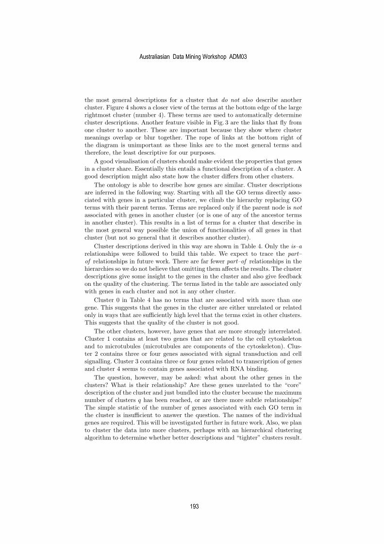
the most general descriptions for a cluster that do not also describe anothercluster. Figure 4 shows a closer view of the terms at the bottom edge of the largerightmost cluster (number 4). These terms are used to automatically determinecluster descriptions. Another feature visible in Fig. 3 are the links that fly fromone cluster to another. These are important because they show where clustermeanings overlap or blur together. The rope of links at the bottom right ofthe diagram is unimportant as these links are to the most general terms andtherefore, the least descriptive for our purposes.

A good visualisation of clusters should make evident the properties that genesin a cluster share. Essentially this entails a functional description of a cluster. Agood description might also state how the cluster differs from other clusters.

The ontology is able to describe how genes are similar. Cluster descriptionsare inferred in the following way. Starting with all the GO terms directly asso-ciated with genes in a particular cluster, we climb the hierarchy replacing GOterms with their parent terms. Terms are replaced only if the parent node is not

associated with genes in another cluster (or is one of any of the ancestor termsin another cluster). This results in a list of terms for a cluster that describe inthe most general way possible the union of functionalities of all genes in thatcluster (but not so general that it describes another cluster).

Cluster descriptions derived in this way are shown in Table 4. Only the is–a

relationships were followed to build this table. We expect to trace the part–

of relationships in future work. There are far fewer part–of relationships in thehierarchies so we do not believe that omitting them affects the results. The clusterdescriptions give some insight to the genes in the cluster and also give feedbackon the quality of the clustering. The terms listed in the table are associated onlywith genes in each cluster and not in any other cluster.

Cluster 0 in Table 4 has no terms that are associated with more than onegene. This suggests that the genes in the cluster are either unrelated or relatedonly in ways that are sufficiently high level that the terms exist in other clusters.This suggests that the quality of the cluster is not good.

The other clusters, however, have genes that are more strongly interrelated.Cluster 1 contains at least two genes that are related to the cell cytoskeletonand to microtubules (microtubules are components of the cytoskeleton). Clus-ter 2 contains three or four genes associated with signal transduction and cellsignalling. Cluster 3 contains three or four genes related to transcription of genesand cluster 4 seems to contain genes associated with RNA binding.

The question, however, may be asked: what about the other genes in theclusters? What is their relationship? Are these genes unrelated to the “core”description of the cluster and just bundled into the cluster because the maximumnumber of clusters q has been reached, or are there more subtle relationships?The simple statistic of the number of genes associated with each GO term inthe cluster is insufficient to answer the question. The names of the individualgenes are required. This will be investigated further in future work. Also, we planto cluster the data into more clusters, perhaps with an hierarchical clusteringalgorithm to determine whether better descriptions and “tighter” clusters result.

Fig. 3. Diagram showing essentially the same information as Fig. 2 except that impor-tant descriptive GO terms are more visible. See text for description of graph

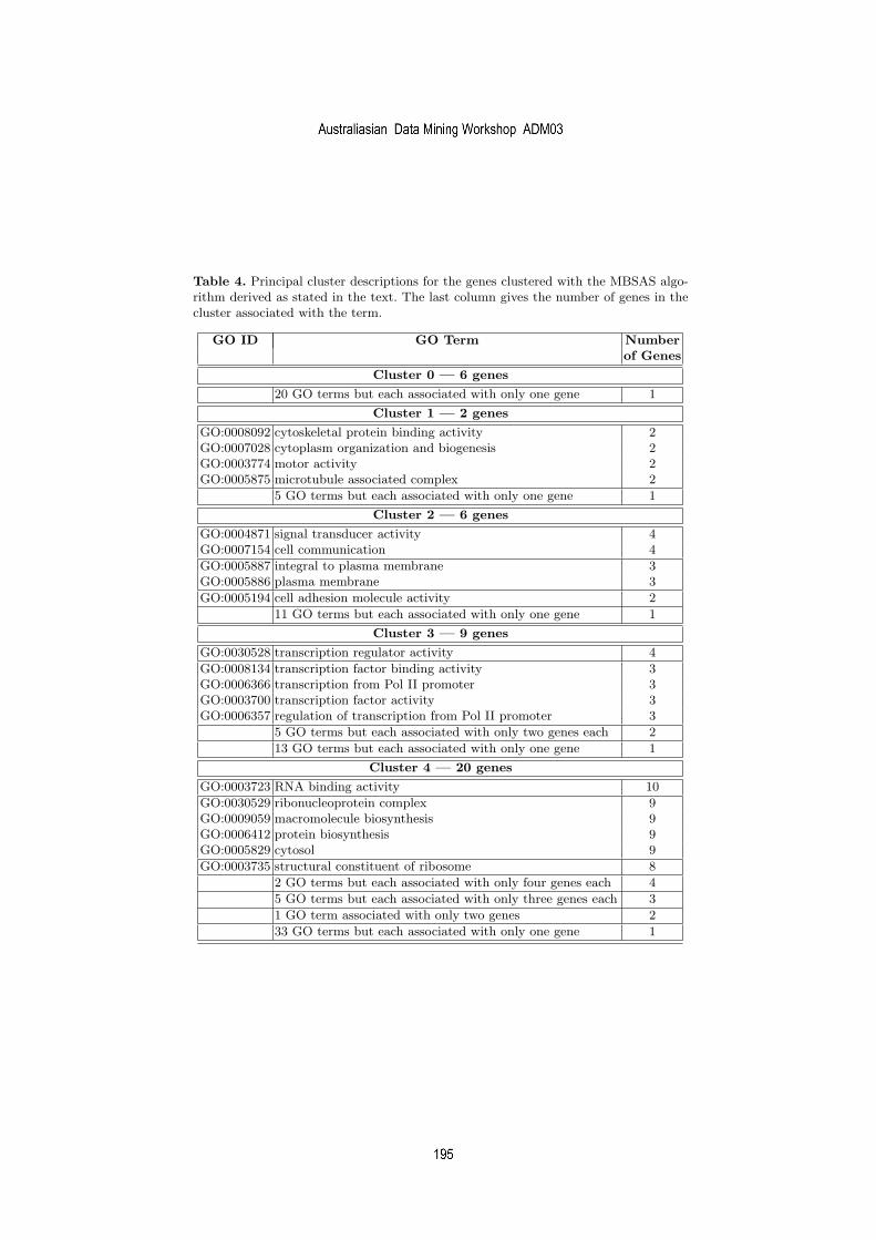
Table 4. Principal cluster descriptions for the genes clustered with the MBSAS algo-rithm derived as stated in the text. The last column gives the number of genes in thecluster associated with the term.

GO ID GO Term Numberof Genes

Cluster 0 — 6 genes

20 GO terms but each associated with only one gene 1

Cluster 1 — 2 genes

GO:0008092 cytoskeletal protein binding activity 2GO:0007028 cytoplasm organization and biogenesis 2GO:0003774 motor activity 2GO:0005875 microtubule associated complex 2

5 GO terms but each associated with only one gene 1

Cluster 2 — 6 genes

GO:0004871 signal transducer activity 4GO:0007154 cell communication 4

GO:0005887 integral to plasma membrane 3GO:0005886 plasma membrane 3

GO:0005194 cell adhesion molecule activity 2

11 GO terms but each associated with only one gene 1

Cluster 3 — 9 genes

GO:0030528 transcription regulator activity 4

GO:0008134 transcription factor binding activity 3GO:0006366 transcription from Pol II promoter 3GO:0003700 transcription factor activity 3GO:0006357 regulation of transcription from Pol II promoter 3

5 GO terms but each associated with only two genes each 2

13 GO terms but each associated with only one gene 1

Cluster 4 — 20 genes

GO:0003723 RNA binding activity 10

GO:0030529 ribonucleoprotein complex 9GO:0009059 macromolecule biosynthesis 9GO:0006412 protein biosynthesis 9GO:0005829 cytosol 9

GO:0003735 structural constituent of ribosome 8

2 GO terms but each associated with only four genes each 4

5 GO terms but each associated with only three genes each 3

1 GO term associated with only two genes 2

33 GO terms but each associated with only one gene 1

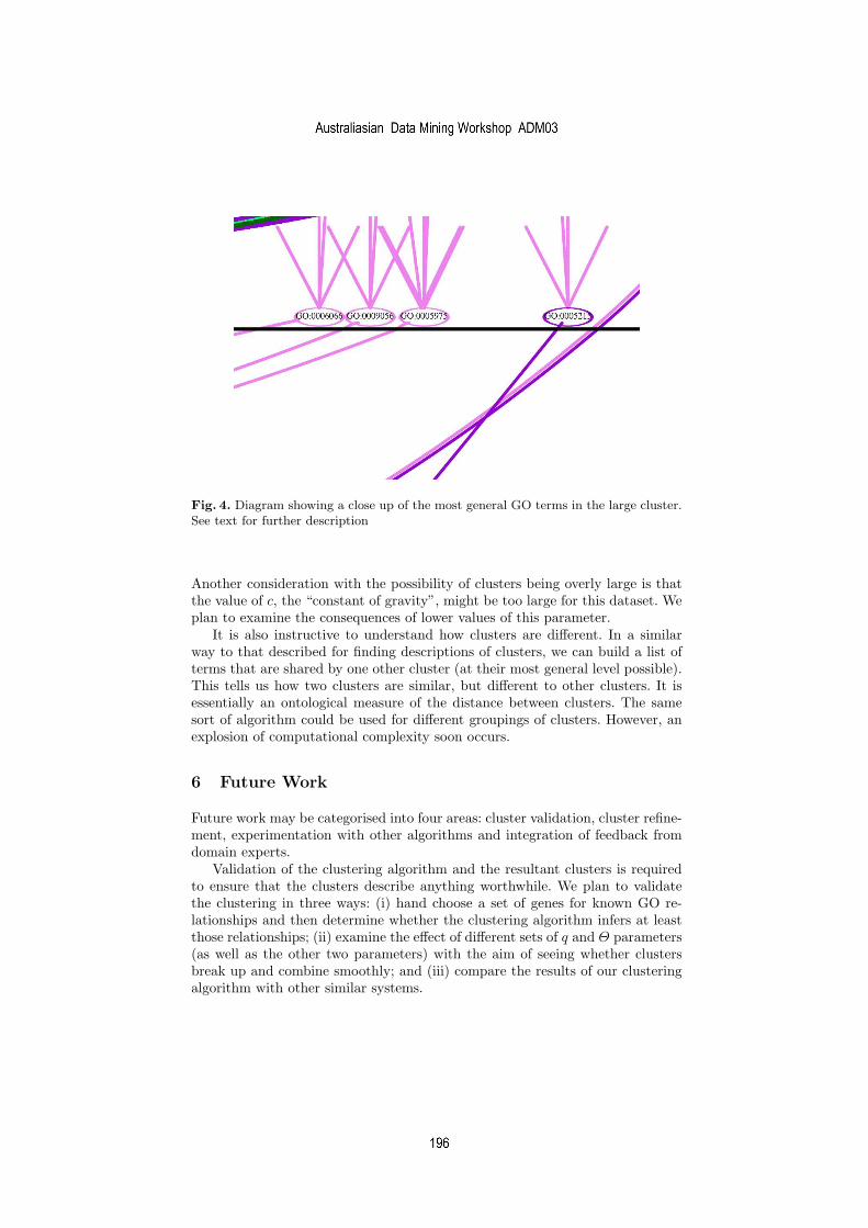
Fig. 4. Diagram showing a close up of the most general GO terms in the large cluster.See text for further description

Another consideration with the possibility of clusters being overly large is thatthe value of c, the “constant of gravity”, might be too large for this dataset. Weplan to examine the consequences of lower values of this parameter.

It is also instructive to understand how clusters are different. In a similarway to that described for finding descriptions of clusters, we can build a list ofterms that are shared by one other cluster (at their most general level possible).This tells us how two clusters are similar, but different to other clusters. It isessentially an ontological measure of the distance between clusters. The samesort of algorithm could be used for different groupings of clusters. However, anexplosion of computational complexity soon occurs.

6 Future Work

Future work may be categorised into four areas: cluster validation, cluster refine-ment, experimentation with other algorithms and integration of feedback fromdomain experts.

Validation of the clustering algorithm and the resultant clusters is requiredto ensure that the clusters describe anything worthwhile. We plan to validatethe clustering in three ways: (i) hand choose a set of genes for known GO re-lationships and then determine whether the clustering algorithm infers at leastthose relationships; (ii) examine the effect of different sets of q and Θ parameters(as well as the other two parameters) with the aim of seeing whether clustersbreak up and combine smoothly; and (iii) compare the results of our clusteringalgorithm with other similar systems.

The clustering algorithm will be refined in the following two ways: (i) thestability of clusters needs to be analysed with respect to the order of presentationof data; and (ii) choice of parameter values requires more understanding.

Different clustering algorithms will be tried. MBSAS was simply a startingpoint. At least k–means and hierarchical clustering algorithms will be attempted.

The clustering behaviour must be refined based on feedback from medicalexperts who understand the different genes and will be able to determine whetherthe clustering increases their understanding of the genes. Cluster analysis likethis project is, in some ways, an exercise in prototyping. Once the domain expertsgain some knowledge they are able to ask other questions.

7 Conclusions

This paper describes a technique for clustering genes according to their func-tionality as defined by associated terms in the Gene Ontology. The clusteringalgorithm is notable for considering the relationships between terms by travers-ing the ontology.

The Gene Ontology is used to visualise the clusters by automatically buildingcluster descriptions. Preliminary results clustering genes give insights into theclusters and the efficacy of the clustering algorithm.

Acknowledgements

We would like to thank the other members of our group, Daniel Catchpoole andDavid Skillicorn for their assistance developing the ideas in this paper and fortheir analysis and gathering of the data and Andre Skusa and Jacob Koehler fortheir comments and discussion on drafts of the paper.

References

1. Fayyad, U.M., Piatetsky-Shapiro, G., et al.: From data mining to knowledge dis-covery in databases. AI Magazine 17 (1996) 37–54

2. Berthold, M., Hand, D.J., eds.: Intelligent Data Analysis. Springer, Heidelberg(2003)

3. Hand, D., Mannila, H., et al.: Principles of Data Mining. The MIT Press, Cam-bridge, MA (2001)

4. Han, J.: How can data mining help bio–data analysis. In: Proceedings 2nd Work-shop on Data Mining in Bioinformatics BIOKDD02, in conjunction with ACMSIGKDD 8th International Conference on Knowledge Discovery and Data Mining,Edmonton, Canada, ACM Press (2002)

5. Parmigiani, G., Garrett, E.S., et al.: The analysis of gene expression data: Anoverview of methods and software. In Parmigiani, G., Garrett, E.S., Irizarry, R.A.,Zeger, S.L., eds.: The analysis of gene expression data, Heidelberg, Springer–Verlag(2003) 1–45

6. Rosenwald, A., Wright, G., et al.: The use of molecular profiling to predict survivalafter chemotherapy for diffuse large–B–cell lymphoma. New England Journal ofMedicine 346 (2002) 1937–1947

7. Hastie, T., Tibshirani, R., et al.: The Elements of Statistical Learning: Data Min-ing, Inference, and Prediction. Springer–Verlag, Heidelberg (2001)

8. The Gene Ontology Consortium: Gene Ontology: tool for the unification of biology.Nature Genetics 25 (2000) 25–29 PubMed ID:10802651.

9. Gene Ontology Consortium: Gene Ontology Consortium. Available on:http://www.geneontology.org (2003) Viewed at 15 October 2003.

10. Norwegian University of Science and Technology: eGOn (explore Gene Ontol-ogy). Available on: http://nova2.idi.ntnu.no/egon/ (2003) Viewed at 23 Octo-ber 2003.

11. Al-Shahrour, F., Dıaz-Uriarte, R., Dopazo, J.: FatiGO. Available on:http://fatigo.bioinfo.cnio.es/ (2003) Viewed at 23 October 2003.

12. Zeeberg, B.R., Feng, W., Wang, G., Wang, M.D., Fojo, A.T., Sunshine, M.,Narasimhan, S., Kane, D.W., Reinhold, W.C., Lababidi, S., Bussey, K.J., Riss,J., Barrett, J., Weinstein, J.N.: GOMiner: A resource for biological interpretationof genomic and proteomic data. Genome Biology 4 (2003)

13. Zeeberg, B.R., Feng, W., Wang, G., Wang, M.D., Fojo, A.T., Sunshine,M., Narasimhan, S., Kane, D.W., Reinhold, W.C., Lababidi, S., Bussey,K.J., Riss, J., Barrett, J., Weinstein, J.N.: GOMiner. Available on:http://discover.nci.nih.gov/gominer/ (2003) Viewed at 23 October 2003.

14. Hosack, D.A., Dennis Jr., G., Sherman, B.T., Lane, H., Lempicki, R.A.: EASE.Available on: http://david.niaid.nih.gov/david/ease.htm (2003) Viewed at 23October 2003.

15. Hosack, D.A., Dennis Jr., G., Sherman, B.T., Lane, H., Lempicki, R.A.: Identifyingbiological themes within lists of genes with EASE. Genome Biology 4 (2003)

16. Han, J., Fu, Y.: Discovery of multiple–level association rules from large databases.In: Proceedings 1995 International Conference on Very Large Data Bases. (1995)420–431

17. Srikant, R., Agrawal, R.: Mining generalized association rules. In: Proceedings1995 International Conference on Very Large Data Bases. (1995) 407–419

18. Diehn, M., Sherlock, G., Binkley, G., Jin, H., Matese, J.C., Hernandez-Boussard,T., Rees, C.A., Cherry, J., Botstein, D., Brown, P.O., Alizadeh, A.A.: SOURCE: aunified genomic resource of functional annotations, ontologies, and gene expressiondata. Nucleic Acids Research 31 (2003) 219–223

19. Theodoridis, S., Koutroumbas, K.: Pattern Recognition. Academic Press, SanDiego, USA (1999)

20. Duda, R.O., Hart, P.E., Stork, D.G.: Pattern Classification. Second edn. JohnWiley and Sons, New York (2001)

Adaptive Mining Techniques for Data Streams using

Algorithm Output Granularity

Mohamed Medhat Gaber1, Shonali Krishnaswamy1, Arkady Zaslavsky 1

1 School of Computer Science and Software Engineering, Monash University,

900 Dandenong Rd, Caulfield East, VIC3145, Australia

{Mohamed.Medhat.Gaber, Shonali.Krishnaswamy,

Arkady.Zaslavsky}@infotech.monash.edu.au

Abstract. Mining data streams is an emerging area of research given the potentially

large number of business and scientific applications. A significant challenge in analy z-

ing/mining data streams is the high data rate of the stream. In this paper, we propose a

novel approach to cope with the high data rate of incoming data streams. We termed

our approach “algorithm output granularity”. It is a resource-aware approach that is

adaptable to available memory, time constraints, and data stream rate. The approach

is generic and applicable to clustering, classification and counting frequent items min-

ing techniques. We have developed a data stream clustering algorithm based on the al-

gorithm output granularity approach. We present this algorithm and discuss its im-

plementation and empirical evaluation. The experiments show acceptable accuracy ac-

companied with run-time efficiency. They show that the proposed algorithm outper-

forms the K-means in terms of running time while preserving the accuracy that our al-

gorithm can achieve.

1 Introduction

A data stream is a sequence of unbounded, real time data items with a very high data

rate that can only read once by an application [2], [16], [17], [24], [25]. Data stream

analysis has recently attracted attention in the research community. Algorithms for

mining data streams and ongoing projects in business and scientific applications have

been developed and discussed in [2], [13], [19]. Most of these algorithms focus on

developing approximate one-pass techniques .

Two recent advancements motivate the need for data stream processing systems

[16],[24] :

• The automatic generation of a highly detailed, high data rate sequence of

data items in different scientific and business applications. For example: satel-

lite, radar, and astronomical data streams for scientific applications, and stock

market and transaction web log data streams for business applications.

• The need for complex analyses of these high-speed data streams such as

clus tering and outlier detection, classification, frequent itemsets and count-

ing frequent items.

There are recent projects that stimulate the need for developing techniques that

analyze high speed data streams in real time. These include:

• JPL/NASA are developing a project called Diamond Eye [5]. They aim to e n-

able remote systems as well as scientists to analyze spatial objects in real time

image stream. The project focuses on enabling “a new era of exploration us-

ing highly autonomous spacecraft, rovers, and sensors”[5].

• Kargupta et al. [19], [21] have developed MobiMine. It is a client/server PDA -

based distributed data mining applic ation for financial data streams.

• Kargupta et al. [20] have developed The Vehicle Data Stream Mining Sy stem

(VEDAS) which is a ubiquitous data mining system that allows contin uous

monitoring and pattern extraction from data streams generated on-board a

moving vehicle .

• Tanner et al. [30] are developing EnVironment for On -Board Pro ces sing

(EVE). This system analyzes data streams continuously generated from

measurements of different satellite on-board sensors using data mining, fe a-

ture extraction, event detection and prediction techniques. Only interesting

patterns are sent to the ground processing centre saving the limited band-

width.

• Srivastava and Stroeve [29] are developing a NASA project for onboard d e-

tection of geophysical processes such as snow, ice and clouds using kernel

clustering methods for data compression conserving the limited bandwidth

needed to send streaming images to the ground centers.

These projects and others demonstrate the need for data stream analysis tech-

niques and strategies that can cope with the high data rate and deliver the analysis

results in real time in resource constrained environments.

There are two strategies for addressing the problem of the high speed nature of

data streams. Input and output rate adaptation of the mining algorithm is the first strat-

egy. The rate adaptation means controlling the input and output rate of the mining

algorithm according to the available resources. The algorithm approximation by d evel-

oping new light-weight techniques that have only one look at each data item is the

second strategy. The main focus of mining data stream techniques proposed so far is

the design of approximate mining algorithms that have only one-pass or less over the

data stream. In this paper, we propose a novel approach that is able to mine data

streams in one pass. Moreover, it is adaptable to memory, time constraints and data

stream rate. We termed our approach as algorithm output granularity (AOG). This

approach has the advantage of simplicity, generality and is an enhancement of the

approximate algorithms research by being resource-aware. That means that the alg o-

rithm can adapt the output rate according to available resources.

The paper is organized as follows. Section 2 is a discussion on issues related to

mining data streams and proposes our algorithm output granularity approach. One-

pass mining techniques using our approach are proposed in section 3. The empirical

studies for clustering data streams using algorithm output granularity are shown and

discussed in section 4. Section 5 presents related work in mining data streams alg o-

rithms. Finally, we conclude the paper and present our future work in section 6.

2 Issues in Mining Data Streams

In this section, we present issues and challenges that arise in mining data streams and

solutions that address these cha llenges. Fig. 1 shows the general processing model of

mining data streams.

Fig. 1. Mining Data Stream Process

Issues and challenges with mining data streams:

1) Unbounded memory requirements due to the continuous feature of the in-

coming data elements.

2) Mining algorithms require several passes over data streams and this is not

applicable because of the high data rate feature of the data stream.

3) Data streams generated from sensors and other wireless data sources create a

real challenge to transfer these huge amounts of data elements to a central

server to be analyzed.

There are several strategies that address these challenges. These include:

1) Input data rate adaptation: this approach uses sampling, filtering, aggrega-

tion, and load shedding on the incoming data elements. Sampling is the pro c-

ess of statistically selecting the elements of the incoming stream that would

be analyzed. Filtering is the semantics sampling in which the data element is

checked for its importance for example to be analyzed or not. A ggregation is

the representation of number of elements in one aggregated elements using

some statistical measure such as the average. While load shedding, which

has been proposed in the context of querying data streams [3], [31], [32], [33]

rather than mining data streams, is the process of eliminating a batch of sub-

sequent elements from being analyzed rather than checking each element that

is used in the sampling technique. Fig. 2 illustrates the idea of data rate adap-

tation from the input side using sampling.

Fig. 2. Data Rate Adaptation using Sampling

2) Output concept level: using the higher concept level in applying data mining

in order to cope with the data rate, that is to categorize the incoming elements

into a limited number of categories and replacing each incoming element with

the matching category according to a specified measure or a look-up table.

This would produce fewer results conserving the limited me mory. Moreover,

it would require fewer number of processing CPU cycles.

3) Approximate algorithms: design one pass mining algorithms to approximate

the mining results according to some acceptable error margin.

4) On-board analysis : To avoid transferring huge amounts of data, the data min-

ing would be done at the data source location. For example, (VEDAS) project

[20], (EVE) project [30] and Diamond Eye project [5]. This however assumes

the availability of significant computational resources at the site of data

stream generation.

5) Algorithm output granularity: This is our proposed solution approach. It

uses a control parameter as a part of the algorithm logic to control the output

rate of the algorithm according to the available memory, the remaining time to

fill the available memory before incremental knowledge integration takes place

and the data rate of the incoming stream. Fig. 3 shows the idea of our pro-

posed approach.

Fig. 3. Algorithm Output Granularity Approach

Algorithm output granularity:

To demonstrate our approach in mining data streams, we first define the following

terms:

Algorithm threshold: is a controlling parameter built in the algorithm logic that e n-

courages or discourages the creation of new outputs according to three factors that

vary over temporal scale:

a) Available memory.

b) Remaining time to fill the available memory.

c) Data stream rate.

Output granularity: is the amount of generated results that are acceptable accord-

ing to specified accuracy measure. This amount should be resident in memory before

doing any incremental integration.

Time threshold: is the required time to generate the results before any incremental

integration according to some accuracy measure. This time might be specified by the

user or calculated adaptively based on the history of running the algorithm.

The main steps for mining data streams using our proposed approach:

1) Determine the time threshold and the algorithm output granularity.

2) According to the data rate, calculate the algorithm output rate and the alg o-

rithm threshold.

3) Mine the incoming stream using the calculated algorithm threshold.

4) Adjust the threshold after a time frame to adapt with the change in the data

rate using linear regression.

5) Repeat the last two steps till the algorithm lasts the time interval threshold.

6) Perform knowledge integration of the results.

The following section will show the use of algorithm output granularity in cluster-

ing, classification and frequent items mining a lgorithms.

3 Algorithm Granularity based Mining Techniques

In the following subsections, we show the application of the algorithm output granu-

larity to clustering, classification and frequent items.

3.1 LWC

In this section, our one-look clustering algorithm (LWC) is explained and discussed.

The algorithm has two main components. The first one is the resource-aware RA com-

ponent that uses the data adaptation techniques to catch up with the high-speed data

stream and at the same time to achieve the optimum accuracy according to the avail-

able resources. The process starts by checking the minimum data rate that could be

achieved using data adaptation techniques with an acceptable accuracy. If the alg o-

rithm can catch up with the minimum data rate, the RA component tries to find a solu-

tion that maximizes the accuracy by increasing the data rate. Otherwise the algorithm

should send a data mining request to a data mining server that can achieve the mini-

mum acceptable accuracy.

The other component is the LWC algorithm. The algorithm follows the following

steps:

1- Data items arrive in sequence with a data rate.

2- The algorithm starts by considering the first point as a center.

3- Compare any new data item with the centers to find the distance.

4- If the distance for all the centers is greater than a threshold, the new item is

considered as a new center; else increase the weight for the center that has

the shortest distance between the data item and the center by 1 and let the

new center equals the weighted average.

5- Repeat 3 and 4.

6- If the number of centers = k (according to the available memory) then create a

new centers vector.

7- Repeat 3, 4, 5, and 6.

8- If memory is full then re -cluster (integrate clusters) and send to the server if

needed.

The algorithm output granularity (k) is represented here by the number of cluster

centers’ kept in memory before doing any incremental re-clustering. The higher the

algorithm granularity the higher is the algorithm accuracy. The threshold value here

represents the minimum distance between any point and the cluster center. The lower

the threshold the more the clusters is created.

Fig. 4 shows the pseudo code for this algorithm. The following is the notation used

in the algorithm pseudo code.

Let D be the data rate in items/second.

Let Max(D) be unfiltered data rate in items/second.

Let Min(D) be filtered and aggregated data rate in items/second.

Let AR be algorithm rate: number of centers generated by the algorithm in cen-

ters/second.

Let Dist be the minimum distance between any point and the cluster center.

Let M be number of memory blocks, each block can store one center.

Let T be the time needed for generating a number of Centers that can fit all the

memory blocks in seconds.

Let TT be the time threshold that is required for the algorithm accuracy in sec-

onds.

Fig. 4. Light-Weight Clustering Algorithm

The algorithm according to the given threshold and the data set domain generates

the maximum number of subsequent data items , each of which represents a center; that

will be given using the following formula:

Maximum number of subsequent data points that could be centers = [(Maxi-mum item value in the data set - Minimum item value in the data set) / threshold].

Since these points in the worst case might be the first points in the data stream in

order for them to be centers, the following formula gives the number of data elements

that would do the comparison over the generated centers:

Cluster Members = Data Set Size - [(Maximum item value in the data set -Minimum item value in the data set) / threshold].

Thus the algorithm complexity is O(nm) , where “n” is the data set size, and “m” is

maximum number of subsequent data points that could be centers.

We have performed experimental evaluation and compared our algorithm with k-

means. The results presented in Section 4 shows that our algorithm outperforms k-

means in running time with an acceptable accuracy.

1. x = 1, c=1, M = number of memory blocks available

2. Receive data item DI[x].

3. Center[c] = DI[x].

4. M = M -1

5. Repeat

a. x = x+1

b. Receive DI[x]

c. For i = 1 to c

Measure the distance between Center[i]

and DI[x]

d. If distance > dist (The threshold)

Then

c=c+1

if (M <> 0)

Then

Center[c] = DI[x]

Else

Recluster DI[]

Else

For j=1 to c

Compare between Center[j] and DI[x] to find

the shortest distance.

Increase the weight for the Center[j] with

the shortest distance.

Center[j] = (Center[j] * weight + DI[x]) /

(weight + 1)

3.2 LWClass

In this section, we present the application of the algorithm output granularity to light

weight K-Nearest-Neighbors classification LWClass. The algorithm starts with

determining the number of instances according to the available space in the main

memory. When a new classified data element arrives, the algorithm searches for the

nearest instance already in the main memory according to a pre-specified distance

threshold. The threshold here represents the similarity measure acceptable by the

algorithm to consider two or more elements as one element according to the element

attributes’ values. If the algorithm finds this element, it checks the class label. If the

class label is the same, it increases the weight for this instance by one, otherwise it

decrements the weight by one. If the weight becomes zero, this element will be

released from the me mory. The algorithm granularity here could be controlled by the

distance threshold value and could be changing over time to cope with the high speed

of the incoming data elements. The algorithm procedure could be described as follows :

1) Data streams arrive item by item. Each item contains attribute values for a1,

a2, …,an attributes and the class category.

2) According to the data rate and the available memory, we apply the algorithm

output granularity as follows:

a) Measure the distance between the new item and the stored ones.

b) If the distance is less than a threshold, store the average of these

two items and increase the weight for this average as an item by 1.

(The threshold value determines the algorithm accuracy and should

be chosen according to the available memory and data rate that d e-

termines the algorithm rate).

This is in case that both items have the same class category. If they

have different class categories, we delete both).

c) After a time threshold for the training, we come up with a sample re-

sult like the one in table 1.

Table 1. Sample LWClass Training Results

A1 A2 … An Cl

ass

Weight

Value(a1) Value(a2) … Value(an) Class

cate-

gory

X (represents that X

items contribute in the

values of this tuple)

Value(a1) Value(a2) … Value(an) Class

cate-

gory

Y

Value(a1) Value(a2) … Value(an) Class

cate-

gory

Z

3) Using the above table, we have some items that we need to classify them.

According to the available time for the classification process, we choose

nearest K-items and these items will be variable according to the time needed

by the process.

4) Find the majority class category taking into account the calculated weights

from the K items and this will be the answer for this classification task.

3.3 LWF

In this section, we present light-weight frequent items LWF algorithm. The algorithm

starts by setting the number of frequent items that will be calculated according to the

available memory. This number changes over time to cope with the high data rate. The

main idea behind the algorithm is the algorithm output granularity. The AG is repre-

sented here by the number of frequent items that the algorithm can calculate as well as

the number of counters that will be re-set after some time threshold to be able to cope

with the continuous nature of the data stream. The algorithm receives the data ele-

ments one by one and tries to find a counter for any new item and increase the item for

the registered items. If all the counters are occupied, any new item will be ignored and

the counters will be decreased by one till the algorithm reaches some time threshold a

number of the least frequent items will be ignored and their counters will be re-set to

zero. If the new item is similar to one of the items in memory according to a similarity

threshold, the average of both items will be allocated and the counter will be increased

by one. The main parameters that can affect the algorithm accuracy are time threshold,

number of calculated frequent items and number of items that will be ignored and their

counter will be re-set after some time threshold. Fig. 5 shows the algorithm outline for

the LWF algorithm.

Fig. 5. LWF Algorithm

4 Empirical studies for LWC

In this section, we discuss our empirical results for the LWC algorithm. The experi-

ments were conducted using Matlab 6.0 in which the LWC is developed and the k-

means algorithm included in the Matlab package is used as a guide to measure the

algorithm accuracy. The experiments were conducted using a machine with Pentium 4

CPU 2.41 GHz, 480 MB of RAM, and running Windows XP Professional operation

system.

There are three main parameters that we measure in our experiments; algo-

rithm threshold, running time and accuracy. We have conducted a number of experi-

ments to evaluate the algorithm.

Experiment 1: (Fig. 6)

Aim: Measure the algorithm running time with different threshold values.

Experiment Setup: Running LWC several times using different threshold values

with a synthesized data set.

Results: The higher the threshold the lower the running time.

1- Set the number of the top frequent items to k.

2- Set a counter for each k.

3- Repeat

a. Receive the item.

b. If the item is new and one of the k counters

are 0

Then

Put this item and increase the counter by 1.

Else

If the item is already in one of the k

counters.

Then

Increase the counter by 1.

Else

If the item is new and all the counters are

full

Then

Check the time

If time > Threshold Time

Then

Re-set number of least n of k counters to 0

Put the new item and increase the counter by

1

Else

Ignore the item.

Fig. 6. LWC Running Time.

Analysis: We have to minimize the threshold according to the available resources

of memory and CPU utilization. The threshold is an rate output adaptation technique.

That is because the threshold value controls the algorithm rate (The higher the thres h-

old the lower the algorithm rate). On the other hand, we can use the threshold as an

application-oriented parameter that does not affect the accuracy; however it might

increase it according to some domain knowledge about the clustering problem that

might be known in advance.

Experiment 2: (Fig. 7)

Aim: Measuring the algorithm accuracy with different threshold values.

Experiment Setup: Running LWC and K-means several times with different thres h-

old values. The experiment is repeated three times with different data set sizes.

Results: The lower the threshold the higher the accuracy of the algorithm which is

measured as follows: Accuracy (LWC) = average (|sorted LWC centers – sorted K-means centers|). The lower this measure will be, the higher the accuracy.

Fig. 7. LWC Accuracy (DS Size measured in number of data items).

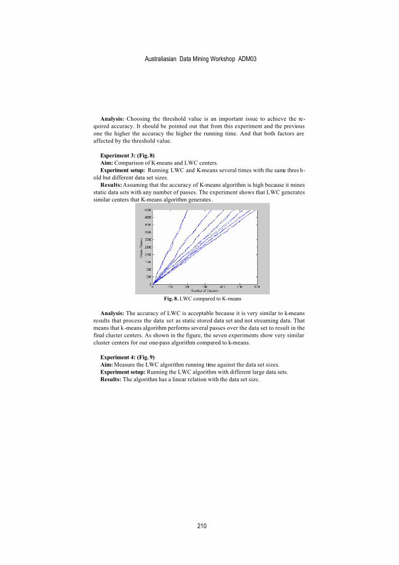
Analysis: Choosing the threshold value is an important issue to achieve the re-

quired accuracy. It should be pointed out that from this experiment and the previous

one the higher the accuracy the higher the running time. And that both factors are

affected by the threshold value.

Experiment 3: (Fig. 8)

Aim: Comparison of K-means and LWC centers.

Experiment setup: Running LWC and K-means several times with the same thres h-

old but different data set sizes.

Results: Assuming that the accuracy of K-means algorithm is high because it mines

static data sets with any number of passes. The experiment shows that LWC generates

similar centers that K-means algorithm generates .

Fig. 8. LWC compared to K-means

Analysis: The accuracy of LWC is acceptable because it is very similar to k-means

results that process the data set as static stored data set and not streaming data. That

means that k-means algorithm performs several passes over the data set to result in the

final clus ter centers. As shown in the figure, the seven experiments show very similar

cluster centers for our one-pass algorithm compared to k-means.

Experiment 4: (Fig. 9)

Aim: Measure the LWC algorithm running time against the data set sizes.

Experiment setup: Running the LWC algorithm with different large data sets.

Results: The algorithm has a linear relation with the data set size.

Fig. 9. LWC running time with different data set sizes

Analysis: the LWC algorithm is efficient for large data sets due to the linearity of

the running time with data set size. This linearity results from performing only one-

pass over the data stream. It is worth to point out here that the data stream rate is the

major factor that control the behavior of LWC since the higher the rate the larger the

size of the data set.

Experiment 5: (Fig. 10)

Aim: Measuring the effect of the threshold on the above experiment.

Experiment setup: Running LWC algorithm with the same data set sizes as the

above experiment, but with decreasing threshold value with each run.

Results: The threshold value affects the running time of the algorithm since the

maximum running time in the above experiment is approximately 12 seconds. The maxi-

mum running time in this experiment is about 47 seconds.

Fig. 10. LWC running time with different data set sizes and threshold values

Analysis: According to the application and/or the required accuracy, we have to

maximize the threshold value to have more efficient algorithm in terms of running time.

The algorithm threshold would be controlled according to the available memory and a

time threshold constraint that represents the algorithm accuracy.

Experiment 6: (Fig. 11)

Aim: Comparison between K-means and LWC efficiency.

Experiment setup: Running LWC (with a small threshold value which results in a

high accuracy) and K-means several times on the same data sets with different sizes

and measuring the running time.

Results: The running time of LWC is low compared to K-means with small data set

sizes.

Fig. 11. K-means and LWC comparison in terms of running time

Analysis: LWC is efficient compared to K-means for small data sets, when we try to

run both on large data sets; we found that LWC outperforms the K-means. The LWC

runs with highest possible accuracy (the least threshold value) and outperforms k-

means with different data set sizes.

The above experiments show an efficient one-look clustering algorithm that is

adaptable to the available resources using our algorithm output granularity approach.

The LWC outperforms k-means in terms of running time and has the advantage of

linearity of running time with the increase in the data set sizes. The algorithm thres hold

is the controlling parameter of algorithm accuracy, efficiency, and algorithm output

rate.

5 Related Work

There are different algorithms proposed to deal with the high speed nature for mining

data streams using different techniques. Clustering data streams has been studied in

[1], [4], [6], [7], [9], [10], [15], [22], [26]. Data stream classification has been studied in

[11], [12], [18], [28], [34]. Extracting frequent items and frequent itemsets have been

studied in [8], [14], [23].

The above algorithms deal with the problem of mining data streams using different

methodologies. These algorithms basically focus on the design of approximate alg o-

rithms for mining data streams. However these approaches are not resource-aware and

do not focus on adaptation strategies to cope with high data rates, our approach for

output rate adaptation is resource-aware approach that can adapt to the available

resources.

6 Conclusions and Future Work

In this paper, we discussed the problems of mining data streams and proposed possi-

ble solutions. Our algorithm output granularity approach in mining data streams has

been presented and discussed. The proposed approach is distinguished from previous

work in mining data streams by being resource-aware. We have developed a one-pass

mining data streams algorithm. The application of the proposed approach to cluster-

ing, classification and counting frequent items has been presented. The implementa-

tion and empirical studies of our LWC algorithm have been demonstrated. The experi-

ments showed an acceptable accuracy accompanied with efficiency in ru nning time

that outperforms k-means alg orithm. Having implemented and tested LWC, we are

developing LWClass and LWF. The application of these algorithms in a ubiquitous

environment is planned for future work. The simplicity, generality, and efficiency of

our proposed approach in mining data streams facilitate the application of the alg o-

rithms in various scientific and business applications that require data stream analysis.

References

1. Aggarwal C., Han J., Wang J., Yu P. S.: A Framework for Clustering Evolving

Data Streams. Proc. 2003 Int. Conf. on Very Large Data Bases (VLDB'03), Be r-

lin, Germany (2003).

2. Babcock B., Babu S., Datar M., Motwani R., and Widom J.: Models and is-

sues in data stream systems. In Proceedings of PODS (2002).

3. Babcock B., Datar M., and Motwani R.: Load Shedding Techniques for Data

Stream Systems (short paper). In Proc. of the 2003 Workshop on Manage-

ment and Processing of Data Streams (MPDS 2003) (2003).

4. Babcock B., Datar M., Motwani R., O'Callaghan L.: Maintaining Variance and

k-Medians over Data Stream Windows. To appear in Proceedings of the 22nd

Symposium on Principles of Database Systems (PODS 2003) (2003).

5. Burl M., Fowlkes C., Roden J., Stechert A., and Mukhtar S. Diamond Eye: A

distributed architecture for image data mining. In SPIE DMKD, Orlando, April

(1999).

6. Charikar M., O'Callaghan L., and Panigrahy R.: Betterstreaming algorithms for

clustering problems. In Proc. of 35th ACM Symposium on Theory of Comput-

ing (STOC) (2003).

7. O'Callaghan L., Mishra N., Meyerson A., Guha S., and Motwani R.: Stream-

ing-data algorithms for high-quality clustering. Proceedings of IEEE Intern a-

tional Conference on Data Engineering, March (2002).

8. Cormode G., Muthukrishnan S.: What's hot and what's not: tracking most fre-

quent items dynamically. PODS 2003. (2003) 296-306

9. Datar M., Gionis A., Indyk P., Motwani R.: Maintaining Stream Statistics over

Sliding Windows (Extended Abstract). In Proceedings of 13th Annual ACM -

SIAM Symposium on Discrete Algorithms (SODA 2002) (2002).

10. Domingos P. and Hulten G., A General Method for Scaling Up Machine

Learning Algorithms and its Application to Clustering. Proceedings of the

Eighteenth International Conference on Machine Learning, 106--113, Wil-

liamstown, MA, Morgan Kaufmann. (2001)

11. Domingos P. and Hulten G. Mining High-Speed Data Streams. In Proceed-

ings of the Association for Computing Machinery Sixth International Confer-

ence on Knowledge Discovery and Data Mining, (2000) 71—80.

12. Ganti V., Gehrke J., Ramakrishnan R.: Mining Data Streams under Block Ev o-

lution. SIGKDD Explorations 3(2): (2002) 1-10.

13. Garofalakis M., Gehrke J., Rastogi R.: Querying and mining data streams: you

only get one look a tutorial. SIGMOD Conference 2002: 635. (2002).

14. Giannella C., Han J., Pei J., Yan X., and Yu P.S.: Mining Frequent Patterns in

Data Streams at Multiple Time Granularities. In Kargupta H., Joshi A., Siv a-

kumar K., and Yesha Y. (eds.), Next Generation Data Mining, AAAI/MIT

(2003).

15. Guha S., Mishra N., Motwani R., and O'Callaghan L.: Clustering data streams.

In Proceedings of the Annual Symposium on Foundations of Computer Sci-

ence. IEEE, November (2000).

16. Golab L. and Ozsu M. T. : Issues in Data Stream Management. In SIGMOD

Record, Volume 32, Number 2, June (2003) 5-14.

17. Henzinger M., Raghavan P, and Rajagopalan S.: Computing on data streams.

Technical Note 1998-011, Digital Systems Research Center, Palo Alto, CA,

May (1998).

18. Hulten G., Spencer L., and Domingos P.: Mining Time -Changing Data

Streams. ACM SIGKDD (2001).

19. Kargupta H.: CAREER: Ubiquitous Distributed Knowledge Discovery from

Heterogeneous Data. NSF Information and Data Management (IDM) Work-

shop (2001).

20. Kargupta. H.: VEhicle DAta Stream Mining (VEDAS) Project.

http://www.cs.umbc.edu/%7Ehillol/vedas.html. (2003).

21. Kargupta, H., Park, B., Pittie, S., Liu, L., Kushraj, D. and Sarkar, K. (2002). Mo-

biMine: Monitoring the Stock Market from a PDA. ACM SIGKDD Explora-

tions. January 2002. Volume 3, Issue 2. Pages 37--46. ACM Press.

22. Keogh E., Lin J., and Truppel W.: Clustering of Time Series Subsequences is

Meaningless: Implications for Past and Future Research. In proceedings of

the 3rd IEEE International Conference on Data Mining. Melbourne, FL.

November (2003) 19-22.

23. Manku G. S. and Motwani R.: Approximate frequency counts over data

streams. In Proceedings of the 28th International Conference on Very Large

Data Bases, Hong Kong, China, August (2002).

24. Muthukrishnan S.: Data streams: algorithms and applications. Proceedings of

the fourteenth annual ACM-SIAM symposium on discrete algorithms (2003).

25. Muthukrishnan S.: Seminar on Processing Massive Data Sets. Available

Online: http://athos.rutgers.edu/%7Emuthu/stream-seminar.html (2003).

26. Ordonez C.: Clustering Binary Data Streams with K-means .ACM DMKD

(2003).

27. Park B. and Kargupta H.. Distributed Data Mining: Algorithms, Systems, and

Applications. Data Mining Handbook. Editor: Nong Ye (2002).

28. Papadimitriou S., Faloutsos C., and Brockwell A.: Adaptive, Hands-Off Stream

Mining. 29th International Conference on Very Large Data Bases VLDB (2003).

29. Srivastava A. and Stroeve J.: Onboard Detection of Snow, Ice, Clouds and

Other Ge ophysical Processes Using Kernel Methods. Proceedings of the

ICML'03 workshop on Machine Learning Technologies for Autonomous

Space Applications (2003).

30. Tanner S., Alshayeb M., Criswell E., Iyer M., McDowell A., McEniry M.,

Regner K., EVE: On-Board Process Planning and Execution, Earth Science

Technology Conference, Pasadena, CA, Jun. 11 - 14, (2002).

31. Tatbul N., Cetintemel U., Zdonik S., Cherniack M. and Stonebraker M.: Load

Shedding in a Data Stream Manager. Proceedings of the 29th International

Conference on Very Large Data Bases (VLDB), September (2003).

32. Tatbul N., Cetintemel U., Zdonik S., Cherniack M. and Stonebraker M.: Load

Shedding on Data Streams. In Proceedings of the Workshop on Management

and Processing of Data Streams (MPDS 03), San Diego, CA, USA, June

(2003).

33. Viglas S. D. and Naughton J.: Rate based query optimization for streaming in-

formation sources. In Proc. of SIGMOD (2002).

34. Wang H., Fan W., Yu P. and Han J.: Mining Concept-Drifting Data Streams

using Ensemble Classifiers. In the 9th ACM International Conference on

Knowledge Discovery and Data Mining (SIGKDD), Aug., Washington DC,

USA (2003).

simeon

Australiasian Data Mining Workshop ADM03

An Analytical Approach for Handling Association Rule Mining Results

Rodrigo Salvador Monteiro1, Geraldo Zimbrão1,2, Jano Moreira de Souza1,2

1 Computer Science Department, Graduate School of Engineering, Federal University of Rio de Janeiro, PO Box 68511, ZIP code: 21945-970,

Rio de Janeiro, Brazil 2 Computer Science Department, Institute of Mathematics,

Federal University of Rio de Janeiro Rio de Janeiro, Brazil

{salvador, zimbrao, jano}@cos.ufrj.br

Abstract. Association rule mining has played an important role in data mining research since its introduction by Agrawal in [2]. An important question that has come up with this new technique is how to analyze the commonly huge number of rules produced by the algorithms. Many proposals have arisen, ranging from simple ideas, like grouping correlated rules up to more ambitious ones, such as the Inductive Databases [19]. Other works attempt to avoid this problem by imposing constraints and interestingness measures during the discovery of as-sociation rules in order to output only the significant rules. We present a new proposal that defines a framework for a Data Warehouse of Association Rules capable of providing a full environment for analyzing association rules. This new approach can benefit naturally from many data warehouse features and, besides, it comprises an interesting framework for proposing new knowledge discovery models.

1 Introduction

Advances in data gathering mechanisms, the use of bar codes in most commercial products, and information on many business and governmental transactions have been flooding us with data, creating an urgent need for new techniques and tools to intelli-gently and automatically aid in the transformation of this data into useful knowledge [8]. Data Mining, known as Knowledge Discovery in Databases – KDD, appeared as a group of methods, techniques and tools capable of meeting this demand.

One of the techniques most widely studied and explored for pattern discovery in large databases is association rule mining. It was presented and formalized by [2], and quickly gained importance for its large applicability. Since then, many works propos-ing new algorithms for association rule mining, such as [3,25,5,4,16,15,23,6,1,11,20,12], beside several others, affirm the importance and at-tention that has been dedicated to this data mining area.

Paradoxically, data mining itself can produce such great amounts of data that there has arisen a new knowledge management problem [17]. Association rule mining fits in

this category and, therefore, it needs solutions for analysis and management of dis-covered knowledge. All solutions proposed so far to help the analysis of a huge volume of association rules have at least one of the following problems or restrictions: 1 – the analysis is restricted to valid rules at one specific moment in time, so it is not possible to confront valid rules in different spots of time; 2 – limited analysis capabilities, such as grouping criteria specification and specific interestingness measures; 3 – serious per-formance problems, and no feasible implementation with the currently-available technology.

As an alternative to avoid the problem, several works have been proposed to push constraints and interestingness measures into the kernel of association rule mining algorithms. However, the great problem concerning this solution is defining which constraints should be pushed and which rule characteristics are interesting. In other words, according to [22], were we to know what we were looking for, the discovery process would be trivial. Besides, by adopting this alternative, the analyst never gets an overview of the rules in the whole database.

The integration of OLAP operations with data mining tasks, proposed by [14], is a great advance in methods and analysis tools to support the analysis/evaluation of pat-terns step in the knowledge discovery process. However, when it comes to association rules, this integration does not take place naturally, according to discussions presented in the same work [14].

The proposal of this ongoing work consists of defining a data warehouse of asso-ciation rules through structure, operation and model specifications in order to provide a complete environment for analyzing association rules. The present article defines the desired functionalities of a data warehouse of association rules. We argue that pro-viding sophisticated tools to assist the analyst in the pattern evaluation/analysis step turns out to be as important as mining association rules. There is no use to mine rules efficiently if we are not able to understand and find them. This new approach can naturally benefit from many data warehouse features, and besides, it constitutes an interesting framework for proposing new knowledge discovery models.

The remainder of this work is organized as follows: section 2 presents the problem definition of mining association rules; section 3 presents the existing approaches for handling association rule mining results; section 4 presents our proposal, the Data Warehouse of Association Rules Framework (DWARF), and; finally, section 5 draws a few conclusions.

2 Association Rule Mining - ARM

Association rule mining is one of the most widely studied and explored techniques for Knowledge Discovery in Databases. Mining association rules mean searching for correlation patterns among facts recorded in one transactional database. Traditionally, the problem is presented through one classic application: the supermarket basket. A client’s supermarket basket consists of a set of items, such as rice, beans, meat, etc. Each purchase corresponds to one transaction. Discovering which supermarket items are frequently sold together is valuable information. As an example, we may discover that 70% of clients who buy sugar-free candy buy diet beverages too. The supermarket

manager, owning this information, can redistribute the items on the shelves; he may also plan promotions, besides getting a better understanding of the business and of his clients’ behavior. One actual example is Wal-Mart. By discovering an association between purchases of diapers and beers, Wal-Mart optimized their store layout in sales points, putting these items side by side. As a result, there was an increase of 30% in these product sales.

Agrawal in [2] was the first to present and formalize the problem of association rule mining. The formal definition from [2] follows below.

2.1 Formal Definition of Association Rule Mining Problem

Let Γ = I1, I2, ..., Im be a set of binary attributes, called items. Let T be a database of transactions. Each transaction t is represented as a binary vector, with t[k] = 1 if t bought item Ik, and t[k] = 0 otherwise. There is one tuple in the database for each transaction. Let X be a set of some items in Γ. We say that a transaction t satisfies X if, for all items Ik in X, t[k] = 1.

Association rules mean an implication of the form X → Ij, where X is a set of some items in Γ, and Ij is a single item in Γ that is not present in X. The rule X → Ij is satisfied in the set of transactions T with the confidence factor 0 ≤ c ≤ 1 iff at least c% of transactions in T that satisfy X also satisfy Ij. Besides, rule X → Ij has the support factor 0 ≤ s ≤ 1, where s is the fraction of transactions in T that satisfy X U Ij.

Support should not be confused with confidence. While confidence is a measure of the rule’s strength, support corresponds to statistical significance.

In this formulation, the problem of rule mining can be decomposed into two sub-problems:

1. Generate all combinations of items that have fractional transaction support above a certain threshold, called minsupport. Call these combinations large itemsets, and all other combinations that do not meet the threshold small itemsets.

2. For a given large itemset Y = I1, I2, ..., Ik, k ≥ 2, generate all rules (at most k rules) that use items from set I1, I2, ..., Ik. Only rules with confidence above a certain threshold are reported.

Computational complexity is concentrated on the first subproblem. Once we have all large itemsets available, the solution of the second subproblem is extremely simple. That is why it is common to see the association rule mining problem reduced to a problem of finding large itemsets.

3 Existing Approaches for Handling ARM Results

Different approaches were proposed for handling results of data mining algorithms. In this section we present the most relevant ones emphasizing their applicability to asso-ciation rules.

3.1 OLAP Mining

Han in [14] defined the concept of OLAP Mining as a mechanism that integrates on-line analytical processing (OLAP) with data mining so that mining can be per-formed at different levels of abstraction at the user’s fingertips.

The concept of OLAP Mining predicts a total integration, it thus being possible to mix OLAP operation with data mining tasks. This is an extremely interesting solution for analyzing data mining tasks results. We mean by OLAP operations the many pos-sible ways of interaction with a data cube in multidimensional data analysis, such as drill-down, roll-up, pivot, slice, dice, etc. In order for such integration to take place, we should be able to express a data mining task execution result as a data cube. Consid-ering the classification and clustering mining tasks, we achieve perfect integration. In such tasks we can associate the pre-existing classes or the newly discovered categories to a new dimension. The same does not happen when considering association rules. A new data cube cannot easily or naturally represent the result of an association rule mining algorithm execution on a data cube. In [14] this integration problem is under-lined, some alternatives are discussed but however, no solution is presented. This fact prevents the execution of OLAP operations to analyze the rules discovered. In other words, the mechanism of OLAP Mining does not provide operation for association rule analysis.

3.2 Inductive Databases

Inductive Databases, defined by Mannila in [19], are databases which, in addition to data, also contain inductive generalizations about the data. This approach has a basic principle: many data mining tasks can be described as problems on how to find inter-esting sentences given a specific logic. Considering the association rule, we can translate it as the problem of finding valid rules on a database given support and con-fidence constraints. Once this concept is adopted, the analyst’s task can be accom-plished by simply querying the database theory using a conventional query language. [10] present a discussion on two alternatives: 1) mining association rules on demand as part of a query execution plan and; 2) discovery of all valid and interesting rules ac-cording to some criteria and storing them in the database. A hybrid approach is also considered.

Citing Goethals and Bussche [10], the framework of the Inductive Databases is an elegant formalization of the interactive mining process. However, we can identify some topics not satisfactorily solved by this framework. They are as follows:

1. Inexistence of sophisticated analysis operations (e.g.: OLAP operations) essential for evaluating huge amounts of data. This deficiency also prevents the analyst from obtaining an overview of the rules in the whole database;

2. Past association rules are not considered as there is no history on past association rules. The database theory corresponds only to the current status of the database.

Considering the mining rule on demand approach there is an additional problem: how to accomplish the cleaning step, which is essential to ensure data quality? Without a good treatment of input data, it is impossible to obtain good results with any data

mining algorithms. Translated into the commonly-used sentence: garbage in, garbage out.

3.3 Interestingness Measures

Data mining algorithms, in special those of association rule mining, typically create a great number of patterns. However, many patterns are irrelevant or obvious, and bring no new knowledge [21]. Many measures have been proposed in the attempt to evaluate the utility and relevance of discovered patterns, which are referenced in the literature as interestingness measures. The use of an interestingness measure provides a ranking ordering the discovered patterns.

The great challenge for interestingness measures is to quantify what is interesting to the analyst. The problem becomes worse if we remember that analysts usually do not know for sure what they are looking for and, therefore, they do not know what is in-teresting. Thus, the analyst can be losing valuable information if we constrain the discovered patterns by some interestingness measure threshold. However, the use of interestingness measures is extremely useful to eliminate obvious patterns and to pro-vide a ranking. It can be very useful when combined with other approaches.

Some examples of interestingness measures that can be used on association rule are: Itemset Measures [3], Rule Templates [17], Interestingness [24,13,7], Surprisingness [9], Reliable Exceptions [18] and Peculiarity [26].

3.4 Visualization Techniques

Some proposals on association rule visualization attempt to provide the analyst with an overview of the entire rule set. The visualization of a rule set corresponds to the prob-lem of visualizing a hipergraph, with even the visualization of one single rule com-prising a complex problem. [17].

A set of association rules can be represented through, for example, a dependence graph (Figure 1) or a bar chart (Figure 2), showing interestingness measures (e.g., support or confidence). In a bar chart, we have limits on the number of dimensions, restricting the visualization to rules with a few items (2 items, the third dimension represents an interestingness measure). In a dependence graph, we do not have limits on the number of rule items. However, we can perceive, observing Figure 1, that even sets of few rules can make the graph unreadable. Besides, the node disposition problem represents a great challenge.

4 Our Proposal

Even considering reasonable thresholds for support and confidence, one can obtain hundreds or thousands of association rules [17]. We argue that forcing other constraints to reduce the number of rules produced may not be a good solution, for the analyst must reduce the scope of his search artificially. There is no doubt that allowing the intro-duction of constraints is an interesting and useful feature to be used by the analyst.

However, we argue that this mechanism must not be used to constrain the rule’s search in order to make the result tractable.

Fig. 1. Dependence graph in Rule Visualizer / Rule Graph [17]

Fig. 2. Bar Chart with interestingness measure in DBMiner Associator [14]

Facing the desirable functionalities and the limitation of the existing approaches, we developed the proposal for a new framework to supply the current deficiencies in the evaluation/analysis of association rules. In this new framework we attempt to maintain the advantages of the existing ideas and solve the problems with new thoughts, pro-viding new analysis features. We call this new framework the Data Warehouse of Association Rules Framework – DWARF.

4.1 Data Warehouse of Association Rules Framework (DWARF)

Our proposal defines a framework in which the features provided by the OLAP Mining mechanism, beside others, can be applied to great numbers of association rules pro-duced by mining algorithms. The definition of a Data Warehouse of Association Rules has the goal of providing a complete and friendly environment in which the analyst will have such powerful tools that he will not have to worry about the number of rules produced.

A Data Warehouse of Association Rules must have the following features:

1. A cube cell being analyzed corresponds to a set of association rules. It should be possible to visualize different aggregate values representing the set, from simple counting to more sophisticated interestingness measures. The rule set visualization must also be possible, varying from simple listing to more elaborate visualization techniques;

2. Allow for the association of interestingness measures, such as support and confi-dence, to DW dimensions. As an example, it must be possible to visualize the whole set of rules by support ranges or to constrain the rules to be considered to any spe-cific range;

3. Have a Time dimension following the traditional DW approach. Any restriction in this dimension must have the effect of considering only valid rules on the con-strained period being analyzed;

4. Have two Item dimensions, one associated to rule antecedent and the other associ-ated to rule consequent. These dimensions can have hierarchies allowing for several organizations and grouping of items;

5. Allow the execution of traditional OLAP operations, such as drill-down, roll-up, pivot, slice, dice, etc, on the rule cube being analyzed;

6. Other dimensions, such as spatial dimension, allowing for the restriction of rules valid in a specific region.

The data necessary to the Data Warehouse of Association Rules operations must be available in some previously-loaded structure just as the traditional Data Warehouse.

Besides the analysis power provided by this new approach, we believe that new knowledge-discovering models can be proposed on the rules stored in the DW. A pre-liminary idea is presented on the next section.

4.2 New Knowledge-Discovering Model Proposal

We can think of identifying changes in a business once we have available, at DWARF, sets of association rules of different points of time. Using, for example, measures of rule similarity, we can identify similarities and differences between two rule sets. Imagine the following scenario: in one month, an analyst recognizes some management decision that should be taken based on the analysis of rules. In the next month it can be interesting to check whether the desired changes have occurred and, mainly, whether unexpected changes have taken place as a side effect of the decision taken.

5 Conclusions

Analyzing great number of association rules is a problem that came up immediately after the definition of the first association rule mining algorithm. Since then, several alternative proposals and solutions have been developed. However, all current ap-proaches have weak points. In this work, we present the Data Warehouse of Associa-tion Rules Framework (DWARF) proposal, which aims at maintaining the advantages of the existing ideas and solving the problems with new ones, providing new analysis features. We defined the DWARF by listing the set of features it must provide.

A great advantage of the DWARF approach is to provide analysis tools that are familiar to the analysts who are used to OLAP tools. Thus, it is extremely easy to be used by managers and decision-makers in a company.

It is important to note that the definition of DWARF provided in this work is part of an ongoing project in which structures capable of providing the desired features in an efficient way will be researched and investigated. We strongly believe that we are in the right path, since other works, such as [22], point to the adaptation algorithms and de-velopment of structures for mining data in secondary and even tertiary storage.

We strongly believe that the consolidation of the DWARF proposal will provide an environment for association rule analysis capable of relieving the analyst from wor-rying about the number of rules produced, there by leaving him free to deal only with his investigation.

References

1. Agarwal, R. C., Aggarwal, C. C., and Prasad, V. V. V.: “A Tree Projection Algorithm for Generation of Frequent Item Sets”. Journal of Parallel and Distributed Computing 61(3): 350-371, 2001.

2. Agrawal, R., Imielinski, T., and Swami, A.: “Mining Association Rules between Sets of Items in Large Databases”. Proceedings of the 1993 ACM SIGMOD Conf., pages 207-216, Washington, DC, May 1993.

3. Agrawal, R., and Srikant, R.: “Fast Algorithms for Mining Association Rules in Large Da-tabases”. Proceedings of the 20th International Conference on Very Large Data Bases, pp. 487-499, Santiago de Chile, Chile, 1994.

4. Bayardo Jr, R. J.: “Efficiently Mining Long Patterns from Databases”. Proceedings of the 1998 SIGMOD Conference, pp. 85-93, 1998.

5. Brin, S., Motwani, R., Ullman, J. D., and Tsur, S.: “Dynamic Itemset Counting and Implica-tion Rules for Market Basket Data”. Proceeding of the 1997 SIGMOD Conference, pp. 255-264, 1997.

6. Burdick, D., Calimlim, M., and Gehrke, J. E.: “MAFIA: A Maximal Frequent Itemset Algo-rithm for Transactional Databases”. Proceedings of the 17th International Conference on Data Engineering, Heidelberg, Germany, April 2001.

7. Dong, G., and Li, J.: “Interestingness of Discovered Association Rules in Terms of Neighborhood-Based Unexpectedness”. In Proc. of Second Pacific-Asia Conference on Re-search and Development in Knowledge Discovery and Data Mining, pp. 72-86, Melbourne, Australia, 1998.

8. Fayyad, U. M., Piatetsky-Shapiro, G., Smyth, P., and Uthurusamy, R.: “Advances in Knowledge Discovery and Data Mining”. AAAI Press, 1998.

9. Freitas, A. A.: “On Objective Measures of Rule Surprisingness”. In Proc. of the Second European Symposium on Principles of Data Mining and Knowledge Discovery, pp. 1-9, Nantes, France, 1998.

10. Goethals, B., and Bussche, J.: “A priori versus a posteriori filtering of association rules.” 1999 ACM SIGMOD Workshop on Research Issues in Data Mining and Knowledge Discovery, 1999.

11. Gouda, K., and Zaki, M. J.: “Efficiently Mining Maximal Frequent Itemsets”. Proceeding of the 2001 ICDM Conference, pp. 163-170, 2001.

12. Grahne, G., and Zhu, J.: “High Performance Mining of Maximal Frequent Itemsets”. Pro-ceedings of the 6th International Workshop on High Performance Data Mining, 2003.

13. Gray, B., and Orlowska, M. E.: “CCAIIA: Clustering Categorial Attributed into Interseting Accociation Rules”. In Proc. of Second Pacific-Asia Conference on Research and Develop-ment in Knowledge Discovery and Data Mining, pp. 132-143, Melbourne, Australia, 1998.

14. Han, J.: “OLAP Mining: An Integration of OLAP with Data Mining”. Proceedings of the 1997 IFIP Conference on Data Semantics (DS-7), pp. 1-11, Leysin, Switzerland, Oct 1997.

15. Han, J., Pei, J., and Yin, Y.: “Mining frequent patterns without candidate generation”. In Proceeding of the 2000 SIGMOD Conference, pp. 1-12, Dallas, Texas, May 2000.

16. Hidber, C.: “Online Association Rule Mining”. Proceedings of the ACM SIGMOD Interna-tional Conference on Management of Data, 1999.

17. Klemettinen, M., Mannila, H., Ronkainen, P., Toivonen, H., and Verkamo, A. I.: “Finding Interesting Rules from Large Sets of Discovered Association Rules”. Proceeding of the Third International Conference on Information and Knowledge Management, pp. 401-407, 1994.

18. Liu, H., Lu, H., Feng, L., and Hussain, F.: “Efficient Search of Reliable Exceptions”. In Proc. of Third Pacific-Asia Conference on Methodologies for Knowledge Discovery and Data Mining, pp. 194-203, Beijing, China, 1999.

19. Mannila, H.: “Inductive Databases and Condensed Representations for Data Mining”. Pro-ceedings of the 1997 International Logic Programming Symposium, pp. 21-30, 1997.

20. Orlando, S., Palmerini, P., Perego, R., and Silvestri, F.: “Adaptive and Resource-Aware Mining of Frequent Sets”. Proceedings of the 2002 IEEE International Conference on Data Mining, pp. 338-345. Maebashi City, Japan, December 2002.

21. Padmanabhan, B., and Tuzhilin, A.: “A Belief-Driven Method for Discovering Unexpected Patterns”. In Proceedings of the Fourth International Conference on Knowledge Discovery and Data Mining, pp. 94-100, New York, 1998.

22. Ramakrishnan, N., and Grama, A. Y.: “Data Mining: From Serendipity to Science”. IEEE Computer, 32(8): 34-37, 1999.

23. Seno, M., and Karypis, G.: “LPMiner: An Algorithm for Finding Frequent Itemsets Using Length-Decreasing Support Constraint”. In Proceeding of the 2001 IEEE International Con-ference on Data Mining, pp. 505-512, San Jose, California, 2001.

24. Silberschatz, A., and Tuzhilin, A.: “On Subjective Measures of Interestingness in Knowledge Discovery”. Proceedings of the First International Conference on Knowledge Discovery and Data Mining, pp. 275-281, Montreal, Canada, 1995.

25. Srikant, R., and Agrawal, R.: “Mining Quantitative Association Rules in Large Relational Tables”. Proc. of 1996 SIGMOD Conference on Management of Data, pages 1-12, Montreal, Quebec, June 1996.

26. Zhong, N., Yao, Y. Y., and Ohsuga, S.: “Peculiarity Oriented Multi-database Mining”. In Proc. of Third European Conference on Principles of Data Mining and Knowledge Discovery, pp. 136-146, Prague, Czech Republic, 1999.

simeon

Australiasian Data Mining Workshop ADM03

Modelling Insurance Risk: A Comparison of Data Mining and Logistic Regression Approaches

Inna Kolyshkina1, Peter Petocz2, Ingrid Rylander3

Abstract

Interest in Data Mining techniques has been increasing recently amongst the statistical profession. This paper presents and discusses a case study showing the application of one of the better-known Data Mining techniques, Classification and Regression Trees (CART®), to a business problem that required modelling risk in insurance, based on a project performed for an insurance company by PWC Actuarial. The nonlinear and nonparametric approach on which CART methodology is based provides good insights into the hidden patterns in such large data sets, with maybe a few million cases and several hundreds of possible predictor variables. Such data sets are common in many areas of insurance, healthcare, telecommunications, credit risk, banking, etc. The paper discusses the use of CART methodology and introduces some innovative model performance measures often used in data mining, such as gain or lift. The results of CART modelling are compared to the results achievable by using more traditional, linear and generalised linear modelling techniques such as logistic regression. Comparisons are made in terms of time taken, predictive power, selection of most important predictors out of large number of possible predictors, handling predictors with many categories (such as postcode or occupation code), interpretability of the model, dealing with missing values, etc. The more practical and non-statistical issues of implementation and client feedback are also discussed.

1 Introduction

1 PricewaterhouseCoopers, GPO Box 2650, SYDNEY NSW 1171, Australia inna.kolyshkina@au.pwc.com

2 Department of Mathematical Sciences, University of Technology, Sydney

peter.petocz@uts.edu.au 3 PricewaterhouseCoopers, GPO Box 2650, SYDNEY NSW 1171, Australia

Ingrid.rylander@au.pwc.com

Interest in Data Mining techniques such as decision trees in the actuarial community has been increasing.

The main reasons for the increasing attractiveness of decision trees are as follows: − It overcomes the shortcomings of linear methods that operate under the assumption

that data is distributed either normally (as is the case in linear regression), or according to another distribution in the exponential family, such as binomial, Poisson, Gamma, inverse Gaussian etc (as it is required for a generalised linear model), which is often not quite the case. Decision trees are less affected by the distributional assumptions.

− It relies more heavily on “brutal force” of computing power than traditional models do, and because of that is less time-consuming and more precise than classical methods. When analyzing a large data set, say with 1 million cases and several hundred potential predictors, traditional approach would require significantly more time and will have difficulties with selecting the important predictors

− Classical methods often have a hard time dealing with categorical variables with a large number of categories (for example, claimant’s occupation code, industry code or postcode), which means that such variables are either left out from the model, or have to be grouped by hand prior to including them in the model).

These problems make it difficult to use linear methods when analysing large sets of data with a mix of all kinds of categorical and numeric variables.

This article gives an example of the application of CART® (Classification and Regression Trees; the name is a registered trade mark, but this has not been indicated throughout) to modelling risk in insurance. This nonlinear, nonparametric approach may provide greater insight into the hidden patterns in the data.

2 Problem and background In workers’ compensation insurance, serious claims (for example, claims that were litigated or claims where the claimant stayed off work for a very long period of time etc), comprise only about 15% of all claims by number, but create some 90% of the incurred cost. This means that in order to reduce the cost in a maximally effective way, an insurer would need to concentrate its attention on such claims. From a practical point of view, the insurer must ensure that the management of claimant injuries is carried out in such a way that the injured person receives the most effective medical treatment at appropriate points in time to prevent his or her injury from becoming chronic and to enable the claimant to return to work in an optimal manner.

To do so, the insurer ideally would need to know, at the time of a claim being received, whether the claim is likely to become serious. But in most cases this is not obvious as there are many factors contributing to the result. Therefore, it would be useful to have a model that would account for all such factors and would be able to predict at the outset of a claim the likelihood of this claim becoming serious.

3 The Data and the Analysis The data available for modelling was represented by several years’ worth of information about a large number of claims from the NSW workers’ compensation scheme.

The data available contained information: − about the claim itself (such as date the claim was registered, policy renewal year of

the claim, date when the claim was closed, date of the claim reopening, whether the claim was litigated, various liability estimates, payments made on the claim, reporting delay etc.

− about the claimant. Data on claimant included demographic characteristics of the client such as sex, age at the time of injury, family situation and whether the claimant had dependants, claimant’s cultural background). Also there were variables related to the claimant’s occupation, type of employment and work duties such as code for industry and occupation, nature of employment (permanent, casual, part or fulltime), wages etc.

− about the injury or disease such as time and place of injury, injury type, body location of the injury, cause or mechanism of injury, nature of injury etc.

Overall there were about 100 variables that might have been considered as potential predictors, most of them categorical with many categories. For example, the variable “occupation code” had more than 250 categories, “injury location code” had more than 80 categories.

The two major purposes of the analysis were: − to identify the most important predictors from a large number of available variables

containing information about a claim at the time when the claim is registered; and − to build a model based on such predictors, which would classify a claim as “likely

to become serious” or “not likely to become serious”.

4 Traditional Statistical Modelling Our first step was to attempt building the model using logistic regression, the traditional statistical modelling approach for analysis of data with binary response. Logistic regression is a well-known classical technique and is easily implemented in SAS, the software package that is mainly used for statistical analysis within our practice as well as by the client, and is a familiar and reliable data analysis tool. We built logistic regression models by using SAS v8 PROC LOGISTIC and PROC GENMOD.

The major difficulty that we encountered in using logistic regression was the fact that most variables in the data (such as location of injury, claimant’s occupation code, industry code and other variables) were categorical with large numbers of categories. This caused a considerable increase in time required for computation, and even more importantly, a high level of sparseness, potentially leading to instability in the model estimates. Although PROC LOGISTIC in version 8 of SAS does have a feature that can handle sparseness (see SAS, 2002), we found that using this feature was time-consuming (it took us 1hr 56 min to run logistic regression with this feature on a sample of 10,000, so we decided that, considering that the model will need to be

refined and rerun several times, it was too time-consuming to use this feature on a larger sample).

To overcome this problem and to be able to use in the model the information contained in such potentially important high-level categorical predictors as, for example, location of injury or occupation code, we had to transform these predictors. We grouped the categories “by hand”, according to recommendations of health management specialists as well as actuaries who have a lot of experience with insurance data, into a smaller set of broader categories.

Selection of the most important predictors and especially predictor interactions was another difficult task. Logistic regression theoretically can select the set of best predictors by using the stepwise method, but this process might take too long if the number of potential predictors is high (above 100 in our example). After several attempts to select the predictors this way ended in the computer crashing, we decided to take the top 30 predictors chosen by CART and allow stepwise logistic regression to further refine the selection. The use of PROC LOGISTIC with a main effects model further identified about 20 significant predictors.

Looking for predictor interactions using logistic regression proved to be time-consuming and again caused sparseness problem because the interaction of two categorical predictors even after we manually reduced the number of categories, has many categories (product of numbers of categories for the both predictors involved)

In Table 1 probability level =p means that the predicted value for a case is 1 if probability predicted by the logistic regression for the case is greater than p and is 0 otherwise, sensitivity is the proportion of true positives correctly identified by the model for a specified probability level and specificity is the proportion of true negatives correctly identified by the model for a specified probability level. Table 1 presents classification results for a few probability levels.

Table 1. Classification results from the logistic regression modeling

0.06 6,199 19,514 22,111 454 53.3 93.2 46.9 78.1 2.30.10 5,354 29,529 12,096 1,299 72.3 80.5 70.9 69.3 4.20.12 4,943 32,585 9,040 1,710 77.7 74.3 78.3 64.6 5.00.14 4,642 34,473 7,152 2,011 81.0 69.8 82.8 60.6 5.50.16 4,419 35,644 5,981 2,234 83.0 66.4 85.6 57.5 5.90.18 4,242 36,410 5,215 2,411 84.2 63.8 87.5 55.1 6.20.20 4,128 36,913 4,712 2,525 85.0 62.0 88.7 53.3 6.40.22 4,028 37,275 4,350 2,625 85.6 60.5 89.5 51.9 6.60.24 3,905 37,595 4,030 2,748 86.0 58.7 90.3 50.8 6.80.26 3,775 37,893 3,732 2,878 86.3 56.7 91.0 49.7 7.10.28 3,644 38,185 3,440 3,009 86.6 54.8 91.7 48.6 7.30.30 3,508 38,470 3,155 3,145 87.0 52.7 92.4 47.4 7.60.40 2,700 39,751 1,874 3,953 87.9 40.6 95.5 41.0 9.00.50 2,002 40,608 1,017 4,651 88.3 30.1 97.6 33.7 10.30.60 1,485 41,015 610 5,168 88.0 22.3 98.5 29.1 11.20.70 955 41,321 304 5,698 87.6 14.4 99.3 24.1 12.10.80 629 41,462 163 6,024 87.2 9.5 99.6 20.6 12.7

False POS False NEGNon-Event Correct Sensitivity SpecificityProb Level Event Non-Event Event

Classification Table

Correct Incorrect Percentages

Table 1 suggests that probability level that is providing the best balance of sensitivity and specificity for logistic regression is 0.18 and this is the probability level that is used for comparison of the confusion matrices for logistic regression and CART.

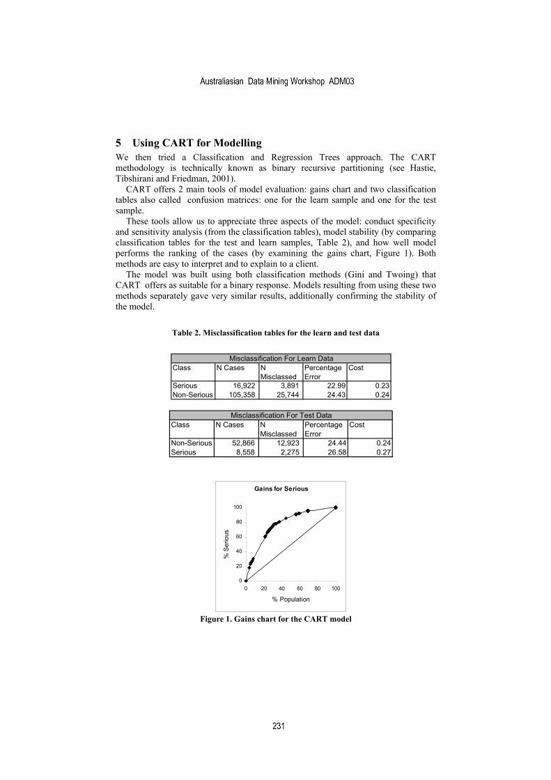
5 Using CART for Modelling We then tried a Classification and Regression Trees approach. The CART methodology is technically known as binary recursive partitioning (see Hastie, Tibshirani and Friedman, 2001).

CART offers 2 main tools of model evaluation: gains chart and two classification tables also called confusion matrices: one for the learn sample and one for the test sample.

These tools allow us to appreciate three aspects of the model: conduct specificity and sensitivity analysis (from the classification tables), model stability (by comparing classification tables for the test and learn samples, Table 2), and how well model performs the ranking of the cases (by examining the gains chart, Figure 1). Both methods are easy to interpret and to explain to a client.

The model was built using both classification methods (Gini and Twoing) that CART offers as suitable for a binary response. Models resulting from using these two methods separately gave very similar results, additionally confirming the stability of the model.

Table 2. Misclassification tables for the learn and test data

Serious 16,922 3,891 22.99 0.23Non-Serious 105,358 25,744 24.43 0.24

Misclassification For Learn DataCostClass N Cases N

MisclassedPercentage Error

Non-Serious 52,866 12,923 24.44 0.24Serious 8,558 2,275 26.58 0.27

Misclassification For Test DataClass N Cases N

MisclassedPercentage Error

Cost

Gains for Serious

0

20

40

60

80

100

0 20 40 60 80 100

% Population

% S

erio

us

Figure 1. Gains chart for the CART model

6 Comparison of Traditional and Data mining Approaches We identified the following differences between the two approaches:

6.1 Computational speed and time requirements

CART models were quicker to build (and therefore easier to refine). For example, running a CART model on data with some 190,000 cases and 25 predictors, some of which had more than 100 categories, took 9 minutes while running a stepwise logistic regression on a 50,000 random sample of the data with reduced numbers of categories for all categorical predictors (maximum 40 categories for a predictor) required reducing the number of categories by hand which involved consultation with health- management and actuarial experts, of writing a SAS program that performs the suggested recoding and running the program, taking a random sample of the data and then running the regression on the sample. This took two to three days and involved the time of the data analyst, actuarial consultant and health management experts.

6.2 Significant predictor selection

CART quickly selected around 20 significant predictors out of over 100. Logistic regression implemented using PROC LOGISTIC in SAS can select “best” predictors, but the process can take a long time. We decided to take the top 30 predictors chosen by CART and allow stepwise logistic regression to further refine the selection.

Theoretically, PROC LOGISTIC in stepwise regression will not necessarily find the right model, even given enough time. The trouble with stepwise methods implemented in statistical packages is that they do not allow for functional form modification or interactions, both of which are crucial to getting the right model. It is fairer to say that stepwise statistical methods cannot be used to learn the correct functional form and cannot identify the needed interactions. The only question is: can they find the best linear model? Even there, the search parameters (forwards, backwards) will affect whether this is true Only ‘all subsets’ can find the best linear approximation – but that approximation may be a terrible model (Steinberg, 2002).

It is worth mentioning here, that if our response variable had been continuous rather than binary (if, for example we needed to predict the cost of treatment), the process of predictor selection would have been even more time-consuming, because we would have needed to build a generalized linear model and use PROC GENMOD rather than PROC LOGISTIC, and PROC GENMOD does not perform predictor selection. And if our target variable had had more than two non-ordinal categories (it was suggested at one stage to use three categories: “litigated claim”, “non-litigated claim with claimant staying on benefits longer that a month” and “other” ), we would not have been able to use either PROC GENMOD or PROC LOGISTIC to fit the model. Both of these limitations would be irrelevant for CART. This demonstrates that CART has better and more usable built-in variable selection methods than are offered by widely used stepwise methods.

6.3 Handling categorical predictors with many categories

Logistic regression could not handle categorical predictors with many categories (as it caused sparsity problem) so we needed to spend time on reducing the number of categories as was discussed above. CART® did not require such time investment as it can deal with categorical predictors with many categories more effectively.

6.4 Picking up interactions of predictors

It was not easy to check the significance of interactions of predictors using logistic regression. Such selection would have to either be “by hand” and therefore would include checking the significance of some interactions chosen based on advice of the experts who are familiar with the data (which could leave out some potentially interesting interactions) or would involve checking all possible interactions which can be very time-consuming.

Another issue with interaction selection is that if the predictors in whose interactions we are interested (for example the claimant’s occupation code and mechanism of injury) have relatively many categories even after reduction of the number of categories, it might again cause the sparsity problem. For example if after reduction of the number of categories the predictors have respectively 9 and 10 categories, their interaction will have 90 categories. This issue will then need to be solved using time-consuming methods as described above.

It is well known that in traditional approach higher-order (even three-way) interactions are usually hard to interpret. CART, on the other hand, because of the nature of its modelling approach, easily picks high-order interactions and the structure of the tree model makes it easy to interpret them.

There are however other ways than stepwise methods to look for interactions such as treating the various levels of interaction as a hierarchy, and bring whole levels in at a time. These ways have not been investigated in this paper.

6.5 Missing values

PROC LOGISTIC automatically excludes from the analysis all observations with any missing values for the explanatory variables. As we were working with a “real-life” data, it was reasonable to expect (as it was the case) that at least in 5% of cases there would be a missing value for one of the 30 predictors. This meant excluding from the analysis about 5% of all observations which was not desirable. CART did not have a problem with handling the missing values and did not require excluding any observations from the analysis.

6.6 Interpretability of the model

CART model is represented in the form of a diagram and so was very visual and easy to interpret and to explain to the client. Logistic regression model is expressed as a

formula involving mathematical notation and can be easier interpreted by a client with some previous experience with logistic regression (or even simple regression) analysis.

6.7 Individual scoring vs segmenting

CART segmented all cases into several groups that were homogeneous in terms of likelihood of a serious claim (all cases within such group were assigned the same estimate of serious claim probability), while logistic regression gave each case an individual estimate of the probability of a serious claim.

6.8 Model evaluation

CART offers 2 main tools of model evaluation: gains chart and two classification tables: one for the learn sample and one for the test sample.

These tools allow us to appreciate three aspects of the model: conduct specificity and sensitivity analysis (from the classification tables), model stability (by comparing classification tables for the test and learn samples),

and how well model performs the ranking of the cases (by examining the gains chart). Both methods are easy to interpret and to explain to a client.

Logistic regression offers a classification table, as well as traditional, standard linear model diagnostics such as model fit indicators, residual diagnostics etc. These diagnostics tools are familiar to most data analysts and allow them to make a judgment about overall model fit as well as analyse outliers, influential observations and other aspects of the model.

6.9 Significance issues for predictors in a parametric linear model built on a data set with large number of cases

Parametric linear models built on data sets with large number of cases, usually have problems with identifying significant predictors. This happens because the number of the degrees of freedom for error are large, which results in practically all model terms being declared by the tests as significant. In other words, hypothesis testing using chi-squared test (which is the usual method used in all parametric linear models), does not work that well for large data sets. To some degree this problem can be overcome by building models on smaller random samples of the data and comparing them. This does mean that time needs to be spent on creating the random samples and rerunning models on them.

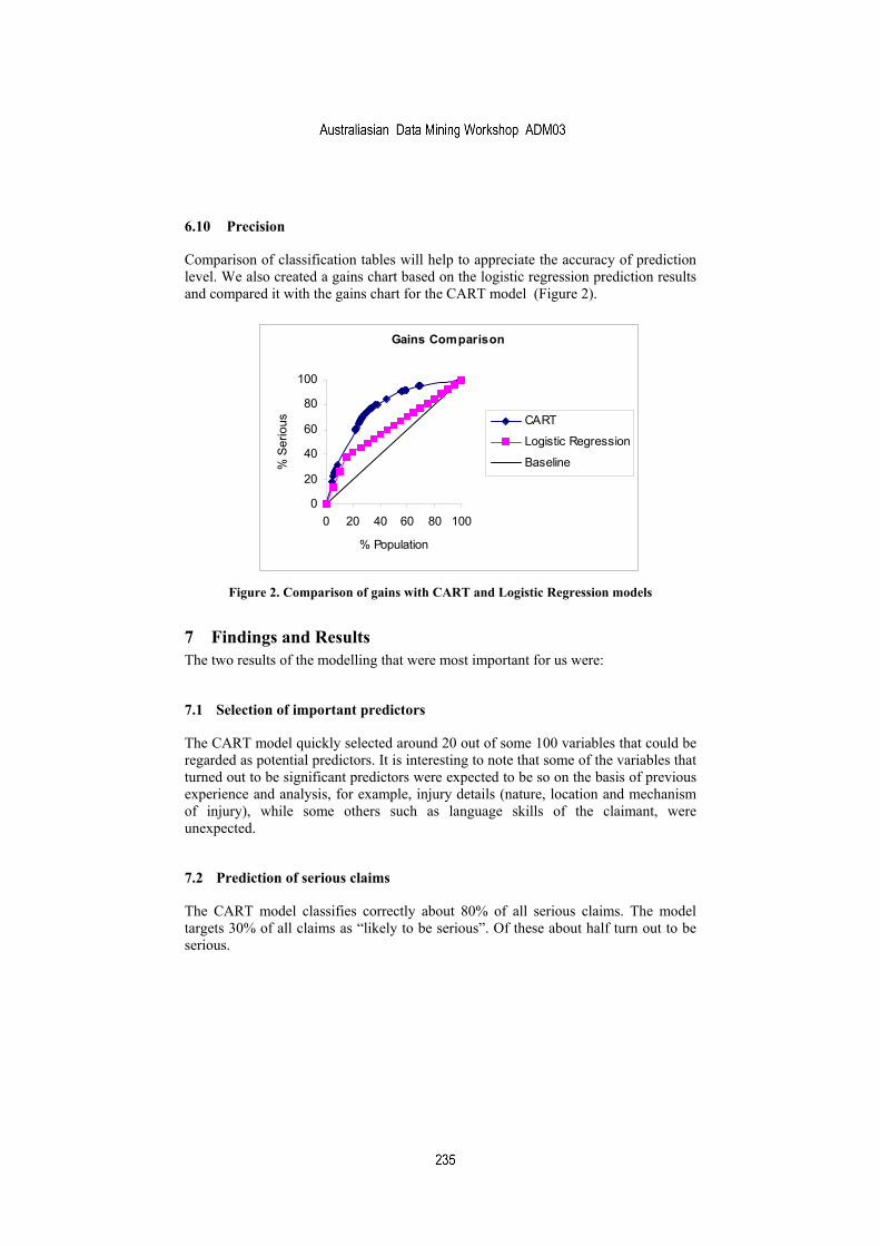
6.10 Precision

Comparison of classification tables will help to appreciate the accuracy of prediction level. We also created a gains chart based on the logistic regression prediction results and compared it with the gains chart for the CART model (Figure 2).

Gains Comparison

0

20

40

60

80

100

0 20 40 60 80 100

% Population

% S

erio

us CART

Logistic Regression

Baseline

Figure 2. Comparison of gains with CART and Logistic Regression models

7 Findings and Results The two results of the modelling that were most important for us were:

7.1 Selection of important predictors

The CART model quickly selected around 20 out of some 100 variables that could be regarded as potential predictors. It is interesting to note that some of the variables that turned out to be significant predictors were expected to be so on the basis of previous experience and analysis, for example, injury details (nature, location and mechanism of injury), while some others such as language skills of the claimant, were unexpected.

7.2 Prediction of serious claims

The CART model classifies correctly about 80% of all serious claims. The model targets 30% of all claims as “likely to be serious”. Of these about half turn out to be serious.

8 Implementation Issues and Client Feedback The model has been incorporated into the insurer’s computer system and automatically generates a “priority score” for each claim. This score is used to determine the level of staff who will be allocated the claim. Claims staff are grouped into three categories based on their experience in managing claims.

The scoring of the claim is however not only done initially, but reviewed at set points in time, and when important information comes to hand. Since all the data fields required for generating a score are captured as part of the claims database, it is easy for staff to get information about the change of score. Workflow processes have been designed to deal with those claims which change in likeliness to be serious.

We are implementing a continuous evaluation and feedback process to improve the model. A report on the results of this monitoring will be developed in due course.

9 Summary and Future Directions In the insurance application discussed in this paper, for the analysis of large data sets, the CART methodology proved superior to the ‘classical’ methodology of logistic regression. Moreover, there is reason to believe that this is not an isolated example (see Salford Systems, 2002). There are situations where the logistic regression methods might be preferred (for instance when the number of predictors is relatively small, most of them are numeric rather than categorical, and the assumptions for logistic regression are clearly valid), but hybrid models using the strengths of both approaches are already being developed and applied (Steinberg and Cardell, 1998a and b). For future improvement of our model, we plan to investigate and apply such hybrid models.

References 1. Breiman, L., Friedman, J., Olshen, R. and Stone, C. (1984). Classification and

Regression Trees. Wadsworth, Pacific Grove, CA. 2. Fisher, N. I. (2001). Crucial issues for statistics in the next two decades.

International Statistical Review, 69(1), 3–4. 3. Friedman, J. H. (2001). The role of statistics in the data revolution. International

Statistical Review, 69(1), 5–10. 4. Francis, L. (2001) .Neural Networks Demystified. In Casualty Actuarial Society

Forum Winter 2001, 252-319. 5. Haberman, S. and Renshaw, A. E. (1998). Actuarial applications of generalized

linear models. In Hand, D. J. and Jacka, S. D. (eds). Statistics in Finance. Arnold, London.

6. Hastie, T., Tibshirani R. and Friedman J.(2001). The Elements of Statistical learning. Data Mining, Inference, and Precision. Springer Series in Statistics

7. McCullagh, P. and Nelder, J. A. (1989). Generalized Linear Models (2nd edition). Chapman and Hall, London.

8. Salford Systems (2002). Classification and Regression Trees (CART®). Details on-line, http://www.salford-systems.com, (accessed 11/04/2002).

9. SAS (2002). [On-line] PROC LOGISTIC in EXACT, http://www.sas.com/service/techsup/intro.html, (accessed 17/04/2002).

10.Smyth, G. (2002). [On-line] Generalised linear modelling, http://www.statsci.org/glm/index.html, (accessed 17/04/2002).

11.Steinberg, D. (2002). Personal communication. 12.Steinberg, D. and Cardell, N. S. (1998a). Improving data mining with new hybrid

methods. Presented at DCI’s Database and Client Server World, Boston, MA. 13.Steinberg, D. and Cardell, N. S. (1998b). The hybrid CART-Logit model in

classification and data mining. Eighth Annual Advanced Research Techniques Forum, American Marketing Association, Keystone, CO.

14.Steinberg, D. and Colla, P. L., (1995). CART: Tree-Structured Nonparametric Data Analysis. Salford Systems, San Diego, CA.

simeon

Australiasian Data Mining Workshop ADM03

Author Index Shamim Alpha 23 A. J. Bagnall 105 Michael Bain 35 Paul Calder 59 Aaron Ceglar 59 Jano Moreira de Souza 217 E. Dekker 143 Paul Dixon 23 Ming Fan 11 Hongjian Fan 11 Mohamed Medhat Gaber 199 Bruno Gaëta 35 Yalei Hao 51 Martin Heckel 95 Markus Hegland 163 B. de la Iglesia 105 G. Janacek 105 Paul J. Kennedy 181 Inna Kolyshkina 227 Shonali Krishnaswamy 199 Shawn W. Laffan 163 Ciya Liao 23 M. A. Mamedov 143 Rodrigo Salvador Monteiro 217 Carl H. Mooney 59 Peter Petocz 227 Gerald Quirchmayr 51 John F. Roddick 59 John F. Roddick 121 Ingrid Rylander 227 G. W. Saunders 143 Simeon J. Simoff 181 Markus Stumptner 51 Yigui Sun 11 Geoffrey I. Webb 1 Edi Winarko 121 Arkady Zaslavsky 199 M. Zhang 105 Weimei Zhi 11 Geraldo Zimbrão 217