Proceedings of the Austrian Robotics Workshop 2014

Proceedings of the

Austrian Robotics Workshop 2014

Johannes Kepler University Linz

Altenbergerstraße 69A-4040 Linz

Hubert Gattringer and Klemens Springer (Eds.)

May 2014, Linz

1. Preface

The Austrian Robotics Workshop seeks to bring together researchers, professionals and practi-tioners working on various topics in robotics to discuss recent developments and challenges inrobotics and its applications. The 2014 edition of the workshop series will be held at JohannesKepler University in May 2014. The organizers envision strengthening the cooperation betweenacademia and industry. Therefore, the contributions and participation from industry is encoura-ged. The topics cover a wide range from industrial robots to mobile and service applications. Astudent session is dedicated to ongoing or early work to encourage Master students to presentand discuss their research topics.We would like to thank all authors, reviewers, presenters and speakers for their contributionsto the workshop. Furthermore, we would like to thank IEEE Robotics and Automation AustriaSection for their support to the workshop. Dedicated thanks go to the Linz Center of Mechatro-nics for generous support.

Program ChairsHubert Gattringer and Klemens Springer

Linz, May 2014

2

2. Program Committee

Johannes Gerstmayr Linz Center of MechatronicsMichael Hofbaur UMIT Hall i. TirolManfred Husty University InnsbruckWilfried Kubinger FH Technikum WienRonald Naderer FerRobotics Compliant Robot TechnologyKurt Niel FH WelsJustus Piater University InnsbruckAndreas Pichler ProfactorKlemens Springer Johannes Kepler University LinzGerald Steinbauer Graz University of TechnologyMarkus Vincze Vienna University of Technology

3. Organizing Committee

Hubert Gattringer Institute for Robotics, JKU LinzKlemens Springer Institute for Robotics, JKU LinzDorothea Rüger Institute for Robotics, JKU LinzJohannes Gerstmayr Linz Center of Mechatronics

4. Plenary LecturesJan Swevers KU LeuvenBruno Siciliano Università degli Studi di Napoli Federico II

4.1 Swevers: Optimal path following for robot systems

This talk presents an overview of our research at the Mechanical Engineering Department (KULeuven, Belgium) on optimal path following for robots. Optimal path following for robots con-siders the problem of moving along a predetermined Cartesian geometric path, while someobjective is minimized: e.g. motion time or energy loss. This presentation first focusses on time-optimal path following. For simplified robot dynamics and convex constraints, the time-optimalpath following problem transforms into a convex optimal control problem that can be solvedefficiently up to a global optimum. A recursive log-barrier based solution method is derivedfor on-line path following that solves this convex problem in real-time by generating approxi-mate solutions and hence yielding a trade-off between time-optimal behaviour and smoothnessof actuator torques or energy efficiency. Next two extensions of this convex problem are dis-cussed. A first extension considers constraints such as velocity-dependent torque constraints ortorque rate constraints that destroy the convexity. An efficient sequential convex programming(SCP) approach is presented to solve the corresponding non-convex optimal control problemsby writing the non-convex constraints as a difference of convex (DC) functions, resulting inconvex-concave constraints. A second extension is the tube following problem. In practice it isoften not required to follow a path exactly but only within a certain tolerance. By deviating

3

from the path, within the allowable tolerance, one could gain in optimality. In our research theallowable deviation from the path is defined as a tube around the given geometric path, and themotion inside the tube is optimized. This transforms the path following problem to a tube fol-lowing problem, which is not convex. However, a solution method is derived that can solve thisnon-convex problem efficiently. The presented approaches are illustrated by means of nume-rical simulations and experiments with a seven DOF robot. This research has been performedin cooperation with Professor Moritz Diehl (now at the Institute of Microsystems Engineering(IMTEK) University of Freiburg, Germany) within the framework of OPTEC (KU Leuven’sCenter-of-Excellence on Optimization in Engineering: http://www.kuleuven.be/optec)

4.2 Siciliano: Grasping and Control of Multi-fingered Hands

The talk reports some recent results achieved within the framework of the European projectDEXMART. An important issue in controlling a multi-fingered robotic hand grasping an objectis the synthesis of the optimal contact points and the evaluation of the minimal contact forcesable to guarantee the stability of the grasp and its feasibility. Both these problems can be solvedonline if suitable sensing information is available. In detail, using images taken by a cameramounted in an eye-in-hand configuration, a surface reconstruction algorithm and a grasp plan-ner evolving in a synchronized parallel way have been designed for fast visual grasp of objectsof unknown geometry. On the other hand, using finger tactile information and contact forcemeasurements, an efficient algorithm was developed to compute the optimal contact forces,assuming that, during the execution of a manipulation task, both the position of the contactpoints on the object and the wrench to be balanced by the contact forces may change with time.Another goal pursued in DEXMART was the development of a human-like grasping approachinspired to neuroscience studies. In order to simplify the synthesis of a grasp, a configurationsubspace based on few predominant postural synergies of the robotic hand has been computed.This approach was evaluated at kinematic level, showing that power and precise grasps can beperformed using up to the third predominant synergy. The talk concludes by outlining activetrends and perspectives in the field.

5. Industry Talks

C. Eberst - Convergent IT Automate the Automation: Programing robots withless risk, less cost and more speed automatically

G. Bachler - Bernecker & Rainer Safe RoboticsIndustrie-Elektronik

D. Perucca - Güdel Powerful Robot Solutions based on Cartesianlinear Systems

M. Lech - taurob taurob tracker - a mobile first-response robot withself-deploying wireless mesh network

U. Pammer - Knapp Pick-it-Easy RobotR. Naderer - FerRobotics Compliant Contact Problem in Robotics - Active Contact

Robot Technology FlangeM. Zillich - Blue Danube Robotics Safe human robot collaboration in service and

industryT. Schönberger - SPS Technik How to automate grinding processes profitableJ. Karner - Josephinum Research Development of a hybrid vehicle for agriculture

and municipalityA. Richtsfeld - DS Automotion Automated guided vehicles (AGVs) for industrial

manufacturing and logistic applications

4

6. Table of Contents

6.1 Regular papers

An Analytical Solution of the Inverse Kinematics Problem of Industrial Serial Manipulatorswith an Ortho-parallel Basis and a Spherical Wrist . . . . . . . . . . . . . . . . . . . . . . . . . . . . . . . . . . . . . . 7

Mathias Brandstötter, Arthur Angerer and Michael Hofbaur

Joint Trajectory Generation Using All Solutions of Inverse Kinematics of General 6-R Robots. . . . . . . . . . . . . . . . . . . . . . . . . . . . . . . . . . . . . . . . . . . . . . . . . . . . . . . . . . . . . . . . . . . . . . . . . . . . . . . . . . . . 12

Ulrich Kuenzer and Manfred L. Husty

A Contribution to Geometric Calibration of Industrial Robots with Laser Pointers . . . . . . . . . 18Lukas Schwarz, Matthias Neubauer and Hubert Gattringer

Identification of vibration-relevant parameters in robotic systems . . . . . . . . . . . . . . . . . . . . . . . . 24Rafael Eder and Johannes Gerstmayr

Adaptive optimal path planning and nonlinear model predictive control for a nonholonomicultraflat overrunable mobile robot . . . . . . . . . . . . . . . . . . . . . . . . . . . . . . . . . . . . . . . . . . . . . . . . . . . . 30

Georg Berndl, Klemens Springer, Hubert Gattringer and Julian Simader

Meta-Heuristic search strategies for Local Path-Planning to find collision free trajectories . . 36Markus Suchi, Markus Bader and Markus Vincze

Capturing expected user experience of robotic systems in the health care sector . . . . . . . . . . . 42Gerald Stollnberger, Christiane Moser, Cornelia Zenz, Manfred Tscheligi, Dorota Szczesniak-

Stanczyk, Marcin Janowski, Wojciech Brzozowski and Andrzej Wysokinski

Quality Inspection performed by a Flexible Robot System . . . . . . . . . . . . . . . . . . . . . . . . . . . . . . 47Martijn Rooker, Michael Hofmann, Jürgen Minichberger, Markus Ikeda, Gerhard Ebenho-

fer, Gerald Fritz and Andreas Pichler

Efficient Estimation of A Priori Distributions for Mobile Robot Navigation . . . . . . . . . . . . . . . 52Maximilian Beinhofer and Wolfram Burgard

Playing Nine Men’s Morris with the Humanoid Robot Nao . . . . . . . . . . . . . . . . . . . . . . . . . . . . . 58Sven Bock, Roland Klöbl, Thomas Hackl, Oswin Aichholzer and Gerald Steinbauer

Multipurpose Redundant Manipulators for Agricultural Tasks . . . . . . . . . . . . . . . . . . . . . . . . . . . 64Christoph Schuetz, Joerg Baur, Julian Pfaff, Thomas Buschmann and Heinz Ulbrich

Design and implementation of a path control for a high-dynamic handling system . . . . . . . . . 69Alexander Winkler and Gernot Grabmair

Optimal Motion Cueing on a Seven Axis Motion Simulator . . . . . . . . . . . . . . . . . . . . . . . . . . . . . 75Johann Schwandtner, Michael Mayrhofer and Josef Hammerl

5

6.2 Student papers

Augmenting a mobile Austrobotics-Platform with sensors for USAR . . . . . . . . . . . . . . . . . . . . 81Michael Kraupp and Mario Grotschar

Arthur: An easy to build, low-cost, ROS based, modular mobile robot for educational purposes. . . . . . . . . . . . . . . . . . . . . . . . . . . . . . . . . . . . . . . . . . . . . . . . . . . . . . . . . . . . . . . . . . . . . . . . . . . . . . . . . . . . 87

Maria Cecilia Perroni and Clemens Doppler

Improving the position estimation of a tracked mobile platform by enhancing odometry withinertial momentum and magnetometer data . . . . . . . . . . . . . . . . . . . . . . . . . . . . . . . . . . . . . . . . . . . . 93

Simon Stürz and Clemens Doppler

Life Sign Detection Based on Sound and Gas Measurements . . . . . . . . . . . . . . . . . . . . . . . . . . . . 97Stefan Imlauer, Konstantin Lassnig, Johannes Maurer and Gerald Steinbauer

Full Autonomous Quadcopter for Indoor 3D Reconstruction . . . . . . . . . . . . . . . . . . . . . . . . . . . 103Gerold Huber, Markus Ikeda, Michael Hofmann, Christoph Heindl and Andreas Pichler

Exploiting the Environment for Object Manipulation . . . . . . . . . . . . . . . . . . . . . . . . . . . . . . . . . . 109Simon Hangl, Senka Krivic, Philipp Zech, Emre Ugur and Justus Piater

Where to look first? Behaviour control for fetch-and-carry missions of service robots . . . . . 115Markus Bajones, Daniel Wolf, Johann Prankl and Markus Vincze

Arduino based I/O-system for rapid prototyping of robotic systems . . . . . . . . . . . . . . . . . . . . . 121Alexander Entinger

An Analytical Solution of the Inverse Kinematics Problem of IndustrialSerial Manipulators with an Ortho-parallel Basis and a Spherical Wrist

Mathias Brandstotter1, Arthur Angerer1, and Michael Hofbaur1

Abstract— An efficient and generic method to compute theinverse kinematics of common serial manipulator arms up to6 DoF is shown in this work. The main focus lies on using onlyessential design dimensions provided in most manufacturingdata sheets instead of tediously deriving the Denavit-Hartenbergparameter set. The simplest description of manipulators withan ortho-parallel basis with offsets and a spherical wrist canbe accomplished by 7 geometrical parameters. We show how tocompute all possible joint angles analytically from a given end-effector pose. A fast and general algorithm has been establishedbased on this slim parameter set.

I. INTRODUCTION

Serial 6R manipulators have at most 16 solutions to theinverse kinematics problem to ensure a desired position andorientation of the end-effector. If the last three axes intersectin a point, the manipulator is characterized as decoupled andthereby the maximum number of solutions is reduced to 8.To position this point (denoted by C in Fig. 1) of a decoupledmanipulator in space there are up to 4 different postures ofthe first three axes. For each positioning solution there existtwo possible solutions for the last three axes for a specifiedend-effector orientation. [1]

In this work we confine ourselves to industrial robotswith 3R ortho-parallel basis structure and spherical wrists.This type of robot structure is by far the most commonone for industrial serial manipulators. A scheme of the 6Rmanipulator with an ortho-parallel substructure is shown inFig. 1. By definition of ortho-parallel 3R manipulators (seeFig. 2) and [2], axes g1 and g2 are orthogonal to each otherwhen a1 is set to zero and axis g2 is parallel to axis g3. Thejoint with axis g2 is the so-called shoulder and the joint withaxis g3 is referred to as elbow. Robots with a spherical wristare decoupled manipulators due to the property that their lastthree axes intersect in point C. A spherical wrist is shownin Fig. 5 and the wrist axes are denoted by g4, g5 and g6.

Pieper [3] showed that the position and the orientationproblem of the end-effector of this type of articulated robots(decoupled manipulators) can be independently solved. Thusthe inverse kinematics calculation can be split up into aposition and an orientation problem which simplifies thecalculation [1].

The conventional method to describe the structure of aserial manipulator was introduced by Denavit and Harten-berg [4]. Hence, most of the calculation methods for the

1Mathias Brandstotter, Arthur Angerer, and Michael Hofbaur arewith the Department of Biomedical Computer Science & Mecha-tronics, Institute of Automation and Control Engineering, UMIT,6060 Hall in Tirol, Austria. mathias.brandstoetter &arthur.angerer & [email protected]

x0

c2

O0

a1

a2

c1

c3

c4

x

ze

e

C

z0

eE=O

(a) Side view

y

z0

0

O0

b

y

ze

e

C

eE=O

(b) Back view

Fig. 1. The two typical views in data sheets of serial robot manipulatorsand our defined home position in this work with the 7 essential geometricalparameters. The coordinate system for the basis and the end-effector arepredefined.

inverse kinematics are based on the notation of the Denavit-Hartenberg parameters (DH-parameters) and thus on matrixmultiplications (see e.g., [5], [6], [7]). Kucuk and Bingul [8]derived the closed solution of sixteen types of industrialmanipulators in a geometrical form, however, they do notinclude offsets in the robot structures. Craig solved theinverse kinematics of the Puma 560 algebraically and theMotoman L-3 partially algebraic and partially geometric [9].

However, using DH-parameters for inverse kinematics cal-culation in practice can be inconvenient. The DH-parameternotation is not unique and different DH-parameters can befound for the same robot structure which makes it difficultto compare robots to each other. The coordinate frameorientation of the base and the end-effector and the jointangle offsets are also not known in many cases and therelation of the robot structure and the corresponding DH-parameters has to be derived tediously.

In the following sections we describe how the inverse

Proceedings of the Austrian Robotics Workshop 201422-23 May, 2014Linz, Austria Regular

7

TABLE IOPW-PARAMETER COLLECTION

KUKA Katana Schunk Staubli Unimation Epson ABB Fanuc KUKA AdeptyouBot Arm 450 6M180 Powerball TX40 Puma 560 C3 IRB 2400/10 R2000iB/200R KR 6 R700 sixx Viper s650

[mm] [10] [11] [12] [13] [5] [14] [15] [16] [17] [18]a1 33 0 0 0 0 100 100 720 25 75a2 0 0 0 0 -20.32 0 -135 -225 -35 -90b 0 0 0 -35 149.09 0 0 0 0 0c1 147 201.5 205 320 660.4 320 615 600 400 335c2 155 190 350 225 431.8 250 705 1075 315 270c3 135 139 305 225 433.07 250 755 1280 365 295c4 217.5 188.3 75 65 56.25 65 85 235 80 80

kinematics can be calculated using only seven robot designparameters that are provided in most manufacturer’s datasheets. With this set any ortho-parallel manipulator withspherical wrist can be described. Almost all industriallyavailable serial 6 DoF manipulators show such a kinematicstructure.

II. ORTHO-PARALLEL MANIPULATORS WITHSPHERICAL WRIST

A. Notation of Parameters

The schemes in Fig. 1 show a spacial 6 DoF manipulatorwith the notation of the link and joint parameters in thebase coordinate system (O0, x0, y0, z0). The end-effectorcoordinate system can be noted by (Oe, xe, ye, ze). We callthe main arm lengths c1, c2, c3, and c4 and the arm-offsets a1 and a2. The lateral offset of the third arm iny0-direction is denoted by b, see Fig. 1(b). The six jointangles are defined as θ1, . . . , θ6. The home position of themanipulator is given by the position of the end-effector E asex0

= a1 + a2, ey0= b, ez0 = c1 + c2 + c3 + c4, as can be

seen in Fig. 1. The joint angels are defined as zero in thisconfiguration (θi = 0 for i = 1 . . . 6).

B. Examples of Popular Industrial Type Robots

In Tab. I the parameters for ten commonly used industrialmanipulators are listed. Only seven parameters are neededto describe the geometry of ortho-parallel manipulators withspherical wrist (OPW-parameters). The Kuka youBot Armand the Katana 450 6M180 are 5 DoF manipulators lackingjoint axis g4 which results in orientation limitations in theworkspace. The remaining manipulators provide a 6 DoFstructure. All of them geometrically differ only in linklengths c1, . . . , c4, shoulder offsets a1, elbow offsets a2 orlateral offsets b. The sign of a parameter corresponds to thedirection of the respective coordinate axis, e.g., a1 is positiveand a2 is negative in Fig. 1(a).

III. KINEMATICS

The kinematics problem can be solved by numerical oranalytic methods. Here we show a geometry based techniquewhich covers the most popular industrial robot arms. Thearrangement of the links and joints is also named as 321kinematic structure with offsets [3]. The special designallows to separate the problem into a 3R ortho-parallel anda 3R wrist subproblem.

The desired pose of the end-effector in the coordinatesystem (O0, x0, y0, z0) can be specified by a 3×1 positionvector u0 = [ux0

, uy0, uz0 ]

T and a 3×3 rotation matrix R0e:

R0e =

e1,1 e1,2 e1,3e2,1 e2,2 e2,3e3,1 e3,2 e3,3

(1)

A. COORDINATES OF POINT C

For the calculation of the inverse kinematics of the 3Rortho-parallel substructure the position of point C in thebase coordinate system has to be known. The coordinates ofpoint C are obtained by moving from the desired end-effectorposition u0 into the negative ze-direction of the end-effectorcoordinate system (Oe, xe, ye, ze) for the length c4:

cx0

cy0

cz0

=

ux0

uy0

uz0

− c4 R0

e

001

where R0e is the orientation of the wrist defined in (1).

B. 3R ORTHO-PARALLEL SUBSTRUCTURE

At most four different postures are possible to positionthe manipulator end-point C of a spatial 3R manipulator toa desired point in space.

The scheme in Fig. 2 shows the 3 DoF manipulator withthe notation of the link and joint parameters in the basecoordinate system (O0, x0, y0, z0). Omitting the rotation atthe manipulator’s base (θ1 = 0), one obtains a partialstructure of the 3R serial robot manipulator and deals witha planar configuration. The kinematics of the projection ofthe substructure in Fig. 3 onto the x1z1 plane is analogue toa planar 2 DoF manipulator with offset a1. The axes of therevolute joints in the side view (Fig. 3) are defined as pointsG2 and G3. The coordinates of point C in (O1, x1, y1, z1)are denoted as

cx1= c2 sin θ2 + k sin(θ2 + θ3 + ψ3) + a1 (2)

cy1= b (3)

cz1 = c2 cos θ2 + k cos(θ2 + θ3 + ψ3) (4)

where ψ3 = atan(a2/c3) and k =√a22 + c23.


8

g3

g2

x0y0

z0

cycx

g1 cz

0

0

0O0

θ1

θ2

θ3

a1

c2

c1

a2

c3

Czcxc

yc

Fig. 2. Scheme with parameters of a serial ortho-parallel 3R manipulator.

1) Forward Kinematics: The coordinates cx0, cy0

and cz0of point C in (O0, x0, y0, z0) as a function of the joint anglesθ1, . . . , θ3 can be computed by

cx0= cx1

cos θ1 − cy1sin θ1 , (5)

cy0= cx1

sin θ1 + cy1cos θ1 , (6)

cz0 = cz1 + c1 , (7)

using (2) to (4).2) Inverse Kinematics: To find all possible joint angles of

the 3R substructure for a given point C in space the followinggeometrical correlations are needed.

The component of the distance G2C in direction x1 isgiven by

nx1= cx1

− a1 , (8)

see Fig. 3.Furthermore, we define s1 as the normal distance between

axis g2 (point G2 in Fig. 3) and point C and calculate it bythe Pythagorean theorem and (8):

s1 =√n2x1

+ c2z1 =√

(cx1 − a1)2 + c2z1 (9)

Substitution of cx1 and cz1 with (2) and (4) and somesimplifications yield

s1 =√c22 + k2 + 2 c2 k cos (θ3 + ψ3) . (10)

If s1 and all design parameters are given, two possiblesolutions of θ3 can be found.

It is useful for our further considerations to group the fourpossible postures of the 3R substructure into pairs. Variableswhich belong to the second posture pair are marked with atilde in contrast to the first pair. A schematic top view withall four postures of the manipulator is given in Fig. 4(a).The first pair of postures shares the same axis g2 for joint 2,

G

C

x

z1

1

θ2

θ3

2

c 2

G3

a1

O1

nx1

a2

c 3

ψ3

ψ2

Fig. 3. Side view of the 3R serial ortho-parallel manipulator and its 2Rsubstructure.

whereas the second pair shares axis g2. The differencebetween the first and the second pair regarding to joint 1 isgiven by θ1. Figure 4(b) shows this geometrical descriptionby the top view. We also note the simple correlation betweenthe two posture pairs:

nx1 = nx1 + 2 a1 (11)

first pair of postures (shoulder front)

C

θ1

G1

g2

g3 ’

x

y0

0

y1

x1

second pair

of postu

res

(shoulder b

a!)

g3

θ1

g2

g3g3

’

(a) A schematic top view of an ortho-parallel manipulator.

b

a1

a1

a1

nx

+nx

nx 1

1

1

C

G1

x

y0

0

y1x1ψ

θ1

1

θ1

(b) The geometrical representation of the schematic top view.

Fig. 4. Geometric construction of the two pairs of postures configurations.


9

To compute s2 similar to (9) we get the normal distancebetween axis g2 and point C for the second possible pair ofpostures using (11):

s2 =√n2x1

+ c2z1 =√

(nx1+ 2 a1)2 + c2z1 (12)

Substitution of nx1in (12) gives

s2 =√(cx1

+ a1)2 + c2z1 . (13)

By comparing (9) and (13) it follows that the two distancess1 and s2 are equal for every point C if a1 = 0.

The projection of the rotated point C about the z0-axisto the x0y0-plane can also be calculated by the sum of aconstant rotation due to the geometrical structure

ψ1 = atan2 (b, nx1+ a1)

and the joint angle θ1;i (see Fig. 4(b) again):

atan2 (cy0 , cx0) = θ1;i + ψ1

hence

θ1;i = atan2 (cy0, cx0

)− atan2 (b, nx1+ a1) .

From now on, we define the notation of the joint angles byθAxis;Solution(s). The second alternative of θ1 can be foundby

θ1;ii = θ1;i − θ1 = θ1;i − 2(π2− ψ1

)= θ1;i + 2ψ1 − π .

The first element of the set of possible solutions of the jointangle θ2 can be found geometrically with the help of Fig. 3(elbow down configuration):

θ2,i = atan2 (nx1, cz1)− ψ2 (14)

whereψ2 = acos

(s21 + c22 − k2

2 s1 c2

)(15)

using the cosine formula. The second solution (θ2,ii) arisesfrom the elbow up configuration, we get

θ2,ii = atan2 (nx1 , cz1) + ψ2 . (16)

The remaining solutions (θ2;iii and θ2;iv) result from the otherpair of postures, i.e., the posture dependent variables have tobe replaced: s1 → s2 in (15), and nx1

→ nx1in (14) and

(16). The same applies to θ3;iii and θ3;iv in (10).

C. 3R WRIST SUBSTRUCTURE

Using the four previously obtained positioning solutionsfor the calculation of direct kinematics the resulting ori-entation of the coordinate frame of point C with respectto the base coordinate system can be computed. For eachpositioning solution the three joints of the spherical wrist(see Fig. 5) have to be adjusted to get the desired orientationof the end-effector. Therefore the coordinate frame R0

c hasto be rotated by an unknown rotation described by rotationmatrix Rc

e which can be computed by composition of therotations

Rce = R0

cTR0

e(17)

g3

a2

c3

ze

xe

ye

θ5

θ6

θ4

c4

g4

g5

g6zcyc

xc

C

x0y0

z0

O0

Fig. 5. Scheme with parameters of a 3R spherical wrist.

where R0e describes the desired wrist orientation. Rc

e in-cludes a zc-axis rotation followed by a yc-axis rotation anda rotation about the new zc-axis:

Rce =

−c4c5c6 − s4s6 −c4c5s6 − s4c6 c4s5s4c5c6 + c4s6 −s4c5s6 + c4c6 s4s5−s5c6 s5s6 c5

where

si = sin(θi), ci = cos(θi), for i = 1 . . . 6 .

R0c is represented by a matrix of the form

R0c =

c1c2c3 − c1s2s3 −s1 c1c2s3 + c1s2c3s1c2c3 − s1s2s3 c1 s1c2s3 + s1s2c3−s2c3 − c2s3 0 −s2s3 + c2c3

.

Evaluation of element (3,3) of matrix equation (17) deliv-ers one joint angle solution for θ5; from the elements (1,3)and (2,3) the related joint angle for θ4 can be obtained;and from (3,1) and (3,2) the appropriate joint angle forθ6 can be calculated. The second solution for the wristangles can be easily computed from the previous solution.In inverse kinematics summary the finally obtained equationsare shown.

For solving the orientation part of the forward kinematicsproblem, matrix R0

e can be computed by evaluating R0c and

Rce in (17).

D. SUMMARY

In this subsection, we will merge the partial joint solutionspreviously derived in the subsections 3R Ortho-ParallelSubstructure and 3R Wrist Substructure. For the calculationof the inverse kinematics, the elements of the base-end-effector transformation matrix R0

e, and the OPW-parametersare necessary. All eight possible solutions of the joint anglesare collected in Tab. II on the next page. It can be noted thatthe orientation part is independent of OPW-parameters.

If a serial manipulator with less than 6 DoF is considered,the absent axes in respect to the 6R manipulator must bekept constant at zero by choosing a correct input.


10

Positioning Part

[cx0cy0

cz0 ]T = [ux0

uy0uz0 ]

T − c4 R0e [0 0 1]T

θ1;i = atan2 (cy0, cx0

)− atan2 (b, nx1+ a1)

θ1;ii = atan2 (cy0, cx0

) + atan2 (b, nx1+ a1)− π

θ2;i,ii = ∓acos(s21 + c22 − k2

2 s1 c2

)+ atan2 (nx1 , cz0 − c1)

θ2;iii,iv = ∓acos(s22 + c22 − k2

2 s2 c2

)−

− atan2 (nx1+ 2 a1, cz0 − c1)

θ3;i,ii = ±acos(s21 − c22 − k2

2 c2 k

)− atan2 (a2, c3)

θ3;iii,iv = ±acos(s22 − c22 − k2

2 c2 k

)− atan2 (a2, c3)

where

nx1 =√c2x0

+ c2y0− b2 − a1

s21 = n2x1+ (cz0 − c1)2

s22 = (nx1 + 2 a1)2 + (cz0 − c1)2

k2 = a22 + c23

Orientation Partθ4;p = atan2(e2,3 c1;p − e1,3 s1;p,

e1,3 c23;p c1;p + e2,3 c23;p s1;p − e3,3 s23;p)θ4;q = θ4;p + π

θ5;p = atan2(√

1−m2p, mp

)

θ5;q = −θ5;pθ6;p = atan2(e1,2 s23;p c1;p + e2,2 s23;p s1;p + e3,2 c23;p,

− e1,1 s23;p c1;p − e2,1 s23;p s1;p − e3,1 c23;p)θ6;q = θ6;p − π

where

mp = e1,3 s23;p c1;p + e2,3 s23;p s1;p + e3,3 c23;p

s1;p = sin(θ1;p) s23;p = sin(θ2;p + θ3;p)

c1;p = cos(θ1;p) c23;p = cos(θ2;p + θ3;p)

p = i, ii, iii, iv q = v, vi, vii, viii

TABLE IIOVERVIEW OF ALL POSSIBLE SOLUTIONS.

SolutionJoint 1 2 3 4 5 6 7 8θ1 θ1;i θ1;i θ1;ii θ1;ii θ1;i θ1;i θ1;ii θ1;iiθ2 θ2;i θ2;ii θ2;iii θ2;iv θ2;i θ2;ii θ2;iii θ2;ivθ3 θ3;i θ3;ii θ3;iii θ3;iv θ3;i θ3;ii θ3;iii θ3;ivθ4 θ4;i θ4;ii θ4;iii θ4;iv θ4;v θ4;vi θ4;vii θ4;viiiθ5 θ5;i θ5;ii θ5;iii θ5;iv θ5;v θ5;vi θ5;vii θ5;viiiθ6 θ6;i θ6;ii θ6;iii θ6;iv θ6;v θ6;vi θ6;vii θ6;viii

IV. CONCLUSION

Denavit-Hartenberg parameters are a common method todescribe the geometric structure of serial manipulators inkinematic calculations. However, the notation of this con-vention is not unique. Hence, for identical industrial robotsdifferent DH-parameter sets may be stated. Furthermore,they cannot be specified intuitively nor verified quickly. Wetherefore proposed a simplified description of the robotsstructure with a strong focus on practicability and applica-bility. The presented method allows to map all serial 6Rmanipulators with an ortho-parallel basis and a sphericalwrist (321 kinematic structure with offsets). Based on theseso-called OPW-parameters a generic analytical solution forthe kinematics problem was given. For an easy and rapid use,an efficient and straightforward procedure for calculating theforward and inverse kinematics was presented.

ACKNOWLEDGMENT

This work was supported by Tiroler Standortagentur un-der the project KineControl of the Translational Researchprogram.

REFERENCES

[1] J. Angeles, ”Fundamentals of Robotic Mechanical Systems: Theory,Methods, and Algorithms,” Mechanical Engineering Series. Springer,2007.

[2] E. Ottaviano, M. Husty, and M. Ceccarelli, ”A study on workspacetopologies of 3R industrial-type manipulators,” CEAI Journal onControl Engineering and Applied Informatics, 8(1):33–41, 2006.

[3] D. L. Pieper, ”The kinematics of manipulators under computer con-trol,” Stanford Artificial Intelligence Report, 1968.

[4] J. Denavit, R. S. Hartenberg, ”A kinematic notation for lower-pairmechanisms based on matrices,” ASME Journal of Applied Mechan-ics, 23:215-221, 1955.

[5] C. S. G. Lee, and M. Ziegler, ”A Geometrical Approach in Solvingthe Inverse Kinematics of PUMA Robots,” Department of Electricaland Computer Engineering, University of Michigan, 1983.

[6] R. P. Paul, B. Shimano, and G. Mayer, ”Kinematic Control Equationsfor Simple Manipulators,” IEEE Transactions on Systems, Man, andCybernetics, 8(11):1398–1406, 1978.

[7] M. A., Gonzlez-Palacios, ”The unified orthogonal architecture ofindustrial serial manipulators,” Robotics and Computer-IntegratedManufacturing, 29(1):257–271, 2013.

[8] S. Kucuk, Z. Bingul, ”The Inverse Kinematics Solutions of IndustrialRobot Manipulators,” Proceedings of the IEEE International Confer-ence on Mechatronics (ICM ’04), pp. 274–279, 2004.

[9] J. J. Craig, ”Introduction to Robotics: Mechanics and Control,”Addison-Wesley Longman Publishing Co., MA, USA, 1989.

[10] KUKA, Mobile manipulator for research and education - KUKAyouBot,” Kuka Roboter GmbH, 2013.

[11] Neuronics, ”Katana 450 Benutzerhandbuch,” Neuronics AG, 2008.[12] Schunk, ”Spezifikationen Powerball Leichtbauarm LWA4.6,” Schunk

GmbH & Co. KG.[13] Staubli, ”Arm - TX series 40 family – Instruction manual,” Staubli

GmbH, 2012.[14] Epson, ”Epson ProSix 6-Axis Robots,” Epson Deutschland GmbH,

2011.[15] ABB, ”Product Specification IRB 2400,” ABB Robotics Products AB.[16] Fanuc, ”R-2000iBTMSeries,” Fanuc Robotics America, Inc., 2009.[17] KUKA, ”KR AGILUS sixx,” KUKA Roboter GmbH, 2013.[18] Adept, ”Adept Viper s650/s850 Robot with MB-60R/eMB-60R User’s


11

Joint Trajectory Generation Using All Solutions of Inverse Kinematicsof General 6-R Robots

U. Kuenzer1 and M. L. Husty2

Abstract— In the paper we present an algorithm that allowsto transform all solutions of the inverse kinematics of a general6-R robot into continuous joint trajectories. For this purpose themotion is discretized and at each instant the inverse kinematicis computed using a fast algorithm developed in [1] and [2]. Inthe set of resulting joint angles continuous paths are determinedand the resulting sets of points are interpolated with quinticsplines. Different boundary conditions for the constructions ofthe splines are discussed.

I. INTRODUCTION

The inverse kinematics of general serial 6-R robots wasin the 80ies of the 20th century considered to be one ofthe most challenging problems in robot kinematics. The firstsolution to this problem was given by Lee and Liang [3].Many papers followed, the most popular being [4], a solutionthat is mostly cited in textbooks when the inverse problemis discussed. An overview of the existing literature can befound in the thesis [1] and [2], where a new approach to theinverse problem was developed. This solution uses the Studyparametrization of the Euclidean displacement group SE(3)and needs much less equations than Raghavan’s algorithm.Furthermore the starting equations are such that they can beformulated completely general, i.e. without specifying theDenavit-Hartenberg parameters, making the algorithm appli-cable to any thinkable robot architecture without reformula-tion. Study parametrization is an algebraic parametrizationof SE(3), using eight parameters, that can be interpreted ashomogeneous coordinates in a seven dimensional projectivespace P 7. To meet the dimensions of the Euclidean dis-placement group the coordinates have to fulfill a quadraticequation, corresponding to a quadric in P 7, the so calledStudy quadric. A detailed information on this parametrizationand its use in kinematics can be found in [5]. Within asoftware developing project called Kinsoft this algorithmwas implemented in C# and this package allows to computeall inverse kinematics solutions also along a given motiontrajectory at as many instances of the trajectory as specified.With motion trajectory a curve on the Study quadric is meant.Mathematically this is an eight dimensional vector functionencoding position end orientation of the end effector (EE). Atany instant the algorithm returns all solutions of the inversekinematics. Having all solutions of the inverse kinematics atmany instances the following problems arise:

1 Ulrich Kuenzer is with Inst. f. Basic Sciences in Engineering,AB Geometry and CAD, University Innsbruck, Austria,[email protected] Manfred Husty is with Inst. f. Basic Sciences in Engineering,AB Geometry and CAD, University Innsbruck, Austria,[email protected]

1) How can the solutions for different joint angles be sep-arated such that a continuous path for each joint angleand each of its different solutions can be generated?

2) How can the discrete solution set be transformed intocurves that have some desired properties, like stablebehaviour at the end points for at least three orders ofdifferentiability?

3) How can the data be used to distinguish the differentsolutions in order to find out which joint trajectory pathis optimal according to some optimizing criteria.

Within this paper the first two items are addressed. InSection II the algorithm to separate the joint trajectorieswill be discussed and in Section III quintic splines will becomputed that fulfil the requirements to be stable at theendpoints. The paper finishes with some conclusions andthe hint how the optimization of the joint trajectories canbe done.

II. SEPERATING THE JOINT PATHS

When the Denavit-Hartenberg parameters of a 6-R robotare specified and a desired trajectory of the EE in positionand orientation is given then the Kinsoft program [6] willreturn a text file that graphically processed yields an output asshown in Fig. 1. On the axis of abscissae of this plot one cansee that 1000 points on the EE trajectory have been used tocompute the inverse kinematics. On the axis of ordinates thecorresponding joint angles are displayed in different coloursin the range of −180 . . . 180. Although it seems that thereare continuous curves the program can only return discretesets of joint angles at each instant.

Remark: The trajectory in this example had been chosensuch that the manipulator hits its boundary which can beseen clearly because of the gap in all joint trajectories.

Fig. 1. Joint angle values resulting form inverse kinematics along an EEtrajectory


12

In the following the different steps are described which arefollowed to separate the joint angle paths. In the first stepthe data are imported from the text file. θml denotes the lth

real solution of the inverse kinematics at time step m. It is avector with six entries which are denoted θml,k, k = 1, . . . 6.Furthermore let nm be the number of real solutions at timeinstance m. Moreover it is assumed that the number of pointson the motion trajectory is known.

The data are stored in two different arrays. One array hasdimension 16×6×m and the other one has dimension 16×m.In the first array the returned angle values are stored and thesecond is used to store the places of the first array whichcontain values. With this procedure false interpretation ofzero lines as solutions can be avoided. Lines in the arraywhich do not contain solutions (i.e. when the solution iscomplex) are discarded. The remaining array, containing thereal solutions of all joint angles at all instances is called θ.

The second step in the algorithm separates the differentsolution paths for each joint angle. Note that according to thewell known solution algorithm of general 6-R robots up to 16different solutions for each joint angle at each instant of thegiven trajectory may exist. Looking for a continuous path ina joint angle one may observe that only so many continuouspaths can exist as the minimal number of solutions in one ofthe points of the motion curve. Joint angles are recorded indegrees and vary between −180 and −180. The boundariesof this interval are identified. In the following a distancebetween different sets of angles is needed:

Definition 1: Let a, b ∈ [−180, 180[6 be two vectors.Then the difference between the two sets of angles is definedas

‖a− b‖Wp :=

∥∥∥∥∥∥∥∥∥∥∥∥

min(|a1 − b1|, 360− (|a1 − b1|))min(|a2 − b2|, 360− (|a2 − b2|))min(|a3 − b3|, 360− (|a3 − b3|))min(|a4 − b4|, 360− (|a4 − b4|))min(|a5 − b5|, 360− (|a5 − b5|))min(|a6 − b6|, 360− (|a6 − b6|))

∥∥∥∥∥∥∥∥∥∥∥∥p

where on the right side any p-Norm from R6 can be used.Furthermore we denote the continuous, already separatedpaths with Ψ. Ψm

l describes the l − th path at instant m.Ψm

l,i, i = 1, ..6 denotes the paths of the different joint anglesat instant m.

An upper bound of solutions is given by the number ofsolutions n1 in the first point of the motion curve. In order tofind a continuation of the first solution of the first point θ11 ,the differences ‖|θ11 − θ2i ‖|W2 , i = 1, . . . , n2 are computed.If the minimum of these differences is smaller than an errorbound ε, then the solution is added to the path. To collectwhich solution in a point has a continuous path an additionalvector ExW is introduced. This vector bears the informationif a starting solution has a continuous path

ExW =

11. . .11

ExW ∈ 0, 1n1×1. (1)

In case a path has no continuation the corresponding entryin ExW is set to zero. In the next time step this solution isno more taken into account. In all following time steps thesolution is linearly approximated and that solution is selectedwhich has the smallest distance to the approximation solutionand additionally is below the error bound. It can happen thatthere is no continuous path then the algorithm terminates.This means that the robot cannot perform the desired task.

A pseudo code of this algorithm is shown in the followingAn implementation is done in matlab.

program path separation

Input parameters:m ∈ N, n ∈ Nm, θ ∈ Rm×16×6, ε

#input: number of time steps m, number of solutions in each

#time step n, array of solutions of the inverse kinematics

# and an error bound epsilon

temp = zeros(m,n1, 6)

#generate temporary array in which all solutions are listed

temp(1, :, :) = θ1

# in the first step all solutions exist

for LI1 = 1, · · · , n1

[Diff, k] = mini=1,··· ,n2

‖temp(1, LI1, :) − θ2i ‖W2

if Diff < ε then

temp(2, LI1, :) = θ2k

else

ExW (LI1) = 0

endif

endfor

# paths in point 2

for LI2 = 2, · · · , (m − 1)

for LI1 = 1, · · · , n1

if ExW (LI1) then

[Diff, k] = mini=1,··· ,nLI2+1

‖temp(LI2, LI1, :) − θLI2+1i

‖

if Diff < ε then

temp(LI2 + 1, LI1, :) = θLI2+1k

else

ExW (LI1) = 0

endif

endif

endfor

endfor

AnzWeg = 0

for LI1 = 1, · · · , n1

AnzWeg = AnzWeg + ExW (LI1)

endfor

# AnzWeg is the number of paths that have in all

#points a solution

Φ = zeros(m,AnzWeg, 6)

i = 1

for LI1 = 1, · · · , n1

if ExW (LI1) then

Φi = temp(:, LI1, :)

i = i + 1

endif

endfor

return:Φ, AnzWeg.

A. Error bound

Defining a meaningful error bound is a challenging task.This error bound defines when a path has no continuation.But this error bound must depend on different issues. Firstof all it must depend on the number of points on the motiontrajectory m, because with the number of points in whichthe inverse kinematics is computed the distance between thedata points diminishes. Furthermore the error bound should


13

be adapted to the used norm. In the algorithm different valuesof the error bound are tested to find out in which range theerror bound has to be chosen such that all paths are found. Itis clear that the most difficulties arise when a path has a bigslope and the error bound is small. On the other hand thisphenomenon causes a big increase of joint velocities and maymean that the manipulator approaches a singularity1. Theproblem in determining a meaningful error bound is that themathematical properties of joint paths are not known. Thereis no easy connection between the motion curve and thejoint paths because the mapping between these two kinematicobjects is non linear. According to our experience in themost cases we have investigated it happens that two solutionswhich do not match have the property that they disagree inat least two angles.

In case that more than one subsequent solution is closerto the preceding solution than allowed by the error boundthen the solution with the smallest distance is chosen. Werethere always the same number of solutions then no errorbound would be necessary because then always a solutionwith minimum distance would exist. The error bound is onlynecessary to decide when a path terminates.

It should be noted that there exist special situations,depending on the parametrization of the joint space, whereall angles have the same value. In such cases it is usefulto find the next point on the joint trajectory with linearapproximation, thereby taking into account the dynamics ofthe manipulator. It is assumed that the path should havea “tangential” continuation and the approximated point ischosen on the computed line and then compared with thevalues returned from the inverse kinematics. This yields acontinuation of the path. Note that identical values for alljoint angles do not automatically mean that the manipulatoris in a singularity.

III. INTERPOLATION OF JOINT TRAJECTORIES

After path separation the joint paths are interpolated usingquintic splines. Boundary conditions are given by the firsttwo derivatives on the interval boundaries. The system ofequations used is classical and can be found in any textbookon spline interpolation (see.e.g. [7] and in the thesis [8]).

The derivatives at the boundary of the interval are notgiven explicitly, they have to be estimated. Discrete esti-mation using the first two points of the data did not yieldsatisfying results, the resulting splines showed unwantedoscillations in the derivatives of the curves near the bound-aries. To obtain better results smoothness of the curves wasused. The data which have to be interpolated result from thesolution of a polynomial system of equations. If the solutionsare not complex then they have to describe a smooth C∞curve in R6. Using this fact the derivatives in the boundarypoint were approximated. To do this the first six and the lastsix points of the data were used to construct a quintic spline.The derivatives of these two splines were used as boundaryconditions for the interpolation of the path splines.

1A detailed discussion of this issue is subject to further research.

IV. EXAMPLE

In the following a classical example from the literature isused to test the algorithm. It is example nr.7 from Wampler-Morgan [9]. Therefore it is called CW7 in the following. TheDenavit-Hartenberg parameters of the manipulator are givenin Tab.I.

a 310

1 0 32

0 0

d 0 0 210

0 0 0

α π2

π18

π2

π18

π2

π18

TABLE IDH-PARAMETER OF EXAMPLE CW7

The motion which has to be performed is given by thematrix:

BC =

1 0 0 0

−1.14017500 − t −0.76011700 −0.64168900 0.10226200

0.13333300 − t 0 0.99107100

t2

−0.63595900 0.76696500 0.08555800

(2)

It can be seen that the trajectory of the end effector followsa linear path without changing the orientation. The algorithmis evaluated in the interval t ∈ [0.2, 1.2], using four differentsets of discrete points on the motion trajectory. In all fourcases four continuous paths are found. Only on very fewpoints the algorithm does not detect all four solutions. Inthese case linear continuation is used to complete the data.Fig.2 shows all paths for all six joint angles.

Fig. 2. Joint angles of the four continuous paths of example CW72

Figs.3 and 4 show the paths 1,2 resp. 3,4 separately.A more general example is taken from Manocha and Zhu

[10]. This example takes a PUMA 762 robot and has theDH-parameters listed in Tab.II.

In this example the starting pose of the end effector isgiven by the matrix

EELM =

1 0 0 0

1340

+ 41200

√2 1

4− 1

4− 1√

214

√2 − 1

21340

+ 79200

√2 − 1

4+ 1√

214

− 14

√2 − 1

21340

√2 1

4

√2 + 1

2− 1

4

√2 + 1

212

. (3)


14

Fig. 3. Paths Nr. 1 und 2 of example CW7

Fig. 4. Paths Nr. 3 und 4 of CW7

a 0 65100

0 0 0 0

d 0 −19100

610

0 0 0

α π2

0 π2

π2

π2

0

TABLE IIDH-PARAMETER OF THE EXAMPLE OF MANOCHA UND ZHU

The motion which has to be performed is given by thematrix

BMM = (4)

1 0 0 0

119t

(1−t2)2

(1+t2)2− 2t(1−t2)

(1+t2)2− 2t

1+t2

− 121t − 4t2(1−t2)

(1+t2)3+

2t(1−t2)

(1+t2)28t3

(1+t2)3+

(1−t2)2

(1+t2)2− 2t(1−t2)

(1+t2)2

157t

2t(1−t2)2

(1+t2)3+ 4t2

(1+t2)2− 4t2(1−t2)

(1+t2)3+

2t(1−t2)

(1+t2)2(1−t2)2

(1+t2)2

.

The motion matrix BM , which describes the motion ofthe end effector is given by the product of the matrices(3) and (4): BM = EELMBMM . In the example theinterval [− 1

2 , 1] was considered. In this motion position andorientation of the end effector are changing with rational

polynomial functions. Using four different sets of points onthe motion trajectory (25, 50, 100, 800 points) always eightcontinuous paths are found.

Fig. 5. Joint angles of the Manocha-Zhu example

In all examples spline interpolation was performed. Asthere is no given curve with which the resulting curves canbe compared, the resulting curves using 25, 50 and 100discrete points on the motion trajectory were compared withthe curve resulting from the 800 point discretization. Thiscurve is used in the following as reference curve. In doingthis it is assumed that the curve which results from 800points discretization yields the best interpolation of the jointtrajectories. The errors of the different paths are computedas norm of the difference between the 800 point curve andthe other curves. The difference is computed component wiseusing the L2 norm. For the computation of the integral in thenorm Gauss-Legendre quadrature rule is used. One problemarises because the differentials in the boundary of the curvesare not known. They have to be estimated. Two possibilitieshave been investigated: one can take the estimations for the800 point curves also for all other curves or one estimateseach curve separately. The results for one path in the CW7example are shown in Tables III and IV.

Nr. points θ1 θ2 θ3 θ4

100-800 0.000774 0.054505 0.002470 0.001306

50-800 0.000879 0.042282 0.002499 0.002719

25-800 0.007556 0.127886 0.010844 0.016427

θ5 θ6

0.000952 0.004246

0.001812 0.003829

0.011930 0.014531

TABLE IIIDIFFERENCE BETWEEN THE CURVES OF THE 1. PATH WITH BOUNDARY

CONDITIONS OBTAINED FORM THE 800-POINT CURVE


15

Nr. points θ1 θ2 θ3 θ4

100-800 0.000768 0.054505 0.002463 0.001255

50-800 0.000569 0.042273 0.002106 0.001074

25-800 0.006157 0.127758 0.006232 0.003209

θ5 θ6

0.000920 0.004241

0.000729 0.003520

0.005375 0.010782

TABLE IVDIFFERENCE BETWEEN THE CURVES OF THE 1. PATH WITH BOUNDARY

CONDITIONS FROM EACH CURVE SEPARATELY

Comparing Tables III and IV one can see that estimationof boundary conditions for each curve separately yieldsbetter results. This behaviour has been observed in severalexamples. Detailed results of different examples can be foundin [8].

The influence of different estimations of the boundary con-ditions on the results of the interpolation curve is discussednow. Three different scenarios have been investigated:

1) Reference curve (800 point curve) with discrete es-timated boundary conditions compared with discreteestimated boundary conditions of the other curves.

2) Reference curve (800 point curve) with discrete esti-mated boundary conditions compared with polynomialestimated boundary conditions of the other curves.

3) Reference curve (800 point curve) with polynomialestimated boundary conditions compared with discreteestimated boundary conditions of the other curves.

It turns out that in almost all cases the polynomial estimatedboundary conditions with the discrete estimated referencecurve yields the best results. This property is obvious becausethe more points on the curve are given the better the discreteestimation will be. Furthermore it can be observed thatdiscrete estimation of the curves with a smaller numberof points yield oscillation at the boundary when secondderivatives of the curve are discussed. A comparison of thesecond derivatives of the joint path curves along a trajectoryis shown in Figs. 6 and 7. It can be seen clearly that thecurves with discrete boundary conditions show oscillationsat the boundary, whereas in case of polynomial estimatesof the boundary conditions smooth results are obtained. Thehigh accelerations at beginning and end of the trajectorieshave to be handled in practical applications. They stem fromequidistant support points of the Cartesian trajectory and thesubsequent parametrization of the joint trajectories.

Fig. 6. Second derivative of a joint trajectory with discrete estimatedboundary conditions

Fig. 7. Second derivative of a joint trajectory with polynomial boundaryconditions

V. CONCLUSION

The inverse kinematics of a general 6-R manipulator yieldsup to 16 solutions for the joint angles when the end effectorpose is given. Using a fast algorithm the inverse kinemat-ics can be computed along a given end effector motion.In the resulting set of joint angles continuous paths havebeen detected and interpolated with quintic splines. Usingpolynomial boundary conditions for the interpolation smoothderivatives of these curves have been derived which yieldcurves for joint velocities and joint accelerations. Havingpolynomial curves for joint trajectories, velocities and accel-eration and jerk it is relatively easy to apply an optimizationprocedure to decide which of the possible solutions is optimal


16

according to a given optimization criterion like e.g. minimumoverall change of joint motion.

REFERENCES

[1] M. Pfurner, Analysis of spatial serial manipulators using kinematicmapping. PhD thesis, University of Innsbruck, October 2006.

[2] M. Husty, M. Pfurner, and H.-P. Schröcker, “A new and efficient algo-rithm for the inverse kinematics of a general serial 6R manipulator,”Mechanism and Machine theory, vol. 42(1), pp. 66–81, 2007.

[3] H. Lee and C. Liang, “Displacement analysis of the general 7-link 7Rmechanism,” Mechanism and Machine Theory, vol. 23, no. 3, pp. 219–226, 1988.

[4] M. Raghavan and B. Roth, “Inverse kinematics of the general 6Rmanipulator and related linkages,” Transactions of the ASME, Journalof Mechanical Design, vol. 115, pp. 228–235, 1990.

[5] M. Husty and H. Schröcker, 21st Century Kinematics, ch. Kinematicsand Algebraic geometry, pp. 85–107. Springer, 2012.

[6] M. Pfurner and M. L. Husty, “Implementation of a new and efficientalgorithm for the inverse kinematics of serial 6R chains,” in NewTrends in Mechanism Science (D. Pisla, M. L. Husty, B. Corves, andM. Ceccarelli, eds.), pp. 91–98, Springer, 2010.

[7] H. Späth, Spline-Algorithmen zur Konstruktion glatter Kurven undFlächen. Oldenburg Verlag, 1973.

[8] U. Kuenzer, “Bestimmung von glatten und optimierten Kurven imRaum der Gelenksvariablen eines allgemeinen 6-R Manipulators ausden Daten der inversen Kinematik,” Master’s thesis, Universität Inns-bruck, 2014.

[9] C. Wampler and A. Morgan, “Solving the 6R inverse position problemusing a generic-case solution methodology,” Mechanism and MachineTheory, vol. 26, no. 1, pp. 91–106, 1991.

[10] D. Manocha and Y. Zhu, “A Fast Algorithm and System for the InverseKinematics of General Serial Manipulators,” in Proceedings of IEEEConference on Robotics and Automation, 1994.


17

A Contribution to Geometric Calibration of Industrial Robots w ithLaser Pointers

Lukas Schwarz, Matthias Neubauer and Hubert GattringerInstitute for Robotics

Johannes Kepler University LinzLinz, Austria

Email: [email protected],matthias.neubauer1, [email protected]

Abstract— This paper introduces a recently developed pro-cedure for geometric calibration of an industrial robot. Thenew method offers improved positioning accuracy with simul-taneously reduced financial expenses. It thus represents analternative to conventional methods which generally involveexpensive measuring systems, e.g. laser trackers, as it dependsentirely on one laser pointer and several quadrant photo diodes.The laser pointer is attached to the robot and the photo diodesare placed at different positions within the room. Subsequently,the robot is moving to various positions, allowing the laser beamto detect one of the photo diodes. The acquired data formsthe basis for the calibration. This paper outlines the theoreticalbackground of this new procedure, as well as its implementationand some experimental results.

I. INTRODUCTION

The requirements for robots employed in industrial set-tings rise with the number of their areas of applications.To meet these demands, modern industrial robots cruciallydepend on high positioning accuracy. However, due tomanufacturing tolerances, geometric deviations between thereal robot and the ideal model, used to describe the robot,do occur. Because of the relevance of this research areageometric robot calibration is currently examined in manyarticles e.g. [11] and [12].The conventional procedure for a robot calibration involvesthe following steps: A mathematical model of the robotdescribes the nominal-position of the tool center pointI r0E(q,pn) depending on the joint coordinatesq and thenominal parameterspn. A measurement system provides thereal-positionI r0E,M. In most cases, deviations between thenominal and measured-position exist (Fig. 1).An exact calibration requires an enhancement of the robotmodel with respect to a list of unknown error parameterspe as described in section II. The goal is to determine aset of valuespe which allow for the nominal-position of therobot I r0E(q,pn,pe) to approximate the measured position asclosely as possible. This means that the joint coordinatesq,provided by the incremental encoders of the robot, and themeasured positions in world coordinatesI r0E,M are knownand used to find the unknown parameterspe.The new method of calibrating a robot, introduced in thispaper, requires an enhancement of the kinematics in order

*This work has been supported by the Austrian COMET-K2 program ofthe Linz Center of Mechatronics (LCM), and was funded by the Austrianfederal government and the federal state of Upper Austria.

I x

I yI z

O

I r0E(q,pn)

I r0E,M

Fig. 1. Robotic system under consideration; solid lines: real position;dashed lines: nominal position.

to evaluate the position of a laser point on a flat sensorplane as shown in section II. Subsequently, the error betweentwo laser points is defined in section III. Furthermore, themechanism by which the modeled error is used for calibrat-ing the robot is described. Section IV outlines the strategyfor solving the nonlinear problem and for identifying thelinear independent parameters. Finally, section V contains acomparison between laser tracker calibration and laser pointcalibration.Usually, orientations of the robot are also measured andused for the calibration. However, in this publication onlypositions are considered.In this paper the two abbreviations LTC and LPC are definedas follows:

• LASERTRACKER CALIBRATION (LTC): A laser trackeris used to measure the position of the tool center pointI r0E,M. This data forms the reference for the calibration.

• LASER POINT CALIBRATION (LPC): Refers to the newway of calibrating a robot, described in this paper.

II. SYSTEM MODELING

The basis for the geometric robot calibration is themodeling of the kinematics with respect to the unknownerror parameterspe. At first, it is described how to handleand include these error parameters, followed by the actualcalculation of the kinematics.

A. Type of errors

Table I, taken from [1], shows an overview of the errorswhich have a negative effect on the position accuracy ofthe tool center point. It is distinguished between ”geometric


18

Geometric errorsJoint offsets: 80 bis 90%

Length- and angle errors: 5 bis 10%Temperature influence: 0 bis 10%

Non geometric errorsGear elasticities without load: 3 bis 4%

Gear elasticities with load: 5 bis 8%Gear errors

(gear ratio, gear backlash, friction): 1 bis 2%Stochastic errors

(eccentricity, resolution): 1 bis 2%

TABLE I

INFLUENCE OF ERRORS FROM[1]

errors” and ”non geometric errors”. The table only lists therelative influence of each error on the overall positioningaccuracy.

B. Modeling of geometric errors

The most important geometric errors include joint offsets,length errors and misaligned axes, see [2]. For a descriptionof these errors the following rotation matrices

Aα =

1 0 0

0 cos(α) sin(α)

0 −sin(α) cos(α)

, (1)

Aβ =

cos(β ) 0 −sin(β )

0 1 0

sin(β ) 0 cos(β )

and (2)

Aγ =

cos(γ) sin(γ) 0

−sin(γ) cos(γ) 0

0 0 1

(3)

describing elementary rotations around the main axis, areused.A joint offset describes the difference between the actual andthe theoretical neutral position (qi = 0) of an axes. It may becaused by an encoder-offset or a permanent deformation ofthe joint due to high load. For a joint rotating with the angleqx around thex-axis the joint offsetpqx is modeled as

A = Aα |α=qx+pqx. (4)

Because of manufacturing tolerances of the robot, the dis-tance of two consecutive joints can differ in all three coor-dinate directions from the nominal values, leading to lengtherrors. For example, the distancel in the direction of thex-axis is modeled as

r =

l + px

py

pz

, (5)

with three unknown length errorspx, py, pz.The misaligned axes describe the deviation from the paral-lelism or the orthogonality of two consecutive joints. Thus,

the rotation around an axis leads to minor rotations aroundthe two other axes. For a joint parallel to the previous jointand rotating with an angleqx around the x-axis the overalljoint transformation is given by

A = Aα |α=qxAβ

∣∣β=pβ

Aγ∣∣γ=pγ

. (6)

The deviation of the parameterspβ and pγ from zerodescribe the parallelism error of thex-axis. To simplify thecalculations and because the misaligned axes are expectedto be small, linearized rotation matrices are used.

C. Modeling of gear backlash

Within the here presented procedure not only geometricerrors but also a gear backlash is considered when modelingthe robot. This backlash is covered by adding a term to (4)which yields

A = Aα |α=qx+pqx+pqxssign(bl) . (7)

Thereby, pqx is the joint offset, pqxs the amplitude andsign(bl) the direction of the gear backlash. Whilepqx andpqxs represent unknown parameters∈ pe which have to beidentified through the calibration, the sign of the backlashmust be known. It can be evaluated in two alternative ways:

1) If the masses and centers of gravity of all robot partsare known, a calculation of its global center of gravityis possible, see [3]. The sign of the global center ofgravity then leads to the sign of the gear backlash.

2) Since the evaluation of the calibration poses is done atstatic positions, the motor torques correspond to theholding torques. Thus, the sign of a specific motortorque is equal to the sign of the backlashsign(bl).

The parameters used in (4)-(6) are split into the nominalparameterspn, consisting of the nominal distances betweentwo consecutive joints and the error parameters

pqx, px, py, pz, pβ , pγi ∈ pe, i = 1. . .n (8)

wheren is the number of joints.

D. Direct kinematics with error parameters for LTC

Direct kinematics returns for given joint anglesq theposition of the tool center pointE, represented in the inertialcoordinate systemI I r0E(q,pn,pe) and orientation of the toolcenter point’s coordinate system with respect to the inertialcoordinate systemAIE(q,pe) of the robots end-effector. Thisis achieved by means of sequential summation of the relativeconnecting vectors

I r0E(q,pn,pe) =E

∑j=1

[AI p pr p j] |p=p( j) (9)

and a sequential multiplication of the relative rotation matri-ces

AIE(q,pe) =E

∏j=1

Ap j|p=p( j), (10)

see e.g. [4] for details. Herep( j) represents the predeces-sor of the j-th joint.


19

E. Direct kinematics with error parameters for LPC

In this case, the position of a laser point – emitted by alaser pointer that is attached to the end-effector of the robot– on a sensor plane must be modeled.Firstly, the equation of a straight line of the laser beam hasto be derived. According to Fig. 2, it is

I rg(aLaser) = I r0E(q,pn,pe)+aLaser IdLaser(q,pe), (11)

with the mounting point of the laser pointerI r0E(q,pn,pe),and the unit vector of the orientationI dLaser(q,pe) =

I z(q,pe), being the third column of the matrixAIE(q,pe).By changing the valueaLaser every point on the laser beamcan be described, see Fig. 2.

Secondly, the normal distance of the center of the inertialcoordinate systemln from the sensor plane and the plane’sorientation must be known. The orientation is given by aunit normal vectorI nSen. Using the Hesse normal form, anequation describing the plane as shown in Fig. 2 is

I nTSen I re = ln, (12)

where I re is an arbitrary point on the plane. In order toevaluate the intersection point of the plane with the straightline, I rg is set toI re and (11) is inserted into (12), resultingin

I nTSen [I r0E(q,pn,pe)+aLaser IdLaser(q,pe)] = ln. (13)

Thus aLaser and later on, by using (11), the coordinates ofthe intersection pointI r0Point(q,pn,pe) are calculated.

I x

I y

I z I nSen

ln

I r0E(q,pn,pe)I r0Point(q,pn,pe)

Sensor plane

Laser

I dLaser(q,p

e )

aLaser

I rg

Fig. 2. Sketch of the enhancement for the LPC kinematics

III. POSITIONING ERROR OF LASER BEAM ONTHE PLANE

A. The basic idea

The basic idea of a LASER POINT CALIBRATION is thefollowing: Two quadrant photo diodes, see [5] for details,

are used simultaneously, where one is placed at pointpl1and the second one at pointpl2. The distance between thetwo sensors is known and described by the vectorI r pl1pl2.To model an error, a virtual sensor plane is chosen whichcontains the two pointspl1 and pl2. Its orientation withrespect to the inertial coordinate system is chosen as welland represented byASenI. Additionally, the normal distanceof this plane to the inertial coordinate systemln must beknown. Figure 3 shows the setup.

I x

I y

I z

Senx

Seny

Senz

ln

pl1

pl2

I r pl1pl2

virtual sensor plane

Fig. 3. Measuring with two photo diodes

In the first robot-position, described by the anglesqpl1, thelaser beam hits the first sensorpl1, while in the secondposition, described by the anglesqpl2, the laser beam hits thesecond sensorpl2. By means ofI r0Point(q,pn,pe), calculatedin section II-E, the measured valuesqpl1 andqpl2 can be usedto determine

I r0Point(qpl1,pn,pe), I r0Point(qpl2,pn,pe), (14)

which contain the unknown error parameterspe. Hence, themodeled error described in the inertial coordinate system is

I ∆zE = I r0Point(qpl2,pn,pe)− I r0Point(qpl1,pn,pe)− I r pl1pl2.(15)

Finally, the vectorI ∆zE is transformed to the sensor coordi-nate system with

Sen∆zE = ASenII ∆zE (16)

which leads to

Sen∆zE =

0Sen∆ySen∆z

. (17)

Only they- andz-entries of the error vectorSen∆zE are usedfor the calibration, becauseSen∆x = 0 since the pointspl1and pl2 lie in the virtual sensor plane.Simulations show that the distanceI r pl1pl2 between the twosensors has considerable influence on the conditioning of the


20

problem. If this distance approaches zero, the method getsill-conditioned and the results can not be used.

B. Realization of the LPC

This section delineates the application of the LPC for anindustrial robot with six degrees of freedom.Firstly, the quadrant photo diodes have to be spatially dis-tributed. According to Fig. 4, three photo diodes are placedat various points within the room under the condition that thelines and planes they span do not overlap. With the minimalamount of three quadrant diodes the maximal amount of errorparameterspe can be identified. More diodes do not increasethe number of identifiable parameters. The positions of thediodes are freely chosen and not optimized up to now.

zin

m

y in mx in m

pl3

pl2

pl1

1

2

3

4 −2

0

2−0.5

0

0.5

1

Fig. 4. Positioning the quadrant photo diodes

Secondly, three virtual sensor planes are defined as shownin Fig. 5. The red sensor plane contains the pointspl1 andpl2, the green sensor plane contains the positionspl2 andpl3, and the blue sensor plane contains the positionspl1 andpl3.

y in mx in m

pl3

pl2

pl1

zin

m

1

2

3

4 −2

0

2−0.5

0

0.5

1

Fig. 5. Three virtual sensor planes

Thirdly, measurements have to be taken. For fifty pairs ofoptimized robot-positions, in each the laser beam hits oneof the sensors, the joint angles and the motor torques are

measured. The optimization of the robot-positions is donewith the nominal kinematics as described in [6]. The differentposes for the chosen sensor points (pl1, pl2, pl3) and theirbeams can be seen in Fig. 5. For further information about theinfluence of positions on the calibration process see [7] and[8]. Since the error parameters are unknown, the laser pointeris positioned with the inverse kinematics using the nominalparameters and thus the laser beam does not necessarily hitthe sensor surface. Hence, axis 5 and 6 of the robot aremanipulated so that the laser beam performs a spiral on thevirtual sensor plane to search for the photo diode. As soonas the laser point is detected, the position is controlled tothecenter of the photo diode. Figure 6 shows this procedure.

movement of the laser point

quadrant photo diode

Fig. 6. Searching for the sensor

Finally, the measured values are used to evaluate (17); herethe three sensor planes are taken into account. The inertialcoordinate system is moved away from its original positionand placed at the intersection of the three planes. By doingthis, the normal distances of the planes from the center ofthe inertial coordinate system (compareln in Fig. 3) are zero.

IV. CALCULATION OF THE ERROR PARAMETERS

In section III, the modeling of the error in the case ofLPC to obtain a nonlinear set of equations for the unknownparameterspe is outlined. The goal is to solve this set ofequations and determinepe. This system of equations is notonly nonlinear, but in general also highly over-determined.To solve this problem, the least squares method, see e.g.[10], is used, which implies that the sum of the quadraticdeviations between nominal- and measured-values should beminimal. For that purpose, the problem is linearized at astarting pointp(0)

e and iteratively solved.

A. Nonlinear optimization problem

The calculation of the unknown error parameterspe cor-responds to a nonlinear optimization problem (numericaldetermination of roots) [8]. The first step is to generate aTaylor series expansion of (15) at the linearization pointp(0)

e

and we get

∆zE = ∆zE(z,q,pn,p(0)e )+

∂∆zE

∂∆pe

∣∣∣∣p(0)e︸︷︷︸

Θ

∆pe+O2+ . . . . (18)


21

Since the error parameters are small, higher order terms in(18) are neglected. Inserting the measured values for differentrobot poses and setting∆zE = 0, (18) follows to

∆zE

(z1,q1,pn,p

(0)e

)

...

∆zE

(zm,qm,pn,p

(0)e

)

︸︷︷︸Q

+

Θ(

q1,pn,p(0)e

)

...

Θ(

qm,pn,p(0)e

)

︸︷︷︸Θ

∆pe = 0.

(19)The information matrixΘ and the vectorQ contain the errorspe. The cost functional which shall be minimized in the leastsquares sense is

eTe2

=(Q+Θ∆pe)

T(Q+Θ∆pe)

2. (20)

It follows that

∂∂∆pT

e

[eTe2

]= ΘTΘ∆pe+ΘTQ = 0 (21)

and further, under the condition that enough measurementvalues are available for a full rank, the solution of∆pe leadsto

∆pe =−[ΘTΘ

]−1 ΘTQ. (22)

The first iteration leads to

p(1)e = p(0)

e +∆p(0)e . (23)

To solve the nonlinear equation (15) more iterations arenecessary

p(n+1)e = p(n)

e −[Θ(n) TΘ(n)

]−1Θ(n) TQ(n), (24)

Figure 7 demonstrates the convergence of∆zE. Since theerrors are small,p(0)

e = 0 can be used as a initial value.Note, linear dependent error parameters have to be eliminatedbefore the numerical calculation. This can be done with thehelp of aQR decomposition, see e.g. [2].

‖ ∆z E

‖ 2

Iteration nr.

1 2 3 4 5 60

0.01

0.02

0.03

0.04

Fig. 7. Convergence of optimization problem

V. RESULTS

The LPC is tested with a Staubli TX90L industrial robotwhich is mounted on a 5 m long linear axis. The position ofthe robot on the linear axis is maintained during the entireprocess. Only the six rotatory degrees of freedom are usedfor the calibration. The robot is modeled according to theprocedure outlined in this paper. A gear backlash is onlyconsidered for the joints 2 and 3. This leads to fifty unknownerror parameters which shall be identified.The solution of the proposed method is compared to thereference of a laser tracker calibration. Furthermore, thelasertracker is used to verify the determined position accuracy.Details for the laser tracker calibration can be found in [11].

A. Error on the sensor plane

As can be seen in Fig. 8, the error as defined in (17)decreases remarkably due to the calibration. Without a cal-ibration, the maximal deviation is 161.2 mm, in contrast to3.4 mm with a calibration.

‖ Se

n∆z E

‖in

m

Identification measurement nr.

0 10 20 30 40 500

0.05

0.1

0.15

0.2

Fig. 8. Error on sensor plane according to (17) before (blue) and after(green) calibration

B. Comparison of identified parameters

Figure 9 shows the identified parameters, both thoseobtained using the LTC and those resulting from LPC. Aquantity of 27 error parameters is compared. It shows a verywell concordance.

C. Comparison of position accuracy

The results of the calibration regarding position accuracyare presented in Fig. 10. Without any calibration, the max-imal deviation is 15.1 mm, LTC leads to 0.9 mm and LPCto 1.7 mm. Thereby, 90% of the verification robot positionshave an error less than 0.5 mm with LTC, and with LPCless than 1.4 mm. To get a significant statement, for theverification, different poses than for the identification areused.


22

p e(1

:13)

inm

/p e(1

4:2

5)in

rad

Parameter nr.

0 5 10 15 20 25−0,01

−0,005

0

0,005

0,01

Fig. 9. Parameterspe of LTC (blue) and LPC (green)

Err

orof

the

tool

cent

erpo

int

inm

Verification measurement nr.

0 50 100 1500

0.005

0.01

0.015

0.02

Fig. 10. Error without calibration (red), with LPC (blue) and with LTC(green)

VI. I NVERSE KINEMATICS WITH ERROR PARAMETERS

The enhanced model including the error parameters of therobot can be used to evaluate the inverse kinematics. Theinverse kinematics calculates the joint coordinatesq(t) as afunction of the position of the tool center pointI r0E(t), theknown pn and the unknownpe parameters.The calculation of the inverse kinematics is carried outnumerically. For that, the Jacobian matrix of the end-effectorvelocities is required. With

zE(t) =

(vE(t)ωωωE(t)

)(25)

it follows

zE =∂ zE

∂ qq = J(q,pn,pe)q. (26)

On the basis of this, an iterative procedure can be used.Linearization of (26) leads to

∆zE = J(q,pn,pe)∆q. (27)

For the first evaluation we get

q(1) = q(0)+∆q(0). (28)

Thus the calculation is carried out iteratively

q(n+1) = q(n)+J(q(n),pn,pe)−1∆q(n). (29)

Since we have very well starting values forq from theprevious time step, few iterations are necessary. Details ofthe numerical calculation of the inverse kinematics can befound in [9].

VII. CONCLUSION

The LASER POINT CALIBRATION is a new, highly eco-nomical procedure for calibrating robots which leads to awell conditioned identification problem. The results showthat this method works and can be used to calibrate a robot.The unknown error parameters of the LPC are similar withthose of the LTC. However, the overall position accuracywith parameters identified with the LPC method is slightlyworse than for parameters identified with the LTC method.Disturbing effects, such as the fact that all parts, e.g. themounting for the laser pointer, are plastic parts printed witha low-quality 3D-printer leave room for improvements.

REFERENCES

[1] L. Beyer, Genauigkeitssteigerung von Industrierobotern. Shaker Ver-lag, 2004.

[2] H. Gattringer,Starr-elastische Robotersysteme, Theorie und Anwen-dung. Springer-Verlag, 2011.

[3] K. Janschek,Mechatronic Systems Design: Methods, Models, Con-cepts. Springer-Verlag, 2012.

[4] H. Bremer, Elastic Multibody Dynamics: A Direct Ritz Approach.Springer-Verlag, 2008.

[5] E. Schrufer, Elektrische Messtechnik: Messung elektrischer undnichtelektrischer Großen. Carl Hanser Verlag, 2012.

[6] M.R. Driels, U.S. Pathre, ”Significance of observation strategy on thedesign of robot calibration experiments,”Journal of Robotic Systems,1990.

[7] Y.Sun, J.M. Hollerbach, ”Observability index selection for robotcalibration,” in Proceedings of the IEEE International Conference onRobotics and Automation, 2008.

[8] C.H. Menq, J.H. Borm, J. Z. Lai, ”Identification and observabilitymeasure of a basis set of error parameters in robot calibration,” Journalof Mechanisms, Transmissions, and Automation in Design, 1989.

[9] W. Khalil and E. Dombre, Modeling, ”Identification and Control ofRobots,”Kogan Page Science, 2004.

[10] B. Siciliano, L. Sciavicco, L. Villani, G. Oriolo,Robotics: Modelling,Planning and Control. Springer, 2009.

[11] M. Neubauer, H. Gattringer, H. Bremer, ”Static Positioning Accuracyof a Redundant Robotic System,” inComputer Aided Systems Theory,in EUROCAST, 2013.

[12] H. Gattringer, R. Riepl, M. Neubauer, ”Optimizing Industrial Robotsfor Accurate High-Speed Applications,”Journal of Industrial Engi-neering, Volume 2013.


23

Identification of vibration-relevant parameters in robotic systems*

Rafael Eder and Johannes Gerstmayr1

Abstract— The time of very heavy robots with bulky andalmost rigid links has passed, both in industrial as well as inservice robotics. There are many reasons for this trend, like highload/weight ratios, high dynamics, low costs and low energyconsumption. As the number of resonances of the robot, whichare placed in the frequency range of operation, increase, itbecomes more difficult to obtain high performance and highaccuracy at the same time. Particularly, customization of robotsfor specific tasks, e.g. by adding sensors, actuators, pipes andcables adds considerable mass to the light-weight robot, and cantotally change the overall performance. In the present paper,some methods are compared for the automatic identificationof vibration relevant parameters. The parameter identificationcan greatly simplify the customization (lot size one) and tuningof robots, either by using the identified parameters for thecontrol design or by optimizing the performance of the robotwithin a simulation model. In comparison to previous works,the proposed approach of a genetic parameter identification iscompared to standard least squares identification techniquesas well as particle swarm optimization and to a Newton-basedmethod.

I. INTRODUCTION

In the present paper, different techniques for parameteridentification within a robotic simulation are evaluated. Anidentification of parameters of a z-transfer or q-transferfunction is state of the art, see e.g. [5], [10]. Identificationtechniques based on least squares are likely to be used in theidentification of robot parameters, especially of inertia andfriction parameters, see e.g. [8], [13]. The latter techniquesusually require a detailed modeling of the robot, e.g. basedon equations of motion with minimal coordinates.

In the present work, the objective is to find an identifi-cation method, which can be directly applied to a simula-tion environment, in which a robot is modeled, while nospecific equation-based modeling is necessary. Furthermore,the identification method shall be applicable to non-standardidentification parameters, such as structural elasticities anddamping, and parameters of the embedded system (e.g. filtersand delays). In order to meet these goals, a genetic algorithmfor identification of parameters specified in a so-called virtualrobot simulation model has been suggested. As an extensionto previously published work, see [3], we present the resultsof a comparison using different identification techniques ap-plied to a high performance tripod. Similar to all of the testedmethods, a considerable number of simulations with differentsets of parameters needs to be performed in order to obtainaccurately matching parameters. Every single simulation -

*This work has been supported by the Linz Center of Mechatronics(LCM) in the framework of the Austrian COMET-K2 programme

1Linz Center of Mechatronics GmbH, Altenberger Str. 69, 4040 Linz,Austria rafael.eder,[email protected]

which corresponds to one evaluation of the cost function- is the most costly part of each identification algorithm.Thus, in order to assess different identification techniques,the number of necessary cost function evaluations is countedand additionally, for a certain number of function evaluations,the obtained accuracies of the identified parameters arecompared. It turned out that the proposed genetic algorithmis clearly superior to alternative methods.

A more comprehensive discussion of the presented resultsis available in the thesis of R. Eder [4], which is currentlyunder submission.

II. IDENTIFICATION OF A LINEAR MECHANICALSYSTEM WITH LEAST SQUARES

The simplest mechanical model of a moving flexible robotarm is given by a one-mass oscillator. In the present section,the challenges of a standard least squares based identificationmethod are sketched in order to emphasize the need foralternatives. The identification based on the discrete transferfunction is shown exemplarily as a very general approach,which is used to identify general parameters of a roboticsystem. Such a system could contain mechanical, electricaland control parameters.

In the following, a one mass oscillator with mass m,stiffness c, damping d and external (controlled) force F isused, defined by the equation of motion for displacement x,

mx+ dx+ cx = F, (1)

with initial conditions e.g. x(0) = 0 and x(0) = 0.We define the output y(t) = x(t) to be dependent on

the velocity of the mass, which is usually available in arobotic system (e.g. calculated from the output of the positionencoder). Thus, it is possible define a transfer function in theLaplace domain,

y(s) = G(s)u(s), (2)

in which y(s) and u(s) are the Laplace transformed outputand input, respectively, and G(s) is the transfer function. Inthe present mechanical system, it reads

G(s) =s

ms2 + ds+ c. (3)

Many possibilities to identify parameters of a one-massoscillator exist, but here we seek for a general approach,applicable to general multibody systems.

Standard identification methods are available for the dis-crete transfer function G(z), which results in

Gz(z) = Vz − 1

z2 + a1z + a0. (4)


24

The parameters V , a0 and a1, which depend on the parame-ters of the mechanical system as well as on the sample timeτ ,

V =e−

12m (d−

√d2−4mc)τ − e− 1

2m (d+√d2−4mc)τ

√d2 − 4mc

,

a0 = e−dm τ ,

a1 = −e− 12m (d−

√d2−4mc)τ − e− 1

2m (d+√d2−4mc)τ . (5)

Least squares methods for estimation of arbitrary transferfunction coefficients compute two independent coefficientsb0 and b1 for the numerator polynomial of the transferfunction,

G∗z(z) =b1z + b0

z2 + a1z + a0, (6)

however, for the present mechanical system, these two iden-tified parameters can be reduced to one parameter,

V = (b1 − b0)/2. (7)

In order to identify the parameters V , a0 and a1, the inputof the system has to be chosen appropriately. After successfulidentification, a major problem is to reconstruct the systemparameters m, c, and d. This step is important, becausethe simulation model of the robot contains the mechanicalparameters in a set of nonlinear equations, which would bedifficult to write in terms of the z-transfer function.

In the case of the one-mass oscillator, and if the terms inthe square roots are positive, it is possible to give explicitformulas, by using the abbreviations

A01 = a1

√a0 +

√a0a2

1 − 4a20,

Dc = 2V lnA01

2a0

(a2

1A01

2√a0−A01

√a0 − a1a0

),

L1 = ln2 A01

2a0,

L2 = ln2(a0). (8)

The reconstructed system parameters follow then as [4]

m =τ a0

(A01a1

2a0− 2√a0

)

A01V ln A01

2V

,

d =a0 ln a0

(2√a0 − A01a1

2a0

)

A01V ln(A01

2a0

) ,

c =1

τDc

[(a2

1a0 − 4a20 + 2

√a0A01a1 −

A01

2√a0a3

1

)L1

+

(a2

0 −a2

1a0

4− A01a1

√a0

2+A01a

31

√a0

8a0

)L2

].(9)

The latter formulas are provided in order to show thecomplex relation of physical parameters to the identifiedparameters. It is clear that every additional parameter, whichshall be identified, might bring in severe complexity in thereconstruction of physical parameters from the coefficientsof the transfer function. In addition to that, robotic systems

usually include nonlinearities which also need to be iden-tified. Alternatively, the symbolic computation of physicalparameters from the coefficients of the transfer function,can be replaced by solving Eqs. (3) and (5) by meansof Newton’s method. As the number of coefficients andparameters is usually not the same, an underlying solutionof an overdetermined system needs to be involved in thesolution of the nonlinear problem, which is not straightforward and difficult to automize.

III. PARAMETER IDENTIFICATION WITHGENETIC ALGORITHM

A genetic algorithm for parameter identification with costfunction in time domain [11], [4] within the dynamic multi-body simulation HOTINT [7] has been proposed. Specialtechniques with cost function in frequency domain wereinvestigated in [12], [3]. The present section highlights themost important changes to a standard genetic optimization,which would not directly work for the identification.

The genetic algorithm uses an evolutionary strategy forsearching the minimum of a cost function which depends onn system parameters. The vector of identified parameters isdefined as

θ = [θ1, θ2, θ3, . . . , θn]T. (10)

In order to obtain the simulation parameters from measure-ments with the real system, the cost function is defined by the(possibly weighted) L2-norm of the difference of simulatedand measured quantities [11]. For the genetic identificationprocess, the user defines M -dimensional simulation outputsysim(θgc, tj) and the corresponding measurement outputsymes(tj). The cost function e = e(θgc) depending on a childparameter vector θgc reads,

e =1

M

M∑

k=1

√√√√ 1

Nt

Nt−1∑

j=0

(ymes,k(tj)− ysim,k(θgc, tj))2.

(11)The set of ms starting parameter vectors for the first

generation g = 1,

Cs =(θg,1,θg,2, . . . ,θg,ms

), (12)

is uniformly distributed in the parameter space. Duringthe selection process, a user-defined number of parametervectors with lowest cost function survives and the numberof generations g is increased. The surviving parameter setsare selected based on the criteria:• minimum cost function• a minimal allowed distance is required between each

pair of surviving parameter vectorsWith this strategy, it is guaranteed that the search is per-formed in a number of different locations, while otherwise infunctions like the Rastrigrin function, see Fig. 10 the searchwould immediately end in one of the local minima if thenumber of surviving parameters is very low. The selectionprocess with vanishing minimal allowed distance is depictedin Fig. 1 and with enabled minimal allowed distance criterion


25

in Fig. 2. The cost function values e dedicated to the sur-viving parameter vectors θgs of generation g may be lowerin case of vanishing minimal allowed distance, compared tothe cost function values dedicated to the surviving parametervectors θgs∗ with enabled minimal distance,

e(θgs) ≤ e(θgs∗ ) ≤ e(θgc), (13)

but more search space is explored with θgs∗ , cmp. Figs. 1 and2. This strategy increases the possibility to find a parametervector very close to the optimal cost function value.

θ1

θ2

θ g c

θ g s

θmin,1

θmin,2 θ

θmax,2

θmax,1

A( )=e( ) θ^

Fig. 1. Selection process without minimal distance criterion.

θ1

θ2

θ g c

θ g s

θmin,1

θmin,2 θ

too close

θmax,2

θmax,1

*

minimal alloweddistance

A( )=e( ) θ^

Fig. 2. Selection process with enabled minimal distance criterion.

Each set of surviving parameters creates a user-definednumber of normal distributed children. The surviving pa-rameter vectors θgs are also considered in the selectionprocess. The number of the generations is increased untila maximum number of generations is computed and theoptimal parameter vector with lowest cost function value isthe result of the optimization. However, the size of the dis-tribution is smaller as compared to the previous generation.This strategy enables a faster convergence to the optimalparameter vector as compared to a pure random search. Itdecreases the distance to the surviving parameter vectorswith increasing generation depending on a range reductionfactor ξ, see Fig. 3. The children parameter vectors θ(g+1)c

are normal distributed. Thus a few number of them maybe located outside this distance. In Fig. 4 resp. Fig. 5,the progress of the minimization of the cost function withrespect to one example variable θi is depicted for generations

θ1

θ2

θ g c

θ g s

θ (g+1)c

θmin,1

θmin,2 θmin,2

θmax,2

θmax,1

θmax,1 θmin,1 (g-1)

θmax,2 min,2θ (g-1)

Fig. 3. Mutation of surviving (parent) parameter vectors θgs.

g = 2 resp. g = 7. Due to the latter described rangereduction factor ξ, and the increase of the generations g,the distance of the children parameters is getting closer totheir parent parameter vectors. The vertical line is dedicatedto the optimal parameter value.

2 4 6 8

x 104

2

4

6

8

10

x 10−4

parameter θi

cost

func

tion

generation g=2

Fig. 4. Minimization progress of GA: parameters of generation 2.

2 4 6 8

x 104

2

4

6

8

10

x 10−4

parameter θi

cost

func

tion

generation g=7

optimum

Fig. 5. Minimization progress of GA: parameters of generation 7.

IV. PARAMETER IDENTIFICATION WITHPARTICLE SWARM OPTIMIZATION

In order to validate and to assess the performance of theproposed genetic algorithm for parameter identification, astandard method - the Particle Swarm Optimization (PSO)[9] is compared to the proposed method.

The PSO has a large number of applications, e.g. thetuning of parameters of controllers [6], [1], inverse controland identification of distinct inertia parameters of industrialrobots [2]. In the field of robotics, the PSO is used in variousapplications [15] like motion planning and control, control


26

of robotic manipulators and arms, voice control of robots,unsupervised robot learning, obstacle avoidance, unmannedvehicle navigation, robot vision path planning, environmentmapping, swarm robotics and robot running. The broad rangeof applications of PSO encourages us to test also the usabilityto an identification problem of mechanical parameters, butalso measurement delay and controller parameters for virtualrobots.

The basic idea of this method is, to use swarm intelligence,similar as nature does. A parameter vector - a particle -is driven by two forces, where one is directed towardsthe best food-source - also called cost function or fitness- indicated by neighbor particles and the other is directedin the ”best visited” position of the particle. The PSOdepends on following parameters: the number of particles,the dimension of particles depending on the number ofidentification parameters, the lower and upper bound of theinitial swarm positions, the maximum velocity, additionallearning factors, the stop condition and inertia weights. Thefirst PSO-population is initialized at random positions withrandom velocities. Afterwards, the cost functions of theinitial particles are evaluated. The inertia weight changesduring every following iteration of PSO - algorithm. Thebest position of the swarm is searched and compared withthe previous best position. After the update of the previousbest position to the actual best position of the swarm, thevelocities are limited to the maximum velocities and theposition of the swarm is updated. If the stop criteria is notreached, the next iteration starts, otherwise, the PSO stops.The stop criterion depends on the absolute tolerance and amaximum number of iterations.

V. TEST EXAMPLES

In this section, we compare the results of a Newton search[14], Particle Swarm Optimization (PSO), cmp. IV as well asour Genetic Algorithm (GA), cmp. III. As extension to theprevious work [3], we also identify nominal parameters θnom

of a tripod (cost function e, see equation 15). The well-knownNewton search uses the gradient and the Hessian matrixof the cost function. The Newton search for the optimalparameters is performed only one time due to the highnumber of cost function evaluations. One main differenceof the algorithms are the initial values. The PSO has onlytwo scalar values for the minimal and maximum range ofthe initial parameters of the search. Newton search needsonly one start parameter vector θ0. Our GA offers thepossibility to define intervals within each component of theparameter value is searched. The PSO and GA are zero-orderalgorithms. They do not need derivatives of the cost function,like the Newton search, so those zero-order algorithms arevery adaptive and can be applied also to discontinuousproblems. We use default values and a swarm size of 10for the PSO. The settings of the GA are shown in Tab. I.

A. Tripod model

In order to compare different optimization techniques, weminimize different cost functions. One cost function is ob-

TABLE IIDENTIFICATION OPTIONS OF GA.

Option Value

Initial population size 20Cardinality |Sg | of surviving parameter set 20Number of children of each survivor 20Number of generations g 15Range reduction factor ξ 0.5Minimal allowed distance dmin,0 0.0Initial random value1 ∈]0, 1[

1 Multiple identifications with different val-ues.

tained from the L2-norm of tripod model, depicted in Fig. 6,with nominal parameters in Tab. II, cmp. [3]. The driveinertia is defined as constant value JD = 80 × 10−6 kgm2

in order to identify only one inertia parameter, the massattached to the tool center point mt. We identify also a timedelay ∆T , which is considered in the nominal simulation. Itrepresents the delayed transmission of the drive torque signaluntil it is written in measurement data. The controller circuitsare implemented as so-called IOBlock in the multibody sim-ulation code. The reference trajectories are similar to signalsof the original industrial controller during a fast pick-and-place motion. The torque due to nonlinear dissipative effectsin the drive reduces the electrical drive torque. Externalgravitation forces act on the rail masses and the tool mass mt

in the simulation. Massless rods connect the rail masses withthe tool mass with constraint equations. Each drive inertiaJD multiplied with the square of the gear factor leads to anequivalent mass me, which is connected to the rail mass.The relative gear damping ζG allows better insight into themechanical properties. The connection between equivalent

TABLE IINOMINAL PARAMETERS AND PARAMETER LIMITS OF A TRIPOD ROBOT

DRIVE FOR IDENTIFICATION.

Parameter symbol θi,min θi,max nominalvalueθi,nom

unit

Measurementdelay

∆T 0 0.1 0.02 s

Gearstiffness

cG 102 3 ×105

2 ×105

N/m

Rel. geardamping

ζG 0 2 0.3 1

Tool mass mt 1 2 1.5 kg

Fig. 6. Tripod: dynamic multibody simulation in HOTINT.


27

TABLE IIICOMPARISON OF GA AND PSO AT TRIPOD PARAMETER

IDENTIFICATION.

Results GA PSO

Computation time (s) 49272 82990Number of simulations 5620 10020Identified ∆T (s) 1.93× 10−2 n.c.aIdentified cG (N/m) 200013 199900Identified ζG 0.30085 0.2995Identified mt (kg) 1.508 n.c.arel. parameter error ∆T (%) 3.04 n.c.arel. parameter error cG (%) -0.01 0.05rel. parameter error ζG (%) -0.28 0.17rel. parameter error mt (%) -0.53 n.c.a

a n.c.=not converged

00.05

0.1

0

2

4−2

−1

0

1

∆ Tζ G

log(e 1)

cost functionoptimum

Fig. 7. Tripod cost function e.

mass me and rail mass mrail is implemented as springdamper element with stiffness cG and gear damping dG,

dG = 2ζG√memrailcG/(me +mrail). (14)

For the identifications, we define the cost function e thetorque of the first tripod drive as simulated ysim(θgc, tj) andnominal outputs ysim(θnom, tj),

e =

√√√√ 1

Nt

Nt−1∑

j=0

(ysim(θnom, tj)− ysim(θgc, tj))2 (15)

The distribution the cost function e, with respect to therelative gear damping ζG and the measurement delay ∆Tparameters is depicted in Fig. 7.

The computation with the GA and PSO with the costfunction e from the tripod simulation are shown in III. Theduration of the identification process depends on the durationof one single simulation. The storing of the simulation dataneeds aproximately 60 percent of the simulation duration.Other techniques for reduction of the computation effortdeal with frequency domain methods, which lead to a lowernumber of simulation needed for the identification process,see e.g. [12]. Newton’s method did not converge due tonegative parameter values during the search. Normalizedseach intervals were used for the PSO (otherwise, the PSOlead to completely wrong results). Furthermore, the PSOneeded an additional parameter limitation - otherwise thePSO uses also negative parameters for the simulation (thosein a physical point of view not correct parameters would

lead without additional limitation of the parameter spaceto extremely high computation times or not convergingsolutions of the simulations).

The GA leads to more accurate results than the PSO. Thecomputation time of the GA is significantly lower than fromthe PSO.

1) Comparison of PSO, Newton and GA: The first costfunction,

e1 =2∑

k=1

θ2k, (16)

is the DeJong- or also called Sphere-function, see Fig. 8. Fur-ther, we compare the identification results from the Griewankfunction,

e2 =

2∑

k=1

θ2k/4000−

2∏

l=1

(cos(θl/√

l)) + 1, (17)

see Fig. 9 and the Rastrigrin function,

e3 = 20 +

2∑

k=1

((θ2k)− 10cos(2πθk)), (18)

see Fig. 10. The absolute tolerance of the identification

−20

24

−10

0

100

20

40

60

θ1

DeJong

θ2

e 1

Fig. 8. DeJong (Sphere-) function.

−20

24

−10

0

100

1

2

3

θ1

Griewank

θ2

e 2

Fig. 9. Griewank function.

results is set to 10−4. We set the start parameter vector ofthe Newton search to θ0 = [4r, 6r]T , with different randomvalues r ∈]0, 1[ for each identification process, for the lattercost functions. The lower bound of the components of theinitial Swarm of the PSO is -1 and the upper bound is6 for the identification of e1-e3. For the GA, we use thelower parameter limit θmin = [−1,−1.5]T and the upperparameter limit θmax = [4, 6]T in order to avoid that theoptimal cost function value is exactly in the center of the


28

−20

24

−10

0

100

50

100

θ1

Rastrigrin

θ2

e 3

Fig. 10. Rastrigrin function.

limited parameter space. The cost functions e1 - e3 arestandard test examples of the PSO. The mean values ofthousand identifications with PSO, Newton search, and GAlead to the mean duration of identification process in Tab.IV, the number of cost function evaluations in Tab. V andthe residuals, cmp. Tab. VI.

TABLE IVMEAN DURATION OF IDENTIFICATION PROCESS (MS).

Algorithm DeJong Griewank Rastrigrin

GA 24.5 23.8 57.8PSO 46.1 113 63.4Newton 4.30 9.22 n.c.a


TABLE VMEAN NUMBER OF COST FUNCTION EVALUATIONS.


GA 1982 1780 4219PSO 2889 6177 4172Newton 7 14 n.c.a


TABLE VIRESIDUAL OF COST FUNCTION.


GA 3.96× 10−5 5.10× 10−5 0.33PSO 5.96× 10−5 2.69× 10−3 0.019Newton 6.25× 10−8 3.0× 10−10 n.c.a


VI. CONCLUSIONS

In the present work, we tested different techniques forparameter identification. An approach with least squaresidentification with time discrete transfer functions of a verysimple one mass oscillator, which could represent the lin-earized dynamics of one robot link, showed that the algebraicrelations between physical parameters and the identified co-efficients of the discrete transfer function are very complex.An automatic solution for different, more complex systems,is not very feasible - especially due to redundant parameters

in the transfer function coefficients which have to be regardedin the least squares algorithm. As expected, the Newtonsearch did not converge for the given problems containingmultiple minima, cmp. Figs. 9 and 10. Nevertheless, if thecost function distribution is simple enough and the startingparameters are close to the optimum, e.g. in the Dejongand Griewank function, see Figs. 8 and 9, the Newtonsearch needs a very low number of computations to findthe minimum.

Our proposed genetic algorithm showed better accuracyand a lower number of needed computations in our testedcases - even the search of nominal tripod parameters leadsto better results than the PSO algorithm. In addition to that,the proposed method needs no algebraic manipulation of thesystem equations and is therefore immediately applicable todifferent problem setups. Further work will focus on a largerset of identified parameters.

ACKNOWLEDGMENTThis work has been supported by the Austrian COMET-

K2 programme of the Linz Center of Mechatronics (LCM),and was funded by the Austrian federal government and thefederal state of Upper Austria.

REFERENCES

[1] Bingul Z.: A Fuzzy Logic Controller tuned with PSO for 2 DOFrobot trajectory control, Int. J. Expert. Syst. Res. Appl. 38(1), pp.1017–1031, 2011.

[2] Bingul Z.: Dynamic identification of Staubli RX-60 robot using PSOand LS methods. Int. J. Expert. Syst. Res. Appl. 38(4), pp. 4136–4149,2011.

[3] Eder, R., Gerstmayr, J., Special Genetic Identification Algorithm withSmoothing in the Frequency Domain, Adv. Eng. Softw. 70(C), pp.113–122, 2014.

[4] Eder, R., Parameter Identification for Virtual Robots. Doctoral thesis,Johannes Kepler University Linz, under submission.

[5] Fliess, M., Fuchshumer, S., Schlacher, K., Sira-Ramirez, H., Discrete-time linear parametric identification: An algebraic approach. JournesIdentification et. Modelisation Experimentale JIME, 2006.

[6] Gaing, Z.-L.: A particle swarm optimization approach for optimumdesign of PID controller in AVR system, IEEE Trans. Energy Convers.19 (2), pp. 384–391, 2004.

[7] Gerstmayr, J., HOTINT: A C++ Environment for the simulationof multibody dynamics systems and finite elements. Proc. of theMultibody Dyn. Eccomas Thematic Conference, pp. 1–20, 2009.

[8] Grotjahn, M., Daemi, M., Heimann, B., Friction and rigid bodyidentification of robot dynamics. Int. J. of Solids and Structures 38,pp. 1889–1902, 2001.

[9] Kennedy, J., Eberhart, R.: Particle Swarm Optimization. Proc. of IEEEInt. Conf. on Neural Networks 4, pp. 1942–1948, 1995.

[10] Ljung, L., System Identification - Theory for the User - SecondEdition. Prentice-Hall, N.J., 1999.

[11] Ludwig, R., Gerstmayr, J.: Automatic Parameter Identification forGeneric Robot Models. Proc. of the ECCOMAS Thematic Conf. onMultibody Dynamics, pp. 1–16, Belgium, 2011.

[12] Ludwig R., Gerstmayr J.: Automatic Parameter Identification forMechatronic Systems. Gattringer and Gerstmayr (eds.) MultibodySystem Dynamics, Robotics and Control: Proc. of a Workshop heldin Linz 2011, pp. 1–17, Springer, Vienna, Austria, 2013.

[13] Neubauer, M., Gattringer, H., Bremer, H., A Persistent Method forParameter Identification of a Seven-Axes Manipulator, In: Proc. ofthe RAAD, 22nd Int. Workshop on Robotics in Alpe-Adria-DanubeRegion, pp. 132–138, Slovenia, 2013.

[14] Pierre, D.A.: Optimization theory with applications, Dover Publica-tions, N. Y., 1986.

[15] Poli, R.: Analysis of the Publications on the Applications of ParticleSwarm Optimizations. J. of Artificial Evolution and Applications,doi:10.1155/2008/685175, pp. 1–10, 2008.


29

Adaptive optimal path planning and nonlinear model predictive controlfor a nonholonomic ultraflat overrunable mobile robot

Georg Berndl, Klemens Springer and Hubert GattringerInstitute for Robotics

Johannes Kepler University LinzLinz, Austria

Email: [email protected],klemens.springer, [email protected]

Julian SimaderDr. Steffan Datentechnik GmbH

Linz, AustriaEmail: [email protected]

Abstract— In this paper an adaptive optimal path planningin combination with nonlinear model predictive control is pre-sented for trajectory tracking of an ultraflat overrunable mobilerobot. As a basis for nonlinear control, the dynamical modelof this nonholonomic robotic system, that is used particularlyfor testing purposes of advanced driver assistance systems, isderived. The aim of this work is to apply model predictivecontrol to minimize the lateral distance between a desiredpath and the current robot position with respect to physicalconstraints of the robot. In order to smoothly approach tothe desired track, in particular at high velocities, a new pathis planned at each sampling instant which heads the mobilerobot back on a desired path. This new reference trajectory forthe model predictive controller is based on B-Splines, wherebythe corresponding control vertices are calculated by meansof a quadratic program with respect to minimal curvature.Implementation details as well as sufficient simulation resultsare shown.

I. INTRODUCTION

In the last years the application of wheeled mobile robots(WMR) in the area of automation industry and servicerobotics was considerably increasing. Hence trajectory track-ing plays an important role in order to improve positioningaccuracy and performance. As a basis for control, kinemat-ical and dynamical modeling of nonholonomic WMRs havebeen exhaustively investigated, see [1], [2]. In [3] a quasi-static feedback controller, that is based on differential flat-ness, see [4], for nonholonomic mobile platforms is derived.Among many control concepts, therewas strong researchtowards sliding mode control (SMC) as well, see [5], [6],for the use in the field of nonholonomic mobile platforms.In [7] the trajectory tracking problem was solved basedon the exact discrete-time model. Besides the conventionalPD controller, model predictive control (MPC), also knownas receding horizon control, became an important controlstrategy in petrochemical industry in the 1980s. Therewiththe trajectory tracking problem for a finite horizon canbe solved in an optimal manner in consideration of stateand input constraints. Due to its high computational burdenit was mainly used for applications with slow samplingtimes. Development in processor technology and of efficientnumerical algorithms, see [8] for a comprehensive overview,

*This work has been supported by the Austrian COMET-K2 program ofthe Linz Center of Mechatronics (LCM), and was funded by the Austrianfederal government and the federal state of Upper Austria.

allows the usage of nonlinear MPC (NMPC) for plants withtime constants in the lower millisecond range nowadays. In[9] the trajectory tracking problem for a WMR is comparedfor a linear as well as a nonlinear MPC approach using akinematical model without slipping conditions. An NMPCapproach based on a dynamical model of a unicycle-like mo-bile robot was proposed in [10]. The main drawback of suchMPC strategies shows up at high velocities in combinationwith small curve radii. Therefore in this paper an adaptiveoptimal path planning strategy in combination with NMPCfor an ultraflat overrunable (UFO) nonholonomic mobilerobot is proposed. In order to approach fast but smoothlyto the desired trajectory, a new curve based on B-Splinesserves as a reference for the NMPC. This new referencetrajectory is optimized with respect to curvature and fastapproximation. Nonlinear model predictive control is solvedusing an efficient real-time iteration algorithm implementedin C-code in the software packageACADO, presented in [11].The paper is organized as follows: Section II describes therobots application scenarios and the main drawback of thecurrentcontrol approach. Section III explains the dynamicalmodel of the mobile robot in detail. In IV the NMPCstrategy is shown. Section V introduces the implemented pathplanning method based on B-Splines. The proposed strategyis applied to the ultraflat mobile robot in VI and results areshown in section VII.

II. PROBLEM FORMULATION

The UFO mobile robot is a drive system used for Ad-vanced Driver Assistance Systems (ADAS) testing. It is aplatform able to move different objects on the road like caror pedestrian dummieswithout the need of having the samekinematic constraints,as shown in Fig. 1. The robot is drivenby two electric drives on the rear axle and one for the steeringand has four wheels. Furthermore, the robot has a settle-down function which makes it possible to unload the wheelsin case of a run-over. These functions allow testing of pre-crash, crash and post-crash real world scenarios. In case ofan impact, the UFO can be overrun and the target is pushedaway. In Fig. 2, a typical junction test scenario is shown,whereby the UFO moves a dummy car. Further scenarios arelane changing or distance keeping. Before such a maneuverstarts, the operator specifies a desired path, the dummy car


30

Fig. 1. Adult, children, bicycle and dummy car objects used forcrash-scenarios

has to track. In order to standardize testing for ADAS, itis very important to minimize the error between the desiredpath and the robot position.The current implementation of the steeringcontrol is basedon an optimization free, predictive control concept withouta sufficient path planning strategy. Hence input and stateconstraints can not be considered and the robot is not ableto follow the track properly at high velocities.

Fig. 2. Junction test scenario

III. M ODELING & SETUP

The overall system of the mobile robot is divided into twoparts. Thecontrolunit responsible for path planning, positioncontrol and data processing on the one hand and the mobilerobot (Fig. 3) on the other hand. In order to ensure real-time capability of the implemented algorithms, apowerfulmicroprocessing system is used for thecontrol unit. Therobot is divided into five bodies. Four out of five consistof a wheel and an axle mounting, whereby the steering ofthe front wheels is mechanically coupled. The fifth bodydescribes the chassis of the robot. The two drivesfor therear wheelsthat are responsible for the required torqueMd tomove the WMR are mounted on the rear axle. The steeringangle γv is actuated by an additional drive generating the

torqueMs. For controlling the wheel and steering positions,encoders and a potentiometer are used for measurement.The mathematical model of the considered mobile robot inFig. 3 with N = 5 bodies is obtained with theProjectionEquation

N

∑i=1

(∂ Rvc

∂ s

)T

(∂ Rωωωc

∂ s

)T

T

i

[Rp+Rωωω IR Rp−R fe

RL +Rωωω IR RL −RMe

]

i

= 0,

(1)see [12]. The() operator denotes the skew-symmetric matrixrepresenting the cross product(ab = a× b). This methodprojects the linearp and angular momentaL , formulated inan arbitrary reference frameR, with the Jacobian matrices(∂ Rvc/∂ s)T and (∂ Rωωωc/∂ s)T into the direction of uncon-strained motion. In this formulationRvc andRωωωc denote thelinear and angular velocities of the center of gravity of eachbody i. The variablesRfe and RMe denote impressed forcesand moments. Based on that, the equations of motion inminimal description are obtained

M(q)s+g(q, s) = Buu = Mmot

(2)

with minimal coordinatesq = [xch ych γch γv]T and minimal

velocitiess= [vch γv]T . The variablesxch, ych andγch describe

the position and orientation of the centerC on the rear axle.The speed of the mobile robot is given byvch. Terms dueto gravity and all other nonlinear effects like Coriolis andcentrifugal forces can be found ing(q, s). Due to the fact thatdissipative terms like friction were disregarded, the mobilerobot moves with the assumption of pure rolling (withoutslipping) between wheels and ground.The constraints forthe rear wheels are

ωwheelRwheel= vch± γchb2, (3)

whereby Rwheel denotes the radius andωwheel the angularvelocity of the wheel.M represents the positive definite massmatrix andB contains the gear ratios and maps the actuatortorquesMmot = [Md Ms]

T into minimal space.

ych

xch

γch

vch

γv

a

b

I x

I y

chx

chy

C

Fig. 3. Overall view of the mobile robot


31

Using the kinematic model

q = H+ (q) s=

cos(γch) 0sin(γch) 01a tan(γv) 0

0 1

(

vch

γv

)(4)

with the Moore-Penrose pseudoinverseH+, the equations ofmotion from (2) can be formulated in state space represen-tation to

x =

(H+ (q) s

M(q)−1 (Bu−g(q, s))

)

y = x(5)

with x =[qT sT

]T. The parametera denotes the axial

distance.

IV. M ODEL PREDICTIVE CONTROL

The main idea of MPC is to minimize the control errorover a finite horizon using an optimization algorithm subjectto state and input constraints. Written in a discretized form,in each sampling stepk an MPC computes the optimalcontrol solution as a result of the minimization of a quadraticcost function

minu

Vk = minu

[nph

∑j=1

∥∥rk+ j − yk+ j|k∥∥2

Q+

nch−1

∑j=0

∥∥uk+ j|k∥∥2

R

]

Q ≥, R > 0

(6)

dependent on the optimization variableu =[uT

k|k, . . . , uTk+nch−1|k

]Twith uk+ j|k = [Md,k+ j|k, Ms,k+ j|k]T .

The notation Md,k+ j|k describes the predicted valueMd

at time tk+ j in sampling instantk. For the evaluation ofthe objective function in (6), the future system outputsyk+ j|k = [xch ych γch γv vch

˙γv]Tk+ j|k are predicted based on

the current measured statexk, the future system inputsuk+ j|k, the finite prediction horizonnph, the finite controlhorizon nch and the dynamical model of the system fromsection III. Then the error between the predicted valuesand the reference trajectoryrk+ j as well as system inputsare penalized. The variablesQ and R denote weightingmatrices, whereby high values inQ entail lower trackingerrors as well as high values inR result in lower inputvalues. The first of thench optimal inputs is applied tothe system. Then the same procedure starts again at thenext sampling instanttk+1 with a new measured statexk+1

and the prediction horizon is shifted forward. Hence MPCis also known as receding horizon control. In contrast toPID control, MPC is able to anticipate future changesand to react accordingly. In the application of trajectorytracking with a WMR, this allows the mobile robot athigher velocities to better approach to curve segments withbig curvatures. A further advantage of MPC is to considerrestrictions on inputs and states

umin ≤ u ≤ umax

xmin ≤ x ≤ xmax.(7)

A main drawback of MPC strategies is the computationalburden of the optimization process. The higher the numberof optimization variables, the longer it takes to find a solutionof (6).In order to set up this optimization problem, a reference tra-jectory rk+ j is required. Therefore, in section V an adaptivepath planning which provides the necessary data is explainedin detail.

V. PATH PLANNING

Due to unsatisfactory resultsby using the desired path asreference path, an adaptive path is implemented which headsthe mobile robot back on the desired path. This shortcomingis due to the fact, that the minimization of the orientationerror and the lateral distance of the nonholonomic WMR areinherently contradicting.Hence, at each sampling timetk a new path is planned whichhas to satisfy the following constraints:

• Boundary condition of startpstart and end pointpend ofthe path.

• Boundary conditions of first derivative and curvaturep′

start, κstart andp′end, κend.

• Continuity of first derivate and curvature over the wholepath.

• Path should be composed of a sequence of segments.This leads to better path control (more inputs to steerthe path).

• Ability to describe line and curve segments.

Cubic basis splines (B-Splines) are able to consider thesedefinitions and are chosen as suitable functions.

A. Derivation of cubic B-Spline basis functions

A cubic B-Spline curve is composed of local shape func-tions (basis functions) of degreem= 3 each. Hence, onesingle point on the two-dimensional curve

pi(u) =

(px,i(u)

py,i(u)

)=

3

∑j=0

b j(u)

(kx, j+i−1

ky, j+i−1

)0≤ u≤ 1

(8)is completely controlled by justm+ 1 = 4 control pointsfor every direction (x and y), called vertices. Each vertexkx/y, j+i−1 is associated with a scalar-valued parametric func-tion

b3(u) = (−u3+3u2−3u+1)/6 (9)

b2(u) = (3u3−6u2+4)/6 (10)

b1(u) = (−3u3+3u2+3u+1)/6 (11)

b0(u) = u3/6 (12)

that define a basis of cubic curves. A more detailed descrip-tion to determine these coefficients is shown in [13] and leadsto basis functions of degreem= 3. As shown in Fig. 4, eachcurve segment is controlled by 4 vertices and the associatedB-Spline. In Fig. 5 the main idea of the path planning schemeis sketched. The B-Spline based path (black, dashed) guidesthe mobile robot back on the desired path (black, solid).This dashed path is composed of several curve segments


32

p1

p2p3

k1 k2 k3 k4 k5 k6

1

p1,end

p2,end p3,end

Fig. 4. Composed curve with three path segments

each defined in (8). According to [14], it is not possible torepresent circle segments exactly with (8). Despite this fact,the approach is sufficient enough for this kind of application.

d 1 d 2 d 3

d 4

d 5

xc

chy

chx

xp

df dfnpathdf

p f ,1 p f ,2p f ,npath

p1,end p2,end

pnpath,endd np

ath−

2

d np

ath−

1

Fig. 5. Composed path with several path segments

B. Determination of the control vertices

Due to simplicity but without loss of generality, the fol-lowing calculations are based on a desired constant velocityvch,d of the WMR.In order to determine the control verticeskx/y, j+i−1, thesum of lateral distancesdi between the B-Spline based andthe desired path is minimized by means of an optimizationproblem

mink∈Rnv

npath−1

∑i=1

i[(px,i |u=1−xf ,i)2+(py,i |u=1−yf ,i)

2] (13)

with k =[kx,0 . . .kx,npath+2,ky,0 . . .ky,npath+2

]. Therebyp f ,i =

[xf ,i yf ,i ]T represent thenpath future points on the desired

path in Fig. 5 (solid line). These are calculated equidistantlystarting at xp, that represents the current mobile robotposition xc projected onto the desired path. The claim ofan equal distancedf is necessary to constrain the curvatureκ as shown later.The number of path segmentsnpath, see Fig. 5, dependson the desired velocityvch and the prediction horizonnph.In order to determine the path, it requires the calculation

of nv = 2npath+6 vertices. This is solved by means of anoptimization problem which can be rewritten into a standardQP problem

mink∈Rnv

12

kTHk +kTg

s.t. Ak ≤ b(14)

with the boundb as well as inequality and equality con-straints determined inA. The matrix H is defined as theHessian matrix andg represents the gradient vector. Thereasons for determining the control vertices by means of anoptimization problem are motivated as follows:

• More equationsnq = 2(npath− 1)+ 10 (5 at start andend, respectively) than unknown control verticesnv =2npath+ 6 (over-determined system of equations) aregiven.

• It allows to influence the curvatureκ on specifiedtrajectory points.

The linear constraints in (14) contain equations to fulfill thecontinuity constraintspstart, p′

start, κstart, pend, p′end andκend.

The Hessian matrix for the optimization problem in (14) tominimize (13) is given exemplarily for the correspondingpath segmentpi(u) with

Hd,i =

1/36 0 1/9 0 1/36 00 1/36 0 1/9 0 1/36

1/9 0 4/9 0 1/9 00 1/9 0 4/9 0 1/9

1/36 0 1/9 0 1/36 00 1/36 0 1/9 0 1/36

.

The linear part is defined as the gradient

gd,i =

−xf i/3−yf i/3−4xf i/3−4yf i/3−xf i/3−yf i/3

.

In order to avoid oscillations in the resulting paths, thatmay lead to bad tracking behavior, curvature is minimizedadditionally. Curvatureκ of a two-dimensional parametriccurve is described by the nonlinear equation

κi =p′x,i(u)p

′′y,i(u)− p′′x,i(u)p

′y,i(u)

(p′x,i(u)2+ p′y,i(u)

2)3/2. (15)

Due to the fact that this can not be reformulated in quadraticform, a direct implementation in (14) is not possible. Thechoice ofdf = 1 (distance between future points) andu =1 (end of a path segment) limits the denominator of (15)approximately to one and the slope terms between−1 ≤p′x,i(u), p′y,i(u)≤ 1. From the nominator, only the terms of thesecond derivativesp′′x,i(u), p′′y,i(u) are used for minimizationbecause all other terms are already known in fixed areas. Thisis equivalent to a decoupled bending minimization of the x-and y-curve. Then the additional requirement to minimizecurvature is formulated

mink∈Rnv

npath−1

∑i=1

p′′x,i |2u=1+ p′′y,i |2u=1. (16)


33

Again, the Hessian matrix is given exemplarily for thecorresponding path segmentpi(u) with

Hκ ,i =

1 0 −2 0 1 00 1 0 −2 0 1−2 0 4 0 −2 00 −2 0 4 0 −21 0 −2 0 1 00 1 0 −2 0 1

.

The overall Hessian matrixH and gradient vectorg arerepresented by

H = f (Hd,i , Hκ ,i)

g= f (gd,i).(17)

The resulting optimization problem can be solved with anappropriate QP solver as mentioned in section VI. The ob-tained geometric pathpi(u) is represented in dependence ofthe parameteru. The only time dependence which influencesthe path is given through the length of the prediction horizonto tph = nphTs with sample timeTs .

C. Reference trajectory

After computation of the geometric pathpi(u), the neces-sary time dependence to obtain the reference trajectoryrk+ j

can be deduced. Based on the desired velocity and acceler-ation of the original trajectory (remember the assumption ofconstant desired speed), the distances

L(u j) = vch,dTs j j = 1,2, ...,nph (18)

to the nph reference trajectory pointsare found. With thedesired robot speedvch,d, the equation

vch,dTs j =nph

∑i=1

∫ 1

0

∥∥p′i(u j)∥∥duj (19)

must hold and defines a relationship between the path pa-rameteru and time. Unfortunately, this expression can not besolved analytically with respect tou. Therefore, an advancednumerical integration method like e.g. the Simpson’s ruleis required. Determiningnph curve parametersu j leads tothe necessary reference trajectoryx j = px(u j), y j = py(u j),

γch = arctan(p′y(u j )

p′x(u j )) and γv = arctan(aκ(u j)).

Due to the minimization ofκ within the optimization prob-lem, the change of the curvature is slower. Therewith theperformance of trajectory tracking is increased.

VI. A PPLICATION

A. Used software packages

The software packageACADO Toolkit [15] was used forthe realization of the NMPC.ACADO is an open sourcesoftware environment and algorithm collection. In order tosolve NMPC problems, it contains all necessary software like

• Hessian approximation methods• Discretization methods (single- or multiple shooting)• Different integrator types (Runge Kutta, Euler method,

Dormand-Prince)Furthermore, it exports optimized, highly efficient C-code.This allows simple implementation on embedded boards. The

optimization is based on a sequential quadratic programming(SQP) method. This iterative method reduces the nonlinearoptimization problem to a quadratic problem (QP) which canbe solved with the software packageqpOASES, see [16].Furthermore,qpOASESis utilized to solve the quadraticprogram defined in (13) and (16).

B. Simulation flow

Figure 6 shows thecontrol scheme. In order to check thebehavior of the closed loop, disturbed parameter values areused for the NMPC model. At each sampling interval, thesimulation process can be divided into the following steps.

1) Project the mobile robot onto the desired path2) Compute future pointsp f ,i

3) Set up the optimization problem4) Compute the geometric pathp5) Compute the reference trajectoryrk+ j

6) Set up the NMPC7) Solve the nonlinear optimization problem8) Start again from 1)

Steps 1 to 5 are computed within the optimal path planningblock in Fig. 6 while steps 6 to 7 describe the proceduresdone by the NMPC block.

DesiredPath

Optim.Path

NMPCDynamical

Model

r uy

xch,d

ych,d

vch,d

xch,ych,vch

Fig. 6. Control scheme of the closed loop

VII. RESULTS

The reference path starts at the originxr = 0m andyr = 0m. The initial condition of the mobile robot isx0 =[0 0.2 0 0 10 0]T , whereby the lateral distance att = 0sis 0.2m and the start speed 10m/s. The weighting matricesare defined asQ = diag[102,102,103,102,102,1] and R =diag[1,1]. The prediction horizon is set tonph = 10 andthe sampling time toTs = 0.05s. The steering angle ismechanically limited to

−14180

π ≤ γv ≤14180

π. (20)

Figure 7 shows tracking results of the WMR when followinga desired path. For the first circle segment a higher steeringangle is necessary than limited in (20). Hence it is notpossible to follow the path exactly, but the NMPC choosesthe steering torqueMs appropriately to minimize the trackingerror over the whole horizon with respect to the limits ofγv,see Fig. 8. As shown in Fig. 9, the initial lateral deviation tothe desired path is minimized immediately. During the firstcircle segment a higher error occurs due to active constraints.For the following trackable segments the error vanishes. Dueto numerical integration and the fact that cubic B-Splines arenot able to represent curve segments exactly, a neglectable


34

mobile robot

desired path

y ch

inm

xch in m0 5 10 15 20 25 30 35

−12

−10

−8

−6

−4

−2

0

Fig. 7. Reference path (blue) and mobile robot path (green)

lower limitupper limitsteering angle

stee

ring

angl

eγ vin

rad

time in s0 0.5 1 1.5 2 2.5 3 3.5 4

−0.25

−0.2

−0.15

−0.1

−0.05

0

0.05

0.1

0.15

0.2

0.25

Fig. 8. Steering angle

error always occurs on curve segments. On line segments atthe end of the path in Fig. 7 the error convergences to zero,see Fig. 9.

VIII. C ONCLUSIONS

In this paper an adaptive optimal path planning approachto lead a mobile robot on a defined reference path usingNMPC is introduced. Therefore a geometric path is plannedbased on B-Splines and approached optimally to the desiredtrajectory with respect to minimal curvature. This path istransformed to a time dependent trajectory solving an integralcondition using the Simpson’s rule. The resulting trajectoryserves as reference for the cascaded nonlinear model predic-tive control, that steers the mobile robot back to the desiredpath in an optimal manner considering state constraints. Inalast step the concept was applied to a nonholonomic mobileplatform, that demonstrates the good performance of theproposed path planning concept as well as the benefit fromMPC with respect to prediction and constraint consideration.Future work will focus on implementing this strategy to thereal robot.

ACKNOWLEDGMENT

This work was thankfully supported by Dr. Steffan Daten-technik Ges.m.b.H, Salzburgerstr. 34, 4020 Linz, Austria -

late

ral

devi

atio

n∥ ∥x c

−x p∥ ∥

inm

time in s0 0.5 1 1.5 2 2.5 3 3.5 4

−0.2

−0.15

−0.1

−0.05

0

0.05

0.1

0.15

0.2

Fig. 9. Error between mobile robot and reference path

see http://www.dsd.at.

REFERENCES

[1] J. Barraquand and J.-C. Latombe, “On nonholonomic mobile robotsand optimal maneuvering,” inProceedings of IEEE InternationalSymposium on Intelligent Control, 1989, pp. 340 – 347.

[2] Y. Zhao and S. BeMent, “Kinematics, dynamics and control ofwheeled mobile robots,” inProceedings of IEEE International Con-ference on Robotics and Automation, vol. 1, 1992, pp. 91 – 96.

[3] C. Woernle, “Flatness-based control of a nonholonomic mobile plat-form,” Zeitung fur Angewandte Mathematik und Mechanik, vol. 78,pp. 43–46, 1998.

[4] M. Fliess, J. Levine, P. Martin, and P. Rouchon, “Flatness and defect ofnon-linear systems: introductory theory and examples,”InternationalJournal of Control, vol. 61, no. 6, pp. 1327–1361, 1995.

[5] J.-M. Yang, I.-H. Choi, and J.-H. Kim, “Sliding mode control ofa nonholonomic wheeled mobile robot for trajectory tracking,” inProceedings of the IEEE International Conference on Robotics &Automation, Leuven, Belgium, 1998.

[6] D. Chwa, J. H. Seo, P. Kim, and J. Y. Choi, “Sliding mode trackingcontrol of nonholonomic wheeled mobile robots,” inProceedings ofthe American Control Conference, 2002.

[7] B. Dumitrascu, A. Filipescu, A. Radaschin, A. Filipescu Jr., andE. Minca, “Discrete-time sliding mode control of wheeled mobilerobots,” in Proceedings of 8th Asian Control Conference, 2011.

[8] M. Diehl, H. J. Ferreau, and N. Haverbeke, “Efficient NumericalMethods for Nonlinear MPC and Moving Horizon Estimation,” inLecture Notes in Control and Information Sciences 384, ser. NonlinearModel Predictive Control. Springer-Verlag, 2009, pp. 391–417.

[9] F. Kuhne, J. M. G. da Silva Jr., and W. F. Lages, “Mobile robottrajectory tracking using model predictive control,” inIEEE 2nd LatinAmerican Robotics Symposium, 2005.

[10] A. Rosales, M. Pea, G. Scaglia, V. Mut, and F. di Sciascio, “Dynamicmodel based predictive control for mobile robots,” inProceedings ofXII Reunin de Trabajo en Procesamiento de la Informacin y Control,2007.

[11] B. Houska, H. J. Ferreau, and M. Diehl, “An Auto-Generated Real-Time Iteration Algorithm for Nonlinear MPC in the MicrosecondRange,”Automatica, vol. 47, no. 10, pp. 2279–2285, 2011.

[12] H. Bremer, Elastic Multibody Dynamics: A Direct Ritz Approach.Springer-Verlag, 2008.

[13] C. de Boor,A Practical Guide to Splines. Springer-Verlag, 1978.[14] J. A. Vince,Mathematics for Computer Graphics. Springer, 2010.[15] B. Houska, H. Ferreau, and M. Diehl, “ACADO Toolkit – An Open

Source Framework for Automatic Control and Dynamic Optimization,”Optimal Control Applications and Methods, vol. 32, no. 3, pp. 298–312, 2011.

[16] qpOASES Homepage, 2007-2011. [Online]. Available:http://www.qpOASES.org


35

Meta-Heuristic search strategies for Local Path-Planning to findcollision free trajectories

Markus Suchi, Markus Bader and Markus Vincze1

Abstract— Driving a mobile robot safely to target locationsis a vital task. Common approaches are dividing this taskin two parts, global and local path-planning. The goal ofthe global planner is to find a feasible global path throughan environment based on previous obtained maps. The localplanner uses the current sensor readings and generates targetvalues for the motor controllers to steer the robot collision freeand consistent with the global plan. Most applied strategiesare sampling based - the control space gets sampled and theresulting trajectories are geometrically tested for collisions.Samples which are free of collision are further weighted using acost functions which is computational expensive. The proposedmethod uses search strategies based on Meta-Heuristics toreduce the expensive evaluation tests. This enables the localpath-planning to run with a higher update rate and to reactfaster to changes in the environment, which allows the robotto drive faster and safer. Results are obtained by a referenceimplementation based on state of the art methods used withinthe Robot Operating System (ROS) navigation stack and showa significant performance boost.

I. INTRODUCTION

Navigation and planning are essential for mobile robots toact in out- and indoor environments. Uncountable articles aredescribing approaches and applied solutions of autonomoussystem driving safely in different domains, e.g. Stanley [17]a self driving car that won the DARPA Grand Challenge bydriving 132 miles through the Mojave desert, or the mobilerobots of Kiva Systems [7] handling goods in distributioncenters and warehouses like Amazon. Articles like [17]and [7] present the relationship between the environmentalcomplexity and the computational on-board power needed todeal with it. Stanley has a six processor computing platformsponsored by Intel whilst Kiva robots are using low costDSP’s for navigation and vision processing1 to drive within aknown environment. The robot shown in Figure 1 is used onour institute. The robot is able to drive autonomous withinour lab/office environment and is equipped with one Intelprocessor (i5@3,4GHz) running Robotic Operation System(ROS)2. While the application domain and computationalpower varies strongly between the robotic systems, all ofthem have to move safely and efficient from one location toanother.

Automation and Control Institute (ACIN), Vienna University ofTechnology, Gusshausstrasse 27-29 / E376, 1040 Vienna, Austria[markus.suchi, markus.bader, markus.vincze]at tuwien.ac.at

1Kiva Systems Uses "Smart" Blackfin-powered Robots for Ware-house Navigation | Analog Devices: http://www.analog.com/en/content/kiva_systems_bf548/fca.html

2Robot Operating System (ROS): http://ww.ros.org/

global path

local path

detected obstacles

local costmap

global costmap

Fig. 1: This figure shows a Pionner3DX and its view of theoffice environment while passing through a door. The blueline shows the global path and the green line the selectedtrajectory of the local planner.

A common strategy to deal with the complex planningproblem is the division into a global and a local planningproblem [12]. Global path-planning requires a simplifiedrepresentation, e.g. static map, of the search problem toefficiently compute an optimal shortest path using variantsof Dijkstra’s [2] or A∗ [9] algorithm, ignoring kinematicand acceleration constraints of the robot. In succession theretrieved global path is used by a local planner for guidingthe robot through the environment. The local planner takessensor readings of the robot into account and is reactiveto changes within the sensor range. It chooses the bestvalues of available motor controls in respect to the kinematicand dynamic constraints of the robot. The main task is toavoid collision with obstacles, by generating feasible velocitycommands to produce a trajectory for the robot near theglobal path. The heuristic strategy presented optimizes thelocal planner.

One of the most popular local planer and reactive colli-sion avoidance method is the Dynamic Window Approach(DWA)[4]. Its based on evaluating a fixed number of tra-jectory samples in a reduced velocity space. A dynamicwindow around the current robot fused with the currentsensor readings of the robot represents a so called costmap.Trajectories are sampled into that costmap and weighted by acost function. Recent adoptions of this method can be found


36

in [15][14]In this paper we propose a method which finds the best

velocity commands by using search strategies based on Meta-Heuristics instead of evaluating a fixed number of trajectoriesin a brute force manner. A combination of Iterated LocalSearch (ILS) with different neighborhood structures, VariableNeighborhood Search (VNS), and a Tabu list provides asignificant documented performance boost.

This enables the local planer to:• run at a higher frequency• simulate trajectories for a longer time interval• moving the robot at higher speed• investigate a larger amount of trajectories• use a higher costmap resolutionThe next section presents related work, followed by a

detailed description of the approach in Section III, and resultsof the experiments are given in Section IV.

II. RELATED WORK

Of particular interest are local planning methods whichapply sampling and simulation of trajectories. Here themaximization step can easily be substituted by the proposedmethod. The next two section describe the recent develop-ments of this family of planners and gives an introductionto the used Meta-Heuristic algorithms.

A. Local Planning and Obstacle Avoidance

A well known method for local planning is the DynamicWindow Approach proposed in [4]. The method discretelysamples the velocity space (v, w) of the robot, where v isthe linear velocity and w the angular velocity of the robot,to create a set of feasible trajectories. The velocity spaceis reduced to the reachable minimal and maximal velocityin one control cycle, taken the acceleration limits of therobot into account. For a fixed amount of velocity samplesthe corresponding trajectories are created using a predefinedgranularity by performing forward simulation for a shortperiod of time, starting at the current position of the robot.Evaluating all trajectories with respect to a weighted costfunction (cf. Equation 1) identifies the best trajectory.

fc(v, w) = αfa(v, w) + βfd(v, w) + γfv(v, w) (1)

The function fa(v, w) judges the angle between the robotsheading and a given goal position. It is maximal if theheading is a straight line to the goal. The distance to theclosest obstacle is calculated in the function fd(v, w). Thefunction fv(v, w) takes the forward velocity into account andrewards faster movements of the robot. This method doesnot use a global plan to guide the robot, so without furtherchanges it is subject to get captured in local minima.

Other applications of this approach in recent planningsystems, adapt the corresponding cost function. The excel-lent move_base3 motion-planning framework introduced

3move_base planning framework: http://wiki.ros.org/move_base

in [14] implements within the navigation stack of RobotOperating System (ROS) local planner which incorporateglobal plans.

One implementation is based on DWA. There is alsothe option to use Trajectory rollout [5] as a local plannerwhich is very related to the DWA, but in contrast improvesin simulating the robots trajectory by accurately applyingacceleration limits over the whole simulation time. Thecost function maximizes characteristics like proximity toobstacles, proximity to the goal, proximity to the global path,and speed. Furthermore a number of escaping strategies tryto avoid the vulnerability to local minima.

Collision detection and cost calculation is performed byusing the footprint of the robot following the calculatedtrajectory. Hence the discretized footprint, which is usuallygiven as a simple polygon, is projected on the costmap.Bresenham’s Line algorithm [1] is used for ray-tracing thecontour of a robot in the discrete workspace. Figure 2ashows the global view of the planning task. In Figure 2b thecorresponding local view is depicted, including all sampledtrajectories which are evaluated using a local costmap.

obstacle

global path

local map

robot

(a) Path planning in global costmap.driveablecollision

trajectories (v, w)

global pathfootprint

obstacle

(b) Trajectory generation for linear, and angular velocities(v, w) in local costmap guided by global path.

Fig. 2


37

Concerning the optimization of the used cost functions themost common approach for DWA and related local planneris to evaluate all possible trajectories in a reduced discretevelocity space. Examples of this approach can be found in[11][14][15].

The Curvature Velocity Method in [16] considers approx-imation techniques like simulated annealing to maximize thecost function using the whole velocity space, but abandonedthe idea due to still high computational costs. Instead ofusing discrete samples of the velocity space, it divides thespace in sets of curvature intervals. Evaluation is performedby evaluating over all curvature intervals.

The proposed method extends the DWA approach, byusing approximation algorithm to maximize the cost functionin a discrete representation of the velocity space.

B. Meta-Heuristic Search

The family of algorithms using Meta-Heuristics is ex-tremely successful in solving combinatorial problems (e.g.Traveling Salesman problem, MAX-Sat problem, schedulingproblems). These algorithms build on the idea of executingmultiple searches to find local optimal solutions in differentparts of the search space using randomization, which togetheryield a global approximate optimal solution.

The basic Local Search (LS) (cf. Algorithm 1) finds alocal optimum according to a cost function cost(x) and afixed sized region around an initial solution in the solutionspace. The set of solutions in this region is denoted as theneighborhood of x. The necessary steps to get from the initialsolution to a solution in the neighborhood is called a move.

Algorithm 1 Local Search (LS)

x← initial solutionrepeat

select a x′ ∈ NEIGHBORHOOD(x)if cost(x′) ≤ cost(x) then

x← x′

end ifuntil stopping criteria satisfied

A nice survey of Iterative Local Search including the basicalgorithm (cf. Algorithm 2) can be found in [13]. The mainidea is to call a local search procedure iteratively, until acertain stopping criteria is satisfied. In each iteration thecurrent solution might be perturbed by changing parts ofthe solution. The following local search takes this alteredsolution as a starting point and returns a new solution. If itsatisfies an acceptance condition (e.g. the best solution sofar), the process restarts with the new solution. In addition,a history of already found solutions may be used to steerperturbation and the acceptance test.

Instead of using a fixed neighborhood, the Basic VariableNeighborhood Search (cf. Algorithm 3) as presented in [8]uses a neighborhood structure of possibly nested neigh-borhoods Nk(x) = N1(x), N2(x), . . . , Nkmax

(x) which to-gether are guaranteed to explore the whole solution space. In

Algorithm 2 Iterative Local Search (ILS)

x0 ← initial solutionx∗ ← LOCALSEARCH(x0)repeat

x′ ← PERTURBATION(x∗,history)x∗′ ← LOCALSEARCH(x′)x∗ ← ACCEPTANCECRITERION(x∗,x∗′,history)

until stopping criteria satisfied

the shaking phase the algorithm chooses a random solutionof the current neighborhood to avoid getting captured inlocal minima. If the solution found by the Local Search doesnot improve the next neighborhood will be considered (cf.Algorithm 4).

Algorithm 3 Variable Neighborhood Search (VNS)

function VNS(x, kmax)repeat

k ← 1repeat

x′ ← SHAKE(x, k)x′′ ← LOCALSEARCH(x′)NEIGHBORHOODCHANGE(x, x′′, k)

until k = kmax

until stopping criteria satisfiedend function

Algorithm 4 Neighborhood Change

function NEIGHBORHOODCHANGE(x, x′, k)if cost(x′) < cost(x) then

x← x′

k ← 1else

k ← k + 1end if

end function

Another successful Meta-Heuristic strategy is Tabu Search(cf. Algorithm 5) proposed in [6]. To avoid local minima aTabu list keeps track of moves which are not allowed duringthe exploration of the current neighborhood. In its simplestform the Tabu list includes all visited solutions. This mightbe too restrictive, or the list might grow too large, henceone can restrict the list to a certain length, and delete e.g.the oldest item in the list in each iteration. One advantageof this method is, that it can be easily combined with otherMeta-Heuristic algorithms.

III. APPROACH

The aforementioned trajectory selection for forward move-ments, evaluation and collision test are costly operations. Thefocus lies on improving this part of the DWA algorithm.The trajectory sampling and selection of the DWA areimplemented in python minimizing a simpler cost function


38

Algorithm 5 Tabu Search

Tabulist← 0x← initial solutionrepeat

X ′ ← NEIGHBORHOOD(x) 6∈ Tabulistx′ ← best solution in X ′

Tabulist = Tabulist ∪ x′x← x′

if x is overall best solution thenstore x as best solution

end ifuntil stopping criteria satisfied

fc(v, w) (cf. Equation 2), where fg(v, w) is the distance ofthe center of the robot in the end position to a predefinedgoal position, and fo(v, w) is the maximal distance to anobstacle on the trajectory path.

fc(v, w) = αfg(v, w)− βfo(v, w) (2)

Instead of performing an exhaustive Brute Force searchon all velocity samples, Meta-Heuristic algorithms are hereused to boost the search performance.

The reduced search space are all tuples of forward and an-gular velocities (v, w) within given limits vmin ≥ v ≤ vmax

and wmin ≥ w ≤ wmax and a step size for discretization byfixing the number of samples.

A. Neighborhood and Local Search (LS)

The neighborhood of a solution is simply defined bymaking a number of discretization steps to reachable regionsfrom the current solution velocity tuple. The 4-neighborhoodmakes a step by either increasing or decreasing the currentlinear and angular velocity by one discretization step (Man-hattan distance = 1). The 8-neighborhood takes all neighborsinto account which are reachable in one discretization step(Moore neighborhood). 16-neighborhood are all neighborsreachable in two steps. This process continues until the wholesearch space is the neighborhood.

Using Local Search the neighborhood is either exhaus-tively searched for the best solution (Best-Improvementheuristic) or stopped after finding the first improving solution(First-Improvement heuristic).

B. Tabu List

Instead of recording all steps made in a Local Searchrun, all visited states are marked as tabu and will not beconsidered as valid solution in future steps of the algorithm.The Tabu list is used by the other Meta-Heuristic algorithmsduring the Local Search.

C. Iterated Local Search (ILS)

The perturbation step is very simplified and just findsthe next random valid velocity tuple. Instead of altering thecurrent solution in each step, we make use of the historyand apply it after a fixed amount of iterations. The algorithm

can use a 4,8, and 16-neighborhood with Best Improvementheuristic for the Local Search.

D. Variable Neighborhood Search (VNS)

For the VNS algorithm local search is performed in oneneighborhood until no improvement occurs. The shakingchooses a random solution in the current neighborhood.If the shaking does not yield any solution, because thewhole neighborhood is tabu, or does not include a colli-sion free trajectory, the next neighborhood is chosen. Anordering of neighborhoods according to their size yieldsthe neighborhood structure N0(x) = 4-connected, N1(x) =8-neighborhood, . . . , Nk(x) = k-steps reachable neighbor-hood. Larger neighborhoods are too costly to evaluate. There-fore the neighborhood structure is bounded above by kmax =8. If no improvement is made up to the Nkmax neighborhood,a new initial solution is generated at random. The VNSalgorithm can be used with Best-, or First-Improvementheuristic for the Local Search.

E. Experiments

To select a benchmark cost a brute force search is per-formed on random generated test instances, evaluating afixed number of trajectories. The time the algorithm needsto find this benchmark solution is used to compare theirperformance.

All algorithms are tested using different minimal, andmaximal velocities to account for different acceleration lim-its. The weighting coefficients of the cost function are fixedto α = 0.01 and β = 1. The local goal is also at a fixedlocation in the map. The step size of the collision test isfixed to 0.015 meter. Forward simulation time is fixed toone second.

The following 60 test instances include different obstaclecounts and random placement of quadratic obstacles:• 15 instances with 1 obstacle and side length 1 meter.• 15 instances with 3 obstacles and side length 1 meter.• 15 instances with 5 obstacles and side length 0.5 meter.• 15 instances with 25 obstacles and side length 0.1 meter.Figure 3 illustrates three random instances. A generated

costmap together with a visualization of consecutive localpath planning steps in a simulation is shown in Figure 4.

(a) (b) (c)

Fig. 3: Figures (a)-(c) show 3 out of 60 random instancesfor experiments. The instances differ in number and size ofobstacles and are used for local costmap creation.

The following list shows the tested algorithms:


39

start-position

end-positiongoal

best trajectory

invalid trajectory

drivable trajectory

iteration 2

iteration 1

distance to obstacle (cm)

0 < γ25 50

Fig. 4: This figure visualizes elements of the local path planerin action over three iteration. The costmap (distances toknown obstacles) is shown in gray. Drive-able trajectoriesare drawn in green, whereas red trajectories collide withobstacles. In each local planning step possible trajectories areweighted with respect to obstacle closeness and progressiontowards goal destination. For example in the second step alonger valid trajectory is rejected, while a shorter trajectorywhich stays farther away from obstacles is selected forexecution. After three local planning applications the robotsafely reaches the goal destination.

• Random Search with Tabu List: A repeated randomguess of a velocity tuple (v, w) (RST).

• Iterated Local Search: Performing Iterated LocalSearch with 4, 8 ,and 16 neighbors and Tabu List (ILS4,ILS8, ILS16).

• Variable Neighborhood Search: Variable Neighbor-hood search with Best-,and First-Improvement heuristic,and Tabu List (VNSB, VNSF).

IV. TEST RESULTS

All tests were performed on a 2.4 GHz, Intel Core 2 Duoprocessor using 4 GB RAM.

In the first experiment the algorithms were applied toall 60 instances to evaluate a broad spectrum of possibleenvironments. Figure 5 illustrates the results using 240trajectories, and using 2400 trajectory samples.

The results show that all algorithms, including RST,outperform the Brute Force generate-and-test method signif-icantly. As expected increasing the number of trajectoriesgreatly favors the Meta-Heuristic algorithms, since theybenefit from larger search spaces. Notice that ILS and VNSalgorithms differ apparently from the RST by exhibitingmuch smaller variance in their test results, indicating thatrandomization alone is not enough to achieve very good andstable performance. Furthermore the VNS exhibit a more

t(sec)

t(sec)

ILS4VNSFVNSBRandomBrute Force

ILS8ILS16

Fig. 5: This figure shows the results of testing all 60randomly generated instances. The top figure shows the runtime performance for 240 trajectories, and the bottom figurefor 2400 trajectories. Compared to brute force search, theMeta-Heuristic algorithms show a significant improvement.

stable performance than the ILS methods. Comparing the ILSalgorithms reveals the connection of the search space size tothe size of the neighborhood. A small number of trajectoriesbenefits smaller sized neighborhoods, whereas increasing thenumber of trajectories benefits larger neighborhoods.

The following tests only include the VNSF, VNSB andILS4 algorithms. The algorithms are executed with specificworld instances, and repeated 50 times. The results inFigure 6 show again that the VNS algorithms significantlyoutperform the Brute Force method.

Analyzing the results of the ILS4 algorithm shows thata too small environment will quickly degrade to randomsearch. Here the use of a neighborhood structure pays offand the VNS approaches perform evidently better than ILS.In addition, the results show that the algorithms perform goodindependent of number and size of obstacles.

As for nearly all optimization problems, the No FreeLunch theorems [18] apply to the local planning domain.Looking at all the results, there is no clear winner amongthe algorithms. Nevertheless using Variable Neighborhoodsearch with Tabu List and Best Improvement heuristic seemto yields the best and most stable overall performance.

In general the run time of the python implementation isnot very efficient compared to tuned C++ implementations.Therefore the absolute numbers of the run time evaluationsshould be handled with care.

V. CONCLUSIONS

Applying Meta-Heuristic search to trajectory selection oflocal planners like DWA is a first step in using the powerof these search procedures in the context of local planning.The results of our experiments in Section IV show, thatalready the small selection using Iterated Local Search,


40

t(sec) t(sec)

ILS4VNSFVNSBBrute Force

(a)

t(sec) t(sec)

ILS4VNSFVNSBBrute Force

(b)

Fig. 6: The results of 50 consecutively executions with (a)240 and (b) 960 trajectories, on particular instances whichdiffer in number and size of obstacles. The blue line marksthe run time for brute force search, which is used as abenchmark.

and Variable Neighborhood Search provide significant per-formance improvement. Therefore it would be of interestto investigate related algorithms like GRASP [3], reducedVNS, or Simulated Annealing [10]. In addition, developingmore sophisticated neighborhood structures, and extendingthe tabu search method would also be valuable.

The proposed method is also applicable for robot mod-els of higher degree of freedom, since dealing with largetrajectory samples is a particular strength of Meta-Heuristicsearch.

The applicability to similar path-planning methods usingtrajectory samples, like Curvature Velocity Method [16], orthe Trajectory Rollout method implemented in move_base,are also subject of further investigations.

One of the next goals is to integrate this trajectory selec-tion in existing planning systems for robots using ROS andanalyze the performance of the algorithms using state of theart methods for costmap calculations and collision testing.With the gained data a fine tuned local planner using Meta-Heuristic based search methods can be tested under real andsimulated environments.

ACKNOWLEDGMENT

The research leading to these results has received fundingfrom the Austrian Science Foundation under grant agreementNo. 835735 (TransitBuddy)

REFERENCES

[1] Jack E Bresenham. Algorithm for computer control of a digital plotter.IBM Systems journal, 4(1):25–30, 1965.

[2] Edsger W Dijkstra. A note on two problems in connexion with graphs.Numerische mathematik, 1(1):269–271, 1959.

[3] Thomas A Feo and Mauricio GC Resende. Greedy randomizedadaptive search procedures. Journal of global optimization, 6(2):109–133, 1995.

[4] D. Fox, W. Burgard, and S. Thrun. The dynamic window approach tocollision avoidance. Robotics Automation Magazine, IEEE, 4(1):23–33, Mar 1997.

[5] Brian P. Gerkey and Kurt Konolige. Planning and control in un-structured terrain. In In Workshop on Path Planning on Costmaps,Proceedings of the IEEE International Conference on Robotics andAutomation (ICRA, 2008.

[6] Fred Glover and Manuel Laguna. Tabu search. Springer, 1999.[7] Erico Guizzo. Three engineers, hundreds of robots, one warehouse.

Spectrum, IEEE, 45(7):26–34, 2008.[8] Pierre Hansen, Nenad Mladenovic, and José A Moreno Pérez. Variable

neighbourhood search: methods and applications. Annals of Opera-tions Research, 175(1):367–407, 2010.

[9] Peter E. Hart, Nils J. Nilsson, and Bertram Raphael. A formal basisfor the heuristic determination of minimum cost paths. IEEE Trans.Systems Science and Cybernetics, 4(2):100–107, 1968.

[10] S. Kirkpatrick, C. D. Gelatt, and M. P. Vecchi. Optimization bysimulated annealing. Science, 220:671–680, 1983.

[11] Domokos Kiss and Gábor Tevesz. Advanced dynamic window basednavigation approach using model predictive control. In Methods andModels in Automation and Robotics (MMAR), 2012 17th InternationalConference on, pages 148–153. IEEE, 2012.

[12] S. M. LaValle. Planning Algorithms. Cambridge University Press,Cambridge, U.K., 2006. Available at http://planning.cs.uiuc.edu/.

[13] Helena R Lourenço, Olivier C Martin, and Thomas Stutzle. Iteratedlocal search. arXiv preprint math/0102188, 2001.

[14] Eitan Marder-Eppstein, Eric Berger, Tully Foote, Brian P. Gerkey, andKurt Konolige. The office marathon: Robust navigation in an indooroffice environment. In ICRA, pages 300–307. IEEE, 2010.

[15] Marija Seder and Ivan Petrovic. Dynamic window based approach tomobile robot motion control in the presence of moving obstacles. InICRA, pages 1986–1991. IEEE, 2007.

[16] Reid Simmons. The curvature-velocity method for local obstacleavoidance. In Robotics and Automation, 1996. Proceedings., 1996IEEE International Conference on, volume 4, pages 3375–3382. IEEE,1996.

[17] S. Thrun, M. Montemerlo, H. Dahlkamp, D. Stavens, A. Aron,J. Diebel, P. Fong, J. Gale, M. Halpenny, G. Hoffmann, K. Lau,C. Oakley, M. Palatucci, V. Pratt, P. Stang, S. Strohband, C. Dupont,L.-E. Jendrossek, C. Koelen, C. Markey, C. Rummel, J. van Niek-erk, E. Jensen, P. Alessandrini, G. Bradski, B. Davies, S. Ettinger,A. Kaehler, A. Nefian, and P. Mahoney. Winning the darpa grandchallenge. Journal of Field Robotics, 2006. accepted for publication.

[18] David H Wolpert and William G Macready. No free lunch theoremsfor optimization. Evolutionary Computation, IEEE Transactions on,1(1):67–82, 1997.


41

Abstract— This paper reflects on capturing user experience of anticipated use (i.e., expected user experience) from users, as well as to investigate their design visions concerning robotic systems in the health care sector. The robotic system should be capable of performing remote examinations such as physical examination with palpation (pressing patient’s stomach to identify pain regions and stiffness of organs) and ultrasonography. In order to raise the acceptance and trust in such systems, which is especially important in the health-care sector, a detailed user requirement analysis is inevitable. The applied robot toolkit approach, in combination with focus-groups, showed great potential of capturing expected user experience of systems at a very early stage of development, even without an actual working system. The results indicate implications on the system design, especially concerning issues related to trust, perceived safety, and social presence. Furthermore, a direction of how information should be provided to the patients.

I. INTRODUCTION

There is a growing interest of the Human-Computer Interaction (HCI) community in the field of User Experience (UX) research. Although the term ‘User Experience’ is widely used in the HCI and also in the Human-Robot Interaction (HRI) community, there is still a lack of a shared definition of UX (cf. Law et al. [1]). One attempt to define UX comes from the International Organization of Standardization [2], which describes UX as: “A person's perceptions and responses that result from the use or anticipated use of a product, system or service.” Law et al. [3] valued this definition as ‘promising’ due to its comparability to survey respondents’ view on UX. The definition addresses the same objects of UX (product, system and service) as in the survey.

Karapanos et al. [4] introduced three phases (orientation, incorporation, and identification), which reflect different

G. Stollnberger is with the ICT&S Center, University of Salzburg, 5020 Salzburg, Austria (e-mail: gerald.stollnberger at sbg.ac.at)

C. Moser is with the ICT&S Center, University of Salzburg, 5020 Salzburg, Austria (e-mail: christiane.moser at sbg.ac.at)

C. Zenz is with the ICT&S Center, University of Salzburg, 5020 Salzburg, Austria (e-mail: zenzco at stud.sbg.ac.at)

M. Tscheligi is with the ICT&S Center, University of Salzburg, 5020 Salzburg, Austria (e-mail: manfred.tscheligi at sbg.ac.at)

D. Szczesniak-Stanczyk is with the Department of Cardiology, Medical University of Lublin, Poland (e-mail: dorotaszczesniakstanczyk at umlub.pl)

M. Janowski is with the Department of Cardiology, Medical University of Lublin, Poland (e-mail: marcin.janowski at umlub.pl)

W. Brzozowski is with the Department of Cardiology, Medical University of Lublin, Poland (e-mail: wojciech.brzozowski at umlub.pl)

A.Wysokinski is with the Department of Cardiology, Medical University of Lublin, Poland (e-mail: a.wysokinski at umlub.pl)

qualities of a product interdepending with the anticipation. In their work, they described anticipation as “the act of anticipating an experience, resulting in the formation of expectations, happens prior to any actual experience of use”, which is closely related to the expected UX description given by Roto [5]. For practitioners, it is beneficial to evaluate UX already in the early phases of product development. Therefore, approaches for studying the expected UX without an actual working system are a very valuable support for their work [3].

In the ReMeDi (Remote Medical Diagnostician) project, a robotic system is developed that enables medical tele-examination of patients. Successful medical treatment depends on a timely and correct diagnosis, but the availability of doctors in rural areas is often limited. Therefore, medical services performed remotely are emerging. The ReMeDi system supports doctors to remotely perform i) a physical examination, including palpation (i.e., pressing the patients stomach with the doctor’s hand and observing the stiffness of the internal organs and the patient’s feedback of discomfort or pain) and/or ii) ultrasonography. The multifunctional robotic system will consist of a control console with advanced interfaces, including a haptic device. The doctor will operate this system at a distant location. The robot with sensors and end effectors is located at the patient’s side; supported throughout the entire procedure by an assistant at the patient’s location (see Fig. 1).

Figure 1: The concept of the ReMeDi system at the patient's location (robot, assistant and patient) and the control console (upper right).

In a complex and sensitive context such as health-care, a positive UX in terms of trust, perceived safety, and the feeling of social presence is essential for such a system. For patients, it is important to get a sense of the doctor being present, although s/he is at a distant location. For the actual

Capturing Expected User Experience of Robotic Systems in the Health Care Sector

G. Stollnberger, C. Moser, C. Zenz, M. Tscheligi, D. Szczesniak-Stanczyk, M. Janowski, W. Brzozowski, and A. Wysokinski


42

UX (during the interaction), the expected UX is an essential aspect, as the quality of the actual UX will be rated against the expected UX. Therefore, the expected UX should be investigated at early stages of development to increase the probability of patients to agree to remote examinations. It is part of the user requirements analysis, to investigate the following research questions (RQs):

RQ1: How do trust, perceived safety, and the feeling of social presence influence the expected user experience of a proposed medical robotic system?

RQ2: How can the robot toolkit approach be used in order to reveal the users’ imagination of such a system?

In this paper, we present how we captured the expected UX of a not yet existing robotic system and used the robot toolkit as a method to investigate the design of this system from the users’ perspective. For this purpose, different paper robot parts, as well as plain paper, are offered in order to let users design their vision about robotic systems. The two focus groups were performed within the scope of the requirements analysis for a robotic system, which should enable doctors performing remote examinations.

II. RELATED WORK

As time is an important factor for UX, Roto [5] introduced three temporal phases to the concept of UX:

1) “Expected User Experience” phase occurs before the actual interaction with a system, driven by experiences with similar systems, expectations, advertisements, and also from descriptions of other people.

2) “Beyond Interaction” phase describes that UX also changes when not interacting with the system. For example, the UX with a smartphone can change in a positive way, if a movie star uses the same device, or in a negative way, if it is revealed that the manufacturer exploits child labor.

3) “During Interaction” phase allows the identification of features and components while interacting with the system or device, creating a positive or negative UX change.

There are many methods available for capturing UX of different systems. Vermeeren et al. [6] collected 96 methods for UX evaluation from academia, as well as from the industry. However, they stated that just one third of them is suitable for the analysis in early development phases in order to avoid failures that can become very expensive in later development stages. They mentioned that just 5 out of 96 methods are proper for investigating UX before the actual use of a system. They are relying on heuristics (playability heuristics [7]), semantic differential techniques (product semantic analysis [8], repertory grid and its variation multiple sorting method [9]), or checklists (property checklist [10]).

All of these methods have their advantages, as well as their drawbacks. However, the fact that there is no actual running system to evaluate in our case, focus groups with a combination of the robot toolkit approach introduced by Weiss et al. [11] seem to be the most promising way for answering our research questions.

III. METHODOLOGY

Weiss et al. [11] argued that a focus group is able to reveal foundational knowledge about UX of robotic agents [11]. It is a data collection method typically used in requirements analysis. A group of participants (in our case, with pre-experiences in being examined by palpation or ultrasonography) discusses several issues based on a semi-structured guideline developed by the researcher. This qualitative approach aims at gathering perceptions, needs, problems, beliefs, expectations, etc. from a target audience and enables to gain deeper insights into a topic. A focus group is not only used to gather opinions and attitudes, but also to explore different issues by giving participants small tasks. An approach used in such tasks can be the toolkit-approach (cf. Fig. 2) introduced by Weiss et al. [11]. We use the toolkit to capture user requirements regarding the anthropomorphism of the robotic system and to raise the future acceptance as well as to lower barriers of use. Different robot parts, as well as plain paper, are offered to the participants of the focus group so they may use their imagination to design how a remote examination robot should look like.

Figure 2: The robot building set [11]

IV. STUDY SETUP

In two countries (Austria and Poland), two focus groups with patients using the robot toolkit approach were conducted in order to investigate the expected UX in a remote medical examination and imagined design of the robotic system. The qualitative data was analyzed by investigating the following UX factors, which should support a positive experience of users.

A. UX factors To be more concrete, the factors (1) trust, (2) perceived

safety, and (3) social presence were investigated, as they are important for an agreement to remote examinations.

In health-care, the relationship between doctor and patient is very important, whereas the robot in a remote examination can be seen as a mediator between the two. Due to the distance between patient and doctor, the factor social


43

presence plays an important role. Social presence is considered as one contributing factor, among others, for the development of trustworthy relationships [12]. Biocca et al. [13] define it as, “a sense of being with another person in a mediated environment or as ‘the moment-to-moment awareness of co-presence of a mediated body and the sense of accessibility of the other being’s psychological, emotional, and intentional states.”

The factor trust should be considered as robotic systems are uncommon to most people. Trust is often distinguished between trust in other people, as well as trust in technology. Mayer et al. [14] provided one definition of trust in a specific technology as, “Trust reflects beliefs that a specific technology has the attributes necessary to perform as expected in a given situation in which negative consequences are possible.”

The concept of trust is closely related to perceived safety, which is one of the key issues in human robot interaction. In the proposed remote examination, there is an interaction between the robot and the patient, i.e., they share a working space, making perceived safety inevitable. It is described by Bartneck et al. [15] as: “the user’s perception of the level of danger when interacting with a robot, and the user’s level of comfort during the interaction.”

B. Participants In order to assess these factors, 9 participants were

recruited, aged between 18 and 73 years (average age = 44.44 years; SD = 19.42), including four men and five women from Austria and Poland. One focus group was held with 4 participants in Poland, another with 5 in Austria. Most of the patients were familiar with physical examinations and palpation, except one (which had not experienced palpation). On average, they have two to four examinations annually. Generally, they agreed that it is important for them to be up to date in terms of new ideas, trends, and developments and that they are interested in new things. When asked whether they want to try out new technologies, patients were evenly divided between those who would and would not be willing.

C. Focus-group setup At the beginning of the focus group, there was a warm-up

phase where the central goal of the focus-group was described, as well as an introduction of the researchers and participants was provided. The two examination techniques, palpation and ultrasonography, were also introduced by showing two short videos (provided by a project partner, the Medical University of Lublin). Participants were then asked to discuss which information is necessary and important for them in such a situation.

After this discussion, participants were introduced to remote examinations using robotic systems by a short video of Medirob Tele1 as an example. In this video, it can be seen that a doctor conducts an ultrasonography over distance on a patient by a robotic device. After the concept of remote examinations was clear to the participants, they were asked

1 Source: http://www.medirob.se/sv/hem.htm

which remote examinations they would agree to allow and under which circumstances. This was followed by a discussion about the responsibilities of the different stakeholders (doctor via the robot and the assistant) and also communication issues between them and the patient.

In the last task of the focus group, the robot toolkit-approach was used in order to provide the participants with the possibility to design the robotic system for the ReMeDi project. Therefore, we extended the original toolkit with additional parts in order to allow a higher flexibility in creating sketches. We added more functional parts to avoid the criticism that the traditional toolkit tends to create too anthropomorphized results. In addition, it was necessary to provide parts that could be needed for the specific examination situation as, for example, the face of the doctor or ultrasound image. All the added parts can be seen in Fig. 3.

Figure 3: Additional parts for the robot toolkit such as different bodies, arms, and faces, as well as ultrasound images.

Each participant got a set of the robot parts and was allowed to draw additional parts. They could develop their idea and vision of the robotic system for a remote examination. Half of the participants were asked to focus on ultrasonography, whereas the other half were asked to design a palpation robot (cf. Fig 4). Afterwards, each sketch was presented and discussed.

Figure 4: Participants of one focus group working with the robot toolkit.


44

V. RESULTS

The patients in the focus group, in general, appreciated the concept of remote examinations. The results were sorted and assigned to their corresponding UX factors, driven by the UX factor definitions given above.

A. RQ1: How do trust, perceived safety, and the feeling of social presence influence the expected user experience of a proposed medical robotic system?

Regarding RQ1, interesting insights were captured for the UX factors. We found out that participants liked the idea of a robotic system for remote examinations and were open-minded (as they are familiar with examination devices such as an x-ray). Therefore, they did not feel uncomfortable, if they are alone with a machine knowing that the assistant is close by.

In order to agree to such a remote examination, the doctor has to be known or needs good reviews from other patients. Otherwise, the perceived safety would be lower as there would be a decreased user’s level of comfort during the interaction. The examination room also plays an important role and has to be in a trustworthy place. Following the definition of perceived safety, these are all issues contributing to this factor.

In case of an emergency, patients want to have an assistant present who can react if something goes wrong that may have negative consequences for the patient (e.g., handle the technical equipment in case of a failure). This enhances both the perceived safety and trust in such a system. Furthermore, there should also be the possibility for the patients to stop or cancel the examination at any time. The health condition of the patient is another issue being strongly connected to perceived safety. Patients would rather agree to a palpation in a healthy condition (routine examination), as otherwise they fear pain or less comfort from remote examination.

During the examination, patients want to see the doctor’s face for two reasons; 1) it is evident that the robotic system is controlled by the doctor all the time and 2) eye-contact is important to them. They do not want the doctor to always look down at the control panel. Otherwise, patients would feel uncomfortable and the doctor would be perceived untrustworthy. Eye-contact is a very important aspect for the feeling of social presence- which was defined as a sense of being with another person, as it was found by Neureiter et al. [16].

Participants pointed out that during such an examination, they want to have the ability to communicate with the doctor at all times. The doctor should explain the ongoing process, implications, and next steps for the remote examination. The possibility for asking questions should be available at all times, which is also a matter of the position of the interface. There is an obvious difference if patients are sitting or lying. Participants in the focus groups strongly believed that they will feel more comfortable when getting as much feedback and explanations as possible from the doctor; this is an indication for the importance of social presence but has also an impact on perceived safety.

One further outcome was that patients would not like a private communication channel between the doctor and the assistant (although some discussed technical aspects could be meaningless for them, for example, changing the resolution of an ultrasound image). The assistant should not be wearing earphones (enabling a private communication) for two reasons. (1) If the assistant, who serves as a second communication partner wears earphones, the patient cannot distinguish whether there is a private communication taking place or not and (2) the assistant might not listen properly to the patient and be distracted. In general, for most of the focus group participants, the idea of a private communication channel is frightening and negatively affecting the trust in the doctor and assistant and, as a consequence, also in the robotic system.

B. RQ2: How can the robot toolkit approach be used in order to reveal the users’ imagination of such a system?

By providing participants with different robot parts to design their own vision of a robotic system, they were able to express their ideas and vision of such a medical robotic system quite clearly, as they had previously discussed the idea of such a system based on their experience of medical examinations. The toolkit enabled the expression of their ideas and imagination and also triggered creativity. The use of the toolkit in combination with focus group allowed researchers to investigate what participants meant by the presentation and the sketches. Some risks with focus groups (cf. [17]), such as a dominant person giving all the responses and not allowing other participants to say something in the focus group, could be mitigated by using this approach. An advantage of the toolkit approach is that it offers various design ideas and implications which make a system more likely to create a positive user experience.

The different created sketches - using the robot toolkit approach - indicated a tendency of a functional robotic system with a multifunctional arm or different arms for performing different tasks such as palpation or ultrasonography (e.g., see Fig. 5).

Figure 5: A sketch created with the robot toolkit showing the robot, the

patient, and an external screen with an ultrasound image.

In the sketches, there was an additional monitor to be able to see the ultrasound images and/or the examination results. In order to enable eye contact, which is an important aspect


45

for the feeling of social presence between the patient and the doctor, the idea to place the monitor in the middle of the robotic system resulted in place of using an external monitor for communication. This means that the screen can be flexible and positioned closely to the patient lying on the examination table to always see the doctor.

According to the focus group participants, the robotic system should also be movable; for this reason, most of the patients chose a robot with wheels. The stability was a more important factor than mobility, i.e., the patient chose a stationary robot supporting the feeling of perceived safety (cf. Fig. 5), for only one person.

In summary, the found issues highlight the importance of considering the UX factors trust, perceived safety, and social presence in the early phase of the design of the ReMeDi system.

VI. CONCLUSION

All in all, the combination of a focus group with the robot toolkit approach showed great potential for assessing expected UX about robotic systems at early stages of development. However, a little adaption was necessary for designing a medical robotic system. By using these methods, we were able to investigate several important UX factors and issues influencing the systems’ design in order to raise trust, perceived safety, as well as the feeling of social presence from the patients’ point of view.

The focus groups showed that the participants were skeptical about medical robotic systems at the beginning. Their attitude changed in a positive way with the more knowledge they gathered about this topic. This indicates that an engagement with a topic can improve the expected UX itself. The capturing of users’ expectations and expected UX, which are depending on their anticipation relying on experience with similar systems or also third-hand descriptions, is a valuable source for systems’ design.

VII. FUTURE WORK

In a next step, the findings about the different UX factors, as well as the implications for the robotic system design, will be assessed quantitatively by a survey in order to validate, if the findings are representative. Qualitative approaches are sometimes criticized to be too subjective; therefore, a combination with a quantitative method can strengthen the assumptions made.

The gained insights will be used as a starting point for the design of the ReMeDi system, which in a later step will be evaluated. The evaluation results can be used to compare the expected UX and the actual UX.

ACKNOWLEDGMENT This work was conducted in the frame of the ReMeDi

project (funded by the European Union under grant agreement n 610902). The Polish part of the research is also financed from the funds for science in the years 2014 - 2016 granted to a co-financed international project. The authors

would like to thank all the partners from the project consortium for their contributions.

REFERENCES [1] Law, E., Roto, V., Vermeeren, A. P., Kort, J., and Hassenzahl, M.

(2008). Towards a shared definition of user experience. In CHI ’08: CHI ’08 extended abstracts on Human factors in computing systems, New York, NY, USA. ACM, 2395–2398.

[2] ISO DIS 9241-210: Ergonomics of human system interaction - Part 210: Human-centred design for interactive systems (formerly known as 13407). International Organization for Standardization (ISO). Switzerland, 2008.

[3] Law, E.L.-C., Roto, V., Hassenzahl, M., Vermeeren, A. P., and Kort, J. (2009). Understanding, scoping and defining user experience: a survey approach. In CHI ’09: Proceedings of the 27th international conference on Human factors in computing systems, New York, NY, USA. ACM, 719–728.

[4] Karapanos, E., Zimmerman, J., Forlizzi, J., and Martens, J.-B. (2009). User experience over time: an initial framework. In Proc. of CHI 09, 729–738.

[5] Roto, V. (2007). User experience from product creation perspective. In Law, E., Vermeeren, A., Hassenzahl, M., and Blythe, M., editors, Proceedings of the COST294- MAUSE affiliated workshop: Towards a UX Manifesto, 31–34.

[6] Vermeeren, A.P.O.S., Law, E.L.-C., Roto, V. Obrist, M. Hoonhout, J. and Väänänen-Vainio-Mattila, K.. (2010). User experience evaluation methods: current state and development needs. In Proceedings of the 6th Nordic Conference on Human-Computer Interaction: Extending Boundaries (NordiCHI '10). ACM, New York, NY, USA, 521-530.

[7] Pinelle, D., Wong, N., and Stach, T. (2008). Heuristic evaluation for games: usability principles for video game design. In Proceeding of the Twenty-Sixth Annual SIGCHI Conference on Human Factors in Computing Systems. CHI '08. ACM, New York, NY, 1453-1462.

[8] Karlsson, M.A. and Wikström, L. (1999): Beyond Aesthetics! Competitor Advantage by an Holistic Approach to Product Design. In Proceedings from the 6th International Product Development Management Conference, Cambridge July 5-6, 1999, 629 -638

[9] Hassenzahl, M. and Wessler, R. (2000). Capturing design space from a user perspective: the repertory grid technique revisited. International Journal of Human—Computer Interaction, 12(3&4), 2000, 441-459.

[10] Jordan, P.W. (2002). Designing pleasurable products: An introduction to the new human factors. CRC Press.

[11] Weiss, A., Wurhofer, D., Lankes, M. and Tscheligi, M. (2009) Autonomous vs. Tele-operated: How People Perceive Human-robot Collaboration with Hrp-2 Proceedings of the 4th ACM/IEEE International Conference on Human Robot Interaction, ACM, 2009, 257-258.

[12] Neureiter, K., Moser, C. and Tscheligi, M. (2014). Social Presence as influencing Factor for Social Capital. In ISPR 2014.

[13] Biocca, F. and Harms, C. (2002). Defining and Measuring Social Presence: Contribution to the Networked Minds Theory and Measure. In Proc. of PRESENCE, 2002, 1-36.

[14] Mayer, R.C., Davis, J.H. and Schoorman F.D. (1995). An integrative model of organizational trust. Academy of Management Review, 20, 709-734.

[15] Bartneck, C., Kuli´c, D., Croft, E. and Zoghbi, S. (2009). Measurement instruments for the anthropomorphism, animacy, likeability, perceived intelligence, and perceived safety of robots. International Journal of Social Robotics, 1(1), 71-81.

[16] Neureiter, K., Murer, M., Fuchsberger, V. and Tscheligi, M. (2013). Hand and eyes: how eye contact is linked to gestures in video conferencing. In CHI ’13 Extended Abstracts on Human Factors in Computing Systems, CHI EA ’13, ACM, 127–132.

[17] Cairns, P., & Cox, A. L. (2008). Research methods for human-computer interaction. Cambridge University Press.


46

Abstract— Smaller lot-sizes and changing requirements towards products requires flexibility and quick reconfiguration possibilities for industrial inspection systems. This paper will present a flexible quality inspection system with intuitive configuration capabilities while guaranteeing a cost effective setup and high precision during runtime.

I. INTRODUCTION

Quality control in an industrial context is predominantly realized as an automated end-of-line inspection system that checks certain specifications of the products. Inspection systems cover various aspects and a broader field of applications including functional analysis with respect to the correct assembly of components as well as quality inspection to assure flawless surface structure. This paper makes a clear distinction between inspection and measurement. Measurement systems provide quantitative information about a product part/piece in terms of physical units and focus on high precision measurement methods. Contrary to inspection systems, which usually generate qualitative information like binary decisions or an assignment of the product to a certain class, e.g. “accept”, “reject” or “manual-correction”. The most important property of such systems is its classification accuracy, since wrong decisions entail higher costs in subsequent processes. In addition, robotic systems and human workers need to able to complement each other and compensate mutual weaknesses through useful work separation. In earlier days, the interaction between human and robot was separated by fences to guarantee absolute safety. Nowadays, safety concepts exist allowing direct interaction between human and robot. The developments in the safety standards, like the new ISO 10218 [1, 2] since the year 2011 are very positive and encouraging. The presented work takes into account those recent trends and results are described in the following.

A. Outline

We propose a flexible and cost effective robotic inspection

system and discuss one particular use-case in the area of an automotive production system. Figure 1 shows the system with the sensor mounted on the robotic arm.

We will highlight the flexible and intuitive configuration of the system towards new products and will furthermore present the individual components required for the system, including the hardware and software applications. The inspection system is setup for quality checks during an

All authors are with the PROFACTOR GmbH, 4407 Steyr-Gleink,

Austria. Corresponding author (e-mail: [email protected]).

assembly process and demonstrates the advances w.r.t. flexibility and intuitive configuration. More precisely, the robot examines the interlocking of plugs, respectively to avoid the loosening of plugs during the assembly process.

The paper is organized as follows: Section II gives an

overview of related work in the field of assistive systems and quality inspection systems. Section III outlines the overall system and highlights requirements and limits. The mechanical and software design of the system is described in Section IV. Experimental results are presented in Section V. Finally, Section VI summarizes and concludes the paper including further research concepts.

II. RELATED WORK

A. Inspection Systems

Machine vision provides various solutions for inspection

tasks utilizing different 2D/3D techniques according to the problem statement [3]. Depending on the application the robot may either handle the image acquisition system, including the camera and the illumination or the product itself. The system proposed in this paper is based on standard industrial robots that guide a vision-based sensor system over a part of complex geometry, such as those described in [4]. Furthermore the robot arm is operating the camera at a sequence of predefined positions and an image is acquired from that position. The system is able to manage various inspection steps at different locations. Each task is processed separately and the processing steps and parameters are set up manually. A typical application is completeness inspection of a complex assembly. The inspection system has to check whether the assembly contains all components, whether the correct type of component is mounted on the assembly and whether the components are in their correct positions.

Quality Inspection performed by a Flexible Robot System

Martijn Rooker, Michael Hofmann, Jürgen Minichberger, Markus Ikeda, Gerhard Ebenhofer, Gerald Fritz, Andreas Pichler

Figure 1: Proposed inspection system using an UR5 from Universal Robots® and the assembled sensor module by ShapeDrive®.


47

B. Assistive Systems

Today’s applicatory human-robot collaboration is affected by a separation of the human worker and the robot, usually by fences. This applies especially in the context of industrial production systems, to ensure safety requirements [5]. In the automotive industry for instance, human workers are completely excluded from the production lines where robots execute assembly steps. Nowadays, cooperation between humans and industrial robots is emerging more and more in diverse research areas. Main topics are human-machine interaction as well as safety requirements, issues and union decrees [6,7,8]. In some industrial applications, mobile platforms with a mounted industrial arm are used for robot cooperation (e.g. welding processes) [9]. For the handling of heavy work pieces in an automated production environment, concepts of human-robot cooperation are developed, in which an industrial robot hands over heavy loads (e.g. rear axle gear unit) to the worker [10]. The robot Baxter [11] is also designed to help in manipulation tasks and it can safely interact with humans and can perform repetitive production tasks very easily, but it is not capable of lifting very heavy goods. Krüger et al. [12] provide a very exact overview of the state of the art in human-robot collaboration. The following section discusses how this work combines the assistive and the inspection aspects into a complete system.

III. SYSTEM OVERVIEW

The proposed robotic inspection system allows a close human-robot interaction useful during the setup and the teach-in phase (depicted in Figure 2, top row). To additionally ensure flexible and sustainable applicability of the system a CAD model of the working cell is no prerequisite for a proper installation. The immediate vicinity of the robotic arm is modelled via the ReconstructMe module [13] and off-the-shelf RGB-D sensor technologies. ReconstructMe is based on the well-known KinectFusion approach proposed in [14]. The result of the environment modelling process is used during path planning, a sub-process within the module denoted as “Kinematic Teach-In” in Figure 2. The configuration of new inspection tasks need to be intuitive and fast. The creation of such a procedure requires two basic steps.

A. Setup the inspection position of the sensor

For the robot movement the target position is required. This

position can be specified by moving the robot hand guided to a position where the mounted sensor has the part for inspection in the field of view. As estimating the field of view is not a trivial task, the user interface provides a live preview of the acquired data (2D image and 3D data) in the user interface. This however assumes that the chosen sensor provides such data as well as the data acquisition can be finished within a reasonable time. Additional inspection positions are configured in exactly the same manner. While the sequence of inspection tasks is left to the user, a planner

module is using the inspection positions in conjunction with the previously calculated 3D environment model to calculate collision free path from one inspection area to the next. The method proposed in [15] is used for this problem and the implementation in [16] is integrated into the system.

B. Definition of the inspection task

The proposed CAD less approach requires the acquisition

of reference data during the configuration phase. This reference specifies the ground truth data later used within the decision module during the online phase. Although the method described here is specific to the use case, we emphasis that this inspection method does not limit the overall system application area. The plug inspection, as mentioned in Section I, assumes two distinct region of interest, which have to be annotated via GUI. Such regions are defined by adding bounding boxes to the data as depicted in Figure 3. Since different inspection positions may have different ground trough models, the system has to be able to handle different 3D reference data according to the corresponding inspection task.

Once the offline process is finished and the inspection task has been defined, the proposed robot system is able to automatically execute the approach and localization step,

Figure 2 Different stages of the inspection system: (top) setup procedure and teaching; (bottom) automatic positioning of the sensor, part localization in 3D and decision making process.

Figure 3: Intuitive Region of Interest (ROI) annotation using simple bounding boxes within the 3D scan.


48

which may also include compensation for small deviations that may occur, e.g. in the positioning of the product to be inspected. The second step is the classification w.r.t. the 3D reference model. Both topics will be addressed in Section IV. The next paragraph summarizes the assumptions and limitations of the proposed inspection system.

C. Prerequisites and Presuppositions

The variability regarding the position of the object under investigation is within 20mm. This in combination with the field of view of the ShapeDrive® Sensor (120mmx70mm) allows compensating the location error within a single image of the scene. Thus complex methods for 3D scene reconstruction using multiple data acquisition can be avoided. The single data acquisition step supports the easy to use configuration process since one inspection position is sufficient. The proposed method assumes the object to be separated into two distinct regions in 3D. The location of these regions to each other defines the decision criteria of the inspection process. In the proposed use-case, the plug as well as the socket are rigid objects and can be recognized within a 3D scan using state of the art methods.

IV. IMPLEMENTATION

The inspection system is designed to be easily integrated into the existing plant infrastructure via a digital input/output interface using ProfiNET an industrial standard for digital input/output interfaces. The system requires only a minimum area of 0,7m² (chassis only) to 1.4m² (chassis and all mounting parts). The system is mechanically connected to the conveyor and can be adapted to a new inspection location inside the production site within one hour.

One major element is the industrial robotic arm, which usually operates with a safety-fence to protect humans nearby. Recent advances in hard and software design allow a cooperative operation with a human worker in the same working cell and a safety-fence can be omitted without trade-offs regarding safety issues. Various compliant robots are already available on the market like the UR10 [17] from Universal Robots, which is capable of handling up to 10 kg, or the KR 5 SI [18] from MRK Systeme GmbH, which is DIN EN ISO 13849 certified and can handle up to 5 kg. The proposed system operates with an UR10 from Universal Robots and enhances the security level by implementing additional constraints regarding the tool center point (TCP) speed. The method is described in one of the subsection A.

The second major module is the sensor system. Although special physical arrangements are commonly used, they confine the area of application. This paper concentrates on a flexible approach without a need to e.g. setup specific lightning conditions. Thus a 3D scanner from SharpeDrive® (model SD-1k) [19] is applied on the end-effector of the robotic arm. The sensor uses the structured light principle utilizing a blue light LED projector in combination with a

suitable band pass filter in front of the integrated CMOS camera. The sensor provides point cloud data for a measurement volume of 120x70x50 mm and allows acquisition of regular high-resolution images (2048x1125 pixel).

The used 3D-sensor for the data acquisition is very independent on the surrounding light conditions. The 3D-sensor uses the structured light principle. To reach the independence of the surrounding light a blue light LED-projector and a suitable blue light band pass filter is used. The 3D-Sensors avoids laser or other dangerous machine vision components, the used LED-projector is harmless

A. Speed Limit for Safe Collaboration

The robot in use [17] meets according to its manufacturer European ISO standard 10218 [1] on safety requirements for industrial robots. The standard limits collaborative robots speed to a maximum of 250mm/s of tool center point (TCP) speed during operation which cannot be parameterized in joint space move operations. In order to comply with safety regulations twofold measures were taken.

(I) A distinct robot task, carried out parallel to all other tasks, programmed in the robot’s native programming language using its built in get_actual_tcp_speed()-command, constantly monitors current Cartesian TCP-speed speed. In case of speed limit violations the robot is stopped immediately and an emergency stop is issued.

(II) The robot is driven by the developed (programming and) runtime environment via commands that trigger joint movements. Cartesian TCP-velocity is derived from the robot’s kinematic description (1). (()) = (()) (1)

An algorithm for further derivation of a global joint speed limit (relative to 100% of the robot’s speed) dependent on acceleration and speed limits as well as target and current TCP position was implemented. The robot’s movements are linear in joint space beginning at the same time, ending at the same time and show trapezoidal (2) (or if degenerated triangular) speed plots with maximum acceleration for each joint. The slowest joint (due to joint angle target, speed and acceleration) is identified and required timing ( , , ) as well as (scaled) shape is imposed on the movements of all other joints. () ≔ , for0 < < 0for < < −, for < < (2)

The algorithm calculates the maximum of ||"()#|| with found quantities for () over discrete points and reassesses the calculation with a new global joint speed limit until the global Cartesian speed limit is met. The found


49

quantity is provided to the move-joint-command and limits Cartesian TCP speed effectively. Results are depicted in Figure 4.

B. Inspection by 3D registration

The basic assumption of the inspection method is based on

the knowledge that the work piece has two sub areas where at least one is detectable. The transformation between the two areas is the object of the inspection and therefore the only relevant metric of the system. The two areas are annotated in the reference data with the provided systems graphical interface. Figure 3 illustrates the visualization with the superimposed bounding box. The auto-calibration is performed after the inspection system has acquired the data from the visual 3D sensor system. The first defined and thus larger area is used to determine the error transformation of the reference image and the current image. Two different algorithms are used to register one 3D model into the other, similar to those in [20, 21]. The first algorithm called Candelor [22] is based on a RANSAC approach and mainly used as a solution for 3D scene interpretation. The method features a highly robust 3D object localization algorithm and due to the prominent appearance of the larger bounding box within the entire scan, this strategy is sufficient for the problem statement at hand. The algorithm is designed to be very robust, highly scalable, and applicable to objects of arbitrary shape. The second algorithm - applied on the previous result - is the well-known iterative closest point (ICP) [23, 24] algorithm, which determines the minimum distance between two point clouds. The main drawback of the ICP is that it is an iterative algorithm which is prone to return a local minimum. However, the connection of both algorithms, first Candelor then ICP, leads to very robust and accurate registration results.

The subsequent inspection algorithm works as follows. Given the transformation derived from the previous step, the same transformation is applied to register the second area annotated during the offline stage of the system. A physical displacement of this bounding-box in the actual scan data

indicates an error in the previous assembly process. It is important to note, that the second area is not used for the calculation of the error transformation. Due to the assumption, that the reference scan is a positive example and therefore more complete than the actual scan; all points should have a corresponding point in the reference data. All points without associated reference point will be counted as an error (see Table 1 for a visualization of the inspection procedure). The inspection process results in a positive feedback, if the prior configured relation between current points and error points is higher than a predefined threshold.

This algorithm allows a very robust inspection of parts which is assembled to a greater work piece.

TABLE 1: SAMPE VISUALIZATION OF DISPLACEMENT ERRORS (BEST VIEWED IN COLOR)

(A) POSITIVE INSPECTION RESULT

(B) NEGATIVE INSPECTION RESULT

V. EXPERIMENTAL RESULTS

The performance evaluation was obtained in a real-world scenario while performing the described inspection of the interlocking of plugs and sockets. The timings in Table 2 summarizes the duration of each particular step during the inspection of one component.

TABLE 2: TIMING FOR THE SPECIFIC INSPECTION STEPS TASK [second]

Approaching the inspection position ~1.8

Data acquisition 4.5

Registration 6.5

Decision <0.1

The confusion matrix in Table 3 depicts the performance of the inspection system evaluating 426 tasks in total. The overall precision of the proposed system is ~99,2%, while the false positive rate is ~7%. None of the negative examples in the evaluation dataset was missed by the system and only 3 out of 386 positive examples where denoted as negative ones.

TABLE 3: CONFUSION MATRIX OF THE INSPECTION SYSTEM

PREDICTED

Positive Ex. Negative Ex.

AC

TU

AL

Test Positive 383 3

Test Negative 0 40

Figure 4: Tool Center Point velocity limitation to assure industrial safety regulations.

TCP velocity


50

VI. CONCLUSION

This work proposed a highly flexible robotic inspection system for quality control. The approach allows the rapid and cost effective adaptation of the inspection task within one hour form one location to another, including the offline setup and teach-in procedure. The approach uses standard 3D image registration methods combined in an effective manner and the overall system is designed for human-robot interaction without any safety fence. In order to meet the safety and security standards an additional module guarantees the required maximum speed of the tool center point. The proposed approach was tested using a real-world inspection task and will be adapted to similar problems in the near future.

VII. ACKNOWLEDGEMENT

This work has been partly supported by the Austrian Research Promotion Agency (FFG) project XROB (831547) and the FP7-ICT EU projects CustomPacker (Grant Nr. 260065) and LocoBot (Grant Nr. 260101).

REFERENCES [1] ISO 10218-1:2011 Robots and robotic devices — Safety requirements

for industrial robots — Part 1: Robots http://www.iso.org/iso/iso_catalogue/catalogue_tc/catalogue_detail.htm?csnumber=51330

[2] ISO 10218-2:2011 Robots and robotic devices — Safety requirements for industrial robots — Part 2: Robot systems and integration http://www.iso.org/iso/iso_catalogue/catalogue_tc/catalogue_detail.htm?csnumber=41571

[3] Malamas, E. N.; Petrakis, E. G.; Zervakis, M.; Petit, L. & Legat, J.-D. A survey on industrial vision systems, applications and tools Image and Vision Computing , 2003, 21, 171 – 188

[4] Biegelbauer G, Vincze M, Noehmayer H, Eberst C (2004) Sensor based robotics for fully automated inspection of bores at low volume high variant parts, IEEE International Conference on Robotics and Automation, 26 April-1 May 2004, 5:4852 – 4857

[5] DIN EN 775 (1993): Manipulating industrial robots - Safety. Beuth Verlag GmbH, Berlin, Germany, 1993

[6] Reinhart, G.; Tekouo, W.; Rösel, W.; Wiesbeck, M.; Vogl, W.: Robotergestützte kognitive Montagesysteme - Montagesysteme der Zukunft. wt Werkstattstechnik online, Vol. 97, No. 9, pp 689–693, 2007.

[7] Reinhart, G; Vogl, W.; Rösel, W.; Wallhoff, F.; Lenz, C.: JAHIR - Joint Action for Humans and Industrial Robots. Intelligente Sensorik - Robotik und Automation, 21. June 2007, Augsburg, Germany

[8] Sebanz, N.; Bekkering, H.; Knoblich, G.: Joint action: bodies and minds moving together. Trends in Cognitive Sciences, Vol. 10, No. 2, pp 70–76, February 2006.

[9] Bischoff, R., Schmirgel, V., Suppa, M., „The SME Worker’s Third Hand“, SME Project. [Online]. Available: http://www.smerobot.org/index.php. Last accessed: March 2013

[10] Parlitz, C.; Meyer, C.: PowerMate – Schrankenlose Mensch-Roboter-Kooperation.Fraunhofer IPA, http://www.ipa.fraunhofer.de/Arbeitsgebiete/robotersysteme, Stuttgart, Germany, 2005

[11] Robot Baxter: A unique robot with unique features [Online]. Available: http://www.rethinkrobotics.com/index.php/products/baxter. Last accessed: March 2013

[12] Krüger, J.; Lien, T. K.; Verl, A.: Cooperation of Human and machine in Assembly Lines. CIRP – Annals, Vol. 58, No, 2, 2009.

[13] ReconstructMe; [online] http://reconstructme.net [14] Izadi, S.; Kim, D.; Hilliges, O.; Molyneaux, D.; Newcombe, R.; Kohli,

P.; Shotton, J.; Hodges, S.; Freeman, D.; Davison, A. & Fitzgibbon, A. KinectFusion: Real-time 3D Reconstruction and Interaction Using a Moving Depth Camera Proceedings of the 24th Annual ACM Symposium on User Interface Software and Technology, ACM, 2011, 559-568

[15] Rusu, R.; Sucan, I.; Gerkey, B.; Chitta, S.; Beetz, M. & Kavraki, L. Real-time perception-guided motion planning for a personal robot Intelligent Robots and Systems, 2009. IROS 2009. IEEE/RSJ International Conference on, 2009, 4245-4252

[16] Sucan, I.; Moll, M. & Kavraki, E. The Open Motion Planning Library Robotics Automation Magazine, IEEE, 2012, 19, 72-82

[17] Universal Robots, “Collaborative Robot Solutions.” [Online] Available: http://www.universal-robots.com/GB/Products.aspx

[18] MRK-Systeme GmbH, “KR 5 SI (SafeInteraktion)”. [Online]. Available: http://www.mrk-systeme.de/e_produkte_interaction.html.

[19] ShapeDrive, [Online], Available: http://www.shape-drive.com [20] Drost, B.; Ulrich, M.; Navab, N. & Ilic, S., “Model globally, match

locally: Efficient and robust 3D object recognition”, Computer Vision and Pattern Recognition (CVPR), 2010 IEEE Conference on, 2010, 998-1005

[21] Kimmel, R.; Klette, R. & Sugimoto, A. (Eds.), „An Efficient RANSAC for 3D Object Recognition in Noisy and Occluded Scenes”, 10th Asian Conference on Computer Vision (ACCV), Springer Berlin Heidelberg, 2011, 6492, 135-148

[22] Candelor; [online], www.candelor.com [23] Besl, P.J.; McKay, Neil D., "A method for registration of 3-D shapes,"

Pattern Analysis and Machine Intelligence, IEEE Transactions on , vol.14, no.2, pp.239,256, Feb 1992

[24] Yang Chen, Gérard Medioni, Object modelling by registration of multiple range images, Image and Vision Computing, Volume 10, Issue 3, April 1992, Pages 145-155


51

Efficient Estimation of Expected Distributionsfor Mobile Robot Navigation

Maximilian Beinhofer and Wolfram Burgard

Abstract— In real-world applications, motion and sensorobservations of mobile robots are typically subject to noiseand errors. A common way to deal with this problem is torepresent the states of a robot at different points in timewith probability distributions. Being able to calculate theexpected distributions of the states of the robot even beforethe robot starts operation is useful for many robotics problemsincluding path planning and optimizing the configuration inwhich to mount sensors on a mobile robot. When searchingfor optimal solutions to these problems, one typically wantsto compute such expected distributions for a large number ofcandidate solutions. Therefore, it is highly important to have anefficient way of calculating the expected distributions. In thispaper, we present a novel approach for efficiently estimatingthe expected distributions of the states of a mobile robotthat uses a linear-quadratic regulator controller designed toguide the robot along pre-calculated trajectories. We exploitthe structure of the stochastic dependencies in the navigationframework for deriving a recursive procedure to calculate theexpected distributions. Compared to the state of the art, thisprocedure reduces the dimensionality of the occurring matrixmultiplications by half. In extensive experiments, we show thatthe reduced dimensionality leads to a considerable reduction ofthe computation time without loss of information.

I. INTRODUCTION

Mobile robots operating in the real world typically have todeal with errors in motion execution and sensor observations.A standard approach to account for these errors is to describethe evolution of the state of the robot during operation bya series of probability distributions [12]. When applyingthis approach to mobile robot localization, the goal is toestimate the posterior probability distributions of the stateof the robot, i.e., the distributions that are conditioned onthe already executed controls and observations. In contrast tothat, we are interested in estimating expected distributions ofthe state of the robot during operation that depend only onthe information about the robot and its task available beforethe robot starts operating, and not on the concrete controlsand observations.

Being able to estimate these expected distributions is usefulin several robotics problems like path planning [3, 11, 14],optimizing the configuration of sensors on a mobile robot [9],or landmark placement [2]. In landmark placement, forexample, expected distributions can be used to find positionsfor artificial landmarks in the environment of a mobile robotthat minimize the uncertainty about its deviation from its

This work has partly been supported by the German ResearchFoundation (DFG) within the Research Training Group 1103 andunder contract number SFB/TR 8. The authors are with the De-partment of Computer Science, University of Freiburg, [email protected]

desired trajectory. When searching for the optimum, thesekinds of approaches typically need to evaluate a large numberof candidate solutions (landmark sets, candidate paths, sensorconfigurations), which makes a short calculation time for theexpected distributions especially important.

In this paper, we present a novel method for efficientlyestimating the expected distributions of the states of a mobilerobot that is controlled by a linear-quadratic regulator (LQR)controller [5]. Our approach linearizes the model of the wholenavigation cycle, including control, motion, and observation,and recursively calculates the expected distributions in thelinearized system.

The contribution of this paper is twofold: first, we presentan approach that considerably reduces the runtime of thecomputation of expected distributions compared to the stateof the art. Second, the derivation of our approach yields theo-retical insights into the considered widely-used [2, 3, 10, 14]linearized system for mobile robot navigation. It builds onthe fact that before the robot starts operating, the posteriorlocalization estimate µt of the robot can be consideredas a random variable, which is highly correlated to thestate of the robot xt. We show that this correlation hasa structure that allows us to decouple the calculation ofthe covariances of µt and xt. With this, our approach canrecursively update the distributions of µt and xt individually,whereas the state of the art [3] recursively updates their jointdistribution. Therefore, compared to [3], our approach reducesthe dimensionality of the occurring matrix multiplications byhalf, which results in a substantial reduction of the runtime ofthe computations. In extensive experiments, we show that ourapproach significantly outperforms other approaches in termsof runtime, while still producing exactly the same results.

II. RELATED WORK

There are several ways to estimate expected distributionsfor dynamic systems: Possibly the most generally applicable,but also computationally most demanding method is MonteCarlo simulation. Roy et al. [11], for example, use MonteCarlo simulation to estimate the expected entropy of the robotstate in their coastal navigation framework. Another methodis to use the posterior distributions of the most likely run ofthe robot as approximations for the expected distributions.Vitus and Tomlin [13] use this method for sensor placement.For a given desired robot trajectory, they aim at placingsensors at a set of locations in the environment that optimizesthe navigation performance of the robot. Mastrogiovanni etal. [9] also use the posterior distributions to estimate thepose uncertainty of a robot before operation. They, however,


52

use these distributions to find the optimal configuration formounting a laser scanner on a mobile robot.

To our knowledge, van den Berg et al. [3] were the firstto introduce a recursive calculation scheme for expecteddistributions in dynamic systems. They call the expecteddistributions a priori distributions, and used them for collision-free path planning. Later, they applied their approach to needlesteering for surgical robots [4]. Since then, their calculationscheme has been applied to different kinds of applications:Vitus and Tomlin [14] used it for chance constrained optimalcontrol, Patil et al. [10] applied it to motion planning indeformable environments, and Beinhofer et al. [2] employedit for landmark placement.

The method presented in this paper calculates expected dis-tributions considerably faster than the one by van den Berg etal. and could therefore benefit all of the above approaches.

III. THE ROBOTIC SYSTEM

We consider the problem of estimating the expected distri-butions of the states xt of a mobile robot traveling along a pre-defined trajectory T . Hereby, the trajectory T = (x?

0:T , u?1:T )

is a time-discrete sequence specifying the desired robotstate x?

t and control command u?t at each time step t. The

actual robot state xt changes over time according to thestochastic motion model

xt = f(xt−1,ut,vt) , (1)

where ut is the actual control command executed at time tand vt ∼ N (0, Qt) is the motion noise, which we assumeto be Gaussian distributed. Due to the stochastic nature ofthe motion model, the actual robot states xt differ from thedesired states x?

t . To reduce this difference, the robot needsto execute control commands ut that differ from the desiredcontrol commands u?

t . We assume that the robot uses anLQR controller [5] to select the control commands. At eachtime step t, the LQR controller executes the control ut thatminimizes the expected quadratic error term

E[ T∑

`=t

((x` − x?` )TC(x` − x?

` ) + (u` − u?` )TD(u` − u?

` ))],

(2)where C and D are positive definite weight matrices.

For localization, the robot has a map of its environment anda sensor that takes noisy observations zt of the surroundingsof the robot according to a sensor model

zt = h(xt,wt) , (3)

where wt ∼ N (0, Rt) is the sensor noise.

A. Expected Distributions

To estimate the states of a mobile robot during oper-ation, one typically applies some kind of filtering frame-work [12] to estimate the posterior probability distributionsp(xt | u1:t, z1:t) of the states of the robot, which are condi-tioned on the already executed controls and observations. Incontrast to that, we are interested in estimating the expecteddistributions of the state xt of the robot even before it starts

operating. Before operation, the concrete controls u1:t andobservations z1:t are not yet known. Therefore, the expecteddistributions p(xt) depend only on the trajectory T , themotion model f , and the sensor model h. Using the law oftotal probability, we can relate the expected distributions p(xt)to the posterior distributions: p(xt) =

∫ ∫p(xt | u1:t, z1:t) p(u1:t, z1:t) du1:t dz1:t . (4)

In general, p(xt) cannot be estimated in closed form, soone solution that is often applied is to approximate the high-dimensional integral defined in (4) via Monte Carlo simulation.Monte Carlo simulation can deal with arbitrary robot models,but is computationally demanding.

In contrast to that, we efficiently estimate p(xt) by lineariz-ing the whole navigation system, consisting of observation,localization, control, and motion, resulting in a Gaussianexpected distribution that can be calculated efficiently viastandard matrix manipulations.

B. The Linearized System

For linearizing the motion model (1) and the sensormodel (3), it is convenient to consider the deviations of thestates, controls, and observations, from their desired valuesinstead of the absolute values themselves. Therefore, wedefine

∆xt := xt − x?t , ∆ut := ut − u?

t , ∆zt := zt − h(x?t ,0).

For the linearization procedure, we follow the approach byvan den Berg et al. [3] and use first-order Taylor expansionsaround the desired trajectory (x?

0:T , u?1:T ), leading to the

approximate identities

∆xt ≈ At∆xt−1 +Bt∆ut + Vt vt , (5)∆zt ≈ Ht∆xt +Wt wt . (6)

with the Jacobians

At =∂f

∂x(x?

t−1,u?t ,0), Bt =

∂f

∂u(x?

t−1,u?t ,0),

Vt =∂f

∂v(x?

t−1,u?t ,0), (7)

Ht =∂h

∂x(x?

t ,0), Wt =∂h

∂w(x?

t ,0) .

In this linearized system, the Gaussian posterior distributionp(∆xt | ∆u1:t,∆z1:t) ∼ N (∆µt,Σt) of the deviation fromthe trajectory can be computed recursively using a KalmanFilter [1]. The Kalman Filter propagates a given initialGaussian distribution p(∆x0) ∼ N (∆µ0,Σ0) according tothe update scheme

∆µt = At∆µt−1 +Bt∆ut (8)

Σt = AtΣt−1ATt + VtQtV

Tt (9)

Kt = ΣtHTt (HtΣtH

Tt +WtRtW

Tt )−1 (10)

∆µt = ∆µt +Kt(∆zt −Ht∆µt) (11)

Σt = (I −KtHt)Σt . (12)

Note that the covariance Σt and the Kalman gain Kt

depend, via the Jacobians, on x?0:t and u?

1:t but not on the


53

actual values of u1:t and z1:t. Therefore they can be calculatedbefore the robot starts operation.

Applied on the mean ∆µt−1 in the Kalman Filter, theLQR controller selects motion commands ut according to

∆ut = Lt∆µt−1 , (13)

where Lt is the feedback matrix that minimizes the quadraticerror defined in (2). Lt depends only on the Jacobians in (7)and the weight matrices C and D and therefore can becalculated before the robot starts operating. See [5] for aderivation of the explicit calculation formula for Lt.

Summing up, we express the whole navigation cycle,which consists of executing a motion command, makingan observation, localizing, and selecting the next motioncommand depending on the localization, by linear functions.

IV. EXPECTED DISTRIBUTIONS IN THELINEARIZED SYSTEM

In this section, we present our novel method for efficientlycalculating expected distributions via recursion for the above-described linearized robotic system. The proofs of all theo-rems in this section can be found in the appendix.

A. The Efficient Calculation Scheme

For the derivation of our efficient calculation scheme, themean ∆µt of the posterior distribution plays a key role.Before the robot starts operating, i.e., before making anyobservations and selecting any motion commands, ∆µt canbe considered as a random variable, which deterministicallydepends on u1:t and z1:t.

Lemma 1. Assuming that ∆x0 is zero-mean Gaussiandistributed, the expected distributions of ∆xt and of ∆µt

are Gaussians with zero mean for all time steps t, i.e.,

∀t ∈ [0, T ] : p(∆xt) ∼ N (0, St) , p(∆µt) ∼ N (0,Mt) .

Up until here, we loosely followed the approach byvan den Berg et al. [3]. However, in the following, we applytechniques different from theirs to derive a more efficient wayfor computing the covariances St of the expected distributions.The main building block for this is the following theorem.

Theorem 1. The covariance St of the expected distributionof ∆xt is the sum of the posterior covariance Σt of ∆xt

and the covariance Mt of the expected distribution of themean ∆µt in the Kalman Filter:

∀t ∈ [0, T ] : St = Σt +Mt . (14)

This also has strong implications on the cross-covarianceof ∆xt and ∆µt:

Corollary 1. Cov(∆xt,∆µt) = Cov(∆µt) (= Mt).

For being able to use Theorem 1 to calculate St, weneed to be able to calculate both Σt and Mt before therobot starts operating. How to calculate Σt in the linearizedsystem is already clear from Equations (9, 10, 12). Note thatthis calculation only uses values that are available beforethe robot starts operating. In the following, we derive an

Algorithm 1 Recursive Calculation of S0:T

Input: S0(= Σ0), M0 = 0Output: S0:T

1: for t = 1 to T do2: M t ← (At +BtLt−1)Mt−1(AT

t + LTt−1B

Tt )

3: Σt ← AtΣt−1ATt + VtQtV

Tt

4: Kt ← ΣtHTt (HtΣtH

Tt +WtRtW

Tt )−1

5: Mt ←M t +KtHtΣt

6: Σt ← (I −KtHt)Σt

7: St ← Σt +Mt

8: end for9: return S0:T

efficient recursive update formula for the covariance Mt

of ∆µt. To do so, we first consider the covariance of thedifference between ∆xt and the mean ∆µt of the posteriordistribution p(∆xt | ∆u1:t,∆z1:t−1) before the integrationof observation ∆zt.

Lemma 2.

Cov(∆xt −∆µt) = Cov(∆xt | ∆u1:t,∆z1:t−1) = Σt.

With this, we can derive an efficient recursive updateformula for the covariance Mt of ∆µt:

Lemma 3.

M0 = 0 , (15)

M t = (At +BtLt−1)Mt−1(ATt + LT

t−1BTt ) , (16)

Mt = M t +KtHtΣt , (17)

where Mt = Cov(∆µt) and M t = Cov(∆µt).

Summing up, we know from Lemma 1 that the expecteddistribution of ∆xt is N (0, St), and therefore that theexpected distribution of xt is N (x?

t , St). Hence, the mean ofthe distribution is already known from the desired trajectory,and we only need to calculate the covariance St. Wecalculate St using the fact that St = Σt +Mt, as shown inTheorem 1. We know the recursive calculation schemes for Σt

and for Mt from the equations in Section III-B and fromLemma 3, respectively. Both only depend on terms that can becomputed before the robot starts operating. Algorithm 1 statesthe complete recursive calculation method for the covariancesof the expected distributions.

B. Comparison to the State of the Art

To our knowledge, the first approach for calculatingexpected distributions in dynamic systems recursively wasderived by van den Berg et al. [3]. In the same linear systemthat we described above, they consider the expected jointdistribution of ∆xt and ∆µt, which is a Gaussian

p([∆xt ∆µt]

T)∼ N

([0 0]T , Jt

), (18)

with

Jt =

[St Cov(xt,µt)

Cov(xt,µt)T Mt

]. (19)


54

They do not decouple the calculation of St and Mt as we dothrough Theorem 1, but they derive the following recursiveupdate scheme for the joint covariance Jt:

J0 =

[Σ0 00 0

], (20)

Jt = FtJt−1FTt +Gt

[Qt 00 Rt

]GT

t , (21)

with

Ft =

[At BtLt−1

KtHtAt At +BtLt−1 −KtHtAt

], (22)

Gt =

[Vt 0

KtHtVt KtWt

]. (23)

They then can extract St as the upper left block of Jt.As can be seen from the equations, their approach re-quires multiplications of matrices of dimension (2 dim(xt)×2 dim(xt)), while our approach multiplies only matrices ofdimension (dim(xt)×dim(xt)). Besides this, their approachneeds exactly the same calculations as ours, because theyalso need to calculate Σt−1 in order to compute Kt. So allother computations being equal, the final recursive calculationof St in our approach is 23 times faster than the one byvan den Berg et al. (if the standard matrix multiplicationalgorithm for n× n-matrices with runtime n3 is applied). Inthe next section, we present a detailed comparison of theruntimes in practice.

V. EXPERIMENTAL EVALUATION

We evaluated our approach in extensive experiments witha differential drive robot motion model and a sensor modelfor measurements consisting of the distance and the relativeangle between the robot and a set of uniquely identifiablelandmarks. In the experiments, we describe the state xt ofthe robot by its pose [xt, yt, θt] in the 2d-plane. We usea discretization of 10 Hz for the time steps, resulting intrajectories with approximately 20 time steps per meter. Wemeasured all runtimes using a single-threaded implementationon an Intel R© CoreTM i7 2.8GHz with 12GB RAM.

A. Runtime Comparison to the State of the Art

In the first set of experiments, we compare the runtimesof our approach, the approach by van den Berg et al. [3](described in Section IV-B), and a Monte Carlo simulation.

To produce results that are independent of a specificscenario, we considered 120 trajectories with lengths between25 m and 300 m, each connecting a different set of randomlysampled goal points in a 15 m × 15 m large environment.Furthermore, for each trajectory we individually sampled amap consisting of 20 landmarks. Figure 1 shows four of thesetrajectories together with the sampled landmark positions.

A detailed comparison of the runtimes of our approach andof the approach by van den Berg et al. can be seen in Figure 2.The figure shows the runtimes needed for the completecalculation of the covariances of the expected distributions,which includes the calculation of Σt and of the Jacobiansdefined in (7). Additionally, in darker colors, it shows the

−5 0 5 10 15 20 25−

50

510

1520

start

goal

1 m

−5 0 5 10 15 20 25

−5

05

1015

20

start

goal

1 m

−5 0 5 10 15 20 25

−5

05

1015

20

start

goal

1 m

−5 0 5 10 15 20 25

−5

05

1015

20

start

goal

1 mFig. 1. Randomly sampled trajectories and 99% confidence ellipses of thecalculated expected distributions. The depicted trajectories have lengths of25m, 50m, 100m, and 200m, respectively (clockwise from upper left).The sampled landmark positions are shown as red triangles.

fractions of the runtimes that were actually spent on thematrix multiplications that our approach speeds up, i.e., thecalculation of St via Mt as in Algorithm 1 and via Jt asin (21), respectively. As can be seen from the figure, ourapproach significantly speeds up the matrix multiplicationpart, and thereby reduces the overall runtime approximatelyby half. The values of the calculated covariances resultingfrom the two approaches differed by at most 3.64 · 10−12,which is within the range of machine precision.

Both our approach and the one by van den Berg et al. areorders of magnitude faster than Monte Carlo simulation. Forexample, estimating the expected distributions for the sampledtrajectories with length 100 m took 36.5 sec on averagewith Monte Carlo simulation. For the same trajectories, ourapproach spent 0.0117 sec and van den Berg’s approachspent 0.0249 sec on average. The runtime of the Monte Carlosimulation depends strongly on the number of simulatedepisodes used. In our comparison, we used 1, 000 episodes,while in practical applications, typically more episodes areneeded to achieve the desired accuracy, e.g., Dellaert et al. [6]use 5, 000 samples for estimating the states of a mobile robot.

B. Application to Landmark Placement

In a second experiment, we applied our approach to theproblem of landmark placement. Given the specifications ofa mobile robot and a desired trajectory, the goal of landmarkplacement is to place a minimum number of landmarksaround a pre-planned trajectory to guarantee a certain boundon the expected navigation performance during operation.Concretely, we consider the landmark placement approach ofBeinhofer et al. [2], which aims at bounding the deviationof the robot from the desired trajectory with high confidence.


55

runtimes for t=25,...,300 for our approach and van den Berg

Trajectory length in m

Run

time

in s

ec

0.00

0.01

0.02

0.03

0.04

0.05

0.06

0.07

25 50 75 100 125 150 175 200 225 250 275 300

Fig. 2. Comparison between the runtimes (stated in sec) of our approach(blue) and the approach by van den Berg et al. (red) on randomly sampledtrajectories with lengths between 25m and 300m. Shown are the meansand 95% error bars. Indicated in dark blue and dark red are the fractions ofthe runtimes that were spent for the actual matrix multiplications that ourapproach accelerates.

−12 −10 −8 −6 −4 −2 0 2

−2

02

46

810

start goal

1 m

Fig. 3. Landmark positions (red triangles) resulting from a placementprocedure that guarantees that the deviation of the robot from the desiredtrajectory (blue dots) stays below 0.5m with 99% confidence (blue ellipses).

To calculate the confidence levels, the iterative landmarkplacement method needs to repeatedly compute expecteddistributions for different landmark configurations (for details,see [2]). As our experiments showed, most of the runtime inthis application is actually spent in the calculation of expecteddistributions. Therefore, calculating the expected distributionswith our approach instead of the approach of van den Berg etal. considerably speeds up the whole landmark placementprocedure.

Figure 3 shows the placed landmarks for the depictedfigure-eight trajectory. The complete landmark placementprocedure took 121 sec with our approach and 218 sec withthe approach of van den Berg et al.

VI. CONCLUSIONS

In this paper, we presented a novel recursive calculationscheme for estimating the expected probability distributionsof the states of a mobile robot even before it starts operation.Our approach decouples the calculation of the covariances ofthe states of the robot and of its localization estimates, whichreduces the runtime of the method. In extensive experiments,we showed that our approach significantly outperforms otherapproaches and that in an application to landmark placement,

it considerably speeds up the whole procedure.

APPENDIX

Proof of Lemma 1. We first prove that the means of ∆xt

and ∆µt are zero. Plugging the equation for the LQR controlselection (13) into the linearized motion model (5) leads to

∆xt = At∆xt−1 +BtLt∆µt−1 + Vt vt . (24)

As vt ∼ N (0, Qt), and the expectation is a linear operator,it follows that

E[∆xt] = At E[∆xt−1] +BtLt E[∆µt−1] . (25)

To derive a similar formula for the expectation of ∆µt, weplug Equation (8) into Equation (11), which yields

∆µt =At∆µt−1 +Bt∆ut

+Kt(∆zt −HtAt∆µt−1 +Bt∆ut) . (26)

Plugging in Equations (13) and (6) results in

∆µt =(At +BtLt −KtHtAt −KtBtLt)∆µt−1

+KtHt∆xt +KtWt wt . (27)

Again using the linearity of the expectation operator andusing the fact that wt ∼ N (0, Rt), we get

E[∆µt] =(At +BtLt −KtHtAt −KtBtLt)E[∆µt−1]

+KtHt E[∆xt] . (28)

Because of the assumption that E[∆x0] = 0, also ∆µ0 = 0,and therefore also E[∆µ0] = 0. An induction with this asthe base case and Equations (25) and (28) as inductive stepyields that E[∆xt] = 0 and E[∆µt] = 0.

A second induction with ∆x0 ∼ N (0, S0) and ∆µ0 = 0as base case and with (24) and (27) as inductive step finallyshows that the expected distributions are Gaussians.

Proof of Theorem 1. From Lemma 1, we know thatE[∆xt] = 0. Therefore, the covariance of p(∆xt) is

St = Cov(∆xt) =

∫∆xt∆xT

t p(∆xt) d∆xt . (29)

Applying the law of total probability [12] on p(∆xt) yields

St =

∫∆xt∆xT

t

∫p(∆xt | ∆u1:t,∆z1:t)

· p(∆u1:t,∆z1:t) d(∆u1:t,∆z1:t) d∆xt . (30)

Fubini’s theorem [7] allows us to reorder the integrals:

St =

∫ ∫∆xt∆xT

t p(∆xt | ∆u1:t,∆z1:t) d∆xt

· p(∆u1:t,∆z1:t) d(∆u1:t,∆z1:t) . (31)

In the following, we use the shorthand notations

dPx := p(∆xt | ∆u1:t,∆z1:t) d∆xt , (32)dPu,z := p(∆u1:t,∆z1:t) d(∆u1:t,∆z1:t) . (33)


56

Next, we add a zero to Equation (31):

St =

∫ ∫ ((∆xt −∆µt)(∆xt −∆µt)

T + ∆xt∆µTt

+ ∆µt∆xTt −∆µt∆µT

t

)dPx dPu,z . (34)

By definition of the covariance it holds thatΣt =

∫(∆xt −∆µt)(∆xt −∆µt)

T dPx, and therefore

St =

∫ (Σt +

∫∆xt∆µT

t dPx +

∫∆µt∆xT

t dPx

−∫

∆µt∆µTt dPx

)dPu,z . (35)

As ∆µt is the expected value of the posterior distributionof ∆xt, it is by definition ∆µt =

∫∆xt dPx, which is

independent of ∆xt given the values of ∆u1:t and ∆z1:t.Applying this definition on (35) and using the independenceproperty to reorder the integrals yields

St =

∫ (Σt +

∫∆xt dPx

∫∆xT

t dPx

)dPu,z . (36)

Again using the definition of ∆µt and the fact that thetranspose is a linear transformation, which therefore can bemoved out of the integral, yields

St =

∫Σt + ∆µt∆µT

t dPu,z . (37)

In the linearized system that we consider, Σt is independent ofthe values of ∆u1:t and ∆z1:t (see Equations (9), (10), (12)).Therefore, we get

St =Σt +

∫∆µt∆µT

t dPu,z . (38)

As the random variable ∆µt is a deterministic function ofthe random variables ∆u1:t and ∆z1:t, and as its expectationis 0, this results in

St = Σt +Mt (39)

Proof of Corollary 1. Follows from the proof of Theorem 1by considering the transformations applied to ∆xt∆µT

t inEquation (34).

Proof of Lemma 2. The result follows directly from theconstruction of the Kalman Filter as described by Kalman [8].The second equation holds by definition of Σt. For linearsystems like the one defined in Section III-B, Kalman hasproven that the filter mean ∆µt is the minimum mean squareerror estimator for ∆xt and that the posterior covariance Σt

equals the covariance of the estimation error ∆xt −∆µt ofthis estimator.

Proof of Lemma 3. The initial belief in the Kalman Filterfor calculating the posterior covariance is deterministicallygiven, therefore Equation (15) holds true. Plugging the LQR

control policy from Equation (13) into the recursive updatescheme for ∆µt stated in Equation (8) yields

∆µt = (At +BtLt−1) ∆µt−1 . (40)

As the covariance is a bilinear form [7], this proves Equa-tion (16). To prove Equation (17), we start by pluggingEquation (6) into Equation (11), resulting in

∆µt = ∆µt +KtHt(∆xt −∆µt) +KtWtwt, (41)

where wt ∼ N (0, Rt). Again with the bilinearity of thecovariance, this yields that

Mt =M t +KtHtCov(∆xt −∆µt)HTt K

Tt

+KtWtRtWTt K

Tt . (42)

Applying Lemma 2 results in

Mt =M t +KtHtΣtHTt K

Tt +KtWtRtW

Tt K

Tt (43)

=M t +Kt(HtΣtHTt +WtRtW

Tt )KT

t . (44)

Next, we replace KTt according to its definition from Equa-

tion (10), leading to

Mt =M t +Kt(HtΣtHTt +WtRtW

Tt )

· (HtΣtHTt +WtRtW

Tt )−1HtΣt (45)

=M t +KtHtΣt , (46)

which finishes the proof.

REFERENCES

[1] Y. Bar-Shalom, T. Kirubarajan, and X. Li. Estimation with Applicationsto Tracking and Navigation. John Wiley & Sons, Inc., 2002.

[2] M. Beinhofer, J. Muller, and W. Burgard. Effective landmark placementfor accurate and reliable mobile robot navigation. Robotics andAutonomous Systems (RAS), 61(10):1060 – 1069, 2013.

[3] J. van den Berg, P. Abbeel, and K. Goldberg. LQG-MP: Optimizedpath planning for robots with motion uncertainty and imperfect stateinformation. In Proc. of Robotics: Science and Systems (RSS), 2010.

[4] J. van den Berg, S. Patil, R. Alterovitz, P. Abbeel, and K. Goldberg.LQG-based planning, sensing, and control of steerable needles. InProc. of the Int. Workshop on the Algorithmic Foundations of Robotics(WAFR), 2010.

[5] D. Bertsekas. Dynamic Programming and Optimal Control. AthenaScientific, 3rd edition, 2005.

[6] F. Dellaert, D. Fox, W. Burgard, and S. Thrun. Monte carlo localizationfor mobile robots. In Proc. of the IEEE Int. Conf. on Robotics &Automation (ICRA), 1999.

[7] O. Kallenberg. Foundations of modern probability. Springer Verlag,2002.

[8] R. E. Kalman. A New Approach to Linear Filtering and PredictionProblems. ASME Journal of Basic Engineering, (82):35–45, 1960.

[9] F. Mastrogiovanni, A. Sgorbissa, and R. Zaccaria. How the location ofthe range sensor affects EKF-based localization. Journal of Intelligent& Robotic Systems, 68(2):121–145, 2012.

[10] S. Patil, J. van den Berg, and R. Alterovitz. Motion planning underuncertainty in highly deformable environments. In Proc. of Robotics:Science and Systems (RSS), 2011.

[11] N. Roy, W. Burgard, D. Fox, and S. Thrun. Coastal navigation: Mobilerobot navigation with uncertainty in dynamic environments. In Proc. ofthe IEEE Int. Conf. on Robotics & Automation (ICRA), 1999.

[12] S. Thrun, W. Burgard, and D. Fox. Probabilistic Robotics. MIT Press,2006.

[13] M. Vitus and C. Tomlin. Sensor placement for improved roboticnavigation. In Proc. of Robotics: Science and Systems (RSS), 2010.

[14] M. Vitus and C. Tomlin. Closed-loop belief space planning for linear,gaussian systems. In Proc. of the IEEE Int. Conf. on Robotics &Automation (ICRA), 2011.


57

Playing Nine Men’s Morris with the Humanoid Robot Nao

Sven Bock, Roland Klobl, Thomas Hackl, Oswin Aichholzer and Gerald Steinbauer

Abstract— Playing games is an important aspect in humanlife in order to develop skills or in terms of entertainment.Games also play a major role in research such as ArtificialIntelligence and Robotics. In this paper we present an approachto enable the humanoid robot Nao to play a board game againsta human opponent. We discuss the challenges that arise bythe task of playing a board game with a humanoid robot,provide solutions for the Nao, and, introduce our proof-of-concept implementation for the board game Nine Men’s Morris.Finally, we will present a first experimental evaluation of theapproach. The main contribution of this paper is the integrationof various techniques into one real robot system, enabling it tomanage a complex task such as playing a board game.

I. INTRODUCTION

Games play an important role ever since the beginning ofmankind. Apart from their obvious purpose of entertainmentgames usually touch other interesting aspects like exploringstrategies and comparing skills with each other. Gameshave already been introduced within education in order toease learning processes or developing certain skills. Playinggames also plays an important role in Artificial Intelligence(AI) and Robotics. When it comes to Artificial Intelligencethe major task concerning playing games is to find efficientalgorithms to solve a game, whereas in the field of Roboticsusually the physical act of playing and the interaction withthe environment is the major issue.

A main goal of our research is to fruitfully combinediverse fields such as game theory, advanced search ap-proaches, computer vision and mobile manipulation. In ear-lier work [1] we already developed an artificial robot oppo-nent that successfully played the board game Pylos againsthumans. In the current paper we present an implementationfor the humanoid robot Nao in order to allow a moreappealing and more general game play between humans androbots. The approach presented in this paper is able to masterthe challenges of playing a board game with the Nao like 3Dperception and mobile navigation for a currently simplifiedsetup. In the paper we present a prototype implementationfor the game Nine Men’s Morris. This first proof-of-conceptimplementation integrates various techniques into a real robotsystem in order to manage playing a board game with ahumanoid robot. Such an integration is hardly seen and isthe key contribution of this paper.

II. GAME SETUP

Nine Men’s Morris is a two player strategy board game. InEurope it is very popular under the name Mill(s). As a robotwe use a standard Aldebaran Nao with actuated fingers.

The authors are with the Institute for Software Technology, Graz Univer-sity of Technology, Graz, Austria. thackl,oaich,[email protected]

23

21 3

10 119

17 18

24 208 16 4

22 21

15 14

7 6 5

19

12

13

Fig. 1: Game Board and Situation from Nine Men’s Morris.The numbers represent the abstract strategic positions.

In a nutshell, both players own nine tokens which areplaced on 24 spots on the board. Fig. 1 shows the boardand a typical game situation. The tokens of the two playersare distinguished by their color. Tokens may only be placedat corners and intersections on the board. There is at mostone token per spot allowed. The game has 3 phases, placingthe tokens, moving the tokens to neighboring spots on thelines, and jumping (i.e., moving a token to any free spot).If a player gets three tokens of his/her color in a straightrow, he/she can remove one token from the opponent. Theobjective of the game is to leave the opponent with fewerthan three tokens, or in a position where no more legal movesare possible. Especially the three different phases of the gamerequire quite different strategies and make it a challenge todetermine the best move.

Colored Tokens

Humanoid Robot Player

Game Board with Net

AR Marker

Table

Fig. 2: Game Setup from Nine Men’s Morris.

In order to play the game with the Nao, we build upthe physical game setup shown in Fig. 2. The setup is acompromise between limitations imposed by the robot, e.g.range of the arms, and an attractive setup for a human player,e.g. appearance and haptics. In order to allow a maximumreach of the arms the game board with a size of 34 cm


58

× 34 cm is placed on a table with a height of 22.7 cm.An elevated AR marker is placed in the center of the boardto compensate the accuracy for the missing gyroscope inthe horizontal plane. In order to allow a reliable grasping,the tokens are cubes up to a side length of 3 cm, madeof modelling clay. Moreover, the tokens are colored clearlydifferently in red and yellow for a clear identification by thevision system, even in poor lighting conditions.

III. GAME PLAYING

Fig. 3 shows an overview of the architecture we used toplay a a board game with the Nao.

Game Engine

High Level Control

Motion Planner

Behaviours

Pla

nner

Req

uest

s

Behaviour Request

Perception

World Model

NaoQi & ROS Bridge

World Model Info

AR Marker Pose

Token Poses

Per

cept

ion

Com

man

ds

Motion Commands

Od

omet

ry Joint Angles

Camera Streams

Database Queries

Fig. 3: System Overview. Solid connections depict flow ofdata. Dashed connections represents flow of commands.

In the following sections we will describe the individualmodules in more detail. For the implementation we use theRobot Operating System (ROS) and NaoQi robot interface.

A. Perception

The main sensors to perceive the environment, besides theodometry, are the two cameras in the head. Unfortunately,stereo vision is not possible because the cameras do nothave an overlapping region. The perception recognizes anAR marker and other features in the image that are usedfor localization. The result of the perception is an abstractdiscrete game state that consists of 24 strategic positions(see Fig. 1). Additionally there is an ideal and a real positionsaved for each token. Ideal positions correspond the strategicpositions in torso coordinates (for placing) on the real gameboard, while real positions hold the information, wheretokens are really located (for grapsing).

Marker and Coordinate Frames: Due to the closedistance of the robot to the board only a part of it is visibleat the time. This complicates the localization of the robot.As a result we use an AR marker of 70 mm side lengthin the center of the board. The transformation between themarker and the robot’s camera is determined using the ARtoolkit1 and the ROS wrapper ar pose2. The marker is 12 mmelevated from the board to reduce occlusion problems when

1http://www.hitl.washington.edu/artoolkit/2http://www.ros.org/wiki/ar pose

tokens are close to the marker. The transformation is used tolocalize the robot and is fused into the world model togetherwith other sensor information.

Visual Odometry: The robot Nao neither has a gyroscopefor the upright z-axis nor does it provide reliable odometrydue to slip during walking. In order to minimize the angularerror we use visual odometry. This supports the estimationof rotations by calculating the horizontal angle differenceof images. During the estimation, the z-axis of the torso isvertical to reduce the rotation to one angle. First a key pointdetector is applied to find interesting points in each image.Afterwards SURF descriptors [2] are computed of bothimages. This descriptor has been used because it combinedthe robustness and speed that is required to solve this task.Then matches between both images are computed using a”radiusMatch”-function that finds matches for descriptors ina given distance. The offset of the matches in pixel in thehorizontal x-axis is used to determine the rotation of therobot.

Calibration and Blob Detection: The colors of the tokensare initialized at startup using the median of the colors at thearea around the strategic positions 15 (first player’s color)and 13 (second player’s color). Using blob detection andmorphological operations, a binary image of token candidatesis generated.

Token Classification: The task of the classification is tovalidate the detected color blobs, to assign valid tokens tostrategic positions and to compute the real 3d positions of thetokens. This is done by rectifying and rotating the binarizedimage to fit defined masks. These masks are polygonal areasaround the ideal positions on the game board (see Fig. 4b).They are used to determine if a token was validly placedand to assign it to the corresponding strategic position. Thefour point correspondences, required for the rectification, arechosen around the focus point of the camera in the systemof the game board. After the pixel positions of all points inthe camera image are computed, the image can be rectifiedusing a perspective transform according to [3].

The result of the rectification procedure is visualized inFig. 4b.

Conflicts on the board are detected if more than one tokenof any color lies in one mask. Fig. 5a depicts such a situation.Such conflicts occur, if tokens are placed carelessly or therobot fails to place a token correctly. In such cases thereexists no clear mapping to the abstract game state. Therefore,the real 3d positions of tokens are saved and the high-levelcontrol is informed about conflicts on the board. A strategyto repair conflicts is described in Section III-D.

B. World Model

The world model stores sensor data, the board occupation,and token positions. Furthermore, it fuses different sensordata to achieve an improved localization and broadcasts allnecessary transformations, e.g. torso to board. The transfor-mation obtained from the AR marker detection is used asabsolute localization of the torso w.r.t. the game board. If


59

(a) Camera image,where the focus pointis surrounded by 4rectangular points

(b) Rectified image withmasks and detected tokens.

Fig. 4: Image rectification. The green points are the 4 pointcorrespondences to the blue points to compute the projectivetransformation. The points are selected around the focuspoint of the camera a few mm above the board plane.

the marker is not detected, the robot’s odometry and visualodometry are used to track the robot’s position.

At each start of a game turn, the robot has to reconsiderthe complete board. It starts iterating through all strategicpositions, updating multiple of them at once, where themajority of their mask is visible.

C. Mobile Manipulation

The task of placing and taking tokens can be seen as amobile manipulation. Because of the limited range of therobot, we use the simplified setup presented in Section II.For the grasping of tokens we assume the pre-defined pre-grasp position shown in Figure 5b. It is defined by the xand y position of the token (taking a token) or the targetposition (putting a token) on the game board, a given heightof 3 cm above the board, and a given pitch of the forearmof 25 . These positions originate from the fact that the Naohas an rotational wrist and fingers with one DOF. We solvethe grasping problem only for one board side and simplytransform the results to the three remaining sides, assumingthe robot always stands perpendicular to the board.

(a) Conflict situation. (b) Pre-grasp position fortokens.

Fig. 5: Token perception and manipulation.

The assumption that the robot stands always on an evensurface and that both feet are always parallel allows us todecompose the complex manipulation planning into three

simpler parts that can be handled separately. The three partscomprise of (1) selection of a suitable robot position andwalking to it, (2) selection of a suitable torso posture, and(3) planning the arm movement to the pre-grasp position.

Dealing with the complete kinematic model of the Naowith 25 joints is very complex for the task. Using the abovedecomposition, the problem reduces itself to two simplekinematic problems. One problem is the inverse kinematicsof the torso posture with only 5 joints assuming the mirroringof the joint angles between the two feet. The other problemis the inverse kinematics for the pre-grasp position startingin the shoulder joint featuring 5 joints as well.

The planning for the mobile manipulation comprises anoff-line and an on-line stage. The off-line stage iterates overa grid with robot positions and a set of torso postures. Itmarks a grid cell with 1 if there is the possibility to graspa token at a given position from the cell center and with0 otherwise. The result of this calculation for the left armdepicted in Fig. 6b. We have to calculate and store the gridonly once for the grasp position xgp = 0, ygp = 0 and oneboard side as we can later translate it to the actual graspingposition and rotate it for the other board sides. Moreover, wesimply mirror the resulting grid to get the results for bothhands. A function solvableIK (x, y, h, φ, xpg , ypg) checksif the pre-grasp position xpg , ypg is reachable for a givenrobot position x, y and a given torso posture h, φ. Thevariables h and φ denote the height of the center of the torsoand the pitch of the torso, respectively.

(a) Gameboardobstaclegrid.

(b) Entireworkspacefor the leftarm

(c)Combinedworkspace

(d)Distancetransform

Fig. 6: The figures show the grid evolving steps. Invalidpositions are colored in black. All figures are shown froman overhead perspective. Fig. 6a depicts the obstacle maskrepresenting the table.The white areas are possible becausethe robot may bend its knees under the table. Fig. 6b showsthe entire workspace of the robot. Fig. 6c depicts the overlayof workspace and obstacle mask. Fig. 6d shows the distancetransform performed on the overlay. The white the pixel isshown in this grayscale image, the farther away are all invalidtorso positions. The green cross depicts the desired pre-graspposition. The robot stays orthogonal to the table.

The on-line stage is shown in Algorithm 1. The algorithmuses a desired grasp position, the grasp position and obstaclegrid, and the information which hand to use as input. Itguides the robot to a position and posture that allows the


60

robot to grasp a token at the desired position. First thealgorithm selects the board side that minimizes the requestedwalking. Then the grasp and obstacle grids are transformed tothe requested grasp position and the selected board side. Theintersection of these two grids provides robot positions fromwhich the desired grasp can be reached without collidingwith the table. An example for such a grid is shown inFig. 6c. The target robot position is selected from a distancetransformation of the combined grid. The distances reflect thesmallest distance to a neighboring cell where the robot is notable to grasp the token. Fig. 6d depicts this transformation.Selecting the maximum yields a high possibility that therobot is still able to grasp even if the robot does not reachthe position exactly due to shortcomings in the navigation.

Once the robot finished its path it checks if the robot isable to grasp the token from the actual position. If this isnot the case, again a target position is selected and a path iscalculated. Once the robot reached a position where it is ableto reach the pre-grasp position it selects the torso posture h,φ that can reach the position and maximizes an objectivefunction (line 17). Usually, we use a higher value for α thanfor β in order to prefer higher torso positions (better cameraview on the board) over a mostly upright position (morestable posture).

Algorithm 1: reachPreGraspPostureinput: xpg , ypg ... desired pre-grasp position

RGP ... robot grasp position gridGBO ... game board obstacle gridhand ... which hand to use

side ← selectSide(xpg ,ypg ,hand)1TRGP ← transGraspGrid(RGP ,side,xpg ,ypg)2TGBO ← transObstacleGrid(GBO ,side,xpg ,ypg)3CG ← TRGP ∩ TGBO4DCG ← calcDistanceGrid(CG)5xr, yr ← argmaxx,yDCG[x, y]6x0, y0 ← getRobotPosition()7p ← planPath(x0,y0,xr ,yr)8executePath(p)9x1, y1 ← getRobotPosition()10while CG[x1]][y1] = 0 do11xr, yr ← argmaxx,yDCG[x, y]12p ← planPath(x1,y1,xr ,yr)13executePath(p)14x1, y1 ← getRobotPosition()15

end16hr, φr ←17argmaxh,φ|solvableIK(x1,y1,h,φ,xgp,ygp)α · h+ β|π − φ|moveTorso(h,φ)18moveArm(h,φ,xgp,ygp)19

D. High Level Control

The high-level control is represented by the state machineshown in Figure 7. Transitions are triggered by events. Thestate machine invokes behaviors according to its actual state.

The state machine comprises the following states:• init initially localizes the robot, calibrates the color, and

asks the user for game information if a saved game iscontinued.

• get game state acquires the current game state.

• get next move requests the next move from thedatabase, based on the current game state.

• execute moves executes the selected move.• wait for player waits for the user finishing her move.• finished either one of the players won or the user

aborted the game by touching the robot’s head.• help an error occurred during execution. The robot waits

for a human to resolve the problem.

init

get game state

get next move

execute moves

wait for player

help

finished

Won

Lost

regular transition event driven transition user driven transition error driven transition

Fig. 7: Main state machine.

Achieving the different subtasks incorporates sending re-quests to the planners as well as communication with thegame engine.

E. Behavior Execution

The framework provides a number of behaviors. Theirexecution is invoked by the high-level control.

Higher Level Movement provides methods to easilymove to a given torso position, control the robot height, andrelax the whole robot.

Look At is used to look at strategic positions and to findthe marker. The marker is searched at the current positionand at the position the marker was last seen. If the marker isstill not found the robot begins to move its head in a circularpattern to find the marker.

Color Calibration initializes the player colors at the startof the game during the initialization phase. It uses headmotion and vision services.

Analyze Field is a behavior that scans the complete board.It requests the positions to look at from the world model andmoves the head to the most interesting position. It activatesthe vision to update the game state in the world model.

Place/Take/Move executes manipulations at a given tokenposition. These manipulations include walking to the posi-tion, the place/take/move action, and a visual confirmationwith a possible repair.

Error Recovery is applied in case the confirmation ofa place/take/move action fails, i.e., the token is not at thedesired position. First the entire game state is updated again.If the token is not located at the desired position after a placeaction we can distinguish two cases. If the token is still on thetable but rolled to an already occupied position we receivea conflict. Such a conflict can be resolved by moving theactual token to its desired position. If we receive no conflict


61

there are two possible reasons. Either the token rolled to anunoccupied position or the token rolled off the table. Bothcases can be detected by comparing the actual game statewith the previous one. For the former case we recognize anadditional token of the given color and simply move it to thedesired position. For the latter case the robot asks for humanassistance as it is not able to resolve this issue by itself.

F. Game Engine

The idea behind the game engine is to pre-process alloptimal moves off-line, so that during a game play of theNao only marginal computer resources are needed for gen-erating the move itself. This is important since performingthe interaction with the environment requires most of theresources of the Nao.

To solve the game play we follow an approach that usesan idea which is called dynamic programming in algorithmtheory. There, every game position which might show up ina game is evaluated only once and stored together with itsevaluation value. This usually saves the exponential overheadin an game tree approach. Of course this approach comes ata price: a lot of memory or disk space is needed to storethe positions and their evaluation, the so-called state-space.Thus, it is still not feasible for games like chess or go.But fortunately Nine Men’s Morris has a rather huge gametree complexity, but a limited state-space complexity, whichmakes dynamic programming applicable.

For Nine Men’s Morris we generated all possible positionswhich can show up during any game, of course takingsymmetry, rotation, and reflection (inner and outer cyclescan be exchanged) into account. This results in a data baseof over 19 billion positions, needing approx. 19.6 GB of diskspace. Using the dynamic programming approach describedabove we evaluated all positions, and stored whether it is afirst player win, a second player win, or a draw. In case oneof the players can force a win, we also stored in how manyhalf moves she can guarantee that win.

The data base provides a simple interface for the othercomponents of the playing Nao. A query can be sent fora position which is currently considered. The database cancheck whether it is a valid position and, if true, providespossible optimal moves with additional information. In thisway it is also easy to check whether a board which isrecognized only with a certain probability could in fact be theresult of a legal move of the opponent. Thus the actual boardcan even be determined if the vision of the Nao deliversseveral different candidates — a kind of consistency check.

IV. EXPERIMENTAL RESULTS

We implemented a prototype version of the playing Naousing ROS and NaoQi. Because of the size of the gamedatabase and the computational demands of the perceptionwe run these parts on an external PC and communicateto the robot over Ethernet. The following tables show theexperimental results of performing small subtasks which areessential for playing Nine Men’s Morris. Table I focuses onthe placement of tokens. This task is considered to be the

easiest one. However, in two cases the token was placed toofar away from its ideal position such that it was classified asnot correct. In one of these cases the repair strategy was ableto resolve the initial error. In all the other cases the robot wasable to successfully place the tokens on the correct positionsin one try.

Place & Repair ∑%Success Fail

Place Success 28 0 28 93.33Fail 1 1 2 6.67∑

29 1 30% 96.67 3.33

TABLE I: Test: Token placement. In one case an initialplacement failure could be repaired using the repair strategy.

Table II illustrates the results concerning the graspingactions. This task also requires a correct classification of thetoken and self-localization. The robot is capable of graspinga token in most cases. However, the grasp fails in some ofthe cases at the first try. This happens, as the robot is notalways able to perform a reliable grasp because of the limitedhand. Although, following the repair, the success rate can besignificantly improved.

Recognition ∑%Success Fail

Grasping Success 18 2 20 66.67Fail 10 0 10 33.33∑

28 2 30% 93.33 6.67

TABLE II: Test: Token grasping. In two cases an initialrecognition failure could be repaired using the repair strategy.

Table III shows the results for the classification of singletokens and recognizing the entire game state. The tablefeatures game scenarios with a low number of tokens as wellas scenarios with 9 tokens per player (see Fig. 8). It has to bementioned that these results were gained by just scanning thegame board scene without having any knowledge of previousgame states. Classification errors mainly occurred on theopposite side (w.r.t. the robot) of the game board.

Number of tests 38 %

Number of classified tokens Correct 359 98.63Wrong 5 1.37

Game state without any misclassification Correct 33 86.84Wrong 5 13.16

TABLE III: Test: Get game state.

Table IV shows the results of walking to a different sideof the board while avoiding collisions. Due to the lack ofsensors providing on-line data while walking, the successrate of this task highly depends on the robots accuracy whileexecuting motion commands. A re-localization while walk-ing parallel to the board is not possible, as the shoulder ofthe robot is blocking the view to the board. Furthermore themarker is very small and difficult to detect under perspectiveview. Without the marker the robot rarely found back to the


62

Fig. 8: Example game situation used in the evaluation.

board. Therefore we detect now the edges of the board togive the robot a course estimation where it is. This estimationallows us to approach to the board until, the robot finds themarker again. This additional procedure greatly increased therobustness of the walking procedure. In case the marker wasnever lost, the robot approaches to the board in one completemove which results in slight collisions due to the inaccuracyof the odometry.

Walk ∑%Success Slight collisions Fail

Marker Found 10 4 0 14 60.87Lost 9 0 0 9 39.13∑

19 4 0 23% 82.61 17.39 0

TABLE IV: Test: Walk around the board.

V. RELATED RESEARCH

There are several other approaches for playing gameswith humanoid robots. For instance the work of [4] presentsa humanoid robot that is able to play ping pong againsta human opponent. Their greatest challenges are the fastaccelerations of the arm and the balance of the robot.

A work that fits better to our task is developed by afrench company named HumaRobotics [5] who presentedan autonomously connect-4 playing Nao. Their result isimpressive because they need no marker, external PC andrecognize when a human player finished its turn to play theirgame. However, they can see the whole gameboard which isorientated upright. This results in minimal projective dis-tortion, the board can be scanned continuously to recognizehuman action and the board serves as a landmark with knownsize and background. Additionally they do not grasp tokensand they can observe the token while throwing it into theboard.

In 2011 [6] proposed an approach of the Nao graspingtokens on a board. This approach is similar to our workbecause they face the same problems as we do, like limitedprocessing power, inaccurate repositioning, reduced stiffnesson continuous operation, limited grasping ability, and selfocclusion of the target position. They use visual servoing tomove the thumb, which is essential for a successful grasp toa target position above the object. They project the thumbonto the table surface to estimate the hand position.

In [7] an approach of a real-time SLAM with a singlecamera computed on a desktop PC is proposed. They focusedon natural long term features and a motion model to reducemotion drift. They inspired our work for projections fromthe image in the 3D scene and the visual odometry.

Recently in [8] the authors presented an integrated ap-proach for the Nao that allows it to grasp general objectslike a cup. The approach combines object recognition basedon stereo vision, a grasp quality estimation, and an A*-basedmotion planner. Although, the performance of this approachis impressive it has the drawback that a special version ofthe Nao with an integrated stereo setup is used.

VI. CONCLUSION AND FUTURE WORK

In this paper we present an approach for playing boardgames with the humanoid robot Nao. A proof-of-conceptimplementation addresses all challenges arising from playinga game with a humanoid robot, such as perceiving thegame board, deciding the next winning move, and mobilemanipulation of the tokens. The approach is a combinationof a strong game engine and a robotics framework. Themain components of the architecture are a competitive gameengine, a reliable 3d scene recognition, and a simplifiedmanipulation approach. The major contribution of this paperis the integration of various techniques in one real systemto allow it to solve a complex task. First experiments showthat the robot is able to autonomously play the game quitestable. Moreover, first empirical figures are given for theperformance of the needed individual capabilities.

In future work we will aim at a native implementation thatruns completely on the robot. Furthermore, the individualskills have to be improved. Mainly we think of a probabilisticrecognition approach for the tokens and the integrationof more advanced planning techniques to master dynamicenvironments as well. Finally, we will extend our approachto other games like chess. Especially this is a real challengebecause the tokens are not homogeneous anymore.

REFERENCES

[1] Oswin Aichholzer, Daniel Detassis, Thomas Hackl, Gerald Steinbauer,and Johannes Thonhauser. Playing pylos with an autonomous robot. InIEEE/RSJ International Conference on Intelligent Robots and Systems(IROS), pages 2507–2508, 2010.

[2] Herbert Bay, Andreas Ess, Tinne Tuytelaars, and Luc Van Gool.Speeded-up robust features (surf). Comput. Vis. Image Underst.,110(3):346–359, 2008.

[3] Richard Hartley and Andrew Zisserman. Multiple view geometry incomputer vision. pages 33–35. Cambridge University Press, 2003.

[4] Yichao Sun, Rong Xiong, Qiuguo Zhu, Jun Wu, and Jian Chu. Balancemotion generation for a humanoid robot playing table tennis. InHumanoid Robots (Humanoids), 2011 11th IEEE-RAS InternationalConference on, pages 19 –25, 2011.

[5] HumaRobotics. Nao plays... connect 4, 2013. Online:http://www.generationrobots.com; accessed June 26 2013.

[6] Thomas Holl and Axel Pinz. Vision-based grasping of objects froma table using the humanoid robot nao. Austrian Robotics Workshop,2011.

[7] Andrew J. Davison. Real-Time Simultaneous Localization and Mappingwith a Single Camera. In Proceedings. Ninth IEEE InternationalConference on Computer Vision, pages 1403 – 1410 vol.2. IEEE, 2003.

[8] Judith Muller and Udo Frese and Thomas Rofer. Grab a Mug - ObjectDetection and Grasp Motion Planning with the Nao Robot. In IEEE-RAS International Conference on Humanoid Robots, 2012.


63

Multipurpose Redundant Manipulators for Agricultural Tasks

Christoph Schuetz, Joerg Baur, Julian Pfaff, Thomas Buschmann and Heinz Ulbrich

Abstract— Selective tasks such as harvesting or spraying ofsingle crops are a promising research topic in agriculturalautomation. Inspired by industrial production, an obviousapproach is to use robot manipulators in greenhouses andorchards. To exploit the potential of redundant manipulators inparticular, advanced motion planning algorithms are needed.In this paper we present the tasks and requirements imposedby the applications within the EU–project CROPS and themanipulator prototypes developed at our institute. We outlinethe kinematic design and hardware configuration as well ascommunication and user interfaces. We discuss suitable motionplanning algorithms and present a separated workspace andconfiguration space trajectory planning in detail. Finally, wegive an overview of the application of the manipulator proto-types within the CROPS project.

I. INTRODUCTION AND BACKGROUND

While many manipulative tasks already have been automatedfor industrial applications, a large number of operations inagriculture are still done by human workers. Especially inthe field of plant maintenance operations such as harvestingof single crops or precision spraying, few projects havebeen reported. One major challenge compared to industry isthe highly diverse and cluttered environment: Manipulatorsand sensors must be able to cope with various geometriesof obstacles and targets. Detection and motion planningalgorithms have to generate new manipulator trajectoriesadapted to every target in a short time horizon. Due toshort and intense seasonal harvesting periods, a multipurposesystem would be desirable to reach high utilization rates.Transferring the automation of industrial applications toagriculture, some research groups used standard industrialmanipulators (usually 6 degrees of freedom (DOF)) whileincreasing the workspace by mounting them on linear axesand/or mobile platforms. Examples can be found for appleharvesting [1], cucumbers [2] or palm fruits [3]. However,standard industrial manipulators are heavy, fixed in theirdimensions and therefore not adjustable to the needs ofdifferent crops or growing periods. Thus, custom manipulatorsystems for specific tasks have been designed such as fororange [4] and kiwi picking [5] or sweet-pepper harves-ting [6]. A multipurpose system for grapes has been designedby MONTA ET AL. [7].The EU-project CROPS aims at developing a modular, mul-tipurpose robot system which is usable for various automated

This research was partly funded by the European Commission in the 7thFramework Programme (CROPS GA no 246252).

C. Schuetz, J. Baur, J. Pfaff, T. Buschmann and H. Ulbrich are with the In-stitute of Applied Mechanics, Technische Universitat Munchen, Boltzmann-str. 15, 85748 Garching, Germany schuetz, baur, pfaff,buschmann, [email protected]

(a) 1st prototype (2012) (b) 2nd prototype (2014)

Fig. 1: Agricultural manipulator prototype generations (bothin 9 DOF configuration) developed and built at TUM.

applications (selective harvesting of sweet-pepper, apples andgrapes, precision spraying of grapes). While other partnerswithin the consortium develop suitable sensor systems andimage processing algorithms for fruit, obstacle and diseasedetection, our institute is responsible for the manipulatorsystem. In the following paper, an overview is given of themanipulator design, its hard- and software architecture andinterfaces. Furthermore, we discuss suitable motion planningalgorithms and present the applications.

II. MANIPULATOR DESIGNFor positioning the end-effectors and sensors, a manipulatorsystem is needed which is able to cope with the varyingrequirements of the investigated applications. The first ge-neration manipulator prototype, developed and built at ourinstitute, was ready at beginning of 2012 and a second,completely redesigned and improved generation has beendelivered to the partners at beginning of 2014 (see Fig. 1).In the following section, requirements for a multipurposemanipulator system are discussed. Furthermore, the designof the kinematics, of the hardware, of the communication aswell as of the user interfaces is presented.


64

A. Task Description and Requirements

The considered applications within the CROPS project are- Selective harvesting of sweet-pepper- Selective harvesting of apples- Selective harvesting of grapes- Precision spraying of grapes

The requirements vary for each application in terms ofreachable workspace and dexterity. We consider sweet-pepper harvesting to be the most challenging task due tothe workspace geometries and the positioning requirements.Hence, we present exemplarily this harvesting scenario indetail.In European regions, sweet-pepper fruits are usually culti-vated in greenhouses, where the climate is mostly humid.Depending on the plant growth, fruits have to be harvestedin a height from 0.3m up to 4m relative to the floor. Theyare often occluded by leaves, stems or other fruits. Thecorridors between the plant rows are narrow (≈ 0.4−0.8m).Furthermore, an average harvesting time of 6 s per fruit isdesired. An example of a scenario based on real plant datais illustrated in Fig. 2.

x

y

Robot Basez

Corridor ≈ 0.8m

0.5m

(a) Topview

y

z

x

0.5 m

(b) Sideview

Fig. 2: Topview and sideview of a greenhouse corridor forsweet-pepper cultivation based on real measurements. Theplants are represented by the shaded green circles while fruitsare drawn in red.

B. Kinematics

While the manipulator is mounted on a mobile platformwhich moves along the corridor (y-Axis), it has to covera large area in z-direction. Thus, we decided to use aprismatic joint (q1 in Fig. 3) and a varying number (up to8) of rotational joints. Since the requirements on dexteritydepend on the respective application, different kinematicconfigurations are possible (see Fig. 3b for 7 DOF, Fig. 3afor 9DOF). In the highest configuration (9DOF) the joints3 − 5 are parallel to enable self-folding of the manipulatorwith minimum space requirements. For more informationabout the kinematic design derived from the workspacerequirements refer to BAUR ET AL. [8].

q1q2

q3q4

q5 q6

q7

q8 q9

(a) Kinematic scheme 9 DOF

q1q2

q4

q3

q5q6

q7

(b) Kinematic scheme 7 DOF

Fig. 3: Kinematic configurations of manipulator prototypegeneration 2.

C. Hardware

In the following section, the hardware components of Gene-ration 2 prototype are presented. For a detailed discussion onthe hardware configuration of Generation 1 prototype referto [8].All joints are driven by 48 V high torque brushless DCmotors (ROBODRIVE1) which are controlled on position orvelocity level and powered by ELMO GOLD2 motor drivers.While the FESTO3 linear bearing at Joint 1 is driven directly,all rotational joints are transmitted by HARMONICDRIVE4

high ratio gears (1 : 50 or 1 : 100). The rotational drivemodules include power electronics, motor, gear, brake andencoders in a waterproof housing. The position is measuredby an incremental encoder on the motor and an absoluteencoder at the driving end. All communication and powerinterfaces are placed on one connector, so no outer cabling isneeded for the manipulator itself (however, the end-effectorcabling is guided outside the manipulator).

D. Communication and User Interfaces

The manipulator drive units are connected via ETHERCAT tothe Real-Time Control Unit (RCU, MATLAB XPCTARGET)which performs the motion planning including self-collisionavoidance and serves as an ETHERCAT master device. TheETHERCAT bus transmits i.a. joint positions, velocities andactive current at a sampling rate of 1 ms. The end-effectorscan be controlled via CAN by the RCU. The end-effectorCAN interface is implemented using an ATMEL AT90CANmicrocontroller. The RCU can interrupt the main powersupply in case of severe errors and is connected via UDP toa user PC running a ROS5 interface node. The ROS interfaceoffers multiple options for controlling the manipulator, someare listed as follows:

- point-to-point movement of the end-effector on astraight line or heuristic path (refer to Sec. III).

1http://www.tq-group.com2http://www.elmomc.com3http://www.festo.com4http://www.harmonicdrive.de/5http://ros.org


65

UDP

User Interface Hardware System

RO

S In

terf

ace

Task Planner

Perception

Visualization

...

analogdigital

interface End-EffectorEnd-Effector

CAN Interface

State Monitor

End-Effector Control

Manipulator Control

Manipulator System

Sensor System

CamerasIllumination

SystemPositioning

System

Ethernet,USB,Etc.

Motion Planning

Real-time Control Unit

EtherCAT

Manipulator

Joint 1

Joint 2

Joint 9

...

CAN

Fig. 4: Communication and interface architecture of the robotsystem with the manipulator prototype 2nd generation.

- online joint velocity control- online end-effector velocity control (W−space)- offline joint trajectories.

The basic communication and user interface scheme is givenin Fig. 4.

III. MOTION PLANNING

Motion planning for the developed 9 DOF (or less, respec-tively) manipulator system provides many opportunities interms of dexterity and obstacle avoidance, but also demandssophisticated algorithms and leads to a high computationalload. Since the environment for selective harvesting tasks iscluttered and unique, new manipulator trajectories have to beplanned for each target. Therefore, fast algorithms are neededto guide the end-effector to the goal position and resolvethe inverse kinematics problem while considering constraintssuch as joint limits or collisions.Assuming the manipulator has n DOF, i.e. its configurationspace C is n-dimensional, and its workspace W is chosen asW ∈ IRm

q = (q0, q1, . . . , qn)T , q ∈ C, C ⊆ IRn (1)

w = (w0, w1, . . . , wm)T , w ∈ W, W ⊆ IRm, (2)

a trajectory q(t) has to be found to reach the goal posewg . This motion planning problem can be solved by variousapproaches. One option is to use sampling-based algorithmssuch as RRT or its derivates. This has been implementedby our project partner KULEUVEN for harvesting of apples[9]. Although this approach shows good results even forheavily obstructed problems, the computational load is rela-tively high and computations take several seconds. Anotherapproach is a separated planning, where first a suitable end-effector path is found and the inverse kinematics problemis solved sequentially. This approach allows a fast, onlinecalculation of the joint trajectories and is presented in thefollowing section.

wgw0

r

y0

x0

stem

fruit

end-effector path

plant radius

Fig. 5: Schematic top view of end-effector path for selectiveharvesting of sweet-pepper.

A. Workspace Path Planning

The end-effector path is a straight line in the simplest case.However, if obstacles obstruct the path, other approaches arerequired. We have developed a heuristic algorithm, which ispresented as follows.The basic idea of the heuristic planning method is the fastgeneration of a workspace trajectory, which is probablyfeasible for the robot manipulator, with a minimum amountof information about the environment. We believe that theminimal amount of information required is the fruit centerand stem position in Cartesian coordinates, wg ∈ IR3 andxst ∈ IR2, respectively (see Fig. 5). It is assumed that thefruit is connected to the stem and is radially accessible.Furthermore, the stem is growing upwards and can thus bedescribed by only two coordinates. To reduce the risk ofcollisions between the robot and branches, leaves and otherfruits, the radius r of the plant can be defined.Fig. 6 shows the resulting path from the starting pointw0 ∈ IR6 computed by the heuristic method. The path isgenerated from way points using cubic spline interpolation.It avoids the plant area until the end of the path andradially moves towards the fruit. The orientation of the end-effector is represented by α, β, and γ, indicating the x-y-z rotations [10] with respect to the base frame. The anglearound the z–axis is calculated in a next step. For gripping,the opening of the gripper jaws should point from the fruit

x

y

z

wg

w0

Fig. 6: Top view of some examples of paths generated withthe heuristic method.


66

Fig. 7: Collision model for the manipulator prototype genera-tion 1 using the framework developed in [14]. Swept-spherevolumes are depicted as a transparent green hull.

toward the stem. This angle γ is easily computed from thefruit and stem positions and is linearly interpolated from theangle γ at the starting point to the desired angle at the entryof the plant area. Without loss of generality, the rotationaround the x– and y– axis at the goal pose is assumed to be0 and is linearly interpolated from the starting configuration.So the path w ∈ IR6is defined by

w (s) = (x, y, z, α, β, γ)T (3)

with the path parameter s ∈ [0, 1]. The time parametrizationof the path is achieved by a fifth order polynomial for thepath parameter s (t). Several paths for typical fruit positionsare shown in Fig. 6.

B. Online Inverse Kinematics

The harvesting manipulator we designed for this applicationhas nine actuated joints for positioning the end-effector. Thusthe configuration space can be defined by q ∈ IR9. Withthe definition of the manipulator workspace (3) the robot iskinematically redundant. Solving the inverse kinematics onthe velocity level is a common approach [11] and given by

q = J#w + αN(−∂H

∂q

)T(4)

J# = W−1JT(JW−1JT

)−1

(5)

N =(I − J#J

)(6)

with the null-space projection matrix N , the gain α, theJacobian J := ∂w

∂q , the weighted pseudoinverse J# and theweighting matrix W . A cost function H (q) can be used tofulfill secondary objectives, like joint limits or self-collisionavoidance (see Fig. 7), projected in the robot’s null–spaceby N . The joint position values are obtained by numericalintegration with drift compensation (see [12], Ch.11.4). Theadvantages of this approach are fast computation (suitablefor real time application) and smooth trajectories. For moreinformation about the algorithm refer to [8], [13].

Fig. 8: 1st manipulator prototype on platform in a green-house for sweet-pepper cultivation. Experiments and systemintegration realized by WAGENINGEN UNIVERSITY ANDRESEARCH CENTER (WUR). Gripper by FESTO.

IV. APPLICATIONS

The presented manipulator prototypes have been successfullyused for the applications listed in Sec. II-A while theevaluation and testing is still going on.The application workpackage for the selective harvestingof sweet-pepper is led by WAGENINGEN UNIVERSITY ANDRESEARCH CENTER, APPLIED PLANT RESEARCH (WUR)and experiments are carried out in greenhouses of col-laborating growers. The manipulator prototype of the 2nd

generation will be equipped with an adaptive jaws gripperwith a scissor like cutting device from FESTO and an end-effector developed by WUR. Fig. 8 shows the 1st manipula-tor prototype in the greenhouse. The manipulator is mountedon a mobile cart which is guided on rails.Conducted by KU LEUVEN, the manipulator has been usedfor selective harvesting of apples in orchards (see Fig. 9).It is mounted on a tractor and equipped with a membranejaws gripper from FESTO.Combined with an autonomous disease detection of grapes,the manipulator has been applied by UNIVERSITA DEGLISTUDI DI MILANO (UNIMI) for precision spraying of


67

Fig. 9: 1st manipulator prototype mounted on a tractorfrom CNH in an orchard for apple cultivation. Experimentsand system integration realized by MEBIOS group at KULEUVEN. Pictures taken by KU LEUVEN.

Fig. 10: 1st manipulator prototype in 6 DOF configurationwith protection cover on platform in a laboratory for diseasedetection of grapes. Experiments and system integration rea-lized by UNIVERSITA DEGLI STUDI DI MILANO (UNIMI).Sprayer by UNIVERSITY OF LJUBLJANA. Picture taken byUNIMI.

grapes. Since the requirements on dexterity were lower thanfor the harvesting applications, the manipulator has beenused in a 6 DOF configuration, protected from droplets by awaterproof cover (Fig. 10).

V. CONCLUSION

Two agricultural manipulator generations have been develo-ped and built from scratch at our institute. Due to the modulardesign, they can be used for various agricultural tasks and areintegrated for the considered applications within the CROPSproject. The presented motion planning algorithms are capa-ble of a fast trajectory generation for the highly redundant

manipulators. Possible improvements on the inverse kine-matics algorithm (online predictive optimization of the null–space movement [15]) have been developed. Furthermore, weinvestigated the application of direct optimization methodswith the presented algorithm as the initial guess [16].

ACKNOWLEDGMENT

The authors would like to thank G. Mayr, S. Gerer andG. Koenig for their technical support and contributions tothe electrical and mechanical design.

REFERENCES

[1] J. Baeten, K. Donne, S. Boedrij, W. Beckers, and E. Claesen, “Au-tonomous Fruit Picking Machine: A Robotic Apple Harvester,” inField and Service Robotics, ser. Springer Tracts in Advanced Robotics,C. Laugier and R. Siegwart, Eds. Springer Berlin / Heidelberg, 2008,vol. 42, pp. 531–539.

[2] E. J. van Henten, J. Hemming, B. A. J. van Tuijl, J. G. Kornet,J. Meuleman, J. Bontsema, and E. A. van Os, “An Autonomous Robotfor Harvesting Cucumbers in Greenhouses,” Auton. Robots, vol. 13,no. 3, pp. 241–258, Nov. 2002.

[3] A. A. Aljanobi, S. A. Al-hamed, and S. A. Al-Suhaibani, “A setup ofmobile robotic unit for fruit harvesting,” in IEEE 19th InternationalWorkshop on Robotics in Alpe-Adria-Danube Region, RAAD 2010,2010, pp. 105–108.

[4] G. Muscato, M. Prestifilippo, N. Abbate, and I. Rizzuto, “A prototypeof an orange picking robot: past history, the new robot and experi-mental results,” Industrial Robot: An International Journal, vol. 32,no. 2, pp. 128–138, 2005.

[5] A. J. Scarfe, R. C. Flemmer, H. H. Bakker, and C. L. Flemmer,“Development of an autonomous kiwifruit picking robot,” in 4thInternational Conference on Autonomous Robots and Agents, ICARA,2009, pp. 380–384.

[6] S. Kitamura and K. Oka, “Recognition and cutting system of sweetpepper for picking robot in greenhouse horticulture,” in IEEE Inter-national Conference on Mechatronics and Automation, vol. 4, 2005,pp. 1807–1812.

[7] M. Monta, N. Kondo, and Y. Shibano, “Agricultural robot in grapeproduction system,” in IEEE International Conference on Roboticsand Automation, vol. 3, 1995, pp. 2504—-2509 vol.3.

[8] J. Baur, J. Pfaff, H. Ulbrich, and T. Villgrattner, “Design and develop-ment of a redundant modular multipurpose agricultural manipulator,”in Advanced Intelligent Mechatronics (AIM), 2012 IEEE/ASME Inter-national Conference on, Kaohsiung, Taiwan, 2012, pp. 823–830.

[9] T. Nguyen and E. Kayacan, “Task and Motion Planning for AppleHarvesting Robot,” in IFAC Conference on Modelling and Control inAgriculture, Horticulture and Post Harvest Industry, no. 2011, Espoo,Finland, 2013, pp. 247–252.

[10] J. J. Craig, Introduction to Robotics: Mechanics and Control. Boston,MA, USA: Addison-Wesley Longman Publishing Co., Inc., 1986.

[11] A. Liegeois, “Automatic supervisory control of the configuration andbehavior of multibody mechanisms,” IEEE Transactions on Systems,Man, and Cybernetics, vol. 7, pp. 868–871, 1977.

[12] B. Siciliano and O. Khatib, Springer Handbook of Robotics. Springer,2008.

[13] J. Baur, J. Pfaff, C. Schuetz, and H. Ulbrich, “Dynamic modelingand realization of an agricultural manipulator,” in Proceedings ofXV International Symposium on Dynamic Problems of Mechanics,DINAME, 2013.

[14] M. Schwienbacher, T. Buschmann, S. Lohmeier, V. Favot, and H. Ul-brich, “Self-collision avoidance and angular momentum compensationfor a biped humanoid robot,” in Robotics and Automation (ICRA),2011 IEEE International Conference on, may 2011, pp. 581 –586.

[15] C. Schuetz, T. Buschmann, J. Baur, J. Pfaff, and H. Ulbrich, “Pre-dictive Online Inverse Kinematics for Redundant Manipulators,” inProceedings of IEEE International Conference on Robotics and Auto-mation, Hong Kong, 2014, (accepted).

[16] C. Schuetz, J. Baur, J. Pfaff, T. Buschmann, and H. Ulbrich, “FastGeneration of Optimal Trajectories for Harvesting Robots,” 2014,(submitted to IEEE IROS 2014).


68

Design and implementation of a path planning for a high-dynamic handlingsystem

Alexander Winkler1 and Gernot Grabmair2

Abstract— The focus of this paper is the design of a soft-ware framework for a pick and place handling system. Thehandling system should provide high dynamics as well ashigh flexibility. Therefor an extensive motion program systemwith a simple script language is developed, which allows theuser to easily adapt motion sequences and teach positions.Furthermore a path interpolation algorithm, including positionand orientation interpolation, is presented. Finally, the conceptwas implemented on a programmable logical controller andmeasurements were made on a prototype. Index terms: pathcalculation; path interpolation; Bezier-curve; motion programsystem; pick and place handling; application; nonlinear filter

I. INTRODUCTION

In this paper a practicable design study of a high-dynamichandling system for application in modular series productionis presented. This design study was worked out in the contextof a diploma thesis. The handling system is devised, e.g., foruse in substrates production for biomedical test devices. Itautomates the loading and unloading of plastic substrates,which are stored in magazines. The geometry of the maga-zines corresponds to a rectangular box with a capacity of 24substrates. The substrates have a dimension of approximately80 × 20 × 1, 5 mm (width x height x depth). The handlingtakes the parts out of the magazine and puts it alternately on 6defined positions (cavities) in the production machine. Theportfolio of substrates is diversified and includes differentgeometries as well as different loading/unloading sequences.Due to the wide product range the handling system requireshigh flexibility and therefor, needs a solid software frame-work with possibility of defining different motion programsand motion sequences. Rather low cycle times, demand forhigh dynamic movements. Combined with limited workspacea reasonable coordination of the movements, in terms ofa path control, is required. The absolute accuracy as wellas the repeatability are demanded to be high. Thus, asufficient placement in the cavity of the production machine,a safe gripping and robust insertion of the substrates in themagazine during the loading sequence are guaranteed.The paper is organized as follows. The introduction givesan overview of the task, the requirements and the axisconfiguration and mechanical structure of the handling arm.Subsequently, we focus on the theory of the path generation,

1AlexanderWinkler is with the Upper Austrian University of Ap-plied Sciences, member of the Control engineering group, Wels, Austria,alexander.winkler at fh-wels.at

2GernotGrabmair is with the Upper Austrian University of AppliedSciences as Professor for Electrical and Control engineering, Wels, Austria,gernot.grabmair at fh-wels.at.

Fig. 1. Axis configuration of the handling arm

which includes movement definition (motion program; scriptlanguage), path calculation with Bezier-curves and timedepended re-parameterization of the TCP (tool center point)curve. Afterwards the implementation of the handling’ssoftware, with demonstration of the MBD (model baseddesign) tool-chain, is presented. Finally some measurementsare discussed.

A. Axis configuration

The handling arm consists of three axes, two translationaland one rotational, a gripper and thus has 3-DOF. Theschematic of the axes is illustrated in Fig. 1. The translationalaxes are realized with linear motors to achieve high accuracyand dynamics. Due to the basic cartesian configurationwith only one rotational DOF, the forward and backwardkinematics are rather trivial and unique. The axis coordinatesystems (compare Fig. 2) are defined according to Denavit-Hartenberg notation and the necessary transformations arederived [6], [7]. For the forward transformation in homoge-nous coordinates one gets

K0K3

T (q1, q2, q3) =

0 0 −1 −a1 − d3sin q3 cos q3 0 q2 + l3 sin q3cos q3 − sin q3 0 l2 + q1 + l3 cos q3

0 0 0 1

(1)

while the inverse kinematics, based on the given pose ofthe TCP

P TCP =

0 0 −1 t1A2 B2 0 t2A3 B3 0 t30 0 0 1

(2)


69

Fig. 2. Axis coordinate systems

Fig. 3. Steps of the path calculation

where entries without influence in the cartesian configura-tion are set to zero, is described with the following function

q =

−l2 −A3l3 + t3−A2l3 + t2

atan2(A3, A2) if 0 ≤ atan2(A3, A2) ≤ π2π + atan2(A3, A2) if − π < atan2(A3, A2) < 0

. (3)

II. PATH GENERATION

The coordinated motion feature of the handling systemrequires a path definition and calculation algorithm. In orderto achieve a sufficient path generation, the following threesteps (Fig. 3) have to be executed:

• define the movements in the motion program by usinga simple script language

• calculate geometric curve of the TCP according to thegiven points

• time-parameterize geometric curve with respect to con-straints (non-linear filter)

As mentioned above, there are 24 different positions in themagazine and 6 changing places in the cavity. Consequen-tially the path of the handling arm differs in each cycleand must be calculated online, just before the movement.Furthermore there is the necessity to specify, which positionsare adapted when the magazine or cavity index changes.

A. Definition of movements

In order to achieve high flexibility, the handling sys-tem’s movements and parameters must be definable in aneasy manner. Therefor, a customized and simple script lan-guage was developed. The language consists of commandsfor setting parameters, motion sequences and gripper state(opened/closed). Robot paths can be generated with differentinterpolation methods, see [6], [7], [2]. For the describedhandling system, there are two different types of motioncommands available:• linear interpolation:

rest-to-rest movement, starting from a given pose andstopping at a defined end pose. The start and end pointare connected via a line.

• continuous interpolation:movement between two poses with any number ofintermediate supporting points. At the supporting pointsthe movement is continued without breaking. In orderto get a smooth cross over, the intermediate points arescattered within a defined radius.

Each motion command consists of additional parameters: thetarget handling pose, composed of position and orientation;if it is continuous motion, a blending radius which definesthe maximum deviation of given coordinates; velocity andacceleration; information, if poses have to be changed withdifferent magazine and cavity indices.

All commands together compose the motion program,which can be partly adapted via a touch screen at themachine. Major changes of the program must be done offline.The basic structure of the motion program is illustratedin Fig. 4. The motion program is text-based and can bewritten with any text editor. For calculating the TCP-path,the textual instructions must be interpreted and point datahas to be generated. After the interpretation procedure, eachmovement is available as a sequence of points in worldcoordinates including corresponding parameters like velocity,acceleration and blending radius. According to the demandedmotion - linear movement between two points or continuousmotion via several points - a minimum number of 2 and amaximum of n poses are given

P i,world =

[Ri ti0T 1

], i = 2, . . . n (4)

with the rotational matrix Ri ∈ R3×3 and the positionvector ti ∈ R3.

B. Calculation of the TCP-path

The path of the TCP must run through the points (givenby position vector and rotation matrix in (4)), which aregenerated from the motion program and is represented inworld coordinates. Therefor a piecewise interpolation methodis chosen. The resulting parametric and piecewise geometriccurve has to accomplish several properties: linear segmentsare required for moving the gripper in and out of themagazine; continuously differentiable; small deviation of thepolygonal line defined by the given points, due to the limited


70

Fig. 4. Motion program structure

Fig. 5. Curve composition

workspace. Thus, the curve is composed of linear segmentsgk with Bezier-blendings bk. To define the blendings, eachpoint needs as additional information a radius ri. Subse-quently, the blending points P

′i and P

′′i can be computed.

The composition of the geometric curve is shown in Fig. 5.A Bezier-curve is defined by [3]

b(u) =h∑

j=0

pjβ(h)j (u), u ∈ [a, b] (5)

with the control points pj ∈ R3, curve parameter u ∈ Rand the so called Bernstein-polynomial

β(h)j (u) =

(h

j

)(u− ab− a

)j (b− ub− a

)h−j, 0 ≤ j ≤ h (6)

with an order of h. One of the properties of a Bezier-curveis, that the curve is in the convex hull of its control points.This leads to a smooth and controllable path. The whole pathof the TCP with n given points is constituted by

K(u) =

gk(u), k odd

bk(u), k even, k = 1, . . . , (2n)− 3 . (7)

Fig. 6. Curve calculation

In order to define the Bezier-curve, the control points haveto be determined. For this application a fifth-order Bezier-curve (C2 continuous) is chosen, consequentially the numberof control points is six. The approach for calculating thecurve is illustrated in Fig. 6. The control points of a singlesegment with u ∈ [0, 1] are calculated by

p0,k = P′i (8)

p1,k = p0,k +αk5t0,k (9)

p2,k = 2p1,k − p0,k (10)

p5,k = P′′i (11)

p4,k = p5,k −αk5t5,k (12)

p3,k = 2p4,k − p5,k (13)

where t0,k and t5,k are the direction vectors at the startand end point of the segment and given by

t0,k =P i − P

′i

| P i − P′i |, t5,k =

P′′i − P i

| P ′′i − P i |

. (14)

The factor αk is the largest solution of (details in [5])

aα2k + bαk + c = 0 (15)

obtained from the condition α =| b′k(a) |=| b

′k(

a+b2 ) |=| b′

k(b) |with

a = 256− 49 | t0,k + t5,k |2 (16)b = 420(p5,k − p0,k)

T (t0,k + t5,k) . (17)

c = −900 | p5,k − p0,k |2 = 0 (18)

For getting a consistent algorithm, the linear segments arealso treated like Bezier-segments, but the blending pointsare chosen in one line with the given point, which leads tothe desired result. The final path is given by

K(u) = bk(u), k = 1, . . . , (2n)− 3 . (19)


71

While the position of the TCP (ti) in (4) is fixed withthe Bezier-curve, the orientation is not yet defined. In anext step the interpolation of the gripper orientation iscalculated. For simplification the given orientation matrix(Ri) in (4) is represented with roll-pitch-yaw (RPY) angles.Between the RPY angles and the rotational matrix exists acorrelation, for this reason one can convert between thesetwo representations [6]. Due to the axis configuration two ofthe RPY angles are constant and only the yaw angle dependson axis coordinate q3.

ψi = 0Ri → θi =

π2

ϕi = −q3. (20)

As a result of the workspace shape and test cases, it makessense to interpolate the yaw-angle during the linear segmentof the Bezier-curve and hold it constant while the blending.From this the angle interpolation follows

w(u) =

qk(u), k odd

qk(u) = const., k even(21)

which is done with a 7th order polynomial (see (22)), toget a very smooth orientation change:

qk(u) = a0 + a1u+ a2u2 + a3u

3 + a4u4 (22)

+ a5u5 + a6u

6 + a7u7

qk(0) = ϕk,start (23)qk(1) = ϕk,end (24)

Finally one point of the whole TCP path - including theposition coordinates and the yaw-angle - is obtained by

P ∗j,world(uj) =

xj,worldyj,worldzj,worldϕj,world

=

(K(uj)w(uj)

)(25)

where the index j indicates the current time step Tj anduj is the current parameter value.

C. Time-parameterization of the curve

The curves (19) and (21), describing all segments, dependafter calculation on the curve parameter u ∈ [0, 1]. In order toget a meaningful and descriptive interval for the parameter,the curve is parameterized approximately according to thearc length. This leads to

u =u− ukλk

, u ∈ [uk, uk+1] (26)

uk =

0, k = 0

uk−1 + λk, k > 0(27)

where k denotes the segment of the curve and λk is thepolygonal approximation of the arc length of a Bezier-curveobtained by

Fig. 7. Non-linear filter 2nd order

λk = 5 | p1,k − p0,k | . (28)

The parameterization of each segment of the yaw-anglecurve is chosen identically, compared with the Bezier-curve.This leads to synchronization of the Bezier-curve and theangle-curve.

Subsequently a time dependence of the curve parametermust be accomplished

t → u(t), t ∈ [a, b] (29)

which is important for evaluating (25) time based. Inrobotics several time optimal motion profiles with differentcontinuity are available and well known (e.g. trapezoidalprofile, double-S-profile) [6], [4]. The profiles differ in thenumber of derivatives which are bounded. The standardcalculation scheme is suitable for offline calculation andbounds which are either constant or known in advance. Anonline adaption would be possible, but rather inconvenient. Amethod for generating motion profiles, which allows onlineadaption of constraints for velocity and acceleration, uses a2nd order nonlinear filter based on a nonlinear control law.The filter is able to process time variable reference signalsand time variable bounds for velocity and acceleration. Thestructure of the filter is shown in Fig. 7 and the time discretecontrol law is given by [8]

ek =qk − rkU

, ek =qk − rkU

, amax = U (30)

C2 =

zk = 1Ts( ekTs

+ ek2 ), zk = ek

Ts

m = floor(1+√

1+8|zk|2 )

σk = zk +zkm + m−1

2 sign(zk)

uk = −Usat(σk) 1+sign(qksign(σk)+vmax−TsU2

(31)

The nonlinear filter is used for calculating the time profileof the curve parameter online. A step from zero to aspecific arc length on the input of the filter leads to a timeoptimal curve, with constraint velocity and acceleration, onthe output, which is calculated sample by sample. The filteris reset after each continuous motion. This approach enablesa time optimal movement along the geometric curves.


72

III. IMPLEMENTATION

The target system is a B&R-Power-Panel with integratedtouch-screen and visualization functionality. The controllerfor the two linear and one rotational axes are from athird-party provider and connected via powerlink to theprogrammable logical controller (PLC). All above mentionedfunctionality (see section II) composes the path generationalgorithm and must be implemented on the target plat-form. Furthermore a visualization as well as the necessaryperipheral functions have to be implemented. The desiredpath of the handling system changes in each cycle, becausethere are 24 position in the magazine and 6 positions inthe cavity. For this reason, the path is online calculatedbefore every single motion. The path generation algorithmwas designed, following a model-based-design approach andtherefor developed in Matlab/Simulink. With the model andgiven point and orientation data, the path calculation can besimulated and verified during the design process. The modelconsists of two main functional units, by name the curvecalculation and the time based curve evaluation routine. Ifa new motion is triggered, in a first step the coefficients(control points) for the interpolating curves are calculated.After the calculation phase the motion can be started bydefining velocity and acceleration constraints and settingthe desired position (arc length/parameter value u) as inputfor the nonlinear filter. The evaluation procedure is samplebased, with a fixed sample time Tj = 1.5ms and providescoordinates in every step. After transforming the values withthe inverse kinematics to axis coordinates, it is sent to theaxes controller. The motors are position controlled with astate controller. So the axes controller get at each sampletime a new desired position value and the handling armfollows the calculated path. The occurrence of contouringerrors was verified heuristically by tests and is within limits.The tool-chain of the implementation on the PLC is presentedin chapter III-A.

The rather extensive motion program system was coded onPLC using the available standard functionality. The textualmotion program with parameters and motion/gripper com-mands is interpreted similar like a parser does it. Then thegathered information is stored in data structures, which arethe basis for the instruction processing. This is done on thePLC, but before the pick and place cycle is started. Afterstarting the working cycle the instructions are executed oneby one and the path is calculated according to the given pointdata of each instruction. The handling always stops beforeopening and closing the gripper and when the magazine isempty or the cavity is full.

There are two possibilities for changing product motionprograms. On the one hand there is the possibility to write themotion program in a common text editor and import it in theprogramming environment of the PLC. After compilation ofthe software project, the motion program is transferred to thePLC and can be used. On the other hand, an existing motionprogram on the PLC can be changed via the visualization ofthe machine. Parameters and positions can be adapted by the

Fig. 8. Code generation

machine user directly on the touch-screen. Furthermore thereis a teach mode available, which allows the user to move theaxes in manual mode to desired positions, which can then betaken over as motion program points for the pick and placecycle mode.

A. Tool-chain (MBD)

Model-Based Design (MBD) is a method of addressingproblems by modeling systems in a descriptive, often graphicway and then adding functionality to the models. In theideal case, these models can be directly transformed intoexecutable code for a specific target. As already mentionedabove, the path calculation algorithm was implemented witha Simulink model. It is self-evident to apply partly the MBDapproach and use automatic code generation for the targetplatform. B&R provides the so called Automation StudioTarget for Simulink [1], which enables the direct C-codegeneration for B&R PLC from Simulink. With this tool itis possible, to transfer the Simulink implementation of thepath calculation and evaluation algorithm to the PLC anduse it like a conventional function block. The integrationof the function block in the PLC is convenient and a widefunctionality of Matlab/Simulink can be easily transferred tothe PLC. Another advantage of the code generation is, thattesting can be done in advance and the same model can beimplemented on the PLC at the push of a button. The model-based-design approach of the handling is illustrated in Fig.8.

B. Measurements

The final implementation of the path calculation algorithmwas evaluated on a prototype with a set of test points, whichcorrespond to the pick and place cycle of the handlingin the field. The points were chosen empirically, so thatthe provided workspace is not violated. On the one hand,the calculated curve and the correlating characteristics ofthe axis coordinates were checked. The curve (see Fig. 9- 10) features C2 continuity and ensures little deviationfrom the polygonal line of the given points. The motionprofile along the path, generated by the nonlinear filter,is shown in Fig. 11. The axis coordinates also providesufficient continuity (C1), which means the velocities arepiecewise continuously differentiable (illustrated in Fig. 12- 13). The rectangular acceleration profiles are despite slightoscillations good trade-offs against complexity of the non-linear filter for jerk constraints. On the other hand the pickand place cycle time was considered. A cycle time of ≤ 4s


73

Fig. 9. Bezier-curve between magazine and cavity

Fig. 10. Bezier-curve detail

was required, which is in consideration of the challengingpick and place procedure in the magazine and cavity quiteambitious. Measurements showed a mean pick and placecycle time for one substrate of approximately Tcycle = 3, 2s,which considerably undermatchs the requirement.

IV. CONCLUSION

The presented software framework of the handling systemfor plastic substrates provides extensive functionality and canbe ubiquitously applicable in production. The customizedmotion program system with the capability of motion defi-nition by means of a script language offers high flexibilityand allows an easy optimization of the path for differentproducts. With the additional path interpolation algorithmusing Bezier-curves, the pick and place cycle time can bereduced considerably to a minimum value of Tcycle = 3, 2sand a smooth motion of the handling arm is achieved. Theteaching possibility via the touch-screen enables the user toadapt the motion program in a fast and easy manner, withoutthe need of extensive programming knowledge. The software

Fig. 11. Curve parameter u and path velocity, acceleration

Fig. 12. y-axis coordinate

Fig. 13. z-axis coordinate

is also suited for machines with other axis configurationperforming similar handling tasks, since only the inversekinematics must be adapted. Consideration of bounds forjerk and higher derivatives is subject of current research.

ACKNOWLEDGMENT

The authors gratefully acknowledge the support of SonyDADC Austria AG: a prototype, on which the design studycould be tested, was provided.

REFERENCES

[1] B&R automation studio help, 2013.[2] George Angeles. Fundamentals of Robotic Mechanical Systems Theory.

Springer Science+Business Media Inc., New York, 3 edition, 2007.[3] Fritz Bierbaum and et al. Numerische Mathematik. Fachbuchverlag

Leipzig im Carl Hanser, Muenchen Wien, 2001.[4] Paul Lambrechts, M. Boerlage, and M. Steinbuch. Trajectory planning

and feedforward design for high performance motion systems. In Amer-ican Control Conference, 2004. Proceedings of the 2004, volume 5,pages 4637–4642 vol.5, June 2004.

[5] Les Piegl and Wayne Tiller. The Nurbs Book. Springer, BerlinHeidelberg New York, 2 edition, 1997.

[6] Wolfgang Weber. Industrieroboter: Methoden der Steuerung undRegelung. Carl Hanser Verlag, Muenchen Wien, 2002.

[7] Dieter W. Wloka. Roboter System 1: Technische Grundlagen. SpringerVerlag, Berlin Heidelberg New York, 1992.

[8] R. Zanasi, C. Guarino Lo Bianco, and A. Tonielli. Nonlinear filtersfor the generation of smooth trajectories. Automatica, 36(3):439–448,March 2000.


74

Abstract— Motion based flight simulators are widely used for

pilot training (e.g. initial and recurrent training, training of

unusual flight scenarios, etc.). To generate a realistic feeling of

flight as well as to stay within the simulator workspace limits,

so-called motion cueing algorithms are used. This problem can

be formulated as an optimal control problem, as shown in this

paper. A solution for open-loop control, as well as for closed-

loop control, is presented. The second method is already

implemented on a seven axis motion simulator and the first

results are presented.

I. INTRODUCTION

The history of motion-based flight simulators is nearly as long as manned flight itself (the first motion-based flight simulator was the Antoinette flight training device, built in 1909 [1]). The demand for flight simulators is increasing from decade to decade. Most airlines run their own full flight simulator for pilot training. Additionally, dangerous maneuvers, such as upset recovery or demonstration of spatial disorientation effects, can only be demonstrated safely in a virtual environment. Several subsystems (out-the-window view, force feedback for pilot flight controls, avionics, communications, etc.) contribute to the overall replication of the experience in an aircraft. In this paper, the replication of the motion experience is the subsystem of interest. Different studies show that good motion replication can enhance the simulation, while bad motion replication is worse than no motion, (e.g. [2], [3]). Developed in the 1950s by Gough [4], the hexapod motion platform is still the most widely used device for generating the motion. To transform the large motion envelope of real aircraft to the limited workspace of a simulator, special algorithms, known as motion cueing algorithms, are needed. This software transforms the motion cues felt by the pilot in the real aircraft, as well as possible, into motion commands for the simulator while remaining within the platform envelope. During the 1970’s a motion cueing algorithm, now known as the classical washout filter, was developed (as referred by [5]). It is the most common cueing software in motion simulation applications [6] today. Basically this type of motion cueing algorithm is based on a set of passive filters (see Fig. 1) and works as follows:

• The low frequency part of motion is removed by high pass filters (because it can’t be reproduced in the limited working space anyway) and only the higher frequency motion dynamics are kept.

• “Tilt coordination” is a well-known trick simulating sustained horizontal linear acceleration. By tilting the

J. Schwandtner is with AMST, Ranshofen, 5282, Austria (+43-7722-892-

226; fax: +43-7722-892-399; e-mail: [email protected]).

M. Mayrhofer and J. Hammerl are with AMST, Ranshofen, 5282,

Austria. (e-mail: michael.mayrhofer, [email protected]).

platform, the tilted gravity vector is used to simulate a tilted gravito-inertial acceleration vector [7].

• Additional high pass filters limit the platform motion and keep the platform in a neutral position; this is called washout.

Despite its popularity, some major drawbacks can be noted:

• It is designed for worst case scenarios; for normal flight envelopes, the simulator workspace is therefore only partially used.

• It is a single degree-of-freedom approach; each platform coordinate is treated individually. This further limits the motion envelope.

• It is a filter based approach; for some scenarios a time lag is often quite noticeable.

Figure 1. Classical washout algorithm, denotes linear acceleration and

angular velocity coming from flight model (A/C).

In this paper, an alternative approach for a more advanced motion simulator is presented. Section 2 describes the problem, and in section 3, an innovative solution is presented. Section 4 shows how this approach can be integrated in a real application. The first results of this approach are presented in section 5. Finally, section 6 gives an overview of what comes next.

II. PROBLEM FORMULATION

A. Motion simulator

In the current work, a seven degree-of-freedom (DOF) motion simulator (AMST ASD, [18], see Fig. 2) is used. This device is mainly used for demonstration (passive) and training (active) of spatial disorientation effects, flight training under night vision conditions, or motion sickness desensitization. Therefore, an additional rotational axis is mounted on top of a conventional hexapod. This axis can rotate without limit around the centre axis (vertical in the start position).

The seven coordinates of the simulator are denoted as

Optimal Motion Cueing on a Seven Axis Motion Simulator

J. Schwandtner, M. Mayrhofer and J. Hammerl


75

q1, q2, q3, q4, q5, q6, q7. (1)

While q1…q6 describe the Tool Center Point (TCP) of the moving platform of the hexapod (3 coordinates for position x, y, z and 3 coordinates for orientation φ, θ, ψ), q7describes the additional yaw rotation (called Rotor, ψ).

Figure 2. AMST ASD

The kinematic limits for each axis are provided in Table 1. The hexapod is driven hydraulically, and the Rotor is belt-driven by an electric motor. Inside the cabin, a generic cockpit, combined with an out-the-window display and a sound system, provides realistic simulation of different flight models (e.g. fast jet, turbo prop and light- or heavy-weight helicopters). The flight models are based on data provided by airplane manufactures and include environmental information, aircraft system, aircraft dynamics and more,

[19]. The values a and ω in Eq. 10 are calculated with these models.

B. Current motion Cueing

Currently three different motion cueing modes are available. For the hexapod system, an adapted motion cueing algorithm based on the classical washout concept (see [1]) is implemented. This mode is used for free-flight simulation; and the Rotor is not used. For demonstration of spatial disorientation (SD) illusions, e.g. Coriolis effects [4], only the Rotor is used. For some specific flight scenarios (e.g. a helicopter “hover turn”), a combination of both, the hexapod and the Rotor, is implemented. In this case, the hexapod cueing is again provided by classical washout, while the heading rate of the helicopter is added 1:1 by the Rotor. All the parameter settings are based on trial and error rather than on scientific development. So there is no direct interaction between the hexapod and the Rotor.

TABLE I. KINEMATIC LIMITS OF AMST ASD

TCP coordinate position velocity acceleration

x / Surge ± 0.45m ± 0.4m/s ± 8m/s²

y / Sway ± 0.45m ± 0.4m/s ± 8m/s²

z / Heave ± 0.34m ± 0.4m/s ± 8m/s² !/ Yaw ± 38° ± 20°/s ± 100°/s² "/ Pitch ± 28° ± 20°/s ± 100°/s² #/ Roll ± 28° ± 20°/s ± 100°/s² !$/ Rotor ± ∞ ± 150°/s ± 15°/s²

III. SOLUTION OF THE PROBLEM

Instead of using a filter based approach, an optimization problem formulation can be used. Two major tasks must be solved, as can be seen in Fig. 3: the deviation of the pilot motion induced by the simulator compared to pilot motion in the real aircraft should be a minimum, and the simulator must stay within its limited workspace. From a mathematical perspective, such a problem can be formulated in a following way: an objective function f&'(, ), t+ (also known as cost function) should be minimized while the constraints, ,'(+, must be kept. If ( is a function('t+, where t is an independent variable (time, in most cases), the problem is called an optimal control problem (OCP, or dynamical optimization). This leads to the approach presented in this paper. OCPs can be found in many fields of engineering; a typical application in aeronautics is flight path planning for space missions, e.g. [8].

Solving this problem, the OCP must first be converted to a non-linear optimization (NLP) problem using discretization. NLP solvers can then be used to solve the NLP.

Figure 3. Motion Filter Design

A. Problem formulation

An optimal control problem can be written as

min(,) I2('t+, )'t+3 min(,) 4 f&'('t+, )'t+, t+dt67&

s.t. (8 f'('t+, )'t+, t+ (2) 9'('0+, ('t;++ < ,'('t+, )'t++ = <

where the cost function I'(, )+ should be minimized.

Therefore, a control function )'t+ has to be determined such that a state function ('t+ can be controlled over a period of time t; respecting the system dynamics described by a system of first-order differential equations. Constraints for the control )'t+ and the states ('t+ can be postulated as inequality constraints, ,'(, )+ = 0. Initial states ('0+ and final states ('t;+ can be set by the equation 9'(+ 0.

Discretizing the state and control functions approximates the infinite dimensional problem (2) by a non-linear problem with a finite number of parameters. The discretized variables


76

( and ) can be grouped to an optimization variable >, as well as the equality and inequality constraints of (2). Hence, this yields a non-linear optimization problem as formulated in (3), where F is the cost function and G are the constraints in (2) min> ?'>+

s.t. @'>+ = <. (3)

With efficient NLP-solvers this problem can be solved.

B. Optimization variables

The accelerations for each DOF are used as control variables ) qA 1, qA 2, qA 3, qA 4, qA 5, qA 6, qA 7 (4)

for the optimization process. These variables can be manipulated by the NLP-solver, so that the cost function will be minimized

It is assumed that the platform control system can perfectly track the reference signal; therefore the differential equations are defined with

) BB68 , (5)

C8 BB6. (6)

So, the states are ( , 8 . (7)

C. Constraints

In general, only the single axis performance limits are given by the manufacturer, as shown in Tab. 1. These limits are used as path constraints. For combined motion, the full single axis envelope cannot be reached. Using as much

motion envelope as possible, the length lE, of the six

hexapod actuators F (i 1…6) must be limited. Applying the inverse kinematics (knowing provides F with i 1. . .6) leads to F − HI + KI + LIM NMI , (8)

see Fig. 4, where HI and NM are the vectors from the origin to the actuator lower joint and platform centroid to the actuator upper joint, respectively (indices O, P show the frame

of reference), vector KI is the vector from the origin on the ground to the platform centroid and LIM is the rotation matrix from the platform reference P to the initial reference O, see [9] for details. The maximum distance which the actuator can move is 0.62m, by applying the norm to (8) the current actuator length

lE, ‖F‖ RF ∙ F (9)

can be calculated and limited.

D. Objective function and weights

The definition of, and later the setting of the weight factors of the cost function is a very important aspect. The simulator should match the aircraft forces acting on the pilot as well as possible, but also the motion should not be jerky and it should return to the platform center (washout).

The first priority can be achieved by

I; T w,'aVE − a+W + wX,'ωVE − ω+W67& , (10)

the second by

IY T wZ,[x[W +wY,uW67& (11)

and the third can be realized by

I]^ T w]^,E'x_a_ − xE]^+.67& (12)

The superscript bcd represents motion generated by the simulator, the superscript efgh represents aircraft motion (see Fig. 3), while the superscript ij represents the desired baseline position (i.e. the platform neutral position). With weight factors w,,wX,,wZ,[,wY,[,w]^,E (i 1…3, j 1…14, l 1…7andm 1…7), the influence of the respective functions can be adjusted. The objective function then is the sum (10), (11) and (12) I IY + I; + I]^. (13)

E. Simulator kinematics

In (10), the motion acting on the pilot generated by the simulator must be known. Real linear accelerations and angular velocities are calculated from the flight model. The motion induced by the simulator is calculated using kinematic equations, see [10].

Figure 4. Platform kinematics

Linear accelerations are the time derivative of velocities represented in an inertial frame. When using a moving reference frame, as in this case, the velocity first has to be transformed into the inertial frame, followed by time derivation and then transformed back into the moving base:

H LI BB6 'LI l + . (14)

The velocity can be written similarly

l LI BB6 'LI m + . (15)

Replacing

K

I

ai

bi

mi

Ai

Bi

h

Pilot Head

moving platform

r

rH


77

LI BB6LI no I, (16)

where no I is a skew symmetric spin tensor applied to the angular velocity nI

no I p 0 −ωq ωrωq 0 −ωZ−ωr ωZ 0 s , (17)

which leads to H HVE mA + 2 no I m8 + no8 I m + no I no I m , (18)

where m LI K + mtI (see Fig. 4) represents the vector from origin to the pilot’s head in the simulator.

The angular velocity nI can either be calculated using (16), where LI is the transformation matrix from the initial reference system O to the moving reference system u, or more easily with nI nVE LvwLxLy z00ψ8 + LvwLx z

0θ80 + Lvw zφ800 + z

00ψ8 , (19)

where ψ → θ →φ →ψ is the rotation order and Ly, Lx , Lvw are the corresponding transformation matrices.

F. Open loop control

As a first step, the new approach was validated using predefined profiles. This is called open loop control; the pilot is not in control. Open loop profiles can be calculated offline and thus computation time is not an important factor. Such profiles are mainly used for special pilot training, e.g. high-G tolerance training [11] or passive spatial demonstration training [12]. By analyzing the results of the open loop optimization, general application knowledge can be gained. Chapter 5 shows an example of an offline optimized trajectory.

G. Closed loop control

For the second step, a real-time solution was developed. This is necessary because the pilot can control the simulated aircraft in real-time (called closed loop control). Building on the open loop solution, two additional tasks must be solved. First, only past information of the envelope flown (reference trajectory) is known – there is no information about the future reference trajectory (the software won’t know what a pilot will do next). Second, there is only limited time for calculating a new solution. Depending on the simulated aircraft type, the calculation time and therefore the response time of the motion simulator must finish within a few hundred milliseconds, otherwise a disturbing phase lag will be noticed by the pilots. Therefore the optimization algorithm must be adapted at this task, namely solving optimization problems again and again. In the control process industry, where calculation time is not so critical, this method has been known for years under the name, Model Predictive Control (MPC), [13]. Up to now, only a few publications have proposed a MPC based motion cueing approach, [14], [15], [16] and [17]. All of them are used for driving simulation. Compared to

flight simulation, the required response time is much shorter (10ms to 50ms+. To fulfill this requirement all of them use a linear MPC formulation, otherwise the computation time would be too long. Therefore, they can only use linear functions for both the objective function and the constraints. As written in [17], for selected maneuvers a linear approach can lead to better results compared to the classical washout concept, but it also shows the absence of the non-linear behavior.

To reduce the order of the optimization problem, a limited optimization interval, called the optimization horizon H, must be solved. This automatically reduces the number of optimization variables > in (3), and hence the computation time. At each time step t, this interval is shifted and a control sequence is calculated that minimizes a cost function over the optimization horizon H. Only the first control value is applied to the system and the process is repeated in the next time step. The future reference trajectory, updated at each time step, is generally assumed to be constant. In the MPC terminology, this method is known as receding horizon control.

Figure 5. MPC Interval

The method described above has been implemented, but it shows that for higher frequency motion dynamics the result will be to jerky. Therefore an alternative method for future trajectory determination was implemented; see Fig. 5. Being at current time t&, an optimized solution for the next time step t is known. Allowing an additional time delay t; (here t; t), the reference trajectory of this segment is already known and can therefore be used as the exact reference in the interval k&, k& + t;. For the remaining prediction interval k& + t;, k, an extrapolation to a defined baseline level is added. Similar to the traditional approach, only the control values for the interval k&, k& +t will be applied to the system, the rest are thrown away.

Both trajectory approximations are delayed with the computation time t; to know the exact trajectory, the second method has an additional time delay t;. But as can be seen in Fig. 6, the behavior of the second method is still as fast as the first method (as long as t is small enough, otherwise the additional time delay t; would cancel the effect of knowing the exact trajectory). Especially for higher frequency, dynamic trajectories, the second method will bring better results.


78

Figure 6. Optimization results using a different reference trajectory

estimation: one sample linear acceleration result (row 1) and one sample

angular velocity result (row 2) are shown. The blue lines represent the

reference trajectory, the green lines are the traditional prediction method and

the red lines are from the new method. Both methods were optimized with t 100ms. IV. INTEGRATION IN A REAL DEVICE

Proving the concept described, the AMST ASD at the company’s headquarters was updated with the AMST-Optimal Motion Control (OMC). Therefore, a bridge interface was implemented to connect the OMC-PC (hp-workstation with Intel® Core

TM i7 processor) to the real-time network of

the ASD. Data are sent with 5ms time intervals from the ASD network (QNX-based control PC) to the OMC-PC. Then, according to the selected time step t of the OMC (here

200ms, to be sure that the optimization problem can be solved in each MPC interval), the required flight model output data are selected and a reference trajectory is calculated. The optimized reference data for the motion platform are then sent back to the ASD network and an interpolation routine is required to run the motion control with the 5ms time interval.

V. RESULTS

A. OMC settings

For closed loop optimization, the new estimation approach (Fig. 5) was used, running with t 200ms and a 1.5s optimization horizon with 7 grid points. Because of less optimization activities, the generic profile was optimized with t 100ms. Due to the limited number of pages permitted, the tuning of the OMC parameters is not reported in detail.

B. Generic profile

To show that both control methods (open loop and control loop) work correctly, a generic profile is used. The linear accelerations and rotational velocities were generated using sinusoidal excitation within the simulator limits for all seven degrees of freedom of the ASD (therefore correct simulation must be possible). Of course, setting the energy weights wZ,[ 0 and wY,[ 0, the open loop profile shows a nearly

perfect match, but also the closed loop control shows correct functioning. A time lag > 200ms between open loop control and closed loop control can be observed because of shifting the reference trajectory and the 100ms optimization time step, see Fig. 7.

Figure 7. Optimized generic profile. The first row shows the resulting linear accelerations and the second row shows the angular velocities acting on the

pilot. The blue lines represent the pilot motion from the flight model (reference), the green curves show the open loop motion and the red curves show the

closed loop pilot motion induced by the simulator. The open loop motion (green) nearly perfectly matches the flight model data (blue), and the closed loop

motion (red) shows a similar trend but time delayed.

0 2 4 6 8 10 12 14 16 18 20-2

-1

0

1

2

f x [m

/s²]

time [s]

0 2 4 6 8 10 12 14 16 18 20-0.2

-0.1

0

0.1

0.2

ωx

[rad

/s]

time [s]

ref

MPC-linear

MPC-exakt

0 5 10 15 20-2

-1

0

1

2

f x

[m/s

²]

time [s]

ref

OL

CL

0 5 10 15 20-2

-1

0

1

2

f y

[m/s

²]

time [s]

0 5 10 15 20-10

-9.9

-9.8

-9.7

-9.6

-9.5

f z [m

/s²]

time [s]

0 5 10 15 20-0.2

-0.1

0

0.1

0.2

ωx

[rad

/s]

time [s]

0 5 10 15 20-0.2

-0.1

0

0.1

0.2

ωy

[rad

/s]

time [s]

0 5 10 15 20-0.5

0

0.5

ωz

[rad

/s]

time [s]


79

Figure 8. Closed loop optimized climb manoeuvre: As in Fig. 4 the first row shows the resulting linear accelerations and the second row shows the angular

velocities acting on the pilot. The blue line represents the pilot motion from the flight model (PC-7). The red line shows the classical washout solution and the

green line shows the OMC solution. Sustained vertical linear acceleration (row 1, column 3) cannot be reproduced with this simulator, but sustained

horizontal linear acceleration (row 1, column 1) can. The OMC clearly uses much more motion than the classical washout.

C. Climb maneuver

As a second example, a more realistic scenario was selected. A climb was flown on the ASD with a built-in flight model (Pilatus PC-7). Both motion cueing solutions, the classical washout and the OMC, were flown and the results can be seen in Fig. 8. Although the OMC is more than 400ms delayed due to the method described above, it still has a faster response to the altitude change than the classical washout algorithm. Additionally the envelope of the motion platform is much better utilized, compared to the classical solution and a better match for the pilot motion can be achieved.

VI. CONCLUSION

In this paper an alternative motion cueing algorithm was

presented. Using an optimal control formulation, the

deviation of motion is minimized, as well as staying within

the constraints of the motion platform envelope. Results are

shown for both open loop control and closed loop control,

and the feasibility of the approach has been confirmed.

In a next step, the computation time should be reduced.

This can be achieved by adjustments of the NLP-solver.

Should the reduced-time optimization problem remain

intractable, a backup strategy must be implemented (this

could be critical when decreasing the sample time t). Currently a first evaluation study is ongoing, 12 pilots are

comparing the classical motion filter with the new one.

Results will be available soon.

REFERENCES

[1] D. A. Vincenzi, J. A.Wise, M. Mouloua and P. A Hancock, Human

factors in simulation and training. CRC Press, 2008.

[2] A. P. Newton and M. C. Best, “The influence of motion on handling

dynamics analysis in full vehicle simulators,” presented at the 8th

International Symposium on Advanced Vehicle Control (AVEC),

Taipei, Taiwan, 2006

[3] M. Idan and M. Nahon, “Off-Line Comparison of Classical and Robust

Flight Simulator Motion Control,” Journal of Guidance, Control and

Dynamics, vol. 13, no. 2, pp. 356–362, 1990.

[4] V. E. Gough and S. G. Whitehall, “Universal tyre test machine,” in

Proc. of the FISITA Ninth International Technical Congress, London

(UK), 1962, pp. 117–137.

[5] L. D. Reid and M. A. Nahon, Flight simulation motion-base drive

algorithms. UTIAS report, no. 296, 307, 319, 1985

[6] M. A. Hassouneh, H. –C. Lee and E. H. Abded, “Washout Filters in

Feedback Control: Benfits, Limitations and Extensions,” American

Control Conference, Proc. of the 2004 (Vol. 5), Boston, USA, 2004

[7] J. E. Bos and W. Bles, “Theoretical considerations on canal-otolith

interaction and an observer model” Biological Cybernetics, pp. 191–

207, 1986.

[8] M. Mayrhofer and G. Sachs, “Mission Safety Concept for a Two-Stage

Space Transportation System,” presented at the AIAA/NAL-NASDA-

ISAS 10th International Space Planes and Hypersonic Systems and

Technologies Conference, AIAA, Norfolg, VA, USA, 1999

[9] J. Schwandtner, “Konstruktion, Modellierung und Regelung eines

Hexapods mit Luftmuskel Aktuatorik,” M.S. thesis, Institute for

Robotics, Universisty of Linz, Linz, Austria, 2007.

[10] H. Bremer, Elastic multibody dynamics. Springer-Verlag, 2008

[11] STANAG 3827 AMD, Minimum requirements for physiological

training of aircrew in high “G” environment. Edition 5, 2010

[12] F. Previc and B. Ercoline, Spatial Disorientation in Aviation. Reston,

V A, American Institute of Astronautics and Aeronautics, 2004

[13] R. Dittmar and B. –M. Pfeiffer, Modellbasierte prädiktive Regelung in

der industriellen Praxis. At-Automatisierungstechnik, vol.54, no.12,

pp. 590-601, Dez 2006

[14] M. Dagdelen, G. Reymond, A. Kemeny M. Bordier and N. Maizi,

Model-based predictive motion cueing strategy for vehicle driving

simulators. Control Eng. Pract. 17(9), pp. 995-1003, 2009

[15] B. D. C. Augusto, “Motion cueing in the Chalmers driving simulator:

An optimization-based control approach,” M.S. thesis, Chalmers

University of Technology, Sweden, 2009.

[16] F. Maran, “Model-based control techniques for Automotive

Applications,” Ph.D. dissertation, Department of Information

Engineering, Univerity of Padova, Italy, 2013

[17] N. J. I. Garett, M.C. Best, “Model predicitive driving simulator motion

cueing algorithm with actuator based constraints,” Vehicle System

Dynamics: Journal of Vehicle Mechanics and Mobility, 51:8, pp. 1151–

1172, 2013.

[18] AMST ASD, www.amst.co.at

[19] AMST, “Mathematical Flight Model Description, ” flight model

documentation, AMST GmbH, 2014

0 20 40 60-3

-2

-1

0

1

2

3

f x [

m/s

²]

time [s]

0 20 40 60-1

-0.5

0

0.5

1

f y [

m/s

²]

time [s]

0 20 40 60-15

-10

-5

f z [m

/s²]

time [s]

0 20 40 60-0.1

-0.05

0

0.05

0.1

ωx [

rad/s

]

0 20 40 60-0.1

-0.05

0

0.05

0.1

ωy [

rad/s

]

0 20 40 60-0.1

-0.05

0

0.05

0.1

ωz [

rad/s

]

ref

OMC

ASD-CW


80

Augmenting a mobile Austrobotics-Platform with sensors for USAR

Michael Kraupp1 and Mario Grotschar2

Abstract— Urban Search and Rescue (USAR) situations posemany challenges and threats to rescue teams. A crucial butvery risky part of USAR is the hazard evaluation at thesite of operation. The use of mobile robots can shorten thetime needed to perform this initial step, thus allowing rescueteams to start their actual work faster. This paper investigateshow the Austrobotics-Platform, a mobile robot powered byrubber tracks, can be extended to meet USAR-requirements. Inparticular the scope of this work comprises sensor integration,Simultaneous Localization and Mapping (SLAM), navigationand basic gesture control of the Austrobotics-Platform. Twooptical sensors, namely a SICK LMS 111 laser rangefinder andthe Microsoft Kinect were choosen for this work. Furthermorea tilting device for the SICK LMS 111 laser rangefinder,was developed and implemented. Due to the fact that theAustrobotics-Platform ships with software components for themeta-operating system Robot Operating System (ROS), the lat-ter is used to provide higher level functionalities. In particularthese are SLAM and point cloud generation. A basic gesturecontrol was implemented with the help of the openNI Kinectdriver and a PID controller. Eventually the mechatronic systemand the gathered sensor data were evaluated. The point clouds’quality was within the expectations implied by the parametersof the laser rangefinder. Although the Kinect outperforms theLiDAR in respect to noise in short range as well as resolutionand speed, it suffers from vulnerability to sunlight. Additionallythe intuitive control can be a significant win for rescue forces.Still a lot of work has to be conducted to have a reliable andeasy to use system.

I. INTRODUCTION

The interdisciplinary field of USAR was coined in 1996[1] to enforce the development of robots that can localize,rescue and possibly provide medical assistance to victims.Major disaster operations that relied on robotic support arefor example the collapse of the WTC (World Trade Center)in 2001, the earthquake in Cheuetsu, Niigata, Japan 2004,the hurricanes Katrina, Rita and Wilma in the USA 2005[2]. Especially the process of hazard evaluation at the spotis crucial but dangerous for action forces [3]. The use ofmobile robots is particularly beneficial at this stage [4].

The basis for most mobile robotic application is a cer-tain degree of autonomy [5]. In order to navigate throughunknown territory the following four processes are required[6]:

• perception• localization• cognition

1Michael Kraupp is student of the study program Mechatronic-s/Robotics UAS Technikum Wien, 1200 Wien Hochstadtplatz 6, [email protected]

2Mario Grotschar is with the Department of Advanced Technologies &Mechatronics UAS Technikum Wien, 1200 Wien Hochstadtplatz 6, [email protected]

• motion controlThis paper will put emphasis on perception and localiza-

tion.

II. PROBLEM DESCRIPTION

As the mobile Austrobotics-Platform shipped without anyperception system, it had to be equipped with sensors in orderto perform localization and perception. The first step wasto evaluate appropriate [7] sensor technologies that meet thevery harsh requirements of USAR. When a literature researchrevealed that laser rangefinders are the most suitable solution,the question of how to generate 3D images arose. Because ofthe high costs of 3D LiDARs (Light Detection And Ranging)a combination of 2D LiDAR with a tilting device was theonly viable alternative. Subsequently the sensor configurationhad to be chosen. Another challenge was the selection ofan appropriate algorithm or software package, which canperform SLAM (Simultaneous Localization And Mapping)in combination with different poses of the sensor device.

In a second step the mean of control had to be chosen. Foran intuitive control of the Austrobotics-Platform alternativecontrol mechanisms were analyzed which enhance the con-ventional movement control via a hand held HID (HumanInput Device). Therefore we explored gesture recognitionand navigation possibilities offered by Microsofts Kinectsensor. Since this sensor was designed for gaming purposesdata about its usability for mobile robotics is rare and hadto be gathered through experiments.

III. METHOD

A. Mobile robotics plattform

The robot used in this work is the Austrobotics-Platformas it can be seen in Figure 1. It is a heavy duty differentialdriven mobile robot. According to its ability to cope withindoor situations (e.g. level differences between rooms) aswell as outdoor challenges it perfectly suites USAR appli-cations. The powerful gear enables the robot to accomplishgradients up to 45 or even pull a minivan. In table I thebasic Austrobotics-Platform specifications [8] are shown.

TABLE ITAUROB TRACKER SPECIFICATIONS

operation voltage 24V DCtemperature range -20 to +60

weight 55 kgdimensions 1000 x 580 x 430 mm

asd IP67gradients 45

Proceedings of the Austrian Robotics Workshop 201422-23 May, 2014Linz, Austria Student

81

Fig. 1. Austrobotics-Platform [9]

Controlling of robot movements is done via local orwireless network. The robot also offers power jacks forexternal devices.

B. LiDAR SICK LMS 111

As a 2D-LiDAR the SICK LMS 111 is well suited foroutdoor and indoor usage on mobile robots [7]. In com-bination with a tilt device the 2D-LiDAR can be used togenerate 3D point clouds of its environment. This data canthen be fused with the Kinect‘s point cloud. Before thedesign and construction of the tilt device one had to think ofthe appropriate sensor configuration. Possible scan methodswere pitching, rolling, yawing and yawing top scans. Despitethe disadvantage of high point densities at the corners, thepitching configuration was chosen as it allows for horizontalscanning. Furthermore the sensor can tilt in such a way thatthe laser beam can sweep across the ground. This implies adrive capable of moving a laser rangefinder very preciselyand fast to any desired pose.

Fig. 2. Tilt device with SICK LMS 111

In figure 2 a rendered image of the complete mechatronicsystem is depicted. The white component represents theSICK LMS 111, which is fixated on two couplings colored inyellow. Connected to the couplings are the axles, which areembedded into the bearings. Shown in red, another couplingconnects the left axle to the servo drive, a Dynamixel AX-18F, which appears in green. The servo is mounted onto thelarge L-profile whereas the smaller L-profiles to both sidesare used for stabilization only.

C. Microsoft Kinect

The Kinect is a cost effective sensing system for obtainingdepth images in real-time. Since it was designed for poseestimation of humans there are a couple of interesting worksavailable ([10] and [11]), which address the interactionbetween humans and robots. They describe a method called”Skeletal Tracking” which was developed at MircrosoftResearch Labs. This method makes use of a database filledwith more than 500k samples of possible human poses (e.g.driving, running, dancing). It finds correspondences of theactual depth image of a human taken by the Kinect andthe database by extracting features of the depth image andsearching for the right pose in a decision-tree. This enablestracking of human body parts (e.g. arms, legs, head). Adetailed explanation how Skeletal Tracking works can befound in [10].

Besides tracking of humans the Kinect can also be used tomap static objects in 3D space. A popular approach for thereconstruction of 3D models from depth images is ”KinectFusion”. For further reference this method is described indetail in [12]. The algorithm fuses depth images taken froman object in different views and can be used as a real-time 3D scanner. The robustness and good performance ofKinect Fusion led to further expansion of this algorithm like”Moving Volume Kinect Fusion” [13] which overcomes thelimitation to a fixed volume and enables map building forrobotic issues as Simultaneous Localization And Mapping(SLAM).

However, the Drawback of this sensor, as already stated,is the lack of information about usability constraints of theKinect in mobile robotics applications. To overcome thisinformation gap accuracy measurements had to be made. Forthat Matlab [14] in combination with the point cloud library(PCL) [15] was used. To determine quantitative accuracyvalues the Principal Component Analysis (PCA) toolboxof Matlab was chosen. This enables the calculation of thestandard deviation in depth sensing.

D. Software Framework

For simplifying the control of the robot throw hardwareabstraction and for increased portability of the developedsoftware a Robot Development Environment (RDE) waschosen namely the Robot Operating System (ROS) [16].The ROS is the commonly used system for robotic devel-opment and therefore offers prebuilt libraries and functionsfor a wide range of applications. Our software expands theexisting algorithms of the ROS by adding support for theAustrobotics-Platform. We developed programs for naviga-tion and simulation as well as a ”robot follower” application.This application makes use of the skeletal tracking ability ofthe Kinect sensor to enable the robot to follow a person.

For the implementation of the Kinect sensor into the ROSthe OpenNI library [17] was chosen. This library grantsaccess to the image and depth data of the Kinect and providesalgorithms for skeletal tracking. The LiDAR is supported bythe LMS1xx and liblms1xx package [18]. SLAM is providedby the hector mapping package [19]. Creating a 3D image


82

with a LiDAR requires assembling multiple layers acquiredwith different tilting angles into a single point cloud. Thisfunctionality is supported by the laser assembler package[20] and is provided as a service.

E. System Architecture

In figure 3 an overview of the systems configuration isgiven.

LMS111 LiDAR Kinect

Austrobotics-PlattformRouter

Onboard ComputerTeleoperation PC

AX-18FServo

Arduino Mega 2560

LAN USB

LANW-LAN USB

Half-Duplax UART

ECU

LAN

Fig. 3. Block diagram of system architecture

The red boxes indicate data sources from the sensors(LiDAR and Kinect). All components that are part of thecommunication or computational infrastructure are coloredgray. The one actuator that moves the LiDAR is representedby the green box. The system can easily be extended due tothe usage of standard interface components. The ElectronicControl Unit (ECU) eventually controls all functions, suchas drive, the flippers etc., of the robot.

IV. IMPLEMENTATION

A. Accuracy assessment

The first step in the usability assessment was to determinethe accuracy of depth measurements of the Kinect in com-parison to the LiDAR. For that a plane surface was placed infront of the sensors. This surface was measured at increasingdistances (in Z) from the sensors (figure 4).

Fig. 4. Measurement setting (PCA)

The resulting data of these measurements are point cloudsin 3D space with their origin at the base of the sensors. These

point clouds were recorded and loaded into Matlab with thePCL library. A sample point cloud of a surface measured ata distance of one meter in front of the Kinect can be seen infigure 5. The color of the points corresponds to their distancein z. Since we measured a plane rectangular surface (width:300 mm height: 400 mm) the distribution of points showsthe measurement to be quite noisy.

Fig. 5. Point cloud of flat plane surface at 1m distance (color encoded)measured with Kinect

There were 32 458 valid points measured on the surface.Divided by the area of the measurement object this givesa resolution of 0.267 points/mm2 on the X-Y plane. Theresolution mainly depends on the distance of the objectbecause the depth camera of the Kinect is internally limitedto 640x480 pixels. This condition also applies to the LiDARdata in its current implementation.

In figure 6 the resulting pointcloud of the measurementswith the LiDAR system is shown. According to the colorof the points, which corresponds to their distance in Z, onecan see that also the LiDAR system produces noisy dataespecially at the edges of the measured plane.

Fig. 6. Pointcloud of plane surcafe at 1m distance (color encoded) measuredwith LiDAR

Another effect in the LiDAR measurements is the occur-rence of empty lines in the point cloud which result in a


83

decreased density of the cloud. The reason for this is theneed for synchronization between the tilting motor positionand the measurements of the LiDAR.

Figure 7 shows a comparison of the resolution from Kinectand LiDAR with increasing distance between sensor andmeasurement object.

Fig. 7. Comparison of resolution with increasing distance

The Kinect has more than double the resolution of theLiDAR system in its current implementation. A better densityand resolution of LiDAR data can easily be achieved by re-ducing motor speed but yields to improve scan-time. Anotherpossibility would be to keep motor velocity but reduce theangle of its movement which would result in a denser pointcloud at the cost of vertical scanning range. However, sinceresolution is sufficient for navigation purposes it was decidedto keep the current implementation.

The volume of data transmitted by the LiDAR system andthe Kinect differs. The LiDAR system can transmit at 25Hzwith an angular resolution of 0.25 or 50Hz with a resolutionof 0.5 which results in 27 000 Points/sec. Microsofts Kinectsystem has a resolution of 640x480 pixels where, under bestcircumstances, each pixel delivers a point. Multiplied withthe maximum frame rate of the Kinect which is 30Hz thetransmitting rate of 9 216k points/sec is achieved. However,the data rate mainly depends on the system resources and onthe measured area. In case of disturbances occurring in thisarea not all points have a valid measurement and thereforedata rate decreases rapidly.

The second step in the accuracy assessment was to de-termine the deviation of points in depth. Here the PCAwas used. The PCA is a method of multivariant statisticsused in many fields of research. The aim of this methodis to calculate the orthogonal main components out of datafrom observations. With this technique a reference planewas calculated through the pointcloud data. This makesit possible to visualize outliers and compute the standarddeviation of the pointcloud data. These calculations weredone in increasing distances (1-4 meters) for both sensors.The results can be seen in figure 8.

Fig. 8. Standard deviation of sensors in Z

With increasing distance the accuracy of the Kinect sensordrops rapidly, which is likely caused by decreasing resolutionand increasing triangulation error. Also the deviation of theLiDAR rises by increasing influence of transformation errorscaused by mechanical clearance as well as initial calibrationand time synchronization issues. To sum up, the Kinect ismore accurate at distances up to around 2.5 meters wherethe standard deviation of the LiDAR is higher but within themanufacturers specification (12-20mm). At greater distancesthe LiDAR is more precise but overall both sensors seem tobe accurate enough for most robotic navigation applications.

B. Usability constraints

The use of the Kinect is limited to indoor applications.This was discovered through experimentation with the influ-ence of sunlight on the measurements. A high infrared part ofthe light leads to holes in the point cloud or even completeloss of the point cloud. This happens due to the fact thatthe Kinect works with infrared light for depth recognition.Moreover, in the indoor region highly illuminated surfacesand reflections can also lead to problems with the consistencyof the measured point cloud. Another difficulty occurs withtransparent objects because these, as it is the case with mostvision based sensors, cannot be detected.

A special effect takes place when placing the Kinect infront of a mirror. In that scenario the measured point cloudhas holes too but in addition the Kinect detects objects inthe mirror image. These artifacts have to be considered whenusing the Kinect in indoor environments. Another limitationfor the use of the Kinect in the USAR field is the fact thatthe Kinect detects suspended particles like fog, smoke ordust. To overcome those constraints an efficient fusion ofthe Kinect sensor data with the LiDAR is needed.

C. The robot follower application

For testing the implementation of the Kinect in the ROSand to explore the ”Skeletal Tracking” ability a robot fol-lower program was designed. This program enables the robot


84

to maintain a constant distance to a person. It makes useof the openNI-Tracker provided with the openNI library.The openNI-Tracker is able to recognize a person in frontof the Kinect and track the movement of its body parts.The coordinates of the lower body parts (legs and hip) arethen used to calculate velocity values for the robot. TheAustrobotics-Platform (Taurob) is controlled via the ROSstandard /cmd vel message which consists of a linear andangular velocity vector. Figure 9 illustrates the situation.

Fig. 9. Steering the robot with velocity message

The velocity calculation for the robots is quite simpleand is represented in formula 1 and 2. The distance andangle between user and Kinect just need to be scaled andtransformed into robot coordinates.

lin.vel =

distancez ∗ const scaling

00

(1)

ang.vel =

0θ ∗ const scaling 2

0

(2)

The linear vector of the velocity is calculated with thedistance between Kinect and a person (distance z [m]) multi-plied by a constant factor (const scaling). The angular part iscalculated with the angle between user and Kinect (θ[]) alsomultiplied by a constant factor for scaling (const scaling 2).Due to the degrees of freedom of the robot one value foreach vector is sufficient. Before the velocity is transmittedto the robot a simple PID controller is used to smoothen thecalculated values. The limited rise time of the PID avoidsrapid movement of the robot. The robot follower applicationwas successfully tested on the Austrobotics-Platform and canbe adapted to other robotic platforms using the ROS andopenNI. The program was designed for easy modificationand therefore it can also be used to control the robot withgestures. For example the robot could drive forward byraising both arms and backwards by lowering them.

V. RESULTS

The Austrobotics-Platform was equipped with a LiDARand a Kinect sensor. Their implementation into the ROSmade it possible to retrieve the robots surrounding in form of

point clouds. With this data algorithms for autonomous nav-igation (hector slam [19]) were successfully tested. Figure10 shows a point cloud of the mobile robotics laboratory atthe UAS Technikum Wien. As one can see, the robot is nowable to perceive and map its environment. With these mapsit can localize himself and drive to a user defined position.This was tested using algorithms provided by the hector slam[19] package in the ROS.

Fig. 10. Point clouds of robot laboratory

Sensors accuracy was evaluated by the calculation of theirresolution and standard deviation. At the maximum measureddistance of 4 meters the Kinect has a resolution of 0.0167points/mm2 and a standard deviation in depth of ≈ 40 mmwhile the LiDAR has a resolution of 0.0091 points/mm2

and a deviation of ≈ 29 mm. This accuracy is sufficient forrobotic navigation purposes since maps for navigation arejust an approximation of the real environment. In additionalgorithms which provide SLAM usually integrate measure-ments over time and therefore they get a more accurate map.

The robot follower application enables the Austrobotics-Platform to react on the movement of a tracked person.This natural form of interaction with people can be usefulin many USAR scenarios or for controlling the robot. Thesoftware was designed to quickly investigate controllingpossibilities offered by the Kinect system and therefore itis directly interfacing with the ECU of the robot by settingtarget velocities. To enable obstacle avoidance a detour throwthe ROS navigation stack by setting sub goals instead ofvelocities is needed, but currently not implemented. Therobot follower application is used for demonstration at theUAS Technikum and was programmed in C++ and compiledin ROS Fuerte running on an Ubuntu [21] system.

VI. DISCUSSION

According to the with higher resolution and similar accu-racy values the Kinect could be considered as replacementfor the moveable LiDAR. But the LiDAR is capable for


85

outdoor usage and provides a significant larger scanning area(270) than the Kinect (57 horizontal x 43 vertical). If theKinect is just considered for indoor applications there areseveral works (e.g. [22] and [23]) present which deal withmultiple Kinect sensors to extend the scanning range.

A serious constraint of the Kinect is its strongly limitedoutdoor usability. Since the sunlight inducts heavy distur-bances the Kinect can just detect surfaces or objects in ashadow region. This restricts the usability in USAR to indoorscenarios whereas in outdoor regions the robot has to rely onthe LiDAR data. A typical indoor scenario could be to rescueunconscious people in a burning house or a contaminatedarea. The Skeletal Tracking ability of the Kinect, as it wasused for the robot follower application, could be applied inthis context for the search of people as well as for estimatingtheir pose. With information about peoples pose a robot couldgrab them efficiently and drag them out of the dangerousarea. Another application of gesture recognition could be anintuitive system for controlling the robots movement or otherfunctionalities. This intuitive form of control could reducetraining times and improve communication effectiveness.Concerning noisy urban areas gesture recognition has ad-vantages compared with other natural interaction techniquesbased on speech. Another advantage is that there is no needfor extra equipment to control the robot. This comes in veryhandy, especially when the operator wears protection gearsuch as gloves etc. Therefore future research will also focuson interactive controls for the Austrobotics-Platform.

VII. CONCLUSIONS

This work may be seen as basis for future develop-ments related to the Austrobotics-Platform. It provides basicknowledge about the implemented sensors and grants futureprospects. One subject we are currently working on is thedevelopment of a fusion algorithm to combine data retrievedby various sensors with different working principles includ-ing vision, laser and ultrasonic. The algorithm fuses all mea-surements to one single 2D or optional 3D representation ofthe robots surrounding. It works as preprocessor for existingSLAM algorithms, increases accuracy of the measurementsand compensates typical sensing problems with mirrors orglass. A second topic for future development is, as alreadystated, the design and implementation of an intuitional wayto steer the robot. This is essential for a safe operation anduser acceptance [24].

ACKNOWLEDGMENT

This work was supported by ”Stadt Wien Kompetenzteamfur Mobile Roboter” at UAS Technikum-Wien. Accordingto the aim of this grant program, bringing together researchand education, the outcome of this work will be used at thebachelor program for mechatronics at UAS Technikum Wien.

REFERENCES

[1] S. Tadokoro, H. Kitano, T. Takahashi, I. Noda, H. Matsubara, A. Shin-joh, T. Koto, K. Takeuchi, T. Takahashi, F. Matsuno, M. Hatayama,J. Nobe, and S. Shimada, “The robocup-rescue project: a robotic

approach to the disaster mitigation problem,” in Robotics and Automa-tion, 2000. Proceedings. ICRA ’00. IEEE International Conference on,vol. 4, 2000, pp. 4089–4094 vol.4.

[2] S. Tadokoro, Rescue Robotics. Dordrecht: Springer, 2009.[3] Y. Baudoin, D. Doroftei, G. De Cubber, S. A. Berrabah, C. Pinzon,

F. Warlet, J. Gancet, E. Motard, M. Ilzkovitz, L. Nalpantidis, andA. Gasteratos, “View-finder : Robotics assistance to fire-fightingservices and crisis management,” in Safety, Security Rescue Robotics(SSRR), 2009 IEEE International Workshop on, Nov 2009, pp. 1–6.

[4] A. Chiou and C. Wynn, “Urban search and rescue robots in test arenas:Scaled modeling of disasters to test intelligent robot prototyping,” inUbiquitous, Autonomic and Trusted Computing, 2009. UIC-ATC ’09.Symposia and Workshops on, July 2009, pp. 200–205.

[5] Z. Riaz, A. Pervez, M. Ahmer, and J. Iqbal, “A fully autonomousindoor mobile robot using slam,” in Information and Emerging Tech-nologies (ICIET), 2010 International Conference on, June 2010, pp.1–6.

[6] R. Siegwart, I. R. Nourbakhsh, and D. Scaramuzza, Introduction toautonomous mobile robots, 2nd ed. Cambridge and Mass: MIT Press,2011.

[7] G. Freitas, B. Hamner, M. Bergerman, and S. Singh, “A practicalobstacle detection system for autonomous orchard vehicles,” in In-telligent Robots and Systems (IROS), 2012 IEEE/RSJ InternationalConference on, Oct, pp. 3391–3398.

[8] W. Mastny, austrobotics Roboterplattform: Bedienungsanleitung, ver-sion 1 ed., 2012.

[9] austrobotics. (2011). [Online]. Available: http://austrobotics.com/[10] J. Shotton, T. Sharp, A. Kipman, A. Fitzgibbon, M. Finocchio,

A. Blake, M. Cook, and R. Moore, “Real-time human pose recognitionin parts from single depth images,” Communications of the ACM,vol. 56, no. 1, pp. 116–124, 2013.

[11] N. Villaroman, D. Rowe, and B. Swan, “Teaching natural user interac-tion using OpenNI and the Microsoft Kinect sensor,” in Proceedingsof the 2011 conference on Information technology education, 2011,pp. 227–232.

[12] S. Izadi, D. Kim, O. Hilliges, D. Molyneaux, R. Newcombe, P. Kohli,J. Shotton, S. Hodges, D. Freeman, A. Davison, et al., “KinectFusion:real-time 3D reconstruction and interaction using a moving depthcamera,” in Proceedings of the 24th annual ACM symposium on Userinterface software and technology, 2011, pp. 559–568.

[13] H. Roth and M. Vona, “Moving Volume KinectFusion,” in BMVC,2012, pp. 1–11.

[14] Mathworks Inc. (2013) Matlab Student. Online. [Online]. Available:http://www.mathworks.de/products/matlab/

[15] Open Perception Inc. (2012) Point Cloud Library (PCL). Online.[Online]. Available: http://wiki.ros.org/perception pcl

[16] Willow Garage Inc. Robot Operating System (ROS). [Online].Available: http://wiki.ros.org/

[17] Primesens Ltd. (2013) OpenNI SDK. Online. [Online]. Avail-able: http://www.openni.org/wp-content/uploads/2013/11/OpenNI-Bin-Dev-Linux-x64-v1.5.7.10.tar.zip

[18] Konrad Banachowicz. (2013) RCPRG-ros-pkg. Online. [Online].Available: http://wiki.ros.org/RCPRG-ros-pkg

[19] Stefan Kohlbrecher, Johannes Meyer. hector slam. Online. [Online].Available: http://wiki.ros.org/hector slam

[20] Vijay Pradeep. (2010) laser assembler: Package. [Online]. Available:http://wiki.ros.org/laser assembler

[21] Canonical Ltd., “Ubuntu Precise,” Online. [Online]. Available:http://www.ubuntu.com/download

[22] B. Kainz, S. Hauswiesner, G. Reitmayr, M. Steinberger, R. Grasset,L. Gruber, E. Veas, D. Kalkofen, H. Seichter, and D. Schmalstieg,“OmniKinect: real-time dense volumetric data acquisition and appli-cations,” in Proceedings of the 18th ACM symposium on Virtual realitysoftware and technology, 2012, pp. 25–32.

[23] Y. Schroder, A. Scholz, K. Berger, K. Ruhl, S. Guthe, and M. Magnor,“Multiple kinect studies,” Computer Graphics, vol. 2, no. 4, p. 6, 2011.

[24] Fraunhofer IPA. ImRoNet - Internetbasierte multimediale/multimodaleNutzerschnittstellen zur Teleoperation von Robotern. [Online].Available: http://www.ipa.fraunhofer.de/568.98.html


86

Arthur: An easy to build, low-cost, ROS based, modular mobile robotfor educational purposes

M. Cecilia Perroni1 and Clemens Doppler2

Abstract— Together, the degree programme for Mechatronicsand the ”Department of Advanced Technologies and Mecha-tronics” at UAS Technikum Wien are trying to improve andextend the curriculum in the field of mobile robotics continu-ously. One major aspect in an educational concept is to alsoinclude hands-on sessions for students. Experience shows, thatlessons with mobile robot hardware are more effective thanstrictly theoretical ones. Students are much more motivatedand interested in controlling robots, if there is a real-worldfeedback they can observe. In order to make this possible,functional robot hardware has to be provided for the students.

Currently, this is not possible in a satisfying way, which ledto the question, how can enough mobile robots be provided ina cost-effective and sustainable way for practical lessons?Basic requirements have been determined by considering at thesame time the technical skills the students should gain and thebasic conditions it has to fulfil (E.g. the robot should be ascompact as possible though able to carry standard size rangingsensors like sonar or Infra-red).

Consequently a research has been done giving the result, thatthere is no suitable system available and that the developmentof a tailor-made platform brings significant benefits comparedto customizing an available one. The central component of therobot is the controller and its software environment. Differentcontrol boards have been evaluated in order to find an openstandard platform which provides enough hardware interfaces,processor power, mobility and an extensive development en-vironment. Keeping in mind modularity, the mechanical andelectrical design has been done. All on-board PCBs (PrintedCircuit Board)and electronic parts have been designed andassembled from scratch. For control, a ROS (Robot OperatingSystem) compliant control software design has been created,which includes a ready to use development framework forstudents.As a result, a modular, cost-effective, easy to build robot thatfulfils the specified technical and educational requirements suchas odometry, ranging sensors, actuators and control has beendeveloped. Furthermore, due to its modularity and simpledesign, it can be easily duplicated and extended to performadditional functions in future.

I. INTRODUCTION

When learning the principles of mobile robotics, not onlya good theoretical knowledge base is needed. Also a hands-on experience is a very important factor in the learningprocess. Engineering is a field of academics which requiresnot only emphasising on gaining theoretical knowledge butalso applying this knowledge on practical applications in realworld examples.[13] A hands-on experience does not only

1M. Cecilia Perroni is student of the study program Mechatron-ics/Robotics, University of Applied Scienes Technikum Wien, Vienna,Austria [email protected]

2Clemenes Doppler is with the Department of Advanced Technologies& Mechatronics, University of Applied Scienes Technikum Wien, Vienna,Austria [email protected]

help to solidify the already acquired theoretical knowledge,but it also motivates students to learn and try out newapproaches. Due to the fact that the university FH TechnikumWien is an university of applied sciences, it is even moreimportant that the curriculum includes a hands-on experiencefor all students. Especially in the field of mobile and servicerobotics, where an unstructured environment can lead tochallenges that may not be modelled in theory. Also, oftenthe understanding of matter deepens by actually using adevice instead of just reading about it.There are a lot of different mobile robot platforms onthe market, that are designed for educational and creativeprojects. Most of them use proprietary hardware or software.One of the most well known examples is the LEGO ”Mind-storm” system, which is also used in other universities. Itis very modular because it makes use of the whole LEGOsystem and it is supported by a lot of software frameworksby now.[10] But the downsides are relatively high pricesfor expansion modules and the proprietary hardware andinterface standard. It is not designed for using industrialcomponents or various data interfaces. Other platforms usea proprietary software framework for programming whichmeans that students would have to learn a custom-builtinstruction set that can not be used in other projects.

Another important motivation to start this project was togive the students a graspable introduction into ROS (RobotOperating System). This is a wide spread framework forcontrolling robots that will also be used for further lecturesand projects. There is a rich support of hardware componentsand software interfaces. Additional ROS provides varioustools for data analysis, visualisation, and simulation.[7]

In this paper the prototype of a robot for teaching theprinciples of mobile robotics is introduced. The robot meetsrequirements such as cost-effectiveness, modularity, and useof standard components, as well in hardware as in software.One aim of the design was that it should be as little needas possible for custom made parts and complex machiningor tools.

II. PROBLEM DESCRIPTION

Concepts in the field of mobile robotics can be taughtin different ways. The most obvious one is to present thetheoretical background to the students in a classroom. Thismay give a good introduction and basic understanding butlacks application of knowledge. Also students motivationto understand details is low because there is no feedbackof a system. To overcome this downside, students can


87

be taken to a PC-Laboratory, where algorithms that havebeen taught in theory can be implemented and tested ina simulation environment that gives virtual feedback. Butalso this approach has some flaws. First, every simulationoperates on models of the real world, which means thatsome kind of abstraction has been done. Hence there willbe some phenomena that do not occur in simulation butwill be an issue for real mobile robots in the real world.Second, most students are just more fascinated and hencemore motivated, if something they create is really movingaround in the classroom. Therefore a hands-on experiencewith mobile robots for students creates a deeper and morecomprehensive understanding of this topic. For practicallessons, robotic hardware is needed. Currently there areonly two identical, autonomous mobile robots for teachingrobotics principles at UAS Technikum Wien. This is notsatisfying for all students in one course. These robots oftype ”Amigobot”, produced by the company Adept, arealready outdated which makes it hard to organize spareparts or expansions. This led to the question, how canenough mobile robots be provided in a cost-effective andsustainable way for practical lessons?

III. SYSTEM REQUIREMENTS AND EVALUATION

The first step before evaluating different options for a newmobile robot system was the definition of the educational andtechnical requirements the system should meet. Furthermorethe constraints given by the UAS Technikum Wien had tobe taken into account.

A. Educational Requirements

When designing an educational robot, the first step has tobe the definition of concepts that students need to learn andapply on this robot. After some discussions with lecturers inrobotics, the following concepts have been defined:

• Odometry• Sensors• Actuators• Differential drive kinematics• ROS (Robot Operating System)The students have already learned the theory behind these

concepts beforehand. The goal of the exercises with the robotis the application of this theoretical knowledge.

B. Technical requirements

Once the educational requirements were defined, the spec-ification of the technical requirements was done. Hence,following requirements related to hardware were defined:

• Two Encoders to retrieve information on the alreadycovered distance (Concepts of odometry and sensors)

• Four sonar or similar sensors to detect distance toeventual obstacles (Concept of sensors)

• Two Motors (one for each wheel), including a gear drivewith the appropriate gear factor (Concepts of actuatorsand differential drive control)

• Possibility of adding more sensors (modularity)

• Two controllable wheels (Concepts of actuators anddifferential drive control)

• One caster wheel (for stability)• Wifi module for communication with PC, (Concept of

ROS programming)• One CPU with enough inputs and outputs to connect

all actuators and sensorsFollowing requirements related to software have been

defined to be fulfilled:• Development of hardware close software, which serves

as interface between the control software (ROS) and thehardware.

• Development of ROS Software (packages and nodes)that will allow the students to control the robot anddevelop their own control software.

C. Environmental constraints

Additional to the specified requirements there are somelimitations given by the university:

• The overall budget must not exceed 250 EUR per unit• The robot has to be as compact as possible to be

portable• Tools available at UAS Technikum Wien should be

sufficient for building the whole robotConsequently a research has been done that showed,

that some universities have already developed their ownrobots which are used for teaching robotics in their differentgraduate and post-graduates computer science and roboticsprograms. An example is the CellBot, a low-cost robotthat uses the students mobile phones as control computers,allowing them to build their own robots [1]. Also Xuemei andGang have developed a modular security and patrol robot.[2]. Nevertheless, these and other robots are not available onthe market and are also not open source and therefore notaccessible to the UAS Technikum Wien.

On the other side, commercial robots could be used. ForExample PR2 from Willow Garage. PR2 is a high sophisti-cated robotics research and development platform [3]. Thedownside of these robots is, that they are very expensive, toocomplex for simple tasks, and not really customizable.

More cost-effective options were evaluated as well, likethe Arduino Robot [4], or the LEGO ”Mindstorm” platform[10]. Both are interesting systems, but do not fulfil allrequirements. The Arduino Robot meets the budget limitbut would need further sensor equipment and has no wificonnection. Hence there is no practical connection to theROS framework possible without further customization. TheLEGO system hardware is very limited to LEGO compo-nents which have proprietary standards. Additional moduleswould be necessary to meet all requirements which makesthis option beyond budget. Another available commercialplatform that meets most of the requirements is the ThymioII, an affordable educational robot which counts with sensors,interface with ROS, and a set of pre programmed behaviours.[16]. The downside of the Thymio platform is that it doesnot allow for further expansions, there is no possibility


88

to add sensors or to change to position of the alreadymounted ones. Another available commercial platform is theTurtlebot, this is a mobile platform that can be used formultiple applications and it has a ROS interface, odometricmeasurement is also available, but only a microsoft kinect isavailable as a distance sensor. [17] It does not only lacks onsensors, but also its price is above the budget. A comparisonof the evaluated platforms is displayed on table 1.

TABLE ICOMMERCIAL ROBOTIC PLATFORMS COMPARISON

Platform Meets hw Allows Integrated Price (EUR)reqs out expansion ROS [4] [10]of the with std. support [18] [19]box interfaces

Mindstorms Yes No No 350Arduino Robot No Yes No 250

Thymio II Yes No Yes 110Turtlebot No Yes Yes 1299

Considering these points, it was decided to design a newmobile platform that is tailor-made for UAS Technikum Wienneeds and requirements.

IV. ELECTRICAL DESIGN

For the electrical design of the robot all components arestandard parts that can be purchased in any electronics store.The selection criteria were their functionality, their costs, andtheir availability on the market or at UAS Technikum Wien.Some of the components at the robotics laboratory could bereused. Following components were chosen for the robot:

A. Motors

Two Faulhaber 2619 006 SR gearmotors were chosen forthe robot. They were available at the UAS Technikum Wienand already mounted to wheels that have an incrementalencoder pattern mounted on them, which is going to be usedfor the calculation of the actual position of the robot. Thisis needed for the students to practice with the concept ofodometry.The motors have a integrated gearbox with a gear factor of33:1 [15].

B. Wheel encoders

Incremental encoders are used for odometry information.The wheel encoders have two main components: a diskwith a grid pattern mounted to the wheels, and opticalsensors that are mounted to a PCB on the chassis. Theresolution of the encoder depends mostly on the pattern ofthe disc mounted on the wheel. There are many ways tocalculate the distance run from the number of pulses thathave been detected. The simplest way is the count only thehigh signals coming from the sensor. This gives a resolutionof 6 milimeters. In order to get a better resolution and alsoto add the possibility of detecting the sense of rotation ofthe wheel a second sensor has been mounted. This allows aresolution of 1.5 milimeters. In order to detect the sense of

rotation of the wheels, the exact positioning of the sensorshave to be taken into account.

C. Distance sensors

The sonar sensors Devantech SRF05 and SRF08, as wellas the infra-red sensors GP2D120 from Sharp have beenchosen for the robot. The option of installing just one typeof sensors was evaluated, but the final decision fell upon theuse of both types since it allows the students to work withdifferent types of sensors and to compare the results that canbe obtained with them and make a decision on which of thesensors are better for the different tasks.

D. Control Board

Available micro controllers and mini PCs on the marketwere taken into consideration to be used on this project. Theaspects taken into account were their costs, their technicalcharacteristics and the functionalities that the robot needsto have at the end. A comparison of the evaluated CPUs isdisplayed on Table 2. The CPU chosen for the robot wasthe BeagleBone Black. BeagleBone Black is a credit-card-sized, low-cost, digital expansion focused Linux computerusing a low cost Sitara XAM3359AZCZ100 Cortex A8 ARMprocessor from Texas Instruments. [5]. This CPU has beenchosen for the robot due to its cost, amount of interfacesand performance. Another advantages among other microcontrollers and mini PCs is that a linux based operatingsystem can be installed directly on the board.

TABLE IICPU COMPARISON

CPU IOs Clock speed Price (EUR)

Arduino Mega 2560 54 16 MHz 49.95Arduino Yun 20 16 MHz 62.60Raspberry Pi 20 700 MHz 47.95

BeagleBone Black 65 1 GHz 49.95

E. A main board

A custom designed PCB was engineered, which providespower supply, connectors, and control elements. Accordingly,the board can be divided into four parts:Motor control: This part of the board contains a H-bridge-driver that allows to control two DC motors with digitaloutputs of the BeagleBone Black. Also the connectors forthe motors are mounted on this part of the board.In-feed: This part of the board contains plugs for the con-nection of a battery pack. 6 Volts are needed for the motorsto operate at its maximum power. A voltage regulator isintegrated, which regulates the battery voltage to a 5 Voltsoutput for the BeagleBone Black. A two positions switchwas also mounted on this part of the board.Control and display: Control elements and LED status dis-play for users. In this part of the board three LEDs werebuilt in to give a feedback to the users. In addition, two


89

buttons were incorporated, one for reset and one to run atest program.Sensors interface: This part of the board contains connectorsfor the sensors that are mounted on the robot and foradditional ones. It will then allow an expansion of the robotwithout the need for new connections to the board. There aretwo kinds of sensor interfaces, one for connection of sonarsensors and one for the connection of infra-red sensors. Thispart of the board is physically divided on two sections. Aschematic of the board is shown on Figure 1.

Fig. 1. Main board schema

F. Energy consumption

After the main electronic components were defined it waspossible to calculate the total energy consumption of therobot. In order to do that, the consumption values of eachcomponent were added together, since they are connected inparallel. Following assumption was done on the calculation:Encoders, distance sensors and the CPU are running con-stantly for four hours. Motors are only running at full speedduring a maximum of two hours. Based on this information,the consumption calculation was done. The results are beingshown on table 3.

TABLE IIIPOWER CONSUMPTION

Device [W] Consumption over 4 hs.[Wh]

Wheel encoders 0.012 0.048Infrared sensors 0.198 0.792Sonar sensors 0.024 0.096

CPU 2.1 8.4Motors 3.6 7.2Total 5.934 16.536

V. MECHANICAL DESIGN

The chassis of the robot is the frame to which all othercomponents are attached directly or indirectly. [6]. As theelectronic components of the robot were already selected,the mechanical design of the chassis is based on the spaceand weight requirements of the components. The chassisalso has to withstand forces caused by movement of therobot.[6].The model was designed with the thought in mind, that notonly it had to be able to hold all the electrical components,

but it also offers the ability to mount new sensors andto demount already mounted ones without the need todissemble the whole robot. The main parts of the chassisare two parallel plates that are connected via standoffs.It was also taken into account that cables from and tothe electrical components have to be routed. Thereforefeed-through holes were placed on the plates.The material chosen for the robot was plexiglas. It wasmainly a practical decision since plexiglas can be obtainedeasily, has a reasonable price, high durability, and does notocclude any components.Another feature included on the chassis were mountingsupports for the ranging sensors. These were done usingaluminium profiles and plexiglas. The angle in whichthe supports are mounted is variable. This will allow thestudents to test the influence of the mounting position ofthe sensors in the measurements they deliver.

An schematic diagram of the whole robot is shown onfigure 2.

Fig. 2. Robot schematics

VI. SOFTWARE DESIGN

The software of the robot was done using ROS runningon Linux. The Robot Operating System (ROS) is a flexibleframework for writing robot software. It is a collection oftools, libraries, and conventions that aim to simplify the taskof creating complex and robust robot behaviour across a widevariety of robotic platforms. [7]

A. Operating system

Although the BeagleBone Black is compatible with manyoperating systems, the one chosen for the robot was theLinux Angstrom distribution. The Angstrom distribution isan embedded Linux distribution used widely on TI-basedembedded boards. [8]. The decision on using Angstromas the operating system for the robot was based on thefact that Angstrom is a distribution that aims at fitting ona small NAND and it is designed for ARM devices. [7].Another important reason to choose Angstrom is that theBeagle-ROS [7] Project uses this operating system as well.


90

B. ROS

The ROS distribution chosen for the software developmentwas ROS Hydro Medusa, since this is the distribution usedon the Beagle-ROS project [?], which allows an integrationof the BeagleBone and BeagleBone Black with ROS. HydroMedusa is the 7th official ROS release and the current one.ROS consists of a core component and so-called nodes whichare interacting with each other via the core. Nodes areorganized in packages. [7]

C. Beagle-ROS

The Beagle-ROS project performs the integration of ROSon the BeagleBone through the meta-ros project, a layer forOpen-Embedded Linux.[7] It provides an easy way to installROS on the BeagleBone and it also contains packages thatwork on the BeagleBone such as motor control and sensorreading.

D. Software development for the robot

The software for the robot is separated into two parts: Ahardware-ROS interface, which provides nodes to communi-cate between the hardware and the ROS framework. And acontrol software, which consists of ROS nodes that are goingto be developed by the students.The schematic of the software development is shown onFigure 2.

Fig. 3. Robot software development schema

In order to follow the same development strategies asthe Beagle-ROS project, the development of the interfacebetween ROS and the actual hardware was done on a host

computer and then cross-compiled using bitbake. BitBakeis, at its simplest, a tool for executing tasks and managingmetadata. [14] It handles cross-compilation and interpackagedependencies among other features.Once the packages are cross-compiled on the host computerthey have to be copied to the BeagleBone Black and installedthere. Once this procedure is done it is possible to executethe packages directly on the BeagleBone Black.The hardware-ROS interface software uses also theAdafruit’s BeagleBone IO Python Library, a set of Pythontools to allow GPIO, PWM, and ADC access on the Beagle-Bone. [11]The control software, consisting of ROS nodes, is going to bedeveloped by the students on a remote PC that also runs ROSHydro. The communication between the student’s softwareand the robot software is done via ethernet network usingROS messages. As a result, the software running on therobot provides data coming from the robot sensors and itreceives commands coming from student implemented ROSnodes running on a host PC. The students just have to focuson developing these nodes to control the robot using theavailable data. For getting familiar with ROS and ROS nodes,a short tutorial with a simple example node will be providedto the students.A summary of the steps on the software development for therobot is presented on the flowchart in figure 3.

Fig. 4. Software development flow

VII. PROTOTYPE BUILDING

The prototype of the robot has been built using tools andmaterials that were available either on the UAS Technikum


91

Wien or on the market. During the design and build processit was always taken into account that it should be able tobuild the robot without the need of special tools, machinesor specialized know-how. Also, all the materials used canbe found on any electronic shop or on hardware stores. Thefinal prototype is shown on figure 4.

Fig. 5. Robot prototype

VIII. COSTS CALCULATION

One of the goals of the project was to make the prototypecost-effective, therefore the cost of all components was afactor that was taken into account during the whole designprocess. In table 4 a summary of the costs of the prototypeis shown. These prices are from March 2014.

TABLE IVBILL OF MATERIALS

Description Quantity Total price (EUR)

BeagleBone Black 1 49.95Edimax WLAN Stick 1 9.99

Faulhaber Motors 2 69.20Motor Driver L293 1 4.29Voltage Regulator 1 0.31Infra-red sensors 2 19.84

Sonar sensors 2 32.62Electronic components - 15.0

Pinhead 2 5.70Batterypack 1 16.95

M3 Stan doffs 10 1.80Caster wheel 1 1.90

Total 227.55

IX. RESULTS AND CONCLUSIONS

This paper proposed the construction and use of acost-effective, easy to build robot for the teaching ofthe principles of mobile robotics. The robot is not onlycost-effective, it also has many other advantages: (1) Itis easy to build with materials that are at hand in everyelectronic and hardware store, (2) it is easy to transport, (3)it is built in a modular way which allows fast rearrangement

of the mounted equipment.The robot provides a handy platform where the studentscan apply their theoretical knowledge. The UAS TechnikumWien is already planning to build more of these robots tobe used in lessons of the mechatronics/robotics program.Also, even though is not planned to make the constructionof the robot be part of the classes, the students willget access to the building documentation of the robot.Furthermore, because the students may want to test theirdeveloped software also at home, it would be desirable tocreate a model of the robot for a robot simulator such asgazebo, which offers the ability to accurately and efficientlysimulate populations of robots in complex indoor andoutdoor environments [12] It is also planned to make thebuilding instructions and sample code freely available.

REFERENCES

[1] Aroca, Rafael V. and Gomes, Rafael B. and Tavares, Dalton M. andSouza, Anderson Abner S. and Burlamaqui, Aquiles M. F. and Caurin,Glauco A. P. and Gonalves, Luiz M. G., Increasing Students’ InterestWith Low-Cost CellBots, IEEE Transactions on Education, vol. 56,2013.

[2] Li Xuemei, Xu Gang, IInterdisciplinary Innovative Education Basedon Modular Robot Platform, ISECS International Colloquium onComputing, Communication, Control, and Management, vol. 5, 2008.

[3] Willow Garage, PR2 Personal Robot 2 [Online], Available from(http://www.willowgarage.com/pages/pr2/overview), [accesed March2014], 2014.

[4] Arduino, Arduino Robot [Online], Available from (agregar website),[accesed March 2014], 2014.

[5] eLinux.org, [Online], Available from:http://elinux.org/Beagleboard:BeagleBone, [accesed March 2014], 2013.

[6] do Nascimento, T. P. and da Costa, A. L. and Paim, C. C., AxeBotRobot the Mechanical Design for an Autonomous OmnidirectionalMobile Robot, in Proc. Electronics, Robotics and Automotive Me-chanics Conference, 2009. CERMA ’09., 2009, pp. 187-192.

[7] ROS-Willow Garage, [Online], Available from: http://www.ros.org/,[accesed March 2014], 2014.

[8] Yocto Project, [Online], Available from:https://www.yoctoproject.org/product/angstrom-distribution, [accesedMarch 2014], 2013.

[9] Mayoral Vilchez, V., [Online], Available from:vmayoral.github.io/beagle-ros/, [accesed January 2014], 2013.

[10] The LEGO Group, V., [Online], Available from:http://www.lego.com/en-us/mindstorms/support/faq/, [accesedDecember 2013], 2013.

[11] Justin Cooper, Adafruit Industries, [Online], Available from:https://github.com/adafruit/adafruit-beaglebone-io-python, [accesedMarch 2014], 2013.

[12] Open Source Robotics Foundation - Gazebo, [Online], Available from:http://gazebosim.org/, [accesed March 2014], 2014.

[13] Mukherjee, T.S.; Purkait, P., ”Learning from an initiative ? Hands-onrobotics workshops by IEEE Student Branch,” Frontiers in EducationConference (FIE), 2011 , vol., no., pp.S4F-1,S4F-5, 12-15 Oct. 2011.

[14] Larson, C. and Blundell, P., BitBake User Manual, [Online], Availablefrom: https://pixhawk.ethz.ch/media/dev/oebb/bb-manual.pdf,[accesed January 2014], 2004.

[15] Faulhaber, [Online], Available from: http://www.faulhaber.com, [ac-cesed December 2013], 2013.

[16] Wikidot.com, Thymio II [Online], Available from(https://aseba.wikidot.com/en:thymio), [accesed April 2014], 2014.

[17] Open soure robotics foundation, Turtlebot 2 [Online], Available from(http://www.turtlebot.com), [accesed April 2014], 2014.

[18] Mobsya, Thymio II [Online], Available from(http://www.mobsya.org/en-shop), [accesed April 2014], 2014.

[19] Robotnik Store, Robotnik [Online], Available from(http://www.robotnikstore.com), [accesed April 2014], 2014.


92

Improving the position estimation of a tracked mobile platform byenhancing odometry with inertial momentum and magnetometer data

Simon Sturz1 and Clemens Doppler2

Abstract— For many applications of mobile robots (naviga-tion, mapping,...) it is crucial to be able to have a preferablyaccurate position estimation of the robot. A very commonmethod for land-based vehicles is the use of wheel encodersto sum up travelled distances over time, which is generallyreferred to as odometry.At UAS Technikum Wien, the Department of Advanced Tech-nologies and Mechatronics has a tracked mobile platform forresearch and development in robotics which feature this kindof odometry. The kinematics are modelled as differential drivewhich is not very accurate especially due to bigger slip of trackscompared to wheels. This leads to fast growing uncertainty ofthe position estimation over time. The idea of this work wasto additionally use a low-cost 9-DOF (degree of freedom) IMU(Inertial Measurement Unit) that provides spatial accelerom-eter, gyroscope, and magnetometer data. Hence the headingof the robot can be estimated by using this data. The driveshaft encoders data is used for calculation of the linear velocityvector of the robot. Combining these two components, headingand linear velocity, a more accurate position estimation can becalculated. Tests showed, that a significant improvement of theposition estimation can be reached. Due to an absolute refer-enced heading by using the magnetometer data, the angulardeviation can be reduced to a few angular degree.Keywords: Odometry, IMU, Position Estimation, DirectionCosine Matrix, Mobile Robotics

I. INTRODUCTION

The Department of Advanced Technologies and Mecha-tronics at UAS Technikum Wien has a mobile robotics plat-form, developed by the company Taurob. Taurob is aiming touse this type of robot for search and rescue in disaster areasand for handling of hazardous objects. The robot dimensionsare about 1000 [mm] in length and 580 [mm] in width.It features tracked locomotion and for purpose of difficultterrain, the front ends of tracks can be lifted up to an angleof about 30 [8]. This platform can be used in two ways: tele-operation by humans or autonomous. Both modi depend ona preferable accurate position estimation. In tele-operationmode the operator needs to know the direction the robotis heading and an approximated distance between the robotand its sender if there is no line of sight. The autonomousmode also uses position data for localization and navigationin unknown terrain.At the moment, position estimation for indoor missions isbased on encoders, applied to the driving shafts, solely.

1Simon Sturz is student of the study program Mechatronics/Robotics,University of Applied Sciences Technikum Wien, Vienna, [email protected]

2Clemens Doppler is with the Department of Advanced Technologies& Mechatonics, University of Applied Sciences Technikum Wien, Vienna,Austria. [email protected]

Hence the reliability of data decreases over time and travelleddistance due to method inherent cumulative error.

II. PROBLEMS AND PROJECT AIMS

Motivation for this project was to find and test a methodfor improving the robots odometry and position estimationif there is no satellite positioning system available. Asadditional sensor an IMU which is enhanced by an additionalmagnetometer was chosen. First objective was to find analgorithm that provides reliable information of orientationand position. Major drawbacks of using IMU data aredrift, temperature influence on calibration and environmentalinfluences. Second question is how to merge IMU datawith encoder odometry? Is it possible to improve positionestimation significantly?

III. ODOMETRY

A common way to track the position of a wheeled vehicleis the use of encoders that capture the travelled distanceof the wheels and their orientation if their rolling directionin relation to the robot body can change. This is widelyreferred to as odometry and also implemented into the Taurobplatform.Due to its tracked locomotion, on inhomogeneous under-ground - like concrete, gravel, carpet, tiles, or other materials- the slip of tracks may be varying during operation. Butencoders cannot detect slip or sliding. A similar problemwill occur if the robot gets stuck while the tracks keepon turning. Odometry would add further movement to theposition estimation. As odometry is always referenced on thestarting position and an incremental method. Hence its erroris cumulative over time and travelled distance. Especially fortracked vehicles the contact point between floor and Robotis not a single point (simplified wheel) but a rectangular area(simplified tracks) [10]. In general the kinematics of such arobot is modelled as differential driven vehicle by reducingthe tracks to common wheels positioned at the center of thisthis tracks. This implies an error because the lateral slidingconstraint for wheels does not hold true for tracks. Slidingof parts of the tracks is inevitable in the event of turning therobot. This increases error of odometry even more.

IV. THE SENSOR

For this project a 9-DOF IMU sensor break out boardfrom Sparkfun (see Fig. 1) was used. This sensor containsan accelerometer (ADXL345), a gyroscope (ITG-3200) anda magnetometer (HMC5883L). All three sensors providespatial data which gives the possibility to calculate the


93

orientation of the board in relation to the earth surface andthe magnetic north pole.The board has an I2C bus interface, which makes it easy toset up the basic configurations like power control and sensorresolution and gives the possibility to read all data with afrequency up to 75[Hz], depending on the configuration.

Fig. 1. Sparkfun SEN-10725 board

V. THE APPLICATION IMU-UTILS

In order to communicate with the sensors a consoleapplication, called imu-utils, was written in C++ andQt on the Raspberry Pi (credit card sized ARM computer).The dependencies of this application are Qt 5.1, the Linuxkernel sources for I2C communication and a ROS (Fuerteversion) installation. ROS is a flexible framework for writingrobot software. It is a collection of tools, libraries, andconventions that aim to simplify the task of creating complexand robust robot behavior across a wide variety of hardwareplatforms. In order to make sure all this dependencies workcorrectly, a special Debian image for the Raspberry Pi wascreated for this project. The Qt 5.1 framework and theROS libraries then had to be compiled for the RaspberryPi, because this packages are not available in the publicrepository. This makes it easy to set up the whole system fora later use. The application imu-utils can be controlledwith parameters and has following functionalities:

• Reading the raw sensor data from the accelerometer,magnetometer and gyroscope

• Adjusting the sampling rate of synchronous sensor databetween 1 − 75[Hz] (limited by the accelerometerconfigured with max. resolution)

• Calibrating each sensor and storing the calibration datafor later use

• Fusing and filtering the sensor data in order to providestable and robust Euler angles (roll, pitch and yaw)

• Displaying the raw data, the calibrated data and theresult angles from the sensor fusion (roll, pitch and yaw)

• Providing a server which publishes IMU data overTCP/IP as JSON (JavaScript Object Notation) mes-sages.

• Providing a ROS node which publishes data in form ofodometry messages

VI. THE APPLICATION IMU-VIEWER

In order to visualize the sensor data in a very intuitive waya desktop application called imu-viewer was developedin C++, Qt and OpenGL. The primary advantage of thisapplication is the possibility to observe live sensor data overnetwork. This makes it very easy to watch the orientation ofthe mobile robot on any computer in the network (also overthe internet if the TCP port is forwarded to the Raspberry Piaddress).

Fig. 2. Snapshot of the application window imu-viewer

The application is able to connect to the applicationimu-utils and read the JSON messages, containing allimportant information from the IMU. The application hasfollowing functionalities:

• The IP address and the TCP port of imu-utils canbe adjusted over the graphical interface. By clickingthe button “Connect server” in Fig. 2 the applicationconnects to imu-utils. On the left side of this buttonis a connection status symbol.

• In the group box “Visualize data” in Fig. 2 the usercan choose between six types of visualization. In thefirst tabulator, a three dimensional model of the sensorshows the orientation of the sensor in relation to theearth surface and the magnetic north pole. In the secondtabulator, a compass shows the heading of the robotin relation to the magnetic north pole. The other fourvisualizations show the calculated orientation anglesand the raw data of each separate sensor over time.

VII. THE “DIRECTION COSINE MATRIX” (DCM)ALGORITHM

To fuse the sensor data from the accelerometer, the magne-tometer and the gyroscope a Direction Cosine Matrix (DCM)Algorithm was developed [7]. Alternatively this sensor fu-sion was done with a complementary or kalman filter, butexperiments have shown that the best results were reachedwith the DCM algorithm. The DCM algorithm fuses andfilters the data from the three sensors, but takes also care of


94

the sensor noise and numerical errors during the calculations[2]. Basically the algorithm uses the accelerometer data tocalculate the roll and pitch angles and the magnetometer toget the heading of the sensor (yaw angle). This algorithmwas originally developed by Peter Bartz [3] with the help ofRobert Mahonys [5] [6] papers. An overview of the algorithmis shown in following Fig. 3:

Fig. 3. Direction Cosine Matrix Algorithm block diagram [7]

In the first step the direction cosine matrix R will beinitialized with the new measured Euler angles (roll = Φ,pitch = Θ, yaw = Ψ) (e.g. cX = cos(X); sX = sin(X)):

R =

cΘcΨ sΦsΘcΨ− cΦsΨ cΦsΘcΨ + sΦsΨcΘsΨ sΦsΘsΨ− cΦcΨ cΦsΘsΨ + sΦcΨ−sΘ sΦcΘ cΦcθ

(1)The data from the gyroscope gives primary information

about angular changes round x-, y-, and z-axis. In orderto work with spatial orientation data in the DCM algorithm,each measurement from the gyroscope has to be numericallyintegrated over time steps (depending on data rate) [4]. Thenumerical errors of this integration will gradually violatethe orthogonality constraints that the direction cosine matrixmust satisfy. Therefore, the error e of the new directioncosine matrix R =

[~x ~y ~z

]has to be calculated and

normalized as follows:

e = ~xT · ~y =[rxx rxy rxz

]·

ryxryyryz

(2)

~xortho = ~x− e

2· ~y ~yortho = ~y − e

2· ~x (3)

~zortho = ~xortho × ~yorthoFollowing equation normalizes the matrix:

~xnorm =1

2(3− ~xortho · ~xortho) ~xortho (4)

~ynorm =1

2(3− ~yortho · ~yortho) ~yortho (5)

~znorm =1

2(3− ~zortho · ~zortho)~zortho (6)

To overcome drift errors of the gyroscope and to make theorientation data more robust, a proportional integral feedbackcontroller PI was used for error correction with globallyreferenced magnetometer and accelerometer data [3].

VIII. ODOMETRY FUSION

In order to fuse the IMU sensor data with the odometrydata of the robot, a separate ROS node (called imu-node)was developed, which is launched together with the ROS-core and the robot odometry nodes. Each odometry messagefrom the ECU (Electronic Control Unit) of the robot containsits planar position and orientation information. Calculatingthe absolute distance value between two consecutive posi-tions give si the travelled distance:

∆si =√

(xi − xi−1)2 + (yi − yi−1)2 (7)

With this distance vector and the IMU heading Ψ, theimproved x- and y-components will be calculated. The sumof all measurements represent the new measured path sn ofthe robot.

sn

[xy

]=

n∑

i=0

[si · sin(Ψ)si · cos(Ψ)

](8)

IX. EXPERIMENTS

In order to show the improvement of the odometry, twoexperiments have been carried out. For data capturing, afunction in imu-node has been added, which writes themeasured data from the odometry, the data from the IMUsensor and the newly calculated path to a comma-separatedvalues (csv) text file. Evaluation and visualization of the datahas been done in Excel.

A. Results Experiment 1

In the first experiment the robot was controlled in a way,that it rotated horizontally three full turns around its centerpoint and finished the movement in the same position as itstarted, referenced on marks on the floor. The laboratory forthis experiment has an even linoleum office floor and thetracks of the robot are made of rubber. The experiment hasbeen repeated several times in both directions. One sampleresult of this measurements can be seen in Fig. 4.

Fig. 4. Results of the first experiment

The angles ω from the IMU and from the encoder odome-try was recorded in an interval between [π < ω < −π]. Thestarting position was set to an angle of 0 [rad]. As one cansee in Fig. 4 the original odometry has an error of ≈ 0.2 [rad]


95

at the end of the experiment whereas the IMU data showsan error of ≈ 0 [rad]. One can also recognize some kind ofclutter of the IMU-angle at ≈ 13 [sec]. The odometry angledoes not show this clutter. This deviation in data comes froma transmission problem between the robot controller andROS which caused uneven robot movement and an aperiodicodometry update. During this little period, the encoder datadid not reach the odometry position calculation in ROS.Therefore the changes of movement were not recognizedby the original robot odometry. This experiments showsthe weaknesses of the odometry during rotations and theimprovement trough the IMU can be observed:

• Increasing error due to cumulative errors(2 [sec] - 12 [sec])

• Numeric error if the odometry data rate is to low(at 13 [sec])

B. Results Experiment 2

In the second experiment the robot was steered manuallyaround a triangular shaped green area of a park. The wholetravelled distance was about ≈ 190 [m]. During this ex-periment all sensor data, odometry position estimations, andorientation estimations were logged into a file and processedinto an Excel sheet to produce the following Fig. 5:

Fig. 5. Results of the second experiment [1]

As one can see in Fig. 5 the blue path, showing therobots basic encoder odometry, has a slight left tendency.This means, even if the robot moves straight in reality, theodometry percepts a left curve. This error comes from adeviation in the encoders. For a reason, the right encoderreturns a longer travelled distance than the left one. There arevarious reasons for this behavior, e.g.: different slip of tracks,a slight difference in track profile, or different diameter ofdriving rolls and thus can be an issue of calibration or en-vironment. The green path in Fig. 5 represents the correctedodometry in cooperating the IMU-data. The results representa much better accuracy, but there are still some deviations.

This deviations may come from an inaccurate calibration ofthe IMU sensor and could be minimized with a more accuratecalibration method of the sensors and of the odometry. Thismore sophisticated method is using much more referencepoints of the magnetometer for a more accurate regressionanalysis. During the experiments, it was also detected, thatsensor temperature has a significant influence on sensorcalibration. This also has to be considered for improvementof odometry.

X. CONCLUSIONSThis project has shown, that through the use of a 9-DOF

IMU board the odometry of a tracked mobile robot can beimproved significantly. The key points of the improvementare the sensor calibration and the sensor fusion/filteralgorithm (DCM). The main weaknesses like slip andcumulative error of an odometry concept merely usingwheel encoders, can be reduced by using additional data.An IMU involving a magnetometer can provide reliabledirection of heading information. Due to the fact, thatthe earth’s magnetic field gives an absolute reference, themeasurement error is not cumulative over time and distance,but constant. Problems that may occur are calibration errorsof the sensor and interference from electromagnetic fields orlarge ferromagnetic objects. By using a 9-DOF IMU board,it would be also possible to measure a three dimensionalodometry of the robot. For future development, this wouldbe a great benefit for exploring urban areas with multiplestory buildings. Another field for further development wouldbe the integration of visual odometry as supposed in [9].This might allow to overcome drift and interference effectsof the IMU.

REFERENCES

[1] Google, 2014, ”Google Maps“, [Online]. Available: http://goo.gl/maps/4feVf

[2] M. Euston and P. Coote and R. Mahony and Jonghyuk Kim and T.Hamel, ”A Complementary Filter for Attitude Estimation of a Fixed-Wing UAV“, IEEE/RSJ Intelligent Robots and Systems, pp 340-345,Sept. 2008.

[3] P. Bartz, ”9 Degree of Measurement Attitude and Heading ReferenceSystem”, GitHub, 2013, [Online]. Available: https://github.com/ptrbrtz/razor-9dof-ahrs.

[4] R. Mahony and T. Hamel and Pflimlin and Jean-Michel, ”NonlinearComplementary Filters on the Special Orthogonal Group“, IEEEAutomatic Control, vol. 53, issue 5, pp 1203-1218, June 2008.

[5] R. Mahony and T. Hamel and Pflimlin and Jean-Michel, ”Complemen-tary filter design on the special orthogonal group SO(3)“, Decision andControl, 2005 and 2005 European Control Conference. CDC-ECC ’05.44th IEEE Conference, pp 1477-1484, Dec. 2005.

[6] R. Mahony and S. H. Cha and T. Hamel,”A coupledestimationandcontrol analysis for attitude stabilisation of mini aerial vehicles“, Nov.2006.

[7] W. Premerlani and P. Bizard, “Direction Cosine Matrix IMU: The-ory”, May 2009, [Online]. Available: http://www.starlino.com/wp-content/uploads/data/dcm tutorial/Starlino DCM Tutorial 01.pdf.

[8] Taurob, 2014, ”Taurob Homepage”, [Online]. Available: http://www.taurob.com/en/node/18.

[9] Nister, D., Naroditsky, O., Bergen, J., ”Visual odometry for groundvehicle applications”, Journal of Field Robotics 23, no. 1: 3-20, 2006

[10] Keiji Nagatani,; Endo, D.; Kazuya Yoshida, ”Improvement of theOdometry Accuracy of a Crawler Vehicle with Consideration ofSlippage”, 2007 IEEE International Conference on Robotics andAutomation, pp 2752 - 2757, April 2007.


96

Life Sign Detection Based on Sound and Gas Measurements

Stefan Imlauer, Konstantin Lassnig, Johannes Maurer and Gerald Steinbauer

Abstract— This paper investigates the problem of improvingrobustness of autonomous victim search in urban search andrescue (USAR) by using sound and gas measurements. Soundmeasurements are collected to detect voices of victims. Gasmeasurements are taken to detect breathing of living trappedpersons. In addition, the gas measurements are used to detectdangerous gas concentration for human rescuers. We presenta hardware and software implementation of the sound and gasbased life sign detection system, and fist evaluation results ofthe properties and the quality of the detections. The system isimplemented using the Robot Operating System (ROS) andis mounted on our rescue robot for the RoboCup Rescuecompetition.

I. INTRODUCTION

This paper investigates the problem of making autonomousvictim search in urban search and rescue (USAR) missionsmore reliable by using microphones and gas sensors to gatheradditional information about the environment. Microphonesare used to take sound measurements. The sound measure-ments are analyzed to recognize human voices around therobot. Gas measurements are provided by a state of the artgas sensor. The gas sensor is able to measure carbon dioxide(CO2), propane and methane. CO2 measurements are usedto detect breathing of living trapped persons. In addition,CO2, propane and methane measurements are used to detectdangerous gas concentration for human rescuers.

The contribution of this work is a hardware and softwareimplementation of a sound and gas based life sign detec-tion system, and first results showing an evaluation of theproperties and the quality of the life sign detections. Thelife sign detection system is implemented using the RobotOperating System (ROS) [1] and is mounted on our rescuerobot for the RoboCup Rescue competition. In the RoboCupRescue competition teams and their robots compete againsteach other in exploring an arena and searching for simulatedvictims [2].

The remaining of the paper is organized as following. Inthe next section we outline some fundamental backgroundand related research. Section III provides a formal problemdefinition. Our solutions for the sound and gas based life signdetection problem is described in Section IV. In Section V anexperimental evaluation of the detection properties is given.In the last Section we conclude the paper and discusses somefuture work.

S. Imlauer and K. Lassnig and J. Maurer and G. Steinbauer arewith the Institute for Software Technology, Graz University of Technol-ogy, Graz, Austria. stefan.imlauer,[email protected],johannes.maurer,[email protected]

II. RELATED RESEARCH AND FUNDAMENTALS

In this section, we review related work on life signdetection and introduce some fundamental background.

The detection of human life signs is essential for searchand rescue missions. Different works investigated how lifesigns can be detected through different sensors. As anexample BioRadar [3], developed by the I-LOV project, isable to detect the heart beats of trapped persons based onradar measurements.

In [4], Maggu et al. propose to use carbon dioxidemeasurements to detect victims. In this work the base ofvictim detection is built upon specific thresholds. In contrastto our work as we propose a solution which is independentfrom a pure threshold consideration. The main reason for thisapproach is to respect different gas saturations in differentenvironments.

Victim detection with sound is also proposed in [5] andtested on micro air vehicles to cover wider search range. Incontrast to our work the detection relies on sound sourcelocalization from whistles. This allows a better localizationand a larger operating distance.

A. Sound Wave Properties

Sound waves propagate as spherical waves through air, arereflected when a surface is hit and swallowed by materials.The propagation can be estimated with the function

x(t, r) = − A

4πrej(ω t−kr).

Function x(t, r) represents the sound pressure of a pointr = [x y z]T in space at a certain time with k as thescalar wavenumber and r the radial distance from the source.Although sound waves are spherical shaped they are oftenreplaced with plane waves to simplify calculations.

Due to the propagation properties, sound waves hit pointsin space at different time. For example consider a soundsource next to you: your ear closer to the source will hear theproduced sound first, the other ear a few milliseconds later.These differences are known as interaural time difference(ITD). The ITD can be used to gather an approximate direc-tion of the sound source by calculating the cross-correlationbetween each microphone input.

B. Measuring Sound

Sound is captured using microphones by measuring themechanical vibration caused by the pressure of sound wavesand converting the vibrations into electrical signals. A largenumber of different microphone technologies exist to convert


97

sound waves into electrical signals. The most common typesare dynamic microphones and capacitor microphone.

Today’s sound measurement hardware consist of two ormore physical microphones forming an array. The micro-phones are placed in different positions and orientations.A microphone array can consist of different microphonetypes, but it is preferred to use similar types in an array. Auseful microphone array consists of at least four microphonesand can be used to detect a sound source within all threedimensions. Microphone arrays are robust against a widevariety of noise types by separating sound sources by theirdirection.

C. Human Speech

Human speech is a sound produced by air pressure whichis pumped by the lung into the larynx and chopped intoaudible pulses. Muscles adjust the pitch and the tone of thevocal cords which is later changed by the tongue, lips andthe mouth to produce highly complex words.

Speech can be divided into smaller pieces from phrases towords, from words to letters. From an acoustic perspectiveit can get even smaller. The smallest parts of all languagesare phonemes.

Speech recognition [6] is a multi-leveled pattern recogni-tion task and search for words inside the sound stream basedon a defined vocabulary. The recognition error increaseswith the size of the vocabulary. For human speech detectionidentifying specific words is not necessary. Thus the useof a large vocabulary is not reasonable for detection. Avocabulary based on phonemes [7] is more suitable for thedetection of human speech. A phonem vocabulary allowsthe detection of the basic components of language and inaddition it is even language independent.

D. Measuring Gases

Gas measurement is needed in a broad range of applica-tions for example in building automation and medical appli-cations. These applications use several methods to measurethe concentration of gases. Gas measurement methods canbe divided into (1) chemical and (2) physical techniques.

Chemical gas measurement techniques are based on chem-ical reactions and are often used to indicate if there is anyhigh concentration of gases in the environmental medium.Chemical techniques are not designed to measure continuousvalues or changes of an concentration. Chemical sensors geteasily influenced by the environment (dust, humidity, etc.)and have a short lifetime.

Physical Methods to measure gases are mostly based onspectrography. The most common types are Molecular Cor-relation Spectrography [8], Quartz Enhanced PhotoacousticSpectrography [9] and Infra-Red Spectrography [10]. Themost interesting sensor type is the non-dispersive infra-red(NDIR) sensor.

The components of a NDIR sensor are an infra-red source,a sample chamber, a wavelength filter and an infra-reddetector. The infra-red light is directed through the samplechamber, where it gets in contact with the gas sample and

its molecules. The gas concentration is estimated by electro-optically measuring the absorption of a gas specific wave-length. The measured infra-red light intensity is inverselyproportional to the gas concentration in the chamber: forexample more CO2 concentration means less infra-red light.

E. Human Breathing

Breathable air is composed of nitrogen N2 (78.08%),oxygen O2 (20.95%), argon Ar (0.93%) and carbon dioxideCO2 (0.04%) and other gases [11]. Carbon dioxide is acolor- and odorless gas and is in general heavier than normalbreathable air. CO2 is generated amongst others through thebreathing of humans with a rate of approximately 10 to 70liters per hour. The exhaled air of an human contains about50, 000 parts per million (ppm) of carbon dioxide. The CO2

concentration of the external air is about 300 to 600 parts permillion (ppm) and of a bad ventilated room about 5, 000 ppm.This small concentrations are not dangerous for a human. Inconcentrations above 200, 000 ppm (= 20%), CO2 is deadlyfor humans by an momentary inhalation. Figure 1 representsan overview of different common CO2 amounts and theirappearance [12].

Fig. 1. Overview of different common CO2 amounts and their appearance.

F. Methane and Propane

Methane and propane are color- and odorless gases, andare nontoxic. Although specific concentrations of these gasescould be dangerous. Mixed with air both gases are extremelyexplosive. Methane is in ambient temperature lighter thanair and highly flammable in concentrations above about 4%.Propane is heavier than air. Therefor in lower and closedregions appear higher concentrations of propane. Thus thereis again the risk of fire and explosions. Additionally bothgases are suppressing oxygen. Hence breathable air gets lessin high concentrations of propane and methane [13].

III. PROBLEM FORMULATION

In this section the life sign detection task is definedformally. We first describe the structure of the consideredenvironment and the robot. Then we will give a formaldefinition of the considered problem.


98

Consider a collapsed building after an earth quakeincluding n victims V = v1, v2, . . . , vn. The lo-cation of each victim vi is defined as the positionpi = (xi, yi, zi)

T . A set of life signs is defined asL = motion, bodyheat, bodyshape, breathing, voice.Each victim vi cause a set of different signs of lifesigns(vi) ⊂ L.

A robot is exploring the collapsed building. The positionof the robot pr(t) at time t is assumed to be determined. Therobot is equipped with a set S of l sensors s1, s2, . . . , sl.Each sensor sj is generating a set of m measurementsZj(t) = z1, z2, . . . .zm at discrete time steps t. Let S(k) ⊂S be the set of all sensors in S whose measurements can beused to detect life signs k.

We define the problem of life sign detection as theprocess of analyzing the measurements Z1, . . . , Zl and theirchronological development to identify signs of life close tothe robot. Furthermore, the relative position to the robot ofthe life sign source has to be determined.

IV. SOUND AND GAS BASED LIFE SIGN DETECTION

In this section we describe our approaches for soundand gas based life sign detection. In following the mainprinciples and used algorithms are described independently.The systems are implemented using the Robot OperatingSystem (ROS) [1] and are mounted on our rescue robot forthe RoboCup Rescue competition. The robot setup is shownin Figure 2.

Fig. 2. Robot model with sensor setup

A. Sound based Life Sign Detection

To record sound and to detect the direction of the emittingsound source a microphone array is used. The microphone isconnected to a speech recognition toolbox. For implementingthe speech recognition we used two different frameworks:PocketSphinx [14] and Hark [15]. The speech recognitiontoolbox analyzes the sound stream, searches for commonvoice pattern and fits words to the sequence in a proba-bilistic way. The speech recognition is based on dictionariescontaining words and phonemes. The words and phonemesare recognized and interpreted to detect human voice. Thedetection result is submitted to to an higher instance. Thedetection flow is visualized in Figure 3 and the basic decisionalgorithm is shown in pseudo code in Algorithm 1.

Fig. 3. Basic model of the victim detection solution via sound

Algorithm 1 is designed to detect speech by reproduces thetalking behavior of a human. When speech occurs it is oftena word sequence and pretty much never a single word. Evenif a victim cries for help some words would be repeated.With that in mind, the algorithm uses the prior probability(prior) which was obtained from previous measurements andreweighs the current probability (prob) in line number sevenor nine. This probability is compared with a defined thresholdto decide if a victim was found. Word and letters receivedifferent probabilities (wProb and lP rob), so that smallerwords get higher and long words less rewards, depending onthe speech recognition toolbox. The decision is influenced byprevious occurrences, therefore, it is important to model anstatic decrease of the prior which is implemented in line two,so that longer speech pauses degenerate to a zero probability.The algorithm 1 analyses each incoming speech occurrence,thus even single words increase the detection probability.Whole sentences cause a sharp probability increase similarto single words spoken in short intervals.

Algorithm 1: Sound Based Life Sign Detection

1 Function foreachRecognizedText(text)Input: text . . . recognized text from speech detectorInput: rScale . . . scale factor for reducing probability over timeInput: bProb . . . bias probabilityInput: wProb . . . word probabilityInput: lP rob . . . letter probabilityInput: tvoice . . . threshold level until voice is detectedInput: prior . . . prior probability valueInput: prob . . . probability valueOutput: detection . . . voice was detected

2 prior ← prior ∗ (rScale− elapsedT ime)3 foreach letter ∈ text do4 wordLength← wordLength+ 15 if letter == space ‖ textEndReached() then6 if wordLength > wSize then7 prob← prior + bProb+ wProb8 else9 prob← prior + bProb+ wLength ∗ lP rob

10 end11 wordLength← 012 end13 end14 prior ← prob15 if prob > tvoice then16 detection← True17 end18 end

B. CO2 based Life Sign Detection

The concept for the gas based life sign detection consistsbasically of three parts. The basic structure is shown inFigure 4. The hardware module, in the sense of an arbitrarygas sensor, performs the measurements. The next block, thedriver block, provides the hardware interface. The driver


99

performs the interpretation of the gained data for sensordiagnostics and to get readable gas values. The final part ofthe gas based life sign detection is the actual victim detectiontask.

Fig. 4. Basic model of the victim detection solution via CO2

To implement the functionality for a reliable victim de-tection through CO2 Algorithm 2 has been designed. Thealgorithm is based on three assumptions: (1) exhaled aircauses a higher CO2 concentration, (2) the CO2 concen-tration decreases with the distance to the breathing personbecause the exhaled CO2 is mixing with ambient air, and(3) high CO2 concentrations make exhaled air of a humanundetectable. The algorithm bases on a circular buffer toperform on-line human breathing detection. The circularbuffer is used to keep a certain amount of gas values becausedue to the gas properties of CO2, a single measurement isnot sufficient for a reliable detection.

Algorithm 2: CO2 Based Life Sign Detection

1 Function foreachMeasurement(m, maxm, p, tco2, Buf)Input: m. . . measurementInput: p . . . sensor positionInput: tco2 . . . CO2 thresholdInput: Buf . . . circular buffer with measurementsInput: maxm . . . maximal detected concentrationOutput: detection . . . breathing detectedOutput: prob . . . accuracy of detectionOutput: location . . . position of detected breathing

2 Buf ← new GasData(m, p)

3 if m > tco2 then4 break5 end6 if m > maxm then7 maxm ← m8 updateDetectionProbability(prob)9 else if m < maxm then

10 location← getDetectionLocation(Buf)11 detection← true12 else13 updateDetectionProbability(prob)14 end15 end

In following we will describe the algorithm in moredetail. Assumption 3 is implemented in line 3. Variabletco2 defines the concentration threshold of carbon dioxidewhich makes the detection of human breathing impossible.From line 6 until line 8 an increasing CO2 concentrationis detected. Increasing gas values indicate getting closer tothe gas sources and a potential victim. The probability ofa breathing human (prob) increases. Line 9 to 11 handle adecreasing CO2 concentration which indicates a potentialvictim detection. The buffered measurement values are usedto estimate the position of the breathing human. Carbondioxide concentration plateaus are treated in line 12 to 14.

This covers the fact that around a victim the concentrationcan stay stable. We call this stable area a plateau. In the caseof a concentration plateau the probability of a detection isincreased too and the the victim position is assumed to belocated in the middle of the detected plateau.

V. EXPERIMENTAL EVALUATION

This section describes the experimental evaluation of ourlife sign detection based on sound and gas measurements.The properties and the reliability of the detection systemsare evaluated and described in the following independently.

A. Sound based Detections

The sound based life sign detection is designed to analyzethe sound waves measured by the robot’s microphone todistinguish between human voices and other noises. The twoframeworks as mentioned in Section IV were tested under thesame environmental conditions to evaluate their properties.

It should be mentioned that both frameworks need to becalibrated first to fulfill a good detection ratio. The calibra-tion was achieved by testing the system with positive soundsignals and tuning the parameter. During the calibration itwas noticed that PocketSphinx is more robust to parametersettings compared to Hark. All tests of PocketSphinx weremade with the same parameter settings, Hark in contrast hasto be tuned for every testing scenario individually to achieveacceptable results.

The experimental setup consist of speakers playing humanspeech produced by a generator to simulate human voice(positive sample) and prerecorded audio files to simulateother noises (negative sample). Each test run includes 100positive and 100 negative samples. Each measurement ismarked as ’POS’ if the detection was correct or ’NEG’ if not.Three scenario setups (Figure 5) were used for the evaluation:

1) Voice Detection Accuracy: For this test scenario themicrophones were positioned in front of the speakerwith a distance of about one meter.

2) Influence of Obstacles: In this scenario an obstacle wasplaced between the speaker and the microphones. Theobstacle has a height of 50cm and a thickness of 40cm.

3) Detection Accuracy in Loud Environment: To simulatethe conditions on a mobile platform producing noisewhile moving, a speaker was placed behind the micro-phones making additional noise.

Table I summarizes the results of the test runs. In thesimulated speech test both PocketSphinx and Hark achievedgood results with a detection ratio over 90%. The overallvictim detection accuracy drops basically due to the noisesamples without speech. Surprisingly the overall accuracyis higher in the second scenario than in the previous one.This can be explained with the results from tests withnegative samples where the frameworks gained 10% morescore but the positive tests got slightly worse as expected.The obstacle had a good impact on damping the noisesbut rarely affected speech signals and thus the recognition.Loud environment in favor influences speech recognitiona lot and the accuracy of PocketSphinx and Hark became


100

Fig. 5. Sound evaluation setups for all three scenarios

relatively modest. PocketSphinx for example made moremistakes on recognizing human speech, whereas Hark hadmore problems with the noise. To conclude, we need tosay that PocketSphinx achieved better results but utilizes thewider potential of Hark and a better understanding of theparameter would probably lead to better results.

Scenario Framework Human/POS Noise/POS AccuracyNr - % % %1 PocketSphinx 96 87 91.51 Hark 92 67 79.52 PocketSphinx 87 98 92.52 Hark 91 71 813 PocketSphinx 58 98 783 Hark 90 54 72

TABLE ISOUND EVALUATION RESULTS SHOWING THE CALCIFICATION

ACCURACY OF THE FRAMEWORKS POCKETSPHINX AND HARK IN

THREE SCENARIO SETUPS.

B. Gas based Detection

1) CO2 sensor properties: A first scenario to evaluatethe measurement of different gas values is to determineinfluence of the distance between the sensor and the gassource. In order to get realistic results within carbon dioxidemeasurements a human has been used as gas source, which isthe most natural and common CO2 source for further victimdetections.

Fig. 6. Distance testing scenario with a human carbon dioxide source.

When performing the tests it was noticeable, that the gasproperties play a more important role than considered at thebeginning. Although there is basically a detection possible ina particular radius. For this test case there has been executedseveral measurements with different distances (Figure 7).

When considering these measurements it is obvious thatthe different distances are directly proportional to the mea-sured gas amounts. Thus there is a large difference betweenthe amount recorded within the (blue) line and the (magenta)line. Despite of the extensive differences of the amounts theiris even quite a strong fluctuation recognizable. Mostly thisgas value variation is produced through ventilation of theexhaled air.

2) CO2 based life sign detection quality: The algorithmused for victim detection analyses a specific amount ofincoming gas measurements. Basically it interprets fallingedges as a new victim detection. In addition it uses occurringplateaus to determine stable gas saturations. Consideringthe values in Figure 7 it can be seems that measurementsat different distances produce plateaus and falling edges.Therefore, the plateau detection seems to be an appropriateapproach for a more reliable victim detections.

0 20 40 60 80 100 120

10−1

100

CO2 Distance Evaluation

t [sec]

CO

2 [lo

g(%

)]

d = 1m

d = 0.75m

d = 0.50m

d = 0.25m

d = 0.15m

Fig. 7. Typical CO2 measurements of human breathing from different dis-tances: (blue) 1m, (green) 0.75m, (red) 0.50m, (cyan) 0.25m, (magenta)0.15m

In addition to the considerations above there has beenfulfilled two other test cases which should take a closerlook at the quality and reproducibility of life sign detectionthrough gas measurements.

3) Gas based risk detection: Since the selected carbondioxide sensor for this application is also able to detectmethane and propane gases gas based risk detection ispossible. Methane and propane equally to CO2 representin high concentrations a danger for humans. In following anevaluation to determine the quality of risk detection basedon propane and CO2 is described. An evaluation of methanebased risk detection was not performed because no methanesource was available.

To determine the quality of a carbon dioxide risk detectiona scenario based on human breathing was used. Hence asmall volume of air in a cone gets saturated intensively by


101

the exhaled air of human. Since carbon dioxide is mostlyheavier than normal ambient air, the CO2 gas is concentratedin the sensor. A deadly amount of CO2 for humans is about20% which is normally not reachable through exhaled air.Therefore, the carbon dioxide threshold has been reduced to2% for this test.

To evaluate the propane risk detection a pocket lighter wasused. Although the lighters gas consists mainly of butanethere is also an propane contingent. Infusing the sensordirectly with the gas of a pocket lighter induces a fast,high increase and therefor dependent on a set threshold asignificant risk detection.

In Figure 8 the result of the experiments are shown.It can be observed that the gas sensor could detect highconcentrations very fast.

0 10 20 30 40 50 6010

−2

10−1

100

101

Gas Intensity Evaluation

t [sec]

Gas [lo

g(%

)]

CO

2

Propane

Fig. 8. Risk Evaluation: Intensive instillation of propane and CO2

VI. CONCLUSIONS AND FUTURE WORK

In this paper we presented two life sign detection ap-proaches based on sound and gas measurements to improvevictim search in USAR missions.

The first approach bases on sound measurements is able todetect human speech by using a special phoneme dictionariescombined with a probabilistic reasoning out of letter andword frequency occurrences. It was shown that sound can besuccessfully used to detect human speech. The experimentsconfirmed that the usage of phoneme, the basic componentsof language, ended up in excellent human speech detectionresults.

The second approach is using gas measurements to deter-mine the presence of victims. The detection system is basedon buffered (elapsed) gas data and works properly, althoughthe behavior of gases is hard to percept and the environmenthas an big impact to the detection performance. In addition,gas measurements were analyzed to find potential risks forrescue forces. It was shown that gas measurements canimprove the quality of victim search and detect risks fromgases.

In future work we will conduct a more detailed evaluationof the two life sign detection approaches and investigatemore realistic scenario. In addition, we have to think aboutcommon comparable scenarios that generate more realistic

sensor measurements to evaluate life-sign detection systemsbased on sound and gas measurement. Moreover, extendingthe system to sound based risk detection and gas based lifesign inspection would be interesting. Explosions, fire or openvalve could be recognized and used for the robot’s missionplanning and reported to the rescue forces. Victim propertieslike breathing frequency and the amount of exhaled CO2

could be used to evaluate the state of health of found victims.All this additional information could be essential for rescueteams to plan their strategy in USAR missions.

ACKNOWLEDGMENTS

This work has been partly funded by the European Fundfor Regional Development (EFRE), the federal governmentof Slovenia and the Land Steiermark under the Tedusar grant.

REFERENCES

[1] M. Quigley, K. Conley, B. P. Gerkey, J. Faust, T. Foote, J. Leibs,R. Wheeler, and A. Y. Ng, “ROS: an open-source Robot OperatingSystem,” in ICRA Workshop on Open Source Software in Robotics,2009.

[2] A. Jacoff, B. Weiss, and E. Messina, “Evolution of a performancemetric for urban search and rescue robots (2003),” DTIC Document,Tech. Rep., 2003.

[3] Q. Hamp, L. Reindl, and A. Kleiner, “Lessons learned from germanresearch for usar,” in Safety, Security, and Rescue Robotics (SSRR),2011 IEEE International Symposium on, Nov 2011, pp. 26–31.

[4] A. Maggu, K. Rana, M. Kumar, M. Dahiya, and S. Chaurasia,“Life detecting robot for rescue operations,” International Journal ofInformation Technology, vol. 4, no. 2, pp. 653–657, 2011.

[5] M. Basiri, F. Schill, P. U. Lima, and D. Floreano, “Robustacoustic source localization of emergency signals from micro airvehicles.” in IROS. IEEE, 2012, pp. 4737–4742. [Online]. Available:http://dblp.uni-trier.de/db/conf/iros/iros2012.htmlBasiriSLF12

[6] A. A. M. Abushariah, T. Gunawan, O. Khalifa, and M. A. M.Abushariah, “English digits speech recognition system based on hid-den markov models,” in Computer and Communication Engineering(ICCCE), 2010 International Conference on, May 2010, pp. 1–5.

[7] T. B. Bernd T. Meyer, M. Wachter and B. Kollmeier, “Phonemeconfusions in human and automatic speech recognition,” in InterspeechConference 2007, Antwerp, BELGIUM, 2007, pp. 2740–2743.

[8] Bhavani-Shanka Kodali MD, “Physics of Capnography,”http://www.capnography.com/new/physics/physical-methods-of-co2-measurement, 22.03.2014.

[9] R. Lewicki, G. Wysocki, A. Kosterev, and F. Tittel, “Carbon dioxideand ammonia detection using 2mum diode laser based quartz-enhancedphotoacoustic spectroscopy,” Applied Physics B, vol. 87, no. 1, pp.157–162, 2007. [Online]. Available: http://dx.doi.org/10.1007/s00340-006-2474-9

[10] InternationalLight Technologies, “NDIR GasSensor Lamps,”http://www.intl-lighttech.com/applications/light-source-apps/ndir-gas-sensor/ndir-gas-sensor-index, 14.03.2013.

[11] P. Brimblecombe, Air composition and chemistry. Cambridge Uni-versity Press, 1996.

[12] T. Bernard, “Ein beitrag zur gewichteten multikriteriellen optimierungvon heizungs-und luftungsregelkreisen auf grundlage des fuzzy deci-sion making [online].” Ph.D. dissertation, Universitat Karlsruhe(TH),2000.

[13] M. A. Green, “Hydrogen safety issues compared to safety issues withmethane and propane,” 2005.

[14] D. Huggins-Daines, M. Kumar, A. Chan, A. Black, M. Ravishankar,and A. Rudnicky, “Pocketsphinx: A free, real-time continuous speechrecognition system for hand-held devices,” in Acoustics, Speech andSignal Processing, 2006. ICASSP 2006 Proceedings. 2006 IEEEInternational Conference on, vol. 1, May 2006, pp. I–I.

[15] K. Nakadai, H. Okuno, H. Nakajima, Y. Hasegawa, and H. Tsujino,“An open source software system for robot audition hark and itsevaluation,” in Humanoid Robots, 2008. Humanoids 2008. 8th IEEE-RAS International Conference on, Dec 2008, pp. 561–566.


102

Full Autonomous Quadcopter for Indoor 3D Reconstruction*

Gerold Huber1, Markus Ikeda1, Michael Hofmann1, Christoph Heindl1, Andreas Pichler1

Abstract— This paper presents system architecture, model-ing, control and experimental results of a fully autonomousunmanned aerial vehicle (UAV). Standard autopilot systems relyon external references for navigation. Outdoor systems oftenutilize (differential) global position systems (GPS), while indoorsystems rely on indoor tracking systems. A low-cost depthcamera and a reconstruction software enable the discussedsystem to navigate autonomously without external sensorsor markers. Inflight data acquisition is not only used fornavigation, but also for reconstruction of a 3D surface modelof an arbitrary object in real time. This project builds onthe open source autopilot project PX4FMU as well as on thereconstruction software RECONSTRUCTM E by PROFACTOR .Experimental results illustrate the approach.

I. INTRODUCTION AND MOTIVATION

A fully autonomous drone is useful in many different ap-plication scenarios (e.g. autonomous map acquisition in un-known terrain or disaster scenarios,...). While many projectsmake use of GPS for outdoor tracking or motion trackingsystems ([1],[2]) for indoor tracking, the aim of this projectwas to work without external sensors, cameras or markersin order to be independent of the surrounding environment.However, this invokes position estimation being the mainchallenge.

In order to overcome the problem of unstable integrationof noisy acceleration or velocity measurements, raw datafrom a depth camera sensor is used for position estimation aswell as online reconstruction of the environment. As a firstapplication scenario for laboratory demonstration, the taskof creating 3D scans (using the reconstruction software RE-CONSTRUCTME by PROFACTOR) fully autonomously waschosen. This is especially interesting for scanning largeobjects where manual sensor guidance is inconvenient orimpossible.

The multicopter system is capable of carrying up to1 kgpayload (including sensors etc.). Due to economic reasons,a so called quadcopter setup (four propeller version multi-copter) was chosen since it is the most common and testedplatform and requires less components than a system withsix or more motors.

II. MODEL DERIVATION

For testing control algorithms on disturbance reliabilityetc., a dynamic model is required.

A. Propulsion Group

The propulsion group consists of an electronic speedcontroller (ESC), the motor and the propeller. The ESCexpects a pulse width modulated (PWM) signal from the

1 PROFACTOR GmbHhttp://www.profactor.at

angular velocityω [rpm]

Mom

entu

m[N

m]

ω2 regression

ω2.5 regression

measurements

angular velocityω [rpm]

Thr

ust[

N]

linear regressionmeasurements

PWM input signalu [µs]

ω[r

pm]

1000 2000 3000 4000 5000 6000 7000 8000

1000 2000 3000 4000 5000 6000 7000 8000

1000 1100 1200 1300 1400 1500 1600 1700 1800 1900 2000

0

0.1

0.2

0

5

10

15

0

5000

10000

Fig. 1: Regression of the propulsion group measurements

microcontroller and controls the motor’s rotational velocity.The forces that are created by this group, are the only controlinputs present in the system. The propellers invoke two mainforces due to the airflow:

a) a thrust force in direction of the rotation axisb) a resistance torque against the rotation

Second order aerodynamic effects such as the ground effector rotor flapping are neglected due to the small rotor diameter(see [3],[4]). A compensation of the imposed torque insteady flight is achieved by using pairs of clockwise andcounterclockwise rotating propellers. Figure 1 shows themeasurements of the angular velocity (ω) over the PWMinput signal (top), which seem to be related fairly linear

ω = kpwmupwm + dpwm (1)

and the relation of thrust force a) (middle) and the resistancetorque b) (bottom) over angular velocity. Literature suggests([4],[5]), that the resulting thrust force and resistance momentare proportional toω2. However, measurements show thatan assumption of proportionalities toω2.5 lead to a betterregression

Fthrust = kF ω2.5

Mres = kM ω2.5 .(2)

Measurements were taken using a12.6V power supply,which corresponds to the fully charged 3 cell battery pack.

Further experiments on the relation of PWM input signalto angular velocity (Fig. 2) show the big impact of theinevitable voltage loss of the battery, due to energy con-sumption during flight. Yet, for the linear regression (1)experiments show that mainly the offsetdpwm is changing.


103

11.0V

11.4V

12.0V

12.6V

linear regression

PWM input signalu [µs]

angu

lar

velo

cityω

[rpm

]

1300 1400 1500 1600 1700 18003000

3500

4000

4500

5000

5500

6000

Fig. 2: Influence of different power supply voltage levels onthe relation PWM signal to angular velocity

identificationmeasurement

ω[r

pm]

time [s]0 5 10 15 20 25 30 35

1000

2000

3000

4000

5000

6000

7000

Fig. 3: Identification of the propulsion group

B. Propulsion Dynamics

In order to identify the parameters for simulation and con-trol strategy, the motor dynamics were measured. Parametersof the propulsion group as a whole were identified. A random10Hz PWM signal was provided as actuating variable andthe propeller’s angular rotation was measured. The validationof the identified transfer function was done by a secondmeasurement with a random1Hz input signal. Figure 3 pointout that an assumption of a simple low pass system

G(s) =ω(s)

upwm(s)=

K

1 + Tps(3)

describes the dynamics of the propulsion group fairly accu-rate.

C. Dynamic Model

To achieve an accurate model for simulation and develop-ment, a mathematical model of the quadcopter was derived,using the projection equation [6] of motion

5∑

i=1

[(∂RvS

∂s

)(∂RωS

∂s

)]T

i

[(Rp+ RωIR Rp− Rf

e)(RL+ RωIR RL− RM

e)]

i

= 0.

(4)With linear velocityv, angular velocityω, linear momentump, angular momentumL, external forcefe and externalmomentMe. The leading indices of vectors and matrices in-dicate the reference coordinate system (R being the referencesystem). It can be chosen as body fixed coordinate system(where e.g. the mass matrix is constant and easy to formulatein case of the reference system being parallel to the bodiesprincipal axes). Splitting the mechanical multi body systeminto single bodies and calculation of the equations for linearand angular momenta independently, simplifies modelingof dynamic systems dramatically. Forces and torques areprojected to minimal coordinates, and final model description

PositionControl

AttitudeControl Quadcopter

PathPlanning

Mixer(x,y,z,Ψ ) (x,y)

(z,Φ,Θ ,Ψ )

qd

qd

qd

Φd ,Θd

u pwm q

q

Fig. 4: Overall control strategy

is found by simply summing up over all five bodies (base +four rotary parts).

To be consistent with the aeronautical standard, a north-east-down coordinate system is used, both as a body fixedand the inertial system. Further, to describe the actual ori-entation, from the inertial to the body fixed system, Eulerrotation angles in the orderZ − Y ′ − X ′′ are used, whichleads to the transformation matrix

ABI = Ax(Φ)Ay(Θ)Az (Ψ) =

cΘcΨ cΘsΨ −sΘsΘsΦcΨ − cΦsΨ sΘsΦsΨ + cΦcΨ cΘsΦ

sΘcΦcΨ + sΦsΨ sΘcΦsΨ − sΦcΨ cΘcΦ

(5)wheres andc representsin andcos functions.Φ, Θ andΨdescribe the roll, pitch and yaw angles respectively.

III. CONTROL STRATEGY

As there is solely one body moving in all six degreesof freedom (DOF) and four attached rotary parts followingminimal coordinates are a natural choice

q =

x

y

z

Φ

Θ

Ψ

q =

x

y

z

Φ

Θ

Ψ

ωA

ωB

ωC

ωD

q =

x

y

z

Φ

Θ

Ψ

ωA

ωB

ωC

ωD

(6)

to describe the system. The variablesx,y and z describethe three translational degrees of freedom whereasΦ,Θ andΨ describe the rotatory degrees of freedom as Euler angles.The angular velocities of the motors are represented byω.As the actual angle of the motor is not of interest, onlysix minimal coordinates on the position level (q) are used.While this system with the motor pwm signals as an inputis used for simulation purposes, the following derivation ofthe control approach uses a simplification where theω’s areused as the input to the system rather than being part of thestate variables as in (6).


104

A. Actuating Variable

Using the minimal coordinates from (6), equation (4) canbe written in matrix form as

M(q)q+ g(q, q) = Qprop(q) +Qgrav(q) +Qdis. (7)

M describes the mass matrix,Q the external forces dueto the propellers, gravity and disturbance andg contains thenonlinear gyroscopic terms. If the system is linearized aroundthe hover state, only the three angles and the altitudez canbe reached directly through the input of the motors, but notthe coordinatesx andy:

Qprop(Θ = 0 ,Φ = 0 ) =

0

0

−kF

(|ωA|2.5 + |ωB |2.5 + |ωC |2.5 + |ωD |2.5

)

−√

12 lkF

(|ωA|2.5 − |ωB |2.5 − |ωC |2.5 + |ωD |2.5

)

−√

12 lkF

(|ωA|2.5 − |ωB |2.5 + |ωC |2.5 − |ωD |2.5

)

−kM

(|ωA|2.5 + |ωB |2.5 − |ωC |2.5 − |ωD |2.5

)

(8)This is not very surprising, as the thrust forces from themotors are all pointing inz-direction. This fact leads toa cascaded control strategy as in Fig. 4, with an innerattitude controller for the direct control of the reachablecoordinatesz, Φ, Θ and Ψ . The outer position controllercontrols the remaining coordinatesx and y. In (8) kF andkM represent the proportional constants of the propulsiongroup as identified in the measurements of Fig. 1. Variablelrepresents the length of the arms and the different signs arecaused from different rotation directions of the rotors. Thefactor

√12 is related to the quadcopter’s X-configuration with

quadratic footprint.

B. Mixer

The mixer is the component that calculates the PWMsignals for the ESC needed to create the desired externalmoments from the attitude controller. If the four externalforces of equation (8) are considered as notional actuatingvector variableu (also suggested in [4]), the equation systemcan simply be reformed to the desired angular velocitiesω:

−ωA =(

14

(− u1

kF−

√2u2

lkF+

√2u3

lkF− u4

kM

))0.4

−ωB =(

14

(− u1

kF+

√2u2

lkF−

√2u3

lkF− u4

kM

))0.4

ωC =(

14

(− u1

kF+

√2u2

lkF+

√2u3

lkF+ u4

kM

))0.4

ωB =(

14

(− u1

kF−

√2u2

lkF−

√2u3

lkF− u4

kM

))0.4

(9)

In a next step the linear relation of PWM-signal to angularrotation as seen in Fig. 1 and respectively in (1) is used tocalculate the motor signals

upwm,i =ωi − dpwm

kpwm(10)

PID∑ ∑ PID+

−

+

−

qd

q q

e qd e u

Fig. 5: Attitude control strategy

Simple PID

Cascaded PID

erro

r[o

]

time [s]

0 1 2 3 4 5−2

0

2

4

6

8

10

Fig. 6: Comparison of attitude controllers

for all i motors.

C. Attitude Control

As widely applied in literature and with satisfying per-formance in comparison to more advanced control strategies([7], [8]), neglecting gyroscopic cross coupling terms a PID-control approach for every coordinate is used. The alreadyimplemented attitude control strategy in the PX4 open sourceframework however uses a cascaded PID-control as illus-trated in Fig. 5. Simulations show (Fig. 6), that the cascadedPID approach can be tuned more dynamically and at thesame time with less overshoot as with using only a simplePID control. A closer look at the equation of motion (7) inz-direction

m(z − g) = −kFΩ︸︷︷︸uz,ff

cos(Φ) cos(Θ) , with Ω =∑

i

ω2.5i

(11)reveals the possibility of an additional feed-forward controlterm

uz,ff =m (g − zd)

cos(Φ) cos(Θ). (12)

Hence, the PID controller inz-direction solely has to com-pensate disturbances. When moving in thexy plane, the feed-forward control also compensates the tilt of the thrust vector(Φ andΘ) regarding thez-axis.

The dependency on the battery’s voltage as mentioned inFig. 2 gets handled with a non staticdpwm parameter in (1)simply using an integral term

dpwm =

∫(zd − z) dt , with dpwm(t = 0) = dpwm,min

(13)and thus setting the integral parts of the altitude controller 5to zero.


105

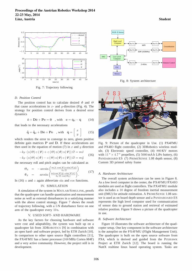
Ψ

Θ

Φ

z

y

x

desired

angl

e[o

]

time [s]

dist

ance

[m]

0 5 10 15 20 25 30 35 40 45 50

0 5 10 15 20 25 30 35 40 45 50

−20

−10

0

10

20

−1.5

−1

−0.5

0

0.5

Fig. 7: Trajectory following

D. Position Control

The position control has to calculate desiredΦ and Θthat cause accelerations inx- and y-direction (Fig. 4). Thestrategy for position control derives from a desired errordynamics

e+De+Pe = 0 , with e = qd − q (14)

that leads to the necessary accelerations

¨q = ¨qd +De+Pe , with q =

[xy

](15)

which renders the error to converge to zero, given positivedefinite gain matricesP and D. If these accelerations arethen used in the equation of motion (7) inx andy direction

−kF (s(Θ)c (Ψ) + c (Θ)s(Φ)s(Ψ))Ω = mx

−kF (s(Θ)s(Ψ)− c (Θ)s(Φ)c (Ψ))Ω = my(16)

the necessary roll and pitch angles can be calculated as

Θd = − arcsin(

m(x cos(Ψ)+sin(Ψ)y)kF Ω

)

Φd = arcsin(

m(cos(Ψ)y−sin(Ψ)x)kF Ω cos(Θd )

).

(17)

In (16) s andc again abbreviatesin andcos functions.

IV. SIMULATION

A simulation of the system in MATLAB /SIMULINK , proofsthat the quadcopter can handle quantization and measurementnoise as well as external disturbances in a satisfying mannerwith the above control strategy. Figure 7 shows the resultof trajectory following, with a5N disturbance force on onearm of the quadcopter every10 s.

V. USED SOFT- AND HARDWARE

As the key factors for choosing hardware and softwarewere cost and adaptability, the system was built up on aquadcopter kit from 3DROBOTICS [9] in combination withan open hard- and software project, led by ETH Zurich [10].In comparison to other open source flight controllers [11],the PX4FMU has a faster processor (168MHz Cortex-M4F)and a very active community. However, the project still is indevelopment.

Low Level Computer

ESC

Motors

Remote Control

Groundstation

High Level Computer Rx/Tx Rx/Tx

Rx/Tx Rx/Tx

Rx/Tx Rx/Tx

RGB−D Sensor

IMU

WiFi

2.4Ghz

3DR (433Mhz)

Fig. 8: System architecture

4 8 3 61

2

57

Fig. 9: Picture of the quadcopter in Use. (1) PX4FMUand PX4IO flight controller, (2) 3DRobotics wireless mod-ule, (3) Electronic speed controller, (4)880KV motorswith 11 ” × 4.7 ” propellers, (5)5000mA h LiPo battery, (6)PANDABOARD ES (7) PRIMESENSE 1.08 depth sensor, (8)Custom 3D printed safety frame

A. Hardware Architecture

The overall system architecture can be seen in Figure 8.As a low level computer in the center, the PX4FMU/PX4IOmodules are used as flight controllers. The PX4FMU modulealso includes a10 degree of freedom inertial measurementunit (IMU) for attitude estimation. A PRIMESENSE1.08 sen-sor is used as on board depth sensor and a PANDABOARD ESrepresents the high level computer used for communicationof sensor data to ground station and retrieval of estimatedrelative position. Figure 9 shows a picture of the quadcopterin use.

B. Software Architecture

Figure 10 illustrates the software architecture of the quad-copter setup. One key component in the software architectureis the autopilot on the PX4FMU (Flight Management Unit).The quadcopter is built on the open source software fromPX4, which is derived and guided from the PIXHAWK

Project at ETH Zurich [12]. The board is running theNuttX realtime linux based operating system. Tasks are


106

PositionControl

AttitudeEstimation

AttitudeControl

VisualisationUser Interface Reconstruct Me Groundstation

High LevelControl Board

Low LevelControl Board

Mixer for Motors

Primesense Depth Stream

NavigationPosition

Estimation

Fig. 10: Software architecture

programmed as a separate applications and communicate viaa publish/subscribe pattern.

The PANDABOARD ES is running Ubuntu 12.04 Serveredition as operating system and for now, it is used only forstreaming the sensor data from the depth camera to a groundstation running the reconstruction software and guidancethrough the tracked coordinates from RECONSTRUCTME.The communication between the low level computer, highlevel computer and the groundstation uses the open sourceMicro Air Vehicle Communication Protocol (MAVLink), asit is the standard protocol used in many UAV projects.

Another key element in the system is the position esti-mation and 3D reconstruction via RECONSTRUCTME [13].It is a 3D scanning software developed by PROFACTOR forexternal reference less part reconstruction with mobile lowcost sensors. The software uses conventional depth camerasensors like the Microsoft Kinect to generate 3D point cloudsand textured surface models. Sensor position is estimated(tracking) during data acquisition alternately with integratingacquired data to a global volume, via fast locale trackingthat makes use of an optimized iterative closest point (ICP)algorithm [14]. For situations where ICP algorithm timesout, a global tracking approach using the object recognitionsoftware CANDELOR[15] is used in RECONSTRUCTME forobject recognition of the acquired surface model in localesensor data. As the quadcopter is very dependent on fasttracking, only the locale tracking method is used to measurethe UAV position and orientation in reference to the scannedobjects.

VI. EXPERIMENT

In a first step the accuracy of the reconstruction via RE-CONSTRUCTME was tested. Figure 11 shows the comparisonof the roll angle estimate from the IMU using a Kalmanfilter on the gyroscope and acceleration measurements, andthe roll angle estimated by the RECONSTRUCTME Softwarecorrected by the delay of136ms and the mean due to thecalibration of0.008 rad with a sampling rate of20Hz. As

ReMe*IMU

time [s]

Φ[r

ad]

*corrected bydelay =−0.136smean =0.008rad

0 2 4 6 8 10 12 14−0.06

−0.04

−0.02

0

0.02

0.04

0.06

Fig. 11: Evaluation of the WiFi RECONSTRUCTME tracking

mentioned in section III-A, the desired trajectory can beprovided in the four coordinatesx,y,z andΨ . As for nowvery dynamic motions are not of interest, only the desiredx, y andz trajectories in the position level of equations (7)and (12) are provided. Hence, setting desired velocitiesqd

and accelerationsqd in these three coordinates to zero.

A. Provided Trajectory

For now, the provided trajectory is not planned dynam-ically, but given with simple parametrized equations forthe setpointsP(t, r, h, hstart,Ψmax). With parameters time,radius, height and maximal angle respectively. The sequenceconsists of an autonomous takeoff, a circular arc with thequadcopter facing its center and an autonomous landingroutine. The coordinate setpoints are updated with10Hz.

To achieve a smooth start of the motors, the autonomoustakeoff routine starts with a setpoint4m below ground andrises up to the actual scanning height of−hstart. The actualarc follows the equation

P(t, r, h,Ψmax ) =

xd

ydzdΨd

=

r(1− cos(Ψ))−rsin(Ψ)

−hΨ

with Ψ = Ψ(Ψmax , t)(18)

and the landing routine again constantly decreases the set-point to 0.2m, waits for the quadcopter to reach it andthan decreases further to−hstart below ground to force themotors to turn off.

B. Result

The result of an experiment can be seen in Fig. 12.The dashed lines in Fig. 12a describe the desired paths,and the solid lines the actual coordinates estimated bythe ReconstructMe Software. All data is logged on thegroundstation with the PX4FMU microcontroller sendingthe measurements on the quadcopter itself via the 3DR


107

wireless module (as seen in Fig. 9) using the MAVLinkProtocol.

Figure 12b shows the desired and actual path of thequadcopter in 3D space. The left hand side show front andtop view, the right hand sight a perspective 3D view of thelogged data as well as the real scene. The scan volume inblack contains the object to scan. The setpoint trajectory ismarked as dashed red line. The actual tracked path is shownin a gradient colored line with marked start and end point.Further, the heading at several intermediate points are plottedin magenta.

The reconstructed surface of the object is shown in Figure12c. The different view angles reveal, that due to the re-stricted angle of the arc trajectory, the backside of the chairis not reconstructed completely.

VII. CONCLUSIONS

Experiments on the real quadcopter show, that positionassumption purely based on the RECONSTRUCTME softwarevia using a320×240 pixel depth sensor and WiFi streamingof the information to the ground station, is sufficient for fullautonomous control of the quadcopter. Measurements revealthat the over all delay of the process chain from sensor viareadout, data streaming via WiFi, actual reconstruction andback streaming of the coordinates is about130ms. Furthersteps will be the dynamic trajectory planning with feedbackof the realtime tracking, and a sensor fusion of a flowcamera and acceleration information of the IMU for positionestimation in case of tracking lost of the reconstructionsoftware as well as mapping of scanned surfaces after selflocalization.

REFERENCES

[1] “OptiTrack,” March 2014. [Online]. Available:http://www.naturalpoint.com/optitrack/

[2] “Vicon,” March 2014. [Online]. Available: http://www.vicon.com/[3] P. Pounds, R. Mahony, P. Hynes, and J. Roberts, “Design ofa four-

rotor aerial robot,” inProc. 2002 Australasian Conference on Roboticsand Automation, vol. 27, 2002, p. 29.

[4] S. Bouabdallah and R. Siegwart, “Full control of a quadrotor,” in Intel-ligent robots and systems, 2007. IROS 2007. IEEE/RSJ internationalconference on Intelligent Robots (IROS). IEEE, 2007, pp. 153–158.

[5] R. Mahony, V. Kumar, and P. Corke, “Multirotor aerial vehicles: Mod-eling, estimation, and control of quadrotor,”Robotics & AutomationMagazine, IEEE, vol. 19, no. 3, pp. 20–32, 2012.

[6] H. Bremer,Dynamik und Regelung mechanischer Systeme. TeubnerStuttgart, 1988.

[7] S. Bouabdallah, “Design and control of quadrotors with application toautonomous flying,”Lausanne Polytechnic University, 2007.

[8] T. Puls, Lokalisations-und Regelungsverfahren fur einen 4-Rotor-Helikopter. Verlag Dr. Hut, 2011.

[9] “3Drobotics,” March 2014. [Online]. Available: http://3drobotics.com/[10] “PX4FMU Autopilot / Flight Management Unit,” March 2014.

[Online]. Available: http://pixhawk.org/modules/px4fm[11] H. Lim, J. Park, D. Lee, and H. J. Kim, “Build your own quadro-

tor: Open-source projects on unmanned aerial vehicles,”Robotics &Automation Magazine, IEEE, vol. 19, no. 3, pp. 33–45, 2012.

[12] L. Meier, P. Tanskanen, F. Fraundorfer, and M. Pollefeys, “Pixhawk:A system for autonomous flight using onboard computer vision,”inRobotics and automation (ICRA), 2011 IEEE international conferenceon Robotics and Automation. IEEE, 2011, pp. 2992–2997.

[13] C. Kopf and C. Heindl, “A portable, low-cost 3d body scanningsystem,” in 4th International Conference on 3D Body ScanningTechnologies, 2013, pp. 417–425.

Ψ

z

y

x

dist

ance

[m],

angl

e[r

ad]

time [s]130 140 150 160 170 180 190

−0.8

−0.6

−0.4

−0.2

0

0.2

0.4

0.6

0.8

(a) Log data in respect of time

z[m

]

y [m] x [m]

z[m

]

y [m]

heading

actual

setpoint

object

y [m]

x[m

]

00.5

1

0

0.5

1

−0.500.5−0.5 0 0.5

−0.5 0 0.5

−1

−0.5

0

−1

−0.5

0

(b) Log data in respect of space and the result of the scan

(c) 3D reconstruction of the object

Fig. 12: Result of an experimental full autonomous 3D scan

[14] S. Izadi, D. Kim, O. Hilliges, D. Molyneaux, R. Newcombe, P. Kohli,J. Shotton, S. Hodges, D. Freeman, A. Davison,et al., “Kinectfusion:real-time 3d reconstruction and interaction using a moving depthcamera,” inProceedings of the 24th annual ACM symposium on Userinterface software and technology. ACM, 2011, pp. 559–568.

[15] “Object Recognition System ”Candelor - Understand 3D,” March2014. [Online]. Available: http://candelor.com


108

Exploiting the Environment for Object Manipulation

Simon Hangl, Senka Krivic, Philipp Zech, Emre Ugur and Justus Piater1

Abstract— Inspired by biological systems, complex object ma-nipulation can benefit from using the environment to stabilizethe involved objects. We show that this holds as well for roboticmanipulation by evaluating how the environment can be used tooptimize a screwing task. We compared the same manipulationwith and without using the environment. We were able toimprove the success rate as well as to minimize the stress for therobots joints by stabilizing the object with pressing it againsta table and by using the robots impedance mode to reduce theapplied forces.

I. INTRODUCTION

Animals use physical support provided by the static envi-ronments in complicated tasks that they cannot achieve usingtheir sensorimotor skills with the tools that they activelycontrol. For example, chimpanzees use stones as active toolsin order to crack the nuts, but they need a stable and staticsurface to crash the stone against [6]. As another example,the chimpanzees can assemble long sticks by inserting oneinto another in order to extend their reachability but theyagain need a static support for stabilization [11]. While theyare very skilled in bi-manual manipulation, insertion of onestick into the other one is still difficult as it requires very finecontrol of both objects. The stick needs to be inserted intoa small hole while maintaining the collinear arrangement ofthe sticks. In order to achieve this task, the chimpanzees useground surface to stabilize one of the objects while focusingon the control of the other one as shown in Fig. 1.

In this paper, we aim to utilize a similar support mecha-nism in order to increase the performance of a robotic bi-manual manipulation task, namely screwing. Screwing is acomplicated task as it involves two objects that need to begrasped and aligned first, and manipulated with fine controlin complex trajectories later. Manually coding such motorprogram is possible (actually this is done in factory settingsin industrial robots), but is very time-consuming and donot scale well to changing objects and noisy environments.Learning such a complex action from scratch is not realisticas well because of the high dimensional search space.

We use learning by demonstration paradigm [4], wherethe robot observes a screwing performance, and imitates theobservation to achieve the task autonomously. As the phys-ical interaction dynamics between the robot and the objectsis very crucial in screwing task, it is not straightforward tomap observed human demonstration to robot’s sensorimo-tor space. Thus, we formulate this problem in kinestheticteaching framework, where the demonstration is performed

1 All Authors belong to Faculty of Mathematics, Com-puter Science and Physics, University of Innsbruck, [email protected]

Fig. 1. These photographs taken during Wolfgang Kohler’s seminalexperiments[11] show that chimpanzees have the ability to benefit fromsupport provided by the environment in order to stabilize one of the objectsduring bi-manual stick assembly task.

with robot’s own body, i.e. the robot is physically guidedthrough screwing. The robot then is able to reproduce thetask based on its one-shot experience. The exact replicationof the demonstrated action trajectory does only perform wellin the exactly same noise-free environment, which is not a re-alistic assumption. In this paper, we use Dynamic MovementPrimitives (DMPs) to learn and reproduce complex screwingaction where the action trajectory is encoded with a smallnumber of parameters [13]. DMPs, inspired from humanmotor control, enable robots to learn complex tasks rangingfrom drum playing [8] to biped locomotion [12]. Recordedmovements are represented as a set of differential equationsthat provide robustness against perturbations, reaching tothe attractor point, adaptation to different initial and goalpositions, and learning of non-linear movement trajectories.

The main focus of this paper is to realize the use ofenvironment support in screwing task in order to increase theperformance. This support is not explicitly encoded in robotcontrol; but instead, the DMP-based screwing action that islearned through kinesthetic teaching is applied in variousconfigurations with and without environment support. Wealso analyze the effect of joint stiffness in different settings,and conclude that the robot with flexible joints achieves thistask best when one of the objects is pressed against a table.

The remainder of this paper is structured as follows.Section III provides an overview of our robotic system andits environment. Section IV then introduces our approach torobot object manipulation and how the robot actually exploitsthe environment. Next, in Section V we discuss the resultsof our experiments as well as positioning them w.r.t. related


109

work. We conclude in Section VI with a summary of themajor contributions and an outlook on future work.

II. RELATED WORK

Aiyama [1] analysed the kinematics of environment-contacting tasks by a position-controlled manipulator with afree-joint structure. For this, both, a kinematic and geometricanalysis of the manipulated object is done. Further, by theoutcomes of these analyses, conditions to achieve desiredmanipulation against friction and loss of contact are deter-mined. Aiyama applied his approach successfully for objectsliding and insertion tasks. Verma et al. [16] investigatedthe robot box-pushing of stationary objects in interactionwith a planar environment that is equipped with embeddedsensors. The purpose of the sensors is to detect pushableobjects. Verma et al. showed that pushes then are moreaccurate if the pose information of the objects, retrieved bythe sensors, is used when pushing. Related work is done inthe area of dynamic interaction, such as cooperative robot-human tasks. Amor et al. [2] employ interaction modelsbetween two humans in on-going interaction tasks with theaim to learn how to respond to human partners. Similar workhas been done by Berger et al. [3], who infer guidanceinformation from a cooperative human-robot task. Theypropose a machine learning approach, which learns statisticalmodel during an interaction phase to predict the outcome offuture interactions. If the actually measured forces deviate,this is considered as robot guidance. Traversaro et. al. [14]estimated friction, inertial and motor parameters by partialleast-square method to be able to detect contacts with theenvironment.

III. SYSTEM DESCRIPTION

Our work is implemented using two KUKA 7 DoFsLightweight robot 4+ with Servo-electric 3-Finger SCHUNKSDH-2 hands mounted on them (Fig. 2). There are threedifferent control strategies offered by the robot arms:• Position control: Exact positioning in both joint angles

and cartesian coordinates is enabled.• Impedance control: In this mode the robot simulates a

virtual spring-damper system, whenever external forcesare applied to it. It is possible to define the impedancesettings either in Cartesian or joint space. The robotallows to set the stiffness of the virtual spring, the springdamping as well as settings for maximum torque or de-viation from the desired position. Important settings thathave been used to implement the described experimentsare listed with their respective minimum and maximumvalues in table I. Impedance control can be of greatuse in robot manipulation as it reduces the stress on therobot joints and enables the robot to react on unexpectedbehaviour (e.g. assembly of complex parts by Giordanoet. al [9])

• Gravity compensation: This controller allows free guid-ance of the robot while it compensates for gravity.

The KUKA LWR is able to safely pick up objects of anapproximate weight of m = 15 kg (Maximum force F =

Short Description MinValue

MaxValue

Unit

Cartesian spring stiffness 0.01 5000 N / mCartesian spring damping 0.01 1 N s / mMaximum applied force (Cartesianspace)

0 150 N

Maximum Cartesian deviation 0.01 100 mmMaximum torque per joint 0 - N m

TABLE IROBOT CONSTANTS

150 N). It provides force and torque sensors for each joint.Further, the controller computes the forces and torques inCartesian space from the force/torque information in jointspace. The arms can be programmed by a combination ofthe KRL (KUKA robot language) and the FRI (Fast ResearchInterface), which allows to control them via an Ethernet con-nection. The high level control has been done by a modifiedversion of OROCOS [7] and the Kukadu framework [10],which provides support for dynamic movement primitives,regression techniques and reinforcement learning. For furtherinformation concerning the robot arm the interested readermight consult [5].Two Schunk SDH-2 hands have been mounted on the arms. Itis a dexterous robotic hand providing pressure sensor panels.It has a total length of 253 mm and consists of three modularfingers. Two fingers can rotate along their vertical axis, whichcan be used to implement different grasping types. Eachfinger itself has two degrees of freedom, which can be used toopen and close the hand. Hence, in total it provides 7 degreesof freedom. The maximal momentum per joint is of specialinterest, as it defines the strength of the grasp. The joints 2,4 and 6 can apply a momentum of M = 2.1 Nm, while thejoints 3, 5 and 7 can provide a momentum of M = 1.4 Nm.However, the actually exerted momentum highly dependson the current hand temperature. High temperature leads tolower momentum and therefore weaker grasps. The handexpects a maximum current of I = 5A and a voltage ofU = 24V. Each finger has two pressure sensor arrays, whereall arrays are made of 6×14 sensor texels and each texel hasa size of s = 3.4 mm. The communication for hand controland sensor data retrieval can be done by two separate serialports.In order to do the evaluation of the proposed approach,two environments have been used. In environment 1 thependulum is pressed against the table during execution of thetask (Fig. 2 left). Environment 2 does not use the table tosupport the screwing execution by stabilizing the pendulum.The table is used only for picking up the pendulum head(Fig. 2 right).For the screwing task implementation we used the pendulumand the pendulum head shown in Fig. 3. To increase thetables friction coefficient, we used a rubber foam sheet onthe table as it can be seen in the Fig. 2.


110

Fig. 2. The robot setup and different configurations used in experiments. Environment 1 uses table (left), whereas in Environment 2 the table has beenremoved (right)

Fig. 3. Objects used for screwing (pendulum head and pendulum); theyare placed on the table and picked up by spherical (pendulum head) andcylindrical grasp (pendulum)

IV. APPROACH

This section describes the overall approach used in this pa-per. Firstly, the framework of dynamic movement primitives(DMP) is described. This section is followed by the descrip-tion of the experimental approach that has been chosen toevaluate the influence of the usage of the environment formore complex manipulation tasks. We used a screwing taskto evaluate the influence of the usage of the environment onthe performance of the manipulation. The used robot settingas well as the used objects have been described in sectionIII.

A. Evaluation environments

To evaluate the influence of the environment we used twodifferent environments (see Fig. 2):• Environment 1: The first environment applies the pre-

viously described screwing approach by pressing thependulum onto the table to stabilize it (left arm). Thetwo objects (pendulum and pendulum head) have beenplaced on a fixed position on the table, where the robotgrasped it. The pendulum has been pressed on the tablewith force while the right arm applies the screwingoperation. This force is due to the teaching processwhere the pendulum end is positioned slightly belowthe level of the table. This enforces the robot to pressthe pendulum against the table because it tries to reachthe desired position.

• Environment 2: Here, the pickup procedure started thesame as in environment 1. As soon as the objects havebeen grasped, the table has been removed, while therest of the execution was the same. This has been doneto ensure comparability of the two approaches as bothscenarios use the same training data to do screwing.

As the table had to be moved to execute the experimentin env. 2 to avoid contact between table and pendulum, theenvironment had to be calibrated before every new executionto get reliable data. This had been required because it wasnot possible to move back the table to the exact desiredposition, which led to changed object locations. As thegrasping positions had been fixed, calibration of the tableposition was necessary. This has been done by performingthe screwing in env. 1 until it succeeded. Afterwards weperformed the next evaluation in env. 2. The results of intotal 20 trials (10 per environment) are presented in sectionV.

B. Learning of Screwing Operation

The screwing operation has been learned by a combinationof programmed grasps and a screwing trajectory learned fromkinesthetic teaching (a human provides a sample trajectoryby guiding the robot). Therefore, the whole manipulation canbe split up in two phases. The first part is responsible forgrasping the two objects (pendulum head with right handand pendulum with left hand). The objects are placed atpredefined locations and orientations, where the graspingpositions have been provided manually to the system. Aftermoving the arms to the desired grasping point, the handsare closed with maximum force in order to be able topick up the objects. Afterwards the objects are prepared forscrewing (see Fig. 2). Depending on the used environment,the pendulum is pressed against the table (Env. 1) or movedto the same position without the presence of the table (Env.2). In phase two the screwing itself is executed by a trajectoryencoded with DMPs in joint space. The screwing operationis started by co-linearly aligning the arm, which is holdingthe pendulum head, to the pendulum. Afterwards, the last


111

joint of the right arm is actuated, which yields a rotation of360 degrees around the pendulum axis, while simultaneouslypressing the pendulum head on the pendulum. To execute thesupervised trajectory, we use dynamic movement primitives[13]. To determine the coefficients of a discrete DMP fromthe supervised trajectory, linear regression is used.

C. Dynamic Movement PrimitivesA Dynamic movement primitive is a parametrized control

policy formulation which comes up with some desirableproperties out of the box. Here, a short overview on themathematical formulation and the most important propertieswill be given. For further information the reader might beinterested in [13].

The core of the mathematical formulation is given inequations 1 and 2. It consists of two dependent first orderdifferential equations, which together form a system ofdifferential equations. A dynamic movement primitive is asystem of differential equations of the form

τ z = αz (βz (g− y)− z)+ f (1)

τ y = z (2)

where g is the goal state, αz and βz are time constants(spring stiffness, damping), τ is a temporal scaling factorand f is an arbitrary continuous function of the form

f (x) =∑N

i=1 ψi(x)wi

∑Ni=1 ψi(x)

x (3)

where ψi are Gaussian basis functions. Here, the variableswi have to be learned as they define the shape of the resultingtrajectory. The constants αz, βz and τ should be selected suchthat the system converges to 90 percent of the goal stateafter t = tmax. By design, DMPs guarantee that the trajectorywill always reach the attractor point g. The execution canbe stretched by changing the temporal scaling factor. Thenon-linear function f is responsible for the shape of thetrajectory, thus containing the DMPs parameters that haveto be learned. A detailed analysis on why DMPs can ensurethese properties is given in [10]. The variable x itself is againdefined by another differential equation (DE), which dependson the type of movement one wants to describe with DMPs.

DMPs provide two different types of movements, namelydiscrete movement and rhythmic movement.

1) Discrete Movement: A discrete movement is a move-ment of finite time. An example for this kind of movementis a reaching task. The DE defining x(t) is given in equation4.

τ x =−αxx, x(0) = 1 (4)

This differential equation can be adjusted to react on devia-tions during the trajectory execution. One possibility is theso-called phase stopping which slows down the trajectoryexecution in case of high deviations from the desired path.This can be formulated by the equation

τ x =−αxx

1+αc (yactual− y)2 (5)

which takes into account the current state of the trajectoryexecution.

2) Rhythmic Movement: A rhythmic movement can beimagined as an infinite repetition of a cyclic movement (startand end point are the same). To be able to represent this, theGaussian basis functions ψi are replaced by

ψi = e−hi(cos(x−ci)−1) (6)

An example for this kind of movement is playing the drumswith the same rhythm [15]. In this paper we only analyse theinfluence of the environment usage on discrete movements.

V. RESULTS AND DISCUSSION

In this section the experimental results will be presentedand discussed. The experimental setting has been describedin section III. In total, 20 trials (10 per environment) havebeen performed. During the experiment, the success rate aswell as the forces measured at end effector positions ofboth arms have been collected. Here, we define a trial to besuccessful if the pendulum head cannot be removed from thependulum without further rotation. A comparison of the forcedata between trials in both environments, hand temperaturedependent success rates in different environments and affectsof impedance mode on the performance are given in thefollowing section.

A. Measured Forces in both Environments

By analysis of our data, four representative samples havebeen identified:• Sample 1 (red): Screwing in env. 1 with position mode.

The execution succeeded.• Sample 2 (green): Screwing in env. 2 with position

mode. The execution failed because of the pendulumslipping through the hand holding it.

• Sample 3 (cyan): Screwing in env. 2 with position mode.The execution succeeded.

• Sample 4 (magenta): Screwing in env. 1 with impedancemode. The stiffness settings have been selected withvalues of 4000 and 250 for Cartesian stiffness and end-effector stiffness respectively. The damping was chosenwith 0.7.

Figures 4-6 visualize the measured forces for all four sam-ples. Fig. 4 presents the absolute value of the measured forcesvectors, whereas Fig. 5 and Fig. 6 show the components ofthe Cartesian force vectors. We omitted the data measureduntil t = 50s as it contains data for grasping the objects,which is the same in all samples. They plot the evolutionof the forces for all four samples over time. In 4, the mostimportant phases are already identifiable.

B. Identification of Phases

In section IV-B the different phases of the manipulationhave been listed. In Fig. 4, these phase can be identified.The first notable event has been observed at t = 60s, whichshows a strong increase of the forces in samples 1 and 4 dueto the robot pressing the pendulum on the table. Note thatthis does not occur in samples 2 and 3, as the robot holds


112

Fig. 4. Absolute value of the measure forces vectors for each arm (Rightarm performs screwing, Left arm holds the pendulum). Colors: Red (Sample1), Green (Sample 2), Cyan (Sample 3), Magenta (Sample 4)

the pendulum freely. The screwing operation starts at timet = 90s. This manipulation leads to increase of the exertedforces on both arms. The screwing phase is the longest oneand continues until t = 165s, where the right arm stops torotate the pendulum head. However, the right hand is stillclosed which is the reason, why some force is measured.Finally, in t = 170 the right hand releases the pendulum head.

C. Comparison of Absolute Forces

We will compare each sample to sample 1, as it had avery high success rate of 90 percent. In general, it can beseen, that by pressing the pendulum against the table, therobot is able to exert higher forces, which is a sign of highstability of the setting. However, this leads to higher stressof the robot joints (compare red and cyan line). Additionally,in the graph for an unsuccessful trial in env. 2 (Fig. 4) it canbe seen that the reason for the failure is due to the inabilityof the robot to apply the forces required to do the screwing(green line). The higher forces in the end of the executionresult from the right arm still pushing the pendulum head onthe pendulum without being able to screw further.Further, experiments in impedance mode have been per-formed (magenta line). It should be noted that this sam-ple resulted in much lower forces while still being ableto perform the screwing successfully. The forces are lowcompared with the unsuccessful sample 2. The differencecan be found in the beginning of the screwing where ahigher force during the phase of catching the pendulum andpendulum head is measured. Therefore it can be concludedthat in the unsuccessful sample 2 the two objects lose contactin the beginning.Indeed, evidence for this assumption can be found in themeasured force at t = 95s, where the measured force jumps8N to 5N (left arm) and 8N to 2N (green line). In the videothat has been recorded during execution the reason can befound: the pendulum is slightly slipping through the left hand

Fig. 5. Measured forces measured for each Cartesian dimension (Right arm- performing screwing operation), Colors: Red (Sample 1), Green (Sample2), Cyan (Sample 3), Magenta (Sample 4)

because the grasp of the left hand is not strong enough tostabilize the system. This motivates why the success ratefor env. 1 is higher than the one for env. 2 (see section V-E). Still, this weakness is not always present, as sample 3is showing (cyan line). In Fig. 4 the force measured at theright arm is even getting higher than the one for sample 1at t = 95s. The success of the screwing in env. 2 is prone toslight variations in the initial grasp, which gives rise for theapproach to use the environment. An inexact grasp in env. 1can still be compensated by the stabilization that is achievedby pressing the pendulum on the table. This is not the casefor env. 2, which leads to a lower success rate. This issuegets an even bigger problem as soon as the object locationsare not fixed any more but estimated by some vision system,as these systems are not exact. However, the usage of thetable (env. 1) does not come without any practical problems.

D. Disadvantages of Using Environment

One typical problem that has been observed over alltrials is the slipping of the pendulum on the table whilemanipulating the two objects. Note that this should not beconfused with the problem of pendulum slipping throughthe hands while holding it. This behaviour can be seen inFig. 6 (Z component) for sample 1. At time t = 95s (beginof screwing) the force increases strongly until a certainmaximum is reached, which then leads to a spontaneousreduction. This effect can be seen even stronger at t =150s. Even though this had no influence on the successof the manipulation, it can potentially apply strong forcechanges on the robot, which can be harmful. These resultsfor sample 1 may lead to future approaches to estimate thefriction coefficient between objects. Similar work has beendone by Aiyama [1], who used kinematic and geometricanalysis to successfully estimate the friction coefficient forobject sliding and insertion tasks. A possible solution to theslipping-pendulum problem has been found in the usage of


113

Fig. 6. Measured forces measured for each Cartesian dimension (Left arm- performing screwing operation), Colors: Red (Sample 1), Green (Sample2), Cyan (Sample 3), Magenta (Sample 4)

the impedance mode where the measured forces have beensmoothed and the slipping has not been observed at all. It canbe seen that the usage of impedance mode led to smoothingof the measured forces (see Fig. 5) by preserving the successrates of sample 1 (see section V-E).

E. Success Rates

The success rates have been measured for the two differentenvironments. The success rate for env. 1 has been deter-mined with 90 percent, whereas the success rate for env. 2has been much lower with 60 percent. By using impedancemode on top of reusing the environment, no significantchange of the success rate has been observed. However, theapplied forces were much lower and smoother as for thesample with position mode. Additionally, the influence of therobot hand temperature should be mentioned as overheatingof the hand led to a strong reduction of the success rates forboth environments. This is due to the fact that the hand wasnot able to apply sufficiently stable grasps if the temperaturehas been to high. Here, even the method with using of theenvironment was not able to improve the performance.

VI. CONCLUSION

In this paper we investigated the potential effect of envi-ronment exploitation to achieve a complex task. As maincontribution we have shown that object manipulation inrobotics can benefit from considering to use the environ-ment tot stabilize the execution. We evaluated environmentexploitation for a screwing task that requires bi-manualmanipulation which potentially benefits from environmentusage, as a table can be used to stabilize the objects.Experimental results show that the success rate can beimproved significantly. Additionally, the stress on the robotjoints can be reduced by setting the robots stiffness settingsappropriately. Further, with this approach, problems such asslipping of the manipulated objects can be overcome. In

future we plan to study how object manipulation can beoptimized by the estimation of the friction coefficient.

ACKNOWLEDGMENT

The research leading to these results has received fundingfrom the European Communitys Seventh Framework Pro-gramme FP7/20072013 (Specific Programme Cooperation,Theme 3, Information and Communication Technologies)under grant agreement no. 610532, Squirrel.

REFERENCES

[1] Y. Aiyama. Kinematics of object sliding task by position-controlledmanipulator with free-joint structure. In Advanced Intelligent Mecha-tronics, 2003. AIM 2003. Proceedings. 2003 IEEE/ASME InternationalConference on, volume 1, pages 320–325. IEEE, 2003.

[2] H. Ben Amor, D. Vogt, M. Ewerton, E. Berger, B. Jung, and J. Peters.Learning responsive robot behavior by imitation. In Intelligent Robotsand Systems (IROS), 2013 IEEE/RSJ International Conference on,pages 3257–3264, Nov 2013.

[3] E. Berger, D. Vogt, N. Haji-Ghassemi, B. Jung, and H. Ben Amor.Inferring guidance information in cooperative human-robot tasks. InProceedings of the International Conference on Humanoid Robots(HUMANOIDS), 2013.

[4] A. Billard, S. Calinon, R. Dillmann, and S. Schaal. Robot program-ming by demonstration. In Springer handbook of robotics, pages1371–1394. Springer, 2008.

[5] R. Bischoff, J. Kurth, G. Schreiber, R. Koeppe, A. Albu-Schaeffer,A. Beyer, O. Eiberger, S. Haddadin, A. Stemmer, G. Grunwald, andG. Hirzinger. The kuka-dlr lightweight robot arm - a new referenceplatform for robotics research and manufacturing. In Robotics (ISR),2010 41st International Symposium on and 2010 6th German Confer-ence on Robotics (ROBOTIK), pages 1–8, June 2010.

[6] C. Boesch and H. Boesch. Optimisation of nut-cracking with naturalhammers by wild chimpanzees. Behaviour, 83(3-4):3–4, 1983.

[7] H. Bruyninckx, P. Soetens, and B. Koninckx. The real-time motioncontrol core of the Orocos project. In IEEE International Conferenceon Robotics and Automation, pages 2766–2771, 2003.

[8] A. Gams, A. J. Ijspeert, S. Schaal, and J. Lenarcic. On-line learningand modulation of periodic movements with nonlinear dynamicalsystems. Autonomous robots, 27(1):3–23, 2009.

[9] P. R. Giordano, A. Stemmer, K. Arbter, and A. Albu-Schaffer. Roboticassembly of complex planar parts: An experimental evaluation. InIntelligent Robots and Systems, 2008. IROS 2008. IEEE/RSJ Interna-tional Conference on, pages 3775–3782, Sept 2008.

[10] S. Hangl. Learning atomic manipulations with dynamic movementprimitives. Master Thesis, University of Innsbruck, 2013.

[11] W. Kohler. The Mentality of Apes. Harcourt Brace and World, NewYork, 1925.

[12] J. Nakanishi, J. Morimoto, G. Endo, G. Cheng, S. Schaal, andM. Kawato. Learning from demonstration and adaptation of bipedlocomotion. Robotics and Autonomous Systems, 47(2):79–91, 2004.

[13] S. Schaal. Dynamic movement primitives - a framework for motorcontrol in humans and humanoid robots. In the international sym-posium on adaptive motion of animals and machines, page p1708,2003.

[14] S. Traversaro, A. Del Prete, R. Muradore, L. Natale, and F. Nori. Iner-tial Parameter Identification Including Friction and Motor Dynamics.In Humanoid Robots, 13th IEEE-RAS International Conference on,Atlanta, USA, October 2013.

[15] A. Ude, A. Gams, T. Asfour, and J. Morimoto. Task-specific gen-eralization of discrete and periodic dynamic movement primitives.Robotics, IEEE Transactions on, 26(5):800 –815, oct. 2010.

[16] A. Verma, B. Jung, and G. S. Sukhatme. Robot box-pushing withenvironment-embedded sensors. In Computational Intelligence inRobotics and Automation, 2001. Proceedings 2001 IEEE InternationalSymposium on, pages 212–217. IEEE, 2001.


114

Where to look first? Behaviour control for fetch-and-carry missions ofservice robots

Markus Bajones1, Daniel Wolf1, Johann Prankl1, Markus Vincze1

Abstract— This paper presents the behaviour control ofa service robot for intelligent object search in a domesticenvironment. A major challenge in service robotics is to enablefetch-and-carry missions that are satisfying for the user in termsof efficiency and human-oriented perception. The proposedbehaviour controller provides an informed intelligent searchbased on a semantic segmentation framework for indoor scenesand integrates it with object recognition and grasping. Insteadof manually annotating search positions in the environment,the framework automatically suggests likely locations to searchfor an object based on contextual information, e.g. next totables and shelves. In a preliminary set of experiments wedemonstrate that this behaviour control is as efficient as usingmanually annotated locations. Moreover, we argue that ourapproach will reduce the intensity of labour associated withprogramming fetch-and-carry tasks for service robots and thatit will be perceived as more human-oriented.

I. INTRODUCTION

The ability of a robot autonomously interacting with a hu-man requires sophisticated cognitive skills including percep-tion, navigation, decision making and learning. Impressiveachievements have already been made in the research fieldof HRI considering robots as tour guides in museums [1],[2], shopping malls [3] and also for assistive robots in thecare and domestic context [4].

However, one of the biggest challenges still is the integra-tion of methods into operational autonomous systems for thedomestic context, which achieve satisfying results for theirend-users. Often a miss-match between user expectations androbot performance can be observed in HRI studies [5], forinstance because the robot behaviour is not legible to theusers or is simply too slow. Imagine you command yourhousehold robot to bring you your mug and the robot couldonly search for it at pre-programmed places: What if the mugis at none of these places or the user rearranged the flat?Another solution could be that the robot would navigate tothe center of the room, rotate several times and then start atime-consuming brute-force object detection everywhere inthe map. This behaviour would already increase flexibility,but would still not be very legible for the user: Why gettingan overview and then start a time-consuming search?

Would it not be much more intelligent and legible if therobot first obtained an overview of the environment and thenlooked at the most probable locations for the mug to be,e.g. on tables or in the cupboard? One way to gain theinformation about this kind of relations is to extract it fromknowledge databases [6].

1Faculty of Electrical Engineering and Information Technology, ViennaUniversity of Technology, 1040 Vienna, Austria bajones, wolf,prankl, [email protected]

Our solution for this problem is to develop a flexiblebehaviour controller for fetch-and-carry tasks implementedwith SMACH, a Python-based library for building hierarchi-cal concurrent state machines, as pictured for our proposedimplementation in Fig. 1. We present a framework that isable to generate locations on-the-fly without the need ofpre-learned object-location relationships and show in a firstexperiment in an ambient-assistive-living lab to proof therobustness of our approach.

The remainder of this paper is structured as follows: First,we review related research on service robots performingfetch-and-carry tasks in Section II. We then outline howthe SMACH framework works in Section III. Each of themodules and their integration in the behaviour controller isthen described in Section IV with a focus on the modules,but not the individual methods. Finally, a first experiment ina living room setting is presented in Section V. A summaryof lessons learned from the experiment and an outlook onfuture work conclude the paper.

INIT

preemptedaborted succeeded

GET_ALL_POSITIONS

aborted

GET_ROBOT_POSE

succeeded

CLEAN_POSITIONS

GET_CURRENT_ROOM

succeeded

MOVE_BASE_GO

CLEAN_UP

failure

LOCATION_REACHED

succeeded

PLAN_PATH

movement

failure

POSE_ITERATOR

aborted

LOCATE_OBJECT

succeeded

SEGMENTATION

succeeded

aborted

aborted

SET_SUCCESS

succeeded

next_room

succeeded

aborted

succeededabortedsucceeded

succeeded

wait for data

succeeded

aborted

Fig. 1: Simplified state machine representation of our “fetch-and-carry” approach. Grey states denote sub-state machines.


115

II. RELATED WORK

Object search and fetch-and-carry tasks represent one ofthe most common tasks of service robots. In traditional fetch-and-carry tasks the robot ”simply” has to pick up an objectfrom a known location and deliver it to the user. For instance,in the RoboCup@Home competition 2008/9 [7] this has beenone of the major tasks. The complexity of this task can vary,e.g. the robot has to identify the correct object from a setof objects or in a cluttered scene or the robot gets a veryconcrete instruction from where to fetch it, such as “Bringme the mug from the kitchen table”. Thus, fetch-and-carryalso includes object recognition and autonomous grasping,popular examples are e.g. [8] and [9].

Recently, the perception part has come more into thefocus of fetch-and-carry tasks by adding the search forobject components. A popular example is George, the curiosattentive semantic robot [10]. The idea of George is similar tothat presented in this paper: Make a robot’s search behaviourmore intelligent. An intelligent search procedure is moreefficient and therefore the fetch-and-carry task become moresatisfying for the end-user. [6] shows an approach to enhancethe fetch-and-carry task by using a web-based knowledgedatabase to reduce possible “search positions”. [11] and [12]have already shown that there is the need to make robot’sbehaviour more efficient and legible for the user.

Therefore, the aim of the work presented in the followingis to enable a domestic service robot to perform fetch-and-carry tasks in a user-satisfying manner. To that end, acognitive robotic system needs to integrate multiple differentsubsystems. Different tools, libraries and frameworks todevelop robotic architectures already exist, such as Rob-letRTechnology by Baier et al. [13], graphical tools such asChoreographe and NAOqi for Nao robots [14], the BehaviourMarkup Language (BML) [15] and the Robot Operatingsystem ROS [16]. A good overview and discussion on theadvantages and disadvantages of all these approaches is givenin [17].

In the following we will present SMACH, a Python-basedframework that allows ROS module integration, we usedto develop a behaviour control combining intelligent objectsearch, grasping objects, and bringing them to the user.

III. SMACHSMACH is a Python-based library for building hierarchical

concurrent state machines, which also provides a ROS inte-grated module to design and execute simple tasks as well ascomplex robot behaviours. SMACH provides the possibilityto quickly create prototype state machines by reusing Pythondesign patterns. Within SMACH a task is defined by the fol-lowing elements: For seamless integration SMACH providesinterfaces to the three communication methods available inROS, i.e. messages, services and Actionlib. Provided is theMonitorState for listening to published topics, executing aservice represented as a state with ServiceState, calling anActionlib interface within SimpleActionState as well as thepossibility of wrapping a state machine inside an Actionlibserver. With SMACH viewer, a tool to debug and visualize

the running state machine, the provided user data as wellas the currently executed states and containers, is alsointegrated.

IV. IMPLEMENTATION

For the fetch-and-carry scenario we compare two differentimplementations of SMACH state machines within a ROSenvironment. Both methods rely on a 2D map of our labora-tory in which we annotate virtual rooms, defined by a closedpolygonal chain for each room, as seen in Fig. 2 to create amultiple room scenario. The annotation of the rooms is usedby a ROS service which returns the name of the room inwhich a given pose is in or unknown if the pose is outsideof any defined room.

A. Manual definition of search positions

Starting from the 2D map we manually place “search posi-tions” at user-defined locations inside the map. To determinethe pose at which the robot begins its task we define a costfunction

c(x, l) = cbat(l)− k1cprob(x, l) + k2cpenalty(l) (1)

modelling the cost to search for a given object x at thepossible search location l. cbat(l) represents the cost ofthe battery usage estimated by the path length to the poseassociated to search location l. cprob(x, l) is the probabilityof object x being found at location l transformed to a costand is initialized with a uniform distribution across all searchlocations. The factors k1 and k2 are introduced to normalizethe cost levels. cpenalty(l) is a penalty term depending onthe room the user is currently in:

cpenalty(l) =

1 l in same room as user0 otherwise

(2)

The penalty term is based on the assumption that the userdoes not ask the robot to look for objects which are in thesame room as the user himself. It ensures that the robotdoes not search in this room unless the object has notbeen detected at the locations in all other possible rooms.Further we use cmin to store the minimum cost value overall c(x, l) for a given object x, the corresponding locationli is stored for navigational purpose. During the search taskall the objects, which can be recognized, and are localizedat a certain position trigger the adaptation of cprob by aBayesian update rule with their initial probabilities given bythe uniform distribution over all defined “search locations”.Through this simple method further (cf. Fig. 3) our robotwill learn in course of time where the user places objects andwhere it should start its search. This provides a way to learnthe location of specific objects based on the users preferenceand does not leverage upon a pre-defined knowledge databaseor data mining from online sources.

B. On the fly extraction of search locations

Our proposed approach automatically generates searchpositions on the fly after entering a room and executingthe algorithm in Fig. 4 which uses semantic segmentation,


116

Fig. 2: Virtual room arrangement in our ambient-assistive-living lab.

Require: User’s current room ruserwhile object located is FALSE do

Set initial cost cmin =∞for all search positions li in l do

Calculate path length cbat(li)Look up cprob(x, li)Look up search position’s room rsp(li)if ruser 6= rsp thencpenalty = 0

elsecpenalty = 1

end ifCalculate c(x, li)if c(x, li) < cmin thencmin = c(x, li)lgoal = li

end ifend forMove to search position lgoalRemove location lgoal from list of search positions lStart object recognitionif object is recognized then

Set object located to TRUEend ifUpdate probabilities of all recognized objects

end whileMove to the userif object located is TRUE then

Inform the user about the object locationelse

Inform the user about the failure to locate the objectend if

Fig. 3: Algorithm: locate object procedure.

returning at least two search positions or none at all (whenno table planes were detected). For this for each recognizedtable plane the first and second principal component axisare calculated and the search positions are placed along thesecond principal axis at a predefined security distance as seenin Fig. 6.

Move to center pose in a roomwhile rotation < 360 do

Rotate 30 ccwCall semantic segmentation serviceReceive possible search posesRemove poses from outside of the known map andoutside the current room

end while

Fig. 4: Algorithm: obtain search poses.

Semantic segmentation: Our proposed point cloud pro-cessing pipeline consists of four steps, depicted in Fig. 5.First, we create an over-segmentation of the scene, clusteringit into many small homogeneous patches. In the second step,we compute a manifold but efficient-to-compute feature setfor each patch in which we include the three eigenvaluesof the scatter matrix of the patch, height values, angle ofthe mean surface normal of the patch with the ground planeand its circular standard deviation as well as mean colorvalues of the patch and its respective standard deviations.The resulting feature vector is then processed by a classifier,which yields a probability for each patch being assigned aspecific label. To that end, we use a randomized decisionforest, a classifier which is intensively discussed in [18].We train the classifier on the publicly available NYU DepthV2 dataset [19], containing 1,449 indoor frames, recordedby a Microsoft Kinect and densely labelled with more than1,000 labels. In the last stage of our processing pipeline theclassification results set up a pairwise Markov Random Field(MRF), whose optimization yields the final labelling. Thislast step smoothes the labelling out to correct ambiguousclassification results due to noisy local patch information.The final labelling then corresponds to the Maximum-a-posteriori of the output of the MRF. In particular, becauseour robot can only grasp objects located on tables, we onlyconsider positions next to large clusters of points labelled “ta-ble” as suitable positions to detect (and consequently grasp)objects. Therefore, after calculating the semantic labels of thecurrent scene, we use simple Euclidean clustering to obtainall tables in the scene. The resulting search positions are thendefined by a simple heuristic, which is explained in Fig. 6.For further details about our semantic segmentation pipelinewe refer to [20].

From this method we gain the knowledge of searchlocations inside the map, which provide a horizontal planein a certain height range (to filter out the floor and thelower surface of wall-mounted cupboards or the ceiling).As these locations depend on the first and second principalcomponents derived from the segmented planes we have to


117

(a) (b)

(c) (d)

floor wall ceiling table

chair cabinet object unknown(e)

Fig. 5: Intermediate steps of our segmentation pipeline.(a) input image. (b) oversegmentation. (c) conditional labelprobabilities (here for label table, red=0, blue=1) (d) finalresult after MRF. (e) Colour code of final result.

d

d

Fig. 6: Heuristic to define search positions for a tablecluster projected on the ground-plane (red points). Blue lines:Principal axes of the cluster. The search positions (greendots) are placed on the second principal axis, adhering asecurity distance d from the edge of the table.

filter out positions which are not reachable (e.g. inside ofanother piece of furniture, or outside of the map) as wellas locations behind a wall. For this we first check if thedetected table surfaces and the robot are within the sameroom boundaries and remove any search locations which donot fulfil this criteria. Secondly we do not consider positionsthat are inside of an occupied grid cell of the static map.

C. Object recognition

After the robot reaches a “search position” it attempts torecognize the object inside the scene and obtain the 6-DOFpose (position and orientation) of the object. The recognizeris called with the RGB-D data collected by the Kinect on therobot’s head. It combines three different recognition pipelines(2D and 3D) and merges the results during the verificationstage. For details of the recognition process we refer to[21]. Results from successfully recognized objects are thenames as well as the poses of all objects. Prerequisite forthe recognition process is a trained model of every objectwhich should be localized.

D. Inform the user

After the robot recognizes the object at a certain pose theuser has to be informed about the current location, thereforethe “search user” procedure is activated. This procedure willplan a path from the current room to the one in which theuser has been detected the last time (either by the robot itselfor by a motion detection system) and move the robot there.After the arrival in this room an attempt to detect the user bycombining 2D face detection technique, introduced by Violaand Jones [22] as well as 3D detection and tracking of humanbody parts [23], [24] will start. If the user is not detectedthe search will continue until all rooms have been visitedby the robot. After detection the user gets informed aboutthe location of objects, during which we use the annotationof the rooms in a reverse order to give the user the nameof the room (e.g. kitchen) instead of the 6-DOF pose. Thisinformation is not a precise substitution of the exact posebut only the first information for the user. The pose is stillavailable so that the robot is able to lead the user to thelocation at which the object was detected.

V. EXPERIMENTS

All experiments were conducted on the first prototype ofour custom made HOBBIT platform [25] (cf. Fig. 7). Its baseis a mobile platform with two drive motors with an integratedgear and attached wheels with differential drive. The percep-tion system consists of one RGB-D camera (ASUS Xtion ProLive) mounted ground-parallel at a height of 40 cm and oneRGB-D camera (Kinect) mounted at 124 cm height as partof the robot’s head on a pan-tilt unit. The lower camera isused for self-localization, the upper one for user and objectdetection, gesture and object recognition and both camerascontribute to the obstacle detection during navigation. Formanipulation PT1 is equipped with an IGUS Robolink armwith a two finger Finray-based gripping system. Further partsof the platform include a 15 inch tablet computer for touch


118

input and speech recognition as well as a 7 inch display forthe purpose of displaying the robot’s face. To stash awayretrieved objects a tray is mounted behind the tablet andabove the robot arm.

Fig. 7: HOBBIT platform - prototype 1.

To evaluate and compare the two implementations de-scribed in Section IV we conducted four tests, each consist-ing of one execution of both implementations. The object thathad to be located was placed according to Tab. I. As objectswe used an Asus Xtion Pro box, a brown handbag and anorange wallet, which were placed at the same locations forthe corresponding search runs. The robot was placed at thesame start location before each pair of runs, with a totalof four different start locations. The number of pre-defined“search positions” for each room was limited to one as this isa sufficient number to scan the table planes given the numberof five virtual rooms inside our lab. For each run we collectedthe following data:

• The duration of the entire run until the robot detectedthe object or ended the search run.

• The number of “search positions”. (Pre-defined, calcu-lated and with outliers removed)

• The success rate of the search run. (Was the objectrecognized on the actual location?)

The handbag object was never successfully localized, butin the case of the semantic segmentation-based approach an-other object, namely the wallet, has been falsely recognizedas handbag. Therefore the search run was aborted afterwards.

VI. DISCUSSION AND OUTLOOK

At a first sight the results of our approach uses up to 2.5times the time of the pre-programmed search task, which wasexpected due to the fact that the robot not only searches onpre-defined tables but also on window sills, shelves, etcetera.We further identified two major time-costing culprits inour system and set-up. First is the sequential order of thesemantic segmentation and the 30-rotation plus the point

object start location objectdetected?

duration[min]:[sec] #

P S P S P S

Asus box KitchenDiningroomtable

Y Y 7:12 16:31 1 9

Handbag Livingroom

Bedroomnightstand N N* 9:52 12:15 1 17

Wallet Centralhall

Livingroomshelf

Y N 7:04 23:07 1 36

Asus box Diningroom

Kitchencupboard N Y 8:51 10:45 1 17

TABLE I: Test run set-up and results. #. . . number of “searchpositions”, N*. . . false positive recognition of the object,P. . . pre-defined locations, S. . . semantic segmentation-based.

cloud acquisition. As they both take almost the same timeto complete (5 sec and 4 sec) we can save 48 sec for eachroom by relying on parallel execution of these tasks. In ourfive virtual room set-up this would lead to a reduction ofup to 4min, depending on the number of actually visitedrooms. This leaves us room for future improvements forour proposed approach. The second culprit is the highernumber of “search positions” (up to 20) that are inside ofthe desired room opposed to only one, which leads to ahigher probability to find an object at the cost of increasedsearch duration. To reduce this number of positions it ispossible to cluster these poses together under the premisethat they are close enough and the field of view will overlapat least a certain amount so that a possibly located tableplane is not discarded. Fig. 8 shows the result of searchposition calculations after a 360 rotation as a number ofblack arrows. Each of them denotes a 2D pose from whichthe robot could look at the detected table planes for the objectrecognition. By enforcing the virtual room constraints, whichensure that a pose is in the same room as the robot to removeposes from behind a wall, and by reducing multiple close byposes to one, the number of poses could be reduced in thisexample to about ten locations for five virtual rooms.

Another approach is to combine the semantic searchalgorithm with the pre-defined locations where the “searchlocations” are autonomously generated once instead of themanual labelling. This would improve the speed of the wholesearch procedure under the cost that the robot cannot adaptseamless to changes in the environment. To improve theflexibility of our approach knowledge databases could beused to select the order in which the rooms should be visitedby the robot. Based on a high probability of an object to be ina certain room (e.g. mug in the kitchen) these rooms wouldbe visited first before then using our on-the-fly generationof “search locations”. Future work to our fetch-and-carryapproach will include an improved semantic segmentation,duration reduction as well as experiments on the prototype2 of our HOBBIT robot.


119

Fig. 8: Manual overlay of 12 search position calculations inour lab.

VII. CONCLUSION

In this paper we presented a SMACH-based behaviourcontrol for more intelligent indoor fetch-and-carry tasks bythe means of semantic segmentation. Our approach does notrequire manually annotated search positions and thereby in-creases flexibility and human-oriented perception. We couldshow the feasibility of the approach by the means of a firstseries of experiments and outlined suggestions how it can befurther improved. After implementing these improvements,we will perform a user study to assess how our approachis evaluated in terms of perceived intelligence and overallsatisfaction by naive users.

ACKNOWLEDGMENT

This work has been partially funded by the European Com-mission under grant agreements FP7-IST-288146 HOBBITand FP7-IST-600623 STRANDS.

REFERENCES

[1] W. Burgard, A. B. Cremers, D. Fox, D. Hahnel, G. Lakemeyer,D. Schulz, W. Steiner, and S. Thrun, “The interactive museum tour-guide robot,” in AAAI/IAAI, 1998, pp. 11–18.

[2] S. Thrun, M. Bennewitz, W. Burgard, A. B. Cremers, F. Dellaert,D. Fox, D. Hahnel, C. Rosenberg, N. Roy, J. Schulte et al., “Minerva:A second-generation museum tour-guide robot,” in In Proceedings ofIEEE International Conference on Robotics and Automation (ICRA)1999., vol. 3. IEEE, 1999.

[3] H.-M. Gross, H.-J. Bohme, C. Schroter, S. Mueller, A. Konig,C. Martin, M. Merten, and A. Bley, “Shopbot: Progress in developingan interactive mobile shopping assistant for everyday use,” in IEEEInternational Conference on Systems, Man and Cybernetics (SMC)2008. IEEE, 2008, pp. 3471–3478.

[4] B. Graf, U. Reiser, M. Hagele, K. Mauz, and P. Klein, “Robotic homeassistant care-o-bot R© 3-product vision and innovation platform,” inIEEE Workshop on Advanced Robotics and its Social Impacts (ARSO),2009. IEEE, 2009, pp. 139–144.

[5] M. Lohse, “The role of expectations in hri,” in New Frontiers inHuman-Robot Interaction. SSAISB (ISBN 190295680X), 2009.

[6] L. Riazuelo, M. Tenorth, D. D. Marco, M. Salas, L. Mosenlechner,L. Kunze, M. Beetz, J. D. Tardos, L. Montano, and J. M. M. Montiel,“Roboearth web-enabled and knowledge-based active perception,” inIROS 2013 Workshop on AI-based Robotics., Tokyo, Japan, November7th 2013.

[7] RoboCup@Home Technical Committee et al., “Rules & regulations.final version,” 2009.

[8] J. Bohren, R. B. Rusu, E. G. Jones, E. Marder-Eppstein, C. Pantofaru,M. Wise, L. Mosenlechner, W. Meeussen, and S. Holzer, “Towardsautonomous robotic butlers: Lessons learned with the pr2,” in IEEEInternational Conference on Robotics and Automation (ICRA) 2011.IEEE, 2011, pp. 5568–5575.

[9] J. Stuckler and S. Behnke, “Benchmarking mobile manipulation ineveryday environments,” in IEEE Workshop on Advanced Roboticsand its Social Impacts (ARSO), 2012. IEEE, 2012, pp. 1–6.

[10] D. Meger, P.-E. Forssen, K. Lai, S. Helmer, S. McCann, T. Southey,M. Baumann, J. J. Little, and D. G. Lowe, “Curious george: Anattentive semantic robot,” Robotics and Autonomous Systems, vol. 56,no. 6, pp. 503–511, 2008.

[11] H. Huttenrauch and K. Severinson Eklundh, “Fetch-and-carry withcero: observations from a long-term user study with a service robot,”in 11th IEEE International Workshop on Robot and Human InteractiveCommunication, 2002. IEEE, 2002, pp. 158–163.

[12] M. L. Walters, K. Dautenhahn, S. N. Woods, and K. L. Koay, “Roboticetiquette: results from user studies involving a fetch and carry task,” in2nd ACM/IEEE International Conference on Human-Robot Interaction(HRI) 2007. IEEE, 2007, pp. 317–324.

[13] T. Baier, M. Huser, D. Westhoff, and J. Zhang, “A flexible softwarearchitecture for multi-modal service robots,” in Multiconference onComputational Engineering in Systems Applications, IMACS., vol. 1.IEEE, 2006, pp. 587–592.

[14] E. Pot, J. Monceaux, R. Gelin, and B. Maisonnier, “Choregraphe:a graphical tool for humanoid robot programming,” in The 18thIEEE International Symposium on Robot and Human InteractiveCommunication, (RO-MAN) 2009. IEEE, 2009, pp. 46–51.

[15] S. Kopp, B. Krenn, S. Marsella, A. N. Marshall, C. Pelachaud,H. Pirker, K. R. Thorisson, and H. Vilhjalmsson, “Towards a com-mon framework for multimodal generation: The behavior markuplanguage,” in Intelligent virtual agents. Springer, 2006, pp. 205–217.

[16] M. Quigley, K. Conley, B. Gerkey, J. Faust, T. Foote, J. Leibs,R. Wheeler, and A. Y. Ng, “Ros: an open-source robot operatingsystem,” in ICRA workshop on open source software, vol. 3, no. 3.2,2009.

[17] F. Siepmann, “Behavior coordination for reusable system design ininteractive robotics,” 2013.

[18] A. Criminisi and J. Shotton, Eds., Decision Forests for ComputerVision and Medical Image Analysis. Springer London, 2013. [Online].Available: http://link.springer.com/10.1007/978-1-4471-4929-3

[19] N. Silberman, D. Hoiem, P. Kohli, and R. Fergus, “Indoor segmenta-tion and support inference from RGBD images,” in ECCV, 2012.

[20] D. Wolf, M. Bajones, J. Prankl, and M. Vincze, “Find my mug:Efficient object search with a mobile robot using semantic segmenta-tion,” in 38th Annual Workshop of the Austrian Association for PatternRecognition (OAGM), 2014.

[21] A. Aldoma, F. Tombari, J. Prankl, A. Richtsfeld, L. Di Stefano,and M. Vincze, “Multimodal cue integration through hypothesesverification for rgb-d object recognition and 6dof pose estimation,” inIEEE International Conference on Robotics and Automation (ICRA)2013. IEEE, 2013, pp. 2104–2111.

[22] P. Viola and M. Jones, “Robust real-time face detection,” InternationalJournal of Computer Vision, vol. 57, no. 2, pp. 137–154, 2004.

[23] N. Grammalidis, G. Goussis, G. Troufakos, and M. G. Strintzis, “3-dhuman body tracking from depth images using analysis by synthesis,”in International Conference on Image Processing, 2001., vol. 2. IEEE,2001, pp. 185–188.

[24] J. Shotton, T. Sharp, A. Kipman, A. Fitzgibbon, M. Finocchio,A. Blake, M. Cook, and R. Moore, “Real-time human pose recognitionin parts from single depth images,” Communications of the ACM,vol. 56, no. 1, pp. 116–124, 2013.

[25] D. Fischinger, P. Einramhof, W. Wohlkinger, K. Papoutsakis, P. Mayer,P. Panek, T. Koertner, S. Hofmann, A. Argyros, M. Vincze, A. Weiss,and C. Gisinger, “Hobbit - the mutual care robot,” ASROB-2013 inconjunction with IEEE/RSJ Intern. Conference on Intelligent Robotsand Systems (IROS), Japan (2013)., 2013.


120

Arduino based I/O-system for rapid prototyping of robotic systems

Alexander Entinger1

Abstract— This paper presents a possible solution for thedifficult balancing act between abstraction and controllabil-ity developers face when designing a complex autonomoussystem. The problem can be tackled by creating dedicatedmicrocontroller based I/O-systems for achieving controllabilityof sensors and actors. Abstraction is provided by the use ofa C++ software framework which hides the communicationwith the microcontroller based I/O-systems and the concreteimplementation from the developer. Verification is achieved forthe complete system using unit testing methods known fromstandard software development.

I. INTRODUCTION

During the development of a complex autonomous systemtwo opposing design criteria have to be taken into consider-ation. An autonomous system should not only be able to runabstract and often ressource consuming algorithms as f.i. pathplanning, object recognition, etc., it should additionally beable to interface with various sensors and actuators requiredfor interaction with its surroundings. A typical approachtaken by system design engineers to solve this problem ispartitioning the system into two sub systems:

1) One or multiple embedded computers, often runninga UNIX derived operating system , e.g. Ubuntu, areused to run complex algorithms which do not need tointeract directly with the hardware. Algorithms can bewritten and evaluated in high level languages as f.i.C++, Python, Octave, etc.

2) Direct access of actuators and sensors is done by sep-arate microcontroller based I/O-systems. Since directaccess to the I/O-peripherals is necessary, low levelprogramming languages such as C and Assembly haveto be used.

This approach combines the advantages of both sub systems.The embedded computer operates on a high abstraction leveland can therefore take advantage of powerful commands. Ad-ditionally preexisting libraries , e.g. path planning libraries,can be integrated in the system control software to enhancefurther its capabilities. The microcontroller based I/O-systemoperates on a low abstraction level and is therefore able tointerface efficiently with actuators and sensors. This paperpresents a possible solution for a microcontroller based I/O-system. The focus is on providing a solution which can beeasily integrated into preexisting systems while keeping costsat a minimum at the same time.

The structure of this paper is as follows: After the intro-duction in Sec. I a general overview of the microcontroller

1Alexander Entinger is founder and chief executive officer ofLXRobotics GmbH Altenbergerstrasse 69, 4040 Linz, [email protected]

baed I/O system and its capabilities is given in Sec. II. Theconcrete implementation is described in Sec. III. As shownin Sec. IV complete verification of both microcontroller I/O-system and C++ framework can be achieved by end-to-endverification using unit tests. In Sec. V the performance of themicrocontroller based I/O system is measured and possibleuse cases and applications are discussed. Conclusions aredrawn in Sec. VI.

II. OVERVIEW

An Arduino Uno board was chosen as the microcontrollerbased I/O-system. The reasons behind that choice are givenin Sec. III. Although there have been previous researchprojects involving the Arduino in context with robotics [1]there has been no research regarding the usage of the Arduinoas a tool for rapid prototyping. The Arduino communicateswith the embedded computer using a serial over usb connec-tion. Within the embedded computer the libary libarduinoiohides the communication protocol from the user and providesabstract functions to access the I/O peripherals of the mi-crocontroller. A graphical overview over the microcontrollerbased I/O system is shown in Fig. 1. The libary libarduinoio

main.cpp

C++ Project

libarduinoio

Executable

Embedded Computer

Arduino Uno n

Arduino Uno 1

Fig. 1. Overview over the modular microcontroller based I/O-system

in combination with customized firmware running on theArduino board provides the following functionality:

• A maximum of 6 analog inputs with a resolution of 10bits.

• A maximum of 12 digital inputs, with the possibility ofenabling or disabling a pullup resistors for each input.Additionally to the current pin logic level the microcon-troller based I/O system can detect the occurence of arising/falling edge since the last readout of the pin state.

• A maximum of 12 digital outputs.• A maximum of 2 hardware puls width modulation

(pwm) outputs. The pulse width can be set between a


121

duration of 1 and 2 ms with a resolution of 1 µs. Theperiod of the pwm signal is 20 ms and therefore ideallysuited to control common servo motors.

• A maximum of 6 software pwm outputs. The pulsewidth can be set between a duration of 1 and 2 mswith a resolution of 100 µs. The software pwm periodis equivalent to the hardware pwm period.

• The I2C-Bridge allows direct control of I2C baseddevices from the control software of the embeddedcomputer.

• A maximum of 2 counters for external events on twodistinguished pins. The counter can be configured toincrement on either a high-to-low or a low-to-hightransition.

• A hardware reset can be triggered using a softwarecommand.

• 16-Bit Board-ID to clearly identify the connected mi-crocontroller based I/O-system in a multi board envi-ronment.

• Retrieval of the chip temperature measured by theonchip temperature sensor. Since the chip does notheat up significantly during operation it can be usedto determine the environmental temperature.

III. IMPLEMENTATIONAt the beginning of this section the protocol used for com-

munication between the embedded computer and the Arduinoboard is documented. Afterwards the reasons for selectingthe Arduino as the microcontroller I/O-system as well as abrief overview over the tasks of the customized microcon-troller firmware are given. Finally the C++ framework whichenables the developer to access directly microcontroller I/O-functionality via abstract commands is described.

A. Communication protocol

The protocol used for communication between the em-bedded computer and the microcontroller I/O system is anextended tag-value-checksum protocol. The basic structureof the protocol is shown in Fig. 2. The symbols shown in

CT DT D0 ... Dn CS

1 Byte

Fig. 2. Basic protocol structure

Fig. 2 have the following meaning:• CT ⇒ Class Tag: This symbol describes to what

command class the following descriptor tag has to beassigned. In total six difference command classes doexist:

1) MISCELLEANOUS ⇒ This class contains allcommands which do not fit in any other class ,e.g. the hardware reset command.

2) GPIO ⇒ This class contains all commands tomanage the general purpose digital inputs/outputs.

3) ANALOG ⇒ This class contains all commands toaccess the analog inputs.

4) I2C⇒ This class contains all commands to accessthe I2C-Bridge functionality.

5) PWM ⇒ This class contains all commands tocontrol the soft- and hardware pwm outputs.

6) COUNTER ⇒ This class controls all commandsto access the two event counters.

• DT ⇒ Descriptor Tag: The descriptor tag providesa more detailed description of the command to beexecuted. Three types of descriptor tags are used:

1) A configuration tag implies that the data bytesfollowing the DT are used to configure the I/Ofunctionality of the command class specified bythe CT. A GPIO CT in combination with a con-figuration DT configures a certain digital pin aseither an input or an output.

2) A write tag implies a write command to the I/Ofunctionality of the command class specified bythe CT. A GPIO CT in combination with a writeDT can be used to set a digital output to a highor low level.

3) A read tag implies a read command to the I/Ofunctionality of the command class specified bythe CT. A GPIO CT in combination with a readDT can be used to read the logic level at a digitalinput pin.

• D0...Dn ⇒ Each command is further parameterisedwith up to n data bytes. The significance of the indi-vidual data byte is derived from the combination of CTand DT.

• CS⇒ Checksum: The checksum is calculated as shownin Eq. (1) using the logical XOR operation.

CS = CT ⊕DT ⊕D0 ⊕ ...⊕Dn (1)

The communication between the embedded computer and themicrocontroller I/O-system is implemented as a synchronousclient-server-system. The client (embedded computer) trans-mits a request to the server (microcontroller I/O-system)and waits for the response. A representative example for arequest-response pair is the retrieval of the Board-ID numberas shown in Table I and Table II.

TABLE IID REQUEST

CT 0x01DT 0x02CS 0x03 (CT ⊕DT )

TABLE IIID RESPONSE

CT 0x01DT 0x02D0 ID High ByteD1 ID Low ByteCS CT ⊕DT ⊕D0⊕D1


122

B. Microcontroller I/O-System

The selection of suitable hardware for the microcontrollerI/O-system was a crucial step for the development of themodular microcontroller based I/O-system. Criteria for theselection have been: availability, costs, support and extend-ability. The Arduino Uno microcontroller platform fullfillsall these requirements: It is widely used by professionalsand amateurs and can be purchased from multiple vendors.Because of its huge success it is safe to assume that theplatform will be available at least for the next couple ofyears. The typical Arduino Uno board can be bought forapproximately 22 e - depending on the vendor. Supportis provided by a continously growing online community.Most of the microcontroller pins are routed to standardizedpin headers. There are many extension boards commonlyknown as shields which connect to the standardized headersto provide additional functionality such as motor control, lcddisplay, etc. Furthermore the platform is completely openwhich means that both software and hardware are availableunder open source licences and can be modified to meetpersonal demands. For these reasons the Arduino has alreadybeen used in other scientific research projects as f.i. in [2].

The Arduino board is based on the Atmel ATMega328Pmicrocontroller which can be characterised as an 8 bit RISCprocessor. The board can be either supplied via USB orfrom an external power source. A Java based IntegratedDevelopment Environment (IDE) can be used for writingso called sketches in the Processing programming language.Virgin Arduinos come with a bootloader which allows directdownload of compiled sketches from the Arduino IDE tothe board. Alternatively, the processor can be programmedusing the 6-pin ISP-header (In-System-Programming) and anAtmel ISP mkII progamming device in combination with theAVR Studio IDE. The latter approach was chosen since itoffers greater flexibility in programme design as the ArduinoIDE which was developed with simplicity in mind.

Fig. 3. Sequence diagram of the customized microcontroller firmware

For the Arduino to serve as the microcontroller I/O-systemwith the functionality described in Sec. II a customizedfirmware has to be developed. The task of the firmware canbe broken down into three main parts :

1) After power up or a reset initialisiation of the micro-controller and its subcomponents is performed.

2) Receiving and parsing of the commands according tothe protocol. Upon the arrival of new data over theserial interface they are first stored in a FIFO. Oncethe main thread is ready to execute new commandsthe data are taken from the FIFO and processed bythe parser. The parser is implemented as a finite statemachine (FSM) and consists of one main and six subparsers. There is one sub parser for each commandclass. After decoding the class tag the main parserdecides which sub parser is responsible for furtherdecoding the command.

3) Execution of the commands and generation of answersaccording to the protocol. The selected sub parseris responsible for performing those actions. The subparser is implemented as FSM, too. The concretecommand to be executed is determined by the subparser after evaluating the DT and optional data bytes.

A sequence diagram of the firmware is shown in Fig. 3.The three main parts initialisation, parsing and execution arecleary identifyable.

C. C++ Framework

A C++ framework is used to represent the microcontrollerI/O-system within the embedded computer. Its main task isthe abstraction of the communication with the Arduino boardfrom the developer. Furthermore high level functions fordirect access to the I/O functionality of the microcontrollerbased I/O-system is provided. A representative example foraccessing the digital output pin D2 is shown in Listing 1.

Listing 1. Accessing the digital output pin D2 using the C++ framework

boost::shared_ptr<arduinoio::gpioOutputPin> oD2 =io.createGpioOutputPin(arduinoio::D2, false);

bool const success = oD2->setPinValue(true));

bool const pin_value = if(oD2->getPinValue());

The Arduino provides a total of 14 digital general purpose(D0 to D13) and 6 analog input (A0 to A5) pins. Of the14 digital pins only 12 can be used for the microcontrollerI/O-system because D0 and D1 are responsible for commu-nication with the embedded computer. Another constraint isthat not every I/O functionality specified in Sec. II can beused with an arbitrary pin of the microcontroller I/O-system.A mapping of I/O functionality to the microcontroller pin isprovided in Table III.

TABLE IIIMAPPING BETWEEN FUNCTIONALITY AND MICROCONTROLLER PINS

I/O Functionality PinsDigital Input D2 - D13

Digital Output D2 - D13Analog Input A0 - A5

Software-PWM-Output D2 - D7Hardware-PWM-Output D9, D10

I2C-Bridge SDA = A4, SCL = A5Counter D2, D3


123

IV. VERIFICATIONUnit tests are a method for software verification frequently

encountered in the world of software development and areused best to verify self-contained software modules. How-ever, the tight coupling between the C++ framework and themicrocontroller firmware circumvents an individual moduletest. A solution to this problem is to interpret the combinationof framework and firmware as one big module and test itusing its exposed interfaces. This approach shall be termedend-to-end verification. For the process to work an additionaltest dependent circuitry has to be added to the I/O pinsof the Arduino board. As test framework Google’s gtestlibrary is used to describe the test cases within the embeddedcomputer. Because testing the digital input/output pins provesto be quite easy, it will be used to illustrate the process ofend-to-end verification. As preparation the hardware pin D2has to be connected with D3, D4 with D5, ... , D12 with D13.In the test software all even pins are initialized as digitaloutputs while all odd pins are initialized as digital inputs. Arandom generator is used to generate signal patterns on thedigital outputs which are in turn read by the digital inputs andcompared within the test software. If the value written to theoutput does not match the value read by the correspondinginput an error has been identified and is reported by the testenvironment. To ensure maximum test coverage up to 1000random patterns are written to each pin.

While testing the digital I/O functionality shows no diffi-culty, verification for most other I/O functionalities is con-siderably harder to achieve. As an example the process forverifiying the analog input functionality shall be described.Since the Arduino microcontroller provides no direct option

2R 2R 2R

RUout

VCC

Bit 0(LSB)

Bit 1(MSB)

Fig. 4. R2R resistor network

for generating analog signals a R2R resistor network is usedto generate different voltage levels to be read by the analoginputs. An example for an R2R network using two digitalpins is illustrated in Fig. 4. The voltage generated at theoutput of the network can be calculated as stated in Eq. (2).

Uout = (B1 ∗ 21 +B0 ∗ 20) ∗ VLSB

VLSB =VCC

22(2)

This R2R network can be used to generate four differentvoltage levels. The Arduino has a total of six analog inputs,therefore twelve digital outputs are required to operate sixindependent R2R networks with a resolution of 4. Again arandom generator is used to provide randomly varying signal

patterns at the output pins. The voltage is measured by theanalog inputs and compared with the internally calculatedvoltage level. It is important to note that the quantificationerror eq as well as resistor value variations ∆R have to betaken into consideration when comparing the measured valueUOut,M with the internally calculated value UOut,C . This canbe handled best by allowing a small deviation of UOut,M

when comparing with UOut,C .

V. APPLICATIONSA key characteristic for the definition of possible applica-

tions for the microcontroller based I/O-system is the averagetime consumed by each I/O command. Table IV displays theduration of selected I/O commands. Configuration commands

TABLE IVDURATION OF SELECTED COMMANDS

Command Duration in msRead ID 4.15532 ms

Read temperatur 5.08272 msRead all analog values 6.49595 ms

Write pin value 4.64086 msRead pin value 4.6447 ms

Read analog value 5.00152 msI2C Write - 1 Byte 4.88282 msI2C Write - 4 Byte 5.65578 msI2C Read - 1 Byte 6.25022 msI2C Read - 4 Byte 6.73164 ms

have not been measured since they usually occur only onceduring the microcontroller based I/O system uptime. Thecommand duration has been determined by measuring thetime passed from call until return of the selected C++ frame-work I/O-function. From the values shown in Table IV it canbe concluded that the main purpose of the microcontrollerbased I/O-system are rapid prototyping applications in whichthe command execution time is not of utmost importance.Representative use cases are the control of servos, measure-ment of battery voltage, toggling of status leds, etc. Themicrocontroller based I/O-system is not suited to conductI/O operations under real-time conditions , e.g. reading outof four analog sensor values with a sampling period of 10ms. Despite those limitations the microcontroller based I/O-system proves its value when it comes to developing a roboticplatform from scratch.

Fig. 5. Mobile robotic platform Beauty Queen

In [3] a model car was converted into a remote controlledplatform for simultaneous localization and mapping using


124

the microcontroller based I/O-system to control the servosand speed controllers of the original model car. A picture ofthe system architecture is shown in Fig. 5. The system is re-mote controlled using a PS3-controller which communicatesvia Bluetooth with an embedded computer running RobotOperating System (ROS). For a brief introduction in ROSsee [4]. Within the embedded computer the PS3-controllercommands are transformed into pwm values required forcontrolling the servos and speed controller of the modelcar by a combination of three ROS nodes as shown in Fig.6. The node ps3 joy communicates via Bluetooth with thePS3-controller and publishes the controller data, e.g. positionof the joysticks and status of the buttons, to an ROS topicwhich is subscribed by ps3 teleop where the controller dataare transformed into abstract steering commands. Publishingdata to and subscribing data from an ROS topic is a commonprocedure to exchange data between nodes in ROS. Thesesteering commands are then used by the arduino uno 1 nodeto calculate concrete pwm values for the servos and speedcontroller. The pwm values are generated by the actor systemwhich is implemented as the microcontroller based I/Osystem described in this paper.

/arduino uno 1 node

/arduino uno 2 node

actor system

RT sensor system

IMU

wheel encoder

speed controller

/odometry node

/gmapping

/ps3 teleop node

/ps3 joy

/kinectKinect sensor

PS3-controller

Software

Hardware

(Arduino I/O-System)

steering servo,gearbox servo

Fig. 6. Beauty Queen system architecture

During the system architecture design phase it was plannedthat the real time sensor system should be implementedusing the exact same microcontroller based I/O system asthe actor system does. However, real time requirementsregarding sampling interval of the sensor data from theInertial Measurement Unit (IMU) and the wheel encoderscould not be met when using the microcontroller basedI/O system. Therefore a separate firmware was developedwhich samples the sensor data within the desired time limitand transmits it to the embedded computer where the ar-duino uno 2 node is responsible for signal conditioning. Thepreprocessed sensor data are then used by the odometry nodeto estimate the current position and orientation. The data ofthe odometry node are fused using the algorithm gmappingpresented in [5] with the data of the Microsoft Kinect sensorto form a digital representation of the robot’s environment.A typical map recorded by the system of a round course ina single family home is shown in Fig. 7.

Fig. 7. Digital map of a circular course in a single family home

VI. CONCLUSION

The microcontroller based I/O system proves to be a usefultool for using rapid prototyping techniques to build a roboticsystem. However, the long duration of a single commandlimits its application to cases where real time requirementshave not to be met. Therefore future efforts will focuson reducing the command duration time and extending themicrocontrolled based I/O system capabilities by migratingthe microcontroller I/O system to a more powerful hardwareplatform

REFERENCES

[1] Araujo, A.; Portugal, D.; Couceiro, M.S.; Rocha, R.P., ”IntegratingArduino-based educational mobile robots in ROS,” Autonomous RobotSystems (Robotica), 2013 13th International Conference on , vol., no.,pp.1,6, 24-24 April 2013 doi: 10.1109/Robotica.2013.6623520

[2] Costanzo, A., ”An arduino based system provided with GPS/GPRSshield for real time monitoring of traffic flows,” Application of Informa-tion and Communication Technologies (AICT), 2013 7th InternationalConference on , vol., no., pp.1,5, 23-25 Oct. 2013 doi: 10.1109/I-CAICT.2013.6722710

[3] A. Entinger, Mobile Robotik auf Basis des Robot Operating System:Prototyp-Entwicklung einer universellen Plattform fur Roboter mitKartografierungs- und Lokalisierungsfunktion, 2013.

[4] ROS: an open-source Robot Operating System Quigley, Morgan., Con-ley, Ken., Gerkey, Brian P.., Faust, Josh., Foote, Tully., Leibs, Jeremy.,Wheeler, Rob., and Ng, Andrew Y. ICRA Workshop on Open SourceSoftware, (2009)

[5] Grisetti, G.; Stachniss, C.; Burgard, W., ”Improved Techniques forGrid Mapping With Rao-Blackwellized Particle Filters,” Robotics,IEEE Transactions on , vol.23, no.1, pp.34,46, Feb. 2007 doi:10.1109/TRO.2006.889486


125

Proceedings of the Austrian Robotics Workshop 2014

Documents

Transcript of Proceedings of the Austrian Robotics Workshop 2014