PROCEEDINGS OF WORKSHOP ON MIGRATION AND URBANISATION

MARCH 10 28" 1986

NEW DELHI

Office of the Registrar General & Census Commissioner, India. Ministry of Home Affairs

Government of India 2/A, Mansingh Road

New Delhi

F OJLe.woJtd Pre·face ..

CON TEN T S

Workshop on Migration and Urbanization

Se.c~~on 1 - Migration

1. A modern theory of classification: and the question, who is migrant?

G.P. ChLtprnct:n

2. Place of birth data and lifetime migrati-on

Rona..-ld Ske.-ldon

3 . A note .on sampling and' migration

R.ona:!.d· Skeldon 4. Place of last residence and duration

of residence

Rona.e.d Ske.-ldon

5. Internal. migra,tion in India: An Asses:sment

S.K. S~nha 6. De lhi~ I S mi.gr.i1.nt pr_oblem: Some- i SSue.s

O.P. Sha.Jr.rna.

7. Impact of migration on the growth of Delhi ••

R.K. PuJti.

8. Mobility amqng Indian, women

O. P. Shalt-rna..

..

Page No.

i

iii

vii

1 - 32

33 - 47

48 - 58

59 - 66

67 - 79

93 -112

113 -128

See~~on II - U~ban~za~~on

9.

10.

ll.

12.

13.

14.

Recent urbanization in India .•

B.K. Roy Projection of urban population

K.S. Na.~a.~aja.n

Trends of urbanization in. India ..

R.K. Pu.~~

An analysis of the density differen~ tiation of the popu1at~on of ~ndia 1961, 1971 and 1~81 .•

G.JJ. Cha.lOman

A note on concepts, definitions a~d measures of urbanization an~ urban growth . '.

M.K. Ja.~n

The simulation of the development of national economies real imaginary case studieS

G.P. Cha~man & r~abeLLe T~a.kok

List of participants .,

Topics covered ip the wor~shop

*** ***** ***

Pa.ge No.

129-149

150-181

182-207

208-221

22<2-241

275-2-77

279-280

FOREWORD

The idea of organising a workshop on migration and urbani­zation was mooted by the Overseas Development Agency (C.D.A.) of the U.K. to the Office of the Registrar General,India in early 1985. The Government of India accepted the proposal and the ini-tial exploratory work was started in September 1985 when ' Dr. J.C. Dewdney, Professor, University of Durham, England, visite~ India and discussed the details of the programme with us. A team of officers finalised the detailed programme and the time ,table of the workshop in consultation with Professor Dewdney. The programme was also agreed to by the British Council in New Delhi.

Twenty three of our middle level officers were selected as participants keeping in view the objective of the workshop, namely to acquaint our officers with the latest research and methodologies in the areas of migration and urbanization.

, As recommended by the C.D.A. CU .K:), the British team consisted

of Dr. Robert W~ Bradnock (School of Oriental & African Studies, University of London) Dr. Ranalk Skeldon (University of Hongkong), Dr. Graham P. Chapman (University of Cambridge), with Professor J.C. Dewdneyas team leader. Resource Persons deputed fram this office were Sarvashri' K.S. Natarajan, S.K. Sinha and M.K. Jain. Dr. B.K.Roy was nominated to lead the workshop from the Indian side.

It is gratifying that the workshop was meticulously planned and ~ampetently conducted.

Considering the long term utility of the vast fund of information imparted and with. the view to make the record of the deliberations available even to others who did not participate, it was decided to publish the proceedings of the workshop ~long with relevant supplementary material.·

Our anxiety to include such material has caused same delay but I hope that the resulting volume will prove useful to researchers and pro~ssiona1s in fostering the knowledge of and investigation into the complexities of migration and urbanization issues of India.

I take this opportunity to express this organisation's gratitude to the Overseas Development Agency of the U.K., the British Council and its officials located in Delhi, the British Experts and our own Offi~ who made this workshop possible and rewarding. ~

New Delhi July 13, 1987

vv.' (v.s~~

Registrar General & Census Commissioner, India

PREFACE

The Overseas Development Agency (U.K.) and the office of the Registrar General, India organised the workshop to reorient the exper1:ise available in this office as the dimensions of migration and urbanizaLion have been ever changing in the context of the contemporary development of the country. The workshop convened by the Registrar General, India during 10 & 27 March, 1986 at New Delhi Nas hence a timely and important deliberation as a reorientatiop programme to the participants of the level of Deputy Directors,Asstt~Dlrecror, ~esearch Office·.cs, including a few Geographers drawn from the field iirectorates of the Census Operations of States/Union Territories and headquarters of the Census of India who have been actively ~ngag8d in the Census 'taking, writing reports or annotatio.ns of :ensus data on various issues of migration and urbanization.

A few words about the workshop may be relevant here. The fellberaLions of the workshop, in general, were organised in two vays, (i) by the ora tical lecturing and (ii) through solving practica~ exercises by the parcicipants followed by discussions. Among the theoratical aspects, the workshop touched upon debatable questions On the concepts and definitions of migration and urbanization. In the realm of migration, a comprehensive evaluation of literature related to motivation and decision making in migration alongwith c.hangirlg levels of various forms of mobility through time were discussed. This led, furthermore, to define total migration and outmigration between areas as well the net migration evaluated. Besides, taxonomic models pertaining to theories of migration and circulatory movement behaviour in populat~ons were elaborated.

The migration and urbanization links were specially analysed with reference to contemporary situations of economic development in India. In addition, important issues of similar problems confronted by Britain, the U.S.A. and some developing countries of South-East Asia in their urbanization systems were also highlighted.

In the practical exercises, the participants were provided data from the Indian census for testing some of the hypothesis on the major themes of theoretical aspects. In addition, a Simulation Model b&sed on an imaginary 'State' was generated to subscribe multi-level geographic responses to economic development and policies. The work­shop also devoted an afternoon session on the values of CensuS Cartography with special reference to migration and urbanization mapping as comprehensive and basic tool for reporting and analysing the subject for examining spatial patterns.

The decision of the Registrar General, India to work out the proceedings of this workshop by including the lectures of the British team and reading materials by the Resource PersonS and others is encouraging to bring out the entire materials in thi~ volume. It has been tried that almost all aspects, as far as possible, are gathered ln the proceedings for ~vhich, a spade work and cooperation of all concerned associated with the workshop is highly acknowledged.

iv

Soon after the workshop w'as over, I could c..ontact the specialists of the British Team and Resource Pereons of tlle wo::kshop for their scr!.pts of papers. A few other papers having d:!,j_'ect rereyance to the frame of the workshop which I could collest frem var.~cus other authors as reading naterials are also included in ~his volume to mak~ it a comprehensive record. It was very encouraging nr..d prcL(. t:'­cally in a short time, all the manu€c..ripts were at my disposal whieh t'l.nde my job easier to go ahead for the final:'zat:'on of: the 'nlume.

A set of 14 papers are p!"esented in this book into two sections viz., \i) Migr~ti0n having eight papers and (ii) Urbanization with six papers, preceded by an official report On the workshop preparec by Shri S.K. Sinha, Senior Research Officer of this office who patiently attended all the events of the workshop during the period. In the end, two appendices are given recording the list of partic~Fants, and ~opics covered in the workshop to make the entire p::oceeding a land~ark for record, reference and consultation.

Organising a workshop like the present one for n per!od of abo~t three weeks is a challenging job consicering the limited resources at our disposal. As soon as the responsibility was given to me, a well knit team of workers assisting for vario~s needs, such as, acc.:mIllodation to the participants in &. city like Delhi and arrangement of transport attracted my mind. A small secretariat worked for this comprising of Mrs. M. Ghosh, Map Officer and her team consis~ing of S!shri P.S. Chhikara, R.N. Chhipa, P.K.Patnaik, P.K. MandaI, Mohd. Ishaq, D, Thakur, Raj Kumar, etc. My steno, Shri S. Agarwal with others ~hared a huge typing responsibility fa!" the workshop • Another most impor;'tant function shared in Map Division was a huge load of reproglapcy and making of transparencies for specialists' visual aids to the pn:: tic i'?ants • S.'911:::i R.R. Ch3kraborty and S.K. Mukherjee assisted by Shri Vishnu Dayal performed this creditably , ... ithout any, grievances. J:n adciition, I could get tho fulL-c..ooperation of the Administraticn Division at eYery step for various supports.

As soon as the publication of the proceedings was plonned, Shri O.P. Sharma, Deputy Director caneforth spontaneously with the assistance of Shri Brahm Dutt, Senior Technical Assistant(VT) and Sh:'i R.D. AjbanL, Technical Assistant(VT) who prepared varitype plates of the entire manuscript which in itself is a great task to complete in such a short time and with accuracy. The ccmparison of the vari­type galley-proofs with the original texts of the papers were done by S/shri Pooran Singh, K.Kumar and B.B. Jain. Miss Suman Gupta and Miss Sarita ulso shared this work to limited extent under the supervision of Shri Mahesh Ram, Research Officer (Map) . Shri P.K.Banerjee,· Senio:' Technical Assistant (Rotaprint) and Shri am P:'akash, Rota Print Machine Operat~r took great pains to execute their part of the job i.e.,printing with great technical competence.Shrl B.P. Jain, Assistant

v

Direc~or in the Pri~ting Cell of th~s office, helped us to arrange fo~ b10ck oaking of maps and diagrans and printing of the proceedings.

L&st but not the least, I am thankful to Shri \.S. Verma,I.A.S., RegistLar General, India to give mc the reaponsibility to organise the workshop and bring out the publica~ion. Also, I am t''llilnkful to the f:coource Persons of the workshop and Shri N. Rama Rao, Lssistant Regist~ar General (C&T) in various ways who ~elped me at every stage :or a successful conplction of the 'W'o!'kshop. The pAtience of the partic:'pants is laudab::"e as they were attentive dur::"ng the span of the entire workshop withot.:.t any ..... oss of time dnd inte;!:'cst 88 thE. cu!'io~sity WAS created by ~he specialists of the British Team du~ing ~he de:iberations at every point. This lead to n ve=y high standard of exchange of views on various technical and profesGionn~ issues on the taemes. I, therefore, owe m)re than I cVn adequately express ii!'st to the Reg::..strar General, InciA to provida a forum, such as this workshop, and ~hen tv the British ~earn for otim~lating ~ecture5, 'vhile: our other COlleagues haYe througnout contribu~ed in many wayo in the success of the workshop.

The support ,;)! }!r. Dll'· id Theobald, First Secretary and Miss G. Majumdar, ~sstt. Progrnnme Offi~er of the B=itish Council diVision, New Deihi is aso nc~owledged whc, nt short r.otice9 were helpful in providing w:i.th <.:ale:ule.tors and other equipments; my grntcfelness to all of them. It is belieyed ~hat this pr(.ceed::!.n~

may p=ovide excl.ting pnpe:.:s to everyone. cor.cerncd to meas,ure and eV3luatc the dynamics of migrati~n and urbanization to a great extent.

~A~ f~~Y~ ~ ~ """'1 .,~ £" ." ~:'1.

Ke\~ Delhi (B.K. ROY) 26 May, 1987 Deputy Registrar Gene~ai(Map)

JJ.9_R_K_?_H.9_P_.9~_~_I.fl~_tl.J_I.9~_l\~_D_y_R§~~_?~JJ.9iJ

~a_r_c~ _ ~ ~ _-_ ~;:r:.c~ _ ~~ '_ ] 2~~ , ____ ~ _R~p~r:_t_

Migratlon is the outcome of a decision making process

by an individual or household. The decision making process 1S

initiated by a relative dissatisfaction with the present place

and/or by perce1ved opportunities at the place of destinatlon

commonly known as 'push' and 'pull' factors. Urbanisation on the

other hand entails a profound process of social and economic

transformatlon, Migration and Urbanl.sation are two very broad

topics linked with any population redistribution policy. The

ultimate aim of any population redistribution policy is to

achieve a desired balanced development of the human settlement

system which may include metropolitan regions, major cities,

growth centres, medium-sized towns, small towns, rural settle­

ments etc. Realising the importance of the linkages between

migration and urbanisation, the Economic and Social Commission

for Asia and the Pac1fic (ESCAP) proposed detailed comparative

studies of m1gration and urbanisation in relation to development •

These were called the 'national migration surveys' and were

undertaken by several countries around early 80's.

•

The Government of India has also been fully aware of

the importance of studying migration in relation to urbanisation

and development. The Registrar General's Office has been the

nodal department for undertaking such studies and data producing

through censuses" The scope of such data has been enlarged in

the 1981 Census greatly 0 However 1t was noted with concern

about the non-availability of migration data at specific urban

levels excluding Million cities.

The idea of organising a works-hop on migration and

urbanisation took shape sometime in early 1985. With the

help of the Overseas Development Agency (ODA) of the UK

Government, a workshop on the application and utility of

indirect methods of estimating fertility and mortality was

organised in March-April 1984. This workshop was intended

to train officers o~the Registrar General's Office in specific

demographic techniques of fertility and mortality.

A follow up programme for the propoSed workshop

on migration and urbanisation was worked out in September,

1985 by Prof. J.C. Dewdney of the University of Durham in -

consultation with the Registrar General, India and later with

a team of Registrar General's Office Officers consisting of

Dr. B.K. Roy, Deputy Registrar General (Map), Dr. N.G. Nag,

Deputy Registrar General (SS), Shri N. Rama Rao, Assistant

Registrar General (C&T), Shri K.S. Natarajan, Assistant

Registrar General (Demography) and Shri M.K. Jain, Senior

Research Officer.

The workshop was not intended to be confined to

migration apd its effects on urbanisation but was to be

very wide ranginSI covering as many aspects of migration

(all types) and urbanisation as could be dealt with in the

time available. A period of three weeks was agreed upon

for this workshop and the duration was fixed tentatively

from March 10 - March 28, 1986. The workshop was actually

held on these days. Reg;;:,arding the possible topics, it was

agreed upon that the course should include comparison of­

Indian census data and methods with those of other countries,

I~

modern methods of census analysis, Cartographic as well as statistical methods, migration theories, historical aspects

of migration, urbanisation as well as its recent trends,

including international migrationso' As the focus was more

on methods and interrelations, larger part of the workshop

was intended to be covered by formal lecture pres~~tions and group discussions and correspondingly smaller el~ment

of practical work. Practical work was also intended to be

mainly on Indian data.

The British expert team consisted of Prof. J.C.

Dewdrtey, University of Durham, Dr. G.P. Chapman, Universi,ty

of Cambridge, Dr. R.Skeldon, University of Hongkong and

Dr. R.W. Bradnock, School of Oriental and African studies,

London. All these experts are famous Geographers specialised

in these fields. Prof. Dewdney was the team leader. In

order to help the British e~perts, who were the main speakers

for the workshop, S/Shri K.S. Natarajan, Assistant Registrar

General (Demography), S.K. Sinha, Senior Research Officer

and M.K. Jain, Senior Research Officer, were made responsible

to work as resource personnel. These resource personnel were

expected to assist the lectures in initiating discussions,

providing necessary census data, reading materials and other

logistic supports. Dr. B.K. Roy, Deputy Registrar General

(Map) was the over-all incharge of the workshop. He was

assisted by this colleagues of the Map Division.

The workshop was formally inaugurated by the

Registrar General,India, Shri V.S. Verma on +Oth March,

1986 at 10.00 AM. The inauguration function was attended by

Dr. D. Theobald, First Secretary, Cultural Affairs of the

British Council, Miss Majumdar, Assistant Programme Officer . of the British Council, beside~ heads of divisions, resource

personnel, the British experts, and the part~cipants. Twenty­

five participants consisting of officers of various divisions

of Registrar General's Office as well as from various

census directorates attended the workshop. The resource

personnel gave a number of reading materials' in the form of

papers and data sheets. A list of the materials available

with this workshop is given in the appendix. Copies of the

papers supplied by the resource persons are also attached.

Prof. Dewdney started the course of the workshop

by lect~ring on the concepts and definition of migration,

types of human mobility, distinguishing migrants from

other movers such as commuters etc. He also stressed on

the problems of international comparability of migration

data and its limitations. He compared the Indian migration

data -from the census with that of the U.K. migration data.

There was a lively discussion on the problem of defining

who is a migrant. The UN definition of migration was also

disqussed in det~il. Persons moving through time and space

(geogr~phical boundaries) and changing the place of their

residence are termed as migrants. Commuters are those who

move from one place to other but return back to the place

of residence and as such do not change the place of residence.

Commuters and migrants together form what is known as

'movers' or 'mobile population'. After introducing the

basic concepts of m~gration, Prof. Dewdney invited Dr. Chapman

who gave interesting lectures on international migration,

data sources and problems and India's role in the international

migration (i.e. Indians living abroad).

Data sources and their reconcilation on Internal

Migration was dealt with by Dr. Skeldon. He took a couple

of lectures on this topic and discussed the Indian data on

Internal Migration. Cerisus h~s re~ained the main source of

internal migration 'in India. He discussed the various

studies on internal migration undertaken by various Indian

scholars,like Zacharia, Mukherjee, Das Gupta etc. and also

the famou!':· ILO study in' Ludhiana: The place of birth data

giving life-time migration and its limitations, were dealt

at length and th~ri duratio~ of residerice and migration by

place of last residerice ~ere also discussed in detail.

Dr,. Skeldon also took a few lectures on the ESCAP national

migration surveys. The primary objective of th,F!se national

migration surveys has been to supplement the migration data

from the census and also "to assist decision makers in

policy formulation on population redistribution and programme

development for controlling the volume and directi~n of

population movements in order to help achieve the national

development goals". (ESCAP,· 1979, 3p.)

The first we~k of the workshop, therefs>re, covered

basic topics on international and internal migration in

India, comparison of Indian data with that of other countries

such as Britain, definition of migration, various concepts

relating to migration and various research studies on

migration in India and also the ESCAP migration surve~s.

-xi i_

In the second week Prof. Dewdney spoke on the

migration rates, ratios, and other indices, in-migration,

outmigrants, gros's-migration, net migration, and migration

streams etc. Dr. Chapman and Dr. Skeldon took lectures on

the types of'migrants by age, sex, economic status,

educational levels, reasons of moves and nature of movers,

distance of move etc. Dr. Chapman discussed in detail the

concept a of 'Population Poteritial f, population density,

cartographic depiction and anal,~sis of migrants integrating

urbanisation and migration. Indirect and direct measures

of migration through th~ vitai statistics method and the _. "

survivorship ratio method were discussed by Dr. Skeldon.

- In the secon_d week itself Dr. Bradnock took a preliminary

lecture on the relationship betwe~n migration and

urb'anisation.

A number of practical exercises were ,attempted by

the participants using Indian data on the various migration

rates etc. Gravity model, Todaro's model and other

migration theories such as that of Ravenstein and Lee were

also discussed by Prof. Dewdney and Dr. Skeldon.

One of the practical exercise was a simulation

model on market behaviours and impact of migration on

economic growth by Dr. Chapman. It was interesting and

he ~volved all the participants. He visualised an economy -

in which there is little interaction between rural and

urban areas. There were cultivators with large and small

families and with uneven land distribution. There are

frequent occurances of, drought and there is lack of

institutional support. The vill~ge has a few rich farmers

and in the town there is the President assisted by his

Industry Minister and the Government Agent. The simula­

tion model included an industrialist, an urban labour and

a banker. The data generated on the basis of five conse­

cutive crops indicated that there is no cooperative effort

i~ the viilage inhabitants and due to frequent drought

conditions and uneven land di~tribution as well as high

fertility and mortality conditions, only a few cultivators

could get the benefits of technological and institutional )

support, due to initiative and risk. This was to assess

how migration in the presumed economic condition originates.

There was lack of rural to urban migration due to high

cost of movement and lack of policy. The simulation model

generated lot of interest among the participants. This

gave a practical 'approach to the linkages between migration

and 'economic development.

In the third week, lectures on urbanisation were

taken by Dr. Bradnock. He discussed the problem of defini­

tion of an area to be declared as urban in the census as

definition of 'urban' varies from country to country. Even

the UN has not been. able to standardise the definition of . . . 'urban' .

Dr. Bradnock discussed the various dimensions of

Indian urbanisation. Urbanisation has implied an increasingly

territorial division of labour. Urban and rural areas

become increasingly interdependent economicall~. Specialisation

and interdependence are the product of industrialisation

and it is the pattern of urbanisation that distinguishes

the modern period from earlier ones. Earlier urban centres ,

served as residences of I~lites, crafts and tradera .and centres

for administrative activities. Indian urb~isation is

characterised by higher urban growth without much economic

growth and industrialisation. Dr. Bradnoqk discussed various

characteristics of Indian urbanisation and introduced various

measures like degree tempo, and scale of urbanisation. He

also discussed problems connected with population projections,

especially projecting urban population and how migration

affects urban growth. He lectured on the problems relating

to projecting population of metropolitan areas and of big

towns and discussed the limitations of the UN method of

projecting urban population using the Urban-Rural Growth

difference (URGD) method. He alsQ gave some insight into

the historicai aspects of urbanisation in India.

In the third week Prof. Dewdney took a couple of

lectures on Census' Cartography. Using UK ·data on migration

between regions etc. Prof. Dewdney discussed and introduced

census cat:~~iraphy and the various problems and its limit.ations.

He and Dr. Champman referred to computerised cartographical

methods as well as the utility of ~emote ~ensing and

photointerpretation. On this topic lively discussions ·took

place with Dr. B.~. Roy, Deputy Registrar General (Map) defending

the present cartographical approach followed in India and

pointing out the limitations of computerised cartography,

map preparation and remote sensing in the Indian conditions.

However, he ~elt a bright future to use this technology in

the Indian ~ensus in near future.

All through the three weeks, the period of the

workshop, lively discussions took place and most of the

participants took acti~e interests. Th~enlightened

the British experts on the field problems of the Indian

Census. The participants were fully exposed to the concepts,

definitions and various methods of migration analysis and

its links with urbanisation and the related problems and

limitations.

The training received by the participants could

be utilised properly if they are offered research projects

and opportunities to work and analyse migration data

pertaining to their states of postings. This workshop was

a great success but J.ultimately the impact of such

specialised, training should be translated into practice by

offering the participants to take up analytical and

research work and preparing reports. It is desirable that

each participant may be requested to prepare a background

paper on migration and urbanisation relating to his/her

field of choice.

The British experts were also satisfied and happy

with the workshop. Theyappreciated the work done by the

resource personnel as well as on the research projects

undertaken by Registrar General's office on migration and

urbanisation.

At the end of the workshop the participants presented

citations and souvenirs to the British Professors. The

concluding sessi0n was attended by the Registrar General,

India, Joint Registrar General, India, Deputy Registrar

General (Map), Assistant Registrar General (C&T), Assistant

Registrar Generil (Map), resource personn~l officers of the

Map Division besides Dr. D. Theobold and Miss Majumdar of

British council. The Registrar General and pRG(Map)

thanked the British Professors and the British Council and

congratulated the participants for their active interest

and hard work. The concluding function ended with a forma'}.

vote of thanks to the Chair.

***** **.* *

SEC T ION -1

MIG RAT ION

~_~Q~~~~_~~~Q~~_Q~_~~~~~!~!~~~~Q~_~_~~Q_~~~_QQ~~!~9.~,

vmo IS A MIGRANT?

G. P. Chapman

INTROVUCTIOM

This paper is an attempt to demonstrate

pedagogica~ly the way in which Atkin's ideas (1974,1977,

1981) on sets of elements, hierarchies of sets, and their

intersection can be applied to many of the thorny old

problems of classification in agricultural analysis and

migration analysis. To do so we have to start with a

rough idea of what is meant by a set, a relatlon, a

hierarchy of sets, and the ideas of holism and

intersection.

I. VEFINITION

a.) El e.m e.n.t.6 a.nd .6 e.:t.6

Without getting trapped by arguments about

'processes' rather than 'things', I will say quite simply

that we will in any given situation define or imagine some

set of basic building block, individuals to be classified,

which represent the fundamental level, the elements, of

the current study. A field biologist might take the

following as some elements: ant, bee, fig tree. A linguist

might, in the classification of languages, take French,

English, Hindi as some of his elements. A set is defined a

as any defi~ed collection of elements. The set may have

a name or be indicated by a symbol. I could define the

set x

:t -} X == \a, b, d

-2-

where the curly brackets indicate the set, and X is

the name of the set, and a, band d are the elements.

An alternative way of defining sets is to say

x = {a / a is a cat living in England]

In general, using a definition to test set membership

like this is less satisfactory, since until all

candidates bav.e been considered we are not sure whether

the test of merobe.rship is going to be a good one which

will give a simple answer in each case. If I were to

say

x ={a/a is a rich man}

the de:Einition would be left very unclear.

A set can have no members, and it is then known

as the Null set and written ¢.

b) Rela.tion.6 be,..tween .6e.t.o

A relation can be envisaged as a matrix of

zeros and units - on one axis of the matrix are the

elements of one set, and on the other axis of the matrix

are the elements of the other (or sometimes the same) set.

If a unit is recorded in the matrix, it means that the

two elements defined by the row and column of that cell

are related in a defined manner. Suppose we have six

people and eight cats, we would define the owning relation

ioj which means that person i owns cat j. We could define

a liking relation - which need not of course be the same

thing at all. One of the important points to notice is

that these relations are found by observing scmething,

and recording data. One could fill one of these matrices

-3-

by imagination, but not necessarily by theorizing.

In most cases observation is the only way the data

is found.

c.l Se.t.6 and E..e..emen.t.6 all.e Logic.a.e...e..y V'<:'66eltent

To show how different sets and elements are,

we are going to consider a paradox, the paradox of the

Barber of Old Delhl.

In Old Delhi, there is a man who is the barber,

who shaves all those men and only those men who do not

shave themselves. Does the barber shave himself?

If -:·.he does shave himself he is not shaved by

the barber, since the barber shaves those men and only

those men who do not shave theselves. But that can't

be right, because he is the barber. On the other hand, no-I;

if he does/shave himself, he cannot be shaved by the

barber, who shaves all those men and only those men

who do not shave themselves. The resolution of this

paradox lies in the fact that we are using two distinct

meanings of the w~rd (barber'. The barber as an element,

a man, is one meaning. The other is the barber as a set,

a set of men defined by the shaving relation - i~e.

the barber is the set of all those men who shave other

men. Even if there is only one man in Delhi who shaves

other men, say Md. Karim, the meaning of the barber as

Md. Karim, an element, is a man, is 'different from the

meaning of the barber as the set of those who shave

others, which is B = {Md. Karim}. Suppose you have a

friend Mr. Riszvi who sits an examination with many

other people. Suppose the set of all successful

candidates is S = {Mde RiszVi}. It is quite clear that

the concept of successful candidates and your friend

Md. Riszvi are not the same.

-4-

Now of course there are many barbers" in Old'Delhi.

But ~et us pretend there is only one. Does the barber, an

element, a man, shave himse-If ? the paradoxical answers

given ~bove can be resolved as follows. If he (~irst

meaning, q man, an element) does, then he is not shaved

by the barber (second meaning, the set of all men who

shave those who do not shave themselves). So we find

we are confusing two logically district meanings within

one sentepce, because both meanings are conveyed by one

word. The solution is to restrict ourselves to one

meaning when asking the question, say that of the element,

and then simply to find out- whether or not the barber

does shave himself - it is a simple matter of data.

It is interesting to note, but not altogether

surprising to discover, that in English the distinction

is implicitly recognized in the sentence, 'I am going

t~ the barber's shop today'. The noun is the singular

(genitive), implying an element, but the meaning is 'I

will go to that barber's_ shop of all the barbers' shops,

to which I normally g~; or I will go to any barber's shop.

The singular and plural meanings are quite evident.

I have found it quite instructive to playa game

in which one thinks of a word, then elevates it by

turning it into qapital letters and thinking of it as

a set, and then wondering how the element and the set

differ. If one thinks of a language, say English, as an

element, a member 6f the set of all languages, what is

ENGLISH? ENGLISH is a set of languages, which includes

English English as but one member, Canadian English,

American English, Punjabi English etc. as others.

-5-

The consequences of the distinction between {b}

and b are profound and far-reaching. Sets are distinct

from elements, and sets of sets are distinct from sets,

and so on up the hierarchy. At the bottorn_ we have elements, -

say a, b, c, d, e, f. At the next level one can have any

sets that one needs or finds useful, including non­

partitional (i.e. intersecting) ones, p~oyiding that

they are all members of the power set of the elements -

that is the set of all possible subsets of the original

set. If there are n original elements, then there ~re

2n members of the power set, any of.w~~ph can be at the

.next hierarchical level above the elements. In this

case we have 27 possible numbers = .128, _such as {a, f, g}

or {e, f, g} - all of them distinct.

11. HIERARCHIES

To some extent this section 'heading is misleading,

because I will show that the first of the t.~ ways of

building a hierarchy is in some sense inferior t~ the second.

The first merely involves enlarging sets at the same

hierarchical level, so the hierarchy is a kind of pseudo­

hierarchy. The second tnvolves climbing the hierarchy

of power sets and displays the holistic natur~ nature of

such operations.

This, the usual approach, simply involves

collecting elements into sets, and joining these sets

into bigger sets. Suppose we have a set of trees

G = {a, b, c, d, e, f] , being respectively mango, coconut,

-6-

neem, bamboo,1 1 banana, jackf.ruit. We can group these into

frui t trees = F, and non-fruit trees = N. We can :.: ;,-.'.:~"~.:

~produce a hierarchy by aggregation as follows:

set of all trees = G = F U .N ;~/' c

f} d} types of trees F = {\ \ e, f

individual tree species abc

The only operation involved is set union U, the addition

or merging of sets.

'We also find that if:-

(meaning la' is within or an element of F)

and F C G (F is a subset of G)

then a E G.

For example, if a banana tree is a fruit tree, and a fruit

tree is a tree, then a banana tree is a tree. The

classification is known as agrregation because only set

union is involved.

Two sets may have elements in common (they intersect)

but are not equal to each other.

If A = {a, b, c} and B = { a, b, f} then A ~ B

That is a simple definition of set theory, but it has

practical use. Suppose~:. we wished to relate the pre-

conditions of an event to an event itself. (This is

1) Anyone who objects that bamboo and banana are not trees will miss the point of much of this paper.

-7-

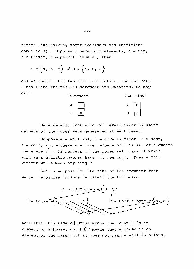
rather like talking about necessary and sufficient

conditions). Suppose I have four elements, a = Car,

b = Driver, c = petrol, d=water, then

A ={a, b, c} -I B ={a, b, d}

and we look at the two relations between the two sets

A and B and the results Movement and Swearing, we may

get: Movement Swearing

A A

B B

Here we will look at a two level hierarchy using

members of the power sets generated at each level.

Suppose a = wall (s), b = covered floor, c = door,

e = roof, since there are five members of this set of elements

there are 2 5 = 32 members of the power set, many of which

will in a holistic manner have 'no meaning'. Does a roof

without walls mean anything?

Let us suppose for the sake of the argument that

we can recognise in some farmstead the following

H, C) I C =

Note that this time a E House means that a wall is an

element of a house, and H E F means that a house is an

element of the far~, but it does not mean a wall is a farm.

-8-

In the case of Aggregative Hierarchies (IIa above),

the name of a class is appropriate to a quality which

can be applied individually to the elements in a class.

Hence all members of the set TREES are trees. This is

inseparable from the fact that we are using set unions

as the only means of 'climbing' the hierarchy, the unions

being defined for a property cornmon to all elements at

any 'level', By constrast, in the holistic combinatorial

use of sPots, since we 'climb' the hie~archy by whole

sets, the name is applied to the set in its entirety,

and need ~ot reflect any property cornmon to all elements.

I I 1.

0.)

PARTITION VS. COVERSET IN AGGREGATIVE ANV HOLlSTIC HIERARCHIES

Ag 9 IL eg a.t.Lv e. H.L eILa,1L c. h.L e1l

For reasons which are difficult to state briefly,

there has in the West been an assumption within formal

intellectual debate that hierarchies should be partitional.

This means th~t something at a lower level belongs to one

and only one class at a higher level. Thus we would not

allow, through dubious claims to scientific logic, the

schemE below for 'serious' study.

/trees~

fruit timber

I~/\ coconut mango neem

It represents an intersecting (coverset) hierarchYJ~u~ to

every-day man not only is such a hierarchy 'true', it is

the very essence of life - multiple categories and

multiple uses of things.

-9-

We will consider first the case of intersection

in the aggregative hierarchy. Suppose we consider that

trees can be grouped into timber trees - the set K -

and fruit_ trees - the set F - and N the trees that-are

neither. K and F could well intersect.

G=FUKUN = c, d, e, f)

66 %

Partitionalists do not like this approach, because

(i) at some points some sets overlap each other, so that

the isolation of some problem or quality for study is

impossible; (ii) at anyone level numbers, for example

the percentages of individuals in the classes of trees

in the above example, do not necessarily add up to a

predetermined total.

Most irritating of all, as soon as we allow

_ intersection, we play havoo with the idea of 'levels'

the idea that one level is 'above' another. Provided

that we maintain a partitional approach, we can even

with these aggregative hierarchies maintain the fiction

that there are indeed higher and lower levels, even although

we have already shown that the aggregative hierarchy

involving only set union actually stays at one level.

-10-

Since, as we have said, the real world is usually full

of intersecting hierarchies, the traditional approach

which is rarely questioned, is to use several ditferent

hierarchies to cross-classify the basic data, making

sure that each of these hierarchies is used separately

(orthogonally) and is itself partitional.

Consider crop varieties,a,b,c,d,e,f,g,h, and

these three orthogonal hierarchies.

genetic history season cereals

\

f\ \\ \. .I .

local LIV HYV r~ce wheat

A contingency table will have dimensions 3 x 3 x 2.

Here we draw the 3 x 3 table, and indicate the third

dimension by saying that leI is wheat and all other rice.

Aus Aman Rabi

HYV a ,be. e ---

LIV g

L

Initially the discussion will be limited to the 3 x 3

table. We can derive a two-level hierarchy on one

-11-

axis as follows:

Aus Aman Rabi

!\ I Aus HYV Aus L

/\~ AID.an HYV Aman LIV Aman L Rabi HYV

and on the other axis as follows:

HYV LIV L (Local)

/1'" ;\ /' '''"'' ~ \ " II \

Aus ;HYV Aman HYV Rabi HYV Aman LIV Aus L Aman L

If we include the third dimension, the rice/wheat

distinction, we can have any of six different arrangements

of three-level hierarchies, two of which are:

wheat rice

t

I rabi wheat

~ '-" "'-,

....... rice Aus

I / '~ "- ~ rabi HYV wheat AIDan HYV

e b,c

Aman LIV rice

g

AIDan L r~ce

h

Aus HYV rice Aus L

a d,f

ric

-12-

Rabi Aus Aman

I I \

Rabi wheat

I

I AIls rice l\man ri\, /~ / /'"

",'" '\ ,,' ." r

Rabi HYV wheat Aus HYV rice Aus, L rice Aman HYV rice .Arnan LIV

e a d,f b,c g

kttan L rice

h

If there is any 'problem' it appears to be tha.t 'We can use the major

orthogonal axes to divide each other at arbitrary levels - e.g. divide

plant type by season, or season by plant type.

Th~se 'problems' are self-inflicted. The 'fact' that there are

these different hierarchies ~s an illusion brought a1x>ut by the unspoken

assumption that the hierarchie.s must be parti tiona 1 - as indeed the

above ones are. All six of the 'possible' hierarchies, two of which

are shown above, are in fact .partitional subsets of the single cover set

(Le. intersecting) hierarchy which rises simultaneously on all three

axes. This simultaneous hierarchy looks like this:

e

a:

d,f

g

b,c h

rice

-13-

The major observation we can make as a result

of this discovery is that partiti~ning is a highly

selective filtering of the overall coverset classification

system, which produces paltry subsets. If one uses such

subsets one is always plagued by the nagging doubt that

one should have done it the other way round - and indeed

the first question at any seminar often lS, 'why did

you not do it the other way round ?'

Such a diagram represents a Gallois lattice,

which has been the subject of investigation by Marsh

(1983} and othe~s.

We will use an example based on foods and diet.

Suppose a = cooked rice, b = unleavened wheat bread, c =

lentils, d = ,fish. The power set of these foods will

have 16 members, but of those 16 only some will constitute

true meals. To nSb rice with lentil but neither rice

nor wheat we will define as not a true meal. So here I

produce my list of true meals.

poor man's meals rich man's meals

Pl= {a,c} p/Z"{a,d} P3= {blC} P4= {b,d}

1<'3={b,C,d} FA= {a,c,d} F5= {a,b,c,d}

Rl= {a,b,c} F2={a,b,d}

elements a b c

According to this schema there are many intersections:

all meals must have at least rice or wheat in them and

at least either lentil or fish. But the poor man can

never have both rice and wheat at the same meal, and never

both lentil and fish. But as any cook knows, wneat and

d

-14-

fish are holistically different as a meal from wheat

and lentils. The whole scheme is based on the holistic

difference of the sets.

Such is the intuitive subtlety of the human

mind we find that quite often both aggregative and

holistic hierarchies are used together. Remember that

we have already sai,d that an aggregative hierarchyuses

the concept .of OR - that F (fruit trees) is Banana OR

Mango OR Jackfruit OR Coconut - whereas the Holistic

Hierarchy uses the concept AND - that a meal is both

staple carbohydrate AND protein. We will define the

set of Carbohydrates C, and the set of P~oteins P.

Although at rock bottom we can return to a long

list of holistic members of the power set, there are

often so many (even with 5 eleme'nts we would have 32

possibilities to consider, with 10 elements 1024

possibilities) that we often use a short hand to reduce

the apparent number, by indicating groups of acceptable

sets. For example, let us define a good diet as G = {c, p} If we use only the holistic power set approach

we get:

G = {c p}

= {{a,b} , {C'd}} which would appear to indicate that a good diet was both

rice and wheat as well as both lentil and fish. What

we actually want to say is:

{(a or b) and (c or d)}

-15-

We can see that this corresponds to an aggregate of the

meals defined above.

G = {PI or P2 or P3 or p4 or Rl or ,R2 or R3 or R4 or RS}.

and that we are trying to achieve a shorthand way of

saying so by ind~cating incorrectly that G = {C r p}

Henceforth in this paper we will use notation

which avoids all this ambiguity. A superscript * will ,_j;

indicate lany element of the set'. Therefore A Good

Diet is any member of the set Gt = {c*, p*}

IV. EXAMPLES

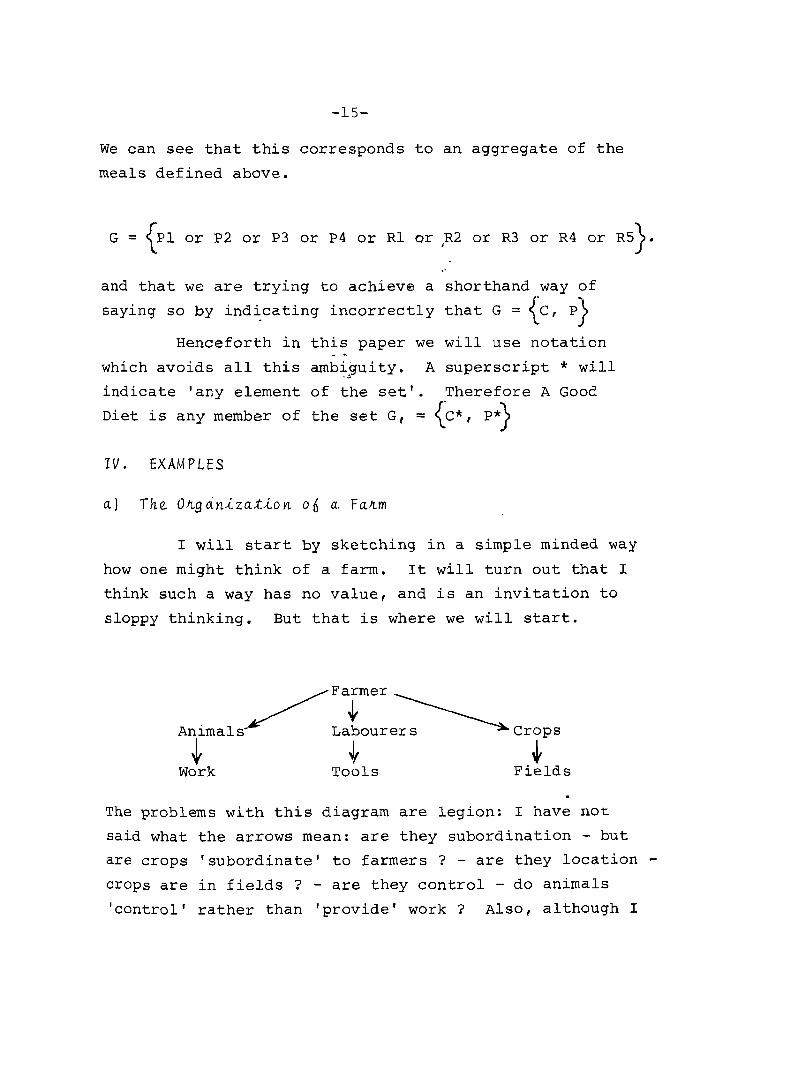
a) Th~ O~gan~za~~on on a Fa~m

I will start by sketching in a simple minded way

how one might think of a farm. It will turn out that I

think such a way has no value, and is an invitation to

sloppy thinking. But that is where we will start.

~Farmer

Animals Latoure~crops ~ t ~

Work Tools Fields

The problems with this diagram are legion: I have not

said what the arrows mean: are they subordination - but

are crops I subordinate I to farmers? - are they location -

crops are in fields ? - are they control - do animals

'control' rather than 'provide' work? Also, although I

-16-

have different levels, are not farmers and labourers

at one level all men? DO not farmers and labourers

work as well as animals ?

If we ap.ply a little rigour to this situation,

we see we must distinguish between elements and sets,

and between sets and the relations between sets.

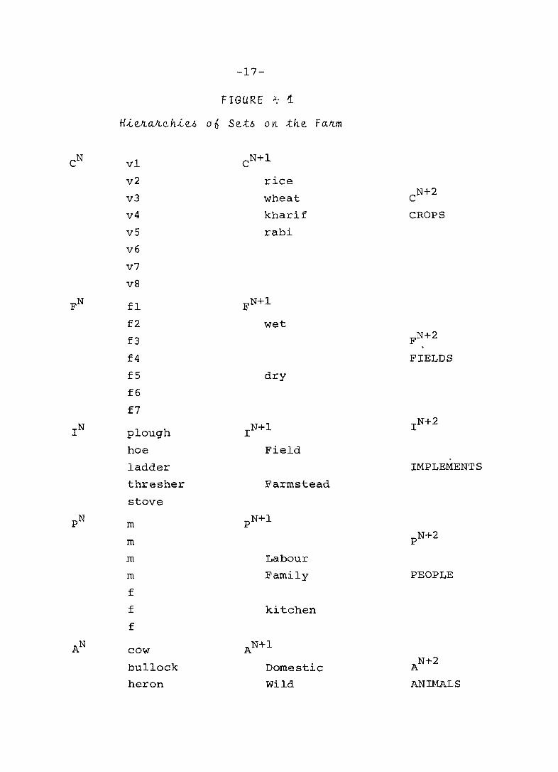
If we try again, we mught define -five hierarchies

here, and many relations between different levels in

the hierarchies. The hierarchies are CROPS, FIELDS,

IMPLEMEN'r_S, PEOPLE, ANIMALS. We can define any

appropriate number of levels we wish: here we mostly

define three, in on~ case two levels. (It seems a rule

of thumb (or the human mind more likely) that in any

given study three levels seems to be the useful number}.

We will identify the hierarchies by the word defining

the single set at the top of each (we do not have to

have a single set at the top: that is merely what I

have done in this case).

The definition of 'the farm' amounts to the

relations between all these sets, ego the ~ow~ng relation

between crop types and fields, the wOJr..k.~ng. relation

between labour and fields, the u~~ng relation between

labourers and implements etc.

-17-

FIGURE ;/.. 1

tLi.. e.fL a.fL c hi e..6 on S e..t.6 on .the.. FafLm

eN vl cN+1

v2 rice

v3 wheat eN+2

v4 kharif CROPS

vS rabi

v6

v7

v8

FN fl FN+l

f2 wet

f3 FN+2 . f4 FIELDS

fS dry

f6

f7

IN plough r N+l r N+2

hoe Field . ladder IMPLEMENTS

thresher Farmstead

stove

pN m pN+l

m pN+2

m Labour

m Family PEOPLE

f

f kitchen

f

AN cow AN+l

bullock Domestic AN+2

heron wild ANIMALS

18

pN+l

pN

-19-

This is a very complex affair: but then reality

is complex ~nd there is no point in pretending otherwise.

We can simplify the way we see thinqs by going up

the hierarchy, but that does not mean that this simple

view does not ultimate 'rest on something much more

complicated which for the time being we chose to ignore.

The relations that define the farm structure are

horizontal, vertical and 'diagonal'. For example, the

relations between people and fields could be:

Diagrammatically the 'whole farm' is indicated

by many relations, not all of which will be monitored

or known, nor indeed all of which WQuld be interesting.

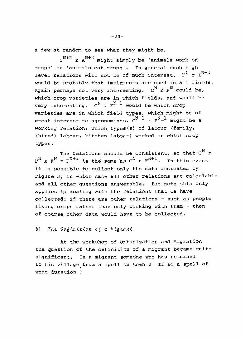
But let us look at the possibilities. We use the

conventional notation that the lowest level of a

hierarchy, saye is N written eN. The next two highest

levels are then e N+l and e N+2 . There are fifteen

nodal points on the diagram, so there are 15 x 14/2 = 105 possihle relations, shown in Fig.a. Let us choose

-20-

a few at random to see what they might be.

e N+2 r AN+2 might simply be 'animals work on

crops' or 'animals eat crops'. In general such high

level relations will not be of much interest. FN r I N+l

would be probably that implements are used in all fields.

Again perhaps not very interesting. eN r FN could be,

which crop varieties are in ~hich fields, and would be

very interesting. ,eN f FN+I would be which crop

varieties are in which field types, which might be of . N+l N+l great interest to agronom1sts. e r P - might be a

working relation: which types(s} of labour (family,

(hired) labour, kitchen lapour) worked on which crop

types.

The relations should be consis~ent, so that eN r N N N+I. h . . N N+I h' t F X F r F 1S t e same as e r F • In t 1S even

it is possible to collect only the data indicated by

Figure 3, in which case all other relations are calculable

and all other questions answerable. But note this only

applies to dealing with the relations that we have

collected: if there are other relations - such as people

liking crops rather than only working with them - then

of course other data would have to be collected.

At the workshop of Urbanization and Migration

the question of the definition of a migrant became quite

significant. Is a migrant someone who has returned

to his village, from a spell in town? If so a spell of

what duration ?

FN.+1

21

A~+2

CN+2

CN+1

....-1 N __ -t-__ ---4I AN

-DEFINITION

pN

----DATA (OBSERVATION)

-22-

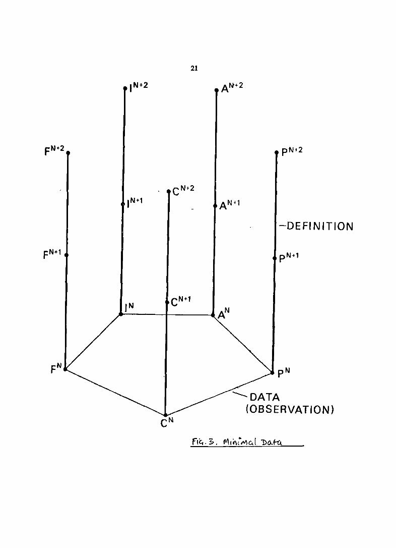
FIGURE 4

n N male pN+l

female Sex p N+2

harijan, Caste PEOPLE

kayasth Age

old etc.

young

etc.

PLN Sonagaon PLN+ l

Rampur Andhra pradesh PLN+2

Begumbazar Bihar PLACES

etc. Urban

Rural

etc.

IN I hour

daily IN+l IN+2

hourly

seasonally Frquency

retu:.r:n Duration JOURNEYS

train Completion

bus Medium

holiday Purpose

money/work etc.

etc.

JBN skilled .J'BN+ l

non-skilled TRAINING JBN+2

professional NO TRAINING

manual AGRICULTURAL JOBS

~tar.:teA]" INDUSTRIAL

agricultural

etc.

-23-

Is movement to another house in the same village

migration? If not, why is movement to the ne~t village

migration ?

I do not know the answer to the question "Who

is a Migrant (', but I do know the' way in which I would

go about defining different kinds of migrants, applying

much of what has been outlined above.

Migrants are PEOPLE, they move between PLACES,

they make JOURNEYS of different kinds, and they have

JOBS with differing characteristics. There may be

many other hierarchies which we could tnink of as

relevant - EDUCATION - for example, but for the moment

we will start with those I have indicated.

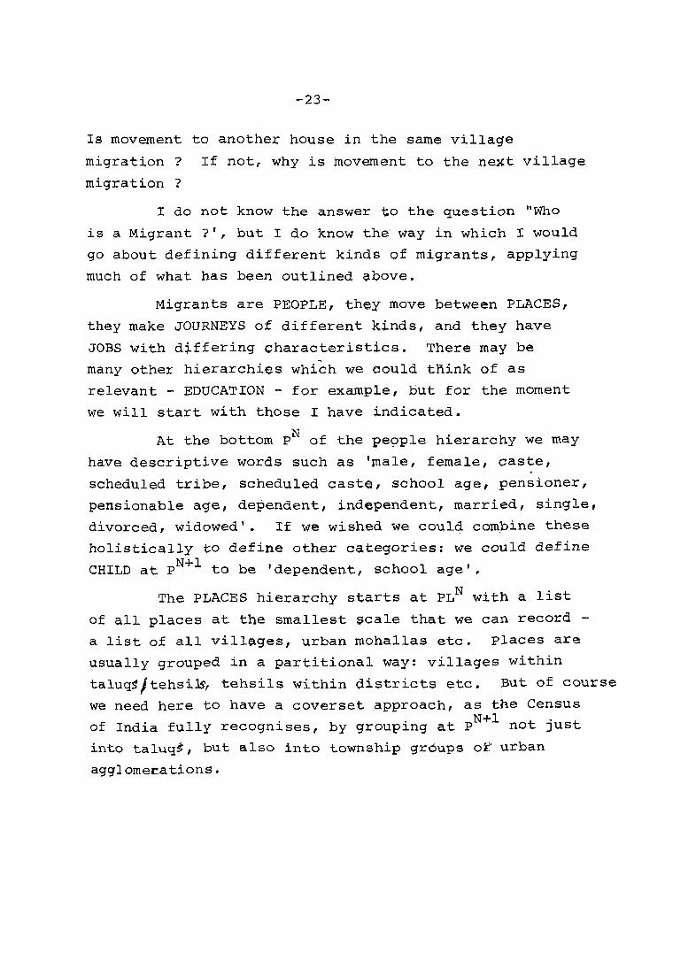
At the bottom pN of the people hierarchy we may

have descriptive words such as 'male, female, caste,

scheduled tribe, scheduled caste, school age, pensioner,

pensionable age, dependent, independent, married, single,

divorced, widowed'. If we wished we could combine these

holistically to define other categories: we could define N+I CHILD at P to be 'dependent, school age'.

The PLACES hierarchy starts at PLN with a list

of all places at the smallest scale that we can record -

a list of all villages, urban mohallas etc. places are

usually grouped in a partitional way: villages within

taluq~/tehsi$, tehsils within districts etc. But of course

we need here to have a coverset approach, as the Census . . N+I t' t of India fully recognlses, by grouplng at P no JUs

into taluq5, but also into township gr6ups oi" urban

agglomer.ations.

-24-

Migrants' JOURNEYS can be characterised by many

words. This time let us think of words at IN+l and N project back to J. rFrequency' would make us think of

Hourly, daily, X per year, seasonal, non-repetitive.

"Completion' would make us think of return and non-return.

'Duration' would make us think of 1 hour, 5 hours, (for

example), 2 days, 2 months. Obviously we will have to

look carefully to see if there are useful cut-off points

in this scheme. We can think of 'Medium', such as plane,

car, motor-bike, b~~, bicycle, foot, train, lorry, camel,

ass etc. We can think of 'Motivation' such as pleasure,

fear ,money, status, pilgrimage, education, dependent,

posting, marriage. Pleasure may make us wonder whether

we can project down even further to I N- l - to the level

of 'skiing, swimming, golf, fishing' etc.

There are many classifications of JOBS, and

some of those may be of use or relevance here. We might

use such words as 'skilled, non-skilled, professional,

manual, clerical, agricultural, light industrial, heavy

industrial, organized industrial, domestic industrial,

extractive' •

These thoughts are enough to begin to sketch out

how we might answer the question 'who is a migrant'.

First let us combine some of the words from JOURNEYS

level IN.

To define COMMUTING wie may need to say:

car

and/or bus

and/or train

and/or walk

and/or bike J r money J

+ l:-nd/ or s ta tu s

-25-

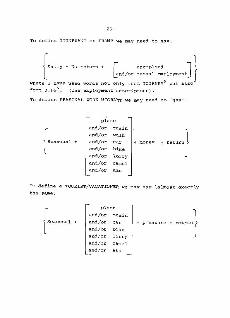
To define ITINERANT or TRAMP we may need to say:-

Daily + No return + r unemplyed 1 L~nd/or casual .employmen~~

N where I have used words not only from JOURNEY but also

from JOBSN. (The employment descriptors).

To define SEASONAL WORK MIGRANT we may need to ·'.say:-

plane

and/or train

and/or walk Seasonal + and/or car + money + return

and/or bike

and/or lorry

and/or camel and/or ass

To define a TOURIST/VACATIONE~ we may say lalmost exactly the same:

plane

and/or t:tain

and/or C&r

and/or b.tke

and/or l<::>rry

and/or cstmel

and/or a~s

+ pleasure + retrun

-26-

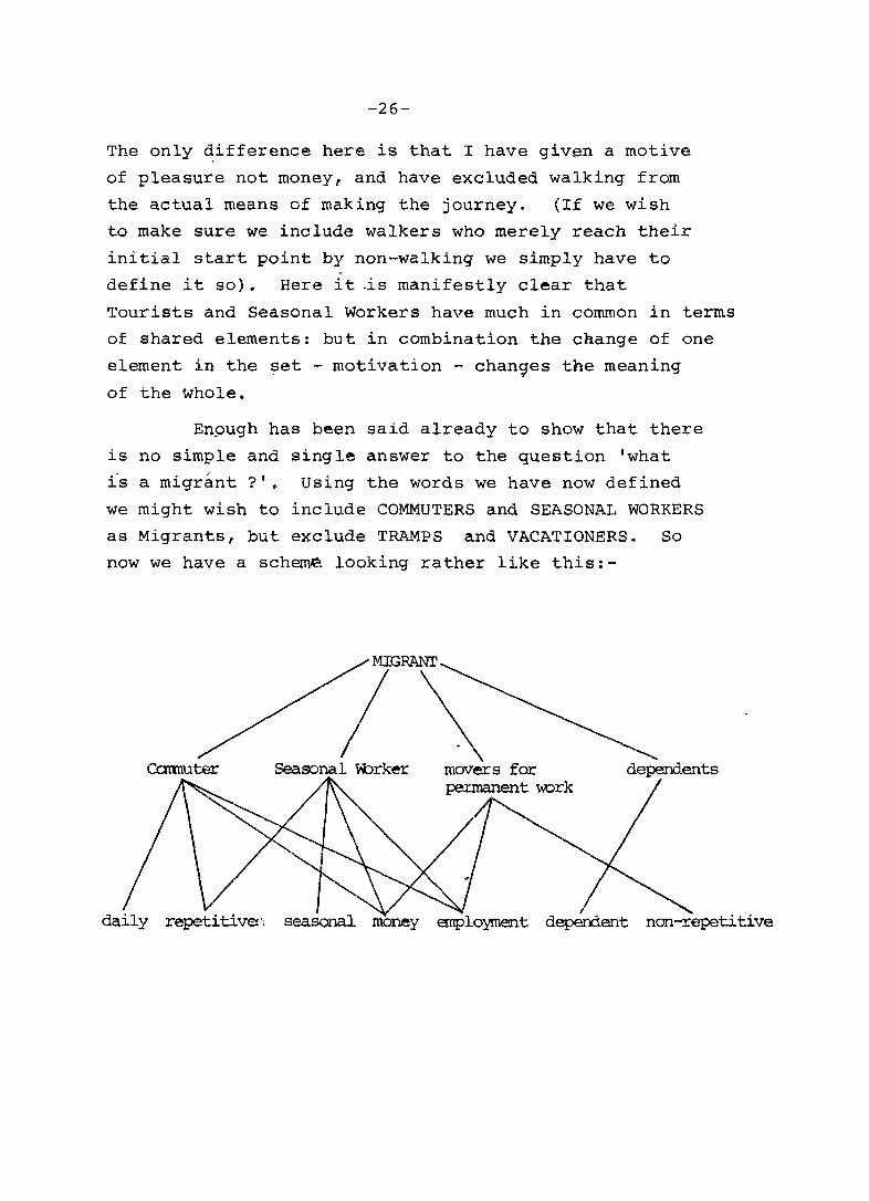
The only ~ifference here is that I have giv~n a motive

of pleasure not money, and have excluded walking from

the actual means of making the journey. (If we wish

to make sure we include walkers who merely reach their

initial start point by non-walking we simply have to

define it so). Here it .is manifestly clear that

Tourists and Seasonal Workers have much in common in terms

of shared elements: but in combination the change of one

element in the set - motivation - chan~es the meaning

of the whole.

Enpugh has been said already to show that there

is no simple and single answer to the question 'what

1S a migrant ?'. Using the words we have now defined

we might wish to include COMMUTERS and SEASONAL WORKERS

as Migrants, but exclude TRAMPS and VACATIONERS. So

now we have a scheme. looking rather like this:-

MIGFANl'

I Cannuter Seasonal \'brker movers for

permanent ~rk

seasonal money employment

............ dependents

non-repetitive

-27-

Note, that if all the data with regard to

individuals is recorded at the lowest level, and then

stor~d in a computer, we can keep changing de~initions

and re-run our computations using new concepts. The

categories and sub-categories of migration are not pre­

ordained. They are d~~~~~d and u~ed by us for whichever

purposes seem sensible avenues of research.

What we have not so far said much about is other

hierarchies - PEOPLE, JOBS, PLACES. If for every

person in the data set all the data about these is

collected as well as the data about the JOURNEY, then

there are two ways in which this data may become of

importan~e. Firstly it may extend and augment the

definitions as we have already done: employment might be

part 0f the definitions of certain types of migrants;

dependency might exclude some persons from the category

of 'primary migrant' and place them in 'seconday migrant'.

The rural-u~ban migrant (PLACES) might be thought of

in a different category from the urban-urban. Secondly,

we may not think so much in terms of using these for

definition, as use them for counting the mappings between

the ditferent parts of the different hierarches: counting

how many SEASONAL migrants are agricultural, or how many

are urban-rural etc.

I conclude this example by a simple illustration

of calculating the percentage of migrants relating to

different combinations of data recorded for them.

-28-

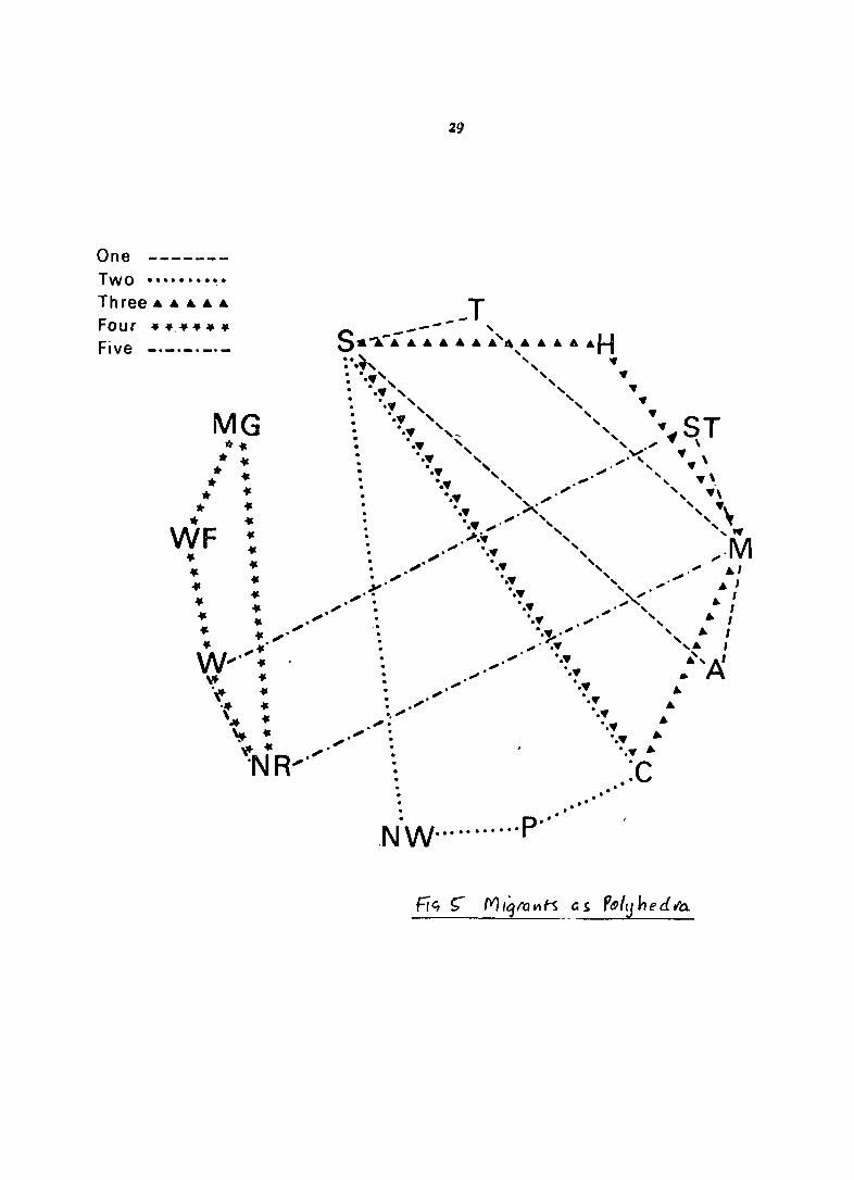
Suppose we observe five persons, us~ng some

of the words from both the JOURNEYS and JOBS

hierarchies~

One: seasonal Strain T money M agriculture A

TWO; seasonal Scar C pleasure P non-worker NW

Threeiseasona1 Scar C money M hawking H

Four; non-repetitive NR walk W marriage MG

wife WF

Five; non-repetitive NR walk W money M servant ST

Each of these five can be represented by a polyhedron

whose vertics represent the elements describing each

person, as in Fig. 5.

If we put all five together there are some

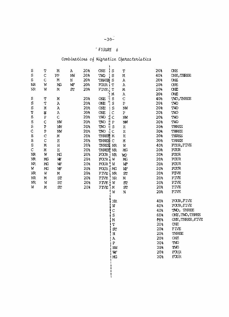
areas of over lap. If now we count .the pe_rcentage

of migrants with different combinations of elements

starting with the greatest number of elements in

combination and going down singleton elements, we ge~

the list shown in Figure 60

This gives us a complete breakdown of the

migration pattern in this data set, enabling us to

ask simple questions and to see if the answers are

useful or not, and ~f not, to ask more complicated

questions.

This procedure has been elaborated at greater

length with respect oto broadcasting statistics in

Cha~~.-, Johnson and Gould (1986).

One Two •......... Three.&. .&. .&. ...... Four ••.•••• Five

MG tt ..

* .. * .. * * '" * * WF

• • ..

· · · · • · · · ·

29

. :c . . . . . p.' .N W···········

-30-

!. fIGURE 6

Comb-in.a.tioltO 06 M,[,gJta.;t.,i.oYl cf:iaJta.c.teJtMtic..6 I

8 T M A 20% ONE :8 T 20% mE 8 C pp NW 20% 'l'W) ·8 M 40% ONE ,THREE I 8 C M H 20% ~8 A 20% ONE NR W M3 WF 20% FOURI T A 20% ONE NR W M sr 20% FlVE~: T M 20% ONE

'j M A 20% ONE 8 T M 20% ONE ~: 8 C 40% TWJ,THREE 8 T A 20% ONE '18 P 20% 'l'W)

8 M A 20% ONE !8 NW 20% TW)

T 1)1 A 20% ONE ic P 20% 'IW)

8 p C 20% 'IW) 01 C NW 20% 'I'W) II 8 C NW 20% 'IW) II P NW 20% TWJ 8 20% 'IW)

II 20% THREE P NW 11 8 H

C P NW 20% 'IW) il c H 20% THREE 8 C M 20% TlffiEIIJ M H 20% THREE S C H 20% THREBl C M 20% THREE S M H 20% ~NR w 40% FaJR, FIVE C M H 20% THREI1t NR MG 20% FOOR NR W l'IG 20% FOUR I NR 'lJt.J' 20% FOOR NR MG WF 20% FooR':: w l'IG 20% FaJR NR MG WF 20% FCUR II W WF 20% FCUR ,I W M3 W 20% FCUR:I MG WF 20% FOUR NR W M 20% FIVE~: NR sr 20% FIVE NR M 8T 20% FIVE I:: NR M 20% FIVE NR W 8T 20% FIVE II W sr 20% FrJE W M ST 20% I sr 20% FIVE FIVE ,I M

~w M 20% FIVE

NR 40% FOUR, FIVE W 40% FOUR,FIVE C 40% 'lID, THREE 8 60% ONE, 'IW), THREE M e0% ONE, THREE ,FIVE

, T 20% ONE sr 20% FIVE H 20% THREE A 20% ONE P 20% 'I'W)

NW 20% TWJ VF 20% FaJJ<-M3 20% FooR

-31-

V" CONCLUSIONS

The clear and unambi.guous description of the real

world is the aim and foundation of man's social science

disc~pline.se Without orderly observations the word

! science r has t,o be dropped in favour of I op].nions' or

I hunch , or even 'prejudice'" Yet it is extremely

d.lff~cult '(.0 observe the soclal world in relat~vely

rlgorous ways.

Part of the problem lies with the soph-istication

and subtlety of the human ob~erve"f', Each of us is

equipped to handle complex problems of pattern recognition,

and complex problems of discrimination. Often we are

intuitively able to handle such complexity without

attempting to analyse it consciously. However, when we

need to collect data systematically, it becomes apparent

that instinct is not enough - we are too individualistic

and inconsistent. So we have to break the problems down

by some system of orderly observation. The system

proposed by At.kin is the best I have yet come across ..

It realises straight '.away that we often instinctively

use relations between sets: but that to record this we

must first work out what the sets are, and only then

observe the relatlons. It recognises that there are

hierarchies of sets, but that these hierarchies need

not be part1tional. It recognises that there are pseudo-

hieraLchies of aggregation, and real hierarchies of

power sets. There are many extensions to the ideas

demonstrated here: to analyses of the structure of

relatJ.ons, and to relating traffic (dynamics) to

backcloth (structure). But these can be explored

elsewhere. (G~uld~ Johnson, Chapman 19S().

PLACE OF BIRTH DATA' AND' L'IFETTME' M'IGRATION

Ronald Skeldon

The question on place of birth in population

censuses and surveys provide~ a basic direct way of

measuring migration. The' movement between place of

birth and place of enumeration is known as "lifetime

migration Il and a "lifetime inigrant 11' is def ined as

someone whO is enumerate'd' in a spatial unit other than

the one in which he or she was born.

Lifetime migration' is a fundamental measure of

population movement, altho'Ug'h now, in the second half

of the 1980s, it .is perhaps not thou~h~ so fundamental

as it once was considered to be. Ih' M'ahU:al' VI - the '" .. ....

Uhit'ed Nations I M'ahUal' on:- M'e;t'h'ods~ 'of' M'ea'sur'ing' Ih'te-rh'al -....._ .

Mi<Jratibn - published in 1970, place of birth is given

pride of place. Many analysts ,of migration would now

accord lifetime migration only a place of secondary

importance, with some considering that it is almost

useless from the point of view of policy-relevarit migration

analysis. This latter view is perhaps a little extreme

but certainly lifetime migration is not the ideal measure

of migration. However, for· certain reasons, it is

still a useful measure. In this chapter the advantages

and disadvantages of the. method will be examined to see

why it has changed from' ~ measure of migr.;ition to but

one measure of migration and the various uses of

birthplace data will also be examined.

-34-

BJ.rthp1'ace data have prov~ided the basis for some

of the classic studies of migration in India lMehrotraf 1974;

Davis 1951; Zachariah, 1964) and Indian analysts have been

in the forefront in the development of techniques to

analyse these data (Zachariah 1977; Nair 1985). Other

useful appraisals of the techniques employed ~n the anaLysis

of lifetime migration can be found in united NatJ.ons (.i970)(

Shryock ~ 'al. (1971), George (1970) and Arriaga (1977),

Let us consider first the disadvantages, The

first major disadv~ntage is that there is no time dimension.

Lifetime migration is the aggregate sum ot all movements

from birthplace to enumeration place for a population

irrespective of when the movements took ~~acee A move made

by an 80 -year-old man who moved 60 years ago w.1.l1 be

included with a move made by an 18-year-old student three

weeks before the census. Policy-makers are usually

interested in the present pattern of migration and lJ.fe£ime

migration is going to provideJpiased picture. We can try

to control this problem in two ways. First, we can examine

lifetime pattern by age group and make thl~easonab1e assumption that younger people are more likely to move and

so the lifetime flows of the 15-19 and 20-24 age cohorts

are given more weight in an analysis~ Secondly, and more

commonly, if a question on duration of residence is

included in the the census then we pan cross-classify the

flows from birthplace to place of enumeration by duration

of residence at place of enumeration: less than 1 year,

1-4 years, 5-9 years and so on.

However, this brings us to the second maJor

disadvantage with lifetime migration: it is a measure of

a single move from birthplace to place of enumeratlon~

A,n individual's migration may not have been so simple:

-35-

it could have involved several moves through intermediate

places between birthp1'ace and pilace of enumeration.

Perhaps even more important is the fact that much

migration is not captured by lifetime migration'at all.

We know that return migration is important in many

countries and particularly in the developing world. Data

from spectfic surveys have shown that there is a high

probability of a second migratimn being a return to place

of ,origin. Given this situation there are a large

number of people who may have spent considerable time

away from their birthplace who are classified as "non­

migrants" or "never moved" under lifetime migration:

their place of enumeration is the same as their place

of birth.

One of the controls fOJ:jproblems:inherent ir{,the

lifetime migration data mentioned above was the inclusion

of a question on residence at place of enumeration.

However, the duration of residence data need not necessarily

refer to the migration from birthplace but to a movement

to the place of enumeration fromsome other place. This

makes any analysis of migrant/non-migrant differentials

(by, for example, age, educational or occupational status)

of dubious value from lifetime migration data.

Finally, lifetime migration does not take into , account the effect of mortality; it measures only those

who have survived at the destination to be enumerated

in the census. Hence, lifetime migration is not an

estimate of gross migration.

It is for the disadvantages outlined above that

migration analysts have relegated lifetime migration to

a secondary position in the study of the process of

migration. Given these disadvantages one might wonder

why we 8*lluld persist with its study. It does, however,

have two related advantages. First, birthplace data

-36-

are often the only migration-relevant data available

and, secondly, the question is easy to incorporate

in a census questionnaire: easy to ask ~nd almost as

easy for the ~espondents to answer. Let me emphasize

at this stage that while we are talking about "birthplace"

the question asked need not necessarily be "Where

were you born ?" but can be a variant - as in the case

of India - "Where was the usual place of residence

of your mother at tfue time of your birth ?" or "Where

were your parents usually living it the time of your

birth?" This question can simply be made culture­

specific to produce a relevant question for each country~

To almost everyone, ~place of birth" is a meaningful

place which will be accurately remembered. This is an

important point in its favour as this is not the case

with some other methods of measuring migration such as

"Where were you usually living five years ago 7" which

is subject to problems of memory lapse. Hence, the

quality of birthplace data is lik~ly to be relatively

high.

Given that the question on birthplace is simple

we are likely to have a long sequence of birthplace

data. India is a classic case since information on

birthplace has been collected in thepountry since 1881.

There is also widespread spatial coverage of birthplace

data. Twenty-seven out of 34 countries in the Asia­

Pacific region collected information on place of birth

in their 1980 round of censuses and this was by far

the most common migration-related question asked. For

the period 1955-65, the United Nations has information

on 109 national censuses taken around tpe world in which

87 recorded information on birthplace.

-37-

Hence, there are disadvantages and advantages

with the use of birthplace data and when we use such

data we must be aware of their strengths and weaknesses.

The ~ of Birthplace ~

(1) The measurement of origin-destination flows

The primary use·of,birthplace data is as a direct

measure of inmigration, outmigration and net-migration

for all the regions of a country. These can be

portrayed in a square origin-destination matrix. The

finer the network of spatial ~nits in a cQuntry, the

greate1the volume of migration that is captured by

the population census. To take an example from the

1981 censusof India, we find that when we use the

state as the migration-defining area 23.4 million people

would be defined as lifetime internal migrants (3.6

per cent of the total population) but if we use the

smallest place of enumeration as the migration-defining

unit, the number of migrants increases to 201.7 million

(or almost 30 per cent of the total population).

Despite the fact that the smaller units capture

more migration, we do not want the number of spatial

units to'. be too large or the origin-destination matrix

will be so complex that we cannot grasp the number of

flows involved. The number of spatial units should

then be IImanageable ll• Also, if the origin-destination

flows are going to be mapped we do not want them to

be so pr~fic that the result is a maze of intercrossing

flows and the main trends are not apparent at all.

For example, it would ",'._ not be desirable to have a

matrix of all the districts of India. state flows can

-38-

be complex enough. Specific matrices can be designed

for speci£ic purposes, although this may mean tedious

aggregration of the data where origin-destination flows

become too comp~ex.

The origin-destination flows can be simplified by

focusing on the net-flows, that is, the balance between

inmigration and outmigration for each spatial unit. It

must always be borne in mind that net-migration represents

the balance between two flows. It does not tell us any­

thing about the volume of inflows or outflows but only

about the interchange of 'population between two areas.

It is a useful measure to' gauge the impact of ' migration

on the red:i·s·t'r'ibution of population. It must also be

remembered that there is no ,such person as a "net-migrant rt •

Net-migration is purely an aggregate measure to which

(individual) characteristics cannot be attributed. The

above clearly does not just apply to ~ifetime migration.

but to any direct method of measuring o~igin-destination

flows.

In the origin-destination matrixtha .number of

inmigrants must equaltbe .number of outmigrants - it is

a zero sum ga~e. In the analysis of internal migration

those 'who are born within the system and who have moved

out to other countries are not captured by the census -

and those who have moved into the system from other

countr~~are discounted and normally considered in a

separate series of tabulations and separate analysis.

Migration of "foreign-born Ii wi thin the system is thus

discounted in lifetime migration.

-39-

The data on the flows of inrnigrants and out­

migrants can be subjected to the standard types o~

demographic analysis, by age, sex, marital statuS',

education and occupation. The migrant population is

often compared with the "non-migrant" or "immobile"·

population but we must remember, of course, that these

terms are misnomers. In comparing two censuses the

intercensal growth of "migrant" and IInon-migrant"

populations can be compared. A very detaile~ analysis

of lifetime mig.rants for India was made by Mehrotra (1974)

from the 1971 census.

For India, lifetime migration can be analysed

at the following levels: inter-country, inter-state,

inter-district and intra-district. The relevant

cat.egories are:

(a) Born here (place of enumeration);

(b) Born elsewhere in this district;

(c) Born in another district in this state (name of district);

(d) Born in another state (name of state);

(e) Born overseas (name of country).

Category (b) has only been identifiable in India since

1961

(2) The measurement of intercensal net migration

The second use of lifetime data is to measure

intercensal net-migration. Where the primary concern is

the role of migration as a component of population growth

or decline, knowledge of net-migration is often sufficient.

"Thus an estimate of net-migration is the most fundamental

migration measurement. For this reason, it occupies

-40-

a disproportionate share of migration researchers'

attention." (Bogue, Hinze and White, 1982) This is

very much a traditional demographer's view and I do

not think that many migration analysts today would

subscribe to ·;-_it. However, net-migration is an important

and valid aspect of migration research. It can, of

COUEse, be estimated without recourse to any migration

questions at all but these indirect techniques are

covered in another chapter and I will concentrate on

the estimation of net-migration using birthplace data.

The following discussion can be pursued at greater length

in United Nations' Ma'Itu:a1 VI (1970).

If 'Itand It+n are the inmigrants to a particular

spatial unit at two censuses at 't' and 't+n' and 0t and

0t+n are the outmigrants from that spatial unit at the

two censuses, then the net-migration that has occurred

dunng the intercensa1 period can be calculated thus:

Net M = (1t +n - 0t+n) - (SIlt _ SO) ° t

Where SI and So are the intercensal 'surviva1 ratios

which allow us to estimate how many of the inmigrants

and outmigrants of the earlier census will survive through , to therater census.

The formula is more commonly presented as:

Net M = (It +n - SIlt) + (SOOt - 0t+n)

The problem with this formula is to estimate S1 and SO·

There are various methods:

a) Overall census survival ratio, that is,

assume SI=So =ST;

b) Area-specific census survival ratios;

c) Age-specific censusfurviva1 ratios.

-41-

The aim of these procedures is to take mortality into

account; that is,t)\e mortality of the inmigrants to and

the outmigrants from a spatial unit during the intercensal

period. If mortality is not taken into account, the

net-migration over the period will be underestimated.

Hence, the assumption is that the migrants, both in and

out, at time t are stable, and the only factor to affect

them will be mortality. Implicit in this approach is

the idea that migratlon is a simple linear process:

a movement from A to B.· This is not the case. Mortality

is but one factor - and I would regard it as not the most

important factor- in the attrition of It anq 0t. On

movement ~nd return movement are more important. Migrants

also tend t+e youn:g adults and while certainly subject

to mortality this is not likely to be the most significant

factor in the reduction of It and 0t.

The overall census survival ratio can be expressed

as follows:

Where n is the intercensal period.

Its use is likely to exaggerate the impact of mortality

)n the outmigrant andtnmigrant populations as the latter

being younger than the population as a whole will be

subject to lower levels of mortality., This problem also

applies to area-specific overall CSRs when we try to take

into consideration differences in survivorship by region

of birth. To calculate area-specific CSRs the populations

born in the individual spatial units in a country and

enumerated anywhere in the nation are compared over the

two intercensal periods. The total population born in

-42-

state x and living anywher'e in India at the first

census period is compared with the population 10 years

of. agelfnd older' at the second period, assuming that

the intercen~al period is 10 years.

Where place of birth statistics are tabulated

by age for all th~ are~l uni~s of birth ~nd residence

separately at both censuses "more accurate estimates

of period net-migr?ltion can be obtained" (United Nations,

1970). These estimates can be made in considerable

detail for each spatial unit by age and for in-born

and out-born persons separately. This third proc~dure

involves much tediQus calculation. The age-specific

CSRs are calculated comparing the 0-4 cohort at census

t with the coh6rt 10-14 at census t+10, the 5-9 with

the 15-19 and so on, for each spatial unit of birth.

A simpler version of' this last approach is to use the

overalL (national) age-specific census survival ratios.

This is perhaps more useful for countries where problems

of age mis-statement are important.

All these,CSR approaches assume a closed system.

If there are losses due to international migration, then

the 'CSRs will be biased downwards. For an interesting

application of adjustments made to deal with international

movements, see George (1970). They also assume two

other criteria; first, that the census interval is ... regular, 5 <i~r 10 years. If it is 9 years (for example,

-papua New Guinea, 1971-80 and Peru 1972-81) or 11 years

(for example, peru, 1961-72) or some other interval,

thenA~he calculation of the age cohorts becomes

exceedingly complex if not impossible. The second

criterion is that there should have been no significant

-43-

boundary changes between the two censuses.

had been, the method could be invalidated.

If there

There is also the question of the population

less then 10 years old (or the population younger than

the intercensal period). Their migration is not

considered in the equation. The proportion under 10

in India 1981 was about 26 per cent of the total

population - a large proportion to omit. While the

young are not the most migratory element in a population,

they do accompany parents. It is alt-lays possible to

make a number of assumptions to try to adj~st the total

I and 0 to account for children (by, for example,

applying the child/woman ratio or a variant thereo.f)

but generally they will be ignored and the net-migration

will refer to the population 10 years of age and more

at the later census, assuming a census interval of

10 years. So, by applying this method, a substantial

volume of total net-migration is likely to be 'omitted

in developing countries, where there are youthful

populations.

Life tables, i~ they exist, can also be used to

survive forwards the inmigrant and outmigrant populations.

However, the CSR methods are in fact preferable as the

life table procedure implies a perfect enumeration of

censuses at the beginning and end of the migration period

in relation to completeness and age reporting which is

just not realistic. Hence, the number ot migrants

estimated by using life table survival ratios reflects

census errors rather than migration. The :CSR method

implies only that errors in each census are approximately

the same in all places, which is a more acceptable

alternative.

-44-

These techniques to measure intercensal net­

migration, or net-migration within a specific time­

period, were once the principal methods available to

migration analyst·s. Now a question ort place of last

previous residence by duration of residence can be

employed to give a simpler and arguably a more useful

estimate of migration between two censuses.

(3) The measurement of period-specific flows

Another method to derive period-specific

estimates from lifetime migration data has been

developed receritly by Franz Willekens at the D~mographic

Research and Training Institute in the Netherlands

and this method was applied to the 1911 census of India

data by Nair (1985). The technique is to create a

"guess" matrix of period flows from the lifetime migration

flows based on the assumption that the ~a·ttern of period

flows is essentially similar to that of the lifetime

flows. The method is known as bi-proportional adjustment,

or iterative proportional fitting, as it is called in

multivariate analysis for two dimensional data.

mij = rio sj . o .. m~J

where mij is the period migration from i to j ;

o .. represents initial of the number of mT] an guess

migrants and in this case is lifetime migration

ri and sj are the row- and cofumn-balancing

factors respecitvely.

A special FORTRAN programme is used to perform

the log linear analysis to generate the data from the

matr-ices. The data required include, obviously, the

lieetime migration flows, and total inmigrants and

-45-

total outmigrants (the marginals) for the specific

time-period to be examined. The latter could come from

specialized localized surveys. Nair tested the estimates

derived from the model with those actually observed

over a 10 years intercensal period in India and about

90 per cent of the calibrated cell counts are within

25 per~ent~f observed flows: 70 per cent within 20 per cent,

40 per cent within 10 pe~ cent, and 25 per cent within

5 per cent.

,'Iii.. ,contrast, estimates for a single year duration

(the year preceding the censuses) show that 56 per cent

of the calibrated flows were within ?5 per cent of the

~ctual numbers, 44 per cent within 20 per cent, 36 per

cent within 10 p~r cent, and only 16 per cent within 5

per cent limits.

This is what one would expect as we know that

more recent migration may have peculiar characteristics

and may not be structurally similar to lifetime flows.

A second model which drops the assumption of structural

similarity between lifetime flows and period-specific

flows (which, of course, is a major weakness) has been

developed but the additional factor in the equation to

deal with thell?rbPo;r:t:io~:a'l deviation of migration flow

from i to j ~uring the specific time-period in relation

to the lifetime pattern depends on local survey data,

findings from another country with more or less similar

characteristics (which might be a rather dubious

assumption) or expert opinion. The methods clearly

haveti1eir disadvantages but a weak estimate of periodicity

may be better than no estimate at all.

-46-

Cone,lus,ion

Lifetime migration is essentially a poor way

of estimating internal migration and it is better to

include other-questions in a census questionnaire to

capture migration. These methods will be examined in

other chapters. DO the weaknesses inherent in

birthplace data then mean that we should abandon the

question on place of birth and the analysis of lifetime

flows? For example, advanced countries such as Japan

and Australia either do not collect information on

birthplace at all or do so only at country level in

order tqgauge inter-national flows. There would, however,

seem to be a reasonable case to maintain "birthplace"

as a key question for the £ollowing reasons: (a) it is

easy to answer; (b) to maintain a continuity of data

and analysis; and (c) as an input to international

migration.

It would appear likely that the analysis of

"birthplace" data will increasingly become limited to

on the study of international migratipn while internal

migration is assessed from questions on last place of

previous residence. In this case, more detailed coding

of country-level birthplace data may be required ':" and

international co-operation needed to facilitate the

drawing-up of origin-destination flows between countries.

Again, information on the timing of the migration is

ideally needed and thi 5 would require an addi tio'nal

question on duration of residence.

-47-

Arriaga, E.E. "Some aspects of measuring internal migration", in A.A. Brown and E. Neuberger (eds.), Tn'ternal M'igr:a:t:ion: A Cbtnfl'a'r'at'ive' 'Pe'rspective, New York, Academic Press, 1977, pp.103-119.

Bogue, D.J., Hinzw, K. and White, M. Techniques of Estimating Net: Migrat'ion, Chicago, community and Family Study Genter, 1982.

Davis, K. ~ Popul;ation 2.!. 'India and Pakistan, Princeton, Princeton University Press, lQ51.

George, M. V. Intern,al M'ig'ra'tion in Canada: Demographic AnalYse's', Ottawa, Doml.nion Bureau of Statistics, 1970.

Mehrotra, G. K. 'Bi'r'thpTace' Migrat:i_££ 'in India, Census of India 1971 Series-I-India, $pecial Monograph NO.1, New Delhi Office of the Registrar General 1974.

Nair, P.S. "Estimation of period-specific gross migration flows from limited data: bi-proportional adjustment approach", Detnbg'r'aphy, Vol.22, 1985: 133-142.

Shryock" H .. ,A. et ale The Me'thods' and Mater'ials of D'eroo9raphy, Washington, U. S. i5e'Partment of Commerce, 1971, Vol. II, Chapter 21.

United Nations. Manu'al' VI: Methods of Measuring Internal Migration, New York;" Departmentof Economl.c and Social Arfairs, Population Studies No.47, 1970.

Zachariah, K.C. A Hi'stor'i'c'al 'Study of Internal Mig:-ation in the Ind.in Sub-c'o'n'tihent' '19'01'-'1931, Bombay, ASl.a Publishing House, 1964.

Zachariah, K.C. "Measur~ment of internal migration from census data", in A. A. BLown and E. Neuberger (eds.), Int'e:r'nal M'ig'r'at;ibn: ~ C'orop'a'r'at'ive Perspec'tive, New York, Academic Press, 1977, pp.121-134.

A Note on Sampling and Migration

Ronald Skeldon

To the designer of sample surveys migration

presents many different problems to those of that other

demographic variable, fertility. Migration is not a

random event; it fluctuates systematically in time and

space. Hence, it is difficult to design a survey that

will capture a representative Sample of migrants. Either

there will be too few or, less commonly, there will be

too many if an area that has been characterized by high

rates at- ipmigration is sampled. Secondly, as migration

is a process involving origin and destination, both these

areas should be sampled. If we are examining an area of

origin, then.~e are sampling or attempting to sample

people who have already gone which is difficult and

requires specialized survey design. It can only be done

through the selection of households with absent members.

Complete households that have moved out are impossible

to sample in regions of origin.

While migration surveys present these very

different aspects compared with other surveys there are

also some similarities. Ultimately, the sample size will

be a function of the resources you have available - money;

trained manpower and logistics - but ultimately money.

Sample sizes in surveys of migration vary from a few

tens of people to tens of thousands - the former conducted

by individuals, oft~n graduate students - and the latter

by national survey organizations, often associated with

national census offices.

Let us consider some of the general issues in

sampling for migr~tion surveys starting with the populatio~

census; ~e shall then look at sampling for large-scale

surveys. The. most cpmprehensive review of the major issues

,to date is by Bi1sborrow (1984) and a specific case of

-49-

sample design for a large scale survey will be found

in ESCAP (1980). The following discussion will draw

heavily from these two sources.

Of the 31 countries in the Asia and Pacific region

that collected migration data during their 1980 round of

censuses, eight did so on a sample basis (Bangladesh,

India, Indonesia, Pakistan, the Philippines, the Republic

of Korea, Sri Lanka and Thailand). This can be done in

one of two ways: a systematic sampling of houses from a

random start (1 in 5 or 1 in 20, for example); or a

random selection of areal units, often enumeration areas.

There are samples derived from a list frame and those

derived from an area frame. There are two variations to

the latter approach; a complete random selection of areal

units acr.oss the country or, more commonly, the sampling

restricted to enumeration areas in the rural areas and

complete coverage given to the urban areas.

It is understandable why countries adopt sampling:

there are clear advantages in terms of costs, particularly

in training and the recruitment of manpower. A short form

is used to collect basic data on a 100 per cent basis and

a longer form for more detailed information. One can also

use the limited, more highly trained, manpower for the

longer form, Howev.er, there are logistical problems in

the field and problems associated with two sets of forms,

two sets of training schedules, two sets of control

procedures and so on. Migration, perhaps because it is

normally accdrded a lower priority, or ·perhaps because

it often entails a battery of questions, 1S normally

included in a longer sample form.

-50-

There are also clear disadvantages with sampling for

migration analysis. If areal sampling is employed in the

city highly distorted results can be generated as we know

that migrants from particular areas of origin tend to

cluster together in particular parts of the urban areas.

Hence exaggeration of one group and omission of other

groups is likely. Areal sampling in urban areas should

therefore be avoided. Systematic sampling of houses is

preferable but is more diffiqu~t to apply and control in

the field. Urban areas should be covered completely

during censuses if this is at all possible. Because of

cost constraints areal sampling may be a ~ecessary evil

in rural areas, but again some communities tend to be

characterized by high rates of outmigration and others

do not. Migration figures generated from samples in censuses

must be interpreted with caution.

The most important fact to take into consideration

is that migrants constitute a minority of the population

under most definitions of migration. This has~wo implications for sample design (a) relatively large

samples will be required .in order to generate an adequate

number of migrants and (b) it will be necessary to use

all available information on the geographic distribution

of the target population and migrants in each country

or region in order to allocate the sample among the

strata.

There are a number of issues that must be resolved.

First, the ~Q~~:!:!!~ of analysis must be identified: a "~.~g d

sub-set of the population for which it is considered

desirable to undertake specific analys~s" (Bilsborrow 1984:

89), for example, inmigrants to New Delhi, seasonal migrants,

-51-

rural-to-urban migrants, and so on. Even in national surveys,

it is desirable to omit some portion of the population because

of its great dispersion, isolation or other problems (e.g.

political) .

Second) the §~E!~~g ~E~~ must be drawn up. Rarely are

there registers available from which to draw migrants. There

is also the problem of the omission from existing sampling

frames of certain,groups of interest to migration analysts,

for example, transients/street dwellers, squatter settlements,

"special dwelling's", or multiple person households which may

be associated with migrant labourers. The concentration on

household lists for sampling has led to an important bias in

migration (and other) surveys, Because of these difficulties it

may be best to use an area frame and each area can be listed

fully for complete coverage or sub-sampling. Area sampling also

tends to be more economical in terms of cost but the dis­

advantages mentioned under lI.sampling in cens'uses II, above, should

always ,be borne in mind.

/ The type of sample has to be decided~ There are

probability samples, in which every element (p~rson or

household) has a known (non-zero) probability of being

selected. There~re "judgement samples" in which a "typical" I

city or area is selected on the basis of judgement or prior

knowledge rather than on a random basis. There is quota

sampling to select a given number of migrants, say 50,

from each area regardless of their prevalence in that area.

Probability sampling is to be preferred.

The important issue of sample size must be resolved.

This will depend on many factors. The matter of resources

has already been mentioned but let us assume that these

exist. Let us also make the following assumptions:

-52-

(a) It wil.l be an independent survey, tP9.t is,

not tagged onto a labour force or expenditure p~~vey;

(b) It is a single as opposed to a ~u~ti~round

survey;

(c) There is considerabls;! informat:ion on

Migration in the country from censuses and other data

sources.

(d) The I survey is required to genera. te national

estimates, plus estimates by urban size classes and

for rural areas as a whole.

(e) The target population is the adult ~opulation

aged 15-64 years defined on a de facto basis.

(f) One person will be randomly selected from the

eligible populatio~ in each household.

The size of the population in each country doe~

not have much effect on the overall sample size since

the precision of the survey estimates depends mostly on

the number of observations in each analytical cell.

The population size only affects the precision through

the finite correction factor, which has a n~gligible

effect when ·the sampling = fractions are small. The

ESCAP sample design, elaborated in 1980, called for a ./

sample of 3,000 interviews per major geographical

category (metropolitan, other urban and rural) that is,

a minimum of 9,000 interviews.

Another consideration is the size of the migrant

sub-group within each geographical stratum as this group

will be subject to more detailed analysis. This proportion

will vary by geographical area; it is quite low in the rural

areas. Taking this into account, the number of target

-53-

interviews for the ESCAP survey was raised to 14,000,

plus an additional 1,000 for the validation reinterviews.

The International Labour Organisation (ILO) (Bilsborrow,

1984: 95) considered this number to be beyond the resources

of most LDCs and argued for a minimum sample of 1,000 -households ln urban areas and 2,000 households in rural

areas, at least half of the households selected to contain

one or more inmigrant or outmigrants.

An important point to bear in mind with a survey

such as the one proposed is that non-sampling error is

likely to be more important th~n sampling error. Hence,

post-enumeration validation checking is extremely

important.

To allocate the sample, it is advantageous to

oversample in geographic areaS with a higher concentration

of migrants. One can use lifetime migration data or 5-year

migration data. The latter are to be preferred but may

not be available for the geoqraphical areas that make up

the strata. The sample allocation could be made upon

the proportion of migrants to be expected in each stratum

or it could be made on an op~imum allocation which takes

into consideration the relative costs, population

variances and the proportion Of migrants in each stratum.

In the former case, the proportional alloca.tion is used

to obtain a self-weighting sample of households, that is,

each sample household would have the same expansion

factor. However, this approach yields a smaller number

of migrants than the optimum allocation method and the

latter method dependent upon a number of assumption, is

often to be preferred. These assumptibns are related to

(a) relative costs between rural and urban areas (experience

has shown that survey costs in rural areas are sometimes

two or more times higher than in urban areas) and (b)

-54-

differential population variances among the strata. A

higher variance in the major metropolitan and other

urban strata results in further oversampling in these

areas. Optimum sample design thus involves se'lecting

a higher proportion of persons in strata where the

variance js greater and/or the cost is less.

Multi-stage sampling, rather than single-stage

sampling, can have important advantages in reducing the

cost of field operations. This is particularly

important where the sample covers a whole country or a

population dispersed ove~ a large region. An example

of multi-stage sampling is given in ~ablQ··.'l·:r· -.. The

World Fertility Survey tended to use single-stage area

samples, although most surveys in low income countries

have been multi-stage. Multi-stage samples normally

require cluster sampl~ng at some point. In cluster sampling, ;ta]Ylpling lun~ts are clusters of respondents, that is, all members

in a household 15 years of age and over, all households

in the smallest or ultimate area unit.. The main

reason fo~using cluste~s is to reduce the cost of

achieving 'a given sampl~~ize.

In choosing the cluster size there are two types

of considerations:

(a) The larger the cluster, the larger the element

of sampling errori

(b) The size of cluster should relate to the organization

of field-work and questionnaire length, for example,

team work loads, depending on the number of expected

completed interviews per team per day.

Essentially, all sampling strategies adopted

in migration survey are, to use Richard Bilsborrow's

words, looking' for a II needle in the haystack II or 1I:fi'.nCii.hg the ri.gtJ.t haystack ':_' that

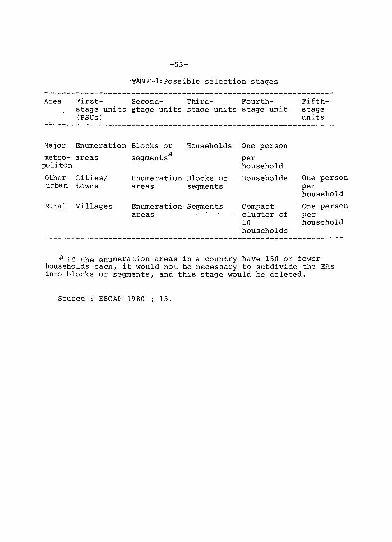
Area

-55-

'IfABlli-l: Possible selection stages

First- Second- Third- Fourth-stage units ~tage units stage units stage unit (PSUs)

, .

Fifth­stage units

-------------------------------------.~-------------------------

Major Enumeration

metro- areas politon

Other Cities/ urban towns

Rural Villages

Blocks or Households

segments~

Enumeration Blocks or areas segments

Enumeration Segments areas

One person

per household

Households

compact cluster of 10 households

One person per household

One person per household

------------------------------------------------~-~--------------

.,a if the enumeration areas in a country have 150 or fewer households each, it would not be necessary to subdivide the EAs into blocks or segments, and this stage would be deleted.

Source ESCAP 1980 15.

-56-

"-

is, trying to ~ocate a minority characteristic or

lI rare element" in a population. There are three viable

approaches to this problem with respect :li; migration

(Bilsborrow 1984: 100 ff):

(a) Stratified sampling with disproportionate

sampling fractions;

(b) Two-phase sampling;

(c) Special lists.

~ '2!_ ~ d'is12:r 'oEo:rt:ioh:a:te; :s'am:el:ihg: ·fr·ac·tion

The f61'lowing metnod is used to locate mig~ants

in destination areas efficiently:

(a) Listing urban areas in relation to the~r

population siz~ and then select with probabili~ies

proportional to their siz~;

(b) Generating tabulations on the number of in-

migrants and outmigrants for~he sampled cities only,

by smallest geographical area available;

(c) Classifying these geographical areas into strata

(two or four are sufficient!, according to the proportion

of households containing migrants;

(d) Listing blocks in each stratum in sequence,

then selecting from a random start.

The ILO recommends that selection should take

place within strata directly in proportion to the

estimated standard error of that proportion (Bilsborrow

1984: 104)

Two-phase sampling or sequential sampling can

also be used to increase thJpumbers of migrants. This

involves the selection of a subsample of elements from . a large sample. The first phase can then be used as a

screening device to identify the!,group of particular

-57-

interest or more detailed information may be gathered

for a randomly selected subsample to save costs. In

the screening procedure, a quick survey is made in all

the potential households of the smallest areal unit

to be selected to identify migrant status and then all

households containing migrants (or a large proportion

of them) and a smaller subsample of households not

containing migrants are selected for the more detailed

interviews. The relative numbers of migrants and

non-migrants to be interviewed will have to be decided

beforehand, for examDle, 50-50 or 90-10.

Quota sampling may be employed (as in the ILO

Punjab survey) at the final stage, For example, 60

households containing inmigrants and 65 not containing

migrants were selected randomly from the pre-listing.

" , '.' ~, • ... ~. T -.

... -+'.

Tracing technique

This is an alternative procedure, not technically

a sampling technique. Family members are traced from

origin to destination. The disadvantages are that it

is difficult to find large numbers of respondents and

it is also expensive.

Conclusion

It is imDortant to bear in mind that sampling

is not just a science, it is also an art. It is

critically important to hring in a sampling expert for

any large 'scale surveYr but at the same time it is

necessary to tailor each sa~~le to the case in hand and

local knowledge and educated questimates may be important

in the sample design, particularly where information on

migrant status and proportions of migrants are lacking.

Flexiblity is as important as Mathematical precision

to generate a useful sample design.

-58-

References

Bi1sborrow, R.E. (1984), "Survey design" in R.E.

Bi1sborrow,

A.S. Oberai and G. Standing (eds.), Migration

in Lo~ Income Couhtries,Guidelines .~ Survey

and Questionhaire Desi_£!n, London, Croom Helm,

pp. 60-87.

ESCAP (1980), National Migration Surveys, Yl. Sampl~ Des'ign Manual, United Nations, New York.

PLACE OF LAST RESIDENCE AND DURATION OF RESIDENCE

Ronald Skeldon

In the previous chapter we looked at the problems

inherent in the use of place of birth data for the

measurement and analysis of migration. In this chapter

I want to focus on what has become the most important

source of data for the study of internal migration; that

is, data on last place of residence (or previous place

of residence), which are often associated with data on

duration of residence.

There are two main approaches to place of last

residence. First, there is the question on last previous

place of residence before coming to the place of enumeration.

This is normally associated with a question on duration

of residence at the place of enumeration. Secondly,

there is the questlon on place of residence at a flxed

previous pOlnt in time, usually 5 years ago or 1 year ago.

This combines information on place of previous resldence

and time with in one question, which has obvious advantages

in the con~ext of census questionnaire design, coding

and processing costs.

I will consider each of these approaches in turn,

examining their strengths and weaknesses. Both approaches

are adopted to overcome the principal weaknesses of the

lifetime migration data with their lack of the time

dimension and the pos~ibilities of intermediate moves

between place of birth and present location. The place-of­

previous-residence questions should also pick up retltl"n

migration. The success with which the two approaches satis­

factorily avoid the problems inherent in the lifetime

-60-

approach varies with the questions adopted.

Place of last prevlous residence

The data are derived from the question, "Where

was your last previous place of residence before corning

to this place 7" In this case we are dealing with the

direct moves to the present place. In some cases this

will have been birt~place but in other cases it will

not. If there is also a question on birthplaceJwe then

have a person's location at three pointsj at birth plac~

at present place and at a previous place before coming

to the present place (if there was any such intermediate

location). These could all be the same or they could

all be different, which if indeed this is the case would

indicate "step" migration. Three categories of migrant

can be distinguished if these data exist (United Nations,

1970). If we refer to the locations at birth, previous

fixed point in time at present place as A, Band C,

we have:

Primary migrants

Secondary migrants

return migrants

A = B = C

A = B = C

A - C = B

The great advantage of this question over a

birt~:place migration question is that, if there is no

previous place of last residence, l.e., it is the same

as present place, then we are on much firmer ground for

classifying these people as "immobile" or "non-migrants"

Analyses of migrant/non-migration differentials can be

made with greater confidence when we are dealing with

this data base, although there are still problems in

relating the characteristics to the time of the move.

-61-

Return migration is also captured through this question

as, if someone has moved from origin A to destination

B and then back to origin A, his place of last previous

residence is destination B.

The problem with using this question by itself

is that again there is no time dimension. Moves from

the last place of residence that occurred £ months ago

are aggregated with those that occurred thirty to forty

years ago. Stratification of the migrants by age would

alleviate this problem, but it does not solve it. For

this reason, this question is usually associated with

a question on duration of residence in present place

since last coming to this place.

Of the thirteen countries in the Asia Pacific

region which as~ed a question on last place of previous

residence~ten also included a duration of residence

question. The combination of tnese two questions form

a powerful tool for the measurement of internal migration

and in a back~round paper on planning for the migration

questions for the 1990 round of censuses I recommended

that this approach should be accorded top priority

if the migration data bases of developing countries were

to be strengthened.

Does this then mean that there are no problems

or weaknesses with this approach? No, it does not.

The main weakness lies in the quality of the information

collected. Although the questions may appear relatively

simple, there is a danger that "last place of usual

residence" will. be misunderstood and both this question

and the one on duration of residence are subject to

problems of memory lapse. People may not remember where

their last usual place of residence actually was, as it

-62-

is a location in_the indete~minate past~ Also, there

is likely to be difficulty ~n ':, remembering exactly

how long it was since a person las~ moved t.o the

present residence: whether it was 7, 8 or 9 years ago.

The problem of durat.ion m~sstatement tends to increase

with length of residence, i.e., answers of those who

arrived at a destination 1 - 4 years ago are going to

be more accurate than those given by peOPle who have

lived in one place for 10 years and more. To some

extent, this can be taken care of through the coding

system in ~etailed classes: by months for the first

year, single years from 1 to 5 years and groups of

years after that, normally 5-9 years, 10-14 years and

more than 15 years. The responses of recent migrants

are considered to be more accurate in any analysis and

this is the group in which we have the greatest interest

anyway. The analysis tends to be by means of duration

cohorts, i.e., those who arrived or left at a particular

time. We can examine the duration cohorts of inmigration

to one area and the duration cohorts of out·.migration

from another area.

Of perhaps greater importance is thE~ problem

of misstatement of location of place of last residence.

,There is the specific problem of memory lapse, or not

remembering exactly where one was, but there is also a

more general point that is worth raising here (and this

problem to some extent also applies to birth place data); .... / .

the level of ~eneralization in specifying place of

previous residence. There is a general tendency for

respondents to state the general area where they' were and

not the exact location, i.e., to specify the province

rather than the district or the district rather than the

-63-

village. On questions relating to place of previous

residence (or to birthplace) the enumerators must be

trained to probe for the smallest possible settlement.

This is particularly important in movement to large

cities where the enumerator cannot be expected to be familiar

wi th all the districts,. l,et alone smaller settlements

of the migration catchment area. The respondent knows

this, so will tend to give the enumerator the name of

the largest settlement he thinks he will recognize.

The nature of this problem needs to be more widely

appreciated and adequate provision made for it in

enumerator training and field edit checking. In theory,

at least, the question on place of previous residence

in association with a question on durationsrould provide

us with the most useful information on internal migration.

A duration of residence question on its own does

not give any indication of the place of origin of the

inmigrants to a given area and therefore no information

on outmigration or on net-migration can be derived from

it. It should not be considered an adequate question

on its own for the analysis of internal migration,

although it is discussed in United Nations Manual VI

(1970) •..

Place of previous residence at ~ fixed point in time

The second general approach to place of previous

residence is to adopt a question on place of usual

residence at a fixed previous point in time. The question

is normally, "Where was your usual place of residence 1

year (5 or 10 years) ago ?tt This will provide in a simple

single question measurement of movement within a definite

period of time. The quality of data may be higher, then,

with the less specific last previous place of residence

question as people ~ill associate a place with a definite

-64-

time. Again, however, the data on a more recent definite

data in the past are likely to be more accurate than those

for more distant dats, i.e., responses to "I year ago"

will be more accurate than those to "10 years ago". Australia,

Newzaland and the Republic of Korea ask both "I year ago"

and "5 years ago". The attraction of this question to census

administrators is that it is just one question with a

consequent reduction in costs, both of training and of coding

and processing. It gives a count of surviving migrants

for a single fixed period of time.

There are disadvantages, however in the method. It

need not necessarily capture the "most recent" or "last"

migration to the present place. Return migration has a

greater probability of being missed than under the last­

previous-place-of-residence question. All moves before

1 year ago or 5 years ago are omitted. Short-term moves

(less than 1 year) associated with circulation are also

likely to be omitted.

The selection of the fixed time-period for the

question is the critical element for consideration: it

should be long enough to permit the accumulation of

enough relatively permanent movements so that the

analyst can detect preveiling patterns of migration and

can depend upon finding numerical frequencies that are

reasonably free from chance variation, but short enough

to obtain accurate data. Five years is generally accepted

as the optimum period.

A notable event such as Independence or another

event that is likely to be instantly recognized by the vast

majority of the respondents can be substituted as the

fixed point of reference. The answer to "where were you

normally living on Independence day?" should provide

-65-

accurate spatial and temporal data. This must be

balanced against the disadvantages that might accrue

if an odd time-period is the result, 7 or 8 years, for

example. In the 1980 census of Papua New Guinea,

Independence was in fact five years before the census

making it a useful measure for that century.

The standard measures of in-, out- and net­

migration can be calculated from the matrix of present

residence and residence "n" years ago or place of last

previous residence.

Implications £f enumeration strategy

A final point that should be borne in mind is that,

irrespective of the types of questions included in a

questionnaire to capture migration, the volume and type

of migration captured will vary depending on the nature

of the enumeration strategy, whether it is de jure or de facto.

De jure enumeration defines the place of present residence

as the place where a person usually lives at the time of

the census or survey. De f,actc enumeration def ines the

place of present residence as the place where the person

is actually found at the time of the census or survey. A

specific "census moment" may be defined, for example,

midnight on 30 June, or a "floating" point may be taken

such as the night before the enumerato~ visit to the

house. There is strong support for the recommendation that

all censuses should be taken on a de jure basis, the

assumption being that "real migration" is a change in

the usual place of residence. There are, however, important

considerations against this approach on 'Jbil'th methodologic~l

~nd conceptual grounds. "Usual place of residence" is

)ften difficult to define and difficult to apply in the

Eield, particularly where enumerators may be poorly trained

-66-

and the respondents illiterate. A definition of usual

place of residence such as the fOllowi~g is not

unusual; "that place in which an individual has resided

more than 6 months, or less than 6 months but where

he intends to stay permanently; or, if a person has been

away from that place for less than 6 months, he intends

to return to it". This is likely to be misinterpreted

in the field situation leading to spurious results.

On a conceptual level, de ju~e registration omits much

short term mobility which is likely to be of value to

policy-makers. For these reasons, a de nae~o system

is to be preferred, even though we may well be comparing

place of "usual residence" in the past with actual

place in the present. This is an annoying but unavoidable

problem, but it is not realistic to ask for actual place

at some indeterminate data in the past.

An example of an interpretation of duration-of­

residence and place-of-Iast-residence data for India

can be found in Skeldon (1985).

R e. 6 e.)(. e. n c. e..6

Skeldon, R. (1985) "Migration in South Asia; An Overview" in L.A. Kosinski and K.M. Elashi 'eds), Populax~on Re.-d~.6~)(.~bu~~on and Ueve.lopmen~ in Sou~h A.6~a, Boston, Reidel, pp. 37-63

united Nations (1970) Manual.6 on Me.~hod.6 on E.6~ima~ing Popula~ion. Manual VI Me.~hod.6 06 Me.a.6u)(.,[ng In~e.~nal Migna~~on, New York.

INTERNAL MIGRATION IN INDIA AN ASSESSMENT

S.K. SINHA

Movement from one place to other in India pr~marily

rests on the individual concerned. The federal structure

of the Indian Union gives freedom of movement within the

country. With the intensification of trade and commerce

coupled with industrial development population mobility is

bound to increase. Movement could either be mere commuting

between place of residence and place of work or a change of

the place of residence itself. Internal migration takes

place when individuals change their place of residence and/

or leave their place of birth within the country. It is

a dynamic process and the volume of internal migrants is

difficul t to be assessed. If onJy the Population Register

exists and movements of persons are recorded, the volume

of both in-and out-migrants for any region could be

assessed accurately.

Indian Population Censuses haye been the major

source (perhaps the only - other than the occasional

information on mobility collected on sample basis by the

National Sample Survey Organisation in its various 'rounds')

of providing the volume of internal migration. Information

on place of birth has been a major item of enquiry in the

individual slip. Till the 1951 census place of birth data

was collected at the district level. Exact place of birth

of the person enumerated and whether the place of birth

was rural/urban was collected for the first time ~n the 1961

census and has been continued in the 1971 and 1981 censuses

also. In addition to the birth place statistics data on

the duration of residence in the place of enumeration

is also being collected in the census since 1961.

Information on the place of enumeration gives estimates

of'lifetime migration' and may not reveal the latest

-68-

information on population mobility. This information was

collected in the 1971 census for the· f~rst time and has been

continued in the 1981 census also. Thus two sets of data

on population mobility (one giving lifetime migration and

the other giving latest mobility) are available from the

CenSus. The 1981 census has also tried to collect data on

the possible reasons of individuals migrating from one place

to other. Of course the limitation of the 1981 census

is that migration data has been collected on a 20 per cent

area sample basis. The 'reasons of migration' in the 1981

census q_re: (a) employment, . (b) education, (c) family moved,

(d) marriage and (e) other reasons.

Based on the place of birth (or the place of last

residence) and the place of enumeration, migrants can be

classified into four migration streams: (1) rural to rural,

(2) rural to urban, (3) urban to rural. and (4) urban to

urban. In order to study the impact of migration on

urbanization these streams except (1) are useful. At the

national level (2) is also not relevant.

Table 1 gives the per cent distribution of

population by type of movement both by birth place and last

residence for 1961, 1971 and .1981 censuses. The pattern

of movements has not changed significantly. Percentage of

foreigners in India has .. declined from 2.2 per cent in 1961

to 1.2 per cent in 1981. The~e has not been any change in

the intelPS"tctte movement. Interdistrict movement wi thin the

state of enumeration has marginally increased whereas

intra.d.istrict movements have declined. The percent of

mobile population has declined from 33 percent in 1961

to 30.7 percent in 1981. By both the concepts only thirty

percent of the population in India changes its place of

residence.

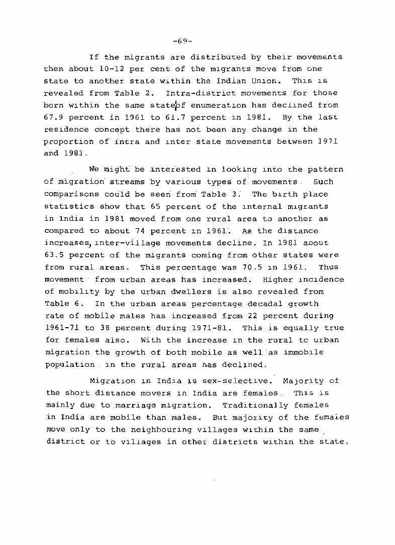
-69-

If the migrants are distributed by their movements

then about 10-12 per cent of the mlgrants move from one

state to another state w~thin the Indian UnlOli. This 15

revealed from Table 2. Intra-district movements for those

born wlthin the same state~f enumeratlon has declined from

67.9 percent in 1961 to 61.7 percent in 1981. By the last

residence concept there has not been any change in the

proportion of intra and lnter state movements between 1971

and 1981.

We might be lnte.rested ln looking lnto the pattern

of migration st'reams by various types of' movements, Such

comparisons could be seen from Table 3; The birth place

statistics show that 65 percent of the lnternal mig.rants

in India in 1981 moved from one rural area t~o another as

compared to about 74 percent ln 1961". As the distance

increases, inter-village movements decllne" In 1981 aDout

63.5 percent of the migrants coming from other states were

from rural areas. This percentage was 70.5 in 1961. Thus

movement from urban areas has lncreased. Higher lncldence

of mobillty by the urban dwellers is also revealed from

Table 6. In the urban areas percentage decadal growth

rate of mobile males has increased from 22 percent during

1961-71 to 38 percent during 1971-81. This is equally true

for females also. With the increase ln the rural to urban

migration the growth of both mobile as well as immabl1e

poplll.ation ln the rural areas has decllned.

Migration In Indla lS sex-selective. Majority of

the short distance movers In India are females. This is

mainly due to marriage migration. Traditlonally females

in India are mobile than males. But majorlty of the females

move only to the neighbouring villages within the same

district or to villages in other districts withln the state.

-70-

Table 5 gives the sex-ratio (males per 1,000 females) of

population by type of movement separately for rural and urban

areas. In 1981 for every 1,000 mobile females in the rural

areas there were only 294 males. In the urban areas there

were 947 mobile males for every 1,000 mobile females.

Information on the duration of residence in the

place of enumeration was collected for the first time in the

1961 census. This was with reference to the place of birth.

Since. 1971 .this _ in.formation is tabulated for migrants by

last residence. In table 4, a: comparison has been made

between the distribution of migrants in rural and urban

areas for 1971 and 1981 censuses by duration of residence

in the place of enumeration. In the urban areas the

share of migrants whose duration of residence in the place

of enumeration was more than ten years increased from 3406

percent in 1971 to 46.4 percent in 1981. Both in the rural

and urban areas share of migrants with duration less than

one year has declined.

Characteristics of migrants from the 1981 census

are still not available. Distribution of migrants by

broad age groups and their marital status as revealed from

the 1971 cerisus are preserited in Table 7 & 8 respectively.

In the urban areas about sixty percent of the male migrants

were aged 25 years and above as against thirty percent among

the non.,...migrants. About half of the non-migrants were aged

below 15 as against about twenty percent of the migrant

population .. _72 percent of the female migrants in rural areas

were married as against only 25 perceht for the non-migrants.

The proport.ion of widowed and divorced females was more

among the migrant females than the non-migrant females. This

is perhaps due to the fact that most of the widowed females

move to their sons/daughters living in other places. Majority

of the non-migrant females both in the rural and urban areas

being young are never married.

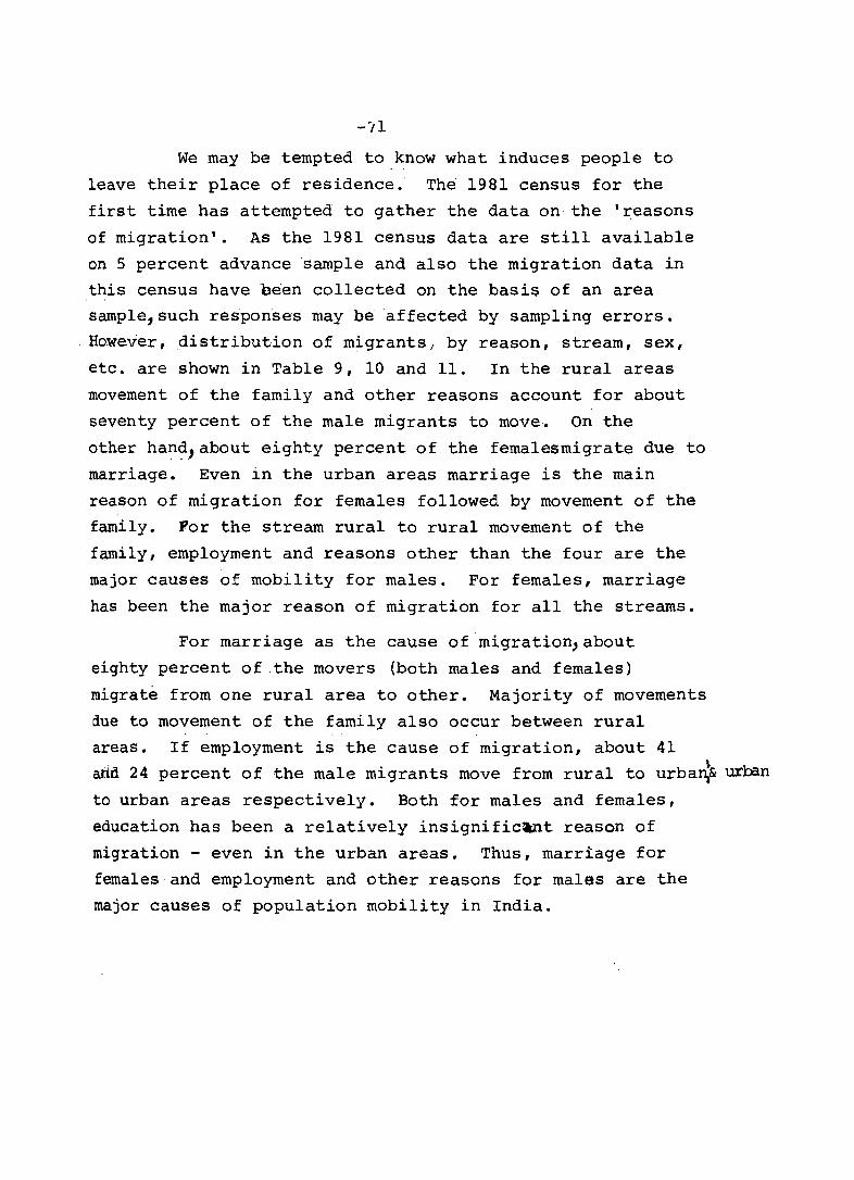
We may be tempted to know what induces people to

leave their place of residence. The 1981 census for the

first time has attempted to gather the data on the 'reasons

of migration'. As the 1981 census data are still available

on 5 percent advance sample and also the migration data in

this census have been collected on the basi$ of an area sample,such responses may be affected by sampling errors.

However, distribution of migrants, by reason, stream, sex,

etc. are shown in Table 9, 10 and 11. In the rural areas

movement of the family and other reasons account for about

seventy percent of the male migrants to move. On the

other hand,about eighty percent of the femalesmigrate due to

marriage. Even in the urban areas marriage is the main

reason of migration for females followed by movement of the

family. For the stream rural to rural movement of the

family, employment and reasons other than the four are the

major causes of mobility for males. For females, marriage

has been the major reason of migration for all the streams.

For marriage as the cause of migration,about

eighty percent of the movers (both males and females)

migrate from one rural area to other. Majority of movements

due to movement of the family also occur between rural

areas. If employment is the cause of migration, about 41

arid 24 percent of the male migrants move from rural to urba~& urban

to urban areas respectively. Both for males and females,

education has been a relatively insignific~t reason of

migration - even in the urban areas. Thus, marriage for

females and employment and other reasons for males are the

major causes of population mobility in India.

-72-

INTERNAL MIGRATION IN INDIA

TABLE - 1

Percentage distribution of population by movement,1961-Bl

-----------------------------------------------------------------Type of movement By place of birth By last t.esidence

--r96I---I§7I---I§§I---I971---19SI--~----------------------------------------------------------------

Birth place/last residence same as the place of enumeratJ.on

67.0 69.6 69.3 69.4 68.8

-----------------------------------------------------------------Bo~{. /last residence elsewhere in the district 20.9 18.9 IB.2 19.2 19.2 of enumeration --'--'---'--'----:_'-,_'_'-'_'-,_,_,-'_"_._---'_"_'---,_ ------------ - --- - - - - ---.- - - - - ----Born/Lastresidence in other distrJ.cts of the state of 6.6 6.4 7.7 6.5 7.6 enumera tion ----------------_._----'_._-_._._._'--' ..... _--_._---------------------------Born/Last residence in other States within India 3.3 3.4 3.6 3.5 3.5 ----------.-_,_._, __ '_._.~_-,-.-----------------,-------------------------Born/Last residence outside India 2.2 1.7 1.2 1.4 0.9 ------------_._---_._---------------------------------------------

Tot~l 100.0 100.0 100.0 100.0 100.0 ------.------'-.-.-'~---'-.--~~--.---'--------------------------------

TABLE-2 -------Percentage distribution of Internal Migrants by movement

1961-81

----------------------------------------------------------------By place of birth By last

Type of movement Residence 1961---1971---1981---1971---1981-----------------------------------------------------------------

(a) Birth Place/Last residence 67.9 65. B 61. 7 65.8 63.4 elsewhere in the district of enumeration ---------------------------------------------------------------

(b) Birth Place/Last residence 21.3 22.4 26.1 22.4 25.0 in other districts of the State of enumeration

-----------~---------------------------------------------------Intra-State Migration

(a) + (b) 89.2 8B.2 B7.8 88.2 88.4 ---------------------------------------------------------------- ___ !~~~!:~~~~~_~~g!~!!2~ ______ !Q~~ ___ !!~~ ___ !£~~ ___ !!~~ ___ !!~§ ----'!:2~e!_i:~~~!!!~!_~!g!~!!~~ ___ !QQ~Q __ !QQ.!.Q __ !QQ~Q __ !QQ~Q __ 1QQ..:.Q

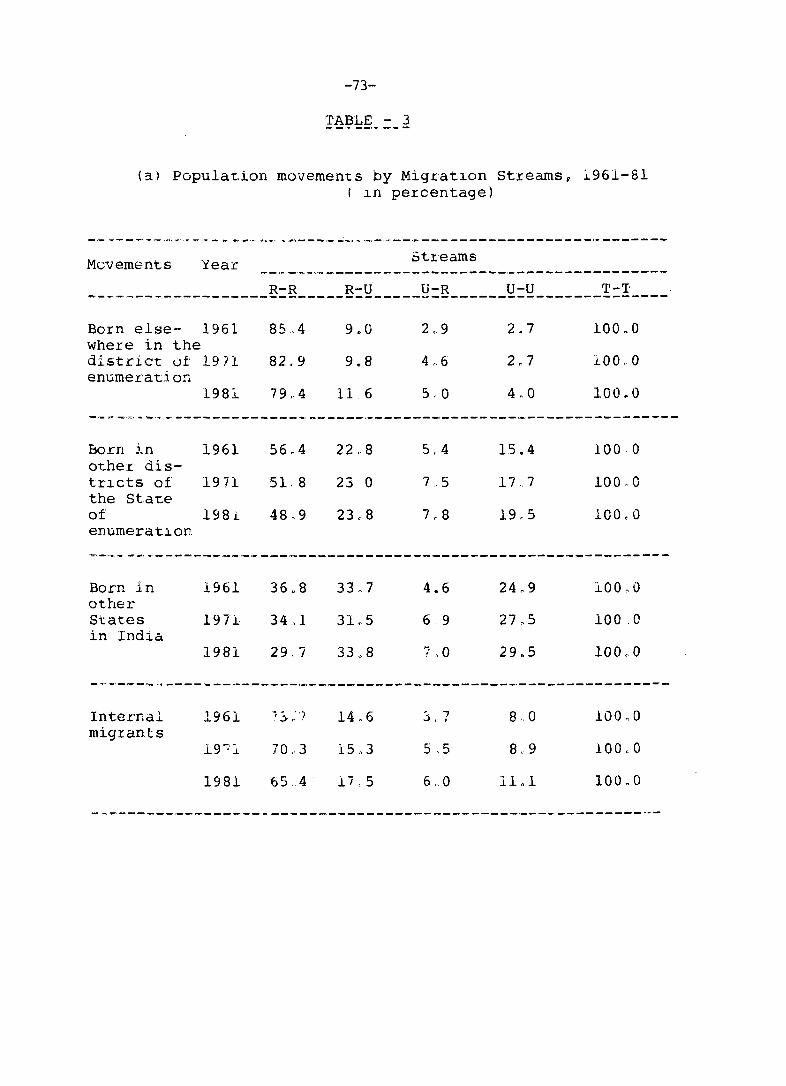
-73-

(aJ Popu1a1:.ion mOvements by Migratlon Streams, 1.961-81 ( in percentage)

-------------------- ------~----------------------------------

Movements Year Streams

R-R R-U U-R U-U T-T -------------------------------------------------------------Born e1se- 1961 85,4 9.0 2,.9 2.7 100.0 where in t.he district of 1971 82,9 9.8 4,,6 2.7 100.0 enume.catlOn.

198i 79,,4 11,6 5.0 400 100.0

Born in 1961 5604 22,8 5.4 15.4 100 0 other dis-tn.cts of 1971 51. 8 23 0 7,,5 17 .. 7 100.0 the State of 1981. 48.9 2308 7,,8 1905 100,0 enumerat.l.on

Born in 1961 36,,8 33,7 4.6 24,,9 10000 other States 1971 34 .. 1 3L5 6.9 2705 100.0 in India

1981 29.7 33.8 ?,O 29.5 100,,0

Internal 1961 -; 3,,'7 14,,6 ~, 7 8.0 100,,0 • migrants

19'":':1 70.,3 15,3 5,5 8,9 100,.0

1981 65A 17.5 6,,0 11.1 100nO

------------------------------------------------------------

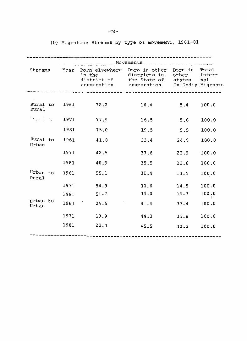
-74-

(b) Migration Streams by type of movement, 1961-81

Streams

______________ ~2Y~IE~~!:~ ______________________ _

Year Born elsewhere in the district of enumeration

Born in other districts in the State of enumeration

Born in Total other Inter-states nal In India Migrants

-----------------------------------------------------------------Rural to 1961 78.2 16.4 5.4 100.0 Rural

1971 77.9 16.5 5.6 100.0

1981 75.0 19.5 5.5 100.0

Rural to 1961 41.8 33.4 24.8 100.0 Urban

1971 42.5 33.6 23.9 100.0

1981 40.9 35.5 23.6 100.0

Urban to 1961 55.1 31.4 13.5 100.0 Rural

1971 54.9 30.6 14.5 100.0

1981 51.7 34.0 14.3 100.0

urban to 1961 25.5 41.4 33.4 100.0 Urban

1971 19.9 44.3 35.8 100.0

1981 22.3 45.5 32.2 100.0

----------------------------------------------------------------

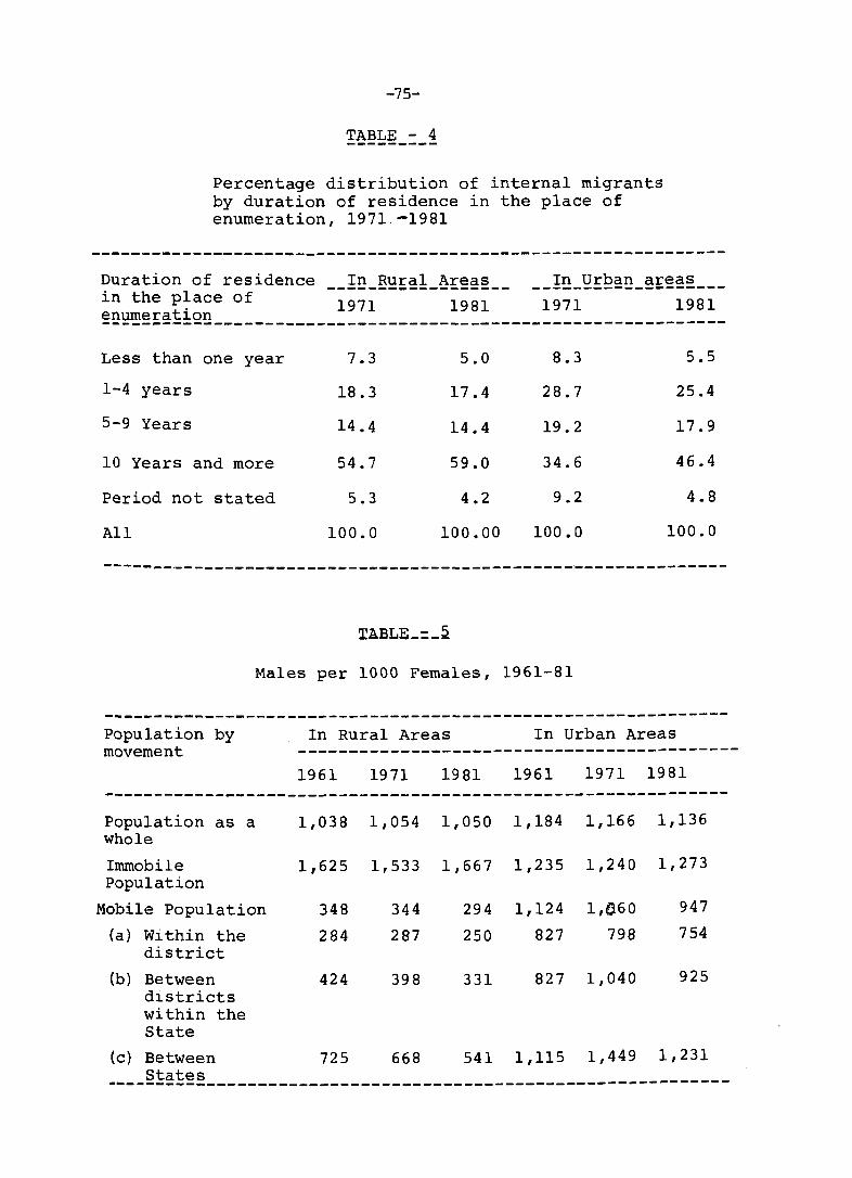
-75-

TABLE - 4 ---------

Percentage distribution of internal migrants by duration of residence in the place of enumeration, 1971 -1981

--------------------------------------------------------------Duration of residence __ !~_g~E~!_~E~~~__ __!~_Qf~~~_~~~~~ __ _ in the place of enumeration 1971 1981 1971 1981 -------------------------------------------------------------Less than one year 7.3 5.0 8.3 5.5

1-4 years 18.3 17.4 28.7 25.4

5-9 Years 14.4 14.4 19.2 17.9

10 Years and more 54.7 59.0 34.6 46.4

Period not stated 5.3 4.2 9.2 4.8

All 100.0 100.00 100.0 100.0

-------------------------------------------------------------

Males per 1000 Females, 1961-81

-------------------------------------------------------------Population by movement

In Rural Areas In Urban Areas -------------------------------------------1961 1971 1981 1961 1971 1981

-------------------------------------------------------------Population as a 1,038 1,054 1,050 1,184 1,166 1,136 whole

Immobile 1,625 1,533 1,667 1,235 1,240 1,273 Population

Mobile Population 348 344 294 1,124 1,e60 947

(a) Within the 284 287 250 827 798 754 district

(b) Between 424 398 331 827 1,040 925 districts within the State

(c) Between 725 668 541 1,115 1,449 1,231 States

---~---------------------------------------------------------

-76-

TABLE - 6

Growth of Population by type and sex 1961-81 (Percent decada1)

Rural Areas Urban Areas Type -----------------------------------------------------

Males Females Males Females ------------------------------------------------------61-71 71-81 61-71 71-81 61-71 71-81 61-71 71-81 ------------------------------------------------------------------

Mobile

Immobile

Total

13.3

24.8

23.2

S.S

17.4

lS.9

6.7

27.3

18.0

29.9

12.1

19.4

TABLE - 7 ---------

21.9

52.4

40.1

37.8

48.6

44.8

29.4

51.8

42.2

Percentage distribution of Population by broad age-groups, sex and residence,1971

S4.4

44.7

48.S

------------------------------------------------------------------Age­groups (Yrs. )

In Rural Areas In Urban Areas - _______ i_- ___________________________________________ ------

Male Female Male Female ------------------------------------------------------------M NM T M NM T M NM T M NM T

---------------------------------------~----------------------------

Below IS 28.3 4S.4 43.0 13.7 64.3 42.5 18.9 49.7 37.5 17.7·58.2 40.8

,'.-"

15..19 9.0 8.S 8.5 9.1 7.3 8.1 9.6 10.8 10.1 9.3·10.6 9.9

20-24 9.6 6.6 7.0 12.9 4.1 7.9 12.2 8.4 9.8 15.4 6.7 9.4

25-49 37.2 27.3 28.7 45.7 17.1 29.4 46.1 22.7 32.0 45.0 17.6 29.5

SO+ lS.9 12.2 12.8 18.6 7.3 12.9 13.2 8.4 10.6 14.6 6.9 10.4

All 100.0 100.0 100.0 100.0 100.0 100.0 100.0 100.0 100.0 100.0 100.0 100.0

------0:-----.-___________________ '_' __ '_' ____ '_'-: __ '_'_'_:-._,_,_, _______ '_'_._'_'_-_______ _

M = Migrants

NM = Non Migrants

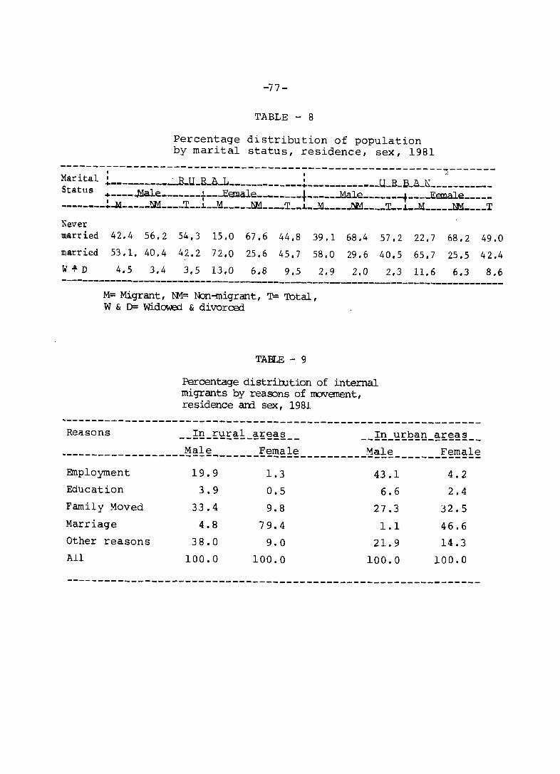
-77-

TABLE - 8

Percentage distribution of population by marital status, residence, sex, 1981

-------~----------------------------~--------------------~-------Marital ~------------B-U_E_~---__________ ~ _____________ U_B-B~_N __________ _ Sta t u s -:-----"Jia,le-------+---Ee:nale------__ t _____ ....Male _______ t ___ -E6Ilale ____ _ --------.~-----~----T_-~--~----_~ ____ T __ ~ _ _M ____ ~ ____ T __ ~_~ ____ ~ ____ T Never married 42.4 56.2 54.3 15.0 67.6 44.8 39.1 68.4 57.2 22.7 68.2 49.0 married 53,1. 40.4 42.2 72.0 25.6 45.7 58.0 29,6 40,5 65,7 25.5 42.4 W-fD 4.5 3.4 3,5 13.0 6.8 9.5 2,9 2,0 2.3 11.6 6.3 8.6 -------------------------------------------------------------------------------

M= Migrant, l\M= Non-migrant, T='lbtal, W & D= Wido.-.ed & divorcerl

TABLE - 9

Percentage distrihltion of internal migrants by reasons of rrovement, residence and SeK, 1981

---------------------------------------------------------------Reasons

Male Female Male Female ---------------------------------------------------------------Employment 19.9 1.3 43.1 4.2 Education 3.9 0.5 6.6 2.4

Family Moved 33.4 9.8 27.3 32.5

Marriage 4.8 79.4 1.1 46.6 Other reasons 38.0 9.0 21. 9 14.3 All 100.0 100.0 100.0 100.0

--------------------------------------------------------------

-78-

TABLE - 10

Percentage distribution of migrants by reasons of movement and stream by sex,

1981

-------------------------------------------~-!-~-~-§---Reasons R-R R-U U-R U-U

Employment 1905 47.5 27.0 41.1

Education 4.2 8.1 3.2 5.2

Family Moved 33.7 23.5 31.9 31.5

Marriage 5.5 4.2 2.2 1.0

Other reasons 37.1 19.2 35.7 21.2

All 100.0 100.0 100.0 100.0

F E MAL E S

Employment 1.1 4.2 3.3 4.4

Education 0.4 2.6 1.0 2.2

Family Moved 8.6 29.3 21.2 35.9

Marriage 81.7 51.5 59.3 43.6

Other reasons 8.2 12.4 15.2 13.9

All 100.0 100.0 100.0 100.0

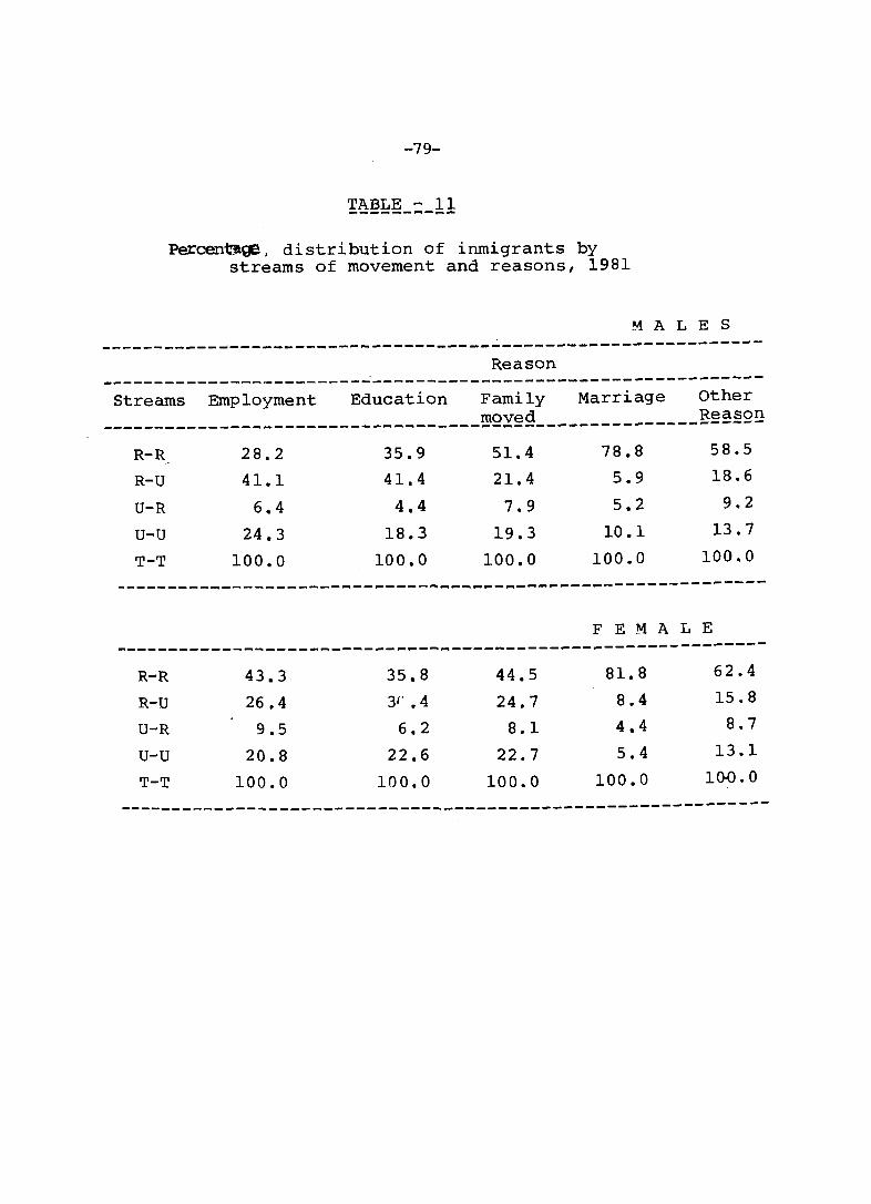
-79-

percenn.ge" distribution of inmigrants by streams of movement and reasons, 1981

MAL E S -------------------------------------------------------------

Reason -------------------------------------------------------------Streams Employment Education Family Marriage other

moved Reason -------------------------------------------------------------R-R 28.2 35.9 51.4 78.8 58.5

R-U 41.1 41.4 21.4 5.9 18.6

U-R 6.4 4.4 7.9 5.2 9.2

U-U 24.3 18.3 19.3 10.1 13.7

T-T 100.0 100.0 100.0 100.0 100.0

-----------------------------~----~-------------------------

F E MAL E -----------------------------------~------------------------

R-R 43.3 35.8 44.5 81. 8 62.4

R-U 26.4 3(' .4 24.7 8.4 15.8

U-R 9.5 6.2 8.1 4.4 8.7

U-U 20.8 22.6 22.7 5.4 13.1

T-T 100.0 100.0 100.0 100.0 10'().0

------------------------------------------------------------

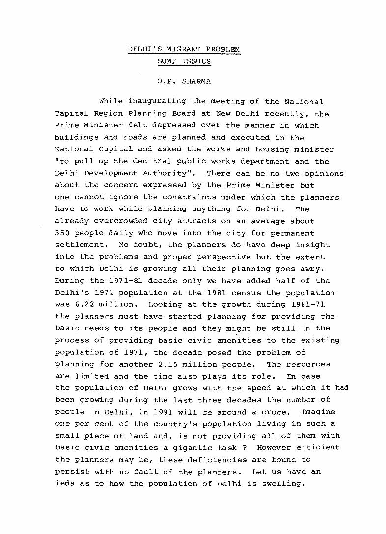
DELHI'S MIGRANT PROBLEM

SOME ISSUES

o.P. SHARMA

While inaugurating the meeting of the National

Capital Region Planning Board at New Delhi recently, the

Prime Minister felt depressed over the manner in which

buildings and roads are planned and executed in the

National Capital and asked the works and housing minister

"to pull up the Cen tral public works department and the

Delhi Development Authority". There can be no two opinions

about the concern expressed by the Prime Minister but

one cannot ignore the constraints under which the planners

have to work while planning anything for Delhi. The

already overcrowded city attracts on an average about

350 people daily who move into the city for permanent

settlement. No doubt, the planners do have deep insight

into the problems and proper perspective but the extent

to which Delhi is growing all their planning goes awry.

During the 1971-81 decade only we have added half of the

Delhi's 1971 population at the 1981 census the population

was 6.22 million. Looking at the growth during 1961-71

the planners must have started planning for providing the

basic needs to its people and they might be still in the

process of providing basic civic amenities to the existing

population of 1971, the decade posed the problem of

planning for another 2.15 million people. The resources

are limited and the time also plays its role. In case

the population of Delhi grows with the speed at which it had

been growing during the last three decades the number of

people in Delhi, in 1991 will be around a crore. Imagine

one per cent of the country's population living in such a

small piece of land and, is not providing all of them with

basic civic amenities a gigantic task? However efficient

the planners may be, these deficiencies are bound to

persist with no fault of the planners. Let us have an

ieda as to how the population of Delhi is swelling.

-81-

Till 19~1 the growth of population of Union

Territory of Delhi was slow. Over the three decades, from

1901, its population increased by 57 per cent from

0 .. 41 million to 0.64mi11ion. Next decade experienced "a

watershed and the population in 1941 increased to

0.92 million, giving a growth rate of 44.27 per cent

1941-51 decade took sudden leap due to exchange of population

between India and Pakistan during 1947, and in the bargain

Delhi gained a lot. The population of Union Territory of

Delhi/lpgJe~~~million in 1941 to 1.47 million in 1951.

Therefore, the decadal rate of growth of population had

been more than 50 per cent and it is steadily going up in

each successive decade. The rate of growth of population

during 1951-61 was 52.44 per cent/·~2.93 per cent during

1961-71 and 53.00 per cent during 1971-81. At the turn

of the century the population of Delhi was only 0.41 million

and during 1901-81 the population increased to 6.22 million,

which means we have added 20 Delhis of 1901 of which

2.15 million or 5 Delhis of 1901 were added during 1971-

81 only. The trend of the growth of population of Union

Territory after 1941 suggests that in addition to large

number of displaced persons, it threw open its gates to the

migrants from other States and Union Territories with the

result that at the 1981 Census there was not even a single

state or Union Territory which had not contributed to De1hi 1s

population growth.

The popUlation of Union Territory of Delhi according

to the 1971 census was 4.07 million, During the decade

1971-81, more than half of Delhi1s 1971 population was

added to Union Territory of Delhi. The population of Union

Te-rri tory of Delhi according to the 1981 Census stood

-82-

at 6.22 million-an addition of 2.15 million people during

the decade. This gives a percentage increase of 53.00.

During 1971-81 out of this 2.15 million population,1.23

million moved to Delhi from other states and Union

Territories and 0.28 million people out of 4.07 million

in 1971 moved out of other States and Union Territories.

Delhi's net gain due to migration was of the order of

0.95 million. If we subtract this in-migration and add

the out-migration, the 1981 population cbmes to 5.55

million as against 4.07 million in 1971. The difference

during the decade works out to 1.48 million which is

supposed to be the natural increase. The growth ~ate,

after taking net migration into account works out to

29.60 per cent which is higher than the national rate

of 25.00 per cent.

The population of Union Territory of Delhi is

predominantly urban. At the 1971 census 89.70 per cent

of its population lived in urban areas comprising Delhi

Municipal Corporation (DMC), New Delhi Municipal Committee

(NDMC) and Delhi Cantonment (Cantt) while this percentage

increased to 92.73 because of declaration of 27 villages

as towns at the 1981 census. According to the 1981 census

the number of villages in Union Territory of Delhi was

258 of which 17 were un-inhabited and 27 treated as towns.

Effectively the number of villages thus comes to 214. Of

these , 27 villages which were treated as towns at the

time of the 198~census, as many as 22 were part of the

Delhi urban agglomeration which also included DMC, NDMC

and Cantonment. Only 5 towns were outside the Delhi and

kept their identity. Of the 0.46 million people living

in rural parts of Union Territory of Delhi in 1981, 0.28

--83--

million were enumerated in 132 inhabited villages of Delhi

tehsil and 0.18 million in 82 inhabited villages of Mehrauli

tehsil.

Out of 6.22 million people enumerated in Union

Territory of Delhi, 3.23 million were born at the place of

enumeration and the remaining 2.99 were migrants. Of these

2.99 million migrants, 0.32 million or 10.84 per cent had

moved to the place of their enumeration from other parts of

Union Territory of Delhi and 2.30 million or 76.92 per cent

had their place of last residence in one of the states o~

Union Territory and the remaining 0.37 million or 12.24 per

cent moved to Delhi from other countries. Of these 0.37

million migrants from other countries 0.33 million were

those whose last residence was Pakistan. A majority of

these 0.33 million people had moved to Delhi after the

partition of the country in 1947 and settled here. However,

because of the instruction to enumerators at the time of

the 1981 census, their place of last residence had been

recorded as Pakistan. If we s~bstract these 0.33 million

people whose last residence was Pakistan then we are left

with 2.66 million total migrants.

The significant contribution towards the population from . t . . growth was of~other states and Un~on err~torTes.Of the

2.99 million total migrants to Delhi, as said earlier, 2.30

million were from other states and Union Territories and out

of these 2.30 million migrants almost half- 48.18 per cent

to be exact, were from Uttar Pradesh. Haryana and punjab

contributed 15.56 and 9.77 per cent of the 2.30 million

migrants. Other states and Union Territories which contributed

more than 1 per cent of these migrants were Bihar (3.99),

r.\adhya Pradesh(2.38) , West Bengal(2.34), Himachal Pradesh

(2.16), Maharashtra (1.78},Tamil Nadu(1.48) and Kerala

(1.13). There is not even a single state or Union Territory

-84-

which has not sent its people to Delhi. Even as far off

place like Lakshadweep has sent 51 of its people to

union Territory of Delhi.

However, if we take only the recent migration,

i.e. those migrants who moved to Delhi during 1971-81

or who have been residing at the place of enumeration

for less than 10 years, the number comes down to 1.23

million, which accounts for 53.48 per cent of the total

2.30 million migrants from different states and Union

Territories, 22.85 per cent of these migrants moved to

the place of their enumeration during 1961-71 i.e. they

had been residing at the place of enumeration between

10 and 19 years. Those who had been residing at the

place of enumeration for 20 years or more accounted for

19.36 per cent and the period in respect of the

remaining 4.31 per cent could not be det~~rnined.

Of the 1.23 million migrants who moved to

Union Territory of Delhi during the last decade of 1971-

81 from other states and Union Territories 'hhe majority

was from Uttar Pradesh. Together they accounted for

50.09 per cent of the migrants from other states and , .. ~~o . . f Unlon Terrltorles who had move~ Unlon Terrltory 0

Delhi during 1971-81. States which accounted for more

than one per cent of such migrants were Haryana (12.93)

Rajasthan (7.63),Punjab(6.49),Bihar(5.77},Madhya Pradesh

(3.07), West Bengal (2.70) ,t.1aharashtra (2 . 01) , . Himachal

Pradesh(1.91), Tamil Nadu(1.66} and Kerala(1.47}.

The flow of migrants has increased substantially

during the recent past, from a majority of the states and

Union Territories. The highest percentage of the total

-85-

migrants who moved to Union Territory during the last

decade was recorded by the states and Union Territories

in the north-east region. For instance, 86.92 per cent

of the migrant.s numbering 428 moved during the last

decade. In the case of Nagaland and Manipu~ the percent­

ages were 81. 29 and 77" 94 and in the case of Meghalaya

the percentage was 77.20. 76.89 per cent of the total

m~grants from Assam moved to Union Territory of Delhi

during 1971-81. In the case of Bihar also the percentage

of migrants who moved to Delhi during 1971-81 was quite

high. They accounted for 77.21 per cent of 0.92 mill~on

migrants. The flow from the neighbouring states, during

the last decade was not so high. For instance, out of

1.11 million total migrants from Uttar Pradesh, 55.61

per cent moved to Delhi during 1971-81. Similar1~ out

of 0.17 million migrants from Rajasthan,53.72 per cent

moved during 1971-81. Of the 0.36 million migrants from

Haryana, 44.46 per cent moved during the last decade

and7~5sition of Punjab is still different. In all 0.22

million people recorded their place of last residence in

Punjab and only 0.08 million or 35.03 per cent moved

during the last decade. It will thus be noticed that

during the recent past, the flow of migrants from the

neighbouring states has been comparatively slow in

relation to far off states and Union Territories though

in absolute terms their number is small.

The question which immediately comes to one's

mind is why so many people get attracted towards Union

Territory of Delhi. Very valuable information has been

collected at the recent census about the reason for

-86-

migration. B:oadly:the reasons for migration have been

classified under five heads employment, educ~tion, marriage,

family moved and the rest. Family moved includes those

who had to move because of the shift of the head of the

household because of employment or in a few cases because

of education, though the degree of the latter category

may not be slgnificant.

Out of 2.30 million tot~l mig~ants, as mentioned

earlier, 1.23 million moved to Delhi du~ing 1971-81. The

highest number wa,s of those who had to move because of

the movement of their family. Their number, out of 1.23·

million was 0.49 million ~ich gives a percentage of 39.42.

Next comes employment. The number of such migrants was

0.42 million and they accounted for 34.48 per oent of the

total migrants. The migration because of marri~ge was

also quite significant. The number of such nrigranbs was

0.16 milllon and they formed 12.63 per cent of the total

migrants. Movement because of education, as one would

expect, was quite iess. Their number was 0.04 million

and they accounted for only 3.33 per cent of the tot~l

migrants. In the case of 10.14 per cent of the total

migrants, the reaSOn for migration could not be determined.

Out of 0.78 million migrants who moved to Union

Territory of Delhi because of emploYlment, as many as

0.42 million or 54.07 per cent were from uttar Pradesp

alone. Haryana, Rajasthan and Punja.b accounted for

10.71, 7.71, and 7.05 per cent of the total migrants' who

moved to Delhi for employment. Out of 0.38 million migrants

who moved to Union Territory of Delhi because of marriage,

0.16 million or 43.45 per cent were. from Uttar Pradesh and

0.11 million or 29.61 per cent were from Haryana. Respective

percentages in the case of Punjab ,and Rajasthan were 9.70

and 6.91.

-87-

Out of 60,337 migrants who came to Delhi

because of education, 27,599 Or 45.74 per cent came

from Uttar Pradesh and 9,927 or 16.45 per cent moved

from Haryana. Respective percentages in the Gas~ of

Punjab and Rajasthan were 8.05 and 5.34.

The maJority of migrants who moved to Union

Territory of Delhi,as said earlie~was because of the

movement of their families. Out of these 0.83 million

migrants, 381,048 or 46.17 per cent were from Uttar

Pradesh and 116,059 or 14.06 per cent were from Haryana,

Punjab and Rajasthan accounted for 11.63 and 8.02 per

cent of the total migrants who moved to union Territory

of Delhi because of the movem~nt of ~heir families.

After the reason "Family moved" which

accounted for the highest percentage, the reason for

migration which accounted for the next highest percentage

was "employment". The share of such migrations for the

country as a whole was 33.78 per cent. States and

Union Territories which had share of such migrants

higher than country's percentage were Bihar (54.63),

Kerala (42.69), Orissa t40.58}, Uttar Pradesh (37.91),

Pondicherry \36.33), Dadra & ~agar Haveli (35.29),

Madhya Pradesh (34.85) and Rajasthan (34.27). The lowest

percentage of such migrants Was from Manipur (17.90).

In the case of Manipur, next to the reason family

moved, the reason of migrant was highest of those

who moved to Un~on Terr~tory for education (23.54).

More than 10 per cent of the migrants from Lakshadweep

moved to Delhi for education.

Movement because of "Marriage", as one could expect,

was quite significant in case of Haryana. Out of 357,709

migrants from Haryana 111,066 or 31.05 per cent moved

-88-

because of "marriage". The share in the case of punjab

was 16.20, in the case of Rajasthan 14.84, in the case

of uttar Pradesh 14.71 and in the case of Gujarat it

was 12.84 per cent. Other states and Union Territories

where the share was more than 10 per cent were Chandigarh

(11.91), Maharashtra (11. 05), Jammu & Kashmir (11.4), Himachal

Pradesh(10.30), Madhya Pradesh(lO.48) and West Bengal

(10.10). The lowest percentage was recorded by Mizoram

(0.61) preceded by Arunachal Pradesh (1.87) and Nagaland

(2.41).

The flow of migrants to Delhi is not confined only

to States and Union Territories of India but also attracts

people from other countries. Total migrants from outside

India at the time of the 1981 were 365,937 and out of

these the place of last residence in the case of

328,211 was Pakistan. If the number of migrants from

Pakistan is subtracted from the total migrants from

other countries we are left with only 37,726 migrants.

Of these 37,726 migrants or ~6.83 per cent were from

Asia including USSR,5.14 per cent from Europe, 3.95 per

cent from Africa 3.49 per cent from Americas, 0.25 per

cent from Ocea~~and in the case of 0.34 per cent the I

country of last residence could not be determined. Out

of the total migrants from other countries, more than

50 per cent were from Nepal, 14.30 per cent were from

Bangladesh and 9.53 per cent from Burma, UK and USA

accounted for 3.21 and 2.64 per cent. It is quite

interesting to note that the migration from other

countries excluding Burma and Bangladesh, was more

during the recent decade 1971-81 than in previous

decades. Out of 0.83 million migrants reporting

I Employment I as reason for migration,0.77 million were

males and 0.06 million were females. Of the 0.77

-89-

million migrants, 32.00 per cent literates and 68.00 per

cent were illiterates. Among the females the majority was

of literates (58.82) and llliterates accounted for 41.18

per cent.

Of the 0.77 million male migrants who came to Delhi

in search of employment, at the time of the 1981 census

as many as 0.72 mlilion or 93.47 per cent were gainfully

employed, 0.23 per cent among them were those who were not

fully engaged ln some economic activity and were employed

marginally and only 6.30 per cent were still searching

for jobs. Thus it will be seen that a very small percentage

of male migrants who moved to Delhi for employmen~ould not succeed in their mission. The plight of females was,

however, miserable. Of the 63,128 female migrants who

came to Delhi for employment only 27,073 or 42.89 per cent

could get employment even though as compared to males the

literacy rate among them was quite high. As many as 35,767 or

56.66 per cent were still non-workers and 0.45per cent

were employed marginally. Though the percentage of non­

worker male migrants who carne to Delhi for employment is only

6.30 but their number was 48,446 whereas the number of

such females was 35,767. Together they accounted for 10.12

per cent of the migrants who carne to Delhi in search of

employment and their number was more than 84 thousand. This

is the positlon with regard to the migrants who carne

to Delhi in search of employment but if we consider the

number of such person in DeIhl by taking into account the

employment seeker among local Dehlites then the number

swells ·tremendously. Not only these but quite a reasonafule

number among those who moved to Delhi because their families

moved, with the passage of time, have also entered the

employment market vlhich further inflates the number of

job seekers.

-90-

It is high time that some steps are taken by

the authorities to regulate this flow of population to

Delhi. Otherwise, if the estimates that by 2001 the

population of Delhi will be around 12 million then the

water supply will have to increase from 496 million

gallons to 1,127 million gallons per day, electricity

supply 'from 650 megawatts to 2500 megawatts~ Transport

facili~ies will also have to be provided. All this

means tremendous burden on t.he exchequer. '. 'n ".::, ,:' .,,~:!

Tc lessen the congestion everybody talks of

shifting the unlinked off1.ces from Delhi to satellite

towns, appears to be a wishful thinking. Shifting of

offices pre-supposes that the families of the employees

will also be shifting. We forget that in majority of

the cases, in addition to the head of the household, his

spouse or children are also employed and this does not

mean that with the shift of the head of the household the

entire family will move. Obviously, the family will stay

back and the head of the household will prefer to

commute daily rather than shifting his family as he would

prefer to undergo the torture of commuting daily rather

than asking his spouse or children. In some cases grown up

children are having higher education in Delhi and shifting

will add to their problems. In case we plan to shift the

offices then we will have to ensure 100 per cent satisfaction

with regard to accommodation schools/colleges and medical

facilities and in the case of those whose spouse or grown

up children are in service, provisions for alterna~~e'1abs

at the stations where the family moves. This is however,

impossible and those who are thinking that shifting offices

to satellite towns will ease the position in Delhi, are

perhaps mistaken~ The best course will thus be that we put

a full stop to the opening of new offices in Delhi so that

those who are already settled in Delhi are not uprooted.

-91-

Another point which the planners should seriously

consider is that the development of NCR by four d~fferent

governments is not going to be a realistic approach. No

doubt the NCR Board will co-ordinate the planning activities

but st~ll the implementing agencies will be adm1nistered

by d~fferent governments. The best course will thus be that

the components of NCR falling 1n Haryana, Rajasthan and

Uttar P~adesh are added to Delhi and let the entire NCR be

admin1stered by a slngle body which will be quite efficient

and effect1ve. There will be no grouse that the portion

lY1ng in one state is being neglected and the other 1S

be1ng given preferential treatment. Today luckily the

party in power at the Centre 1S admin1ster1ng ~he governments

in all the three adjoining states. In the event of any

party other than the one 1n power the Centre assumes charge

in a particular state that may adversely affect the smooth

1mplementat10n of the NCR plan. The right course will thus

be that let all the three ad)oin1ng states, surrender those

of their areas in favour of Delhi so that the development

of all the sat~~lite towns falling in three different states

~s planned and implemented effectively by a s~ngle agency.

The Uttar Pradesh government has sent its sub-region plan of

Rs. 748 crores, the Rajasthan government of Rs.215 crores

and Haryana governmen-t; of Rs.£20 crores. The Ch~ef Min1ster

of uttar Pradesh felt that like Delh~ the plan for the three

such regions should also be raised to Rs. 2000 crores. Further

the state capitals of the three states are far off from

the areas which fall in NCR. Ln case the above suggest~on

~s agreed to then the implementati0r{and monitoring of the

plan schemes w~ll be easier and more effic1ent otherWlse

the results will not be very much satisfactory, as the

exper~ence-6f past two decades tells.

-92-

Well, whatsoever the future course of action is adopted

for the development of NCR, the fear that the population of

Delhi is going to swell to more than 12 million by 2001 holds

good as sealing the borders of Delhi for the future migrants

will be unconstitutional. Our planners, will have to be v~gil­

ant and seriously think of providing the minimum baS1C CiV1C

amenlt~es. Even today, we are not in a position to manage

the required quantity of electricity, water, transport and

other such amenities and providing full satisfaction to

more than 12 milllon people by 2001 is not an easy job . W\th

the upcoming of huge housing complexes and tremendous

addition to the industrial un~ts, the green belt ~s slowly

disappearing and with the present rate of populatlon growth

of Delhi one will not be wrong in saying that a time wlll

come when Dehlites may not get even fresh air to breathe.

Attraction of migrants to Delhi in spite of all these

hazards means that for in-migrants Delhi still appears

much better place to survive and Delhi is a sort of paradise

for the migrants.

IMPACT OF MIGRATION ON THE GROWTH OF DELHI

R. K. PURl

Delhl's population has been increasing rapidly.

Its population increased from 40.66 lakhs in 1971 to 62.20

lakhs in 1981 i.e., an increase of 21.54 l~khs or by 53

per cent in the last decade. How much of this increase was

due to migratlon? What are the reasons for migration into

Delhl? ~"hat is the age distribution of the inmigrants;

how many of them are literates and illiterates; what

are the educational qualifications of 'the inmigrants;

what are thelr economic characteristics? These are

the various issues to which this paper is devoted.

According to Census of India, migrants are

classified in two ways; (1) migrants by place of birth

(POB) and (2) migrants by place of last residence (POLR).

The POB migrants are usually reterred to as life-time

migrants and their break-down into durations of residence

is not given. Migrants by POLR are, however, sub­

classified into various durations of residence such as

less than I year, 1 to 4 years, 5 to 9 years, 10 to 19

years and 20+ years. Excepting D-l table of census

tabulatlons (which gives POB data), all other tables

are based on the POLR data. So, essentially this paper

is based on POLR data. Slnce Delhi union territory is

only a single district and is almost urban in its

entirely I the migI"ation from rural to urban areas wi thin

Delhi is not considered in this paper and the analysis

pertains mainly to the flow of migrants from other states

of India to Delhi union territory.

The views expressed in this paper are those of author and do not necessarily represent the office to which he belongs.

~94-

Based on POB data, there were a total-of 28.21

1akh persons in Delhi in 1981 who had been born outside

Delhi as against 19.60 1akhs in 1971. 23.52 1akhs of there

migrants were born in other states of India while 4.69

1akhs were born in other countries (mostly in Pakistan in

pre-partition days). 45.34 per cent of Delhi's population

in 1981 were POB migrants into Delhi as against 48.21 per

cent in 1971. This percentage has declined as the

percentage of those born in foreign countt:ies has declined

sharply from 12.47 to 7.54, even though the percentage of

inmigrants born in other parts of India has gone-up from

35.7 to 37.8.

On the basis of last residence, there w~ a

total of 26.6 lakh persons in 1981 who have migrated into

Delhi as against 19.1 lakhs in 1971. Of these, 22.99 1akhs

migrants had come from other states of India while 3.66

1akhs had come from other countries i.e., 37.0 per cent

of Delhi's population in 1981 were migrants from other

states of India and 5.9 per cent from other countries. In

19 7 1, the corresponding figures were 37.4 and 9.5.

1.81 ~akh migrants had migrated into Delhi during

the last one year (prior to 1981 census.) , 6.46 1akhs had

a duration of residence of 1 to 4 years and 4.65 lakhs had a

duration of residence in Delhi of 5 to 9 years. A total

of 12.92 lakh persons have migrated into Delhi during

1971-81, constituting 48.46 per cent of all the migrants.

(Migrants with 0-9 years duration have been treated as

migrants during 1971"'81 in this pape:r). It would thus be

seen that the rate of migration into Delhi has been

increasing very fast. The average annual rate of inmigration

into Delhi was 0.93 lakh during 1971-76, 1.62 1akhs during

1976-80, and 1.81 lakhs in 1980-81 (The corresponding

annual average rates of inmigration during 1961-66, 1966-70

-95-

and 1970-71 were 0.61, 0.94 and 1.32 lakhs respec~ively.

The average annual rate of inmigration during 1971-81 was

1.29 lakhs per year as against On81 1akhs during 1961-71.

Of the total inmigrants during the last decade,

12.30 1akhs were from other states of India and 0.62 lakhs

were from other countries.

The inmigrants into Delhi from other states and

union territories of India during 1971-81 numbered 12.3

lakhs out of whom more than half (50.1 per cent) were from­

Uttar Pradesh, 12.9 per cent from Haryana, 7.6 per cent

from Rajasthan, 6.4 per cent from Punjab and 5.8 per cent

from Bihar. 3 per cent of the inmigrants into Delhi during

the last decade were from these five states. Other major

states which had contributed more than 1 per cent of

inmigration into Delhi were Madhya Pradesh (3.1), West

Bengal (2.7), Maharashtra (2.0), Himachal Pradesh (1.9),

Tamil Nadu (1.7) and Kerala (1.5)

Of the total migrants from other states during

1971-81, 6.95 lakhs (57 per cent) had come into Delhi from

the rural" areas and 5.28 lakhs (43 per cent) had come from

the urbadrreas. 57 per cent of the rural migrants were

from Uttar Pradesh, 14 per cent from Haryana, 9 per cent

from Rajasthan, 7 per cent from Bihar and 3.7 per cent from

Punjab. Of the migrants from urban areas 42 per cent were ftom

uttar Pradesh, 11.5 per cent from Haryana, 10 per cent

from Punjab, 6 per cent from Rajasthan and 4 per cent were

from Bihar. While the proportion of migrants with rural

origin was higher in case of Uttar Pradesh, Haryana, Rajasthan

and Bihar, the proportion of migrants from urban origin was

-96-

much more in the case of Punjab. It is further seen that

as the distance increased the proportion of migrants with

urban origin was higher than the proportion of migrants

with rural origin. For example, 70 to 87 per cent of

migrants from distant states of Andhra Pradesh, Assam,

Gujarat, Jammu & Kashmir, Karnataka, Maharashtra, Tamil Nadu

and West Bengal were from urban areas. Kerala (52 per

cent), Orissa (55 per cent) and Bihar (30 per cent) were

the only three distant states from which the proportions

of urban migrants were lower. On the other hand, Punjab

was the only nearby state from which the proportion of

urban migrants (67 per cent) was very high. The proportion

of urban migrants from the four .other major. states

contributing to Delhi's inmigration were - 36 per cent in

case of Uttar Pradesh, 38 per cent for Haryana, 34 per cent

for Rajastha~~30 per cent for Bihar. In case of Madhya

Pradesh~this percentage was 45. Thus, Punjab, Kerala,

Orissa and Bihar are the only exceptions to the rule. Orissa

and Bihar are predominantly outmigrating states due to

extreme poverty conditions in the rural areas while in case

of Kerala, the rural-urban distinction is very m~ch blurred

due to very large rural settlements akin to urban areas.

On the other hand, Punjab has itself become an inmlgrating

state for rural labour ~eading to very little outrnigration

from its rural areas.

Of the 12.3 lakh inmigrants from other states during

last decade, 6.95 lakhs (56.6 per cent) were males and

5.34 lakhs (43.4 per cent) were females. The sex-ratio among

the migrants from urban areas was 936 females per 1000 males

and 660 in case of migrants from the rural areas; the sex­

ratio for migrants from all areas being 768. The sex-ratio

-97-

for the total population of Delhi in 1981 was 808. If we

exclude the migrant population of the last decade, then

the sex-ratio of Delhi would have. been 818.

The broad age distribution of the migrants to Q~1!!!

Q;~~~ Agglomeration during 1971-91 was as under:-

--------------------------------~-~-----------------------

Age-groups E~r2~n£~g~_!::Q_iQt~1_~ig:!~!}i§

Male Female ---------------------------------------------------------

0 - 14 19.70 20.71

15 - 29 45.87 49.74

30 - 59 31.49 25.74

60+ 2.93 3.81 ----------------------------------------------------------

Thus, half of the female migrants during the last

decade were in the age group 15-29 while amongst males this

percentage was 46 per cent. More than three-fourths of

both male and female migrants were in the labour force age­

group (15-59).

~n9st males in the age-group 15-29, 27 per cent

of the migrants were illiterates, 35 pe+, cent were literate

but below matric, 27 per cent were matric but below

graduates and less than 9 per cent were graduates (other

than technical degree). Even in the age-group 30-59, 30

per cent of the migrants during the last decade were

illiterates while 25 per cent were literate and below

matric, 22 per cent were matric but below graduates, 16

per cent were graduates without technicaldigree while 6

per cent had either a technical degree or diploma.

-98-

Amongst females in the age-group 15-29, 43 per cent

were illiterate, 24 per cent were literate but below matric,

20 per cent were matric but below graduates and 11 percent

were graduates wlthout technical degrees. 48 per cent of

the female migrants ln the age-group 30-59 were illiterates,

20 per cent were llterate but below matric 16 per cent were

graduates and above without technical degree and over three

per cent were holding a technical degree or diploma. Both

among males and females, the proportion of those holding a

technical degree was much more than those who had technical

diplomas or certificates. In the age-group 15-29, 63 per

cent of the males and 67 per cent of the females were either

illiterate or literate but below matric. In the age-group

of 30-59, 56 per cent of the male and 68 per cent of the

female migrants were either illiterates or literates but

below matric.

There were 787 females per 1000 males amongst

migrants of all durations to Delhi union territory. The

sex-ratio was 806 in the age-group 0-14, 779 in the age­

group 15-29, 768 in the age-group 30-59 and 912 in the 60+

age group. It is, however, noticed that among the recent

migrants the sex ratio was much lower. Among current

migrants (Less than 1 year duration), sex-ratio was 707

(808 in the age-group 0-14, 706 in the age-group 15-29

and 572 only in the age-group 30-59). Amongst migrants of

1- 4 years duratlon, the sex-ratio was 738 (776 in the age­

group 0-14, 794 ln the age-group 15-29 and 591 in the age­

group 30-59). ~~ongst mlgrants of 5 to 9 years duratlon,

the sex-ratio was 796 (819 in the age group 0-14, 902, in

the age-group 15-29 and 655 in the age-group 30-59). Inmigrants

of duration 10 years and above had a sex-ratio of 801

(851 in the age-group 0-14/ 657 in the age-group 15-29

and 828 in the age-group 30-59). Amongst the recent

migrants, the sex-ratio was particularly low in the age­

group 30-59.

-99-

In case of male migrants from other states lnto

Delhi during 1971-81, 55.8 per cent had migrated for

employment 29.3 per cent due to faml1y movement and 4.1

percent for educatlon. In case of male migrants from rural

areas 60.5 per cent had come for employment, 26.2 per cent

due· to faml1y movement and 3.8 per cent for educatl0n,

while in case of male mlgrants from urban areas 48.4

per cent had come for employment, 34 per cent for movement

of family and 4.5 per cent for education.

In case of females, 52.6 per cent had come due to

family movement, 28.6 per cent due to marriage, 6.8 per cent

for employment and 2.3 per cent for education. In case of

female migrants from the rural areas, 53.8 per cent had

moved' due to shifting of family 27.4 per cent due to

marriage, 7.4 per cent for employment and 2.1 per cent for

education. In case of female urban migrants, 51.3 per cent

had come due to family movement. 30.1 per cent for marriage,

5.9 per cent for employment and 2.6 per cent for education.

Thus, 81 per cent of the fenale migrants from rural areas

as well as from urban areas have come into Delhi either due

to marriage or family movement.

Q!§~~!£~~!2D~2f_~!9f~~t§_~9_~~Q~~_~~~~§_f~E2fi!~9

~~~1QX~§N!_~§_~§~§Q~_EQf_~!9I~i!2g

6.90 lakh males and 0.52 lakh females had corne

into the urban areas of DeIhl for reasons of employment.

Amongst males 31 per cent were ll~iterates, 32 per cent

were literates but were below matric, 23 per cent were

matriculates but below graduates, 10.6 per cent were

graduates and above tother than technical degree}, 2 per

cent were graduates with technical degree and 1 per cent

had technical diplomas. Amongst females 58 per cent were

-100-

illiterates, 18 per cent were literates but below matric, 12 per cent were matriculate$ but below graduates, 8.5

per cent were graduates and Cibove (other than technical

degree), 2 per cent were

had tebhnical diplomas.

3/4th of females who had

tecnnical graduates and 1 per cent

That is roughly 2/3rd of males and

come into Delhi for employment

were either illiterate or we~e below matric. In case of

migrants from the rural area$ more than 70 per cent of

males and 90 per cent of femCiles were either illiterates or

below matric. I£~S surprising to note that a very large

percentage of the migrants f~om the urban areas were also

illiterates - 24 per cent in case of males and 40 per cent

in case of females. Another 28 per cent of the male migrants

and 23 per cent of the female migrants from the urban areas

were less than matric. In other words, 2/3rd of the male

migrants and 3/4th of the female migrants into Delhi coming

for employment could have been absoreed only in unskilled

jobs.

93.5 per cent of male migrants reporting employment

as reason for migration were main workers, 0.2 per cent

were marginal workers and 6.3 per cent were non-workers.

Of the male migrants reporting employment as a reason for

migration, 2 per cent were below the age 15, 6.7 per cent

were in the age-group l5-,~.9, 14.4 per cent were in the

age-group 20-24, 16.2 per cent were in the age-group 25-29

and 60.7 per cent were of the age 30 and above.

Amongst the female migrants reporting employment

as reason for migration, 43 per cent were main workers

and 57 per cent were non-workers, the percentage of

marginal workers being negligible. 9 per cent of them

were below the age 15.7 per cent were in the age-group

15-19, 15 per cent each in the age-group 20-24 and

25-29 and 54 per cent were 30 and above.

-101-

When we look at the migrants by different durations,

we find that among C'l:.rrent male migrants, 89.8 per cent were

main workers as agalnst 94,3 per cent for 1-4 years duration

and 93.7 for 5+ duration. Of current male mlgrant~ 6 per " cent were under ageJ lS.l7 per cent in age 15-19, 24 per cent

in age 20-24. 18.5 per cent in 25-29 and 34 per cent were

of the age 30+. Among migrants of 1-4 years duratlon, 4 per

cent were below age 15.14 per cent were in age-group 15-19,

26 per cent In}~O-241 21 per cent lIf?15-29 and 35 per cent

were of the age 30+ Among migrants of 5+ duration, 0.45

per. cent were of age 0-14, 2.3 per cent of age 15-19, 8 per

cent of 20-24, 14 per cent of 25-29 and 75 per cent of

30~. That is, 60 per cent of male current migrants were

of age 15-29, as against 61 per cent ln 1-4 years duration

migrants and 24 per cent o111y among 5+ duration.

Among females, 65 per cent of the current migrants

were main workers, as agalnst 46 per cent for 1-4 years

dUratlon and 36 pe~ cent for 5+ dUratlon. 35 per cant of

current female mlgrants were above age 30, as against 36 per

cent in case of l-4 years duratlon, and 72 per cent in

case of 5+ duration. 49 per cent of current female migrants

were in age-group 15-29; the corresponding percentages for

1-4 years duration and 5+ duratio~being 50 per cent and I

25 per cent.

occupational dlstribution of mlgrants reporting ~~E12~~~~_~~_f~~22n_t~£_~!gE~t!QQ~ ___________ _

Of the male migrant workers report.ing employment

as reason for migration, 7072. per cent were engaged in

occupaticnal dlvislon 0-1 (professional, technical and

related workel:s;, 5.42 per cent were engaged in division-2

(administrative, executive and managerial workers), 13.24

percent. were in divlsion-3 (clerical and related workers) .

-102-

11.09 per cent were in division-+ (Sales workers) 12.69

per cent. were in division-5 (service workers), 1.15 per

cent were in division-6 (farmers, fishermen, hunters,

loggers and related workers) and 47.49 per cent were in the

division 7,8 and 9 (production and related workers,transport

equipment operators and labourers). Amonst females, 20.53

per cent were In division 0 and 1 2.50 per cent were

in division-2, 10022 per cent in division 3, ,3.30 per cent

in division-4, 26.78 per cent ~vere in division-5, 0.48

per. cent were in division-6 and 35.11 per cent were in

division 7, 8 and 9.

Recent migrants are concentrated more in

occupational divisions 7,8 and 9. Amongst males, 44 per

cent of the migrants of 5 years and above duration were in

the occupational division 7,8 and 9 ~hereas among 1 to 4

years duration group this percentage was 53.22. That is,

as the duration decreases, the percentage of male migrants

engaged in division 7,8 and 9 increases at the cost of

decreases, in divisions 0,1,3 and 4.

trend was all the more discernible.

Among females, this

As against 23.57

per cent among 5+ duration, the percentage of females in

division _ 7,8 and 9 had gone upto 33.93 among 1 to 4 years

durations and 62.62 among current migrants of less than

1 year duration. On the other hand, the percentage of

:temales in divisions 0,1,2,3 and 4 declines very sharply

as the duration of residence decreases. 27.73 per cent

of the female migrants in the 5 years and above duration

were in the division-O and l~ as against this 15.68 per

cent female migranuwith 1 to 4 years duration and 8.93 per

cent of less than 1 year duration were occupied in these

divisions. The position is almost similar in respect of

divisions 2 and 3.

-103-

The place of last residence data gives us directly

the net migration into Delhi during 1971-81. The volume

of immigrants is available from the migration tables published

for the union territory of Delhi based on 100 per cent

data but the volume of out-migration from Delhi based on

100 per cent data has not yet been published. For estimat1ng

the amount of net migration, .the volume of outmigration

has therefore been used from the 5 per cent census data

already published. The following table gives net migration

into Delhi by POLR data during 1971-81.

Immigrants

Outmigrants

Net ~igrants

Males -----731,584

115,404

616,100

Females Persons -_._,-_:_- --'_"--"--

559,918 1,291,502

162,641 278,045

397,277 l,013,457

----------------------------------------------------------

As against 12.92 lakh persons immigrating into

Delhi from other states and other countries, 2.78 lakh had

outmigrated from Delhi during 1971-81, leaving a net

migration of 10.13 lakh persons into Delhi. Amongst the

net migrartts. 6.16 lakh were males and 3.97 lakh were

females.

However, net migration has also been calculated

by using POB data and also indirectlY,by applying life

table survival ratios to age data of 1971 and 81 Censuses.

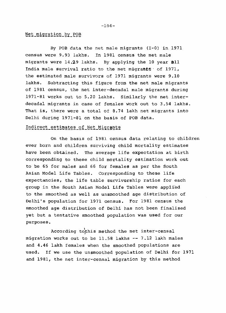
-104-

By POB data the net male migrants (I-D) in. 1971

census were 9.93 lakhs. In 1981 census the net male

migrants were 14.29 lakhs. By applying the 10 year all

India male survival ratio to the net rnigrant$' of 1971,

the estimated male survivors of 1971 migrants were 9.10

lakhs. Subtracting this figure from the net male migrants

of 1981 census, the net inter-decada:l male migrants during

1971-81 works out to 5.20 lakhs. Similarly the net inter­

decadal migrants in case of females work out to 3.54 lakhs.

That is, there were a total of 8.74 lakh net migrants into

Delhi during 1971-81 on the basis of POB data.

On the basis of 1981 census data relating to children

ever born and children surviving child mortality estimates

have been obta.ined. The average life expectation at birth

corresponding to these child mortality estimation work out

to be 65 for males and 66 for females as per the South

Asian Model Life Tables. Corresponding to these life

expectancies, the life table survivorship ratios for each

group in the South Asian Model Life Tables wer.e applied

to the smoothed as well as unsmoothed age distribution of

Delhi's population for 1971 census. For 1981 census the

smoothed age distribution of Delhi has not been finalised

yet but a tentative smoothed population was used for our

purposes.

According td~his method the net inter-censal

migration works out to be 11.58 lakhs -- 7.12 lakh males

and 4.46 lakh females when the smoothed populations are

used. If we use the unsmoothed population of Delhi for 1971

and 1981, the net inter-censal migration by this method

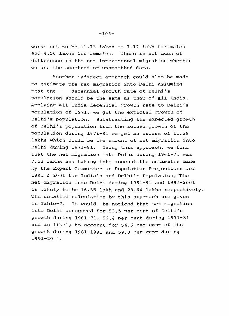
-105-

work out to be 11.73 lakes -- 7.17 lakh for males

and 4.56 lakes for females. There is not much of

difference in the net inter-censal migration whether

we use the smoothed or un smoothed data.

Another indirect approach could also be made

to estimate the net migration into Delhi assuming

that the decennial growth rate of Delhi's

population should be the same as that of all India.

Applying ~.ll India decennial growth rate to DeIhl's

population of 1971, we get the expected growth of

Delhi's population. Substracting the expected growth

of Delhi's population from the actual growth of the

population during 1971-81 we get an excess of 11.29

lakhs which would be the amount of net migration into

Delhi during 1971-81. using this approach, we find

that the net migration into Delhi during 1961-71 was

7.53 lakhs and taking into account the estimates made

by the Expert Committee on Population Projections for

1991 & 2001 for India's and Delhi's Population, ~he

net migration into Delhi during 1981-91 and 1991-2001

is likely to be 16.55 lakh and 23.64 lakhs respectively.

The detailed calculation by this approach are given

in Table-7. It would be noticed that net migration

into Delhi accounted for 53.5 per cent of Delhi's

growth during 1961-71, 52.4 per cent during 1971-81

and is likely to account for 54.5 per cent of its

growth during 1981-1991 and 59.0 per cent during

1991-20 1.

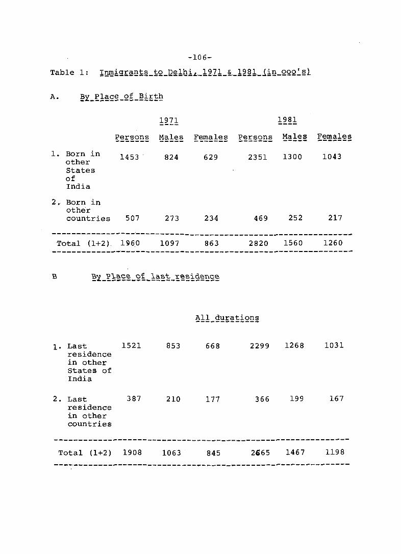
-106-

A. ~l_~!!S!_Q~-~!f~~

1971 1981

Persons Males Females Persons Males Females ------- ----- _,----'-- ------- ----- -------l. Born in 1453 824 629 2351 1300 1043

other states of India

2. Born in other countries 507 273 234 469 252 217

-----------------~-------------------------------------------Total (1+2). 1960 1097 863 2820 1560 1260

-------------------------------------------------------------

1· Last 1521 853 668 2299 1268 1031 residence in other states of India

2. Last 387 210 177 366 199 167 residence in other countries

------------------------------------------------------------Total (1+2) 1908 1063 845 2665 1467 1198

------------------------------------------------------------

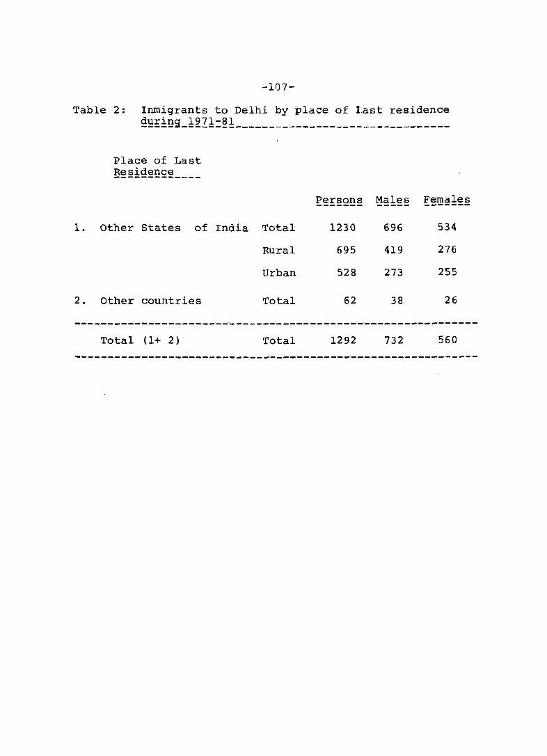
-107-

Table 2: Inmigrants to Delhi by place of last residence ~~~!~s_!2Z!:~! _______________________________ _

Place of Last B~~!~~~2~ ____

Persons Males Females ------- --_"_- -------

l. Other States of India Total 1230 696 534

Rural 695 419 276

Urban 528 273 255

2. Other countries Total 62 38 26

- ------- - _--------'--_"--"_ -- ----- - -- - - - - - ---_"-- -- - - - - -- -- - - - --Total (1+ 2) Total 1292 732 560

------------------------------------------------------------

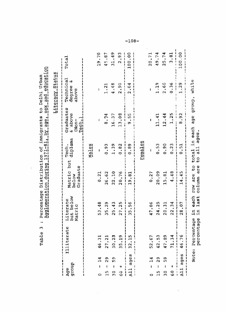
-108-

I I 0 !""-' 0\ 1"'"1 0 • '"""'

qt qt M • 0 • M f"- 00 "'" 0\ 0 ( I'""- l"- I'""- 00 I 0 I It! 0 I • I . 1 . I .jJ 0\ L{) rl N • 0 I 0 0\ L() 1"'"1 I 0 0 M "'" (V) I 0 I N "'" N I 0

1:' 8 I rl r rl 01 I I

• ..-1' {J)I I i I: .jJ I ::II I I It! It! I .jJ1 ...-t I I

..0 ()I It! I It!t.a I <1,1

1-1 ::II +ll () .-1 00 0 "'" I 0\ 0 ..0 I 0\ ...-'

::> rO 1 (1)1 -..-I (I) N '<:I' 0\ 0 I rl 1..0 ('V') I N • ..-1 (1)1 1 I: (I) (I) o I . I 0 1 .c

• ..-1 I :>I .c: 1-1 :> .-1 <QI N N , rl N 0 I r-t I ~ ..c: '0 I ()I () tJI 0 1 MI:l It! I (1)(1)..0 1 (I) It! I 1-11 8'0 It! t P-I Q I (1)1 " r ~ ,

~I .jJ1 H i I 0 0 (1)1 ·..-11 (J) I I 1 1-1 +l (J)I HI (I) I I , ~

I +l (I) I "'" f"- 00 I IJ) t rl qt L() N Ul .. I It! :> ..--1 r-- (V) 0 I L() 1 "'" "'" N 0\ (I)

+l (1)1 ::I 0 I oU 0 I . I ~ I: trt ro..o I:.c:. 00 \0 ('V') , 0\ rl N rl , 00 I It! It! It! I 10 It! 0 ()I rl M I rl .--I I I 1-1 I 1-1 Z (1)1 i I i ..c: ~:>I t!) t.a - 81 I I I () 0

• ..-1 ..01 I I j I I 10 (J)

El I 1 I I • I (I) (I)

s::: ... It! I ! I I I ~ ·..-IMI S l I I {J)I I I I: It!

001 o 0 I {J)I ('V') (j\ N I 0\ I (1)1 (V) 0 ('V') I M I • ..-1 4-t II .c:.--I I (1)1 0\ (V) 00 I 00 I , ..... H L{) 0\ N I L() I M o rll ()~ I .--II . 1 • I 101 o I, 0 I .--1.--1

1'""-1 (1) • ..-1 I It! I 0 rl 0 I 0 I El' a 0 0 I 0 I 10 It! I: 0\1 E-l'O I ::E:I I 1 (1)1 I 1 +l o .--II I , Ii-II 1 I o 0

• ..-1 I +l 1 I I I +l+l +ltrt ::I I \ I I ::I S::I ..0 (I) I 1 I I 0 (I)

..0 ·..-11 +l , I I I +l 1-1 • ..-1 1-11 () 10 I r-I N a 1..0 I M I'""- 0\ M 00 j L{) I It! 1-1 ::I I • ..-1 ~ ::I I N 1..0 rl I'""- I 00 , N a 00 "'" I "'" M (I) +l '01 1-10'0 I . I o I 0 0 I 0 I 1-1 I: (J) I +l rl 10 I 0 \0 N 0 I 0\ I 0 a L{) "'" I "'" I 10 S

• ..-1 1:1 10 (I) 1-1 I N N N i r-I I N r-I I M I ::I Q 01 ~..ot!) I 1 I I I ~r-I

·..-11 I I I 1 I o 0 (I) +ll I I I I 1-1 () ~ 101 Ii I I I 10 1-11 ~ I 1 I ..c:+l +l (I) 1 (I) 0 1 I 1 () (J)

I: Ell +l..-l co 0\ (V) L{) I 1..0 I I.D L{) ..-I qt i I'""- res 10 (I) 01 10 (I) () qt N "'" N ~ L{) r a N ('V') ('V') I 0 diM () ..-II 1-1..0 • ..-1 0 , o I • r I-Itrt (I) 1-1 (Y) L{) L{) I'""- L{) I I'""- qt 0 N I co I: I: (l)trt +l+l+l L{) ('V') N N ('V') I qt N N N I N • ..-1 • ..-1 Pol o<C 1 .r-! ::I 10 I I

H..o~ I • Q; (I) I I O'l~ I I It! It!

('V') (I) I I +l+l +l I i I: I:

(I) 10 1 I (j) (I) ..-I 1-1 ..-I M m 0\ L() i f"- (V) 0\ qt I I.D tl () ..0 (I) (V) N N rl ..-I 1 I.D L{) co ('V') , r-- 1-1 1-1 It! +l • • • I (I) (I) 8 .r-! \0 I'""- a L() N ~ N N r-- ..-I I 1..0 Al~

r-I qt N ('V') ('V') ('V') ! L() "'" "'" I'""- I "'" rl , I H I (I)

(J) (J) +l qt (j\ 0'\ (1)1 "'" 0\ 0\ (I) 0 rl N L{) ~I M N L() ~ :z

~ 10 10 ::I + +

(I) 0 r-I , rl tJll-I L{') a (:;:) ..-I L{) 0 0 rl ~tJ'I 0 rl (Y) 1..0 ~ 0 rl ('V') I.D ~

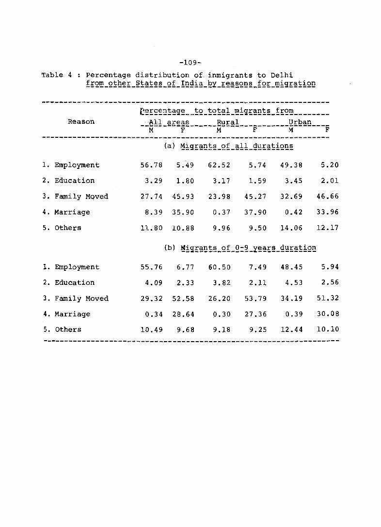
-109-

Table 4 Percentage distribution of. inmigrants to Delhi ~f2t:!!_2!:h~!:_§!:~!:~~_2~_!!!9!~_eY_!:~~2Q!!~_~Q!:_m!9:!:~!:~Q!!

----------------------------------------------------------------C~E9~!!!:~9:~_ .. _!:2_!:<2!:~!_l!!!9:E~!!!:2_~E<2I] ________

Reason . 'All areas Rural Urban ------------------------------------------M F M F M F

----------------------------------------------------------------(a) ~~9:f~!!!:~_Qf_~!1_9~!:~!:!Q!!§

1. Employment 56.78 5.49 62.52 5.74 49.38 5.20

2. Education 3.29 1.80 3.17 1. 59 3.45 2.01

3. Family Mqved 27.74 45.93 23.98 45.27 32.69 46.66

4. Marriage 8.39 35.90 0.37 37.90 0.42 33.96

5. Others 11.80 10.88 9.96 9.50 14.06 12.17

(b) ~!9:E~!!!:2_Q~_Q:~_Y~~E2_9~!:~E!2!!

1- Employment 55.76 6.77 60.50 7.49 48.45 5.94

2. Education 4.09 2.33 3.82 2.11 4.53 2.56

3. Family Moved 29.32 52.58 26.20 53.79 34.19 51.32

4. Marriage 0.34 28.64 0.30 27.36 0.39 30.08

5. Others 10.49 9.68 9.18 9.25 12.44 10.10

------------------------------------------------------------------

Table 5

-110-

Percentage distribut10n of inmigrants of all durations reporting employment as reason for migration, by sex, age and by category of !2E~~!! ___________________________________ _

-------------------------------------------------------------Age-group Main workers Marginal workers Non-workers Total

---------------------------------------------------------------Males --'-'-_.

a - 14 1.14 3.88 14.05 1. 96

15 - 19 6.40 18.85 11. 26 6.73

20 - 24 14.55 26.33 11. 97 14.41

25 - 29 16.99 15.99 4.79 16.22

30 + 60.90 34.84 57.99 60.66

All ages 93~47 0.23 . 6.30 100.00

---------------------------------------------------------------Females -------

0 - 14 4.18 1. 74 12.83 9.07

15 ... 19 8.53 6.62 6.54 7.39

20 - 24 16.08 17.07 13.57 14.66

25 - 29 16.57 13.94 13.28 14.69

30 + 54.60 60.98 53.72 54.13

All ages 42.89 0.45 56.66 100.00

--------------------------------_.,---------_,---------------------

Note: Percentages in each column are to all ages, where as percentages in last row (all ages) are to total.

-111-

Table 6 - Percentage distribution of migrant workers reporting employment as reason for migration in various occupational divisions.

--------------------------------------------------------------Duration of Residence Divisions

---~-------------------------------------0-1 2 3 4 5 6 7 8 &9 --~~-~ .. --------------------------------------------------------MALES -----Less than 1 year 5.50 5.20 6.36 7.03 16.61 0.88 57.58 duration

1 to 4 year dura,tion

, 5+ dura tion

6.22 5.21 9.38 9.34 14.74 0.97 53.22

8.56 5.48 15.49 12.25 11.40 1.26 44.21

_._'---'--.---'----'-------_ .. _---'_._--'_'_'_'--'_._'_'---------------------------All durations 7.72 5.42 13.24 11.09 12.69 1.15 47.49

----------------------------------------------------------------FEMALES -------

Less than 1 year a.93 ' 0.96 3.59 2.02 21. 50 0.06 62.62 duration

1 to 4 year 15.68 2.16 10.24 2.57 28.48 0.26 39.93 duration

5+ duration 27.73 3.20 12.04 4.33 26.78 0.76 23.57

----------------------------------------------------------------All duration 20.53 2.50 10.22 3.30 26.78 0.48 35.11

----------------------------------------------------------------

o-i ~ 0

rJll 0 () o-i o-i .;r M ~ I 'r-! ",,0 00 "" 0 r--01 +J+Jr--O o-i o-i (Y) \0 01 edU r-I U"\ .;r U"\ 0'1 01 I-IQ) .

I t::1I4-I r-l >< M N "" 00 ~I 'r-! 4-1 0 U1 U1 U1 U1

·r-!I ::E:Q)()U"\ I

~I 01

'MI 1.01 .j.)1 ·1 lIS I .-II 4-1 1-1

.-II r-ll 01 0 Q) 01 ::11 t)1 rJl :>.-1 M C'I U1 "" 01 04 II (I). Oro.t: U"\ N U1 1.0 NI 01 lOl rJl'M I-I.j.) r-- r-l 1.0 M II Pit '1 Q)..c: • !:' ~ .-i .-I N

.-II .-II U.-I !l!.j.) 0 \01 01 XQ)omlo-l 0'11 UI Jl:IOPiCt::1I .-II

I ::t:1 C

~: 4-1 0 ..c: '0 0 .r-! t::1I Q) +J ""

01 Q) .-I II) .j.) C +J ~ ·1 <0:1' l/) 0 U"\ 15:::1 +J ed.a ~ ed 'M cd 0 .-II U1 N 00 <0:1' ~I U H .+J .,.., r-I § H H 01 1.0 00 0 M 1.0

I Q) !:' ).a :::1 t::1I 01 r-l r-I r-I 001 o...j.)Or-lo..lI)Q) I • I >< rtl l-! Q) 0 (I).c: 4-1 ~I HI riI s:: t::1I 0 0.. ed +J 0,"" 1 :Ill HI rill (I) 01 ~ ..c:

1 ·14 .j.) r-- qo 1/) C'I ZI .c:) 0 l/) M 0 01 r-IO lO oqo .-I 0 0

t· Q) H .. .. -, .. E-41 UI

Ot::1l .-I N M <0:1'

rill r:tIl a r:tIl r-I 0 rill ed .r-!

I .,.., 4-1(1)+1 00 M .-I U"\ ZI s::..c: 0 - m M I""- M 00 01 ~ +J ro r-I 0'1 0 0'1 r-,. HI Q») Q)'M::I U1 N r-I I""-81 00+1'00..

fZ: Q)I-Im~o "" IJ) N I""-Ot::1llo-lHtl. N N N .-I

~I HI ::E:I I .,.., 0'1 \0 0 IJ) <0:1'

I .c: Lf) \0 N L{') 1.0 I .-I MI \0 0 N N N

S::I Q) I""- 01 Q N "" \0 0'1 M

'MI .-I Q) +JI r-I (1j1 ,Q .-II (1j ::II Ul 0 Ul 0'1 en 8 P.I (Y) \0 00 .;r 0'1

01 ro N .-I r-I N 0 A.I .r-!

I '0 N 0'1 00 Lf) I""- \0 I s:: M "" 00 M 00 I H qo U1 \0 00 0'1

1-1 r-I r-I r-I r-I r-I ed 1.0 I""- 00 0'1 0 Q) r-I 0'1 0'1 0'1 C'I 0 )'i r-I r-I r-I r-I N

MOBILITY AMONG INDIAN WOMEN

O.P . SHARMA

In common parlance, migration is termed as change

in the place of residence of a person from one geographical

unit to another. If the movement in within the boundaries

of a nation, it is known as 'Internal migration' while the

movement across the International boundaries is called

'International migration'. In ancient times, the movement

of people wa~ in the fl'eJm of 'group movement' and the

members of the tribal societies rarely ve~tured singly. The

tribes led a nomadic life wandering in search of places where

they could find sustenance. It is believed now that "first

true man originated somewhere in east Africa and wandered

over a period of many centuries untiLi.all the major conti­

nents were occupied by human beings".

The bulk of civilisation and inventlons of agricul­

ture resulted in new innovatory types of migration. The

first half of the current century was the hey-day of free

individual migration. Study of international migration has

drawn more and more attention of demographers but the internal

migration, which surpassed the international migration, has

not received the attention that it rightly deserves. "The

right of free movement as often as one wishes within a nation's

territorial boundaries is constitutionally guaranteed and

is regarded as inherent in the very concept of citizenship'.

However, the major internal migratory movements in the

modern world represent similar responses to 'pushes' and

'pulls' of economic diversity in different regions o£ a country.

-114-

. In the modern society society, migration is a question

on which the po.licy makers are never unanimous, more so when

the study involves female migration. One school of thought

is that the female migration does not contribute materially

to the process of speeding up of economic development and

modernisation. Others hold the view that economic development

is hampered because of lack of planning with regard to the

movement of population from one area to another, thereby

disturbing the economy of both the places, from where they

move and of the places to which they move. This is a highly

debatable question, particularly, when we analyse the

female migration data.

In the Indian context, the movement of females in

general, is not because of economic reasons but because of

social reasons. Majority of the female migration is due to

marriage. Thus, femal~are more migratory than males but

this is because of the age-old system of marriage. The

migration, on account of employment or education, is very

limited in India as unmarried female do not generally leave

their parental homes. The second most predominant reason

for migration among females is 'family moved'. The present

study is mainly devoted to the analysis of the social

characteristics of the female migrants.

India's population at the sunrise of March 1, 1981

was 665,29 million of which 343.93 million were males and

321.36 million were females. This does not includ~·?~opulation of Assam where census could not be taken. If we add the

projected population of Assam for 1981, the population of

the country would be around 685.18 million. Since no census

could be taken in .Assam in 1981, analysis of the

available migration data excludes Assam.

TOTAL MIGRANTS

WITHIN INDIA

WITHIN DISTT.

OTHER DISTTS. OF STATE/u.T.

OTHER STATES/U.T.

OUTSIDE INDIA

ASIA

OTHER CONTINENTS

~ OTHERS

f::::::1 MARRIAGE

115

FEMALE MIGRANTS (Pfoce of Lost Residence) 1981

-o 0

PER C E N TAG E

I\) ~

o 0 ~ (JI 0) 000

.." CD o 0

cD 0 o 0

"" ::0 o

zil: ~~~~~~~~~~~~~~~--~~~ ~~

)Io:::j ~~~~~~~~~~~~~~~~~~~ x

z

o N"J~cr7"-~~~~~:""':"':"~":""::""~~~~~~~~ i ~ ~

5:!cno ~,..c,.r,.~;,.c,c,~~,_,:.,;..,:.y:.rr~~~""'"'?Ir:~~~~ )10 c I:

."

REASON OF MIGRATION

~ EMPLOYMENT ~ FAMILY MOVED

• EDUCATION

-11'6 -

Of the 321.36 million females in the country, again

excluding ~sam, in respect of 176.69 million population

the place of last residence was the place of their enumera­

tion and 144.67 million were migrants. In the 1981 Census,

a person was considered as a migrant if the place where

he was enumerated was other than the place of his last·

residence. Thus 144.67 million females, who were classified

as migrants, included 96.70 million whose place of last

residence was other than the place of thelr enu~eration but

within the district itself and 32.84 million had moved

from other districts of the same State/Union territory.

As many as 12.25 million had moved from outside the State

of Union territory to the place of enumeration. The

remaining 2.88 million moved to India from other countries.

This means that, in 1981, female migrants, based on place

of last residence, accounted for 45.02 per cent, against

43.26 per cent in 1971, of the total female population

of the the country excluding Assam. Out of the 144.67

million female migrants, against 68.98 per cent in 1971

66.84 per cent had the place of their last residence within

the district of enumeration; and 22.70 per cent in 1981,

against 19.80 per cent in 1971, had moved to the place of

enumeration from other districts of the same State/Union

territory. PBainst 8.09 per cent in 1971, 8.47 per cent in

1981, had their place pf last residence in other statel

Union territories. Further, against 3.13 per cent in 1971

as many as 1.99 per cent in 1981 had moved io India from

other countries. It is apparent that during the decade

1971-81 migration from within the country has increased

as compared to from outside the countrv. Among- the female

migrants from within the country, relatively the long­

distance migration waS('higher in 1981 as compared to 1971

-117-

whilst the short dlstance migratlon, i.e. from within the

district, declined from 68.98 per cent In 1971 to 66.84

per cent in 1981. In the case of those who had moved from

other states, the share of the total female migrants has

gone up sllghtly from 8.09 per cent In 1971 to 8.47 per

cent In 1981.

The higher percentage of female migrants from wlthin

the state or Unlon t:erritory of thelr enumeration can

largely be attributed to their marriage. Detailed analysis

of the reasons of migration has been attempted in the later

part of this study. Of the 12.25 million lnter-state female

migrants, the pride of place had gone to Uttar pradesh,

which accounted for 16.66 per cent of the total lnter-state

female migrants followed by Bihar with 8.80 per cent. Other

states whlch accounted for more than five per cent of the

inter-state migrants were Madhya Pradesh(8.16), Rajasthan

(7.48), Maharashtra l6,,98), Karnataka (6.62), Haryana(6.20) ,

Punjab (5.53), Andhra Pradesh (5.53) and Tamil Nadu (5.33).

Of the 144.67 million female migrants in 1981,

the place of last residence of 2.88 million was ln other

countries. This gives a percentage of 1.99 ln 1981 against

3.13 in 1971.:(jf these 2.88 million female migrants, 98.74

per cent had their last residence ln countries of ~..sia, 0.77

per cent in Africa, 0.03 per cent In Burope, 0.17 i~7'Americas and 0.02 per cent In the countries of Oceania. Out of

2.85 million female migrants who moved to India from

countries in ASla as many as 1.49 mlliion or 52.49 per cent and

moved from Bangladesh,/0.89 million or 31.27 per cent from

Pakistan. Other countrles whose share was more than one

per cent were Nepal (8.96), Sri Lanka (3.40) and Burma

(2.05).

-118-

Of the total female migrants, who had moved to the

place of their enumeration at different points of 3.67 per

cent had been residing at the place of their enumeration

for less than one year, 16.83 per cent for a period rang­

ing from one to four years and 14.71 per cent for a period

ranging from five to nine years. This means that 35.21

per cent of the female migrants moved during 1971-81.

Those who moved to the place of their enumeration between

1961-71, viz, those who have been residing at the place

of enumeration for the periods ranging between 10and 19

years, accounted for 23.69 per cent of the total female

migrants. As many as 37.71 per cen'c female migrants were

those who had been residing at the place of their enumera­

tion for 20 years or more. The duration of stay at the

place of enumeration in respect of 3.38 per cent of the

total female migrants, however, was not reported, The

female migrants vlho had- moved to ~the p~lac.e. of thelr

enumeration either from other 9arts of the district or

other districts of the State/Union territory or even other

states/Union territories, also present the same pattern

Out of the 141.79 million female migrants 'liTho moved to the

place of enumeration fro~ within the country, 35.53 per

cent moved to the place of enumeration during 1971-81,

23.65 per cent during 1961-71 and 37.41 per cent earlier

than that. The duration of residence at the place of

enumeration in respect of 3.38 per cent was not reported.

with regard to those who moved from other countries the

position is slightly different. During the recent past,

the movement of females to India from other countrles

has slightly gone down. Out of the total female migrants

from other countries, as many as 52.39 per cent had

been residing at the place of their enumeration for

more than two decades, 24.32 per cent moved during 1961-

71 and 19.62 per cent during 1971-81. Thus, it will be

-119-

seen that during the past decade the magnitude of

female migration from outside India has gone down

considerably.

If we analyse the data relating to the females

who have migrated from different countries we find

that out of 2.88 million female migrants who migrated

from other countries during 1981-82, 0.57 million

female migrants 96.96 per cent of those migrated from

Asian countries. 1.47 per cent from ~£rican countries,

0.94 per cent from countries in Europe, 0.59 per cent

from countries in the Americas and 0.04 per cent

from the countries in Oceania. During the last decade

the migration of females had been of the highest

order from countries of Europe and the Americas.Cf the

4,879 females who migrated to India from countries

in the Americas, as many as 68.03 per cent came to the

place of enumeration in India during 1971-81, while

62.00 per cent of the 8,632 female migrants from

countries in Europe (excluding USSR) came to India during

1971-81. Those who migrated to India during 1961-71 from

countries in the F.mericas and Europe accounted for 20.13

per cent and 18.44 per cent of the total female migrants

from these two continents, respectively. The respective

percentage of those who moved to India prior to 1961 were

3.95 and 12.82.

The reasons as revealed during census for this kind

of migration among females are discussed inthe following

paragraphs.

-120-

Out ot the 144.67 million female migrants. 72.34

per cent moved because of marriage and 14.72 per cent

because of the movement of their family. So, 87.06 per

cent of the female migrants moved per force. Only 1.92

per cent among them moved because of employment and 0.88

per cent in pursuit of education. The reason of migration

in respect of 14.67 million or 10.14 per cent of the total

female migrants was other than the four mentioned above.

Almost the same pattern is discernible when we look at the

data of female migrants whose last residence was within

the country. Of the 141.79 million female migrant from

with the country. 73.37 per cent moved because of marriage,

14.27 per cent because of movement of their families, 1.92

per cent on account of employment and 0.88 per cent in

pursuit of education. Reasons for migration in respect

of 9.56 per cent were other than the four mentioned above.

The pattern is quite different in respect of those whose

last residence was outside India. Of the 2.88 million such

female migrants. 37.02 per cent moved because of the

movement of their families 21.61 per cent because of

marriage, 1.57 per cent for reasons of employment and 0.69

per cent because of education. In the case of 38.91 per

cent the reason of migration was other than these four.

Now let us analyse further the female migrants

who moved to the place of enumeration from within the

country. As stated earlier, the highest percentage of

the 141.66 million female migrants whose place of last

residence was within the country (73.37 per cent) moved

for reasons of marrlage. The magnitude of the movement

because of marriage decreased with the increase of

distance. In the case of 96.70 million female migrants

who moved to the place of enumeration from within the

district of Enumeration 78.18 per cent moved because

-121-

of marriage. Movement among 32.84 million female migrants

from districts of the state/Union te:rritory, came down

to 66.53 per cent primarily because of increase in the

distance between the place of their last residence and

enumeration p..cross the state boundary the percentage

goes down still further.;- as out of 12 . .a~ million female

migrants who moved from other states/Union territories,

the percentage of those who moved because of contracting

of marriage, goes down further to 53.77 per cent. On the

contrary, movement in the volume of fetrtale mJ.gratidn

is 1n dir~ct proportion to the increase/decrease in the

distance between the place of last residence and place of

enumeration. The percentage of female migrants who left

the place of their residence because of the movement of

their family in respect of those who moved from within

the district of enumeration, was 10.60. Of those who moved

from other dis:trict o:l;·the same state/Union territory

increased to 19~79 and it increased further to 28.41 per

cent in respect of those who moved from other statefJnion

territories.

Similar is the case of those who moved on account

of· reasons of employment or education. In the Gase of those

who moved for reason of employment from within the district,

the percentage was 1.29. while those \.vho moved from other

districts of the state/Union territory, it was 2.83 and

in respect of those who moved from other statefunion

territories their percentage was 4.51. In respect of those

whose reason for migration was education, their respective

percentages were 0.70, 1.16 and 1.54. Thus, it will be

noticed that with the increase of distance the volume of

movement on account of marriage, decreased whJ.le in the

case of 'family moved', 'enlployment' or 'education' the

volume of migration increased. So, the bulk of the female

migration is due mainly to compulsion of marriage or family

movement.

122

FEMALE MIGRANTS

(PLACE OF LAST RESIDENCE)

1971 (111.19 Million)

WITHIN DISTRICT

~ OTHER DISTRICTS

1981 (144.67 Million)

.. · .. . · .. . . . . . . · ... :66.84% . · .

· ... . . . · . · .. ' .......

.. OTHER STATES

OTHER COUNTRIES

-123-

The analysls of the female migrants who !TI0ved to the

place of enumeration because of employment, reveals quite

an interesting pictllre~ In all, 277 million females moved

to the place of enumeration from wlthin the country be­

cause ot employment.It is not necessary that those who

moved because of employment got gainful employment after

their movement to the place of enumeration. It 1S quite

interesting to note that on March 1, 1981, the reference

data for the 1981 cenSllS, only 1.22 ~i1lion or 43.89 per

cent out of them were gainfully employed and classified

as main workers and 0.10 million or 3.57 per cent as marginal

workers and 52.55 per cent as non-workers. Main workers~

according to the definition adopted at the time of

the 1981 census, were those who had worked for the major

part of the year preceding the date of enumeration while

marginal workers were those who had not worked for the

major part of the preceding year concerned but nevertheless

had done some work any time during the reference period.

It will thus be seen that those females who migrated

for reasons of employment, after arriving at the place

of their enumeration did not necessarily get employment.

However, those who moved recently to the place of their

enumeration had comparat1vely higher percentage of main

workers as compared to the earlier period. For instance,

those who moved to the place of their enumeration because'

of employment during the last one year, their percentage

was 64.04. Among those who moved between one and four years,

44.10 per cent were main workers and those who moved e~rlier

than that had percent.age of main workers as 40.96. It

appears that those who moved because of employment in the

beginning get employment and with the passage of ti.'1\e they

were thrown out of employment and fell in the category of

non-workers. The percentage of non-workers among the females

who moved because of employment during the year preceding

the enumeration was 35.58, which increased to 53.04 per cent

-124-

in respect of those who moved to the place of enumeration

between one and four years but came down to 46.83 per cent

in respect of those \vho moved prior to thlS period."

The age distribution of the female migrants,who

moved to the place of their enumeratl0n, because of employ­

ment, indicates that the proportion of higher age group was

substantially high. Of the 2.77 million female migrants

from within the country, as many as 52.90 per cent were

aged 30 years or more and only 14.86 per cent were between

15 to 30 years of age. Against this, the percentage of

30 years and older female migrants who were labelled

as main workers was 58.18 and that of the girls less than

15 years of age was only 5.40. 1mong those marginal femai.es.'

who migrated from within the country for reasons of

employment. 1.46 million were non-workers and out of these,

48.12 per cent were aged 30 years or more. Girls below 15

years of age accounted for 23.20 per cent of the non-

worker population.

It is quite interesting to note that those female

migrants who had moved to the place of enumeration during

last year and who were classified as main workers at the

time of the 1981 census, 37.08 per cent were aged 30 years

or more. The percentage went up in the course of time, which

reached 42.49 among those who moved between one and

four years and 77.01 among those who moved prior to this

were aged 30 years or more. Same is the position with

regard to those who moved to the place of enumeration

because of employment but were classified as non-workers at

the time of the 1981 census. Those who moved during the

year preceding the enumeration and were aged 30 years

or more accounted for 22.17 per cent of the total non­

working female migrants, whereas the corresponding

percentages for those who migrated between one and

four years and 5 years or more were 28.47 and 65.86,

respectively.

-125-

Of the 2.77 million female migrants who left the

place of their last residence because of employment,

12.91 per cent moved during the year preceding the enu­

meration, 32.95 per cent between one and four years and

51.50 per cent earlier than that. Of the 0.41 million

aged between 15 years of age,20.77 per cent had been

residing at the place of enumeration for less than one year,

48.32 per cent between one and four years and 24.63 per

cent for the last 5 years or more. Of the 1.47 million

aged 30 years or more, 7.76 per cent had been residing

at the place of enumeration for less than one year,

21.83 per cent between one and four years and 68.94 per

cent for five years or more. The pattern of the other

age groups is almost identical to that observed in the

case of those who were less than 15 years.of age.

Another important factor in relation to migration

is the literacy rate observed among the female migrants.

Of the 2.77 million female migrants who moved because of

employment, 1.14 million or. 41.05 per cent were literates

and remaining 58.95 per cent fell in the category of

illiterates. The literacy rate varied considerably among

different age groups. For instance, while 34.22 per r

cent of the female migrants who were less than 15 years

of age at the time of the 1981 census were reported to

literates', the percentage in respect of those who were

Df: 3D years or more was 36.61 ..... ~~~~~

~~~ The highest literacy rate (54.61 per cent), however,

was observed among female migrants who were aged 25-29 years.

followed by age groups 20-24(52.26) and 15-19(45.05).

Let us look at the distribution of total female

migrants and literates among them. Of the total female

migrants 52.90 per cent and 41.18 per cent of the literate

-126-

female migrants were aged 30 years or more and against

14.86 per cent among the total female migrants, the share

of the literate female migrants of younger age bracket

of less than 15 years was 12.39 on~y. Almost the same

distribution is observed in the case of illiterate female

migrants. Of the 1~63 million illiterate female migrants

who moved because of employment 56.89 per cent were

aged 30 years or more and 16.59 per cent were of less

than 15 years of age.

Ou·t-migration is stimulated by the existing educa­

tional system and non-availability of facilities which

compel the youngsters to leave their native places to

the areas having desired educational facilities which

help them to pursue their education. No doubt the movement

of 1.27 million girls in pursuit of higher education is

quite an encouraging phenomenon. That is why by and large

female migrants have a higher literacy rate as compared

with the literacy rate observed in the case of total female

population in the country and much higher than those

females who never migrated. Not only that, more than

45 thousand females coming to India from other countries

for higher education, is a reflection on the prevailing

status of educational institutions in the neighbouring

countries and of the high standards of the educational

institutions in India. Out of 45,445 females who came

to India for education as many as 43,170 came from

countries in Asia and remaining ~,275 from other continents.

Migration due to economic reasons is also of vital

importance, Out of 2.77 million females left the place

of their last residence for 'employment' and they inclu­

ded females of all ages, though the highest percentage

(52.90) comprised of those who were aged 30 years or more

-127-

but the percent.age in respect of teenagers was also quite

hlgho Out of 2.77 million female migrants who moved because

of 'employment',as many as 22.58 per cent were less than

20 years of age and 24,.47 per cent aged 20-29 years. So

the mlgration among Indian females because of employment

contrary to the general expectations, is not restricted to

aged females but their age distribution is quite uniform

among different age brackets.

Whatever be the reason of mlgration, the fact remains

that females in India are quite mobile and the mobility

is going up gradually. As in 1971, the percentage of

female migrants to total female population was 43.26,

which increased to ~5.02 in 1981.

Because of the basic differences in the nature of mig­

ration between male and female migrants, we find that sub­

stantial proportion of female migrants from within the state

were from rural areas. In 1981, out of the total female

migrants from within the state, 87.51 per cent were from

rural areas and 12.28 per cent from urban areas.

As distances increase, the rural to rural movement

for reasons of marriage declines while urban to urban

increases. For instance, of the female migrants who moved

because of marriage from other districts of the state,

81.20 per cent moved from rural areas and 68.7.5 per cent

among them moved to rural areas and 12.45 per cent to

urban areas. Of the 18.61 per cent who moved from urban

areas, 6.87 per cent moved to villages and the urban to

urban stream accounted for 11.74 per cent. If we still

go further and study the female migrants who moved because

of marriage from other states/Union territories, we find

that of the total female migrants who moved because of

-128-

marriage from other states, 70.04 per cent came from

rural areas and 29.50 per cent from urban areas. Again,

out of 70.04 per cent who moved from rural areas of

other states/Union territories, 50.75 per cent moved

to villages and 19.29 per cent to urban areas.

Sim11arly, out of 29.50 per cent females who

migrated from urban parts of other" states/Union

territories, only 7.60 per cent moved to villages and

21.90 per cent to urban areas. It will thus be seen

that a sizeable migration among females is because

of marriage and movement of family and not because of

economic reasons, which holds good in the case of males.

All these lead to a note of caution that while handling

migration data, the sex differential will have to be

kept in mind. In case migration data are handled in

the1r totality, the results may be misleading, as wide

variations exist among the male and female migrants.

SEC T ION - 2

U R BAN I Z A T ION

RECENT UR~NIZATION IN INDIA: SCENARIO

B. K. ROY'·

ABSTRACT :

The paper on 'Recent Urbanlzation in India' seeks

to explain the pattern of urbane situations ln India. The

paper is primarlly based on census data and supported to

some extent by other studies and Government documents. The

combination of these tries to focus some issues on the

subject. The Vlews expressed in this paper are entirely

of the author and in no way related to the author's

affiliation to his servi.ce ln the Government of India and

the Census Organisation of India.

INTROVUCTI0N :

Urbanization depends largely on the development of

industrialization, infra-structure within cities, towns and

their neighbourhoods. The economic system within a country

generating migration opportunities at locations is a refined

input in urbanization. HOwever, the concept and definition

of urbanization is an outcome of declaring urban population

at the time point within a space, constituted or chartered

and this is usually given by the censuses of the Countries.

In particular, the census has to provide a frame of urban

spaces with populatlon to assess developments and urbanization.

Due to defined limitations and contrasts in various countries

and within a country, the degree of urbanization needs

defining by the ~parameter, urban population to total

popUlation. Several Demographers, Economists, Statisticians

and Geographers define urbanization with specific views and

tools in several ways. Demographers usually try to see

urbanisation according to urban population to total population,

-130-

accretion of population in urban areas, per cent urban

populat~on alike. Economists usually try to relate

population growth, pattern of demand and technology on

the process of urbanization. Statisticians follow a

common goal and try to relate production functions,

growth rate of urban population involving labour and

non-rural based demands and create models on macro and

micro levels and foresee urban populat1on projections.

Sometimes, this is the ma~n goal of Demographers,Economists

and Stat~sticlans in tackling issues related to urbanization

(Goldstein & SLY 1975). Geographers consider urban~zation

in relation to distribution of urban spaces and see

proportions and growth of urban population at a level

usually given in censuses. At occasions, juriSdiction an·a.

morphogenesis of towns lead geographers to opine on the

process of urbanization. In addition, occasionally

Geographers have also tested "gravity model concept"

to focus issues partly or fully real ted to urbanization

and urban zonations in broader perspective (Roy 1977).

A vast literature accordingly is available to determine

perspectives and techniques in the evaluation of

urbanization in the country.

METHOVOLOGY & SOURCE:

Keeping in view the above developments, the

author tries to proJect recent urbanization levels and

patterns in India mainly according to census data of' 1981

by three measuring standpoints (i) At all India perspective

keeping districts and urban centres in view, a delineation

of urbanization index (U.I) is presented on the basis of

the following notation :

u. I. = 1 (A + B + C + D + E + F) '6 (p P p P p P)

-131-

Where U. I. represents urbanization index and A to

E represent the number of census towns in size classes

I through VI respectively and (P); population of towns

in the size group.

This procedure may reduce the census data system

for assessment at district level easy comprehension and

a general consensus can be measured regarding the

characte:rlstlcs of numbers and population in these

groups bringing t,hem all to one measuring rod. This

is preferred over the hypothesis of finding proportions

of urban population to total population because of

generating inter se positioning of districts in the

country and spell out levels. Readers may very well

carry out other concepts of measuring urbanization and

may compare dlsparities in this regard.

Besides, in the paper specific mention of the Class

I urban areas are referred to with emphasis of the million

cities regarding their growth and accretion linking the

pattern as defined in methodology (i) above. In this

process by (ii) reconstituting information on morphogenesis

of Lucknow as case studying the pattern of landscape

change due to urban spread during 1971-81 censuses is also

indicated to see the internal allocation of landuses.

(iii) Further, by a case study of standard urban Area of

Gulbarga (Farnataka) a view is presented giving its

probable input in future urbanization in the country for

further research. These three criterian of urban

exposition may give some clues to the readers about the

recent urbanization and its consequences in the process

of development which may be considered in generating

multi-level economic-demographic models (Wegener 1982)

by the schol,ars for various regions of the country.

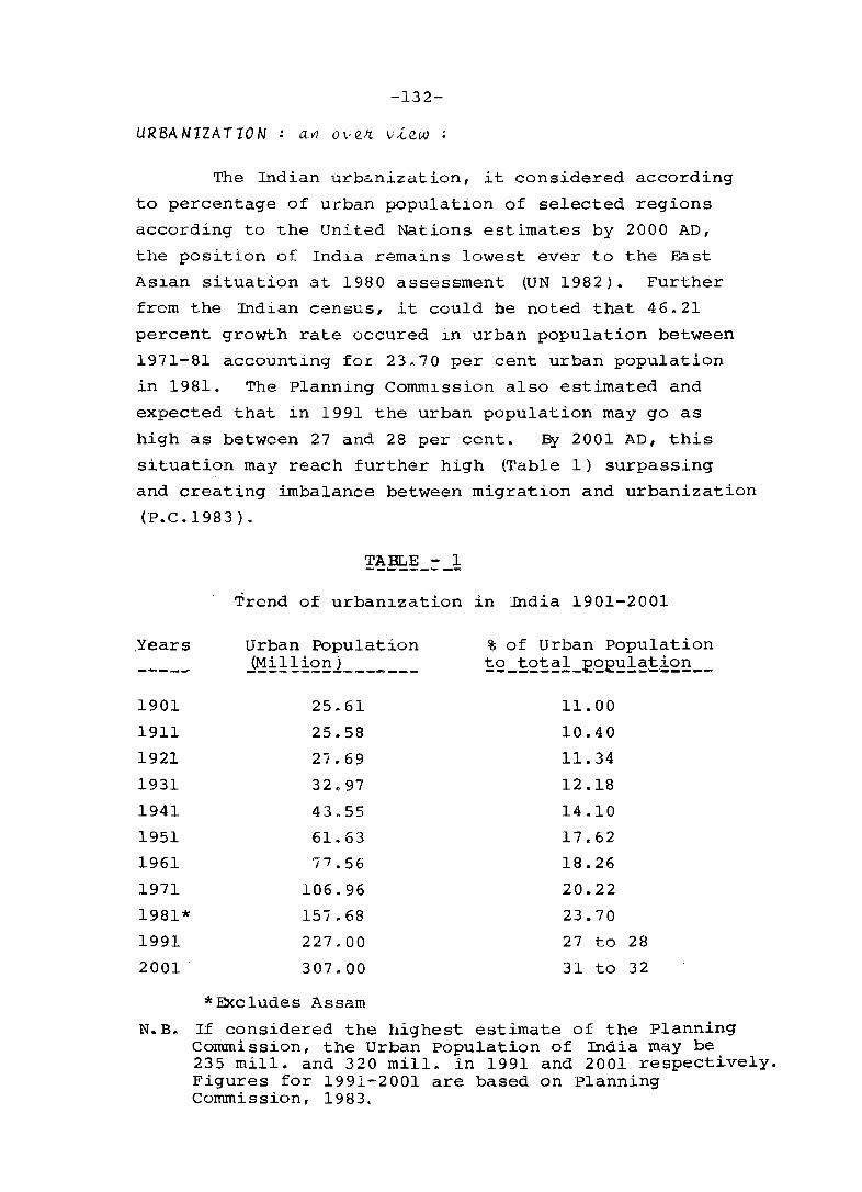
-132-

URBANIZATION: av1 O\;e!'1. v,[e.w :

The Indian urbQnization, it considered according

to percentage of urban population of selected regions

according to the United Nations estimates by 2000 AD,

the position of Ind.l.a rema~ns lowest ever to the East

As~an situation at 1980 assessment WN 1982). Further

from the Indian census, it could be noted that 46~21

percent growth rate occured in urban population between

1971-81 accounting for 23.70 per cent urban population

in 1981. The Planning Comm~ssion also estimated and

expected that in 1991 the urban population may go as

high as between 27 and 28 per cent. B¥ 2001 AD, this

situation may reach further high ttable 1) surpassing

and creating imbalance between migration and urbanization

(P.C.1983).

TABLE - 1 ----,_,_-. -

Trend of urban~zation in India 1901-2001

Years Urban Population % of Urban Population _ ---_. J~!±!!2Bl_~ _____ t2_t2~~!_E2E~!~t:!:2B __

1901 25.61 11.00

1911 25.58 10.40

1921 27.69 11.34

1931 32.97 12.18

1941 43"55 14.10

1951 61.63 17.62

1961 ',7.56 18.26

1971 106.96 20.22

1981* 157.68 23.70

1991 227.00 27 to 28 2001 . 307.00 31 to 32

* Excludes Assam

N.B. If considered the highest estimate of the Planning Commission, the Urban Population of India may be 235 mill. and 320 mill. in 1991 and 2001 respectively. Figures for 1991-2001 are based on Planning Commission, 1983.

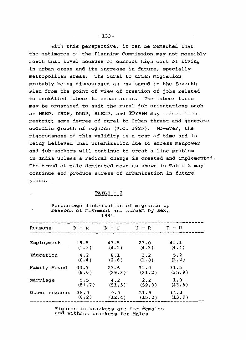
-133-

With this perspective, it can be remarked that

the estimates of the Planning Commission may not possibly

reach that level because of current high cost of living

in urban areas and its increase in future, specially

metropolitan areas. The rural to urban migration

probably being discouraged as envisaged in the Seventh

Plan from the point of view of creation of jobs related

to unsk~lled labour to urban areas. The labour force

may be organised to suit the rural job orientations such

as NREP, IRDP, DRDP, RLEGP, and l"ltYSEM may ';~::~'::-"'.':-'.'.',:-,,"

restrict some degree of rural to Urban thrust and generate

economic growth of regions (P.C. 1985). However, the

rigorousness of this validity is a test of time and is

being believed that urbanization due to excess manpower

and job-seekers will continue to creat a line problem

in India unless a radical change is created and implemented.

The trend of male dominated move as shown in Table 2 may

continue and produce stress of urbanization in future

years.

TA R.E - 2

Percentage distribution of migrants by reasons of movement and stream by sex,

1981

--------------------------------------------------------Reasons R - R R - U U - R U - U --------------------------------------------------------Employment 19.5 47.5 27.0 41.1

(1.1 ) (4.2) (4.3) (4.4)

Etlucation 4.2 8.1 3.2 5.2 (0.4) (2.6) (1.0) (2.2)

Family Moved 33.7 23.5 31.9 31.5 (8.6) (29.3) (21.2) (35. 9 )

Marriage 5.5 4.2 2.2 1.0 (81. 7 ) (51.5) (59.3) (43.6)

Other reasons 38.0 9.0 21.9 14.3 (8.2) (12.4) (15.2) (13.9)

--------------------------------------------------------Figures in-brackets are for F.emales and without brackets for Males

-134-

URBANIZATION LEVEL : P~e~ent Scena~io

The foregoing statements revealed some aspects

of present and the future of urbanization. Now turning

to the methodology as envisaged in this paper to work

out U.I., reveals the other aspect of level of urbanization

in the country. On the outset, it may be noted that

the definition of declaring a place as urban also remains

the same in the Indian census of 1981 as of previous

censuses.

During 1971-81, the economic development in

raising the cities and towns has not been as such

stimulating but the census in the process has classified

urban areas giving too much emphasis on out-growth and

unchartered perepheral growth in 1981 and hence the

decadal urban population has reached high figures of

46.21 per cent variation.

The situation as transformed in the U.I. and

mapped (Fig.l) show such reflections in urbanization

largely due to urban population swealing. Interestingly,

the mountaneous regions over Jammu & Kashmir, Himachal

Pradesh, Sikkim and districts of West Kameng and Lohit

of Arunachal Pradesh have emerged as urbanized zones

in the country in U.I. Level-l. Even the state of

Manipur excluding districts of Manipur Central and

Tengnoupal represent this level. These districts claim

4. 48K of the total population and only 3;! of total urban

population of the nation. The contribution of number of

Class I & II towns stands at only 1.86:': and 2.22:,

respectively. Other towns from Class III to VI contributed

largely in the region making 7.43: of the total size classes

of the group.

ARABIAN SEA

tOA,O.IUIl • 011,1

Goa 0 GO"IOA.AN a DIU P POHOICHE: RRY

, ,

I"

I I

A

land upon Sur .... ,y of Indio map .Itl'l the p'lml5'lon of the Sur ... ,ytJr Gln,rolof 111(110

Tilt hrr,torlo;Jl _0"-., of Indio .1It'l'd ,nt~ 1M •• 0 to Il d"ton" of twelvo ""tlcal mil" mto.urea from th, 0Slpropriof. lias. line

c

,I

II

135

URBANIZATION INDEX BOUNDARY,INTERNATIONAL_._._ BOUNDAFtV. STAn/UNION TERRITORY __ ._

.OM

'"

DISTRICT...... .•. __ _

IUlO.£TItI' IOO!O 0 100 too 100 400

l-s I j ~*==k nO

BAY '0 F

BENGAL

IJRBAN!ZATION INDEX

~ 0'0115 8 ABOVE

R 0010 - l)'Olq

-.0 O·OO~ - 0-009

[lID 0'004 a BEI.OW

o ENTIRElY RURAL

8 DATA NOT AVAILAaL~

UNI- URBAN AR.EA

NO CENSUS WAS CONDUCTED IN ASSAM IN 1,"

E A N

0'

FIG. I

1996

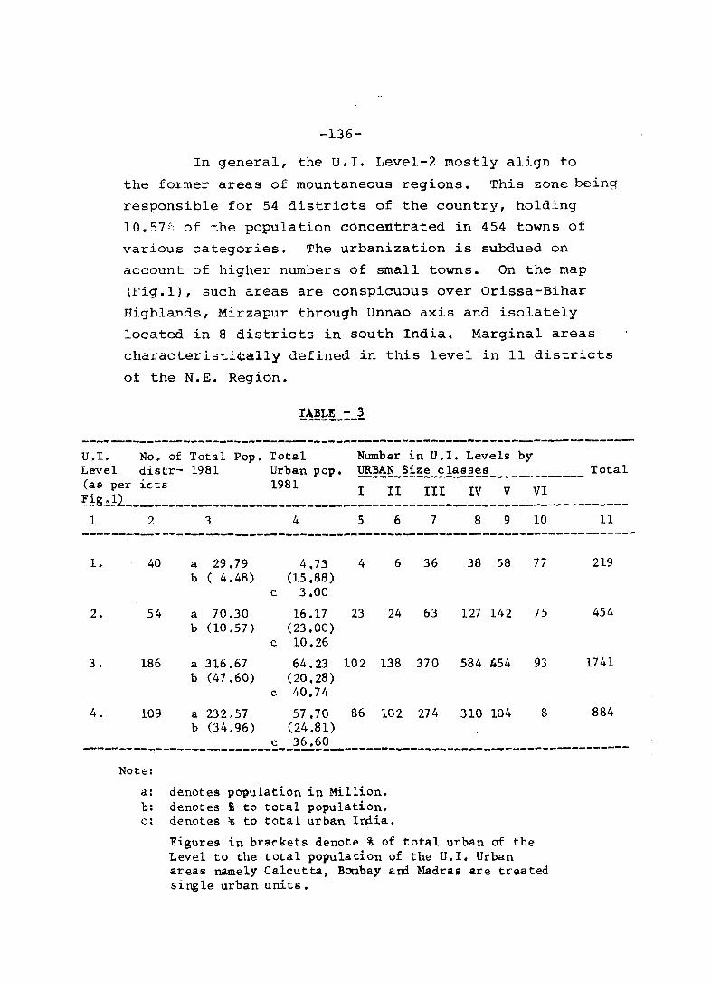
-136-

In general, the U.I. Level-2 mostly align to

the former areas of mountaneous regions. This zone being

responsible for 54 districts of the country, holding

10.57~ of the population concentrated in 454 towns of

various categories. The urbanization is subdued on

account of higher numbers of small towns. On the map

(Fig.l), such areas are conspicuous over Orissa-Bihar

Highlands, Mirzapur throu9h Unnao axis and isolately

located in 8 districts in south India. Marginal areas

characteristically defined in this level in 11 districts

of the N.E. Region.

TABLE - 3 ----~----

----------------------------------------------------------------------------U.I. No. of Total Pop. Total Number in U.I. Levels by Level distr- 1981 Urban pop. ~~!~_~~~~_~1~~~~~ _____________ Total

(~s per icts 1981 I II III IV V VI ~~g~lL ____________________________________________________________________ _

1 2 3 4 5 6 7 8 9 10 11 ----------------------------------------------------------------------------1. 40

2. 54

3 . 186

4. 109

a 29.79 4.73 4 6 36 38 58 77 b ( 4.48) (15.88)

c 3.00

a 70.30 16.17 23 24 63 127 142 75 b (10.57)

a 316.67 b (47.60)

(23.00) c 10.26

64.23 102 138 370 584 454 (20.28)

c 40.74

a 232.57 57.70 86 102 274 310 104 b (34.96) (24.81)

93

8

219

454

1741

884

c 36.60 -----.----~-----------------------------------------------------------------

Note:

a: denotes population in Million. b: denotes l to total population. c: denotes % to total urban India.

Figures in braekets denote % of total urban of the Level to the total population of the U.I. Urban areas namely Calcutta, Bombay and Madras are treated single urban units.

-137-

U.I. Level-3 represents situation in a majority

of 186 districts which alone has the pride to have 40.74%

of the nations urban share with 64.23 million urban

people. In this zone the number of urban areas from

Class I through VI accounts for maximum in the country

(Table 3). It seems a big: .. support in the urban activities

is rendered by even smaller towns, however their service

area is variant and could not be corelated as how far

these small towns are dependent or interdependent. A

major number 59.89% of total number of class V towns

lies in this level. The marketing of agriculture produce

mostly forms the functions of these towns.

Urbanization in U.I. Level-4 has typical character­

istics as far as geographical distribution is concerned.

The coverage of districts be.ing 109 in the country in

this level, contains 86 Class-I towns (39.45%) of the

country. The ratio between Class II & III gives rise

to equitable support in development of such towns than

others in the region. In general the towns generating

urbanism in this level are concentrated on the one hand

in some areas and sparsely located on the other particular

geographical areas, thus exerting pressure of urban

population high in the former regions and very weak in

the later regions which are mostly agriculturally under­

developed tracts and forested and mining regions of the

country.

Another important dimension of urbanization during

the last ten years is the accretion of population in urban

areas within the U.I. Levels defined above. The incidence

of accretion have pronounced effect on Class I areas in

a major way and such centres have enhanced or depressed

the U.I. Levels in the inter-se position of districts in

this level.

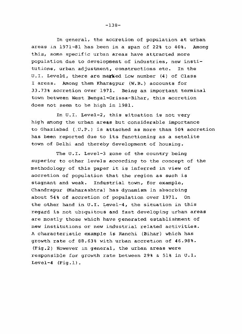
-138-

In general, the accretion of population at urban

areas in 1971-81 has been in a span of 22% to 40%. Among

this, some specific urban areas have attracted more

population due to development of industries, new insti­

tutions, urban adjustment, constructions etc. In the

D.I. Level~, there are mat~ed Low number (4) of Class

I areas. Among them Kharagpur (W.B.) accounts for

33.73% accretion over 1971. Being an important terminal

town between West Bengal-Orissa-Bihar, this accretion

does not seem to be high in 1981.

In U.I. Level-2, this situation is not very

high among the urban areas but considerable importance

to Ghaziabad (.U.P.) is Qttached as more than 50% accretion

has been reported due to its functioning as a setelite

town of Delhi and thereby development of housing.

The D.I. Level-3 ~one of the country being

superior to other levels according to the concept of the

methodology of this paper it is inferred in view of

accretion of population that the region as such is

stagnant and weak. Industrial town, for example,

Chandrapur (Maharashtra) has dynamism in absorbing

about 54% of accretion of population over 1971. On

the other hand in D.I. Level-4, the situation in this

regard is not ubiquitous and fast developing urban areas

are mostly those which have generated establishment of

new institutions or new industrial related activities.

A characteristic example is Ranchi (Bihar) which has

growth rate of 88.63% with urban accretion of 46.98%.

(Fig.2) However ln general, the urban areas were

responsible for growth rate between 29% & 51% in D.I.

Level-4 (Fig.l).

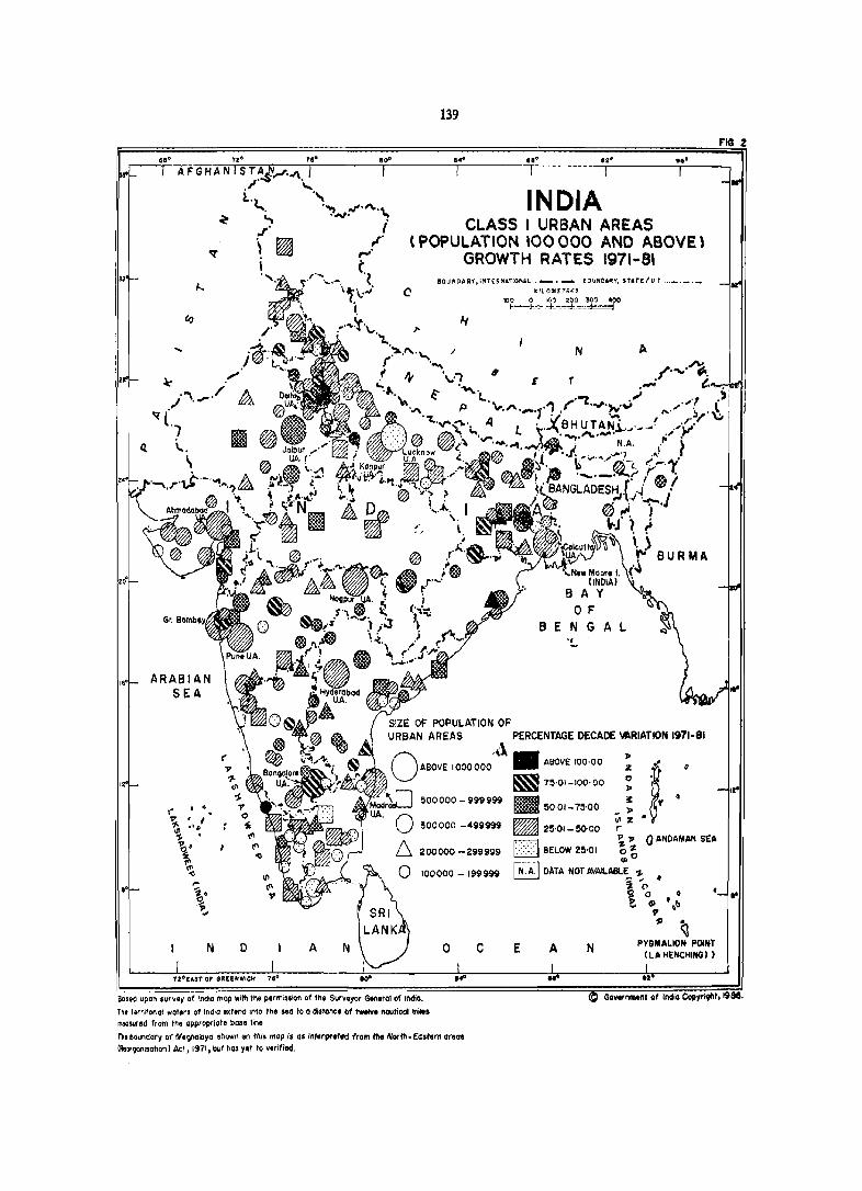
139

l..~. INDIA ~ ....

J' "

v ~

...,....,1"'."'.\, ;

,t' rJ'

t.

CLASS I URBAN AREAS (POPULATION 100000 AND ABOVE)

GROWTH RATES 1971-81

ARABIAN SEA

.-~. 9-.~

N

(

500000 - 999999

300000 -499999

200000 -299999

100000 - 199999

0 A c

Bolld upo, .urVIY of India mop w;tII the perrr,i •• ;on of the Surveyor General of Indio.

n. lerrilorlol waters 01 InalO exl.nd Into Ihe sea 100 di.,onc. Of tw .... naulical "'iltt mllosured from the appropriate bose 'ine

r~. couna'ary o( MI9Mlayo .fiown on ffils mop i. o. int.rpr.t,d from tile North. Eo.tern aroa4 (lIoor9OOl$ollon) Act, 1971, bul has yot to verified.

N

E 1

po

~ .~~ ~ 50.01- 715'00 11: &Wl8 _ J>

~ I/IZ ~ 25·01- !5O'OO r

1<::::'.:1 BELOW 215'01 ~ ~ a ANOAMAN SEA

III

~ DATA NOT AVAILABLE .,. ~... 41

E A N

~ <;, 0 e f> '.b •

" ~ PYGMA~ION POINT

(LA HENCHING) )

-140-

URBANIZATION & MILLION CITIES

Another face of urbanization in India is of the

contribution of the 12 million cities of 1981. These

centres play major roles in national and regional

migration. A prediction of projected population sometimes

is deviated due to many unknown factors operating in

such cities. Kings Lay Davis (1962) estimated the size of

population of 10 major centres in India at 1970 base

upto 2000 A.D. But by 1981, the census of India declared

2 additional centres of Jaipur and Lucknow as million

cities by marginal population. However, the Planning

Commission has also ventured to forecast some other 12

cities (Coimbatore, Patna, Surat, Madurai, Indore, Varanasi,

Agra, Jabalpur, Vadodara, Dhanbad Bhopal and Ulhasnagar)

which may attain million mark in 1991 census according to

their growth rate. The growth may be judged whether three

million jobs if created annually in the 7th Five year

Plan may add, in addition, the anticipated rural to urban

migration (1981-91) to these cities? The new policy of

the Planning Commission in reorganising labour force and

manpower planning as outlined earlier may also react this.

Considering the million cities of India at this

stage, the individual percentage variation in them (1971-81)

shows and maximum at Banglore (75.90%), Jaipur (60.32%),

Delhi (57.14%) and other cities of Calcutta and Bombay

between 23% & 38% and all other remaining million cities

between 23% ~ 48%. This very well responds to the index

of dissimilarity in them(Table-4), that is, the shift

towards development is not so much discernable. The

high inference for Calcutta (1.37) is mainly due to the

contributions of towns of the agglomeration. This

trend also in addition indicated haphazard urbanization

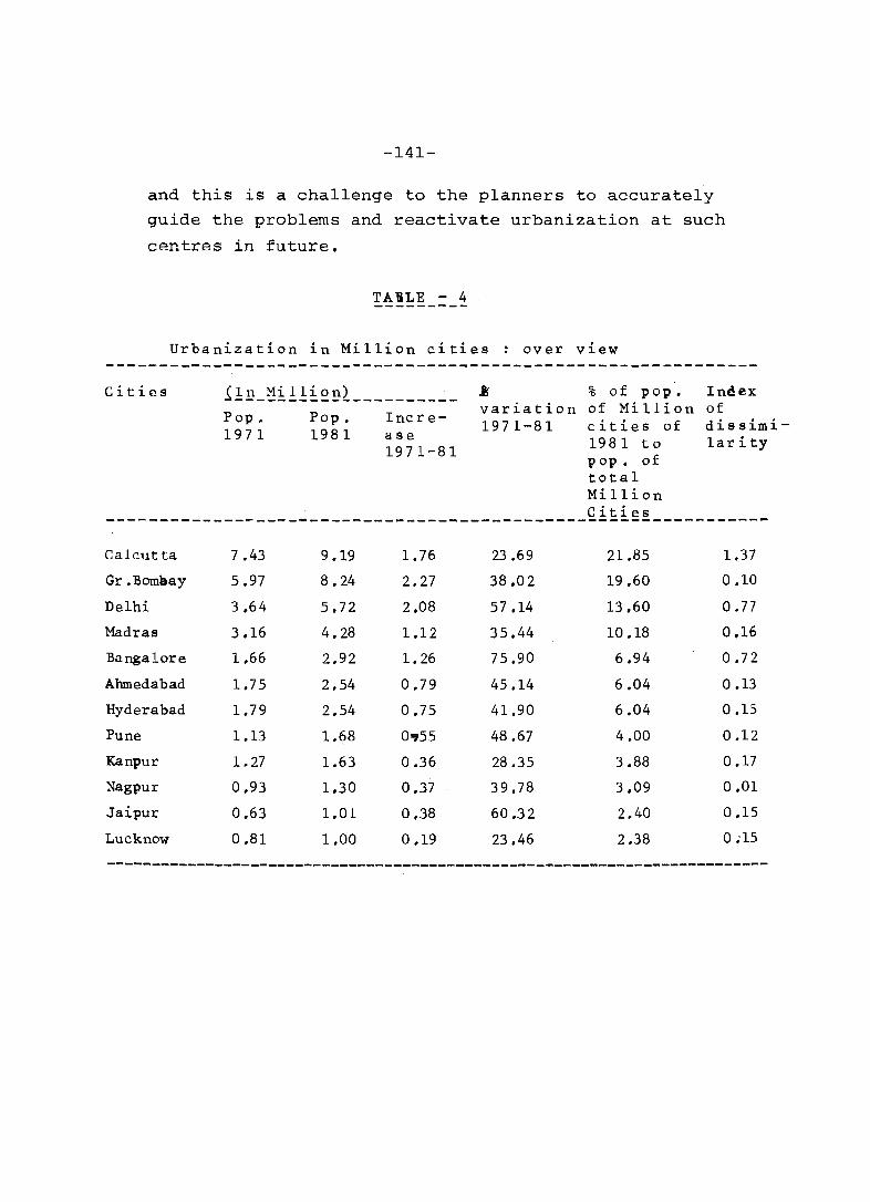
-141-

and this is a challenge to the planners to accurately

guide the problems and reactivate urbanization at such

centres in future.

TABLE - 4 ---------

Urbanization in Million cities: over view

Cities ~!D_~~!!~~QL ________ ~_ ..8' % of pop. Index

Pop. Pop. Inc r e- variation of Million of 1971-81 cities of dissimi-

1971 1981 aBe 1981 to 1ar i ty 1971-81 pop. of

total Million

--------------------------------------------_£~~~~~--- --------Calcut ta 7.43 9.19 1.76 23.69 21.85 1.37

Gr.Bomaay 5.97 8.24 2.27 38.02 19.60 0.10

Delhi 3.64 5.72 2.08 57.14 13 ,60 0.77

Madras 3.16 4.28 1.12 35.44 10.18 0.16

Banga10re 1.66 2.92 1.26 75.90 6.94 0.72

Ahmedabad 1.75 2.54 0.79 45.14 6.04 0.13

Hyderabad 1.79 2.54 0.75 41.90 6.04 0.15

Pune 1.13 1.68 0'755 48.67 4.00 0.12

Kanpur 1.27 1.63 0.36 28.35 3.88 0.17

Nagpur 0.93 1.30 0.37 39.78 3.09 0.01

Jaipur 0.63 1.01 0.38 60 .32 2.40 0.15

Lucknow 0.81 1.00 0.19 23.46 2.38 0 .. 15

--------------------------------------------------------------------------

-142-

MORPHOLOGICAL CHANGES

Concomitant to the population increase in urban

areas gives rise in the change of morphogenesis of

the townscape. This general system obviously operates.

In Indian urbanization, this gives birth to several

problems such as high land prices, under hand dealings

of land transfers and above all creation of congestion

with least amenities. In the million cities, the

expansion of areas for various needs and the responsibilities

of Planning agencies are very arduous. The census has

shown that towns and cities have crossed the chartered

jurisdiction in almost all towns of major concentration.

In general the extensions are not so well organised

considering the policy whatsoever laid-down for urban

development at this stage.

With a case analysis of Lucknow some of the

fa~s of urban landscape of this city are analysed to

drive to the notion outlined above specially expansion

of areas, vis-a-vis, adjustments (Table-5).

-143-

0 1.0 0 C"-J .-l .-l C 1.0 0 ex:. ('I")

-. t «j · .w 0 r-- 0 0 0 0 0 N 0 -::t .-l

1:-1 ..-! ~ .-l .......

1.0 ~ 0'\ r-I '" ,....... -::t r--; -q .-l 00 ,,-..

~I 0'\ . & . 0 .......,- ('I") N 0 0'\ r-I 0 H, ('I") '-:j" N N ('I") 00 p::jl I <.1 0'\

~ N

II'1 0 r- ('I") '" 0 .---. 0 r- ('I") 00 '" ~ co . · .-l .-:j" 0 ('I") 00 00

~ N ('I") .-l ..-I 7 ..-I lID ~

~ <U «j :::s C) -.-I 0 p::j

:;J ".-I ,_, <U ..., 0'\ N lI"\ -::t -.::t > .j.J t::: m A "........ N 0- -.::t 0 .-l H II) «j Po

~ r-- · . <U :::s .--I «j .__. N N .-I N 0 til -g ..-I El ::::> ('I") <U 1 <i.J H t:J t:::

Z • .-1 10 0 0 .-l r-.. ".-I H .0 '" :I: 10 Hi 00 lI"\ .-l 0'\ 0 .e '-" .j.J

~ "........ 0'\ N -.::t 0'\ N ",..... t:::

'" . · · 0'\ <U

~ .....,. 0 r-1 .-l r-l 0'\ ",..... <U .__.

15 U) ('I") > '-' ".-I H

~ .j.J <U :::s ~ til ..... (I}

~ H ,0 til -< II'1 N 00 II'1 ..... lID .j.J til <U

'" -.::t .-l 00 0 00 fl.I II) H El z lI"\ <U -.-I ~ ~ -._..' N ('I") N -::t 0'\ t::: t::: t:J

N -,4 -.-I t::: -.-I

~ III El <U H

~ ~ ~ .j.J tnl 0 <U

I ~ a I I ~ '" -.::t U) ~ ('I") ,.-... ,.-... ,.-... • .-1 , ,-;... M r-- M ('I") N N U) 00 t::: 1!I:11. ~ -::t .._, '-'" .._, til ... :u u '-' r-l .-l C'J ('I") 0 ..-I ~I ::J 0\ Q. <I ,:..l .-l ~I .-l .-l ~ t:::

~ ell ~ 0 .. .-I 0 Po

Lf'\ '" N N -.::t ~ 0 '.-1 :::s I'Ll ",..... U) N N r-- N .,4 +J til ('I") .. · <U +J til "C P '-' N ('I") ,-! r-l ...... "C ell <U <U

~ -.::t • .-1 t:J ,_, UJ I OIl :::s t:J til

;S <U "C <U ~ p::j flI;1 p::j .._,

z 0 0\ M ('I") r- ,.-... ¢ ".--,.

H ,.-.." C'") U) 0'\ .-l r- .-l r--N-- .. '-' '-" '--'

(/) ..._... -::t -::t N '.::1' -.::t f3l N C I Z I!D

~ <U • ...!

U 1.0 1.0 "1 -.::t -0 H ,-.... Lf'\ -::t r- 1.0 -::t 0 .-l ,_ ,0 tJ8 .._,

00 \,()

~ II'1 r-- <U N C"") r-- 0 .j.J

r-l ell ell ell It) Ql <U H N

~ N H

III til ~ J! 0 EI> '4 ..... .-l ..... H ell t::: t\f t::: t::: til +J ".-1 .w ".-I 0

'8 doP 0 oV> 0 .... +J til .w til .w

(/) ::i <U <U ell W 0 '+-I H '+-I ,_, Q .-l .j.J H ~ 0 < 0 < -..-{ 00 0 p::j I Z

8 lID <U.-l ::s ~~ t:.:: II) .--I .-l

~ P r-- 00 <11..-1 <U 0'\ 0\ ..c::

u U .-I .-I UdP

-144-

This table shows that the urban agglomeration of Lucknow

has added extension of areas over Ram Sagar Misra Nagar

and HAL Colony in the North and Hind Nagar Colony and RAC

Area in 1981. This has raised the geographic area of

the city from 127.65 km2 to 140.82 km2 in 1981.

The urge of adjustment with increase of 0.19

million people in Lucknow in 1981 demanded obivously

larger proportion for residential purposes. The business

area at the expansion level is accommodated vertical

to certain extent while the public services area have not

increased. Educational, industrial and administrative

areas have gained a bit the recreational facilities,

planning of par~kf",' play-grounds etc. (1.45%) in

comparision to a norm fixed by the Town & Country Planning

(4%) is not taken into account in this city. Ecological

balance, thus, lost.

This shows that newly urbanised areas such as of

Lucknow, although create some infra-structure mostly

derived from open spaces and hence there is a loss of

38.66% area during 1971-81. Such trends are operating

almost in all urban areas of the country due to urbanization.

This maladjustment can be reorganised if an over-view of

urbanization policy is spelt out for various classes of

cities & towns in advance or in stages of its perspective

growth.

RURAL-URBAN DUALISM IN PERSPECTIVE URBANIZATION:

Urban-rural dualism in urbanization process is

already operative in the country due to growing out-growths

and peripheral development as outlined above. precisely,

this problem may emerge in future in a broader perspective

in relation to areas constituted for the 332 Standard

Urban Areas (SUAs) in the country. These areas are

145

~==============================.=,-=.=,~=. ====~

-146-

evolved with a core of 50,000 & above urban population

alongwith rural areas (Villages) having socio-economic

linkages and hoped that these may generate a specific

urban-rural organism by 1991 when the time period of 30

years of constitution of these areas attain a span.

A characteristic example is cited out of these

SUAs from the SUA of Gulbarga (Karnataka). The core

built-up of Gulbarga SUA is quite mature but the urban

areas (Chartered jurisdiction) is open and the rural

space is infested with scrubs. The rural components

have various degree of growth of population (Fig.3)

It is anticipated that the rural areas which lie

along the main arteries of roads may be preferred by

private individuals and agencies to habilitate without

any planning to take advantage of the urban core of

Gulbarga and create a peculiar urbanization. This peculiar

urbanization may be related to the emergence of ribban

habitats to be followed bysporadic and sprinkling homesteads

causing a disintegration of rural habitats of the area.

It means relccation may be cyclic and this process may

not allow the planners to provide a good base, if a

policy is not evolved early. In long run, on account of

psychological notions typical outgrowths may develop

in the SUAs of the country adding more problems in future.

Fear of this trend is quite logical in view of increasing

out-growths elsewhere without sufficient amenities. In

the Indian conditions, such habitats grow practically

without amenities and then by democratic process facilities

are demanded by the dwellers from the local agencies.

This unhealthy situation in urbanization can be

modelled before hand if a law is framed to develop the

SUAs of the country by the Government. This system may

render to protect woods-scrubs, create planned residential

-147-

area ln larger terms consldering growth potentials by

2025 A.D .• This agency, if constituted may investigate

constantly development forces and plan.a most appropriate

urban-rural organism helping a new organised urbanization

even on regional basis.

SUMMARY

The contemporary urbanlzation ln India is leading

towards irrational consequences for the habitats in

gene:ral~ The effect of human concentration without a

migration policy in regions and locations may adversely

affect human satisfacttion. The data base although

good; sometimes create problems to have a firm view on

all classes of towns. In general, the small towns which

may be serving the immediate rural areas and a link with

their higher orders have remained mostly non-dynamice

This is supported by the fact that declassifications

and towns regaining '.urban status during censuses vary

from time to time (Table 6). In 1981 about one million

urban population was ruralised in some 101 towns and

abou t 2.68 million c ;:e;r.eT-- ·:While rural population got

status as urban. A large number (6l8) of towns was

declared new urban areas contributing about 5.55 million

population in the country.

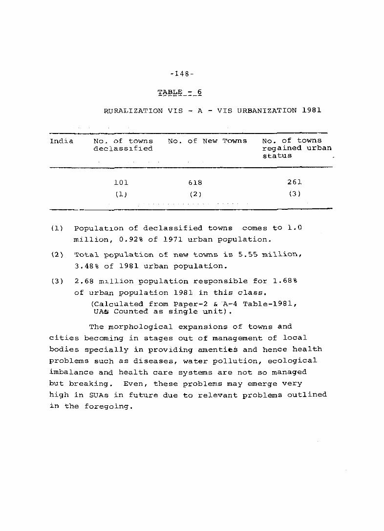
India

-148-

TABLE - 6 -,_.-------

RURALIZATION VIS - A - VIS URBANIZATION 1981

No .. of towns declass~fied

101

(1)

No. of New Towns

618

(2 )

No. of towns regained urban status

261

(3 )

ll) Populat~on of declassified towns comes to 1.0

million, 0.92% of 1971 urban population.

{2) Total population of new towns is 5.55 million,

3.48% of 1981 urban population.

(3) 2.68 mlilion population responsible for 1.68%

of urban population 1981 in this class.

(Calculated from Paper-2 & A-4 Table-198l, UAS Counted as single unit).

The morphological expansions of towns and

cities becoming in stages out of management of local

bodies specially in providing amenties·and hence health

problems such as diseases, water pollution, ecological

imbalance and health care systems are not so managed

but breaking. Even, these problems may emerge very

high in SUAs in future due to relevant problems outlined

in the foregoing.

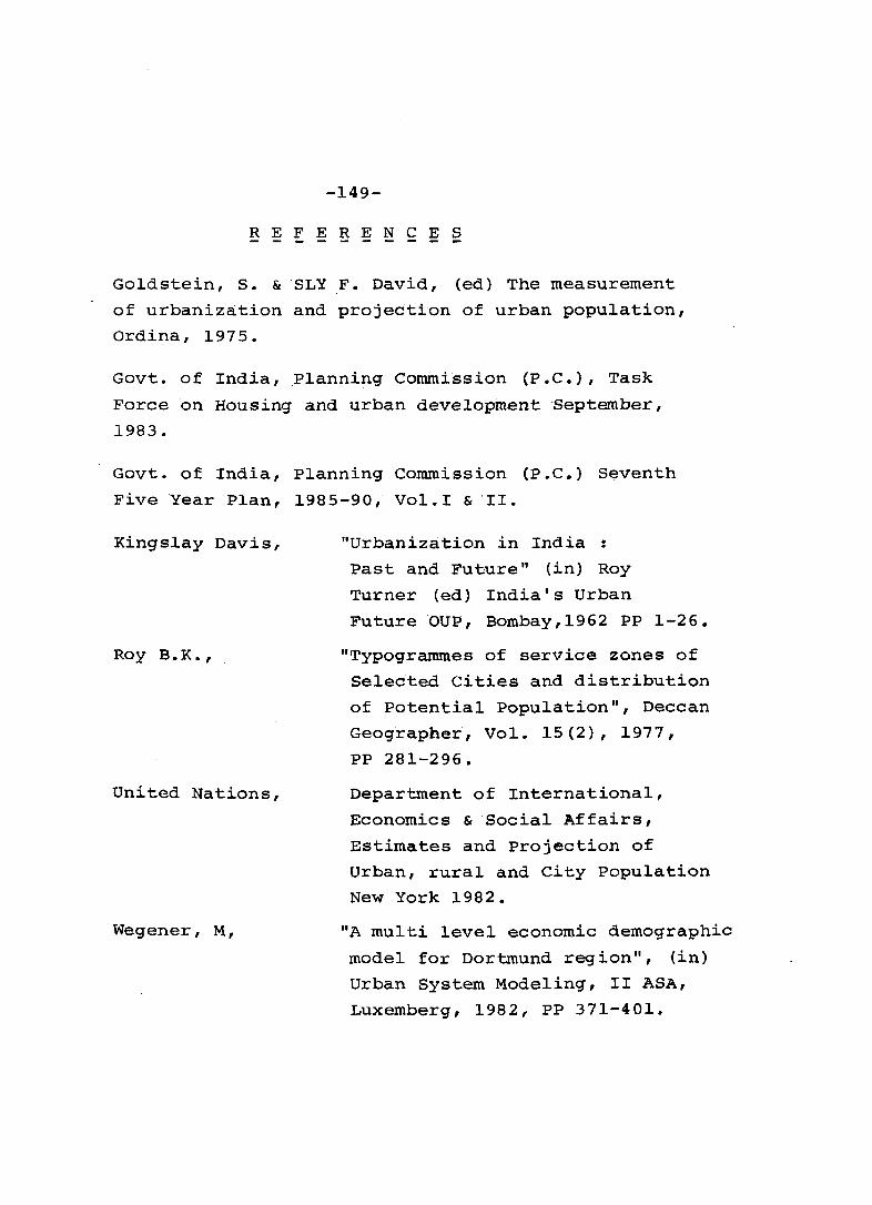
-149-

REF ERE N C E S

Goldstein, S. & SLY .F. David, (ed) The measurement

of urbanization and projectLon of urban population,

Ordina, 1975.

Govt. of India, Planning Commission (P.C.), Task

Force on Housing and urban development September,

1983.

Govt. of India, Planning Commission (P.C.) SE;!venth

Five Year Plan, 1985-90, Vol.I & ·II.

Kingslay Davis,

Roy B.K.,

United Nations,

Wegener, M,

"Urbaniz~tion in India :

Past and Future" (in) Roy

Turner (ed) India's Urban

Future aup, Bombay,1962 PP 1-26.

"Typogrammes of service zones of

Selected Cities and distribution

of Potential population", Deccan

Geographer, Vol. 15(2), 1977,

PP 281-296.

Department of International,

Economics & Social Affairs,

Estimates and Projection of

Urban, rural and City population

New York 1982.

"A multi level economic demographic

model for Dortmund region", (in)

Urban System Modeling, II ASA,

Luxemberg, 1982, PP 371-401.

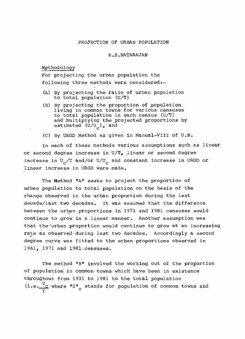
PROJECTION OF URBAN POPULATION

K.SoNATARAJAN

~~_-t:.~~~.91 ~2Y For projecting the urban population the

following three methods were considered:-

(A) By projecting the ratio of urban population to total population (U/T)

(B) By projecting the proportion of population living in common towns for various censuses to total population in each census (U/T) and multiplying the projected proportions by estimated (u/u )~ and c

(C) By URGD Method as given in Manual-VIII of U.No

In each of these methods various assumptions such as linear

or second degree increase in U/T •. linear or second degree

increase in Uc/T and/or U/Uc and constant increase in URGD or

linear inerease in URGD were made.

The Method lAo seeks to project the proportion of

urban population to total population on the basis of the

change observed in the urban proportion during the last

decade/last two decades o It was assumed that the difference

between the ur~an proportions in 1971 and 1981 censuses would

continue to grow in a linear manner. Another assumption was

that the/urban proportion would continue to grow at an increasing

rate as observed during last two decades o Accordingly a second ./

degree curve was fitted to the urban proportions observed in

1961, .1971 and 19812censusesQ

The method oBI involved the working out of the proportion

of population in common towns which have been in existence

throughout from 1931 to 1981 to the total population

(ioeo' Uc where BU' stands for population of common towns and T c

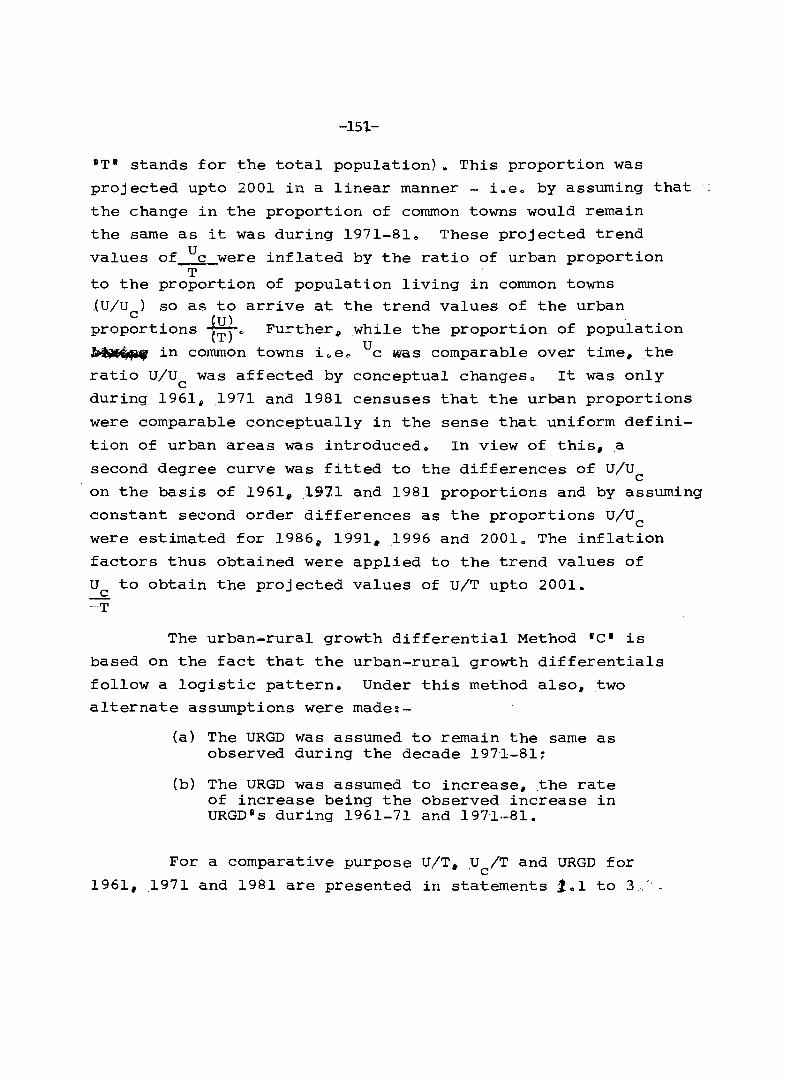
-151.-

"T' stands for the total population) .. This proportion was

projected upto 2001 in a linear manner - iweo by assuming that

the change in the proportion of common towns would remain

the same as it was during 1971-810 These projected trend

values of ~_were inflated by the ratio of urban proportion T

to the proportion of population living in common towns

,(ulu ) so as to arrive at the trend values of the urban c proportions ~~; 0 Fu=ther~ while the proportion of population

~ in common towns L,e" Uc was comparable over time, the

ratio u/u was affected by conceptual changeso It was only c during 1961, 1971 and 1981 censuses that the urban proportions

were comparable conceptually in the sense that uniform defini­

tion of urban areas was introduced 0 In view of this, a

second degree curve was fitted to the differences of u/u c on the basis of 1961, ,1.9'11 and 1981 proportions and by assuming

constant second order differences as the proportions u/Uc were estimated for 1986. 1991. 1996 and 2001. The inflation

factors thus obtained were applied to the trend values of

Uc to obtain the projected values of U/T upto 2001.

'-'T

The urban-rural growth differential Method IC' is

based on the fact that the urban-rural growth differentials

follow a logistic pattern. Under this method also, two

alternate assumptions were made:-

(a) The URGD was assumed to remain the same as observed during the decade 1971-817

(b) The URGD was assumed to increase, ,the rate of increase being the observed increase in URGD·s, during 1961-71 and 1971-81.

For a comparative purpose U/T. ,U ciT and URGD for

1961, 1971 and 1981 are presented in statements 1'01 to 3

-152-statement .' 1:-0bserved U/T* in 1961 1971 & 1981 ___________ - _________ L __________ _

----------------------------------------------------state/Union Territory

Census Year ---------------------------------1961 1971 1981

------ - - ---------------------------------------------1 2 3 4 ----------------------------------------------------

Andhra Pradesh Assam Bihar Gujarat Haryana Himachal Pradesh

Jammu & ·Kashmir Karnataka Kerala Madhya pradesh Maharashtra Manipul:

Megha1aya Nagaland Orissa Punjab Rajasthan Sikkim

Tamil Nadu Tripura Uttar Pradesh West Bengal Andaman & Nicobar

Islands Arunachal pradesh

Chandigarh Dadra & Nagar

Haveli Delhi Goa Daman & Diu Lakshadweep Mizoram Pondicherry

17c44 7c69 8~43 25~77 17g23 6~34

16~, 66 22,.33 15 .. 11 14,29 28,,22 8,68

15.27 5 .. 19 6,32

23,06 16.28 4~22

26 0 69 9,,02

12.85 24,,45 22.14

88£75 16 •. 06

5,36 24,,11

19,,31 8 _,82

10eOO 28,,08 17,,66

6.99

18,,59 24,,31 16~24 16~29 31~17 13,,19

14,.55 9095 8.,41

23~73

17 ~'3. 9,.31

30.26 10,43 14002 24~75 22.77

3,,70

90.55

89,,70 26.44

23 c32 10029 12047 31~10 21Q88

7e61.

21,,05 28J89 18c74 20029 35~03 26042

18,,07 15u52 11.,79 27v68 21 .. 05 16015

32c95 10.99 17.95 26,,4:1 26.30

6.56

93063 6v67

92~73 32e37 46 .. 28 23~67 52 .. 28

----------------~-------~----~---------------------*Proportion of urban to total population

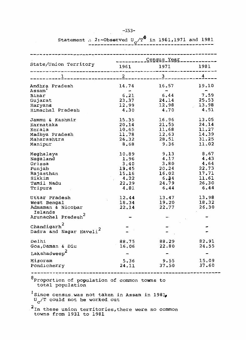
-153-

Statement ,_ 2:-0bsarved U /Te in 1961,1971 and 1981 c -----------------------------------------

-------------------------------------------------------------__________ £~u§~§_X~e~ ___________ _ State/union Territory 1961 1971 1981

123 4 ------------------------,--_._---'-------------------------------AndhrCfl Pradesh Assam' Blhar Gujarat Haryanid Himachal Pradesh

Jammu & Kashmir Karnataka Kerala Madhya Pradesh Maharashtra Manipur

Meghalaya Naga1and Orissa Punjab Rajasthan Sikkim Tamil Nadu Tr;ipura

uttar Pradesh west Bengal Admaman & Nicobar

Islands 2 Aruna.cha1 Pradesh

chandigarh2

Dadra and Nagar Have1i2

Delhi Goa,Daman & Diu

Lakshadweep2

Mizoram Pondicherry

14<74

6 0 21 23037 12 0 99 4.30

15035 20.14 10.65 11 0 78 26.32

8.68

10089 1.96 3~40

19.45 15.16

4.22 22.29 4.81

12.44 18.34 22.14

88.75 16.06

5.36 24.11

16.57

6.44 24.14 12.98

4070

16096 21.55 11.68 12.63 28.51

g e 36

9.13 4.17 3.80

20.24 16.02

6 .. a4 24.79

6.44

13.47 19.20 22.77

88.29 22.80

9 0 55 37.50

@proportion of population of common towns to total population

I 'Since census.was not taken in Assam in 1981,. Uc/T could not be worked. out

2 h . . . In t ese unlon terrltories,there were no common towns from 1931 to 1981

19.10

7e59 25.53 13.98

4051

13.05 24014 11.27 14 .. 39 31.25 11 0 02

8 0 67 4.43 4.64

22,,73 17.71 11.61 26.30

6.44

13.98 18.32 26.30

82.91 24s55

15009 37.60

-154:"

Statement 3 ',";', Annual exponential. growth rates for urban and rural areas and their dUf,erellce' 1961-71,1911-S1 ---..,..-----------~'1~----------":"".:---

----------~--------------------------~-----------------------

states/Union Territories

. "', ~

, Growth RAte .' '. ' --"I"'"".:~~- ..... --~~·~-'--~r.~---------~--------~...-·---___ ~2~~:r~__ ~2r~:~~____ _ __ ~~ _______ _ U r b a 1'1., R u ~.a 1 N r ban R u r all 9 61 - 7 1 1 97 1 - 8 1

-'--'-'--~_':""'-''''!'''''--:-~~~-,.. --~~---------.,__----------------------------------.. -----1 2 3 4 5 6 7

-----.._--._.~..,.,,_"r'__.,,·r.....,--· ___ '.'P ______ """:"-------------------- ___________ - __________ _

1., Anlihra l'-radesh 2. Assam 3 ~ Bifutr 4, Gujarat 50 Ha-ryana

6" Himaeha1 fradesh 7 0 Jammu & Ra s1:mdr 8 0 Karnataka 9., Ker.a1a

10~ Madhya Pradesh

11 c Mabarashtra 12, Manipur 13 ~ Meghalaya 14" Naga1and 15, Or. is s.a

16. !'hi\j a b 17" Rajastlian 18, Sikkim 19 n Tamil Nadu 20 0 Tripura

21" Utt:al!' Pradesh 22, West Betlial '" 23 0 Aadaman & Nicobar

" Islands 24. Arunachal Pradesh?+ 25 u Chandi.garh 26" Dadra. &' Nag.arHave1H 27, Delhi 28, Gaa Daman ~ Diu 29" Lakshadweep+ 30, Mizoram 310 Pondicherry

India . . " ~ ",

2.,92 5,01 3 0 64 3.,44 3.,04

:L05 3,,69 3.02 3,,05 3.83

3 0 42 7,37 2,,25 90 B7 5.09

2,25 3~25

10 0 55 3.27 4,55

13,,53

L~67 2,.82 l.o 76 2.,26 2~74

2.00 2,36 1,91 2,,20 2.29

2 0 01 2 ,~6B 2~82

2.B4 2.01

1,88 . 2029 2,02 1.51 2 0 94

1,,65

3,36 L82

1,53 -0 .. 24

L96

3~96 4,62 4,37 3.047 4 .. 67

2,,98 3,,84 4.10 3,,19 4,45

3,36 9,,76 4.,95 B~50 5,,22

3~68

4 c,62 9-;;54 2047 3 ~29

4~74

2$76 6~.38

11 .. 71 4,66

3 c 84

L57 2 0 92 L88 2,,01 2,)00

2.06 2(29 1,75 1046 1.:76

1 Q 62 1016 2(36 3.42 1,46

1.61 2043 3,33 1,22 2.71

1,68

2,,37 0,,53

1081 _._ .... _______ ., .... -.; ___ ... _________ ~---------------------_

1¢25 2.19 1~88 1018 0,30

LOS 1.33 L11 0,,85 1.54

1~41 4,69

-0,,57 7 e03 3~08

0 0 38 0.96 8,,53 10 75 1.61

8.21 Be l5

1025

2.39 1011 2 .• 49 L45 2.67

0 0 92 1~55 2 0 35 1074 2,,69

1J5 8~60

2~52 5~08 3",76

'Z o 07 ,2~19 6~22

10 25 0,,58

4.28

3 0 81 2,,87

9,,34 4 4 13

2,,03

+In thase Union Territories there were no urban areas in 1961 and 1971

Flve estlmates of the percentage of urban popu­

lation to t.ot.al poplllat.ior.. for: t.he years 1986( 1991, 1996

and 2001 were thus obtained_ These percentages varied

between 30.15 to 34 .. 98 for the year 2001" 'rhe constant

URGD method estlmated thlS pe:centage as 31~35. The extra­

polation based on UIU gave a percentage of 32 0 14 while c the fittlng of second degree curve to UIT gave a percentage

of 34.57 The assumption of lncreaslrig URGD gave an urban

percentage of 34.98 for the year 2001e

The projected proportlon of urban populatlon to

totCll populati()ll by various me'"ChodE. (All India) are given

in statement - .4

Statement .4 - Projected percentage of vrban ~opu1atlon to total population by various methods - All India ------------------------

* (U/T) (U/T) Using V/U U .R.G .D.. U ,:R.,G,D,· Year Linear Second inf1ationc constant increasing ________________ ~~~E~~ ___ ~!2!2E _______ --______________ ____ _

-!-------~---------~---------!----------~----------~-------1981 23.31 23.31 23.31 23 0 31 23.31

1986 25"01 25076 25.·30 25,18

1991

1996 2001

26,72

28,,42 30,13

28,,20

31,39

34~.57

27,,36

29._70

32 0 14

27-14

29 20

31.35

*The rate of increase was the observed increase during 1961-71 and 1971-81r

25 c' 4 ° 28<00

31,17

34.98

The urban projections were made for each state and

union territory se9arately by various methods. A pooled

estimate was derived for India by adding up the urban

. population of all states and union terri::oriesr

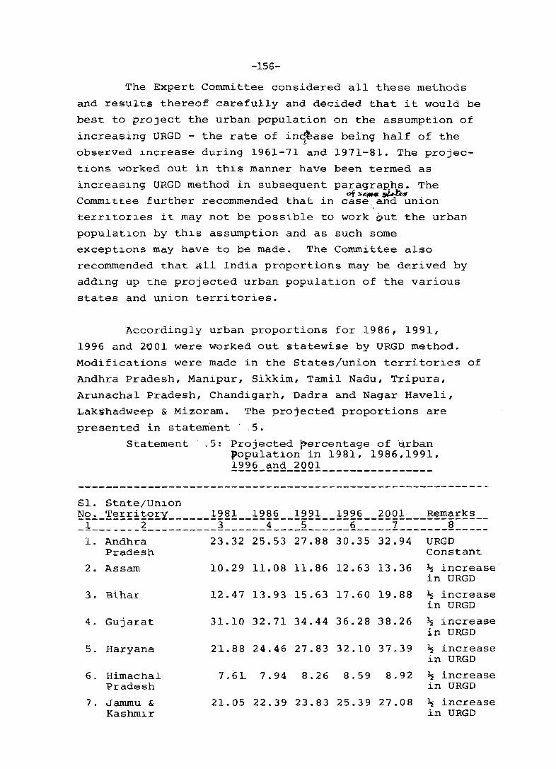
-156-

The Expert Committee considered all these methods

and results thereof carefully and decided that it would be

best to proJect the urban population on the assumption of

increasing URGD - the rate of in~ase being half of the [-

observed lncrease during 1961-71 and 1971-81. The projec-

tions worked out in this manner have been termed as

increasing URGD method in subsequent paragrap'hs. The , of S" .. iJ,.hll .

Commlttee further recommended that ln case,and union

terrltorles it may not be possible to work out the urban

populatlon by thlS assumption and as such some

exceptl.ons may have to be made. The Committee also

recommended that All India proportions may be derived by

adding up the projected urban population of the various

states and union territories.

Accordingly urban proportions for 1986, 1991,

1996 and 2Q01 were worked out statewise by URGD method.

Modifications were made in the States/union territories of

Andhra Pradesh, Manipur, Sikkim, Tamil Nadu, Tripura,

Arunachal Pradesh, Chandigarh, Dadra and Nagar Haveli,

Lak~hadweep & Mizoram. The projected proportions are

presented in statement - .5.

8l.

Statement .5: Projected percentage of tirban population in 1981, 1986,1991, 1996 and 2001 -----------------------------

StatejUn:L.on ~2~_~~~~~~2!Y ______ 12~1 __ !2~2 __ 122! __ !22~ __ ~QQ1 ___ ~~~~f~~ __ _ 1 _______ ~ __________ ~ ______ 1 ____ ~ ______ § _____ 1 _______ § _____

l. Andhra 23.32 25.53 27.88 30.35 32.94 URGD Pradesh Constant

2. Assam 10.29 11.08 11.86 12.63 13.36 ~ increase in URGD

30 Bihar 12.47 13.93 15.63 17.60 19.88 ~ increase in URGD

4. Gujarat 31.10 32.71 34.44 36.28 38.26 ~ increase in URGD

5. Haryana 21.88 24.46 27.83 32.10 37.39 ~ increase in URGD

60 Himachal 7.6L 7.94 8.26 8.59 8.92 ~ increase Pradesh in URGD

7 • Jammu & 21.05 22.39 23.83 25.39 27.08 ~ increase Kashmir in URGD

-15~-

-----------------------------------------------------------------S1. State/Union No. Territory 1981 1986 1991 1996 2001 Remarks -1-------2------------3------4-----5-----6-----7-------8--------------------------------------------------------------------------

8. Karnataka 28.89 31. 50 34.59 38.17 42.27 ~ increase in URGD

9. Kera1a 18.75 20.18 21. 88 23.88 26.22 ~ increase in URGD

10. Madhya Pradesh 20.29 22.62 25.43 28.76 32.65 ;!.,; 2 increase in URGD

11. Maharashtra 35.03 37.08 39.28 41. 63 44.11 ~ increase ir. URGD

12. Manipur 26.42 28.41 30.40 32.39 34.38 U/1J ", " .' q ,

13. Megha1aya 18.07 20.32 23.47 27.73 33.31 ~ increase J..n URGD

14. Naga1and 15.52 19.00 22.61 26.21 29.65 ~ increase in URGD

15. Orissa 11. 80 13.94 16.51 19.59 23.24 ~ increase in URGD

16. Punjab 27.68 29.98 32.85 36.34 40.49 ~ increase in URGD

17. Rajasthan 21. 05 23.03 25.44 28.31 31. 71 ~ incr-ease J..n URGD

18. Sikkim 16.15 19.82 23.48 27.15 30.81 U/U c 19. TrJ..pura 10.99 11. 28 11. 58 11. 88 12.19 URGD cons-cant

20. Tamil Nadu 32.95 34.34 35.76 37.20 38.67 URGD constant

21. Uttar Pradesh 17.95 20.37 23.46 27.33 32.10 ~ increase in URGD

22. West Bengal 26.47 27.43 28.60 30.00 31.64 ~ increase in URGD

23. Andaman & Nico-26.30 28.36 30.91 34.01 37.72 ~ increase bar Islands J..n RGD

24. Arunachal Pradesh 6.56 7.99 9·~ ~2 10.85 12.28 Li.near U/T 25. Chandigarh 93.63 94.79 95.75 96.54 97.29 URGD CONSTANT

26. D§dra & Nagar 6.67 6.67 6.67 6.67 special aveli t)iethod

27. Delhi 92.73 94.00 95.22 96.32 97.28 ~ in-:::rease in URGD

28. Goa, Darnan & 32.37 35.19 37.11 37.95 37.99 ~ incr:ease " Diu J..n URGD

29. Laksttadweep 46.28 46.28 73.56 73.56 73.56 special method

30. Mizoram 24.67 29.20 33.73 38.26 42.79 T]/lJ c 31. Pondicherry 52.28 56.88 60.14 62.10 62.82 ~ inc:cease

in URGD

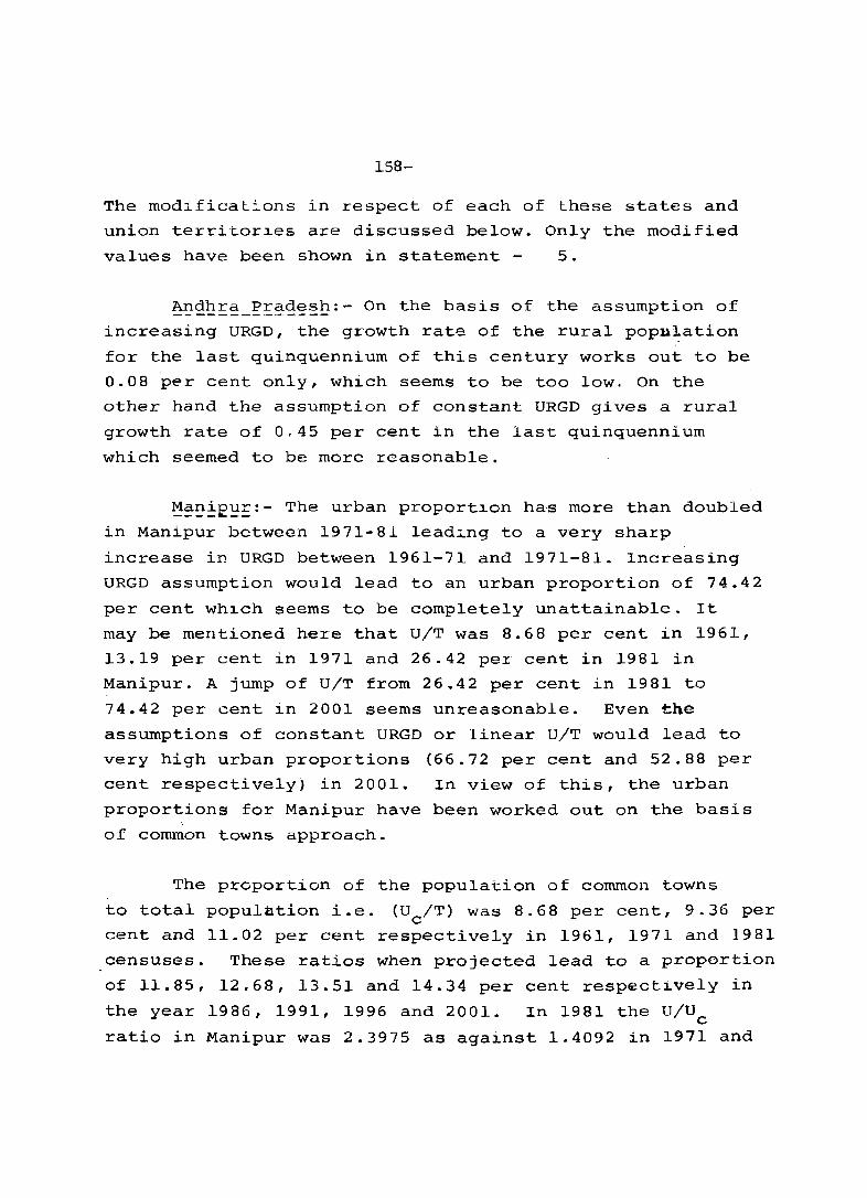
158-

The modifications in respect of each of these states and

union territor1es are discussed below. Only the modified

values have been shown in statement - 5.

~~~~~~_~~~~~~~:- On the basis of the assumption of

increasing URGD, the growth rate of the rural popu~ation

for the last quinquennium of this century works out to be

0.08 per cent only, which seems to be too low. On the

other hand the assumption of constant URGD gives a rural

growth rate of 0.45 per cent in the last quinquennium

which seemed to be more reasonable.

~~~~e~E : - The urban proport1on ha·s more than doubled

in Manipur between 1971-81 lead~ng to a very sharp

increase in URGD between 1961-71 and 1971-81. Increasing

URGD assumption would lead to an urban proportion of 74.42

per cent Wh1Ch seems to be completely unattainable. It

may be mentioned here that U/T was 8.68 per cent in 1961,

13.19 per cent in 1971 and 26.42 per cent in 1981 in

Manipur. A jump of U/T from 26.42 per cent in 1981 to

74.42 per cent 1n 2001 seems unreasonable. Even the

assumptions of constant URGD or linear U/T would lead to

very high urban proportions (66.72 per cent and 52.88 per

cent respectively) in 2001. In view of this, the urban

proportions for Manipur have been worked out on the basis ,

of common towns approach.

The proportion of the population of common towns

to total population i.e. (Uc/T) was 8.68 per cent, 9.36 per

cent and 11.02 per cent respectively in 1961, 1971 and 1981

censuses. These ratios when projected lead to a proportion

of 11.85, 12.68, 13.51 and 14.34 per cent resp€ctively in

the year 1986, 1991, 1996 and 2001. In 1981 the U/U c ratio in Manipur was 2.3975 as against 1.4092 in 1971 and

-159-1.0000 in 1961. The projection of U/U ratio on the c baSiS of either by linear trend or a second degree

trend leads to unacceptably high value of urban

proportion for Manipur. In view of this it was assumed

that the ratio ulu would remain constant upto 2001. c Under this assumption the urban proportion was estimated

to increase from 26.42 per cent in 1981 to 34.38 per

cent in the year 2001.

~~~~~~:- Sikkim's urban proportions were 4.22 per

cent in 1961, 9.37 per cent in 1971 and 16.15 per cent

in 1981. In this case, URGD declined between 1961-71

and 1971-81. Even so, the assumption of inc~sing or

decreasing URGD gives an urban proportion of 35.07 per

cent in 2001 which seems to be exceedingly high. In

this case also, the common towns approach has been used

assuming that U/U observed in 1981 will remain constant c upto the year 2001. This gives U/T of 30.81 per cent in

2001.

T~~!!_~~9~:- In this case, URGD has been declining

between 1961-71 and 1971-81 and extrapolating this trend

would in fact amount to declining URGD, which would give

U/T of 35.36 per cent in 2001 as against 32~95 per cent

in 1981. This seems to be too low. Therefore, in this

case, the assumption of constant URGD was made for

projecting urban proportions. The assumption of constant

URGD would lead to an urban proportion of 38.67 per

cent in 2001.

!E!E~E~:- In this case also URGD has been declining

between 1961-71 and 1971-81. Extrapolating this trend

leads to a declining urban proportion after 1991 which

does not seem possible. Therefore, in this case an

assumption of constant URGD, Wit~tRGD being same as

-160-

1971-8~ was made for projecting urban proportion. This

assumption would mean that the urban proportion would

increase from 10.99 per cent in 1981 to 12.19 per cent

in 2001.

Arunachal Pradesh: In case of Arunachal pradesh, -----'-----,_,"_,-----there was no urban population in 1961. The question of

applying the principle of in~asing URGD, therefore,

does not arise. The assumption of constant URGD would

give an urban proportion of 18.99 per cent in the year

2001 as against 6.56 per cent in 1981 and 3.70 per cent

in 1971. This seems to be too high particularly in a

hil~ area like Arunachal Pradesh. The urban proportions

have therefore been projected for Arunachal Pradesh by

assuming linear increase in U/T which would give a ratio

of 12.28 per cent in 2001.

gh~~~is~fh:- In Chandigarh's case the URGD had

declined between 1961-71 and 1971-81 and extrapolating

this trend would in fact amount to declining URGD assumption.

This would give U/T of 96.43 per cent in 2001. It was

thought to be more reasonable to make the assumption of

constant URGD in this case which would give U/T of 97.19

per cent in 2001.

Q~~E~_~!:~_~~S~!:_!:!~y~!!..:.- There Has no urban population in this union territory before 1981. The urban

proportion recorded in 1981 was 6.67 per cent. On examining

the population of various villages in 1981 it was felt

that no new town may come up in this anion territory upto

1991. Therefore, it has been assumed that the urban

proportion in this case may remain the same upto 2001.

~~~~~~~~~~J2:..-Lakshadweep had also some urban areas in 1981 for the first time; the urban proportion

-161-

being 46.28 per cent in 1981, In Lakshadweep, no island

has got a municipality or a corporation or cantonment

board or notif'ied town area committee, etc. In 1981,

all the islands had a density of population of more

than 400 persons per square kilometre and also 100 per

cent of the wo~kers in these islands were engaged in

non-agricultural occupations. On~y four islands namely,

Andrott, Minicoy, Kavaratti andAmini had a population

of more than 5 ,'~' persons. After considering

these factors, ,Minicoy, Kavaratti and Amini were treated

as census towns in 1981., On the basis of the estimated

exponentia~ growth rate which can be achieved from 1981

to 2001, Agatti islands may also have a population of

about. 5 f OOl: " ~, by 1991. It is, therefore, felt that

both Andrott and Agatt~ islands would be treated as

urban by 1991. On this basis, the urban proportion in

Lakshadweep would be 73.56 per cent in the year 1991

and 2001,

~!~9E~~:- Mizoram had an urban proportion of 5.36

per cent in 1961, 11.36 per cent in 1971 and 24.67

per cent in 1981. The assumption of increasing URGD

would give a high urban proportion of 71.96 per cent

in the year 2001. Even the assumption of constant URGD

gives an urban proportion of 68.14 per cent while the

assumption of linear increase in U/T gives an urban

proportion of 51_29 per cent which also seems to be

very high- The urban proportions in this case had been

worked out on the basis of conunon towns approach. by

assuming that U/U observed in 1981 would remain constant c upto 2001. This gave an urban proportion of 42.79 per

cent in 2001.

In case of Haryana and Punjab, the projected urban

proportions on the assumption of increasing URCD would

be 37.39 per cent and 40.49 per cent respectively in 2001.

-162-

The proJected rural population on this basis would give

a negative rural.gro\vth rate during 1996-2001 in both

these states. A very large portion of Haryana in

Faridabad, Gurgaon, Rohtak and Sonipat districts forms

a part of the National Capital Region in whi~h the urban

population is expocted to yrow very fast in the next

20 yearso Under the. impact of development of NCR, many

of the rural a::::'eas of Haryana I falling wi thin the NCR,

may become uL·ban. In vie'!," of this, a negative rural

growth rate during 1996-2001 in Haryana is quite plausi­

ble.

In Punjab's case, the urban proportion in 1981 was

already very hi.gh (27.68 per cetit) ~ With the economic

prosperity in punjab due to the development of the small

scale industries and agriculture, there is every likelihood

of an acceleration in the pace of urbanisation resulting

in a negative rural growth rate by the end of this century.

The projected urban an~ rural popUlations for the

year 1986, 1991, 1996 and 2001 and th~ir annual exponential

growth rates for each quinquennium are presented in Table - ... 1.

On the basis of the pooled urban population .the

All India urban proportions for 1986, 1991, 1996 and 2001

are as under:-

-Statement :'.,6 : - !?E~j~SE:~9_~Ee~~_~E<2e9E~!2!!~

E·~;_~'!_!~9~~_JE~9!~9l"

--------------------------------------------------------Year proj~cted U!T(%) --------------------------------------------------------

1981 23.31 1986 25~26 1991 27.49 1996 30.06 2001 . 33.06 --------------------------------------------------------

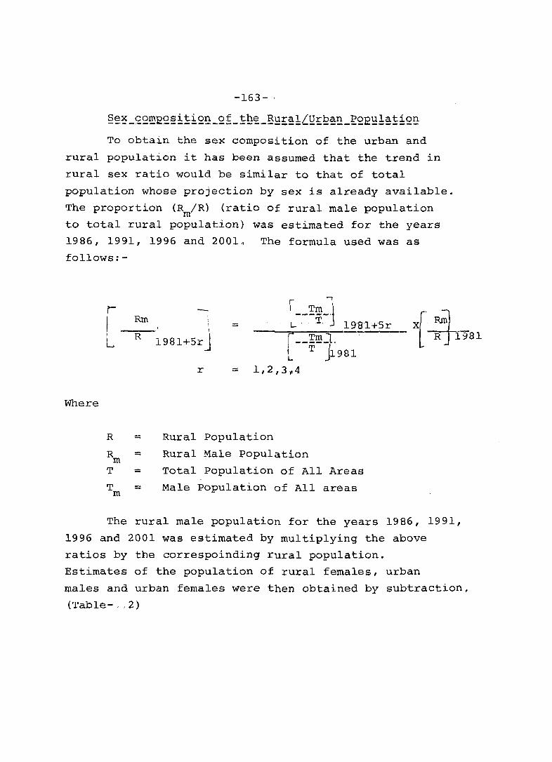
-163- ,

To obtain the sex composition of the urban and

rural population it has been assumed that the trend in

rural sex ratio would be similar to that of total

population whose projection by sex is already available.

The proportion (R /R) (ratio of rural male population rn

to total rural population) was estimated for the years

1986, 1991, 1996 and 20010 The formula used was as

follows:-

[ [--!~-J Rm , ,T, 19'81+Sr i4 , = R ~98l+5rJ [ --~~i981 R 1981

r = 1,2,3,4

Where

R = Rural Population

R = Rural Male Population m T = Total Population of All Areas

T m = Male Population of All areas

The rural male population for the years 1986, 1991,

1996 and 2001 was estimated by multiplying the above

ratios by the correspoinding rural population.

Estimates of the population of rural females, urban

males and urban females were then obtained by subtraction,

(Table- , ,2)

-164-

Estimates of the rural and urban population

were available by sex for the years 1981, 1986, 1991,

1996 and 2001. Age distribution of the projected

population for India and 15 major states into broad

age groups 0-14, 15-29, 30-44, 45-59 and 60+ was

obtained by the method of "difference eliminations".

The various steps involved were as follows. All the

calculations were done separately for each sex.

The age distribution of the rural and urban

areas of India and 13 major states as reported in 1981

census was assembled in a 15 x 2 matrix form1i.e'Jin

age groups 0-4, 5-9 .•....••..•••. 65-69, and 70+ in

rural and urban areas. The marginal totals were then

adjusted to correspond to 1981 smoothed age . :as: on

1st "March by repeated iterations.

Total population by broad age groups and the

rural-urban break-up of the total population were

available for the years 1986, 1991, 1996 and 2001.

Based on the 1981 rural/urban age distribution as

obtained above the age distribution for the subsequent

quinquennial years was obtained by tw~~fterations (by method of difference elimination) and has been

shown in Table - ' .. 3 •

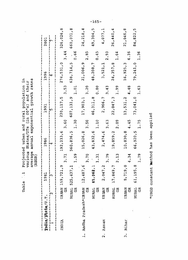
-165-

m co ~ L() r-I .~ co ll"I .. ... ... 0.0 rl 00 "<:I' r- 0 1.0 N

I N r- rl 0 r- "<:I' -.:t' N ...-i I 0 0 N M 0 ~ 0 00 0 11- ... ... ... 0 I 0.0 0 ~ C1\ -.:t' 0.0 ...-i -.:t' N I N 1.0 N ~ N N co

I M 0.0 I I -.:t' 0.0 L() ll"I M ~ 1.0 0.0 , '<:t' 0.0 co ~ C1\ 0.0 M M I I M 0 N 0 N M '<:t' ...-i I ! 0 U) C1\ I- M co M 0 I ... ... ... , ...-i "'" 0.0 co M r- Ll'l M , M ...-i 0 0 N Ll'l N -.:t'

0.0 , Ll'l " 0 N ~ M C1\ N C1\ io.o ...

I C1\ t ~ 00 ...-i co M "<:I' 1.0 C1\ s:: rn I rl I I- M N -.:t' N ...-i r-

• .-i $..I Q) f , N 0.0 -.-i +J ~ I

s:: Q) ItS I I M r-l 0 0 M C1\ ex> M o .c:: $..I I ! L() 0 N co ~ C1\ '<:t' 1.0 . .-i +J , I +' .s:: , I M ...-i M 0 ~ r-I '<:t' r-I 1tS'tj+J , t ...-is::~ I , L() Cl'i ...-i co r- M N 0 ::1 nj 0 I i 0.. H I , r- rl M rl 0.0 I- M M O-t'l , M I .-l M 0 M 1.0 "<:I' M ~ 0.. til I '" I .-l M '" M C1\ 0 Ll'l 0

= rl I '" IL() ... ... .-loro ! .-l I 0 l- I- 0.0 N N M M ro O·.-i I ! M 0 .-l -.:t' N M r- "0 l-l +J I I N 1.0 Q) ::1 ~ s:: I I. • .-i ).j-r-f Q) I I 0 0 0 0 M m L() Lf'l M

......... ~ I I 1.0 M L() M 0.0 0 '<:t' I- 0.. "0 0 I I PI S::tIl~ I I M M M M M N ~ .-l n:l n:lE-i;< , (

::;:'Q) I I 0.0 U) co 1.0 1.0 N 00 L() s:: s::'-... I I ... Q) n:ltll..-i ( I M 1.0 0.0 N ~ C1\ 0 0 Q)

..Q Q) ro I \0 I M M N M I- L() M N ..Q H+J:;:1 I co I N co 0 co -.:t' co 00 '" ::1 ro s:: I C1\ I~ ... ... til

+J s:: I .-l 1 N 0 U) M N '" 0 1.0 ro "0 Ci)ro , I C1\ 1.0 .-l ~ M M 1.0 ..c:: Q) ! I .-l L()

+J til OJ , I "0 o :;j Ol·~ I I M m 0 M '" M -.:t' '" 0 Q)On:l~ I I r- L() I- M I- M M r- ..c::

-n-r-f l-l (.!) I I +J OHOJriI I I M M M M M N -.:t' M

~ l-lro:;>,::x: [ I AI:>n:l- I I C1\ M \0 M N I- 0 co

I I +J I I .-l r- I- (.'If r- m '"

L() s:: M I .-l I N M 00 \1> -.:t' -.:t' M m n:l , co 1M I- oqc -.:t' 0. 0 co I- M +J

i C1\ I til I .-i I C1\ It) N r! N I- 00 r-I s::

Q) I I L() N r-I * ,....; 1.0 0 .-i J I ,....; L() 0 .a ! I n:l I I Zp::; ...:IP::; ZP::; ....:lP::; ZP::; H P::; Z~ ...:IP::; 0

E-t I , I ~(.!) ~(.!) ~(.!) ~t!J ~(.!) ~ (.!) ~(.!) ~(.!) ~ I IN I p:; I • I I P::; ::J P::; 0 P::; ~

P::; ::J 0 I E-l , I 0 p:; 0 p:; 0 0 p:; -Ie l • 1 I -IC I 0 I ~ .c:: ~ '. I I til I N • I Q) i . -H I I "0 ! .~ I I ro i ~ J I ~ I I , AI I '-... I , I «I I I oc:!'! ro @ H I <!'I 1M i H ..c:: ro I ~ I I 0 "0 til ..c:: I I I Z s:: til -.-i I t-t I I H ..:x: ..:x: ~

---i N M

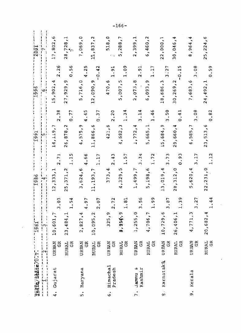
\.0

r. N I~""""'I, I 0 10.. II" 00 10. I IN' ' I l""-I' r-i , ,

I I I 1\.0 r r 10'1 :1.0 I 10'1 , Ir-! I 1 1

I I. l"-I ..

',r-i I I 0'\ ~O'\ Ii.f'l I --1 10'1 r t -i Ir-i ~ I I -.:l'

;\.0 I

lCO ''<::1'' 10'\ I ,

Ir-i I I

r-i

\0 N

o

eo 0'\ N \.0 I""- .. ;;~. 0 .. co l"-N

1.0 I,{")

L()

N

N

N 0 "<:I' 0 I

co ("')

N

N

eo r­eo

1.0 N

I' I""-

o

,-1 I,{")

I"- rl

o 0'\ .. \0 0 r-i 0'\ I' 0

I,{") N

I,{")

l""­I,{")

.-I

...

I""­M

o

I I I ,

N I,{")

1 I , I , I

I I

i , I , I I 'r-i I • !:CO IM~ 1.0'\ I I, i.r-i • , r. I

I I , ~ I , iNI I I , I I I ! J I f ! 1 I. h I t Ir-i t I I: J I, I , j I I ,

r-i N

.-I o 1.0

o r-i

I' I""-0'\ 0

~ N

~ N

I""- I.f'l N 0'\ eo 0

N 0 r-I

-166-

o .. ...

co r-i L()

..

00 00 N ...

o l"­I' 0 ~ 0

o N

N

L()

0'\ o

("') r-"'" l.{)

N rl

~ I.f'l

("') 0'\ I' N ("') M

L()

N ("')

\0

<oJ'

N r-I I"- eo

.. ("') M I""- 0'\ o 0

N r­I"-

-i

...

rl

\0 0'\

o

L() l,{")

N

-i

I,{") 0'\

r-

1.0 o I'

'<::I'

o o o N N

o M

M 0

("') N

o \.0 1.0

0'\ N

I

("') 0

~ 0

0'1 N ..-l r-I o M

("') 00 -1 N

0'1 N I'

o r-i

\0 o ~

1.0 N

00

\0

M 00 \0

I,{")

00 l,{")

o N \0 ..

00 o

co o ("')

I"­..-l

l"­N

"'" N N

I.f'l N

..

o

-i ("')

N

N N

N CO \0

o N

N 00

o

N r-I

I I I I I 1.-1 10 10 IN 1 J I I ! I I I I J 11.0 10'1 10'1 1.-1 ! I I I I I I I I I

I I I I I I , II'!

I I I I I I I I I I I

I r I I I I I I 1 I I I I

\.01

HI' 0'1 Ilf"ll 0'1 I I H I I

.I I I I I I I I I I I I I I I I I J I J J I

1.0 I I CO lo::r I

I 0'1 I I H J I I I I I I J I J I I I I I I J I I I I I I I H I I CO IMl I 0'\ 1 I r-l 1 I I I I I I I 1 I I I I I Nt

I E-i ' I I ::;:J I­I Q) l.+J I rtl I -I-l I ! (J) I I I ........... I r-ll I ro I I I • .-1 I 1 1 ro I I I s:: I I I H I I I I I

CO .. o 0'\ r-l

o N

CO

N o::r M

\.0 .-1

1.1)

CO I.{) ... o r-l

o M

CO CO

M

M N

M I' I.{)

o I.{)

I.{)

M r-l o o I.{)

N N 0'\

0'1

o::r N o

N N

o

lJ)

CO

o

lJ)

N

r-l

CO M

o .. o CO 1.0

M M

\.0

CO 1.0 If''l

0'1 N

I'

1.0 If''l CO

If''l N

(1")

0'1 0'1

M N

CO If''l

N

o \.0

N

zp:; i5§t!J p:; ::::>

I .c: til ro ro ~ ~4J ro .c: ro ~

M r-l

CO '<j'

If''l o::r

'<j'

If''l I' CO

I.{) .. o 0'1 I'

o 0::2'

1.0 If''l

o

If''l 1.0

o

N CO

o

co

\.0

"'" L()

N M

I.{)

CO

N

0'\ o

\.0 I.{)

M

-167-

co

L()

If''l

"'" \.0

r-l

\.0 o

r-l

\.0 0'\

M

o . co

CO

If''l M If''l

If''l

1.0 o '<:I'

.-1

.-1 M

.-1 '<:I' N

If''l

N If''l

If''l

o M

M .-1

If''l

L()

1.0 0'1 M

.-1

I'

L()

N M

N

M N N

1.0 M

o

'<j'

o

r-I 1.0

.-1

N N

N

N

I' L()

N

o co M

N

o N r-l

"'" lJ)

If''l

I.{) M

Q"\ o CO

N

o o co co

N

co r-l

(1")

L()

M 0'\ M

I.{)

N

(1")

N o

ro til Ul

• .-1 H o

I.{)

:--i

0'1 0'1

o M

l!)

l!)

M

l!)

r--­N

o (1")

I.{)

N

1.0 N

o

o \.0 N

M N

r--­M

o

N CO

o

.-1 H

.-1

I I

...-II o II'

, 0 I -, N 1 I I 1 t I I I I

I I I I I I I

\01 '" 1\0

"" ...-II I , I I I I I I I I

...-II 0'\ hi)

"'I ...-II

I , I I I I J I I I

\01 CO I~ 0'1 ...-I

r-I CO ('I') 0'\1 ...-II

I J I I I I IN I I I

• I 8 ,

i(l Q)I

+II nil -\-)1 U) 1...-1

" rol .r-! I "01 ~I HI

I

CO ('I') ...-I

N 0'\ N N

M 0 I

CO 0

'" ...-I Lf') M

I' ('I')

...-I

...-I N

...-I 0

('I') 0

~ 0'\ ..

.. M Lf')

Lf')

Lf')

..

M 0

N r-I

N M

...-I

N CO

N 0 U"I M I' N

... r-- M Lf') 0 N r-I .. ...

N .. I' N o ...

Lf')

o ...-I N

r--

M .. o I' ...-I ... o M

~

'r-I Lf')

o ...

CO ...-I

N

-168-

... N 0'\ 0'\ CO 0 CO ...-I ~ M

0'\ ~ ('I') 0'\ ~ CO

~ r-I ...-I

...-I N \0

N ...-I 0 ~ CO \0 ...-I M N

N N

N M r--0'\ 0 0'\

Lf') N ...-I

r-- ~ ~ ... ... Lf') ~ ...-I o ~ I' r-I M ...-I

o N

\0 ~ N

...

co ...-I

r-- ~ N

o

lI'I o ('I')

M

lI'I \0 N

lI'I Lf')

o ..

Lf')

...-I

co ~

co M

CO N Lf') ...-I

o N

('I') Lf')

I' ('I')

o N

N co ... I.D co ('I') 0'\ N N

\0 ('I')

o

M N Lf')

I' 0

'" \0 o N

M N

\0

Lf')

N N

o N

N o

...-I M \0

o lI'I CO 0'\ \0 Lf')

\0 ...-I ~

N M N U"I ...-I

...-I

M co ...-I Lf') 0 Lf')

...-I Lf') 0

...-I Lf') ~ 0'\ M ~

~ N \0

N ...-I '" ~ 0

...-I I' \0 I' I' 0 0'\

...-I Lf') 0

N Lf') N

...-I \0 \0 CO ...-I Lf')

N 0 ~

N N ~

M \0 o

N

...

M 0 ...-I

...-lOCO o 0'\ N

N ~ ...-I

o

~

\0 o Lf')

N

..

Z~

~~ ~ ~

.c: til Q)

"0 nI l-! p..

H nI +J +J ~

CO

'" I'

'"

-169-\0 M co 0"1 ....-t U1 co U1 .... ... ... r- co \0 co U1 1"1 N 1"1 1"1 ~

1 0"1 ~ I./') I./') N 0"1 I./') I"'i" 0'" -.;to I 0"1 co ,.....f N M 00 r-I 1"1 r-I r-t

r-i I I 0 1r-1 1"1 r-i r-t 0 I N I./')

N 1

~ 0 1"1 0"1 N N N N 0 0 1"1 co M 00 ~ \0 ~ ....-t N 1"1

N 0 I./') r-t ~ r-t ~ 0 r-t r-t

0"1 0"1 1"1 I./') 1"1 00 r-t "'" .. .. -.;to ~ ,.....f I./') 0 1"1 ~ r--l ,..... I./') -.;to 0 N 1"1 0 N r-.. 1"1' 0"1 .... 1"1

\0 1"1 co ,.....f N r--l co 0"1 1"1 r-I 0"1 \0 0"1 r-t 0"1 r--l N ~

00 1"1 0 0 I./') r-t N I./') N 1"1 -.;to r-t r- 0"1 0 0"1 00 I./') r- r-N r-t 1..1") N I./') r-l ~ 0 r-l r-t

1"1 1"1 r- 0"1 1"1 N .. I./') N ~ 1"1 0"1 00 \0 ~ 0"1 -.;to

r-I 1./) r- 0 r-"" 'tj' N co"" N 0"1 II./') co 0 0"1 N r- r- r- 1"1 r-I 0"1 I r-I I 00 r-

1 r-t ~ I I I -.;to 00 1"1 0"1 r- -.;to r-I 0"1 00 r-I I \0 .qo 0"1 .qo 00 N N 00 1"1 ~ 1 I N r--l I./') 1"1 I./') ~ 1..1") 0 N N 1 I 0 1"1 .....-I -.;to r- r-I I , IJ1 0"1 00 .....-I M 0"1 0"1 00 0"1 0

\0 I N .....-I r-:' r- o:S \0 I./') 0' r-' r--l 00 1"<1' I./') r- \0 .....-I I./') \0 IJ1 M r--l 0"1 I r--l I \.0 M

I .....-I "<I' I I 0"1 r--l r-t ~ 00 r-t r-t ~ r-t r-I \0 r- N r-I r- U') \0 r- r- U')

I I N r--l \0 ~ \0 N LO r--l N N I I r- 0"1 .....-I <o::J' 00 I

r-I I \0 1"1 r- 0"1 .qo C; N co ~ co 00 1M .q. 1"1 0"1" 1"1 r-l' "'. N CO .... \0'" 0"1 \ <o::J' r-I .qo r-I .qo tn .qo N 0"1 r-I I .. ...

I .qo 0 I r-t -.;to I I I I ZP=: .....:JP=: ZP=: ~~ ZP=: .....:J~ ZP=: .....:Jt:t.: ZP=: .....:J~ I r't!(!} ~(!) ,c:r;(!} ~(!) ~c:J I'(t..!:l ~c:J 1'(c:J ~0 IN JX:I I:Q o:l o:l o:l I 1 P=: 0 P=: ~

0:; :::::> 0::; ~ 0:: :::::> I :::::> p:; :::::> p 0:: P D 0::; I

• l : . ., o..-f

E-i \ ....-t r--l • I m ..c: <l>

:::::> I tTl ~ r-I lo-I :::.-'Q) I ~ m m m

I <l> !:: )...I til ..c:..c: til 0 ::r: +l 1 IX! mm'O 0 C1) o..-f m I E ,.Q !:: m <l> "d m H

-I +l Ir-t +J mOm ~'O !:: lo-I m I en I C1) 'OOr-l ~ res m "d .. tTl I ........ I <l> !::o..-f II) ~ lo-I ..c: Ctl m 1 res I s: ~ZH ~p. U oz I o..-f I I '0 I I s.:::: I N 1"1 ~ IJ1 \0 I H I N N N N N

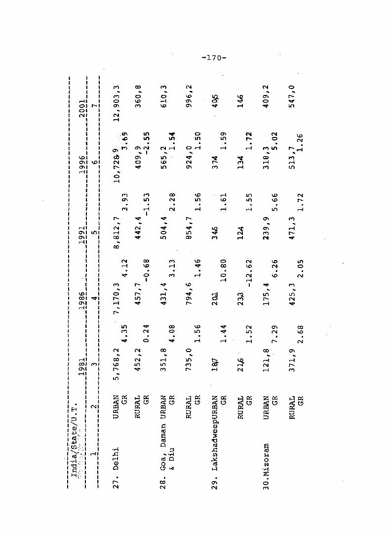
1 I 1 I I

.-II 01 r-01 NI

I I I I I I I I

\01 0'\1\0 0'\1 r-I

.-I 0'\1 0'\1 .-II

I I I I I 1 ,

, 1 I I

\01 COl 0'\1 .-II

I I 1 I I I I I I I

.-41 COl 0'\1 .-II

1 1 I 1 I I

E-I I • I

::> 1 .......... 1 (l), I +J ' I nf' I +I. I tf.l .', ' I .......... ~-. I (Ij " J

·M . ' J '0'; I s:: " . I H""I

I I

L{) I 1 I I I I I I I 1 I J I I

.qt, I , I I I I I I I I I I I

MI I I I I I I I I

NI I I I I I I I I I

,.....jl , I I I I I I

M ... M o 0'\ ... N .-I

r-­

N r-I CO

CO

M

o r-­,.....j

r--

N ... CO 1.0 r--L{)

• ..-1 ..c: .-I (l) Q

r-­N

M 0'\

M

L{)

M

... o 1.0 M

0\ N ... I

0\ o ~

..

M L{)

.-I I

CO \0

o I

oq< N

o

M

o .-I \0

... L{)

1.0 L{)

...

CO ...

CO N

CO N

N

CO o

N

\0 0\ 0'\

o LIl

o r-I

.qt N 0'\

..

o ..

\0 L{)

r-I

1.0 LIl

r-I

-170-

o CO

o .-I

L{) L{)

r-I

N \0

N r-I I

N ..

N o

M LIl ... CO .-I M

0'\ M N

CO .. r-I N .-I

o M

\0 N

\0

0'\ N

r-

..

..

0'\

r-I r-­M

L{)

o N

CO 1.0

N

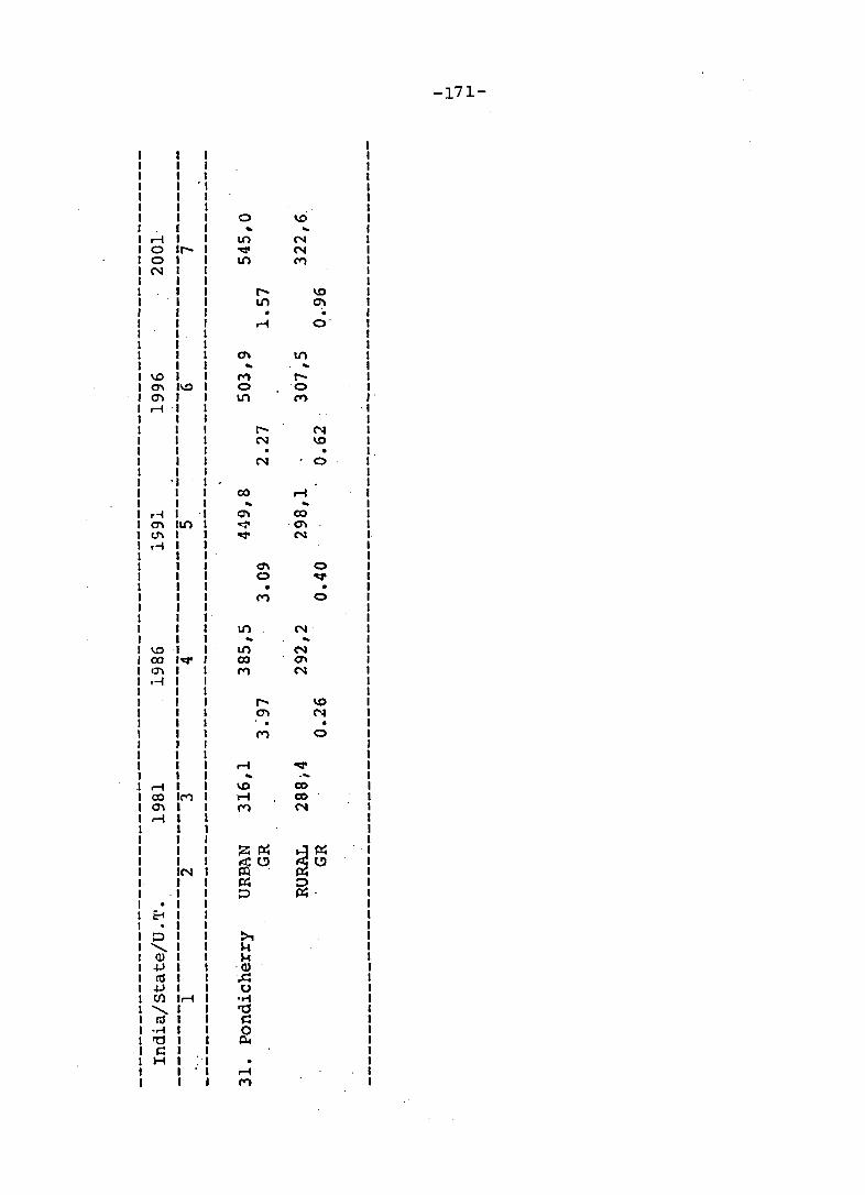
-171-

I I I I I I I ., I 1 I I I 0 \0 I .. ..

r-i I Li"I N 0 It- 00:1' N 0 I Li"I ('I'l

N 1 I I t- \0 I tn ~ I • . I r-i O· 1 I 1 0\ tn I .. ..

\.0 I ('I'l [' 0'1 1\0 0 0 0'1 I tn ('I'l , r-I ·1 ·1

1 I I t- N I I N \0 I I I. I N 0 I

"I I CO .....c 1 .. ..

.-1 I 0'1 CO 0\ ILi"I .,-:0 . 0'1 ~ 00:1' N r-i

0'1 0 0 oc:r • •

('I'l 0

Li"I N .. .. \0 Li"I N CO 00:1' CO 0'1 '1'\ I M N ,~ I

I I [' \0 I 0'1 N I .. I M 0 , I 1 .....c oc:r I .. ....

.....c I ID CO CO 1M r-t CO 0'1 I ('I'l N r-i I

I 1 I I I I ZP::: ~~ I I ~t.:l ~t.:l IN I ~ . I I ~ ::>

·1 I D ~. . I 1 8 I 1 . I I ::> 1 I >t ......... I 1 H

Q) I H +l I Q) ~ 1 .c: +l I 0 CJ) 1...-1 .r-i

......... I ro rtI I s::

.r-! I 0 ro I Po. s:: I H I

I r-t I M

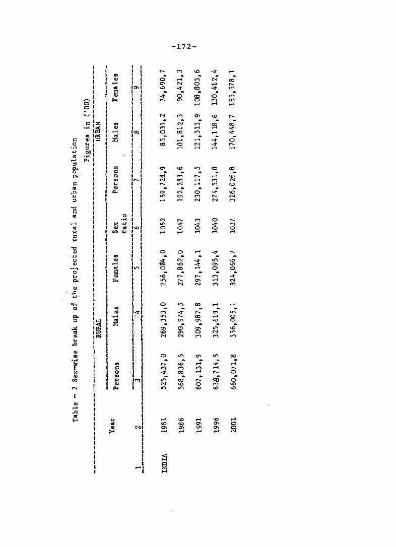
-172-

I I ...... C"i \0 -:t" ~

11) , .. .. OJ I 0 ~ C"i N co ~ ,

~ N 0 ~ ...... at I~ \0 "" co -:t" t.I"I

IiI I .. .. .. I "" 0 00 0 t.I"I

'"' ~ I ...... ~ 0 C"i t.I"I 0 I ~ ~ ~ 0 , , ......... t N C"i ~ \0 ...... .. .. .. s:: Z lit I ....-I N C"i co co ." :~ OJ I C"i ~ ~ ~ "" .... 100 0 00 C"i ~ "" ~ '~ ~ -s:: If) .... .... "" 0

0 ,.., 00 0 N "" r-...... :::l M r-I r-I .-I .u 00 t'Il ."

r-I "" :::l P- el) ~ \0 If) 0 00 0 s:: I .. .. .. P- o , . "11 C"i ...... .... \0

eI) ,..... N V'I r-I C"i N s:: ,.., ...... N .... ""' 0 at OJ .. .. .. .. .0 p.., ~ N 0 "" \0 ,_.

""' ~ C"i ,..... N :::l ~ ...-I N N C"i

""0 s:: at 0 ..... N ,..... C"i 0 ,.....

r-I >< .u ""' "" ~ "" C"i t'Il , OJ at \0 0 0 0 0 0 ,_. I til ,.., I ~ .... .... r-I .... :::l I I s.. I I

I I ""0 I I

olJ I I 0 0 .... "" ...... .u I .., I .. (J I OJ I "" N ~ t.I"I \0 C1.I I .... I I 00 \0 ~ ~ \0

-'""'l I at Ilf) I 0 00 .... 0 0 0 t ~ I I "' .. ,_. I , I -.0 ...... ...... C"i "" P- I ~ I , Ir'\ ,..... ~ .... ('J

I , I N N N C"i C"i <11, I , f ~ • I ) .u . I , , , f I

l4-I , I I 0 Ir'\ 00 .... ....

0 I eI) I f .. .. ~ Qj I~r C"i ""

,..... ~ ""' P- I ~ /: .1 ""' ,..... 00 ~ 0 ::l

~ I ~ I , M ~ ~ -.0 0 I I I ..

~ f I I ~ 0 ~ If) \0 t'Il l~ I I -.0 ~ 0 N C"i OJ I I I N N M C"i C"i ,_. I I I

,Cl , , I I I I I I

<11 I I I .., I I I I 0 I.f) ~ ""' 00 ...... I I .. .. .. r , II) I , ,..... \C) .... -:t" ....

I I s:: I I C"i C"i C"") .... ,..... >< I I 0 i "" 00 .... ,..... 0 OJ I II) I .. ..

en I ,..,. I C"i I LI"I 00 ,..... <:u 0

I , Qj f , N \0 0 C"i -.0

N I p.., I I IJ") ""' \C) \C) -.0 I I

I CI) I .... I

,.c I at I

£-< ,_. I rl \0 ~ \0 ,.....I

cd. I co co ~ ~ 0 CI) N ~ ~ ~ ~ 0

>-' M ~ ,.....I rl N

~ @ H

tJ)

j

rJ)

i ~

MOM'<:;J'CO ... .. -.. .... .... \.Or-en'<:;J'CO r-lJ"IenU"lU"l OMr-Men .. ... .... .. .... \.0 r-CO Or-l

r-lr-l

M co co U"l \.0 .... ~ .... .. ... r-l 0'\ M N 0'\ r-l \.0 0 U"l U"l '<:;J'1.Or-lI.ON ......... \.Or-O'\ON

r-lr-l

\.OCOr-len'<:;J' ... ... .. ~ .. r- \.0 M 1.0 CO CONOOr-l '<:;J'~O 0'\ 0 N

... ... .. ... .... N U"l r- r-l '<:;J' r-l r-l r-l N N

U"lOOOCO II-. ..........

'<:;J'MN\.OO'\ \.OMNOI.O MCO r-lr-l \0

lilt ... .... .... ...

Or-lM'<:;J'~ NN NNN

1.0 \0 co r- r-... .. ... ... ... r-enenN"<r 0'\ 0'\ CO OM \.0 0'\ r-l r-l 1.0

.... ... .... .... ... Or-lM'<:;J''<:;J' NNC"iINN

r-lI.OCOr-1/) ... .... .... .... ... NNr-lCO~ \OMr-lOO OCOMNM

..... ... ... .... ....

r-lM 1.0 CO 0'\ q<'<:;J''<:;J'"<:I'"<:I'

..s:: tJ) Q)

~ rU

~

~ . .-I

-173-

"<:I'ooN"<:I'",-.... .... ... ... ... 0'\0'<;1'1.0.-1 00 0'\ N CO Li"I OOOMI/)OO ... ... ... ...

r-lr-lr-l.-l

00 CO I/) r- \.0 ... .... .. .. ...

t-MN"<:I'Li"I Li"lCO"<:l'MN .-IMl..OenN ................. r-lr-lr-lr-lN

N\Or-r-lr-l ... ... ... ... ...

r-"<:I'I.Or-lr­qtr-I..ONr­o <:S'0'\Li"l0 ... ............ NNNM"<f'

OMenr-lr-l ... ... ... .. .... o Mr-IMI..O "<:I'1..Ot-MCO Li"lI/)I..OCOoo

... ... ... ... ... COO'\Or-lN

...-1...-1.-1

t-NMCO"<f' .... ..... .... ... .... 0'I0'\r-r-0 "<f'Li"I"<:I'I/)"<f' COCOOM<:S' ................ r-O'\N"<:I' 1..0 .-I...-INNN

m ~ . N

O..;l'OCOI..O ... ... -.. ... .... enM CO "<:I' en Ii") r- <XHt'l 0 en 0'1 N 0'1 0

... ... .... .... ... M"<f'I..Or-O

...-I

OqtNI/)N ... .... ... .... ...

Or-MOr-1..0 I/) "<:I' r- M r-CONO'\O ... ... - ....... '<:S'1/)t-CO::l

OCONMCO -. ... ... ... ... 0'\0.-11/)\.0 ...-IMMN"<:I' r-CO I/) 0'1 0

.... ... ... .... ... CO OM \.0...-1

.-I...-I...-IN

N I" co r-l Li"I .. ... ... ilia ..

Li"I'<:;J'O\Ot­N...-I\OI"Li"I OO'\ONN ............... ON\OO'IN MMMM"<r

1.000 N 0'\0 ... ... ... ... ...

o I/) O"<r U"l r-Oco\O\O . ...-1 0 0'1 0'\ U"l ... ... .... ... ... ...-I..;I'I..OO'IN MMMM"<f'

co I/) 0 0 U"l ... .... ... ... ... If'l 0·...-1 .-I N O'IN..;I'q<N r-lenONCO

... ... ... ... ....

.-I \.0 MO'\..;I' \O~r-r-co

~ ~

M

U)O'It-NM ... ... ... .. " en \0 co 0'1 """ M 0'\ co \0 .-I OOOt--I..O\o ................ L!')LflI..Or-CO

O'\=",ONM .............. L!')\.Or-lMCO

~~~~~ ... ...... -.. ... L!')\.Or-coO'\

t--r-lr-'<:;J'\.D .... ... ... ... III.

r-lMO'\NN OHlr-lOO I..OMr-tO'lCO

... ... ..... ... ... ON '<:S' If'll'' r-lr-lr-lr-l.-t

MOOI/)NOO qtMNNr-t 00000 r-lr-tr-tr-tr-l

'<:S'Nr-t"<rLfl ... ... .... .... ....

1".-I..:rL!')r­O'\OOr-r-tM '<:3'''''''NooN

... ....... ilia

.-INMM"<r r-l r-l r-t r-t .-t

t--O.-tlf'l\O ... ... ... ... ....

\.0 0 """ """ 0 OO~Or-tO\ 0'\ CI) \0 r-t ~

... ... ... .. ... r-lNM..;I''<:3' r-lr-tr-t.-tr-l

r-l N N 0'1 .-t .. ... ... ... ... '<:S'r-lOOO'\oo oor-t--NN '<:3'Moomr-

... ... ... ... ... ML!')\.Or-OO NNNNN

-M ~ on

S . '<;I'

"<:I'r-lMNoo ... ... ... .... .... 00 Lfl '<:S' 0 L!') en t- N \.D 0'1 N\.Dr-l\ON -. ... .... ... ... r-lr-lNNM

o If'l \.0 co N .... ... ... ... ...

en 0'\ r-t L!') 1'0 N'<:S'Lfllf'lr­If'lO'\'<;I'Or-.. ... ... ... ... r-t.-lNMM

"<:I'\.DO'IOO .... ... ... ... .. r-'<:S'lf'l\.OO'I NNr-.-I\.O 00\.0 \0 r-O .. --. ... .... ... NM '<;I' I/)t-

1'1"10'<:3'"",,0 .... .. ... ... ... ~OOON .-Ilf'looO'\t-­I'NLt'l\oLt'l

... ... .. """U"lLt'lLt'lLt'l

O'\t--NLflN ... .... .... .... ... OM 1..0 OL!') (X) '<:S' co 0 \.0 MO'\N'<:3'N .... ... ... ... ... Lt'llJ"ll..O\.D1..O

Nr-l..OenN .... ... ... .... .... Lt'l 1'1"11..0 Ot-0'\ 0'11..0 O'IM 0-.-100000.

"'" .... ... .. ..... Or-l.-lNr-l .-I.-I,.....j.-l.-l

rU

! . If'l

Ul Q)

-~-~ ~~ .& -.-I

M~

co

N

r-I

'<:I'O.q..q<LI'\ ... .... " .... ...

O'\"Id'OOO'l.::t' U"\ CD 0'1 " r-1 rlNU"\Or--- .~ ........ -U"\I.O-r--O'\O

r-I

N.::t'L()O'II.O ... ... .... .... ... 01.01..01.OU"\ r--:"")ooooo L()r--O\oN

... .. L() 1..0 00 0'1 r-I

r-I

'J:>"<t'O'IM..-4 ... ... " ... .... 0'1 a-. ~ 1..0 0 N r-i 00 00-0 r--o\O\Oo .. .... ... .... .. O<""lL()ooN rlr-l..-lr-lN

r-IO.::t'Nqt ... " ... ... ...

\ON 0 0'1\0 O.-ll..Ol.t)qt "'<""I\ONO ... .. ..... "'"' ... 1..0000'100 NNN<""IM

I . \D

-174-

0'1 1..Or-i Or-i ... .... ... .. ...

000r--1.O r-1~<""IOOM "<t'OOMOO\(\ ............ -. ... NNMMq<

rt')"<t'r--I..O.::t' ... ... ... -- ._.

.-I 011'1 M"<t'

f:: ~~ ~ ~ ... ... .... .. ~

'<:I' L() 1..0 r-- co

0..-1['0..-1:""'1 ..,. .. ... .... ... U"\ONOO ..-I C> L() \(\ N \(\MO'I~CO .... ... -. ... ... O..-lr-iNN ....-I,..-jr-l..-l ......

~O'IO'IC>M ... ~ ... .... .. r--OONqt 1.0<""11.0 ..... 0 ..-IO'II.()Oo:to .. ... '" ... .. OO ...... NN ...... .-I ...... ..-I .-f

"Id'01..O..-I1.O -... ... ... ... , N.-IMNqt co <""I"'" 0'1 N I.ON1I'\~N

.... .... .... ... ... ON M"<t' I.Il NC'4NNN

ItS

~ & l""-

~ 0\ 00 00 .-1 ................. \0 r-I NOr-­OOI..O"Id'C'I.-f In.-fl''')r-II.()

.... .... .. ... ... 01"')1..00"<t' r-I-I..-4NN

.-1..-1U'l~<""I .. .. ... ... .. 1..0 r-- 1.0 \0 r-­NI..OI.OU"IN rt')O'IC""lMI..O

.... ... ... .... ... o ....... 1"') ~ qo NNNNN

<""ICO"ld'..-I~ -.. ... .. .. ... 1.0 r- r- r- \0 1.01.01.011'\"0:1' N01l'\\DO\ .. ... ... .. .. ..... <""I.'dO L() In NNNNN

1 &::

j 00

pooooo .. .. .. .. ....

(",)0'10'1..-400 \oONooN NCO-l:o:J' ..... .. , .......... Or-lN<""I'dO NNNNN

i I . 0\

OOQI\OCOr--O .... .. ... .... ....

MO'I"Id'<""I..-4 .... OOQIU'l ..... N I.O .... I"'-I.OOOQI ~ ........... ....

.... NNM'I$'

MN\.()(''dO .. ... .. ... .. O<""lr-l<""ll..O .-I N 0\ \0 M .-10-1\0 ..... .. ... '- .... .... M"Id'IJ')\Doo

Or-O.-lO .. ... ... .... ....

Or-MNL() \O("')IJ')Ln\O NCON<""Ia> ... .. .. .. .. M.., \D r- r-­NNNNN

I -ri

~ . 0 .....

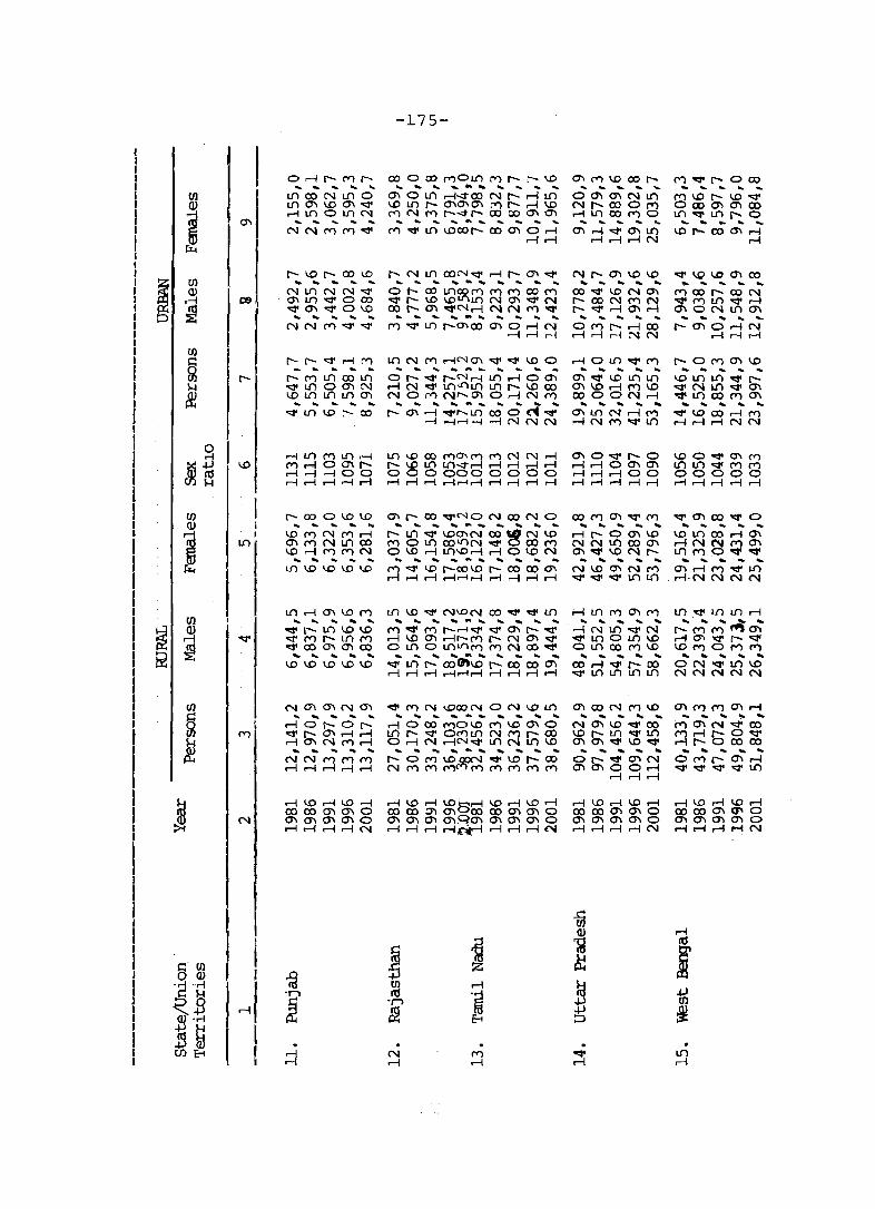
s:: til o Q) -r-! .. r-!

~B 1!-r-!

~~

09,

, ,

L()

N

r-I

Orll"-MI"-.... ~" .... "

I.{') 00 NL!"l 0 I.{')m\OO'\"" r-IL()OI.{')N

... ... .... ... .... NNMM""

r-\.Dr-COID ................. NL()NN-.::I' 0'\ L() "d' 0 CO "dOO'\qtO\.O

...... .... .. ... ... NNM-.::I'''<J'

r-l"-qtr-lM ... ... ... , ... r-ML()COll"l qtL()OO'\N 1.OL()L()Ll)0'I

r- CO 0 \.0 \.D .... ... ... ... ...

I.DMNM..-I O'IMNL()CO I.Or-I("t)MN ... .... ... ... ... I.{') 1.0 1.0 1.0 1.0

I.{') ..-I m 1.0 M .. .... .... ... .. "<t'r-L()\.O\O "<t' ("t) r- Ll) M "d' 00 0'\ 0'1 CO

... ... .... ... .. \.0 1.0 \.0 \.0 1.0

NO'IO'\NO'I .... .... ... .. ....

..-lOr-Or­qt['-O'I..-I..-I r-IO'\NM..-I " ... ... "" ....

NNMMM ..-I..-Ir-I....-f..-l

~ -rl

& r-I r-I

-175-

co 0 co MOl.{') M I"- 1"- \0 ................................ 0'\ 0 I.{') ....-f~ 00 N I"- ....-f L!"l \0 If') r- 0'\'" 0'\ !'"") I"- r-I \0 M N M I"-~I"- 00 00 0'1 0'1 .... -.. ....................... .... M -:I' I.{') \.D001"- 00 0'1 0 r-I

..-I r-I

r- N I.{') CON "'" rl I"- 0'\ "" .... .... .... .......... ... ... ._ .... o 1'- CO L()OO M M M CO M "" I"- \0 \0 11"11..(') N 0'1 "" N 00 r- 0'\ ..,.Nr-I N N M "'" .............. -................... M ..,. I..(') r-O'\oo 0'\ 0 r-I N

...-lrlr-l

I.{') N M .-I':'J m ..,. "" \0 0 ................................ Or-"" r-N rl L() ..-I 0 0'1 ..-I N "'" L() <t) L() L() r- \0 CO NOM Nr--.O'\ 0 r-I N M r: r;; rl ";r--al.{')~ ~ 0 <i ..;

-! r-I,-I--j r-I N N N

0'1 r- CO ..,.NO N CO N 0 .............. -............... I"- L!"l "" \00'\ N CO ttl N 1.0 MOl..(') 001l"lN "" C CO M o \0 r-I L()\,O r-I r-I 0 1.0 N .... .... .... .... ...... -. .... ... ... M "" \,0 1"-00 I.D r- CO CO 0'1 ....-f ....-f ..-I ..-1,-1 r-I r-I ..-I ..-I ..-I

L() 1.0 "'" N \.ON CO ..,. "'" I.[) ... ........................... ... M "" M r-.-l -:I' "'" 0'1 I"- "" ..-I \0 0'1 rl r-- M r- N 0'1 -:I' o I..(') 0 1.[)1I"IM M NCO"" ... ... ... ........ ... .... .. ... "" I.[) I"- 00 (J\\O r- CO CO m r-I rl ..-I ..-I.-l r-I r-I ....-f ..-I r-I

"" M N \.DCO NON \.D I.[) .. .. .... ... ...... .. ... ... .... r-I 0 CO MO ID M \.D 0'1 0 Ll) r- "'" OMI.{') N M r- CO o ..-I N ..-I N "" L() N Ll) \0 ....................... -. .. r- 0 M \.D OON "d' \0 I"- CO N M ("I') MM("I') M M M M

~ ~ Z

til r-I ItS .~ .~

8! 8

N M rl ..-I

mM\oCOI"-... ............ 00'1 m NLl) NI'OOOM r-IL() CO MO .. .... .... .... ..... 0'\ r-I"d' O'ILl)

r-Ir-I..-IN

N['-O'I\OI.O ~ ... ... .... ...

00 "d' \0 N 0'1 I"-OONMN l"-"dOr-Im..-l .... ... ... .... .... OMl"-rlCO r-Ir-Ir-INN

r-I 01..(') "d'M .... ... .... --. ... O'I"d'IDL()Ll) O'\\Or-IM\O OOOON..-I

... .. ... .... ~

O'II..(')NrlM ,......jNM"d'1.[)

COMO'\"d'M ... ... .... ... ...

r-I I"- 0 0'1 \.D NNI..(')OOm m"d'\oNr-

... , ............ N\OO'INM "d' "d' qt L() L()

..-ILl)MmM ... ... ... ... ....

-INL()"d'N "d'I..(')OI.[)\O OL() 00 MI.O ... ... ... ... ... COr-l"dOr-OO "d'l.{')lI"lL()L()

0'1 CO N M 1.0 .... .. ... ... ... NO'II.O'<t'CO \.Or-Ll)'<t'Ll) 0'I0'\"d01.O"d'

... ... ... .... ... Or-"d'O'IN 0'10'\00..-1

....-f..-l....-f

iii Q)

~ & td :e ::;;.

"<J' ..-I

M'OIi:I'r-OOO ................. MI.Or-I.O"d' 0000'10'\00 L()'<:S'lI"lr-O .... ....... -.. ... 1.0 ""' CO 0'\ r-I

..-I

"dO IQI..O 0'1 CO ~ ... .... .... ....

MCOr-OON "<t'MLl)'<:S'..-I O'\ONI.{')O'\

... ... , .... ... r-O'IOr-lN

....-f r-I .--f

r-OM 0'\ 1.0 ... ... ... ... ...

1.01..(')Ll)"d'1"­'<:S'NLl)'<:S' 0'\ "<t'L()COMO'\ ... .... ..... ... ....

"d'I.OCOr-lM ..-I ..-I r-I N N

'<:S' 0'1 CO qt 0 ... ... ... ... ... I.OL()OOr-lO'\ .-INNM'" L()MO"d''<t' ... ............. 0'\ r-I M "d' L()

. ....-f·N N N N

Ll)"d'Ll)l..(')r-I

~~~~m ...... 0'1""'r-"<J' I.O(""')OMM ... ... ... ... .. ONqtL()1.O NNNNN

O'IMMO'Ir-i ... ... .. ,.. ....

MO'\N"d' 00 ("I')....-fr-O"<J' ..-I 1"-0 00 CO

... ... -. -. ... O(""')r-O'\r-I "d'''dO''d'''dOLl)

r-I ItS

m "'-' til j

L() ..-I

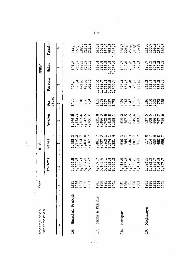
N

-176-

("W')("W')Lfl""'CT'I ............ ~ .... '<:I'CXlNI'""-...-l '<:I'\OO"Ir-I .... ...-lr-lr-iNN

\or-Ir-INrl .................... ..-I Lfl 0"1 1""1\0 CXl ON Lfll'""­..-INN"fN

CT'I '<:I' \0 \0 0 ... .... .... .... .... LflM..-IOOO NI'""-NI'""-r-I 1""1 1""1"" '<:I' Lfl

\QM\OLflO .... .... .. .. ...

\0 .... 1-1-1.0 1.01'""-1.0'<:1'0 CT'I..-lMLflI'""-

... .... ... .... , ..-lNNNN

MNI-Ol-... ... ... .... .....

00 Lfl'<:!'ON 00 Lfl.-l 1.0 00 CT'I..-lMoqoLfl

... -. ... .... --. .-INNNN

I!IbLflMIJ"lI'""­" .............. """CT'INI'""-CXl I..{') N 00 0 00 0"1 1""1 1.0 ON

lit .... ... ... ....

("W') "<3' '<:!' I..{') I..{')

. 1.0 .-I

\OCT'ICT'I("W')N ..................... l{")NI..{')MM 0001""100'<:1' lJ"I 1-00 CT'Ir-I ...

r-I

CT'I 1.0 1.0 01..{') I.OCT'IMCT'I1fl \0 I'""- CT'I 0 N .....

ri ri

OI'""-"<3'OO..-l ................. l{")O"INMCT'I lJ"ICT'Il'""-l'""-CT'I N .... r-OM , .._ .......... ..-l...-l...-lNN

01""10001""1 ... ... .... ... ....

l{")I.ONCT'IOO NI.OOriO N"""r-CT'I...-l ... ... ... ... ... NNNNM

I'""-Mr-iriCT'l ._ '" ... .... .... r-i('.JM'<t'ri 00 1""11.0 I'""-Ifl '<:I' I'""- 0"1 ..-l .1""1 ... " .......... NNNMM

1'""-\.0 r-I CT'IN , .... .... ... .... 1'""-00 IJ"l ("W')O o CT'I \.0 0"1 \0 I'""- r-I \.0 0 '<:I' ... ...... ... ..... ... qtlJ"llfl\.O\O

r-CT'IOOOOOO .... ................. '<t'''''''\.OOr­OON\.O..-ll{") r-iNNMM

r-OOO"<3'M .... .. ... .... .... ON 01'""-00 0"1 MOON r­r-iNNMM

'<3'I'""-OON..-l ... -... ... ... ... Ifl 1-\.000 \0 I'""-lf}qtMM M"""I..{')\Or-

NIf}If}'<t'r-.................. Ifll-r-ICT'IM r-I 1.0 r-I .... 00 Lf) If} 1.0 1.0 1.0

MI-MI-N ... ... ... ... ... OIf}ON..-l 1""1 ooqt OON 1fl1..{')1.01.O[,

IJ"lNOOriO'l .... ... ... ... ...

If} ("W')r-IN .... -.:If If} I..{') M 0 O..-lNM'<:I' ... ... .. .... ....

..-Ir-Ir-Ir-Ir-I

00 .-I

I.OI'""-MOI.D .... ..... .... .... .... ..,.00"11.00"1 ..-llJ"lO"lI.Ot.n r-Ir-I..-lNM

r-NNOOM .................. \.Or-II'""-O"I\.O NI.OOI.OIfl r-Ir-INNM

MCT'ILf)OO 0"1 ... ... .... ... -..

..-lr-ll.OLf)1J"l

..,.riQMr-I NM'<:I'Lf)1'""-

1.00lflMOO MriOI-Lf) 0000'1 0"1 r-I r-I r-I .

Lf)lflrir-O ... ............ r-oo 1.0 ['0"1 MOI.OOr-i Ifl 1.0 1.0 r- I'""-

0['\0001-.... .... .... .. ..

[' .... 0'10000 Ifl r-I Ifl 00 eEl Ifl 1.0 1.0 1.0 1.0

IflN ['LO I-"" ... .. ... .... '<:I' M Ifl 1.0 I'""­CT'I N N 0'1 0 ONMM"'II' " .... .... .... ... r-I ri .-{ .-{ r-i

. 0"1 .-I

s:: til

.~ .~ s:: H

.t2..B _a-,-i rl

~~

N~"'d'COCO " ... ..... .... ..... ~ ("I') L() 1..0 \0 ;-O"'d'~l!)

...-l r-I r-I N

N...-l...-lN~ ... ._ ,... ... "lit

o 01'-("1') L() N co l!) L() 1.0 r-Ir-IN("I')'<::f'

01'-\0("1')\0 ,.. .... ... ... ... o l!)r-ICO ("I') r-I\.ONf'-.("I') ("I')("I')"'d''<::f'1..()

1'-~"'d'~0 .. .... .... ..... .... "'" r-I CO L() N "<:tOl!)r-Il'­("I')'<::f''<::f'L()L()

1'-\0 ON 1.0 .... .. ... .. .... '<::f'I'-O"'d' I..() I..()\OCO~O I.OI'-CO~r-I ..

r-I

] ..--I m

i 0 N

-177-

Ol'-r-l("l')"'d' .... ... .... .... .... ...-lr-ll..()...-lO\ N("I')'<1'1.01'-

r-I I'- 1.0 CO 0 " " ... .... -.

0("1')00("1') ~"'d'I.OCOO

r-I

...-l'<::f'I'-...-lo::t' ... .... .... ... ....

...-lL()l!)NN L'1 I'- 0 o::t' 00

r-Ir-Ir-I

0("1') I..() \01'-.... .... .... .. , ("I')rlO\l.O~ No::t'l..()l'-OO r-Ir-Ir-lr-lr-l

("I')r-O\\OO"I .. .... .... .... .... N (""')'<1' o::t'O\ ""'1.0 00 Or-l r-Irlr-lNN

("",)O'<1'NI.O .... .... .... .. .. L() L() '<1' .-i 0\ 1.0 0 .q< 00 0 N (""') ("I") M"<:S'

.~.

~ U)

....-I N

NOl!)"<1'l!) .... .... .... .... ....

I..()"<I"Nr-IO r-IMl!)I'-C1\ r-lr-lr-l...-lr-l

1.0"<1"0001..() .... ... ... .. .... I..()NOOI.O("I") NI.OO"I("I")I'­NNN("I")("1")

00 1.0 1.0 "'d' .q< I..() L{) L{) L() I..() 00000 r-lr-l...-l...-lr-l

oo'<t'OOrlO ... .... ... ... ...

1'-(""')0"1(""')0 00 0 Orlt-{ ooOrlN("",) .... .... .... ...

r-Irlrlr-l

l.Oo....rOOr-l .. ... .... ... ... 0\ 0 t-{oo 0 (""')1.01'-1'-00 O"IOr-lN(""')

.... III. .... ....

rlrlrlr-l

.q<"<:t'N~.-I ..... ... ... ... ...

l'-("",)rlrlO N \0 00 ~ 0'> ooON...r1.O

.... ... .... .... ....

..--INNNN

e a. .,-i tl

N N

OONL()Ml!) ... .............. OONO\oo NM"<t'L{)1'-

~\OI'-OM ..................... 00 I'- 00 N 00 NM.qtI.Or-

I'-CONMoo .... .............. cnl'-..--Irl\O '<t'I.OO"INL{)

rl....-l

I'-ooc-OM ... .. .._ ... .... Ooof'-.OON I.Or--O'>....-IM

....-1....-1

-.::rMOl!) \0 ... .............. 00 N 1.0 I'- \0 I'-~O....-lN

r-I....-Ir-I

....-11..0..--11.0....-1 oooommo 0\ 0'\ 0'\ '" 0 rlrl..--lr-lN

til

N tn H

Z ~

~

M N

l{)

N

Or-O'<::l'N .... .... ... .... ... I..OMMMl{) r-INM'<::I'l{)

'<::I'---jO"lMr-I .... .... .... .... ...

r-Ioor-Ol{) '<::I'1.{')r-ON

r--ir--i

I.{')NI..ONM ... .... " ... ...

l..Or-oo\oN r-r-II.{')O"IM NMMM'<::I'

O"INM\oN -.. .... .... .... ... MNOr-r-I r-Il{)O'IN\o MMM'<::I''<::I'

"<2''<::1'0''1001.{') ..... .... ... .... ...

OO"looMM O"I1..O"<2'NO"I l{) 1..0 r- CO CO

. "<2' N

-178-

1..O"<2'''<2'lnr-- -.. .... .... ... "<2'001.{')1..0 ool.{')MNM r-INM"<2'L()

N M O'''D r-I ... ... .... .... ...

000"1 l{) 001..0 MOO"lO"lr-l N M ('Y) '<::1'1..0

00 r- M .--j co lilt. .... .... ... ....

NO"I"''<::I'N Nl{)NNI.{') "<2'r..nr-O"Ir-I ..

r-I

r-O"Ir-MI..O ................... r-IN M'<::I' "<2' r-Ir-Ir-Ir-Ir-I

r-1O"1r..ncx>r-.... .. ,.._ .... .... r-r-oocx>CO rlr-lr-lr-lr-l

oXIOONr-IM .... ... .... ... ... OOONMM NMMMM

O"IO"\O"Ir-M .... ... ... ... .. \0 r-000"l 0

r-I

0"1 l{)OOr-l 0"1 .... ... ... ... .... r-MO"IMI..O "<2' r..n I.{') 1..0 1..0

0"1 1..0 r-M 1..0 .... ... ... - ....

OOl..OqtNr­qtL()I..Or-r-

OOr-lN'<::I'1.{') .._ ... .... ..... ,

1..00qtl.{')qt O"Ir-INMqt

r-Ir-Ir-Ir-I

0"100"1 L() 0 ... .... .... ... ... r-NCOO:"'"l r- M CO r- r­L()N 0"1 cx>00

.... .... .... ~ " NMC")'llfr..n

MC"')oo"<2'M ... ................ OOOMOOO O"IMNL()M r-I 0"1 CO 00 0 .................. MMqtl.{')r-

('., M r- 0"1 M

U;ON~M 1..Dr-r--iNO l"'o'r-IGaI"-O"I .... .... ... .... ... IIll"-000:".l

r-Ir-I

oor--iO"l(eqt ....... -.. ...... O"Ir-Ir-IMI..O "",l{)'<:J'NO"I NNNN-I

Nr-"<2'O"Ioo ... ... .... ... ... Nr-NO"IO L()L()qtOI..O qt"",'<;I'qtM

.. l"­N

00

fJl

§ fJl

~

N

"<f'ONO'\1"-.... ..... .. ... ... OOOO"<f'('I")lll I.OO"<f'r-O'\ r-lNNNN

o::I'o::I'N('I")1.O ... ..... .... .... ...

(V')(V')0r-l"<f' 00 N 1.0 0'1 r-l r-lNNN('I")

CO"""o::I'N(V') ... ..... ... ... ....

r-lr-lo::l'1ll0 lll('l")OI.Or-i (V')"<f'1llL(')1.O

0'I000'\0l.[) ... .. .... " .... 0'10.-1('('1") 1.00('1")1.00 (V') "<f' "<f' "<f' I..(')

r-i 00 CO Or-... .... .... .... ....

L(')(V')Nr-N \OO'INI..(')O'I (V') (V') "<f' "<f' "<f'

O\Or--ON ... , ..... ~ .... I..(') "<f'''<f'''<f'1.O (V')O"II..(')NO'I r-- r-- 00 0'1 0'1

. 00 N

-179-

NCOO'l(V')oo .... .... ... ... ....

0'10'1\0000'1 r-fr-fr-f

I..(') M\O r-ir--.... .... .... ... ...

0'I0r--0'I0 r-ir-ir-lN

r--r-II..(')"""I..(') ... .... ... ... .... COO'<:t'r--O r-iN(V')('I")'<:t'

0'10'1000 r-i0000 00000 r-ir-ir-lr-lr-i

r-- "" N r-- M ... ... .. .... .... o ,-HD "" (' r-l r-i

O'Ir-Nr-M .... ... ... .... ..... Or-l \0 \Or-­r-ir-i

\0 (V')"<f' "<f'\o .... ... ... .... ...

r-iMNM'<:t' NNr-ir-ir-l

0'1 N

M '<:t' (V') "" r-... ... ... ... ... '<:t'N\Or--1..(') \OO'IN\or-i

r-ir-iN

CO'<:t'O'IMN .................. r-i I..(') 0'1 00 0'1 Nr--(V')r-iO r-ir-lN(V')"<f'

00 0'1 (V') r-- N r--r--OO 00 0'1 00000 r-ir-ir-ir-lr-i

O\O(V')NI..(') ... .... .... ... ... O'I"<f'lDlDr-I r--ON"<f'\O r-iNNNN

0'1 r--O I..(') I..(') ... ... " ... .. NOI..(')r--1..(') O'IN"<f'\oOO r-iNNNN

0'I(V')(V')r--0 ... ... ... ... ... r-Il..(')r-iMr-­r--Nr--r-i"<f' M"<f'''<f''''1..(')

r-i \0 r-i \0 r-i 00000'10'10 0'10'10'10'10 r-Ir-fr-ir-iN

. o M

"'3'NOO\O ................. r--NI..(')NN LOO'INI.[)r­rlr-lNNN

r--MOOO'l'<:t' .... ............ OOM"<f'r-IN 1.{)000NLOr-­rlr-lNNN

rl 1.(')00 0'1 0 .... ... .... .... ...

\OI.(')O'IMLO rlOO"<f'O"<f' ("t)(V')oo:t'LOLO

O'II..(')O'I\oN -.. .... .... .... ... I.{)t-O'Ioo:t'N "<f'''<f'''<f'L(') \0 rlr-lr-lr-ir-i

oq.Nr-lL(') \0 ... ....... , .. ooNOOr--N 00 d'\ 0'1 a N NNN(V')(V')

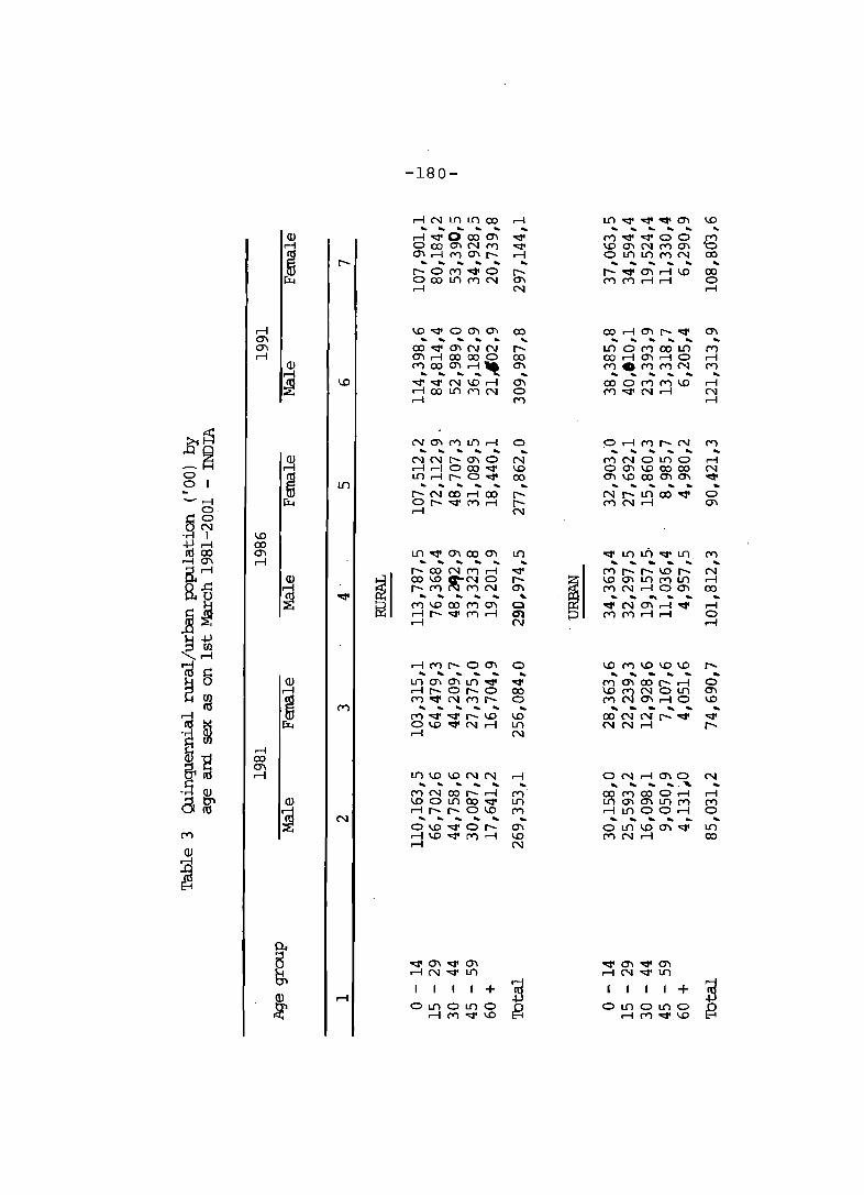
-180-

.--INLf)Lf'lCO .--I Lf'l qt ...,. qo 0'1 1.0

~~ocO~ .. .. ... .. .. ..

Q) '<:f' M'<:f''<:f'OO ~ .-t OCOCTINM '<:f' 1.0 0'1 N M 0'1

~ O'I.--IMO'II"' .--I o Lf'lLf'lMN co .. -.. ........... .. .............. .. ... 1"'0MqoO I"' I"'qoO'l.--l1.O co OCOLf)MN 0'1 MM.--Irl 0 .--I N .--I

.--I 1.0 '<:f' 0 0'1 0'1 co co .--I 0'1 ['. qt 0'1 0'1 .. .. .. .. .. .. .. .. .. .. ... 0'1 COo::rO'lNN I"' I..{') OM COl..{') M .--I 0'1.--100000 co co.--l O'I.-t 0 rl

Q) MCOO'l.--l"t 0'1 M.MMN M .-t -.. .... .... .. .. .. ... .. .. .. .. ~ '<:f'...,.NI.O.--I 0'1 COOMMI.O .--I

.--ICOLf)MN 0 MqtNrl N

.--I M .--I

£~ N 0'1 M I..{') .--I 0 O.--lMI"'N M

-~ .. .. .. ... .. .. .. .. .. .. ..

~ NN['.0"I0 N MNOUIO .-t .--I .-1 0 00 qt 1.0 00'1 1.0 00 CO N

0

~ 11").--11"'0...,. co 0'1 1.0 00 0'1 0'1 qo

0 I.[) .. .. ... .. .. .. .. .. .. .. .. .. ['.N COrl CO r--- Nr---Lf'lCO'<:f' 0

- .-t ~ OI"''<:f'M.-t r--- MNrl 0'1 O· .--I N

§ 0 N

"r! I 1.0 .j.J .-I co

Lf'lu) lOCO 0'1 Lf'lqoCTICOO'l Lf'l '<:f' ...,. I.[) M .-I 0'1 .--I ... .. ... .. .. .. .. .. ... ... .. .. 8. rl

~I I"'CONC"'1.-1 qo Mr---I"'I.OI"' N

Q) CO 1.0 ~N 0 r---

i 1.0 0'1 Lf'l M Lf'l .--I au .--I r---M MN 0'1 MN.--IOO'l co

~ ...,. .. .. .. .. .. L .. .. ... .. ... ..

~~ M 1.0 00 M 0"1 Q ...,. N 0"1 r-l qt rl .-I['.'<:f'M.--I ~ MMr-lr-l 0 r-l N r-l

~~ cd r-lMr---OO'l 0 1.0 M 1.0 1.0 1.0 r---

§ .. .. .. .. .. .. ... ... ... ... ... ... a Q) I.[) 0'1 0'1 Ulqt '<:f' M 0'1 ex) I"' r-l 0

.--I .--II"'Or--O co I.OMNOI..{') 0'1 til

m M'<:f'NMI"' 0 MNO'Ir-lO 1.0

10 ... .. .. .. .. ... ... .. ... ... ... ... r-l M qt '<:f' r-- 1.0 1.0 OONNr---'<:f' "'" .~ m ~ OI.Oo::rN.--I Lf'l N N .--I r---

r-l N

~~ .-t co 0'1 r-l Lf'lI.OI.ONN r-l ON.--IO'IO N .s ... .. .. .. .. .. ... .. .. .. "- ..

Q) MNool"'r-l M CO Mex)Or-l r-l a g' Q) 1.0 0 I.[) co qo Lf'l I.[)O'IO'II.[)M M

~ .--I1"'r---OI.O C"'1 .-I I..{') 00r-l 0

N ... .. ... ... .. ... ... .. .. ... ... .. 01.O'<;f' 0 I"' 0'1 o I..{') 1.0 0"1 '<;f' UI

M .--I1.Oo::rM.-I 1.0 MNr-l ex) .--I N

Q)

~ 8

0..

B '<;f'0'Io::r0"l qo 0'1 o::r 0'1 §, r-lNqtLO .--IN '<;f' I.[)

I I + ~ I f f+ ~ ~ 0 I..{') o LO 0 g 0 I..{') o Lf'l 0 g .--I M ...,. 1.0 .--I M ...,. 1.0

-181-

rll"--rlrlr- r- N,..-!'<:!'r-I"-- rl , ... , , ... ... , , ... , Q) O"""O'ICO""" 1.0 1.0 N co If) IJ') co rl

""" \0 """ ;'V) r- \.0 r-IO'<:!'r-1"') I"--

~ .-1 OIJ')NNm 0 If) 0('"1')0"11"-- l() rl ... ... ... ... ...... .. ... .... ...

I"') 1.0 lfl N 1.0 "" I.Omr-lr-o IJ') 0 co 1.0 "" N :"l """"('"I')rlr-l l() rl I"') rl

r-I 0 0 N

rlOI"--OM rl ('"I')CONO""" r-.... .. .. ... .. ... ... ... ..... ... Q) I.Orlr-lCOCO l()

o "" 0 0'1 """ co r-I 0 Lf'lOrl""CO 0 l() 0"1 ('"I') C"") I"') '<:!'

~ r-I O'INNr-CO 0 I.O:"J('"I')OOM '<:!' ..., ................ .. ... .... ... ... .. ... mmr-r-Ir- 1.0 r-'<:!'OOO'IO 0 OOOI.O""N M ""L{')('"I')r-I.-i r-rl M rl

~, ~ NIJ')r-'<:!'1.O '<:!'

::> 1.O'<:!'r-l.Orl '<:!' ..... ... ... ... ... .. ... ... .. ...

Q) ('"I'),-jrlmm If) 1.00000000 N r-I 00'1""",,0 0'1 mr-('"I')Nr- r-I

m 1.O"""r-I..{)r- 0 O""'<;f'N..-! '<;f'

0'1 ... ... .... .... ... r- """ co co ('"I') ('"I') N...-I'<;f''''''' 00 0

~ 0 COIf)MN rl """'<:!'N..-! ('"I') rl ('"I') rl

1.0 0'1 0'1 r-I

rlN 0'1""" I.!"l rl co ('"I') 1.0 00 ..-! 1.0 ... .. .. .. ... , .. .. 1.0 lfl ='J r- r- 0"1 m"d'r-O'II"-- 00 0'1 00 00 ,"'f) r-I r-I 0"1""('"1')1"--0 r-I

Q) lflO'<:!'r-r- 1.0 ('"1')""1.000 r-I r-I cq .. .. ... ... ... .. ... .. .. .. .. ~ """

co 0"1 co '<;f' I..{) ('"1')1.0",,1.0 CO '<;f' r-I COIf)('"I')N N "" "d' ='J rl "" rl ('"I') rl

! "" 0'\<::1'0'1 """ 0'1 ""

0'1 ,--I N '<:!' I..{) <--l N "d' lfl

~ r-I , + , I I + ~ Q)

!l 0 IJ') 01..{)0 01..{) 0 L() 0 rl ('"I') """ 1.0 r-I('"I')o::I' 1.0

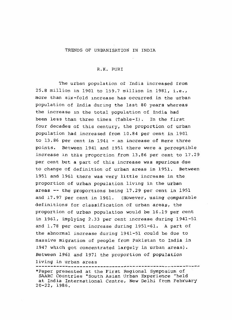
TRENDS OF URBANISATION IN INDIA

R.K. PURl

The urban population of India increased from

25.8 million in 1901 to 159.7 million in 1981, i.e.,

more than six-fold lncrease has occurred in the urban

population of India during the last 80 years whereas

the increase ln the total population of India had

been less than three times (Table-I). In the first

four decades of this century, the proportion of urban

population had increased from 10.84 per cent in 1901

to 13.86 per cent in 1941 - an 1ncrease of mere three

points. Between 1941 and 1951 there were a perceptible

increase 1n this proportion from 13.86 per cent to 17.29

per cent but a part of this increase was spurious due

to change of definition of urban areas in 1951. Between

1951 and 1961 there was very little increase in the

proportion of urban population living in the urban

areas -- th~ proportions being 17.29 per cent in 1951

and 17.97 per cent in 1961. (However, using comparable

definitions for classification of urban areas, the

proportion of urban population would be 16.19 per cent

in 1961, implying 2.33 per cent increase during 1941-51

and 1.78 per cent increase during 1951-61. A part of

the abnormal increase during 1941-51 could be due to

massive migration of people from Pakistan to India in

1947 WhlCh got concentrated largely in urban areas).

Between 1961 and 1971 the proportion of population

living in urban areas --------------------------------------------------------*Paper presented at the First Regional Symposium of

SAARC Countries "South Asian Urban Experience "held at India International Centre, New Delhi from February

20-22, 1986.

-183-

increased by about two per cent from 17.97 per cent to

19.91 per cent and during the last decade the increase was

as much as 3.4 per cent -- from 19.91 per cent in 1971 to

23.31 per cent in 1981. Thus, the real thrust of urbanisation

in India has occurred only in post-independence era after

the advent of planning and industrialisation. (For

definition of urban areas in India, please see Annexure I).

Even in 1981 the p-ropotion of total population

living in urban areas in India is not very high as compared

to many of the other under-developed countries. In 1980,

41 per cent of the world's population lived in urban areas.

In the advanced countries this percentage was 71 whereas

in the less developed countries it was 31. In Latin American

countries this percentage was as high as 65 per cent, being

very close to that obtaining in advanced countries. Even in

South Asia as a whole, 24.78 per cent of the population lived

in urban areas in 1980 -- India's percentage was lower than

this average. Amongst the" countries participating in this

symposium, Pakistan had the highest proportion of urban

population (28.17 ~et cent) followed by Sri Lanka (26.56

per cent) and India (23:31 pet cent). Bangladesh, Maldives,

Nepal and Bhutan had very low level of urbanisation: their

respective proportion~ being 11.24 per cent, 10.54 per cent,

4.98 per 'cent and 3.92 per" cent respectively (Table II). The

average annual increase of urban population in India has also

been less thantftnt

most of the countries of the 'region.

Maldives alone- (which has very little urban population) had

a slower rate of growth of its urban population in the region.

The average annual growth rate of urban population in India

was 3:84 per cent in sev~nties as against 6.45 per cent for

Bangladesh, 4.65 pet cent for Nepal, 4.49 per cent for Bhutan,

4.03 per cent for Pakistan,3;63 per cent for Sri Lanka and

2.54 per cent for Maldives.

-184-

We shall now consider the growth of urban population

in the major states of India between 1951 and 1981.

Maharashtra was the most urbanised state in 1951 and it

continued to be in that position till 1981 (Table III).

In 1951 the least urbanised state was Orissa closely followed

by Bihar; these two being the only states where the proportion

of total population living in urban areas was less than 10

per cent in 19510 In 1981 also these two states lagged

behind all other states In urb~nisation, the percentage of

their population living in urban areas being 11.79 and 12.47

only. However, the pace of increase in the urban population

of Orissa has been much more than that in Bihar during the

last 30 years. In 1951, Maharashtra, Gujarat, Tamil Nadu,

West Bengal, Karnataka and Punjab ',had more than 20 per cent

of its population living in urban areas. In 1981 the states

still below the 20 per cent urbanisation llvel were Kerala,

Uttar Pradesh, Bihar and Orissa in that order. Besides

these states, the other states which had lower than "11 India

average were Madhya Pradesh, R.ajasthan and Haryana. On the

other hand,' the states of Maharashtra, Tamil Nadu and Gujarat

had crossed 30 per cent level in 1981. Karnataka Punjab and

West Bengal had a much higher proportion than the all India

average of 23.'31. It would be noticed that Rajasthan has

slipped down in urbanisation. In 1951, its proportion of

urban population was much higher than the all India average,

whereas in 1981 it was lower.

West Bengal was the only state where the process

of urbanisation has slowed down quite a lot. From a

proportion of 23.88 per cent in 1951 West Bengal has moved

up very slowly to a proportion of 24.45 per cent in 1961,

24.75 in 1971 and 26.47 per cent in 1981. The pace of the

-185-

growth of urban population has slowed down in Tamil Nadu

also during the last decade. The urban proportion of

Tamil Nadu increased from 30.26 per cent in 1971 to 32.95

only in 1981. On the other hand, the states of Andhra

Pradesh, Haryana, Karnafka, Madhya Pradesh, Maharashtra,

Orissa, Punjab and Rajasthan had a sharper increase in the

urban population during 1971-81.

When we look at the decennial growth rates, we

notice~hat the ~ll India urban population increased by 26.41

per cent in 1951-61, 37.91 per cent in 1961-71 and 46.78

per cent in 1971-81. During 1971-81, the states of Orissa

and uttar Pradesh had a more than 60 per cent increase in

the urban population between 1971-81, closely followed by

Haryana and Rajasthan. Andhra Pradesh, Bihar, Karnataka

and Punjab were the other states which experienced sharp

decennial growth of their urban population during 1971-81.

There was a sharp decline of decennial urban growth in

Tamil Nadu, while in the states of Gujarat, Kerala,

Maharashtra, Orissa and West Bengal the decennial growth

rate of urban population in the last two decades were

almost the same.

We have not considered above the case of Assam,

as no census was taken there in 1981. Apart from Himachal

Pradesh (which has difficult hilly terrain in large parts) ,

Assam is the least urbanised state of India. In 1951, the

proportion of its population living in urban areas was

4.38, which increased to 7.·69 in 196i and 8.82 in 1971.

The estimated proportion for 1981 was 10.29.

The analysis of the statewise urban growth rates

from 1951 to 1981 shows that the states like Maharashtra,

Gujarat, Tamil Nadu and West Bengal which had already

reached a comparatively high proportion of urban population

-186-

are not growing so fast in the'ir urban population whereas the states which were less urbanised earlier are growing

sharply in their urban population such as the states of

Bihar, Haryana, Madhya Pradesh, Orissa and uttar Pradesh.

However, Kerala does not fit into this pattern. Though

Kerala is a less urbanised state yet the rate of growth of

urban population h~s been less than All India average. In

1951, 43;63 per cerit of urban population of India lived

in the four most urbanised states of Maharashtra, Gujarat,

Tamil Nadu and West Bengal. Their share is declining over

the years. It carne down to 43.09 in 1961, 42.74 in 1971

and 39.44 in 1981.

In 1901, 25.81 per cerit of the total urban

population of India lived in elass-I towns. This ratio did

not increase very much upto 1931 when 30 per cent of the

urban population lived in elass-I towns. But since then the

proportion of urban population living in ~lass-I towns

has increased very sharply in every decade. It went upto

37 per cent in 1941, 43 per cent in 1951, 50 per cent in

1961, 56 per cent in 1971 and 60 per cent in 1981. Of the

160 million urban population of India in 1981 (including

estimated urban population of Assam), 96 million lived in

class-I cities/urban agglomerations only. On the other hand,

the population in class-II towns has re~ned constant at

about 11 per cent from 1901 to 1971 and around 16 to 18 per

cent of the urban population lived in class-III towns. The

percentage of urban population living in class-IV, Vand

VI towns has been declining over the various decades.

-187-

From 1961 onwards the rate of increase in the proportion of

population of Class-I towns has been slowly declining*.

Looking at it in other waY,70 per cent of the total

increase in urban population during 1961-71 took place

in class-I cities, .12 per cent in class II towns, 13 per

cent in class-III towns and 6 percent only in class-IV

towns whereas the popul'ation in class-V and class-VI towns

actually declined during 1961-71. During 1971-81, 69 per

cent of the increase in the urban population was in class-I

cities, 12.5 per cent in class-II towns, 10 per cent in

class-III towns, 6 per cent in class IV towns o The population

in class-V and class-VI towns which has declined during

1961-71 increased considerably during 1971-81; 1.5 per cent

of the increase in urban population in this decade being in

class-V towns and 0.6 per cent in class-VI towns. During

1961-71 the annual average exponential growth rate of the

population in c1ass-I cities was 4.20 per cent which increased

to 4.54 per cent during 1971-81. The annual average

exponential growth rate of class--II towns increased from 3.40

per cent to 4.17 per cent, that of class-IV from.l.71 to 2.17,

of class...;.V from -1.09 to +1.45 and of class-VI from -2.18 to of the

+4.79. That is, the increase in -&11 India average/annual

growth rate of urban population from 3.19 in 1961-71 to 3.82

in 1971-81 was shared by all classes of towns except class-II

towns wherein there was a marginal decline.

*For 1901-71, the data source is statement 16 in fly leaf to table A-IV·of Part II A, General Population Tables, 1971, page 2050 For 1981, the population in class-I has been estimated by including those towns of Assam which are estimated to have one lakh' or more population in 1981. In 1981, the distribution of urban population by various size classes is not published yet. As such the figures mentioned here are provisional (excluding Assam and Jammu & Kashmir)" as per paper 2 of 1981, published by Registrar General's ~ffice.

-188-

The urban population has been growing at a much

faster rate than the total population since 1961. The

decennial growth rate of the total population was 24.59

per cent during 1961-71, and 25.21 per cent during 1971-81

whereas the urban growth rates were 37.91 per cent and

46.78 per cent respectively. If it is assumed that the

rate of natural increase of the urban population is the

same as that of the. rural population, the excess growth

rate in the urban population could be ascribed to (i)

Addition of new towns: (ii) Migration from the rural

areas, and (iii) Migration from abroad. The assumption

of the natural increase in rural and urban areas being

almost the same is supported by the SRS data. In Table IV,

we have worked out the effect of migration on urban

growth. Applying the decennial growth rate of total

population of each decade to the urban population at the

beginning of the decade we got the growth of urban

population during the decade if the natural rate of

increase are assumed to be the same. The difference

between these figures and the actual urban growth is

composed of; (i) Population of new towns added in the

decade and (ii) migration from rural areas and abroad.

20.95 per cent of the growth of urban population in

1971-81 was dl,le to addition of nE~W towns and 5.51 lakhs

persons had migrated to urban areas (excluding Assam)

from abroad. Excluding these persons, there would be 120

1akh persons in urban areas who rnigrated from rural areas

in the last decade, That is,migration from rural to urban

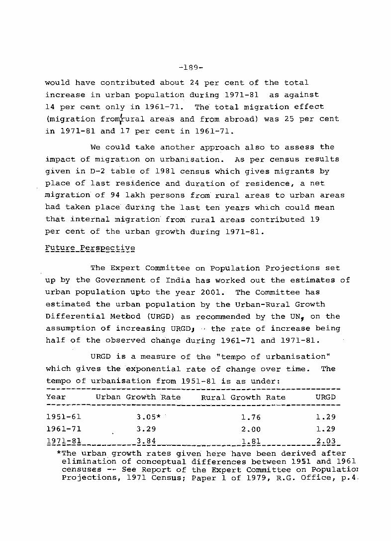
-189-

would have contributed about 24 per cent of the total

increase in urban population during 1971-81 as against

14 per cent only in 1961-71. The total migration effect

(migration fro~ural areas and from abroad) was 25 per cent

in 1971-81 and 17 per cent in 1961-71.

We could take another approach also to assess the

impact of migratlon on urb~nisation. As per census results

given in D-2 table of 1981 census which gives migrants by

place of last residerice and duration of residence, a net

migra.t:ion of 94 1akh persons from rural areas to urban areas

had taken place during the last ten years which could mean

that internal migration from rural areas contributed 19

per cent of the urban growth during 1971-81.

The Expert Committee on Population Projections set

up by the Government of India has worked out the estimates of

urban population upto the year 2001. The Committee has

estimated the urban population by the Urban-Rural Growth

Differential Method (URGD) as recommended by the UN, on the

assumption of increasing URGDJ .. the rate of increase being

half of the observed change during 1961-71 and 1971-81.

URGD is a measure of the "tempo of urbanisation"

which gives the exponential rate of change over time. The

tempo of urbanisation from 1951-81 is as under: ______ ,_' __ " ___ ·_·_'_'_' __ '_'_'_' ____ ,__'_,_'_"_'_'_"_r_. __ . ______________ . _______ _ Year Urban Growth Rate Rural Growth Rate URGD ----- --'_ ---'_'_'_"_'_'_ -_'_'_'_'_'---_'_ -_,_"_._._. __ '_'_ ----_'_ - - - -_' __ '- - ------1951-61 3.05* 1.76 1.29

1961-71 3.29 2.00 1.29

1971-81 3.84 1.81 2.03 -----. __ '_ ------_"_.--._._-_._. __ '_,-_"_-,_"_,_ .. _ -_'--- _'_ --_._ --- - - - - - --------*The urban growth rates giveri here have been derived after elimination of conceptual differences between 1951 and 1961 censuses -- See Report of the Expert Committee on Populatiol Projections, 1971 Census; Paper 1 of 1979, R.G. Office, p.4,

-190-

United Nations has noted that emperical observations

of a variety of circumstances have shown that URGD remains

more or less constant for short period of times and that

this seems to be true irrespective of current level of

urbanisation or whether the rural population is increasing

or decreasing. Accordingly_" the UN has made population

estimates assuming a constant VRGD. However, the Indian

experience during last decade shows an increasing URGD.

Therefore, in India's case the assumption of increasing

URGD !:jeems more relevant for making population ,.

estimates for the future. The moot question is what amount

of increase in URGD should be taken. The Expert Committee

has assumed half of the increase in URGD. On this

assumption URGD for 1981-91 and 1991-2001 would be 2.21

and 2.64 respectively.

The projected urban population of India and 15

major states is presented in Table V. ..Apart from the

approach adopted by the Expert Committee, there could be

two other approaches to make estimates of population for

the future. These two approaches are:

1. by projecting the ratio of urban to total population tUjT) line~rly and by second degree; and

2. by projecting the proportion of population living in towns common from 1931 to 1981 censuses to total population of each census (U/T) and multiplying the projected

proportions by estimated uju . c

The first approach seeks to project the proportion

of urban population to total population on the basis of the

change observed in the urban proportion during the last

decade/last two decades. It is assumed firstly that the

difference between the urban proportions in 1971 and 1981

census would continue to grow in a linear manner, assuming

a constant growth of the urban prop6rtion. Second

assumption is that the urban proportion would continue to

grow at an lncreasing rate as observed between last two

decades. Accordingly a second degree curve was fitted to

the urban proportions observed in 1961~'1971 and 1981

censuses. As per this method, the U/T was estimated to

be 30.13 by linear assumption and 34.49 by second degree

curve in 2001. The respective estimated urban populations

were 297 million and 341 million respectively.

The second approach involves the working out of

the proportion of population in common towns which have

been in existence throughout for 1931 to 1981 to thEll total

popuLation (i.e. UfT) wherelu~ stands for population

of common towns and 'T' stands for the total population).

This proportion has been projected upto 2001 in a 1ine~r

manner i.e., by assuml.ng that the change in the proportion

of common towns would remain the same as it was during

1971-81. These projected trend values of U6T have been

inflated by the ratio of urban population to the

population Ilving in common towns (O/De ) so as to arrive

at the trend values of the total urban proportions (UfT).

While the proportion of population in common towns, i.e. of

Ue is comparable over time, the ratio/D/De is affected by

conceptual changes. It is only during 1961, 1971 and

1981 censuses that the urban proportions are comparable

conceptually in the sense that uniform definition of urban

areas was introduced.

In view of this, a second degree curve was fitted

to the difference of U/Ue on the basis of 1961, 1971 and 1981

proportions and by assuming constant second order differences of

the proportions;D/Ue were estimated for 1991 and 2001.

-192-

The inflation factors thus obtained were applied to the trend

values of Ue/T to obtain the trend values of U/T upto 2001. This

method, thus, involves two assumptions: (a) Ue/T would grow

in future In a Ilnear £ashlon, but (b) U/Ue would grow at

an increaslng rate. On this basis, U/T was estimated to be

32.14 and the urban populc..tion '<'. 317 in 2001.

Even when India enters the 21st century, one-third

of its total population would be residing in urban areas

and two-third would continue to live in rural areas.

(Even if the urban population of India is assumed to grow

by increasing URGD, the proportion of urban population to

t:otal population in the year 2001 would be 35 per cent only).

The urban popuiation of India would increase from 159.7

million in 1981 to 230.1 million in 1991 and 326.0.million

in 2001. The annual exponential growth rate of urban

population which was 3.21 per cent during 1961~71 and 3;84

per cent during 1971-81 would gradually fall down to 3.71

during 1981-86 3.60 in 1986-91, 3.53 in 1991-96 and 3.44

pe! cent during 1996-2001. Maharashtra, Gujarat, Tamil Nadu

and West Bengal together had 63.0 million urban population

in 1981 which would increase to 82.7 million in 1991, and

104.5 mlilion in 2001. That is, the contribution of these

four most urbanised States to total urban population would be

declining from 39.4 per cent in 1981 to 35.9 per cent in

1991 and 32.1 per cent in 2001 (Table Y).

Of the major states, only three states namely,

Karnataka, Maharashtra and Punjab would achieve urban

proportion of more than 40 per cent in 2001 (Table VI) .

Gujarat, Haryana and Tamil Nadu would have an urban proportion

between 35 and 40 per cent. Assam and Bihar would have

less than 20 per cent of their population living in urban

areas even in the year 2001. Maharashtra would continue to

be the most urbanised state in 2001(44 per cent) while

Karnataka would be the second in rank followed by Punjab.

-193-

Using the estimates made by the Expert Committee

for total urban population, we have estimated the population

in class-I and million plus cities. The population in

class I cities upto 2001 has been estimated by using URGD

method, assuming that the population in these cities would

grow generally on the assumption of constant URGD. Here

the term URGD has been used to refer to the growth

differentials between population of all the class-I urban

agglomerations in a state and the rest of the population

in that state. In 1961, 5p.7 per cent of the total urban

population of India lived, in Class-I cities. This

proportion had gone upto 55.8 in 1971 and 60.1 in 1981. .. ,',

It is estimated that roughly 63 per cent of the urban

population of India in 2001 would be living in class-I cit·iea;

As a ratio of the total population, 9.1 per cent of India's

population lived in Class-I cities in 1961, 11.1 in 1971

and 14.0 in 1981. This would go upto 20.8 in the year 2001.

Of the major states, it is estimated that more than 75 per

cent of the urban population would be living in class-I

cities in the year 2001 in the states of Gujarat (77 per

cent), Maharashtra (83 per cent} and West Bengal (78 per

cent). The annual exponential growth rate of the population

in Class-I was 4.2 during 1961-71, 4.6 during 1971-81 and

is estimated to be 4.0 in 1981-91 and 3.6 in 1991-2001

whereas the growth rate of total urban population were 3.2,

3.84, 3.65 and 3.48 per cent respectively. That is, the

population in class-I towns has been growing at a much

faster pace than that in the urban areas as a whole and

would continue to do so upto 2001. However, the gap between

these two rates would narrow from 0.8 per cent in 1971-81

to 0.1, in 1991-2001.

-194-

The population in million plus cities has also been

estimated by the URGD method; the term URGD referring to

the growth differentials between the growth rate of a

particular city and the growth rate of the population of the

state in Which(~~ty lies. We estimated the population of

1991 and 2001 individually for all those cities which had

a population of 5 lakhs or more in 1981, to see which of

them are likely to achleve a million or more population

over the next two decades. These estimates were counter­

checked by taking the growth differentials between a city's

population and the urban population of the state as well

as the urban population of Indla. It is estimated that the

number of million plus cities would go upto 25 in 1991

and 36 in 2001. According to these estimates, Greater

Bombay, Calcutta and Delhi would have more than ten million

population each in 2001, while Bangalore and Madras would

have more than 5 mlllion population each. The population

of each of these cities in 2001 is given in Table VII.

The population in the million plus cities would go up from

42 million in 1981 to 73 million in 1991 and 112 million in

2001, constituting 26 per cent of the urban population in

1981, 32 per cent in 1991 and 34 per cent in 2001. That ' ..

is, an increasing proportionpf India's urban population

will live in very large cities. In 1980, Bombay, Calcutta,

Delhi and Madras ranked 16th114~ 22nd and 23rd among the 111.

25 largest cities of the world. According to(UN estimates,

they would move upto 7th, 8th, 17th and 13th ranks

respectively in 2001.

We would like to emphasise here that the estimates

of population for class-I cities and million plus cities

are essentially rough estimates which could be refined further

on the basis of other assumptions.

-195-

!~I]E2_2:f_~fee!}_S2!}S~!2:!:fe:!:!2!}

If we sub-divide the urban population into two

sub-populations such as the population of cities and

the,'rest of the urban population or the population of million

plus cities and the~est of the ~rban population etc., we

can measu__~e the "tempo of concentration" in a particular

class of cities. The percentage of city population in the

combined urban population, at any given time, may be called

the "level of concentration of the urban population", and

increases in that level may be considered as measurable in

terms of "Tempo of concentration". That is, the tempo of

urban concentration can be measured for any particular

class of cities. Based on the estimates of urban population

as presented above, we have measured the tempo'~ of urban

concentration from 1961-2001 in Class-I cities as well as

in million plus cities. Though the level of concentration

in class-I cities is increasing continuously between 1961 and

2001, the tempo of concentration is found to be declining

in each decade. The level of concentration in class-I

cities in 1961 was 50.69 per cent which would increase to

62.86 per cent by the year 2001.- But the rate of increase

in the level of concentration in each decade would decrease

from 5.13 per cent during 1961-71 to 0.52 per cent during

1991-2001. In case of million plus citie~, however, there

is no clear trend of tempo of concentration. In this case

also, the level of concentration in million plus cities

would increase from 22.9 per cent in 1961 to 34.2 per cent

in 2001. However, the rate of increase in the level of

concentration or the tempo of concentration decreased

from 2.6 per cent during 1961-71 to 0.9 per cent in 1971-81

which would again increase to 5.3 per cent in 1981-91

and would later decrease in 1991-2001 to 2.5 per cent. In

case of Class-I cities, there is no discoMntinuity in the

-196-

tempo of concentration because the number of ~lass-I cities

in 1981 is quite large and any small additions to this

number in each decade is a continuous event giving us no

discontinuity. On the other hand, there were only 9 million

plus cities in 1971 whose number increased to 12 in 1981.

This number is estimated to increase to 25_1991 and 36 in

2001. The increase in the number of million plus cities

from 12 to 25 during 1981-91 is essentially a discontinuous

event up-setting the tempo of concentration in million plus

cities shows an irregular trend from 1961to 2001.

In 1981, 26 per cent of the urban population lived

in the 12 million plus cities and 60 per cent of the urban

population lived in class-I cities. In 2001 these percentages

would increase to 34 and 63 respectively. In 1981 26 per

cent of urban population in Northern Zone lived in Delhi

alone, while Bombay accounted for 25 per cent of the urban

population in the Western Zone and Calcutta accounted for 31 . the S h per cent of the urban popu1at~on of~Eastern Zone. uc

high levels of urban concentration in individual cities have

got great sociological implications in . less developed

countries.

These cities have tvao vastly different classes of

population - one which is highly educated and affluent, and

the other which consists of a lumpen class who are uneducated,

under-privileged and deprived and many a times living away f~orn

their families in shanty dwellings deprived of the general

amenities of city life. In 1981, the sex ratio was 772 in

Bombay, 781 in Calcutta and 808 females per 1000 males in

Delhi as against the average of 878 for the urban population of

India. In these three cities, the literacy rates for 5+

population were 77, 72 and 71 respectively.

-197-

This dichotomy breeds two distinct class.of people in big

cities- the "haves" and the ·have_'nots". Urbanisation

generally, .connotes better standard in livings in the

urban areas. But this is not true for the large class of

"have-nots" in big cities. The tendency towards

concentration in big cities is therefore, fraught with

grave dangers, and ought to be reversed.

-198-

ANNEXURE - I

DEFINITION OF URBAN AREAS

One of the basic characteristics of the population

obtained through the census is the rural and urban

distribution of the people. The distinction between rural

and urban is not always amenable to a single definition

which could be applicable to all countries or for that

matter, even within the same country. Quite often it has

been asserted that an urban area should be distinguished not

merely on the basis of defined demographic characteristics

but also on the basis of the level of the infrastructure,

facilities. Ideally, it would be useful to define urban

areas irit-erms of the level of infrastructure development

and the availability of amenities in a given area but

criteria based on such considerations have not been adopted

in defining an urban area in India. Largely for purposes

of maintenance of comparabllity and for administrative

convenience, the definition of an urban unit which was adopted

at the 1971 census has been continued which, in act, has

been adopted from 1951 onwards. An urban area is defined

as follows:

a)

b)

All places with a municipality, corporation, cantonment board or notified town area committee, etc.

All other places which satisfy the following criteria:

i) a minimum populatlon of 5,000;

ii) atleast 75 per cent of male working population engaged in non-agricultural pursuits; and

ili) a density of population of at least 400 persons per sq.km. tl,OOO persons per sq. mile).

199-

In addition, the Directors of Census Operations

were also requested to classify marginal cases as rural

or urban taking into consideration local circumstances.

Such marginal cases which would have qualified to have

been classified as urban units would include major

project colonies, areas of intensive industrial

development, railway colonies and important tourist

centres etc.

It will be noticed from the definition that there

are two distinct types of urban units. Those units which

satisfy criterion (a) by virtue of a statutory notification

are, by definition, urban and are referred to by the

momenclature adopted in the relevant notification. In

other words, theeewouid be referred to as a municipal

corporation, municipal board eantonment board, a notified

area committee, etc. The other types of urban units would

be those which satisfy criterion (b) this would generally

include places which would otherwise have been considered

as rural, i.e., as villages. Places which are defined

as urban because they satisfy criterion (b) are, for

convenience, referred to as census towns or non-municipal

towns. This is to distinguish them from what are considered

statutory towns under criterion (a). -It must be mentioned

that quite often villages which are classified for census

purposes as urban units under criterion (b) may continue

to be included in the village list in the revenue records.

However, in census publications, the relevant cross

references are generally available and the reader would be

able to identify such cases.

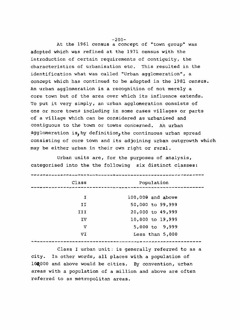
-200-At the 1961 census a concept of "town group" was

adopted which was refined at the 1971 census with the

introduction of certain requirements of contiguity, the

characteristics of urbanisation etc. This resulted in the

identification what was called "Urban agglomeration", a

concept which has continued to be adopted in the 1981 census.

An urban agglomeration is a recognition of not merely a

core town but of the area over which its influence extends.

To put it very simply, an urban agglomeration consists of

one or more towns including in some cases villages or parts

of a village which can be considered as urbanised and

contiguous to. the town or towns concerned. An urban

asglomeration iSJ by definition) the continuous urban spread

consisting of core town and its adjoining urban outgrowth which

may be either urban in their own right or rural.

Urban units are, for the purposes of analysis,

categorised into the the following six distinct classes:

city.

100,000

Class Population

I 100,009 and above

II 50,000 to 99,999

III 20,000 to 49,999

IV 10,000 to 19,999

V 5,000 to 9,999

VI Less than 5,000

Class I urban unit~ is generally referred to as a

In other words, all places with a population of

and above would be cities. By convention, urban

areas with a population of a million and above are often

referred to as metropolitan areas.

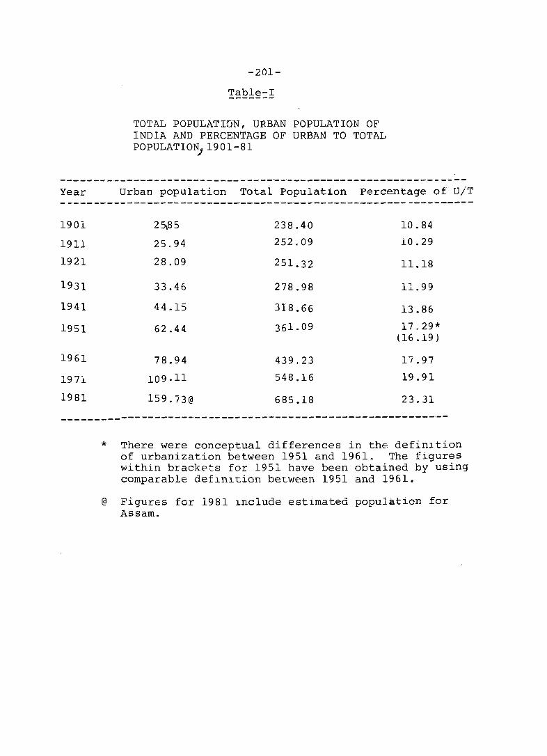
-201-

Table-I -------

TOTAL POPULATION, URBAN POPULATION OF INDIA AND PERCENTAGE OF URBAN TO TOTAL POPULATION) 1901-81

-------------------------------------------------------------Year Urban population Total Population Percentage of U/T --------------------------------------------------------------1901

1911

1921

1931

1941

1951

1961

1971.

1981

---------

*

@

2~85 238.40 10.84

25.94 252.09 lO.29

28.09 251.32 11.18

33.46 278.98 11.99

44.15 318.66 13.86

62.44 361.,09 17,.29* (16.19)

78.94 439.23 17.97

109. 1 1 548.16 19.91

159.73@ 685.18 23.31

-------------------------------------------------

There were conceptual differences in the definltion of urbanization between 1951 and 1961. The figures within brackets for 1951 have been obtained by using comparable deflnltion between 1951 and 1961.

Figures for 1981 lnclude estimated popul.tion for Assam.

Ballgladesh

Bhutan

India

Ma1d~ves

Nepal

Pakistan

Sri Lanka

-202-

'fabj E: II --,- _,_'_'--,_"

ANNUAL AVERAGE GROWTH RATE AND PE~CU~'1'.ACE OF URBAN POPULATION IN sApe COUNTRIES,196G-80

AnnU2d average gr0wt:h Peic:e.nt,a:ge of urban .~f_,,~~e~f!.;_E,£E~b~,!:,£~!2!_r,-' .~ _____ EeE~!,e!:1,2,!! __ ,_. __ _ 1960-7G . 197a-80 1960 1970 1980

6.74 6A5 5.15 7.61 11.24

4,13 4.49 2.50 3.10 3.92

3,21 3.84 17.97 19.91 23.31

1,,97 2054 11.21 11.00 10.54

4.33 4,65 3.11 3.91 4 0 98

4.04 4.03 22.11 24.89 28017

4.35 3.63 17.92 21..86 26.56

-------------------------------------------------------------

Source: UN, Bsti.mates and p:t:oJectl.ons of Urban, Rural and city Populat~on, 1950-2025, the 1980 assessment. N.Y. 1982 ,For countries other than India) For India, the figuxes are for 1961, 1971. and 1981 censuses:.

-2(')3-

TABLE III

PROPORTION OF URBAN POPULATION TO TOTAL POPULATION AND DECENNIAL GROWTH OF URBAN POPULATION IN MAJOR STATES, 1951-81

------------------------------------'-------------------------------S. State U/T (per cent) Decennial growth rate No. ------------------------- -----------------------

1951 1961 1971 1981 1951-61 1961-71 1971-81 ------------------------------------------------_._-----------------

1. Andhra Pradesh17.42 17.44 19.31 23.32 15.76 33.64 49.03

2. Assam 4.38 7.69 8.82 10.29 J26.57 65.55 58.30

3. Bihar 6.77 8.43 10.00 12.47 49.03 43.58 55.22

4. Gujarat 27.27 25.77 28.08 31.10 20.07 40.66 41. 77

5. Haryana 17.07 17.23 17.66 21.88 35.02 35.29 59.97

6. Karnataka 22.95 22.33 24.31 28.89 18.26 34.94 51.08

7. Kera1a 13.48 15.11 16.24 18.74 39.89 35.42 37.96

8. Madhya Pradesh12.02 14.29 16.29 20.29 47.70 46.24 56.50

9. Maharashtra 28.75 28.22 31.17 35.03 21.32 40.41 40.32

10. Orissa 4.06 6.32 8.41 11. 79 86.79 65.76 69.12

11. punjab 21. 72 23.06 23.73 27.68 29.06 25.07 44.89

12. Rajasthan 18.50 16.28 17.63 21.05 11.04 38.05 59.18

13. Tamil Nadu 24.35 26.69 30.26 32.95 22.59 38.32 28.21

14. uttar Pradesh 13.63 12.85 14.02 17.95 9.90 30.43 61.13

15. west Bengal 23.88 24.45 24.75 26.47 33.97 28.17 32.00

India 17.29 17.97 19.91 23.31 26.41 37.91 46.78

------------------------------------------------------------------

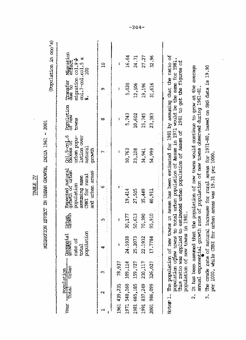
~I

il

r-l o o N

I

r-l 1.0 ~ r-l

5 R

I

-Ul

o r-l

1.0 .

r-I

I .

-204-

"<:f' r-l I""- 1.0 1.0 I""- N ~ . . . 1.O"<S't-N ...-! N N M

o 1.0 1.0 1.0 N 0 ~ ...-! o J1") r-l 1.0 " .... .... ..... J1") N ~ r-l

..-l r-l M

MNI.()M

"'" a "'" 00 I""- 1.0 I""- M .... .... .... .... J1") a J1") M

r-l ...-l N

M 00 ...-l ~

1.0 0 "'" ~ I""- r-l ~ ~ ... .... .... ... Sl g] ~ ;j!;

"'" J1") ~ ...-l ...-l 0 "'" ...-l "'" J1") "'" ~ .... ..... .... .... ~ I""- Ln 0 r-l N M "'"

I""- MOO r-- r-l ~ r-l r-l 1.0 M ~

... .... .... ... o a 0 J1") M J1") c- ~

00 M N -.::J' MI""-MOO ~ 0 ~ I""-J1") N r-l l""-. .. ... . "'" J1") N l""-N N N .-!

I""- "'" I""- r- r­Mr-IN.....-IN 0"1 ...-l I""- r-l 0

... ... .... ... lito

OO~~OI.O 1""-0 J1") MN

r-l r-l N M

J1") 0 J1") ~ ~

M 1.0 00 "'" ~ N r-l .-I N 0

..... ... .... ... .... ~ 00 J1") I""- 1.0 M "'" 00 M 00 -.::J'J1")1.000~

...-! r-l r-I r-l .....-I 1.0 r-- OO.~ 0

~ ~ ~ ~ ~

. . . r-f N M

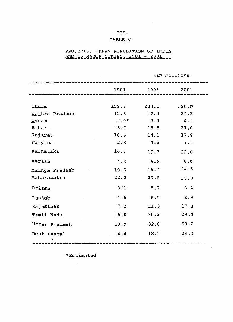
-205-

!~~~§-Y

PROJECTED URBAN POPULATION OF INDIA AND 15 MAJOR STATES 1981 - 2001 ________ ' __ ' ________ '_ L _____ ,_,_, __ ' _____ _

(in millions)

-----------------------------,-,--'-.-.--'-.-.--~-------------------

1981 1991 2001 - ---------_"_"----_"_"_"_"_'-'_-'------- - ----- - - - - - - - - - - - - - - - - - - - - - --

India 159.7 230.1 326.0

Andhra Pradesh 12.5 17.9 24.2

Assam 2.0* 3.0 4.1

Bihar 8.7 13 .. 5 21.0

Gujarat 10.6 14.1 17.8

Haryana 2.8 4.6 7.1

Karnataka 10.7 15.7 22.0

Kera1a 4.8 6.6 9.0

Madhya Pradesh 10.6 16.3 24.5

Maharashtra 22.0 29.6 38.3

Orissa 3.1 5.2 8.4

Punjab 4.6 6.5 8.9

Rajasthan 7.2 11.3 17.8

Tamil Nadu 16.0 20.2 24.4

Uttar Pradesh 19.9 32.0 53.2

West Bengal 14.4 18.9 24.0 • ,

- ------~-_,--------,_,--"_,_'_'_._.-:----'_ -----_'._---------- - - - - ----

" *Estimated

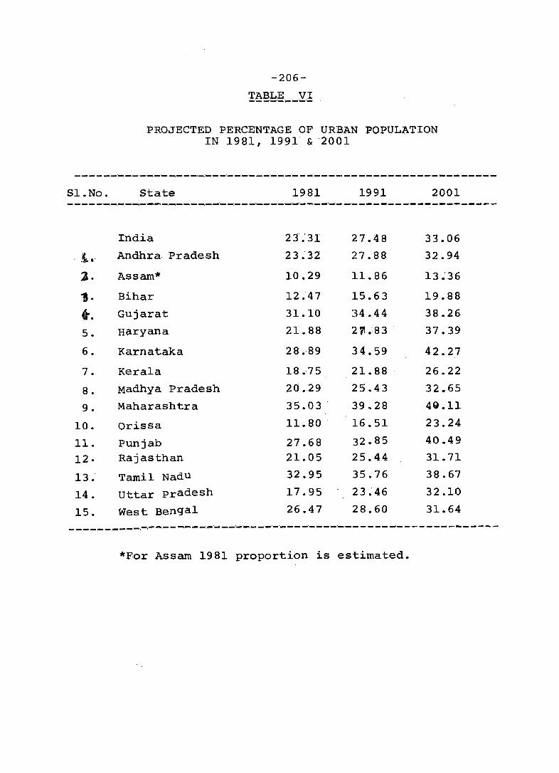
Sl.No.

-206-

TABLE VI _"_ -'_'_'_"_'-'-

PROJECTED PERCENTAGE OF URBAN POPULATION IN 1981, 1991 & -2001

State 1981 1991 2001 -_ ----' __ ,_-'-' ___ I-i_-._-t-._:_:_:_,_'-:_·_·_'_'_'_'_' __ '_'_:_ -' _ _ ._,_._"_ - _"_ -- - - -- _"_ - --

India 23 .. 31 27.48 33.06

. .t..- Andhra. Pradesh 23.32 27.88 32.94

1'- Assam* 10.29 11.86 13 .. 36

1· Bihar 12.47 15.63 19.88

t. Gujarat 31.10 34.44 38.26

5. Haryana 21.88 2 r. .·83 37.39

6 . Karnataka 28.-89 34.59 42.27

7. Kera1a 18.75 21.88 26.22

8. Madhya Pradesh 20.29 25.43 32.65

9. Maharashtra 35.03 - 39.28 40.11

10. Orissa 11.80 . 16.51 23.24

11. Punjab 27.68 32.85 40.49

12. Rajasthan 21.05 25.44 31.71

13. Tamil Nadu 32.95 35.76 38.67

14. Uttar Pradesh 17.95 23.46 32.10

15. west Bengal 26.47 28.60 31.64

*For Assam 1981 proportion is estimated.

-207-TABLE VJJ:-

CITIES WITH AN ESTIMATED POPULATION OF ONE MILLION AND ABOVE IN 2001

-------------,--_.-:-"_ -- - ------------_._,_._------._ - -- - ----- - -----

s:.. No. City Population (in mi,llion) ----------------------------------------------------------

1. 2. 3. 4. 5. 6. 7. 8. 9.

10. 11. 12. 13. 14. 15. 16. 17., 18. 19. 20. 21. 22. 23. 24. 25. 26 •

. 27. 28. 29. 30. 31. 32. 33. 34. 35. 36.

Greater Bombay Calcutta Delhi Banga10re Madras Hyderabad Ahmedabad Pune Bhopal Sur at Kanpur Patna Jaipur Nagpur Indore Ranchi Vadodara U1ahasnagar ' Jamshedpu~ Vishakhapatnarn Dhanbad Lucknow Madurai Jaba1pur Coimbatore Vijayawada Varanasi' Jodhpur Cochin Ludhiana Srinagar Meerut Agra Gwalior T:~t.ii rappa IIi Allahabad

13.95 12.93 12.90

7.63 7.37 4.62 4.55 3.31 3~07 2.59 2.57 2.50 2.38 2.27 1.77 1.75 1.58 1.55 1.52 1.50 1.47 1.46 1.39 1.39 1.36 1.22 1.31 1.19 1.19 1.18 1.09

. 1.08 1.00 1.00 1.00 1.00

AN ANALYSIS OF THE DENSITY DIFFERENTIATION OF THE POPULATION

OF INDIA, 1961, 1971 and 1981

G. P. CHAPMAN

In.tILoduc..t.ion

During the course of urbanization, increasing propo­

rtions of a nation's population become concentrated at higher ,

densities, and a decreasing proportion relatively speaking

occupy rural areas at relatively lower densities. However,

accompanying these changes there are usually changes occurr­

ing at other scales as well: relatively speaking some regions

become more densely settled, and some less densely settled.

The analysis of these trends is possible using statistics

derived from Information Theory, ~~ which have useful

disaggregative properties. The national trends may be

decomposed into any number of scales, but usually there is

little point in proposing too many scales of analysis. The

finest scale possible will depend upon the smallest scale

of data unit used.

In an earlier paper (Chapman, 1973) the author used

simple Information Theoretic indices to consider the behaviour

of population densities in the USA and in the UK over the

last 100 or so years. The national trend :in the USA showed

increasing differentiation of population density, as one

would suspect from the history of its urbanization, but a

disaggregation of the national trend showed quite clearly that

the density differentiation between states was decreasing

over time, while the density differentiation within states was

increasing. Quite simply, at regional and national scales, the

population was still spreading out from its historic concentra­

tions, mostly in the !aste'rn Seaboard. But at a local scale,

differentation between country and town was ocourring fast,

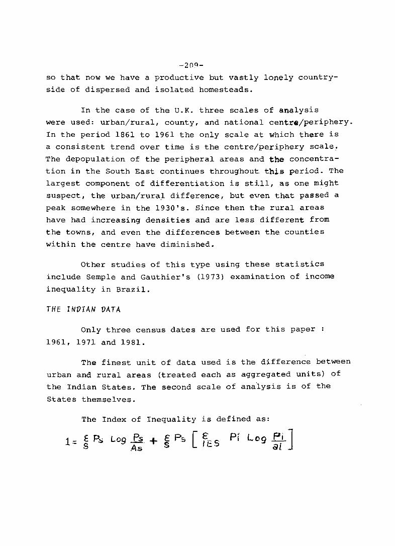
-2()Q-

so that now we have a productive but vastly lonely country­

side of dispersed and isolated homesteads.

In the case of the U.K. three scales of analysis

were used: urban/rural, county, and national centre/~eriphery.

In the period 1861 to 1961 the only scale at which there is

a consistent trend over time is the centre/periphery scale~

The depopulation of the peripheral areas and. the concentra.,..

tion in the South East continues throughout. this period. The

largest component of differentiation is still, as one might

suspect, the urban/rura.l difference, but even that passed a

peak somewhere in the 1930's. Since then the rural areas

have had increasing densities and are less different from

the towns, and even the differences between the counties

within the centre have diminished.

Other studies of this type using these statistics

include Semple and Gauthier's (1973) examination of income

inequality in Brazil.

THE INVIAN VATA

Only three census dates are used for this paper

1961, 1971 and 1981.

The finest unit of data used is the difference between

urban and rural areas (treated each as aggregated units) of

the Indian States. The second scale of ana·lysis is of the

States themselves.

The Index of Inequality is defined as:

Pi L09 Pj ] al .

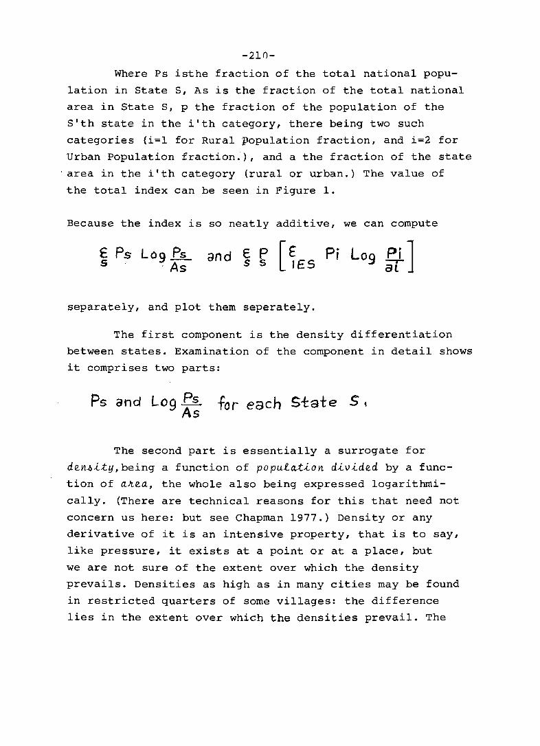
-210-

Where Ps isthe fraction of the total national popu­

lation in State S, As is the fraction of the total national

area in State S, p the fraction of the population of the

Sith state in the ilth category, there being two such

categories (i=l for Rural population fraction, and i=2 for

Urban Population fraction.), and a the fraction of the state

. area in the ilth category (rural or urban.) The value of

the total index can be seen in Figure 1.

Because the index is so neatly additive, we can compute

E Ps L09 Ps s , As and E. P [€ Pi

S s IES . Log .e,LJ at

separately, and plot them seperately.

The first component is the density differentiation

between states. Examination of the component in detail shows

it comprises two parts:

Ps and Log Ps for each State S 1

As

The second part is essentially a surrogate for

den~~~y,being a function of popula~~on d~v~ded by a func­

tion of a~ea, the whole also being expressed logarithmi­

cally. (There are technical reasons for this that need not

concern us here: but see Chapman 1977.) Density or any

derivative of it is an intensive property, that is to say,

like pressure, it exists at a point or at a place, but

we are not sure of the extent over which the density

prevails. Densities as high as in many cities may be found

in restricted quarters of some villages: the difference

lies in the extent over which the densities prevail. The

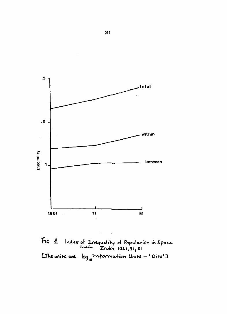
tV :J

.3

.2

g 1 c::

1.961

211

total

within

between

71 81

-212-

first part of the component is the state share of national

population: this is used to wetiJght the density derivative.

This is an extensive property - it says for how many people

the density condition prevails. The national inequality

figure is therefore the density (intensive property) figures

of all the states weighted by the population significance

(extensive property) of the states.

The trend for India is shown in Figure 1 as one of

the two parts into which the national overall statistic

is divided. It seems that there was quite a shift in the

density inequality between 1961 and 1971, but little shift

between 1971 and 1981. What is quite obvious is that there

is no major redistribution going on at the regional scale

equivalent to wh~has happened regionally in the USA. Nor

is there ~~~ an evening-out of population densities

similar to that which happened at the county scale in

England and Wales after the 1930'.

Because the Between State Component has two parts

we can actually draw an inequality diagram in which the

position of the states is clearly seen. These are shown

in Figures 2a to 2c. The horizontal· line represents

average national density, and those states above the line

are above national density, those below are below the

national density. The length horizontally of the line is

1 (unity). Therefore the line is fractioned according to

the fractions of the national population. The area of

the rectangle for each state is thus the result of the

combination of the intensive property (vertical axis) and

the extensive property {horizontal axis.} Thus it is

immediately clear that not only are U.P., Bihar, West

Bengal and Tamil Nadu densely settled, they are exten­

sively so. Something similar appears to be true of

-213-

Kerala, Punjab and Haryana. On the negative side, not

only the emptiness but the extensiveness of that empti­

ness is evident for Rajasthan and Madhya Pradesh. As

the scales of spatial units get smaller,it is not

!urprising that specific densities depart increasingly

from the national average. Visually apparent on the

diagrams are Delhi and Jammu and Kashmir, for opposite

reasons,. It is significant and demonstrative that

Delhi should have such a visual impact: in national

terms this concentration of population is significant.

The diagrams show the relatively small change over time,

the bAggest change being between 1961 and 1971.

The numerical values for the areas of these

rectangles are also given in Table 1, between state

lnequality. Here we can highlight change over time

for the individual states. The comparative stability

of the national picture is reflected in the compara­

tive stability of .osr state figures. Interesting

changes include the consistent increase of Delhi, and

the decreases of Jammu and Kashmir and Himachal Pradesh

Since we hear so much about the pressure on the

environment in these two states, it is interesting to

note that in relative terms they are remarkable

precisely for diminishing relative population pressures.

214

<.0 ... -" > ~. en iii " . ...... 0' z c _ ... c.;: ._ ~ I.L. K 1M

... .. .. 0 ... ..

..,,' ... eo, 10 10 14' A.lISNJO - A.lW140lid lAISNUNI

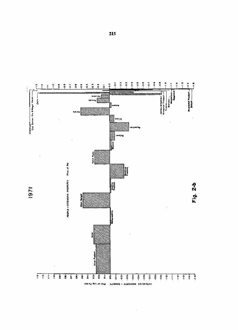
;; : z .. , o ~

~ ~ .0 !!' • ." 0 CCl : '"

.... "" m

;r '0 ;; ;;;

'" .. a: ... Do 0 a: Do

... > 0; z ... .. )( ... I ... ....

Do 0 ... Do

21S

. .. co

.; o o .

~ N

0. ._ LI.

II..,ltd e01 JO ,Old) A,LISNJO - A1Y3dOlid JI\ISNUNI

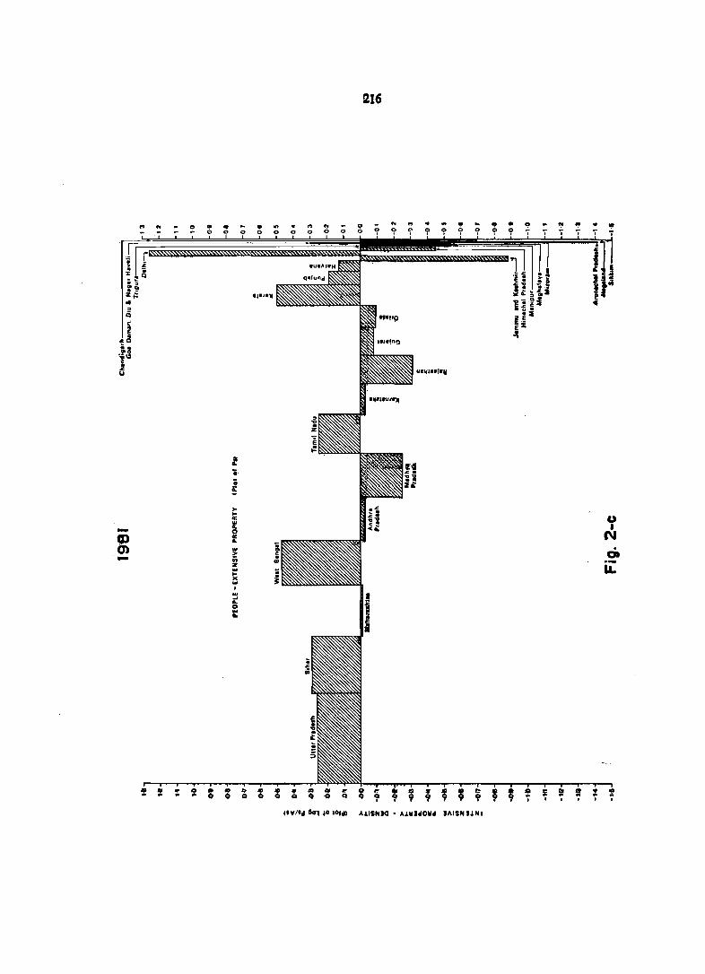
216

I ,& .

• ~

>-.. U a:

w • - .. 0 N CD a: ...

<n ~ Q - iii ._

z La. ... .. .. ... . ~ ... 0 t

"'til", eo, 10101"" "'.LISNiO - "A.IUdOIl'" illlSN UN,

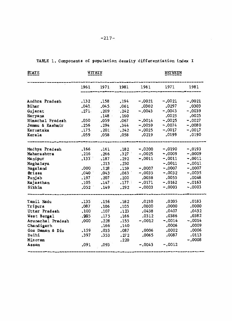
-217-

TABLE 1. Components of population density differentiation index I

STATE WrrHIN BETWEEN ------ ---------------------------------------------------~----------------------------

1961 1971 1981 1961 1971 1981

------------~-------------------------------------

Andhra Pradesh .132 .158 .194 - .0021 - .0021 -.0021 Bihar .041: .045 •. 061 .0302 .0297 .0303 Gujarat .271, .209' .242 -.0043 -.0043 -.0039 Haryana .148 ' .160 .0025 .0025 Himachal Pradesh .050 .059 .067 -.0014 - .0025 - .0027 Jatmnu & Kashmir .256 .294 .344 -.0059 -.0074 - .0080 Karnataka .175 .201 .242, -.0025 -.0017 - .0017 Kera1a .059 .058 .058 .0219 .0199 .0190

----------------~---------------------------------------------------------

Madhya Pradesh .166 .,161 .182 -.0200 -.0190 -.0193 Maharashtra .216 .266 .327 -.0025 -.0009 -.0009 Manipur .133 .. 187 .292 - .0011 - .0011 - .0011 Megha1aya .213 .230 - .0011 - .0011 Naga1and .000 .128 .159 -.0007 -.0007 -.0007 aJrissa .040 ' .043 .063 - .0035 - .0032 -.0035 Punjab .197 .207 .200 .0038 .0055 .0048 Rajasthan .105 .,147 .177 - .0171 -.0162 -.0163 Sikkim .052 .149 .292 -.0003 -.0003 -.0003

--------------------------------------------------------------------------Tamil Nadu .135 .. 156 .182 .0210 .0205 .0183 Tripura .087 .106 .105 .0000 .0000 .0000 Uttar Pradesh .100 .107 .123 .0438 .0407 .0432 West Bengal ,.~Q5 .175 .166 .0312 .0386 .0382 Arunachal Pradesh .000 .228 .155 -.0012 -.0014 -.0014 Chandigarh .166' .140 .0006 .0009 Goa Daman & Diu .159 .033 .087 .0006 .0002 .0006 Delhi .397 .353 .272 .0065 .0087 .0113 Mizoram .220 -.0008 Assam .091 .093 -.0043 -.0012

-------------------------------------------------------------------------

-218-

The \'Ji thln State figures of T,able 1 are those for:-

E_. _ Pi Log PI ~t:~9 ai

and therefore reflect urban rural differentiation having

already accounted for the differing average density of

each state. The figures show that Maharashtra has the

most extreme density differentiation, and that it has been

increasing. This is not surprising to those who know

Bombay and Poona and the dry tracts of the plateaux. But i

it is interesting to note that Jammu & Kashmir has a

similar level and trend. Given its own relatively low

densities overall, it nevertheless has a very high urban

differentiation. By contrast, Himachal Pradesh has as

little differentiation as, in its own context, Bihar.

So Jammu & Kashmir and Himachal Pradesh appear alike in

that they are relatively empty and emptying montane

states, but unalike in the way that urban population

concentrations are building up in Jammu and Kashmir.

Perhaps the most staggering change is in Sikkim, "7here

clearly there has been a rapid and major shift. Has this

presaged the recent political troubles in the State?

vJest Bengal and Delhi have similar trends for

very different ~ ~~~ reasons. Clearly in West

Bengal population growth within defined urban areas has

decreased, but has increased in areas which are still

defined as rural. In the case of Delhi Union Territory,

so little popalation is rural that any increase in urban

populatlon and area results in a reduction of inequality -

all the population becoming homgeneously urban.

Combining the two component values together enables

one to make a cross-classification of the states in 1961

as follows as shown in Table 2. The critical values chosen

-219-

were greater than .120 to indicate high urban/rural differen­

tiation, and positive values to indicate high state densities.

The classification seems to distinguish between the lowly

urbanised densely settled states (Bihar etc.), the lowly

urbanised low density mountain and desert states (Himachal

Pradesh etc.) the low density urban states (Andhra Pradesh

etc.) and the high density more urbanised states (Haryana

etc.). The situation in 1981 changes in one respect only:

several states g? from the low density less urbanised to

the low density highly urbanised category: these are Naga­

land, Orissa, Sikkim, Tripura and Arunachal Pradesh. This

paints a portrait of the greatest relative change in these

twenty years in the settlement characteristics of these

peripheral states with the much faster relative urbaniza­

tion of their populations.

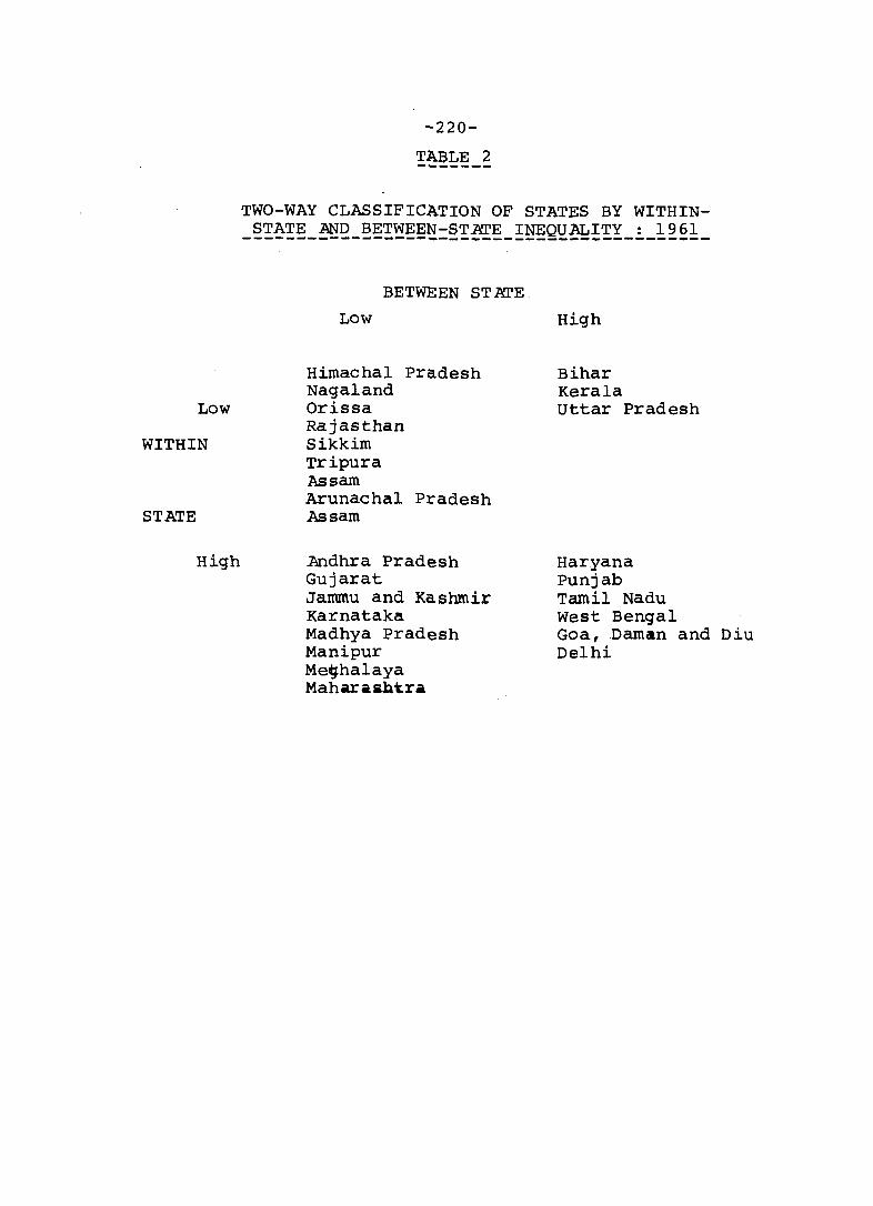
Low

WITHIN

STATE

High

-220-

TABLE 2 -------

TWO-WAY CLASSIFICATION OF STATES BY WITHIN­STATE AND BETWEEN-ST~E INEQUALlTY : 1961 -----------------~-------------------------

BETWEEN STATE

Low

Himachal Pradesh Nagaland Orissa Rajasthan Sikkim Tripura Assam Arunachal Pradesh Assam

.Andhra Pradesh Gujarat Jammu and Kashmir Karnataka Madhya Pradesh Manipur Meqhalaya Mahar.antra

High

Bihar Kerala uttar Pradesh

Haryana Punjab Tamil Nadu west Bengal Goa, Daman and Diu Delhi

-221-

CONCLUSIONS

using the two sca1esfQr urban/rural within state,

and the States themselves, and the three dates 1961, 1971

and 1981, it has been shown that most of the density

differentiation of the population is occurring at the

level of urban rural differences within the states. The

Between State differentiation has changed from 1961 to 1971,

but not much since, The greatest relative changes since

1961 have been in the changing character of certain

peripheral states.

Cha:pman G.P.

Chapman G.P.

Chapman G.P.

(1970) 'The Application of Information Theory to the Analysis of Population Distributions in Space' Economic Geo­g~aphy Vol. 46,NO. 2 J Supp1ement pp 317-331

(1973) 'The Spatial Organization of the population of the united States and England and Wales' Economic Geog~aphy Vol. 49 NO.4", pp 325-343

(1977) Human and Envi~onmentai Sy~tem~ Academic Press, London and New York, pp. 421

Semple R.K. and Gauthier H.L. (1972) 'Spatial Trends in Income Inequalities in Brazil' Geog~a­phical Analy~i~ Vo1.I~ NO.2 J p 169-

A note on concepts, definitions and measures of .. URBANIZATION and URBAN GROWTH

M.K. JAIN

Urbanization is a product of economic, social and

~litical processes which in the context of culture operate

to create spatial patterns of population distribution.

This is considered as an indicator of modernization or the

sign of growth and economic progress. As a process,it invol­

ves two aspects vif., ti) the movement of people from rural

to urban places where, they engage in primarily non-rural

functions or occupations, and (ii) the change in their life­

style from rural to urban with its associated values,

attitudes and behaviours. The important variables in the

former are population, density and economic functions

whereas, social, psychological and behavioural factors

are the important variables in the latter l ). This process

reveals through temporal, spatial and sectoral changes in

demographic, social, economic, technological and environ­

mental aspects of a life in a given society. These changes

manifest themselves in increasing concentration of population

in the human settlements larger than villages, in increasing

involvement of people in secondary and tertiary production

and the progressive adoption of certain social traits which

arelkypical of rural societies. Statistically, the degree/

extent/level of urbanization denotes the proportion of

population of a country or its region/state enumerated in

urban areas at a particular point of time.

l)Burn, S.D. and Williams, J.P. (eds)Citle~ 06 the Wo~ld: Wo~ld Reglon~l U~b~n Vevelopment, 1983.

-223-

The process of urbanization is usually studied by

the social scientists both as dependent and independent

variables for explaining behavioural, structural and

demographic aspects of the society.

(1) Behav~ou~al :- In this context, the urbanization is

concieved as a causal factor of modernization2). In other

words, sociologists are of the view that the rural-urban

dichotomy is due to the process of diffusion of certain

modernization traits or characteristics in a population.

Thus the Process of urbanization is revealed through the-

- increasing process of differentiation;

- heterogeneity and segregation;

- competition and formal control mechanism;

- anonymity and transitory character of social relationships; and

- loose kinship bonds and lack of solidarity.

It is also however mentioned in this connection that

there is no universal process of transformation of social

values but is related to the specific cultural context.

(2) St~uetu~al :- Under this realm, the economists perceive

it as a product of increasing economic specialization and

advancing technology which result into the accumulation of

people. In other words, it is a process whereby the primary

functions are replaced by secondary and tertiary functions.

Thus, the city growth. is construed as a result of the cencentra­

tion of differentiated but functionally integrated speciali­

sation in rational locations3 ).

2)Hauser,p.M.,"urbanization: An overview" in P.M. Hauser and Leo F. Schnore (eds~ The Study 06 U~ban~zat~on, New York, John Wiley,1967, p.1-4l.

3)Berry, Brain J.L.,"Some Relations of Urbanization and Basic Patterns of Economic Development"in F.R.Pitts(ed.) U~ban SY.6tem.6 06 Eeonom~e Vevelopment, Eugenic.,·· .. New York,1962.

-224-

(3) V~mog~dphIQ :- In the demographic context, as explained

by H.T. Eldridge;) the urbanization - as a process of popu­

lation concentration - involves two elements - (1) "the

multiplication of points of concentration" and (2) "the

increase in the size of individual concentration". Some

demographers consider it as a way of ordering a population . . . 5) ~n a g~ven env~ronment .

The definition of an urban area varies from one

country to another and from one point of time to another in

certain countries. Moreover, it is virtually impossible to

evolve a universally acceptable definition of an urban area.

These difficulties arise mainly on three accounts i.e.

(1) There is no point in the settlement conti~ flowing

from larger to smaller population clusters where, urbanity

d . d 1 . . fore t f ~sappears an rura ~ty beg1ns. Ther~ one has to resor or

arbitrary divisions regarding the distinctions between urban

and-rural areas. Problems however crop-up when one tries to

define the marginal or fringe areas which are known as

suburban village or urban areas. Thus, the criterion of a

minimum population size for defining a place as urban suffers

from lack of reality.

(2) Similarly, the concept of urban character also changes

due to constant changes in the functions and form of urban

areas. These changes occur due to emergence of new industrial

and technological advancement. Thus, the idea of certain ,

minimum collection of functions for defining an urban area is

also not much helpful. -------------------------------------4)Hauser, P.M. Op. CI~.

5)Lampard Eric E., "Historical Aspects of Urbanization" P.M.Hauser and O.D.Duncan(eds.) Th~ S~udy 06 Popula~lon Unv.press Chicago,1959,pp.529-54.

-225-

(3) As regards the cr.iterion o~ of:':icial desi~nation

for defining a place .. as urlba",. !~ i. noted th"'lt. this

cri teriori is anachronistic a.nd lori.,il ~a.use there is

always' a time qap between a place attaining urban character

and its being ascribed with an official designation'such

as municipality, town area committee etc. Moreover, such

designations are accorded by the national/provincial

governments which amounts to temporal and spatial variations.

united Nations, after considering all these factors,

recommended that the countries should tabulate data for

urban and rural areas based on the definitiomadopted by

them for treating a place as urban On the basis of (a) type

of local gOvernment, (b) number of inhabitants, (c) population

engaged in non-agricultural activities, and in addition, they

should provide standard tabulation by size of locality for

international comparisions in lieu of a standard tabulation

by rural and urban residence 6).

ConQep~~ and de6~n~~~on~ u~ed 604 p4e~ent~~g u4b«n ~ta~~~~~Q~ ~n rnd~a :

Town: In India, the administrative or civic status of

a place has served as the main criterion for treating it as a

town right from the beginning of the census-taking in the

late 19th century. Besides, certain criteria such as the

minimum population size, density and the sectoral distribution

of workers have also been considered for treating a non­

statutory place as urban. Lastly, the Directors of Census

Operations of the states were, given some discretionary

powers to include any place which according to them possessed

pronounced urban characteristics. A town was defined mostly

6)United Nations, P4~nQ~pie~ and ReQommendat~on~ 604 the Populat~on Cen~u~ 06 1970,Deptt. of Economic and Social Affairs, New York, 1971.

-226-

in a similar manner upto 1951 Census. It meant (i) every

municipality; (ii) all civil lines not included within

the municipal limits; (iii) every cantonment; and (iv) every

other continuous cOllection of houses inhabited by not

less than 5,000 persons which the Provincial Census

Superintendent (Director) decided to treat as a town for

census purposes.

In dealing with the questions arising under (v) the

provincial Census Superintendents (now desi9nated as

Directors of Census Operations) gave due regard to the

character of the population, relative density of dwellings

and importance of the place as a centre of trade and avoid

treating overgrown villages as towns which had no urban

characteristics.

The number of towns and the urban population changed

from census to census in view of the upgrading of villages

due to their acquiring urban characteristics or downgrading

of towns which lost their urban characteristics. It was

the practice to treat some places even with a population of

less than 5,000 as towns in the former princely states since

they were of local importance.

The definition adopted for a town lttl·. the 1971 Census

which followed the 1961 pattern was as follows:-

(a) All statutory towns i.e., all places with a municipality, corporation,municipal corpora­tion, municipal board, cantonment board or notified town area etc.,

(b) All other places which satisfy the following criteria:-

i) A minimum population of 5,000,

-227-

(ii) At least seventy five per cent of the

male working population engaged in

non-agricultural (and allied) activity,

and

(iii) A density of population of at least

400 sq. km. (1000 per sq.mile).

The Directors of Census Operations were also given

some discretion in respect of some marginal cases to

include, in consultation with the State government, some

places that had other distinct urban characteristics and

to exclude certain areas which could not be considered

as urban7 ) .

It was felt that the criteria adopted in 1971 Census

were adequate to make proper rural/urban classification.

Therefore, in order to maintain the comparability of data

it was decided to retain the same criteria at the 1981

Census also8 ) . A few minor changes indicated below were

however, made.

(a) ~vhile applying the test of occupation of the male working population to determine whether an area should be considered as urban or rural, the occu­pations of livestock, forestry, fishing, hunting and plantations, orchards, etc. classified under category III which were treated as non-agricultural till 1971 were treated as agricultural activity for the 1981 Census.

7)census of India, 1961, Gene~af Pop~fa~ion Tabfe~, Part II-A(i) India, New Delhi, 1964 p. 51-52

8)Census of India, 1981,Gene~af Pop~fation Tabfe¢, Part II-A(i) India, New Delhi,1985, pp.20-21.

-228-

(b) All urban units which are notified by State Governments as towns and having statutory govern­ing bodies as well as all such places in respect of which town area committee or the like have notified by the State governments after 1971 Census were also included in 1981 urban frame though some of them did not satisfy the three basic criteria (Population, Density and Occupation) .

(c) The third criterion according to which the Directors of Census Operations were empowered to declare an area as urban in consultation with the State governments were applicable to only those places which had distinct urban characteristics and physical amenities, such as newly established industrial areas, special project areas, large housing colonies, places of tourist interest, railway colonies, etc., though they also do not strictly satisfy the criteria laid down for classification of an area as urban.

In some cases, the changes in the urban frame were

caused due to jurisdictional changes in towns/villages

during the intercensal period. Those units which were

treated as Census Towns for the first time in 1971 without

satisfying the prescribed criteria were again examined taking

into consideration their present position (development/

expansion etc.) and were dropped from the list, in case

they were found to have been not fit for consideration as

urban units. However, a few places have been retained as

. such on the recommendations of the Directors of Census

Operations.

ii) U~ba~ aggiome~a~lo~

with rapid industrialisation, mobilisation of

resources and induced development efforts allover the

country, the trend of urbanisation accelerated considerably

in the post independence period. This tendency demanded

need for immediate and perspective urban planning with

-229-

the opening of new means of communica tion channel and

consequent increased mobility of population and resources,

the cities and towns exerted great influence over

surrounding rural and urban settlements. In partial

recognition of these facts, the census organisation

introduced the concept of 'Town Group' in 1961. This

comprised independent urban units not necessarily contigu­

ous to one another but interdependent on each other to

some extent. It was, however, later on found out that

the concept of 'Town Group' lacked technical fineness in

the sense that owing to the change of boundaries of the

constituent towns, the data generated thereon would become

incomparable from census to census. In most cases, the lack

of contiguity between the constituent urban units existed

and the intervening non-municipal areas and the spillover

areas of a town were left out of reckoning. As a result,

the concept failed to meet the expectation and need of urban

planners.

In order to amend the lacunae of· the concept of

Town Group, the concept of lJ.rban Agglomeration was adopted

for the first time during the 1971 Census. It was followed

for the 1981 Census. This concept was adopted in recognition

of the fact that in several areas, around a core city or

statutory town have come up fairly large well recognised

railway colonies, university campuses, port areas,

military campus, etc., and even though they are outside the

statutory limits of the corporation, municipality or

cantonment, they fall within the revenue limits of the

village or villages which is or are contiguous to the town.

It may not be altogether realistic to treat such areaS

lying outside the statutory limits of a town as rural

uni ts i at the same time, each such individuaL area by i tS.elf

-230-

may not satisfy the minimum population limit to qualify

it to be treated as an independent urban unit. Such

areas, therefore, deserve to be reckoned along with the

town and continuous spread including such urban out­

growths would deserve to be treated as an integrated

urban area. Each such agglomeration may be made up of

more than one statutory town adjoining one another such

as a municipality and the adjoining cantonment and also

other adjoining urban growths such as a railway colony,

university campus, etc. Such outgrowths which did not

qualify to be treated as individual towns in their own

right should be treated as urban appendages of the units

to which they are contiguous.

The following are the possible different situations

in which urban agglomerations would be constituted:

i) a city town with a continuous outgrowths - the part of growth being outside the statutory limits but falling within the boundaries of the adjoin­ing village or villages; or

ii) two or more adjoining towns with their outgrowths as in (i) above; or

iii) a city and one or more adjoining towns with their outgrowths all of which form a continuous spread.

In varying local conditions, there could be similar

other combinations which could be treated as agglomeration,

provided they possessed the necessary characteristics and

satisfy the conditions of urbanization, contiguity and

viability. Thus, the concept of urban agglomeration repre­

sented a continuous urban spread constituting a town and

its adjoining urban outgrowth or two or more physically

contiguous towns or cities together with contiguous well

~~£~~~!~~~_~~~~~_~~~~~~~~~_~~_~ny, of such towns9

).

9)Ibid

-231-

iii) Outgnowth: The urban outgrowth of a town represents

an area which possesses the requisite.urban features

in terms of infrastructure, viz., the characteristics and

amenities. Moreover, this has to be a viable unit such

as village or a hamlet or an enumeration block and which

is identifiable in relation to its boundaries and location.

These are, generally speaking, well recognised railway

colonies, university campuses, port areas, military camps.

etc., which have come up around a core city/town. In

other words, outgrowth are the areas lying outside the

statutory limits of a town, which by themselves did not

satisfy some of the prescribed eligibility tests to

qualify for treating them as the independent urban units.

iv) Standand Unban Anea: This concept was also adopted

for the first time at 1971 Census for studYlng the trends

of urbanisation around some large nuclei. Its main

purpose was to provide comparable data for a constant

statistical-spatial reporting unit WhlCh was to serve

as the basis of urban development planning for the concerned

city or town. The necessity for adopting such a concept

was felt because the lack of contiguiting such a concept

was felt because the lack of contiguity between the

constituent urban units existed and the intervening non­

municipal areas and the spillover areas of a town were left

out of reckoing. As a result, the concept of Town Group

failed to meet the expectation and need of urban planners.

Meanwhile, . in the mid-sixties, urban planners were

busy preparing Master ,lans for the cities and towns.

This exercise required data in respect of contiguous

urban units, on the one hand and partlally urbanizable

rural areas around the Cities/towns, on the other.

As census statistics presented on the basis

-232-

of Town Groups were not of much help to the urban planners,

the census organisation as well as the major data users

were exploring the possibility of an alternative suitable

concept. Around this time, International Geographical

Congress (IGC) was being held and it recommended replacement

of Town Group with 'Planning Areas' as developed by

Town and Country Planning Organisation (T.C.P.O.). Thus,

the two new concepts viz., urban Agglomeration (UA) and

Standard Urban Areas (SUA) were introduced at the 1971

Census. S.U.A. is defined as the "definite, stable and

projected growth areas of a city or town having 50,000 or

more population in 1971 as it would be in 1991, taking

into account not only the towns and villages which will

get merged into it but also the intervening areas which

are potentially urban". 10)Thus, it is a long term planning

area and is to remain as a constant statistical reporting

unit during the three successive Censuses - 1971, 1981 and

1991 irrespective of the changes in the boundaries of the

local administrative units within the tracts.

Characteristic features of a S.U.A. are that

it should have (i) a core town of minimum population of

50,000, (ii) contiguous areas made up of other urban as

well as rural administrative units should have alose

mutual socio-economic linkages with the core town and

(iii) the probability that the entire area will get

urbanised within the span of 2-3 decades.

10)census of India, 1971, Gene~ai Popuia~~on Tabie¢ (S~anda~d U~ban A~ea¢l Part II - A (iii), India, New Delhi, 1982 pp.iii - iv

-233-

In identifying the constituent units of S.U.A. the

following yardsticks were conventionally used:

a) a core tmvn with a population of 50, 000 or above by 1971 census;

b} predominant urban land use:

c) intensive inter-action with the urban centres as reflected in commutation for the purpose of work and secondary education facilities; extension of city bus service, sale of commodities like milk,dairy products, vegetables (other than those transported by rail or truck head) and purchase of ~ood-grains, cloth and general provisions, etc., by the consumers directly.

(d) anticipating urban growth as a result of locational· decisions relating to industry, market, transport and communication, administrative and servicing functions.

e) ~xistence of big villages with a large proportion of working force engaged in non-agricultural pursuite.

It is obvious from the definition of the S.U.A. that, it is a dynamic areal spread. The constituent units within S.U.A. tract, over the period of 1971-81, are

supposed to undergo various changes - both physical and

demographic.

(l) Ve9~ee 06 U~bdnizdtion - PU = 10~ where, lUI & 'pI

represent the urban and total populations of a country.

It indicates the absolute or relative number of people who

live in defined uri:Ja\. places. For measuring the degree of

11) for details on measures given hereunder please see, (i) E.E. Arriaga, A New Approach to the "Measurement of Urbanizat:lon"

Ec.Onorni.c. Veve£.0l=ffle.n.t and. CuLtu.M.i. Change, 1970, Vol .18, No.2, pp 206-2! 8.

(ii)

(iii)

(iv)

Gibbs, Jack P., ''The Measurement of Urbanization", Soc).a.t Fo~c.e6, Vol.45, No.2, 1966,pp.170-177 Goldstein S. and David Sly (eels .),The. mea.6uAement on U~baMzation and r~ojec.tion 06 U~ban Population,lUSSP,Belgium 1974,pp,19-87, Shr¥~C;~LHenery,Jacob S.Siegal am A.ssociates,The. Me.thocU al1d ~dt~ of.. Ve.moglLaphy,u .S. Bureau of CensusjWashington,Vol.I • 97. , pp. 17 (,-183 •

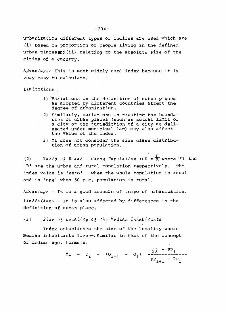
-234-

urbanization different types of indices are used which are

(i) based on proportion of people living in the defined

urban placesaed (ii) relating to the absolute size of the

cities of a country.

AqlJa.nta.ge.: This is most widely used index because it is

very easy to calculate.

1) Variations in the definition of urban places as adopted ,by different countries affect the degree of urbanization.

2) Similarly, variations in treating the bounda­ries of urban places (such as actual limit of a city or the jurisdiction of a city as deli­neated under municipal law) may also affect the value of the index.

3) It does not consider the size class distribu­tion of urban population.

(2) Ra.t,i.o 06 RuJta.{ - UJtbayt Popu{at,i.on :UR = *" where 'u' and

'R' are the urban and rural population respectively. The

index value is 'zero' - when the whole population is rural

and is 'one' when 50 p.c. population is rural.

Advantage. - It is a good measure of tempo of urbanization.

L,i.m,i.ta.t,i.oyt~ - It is also affected by differences in the

definition of urban place.

(3) S-Lze. 06 Loc.a{,i.ty o~ the. Me.d-Lan Inhabitan:t~:

Index establishes the size of the locality where

median inhabitants live-.Similar to that of the concept

of median age, formula 0

Q. ) 1.-

5D - PP. 1.

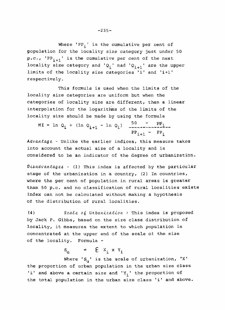
-235-

Where 'PPi ' is the cumulative per cent of

population for the locality size category just under 50

p.c., 'PPi +l ' is the cumulative per cent of the next

locality size category and 'Qi' nad 'Qi+l' are the upper

limits of the locality size categories Ii' and 'i+l'

respectively.

This formula is used when the limits of the

locality size categories are uniform but when the

categories of locality size are different, then a linear

interpolation for the logarithms of the limits of the

locality size should be made by using the formula

50 pp. MI = In Qi

+ (In Qi

+l

- In Qi) ____________ ! __

Pp. 1

Advantage - Unlike the earlier indices, this measure takes

into account the actual size of a locality and is

considered to be an indicator of the degree of urbanization.

V~hadvantageh - (1) This index is affected by the particular

stage of the urbanization in a country, (2) In countries,

where the per cent of population in rural areas is greater

than 50 p.c. and no classification of rural localities exists

index can not be calculated without making a hypothesis

of the distribution of rural localities.

(4) Seale on U4banization : This index is proposed

by Jack P. Gibbs, based on the size class distribution of

locality, it measures the extent to which population is

concentrated at the upper end of the scale ot the size

of the locality. Formula-

= E X. x Y. 1 1

Where 's ' is the scale of urbanization, 'X' u the proportion of urban population in the urban size class

Ii' and above a certain size and 'Yi ' the proportion of

the total population in the urban size class Ii' and above.

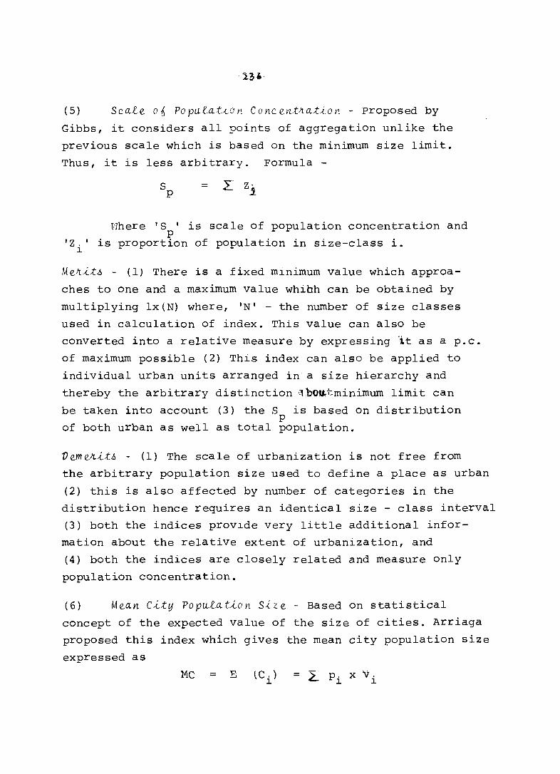
(5) SQale 06 Popula~~on Concen~~a~Ion - proposed by

Gibbs, it considers all points of aggregation unlike the

previous scale which is based on the minimum size limit.

Thus, it is less arbitrary. Formula-

Where '8 ' is scale of population concentration and p

'Z.' is proportion of population in size-class i. 1

MeJt.{_~-6 - (1) There is a fixed mlnimum value which approa­

ches to one and a maximum value whibh can be obtained by

multiplying lx(N) where, 'N' - the number of size classes

used in calculation of index. This value can also be

converted into a relative measure by expressing ·i.t as a p.c.

of maximum possible (2) This index can also be applied to

individual urban units arranged in a size hierarchy and

thereby the arbitrary distinction qbOu.,t::minimum limit can

be taken into account (3) the 8 is based on distribution p

of both urban as well as total population.

VemeJt.{_~-6 - (1) The scale of urbanization is not free from

the arbitrary population size used to define a place as urban

(2) this is also affected by number of categories in the

distribution hence requires an identical size - class interval

(3) both the indices provide very little additional infor­

mation about the relative extent of urbanization, and

(4) both the indices are closely related and measure only

population concentration.

(6) Mean C.{_~y Popula~.{_on Size - Based on statistical

concept of the expected value of the size of cities. Arriaga

proposed this index which gives the mean city population size

expressed as

Me = E l e . ) 1

= ~ p. xV. 1 1

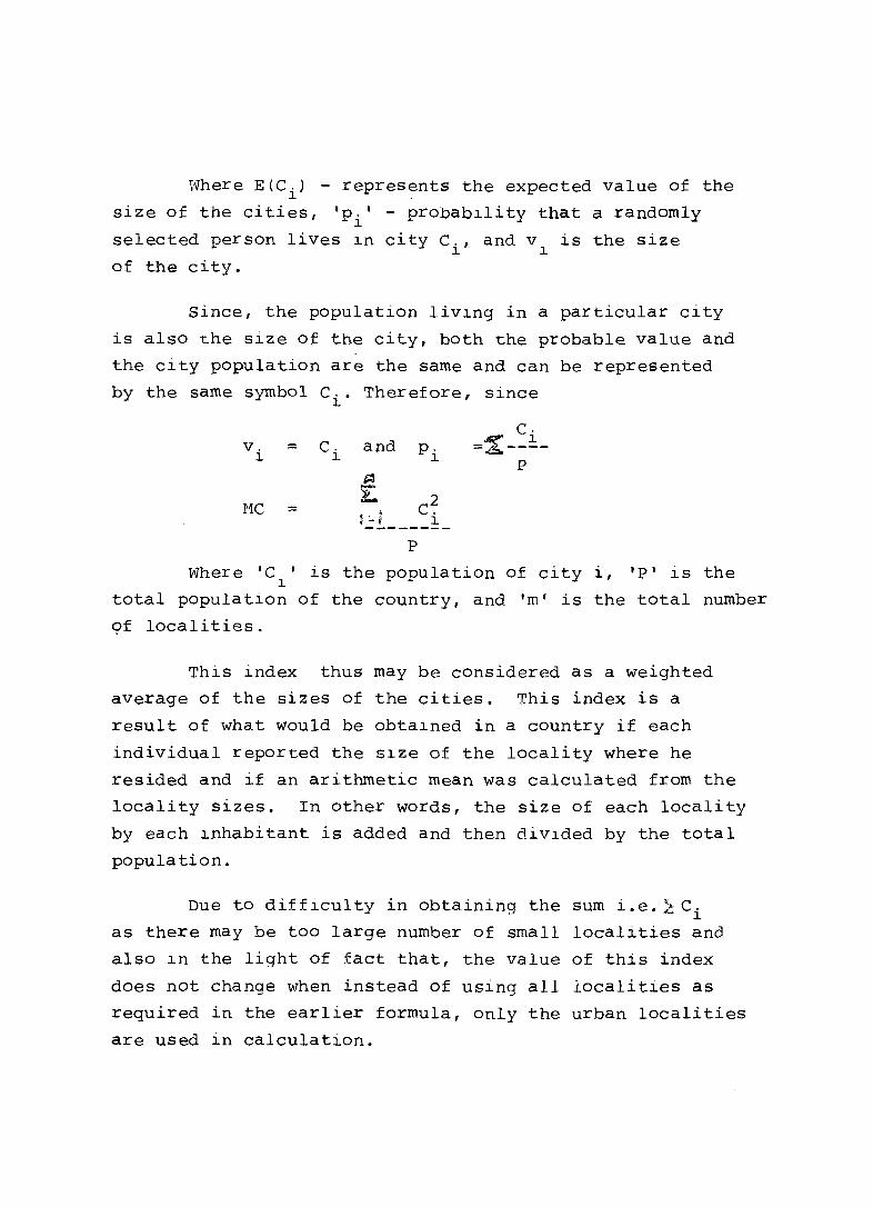
Where E(C,) - represents the expected value of the 1

size of the cities, 'p,' - probab1lity that a randomly 1

selected person lives in city C., and v, is the size 1 1

of the city.

Since, the population livlng in a particular city

is also the size of the city, both the probable value and

the city population are the same and can be represented

by the same symbol C .. Therefore, since 1

. Ci v. = C. and p. =~----1 1 1 P

~

i: C~ MC = t '_ i1 1

P

Where 'e' 1S the population of city 1, 'P' 1S the 1

total population of the country, and 'm' is the total number

9f localities.

This index thus may be considered as a weighted

average of the sizes of the cities. This index is a

result of what would be obta1ned in a country if each

individual reported the Slze of the locality where he

resided and if an arithmetic mean was calculated from the

locality sizes. In other words, the size of each locality

by each 1nhabitant is added and then divlded by the total

population.

Due to difflculty in obtaining the sum i.e. 2: Ci as there may be too large number of small localities and

also in the light of fact that, the value of this index

does not change when instead of uSlng all localities as

required in the earlier formula, only the urban localities

are used ln calculation.

MC =

11\

:£ C~ i:.1_ __ ~ p

here, instead of all localities, only urban localities

are considered. Th1S index can be considered the pro-

duct of two factors i.e. n

MC = E i;:l_~~_ x

N E i=l

n

E i=l

C~ 1

C. 1

Where the first factor represents the urban

proportion of population and the second, the mean

city populatlon size of residence of the urban

population.

If information is not available for each parti­

cular city, but for locality size categories, the index

can be calculated as

MC a =

s E K.Z.

= . -1 J J _1= ______ _

S 2 l: K./m. J=l J J

p p

TrJhere 'IC' is the population in the city size 1

category 'J' , 'm.' 1S the total number of cities in J

the category 'J', IS' is the total number of city size

categories and 'z' is the geometric mean of the city

size' categor~~.". Formula MC is used when the number a of cities included in each category is known, and MCb is used when it is not known for each category. In

this case, the highest city size category is generally

open and there is no category mean. If only a city is

included~the value of ~K. will be equal to K. otherwise ~ - J )

it should be an estimate of the average size of cities

included in the open category.

Cha~aQt~~~~tiQ~: tl) The index does not change significantly

even when the urban definition does. For example, in case of

Panama and Venezuela, the following was the difference when

the index values were computed by considering all urban

localities and only one (in case of Panama) and four

(in case of Venezuela) metropolices respectively.

Panama 1960 Venezuela 1961

Index considering all localities

Index considering the cities of 100,000 or more population

(in OOOs)

85

81

345

336

(2) The index gives absolute value and not the relative

and thus facilitates the international comparison.

L~m~tat~o~~ - (1) Index is affected by the delineation

of city boundaries.

(2) since the square of the population of the

cities is used in calculation in extreme cases, the weight

of the largest city/cities might be "too large".

(7) City Cone~nt~at~o~ I~d~x - This is also based on the

concept of the mean city population size. It compares the

achieved mean city population size Me, with the possible

maximumbity size in a population i.e., total population. I

Thus the index is

cc = _MC_ P

Where, Me is the degree of urbanization and P is the

total population or in other words,

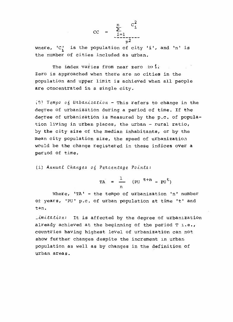
i=l CC = n ~

C~ 1

---------p2

wnere, 'C' is the population of city 'i', and 'n' is 1

the number of cities included as urban.

The index var ies from near zero to L Zero is approached when there are no cities in the

population and upper limit is achieved when all people

are concentrated in a single city.

;~\ Tempo 06 Unban~zat~on - This refers to change in the

deg~ee of urbanization during a period of time. If the

degree of urbanization is measured by the p.c. of popula­

tion living in urban places, the urban - rural ratio,

~y the city size of the median inhabitants, or by the

mean city population size, the speed of urbanizatio~

wou!d be the change registered in these indices over a

perl.od of time.

(i, Annu.al Change.6 06 Penc.en.tage Po~nt.6:

1 TA =

n

Where, 'TA' - the tempo of urbanization 'n' number

of years, 'PU' p.c. of urban population at time It I aLd

t+n.

~~m~~at~on: It is affected by the degree of urbanization

already achieved at the beginning of the period T i.e.,

countries having highest level of urbanization can not

show further changes despite the increment l.n urban

population as well as by changes in the definition of

urban areas.

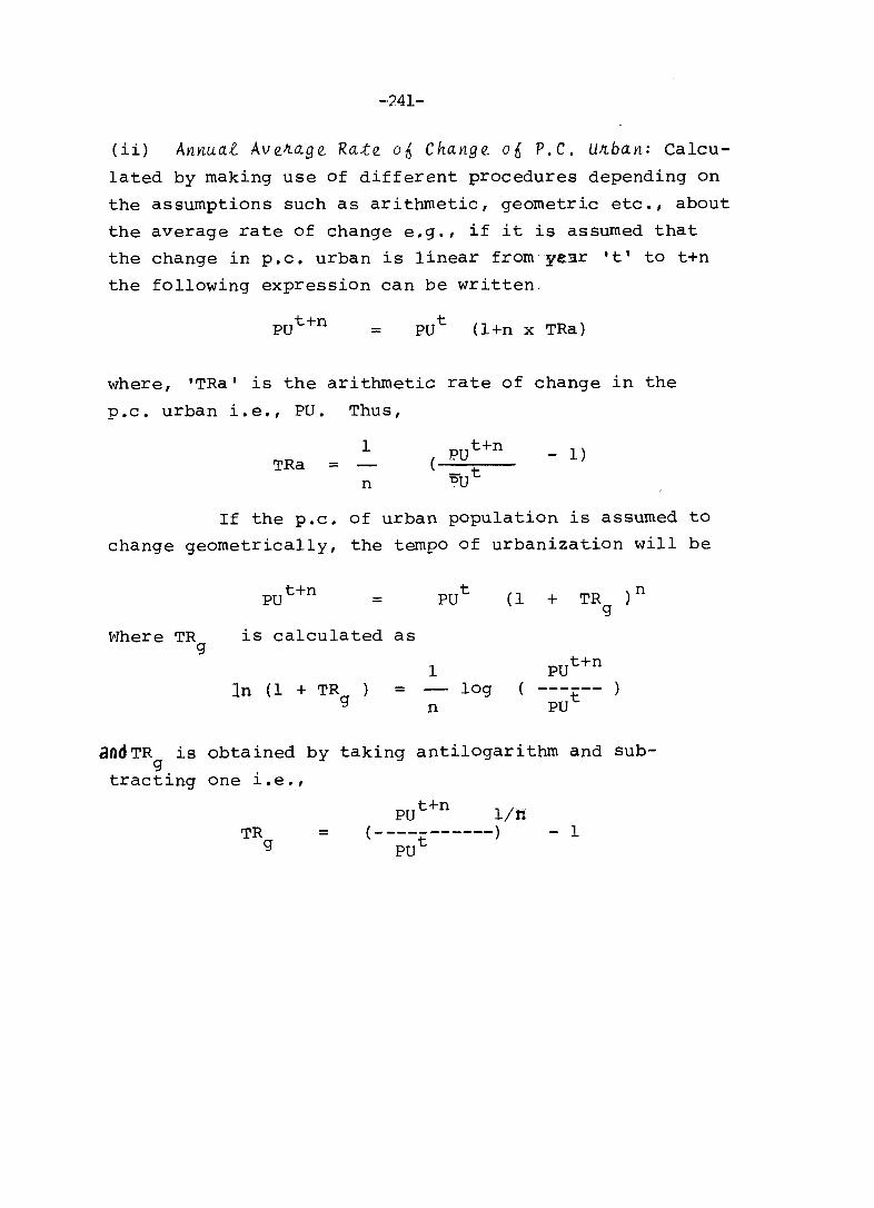
-·7.41-

(ii) Annual Ave~age Rate 06 Change on P.C. U~ban: Calcu­

lated by making use of different procedures depending on

the assumptions such as arithmetic, geometric etc., about

the average rate of change e.g., if it is assumed that

the change in p. c. urban is linear from' ye_:ar 't I to t+n

the following expression can be written.

pu t +n = PU t ( 1 +n x TRa)

where, 'TRa' is the arithmetic rate of change in the

p.c. urban i.e., PU. Thus,

1 - 1) TRa =

n

If the p.c. of urban population is assumed to

change geometrically, the tempo of urbanization will be

= (1 + TR )n g

Where TR g

is calculated as

ln (1 + TR g

1 = log

n ---.---put

andTR is obtained by taking antilogarithm and sub­g

tracting one i.e.,

TR g = PU t +n lib

(- ----------) - 1 put

THE SIMULATION OF THE DEVELOPMENT OF NATIONAL ECONOMICS

REAL IMAGINARY CASE STUDIES

G. P. CHAPMAN

&

ISABELLE TSAKOK

The structure of a gaming simulation of a whole

national economy (Ruristan) in the course of development

is outlined. The model is based on two sectors, urban­

industrial and rural-agricultural, with traders linking

the two parts. There is also overseas trade in dollars

with the rest of the World. The country of ab9ut 35

players is run by its own government, and in the course

of one day goes through six simulated years. Two examples

of recent game runs are discussed. The utility of the

experience in shaping new ideas and understanding of the

development process is discussed, and the psychological

impact on players sensitivity is highlighted. It is shown

why such simulations are radically different from computer

simulations, and why what happens is in many ways real.

The name of the game is EXaction (derived from

the exaction by urban areas of surplus from rural areas),

and is an extension and elaboration of the Green

Revolution Game (Chapman and Dowler, 1982, Chapman 1983)

designed to a requirement of the World Bank. Up to 24

players grouped in pairs are responsible for the running

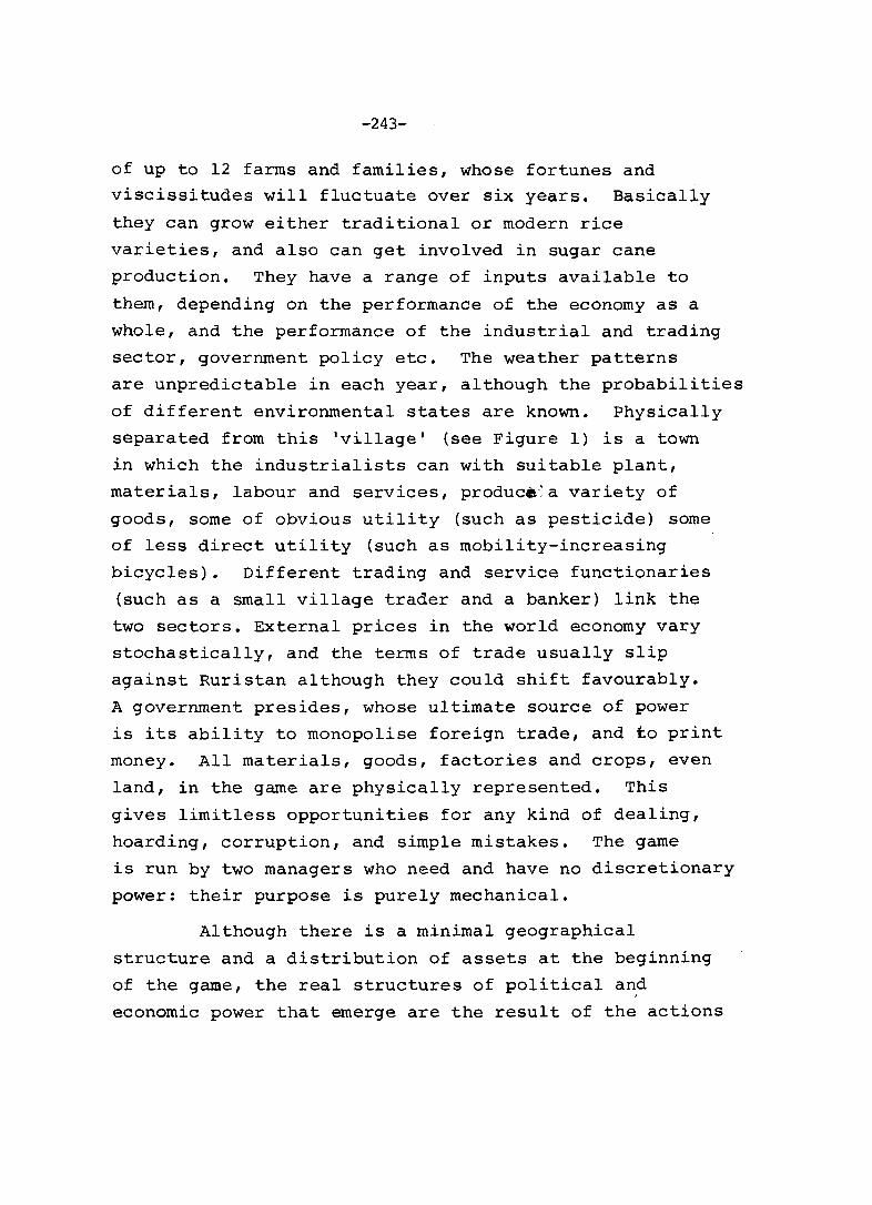
-243-

of up to 12 farms and families, whose fortunes and

viscissitudes will fluctuate over six years. Basically

they can grow either traditional or modern rice

varieties, and also can get involved in sugar cane

production. They have a range of inputs available to

them, depending on the performance of the economy as a

whole, and the performance of the industrial and trading

sector, government policy etc. The weather patterns

are unpredictable in each year, although the probabilities

of different environmental states are known. Physically

separated from this 'village' (see Figure 1) is a town

in which the industrialists can with suitable plant,

materials, labour and services, produc.~a variety of

goods, some of obvious utility (such as pesticide) some

of less direct utility (such as mobility-increasing

bicycles). Different trading and service functionaries

(such as a small village trader and a banker) link the

two sectors. External prices in the world economy vary

stochastically, and the terms of trade usually slip

against Ruristan although they could shift favourably.

A government presides, whose ultimate source of power

is its ability to monopolise foreign trade, and to print

money. All materials, goods, factories and crops, even

land, in the game are physically represented. This

gives limitless opportunities for any kind of dealing,

hoarding, corruption, and simple mistakes. The game

is run by two managers who need and have no discretionary

power: their purpose is purely mechanical.

Although there is a minimal geographical

structure and a distribution of assets at the beginning

of the game, the real structures of political a~d

economic power that emerge are the result of the actions

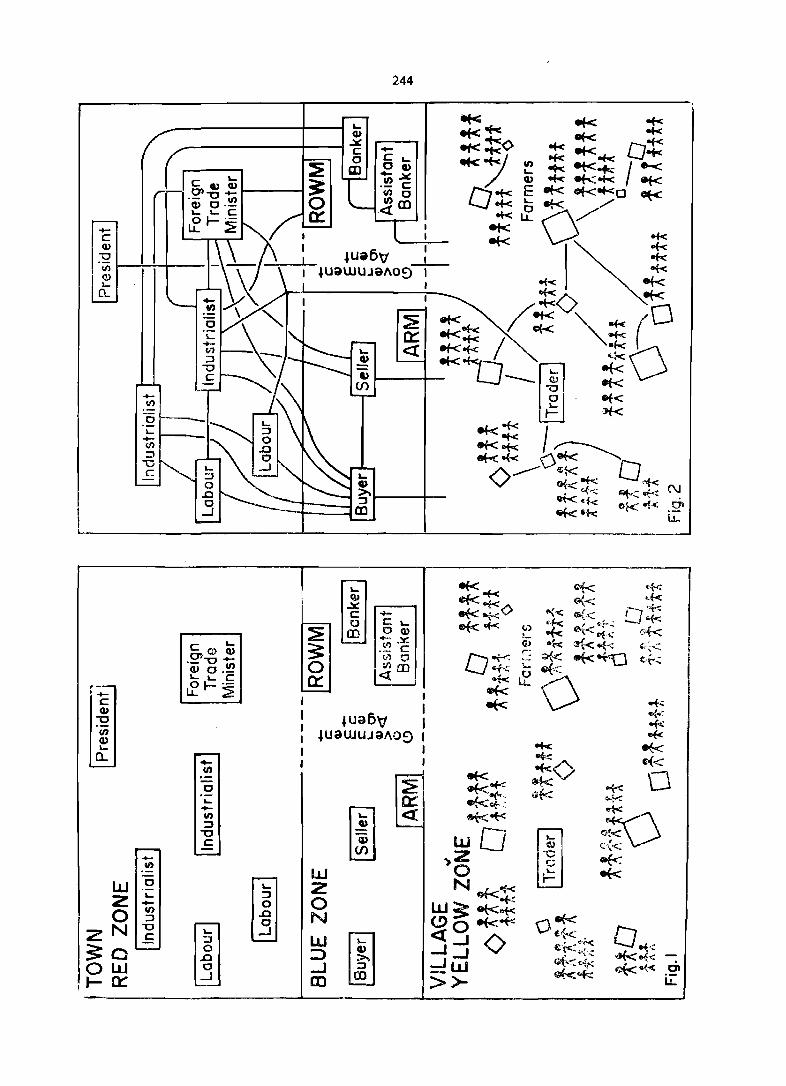
-en

LU 0

Z ~ o 3

zN-g ~Cl OW

I J- 0::

-en

.~ '--en :J

"'0 C

244

~--c'­a Q) 't).x .. _ c (I') 0

I~m , I

l Jua5v I I JuaWUJaJ\o9: I I I I

w z o N LU ::> _J CO

-245-

of the players themselves: how they cooperate, compete,

misunderstand, and learn 'right' and 'wrong' lessons.

The unravelling of what happened, the examination of

national and personal statistics that reveal fragmentary

truths of what occurred, the motivations and policies

of the players, are all examined in a de-briefing that

may take several days more. In fact the interlocking

social, economic, environmental and technical dimensions

make it a field ground for the exploration of many concepts

in development studies.

Two examples of game runs are illustrated next.

The statistical data collected at the end of the runs

are given in Tables la '.to ld and 2a to 2c. The first

example explains how the tables are arranged before

commenting on the run itself. In both cases the

identities of the players are not revealed. Apparently

derogatory references are to players in their game roles,

not to them in real life.

B) Two example~ 06 Game Run~

l) A game 4un a~ ~he 066ice 06 ~he Regi~~4a4 Gene4al

06 India in New Velhi, AP4il 1986.

Four tables have been prepared - showing

weather patterns, pest incidence, and crop type (Table la)

farm and family sizes, births and deaths, consumption,

surpluses and deficits (Table lb) Individual Financial

Performance for both rural and urban sectors (Table Ie)

and National Parameters showing production and some demand

features, imports and exports, balance of payments and

amassed reserves (Table ld).

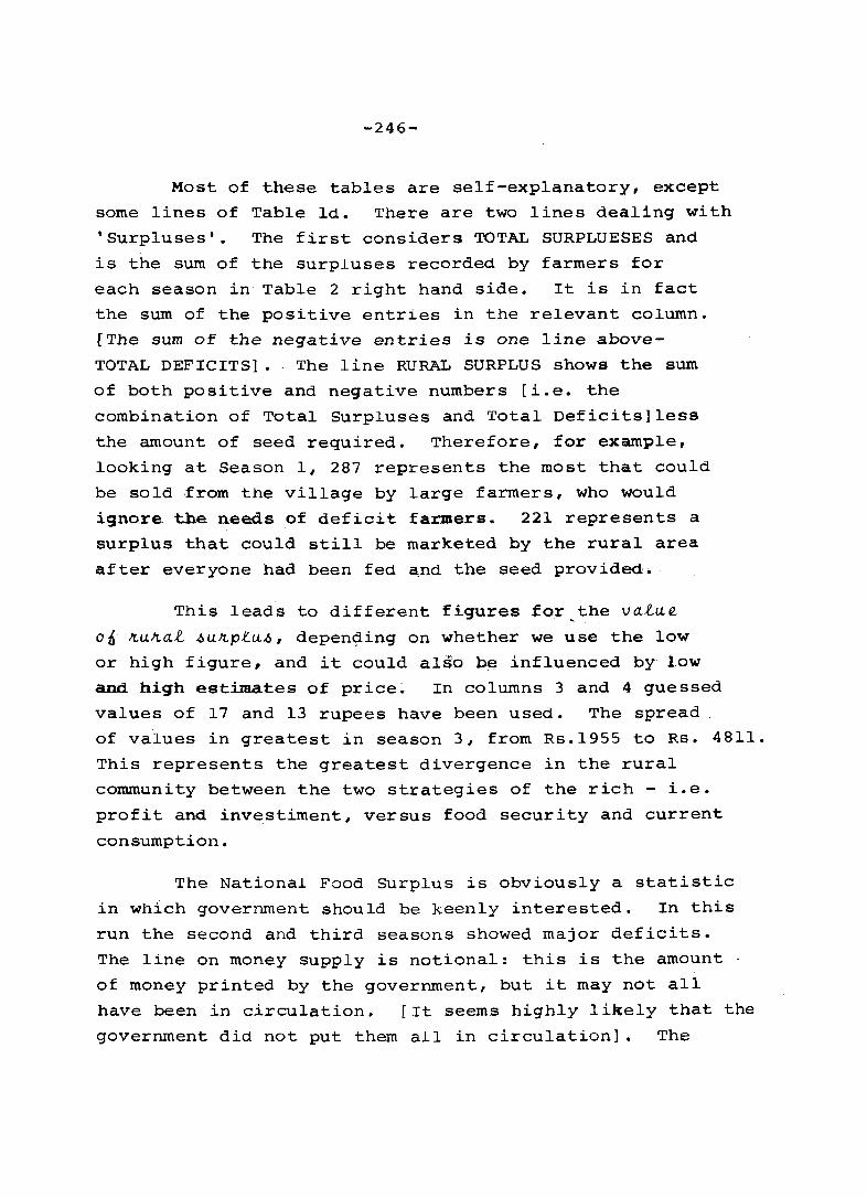
-246-

Most of these tables are self-explanatory, except

some lines of Table Id. There are two lines dealing with

'Surpluses'. The first considers TOTAL SURPLUESES and

is the sum of the surpluses recorded by farmers for

each season in Table 2 right hand side. It is in fact

the sum of the positive entries in the relevant column.

[The sum o£ the negative entries is one line above-

TOTAL DEFICITS]. The line RURAL SURPLUS shows the sum

of both positive and negative numbers [i.e. the

combination of Total Surpluses and Total Deficits]less

the amount of seed required. Therefore, for example,

looking at Season I, 287 represents the most that could

be sold ·from the village by large farmers, who would

ignore. the needs of deficit farmers. 221 represents a

surplus that could still be marketed by the rural area

after everyone had been fed and the seed provided,.

This leads to different figures for the va~ue . ~

on ~u~a~ ~u~p~u~, depen~ing on whether we use the low

or high figure, and it could also bE;! influenced by low

and high est~tes of price~ In columns 3 and 4 guessed

values of 17 and 13 rupees have been used. The spread

of values in greatest in season 3, from Rs.1955 to Rs. 4811.

This represents the greatest divergence in the rural

community between the two strategies of the rich - i.e.

profit and investiment, versus food security and current

consumption.

The National Food Surplus is obviously a statistic

in which government should be keenly interested. In this

run the second and third seasons showed major deficits.

The line on money supply is notional: this is the amount

of money printed by the government, but it may not all

have been in circulation. [It seems highly likely that the

government did not put them all in circulation]. The

-247-

exchange rate is that officially proclaimed by

government, and in this case is real since the Government

maintained a monopoly on foreign trade and foreign

exchange. The balance of payment figures are in $ and

are self-explanatory. The terms of trade are simple

commodity terms -

Pex x 100 Pex = Index of Export = 100 at Prices

Pim Pim = Index of Import = 100 at Prices

without reckoning volume. The agricultural component

is omitted since no trade (export) in agricultural

surplus occurred, although in this case the actual

world pr~ces declined rapidly in the last two years.

Start

Start

The composition of G.N.P. is self-evident. The

concept of 'rural trade' is important - it represents the

two surplus figures of value of Rural Surplus (see

above in the table) expressed as % of G.N.P. If these

are added to % Industrial GNP, and subtracted from 100%,

a range of two figures will be given for estimating

how much of the total economy is subsistence agriculture.

(In season 1 this is 47% or 52%). The last two lines

of the Table show the food saved each year as a result

of stress deaths, and the cumulative value of that food

in $ terms at current world pr1ces.

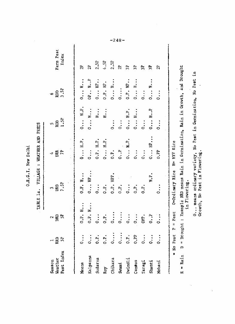
-248-

.j..J

<Il Q) X

P-< Q)

e '8 P-o P-o P-o 14 H If! II) II)

ell P-o P-o . . P-o p... p... p... Po P-< .u ~ N N N -d" N N C""'l M C""'l M N .c

tID (::: g .....

14 P-o A .u

III · p.. P-o p.. ""8 Q)

::d ::d ::d ::d ::z:: ::z:: ::d ::d p... P-o ell

A U"\ 0

"" ~ P-< p.. ~ Z M P-< ...c::

0 0 0 0 0 0 0 0 0 0 0 .j..J (::: ~

0 0

~ .....

.j..J

P-o p.. (::: sg p...

::c ..... . .... ::c :z: ::c ::d ::d :z: s:: e

P-t 14 § Lf'\ • ..-1 Q)

tf} Lf'\ ~ CJ E-I ~ .-I 00 .0 0 0 0 0 0 0 0 0 s:: r.zl d' • ..-1 p...-

O -1-1

~ ..... 00

-1-1 Q)

< p.. p.. p.. p... Q) ~

p..

· . p.. U -..-I ~ :z: :z: :z: ;z :z: -..-I -..-I 0 .c gg ~ e z .-I

~ p... p... p..

Q)

i -d" ...... p.. Po p.. g: Q)

>:~ A CJ o. 0 0 0 0 0 0 0 0 0 0 ::d -1-1-..-1

~ s:: Q) 14 II) If '..-1 • ...t Q)

Z :z: 14 ~ s:: ell 0 r.zl '..-1 >...-1

H t:!J CI) ell rz. ;:S u ,:r::: t-c CJ p... p.. • ..-1 . o-l · ~ Po< . ~ m cd·..-I

~ H ::d ::z:: ::c s:: c: ::> p.. :>,. cd ~

• ..-1 -1-1 0

~ Lf'\ 14 ELl "'0 00

C""'l Po P-< p... p... Po p... ~ e·..-I

"'" Cl)

...... H op... (If 0 0 0 0 0 0 0 0 0 0 • ..-1

~ Q)

...-I "'C ~ II) 0

~ 0 S::Z r.zl ...-I ell

Ii II • Cl) rz. Cl) .~

0 ...-I e'fl -< PcS:: E-r · e·..-I · ~ ::c ::d cd • 0

-1-1 ~ • 14

~ p... p... <Il 00

N Lf'\ Po< Po< Po< P-< . Q)

A . Po< P-< 0 0 0 0 0 0 0 0 0 0 0

If -1-1 ...c::

Po< tID ::l 0

Po -1-1

"'" ~ Po< p.. Po P-< p.. <Il A

...-I Lf'\ . . Q)

0 0 0 0 0 0 0 0 0 0 0 p... II

0 A Z

~ II

~ ~ s:: ~ ell cd • ..-1 '..-1 s:: H s:: s::

"'" ...-I m • ..-1 .;-4 • ..-1 ~ 0 ...c:: \! til

"'" ~ ..... -g ::l bO .u s::

II) .u -1-1 Po cd ~ ! cd c cd cd

~ II) Q) .-l "'d :>,. ..... • ..-1 H l! ,.c.: II

ELl Q) ~ ~ ~ 0 .c ~ ~ CI) tIS ~ to Il.. ~ D A U E-I tf} ~

-249-

N 00 r-. N ..... ..... r-. ~ .-I .-I .....

<""l 0 I ~ I -:t I 00 .-I I

ll"\ N -t) ..... r- oo r-. "" ..... 00 N .--I -:t -t) N ..... -::t ..... -:t .-I

.--I I I

.--I ll"\ r- 0 -:t 0\ 0\ ll"\ .--I 0 \C)

I 00 <""l -:t <""l N I ll"\ -::t .-I I .-I I

N 00 ll"\ .-I 0 0\ -:t 00 -:t -t) 00 N 00 .--I ~ ~ ~ .--I N N

.--I I J I , J

0\ ~ 00 N N 00 -:t 00 R ll"\ .....

.-I .-I .--I <""l N <""l I .-I , I I

-:t

c:: 0

-t) -t) ~

N 00 00 -:t 00 -:t ~ -:t C"1 .-I <""l I .--I .--I I

III qJ cu ..,

<1-1 0

ll"\ 0 0 ll"\ 0 0 ll"\ 0 0 0 ll"\ ll"\ -:t 0\ ~ ll"\ 0 an -t) -:t -:t -:t

.-I '"g II)

ll"\ 0 0 ~ an 0 ll"\ 0 0 0 0 ll"\ ...:T 00 ...:T 0 -:t U'l U'l -:t -:r

.-I ~ <lJ qJ

ll"\ 0 0 ll"\ 0 0 an 0 ll"\ 0 ll"\ ll"\ ll"\ ....... ~ ...:T 0 -:t -:t -:t -:t 00

.--I

.~ c:: .....

~ 0 .... "d ~

0 0 0 0 0 0 an 0 0 0 0 ll"\ -:t -t) ll"\ co 0 C"1 -:t -:t ...:T 0\

.-I ~ .5 0 ....

-E'I 1-1 0 0 0 0 0 0 lI'\ 0 0 0 0 ....... -:t -t) IJ") ,.._ 0\ ("") -:r ....... -:t 00

+.I ~ CIt III ..... . ...

~ ~ ~ S; ~ ~ ~ ~ :2 ~ ~ .-I .-I .-I .-I .-I ~ .-I ... + ... ... + I +

e:l .--I .-I .-I .-I ....... \0 I + I ... + I

&. ~ 0 p:I ~

.a 'S "'-' til .~ ....l ~

....... .--I .--I ~ ....... (g .-I .-I .-I S ... + + I I I I ... ... I e ~ . CIt Z ~ j:Q.

A e:l -:t ..... .-I IJ") .-I I + + I ...

II II

iC iC iC

.-I .-I ... ... .a

~

CIt cu

"'Ct ,.c::: iC iC iC iC iC -t) -t) ..... ll"\ an N ....... 00 -:t -t) IJ") ..... .....

~ III m co cu "'Ct J.I

....... ....... \0 00 "1 IJ") ...... 0 0 ~ C"1 . . . . . . . . . ~ <II III 00

N .-I ..... N N .-I .-I ("") ..... C"1 I til "'Ct J 0 "'Ct 0 .....

00 \0 00 ....... 0\ 0 .-I

lI'\ \0 0\ -t) a ~ 0 .......

.-I ..... . ~ 0\ an -:t -:r -:t ~ \0 ("") -:t ~ n II

e:l ....... .-I

! i! m .... c:: 1-1 ..... .., .... . ... . ...

~ qJ 1-1 ~

.... -g ::t lID +.I c:: ~ qJ i

.., qJ a:: qJ

cu ..... 'g >. .... .... c:: 1-1 .! ..c: cu ~ 0 ,.c::: ~ III qJ :a ;:IS til p:I C,) til e:l C,) ~ til

I ,

-251)-

O.R.G.I. New Delhi

TABLE Ie. INDIVIDUAL FINANC tiL PERFORMANCE

Profit and Loss Urban

Industrialist 1 Starting Assets Assets

Rs 2960/­__ !3:~_:!-'~~~QL: __

Profi t ----__ ~~2QL: __ Industrialist 1 started with 5 factories, and ended with 4 -but also had two generators and considerable stocks of output.

Labour 1 Profit Rs 3520/-[from starting assests of Rs 500/- + 40 mds.rice)

People: 5 adults 5 children at start: 7 and 7 at end.

·':~_rlq;; t~~:7~ ".~~.:~.;j L

BUYER

SELLER BANK

TRADER

RURAL

Meena Kalpana Su"'J.darna Roy Chikara Swami Dwindli Census Taragi Shanti Mohani

Industrialist 2 and Labour 2

These two combined to form a worker/manager cooperative.

Starting Assets Ending Assets

Profit

4557/­_.LE.~2L:_ __ .2.E~L:_

Starting Ass.ets 5 factories: ending assets 8 factories

Profit of Rs

Profit of Rs Profit of Rs

??

GROSS PROFIT 1644 (1344) 7377 (9777)

440 1628 (1028) -449 -632 1044 (-156) 3814 (4414)

-2359 3477 (2877) -512 (-812)

People: 5 adults 5 children at start: 8 and 5 a t end.

548 On starting assets of Rs 1000/-

2073 On starting assets of the 1700/-2914 (Ending ASsets include Debtors Rs 4873/-)

PROFIT PER START ING ACRE SA E.A. 548 (448) 3 4 819 (1086) 9 5

88 5 5 407 ( 257) 4 5

-ll2 4 4 -158 4 3

348 (-52) 3 5 636 (736) 6 5

-786 3 3 869 (719) 4 5

-178 (-270) 3 4

() = Without Land Redistribution SA ::: Starting Acres EA ::: Ending Acres

-251-

O.R.G,I. New Delhi

TABLE Id.. NATIONAL PARAHETERS ------------------------------YEAR 1 2 3 4 5 6

WEATHER RRD DRn DRD DRR RDD RDD PESTS INDEX 5 5 1.5 7 1.5 3.5 7. HYV 9% 237. 23% 41% 37% PRODUCTION 894 763 786 968 881 850 ACRES 48 48 46 45 48 48 YIELD 18.6 15.9 - li.l 21.5 lS.3 11.' RURAL CONSUMPTION 625 645 625 605 570 610 TOTAL DEFICITS -18 -99 -122 -87 -39 -50 TOTAL SURPLUSES 287 217 283 450 350 290 RURAL SURPLUS (AFT ER SEED) 221 70 115 318 263 192 PRICE 15 18 15-1~ 1.--14 14 14 , VALUE 3315-4305 1260-3366 1955-4811 4134-5850 3682-4900 2688-3640 URBAN CONSUMPTION 150 160 170 180 200 215 NATIONAL CONSUMPT ION 775 805 795 785 770 825 NATIONAL FOOD SURPLUS 71 -90 -105 141 51 -23-RURAL'-f~B7D +2 +3-9D -2-7D,.S -2-6D+3 +6-2 l'RBAN BID +1 +2 +1 +2 +2 HONEY SUP;aLY 4800 9800 9800 9800 14800 EXCHANGE RATE 8:1 8: 1 8.25: 1 8.25: 1 8.75:1 $ IMPORTS RICE 80 $I.AGRIC.INPUTS 214 72 $LIND. HAT. 120 139 105 116 2~!! $I.FACTORIES 62 121 127 $E .AGRIC. $E • INDUSTRIAL 375 259 165 803 1581 1$ TOTAL 182 139 105 531 402 E$ TOTAL 375 259 165 803 1581 BAlANCE OF PA1'MENTS +193 +120 +60 +272 +1179 } RESERVES 443 563 623 895 2074 TERMS OF TRADE 100 105 100 91 86

(AGRICULTURAL T.o.T. WOULD HAVE BEEN WORSE) GDP .AGRIC 13410 13734 12580 12077 11662 1190er--GOP. INDUST. 5976 10476 6100 5400 9540 9430 GNP 1938b 24210 18680 17477 21202 21330 % AGRIe 69 57 67 76 56 55 7. Hi'OUST. 31 43 33 24 44 45 RURAL TRADE 17-227- 5-137. 10-227- 24-337- li-23% 13-17% FOOD SAVED THROUGH STRESS DEATHS

a 50 90 135 145 CUMUlATIVE VALUE IN $ 0 137 385 765 1044

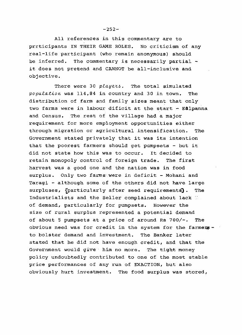
-252-

All references in this commentary are to

prrticipants IN THEIR GAME ROLES. No criticism of any

real-life participant (who remain anonymous) should

be inferred. The commentary is necessarily partial -

it does not pretend and CANNOT be all-inclusive and

objective.

There were 30 playe~~. The total simulated

popula~ion was 114,84 in country and 30 in town. The

distribution of farm and family sizes meant that only

two farms were in labour dificit at the start - Kalpanna

and Census. The rest of the village had a major

requirement for more employment opportunities either

through migration or agricultural intensification. The

Government stated privately that it was its intention

that the poorest farmers should get pumpsets - but it

did not state how this was to occur. It decided to

retain monopoly control of foreign trade. The first

harvest was a good one and the nation was in food

surplus. Only two farms:,.'were in deficit - Mohani and

Taragi - although some of the others did not have large

surpluses, {particularly after seed requirements). The

Industrialists and the Seller complained about lack "

of demand, particularly for pumpsets. However the

size of rural surplus represented a potential demand

of about 5 pumpsets at a price of around Rs 700/-. The

obvious need was for credit in the system for the farme~­

to bolster demand and investment. The Banker later

stated that he did not have enough credit, and that the

Government would give:' him no more. The tight money

policy undoubtedly contributed to one of the most stable

price performances of any run of EXACTION, but also

obviously hurt investment. The food surplus was stored,

-253-

and export of food banned. The Government had the

option of exporting industrial out~ut, or using foreign

exchange reserves, to finance next year's industrial

prcduction. They opted for the former, and f.e.

reserves actually rose. One of the industrialists

formed a successful (and ultimately expansionist)

alliance with labour : the other kept distant from his

labour.

Season 2 was a bad year. Even with a carry­

over of food from the previous year it was obvious

that some food would have to be imported - the

government thought that some would be imported for

the urban poor. The deficit of -99 represents about

12 people at risk - or if -99 + 71 from stored food

-28, about 3 'people at risk. The Government, under

pressure from Kalpa~ proclaimed a minimum price of

rice - which of course stimulated the export to the

=

town of surpluses from the 4 farms with saleable amounts.

But 4 farms were in serious deficit, and the other 3

hardly surviving. Since food arrived in the urban area

the Government relaxed - and sold it at subsidised prices

because of political.',lobbying by urban labour. The

question was, who would suffer? The answer was the

rural poor - 9 people dying of food-stress. This

suggests that food must again have been kept in store.

The deaths occurred on Taragi and Meena - both farms

which showed a slow and confused response to their

problems. Mohani, in as much trouble, staved off death

longer by borrowing, by theft, and by pressure on their

employer Kalpanna. The Government seemed farily unaware

of the events. The farmers complained about lack of

inputs: the industrialists about lack of demand. Bank

credit was exhausted and most of it had been used on

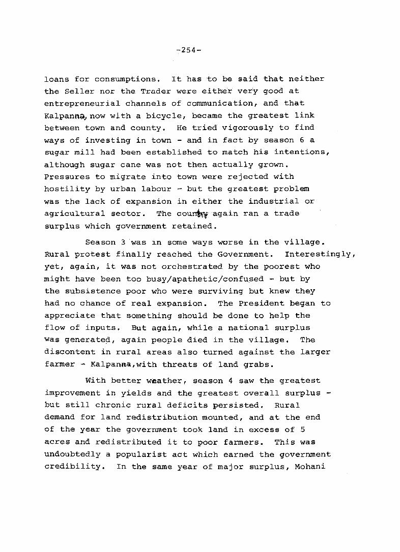
-254-

loans for consumptions. It has to be said that neither

the Seller nor the Trader were either very good at

entrepreneurial channels of communication, and that

Kalpann~now with a bicycle, became the greatest link

between town and county, He tried vigorously to find

ways of investing in town - and in fact by season 6 a

sugar mill had been established to match his intentions,

although sugar cane was not then actually grown.

Pressures to migrate into town were rejected with

hostility by urban labour - but the greatest problem

was the lack of expansion in either the industrial or

agricultural sector. The counhv:again ran a trade

surplus which government retained.

Season 3 ·was in some ways worse in the village.

Rural protest finally reached the Government. Interestingly,

yet, again, it was not orchestrated by the poorest who

might have been too busy/apathetic/confused - but by

the subsistence poor who were surviving but knew they

had no chance of real expansion. The President began to

appreciate that something should be done to help the

flow of inputs. But again, while a national surplus

was generate~, again people died in the village. The

discontent in rural areas also turned against the larger

farmer - Kalpanflc"i,with threats of land grabs.

With better weather, season 4 saw the greatest

improvement in yields and the greatest overall surplus -

but still chronic rural deficits persisted. Rural

demand for land redistribution mounted, and at the end

of the year the government took land in excess of 5

acres and redistributed it to poor farmers. This was

undoubtedly a popularist act which earned the government

credibility. In the same year of major surplus, Mohani

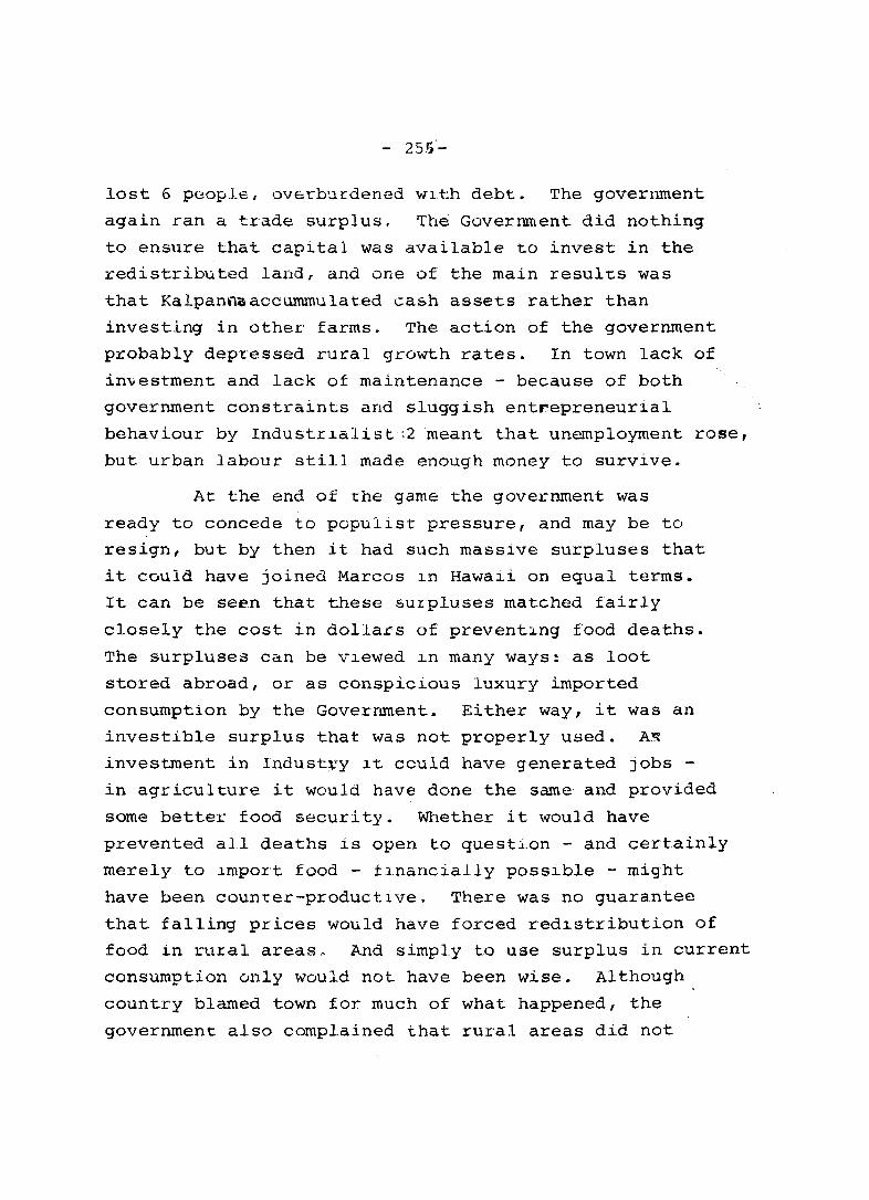
- 25.~-

lost 6 people I oVE:rburdened wl.t~h debt. The government

again ran a trade surplus. '[he Goverrnuent did nothing

to ensure that capital was available to invest in the

redistributed land, and one of the main results was

that Kalpanmsaccumrnulated cash assets rather than

investing in other' farms. The action of the government

probably depressed rural growth rates. In town lack of

investment and lack of maintenance - because of both

government constraints and sluggish entrepreneurial

behaviour by Industrlalist ~2 meant t.hat unemployment rose,

but urban labour still made enough money to survive.

At the end of the game the government was

ready to concede to populist pressure, and may be to

resign, but by then it had such massive surpluses that

it could have joined Marcos ln Hawali on equal terms ..

It can be seen that these surpluses matched fairly

closely the cost in dollars of preventJ.ng food deaths.

The surpluses can be vlewed In many ways: as loot

stored abroad, or as conspicious luxury imported

consumption by the Government. Either way, it was an

investible surplus that was not properly used. A~

investment in IndustrY it could have generated jobs -

in agriculture it would have done the same and provided

some better food securi.ty. Whether it would have

prevented all deaths is open to question - and certainly

merely to lmport food - flnancially possible - might

have been counter-productive. There was no guarantee

that falling prices would have forced redlstribution of

food in rural areas.- And simply to use surplus in current

consumption only would not. have been wise. Although

country blamed town for much of what happened, the

government also complained that rural areas did not

-256-

articulate their demands clearly - and did not cane

up with well-formulated plans. Certainly the rural

areas had a remarkably low level of political cooperation -

but then the interest of the rich and the poor diverged

so much that it was difficult to make demands for the

whole constituency. Kalpannacould have succ~ded in the

early years as a leader, but preferred an individual

role, though he proclaimed he had all-along helped as

many people as possible.

The Government for its part remained poorly

informed about what was happening in rural areas -

and was quite prepared to hide away from it - and was

inherently far too conservative - though stable prices

did result. It also has to be said that the weather

was very bad. But for all that, there was surplus

capital. However, perhaps if all persons had survived,

the surplus would .have been consumed, and the end

result would have been similarly low levels of investment.

The mortality rate in rural areas was very high - and

unemployment also high, both contributing to a strong

push factor. The fact that migration did not occur

was also due to the lack of investment, and an absent

pull factor. Had migration been possible, rural mortality

rates would have been different. The reason for this

state of affairs was not solely a poor government policy:

it was also because of very poor rural political cohesion,

very poor information channels from rural to urban areas

or vice-versa, poor articulation of the service secber,

and possible inadequate credit.

-257 -

2) The Schc(!i 06 Vne,f("pme.rd. S.tudA~e.-6, UI1,lve.tt.-6A-f:.y 06 Ea.6.t AVlg.t--<.C(

'rhis was the smallest game yet run: t.here were

in total 22 particlpants, being arranged in six farms,

one with three players, and the minimal nine urbani

trading roles. This meant that there was no assistan"':

Banker with a bicycle, and only one industrialist and

one urban labour player. They quickly formed a profit­

sharing partnership.

The room geography was fairly restricted, though

there was an adjoining room into which the government

could retire. They chose not to do so once the game

had got well under way, preferring instead (_ ~.o confronr.

crlsis somewhere close behind the front.lines,

The government had strong views before the game

that it would intervene' in food markets, and in the

trading sectors. It accordingly maintained a near

monopoly on overseas trade. The distribution of farm

sizes and family sizes in the village meant that no

farm was in labour deficit at the start: there was

little economlC reason forcing farms to interact.

In year 1 fortune smiled. The perfect weather

and extremely low pest lncldence meant that the highest

average yield ever recorded in any game produced a bumper

crop. The government felt that It had a storage problem

on its hands, and also realised that there might be a

liquidity crisis, since the Buyer had too few funds with

which to buy up the surplus. The government did not

supply more rooney-to the Bank, even though he had lent

money to the Buyer, and the Buyer and others in the tracing

-25~-

Table 28." School of Development· Stadies, Norwicp

FARM SIZES, FAMILY SIZES, CONSUMPrION, SURPLUSES AND DEFICITS .. •• I

FARM NAME SF EF

Sitihajar 6 7

Greenfield 6 6

Murphy 8 9

Chaudhuri 6 8

Shastri 9 13

Quino 5 9

KEY

SF ; Starting Family Size EF - Ending Family Size

B/D

+1.

-ID +2

+2

+4

+4

SA S.ML YRS- YRS-in 1:-4 .

3 2.0 4, 4

4 1.5 2 2

6 1.33 2 0

3 2.0 2 2

3 3.0 5 3

3 1.66 1 1

B/n; biI:ths (+) Deaths (-) for food-stress death SA = starting Acres S.ML~Starting Family/Land ratio YRS= numbers of years in food deficit

FT.

NP NA/SP

1480 493

1320 330

10000 1660

2231 743

-737 -245

2030 676

YRS-in 1-4 = Number of first four years deficit (before land redistribution) NP = Net profit NP/SA = Net Profit per starting acre.

Table 2b. Sc.hool of Development Studies

CROPPING PATTERN, WEATHER AND PEST S

1 2 3 4 5 6 RRR RDD RDR DRD RDD DRD

Sitihajar O.p. 0" • p o ill. t" O. II' .. o til • p 01"1'

Greenfield o CO" (f H" .1' o iJ fI'" H.p. 01' •• H1' •• O.p.H.p.

Murphy Oft" 0 o ~ 0 .~ H l"I tt. o t" '" • O •••

Chaudhuri 0., 0 '" o 0 ~ \) o ••• H •• If o .•. H.1' O.p.H.p. O ••• Hpt1 0

Shastri O. It • 0" \! oR (I l" o .p.H.p.' O.p.H ••• Op •• Rpp. O.,.Hpp.

Quino 0:;> • ., O.ooH"p. o. " . Op •• R.p. o ••• H e •• o .p.R •••

--- means nothing grown.

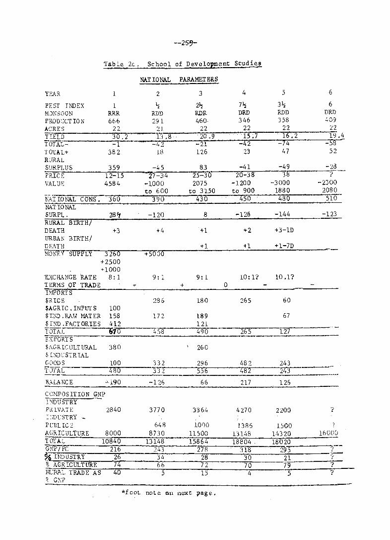
--25~-

Tabl.e 2c, School of Devclopml?-nt Studies

NATIONAL PARAMETERS

YFjl.R 1. 2 3 4 5 6

PEST INDEX 1 ~ 2~ 7~ 3~ 6 HJNSOON RRR RDD RDE. DRD RDD DRD

PRODljCT 10 N 666 291 460· 346 '358 409 A(~~RES 22 21 22 22 22 22 Y]:El,D 30.2 i3 .8 . 20.9 .. '15 ~ 7 16.2 19.4 T'OTAL- -1 -42 -21 -42 -74 ~ TGrAt+ 382 18 126 23 47 52 RURAL SURPLUS 359 -4.5 83 -41 -49 -2B

PRIcE 12-15 2~i4 25-30 20-38 ~ T-VALUE 4584 -1000 2075 -1200 -3000 -2300

to 600 to 3150 to 900 1880 2080

NAT IONAL CONS, 360 390 430 450 480 -S10 NAT ION...<\L SURPl. 2S r1 -120 8 -126 -144 -123 RURAL BIRTH/ DEATH +3 +4 +1 +2 +3-lD URBA~ BIRTH/ DEATH +1 +1 +1-7D MONEY SUPPLY 3260 +50:1

+2500 +1000

'E...'\CHANGE 'RATE 8: 1 9: 1 9: 1 10:1? 10.1? TERMS .OF TRADE 1- + 0 D1PORTS $RICE 286 180 265 60 $AGR IC • IN:?ur S 100 $Il'lD .RAH MATER 158 172 189 67 $I~D . F !\CT OR IE S 412 121

"10 ------__.-.--_ ...

TarAt 458 490 265 127 I;{PORTS - ---$AGR Ie UlT URAL 380 260 $ I:"1)USTRIAL GOODS 100 132 296 ll82 243 T'JfAL ZECi 332 556 482 2··13

BALANCE ;"190 -126 66 217 126

COMPOSITION GNP J:\i)USTRY PRlVATE 2840 3770 3364 4270 2200 't I:;m;STRY rUEL Ie ~ 648 101)0 1385 1500 AGRICULTURE 8000 8730 11500 131~8 1'1320 16000 TOTAL 10840 13148 15864 18804 . 18020 GNP / PC 216 243 27R 118 295 1--% INIYUSTRY 26 -34 28 30 21 ? % ACR IClJLTURE 74 66 72 70 79 ? RCAAL TRADE AS 40 5 15 4 5 ? ~ l. G!-;P

*foot note 0.11 next page.

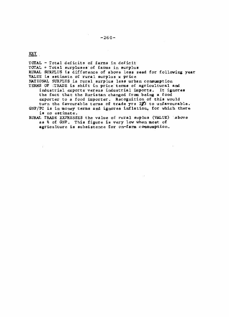
-260-

KEY -TOTAL - Total deficits of farms in deficit TOTAL + Total surpluses of farms in surplus RURAL SURPLUS is difference of above less seed for following year VALUE is estimate of rural surplus x price NATIONAL SURPLUS is rural surplus less urban consumption TERMS OF .~TRADE is shift in price terms of agricultural and

industrial exports'versus industrial imports. It ignores the fact that the Ruristan changed from being a food exporter to a food importer. Recognition of this would turn the favourable terms of trade yrs ztJ, to unfavourable.

GNP/PC is in money terms and ignores inflation. for which there is no estimate.

RURAL TRADE EXPRESSES the value of rural suplus (VALUE) '"above as % of GNP. This figure is very low when most of agriculture is subsistence for on-farm c~nsumption.

-261 ':-

system were either refused or would not use promisory

notes., The buyer was also restricted from export~ng.

The net result of the confusion was that somewhe~c

near 100 mds of rice rotted, the Buyer lost money, and

the Industrialist invested in a godown factcry.

Host1.li ty between the trading sector and the go'\rernment

i)."\.creased. The Industrialist complained f:>1< lack of

rural demand, and exported much of ind\.: strial output.

In foct potential rural demand was as -high as it has

ever been in any game, if only the liquidity prob:_em

had be£\n handled right. The government decj_ded to

invest in its own agro-chemical pJ.ant, which was

relatively capital intensi~e.

Season 2 brought a catastrophic fall in output,

in the fact of a drol1ght ,. There was also the beginnings

of a breakdown in law and order in the rural are.s, j\

dispute over land meant that Greenfield lost p:::-od1.'.ct:.Ol"

for one year fran one acre, Rural confidencQ €.bb~c.,

and host.ili ty focussed on the largest fanne.c, vo1.t1.b:~

Murphy. The govermnent met the crisis by export:"ng a:_l

ir:dus'trial output, and importing rice. Fear.ing the

Banker was uncooperative, it cut him out by refusing

him more credit= This left the count"xy with (1

shortage of man-power in thE. service sector. Exactly

how this shortage was to be met was never made clear:

ad hoc pol-icies of ine£t2asing the money supply ,,'ere

persued in an attempt to raise rural demand_

In season 3 the country was again in slight sur~lus,

though it tC10k some time for the government to rea::.j_s~

tha tit was indeed. a sma 11 one, Murphy had a f e.ir l_y

large surplus, and the government became f:t:xatec. 0:1 the

belief that he was hiding it. The whole trading sys~em

was na~ionalised to control the export of su=p3~ses,

-262-

yet rice was both exported and imported. It became

clear that Murphy had succeeded in selling his stocks

He also managed to promulgate a rumour that he was

undercutting urban prices for new pumpsets. The rumour

(subsequently shown to be true) that Murphy had acquired

massive rupee hoardings unnerved the government in its­

attempts to increase liquidity. Murphy never invested

these surpluses on his own land, thereby failing to

increase his demand for labour from the smaller farmers.

The Seller, now forced to sell at controlled prices

lost motivation, and lacked anyway the credit to supply

the smaller farmers. The smaller ones, except Green­

field, formed a cooperative (this happened in nascent

form in the first year) which they felt helped their

survival in the face of government indifference, and

certainly provided a reasonable political mouthpiece.

The Government's production of agro-chemicals was

again exported, through 'lack of demand'.

Comparative failures in agriculture in the

next two seasons forced the country into crisis. The

government abandoned any long term perspective view on

the economy, and committed itself to land redistribution.

This it forced through with the supoort of ,the smaller

peasants and against Murphy's opposition, but he had

so failed to capitalise-.on his position in the rural

area, and instead of exercising patronage had antagonised

others, that he had no power base for resistance. It

was quite obvious that the farmers saw this as in their

best interests and as evidence that for the first time

the government took notice of 'the real productive base

in the economy' (their view). It also became clear that

the government had not thought about the consequences of

-26l-

failing to invest: it exhausted its foreign exchange

in buying food abroad, and allowed industry to spiral

into decline. It despatched an emergency mission to

seek a foreign loan, but failed to provide any

statistics on the National Accounts, which hindered

negotiations. In the fifth year there was considerable

death in the urban areas.

Throughout the linkages between the different

parts of the economy failed to work smoothly.

Interference by the government and nationalisation

were thought to be cost-free adventures. The quasi

monopoly on foreign exchange meant that there was no

effective relationship between internal and external

prices. The Industrialists and the government itself

became two enclave sectors, dealing in

haYing no relationship to the internal

through very small demands for labour.

dollars, and

economy except

The putative

exchange rate had no real meaning. The prices for

agro-c;chemicals were kept low and constant, which

meant a real subsidy, but were not in demand because

the farmers thought them useless without pumpsets,

and the government never really understood why these

were not in wider use in the village - indeed it probably

had no idea at all of the percentage of irri.ation.

In this run it is probably fair to say that

the government did not respond flexibly enough to the

favourabl.e circumstances in the first year, and that a

real investment opportunity was lost: that it mis­

calculated the increase in managerial time required as

a result of nationalization; that it overemphasised

the Significance of Murphy's 'parallel economy' and

devoted too much time to destroying it; that the peasant

-264-

sector had no real idea of the productive value of

the urban sector and collectively viewed all urban

persons as unhelpful and parasitic. But clearly the

Government had difficult problems to deal with,

once of which, population growth, was never mentioned

even in the debriefing. It should also be said that

because of the small size of the economy, output in

both rural and urban areas fluctuated more than usual,

and this instability had much to do with the psychological

pressures that forced government to abandon a perspective

view.

'Initial Aims were

to stimulate industrial production to provide the

rural areas with necessary inputs.

to ensure food availability by giving a loan to

industrialists to produce godowns

to give loans to the industrial sector to produce

pump sets

to prohibit the export of all but one pumpset in

any year, and to encourage the export of bicycles •

. 'l.6 .t y e. a.}(.

'We thought we had a massive liquidity crisis,

and therefore we printed money, b.t did not release it

through the banking sector. We used the money to buy

up surplus. Foreign exchange was used to build a

fertilizer factory. Money was also given to industry

as a loan to pay labourers so they could buy their

food.

Problems: 60 mds of rice not stored but lost, a lack

of control in the rural area's and some hoarding - Murphy

stole a godown from the Buyer and used it for hoarding.

-2f)~-

7. Yl.d Ye.(Vt

'Afte~ the first year we had nothing but bad

we~ther, and low ag~icultural output, therefore the

go-uerrunent was forced to import rice. The gove=nment

had to run the agro-chemical plant - which used foreign

exchange, but output was either exported or directeq

to the nationalised economy. This was one of the most

successful government interventions. The marketing

system in the rural areas was very unclear. The

government felt it had to intervene in marketing, the

Buyer and Seller were not functioning properly" The5.!."

lack of liquidity was the main reason for. nationalising

them.

3ILd Ye.a-IL

'The year was a breakeven in agricultural

production. We did not want to import food, bu.t were

forced to do so and to sell it at subsidised prices.

There was a dual economy in the rural areas: so we

nationalised the Trader. Attempts to control Murphy

were unsuccessful. The Industrial sector \01as in crisis

with failures and decreased output. There was a

problem throughout w':'th the linkages between the! r.'u!:a]_

and urban sectors. This problem was never sol~·p-d.

The government wanted to provide industrial produ.c'ts

to the rural areas but this policy failed partly

because of the unequal structure in the rural areas,

and also because of bad agricultural production and

the need to feed industrial labourers, which lead to

the forced export of industrial output,

-26 (,-

4:th Yea.Jt.

'Another bad year. We stimulated the formation

of the cooperative by giving interest-free loans

through the Seller. Rural areas got access to subsidised

inputs of fertilizer, pestic~de and pumpsets. We

redistributed Murphy. Urban areas were in food deficit'.

Ma.na.geJt.'~ Com~n:ta.Jt.y on ;the PJt.e~iden;t'~ V~ew

The initial policy aims are stated from an

industrial urban viewpoint: and from the viewpoint of

production not marketing. The rural areas will

supposedly respond to the planned stimuli. Even at this

level the policy is arbitrary: why government itself

should set up in agro-chemicals rather than giving

them to the Industrialist is not clear. When it

becomes clear to government that the system is not

working as it hoped, it assumes that what it does no~

undeJt.~;ta.nd is nece~~aJt.~~y no;t woJt.k~ng well, and that

therefore in exercising its sense of responsibility

and accountability it must nationalise the system.

When the reconstructed system still fails to work,

blame is put on the weather, also on the fact that the

linkages between urban and rural areas represented a

problem that was never fully solved. The implication

is that still further control was necessary.

The government never asked itself what was its

own source of power, and ~ts failure to do so was part

of the reason for its failure to understand what was

going on. It held the major financial instruments of

the economy, and the urban sector generally held the

trading and production keys that would make technolog~cal

-26'1-

change possible in rural areas. The ru,!:"al areas

were either at or near subsistence, or elee in a

dependent trading position. Being po}.itica:ly

weak and with poor communica t~ons t.hey were unable

to persuade government to consider seriously

policies which would free that trading networks

rather than stifle them, extend the financ:_al

l.nfrastructure, and which would proV'ide a

coordinated and balanced package of inputs. The

top-down structure could probably only serve ,.g:.der

interests by voluntarily becoming more bottom \:~p.

To do so would not be an abdication of power and

responsibility, even though it might seem so at

the time.

C) The U~~~~~y on ~he Game

Clearly this game can be considered in many

different lights. It can be examined as a teaching

tool, which carries many different kinds of lessons

for different participants, but it can also be

considered for what it reveals about the nature of

academic enquiry into the development processo

~l A~ a ~each~ng ~ool

As a teachinq tool it is unconventional.

There is no I teacher I who pronounces (l.ect!!t2:eS) to

a relatiyely passive audience - teaching by instruction.

This is learning by experience, but the experi~nce that

will be created and the lessons that will be learnt are

not predictable. To that extent if the Manager

r::onsiders himself a teacher then he may f::"nd the expcriencp.

too threatening, not knowing where it will go. By

-261-

definition, it is also very interdisciplinary. We

have seen sociologists give comprehensive analyses

of a game run in terms of group dynamics, when the

same game has been 'completely' explained in economic

terms. More usually one finds the limits to

disciplinary perspectives exposed: that the economic

viewpoint will give an insight only into so much,

resting on some--:poli tical assumption, or indeed vice­

versa. At the individual level one understands that

using a few selected variabl"es does not summarise

the individual and his circumstances: that each

farmer is a whole person in a social, environmental

and economic context, and that-any explanation has

to include concepts such as responsibility, foolishness,

hassle, nervous energy, anger, envy. One also understands

that everything at both micro and micro-level is

contingent. The President may make a 'wrong' decision

because of lack of information, or because the terms

of trade go wrong, or because of political problems

in the village. In other words what could have been

a right decision was contingent on many other factors.

We have used the game with the following

target groups (but this is not an exhaustive list).

1. Specialists who need to put their own particular

expertise in a broader context.

2. practitioners and students of macro-economics,

finance and banking, who are exposed to the

relationships between macro-and micro policy.

3. Students of development policy who have no

experience against which to evaiuate critically

the literature they read.

4. Professionals and volunteers who are going to work

in development projects to enhance understanding

of the relationships between town and country,

government and farmer perception.

-269-

5. Policy maskers who wish to generate

research hypotheses and undertake

sensitivity analyses of policy implementation.

6. Extension agents and their managers •

. Usually the game is run during a residential

course or seminar which lasts a week or more.

It is also used in universities, but one

should not under-estimate the difficulty of persuading

colleagues to surrender a day and a half or more of

the timetable to one particular individual's

unconventional teaching ideas.

3, The Cha,e.£..en.ge ;to Ac.adem-<-c. Enqu.-<-!t.y

The second light from which we can leok at.

the game is the challenge it represents to academic

enquiry. We think it fair to say that this is the

closest anyone has yet got to . ·~.6el!ing' a whole

national political economy/social formation.

But even though all that takes place does so

usually within one room, no participant has other than

a fragmentary view of the 'total information' (whatever

that might be) that was potentially available, and no

participant can state what was the whole picture. In

the same way that what happens is always contingent, so

all understanding is partial and contingent on the

viewpoint and information, and nee£..-<-l1g.6, of the observers.

All the information is in one sense subjective: for

every piece of information a participant seeks to

acquire, there was always a limitless amount of other

things about which he CQuld have enquired. And what

-27~-

he does depends on what information he does acquire,

and that will affect the information that other

participants collect.

In other words, the game is a true human

community of reflexive human beings. These are the

basic buildings blocks: not the geography of the room

and the mechanics of the game. These building blocks

have differential memory, diplomatic and negotiating

skills. different training. The combinations of these

attributes and the emergent properties of the whole

are unpredictable. This unpredictability is related

to the reality of the game. Although in one sense the

game is unreal (all participants will suggest additions

for 'more reality') it is because what happens is so

manifestly the result of what participants do, that

clearly the result is 'real'. And because the results

are so unpredictable, that also increases the credibility

of the model. In the end we find that understanding

has nothing to do with prediction.

We believe there is no other way of modelling

a national political economy. (We are not referring

to descriptive or analytical models, but to dynamic

simulations). Such national systems are characterised

by emergent effects, unrepeatable idiosynchratic

performance. They are relexive, acting on components

decision makers, who through their own perception and

actions act on the system. All of these perceptions

are by definition based on partial information and

misinformation. These properties cannot be replicated

on a computer, but only in a system with human beings

as the components. (This argument is developed fully

in Chapman 1984).

-271-

The majority of explanatory accounts of

national development patterns and processes each claim

to have found the majority of the 'truth', even when

these major parts of the truth are so patently conflicting -

which of course accounts for the intensity of the

debates. These differences stem from the fact that no

observer observes the whole 'whole', and that each

observes only some subjectively defined whole. But

when he is a 'passive external' observer of the 'real'

world (a real nation state), whose extent ranges far beyond

is visual boundaries, he is not so confronted by the

necessity of feeling the extent to which he is

ignorant of the 'whole'. Tbe gaming simulation makes

everyone much humbler about the extent of knowledge

and theorising possible, and emphasizes the difference

between prediction and understanding. Ultimately of

course the point of all education and theorising for

the majority is better actors, not better predictors.

A second challenge to academic enquiry comes from the

interdisciplinary nature of the experience of such games

and th€ir interpretation. An economic data set may be

explained by economic concepts. A demographic data set

may be explained by demographic concepts. In the 'real'

world we are used to the separate collection and

presentation of such data, by departments of Industry

and by Registrar Generals perhaps. In the case of these

simulations the starting point is not pre-selected data,

but the experience in which the data can be generated.

We hope it can stimulate the collection and analysis of

interdisciplinary material and the modes of analysis

that can acoompany it, and also open insights into the

relationship between understanding which occurs at

different hierarchical levels.

-27~-

Chapman, G.P. and Dowler, E.A. (1982) The Green

Revolution Game, Cambridge.

Chapman, G.P. (1983) The Evolution and Impact of

the Green Revolution Game and Exaction, mimeo

Dept. of Geography, Cambridge and World Bank,

Washington.

Chapman, G.P. (1984) 'Gaming Simulations and Systems

Analysis: Two Factions of the Truth' Dialoguing

with Decision Makers International Institute of

Applied Systems Analysis, Laxemburg, Aust~ia, mimeo.

Chapman, G.P. and Tsakok, I. (1985) Exaction Development

Policy Ltd, Cambridge

· A P PEN DIe E S

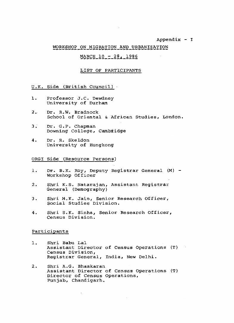
Appendix - I

WORKSHOP ON MIGRATION AND URBANIZATION -----.... ----_._---_ .......... - ... -----------------,... MARCH 10 - 28 1986 ____________ ~L ____ _

LIST OF PARTTCIPANTS

u. K. Side (British Counci'l)

1. Professor J.C. Dewdney University of Durham

2. Dr. R.W. Bradnock School of Oriental & African Studies, LOndon.

3. Dr. G.P. Chapman Downing College, Cambtidge

4. Dr. R. Skeldon University of Hongkong

ORG! Side '(Resource Persons)

1. Dr. B.K. Roy, Deputy Registrar General (M) -Workshop Officer

2. Shri K.S. Natarajan, Assistant Registrar General (Demography)

3. Shri M.K. Jain, Senior Research Officer, Social Studies Division.

4. Shri S.K. Sinha, Senior Research Officer, Census Division.

Participants

1. Shri Babu Lal Assistant Director of Census Operations (T) Census Division, Registrar General, India, New Delhi.

2. Shri A.G. Bhaskaran Assistant Director of Census Operations (T) Director of Census Operations, Punjab, Chandigarh.

-276-

3. Dr. S. Boopathy, Linguist Language Division, Registrar General, India, Calcutta

4. Shr~ Budh Singh Assistant Director of Census Operations (T) Social Studies Division, Registrar General, India, New Delhi.

5. Shri S.P. Desai, Assistant Director of Census Operations (T) Director of Census Operations, Goa, Daman & Diu, Panaji.

6. Shri A.K. Dutta Deputy Director of Census Operations Director of Census Operations, West Bengal, Calcutta.

7. Shri S.P. Grover, Deputy Director of Census Operations, Director of Census Operatoins, Madhya Pradesh, Bhopal.

8. Shri Hari Kishan Assistant Director of Census Operations Director of Census Operations, Rajasthan, Jaipur

9. Shri Karan Singh Assistant Director of Census Operations (T) Director of Census Operations, Punjab, Chandigarh.

iO. Shri Y.G. Krishnamurthy, Deputy Director of Census Operations Director of Census Operations, Andhra Pradesh, Hyderabad

11. Shri Mahesh Ram Research Officer, Map Division, Registrar General, India, New Delhi.

12. Shri H.S. Meena Assistant Director of Census Operations (T) Director of Census Operations, Bihar, Patna.

13. Shri v.s. Nagle Investigator

-277-

Director of Census Operations~ Maharashtra, Bombay

14. Shri J.K. Patel Deputy Director of Census Operations Director of Census operations, GUjarat, Ahmedabad.

15. Shri Phool Singh Deputy Director of Census Operations Demography Division Registrar General, India, New Delhi

16. Shri S.R. Puri Research Officer (Map) Director of Census Operations, Haryana, Chandigarh.

17. Dr. Rajendra Kumar Gupta Geographer Director of Census Operations, Assam, Guwahati

18. Shri R.P. Singh, Research Officer (Map) Director of Census Operations, Uttar Pradesh, Lucknow

19. Smt. Suman Parashar Assistant Director of Census Operations (T) Social Studies Division, Registrar General,India, New Delhi

20. Shri S.D. Tyagi Research Officer, Map Division, Registrar General, India, New Delhi.

21. Shri K.N. Unni Senior Research Officer Demography DiVision, Registrar General, India, New Delhi.

22. Shri R.K. Puri Deputy Director of Census Operations, Demography Division, Registrar General, India, New Delhi.

23. Shri Subhash Garg Assistant Director of Census Operations, Demography DiVision, Registrar General, India, New Delhi.

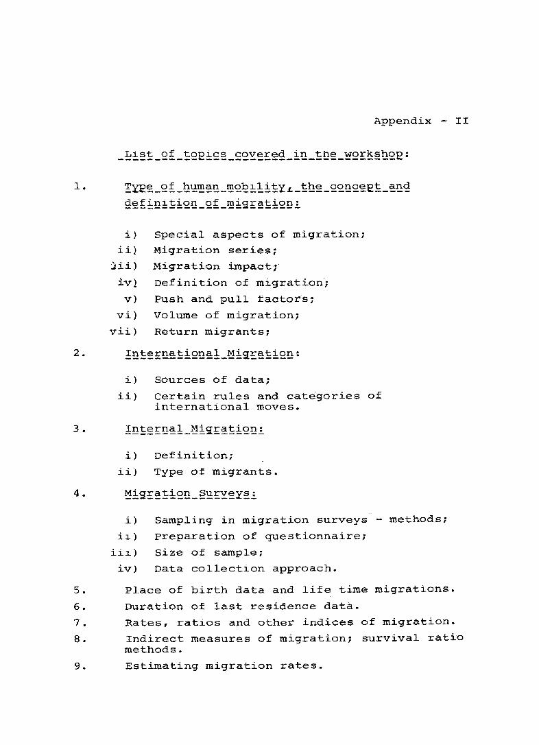
Appendix - II

1. !~E~_2~_h~~e~_~~~~1~~YL_~h~_2~~s~et_~~~

£~;~n!~!~~_~~_~i9E~~!2nl

i)

iil ';i3..)

tv)

v}

vi)

vii)

Special aspects of migration;

Migration series;

Migration impact;

Definition o£ migration;

Push and pull factors1

Volume of migration;

Return migrants;

i) Sources of data;

ii) certain rules and categories of international moves.

i) Definition;

ii) Type of migrants.

i)

i1)

iii)

iv)

Sampling in migration surveys - methods;

preparation of questionnaire;

Size of sample;

Data collection approach.

5. Place of birth data and life time migrations.

6. Duration of last residence data.

7. Rates, ratios and other indices of migration.

8. Indirect measures of migration; survival ratio methods.

9. Estimating migration rates.

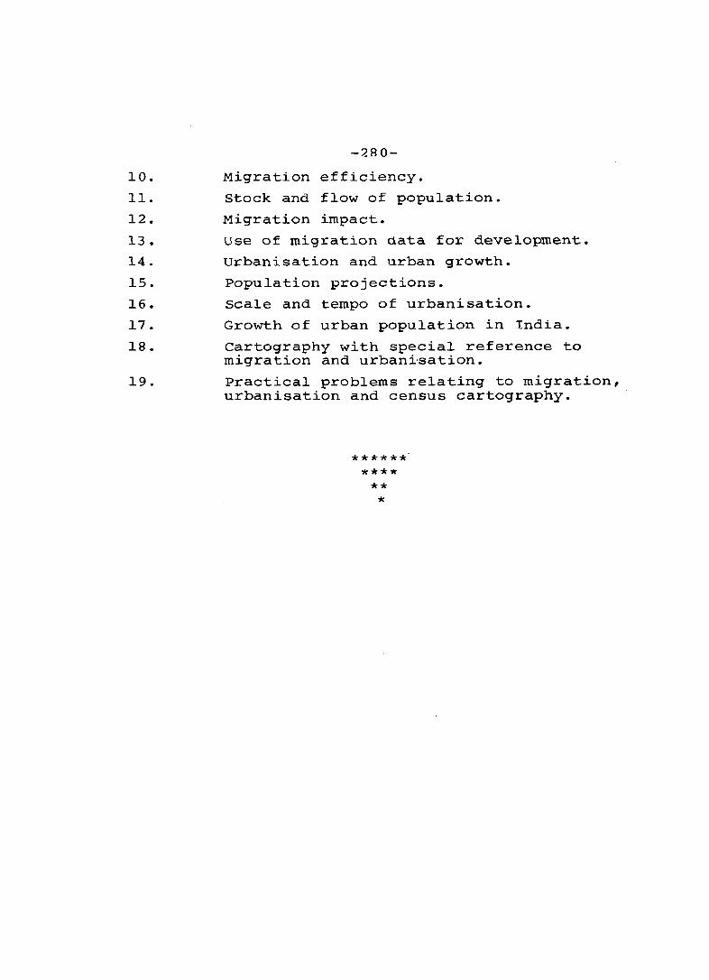
10.

11.

12.

13.

14.

15.

16.

17.

18.

19.

-280-

Migratl0n efflciency.

Stock and flow of population.

Migration impact.

use of migration data for development.

urbanisation and urban growth.

Population projections.

Scale and tempo of urbanisation.

Growth of urban population in Indla.

Cartography with special reference to migration and urban~sation.

Practical problems relating to migration, urbanisation and census cartography.

****** ****

** *