
Pre-Proceedings of the Workshop on Cognitive Computation
158
29th Annual Conference on Neural Information Processing Systems (NIPS 2015) Pre-Proceedings of the Workshop on Cognitive Computation: Integrating Neural and Symbolic Approaches (CoCo @ NIPS 2015) Tarek R. Besold, Artur d’Avila Garcez, Gary F. Marcus, and Risto Miikkulainen (eds.) Montreal, Canada, 11th & 12th of December 2015
-
Upload
khangminh22 -
Category
Documents
-
view
0 -
download
0
Transcript of Pre-Proceedings of the Workshop on Cognitive Computation

29thAnnualConferenceonNeuralInformationProcessingSystems(NIPS2015)
Pre-ProceedingsoftheWorkshoponCognitiveComputation:
IntegratingNeuralandSymbolicApproaches(CoCo@NIPS2015)
TarekR.Besold,Arturd’AvilaGarcez,GaryF.Marcus,andRistoMiikkulainen(eds.)
Montreal,Canada,11th&12thofDecember2015

InvitedSpeakersofCoCo@NIPS2015
• AntoineBordes,FacebookAIResearch.• RinaDechter,UCIrvine.• PedroDomingos,UniversityofWashington.• RamanathanV.Guha,GoogleInc.• GaryF.Marcus,NYUandGeometricIntelligence.• StephenH.Muggleton,ImperialCollegeLondon.• DanielL.Silver,AcadiaUniversity.• PaulSmolensky,JohnsHopkinsUniversity.• JoshTenenbaum,MassachusettsInstituteofTechnology.• GregWayne,DeepMind,GoogleInc.• MichaelWitbrock,CycorpInc.

Contents:ContributedPapersOralpresentations:TuringComputationwithRecurrentArtificialNeuralNetworks(Carmantini,BeimGraben,Desroches&Rodrigues)LiftedRelationalNeuralNetworks(Sourek,Aschenbrenner,Zelezny&Kuzelka)RelationalKnowledgeExtractionfromNeuralNetworks(Franca,Garcez&Zaverucha)CombinatorialstructuresandprocessinginNeuralBlackboardArchitectures(VanderVelde&DeKamps)Posterpresentations:Requestconfirmationnetworksforneuro-symbolicscriptexecution(Bach&Herger)Tree-StructuredCompositioninNeuralNetworkswithoutTree-StructuredArchitectures(Bowmann,Manning&Potts)ARecurrentNeuralNetworkforMultipleLanguageAcquisition:StartingwithEnglishandFrench(Hinaut,Twiefel,Petit,Dominey&Wermter)EfficientneuralcomputationintheLaplacedomain(Howard,Shankar&Tiganj)NeuralNetworkModelofSemanticProcessingintheRemoteAssociatesTest(Kajic&Wennekers)

ProbabilityMatchingviaDeterministicNeuralNetworks(Kharratzadeh&Shultz)TheUsefulnessofPastKnowledgewhenLearningaNewTaskinDeepNeuralNetworks(Montone,O’Regan&Terekhov)SymbolGroundinginMultimodalSequencesusingRecurrentNeuralNetworks(Raue,Byeon,Breuel&Liwicki)ExtractingInterpretableModelsfromMatrixFactorizationModels(SanchezCarmona&Riedel)EarlyDetectionofCombustionInstabilitybyNeural-SymbolicAnalysisonHi-SpeedVideo(Sarkar,Lore&Sarkar)PredictingEmbeddedSyntacticStructuresfromNaturalLanguageSentenceswithNeuralNetworkApproaches(Senay,Zanzotto,Ferrone&Rigazio)BuildingMemorywithConceptLearningCapabilitiesfromLarge-scaleKnowledgeBase(Shi&Zhu)Fractalgrammarswhichrecoverfromperturbation(Tabor)AnalogyMakingandLogicalInferenceonImagesUsingCellularAutomata-basedHyperdimensionalComputing(Yilmaz)

Turing Computation with
Recurrent Artificial Neural Networks
Giovanni S. Carmantini
School of Computing and MathematicsPlymouth University, Plymouth, United Kingdom
Peter beim Graben
Bernstein Center for Computational Neuroscience BerlinHumboldt-Universitat zu Berlin, Berlin, [email protected]
Mathieu Desroches
Inria Sophia-Antipolis MediterraneeValbonne, France
Serafim Rodrigues
School of Computing and MathematicsPlymouth University, Plymouth, United [email protected]
Abstract
We improve the results by Siegelmann & Sontag [1, 2] by providing a novel andparsimonious constructive mapping between Turing Machines and Recurrent Ar-tificial Neural Networks, based on recent developments of Nonlinear DynamicalAutomata. The architecture of the resulting R-ANNs is simple and elegant, stem-ming from its transparent relation with the underlying NDAs. These characteris-tics yield promise for developments in machine learning methods and symboliccomputation with continuous time dynamical systems. A framework is providedto directly program the R-ANNs from Turing Machine descriptions, in absence ofnetwork training. At the same time, the network can potentially be trained to per-form algorithmic tasks, with exciting possibilities in the integration of approachesakin to Google DeepMind’s Neural Turing Machines.
1 Introduction
The present work provides a novel and alternative approach to the one offered by Siegelmann andSontag [1, 2] of mapping Turing machines to Recurrent Artificial Neural Networks (R-ANNs). Herewe employ recent theoretical developments from symbolic dynamics enabling the mapping fromTuring Machines to two-dimensional piecewise affine-linear systems evolving on the unit square, i.e.Nonlinear Dynamical Automata (NDA)[3, 4]. With this in place, we are able to map the resultingNDA onto a R-ANN, therefore providing an elegant constructive method to simulate a Turing ma-chine in real time by a first-order R-ANN. There are two main advantages to the proposed approach.The first one is the parsimony and simplicity of the resulting R-ANN architecture in respect to pre-vious approaches. The second one is the transparent relation between the network and its underlyingpiecewise affine-linear system. These two characteristics open the door to key future developmentswhen considering learning applications (see Google DeepMind’s Neural Turing Machines[5] for arelevant example with promising future integration possibilities) – with the exciting possibility ofa symbolic read-out of a learned algorithm from the network weights – and when considering ex-tensions of the model to continuous dynamics, which could provide a theoretical basis to query thecomputational power of more complex neuronal models.
1

2 Methods
In this section we outline a mapping from Turing machines to R-ANNs. Our construction involvestwo stages. In the first stage a Generalized Shift [3] emulating a Turing Machine is built, and itsdynamics encoded on the unit square via a procedure called Godelization, defining a piecewise-affine linear map on the unit square, i.e. a NDA. In the second stage, the resulting NDA is mappedonto a first-order R-ANN. Next, the theoretical methods employed are discussed in detail.
2.1 Turing Machines
A Turing Machine [6] is a computing device endowed with a doubly-infinite one-dimensional tape(memory support with one symbol capacity at each memory location), a finite state controller and aread-write head that follows the instructions encoded by a � transition function. At each step of thecomputation, given the current state and the current symbol read by the read-write head, the machinecontroller determines via � the writing of a symbol on the current memory location, a shift of theread-write head to the memory location to the left (L) or to the right (R) of the current one, and thetransition to a new state for the next computation step. At a computation step, the content of the tapetogether with the position of the read-write head and the current controller state define a machineconfiguration.
More formally, a Turing Machine is a 7-tuple MTM = (Q,N,T, q0,t, F, �), where Q is a finite setof control states, N is a finite set of tape symbols containing the blank symbol t, T ⇢ N \ {t}is the input alphabet, q0 is the starting state, F ⇢ Q is a set of ‘halting’ states and � is a partialtransition function, determining the dynamics of the machine. In particular, � is defined as follows:
� : Q⇥N ! Q⇥N⇥ {L,R}. (1)
2.2 Dotted sequences and Generalized Shifts
A Turing machine configuration can be described by a bi-infinite dotted sequence on some alphabetA; it can then be defined as:
s = . . . di�3di�2di�1 .di0di1di2 . . . , (2)
where l = . . . di�3di�2 describes the part of the tape on the left of the read-write head, r =
di0di1di2 . . . describes the part on its right, q = d
i�1 describes the current state of the machinecontroller, and the dot denotes the current position of the read-write head, i.e. the symbol to itsright. The central dot splits the tape into two one-sided infinite strings ↵0,�, where ↵0 is the leftpart of the dotted sequence in reverse order. The first symbol in ↵ represents the current state of theTuring Machine, whereas the first symbol in � represents the symbol currently under the controller’shead. The transition function � can be straightforwardly extended to a function ˆ� operating on dottedsequences, so that ˆ� : A
Z ! A
Z.
A Generalized Shift acts on dotted sequences, and is defined as a pair MGS
= (A
Z,⌦), with A
Z
being the space of dotted sequences, ⌦ : A
Z ! A
Z defined by
⌦(s) = �F (s)(s�G(s)) (3)
with
F : A
Z ! Z (4)
G : A
Z ! A
e (5)
where � shifts the symbols to the left or to the right, or does not shift them at all, as determined bythe function F (s). In addition, the Generalized Shift can operate a substitution, with G(s) beingthe function which substitutes a substring of length e in the Domain of Effect (DoE) of s with anew substring. Both the shift and the substitution are functions of the content of the Domain of
Dependence (DoD), a substring of s of length `.
A Turing Machine can be emulated by a Generalized Shift with DoD = DoE = di�2di�1 .di0 and
the functions F,G appropriately chosen such that ⌦(s) =
ˆ�(s) for all s (see [7] for a detailedexposition).
2

2.3 G
¨
odel codes
Godel codes (or Godelizations) [8] map strings to numbers and, in particular, allow the mapping ofthe space of one-sided infinite sequences to the real interval [0, 1]. Let AN be the space of one-sidedinfinite sequences over an alphabet A, s be an element of AN, r
k
the k-th symbol in s, � : A ! Na one-to-one function associating each symbol in the alphabet A to a natural number, and g thenumber of symbols in A. Then a Godelization is a mapping from A
N to [0, 1] ⇢ R defined as:
(s) :=
1X
k=1
�(rk
)g�k. (6)
Conveniently, Godelization can be employed on a Turing machine configuration, represented as adotted sequence ↵.� 2 A
Z. The Godel encoding x
and y
of ↵0 and � define a representation of s(
x
(↵0),
y
(�)) known as symbol plane or symbologram representation, which is contained in theunit square [0, 1]
2 ⇢ R2. The choice of encoding x
and y
to use on the machine configurationsis arbitrary. Therefore, to enable the construction of parsimonious Nonlinear Dynamical Automataour encoding will assume that � always contains tape symbols only, and that the first symbol of ↵0 isalways a state symbol, the rest being tape symbols only. Based on these assumptions, the particularencoding is defined as:
x
(↵0) = �
q
(a1)n�1q
+
1X
k=1
�s
(ak+1)n
�k
s
n�1q
,
y
(�) =
1X
k=1
�s
(bk
)n�k
s
,
(7)
with nq
= |Q|, i.e. the number of states in the Turing Machine, ns
= |N|, i.e. the number of tapesymbols in the Turing Machine, �
q
and �s
enumerating Q and N respectively, and with ak
and bk
being the k-th symbol in ↵0 and � respectively.
2.3.1 Encoded Generalized Shift and affine-linear transformations
The substitution and shift operated by a Generalized Shift on a dotted sequence s = ↵.� can be rep-resented as an affine-linear transformation on (
x
(↵0),
y
(�)), i.e. the symbologram representationof s. In particular, a substitution and shift on a dotted sequence can be broken down into substi-tutions and shifts on its one-sided components. In the following, we will show how substitutionsand shifts on a one-sided infinite sequence can be represented as affine-linear transformations onits Godelization. These results will be useful in showing how the symbologram representation of aGeneralized Shift leads to a piecewise affine-linear map on a rectangular partition of the unit square.Let s = d1d2d3 . . . be a one-side infinite sequence on some alphabet A. Substituting the n-thsymbol in s with ˆd
n
yields s = d1 . . . dn�1ˆdn
dn+1 . . ., so that
(s) = �(d1)g�1
+ . . . �(dn�1)g
�(n�1)+ �(d
n
)g�n
+ �(dn+1)g
n+1+ . . . ,
(s) = �(d1)g�1
+ . . . �(dn�1)g
�(n�1)+ �( ˆd
n
)g�n
+ �(dn+1)g
n+1+ . . . ,
= (s)� �(dn
)g�n
+ �( ˆdn
)g�n.
As the previous example illustrates, Godelizing a sequence resulting from a symbol substitution isequivalent to applying an affine-linear transformation on the original Godelized sequence. In partic-ular, the parameters of the affine-linear transformation only depend on the position and identities ofthe symbols involved in the substitution. Shifting s to the left by removing its first symbol or shiftingit to the right by adding a new one yields respectively s
l
= d2d3d4 . . . and sr
= b d1d2d3d4 . . .,where b is the newly added symbol. In this case
(sl
) = �(d2)g�1
+ �(d3)g�2
+ �(d4)g�3
+ . . .
= g (s)� �(d1),
and
(sr
) = �(b)g�1+ �(d1)g
�2+ �(d2)g
�3+ �(d3)g
�4+ . . .
= g�1 (s) + �(b)g�1.
3

Again, the resulting Godelized shifted sequence can be obtained by applying an affine-linear trans-formation to the original Godelized sequence.
2.4 Nonlinear Dynamical Automata
A Nonlinear Dynamical Automaton (NDA) is a triple MNDA
= (X,P,�), with P being a rectan-gular partition of the unit square, that is
P = {Di,j ⇢ X| 1 i m, 1 j n, m, n 2 N}, (8)
so that each cell Di,j is defined as the cartesian product Ii
⇥ Jj
, with Ii
, Jj
⇢ [0, 1] being realintervals for each bi-index (i, j), Di,j \Dk,l
= ; if (i, j) 6= (k, l), andS
i,j
Di,j
= X .The couple (X,�) is a time-discrete dynamical system with phase space X = [0, 1]
2 ⇢ R2 (i.e. theunit square) and with flow � : X ! X , a piecewise affine-linear map such that �|Di,j
:= �
i,j .Specifically, �i,j takes the following form:
�
i,j
(x) =
✓ai,jx
ai,jy
◆+
✓�i,j
x
0
0 �i,j
y
◆✓xy
◆. (9)
The piecewise affine-linear map � also requires a switching rule ⇥(x, y) 2 J1,mK⇥ J1, nK to selectthe appropriate branch, and thus the appropriate dynamics, as a function of the current state. Thatis, �(x, y) = �
i,j
(x, y) () ⇥(x, y) = (i, j).
Each cell Di,j of the partition P of the unit square can be seen as comprising all the Godelizeddotted sequences that contain the same symbols in the Domain of Dependence. That is, for a Gen-eralized Shift simulating a Turing Machine, the first two symbols in ↵0 and the first symbol in �.The unit square is thus partitioned in a number of I intervals equal to m = n
q
ns
, and one of J inter-vals equal to n = n
s
, with nq
being the number of states in Q and ns
the number of symbols in N, fora total of n
q
n2s
cells. As each cell corresponds to a different Domain of Dependence of the underly-ing Generalized Shift in symbolic space, it is associated with a different affine-linear transformationrepresenting the action of a substitution and shift in vector space. The transformation parameters(ai,j
x
, ai,jy
) and (�i,j
x
,�i,j
y
) can be derived using the methods outlined in subsubsection 2.3.1.Thus, a Turing Machine can be represented as a Nonlinear Dynamical Automaton by means of itsGodelized Generalized Shift representation.
3 NDAs to R-ANNs
The aim of the second stage of our methodology is to map the orbits of the NDA (i.e. �i,j
(x, y)) toorbits of the R-ANN, which we will denote by ⇣i,j(x, y).
Let ⇢(·) denote the proposed map. Its role is to encode the affine-linear dynamics at each �
i,j branchin the architecture and weights of the network, and emulate the overall dynamics � by suitably acti-vating certain neural units within the R-ANN given the switching rule ⇥. Therefore, we genericallydefine the proposed map as follows:
⇣ = ⇢(I,A,�,⇥), (10)
where I is the identity matrix mapping (identically) the initial conditions of the NDA to the R-ANN and A is the adjacency matrix specifying the network architecture and weights, which willbe explained in subsequent sections. In addition, ⇢ defines different neural dynamics for each typeof the neural units, that is, ⇣ = (⇣1, ⇣2, ⇣3) corresponding to MCL, BSL and LTL, respectively(see below for the definitions of these acronyms). The details of the R-ANN architecture and itsdynamics are subsequently discussed.
3.1 Network architecture and neural dynamics
The proposed map, ⇢, attempts to mirror the affine-linear dynamics (given by Equation 9) of an NDAon the partitioned unit square (see Equation 8) by endowing the R-ANN with a structure capturingthe characteristic features of a piecewise-affine linear system, i.e. a state, a switching rule and a setof transformations.
4

Branch Selection
Layer
LinearTransformation
Layer
MachineConfiguration
LayerExternal Input
Figure 1. Connectivity between neural layers within the network.
To achieve this, we propose a network architecture with three layers, namely a Machine Configura-tion Layer (MCL) encoding the state, a Branch Selection Layer (BSL) implementing the switchingrule and a Linear Transformation Layer (LTL), as depicted in Figure 1.The neural units within the various layers make use of either the Heaviside (H) or the Ramp (R)activation functions defined as follows:
H(x) =
⇢0 if x < 0
1 if x � 0
(11) R(x) =
⇢0 if x < 0
x if x � 0
. (12)
Since � is a two-dimensional map, this suggests only two neural units (cx
, cy
) in the MCL layerencoding its state at every step. A set of BSL units functionally acts as a switching system thatdetermines in which cell Di,j the current Turing machine configuration belongs to and then triggersthe specific LTL unit emulating the application of an affine-linear transformation �
i,j on the currentstate of the system. The result of the transformation is then fed back to the MCL for the nextiteration. On the symbolic level, one iteration of the emulated NDA corresponds to a tape and stateupdate of the underlying Turing machine, which can be read out by decoding the activation of theMCL neurons.
3.1.1 Machine Configuration Layer
The role of the MCL is to store the current Godelized configuration of the simulated Turing Machineat each computation step, and to synaptically transmit it to the BSL and LTL layers. The layer com-prises two neural units (c
x
and cy
), as needed to store the Godelized dotted sequence representing aTuring Machine configuration (see Equation 7).
The R-ANNs is thus initialized by activating this layer, given the NDA initial conditions(
x
(↵0),
x
(�)) which are identically transformed via I by the map ⇢(·) as follows:(c
x
, cy
) = ( x
(↵0),
x
(�)) ⌘ ⇣1 = ⇢(I, ·, ·, ·)|( x
(↵0), x
(�)) (13)At each iteration, the units in this layer receive input from the LTL units, and are activated via theramp activation function (Equation 12); in other words ⇣1 ⌘ (c
x
, cy
) = (R(
Pi
tix
), R(
Pj
tjy
)).Finally, the MCL synaptically projects onto the BSL and LTL (refer to Figure 2 for details of theconnectivity).
3.1.2 Branch Selection Layer
The BSL embodies the switching rule ⇥(x, y) and coordinates the dynamic switching between LTLunits. In particular, if at the current step the MCL activation is (c
x
, cy
) 2 Di,j
= Ii
⇥ Jj
, withIi
= [⇠i
, ⇠i+1) being the i-th interval on the x-axis and J
j
= [⌘j
, ⌘j+1) being the j-th interval on
the y-axis, the BSL units activate only the (ti,jx
, ti,jy
) units in the LTL. In this way, only one coupleof LTL units is active at each step. The switching rule is mapped by ⇢(·) as follows:
⇣2(x, y) = ⇢(·, ·, ·,⇥(x, y) = (i, j)). (14)The BSL is composed of two groups of Heaviside (Equation 11) units, implementing respectivelythe x and the y component of the switching rule of the underlying piecewise affine-linear system,namely: i) the b
x
group receives input with weight 1 from the cx
unit of the MCL layer, and com-prises n
q
ns
units (i.e. bix
, 1 i nq
ns
); ii) the by
group receives input with weight 1 from cy
andcomprises n
s
units (i.e. bjy
, 1 i ns
). The activation of the two groups of units is defined as:
bix
= H(cx
� ⇠i) with ⇠i = min(Ii
),
bjy
= H(cy
� ⌘j) with ⌘j = min(Ji
).(15)
5

LTLBSLMCL
0 h_2
hh_2
D1,3
D2,3
0
h_2
-h_2
h_2
1
1
1
11
h_2
-h_2
bx0 1
1
3
cx0 1
1
h_2
-h_2
bx0 1
1
2
h_2
bx0 1
1
1
0 1
1
by2
0 1
1
by10 1
1
cy h_2
D1,1
D2,1
D1,2
D2,2
(a) Branch Selection Layer
D1,2h_2
0 1
1
ty
-h_21
1
h_2
1
1
-h_2
11 1
0 1
1
by2
0 1
1
cy0 1
1
by1
bx0 1
1
1 bx0 1
1
2 bx0 1
1
3
cx0 1
1
tx0 1
1
(b) Complete branch connection layout
Figure 2. Detailed feedforward connectivity and weights for a neural network simulating a NDAwith only 6 branches.
Each bix
and bjy
BSL unit has an activation threshold, defined as the left boundary of the Ii
and Jj
intervals, respectively, and implemented as input from an always-active bias unit (with weight �⇠i
for the bix
unit and �⌘j for bjy
). Therefore, an activation of (cx
, cy
) in the MCL corresponding toa point on the unit square belonging to cell Di,j , would trigger active all units bk
x
with k i. Thesame would occur for all neural units bk
y
with k j.1
Each bix
unit establishes synaptic excitatory connections (with weight h
2 ) to all LTL units corre-sponding to cells Dk,i (i.e. (tk,i
x
, tk,iy
)) and inhibitory connections (with weight �h
2 ) to all LTL unitscorresponding to cells Dk,i�1 (i.e. (tk,i�1
x
, tk,i�1y
)), with k = 1, . . . , ns
; for a graphical represen-tation see Figure 2. Similarly, each bj
y
unit establishes synaptic excitatory connections to all LTLunits corresponding to cells Dj,k and inhibitory connections to all LTL units corresponding to cellsDj�1,k, with k = 1, . . . , n
q
ns
. Together, the bix
and bjy
units completely counterbalance throughtheir synaptic excitatory connections the natural inhibition (of bias h, which value and definition willbe discussed in the following section) of the LTL units corresponding to cell Di,j (i.e. (ti,j
x
, ti,jy
)).
In other words each couple of LTL units (ti,ix
, ti,jy
) receives an input of Bi
x
+Bj
y
, defined as follows:
Bi
x
= bix
h
2
+ bi+1x
�h
2
,
Bj
y
= bjy
h
2
+ bj+1y
�h
2
,
(16)
where the input sum
Bi
x
+Bj
y
=
8<
:
h if (cx
, cy
) 2 Di,j
h
2 if cx
2 Ii
, cy
62 Jj
or cx
62 Ii
, cy
2 Jj
0 if (cx
, cy
) 62 Di,j
(17)
only triggers the relevant LTL unit if it reaches the value h. That is, if (cx
, cy
) 2 Di,j
then Bi
x
+Bj
y
=
h, and the pair (ti,ix
, ti,jy
) is selected by the BSL units. Otherwise (ti,ix
, ti,jy
) stays inactive as Bi
x
+Bj
y
is either equal to h
2 or 0, which is not enough to win the LTL pair natural inhibition. An example ofthis mechanism is shown in Figure 2 , where the LTL units in cell D1,2 are activated via mediationof b
x
= {b1x
, b2x
, b3x
} and by
= {b1y
, b2y
}. Here, both b3x
and b2y
are not excited since cx
and cy
,respectively, are not activated enough to drive them towards their threshold. However, b2
x
excites(with weights h
2 ) the LTL units in cell D2,2 and D1,2 and inhibits (with weights �h
2 ) the LTL unitsin cell D2,1 and D1,1. Equally, b2
y
excites (with weights h
2 ) the LTL units in cell D2,1, D2,2 and
1Note that the action of the BSL could be equivalently implemented by interval indicator functions repre-sented as linear combinations of Heaviside functions.
6

D2,3 and inhibits (with weights �h
2 ) the LTL units in cells D1,1, D1,2 and D1,3. The b1x
and b1y
units excite cells {D2,1, D1,1} and {D1,1, D1,2, D1,3}, respectively, but these do not inhibit anycells (due to boundary conditions).
3.1.3 Linear Transformation Layer
The LTL layer can be functionally divided in sets of two units, where each couple applies twodecoupled affine-linear transformations corresponding to one of the branches of the simulatedNDA. On the symbolic level, this endows the LTL with the ability to generate an updated ma-chine configuration from the previous one. In the LTL, a branch (i, j) of a NDA, �i,j
(x, y) =
(�i,j
x
x + ai,jx
,�i,j
y
y + ai,jy
), is simulated by the LTL units (ti,jx
, ti,jy
). Mathematically, this inducesthe following mapping:
(ti,jx
, ti,jy
) = ⇣i,j3 (x, y) = ⇢(·, ·,�i,j
(x, y), ·). (18)
The affine-linear transformation is implemented synaptically, and it is only triggered when the BSLunits provide enough excitation to enable (ti,j
x
, ti,jy
) to cross their threshold value and execute theoperation. The read-out of this process corresponds to:
ti,jx
= R(�i,j
x
cx
+ ai,jx
� h+Bi
x
+Bj
y
),ti,jy
= R(�i,j
y
cy
+ ai,jy
� h+Bi
x
+Bj
y
).(19)
A strong inhibition bias h (implemented as a synaptic projection from a bias unit) plays a key rolein rendering the LTL units inactive in absence of sufficient excitation. The bias value is defined asfollows
�h
2
�max
i,j,k
(ai,jk
+ �i,j
k
) with k = {x, y}. (20)
Hence, each of the BSL inputs Bi
x
and Bi
y
contributes respectively to half of the necessary excitation(h2 ) needed to counterbalance the LTL’s natural inhibition (refer to Equation 16 and Equation 17).
The LTL units receive input from the two CSL units (cx
, cy
), with synaptic weights of (�i,j
x
,�i,j
y
),and they are also endowed with an intrinsic constant LTL neural dynamics (ai,j
x
, ai,jy
). If the inputfrom the BSL layer is enough for these neurons to cross the threshold mediated by the Ramp activa-tion function, the desired affine-linear transformation is applied. The read-out is an updated encodedTuring machine configuration, which is then synaptically fed back to the CSL units (c
x
, cy
), readyfor the next iteration (or next Turing machine computation step on the symbolic level).
3.1.4 NDA-simulating first order R-ANN
The NDA simulation (and thus Turing machine simulation) by the R-ANN is achieved by a combi-nation of synaptic and neural computation among the three neural types (MCL, BSL, and LTL) andwith a total of
nunits = 2
|{z}MCL
+ns
+ ns
nq| {z }
BSL
+2n2s
nq| {z }
LTL
+ 1
|{z}bias unit
(21)
neural units, where nq
and ns
are the number of states and the number of symbols in the TuringMachine to be simulated, respectively. These units are connected as specified by an adjacencymatrix A of size nunits ⇥ nunits, following the connectivity pattern described in Figure 1 and withsynaptic weights as entries from the set
{0, 1, h2
,�h
2
} [ {ai,jk
� h | i = 1, . . . , nq
ns
, j = 1, . . . , ns
, k = x, y},
the second component being the set of biases.
An important modelling issue to consider is that of the halting conditions for the ANN, i.e. when toconsider the computation completed. In the original formulation of the Generalized Shift, there is noexplicit definition of halting condition. As our ANN model is based on this formulation, a deliberatechoice has to be made in its implementation. Two choices seem to be the most reasonable. The firstone involves the presence of an external controller halting the computation when some conditionsare met, i.e. an homunculus [4]. The second one is the implementation of a fixed point condition,
7

intrinsic to the dynamical system, representing a TM halting state as an Identity branch on the NDA.In this way a halting configuration will result in a fixed point on the NDA, and thus on the R-ANN.In other words, the network’s computation is considered completed if and only if
⇣1(x0, y0) = (x0, y0). (22)
In the present study we decided to use a fixed point halting condition, but the use of a homunculus
would likely be more appropriate in other contexts such as interactive computation [9, 10, 11] orcognitive modelling, where different kinds of fixed points are required in order to describe sequentialdecision problems [12], such as linguistic garden paths [4, 10].
The implementation of the R-ANN defined like so simulates a NDA in real-time and, thus, it sim-ulates a Turing Machine in real time. More formally, it can be shown that under the map ⇢(·)the commutativity property ⇣ � ⇢ = ⇢ � � is satisfied, which extends the previously demonstratedcommutativity property between Turing machines and NDAs [9, 13, 14].
4 Discussion
In this study we described a novel approach to the mapping of Turing Machines to first-order R-ANNs. Interestingly, R-ANNs can be constructed to simulate any piecewise affine-linear system ona rectangular partition of the n-dimensional hypercube by extending the methods discussed
The proposed mapping allows the construction, given any Turing Machine, of a R-ANN simulatingit in real time. As an example of the parsimony we claim, a Universal Turing Machine can besimulated with a fraction of the units than previous approaches allowed for: the proposed mappingsolution derives a R-ANN that can simulate Minsky’s 7-states 4-symbols UTM [15] in real-time with259 units (as per Equation 21), approximately 1/3 of the 886 units needed in the solution proposedby Siegelmann and Sontag [1], and with a much simpler architecture.
In future work we plan to overcome some of the issues posed by the mapping and parts of its under-lying theory, especially in relation to learning applications. Key issues to overcome are the missingend-to-end differentiability, and the need for a de-coupling of states and data in the encoding. Afuture development would see the integration of methods of data access and manipulation akin tothat in Google DeepMind’s Neural Turing Machines [5]. A parallel direction of future work wouldsee the mapping of Turing machines to continuous-time dynamical systems (an example with poly-nomial systems is provided in [16]). In particular, heteroclinic dynamics [12, 13, 17, 18] – withmachine configurations seen as metastable states of a dynamical system – and slow-fast dynam-ics [19, 20] are promising new directions of research.
References
[1] H. T. Siegelmann and E. D. Sontag, “On the computational power of neural nets,” Journal of
computer and system sciences, vol. 50, no. 1, pp. 132–150, 1995.
[2] H. T. Siegelmann and E. D. Sontag, “Turing computability with neural nets,” Appl. Math. Lett,vol. 4, no. 6, pp. 77–80, 1991.
[3] C. Moore, “Unpredictability and undecidability in dynamical systems,” Physical Review Let-
ters, vol. 64, no. 20, p. 2354, 1990.
[4] P. beim Graben, B. Jurish, D. Saddy, and S. Frisch, “Language processing by dynamical sys-tems,” International Journal of Bifurcation and Chaos, vol. 14, no. 02, pp. 599–621, 2004.
[5] A. Graves, G. Wayne, and I. Danihelka, “Neural turing machines,” arXiv preprint
arXiv:1410.5401, 2014.
[6] A. M. Turing, “On computable numbers, with an application to the entscheidungsproblem,”Proc. London Math. Soc, vol. 42, 1937.
[7] C. Moore, “Generalized shifts: unpredictability and undecidability in dynamical systems,”Nonlinearity, vol. 4, no. 2, p. 199, 1991.
[8] K. Godel, “Uber formal unentscheidbare satze der principia mathematica und verwandter sys-teme i,” Monatshefte f¨ur Mathematik und Physik, vol. 38, pp. 173 – 198, 1931.
8

[9] P. beim Graben, “Quantum Representation Theory for Nonlinear Dynamical Automata,” inAdvances in Cognitive Neurodynamics ICCN 2007, pp. 469–473, Springer, 2008.
[10] P. beim Graben, S. Gerth, and S. Vasishth, “Towards dynamical system models of language-related brain potentials,” Cognitive neurodynamics, vol. 2, no. 3, pp. 229–255, 2008.
[11] P. Wegner, “Interactive foundations of computing,” Theoretical Computer Science, vol. 192,pp. 315 – 351, 1998.
[12] M. I. Rabinovich, R. Huerta, P. Varona, and V. S. Afraimovich, “Transient cognitive dynamics,metastability, and decision making,” PLoS Computational Biology, vol. 4, no. 5, p. e1000072,2008.
[13] P. beim Graben and R. Potthast, “Inverse problems in dynamic cognitive modeling,” Chaos:
An Interdisciplinary Journal of Nonlinear Science, vol. 19, no. 1, p. 015103, 2009.[14] P. beim Graben and R. Potthast, “Universal neural field computation,” in Neural Fields,
pp. 299–318, Springer, 2014.[15] M. Minsky, “Size and structure of universal turing machines using tag systems,” in Recursive
Function Theory: Proceedings, Symposium in Pure Mathematics, vol. 5, pp. 229–238, 1962.[16] D. S. Graca, M. L. Campagnolo, and J. Buescu, “Computability with polynomial differential
equations,” Advances in Applied Mathematics, vol. 40, no. 3, pp. 330–349, 2008.[17] I. Tsuda, “Toward an interpretation of dynamic neural activity in terms of chaotic dynamical
systems,” Behavioral and Brain Sciences, vol. 24, pp. 793 – 810, 2001.[18] M. Krupa, “Robust heteroclinic cycles,” Journal of Nonlinear Science, vol. 7, no. 2, pp. 129–
176, 1997.[19] M. Desroches, M. Krupa, and S. Rodrigues, “Inflection, canards and excitability threshold in
neuronal models,” Journal of mathematical biology, vol. 67, no. 4, pp. 989–1017, 2013.[20] M. Desroches, A. Guillamon, R. Prohens, E. Ponce, S. Rodrigues, and A. E. Teruel, “Ca-
nards, folded nodes and mixed-mode oscillations in piecewise-linear slow-fast systems,” SIAM
Review, vol. in press, 2015.
9

Lifted Relational Neural Networks
Gustav SourekCzech Technical University
Prague, Czech [email protected]
Vojtech AschenbrennerCharles University
Prague, Czech [email protected]
Filip ZeleznyCzech Technical University
Prague, Czech [email protected]
Ondrej Kuzelka⇤
Cardiff UniversityCardiff, United Kingdom
Abstract
We propose a method combining relational-logic representations with neural net-work learning. A general lifted architecture, possibly reflecting some backgrounddomain knowledge, is described through relational rules which may be hand-crafted or learned. The relational rule-set serves as a template for unfolding pos-sibly deep neural networks whose structures also reflect the structures of giventraining or testing relational examples. Different networks corresponding to dif-ferent examples share their weights, which co-evolve during training by stochasticgradient descend algorithm. Discovery of notable latent relational concepts andexperiments on 78 relational learning benchmarks demonstrate favorable perfor-mance of the method.
1 Introduction
Lifted models also known as templated models have attracted significant attention recently [10] in ar-eas such as statistical relational learning. Lifted models define patterns from which specific (ground)models can be unfolded. For example, a lifted Markov network model [18] may express that friendsof smokers tend to be smokers and such a pattern then constrains the probabilistic relationships in allsets of vertices corresponding to particular friends-smokers in the derived ground Markov network.The lifted patterns are typically encoded in relational logic-based languages.
Here we contribute a method for (deep) lifted feed-forward neural network learning, in which theground network structure is unfolded from a set of weighted rules in relational logic. The relationalrules are instantly interpretable and can be handcrafted by a domain expert or learned, e.g. throughtechniques of Inductive Logic Programming (ILP) [5]. Weights of the ground neural networks aredetermined by the weighted relational rules and can be learned by stochastic gradient descend al-gorithm. This means that weights between different ground neurons constructed from the samerelational rule are tied in our framework, similarly to how weights are shared in lifted graphicalmodels in statistical relational learning or how weights are tied together by application of filters inconvolutional neural networks in deep learning. A salient property of our approach distinguishing itfrom previous studies on adapting neural networks for relational learning is that the ground networkstructure depends not only on the relational rule set but also on a particular example, i.e., differ-ent networks are constructed for different examples to exploit their particular relational properties.However, the different networks share their weights as these are all bound to the relational rules, andso weight-updates performed for one training example are reflected in networks produced for otherexamples, which allows the model to learn directly from relational data.
⇤Corresponding author.
1

The main advantage of the presented approach is that it can effectively learn weights of latent non-ground relational structures, which is close in principle to predicate invention in ILP [5]. This is adifficult task for existing lifted systems based on probabilistic inference because there one typicallyneeds to run expensive expectation maximization algorithms in order to learn parameters when la-tent structures are present. On the other hand, deep neural networks, which we exploit in our work,have been shown to effectively learn latent structures, although obviously only in the ground non-relational settings. By combining relational logic with deep neural networks, we obtain a frameworkflexible enough to learn weights of latent relational structures, which we also verify experimentally.While there have been several works combining propositional or relational logic with neural net-works [21, 3, 6], none of the existing methods is able to learn weights of latent non-ground relationalstructures 1.
2 Lifted Relational Neural Networks
A lifted relational neural network (LRNN) N is a set of weighted definite clauses, i.e. pairs (Ri
, wi
)
where Ri
is a function-free definite clause and wi
is a real number. When N is a set of weighteddefinite clauses, N ⇤ will denote the corresponding set of the definite clauses without weights, i.e.N ⇤
= {C : (C,w) 2 N}. The set N must satisfy the following non-recursiveness2 requirement:there must exist a strict ordering � of predicates such that if there is a rule with a predicate p1 in thehead and a predicate p2 in the body then p1 � p2.
Given a LRNN N , let H be the least Herbrand model of N ⇤. We define grounding of the LRNN Nas N = {(h✓ b1✓ ^ · · · ^ b
k
✓, w) : (h b1 ^ · · · ^ bk
, w) 2 N and {h✓, b1✓, . . . , bk✓} ✓ H}.That is, N is defined as the set of ground definite clauses which can be obtained by grounding rulesfrom the LRNN and which are active in the least Herbrand model of N ⇤ (a rule is active in H if itsbody is true in H). As already outlined in Introduction, LRNNs are templates for creating groundneural networks. The requirement that ground rules should be active in H is beneficial for practicebecause it provides us with flexibility in controlling complexity and tractability of the constructedground neural networks.Example 1. Let
N ={(mother(C,M) parent(C,M) ^ female(M), 1),
(father(C,F ) parent(C,F ) ^ male(F ), 2),
(female(alice), 1), (parent(bob, alice), 1), (parent(eve, alice), 1)}.Then for its grounding we have
N ={(mother(bob, alice) parent(bob, alice) ^ female(alice), 1),(mother(eve, alice) parent(eve, alice) ^ female(alice), 1),(female(alice), 1), (parent(bob, alice), 1), (parent(eve, alice), 1)}.
Notice that N does not contain the predicates male/1 or father/2 as there are no ground atoms basedon them in the least Herbrand model of N .Definition 1. Let N be a LRNN, and let N be its grounding. Let g_, g^ and g⇤^ be families ofmultivariate functions with exactly one function for each number of arguments. The ground neuralnetwork of N is a feedforward neural network constructed as follows.
• For every ground atom h occurring in N , there is a neuron Ah
, called atom neuron. Theactivation functions of atom neurons are from the family g_.
• For every ground fact (h,w) 2 N , there is a neuron F(h,w), called fact neuron, which hasno input and always outputs a constant value.
1Exemplification of latent non-ground relational concept learning and a more detailed description of LiftedRelational Neural Networks can be found in [20].
2The reason why we do not allow recursion will be clearer when we explain weight learning in the nextsection. Here, we just note that rule sets without recursion will allow us to directly exploit gradient descenttraining of feed-forward neural networks.
2

• For every ground rule h✓ b1✓ ^ · · · ^ bk
✓ 2 N ⇤, there is a neuron Rh✓ b1✓^···^bk✓,
called rule neuron. It has the atom neurons Ab1✓, . . . , Abk✓ as inputs, all with weight 1.
The activation functions of rule neurons are from the family g^.
• For every rule (h b1 ^ · · · ^ bk
, w) 2 N and every h✓ 2 H, there is a neu-ron Aggh✓
(h b1^···^bk,w), called aggregation neuron. Its inputs are all rule neuronsR
h✓
0 b1✓0^···^bk✓0 where h✓ = h✓0 with all weights equal to 1. The activation functions of
the aggregation neurons are from the family g⇤^.
• Inputs of an atom neuron Ah✓
are the aggregation neurons Aggh✓
(h b1^···^bk,w) and factneurons F(h✓,w). The weights of the input neurons are the respective w’s.
Example 2. Let us consider the following LRNN
N ={(foal(A) parent(A,P ) ^ horse(P ), wm
), (foal(A) sibling(A,S) ^ horse(S), wn
),
(horse(dakotta), w1), (horse(cheyenne), w2), (horse(aida), w3),
(parent(star, aida), w6), (parent(star, cheyenne), w5), (sibling(star, dakotta), w4)}.The LRNN N and its ground neural network are shown in Fig. 1.
horse(dakota)
Facts
horse(cheyenne)
horse(aida)
parent(star,aida)
parent(star,cheyenne)
sibling(star,dakotta)
parent(A,P)
Rule-bodies
horse(X)
sibling(B,S)
foal(H)
Rule-headsA=
H
1
1
B=
H
1
parent(star,aida)
Fact neurons
horse(aida)
parent(star,cheyenne)
horse(cheyenne)
sibling(star,dakotta)
horse(dakotta)
parent(star,aida)
Atoms neurons
_
horse(aida)_
parent(star,cheyenne)_
horse(cheyenne)_
sibling(star,dakotta)_
horse(dakotta)_
foal(star)
Rule neurons
^
foal(star)^
foal(star)^
foal(star)
Aggregation neurons
^⇤
foal(star)^⇤
foal(star)
Atom neuron
_
w1
w6
w2
w5
w4
w3
1
1
1
1
1
1
1
1
1
wm
wn
Figure 1: Depiction of the rule-based template (left) of LRNN N from Ex. 2, and its correspondingground neural network N (right), with colors denoting the predicate signatures, rectangular nodescorresponding to ground and circular to lifted literals, respectively.
What distinguishes LRNNs from ordinary neural networks the most is the following property. Hav-ing a pre-trained LRNN N described by some general rules, we can extend it with description ofa particular case to obtain a ground neural network and then use the latter for prediction. This issimilar in spirit to lifted graphical models.Example 3. For instance, N may describe general rules for explosiveness of molecules (e.g., rep-resented by a predicate explosive) and M1 and M2 may be sets of (weighted) facts describing twoparticular molecules. Then to use the LRNN N for predicting whether M1 and M2 are explosive,we can simply construct ground NNs of N [M1 and N [M2, and compute the output of therespective atom neurons explosive1 2 N [M1 and explosive2 2 N [M2. As a distinctive featureof lifted models, the two ground LRNNs for the two example molecules may have very different sizeand structure because the least Herbrand models of N ⇤ [M⇤
1 and of N ⇤ [M⇤2, which determine
the structures of the ground LRNNs, may be very different (because the structure and the size of themolecules described by M1 and M2 are different). An illustration of this effect, for two examplemolecules and a template N from Fig. 2, is displayed in Fig. 3.
Depending on the used families of activation functions g_, g^ and g⇤^, we can obtain neural networkswith different behavior. For intuitiveness, in order for rules (h b1^· · ·^bk, w) to behave similarlyto “if-then” rules, we should prefer the outputs of rule neurons to be high (e.g. close to 1) if andonly if all the inputs from the atom neurons corresponding to the literals from the body of therule have high outputs. Similarly, we should prefer the output of the atom neurons, which shouldintuitively behave similarly to disjunction, to be high if and only if at least one of the rule neurons orfact neurons, which are inputs for the given atom neuron, has high output. Logical operators fromvarious fuzzy logics [11] may serve as an inspiration for selecting suitable activation functions.
3

H1H(h1)
bond(h1, h2) H2 H(h2
)
bond(h2, h1)
O1
bond(o1, h2)
bond(o1, h1)
O(o1)
H1 H(h2)
bond(h2, o1)
H2 H(h1)
bond(h1, o1)
Atom
-types group-types
ato
m-atom-bond
graphlet-features
output-value
O(X1)
H(Xn
)
...N(X2)
gr1(A)
b(A,B)
gr2(B)
f1(A,B)
...fm
(B,A)
explosive
X1 = Aw
o1
Xn=
A
w h
1
X2=
A
wn
1
wo
2
X1=
B
wh2
Xn = B
wn
2
X2=
B
1
1
1
A= A
1
A =
A
B =
B1
B=
B
1
wf1
wf
m
Figure 2: Two example molecules (left), described by surrounding sets of ground facts M1 and M2,are being merged with the lifted LRNN N , composed of general weighted rules loosely pointing toexplosiveness of molecules (right), to form two ground networks displayed in Fig. 3. The rulesin N provide adaptive means to create latent groups (gr
i
) of atom types (O . . .H) that, through abond predicate (b(A,B)) connecting couples of atoms, form relational features (e.g., f1(A,B) gr1(A)^ bond(A,B)^ gr2(B)), which set the basis for the final explosiveness output. For the sakeof space we assume a single relational (graphlet) feature f1 only.
H(h1)
H(h2)
gr1(h1) gr2(h1
)
b(h1, h2) b(h2, h1
)
gr1(h2) gr2(h2
)
f1(h1, h2)
f1(h2, h1)
explosive
wh
1
wh
2
wh
1
wh2
1
1
1
1
1
1
1
1
1
1
wf
1
w f
1
H(h1)
O(o1)
H(h2)
gr1(o1) gr2(o1)
b(h1, o1) b(o1, h1)
gr1(h1) gr2(h1
)
b(o1, h2) b(h2, o1)
gr1(h2) gr2(h2
)
f1(o1, h1)
f1(h1, o1)
f1(o1, h2)
f1(h2, o1)
explosive
w h
1
wh
2
wo1
wo2
wh
1
wh
2
1
1
1
1
1
1
1
1
1
1
1
1
1
1
1
1
1
1
1
1
wf
1wf
1
w f
1
wf
1
Figure 3: Two groundings N [M1 and N [M2 formed by merging the two example moleculeswith the LRNN N from Fig. 2. The shared predicate signatures and weights tied by the templateare denoted by colors. For the sake of space we display only ground rule sets instead of completeground networks (i.e., fact and aggregation neurons are omitted), Fig. 1 illustrates the (direct) corre-spondence of such a set to a full ground neural network.
Example 4. In Goedel fuzzy logic, conjunction b1^· · ·^bk, where bi
are fuzzy logic literals, is givenas min
i
bi
and disjunction b1 _ · · · _ bk
is given as max
i
bi
. To emulate reasoning in Goedel logic,we could simply set g^(b1, . . . , bk) = min
i
bi
, g⇤^(b1, . . . , bm) = max
i
bi
, and g_(b1, . . . , bm) =
max
i
bi
. Here, the output of any rule neuron Rh b1^···^bk is the minimum value which makes the
fuzzy truth value of the implication h b1^ · · ·^bk equal to 1 in the Goedel fuzzy logic. Likewise,the output of any aggregation neuron is the minimum value which makes the fuzzy truth value of allthe respective ground implications equal to 1 simultaneously. This way, LRNNs can emulate fuzzylogic programming.
Next, we introduce two particular collections of activation functions inspired by fuzzy logic whichwill be used in the experiments (note that the activation functions shown in the above example wouldnot be very suitable for gradient-based learning).
4

Definition 2 (Max-Sigmoid Activation Functions). The Max-Sigmoid (MS) collec-tion of activation functions is composed of the following three families of functions:g^(b1, . . . , bk) = sigm
⇣Pk
i=1 bi � k + b0⌘, g⇤^(b1, . . . , bm) = max
i
bi
, and g_(b1, . . . , bk) =
sigm⇣P
k
i=1 bi + b0⌘
.
The rationale for this family of activation functions is as follows. As already mentioned, the activa-tion function g^ should have high output if and only if all its inputs are high. To achieve this, we cancrudely approximate Lukasiewicz fuzzy conjunction, which is given as max{0, b1+· · ·+b
k
�k+1},by the function sigm (b1 + · · ·+ b
k
� k + b0). The activation function g⇤^ outputs the value equalto the highest of its inputs. Example 5 illustrates that this can be seen as finding the best “match”of a pattern (rule). The activation function g_ should have high output if at least one of the inputsis high or if all inputs are somewhat high. To satisfy this, we can crudely approximate Lukasiewiczfuzzy disjunction, which is given as min{1, b1+· · ·+b
k
} by the function sigm (b1 + · · ·+ bk
+ b0).Example 6 illustrates the intuition for the activation function g_.Example 5. Let us consider the LRNN
N ={(hasBrightEdge isBright(E), 1), (isBright(E) edge(E,U, V ) ^ bright(U) ^ bright(V ),
1), (bright(U) yellow(U), 2), (bright(U) red(U), 1), (bright(U) blue(U), 0.5)}.Let us also have a set G describing a graph with colored vertices.
G ={(edge(e1, v1, v2), 1), (edge(e2, v2, v3), 1), (edge(e3, v3, v4), 1), (edge(e4, v4, v1), 1),(red(v1), 1), (blue(v2), 1), (yellow(v3), 1), (yellow(v4), 1)}
The output of the atom neuron AhasBrightEdge will only depend on the “brightest edge”, i.e. in thiscase on the edge e3. The output would be the same for any other colored graph G0, which wouldalso contain an edge connecting two yellow vertices. Thus, for instance, if we considered somephysicochemical property of atoms (e.g. their partial charge) instead of brightness of colors, andmolecules instead of colored graphs, the corresponding networks could detect presence of a molec-ular substructure similar to a prescribed pattern.Example 6. Let us have the LRNN
N ={(highPressure(X) stressed(X), 1), (highPressure(X) obese(X), 1),
(highPressure(X) exercises(X),�1)}and the set of weighted facts P = {(stressed(alice), 1), (obese(alice), 1), (stressed(bob), 1),(exercises(bob), 1)}. Outputs of aggregation neurons corresponding to rules from N with the samepredicate in the head are combined using the activation functions g_. Intuitively, rules and facts withthe same predicate in the head can be seen as forming a logistic regression on the values given by theaggregation neurons from the lower layers. When the LRNN has just one layer, as in this example,one can achieve the same effect using techniques from propositionalization [12] – treating the bodiesof the rules as features and feeding them as attributes to a logistic regression classifier. However, assoon as the LRNN has more layers, this effect cannot be emulated using propositionalization. In thisparticular example, if we construct the ground LRNN of N [ P then the output of the atom neuronAhighPressure(alice) will be higher than the output of the atom neuron AhighPressure(bob) (because alice isstressed and obese whereas bob is just stressed and exercises).
The Max-Sigmoid activation function is obviously not the only one possible. It is useful when weare interested in detecting one or more patterns (such as the existence of an edge as bright as possiblein Example 5) but less useful in situations similar to the one depicted in the next example.Example 7. Let us consider the following simple LRNN for predicting individuals infected by flu
N ={(hasFlu(A) friends(A,B) ^ hasFluDiagnosed(B), 1)}and a set of weighted ground facts P about a group of people and their friendships. If we constructedthe ground neural networks of N [ P using the activation functions from the Max-Sigmoid familythen the prediction of whether an individual has flu would be entirely based on the existence of atleast one person who already had flu diagnosed. It would be obviously more meaningful to base thepredictions on the fraction of one’s friends who had flu diagnosed.
5

A family of activation functions which are more appropriate in situations similar to to the one de-scribed in the above example is given by the next definition.Definition 3 (Avg-Sigmoid Activation Functions). The Avg-Sigmoid (AS) collection of acti-vation functions is composed of the following three families of functions: g^(b1, . . . , bk) =
sigm⇣P
k
i=1 bi � k + b0⌘, g⇤^(b1, . . . , bm) =
1m
Pm
i=1 bi, and g_(b1, . . . , bk) =P
k
i=1 bi + b0.
Another advantage of the Avg-Sigmoid family of activation functions over the Max-Sigmoid familyis also that the functions from the Avg-Sigmoid family are everywhere differentiable (which sim-plifies learning). We note that other activation function families based on combinations of differentaggregation functions might also be exploited for LRNN learning. Further learning scenarios andLRNN modeling constructs can be found in [20].
3 Weight Learning
Let us have a LRNN N and a set of training examples E = {E1, . . . , Em} where each Ej is somestructure represented by a set of weighted propositions (e.g., left part of Fig. 2), i.e. a LRNNcontaining only facts3. Let us also have a set Q = {{(q11 , t11), . . . , (q1
k1, t1
k1)} , . . . , {(qm1 , tm1 ), . . . ,
(qmkm
, tmkm
)}} where qji
are ground atoms, which we call training query atoms, and tji
are their targetvalues. For any query atom qj
i
, let yji
denote the output of the atom neuron Aq
ji
in the ground neural
network of N [ Ej . The goal of the learning process is to find weights wh
of the rules (and possiblyfacts) in N minimizing cost J on the training query atoms J(Q) =
Pm
j=1
Pkj
i=1 cost(yji
, tji
) wherecost is some predefined cost function which measures the discrepancy between the output of theatom neurons of the training query atoms and their desired target values. Similarly to conventionalNNs, weight adaptation is performed by gradient descent steps w
h
wh
�� @J(Q)@wh
where � is somegiven learning rate. The main difference is that in the case of LRNNs, the ground neural networksmay be very different for different learning examples Ej . However, this is not a fundamental problembecause the weights for all the ground neural networks N [ Ej are fully specified in the LRNN N .Moreover, the weights from N can be repeated multiple times within a single N [ Ej , but sincerecursion is not allowed, the same weight can appear at most once on any simple path from a factneuron to an atom neuron. Therefore it is possible to learn the weights using conventional onlinestochastic gradient descent algorithm4, except that the increments for the shared weights must beaccumulated, which is a simple consequence of linearity of partial differentiation.
Specifically, our weight-learning algorithm works as follows. First, it grounds the given LRNN Nw.r.t. every example Ej from the dataset which gives it a set of ground neural networks N [ Ej withshared weights (it keeps the information about the origin of each weight so that it could update therespective weights in the template in each step of the iteration). It then iterates over the ground net-works in a random order, computes gradient of the error function for the current particular examplegiven the current weights in the template, updates the weights accordingly and continues iteratingthese steps (i.e., the standard stochastic gradient descent procedure). In order to reduce the risk ofgetting stuck in poor quality local optima, we also employ a restart strategy for this algorithm. Amore detailed version of LRNN weight learning can be found in [20].
4 Related Work
The main inspiration for the work presented in this paper are lifted graphical models such as Markovlogic networks [18] or Bayesian logic programs [9]. However, none of these existing lifted graph-ical models is particularly well suited for learning parameters of latent relational structures. Ourapproach is also generally related to prior art in combining logical rules with neural networks, alsoknown as neural-symbolic integration [4], such as in the KBANN system. While the KBANN [21]also constructs the network structure from given rules, these rules are propositional rather than re-lational and do not serve as a lifted template. Therefore it is impossible to learn relational latent
3The restriction of learning from facts only is actually not necessary but it will simplify this presentation.4Learning is slightly more complicated for LRNNs with the Max-Sigmoid family of activation functions
because the max operator introduces non-differentiable points to the optimization problem.
6

structures such as soft clustering of first-order-logic constants. A more recent system CILP++[6]utilizes a relational representation, which is however converted into a propositional form through apropositionalization technique [12]. This again means that latent non-ground relational structurescannot be learned by CILP++ either. A somewhat more closely related paper of FONN method [3]also designs a technique forming a network from relational rule set however this rule set is flat,producing only 1-layer (shallow) networks in which relational patterns are not hierarchically aggre-gated. While there are many other approaches of neural-symbolic integration aiming at relational(and first-order) representations [1], e.g. based on the CORE method [8], they typically search fora uniform model of the logic program in scope and thus principally differ from the presented liftedmodeling approach.
While standard feed-forward neural networks can be seen as a special case of LRNNs, since anysuch a fixed neural architecture can be encoded in a corresponding ground rule set with respectiveactivation functions, a salient aspect of our method is that it allows for learning from structured(relational) examples, rather than just attribute vectors. There has been previous work on adaptingneural networks to cope with certain facets of relational representations. For example, extension tomulti-instance learning was presented in [17]. A similarly directed work [2] facilitated aggregativereasoning to process sets of related tuples from relational database as a sequence through recur-rent neural network structure, which was also presented for more general structures in [19]. Theseapproaches are principally different from the presented method as they do not follow the lifted mod-eling strategy to cope with variations in structure of relational samples.
5 Experiments
In this section we describe experiments performed on 78 datasets of organic molecules: Mutagenesisdataset [15], four datasets from the predictive toxicollogy challenge and 73 NCI-GI datasets [16].The Mutagenesis dataset contains 188 molecules with labels denoting their mutagenicity. A numberof the results published on the mutagenesis dataset use extended set of features, providing additionalexpert knowledge on properties of molecules, degrading the role of learning capabilities in relationalmodels (i.e. the expert features are discriminative enough by themselves). We do not use any of theextra features as we utilize only atom-bond information. The predictive toxicology challenge dataset(PTC) [7] is composed of four datasets of molecules labeled by their toxicity for female rats (fr),mouse (fm) and male rat (mr) and mouse (mm). Each of the NCI-GI datasets contains severalthousands of molecules labeled by their ability to inhibit growth of different types of tumors. Wecompare performance of LRNNs to state-of-the-art relational learners kFOIL [13] and nFOIL [14],where kFOIL combines relational rule learninng with support vector machines and nFOIL combinesrelational rule learning with naive Bayes learning.
For LRNNs we use a simple hand-crafted template which is principally identical to the templatediscussed in Figure 2. Using such a generic template for all the datasets, we make sure that there isno additional expert knowledge involved 5. The idea is that in the process of learning, useful latentrelational concepts are created within the neural network by the means of weight adaptation ratherthan by explicit enumeration, in contrast to propositional approaches and ILP [5]. Indeed, none ofthe rules used in this template is useful on itself for prediction as a hard logic rule without weightadaptation.
To set the parameters of LRNNs we use the empirical risk minimization principle on the trainingcross-validation folds to select the parameters such as step size, restarts, number of iterations, etc.This way we obtain unbiased estimates of performance of our methods since test data is neverinvolved in parameter selection. The time for training a LRNN was in the order of few hours forthe larger NCI-GI datasets. The results of the experiments are summarized in Figure 4. LRNNsperform clearly the best of the algorithms in terms of accuracy as they have lower prediction errorthan kFOIL and nFOIL on significant majority of datasets. We also tried to compare LRNNs withanother recent algorithm combining logic and neural networks called CILP++ [6], but we were notable to set up a proper relational representation for CILP++ and thus direct comparison remains asa part of our future work.
5I.e., the template does not relate to toxicity or any other specific property of molecules and might be aswell used for other classification tasks, too.
7

0
0.05
0.1
0.15
0.2
0.25
0.3
0.35
0.4
0.45
0.5
P3
88m
uta
gen
esis
P3
88_A
DR
SN12
K1
DM
S_11
4X
F_4
98M
19
_MEL
NC
I_H
522 SR
DM
S_27
3K
M2
0L2
LXFL
_5
29SN
B_
78R
XF_
39
3M
OLT
_4D
LD_
1R
PMI_
822
6H
S_57
8T
PC
_3
RX
F_6
31
MC
F7M
DA
_M
B_2
31_
ATC
CU
251
MD
A_
NK
_56
27
86_0
BT_
54
9N
CI_
H22
6N
CI_
H46
0T_
47D
nci
-gi
SK_
ME
L_5
UO
_31
SNB
_75
HO
P_1
8H
T29
SF_2
68
HC
T_11
6N
CI_
H23
MD
A_
MB
_435
LOX
_IM
VI
MA
LME_
3M
CC
RF_
CEM
HL_
60_T
Bp
tc-f
rSF
_29
5O
VC
AR
_4
EKV
XH
OP
_92
A4
98
AC
HN
HC
T_15
OV
CA
R_
8O
VC
AR
_3
KM
12
HO
P_6
2C
OLO
_20
5N
CI_
AD
R_R
ESU
AC
C_
62H
CC
_29
98
DU
_1
45SK
_M
EL_
2IG
RO
V1
M1
4TK
_10
SF_5
39
SNB
_19
CA
KI_
1SW
_62
0SN
12C
UA
CC
_25
7N
CI_
H32
2M
SK_
ME
L_2
8A
54
9_A
TC
CSK
_O
V_3
OV
CA
R_
5p
tc-m
mp
tc-m
rp
tc-f
m
Err
or
LRNN test error comparison
nFoil kFoil LRNN
Figure 4: Prediction errors of LRNNs, kFOIL and nFOIL measured by cross-validation on 78datasets of organic molecules.
In order to test the discovery of latent relational concepts, we performed an additional experimentwith the Mutagenesis dataset. The relational concepts we were interested in were chains of varyinglengths (up to 5 atoms). We trained the resulting LRNN to optimize the template’s weights, howeverhere we were more interested in extracting the learned patterns. We determined the chains of atomswhich gave the highest output for the learned latent predicates. We obtained the following atomchain structures: C-C-F, N-O, C-Cl, C-Br, C-C-O, O-N-C. At least some of these structures appearto be directly relevant for the mutagenicity as they contain organic structures containing halogenatoms (Br, F and Cl). The other structures may be relevant to mutagenicity in combination withother structures.
Further, we have also investigated and confirmed the capability of LRNNs to learn proper weights ofthe latent non-ground relational concepts. This can be demonstrated e.g. on soft clustering of FOLpredicates, a demonstration of which can be found in [20], together with evaluation and a closerdescription of the latent relational concept learning with Lifted Relational Neural Networks.
6 Conclusions
In this paper, we have introduced a method combining relational-logic representations with feedfor-ward neural networks. The introduced method is close in spirit to lifted graphical models as it canbe viewed as providing a lifted template for construction of ground neural networks. The performedexperiments indicate that it is possible to achieve state-of-the-art predictive accuracies by weightlearning with very generic templates and that it is able to induce notable latent relational concepts.There are many directions for future work including structure learning, transfer learning or studyingdifferent collections of activation functions. An important future direction is also the question ofextending LRNNs to support recursion.
Acknowledgments
GS and FZ are supported by Cisco sponsored research project “Modelling network traffic with re-lational features”. While with CTU, OK was supported by the Czech Science Foundation throughproject P202/12/2032 and now by a grant from the Leverhulme Trust (RPG-2014-164).
8

References[1] Sebastian Bader and Pascal Hitzler. Dimensions of Neural-symbolic Integration - A Structured
Survey. arXiv preprint, page 28, 2005.[2] H Blockeel and W Uwents. Using neural networks for relational learning. In ICML-2004
Workshop on Statistical Relational Learning and its Connection to Other Fields, 2004.[3] M Botta, Giordana A, and R Piola. Combining first order logic with connectionist learning. In
Proceedings of the 14th International Conference on Machine Learning, 1997.[4] Artur S. d’Avila Garcez, Krysia Broda, and Dov M. Gabbay. Neural-Symbolic Learning Sys-
tems: Foundations and Applications. 2012.[5] Luc De Raedt. Logical and Relational Learning. Springer, 2008.[6] Manoel VM Franca, Gerson Zaverucha, and Artur S dAvila Garcez. Fast relational learning
using bottom clause propositionalization with artificial neural networks. Machine learning,94(1):81–104, 2014.
[7] Christoph Helma, Ross D. King, Stefan Kramer, and Ashwin Srinivasan. The predictive toxi-cology challenge 2000–2001. Bioinformatics, 17(1):107–108, 2001.
[8] Steffen Holldobler, Yvonne Kalinke, and Hans Peter Storr. Approximating the semantics oflogic programs by recurrent neural networks. Applied Intelligence, 11(1):45–58, 1999.
[9] Kristian Kersting and Luc De Raedt. Towards combining inductive logic programming withbayesian networks. In Inductive Logic Programming, 11th International Conference, ILP2001, Strasbourg, France, September 9-11, 2001, Proceedings, pages 118–131, 2001.
[10] A Kimmig, L Mihalkova, and L Getoor. Lifted graphical models: a survey. Machine Learning,99(1):1–45, 2015.
[11] George Klir and Bo Yuan. Fuzzy sets and fuzzy logic, volume 4. Prentice Hall New Jersey,1995.
[12] Mark-A Krogel, Simon Rawles, Filip Zelezny, Peter A Flach, Nada Lavrac, and Stefan Wrobel.Comparative evaluation of approaches to propositionalization. Springer, 2003.
[13] N. Landwehr, A. Passerini, L. De Raedt, and P. Frasconi. kFOIL: learning simple relationalkernels. In AAAI’06: Proceedings of the 21st national conference on Artificial intelligence,pages 389–394. AAAI Press, 2006.
[14] Niels Landwehr, Kristian Kersting, and Luc De Raedt. Integrating naive bayes and foil. TheJournal of Machine Learning Research, 8:481–507, 2007.
[15] Huma Lodhi and Stephen Muggleton. Is mutagenesis still challenging. ILP-Late-BreakingPapers, 35, 2005.
[16] Liva Ralaivola, Sanjay J. Swamidass, Hiroto Saigo, and Pierre Baldi. Graph kernels for chem-ical informatics. Neural Netw., 18(8):1093–1110, 2005.
[17] J Ramon and L De Raedt. Multi instance neural networks. In Proceedings of the ICMLWorkshop on Attribute-Value and Relational Learning, 2000.
[18] Matthew Richardson and Pedro Domingos. Markov logic networks. Machine learning, 62(1-2):107–136, 2006.
[19] Franco Scarselli, Marco Gori, Ah Chung Tsoi, Markus Hagenbuchner, and Gabriele Monfar-dini. The graph neural network model. IEEE transactions on neural networks / a publicationof the IEEE Neural Networks Council, 20(1):61–80, January 2009.
[20] Gustav Sourek, Vojtech Aschenbrenner, Filip Zelezny, and Ondrej Kuzelka. Lifted RelationalNeural Networks. arXiv preprint, 2015.
[21] Geofrey G Towell, Jude W Shavlik, and Michiel O Noordewier. Refinement of approximatedomain theories by knowledge-based neural networks. In Proceedings of the eighth Nationalconference on Artificial intelligence, pages 861–866. Boston, MA, 1990.
9
Relational Knowledge Extraction from Neural
Networks
Manoel Vitor Macedo Franca
Department of Computer ScienceCity University London
London, United Kingdom EC1V [email protected]
Artur S. d’Avila Garcez
Department of Computer ScienceCity University London
London, United Kingdom EC1V [email protected]
Gerson Zaverucha
Prog. de Eng. de Sistemas e ComputacaoUniversidade Federal do Rio de Janeiro
Rio de Janeiro, Brazil 21941–[email protected]
Abstract
The effective integration of learning and reasoning is a well-known and challeng-ing area of research within artificial intelligence. Neural-symbolic systems seekto integrate learning and reasoning by combining neural networks and symbolicknowledge representation. In this paper, a novel methodology is proposed for theextraction of relational knowledge from neural networks which are trainable bythe efficient application of the backpropagation learning algorithm. First-orderlogic rules are extracted from the neural networks, offering interpretable sym-bolic relational models on which logical reasoning can be performed. The well-known knowledge extraction algorithm TREPAN was adapted and incorporatedinto the first-order version of the neural-symbolic system CILP++. Empirical re-sults obtained in comparison with a probabilistic model for relational learning,Markov Logic Networks, and a state-of-the-art Inductive Logic Programming sys-tem, Aleph, indicate that the proposed methodology achieves competitive accu-racy results consistently in all datasets investigated, while either Markov LogicNetworks or Aleph show considerably worse results in at least one dataset. It isexpected that effective knowledge extraction from neural networks can contributeto the integration of heterogeneous knowledge representations.
1 Introduction
Integrating learning and reasoning efficiently and accurately has a vast track of research and publica-tions in artificial intelligence [1, 2, 3, 4]. This integration can be done at different stages of learning,from data pre-processing, feature extraction, the learning algorithm, up to reasoning about learning.Neural-symbolic systems seek to integrate learning and reasoning by combining neural networksand symbolic knowledge representations using, e.g., propositional logic or first-order logic.
Relational learning can be described as the process of learning a first-order logic theory from ex-amples and domain knowledge [5, 6]. Differently from propositional learning, relational learningdoes not use a set of attributes and values. Instead, it is based on objects and relations among ob-jects, which are represented by constants and predicates, respectively. Relational learning has hadapplications in bioinformatics, graph mining and link analysis [7, 8].
1

Inductive Logic Programming (ILP) [5] performs relational learning either directly by manipulat-ing first-order rules or through a process called propositionalization [9, 10, 11], which brings therelational task down to the propositional level by representing subsets of relations as features thatcan be used as attributes. In comparison with direct ILP, propositionalization normally exchangesaccuracy for efficiency [12], as it enables the use of fast attribute-value learners [13, 10, 9], althoughthe translation of first-order rules into features can cause information loss [14].
Much work has been done combining relational learning tasks with propositional learners, includ-ing decision trees or neural networks [15, 16, 17, 18, 19]. In this paper, we are interested in the,less investigated, inverse problem: how to extract first-order logic descriptions from propositionallearners, in particular, neural networks, trained to solve relational learning tasks?
We extend the well-known CILP neural-symbolic system [3] to allow the extraction of meaningfulfirst-order logic rules from trained neural networks. Propositionalization and subsequent attribute-value learning can destroy the original relational structure of the task at hand, so much so that theprovision of interpretable relational knowledge following learning is made impossible [14]. In thispaper, we show that by adapting the first-order version of the CILP system, called CILP++ [13], so asto enable the application of a variation of the well-known TREPAN knowledge extraction algorithm[20], a revised set of first-order rules can be extracted from trained neural networks efficiently andaccurately, enabling first-order logical reasoning about what has been learned by the network. Theresult is a neural network, trained using an efficient backpropagation learning algorithm, and capableof receiving “first-order” examples as input and producing first order rules as output. The abilityto perform reasoning directly opens a number of research and application possibilities integratingreasoning and learning [21, 7, 8, 22].
We have compared relational knowledge extraction in CILP++ with state-of-the-art ILP systemAleph [23] and Markov Logic Networks (MLN’s) [15] on the Mutagenesis [7], UW-CSE [8],Alzheimer-amine [21] and Cora [22] datasets. Results indicate that the relational theories extractedfrom CILP++ have high fidelity to the trained neural network models, and that the use of neuralnetworks can provide considerable speed-ups while achieving comparable accuracy and area underROC curve results.
The choice of using MLN’s and Aleph for empirical comparisons is due the nature of their method-ology for tackling relational learning, which are distinctively different: MLN’s take a probabilisticapproach for the relational learning problem, by attempting to find a distribution model that fits theground atoms of a hypothesis interpretation as best as possible, while Aleph performs relationallearning by searching the Herbrand space [5] of possible literals for a given dataset.
The remainder of the paper is as follows: section 2 introduces CILP++, the neural-symbolic systemthat uses the proposed approach in this paper for relational knowledge extraction from trained neuralnetworks. Section 3 presents obtained experimental results with CILP++ on the Mutagenesis, UW-CSE, Alzheimer-amine and Cora datasets, comparing against MLN’s and Aleph. Lastly, section 4discusses outcomes from the experiments performed and also does an overview of other systemsthat are closely related with the work being presented in this paper.
CILP++ is available from Sourceforge (https://sourceforge.net/projects/cilppp/) and experimental settings will be made available for download.
2 Relational Learning with Neural Networks
This section introduces the proposed system for relational knowledge extraction from trained neuralnetworks. It starts by presenting each module of the CILP++ system and how they can be adaptedto allow direct first-order knowledge extraction and inference from the trained models.
2.1 Bottom Clause Propositionalization
Relational learning with CILP++ starts by applying bottom clause propositionalization (BCP) ontothe first-order examples set. Each first-order example, in the form of a instantiated target clause, e.g.target(a1, . . . ,an), is converted into a numerical vector that a neural network can use as input. Inorder to achieve this, each example is transformed into a bottom clause and mapped onto features
2

on an attribute-value table, and numerical vectors are generated for each example. Thus, BCP hasthree steps: bottom clause generation, feature generation and attribute-value mapping.
Firstly, before describing each BCP step, we present three first-order concepts which are used in thiswork: clause, relational domain and bottom clause.
– A clause is a definition of relations between facts, with structure
pt(V1t , . . . ,Vnt ) :- p1(V11 , . . . ,Vn1), p2(V12 , . . . ,Vn2), . . . , pm(V1m , . . . ,Vnm),
where {pi,1 i m}S
{pt} is a set of predicates (relations), Vj is a set of variables,p1(V11 , . . . ,Vn1), p2(V12 , . . . ,Vn2), . . . , pm(V1m , . . . ,Vnm) are literals and :- represents implication. Lit-erals on the left-hand side of the consequence operator are known as head literals and literals on theright-hand side are known as body literals.
– A relational domain is a tuple < E,BK >, where: E is a set of ground atoms of target concept(s)(i.e. first-order logic examples), in which labels are truth-values; and BK is a set of clauses knownas background knowledge, which can be facts (grounded single-literal clauses that define what isknown about a given task) or clauses, as define above.
– A bottom clause is a boundary in the hypothesis search space during ILP learning [24], and is builtfrom one random positive example, background knowledge and language bias (a set of clauses thatdefine how clauses can be built in an ILP model). A bottom clause is the most specific clause (withmost literals) that can be considered a candidate hypothesis.
Having introduced clauses and relational domain, we are in position to describe BCP. In the first stepof BCP, bottom clause generation, each example ei from a first-order example set E is given to thebottom clause generation algorithm [25] to create a corresponding bottom clause set E?, containingone bottom clause ?i for each example ei. To do so, a slight modification is needed to allow thesame hash function to be shared among all examples, in order to keep consistency between variableassociations, and to allow negative examples to have bottom clauses as well; the original algorithmdeals with positive examples only. An extensive algorithm description is provided in [13].
In order to illustrate each BCP step, we introduce a small family relationship relational domain [26],with background knowledge
BK = {mother(mom1, daughter1), wife(daughter1, husband1), wife(daughter2, husband2)},
with one positive example and one negative example motherInLaw(mom1, husband1) and moth-erInLaw(daughter1, husband2), respectively. It can be noticed that the relation between mom1 andhusband1, which the positive example establishes, can be alternatively described by the sequence offacts mother(mom1, daughter1) and wife(daughter1, husband1) in the background knowledge. Thisstates semantically that mom1 is a mother-in-law because mom1 has a married daughter, namely,daughter1. Applied to this example, the bottom clause generation algorithm would create a clause?i = motherInLaw(A,B) mother(A, C), wife(C, B). Comparing ? with the sequence of factsabove, we notice that ?i describes one possible meaning of mother-in-law: “A is a mother-in-law ofB if A is a mother of C and C is wife of B”, i.e. the mother of a married daughter is a mother-in-law.To generate features from bottom clauses, BCP generates one bottom clause for each (positive ornegative) example e, which we denote as ?e. At the end of the first step of BCP, we end with abottom clause set containing both positive and negative examples:
E? = {motherInLaw(A,B) :�mother(A,C),wi f e(C,B);⇠ motherInLaw(A,B) :�wi f e(A,C)} .
In the second step, feature generation, a feature table F is generated from E?. Earlier versions ofCILP++ used bottom clause literals directly as features, but this approach can lead to inconsistenciesif knowledge is to be extracted from models which used such features [27]. In order to tackle this,an adapted version of the first-order feature generation algorithm presented in [16] has been used togenerate independent propositional features which represent first-order descriptions.
For illustrating the second step of BCP, consider the following bottom clause R?:
3

motherInLaw(A,B) : �parent(A,C),wi f e(C,B),wi f e(A,D),brother(B,D)
Semi-propositionalization [16] is used to generate a set of first-order features for R?. First-orderfeatures are sets of literals that share variables that are not inside any head literal. Those variablesare known as local variables. From the family relationship example, the following features areobtained:
F1 = {parent(A,C),wi f e(C,B)}F2 = {wi f e(A,D),brother(B,D)}
BCP treats each decomposition as a feature and in the example above, two clauses would be gener-ated from the decomposition of R?:
L1(A,B) : �parent(A,C),wi f e(C,B)L2(A,B) : �wi f e(A,D),brother(B,D)
Therefore, R? can be rewritten as the following semi-propositional rule R0?:
motherInLaw(A,B) : �L1(A,B),L2(A,B)
If the only example to be propositionalized by BCP is r, the feature table F would, at the end, containonly two elements: L1(A,B) and L2(A,B).
Lastly, in the third step of BCP, the feature table F is applied onto E in order to generate binaryvectors that a neural network can process. The algorithm, implemented on CILP++, is as follows:
1. Let |F | be the number of elements in F ;2. Let Ev be the set of binary vectors, converted from E, initially empty;3. For each example ei 2 E do
(a) For each feature f j 2 F doi. Query E against the correspondent first-order description L j of f j against the rela-
tional domain background knowledge BK;ii. If query succeeds, assign 1 to the position j binary vector vi; if not, assign 0
instead;(b) Associate a label 1 to vi if ei is a positive example, and �1 otherwise;(c) Add vi to Ev;
4. Return Ev.
Continuing the family relationship example: |F | is equal to 2, since there is only two features in thetable: L1(A,B) and L2(A,B). Since r contain both features on its bottom clause, vr = (1,1). See [13]for more details.
2.2 Neural Network Learning and Relational Knowledge Extraction
CILP++ uses resilient backpropagation [28], with early stopping [29] for learning. Resilient back-propagation takes into account only the sign of the partial derivative over all training examples (notthe magnitude), and acts independently on each weight. For each weight, if there was a sign changeof the partial derivative of the total error function compared to the last iteration, the update value forthat weight is multiplied by a factor h�, where h�< 1. If the last iteration produced the same sign,the update value is multiplied by a factor of h+ where h+ > 1. The update values are calculated
4
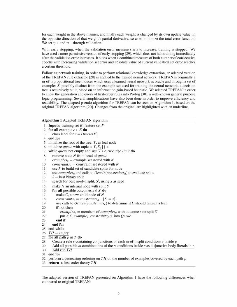
for each weight in the above manner, and finally each weight is changed by its own update value, inthe opposite direction of that weight’s partial derivative, so as to minimize the total error function.We set h+ and h� through validation.
With early stopping, when the validation error measure starts to increase, training is stopped. Wehave used a more permissive version of early stopping [29], which does not halt training immediatelyafter the validation error increases. It stops when a combined measure of both number of consecutiveepochs with increasing validation set error and absolute value of current validation set error reachesa certain threshold.
Following network training, in order to perform relational knowledge extraction, an adapted versionof the TREPAN rule extractor [20] is applied to the trained neural network. TREPAN is originally am-of-n propositional tree inducer which uses a learned neural network as oracle and through a set ofexamples S, possibly distinct from the example set used for training the neural network, a decisiontree is recursively built, based on an information gain-based heuristic. We adapted TREPAN in orderto allow the generation and query of first-order rules into Prolog [30], a well-known general purposelogic programming. Several simplifications have also been done in order to improve efficiency andreadability. The adapted pseudo-algorithm for TREPAN can be seen on Algorithm 1, based on theoriginal TREPAN algorithm [20]. Changes from the original are highlighted with an underline.
Algorithm 1 Adapted TREPAN algorithm1: Inputs: training set E, feature set F2: for all example e 2 E do
3: class label for e = Oracle(E)4: end for
5: initialize the root of the tree, T , as leaf node6: initialize queue with tuple < T,E,{}>7: while queue not empty and size(T )< tree size limit do
8: remove node N from head of queue9: examplesn = example set stored with N
10: constraintsn = constraint set stored with N11: use F to build set of candidate splits for node12: use examplesn and calls to Oracle(constraintsn) to evaluate splits13: S = best binary split14: search for best m-of-n split, S0, using S as seed15: make N an internal node with split S016: for all possible outcomes s 2 S0 do
17: make C, a new child node of N18: constraintsc = constraintsn [{S0 = s}19: use calls to Oracle(constraintsc) to determine if C should remain a leaf20: if not then
21: examplesc = members of examplesn with outcome s on split S022: put <C,examplec,constraintsc > into Queue23: end if
24: end for
25: end while
26: T H = empty27: for all path p in T do
28: Create a rule r containing conjunctions of each m-of-n split conditions s inside p29: Add all possible m combinations of the n conditions inside s as disjunctive body literals in r30: Add r to T H31: end for
32: perform a decreasing ordering on T H on the number of examples covered by each path p33: return a first-order theory T H
The adapted version of TREPAN presented on Algorithm 1 have the following differences whencompared to original TREPAN:
5
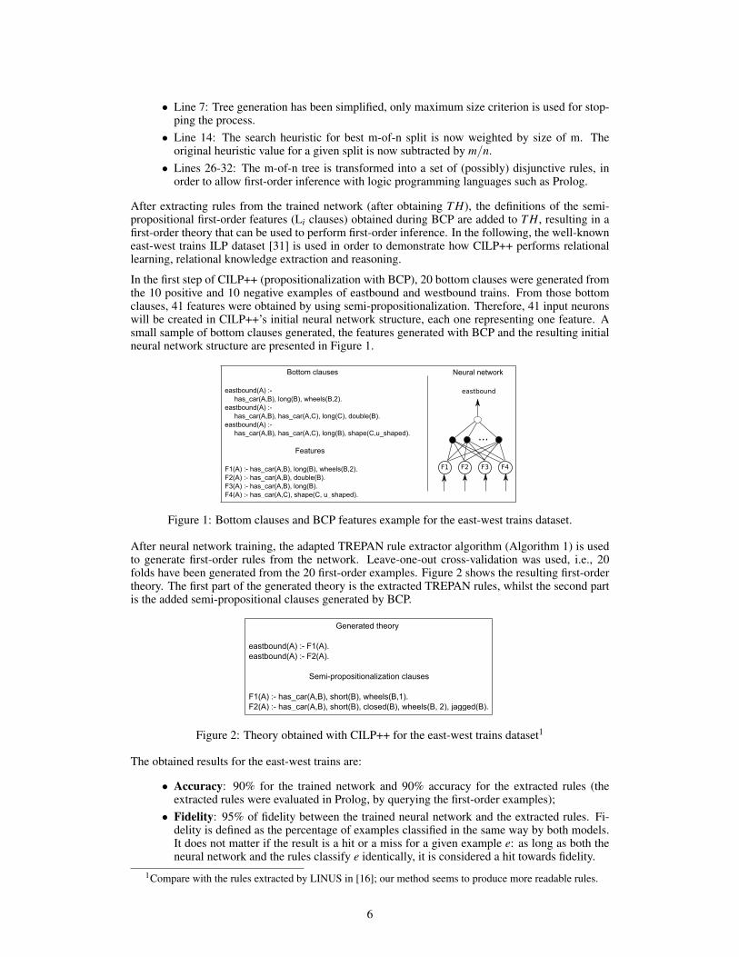
• Line 7: Tree generation has been simplified, only maximum size criterion is used for stop-ping the process.
• Line 14: The search heuristic for best m-of-n split is now weighted by size of m. Theoriginal heuristic value for a given split is now subtracted by m/n.
• Lines 26-32: The m-of-n tree is transformed into a set of (possibly) disjunctive rules, inorder to allow first-order inference with logic programming languages such as Prolog.
After extracting rules from the trained network (after obtaining T H), the definitions of the semi-propositional first-order features (Li clauses) obtained during BCP are added to T H, resulting in afirst-order theory that can be used to perform first-order inference. In the following, the well-knowneast-west trains ILP dataset [31] is used in order to demonstrate how CILP++ performs relationallearning, relational knowledge extraction and reasoning.
In the first step of CILP++ (propositionalization with BCP), 20 bottom clauses were generated fromthe 10 positive and 10 negative examples of eastbound and westbound trains. From those bottomclauses, 41 features were obtained by using semi-propositionalization. Therefore, 41 input neuronswill be created in CILP++’s initial neural network structure, each one representing one feature. Asmall sample of bottom clauses generated, the features generated with BCP and the resulting initialneural network structure are presented in Figure 1.
Bottom clauses
eastbound(A) :- has_car(A,B), long(B), wheels(B,2).eastbound(A) :- has_car(A,B), has_car(A,C), long(C), double(B).eastbound(A) :- has_car(A,B), has_car(A,C), long(B), shape(C,u_shaped).
Features
F1(A) :- has_car(A,B), long(B), wheels(B,2). F2(A) :- has_car(A,B), double(B).F3(A) :- has_car(A,B), long(B).F4(A) :- has_car(A,C), shape(C, u_shaped).
Neural network
F1 F2 F3 F4
...
eastbound
Figure 1: Bottom clauses and BCP features example for the east-west trains dataset.
After neural network training, the adapted TREPAN rule extractor algorithm (Algorithm 1) is usedto generate first-order rules from the network. Leave-one-out cross-validation was used, i.e., 20folds have been generated from the 20 first-order examples. Figure 2 shows the resulting first-ordertheory. The first part of the generated theory is the extracted TREPAN rules, whilst the second partis the added semi-propositional clauses generated by BCP.
Generated theory
eastbound(A) :- F1(A). eastbound(A) :- F2(A). Semi-propositionalization clauses
F1(A) :- has_car(A,B), short(B), wheels(B,1).F2(A) :- has_car(A,B), short(B), closed(B), wheels(B, 2), jagged(B).
Figure 2: Theory obtained with CILP++ for the east-west trains dataset1
The obtained results for the east-west trains are:
• Accuracy: 90% for the trained network and 90% accuracy for the extracted rules (theextracted rules were evaluated in Prolog, by querying the first-order examples);
• Fidelity: 95% of fidelity between the trained neural network and the extracted rules. Fi-delity is defined as the percentage of examples classified in the same way by both models.It does not matter if the result is a hit or a miss for a given example e: as long as both theneural network and the rules classify e identically, it is considered a hit towards fidelity.
1Compare with the rules extracted by LINUS in [16]; our method seems to produce more readable rules.
6

Table 1: Accuracy results (ACC) with standard deviations, area under ROC curve results (AUC) andruntimes in seconds (RUN) for the Mutagenesis, UW-CSE and Alzheimers-anime datasets
SYSTEM METRICS DATASETS
Mutagenesis UW-CSE Alzheimer-amine Cora
Aleph ACC 80.85%(±10.51) 85.11%(±7.11) 78.71%(±5.25) ��AUC 0.80(0.02) 0.81(±0.07) 0.79(±0.09) ��RUN 721 875 5465 ��
MLN ACC 62.11%(±0.022) 75.01%(±0.028) 50.01%(±0.002) 70.10%(±0.191)AUC 0.67(±0.022) 0.76(±0.12) 0.51(±0.02) 0.809(±0.001)RUN 4341 1184 9811 97148
CILP++ ACC 91.70%(±5.84) 77.17%(±9.01) 79.91%(±2.12) 68.91%(±2.12)AUC 0.82(±0.02) 0.77(±0.07) 0.80(±0.01) 0.79(±0.02)RUN 851 742 3822 11435
Table 2: Rule accuracy results (ACC) with standard deviations and fidelity (FID) for the Mutagene-sis, UW-CSE, Alzheimer-anime and Cora datasets
SYSTEM METRICS DATASETS
Mutagenesis UW-CSE Alzheimer-anime Cora
Aleph ACC 80.85%(±10.51) 85.11%(±7.11) 78.71%(±5.25) ��
CILP++ ACC 77.72(±2.12) 81.98(±3.11) 78.70%(±6.12) 67.98%(±5.29)FID 0.89 0.90 0.88 0.82
3 Experimental Results
CILP++ has been tested empirically and results over ten-fold cross validation for the trained neuralnetwork can be seen on Table 1. CILP++ is being tested against a well-known ILP system, Aleph[23] and Markov Logic Networks (MLN’s) [15]. Four relational domains have been used: Mu-tagenesis [7], UW-CSE [8], Alzheimers-anime [21] and Cora [22]. The same parameters as [13]have been used for training CILP++. For Aleph, the settings suggested in [18] have been used.For MLN’s, the reported results on three publications [15, 32, 33] have been collected. Lastly, onTREPAN, treesizel imit has been set as 5. All experiments were run on a 3.2 Ghz Intel Core i3-2100with 4 GB RAM.
Results show that CILP++ has comparable accuracy and AUC measurements with both Aleph andMLN’s, while having considerably better runtimes. While CILP++ was able to run and generatecompetitive results on all tested datasets, Aleph ran out of memory while running Cora. StandardMLN’s performed very poorly on Alzheimer-amine [32] and had higher training times.
Table 2 shows comparative results with Aleph for querying the extracted first-order rules from thetrained CILP++ neural network on Prolog. Also, fidelity measurements are provided.
Results show that competitive accuracy with Aleph has been maintained after extraction, and alsogood fidelity measures have been obtained in comparison with the trained neural network. Thisindicates that CILP++ neural networks are capable of efficiently solve relational tasks with BCP.
4 Concluding Remarks
In this paper, we have presented an integrated and efficient method and system for the extractionof first-order logic rules from neural networks. Experimental results show that the first-order rulesextracted from trained neural networks, in terms of accuracy and AUC, are comparable with a well-
7

known probabilistic system for relational learning, MLN’s, and a search-based ILP system, Aleph,while being considerably faster. Those results indicate the promise of CILP++ as a relational learner.
Further comparisons with related work include the analysis of propositionalization-based systemssuch as LINUS/DINUS/SINUS [9, 11] and RelF[34], which rely on the quality of their featuregeneration to reduce the information loss of the propositionalization approach and, consequently,within the rules extracted from the learner. Both the LINUS/DINUS/SINUS family of ILP systemsand RelF generate a number of constrained first-order features f from the Herbrand base H (H is theset of possible clauses for a given domain knowledge). From the collection of features f , a final setof features F is obtained for representing the training examples, according to a given score function.CILP++, on the other hand, uses the concept of bottom clause, which is a clause that uniquelydescribes a single relational example. CILP++ uses bottom clauses to train a neural network, and analgorithm based on the concept of semi-propositionalization [16, 27] to generate F .
Approaches based on Bayesian networks [35] also perform relational learning, but represent thelearned knowledge without the use of explicit relational rules. Statistical Relational Models [36]contain a rich representation language which combines a frame-based logical representation withprobabilistic semantics based on bayesian networks. BLOG [37] is a first-order probabilistic model-ing language that specifies probability distributions over possible worlds with varying sets of objects.A BLOG model contains statements that define conditional probability distributions for a certain setof random variables; the model also specifies certain context-specific independence properties. In-ference is done on BLOG using Markov Chain Monte Carlo [38] algorithms. In CILP++, inferenceis deterministic with first-order rules learned from the neural (statistical) model being applicabledirectly onto a Prolog theorem prover for reasoning.
As future work, a study on how CILP++ deals with noisy datasets (noise in the background knowl-edge and/or examples) can provide interesting results, due to how backpropagation naturally dealswith incomplete data and noisy inputs. Also, an investigation on how CILP++ can be adapted to dealdirectly with numeric data can overcome a well-known flaw in ILP systems, which is its inabilityto deal directly with numbers. ILP systems use auxiliary predicates to indicate relations betweennumeric variables such as greater-than, less-than and so on.
References
[1] S. Holldobler and Y. Kalinke, “Towards a massively parallel computational model for logic program-ming,” in In: Proceedings of the ECAI94 Workshop on Combining Symbolic and Connectionist Process-ing, pp. 68–77, 1994.
[2] G. G. Towell and J. W. Shavlik, “Knowledge-Based Artificial Neural Networks,” Artif. Intell., vol. 70,no. 1-2, pp. 119–165, 1994.
[3] A. S. D. Garcez and G. Zaverucha, “The Connectionist Inductive Learning and Logic Programming Sys-tem,” Applied Intelligence, vol. 11, pp. 59–77, 1999.
[4] R. Basilio, G. Zaverucha, and V. Barbosa, “Learning Logic Programs with Neural Networks,” in InductiveLogic Programming, vol. 2157 of LNAI, pp. 15–26, Springer Berlin / Heidelberg, 2001.
[5] S. Dzeroski and N. Lavrac, Relational Data Mining. Relational Data Mining, Springer, 2001.[6] L. De Raedt, Logical and Relational Learning. Cognitive Technologies, Springer, 2008.[7] A. Srinivasan and S. H. Muggleton, “Mutagenesis: ILP experiments in a non-determinate biological
domain,” in Proceedings of the 4th International Workshop on Inductive Logic Programming, volume 237of GMD-Studien, pp. 217–232, 1994.
[8] J. Davis, E. S. Burnside, I. de Castro Dutra, D. Page, and V. S. Costa, “An integrated approach to learningbayesian networks of rules,” in ECML (J. Gama, R. Camacho, P. Brazdil, A. Jorge, and L. Torgo, eds.),vol. 3720 of Lecture Notes in Computer Science, pp. 84–95, Springer, 2005.
[9] N. Lavrac and S. Dzeroski, Inductive logic programming: techniques and applications. Ellis Horwoodseries in artificial intelligence, E. Horwood, 1994.
[10] F. Zelezny and N. Lavrac, “Propositionalization-based Relational Subgroup Discovery With RSD,” Ma-chine Learning, vol. 62, pp. 33–63, 2006.
[11] S. Kramer, N. Lavrac, and P. Flach, “Relational Data Mining,” ch. Propositionalization approaches torelational data mining, pp. 262–286, New York, NY, USA: Springer-Verlag New York, Inc., 2000.
[12] M.-A. Krogel, S. Rawles, F. Zelezny, P. Flach, N. Lavrac, and S. Wrobel, “Comparative Evaluation OfApproaches To Propositionalization,” in ILP, vol. 2835 of LNAI, pp. 194–217, Springer-Verlag, 2003.
8

[13] M. V. M. Franca, G. Zaverucha, and A. dAvila Garcez, “Fast relational learning using bottom clausepropositionalization with artificial neural networks,” Machine Learning, vol. 94, no. 1, pp. 81–104, 2014.
[14] M. V. M. Franca, A. S. D. Garcez, and G. Zaverucha, “Relational Knowledge Extraction from Attribute-Value Learners,” in 2013 Imperial College Computing Student Workshop, vol. 35 of OpenAccess Seriesin Informatics (OASIcs), (Dagstuhl, Germany), pp. 35–42, Schloss Dagstuhl, 2013.
[15] M. Richardson and P. Domingos, “Markov logic networks,” Machine Learning, vol. 62, pp. 107–136,2006.
[16] N. Lavrac and P. A. Flach, “An extended transformation approach to inductive logic programming,” ACMTrans. Comput. Logic, vol. 2, no. 4, pp. 458–494, 2001.
[17] B. Kijsirikul and B. K. Lerdlamnaochai, “First-Order Logical Neural Networks,” Int. J. Hybrid Intell.Syst., vol. 2, pp. 253–267, Dec. 2005.
[18] A. Paes, F. Zelezny, G. Zaverucha, D. Page, and A. Srinivasan, “ILP Through Propositionalizationand Stochastic k-Term DNF Learning,” in ILP, vol. 4455 of LNAI, (Berlin, Heidelberg), pp. 379–393,Springer-Verlag, 2007.
[19] R. Basilio, G. Zaverucha, and A. S. Garcez, “Inducing Relational Concepts with Neural Networks via theLINUS System,” in In ICONIP, pp. 1507151–0, 1998.
[20] M. Craven and J. W. Shavlik, “Extracting Tree-Structured Representations of Trained Networks,” in NIPS,pp. 24–30, 1995.
[21] R. King and A. Srinivasan, “Relating chemical activity to structure: An examination of ILP successes,”New Generation Computing, vol. 13, no. 3-4, pp. 411–434, 1995.
[22] M. Bilenko and R. J. Mooney, “Adaptive duplicate detection using learnable string similarity measures,”in Proceedings of the ninth ACM SIGKDD international conference on Knowledge discovery and datamining, KDD ’03, (New York, NY, USA), pp. 39–48, ACM, 2003.
[23] A. Srinivasan, “The Aleph System, version 5.” http://www.cs.ox.ac.uk/activities/machlearn/Aleph/aleph.html, 2007. Last accessed on may/2013.
[24] S. Muggleton, “Inverse Entailment and Progol,” New Generation Computing, Special issue on InductiveLogic Programming, vol. 13, no. 3-4, pp. 245–286, 1995.
[25] A. Tamaddoni-Nezhad and S. Muggleton, “The lattice structure and refinement operators for the hypoth-esis space bounded by a bottom clause,” Machine Learning, vol. 76, no. 1, pp. 37–72, 2009.
[26] S. Muggleton and L. D. Raedt, “Inductive Logic Programming: Theory and Methods,” Journal of LogicProgramming, vol. 19, no. 20, pp. 629–679, 1994.
[27] M. V. M. Franca, G. Zaverucha, and A. S. D. Garcez, “Neural relational learning through semi-propositionalization of bottom clauses,” in AAAI Spring Symposium Series, 2015.
[28] R. A. Jacobs, “Increased rates of convergence through learning rate adaptation,” Neural Networks, vol. 1,no. 4, pp. 295–307, 1988.
[29] L. Prechelt, “Early stopping - but when?,” in Neural Networks: Tricks of the Trade, volume 1524 of LNCS,chapter 2, pp. 55–69, Springer-Verlag, 1997.
[30] R. A. Kowalski, “The early years of logic programming,” Commun. ACM, vol. 31, pp. 38–43, Jan. 1988.[31] J. Larson and R. S. Michalski, “Inductive inference of VL decision rules,” SIGART Bull., no. 63, pp. 38–
44, 1977.[32] T. N. Huynh and R. J. Mooney, “Discriminative structure and parameter learning for markov logic net-
works,” in Proceedings of the 25th International Conference on Machine Learning, ICML ’08, (NewYork, NY, USA), pp. 416–423, ACM, 2008.
[33] S. Kok and P. Domingos, “Learning the structure of markov logic networks,” in Proceedings of the 22NdInternational Conference on Machine Learning, (New York, NY, USA), pp. 441–448, ACM, 2005.
[34] O. Kuzelka and F. Zelezny, “Block-wise construction of tree-like relational features with monotone re-ducibility and redundancy,” Machine Learning, vol. 83, pp. 163–192, 2011.
[35] J. Pearl, Causality: Models, Reasoning, and Inference. Cambridge University Press, 2000.[36] N. Friedman, L. Getoor, D. Koller, and A. Pfeffer, “Learning probabilistic relational models,” in In IJCAI,
pp. 1300–1309, Springer-Verlag, 1999.[37] B. Milch, B. Marthi, S. Russell, D. Sontag, D. L. Ong, and A. Kolobov, “BLOG: probabilistic models
with unknown objects,” IJCAI, (San Francisco, CA, USA), pp. 1352–1359, Morgan Kaufmann PublishersInc., 2005.
[38] A. E. Gelfand and A. F. M. Smith, “Sampling-based approaches to calculating marginal densities,” Jour-nal of the American Statistical Association, vol. 85, no. 410, pp. 398–409, 1990.
9

Combinatorial structures and processing in Neural
Blackboard Architectures
Frank van der Velde
CTIT, CPE-BMSUniversity of Twente, Enschede
IOP, LeidenThe Netherlands
Marc de Kamps
Institute for Artificial Intelligenceand Biological Systems
University of LeedsLeeds, United Kingdom
Abstract
We discuss and illustrate Neural Blackboard Architectures (NBAs) as the basis forvariable binding and combinatorial processing the brain. We focus on the NBA forsentence structure. NBAs are based on the notion that conceptual representationsare in situ, hence cannot be copied or transported. Novel combinatorial struc-tures can be formed with these representations by embedding them in NBAs. Wediscuss and illustrate the main characteristics of this form of combinatorial pro-cessing. We also illustrate the NBA for sentence structures by simulating neuralactivity as found in recently reported intracranial brain observations. Furthermore,we will show how the NBA can account for ambiguity resolution and garden patheffects in sentence processing.
1 Introduction
We outline and illustrate the implementation and processing of combinatorial structures in NeuralBlackboard Architectures (or NBAs). First, we will discuss the ideas on which NBAs are based.Then, we will illustrate sentence representation and processing in the NBA for sentence structure[1]. Next, we will simulate neural activation patterns that arise in the NBA during sentence process-ing and relate it to recently reported intracranial brain observations. Finally, we will illustrate anddiscuss how the NBA handles linguistic phenomena such as unproblematic ambiguities and gardenpath sentences [2].
2 In situ concept representations
The development of Neural Blackboard Architectures is based on the notion that representationsin the brain, such as representations of concepts, are ‘in situ’, in line with the neural assembliesproposed by Hebb [3]. Figure 1 (based on [4]) illustrates this with the concept cat. As Hebb argued,a neural assembly develops over time as neurons that process information about a concept becomeinterconnected. These neurons could be located in different parts of the brain, depending on thenature of the underlying concept. So, in case of a concept like cat, they will consist of neurons inthe visual and auditory cortex, involved in the perception of cats. They could also consist of neuronsinvolved in actions related to cats (e.g., pronouncing the word cat).
Concept representations with neural assemblies could be distributed, but parts of the assembly couldalso consist of more local representations. They could consist of neurons involved in processinginformation about the concepts, but also of neurons involved in actions related to concepts. Thisentails that both incoming and outgoing connections determine the nature of a concept representation[5]. Furthermore, unlike the original assemblies as described by Hebb, concepts as intended here
1

emotion
action
pet paw
is has Sentence blackboard
Phonology blackboard
Perception blackboards
Other blackboards
cat
Figure 1: In situ concept representation (based on [4]).
are not only associative neural structures. They also incorporate relations, as illustrated with therelations is pet and has paw in Figure 1.
The assembly or web-like structure of a concept representation entails that concepts representationsare ‘in situ’ [4]. That is, wherever a concept is activated it always consists of the activation ofthe assembly of that concept or a part of it. In this view, it is not possible to make a copy of aconcept representation and store it elsewhere in the brain to, for example, create a combinatorialstructure with it or use it in a reasoning process. In this sense, in situ concept representations arefundamentally different from symbols in symbol architectures [6]. Due to the in situ nature ofconcepts representations, they are also grounded in perception or action (depending on the nature ofthe concept).
The in situ nature of neuronal concept representations imposes constraints on the way they canbe combined in higher-level cognitive combinatorial structures, such as sentences. In situ conceptrepresentation cannot be copied or transported to construct combinatorial structures. Instead, as il-lustrated in Figure 1, they are embedded in ‘neural blackboards’ to form combinatorial structures.We assume that there will be specific neural blackboards for specific forms of combinatorial struc-tures, and concept representations will be embedded in a number of them depending on the nature ofthat concept and the role it plays in specific combinatorial structures. For example, the concept catwill be embedded in a phonology blackboard, forming the word cat based on familiar phonemes. Itwill also be embedded in a sentence blackboard, needed to form sentence structures. It could also beembedded in a perception blackboard underlying the combinatorial nature of visual cognition [7].Other blackboards, e.g., needed for sequential processing or reasoning, could be included as well.
The neural blackboards allow the construction of (potentially novel) combinatorial structures basedon (familiar) in situ concept representations, using forms of variable binding (depending on thespecific blackboard). They aim to satisfy the following characteristics:
• The concept representations remain in situ (and thus grounded) even when they are a partof (novel) combinatorial structures.
• The combinatorial structures or parts thereof are content addressable, even with novel com-binatorial structures (of familiar constituents).
• The variable binding of concepts in blackboards creates the connection paths needed toproduce behavior (linking sensory and motor activation), even with (novel) combinatorialstructures.
We will discuss and illustrate these characteristics using the sentence blackboard.
3 Sentence neural blackboard
Figure 2 illustrates the structure of the sentence Sonnet sees (the) dog in the Neural BlackboardArchitecture for sentence structure [1]. Here, we assume that the words sees and dog are familiar
2

Nx
Sy
Vz
sees
W1
1
Phonology blackboard
Structure assemblies
Wordassemblies
Nu
2 3
/so/ /nn/ /et/
dog
Sentence blackboard
Conditionalconnections:
Figure 2: Sentence representation in a sentence neural blackboard.
constituents but Sonnet is a new name, not heard before. The representations of sees and dog consistof neural assembly structures (‘word assemblies’), in line with the concept cat in Figure 1. Forsimplicity, we represent them with ovals, but the full connection structure is always implied.
The sentence blackboard allows the creation of a (temporal) connection structure that binds the wordassemblies in line with the relations expressed by the sentence. To this end, the NBA consists of‘structure assemblies’ such as N
x
and Nu
in Figure 2 (representing nouns) and Sy
(sentence) and Vz
(verb). The word assemblies can bind to structure assemblies of their kind, and structure assembliescan bind to each other in line with the sentence structure. The binding process results from specific‘conditional connections’ (outlined below).
As noted in [8], humans have the ability to include new words and names in (even novel) sentencesstructures, exemplified here with the name Sonnet. However, the ability to include novel words insentences is restricted to new words based on familiar phonemes. In the NBA this ability resultsfrom a phonology blackboard in which new names can be formed based on familiar phonemes [9].The phonology blackboard interacts with the sentence blackboard, which allows the incorporationof the new name in a sentence structure [10]. Here, Sonnet activates a set of phonemes (illustratedwith the pseudo phonemes so, nn, and et), which bind to a structure assembly in the phonologyblackboard (W1). In turn, this structure assembly binds to the sentence structure in the sentenceblackboard.
N1
S1
V1
N2
nn v
v
t
tcat
sees
dog
N1 X n
i
di
Conditional connections
Controlcircuit
Structure assemblies
Word assemblies
Structure assemblies: = Main assemblies = SubassembliesS1 v
WMcircuit
Figure 3: Binding in the sentence neural blackboard.
The binding process in the NBA is illustrated in more detail in Figure 3 with the sentence cat seesdog. The conditional connections, here the red and black thick lines, consist of gating circuits. In theNBA, each word assembly (e.g., of a noun) is connected to a set of structure assemblies of the samekind (all N
i
assemblies in the case of a noun) with gating circuits. (The number of these connectionscan be reduced by representing words in the phonology blackboard first, see [9].) In turn, eachstructure assembly consists of a ‘main assembly’, such as N1, and (a set of) subassemblies, such asn or t. The connection between a main assembly and a subassembly consists of a gating circuit aswell.
3

Structure assemblies of different kinds, such as V1 and N2, are connected by their subassemblies ofthe same kind. Here, their t (theme) subassemblies, which represents the fact that a verb can have atheme (object). This connection also consists of a gating circuit.
The gating circuits operate by disinhibition (di), illustrated in Figure 3. So, when N1 is active,it activates a neuron (or neuron population) X and an inhibitory neuron (or population) i. Thelatter inhibits X , which blocks the flow of activation. But when i itself is inhibited (by neuron orpopulation di) activation can flow from N1 (via X) to n.
Gating circuits can be disinhibited (or ‘activated’) in one of two different ways. In case of gatingcircuits between main assemblies and subassemblies the activation results from an external controlcircuit that activates the di population. This is how syntactical operations affect binding in theblackboard. A control circuit could have recognized that sees dog represent a verb and a theme. Itthen activates all di populations in the gating circuits between all V
i
and Nj
assemblies and their tassemblies. As a result, the active V
i
and Nj
will activate their t subassembly.
Gating circuits between subassemblies and between word and main assemblies are activated by(specific) ‘working memory’ (WM) populations. A WM population remains active for a while, afterinitial activation, by reverberating activation in the population [11]. An active WM population bindsthe assemblies to which it is connected in the manner outlined below.
3.1 Variable binding in a connection path
Figure 4 illustrates how binding is achieved in the NBA. The parts (a), (b) and (c) illustrate the samebinding process with increasing detail. In (a), the binding between the t subassemblies of V1 (orV1-t) and N2 (N2-t) in Figure 3 is repeated. Figure 4b illustrates that this binding is based on a‘connection matrix’, which consists of columns and rows of ‘connection nodes’ illustrated in Figure4c.
N2-t
V1-t
( = inhibition)
Connection matrix
Xi Xin
Yj
Yin
WM
i
di
di
i
Connection node
V1
N2
t
t
(a) (b) (c)
Figure 4: Binding by activity in a Connection Matrix (based on [1]).
Each specific Vi
-t and Nj
-t pair of subassemblies is interconnected in a specific connection node, lo-cated in a connection matrix dedicated to binding V
i
-t and Nj
-t subassemblies. In general, when twoassemblies X
i
and Yj
(e.g., V1-t and N2-t) are concurrently active in the processing of a sentence,they activate a WM population in their connection node by means of a gating circuit, as illustratedin Figure 4c. In turn, the active WM population disinhibits a gating circuit by which activation canflow from X
i
to Yj
, and another such circuit, not show in (c), by which activation can flow from Yj
to Xi
. As long as their WM population is active, Xi
and Yj
are ‘bound’ because activation will flowfrom one to the other whenever one of them is (initially) activated.
The NBA allows any noun to bind to any verb in any thematic role using dedicated connectionmatrices. Also, the NBA has structure assemblies that can bind to other structure assemblies, suchas S1 in Figure 3, or clause structure assemblies ([1]). In this way, hierarchical sentence structurescan be represented, such as relative or complement clauses.
4

A given word assembly can bind to different structure assemblies at the same time, allowing thecreation of sentence structures in which words are repeated (e.g., cat sees cat). Yet, word assembliesremain is situ in this way, so words in sentence structures are always accessible and grounded.
The role of the NBA is thus to establish a ‘connection path’ for any sentence structure that canbe formed in a language. Although it has been questioned whether this would be possible [8],an available connection path is in fact a necessary condition for any model of (neuronal) variablebinding. That is, whenever two neuronal representations are bound in a functional way, there issome kind of (direct or indirect) connection path between those representations. This path is neededto produce (meaningful) behavior based on the functional binding at hand. For example, to answerquestions about the relation expressed by the binding [10]. The ability of the brain to establish suchconnection paths derives from its ‘small-word’ like connection structure [12]. The NBA indeed hassuch a structure [1].
In the NBA the connection matrices are given. But in a pilot simulation [13] we investigated thepossible development of such a connection structure. The simulations indicated that a structurelike a connection matrix could arise during development, based on initially random activation andconnection patterns. But, of course, each node in the connection matrix would also have to have thecircuits as illustrated in Figure 4c for the binding process to occur.
3.2 Content addressable sentence structures
The role of the NBA to (temporarily) create a connection path needed for the production of behavioris illustrated in Figure 5. This figure illustrates how the NBA can answer (binding) questions (for asimulation, see [1]).
N1
N2
nn v
v
t
t
John
knows
v
Bill knows?
N4
tt
Mary
Bill
S1S2
sees
nv
n
N3V2 V1
Figure 5: Content addressable sentence structures and competition in the NBA in answering (bind-ing) questions. Grey nodes are active.
The structure of the sentence Bill knows John, stored in the NBA, can be used to answer a (binding)question like “What does Bill know?” (or Bill knows?). The question activates the assembliesfor Bill and knows and provides information that Bill is the subject of knows. This results in theactivation of the sentence structure Bill knows. The question also asks for the theme of the relationBill knows, which can be used to activate the gating circuits for the theme (t) subassemblies. Thiswill initiate a flow of activation from V1 to N2 and thus to John in Figure 5, producing the answerto the question.
The NBA can correctly produce the answer even when, for example, Bill is a constituent of othersentences as well, as in Bill sees Mary. The representation of Bill is the same in situ word assemblyin both sentences (which directly derives from the notion of in situ representation). As noted above,they are distinguished in the NBA by the binding with different noun main assemblies (here, N1 vsN3). The question Bill knows? activates Bill, which in turn activates both N1 and N3 to which it isbound. Because the question entails that Bill is the subject, this results in the activation of both S1and S2.
However, the question also identifies knows as the verb and not sees. This results in the activationof V1 which inhibits the activation of V2, because main assemblies of the same kind inhibit eachother in the NBA [1]. In this way, asking for the theme produces the correct answer John (bound toknows) instead of the incorrect answer Mary (bound to sees).
5
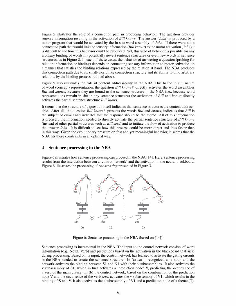
Figure 5 illustrates the role of a connection path in producing behavior. The question providessensory information resulting in the activation of Bill knows. The answer (John) is produced by amotor program that would be activated by the in situ word assembly of John. If there were not aconnection path that would link the sensory information (Bill knows) to the motor activation (John) itis difficult to see how this behavior could be produced. Yet, this kind of behavior is possible for anyarbitrary binding of words in (potentially novel) sentence structures or even new words in sentencestructures, as in Figure 2. In each of these cases, the behavior of answering a question (probing forrelation information or binding) depends on connecting sensory information to motor activation, ina manner that satisfies the binding relations expressed by the relation at hand. The NBA producesthis connection path due to its small-world like connection structure and its ability to bind arbitraryrelations by the binding process outlined above.
Figure 5 also illustrates the role of content addressability in the NBA. Due to the in situ natureof word (concept) representation, the question Bill knows? directly activates the word assembliesBill and knows, Because they are bound to the sentence structure in the NBA (i.e., because wordrepresentations remain in situ in any sentence structure) the activation of Bill and knows directlyactivates the partial sentence structure Bill knows.
It seems that the structure of a question itself indicates that sentence structures are content address-able. After all, the question Bill knows? presents the words Bill and knows, indicates that Bill isthe subject of knows and indicates that the response should be the theme. All of this informationis precisely the information needed to directly activate the partial sentence structure of Bill knows(instead of other partial structures such as Bill sees) and to initiate the flow of activation to producethe answer John. It is difficult to see how this process could be more direct and thus faster thanin this way. Given the evolutionary pressure on fast and yet meaningful behavior, it seems that theNBA fits these constraints in an optimal way.
4 Sentence processing in the NBA
Figure 6 illustrates how sentence processing can proceed in the NBA [14]. Here, sentence processingresults from the interaction between a ‘control network’ and the activation in the neural blackboard.Figure 6 illustrates the processing of cat sees dog presented in Figure 3.
N1
S1
V1
N2
nn v
v
t
tcat
sees
dog
N1
S1
V1
nn v
v
tcat
seesN1
S1
nn v
cat
N-n-S S-v
Vcat
N
V-v V-t
T
sees
V
N-t
dog
N
(a) (b) (c)
Figure 6: Sentence processing in the NBA (based on [14]).
Sentence processing is incremental in the NBA. The input to the control network consists of wordinformation (e.g. Noun, Verb) and predictions based on the activation in the blackboard that ariseduring processing. Based on its input, the control network has learned to activate the gating circuitsin the NBA needed to create the sentence structure. In (a) cat is recognized as a noun and thenetwork activates the binding between S1 and N1 with their n subassemblies. It also activates thev subassembly of S1, which in turn activates a ‘prediction node’ V, predicting the occurrence ofa verb of the main clause. In (b) the control network, based on the combination of the predictionnode V and the occurrence of the verb sees, activates the v subassembly of V1, which results in thebinding of S and V. It also activates the t subassembly of V1 and a prediction node of a theme (T),
6

anticipating an object of the verb. In (c), the combination of the T node and the noun dog results inthe binding of V1 and N2 with their t subassemblies.
In [14] we trained a control network with a set of training sentences with different syntactic forms(e.g., subject, theme, relative clause, complement clause). The network could then control a sub-stantially larger set of sentences in which these syntactic forms were combined in different ways.For example, the control network could produce the correct binding operations in sentences witharbitrary deep (center) embeddings. However, the binding process in the NBA starts to break downwith these sentences after one or two embeddings, due to competitions with the connection matricesinvolved [1, 14]. Hence, the NBA could account for both competence and performance aspects oflanguage processing.
4.1 Simulating neuronal activation during sentence processing
Brain activation observed with fMRI indicates that neuronal activation increases for longer and morecomplex sentences [15]. Observations with intracranial electrodes provided more detailed informa-tion [16]. In particular, when (sub) phrases in a sentence are formed (or ‘merged’ in linguistic terms)neuronal activity first increases but then briefly decreases.
Figure 7 shows the activity in the NBA when the sentence Ten sad student of Bill Gates will movefrom [16] is processed (taking Bill Gates as a single noun). Figure 7 (left) shows the basic structureof the sentence in the NBA. Figure 7 (right) shows the sum of all activity (Total) in the NBA, and thesum activities of the main assemblies (MA), the subassemblies (SA), and the WM populations in theconnection matrices. All assemblies and gating circuits are modeled with Wilson Cowan populationdynamics [17]. MA and SA assemblies have reverberating activity as well (until they are inhibited).Activation values are normalized to fit in one plot.
nS1
AX1
V1
v
va
NM1 PP1
nm np
na
Adj1
students
of
N1
pn
N2
ten
sad
B-Gates
will
move
Total
MA
SA
WM
Ten sad students of B-G will move (ms)
Figure 7: NBA activity in processing Ten sad student of Bill-Gates will move.
The sum of all activity resembles the patterns observed in [16]. For example, after Ten sad students(forming a phrase) activation increases but then drops, as with other phrases in the sentence. This isin particular due to the subassemblies, which are inhibited by feedback from their connection matrixwhen a binding has succeeded. But overall activation increases with sentence length and complexity[15].
Figure 8 illustrates the neural activity in the NBA when it resolves an unproblematic ambiguity(UPA) presented in [2]. Here, it is UPA13a (Bird found in room died) vs UPA13b (Bird found inroom debris). The NBA resolves ambiguities by a competition between conflicting WM populations[18]. The NBA structure of both sentences and the conflicts (red dashed lines) are illustrated in thefigure (left).
The assumption is that UPA13a is the basis interpretation. So, found is the verb of a relative clausebound to bird. Simulation shows that this incremental sentence processing proceeds without prob-lems. So, the processing of UPA13b starts in the same way. The figure shows the individual WMactivations obtained with UPA13b, which reveal the bindings achieved (the sum of this activitywould result in a plot as in Figure 7). When bird (N1) is presented it binds to S1, indicated by theblack line S1-N1 representing the WM binding population. After the initial activation by the word,this population remains active at a sustained level, so the binding remains intact during (and after)
7
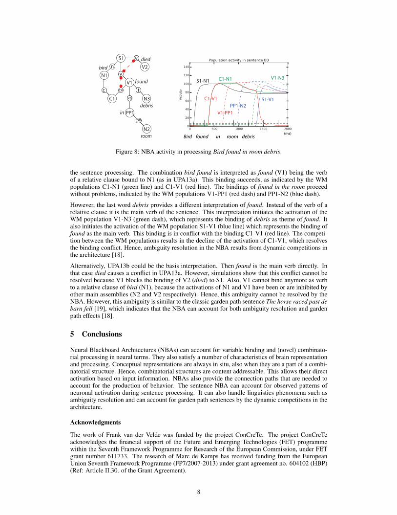
N1
nS1
V2
v
birdv
C1
V1
N3
cv tcvp
PP1
N2
pn
died
found
debrisin
room
S1-N1
Bird found in room debris (ms)
C1-N1
C1-V1
V1-PP1PP1-N2
V1-N3
S1-V1
Figure 8: NBA activity in processing Bird found in room debris.
the sentence processing. The combination bird found is interpreted as found (V1) being the verbof a relative clause bound to N1 (as in UPA13a). This binding succeeds, as indicated by the WMpopulations C1-N1 (green line) and C1-V1 (red line). The bindings of found in the room proceedwithout problems, indicated by the WM populations V1-PP1 (red dash) and PP1-N2 (blue dash).
However, the last word debris provides a different interpretation of found. Instead of the verb of arelative clause it is the main verb of the sentence. This interpretation initiates the activation of theWM population V1-N3 (green dash), which represents the binding of debris as theme of found. Italso initiates the activation of the WM population S1-V1 (blue line) which represents the binding offound as the main verb. This binding is in conflict with the binding C1-V1 (red line). The competi-tion between the WM populations results in the decline of the activation of C1-V1, which resolvesthe binding conflict. Hence, ambiguity resolution in the NBA results from dynamic competitions inthe architecture [18].
Alternatively, UPA13b could be the basis interpretation. Then found is the main verb directly. Inthat case died causes a conflict in UPA13a. However, simulations show that this conflict cannot beresolved because V1 blocks the binding of V2 (died) to S1. Also, V1 cannot bind anymore as verbto a relative clause of bird (N1), because the activations of N1 and V1 have been or are inhibited byother main assemblies (N2 and V2 respectively). Hence, this ambiguity cannot be resolved by theNBA. However, this ambiguity is similar to the classic garden path sentence The horse raced past debarn fell [19], which indicates that the NBA can account for both ambiguity resolution and gardenpath effects [18].
5 Conclusions
Neural Blackboard Architectures (NBAs) can account for variable binding and (novel) combinato-rial processing in neural terms. They also satisfy a number of characteristics of brain representationand processing. Conceptual representations are always in situ, also when they are a part of a combi-natorial structure. Hence, combinatorial structures are content addressable. This allows their directactivation based on input information. NBAs also provide the connection paths that are needed toaccount for the production of behavior. The sentence NBA can account for observed patterns ofneuronal activation during sentence processing. It can also handle linguistics phenomena such asambiguity resolution and can account for garden path sentences by the dynamic competitions in thearchitecture.
Acknowledgments
The work of Frank van der Velde was funded by the project ConCreTe. The project ConCreTeacknowledges the financial support of the Future and Emerging Technologies (FET) programmewithin the Seventh Framework Programme for Research of the European Commission, under FETgrant number 611733. The research of Marc de Kamps has received funding from the EuropeanUnion Seventh Framework Programme (FP7/2007-2013) under grant agreement no. 604102 (HBP)(Ref: Article II.30. of the Grant Agreement).
8

References
1] van der Velde, F. & de Kamps, M. (2006). Neural blackboard architectures of combinatorialstructures in cognition. Behavioral and Brain Sciences, 29, 37-70.
[2] Lewis, R. L. (1993). An Architecturally-based Theory of Human Sentence Comprehension.Thesis Carnegie Mellon University, Pittsburgh, PA.
[3] Hebb, D. O. (1949). The organisation of behaviour. New York: Wiley.
[4] van der Velde, F & de Kamps, M. (2011). Compositional connectionist structures based on insitu grounded representations. Connection Science, 23, 97-107.
[5] van der Velde, F (2015). Communication, concepts and grounding. Neural networks, 62, 112 -117.
[6] Newell, A. (1990). Unified theories of cognition. Cambridge, MA: Harvard University Press.
[7] Van der Velde, F. & de Kamps, M. (2001). From knowing what to knowing where: Modelingobject-based attention with feedback disinhibition of activation. Journal of Cognitive Neuroscience,13(4), 479-491.
[8] Feldman, J. (2013). The neural binding problem(s). Cognitive Neurodynamics, 7, 1-11.
[9] Van der Velde, F. & de Kamps, M. (2006). From neural dynamics to true combinatorial structures(reply to commentaries). Behavioral and Brain Sciences, 29, 88-108.
[10] van der Velde, F. & de Kamps, M. (2015). The necessity of connection structures in neuralmodels of variable binding. Cognitive neurodynamics, 9, 359-370. DOI 10.1007/s11571-015-9331-7
[11] Amit, D. (1995). The Hebbian paradigm reintegrated: Local reverberations as internal repre-sentations. Behavioral and Brain Sciences, 18, 617-657.
[12] Shanahan, M. (2010). Embodiment and the inner life. Oxford: Oxford University Press.
[13] van der Velde, F. & de Kamps, M. (2011). Development of a connection matrix for productivegrounded cognition. IEEE International Conference on Development and Learning (ICDL) (Vol 2),1-6. DOI: 10.1109/DEVLRN.2011.6037343
[14] van der Velde, F & de Kamps, M. (2010). Learning of control in a neural architecture ofgrounded language processing. Cognitive Systems Research, 11, 93-107.
[15] Pallier, C., Devauchelle, A-D. & Dehaene, S. (2011). Cortical representation of the constituentstructure of sentences. PNAS, 108, 2522-27.
[16] Nelson, M. J., El Karoui, I., Rangarajan, V., Pallier, C., Parvizi, J., Cohen, L., Naccache, L. &Dehaene, S. (2014). Constituent structure representations revealed with intracranial data. Societyfor Neuroscience Annual Meeting. Washington, DC, USA.
[17] Wilson, H. R. & Cowan, J. D (1972). Excitatory and inhibitory interactions in localized popu-lations of model neurons. Biophysical Journal, 12, 1-24.
[18] van der Velde, F. & de Kamps, M. (2015). Ambiguity resolution in a Neural BlackboardArchitecture for sentence structure. In Tarek R. Besold & Kai-Uwe Kuhnberger (eds.), Proceedingsof the KI 2015 Workshop on Neural-Cognitive Integration. Dresden, Germany.
[19] Bever, T. G. (1970). The cognitive basis for linguistic structures. In Hayes, J. R., (ed.) Cogni-tion and the Development of Language. New York: Wiley.
9

Request confirmation networksfor neuro-symbolic script execution
Joscha Bach⇤
Program for Evolutionary DynamicsHarvard University
Cambridge, MA [email protected]
Priska Hergermicropsi industries GmbH
Berlin, [email protected]
Abstract
We propose Request Confirmation Networks (ReCoNs) to combine neural learn-ing with the sequential, hierarchical detection of sensory features, and to facilitateplanning and script execution. ReCoNs are spreading activation networks withunits that contain an activation and a state, and are connected with typed directedlinks that indicate partonomic relations and spatial or temporal succession. Bypassing activation along the links, ReCoNs can perform both neural computationsand controlled script execution. We demonstrate an application of ReCoNs in thecognitive architecture MicroPsi2 for an active perception task in a virtual environ-ment.
1 Introduction
MicroPsi is a cognitive architecture that combines neuro-symbolic representations [1] with situatedperception and a motivational system [2], [3]. MicroPsi agents live in an open environment thatthey have to explore and navigate; currently we are using the game environment Minecraft [4]. Tothis end, agents require mechanisms for bottom-up/top-down perception, reinforcement learning,motivation, decision making and action execution. We are using MicroPsi to study how to combineperceptual and conceptual representations, and to facilitate autonomous learning with full perceptualgrounding.
Cognitive architectures with perceptual grounding require a way to combine symbolic and sub-symbolic operations: planning, communication and reasoning rely on discrete, symbolic representa-tions, while fine-grained visual and motor interaction requires distributed representations. The stan-dard solution consists in a hybrid architecture that combines a neural network layer with a carefullycrafted model that learns to compress the perceptual input, and a layer that facilitates deliberationand control using symbolic operations and uses the extracted regularities [5]. However, while sucha dual architecture appears to be a straightforward solution from an engineering point of view, webelieve that there is a continuum between perceptual and conceptual representations, i.e. that bothshould use the same set of representational mechanisms, and primarily differ in the operations thatare performed upon them. In our view, symbolic/localist representations are best understood as aspecial case of subsymbolic/distributed representations, for instance ones where the weights of theconnecting links are close to discrete values. Highly localist features often emerge in neural learn-ing, and rules expressed as discrete-valued links can be used to initialize a network for capturingmore detailed, distributed features (see KBANN [6]).
MicroPsi’s representations combine neural network principles and symbolic operations via recurrentspreading activation networks with directed links. The individual nodes in the network process
⇤ http://micropsi.com
1

information by summing up the activation that enters the nodes through slots, and calculating afunction for each of their gates, which are the origin of links to other nodes. Node types differ bythe number of gates and slots they have and by the functions and parameters of their gates. Typedlinks can be expressed by the type of their gate of origin.
The most common node type in earlier MicroPsi implementations is called a concept node. Conceptnodes possess seven gate types (with approximate semantics in parentheses): gen (associated), por(successor), ret (predecessor), sur (part-of), sub (has-part), exp (is-exemplar-of), cat (is-a). Conceptnodes can be used to express hierarchical scripts [7] by linking sequences of events and actions usingpor/ret, and subsuming these sequences into hierarchies using sub/sur.
In MicroPsi2, a perceptual representation amounts to a hierarchical script to test for the presenceof the object in the environment. At each level of the hierarchy, the script contains disjunctionsand subjunctions of substeps, which bottom out in distributed substeps and eventually in sensornodes that reflect measurements in the environment and actuator nodes that will move the agent orits sensors. Recognizing an object requires the execution of this hierarchical script. In the past,this required a central executive that used a combination of explicit backtracking and activationpropagation. We have replaced this mechanism with a completely distributed mode of executioncalled request confirmation network that only requires the propagation of activation along the linksof connected nodes.
2 Request confirmation networks
Modeling perception in a cognitive architecture requires an implementation of top-down/bottom-upprocessing, in which sensors delivers cues (bottom-up) to activate higher-level features, while per-ceptual hypotheses produce predictions of features that have to be verified by active sensing (top-down). When using a neural network paradigm, the combination of bottom-up and top-down pro-cessing requires recurrency. Request confirmation networks are a solution to combine constrainedrecurrency with the execution of action sequences. They provide a neural solution for the imple-mentation of sensorimotor scripts.
Request Confirmation Networks (ReCoN) are implemented within MicroPsi2’s formalism but are infact a more general paradigm for auto-executable networks of stateful nodes with typed links. Wetherefore provide a general definition that is independent of our implementation.
A request confirmation network can be defined as a set of units U and edges E with
U = {script nodes [ terminal nodes}E = {sub, sur, por, ret}
A script node has a state s where
s 2 {inactive, requested, active, suppressed, waiting, true, confirmed, failed}
and an activation a 2 Rn, which can be used to store additional state. (In MicroPsi2, the activationis used to store the results of combining feature activations along the sub links). A terminal nodeperforms a measurement and has a state s 2 {inactive, active, confirmed}, and an activation a 2 Rn,which represents the value obtained from the measurement. An edge is defined by hu
s
, ut
, type 2{por, ret, sub, sur}, w 2 Rni, whereby u
s
and ut
denote the source and target unit, por connects toa successor node, ret to a predecessor node, sub to a parent node, and sub connects to a child node.w is a link weight with n dimensions that can be used to perform additional computations. Eachpair of nodes (u
s
, ut
) is either unconnected or has exactly one pair of links of the types por/ret, orsub/sur. Each script node must have at least one link of type sub, i.e. at least one child that is eithera script node or a terminal node. Script nodes can be the source and target of links of all types,whereas terminal nodes can only be targeted by links of type sub, and be the origin of links of typesur.
ReCoNs solve the problem of constraining the flow of control in a hierarchical script on the levelof individual units without using topological information, i.e. without a centralized interpreter orinforming individual units about their neighboring elements. To do this, they need to store the exe-cution state within the script elements in a distributed manner; each of these units is a state machinewith one of eight states (as defined above). Each unit implements connections to its neighbors using
2
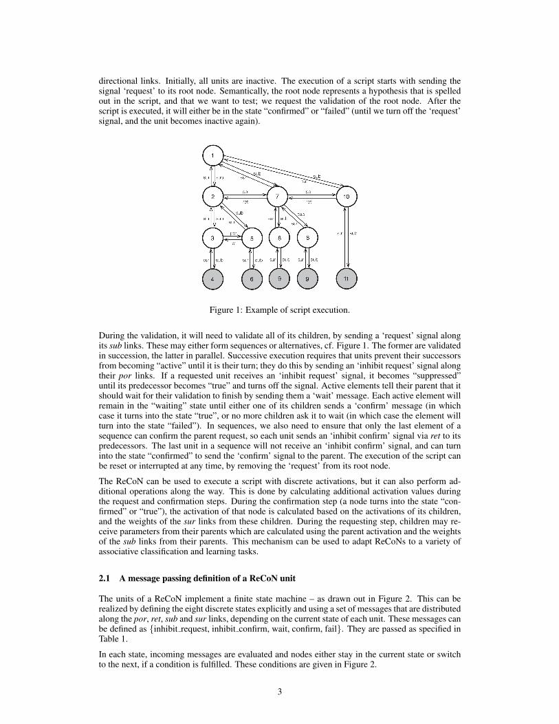
directional links. Initially, all units are inactive. The execution of a script starts with sending thesignal ‘request’ to its root node. Semantically, the root node represents a hypothesis that is spelledout in the script, and that we want to test; we request the validation of the root node. After thescript is executed, it will either be in the state “confirmed” or “failed” (until we turn off the ‘request’signal, and the unit becomes inactive again).
Figure 1: Example of script execution.
During the validation, it will need to validate all of its children, by sending a ‘request’ signal alongits sub links. These may either form sequences or alternatives, cf. Figure 1. The former are validatedin succession, the latter in parallel. Successive execution requires that units prevent their successorsfrom becoming “active” until it is their turn; they do this by sending an ‘inhibit request’ signal alongtheir por links. If a requested unit receives an ‘inhibit request’ signal, it becomes “suppressed”until its predecessor becomes “true” and turns off the signal. Active elements tell their parent that itshould wait for their validation to finish by sending them a ‘wait’ message. Each active element willremain in the “waiting” state until either one of its children sends a ‘confirm’ message (in whichcase it turns into the state “true”, or no more children ask it to wait (in which case the element willturn into the state “failed”). In sequences, we also need to ensure that only the last element of asequence can confirm the parent request, so each unit sends an ‘inhibit confirm’ signal via ret to itspredecessors. The last unit in a sequence will not receive an ‘inhibit confirm’ signal, and can turninto the state “confirmed” to send the ‘confirm’ signal to the parent. The execution of the script canbe reset or interrupted at any time, by removing the ‘request’ from its root node.
The ReCoN can be used to execute a script with discrete activations, but it can also perform ad-ditional operations along the way. This is done by calculating additional activation values duringthe request and confirmation steps. During the confirmation step (a node turns into the state “con-firmed” or “true”), the activation of that node is calculated based on the activations of its children,and the weights of the sur links from these children. During the requesting step, children may re-ceive parameters from their parents which are calculated using the parent activation and the weightsof the sub links from their parents. This mechanism can be used to adapt ReCoNs to a variety ofassociative classification and learning tasks.
2.1 A message passing definition of a ReCoN unit
The units of a ReCoN implement a finite state machine – as drawn out in Figure 2. This can berealized by defining the eight discrete states explicitly and using a set of messages that are distributedalong the por, ret, sub and sur links, depending on the current state of each unit. These messages canbe defined as {inhibit request, inhibit confirm, wait, confirm, fail}. They are passed as specified inTable 1.
In each state, incoming messages are evaluated and nodes either stay in the current state or switchto the next, if a condition is fulfilled. These conditions are given in Figure 2.
3

Unit state POR RET SUB SUR
inactive (ø) – – – –requested (R) inhibit request inhibit confirm – wait
active (A) inhibit request inhibit confirm request waitsuppressed (S) inhibit request inhibit confirm – –
waiting (W) inhibit request inhibit confirm request waittrue (T) – inhibit confirm – –
confirmed (C) – inhibit confirm – confirmfailed (F) inhibit request inhibit confirm – –
Table 1: Message passing in ReCoNs.
Figure 2: State transitions.
2.2 A neural definition of a ReCoN unit
It is possible to realize a ReCoN unit with an ensemble of artificial neurons. Figure 3 shows anarrangement of ten simple threshold elements with only excitatory and inhibitory links that satisfiesthese conditions. Let the activation of a neuron be defined as
↵j
=
⇢ P(w
ij
· ↵i
) if wij
· ↵i
� 0 for allwij
,↵i
0 otherwise
i.e. any incoming activation on a link with a negative weight is sufficient to entirely inhibit theneuron. A message is any activation value sent over a link that crosses the boundary between units.Units may send the message ‘request’ to their children (top-down), ‘wait’ and ‘confirm’ to theirparents (bottom-up), ‘inhibit request’ to their successors, and ‘inhibit confirm’ to their predecessors(lateral inhibition).
4

We want all activity in a unit to cease as soon as the unit is no longer requested. Thus, all activationin the unit is derived from the activation of the incoming request message. The request activation isdirectly sent to the neurons IC, IR, and W. IC will inhibit confirm signals by predecessor units, andIR will inhibit requests to child nodes by successor units, before the current unit is confirmed. Winforms the parent node that it has active (non-failed) children, by sending the ‘wait’ message. IRalso prevents the unit from confirming prematurely; i.e. before it has received a ‘confirm’ messageby one of its children.
IC then passes on its activation to R, and R sends out a request to the unit’s children, unless it isinhibited by the predecessor node. To give predecessor nodes enough time to send the inhibitionsignal, the flow of activation between IC and R is delayed by DR. F becomes active as soon as theunit has no more active children, and represents the failure state of the unit. Like all states, it mustreceive its activation from the initial request. It cannot be allowed to fail before the unit has sent arequest to its children, so F is inhibited by the predecessors ‘inhibit request’ message at the neuronR . F can also not fail before the children cease sending their ‘wait’ message, so it is inhibited bythat message. F must also allow enough time for requested children to respond with this message,so its activation is delayed by the helper neuron DF. Once F becomes active (i.e. the unit fails), itstops the ‘request’ to the children by inhibiting R, and the ‘wait’ to the parent, by inhibiting W. (Fcannot get its activation directly from R, because F will later inhibit R and would thus remove itsown activation; therefore it is activated through the helper neuron R ).
The neuron T represents that the unit has been confirmed (true). It receives its activation from theoriginal request, but is not allowed to become active through the inhibition by IC. Only if IC isturned off by the ‘confirm’ message of one of its children, T becomes active and will turn off W (the‘wait’ message to the parent), R (the request of the children) and IR (the inhibition of the successors,and itself). If the unit has no successors (i.e. receives no ‘inhibit confirm’ message), it will signalT’s value via C as a ‘confirm’ message to the unit’s parent. This is just one of many possible waysin which a ReCoN unit could be realized with artificial neurons.
Figure 3: Schematic of a neural ReCoN specification.
In MicroPsi2, the functionality of this circuitry is embedded in a single node, which requires a onlyone calculation step and reduces memory usage; cf. section 3.1.
5

3 Implementation
3.1 A compact implementation of ReCoNs
Rather than explicitly modeling the state machine of a ReCoN unit, this implementation makes useof the fact that the state of a ReCoN unit is fully determined by the activation of connected nodesin the previous time step. States are implemented as a set of simple arithmetic rules operating onincoming activation from connected nodes and the node itself. Nodes can link to themselves using“gen loops” to store the states “true”, “confirmed”, and “failed”. Activation as well as all linkweights are numbers enabling real-value information processing and neural learning.
In this implementation, por/ret activation 2 {�1, 0, 1} is used to control the flow of sub requests({0, 1}) and sur confirmation. The real-valued sur activations can be interpreted as probabilistic inthe range [0, 1] or take on the value �1 to indicate a solid fail. They control por/ret activation in thenext higher layer.
Activation is spread in discrete steps. Each step consists of two phases: Propagation and calculation.Propagation is simply: z = W · a where W is a matrix of link weights and a is the activationvector. Calculation is f
gate
(fnode
(z)), where fgate
is an activation function specified per link typeand f
node
implements the ReCoN behavior. The following definitions describe the behavior of thenode functions f
node
per link type.
fgen
node
=
⇢zsur if (zgen · zsub = 0) _ (9 linkpor ^ zpor = 0)zgen · zsub otherwise
fpor
node
=
⇢0 if zsub 0 _ (9 linkpor ^ zpor 0)zsur + zgen otherwise
fret
node
=
⇢1 if zpor < 00 otherwise
fsub
node
=
⇢0 if zgen 6= 0 _ (9 linkpor ^ zpor 0)zsub otherwise
fsur
node
=
8<
:
0 if zsub 0 _ (9 linkpor ^ zpor 0)(zsur + zgen) · zret if 9 linkret
zsur + zgen otherwise
An undesirable property of this implementation is that new activation is not solely based on incomingactivation but also depends on local knowledge about the existence of por/ret links1.
3.2 Using ReCoNs for an active perception task
Active perception with ReCoNs is based on learned representations that are encoded in the structureand weights of links. Whenever the system encounters a new situation (for instance, after a locomo-tion action) it will form a model of its environment as a combination of verifiable hypotheses. Athigher levels, these hypotheses can contain object representations and geometric relations betweenobjects, at the lower levels features and eventually input patches that make up the visual structure ofthese objects. In the basic variant implemented so far, hypotheses are based on a single autoencoderthat captures features of the scene as a whole.
Hypotheses are verified by activating their top-most node with a request (i.e. sending activation toits sub slot). From there, activation spreads downwards through the sub-hypotheses defined by thenode’s children, which are verified sequentially. If all existing hypotheses fail, the agent constructsa new one, scanning its visual field and connecting the localized feature nodes into a hierarchy. We
1 The source code is available from https://github.com/joschabach/micropsi2. Formulas found in the codeare slightly more complex as they include additional features like time-based failing and searchability whichare not relevant in this context.
6

built a MicroPsi agent that moves about in a Minecraft world along a transition graph, samples itsvisual environment and learns to recognize scenes on the graph with a request confirmation network.
The agent does not process the entire visual field at once, but uses a rectangular fovea with a 16⇥16sensor matrix. Using actuators, it can move this fovea to fixate a point (and thus a 16 ⇥ 16 patch)in its field of vision. The possible fixation points are constrained to allow for a 50 percent overlapbetween neighboring patches.
These patches are learned using a denoising autoencoder [8] with zero-masking Bernoulli noise anda corruption level of 0.3. A 2-dimensional perspective projection of the Minecraft block world ata given position serves as input to the autoencoder. Figure 4b shows, for one such position, thevisual field as the standard Minecraft client would present it to a human player (top), the projectionprovided as visual input to the agent (center), and a visualization of the features at that position aslearned by the autoencoder (bottom).
(a) Transition graph of theagent.
(b) Training data – Minecraft vanilla client (top),visual input (center), learnt features (bottom).
Figure 4: Action space and input sample of a MicroPsi2 agent in Minecraft
The autoencoder hidden nodes play the role of terminal nodes to the ReCoN units. Features de-tected by the hidden nodes are fed into a localized feature grid, where each combination of featureand fixation point is expressed as a pair of por/ret connected ReCoN units. Each pair is sur/sub con-nected to a parent unit. The first node of the por/ret sequence is sub/sur connected to the actuatornode that was active when the feature was detected, the second has an incoming sur link from oneof the hidden nodes of the autoencoder (see Figure 5a). The grid as a whole associates expectedfeatures with all possible fixation points. Each grid element represents a feature at a given locationin the agent’s visual field, together with the action required to reach that location. Since hypothesesare constructed as sequences of grid nodes, which contain actuators for moving the fovea, they aresimple sensorimotor scripts. New hypotheses are formed based on those features that are deemedrelevant to the current situation. Here, relevance is simply defined by an activation value exceedinga threshold of 0.8. Figure 5b shows the structure and connectivity of such a hypothesis.
To evaluate the functionality of this implementation, we let the agent move around in the Minecraftworld using a number of fixed locations. As expected the agent learned hypotheses for all locations,subsequently stopped forming new hypotheses, and successfully recognized all the locations.
7
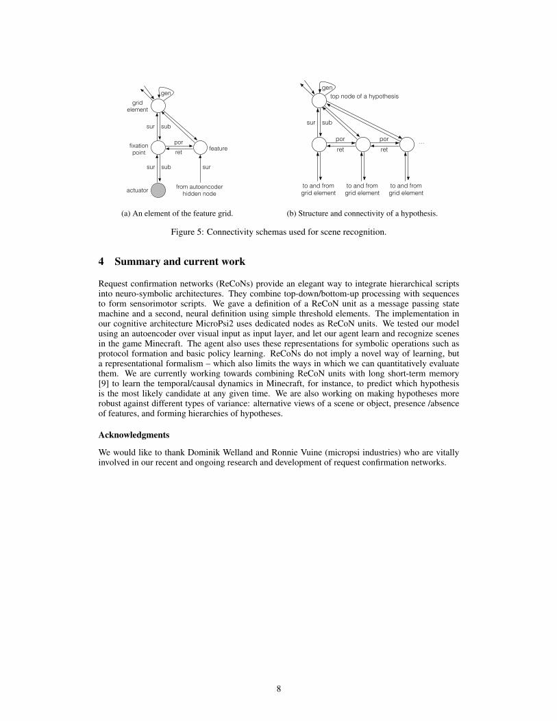
sur
retpor
from autoencoderhidden node
gridelement
sub
fixationpoint feature
actuator
sursur sub
gen
(a) An element of the feature grid.
sur
retpor
gen
…retpor
to and fromgrid element
to and fromgrid element
to and fromgrid element
top node of a hypothesis
sub
(b) Structure and connectivity of a hypothesis.
Figure 5: Connectivity schemas used for scene recognition.
4 Summary and current work
Request confirmation networks (ReCoNs) provide an elegant way to integrate hierarchical scriptsinto neuro-symbolic architectures. They combine top-down/bottom-up processing with sequencesto form sensorimotor scripts. We gave a definition of a ReCoN unit as a message passing statemachine and a second, neural definition using simple threshold elements. The implementation inour cognitive architecture MicroPsi2 uses dedicated nodes as ReCoN units. We tested our modelusing an autoencoder over visual input as input layer, and let our agent learn and recognize scenesin the game Minecraft. The agent also uses these representations for symbolic operations such asprotocol formation and basic policy learning. ReCoNs do not imply a novel way of learning, buta representational formalism – which also limits the ways in which we can quantitatively evaluatethem. We are currently working towards combining ReCoN units with long short-term memory[9] to learn the temporal/causal dynamics in Minecraft, for instance, to predict which hypothesisis the most likely candidate at any given time. We are also working on making hypotheses morerobust against different types of variance: alternative views of a scene or object, presence /absenceof features, and forming hierarchies of hypotheses.
Acknowledgments
We would like to thank Dominik Welland and Ronnie Vuine (micropsi industries) who are vitallyinvolved in our recent and ongoing research and development of request confirmation networks.
8

References
[1] Ioannis Hatzilygeroudis and Jim Prentzas. Neuro-symbolic approaches for knowledge representation inexpert systems. International Journal of Hybrid Intelligent Systems, 1(3-4):111–126, 2004.
[2] Joscha Bach. Principles of synthetic intelligence PSI: an architecture of motivated cognition, volume 4.Oxford University Press, 2009.
[3] Joscha Bach. Modeling motivation in micropsi 2. In Artificial General Intelligence, pages 3–13. Springer,2015.
[4] Daniel Short. Teaching scientific concepts using a virtual world – minecraft. Teaching Science - Journalof the Australian Science Teachers Association, 58(3):55, 2012.
[5] Stefan Wermter and Ron Sun, editors. Hybrid neural systems. Springer Science & Business Media, 2000.[6] Geoffrey G Towell and Jude W Shavlik. Knowledge-based artificial neural networks. Artificial intelli-
gence, 70(1):119–165, 1994.[7] Roger C Schank and Robert P Abelson. Scripts, plans, and knowledge. Yale University, 1975.[8] Pascal Vincent, Hugo Larochelle, Yoshua Bengio, and Pierre-Antoine Manzagol. Extracting and compos-
ing robust features with denoising autoencoders. In Proceedings of the 25th international conference onMachine learning, pages 1096–1103. ACM, 2008.
[9] Sepp Hochreiter and Jurgen Schmidhuber. Long short-term memory. Neural computation, 9(8):1735–1780, 1997.
[10] Paul J Werbos. Generalization of backpropagation with application to a recurrent gas market model.Neural Networks, 1(4):339–356, 1988.
[11] Ronald J Williams and David Zipser. Experimental analysis of the real-time recurrent learning algorithm.Connection Science, 1(1):87–111, 1989.
9

Tree-Structured Composition in Neural Networks
without Tree-Structured Architectures
Samuel R. Bowman, Christopher D. Manning, and Christopher Potts
Stanford UniversityStanford, CA 94305-2150
{sbowman, manning, cgpotts}@stanford.edu
Abstract
Tree-structured neural networks encode a particular tree geometry for a sentencein the network design. However, these models have at best only slightly out-performed simpler sequence-based models. We hypothesize that neural sequencemodels like LSTMs are in fact able to discover and implicitly use recursive com-positional structure, at least for tasks with clear cues to that structure in the data.We demonstrate this possibility using an artificial data task for which recursivecompositional structure is crucial, and find an LSTM-based sequence model canindeed learn to exploit the underlying tree structure. However, its performanceconsistently lags behind that of tree models, even on large training sets, suggest-ing that tree-structured models are more effective at exploiting recursive structure.
1 Introduction
Neural networks that encode sentences as real-valued vectors have been successfully used in a widearray of NLP tasks, including translation [1], parsing [2], and sentiment analysis [3]. These modelsare generally either sequence models based on recurrent neural networks, which build representa-tions incrementally from left to right [4, 1], or tree-structured models based on recursive neuralnetworks, which build representations incrementally according to the hierarchical structure of lin-guistic phrases [5, 6].
While both model classes perform well on many tasks, and both are under active development, treemodels are often presented as the more principled choice, since they align with standard linguis-tic assumptions about constituent structure and the compositional derivation of complex meanings.Nevertheless, tree models have not shown the kinds of dramatic performance improvements over se-quence models that their billing would lead one to expect: head-to-head comparisons with sequencemodels show either modest improvements [3] or none at all [7].
We propose a possible explanation for these results: standard sequence models can learn to exploitrecursive syntactic structure in generating representations of sentence meaning, thereby learning touse the structure that tree models are explicitly designed around. This requires that sequence modelsbe able to identify syntactic structure in natural language. We believe this is plausible on the basisof other recent research [8, 9]. In this paper, we evaluate whether LSTM sequence models are ableto use such structure to guide interpretation, focusing on cases where syntactic structure is clearlyindicated in the data.
We compare standard tree and sequence models on their handling of recursive structure by trainingthe models on sentences whose length and recursion depth are limited, and then testing them onlonger and more complex sentences, such that only models that exploit the recursive structure willbe able to generalize in a way that yields correct interpretations for these test sentences. Our methodsextend those of our earlier work in [10], which introduces an experiment and corresponding artificialdataset to test this ability in two tree models. We adapt that experiment to sequence models by
1

not p3^ p3
p3 @ p3 or p2(not p2) and p6 | not(p6 or (p5 or p3))
p4 or (not((p1 or p6) or p4)) @ not((((not p6) or (not p4)) and (not p5)) and (p6 and p6))
Table 1: Examples of short to moderate length pairs from the artificial data introduced in [10]. Weonly show the parentheses that are needed to disambiguate the sentences rather than the full binarybracketings that the models use.
decorating the statements with an explicit bracketing, and we use this design to compare an LSTMsequence model with three tree models, with a focus on what data each model needs in order togeneralize well.
As in [10], we find that standard tree neural networks are able to make the necessary generalizations,with their performance decaying gradually as the structures in the test set grow in size. We addi-tionally find that extending the training set to include larger structures mitigates this decay. Thenconsidering sequence models, we find that a single-layer LSTM is also able to generalize to unseenlarge structures, but that it does this only when trained on a larger and more complex training setthan is needed by the tree models to reach the same generalization performance.
Our results engage with those of [8] and [2], who find that sequence models can learn to recognizesyntactic structure in natural language, at least when trained on explicitly syntactic tasks. The sim-plest model presented in [8] uses an LSTM sequence model to encode each sentence as a vector,and then generates a linearized parse (a sequence of brackets and constituent labels) with high accu-racy using only the information present in the vector. This shows that the LSTM is able to identifythe correct syntactic structures and also hints that it is able to develop a generalizable method forencoding these structures in vectors. However, the massive size of the dataset needed to train thatmodel, 250M tokens, leaves open the possibility that it primarily learns to generate only tree struc-tures that it has already seen, representing them as simple hashes—which would not capture unseentree structures—rather than as structured objects. Our experiments, though, show that LSTMs canlearn to understand tree structures when given enough data, suggesting that there is no fundamentalobstacle to learning this kind of structured representation. We also find, though, that sequence mod-els lag behind tree models across the board, even on training corpora that are quite large relative tothe complexity of the underlying grammar, suggesting that tree models can play a valuable role intasks that require recursive interpretation.
2 Recursive structure in artificial data
Reasoning about entailment The data that we use define a version of the recognizing textual
entailment task, in which the goal is to determine what kind of logical consequence relation holdsbetween two sentences, drawing on a small fixed vocabulary of relations such as entailment, con-tradiction, and synonymy. This task is well suited to evaluating neural network models for sentenceinterpretation: models must develop comprehensive representations of the meanings of each sen-tence to do well at the task, but the data do not force these representations to take a specific form,allowing the model to learn whatever kind of representations it can use most effectively.
The data we use are labeled with the seven mutually exclusive logical relations of [11], which dis-tinguish entailment in two directions (@, A), equivalence (⌘), exhaustive and non-exhaustive con-tradiction (^, |), and two types of semantic independence (#, `).
The artificial language The language described in [10] (§4) is designed to highlight the use of re-cursive structure with minimal additional complexity. Its vocabulary consists only of six unanalyzedword types (p1, p2, p3, p4, p5, p6), and, or, and not. Sentences of the language can be straightfor-wardly interpreted as statements of propositional logic (where the six unanalyzed words types arevariable names), and labeled sentence pairs can be interpreted as theorems of that logic. Someexample pairs are provided in Table 1.
Crucially, the language is defined such that any sentence can be embedded under negation or con-junction to create a new sentence, allowing for arbitrary-depth recursion, and such that the scope of
2

negation and conjunction are determined only by bracketing with parentheses (rather than bare wordorder). The compositional structure of each sentence can thus be an arbitrary tree, and interpretinga sentence correctly requires using that structure.
The data come with parentheses representing a complete binary bracketing. Our models use thisinformation in two ways. For the tree models, the parentheses are not word tokens, but rather areused in the expected way to build the tree. For the sequence model, the parentheses are word tokenswith associated learned embeddings. This approach provides the models with equivalent data, sotheir ability to handle unseen structures can be reasonably compared.
The data Our sentence pairs are divided into thirteen bins according to the number of logicalconnectives (and, or, not) in the longer of the two sentences in each pair. We test each model oneach bin separately (58k total examples, using an 80/20% train/test split) in order to evaluate howeach model’s performance depends on the complexity of the sentences. In three experiments, wetrain our models on the training portions of bins 0–3 (62k examples), 0–4 (90k), and 0–6 (160k), andtest on every bin but the trivial bin 0. Capping the size of the training sentences allows us to evaluatehow the models interpret the sentences: if a model’s performance falls off abruptly above the cutoff,it is reasonable to conclude that it relies heavily on specific sentence structures and cannot generalizeto new structures. If a model’s performance decays gradually1 with no such abrupt change, then itmust have learned a more generally valid interpretation function for the language which respects itsrecursive structure.
3 Testing sentence models on entailment
We use the architecture depicted in Figure 1a, which builds on the one used in [10]. The modelarchitecture uses two copies of a single sentence model (a tree or sequence model) to encode thepremise and hypothesis (left and right side) expressions, and then uses those encodings as the fea-tures for a multilayer classifier which predicts one of the seven relations. Since the encodings arecomputed separately, the sentence models must encode complete representations of the meanings ofthe two sentences for the downstream model to be able to succeed.
Classifier The classifier component of the model consists of a combining layer which takes the twosentence representations as inputs, followed by two neural network layers, then a softmax classifier.For the combining layer, we use a neural tensor network (NTN, [12]) layer, which sums the outputof a plain recursive/recurrent neural network layer with a vector computed using two multiplicationswith a learned (full rank) third-order tensor parameter:
~y
NN
= tanh(M
~x
(l)
~x
(r)
�+~
b )(1)
~y
NTN
= ~y
NN
+ tanh(~x(l)TT[1...n]~x
(r))(2)
Our model is largely identical to the model from [10], but adds the two additional tanh NN layers,which we found help performance across the board, and also uses the NTN combination layer whenevaluating all four models, rather than just the TreeRNTN model, so as to ensure that the sentencemodels are compared in as similar a setting as possible.
We only study models that encode entire sentences in fixed length vectors, and we set aside modelswith attention [13], a technique which gives the downstream model (here, the classifier) the potentialto access each input token individually through a soft content addressing system. While attentionsimplifies the problem of learning complex correspondences between input and output, there isno apparent reason to believe that it should improve or harm a model’s ability to track structuralinformation like a given token’s position in a tree. As such, we expect our results to reflect the samebasic behaviors that would be seen in attention-based models.
1Since sentences are fixed-dimensional vectors of fixed-precision floating point numbers, all models willmake errors on sentences above some length, and L2 regularization (which helps overall performance) ex-acerbates this by discouraging the model from using the kind of numerically precise, nonlinearity-saturatingfunctions that generalize best.
3

7-way softmax classifier
100d tanh NN layer
100d tanh NN layer
100d tanh NTN layer
50d premise 50d hypothesis
sentence modelwith premise input
sentence modelwith hypothesis input
(a) The general architecture shared across models....
a or b
a or b
or b
(b) The architecture for the tree-structured sen-tence models. Terminal nodes are learned em-beddings and nonterminal nodes are NN, NTN, orTreeLSTM layers.
a
a
or
a or
b
a or b ...
(c) The architecture for the sequence sentencemodel. Nodes in the lower row are learned em-beddings and nodes in the upper row are LSTMlayers.
Figure 1: In our model, two copies of a sentence model—based on either tree (b) or sequence(c) models—encode the two input sentences. A multilayer classifier component (a) then uses theresulting vectors to predict a label that reflects the logical relationship between the two sentences.
Sentence models The sentence encoding component of the model transforms the (learned) em-beddings of the input words for each sentence into a single vector representing that sentence. Weexperiment with tree-structured models (Figure 1b) with TreeRNN (eqn. 1), TreeRNTN (eqn. 2),and TreeLSTM [3] activation functions. In addition, we use a sequence model (Figure 1c) with anLSTM activation function [14] implemented as in [15]. In experiments with a simpler non-LSTMRNN sequence model, the model tended to badly underfit the training data, and those results are notincluded here.
Training We randomly initialize all embeddings and layer parameters, and train them using mini-batch stochastic gradient descent with AdaDelta [16] learning rates. Our objective is the standardnegative log likelihood classification objective with L2 regularization (tuned on a separate train/testsplit). All models were trained for 100 epochs, after which all had largely converged without signif-icantly declining from their peak performances.
4 Results and discussion
The results are shown in Figure 2. The tree models fit the training data well, reaching 98.9, 98.8,and 98.4% overall accuracy respectively in the 6 setting, with the LSTM underfitting slightly at94.8%. In that setting, all models generalized well to structures of familiar length, with the treemodels all surpassing 97% on examples in bin 4, and the LSTM reaching 94.8%. On the longertest sentences, the tree models decay smoothly in performance across the board, while the LSTMdecays more quickly and more abruptly, with a striking difference in the 4 setting, where LSTMperformance falls 10% from bin 4 to bin 5, compared to 4.4% for the next worse model. However,the LSTM improves considerably with more ample training data in the 6 condition, showing onlya 3% drop and generalization results better than the best model’s in the 3 setting.
All four models robustly beat the simple baselines reported in [10]: the most frequent class occursjust over 50% of the time and a neural bag of words model does reasonably on the shortest examplesbut falls below 60% by bin 4.
4

deep$3 50d(TreeRNN 50d(TreeRNTN 50d(LSTM1 1 1 0.93592 0.99242 0.98485 0.984853 0.95132 0.97895 0.936844 0.86342 0.93123 0.751675 0.79125 0.89025 0.655416 0.74852 0.86128 0.571227 0.6944 0.8073 0.507648 0.67253 0.78242 0.472539 0.61883 0.75772 0.4598810 0.55799 0.75055 0.426711 0.56949 0.70508 0.420312 0.50459 0.66667 0.3639
deep$4 50d(TreeRNN 50d(TreeRNTN 50d(LSTM1 1 1 0.987182 0.9899 0.99242 0.984853 0.98947 0.98684 0.939474 0.9618 0.96084 0.877755 0.9386 0.94781 0.761326 0.91098 0.91395 0.686947 0.8871 0.90323 0.603578 0.87363 0.87033 0.554959 0.80556 0.86883 0.5046310 0.7768 0.84683 0.4463911 0.7728 0.80339 0.4881412 0.7461 0.78899 0.43119
deep$6 50d(TreeRNN 50d(TreeRNTN 50d(LSTM1 1 0.98718 0.974362 1 0.99747 0.984853 0.99605 0.98289 0.948684 0.97803 0.96562 0.912135 0.97774 0.95088 0.873376 0.97404 0.94436 0.824937 0.95586 0.91851 0.782688 0.94396 0.8967 0.730779 0.89815 0.88272 0.66821
40%
50%
60%
70%
80%
90%
100%
1 2 3 4 5 6 7 8 9 10 11 12
Acc
urac
y
Size of longer expression
40%
50%
60%
70%
80%
90%
100%
1 2 3 4 5 6 7 8 9 10 11 12
Acc
urac
y
Size of longer expression
40%
50%
60%
70%
80%
90%
100%
1 2 3 4 5 6 7 8 9 10 11 12
Acc
urac
y
Size of longer expression
50d TreeRNN
50d TreeRNTN
50d LSTM
deep$3 50d(TreeRNN 50d(TreeRNTN 50d(TreeLSTM50d(LSTM Post$submission,(epoch(1001 1 0.98718 1 0.987182 0.9899 0.98232 0.99747 0.987373 0.925 0.94868 0.96184 0.942114 0.85482 0.90831 0.89303 0.771735 0.79509 0.83653 0.83269 0.660786 0.73145 0.78858 0.78338 0.565287 0.71647 0.75467 0.77759 0.53828 0.64286 0.68681 0.7033 0.508799 0.62037 0.65741 0.66821 0.4243810 0.5798 0.63457 0.6455 0.43111 0.505 0.61695 0.6033 0.437212 0.529 0.58104 0.5902 0.4189
Drop( 0.07018 0.04037 0.06881 0.17038
deep$4 50d(TreeRNN 50d(TreeRNTN 50d(TreeLSTM50d(LSTM1 1 1 1 0.974362 0.9899 0.99747 0.99495 0.992423 0.97895 0.98816 0.98816 0.965794 0.93696 0.95511 0.96084 0.90645 0.90714 0.92556 0.93246 0.823486 0.85831 0.88947 0.89688 0.683237 0.8455 0.87691 0.87606 0.619698 0.8022 0.82308 0.82418 0.562649 0.77006 0.78241 0.76698 0.5030910 0.7527 0.78556 0.77899 0.4923411 0.7016 0.71525 0.73898 0.4440712 0.7584 0.76147 0.69725 0.39755
Drop( 0.02982 0.02955 0.02838 0.08292
deep$6 50d(TreeRNN 50d(TreeRNTN 50d(TreeLSTM50d(LSTM1 0.97436 1 1 0.974362 0.99747 0.9974 1 0.984853 0.99605 0.9815 0.99868 0.980264 0.98567 0.9742 0.98281 0.96185 0.97698 0.9585 0.96853 0.919426 0.96513 0.9273 0.94733 0.874637 0.95756 0.9388 0.93633 0.842958 0.94505 0.9098 0.90659 0.779129 0.91821 0.875 0.87809 0.70833
40%
50%
60%
70%
80%
90%
100%
1 2 3 4 5 6 7 8 9 10 11 12
Acc
urac
y
Size of longer expression
50d TreeRNN
50d TreeRNTN
50d TreeLSTM
50d LSTM
40%
50%
60%
70%
80%
90%
100%
1 2 3 4 5 6 7 8 9 10 11 12
Acc
urac
y
Size of longer expression
50d TreeRNN
50d TreeRNTN
50d TreeLSTM
50d LSTM
40%
50%
60%
70%
80%
90%
100%
1 2 3 4 5 6 7 8 9 10 11 12
Acc
urac
y
Size of longer expression
50d TreeRNN
50d TreeRNTN
50d TreeLSTM
50d LSTM
(a) Training on sz. 3.
deep$3 50d(TreeRNN 50d(TreeRNTN 50d(TreeLSTM50d(LSTM Post$submission,(epoch(1001 1 0.98718 1 0.987182 0.9899 0.98232 0.99747 0.987373 0.925 0.94868 0.96184 0.942114 0.85482 0.90831 0.89303 0.771735 0.79509 0.83653 0.83269 0.660786 0.73145 0.78858 0.78338 0.565287 0.71647 0.75467 0.77759 0.53828 0.64286 0.68681 0.7033 0.508799 0.62037 0.65741 0.66821 0.4243810 0.5798 0.63457 0.6455 0.43111 0.505 0.61695 0.6033 0.437212 0.529 0.58104 0.5902 0.4189
Drop( 0.07018 0.04037 0.06881 0.17038
deep$4 50d(TreeRNN 50d(TreeRNTN 50d(TreeLSTM50d(LSTM1 1 1 1 0.974362 0.9899 0.99747 0.99495 0.992423 0.97895 0.98816 0.98816 0.965794 0.93696 0.95511 0.96084 0.90645 0.90714 0.92556 0.93246 0.823486 0.85831 0.88947 0.89688 0.683237 0.8455 0.87691 0.87606 0.619698 0.8022 0.82308 0.82418 0.562649 0.77006 0.78241 0.76698 0.5030910 0.7527 0.78556 0.77899 0.4923411 0.7016 0.71525 0.73898 0.4440712 0.7584 0.76147 0.69725 0.39755
Drop( 0.02982 0.02955 0.02838 0.08292
deep$6 50d(TreeRNN 50d(TreeRNTN 50d(TreeLSTM50d(LSTM1 0.97436 1 1 0.974362 0.99747 0.9974 1 0.984853 0.99605 0.9815 0.99868 0.980264 0.98567 0.9742 0.98281 0.96185 0.97698 0.9585 0.96853 0.919426 0.96513 0.9273 0.94733 0.874637 0.95756 0.9388 0.93633 0.842958 0.94505 0.9098 0.90659 0.779129 0.91821 0.875 0.87809 0.70833
40%
50%
60%
70%
80%
90%
100%
1 2 3 4 5 6 7 8 9 10 11 12
Acc
urac
y
Size of longer expression
50d TreeRNN
50d TreeRNTN
50d TreeLSTM
50d LSTM
40%
50%
60%
70%
80%
90%
100%
1 2 3 4 5 6 7 8 9 10 11 12
Acc
urac
y
Size of longer expression
50d TreeRNN
50d TreeRNTN
50d TreeLSTM
50d LSTM
40%
50%
60%
70%
80%
90%
100%
1 2 3 4 5 6 7 8 9 10 11 12
Acc
urac
y
Size of longer expression
50d TreeRNN
50d TreeRNTN
50d TreeLSTM
50d LSTM
(b) Training on sz. 4.
deep$3 50d(TreeRNN 50d(TreeRNTN 50d(TreeLSTM50d(LSTM Post$submission,(epoch(1001 1 0.98718 1 0.987182 0.9899 0.98232 0.99747 0.987373 0.925 0.94868 0.96184 0.942114 0.85482 0.90831 0.89303 0.771735 0.79509 0.83653 0.83269 0.660786 0.73145 0.78858 0.78338 0.565287 0.71647 0.75467 0.77759 0.53828 0.64286 0.68681 0.7033 0.508799 0.62037 0.65741 0.66821 0.4243810 0.5798 0.63457 0.6455 0.43111 0.505 0.61695 0.6033 0.437212 0.529 0.58104 0.5902 0.4189
Drop( 0.07018 0.04037 0.06881 0.17038
deep$4 50d(TreeRNN 50d(TreeRNTN 50d(TreeLSTM50d(LSTM1 1 1 1 0.974362 0.9899 0.99747 0.99495 0.992423 0.97895 0.98816 0.98816 0.965794 0.93696 0.95511 0.96084 0.90645 0.90714 0.92556 0.93246 0.823486 0.85831 0.88947 0.89688 0.683237 0.8455 0.87691 0.87606 0.619698 0.8022 0.82308 0.82418 0.562649 0.77006 0.78241 0.76698 0.5030910 0.7527 0.78556 0.77899 0.4923411 0.7016 0.71525 0.73898 0.4440712 0.7584 0.76147 0.69725 0.39755
Drop( 0.02982 0.02955 0.02838 0.08292
deep$6 50d(TreeRNN 50d(TreeRNTN 50d(TreeLSTM50d(LSTM1 0.97436 1 1 0.974362 0.99747 0.9974 1 0.984853 0.99605 0.9815 0.99868 0.980264 0.98567 0.9742 0.98281 0.96185 0.97698 0.9585 0.96853 0.919426 0.96513 0.9273 0.94733 0.874637 0.95756 0.9388 0.93633 0.842958 0.94505 0.9098 0.90659 0.779129 0.91821 0.875 0.87809 0.70833
40%
50%
60%
70%
80%
90%
100%
1 2 3 4 5 6 7 8 9 10 11 12
Acc
urac
y
Size of longer expression
50d TreeRNN
50d TreeRNTN
50d TreeLSTM
50d LSTM
40%
50%
60%
70%
80%
90%
100%
1 2 3 4 5 6 7 8 9 10 11 12
Acc
urac
y
Size of longer expression
50d TreeRNN
50d TreeRNTN
50d TreeLSTM
50d LSTM
40%
50%
60%
70%
80%
90%
100%
1 2 3 4 5 6 7 8 9 10 11 12
Acc
urac
y
Size of longer expression
50d TreeRNN
50d TreeRNTN
50d TreeLSTM
50d LSTM
(c) Training on sz. 6.
deep$3 50d(TreeRNN 50d(TreeRNTN 50d(TreeLSTM50d(LSTM From(Sat(morn,(pass(1000001 0.98718 1 1 12 0.98737 0.9798 0.9899 0.992423 0.91447 0.95263 0.95921 0.946054 0.84336 0.89016 0.88921 0.777465 0.78511 0.82655 0.83269 0.649276 0.72774 0.77448 0.78338 0.544517 0.71647 0.73769 0.7691 0.531418 0.65275 0.66044 0.70659 0.49899 0.62963 0.63272 0.66667 0.4290110 0.593 0.60613 0.6652 0.400411 0.4983 0.57966 0.6 0.471112 0.5198 0.59327 0.5963 0.425
deep$4 50d(TreeRNN 50d(TreeRNTN 50d(TreeLSTM50d(LSTM1 1 1 12 0.99242 0.98232 13 0.96184 0.96447 0.981584 0.91882 0.91691 0.954155 0.88565 0.87951 0.915586 0.8457 0.83754 0.864247 0.81579 0.8107 0.853148 0.76484 0.76264 0.816489 0.73611 0.73611 0.7515410 0.7133 0.7396 0.7899311 0.6779 0.6711 0.7152512 0.6758 0.6911 0.72171
deep$6 50d(TreeRNN 50d(TreeRNTN 50d(TreeLSTM50d(LSTM1 0.98718 0.88462 1 0.987182 0.98737 0.90657 0.99747 0.972223 0.97895 0.83553 0.99605 0.961844 0.95129 0.81089 0.98663 0.917865 0.92632 0.79586 0.96777 0.867236 0.90579 0.77374 0.94214 0.810097 0.89049 0.7691 0.94058 0.781838 0.85385 0.72527 0.90549 0.725279 0.83025 0.70833 0.8858 0.65278
40%
50%
60%
70%
80%
90%
100%
1 2 3 4 5 6 7 8 9 10 11 12
Acc
urac
y
Size of longer expression
50d TreeRNN
50d TreeRNTN
50d TreeLSTM
50d LSTM
40%
50%
60%
70%
80%
90%
100%
1 2 3 4 5 6 7 8 9 10 11 12
Acc
urac
y
Size of longer expression
50d TreeRNN
50d TreeRNTN
50d TreeLSTM
50d LSTM
40%
50%
60%
70%
80%
90%
100%
1 2 3 4 5 6 7 8 9 10 11 12
Acc
urac
y
Size of longer expression
50d TreeRNN
50d TreeRNTN
50d TreeLSTM
50d LSTM
Figure 2: Test accuracy on three experiments with increasingly rich training sets. The horizontalaxis on each graph divides the test set expression pairs into bins by the number of logical operatorsin the more complex of the two expressions in the pair. The dotted line shows the size of the largestexamples in the training set in each experiment.
101112
50d(TreeRNN 50d(TreeRNTN 50d(TreeLSTM50d(LSTM0 0.5252 0.5252 0.5252 0.5252
0.03 0.64626 0.61427 0.66063 0.582240.1 0.7282 0.76321 0.7661 0.665480.3 0.8447 0.91731 0.89632 0.76521 0.97732 0.95634 0.96451 0.90911
Size of longer expression
50%
60%
70%
80%
90%
100%
0% 3% 10% 30% 100%
Acc
urac
y ac
ross
all
bins
Amount of training data used (nonlinear scale)
50d TreeRNN
50d TreeRNTN
50d TreeLSTM
50d LSTM
Figure 3: Learning curve for the 6 experiment.
The learning curve (Figure 3) suggests that additional data is unlikely to change these basic results.The LSTM lags behind the tree models across the curve, but appears to gain accuracy at a similarrate.
5 Conclusion
We find that all four models are able to effectively exploit a recursively defined language to interpretsentences with complex unseen structures. We find that tree models’ biases allow them to do thiswith greater efficiency, outperforming sequence-based models substantially in every experiment.However, our sequence model is nonetheless able to generalize smoothly from seen sentence struc-tures to unseen ones, showing that its lack of explicit recursive structure does not prevent it fromrecognizing recursive structure in our artificial language.
We interpret these results as evidence that both tree and sequence architectures can play valuableroles in the construction of sentence models over data with recursive syntactic structure. Tree ar-chitectures provide an explicit bias that makes it possible to efficiently learn to compositional in-terpretation, which is difficult for sequence models. Sequence models, on the other hand, lack thisbias, but have other advantages. Since they use a consistent graph structure across examples, it iseasy to accelerate minibatch training in ways that yield substantially faster training times than arepossible with tree models, especially with GPUs. In addition, when sequence models integrate eachword into a partial sentence representation, they have access to the entire sentence representation upto that point, which may provide valuable cues for the resolution of lexical ambiguity, which is notpresent in our artificial language, but is a serious concern in natural language text.
Finally, we suggest that, because of the well-supported linguistic claim that the kind of recursivestructure that we study here is key to the understanding of real natural languages, there is likely tobe value in developing sequence models that can more efficiently exploit this structure without fullysacrificing the flexibility that makes them succeed.
Acknowledgments
We gratefully acknowledge a Google Faculty Research Award, a gift from Bloomberg L.P., andsupport from the Defense Advanced Research Projects Agency (DARPA) Deep Exploration and Fil-
5

tering of Text (DEFT) Program under Air Force Research Laboratory (AFRL) contract no. FA8750-13-2-0040, the National Science Foundation under grant no. IIS 1159679, and the Department ofthe Navy, Office of Naval Research, under grant no. N00014-13-1-0287. Any opinions, findings,and conclusions or recommendations expressed in this material are those of the authors and do notnecessarily reflect the views of Google, Bloomberg L.P., DARPA, AFRL, NSF, ONR, or the USgovernment.
References
[1] Ilya Sutskever, Oriol Vinyals, and Quoc V. Le. Sequence to sequence learning with neuralnetworks. In Proc. NIPS, 2014.
[2] Chris Dyer, Miguel Ballesteros, Wang Ling, Austin Matthews, and Noah A. Smith. Transition-based dependency parsing with stack long short-term memory. In Proc. ACL, 2015.
[3] Kai Sheng Tai, Richard Socher, and Christopher D. Manning. Improved semantic representa-tions from tree-structured long short-term memory networks. In Proc. ACL, 2015.
[4] Jeffrey L. Elman. Finding structure in time. Cognitive science, 14(2), 1990.[5] Christoph Goller and Andreas Kuchler. Learning task-dependent distributed representations
by backpropagation through structure. In Proc. IEEE International Conference on Neural
Networks, 1996.[6] Richard Socher, Jeffrey Pennington, Eric H. Huang, Andrew Y. Ng, and Christopher D. Man-
ning. Semi-supervised recursive autoencoders for predicting sentiment distributions. In Proc.
EMNLP, 2011.[7] Minh-Thang Luong Li, Jiwei, Dan Jurafsky, and Eudard Hovy. When are tree structures nec-
essary for deep learning of representations? Proc. EMNLP, 2015.[8] Oriol Vinyals, Lukasz Kaiser, Terry Koo, Slav Petrov, Ilya Sutskever, and Geoffrey Hinton.
Grammar as a foreign language. In Proc. NIPS, 2015.[9] Andrej Karpathy, Justin Johnson, and Fei-Fei Li. Visualizing and understanding recurrent
networks. arXiv:1506.02078, 2015.[10] Samuel R. Bowman, Christopher Potts, and Christopher D. Manning. Recursive neural net-
works can learn logical semantics. In Proc. of the 3rd Workshop on Continuous Vector Space
Models and their Compositionality, 2015.[11] Bill MacCartney and Christopher D. Manning. An extended model of natural logic. In Proc.
of the Eighth International Conference on Computational Semantics, 2009.[12] Danqi Chen, Richard Socher, Christopher D. Manning, and Andrew Y. Ng. Learning new facts
from knowledge bases with neural tensor networks and semantic word vectors. In Proc. ICLR,2013.
[13] Dzmitry Bahdanau, Kyunghyun Cho, and Yoshua Bengio. Neural machine translation byjointly learning to align and translate. In Proc. ICLR, 2015.
[14] Sepp Hochreiter and Jurgen Schmidhuber. Long short-term memory. Neural computation, 9(8), 1997.
[15] Wojciech Zaremba, Ilya Sutskever, and Oriol Vinyals. Recurrent neural network regularization.In Proc. ICLR, 2015.
[16] Matthew D. Zeiler. ADADELTA: an adaptive learning rate method. arXiv:1212.5701, 2012.
6

A Recurrent Neural Network for Multiple LanguageAcquisition: Starting with English and French
Xavier Hinaut∗
Dept. of Informatics, Uni. of HamburgHamburg, Germany
Johannes TwiefelDept. of Informatics, Uni. of Hamburg
Hamburg, [email protected]
Maxime PetitSBRI, INSERM 846
Bron, [email protected]
Peter DomineySBRI, INSERM 846
Bron, [email protected]
Stefan WermterDept. of Informatics, Uni. of Hamburg
Hamburg, [email protected]
Abstract
How humans acquire language, and in particular two or more different languageswith the same neural computing substrate, is still an open issue. To address thisissue we suggest to build models that are able to process any language from thevery beginning. Here we propose a developmental and neuro-inspired approachthat processes sentences word by word with no prior knowledge of the semanticsof the words. Our model has no “pre-wired” structure but only random and learnedconnections: it is based on Reservoir Computing. Our previous model has beenimplemented in the context of robotic platforms where users could teach basicsof the English language to instruct a robot to perform actions. In this paper, weadd the ability to process infrequent words, so we could keep our vocabulary sizevery small while processing natural language sentences. Moreover, we extend thisapproach to the French language and demonstrate that the network can learn bothlanguages at the same time. Even with small corpora the model is able to learnand generalize in monolingual and bilingual conditions. This approach promisesto be a more practical alternative for small corpora of different languages thanother supervised learning methods relying on big data sets or more hand-craftedparsers requiring more manual encoding effort.
1 Introduction
How do children learn language? In particular, how do they link the structure of a sentence to itsmeaning? This question is linked to the more general issue: How does the brain link sequences ofsymbols to internal symbolic or sub-symbolic representations? We propose a framework to under-stand how language is acquired based on a simple and generic neural architecture [1, 2] which is nothand-crafted for a particular task, but on the contrary can be used for a broad range of applications(see [3] for a review). This idea of “canonical” neural circuits has been coined by several authors:
∗www.informatik.uni-hamburg.de/˜hinaut ; source code available soon at github.com/neuronalX
1

it is an aim in computational neuroscience to model generic pieces of cortex [4, 5]. As such sim-plified canonical circuits we use Echo State Networks (ESN) [1] which are neural networks witha random recurrent layer and a single linear output layer (called “read-out”) modified by online oroffline learning.
Much research has been done on language processing with neural networks [6, 7, 8] and morerecently also with Echo State Networks (ESN) [9, 10]. The tasks used were diverse, from predictingthe next symbol (i.e. word) in a sentence to thematic role assignment. In this paper, the task weperform is the latter. Previously the kind of inputs sequence used was mainly based on one-levelsymbols, i.e. symbols that belong to the same level of abstraction (e.g. only words). Howeverlanguage, like many other cognitive tasks, contains several levels of abstraction, which could berepresented hierarchically from phonemes to discourse. Hierarchical processing is a strategy of thebrain, from raw perception layers to abstract processing, and even inside the higher-level cognitivecomputations performed by the prefrontal cortex there exists a hierarchy of processes [11].
Some recent results with end-to-end word recognition from raw audio data with RNN are impressive[12]. This could give some insights on what kinds of features are extracted by the brain duringspeech processing. However, to uncover language acquisition mechanisms other modelling methodsare needed. It is likely that the brain builds hierarchical representations in a more incremental andless supervised way: each newly built abstraction enables the formation of the next higher-orderabstraction, instead of abstracting all at once. We hypothesize that the brain canonical circuits, suchas the simple version proposed, can deal with different levels of abstraction mixed at the same time.In this paper, we present an initial model version which is able to deal with three kind of symbols:Function Words (FWs), Semantic Words (SWs) and Infrequent function Words (IWs). This modelprocesses IWs and SWs as categories of words, thus they are on a different level of abstraction thanFWs, which are processed as words (see Figure 1). Therefore, we have two levels of abstraction.Moreover, we show for the first time that this model is able to learn and generalize over a Frenchcorpus, and additionally over two languages at the same time, namely English and French.
2 Reservoir computing and grammatical construction approach
2.1 Echo State Networks (ESN)
The model is based on an Echo State Network (ESN) with leaky neurons. The units of the recurrentneural network have a leak rate (α) hyper-parameter, which corresponds to the inverse of a timeconstant. These equations define the update of the ESN:
x(t+ 1) = (1− α)x(t) + αf(W inu(t+ 1) +Wx(t)) (1)
y(t) = W outx(t) (2)
with x(t), u(t) and y(t) the reservoir state, the input vector and the read-out vector respectively attime t, α the leak rate, W , W in and W out the reservoir, the input and the output matrices respec-tively and f is the tanh activation function. After collection of all reservoir states the followingequation defines how the read-out weights are computed:
W out = Y d[1;X]+ (3)
with Y d the concatenation of the desired outputs, X the concatenation of the reservoir states overall time steps and M+ the Moore-Penrose pseudo-inverse of matrix M .
2.2 The sentence comprehension model with grammatical constructions approach
The proposed model processes sequences of symbols as input (namely sequences of words) andgenerates a dynamic probabilistic estimation of static symbols (namely thematic roles), see Figures 1and 2. This work is based on a previous approach modelling human language understanding [13,14], human-robot interaction [15, 16], and language acquisition in a developmental perspective (withincremental and online learning) [17]. Recently an “inverse” version of the model was able toproduce sentences depending on the words of focus [18]. The general aim of having an architectureworking with robots is to use them to model and test hypotheses about child learning processes oflanguage acquisition [19]. It is also interesting to enhance the Human-Robot Interactions and it has
2

the
on
to
and
SW
…P
AL
put (toy, left)P(A, L)
Semantic words (SWs)
Reservoir(Hidden Layer)
SW
1S
W2
SW
3
P: PredicateA: AgentL: Location
Meaning: P (A, L)
Read-outLayer
InputLayer
on the left please put the toy .SW1 SW2 SW3
leftputtoy
Memory of SWs
Function words (FWs)and abstract symbols P
A
L
P
A
L left
put
toy
Inactive connectionActive connection
Learnable connections
Fixed connectionsConnection
&(e.g. please)
&: Infrequent FW symbolSW: Semantic Word symbol
(e.g. toy)
Input / Output
Figure 1: The sentence comprehension model enhanced with IW replacement.
already been implemented in humanoid robotic architectures (iCub and Nao) [15, 20] to enable usersto use natural language instead of stereotyped vocal commands during interactions. To illustrate howthe system works a video is available at [20].
Mapping the surface form (sequence of words) onto the deep structure (meaning) of a sentence isnot an easy task since making word associations is not sufficient. For instance, a system relyingonly on the order of semantic words (cat, scratch, dog) to assign thematic roles is not enough for thefollowing simple sentences, because even if cat and dog appear in the same order they have differentroles: “The cat scratched the dog” and “The cat was scratched by the dog”. It was shown thatinfants are able to quickly extract and generalize abstract rules [21], and we want to take advantageof this core ability. Thus, to be able to learn such a mapping (from sequence of words to meaning)with a good generalization ability it seems natural to rely on abstractions of sentences rather thansentences themselves. In order to teach the model to extract the meaning of a sentence, we base ourapproach on the notion of grammatical construction: the mapping between a sentence’s form and itsmeaning [22]. Constructions are an intermediate level of meaning between the smaller constituentsof a sentence and the full sentence itself. Based on the cue competition hypothesis of Bates et al. [23]we make the assumption that the mapping between a given sentence and its meaning can rely on theorder of words, and particularly on the pattern of function words and morphemes [14]. In our model(see Figure 1), this mapping corresponds to filling in the Semantic Words (SWs) of a sentence intothe different slots (the thematic roles) of a basic event structure that could be expressed in a predicateform like action(object, location). This predicate representation enables us to integrate it into therepresentation of actions in a robotic architecture.
As can be seen in Figure 1, the system processes inputs as follows: from a sentence (i.e. sequence ofwords) as input (left) the model outputs (right) a command that can be performed by a robot (i.e. the-matic roles for each Semantic Word). Before entering the neural network, words are preprocessed,transforming the sentence into a grammatical construction: Semantic Words, i.e. nouns and verbsthat have to be assigned a thematic role, are replaced by the SW symbol; Infrequent function words(IWs) are replaced by the & symbol. The processing of the grammatical construction is sequential:words are given one at a time, and the final thematic roles for each SW is read-out at the end of thesentence. Only the necessary outputs are shown in the figure for this example. In contrast to previousrecurrent neural models [7, 9, 6, 10], the proposed model processes grammatical constructions, notsentences, thus permitting to bind a virtually unlimited number of sentences based only on a smalltraining corpus, and enabling to process future sentences with currently unknown semantic words.Therefore, it is suited for modelling developmental language acquisition.
3
2.3 What to do with unknown symbols?
Children should be able to (at least partially) understand sentences with some unknown words andto extract the meaning of these new words from their environment [19]. Such a capability enableschildren to understand that in the sentence “The cat shombles the mouse” shombles is probablya verb and to potentially maps its meaning from the context. Even if some words are useless tounderstand the core meaning of a sentence, for instance “Could you & put some water in the cup?”,with & symbolizing an unknown word (e.g. “please”), the child could still understand what is askedand perform the corresponding action. This ability to (partially) understand a sentence with unknownwords is probably crucial (1) for the ability of children to bootstrap the language understandingprocess, and (2) to quickly learn new words and infer their meaning from the context. On theapplication side, when interacting with a robot through language, speech recognition will be morerobust when the number of words that must be recognized is reduced [24]. That is why we proposeto include a new kind of input symbol (&) to deal with infrequent words (see subsection 3.3).
3 Methods and experiments
3.1 Bilingual experiment
Our goal here is to see whether a neural network with no imposed structure (a random reservoir)could learn to process both English and French sentences and to provide the corresponding actioncommands that could be performed by a robot. For the experiments we use the same set of parame-ters in order to demonstrate that it is not necessary to tune the parameters for each language.
3.2 Natural language material
Corpora were obtained by asking naive users (agnostic about how the system works) to watch severalactions in a video and give the commands corresponding to the motor actions performed, as ifthey wanted a robot to perform the same action. The video used is available online with the firstexperiments we did with robots [15]. Five users were recruited for each language, each user provided38 commands: for each language there is a total of 190 sentences. The English corpus is a subsetof the one used in [15]. A selection of sentences is provided in Table 1. For instance, for the“Action order” sentences, one can see that the order of actions to be performed does not necessarilycorrespond to the semantic word order in the sentence. The particular function of the FW “after” isdifficult to get for the model because it appears in the middle of both sentences even if the actionsto be performed are reversed. Note also that some sentences provided by users are grammaticallyincorrect (see Table 1). Each corpus is made of grammatical constructions, not sentences: thismeans that all the SWs, nouns and verbs, that should be attributed a role have been replaced bya common Semantic Word symbol “SW” in the corpus. In this way, we prevent the network tolearn semantic information form nouns and verbs. Several sentences may then be recoded with thesame grammatical constructions. The ratios of unique grammatical constructions in the corpora are:0.410 (78/190) for French (FR), 0.616 (117/190) for English (EN) and 0.513 (195/380) for bilingual(FR+EN) corpora.
3.3 Infrequent symbols category
As mentioned in subsection 2.3 it is important, for a child or a robot, to be able to deal with unknownwords. Out-of-vocabulary (OOV) words are a general problem in Natural Language Parsing [25].In comparison to the previous approach developed [15] we implemented an additional method thatreplaces most infrequent words in the corpus. We used a threshold θ (θ = 7, see subsection 3.5)that defines the limit under which a Function Word (FW) is considered infrequent and replaced bythe Infrequent Word (IW) symbol “&”. The preprocessing was performed on the whole datasetbefore performing the simulations. This new method enables us to process unknown words, whichis a desirable property for online interaction when the model is implemented in a robotic platform.However, there is no a priori insight that would state whether this infrequent word replacement willenhance or decrease the generalization performances of the neural network model.
4
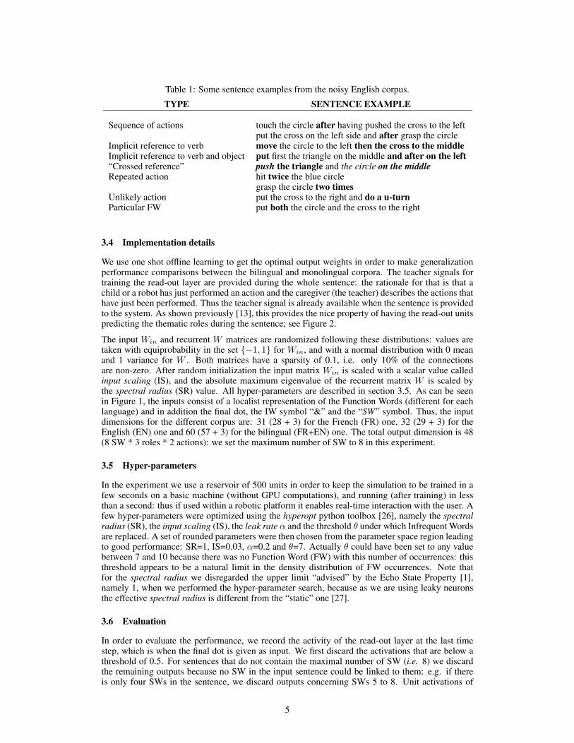
Table 1: Some sentence examples from the noisy English corpus.
TYPE SENTENCE EXAMPLE
Sequence of actions touch the circle after having pushed the cross to the leftput the cross on the left side and after grasp the circle
Implicit reference to verb move the circle to the left then the cross to the middleImplicit reference to verb and object put first the triangle on the middle and after on the left“Crossed reference” push the triangle and the circle on the middleRepeated action hit twice the blue circle
grasp the circle two timesUnlikely action put the cross to the right and do a u-turnParticular FW put both the circle and the cross to the right
3.4 Implementation details
We use one shot offline learning to get the optimal output weights in order to make generalizationperformance comparisons between the bilingual and monolingual corpora. The teacher signals fortraining the read-out layer are provided during the whole sentence: the rationale for that is that achild or a robot has just performed an action and the caregiver (the teacher) describes the actions thathave just been performed. Thus the teacher signal is already available when the sentence is providedto the system. As shown previously [13], this provides the nice property of having the read-out unitspredicting the thematic roles during the sentence; see Figure 2.
The input Win and recurrent W matrices are randomized following these distributions: values aretaken with equiprobability in the set {−1, 1} for Win, and with a normal distribution with 0 meanand 1 variance for W . Both matrices have a sparsity of 0.1, i.e. only 10% of the connectionsare non-zero. After random initialization the input matrix Win is scaled with a scalar value calledinput scaling (IS), and the absolute maximum eigenvalue of the recurrent matrix W is scaled bythe spectral radius (SR) value. All hyper-parameters are described in section 3.5. As can be seenin Figure 1, the inputs consist of a localist representation of the Function Words (different for eachlanguage) and in addition the final dot, the IW symbol “&” and the “SW” symbol. Thus, the inputdimensions for the different corpus are: 31 (28 + 3) for the French (FR) one, 32 (29 + 3) for theEnglish (EN) one and 60 (57 + 3) for the bilingual (FR+EN) one. The total output dimension is 48(8 SW * 3 roles * 2 actions): we set the maximum number of SW to 8 in this experiment.
3.5 Hyper-parameters
In the experiment we use a reservoir of 500 units in order to keep the simulation to be trained in afew seconds on a basic machine (without GPU computations), and running (after training) in lessthan a second: thus if used within a robotic platform it enables real-time interaction with the user. Afew hyper-parameters were optimized using the hyperopt python toolbox [26], namely the spectralradius (SR), the input scaling (IS), the leak rate α and the threshold θ under which Infrequent Wordsare replaced. A set of rounded parameters were then chosen from the parameter space region leadingto good performance: SR=1, IS=0.03, α=0.2 and θ=7. Actually θ could have been set to any valuebetween 7 and 10 because there was no Function Word (FW) with this number of occurrences: thisthreshold appears to be a natural limit in the density distribution of FW occurrences. Note thatfor the spectral radius we disregarded the upper limit “advised” by the Echo State Property [1],namely 1, when we performed the hyper-parameter search, because as we are using leaky neuronsthe effective spectral radius is different from the “static” one [27].
3.6 Evaluation
In order to evaluate the performance, we record the activity of the read-out layer at the last timestep, which is when the final dot is given as input. We first discard the activations that are below athreshold of 0.5. For sentences that do not contain the maximal number of SW (i.e. 8) we discardthe remaining outputs because no SW in the input sentence could be linked to them: e.g. if thereis only four SWs in the sentence, we discard outputs concerning SWs 5 to 8. Unit activations of
5

discarded SW outputs represent predictions about SWs that will never occur (see Figure 2). Finally,if there is several possible roles for a particular SW we do a winner-take-all and keep the role unitwith the highest activation.
Pointe le triangle puis attrape le.
0.2
0.0
0.2
0.4
0.6
0.8
1.0
1.2
SW le SW puis SW le .
SW1-P1SW2-O1
SW3-P2
SW4-O2
SW2-O2
SWtheSWthenSW at it0.2
0.0
0.2
0.4
0.6
0.8
1.0
1.2Touch the circle then point at it.
.
SW1-P1SW2-O1
SW3-P2
SW4-O2
SW2-O2
0.2
0.0
0.2
0.4
0.6
0.8
1.0
1.2Pointe le triangle et & touche le cercle.
SW le SW et SW le .SW&
SW1-P1SW2-O1
SW3-P2
SW4-O2
SW2-O2
SW la SW à puis SW .laSW0.2
0.0
0.2
0.4
0.6
0.8
1.0
1.2Déplace la croix à droite puis pointe la.
SW1-P1SW2-O1
SW3-P2SW4-O2
SW2-O2
SW4-P2SW3-L1
Figure 2: Examples of read-out units activations for different sentences.
4 Results
We start by providing a quantitative analysis (generalization capabilities) of the model for the dif-ferent corpora, and then we perform a qualitative analysis by examining the output activity of themodel for particular sentences.
4.1 Quantitative analysis
First we analyse the generalization errors and standard deviation for a 10-fold cross validation av-eraged over 50 different network instances. Since there are several thematic roles to be recognizedin each sentence, the full meaning of a sentence is correct only if all roles are correct; if one role ormore is incorrect the sentence is regarded as recognized incorrectly (i.e. sentence error of 1). Weprovide here the means and standard deviations of the sentence errors: 0.158 (+/-0.012) for the FRcorpus, 0.214 (+/-0.022) for the EN corpus, and 0.206 (+/-0.013) for the FR+EN corpus. The ENcorpus seems to incorporate some slightly more complex sentences than the FR corpus and has lessredundant grammatical constructions than the French one: this probably explains the higher genera-lization error for the EN corpus. Even if results are not directly comparable, the new result for theEnglish corpus outperforms the previous performance of 24.2% obtained1 in [15].
It is remarkable that the performance for the FR+EN corpus (0.206) is not very impaired comparedto the average error of the corpora processed separately (0.186).
1Results in [15] were obtained by taking the best of an ensemble of ten reservoirs with twice the number ofunits (1000 instead of 500) and leave-one-out CV (instead of 10-fold CV). Moreover the training corpus wastwo times larger.
6

4.2 Qualitative analysis
In this subsection we use the same instances for the input and reservoir weight matrices, only theread-out weight matrices are different (due to learning on different corpora). We analysed the read-out layer activity for the French and English training corpora and selected some interesting sentences(see Figure 2). For clarity and to limit the number of curves per plot only relevant output units havebeen kept, others have been discarded. The dotted line indicates the decision boundary threshold forthe final extraction of thematic roles. In Figure 2 read-out units activations (i.e. outputs of the model)can be seen for four sentences: three in French2 and one in English. Sentences before preprocessingare shown on top of each plot; corresponding grammatical constructions processed by the reservoirare shown on the x-axis. The top left plot shows activations for a grammatical construction that wasboth in the training and testing set of the given cross-validation. For trained grammatical construc-tions the output activations show online probabilistic estimations for the different roles based on thestatistics of the training set. The three remaining plots were taken from grammatical constructionsthat were not in training set but which generalized correctly. For instance, we can see in the topright plot of Figure 2 that the model is able to generalize to the correct roles even in the presence ofan infrequent word (IW symbolized by &). In all plots of the figure, two output roles units are ac-tive near the maximum value (i.e. 1) since the beginning of the sentence: SW1-Predicate-1st action(SW1-P1; blue curve) unit and SW2-Predicate-1st action (SW2-O1; red curve) unit. This is becausefor most sentences, the first two SWs are the predicate and object of the first action; i.e. the order ofactions is not reverse by words like before or after.
We choose to focus more on the French language since this is the first time we demonstrate ge-neralization capabilities with this language, and also because it has two interesting properties thatEnglish does not have: the words le or la (the in English) are gender specific, and they could bedeterminers or pronouns. We can see both functions in this sentence: “Pointe le triangle puis at-trape le.” (“Point the triangle then catch it.”): the first le is a determiner, and the second one is apronoun referring to the triangle. As we can see in the top left plot of Figure 2, at the time step afterthe second occurrence of le (i.e. at the final dot) there is a particular “re-analysis” of the sentencebecause this occurrence of le is a pronoun, which implies that the object of the second action (O2)is not a potential semantic word (SW4) that could have followed le, the O2 is rather the same one asthe first action, namely the SW in position 2 (SW2) in the sentence. That is why the activity of theoutput unit SW4-Object-2nd action (SW4-O2, the unit that binds O2 with SW4; cyan curve), goesdown to zero and the activity of the output unit SW2-Object-2nd action (SW2-O2; purple curve)goes up to one. On the contrary, in the top right of Figure 2 the input of the last SW (SW4) confirmsthe determiner function of le, thus the activity of the unit SW4-O2 (cyan curve) increases abovethe threshold, and the activity of SW2-O2 (purple curve) goes down. The input of the infrequentword symbol “&” seems to “perturb” the on-going predictions compared to the top left plot: theseactivities may not reflect the statistics of the training corpus since the occurrence of “&” at this pre-cise point in the sequence makes this sequence unique and produces a reservoir state that was notused during training. The bottom right plot of Figure 2 shows similar outputs as the top left plot,but for a sentence containing a location for the first action (SW3-L1; yellow curve). One can seehow the following output activities of units SW3-P2 and SW4-O2 are modified in consequence. Inthe bottom left of Figure 2 is the readout activity for an equivalent English sentence of the Frenchsentence in top left plot. One can see that the unit activations are similar until the last word in thesentence: it and le respectively. Some differences of units activation could be explained by the factthat the English sentence was not in the training set. This means that we have a model that is ableto represent on-going sequences of words in two different languages with the same predictions ofroles.
5 Discussion
A neuro-inspired model based on Reservoir Computing that processes sentences word by wordwith no prior semantic knowledge was used. The only assumptions are that the system is able todistinguish semantic words (SW) from function words (FW), because SWs are related to objects oractions the child or the robot already knows. Nouns and verbs were not distinguished in this SW
2Translation of sentences: (top left) “Point the triangle and catch it.”; (top right) “Point the triangle and &touch the circle.”; (bottom right) “Move the cross to the left then point at it.”.
7

abstract symbolic category. The model processed grammatical constructions instead of sentences[22, 19] based on noisy natural language corpora produced by human users.
For the first time we showed that our architecture could process three different kinds of symbolicinputs: function words, semantic words and infrequent words. Moreover we showed that this archi-tecture is able to process and generalize over the French language newly provided. Furthermore, weoutperformed previous results obtained in [15] with the English corpus. Generalization performanceon these noisy corpora, produced by users, is interesting considering the small corpus we used, about200 sentences for each language: 84.2% for the French, 78.6% for the English and 79.4% for thebilingual corpora respectively. These figures indicate the percentage of sentences that have all theirroles fully recognized, which means that the thematic role performance is higher.
When used in a robotic or other platforms, if a sentence is recognized partially (i.e. few roles inthe sentence are incorrect), the system may recover based on further contextual and semantic post-processing, thereby reducing the number of sentences not recognized. In fact, these good perfor-mances could be enhanced by post-processing because as it has been shown in [13] that most of thesentences not fully recognized have only one or few erroneous roles. Moreover we showed here forthe first time that the system was able to understand grammatical constructions that had infrequentunknown function words. This is not only interesting from the point of view of language acquisition[19] but also from the application side because it provides a natural way of dealing with the out-of-vocabulary (OOV) words problem [25]. In further work we will explore distributional encodingof semantic words based only on the context available to the system. For instance we could useword2vec representation [28] which is based on huge corpora. In this language acquisition perspec-tive, an issue would be to create such representations with small corpora where not much contextinformation is available, and moreover where this context information is available incrementally.
This bilingual experiment shows that the chosen architecture has interesting properties for multi-lingual processing. The network was able to learn and generalize without an important drop-off inperformance. What is surprising is to have such a high performance for a fixed reservoir size evenwith an input dimension that doubled in size for the bilingual corpus, compared to the monolingualexperiments: the bilingual corpus contained twice more function words than the French one or theEnglish one. Moreover, the reservoir state spaces explored for each of the corpora are quite differ-ent, due to the different sets of inputs, nevertheless the linear regression performed by the read-outlayer is still able to combine state spaces produced by very different inputs towards the same outputroles. Deeper analysis of the reservoir states and read-out weights may provide some more explana-tion why the bilingual model is working better than one would expect. It is possible that the modelbenefits from the regularities of the syntax similarities between French and English. Further workis needed to compare this bilingual neural model to other models [29] and to analyse which insightsit can give on bilingual language acquisition and second language acquisition [30] (if using an in-cremental learning). For instance, would a bilingual model that builds its own self-organized inputword representations (shared by the two languages) be able to benefit from both languages and ge-neralize better than a monolingual model? It would be also interesting to evaluate the ability of thecurrent model to process grammatical constructions that have parts in French and parts in English.
Acknowledgments
This research was supported by a Marie Curie Intra European Fellowship within the 7th EuropeanCommunity Framework Programme: EchoRob project (PIEF-GA-2013-627156). Authors are grate-ful to Cornelius Weber and Dennis Hamester for their very useful and interesting feedback.
References
[1] Jaeger, H. (2001) The echo state approach to analysing and training recurrent neural networks. Bonn,Germany: German National Research Center for Information Technology GMD Technical Report, 148, 34.
[2] Dominey, P. F. (1995) Complex sensory-motor sequence learning based on recurrent state representationand reinforcement learning. Biological Cybernetics, 73, pp. 265–274.
[3] Lukosevicius, M., & Jaeger, H. (2009) Reservoir computing approaches to recurrent neural network training.Computer Science Review 3: 127–149.
[4] Rigotti, M. et al. (2013). The importance of mixed selectivity in complex cognitive tasks. Nature,497(7451), 585–590.
8

[5] Maass W., Natschlger T., & Makram H. (2003) A Model for Real-Time Computation in Generic NeuralMicrocircuits. In Proc. of NIPS 2003, 213–220.
[6] Elman J (1990) Finding structure in time. Cognitive Science 14: 179–211.
[7] Miikkulainen, R. (1996) Subsymbolic case-role analysis of sentences with embedded clauses. CognitiveSci 20: 47–73.
[8] Wermter, S., Arevian, G., & Panchev, C. (2000) Meaning Spotting and Robustness of Recurrent Networks.In Proc. of IJCNN, pp. III-433-438. Como, Italy.
[9] Tong, M. H. et al. (2007) Learning grammatical structure with Echo State Networks. Neural networks 20:424–432.
[10] Frank, S. L. (2006). Strong systematicity in sentence processing by an Echo State Network. In Proc. ofICANN 2006, pp. 505–514.
[11] Koechlin, E., & Jubault, T. (2006). Broca’s area and the hierarchical organization of human behavior.Neuron, 50(6), 963-974.
[12] Hannun, A. et al. (2014) Deep Speech: Scaling up end-to-end speech recognition. arXiv:1412.5567
[13] Hinaut, X., & Dominey, P. F. (2013) Real-Time Parallel Processing of Grammatical Structure in the Fronto-Striatal System: A Recurrent Network Simulation Study Using Reservoir Computing. PLoS ONE 8(2): e52946.
[14] Dominey, P. F., Hoen, M., & Inui, T. (2006) A neurolinguistic model of grammatical construction process-ing. Journal of Cognitive Neuroscience, 18(12):2088–2107.
[15] Hinaut, X. et al. (2014) Exploring the Acquisition and Production of Grammatical Constructions ThroughHuman-Robot Interaction. Frontiers in NeuroRobotics 8:16.
[16] Dominey, P. F., & Boucher, J. D. (2005). Developmental stages of perception and language acquisition ina perceptually grounded robot. Cognitive Systems Research, 6(3), 243-259.
[17] Hinaut, X., & Wermter, S. (2014) An Incremental Approach to Language Acquisition: Thematic RoleAssignment with Echo State Networks. In Wermter, S. et al., Proc. of ICANN 2014, pp. 33-40.
[18] Hinaut, X. et al. (2015) Cortico-Striatal Response Selection in Sentence Production: Insights from neuralnetwork simulation with Reservoir Computing. Brain and Language, vol. 150, Nov. 2015, pp. 54–68.
[19] Tomasello M (2003) Constructing a language: A usage based approach to language acquisition. Cam-bridge, MA: Harvard University Press. 388 p.
[20] Hinaut, X. et al. (2015) Humanoidly Speaking – How the Nao humanoid robot can learn the name ofobjects and interact with them through common speech. Video, IJCAI 2015. http://bit.ly/humanoidly-speaking
[21] Marcus, G. F. et al. (1999). Rule learning by seven-month-old infants. Science 283, 77–80.
[22] Goldberg, A. (1995) Constructions: A Construction Grammar Approach to Argument Structure; Faucon-nier G, Lakoff G, Sweetser E, editors. Chicago: University of Chicago Press. 265 p.
[23] Bates, E. et al. (1982) Functional constraints on sentence processing: a cross-linguistic study. Cognition11: 245–299.
[24] Twiefel, J. et al. (2014) Improving Domain-independent Cloud-based Speech Recognition with Domain-dependent Phonetic Post-processing. In Brodley C.E. et al. (eds.). Proc. of AAAI 2014, pp. 1529-1535.
[25] Jurafsky, D., and Martin, J. H. (2009) Speech and Language Processing: An Introduction to NaturalLanguage Processing, Computational Linguistics, and Speech Recognition. Pearson International, 2nd edition.
[26] Bergstra, J., Yamins, D., & Cox., D. D. (2013) Hyperopt: A Python library for optimizing the hyperpa-rameters of machine learning algorithms. In SciPy13.
[27] Jaeger, H. et al. (2007). Optimization and applications of echo state networks with leaky-integratorneurons. Neural Networks, 20(3), 335-352.
[28] Mikolov, T. et al. (2013) Distributed Representations of Words and Phrases and their Compositionality. InProc. of NIPS 2013.
[29] Frank, S. L. (2014). Modelling reading times in bilingual sentence comprehension. In P. Bello et al. (Eds.),Proc. of CogSci 2014, pp. 1860–1861.
[30] Berens, M. S.; Kovelman, I. & Petitto, L.-A. (2013) Should Bilingual Children Learn Reading in TwoLanguages at the Same Time or in Sequence? Bilingual Research Journal, 36, pp. 35–60.
9

Efficient neural computation in the Laplace domain
Marc W. Howard, Karthik H. Shankar, and Zoran TiganjDepartment of Psychological and Brain Sciences
Boston University{marc777,shankark,zorant}@bu.edu
Abstract
Cognitive computation ought to be fast, efficient and flexible, reusing the sameneural mechanisms to operate on many different forms of information. In orderto develop neural models for cognitive computation we need to develop neurally-plausible implementations of fundamental operations. If the operations can beapplied across sensory modalities, this requires a common form of neural coding.Weber-Fechner scaling is a general representational motif that is exploited by thebrain not only in vision and audition, but also for efficient representations of time,space and numerosity. That is, for these variables, the brain appears to supportfunctions f(x) by placing receptors at locations x
i
such that xi
� x
i�1 / x
i
. Theexistence of a common form of neural representation suggests the possibility ofa common form of cognitive computation across information domains. EfficientWeber-Fechner representations of time, space and number can be constructed us-ing the Laplace transform, which can be inverted using a neurally-plausible matrixoperation. Access to the Laplace domain allows for a range of efficient compu-tations that can be performed on Weber-Fechner scaled representations. For in-stance, translation of a function f(x) by an amount � to give f(x+�) can be read-ily accomplished in the Laplace domain. We have worked out a neurally-plausiblemapping hypothesis between translation and theta oscillations. Other operations,such as convolution and cross-correlation are extremely efficient in the Laplacedomain, enabling the computation of addition and subtraction of neural represen-tations. Implementation of neural circuits for these elemental computations wouldallow hybrid neural-symbolic architectures that exhibit properties such as compo-sitionality and productivity.
1 Introduction
Cognitive computation in the brain is fast, efficient and flexible. Emulating this ability would resultin extremely important technological advances. A general computational framework should be ableto operate on a wide range of content without learning each exemplar. Such a framework shouldgeneralize across not only different specific operands but also across sensory domains, providing ageneral computational language for cortical computation. Mathematical operations are an importantaspect of symbolic processing. Because of the combinatorics of these problems, learning each setof operands and the appropriate outcome is not feasible.
This paper argues that
1. The brain represents functions of many quantities, including time, using a common formof coding that we refer to as Weber-Fechner scaling.
2. Some of these quantities can be efficiently computed using the Laplace domain and aneurally-plausible mechanism for approximating the inverse Laplace transform.
1

3. Computational operations, including translation, convolution, and an analog of cross-correlation, can be efficiently computed in a neurally-plausible way with access to theLaplace domain.
This suggests the hypothesis that the brain uses the Laplace domain as a common computationalcurrency across modalities, enabling reuse of the same neural mechanisms for flexible computationson a range of different kinds of information.
1.1 Weber-Fechner scaling of one-dimensional functions in the brain
In this paper we restrict our attention to one-dimensional quantities defined over the positive real linefrom zero (or some relatively small value) to some large (effectively unbounded) value. We arguethat the brain represents functions over variables with these properties using Weber-Fechner scaling.If the ith receptor has a receptive fields centered at x
i
, then we define Weber-Fechner scaling tomean that
1. the spacing of adjacent receptors is such that xi
� x
i�1 / x
i
.
2. the width of the receptive field of the unit at xi
should be proportional to x
i
.
These two constraints imply a logarithmic scale internal scale for x, which we label ⇤x to avoid
confusion between external physical variables and internal representations. We refer to this codingscheme as a Weber-Fechner scale because it can readily implement the behavioral Weber-Fechnerlaw [2].
There is good evidence that Weber-Fechner scaling is obeyed in the brain in coding extrafovealretinal position [7, 21]. In the case of vision, Weber-Fechner scaling can be attributed to the struc-ture of the retinal circuitry. However, Weber-Fechner scaling appears to be more general. Neuralevidence [15] suggests that Weber-Fechner scaling applies to neural representations of numerosity.For instance, [14] observed approximately Weber-Fechner coding for numerosity in the activity ofPFC neurons during the delay period of a working memory task. Different neurons had differentpreferred numerosities. The width of the tuning curves went up linearly with the cell’s preferrednumerosity.1 Weber-Fechner scaling for numerosity cannot be attributed to a property of a physicalreceptor.
Behavioral [1] and theoretical work [16] suggests that this Weber-Fechner coding scheme should ex-tend also to functions of remembered time. Indeed, a growing body of neurophysiological evidencesuggests that representations of time also obey Weber-Fechner scaling. Figure 1 shows evidence il-lustrating evidence suggesting that the neural representation of time may obey Weber-Fechner scal-ing. First, the observation of time cells suggests that the brain supports functions of past time [12].During the delay of a memory task, different time cells fire sequentially at circumscribed periods ofthe delay. At any moment, observation of the set of active cells provides an estimate of the time inthe past at which the delay began. Time cells have now been observed in a variety of brain regionswith similar qualitative properties that suggest Weber-Fechner coding. It is known that the width ofthe receptive fields of time cells increases with delay in the hippocampus [5, 11], medial entorhinalcortex [10], mPFC [19] and striatum [13]. Moreover, the density of preferred times decreases withthe delay [11, 10, 13, 19]. Collaborative work to quantitatively assess Weber-Fechner coding in alarge dataset of hippocampal time cells is ongoing.
If the neural representation of time obeys Weber-Fechner scaling this is a non-trivial computationalchallenge. A representation of a timeline must update itself in real time. Because the spacingbetween t
i
and t
i+1 is different than the spacing between t
i+1 and t
i+2, information would have toflow at different rates for different values of t. This seems neurally implausible. We have proposed asolution to this challenge—updating the Laplace transform of history rather than history itself—thatwe argue also lends itself readily to efficient and flexible computation.
1Although they did not assess the spacing in a quantitative way, the number of neurons did go down withpreferred numerosity.
2
a b c
109
Figure 3.1: Temporally‐modulated activity spans the time on the treadmill. Each row represents the normalized firing rate of one neuron, sorted by the location of peak firing. Neurons were included if they were active on the treadmill and had temporal information ≥ 0.2 bits/spike.
3.6. Figures
Time [s]
Cel
l #
0 1 2 3 4 5
20
40
60
80
100
120
Figure 2 Paton
latency0 10 20 30 40
wid
th a
t hal
f hei
ght
0
5
10
15
20
response latency (s)
resp
onse
wid
th (s
)
10 20 300
0
20
15
10
5
40
B time relative to reward (s)
cell
#
FI = 12 FI = 24 FI = 36 FI = 48 FI = 60A
−12 0 12
20
40
60
−24 0 24
20
40
60
−36 0 36
20
40
60
−48 0 48
20
40
60
−60 0 60
20
40
60 0
5
10 firing rate (z)
psth peak latency as interval fraction0 0.2 0.4 0.6 0.8
frequ
ency
0
2
4
6
8
10
12
14
16
18
response latency(time/FI)
0.2 0.4 0.60 0.8
0
8642
10
18161412
coun
t
C
20
40
60
0-12 12−12 0 12
20
40
60
−24 0 24
20
40
60
−36 0 36
20
40
60
−48 0 48
20
40
60
−60 0 60
20
40
60
20
40
60
0-24 24
20
40
60
0-36 36
20
40
60
0-48 48
20
40
60
0-60 60
10
5
0
Figure 1: A neural Weber-Fechner scaling for time? In each plot, false color firing rate maps areshown as a function of time for a number of extracellularly-recorded neurons. The neurons areordered according to their time of peak firing. If the neurons showed linear spacing, these plotswould appear as a straight “ridge” of constant width. To the extent the ridges are curved, that impliesa decreasing number density of neurons with preferred time of firing, consistent with Property 1. Tothe extent that the ridges get wider during the delay, this implies an increase in receptive field withpreferred time of firing, consistent with Property 2. a. Neurons in medial entorhinal cortex duringrunning on a treadmill [10]. The duration of the delay was on average 16 s (see [10] for details). b.Neurons in medial PFC during the delay of a temporal discrimination task [19]. c. Neurons in thestriatum during the 60 s prior to (left) and following reward in a fixed interval procedure [13]. Notethat the ordering is such that neurons with time fields earlier in the delay are at the bottom of thefigure rather than the top.
2 Constructing Weber-Fechner scale functions of “hidden” variables usingthe Laplace transform
We have developed a formal mechanism for efficiently representing a Weber-Fechner timeline. Thekey insight is that while the timeline itself cannot be evolved self-sufficiently in time, the Laplacetransform of the timeline can be [16]. The model can be understood as a two-layer feedforwardarchitecture (Fig 2). At each moment a single input node f(t) projects to a set of units F (s) thatstore the Laplace transform up to the current moment; s indexes the different units. Through a localset of feed forward connections (represented by an operator L-1
k ), the second layer approximatelyinverts the encoded Laplace transform to represent a fuzzy reconstruction of the actual stimulushistory itself, ˜
f(
⇤⌧). The operator L-1
k implements the Post inversion formula keeping k terms andcan be readily implemented with simple feedforward projections [16].
This simple computational scheme for representing a Weber-Fechner timeline is sufficient to ac-count for canonical behavioral effects in a variety of learning and memory paradigms across species[6]; the long functional time constants necessary to encode F (s) could be computed using knownneurophysiological mechanisms [18]. This mechanism can be straightforwardly generalized to rep-resent one-dimensional spatial position, numerosity or any other variable whose time derivative isavailable at each moment [5]. More precisely, by modulating the differential equations governingthe Laplace transform by ↵(⌧) = dx/dt we can obtain the Laplace transform with respect to x
rather than t. This mechanism is sufficient to account for a variety of neurophysiological findingsregarding place cells and time cells in the hippocampus [5] and can be generalized to numerosity.For instance, if we initialize a representation with f(⌧ = 0) set to a single delta function input, thenlet it evolve with ↵(⌧) set to the rate of change of some variable x during an interval T , then at theend of the interval ˜
f(
⇤x, T ) will give a scale-invariant estimate of the net quantity x accumulated
from time 0 to time T . When ↵(⌧) is set to zero, the estimate of ˜
f stops changing so that ↵ can alsobe used as a control signal to maintain information in working memory.
As with all path integration models, this approach is subject to cumulative error. That is if↵(⌧) = dx/dt + ⌘, the estimate of ˜
f(
⇤x) will grow more imprecise over time. However, note that
in the absence of noise, the “blur” in the representation of time, place, and number does not reflectstochastic variability. Rather, the blur is more analogous to a tuning curve with non-zero width.
3

a b
Figure 2: a. Schematic of the model for encoding a temporal history f(⌧). At each time step, input from asingle node provides input to a set of nodes F (s). Each node of F is indexed by a different value of s which canbe identified with the real Laplace variable. Nodes in F (s) project locally to another set of nodes in f(
⇤⌧) via
an operator L-1k . The nodes in f approximate the original function f(⌧). The error in f(
⇤⌧) is scale invariant.
We choose the distribution of nodes across s and thus also ⇤⌧ to implement Weber-Fechner spacing (not shown).
b. Nodes in f behave like neural time cells. In this plot the input f(⌧) and the activity of two nodes in F (s)
with different values of s and two corresponding nodes in f(⇤⌧) are shown evolving in time. Note that the units
in F (s) behave like charging and discharging capacitors with different rate constants (controlled by their valueof s). The units in f(
⇤⌧) behave like neural time cells, responding a characteristic time after the input. The time
at which each unit’s activity peaks is controlled by ⇤⌧ = k/s.
3 Flexible computations in the Laplace domain
If time, space, and number, as well as sensory representations share a common coding scheme, thenmechanisms for computing with representations of that form could be reused across many typesof information. Here we sketch neurally implementable mechanisms for three operations in theLaplace domain, translation, convolution, and a close analog of cross-correlation. Of these three,translation is the most thoroughly worked out, with a detailed mapping hypothesis onto neurophys-iological mechanisms related to theta oscillations [17]. Translation of functions of time can be usedto anticipate the future to inform decision-making in the present; translation of functions of othervariables can be used to imagine alternative states of the world to inform decision-making in theworld in its current state. Convolution and cross-correlation can be used for the addition and sub-traction of functions, respectively (among other uses). Because the Post inversion formula is notwell-defined for �s, we describe an analog of cross-correlation that can be implemented within theneural framework we have developed.
3.1 A neural mechanism for translation via hippocampal theta oscillations.
Access to the Laplace domain facilitates flexible translation of one-dimensional representations. Afunction f(x) can be translated to obtain f(x + �) in the Laplace domain via a simple point-wisemultiplication with the function exp(�s�) where s is the Laplace domain variable. This can under-stood in the context of the two layer network as modulation of the synaptic weights in L-1
k between F
and ˜
f [22]. Consideration of the computational requirements for translation in the Laplace domaincoupled with the hypothesis that hippocampal theta phase precession implements translation leadsto several results [17].
The resulting neural model accomplishes translation across scales and at the same time explains andorganizes a broad variety of neurophysiological findings related to hippocampal theta oscillations.The hypothesis is that theta oscillations implement translation from zero to some large value withineach theta cycle. This successive translation of the present into the past enables prediction of the fu-
4

a b
Figure 3: A neurophysiological mechanism for translation of one-dimensional functions exploiting theta os-cillations. a. A generalized circuit for computing and translating scale-invariant functions of one-dimensionalvariables. ↵(⌧) enables the same circuit to represent functions of time or any other one-dimensional quantityfor which the time derivative is available. Thus, if f(⌧) can be rewritten as f (x (⌧)) and ↵(⌧) = dx/d⌧ ,then the reconstruction is with respect to x rather than ⌧ and we write ⇤
x. � provides a mechanism to translatethe function. b. Theta phase precession shows properties resembling translation to different future points ofthe trajectory within a theta cycle. Top: neurophysiological data from [9]. Place cells from different positionsalong the dorsoventral axis of the hippocampus have place cells of different size. However, cells at all scalesstill precess over the same range of phases. Bottom: model predictions show the same qualitative patterns [17].
ture at successively more distant points. This model accounts for the finding that all scales (differentvalues of s) phase precess through the same range of local theta phases (Fig. 3). Moreover, coherenttranslation requires that both past time (controlled by the values of s) and future time (controlled bythe rate at which � changes within a theta cycle) obey Weber-Fechner scaling. Finally, the modelpredicts that cells coding for predicted events should ramp up their firing from the time at whichthe prediction becomes available to the time at which the predicted stimulus is obtained, phase pre-cessing through at most one theta cycle. This prediction is analogous to findings for neurons in theventral striatum [20].
We found good evidence aligning translation of functions of space and time from 0 to some largevalue of � to neurophysiological findings during hippocampal theta oscillations. However, trans-lations with other properties could be implemented during other neurophysiological events. Forinstance, translation by negative values would correspond to search through memory for the past;translation to a single non-zero value of � (rather than sweeping through a range of values) wouldfacilitate retrieval of a memories at a specific range of past times [4]. In two spatial dimensions, onecan imagine a series of translations tracing out an imagined path in a navigation task [8]. In the vi-sual modality, translation could be used to simulate planned (or imagined) eye movements or motionof objects in the world. Although these translations could have somewhat different neurophysiolog-ical signatures, they are all computationally related to one another. And in all cases, the translationfacilitates decision-making and behavior in the present by enabling examination of imagined statesof the world.
3.2 Arithmetic operations on functions through parallel computations
Access to the Laplace domain facilitates operations other than translation. In the same way thatpoint-wise multiplications in the Laplace domain can be achieved in a parallel fashion to implementtranslation of any function, it is also possible to perform addition and subtraction operations on anytwo functions by point-wise parallel computations with similar efficiency in the Laplace domain. Forthis, we start with a definition of the operations addition and subtraction on numbers represented bydistribution functions.
Let f(x) and g(x) be functions representing two distributions of possible values for the number xin the range 0 to x
max
. Outside this range, the functions are assumed to vanish. We shall define theoperation of ‘addition’ of these two distributions to be [f + g](x) to be the convolution of the two
5
functions.[f + g](x) ⌘
Z 1
0f(x
0)g(x� x
0) dx
0
The justification for this definition is rather straightforward. By considering the two functions to beDirac delta functions at two different positions, x1 and x2, note that [f + g] is a Dirac delta functionat x1 + x2. Moreover, the addition operation is bilinear with respect to the two functions, and hencethe above generalized definition for addition is justified. Importantly, since we have access to theLaplace transform of the functions, namely F (s) and G(s), the addition operation can be performedin the Laplace domain. The Laplace transform of [f + g] is simply the point wise multiplicationof F (s) and G(s), which can be computed in a parallel fashion, independently for each s value.Finally, the L-1
k operator can be employed to invert the Laplace transform of [f + g] and obtain afuzzy addition operation.
It is easy to convince oneself that subtraction operation can similarly be defined to be2
[f � g](x) ⌘Z 1
0f(x
0)g(x
0+ x) dx
0
By defining a reflected function g
r
(x) = g(x
max
� x), it can be seen that the Laplace transform of[f � g] is simply the point wise multiplication of the Laplace transform of f(x) and g
r
(x). A pointof subtlety here is that for the subtraction operation, we have to consider both positive and negativevalues of x although the two functions are assumed to be non vanishing only for x > 0. However,noting that [f � g](x) = [g � f ](�x) for positive x, we can perform the subtraction operationfor negative x values also. In this entire process, only positive values of s are utilized, and hencethe inverse Laplace operator L-1
k is always well defined and the entire process can be performed inparallel.
We have not yet carefully considered the neurophysiological substrates that could support thesearithmetic operations. However, the computational efficiency of performing these operations in theLaplace domain is considerable. Given these considerations, it may be reasonable for the brain toencode the Laplace transform even for variables that are provided along a Weber-Fechner scale dueto the property of the sensory receptors.
4 Discussion
We suggest that the brain uses a common form of coding, Weber-Fechner scaling, to representunbounded one-dimensional quantities. It can be shown that Weber-Fechner scaling is an optimalresponse to signals that are long-range correlated, which are found throughout the natural world[16]. Weber-Fechner scaling allows for representation of exponential scales with linear resources.
Representation of variables such as time, space and numerosity is greatly facilitated by access to theLaplace transform. Many computations can be efficiently performed in the Laplace domain. Forinstance, translation of representations of space and time toward the past can be used to estimatethe future. Recent work has developed a detailed mapping between a translation operator and hip-pocampal theta oscillations. We sketched implementable operations for addition and subtraction offunctions on a Weber-Fechner scale. These operations could be used for combining functions, or forcomparing one function to another. Because the outcome of a specific operation does not need belearned, but can be computed on-line, the existence of these operations provides an important steptowards endowing neural systems with the properties of productivity and compositionality that aretaken to be essential aspects of symbolic computation and cognition more broadly [3]. For instance,it is clear that arithmetic obeys the properties of compositionality and productivity (modulo edgeeffects). If the result of an addition operation is a function with the same neural code as the addends,then one can in principle represent an effectively infinite number of possible problems. For instance,given only two input functions f and g one could compute f + g, or (f + g)+ g, or (f +f)+ g, etc.
There are several design considerations that are important in developing this into a general frame-work for cognitive computation. The first consideration is whether computation for different infor-mation should be performed in a central location, as in a von Neumann architecture or performed
2The challenge of this approach is that the Post inversion formula does not work when the transform isgrowing exponentially as with �s. If that were not the case, cross-correlation would suffice to implementsubtraction.
6
locally. The answer may depend on the form of operation. Consider Fig. 3a. Different settings for↵(⌧) and different settings for f(⌧) can give rise to a very broad range of representations, corre-sponding to a broad taxonomy of cells in the hippocampus and related structures [5]. All of theserepresentations can be translated by modulating the same weights used to construct the representa-tion (modulation by �). Here the control signal for translation is a scalar per representation and theoutput of the computation can be written to the same cells that are used to hold the representationitself.3 This means that the cost of local implementation of translation is small per translatable func-tion. In contrast, addition and subtraction operators require additional resources to hold the outputof the computation. The storage cost of implementing this operation locally would be relativelysubstantial. Moreover, because there are many pairwise combinations of representations that mightneed to be combined, there is in addition a considerable wiring cost associated with local processing.For these reasons addition and subtraction of functions ought not to be performed locally.
Acknowledgments
We acknowledge helpful discussions with Eric Schwartz, Haim Sompolinsky, Kamal Sen, XuexinWei, and Michele Rucci. This work was supported by BU’s Initiative for the Physics and Mathe-matics of Neural Systems and AFOSR FA9550-12-1-0369.
References
[1] BALSAM, P. D., AND GALLISTEL, C. R. Temporal maps and informativeness in associativelearning. Trends in Neuroscience 32, 2 (2009), 73–78.
[2] FECHNER, G. Elements of psychophysics. Vol. I. Houghton Mifflin, 1860/1912.[3] FODOR, J. A., AND PYLYSHYN, Z. W. Connectionism and cognitive architecture: A critical
analysis. Cognition 28, 1 (1988), 3–71.[4] FOSTER, D. J., AND WILSON, M. A. Reverse replay of behavioural sequences in hippocam-
pal place cells during the awake state. Nature 440, 7084 (2006), 680–3.[5] HOWARD, M. W., MACDONALD, C. J., TIGANJ, Z., SHANKAR, K. H., DU, Q., HAS-
SELMO, M. E., AND EICHENBAUM, H. A unified mathematical framework for coding time,space, and sequences in the hippocampal region. Journal of Neuroscience 34, 13 (2014),4692–707.
[6] HOWARD, M. W., SHANKAR, K. H., AUE, W., AND CRISS, A. H. A distributed representa-tion of internal time. Psychological Review 122, 1 (2015), 24–53.
[7] HUBEL, D. H., AND WIESEL, T. N. Uniformity of monkey striate cortex: a parallel relation-ship between field size, scatter, and magnification factor. Journal of Comparative Neurology158, 3 (1974), 295–305.
[8] JOHNSON, A., AND REDISH, A. D. Neural ensembles in CA3 transiently encode paths for-ward of the animal at a decision point. Journal of Neuroscience 27, 45 (2007), 12176–89.
[9] KJELSTRUP, K. B., SOLSTAD, T., BRUN, V. H., HAFTING, T., LEUTGEB, S., WITTER,M. P., MOSER, E. I., AND MOSER, M. B. Finite scale of spatial representation in the hip-pocampus. Science 321, 5885 (2008), 140–3.
[10] KRAUS, B. J. Time and distance coding by the hippocamus and medial entorhinal cortex.PhD thesis, Boston University, 2012.
[11] KRAUS, B. J., ROBINSON, 2ND, R. J., WHITE, J. A., EICHENBAUM, H., AND HASSELMO,M. E. Hippocampal ”time cells”: time versus path integration. Neuron 78, 6 (2013), 1090–101.
[12] MACDONALD, C. J., LEPAGE, K. Q., EDEN, U. T., AND EICHENBAUM, H. Hippocampal“time cells” bridge the gap in memory for discontiguous events. Neuron 71, 4 (2011), 737–749.
[13] MELLO, G. B., SOARES, S., AND PATON, J. J. A scalable population code for time in thestriatum. Current Biology 25, 9 (2015), 1113–1122.
[14] NIEDER, A., AND MERTEN, K. A labeled-line code for small and large numerosities in themonkey prefrontal cortex. Journal of Neuroscience 27, 22 (2007), 5986–93.
3This is possible because the original untranslated function can be recovered simply by setting � = 0.
7
[15] NIEDER, A., AND MILLER, E. K. Coding of cognitive magnitude: compressed scaling ofnumerical information in the primate prefrontal cortex. Neuron 37, 1 (2003), 149–57.
[16] SHANKAR, K. H., AND HOWARD, M. W. Optimally fuzzy temporal memory. Journal ofMachine Learning Research 14 (2013), 3753–3780.
[17] SHANKAR, K. H., SINGH, I., AND HOWARD, M. W. Neural mechanism to simulate a scale-invariant future. arXiv preprint arXiv:1503.03322 (2015).
[18] TIGANJ, Z., HASSELMO, M. E., AND HOWARD, M. W. A simple biophysically plausiblemodel for long time constants in single neurons. Hippocampus 25, 1 (2015), 27–37.
[19] TIGANJ, Z., KIM, J., JUNG, M. W., AND HOWARD, M. W. Temporal coding across scalesin the rodent mPFC. Cerebral Cortex (In revision).
[20] VAN DER MEER, M. A. A., AND REDISH, A. D. Theta phase precession in rat ventral striatumlinks place and reward information. Journal of Neuroscience 31, 8 (2011), 2843–54.
[21] VAN ESSEN, D. C., NEWSOME, W. T., AND MAUNSELL, J. H. The visual field repre-sentation in striate cortex of the macaque monkey: asymmetries, anisotropies, and individualvariability. Vision Research 24, 5 (1984), 429–48.
[22] WYBLE, B. P., LINSTER, C., AND HASSELMO, M. E. Size of CA1-evoked synaptic poten-tials is related to theta rhythm phase in rat hippocampus. Journal of Neurophysiology 83, 4(2000), 2138–44.
8

Neural Network Model of Semantic Processing in the
Remote Associates Test
Ivana Kaji
´
c
School of ComputingPlymouth University
Plymouth, Drake Circus, PL4 8AAUnited Kingdom
Thomas Wennekers
School of ComputingPlymouth University
Plymouth, Drake Circus, PL4 8AAUnited Kingdom
Abstract
The ability to generate novel, unique and useful ideas is an important trait of intel-ligent behaviour. It is also a virtue of a creative individual in many scientific andartistic domains. In this study we are concerned with the Remote Associates Test(RAT), a task widely used in psychology and neuroscience to study insight andcreative problem solving. The RAT is used to assess the ability of an individualto generate novel relationships among familiar words. The test consists of wordtriplets (e.g. cream, water, skate) and the task is to find a unique word associ-ated with all three words. Here, we aim to identify a basic set of computationalmechanisms underlying cognitive processes in the RAT solving. To this end, wepropose a multi-layer neural network based on biologically and cognitive realisticmechanisms. The search for a solution in a RAT problem is realised by spreadingof activity among word associations in a semantic layer, and the selection of a re-sponse by a winner-take-all layer. The model yields human-like performance anddistinguishes between easy and difficult RAT problems. The modelling findingsare consistent with the existing theories in creativity research, confirming that lessstereotypical word associations are important for the good performance on theRAT.
1 Introduction
The adjective ”creative” is often attributed to new, valuable and surprising ideas and objects [1]. It isseen as a positive quality of an individual. Various tests and questionnaires have been devised in theattempt of measuring different aspects of creative thinking. Of particular interest to neuroscienceand cognitive science have been cognitive abilities such as working memory, sustained attention andcognitive flexibility underlying behaviour assessed with creativity tests [2].
Divergent thinking tests measure the ability to generate new, meaningful and relevant ideas. Anexample of a task in a divergent thinking test is to think of as many possible practical uses of acertain object, such as a cooking pot or a brick [3]. In contrast to divergent thinking tests, convergentthinking tests have a correct, not necessarily unique, solution. A convergent task commonly used tostudy insight is the ”9 dots” puzzle, where nine dots have been arranged in three rows and the taskis to connect them with four straight lines. Another common task is the Remote Associates Test(RAT) used to measure the ability to form novel and meaningful word associations. While thesetests are broadly used in creativity research, solving them requires a range of functions [2, 4] whichcan facilitate or hinder the performance and the process of problem solving. Thus, to understandthe assessed process of ideation it is important to identify and understand the underlying cognitiveprocesses.
1

1.1 The Remote Associates Test
In this study we are concerned with the modelling of cognitive processes underlying solving ofthe Remote Associates Test (RAT). The RAT has been widely used in cognitive neuroscience andpsychology [5–7] to study insight, problem solving and creative thinking since it was conceived in1962 [8]. It was developed to measure the ability of an individual to form new associations amongseemingly unrelated words. The test consists of word triplets and the task is to find a word associatedwith all three words for every triplet. An example of a RAT problem is a word triplet cream, water,skate with a solution ice. The performance on the RAT is measured as the number of correctlysolved items within a given time limit. Mednick’s theory on associative hierarchies [8] suggests thathighly creative individuals are able to form rare, uncommon and remote word associations. Thisis in contrast with associations formed by less creative individuals who respond with fewer, morecommon and stereotypical associations. In the present study we investigate this idea by analysinghow different word pair associations influence the test performance. The simplicity of the paradigm,availability of a battery of tests in various languages and the opportunity to administer the testin neuroimaging studies [4, 5] have made the RAT ubiquitous in the study of associative basis ofsemantic cognition.
An interesting cognitive aspect of the RAT solving is the semantic search process in which an in-dividual attempts to find a solution to a RAT problem. Insight solutions to a RAT problem occurabruptly, without voluntary control of a person solving the task, and are preceded by unconsciousprocessing [5]. In contrast, analytical solutions are derived gradually as the person attempts to solvea task [9]. Analytical solving usually allows more time to respond, which correlates with bettertest performance [10, 11]. One of the first proposals of semantic processing in the RAT involvingsubconscious processing is the spreading activation theory [12]: every cue word activates a subsetof words in a semantic network. Overlapping activations of a unit crossing the threshold give riseto a solution. However, this theory does not provide an account of mechanisms which underlie thesearch process nor does it explain the variety in performance. Better understanding of the analyticalRAT solving has been provided by studies analysing human responses when participants solve RATproblems by reporting every word they think of [13, 14]. Common findings confirm that the searchprocess is restricted by all three cues, with one primary cue being used to generate a response. Evi-dence was provided in favor of a local sequential search process in the RAT [13], meaning that thenext guess is chosen based on the previous one.
The RAT has been also investigated in various computational studies [15–18]. Statistical approachesusing large corpora of text and natural language processing tools have yielded a performance whichis comparable to or even better than the human performance on the test [16, 17]. Mednick’s theoryon associative hierarchies [8] was scrutinised by identifying relevant properties of a semantic net-work of an individual [18–20]. Semantic networks of individuals scoring well on the RAT satisfysmall-world network properties, where every word in the network can be reached in a few stepsby following associated words of any other word. Qualitative differences in associative networksbetween individuals with low and high creative abilities have been described in [19]. A modellingstudy investigating the generation of ideas in spontaneous thought in a neural network [20] con-firmed that scale-free and small-world network properties are important for efficient search in thememory generating conventional and creative ideas. A Markov Chain Monte Carlo model [15]successfully reproduced experimentally derived human response patterns [13] supporting findingson the local search strategy. While providing valuable insights into the understanding of memorysearch, these models offers a limited explanation of the cognitive mechanisms involved in the se-mantic processing in the RAT and their relation to the test performance.
Summarising the existing work, the evidence suggests that both the executive cognitive componentguiding the search process and the organisation of the semantic network are important for the seman-tic processing in the RAT. To identify a minimal set of computational primitives underlying theseprocesses, we propose a neural network in which every layer realises a different function interpretedin the theoretical framework of semantic processing
2 The Model
We propose a neural network model of the RAT solving based on the spreading activation [12]and a winner-take-all (WTA) mechanism. Solving of a RAT problem is realised as a search for a
2

Algorithm 1 Search by spreading activation and a winner-take-all functionnr visited 0visited = [ ]for i 1, N do
activationsi 0for all c in cues do
Ic 1j �1while nr visited < max nodes do
for all neighbours i of the current node j do
if wij > #s then
activationsi activationsi + wijactivationsj
activationsi activationsi + Ii
visited visited+ j
nr visited nr visited+ 1if j == target then
break
j WTA(activations)
solution in a semantic network. To better understand the workings of the neural network, we firstpresent the search algorithm which is then implemented by the network. The equations of the neuralnetwork model are presented together with an explanation of how algorithm components map tocomputations performed by neuron-like units.
2.1 Search Algorithm
The search for a solution is done separately for every RAT problem consisting of three cue wordsand a target solution. For every problem, the word cues are used to initialise the search process.In every step of the search process, a word is selected as a candidate solution to a problem. Everyword is represented as a node in a graph and every node has a level of activity which changes as thesearch unfolds. Thus, the search for a solution to a RAT problem is modelled as a graph traversaland the direction of the search is determined by the levels of node activities. If the selected nodematches the target word, or a certain number of words in the search has been exhausted, the searchprocess terminates.1 The activity of neighbours of a currently visited node is elevated by the amountproportional to the connection strength between the node and its neighbours. Connection strengthsfor N = 5018 words are derived from a freely available database of word association strengthsacquired in a free association task [21]. In the task, the participants were instructed to write a singleword which first came to their mind when prompted with a cue word. To obtain the associativestrength between word pairs, the number of participants who responded with a specific word to acue was divided by the number of participants performing the same task. Only responses whichwere given by at least two participants were considered.
After elevating the activities of neighbouring nodes, a new node will be selected by the WTA func-tion and the old node will be annotated as visited. In the algorithm, the WTA function sorts nodeindices based on their activities and returns the index of a node with the highest activity level whichhas not been visited before. In this way, words which have already been considered as a solutionwill not appear again in the search process. If two nodes have the same level of activity, the firstnode returned by the sort algorithm will be selected. The search path is created by appending everyvisited node to the list of previously visited nodes.
In the beginning, the activity of all nodes is set to zero. Every node receives an external input, whichis set to one only for the nodes representing the problem cues, and zero for all other nodes. Basedon high activity levels, the WTA sequentially selects three problem cues and the activity spreadsthrough the network from the problem cues first. Only after all three cues have been visited, the
1Here we do not model the process of determining whether a response is a solution to the RAT problem.Instead, we focus on the process of ideation of possible words, assuming when an individual comes up with aword they will be able to determine if it is a correct solution by comparing it against the task constraints.
3

SemanticLayer
WTALayer
InhibitioryLayer
+
Figure 1: Neural network model of the semantic search in the RAT. The word with the highestactivity level in the semantic layer is selected by the WTA layer as a response to a RAT problem.If the selected word does not match the solution the inhibitory layer suppresses the activity of theselected word allowing the WTA to select the next winner.
WTA will select a new node as a candidate solution. The process terminates when the selectedresponse matches the target or when a certain number of nodes has been visited. The pseudocodefor the search algorithm is shown in Algorithm 1. In every step the WTA function selects a node j,which is appended to the list of visited nodes after it has been processed. In the first iteration, thereis no spreading of the activity from any node as there is no winning node (j = �1). This occurs inthe second step when the WTA has selected the first problem cue receiving the external input. Thiscondition is handled in the code and omitted here for clarity.
To explore the influence of different word pair association strengths on the RAT performance, weimplement spreading of activity only to those neighbours whose connection strength to the process-ing node is greater than the spreading threshold #s.2 Weak connection strengths stand for rare anduncommon associations, which according to Mednick’s theory [8] are more likely to be generatedby highly creative individuals. Increasing the threshold corresponds to removal of such associationpairs, resulting in longer number of steps between two nodes or, for very high thresholds, inabilityto reach a node.
2.2 Neural Network
A three-layer neural network model is used to simulate solving of RAT problems using the searchalgorithm described in Algorithm 1. The three layers are the semantic layer, winner-take-all (WTA)layer and inhibitory layer. All three layers have distinct functional roles. The model scheme is shownin Figure 1. The semantic layer represents a semantic network, consisting of a vocabulary and theassociative relationships between the words in the vocabulary. The WTA layer selects a winningunit simulating a solution guess to a RAT problem. The spread of activity from a winning unit inthe semantic layer is done via feedback connections from the WTA layer to the semantic layer. Ifthe selected word is not a solution to the RAT problem, the inhibitory layer suppresses the activityof the winning unit in the WTA layer. This allows the next unit with the highest activity level to winin the next step. The activity of units in all layers is updated in parallel in each time step.
The activity of units in the first layer can be written as:
2This is equivalent to rectifying all wij < #s to zero.
4

ai(t+ 1) = ai(t) + ⇢a
✓ NX
j=1
Wijzj(t)aj(t) + Ii(t)
◆(1)
zi(t) = ⇥(wi(t)� #w) (2)kz(t)k = 1 (3)
where ai(t) describes a non-decaying activity of a unit i at time t where i = 1, . . . , N . Wij is theconnection strength from the unit j to the unit i, extracted from the database of free associations[21]. The constant ⇢a is inversely proportional to the stimulus length tn and allows the analyticalderivation of precise values of activity levels (not shown). The binary vector z(t) always has exactlyone or zero active elements, with the active element representing the currently visited node (variablej in Algorithm 1) in the semantic layer. The winner is a word considered as a solution to the RATproblem. Consistent with the algorithm, only the activity of nodes whose edges incident to thewinning node are greater than the spreading threshold #s, or the activity of nodes receiving externalinput, will be elevated. Thresholding is done by setting the weights smaller than #s in the connectionmatrix W to zero. The winning node is set based on unit activities in the WTA layer. If a unit inthe WTA layer crosses the threshold #w, the Heaviside step function will toggle the correspondingbit in z(t). Only at the beginning of a simulation, the external input I(t) is used to sequentiallyincrease the activity of cue nodes in the semantic layer. This in turn will elevate the activity of theunits in the WTA layer yielding a winner whose feedback connection will activate the spread ofactivity from a winning unit in the semantic layer. The first three winners are thus going to be thethree problem cues. Ii(t) is clamped to one for the duration tn starting at non-overlapping times tifor nodes representing problem cues: t = ti : Icuei(ti) = 1 where cuei is the index of a problemcue i 2 {1, 2, 3}. The activity of the units in the WTA layer is described as:
wi(t+ 1) = wi(t) + ⇢w
⇥c1zi(t) + c2 eai(t)� c3y(t)� c4r(t) + c5⌘i(t)
⇤(4)
y(t+ 1) =NX
j=1
zj(t) (5)
Units in this layer receive one-to-one feedforward input eai from the units in the first layer. The firstWTA unit to cross the threshold #w will be the one receiving the strongest normalised input eai(t).3.It will activate the self-excitatory connection of a strength c1, and the input to the single inhibitoryneuron y(t) (a unit with the ’+’ sign in Figure 1). The inhibitory neuron will project feedbackconnections to all units in the layer, such that the activity of all the units apart from the winningone will be suppressed and kept below the threshold #w. The winning neuron will also toggle thecorresponding bit in the z(t) as described in equation 2 and elevate activities of its neighbours inthe semantic layer. Due to the self-excitation, the activity of a winning unit in the WTA layer willcontinue to increase until suppressed by a unit in the third layer. The noise term ⌘i(t) randomlydrawn from a uniform distribution is added to allow the WTA to select a winning unit when two ormore units receive the same input ea(t) from the semantic layer. Finally, after a unit zi(t) has beenactive for a certain amount of time tn it will activate the corresponding inhibitory unit in the thirdlayer:
ri(t+ 1) = ri(t) +⇥
✓ tX
j=t�tn
zi(tj)� tn
◆(6)
The feedback connections to the WTA layer will inhibit the activity of the winning unit. As inputintegration in r(t) is non-decaying, the inhibition will be permanent preventing the winning unitfrom winning again. A new unit will be selected in the semantic layer based on the highest level ofactivity eai(t).
3 eai(t) =ai(t)ak(t)
where k = argmaxj aj(t). The activity has been normalised to bound the input range forthe units in the WTA layer. Knowing the input range it is possible to analytically derive the parameter valuesfor which the precision of the competition mechanism can be controlled.
5

Figure 2: Normalised unit activities in the semantic layer (left) and the winning units (right) forone simulation of a RAT problem with the problem cues: river, note, account. The solution bank isfound as a second response, after money. Because the first three winners are the problem cues theyare not considered as potential solutions. Red dashed lines in the left plot represent a moment whena winning unit has been selected and determines the onset of spreading activity to its neighbouringunits.
Figure 2 shows unit activities in the network over a course of time while solving a RAT problem:river, note, account. First three winners in the network are the cues river, note and account andtherefore not considered as solutions. The first response money is inhibited as it does not match thesolution to this RAT problem. The correct response bank is chosen next and the simulation of thisRAT problem is terminated. For visual clarity, only a small fraction of activated units in the semanticlayer is shown.
3 Results
To test the model performance we use 117 out of 144 RAT items [10] for which the cues and thetarget are available in the free association database [21]. To obtain problem difficulties, we divide117 problems into three categories (easy, medium and hard) based on the percentage of participantssolving an item in the 15 seconds condition [10]. The percentage of participants solving a problemvaries between 0% and 96% and we divide the categories in three equal parts: easy problems aresolved by 64%–96% participants (17 problems), medium by 32%–64% (43 problems) and hardproblems by 0%–32% participants (58 problems).
The performance on all three categories is tested by varying two model parameters: the numberof responses and the spreading threshold. The number of responses is the number of words inthe search path, starting from the first word selected by the WTA. If the correct response was notamong that predetermined number of responses, the problem is annotated as unsolved. As a firstapproximation, the number of responses can be related to the time allowed to produce the answer.The basic assumption is that with more time a participant will be able to think of more words. Thesecond parameter is the spreading threshold #s in the semantic layer. By increasing the thresholdwe are discarding all word pair associations with the association strength weaker than the threshold.Lower association strengths correspond to word association pairs given by fewer individuals in thefree association task [21]. Thus, increasing the thresholding reduces the number of uncommonand rare cue-target associations. Such associations, interpreted in the context of Mednick’s theoryon associative hierarchies [8], are more likely to be produced by highly creative individuals, asthe associations of low creative individuals are characterised by stereotypy and commonality. Weexplore the relationship between the importance of such associations and the performance on theRAT.
Network simulation results for 117 problems and the three difficulty categories are shown in Figure3. As expected, the performance on the RAT increases with the number of responses. Compared tothe medium and hard items, all easy items are solved with fewer responses (10 responses). Approx-imately 20% of easy problems are solved with a single response, implying that the solution to easyRAT items is a close association between one of the problem cues and the solution. Close associatesare strong word associations, in this case, the word pairs with high association strengths in the free
6

Figure 3: Performance on the easy, medium and difficult RAT items depending on the number ofresponses in the search process (left) and the spreading threshold (right). Increasing the thresholdremoves word pair associations with association strengths weaker than the threshold.
association database [21]. Such close associations emerge because many participants in the freeassociation task have responded with the same word to a cue word. A continuous increase in theperformance for medium and hard problems is observed when 15 or more responses are considered.For the purposes of current analysis, we have restricted the range of responses to an interval whichcould be interpreted in the context of known data. Participants instructed to report every word theyconsider as a solution when trying to solve a RAT problem on average produce eight words withintwo minutes [13], although there are large variations in the number of responses. As we are notexplicitly modelling this process, we take this number as a reference. Therefore, we assume thisnumber to be greater in the model which does not model a specific cognitive strategy that woulddifferentiate between reported and unreported words. The average percentage of solved items for117 tested problems for humans in 15 sec condition was 28.8%. With six responses the model yieldssimilar performance (28.2%) on the same set of problems.
Right plot in Figure 3 shows how removing word associations has different effects on the test per-formance depending on the problem difficulty. The weight value of 0.4 is the 98th percentile of allnon-zero association strengths in the free association database [21]. Overall, removing word associ-ations impairs the performance on the test for all problem difficulties. However, easier and difficultproblems are affected differently. Relative to the performance on the RAT without pruning of asso-ciations (#s = 0), the drop in performance by 50% occurs at lower threshold values for problems ofmedium difficulty compared to easy problems. For easy items, 50% decrease in performance occurswhen all word pairs of association strength #s = 0.23 (94th percentile) or lower are removed, whilefor the items of medium difficulty this already occurs for the threshold value of #s = 0.12 (87thpercentile). This effect is also observed for smaller drops in performance when comparing the per-formance on the RAT problems of medium and hard difficulty with easy RAT problems, and whenusing a different number of words (here only shown for 15 words). This indicates that less commonword pair associations are important for the better performance on the difficult RAT problems.
4 Discussion
With this work we have aimed to identify a basic set of computational mechanisms underlying thesemantic processing in the RAT solving. This has been done by devising a neural network model in away consistent with the existing understanding of human semantic processing. Semantic layer in themodel implements a localist representation of lexical knowledge. Memory search in the semanticlayer is realised by spreading activation and a WTA network, both cognitively realistic mechanisms.The spreading of activity has been specified in the context of associative hierarchies relevant forcharacterising creative abilities of an individual [8]. It is assumed to occur at the subconsciouslevel of semantic processing [12, 22]. The WTA mechanism and the inhibitory layer responsiblefor selecting a single word in the vocabulary are reminiscent of attentional mechanisms mediatingcognitive control attributed to the function of the frontal brain areas [4, 5]. The focus of attentionis directed towards a single word which is selected among several competing alternatives. Anterior
7

cingulate cortex (ACC) has been shown to play an important role in attentional switches and conflictresolution in case of competing alternatives [23, 24].
The model is able to distinguish between easy and difficult RAT problems in the normative RATdata set [10]: easy items are solved within fewer response attempts and, compared to the moredifficult items, are less affected by the removal of unusual word associations. This is in accordancewith Mednick’s theory on associative hierarchies [8] according to which creative individuals aremore likely to produce less stereotypical and uncommon word associations. Thus, lower thresholdvalues in the model might be related to the ability of an individual to consider such associations.Alternatively, and not exclusively, this could be a property of the organisation of an individual’ssemantic network. The semantic network constructed from a free association database [21] satisfiessmall-world properties with power-law degree distribution [25] important for a good performanceon the RAT [19]. Therefore, semantic networks of individuals scoring lower on the RAT might lacksuch associations, resulting in compromised small-world network organisation. When interpretedin the context of number of words needed to produce a correct response to a RAT problem, moredifficult items have a solution which is more distant from the problem cues in the search path. Thiswould justify the difficult RAT problems as having more ”remote” associations.
While the proposed model is based on theories of semantic processing and biologically realisticmechanisms, a detailed theory of different cognitive strategies in the RAT is needed to model thedifferences in the underlying processes. Different hemispheric contributions in semantic processinghave been observed when people solve the RAT by insight and analytically [5]. It is to expect thatanalytic solving requires greater engagement of semantic and working memory, reasoning and othersystems involved in problem solving. Therefore, different and possibly overlapping brain networkswould require a more comprehensive, large-scale brain model, simulating interactions among sev-eral brain regions realising different cognitive functions. With this work, instead of capturing theprocessing spanning several brain regions, we have focused on a minimal set of basic neurocompu-tational mechanisms independently of a cognitive strategy. Future work will address the extensionand expansion of the model. One advantage of a large-scale model would be a biologically realis-tic, distributed representation of sensory information which can better capture associative nature ofword representations at the neural level. It remains to be explored how a higher level of biologicalrealism can inform our understanding of associative knowledge and creative problem solving.
5 Conclusion
We have developed and presented a neural network model of semantic processing in the RemoteAssociates Test, a commonly used paradigm in the research of insight and creative problem solving.The model is based on the theory of spreading activation in semantic processing, and uses neurallyrealistic computations. We have shown that the model exhibits human like performance on thetask, demonstrating that uncommon and less stereotypical associations are important for a goodperformance on difficult test problems. Finally, the Python scripts used for the processing of the freeassociation data and the complete source code are available online at http://github.com/ikajic/remote_associates_test.
Acknowledgments
The authors would like to thank Terry Stewart, Vaibhav Tyagi, and Michael Klein for discussionsthat helped to improve this paper. They would also like to thank Haline Schendan and Giorgio Ganisfor their valuable comments and insights throughout the project. This work has been supported bythe Marie Curie Initial Training Network FP7-PEOPLE-2013-ITN, CogNovo, grant number 604764.
References
[1] Margaret A. Boden. The Creative Mind: Myths and Mechanisms. Routledge, 2 edition, November 2003.
[2] Dietrich Arne. The Cognitive Neuroscience of Creativity. Psychonomic Bulletin & Review, 11(6):1011–1026, 2004.
[3] E. Paul Torrance. Guiding creative talent. Prentice-Hall, 1962.
8
[4] Andreas Fink, Mathias Benedek, Roland H. Grabner, Beate Staudt, and Aljoscha C. Neubauer. Creativitymeets neuroscience: Experimental tasks for the neuroscientific study of creative thinking. Methods,42(1):68–76, 2007.
[5] John Kounious and Mark Beeman. The cognitive neuroscience of insight. Annual Review of Psychology,65:71–93, 2014.
[6] Sebastien Helie and Ron Sun. Incubation, insight, and creative problem solving: a unified theory and aconnectionist model. Psychological Review, 117(3):994–1024, 2010.
[7] Mark Jung-Beeman, Edward M. Bowden, Jason Haberman, Jennifer L. Frymiare, Stella Arambel-Liu,Richard Greenblatt, Paul J. Reber, and John Kounios. Neural Activity When People Solve Verbal Prob-lems with Insight. PLoS Biology, 2(4):e97, 04 2004.
[8] Sarnoff A. Mednick. The associative basis of the creative process. Psychological Review, 69(3):220–232,1962.
[9] Roderick W. Smith and John Kounios. Sudden insight: All-or-none processing revealed by speed–accuracy decomposition. Journal of Experimental Psychology: Learning, Memory, and Cognition,22(6):1443, 1996.
[10] Edward M. Bowden and Mark Jung-Beeman. Normative data for 144 compound remote associate prob-lems. Behavior Research Methods, Instruments, & Computers: A Journal of the Psychonomic Society,Inc, 35(4):634–639, 2003.
[11] Stephen G. Harkins. Mere effort as the mediator of the evaluation-performance relationship. Journal ofPersonality and Social Psychology, 91(3):436–455, 2006.
[12] Allan M. Collins and Elizabeth F. Loftus. A spreading-activation theory of semantic processing. Psycho-logical Review, 82(6):407 – 428, 1975.
[13] Kevin A. Smith, David E. Huber, and E Vul. Multiply-constrained semantic search in the remote asso-ciates test. Cognition, 128:64–75, 2013.
[14] Eddy J. Davelaar. Semantic search in the remote associates test. Topics in Cognitive Science, 7(3):494–512, 2015.
[15] David D. Bourgin, Joshua T. Abbott, Thomas L. Griffiths, Kevin A. Smith, and Edward Vul. EmpiricalEvidence for Markov Chain Monte Carlo in Memory Search. In Annual Conference of the CognitiveScience Society, 2014.
[16] Ariel Klein and Toni Badia. The Usual and the Unusual: Solving Remote Associates Test Tasks Us-ing Simple Statistical Natural Language Processing Based on Language Use. The Journal of CreativeBehavior, 49(1):13–37, 2015.
[17] Hannu Toivonen, Oskar Gross, Jukka M. Toivanen, and Alessandro Valitutti. On Creative Uses of WordAssociations. In Synergies of Soft Computing and Statistics for Intelligent Data Analysis, volume 190 ofAdvances in Intelligent Systems and Computing, pages 17–24. Springer Berlin Heidelberg, 2013.
[18] Padraic Monaghan, Tom Ormerod, and Ut N. Sio. Interactive activation networks for modelling problemsolving. In Computational models of cognitive processes: Proceedings of the 13th Neural Computationand Psychology Workshop, volume 21, pages 185–195, 2014.
[19] Yoed N. Kenett, David Anaki, and Miriam Faust. Investigating the structure of semantic networks in lowand high creative persons. Frontiers in Human Neuroscience, 8(407), 2014.
[20] Nagendra Marupaka, Laxmi R. Iyer, and Ali A. Minai. Connectivity and thought: the influence of seman-tic network structure in a neurodynamical model of thinking. Neural Networks, 32:147–158, 2012.
[21] Douglas L. Nelson, Cathy L. McEvoy, and Thomas A. Schreiber. The University of South Florida FreeAssociation, Rhyme, and Word Fragment Norms. Behavior Research Methods, Instruments, & Comput-ers, 36(3):402–407, 2004.
[22] Ilan Yaniv and David E. Meyer. Activation and metacognition of inaccessible stored information: potentialbases for incubation effects in problem solving. Journal of Experimental Psychology: Learning, Memory,and Cognition, 13(2):187, 1987.
[23] Matthew M. Botvinick, Jonathan D. Cohen, and Cameron S. Carter. Conflict monitoring and anteriorcingulate cortex: an update. Trends in Cognitive Sciences, 8(12):539 – 546, 2004.
[24] John G. Kerns, Jonathan D. Cohen, Angus W. MacDonald, Raymond Y. Cho, V. Andrew Stenger, andCameron S. Carter. Anterior Cingulate Conflict Monitoring and Adjustments in Control. Science,303(5660):1023–1026, 2004.
[25] Mark Steyvers and Joshua B Tenenbaum. The Large-scale structure of semantic networks: Statisticalanalyses and a model of semantic growth. Cognitive Science, 29(1):41–78, 2005.
9
Probability Matching via Deterministic NeuralNetworks
Milad KharratzadehDepartment of Electrical & Computer Engineering
McGill UniversityMotreal, Canada
Thomas ShultzDepartment of Psychology
& School of Computer ScienceMcGill UniversityMontreal, Canada
Abstract
We propose a constructive neural-network model comprised of deterministic unitswhich estimates and represents probability distributions from observable events— a phenomenon related to the concept of probability matching. We use a formof operant learning, where the underlying probabilities are learned from positiveand negative reinforcements of the inputs. Our model is psychologically plausiblebecause, similar to humans, it learns to represent probabilities without receivingany representation of them from the external world, but rather by experiencingindividual events. Also, we discuss how the estimated probabilities can be used ina setting with deterministic units to produce matching behaviour in choice. Ourwork is a step towards understanding the neural mechanisms underlying probabil-ity matching behavior by specifying processes at the algorithmic level.
1 Introduction
The matching law states that the rate of a response is proportional to its rate of observed rein-forcement and has been applied to many problems in psychology and economics [1, 2]. A closelyrelated empirical phenomenon is probability matching where the predictive probability of an eventis matched with the underlying probability of its outcome [3]. For example, in decision theory, manyexperiments show that participants select alternatives proportional to their reward frequency. Thismeans that in many scenarios, instead of maximizing their utility by always choosing the alternativewith the higher chance of reward, they match the underlying probabilities of different alternatives.This is in contrast with the reward-maximizing strategy of always choosing the most probable out-come. The apparently suboptimal behaviour of probability matching is a long-standing puzzle in thestudy of decision making under uncertainty and has been studied extensively [4–9].
In this paper, we provide a psychologically plausible neural framework to explain probability match-ing at Marr’s implementation level [10]. We introduce an artificial neural network framework whichcan be used to explain how deterministic neural networks can learn to represent probability distri-butions, even without receiving any direct representations of these probabilities from the externalworld. We offer an explanation of how the network is able to estimate and represent probabilitiessolely from observing the occurrence patterns of events, in the manner of probability matching. Inthe context of Bayesian models of cognition, such probability-matching processes could explain theorigin of the prior and likelihood probability distributions that are currently assumed or constructedby modelers. Thus, in contrast to current literature that proposes probability matching as an alterna-tive to Bayesian models [11, 12], we argue that probability matching can be seen as part of a largerBayesian framework to learn prior and likelihood distributions which can then be used for Bayesianinference.
1

2 Problem Statement
We provide a neural-network framework with deterministic units capable of implementing probabil-ity matching, i.e., learning the underlying probabilities (knowledge) and making choices using thoseprobabilities (use). We assume that a direct representation of these probabilities from the externalworld is not available, and the probabilities must be estimated from input instances reinforced atvarious frequencies. For example, for a stimulus, s, reinforced on k out of its total n presentationsin the training set, probability matching yields bP (s) = k/n.
Mathematically, we assume the task of learning a probability mass function P : H ! [0, 1], whereH is a discrete hypothesis space. The training set consists of a collection of input instances rein-forced with a frequency proportional to an underlying probability function; i.e., the hypothesis h
i
ispaired with observations sampled from Bernoulli (P (h
i
)) where 1 corresponds to a positive rein-forcement and 0 corresponds to a negative reinforcement. Then, the knowledge part of probabilitymatching reduces to estimating the actual probabilities from these 0 or 1 observations. This is inaccordance with the real-world scenarios, where observations are in the form of events which canoccur or not (represented by outputs of 1 and 0, respectively) and the learner does not have accessto the actual probabilities of those events.
We use deterministic neural networks where each unit takes a weighted sum of inputs from someother units and, using its activation function, computes its output. These outputs are propagatedthrough the network until the network’s final outputs are computed in the last layer. We considera neural network with a single input unit (taking h
i
) and a single output unit (representing theprobability). Our goal is to learn a network that outputs P (h
i
) when hi
is presented at the input.
In classical artificial neural networks, the target values are fixed and deterministically derived fromthe underlying function and the corresponding inputs. However, in the problem we consider here, wedo not have access to the final, fixed targets (i.e., the actual probabilities). Instead, the training set iscomposed of input instances that are reinforced with various frequencies. An important question iswhether a network of deterministic units can learn the underlying probability distributions from such0, 1 observations. And if yes, how? We answer these two questions in Sections 4 and 5, respectively.Then, in Section 6, we show the learned probabilities can be used to produce matching behaviour.
3 Related Work
Our proposed scheme differs from the classical approach to neural networks in that there is no one-to-one relationship between inputs and output. Instead of being paired with one fixed output, eachinput is here paired with a series of 1s and 0s presented separately at the output unit. Moreover, inour framework, the actual targets (underlying probabilities) are hidden from the network and, in thetraining phase, the network is presented only with inputs and their probabilistically varying outputs.
The main difference of our work with the current literature (and the main novelty of this work) isthe use of a population of deterministic units to learn the probabilities and producing the match-ing behaviour. The relationship between neural network learning and probabilistic inference hasbeen extensively studied mainly with stochastic units that fire with particular probabilities. Boltz-mann machines [13] and their various derivatives, including Deep Learning in hierarchical restrictedBoltzmann machines (RBM) [14], have been proposed to learn a probability distribution over a setof inputs. There are many other papers studying probabilistic computations that can be done usingsimilar networks (e.g., [15–18]). See [19] for a more comprehensive review.
In our model, representation of probability distributions emerges as a property of a network of de-terministic units rather than having individual units with activations governed by some probabilitydistribution. Moreover, models with stochastic units such as RBM “require a certain amount of prac-tical experience to decide how to set the values of numerical meta-parameters” [20], which makesthem neurally and psychologically implausible for modeling probability matching in the relativelyautonomous learning of humans or animals. As we see later, our model implements the probabilitymatching in a relatively autonomous, neurally–plausible fashion, by using deterministic units in aconstructive learning algorithm that builds the network topology as it learns.
2

4 Statistical Properties
In this section, we show that the successful training of a deterministic neural network to minimizethe output error for the problem defined in Section 2 results in learning the underlying probabilities.
Remember that the training set consists of hypotheses, hi
, paired with a sequence of probabilisticoutputs, r
ij
, set to either 1 (positive reinforcement) or 0 (negative reinforcement). The frequencyof the reinforcement (outputs of 1) is determined by the underlying probability distribution. Thestructure of the network and the weights are adjusted (more details later) to minimize the sum-of-squares error:
E =
1
2
X
i,j
(oi
� rij
)
2, (1)
where oi
is the network’s output when hi
is presented at the input layer. We show that minimizingthis error, results in learning the underlying distribution: if we present a sample input, the outputof the network would be its probability of being reinforced. Note that we never present this prob-ability explicitly to the network. This means that the network learns and represents the probabilitydistributions from observing patterns of events.
The statistical properties of feed-forward neural networks with deterministic units have been studiedas non-parametric density estimators. Denote the inputs of a network with X and the outputs withY (both can be vectors). In a probabilistic setting, the relationship between X and Y is determinedby the conditional probability P (Y |X). In [21] and [22], White showed that under certain assump-tions, feed-forward neural networks with a single hidden layer can consistently learn the conditionalexpectation function E(Y |X). However, as White mentions, his analyses “do not provide more thanvery general guidance on how this can be done” and suggests that “such learning will be hard” [21, p.454]. Moreover, these analyses “say nothing about how to determine adequate network complexityin any specific application with a given training set of size n” [21, p. 455]. In this section, weextend these results to a more general case with no restrictive assumptions about the structure of thenetwork and the learning algorithm. Then, in the next section, we propose a learning algorithm thatautomatically determines the adequate network complexity in any specific application.
In the following, we state the theorem and our learning technique for the case where Y 2 {0, 1},since in this case E(Y = 1|X) = P (Y = 1|X). Thus, learning results in representing the under-lying probabilities in the output unit. The extension of the theorem and learning algorithm to moregeneral cases is straightforward.
Theorem 1. Assume that P : H ! R is a probability mass function on a hypothesis space, H ,and we have observations {(h
i
, rij
) | rij
⇠ Bernoulli(P (hi
)), hi
2 H}. Define the network erroras the sum–of–squares error at the output:
Ep
=
1
2
X
i
nX
j=1
(oi
� rij
)
2. (2)
where oi
is the network’s output when hi
is presented at the input, and rij
is the probabilistic outputdetermining whether the hypothesis h
i
is reinforced (rij
= 1) or not (rij
= 0). Then, any learningalgorithm that successfully trains the network to minimize the output sum–of–squared error yieldsprobability matching (i.e., reproduces f in the output).
Proof. Minimizing the error, we have:
rEp
=
✓@E
p
@o1, . . . ,
@Ep
@om
◆=
0
@n · o1 �nX
j=1
r1j , . . . , n · om
�nX
j=1
rmj
1
A= 0 (3)
) o⇤i
=
nX
j=1
rij
n, 8i. (4)
According to the strong law of large numbers o⇤i
a.s.! E[rij
] = P (hi
), 8hi
2 H , where a.s.! denotesalmost sure convergence. Therefore, the network’s output converges to the underlying probabilitydistribution, P , at all points.
3

Theorem 1 shows the important point that neural networks with deterministic units are able toasymptotically estimate an underlying probability distribution solely based on observable reinforce-ment rates. Unlike previous similar results in literature [21–23], Theorem 1 does not impose anyconstraint on the network structure, the learning algorithm, or the distribution being learned. How-ever, an important assumption in this theorem is the successful minimization of the error by thelearning algorithm. As pointed out earlier, two important questions remain to be answered: (i) howcan this learning be done? and (ii) how can adequate network complexity be automatically identi-fied for a given training set? In the next section, we address these problems and propose a learningframework to successfully minimize the output error.
5 The Learning Algorithm
The outputs in the training set, paired with input hypotheses, are 0 or 1. Our goal in probabilitymatching is not to converge to any of these values, but to the underlying probability. To achieve thatgoal we use the idea of learning cessation [24]. The learning cessation method monitors learningprogress in order to autonomously abandon unproductive learning. It checks the absolute differenceof consecutive errors and if this value is less than a fixed threshold multiplied by the current error fora fixed number of consecutive learning phases (called patience), learning is abandoned. This tech-nique for stopping deterministic learning of stochastic patterns does not require the psychologicallyunrealistic validation set of training patterns [25, 26].
Our method is presented in Algorithm 1 where we represent the whole network (units and connec-tions) by the variable NET. Also, the learning algorithm we use to train our network is representedby the operator train one epoch, where an epoch is a pass through all of the training pat-terns. We can use any algorithm to train our network, as long as it successfully minimizes the errorterm in (2). Next, we present a learning algorithm that can achieve that goal.
Algorithm 1 Probability matching with neural networks and learning cessationInput: Training Set S
train
= {(hi
, rij
) | hi
2 X ; rij
⇠ Bernoulli(P (hi
))};Cessation threshold ✏
c
; Cessation patience patienceOutput: Learned network outputs {o
i
, i = 1, . . . ,m}counter 0, t 0
while true do({o
i
| i = 1, . . . ,m},NET) train one epoch(NET, Strain
) . Updating the networkEp
(t) 12
Pm
i=1
Pn
j=1(oi � rij
)
2 . Computing the updated errorif |E
p
(t)� Ep
(t� 1)| � ✏c
· |Ep
(t)| then . Checking the learning progresscounter 0
elsecounter counter + 1
if counter = patience thenbreak
end ifend ift t+ 1
end while
Theorem 1 proves that the minimization of the output sum–of–squared error yields probabilitymatching. However, the unusual properties of the training set we employ (such as the probabilisticnature of input/output relations) as well as the fact that we do not specify the complexity of the un-derlying distribution in advance may cause problems for some neural learning algorithms. The mostwidely used learning algorithm for neural networks is Back Propagation, also used in [27] in the con-text of probability matching. In Back Propagation (BP), the output error is propagated backward andthe connection weights are individually adjusted to minimize this error. Despite its many successesin cognitive modeling, we do not recommend using BP in our scheme for two important reasons.First, when using BP, the network’s structure must be fixed in advance (mainly heuristically). Thismakes it impossible for the learning algorithm to automatically adjust network complexity to the
4

problem at hand [21]. Moreover, this property limits the generalizability and autonomy of BP andalso, along with back-propagation of error signals, makes it psychologically implausible. Second,due to their fixed design, BP networks are not suitable for cases where the underlying distributionchanges over time. For instance, if the distribution over the hypothesis space gets much more com-plicated over time, the initial network’s complexity (i.e., number of hidden units) would fall short ofthe required computational power.
Instead of BP, we use a variant of the cascade correlation (CC) method called sibling-descendantcascade correlation (SDCC) which is a constructive method for learning in multi-layer artificialneural networks [28]. SDCC learns both the network’s structure and the connection weights; itstarts with a minimal network, then automatically trains new hidden units and adds them to theactive network, one at a time. Each new unit is employed at the current or a new highest layer andis the best of several candidates at tracking current network error.
The SDCC network starts as a perceptron topology, with input units coding the example input (inour case, a single unit coding the input) and output units coding the correct response to that input (inour case, a single unit representing the probability). In a constructive fashion, deterministic units arerecruited into the network one at a time as needed to reduce error. In classical CC, each new recruitis installed on its own layer, higher than previous layers. The SDCC variant is more flexible in thata recruit can be installed either on the current highest layer (as a sibling) or on its own higher layeras a descendent, depending on which location yields the higher correlation between candidate unitactivation and current network error [28]. In both CC and SDCC, learning progresses in a recurringsequence of two phases – output phase and input phase. In output phase, network error at the outputunits is minimized by adjusting connection weights without changing the current topology. In theinput phase, a new unit is recruited such that the correlation between its activation and network erroris maximized. In both phases, the optimization is done by the Quickprop algorithm [29].
SDCC offers two major advantages over BP. First, it constructs the network in an autonomous fash-ion (i.e., a user does not have to design the topology of the network, and also the network canadapt to environmental changes). Second, its greedy learning mechanism can be orders of magni-tude faster than the standard BP algorithm [30]. SDCC’s relative autonomy in learning is similarto humans’ developmental, autonomous learning [31]. With SDCC, our method implements psy-chologically realistic learning of probability distributions, without any preset topological design.The psychological and neurological validity of cascade-correlation and SDCC has been well doc-umented in many publications [32, 33]. These algorithms have been shown to accurately simulatea wide variety of psychological phenomena in learning and psychological development. Like alluseful computational models of learning, they abstract away from neurological details, many ofwhich are still unknown. Among the principled similarities with known brain functions, SDCC ex-hibits distributed representation, activation modulation via integration of neural inputs, an S-shapedactivation function, layered hierarchical topologies, both cascaded and direct pathways, long-termpotentiation, self-organization of network topology, pruning, growth at the newer end of the networkvia synaptogenesis or neurogenesis, weight freezing, and no need to back-propagate error signals.
6 Generating Matching Behaviour with Deterministic Units
The term “probability matching” either refers to learning the underlying probabilities or to makingchoices using those probabilities. So far, we explained how a neural network can learn to estimatethe probabilities. In this section, we discuss how this estimated probability can be used in a settingwith deterministic units to produce matching behaviour in choice. We show that deterministic unitswith simple thresholding activation functions and added Gaussian noise in the input can generateprobabilistic outputs similar to probability matching behaviour. Assume that we have a neuron withtwo inputs: the estimated probability that a response is correct, 0 v 1, and a zero–meanGaussian noise, ✏ ⇠ N (0, �). Then, given the thresholding activation function, the output will be 1if v + ✏ > ⌧ and 0 if v + ✏ ⌧ for a given threshold ⌧ . Therefore, the probability of producing 1 atthe output is:
P (output = 1|v, ⌧, �) = P (v + ✏ > ⌧) = P (✏ > ⌧ � v) =
f(v)z }| {
0.5� 0.5 erf✓⌧ � v
�p2
◆, (5)
5

where erf denotes the error function: erf(x) = (2/p⇡)
Rx
0 e�t
2
dt. It is easy to see that f(v) liesbetween 0 and 1 and, for appropriate choices of ⌧ and �, we have f(v) ' v for 0 < v < 1
(see Fig. 1). Thus, a single thresholding unit with additive Gausian noise in the input can use theestimated probabilities to produce responses that match the response probabilities (similar to thematching behaviour of people using probabilistic knowledge to make their choices).
0 0.1 0.2 0.3 0.4 0.5 0.6 0.7 0.8 0.9 10
0.2
0.4
0.6
0.8
1
Estimated probability given as input (v)
Pro
ba
bili
ty o
f p
rod
uci
ng
1 a
s o
utp
ut
f (v) = 0.5− 0.5 erf((τ − v)/(γ√
2))f (v) = v
Figure 1: A deterministic unit with a thresholding activation function generating responses thatmatch the probabilities that each response is correct (⌧ = 1, � = 0.35)
7 Simulation Study
7.1 Probability Matching
Through simulations, we show that our proposed framework is indeed capable of learning the under-lying distributions. We consider two cases here, but similar results are observed for a wide range ofdistributions. First, we consider a case of four hypotheses with probability values 0.2, 0.4, 0.1, and0.3. Also, we consider a Normal probability distribution where the hypotheses correspond to smallintervals on the real line from �4 to 4. For each input sample we consider 15 randomly selectedinstances in each training epoch. As before, these instances are positively or negatively reinforcedindependently and with a probability equal to the actual underlying probability of that input. Weuse SDCC with learning cessation to train our networks. Fig. 2, plotted as the average and stan-dard deviation of the results for 50 networks, demonstrates that for both discrete and continuousprobability distributions, the network outputs are close to the actual distribution. Although, to savespace, we show the results for only two sample distributions, our experiments show that our model isable to learn a wide range of distributions including Binomial, Poisson, Gaussian, and Gamma [34].Replication of the original probability distribution by our model is important, because, contrary toprevious models, it is done without stochastic neurons and without any explicit information aboutthe actual distribution or fitting any parameter or structure in advance. Moreover, it is solely basedon observable information in the form of positive and negative reinforcements.
h1 h2 h3 h40
0.1
0.2
0.3
0.4
0.5
0.6
0.7
0.8
Hypothesis
Pro
babili
ty
Network’s outputsActual probabilities
(a) Discrete distribution
−4 −3 −2 −1 0 1 2 3 40
0.1
0.2
0.3
0.4
0.5
Input
PD
F
Actual probabilitiesNetwork’s outputs
(b) Continuous distribution (Normal)
Figure 2: Replication of the underlying probability distribution by our SDCC model. The results(mean and standard deviation) are averaged over 50 different networks.
6

7.2 Adapting to Changing Environments
In many naturally–occurring environments, the underlying reward patterns change over time. Forexample, in a Bayesian context, the likelihood of an event can change as the underlying conditionschange. Because humans are able to adapt to such changes and update their internal representationsof probabilities, successful models should have this property as well. We examine this propertyin the following example experiment. Assume we have a binary distribution where the possibleoutcomes have probabilities 0.2 and 0.8, and these probabilities change after 400 epochs to 0.8 and0.2, respectively. In Fig. 3(a), we show the network’s outputs for this scenario. We perform a similarsimulation for the continuous case where the underlying distribution is Gaussian and we change themean from 0 to 1 at epoch 800; the network’s outputs are shown in Fig. 3(b). We observe that inboth cases, the network successfully updates and matches the new probabilities.
We also observe that adapting to the changes takes less time than the initial learning. For example, inthe discrete case, it takes 400 epochs to learn the initial probabilities while it takes around 70 epochsto adapt to the new probabilities. The reason is that for the initial phase, constructive learning has togrow the network until it is complex enough to represent the probability distribution. However, oncethe environment changes, the network has enough computational capability to quickly adapt to theenvironmental changes with a few internal changes (in weights and/or structure). We verify this inour experiments. For instance, in the Gaussian example, we observe that all 20 networks recruited5 hidden units before the change and 11 of these networks recruited 1 and 9 networks recruited 2hidden units afterwards. We know of no precise psychological evidence for this reduction in learningtime, but our results serve as a prediction that could be tested with biological learners. This wouldseem to be an example of the beneficial effects of relevant existing knowledge on new learning.
0 100 200 300 400 500 600 7000
0.2
0.4
0.6
0.8
1
Number of epochs
Netw
ork
’s o
utp
uts
(P
MF
)
stimulus 1stimulus 2
Probability Change
(a) Discrete case−3 −2 −1 0 1 2 30
0.1
0.2
0.3
0.4
Input
Netw
ork
’s o
utp
uts
(P
DF
)
epoch 800epoch 820epoch 860epoch 1100
(b) Continuous case
Figure 3: Reaction of the network to the changes in target probabilities.
8 Discussion
A mentioned before, probability matching (choosing alternatives proportionally to their reward fre-quency) is in contrast with the reward-maximizing strategy of always choosing the most proba-ble outcome. There are numerous, and sometimes contradictory, attempts to explain this choiceanomaly. Some suggest that probability matching is a cognitive shortcut driven by cognitive limita-tions [3, 4]. Others assume that matching is the outcome of misperceived randomness which leadsto searching for patterns even in random sequences [5, 35]. It is shown that as long as people donot believe in the randomness of a sequence, they try to discover regularities in it to improve accu-racy [6]. It is also shown that some of those who perform probability matching in random settingshave a higher chance of finding a pattern when one exists [7]. In contrast to this line of work,some researchers argue that probability matching reflects a mistaken intuition and can be overriddenby deliberate consideration of alternative choice strategies [8]. In [9], the authors suggest that asequence-wide expectation regarding aggregate outcomes might be a source of the intuitive appealof matching. It is also shown that people adopt an optimal response strategy if provided with (i)large financial incentives, (ii) meaningful and regular feedback, or (iii) extensive training [36].
Our neural-network framework is compatible with all these accounts of probability matching.Firstly, probability matching is the norm in both humans [37] and animals [38, 39]. It is clearthat in these settings agents who match probabilities form an internal representation of the outcome
7

probabilities. Even for particular circumstances where a maximizing strategy is prominent [7,36], itis necessary to have some knowledge of the distribution to produce optimal-point responses. Havinga sense of the distribution provides the flexibility to focus on the most probable point (maximizing),sample in proportion to probabilities (matching), or even generate expectations regarding aggregateoutcomes (expectation generation), all of which are evident in psychology experiments.
Probabilistic models of cognition can be defined with either symbolic or continuous representations,or hybrids of both. In fact, more effective routes to understanding human intelligence can be foundby combining these two traditionally opposing approaches using a statistical inference scheme overstructured symbolic knowledge representations [40]. Our proposed neural interpretation of proba-bilistic representations helps to explore that interface in greater depth.
References
[1] R. J. Herrnstein, “Relative and absolute strength of response as a function of frequency ofreinforcement,” Journal of the Experimental Analysis of Behaviour, vol. 4, pp. 267–272, 1961.
[2] ——, The Matching Law: Papers on Psychology and Economics, H. Rachlin and D. Laibson,Eds. Cambridge, MA: Harvard University Press, 2000.
[3] N. Vulkan, “An economist’s perspective on probability matching,” Journal of Economic Sur-veys, vol. 14, no. 1, pp. 101–118, 2000.
[4] R. F. West and K. E. Stanovich, “Is probability matching smart? associations between proba-bilistic choices and cognitive ability,” Memory & Cognition, vol. 31, no. 2, pp. 243–251, 2003.
[5] G. Wolford, S. E. Newman, M. B. Miller, and G. S. Wig, “Searching for patterns in randomsequences.” Canadian Journal of Experimental Psychology/Revue canadienne de psychologieexperimentale, vol. 58, no. 4, p. 221, 2004.
[6] J. I. Yellott Jr, “Probability learning with noncontingent success,” Journal of mathematicalpsychology, vol. 6, no. 3, pp. 541–575, 1969.
[7] W. Gaissmaier and L. J. Schooler, “The smart potential behind probability matching,” Cogni-tion, vol. 109, no. 3, pp. 416–422, 2008.
[8] D. J. Koehler and G. James, “Probability matching in choice under uncertainty: Intuition versusdeliberation,” Cognition, vol. 113, no. 1, pp. 123–127, 2009.
[9] G. James and D. J. Koehler, “Banking on a bad bet probability matching in risky choice islinked to expectation generation,” Psychological Science, vol. 22, no. 6, pp. 707–711, 2011.
[10] D. Marr, Vision. San Francisco, CA: W. H. Freeman, 1982.[11] J. S. Bowers and C. J. Davis, “Bayesian just-so stories in psychology and neuroscience.” Psy-
chological Bulletin, vol. 138, no. 3, pp. 389–414, 2012.[12] F. Eberhardt and D. Danks, “Confirmation in the cognitive sciences: The problematic case of
Bayesian models,” Minds and Machines, vol. 21, no. 3, pp. 389–410, 2011.[13] H. Ackley, G. Hinton, and J. Sejnowski, “A learning algorithm for Boltzmann machines,”
Cognitive Science, pp. 147–169, 1985.[14] G. Hinton and S. Osindero, “A fast learning algorithm for deep belief nets,” Neural Computa-
tion, vol. 18, pp. 1527 – 1554, 2006.[15] J. Movellan and J. L. McClelland, “Learning continuous probability distributions with sym-
metric diffusion networks,” Cognitive Science, vol. 17, pp. 463–496, 1993.[16] J. L. McClelland, “Connectionist models and bayesian inference,” Rational models of cogni-
tion, pp. 21–53, 1998.[17] T. S. Jaakkola, L. K. Saul, and M. I. Jordan, “Fast learning by bounding likelihoods in sigmoid
type belief networks,” in Advances in Neural Information Processing Systems 22, 1996.[18] J. L. McClelland, D. Mirman, D. J. Bolger, and P. Khaitan, “Interactive activation and mutual
constraint satisfaction in perception and cognition,” Cognitive science, vol. 38, no. 6, pp. 1139–1189, 2014.
[19] M. Kharratzadeh and T. R. Shultz, “Neural implementation of probabilistic models of cogni-tion,” arXiv preprint arXiv:1501.03209, 2015.
8

[20] G. Hinton, “A practical guide to training restricted boltzmann machines,” Momentum, vol. 9,no. 1, p. 926, 2010.
[21] H. White, “Learning in artificial neural networks: A statistical perspective,” Neural computa-tion, vol. 1, no. 4, pp. 425–464, 1989.
[22] S. Geman, E. Bienenstock, and R. Doursat, “Neural networks and the bias/variance dilemma,”Neural computation, vol. 4, no. 1, pp. 1–58, 1992.
[23] D. E. Rumelhart, R. Durbin, R. Golden, and Y. Chauvin, “Backpropagation: The basic theory,”in Backpropagation: Theory, Arcitecture, and applications, Y. Chauvin and D. E. Rumelhart,Eds., Hillsdale, NJ, USA, 1995, pp. 1–34.
[24] T. Shultz, E. Doty, and F. Dandurand, “Knowing when to abandon unproductive learning,”in Proceedings of the 34th Annual Conference of the Cognitive Science Society, Austin, TX:Cognitive Science Society, 2012, pp. 2327–2332.
[25] L. Prechelt, “Early stopping - but when?” in Neural Networks: Tricks of the Trade, ser. LectureNotes in Computer Science, G. Orr and K.-R. Muller, Eds. Berlin: Springer, 1998, vol. 1524,pp. 55–69.
[26] C. Wang, S. S. Venkatesh, and J. S. Judd, “Optimal stopping and effective machine complexityin learning,” in Advances in Neural Information Processing Systems 6. Morgan Kaufmann,1993, pp. 303–310.
[27] M. Dawson, B. Dupuis, M. Spetch, and D. Kelly, “Simple artificial neural networks that matchprobability and exploit and explore when confronting a multiarmed bandit,” IEEE Transactionson Neural Networks, vol. 20, no. 8, pp. 1368–1371, 2009.
[28] S. Baluja and S. E. Fahlman, “Reducing network depth in the cascade-correlation learningarchitecture,” Carnegie Mellon University, School of Computer Science, Tech. Rep., 1994.
[29] S. E. Fahlman, “Faster-learning variations on back-propagation: An empirical study,” in Proc.of the Connectionist Models Summer School. Los Altos, CA: Morgan Kaufmann, 1988, pp.38–51.
[30] S. E. Fahlman and C. Lebiere, “The cascade-correlation learning architecture,” in Advances inNeural Information Processing Systems 2. Loas Altos, CA: Morgan Kaufmann, 1990, pp.524–532.
[31] T. Shultz, “A constructive neural-network approach to modeling psychological development,”Cognitive Development, vol. 27, pp. 383–400, 2012.
[32] ——, Computational Developmental Psychology. Cambridge, MA: MIT Press, 2003.[33] ——, “Computational models of developmental psychology,” in Oxford Handbook of develop-
mental Psychology, Vol. 1: Body and mind, P. D. Zelazo, Ed. Newyork: Oxford UniversityPress, 2013.
[34] M. Kharratzadeh and T. Shultz, “Neural-network modelling of Bayesian learning and infer-ence,” in Proceedings of the 35th Annual Meeting of Cognitive Science. Austin, TX: CognitiveScience Society, 2013, pp. 2686–2691.
[35] G. Wolford, M. B. Miller, and M. Gazzaniga, “The left hemisphere’s role in hypothesis forma-tion.” The Journal of Neuroscience, 2000.
[36] D. R. Shanks, R. J. Tunney, and J. D. McCarthy, “A re-examination of probability matchingand rational choice,” Journal of Behavioral Decision Making, vol. 15, no. 3, pp. 233–250,2002.
[37] D. R. Wozny, U. R. Beierholm, and L. Shams, “Probability matching as a computational strat-egy used in perception,” PLoS computational biology, vol. 6, no. 8, p. e1000871, 2010.
[38] K. L. Kirk and M. Bitterman, “Probability-learning by the turtle,” Science, vol. 148, no. 3676,pp. 1484–1485, 1965.
[39] U. Greggers and R. Menzel, “Memory dynamics and foraging strategies of honeybees,” Be-havioral Ecology and Sociobiology, vol. 32, no. 1, pp. 17–29, 1993.
[40] T. L. Griffiths, C. Kemp, and J. B. Tenenbaum, “Bayesian models of cognition,” 2008.
9

The Usefulness of Past Knowledge when Learning aNew Task in Deep Neural Networks
Guglielmo Montone⇤Laboratoire Psychologie de la Perception
Universite Paris Descartes75006 Paris, France
J. Kevin O’Regan⇤
Laboratoire Psychologie de la PerceptionUniversite Paris Descartes
75006 Paris, [email protected]
Alexander V. Terekhov⇤Laboratoire Psychologie de la Perception
Universite Paris Descartes75006 Paris, France
Abstract
In the current study we investigate the ability of a Deep Neural Network (DNN) toreuse, in a new task, features previously acquired in other tasks. The architecturewe realized, when learning the new task, will not destroy its ability in solvingthe previous tasks. Such architecture was obtained by training a series of DNNson different tasks and then merging them to form a larger DNN by adding newneurons. The resulting DNN was trained on a new task, with only the connectionsrelative to the new neurons allowed to change. The architecture performed verywell, requiring few new parameters and a smaller dataset in order to be trainedefficiently and, on the new task, outperforming several DNNs trained from scratch.
1 Introduction
Deep Neural Networks (DNNs) have yielded impressive results during the last decade, in many casesoutperforming other existing machine learning algorithms, bringing the dream of building intelligentmachines closer to becoming a reality. But despite these impressive results, DNNs are still limitedin their ability to replicate many characteristics of the human brain. The learning process in humans,for example, seems to involve the creation of abstract concepts and strategies. Such concepts andstrategies can then be re-applied to new scenarios that share symbols or relations between symbolswith familiar tasks. This capacity is accompanied by two other human abilities that it would be veryuseful to reproduce in DNNs: the ability to learn a new task from a very limited set of examples, andthe ability to use a gradual and sequential learning process, where more complex tasks are presentedonly after the learner is familiar with simpler tasks.
The brain can be considered as a very large neural network where some areas are principally involvedin one specific task or computation and others are used for multiple tasks. Two characteristics of thebrain likely contribute to the development of abstraction abilities in humans. Specifically, the neuralsystem is able to:
• store previously learned capacities,• reuse areas used for solving previous tasks to solve a new task.
⇤lpp.psycho.univ-paris5.fr/feel/
1

One strategy for implementing such characteristics in a DNN could consist of a training algorithmthat differentiates between the areas in the network that have been highly involved in solving aprevious task from areas that were exploited less intensively. In this way could be possible to realizea training algorithm such that the areas involved in previous tasks would be slightly effected by thetraining while the areas less exploited previously would be more deeply modified.
It is likely that a network trained in such a way would be able not only to store previously learnedtasks, but also to reuse some previously learned features and strategies when performing a new task.In this paper we present a step towards building such a network. To do so, we first trained severalnetworks on different tasks. We then connected the networks together in a larger DNN, adding newgroups of neurons. The resulting architecture was then trained on a new task, with only the newlyintroduced areas involved in the training. Our aim was to show that such an architecture is able tosolve several tasks and to reuse areas trained on previous task to perform new tasks.
Many interesting attempts to implement these desired characteristics in a DNN can be found in theliterature. The pre-training of a network is one example. In this technique, before a network istrained on the desired task, it is trained on a similar task in either a supervised or unsupervised fash-ion. This technique has been shown to work as a regularizer [8], and when used with the dropout
[11] technique, has been shown to produce clear advantages compared to a network that is trainedfrom scratch. Advantages that are particularly evident when the first and second tasks are function-ally similar or when the tasks have a common input format [10]. However, training on a second taskis often accompanied by catastrophic forgetting of the first task, with performance on the first taskseverely reduced by the new training.
Another technique, usually referred to as multitask learning [5], is also relevant to the constructionof networks that benefit from learning several tasks. This technique consists of simultaneouslytraining a DNN on several tasks. It has been recently applied in the domain of natural languageprocessing [6, 7, 13]. Multitask learning has shown promising results. It seems that simultaneouslylearning on several tasks forces the network to learn more general features, which results in thenetwork performing well even when trained on smaller datasets. However, the major disadvantageof this technique is that the network must be trained on all tasks in parallel, making it impossibleto sequentially train the network with tasks of increasing difficulty. Although it has not yet beenwidely studied, a sequential learning strategy, similar to Bengio’s curriculum learning, could bequite powerful in training DNN [3].
The method we propose in this paper consists of training a series of DNNs on different tasks. Thesenetworks are then connected with groups of new neurons, forming a bigger network to be trained ona task similar to the previous ones. Importantly, only connections relative to newly added neuronsare learned during the new training. Using this method, the architecture does not suffer from catas-trophic forgetting; and more importantly, as we will show, it can exploit the positive properties ofpre-training and multitasking, namely:
• a smaller dataset is sufficient for training on a new task,• fewer computational resources are needed in order to learn a new task.
In the next section, we illustrate the way in which we merge various DNNs into a single larger net-work. In section 1.2 we describe the artificially created tasks, and explain why they are particularlywell suited for investigating the ability of the network to reuse previously learned features. In section2 we give specific details about the DNNs used and the learning procedure. In section 3 we presentthe results. In the last section we suggest directions for further research.
1.1 Merging DNNs
Imagine that we have trained a DNN on several tasks at the same time, and that we have a learningalgorithm which is able to differentiate between the areas of the network that were heavily used inany of the tasks and those that were less used. Now let us imagine training the network on a newtask, and suppose that the training algorithm could be constructed so as to focus on the areas thatwere less used for the previous tasks. Such an architecture, we hypothesized, would be able to learnmultiple tasks, even when presented in a sequential order, and would be able to efficiently reuse
previously trained areas. The work presented here empirically confirms the previous hypothesis.The procedure used was as follows.
2
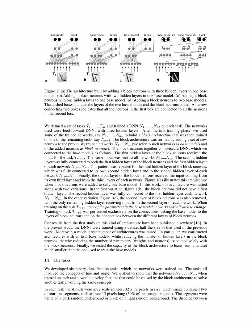
base model block base model block base model #1 base model #2 block
a b c d
T1 T2 T3
base model block
T2
Figure 1: (a) The architecture built by adding a block neurons with three hidden layers to one basemodel. (b) Adding a block neurons with two hidden layers to one base model. (c) Adding a blockneurons with one hidden layer to one base model. (d) Adding a block neurons to two base models.The dashed boxes indicate the layers of the two base models and the block neurons added. An arrowconnecting two boxes indicates that all the neurons in the first box are connected to all the neuronsin the second box.
We defined a set of tasks T1, . . . , TM and trained a DNN N1, . . . , NM on each task. The networksused were feed-forward DNNs with three hidden layers. After the first training phase, we usedsome of the trained networks, say N1, . . . , Nm, to build a block architecture that was then trainedon one of the remaining tasks, say Tm+1. The block architecture was formed by adding a set of newneurons to the previously trained networks N1,...,Nm (we refer to such networks as base models andto the added neurons as block neurons). The block neurons together comprised a DNN, which weconnected to the base models as follows. The first hidden layer of the block neurons received theinput for the task Tm+1. The same input was sent to all networks N1,...,Nm. The second hiddenlayer was fully connected to both the first hidden layer of the block neurons and the first hidden layerof each network N1,...,Nm. This pattern was repeated for the third hidden layer of the block neurons,which was fully connected to its own second hidden layer and to the second hidden layer of eachnetwork N1,...,Nm. Finally, the output layer of the block neurons received the input coming fromits own third layer and from the third layers of each network. Figure 1(a) illustrates this architecturewhen block neurons were added to only one base model. In this work, this architecture was testedalong with two variations. In the first variation, figure 1(b), the block neurons did not have a firsthidden layer. The second hidden layer was fully connected to the first hidden layer each networkN1,...,Nm. In the other variation, figure 1(c), the second layer of block neurons was also removed,with the only remaining hidden layer receiving input from the second layer of each network. Whentraining on the task Tm+1 none of the parameters in the base model networks was allowed to change.Training on task Tm+1 was performed exclusively on the connections linking the base model to thelayers of block neurons and on the connections between the different layers of block neurons.
Our results from the first study on this kind of architecture have been published elsewhere [16]. Inthe present study, the DNNs were trained using a dataset half the size of that used in the previouswork. Moreover, a much larger number of architectures was tested. In particular, we constructedarchitectures with up to 5 base models, while reducing the number of hidden layers in the blockneurons, thereby reducing the number of parameters (weights and neurons) associated solely withthe block neurons. Finally, we tested the capacity of the block architecture to learn from a datasetmuch smaller than the one used to train the base models.
1.2 The tasks
We developed six binary classification tasks, which the networks were trained on. The tasks allinvolved the concepts of line and angle. We wished to show that the networks N1, . . . , Nm, whentrained on such tasks, would develop features that could be reused by the block architecture to solveanother task involving the same concepts.
In each task the stimuli were gray scale images, 32 x 32 pixels in size. Each image contained twoto four line segments, each at least 13 pixels long (30% of the image diagonal). The segments werewhite on a dark random background or black on a light random background. The distance between
3

a b c d e f
Figure 2: Examples of stimuli: (a) ang crs – line segments forming an angle vs. two crossing linesegments; (b) ang crs ln – same, with an additional non-crossing line segment; (c) ang tri ln – anglevs. triangle; (d) blt srp – blunt angle vs. sharp angle; (e) blt srp ln – same, with a non-crossing linesegment; (f) crs ncrs – two crossing line segments vs. two non-crossing line segments.
the end points of each line segment and every other line segment was at least 4 pixels (10% of theimage diagonal). In order to obtain anti-aliased images, the lines were first generated on a grid threetimes larger (96 x 96). The images were then filtered with a Gaussian filter with a sigma of 3 pixels,and down-sampled to the final dimensions. The 6 tasks were (see examples in figure 2):
ang crs: requires classifying the images into those containing an angle (between 20� and 160�) anda pair of crossing line segments (the crossing point must lay between 20% and 80% along eachsegment’s length).
ang crs ln: the same as ang crs, but has an addition line segment crossing neither of the other linesegments.
ang tri ln: distinguishes between images containing an angle (between 20� and 160�) and a triangle(with each angle between 20� and 160� ); each image also contains a line segment crossing neitherangle nor triangle.
blt srp: requires classifying the images into those having blunt (between 100� and 160�) and thosehaving sharp (between 20� and 80�) angles in them.
blt srp ln: the same as blt srp, but has an additional line segment, crossing neither of the linesegments forming the angle.
crs ncrs: distinguishes between a pair of crossing and a pair of non-crossing lines (the crossingpoint must lay between 20% and 80% of each segment length).
Each stimulus was generated by randomly selecting the parameters describing each figure (lengthand orientation of straight segments, amplitude and orientation of the angles) and verifying that allconditions were satisfied. Four different types of random backgrounds were generated with fourpatterns changing with different velocities. For our experiments we generated 350,000 stimuli foreach condition.
2 Network details
The networks used were feed-forward DNNs with three hidden layers. The number of hidden unitsin the different experiments varied, but the largest network had 200, 100, and 50 units in its first,second, and third hidden layers, respectively. We refer to these networks with the letters NN fol-lowed by the number of neurons in each layer. Thus, the name of the network just described wouldbe NN-200-100-50.
We constructed different types of block architectures by varying the type of base models used, thenumber of base models used, and the number of neurons per layer in the block neurons. We refer toa block architecture obtained by connecting base models to a DNN with 100 units in the first hiddenlayer, 50 units in the second hidden layer, and 50 units in the third hidden layer as BA-100-50-50.We refer to an architecture with no hidden units in the first layer and 50 units in the other two hiddenlayers as BA-0-50-50, while an architecture with no units in the first and second hidden layers and50 units in the third layer would be named BA-0-0-50.
4

All networks used a softmax logistic regression as the output layer. The activation functions of theneurons of the network were rectified linear units (ReLUs) [14]. Each network was trained to mini-mize a cost function which combines three terms: the negative log-likelihood of the prediction giventhe data, and two regularization terms. The first regularization term forces sparsity in the neuronsactivation and consists of the KL divergence between the mean activation of each neuron and a uni-form probability distribution of value 0.05. The second regularization term is the squared sum of allthe weights in the networks. The coefficient of the first regularization term was equal to 0.01. Theweight-limiting coefficient was set to 0.0001. The weights of the k-th hidden level were initialized,according to [9], with random uniformly distributed values in the range ±
p6/(n(k�1) + n(k)),
where n(k) is the number of neurons at the k-th level and n(0) is equal to the number of inputs. Thebiases were all initialized to 0.
The total dataset was split into training (330,000 samples), validation (10,000 samples), and test(10,000 samples) datasets. All of the architectures were trained on the entire training dataset usingmini-batch gradient descent learning with a batch size of 20. The initial learning rate for the gradientdescent was set to 0.01, and it decreased by a factor 0.985 after every epoch. We used early stoppingof the training process if the error on the validation dataset did not decrease after 5 epochs. The testscore corresponding to the minimal validation error is presented as the performance of the network.The initial learning rate was selected using a human-guided search. Different values of the initiallearning rate were tested, with uniform steps for the logarithm of the tested values taken over theinterval [log(0.1), log(10�6)].
All code was written in python using Theano [1, 4]. Source files are available online: https://github.com/feel-project/abstraction
3 Results
In this section, we first report the results obtained by training a DNN on each of the previouslydescribed tasks. Then we report the results of training different block architectures on the sametasks. We present the results for block architectures with one or two base models, then the results forthose with three, four, or five base models. The number of possible architectures that can be built bychanging the base models, the number of block neurons and the task on which the block architectureis trained, is very large, and exploring all possibilities was not feasible. Instead, we tried to selectthe conditions that best allowed us to obtain an understanding of the performance of the blockarchitectures. The performance was evaluated by computing the percentage of misclassified sampleson the test dataset. Each architecture was trained five times, randomly initializing its weights. Themean performance over the five repetitions and the best and worst performance are reported in thetables.
Original networks
Prior to building block architectures, we trained a DNN on each task. The networks used were oftype NN-200-100-50, with 200, 100, and 50 nodes in the first, second, and third layers, respectively.Networks of this type were used as base models for all of the block architectures. The percentagesof misclassified test examples for these networks are shown in table 1 together with the results forother architectures, namely NN-30-20-10, NN-60-40-30 and NN-70-50-30. Each of these last threenetworks had approximately the same number of parameters (weight of the networks) of some ofthe block architectures, making interesting performance comparisons possible.
One and two base-model architectures
The percentages of misclassified test examples for block architectures with one and two base modelsare presented in the tables 2 and 3, respectively. The architectures that performed better than (orequal to) the network NN-200-100-50, which was trained from scratch, are shown in bold. In thesetables, the tasks on which the block architectures were trained are listed together with the tasks onwhich the base models were trained (in parentheses).
Architectures with just one base model (table 2) rarely outperformed the original network, NN-200-100-50. This only happened when the task on which the block architecture was trained wassimilar to the one used to train the base model, namely for the conditions ang crs ln (ang crs) and
5

Table 1: Original networks result.condition 200-100-50 70-50-30 60-40-20 30-20-10ang crs 5.5 (5.4–5.9) 8.6 (8.1–9.3) 9.4 (8.9–9.8) 13.3 (12.8–15.0)ang crs ln 13.6 (12.5–15.2) 17.2 (16.5–17.4) 18.3 (16.7–18.8) 21.9 (21.5–23.5)ang tri ln 6.1 (5.5–6.8) 9.7 (8.8–10.1) 11.4 (10.6–14.0) 14.1 (13.4–15.2)blt srp 2.0 (1.8–2.3) 3.4 (3.1–3.8) 3.7 (3.4–4.2) 5.9 (5.1–6.3)blt srp ln 6.5 (6.4–6.9) 10.7 (10.0–13.7) 12.5 (11.6–14.1) 17.2 (16.6–19.5)crs ncrs 2.8 (2.3–2.9) 3.7 (3.2–4.3) 4.5 (4.1–5.2) 5.5 (4.6–6.1)
The numbers correspond to the median (min–max) percentage of misclassified examples.
blt srp (blt srp ln). Even when a second base model was added, ang crs ln and blt srp remainedthe only two tasks on which the block architecture outperformed the original network, NN-200-100-50. It is interesting to compare the results of the architecture BA-100-50-50 with one base modelto those of the architecture BA-0-50-50 with two base models. In this example, even though ithas fewer parameters, the architecture with two base models outperforms that with one in three ofthe four tasks on which it was tested, namely blt srp, blt srp ln and ang crs. This result seem tosuggests that increasing the number of base models yields better results than increasing the numberof neurons in the block architecture. We decided to further study this possibility by adding evenmore base models.
Table 2: Adding blocks to one base model.condition 0-50-50 0-100-50 100-50-50ang crs ln (ang crs) 13.8(13.7–14.3) 13.4 (13.1–13.6) 13.2 (13.1 – 14.0)blt srp ln (blt srp) 9.2 (8.8–9.4) 8.4(8.3–8.6) 8.1 (8.0–8.6)ang crs (ang crs ln) 6.0 (5.9 – 6.2) 5.8 (5.7–6.1) 6.3 (6.0–6.4)blt srp (blt srp ln) 1.8(1.7–1.9) 1.6(1.5–1.9) 1.8 (1.5–2.3)ang tri ln (ang crs ln) 11.2 (11.1–11.7) 10.8 (10.2–11.1) 7.5(7.1–8.0)blt srp ln (ang crs ln) 11.7 (11.3–12.3) 10.9 (10.5–11.2) 8.0 (7.6–8.7)ang crs ln (ang tri ln) 17.3 (16.6–18.2) 16.6 (15.9–17.2) 14.4 (13.4–14.7)ang crs ln (blt srp ln) 18.1 (17.2–18.6) 17.1 (16.2–17.3) 14.5 (14.3–14.9)
The tasks on which the block architectures were trained are listed together with the tasks on which the basemodels were trained (in parentheses). The architectures that performed better than (or equal to) the networks
NN-200-100-50 trained from scratch are shown in bold. This is also the case for Tables 3-8.
Table 3: Adding blocks to two base models.condition 0-50-50 0-100-50 50-50-50ang crs ln (ang tri ln+crs ncrs) 13.7 (13.1–14.2) 13.2 (12.9–13.3) 13.1(12.7–13.8)ang crs ln (ang tri ln+blt srp ln) 14.2(13.8–14.6) 13.6(12.9–13.8) 13.5(12.9–14.2)blt srp (ang tri ln+crs ncrs) 1.9 (1.8–2.3) 1.6(1.5–1.7) 1.8(1.6–2.1)blt srp (ang tri ln+ang crs ln) 2.0(1.7–2.3) 1.5(1.4–1.8) 1.7(1.5–1.7)blt srp (ang tri ln+blt srp ln) 1.5 (1.3–1.7) 1.3 (1.3–1.6) 1.4 (1.2–1.7)blt srp ln (ang tri ln+ang crs ln) 7.6 (7.5–7.8) 7.3 (7.1–7.8) 6.9 (6.8–7.3)blt srp ln (ang tri ln+crs ncrs) 7.6 (7.5–7.8) 7.3 (7.1–7.8) 6.9 (6.8–7.3)ang crs (ang tri ln+blt srp ln) 6.2 (6.0–6.3) 5.7 (5.6–5.9) 5.6 (5.5–5.7)ang crs (ang tri ln+ang crs ln) 6.2 (6.0–6.3) 5.7 (5.6–5.9) 5.6 (5.5–5.7)
Architectures with more than two base models
In this paragraph we present the results obtained adding three, four and five base-models to twokinds of block-architectures: BA-0-50-50 and BA-0-0-50. In table 4 are presented the percentagesof misclassified test examples obtained using three base-models. The results for the architectureBA-0-50-50 were better than those obtained for the architecture NN-60-40-20 that has the samenumber of parameters(approximately 60,000 weights), and better, for nearly all tasks, than thosefor the architecture NN-200-100-50. This suggest that the block architecture highly benefits from
6

Table 4: Adding blocks to three base-models.condition 0-50-50 0-0-50ang crs (ang tri ln+crs ncrs+blt srp) 5.5 (5.2–5.8) 6.0 (5.7–6.1)ang crs (ang tri ln+ang crs ln+crs ncrs) 4.0 (3.9–4.1) 4.5 (4.2 – 4.6)ang crs (ang tri ln+crs ncrs+blt srp ln) 4.6 (4.3–4.8) 5.9 (5.6 – 6.0)ang crs ln (ang tri ln+crs ncrs+blt srp ln) 11.3 (10.9–11.8) 15.0 (14.1 – 16.3)ang crs ln (ang tri ln+crs ncrs+blt srp) 12.0 (11.6–12.5) 15.2 (15.0–15.9)blt srp (ang crs+ang tri ln+crs ncrs) 1.4 (1.4–1.6) 2.2 (2.0 –2.3)blt srp (ang crs ln+ang tri ln+crs ncrs) 1.5 (1.3–1.8) 2.4 (2.0–3.0)blt srp ln (ang crs ln+ang tri ln+crs ncrs) 7.0 (6.7–7.4) 10.2(9.9 –10.5)blt srp ln (ang crs+ang tri ln+crs ncrs) 6.9 (6.7–7.4) 9.8 (9.3–10.1)
being constituted by several base models trained on different tasks. Eliminating the second hiddenlayer from the block architecture yielded much poorer results. For example, the architecture BA-0-0-50 outperformed NN-200-100-50 on only one task. However, the results for BA-0-0-50 improvedsignificantly when the number of base models was increased to four (Table 5). This performancewas comparable to that of BA-0-50-50 with three base models. However, at the same time, it seemsthat for the architecture BA-0-0-50 with four base models the choice of the base models has a biginfluence on the final performance. This can be observed, for example, in the task ang crs ln whereusing to performance drops from 11.4 to 14.1 when just one of the base model is changed.
Table 5: Adding blocks to four base models.condition 0-50-50 0-0-50ang crs (ang tri ln+crs ncrs+blt srp+blt srp ln) 4.9 (4.8–5.6) 5.3 (5.0–5.7)ang crs (ang tri ln+ang crs ln+crs ncrs+blt srp ln) 3.6 (3.4–3.8) 4.3 (4.0–4.7)ang crs (ang tri ln+crs ncrs+blt srp ln+ ang crs ln) 3.8 (3.5–4.0) 4.2 (4.0–4.4)ang crs ln (ang tri ln+crs ncrs+blt srp ln+ang crs) 9.7 (9.3–10.1) 11.4 (11.1–12.1)ang crs ln (ang tri ln+crs ncrs+blt srp+blt srp ln) 10.9 (10.6–11.1) 14.1 (13.6–14.4)blt srp (ang crs+ang tri ln+crs ncrs+blt srp ln) 1.1 (1.0–1.2) 1.3 (1.1–1.5)blt srp (ang crs ln+ang tri ln+crs ncrs+ang crs) 1.2 (1.0–1.4) 1.8 (1.7–2.0)blt srp ln (ang crs ln+ang tri ln+crs ncrs+ang crs) 5.9 (5.6–6.2) 10.2 (10.0–10.5)blt srp ln (ang crs+ang tri ln+crs ncrs+ang crs ln) 5.8 (5.6–6.0) 9.9 (9.3–10.1)
In Table 6, we list the results obtained using five base models. In this case, for each task, all of thenetworks trained on each of the other tasks were used. Both architectures BA-0-50-50 and BA-0-0-50 outperformed the architecture NN-70-50-30, which had the same number of parameters, as wellas the architecture NN-200-100-50. It is interesting to note here that the performance on the taskang crs ln (11.3) is near to the best of the performance obtained using 4 base models. This probablysuggest that the architecture has been able to select among the base models the ones more useful forthe new task.
Table 6: Adding blocks to five base models.condition 0-50-50 0-0-50ang crs (all models used except ang crs) 3.6 (3.3–3.8) 4.1 (3.6–4.3)ang crs ln (all models used except ang crs ln) 9.5 (9.3–9.9) 11.3 (11.0–11.8)blt srp (all models used except blt srp) 1.0 (0.9–1.3) 1.2 (1.0–1.3)blt srp ln (all models used except blt srp ln) 4.7 (4.4–4.9) 6.5 (6.2–7.0)crs ncrs (all models used except crs ncrs) 1.1 (1.0–1.1) 1.1 (1.0–1.2)ang tri ln (all models used except ang tri ln) 4.9 (4.6–5.0) 7.6 (7.4–7.8)
On a smaller dataset
As mentioned in the introduction, we also wished to verify that the proposed architecture could betrained with a smaller dataset than a network trained from scratch. In this paragraph we present
7

the results obtained by training the same architectures presented in Tables 5 and 6 with a datasetof 200,000 examples. The architectures in Tables 5 and 6 were trained on a dataset of 350,000examples. The percentages of misclassified examples, presented in Tables 7 8, showed that evenwith a much smaller training dataset, with four or five base models the architecture BA-0-50-50outperformed the network trained from scratch, NN-200-100-50. The other architecture, BA-0-0-50, had worse results then NN-200-100-50, especially for the more complex tasks, namely blt srp ln
and ang tri ln.
Table 7: Adding blocks to four base models. Dataset of 200.000 examples.condition 0-50-50 0-0-50ang crs (ang tri ln+crs ncrs+blt srp+blt srp ln) 5.0 (4.8–5.2) 5.8 (5.4 – 6.3)ang crs (ang tri ln+ang crs ln+crs ncrs+blt srp ln) 4.3 (4.0–4.5) 4.6 (4.0 – 5.0)ang crs (ang tri ln+crs ncrs+blt srp ln+ ang crs ln) 4.3 (4.1–4.8) 4.7 (4.3–5.5)ang crs ln (ang tri ln+crs ncrs+blt srp ln+ang crs) 10.7 (10.4–11.3) 12.0 (11.5–12.4)ang crs ln (ang tri ln+crs ncrs+blt srp+blt srp ln) 12.4 (12.0–12.6) 15.1 (14.6–15.5)blt srp (ang crs+ang tri ln+crs ncrs+blt srp ln) 1.2 (1.1–1.4) 1.4 (1.3–1.5)blt srp (ang crs ln+ang tri ln+crs ncrs+ang crs) 1.8 (1.7–2.0) 2.1 (1.7 – 2.4)blt srp ln (ang crs ln+ang tri ln+crs ncrs+ang crs) 6.4 (6.3–6.6) 9.7(9.2–10.6)blt srp ln (ang crs+ang tri ln+crs ncrs+ang crs ln) 6.5 (6.3–6.8) 9.8(9.4–10.3)
Table 8: Adding blocks to five base models. Dataset of 200.000 examples.condition 0-50-50 0-0-50ang crs (all models used except ang crs) 4.3 (4.0–4.7) 4.4 (3.9–4.7)ang crs ln (all models used except ang crs ln) 10.6 (10.4 – 10.8) 11.7 (11.2 – 12.1)blt srp (all models used except blt srp) 1.2 (0.9 – 1.9) 1.4 (1.1 – 1.8)blt srp ln (all models used except blt srp ln) 5.6 (5.2 – 5.9) 7.2 (6.8 – 8.0)crs ncrs (all models used except crs ncrs) 1.2 (1.0–1.3) 1.2 (1.0–1.3)ang tri ln (all models used except ang tri ln) 5.8 (5.7–6.0) 8.6 (8.3–9.0)
4 Conclusions
DNNs are known to have some abstraction abilities [15]. These abstractions, however, are verylimited compared to those typical of humans, where different concepts recall each other througha vast network of relationships. One possible aspect of the creation of such powerful abstractionscould be that humans are continuously engaged in different tasks which are each solved with alimited set of resources that must be shaped in order to optimize performance on the largest numberof tasks.
In this paper we built a DNN by training several DNNs on different tasks and then merging themwith a group of added neurons. The resulting architecture was capable of performing several tasks.Moreover, it was very efficiently trained, using a dataset smaller than that used for the originalDNNs and adding only a small number of new neurons. Our results are consistent with previousexperimental observations that training deep architectures is easier when cues to the function thatintermediate levels should compute are provided ([2, 17]) and when training is not performed on thewhole network at the same time [12].
Our study can be considered a first step toward the construction of DNN architectures which areable to use areas trained on previous tasks when learning a new task. This type of procedure shouldfocus on training areas of the network that have not previously been used, while only slightly mod-ifying areas already trained on previous tasks. Such an architecture would maintain the positivecharacteristics described for our architectures, and would be capable of sequential learning.
Acknowledgments
This work was funded by the European Research Council (FP 7 Program) ERC Advanced Grant“FEEL” to KO’R
8

References
[1] Frederic Bastien, Pascal Lamblin, Razvan Pascanu, James Bergstra, Ian J. Goodfellow, ArnaudBergeron, Nicolas Bouchard, and Yoshua Bengio. Theano: new features and speed improve-ments. Deep Learning and Unsupervised Feature Learning NIPS 2012 Workshop, 2012.
[2] Yoshua Bengio. Evolving culture versus local minima. In Growing Adaptive Machines, pages109–138. Springer, 2014.
[3] Yoshua Bengio, Jerome Louradour, Ronan Collobert, and Jason Weston. Curriculum learning.In Proceedings of the 26th annual international conference on machine learning, pages 41–48.ACM, 2009.
[4] James Bergstra, Olivier Breuleux, Frederic Bastien, Pascal Lamblin, Razvan Pascanu, Guil-laume Desjardins, Joseph Turian, David Warde-Farley, and Yoshua Bengio. Theano: a CPUand GPU math expression compiler. In Proceedings of the Python for Scientific Computing
Conference (SciPy), June 2010. Oral Presentation.[5] Rich Caruana. Multitask learning. Machine learning, 28(1):41–75, 1997.[6] Ronan Collobert and Jason Weston. A unified architecture for natural language processing:
Deep neural networks with multitask learning. In Proceedings of the 25th international con-
ference on Machine learning, pages 160–167. ACM, 2008.[7] Li Deng, Jinyu Li, Jui-Ting Huang, Kaisheng Yao, Dong Yu, Frank Seide, Michael Seltzer,
Geoffrey Zweig, Xiaodong He, Jason Williams, et al. Recent advances in deep learning forspeech research at microsoft. In Acoustics, Speech and Signal Processing (ICASSP), 2013
IEEE International Conference on, pages 8604–8608. IEEE, 2013.[8] Dumitru Erhan, Yoshua Bengio, Aaron Courville, Pierre-Antoine Manzagol, Pascal Vincent,
and Samy Bengio. Why does unsupervised pre-training help deep learning? The Journal of
Machine Learning Research, 11:625–660, 2010.[9] Xavier Glorot and Yoshua Bengio. Understanding the difficulty of training deep feedforward
neural networks. In International conference on artificial intelligence and statistics, pages249–256, 2010.
[10] Ian J Goodfellow, Mehdi Mirza, Da Xiao, Aaron Courville, and Yoshua Bengio. An empir-ical investigation of catastrophic forgeting in gradient-based neural networks. arXiv preprint
arXiv:1312.6211, 2013.[11] Geoffrey E Hinton, Nitish Srivastava, Alex Krizhevsky, Ilya Sutskever, and Ruslan R Salakhut-
dinov. Improving neural networks by preventing co-adaptation of feature detectors. arXiv
preprint arXiv:1207.0580, 2012.[12] Hugo Larochelle, Yoshua Bengio, Jerome Louradour, and Pascal Lamblin. Exploring strategies
for training deep neural networks. The Journal of Machine Learning Research, 10:1–40, 2009.[13] Xiaodong Liu, Jianfeng Gao, Xiaodong He, Li Deng, Kevin Duh, and Ye-Yi Wang. Represen-
tation learning using multi-task deep neural networks for semantic classification and informa-tion retrieval. Proc. NAACL, May 2015.
[14] Vinod Nair and Geoffrey E Hinton. Rectified linear units improve restricted boltzmann ma-chines. In Proceedings of the 27th International Conference on Machine Learning (ICML-10),pages 807–814, 2010.
[15] Anh Nguyen, Jason Yosinski, and Jeff Clune. Deep neural networks are easily fooled: Highconfidence predictions for unrecognizable images. arXiv preprint arXiv:1412.1897, 2014.
[16] Alexander V Terekhov, Guglielmo Montone, and J Kevin ORegan. Knowledge transfer indeep block-modular neural networks. In Biomimetic and Biohybrid Systems, pages 268–279.Springer, 2015.
[17] Jason Weston, Frederic Ratle, Hossein Mobahi, and Ronan Collobert. Deep learning via semi-supervised embedding. In Neural Networks: Tricks of the Trade, pages 639–655. Springer,2012.
9

Symbol Grounding in Multimodal Sequences using
Recurrent Neural Networks
Federico Raue
University of Kaiserslautern, GermanyDFKI, Germany
Wonmin Byeon
University of Kaiserslautern, GermanyDFKI, Germany
Thomas M. Breuel
University of Kaiserslautern, [email protected]
Marcus Liwicki
University of Kaiserslautern, [email protected]
Abstract
The problem of how infants learn to associate visual inputs, speech, and internalsymbolic representation has long been of interest in Psychology, Neuroscience,and Artificial Intelligence. A priori, both visual inputs and auditory inputs arecomplex analog signals with a large amount of noise and context, and lacking ofany segmentation information. In this paper, we address a simple form of thisproblem: the association of one visual input and one auditory input with eachother. We show that the presented model learns both segmentation, recognitionand symbolic representation under two simple assumptions: (1) that a symbolicrepresentation exists, and (2) that two different inputs represent the same symbolicstructure. Our approach uses two Long Short-Term Memory (LSTM) networks formultimodal sequence learning and recovers the internal symbolic space using anEM-style algorithm. We compared our model against LSTM in three differentmultimodal datasets: digit, letter and word recognition. The performance of ourmodel reached similar results to LSTM.
1 Introduction
Our brain has an important skill that is to assign semantic concepts to their sensory input signals,such as, visual, auditory. In other words, the sensory inputs can be considered as meaninglessphysical information and the semantic concepts are linked to their physical features. This scenariocan be seen as Symbol Grounding Problem (SGP) [1].
Infants in their development ground the semantic concepts to their sensory inputs. For example,several cognitive researchers found a relation between the vocabulary acquisition (audio) and objectrecognition (visual) [2, 3]. Recently, Asano et al. [4] recorded the infant brain activity using threeElectroencephalogram (EEG) measures. They found that infants are sensitive to the correspondencebetween visual stimulus and their sound-symbolic match or mismatch. Furthermore, the lack of oneof these components affects the learning behavior, i.e., deafness or blindness [5, 6].
Several models have been proposed for grounding concepts in multimodal scenarios. Yu and Bal-lard [7] developed a multimodal learning algorithm that maximize the probabilities between spokenwords and the visual perception using EM approach. Nakamura et al. [8] developed a different ap-proach based on a latent Dirichlet allocation (LDA) for multimodal concepts. They used not onlyvisual and audio information but also haptic information for grounding the concept.
1
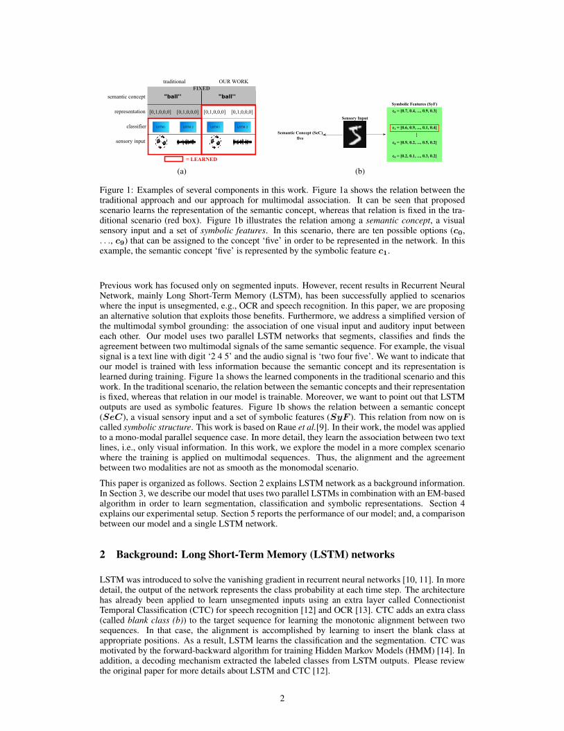
representation
classifier
semantic concept
sensory input
LSTM1
[0,1,0,0,0] [0,1,0,0,0]
LSTM 2
"ball''
LSTM1
[0,1,0,0,0] [0,1,0,0,0]
LSTM 2
"ball''
traditional OUR WORK
= LEARNED
FIXED
(a)
Semantic Concept (SeC)five
Sensory Input
Symbolic Features (SyF)c0 = [0.7, 0.4, ..., 0.9, 0.3]
c1 = [0.6, 0.9, ..., 0.1, 0.4]
c8 = [0.9, 0.2, ..., 0.5, 0.2]
c9 = [0.2, 0.1, ..., 0.3, 0.2]
....
(b)
Figure 1: Examples of several components in this work. Figure 1a shows the relation between thetraditional approach and our approach for multimodal association. It can be seen that proposedscenario learns the representation of the semantic concept, whereas that relation is fixed in the tra-ditional scenario (red box). Figure 1b illustrates the relation among a semantic concept, a visualsensory input and a set of symbolic features. In this scenario, there are ten possible options (c0,. . ., c9) that can be assigned to the concept ‘five’ in order to be represented in the network. In thisexample, the semantic concept ‘five’ is represented by the symbolic feature c1.
Previous work has focused only on segmented inputs. However, recent results in Recurrent NeuralNetwork, mainly Long Short-Term Memory (LSTM), has been successfully applied to scenarioswhere the input is unsegmented, e.g., OCR and speech recognition. In this paper, we are proposingan alternative solution that exploits those benefits. Furthermore, we address a simplified version ofthe multimodal symbol grounding: the association of one visual input and auditory input betweeneach other. Our model uses two parallel LSTM networks that segments, classifies and finds theagreement between two multimodal signals of the same semantic sequence. For example, the visualsignal is a text line with digit ‘2 4 5’ and the audio signal is ‘two four five’. We want to indicate thatour model is trained with less information because the semantic concept and its representation islearned during training. Figure 1a shows the learned components in the traditional scenario and thiswork. In the traditional scenario, the relation between the semantic concepts and their representationis fixed, whereas that relation in our model is trainable. Moreover, we want to point out that LSTMoutputs are used as symbolic features. Figure 1b shows the relation between a semantic concept(SeC), a visual sensory input and a set of symbolic features (SyF ). This relation from now on iscalled symbolic structure. This work is based on Raue et al.[9]. In their work, the model was appliedto a mono-modal parallel sequence case. In more detail, they learn the association between two textlines, i.e., only visual information. In this work, we explore the model in a more complex scenariowhere the training is applied on multimodal sequences. Thus, the alignment and the agreementbetween two modalities are not as smooth as the monomodal scenario.
This paper is organized as follows. Section 2 explains LSTM network as a background information.In Section 3, we describe our model that uses two parallel LSTMs in combination with an EM-basedalgorithm in order to learn segmentation, classification and symbolic representations. Section 4explains our experimental setup. Section 5 reports the performance of our model; and, a comparisonbetween our model and a single LSTM network.
2 Background: Long Short-Term Memory (LSTM) networks
LSTM was introduced to solve the vanishing gradient in recurrent neural networks [10, 11]. In moredetail, the output of the network represents the class probability at each time step. The architecturehas already been applied to learn unsegmented inputs using an extra layer called ConnectionistTemporal Classification (CTC) for speech recognition [12] and OCR [13]. CTC adds an extra class(called blank class (b)) to the target sequence for learning the monotonic alignment between twosequences. In that case, the alignment is accomplished by learning to insert the blank class atappropriate positions. As a result, LSTM learns the classification and the segmentation. CTC wasmotivated by the forward-backward algorithm for training Hidden Markov Models (HMM) [14]. Inaddition, a decoding mechanism extracted the labeled classes from LSTM outputs. Please reviewthe original paper for more details about LSTM and CTC [12].
2

0 50 100 150 200 250 300
0
2
4
6
8
10
0 50 100 150 200 250 300LSTM1
020406080100120140160
LSTM2
0 20 40 60 80 100120140160LSTM2
050100150200250300
LSTM1
LSTM1
LSTM2ForwardStep
Forward Step
Output1
Output2
Forward Backward 1
DTW
Input Labelγ3γ8γ3γ2γ1
Input Labelβ3β8β3β2β1
0 50 100 150
0
2
4
6
8
100 50 100 150
0
2
4
6
8
10
0 50 100 150 200 250 300
0
2
4
6
8
10
0 50 100 150
0
2
4
6
8
10
statisticalconstraint
2
Image Input
Audio Input
0 50 100 150 200 250 300
0
2
4
6
8
10
BackwardStep
BackwardStep
Forward Backward 2
forward backward 2 align to LSTM1forward backward 1 align to LSTM2
statisticalconstraint
1
Figure 2: Overview of symbolic association framework. The statistical constraints (� and �) guideeach LSTM to the internal representation (symbolic feature) for each semantic concept. Also, themonotonic behavior is exploited by DTW. In this manner, LSTM1 output is used as target forLSTM2, and vice versa.
3 Multimodal Symbolic Association
As we mentioned in Section 1, the goal of our model is to learn the agreement in a multimodalsymbolic sequences. In this case, the term ‘agreement’ is referred to the output classification ofboth LSTMs are the same (regardless of the modalities). In other words, both LSTMs learn thesegmentation, the classification and the symbolic structure in a simplified multimodal scenario.
More formally, we define the multimodal symbolic association problem in the following manner. Amultimodal dataset is defined by M = {(x
a,t1 ;xv,t2 ; s1,...,n)|xa,t1 2 X
a
,x
v,t2 2 X
v
, s1,...,n 2SeC}. X
a
and X
v
are sets of audio and visual sequences, respectively. The length of both se-quences can be different. s1,...,n define the semantic concept sequence of size n that is representedby two modalities (X
a
and X
v
). As mentioned, the goal is to learn the same symbolic structurethat is represented by both modalities. In more detail, each semantic concept is grounded by a sim-ilar symbolic feature in both modalities. Also, all semantic concepts are represented by differentsymbolic features.
In this work, we are proposing a framework that combines two LSTMs for learning a unified sym-bolic association between two modalities. The intuition behind this idea is to convert from a multi-modal input feature space to a common output class space, where two modalities can be associated.Thus, LSTM outputs have the same size. Also, we introduce an EM-training rule based on twoconstraints: (1) a symbolic representation exists, and (2) two different inputs represent the samesymbolic structure. Figure 2 shows a general view of our framework.
In more detail, our model works in the following manner. First, the sequences xa,t1 and x
v,t2 arepassed to each LSTM (LSTM1, LSTM2). Then, LSTM outputs (z
a,t1 , zv,t2 ) and the semanticconcept sequence (s1, . . . , sn) are feeding to the statistical constraint (� and �). We want to indicatethe LSTM output are used as symbolic feature (SyF). This component selects the most likely rela-tion between semantic concepts and the symbolic features (Section 3.1). As a result, this relationprovides information in order to apply the forward-backward algorithm for training (cf. Section 2).Previous steps are independently applied to each LSTM. As we mentioned before, the goal of ourmodel is to learn a unified symbolic structure. With this in mind, the next step in our framework isto align both outputs from the forward-backward algorithm. Our model exploits the monotonic be-havior and both sequences are aligned by Dynamic Time Warping (Section 3.2). The aligned outputof one LSTM is used as a target of the other LSTM, and vice versa.
3

γ4 γ3 γ6
0 2 4 6 8 100.075
0.080
0.085
0.090
0.095
0.100
SyF
Average - LSTM output
LSTM
ForwardStep
SENSORY INPUT436
Weighted Average
0 2 4 6 8 100.040.050.060.070.080.090.100.110.120.13
SyF
(SeC 4 - SyF 5)
ẑ(Se
c-4)
0 2 4 6 8 100.05
0.06
0.07
0.08
0.09
0.10
0.11
SyF
(SeC 3 - SyF 0)
ẑ(Se
c-3)
0 2 4 6 8 100.040.050.060.070.080.090.100.11
SyF
(SeC 6 - SyF 8)
ẑ(Se
c-6)
Figure 3: Example of the statistical constraint. The semantic weights (�4,�3,�6) modify the av-erage output of LSTM. It can be seen that only one symbolic feature spikes among all for eachsemantic concept.
3.1 Statistical Constraint
The goal of this component is to learn the structure between the semantic concepts (SeC) and thesymbolic feature (SyF) that are represented by the output of LSTM networks. Our proposed train-ing rule is based on EM algorithm [15]. With this in mind, we define a set of weighted concepts(�1, . . . ,�c
) where c 2 SeC and each �
c
is represented by a vector �c
= [�c,0, . . . , �c,k] where k
is the size of the LSTM output. As a result, the relation can be retrieved by a winner-take-all rule.Figure 3 shows an example of the statistical constraint.
The E-Step finds the structure between SeC and SyF. First, we construct the matrix Z which isdefined by
Z =⇥z(1), . . . , z(c)
⇤; c 2 SeC (1)
z(c) =1
T
TX
t=1
(zt)�(c); c 2 SeC (2)
where zt is a column vector that represents LSTM output1 at time t, t 2 [1, . . . , T ] is the timesteps.The column vector z(c) is the weighted average of LSTM output. Next, we convert from matrixZ to matrix Z
⇤. A row-column elimination is applied in order to find the symbolic structure forthe training. The maximum element (i, j) in Z is set to 1 and the elements at the same row i andcolumn j are set to 0 except the element (i, j). This procedure is repeated |SeC| times. As a result,only one symbolic representation is selected for each semantic concept.
The M-Step updates the set of weighted concepts given the current symbolic structure (Z). In thiscase, we are assuming a uniform distribution of semantic concepts. We define the following costfunction
cost(c) =
✓z(c)� 1
|SeC|z⇤(c)
◆2
; c 2 SeC (3)
where z
⇤(c) is a column-vector of matrix z
⇤. The update of �(c) is accomplished by applyinggradient descent
�(c) = �(c)� ↵ ⇤r�cost(c); c 2 SeC (4)where ↵ is the learning rate and rcost(c) is the derivatives of the cost function with respect to�(c).
1For explanation purposes, the index that represents the modality is dropped, i.e, zt ⌘ za,t1
4

VISUAL COMPONENT AUDIO COMPONENTDIGIT RECOGNITION LETTER RECOGNITION
VISUAL COMPONENT AUDIO COMPONENT
VISUAL COMPONENT AUDIO COMPONENT
WORD RECOGNITION
Figure 4: Several examples of the generated multimodal datasets.
After the symbolic structure is learned, the semantic concept is grounded to the symbolic feature,and vice versa. As a result, the semantic concept can be retrieved from the symbolic feature by themaximum element of the following equation:
c
⇤ = arg max
c
z
�c,k⇤
k
⇤ (5)
where k⇤ is the class decoded from LSTM outputs2, �(c,k⇤) is the value at position k
⇤ in the columnvector �(c).
3.2 Dynamic Time Warping (DTW)
The goal of the second component of our modified learning rule is to align the output of bothnetworks. In other words, the alignment is a mapping function between both networks. Thus,the output of one network can be converted as an approximated output to the other network. Thismapping is important for calculating the error for updating the weights in the backpropagation step.We apply Dynamic Time Warping (DTW) [16] because of its monotonic behavior scenario. For thispurpose, a distance matrix is calculated between each timestep of the forward-backward algorithmfrom both networks. Equation 6 shows the standard constrains of the path in DTW.
DTW [i, j] = dist[i, j] +min
(DTW [i� 1, j � 1]DTW [i� 1, j]DTW [i, j � 1]
(6)
where dist[i, j] is the distance between the timestep i of LSTM1 and the timestep j of LSTM2.
4 Experimental Design
4.1 Datasets
We generated three multimodal datasets for the following sequence classification scenarios: hand-written digit recognition, printed letter recognition, and word recognition. Each dataset has twocomponents: visual and audio. The visual component is a text line (bitmap) and the audio compo-nent is a speech (wav file). Both components represent the same semantic sequence. For example,the semantic sequence ‘3 8 3 2 1’ is represented by a bitmap with those digits and an audio file with‘three eight three two one’. Figure 4 shows several examples of the multimodal datasets.
Digit Recognition The first dataset was generated based on a combination between MNIST [17] andFestival Toolkit [18]. This dataset has ten semantic concepts. Sequences were randomly generatedbetween 3 and 8 digits. The visual component was generated using MNIST dataset. MNIST hasalready a training set and a testing set. Thus, we kept the same division for creating our rainingset and testing set. Each selected digit was attached before and after a random blank background(between 3 and 10 columns). All the selected digits were horizontally stacked. For the audio com-ponent, the audio file was generated given the sequences obtained from the visual component and
2cf. Section 2
5

= correct = incorrect
0 50 100 150 200 250
0
5
10
15
20
25
0 50 100 150 200
0
5
10
15
20
25
0 20 40 60 80 100 120 140
0
2
4
6
8
10
0 50 100 150 200 250
0
5
10
15
20
25
0 50 100 150 200
0
5
10
15
20
25
INPUT SEQUENCE DTW COST MATRIXOUR MODEL (OUTPUTS)
0 50 100 150 200 250LSTM1
020406080
100120140160
LSTM
2
0 20 40 60 80 100 120 140 160LSTM2
050
100150200250
LSTM
1
0 50 100 150 200 250
0
2
4
6
8
100 50 100 150
0
2
4
6
8
10
0 50 100 150 200LSTM1
020406080
100120140
LSTM
2
0 20 40 60 80 100 120 140LSTM2
0
50
100
150
200
LSTM
1
0 50 100 150 200 250LSTM1
020406080
100120140160
LSTM
2
0 20 40 60 80 100 120 140 160LSTM2
050
100150200250
LSTM
1
0 50 100 150 200LSTM1
020406080
100120140
LSTM
2
0 20 40 60 80 100 120 140LSTM2
0
50
100
150
200
LSTM
1
0 50 100 150 200
0
2
4
6
8
10
0 50 100 150
0
2
4
6
8
100 50 100 150 200 250
0
2
4
6
8
10
0 50 100 150 200
0
2
4
6
8
100 20 40 60 80 100 120 140
0
2
4
6
8
10
Figure 5: Several examples of the DTW cost matrix. The audio component of the sequences wasomitted. The cost matrix (right) shows the path (red line) pass through nine regions. These regionsrepresent the blank class and the semantic concepts.
selected between four artificial voices. As a result, the training set has 50,000 sequences and testingset has 15,000 sequences.
Letter Recognition The second dataset was generated following a similar procedure as the previ-ous dataset. This dataset has 27 semantic concepts. We generated text lines of letters as the visualcomponent. The length was randomly selected between 3 and 8 lower characters. The audio com-ponent was generated similar to the first dataset using Festival Toolkit. In contrast to MNIST, thisdataset does not have an explicit division for the training set and the testing set. Thus, we decided togenerate a slightly bigger dataset of 60,000 sequences.
Word Recognition The last multimodal dataset is generated based on the audio of the GRID audio-visual sentence corpus [19]. This dataset has 52 semantic concepts. The audio has a fixed sequencelength of eight semantic concepts. Also, the audio component is composed by 34 talkers, 18 weremales and 16 were females. We generated the text lines of each sequence semantic sequence. Thesize of this dataset is 34,000 sequences.
4.2 Input Features and LSTM Setup
The visual component was used raw-pixel values between 0.0 and 1.0. The audio component wasconverted to Mel-Frequency Cepstral Coefficient (MFCC) using HTK toolkit3. The following pa-rameters were selected for extracting MFCC: a Fourier-transform-based filter-bank with 40 coeffi-cients (plus energy) distributed on a mel-scale, including their first and second temporal derivatives.As a result, the size of the vector was 123. Also, the audio component was normalized to zero meanand unit variance. The training set of the audio component was normalized to zero mean and unitvariance.
As a baseline, each component was evaluated using LSTM with CTC layer in order to test theperformance of our model. The following parameters were selected for the visual component. Thememory size is 20 for the first two datasets and 40 for the last dataset, the learning rate of thenetwork is 1e-5 and the momentum is 0.9. The parameters for the audio component are similar butthe memory size is 100. The statistical constraint were initialized with 1.0 and the learning rate wasset to 0.01 for both networks.
5 Results and Discussion
In this paper, the performance of the presented model and the standard LSTM were compared.We want to point out that our goal is not to outperform the standard LSTM, but to know if the
3http://htk.eng.cam.ac.uk
6

Table 1: Label Error Rate (%) between the standard LSTM and our model. We want to point outthat our goal is not to outperform the standard LSTM.
METHOD DIGITS LETTERS WORDS
STANDARD LSTM VISUAL 3.42± 0.84 0.09± 0.05 0.45± 0.68AUDIO 0.08± 0.06 1.06± 0.14 3.68± 0.27
OUR MODELVISUAL 2.69± 0.55 0.35± 0.33 0.51± 0.84AUDIO 0.15± 0.08 1.24± 0.50 3.77± 0.40
STANDARD LSTMINPUT SEQUENCE OUR MODEL (OUTPUTS)
0 50 100 150 200 250
0
5
0
5
0
5
0 50 100 150 200
0
5
0
5
0
5
0 50 100 150 200 250
0
5
0
5
0
5
= correct = incorrect
0 50 100 150 200
0
5
0
5
0
5
0 50 100 150 200 250 300 350
0
5
0
5
0
5
0 50 100 150 200 250
02468
100 50 100 150 200 250
02468
100 50 100 150
02468
10
0 50 100 150 200
02468
100 50 100 150
02468
100 50 100 150
02468
100 50 100 150 200
02468
10
0 50 100 150 200
02468
100 50 100 150
02468
100 50 100 150 200
02468
100 50 100 150
02468
10
0 50 100 150 200 250 300 350
02468
100 50 100 150
02468
100 50 100 150
02468
100 50 100 150 200 250 300 350
02468
10
0 50 100 150 200 250
02468
100 20 40 60 80 100 120 140
02468
100 50 100 150 200 250
02468
100 20 40 60 80 100 120 140
02468
10
0 50 100 150
02468
10
Figure 6: Symbolic Structure between our model and LSTM. The audio component was omitted.Both networks converge to the structure (SyF, SeC): (0, 2), (1, 5), (2, 6), (3, 9), (4, 3), (5, 7), (6,blank-class), (7, 0), (8, 1), (9, 8), (10, 4). It is noted that both models shows similar behaviorrelated to the symbolic structure. LSTM uses a pre-defined structure before the training, whereasthe presented model learns the structure during training
performance of our model was in good range. Note that our model has less information than LSTMnetworks. We randomly selected 10,000 sequences and 3,000 sequences as a training set and testingset (respectively). This random selection was repeated ten times. In the word recognition dataset,we randomly selected 50% male voices and 50% female voices for each training and testing set. Weare reporting Label Error Rate (LER), which is defined by
LER =1
|Z|X
(x,y)2Z
ED(x, y)
|y| (7)
where ED is the edit distance between the classification of the network x and the correct outputclassification y and Z is the size of the dataset. Table 1 shows that our model reaches a similarperformance to the standard LSTM. In more detail, Fig. 5 shows several examples of the outputclassification of our model. The first row shows a correct classification of both LSTMs. In thiscase, both structures of the semantic concepts and the symbolic features are the same. It can be seenthat the semantic concept ‘5861’ is represented by the symbolic feature ‘2867’ (dark blue in column2-3) in both LSTMs. In addition, DTW cost matrix shows an example of the alignment betweenthe both LSTMs. We mentioned in Section 2 that CTC layer adds an extra class. Consequently, oursequence example is converted to ‘b5b8b6b1b’ (nine elements). The DTW cost matrix shows nineregions that the DTW path (red line) crossed. In other words, the alignment happened in the samesemantic concept. Furthermore, the alignment still follows the same behavior, even if one or bothoutput classification are wrong.
7

OUTPUT 1 OUTPUT 2FORWARD
BACKWARD 1FORWARD
BACKWARD 2 DTW 1 DTW 2
INITIALSTATE
AFTER 1000SEQUENCES
AFTER 5000SEQUENCES
AFTER 20000SEQUENCES
0 50 100 150 200 250 300
0
2
4
6
8
10
INPUT SEQUENCES
0 50 100 150 200 250 300
0
2
4
6
8
100 50 100 150
0
2
4
6
8
100 50 100 150 200 250 300
0
2
4
6
8
100 50 100 150
0
2
4
6
8
10 0 50 100150200250300LSTM1
020406080
100120140160
LSTM
2
0 20406080100120140160LSTM2
050
100150200250300
LSTM
1
0 50 100 150 200 250 300
0
2
4
6
8
10
0 50 100 150 200 250 300
0
2
4
6
8
10
0 50 100 150 200 250 300
0
2
4
6
8
10
0 50 100 150
0
2
4
6
8
10
0 50 100 150
0
2
4
6
8
10
0 50 100 150
0
2
4
6
8
10
0 50 100 150 200 250 300
0
2
4
6
8
10
0 50 100 150 200 250 300
0
2
4
6
8
10
0 50 100 150 200 250 300
0
2
4
6
8
10
0 50 100 150
0
2
4
6
8
10
0 50 100 150
0
2
4
6
8
10
0 50 100 150
0
2
4
6
8
10
0 50 100150200250300LSTM1
020406080
100120140160
LSTM
2
0 50 100150200250300LSTM1
020406080
100120140160
LSTM
2
0 50 100150200250300LSTM1
020406080
100120140160
LSTM
2
0 20406080100120140160LSTM2
050
100150200250300
LSTM
1
0 20406080100120140160LSTM2
050
100150200250300
LSTM
1
0 20406080100120140160LSTM2
050
100150200250300
LSTM
1
Figure 7: Steps of the training rule. In the beginning, the output of the networks is sparse and theypoint to align first the blank-class (first three rows). The forward backward algorithm shows highvalues (dark blue) where the blank-class appears. After the blank-class is aligned, the remainingsymbolic features are slowly converging to the same representation. The last row shows that bothoutputs classify the multimodal sequence with similar symbolic features. The DTW cost matrixshows the alignment (red line) between the symbolic features. The alignment has two cases: blank-class to blank-class and semantic concepts to semantic concepts.
Figure 6 shows examples of the symbolic structure. It can be noted that the presented model has asimilar behavior as the standard LSTM. For example, our model also learns the blank class for seg-menting the semantic concepts. The difference is mainly in the symbolic features for each semanticconcept. It is observed that the standard LSTMs used a pre-defined structure between the seman-tic concepts and the symbolic features. For example, the semantic concept ‘1’ is represented bythe symbolic feature ‘1’, the same happened with the rest of semantic concepts. In the other hand,our model learns the structure for each LSTM and both LSTMs converge to a common symbolicstructure.
Figure 7 shows the behavior of our model during training. In the beginning, the output of thenetworks has sparse values and the DTW cost matrices do not have clear regions as in Figure 6.After 10,000 sequences, both networks align first to blank class. DTW cost matrices start showingsome initial regions of alignment. After 50,000 sequences, the blank class changes because thestructure of the semantic concepts and the symbolic features are not stable. After 20,000 sequences,both networks converge to a common a structure and the DTW cost matrices show a clear DTWpath similar to Figure 6.
6 Conclusions
This paper has demonstrated that learning symbolic representations of unsegmented sensory inputsis possible with a minimum of assumptions, namely that symbolic representations exist, that twoinputs represent the same symbolic content and that classes follow prior distribution. One limitationof our model is the constraint to one-dimension. However, there are many applications in thiscontext, e.g., combining eye tracking system with audio. We will validate our findings with morerealistic scenarios, i.e., unknown semantic concepts, aligning a two-dimensional image and a one-dimensional speech, handling missing semantic concepts in one component or both components ofthe sequence. Finally, it can be seen that this scenario is simple but assigning semantic meanings tosymbols is important for language development and remains as an open problem [20, 21, 22].
8

References
[1] S. Harnad, “The symbol grounding problem,” Physica D: Nonlinear Phenomena, vol. 42, no. 1,pp. 335–346, 1990.
[2] M. T. Balaban and S. R. Waxman, “Do words facilitate object categorization in 9-month-oldinfants?” Journal of experimental child psychology, vol. 64, no. 1, pp. 3–26, Jan. 1997.
[3] L. Gershkoff-Stowe and L. B. Smith, “Shape and the first hundred nouns.” Child development,vol. 75, no. 4, pp. 1098–114, 2004.
[4] M. Asano, M. Imai, S. Kita, K. Kitajo, H. Okada, and G. Thierry, “Sound symbolism scaffoldslanguage development in preverbal infants,” cortex, vol. 63, pp. 196–205, 2015.
[5] E. S. Andersen, A. Dunlea, and L. Kekelis, “The impact of input: language acquisition in thevisually impaired,” First Language, vol. 13, no. 37, pp. 23–49, Jan. 1993.
[6] P. E. Spencer, “Looking without listening: is audition a prerequisite for normal developmentof visual attention during infancy?” Journal of deaf studies and deaf education, vol. 5, no. 4,pp. 291–302, Jan. 2000.
[7] C. Yu and D. H. Ballard, “A multimodal learning interface for grounding spoken language insensory perceptions,” ACM Transactions on Applied Perception (TAP), vol. 1, no. 1, pp. 57–80,2004.
[8] T. Nakamura, T. Araki, T. Nagai, and N. Iwahashi, “Grounding of word meanings in latentdirichlet allocation-based multimodal concepts,” Advanced Robotics, vol. 25, no. 17, pp. 2189–2206, 2011.
[9] F. Raue, W. Byeon, T. Breuel, and M. Liwicki, “Parallel Sequence Classification using Recur-rent Neural Networks and Alignment,” in Document Analysis and Recognition (ICDAR), 201513th International Conference on.
[10] S. Hochreiter and J. Schmidhuber, “Long Short-Term Memory,” Neural Computation, vol. 9,no. 8, pp. 1735—-1780, 1997.
[11] S. Hochreiter, “The Vanishing Gradient Problem During Learning Recurrent Neural Nets andProblem Solutions,” International Journal of Uncertainty, Fuzziness and Knowledge-BasedSystems, vol. 06, no. 02, pp. 107–116, Apr. 1998.
[12] A. Graves, S. Fernandez, F. Gomez, and J. Schmidhuber, “Connectionist temporal classifica-tion,” in Proceedings of the 23rd international conference on Machine learning - ICML ’06.New York, New York, USA: ACM Press, 2006, pp. 369–376.
[13] T. Breuel, A. Ul-Hasan, M. Al-Azawi, and F. Shafait, “High-performance ocr for printed en-glish and fraktur using lstm networks,” in Document Analysis and Recognition (ICDAR), 201312th International Conference on, Aug 2013, pp. 683–687.
[14] C. M. Bishop, Pattern Recognition and Machine Learning (Information Science and Statistics).Secaucus, NJ, USA: Springer-Verlag New York, Inc., 2006.
[15] A. Dempster, N. Laird, and D. Rubin, “Maximum likelihood from incomplete data via the EMalgorithm,” Journal of the Royal Statistical Society., vol. 39, no. 1, pp. 1–38, 1977.
[16] D. J. Berndt and J. Clifford, “Using Dynamic Time Warping to Find Patterns in Time Series,”pp. 359–370, 1994.
[17] Y. Lecun and C. Cortes, “The MNIST database of handwritten digits.”[18] P. Taylor, A. W. Black, and R. Caley, “The architecture of the festival speech synthesis system,”
1998.[19] M. Cooke, J. Barker, S. Cunningham, and X. Shao, “An audio-visual corpus for speech per-
ception and automatic speech recognition,” The Journal of the Acoustical Society of America,vol. 120, no. 5, pp. 2421–2424, 2006.
[20] C. J. Needham, P. E. Santos, D. R. Magee, V. Devin, D. C. Hogg, and A. G. Cohn, “Protocolsfrom perceptual observations,” Artificial Intelligence, vol. 167, no. 1, pp. 103–136, 2005.
[21] L. Steels, “The symbol grounding problem has been solved, so whats next ?” Symbols, Em-bodiment and Meaning. Oxford University Press, Oxford, UK, no. 2005, pp. 223–244, 2008.
[22] S. Coradeschi, A. Loutfi, and B. Wrede, “A short review of symbol grounding in robotic andintelligent systems,” KI-Kunstliche Intelligenz, vol. 27, no. 2, pp. 129–136, 2013.
9

Extracting Interpretable Models from Matrix
Factorization Models
Ivan Sanchez Carmona
Department of Computer ScienceUniversity College London
Sebastian Riedel
Department of Computer ScienceUniversity College London
Abstract
Matrix factorization models have been successfully used in many real-world tasks,such as knowledge base completion and recommendation systems. However, ex-plaining the causes that elicit a particular prediction by a manual inspection ofits latent representations is a difficult task. In this paper we try to overcome thisproblem by exploring descriptive model classes in their ability to faithfully ap-proximate the behavior of a pre-trained matrix factorization model. Crucially,our choice of descriptive model will allow us to provide an interpretable struc-tured proof for each prediction of the original model. We compare the descriptivemodels in these two scopes: Fidelity and interpretability. We find that Bayesiannetwork trees, a class of models that has not been considered for this purpose be-fore, capture the matrix factorization model faithfully while providing multi-stepexplanations of predictions.
1 Introduction
A highly desirable property of a predictive system is the ability to provide an interpretable expla-nation of a particular prediction. Matrix factorization (MF) models, due to their advantages (highaccuracy and scalability), have been used in real-world tasks such as recommendation systems [1],and knowledge base population [2]. These models are a type of latent variable model (LVM) where aset of latent vectors is learned from a matrix of relational data. However, they are deficient in provid-ing an explanation of the relations among observed variables that elicit a particular prediction. Thislack of interpretability prevents them from both providing a support for the predictions and fromanalysing errors. These two properties would not only benefit NLP tasks, but also decision-supporttasks, such as credit-risk evaluation [3], and medical diagnosis.
One solution to this problem is to focus on designing more interpretable models from the onsetsuch as [4], but this often means trading off accuracy and scalability. Another option is to usevisualization methods [5], where high-dimensional vectors are projected into a two-dimensionalspace. Such methods are useful for model inspection, but it is unclear how they can provide fine-grained multi-step explanations of a prediction in the way that, say, rule-based systems can. Webelieve this granularity is important to spot higher level problems in the model that go beyond ”onevector is too close to another.”
Here we investigate an alternative option: Learn an interpretable descriptive model that mimics thebehavior of the original LVM model as close as possible. While we still use the original LVM tomake predictions, we use the descriptive model to explain these predictions. Our goal then is to finddescriptive models for (so-called) donor LVMs that faithfully capture the idiosyncrasy of the donorLVM (they respond similarly to same inputs), while their anatomy remains interpretable.
Our starting point is work by [6] on extracting decision trees (DT) from neural networks. We aimto apply a variant of their method to the MF model of [2] to get DTs that can be used to explain
1
extracted relations. We identify two core problems with this approach: 1) we can capture someof the decision boundaries of the MF model, but we cannot capture its ranking behaviour whichis most relevant for applying the model in practice; 2) the [2] model is a full joint model over auniversal schema of both surface form relations such as X-a-professor-at-Y and Freebase relationssuch as employee(X,Y); representing each of these thousands of relations with an own decision treeboth makes the model harder to interpret, and less faithful as far as model structure is concerned.
To overcome the problems above we propose to use a class of descriptive models that have notbeen used before for this purpose: tree-structured Bayesian networks (BN) [7]. Such BNs are inter-pretable, as their sparse connectivity explains the most important correlations. As joint probabilisticmodels they are able to capture both the joint nature of the donor MF model, and its ranking be-haviour. But in contrast to more complex probabilistic models, they are much easier to train.
We quantitatively compare the learned BN trees to two baselines: A variant of [6] and a method toextract logical rules from the MF model. We compare fidelity of the descriptive models by measuringhow well their rankings match the ranking of the original MF model on test data. Fidelity is a crucialmetric for a descriptive model: It may be very interpretable, but without high fidelity it explains thewrong behaviour.
We qualitatively compare our approach to the baselines by contrasting the explanations of two wrongpredictions of the MF model. In the BN tree these explanations are represented as subgraphs thatspan from observed nodes to the node predicted (Figure 2).
2 Background
We describe the predictive model (MF) and the descriptive models (BN tree, logic rules, decisiontrees).
2.1 Matrix Factorization
Objectives in a MF formulation are a) to learn a low-rank matrix Xm⇥n = UV 0 that reconstructsa given matrix of relational data Ym⇥n, where Um⇥k and Vn⇥k are latent factors, and b) to predictconfidence values for unobserved cells (matrix completion). We use a variant of the MF modelin [2], where each row of the matrix Y corresponds to a pair of entities (e.g. (London,England)),and each column corresponds to either a surface form or a Freebase relation (e.g. capitalOf ). Thematrix X is learned by minimizing a logistic loss function over data. Each latent vector Up is adistributed representation of a pair of entities. Similarly, each vector V 0
r represents a relation. Thelatent vectors of pair p and relation r define the prediction xr,p 2 [0, 1] of the fact that relation rholds for pair p as xr,p = sigmoid(UpV
0r ).
An alternative view of a matrix factorization model is as a one-hidden-layer neural network [8],where the activation function is linear in the hidden neurons and non-linear (sigmoid) in the outputlayer. The latent factors U , V correspond to the parameters of the network, i.e., the weights in thehidden and output layers. The model can be re-written as y = sigmoid(UV 0
x), where x is a one-hotinput vector and sigmoid is a component-wise function.
2.2 Logic Rules
We choose implication rules as a baseline due to their comprehensibility and to the maturity of ruleextraction algorithms [9]. The rules learned are of the form 8x, y : A(x, y) ) B(x, y), where A, Bare predicates. All rules are range restricted (arguments occur in both body and head predicates).A rule, as the simplest building block in an explanation, accounts for the cause of predicting therealization of a fact. For example, the rule professorAt(x, y) ) employeeAt(x, y) would explain thecause of predicting the fact that x is an employeeAt y by observing the realization of the body of therule as a true fact.
2.3 Decision Trees
A decision tree [10] is a hierarchical classification model. Each internal node corresponds to aninput variable. The root node is the highest in the hierarchy (it splits first the input space). Leaf
2

nodes represent the class decision. We choose DTs as a baseline due to their main properties: a)interpretability (a path in the tree can be seen as a conjuctive logic rule), and b) suitability forestimating class probabilities (maximum likelihood estimation in each leaf).
2.4 Bayesian Networks
Decision trees can capture, to some extent, the probabilistic nature of the MF model, but they donot define a joint model across the complete relational schema. A set of logical rules can provide afuller picture, and a notion of a proof that covers reasoning in various parts of the schema, but theycannot simulate the ranking behaviour of the MF model well.
We think that Bayesian networks can overcome both issues. A BN is the set of conditional inde-pendencies holding for a set of random variables in the form of a directed acyclic graph. A nodecorresponds to a random variable. A directed edge between two nodes, xi ! xj , represents a localinfluence which defines a conditional probability distribution (CPD): p(xj |xi) (a parameter of theBN). A BN encodes a factorized probability distribution over the variables of the form p(x1 , ..., xn)=
Qi pi(xi |Parents(xi)), where Parents(xi) is the set of nodes that have an outgoing edge to xi,
(e.g. Figure 2).
3 Related Work
Learning descriptive models from complex donor models such as neural networks [11, 12, 13, 14]and support vector machines [15] has been previously considered. They extract both a set of logicrules and decision trees with the objective of behavior explanation. Nevertheless, the methods usedare not suitable for the donor model we propose due to structural constraints. Moreover, to the bestof our knowledge, this is the first time a joint probability model (Bayesian network) is comparedwith a classifier (decision trees) with the purpose of prediction explanation for a matrix factorizationmodel.
4 Learning Interpretable Models
We treat the MF model as both a joint probability model and a classifier due to the nature of thedescriptive models. To learn a BN tree and a set of logic rules we take each row of the MF model asa training instance and each colum as a variable. To learn decision trees we take input vectors fromthe training data used for training the original MF model and attach them with class labels from theMF predictions, i.e., the MF model re-labels input instances.
4.1 Extracting Logic Rules
We used mutual information as a support measure for rule acceptance. A rule is accepted if thestrength of dependency between two predicates (columns in the MF model) surpasses a thresholdm (we manually selected m=0.1 based on predictive performance). The directionality of each ruleis then determined by its confidence, if p(B |A) > p(A|B)then A ) B else B ) A. We opted foran information-theoretic based measure due to its property of assigning monotonically increasingvalues to more statistically dependent variables. We refrained from using an inductive logic pro-gramming approach due to its requirement of negative examples [16]. In order to obtain a testprediction we applied a transitive closure over a set of observed facts (i.e., we apply modus ponens).
4.2 Extracting Decision Trees
We used the R package rpart [17] in order to extract decision trees. Learning a decision tree corre-sponds to recursively adding nodes to its hierarchy, partitioning the input space. Node selection isperformed by minimizing a cost function that measures the number of instances correctly classifiedafter partitioning. In each leaf of the tree maximum likelihood estimation is performed in order tocompute the probability of the class variable given the input variables in the path from the root nodeto the leaf. Once the tree has been learned, classifying a test instance corresponds to traversing thetree along the path that matches the observed facts until a leaf node is reached.
3

4.3 Extracting Bayesian Networks
Learning the structure of a BN is NP-hard [18]. This means that we can either resort to approximatealgorithms, or restrict the model class. In preliminary experiments we found it extremely difficult tolearn useful, interpretable BNs with approximate learning schemes primarily due to the scale of thedata. Therefore, we constrained the structure of the BN to be a tree.
Learning the structure of such BNs reduces to finding a maximum spanning tree with respect tomutual information between variables (columns in the MF model). This problem can be solvedoptimally in O(N2) using Prim’s algorithm, where N is the number of variables. Parameter es-timation is performed by smoothed maximum likelihood estimation (we share parameters accrosstraining instances).
Besides being easy to learn, a BN tree is also easy to interpret in that each variable can have atmost one parent, and the complete model is described using only N edges. In addition, inference inBN trees is linear in N , which makes it easy to evaluate the fidelity of the model by computing itspredictions on test data.
5 Experiments
We use the predictions from the MF model as training data for learning the descriptive models: Wepredict a confidence value for each cell in the MF model and threshold them at t=0.5 (we tried fordifferent t in [0,1]). Training datasets are of size 4111 variables by 39864 instances. We obtained4572 logic rules, a BN tree with 4111 nodes, and 19 decision trees (we chose 19 target variables)with average depth of 5 nodes. We evaluated the descriptive models on the test set of [2]. Weperformed two types of model analyses: Fidelity and interpretability.
Fidelity Figure 1a shows the 11-point average precision curves of the descriptive models withrespect to the predictions of the MF donor model. We see that the logic rules learned are not afaithful representation of the predictive model: The ranked list of facts produced by the logic rulespoorly matches the predictions of the MF model. This might be due to their deterministic nature:Since their response is in a binary domain they are not able to provide a confidence value in [0,1].This makes it difficult to capture the ranking behavior of the MF model.
The decision trees provide more sensible confidence scores and hence rankings. This is reflectedin better average precision curves. The BN model outperforms the other models substantially. Webelieve that this is a consequence of its probabilistic formulation, and the ability to capture the jointnature of the MF model better.
We also compute generalization performance of the descriptive models on a gold test sample andcompare against generalization performance of the MF donor model. Figure 1b shows how lowfidelity models (logic rules, decision trees) generalize poorly whereas high fidelity models (Bayesiannetwork tree) have a generalization performance comparable to the original donor model. Thisconfirms that the descriptive models approximates the MF model well.
Interpretability We show two examples of explanations for wrong predictions as producedby the descriptive models. Figure 2a shows possible causes for the MF model predicting thewrong fact arenaStadium(PhiladelphiaEagles, Canton) as a true fact with confidence of 0.885:The observed node, playAt, influences the next nodes in the trajectory towards the target nodearenaStadium. A clear error of the MF model is indicated by the connection in the BN:beatAt ! arenaStadium (a team x beating another team at arena y does not necessarily entailsthat y is its home stadium).
Following the above example, the explanation from the decision tree learned for the relationarenaStadium is the rule: if playAt = 1 then p(arenaStadium = 1 ) = 1 .0 . We think that theinterpretability of the DT and the BN are quite comparable in this case. By contrast, the logical sys-tem does not even predict this fact as it did not recover the playAt(x, y) ) arenaStadium(x, y)implication.
Figure 2b shows the explanation for the MF model wrongly predicting as a true fact:reviewMovie(DanielKahneman,Nobel) (Kahneman is a Nobel price winner, not a reviewer for
4

(a) Fidelity of the descriptive models to the matrix fac-torization model.
(b) Generalization of the descriptive models and the MFmodel on gold test data.
Figure 1: Fidelity and generalization of the descriptive models.
arenaStadium
playAt defeatAt beatAt
(a) variable predicted: arenaStadium
nominateFor
receive
winner
reviewMovie
win award
laureate
(b) variable predicted: reviewMovie
Figure 2: Two snippets from the BN tree: Influences from observed to predicted variables as anexplanation of the causes that elicited a wrong prediction by the MF model. Bold arrows: wronginfluences, bold nodes: observed variables.
a movie called Nobel). Given that reviewMovie is not one of the 19 target variables no decisiontree was learned for it, so no explanation from this model can be sought. On the other hand, in theset of logic rules none of the observed variables appeared, meaning that their statistical dependencewith respect to other variables was low.
6 Conclusion
The problem of finding interpretable descriptive models for latent variable models has been dis-cussed before. But we believe it is time to revisit it due to their recent successes and the increasingcomplexity of the tasks they address. In this work we looked at matrix factorization models forknowledge base population, a more complex task than the classification problems considered in ex-
5

Table 1: CPDs for Figure 2a.
A:parent! B:child p(B = 1|A = 1) p(B = 0|A = 0)
playAt ! defeatAt 0 .8651 0 .9978defeatAt ! beatAt 0 .8435 0 .9999beatAt ! arenaStadium 0 .8186 0 .9989
isting literature. We proposed Bayesian network trees as a descriptive model and compared to twobaselines: logic rules and decision trees. We found that BN trees provide a very competitive combi-nation of fidelity and interpretability outperforming the baselines. We believe this model is prone tobe used for analysing the latent variable model model by spotting wrong edges in its structure. In thefuture we like to investigate further representations, develop better ways to quantitatively evaluatethe utility of a descriptive model, and apply the approach to other LVM models in NLP (such as asthe matrix factorization formulation of the word2vec model).
Acknowledgments
The first author is sponsored by CONACYT. The second author is sponsored in part by the Paul AllenFoundation through an Allen Distinguished Investigator grant and in part by a Marie Curie CareerIntegration Fellowship. Thanks to Ivan Meza Ruiz for helpful discussions and to the anonymousreviewers who provided insightful comments.
References
[1] Yehuda Koren, Robert Bell, and Chris Volinsky. Matrix factorization techniques for recom-mender systems. Computer, 42:30–37, 2009.
[2] Sebastian Riedel, Limin Yao, Benjamin M. Marlin, and Andrew McCallum. Relation extrac-tion with matrix factorization and universal schemas. In Joint Human Language TechnologyConference/Annual Meeting of the North American Chapter of the Association for Computa-tional Linguistics (HLT-NAACL), June 2013.
[3] Bart Baesens, Rudy Setiono, Christophe Mues, and Jan Vanthienen. Using neural network ruleextraction and decision tables for credit-risk evaluation. Management science, 49(3):312–329,2003.
[4] Benjamin Letham, Cynthia Rudin, Tyler H McCormick, and David Madigan. Interpretableclassifiers using rules and bayesian analysis: Building a better stroke prediction model. 2013.
[5] Laurens van der Maaten and Geoffrey Hinton. Visualizing data using t-sne. The Journal ofMachine Learning Research, 9(2579-2605):85, 2008.
[6] Mark W Craven and Jude W Shavlik. Extracting tree-structured representations of trainednetworks. Advances in Neural Information Processing Systems (NIPS-8), pages 24–30, 1996.
[7] Daphne Koller and Nir Friedman. Probabilistic graphical models: principles and techniques.MIT press, 2009.
[8] Behnam Neyshabur, Ryota Tomioka, and Nathan Srebro. In search of the real inductive bias:On the role of implicit regularization in deep learning. Proc. 3rd ICLR, 2015.
[9] Jiawei Han, Micheline Kamber, and Jian Pei. Data mining: Concepts and techniques, 3rdedition. 2011.
[10] Kevin P Murphy. Machine learning: a probabilistic perspective. MIT press, 2012.[11] Jens Lehmann, Sebastian Bader, and Pascal Hitzler. Extracting reduced logic programs from
artificial neural networks. In IJCAI Workshop on Neural-Symbolic Learning and Reasoning,2005.
[12] Sebastian Thrun. Extracting rules from artificial neural networks with distributed representa-tions. Advances in neural information processing systems, pages 505–512, 1995.
6

[13] Hyeoncheol Kim, Tae-Sun Yoon, Yiying Zhang, Anupam Dikshit, and Su-Shing Chen. Pre-dictability of rules in hiv-1 protease cleavage site analysis. In Computational Science (ICCS),pages 830–837. 2006.
[14] AS d’Avila Garcez, Krysia Broda, and Dov M Gabbay. Symbolic knowledge extraction fromtrained neural networks: A sound approach. Artificial Intelligence, 125(1):155–207, 2001.
[15] Nahla Barakat and Andrew P Bradley. Rule extraction from support vector machines: a review.Neurocomputing, 74(1):178–190, 2010.
[16] Luis Antonio Galarraga, Christina Teflioudi, Katja Hose, and Fabian Suchanek. Amie: associ-ation rule mining under incomplete evidence in ontological knowledge bases. In Proceedingsof the 22nd international conference on World Wide Web, pages 413–422. International WorldWide Web Conferences Steering Committee, 2013.
[17] Terry M Therneau, Beth Atkinson, Brian Ripley, et al. rpart: Recursive partitioning. R packageversion, 3:1–46, 2010.
[18] David Maxwell Chickering. Learning bayesian networks is np-complete. In Learning fromdata, pages 121–130. Springer, 1996.
7

Early Detection of Combustion Instability byNeural-Symbolic Analysis on Hi-Speed Video
Soumalya SarkarUnited Technology Research Center
East Hartford, CT [email protected]
Kin Gwn LoreMechanical Engineering, Iowa State University
Ames, IA [email protected]
Soumik SarkarMechanical Engineering, Iowa State University
Ames, IA [email protected]
Abstract
This paper proposes a neural-symbolic framework for analyzing a large volumeof sequential hi-speed images of combustion flame for early detection of insta-bility that is extremely critical for engine health monitoring and prognostics. Theproposed hierarchical approach involves extracting low-dimensional semantic fea-tures from images using deep Convolutional Neural Networks (CNN) followed bycapturing the temporal evolution of the extracted features using Symbolic TimeSeries Analysis (STSA). Furthermore, the semantic nature of the CNN featuresenables expert-guided data exploration that can lead to better understanding of theunderlying physics. Extensive experimental data have been collected in a swirl-stabilized dump combustor at various operating conditions for validation.
1 Introduction
Recent advancements in deep learning shows that neural approaches are excellent at low-level fea-ture extraction from raw data, automated learning and discriminative tasks. However, such modelsstill may not be suited as much for logical reasoning, interpretation and domain knowledge incor-poration. On the other hand, symbolic approaches can potentially alleviate such issues as they areshown to be effective in high-level reasoning and capturing sequence of actions. Therefore, a hy-brid neural-symbolic [1] learning architecture has the potential to execute high-level reasoning tasksusing the symbolic part based on the automated features extracted by the neural segment.
In this paper, we propose a neural-symbolic anomaly detection framework for the crucial physicalprocess of combustion where a pure black box model is unacceptable in order to enable domaininterpretation and better understanding of the underlying complex physics. Combustion instability,that reduces the efficiency and longevity of a gas-turbine engine, is considered a significant anomalycharacterized by high-amplitude flame oscillations at discrete frequencies. These frequencies typ-ically represent the natural acoustic modes of the combustor. Combustion instability arises from apositive coupling between the heat release rate oscillations and the pressure oscillations, providedthis driving force is higher than the damping present in the system. Coherent structures are fluid me-chanical structures associated with coherent phase of vorticity, high levels of vorticity among otherdefinitions [2]. These structures, whose generation mechanisms vary system wise, cause large scale
1
velocity oscillations and overall flame shape oscillations by curling and stretching. These structurescan be caused to shed/generated at the duct acoustic modes when the forcing (pressure) amplitudesare high. The interesting case of the natural shedding frequency of these structures, causing acousticoscillations, has been observed by Chakravarthy et al. [3]. There is a lot of recent research intereston detection and correlation of these coherent structures to heat release rate and unsteady pressure.The popular methods resorted for detection of coherent structures are proper orthogonal decompo-sition (POD) [4] (similar to principal component analysis [5]) and dynamic mode decomposition(DMD) [6], which use tools from spectral theory to derive spatial coherent structure modes.
Although it is known that abundant presence of coherent structure indicates instability, it is quitedifficult to visually characterize such structures. Furthermore, it becomes particularly difficult toidentify precursors of instability due to the lack of physical understanding of the coherent structures.In this paper, we show that a deep CNN [7] based feature extractor can learn meaningful patternsfrom unstable flame images that can be argued as coherent structures. Then a symbolic model cancapture the temporal dynamics of appearance of such patterns as a flame makes transition from stableto unstable states which results in an early detection of instability. Specifically, we use a recentlyreported Symbolic time series analysis (STSA) [8], a fast probabilistic graphical modeling approach.Among many other applications such as fault detection in gas turbine engines [9], STSA has beenrecently applied on pressure and chemiluminescence time series for early detection of Lean-blowout [10] and thermo-acoustic instability [11]. Note, a fully neural temporal model (e.g., deep RNN)would not be preferable as it is important to understand specific transitions among various coherentstructures. Major contributions of the paper are delineated below.
• A novel data-driven framework, with CNN at lower layer and STSA at upper layer, isproposed for early detection of thermo-acoustic instability from hi-speed videos.
• In the above framework, the CNN layers extract meaningful shape-features to represent thecoherent structures of varied sizes and orientations in the flame images. This phenomenonenables STSA at the temporal modeling layer to capture all the fast time scale precursorsbefore attaining persistent instability.
• The proposed theory and the associated algorithms have been experimentally validated fortransition data at multiple operating conditions in a swirl-stabilized combustor by charac-terizing the stable and unstable states of combustion.
• Training and testing of the proposed framework have been performed on different operatingconditions (e.g., air flow rate, fuel flow rate, and air-fuel premixing level) of the combustionprocess to test the transferability of the approach. Performance of the proposed framework(‘CNN+STSA’) have been evaluated by comparison with that of a framework, where CNNis replaced by another extensively used dimensionality reduction tool, principal componentanalysis (PCA) [5].
2 Problem Setup and Experiments
To collect training data for learning the coherent structures, thermo-acoustic instability was inducedin a laboratory-scale combustor with a 30 mm swirler (60 degree vane angles with geometric swirlnumber of 1.28). Figure 1 (a) shows the setup and a detail description can be found in [12]. In thecombustor, 4 different instability conditions are induced: 3 seconds of hi-speed videos (i.e., 9000frames) were captured at 45 lpm (liters per minute) FFR (fuel flow rate) and 900 lpm AFR (air flowrate) and at 28 lpm FFR and 600 lpm AFR for both levels of premixing. Figure 1 (b) presents se-quences of images of dimension 100 × 237 pixels for unstable (AFR = 900lpm, FFR = 45lpmand full premixing) state. The flame inlet is on the right side of each image and the flame flowsdownstream to the left. As the combustion is unstable, figure 1 (b) shows formation of mushroom-shaped vortex (coherent structure) at t = 0, 0.001s and the shedding of that towards downstreamfrom t = 0.002s to t = 0.004s. For testing the proposed architecture, 5 transition videos of 7seconds length were collected where stable combustion progressively becomes unstable via inter-mittancy phenomenon (fast switching between stability and instability as a precursor to persistentinstability) by reducing FFR or increasing AFR. The transition protocols are as follows (all units are
2

lpm): (i) AFR = 500 and FFR = 40 to 28, (ii) AFR = 500 and FFR = 40 to 30, (iii) FFR = 40 andAFR = 500 to 600, (iv) AFR = 600 and FFR = 50 to 35, (v) FFR = 50 and AFR = 700 to 800. Thesedata sets are mentioned as 50040to38, 50040to30, 40500to600, 60050to35 and 50700to800 respectivelythroughout the rest of this paper.
(a)
t = 0 s t = 0.001 s t = 0.002 s
t = 0.003 s t = 0.004 s
(b)Figure 1: (a) Schematics of the experimental apparatus. 1 - settling chamber, 2 - inlet duct, 3 - inletoptical access module (IOAM), 4 - test section, 5 & 6 - big and small extension ducts, 7 - pressuretransducers, Xs - swirler location, Xp - transducer port location, Xi - fuel injection location, (b)Visible coherent structure in greyscale images at 900 lpm AFR and full premixing for 45 lpm FFR
3 Neural symbolic dynamics
This section describes the proposed architecture for early detection of thermo-acoustic instability ina combustor via analyzing a sequence of hi-speed images. Figure 2 presents the schematics of theframework where a deep CNN is stacked with symbolic time series analysis (STSA). In the trainingphase, images (or a segment of the images) from unstable state for various operating conditions areused as the input to the CNN.
Input hi-speed flame video100 x 237
33 x 34Convolution(20 Kernels)
2 x 2Subsampling
23 x 23Convolution
2 x 2Subsampling
Fully Connected
Output LayerFeature Maps
6 x 40Feature Maps
12 x 80Feature Maps
34 x 102Feature Maps
68 x 204
(50 Kernels)(2D Maxpooling) (2D Maxpooling)
Training with Detailed ConditionOf instability
time
State transition matrix
Symbol sequence
Generalized D-Markov Machine
… …
_2
State splitting
State merging
PartitioningDeep Convolutional Neural Network
Inst
abili
ty m
easu
re
time
Stable
Early detection of Instability
time
Figure 2: Neural-Symbolic Dynamics Architecture
While testing, sigmoid outputs from the fully connected layer can be utilized as a symbol sequenceto facilitate in capturing the temporal evolution of coherent structures in the flame, thereby servingas a precursor in the early detection of unstable combustion flames. In STSA module, the time-series is symbolized via partitioning the signal space and a symbol sequence is created as shown inthe figure 2. A generalized D-Markov machine is constructed from the symbol sequence via statesplitting and state merging [13, 14], which models the transition from one state to another as statetransition matrix. State transition matrix is the extracted feature which represents the sequence ofimages, essentially capturing the temporal evolution of coherent structures in the flame. Deep CNNand STSA structures are explained in the sequel.
3.1 Deep Convolutional Neural Network
The recent success of the deep learning architecture can be largely attributed to the strong emphasison modeling multiple levels of abstractions (from low-level features to higher-order representations,i.e., features of features) from data. For example, in a typical image processing application whilelow-level features can be partial edges and corners, high-level features may be a combination of
3

edges and corners to form part of an image [7]. Among various deep learning techniques, Convo-lutional Neural Network (CNN) [15] is an attractive option for extracting pertinent features fromimages in a hierarchical manner for detection, classification, and prediction. For the purpose ofthe study, CNN remains a suitable choice as it preserves the local structures in an image at variousscales. Hence, it is capable to extract local coherent structures of various sizes in a flame image.CNNs are also easier to train while achieving a comparable (and often better) performance despitethe fact that it has fewer parameters relative to other fully connected networks with the same numberof hidden layers.
In CNNs, data is represented by multiple feature maps in each hidden layer as shown in the figure 2.Feature maps are obtained by convolving the input image by multiple filters in the correspondinghidden layer. To further reduce the dimension of the data, these feature maps typically undergonon-linear downsampling with a 2 × 2 or 3 × 3 maxpooling. Maxpooling essentially partitions theinput image into sets of non-overlapping rectangles and takes the maximum value for each partitionas the output. After maxpooling, multiple dimension-reduced vector representations of the input isacquired and the process is repeated in the next layer to learn a higher representation of the data.At the final pooling layer, resultant outputs are linked with the fully connected layer where sigmoidoutputs from the hidden units are post-processed by a softmax function in order to predict the classthat possesses the highest joint probability given the input data. This way, coherent structures in theunstable flame can be learned at different operating condition.
3.2 Symbolic Time Series Analysis (STSA)
STSA [16] deals with discretization of dynamical systems in both space and time. The notion ofSTSA has led to the development of a (nonlinear) data-driven feature extraction tool for dynamicalsystems. Rao et al. [17] and Bahrampour et al. [18] have shown that the performance of this PFSA-based tool as a feature extractor for statistical pattern recognition is comparable (and often superior)to that of other existing techniques (e.g., Bayesian filters, Artificial Neural Networks, and PrincipalComponent Analysis [5]). The trajectory of the dynamical system is partitioned into finitely manymutually exclusive and exhaustive cells for symbolization, where each cell corresponds to a singlesymbol belonging to a (finite) alphabet Σ. There are different types of partitioning tools, suchas maximum entropy partitioning (MEP), uniform partitioning (UP) [19] and maximally bijectivepartitioning [20]. This paper has adopted MEP for symbolization of time series, which maximizesthe entropy of the generated symbols by putting (approximately) equal number of data points ineach partition cell. The next step is to construct probabilistic finite state automata (PFSA) from thesymbol strings to encode the embedded statistical information. PFSA is a 4-tuple K = (Σ, Q, δ,π)which consists of a finite set of states (Q) interconnected by transitions [21], where each transitioncorresponds to a symbol in the finite alphabet (Σ). At each step, the automaton moves from onestate to another (including self loops) via transition maps (δ : Q×Σ → Q) according to probabilitymorph function (π : Q × Σ → [0, 1]), and thus generates a corresponding block of symbols sothat the probability distributions over the set of all possible strings defined over the alphabet arerepresented in the space of PFSA.
3.2.1 Generalized D-Markov Machine [10]
D-Markov machine is a model of probabilistic languages based on the algebraic structure of PFSA.In D-Markov machines, the future symbol is causally dependent on the (most recently generated)finite set of (at most) D symbols, where D is a positive integer. The underlying FSA in the PFSA ofD-Markov machines are deterministic. The complexity of a D-Markov machine is reflected by theentropy rate which also represents its overall capability of prediction. A D-Markov machine and itsentropy rate are formally defined as:
Definition 3.1 (D-Markov) A D-Markov machine is a statistically stationary stochastic processS = · · · s−1s0s1 · · · (modeled by a PFSA in which each state is represented by a finite history of atmost D symbols), where the probability of occurrence of a new symbol depends only on the last Dsymbols, i.e.,
P [sn | · · · sn−D · · · sn−1] = P [sn | sn−D · · · sn−1] (1)
4
D is called the depth. Q is the finite set of states with cardinality |Q| ≤ |Σ|D, i.e., the states arerepresented by equivalence classes of symbol strings of maximum length D, where each symbolbelongs to the alphabet Σ. δ : Q×Σ → Q is the state transition function that satisfies the followingcondition: if |Q| = |Σ|D , then there exist α,β ∈ Σ and x ∈ Σ⋆ such that δ(αx,β) = xβ andαx, xβ ∈ Q.
Definition 3.2 (D-Markov Entropy Rate) The D-Markov entropy rate of a PFSA (Σ, Q, δ,π) isdefined in terms of the conditional entropy as:
H(Σ|Q) !!
q∈Q
P (q)H(Σ|q) = −!
q∈Q
!
σ∈Σ
P (q)P (σ|q) log P (σ|q)
where P (q) is the probability of a PFSA state q ∈ Q and P (σ|q) is the conditional probability of asymbol σ ∈ Σ given that a PFSA state q ∈ Q is observed.
3.2.2 Construction of a D-Markov Machine [13]
The underlying procedure for construction of a D-Markov machine from a symbol sequence consistsof two major steps: state splitting and state merging [13, 14]. In general, state splitting increases thenumber of states to achieve more precision in representing the information content of the dynamicalsystem. State merging reduces the number of states in the D-Markov machine by merging thosestates that have similar statistical behavior. Thus, a combination of state splitting and state mergingleads to the final form of the generalized D-Markov machine as described below.
State Splitting: The number of states of a D-Markov machine of depth D is bounded above by |Σ|D,where |Σ| is the cardinality of the alphabet Σ. As this relation is exponential in nature, the numberof states rapidly increases as D is increased. However, from the perspective of modeling a symbolsequence, some states may be more important than others in terms of their embedded informationcontents. Therefore, it is advantageous to have a set of states that correspond to symbol blocks ofdifferent lengths. This is accomplished by starting off with the simplest set of states (i.e., Q = Σfor D = 1) and subsequently splitting the current state that results in the largest decrease of theD-Markov entropy rate. The process of splitting a state q ∈ Q is executed by replacing the symbolblock q by its branches as described by the set {σq : σ ∈ Σ} of words. Maximum reduction of theentropy rate is the governing criterion for selecting the state to split. In addition, the generated set ofstates must satisfy the self-consistency criterion, which only permits a unique transition to emanatefrom a state for a given symbol. If δ(q,σ) is not unique for each σ ∈ Σ, then the state q is splitfurther. The process of state splitting is terminated by either the threshold parameter ηspl on the rateof decrease of entropy rate or a maximal number of states Nmax. For construction of PFSA, eachelement π(σ, q) of the morph matrix Π is estimated by frequency counting as the ratio of the numberof times, N(qσ), the state q is followed (i.e., suffixed) by the symbol σ and the number of times,
N(q), the state q occurs; the details are available in [13]. The estimated morph matrix "Π and the
stationary state probability vector "P (q) are obtained as:
π(q,σ) !1 +N(qσ)
|Σ|+N(q)∀σ ∈ Σ ∀q ∈ Q; "P (q) !
1 +N(q)
|Q|+#
q′∈Q
N(q′)∀q ∈ Q (2)
where#
σ∈Σ π(σ, q) = 1 ∀q ∈ Q. Then, the D-Markov entropy rate (see Definition 3.2) is com-puted as:
H(Σ|Q) = −!
q∈Q
!
σ∈Σ
P (q)P (σ|q) logP (σ|q) ≈ −!
q∈Q
!
σ∈Σ
"P (q)π(q,σ) log π(q,σ)
State Merging: While merging the states, this algorithm aims to mitigate this risk of degradedprecision via a stopping rule that is constructed by specifying an acceptable threshold ηmrg on thedistance Ψ(·, ·) between the merged PFSA and the PFSA generated from the original time series.The distance metric Ψ(·, ·) between two PFSAs K1 = (Σ, Q1, δ1,π1) and K2 = (Σ, Q2, δ2,π2) isas follows:
Ψ(K1,K2) ! limn→∞
n!
j=1
$$P1(Σj)− P2(Σj)$$ℓ1
2j+1(3)
5
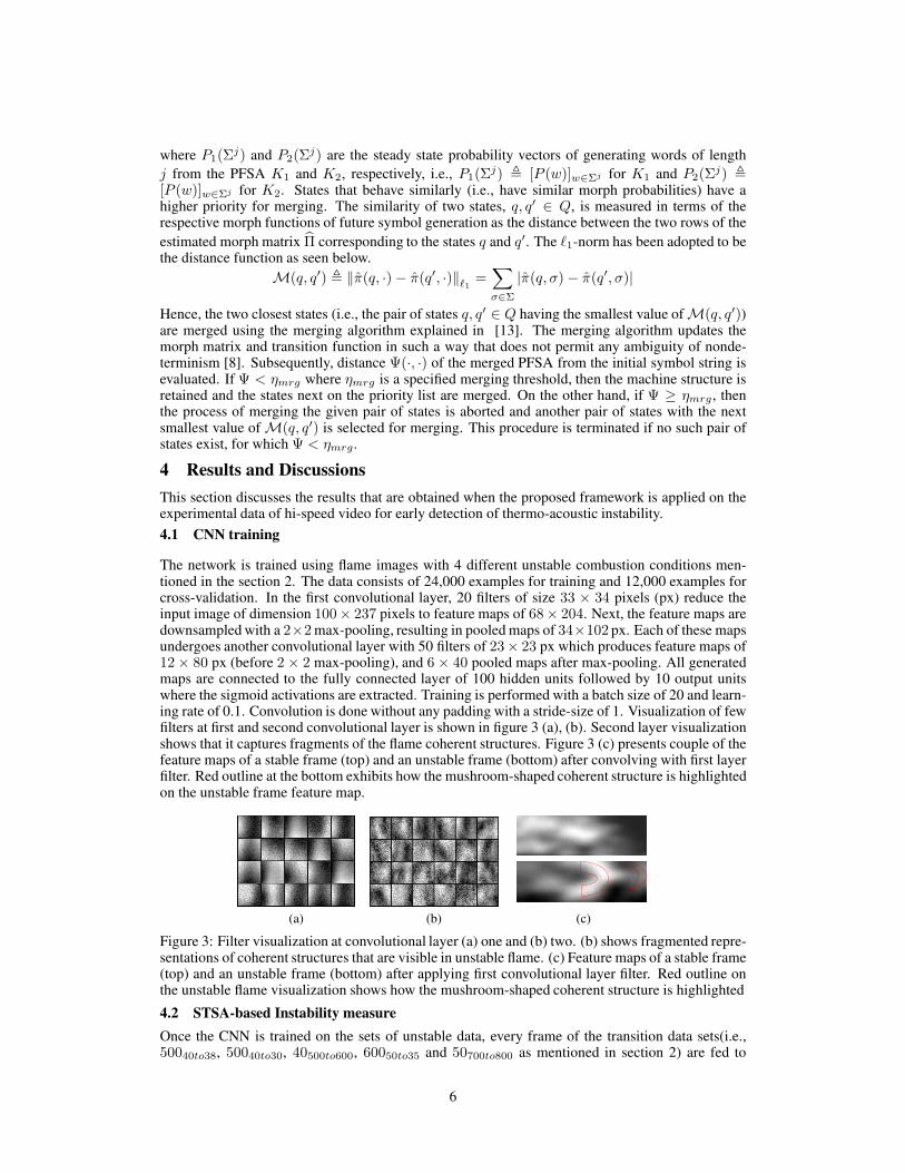
where P1(Σj) and P2(Σj) are the steady state probability vectors of generating words of length
j from the PFSA K1 and K2, respectively, i.e., P1(Σj) ! [P (w)]w∈Σj for K1 and P2(Σj) ![P (w)]w∈Σj for K2. States that behave similarly (i.e., have similar morph probabilities) have ahigher priority for merging. The similarity of two states, q, q′ ∈ Q, is measured in terms of therespective morph functions of future symbol generation as the distance between the two rows of the
estimated morph matrix !Π corresponding to the states q and q′. The ℓ1-norm has been adopted to bethe distance function as seen below.
M(q, q′) ! ∥π(q, ·)− π(q′, ·)∥ℓ1 ="
σ∈Σ
|π(q,σ)− π(q′,σ)|
Hence, the two closest states (i.e., the pair of states q, q′ ∈ Q having the smallest value of M(q, q′))are merged using the merging algorithm explained in [13]. The merging algorithm updates themorph matrix and transition function in such a way that does not permit any ambiguity of nonde-terminism [8]. Subsequently, distance Ψ(·, ·) of the merged PFSA from the initial symbol string isevaluated. If Ψ < ηmrg where ηmrg is a specified merging threshold, then the machine structure isretained and the states next on the priority list are merged. On the other hand, if Ψ ≥ ηmrg , thenthe process of merging the given pair of states is aborted and another pair of states with the nextsmallest value of M(q, q′) is selected for merging. This procedure is terminated if no such pair ofstates exist, for which Ψ < ηmrg.
4 Results and Discussions
This section discusses the results that are obtained when the proposed framework is applied on theexperimental data of hi-speed video for early detection of thermo-acoustic instability.
4.1 CNN training
The network is trained using flame images with 4 different unstable combustion conditions men-tioned in the section 2. The data consists of 24,000 examples for training and 12,000 examples forcross-validation. In the first convolutional layer, 20 filters of size 33 × 34 pixels (px) reduce theinput image of dimension 100× 237 pixels to feature maps of 68× 204. Next, the feature maps aredownsampled with a 2×2max-pooling, resulting in pooled maps of 34×102 px. Each of these mapsundergoes another convolutional layer with 50 filters of 23× 23 px which produces feature maps of12× 80 px (before 2 × 2 max-pooling), and 6 × 40 pooled maps after max-pooling. All generatedmaps are connected to the fully connected layer of 100 hidden units followed by 10 output unitswhere the sigmoid activations are extracted. Training is performed with a batch size of 20 and learn-ing rate of 0.1. Convolution is done without any padding with a stride-size of 1. Visualization of fewfilters at first and second convolutional layer is shown in figure 3 (a), (b). Second layer visualizationshows that it captures fragments of the flame coherent structures. Figure 3 (c) presents couple of thefeature maps of a stable frame (top) and an unstable frame (bottom) after convolving with first layerfilter. Red outline at the bottom exhibits how the mushroom-shaped coherent structure is highlightedon the unstable frame feature map.
(a) (b) (c)
Figure 3: Filter visualization at convolutional layer (a) one and (b) two. (b) shows fragmented repre-sentations of coherent structures that are visible in unstable flame. (c) Feature maps of a stable frame(top) and an unstable frame (bottom) after applying first convolutional layer filter. Red outline onthe unstable flame visualization shows how the mushroom-shaped coherent structure is highlighted
4.2 STSA-based Instability measure
Once the CNN is trained on the sets of unstable data, every frame of the transition data sets(i.e.,50040to38, 50040to30, 40500to600, 60050to35 and 50700to800 as mentioned in section 2) are fed to
6

the CNN. Each sigmoid activation unit out of ten at the last fully connected layer generates atime series for one transition data set. For capturing the fast change in a transition data, a win-dow of 0.5 seconds (1500 frames) is traversed over the hi-speed video with an overlap of 80%to keep the response speed at 10 Hz, which is necessary for real-time combustion instabilitycontrol. The time window output of a sigmoid activation unit is symbolized by maximum en-tropy partitioning (MEP) with an alphabet size of |Σ| = 3. Considering the first window tobe reference stable state, a generalized D-Markov machine is constructed by state splitting withNmax = 10 and state merging with ηmrg = 0.05. Nmax is chosen as 10 because windowlength is not enough to learn a large state machine. For the alphabet {1, 2, 3}, the set of statesafter state splitting is {11, 21, 31, 2, 113, 213, 313, 23, 133, 233, 333} and state merging leads to{11, 21, 31, 2, {113, 313}, 213, {23, 133}, {233, 333}} for one of the sigmoid activation outputs inthe transition video 60050to35. State probability vector, arising from D-Markov machine at eachtime window, is the feature capturing the extent of instability which is transmitted through the cor-responding sigmoid hidden unit. Instability measure of a time window is defined as the l2 normdistance from the reference stable time window.
Figure 4: Variation of the proposed instability measure with time for the transition video named60050to35. Multiple regions on the measure curve denote different combustion states such as stable,temporary intermittancy (a significant precursor to persistent instability) and unstable . They are cor-responded to varied coherent structures (bounded by red box) that are detected by the ‘CNN+STSA’framework. On the right, rms variation of the pressure is shown as it is one of the most commonlyused instability measures. Progression of Prms can not detect the aforementioned precursors.
Figure 4 shows an aggregated progression (summation of individual instability measure obtainedfrom each sigmoid activation unit) of instability measure for 60050to35. The rms curve of thepressure on right of the figure 4 gives a rough idea about the ground truth regarding stability. Twofold advantages of the proposed instability measure over Prms are as follows: (i) intermittancyphenomenon (region 2 and 3 on figure 4) is captured by this measure because it can detect variable-size mildly-illuminated mushroom-shaped coherent structure (bounded by red box in the figure 4)in the ‘CNN+STSA’ framework whereas Prms ignores these important precursors to instability and(ii) region 4 of the figure 4 shows that the proposed measure rises faster towards instability. Othertransition data sets also exhibit similar nature regarding this measure. Hence, the proposed measureperforms better in early detection of instability than other commonly used measures such as Prms.
4.3 Comparison with ‘PCA+STSA’
To compare with the proposed approach, Principal Component Analysis (PCA) [5], a well-knowndimensionality reduction technique is used as a replacement of CNN module. Figure 5 (a) showsthat the transition (stable to unstable) increment of aggregated instability measure for ‘CNN+STSA’is larger than that for ‘PCA+STSA’ in all transition data. This will result in more precise instabilitycontrol in real time. The condition 50700to800 is observed in figure 5 (b) as the transition jump forboth frameworks are very close. A close observation of the instability measure variation reveals that‘CNN+STSA’ can detect an intermittancy precursor (region 1 at figure 5 (b)) although the coherentstructure formation is not very prominent. However, ‘PCA+STSA’ misses this precursor before
7

arriving at the inception of persistent instability. A probable rationale behind this observation is that,while PCA is averaging the image vector based on just maximum spatial variance, CNN is learningsemantic features based on the coherent structures of varied illumination, size and orientation seenduring unstable combustion.
1 2 3 4 52
2.5
3
3.5
4
4.5
5
5.5
Tansition conditions
Tran
sitio
n ju
mp
in in
stab
ility
mea
sure
CNN + STSAPCA + STSA
(a)
1 2 3 4 5 6 70
0.5
1
1.5
2
2.5
time (sec)
Insta
bili
ty m
ea
su
re
1 2 3 4 5 6 70
0.5
1
1.5
2
2.5
time (sec)
Insta
bili
ty m
ea
su
re CNN+STSA PCA+STSA
(1) Intermittancy
11
(b)
Figure 5: (a) Comparison of sudden change in instability measure when instablity sets in for differenttransition conditions which are 1. 50040to38, 2. 50040to30, 3. 40500to600, 4. 60050to35 and 5.50700to800. The jump is larger for ‘CNN+STSA’ than ‘PCA+STSA’. (b) Variation of instabilitymeasure for both ‘CNN+STSA’ than ‘PCA+STSA’ at transition condition 50700to800. The measurearising from ‘CNN+STSA’ can detect the intermittancy precursor whereas it is mostly ignored by‘PCA+STSA’. A frame with an intermittancy coherent structure in a red box is shown on the top.
5 Conclusions and future work
The paper proposes a framework that synergistically combines the recently introduced concepts ofCNN and STSA for early detection of thermo-acoustic instability in gas turbine engines. Extensiveset of experiments have been conducted on a swirl-stabilized combustor for validation of the pro-posed method. Sequences of hi-speed greyscale images are fed into a multi-layered CNN to modelthe fluctuating coherent structures in the flame, which are dominant during unstable combustion.Fragments of coherent structures are observed in the CNN filter visualization. Therefore, an en-semble of time series data is constructed from sequence of images based on the sigmoid activationprobability vectors of last hidden layer at the CNN. Then, STSA is applied on the time series that isgenerated from an image sequence and ‘CNN+STSA’ is found to exhibit larger change in instabilitymeasure while transition to instability than ‘PCA+STSA’. The proposed framework detects all theintermittent precursors for different transition protocols, which is the most significant step towardsdetecting the onset of instability early enough for mitigation. In summary, while CNN captures thesemantic features (i.e., coherent structures) of the combustion flames at varied illuminations, sizesand orientations, STSA models the temporal fluctuation of those features at a reduced dimension.
One of the primary advantages of the proposed semantic dimensionality reduction (as opposed toabstract dimensionality reduction, e.g., using PCA) would be seamless involvement of domain ex-perts into the data analytics framework for expert-guided data exploration activities. Developingnovel use-cases in this neural-symbol context will be a key future work. Some other near-term re-search tasks are: (i) dynamically tracking multiple coherent structures in the flame to characterizethe extent of instability, (ii) multi-dimensional partitioning for direct usage of the last sigmoid layerand (iii) learning CNN and STSA together.
Acknowledgment
Authors sincerely acknowledge the extensive data collection performed by Vikram Ramanan and Dr.Satyanarayanan Chakravarthy at Indian Institute of Technology Madras (IITM), Chennai. Authorsalso gratefully acknowledge the support of NVIDIA Corporation with the donation of the GeForceGTX TITAN Black GPU used for this research.
8

References
[1] A. Garcez, T. R. Besold, L. de Raedt, P. Foeldiak, P. Hitzler, T. Icard, K. Kuehnberger, L. C. Lamb,R. Miikkulainen, and D. L. Silver. Neural-symbolic learning and reasoning: Contributions and challenges.Proceedings of the AAAI Spring Symposium on Knowledge Representation and Reasoning: IntegratingSymbolic and Neural Approaches, Stanford, March 2015.
[2] A. K. M. F. Hussain. Coherent structures - reality and myth. Physics of Fluids, 26(10):2816–2850, 1983.
[3] S. R. Chakravarthy, O. J. Shreenivasan, B. Bhm, A. Dreizler, and J. Janicka. Experimental characterizationof onset of acoustic instability in a nonpremixed half-dump combustor. Journal of the Acoustical Societyof America, 122:120127, 2007.
[4] G Berkooz, P Holmes, and J L Lumley. The proper orthogonal decomposition in the analysis of turbulentflows. Annual Review of Fluid Mechanics, 25(1):539–575, 1993.
[5] C. M. Bishop. Pattern Recognition and Machine Learning. Springer, New York, NY, USA, 2006.
[6] P. J. Schmid. Dynamic mode decomposition of numerical and experimental data. Journal of Fluid Me-chanics, 656:5–28, 2010.
[7] K. Kavukcuoglu, Y. L. Sermanet, P. Boureau, K. Gregor, M. Mathieu, and Y. LeCun. Learning convolu-tional feature hierachies for visual recognition. In NIPS, 2010.
[8] A. Ray. Symbolic dynamic analysis of complex systems for anomaly detection. Signal Processing,84(7):1115–1130, July 2004.
[9] S. Sarkar, K. Mukherjee, S. Sarkar, and A. Ray. Symbolic dynamic analysis of transient time seriesfor fault detection in gas turbine engines. Journal of Dynamic Systems, Measurement, and Control,135(1):014506, 2013.
[10] S. Sarkar, A. Ray, A. Mukhopadhyay, R. R. Chaudhari, and S. Sen. Early detection of lean blow out (lbo)via generalized d-markov machine construction. In American Control Conference (ACC), 2014, pages3041–3046. IEEE, 2014.
[11] V. Ramanan, S. R. Chakravarthy, S. Sarkar, and A. Ray. Investigation of combustion instability in a swirl-stabilized combustor using symbolic time series analysis. In Proc. ASME Gas Turbine India Conference,GTIndia 2014, New Delhi, India, pages 1–6, December 2014.
[12] S. Sarkar, K.G. Lore, S. Sarkar, V. Ramanan, S.R. Chakravarthy, S. Phoha, and A. Ray. Early detection ofcombustion instability from hi-speed flame images via deep learning and symbolic time series analysis.In Annual Conference of The Prognostics and Health Management, pages pre–prints. PHM, 2015.
[13] K. Mukherjee and A. Ray. State splitting and state merging in probabilistic finite state automata for signalrepresentation and analysis. Signal Processing, 104:105–119, November 2014.
[14] S. Sarkar, A. Ray, A. Mukhopadhyay, and S. Sen. Dynamic data-driven prediction of lean blowout ina swirl-stabilized combustor. International Journal of Spray and Combustion Dynamics, 7(3):in–press,2015.
[15] A. Krizhevsky, I. Sutskever, and G. E. Hinton. Imagenet classification with deep convolutional neuralnetworks. In NIPS, 2012.
[16] C. Daw, C. Finney, and E. Tracy. A review of symbolic analysis of experimental data. Review of ScientificInstruments, 74(2):915–930, 2003.
[17] C. Rao, A. Ray, S. Sarkar, and M. Yasar. Review and comparative evaluation of symbolic dynamicfiltering for detection of anomaly patterns. Signal, Image and Video Processing, 3(2):101–114, 2009.
[18] S. Bahrampour, A. Ray, S. Sarkar, T. Damarla, and N.M. Nasrabadi. Performance comparison of featureextraction algorithms for target detection and classification. Pattern Recogntion Letters, 34(16):2126–2134, December 2013.
[19] V. Rajagopalan and A. Ray. Symbolic time series analysis via wavelet-based partitioning. Signal Pro-cessing, 86(11):3309–3320, November 2006.
[20] S. Sarkar, A. Srivastav, and M. Shashanka. Maximally bijective discretization for data-driven modelingof complex systems. In Proceedings of American Control Conference, Washington, D.C., 2013.
[21] M. Sipser. Introduction to the Theory of Computation, 3rd ed. Cengage Publishing, Boston, MA, USA,2013.
9

Predicting Embedded Syntactic Structures
from Natural Language Sentences
with Neural Network Approaches
Gregory Senay
Panasonic Silicon Valley LabCupertino, CA 95014
Fabio Massimo Zanzotto
University of Rome Tor VergataViale del Politecnico, 1, 00133 Rome, Italy
Lorenzo Ferrone
University of Rome Tor VergataViale del Politecnico, 1, 00133 Rome, [email protected]
Luca Rigazio
Panasonic Silicon Valley LabCupertino, CA 95014
Abstract
Syntactic parsing is a key component of natural language understanding and, tradi-tionally, has a symbolic output. Recently, a new approach for predicting syntacticstructures from sentences has emerged: directly producing small and expressivevectors that embed in syntactic structures. In this approach, parsing producesdistributed representations. In this paper, we advance the frontier of these novelpredictors by using the learning capabilities of neural networks. We propose twoapproaches for predicting the embedded syntactic structures. The first approachis based on a multi-layer perceptron to learn how to map vectors representingsentences into embedded syntactic structures. The second approach exploits re-current neural networks with long short-term memory (LSTM-RNN-DRP) to di-rectly map sentences to these embedded structures. We show that both approachessuccessfully exploit word information to learn syntactic predictors and achieve asignificant performance advantage over previous methods. Results on the PennTreebank corpus are promising. With the LSTM-RNN-DRP, we improve the pre-vious state-of-the-art method by 8.68%.
1 Introduction
Syntactic structure is a key component for natural language understanding [8], with several studiesshowing that syntactic information helps in modeling meaning [21, 14, 25]. Consequently, a veryactive area in natural language processing is building predictors of symbolic syntactic structuresfrom sentences; such predictors, called parsers, are commonly implemented as complex recursiveor iterative functions. Even when learned from data, the recursive/iterative nature of parsers isgenerally not changed since learning is confined to a probability estimation of context-free rules[9, 6] or learning of local discriminative predictor ([23, 26]).
1

Despite the effort in building explicit syntactic structures, they are rarely used in that form for se-mantic tasks such as question answering [28], recognizing textual entailment [13], semantic textualsimilarity [1]. These tasks are generally solved by learning classifiers or regressors. Hence, syntacticstructures are unfolded to obtain syntactic-rich feature vectors [14], used within convolution kernelfunctions [17], or guiding the application of recursive neural networks [25]. Syntactic structures arefirst discovered by parsers, then, unfolded by “semantic learners” in explicit or implicit syntacticfeature vectors.
Distributed syntactic trees [30] have offered a singular opportunity to redraw the path between sen-tences and feature vectors used within learners of semantic tasks. These distributed syntactic treesembed syntactic trees in small vectors. Hence, a possibility is to learn functions to map sentences indistributed syntactic trees [29]. These functions have been called distributed representation parsers
(DRPs) [29]. However, these distributed representation parsers suffer from major limitations be-cause, due to data sparsity, these functions can only transform part-of-speech tag sequences in syn-tactic trees without the lexical information.
In this paper, we propose two novel approaches based on neural networks for building predictors ofdistributed syntactic structures. The first model is based on a multi-layer perceptron (MLP) whichlearns how to map sentences, transformed into vectors to distributed syntactic representations. Thesecond model is based on a recurrent neural network (RNN) with long short-term memory (LSTM)which learns to directly map sentences to distributed trees. Both models show the ability to positivelyexploit words in learning these predictors and significantly outperform previous models [29].
The paper is organized as follows: Section 2 describes the background by reporting on the dis-tributed syntactic trees and the idea of distributed representation parsers; Section 3 introduces ourtwo novel approaches for distributed representation parsing: the model based on a multi-layer per-ceptron (MLP-DRP) and the model based on long short-term memory (LSTM-RNN-DRP); Section4 reports on the experiments and the results. Finally, section 5 draws conclusions.
2 Background
2.1 Distributed Syntactic Trees: Embedding Syntactic Trees in Small Vectors
Embedding syntactic trees in small vectors [30] is a key idea which changes how syntactic infor-mation is used in learning. Stemming from the recently revitalized research field of DistributedRepresentations (DR) [18, 24, 4, 12, 25], distributed syntactic trees [30] have shown that it is possi-ble to use small vectors for representing the syntactic information. In fact, feature spaces of subtreesunderlying tree kernels [10] are fully embedded by these distributed syntactic trees.
We want to give an intuitive idea how this embedding works. To explain this idea, we need to startfrom the definition of tree kernels [10] used in kernel machines. In these kernels, trees T are seen ascollections of subtrees S(T ) and a kernel TK(T1, T2) between two trees performs a weighted countof common subtrees, that is:
TK(T1, T2) =X
⌧i2S(T1),⌧j2S(T2)
!
⌧i!⌧j�(⌧i, ⌧j)
where !
⌧i and !
⌧j are the weights for subtrees ⌧
i
and ⌧
j
and �(⌧i
, ⌧
j
) is the Kronecker’s deltabetween subtrees. Hence, �(⌧
i
, ⌧
j
) = 1 if ⌧i
= ⌧
j
else �(⌧i
, ⌧
j
) = 0. Distributed trees, in somesense, pack sets S(T
s1) in small vectors. In the illustration of Figure 1, this idea is conveyed bypacking images of subtrees in a small space, that is, the box under DT (T
s1). By rotating andcoloring subtrees, the picture in the box under DT (T
s1) still allows us to recognize these subtrees.Consequently, it is possible to count how many subtrees are similar by comparing the picture inthe box under DT (T
s1) with the one under DT (Ts2). We visually show that it is possible to pack
subtrees in small boxes, hence, it should be possible to pack this information in small vectors.
The formal definition of these embeddings, called distributed syntactic trees DT (T ), is the follow-ing:
DT (T ) =X
⌧i2S(T )
!
i
~⌧
i
=X
⌧i2S(T )
!
i
dt(⌧i
)
2

T
s1 S(Ts1) DT (T
s1) 2 Rd
DT (Ts2) 2 Rd
T
s2
Figure 1: Distributed tree idea
where S(T ) is the set of the subtrees ⌧
i
of T , dt(⌧i
) = ~⌧
i
is a vector in Rd corresponding to thesubtree ⌧
i
, and !
i
is the weight assigned to that subtree. These vectors are obtained compositionallyusing vectors for node labels and shuffled circular convolution ⌦ as a basic composition function.For example, the last subtree of S(T
s1) in Figure 1 has the following vector:
dt(T1) = (~S ⌦ ( ~
NP ⌦ ~
John)⌦ ( ~
V P ⌦ ( ~
V B ⌦ ~
killed)⌦ ( ~
V P ⌦ ~
Bob)))
Vectors dt(⌧i
) have the following property:
�(⌧i
, ⌧
j
)� ✏ < |dt(⌧i
) · dt(⌧j
)| < �(⌧i
, ⌧
j
) + ✏ (1)with a high probability. Therefore, given two trees T1 and T2, the dot product between the tworelated, distributed trees approximates the tree kernel between trees TK(T1, T2), that is:
DT (T1) ·DT (T2) =X
⌧i2S(T1),⌧j2S(T2)
!
⌧i!⌧jdt(⌧i) · dt(⌧j) ⇡ TK(T1, T2)
with a given degree of approximation [30]. Hence, distributed syntactic trees allow us to encodesyntactic trees in small vectors.
2.2 Distributed Representation Parsers
Building on the idea of encoding syntactic trees in small vectors [30], distributed representationparsers (DRPs) [29] have been introduced to predict these vectors directly from sentences. DRPsmap sentence s to predicted distributed syntactic trees DRP (s) (Figure 2), and represent the ex-pected distributed syntactic trees DT (T
s
). In Figure 2, DRP (s1) is blurred to show that it is apredicted version of the correct distributed syntactic tree, DT (T
s1). The DRP function is generallydivided in two blocks: a sentence encoder SE and a transducer P , which is the actual “parser” asit reconstructs distributed syntactic subtrees. In contrast, the sentence encoder SE maps sentencesinto a distributed representation. For example, the vector SE(s1) represents s1 in Figure 2 andcontains subsequences of part-of-speech tags.
s1 SE(s1) 2 Rd
DRP (s1) 2 Rd
John/NN killed/VBBob/NN
!SentenceEncoder
(SE)! ! Transducer
(P) !
Distributed Representation Parser (DRP)
Figure 2: Visualization of the distributed representation parsing
Formally, a DRP is a function DRP : X ! R
d that maps sentences into X to distributed trees inR
d. The sentence encoder SE : X ! R
d maps sentences into X to distributed representation ofsentence sequences defined as follows:
SE(s) =X
seqi2SUB(s)
~seq
i
3
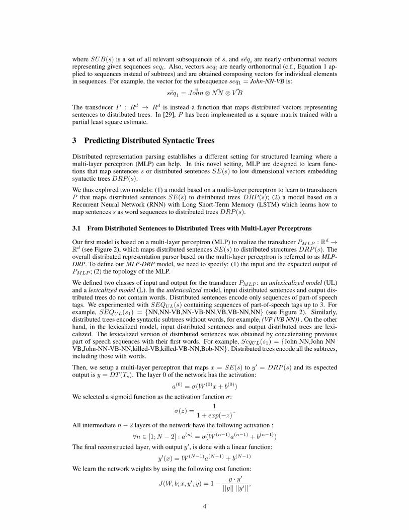
where SUB(s) is a set of all relevant subsequences of s, and ~seq
i
are nearly orthonormal vectorsrepresenting given sequences seq
i
. Also, vectors seqi
are nearly orthonormal (c.f., Equation 1 ap-plied to sequences instead of subtrees) and are obtained composing vectors for individual elementsin sequences. For example, the vector for the subsequence seq1 = John-NN-VB is:
~seq1 = ~
John⌦ ~
NN ⌦ ~
V B
The transducer P : R
d ! R
d is instead a function that maps distributed vectors representingsentences to distributed trees. In [29], P has been implemented as a square matrix trained with apartial least square estimate.
3 Predicting Distributed Syntactic Trees
Distributed representation parsing establishes a different setting for structured learning where amulti-layer perceptron (MLP) can help. In this novel setting, MLP are designed to learn func-tions that map sentences s or distributed sentences SE(s) to low dimensional vectors embeddingsyntactic trees DRP (s).
We thus explored two models: (1) a model based on a multi-layer perceptron to learn to transducersP that maps distributed sentences SE(s) to distributed trees DRP (s); (2) a model based on aRecurrent Neural Network (RNN) with Long Short-Term Memory (LSTM) which learns how tomap sentences s as word sequences to distributed trees DRP (s).
3.1 From Distributed Sentences to Distributed Trees with Multi-Layer Perceptrons
Our first model is based on a multi-layer perceptron (MLP) to realize the transducer PMLP
: Rd !Rd (see Figure 2), which maps distributed sentences SE(s) to distributed structures DRP (s). Theoverall distributed representation parser based on the multi-layer perceptron is referred to as MLP-
DRP. To define our MLP-DRP model, we need to specify: (1) the input and the expected output ofP
MLP
; (2) the topology of the MLP.
We defined two classes of input and output for the transducer PMLP
: an unlexicalized model (UL)and a lexicalized model (L). In the unlexicalized model, input distributed sentences and output dis-tributed trees do not contain words. Distributed sentences encode only sequences of part-of speechtags. We experimented with SEQ
UL
(s) containing sequences of part-of-speech tags up to 3. Forexample, SEQ
UL
(s1) = {NN,NN-VB,NN-VB-NN,VB,VB-NN,NN} (see Figure 2). Similarly,distributed trees encode syntactic subtrees without words, for example, (VP (VB NN)) . On the otherhand, in the lexicalized model, input distributed sentences and output distributed trees are lexi-calized. The lexicalized version of distributed sentences was obtained by concatenating previouspart-of-speech sequences with their first words. For example, Seq
UL
(s1) = {John-NN,John-NN-VB,John-NN-VB-NN,killed-VB,killed-VB-NN,Bob-NN}. Distributed trees encode all the subtrees,including those with words.
Then, we setup a multi-layer perceptron that maps x = SE(s) to y
0 = DRP (s) and its expectedoutput is y = DT (T
s
). The layer 0 of the network has the activation:
a
(0) = �(W (0)x+ b
(0))
We selected a sigmoid function as the activation function �:
�(z) =1
1 + exp(�z).
All intermediate n� 2 layers of the network have the following activation :
8n 2 [1;N � 2] : a(n) = �(W (n�1)a
(n�1) + b
(n�1))
The final reconstructed layer, with output y0, is done with a linear function:
y
0(x) = W
(N�1)a
(N�1) + b
(N�1)
We learn the network weights by using the following cost function:
J(W, b;x, y0, y) = 1� y · y0
||y|| ||y0|| ,
4

that evaluates the cosine similarity between y and y
0.
Learning unlexicalized and lexicalized MLP-DRPs is feasible even if the two settings hide differentchallenges. The unlexicalized MLP-DRP exposes network learned with less information to encode.However, the model cannot exploit the important information on words. In contrast, the lexicalizedMLP-DRP can exploit words but it has to encode more information. Experiments with the twosettings are reported in Section 4.
3.2 From Word Sequences to Distributed Trees with Long Short Term Memory
Our second model is more ambitious: it is an end-to-end predictor of distributed syntactic treesDRP (s) from sentences s. We based our approach on recurrent neural networks (RNN) since RNNshave already proven their efficiency to learn complex sequence-to-sequence mapping in speechrecognition [16] and in handwriting [15]. Moreover, RNNs have been also successfully used tolearn mapping functions between word sequences through sentence embedding vectors [7, 2].
Our end-to-end predictor of distributed syntactic structures is built on the recurrent neural networkmodel with long-short term memory (LSTM-RNN) [20] to overcome the vanishing gradient prob-lem. However, to increase computational efficiency, in this model the activation of the output gateof each cell does not depend on its memory state.
Figure 3: Structure of our LSTM-RNN-DRP encoder and a detail of the LSTM neuron
The resulting distributed representation parser LSTM-RNN-DRP is then defined as follows: Inputsentences s are seen as word sequences. To each word in these sequences, we assigned a unit basevector x
t
2 RL where L is the size of the lexicon. x
t
is 1 in the t-th component representing theword and 0 otherwise. Words are encoded with 4 matrices W
i
,W
c
,W
f
,W
o
2 Rm⇥L. Hence, m isthe size of word encoding vectors. The LSTM cells are defined as follows: x
t
is an input word tothe memory cell layer at time t. i
t
is the input gate define by:
i
t
= �(Wi
x
t
+ U
i
h
t�1 + b
i
), (2)
where � is a sigmoid. Ct
is the candidate values of the states of the memory cells:
C
t
= tanh(Wc
x
t
+ U
c
h
t�1 + b
c
). (3)
f
t
is the activation of the memory cell’s forget gates:
f
t
= �(Wf
x
t
+ U
f
h
t�1 + b
f
). (4)
Given i
t
, ft
and C
t
, Ct
memory cells are computed with:
C
t
= i
t
? C
t
+ f
t
? C
t�1, (5)
where ? is the element-wise product. Given the state of the memory cells, we compute the outputgate with:
o
t
= �(Wo
x
t
+ U
o
h
t�1 + b1)
h
t
= o
t
? tanh(Ct
)(6)
The non recurrent part of this model is achieved by an average pooling of the sequence representationh0, h1, ..., hn
, the 4 matrix W⇤ are concatenated into a single one: W , the U⇤ weight matrix into U
5
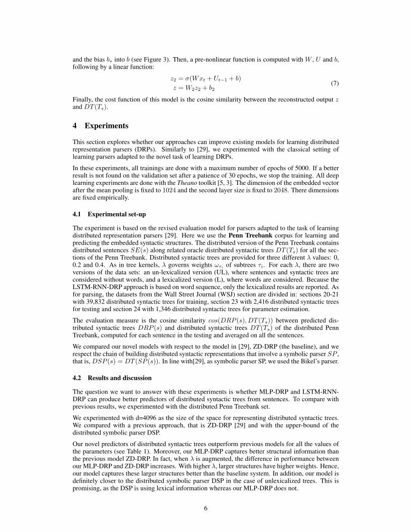
and the bias b⇤ into b (see Figure 3). Then, a pre-nonlinear function is computed with W , U and b,following by a linear function:
z2 = �(Wx
t
+ U
t�1 + b)
z = W2z2 + b2(7)
Finally, the cost function of this model is the cosine similarity between the reconstructed output zand DT (T
s
).
4 Experiments
This section explores whether our approaches can improve existing models for learning distributedrepresentation parsers (DRPs). Similarly to [29], we experimented with the classical setting oflearning parsers adapted to the novel task of learning DRPs.
In these experiments, all trainings are done with a maximum number of epochs of 5000. If a betterresult is not found on the validation set after a patience of 30 epochs, we stop the training. All deeplearning experiments are done with the Theano toolkit [5, 3]. The dimension of the embedded vectorafter the mean pooling is fixed to 1024 and the second layer size is fixed to 2048. There dimensionsare fixed empirically.
4.1 Experimental set-up
The experiment is based on the revised evaluation model for parsers adapted to the task of learningdistributed representation parsers [29]. Here we use the Penn Treebank corpus for learning andpredicting the embedded syntactic structures. The distributed version of the Penn Treebank containsdistributed sentences SE(s) along related oracle distributed syntactic trees DT (T
s
) for all the sec-tions of the Penn Treebank. Distributed syntactic trees are provided for three different � values: 0,0.2 and 0.4. As in tree kernels, � governs weights !
⌧i of subtrees ⌧
i
. For each �, there are twoversions of the data sets: an un-lexicalized version (UL), where sentences and syntactic trees areconsidered without words, and a lexicalized version (L), where words are considered. Because theLSTM-RNN-DRP approach is based on word sequence, only the lexicalized results are reported. Asfor parsing, the datasets from the Wall Street Journal (WSJ) section are divided in: sections 20-21with 39,832 distributed syntactic trees for training, section 23 with 2,416 distributed syntactic treesfor testing and section 24 with 1,346 distributed syntactic trees for parameter estimation.
The evaluation measure is the cosine similarity cos(DRP (s), DT (Ts
)) between predicted dis-tributed syntactic trees DRP (s) and distributed syntactic trees DT (T
s
) of the distributed PennTreebank, computed for each sentence in the testing and averaged on all the sentences.
We compared our novel models with respect to the model in [29], ZD-DRP (the baseline), and werespect the chain of building distributed syntactic representations that involve a symbolic parser SP ,that is, DSP (s) = DT (SP (s)). In line with[29], as symbolic parser SP, we used the Bikel’s parser.
4.2 Results and discussion
The question we want to answer with these experiments is whether MLP-DRP and LSTM-RNN-DRP can produce better predictors of distributed syntactic trees from sentences. To compare withprevious results, we experimented with the distributed Penn Treebank set.
We experimented with d=4096 as the size of the space for representing distributed syntactic trees.We compared with a previous approach, that is ZD-DRP [29] and with the upper-bound of thedistributed symbolic parser DSP.
Our novel predictors of distributed syntactic trees outperform previous models for all the values ofthe parameters (see Table 1). Moreover, our MLP-DRP captures better structural information thanthe previous model ZD-DRP. In fact, when � is augmented, the difference in performance betweenour MLP-DRP and ZD-DRP increases. With higher �, larger structures have higher weights. Hence,our model captures these larger structures better than the baseline system. In addition, our model isdefinitely closer to the distributed symbolic parser DSP in the case of unlexicalized trees. This ispromising, as the DSP is using lexical information whereas our MLP-DRP does not.
6
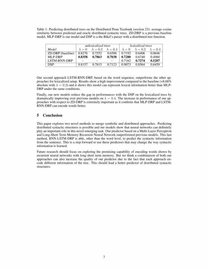
Table 1: Predicting distributed trees on the Distributed Penn Treebank (section 23): average cosinesimilarity between predicted and oracle distributed syntactic trees. ZD-DRP is a previous baselinemodel, MLP-DRP is our model and DSP is a the Bikel’s parser with a distributed tree function.
unlexicalized trees lexicalized trees
Model � = 0 � = 0.2 � = 0.4 � = 0 � = 0.2 � = 0.4ZD-DRP (baseline) 0.8276 0.7552 0.6506 0.7192 0.6406 0.0646MLP-DRP 0.8358 0.7863 0.7038 0.7280 0.6740 0.4960LSTM-RNN-DRP - - - 0.7162 0.7274 0.5207
DSP 0.8157 0.7815 0.7123 0.9073 0.8564 0.6459
Our second approach LSTM-RNN-DRP, based on the word sequence, outperforms the other ap-proaches for lexicalized setup. Results show a high improvement compared to the baseline (+8.68%absolute with � = 0.2) and it shows this model can represent lexical information better than MLP-DRP under the same conditions.
Finally, our new models reduce the gap in performances with the DSP on the lexicalized trees bydramatically improving over previous models on � = 0.4. The increase in performance of our ap-proaches with respect to ZD-DRP is extremely important as it confirms that MLP-DRP and LSTM-RNN-DRP can encode words better.
5 Conclusion
This paper explores two novel methods to merge symbolic and distributed approaches. Predictingdistributed syntactic structures is possible and our models show that neural networks can definitelyplay an important role in this novel emerging task. Our predictor based on a Multi-Layer Perceptronand Long-Short Term Memory Recurrent Neural Network outperformed previous models. This lastmethod, RNN-LSTM-DRP is able, other than the word level, to predict the syntactic informationfrom the sentence. This is a step forward to use these predictors that may change the way syntacticinformation is learned.
Future research should focus on exploring the promising capability of encoding words shown byrecurrent neural networks with long-short term memory. But we think a combinaison of both ourapproaches can also increase the quality of our predictor due to the fact that each approach en-code different information of the tree. This should lead a better predictor of distributed syntacticstructures.
7
References
[1] E. Agirre, D. Cer, M. Diab, A. Gonzalez-Agirre, and W. Guo. *sem 2013 shared task: Semantic textualsimilarity. In *SEM, pages 32–43, USA, 2013. ACL.
[2] D. Bahdanau, K. Cho, and Y. Bengio. Neural machine translation by jointly learning to align and translate.arXiv:1409.0473, 2014.
[3] F. Bastien, P. Lamblin, R. Pascanu, J. Bergstra, I. Goodfellow, A. Bergeron, N. Bouchard, D. Warde-Farley, and Y. Bengio. Theano: new features and speed improvements. arXiv:1211.5590, 2012.
[4] Y. Bengio. Learning deep architectures for AI. Foundations and Trends in Machine Learning, 2(1), 2009.[5] J. Bergstra, O. Breuleux, F. Bastien, P. Lamblin, R. Pascanu, G. Desjardins, J. Turian, D. Warde-Farley,
and Y. Bengio. Theano: a cpu and gpu math expression compiler. In Proceedings of SciPy , 2010.[6] E. Charniak. A maximum-entropy-inspired parser. In Proc. of the 1st NAACL, 2000.[7] K. Cho, B. Merrienboer, C. Gulcehre, F. Bougares, H. Schwenk, and Y. Bengio. Learning phrase repre-
sentations using rnn encoder-decoder for statistical machine translation. arXiv:1406.1078, 2014.[8] N. Chomsky. Aspect of Syntax Theory. MIT Press, Cambridge, Massachussetts, 1957.[9] M. Collins. Head-driven statistical models for natural language parsing. Comput. Linguist., 29(4), 2003.
[10] Michael Collins and Nigel Duffy. Convolution kernels for natural language. In NIPS, 2001.[11] Michael Collins and Nigel Duffy. New ranking algorithms for parsing and tagging: Kernels over discrete
structures, and the voted perceptron. In Proceedings of ACL02. 2002.[12] R. Collobert, J. Weston, L. Bottou, M. Karlen, K. Kavukcuoglu, and P. Kuksa. Natural language process-
ing (almost) from scratch. J. Mach. Learn. Res., 12, 2011.[13] I. Dagan, D. Roth, M. Sammons, and F.M. Zanzotto. Recognizing Textual Entailment: Models and
Applications. Synthesis Lectures on HLT. Morgan&Claypool Publishers, 2013.[14] Daniel Gildea and Daniel Jurafsky. Automatic Labeling of Semantic Roles. Comp. Ling., 28(3), 2002.[15] A. Graves. Supervised sequence labelling with recurrent neural networks, volume 385. Springer, 2012.[16] A. Graves, A. R. Mohamed, and G. Hinton. Speech recognition with deep recurrent neural networks. In
ICASSP, IEEE, 2013.[17] D. Haussler. Convolution kernels on discrete structures. Tech.Rep., Univ. of California at S. Cruz, 1999.[18] G. E. Hinton, J. L. McClelland, and D. E. Rumelhart. Distributed representations. In D. E. Rumelhart
and J. L. McClelland, editors, Parallel Distributed Processing: Explorations in the Microstructure of
Cognition. Volume 1: Foundations. MIT Press, Cambridge, MA., 1986.[19] S. Hochreiter, Y. Bengio, P. Frasconi, and J. Schmidhuber. Gradient flow in recurrent nets: the difficulty
of learning long-term dependencies, 2001.[20] S. Hochreiter and J. Schmidhuber. Long short-term memory. Neural computation, 9(8), 1997.[21] B. MacCartney, T. Grenager, M. -C. de Marneffe, D. Cer, and C. D. Manning. Learning to recognize
features of valid textual entailments. In Proceedings of NAACL, New York City, USA, 2006.[22] M. P. Marcus, B. Santorini, and M. A. Marcinkiewicz. Building a large annotated corpus of english: The
penn treebank. Computational Linguistics, 19:313–330, 1993.[23] J. Nivre, J. Hall, J. Nilsson, A. Chanev, G. Eryigit, S. Kubler, S. Marinov, and E. Marsi. Maltparser: A
language-independent system for data-driven dependency parsing. Nat. Lang. Eng., 13(2), 2007.[24] T. A. Plate. Distributed Representations and Nested Compositional Structure. PhD thesis, 1994.[25] R. Socher, E. H. Huang, J. Pennington, A. Y. Ng, and C. D. Manning. Dynamic pooling and unfolding
recursive autoencoders for paraphrase detection. In NIPS. 2011.[26] Richard Socher, Cliff Chiung-Yu Lin, Andrew Y. Ng, and Christopher D. Manning. Parsing natural
scenes and natural language with recursive neural networks. In Proceedings of ICML, 2011.[27] R. Socher, A. Perelygin, J. Y. Wu, J. Chuang, C. D. Manning, A. Y Ng, and C. Potts. Recursive deep
models for semantic compositionality over a sentiment treebank. In Proceedings of EMNLP, 2013.[28] Ellen M. Voorhees. The trec question answering track. Nat. Lang. Eng., 7(4):361–378, 2001.[29] F.M. Zanzotto and L. Dell’Arciprete. Transducing sentences to syntactic feature vectors: an alterna-
tive way to ”parse”? In Proceedings of the Workshop on Continuous Vector Space Models and their
Compositionality, 2013.
[30] F.M. Zanzotto and L. Dell’Arciprete. Distributed tree kernels. In Proceedings of ICML, 2012.
8

Building Memory with Concept LearningCapabilities from Large-scale Knowledge Base
Jiaxin Shi? Jun Zhu†
Department of Computer ScienceTsinghua University
Beijing, [email protected]
Abstract
We present a new perspective on neural knowledge base (KB) embeddings, fromwhich we build a framework that can model symbolic knowledge in the KB to-gether with its learning process. We show that this framework well regularizes pre-vious neural KB embedding model for superior performance in reasoning tasks,while having the capabilities of dealing with unseen entities, that is, to learn theirembeddings from natural language descriptions, which is very like human’s be-havior of learning semantic concepts.
1 Introduction
Recent years have seen great advances in neural networks and their applications in modeling imagesand natural languages. With deep neural networks, people are able to achieve superior performancein various machine learning tasks [1, 2, 3, 4]. One of those is relational learning, which aims atmodeling relational data such as user-item relations in recommendation systems, social networksand knowledge base, etc. In this paper we mainly focus on knowledge base.
Generally a knowledge base (KB) consists of triplets (or facts) like (e1, r, e2), where e1 and e2
denote the left entity and the right entity, and r denotes the relation between them. Previous works onneural KB embeddings model entities and relations with distributed representation, i.e., vectors [5]or matrices [6], and learn them from the KB. These prove to be scalable approaches for relationallearning. Experiments also show that neural embedding models obtain state-of-art performance onreasoning tasks like link prediction. Section 2 will cover more related work.
Although such methods on neural modeling of KB have shown promising results on reasoning tasks,they have limitations of only addressing known entities that appear in the training set and do notgeneralize well to settings where we have unseen entities. Because they do not know embeddingrepresentations of new entities, they cannot establish relations with them. On the other hand, thecapability of KB to learn new concepts as entities, or more specifically, to learn what a certain nameused by human means, is obviously highly useful, particularly in a KB-based dialog system. Weobserve that during conversations human does this task by first asking for explanation and then es-tablishing knowledge about the concept from other peoples’ natural language descriptions. Thisinspired our framework of modeling human’s cognitive process of learning concepts during con-versations, i.e., the process from natural language description to a concept in memory.1 We usea neural embedding model [5] to model the memory of concepts. When given description text ofa new concept, our framework directly transforms it into an entity embedding, which captures se-mantic information about this concept. The entity embedding can be stored and later used for other
1Concept learning in cognitive science usually refers to the cognitive process where people grow abstractgeneralizations from several example objects [7]. We use concept learning here to represent a different behavior.
1
semantic tasks. Details of our framework are described in Section 3. We will show efficiency of thisframework in modeling entity relationships, which involve both natural language understanding andreasoning.
Our perspective on modeling symbolic knowledge with its learning process has two main advan-tages. First, it enables us to incorporate natural language descriptions to augment the modeling ofrelational data, which fits human’s behavior of learning concepts during conversations well. Second,we also utilize the large number of symbolic facts in knowledge base as labeled information to guidethe semantic modeling of natural language. The novel perspective together with framework are thekey contributions of this work.
2 Related work
Statistical relational learning has long been an important topic in machine learning. Traditionalmethods such as Markov logic networks [8] often suffer from scalability issues due to intractableinference. Following the success of low rank models [9] in collaborative filtering, tensor factor-ization [10, 11] was proposed as a more general form to deal with multi-relational learning (i.e.,multiple kinds of relations exist between two entities). Another perspective is to regard elements infactorized tensors as probabilistic latent features of entities. This leads to methods that apply non-parametric Bayesian inference to learn latent features [12, 13, 14] for link prediction. Also, attemptshave been made to address the interpretability of latent feature based models under the frameworkof Bayesian clustering [15]. More recently, with the noticeable achievements of neural embeddingmodels like word vectors [16] in natural language processing area, various neural embedding models[6, 17, 5, 4, 18] for relational data have been proposed as strong competitors in both scalability andpredictability for reasoning tasks.
All these methods above model relational data under the latent-feature assumption, which is a com-mon perspective in machine learning to gain high performance in prediction tasks. However, thesemodels leave all latent features to be learnt from data, which suffers from substantial increments ofmodel complexity when applying to large-scale knowledge bases. For example, [10] can be seenas having a feature vector for each entity in factorized tensors, while [6] also represents entities inseparate vectors, or embeddings, thus the number of parameters scales linearly with the number ofentities. A large number of parameters in these models often increases the risk of overfitting, but fewof these works have proposed effective regularization techniques to address it. On the other hand,when applying these models to real world tasks (e.g., knowledge base completion), most of themhave a shared limitation that entities unseen in training set cannot be dealt with, that is, they canonly complete relations between known entities, which is far from what human’s ability of learningnew concepts can achieve. From this perspective, we develop a general framework that is capableof modeling symbolic knowledge together with its learning process, as detailed in Section 3.
3 The framework
Our framework consists of two parts. The first part is a memory storage of embedding representa-tions. We use it to model the large-scale symbolic knowledge in the KB, which can be thought asmemory of concepts. The other part is a concept learning module, which accepts natural languagedescriptions of concepts as the input, and then transforms them into entity embeddings in the samespace of the memory storage. In this paper we use translating embedding model from [5] as ourmemory storage and use neural networks for the concept learning module.
3.1 Translating embedding model as memory storage
We first describe translating embedding (TransE) model [5], which we use as the memory storage ofconcepts. In TransE, relationships are represented as translations in the embedding space. Supposewe have a set of N true facts D = {(e1, r, e2)}N as the training set. If a fact (e1, r, e2) is true, thenTransE requires e1 + r to be close to e2. Formally, we define the set of entity vectors as E, the setof relation vectors as R, where R,E ⇢ Rn, e1, e2 2 E, r 2 R. Let d be some distance measure,which is either the L1 or L2 norm. TransE minimizes a margin loss between the score of true facts
2

in the training set and randomly made facts, which serve as negative samples:
L(D) =
X
(e1,r,e2)2D
X
(e01,r0,e02)2D0
(e1,r,e2)
max(0, � + d(e1 + r, e2)� d(e
01 + r
0, e
02)), (1)
where D
0(e1,r,e2)
= {(e01, r, e2) : e
01 2 E} [ {(e1, r, e02) : e
02 2 E}, and � is the margin. Note
that this loss favors lower distance between translated left entities and right entities for training factsthan for random generated facts in D
0. The model is optimized by stochastic gradient descent withmini-batch. Besides, TransE forces the L2 norms of entity embeddings to be 1, which is essentialfor SGD to perform well according to [5], because it prevents the training process from triviallyminimizing loss by increasing entity embedding norms.
There are advantages of using embeddings instead of symbolic representations for cognitive tasks.For example, it’s kind of easier for us to figure out that a person who is a violinist can play vi-olin than to tell his father’s name. However, in symbolic representations like knowledge base,the former fact <A, play, violin> can only be deduced by reasoning process through facts<A, has profession, violinist> and <violinist, play, violin>, which is atwo-step procedure, while the latter result can be acquired in one step through the fact <A, has
father, B>. If we look at how TransE embeddings do this task, we can figure out that A playsviolin by finding nearest neighbors of A’s embedding + play’s embedding, which costs at mostthe same amount of time as finding out who A’s father is. This claim is supported by findings incognitive science that the general properties of concepts (e.g., <A, play, violin>) are morestrongly bound to an object than its more specific properties (e.g., <A, has father, B>) [19].
3.2 Concept learning module
As mentioned earlier, the concept learning module accepts natural language descriptions of con-cepts as the input, and outputs corresponding entity embeddings. As this requires natural languageunderstanding with knowledge in the KB transferred into the module, neural networks can be goodcandidates for this task. We explore two kinds of neural network architectures for the concept learn-ing module, including multi-layer perceptrons (MLP) and convolutional neural networks (CNN).
For MLP, we use one hidden layer with 500 neurons and RELU activations. Because MLP is fully-connected, we cannot afford the computational cost when the input length is too long. For large scaledatasets, the vocabulary size is often as big as millions, which means that bag-of-words featurescannot be used. Here, we use bag-of-n-grams features as inputs (there are at most 263 = 17576
kinds of 3-grams in pure English text). Given a word, for example word, we first add starting andending marks to it like #word#, and then break it into 3-grams (#wo, wor, ord, rd#). Suppose wehave V kinds of 3-grams in our training set. For an input description, we count the numbers of allkinds of 3-grams in this text, which form a V -dimensional feature vector x. To control scale of theinput per dimension, we use log(1 + x) instead of x as input features. Then we feed this vector intothe MLP, with the output to be the corresponding entity embedding under this description.
Since MLP with bag-of-n-grams features loses information of the word order, it has very little senseof the semantics. Even at the word level, it fails to identify words with similar meanings. From thispoint of view, we further explore the convolutional architecture, i.e. CNN together with word vectorfeatures. Let s = w1w2...wk be the paragraph of a concept description and let v(wi) 2 Rd be thevector representation for word wi. During experiments in this paper, we set d = 50 and initializev(wi) with wi’s word vector pretrained from large scale corpus, using methods in [16]. Let As bethe input matrix for s, which is defined by:
A
s:,i = v(wi), (2)
where A
s:,i denotes the ith column of matrix A
s. For the feature maps at the lth layer F
(l) 2Rc⇥n⇥m, where c is the number of channels, we add the convolutional layer like:
F
(l+1)i,:,: =
cX
j=1
F
(l)j,:,: ⇤K
(l)i,j,:,:, (3)
where K
(l) denotes all convolution kernels at the lth layer, which forms an order-4 tensor (outputchannels, input channels, y axis, x axis). When modeling natural language, which is in a sequence
3

Table 1: CNN layers
Layer Type Description1 convolution kernel: 64⇥ 50⇥ 1, stride: 12 convolution kernel: 64⇥ 1⇥ 3, stride: 13 max-pooling pooling size: 1⇥ 2, stride: 24 convolution kernel: 128⇥ 1⇥ 3, stride: 15 convolution kernel: 128⇥ 1⇥ 3, stride: 16 max-pooling pooling size: 1⇥ 2, stride: 27 convolution kernel: 256⇥ 1⇥ 3, stride: 18 max-pooling pooling size: 1⇥ 2, stride: 29 convolution kernel: 512⇥ 1⇥ 3, stride: 110 max-pooling pooling size: 1⇥ 2, stride: 211 dense size: 50012 output layer normalization layer
form, we choose K
(l) to have the same size in the y axis as feature maps F (l). So for the first layerthat has the input size 1 ⇥ D ⇥ L, we use kernel size D ⇥ 1 in the last two axes, where D is thedimension of word vectors. After the first layer, the last two axes of feature maps in each layerremain to be vectors. We list all layers we use in Table 1, where kernels are described by outputchannels ⇥ y axis ⇥ x axis.
Note that we use neural networks (either MLP or CNN) to output the entity embeddings, whileaccording to Section 3.1, the embedding model requires the L2-norms of entity embeddings to be1. This leads to a special normalization layer (the 12th layer in Table 1) designed for our purpose.Given the output of the second last layer x 2 Rn, we define the last layer as:
ek =
w
Tk,:x+ bk
[
Pnk0=1(w
Tk0,:x+ bk0
)
2]
1/2(4)
e is the output embedding. It’s easy to show that kek2 = 1. Throughout our experiments, we foundthat this trick plays an essential role in making joint training of the whole framework work. We willdescribe the training process in Section 3.3.
3.3 Training
We jointly train our embedding model and concept learning module together by stochastic gradientdescent with mini-batch and Nesterov momentum [20], using the loss defined by equation 1, wherethe entity embeddings are given by outputs of the concept learning module. When doing SGD withmini-batch, We back-propagate the error gradients into the neural network, and for CNN, finallyinto word vectors. The relation embeddings are also updated with SGD, and we re-normalize themin each iteration to make their L2-norms stay 1.
4 Experiments
4.1 Datasets
Since no public datasets satisfy our need, we have built two new datasets to test our method andmake them public for research use. The first dataset is based on FB15k released by [5]. We dumpnatural language descriptions of all entities in FB15k from Freebase [21], which are stored underrelation /common/topic/description. We refer to this dataset as FB15k-desc2. The otherdataset is also from Freebase, while we make it much larger. In fact, we include all entities that havedescriptions in Freebase and remove triplets with relations in a filter set. Most relations in the filterset are schema relations like /type/object/key. This dataset has more than 4M entities, forwhich we call it FB4M-desc3. Statistics of the two datasets are presented in Table 2.
2FB15k-desc: Available at http://ml.cs.tsinghua.edu.cn/˜jiaxin/fb15k desc.tar.gz3FB4M-desc: Available at http://ml.cs.tsinghua.edu.cn/˜jiaxin/fb4m desc.tar.gz
4

Table 2: Statistics of the datasets.
Dataset Entities Relations Descriptions Triplets (Facts)Vocabulary Length Train Validation Test
FB15k-desc 14951 1345 58954 6435 483142 50000 59071FB4M-desc 4629345 2651 1925116 6617 16805830 3021749 3023268
Table 3: Link prediction results on FB15k-desc.
Model Mean rank Hits@10 (%)Left Right Avg Left Right Avg
TransE[5] - - 243 - - 34.9Ours 252 176 214 34.3 41.1 37.7
Note that the scale is not the only difference between these two datasets. They also differ in splittingcriteria. FB15k-desc follows FB15k’s original partition of training, validation and test sets, in whichall entities in validation and test sets are already seen in the training set. FB4M-desc goes thecontrary way, as it is designed to test the concept learning ability of our framework. All facts invalidation and test sets include an entity on one side that are not seen in the training set. So whenevaluated on FB4M-desc, a good embedding for a new concept can only rely on information fromthe natural language description and knowledge transferred in the concept learning module.
4.2 Link prediction
We first describe the task of link prediction. Given a relation and an entity on one side, the task isto predict the entity on the other side. This is a natural reasoning procedure which happens in ourthoughts all the time. Following previous work [5], we use below evaluation protocol for this task.For each test triplet (e1, r, e2), e1 is removed and replaced by all the other entities in the trainingset in turn. The neural embedding model should give scores for these corrupted triplets. The rankof the correct entity is stored. We then report the mean of predicted ranks on the test set as the leftmean rank. This procedure is repeated by corrupting e2 and then we get the right mean rank. Theproportion of correct entities ranked in the top 10 is another index, which we refer to as hits@10.
We test our link prediction performance on FB15k-desc and report it in Table 3. The type of conceptlearning module we use here is CNN. Note that all the triplets in training, validation and test setsof FB15k-desc are the same as FB15k, so we list TransE’s results on FB15k in the same table.Compared to TransE which cannot make use of information in descriptions, our model performsmuch better, in terms of both mean rank and hits@10. As stated in Section 4.1, all entities in thetest set of FB15k are contained in the training set, which, together with the results, shows thatour framework well regularizes the embedding model by forcing embeddings to reflect informationfrom natural language descriptions. We demonstrate the concept learning capability in the nextsubsection.
4.3 Concept learning capabilities
It has been shown in Section 4.2 that our framework well regularizes the neural embedding model formemory storage. Next we use FB4M-desc to evaluate the capability of our framework on learningnew concepts and performing reasoning based on learnt embeddings. We report the link predictionperformance on FB4M-desc in Table 4. Note that the test set contains millions of triples, whichis very time-consuming in the ranking-based evaluation. So we randomly sample 1k, 10k and 80ktriplets from the test set to report the evaluation statistics. We can see that CNN consistently outper-forms MLP in terms of both mean rank and hits@10. All the triplets in the test set of FB4M-descinclude an entity unseen in the training set on one side, requiring the model to understand naturallanguage descriptions and to do reasoning based on it. As far as we know, no traditional knowledgebase embedding model can compete with us on this task, which again claims the novelty of ourframework.
5

Table 4: Link prediction results (of unseen entities) on FB4M-desc.
Model Mean rank Hits@10 (%)1k samples 10k samples 80k samples 1k samples 10k samples 80k samples
MLP 62657 62914 64570 13.2 13.95 14.06CNN 50164 54033 54536 14.8 14.29 14.52
Table 5: Concept learning examples by our method on FB4M-desc.
Left entity Description Hit@10 facts (partial)Rank Relation, right entity
Lily Burana
Lily Burana is an Americanwriter whose publicationsinclude the memoir I Love aMan in Uniform: A Memoirof Love, War, and OtherBattles, the novel Try andStrip ...
0 /people/person/profession,
writer
1 /people/person/profession,
author
0 /people/person/gender,
female
0 /people/person/nationality,
the United States
Ajeyo
Ajeyo is a 2014 Assameselanguage drama filmdirected by Jahnu Barua ...Ajeyo depicts the strugglesof an honest, idealrevolutionary youth GajenKeot who fought against thesocial evils in rural Assamduring the freedommovement in India. Thefilm won the Best FeatureFilm in Assamese award inthe 61st National FilmAwards ...
0 /film/film/country, India
7 /film/film/film festivals,
Mumbai Film Festival
7 /film/film/genre, Drama
9 /film/film/language,
Assamese
4272 Entsuji
4272 Entsuji is a main-beltasteroid discovered onMarch 12, 1977 by HirokiKosai and KiichiroHurukawa at KisoObservatory.
9/astronomy/astronomical
discovery/discoverer,
Kiichir Furukawa
0 /astronomy/celestial
object/category, Asteroids
2 /astronomy/star system body/
star system, Solar System
4/astronomy/asteroid/member
of asteroid group, Asteroid
belt
0 /astronomy/orbital
relationship/orbits, Sun
Finally, we show some examples in Table 5 to illustrate our framework’s capability of learning con-cepts from natural language descriptions. From the first example, we can see that our frameworkis able to infer <Lily Burana, has profession, author> from the sentence “Lily Bu-rana is an American writer.” To do this kind of reasoning requires a correct understanding of theoriginal sentence and knowledge that writer and author are synonyms. In the third example, withlimited information in the description, the framework hits correct facts almost purely based on itsknowledge of astronomy, demonstrating the robustness of our approach.
6

5 Conclusions and future work
We present a novel perspective on knowledge base embeddings, which enables us to build a frame-work with concept learning capabilities from large-scale KB based on previous neural embeddingmodels. We evaluate our framework on two newly constructed datasets from Freebase, and theresults show that our framework well regularizes the neural embedding model to give superior per-formance, while has the ability to learn new concepts and use the newly learnt embeddings to dealwith semantic tasks (e.g., reasoning).
Future work may include consistently improving performance of learnt concept embeddings onlarge-scale datasets like FB4M-desc. For applications, we think this framework is very promisingin solving problems of unknown entities in KB-powered dialog systems. The dialog system can askusers for description when meeting an unknown entity, which is a natural behavior even for humanduring conversations.
References[1] Alex Krizhevsky, Ilya Sutskever, and Geoffrey E Hinton. Imagenet classification with deep
convolutional neural networks. In Advances in neural information processing systems, pages1097–1105, 2012.
[2] Geoffrey Hinton, Li Deng, Dong Yu, George E Dahl, Abdel-rahman Mohamed, Navdeep Jaitly,Andrew Senior, Vincent Vanhoucke, Patrick Nguyen, Tara N Sainath, et al. Deep neural net-works for acoustic modeling in speech recognition: The shared views of four research groups.Signal Processing Magazine, IEEE, 29(6):82–97, 2012.
[3] Ilya Sutskever, Oriol Vinyals, and Quoc VV Le. Sequence to sequence learning with neuralnetworks. In Advances in neural information processing systems, pages 3104–3112, 2014.
[4] Richard Socher, Danqi Chen, Christopher D Manning, and Andrew Ng. Reasoning with neuraltensor networks for knowledge base completion. In Advances in Neural Information Process-ing Systems, pages 926–934, 2013.
[5] Antoine Bordes, Nicolas Usunier, Alberto Garcia-Duran, Jason Weston, and OksanaYakhnenko. Translating embeddings for modeling multi-relational data. In Advances in NeuralInformation Processing Systems, pages 2787–2795, 2013.
[6] Antoine Bordes, Jason Weston, Ronan Collobert, and Yoshua Bengio. Learning structured em-beddings of knowledge bases. In Conference on Artificial Intelligence, number EPFL-CONF-192344, 2011.
[7] Joshua B Tenenbaum, Charles Kemp, Thomas L Griffiths, and Noah D Goodman. How togrow a mind: Statistics, structure, and abstraction. science, 331(6022):1279–1285, 2011.
[8] Matthew Richardson and Pedro Domingos. Markov logic networks. Machine learning, 62(1-2):107–136, 2006.
[9] Yehuda Koren, Robert Bell, and Chris Volinsky. Matrix factorization techniques for recom-mender systems. Computer, (8):30–37, 2009.
[10] Maximilian Nickel, Volker Tresp, and Hans-Peter Kriegel. A three-way model for collectivelearning on multi-relational data. In Proceedings of the 28th international conference on ma-chine learning (ICML-11), pages 809–816, 2011.
[11] Maximilian Nickel, Volker Tresp, and Hans-Peter Kriegel. Factorizing yago: scalable machinelearning for linked data. In Proceedings of the 21st international conference on World WideWeb, pages 271–280. ACM, 2012.
[12] Charles Kemp, Joshua B Tenenbaum, Thomas L Griffiths, Takeshi Yamada, and Naonori Ueda.Learning systems of concepts with an infinite relational model. In AAAI, volume 3, page 5,2006.
[13] Kurt Miller, Michael I Jordan, and Thomas L Griffiths. Nonparametric latent feature modelsfor link prediction. In Advances in neural information processing systems, pages 1276–1284,2009.
[14] Jun Zhu. Max-margin nonparametric latent feature models for link prediction. In Proceedingsof the 29th International Conference on Machine Learning (ICML-12), pages 719–726, 2012.
7

[15] Ilya Sutskever, Joshua B Tenenbaum, and Ruslan R Salakhutdinov. Modelling relational datausing bayesian clustered tensor factorization. In Advances in neural information processingsystems, pages 1821–1828, 2009.
[16] Tomas Mikolov, Ilya Sutskever, Kai Chen, Greg S Corrado, and Jeff Dean. Distributed repre-sentations of words and phrases and their compositionality. In Advances in neural informationprocessing systems, pages 3111–3119, 2013.
[17] Antoine Bordes, Xavier Glorot, Jason Weston, and Yoshua Bengio. A semantic matchingenergy function for learning with multi-relational data. Machine Learning, 94(2):233–259,2014.
[18] Zhen Wang, Jianwen Zhang, Jianlin Feng, and Zheng Chen. Knowledge graph and text jointlyembedding. In Proceedings of the 2014 Conference on Empirical Methods in Natural Lan-guage Processing (EMNLP), pages 1591–1601, 2014.
[19] James L McClelland and Timothy T Rogers. The parallel distributed processing approach tosemantic cognition. Nature Reviews Neuroscience, 4(4):310–322, 2003.
[20] Ilya Sutskever, James Martens, George Dahl, and Geoffrey Hinton. On the importance ofinitialization and momentum in deep learning. In Proceedings of the 30th international con-ference on machine learning (ICML-13), pages 1139–1147, 2013.
[21] Kurt Bollacker, Colin Evans, Praveen Paritosh, Tim Sturge, and Jamie Taylor. Freebase: acollaboratively created graph database for structuring human knowledge. In Proceedings ofthe 2008 ACM SIGMOD international conference on Management of data, pages 1247–1250.ACM, 2008.
8

” ”
Fractal grammars which recover from perturbations
Whitney Tabor ([email protected])
Department of Psychology, University of ConnecticutStorrs, CT 06269-1020 USA
Abstract
Neural symbolic integration may be a natural phenomenon of dynamical systems.Attractors—subsets of a state space to which a dynamical system returns whenperturbed—are a broadly relevant dynamical systems phenomenon. The mathe-matical theory has mainly focused on autonomous dynamical systems (i.e., notdriven by an environment) of the form f : X ! X (where x(t+1) = f(x(t)) [it-erated map] or dx
dt
= f(x) [differential equation]), and discovered a rich inventoryof attractors, including stable fixed points, limit cycles, and chaos. Here, I focuson the iterated map case and consider certain nonautonomous dynamical systemscharacterized by a finite set of functions f1, f2, ..., fk : X ! X and a language onalphabet ⌃ = {1, . . . , k} of one-sided infinite strings which applies the functionsin particular orders starting from a specified initial state x(0) in X . I extend thedefinition of attractor by considering cases where the system returns to an invari-ant proper subset when perturbed in the environment of the language. The news ofthis paper is that there is a class of nonautonomous dynamical systems that haveattractors for mirror recursion languages, a type of language arguably central tonatural language syntax.Keywords: dynamical systems theory, attractors, asymptotic stability, grammar,context free languages, mirror recursion languages; neural-symbolic integration
1 Introduction
This paper approaches neural symbolic integration by interpreting certain dynamical systems, whichcan be implemented in neural networks, as symbol processors. It uses insights from the classicaltheory of computation (Chomsky Hierarchy) to explore and categorize the behavior of these models,thus helping to relate them to previous, symbolically oriented work in cognitive science, especiallythat on natural language syntax. It begins with a brief review of methods for symbol processing us-ing discrete-update recurrent neural networks, making a transition in the process, from a perspectivein terms of neural information processing to a perspective in terms of dynamical systems theory.This leads to the question of stability—here, by ”stability”, I mean the ability of a network pro-cessing a complex language to get back on track if something throws it off. The paper proposes aprecise definition of stability, suitable to complex language processing, and shows that at least oneinteresting class of dynamical systems for language processing possesses this property. The paperconcludes with some remarks on implications for sentence processing research, dynamical systemsresearch, and the project of neural-symbolic integration.
1.1 Elman Net and Subsequent Work
Elman (1991) found that a discrete update recurrent neural network (the “Simple Recurrent Net-work”) trained on sequences of symbols encoded as indexical bit vectors learned to keep track ofEnglish-like center-embedding dependencies, suggesting that the network might be able to model
1
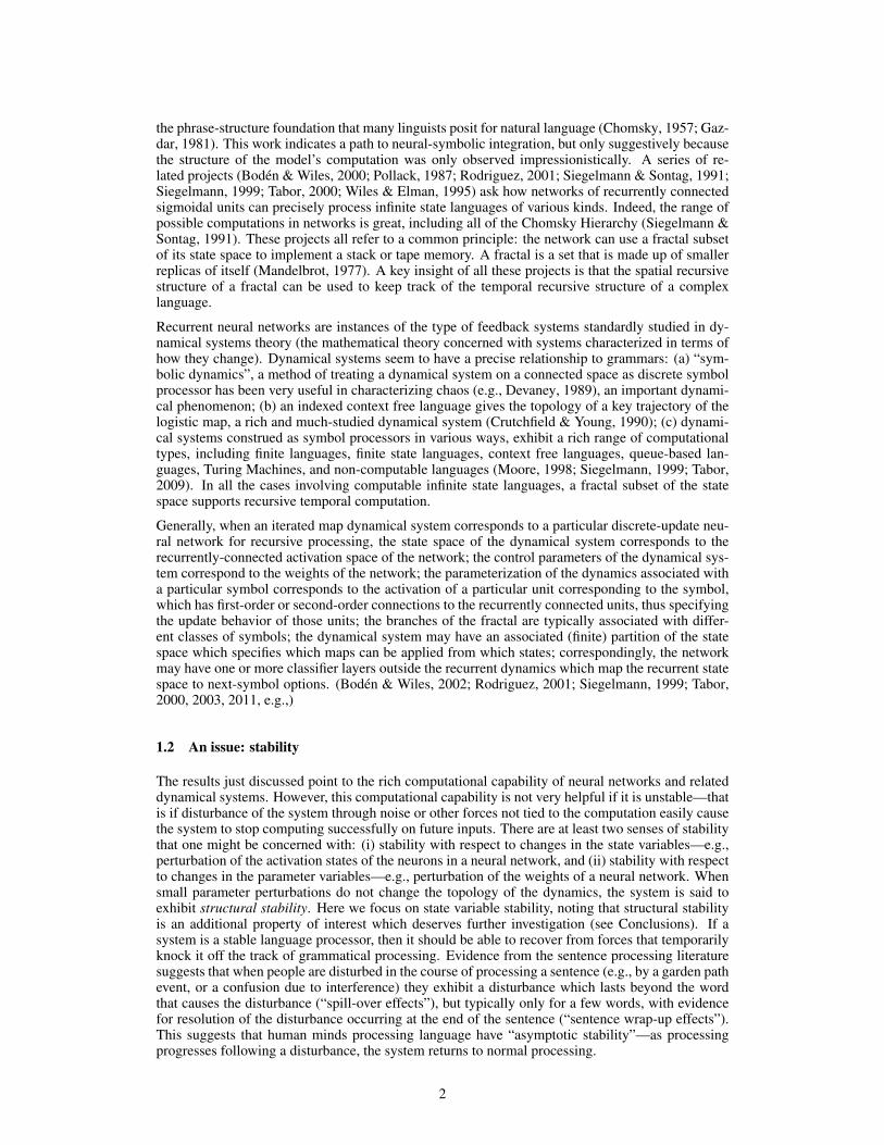
the phrase-structure foundation that many linguists posit for natural language (Chomsky, 1957; Gaz-dar, 1981). This work indicates a path to neural-symbolic integration, but only suggestively becausethe structure of the model’s computation was only observed impressionistically. A series of re-lated projects (Boden & Wiles, 2000; Pollack, 1987; Rodriguez, 2001; Siegelmann & Sontag, 1991;Siegelmann, 1999; Tabor, 2000; Wiles & Elman, 1995) ask how networks of recurrently connectedsigmoidal units can precisely process infinite state languages of various kinds. Indeed, the range ofpossible computations in networks is great, including all of the Chomsky Hierarchy (Siegelmann &Sontag, 1991). These projects all refer to a common principle: the network can use a fractal subsetof its state space to implement a stack or tape memory. A fractal is a set that is made up of smallerreplicas of itself (Mandelbrot, 1977). A key insight of all these projects is that the spatial recursivestructure of a fractal can be used to keep track of the temporal recursive structure of a complexlanguage.
Recurrent neural networks are instances of the type of feedback systems standardly studied in dy-namical systems theory (the mathematical theory concerned with systems characterized in terms ofhow they change). Dynamical systems seem to have a precise relationship to grammars: (a) “sym-bolic dynamics”, a method of treating a dynamical system on a connected space as discrete symbolprocessor has been very useful in characterizing chaos (e.g., Devaney, 1989), an important dynami-cal phenomenon; (b) an indexed context free language gives the topology of a key trajectory of thelogistic map, a rich and much-studied dynamical system (Crutchfield & Young, 1990); (c) dynami-cal systems construed as symbol processors in various ways, exhibit a rich range of computationaltypes, including finite languages, finite state languages, context free languages, queue-based lan-guages, Turing Machines, and non-computable languages (Moore, 1998; Siegelmann, 1999; Tabor,2009). In all the cases involving computable infinite state languages, a fractal subset of the statespace supports recursive temporal computation.
Generally, when an iterated map dynamical system corresponds to a particular discrete-update neu-ral network for recursive processing, the state space of the dynamical system corresponds to therecurrently-connected activation space of the network; the control parameters of the dynamical sys-tem correspond to the weights of the network; the parameterization of the dynamics associated witha particular symbol corresponds to the activation of a particular unit corresponding to the symbol,which has first-order or second-order connections to the recurrently connected units, thus specifyingthe update behavior of those units; the branches of the fractal are typically associated with differ-ent classes of symbols; the dynamical system may have an associated (finite) partition of the statespace which specifies which maps can be applied from which states; correspondingly, the networkmay have one or more classifier layers outside the recurrent dynamics which map the recurrent statespace to next-symbol options. (Boden & Wiles, 2002; Rodriguez, 2001; Siegelmann, 1999; Tabor,2000, 2003, 2011, e.g.,)
1.2 An issue: stability
The results just discussed point to the rich computational capability of neural networks and relateddynamical systems. However, this computational capability is not very helpful if it is unstable—thatis if disturbance of the system through noise or other forces not tied to the computation easily causethe system to stop computing successfully on future inputs. There are at least two senses of stabilitythat one might be concerned with: (i) stability with respect to changes in the state variables—e.g.,perturbation of the activation states of the neurons in a neural network, and (ii) stability with respectto changes in the parameter variables—e.g., perturbation of the weights of a neural network. Whensmall parameter perturbations do not change the topology of the dynamics, the system is said toexhibit structural stability. Here we focus on state variable stability, noting that structural stabilityis an additional property of interest which deserves further investigation (see Conclusions). If asystem is a stable language processor, then it should be able to recover from forces that temporarilyknock it off the track of grammatical processing. Evidence from the sentence processing literaturesuggests that when people are disturbed in the course of processing a sentence (e.g., by a garden pathevent, or a confusion due to interference) they exhibit a disturbance which lasts beyond the wordthat causes the disturbance (“spill-over effects”), but typically only for a few words, with evidencefor resolution of the disturbance occurring at the end of the sentence (“sentence wrap-up effects”).This suggests that human minds processing language have “asymptotic stability”—as processingprogresses following a disturbance, the system returns to normal processing.
2

Motivated by these observations, we establish, in the next section, a definition of stability forsymbol-driven dynamical automata.
2 Back in Kansas Stability
In classical formal grammar theory, languages are sets of finite-length strings. In the present work,we consider languages to be sets of one-sided infinite length strings. This simplifies the formalism.We can assign each language on the Chomsky Hierarchy a place in this framework by consider-ing, for language L, the set of all one-sided infinite concatenations of strings from L, which wedenote L
1, thinking of this as a model of all the sentences that a speaker hears and/or produces insuccession in their lifetime.
Def. An iterated function system (Barnsley, [1988]1993; Hutchinson, 1981) is a (finite) set of func-tions IFS = {f1, . . . , fk} that map from a space X to itself. We assume that X is a completemetric space with metric d.
Def. A one-sided-infinite-string language, L, is a set of one-sided infinite strings drawn from a finitealphabet, ⌃ = {1, . . . , k}. We assume that for every member j of ⌃, there is some string of L whichcontains k.
For x 2 X , and S = �1�2 . . .�N
a finite string of symbols drawn from ⌃, we use the notationIFS
S
(x) to denote the function f
�1(f�2(. . . (f�N (x)) . . .)).
Def. Consider a point x(0) in X . The labeling, Labx(0), of IFS driven by L is a function from
points in X to the power set of ⌃, such that j 2 Lab
x(0)(x) iff there is a finite initial substring, S,of some string in L such that IFS
S
(x(0)) = x and the string formed by adding j to the end of S isalso an initial substring of some string in L.
Def. Lab
x(0) is said to process a symbol j at a point x iff j 2 Lab
x(0)(x) and the system moves fromx to f
j
(x). A labelling Lab
x(0) under IFS is said to process a string S iff starting at x(0), everysymbol of S is processed in sequence. The language of Lab
x(0) under IFS is the set of one-sidedinfinite strings processed by Lab
x(0) under IFS. We say that an IFS � L systems is on Lab
x(0)when it visits a point x if all continuations of the current string under L are processed by Lab
x(0).
Def. Consider x 2 X and j 2 ⌃. The distance d((x, j), Labx(0)) from the ordered pair (x, j) to the
labeling, Labx(0), is inf{d(x, y)) : y 2 X and j 2 Lab
x(0)(y)}.
In other words, assuming a standard (infimum-based) definition of point-set distance, the distance ofa point-symbol ordered pair, (x, j), to a labeling is the distance from x to the set of points at whichj can come next under the labelling.
Def. A sequence of ordered point-symbol pairs (x(n),�n
) for n = {0, 1, 2, . . .} is said toconverge to a labeling Lab
x(0) if, for every ✏, there exists N such that M > N impliesd((x(M),�
M
), Labx(0)) < ✏.
Def. Consider an IFS on a complete metric space X with functions ⌃ = {1, . . . , k} and a one-sided infinite string language L on ⌃. For initial state, x(0), consider the labeling Lab
x(0) inducedby L. Consider the sequence of point-symbol pairs PSP
S
= {(x(n),�n
), n = 0, 1, . . .} inducedby a member, S = �1�2 . . ., of L (i.e., x((n + 1)) = f
�n(x(n)) for all n). If, when the system isperturbed within a radius � of x(n) for any (x(n),�
n
) 2 PSP
S
and then driven henceforth by theremaining symbols of S, it converges to Lab
x(0), then it is said to exhibit Back in Kansas Stabilityfrom x(0) when driven by S. If there is a � such that all futures from x(0) converge when perturbedonce within �, then the system is said to exhibit Back In Kansas stability from x(0). We say, in sucha case, that points of Lab
x(0) with nonempty labeling, along with their labels, are an attractor ofthe IFS-L.
The idea of Back in Kansas Stability is that the system is expected to recover its rhythm, not underthe influence of some external signal, but rather simply through exposure to sufficient material fromthe familiar language. We adopt this approach because, as noted above, studies of sentence process-ing provide evidence that recovery from disturbance in sentence processing often takes place acrossmultiple words and seems to involve a convergence process.
3

3 Lack of Back in Kansas Stability in existing fractal models
We next offer some demonstrations that existing fractal computers lack Back in Kansas Stability.As noted above, Moore (1998) describes a one-dimensional dynamical automaton that implementsa stack memory for recognizing context free languages. For a stack alphabet of k symbols, Moore’ssystem uses a Cantor-set with k � 1 gaps between the fractal branches. Pushing and popping areaccomplished by
push
i
(x) = ↵x+ (1� ↵) i
k
pop
i
(x) = push
i
�1(x)(1)
where 1 i k is the symbol being pushed or popped and 0 < ↵ <
12k+1 is a constant, and x(0) =
1. This system has the property that grammatical processing is restricted to the interval [0, 1], butan erroneous stack operation (e.g., pop
j
(pushi
(x)) where j 6= i) results in |x| > 1 (Moore’s systemuses this property to detect ungrammatical transitions). Because push and pop are inverses acrossthe entire state space and grammatical processing (to empty stack) implements a corresponding popfor every push, the displacement created by any error persists no matter how many grammaticalsentences follow the error (hence the system does not have Back in Kansas Stability). For example,if one implements S ! ✏, S ! 1 S 2, S ! 3 S 4 with a two-symbol stack alphabet, choosing↵ = 1
7 <
12·2+1 , then the once-erroneous sequence 13121212 . . . results in an endless cycle between
-2 and 0.1429—that is, the system never returns to Lab
x(0), and, the magnitude of the distancebetween the state and Lab
x(0) endlessly visits a positive constant.
Similarly, Tabor (2000) describes a fractal grammar which processes the non-finite-state context freelanguage, S ! A B C D, A ! a (S), B ! b (S), C ! c (S), D ! d (S). The model’s state space isR
2 with initial state (1/2, 1/2) and the IFS is given by
f
a
(x) = x
2 +�1/2
0
�
f
b
(x) = x� �1/20
�
f
c
(x) = x+� 01/2
�
f
d
(x) = 2⇣x� � 0
1/2
�⌘(2)
The points with nonempty labels in Lab
x(0) form a ”Sierpinski Gasket”, a kind of two-dimensionalCantor Set. In this system, as in Moore’s, all the functions are affine, and the map f
d
�fc
�fb
�fa
(x)is identity across the whole state space. Since the language always completes every abcd sequencethat is begun, this system, like Moore’s, repeatedly revisits the magnitude of any displacement fromLab
x(0), independently of the value of x(0).
These systems have a form of stability generally recognized in dynamical systems theory—thereis a bound on how far the system travels away from the invariant set of interest—but they lack theasymptotic stability that seems to characterize human behavior. The lack of asymptotic stabilityis related to the fact that transitions from empty stack to empty stack implement identity acrossthe state space. But identity is only required for grammatical processing, which, in these cases, isrestricted to a proper subset of the state space. It will not disturb grammatical processing to modifythe map in locations away from this manifold. In the next section, we show, for an important classof languages, a simple way of modifying the off-manifold maps, so that the system gets back ontothe manifold when it has been knocked off, provided it receives exposure to enough grammaticalmaterial following perturbation.
4 The Simplest Context Free Language, 1n2n
We begin with the simplest context free language, 1n2n, and then generalize to all mirror recursionlanguages, L
mirror-, of the form, S ! ✏, S ! �11 S �12, S ! �21 S �22, . . . , S ! �
1 S �
2.Mirror recursion seems to capture the gist of center-embedding structures in languages around the
4

world. Corballis (2007) argues that mirror recursion is the crucial recursive behavior that distin-guishes human languages from animal languages. Although it is true that no human language ex-hibits center embedding easily beyond one center-embedded clause, the degradation, as one testssuccessively deeper levels of embedding appears to be graceful (Lewis, 1996), and Christiansen &Chater (1999) argue that a Simple Recurrent Network captures this quality of the human languagecase well. Moreover, Rodriguez (2001) and Tabor et al. (2013) provide evidence that Simple Re-current Networks trained on center-embedded material are approximating fractal grammars. Theseobservations motivate focusing on the mirror recursion case in the effort to understand how fractalgrammars can be stable.
Let L1n2n be the one-sided-infinite-string language, {1n2n}1. Let X = [�2, 2] and let IFS1-d begiven by
f1(x) = x
2 + 1f2(x) = 2x+ 2 x < �1
0 �1 x < 1�2x+ 2 1 x
(3)
Note that the 2-map is not affine but approximately quadratic. Figure 1 shows the IFS alongwith Lab0 and illustrates recovery from a perturbation. In fact, this system always recovers fromperturbation.
Figure 1: Cobweb diagram of IFS1�d
driven by L1n2n from x(0) = 0. The numbers incurly brackets show some of the nonempty state labels. All points in the complement of A ={. . . ,� 7
4 ,� 32 ,�1, 0, 1, 3
2 ,74 , . . .} have empty label. The dotted line shows a perturbed trajectory
which recovers. After processing a single 1 (x(1) = 1), the IFS was perturbed to 1.15. Subsequentlyit encountered the completion of the perturbed sentence (“. . . 1 2 2”), followed by a single completesentence (“1 1 2 2”), by which point it was at 0 and back on the attractor.
Thm 1. The system IFS1-d-L1n2n processes L1n2n from x(0) = 0 and is Back in Kansas stablefrom that point.
The proof (see Appendix 1) first demonstrates that the language L1n2n is processed by IFS1-d fromx(0) = 0. Then it shows that, starting from any point in the state space, if the system receivesthe tail of any string from {1n2n}1, it will be back on Lab0 within two sentences (“finite-time”convergence). This is a much stronger outcome than is required for Back in Kansas stability. Therapid convergence stems from fact that the horizontal section of the 2-map resets the system whenit lands between -1 and 1. We have adopted a broad definition here, allowing also non-finite-timeconvergence, because simulation experiments which we will not discuss further here suggest that
5

similar convergence behavior occurs in systems with a single maximum, rather than a plateau, exceptthat the convergence takes infinite time.
5 General Mirror Recursion
For 2 symbols, let x(0) be the origin in R
+1. Define IFS(+1)-d for = 1, 2, . . . , i 2 {1, . . . ,}by
�1 < x1 < �1 �1 x1 < 1 1 x1 < 1
f
i
(x) =
0
BBBBBBBB@
x1/2 + 1x2/2. . .
x
i
/2x
i+1/2� 1x
i+2/2. . .
x(+ 1)/2
1
CCCCCCCCA
f
i
(x) =
0
BBBBBBBB@
x1/2 + 10
. . .
0�10
. . .
0
1
CCCCCCCCA
f
i
(x) =
0
BBBBBBBB@
x1/2 + 1x2/2. . .
x
i
/2x
i+1/2� 1x
i+2/2. . .
x(+ 1)/2
1
CCCCCCCCA
f2i(x) =
0
BBBBBBBB@
2x1 + 22x2
. . .
2xi
2xi+1 + 22x
i+2
. . .
2x(+ 1)
1
CCCCCCCCA
f2i(x) = 0
f2i(x) =
0
BBBBBBBB@
�2x1 + 22x2
. . .
2xi
2xi+1 + 22x
i+2
. . .
2x(+ 1)
1
CCCCCCCCA
Here, the -1 in the state change from the middle region for fi
(x) is on dimension i+ 1.
Thm 2. Each system in the class {IFS(+1)-d-LMirror-} for 2 {1, 2, . . .} is Back in Kansasstable from x(0) = O, the origin in R
+1.
Appendix 2 sketches the proof of Theorem 2.
6 Conclusions
This paper has defined Back in Kansas Stability for nonautonomous dynamical systems, consistingof functions f1, . . . , fk : X ! X on a complete metric space, driven by a language L on ⌃ ={1, 2, . . . , k}. The definition was motivated by the fact that people who undergo a disturbancewhen processing complex natural language structures seem to recover naturally during the course ofprocessing additional words. This idea makes a prediction that many other parsing models—thosethat tie parsing strictly to the information content of received words—do not make: recovery froma garden path might be helped by words following the disambiguating word even if these wordsprovide no additional structural information; some evidence in support of this idea comes fromcertain types of length effects in sentence processing where long disambiguating regions are easierthan short ones—see Tabor & Hutchins (2004).
Another motivation came from the fact that stability is an important organizing principle of dynam-ical systems broadly, so when working with neural network dynamical systems, it is desirable tocharacterize their stability. The mirror recursion finding prompts a more specific observation: in thecase of iterated maps, the well-known attractors of autonomous dynamical systems are distinguishedby their cardinalities—a fixed point is a single point, a limit cycle contains a finite number of points,a chaotic attractor has uncountably many points. The case of mirror recursion with Back in KansasStability fills in this picture by identifying countably infinite attractive sets. It may be informativeto ask what conditions support countably infinite attractors and why they are not prominent in thestudy of autonomous dynamical systems.
6
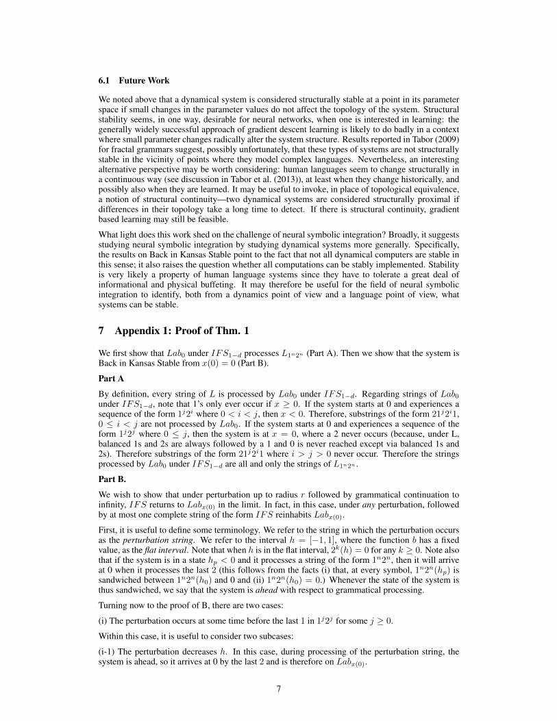
6.1 Future Work
We noted above that a dynamical system is considered structurally stable at a point in its parameterspace if small changes in the parameter values do not affect the topology of the system. Structuralstability seems, in one way, desirable for neural networks, when one is interested in learning: thegenerally widely successful approach of gradient descent learning is likely to do badly in a contextwhere small parameter changes radically alter the system structure. Results reported in Tabor (2009)for fractal grammars suggest, possibly unfortunately, that these types of systems are not structurallystable in the vicinity of points where they model complex languages. Nevertheless, an interestingalternative perspective may be worth considering: human languages seem to change structurally ina continuous way (see discussion in Tabor et al. (2013)), at least when they change historically, andpossibly also when they are learned. It may be useful to invoke, in place of topological equivalence,a notion of structural continuity—two dynamical systems are considered structurally proximal ifdifferences in their topology take a long time to detect. If there is structural continuity, gradientbased learning may still be feasible.
What light does this work shed on the challenge of neural symbolic integration? Broadly, it suggestsstudying neural symbolic integration by studying dynamical systems more generally. Specifically,the results on Back in Kansas Stable point to the fact that not all dynamical computers are stable inthis sense; it also raises the question whether all computations can be stably implemented. Stabilityis very likely a property of human language systems since they have to tolerate a great deal ofinformational and physical buffeting. It may therefore be useful for the field of neural symbolicintegration to identify, both from a dynamics point of view and a language point of view, whatsystems can be stable.
7 Appendix 1: Proof of Thm. 1
We first show that Lab0 under IFS1�d
processes L1n2n (Part A). Then we show that the system isBack in Kansas Stable from x(0) = 0 (Part B).
Part A
By definition, every string of L is processed by Lab0 under IFS1�d
. Regarding strings of Lab0under IFS1�d
, note that 1’s only ever occur if x � 0. If the system starts at 0 and experiences asequence of the form 1j2i where 0 < i < j, then x < 0. Therefore, substrings of the form 21j2i1,0 i < j are not processed by Lab0. If the system starts at 0 and experiences a sequence of theform 1j2j where 0 j, then the system is at x = 0, where a 2 never occurs (because, under L,balanced 1s and 2s are always followed by a 1 and 0 is never reached except via balanced 1s and2s). Therefore substrings of the form 21j2i1 where i > j > 0 never occur. Therefore the stringsprocessed by Lab0 under IFS1�d
are all and only the strings of L1n2n .
Part B.
We wish to show that under perturbation up to radius r followed by grammatical continuation toinfinity, IFS returns to Lab
x(0) in the limit. In fact, in this case, under any perturbation, followedby at most one complete string of the form IFS reinhabits Lab
x(0).
First, it is useful to define some terminology. We refer to the string in which the perturbation occursas the perturbation string. We refer to the interval h = [�1, 1], where the function b has a fixedvalue, as the flat interval. Note that when h is in the flat interval, 2k(h) = 0 for any k � 0. Note alsothat if the system is in a state h
p
< 0 and it processes a string of the form 1n2n, then it will arriveat 0 when it processes the last 2 (this follows from the facts (i) that, at every symbol, 1n2n(h
p
) issandwiched between 1n2n(h0) and 0 and (ii) 1n2n(h0) = 0.) Whenever the state of the system isthus sandwiched, we say that the system is ahead with respect to grammatical processing.
Turning now to the proof of B, there are two cases:
(i) The perturbation occurs at some time before the last 1 in 1j2j for some j � 0.
Within this case, it is useful to consider two subcases:
(i-1) The perturbation decreases h. In this case, during processing of the perturbation string, thesystem is ahead, so it arrives at 0 by the last 2 and is therefore on Lab
x(0).
7
(i-2) The perturbation increases h. In this case, the system is in [-2, -1] at the end of the string.Therefore, the system is ahead during the processing of the subsequent string. Consequently, itreaches Lab
x(0) by the end of the post-perturbation string.
(ii) The perturbation occurs after the last 1 and before the last 2 in 1j2j for some j � 0.
Again, we consider two cases:
(ii-1) The perturbation decreases h. In this case, the system is still in [-2, -1] at the end of the stringand the future states follow the pattern of (i-2) above.
(ii-2) The perturbation increases h. If, after the increase, h < �1, then the remaining 2’s bring thesystem to the flat interval and the case is like (i-1) above. If, after the increase, �1 h 1, then theremaining 2’s keep the system at 0 and the system is on the attractor at the start of the next string. If,after the increase, h > 1, then the system is in [-2, -1] at the end of the string and the future follows(i-2) above.
Thus, in all cases, the system returns to Lab
x(0) at least by the end of the post-perturbation string.
8 Appendix 2: Sketch of Proof of Thm. 2
The proof of this theorem builds on the proof of Theorem 1. The system behaves on the first di-mension as if the string were 1n2n with all the push symbols invoking 1 and all the pop symbolsinvoking 2, following the same dynamics as in the 1-dimensional case above. Whenever the systemis in the flat region of the pop maps and in the second half of a sentence, dimension 1 becomes 0 andstays there until the end of the sentence. Then, the start of the new sentence resets all the dimensionsto the appropriate values so the effect of perturbation on any dimension is removed. By Thm. 1, thiswill always happen within two sentences of a perturbation.
Furthermore, when the system, initialized to x(0) = 0, is unperturbed, f2i(x) � f
i
(x) implementsidentity for visited points, x and every stack state corresponds to a distinct point in X because thepush maps on X form a just-touching fractal (Barnsley, [1988]1993) so the unperturbed system ink + 1 dimensions processes L
Mirror�k
.
Acknowledgments
Thanks to Harry Dankowicz and Garrett Smith for comments on an earlier version of this work. Wegratefully acknowledge support from NSF PAC grant 1059662 and NSF INSPIRE 1246920.
References
Barnsley, M. ([1988]1993). Fractals everywhere, 2nd ed. Boston: Academic Press.Boden, M., & Wiles, J. (2000). Context-free and context sensitive dynamics in recurrent neural
networks. Connection Science, 12(3), 197–210.Boden, M., & Wiles, J. (2002). On learning context-free and context-sensitive languages. IEEE
Transactions on Neural Networks, 13(2), 491–493.Chomsky, N. (1957). Syntactic structures. The Hague: Mouton and Co.Christiansen, M. H., & Chater, N. (1999). Toward a connectionist model of recursion in human
linguistic performance. Cognitive Science, 23, 157–205.Corballis, M. C. (2007). Recursion, language, and starlings. Cognitive Science, 31, 697–704.Crutchfield, J. P., & Young, K. (1990). Computation at the onset of chaos. In W. H. Zurek (Ed.),
Complexity, entropy, and the physics of information (pp. 223–70). Redwood City, California:Addison-Wesley.
Devaney, R. L. (1989). An introduction to chaotic dynamical systems, 2nd ed. Redwood City, CA:Addison-Wesley.
Elman, J. L. (1991). Distributed representations, simple recurrent networks, and grammatical struc-ture. Machine Learning, 7, 195–225.
8
Gazdar, G. (1981). On syntactic categories. Philosophical Transactions (Series B) of the RoyalSociety, 295, 267-83.
Hutchinson, J. E. (1981). Fractals and self similarity. Indiana University Mathematics Journal,30(5), 713-747.
Lewis, R. (1996). Interference in short-term memory: The magical number two (or three) in sentenceprocessing. Journal of Psycholinguistic Research, 25(1).
Mandelbrot, B. (1977). Fractals, form, chance, and dimension. San Francisco: Freeman.Moore, C. (1998). Dynamical recognizers: Real-time language recognition by analog computers.
Theoretical Computer Science, 201, 99–136.Pollack, J. (1987). On connectionist models of natural language processing. (Unpublished doctoral
dissertation, University of Illinois.)Rodriguez, P. (2001). Simple recurrent networks learn context-free and context-sensitive languages
by counting. Neural Computation, 13(9), 2093-2118.Siegelmann, H. T. (1999). Neural networks and analog computation: Beyond the turing limit.
Boston: Birkhauser.Siegelmann, H. T., & Sontag, E. D. (1991). Turing computability with neural nets. Applied Mathe-
matics Letters, 4(6), 77-80.Tabor, W. (2000). Fractal encoding of context-free grammars in connectionist networks. Expert
Systems: The International Journal of Knowledge Engineering and Neural Networks, 17(1), 41-56.
Tabor, W. (2002). The value of symbolic computation. Ecological Psychology, 14(1/2), 21–52.Tabor, W. (2003). Learning exponential state growth languages by hill climbing. IEEE Transactions
on Neural Networks, 14(2), 444-446.Tabor, W. (2009). A dynamical systems perspective on the relationship between symbolic and
non-symbolic computation. Cognitive Neurodynamics, 3(4), 415-427.Tabor, W. (2011). Recursion and recursion-like structure in ensembles of neural elements. In
H. Sayama, A. Minai, D. Braha, & Y. Bar-Yam (Eds.), Unifying themes in complex systems. pro-ceedings of the viii international conference on complex systems (p. 1494-1508). Cambridge, MA:New England Complex Systems Institute. (http//necsi.edu/events/iccs2011/proceedings.html)
Tabor, W., Cho, P. W., & Szkudlarek, E. (2013). Fractal analysis illuminates the form of connec-tionist structural gradualness. Topics in Cognitive Science, 5, 634–667.
Tabor, W., & Hutchins, S. (2004). Evidence for self-organized sentence processing: Digging ineffects. Journal of Experimental Psychology: Learning, Memory, and Cognition, 30(2), 431-450.
Wiles, J., & Elman, J. (1995). Landscapes in recurrent networks. In J. D. Moore & J. F. Lehman(Eds.), Proceedings of the 17th annual cognitive science conference. Lawrence Erlbaum Asso-ciates.
9

Analogy Making and Logical Inference on Imagesusing Cellular Automata based Hyperdimensional
Computing
Ozgur Yilmaz⇤Department of Computer Engineering
Turgut Ozal UniversityAnkara Turkey
Abstract
In this paper, we introduce a framework of reservoir computing that is capableof both connectionist machine intelligence and symbolic computation. Cellularautomaton is used as the reservoir of dynamical systems. A cellular automaton isa very sparsely connected network with logical nodes and nonlinear/logical con-nection functions, hence the proposed system corresponds to a binary valued andnonlinear neuro-symbolic architecture. Input is randomly projected onto the ini-tial conditions of automaton cells and nonlinear computation is performed on theinput via application of a rule in the automaton for a period of time. The evolutionof the automaton creates a space-time volume of the automaton state space, andit is used as the reservoir. In addition to being used as the feature representationfor pattern recognition, binary reservoir vectors can be combined using Booleanoperations as in hyperdimensional computing, paving a direct way symbolic pro-cessing. To demonstrate the capability of the proposed system, we make analogiesdirectly on image data by asking ’What is the Automobile of Air’?, and make log-ical inference using rules by asking ’Which object is the largest?’
1 Introduction
We have introduced a holistic intelligence framework capable of simultaneous pattern recognitionYilmaz (2015b) and symbolic computation Yilmaz (2015a,c). Cellular automaton is the main com-putational block that holds a distributed representation of high order input attribute statistics as inneural architectures (Figure 1 b). The proposed architecture is a cross fertilization of cellular au-tomata, reservoir computing and hyperdimensional computing frameworks (Figure 1 a). The cellularautomata (CA) computation can be viewed as a feedforward network with logical nodes and con-nections, as shown in Figure 1 c. In this paper, we analyze the symbolic computation capability ofthe system on making analogies and rule based logical inferences, directly on the image data. Theresults show that (Figure 2), binary vector representation of images derived through CA evolutionprovide very precise analogies and accurate rule based inference, even though very small number ofexamples are provided. In the next subsection we review cellular automata 1, then introduce relevantneuro-symbolic computation studies. Finally, we state our contribution.
⇤Web: ozguryilmazresearch.net1The literature review is narrowed down in this paper due to space considerations. Please visit our pub-
lished papers to get a wider view of our architecture among existing reservoir and hyperdimensional computingapproaches.
1

Reservoir Computing
CellularAutomata
Hyperdimensional Computing
a
Input
Win
Output
Wout
CA Rule
Cellular Automata Reservoir
time
b
12
34
5
31
42
5
42
15
3
A0
. . .
A1 A2 A3
c
Figure 1: a. Our work is a cross fertilization of cellular automata, reservoir computing and hyperdi-mensional computing frameworks. b. In cellular automata reservoir, data is projected onto cellularautomaton instead of a real valued node as in classical neural networks. c. The network formed bythe cellular automaton feature space of rule 90. It can be viewed as a time unrolled feedforwardnetwork, however the connections are not all-to-all between layers due to partitioning of differentpermutations, given as separate rows. And the connections are not algebraic but logical, i.e. XORoperation. See Yilmaz (2015b) for details.
1.1 Cellular Automata
Cellular automaton is a discrete computational model consisting of a regular grid of cells, each in oneof a finite number of states (Figure 1 c). The state of an individual cell evolves in time according toa fixed rule, depending on the current state and the state of its neighbors. The information presentedas the initial states of a grid of cells is processed in the state transitions of cellular automaton andcomputation is typically very local. Essentially, a cellular automaton is a very sparsely connectednetwork with logical nodes and nonlinear/logical connection functions (Figure 1 c). Some of thecellular automata rules are proven to be computationally universal, capable of simulating a Turingmachine (Cook, 2004).
The rules of cellular automata are classified according to their behavior: attractor, oscillating,chaotic, and edge of chaos (Wolfram, 2002). Turing complete rules are generally associated with thelast class (rule 110, Conway game of life). Lyapunov exponent of a cellular automaton can be com-puted and it is shown to be a good indicator of the computational power of the automata (Baetens &De Baets, 2010). A spectrum of Lyapunov exponent values can be achieved using different cellularautomata rules. Therefore, a dynamical system with specific memory capacity (i.e. Lyapunov expo-nent value) can be constructed by using a corresponding cellular automaton. The time evolution ofthe cellular automata has very rich computational representation Mitchell et al. (1996), especially forthe edge of chaos dynamics. The proposed algorithm in this paper exploits the entire time evolutionof the CA and uses the states as the reservoir LukosEvicIus & Jaeger (2009); Maass et al. (2002) ofnonlinear computation.
1.2 Symbolic Computation on Neural Representations
Uniting the expressive power of mathematical logic and pattern recognition capability of distributedrepresentations (eg. neural networks) has been an open question for decades although several suc-cessful theories have been proposed (Garcez et al., 2012; Bader et al., 2008; Marcus, 2003; Mi-ikkulainen et al., 2006; Besold et al., 2014; Pollack, 1990). The difficulty arises due to the very
2

different mathematical nature of logical reasoning and dynamical systems theory. Along with manyother researchers, we conjecture that combining connectionist and symbolic processing requirescommonalizing the representation of data and knowledge.
Along the same vein, (Kanerva, 2009) introduced hyperdimensional computing that utilizes high-dimensional random binary vectors for representing objects, predicates and rules for symbolic ma-nipulation and inference. The general family of the methods is called ’reduced representations’ or’vector symbolic architectures’, and detailed introductions can be found in (Plate, 2003; Levy &Gayler, 2008). In this approach, high dimensionality and randomness enable binding and groupingoperations that are essential for one shot learning, analogy-making, hierarchical concept buildingand rule based logical inference. Most recently (Gallant & Okaywe, 2013) introduced random ma-trices to this context and extended the binding and quoting operations. The two basic mathematicaltools of reduced representations are vector addition and XOR.
In this paper, we borrow these tools of hyperdimensional computing framework, and build a se-mantically more meaningful representation by removing the randomness and replacing it with thecellular automata computation. This provides not only a more expressive symbolic computationarchitecture, but also enables pattern recognition capabilities otherwise not possible with randomvectors.
1.3 Contributions
We provide a low computational complexity method Yilmaz (2015b) for recurrent computation us-ing cellular automata based hyperdimensional computing. It is shown that the framework has a greatpotential for symbolic processing such that the cellular automata feature space can directly be com-bined by Boolean operations as in hyperdimensional computing, hence they can represent conceptsand form a hierarchy of semantic interpretations. We demonstrate this capability by making analo-gies directly on images and infer relationships using logical rules. In the next section, we give thedetails of the algorithm, and then provide results experiments that demonstrate our contributions.
2 Cellular Automata Feature Expansion
In our reservoir computing method, data are passed on a cellular automaton instead of an echostate network and the nonlinear dynamics of cellular automaton provide the necessary projectionof the input data onto an expressive and discriminative space. Compared to classical neuron-basedreservoir computing, the reservoir design is trivial: cellular automaton rule selection. Utilization ofedge of chaos automaton rules ensures Turing-complete computation in the reservoir, which is notguaranteed in classical reservoir computing approaches.
The reservoir computing system receives the input data. First, the encoding stage translates theinput into the initial states of a 1D elementary cellular automaton. For binary input data, eachfeature dimension can randomly be mapped onto the cells of the cellular automaton. For this typeof mapping, the size of the CA should follow the input data’s feature dimension. After encoding,suppose that the cellular automaton is initialized with the vector A0
P1 , in which P1 correspondsto a random permutation of raw input data. Then, cellular automata evolution is computed using aprespecified rule, Z (1D elementary CA rule), for a fixed period of iterations (I):
A1P1 = Z(A0
P1),
A2P1 = Z(A1
P1),
...
AI
P1 = Z(AI�1
P1).
The evolution of the cellular automaton is recorded such that, at each time step a snapshot of thewhole states in the cellular automaton is vectorized and concatenated. Therfore, we concatenate theevolution of cellular automata to obtain a reservoir for a single permutation:
AP1 = [A0P1 ;A1
P1 ;A2P1 ; ...A
I
P1 ]
It is experimentally observed that multiple random permutation mappings significantly improve ac-curacy. There are R number of different random mappings, i.e., separate CA reservoirs, and they
3

are combined into a large reservoir feature vector:
AR = [AP1 ;AP2 ;AP3 ; ...APR ].
The computation in CA takes place when cell activities due to nonzero initial values (i.e., input)mix and interact. Both prolonged evolution duration (large I) and existence of different randommappings (large R) increase the probability of long-range interactions, hence improve computationalpower and enhance representation.
3 Symbolic Processing and Non-Random Hyperdimensional Computing
Hyperdimensional computing uses random very large-sized binary vectors to represent objects, con-cepts, and predicates. Then, appropriate binding and grouping operations are used to manipulate thevectors for hierarchical concept building, analogy-making, learning from a single example, etc., thatare hallmarks of symbolic computation. The large size of the vector provides a vast space of randomvectors, two of which are always nearly orthogonal. Yet, the code is robust against a distortion inthe vector due to noise or imperfection in storage because after distortion it will still stay closer tothe original vector than the other random vectors.
The grouping operation is normalized vector summation, and it enables forming sets of ob-jects/concepts. Suppose we want to group two binary vectors, V1 and V2. We compute their element-wise sums, and the resultant vector contains 0, 1 and 2 entries. We normalize the vector by acceptingthe 0 entries as they are, transforming 2 entries into 1. Note that, these are consistent within the twoinitial vectors. Then, the inconsistent entries are randomly decided: 1 entries as transformed into 0or 1. Many vectors can be combined iteratively or in a batch to form a grouped representation of thebundle. The resultant vector is similar to all the elements of the vector due to the fact that consistententries are untouched. The elements of the set can be recovered from the reduced representation byprobing with the closest item in the memory, and consecutive subtraction. Grouping is essential fordefining ’a part of’, ’contains’ relationships. + symbol will be used for normalized summation inthe following arguments.
There are two binding operations: bitwise XOR (circled plus symbol, �) and permutation 2. Bind-ing operation maps (randomizes) the vector to a completely different space, while preserving thedistances between two vectors. As stated in Kanerva (2009), ”...when a set of points is mappedby multiplying with the same vector, the distances are maintained, it is like moving a constellationof points bodily into a different (and indifferent) part of the space while maintaining the relations(distances) between them. Such mappings could play a role in high-level cognitive functions such asanalogy and the grammatical use of language where the relations between objects is more importantthan the objects themselves.
A few representative examples to demonstrate the expressive power of hyperdimensional computing:
1. We can represent pairs of objects via multiplication. OA,B
= A � B where A and B are twoobject vectors.
2. A triplet is a relationship between two objects, defined by a predicate. This can similarly beformed by T
A,P,B
= A� P �B. These types of triplet relationships are very successfully utilizedfor information extraction in large knowledge bases Dong et al. (2014).
3. A composite object can be built by binding with attribute representation and summation. For acomposite object C,
C = X �A1 + Y �A2 + Z �A3,
where A1, A2 and A3 are vectors for attributes and X , Y and Z are the values of the attributes for aspecific composite object.
4. A value of an attribute for a composite object can be substituted by multiplication. Suppose wehave assignment X�A1, then we can substitute A1 with B1 by, (X�A1)� (A1�B1) = X�B1.It is equivalent to say that A1 and B1 are analogous. This property is essential for analogy making.
2Please see Kanerva (2009) for the details of permutation operation, as a way of doing multiplication.
4

5. We can define rules of inference by binding and summation operations. Suppose we have a rulestating that ”If x is the mother of y and y is the father of z, then x is the grandmother of z” 3. Defineatomic relationships:
Mxy
= M1 �X +M2 � Y,
Fyz
= F1 � Y +M2 � Z,
Gxz
= G1 �X +G2 � Z,
then the rule is,
Rxyz
= Gxz
� (Mxy
+ Fyz
).
Given the knowledge base, ”Anna is the mother of Bill” and ”Bill is the father of Cid”, we can infergrandmother relationship by applying the rule R
xyz
:
Mab
= M1 �A+M2 �B,
Fbc
= F1 �B +M2 � C,
G0
ac
= Rxyz
� (Mab
+ Fbc
),
where vector G0
ac
is expected to be very similar to Gac
, which says ”Anna is the grandmother ofCid”. Please note that the if-then rules represented by hyperdimensional computing can only beif-and-only-if logical statements because operations used to represent the rules are symmetric.
Without losing the expressive power of classical hyperdimensional computing, we are introducingcellular automata to the framework. In our approach, we use binary cellular automata reservoirvector as the representation of objects and predicates instead of random vectors to be used for sym-bolic computation. There are two major advantages of this approach over random binary vectorgeneration:
1. Reservoir vector enables connectionist pattern recognition and statistical machine learning (asdemonstrated in Yilmaz (2015b)) while random vectors are mainly tailored for symbolic computa-tion.
2. The composition and modification of objects can be achieved in a semantically more meaningfulway. The semantic similarity of the two data instances can be preserved in the reservoir hyperdi-mensional vector representation, but there is no straightforward mechanism for this in the classicalhyperdimensional computing framework.
4 Experiments on Analogy Making
In order to demonstrate the power of enabled logical operation, we will use analogy making. Anal-ogy making is crucial for generalization of what is already learned. We tested the capability of oursymbolic system using images. The example given here follows ”What is the Dollar of Mexico?”in Kanerva (2009). However in the original example, sensory data (i.e. image) is not consideredbecause there is no straightforward way to introduce sensory data into the hyperdimensional com-puting framework. The benefit of using non-random binary vectors is obvious in this context.
We have previously shown that binarization of the hidden layer activities of a feedforward networkis not very detrimental for classification purposes Yilmaz et al. (2015). For an image, the binaryrepresentation of the first hidden layer activities holds an indicator for the existence of Gabor likecorner and edge features. In order to test the symbolic computation performance of CA features onbinarized hidden layer activities, we use CIFAR 10 dataset Krizhevsky & Hinton (2009). We usedthe first 500 training/test images and obtained single layer hidden neuron representation using thealgorithm in Coates et al. (2011) (200 number of different receptive fields, receptive fields size of 6pixels). The neural activities are binarized according to a threshold and, on average, 22 percent ofthe neurons fired with the selected threshold. After binarization of neural activities, CA features canbe computed on the binary representation as explained in section 2. We formed a separate conceptvector for each class (total 10 classes, 50 examples for each class) using binary neural representationof CIFAR training data and vector addition defined in Snaider (2012). These are the basis classconcepts extracted from the visual database.
3The example is adapted from Kanerva (2009).
5

a b
Figure 2: a. Analogy making experiment results. The feature expansion (defined as the productR⇥ I) due to cellular automata evolution is given in the x axis (log scale) and the percent correct isgiven in the y axis. b. Rule based logical inference experiment results.
We formed two new concepts called Land and Air:
Land = Animal �Horse+ V ehicle�Automobile,
Air = Animal �Bird+ V ehicle�Airplane.
In these two concepts, CA features of Horse and Bird images are used to bind with the Animalfiller, and CA features of Automobile and Airplane images are used to bind with the Vehicle filler4. Animal and Vehicle fields are represented by two random vectors 5, those with the same size asthe CA features. Multiplication is performed by xor (�) operation and vector summation is againidentical to Snaider (2012). The products, Land and Air are also CA feature vectors, and theyrepresent the merged concept of observed animals and vehicles in Land and Air respectively. Wecan ask the analogical question ”What is the Automobile of Air?”, AoA in short. The answer cansimply be given by this equality (inference):
AoA = Automobile� Land�Air.
AoA is a CA feature vector and expected to be very similar to Airplane concept vector. We tested theanalogical accuracy using unseen Automobile test images (50 in total), computing their CA featurevectors followed by AoA inference, then finding the closest concept class vector to AoA vector(max inner product). It is expected to be the Airplane class. The result of this experiment is givenin Figure 2 a 6 for various R and I combinations. The multiplication of the two defines the amountof feature expansion due to cellular automata state space. The analogy on CA features is 98 percentaccurate (for both R and I equals 128), whereas if the binary hidden layer activity is used insteadof CA features (corresponds to R and I equal to 1), the analogy is only 21 percent accurate. Thisresult clearly demonstrates the benefit of CA feature expansion for symbolic computation.
The devised analogy implicitly assumes that Automobile concept is already encoded in the conceptof Land. What if we ask ”What is the Truck of Air?”? Even though Truck images are not used inbuilding the Land concept, due to the similarity of Truck and Automobile concepts, we might stillget good analogies. The results on this second order analogy is contrasted in Table 1. Automobileand Horse (i.e. ”What is the Horse of Air?”, the answer should be Bird.) are first order analogiesand they result in comparably superior performance as expected, but second order analogy is muchhigher than chance level (i.e., 10 percent).
Please note that these analogies are performed strictly on the sensory data, i.e., images. Given an im-age, the system is able to retrieve a set of relevant images that are linked through a logical statement.
4There are 50 training images for each class. CA rule 110 is used for evolution. And mean of 20 MonteCarlo simulations is given to account for randomness in experiments
5Also 22 percent non-zero elements6These are extended results for our previous publication Yilmaz (2015a). We were unable to test for large
R and I values due to hardware limitations.
6

Automobile Horse Truck79 68 52
Table 1: Analogy-making experiment results on CIFAR 10 dataset (subset). R and I are both 32.The accuracy of the analogy is given for first (given in bold) and second order analogies. See textfor details.
A very small number of training data is used, yet we can infer conceptual relationships betweenimages surprisingly accurately. However, again it should be emphasized that this is only a singleexperiment with a very limited analogical scope, and more experiments are needed to understandthe limits of the proposed architecture.
It is possible to build much more complicated concepts using hierarchies. For example, Land andAir are types of environments and can be used as fillers in Environment field. Ontologies are helpfulto narrow down the set of required concepts for attaining a satisfactory description of the world.Other modalities such as text data are also of great interest, (see Mikolov et al. (2013); Penningtonet al. (2014) for state-of-the-art studies), as well as information fusion on multiple modalities (e.g.,Image and text).
5 Experiments on Rule Based Inference
In order to test proposed architecture’s capability for logical inference, we define a rule and form aknowledge base on image data. Then we make an inference on the knowledge base by applying therule. The inference may or may not be right, hence the symbolic system is not completely sound. 7
For demonstration of logical inference on our system, we define size relationships among differentobjects using the following rule set.Object in image X is larger than object in image Y :
Lxy
= L1 �X + L2 � Y.
Object in image X is smaller than object in image Z:
Sxz
= S1 �X + S2 � Z.
And finally, we state the largest object is in image Z:
Tz
= T1 � Z.
Then the rule is stated as ’If object in X is larger than object in Y and smaller than object in Z,largest object is in Z’. The rule vector is computed as the manipulation of object vectors usinghyperdimensional computing framework:
Rxyz
= Tz
� (Lxy
+ Sxz
).
Our knowledge base is again formed on the images of CIFAR 10 dataset. First, we use Truck,Automobile, and Airplane images (50 each) to compute X , Y and Z concept vectors (CA rule 110);then we obtain the rule vector R
xyz
as explained above utilizing the concept vectors. In a completelydifferent set of test image triplet, we make use of single Truck, Automobile, and Airplane imagesand compute their vector representation; a, b and c respectively. Knowledge base is created on theobject vectors in three test images:
Lab
= L1 � a+ L2 � b,
Sac
= F1 � a+M2 � c,
as ’object in image a is larger than object in image b, and object in image a is smaller than objectin image c’. Can we infer the largest object? When we apply the rule vector on existing knowledgebase, we get an estimate for the vector representation of the largest object:
Test
= Rxyz
� (Lab
+ Sac
).
We compute the Hamming distance of Test
to existing object vectors (i.e. a, b and c), then it ispossible to decide on the estimated largest object, i.e. closest vector to T
est
which should be vector7The completeness of the system requires a proof and it is a future work.
7

c. The average accuracy of 50 different test image triplets are shown in Figure 2 b. The chancelevel is 33 percent and it is observed that the binary neural representation (i.e., both R and I is equalto 1) is around 50 percent accurate, whereas cellular automata state space provides a 100 percentinference accuracy for a relatively small reservoir size. Please note that, similar to analogy makingexperiments logical inference is performed directly on image data and we can make object sizeinference using a very small number of example images (50).
6 Discussion
Along with the pattern recognition capabilities of cellular automata based reservoir computing Yil-maz (2015b), hyperdimensional computing framework enables symbolic processing. Due to thebinary categorical indicator nature of the representation, the rules that make up the knowledge baseand feature representation of the data that make up the statistical model live on the same space,which is essential for combining connectionist and symbolic capabilities. It is possible to makeanalogies, form hierarchies of concepts, and apply logical rules on the reservoir feature vectors 8.
To illustrate the logical query, we have shown the capability of the system to make analogies onimage data. We asked the question ”What is the Automobile of Air?” after building Land and Airconcepts based on the images of Horse, Automobile (Land), Bird and Airplane (Air). The correctanswer is Airplane and the system infers this relationship with 98 percent accuracy, with only 50training images per class. Additionally we have tested the performance of our architecture on rulebased logical inference on images. We defined an object size related rule on image data, provided aknowledge base and inferred the largest object strictly using the image features.
Neural network data embeddings (eg. Kiros et al. (2014); Mikolov et al. (2013)) are an alternativeto our approach, in which representation suitable for logical manipulation is learned from the datausing gradient descent. Although these promising approaches are showing state-of-the-art results,they are bound to suffer from the dilemma of ’no free lunch’ because the representation is data-specific. The other extreme is random embeddings adopted in hyperdimensional computing andreduced vector representation approaches. Although randomness maximizes the orthogonality ofvectors and optimizes the effective usage of the space, it does not allow statistical machine learningor semantically meaningful modifications on existing vectors. Our approach lies in the middle: itdoes not create random vectors, thus can manipulate existing vectors and use machine learning, butdo not learn the representation from the data therefore it is less prone to overfitting as well as to thedilemma of ’no free lunch’. Moreover, cellular automata reservoir is orders of magnitude faster thanneural network counterparts Yilmaz (2015b).
7 Acknowledgments
This research is supported by The Scientific and Technological Research Council of Turkey(TUBITAK) Career Grant, No: 114E554.
ReferencesBader, S., Hitzler, P., & Holldobler, S. (2008). Connectionist model generation: A first-order ap-
proach. Neurocomputing, 71, 2420–2432.Baetens, J. M., & De Baets, B. (2010). Phenomenological study of irregular cellular automata based
on lyapunov exponents and jacobians. Chaos: An Interdisciplinary Journal of Nonlinear Science,20, 033112.
Besold, T. R., Garcez, A. d., Kuhnberger, K.-U., & Stewart, T. C. (2014). Neural-symbolic networksfor cognitive capacities. Biologically Inspired Cognitive Architectures, (pp. iii–iv).
Coates, A., Ng, A. Y., & Lee, H. (2011). An analysis of single-layer networks in unsupervisedfeature learning. In International Conference on Artificial Intelligence and Statistics (pp. 215–223).
8Linear CA rules, such as rule 90 allow superposition of initial conditions. This property provides a sym-bolic system with much more powerful expressive capability Yilmaz (2015a).
8

Cook, M. (2004). Universality in elementary cellular automata. Complex Systems, 15, 1–40.Dong, X., Gabrilovich, E., Heitz, G., Horn, W., Lao, N., Murphy, K., Strohmann, T., Sun, S., &
Zhang, W. (2014). Knowledge vault: A web-scale approach to probabilistic knowledge fusion.In Proceedings of the 20th ACM SIGKDD international conference on Knowledge discovery and
data mining (pp. 601–610). ACM.Gallant, S. I., & Okaywe, T. W. (2013). Representing objects, relations, and sequences. Neural
computation, 25, 2038–2078.Garcez, A. S. d., Broda, K., & Gabbay, D. M. (2012). Neural-symbolic learning systems: founda-
tions and applications. Springer Science & Business Media.Kanerva, P. (2009). Hyperdimensional computing: An introduction to computing in distributed
representation with high-dimensional random vectors. Cognitive Computation, 1, 139–159.Kiros, R., Salakhutdinov, R., & Zemel, R. S. (2014). Unifying visual-semantic embeddings with
multimodal neural language models. arXiv preprint arXiv:1411.2539, .Krizhevsky, A., & Hinton, G. (2009). Learning multiple layers of features from tiny images. Com-
puter Science Department, University of Toronto, Tech. Rep, .Levy, S. D., & Gayler, R. (2008). Vector symbolic architectures: A new building material for artifi-
cial general intelligence. In Proceedings of the 2008 conference on Artificial General Intelligence
2008: Proceedings of the First AGI Conference (pp. 414–418). IOS Press.LukosEvicIus, M., & Jaeger, H. (2009). Reservoir computing approaches to recurrent neural net-
work training. Computer Science Review, 3, 127–149.Maass, W., Natschlager, T., & Markram, H. (2002). Real-time computing without stable states: A
new framework for neural computation based on perturbations. Neural computation, 14, 2531–2560.
Marcus, G. F. (2003). The algebraic mind: Integrating connectionism and cognitive science. MITpress.
Miikkulainen, R., Bednar, J. A., Choe, Y., & Sirosh, J. (2006). Computational maps in the visual
cortex. Springer Science & Business Media.Mikolov, T., Sutskever, I., Chen, K., Corrado, G. S., & Dean, J. (2013). Distributed representations
of words and phrases and their compositionality. In Advances in Neural Information Processing
Systems (pp. 3111–3119).Mitchell, M. et al. (1996). Computation in cellular automata: A selected review. Nonstandard
Computation, (pp. 95–140).Pennington, J., Socher, R., & Manning, C. D. (2014). Glove: Global vectors for word representation.
Proceedings of the Empiricial Methods in Natural Language Processing (EMNLP 2014), 12,1532–1543.
Plate, T. A. (2003). Holographic reduced representation: Distributed representation for cognitivestructures, .
Pollack, J. B. (1990). Recursive distributed representations. Artificial Intelligence, 46, 77–105.Snaider, J. (2012). Integer sparse distributed memory and modular composite representation, .Wolfram, S. (2002). A new kind of science volume 5. Wolfram media Champaign.Yilmaz, O. (2015a). Symbolic Computation using Cellular Automata based Hyperdimensional
Computing. Neural Computation, .Yilmaz, O. (2015b). Machine Learning using Cellular Automata based Feature Expansion and
Reservoir Computing. Journal of Cellular Automata, .Yilmaz, O. (2015c). Connectionist-Symbolic Machine Intelligence using Cellular Automata based
Reservoir-Hyperdimensional Computing. arXiv preprint arXiv:1503.00851, .Yilmaz, O., Ozsarac, I., Gunay, O., & Ozkan, H. (2015). Cognitively inspired real-time vi-
sion core. Technical Report, . Available at http://ozguryilmazresearch.net/Publications/NeuralNetworkVisionCore_YilmazEtAl2015.pdf.
9