ACL 2019

The 57th Annual Meeting of theAssociation for Computational Linguistics

Proceedings of the Student Research Workshop

July 28 - August 2, 2019Florence, Italy

c©2019 The Association for Computational Linguistics

Order copies of this and other ACL proceedings from:

Association for Computational Linguistics (ACL)209 N. Eighth StreetStroudsburg, PA 18360USATel: +1-570-476-8006Fax: +1-570-476-0860acl@aclweb.org

ISBN 978-1-950737-47-5

ii

Introduction

Welcome to the ACL 2019 Student Research Workshop! The ACL 2019 Student Research Workshop(SRW) is a forum for student researchers in computational linguistics and natural language processing.The workshop provides a unique opportunity for student participants to present their work and receivevaluable feedback from the international research community as well as from faculty mentors.

Following the tradition of the previous years’ student research workshops, we have two tracks: researchpapers and research proposals. The research paper track is a venue for Ph.D. students, Masters students,and advanced undergraduates to describe completed work or work-in-progress along with preliminaryresults. The research proposal track is offered for advanced Masters and Ph.D. students who have decidedon a thesis topic and are interested in feedback on their proposal and ideas about future directions fortheir work.

This year, the student research workshop has received a great attention, reflecting the growth of the field.We received 214 submissions in total: 27 research proposals and 147 research papers. Among these, 7research proposals and 22 research papers were non-archival. We accepted 71 papers, for an acceptancerate of 33%. After withdrawals and excluding non-archival papers, 61 papers are appearing in theseproceedings, including 14 research proposals and 47 research papers. All of the accepted papers will bepresented as posters in late morning sessions as a part of the main conference, split across three days(July 29th-31th).

Mentoring is at the heart of the SRW. In keeping with previous years, students had the opportunityfor pre-submission mentoring prior to the submission deadline. Total of 64 papers participated in pre-submission mentoring program. This program offered students a chance to receive comments from anexperienced researcher, in order to improve the quality of the writing and presentation before makingtheir submission. In addition, authors of accepted SRW papers are matched with mentors who will meetwith the students in person during the poster presentations. Each mentor prepares in-depth comments andquestions prior to the student’s presentation, and provides discussion and feedback during the workshop.

We are deeply grateful to our sponsors whose support will enable a number of students to attend theconference. We would also like to thank our program committee members for their careful reviews ofeach paper, and all of our mentors for donating their time to provide feedback to our student authors.Thank you to our faculty advisors Hannaneh Hajishirzi, Aurelie Herbelot, Scott Yih, Yue Zhang for theiressential advice and guidance, and to the members of the ACL 2018 organizing committee, in particularDavid Traum, Anna Korhonen and Lluís Màrquez for their helpful support. Finally, kudos to our studentparticipants!

iii

Organizers:Fernando Alva-Manchego, University of SheffieldEunsol Choi, Univeristy of WashingtonDaniel Khashabi, University of Pennsylvania

Faculty Advisor:Hannaneh Hajishirzi, University of WashingtonAurelie Herbelot, University of TrentoScott Yih, Facebook AI ResearchYue Zhang, Westlake University

Faculty Mentors:Andreas Vlachos - U of CambridgeArkaitz Zubiaga - University of WarwickAurelie Herbelot - University of TrentoBonnie Webber - U of EdinburghDavid Chiang - University of Notre DameDiyi Yang - CMUEkaterina Kochmar - U of CambridgeEmily M. Bender - U of WashingtonGerald Penn - U of TorontoGreg Durrett - University of Texas, AustinIvan Vulic - U of CambridgeJacob Andreas - MITJacob Eisenstein - Georgia TechMasoud Rouhizadeh - Johns Hopkins UniversityMatt Gardner - AI2Melissa Roemmele - SDLCarolina Scarton - University of SheffieldNatalie Schluter - U of CopenhagenGiovanni Semeraro - University of Bari Aldo MoroGunhee Kim - Seoul National UniversityParisa Kordjamshidi - Tulane UniversitySaif M. Mohammad - National Research Council CanadaPaul Rayson - Lancaster UniversityStephen Roller - FacebookValerio Basile - U of TurinWei Wang - University of New South WalesYue Zhang - Westlake UniversityZhou Yu - UC Davis

Program Committee:Abigail See - Stanford UAdam Fisch - MITAida Amini - UWAlexandra Balahur - European CommissionAli Emami - McGillAlice Lai - MicrosoftAlina Karakanta - U of Saarland

v

Amir Yazdavar - Wright State UAmrita Saha - IBMAntonio Toral - U of GroningenAnusha Balakrishnan - FBAri Holtzman - UWArun Tejasvi Chaganty - Stanford UAvinesh P.V.S - TU DarmstadtBen Zhou - U of PennsylvaniaBernd Bohnet - Google AIBharat Ram Ambati - AppleBill Yuchen Lin - USCBruno Martins - U of LisbonChandra Bhagavatula - AI2Chen-Tse Tsai - BloombergChuan-Jie Lin - National Taiwan Ocean UniversityDallas Card - U of WashingtonDat Quoc Nguyen - U of EdinburghDayne Freitag - SRIDivyansh Kaushik - CMUDouwe Kiela - U of CambridgeEhsan Kamalloo - U of AlbertaEhsaneddin Asgari - UC BerkeleyElaheh Raisi - VTErfan Sadeqi Azer - Indiana UGabriel Satanovsky - AI2Ge Gao - UWHardy - U of SheffieldIvan Vulic - U of CambridgeJeenu Grover - IITJeff Jacobs - Columbia UJiangming Liu - U of EdinburghJiawei Wu - UCSBJohn Hewitt - StanfordJonathan P. Chang - Cornell UJulien Plu - EuroComJustine Zhang - Cornell UKalpesh Krishna - UMASSKartikeya Upasani - FBKevin Lin - UWKevin Small - AmazonKun Xu - PKUKurt Espinosa - U of ManchesterLeo Wanner - Pompeu Fabra ULeon Bergen - UCSDLuciano Del Corro - MPIMaarten Sap - UWMadhumita Sushil - University of AntwerpMalihe Alikhani - Rutgers UManex Agirrezabal - U of CopenhagenManish Shrivastava - IITMarco Turchi - U of Bristol

vi

Marco Antonio Sobrevilla Cabezudo - Universidade de São PauloMarcos Garcia - University of Santiago de CompostelaMichael Sejr Schlichtkrull - U of AmsterdamMiguel Ballesteros - IBM researchMiguel A. Alonso - University of A CoruñaMohammad Sadegh Rasooli - Columbia UMona Jalal - Boston UNajoung Kim - JHUNegin Ghasemi - Amirkabir University of TechnologyNelson F. Liu - UWOmid Memarrast - U of Illinois, ChicagoOmnia Zayed - Insight Center (NUI Galway)Pradeep Dasigi - AI2Reza Ghaeini - Oregon StateRezvaneh Rezapour - U of Illinois, Urbana-ChampaignRob Voigt - StanfordRoberto Basili - University of RomaRoee Aharoni - Bar-Ilan URui Meng - U PittRuken Cakici - Middle East Technical UniversitySaadia Gabriel - UWSanjay Subramanian - UPennSebastian Schuster - Stanford USedeeq Al-khazraji - RITSepideh Sadeghi - Tufts USewon Min - UWShabnam Tafreshi - George Washington UShamil Chollampatt - National University of Singapore (NUS)Shuai Yuan - GoogleShyam Upadhyay - GoogleSihao Chen - U of PennsylvaniaSina Sheikholeslami - KTHSowmya Vajjala - Iowa State USudipta Kar - U of HoustonThomas Kober - U of SussexValentina Pyatkin - U of RomeVasu Sharma - CMUVivek Gupta - U of UtahVlad Niculae - Instituto de Telecomunicações, LisbonWuwei Lan - Ohio State UYanai Elazar - BIUZeerak Waseem - U of SheffieldZiyu Yao - OSU

vii

Table of Contents

Distributed Knowledge Based Clinical Auto-Coding SystemRajvir Kaur . . . . . . . . . . . . . . . . . . . . . . . . . . . . . . . . . . . . . . . . . . . . . . . . . . . . . . . . . . . . . . . . . . . . . . . . . . . . . 1

Robust to Noise Models in Natural Language Processing TasksValentin Malykh . . . . . . . . . . . . . . . . . . . . . . . . . . . . . . . . . . . . . . . . . . . . . . . . . . . . . . . . . . . . . . . . . . . . . . . . 10

A Computational Linguistic Study of Personal Recovery in Bipolar DisorderGlorianna Jagfeld . . . . . . . . . . . . . . . . . . . . . . . . . . . . . . . . . . . . . . . . . . . . . . . . . . . . . . . . . . . . . . . . . . . . . . . 17

Measuring the Value of Linguistics: A Case Study from St. Lawrence Island YupikEmily Chen . . . . . . . . . . . . . . . . . . . . . . . . . . . . . . . . . . . . . . . . . . . . . . . . . . . . . . . . . . . . . . . . . . . . . . . . . . . . 27

Not All Reviews Are Equal: Towards Addressing Reviewer Biases for Opinion SummarizationWenyi Tay . . . . . . . . . . . . . . . . . . . . . . . . . . . . . . . . . . . . . . . . . . . . . . . . . . . . . . . . . . . . . . . . . . . . . . . . . . . . . 34

Towards Turkish Abstract Meaning RepresentationZahra Azin and Gülsen Eryigit . . . . . . . . . . . . . . . . . . . . . . . . . . . . . . . . . . . . . . . . . . . . . . . . . . . . . . . . . . . 43

Gender Stereotypes Differ between Male and Female WritingsYusu Qian . . . . . . . . . . . . . . . . . . . . . . . . . . . . . . . . . . . . . . . . . . . . . . . . . . . . . . . . . . . . . . . . . . . . . . . . . . . . . 48

Question Answering in the Biomedical DomainVincent Nguyen . . . . . . . . . . . . . . . . . . . . . . . . . . . . . . . . . . . . . . . . . . . . . . . . . . . . . . . . . . . . . . . . . . . . . . . . 54

Knowledge Discovery and Hypothesis Generation from Online Patient Forums: A Research ProposalAnne Dirkson . . . . . . . . . . . . . . . . . . . . . . . . . . . . . . . . . . . . . . . . . . . . . . . . . . . . . . . . . . . . . . . . . . . . . . . . . . 64

Automated Cross-language Intelligibility Analysis of Parkinson’s Disease Patients Using Speech Recog-nition Technologies

Nina Hosseini-Kivanani, Juan Camilo Vásquez-Correa, Manfred Stede and Elmar Nöth. . . . . . . .74

Natural Language Generation: Recently Learned Lessons, Directions for Semantic Representation-based Approaches, and the Case of Brazilian Portuguese Language

Marco Antonio Sobrevilla Cabezudo and Thiago Pardo . . . . . . . . . . . . . . . . . . . . . . . . . . . . . . . . . . . . . 81

Long-Distance Dependencies Don’t Have to Be Long: Simplifying through Provably (Approximately)Optimal Permutations

Rishi Bommasani . . . . . . . . . . . . . . . . . . . . . . . . . . . . . . . . . . . . . . . . . . . . . . . . . . . . . . . . . . . . . . . . . . . . . . . 89

Predicting the Outcome of Deliberative Democracy: A Research ProposalConor McKillop . . . . . . . . . . . . . . . . . . . . . . . . . . . . . . . . . . . . . . . . . . . . . . . . . . . . . . . . . . . . . . . . . . . . . . . 100

Active Reading Comprehension: A Dataset for Learning the Question-Answer Relationship StrategyDiana Galván-Sosa . . . . . . . . . . . . . . . . . . . . . . . . . . . . . . . . . . . . . . . . . . . . . . . . . . . . . . . . . . . . . . . . . . . . 106

Paraphrases as Foreign Languages in Multilingual Neural Machine TranslationZhong Zhou, Matthias Sperber and Alexander Waibel . . . . . . . . . . . . . . . . . . . . . . . . . . . . . . . . . . . . . 113

Improving Mongolian-Chinese Neural Machine Translation with Morphological NoiseYatu Ji, Hongxu Hou, Chen Junjie and Nier Wu. . . . . . . . . . . . . . . . . . . . . . . . . . . . . . . . . . . . . . . . . . .123

Unsupervised Pretraining for Neural Machine Translation Using Elastic Weight ConsolidationDušan Variš and Ondrej Bojar . . . . . . . . . . . . . . . . . . . . . . . . . . . . . . . . . . . . . . . . . . . . . . . . . . . . . . . . . . 130

ix

MaOri Loanwords: A Corpus of New Zealand English TweetsDavid Trye, Andreea Calude, Felipe Bravo-Marquez and Te Taka Keegan . . . . . . . . . . . . . . . . . . . 136

Ranking of Potential QuestionsLuise Schricker and Tatjana Scheffler . . . . . . . . . . . . . . . . . . . . . . . . . . . . . . . . . . . . . . . . . . . . . . . . . . . . 143

Controlling Grammatical Error Correction Using Word Edit RateKengo Hotate, Masahiro Kaneko, Satoru Katsumata and Mamoru Komachi . . . . . . . . . . . . . . . . . 149

From Brain Space to Distributional Space: The Perilous Journeys of fMRI DecodingGosse Minnema and Aurélie Herbelot . . . . . . . . . . . . . . . . . . . . . . . . . . . . . . . . . . . . . . . . . . . . . . . . . . . 155

Towards Incremental Learning of Word Embeddings Using Context InformativenessAlexandre Kabbach, Kristina Gulordava and Aurélie Herbelot . . . . . . . . . . . . . . . . . . . . . . . . . . . . . .162

A Strong and Robust Baseline for Text-Image MatchingFangyu Liu and Rongtian Ye . . . . . . . . . . . . . . . . . . . . . . . . . . . . . . . . . . . . . . . . . . . . . . . . . . . . . . . . . . . . 169

Incorporating Textual Information on User Behavior for Personality PredictionKosuke Yamada, Ryohei Sasano and Koichi Takeda . . . . . . . . . . . . . . . . . . . . . . . . . . . . . . . . . . . . . . . 177

Corpus Creation and Analysis for Named Entity Recognition in Telugu-English Code-Mixed Social Me-dia Data

Vamshi Krishna Srirangam, Appidi Abhinav Reddy, Vinay Singh and Manish Shrivastava . . . . 183

Joint Learning of Named Entity Recognition and Entity LinkingPedro Henrique Martins, Zita Marinho and André F. T. Martins . . . . . . . . . . . . . . . . . . . . . . . . . . . . 190

Dialogue-Act Prediction of Future Responses Based on Conversation HistoryKoji Tanaka, Junya Takayama and Yuki Arase . . . . . . . . . . . . . . . . . . . . . . . . . . . . . . . . . . . . . . . . . . . . 197

Computational Ad Hominem DetectionPieter Delobelle, Murilo Cunha, Eric Massip Cano, Jeroen Peperkamp and Bettina Berendt . . . 203

Multiple Character Embeddings for Chinese Word SegmentationJianing Zhou, Jingkang Wang and Gongshen Liu . . . . . . . . . . . . . . . . . . . . . . . . . . . . . . . . . . . . . . . . . 210

Attention over Heads: A Multi-Hop Attention for Neural Machine TranslationShohei Iida, Ryuichiro Kimura, Hongyi Cui, Po-Hsuan Hung, Takehito Utsuro and Masaaki Nagata

217

Reducing Gender Bias in Word-Level Language Models with a Gender-Equalizing Loss FunctionYusu Qian, Urwa Muaz, Ben Zhang and Jae Won Hyun. . . . . . . . . . . . . . . . . . . . . . . . . . . . . . . . . . . .223

Automatic Generation of Personalized Comment Based on User ProfileWenhuan Zeng, Abulikemu Abuduweili, Lei Li and Pengcheng Yang . . . . . . . . . . . . . . . . . . . . . . . 229

From Bilingual to Multilingual Neural Machine Translation by Incremental TrainingCarlos Escolano, Marta R. Costa-jussà and José A. R. Fonollosa. . . . . . . . . . . . . . . . . . . . . . . . . . . .236

STRASS: A Light and Effective Method for Extractive Summarization Based on Sentence EmbeddingsLéo Bouscarrat, Antoine Bonnefoy, Thomas Peel and Cécile Pereira . . . . . . . . . . . . . . . . . . . . . . . . 243

Attention and Lexicon Regularized LSTM for Aspect-based Sentiment AnalysisLingxian Bao, Patrik Lambert and Toni Badia . . . . . . . . . . . . . . . . . . . . . . . . . . . . . . . . . . . . . . . . . . . . 253

x

Controllable Text Simplification with Lexical Constraint LossDaiki Nishihara, Tomoyuki Kajiwara and Yuki Arase . . . . . . . . . . . . . . . . . . . . . . . . . . . . . . . . . . . . . .260

Normalizing Non-canonical Turkish Texts Using Machine Translation ApproachesTalha Çolakoglu, Umut Sulubacak and Ahmet Cüneyd Tantug . . . . . . . . . . . . . . . . . . . . . . . . . . . . . 267

ARHNet - Leveraging Community Interaction for Detection of Religious Hate Speech in ArabicArijit Ghosh Chowdhury, Aniket Didolkar, Ramit Sawhney and Rajiv Ratn Shah . . . . . . . . . . . . . 273

Investigating Political Herd Mentality: A Community Sentiment Based ApproachAnjali Bhavan, Rohan Mishra, Pradyumna Prakhar Sinha, Ramit Sawhney and Rajiv Ratn Shah281

Transfer Learning Based Free-Form Speech Command Classification for Low-Resource LanguagesYohan Karunanayake, Uthayasanker Thayasivam and Surangika Ranathunga . . . . . . . . . . . . . . . . 288

Embedding Strategies for Specialized Domains: Application to Clinical Entity RecognitionHicham El Boukkouri, Olivier Ferret, Thomas Lavergne and Pierre Zweigenbaum . . . . . . . . . . . 295

Enriching Neural Models with Targeted Features for Dementia DetectionFlavio Di Palo and Natalie Parde . . . . . . . . . . . . . . . . . . . . . . . . . . . . . . . . . . . . . . . . . . . . . . . . . . . . . . . . 302

English-Indonesian Neural Machine Translation for Spoken Language DomainsMeisyarah Dwiastuti . . . . . . . . . . . . . . . . . . . . . . . . . . . . . . . . . . . . . . . . . . . . . . . . . . . . . . . . . . . . . . . . . . . 309

Improving Neural Entity Disambiguation with Graph EmbeddingsÖzge Sevgili, Alexander Panchenko and Chris Biemann . . . . . . . . . . . . . . . . . . . . . . . . . . . . . . . . . . . 315

Hierarchical Multi-label Classification of Text with Capsule NetworksRami Aly, Steffen Remus and Chris Biemann . . . . . . . . . . . . . . . . . . . . . . . . . . . . . . . . . . . . . . . . . . . . 323

Convolutional Neural Networks for Financial Text RegressionNesat Dereli and Murat Saraclar . . . . . . . . . . . . . . . . . . . . . . . . . . . . . . . . . . . . . . . . . . . . . . . . . . . . . . . . 331

Sentiment Analysis on Naija-TweetsTaiwo Kolajo, Olawande Daramola and Ayodele Adebiyi . . . . . . . . . . . . . . . . . . . . . . . . . . . . . . . . . . 338

Fact or Factitious? Contextualized Opinion Spam DetectionStefan Kennedy, Niall Walsh, Kirils Sloka, Andrew McCarren and Jennifer Foster . . . . . . . . . . . 344

Scheduled Sampling for TransformersTsvetomila Mihaylova and André F. T. Martins . . . . . . . . . . . . . . . . . . . . . . . . . . . . . . . . . . . . . . . . . . . 351

BREAKING! Presenting Fake News Corpus for Automated Fact CheckingArchita Pathak and Rohini Srihari . . . . . . . . . . . . . . . . . . . . . . . . . . . . . . . . . . . . . . . . . . . . . . . . . . . . . . . 357

Cross-domain and Cross-lingual Abusive Language Detection: A Hybrid Approach with Deep Learningand a Multilingual Lexicon

Endang Wahyu Pamungkas and Viviana Patti . . . . . . . . . . . . . . . . . . . . . . . . . . . . . . . . . . . . . . . . . . . . . 363

De-Mixing Sentiment from Code-Mixed TextYash Kumar Lal, Vaibhav Kumar, Mrinal Dhar, Manish Shrivastava and Philipp Koehn . . . . . . . 371

Unsupervised Learning of Discourse-Aware Text Representation for Essay ScoringFarjana Sultana Mim, Naoya Inoue, Paul Reisert, Hiroki Ouchi and Kentaro Inui . . . . . . . . . . . . . 378

xi

Multimodal Logical Inference System for Visual-Textual EntailmentRiko Suzuki, Hitomi Yanaka, Masashi Yoshikawa, Koji Mineshima and Daisuke Bekki . . . . . . . 386

Deep Neural Models for Medical Concept Normalization in User-Generated TextsZulfat Miftahutdinov and Elena Tutubalina . . . . . . . . . . . . . . . . . . . . . . . . . . . . . . . . . . . . . . . . . . . . . . . 393

Using Semantic Similarity as Reward for Reinforcement Learning in Sentence GenerationGo Yasui, Yoshimasa Tsuruoka and Masaaki Nagata . . . . . . . . . . . . . . . . . . . . . . . . . . . . . . . . . . . . . . 400

Sentiment Classification Using Document Embeddings Trained with Cosine SimilarityTan Thongtan and Tanasanee Phienthrakul . . . . . . . . . . . . . . . . . . . . . . . . . . . . . . . . . . . . . . . . . . . . . . . 407

Detecting Adverse Drug Reactions from Biomedical Texts with Neural NetworksIlseyar Alimova and Elena Tutubalina . . . . . . . . . . . . . . . . . . . . . . . . . . . . . . . . . . . . . . . . . . . . . . . . . . . 415

Annotating and Analyzing Semantic Role of Elementary Units and Relations in Online Persuasive Argu-ments

Ryo Egawa, Gaku Morio and Katsuhide Fujita . . . . . . . . . . . . . . . . . . . . . . . . . . . . . . . . . . . . . . . . . . . . 422

A Japanese Word Segmentation ProposalStalin Aguirre and Josafá Aguiar . . . . . . . . . . . . . . . . . . . . . . . . . . . . . . . . . . . . . . . . . . . . . . . . . . . . . . . . 429

xii

Conference Program

Monday, July 29, 2019

Poster Session 1 : Research Proposals

10:30–12:10 Distributed Knowledge Based Clinical Auto-Coding SystemRajvir Kaur

10:30–12:10 Robust to Noise Models in Natural Language Processing TasksValentin Malykh

10:30–12:10 A Computational Linguistic Study of Personal Recovery in Bipolar DisorderGlorianna Jagfeld

10:30–12:10 Measuring the Value of Linguistics: A Case Study from St. Lawrence Island YupikEmily Chen

10:30–12:10 Not All Reviews Are Equal: Towards Addressing Reviewer Biases for Opinion Sum-marizationWenyi Tay

10:30–12:10 Towards Turkish Abstract Meaning RepresentationZahra Azin and Gülsen Eryigit

10:30–12:10 Gender Stereotypes Differ between Male and Female WritingsYusu Qian

10:30–12:10 Question Answering in the Biomedical DomainVincent Nguyen

10:30–12:10 Knowledge Discovery and Hypothesis Generation from Online Patient Forums: AResearch ProposalAnne Dirkson

10:30–12:10 Automated Cross-language Intelligibility Analysis of Parkinson’s Disease PatientsUsing Speech Recognition TechnologiesNina Hosseini-Kivanani, Juan Camilo Vásquez-Correa, Manfred Stede and ElmarNöth

xiii

Monday, July 29, 2019 (continued)

10:30–12:10 Natural Language Generation: Recently Learned Lessons, Directions for SemanticRepresentation-based Approaches, and the Case of Brazilian Portuguese LanguageMarco Antonio Sobrevilla Cabezudo and Thiago Pardo

10:30–12:10 Long-Distance Dependencies Don’t Have to Be Long: Simplifying through Prov-ably (Approximately) Optimal PermutationsRishi Bommasani

10:30–12:10 Predicting the Outcome of Deliberative Democracy: A Research ProposalConor McKillop

10:30–12:10 Active Reading Comprehension: A Dataset for Learning the Question-Answer Re-lationship StrategyDiana Galván-Sosa

Poster Session 1 (continued) : Non-Archival Research Papers and Proposals

10:30–12:10 Developing OntoSenseNet: A Verb-Centric Ontological Resource for Indian Lan-guages and Analysing Stylometric Difference in Men and Women Writing using theResource

10:30–12:10 Imperceptible Adversarial Examples for Automatic Speech Recognition

10:30–12:10 Public Mood Variations in Russia based on Vkontakte Content

10:30–12:10 Analyzing and Mitigating Gender Bias in Languages with Grammatical Gender andBilingual Word Embeddings

10:30–12:10 Multilingual Model Using Cross-Task Embedding Projection

10:30–12:10 Sentence Level Curriculum Learning for Improved Neural Conversational Models

10:30–12:10 On the impressive performance of randomly weighted encoders in summarizationtasks

10:30–12:10 Automatic Data-Driven Approaches for Evaluating the Phonemic Verbal FluencyTask with Healthy Adults

10:30–12:10 On Dimensional Linguistic Properties of the Word Embedding Space

xiv

Monday, July 29, 2019 (continued)

10:30–12:10 Corpus Creation and Baseline System for Aggression Detection in Telugu-EnglishCode-Mixed Social Media Data

Tuesday, July 30, 2019

Poster Session 2: Research Papers

10:30–12:10 Paraphrases as Foreign Languages in Multilingual Neural Machine TranslationZhong Zhou, Matthias Sperber and Alexander Waibel

10:30–12:10 Improving Mongolian-Chinese Neural Machine Translation with MorphologicalNoiseYatu Ji, Hongxu Hou, Chen Junjie and Nier Wu

10:30–12:10 Unsupervised Pretraining for Neural Machine Translation Using Elastic WeightConsolidationDušan Variš and Ondrej Bojar

10:30–12:10 MaOri Loanwords: A Corpus of New Zealand English TweetsDavid Trye, Andreea Calude, Felipe Bravo-Marquez and Te Taka Keegan

10:30–12:10 Ranking of Potential QuestionsLuise Schricker and Tatjana Scheffler

10:30–12:10 Controlling Grammatical Error Correction Using Word Edit RateKengo Hotate, Masahiro Kaneko, Satoru Katsumata and Mamoru Komachi

10:30–12:10 From Brain Space to Distributional Space: The Perilous Journeys of fMRI DecodingGosse Minnema and Aurélie Herbelot

10:30–12:10 Towards Incremental Learning of Word Embeddings Using Context InformativenessAlexandre Kabbach, Kristina Gulordava and Aurélie Herbelot

10:30–12:10 A Strong and Robust Baseline for Text-Image MatchingFangyu Liu and Rongtian Ye

10:30–12:10 Incorporating Textual Information on User Behavior for Personality PredictionKosuke Yamada, Ryohei Sasano and Koichi Takeda

xv

Tuesday, July 30, 2019 (continued)

10:30–12:10 Corpus Creation and Analysis for Named Entity Recognition in Telugu-EnglishCode-Mixed Social Media DataVamshi Krishna Srirangam, Appidi Abhinav Reddy, Vinay Singh and Manish Shri-vastava

10:30–12:10 Joint Learning of Named Entity Recognition and Entity LinkingPedro Henrique Martins, Zita Marinho and André F. T. Martins

10:30–12:10 Dialogue-Act Prediction of Future Responses Based on Conversation HistoryKoji Tanaka, Junya Takayama and Yuki Arase

10:30–12:10 Computational Ad Hominem DetectionPieter Delobelle, Murilo Cunha, Eric Massip Cano, Jeroen Peperkamp and BettinaBerendt

10:30–12:10 Multiple Character Embeddings for Chinese Word SegmentationJianing Zhou, Jingkang Wang and Gongshen Liu

10:30–12:10 Attention over Heads: A Multi-Hop Attention for Neural Machine TranslationShohei Iida, Ryuichiro Kimura, Hongyi Cui, Po-Hsuan Hung, Takehito Utsuro andMasaaki Nagata

10:30–12:10 Reducing Gender Bias in Word-Level Language Models with a Gender-EqualizingLoss FunctionYusu Qian, Urwa Muaz, Ben Zhang and Jae Won Hyun

10:30–12:10 Automatic Generation of Personalized Comment Based on User ProfileWenhuan Zeng, Abulikemu Abuduweili, Lei Li and Pengcheng Yang

10:30–12:10 From Bilingual to Multilingual Neural Machine Translation by Incremental Train-ingCarlos Escolano, Marta R. Costa-jussà and José A. R. Fonollosa

10:30–12:10 STRASS: A Light and Effective Method for Extractive Summarization Based on Sen-tence EmbeddingsLéo Bouscarrat, Antoine Bonnefoy, Thomas Peel and Cécile Pereira

10:30–12:10 Attention and Lexicon Regularized LSTM for Aspect-based Sentiment AnalysisLingxian Bao, Patrik Lambert and Toni Badia

10:30–12:10 Controllable Text Simplification with Lexical Constraint LossDaiki Nishihara, Tomoyuki Kajiwara and Yuki Arase

xvi

Tuesday, July 30, 2019 (continued)

10:30–12:10 Normalizing Non-canonical Turkish Texts Using Machine Translation ApproachesTalha Çolakoglu, Umut Sulubacak and Ahmet Cüneyd Tantug

10:30–12:10 ARHNet - Leveraging Community Interaction for Detection of Religious HateSpeech in ArabicArijit Ghosh Chowdhury, Aniket Didolkar, Ramit Sawhney and Rajiv Ratn Shah

10:30–12:10 Investigating Political Herd Mentality: A Community Sentiment Based ApproachAnjali Bhavan, Rohan Mishra, Pradyumna Prakhar Sinha, Ramit Sawhney and RajivRatn Shah

WEDNESDAY, July 31, 2019

Poster Session 3 : Research Papers 2

10:30–12:10 Transfer Learning Based Free-Form Speech Command Classification for Low-Resource LanguagesYohan Karunanayake, Uthayasanker Thayasivam and Surangika Ranathunga

10:30–12:10 Embedding Strategies for Specialized Domains: Application to Clinical EntityRecognitionHicham El Boukkouri, Olivier Ferret, Thomas Lavergne and Pierre Zweigenbaum

10:30–12:10 Enriching Neural Models with Targeted Features for Dementia DetectionFlavio Di Palo and Natalie Parde

10:30–12:10 English-Indonesian Neural Machine Translation for Spoken Language DomainsMeisyarah Dwiastuti

10:30–12:10 Improving Neural Entity Disambiguation with Graph EmbeddingsÖzge Sevgili, Alexander Panchenko and Chris Biemann

10:30–12:10 Hierarchical Multi-label Classification of Text with Capsule NetworksRami Aly, Steffen Remus and Chris Biemann

10:30–12:10 Convolutional Neural Networks for Financial Text RegressionNesat Dereli and Murat Saraclar

xvii

WEDNESDAY, July 31, 2019 (continued)

10:30–12:10 Sentiment Analysis on Naija-TweetsTaiwo Kolajo, Olawande Daramola and Ayodele Adebiyi

10:30–12:10 Fact or Factitious? Contextualized Opinion Spam DetectionStefan Kennedy, Niall Walsh, Kirils Sloka, Andrew McCarren and Jennifer Foster

10:30–12:10 Scheduled Sampling for TransformersTsvetomila Mihaylova and André F. T. Martins

10:30–12:10 BREAKING! Presenting Fake News Corpus for Automated Fact CheckingArchita Pathak and Rohini Srihari

10:30–12:10 Cross-domain and Cross-lingual Abusive Language Detection: A Hybrid Approachwith Deep Learning and a Multilingual LexiconEndang Wahyu Pamungkas and Viviana Patti

10:30–12:10 De-Mixing Sentiment from Code-Mixed TextYash Kumar Lal, Vaibhav Kumar, Mrinal Dhar, Manish Shrivastava and PhilippKoehn

10:30–12:10 Unsupervised Learning of Discourse-Aware Text Representation for Essay ScoringFarjana Sultana Mim, Naoya Inoue, Paul Reisert, Hiroki Ouchi and Kentaro Inui

10:30–12:10 Multimodal Logical Inference System for Visual-Textual EntailmentRiko Suzuki, Hitomi Yanaka, Masashi Yoshikawa, Koji Mineshima and DaisukeBekki

10:30–12:10 Deep Neural Models for Medical Concept Normalization in User-Generated TextsZulfat Miftahutdinov and Elena Tutubalina

10:30–12:10 Using Semantic Similarity as Reward for Reinforcement Learning in Sentence Gen-erationGo Yasui, Yoshimasa Tsuruoka and Masaaki Nagata

10:30–12:10 Sentiment Classification Using Document Embeddings Trained with Cosine Simi-larityTan Thongtan and Tanasanee Phienthrakul

10:30–12:10 Detecting Adverse Drug Reactions from Biomedical Texts with Neural NetworksIlseyar Alimova and Elena Tutubalina

xviii

WEDNESDAY, July 31, 2019 (continued)

10:30–12:10 Annotating and Analyzing Semantic Role of Elementary Units and Relations in On-line Persuasive ArgumentsRyo Egawa, Gaku Morio and Katsuhide Fujita

10:30–12:10 A Japanese Word Segmentation ProposalStalin Aguirre and Josafá Aguiar

xix

Proceedings of the 57th Annual Meeting of the Association for Computational Linguistics: Student Research Workshop, pages 1–9Florence, Italy, July 28 - August 2, 2019. c©2019 Association for Computational Linguistics

Distributed Knowledge Based Clinical Auto-Coding System

Rajvir KaurSchool of Computing, Engineering and Mathematics

Western Sydney University, Australia18531738@student.westernsydney.edu.au

AbstractCodification of free-text clinical narrativeshave long been recognised to be beneficialfor secondary uses such as funding, insuranceclaim processing and research. In recent years,many researchers have studied the use of Nat-ural Language Processing (NLP), related Ma-chine Learning (ML) methods and techniquesto resolve the problem of manual coding ofclinical narratives. Most of the studies are fo-cused on classification systems relevant to theU.S and there is a scarcity of studies relevant toAustralian classification systems such as ICD-10-AM and ACHI. Therefore, we aim to de-velop a knowledge-based clinical auto-codingsystem, that utilise appropriate NLP and MLtechniques to assign ICD-10-AM and ACHIcodes to clinical records, while adhering toboth local coding standards (Australian Cod-ing Standard) and international guidelines thatget updated and validated continuously.

1 Introduction

Documentation related to an episode of care ofa patient, commonly referred to as a medicalrecord, contains clinical findings, diagnoses, inter-ventions, and medication details which are invalu-able information for clinical decisions making.To carry out meaningful statistical analysis, thesemedical records are converted into a special set ofcodes which are called Clinical codes as per theclinical coding standards set by the World HealthOrganisation (WHO). The International Classifi-cation of Diseases (ICD) codes are a special setof alphanumeric codes, assigned to an episode ofcare of a patient, based on which reimbursement isdone in some countries (Kaur and Ginige, 2018).Clinical codes are assigned by trained profession-als, known as clinical coders, who have a soundknowledge of medical terminologies, clinical clas-sification systems, and coding rules and guide-lines. The current scenario of assigning clinical

codes is a manual process which is very expensive,time-consuming, and error-prone (Xie and Xing,2018). The wrong assignment of codes leads toissues such as reviewing of whole process, finan-cial losses, increased labour costs as well as delaysin reimbursement process. The coded data is notonly used by insurance companies for reimburse-ment purposes, but also by government agenciesand policy makers to analyse healthcare systems,justify investments done in the healthcare industryand plan future investments based on these statis-tics (Kaur and Ginige, 2018).

With the transition from ICD-9 to ICD-10 in1992, the number of codes increased from 3,882codes to approximately 70,000, which furthermakes manual coding a non-trivial task (Subotinand Davis, 2014). On an average, a clinical codercodes 3 to 4 clinical records per hour, resultingin 15-42 records per day depending on the expe-rience and efficiency of the human coder (Santoset al., 2008; Kaur and Ginige, 2018). The costincurred in assigning clinical codes and their fol-low up corrections are estimated to be 25 billiondollars per year in the United States (Farkas andSzarvas, 2008; Xie and Xing, 2018). There areseveral reasons behind the wrong assignment ofcodes. First, assignment of ICD codes to patient’srecords is highly erroneous due to subjective na-ture of human perception (Arifoglu et al., 2014).Second, manual process of assigning codes is a te-dious task which leads to inability to locate crit-ical and subtle findings due to fatigue. Third, inmany cases, physicians or doctors often use ab-breviations or synonyms, which causes ambiguity(Xie and Xing, 2018).

A study by (McKenzie and Walker, 2003), de-scribes changes that have occurred in the coderworkforce over the last eight years in terms of em-ployment conditions, duties, resources, and accessto and need for continuous education. Similarly,

1

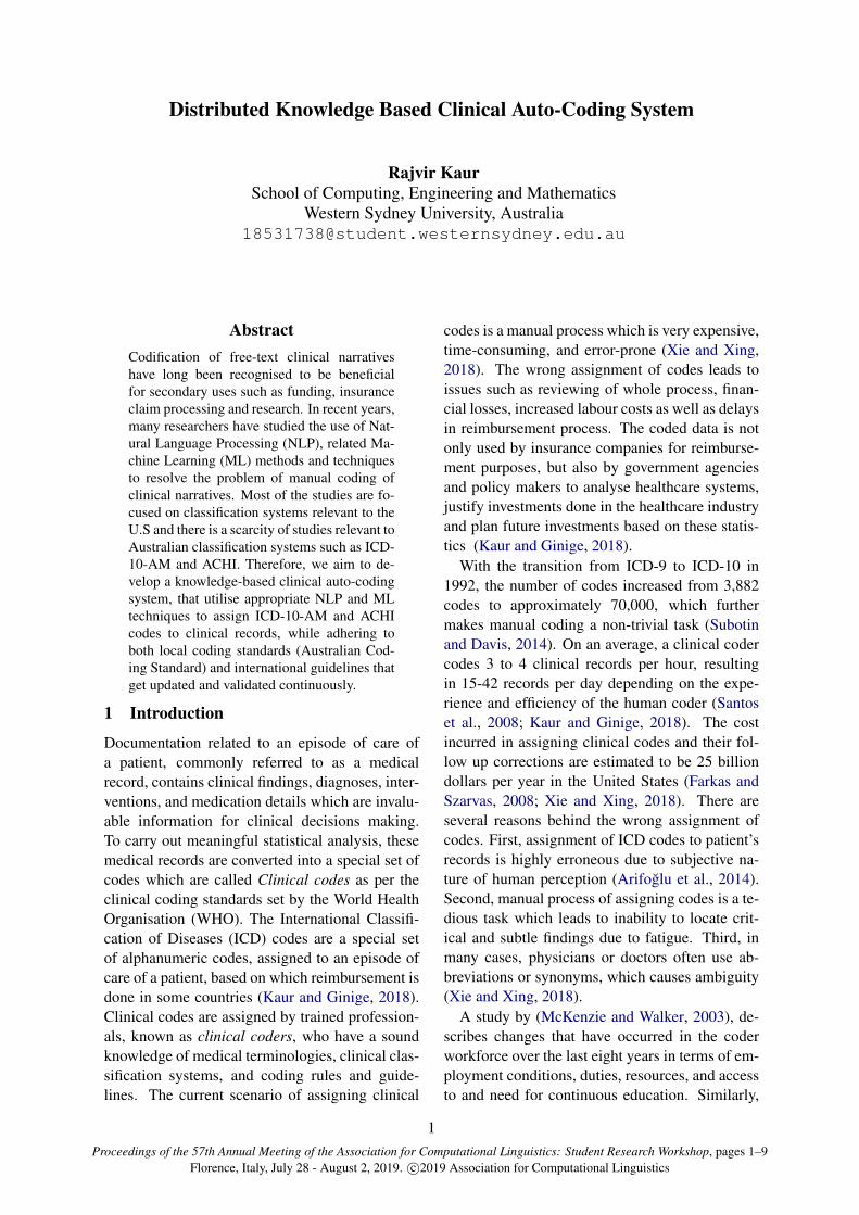
Figure 1: A distributed knowledge-based clinical auto-coding system

another study (Butler-Henderson, 2017), high-lights major future challenges that health informa-tion management practitioners and academics willface with an ageing workforce, where more than50% of the workforce is aged 45 years or older.

To reduce coding errors and cost, research is be-ing conducted to develop methods for automatedcoding. Most of the research in auto-coding is fo-cused on ICD-9-CM (Clinical Modification), ICD-10-CM, ICD-10-PCS (Procedure Coding System)which are US modifications. Very limited studiesare focused on ICD-10-AM (Australian Modifica-tion) and Australian Classification of Health Inter-vention (ACHI).Hence, our research aims to de-velop a distributed knowledge-based clinical auto-coding system that would leverage on NLP andML techniques, where a human coders will givetheir queries to the coding system and in revert thesystem will suggest a set of clinical codes. Fig-ure 1 shows a possible scenario, how a distributedknowledge-based coding system will be used inpractice.

2 Related Work

In early 19th century, a French statistician JacquesBertillon, developed a classification system torecord causes of death. Later in 1948, the WHOstarted maintaining the Bertillon classification andnamed it as International Statistical Classificationof Disease, Injuries and Causes of Death (Cumer-lato et al., 2010). Since then, roughly every tenyears, this classification had been revised and in1992, ICD-10 was approved. Twenty-six (26)

years after the introduction of ICD-10, the nextgeneration of classification ICD-11 is released inMay 2019 but not yet implemented (Kaur andGinige, 2018). ICD-11 increases the complexityby introducing a new code structure, a new chap-ter on X-Extension Codes, dimensions of exter-nal causes (histopathology, consciousness, tem-porality, and etiology), and a new chapters onsleep-awake disorder, conditions related to sexualhealth, and traditional medicine conditions (Or-ganisation, 2016; Hargreaves and Njeru, 2014;Reed et al., 2016).

In previous research related to clinical narra-tive analysis, different methods and techniquesranging from pattern matching to deep learn-ing approaches are applied to categorise clini-cal narratives into different categories (Mujtabaet al., 2019). Several researchers across theglobe have employed text classification to cate-gorise clinical narratives into various categoriesusing machine learning approaches including su-pervised (Hastie et al., 2009), unsupervised (Koand Seo, 2000), semi-supervised (Zhu and Gold-berg, 2009), ontology-based (Hotho et al., 2002),rule-based (Deng et al., 2015), transfer (Pan andYang, 2010), and multi-view learning (Aminiet al., 2009).

(Cai et al., 2016) reviewed the fundamentalsof NLP and describe various techniques such aspattern matching, linguistic approach, statisticaland machine learning approaches that constituteNLP in radiology, along with some key applica-tions. (Larkey and Croft, 1995) studied three dif-ferent classifiers namely: k-nearest neighbor, rel-

2

evance feedback and Bayesian independence clas-sifiers for assigning ICD-9 codes to dictated in-patient discharge summaries. The study foundthat a combination of different classifiers producedbetter results than any single type of classifier.(Farkas and Szarvas, 2008) proposed a rule-basedICD-9-CM coding system for radiology reportsand achieved good classification performances ona limited number of ICD-9-CM codes (45 in total).Similarly, (Goldstein et al., 2007; Pestian et al.,2007b; Crammer et al., 2007) also proposed au-tomated system for assigning ICD-9-CM codes tofree text radiology reports.

(Koopman et al., 2015) proposed a system forautomatic ICD-10 classification of cancer fromfree-text death certificates. The classifiers weredeployed in a two-level cascaded architecture,where the first level identifies the presence of can-cer (i.e., binary form cancer/no cancer), and thesecond level identifies the type of cancer. How-ever, all ICD-10 codes were truncated into threecharacter level.

All the above mentioned research studies arebased on some type of deep learning, machinelearning or statistical approach, where the infor-mation contained in the training data is distillateinto mathematical models, which can be success-fully employed for assigning ICD codes (Chiar-avalloti et al., 2014). One of the main flaws inthese approaches is that training data is annotatedby human coders. Thus, there is a possibility of in-accurate ICD codes. Therefore, if clinical recordslabelled with incorrect ICD codes are given as aninput to an algorithm, it is likely that the modelwill also provide incorrect predictions.

2.1 Standard Pipeline for Clinical TextClassification

Various research studies have used different meth-ods and techniques to handle and process clinicaltext, but the standard pipeline is utilised in someshape or form. This section details the steps in thestandard pipeline in machine learning, as it is re-quired for the auto-coding.

2.1.1 Types of clinical recordClinical text classification techniques have beenemployed on different types of clinical recordssuch as surgical reports (Stocker et al., 2014; Rajaet al., 2012), radiology reports (Mendona et al.,2005), autopsy reports (Mujtaba et al., 2018),death certificates (Koopman et al., 2015), clini-

cal narratives (Meystre and Haug, 2006; Friedlinand McDonald, 2008), progress notes (Frost et al.,2005), laboratory reports (Friedlin and McDonald,2008; Liu et al., 2012), admission notes and pa-tient summaries (Jensen et al., 2012), pathologyreports (Imler et al., 2013), and unstructured elec-tronic text (Portet et al., 2009). In this research, weaim to primarily use clinical discharge summariesas the input text data.

2.1.2 Datasets available

The data sources used in various research stud-ies can be categorised into two types: homoge-neous sources and heterogeneous sources, whichcan further be divided into three subtypes: binaryclass, multi-class single labeled, multi-class multi-labeled datasets (Mujtaba et al., 2019). There arefew datasets that are publicly available such asPhysioNet1, i2b2 NLP dataset2, and OHSUMED3.In this research, we aim to use both publicly avail-able and data acquired from hospitals.

2.1.3 Preprocessing

Preprocessing is done to remove meaningless in-formation from the dataset as the clinical narra-tives may contain high level of noise, sparsity,mispelled words, grammatical errors (Nguyen andPatrick, 2016; Mujtaba et al., 2019). Different pre-processing techniques are applied in research stud-ies including sentence splitting, tokenisation, spellerror detection and correction, stemming and lem-matisation, normalisation (Manning et al., 2008),removal of stop words, removal of punctuation orspecial symbols, abbreviation expansion, chunk-ing, named entity recognition (Bird et al., 2009),negation detection (Chapman et al., 2001).

2.1.4 Feature Engineering

Feature engineering is the combination of featureextraction, feature representation, and feature se-lection (Mujtaba et al., 2019). Feature extraction isthe process of extracting useful features which in-cludes Bag of Words (BoW), n-gram, Word2Vec,and GloVe. Once features are extracted, next stepis to represent in numeric form to feature vectorsusing either binary representation, term frequency(tf), term frequency with inverse document fre-quency (tf-idf), or normalised tf-idf.

1https://physionet.org/mimic2/2https://www.i2b2.org/NLP/DataSets/3http://davis.wpi.edu/xmdv/datasets/ohsumed.html

3

2.1.5 ClassificationFor classification, various research studies haveused classifiers such as Support Vector Machine(SVM) (Cortes and Vapnik, 1995), k-NearestNeighbor (kNN) (Altman, 1992), ConvolutionalNeural Network (CNN) (Karimi et al., 2017), Re-current Neural Network (RNN), Long short-termmemory (LSTM)(Luo, 2017), and Gated Recur-rent Unit (GRU) (Jagannatha and Yu, 2016).

2.1.6 Evaluation MetricsThe performance of clinical text classificationmodels can be measured using standard evalua-tion metrics which include precision, recall, F-measure (or F-score), accuracy, precision (mi-cro and macro-average), recall (micro and macro-average), F-measure (micro and macro-average),and area under the curve (AUC). These metricscan be computed by using values of true positive(TP), false positive (FP), true negative (TN), andfalse negative (FN) in the standard confusion ma-trix (Mujtaba et al., 2019).

3 Experimental Framework

3.1 Data collection and ethics approval

This research has ethics approval from WesternSydney University Human Research Ethics Com-mittee (HREC) under reference No: H12628 touse 1,200 clinical records. The ethics approvalis valid for the next four years until 11th April,2023. In addition, we also have access to publiclyavailable dataset such as MIMIC-III and Compu-tational Medicine Center (CMC) (Pestian et al.,2007a). Apart from this, more clinical recordsfrom acute or sub-acute hospitals will also be col-lected.

3.2 Proposed Research

Within the broader scope of this proposal, thework will be focused on the research questionsgiven below:

How to optimise the use of computerised algo-rithms to assign ICD-10-AM and ACHI codesto clinical records, while adhering to local cod-ing standard (for example, Australian CodingStandard (ACS)) and international guidelines,leveraging on a distributed knowledge-base?

To address main research question, the follow-ing sub-research questions will be investigated:

Why do certain algorithms perform differentlywith similar dataset?The No free lunch theorem (Wolpert, 1996) statesthat there is no such algorithm that is universallybest for every problem. If one algorithm does re-ally good for a given dataset, it may not do reallywell for other dataset. For example, one cannotsay that SVM always does better prediction thanNaıve Bayes or Decision Tree all the times. Theintention of ML or statistical learning research isnot to find the universally best algorithm, but thereason is that most of the algorithms work on thesample data and then make predictions or infer-ence out of that. We cannot make proper truthfulprediction just by working on a sample data. Infact, the results are all probabilistic in nature, not100% true or certain. The study (Kaur and Ginige,2018), performed comparative analysis on differ-ent approaches such as pattern matching, rule-based, ML, and hybrid. Each of the above men-tioned methods and techniques performed differ-ently in every case, but there was no explanationsgiven behind the performance of each algorithm.Moreover, this study did not used ACS rules whileassigning ICD-10-AM and ACHI codes.

There are few reasons that may have effectedthe algorithms performance used for codificationof ICD-10-AM and ACHI codes in the previ-ous study (Kaur and Ginige, 2018). Firstly, do-main knowledge is very essential before assigningcodes. In Australia, coding standards are used forclinical coding purpose to provide consistency ofdata collection, and support secondary classifica-tions based on ICD such as the Australian RefinedDiagnosis Related Groups (AR-DRGs). There-fore, during ICD-10-AM and ACHI code assign-ment, ACS rules are considered. If these ACSrules are not considered, then there is a possibil-ity of wrong assignment of codes. Secondly, thestudy (Kaur and Ginige, 2018) had very limitednumber of medical records due to which the al-gorithms were unable to learn and predict correctcodes properly. A similar study (Kaur and Ginige,2019) done by the same set of authors using thesame dataset describes that the dataset contains420 unique labels, out of which 221 labels ap-peared only once in the whole dataset, 77 labelsappeared twice, and only 24 labels appeared morethan 15 times. Therefore, it lowers the learningrate of the algorithms.

To overcome the above stated problems, we

4

will make use of ACS in conjunction in ICD-10-AM and ACHI codes, and use large-scale dataso that the algorithms can learn properly andmake correct predictions. In order to processraw data, feature engineering will be carried outto transform the raw data into feature vectors.Moreover, in NLP, word embeddings has the abil-ity to capture high-level semantic and syntacticproperties of text. A study by (Henriksson et al.,2015) leverages word embeddings to identifyadverse drug events from clinical notes andshows that using word embeddings can improvethe predictive performance of machine learningmethods. Therefore, in our research, we willexplore semantic and syntactic properties of textto improve the performance of algorithms whichgive different performance on the same dataset.

How to assign ICD codes before referring to lo-cal and international standards and guidelines?In the U.S, the Centers for Medicare and Med-icaid Services (CMS) and the National Centerfor Health Statistics (NCHS), provide the guide-lines for coding and reporting using the ICD-10-CM. These guidelines are a set of rules that havebeen approved by the four organisations: Amer-ican Hospital Association (AHA), the AmericanHealth Information Association (AHIMA), CMS,and NCHS (for Health Statistics). Similarly, inAustralia, the clinical coding standards i.e., ACSrules are designed to be used in conjunction withICD-10-AM and ACHI and are applicable to allpublic and private hospitals in Australia (for Clas-sification Development, 2017). The clinical codesare not only assigned based on the informationprovided on the front sheet or the discharge sum-mary but a complete analysis is performed by fol-lowing the guidelines given in the ACS.

Since the introduction of ICD-10 in 1992, manycountries have modified the WHO’s ICD-10 clas-sification system into their country specific report-ing purpose. For example, ICD-10-CA (CanadianModification) and ICD-10-GM (German Modi-fication). There are few major difference be-tween the US and Australian classification sys-tems. Firstly, there are few additional ICD-10-AM codes that are more specific (approximately4, 915 codes) that are coded only in Australia and15 other countries including Ireland, and SaudiArabia that use Australian classification systemas their national classification system. For exam-

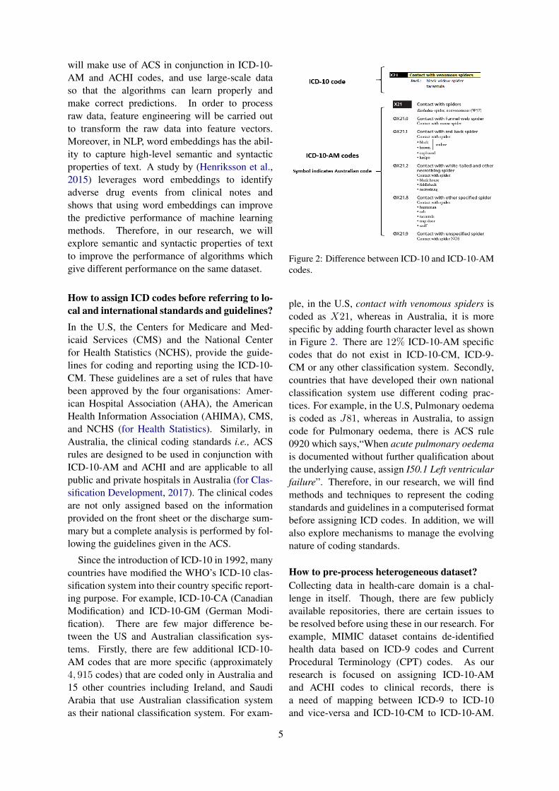
Figure 2: Difference between ICD-10 and ICD-10-AMcodes.

ple, in the U.S, contact with venomous spiders iscoded as X21, whereas in Australia, it is morespecific by adding fourth character level as shownin Figure 2. There are 12% ICD-10-AM specificcodes that do not exist in ICD-10-CM, ICD-9-CM or any other classification system. Secondly,countries that have developed their own nationalclassification system use different coding prac-tices. For example, in the U.S, Pulmonary oedemais coded as J81, whereas in Australia, to assigncode for Pulmonary oedema, there is ACS rule0920 which says,“When acute pulmonary oedemais documented without further qualification aboutthe underlying cause, assign I50.1 Left ventricularfailure”. Therefore, in our research, we will findmethods and techniques to represent the codingstandards and guidelines in a computerised formatbefore assigning ICD codes. In addition, we willalso explore mechanisms to manage the evolvingnature of coding standards.

How to pre-process heterogeneous dataset?Collecting data in health-care domain is a chal-lenge in itself. Though, there are few publiclyavailable repositories, there are certain issues tobe resolved before using these in our research. Forexample, MIMIC dataset contains de-identifiedhealth data based on ICD-9 codes and CurrentProcedural Terminology (CPT) codes. As ourresearch is focused on assigning ICD-10-AMand ACHI codes to clinical records, there isa need of mapping between ICD-9 to ICD-10and vice-versa and ICD-10-CM to ICD-10-AM.

5

There are some existing look-up, translators, ormapping tools, which will translate ICD-9 codesinto ICD-10 codes and vice versa (Butler, 2007).Therefore, we will explore and use the existingmapping tools to convert ICD-9 to ICD-10 codes,ICD-10 to ICD-10-AM codes or another classifi-cation system in order to train the model that isnot annotated using ICD-10-AM and ACHI codes.

What sort of a distributed knowledge-basedsystem would support the assigning clinicalcodes?The majority of studies have used ML, hybrid, anddeep learning approaches for clinical text classifi-cation. There are two main challenges that onehas to face while doing research in health-caredomain. First, to train the model when data isscarce. The ML based algorithms for classificationand automated ICD code assignment are charac-terised by many limitations. For example, knowl-edge acquisition bottleneck, in which ML algo-rithms require a large number of annotated datafor constructing an accurate classification model.Therefore, many believe that the quality of MLbased algorithms highly depended on data ratherthan algorithms (Mujtaba et al., 2019). Even af-ter a great efforts, researchers are able to col-lect millions of data, there is still a possibilitythat the occurrence of some diseases and inter-ventions will not be enough to train the modelproperly and give correct codes. However, whendata is insufficient, transfer learning or fine tun-ing are other possible options to look into (Singh,2018). Secondly, it is difficult and expensive toassign ground truth codes (or label) to the clini-cal records. Although, the above mentioned ap-proaches are capable of providing good results, butthese approaches require annotated data in order totrain the model. The labelling process requires hu-man expert to assign labels (or ICD codes) to eachclinical record. For example, the study (Kaur andGinige, 2018) contains 190 de-identified dischargesummaries belonging to diseases and interventionsof respiratory and digestive system. The dischargesummaries were in the hand written form, whichwere later converted into digital form and assignedground truth codes with the help of a human ex-pert. Thus, a considerable amount of effort wasexerted in preparing the training data.

Therefore, in our research we aim to develop adistributed knowledge-base system where humans

(clinical coders) and machines can work togetherto overcome the above mentioned challenges. Ifmachine is unable to predict the correct ICD codefor a given disease or intervention then humansinput will be considered. Moreover, the humancoder can also verify the codes assigned by ma-chine.

3.3 Baseline MethodsThere are three main approaches for automatedICD codes assignment: (1) machine learning;(2) hybrid (combining machine learning and rule-base); and (3) deep learning. Deep learning mod-els have demonstrated successful results in manyNLP tasks such as language translation (Zhangand Zong, 2015), image captioning (LeCun et al.,2015) and sentiment analysis (Socher et al., 2013).We will work on different ML and deep learn-ing models including LSTM, CNN-RNN, andGRU. Pre-processing will be done using standardpipeline and convert the assigned labels basedon Australian classification system using existingmapping tools. Feature extraction will be doneusing non-sequential and sequential features fol-lowed by training and testing of the model usingbaseline models and deep learning models.

4 Conclusion

In this research proposal, we aim to develop aknowledge-based clinical auto-coding system thatuses computerised algorithms to assign ICD-10-AM, ACHI, ICD-11, and ICHI codes to an episodeof care of a patient while adhering coding guide-lines. Further, we will explore how ML modelscan be trained with limited dataset, mapping be-tween different classification systems, and avoid-ing labelling efforts.

Acknowledgments

I would like to thank my supervisors, Dr. JeewaniAnupama Ginige, Dr. Oliver Obst and VeraDimitropoulos for their feedback that greatlyimproved the paper. This research is supportedby Western Sydney University PostgraduateResearch Scholarship.

ReferencesN. S. Altman. 1992. An introduction to kernel and

nearest-neighbor nonparametric regression. TheAmerican Statistician, 46(3):175–185.

6

M.R. Amini, N. Usunier, and C. Goutte. 2009. Learn-ing from multiple partially observed views - an ap-plication to multilingual text categorization. pages28–36, Vancouver, BC. Conference of 23rd AnnualConference on Neural Information Processing Sys-tems, NIPS 2009 ; Conference Date: 7 December2009 - 10 December 2009.

Damla Arifoglu, Onur Deniz, Kemal Alecakır, andMeltem Yondem. 2014. Codemagic: Semi-automatic assignment of ICD-10-AM codes to pa-tient records. In Information Sciences and Systems2014, pages 259–268. Springer International Pub-lishing.

Steven Bird, Ewan Klein, and Edward Loper. 2009.Natural Language Processing with Python: analyz-ing text with the natural language toolkit. ” O’ReillyMedia, Inc.”.

Rhonda R Butler. 2007. ICD-10 general equivalencemappings: Bridging the translation gap from ICD-9.Journal of American Health Information Manage-ment Association, 78(9):84–86.

Kerryn Butler-Henderson. 2017. Health informationmanagement 2025. what is required to create a sus-tainable profession in the face of digital transforma-tion?

Tianrun Cai, Andreas A. Giannopoulos, Sheng Yu,Tatiana Kelil, Beth Ripley, Kanako K. Kumamaru,Frank J. Rybicki, and Dimitrios Mitsouras. 2016.Natural language processing technologies in radiol-ogy research and clinical applications. RadioGraph-ics, 36(1):176–191. PMID: 26761536.

Wendy W. Chapman, Will Bridewell, Paul Hanbury,Gregory F. Cooper, and Bruce G. Buchanan. 2001.A Simple Algorithm for Identifying Negated Find-ings and Diseases in Discharge Summaries. Journalof Biomedical Informatics, 34(5):301 – 310.

Maria Teresa Chiaravalloti, Roberto Guarasci, Vin-cenzo Lagani, Erika Pasceri, and Roberto Trunfio.2014. A coding support system for the icd-9-cmstandard. In 2014 IEEE International Conferenceon Healthcare Informatics, pages 71–78.

Australian Consortium for Classification Development.2017. Australian Coding Standards for ICD-10-AMand ACHI. Independent Hospital Pricing Authority.

Corinna Cortes and Vladimir Vapnik. 1995. Support-Vector Networks. Machine Learning, 20(3):273–297.

Koby Crammer, Mark Dredze, Kuzman Ganchev,Partha Pratim Talukdar, and Steven Carroll. 2007.Automatic code assignment to medical text. In Pro-ceedings of the Workshop on BioNLP 2007: Biolog-ical, Translational, and Clinical Language Process-ing, BioNLP ’07, pages 129–136, Stroudsburg, PA,USA. Association for Computational Linguistics.

Megan Cumerlato, Lindy Best, Belinda Saad, andN.S.W.) National Centre for Classification inHealth (Sydney. 2010. Fundamentals of morbiditycoding using ICD-10-AM, ACHI, and ACS seventhedition. Sydney : National Centre for Classificationin Health. ”June 2010”–T.p.

Y. Deng, M.J. Groll, and K. Denecke. 2015. Rule-based cervical spine defect classification using med-ical narratives. Studies in Health Technology andInformatics, 216:1038. Conference of 15th WorldCongress on Health and Biomedical Informatics,MEDINFO 2015 ; Conference Date: 19 August2015-23 August 2015.

Richard Farkas and Gyorgy Szarvas. 2008. Automaticconstruction of rule-based ICD-9-CM coding sys-tems. BMC Bioinformatics, 9(3):S10.

F. Jeff Friedlin and Clement J. McDonald. 2008. ASoftware Tool for Removing Patient IdentifyingInformation from Clinical Documents. Journalof the American Medical Informatics Association,15(5):601–610.

H. Robert Frost, Dean F. Sittig, Victor J. Stevens, andBrian Hazlehurst. 2005. MediClass: A System forDetecting and Classifying Encounter-based ClinicalEvents in Any Electronic Medical Record. Journalof the American Medical Informatics Association,12(5):517–529.

Ira Goldstein, Anna Arzumtsyan, and Ozlem Uzuner.2007. Three approaches to automatic assignment oficd-9-cm codes to radiology reports. In AMIA An-nual Symposium Proceedings, volume 2007, page279. American Medical Informatics Association.

Jenny Hargreaves and Jodee Njeru. 2014. ICD-11: Adynamic classification for the information age.

Trevor Hastie, Robert Tibshirani, and Jerome Fried-man. 2009. Overview of Supervised Learning, pages9–41. Springer New York, New York, NY.

National Center for Health Statistics. ICD-10-CM Of-ficial Guidelines for Coding and Reporting.

Aron Henriksson, Maria Kvist, Hercules Dalianis, andMartin Duneld. 2015. Identifying adverse drugevent information in clinical notes with distribu-tional semantic representations of context. Journalof Biomedical Informatics, 57:333 – 349.

Andreas Hotho, Alexander Maedche, and SteffenStaab. 2002. Ontology-based text document clus-tering. KI, 16(4):48–54.

Timothy D. Imler, Justin Morea, Charles Kahi, andThomas F. Imperiale. 2013. Natural languageprocessing accurately categorizes findings fromcolonoscopy and pathology reports. Clinical Gas-troenterology and Hepatology, 11(6):689 – 694.

7

Abhyuday N Jagannatha and Hong Yu. 2016. Bidi-rectional RNN for medical event detection in elec-tronic health records. In Proceedings of the con-ference. Association for Computational Linguistics.North American Chapter. Meeting, volume 2016,page 473. NIH Public Access.

Peter B Jensen, Lars J Jensen, and Søren Brunak. 2012.Mining electronic health records: towards better re-search applications and clinical care. Nature Re-views Genetics, 13(6):395.

Sarvnaz Karimi, Xiang Dai, Hamedh Hassanzadeh,and Anthony Nguyen. 2017. Automatic diagno-sis coding of radiology reports: A comparison ofdeep learning and conventional classification meth-ods. In BioNLP 2017, pages 328–332. Associationfor Computational Linguistics.

Rajvir Kaur and Jeewani Anupama Ginige. 2018.Comparative Analysis of Algorithmic Approachesfor Auto-Coding with ICD-10-AM and ACHI. Stud-ies in Health Technology and Informatics, 252:73–79.

Rajvir Kaur and Jeewani Anupama Ginige. 2019.Analysing effectiveness of multi-label classificationin clinical coding. In Proceedings of the Aus-tralasian Computer Science Week Multiconference,ACSW 2019, pages 24:1–24:9, New York, NY,USA. ACM.

Youngjoong Ko and Jungyun Seo. 2000. Automatictext categorization by unsupervised learning. InProceedings of the 18th Conference on Computa-tional Linguistics - Volume 1, COLING ’00, pages453–459, Stroudsburg, PA, USA. Association forComputational Linguistics.

Bevan Koopman, Guido Zuccon, Anthony Nguyen,Anton Bergheim, and Narelle Grayson. 2015. Auto-matic ICD-10 classification of cancers from free-textdeath certificates. International Journal of MedicalInformatics, 84(11):956 – 965.

Leah S Larkey and W Bruce Croft. 1995. Auto-matic assignment of ICD-9 codes to discharge sum-maries. Technical report, Technical report, Univer-sity of Massachusetts at Amherst, Amherst, MA.

Yann LeCun, Yoshua Bengio, and Geoffrey Hinton.2015. Deep learning. Nature, 521(7553):436.

Hongfang Liu, Kavishwar B Wagholikar, Kathy LMacLaughlin, Michael R Henry, Robert A Greenes,Ronald A Hankey, and Rajeev Chaudhry. 2012.Clinical decision support with automated text pro-cessing for cervical cancer screening. Journalof the American Medical Informatics Association,19(5):833–839.

Yuan Luo. 2017. Recurrent neural networks for classi-fying relations in clinical notes. Journal of Biomed-ical Informatics, 72:85 – 95.

Christopher D. Manning, Prabhakar Raghavan, andHinrich Schutze. 2008. Introduction to InformationRetrieval. Cambridge University Press, New York,NY, USA.

Kirsten McKenzie and Sue M Walker. 2003. The Aus-tralian coder workforce 2002: a report of the Na-tional Clinical Coder Survey. National Centre forClassification in Health.

Eneida A. Mendona, Janet Haas, Lyudmila Shagina,Elaine Larson, and Carol Friedman. 2005. Extract-ing information on pneumonia in infants using natu-ral language processing of radiology reports. Jour-nal of Biomedical Informatics, 38(4):314 – 321.

Stphane Meystre and Peter J. Haug. 2006. Natural lan-guage processing to extract medical problems fromelectronic clinical documents: Performance evalua-tion. Journal of Biomedical Informatics, 39(6):589– 599.

Ghulam Mujtaba, Liyana Shuib, Norisma Idris,Wai Lam Hoo, Ram Gopal Raj, Kamran Khowaja,Khairunisa Shaikh, and Henry Friday Nweke. 2019.Clinical text classification research trends: System-atic literature review and open issues. Expert Sys-tems with Applications, 116:494 – 520.

Ghulam Mujtaba, Liyana Shuib, Ram Gopal Raj, Ret-nagowri Rajandram, and Khairunisa Shaikh. 2018.Prediction of cause of death from forensic autopsyreports using text classification techniques: A com-parative study. Journal of Forensic and LegalMedicine, 57:41 – 50. Thematic section: BigdataGuest editor: Thomas LefvreThematic section:Health issues in police custodyGuest editors: PatrickChariot and Steffen Heide.

Hoang Nguyen and Jon Patrick. 2016. Text mining inclinical domain: Dealing with noise. In Proceed-ings of the 22Nd ACM SIGKDD International Con-ference on Knowledge Discovery and Data Mining,KDD ’16, pages 549–558, New York, NY, USA.ACM.

World Health Organisation. 2016. ICD-11 RevisionConference Report.

Sinno Jialin Pan and Qiang Yang. 2010. A survey ontransfer learning. IEEE Transactions on Knowledgeand Data Engineering, 22(10):1345–1359.

John P. Pestian, Chris Brew, Pawel Matykiewicz,DJ Hovermale, Neil Johnson, K. Bretonnel Cohen,and Wlodzislaw Duch. 2007a. A shared task involv-ing multi-label classification of clinical free text. InBiological, translational, and clinical language pro-cessing, pages 97–104. Association for Computa-tional Linguistics.

John P. Pestian, Christopher Brew, PawełMatykiewicz,D. J. Hovermale, Neil Johnson, K. Bretonnel Co-hen, and WDuch. 2007b. A shared task involving

8

multi-label classification of clinical free text. In Pro-ceedings of the Workshop on BioNLP 2007: Biolog-ical, Translational, and Clinical Language Process-ing, BioNLP ’07, pages 97–104, Stroudsburg, PA,USA. Association for Computational Linguistics.

Francois Portet, Ehud Reiter, Albert Gatt, Jim Hunter,Somayajulu Sripada, Yvonne Freer, and CindySykes. 2009. Automatic generation of textual sum-maries from neonatal intensive care data. ArtificialIntelligence, 173(7-8):789–816. AvImpFact=2.566estim. in 2012.

Ali S. Raja, Ivan K. Ip, Luciano M. Prevedello,Aaron D. Sodickson, Cameron Farkas, Richard D.Zane, Richard Hanson, Samuel Z. Goldhaber,Ritu R. Gill, and Ramin Khorasani. 2012. Ef-fect of computerized clinical decision support onthe use and yield of ct pulmonary angiography inthe emergency department. Radiology, 262(2):468–474. PMID: 22187633.

Geoffrey M. Reed, Jack Drescher, Richard B. Krueger,Elham Atalla, Susan D. Cochran, Michael B. First,Peggy T. Cohen-Kettenis, Ivn Arango-de Montis,Sharon J. Parish, Sara Cottler, Peer Briken, andShekhar Saxena. 2016. Disorders related to sexu-ality and gender identity in the icd-11: revising theicd-10 classification based on current scientific evi-dence, best clinical practices, and human rights con-siderations. World Psychiatry, 15(3):205–221.

Suong Santos, Gregory Murphy, Kathryn Baxter, andKerin M Robinson. 2008. Organisational factorsaffecting the quality of hospital clinical coding.Health Information Management Journal, 37(1):25–37.

Sonit Singh. 2018. Pushing the limits of radiology withjoint modeling of visual and textual information. InProceedings of ACL 2018, Student Research Work-shop, pages 28–36. Association for ComputationalLinguistics.

Richard Socher, Alex Perelygin, Jean Wu, JasonChuang, Christopher D. Manning, Andrew Ng, andChristopher Potts. 2013. Recursive deep modelsfor semantic compositionality over a sentiment tree-bank. In Proceedings of the 2013 Conference onEmpirical Methods in Natural Language Process-ing, pages 1631–1642. Association for Computa-tional Linguistics.

Christof Stocker, Leopold-Michael Marzi, ChristianMatula, Johannes Schantl, Gottfried Prohaska,Aberto Brabenetz, and Andreas Holzinger. 2014.Enhancing patient safety through human-computerinformation retrieval on the example of german-speaking surgical reports. In 2014 25th Interna-tional Workshop on Database and Expert SystemsApplications, pages 216–220.

Michael Subotin and Anthony Davis. 2014. A sys-tem for predicting icd-10-pcs codes from electronichealth records. In Proceedings of BioNLP 2014,

pages 59–67, Baltimore, Maryland. Association forComputational Linguistics.

David H. Wolpert. 1996. The lack of a priori distinc-tions between learning algorithms. Neural Compu-tation, 8(7):1341–1390.

Pengtao Xie and Eric Xing. 2018. A neural architec-ture for automated icd coding. In Proceedings of the56th Annual Meeting of the Association for Compu-tational Linguistics (Volume 1: Long Papers), pages1066–1076. Association for Computational Linguis-tics.

J. Zhang and C. Zong. 2015. Deep neural networks inmachine translation: An overview. IEEE IntelligentSystems, 30(5):16–25.

Xiaojin Zhu and Andrew B Goldberg. 2009. Intro-duction to semi-supervised learning. Synthesis lec-tures on artificial intelligence and machine learning,3(1):1–130.

9

Proceedings of the 57th Annual Meeting of the Association for Computational Linguistics: Student Research Workshop, pages 10–16Florence, Italy, July 28 - August 2, 2019. c©2019 Association for Computational Linguistics

Robust-to-Noise Models in Natural Language Processing Tasks

Valentin MalykhNeural Systems and Deep Learning Laboratory, Moscow Institute of Physics and Technology,

Samsung-PDMI Joint AI Center, Steklov Mathematical Institute at St. Petersburgvalentin.malykh@phystech.edu

Abstract

There are a lot of noisy texts surrounding aperson in modern life. A traditional approachis to use spelling correction, yet the existingsolutions are far from perfect. We propose arobust to noise word embeddings model whichoutperforms existing commonly used modelslike fasttext and word2vec in different tasks.In addition, we investigate the noise robustnessof current models in different natural languageprocessing tasks. We propose extensions formodern models in three downstream tasks, i.e.text classification, named entity recognitionand aspect extraction, these extensions showimprovement in noise robustness over existingsolutions.

1 Introduction

The rapid growth of the usage of mobile elec-tronic devices has increased the number of userinput text issues such as typos. This happens be-cause typing on a small screen and in transport(or while walking) is difficult, and people acci-dentally hit wrong keys more often than when us-ing a standard keyboard. Spell-checking systemswidely used in web services can handle this issue,but they can also make mistakes. These typos areconsidered to be noise in original text. Such noiseis a widely known issue and to mitigate its pres-ence there were developed spelling correcting sys-tems, e.g. (Cucerzan and Brill, 2004). Althoughspelling correction systems have been developedfor decades up to this day, their quality is still farfrom perfect, e.g. for the Russian language it is85% (Sorokin, 2017). So we propose a new wayto handle noise i.e. to make models themselvesrobust to noise.

This work is considering the main area of noiserobustness in natural language processing and, inparticular, in four related subareas which are de-scribed in corresponding sections. All the subar-

eas share the same research questions applied to aparticular downstream task:

RQ1. Are the existing state of the art modelsrobust to noise?

RQ2. How to make these models more robustto noise?

In order to answer these RQs, we describe thecommonly used approaches in a subarea of interestand specify their features which could improve ordeteriorate the performance of these models. Thenwe define a methodology for testing existing mod-els and proposed extensions. The methodology in-cludes the experiment setup with quality measureand datasets on which the experiments should berun.

This work is organized as follows: in Section2 the research on word embeddings is motivatedand proposed, in further sections, i.e. 3, 4, 5,there are propositions to conduct research in thearea of text classification, named entity recogni-tion and aspect extraction respectively. In Section6 we present preliminary conclusions and proposefurther research directions in the mentioned areasand other NLP areas.

2 Word Embeddings

Any text processing system is now impossible toimagine without word embeddings — vectors en-code semantic and syntactic properties of individ-ual words (Arora et al., 2016). However, to usethese word vectors user input should be clean (i.e.free of misspellings), because a word vector modeltrained on clean data will not have misspelled ver-sions of words. There are examples of modelstrained on noisy data (Li et al., 2017), but this ap-proach does not fully solve the problem, becausetypos are unpredictable and a corpus cannot con-tain all possible incorrectly spelled versions of aword. Instead, we suggest that we should make

10

algorithms for word vector modelling robust tonoise.

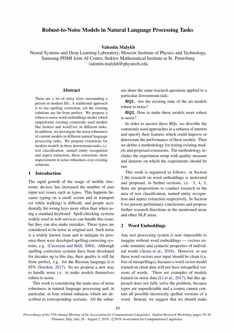
Figure 1: RoVe model architecture.

We suggest a new architecture RoVe (RobustVectors).1 It is presented on Fig. 1. The mainfeature of this model is open vocabulary. It en-codes words as sequences of symbols. This en-ables the model to produce embeddings for out-of-vocabulary (OOV) words. The idea as suchis not new, many other models use character-level embeddings (Ling et al., 2015) or encodethe most common ngrams to assemble unknownwords from them (Bojanowski et al., 2016). How-ever, unlike analogous models, RoVe is specifi-cally targeted at typos — it is invariant to swaps ofsymbols in a word. This property is ensured by thefact that each word is encoded as a bag of charac-ters. At the same time, word prefixes and suffixesare encoded separately, which enables RoVe toproduce meaningful embeddings for unseen wordforms in morphologically rich languages. Notably,this is done without explicit morphological analy-sis. This mechanism is depicted on Fig. 2.

Another feature of RoVe is context dependency— in order to generate an embedding for a wordone should encode its context (the top part ofFig. 1). The motivation for such architecture isthe following. Our intuition is that when process-ing an OOV word our model should produce anembedding similar to that of some similar word

1An open-source implementation is available here:https://gitlab.com/madrugado/robust-w2v

from the training data. This behaviour is suit-able for typos as well as unseen forms of knownwords. In the latter case we want a word to get anembedding similar to the embedding of its initialform. This process reminds lemmatisation (reduc-tion of a word to its initial form). Lemmatisationis context-dependent since it often needs to resolvehomonymy based on word’s context. By makingRoVe model context-dependent we enable it to dosuch implicit lemmatisation.

At the same time, it has been shown that em-beddings which are generated considering word’scontext in a particular sentence are more infor-mative and accurate, because a word’s immediatecontext informs a model of the word’s grammat-ical features (Peters et al., 2018). On the otherhand, use of context-dependent representations al-lowed us to eliminate character-level embeddings.As a result, we do not need to train a model thatconverts a sequence of character-level embeddingsto an embedding for a word, as it was done in(Ling et al., 2015).

2.1 Methodology

We suppose to compare RoVe with common wordvector tools: word2vec (Mikolov et al., 2013) andfasttext (Bojanowski et al., 2016).

We score the performance of word vectors gen-erated with RoVe and baseline models on threetasks: paraphrase detection, sentiment analysis,identification of text entailment. We considerthese tasks to be binary classification ones, so weuse ROC AUC measure for model quality evalua-tion.

For all tasks we suppose to train simple baselinemodels. This is done deliberately to make sure thatthe performance is largely defined by the quality ofvectors that we use. For all the tasks we will com-pare word vectors generated by different modifica-tions of RoVe with vectors produced by word2vecand fasttext models.

We presume to conduct the experiments ondatasets for three languages: English (analyticallanguage), Russian (synthetic fusional), and Turk-ish (synthetic agglutinative). Affixes have differ-ent structures and purposes in these types of lan-guages, and in our experiments we show that ourcharacter-based representation is effective for allof them.

For the above mentioned tasks we are go-ing to use the following corpora: Paraphraser.ru

11

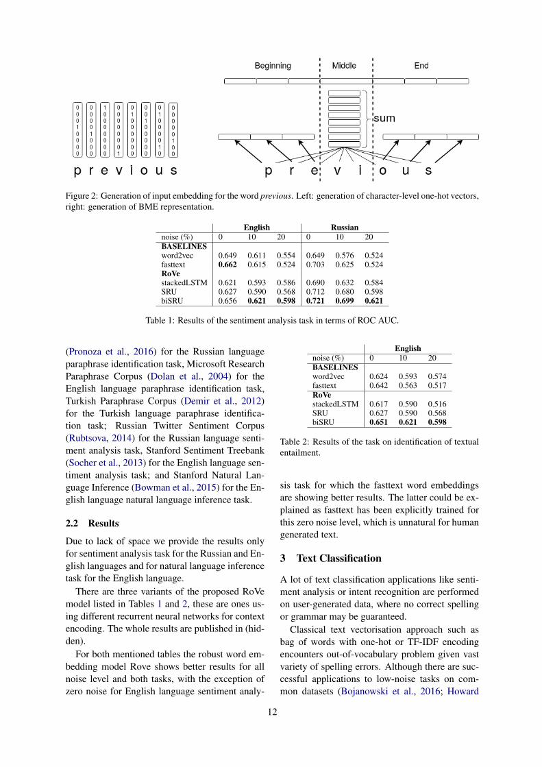
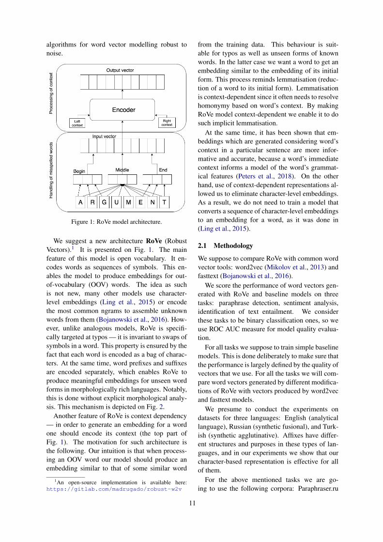
Figure 2: Generation of input embedding for the word previous. Left: generation of character-level one-hot vectors,right: generation of BME representation.

English Russiannoise (%) 0 10 20 0 10 20BASELINESword2vec 0.649 0.611 0.554 0.649 0.576 0.524fasttext 0.662 0.615 0.524 0.703 0.625 0.524RoVestackedLSTM 0.621 0.593 0.586 0.690 0.632 0.584SRU 0.627 0.590 0.568 0.712 0.680 0.598biSRU 0.656 0.621 0.598 0.721 0.699 0.621

Table 1: Results of the sentiment analysis task in terms of ROC AUC.

(Pronoza et al., 2016) for the Russian languageparaphrase identification task, Microsoft ResearchParaphrase Corpus (Dolan et al., 2004) for theEnglish language paraphrase identification task,Turkish Paraphrase Corpus (Demir et al., 2012)for the Turkish language paraphrase identifica-tion task; Russian Twitter Sentiment Corpus(Rubtsova, 2014) for the Russian language senti-ment analysis task, Stanford Sentiment Treebank(Socher et al., 2013) for the English language sen-timent analysis task; and Stanford Natural Lan-guage Inference (Bowman et al., 2015) for the En-glish language natural language inference task.

2.2 Results

Due to lack of space we provide the results onlyfor sentiment analysis task for the Russian and En-glish languages and for natural language inferencetask for the English language.

There are three variants of the proposed RoVemodel listed in Tables 1 and 2, these are ones us-ing different recurrent neural networks for contextencoding. The whole results are published in (hid-den).

For both mentioned tables the robust word em-bedding model Rove shows better results for allnoise level and both tasks, with the exception ofzero noise for English language sentiment analy-

Englishnoise (%) 0 10 20BASELINESword2vec 0.624 0.593 0.574fasttext 0.642 0.563 0.517RoVestackedLSTM 0.617 0.590 0.516SRU 0.627 0.590 0.568biSRU 0.651 0.621 0.598

Table 2: Results of the task on identification of textualentailment.

sis task for which the fasttext word embeddingsare showing better results. The latter could be ex-plained as fasttext has been explicitly trained forthis zero noise level, which is unnatural for humangenerated text.

3 Text Classification

A lot of text classification applications like senti-ment analysis or intent recognition are performedon user-generated data, where no correct spellingor grammar may be guaranteed.

Classical text vectorisation approach such asbag of words with one-hot or TF-IDF encodingencounters out-of-vocabulary problem given vastvariety of spelling errors. Although there are suc-cessful applications to low-noise tasks on com-mon datasets (Bojanowski et al., 2016; Howard

12

and Ruder, 2018), not all models behave well withreal-world data like comments or tweets.

3.1 MethodologyWe do experiments on two corpora: Airline Twit-ter Sentiment 2 and Movie Review (Maas et al.,2011), which are marked up for sentiment analy-sis task.

We conduct three types of experiments: (a) thetrain- and testsets are spell-checked and artificialnoise in inserted; (b) the train- and testsets are notchanged (with the above mentioned exception forRussian corpus) and no artificial noise is added;and (c) the trainset is spell-checked and noised, thetestset is unchanged.

These experimental setups are meant to demon-strate the robustness of tested architectures to arti-ficial and natural noise.

As baselines we use architectures based on fast-text word embedding model (Bojanowski et al.,2016) and an architecture which follows (Kimet al., 2016). Another baseline, which is purelycharacter-level, will be adopted from the work(Kim, 2014).

3.2 ResultsFig. 3 contains results for 4 models:

• FastText, which is recurrent neural networkusing fasttext word embeddings,

• CharCNN, which is a character-based convo-lutional neural network, based on work (Kim,2014),

• CharCNN-WordRNN - a character-basedconvolutional neural network for word em-beddings with recurrent neural network forentire text processing; it follows (Kim et al.,2016),

• and RoVe, which is a recurrent neural net-work using robust to noise word embeddings.

One could see in the figure that the model whichuses robust word embeddings is more robust tonoise itself starting from 0.075 (7.5%) noise level.

4 Named Entity Recognition

The field of named entity recognition (NER) re-ceived a lot of attention in past years. This task

2Publicly available here: https://www.kaggle.com/crowdflower/twitter-airline-sentimen

is an important part of dialog systems (Bechet,2011). Nowadays dialog systems become moreand more popular. Due to that the number of dia-log system users is increased and also many userscommunicate with such systems in inconvenientenvironments, like being in transport. This makesa user to be less concentrated during a conversa-tion and thus causes typos and grammatical errors.Considering this we need to pay more attention toNER models robustness to this type of noise.

4.1 Methodology

We conduct three types of experiments: (a) thetrainset and testset are not changed and no artifi-cial noise is induced; (b) the artificial noise is in-serted into trainset and testset simultaneously; and(c) the trainset is being noised, the testset is un-changed.

These experimental setups are meant to demon-strate the robustness of tested architectures to arti-ficial and natural noise (i.e. typos).

The proposed corpora to use are: Englishand Russian news corpora, CoNLL’03 (TjongKim Sang and De Meulder, 2003) and Persons-1000 (Mozharova and Loukachevitch, 2016) re-spectively, and French social media corpusCAp’2017 (Lopez et al., 2017).

We investigate variations of the state of the artarchitecture for Russian (Anh et al., 2017) and En-glish (Lample et al., 2016) languages and applythe same architecture to the French language cor-pus.

5 Aspect Extraction

Aspect extraction task could provide informationto make dialogue systems more engaging for user(Liu et al., 2010).

Therefore, we have decided to study theAttention-Based Aspect Extraction (ABAE)model (He et al., 2017) robustness using ar-tificially generated noise. We propose threeextensions for an ABAE model, which aresupposedly more noise robust. There are:

• CharEmb - a convolutional neural networkover characters in addition to word as a wholeembeddings; these two embeddings are con-catenated and used in ABAE model;

• FastText - an ABAE model using fasttextword embeddings;

13

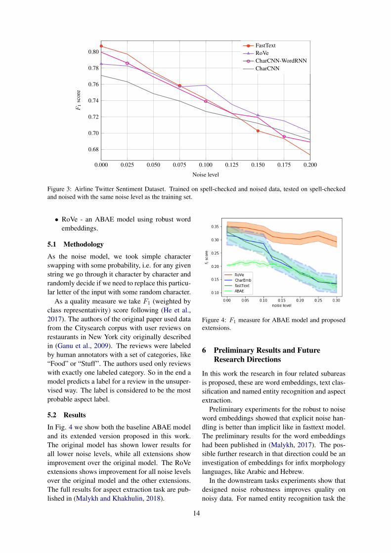
0.000 0.025 0.050 0.075 0.100 0.125 0.150 0.175 0.200

0.68

0.70

0.72

0.74

0.76

0.78

0.80

Noise level

F1

scor

e

FastTextRoVeCharCNN-WordRNNCharCNN

Figure 3: Airline Twitter Sentiment Dataset. Trained on spell-checked and noised data, tested on spell-checkedand noised with the same noise level as the training set.

• RoVe - an ABAE model using robust wordembeddings.

5.1 Methodology

As the noise model, we took simple characterswapping with some probability, i.e. for any givenstring we go through it character by character andrandomly decide if we need to replace this particu-lar letter of the input with some random character.

As a quality measure we take F1 (weighted byclass representativity) score following (He et al.,2017). The authors of the original paper used datafrom the Citysearch corpus with user reviews onrestaurants in New York city originally describedin (Ganu et al., 2009). The reviews were labeledby human annotators with a set of categories, like“Food” or “Stuff”. The authors used only reviewswith exactly one labeled category. So in the end amodel predicts a label for a review in the unsuper-vised way. The label is considered to be the mostprobable aspect label.

5.2 Results

In Fig. 4 we show both the baseline ABAE modeland its extended version proposed in this work.The original model has shown lower results forall lower noise levels, while all extensions showimprovement over the original model. The RoVeextensions shows improvement for all noise levelsover the original model and the other extensions.The full results for aspect extraction task are pub-lished in (Malykh and Khakhulin, 2018).

Figure 4: F1 measure for ABAE model and proposedextensions.

6 Preliminary Results and FutureResearch Directions

In this work the research in four related subareasis proposed, these are word embeddings, text clas-sification and named entity recognition and aspectextraction.

Preliminary experiments for the robust to noiseword embeddings showed that explicit noise han-dling is better than implicit like in fasttext model.The preliminary results for the word embeddingshad been published in (Malykh, 2017). The pos-sible further research in that direction could be aninvestigation of embeddings for infix morphologylanguages, like Arabic and Hebrew.

In the downstream tasks experiments show thatdesigned noise robustness improves quality onnoisy data. For named entity recognition task the

14

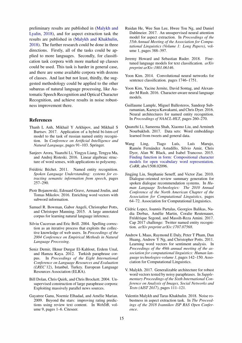
preliminary results are published in (Malykh andLyalin, 2018), and for aspect extraction task theresults are published in (Malykh and Khakhulin,2018). The further research could be done in threedirections. Firstly, all of the tasks could be ap-plied to more languages. Secondly, for classifi-cation task corpora with more marked up classescould be used. This task is harder in general case,and there are some available corpora with dozensof classes. And last but not least, thirdly, the sug-gested methodology could be applied to the othersubareas of natural language processing, like Au-tomatic Speech Recognition and Optical CharacterRecognition, and achieve results in noise robust-ness improvement there.

ReferencesThanh L Anh, Mikhail Y Arkhipov, and Mikhail S

Burtsev. 2017. Application of a hybrid bi-lstm-crfmodel to the task of russian named entity recogni-tion. In Conference on Artificial Intelligence andNatural Language, pages 91–103. Springer.

Sanjeev Arora, Yuanzhi Li, Yingyu Liang, Tengyu Ma,and Andrej Risteski. 2016. Linear algebraic struc-ture of word senses, with applications to polysemy.

Frederic Bechet. 2011. Named entity recognition.Spoken Language Understanding: systems for ex-tracting semantic information from speech, pages257–290.

Piotr Bojanowski, Edouard Grave, Armand Joulin, andTomas Mikolov. 2016. Enriching word vectors withsubword information.

Samuel R. Bowman, Gabor Angeli, Christopher Potts,and Christoper Manning. 2015. A large annotatedcorpus for learning natural language inference.

Silviu Cucerzan and Eric Brill. 2004. Spelling correc-tion as an iterative process that exploits the collec-tive knowledge of web users. In Proceedings of the2004 Conference on Empirical Methods in NaturalLanguage Processing.

Seniz Demir, Ilknur Durgar El-Kahlout, Erdem Unal,and Hamza Kaya. 2012. Turkish paraphrase cor-pus. In Proceedings of the Eight InternationalConference on Language Resources and Evaluation(LREC’12), Istanbul, Turkey. European LanguageResources Association (ELRA).

Bill Dolan, Chris Quirk, and Chris Brockett. 2004. Un-supervised construction of large paraphrase corpora:Exploiting massively parallel news sources.

Gayatree Ganu, Noemie Elhadad, and Amelie Marian.2009. Beyond the stars: improving rating predic-tions using review text content. In WebDB, vol-ume 9, pages 1–6. Citeseer.

Ruidan He, Wee Sun Lee, Hwee Tou Ng, and DanielDahlmeier. 2017. An unsupervised neural attentionmodel for aspect extraction. In Proceedings of the55th Annual Meeting of the Association for Compu-tational Linguistics (Volume 1: Long Papers), vol-ume 1, pages 388–397.

Jeremy Howard and Sebastian Ruder. 2018. Fine-tuned language models for text classification. arXivpreprint arXiv:1801.06146.

Yoon Kim. 2014. Convolutional neural networks forsentence classification. pages 1746–1751.

Yoon Kim, Yacine Jernite, David Sontag, and Alexan-der M Rush. 2016. Character-aware neural languagemodels.

Guillaume Lample, Miguel Ballesteros, Sandeep Sub-ramanian, Kazuya Kawakami, and Chris Dyer. 2016.Neural architectures for named entity recognition.In Proceedings of NAACL-HLT, pages 260–270.

Quanzhi Li, Sameena Shah, Xiaomo Liu, and ArminehNourbakhsh. 2017. Data sets: Word embeddingslearned from tweets and general data.

Wang Ling, Tiago Luıs, Luıs Marujo,Ramon Fernandez Astudillo, Silvio Amir, ChrisDyer, Alan W. Black, and Isabel Trancoso. 2015.Finding function in form: Compositional charactermodels for open vocabulary word representation.CoRR, abs/1508.02096.

Jingjing Liu, Stephanie Seneff, and Victor Zue. 2010.Dialogue-oriented review summary generation forspoken dialogue recommendation systems. In Hu-man Language Technologies: The 2010 AnnualConference of the North American Chapter of theAssociation for Computational Linguistics, pages64–72. Association for Computational Linguistics.

Cedric Lopez, Ioannis Partalas, Georgios Balikas, Na-dia Derbas, Amelie Martin, Coralie Reutenauer,Frederique Segond, and Massih-Reza Amini. 2017.Cap 2017 challenge: Twitter named entity recogni-tion. arXiv preprint arXiv:1707.07568.

Andrew L Maas, Raymond E Daly, Peter T Pham, DanHuang, Andrew Y Ng, and Christopher Potts. 2011.Learning word vectors for sentiment analysis. InProceedings of the 49th annual meeting of the as-sociation for computational linguistics: Human lan-guage technologies-volume 1, pages 142–150. Asso-ciation for Computational Linguistics.

V. Malykh. 2017. Generalizable architecture for robustword vectors tested by noisy paraphrases. In Supple-mentary Proceedings of the Sixth International Con-ference on Analysis of Images, Social Networks andTexts (AIST 2017), pages 111–121.

Valentin Malykh and Taras Khakhulin. 2018. Noise ro-bustness in aspect extraction task. In The Proceed-ings of the 2018 Ivannikov ISP RAS Open Confer-ence.

15

Valentin Malykh and Vladislav Lyalin. 2018. Namedentity recognition in noisy domains. In The Pro-ceedings of the 2018 International Conference onArtificial Intelligence: Applications and Innova-tions.

Tomas Mikolov, Ilya Sutskever, Kai Chen, G.s Cor-rado, and Jeffrey Dean. 2013. Distributed represen-tations of words and phrases and their composition-ality. 26.

Valerie Mozharova and Natalia Loukachevitch. 2016.Two-stage approach in russian named entity recog-nition. In Intelligence, Social Media and Web(ISMW FRUCT), 2016 International FRUCT Con-ference on, pages 1–6. IEEE.

Matthew E. Peters, Mark Neumann, Mohit Iyyer, MattGardner, Christopher Clark, Kenton Lee, and LukeZettlemoyer. 2018. Deep contextualized word rep-resentations. CoRR, abs/1802.05365.

Ekaterina Pronoza, Elena Yagunova, and AntonPronoza. 2016. Construction of a russian para-phrase corpus: Unsupervised paraphrase extraction.573:146–157.

Yuliya Rubtsova. 2014. Automatic term extraction forsentiment classification of dynamically updated textcollections into three classes. In International Con-ference on Knowledge Engineering and the Seman-tic Web, pages 140–149. Springer.

R Socher, A Perelygin, J.Y. Wu, J Chuang, C.D. Man-ning, A.Y. Ng, and C Potts. 2013. Recursive deepmodels for semantic compositionality over a senti-ment treebank. 1631:1631–1642.

Alexey Sorokin. 2017. Spelling correction for mor-phologically rich language: a case study of russian.In Proceedings of the 6th Workshop on Balto-SlavicNatural Language Processing, pages 45–53.

Erik F Tjong Kim Sang and Fien De Meulder.2003. Introduction to the conll-2003 shared task:Language-independent named entity recognition. InProceedings of the seventh conference on Naturallanguage learning at HLT-NAACL 2003-Volume 4,pages 142–147. Association for Computational Lin-guistics.

16

Proceedings of the 57th Annual Meeting of the Association for Computational Linguistics: Student Research Workshop, pages 17–26Florence, Italy, July 28 - August 2, 2019. c©2019 Association for Computational Linguistics

A computational linguistic study of personal recovery in bipolar disorder

Glorianna JagfeldSpectrum Centre for Mental Health Research

Lancaster UniversityUnited Kingdom

g.jagfeld@lancaster.ac.uk

Abstract

Mental health research can benefit increas-ingly fruitfully from computational linguis-tics methods, given the abundant availabilityof language data in the internet and advancesof computational tools. This interdisciplinaryproject will collect and analyse social me-dia data of individuals diagnosed with bipolardisorder with regard to their recovery experi-ences. Personal recovery - living a satisfyingand contributing life along symptoms of se-vere mental health issues - so far has only beeninvestigated qualitatively with structured in-terviews and quantitatively with standardisedquestionnaires with mainly English-speakingparticipants in Western countries. Comple-mentary to this evidence, computational lin-guistic methods allow us to analyse first-person accounts shared online in large quan-tities, representing unstructured settings and amore heterogeneous, multilingual population,to draw a more complete picture of the aspectsand mechanisms of personal recovery in bipo-lar disorder.

1 Introduction and background

Recent years have witnessed increased perfor-mance in many computational linguistics taskssuch as syntactic and semantic parsing (Collobertet al., 2011; Zeman et al., 2018), emotion classifi-cation (Becker et al., 2017), and sentiment analy-sis (Barnes et al., 2017, 2018a,b), especially con-cerning the applicability of such tools to noisy on-line data. Moreover, the field has made substantialprogress in developing multilingual models andextending semantic annotation resources to lan-guages beyond English (Pianta et al., 2002; Boas,2009; Piao et al., 2016; Boot et al., 2017).

Concurrently, it has been argued for mentalhealth research that it would constitute a ‘valu-able critical step’ (Stuart et al., 2017) to analyse

first-hand accounts by individuals with lived ex-perience of severe mental health issues in blogposts, tweets, and discussion forums. Several se-vere mental health difficulties, e.g., bipolar dis-order (BD) and schizophrenia are considered aschronic and clinical recovery, defined as being re-lapse and symptom free for a sustained period oftime (Chengappa et al., 2005), is considered dif-ficult to achieve (Forster, 2014; Heylighen et al.,2014; U.S. Department of Health and Human Ser-vices: The National Institute of Mental Health,2016). Moreover, clinically recovered individ-uals often do not regain full social and educa-tional/vocational functioning (Strakowski et al.,1998; Tohen et al., 2003). Therefore, researchoriginating from initiatives by people with livedexperience of mental health issues has been advo-cating emphasis on the individual’s goals in recov-ery (Deegan, 1988; Anthony, 1993). This move-ment gave rise to the concept of personal recov-ery (Andresen et al., 2011; van Os et al., 2019),loosely defined as a ‘way of living a satisfying,hopeful, and contributing life even with limitationscaused by illness’ (Anthony, 1993). The aspectsof personal recovery have been conceptualised invarious ways (Young and Ensing, 1999; Mansellet al., 2010; Morrison et al., 2016). According tothe frequently used CHIME model (Leamy et al.,2011), its main components are Connectedness,Hope and optimism, Identity, Meaning and pur-pose, and Empowerment.

Here, we focus on BD, which is characterisedby recurring episodes of depressed and elated(hypomanic or manic) mood (Jones et al., 2010;Forster, 2014). Bipolar spectrum disorders wereestimated to affect approximately 2% of the UKpopulation (Heylighen et al., 2014) with ratesranging from 0.1%-4.4% across 11 other Euro-pean, American and Asian countries (Merikangaset al., 2011). Moreover, BD is associated with a

17

high risk of suicide (Novick et al., 2010), makingits prevention and treatment important tasks forsociety. BD-specific personal recovery research ismotivated by mainly two facts: First, the pole ofpositive/elevated mood and ongoing mood insta-bility constitute core features of BD and pose spe-cial challenges compared to other mental healthissues, such as unipolar depression (Jones et al.,2010). Second, unlike for some other severe men-tal health difficulties, return to normal functioningis achievable given appropriate treatment (Coryellet al., 1998; Tohen et al., 2003; Goldberg and Har-row, 2004).

A substantial body of qualitative and quan-titative research has shown the importance ofpersonal recovery for individuals diagnosed withBD (Mansell et al., 2010; Jones et al., 2010, 2012,2015; Morrison et al., 2016). Qualitative evidencemainly comes from (semi-)structured interviewsand focus groups and has been criticised for smallnumbers of participants (Stuart et al., 2017), lack-ing complementary quantitative evidence fromlarger samples (Slade et al., 2012). Some quanti-tative evidence stems from the standardised bipo-lar recovery questionnaire (Jones et al., 2012) anda randomised control trial for recovery-focusedcognitive-behavioural therapy (Jones et al., 2015).Critically, previous research has taken place onlyin structured settings.

What is more, the recovery concept emergedfrom research primarily conducted in English-speaking countries, mainly involving researchersand participants of Western ethnicity. This mighthave led to a lack of non-Western notions of well-being in the concept, such as those found in in-digenous peoples (Slade et al., 2012), limiting itsthe applicability to a general population. Indeed,the variation in BD prevalence rates from 0.1% inIndia to 4.4% in the US is striking. It has beenshown that culture is an important factor in the di-agnosis of BD (Mackin et al., 2006), as well ason the causes attributed to mental health difficul-ties in general and treatments considered appropri-ate (Sanches and Jorge, 2004; Chentsova-Duttonet al., 2014). While approaches to mental healthclassification from texts have long ignored the cul-tural dimension (Loveys et al., 2018), first studiesshow that online language of individuals affectedby depression or related mental health difficultiesdiffers significantly across cultures (De Choud-hury et al., 2017; Loveys et al., 2018).

Hence, it seems timely to take into account thewealth of accounts of mental health difficultiesand recovery stories from individuals of diverseethnic and cultural backgrounds that are availablein a multitude of languages on the internet. Corpusand computational linguistic methods are explic-itly designed for processing large amounts of lin-guistic data (Jurafsky and Martin, 2009; O’Keeffeand McCarthy, 2010; McEnery and Hardie, 2011;Rayson, 2015), and as discussed above, recent ad-vances have made it feasible to apply them tonoisy user-generated texts from diverse domains,including mental health (Resnik et al., 2014; Ben-ton et al., 2017b). Computer-aided analysis ofpublic social media data enables us to address sev-eral shortcomings in the scientific underpinning ofpersonal recovery in BD by overcoming the smallsample sizes of lab-collected data and includingaccounts from a more heterogeneous population.

In sum, our research questions are as follows:(1) How is personal recovery discussed online byindividuals meeting criteria for BD? (2) What newinsights do we get about personal recovery andfactors that facilitate or hinder it? We will in-vestigate these questions in two parts, looking atEnglish-language data by westerners and at multi-lingual data by individuals of diverse ethnicities.

2 Data

Previous work in computational linguistics andclinical psychology has tended to focus on thedetection of mental health issues as classificationtasks (Arseniev-Koehler et al., 2018). Datasetshave been collected for various conditions includ-ing BD using publicly available social-media datafrom Twitter (Coppersmith et al., 2015) and Red-dit (Sekulic et al., 2018; Cohan et al., 2018). Un-fortunately, the Twitter dataset is unavailable forfurther research.1 In both Reddit datasets, mentalhealth-related content was deliberately removed.This allows the training of classifiers that try topredict the mental health of authors from excerptsthat do not explicitly address mental health, yetit renders the data useless for analyses on howmental health is talked about online. Due to thislack of appropriate existing publicly accessibledatasets, we will create such resources and makethem available to subsequent researchers.

We plan to collect data relevant for BD in gen-

1Email communication with the first author of Copper-smith et al. (2015).

18

eral as well as for personal recovery in BD fromthree sources varying in their available amountversus depth of the accounts we expect to find:1) Twitter, 2) Reddit (focusing on mental health-related content unlike previous work), 3) blogs au-thored by affected individuals. Twitter and Redditusers with a BD diagnosis will be identified au-tomatically via self-reported diagnosis statements,such as ‘I was diagnosed with BD-I last week’.To do so, we will extend on the diagnosis pat-terns and terms for BD provided by Cohan et al.(2018)2. Implicit consent is assumed from userson these platforms to use their public tweets andposts.3 Relevant blogs will be manually identified,and their authors will be contacted to obtain in-formed consent for using their texts.

Since language and culture are important fac-tors in our research questions, we need informa-tion on the language of the texts and the coun-try of residence of their authors3, which is notprovided in a structured format in the three datasources. For language identification, Twitter em-ploys an automatic tool (Trampus, 2015), whichcan be used to filter tweets according to 60 lan-guage codes, and there are free, fairly accuratetools such as the Google Compact Language De-tector4, which can be applied to Reddit and blogposts. The location of Twitter users can be auto-matically inferred from their tweets (Cheng et al.,2010) or the (albeit noisy) location field in theiruser profiles (Hecht et al., 2011). Only one attemptto classify the location of Reddit users has beenpublished so far (Harrigian, 2018) showing mea-gre results, indicating that the development of ro-bust location classification approaches on this plat-form would constitute a valuable contribution.

Some companies collect mental health-relatedonline data and make them available to researcherssubject to approval of their internal review boards,e.g., OurDataHelps5 by Qntfy or the peer-supportforum provider 7 Cups6. Unlike ‘raw’ social me-dia data, these datasets have richer user-providedmetadata and explicit consent for research usage.On the other hand, less data is available, the pro-cess to obtain access might be tedious within theshort timeline of a PhD project and it might be im-

2http://ir.cs.georgetown.edu/data/smhd/

3See Section 4 for ethical considerations on this.4https://github.com/CLD2Owners/cld25https://ourdatahelps.org/6https://7cups.com/

possible to share the used portions of the data withother researchers. Therefore, we will follow up thepossibilities of obtaining access to these datasets,but in parallel also collect our own datasets toavoid dependence on external data providers.

3 Methodology and Resources

As explained in the introduction, the overarchingaim of this project is to investigate in how farinformation conveyed in social media posts cancomplement more traditional research methods inclinical psychology to get insights into the recov-ery experience of individuals with a BD diagnosis.Therefore, we will first conduct a systematic liter-ature review of qualitative evidence to establish asolid base of what is already known about personalrecovery experiences in BD for the subsequent so-cial media studies.

Our research questions, which regard the expe-riences of different populations, lend themselvesto several subprojects. First, we will collect andanalyse English-language data from westerners.Then, we will address ethnically diverse English-speaking populations and finally multilingual ac-counts. This has the advantage that we can builddata processing and methodological workflowsalong an increase in complexity of the data col-lection and analysis throughout the project.

In each project phase, we will employ a mixed-methods approach to combine the advantages ofquantitative and qualitative methods (Tashakkoriand Teddlie, 1998; Creswell and Plano Clark,2011), which is established in mental health re-search (Steckler et al., 1992; Baum, 1995; Saleet al., 2002; Lund, 2012) and specifically recom-mended to investigate personal recovery (Leon-hardt et al., 2017). Quantitative methods are suit-able to study observable behaviour such as lan-guage and yield more generalisable results bytaking into account large samples. However,they fall short of capturing the subjective, id-iosyncratic meaning of socially constructed real-ity, which is important when studying individuals’recovery experience (Russell and Browne, 2005;Mansell et al., 2010; Morrison et al., 2016; Croweand Inder, 2018). Therefore, we will apply anexplanatory sequential research design (Creswelland Plano Clark, 2011), starting with statisticalanalysis of the full dataset followed by a manualinvestigation of fewer examples, similar to ‘distantreading’ (Moretti, 2013) in digital humanities.

19

Since previous research mainly employed(semi-)structured interviews and we do not expectto necessarily find the same aspects emphasised inunstructured settings, even less so when looking ata more diverse and non-English speaking popula-tion, we will not derive hypotheses from existingrecovery models for testing on the online data. In-stead, we will start off with exploratory quantita-tive research using comparative analysis tools suchas Wmatrix (Rayson, 2008) to uncover importantlinguistic features, e.g., on keywords and key con-cepts that occur with unexpected frequency in ourcollected datasets relative to reference corpora.The underlying assumption is that keywords andkey concepts are indicative of certain aspects ofpersonal recovery, such as those specified in theCHIME model (Leamy et al., 2011), other pre-vious research (Mansell et al., 2010; Morrisonet al., 2016; Crowe and Inder, 2018), or novelones. Comparing online sources with transcriptsof structured interviews or subcorpora originatingfrom different cultural backgrounds might uncoveraspects that were not prominently represented inthe accounts studied in prior research.

A specific challenge will be to narrow downthe data to parts relevant for personal recovery,since there is no control over the discussed top-ics compared to structured interviews. To inves-tigate how individuals discuss personal recoveryonline and what (potentially unrecorded) aspectsthey associate with it, without a priori narrow-ing down the search-space to specific known key-words seems like a chicken-and-egg problem. Wepropose to address this challenge by an iterativeapproach similar to the one taken in a corpus lin-guistic study of cancer metaphors (Semino et al.,2017). Drawing on results from previous qualita-tive research (Leamy et al., 2011; Morrison et al.,2016), we will compile an initial dictionary ofrecovery-related terms. Next, we will examine asmall portion of the dataset manually, which willbe partly randomly sampled and partly selected tocontain recovery-related terms. Based on this, wewill be able to expand the dictionary and addi-tionally automatically annotate semantic conceptsof the identified relevant text passages using a se-mantic tagging approach such as the UCREL Se-mantic Analysis System (USAS) (Rayson et al.,2004). Crucially for the multilingual aspect ofthe project, USAS can tag semantic categories ineight languages (Piao et al., 2016). Then, se-

mantic tagging will be applied to the full corpusto retrieve all text passages mentioning relevantconcepts. Furthermore, distributional semanticsmethods (Lenci, 2008; Turney and Pantel, 2010)can be used to find terms that frequently co-occurwith words from our keyword dictionary. Occur-rences of the identified keywords or concepts canbe quantified in the full corpus to identify the im-portance of the related personal recovery aspects.

Linguistic Inquiry and WordCount (LIWC) (Pennebaker et al., 2015) is afrequently used tool in social-science text analysisto analyse emotional and cognitive componentsof texts and derive features for classificationmodels (Cohan et al., 2018; Sekulic et al., 2018;Tackman et al., 2018; Wang and Jurgens, 2018).LIWC counts target words organised in a man-ually constructed hierarchical dictionary withoutcontextual disambiguation in the texts underanalysis and has been psychometrically validatedand developed for English exclusively. Whiletranslations for several languages exist, e.g.,Dutch (Boot et al., 2017), and it is questionableto what extent LIWC concepts can be transferredto other languages and cultures by mere trans-lation. We therefore aim to apply and developmethods that require less manual labour and areapplicable to many languages and cultures. Oneoption constitute unsupervised methods, suchas topic modelling, which has been applied toexplore cultural differences in mental-healthrelated online data already (De Choudhury et al.,2017; Loveys et al., 2018). The DifferentialLanguage Analysis ToolKit (DLATK) (Schwartzet al., 2017) facilitates social-scientific languageanalyses, including tools for preprocessing, suchas emoticon-aware tokenisers, filtering accordingto meta data, and analysis, e.g. via robust topicmodelling methods.

Furthermore, emotion and sentiment analysisconstitute useful tools to investigate the emotionsinvolved in talking about recovery and identifyfactors that facilitate or hinder it. There aremany annotated datasets to train supervised clas-sifiers (Bostan and Klinger, 2018; Barnes et al.,2017) for these actively researched NLP tasks.Machine learning methods were found to usu-ally outperform rule-based approaches based onlook-ups in dictionaries such as LIWC. Again,most annotated resources are English, but stateof the art approaches based on multilingual em-

20

beddings allow transferring models between lan-guages (Barnes et al., 2018a).

4 Ethical considerations

Ethical considerations are established as essentialpart in planning mental health research and mostresearch projects undergo approval by an ethicscommittee. On the contrary, the computationallinguistics community has started only recently toconsider ethical questions (Hovy and Spruit, 2016;Hovy et al., 2017). Likely, this is because com-putational linguistics was traditionally concernedwith publicly available, impersonal texts such asnewspapers or texts published with some tempo-ral distance, which left a distance between the textand author. Conversely, recent social media re-search often deals with highly personal informa-tion of living individuals, who can be directly af-fected by the outcomes (Hovy and Spruit, 2016).

Hovy and Spruit (2016) discuss issues that canarise when constructing datasets from social me-dia and conducting analyses or developing pre-dictive models based on these data, which we re-view here in relation to our project: Demographicbias in sampling the data can lead to exclusionof minority groups, resulting in overgeneralisationof models based on these data. As discussed inthe introduction, personal recovery research suf-fers from a bias towards English-speaking West-ern individuals of white ethnicity. By studyingmultilingual accounts of ethnically diverse pop-ulations we explicitly address the demographicbias of previous research. Topic overexposure istricky to address, where certain groups are per-ceived as abnormal when research repeatedly findsthat their language is different or more difficultto process. Unlike previous research (Copper-smith et al., 2015; Cohan et al., 2018; Sekulicet al., 2018) our goal is not to reveal particularitiesin the language of individuals affected by men-tal health problems. Instead, we will compare ac-counts of individuals with BD from different set-tings (structured interviews versus informal onlinediscourse) and of different backgrounds. Whilethe latter bears the risk to overexpose certain mi-nority groups, we will pay special attention to thisin the dissemination of our results.

Lastly, most research, even when conductedwith the best intentions, suffers from the dual-useproblem (Jonas, 1984), in that it can be misused orhave consequences that affect people’s life nega-

tively. For this reason, we refrain from publishingmental health classification methods, which couldbe used, for example, by health insurance compa-nies for the risk assessment of applicants based ontheir social media profiles.

If and how informed consent needs to be ob-tained for research on social media data is a de-bated issue (Eysenbach and Till, 2001; Beningeret al., 2014; Paul and Dredze, 2017), mainly be-cause it is not straightforward to determine if postsare made in a public or private context. From alegal point of view, the privacy policies of Twit-ter7 and Reddit8, explicitly allow analysis of theuser contents by third party, but it is unclear towhat extent users are aware of this when posting tothese platforms (Ahmed et al., 2017). However, inpractice it is often infeasible to seek retrospectiveconsent from hundreds or thousands of social me-dia users. According to current ethical guidelinesfor social media research (Benton et al., 2017a;Williams et al., 2017) and practice in compara-ble research projects (O’Dea et al., 2015; Ahmedet al., 2017), it is regarded as acceptable to waiveexplicit consent if the anonymity of the users ispreserved. Therefore, we will not ask the accountholders of Twitter and Reddit posts included in ourdatasets for their consent.

Benton et al. (2017a) formulate guidelines forethical social media health research that pertain es-pecially to data collection and sharing. In line withthese, we will only share anonymised and para-phrased excerpts from the texts, as it is often possi-ble to recover a user name via a web search for theverbatim text of a post. However, we will make theoriginal texts available as datasets to subsequentresearch under a data usage agreement. Since the(automatic) annotation of demographic variablesin parts of our dataset constitutes especially sensi-tive information on minority status in conjunctionwith mental health, we will only share these an-notations with researchers that demonstrate a gen-uine need for them, i.e. to verify our results or toinvestigate certain research questions.

Another important question is in which situa-tions of encountering content indicative of a riskof self-harm or harm to others it would be appro-

7https://cdn.cms-twdigitalassets.com/content/dam/legal-twitter/site-assets/privacy-policy-new/Privacy-Policy-Terms-of-Service_EN.pdf

8www.redditinc.com/policies/privacy-policy

21

priate or even required by duty of care for the re-search team to pass on information to authorities.Surprisingly, we could only find two mentions ofthis issue in social media research (O’Dea et al.,2015; Young and Garett, 2018). Acknowledgingthat suicidal ideation fluctuates (Prinstein et al.,2008), we accord with the ethical review board’srequirement in O’Dea et al. (2015) to only analysecontent posted at least three months ago. If theresearch team, which includes clinical psycholo-gists, still perceives users at risk we will make useof the reporting facilities of Twitter and Reddit.

As a central component we consider the in-volvement of individuals with lived experience inour project, an aspect which is missing in the dis-cussion of ethical social media health research sofar. The proposal has been presented to an advi-sory board of individuals with a BD diagnosis andwas received positively. The advisory board willbe consulted at several stages of the project to in-form the research design, analysis, and publica-tion of results. We believe that board memberscan help to address several of the raised ethicalproblems, e.g., shaping the research questions toavoid feeding into existing biases or overexposingcertain groups and highlighting potentially harm-ful interpretations and uses of our results.

5 Impact and conclusion

The importance of the recovery concept in thedesign of mental health services has recentlybeen prominently reinforced, suggesting recovery-oriented social enterprises as key component ofthe integrated service (van Os et al., 2019). Wethink that a recovery approach as leading princi-ple for national or global health service strategies,should be informed by voices of individuals as di-verse as those it is supposed to serve. Therefore,we expect the proposed investigations of views onrecovery by previously under-researched ethnic,language, and cultural groups to yield valuable in-sights on the appropriateness of the recovery ap-proach for a wider population. The datasets col-lected in this project can serve as useful resourcesfor future research. More generally, our social-media data-driven approach could be applied to in-vestigate other areas of mental health if it provessuccessful in leading to relevant new insights.

Finally, this project is an interdisciplinary en-deavour, combining clinical psychology, inputfrom individuals with lived experience of BD, and

computational linguistics. While this comes withthe challenges of cross-disciplinary research, it hasthe potential to apply and develop state-of-the-artNLP methods in a way that is psychologically andethically sound as well as informed and approvedby affected people to increase our knowledge ofsevere mental illnesses such as BD.

Acknowledgments

I would like to thank my supervisors Steven Jones,Fiona Lobban, and Paul Rayson for their guidancein this project. My heartfelt thanks go also to ChrisLodge, service user researcher at the SpectrumCentre, and the members of the advisory panelhe coordinates that offer feedback on this projectbased on their lived experience of BD. Further, Iwould like to thank Masoud Rouhizadeh for hishelpful comments during pre-submission mentor-ing and the anonymous reviewers. This project isfunded by the Faculty of Health and Medicine atLancaster University as part of a doctoral scholar-ship.

ReferencesWasim Ahmed, Peter A. Bath, and Gianluca Demartini.

2017. Using Twitter as a data source: an overviewof ethical, legal and methodological challenges. InKandy Woodfield, editor, The Ethics of Online Re-search, pages 79–107. Emerald Books.

Retta Andresen, Peter Caputi, and Lindsay G Oades.2011. Psychological Recovery: Beyond Mental Ill-ness. John Wiley & Sons, Ltd, Chichester, WestSussex.

William A. Anthony. 1993. Recovery from mental ill-ness: the guiding vision of the mental health systemin the 1990s. Psychosocial Rehabilitation Journal,16(4):11–23.

Alina Arseniev-Koehler, Sharon Mozgai, and StefanScherer. 2018. What type of happiness are youlooking for? - A closer look at detecting mentalhealth from language. In Proceedings of the FifthWorkshop on Computational Linguistics and Clini-cal Psychology: From Keyboard to Clinic, pages 1–12.

Jeremy Barnes, Roman Klinger, and Sabine Schulte imWalde. 2017. Assessing State-of-the-Art SentimentModels on State-of-the-Art Sentiment Datasets. InProceedings of the 8th Workshop on ComputationalApproaches to Subjectivity, Sentiment and SocialMedia Analysis, pages 2–12.

Jeremy Barnes, Roman Klinger, and Sabine Schulte imWalde. 2018a. Bilingual Sentiment Embeddings:

22

Joint Projection of Sentiment Across Languages. InProceedings of the 56th Annual Meeting of the Asso-ciation for Computational Linguistics (ACL), pages2483–2493, Melbourne.

Jeremy Barnes, Roman Klinger, and Sabine Schulte imWalde. 2018b. Projecting Embeddings for DomainAdaptation: Joint Modeling of Sentiment Analysisin Diverse Domains. In Proceedings of the 27th In-ternational Conference on Computational Linguis-tics, pages 818–830.

Frances Baum. 1995. Researching public health: Be-hind the qualitative-quantitative methodological de-bate. Social Science and Medicine, 40(4):459–468.

Karin Becker, Viviane P. Moreira, and Aline G. L.dos Santos. 2017. Multilingual emotion classifica-tion using supervised learning: comparative exper-iments. Information Processing and Management,53(3):684–704.

Kelsey Beninger, Alexandra Fry, Natalie Jago, HayleyLepps, Laura Nass, and Hannah Silvester. 2014. Re-search using Social Media; Users’ Views.

Adrian Benton, Glen Coppersmith, and Mark Dredze.2017a. Ethical Research Protocols for Social MediaHealth Research. Proceedings of the First Workshopon Ethics in Natural Language Processing, page94102.

Adrian Benton, Margaret Mitchell, and Dirk Hovy.2017b. Multi-Task Learning for Mental Health us-ing Social Media Text. In Proceedings of the 15thConference of the European Chapter of the Asso-ciation for Computational Linguistics (EACL), vol-ume 1, pages 152–162.

Hans C. Boas, editor. 2009. Multilingual FrameNets inComputational Lexicography: Methods and Appli-cations. Mouton de Gruyter, Berlin.

Peter Boot, Hanna Zijlstra, and Rinie Geenen. 2017.The Dutch translation of the Linguistic Inquiry andWord Count (LIWC) 2007 dictionary. Dutch Jour-nal of Applied Linguistics, 6(1):65 – 76.

Laura-Ana-Maria Ana Maria Bostan and RomanKlinger. 2018. An Analysis of Annotated Corporafor Emotion Classification in Text. In Proceed-ings of the 27th International Conference on Com-putational Linguistics, pages 2104–2119. Associa-tion for Computational Linguistics.

Zhiyuan Cheng, James Caverlee, and Kyumin Lee.2010. You are where you tweet: A content-based ap-proach to geo-locating Twitter users. Proceedings ofthe 19th ACM International Conference on Informa-tion and Knowledge Management, pages 759–768.

K. N. Roy Chengappa, John Hennen, Ross J.Baldessarini, David J. Kupfer, Lakshmi N. Yatham,Samuel Gershon, Robert W. Baker, and MauricioTohen. 2005. Recovery and functional outcomesfollowing olanzapine treatment for bipolar I mania.Bipolar Disorders, 7(1):68–76.

Yulia E. Chentsova-Dutton, Andrew G. Ryder, andJeanne Tsai. 2014. Understanding depression acrosscultural contexts. In Ian H. Gotlib and Constance L.Hammen, editors, Handbook of Depression, pages337–354. Guilford Press.

Arman Cohan, Bart Desmet, Sean Macavaney, AndrewYates, Luca Soldaini, Sean Macavaney, and NazliGoharian. 2018. SMHD: A Large-Scale Resourcefor Exploring Online Language Usage for Multi-ple Mental Health Conditions. In Proceedings ofthe 27th International Conference on ComputationalLinguistics (COLING), pages 1485–1497, Santa Fe.Association for Computational Linguistics.

Ronan Collobert, Jason Weston, Lon Bottou, MichaelKarlen, Koray Kavukcuoglu, and Pavel Kuksa.2011. Natural language processing (almost) fromscratch. Journal of Machine Learning Research,12:2493–2537.

Glen Coppersmith, Mark Dredze, Craig Harman, andKristy Hollingshead. 2015. From ADHD to SAD:Analyzing the Language of Mental Health on Twit-ter through Self-Reported Diagnoses. In Confer-ence of the North American Chapter of the Associ-ation for Computational Linguistics Human Lan-guage Technologies (NAACL), pages 1–10.

William Coryell, Carolyn Turvey, Jean Endicott, An-drew C. Leon, Timothy Mueller, David Solomon,and Martin Keller. 1998. Bipolar I affective disor-der: Predictors of outcome after 15 years. Journalof Affective Disorders, 50(2-3):109–116.

John W. Creswell and Vicki L. Plano Clark. 2011. De-signing and Conducting Mixed Methods Research.SAGE Publications.

Marie Crowe and Maree Inder. 2018. Staying well withbipolar disorder: A qualitative analysis of five-yearfollow-up interviews with young people. Journal ofPsychiatric and Mental Health Nursing, 25(4):236–244.

Munmun De Choudhury, Tomaz Logar, Sanket S.Sharma, Wouter Eekhout, and Ren Clausen Nielsen.2017. Gender and Cross-Cultural Differences in So-cial Media Disclosures of Mental Illness. In Pro-ceedings of the 2017 ACM Conference on ComputerSupported Cooperative Work and Social Computing,pages 353–369.

Patricia E. Deegan. 1988. Recovery: The lived experi-ence of rehabilitation. Psychosocial RehabilitationJournal, 11(4):11–19.

Gunther Eysenbach and James E. Till. 2001. Ethical is-sues in qualitative research on internet communities.BMJ, 323(7055):1103–1105.

Peter Forster. 2014. Bipolar Disorder. Encyclopedia ofthe Neurological Sciences, pages 420–424.

23

Joseph F. Goldberg and Martin Harrow. 2004. Con-sistency of remission and outcome in bipolar andunipolar mood disorders: A 10-year prospec-tive follow-up. Journal of Affective Disorders,81(2):123–131.

Keith Harrigian. 2018. Geocoding without geotags: atext-based approach for reddit. In Proceedings of the2018 EMNLP Workshop W-NUT: The 4th Workshopon Noisy User-generated Text, pages 17–27.

Brent Hecht, Lichan Hong, Bongwon Suh, and Ed H.Chi. 2011. Tweets from Justin Bieber’s heart: thedynamics of the location field in user profiles. InProceedings of the SIGCHI Conference on HumanFactors in Computing Systems, pages 237–246.

Ann Heylighen, Herman Neuckermans, YokoAkazawa-Ogawa, Mototada Shichiri, KeikoNishio, Yasukazu Yoshida, Etsuo Niki, Yoshi-hisa Hagihara, R. C. Dempsey, P. A. Gooding,Steven Huntley Jones, Nadia Akers, Jayne Eaton,Elizabeth Tyler, Amanda Gatherer, Alison Brabban,Rita Marie Long, Anne Fiona Lobban, Raya A.Jones, Kallia Apazoglou, Anne-Lise Kung, PaoloCordera, Jean-Michel Aubry, Alexandre Dayer,Patrik Vuilleumier, Camille Piguet, Russell S.J.,Prof Steven Jones, Anne Cooke, Anne Cooke, KarinFalk, I. Marshal, Steven Huntley Jones, Gina Smith,Lee D Mulligan, Fiona Lobban, Heather Law,Graham Dunn, Mary Welford, James Kelly, JohnMulligan, Anthony P Morrison, Elizabeth Tyler,Anne Fiona Lobban, Chris Sutton, Colin Depp,Sheri L Johnson, Ken Laidlaw, Steven HuntleyJones, Greg Murray, Nuwan D Leitan, Neil Thomas,Erin E Michalak, Sheri L Johnson, Steven HuntleyJones, Tania Perich, Lesley Berk, Michael Berk,Timothy H. Monk, Joseph F. Flaherty, Ellen Frank,Kathleen Hoskinson, David J. Kupfer, AilbheSpillane, Karen Matvienko-Sikar, Celine Larkin,Paul Corcoran, and Ella Arensman. 2014. Bipolardisorder: assessment and management, volume 7.National Institute for Health and Care Excellence.

Dirk Hovy, Shannon Spruit, Margaret Mitchell,Emily M Bender, Michael Strube, and Hanna Wal-lach. 2017. Proceedings of the First ACL Workshopon Ethics in Natural Language Processing. Associ-ation for Computational Linguistics.

Dirk Hovy and Shannon L. Spruit. 2016. The SocialImpact of Natural Language Processing. In Pro-ceedings of the 54th Annual Meeting of the Asso-ciation for Computational Linguistics (ACL), pages591–598.

Hans Jonas. 1984. The Imperative of Responsibility:Foundations of an Ethics for the Technological Age.University of Chicago Press, Chicago.

Steven Jones, Fiona Lobban, and Anne Cook. 2010.Understanding Bipolar Disorder - Why some peopleexperience extreme mood states and what can help.British Psychological Society.

Steven Jones, Lee D. Mulligan, Sally Higginson, Gra-ham Dunn, and Anthony P Morrison. 2012. Thebipolar recovery questionnaire: psychometric prop-erties of a quantitative measure of recovery experi-ences in bipolar disorder. Journal of Affective Dis-orders, 147(1-3):34–43.

Steven H. Jones, Gina Smith, Lee D. Mulligan,Fiona Lobban, Heather Law, Graham Dunn, MaryWelford, James Kelly, John Mulligan, and An-thony P. Morrison. 2015. Recovery-focusedcognitive-behavioural therapy for recent-onset bipo-lar disorder: randomised controlled pilot trial.British Journal of Psychiatry, 206(1):58–66.

Daniel Jurafsky and James H. Martin. 2009. Speechand Language Processing (2nd Edition). Prentice-Hall, Inc., Upper Saddle River, USA.

Mary Leamy, Victoria Bird, Clair Le Boutillier, JulieWilliams, and Mike Slade. 2011. Conceptual frame-work for personal recovery in mental health: Sys-tematic review and narrative synthesis. British Jour-nal of Psychiatry, 199(6):445–452.

Alessandro Lenci. 2008. Distributional semantics inlinguistic and cognitive research. Italian Journal ofLinguistics, 20(1):1–31.

Bethany L. Leonhardt, Kelsey Huling, Jay A. Hamm,David Roe, Ilanit Hasson-Ohayon, Hamish J.McLeod, and Paul H. Lysaker. 2017. Recovery andserious mental illness: a review of current clini-cal and research paradigms and future directions.Expert Review of Neurotherapeutics, 17(11):1117–1130.

Kate Loveys, Jonathan Torrez, Alex Fine, Glen Mori-arty, and Glen Coppersmith. 2018. Cross-culturaldifferences in language markers of depression on-line. In Proceedings of the Fifth Workshop onComputational Linguistics and Clinical Psychology:From Keyboard to Clinic, pages 78–87.

Thorleif Lund. 2012. Combining Qualitative andQuantitative Approaches: Some Arguments forMixed Methods Research. Scandinavian Journal ofEducational Research, 56(2):155–165.

Paul Mackin, Steven D. Targum, Amir Kalali, DrorRom, and Allan H. Young. 2006. Culture and as-sessment of manic symptoms. British Journal ofPsychiatry, 189(04):379–380.

Warren Mansell, Seth Powell, Rebecca Pedley, NiaThomas, and Sarah Amelia Jones. 2010. The pro-cess of recovery from bipolar I disorder: A qualita-tive analysis of personal accounts in relation to anintegrative cognitive model. British Journal of Clin-ical Psychology, 49(2):193–215.

Tony McEnery and Andrew Hardie. 2011. CorpusLinguistics: Method, Theory and Practice. Cam-bridge Textbooks in Linguistics. Cambridge Univer-sity Press.

24

Kathleen R. Merikangas, Robert Jin, Jian-ping He,Ronald C. Kessler, Sing Lee, Nancy A. Sampson,Maria Carmen Viana, Laura Helena Andrade, ChiyiHu, Elie G. Karam, Maria Ladea, Maria Elena Med-ina Mora, Mark Oakley Browne, Yutaka Ono, JosePosada-Villa, Rajesh Sagar, and Zahari Zarkov.2011. Prevalence and correlates of bipolar spectrumdisorder in the world mental health survey initiative.Archives of general psychiatry, 68(3):241–251.

Franco Moretti. 2013. Distant reading. Verso, Lon-don.

Anthony P. Morrison, Heather Law, Christine Bar-rowclough, Richard P. Bentall, Gillian Haddock,Steven Huntley Jones, Martina Kilbride, Eliza-beth Pitt, Nicholas Shryane, Nicholas Tarrier, MaryWelford, and Graham Dunn. 2016. Psychologi-cal approaches to understanding and promoting re-covery in psychosis and bipolar disorder: a mixed-methods approach. Programme Grants for AppliedResearch, 4(5):1–272.

Danielle M. Novick, Holly A. Swartz, and Ellen Frank.2010. Suicide attempts in bipolar I and bipolar IIdisorder: a review and meta-analysis of the evi-dence. Bipolar disorders, 12(1):1–9.

Bridianne O’Dea, Stephen Wan, Philip J. Batterham,Alison L. Calear, Cecile Paris, and Helen Chris-tensen. 2015. Detecting suicidality on Twitter. In-ternet Interventions, 2(2):183–188.

Anne O’Keeffe and Michael McCarthy. 2010. TheRoutledge Handbook of Corpus Linguistics. Rout-ledge Handbooks in Applied Linguistics. Routledge.

Jim van Os, Sinan Guloksuz, Thomas Willem Vijn,Anton Hafkenscheid, and Philippe Delespaul. 2019.The evidence-based group-level symptom-reductionmodel as the organizing principle for mental healthcare: time for change? World Psychiatry, 18(1):88–96.

Michael J. Paul and Mark Dredze. 2017. SocialMonitoring for Public Health. Synthesis Lectureson Information Concepts, Retrieval, and Services,9(5):1–183.

James W. Pennebaker, Ryan L. Boyd, Kayla Jordan,and Kate Blackburn. 2015. The Development andPsychometric Properties of LIWC2015. Technicalreport, University of Texas at Austin, Austin.

Emanuele Pianta, Luisa Bentivogli, and Christian Gi-rardi. 2002. MultiWordNet: developing an alignedmultilingual database. In Proceedings of the 1st In-ternational WordNet Conference, pages 293–302.

Scott Piao, Paul Rayson, Dawn Archer, FrancescaBianchi, Carmen Dayrell, Ricardo-mara Jimenez,Dawn Knight, Michal Kren, Laura Lofberg,Muhammad Adeel Nawab, Jawad Shafi, Phoey Lee

Teh, and Olga Mudraya. 2016. Lexical Cover-age Evaluation of Large-scale Multilingual Seman-tic Lexicons for Twelve Languages. Tenth Interna-tional Conference on Language Resources and Eval-uation, pages 2614–2619.

Mitchell J. Prinstein, Matthew K. Nock, Valerie Simon,Julie Wargo Aikins, Charissa S. L. Cheah, and An-thony Spirito. 2008. Longitudinal Trajectories andPredictors of Adolescent Suicidal Ideation and At-tempts Following Inpatient Hospitalization. Journalof Consulting and Clinical Psychology, 76(1):92–103.

Paul Rayson. 2008. From key words to key semanticdomains. International Journal of Corpus Linguis-tics, 13(4):519–549.

Paul Rayson. 2015. Computational tools and methodsfor corpus compilation and analysis. In DouglasBiber and Randi Reppen, editors, The CambridgeHandbook of English corpus linguistics, pages 32–49. Cambridge University Press.

Paul Rayson, Dawn Archer, Scott Piao, and TonyMcEnery. 2004. The UCREL semantic analysis sys-tem. Proceedings of the beyond named entity recog-nition semantic labelling for NLP tasks workshop,(February 2017):7–12.

Philip Resnik, Rebeca Resnik, and Margaret Mitchell.2014. Proceedings of the Workshop on Compu-tational Linguistics and Clinical Psychology FromLinguistic Signal to Clinical Reality. Associationfor Computational Linguistics.

Sarah J. Russell and Jan L. Browne. 2005. Staying wellwith bipolar. Australian & New Zealand Journal ofPsychiatry, 39(3):187–193.

Joanna E. M. Sale, Lynne H. Lohfeld, and Kevin Brazil.2002. Revisiting the Quantitative-Qualitative De-bate: Implications for Mixed-Methods Research.Quality & Quantity, 36:43–53.

Marsal Sanches and Miguel Roberto Jorge. 2004.Transcultural aspects of bipolar disorder. BrazilianJournal of Psychiatry, 26(3):54–56.

H. Andrew Schwartz, Salvatore Giorgi, Maarten Sap,Patrick Crutchley, Johannes C. Eichstaedt, and LyleUngar. 2017. DLATK: Differential Language Anal-ysis ToolKit. In Proceedings of the 2017 EMNLPSystem Demonstrations, pages 55–60.

Ivan Sekulic, Matej Gjurkovic, and Jan Snajder. 2018.Not Just Depressed: Bipolar Disorder Prediction onReddit. In WASSA@EMNLP, 2001, pages 72–78,Brussels. Association for Computational Linguis-tics.

Elena Semino, Zsfia Demjen, Andrew Hardie, SheilaPayne, and Paul Rayson. 2017. Metaphor, Cancerand the End of Life: A Corpus-Based Study.

25

M. Slade, M. Leamy, F. Bacon, M. Janosik,C. Le Boutillier, J. Williams, and V. Bird. 2012.International differences in understanding recovery:Systematic review. Epidemiology and PsychiatricSciences, 21(4):353–364.

Allan Steckler, Kenneth R. McLeroy, Robert M.Goodman, Sheryl T. Bird, and Lauri McCormick.1992. Toward Integrating Qualitative and Quanti-tative Methods: An Introduction. Health Education& Behavior, 19(1):1–8.

Stephen M. Strakowski, Paul E. Keck, Susan L. McEl-roy, Scott A. West, Kenji W. Sax, John M. Hawkins,Geri F. Kmetz, Vidya H. Upadhyaya, Karen C. Tu-grul, and Michelle L. Bourne. 1998. Twelve-MonthOutcome After a First Hospitalization for Affec-tive Psychosis. Archives of General Psychiatry,55(1):49–55.

Simon Robertson Stuart, Louise Tansey, and EthelQuayle. 2017. What we talk about when we talkabout recovery: a systematic review and best-fitframework synthesis of qualitative literature. Jour-nal of Mental Health, 26(3):291–304.

Allison M. Tackman, David A. Sbarra, Angela L.Carey, M. Brent Donnellan, Andrea B. Horn,Nicholas S. Holtzman, To’Meisha S. Edwards,James W. Pennebaker, and Matthias R. Mehl.2018. Depression, Negative Emotionality, andSelf-Referential Language: A Multi-Lab, Multi-Measure, and Multi-Language-Task Research Syn-thesis. Journal of Personality and Social Psychol-ogy, (March).

Abbas Tashakkori and Charles Teddlie. 1998. Mixedmethodology: Combining qualitative and quantita-tive approaches, volume 46. Sage.

Mauricio Tohen, Carlos A. Zarate, John Hennen,Hari Mandir Kaur Khalsa, Stephen M. Strakowski,Priscilla Gebre-Medhin, Paola Salvatore, andRoss J. Baldessarini. 2003. The McLean-Harvardfirst-episode mania study: Prediction of recoveryand first recurrence. American Journal of Psychi-atry, 160(12):2099–2107.

Mitja Trampus. 2015. Evaluating language identifica-tion performance.

Peter D. Turney and Patrick Pantel. 2010. From Fre-quency to Meaning: Vector Space Models of Se-mantics. Journal of Artificial Intelligence Research,37:141–188.

U.S. Department of Health and Human Services:The National Institute of Mental Health. 2016.Schizophrenia.

Zijian Wang and David Jurgens. 2018. It’s going to beokay: Measuring Access to Support in Online Com-munities. In Proceedings of the 2018 Conference onEmpirical Methods in Natural Language Processing(EMNLP), pages 33–45.

Matthew L. Williams, Pete Burnap, and Luke Sloan.2017. Towards an Ethical Framework for Publish-ing Twitter Data in Social Research: Taking into Ac-count Users Views, Online Context and AlgorithmicEstimation. Sociology, 51(6):1149–1168.

Sean D. Young and Renee Garett. 2018. Ethical is-sues in addressing social media posts about suici-dal intentions during an online study among youth:case study. Journal of Medical Internet Research,20(5):1–5.

Sharon L. Young and David S. Ensing. 1999. Explor-ing recovery from the perspective of people withpsychiatric disabilities. Psychiatric RehabilitationJournal, 22(3):219–231.

Daniel Zeman, Jan Hajic, Martin Popel, Milan Straka,Joakim Nivre, Filip Ginter, Slav Petrov, and StephanOepen. 2018. Proceedings of the CoNLL 2018Shared Task: Multilingual Parsing from Raw Textto Universal Dependencies. In The SIGNLL Confer-ence on Computational Natural Language Learning.

26

Proceedings of the 57th Annual Meeting of the Association for Computational Linguistics: Student Research Workshop, pages 27–33Florence, Italy, July 28 - August 2, 2019. c©2019 Association for Computational Linguistics

Measuring the Value of Linguistics:A Case Study from St. Lawrence Island Yupik

Emily ChenUniversity of Illinois Urbana-Champaign / Urbana, IL

echen41@illinois.edu

AbstractThe adaptation of neural approaches to NLPis a landmark achievement that has called intoquestion the utility of linguistics in the de-velopment of computational systems. Thisresearch proposal consequently explores thisquestion in the context of a neural morpho-logical analyzer for a polysynthetic language,St. Lawrence Island Yupik. It asks whether in-corporating elements of Yupik linguistics intothe implementation of the analyzer can im-prove performance, both in low-resource set-tings and in high-resource settings, where richquantities of data are readily available.

1 Introduction

In the years to come, the advent of neural ap-proaches will undoubtedly stand out as a pivotalpoint in the history of computational linguisticsand natural language processing. The introductionof neural techniques has resulted in system imple-mentations that are performant, but highly depen-dent on algorithms, statistics, and vast quantitiesof data. Still we consider this work to belong tocomputational linguistics, which raises the ques-tion: Where does linguistics fit in?

Researchers have endeavored to answer thisquestion, though some years before the popular-ization of neural approaches, demonstrating inparticular the value of linguistics to morpholog-ical and syntactic parsing (Johnson, 2011; Ben-der, 2013) as well as machine translation (Raskin,1987). This question is all the more relevant nowin light of machine learning; as such, the researchproposed herein is an exploration of the value oflinguistics and how its pairing with neural tech-niques consequently affects system performance.

2 Previous Work

As this question is too broad in scope to exploreas is, we instead apply it to a specific context, and

ask how the use of linguistics can facilitate the de-velopment of a neural morphological analyzer forthe language St. Lawrence Island Yupik.

St. Lawrence Island Yupik, hereafter Yupik,is an endangered, polysynthetic language of theBering Strait region that exhibits considerablemorphological productivity. Yupik words maypossess several derivational suffixes, such as -pigin (1), which are responsible for deriving newwords from existing ones: mangteghapig- ‘Yupikhouse’ from mangteghagh- ‘house’. Derivationalsuffixes are then followed by inflectional suffixeswhich mark grammatical properties such as case,person, and number.

(1) mangteghapiputmangteghagh- -pig- -puthouse- -real- ABS.PL.1PLPOSS

‘our Yupik houses’ (Nagai, 2001, p.22)

Analyzing a Yupik word into its constituentmorphemes thus poses a challenge given the po-tential length and morphological complexity ofthat word, as well as the fact that its morphemes’actual forms may have been altered by the lan-guage’s morphophonology (see § 4.2), as illus-trated in (1). Moreover, since there exist fewYupik texts that could qualify as training data fora neural morphological analyzer, Yupik may alsobe considered a low-resource language.

Low-resource settings offer initial insights intohow linguistics impacts a morphological ana-lyzer’s performance. While many neural systemsperform well when they are trained on a multi-tude of data points, studies have shown that uti-lizing linguistic concepts and incorporating lan-guage features can enhance performance in set-tings where training data is scarce.

With respect to the task of morphological anal-ysis in particular, Moeller et al. (2019) demon-strated that when data was limited to 10,000 to

27

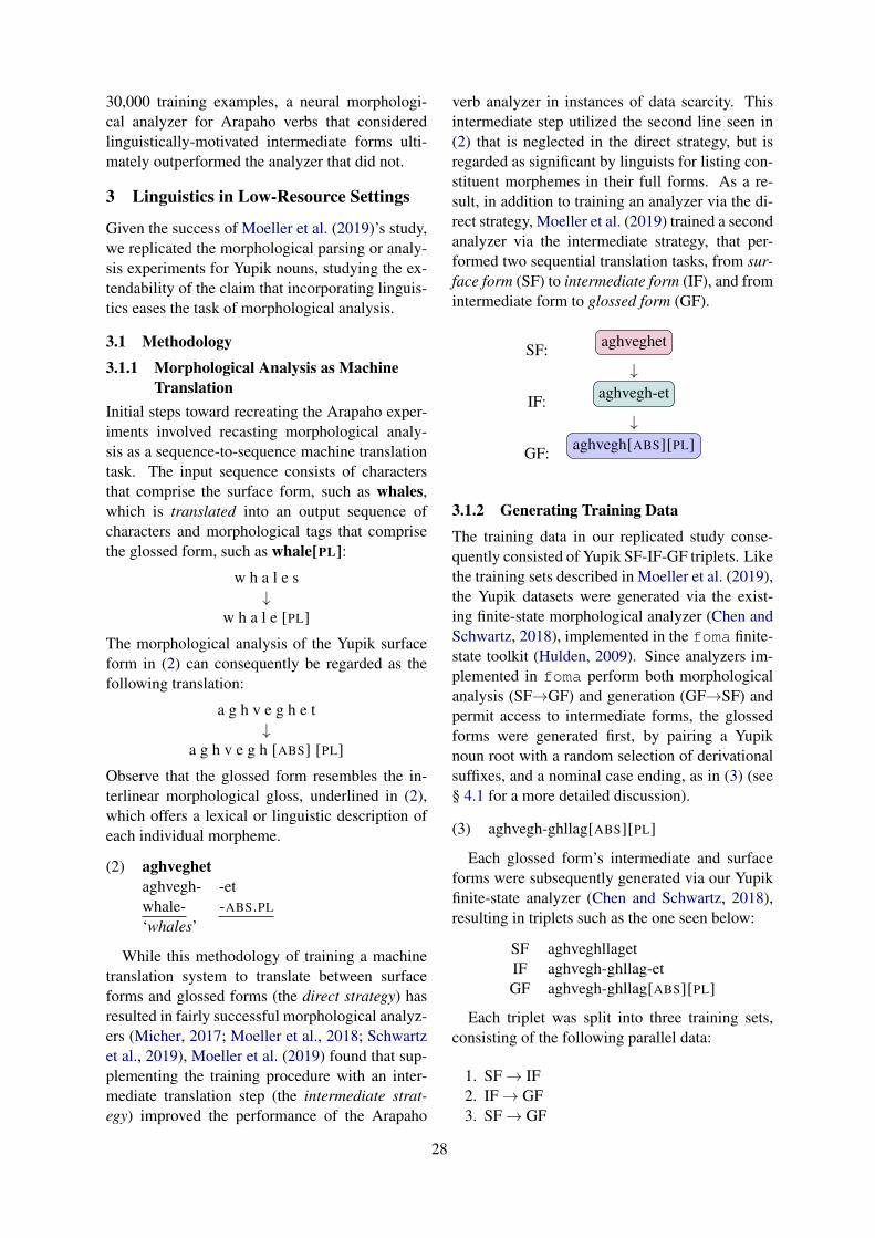
30,000 training examples, a neural morphologi-cal analyzer for Arapaho verbs that consideredlinguistically-motivated intermediate forms ulti-mately outperformed the analyzer that did not.

3 Linguistics in Low-Resource Settings

Given the success of Moeller et al. (2019)’s study,we replicated the morphological parsing or analy-sis experiments for Yupik nouns, studying the ex-tendability of the claim that incorporating linguis-tics eases the task of morphological analysis.

3.1 Methodology3.1.1 Morphological Analysis as Machine

TranslationInitial steps toward recreating the Arapaho exper-iments involved recasting morphological analy-sis as a sequence-to-sequence machine translationtask. The input sequence consists of charactersthat comprise the surface form, such as whales,which is translated into an output sequence ofcharacters and morphological tags that comprisethe glossed form, such as whale[PL]:

w h a l e s↓

w h a l e [PL]

The morphological analysis of the Yupik surfaceform in (2) can consequently be regarded as thefollowing translation:

a g h v e g h e t↓

a g h v e g h [ABS] [PL]

Observe that the glossed form resembles the in-terlinear morphological gloss, underlined in (2),which offers a lexical or linguistic description ofeach individual morpheme.

(2) aghveghetaghvegh- -etwhale- -ABS.PL

‘whales’

While this methodology of training a machinetranslation system to translate between surfaceforms and glossed forms (the direct strategy) hasresulted in fairly successful morphological analyz-ers (Micher, 2017; Moeller et al., 2018; Schwartzet al., 2019), Moeller et al. (2019) found that sup-plementing the training procedure with an inter-mediate translation step (the intermediate strat-egy) improved the performance of the Arapaho

verb analyzer in instances of data scarcity. Thisintermediate step utilized the second line seen in(2) that is neglected in the direct strategy, but isregarded as significant by linguists for listing con-stituent morphemes in their full forms. As a re-sult, in addition to training an analyzer via the di-rect strategy, Moeller et al. (2019) trained a secondanalyzer via the intermediate strategy, that per-formed two sequential translation tasks, from sur-face form (SF) to intermediate form (IF), and fromintermediate form to glossed form (GF).

SF: aghveghet

↓

IF: aghvegh-et

↓

GF: aghvegh[ABS][PL]

3.1.2 Generating Training Data

The training data in our replicated study conse-quently consisted of Yupik SF-IF-GF triplets. Likethe training sets described in Moeller et al. (2019),the Yupik datasets were generated via the exist-ing finite-state morphological analyzer (Chen andSchwartz, 2018), implemented in the foma finite-state toolkit (Hulden, 2009). Since analyzers im-plemented in foma perform both morphologicalanalysis (SF→GF) and generation (GF→SF) andpermit access to intermediate forms, the glossedforms were generated first, by pairing a Yupiknoun root with a random selection of derivationalsuffixes, and a nominal case ending, as in (3) (see§ 4.1 for a more detailed discussion).

(3) aghvegh-ghllag[ABS][PL]

Each glossed form’s intermediate and surfaceforms were subsequently generated via our Yupikfinite-state analyzer (Chen and Schwartz, 2018),resulting in triplets such as the one seen below:

SF aghveghllagetIF aghvegh-ghllag-etGF aghvegh-ghllag[ABS][PL]

Each triplet was split into three training sets,consisting of the following parallel data:

1. SF → IF2. IF → GF3. SF → GF

28

The first two sets were used to train the analyzervia the intermediate strategy, and the last set wasused to train the analyzer that adhered to the di-rect strategy. Lastly, whereas Moeller et al. (2019)developed training sets consisting of 14.5K, 18K,27K, 31.5K, and 36K examples, the Yupik train-ing sets varied from 1K to 20K examples in incre-ments of 5000, to more realistically represent thelow-resource setting of Yupik.

3.1.3 Training ParametersFor training, each parallel dataset was tokenizedby character and randomly partitioned into a train-ing set, a validation set, and a test set in a 0.8 /0.1 / 0.1 ratio. The two analyzers trained on eachof these datasets were then implemented as bidi-rectional recurrent encoder-decoder models withattention (Schuster and Paliwal, 1997; Bahdanauet al., 2014) in the Marian Neural Machine Trans-lation framework (Junczys-Dowmunt et al., 2018).We used the default parameters of Marian, de-scribed in Sennrich et al. (2016), where the en-coder and decoder consisted of one hidden layereach, and the model was trained to convergencevia early stopping and holdout cross validation.

3.2 Results

0 5 10 15 20 250

25

50

75

100

Training Examples (in thousands)

Acc

urac

y(%

)

SF-IF-GFSF-GF

Figure 1: Accuracy scores of the analyzers trainedon the intermediate and direct strategies, for all fivedatasets

The two trained analyzers for each dataset wereevaluated on identical held-out test sets in order tocompare their performances. As illustrated in Fig-ure 1, it was only in the lowest data setting thatthe intermediate strategy outperformed the directstrategy with respect to accuracy. In all other in-

stances, the direct strategy emerged as the bettertraining methodology.

We speculate that this disparity in our resultsand that of Moeller et al. (2019) is due to differ-ences in the morphophonological systems of Ara-paho and Yupik and their effects on spelling. Ara-paho’s morphophonology, in particular, can radi-cally alter the spelling of morphemes in the GFversus SF of a given word, as seen below (Moelleret al., 2019). It is possible that the intermediatestep consequently assists the Arapaho analyzer inbridging this orthographical gap.

SF nonoohobeenIF noohoweenGF [VERB][TA][ANIMATE-OBJECT]

[AFFIRMATIVE][PRESENT][IC]noohow[1PL-EXCL-SUBJ][2SG-OBJ]

In Yupik, however, there is considerably lessvariation in the spelling (see § 3.1.2). This maymean the addition of the intermediate step in theYupik analyzer only creates more room for error,and the direct strategy fares better as a result.

Though the results of our replicated study seemto point to the expendability of linguistics for thetask of morphological analysis, calculating theLevenshtein distances between the incorrect out-puts of each analyzer and their gold standard out-puts offers a novel interpretation.

For every morphological analysis flagged as in-correct, its Levenshtein distance to the correctanalysis was calculated, and all such distanceswere averaged for each analyzer (see Figure 2).

0 5 10 15 200

5

10

15

20

25

Training Examples (in thousands)

Lev

ensh

tein

Dis

tanc

e

SF-IF-GFSF-GF

Figure 2: Average Levenshtein distances of the analyz-ers trained on the intermediate and direct strategies, forall five datasets

29

(4) nunivagseghatnunivagseghagh- -ttundra.vegetation- -ABS.PL

‘tundra vegetation’ (Nagai, 2001, p.60)

(5) SivuqaghhmiinguungaSivuqagh- -mii- -ngu- -u- -ngaSt. Lawrence Island- -resident.of- -to.be. -INTR.IND- -1SG

‘I am a St. Lawrence Islander’ (Jacobson, 2001, p.42)

(6) ilughaghniighunneghtughllagyalghiitilughagh- -niigh- -u- -negh- -tu- -ghllag- -yalghii- -tcousin- -tease- -do- -very.many- -do.habitually- -very- -INTR.PTCP OBL- -3PL

‘Many cousins used to teach each other a lot’ (Apassingok et al., 1993, p.47)

We found that the average Levenshtein distancefor the analyzer trained on the intermediate strat-egy was statistically less than that of the directstrategy analyzer (p < 0.0001), with the excep-tion of the lowest data setting. At 15K and 20Ktraining examples, for instance, the average Lev-enshtein distances differed by nearly 10 or 11 op-erations. Furthermore, there did not appear to be astatistically significant difference in the complex-ity of the analyses being flagged as incorrect; thedirect strategy was just as likely as the intermedi-ate strategy to misanalyze simple words with oneor two derivational suffixes.

The shorter Levenshtein distances suggest thatthe analyzers trained on the intermediate strategyconsistently returned analyses that better resem-bled the correct answers as compared to their di-rect strategy counterparts. Therefore, even thoughthe direct strategy proved superior to the interme-diate strategy with respect to general accuracy, theoutputs of the intermediate strategy may be morevaluable to students of Yupik who are more relianton the neural analyzer for an initial parse.

4 Linguistics in High-Resource Settings

The replicated study suggests that the accuracyof the analyzer is proportional to the quantity oftraining examples, especially for the direct strat-egy, as evidenced in Figure 1. Additional experi-ments demonstrated, however, that even using thefinite-state analyzer to generate as many as 10 mil-lion training examples resulted in the accuracy ofthe neural analyzer plateauing around 88.77% fortypes and 87.19% for tokens on a blind test setthat encompassed 659 types and 796 tokens re-

spectively. This raises the question as to whether itis possible to improve the neural analyzer to com-petitive accuracy scores above 90% by reinforcingthe direct strategy with aspects of Yupik linguis-tics whose effects have yet to be explored. Thus,the remainder of this proposal introduces these lin-guistic aspects and suggests means of integratingthem into the high-resource implementation of theneural analyzer.

4.1 Integrating Yupik Morphology

One aspect of Yupik that may be useful is its wordstructure, which typically adheres to the followingtemplate, where ( ) denotes optionality:

Root + (Derivational Suffix(es)) + InflectionalSuffix(es) + (Enclitic)

Most roots can be identified as common nounsor verbs and are responsible for the most morpho-logically complex words in the language, as theyare the only roots that can take derivational suf-fixes. Moreover, all derivational morphology issuffixing in nature, and Yupik words may haveanywhere from zero to seven derivational suffixes,with seven being the maximum that has been at-tested in Yupik literature (de Reuse, 1994). Lastly,there are two types of inflection in Yupik: nominalinflection and verbal inflection.

This word structure consequently results inYupik words of varying length as well as varyingmorphological complexity (see (4), (5), and (6)),which in turn constitutes ideal conditions for cur-riculum learning.

Curriculum learning, with respect to machinelearning, is a training strategy that “introduces dif-

30

ferent concepts at different times, exploiting previ-ously learned concepts to ease the learning of newabstractions” (Bengio et al., 2013). As such, “sim-ple” examples are presented in the initial phasesof training, with each phase introducing examplesthat are progressively more complex than the last,until the system has been trained on all phases, thatis, the full curriculum.

The morphological diversity of Yupik words isnaturally suited for curriculum learning, and maypositively impact the accuracy of the neural ana-lyzer. One proposed experiment of this paper is torestructure the training dataset, such that the neu-ral analyzer is trained on the simplest Yupik wordsfirst, that is, those words consisting of an inflectedroot with zero derivational suffixes. Each suc-cessive phase introduces words with an additionalderivational suffix, until the last phase presents themost morphologically complex words attested inthe language.

4.2 Integrating Yupik Morphophonology

A second aspect of Yupik linguistics that may beintegrated is its complex morphophonological rulesystem. In particular, the suffixation of deriva-tional and inflectional morphemes in Yupik is con-ditioned by morphophonological rules that applyat each morpheme boundary and obscure them,rendering a surface form that may be unrecogniz-able from the glossed form, as in (7):

(7) kaanneghituqkaate- -nghite- -u- -qarrive- -did.not- -INTR.IND- -3SG

‘he/she did not arrive’ (Jacobson, 2001, p.43)

Moreover, each morphophonological rule hasbeen assigned an arbitrary symbol in the Yupikliterature (Jacobson, 2001), and so, every deriva-tional and inflectional suffix can be written with allof the rules associated with it, as in (8). Here, @modifies root-final -te, – deletes root-final conso-nants, ∼f deletes root-final -e, and (g/t) designatesallomorphs that surface under distinct phonologi-cal conditions.

(8) kaanneghituqkaate- -@–nghite- -∼f(g/t)u- -qarrive- -did.not- -INTR.IND- -3SG

‘he/she did not arrive’ (Jacobson, 2001, p.43)

A second proposed experiment will conse-quently explore the potential insight provided by

including these morphophonological symbols inthe training examples, studying whether the sym-bols facilitate learning of the surface form toglossed form mapping or whether these additionalcharacters actually introduce noise. Since mini-mal pairs do exist to differentiate the phonolog-ical conditions under which each symbol applies(see (9)), inclusion of the symbols may in fact as-sist the system in learning the morphophonologi-cal changes that are induced by certain suffixes.

(9) nuna–ghllak → nunaghllakqulmesiite–ghllak → qulmesiiteghllakanyagh–ghllak → angyaghllaksikig–ghllak → sikigllakkiiw–ghllak → kiiwhllagek

Lastly, Yupik morphophonology may also be in-tegrated into a curriculum learning training strat-egy, where separating the “easy-to-learn” trainingexamples from the “hard-to-learn” training exam-ples can be accomplished in the following ways:

1. Quantifying the number of morphophonolog-ical rules associated with a given morpheme,such that the simplest training examples en-compass all suffixes with zero symbols at-tached, such as -ni ‘the smell of; the odorof; the taste of ’ (Badten et al., 2008, p.658).Subsequent phases successively increase thisquantity by one.

2. Ranking the morphophonological rules them-selves by difficulty, such that the initial phaseintroduces Yupik suffixes with the rules thathave been deemed “easiest to learn”, whilefuture phases gradually introduce those thatare “harder to learn” 1.

5 Presenting A Holistic Experiment

In summary, the objective of this proposed re-search is to utilize aspects of the Yupik language toreinforce the direct strategy in high-resource set-tings, guiding how the training examples are struc-tured and the nature of their content. Previoussections share possible ways in which these lin-guistic elements of Yupik may be taken into ac-count, but they can in fact be integrated into a sin-gle holistic experiment that trains multiple analyz-ers with varying degrees of linguistic information.

1A difficulty ranking was elicited from a single studentduring fieldwork conducted in March 2019, as most Yupikstudents had not yet mastered the symbols and the rules theyrepresented.

31

In particular, we propose developing several setsof training data with the following characteristics:

1. Includes the morphophonological symbols(§ 4.2)

2. Ranks the training examples with respect tothe number of morphemes (§ 4.1)

3. Ranks the training examples with respect tothe number of morphophonological symbolsper morpheme (§ 4.2)

4. Ranks the training examples with respect tothe learning difficulty of the symbols (§ 4.2)

Each training dataset will incorporate as manyor as few of these characteristics as desired, fora total of 15 datasets (

(44

)+

(43

)+

(42

)+

(41

)),

and by extension, 15 neural analyzers. We expectany training set that involves morphophonologicalsymbols to improve upon the existing analyzer’sability to distinguish between otherwise homo-graphic suffixes, often a point of confusion. Tak-ing morpheme count into consideration may alsoimprove the analyzer’s handling of words with rel-atively few derivational suffixes (∼0-3), leavingthe bulk of errors to instead comprise the mostmorphologically complex words. Furthermore, byvirtue of training on an organized dataset ratherthan a randomly selected one, we predict that theanalyzer will be exposed to a much more equaldistribution of Yupik roots and suffixes. It shouldthen be less likely than it is now to invent rootsand suffixes that conform morphophonologically,but do not actually exist in the attested lexicon.Lastly, the performance of these analyzers can becompared to the performance of a baseline system,that is simply trained on the direct strategy with-out any morphophonological symbols or structureto its training data.

6 Conclusion

Moeller et al. (2019) and the replicated study forYupik presented herein suggest that the use of lin-guistics can positively impact the performances ofneural morphological analyzers, at least in lowerresource settings. The proposed research, how-ever, seeks to extend this observation to any datasetting, and explore the effects of incorporatingvarying degrees of linguistic information in thetraining data, in hopes of shedding light on howbest to approach to the task of morphological anal-ysis via machine learning.

Acknowledgments

Portions of this work were funded by NSF Doc-umenting Endangered Languages Grant #BCS1761680, and a University of Illinois GraduateCollege Illinois Distinguished Fellowship. Specialthanks to the Yupik speakers who have shared theirlanguage and culture with us.

ReferencesAnders Apassingok, (Iyaaka), Jessie Uglowook,

(Ayuqliq), Lorena Koonooka, (Inyiyngaawen), andEdward Tennant, (Tengutkalek), editors. 1993.Kallagneghet / Drumbeats. Bering Strait SchoolDistrict, Unalakleet, Alaska.

Linda Womkon Badten, Vera Oovi Kaneshiro,Marie Oovi, and Christopher Koonooka. 2008.St. Lawrence Island / Siberian Yupik Eskimo Dictio-nary. Alaska Native Language Center, Universityof Alaska Fairbanks.

Dzmitry Bahdanau, Kyunghyun Cho, and Yoshua Ben-gio. 2014. Neural machine translation by jointlylearning to align and translate. arXiv preprintarXiv:1409.0473.

Emily M. Bender. 2013. Linguistic Fundamentals forNatural Language Processing: 100 Essentials fromMorphology and Syntax. Morgan & Claypool Pub-lishers.

Yoshua Bengio, Aaron Courville, and Pascal Vincent.2013. Representation learning: A review and newperspectives. IEEE Transactions on Pattern Analy-sis and Machine Intelligence, 35(8):1798–1828.

Emily Chen and Lane Schwartz. 2018. A morpho-logical analyzer for St. Lawrence Island / Cen-tral Siberian Yupik. In Proceedings of the 11thLanguage Resources and Evaluation Conference,Miyazaki, Japan.

Mans Hulden. 2009. Foma: A finite-state compiler andlibrary. In Proceedings of the 12th Conference ofthe European Chapter of the Association for Com-putational Linguistics, pages 29–32. Association forComputational Linguistics.

Steven A. Jacobson. 2001. A Practical Grammar of theSt. Lawrence Island / Siberian Yupik Eskimo Lan-guage, Preliminary Edition, 2nd edition. Alaska Na-tive Language Center, Fairbanks, Alaska.

Mark Johnson. 2011. How relevant is linguistics tocomputational linguistics? Linguistic Issues in Lan-guage Technology, 6.

Marcin Junczys-Dowmunt, Roman Grundkiewicz,Tomasz Dwojak, Hieu Hoang, Kenneth Heafield,Tom Neckermann, Frank Seide, Ulrich Germann,Alham Fikri Aji, Nikolay Bogoychev, Andre F. T.

32

Martins, and Alexandra Birch. 2018. Marian: Fastneural machine translation in C++. In Proceedingsof ACL 2018, System Demonstrations, pages 116–121, Melbourne, Australia. Association for Compu-tational Linguistics.

Jeffrey Micher. 2017. Improving coverage of an inuk-titut morphological analyzer using a segmental re-current neural network. In Proceedings of the 2ndWorkshop on the Use of Computational Methods inthe Study of Endangered Languages, pages pp. 101–106, Honolulu. Association for Computational Lin-guistics.

Sarah Moeller, Ghazaleh Kazeminejad, Andrew Cow-ell, and Mans Hulden. 2018. A neural morpholog-ical analyzer for Arapaho verbs learned from a fi-nite state transducer. In Proceedings of the Work-shop on Computational Modeling of PolysyntheticLanguages, Santa Fe, New Mexico. Association forComputational Linguistics.

Sarah Moeller, Ghazaleh Kazeminejad, Andrew Cow-ell, and Mans Hulden. 2019. Improving low-resource morphological learning with intermediateforms from finite state transducers. Proceedings ofthe Workshop on Computational Methods for En-dangered Languages: Vol. 1.

Kayo Nagai. 2001. Mrs. Della Waghiyi’s St. LawrenceIsland Yupik Texts with Grammatical Analysis.Number A2-006 in Endangered Languages of thePacific Rim. Nakanishi Printing, Kyoto, Japan.

Victor Raskin. 1987. Linguistics and natural languageprocessing. Machine Translation: Theoretical andMethodological Issues, pages 42–58.

Willem J. de Reuse. 1994. Siberian Yupik Eskimo —The Language and Its Contacts with Chukchi. Stud-ies in Indigenous Languages of the Americas. Uni-versity of Utah Press, Salt Lake City, Utah.

Mike Schuster and Kuldip K. Paliwal. 1997. Bidirec-tional recurrent neural networks. IEEE Transactionson Signal Processing, 45(11):2673–2681.

Lane Schwartz, Emily Chen, Sylvia Schreiner, andBenjamin Hunt. 2019. Bootstrapping a neural mor-phological analyzer for St. Lawrence Island Yupikfrom a finite-state transducer. Proceedings of theWorkshop on Computational Methods for Endan-gered Languages: Vol. 1.

Rico Sennrich, Barry Haddow, and AlexandraBirch. 2016. Edinburgh neural machine trans-lation systems for WMT 16. arXiv preprintarXiv:1606.02891.

33

Proceedings of the 57th Annual Meeting of the Association for Computational Linguistics: Student Research Workshop, pages 34–42Florence, Italy, July 28 - August 2, 2019. c©2019 Association for Computational Linguistics

Not All Reviews are Equal:Towards Addressing Reviewer Biases for Opinion Summarization

Wenyi TayRMIT University, AustraliaCSIRO Data61, Australia

wenyi.tay@student.rmit.edu.au

Abstract

Consumers read online reviews for insightswhich help them to make decisions. Giventhe large volumes of reviews, succinct reviewsummaries are important for many applica-tions. Existing research has focused on miningfor opinions from only review texts and largelyignores the reviewers. However, reviewershave biases and may write lenient or harsh re-views; they may also have preferences towardssome topics over others. Therefore, not all re-views are equal. Ignoring the biases in reviewscan generate misleading summaries. We aimfor summarization of reviews to include bal-anced opinions from reviewers of different bi-ases and preferences. We propose to model re-viewer biases from their review texts and rat-ing distributions, and learn a bias-aware opin-ion representation. We further devise an ap-proach for balanced opinion summarization ofreviews using our bias-aware opinion repre-sentation.

1 Introduction

Consulting online reviews on products or servicesis popular among consumers. Opinions in re-views are scrutinised to make an informed deci-sion on which product to buy, what service to use,or which point-of-interest to visit. An opinionis a view or judgment formed about something,not necessarily based on fact or knowledge.1 Inthe context of online reviews, opinions contain in-formation about the target (“something”) and thesentiment (“view or judgment”) that is associatedwith it. There can also be more than one opinionin a review.

Opinion mining research is dedicated to tasksthat involves opinions (Pang and Lee, 2008). Cur-rent research in opinion mining mostly focuses

1Oxford dictionary

only on review texts. Some key tasks include sen-timent polarity classification (Hu and Liu, 2004b)at levels of words, sentences or documents, andopinion target (e.g., aspect) identification and clas-sification.

Opinion summarization from reviews is an im-portant task related to opinion mining. Early workon opinion summarization aims for structured rep-resentation of aspect-sentiment pairs (Hu and Liu,2004a), where the positive and negative sentimentfor each aspect are extracted from review texts andaggregated. Opinion summaries in natural lan-guage texts contain richer, detailed description ofopinions and are easier for end users to under-stand. Existing studies mainly use the review textsfor summarization.

However, reviewers are unique individuals withbeliefs and preferences. Reviewers have prefer-ences towards certain aspects, for example ser-vice or cleanliness in hotel reviews (Wang et al.,2010). Different reviewers can have different waysof expressing their opinions (Tang et al., 2015b).Also, some reviewers are lenient in their assess-ment of products or services, while others areharsher (Lauw et al., 2012). Overall, an opinionis a reflection of the reviewer as it encompassestheir biases. Thus, not all reviews are equal.

Depending on the application, biases capturedin the reviews can be amplified. Hu et al. (2006)suggest that reviewers write reviews when they areextremely satisfied or when they are extremely up-set. Existing summarization techniques often treatall reviews equally by selecting salient opinionswhich may not necessarily be representative fordifferent reviewers. We aim to compensate for bi-ases in reviews, especially for review summariza-tion. We focus on the following research ques-tions:

1. How to model a reviewer’s bias? What in-

34

formation from a reviewer should be used tomodel a reviewer’s bias?

2. How to learn a representation for reviews thatcaptures reviewer biases as well as the opin-ion?

3. How to generate a balanced opinion summaryof reviews written by different reviewers?

Below, we outline the relevant past studies as wellas our our research proposal to address these ques-tions.

2 Related Work

Our research is related to two research areas sum-marized below.

2.1 Opinion and Reviewer ModelingWe identified two studies that jointly model opin-ions and reviewers. Wang et al. (2010) investi-gate the problem of decomposing the overall re-view rating into aspect ratings using a hotel do-main dataset. The authors model opinions and re-viewers using a generative approach. Reviewersare modeled to reflect their individual emphasis onvarious aspects. The authors demonstrate that de-spite giving the same overall review rating, tworeviewers can value and rate aspects differently.Meanwhile, Li et al. (2014) present a topic modelincorporating reviewer and item information forsentiment analysis. Through probabilistic matrixfactorisation of reviewer-item matrix, the latentfactors are included in a supervised topic modelguided by sentiment labels. The proposed modeloutperforms baselines in predicting the sentimentlabel given the review text, reviewer and item on amovie review dataset and a microblog dataset.

Opinion modeling Opinion can be representedas a aspect-sentiment tuple (Hu and Liu, 2004b).In order to obtain the components of the opinion,aspect identification and sentiment classificationare key. Both tasks can be treated separately orcombined. For aspect identification, aspects canbe identified with the help of experts (Hu and Liu,2004b; Zhang et al., 2012). The drawback is that itrequires input from experts and is specific to a do-main. This triggered studies that seek to discoveraspects in an unsupervised manner using topicmodels (Brody and Elhadad, 2010; Moghaddamand Ester, 2010). However, such methods may notalways produce interpretable aspects. Subsequent

models are developed to discover interpretable as-pects (McAuley and Leskovec, 2013; Titov andMcDonald, 2008a,b). To determine opinion polar-ity, lexicon-based (Hu and Liu, 2004b) and clas-sification (Dave et al., 2003) approaches are of-ten used. However, modeling opinions based onaspects and sentiment separately is not sufficientas the sentiment words can depend on the aspect.More recent models focus on incorporating con-text to model opinions. Such approaches includejoint aspect-sentiment models (Lin and He, 2009),word embeddings (Maas et al., 2011), and neuralnetwork models (He et al., 2017).

Alternatively, opinions can potentially be repre-sented as a high-dimensional vector. Opinion rep-resentation in this form is a relatively unexploredspace. However, in the closely related area ofsentiment classification, sentences and documentsare represented as vectors to be used as inputs forclassification (Conneau et al., 2017; Tang et al.,2015a). The idea is to model a sequence of wordsas a high-dimensional vector that captures the re-lationships of words. Similarly, opinions are se-quences of sentences, thus it is appropriate to buildon the work in sentence and document representa-tion. One of the earliest work is an extension ofword2vec (Mikolov et al., 2013) to learn a dis-tributed representation of text (Le and Mikolov,2014). More recently, pre-trained sentence en-coders trained on a large general corpus aim tocapture task-invariant properties that can be fine-tuned for downstream tasks (Cer et al., 2018; Con-neau et al., 2017; Kiros et al., 2015). On anotherfront, progress in context-aware embeddings (Pe-ters et al., 2018) and pre-trained language mod-els (Devlin et al., 2018; Howard and Ruder, 2018)provide other options to capture context that canbe used to obtain sequence representation. Allthese studies focus on encoding topical semanticsof text sequences, where opinions are not explic-itly modeled.

Reviewer modeling Various reviewer charac-teristics that are modeled include expertise (Liuet al., 2008), reputation (Chen et al., 2011; Shaalanand Zhang, 2016), characteristics of languageuse (Tang et al., 2015b) and preferences (Zhenget al., 2017). Some of these modelings areachieved using reviewer aggregated statistics andreview meta-data. Reviewer expertise is modeledby number of reviews, where larger number of re-views suggests higher expertise (Liu et al., 2008).

35

Reviewer reputation can be modeled by the num-ber of helpfulness votes and total votes received bythe reviewer. A higher ratio of helpfulness votesto total votes suggests a better reputation (Shaalanand Zhang, 2016). In another reviewer reputa-tion model, reviewers are modeled to have domainexpertise which corresponds to the product cate-gories that the reviewer reviewed on (Chen et al.,2011).

Review text is also used in reviewer model-ing. When predicting ratings from review text,the same sentiment bearing word, for example“good”, can mean different sentiment intensity todifferent reviewers. Tang et al. (2015b) model re-viewers’ word use by using review text and its cor-responding review rating. The resulting reviewer-modified word representations capture variationsin reviewers’ word use that translates to betterrating prediction. Recently, review text is usedin addition to review ratings to model users anditems together for recommendation (Zheng et al.,2017). Using all the reviews written by the re-viewer, the model learns a latent representation ofthe reviewer. All the above approaches focus onmodeling the reviewer. However, our focus is tomodel opinions, where reviewer information is tobe used as a factor during the process of modeling.

For our proposed work, we explore using reviewtext, review ratings and meta data to model review-ers except for helpfulness votes. The helpfulnessmechanism is shown to be biased (Liu et al., 2007)and it is still not well understood what we can inferfrom such votes (Ocampo Diaz and Ng, 2018).

2.2 Opinion Summarization

Opinion summarization aims to capture salientopinions within a collection of document, in ourcase online reviews. Key challenges in summariz-ing opinions from a collection of documents arehighlighted by Pang and Lee (2008): (1) How toidentify documents and parts of the document thatare of the same opinion; and (2) How to decide twosentences or texts have the same semantic mean-ing.

To identify documents and parts of documentsof the same opinion, one strategy is to use re-view ratings as a means to identify similar opin-ion. However, review ratings have drawbacks suchas rating scales differ for different review sources,different assessment criteria among reviewers andreviewers may not share the same opinion despite

giving the same overall rating. Review ratings canbe adjusted to correct for different assessment cri-teria by comparing the reviewers’ rating behaviourrelative to the community rating behaviour (Lauwet al., 2012; Wadbude et al., 2018). The reviewrating only captures the overall sentiment polarityof the review but not the individual opinions thatmake up the review. As such, the authors proposeto decompose the review rating into aspect ratingsaccording to the review text (Wang et al., 2010).Alternatively, the same opinions can be found bymining aspects and sentiment polarity of each re-view. Opinion summarization can be seen as a taskthat builds on top of the opinion mining task.

In deciding if two sentences or texts have thesame semantic meaning, the crux lies in the rep-resentation of sentences and text. Sentences withthe same meaning have good overlap in words(Ganesan et al., 2010). More recent approachesadopt representing sentences or texts as high-dimensional vectors such that similar represen-tations have similar meaning (Le and Mikolov,2014; Tang et al., 2015a).

The presentation of the opinion summary de-pends on two considerations, (1) the needs of thereader; and (2) the approach to construct opin-ion summaries. An opinion summary can be pre-sented in different ways, catering to the differ-ent needs of readers. The summary can be onone product (Angelidis and Lapata, 2018; Hu andLiu, 2004a), comparing two products (Sipos andJoachims, 2013) or generate a summary in re-sponse to a query (Bonzanini et al., 2013).

There are two main ways of constructing opin-ion summaries. The extractive opinion summariesare summaries put together by selecting sentencesor word segments (Angelidis and Lapata, 2018;Xiong and Litman, 2014). For abstractive sum-maries, the summary is generated from scratch(Ganesan et al., 2010; Wang et al., 2010).

An early work in opinion summarization pro-posed an aspect-based summary by organising allopinions according to aspects and their sentimentpolarity (Hu and Liu, 2004a). Although there is notextual summarization involved, it inspired futurework to focus on including aspects into the gen-erated summary regardless whether it is extractiveor abstractive.

For extractive summarization, the objective isto identify salient sentences, at the same time re-ducing redundancy in the selected sentences. An-

36

gelidis and Lapata (2018) score opinion segmentsaccording to the aspect and the sentiment polar-ity. In another work, sentences in the review arescored according to a combination of textual fea-tures and latent topics discovered by helpfulnessvotes (Xiong and Litman, 2014). To reduce re-dundancy in selected sentences, a greedy algo-rithm can be applied to add one sentence at a timeto form the summary. The greedy algorithm im-poses the criterion that the selected sentence mustbe different from the sentences that are alreadyin the summary (Angelidis and Lapata, 2018).As most extractive summarization techniques areclosely coupled with identifying opinions from re-view texts, the outcome is a set of sentences thatare salient in terms of topic coverage, but they maynot necessarily be the most representative opinionsfrom reviewers.

On the other hand, abstractive methods firstlearn to identify the salient opinions before gen-erating a shorter text to reflect the opinion. Agraph-based method is proposed by Ganesan et al.(2010) which models a word with its Part-of-Speech (POS) tag as nodes and directed edges torepresent the order of words. The edge weightsincreases when the sequence of words is repeated.The summary is generated by capturing the pathswith high edge weights. In a recent study, anencoder-decoder network is employed to generatean abstractive summary of movie reviews (Wangand Ling, 2016).

3 Proposed Methodology

The intuition for our research is that summariza-tion techniques that rely on similarity betweenopinions to identify salient opinions benefit fromclustering similar opinions together and separat-ing different opinions into different clusters. Bymodeling reviewers with opinions, we aim to cap-ture biases reviewers bring into their opinions. Wenext elaborate our approaches to modeling user bi-ases, learning bias-aware opinion representationsand balanced opinion summarization.

3.1 Bias-Aware Opinion Representation

To achieve a bias-aware opinion representation,we model opinions and reviewer biases for eachsentence in a review. We assume that one sentencecontains one opinion (Hu and Liu, 2004b). Weenvision two possible approaches to learn a bias-aware opinion representation: (1) Two-step pro-

cess by modeling opinions then adjust the opinionsaccording to reviewer biases; and, (2) Generativeapproach using text, rating and reviewer informa-tion.

Using a two-step process, our main objective isto first learn a representation of the sentences tocapture the opinion and this is not a trivial task.Ideally, we expect our opinion representation toexhibit two key characteristics: (1) Similar opin-ions need to be close in its representation. Us-ing opinions for restaurant reviews as an exam-ple, “The soup is rich and creamy” and “Deliciousfood” are similar opinions but expressed differ-ently; and, (2) Opinion models should be able totease apart different opinions.

In terms of representing opinions that are simi-lar, a promising technology for us is to make use ofpre-trained sentence encoders and language mod-els (Cer et al., 2018; Devlin et al., 2018; Peterset al., 2018; Conneau et al., 2017). These pre-trained models have the advantage of transferringthe learned information from large corpora. How-ever, we hypothesize that even with the use ofpre-trained models, we are unable to capture sen-timent polarity of opinions accurately. It will besimilar to the problem that word embeddings arenot able to capture sentiment polarity (Maas et al.,2011). One potential direction is to adopt super-vised learning using labeled aspect and sentimentpolarity labels to improve our opinions represen-tation. But labeled data is expensive to acquireand the granularity of aspect can vary with differ-ent aspect annotation guidelines. We propose touse review ratings as supervision signal to improveour opinion representation as ratings can provide aguide to sentiment polarity of opinions.

Towards learning bias-aware opinion represen-tations, we further refine the learnt opinion vec-tors via modeling reviewer biases from their re-views and ratings. Reviewer biases can influencetheir star rating and textual expressions. The keyto model reviewer biases is learning a distributionof latent factors and sentiment polarity from thereviews and their rating distributions for the re-viewer. The refinement will be a user matrix thatlearn weights corresponding to the opinion repre-sentation. This can also be seen as the matrix thatrepresents the biases of reviewers. We plan to ex-plore different ways to learn this matrix. One op-tion to model reviewers’ biases is to learn repre-sentations from their past reviews such as using

37

techniques in recommender systems literature tomodel reviewers using review text (Zheng et al.,2017). Alternatively, other associated review in-formation such as review ratings and even meta-data of reviews can possibly guide the modelingof biases. We can also explore textual features ofreview such as the position of opinions may alsoprovide clues to model reviewers.

For our second possible approach, we adopt agenerative approach to model opinions as topicsusing reviewer information as latent factors (Liet al., 2014; Wang et al., 2010). However, the topicmodel approach is restricted to using words as to-kens. The neural topic model (Cao et al., 2015) isa potential technique to utilise word embeddingsto improve the learning of topics in the collectionof reviews.

3.2 Balanced Opinion Summarization

Summaries generated by the existing summariza-tion techniques are accurate to the collection ofreviews it summarizes. They are not a reflectionof the true opinion towards the product. In viewthat opinions capture reviewer biases, we proposea novel way of summarizing opinions.

Instead of the usual summary that is presentedas a paragraph of selected sentences, we are in-spired by the work of Paul et al. (2010) and Wanget al. (2010), where opposing opinions are con-trasted. We propose a balanced opinion summary,where we summarize and contrast the opinionsof reviewers having different biases. For exam-ple, we contrast opinions of a reviewers who arelenient against reviewers who are critical. Thisallows us to present a balanced summary to thereader. The biases can be latent factors that willbe discovered during the modeling process.

We propose to achieve a balanced summarythat selects salient opinions from reviewers withdifferent biases. We hypothesize that the bias-aware opinion representation will form clustersof similar opinions from reviewers with similarbiases. Building on a graph-based approach tosummarization like LexRank (Erkan and Radev,2004) and Yin and Pei (2015), opinions can berepresented as nodes and edges as the similaritybetween bias-aware opinion representation. Thedensity of the graph can be adjusted by the similar-ity threshold imposed on the graph. The saliencyof the opinions can then be obtained by apply-ing PageRank on the graph. In doing so, we

also model the similar opinions that signals agree-ment or consensus among reviewers. After rank-ing opinions based on its salience, we can utilisea diversity objective through a greedy approachor Maximal Marginal Relevance (MMR) to selectsalient opinions that are different.

4 Evaluation

Datasets Suitable datasets in the restaurant do-main for our research questions are: (1) NY citysearch (Ganu et al., 2013); (2) SemEval 2016ABSA Restaurant Reviews in English (Pontikiet al., 2016); and, (3) Yelp dataset challenge2. Alldatasets contain user ID, product ID, review textand review rating, which will allow us to modelopinions. In addition, datasets (1) and (2) arelabeled with aspect and sentiment polarity. Al-though we choose to work in the restaurant do-main for our proposed work, our models are notdomain-specific. Other potential review datasetsare on product and hotel reviews (McAuley et al.,2015; Wang et al., 2010).

We approach evaluation in a two part process.First, we evaluate our proposed model on howwell it learns a representation of opinion sentence.Next, we compare summaries generated with ourbias-aware opinion representation with selectedbaseline models.

4.1 Bias-Aware Opinion Representation

Our objective is to learn a bias-aware opinion rep-resentation such that similar opinions from re-viewers with similar bias should cluster togetherand different opinions form different clusters.We apply the evaluation method used to evalu-ate vector representation of text sequences by Leand Mikolov (2014). We believe this evaluationmethod is applicable for our representation. Webegin with a dataset of labeled opinions. From thelabeled dataset, a triplet of opinions is created withthe first and second opinions of the triplet to be ofthe same opinion, and first and third opinions to beof different opinions. We compute the similarityof opinion between a pairs of the triplet of repre-sentation. We expect the first and second opinionto produce a higher similarity as compared to thesimilarity of the first and third opinion. Of all thetriplets we create, we will report the error rate. Er-ror rate here refers to the number of triplets that

2https://www.yelp.com/dataset/challenge

38

first and third opinion is more similar than first andsecond opinion over the total number of triplets.

Our second evaluation will be a cluster analy-sis of opinion representations. We expect homo-geneous clusters of similar opinions from review-ers with similar bias and different clusters for dif-ferent opinions with reviewer biases. A potentialapproach will be to perform a k-means clusteringwhere the number of clusters k can be determinedby an elbow plot. The quality of clusters can beevaluated using the Silhouette Score.

In order to evaluate the bias-aware opinion rep-resentation, we look to answer a related question.Suppose each opinion captures the opinion tar-get, the polarity and reviewer bias. Each opinionwithin the review contributes to the overall rating.The task is to predict the overall rating based on re-view text. The model will be trained on a trainingset of review text, reviewer information and rat-ing. If the model accurately captures the opinionand reviewer bias in the representation, the repre-sentative should improve the ability to predict theoverall rating of the review given the review textand reviewer information.

4.2 Summarization

Evaluating summaries is a challenging problem.There are two options to evaluate summaries.First, an automatic evaluation method using met-rics such as ROUGE and BLEU. However, suchmethod requires a gold standard summary. Ob-taining a gold standard summary for our purpose isa challenging task. The second method of evalua-tion is a user-study type evaluation. Users are pre-sented with generated summaries and are asked tojudge the summary according to given criteria orto compare between different summaries. Somebaseline models to compare against are Lexrank(Erkan and Radev, 2004) to represent word levelmodels and DivSelect+CNNLM to represent vec-tor representation models (Yin and Pei, 2015). Weintend to evaluate our summaries using a user-study.

5 Summary

Not all reviews are equal as reviews capture biasesof their reviewers. These biases can be amplifiedwhen we analyse a collection of reviews that isnot representative of the consumers of the prod-uct. As such, analysis on the collection of reviewsis not representative and can potentially impact

readers who depend on the analysis for decision-making. To address this problem, we propose tomodel opinion with its reviewer using review textand review rating to obtain a bias-aware opinionrepresentation. We plan to demonstrate the util-ity of the representation in opinion summarization.Specifically, the representation will be useful inthe scoring the sentences for saliency and selectionof sentences for generating a balanced summary.Although we focus on modeling opinions for opin-ion summarization, we believe the same modelingconcepts can also be applied to recommendation.We leave evaluation of bias-aware opinion repre-sentation on recommendations to future work.

Acknowledgments

I thank the anonymous reviewers for their thor-ough and insightful comments. I am grateful tomy supervisors, Xiuzhen Zhang, Sarvnaz Karimiand Stephen Wan for their guidance and sup-port. Wenyi is supported by an Australian Gov-ernment Research Training Program Scholarshipand a CSIRO Data61 Top-up Scholarship.

ReferencesStefanos Angelidis and Mirella Lapata. 2018. Sum-

marizing Opinions: Aspect Extraction Meets Senti-ment Prediction and They Are Both Weakly Super-vised. In Proceedings of the Conference on Empiri-cal Methods in Natural Language Processing, pages3675–3686, Brussels, Belgium.

Marco Bonzanini, Miguel Martinez-Alvarez, andThomas Roelleke. 2013. Extractive Summarisationvia Sentence Removal: Condensing Relevant Sen-tences into a Short Summary. In Proceedings of theInternational ACM SIGIR Conference on Researchand Development in Information Retrieval, pages893–896, Dublin, Ireland.

Samuel Brody and Noemie Elhadad. 2010. An Un-supervised Aspect-sentiment Model for Online Re-views. In Annual Conference of the North AmericanChapter of the Association for Computational Lin-guistics, pages 804–812, Los Angeles, CA.

Ziqiang Cao, Sujian Li, Yang Liu, Wenjie Li, and HengJi. 2015. A Novel Neural Topic Model and Its Su-pervised Extension. In Proceedings of the AAAIConference on Artificial Intelligence, pages 2210–2216, Austin, TX.

Daniel Cer, Yinfei Yang, Sheng-yi Kong, Nan Hua,Nicole Limtiaco, Rhomni St. John, Noah Constant,Mario Guajardo-Cespedes, Steve Yuan, Chris Tar,Brian Strope, and Ray Kurzweil. 2018. UniversalSentence Encoder for English. In Proceedings of the

39

Conference on Empirical Methods in Natural Lan-guage Processing, pages 169–174, Brussels, Bel-gium.

Bee-Chung Chen, Jian Guo, Belle Tseng, and Jie Yang.2011. User Reputation in a Comment Rating En-vironment. In Proceedings of the ACM SIGKDDInternational Conference on Knowledge Discoveryand Data Mining, pages 159–167, San Diego, CA.

Alexis Conneau, Douwe Kiela, Holger Schwenk, LoıcBarrault, and Antoine Bordes. 2017. SupervisedLearning of Universal Sentence Representationsfrom Natural Language Inference Data. In Proceed-ings of the Conference on Empirical Methods in Nat-ural Language Processing, pages 670–680, Copen-hagen, Denmark.

Kushal Dave, Steve Lawrence, and David M. Pennock.2003. Mining the Peanut Gallery: Opinion Ex-traction and Semantic Classification of Product Re-views. In Proceedings of the International Confer-ence on World Wide Web, pages 519–528, Budapest,Hungary.

Jacob Devlin, Ming-Wei Chang, Kenton Lee, andKristina Toutanova. 2018. BERT: Pre-training ofdeep bidirectional transformers for language under-standing. arXiv preprint arXiv:1810.04805.

Gunes Erkan and Dragomir R Radev. 2004. Lexrank:Graph-based Lexical Centrality as Salience in TextSummarization. Journal of Artificial IntelligenceResearch, 22:457–479.

Kavita Ganesan, ChengXiang Zhai, and Jiawei Han.2010. Opinosis: A Graph Based Approach to Ab-stractive Summarization of Highly Redundant Opin-ions. In Proceedings of the International Confer-ence on Computational Linguistics, pages 340–348,Beijing, China.

Gayatree Ganu, Yogesh Kakodkar, and AmeLie Mar-ian. 2013. Improving the Quality of Predictions Us-ing Textual Information in Online User Reviews. In-formation Systems, 38(1):1–15.

Ruidan He, Wee Sun Lee, Hwee Tou Ng, and DanielDahlmeier. 2017. An Unsupervised Neural Atten-tion Model for Aspect Extraction. In Proceedingsof the Annual Meeting of the Association for Com-putational Linguistics, pages 388–397, Vancouver,Canada.

Jeremy Howard and Sebastian Ruder. 2018. UniversalLanguage Model Fine-tuning for Text Classification.In Proceedings of the Annual Meeting of the Asso-ciation for Computational Linguistics, pages 328–339, Melbourne, Australia.

Minqing Hu and Bing Liu. 2004a. Mining and Sum-marizing Customer Reviews. In Proceedings of theACM SIGKDD International Conference on Knowl-edge Discovery and Data Mining, pages 168–177,Seattle, WA.

Minqing Hu and Bing Liu. 2004b. Mining OpinionFeatures in Customer Reviews. In Proceedings ofthe National Conference on Artifical Intelligence,pages 755–760, San Jose, CA.

Nan Hu, Paul A. Pavlou, and Jennifer Zhang. 2006.Can Online Reviews Reveal a Product’s True Qual-ity?: Empirical Findings and Analytical Model-ing of Online Word-of-mouth Communication. InProceedings of the ACM Conference on ElectronicCommerce, pages 324–330, Ann Arbor, MI.

Ryan Kiros, Yukun Zhu, Ruslan Salakhutdinov,Richard S. Zemel, Antonio Torralba, Raquel Urta-sun, and Sanja Fidler. 2015. Skip-thought Vectors.In Proceedings of the International Conference onNeural Information Processing Systems - Volume 2,pages 3294–3302, Montreal, Canada.

Hady W Lauw, Ee-Peng Lim, and Ke Wang. 2012.Quality and Leniency in Online Collaborative Rat-ing Systems. ACM Transactions on the Web(TWEB), 6(1):4.

Quoc Le and Tomas Mikolov. 2014. Distributed Rep-resentations of Sentences and Documents. In Pro-ceedings of the International Conference on Inter-national Conference on Machine Learning - Volume32, pages II–1188–II–1196, Beijing, China.

Fangtao Li, Sheng Wang, Shenghua Liu, and MingZhang. 2014. SUIT: A Supervised User-Item BasedTopic Model for Sentiment Analysis. In Proceed-ings of the AAAI Conference on Artificial Intelli-gence, pages 1636–1642, Quebec, Canada.

Chenghua Lin and Yulan He. 2009. Joint Senti-ment/Topic Model for Sentiment Analysis. In Pro-ceedings of the ACM Conference on Informationand Knowledge Management, pages 375–384, HongKong, China.

Jingjing Liu, Yunbo Cao, Chin-Yew Lin, Yalou Huang,and Ming Zhou. 2007. Low-Quality Product Re-view Detection in Opinion Summarization. In Pro-ceedings of the Joint Conference on Empirical Meth-ods in Natural Language Processing and Computa-tional Natural Language Learning, pages 334–342,Prague, Czech Republic.

Yang Liu, Xiangji Huang, Aijun An, and Xiaohui Yu.2008. Modeling and Predicting the Helpfulness ofOnline Reviews. In IEEE International Conferenceon Data Mining, pages 443–452, Pisa, Italy.

Andrew L. Maas, Raymond E. Daly, Peter T. Pham,Dan Huang, Andrew Y. Ng, and Christopher Potts.2011. Learning Word Vectors for Sentiment Anal-ysis. In Proceedings of the Annual Meeting of theAssociation for Computational Linguistics: HumanLanguage Technologies, pages 142–150, Portland,OR.

Julian McAuley and Jure Leskovec. 2013. Hidden Fac-tors and Hidden Topics: Understanding Rating Di-mensions with Review Text. In Proceedings of the

40

ACM Conference on Recommender Systems, pages165–172, Hong Kong, China.

Julian McAuley, Christopher Targett, Qinfeng Shi, andAnton van den Hengel. 2015. Image-Based Rec-ommendations on Styles and Substitutes. In Pro-ceedings of the International ACM SIGIR Confer-ence on Research and Development in InformationRetrieval, pages 43–52, Santiago, Chile.

Tomas Mikolov, Ilya Sutskever, Kai Chen, Greg Cor-rado, and Jeffrey Dean. 2013. Distributed Repre-sentations of Words and Phrases and Their Compo-sitionality. In Proceedings of the International Con-ference on Neural Information Processing Systems -Volume 2, pages 3111–3119, Lake Tahoe, NV.

Samaneh Moghaddam and Martin Ester. 2010. Opin-ion Digger: An Unsupervised Opinion Miner fromUnstructured Product Reviews. In Proceedings ofthe ACM International Conference on Informationand Knowledge Management, pages 1825–1828,Toronto, Canada.

Gerardo Ocampo Diaz and Vincent Ng. 2018. Model-ing and Prediction of Online Product Review Help-fulness: A Survey. In Proceedings of the AnnualMeeting of the Association for Computational Lin-guistics (Volume 1: Long Papers), pages 698–708,Melbourne, Australia.

Bo Pang and Lillian Lee. 2008. Opinion mining andsentiment analysis. Foundations and Trends in In-formation Retrieval, 2(12):1–135.

Michael Paul, ChengXiang Zhai, and Roxana Girju.2010. Summarizing Contrastive Viewpoints inOpinionated Text. In Proceedings of the Confer-ence on Empirical Methods in Natural LanguageProcessing, pages 66–76, Cambridge, MA.

Matthew Peters, Mark Neumann, Mohit Iyyer, MattGardner, Christopher Clark, Kenton Lee, and LukeZettlemoyer. 2018. Deep Contextualized Word Rep-resentations. In Proceedings of the Conference ofthe North American Chapter of the Association forComputational Linguistics: Human Language Tech-nologies, pages 2227–2237, New Orleans, LA.

Maria Pontiki, Dimitris Galanis, Haris Papageorgiou,Ion Androutsopoulos, Suresh Manandhar, Moham-mad AL-Smadi, Mahmoud Al-Ayyoub, YanyanZhao, Bing Qin, Orphee De Clercq, VeroniqueHoste, Marianna Apidianaki, Xavier Tannier, Na-talia Loukachevitch, Evgeniy Kotelnikov, Nuria Bel,Salud Marıa Jimenez-Zafra, and Gulsen Eryigit.2016. SemEval-2016 Task 5: Aspect Based Sen-timent Analysis. In Proceedings of the Interna-tional Workshop on Semantic Evaluation, pages 19–30, San Diego, CA.

Yassien Shaalan and Xiuzhen Zhang. 2016. A time andopinion quality-weighted model for aggregating on-line reviews. In Australasian Database Conference,pages 269–282. Springer.

Ruben Sipos and Thorsten Joachims. 2013. GeneratingComparative Summaries from Reviews. In Proceed-ings of the ACM International Conference on In-formation & Knowledge Management, pages 1853–1856, San Francisco, CA.

Duyu Tang, Bing Qin, and Ting Liu. 2015a. Docu-ment Modeling with Gated Recurrent Neural Net-work for Sentiment Classification. In Proceedingsof the Conference on Empirical Methods in Natu-ral Language Processing, pages 1422–1432, Lisbon,Portugal.

Duyu Tang, Bing Qin, Ting Liu, and Yuekui Yang.2015b. User Modeling with Neural Network for Re-view Rating Prediction. In Proceedings of the Inter-national Conference on Artificial Intelligence, pages1340–1346, Buenos Aires, Argentina.

Ivan Titov and Ryan McDonald. 2008a. A Joint Modelof Text and Aspect Ratings for Sentiment Sum-marization. In Proceedings of the Annual Meet-ing of the Association for Computational Linguis-tics: Human Language Technologies, pages 308–316, Columbus, OH.

Ivan Titov and Ryan McDonald. 2008b. ModelingOnline Reviews with Multi-grain Topic Models.In Proceedings of the International Conference onWorld Wide Web, pages 111–120, Beijing, China.

Rahul Wadbude, Vivek Gupta, Dheeraj Mekala, andHarish Karnick. 2018. User Bias Removal in Re-view Score Prediction. In Proceedings of the ACMIndia Joint International Conference on Data Sci-ence and Management of Data, pages 175–179,Goa, India.

Hongning Wang, Yue Lu, and Chengxiang Zhai. 2010.Latent Aspect Rating Analysis on Review Text Data:A Rating Regression Approach. In Proceedingsof the ACM SIGKDD International Conference onKnowledge Discovery and Data Mining, pages 783–792, Washington, DC.

Lu Wang and Wang Ling. 2016. Neural Network-Based Abstract Generation for Opinions and Ar-guments. In Proceedings of the Conference ofthe North American Chapter of the Association forComputational Linguistics: Human Language Tech-nologies, pages 47–57, San Diego, CA.

Wenting Xiong and Diane Litman. 2014. EmpiricalAnalysis of Exploiting Review Helpfulness for Ex-tractive Summarization of Online Reviews. In Pro-ceedings of the International Conference on Compu-tational Linguistics: Technical Papers, pages 1985–1995, Dublin, Ireland.

Wenpeng Yin and Yulong Pei. 2015. Optimizing Sen-tence Modeling and Selection for Document Sum-marization. In Proceedings of International Con-ference on Artificial Intelligence, pages 1383–1389,Buenos Aires, Argentina.

41

Kunpeng Zhang, Yu Cheng, Wei-keng Liao, and AlokChoudhary. 2012. Mining Millions of Reviews: ATechnique to Rank Products Based on Importance ofReviews. In Proceedings of the International Con-ference on Electronic Commerce, pages 12:1–12:8,Liverpool, United Kingdom.

Lei Zheng, Vahid Noroozi, and Philip S. Yu. 2017.Joint Deep Modeling of Users and Items Using Re-views for Recommendation. In Proceedings of theACM International Conference on Web Search andData Mining, pages 425–434, Cambridge, UnitedKingdom.

42

Proceedings of the 57th Annual Meeting of the Association for Computational Linguistics: Student Research Workshop, pages 43–47Florence, Italy, July 28 - August 2, 2019. c©2019 Association for Computational Linguistics

Abstract

Using rooted, directed and labeled graphs,

Abstract Meaning Representation (AMR)

abstracts away from syntactic features such

as word order and does not annotate every

constituent in a sentence. AMR has been

specified for English and was not supposed

to be an Interlingua. However, several

studies strived to overcome divergences in

the annotations between English AMRs

and those of their target languages by

refining the annotation specification.

Following this line of research, we have

started to build the first Turkish AMR

corpus by hand-annotating 100 sentences

of the Turkish translation of the novel “The

Little Prince” and comparing the results

with the English AMRs available for the

same corpus. The next step is to prepare the

Turkish AMR annotation specification for

training future annotators.

1 Introduction

For a long time, semantic annotation of natural

language sentences was split into subtasks, i.e.

there were independent semantic annotations for

named entity recognition, semantic relations,

temporal entities, etc. The ultimate goal of

Abstract Meaning Representation (AMR) is to

build a SemBank of English sentences paired with

their whole-sentence logical meaning. To do this,

one of the primary rules in AMR annotating

sentences is to disregard many syntactic

characteristics to unify the semantic annotations

into a simple, readable SemBank (Banarescu et

al., 2013).

According to the Abstract Meaning

Representation specification, AMR is not an

Interlingua. The assertion has attracted

researchers’ attention to sample AMR formalism

on different languages. Several researches have

been done to examine the compatibility of AMR

framework with other languages such as Chinese

and Czech (Xue et al., 2014; Hajic et al., 2014; Li

et al., 2016). Other studies proposed methods to

generate AMR annotations for languages with no

gold standard dataset by implementing cross

lingual and other rule based methods (Damonte

and Cohen, 2017; Vanderwende et al., 2015).

In this work, we have manually annotated

100 sentences from the Turkish translation of the

novel “The Little Prince” with AMRs to describe

the differences between these annotations and

their English counterparts. The next step is to

prepare the Turkish AMR guideline based on the

differences extracted in the previous phase for

training future annotators who wish to construct

the first Turkish AMR bank by hand-annotating

1562 sentences of “The Little Prince” for which

the English AMR bank is available.

2 Abstract Meaning Representation

Abstract Meaning Representation is defined as a

simple readable semantic representation of

sentences with rooted, directional labeled graphs

(Flanigan et al., 2014). The main goal was set to

build a SemBank resembling the proposition bank

which is independent and disregards syntactic

idiosyncrasies.

The building blocks of AMR graphs are

concepts represented in nodes and relations that

hold among these concepts as the edges of the

graph. Thus, instead of using syntactic features,

AMR focuses on the relationships among

concepts, some of which are extracted from

PropBank and other words. Example 1 shows the

English AMR for the sentence “I have had to

grow old.” The root of the graph is a reference to

the sense obligate-01 and is extracted from

Towards Turkish Abstract Meaning Representation

Zahra Azin Gülşen Eryiğit

Informatics Institute Department of Computer Engineering

Istanbul Technical University Istanbul Technical University

Istanbul, Turkey Istanbul, Turkey

azin18@itu.edu.tr gulsen.cebiroglu@itu.edu.tr

43

Example 1: The AMR annotation graph for the

sentence “ I have had to grow old.”

PropbBank frames as the sentence contains the

syntactic modal had to.

AMR does not annotate every single

word in the sentence since its goal is to represent

the analysis of a sentence in predicative and

conceptual levels. Furthermore, AMR does not

represent inflectional morphology for syntactic

categories like tense which results in the same

meaning representation of similar sentences with

different wordings or word order. For example,

the two sentences “The boss has decided to fire

the employee.” and “This is the boss decision to

fire the employee.” have same AMR annotations.

3 AMR Resources

Inspired by the UNL project1, a freely

downloadable annotated corpus of the novel “The

Little Prince” containing 1562 sentences has been

released by the project initiators2. The purpose was

to release a corpus so that other researchers could

compare their annotated sentences based on the

same text. There is another annotated corpus, Bio

AMR, freely available on the same website which

contains cancer-related articles including about

1000 sentences. Moreover, Abstract Meaning

Representation release 2.0 which contains more

than 39,260 annotated sentences was developed by

the Linguistic Data Consortium (LDC),

SDL/language Weaver, Inc., The University of

1 http://www.unlweb.net/unlweb/ 2 https://amr.isi.edu/download.html

Colorado, and the University of Southern

California and is distributed via the LDC catalog.

4 AMR Parsing

The ultimate goal of semantic formalisms such as

Abstract Meaning Representation in natural

language processing is to automatically map

natural language strings to their meaning

representations. In an AMR parsing system, we

work on graphs which have their own

characteristics specified by AMR formalism.

These properties like reentrancy in which a single

concept participates in multiple relations or the

possibility to represent a sentence with different

word orders by a single AMR make the parsing

phase challenging. On the bright side, similar to

dependency trees, AMR has a graph structure in

which nodes contain concepts and edges represent

linguistic relationships.

Several AMR parsing algorithms have

been proposed so far (Wang et al., 2015;

Vanderwende et al., 2015; Welch et al., 2018;

Damonte et al., 2016; Damonte and Cohen, 2016)

among which JAMR is the first open-source

automatic parser published by the project

initiators3. It works based on a two-stage

algorithm in which concepts and then relations are

identified using statistical methods. On the other

hand, the transition-based method which

transforms the dependency tree to an AMR graph

seems promising because of its use of available

dependency trees for different languages (Wang

et al., 2015).

Sometimes, in natural language

processing, due to limited resources or lack of

NLP tools, researchers seek to discover methods

to get the most out of it. Cross-lingual Abstract

Meaning Representation parsing (Damonte and

Cohen, 2017) for which we do not require a

standard gold data seems to overcome the

structural differences between English and a

target language in AMR annotation process using

“annotation projection” method. The parser

works based on annotation projection from

English to a target language and has been trained

for Italian, German, Chinese, and Spanish.

3 https://github.com/jflanigan/JAMR

o/obligate-

01 ARG1

i/i g/grow-02

ARG2

o2/old

ARG2

ARG1

44

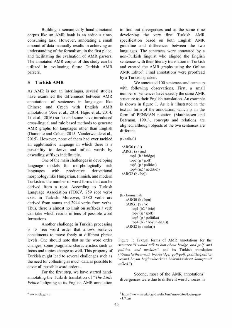
Figure 1: Textual forms of AMR annotations for the

sentence “I would talk to him about bridge, and golf, and

politics, and neckties.” and its Turkish translation

(“Onlarla/them-with briç/bridge, golf/golf, politika/politics

ve/and boyun bağları/neckties hakkında/about konuştum/I

talked.”)

Building a semantically hand-annotated

corpus like an AMR bank is an arduous time-

consuming task. However, annotating a small

amount of data manually results in achieving an

understanding of the formalism, in the first place,

and facilitating the evaluation of AMR parsers.

The annotated AMR corpus of this study can be

utilized in evaluating future Turkish AMR

parsers.

5 Turkish AMR

As AMR is not an interlingua, several studies

have examined the differences between AMR

annotations of sentences in languages like

Chinese and Czech with English AMR

annotations (Xue et al., 2014; Hajic et al., 2014;

Li et al., 2016) so far and some have introduced

cross-lingual and rule based methods to generate

AMR graphs for languages other than English

(Damonte and Cohen, 2015; Vanderwende et al.,

2015). However, none of them had ever tackled

an agglutinative language in which there is a

possibility to derive and inflect words by

cascading suffixes indefinitely.

One of the main challenges in developing

language models for morphologically rich

languages with productive derivational

morphology like Hungarian, Finnish, and modern

Turkish is the number of word forms that can be

derived from a root. According to Turkish

Language Association (TDK)4, 759 root verbs

exist in Turkish. Moreover, 2380 verbs are

derived from nouns and 2944 verbs from verbs.

Thus, there is almost no limit on suffixes a verb

can take which results in tens of possible word

formations.

Another challenge in Turkish processing

is its free word order that allows sentence

constituents to move freely at different phrase

levels. One should note that as the word order

changes, some pragmatic characteristics such as

focus and topics change as well. This property of

Turkish might lead to several challenges such as

the need for collecting as much data as possible to

cover all possible word orders.

For the first step, we have started hand-

annotating the Turkish translation of “The Little

Prince” aligning to its English AMR annotation

4 www.tdk.gov.tr

to find out divergences and at the same time

developing the very first Turkish AMR

specification based on both English AMR

guideline and differences between the two

languages. The sentences were annotated by a

non-Turkish linguist who aligned the English

sentences with their literary translation in Turkish

and created the AMR graphs using the Online

AMR Editor5. Final annotations were proofread

by a Turkish speaker.

We annotated 100 sentences and came up

with following observations. First, a small

number of sentences have exactly the same AMR

structure as their English translation. An example

is shown in figure 1. As it is illustrated in the

textual form of the annotation, which is in the

form of PENMAN notation (Matthiessen and

Bateman, 1991), concepts and relations are

aligned, although objects of the two sentences are

different.

(t / talk-01

:ARG0 (i / i)

:ARG1 (a / and

:op1 (b / bridge)

:op2 (g / golf)

:op3 (p / politics)

:op4 (n2 / necktie))

:ARG2 (h / he))

(k / konuşmak

:ARG0 (b / ben)

:ARG1 (v / ve

:op1 (b2 / briç)

:op2 (g / golf)

:op3 (p / politika)

:op4 (b3 / boyun-bağı))

:ARG2 (o / onlar))

Second, most of the AMR annotations’

divergences were due to different word choices in

5 https://www.isi.edu/cgi-bin/div3/mt/amr-editor/login-gen-

v1.7.cgi

45

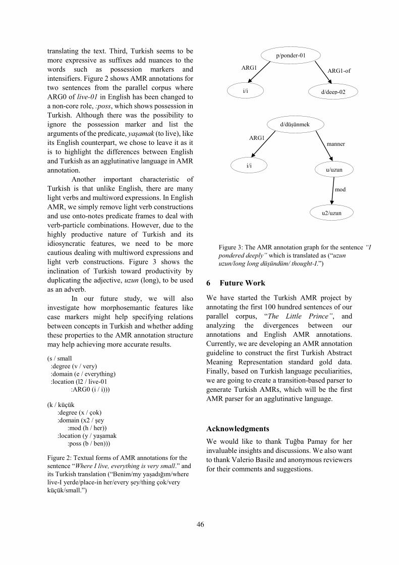
Figure 3: The AMR annotation graph for the sentence “I

pondered deeply” which is translated as (“uzun

uzun/long long düşündüm/ thought-I.”)

translating the text. Third, Turkish seems to be

more expressive as suffixes add nuances to the

words such as possession markers and

intensifiers. Figure 2 shows AMR annotations for

two sentences from the parallel corpus where

ARG0 of live-01 in English has been changed to

a non-core role, :poss, which shows possession in

Turkish. Although there was the possibility to

ignore the possession marker and list the

arguments of the predicate, yaşamak (to live), like

its English counterpart, we chose to leave it as it

is to highlight the differences between English

and Turkish as an agglutinative language in AMR

annotation.

Another important characteristic of

Turkish is that unlike English, there are many

light verbs and multiword expressions. In English

AMR, we simply remove light verb constructions

and use onto-notes predicate frames to deal with

verb-particle combinations. However, due to the

highly productive nature of Turkish and its

idiosyncratic features, we need to be more

cautious dealing with multiword expressions and

light verb constructions. Figure 3 shows the

inclination of Turkish toward productivity by

duplicating the adjective, uzun (long), to be used

as an adverb.

In our future study, we will also

investigate how morphosemantic features like

case markers might help specifying relations

between concepts in Turkish and whether adding

these properties to the AMR annotation structure

may help achieving more accurate results.

(s / small

:degree (v / very)

:domain (e / everything)

:location (l2 / live-01

:ARG0 (i / i)))

(k / küçük

:degree (x / çok)

:domain (x2 / şey

:mod (h / her))

:location (y / yaşamak

:poss (b / ben)))

Figure 2: Textual forms of AMR annotations for the

sentence “Where I live, everything is very small.” and

its Turkish translation (“Benim/my yaşadığım/where

live-I yerde/place-in her/every şey/thing çok/very

küçük/small.”)

6 Future Work

We have started the Turkish AMR project by

annotating the first 100 hundred sentences of our

parallel corpus, “The Little Prince”, and

analyzing the divergences between our

annotations and English AMR annotations.

Currently, we are developing an AMR annotation

guideline to construct the first Turkish Abstract

Meaning Representation standard gold data.

Finally, based on Turkish language peculiarities,

we are going to create a transition-based parser to

generate Turkish AMRs, which will be the first

AMR parser for an agglutinative language.

Acknowledgments

We would like to thank Tuğba Pamay for her

invaluable insights and discussions. We also want

to thank Valerio Basile and anonymous reviewers

for their comments and suggestions.

p/ponder-01

i/i

ARG1

d/deep-02

ARG1-of

d/düşünmek

i/i

ARG1

u/uzun

u2/uzun

manner

mod

46

References

Atalay, N. B., Oflazer, K., & Say, B. 2003. The

annotation process in the Turkish treebank.

In Proceedings of 4th International Workshop on

Linguistically Interpreted Corpora (LINC-03) at

EACL 1003. http://aclweb.org/anthology/W03-2405

Banarescu, L., Bonial, C., Cai, S., Georgescu, M.,

Griffitt, K., Hermjakob, U., ... & Schneider, N. 2013.

Abstract meaning representation for sembanking.

In Proceedings of the 7th Linguistic Annotation

Workshop and Interoperability with

Discourse (pp.178-186).

http://aclweb.org/anthology/W13-2322

Damonte, M., Cohen, S. B., & Satta, G. 2016. An

incremental parser for abstract meaning

representation. arXiv preprint arXiv:1608.06111.

http://aclweb.org/anthology/E17-1051

Damonte, M., & Cohen, S. B. 2017. Cross-lingual

abstract meaning representation parsing. arXiv

preprint arXiv:1704.04539. https://doi.org/

10.18653/v1/N18-1104

Flanigan, J., Thomson, S., Carbonell, J., Dyer, C., &

Smith, N. A. 2014. A discriminative graph-based

parser for the abstract meaning representation.

In Proceedings of the 52nd Annual Meeting of the

Association for Computational Linguistics (Volume

1: Long Papers) (Vol. 1, pp. 1426-1436).

https://doi.org/ 10.3115/v1/P14-1134

Hajic, J., Bojar, O., & Uresova, Z. 2014. Comparing

Czech and English AMRs. In Proceedings of

Workshop on Lexical and Grammatical Resources

for Language Processing (pp. 55-64).

https://doi.org/ 10.3115/v1/W14-5808

Li, B., Wen, Y., Weiguang, Q. U., Bu, L., & Xue, N.

2016. Annotating the little prince with chinese amrs.

In Proceedings of the 10th linguistic annotation

workshop held in conjunction with acl 2016 (law-x

2016) (pp. 7-15). https://doi.org/ 10.18653/v1/W16-

1702

Mathiessen, C. M., & Bateman, J. 1991. Text

Generation and Systemic-Functional

Linguistics. London: Pinter.

Şahin, G. G. 2016. Verb sense annotation for Turkish

propbank via crowdsourcing. In International

Conference on Intelligent Text Processing and

Computational Linguistics (pp. 496-506). Springer,

Cham.

Vanderwende, L., Menezes, A., & Quirk, C. 2015. An

AMR parser for English, French, German, Spanish

and Japanese and a new AMR-annotated corpus.

In Proceedings of the 2015 conference of the north

american chapter of the association for

computational linguistics: Demonstrations (pp. 26-

30). https://doi.org/ 10.3115/v1/N15-3006

Wang, C., Xue, N., & Pradhan, S. 2015. Boosting

transition-based AMR parsing with refined actions

and auxiliary analyzers. In Proceedings of the 53rd

Annual Meeting of the Association for

Computational Linguistics and the 7th International

Joint Conference on Natural Language Processing

(Volume 2: Short Papers) (Vol. 2, pp. 857-862).

https://doi.org/ 10.3115/v1/P15-2141

Wang, C., Xue, N., & Pradhan, S. 2015. A transition-

based algorithm for amr parsing. In Proceedings of

the 2015 Conference of the North American Chapter

of the Association for Computational Linguistics:

Human Language Technologies(pp. 366-375).

https://doi.org/ 10.3115/v1/N15-1040

Welch, C., Kummerfeld, J. K., Feng, S., & Mihalcea,

R. 2018. World Knowledge for Abstract Meaning

Representation Parsing. In Proceedings of the

Eleventh International Conference on Language

Resources and Evaluation (LREC-2018).

http://aclweb.org/anthology/L18-1492

Xue, N., Bojar, O., Hajic, J., Palmer, M., Uresova, Z.,

& Zhang, X. 2014. Not an Interlingua, But Close:

Comparison of English AMRs to Chinese and

Czech. In LREC (Vol. 14, pp. 1765-1772).

http://www.lrecconf.org/proceedings/lrec2014/pdf/3

84_Paper.pdf

47

Proceedings of the 57th Annual Meeting of the Association for Computational Linguistics: Student Research Workshop, pages 48–53Florence, Italy, July 28 - August 2, 2019. c©2019 Association for Computational Linguistics

Gender Stereotypes Differ between Male and Female Writings

Yusu QianTandon School of Engineering

New York University6 MetroTech CenterBrooklyn, NY 11201yq729@nyu.edu

Abstract

Written language often contains gender stereo-types, typically conveyed unintentionally bythe author. Existing methods used to evaluategender stereotypes in a text compute the dif-ference in the co-occurrence of gender-neutralwords with female and male words. To studythe difference in how female and male au-thors portray people of different genders, wequantitatively evaluate and analyze the gen-der stereotypes in their writings on two dif-ferent datasets and from multiple aspects, in-cluding the overall gender stereotype score,the occupation-gender stereotype score, theemotion-gender stereotype score, and the ra-tio of male words used to female words. Weshow that writings by females on average havelower gender stereotype scores. We also findthat emotion words in writings by males havemuch lower stereotype scores than the aver-age score of all words, while in writings byfemales the scores are similar. We study andinterpret the distributions of gender stereotypescores of individual words, and how they differbetween male and female writings.

1 Introduction

Gender stereotypes in language have been receiv-ing more and more attention from researchersacross different fields. In the past, these studieshave been carried out mainly by conducting sur-veys with humans (Williams and Best, 1977), re-quiring a large amount of human labor. Garg et al.(2018) quantified gender stereotypes by analyzingword embeddings trained on US Census over thepast 100 years. Word embeddings capture gen-der stereotypes in the training data and transferthem to downstream applications (Bolukbasi et al.,2016). For example, if programmer appears morefrequently with he than she in the training corpus,in the word embedding it will have a closer dis-tance to he compared with she.

In this study, we analyze gender stereotypesdirectly from writings under different metrics.Specifically, we compare the writings by malesand females to see how gender stereotypes differbetween writings by the gender of authors. Ourresults show that writings by female authors con-tain much fewer gender stereotypes than writingsby male authors. We recognize that there are morethan two types of gender, but for the sake of sim-plicity, in this study we consider just female andmale.

To the best of our knowledge, this study is thefirst quantitative analysis of how gender stereo-types differ between writings by authors of differ-ent genders. Our contributions are as follows: 1)we show that writings by females contain fewergender stereotypes; 2) we find that over the pastfew decades, gender stereotypes in writings bymales have decreased.

2 Related Work

Quantifying Gender Stereotypes It has beennoticed that stereotypes might be implicitly intro-duced to image corpora and text corpora in proce-dures such as data collection (Misra et al., 2016;Gordon and Durme, 2013). Particularly in gen-der stereotypes, Garg et al. (2018) bridged socialscience with machine learning when they quanti-fied gender and ethnic stereotypes in word embed-dings. Park et al. (2018) measured gender stereo-types on various abusive language models, whileanalyzing the effect of different pre-trained wordembeddings and model architectures. Zhao et al.(2018) showed the effectiveness of measuring andcorrecting gender stereotypes in co-reference res-olution tasks.

Categorizing Text by Author Gender Shimoniet al. (2002) proposed techniques to categorizetext by author gender. They selected multiple fea-

48

tures, for example, determiners and prepositions,and calculated their frequency means and standarderrors in texts. They showed that the distributionsof some of these features differ between writingsby female and male. Mukherjee and Liu (2010)used POS sequence patterns to capture stylisticregularities in male and female writings. To re-duce the number of features, they also proposed aselection method. They showed that author gen-der can be revealed by multiple features of theirwritings. Cheng et al. (2011) based on psycho-linguistics and gender-preferential cues to build afeature space and trained machine learning modelsto identify author gender. They pointed out thatfunction words, word-based features and struc-tural features can act as gender discriminators. Allthese three studies achieved accuracy above 80%for identifying author gender.

3 Methodology

3.1 DatasetIn the first experiment, we use a dataset by Lahiri(2013), which consists of 3,036 English bookswritten by 142 authors. Among these, 189 bookswere written by 14 female authors, others wereproduced by male authors.

In the second experiment, we use a dataset bySchler et al. (2006), which consists of 681,288posts from 19,320 bloggers; approximately 35posts and 7250 words from each blogger. Theblogs are divided into 40 categories, for example,agriculture, arts and science, etc. Female bloggersand male bloggers are of equal number.

3.2 Evaluation MethodsOverall Gender Stereotypes We define thegender stereotype score of a word as:

b(w) =

∣∣∣∣logc(w,m)

c(w, f)

∣∣∣∣ ,

where f is a set of female words, for example, she,girl, and woman. m is a set of male words, for ex-ample, he, actor, and father. c(w, g) is the numberof times a gender-neutral word w co-occurs withgendered words. The gendered word lists are byZhao et al. (2018).We use a window size of 10when calculating co-occurrence.

A word is used in a neutral way if the stereo-type score is 0, which means it occurs equally fre-quently with male words and females word in thetext. The overall stereotype score of a text, Tb,

is the sum of stereotype scores of all the gender-neutral by definition words that have more than 10co-occurrences with gendered words in the text,divided by the total count of words calculated, N .

Tb =1

N

∑

w∈Nb(w)

Ratio of Male Words to Female Words Tocompare the frequency of male words with that offemale words in a text, we calculate the ratio ofmale word count to female word count and denoteit by R.

Occupation-Gender Stereotypes Occupationstereotypes are the most common stereotypes instudies on gender stereotypes (Lu et al., 2018).A few decades ago, females normally worked asdairy maids, housemaids and nurses, etc, whilemales worked as doctors, smiths, and butchers,etc. Nowadays both genders have more choiceswhen looking for a job and for most occupations,there isnt a restriction on gender. Therefore, it isinteresting to study how occupation stereotypeschange over the years in female and male writings.

Occupation stereotypes score, Ob, in a text is theaverage stereotype score of a list of 200 gender-neutral occupations, O, in the text.

Ob =1

|O|∑

w∈Ob(w)

Emotion-Gender Stereotypes Emotion stereo-types are another kind of common gender stereo-types. In writings, especially novels, differentgenders are associated closely with different emo-tions, resulting in emotion stereotypes.

Emotion stereotypes score, Eb, in a text is theaverage stereotype score of a list of 200 emotionwords, E, in the text.

Eb =1

|E|∑

w∈Eb(w)

Distribution of Stereotype Scores We comparethe distributions of stereotype scores to analyzedifferences in writings by females and writings bymales. We consider the following aspects of dis-tributions: mean, variance, skewness, and kurto-sis. We use Sv, Ss, and Sk to denote the averageof variance, skewness, and kurtosis respectively ofthe distributions of stereotype scores. We plan toalso add directions to individual scores by remov-ing the absolute value function when calculating

49

Gutenberg Novels BlogsTb R Ob Eb Sv Ss Sk Tb R Ob Eb Sv SS Sk

f 0.54 1.14 0.70 0.62 0.25 1.58 3.48 0.56 1.46 0.72 0.56 0.21 1.74 4.81m 1.41 3.40 1.62 1.04 0.43 0.60 0.92 0.74 2.79 0.82 0.52 0.29 1.26 2.35

Table 1: Statistics of gender stereotypes in female and male writings

Figure 1: Distribution of stereotype scores in novels written by female(left) and male(right) authors

the scores, and analyze the distribution. We usethe absolute function for most of the experimentsbecause positive and negative values will canceloff each other when they are summed up.

Words Most Biased We alter the equation usedfor evaluating individual stereotype scores by re-moving the absolute value function, so that wordsoccurring more with female words have negativevalues and words occurring more with male wordshave positive values. By sorting individual stereo-type scores, we collect lists of words most biasedtowards the female gender or the male gender.

4 Results

4.1 Gender Stereotypes in Novels

We categorize 3036 books written in English andanalyze the overall gender stereotypes in writingsby each author. When sorted by overall stereo-type scores from low to high, 12 female authorsout of 14 are ranked among the top 20, or in an-other word, top 13.8%.

The average ratio of the total number of malewords to female words in novels by female authorsis close to 1, indicating that female authors men-tion the two genders in their novels almost equallyfrequently. Male authors, on the other hand, tendto write three times more frequently about theirown gender.

Figure 1 shows the distribution of stereotypescores in example novels written by female andmale authors. Inspection shows that the individualscores of female writings tend to cluster aroundscore value 0 or other small values close to 0, andthe percentage of words among all words calcu-lated constantly decreases when stereotype scoreincreases, while the individual scores of male writ-ings tend to cluster around score values between0.5 and 1.5, and the percentage of words amongall words calculated first increases and then de-creases.

Statistical analysis on the distributions confirmsour observation. Table 1 shows that the averagevariance of stereotype scores in male writings ismuch larger than that of female writings, indicat-ing that stereotype scores in female writings tendto gather near the mean while those in male writ-ings spread out more broadly. The distributionof stereotype scores in female writings has bothlarger average skewness and larger kurtosis, in ac-cordance with our observation that the distributionis skewed right with a sharp peak at a small stereo-type score. In contrast, the distribution of stereo-type scores in male writings has much smaller av-erage skewness and kurtosis, in accordance withour observation that the distribution has tails onboth left and right sides and has a less distinctpeak.

50

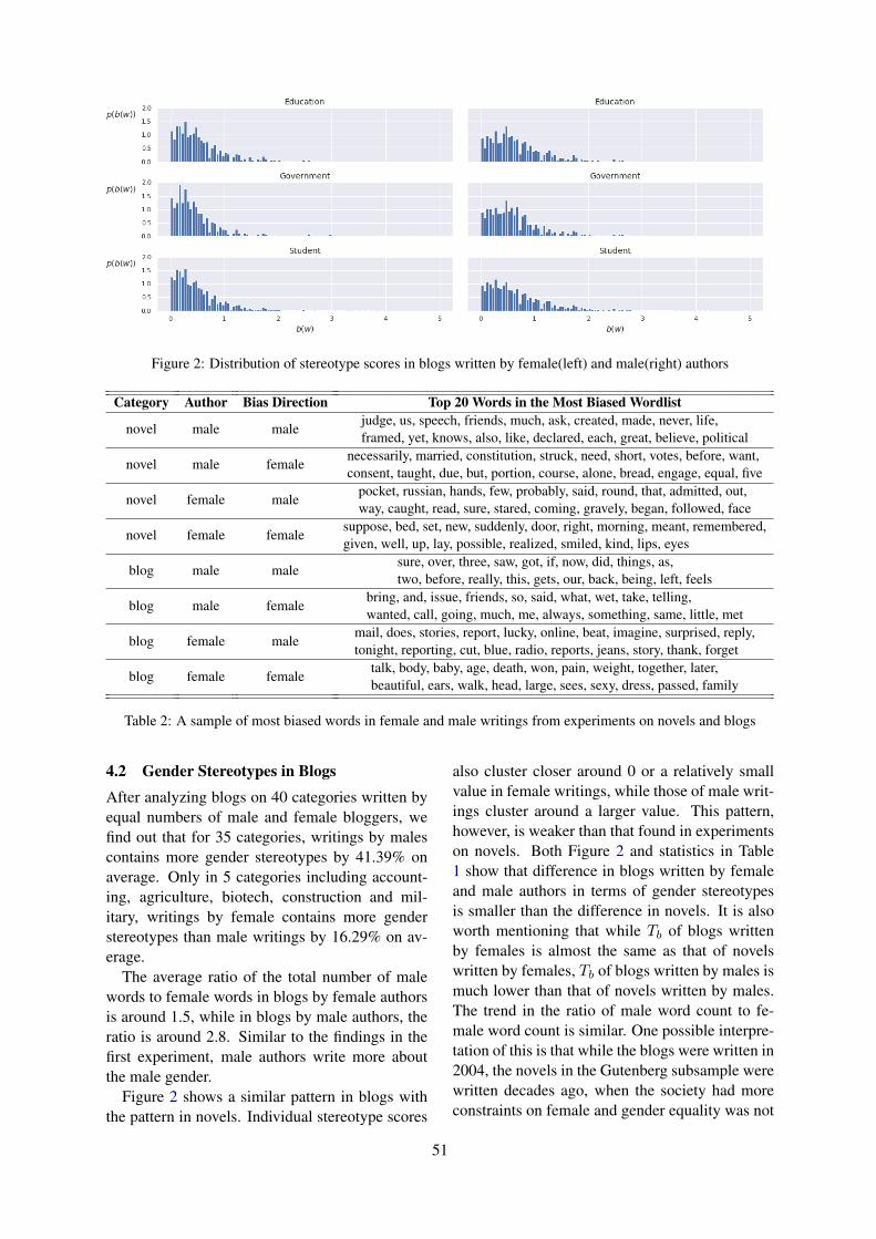
Figure 2: Distribution of stereotype scores in blogs written by female(left) and male(right) authors

Category Author Bias Direction Top 20 Words in the Most Biased Wordlist

novel male malejudge, us, speech, friends, much, ask, created, made, never, life,framed, yet, knows, also, like, declared, each, great, believe, political

novel male femalenecessarily, married, constitution, struck, need, short, votes, before, want,consent, taught, due, but, portion, course, alone, bread, engage, equal, five

novel female malepocket, russian, hands, few, probably, said, round, that, admitted, out,way, caught, read, sure, stared, coming, gravely, began, followed, face

novel female femalesuppose, bed, set, new, suddenly, door, right, morning, meant, remembered,given, well, up, lay, possible, realized, smiled, kind, lips, eyes

blog male malesure, over, three, saw, got, if, now, did, things, as,two, before, really, this, gets, our, back, being, left, feels

blog male femalebring, and, issue, friends, so, said, what, wet, take, telling,wanted, call, going, much, me, always, something, same, little, met

blog female malemail, does, stories, report, lucky, online, beat, imagine, surprised, reply,tonight, reporting, cut, blue, radio, reports, jeans, story, thank, forget

blog female femaletalk, body, baby, age, death, won, pain, weight, together, later,beautiful, ears, walk, head, large, sees, sexy, dress, passed, family

Table 2: A sample of most biased words in female and male writings from experiments on novels and blogs

4.2 Gender Stereotypes in BlogsAfter analyzing blogs on 40 categories written byequal numbers of male and female bloggers, wefind out that for 35 categories, writings by malescontains more gender stereotypes by 41.39% onaverage. Only in 5 categories including account-ing, agriculture, biotech, construction and mil-itary, writings by female contains more genderstereotypes than male writings by 16.29% on av-erage.

The average ratio of the total number of malewords to female words in blogs by female authorsis around 1.5, while in blogs by male authors, theratio is around 2.8. Similar to the findings in thefirst experiment, male authors write more aboutthe male gender.

Figure 2 shows a similar pattern in blogs withthe pattern in novels. Individual stereotype scores

also cluster closer around 0 or a relatively smallvalue in female writings, while those of male writ-ings cluster around a larger value. This pattern,however, is weaker than that found in experimentson novels. Both Figure 2 and statistics in Table1 show that difference in blogs written by femaleand male authors in terms of gender stereotypesis smaller than the difference in novels. It is alsoworth mentioning that while Tb of blogs writtenby females is almost the same as that of novelswritten by females, Tb of blogs written by males ismuch lower than that of novels written by males.The trend in the ratio of male word count to fe-male word count is similar. One possible interpre-tation of this is that while the blogs were written in2004, the novels in the Gutenberg subsample werewritten decades ago, when the society had moreconstraints on female and gender equality was not

51

paid as much attention to as it is today.

4.3 Gender Stereotypes Categories

For both two datasets, Ob is larger than Tb, indi-cating that occupation words in both female andmale writings contain more gender stereotypesthan most other words. Eb is almost the same asTb in female writings, while it is much lower thanTb in male writings, indicating that gender stereo-types in emotion words are not the main contribu-tors to the overall gender stereotypes in male writ-ings.

5 Conclusion and Discussion

In this study, we perform experiments on twodatasets to analyze how gender stereotypes dif-fer between male and female writings. From ourpreliminary results we observe that writings byfemale authors contain fewer gender stereotypesthan writings by male authors. This differenceappears to have narrowed over time, mainly bythe reduction of gender stereotypes in writingsby male authors. We plan to: 1)further analyzethe typical types of gender stereotypes in writingsby authors of different genders and how they re-semble with or differ from each other, by study-ing the most biased words and the average stereo-type scores of different categories of words, forexample, verbs, adjectives, etc.; 2) perform ex-periments on more writings from the past centuryto inspect more closely if there exists a trend inthe transformation of gender stereotypes; 3) ex-isting stereotype evaluation methods evaluate ev-ery word not in the excluded word lists, in ourcase, the male and female word lists. Some fre-quently used words, such as the, one, and an, arenot considered to be able to contain stereotypes,unlike words such as strong, doctor, and jealous,which are more closely associated with one gen-der in writings. We plan to seek a way to filtergender-neutral words and only keep those capableof carrying stereotypes for stereotype quantifica-tion.

6 Acknowledgments

Many thanks to Gang Qian, Cuiying Yang, Pe-dro L. Rodriguez, Hanchen Wang, and Tian Liufor helpful discussion, and reviewers for detailedcomments and advice.

ReferencesTolga Bolukbasi, Kai-Wei Chang, James Zou,

Venkatesh Saligrama, and Adam Kalai. 2016. Manis to computer programmer as woman is to home-maker? debiasing word embeddings. In NIPS’16Proceedings of the 30th International Conferenceon Neural Information Processing Systems, pages4356–4364.

Na Cheng, Rajarathnam Chandramouli, and K. P. Sub-balakshmi. 2011. Author gender identification fromtext. Digital Investigation, 8(1):78–88.

Nikhil Garg, Londa Schiebinger, Dan Jurafsky, andJames Zou. 2018. Word embeddings quantify100 years of gender and ethnic stereotypes. Pro-ceedings of the National Academy of Sciences,115(16):E3635–E3644.

Jonathan Gordon and Benjamin Van Durme. 2013. Re-porting bias and knowledge acquisition. In Proceed-ings of the 2013 workshop on Automated knowledgebase construction, AKBC@CIKM 13, San Fran-cisco, California, USA, October 27-28, 2013, pages25–30.

Shibamouli Lahiri. 2013. Complexity of word collo-cation networks: A preliminary structural analysis.CoRR, abs/1310.5111.

Kaiji Lu, Piotr Mardziel, Fangjing Wu, PreetamAmancharla, and Anupam Datta. 2018. Gen-der bias in neural natural language processing.ArXiv:1807.11714v1.

Ishan Misra, C. Lawrence Zitnick, Margaret Mitchell,and Ross B. Girshick. 2016. Seeing through thehuman reporting bias: Visual classifiers from noisyhuman-centric labels. In 2016 IEEE Conference onComputer Vision and Pattern Recognition, CVPR2016, Las Vegas, NV, USA, June 27-30, 2016, pages2930–2939.

Arjun Mukherjee and Bing Liu. 2010. Improving gen-der classification of blog authors. In Proceedings ofthe 2010 Conference on Empirical Methods in Natu-ral Language Processing, EMNLP ’10, pages 207–217, Stroudsburg, PA, USA. Association for Com-putational Linguistics.

Ji Ho Park, Jamin Shin, and Pascale Fung. 2018. Re-ducing gender bias in abusive language detection. InProceedings of the 2018 Conference on EmpiricalMethods in Natural Language Processing, Brussels,Belgium, October 31 - November 4, 2018, pages2799–2804.

Jonathan Schler, Moshe Koppel, Shlomo Argamon,and James Pennebaker. 2006. Effects of age andgender on blogging. In Computational Approachesto Analyzing Weblogs - Papers from the AAAI SpringSymposium, Technical Report, volume SS-06-03,pages 191–197.

52

Anat Rachel Shimoni, Moshe Koppel, and ShlomoArgamon. 2002. Automatically Categorizing Writ-ten Texts by Author Gender. Literary and LinguisticComputing, 17(4):401–412.

John E. Williams and Deborah L. Best. 1977. Sexstereotypes and trait favorability on the adjectivecheck list. Educational and Psychological Measure-ment, 37(1):101–110.

Jieyu Zhao, Yichao Zhou, Zeyu Li, Wei Wang, andChang Kaiwei. 2018. Learning gender-neutral wordembeddings. In Proceedings of the 2018 Confer-ence on Empirical Methods in Natural LanguageProcessing, page 48474853. Association for Com-putational Linguistics.

53

Proceedings of the 57th Annual Meeting of the Association for Computational Linguistics: Student Research Workshop, pages 54–63Florence, Italy, July 28 - August 2, 2019. c©2019 Association for Computational Linguistics

Question Answering in the Biomedical Domain

Vincent NguyenResearch School of Computer Science, Australian National University

Data61, CSIROvincent.nguyen@anu.edu.au

Abstract

Question answering techniques have mainlybeen investigated in open domains. How-ever, there are particular challenges in extend-ing these open-domain techniques to extendinto the biomedical domain. Question answer-ing focusing on patients is less studied. Wefind that there are some challenges in patientquestion answering such as limited annotateddata, lexical gap and quality of answer spans.We aim to address some of these gaps by ex-tending and developing upon the literature todesign a question answering system that candecide on the most appropriate answers forpatients attempting to self-diagnose while in-cluding the ability to abstain from answeringwhen confidence is low.

1 Introduction

Question Answering (QA) is the downstream taskof information seeking wherein a user presentsa question in natural language, Q, and a systemfinds an answer or a set of answers from a col-lection of natural language documents or knowl-edge bases (Lende and Raghuwanshi, 2016), A,that satisfies the user’s question (Molla and Gon-zlez, 2007).

Questions fall into one of two categories: fac-toid and non-factoid. Factoid QA provides brieffacts to the users’ questions; for example, Ques-tion: What day is it? Answer: Monday. Non-factoid question answering is a more complextask. It involves answering questions that requirespecific knowledge, common sense or a proceduredue to ambiguity or the scope of the question. Anexample from the Yahoo non-factoid question an-swer dataset1 illustrates this: Question: Why is itconsidered unlucky to open an umbrella indoors?.The answer is not apparent and requires specificknowledge about cultural superstitions.

1https://ciir.cs.umass.edu/downloads/nfL6/

Question answering is fundamental in high-level tools such as chatbots (Qiu et al., 2017;Yan et al., 2016; Amato et al., 2017; Ram et al.,2018), search engines (Kadam et al., 2015), andvirtual assistants (Yaghoubzadeh and Kopp, 2012;Austerjost et al., 2018; Bradley et al., 2018). How-ever, being a downstream task, question answeringsuffers from pipeline error, as it often relies on thequality of several upstream tasks such as coref-erence resolution (Vicedo and Ferrandez, 2000),anaphora resolution (Ram et al., 2018), named en-tity recognition (Aliod et al., 2006), informationretrieval (Mao et al., 2014), and tokenisation (De-vlin et al., 2019).

Thus, there has been a growing demand forthese QA systems to deliver precise question-specific answers (Pudaruth et al., 2016) and con-sequently has sparked much research into improv-ing upon relevant natural language processing ap-proaches (Malik et al., 2013), datasets (Rajpurkaret al., 2016; Kocisky et al., 2017) and informa-tion retrieval techniques (Weienborn et al., 2013;Mao et al., 2014). These improvements have al-lowed the domain to evolve from shallow keywordmatching to contextual and semantic retrieval sys-tems (Kadam et al., 2015). However, most ofthese techniques have been focused on the open-domain (Soares and Parreiras, 2018) and the chal-lenges harbouring the biomedical domain have notbeen well addressed and remain unsolved. Here,we define biomedical QA as either factoid or non-factoid QA on biomedical literature.

One such challenge is due to the creationof complex medical queries which require ex-pert knowledge and up to four hours perquery (Russell-Rose and Chamberlain, 2017) toadequately answer. This requirement of expertknowledge leads to a lack of high-quality, publiclyavailable biomedical QA datasets. Furthermore,medical datasets tend to be locked behind ethical,obligatory agreements and are usually small due to

54

cost constraints and lack of domain experts for an-notation (Pampari et al., 2018; Shen et al., 2018).Therefore, open-domain techniques which assumedata-rich conditions are not suitable for direct ap-plication to the biomedical domain.

Another challenge is clinical term ambiguity,which is due to the temporally and spatially vary-ing nature of clinical terminology, and the fre-quent use of abbreviation and esoteric medical ter-minology (Lee et al., 2019) (see Table 1 for ex-amples). It is difficult for systems to adequatelydisambiguate clinical words to be used in down-stream QA systems due to the complexity of theambiguity of medical terminology, such as abbre-viations, due to their varying contexts. Thoughthere are existing tools such as MetaMap (Aron-son and Lang, 2010) to disambiguate these termsby mapping them to the UMLS (Unified Medi-cal Language System) metathesaurus, coverage ofthese systems is low and mappings are often inac-curate (Wu et al., 2012).

Furthermore, systems in the open-domain typ-ically retrieve a long answer before extracting ashort continuous span of text to present to theuser (Soares and Parreiras, 2018; Rajpurkar et al.,2016). However, for biomedical responses, it isnot always sufficient to retrieve short answer con-tinuous spans, and Answer Evidence spans that arediscontinuous that cross the sentence boundary areoften required (Pampari et al., 2018; Hunter andCohen, 2006; Nentidis et al., 2018).

These problems are not yet solved in thebiomedical domain and are reflected in theBioASQ challenge (Nentidis et al., 2018), an an-nual challenge with a biomedical question answer-ing track. Currently, the state-of-the-art systemsdo not perform much better than random guesswith an accuracy of 66.67% for binary questionanswering (Chandu et al., 2017), 24.24% for fac-toid (ranked list of named entities as answers) andan F1-score of 0.3312 for list-type (unranked listof named entities) (Peng et al., 2015) suggestingthat there is much room for improvement in termsof algorithms and research.

Furthermore, we found that there is a lack ofa biomedical question answering system directedfor patients. Biomedical question answering forpatients is important as studies from the Pew Re-search Centre have shown that 35% of U.S. adultshave diagnosed themselves using the information

they found online2. Of these adults, 35% saidthat they did not get a professional opinion ontheir self-diagnosis, illustrating that patients mayblindly trust the results of search engines withoutconsulting a medical professional. This is causefor concern, as search engines tend to display themost severe ailments first which could lead to apotential waste of hospital resources or deteriora-tion in patient health (Korfage et al., 2006).

Furthermore, although there are negatives tosearching symptoms via search engine, for the par-ticipants who visited doctors after self-diagnosis,research has revealed that doctor-patient relation-ships and patient compliance with treatment im-prove as the patients have a clearer understandingof their symptoms and potential disease after self-diagnosis (Cocco et al., 2018). These studies mo-tivate the need for a strong biomedical questionanswering question for patients as it will benefitpatients who self-diagnose and patients who seekmedical advice after looking up their symptomsonline.

Finally, we highlight that there is a lexical andsemantic gap between clinical and patient lan-guage. For example, the expression “hole in lung“taken literally is about a punctured lung. However,this colloquialism refers to the condition knownas Pleurisy (Ben Abacha and Demner-Fushman,2019; Abacha and Demner-Fushman, 2016), illus-trating that patients do not have the level of literacyto formulate complex medical queries nor under-stand them (Graham and Brookey, 2008).

We aim to address the challenges in applyingquestion answering to biomedical question an-swering for patients. We highlight that the cur-rent gaps of biomedical QA research stem fromlack of clinical disambiguation tools, lack of high-quality data, the quality of answer spans, weakalgorithms and clinical-patient lexical gaps. Ourgoal is to present a patient biomedical QA systemthat can address the gaps in biomedical researchand allows a patient to query their symptoms, dis-eases or available treatment options accurately, butwill also abstain from providing answers in caseswhere there is low confidence in the best answer,question malformation or insufficiency of data toanswer the question.

2https://www.pewinternet.org/2013/01/15/health-online-2013/

55

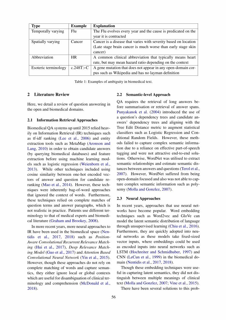
Type Example ExplanationTemporally varying Flu The Flu evolves every year and the cause is predicated on the

year it is contractedSpatially varying Cancer Cancer is a disease that varies with severity based on location

(Late stage brain cancer is much worse than early stage skincancer)

Abbreviation HR A common clinical abbreviation that typically means heartrate, but may mean hazard ratio depending on the context

Esoteric terminology c.248T>C A gene mutation that does not appear in any open-domain cor-pus such as Wikipedia and has no layman definition

Table 1: Examples of ambiguity in biomedical text.

2 Literature Review

Here, we detail a review of question answering inthe open and biomedical domains.

2.1 Information Retrieval Approaches

Biomedical QA systems up until 2015 relied heav-ily on Information Retrieval (IR) techniques suchas tf-idf ranking (Lee et al., 2006) and entityextraction tools such as MetaMap (Aronson andLang, 2010) in order to obtain candidate answers(by querying biomedical databases) and featureextraction before using machine learning mod-els such as logistic regression (Weienborn et al.,2013). While other techniques included usingcosine similarity between one-hot encoded vec-tors of answer and question for candidate re-ranking (Mao et al., 2014). However, these tech-niques were inherently bag-of-word approachesthat ignored the context of words. Furthermore,these techniques relied on complete matches ofquestion terms and answer paragraphs, which isnot realistic in practice. Patients use different ter-minology to that of medical experts and biomedi-cal literature (Graham and Brookey, 2008).

In more recent years, more neural approaches toIR have been used in the biomedical space (Nen-tidis et al., 2017, 2018) such as Position-Aware Convolutional Recurrent Relevance Match-ing (Hui et al., 2017), Deep Relevance Match-ing Model (Guo et al., 2017) and Attention BasedConvolutional Neural Network (Yin et al., 2015).However, though these approaches do not rely oncomplete matching of words and capture seman-tics, they either ignore local or global contextswhich are useful for disambiguation of clinical ter-minology and comprehension (McDonald et al.,2018).

2.2 Semantic-level Approach

QA requires the retrieval of long answers be-fore summarisation or retrieval of answer spans.Punyakanok et al. (2004) introduced the use ofa question’s dependency trees and candidate an-swers’ dependency trees and aligning with theTree Edit Distance metric to augment statisticalclassifiers such as Logistic Regression and Con-ditional Random Fields. However, these meth-ods failed to capture complex semantic informa-tion due to a reliance on effective part-of-speechtagging and were not attractive end-to-end solu-tions. Otherwise, WordNet was utilised to extractsemantic relationships and estimate semantic dis-tances between answers and questions (Terol et al.,2007). However, WordNet suffered from beingopen-domain focused and also was not able to cap-ture complex semantic information such as poly-semy (Molla and Gonzlez, 2007).

2.3 Neural Approaches

In recent years, approaches that use neural net-works have become popular. Word embeddingtechniques such as Word2vec and GloVe canmodel the latent semantic distribution of languagethrough unsupervised learning (Chiu et al., 2016).Furthermore, they are quickly adopted into neu-ral networks as these models take fixed-sizedvector inputs, where embeddings could be usedas encoded inputs into neural networks such asLSTM (Hochreiter and Schmidhuber, 1997) andCNN (LeCun et al., 1999) in the biomedical do-main (Nentidis et al., 2017, 2018).

Though these embedding techniques were use-ful in capturing latent semantics, they did not dis-tinguish between multiple meanings of clinicaltext (Molla and Gonzlez, 2007; Vine et al., 2015).

There have been several solutions to this prob-

56

lem (Peters et al., 2018; Howard and Ruder,2018; Devlin et al., 2019) proposed but they arenot relevant specifically to the biomedical do-main. Instead, we highlight BioBERT (Lee et al.,2019), a biomedical version of BERT (Devlinet al., 2019) which is a deeply bidirectional trans-former (Vaswani et al., 2017) that is able to incor-porate rich context into the encoding or embed-ding process that has pre-trained on the Wikipediaand PubMed corpora. However, this model fails toaccount for the spatial and temporal aspects of dis-eases in biomedical literature as temporality is notencoded into its input. Furthermore, Biobert usesa WordPiece tokeniser (Wu et al., 2016) whichkeeps a fixed-size vocabulary dictionary for learn-ing new words. However, the vocabulary withinthe model is derived from Wikipedia, a generaldomain corpus, and thus Biobert is unable to learndistinct morphological semantics of medical termslike -phobia, where ’-‘ denotes suffixation, mean-ing fear as it only has the internal representationfor -bia.

3 Research Plan

We list the research questions to address someof the research gaps in biomedical QA and thesystem we aim to design, alongside baseline ap-proaches and methodology as starting points. Wewill also mention future directions to address theseresearch questions.

RQ1: What are the limitations of currentbiomedical QA? The limitations in currentbiomedical QA include the lack of: sufficientambiguity resolution tools (Wu et al., 2012),robust techniques to using semantic neural ap-proaches (Lee et al., 2019; Nentidis et al., 2018).The lack of strong comprehension from systemsto produce sufficient answer spans that cross thesentence boundary as reflected by poor resultsin ideal answer production in BioASQ (Nentidiset al., 2018, 2017) and addressing issues usingreal-world patient queries rather than artificiallycurated queries (Pampari et al., 2018; Guo et al.,2006) which contain colloquial ambiguous non-medical terminology such as hole in lung.

In our research, we aim to address each of thesegaps by researching into: higher coverage clini-cal ambiguity tools that use contexts in the spatialand temporal domains, summarisation techniquesthat can translate from biomedical terminology topatient language (Mishra et al., 2014; Shi et al.,

2018) and tuning biomedical models to solve com-plex answer span tasks that cross sentence bound-aries (Kocisky et al., 2017) or require commonsense (Talmor et al., 2018).

RQ2: Data-driven approaches require high-quality datasets. How can we construct orleverage existing datasets to mimic real-worldbiomedical question answering? By leverag-ing existing techniques such as variational auto-encoder (Shen et al., 2018) and Snorkel (Bachet al., 2018), we will be able to generate, label andprocess additional data that can meet stringent datarequirements of neural approaches.

However, synthetic datasets generally performweaker than handcrafted datasets (Bach et al.,2018). In order to bridge this gap in the re-search, we propose augmenting these data gener-ation methods via crowd-sourcing methods withtextual entailment (Abacha and Demner-Fushman,2016) and natural language inference (Johnsonet al., 2016) to improve the quality of the gener-ated labels and data. For instance, we can use fo-rums like Quora or medical specific forums suchas Health243 and utilise techniques such as ques-tion entailment to find questions that are relatedto ones seen in the dataset in order to generatehigher-quality annotated labels.

We will then develop techniques that can com-bine synthetic and higher-quality labelled datasetsthat can be utilized downstream in a QA system.We will compare this against baselines such asmajority voting and Snorkel to evaluate our ap-proaches.

Allowing the model to abstain from a deci-sion, through comprehension, has been the focusof many datasets as of late (Rajpurkar et al., 2016;Kocisky et al., 2017). We can use these datasets asa starting problem to solve before applying thesetechniques to the biomedical domain. However,we will also develop and research further tech-niques in order to allow for improved confidenceand low uncertainty from the model.

RQ3: How do we indicate the confidence of theanswer that the model has provided? Often re-searchers interpret softmax or confidence scoresfrom the classifier models as direct correlations toprobability but often forget about uncertainties inthis measurement (Kendall and Gal, 2017). Dueto the real-world application and sensitivity of pre-

3https://www.health24.com/Experts

57

dictions in a health-based QA system, there needsto be guarantees that predictions are of both highaccuracy and low uncertainty.

In order to account for uncertainty, techniquessuch as Inductive Conformal Prediction (Pa-padopoulos, 2008) and Deep Bayesian Learn-ing (Siddhant and Lipton, 2018) can be used tomodel epistemic uncertainty, which is not inher-ently captured by the model during training, in or-der to make the loss function more robust to noiseand uncertainty and thereby strengthen the predic-tions of the model. This would then allow soft-max scores to be used as confidence scores withina reasonable level of uncertainty.

RQ4: How do we include temporality or lo-cality of diseases into answers? Diseases arenon-static, they evolve such as the flu or are sea-sonal such as the summer cold. Current modelsutilise only static vector inputs, such as word em-beddings, that do not account for this temporal as-pect of the input. Furthermore, though diseasesare non-static, they may be more likely in differentcountries as there is a spatiotemporal relationshipwhere countries will experience different seasonsand thus different diseases. In order to accommo-date for these relationships, we can draw on priorresearch as starting points such as space-time lo-cal embeddings (Sun et al., 2015), dynamic wordembeddings (Bamler and Mandt, 2017) or time-embeddings (Barbieri et al., 2018) as baselines andextend them into the biomedical setting.

RQ5: How do we bridge the semantic gap be-tween clinical text and terminology that a pa-tient can understand? Most patients lack theexpertise in utilising resources such as biomed-ical literature in order to self-diagnose. There-fore, knowledge or answers should be presentedin a form that they can understand (Graham andBrookey, 2008). Biomedical language and pa-tient language can be construed as two sepa-rate languages as biomedical language changesand evolves over time (Yan and Zhu, 2018) andalso pose the same problems (Hunter and Cohen,2006). Therefore, we can model this problem asa language translation problem and thus can usetechniques in neural machine translation (Qi et al.,2018; Chousa et al., 2018) based on word embed-dings.

However, as biomedical language and patientEnglish are primarily borne of the same language,this poses unique problems. For instance, a token

in plain English may translate to several tokens inthe biomedical space or vice versa. This is knownas the alignment problem (Qi et al., 2018). We canpotentially remedy this by borrowing ideas fromn-gram embedding (Zhao et al., 2017) as a startingpoint or using Biobert (Lee et al., 2019) projectedto a dual-language embedding space and use atten-tion to produce the alignment. Furthermore, thereare biomedical abbreviations that need to be dis-ambiguated before translation (Festag and Spreck-elsen, 2017), for which we would use direct, rule-based approaches using thesauri or tools such asMetamap (Aronson and Lang, 2010) as our base-line approaches and extend upon using data-drivenapproaches (Wu et al., 2017).

4 Experimental Framework

4.1 Datasets

High-quality data is required to address the chal-lenges we outlined. We therefore consider thefollowing datasets: (1) MEDNLI (Johnson et al.,2016; Goldberger et al., 2000) for medical lan-guage inference; (2) i2b2 in the form of em-rQA (Pampari et al., 2018) for synthetic question-answer pairs; (3) SQuAD (Rajpurkar et al.,2016) for open-domain transfer learning; (4) thequestion-answering datasets provided on MediQA20194; (5) the question entailment dataset andMedQuAD (Ben Abacha and Demner-Fushman,2019); (5) CLEF eHealth (Suominen et al., 2018)to utilize and evaluate IR methods; and (6) we willsupplement our datasets by generating labels forunlabelled data by leveraging the signals from thelabelled datasets through the use of tools such asSnorkel (Bach et al., 2018) and CVAE (Shen et al.,2018).

4.2 Evaluation Metrics

In our experiments, we will evaluate oursummarisation strategies with metrics such asROGUE (Lin, 2004), in particular, rogue-2 (Owczarzak and Dang, 2009) and BLEU (Pap-ineni et al., 2002). For question-answering, we usestandard ranking metrics such as Mean AveragePrecision and Mean Reciprocal Rank for evaluat-ing candidate ranking and standard metrics suchas f1-score, Precision, Accuracy and more medi-cal targeted metrics such as sensitivity and speci-ficity (Parikh et al., 2008).

4https://sites.google.com/view/mediqa2019

58

4.3 Proposed Framework

From the research questions mentioned, we pro-pose a framework to unify their solutions.

Embeddings To begin, we need to construct ourdate/seasonal embeddings (Barbieri et al., 2018),to do this, we will need datasets that have mentionsof the seasonality and locality of disease entities.Also, we will require embeddings that are repre-sentative of the text, we will consider state-of-the-art word-level context sensitive embeddings (Leeet al., 2019; Peters et al., 2018) and word-levelcontext insensitive embeddings (Chiu et al., 2016)and ensure they properly represent the biomedi-cal datasets. For instance, BERT will need to pre-trained with a biomedical vocabulary rather thana general purpose open-domain one, and, in doingso, we will be able to resolve ambiguity in poly-semy or abbreviations.

Furthermore, we will also be researchingmethodologies to handle out-of-vocabulary wordsas the current WordPiece tokenization (Devlinet al., 2019) or character-level embeddings (Barbi-eri et al., 2018) would not be sufficient to addressesoteric terminology (Lee et al., 2019). The timeembeddings and the word-level embeddings willbe concatenated and used as input to the model.

Model Architecture Given the success of multi-task learning (Zhao et al., 2018; Liu et al., 2019),and having been proposed as the blocking task inNLP (McCann et al., 2018) that needs to be solved.We therefore apply multi-task learning to thisproblem. From the state of the art multi-task learn-ing models, we borrow the fundamental buildingblocks such as multi-headed self-attention (Liuet al., 2019) and multi-pointer generation (Mc-Cann et al., 2018) to be used as decisions in aNeural Architecture Search (NAS) (Zoph and Le,2016). NAS will use reinforcement learning tech-niques to find a suitable architecture for multi-tasklearning. We elect to find the architecture to rep-resent our problem this way due to one main rea-son. The reason is that the field of deep learningin NLP is quickly changing, and thus the state-of-the-art techniques will always change. There-fore, by having a tool that builds architecturesfrom the building blocks of state-of-the-art mod-els is vital. However, crucially, we must add Het-eroscedastic Aleatoric Uncertainty and EpistemicUncertainty minimisation to the model by adjust-ing the loss function and weight distribution which

will allow the model to be more certain about deci-sions (Kendall and Gal, 2017). One such decisionmust be the ability to abstain from answering.

Concretely, we use NAS to discover models forNMT from clinical text to the patient languageby conditioning to an encoder-decoder structure.From here, using this model a starting point, NASwill add task-specific layers that will minimise thejoint loss over the biomedical tasks such as ques-tion answering (Nentidis et al., 2018), questionentailment (Abacha and Demner-Fushman, 2016)and natural language inference (Johnson et al.,2016). In doing so, multi-task learning will allowfor stronger generalisability and end-to-end train-ing (McCann et al., 2018; Liu et al., 2019).

5 Summary

We highlight gaps within the literature in ques-tion answering in the biomedical domain. Weoutline challenges associated with implementingthese systems due to the limitations of currentwork: lack of annotated data, ambiguity in clin-ical text and lack of comprehension of ques-tion/answer text by models.

We motivate this research in the area of patientQA due to the high volume of medical queries insearch engines that are trusted by patients. Our re-search aims to build upon the strengths of the cur-rent state-of-the-art and research new strategies insolving technical challenges to support a patientin retrieving the answers they require with low un-certainty and high confidence.

Acknowledgements

I thank for my supervisors, Dr Sarvnaz Karimi andDr Zhenchang Xing for providing invaluable in-sight into the writing of this proposal. This re-search is supported by the Australian ResearchTraining Program and the CSIRO PostgraduateScholarship.

ReferencesBen Abacha and Demner-Fushman. 2016. Recogniz-

ing Question Entailment for Medical Question An-swering. American Medical Informatics AssociationAnnual Symposium Proceedings, 2016:310–318.

Diego Aliod, Menno Zaanen, and Daniel Smith. 2006.Named entity recognition for question answering. InThe Australasian Language Technology Association,Sydney, Australia.

59

Flora Amato, Stefano Marrone, Vincenzo Moscato,Gabriele Piantadosi, Antonio Picariello, and CarloSansone. 2017. Chatbots meet ehealth: Automa-tizing healthcare. In Proceedings of the Workshopon Artificial Intelligence with Application in Healthco-located with the 16th International Conferenceof the Italian Association for Artificial Intelligence,Bari, Italy.

Alan Aronson and Francois-Michel Lang. 2010. Anoverview of Metamap: Historical perspective andrecent advances. Journal of the American MedicalInformatics Association, 17(3):229–236.

Jonas Austerjost, Marc Porr, Noah Riedel, DominikGeier, Thomas Becker, Thomas Scheper, DanielMarquard, Patrick Lindner, and Sascha Beutel.2018. Introducing a virtual assistant to the lab: Avoice user interface for the intuitive control of lab-oratory instruments. SLAS Technology: TranslatingLife Sciences Innovation, 23:476–482.

Stephen Bach, Daniel Rodriguez, Yintao Liu, ChongLuo, Haidong Shao, Cassandra Xia, Souvik Sen,Alexander Ratner, Braden Hancock, Houman Al-borzi, Rahul Kuchhal, Christopher Re, and RobMalkin. 2018. Snorkel drybell: A case study in de-ploying weak supervision at industrial scale. Com-puting Research Repository, abs/1812.00417.

Robert Bamler and Stephan Mandt. 2017. Dy-namic Word Embeddings. arXiv e-prints, pagearXiv:1702.08359.

Francesco Barbieri, Luıs Marujo, Pradeep Karuturi,William Brendel, and Horacio Saggion. 2018. Ex-ploring emoji usage and prediction through a tempo-ral variation lens. Computing Research Repository,abs/1805.00731.

Asma Ben Abacha and Dina Demner-Fushman.2019. A question-entailment approach to ques-tion answering. Computing Research Repository,abs/1901.08079.

Nick Bradley, Thomas Fritz, and Reid Holmes. 2018.Context-aware conversational developer assistants.In Proceedings of the 40th International Conferenceon Software Engineering, pages 993–1003, NewYork, NY, US.

Khyathi Chandu, Aakanksha Naik, Aditya Chan-drasekar, Zi Yang, Niloy Gupta, and Eric Nyberg.2017. Tackling biomedical text summarization:OAQA at BioASQ 5B. In BioNLP 2017, pages 58–66, Vancouver, Canada,.

Billy Chiu, Gamal Crichton, Anna Korhonen, andSampo Pyysalo. 2016. How to train good word em-beddings for biomedical NLP. In Proceedings ofthe 15th Workshop on Biomedical Natural LanguageProcessing, pages 166–174, Berlin, Germany.

Katsuki Chousa, Katsuhito Sudoh, and Satoshi Naka-mura. 2018. Training neural machine translationusing word embedding-based loss. Computing Re-search Repository, abs/1807.11219.

Anthony Cocco, Rachel Zordan, David Taylor, TraceyWeiland, Stuart Dilley, Joyce Kant, Mahesha Dom-bagolla, Andreas Hendarto, Fiona Lai, and JennieHutton. 2018. Dr Google in the ED: searching foronline health information by adult emergency de-partment patients. The Medical Journal of Aus-tralia, 209:342–347.

Jacob Devlin, Ming-Wei Chang, Kenton Lee, andKristina Toutanova. 2019. BERT: Pre-training ofdeep bidirectional transformers for language un-derstanding. In Proceedings of the Conference ofthe North American Chapter of the Association forComputational Linguistics: Human Language Tech-nologies, Minneapolis, MN.

Sven Festag and Cord Spreckelsen. 2017. WordSense Disambiguation of Medical Terms via Recur-rent Convolutional Neural Networks, volume 236.Health Informatics Meets eHealth.

Ary Goldberger, Luis Amaral, Leon Glass, JeffreyHausdorff, Plamen Ivanov, Roger Mark, Joseph Mi-etus, George Moody, Chung-Kang Peng, and Eu-gene Stanley. 2000. PhysioBank, PhysioToolkit,and PhysioNet: components of a new research re-source for complex physiologic signals. Circula-tion, 101(23):E215–220.

Suzanne Graham and John Brookey. 2008. Do patientsunderstand? The Permanente journal, 12(3):67–69.

Jiafeng Guo, Yixing Fan, Qingyao Ai, and BruceCroft. 2017. A deep relevance matching model forad-hoc retrieval. Computing Research Repository,abs/1711.08611.

Yikun Guo, Robert Gaizauskas, Ian Roberts, andGeorge Demetriou. 2006. Identifying personalhealth information using support vector machines.In i2b2 Workshop on Challenges in Natural Lan-guage Processing for Clinical Data, Washington,DC, US.

Sepp Hochreiter and Jrgen Schmidhuber. 1997. Longshort-term memory. Neural Computing, 9(8):1735–1780.

Jeremy Howard and Sebastian Ruder. 2018. Univer-sal language model fine-tuning for text classifica-tion. In Proceedings of the 56th Annual Meeting ofthe Association for Computational Linguistics (Vol-ume 1: Long Papers), pages 328–339, Melbourne,Australia.

Kai Hui, Andrew Yates, Klaus Berberich, and Gerardde Melo. 2017. A position-aware deep model forrelevance matching in information retrieval. Com-puting Research Repository, abs/1704.03940.

Lawrence Hunter and Bretonnel Cohen. 2006.Biomedical language processing: what’s beyondpubmed? Molecular Cell, 21(5):589–594.

60

Alistair Johnson, Tom Pollard, Lu Shen, Li-weiLehman, Mengling Feng, Mohammad Ghassemi,Benjamin Moody, Peter Szolovits, Anthony Celi,and Roger Mark. 2016. MIMIC-III, a freely accessi-ble critical care database. Scientific Data, 3:160035.

Aniket Kadam, Shashank Joshi, Sachin Shinde, andSampat Medhane. 2015. Notice of retraction ques-tion answering search engine short review and road-map to future qa search engine. In Interna-tional Conference on Electrical, Electronics, Sig-nals, Communication and Optimization, pages 1–8,Visakhapatnam, India.

Alex Kendall and Yarin Gal. 2017. What uncertain-ties do we need in bayesian deep learning for com-puter vision? Computing Research Repository,abs/1703.04977.

Tomas Kocisky, Jonathan Schwarz, Phil Blunsom,Chris Dyer, Karl Hermann, Gabor Melis, and Ed-ward Grefenstette. 2017. The narrativeqa read-ing comprehension challenge. Computing ResearchRepository, abs/1712.07040.

Ida Korfage, Harry Koning, Monique Roobol, FritzSchrder, and Marie-Louise Essink-Bot. 2006.Prostate cancer diagnosis: The impact on pa-tients mental health. European Journal of Cancer,42(2):165 – 170.

Yann LeCun, Patrick Haffner, Leon Bottou, andYoshua Bengio. 1999. Object recognition withgradient-based learning. In Shape, Contour andGrouping in Computer Vision, page 319, London,UK.

Jinhyuk Lee, Wonjin Yoon, Sungdong Kim,Donghyeon Kim, Sunkyu Kim, Chan Ho So,and Jaewoo Kang. 2019. BioBERT: A pre-trainedbiomedical language representation model forbiomedical text mining. arXiv e-prints, pagearXiv:1901.08746.

Minsuk Lee, James Cimino, Hai Zhu, Carl Sable, Vi-jay Shanker, John Ely, and Hong Yu. 2006. Beyondinformation retrieval–medical question answering.American Medical Informatics Association AnnualSymposium Proceedings, 2006:469–473.

Sweta Lende and Mukesh Raghuwanshi. 2016. Ques-tion answering system on education acts using nlptechniques. In World Conference on FuturisticTrends in Research and Innovation for Social Wel-fare (Startup Conclave), pages 1–6, Coimbatore, In-dia.

Chin-Yew Lin. 2004. ROUGE: A package for auto-matic evaluation of summaries. In Text Summariza-tion Branches Out: Proceedings of the Associationfor Computational Linguistics Workshop, pages 74–81, Barcelona, Spain.

Xiaodong Liu, Pengcheng He, Weizhu Chen, and Jian-feng Gao. 2019. Improving multi-task deep neural

networks via knowledge distillation for natural lan-guage understanding. Computing Research Reposi-tory, arXiv:1904.0948.

Nidhi Malik, Aditi Sharan, and Payal Biswas. 2013.Domain knowledge enriched framework for re-stricted domain question answering system. In IEEEInternational Conference on Computational Intelli-gence and Computing Research, pages 1–7, Madu-rai, Tamilnadu, India.

Yuqing Mao, Chih-Hsuan Wei, and Zhiyong Lu. 2014.NCBI at the 2014 BioASQ challenge task: Large-scale biomedical semantic indexing and question an-swering. In Conference and Labs of the EvaluationForum, Sheffield, UK.

Bryan McCann, Nitish Shirish Keskar, Caiming Xiong,and Richard Socher. 2018. The natural language de-cathlon: Multitask learning as question answering.Computing Research Repository, abs/1806.08730.

Ryan McDonald, Georgios-Ioannis Brokos, and IonAndroutsopoulos. 2018. Deep relevance ranking us-ing enhanced document-query interactions. Com-puting Research Repository, abs/1809.01682.

Rashmi Mishra, Jiantao Bian, Marcelo Fiszman, Char-lene Weir, Siddhartha Jonnalagadda, Javed Mostafa,and Guilherme Del Fiol. 2014. Text summarizationin the biomedical domain: a systematic review ofrecent research. Journal of Biomedical Informatics,52:457–467.

Diego Molla and Jos Gonzlez. 2007. Question answer-ing in restricted domains: An overview. Computa-tional Linguistics, 33:41–61.

Anastasios Nentidis, Konstantinos Bougiatiotis, Anas-tasia Krithara, Georgios Paliouras, and IoannisKakadiaris. 2017. Results of the fifth edition of thebioasq challenge. In Biomedical Natural LanguageProcessing, pages 48–57, Vancouver, Canada.

Anastasios Nentidis, Anastasia Krithara, Konstanti-nos Bougiatiotis, Georgios Paliouras, and IoannisKakadiaris. 2018. Results of the sixth editionof the BioASQ challenge. In Proceedings of the6th BioASQ Workshop A challenge on large-scalebiomedical semantic indexing and question answer-ing, pages 1–10, Brussels, Belgium.

Karolina Owczarzak and Hoa Dang. 2009. Evaluationof automatic summaries: Metrics under varying dataconditions. In Proceedings of the Workshop on Lan-guage Generation and Summarisation, pages 23–30,Stroudsburg, PA, US.

Anusri Pampari, Preethi Raghavan, Jennifer Liang, andJian Peng. 2018. emrqa: A large corpus for questionanswering on electronic medical records. Comput-ing Research Repository, abs/1809.00732.

Harris Papadopoulos. 2008. Inductive Conformal Pre-diction: Theory and Application to Neural Net-works.

61

Kishore Papineni, Salim Roukos, Todd Ward, and Wei-Jing Zhu. 2002. Bleu: A method for automatic eval-uation of machine translation. In Proceedings of40th Annual Meeting of the Association for Com-putational Linguistics, pages 311–318, Philadelphia,Pennsylvania, US.

Rajul Parikh, Annie Mathai, Shefali Parikh, ChandraSekhar, and Ravi Thomas. 2008. Understanding andusing sensitivity, specificity and predictive values.Indian Journal of Ophthalmology, 56(1):45–50.

Shengwen Peng, Ronghui You, Zhikai Xie, BeichenWang, Yanchun Zhang, and Shanfeng Zhu. 2015.The fudan participation in the 2015 bioasq chal-lenge: Large-scale biomedical semantic indexingand question answering. In Conference and Labs ofthe Evaluation Forum 2015: Conference and Labs ofthe Evaluation Forum Experimental IR meets Mul-tilinguality, Multimodality and Interaction, volume1391, Toulouse, France.

Matthew Peters, Mark Neumann, Mohit Iyyer, MattGardner, Christopher Clark, Kenton Lee, and LukeZettlemoyer. 2018. Deep contextualized wordrepresentations. Computing Research Repository,abs/1802.05365.

Sameerchand Pudaruth, Kajal Boodhoo, and LushikaGoolbudun. 2016. An intelligent question answer-ing system for ICT. In 2016 International Con-ference on Electrical, Electronics, and Optimiza-tion Techniques, pages 2895–2899, Paralakhemundi,Odisha, India.

Vasin Punyakanok, Dan Roth, and Wen tau Yih. 2004.Mapping dependencies trees: An application toquestion answering. In In Proceedings of the 8th In-ternational Symposium on Artificial Intelligence andMathematics, Fort, Fort Lauderdale, Flordia.

Ye Qi, Devendra Sachan, Matthieu Felix, Sarguna Pad-manabhan, and Graham Neubig. 2018. When andwhy are pre-trained word embeddings useful forneural machine translation? Computing ResearchRepository, abs/1804.06323.

Minghui Qiu, Feng-Lin Li, Siyu Wang, Xing Gao, YanChen, Weipeng Zhao, Haiqing Chen, Jun Huang,and Wei deep-multi-task-learning Chu. 2017. Al-iMe chat: A sequence to sequence and rerank basedchatbot engine. In Proceedings of the 55th AnnualMeeting of the Association for Computational Lin-guistics (Volume 2: Short Papers), pages 498–503,Vancouver, Canada.

Pranav Rajpurkar, Jian Zhang, Konstantin Lopyrev, andPercy Liang. 2016. Squad: 100, 000+ questionsfor machine comprehension of text. Computing Re-search Repository, abs/1606.05250.

Ashwin Ram, Rohit Prasad, Chandra Khatri, AnuVenkatesh, Raefer Gabriel, Qing Liu, Jeff Nunn,Behnam Hedayatnia, Ming Cheng, Ashish Nagar,Eric King, Kate Bland, Amanda Wartick, Yi Pan,

Han Song, Sk Jayadevan, Gene Hwang, and Art Pet-tigrue. 2018. Conversational AI: the science behindthe alexa prize. Computing Research Repository,abs/1801.03604.

Tony Russell-Rose and Jon Chamberlain. 2017. Expertsearch strategies: The information retrieval practicesof healthcare information professionals. JMIR Med-ical Informatics, 5(4):e33.

Sheng Shen, Yaliang Li, Nan Du, Xian Wu, YushengXie, Shen Ge, Tao Yang, Kai Wang, XingzhengLiang, and Wei Fan. 2018. On the generationof medical question-answer pairs. Computing Re-search Repository, abs/1811.00681.

Tian Shi, Yaser Keneshloo, Naren Ramakrishnan, andChandan Reddy. 2018. Neural abstractive textsummarization with sequence-to-sequence models.Computing Research Repository, abs/1812.02303.

Aditya Siddhant and Zachary Lipton. 2018. Deepbayesian active learning for natural language pro-cessing: Results of a large-scale empirical study.In Proceedings of the 2018 Conference on Empiri-cal Methods in Natural Language Processing, pages2904–2909, Brussels, Belgium.

Marco Soares and Fernando Parreiras. 2018. A lit-erature review on question answering techniques,paradigms and systems. Journal of King Saud Uni-versity - Computer and Information Sciences.

Ke Sun, Jun Wang, Alexandros Kalousis, and StephaneMarchand-Maillet. 2015. Space-time local embed-dings. In Advances in Neural Information Process-ing Systems 28, pages 100–108.

Hanna Suominen, Liadh Kelly, Lorraine Goeuriot,Aurelie Neveol, Lionel Ramadier, Aude Robert,Evangelos Kanoulas, Rene Spijker, Leif Azzopardi,Dan Li, Jimmy, Joao Palotti, and Guido Zuccon.2018. Overview of the conference and labs of theevaluation forum ehealth evaluation lab 2018. In Ex-perimental IR Meets Multilinguality, Multimodality,and Interaction, pages 286–301, Avignon, France.

Alon Talmor, Jonathan Herzig, Nicholas Lourie, andJonathan Berant. 2018. Commonsenseqa: Aquestion answering challenge targeting common-sense knowledge. Computing Research Repository,abs/1811.00937.

Rafael Terol, Patricio Martinez-Barco, and ManuelPalomar. 2007. A knowledge based method for themedical question answering problem. Computers inBiology and Medicine, 37(10):1511–1521.

Ashish Vaswani, Noam Shazeer, Niki Parmar, JakobUszkoreit, Llion Jones, Aidan Gomez, LukaszKaiser, and Illia Polosukhin. 2017. Attention isall you need. Computing Research Repository,abs/1706.03762.

62

Jose Vicedo and Antonio Ferrandez. 2000. Importanceof pronominal anaphora resolution in question an-swering systems. In Proceedings of the 38th AnnualMeeting of the Association for Computational Lin-guistics, pages 555–562, Hong Kong.

Lance Vine, Mahnoosh Kholghi, Guido Zuccon, Lau-rianne Sitbon, and Anthony Nguyen. 2015. Anal-ysis of word embeddings and sequence features forclinical information extraction. In Proceedings ofthe Australasian Language Technology AssociationWorkshop 2015, pages 21–30, Parramatta, Australia.

Dirk Weienborn, George Tsatsaronis, and MichaelSchroeder. 2013. Answering factoid questions in thebiomedical domain. In CEUR Workshop Proceed-ings, volume 1094, Valencia, Spain.

Yonghui Wu, Joshua Denny, Trent Rosenbloom, Ran-dolph Miller, Dario Giuse, and Hua Xu. 2012. Acomparative study of current clinical natural lan-guage processing systems on handling abbreviationsin discharge summaries. American Medical Infor-matics Association Annual Symposium Proceedings,2012:997–1003.

Yonghui Wu, Joshua Denny, Rosenbloom Trent, Ran-dolph Miller, Dario Giuse, Lulu Wang, CarmeloBlanquicett, Ergin Soysal, Jun Xu, and Hua Xu.2017. A long journey to short abbreviations: de-veloping an open-source framework for clinical ab-breviation recognition and disambiguation (CARD).Journal of the American Medical Informatics Asso-ciation, 24(e1):e79–e86.

Yonghui Wu, Mike Schuster, Zhifeng Chen, Quoc Le,Mohammad Norouzi, Wolfgang Macherey, MaximKrikun, Yuan Cao, Qin Gao, Klaus Macherey, JeffKlingner, Apurva Shah, Melvin Johnson, Xiaob-ing Liu, Lukasz Kaiser, Stephan Gouws, YoshikiyoKato, Taku Kudo, Hideto Kazawa, Keith Stevens,George Kurian, Nishant Patil, Wei Wang, CliffYoung, Jason Smith, Jason Riesa, Alex Rudnick,Oriol Vinyals, Greg Corrado, Macduff Hughes, andJeffrey Dean. 2016. Google’s neural machine trans-lation system: Bridging the gap between human andmachine translation. Computing Research Reposi-tory, abs/1609.08144.

Ramin Yaghoubzadeh and Stefan Kopp. 2012. Towarda virtual assistant for vulnerable users: Designingcareful interaction. In Proceedings of the 1st Work-shop on Speech and Multimodal Interaction in As-sistive Environments, pages 13–17, Jeju, Republic ofKorea. Association for Computational Linguistics.

Erjia Yan and Yongjun Zhu. 2018. Tracking wordsemantic change in biomedical literature. Interna-tional Journal of Medical Informatics, 109:76 – 86.

Zhao Yan, Nan Duan, Junwei Bao, Peng Chen, MingZhou, Zhoujun Li, and Jianshe Zhou. 2016. Doc-Chat: An information retrieval approach for chatbotengines using unstructured documents. In Proceed-ings of the 54th Annual Meeting of the Association

for Computational Linguistics (Volume 1: Long Pa-pers), pages 516–525, Berlin, Germany. Associationfor Computational Linguistics.

Wenpeng Yin, Hinrich Schutze, Bing Xiang, andBowen Zhou. 2015. ABCNN: attention-basedconvolutional neural network for modeling sen-tence pairs. Computing Research Repository,abs/1512.05193.

Sendong Zhao, Ting Liu, Sicheng Zhao, and Fei Wang.2018. A neural multi-task learning framework tojointly model medical named entity recognition andnormalization. Computing Research Repository,abs/1812.06081.

Zhe Zhao, Tao Liu, Shen Li, Bofang Li, and XiaoyongDu. 2017. Ngram2vec: Learning improved wordrepresentations from ngram co-occurrence statistics.In Proceedings of the 2017 Conference on Empiri-cal Methods in Natural Language Processing, pages244–253, Copenhagen, Denmark.

Barret Zoph and Quoc Le. 2016. Neural architecturesearch with reinforcement learning. Computing Re-search Repository, abs/1611.01578.

63

Proceedings of the 57th Annual Meeting of the Association for Computational Linguistics: Student Research Workshop, pages 64–73Florence, Italy, July 28 - August 2, 2019. c©2019 Association for Computational Linguistics

Knowledge discovery and hypothesis generation from online patientforums: A research proposal

Anne DirksonLeiden Institute of Advanced Computer Science, Leiden University

Niels Bohrweg 1, Leiden, the Netherlandsa.r.dirkson@liacs.leidenuniv.nl

Abstract

The unprompted patient experiences shared onpatient forums contain a wealth of unexploitedknowledge. Mining this knowledge and cross-linking it with biomedical literature, could ex-pose novel insights, which could subsequentlyprovide hypotheses for further clinical re-search. As of yet, automated methods for openknowledge discovery on patient forum textare lacking. Thus, in this research proposal,we outline future research into methods formining, aggregating and cross-linking patientknowledge from online forums. Additionally,we aim to address how one could measure thecredibility of this extracted knowledge.

1 Introduction

In the biomedical realm, open knowledge dis-covery from text has traditionally been limitedto semi-structured data, such as electronic healthrecords, and biomedical literature (Fleuren andAlkema, 2015). Patient forums (or discussiongroups), however, contain a wealth of unexploitedknowledge: the unprompted experiences of the pa-tients themselves. Patients indicate that they relyheavily on the experiences of others (Smailhodzicet al., 2016), for instance for learning how to copewith their illness on a daily basis (Burda et al.,2016; Hartzler and Pratt, 2011).

In recent years, researchers have begun to ac-knowledge the value of such knowledge from ex-perience, also called experiential knowledge. Itis increasingly recognized as complementary toempirical knowledge (Carter et al., 2013; Knot-tnerus and Tugwell, 2012). Consequently, patientforum data has been used for a range of health-related applications from tracking public healthtrends (Sarker et al., 2016b) to detecting adversedrug responses (Sarker et al., 2015). In contrast toother potential sources of patient experiences such

as electronic health records or focus groups, pa-tient forums offer uncensored and unsolicited ex-periences. Moreover, it has been found that pa-tients are more likely to share their experienceswith their peers than with a physician (Davisonet al., 2000).

Nonetheless, so far, the mining of experien-tial knowledge from patient forums has been lim-ited to the extraction of adverse drug responses(ADRs) that patients experience when taking pre-scription drugs. Yet, patient forums contain anabundance of valuable information hidden in otherexperiences. For example, patients may report ef-fective coping techniques for side effects of med-ication. Nevertheless, automated methods foropen knowledge discovery from patient forumtext, which could capture a wider range of expe-riences, have not yet been developed.

Therefore, we aim to develop such automatedmethods for mining anecdotal medical experi-ences from patient forums and aggregating theminto a knowledge repository. This could then becross-linked to a comparable repository of curatedknowledge from biomedical literature and clini-cal trials. Such a comparison will expose anynovel information present in the patient experi-ences, which could subsequently provide hypothe-ses for further clinical research, or valuable aggre-gate knowledge directly for the patients.

Although hypothesis generation in this mannercould potentially advance research for all patientgroups, we expect it to be the most promising forpatients with rare diseases. Research into thesediseases is scarce (Ayme et al., 2008): their rar-ity obstructs data collection and for-profit indus-try considers this research too costly. Aggregationof data from online forums could spur the coordi-nated, trans-geographic effort necessary to attainprogress for these patients (Ayme et al., 2008).

64

Problem statement Patient experiences areshared in abundance on patient forums. Experi-ential knowledge expressed in these experiencesmay be able to advance understanding of thedisease and its treatment, but there is currentlyno method for automatically mining, aggregating,cross-linking and verifying this knowledge.

Research question To what extent can auto-mated text analysis of patient forum posts aidknowledge discovery and yield reliable hypothe-ses for clinical research?

Contributions Our main contributions to theNLP field will be: (1) methods for extracting ofaggregated knowledge from patient experienceson online fora, (2) a method for cross-linkingcurated knowledge and complementary patientknowledge, and (3) a method for assessing thecredibility of claims derived from medical user-generated content. We will release all code andsoftware related to this project. Data will be avail-able upon request to protect the privacy of the pa-tients.

2 Research Challenges

In order to answer this research question, five chal-lenges must be addressed:

• Data Quality Knowledge extraction from so-cial media text is complicated by colloquiallanguage, typographical errors, and spellingmistakes (Park et al., 2015). The complexmedical domain only aggravates this chal-lenge (Gonzalez-Hernandez et al., 2017).• Named Entity Recognition (NER) Previous

work has been limited to extracting drugnames and adverse drug responses (ADRs).Consequently, methods for extracting othertypes of relevant entities, such as those re-lated to coping behaviour, still need to bedeveloped. In general, layman’s terms andcreative language use hinder NER from user-generated text (Sarker et al., 2018).• Automatic Relation Annotation Relation ex-

traction from forum text has been exploredonly for ADR-drug relations. A more openextraction approach is currently lacking. Thetypically small size of patient forum dataand the subsequent lack of redundancy is themain challenge for relation extraction. Otherchallenges include determining the presence,

direction and polarity of relations and nor-malizing relationships in order to aggregateclaims.• Cross-linking with Curated Knowledge In or-

der to extract novel knowledge, the extractedknowledge should be compared with curatedsources. Thus, methods need to be developedto build comparable enough knowledge basesfrom both types of knowledge.• Credibility of Medical User-generated Con-

tent In order to assess the trustworthinessof novel, health-related claims from user-generated online content, a method for mea-suring their relative credibility must be devel-oped.

3 Prior work

In this section, we will highlight the prior workfor each of these research challenges. Hereafter, insection 4, we will outline our proposed approachto tackling them in light of current research gaps.

3.1 Data quality

The current state-of-the-art lexical normalizationpipeline for social media was developed by Sarker(2017). Their spelling correction method de-pends on a standard dictionary supplemented withdomain-specific terms to detect mistakes, and ona language model of generic Twitter data to cor-rect these mistakes. For domains that have manyout-of-vocabulary terms compared to the availabledictionaries and language models, such as medicalsocial media, this is problematic and results in alow precision for correct domain-specific words.

Besides improving data quality through spellingnormalization, it is essential to identify whichforum posts contain patient experiences beforeknowledge can be extracted from these experi-ences. Previous research into systematically dis-tinguishing experiences on patient forums is lim-ited to a single study on Dutch forum data (Ver-berne et al., 2019). They identified narrativesusing only lower-cased words as features. Fur-thermore, specialized classifiers for differentiatingfactual statements about ADRs and personal ex-periences of ADRs on social media have also beendeveloped (e.g. Nikfarjam et al. (2015)). How-ever, these are too specialized to be suited for iden-tifying patient experiences in general.

65

3.2 NER on health-related social media

Named entity recognition on patient forums is cur-rently restricted to the detection of ADRs to pre-scription drugs (Sarker et al., 2015). Leaman et al.(2010) were the first to extract ADRs from patientforum data by matching tokens to a lexicon of sideeffects compiled from three medical databases andmanually curated colloquial phrases. As lexicon-based approaches are hindered by descriptive andcolloquial language use (O’Connor et al., 2014),later studies attempted to use association mining(Nikfarjam and Gonzalez, 2011). Although par-tially successful, concepts occurring in infrequentor more complex sentences remained a challenge.

Consequently, more recent studies have em-ployed supervised machine learning, which candetect inexact matches. The current state-of-the-art systems use conditional random fields (CRF)with lexicon-based mapping (Nikfarjam et al.,2015; Metke-Jimenez and Karimi, 2015; Sarkeret al., 2016a). Key to their success is their abilityto incorporate textual information. Information-rich semantic features, such as polarity (Liu et al.,2016); and unsupervised word embeddings (Nik-farjam et al., 2015; Sarker et al., 2016a), werefound to aid the supervised extraction of ADRs.As of yet, deep learning methods have not beenexplored for ADR extraction from patient forums.

For subsequent concept normalization of ADRsi.e. their mapping to concepts in a controlled vo-cabulary, supervised methods outperform lexicon-based and unsupervised approaches (Sarker et al.,2018). Currently, the state-of-the-art system isan ensemble of a Recurrent Neural Network andMultinomial Logistic Regression (Sarker et al.,2018). In contrast to previous research, we aimto extract a wider variety of entities, such as thoserelated to coping, and thus we will also extendnormalization approaches to a wider range of con-cepts.

3.3 Automated relation extraction onhealth-related social media

Research on relation extraction from patient fo-rums has been explored to a limited extent in thecontext of ADR-drug relations. Whereas earlierstudies simply used co-occurrence (Leaman et al.,2010), Liu and Chen (2013) opted for a two-stepclassifier system with a first classifier to determinewhether entities have a relation and a second todefine it. Another study used a Hidden Markov

Model (Sampathkumar et al., 2014) to predict thepresence of a causal relationship using a list ofkeywords e.g. ‘effects from’. More recently, Chenet al. (2018) opted for a statistical approach: Theyused the Proportional Reporting Ratio, a statisticalmeasure for signal detection, which compares theproportion of a given symptom mentioned with acertain drug to the proportion in combination withall drugs. In order to facilitate more open knowl-edge discovery on patient forums, we aim to inves-tigate how other relations than ADR-drug relationscan be extracted.

3.4 Cross-linking medical user-generatedcontent with curated knowledge

Although the integration of data from differentbiomedical sources has become a booming topicin recent years (Sacchi and Holmes, 2016), onlytwo studies have cross-linked user-generated con-tent from health-related social media with struc-tured databases. Benton et al. (2011) comparedco-occurrence of side effects in breast cancer poststo drug package labels, whereas Yeleswarapu et al.(2014) combined user comments with structureddatabases and MEDLINE abstracts to calculatethe strength of associations between drugs andtheir side effects. We aim to develop cross-linking methods with curated sources that go be-yond ADR-drug relations in order to extract diver-gent novel knowledge from user-generated text.

3.5 Credibility of medical user-generatedcontent

As the Web accumulates user-generated content, itbecomes important to know if a specific piece ofinformation is credible or not (Berti-Equille andBa, 2016). For novel claims, the factual truth canoften not be determined, and thus credibility is thehighest attainable.

So far, the approaches to automatically assess-ing credibility of health-related information on so-cial media has been limited to three studies (Vi-viani and Pasi, 2017a). Firstly, Vydiswaran et al.(2011) used textual features to compute trustwor-thiness based on community support. They eval-uated their approach using simulated data withvarying amounts of invalid claims, defined as dis-approved or non-specific treatments, e.g. paraceta-mol. Secondly, Mukherjee et al. (2014) developeda semi-supervised probabilistic graph that uses anexpert medical database of known side effects asa ground truth to assess the credibility of rare or

66

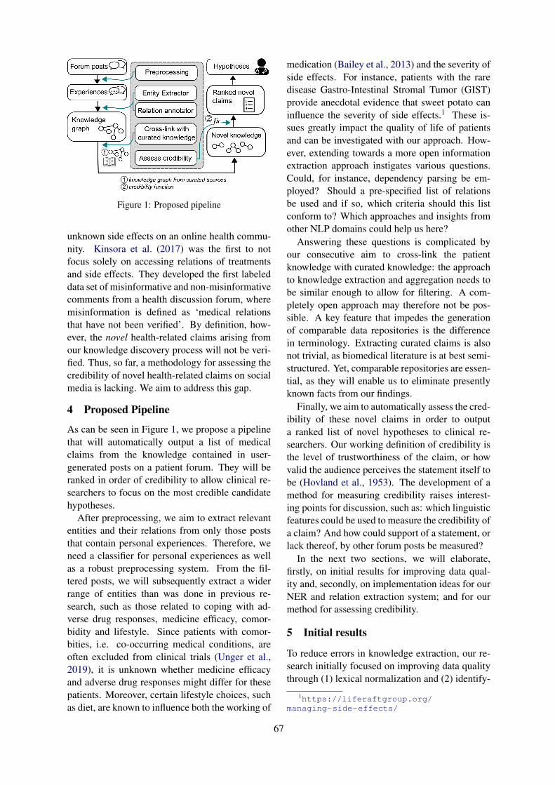
Figure 1: Proposed pipeline

unknown side effects on an online health commu-nity. Kinsora et al. (2017) was the first to notfocus solely on accessing relations of treatmentsand side effects. They developed the first labeleddata set of misinformative and non-misinformativecomments from a health discussion forum, wheremisinformation is defined as ‘medical relationsthat have not been verified’. By definition, how-ever, the novel health-related claims arising fromour knowledge discovery process will not be veri-fied. Thus, so far, a methodology for assessing thecredibility of novel health-related claims on socialmedia is lacking. We aim to address this gap.

4 Proposed Pipeline

As can be seen in Figure 1, we propose a pipelinethat will automatically output a list of medicalclaims from the knowledge contained in user-generated posts on a patient forum. They will beranked in order of credibility to allow clinical re-searchers to focus on the most credible candidatehypotheses.

After preprocessing, we aim to extract relevantentities and their relations from only those poststhat contain personal experiences. Therefore, weneed a classifier for personal experiences as wellas a robust preprocessing system. From the fil-tered posts, we will subsequently extract a widerrange of entities than was done in previous re-search, such as those related to coping with ad-verse drug responses, medicine efficacy, comor-bidity and lifestyle. Since patients with comor-bities, i.e. co-occurring medical conditions, areoften excluded from clinical trials (Unger et al.,2019), it is unknown whether medicine efficacyand adverse drug responses might differ for thesepatients. Moreover, certain lifestyle choices, suchas diet, are known to influence both the working of

medication (Bailey et al., 2013) and the severity ofside effects. For instance, patients with the raredisease Gastro-Intestinal Stromal Tumor (GIST)provide anecdotal evidence that sweet potato caninfluence the severity of side effects.1 These is-sues greatly impact the quality of life of patientsand can be investigated with our approach. How-ever, extending towards a more open informationextraction approach instigates various questions.Could, for instance, dependency parsing be em-ployed? Should a pre-specified list of relationsbe used and if so, which criteria should this listconform to? Which approaches and insights fromother NLP domains could help us here?

Answering these questions is complicated byour consecutive aim to cross-link the patientknowledge with curated knowledge: the approachto knowledge extraction and aggregation needs tobe similar enough to allow for filtering. A com-pletely open approach may therefore not be pos-sible. A key feature that impedes the generationof comparable data repositories is the differencein terminology. Extracting curated claims is alsonot trivial, as biomedical literature is at best semi-structured. Yet, comparable repositories are essen-tial, as they will enable us to eliminate presentlyknown facts from our findings.

Finally, we aim to automatically assess the cred-ibility of these novel claims in order to outputa ranked list of novel hypotheses to clinical re-searchers. Our working definition of credibility isthe level of trustworthiness of the claim, or howvalid the audience perceives the statement itself tobe (Hovland et al., 1953). The development of amethod for measuring credibility raises interest-ing points for discussion, such as: which linguisticfeatures could be used to measure the credibility ofa claim? And how could support of a statement, orlack thereof, by other forum posts be measured?

In the next two sections, we will elaborate,firstly, on initial results for improving data qual-ity and, secondly, on implementation ideas for ourNER and relation extraction system; and for ourmethod for assessing credibility.

5 Initial results

To reduce errors in knowledge extraction, our re-search initially focused on improving data qualitythrough (1) lexical normalization and (2) identify-

1https://liferaftgroup.org/managing-side-effects/

67

ing messages that contain personal experiences.2

Lexical normalization Since the state-of-the-art lexical normalization method (Sarker, 2017)functions poorly for social media in the health do-main, we developed a data-driven spelling correc-tion module that is dependent only on a genericdictionary and thus capable of dealing with smalland niche data sets (Dirkson et al., 2018, 2019b).We developed this method on a rare cancer fo-rum for GIST patients3 consisting of 36,722 posts.As a second cancer-related forum, we used a sub-reddit on cancer of 274,532 posts 4.

For detecting mistakes, we implemented a de-cision process that determines whether a token isa mistake by, firstly, checking if it is present ina generic dictionary, and if not, checking for vi-able candidates. Viable candidates, which are de-rived from the data, need to have at least doublethe corpus frequency and a high enough similarity.This relative, as opposed to an absolute, frequencythreshold enables the system to detect commonspelling mistakes. The underlying assumption isthat correct words will occur frequently enoughto not have any viable correction candidates: theywill thus be marked as correct. Our method at-tained an F0.5 score of 0.888. Additionally, itmanages to circumvent the absence of specializeddictionaries and domain- and genre-specific pre-trained word embeddings. For correcting spellingmistakes, relative weighted edit distance was em-ployed: the weights are derived from frequen-cies of online spelling errors (Norvig, 2009). Ourmethod attained an accuracy of 62.3% comparedto 20.8% for the state-of-the-art method (Sarker,2017). By pre-selecting viable candidates, this ac-curacy was further increased by 1.8% point.

This spelling correction pipeline reduced out-of-vocabulary terms by 0.50% and 0.27% in thetwo cancer-related forums. More importantly, itmainly targeted, and thus corrected, medical con-cepts. Additionally, it increased classification ac-curacy on five out of six benchmark data sets ofmedical forum text (Dredze et al. (2016); Paul andDredze (2009); Huang et al. (2017); and Task 1and 4 of the ACL 2019 Social Media Mining 4Health shared task5).

2Code and developed corpora can be found on https://github.com/AnneDirkson

3https://www.facebook.com/groups/gistsupport/

4www.reddit.com/r/cancer5https://healthlanguageprocessing.org/

Personal experience classification As researchinto systematically distinguishing patient experi-ences was limited to Dutch data with only one fea-ture type (Verberne et al., 2019), we investigatedhow they could best be identified in English forumdata (Dirkson et al., 2019a). Each post was classi-fied as containing a personal experience or not. Apersonal experience did not need to be about theauthor but could also be about someone else.

We found that character 3-grams (F1 = 0.815)significantly outperform psycho-linguistic fea-tures and document embeddings in this task.Moreover, we found that personal experienceswere characterized by the use of past tense, health-related words and first-person pronouns, whereasnon-narrative text was associated with the futuretense, emotional support words and second-personpronouns. Topic analysis of the patient experi-ences in a cancer forum uncovered fourteen medi-cal topics, ranging from surgery to side effects. Inthis project, developing a clear and effective an-notation guideline was the major challenge. Al-though the inter-annotator agreement was substan-tial (κ = 0.69), an error analysis revealed that an-notators still found it challenging to distinguish amedical fact from a medical experience.

6 Current and Future work

In the upcoming second year of the PhD project,we will focus on developing an NER and relationextraction (RE) system (Section 6.1). After that,we will address the challenge of credibility assess-ment (Section 6.2).

6.1 Extracting entities and their relations

For named entity recognition, we are currently ex-perimenting with BiLSTMs combined with Con-ditional Random Fields. Our system builds on thestate-of-the-art contextual flair embeddings (Ak-bik et al., 2018) trained on domain-specific data(Dirkson and Verberne, 2019). Our next step willbe to combine these with Glove or Bert Embed-dings (Devlin et al., 2018). We may also incorpo-rate domain knowledge from structured databasesin our embeddings, as this was shown to im-prove their quality (Zhang et al., 2019). The ex-tracted entities will be mapped to a subset of pre-selected categories of the UMLS (Unified MedicalLanguage System) (National Library of Medicine,

smm4h/challenge/

68

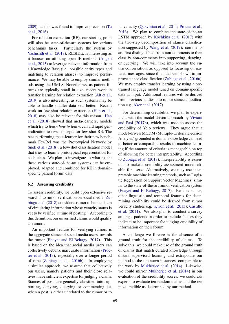
2009), as this was found to improve precision (Tuet al., 2016).

For relation extraction (RE), our starting pointwill also be state-of-the-art systems for variousbenchmark tasks. Particularly the system byVashishth et al. (2018), RESIDE, is interesting asit focuses on utilizing open IE methods (Angeliet al., 2015) to leverage relevant information froma Knowledge Base (i.e. possible entity types andmatching to relation aliases) to improve perfor-mance. We may be able to employ similar meth-ods using the UMLS. Nonetheless, as patient fo-rums are typically small in size, recent work intransfer learning for relation extraction (Alt et al.,2019) is also interesting, as such systems may beable to handle smaller data sets better. Recentwork on few-shot relation extraction (Han et al.,2018) may also be relevant for this reason. Hanet al. (2018) showed that meta-learners, modelswhich try to learn how to learn, can aid rapid gen-eralization to new concepts for few-shot RE. Thebest performing meta-learner for their new bench-mark FewRel was the Prototypical Network bySnell et al. (2018): a few-shot classification modelthat tries to learn a prototypical representation foreach class. We plan to investigate to what extentthese various state-of-the-art systems can be em-ployed, adapted and combined for RE in domain-specific patient forum data.

6.2 Assessing credibility

To assess credibility, we build upon extensive re-search into rumor verification on social media. Zu-biaga et al. (2018) consider a rumor to be: “an itemof circulating information whose veracity status isyet to be verified at time of posting”. According tothis definition, our unverified claims would qualifyas rumors.

An important feature for verifying rumors isthe aggregate stance of social media users towardsthe rumor (Enayet and El-Beltagy, 2017). Thisis based on the idea that social media users cancollectively debunk inaccurate information (Proc-ter et al., 2013), especially over a longer periodof time (Zubiaga et al., 2016b). In employinga similar approach, we assume that collectivelyour users, namely patients and their close rela-tives, have sufficient expertise for judging a claim.Stances of posts are generally classified into sup-porting, denying, querying or commenting i.e.when a post is either unrelated to the rumor or to

its veracity (Qazvinian et al., 2011; Procter et al.,2013). We plan to combine the state-of-the-artLSTM approach by Kochkina et al. (2017) withthe two-step decomposition of stance classifica-tion suggested by Wang et al. (2017): commentsare first distinguished from non-comments to thenclassify non-comments into supporting, denying,or querying. We will take into account the en-tire conversation, as opposed to focusing on iso-lated messages, since this has been shown to im-prove stance classification (Zubiaga et al., 2016a).We may employ transfer learning by using a pre-trained language model tuned on domain-specificdata as input. Additional features will be derivedfrom previous studies into rumor stance classifica-tion e.g. Aker et al. (2017).

For determining credibility, we plan to experi-ment with the model-driven approach by Vivianiand Pasi (2017b), which was used to assess thecredibility of Yelp reviews. They argue that amodel-driven MCDM (Multiple-Criteria DecisionAnalysis) grounded in domain knowledge can leadto better or comparable results to machine learn-ing if the amount of criteria is manageable on topof allowing for better interpretability. Accordingto Zubiaga et al. (2018), interpretability is essen-tial to make a credibility assessment more reli-able for users. Alternatively, we may use inter-pretable machine learning methods, such as Logis-tic Regression or Support Vector Machines, simi-lar to the state-of-the-art rumor verification system(Enayet and El-Beltagy, 2017). Besides stance,other linguistic and temporal features for deter-mining credibility could be derived from rumorveracity studies e.g. Kwon et al. (2013); Castilloet al. (2011). We also plan to conduct a surveyamongst patients in order to include factors theyindicate to be important for judging credibility ofinformation on their forum.

A challenge we foresee is the absence of aground truth for the credibility of claims. Tosolve this, we could make use of the ground truthof claims that match curated knowledge throughdistant supervised learning and extrapolate ourmethod to the unknown instances, comparable tothe work by Mukherjee et al. (2014). Likewise,we could mirror Mukherjee et al. (2014) in ourevaluation of the credibility scores: we could askexperts to evaluate ten random claims and the tenmost credible as determined by our method.

69

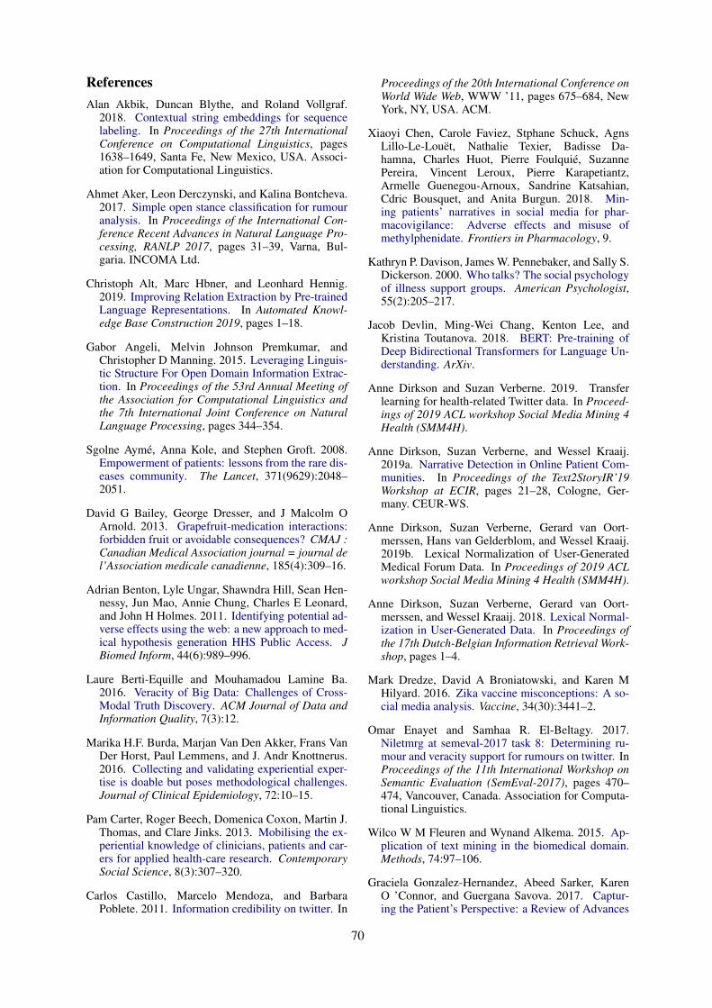
ReferencesAlan Akbik, Duncan Blythe, and Roland Vollgraf.

2018. Contextual string embeddings for sequencelabeling. In Proceedings of the 27th InternationalConference on Computational Linguistics, pages1638–1649, Santa Fe, New Mexico, USA. Associ-ation for Computational Linguistics.

Ahmet Aker, Leon Derczynski, and Kalina Bontcheva.2017. Simple open stance classification for rumouranalysis. In Proceedings of the International Con-ference Recent Advances in Natural Language Pro-cessing, RANLP 2017, pages 31–39, Varna, Bul-garia. INCOMA Ltd.

Christoph Alt, Marc Hbner, and Leonhard Hennig.2019. Improving Relation Extraction by Pre-trainedLanguage Representations. In Automated Knowl-edge Base Construction 2019, pages 1–18.

Gabor Angeli, Melvin Johnson Premkumar, andChristopher D Manning. 2015. Leveraging Linguis-tic Structure For Open Domain Information Extrac-tion. In Proceedings of the 53rd Annual Meeting ofthe Association for Computational Linguistics andthe 7th International Joint Conference on NaturalLanguage Processing, pages 344–354.

Sgolne Ayme, Anna Kole, and Stephen Groft. 2008.Empowerment of patients: lessons from the rare dis-eases community. The Lancet, 371(9629):2048–2051.

David G Bailey, George Dresser, and J Malcolm OArnold. 2013. Grapefruit-medication interactions:forbidden fruit or avoidable consequences? CMAJ :Canadian Medical Association journal = journal del’Association medicale canadienne, 185(4):309–16.

Adrian Benton, Lyle Ungar, Shawndra Hill, Sean Hen-nessy, Jun Mao, Annie Chung, Charles E Leonard,and John H Holmes. 2011. Identifying potential ad-verse effects using the web: a new approach to med-ical hypothesis generation HHS Public Access. JBiomed Inform, 44(6):989–996.

Laure Berti-Equille and Mouhamadou Lamine Ba.2016. Veracity of Big Data: Challenges of Cross-Modal Truth Discovery. ACM Journal of Data andInformation Quality, 7(3):12.

Marika H.F. Burda, Marjan Van Den Akker, Frans VanDer Horst, Paul Lemmens, and J. Andr Knottnerus.2016. Collecting and validating experiential exper-tise is doable but poses methodological challenges.Journal of Clinical Epidemiology, 72:10–15.

Pam Carter, Roger Beech, Domenica Coxon, Martin J.Thomas, and Clare Jinks. 2013. Mobilising the ex-periential knowledge of clinicians, patients and car-ers for applied health-care research. ContemporarySocial Science, 8(3):307–320.

Carlos Castillo, Marcelo Mendoza, and BarbaraPoblete. 2011. Information credibility on twitter. In

Proceedings of the 20th International Conference onWorld Wide Web, WWW ’11, pages 675–684, NewYork, NY, USA. ACM.

Xiaoyi Chen, Carole Faviez, Stphane Schuck, AgnsLillo-Le-Louet, Nathalie Texier, Badisse Da-hamna, Charles Huot, Pierre Foulquie, SuzannePereira, Vincent Leroux, Pierre Karapetiantz,Armelle Guenegou-Arnoux, Sandrine Katsahian,Cdric Bousquet, and Anita Burgun. 2018. Min-ing patients’ narratives in social media for phar-macovigilance: Adverse effects and misuse ofmethylphenidate. Frontiers in Pharmacology, 9.

Kathryn P. Davison, James W. Pennebaker, and Sally S.Dickerson. 2000. Who talks? The social psychologyof illness support groups. American Psychologist,55(2):205–217.

Jacob Devlin, Ming-Wei Chang, Kenton Lee, andKristina Toutanova. 2018. BERT: Pre-training ofDeep Bidirectional Transformers for Language Un-derstanding. ArXiv.

Anne Dirkson and Suzan Verberne. 2019. Transferlearning for health-related Twitter data. In Proceed-ings of 2019 ACL workshop Social Media Mining 4Health (SMM4H).

Anne Dirkson, Suzan Verberne, and Wessel Kraaij.2019a. Narrative Detection in Online Patient Com-munities. In Proceedings of the Text2StoryIR’19Workshop at ECIR, pages 21–28, Cologne, Ger-many. CEUR-WS.

Anne Dirkson, Suzan Verberne, Gerard van Oort-merssen, Hans van Gelderblom, and Wessel Kraaij.2019b. Lexical Normalization of User-GeneratedMedical Forum Data. In Proceedings of 2019 ACLworkshop Social Media Mining 4 Health (SMM4H).

Anne Dirkson, Suzan Verberne, Gerard van Oort-merssen, and Wessel Kraaij. 2018. Lexical Normal-ization in User-Generated Data. In Proceedings ofthe 17th Dutch-Belgian Information Retrieval Work-shop, pages 1–4.

Mark Dredze, David A Broniatowski, and Karen MHilyard. 2016. Zika vaccine misconceptions: A so-cial media analysis. Vaccine, 34(30):3441–2.

Omar Enayet and Samhaa R. El-Beltagy. 2017.Niletmrg at semeval-2017 task 8: Determining ru-mour and veracity support for rumours on twitter. InProceedings of the 11th International Workshop onSemantic Evaluation (SemEval-2017), pages 470–474, Vancouver, Canada. Association for Computa-tional Linguistics.

Wilco W M Fleuren and Wynand Alkema. 2015. Ap-plication of text mining in the biomedical domain.Methods, 74:97–106.

Graciela Gonzalez-Hernandez, Abeed Sarker, KarenO ’Connor, and Guergana Savova. 2017. Captur-ing the Patient’s Perspective: a Review of Advances

70

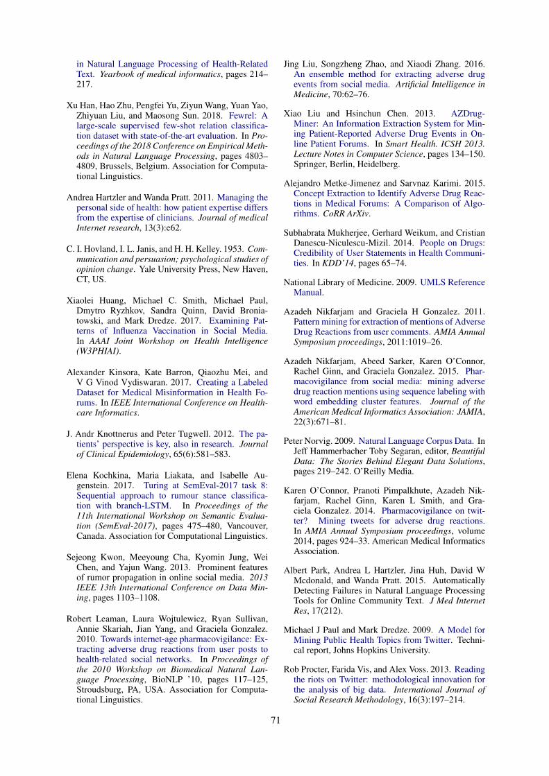
in Natural Language Processing of Health-RelatedText. Yearbook of medical informatics, pages 214–217.

Xu Han, Hao Zhu, Pengfei Yu, Ziyun Wang, Yuan Yao,Zhiyuan Liu, and Maosong Sun. 2018. Fewrel: Alarge-scale supervised few-shot relation classifica-tion dataset with state-of-the-art evaluation. In Pro-ceedings of the 2018 Conference on Empirical Meth-ods in Natural Language Processing, pages 4803–4809, Brussels, Belgium. Association for Computa-tional Linguistics.

Andrea Hartzler and Wanda Pratt. 2011. Managing thepersonal side of health: how patient expertise differsfrom the expertise of clinicians. Journal of medicalInternet research, 13(3):e62.

C. I. Hovland, I. L. Janis, and H. H. Kelley. 1953. Com-munication and persuasion; psychological studies ofopinion change. Yale University Press, New Haven,CT, US.

Xiaolei Huang, Michael C. Smith, Michael Paul,Dmytro Ryzhkov, Sandra Quinn, David Bronia-towski, and Mark Dredze. 2017. Examining Pat-terns of Influenza Vaccination in Social Media.In AAAI Joint Workshop on Health Intelligence(W3PHIAI).

Alexander Kinsora, Kate Barron, Qiaozhu Mei, andV G Vinod Vydiswaran. 2017. Creating a LabeledDataset for Medical Misinformation in Health Fo-rums. In IEEE International Conference on Health-care Informatics.

J. Andr Knottnerus and Peter Tugwell. 2012. The pa-tients’ perspective is key, also in research. Journalof Clinical Epidemiology, 65(6):581–583.

Elena Kochkina, Maria Liakata, and Isabelle Au-genstein. 2017. Turing at SemEval-2017 task 8:Sequential approach to rumour stance classifica-tion with branch-LSTM. In Proceedings of the11th International Workshop on Semantic Evalua-tion (SemEval-2017), pages 475–480, Vancouver,Canada. Association for Computational Linguistics.

Sejeong Kwon, Meeyoung Cha, Kyomin Jung, WeiChen, and Yajun Wang. 2013. Prominent featuresof rumor propagation in online social media. 2013IEEE 13th International Conference on Data Min-ing, pages 1103–1108.

Robert Leaman, Laura Wojtulewicz, Ryan Sullivan,Annie Skariah, Jian Yang, and Graciela Gonzalez.2010. Towards internet-age pharmacovigilance: Ex-tracting adverse drug reactions from user posts tohealth-related social networks. In Proceedings ofthe 2010 Workshop on Biomedical Natural Lan-guage Processing, BioNLP ’10, pages 117–125,Stroudsburg, PA, USA. Association for Computa-tional Linguistics.

Jing Liu, Songzheng Zhao, and Xiaodi Zhang. 2016.An ensemble method for extracting adverse drugevents from social media. Artificial Intelligence inMedicine, 70:62–76.

Xiao Liu and Hsinchun Chen. 2013. AZDrug-Miner: An Information Extraction System for Min-ing Patient-Reported Adverse Drug Events in On-line Patient Forums. In Smart Health. ICSH 2013.Lecture Notes in Computer Science, pages 134–150.Springer, Berlin, Heidelberg.

Alejandro Metke-Jimenez and Sarvnaz Karimi. 2015.Concept Extraction to Identify Adverse Drug Reac-tions in Medical Forums: A Comparison of Algo-rithms. CoRR ArXiv.

Subhabrata Mukherjee, Gerhard Weikum, and CristianDanescu-Niculescu-Mizil. 2014. People on Drugs:Credibility of User Statements in Health Communi-ties. In KDD’14, pages 65–74.

National Library of Medicine. 2009. UMLS ReferenceManual.

Azadeh Nikfarjam and Graciela H Gonzalez. 2011.Pattern mining for extraction of mentions of AdverseDrug Reactions from user comments. AMIA AnnualSymposium proceedings, 2011:1019–26.

Azadeh Nikfarjam, Abeed Sarker, Karen O’Connor,Rachel Ginn, and Graciela Gonzalez. 2015. Phar-macovigilance from social media: mining adversedrug reaction mentions using sequence labeling withword embedding cluster features. Journal of theAmerican Medical Informatics Association: JAMIA,22(3):671–81.

Peter Norvig. 2009. Natural Language Corpus Data. InJeff Hammerbacher Toby Segaran, editor, BeautifulData: The Stories Behind Elegant Data Solutions,pages 219–242. O’Reilly Media.

Karen O’Connor, Pranoti Pimpalkhute, Azadeh Nik-farjam, Rachel Ginn, Karen L Smith, and Gra-ciela Gonzalez. 2014. Pharmacovigilance on twit-ter? Mining tweets for adverse drug reactions.In AMIA Annual Symposium proceedings, volume2014, pages 924–33. American Medical InformaticsAssociation.

Albert Park, Andrea L Hartzler, Jina Huh, David WMcdonald, and Wanda Pratt. 2015. AutomaticallyDetecting Failures in Natural Language ProcessingTools for Online Community Text. J Med InternetRes, 17(212).

Michael J Paul and Mark Dredze. 2009. A Model forMining Public Health Topics from Twitter. Techni-cal report, Johns Hopkins University.

Rob Procter, Farida Vis, and Alex Voss. 2013. Readingthe riots on Twitter: methodological innovation forthe analysis of big data. International Journal ofSocial Research Methodology, 16(3):197–214.

71

Vahed Qazvinian, Emily Rosengren, Dragomir R.Radev, and Qiaozhu Mei. 2011. Rumor has it: Iden-tifying misinformation in microblogs. In Proceed-ings of the 2011 Conference on Empirical Methodsin Natural Language Processing, pages 1589–1599,Edinburgh, Scotland, UK. Association for Compu-tational Linguistics.

Lucia Sacchi and John H Holmes. 2016. Progress inBiomedical Knowledge Discovery: A 25-year Ret-rospective. Yearbook of medical informatics, pages117–29.

Hariprasad Sampathkumar, Xue-Wen Chen, andBo Luo. 2014. Mining Adverse Drug Reactionsfrom online healthcare forums using Hidden MarkovModel. BMC Medical Informatics and DecisionMaking, 14.

Abeed Sarker. 2017. A customizable pipeline for socialmedia text normalization. Social Network Analysisand Mining, 7(1):45.

Abeed Sarker, Maksim Belousov, Jasper Friedrichs,Kai Hakala, Svetlana Kiritchenko, FarrokhMehryary, Sifei Han, Tung Tran, Anthony Rios,Ramakanth Kavuluru, Berry de Bruijn, FilipGinter, Debanjan Mahata, Saif M Mohammad,Goran Nenadic, and Graciela Gonzalez-Hernandez.2018. Data and systems for medication-relatedtext classification and concept normalization fromTwitter: insights from the Social Media Miningfor Health (SMM4H)-2017 shared task. Journalof the American Medical Informatics Association,25(10):1274–1283.

Abeed Sarker, Rachel Ginn, Azadeh Nikfarjam, KarenO‘Connor, Karen Smith, Swetha Jayaraman, Te-jaswi Upadhaya, and Graciela Gonzalez. 2015. Uti-lizing social media data for pharmacovigilance: Areview. Journal of Biomedical Informatics, 54:202–212.

Abeed Sarker, Azadeh Nikfarjam, and Graciela Gonza-lez. 2016a. Social Media Mining Shared Task Work-shop. In Pacific Symposium Biocomputing, pages581–592.

Abeed Sarker, Karen O‘Connor, Rachel Ginn, MatthewScotch, Karen Smith, Dan Malone, and GracielaGonzalez. 2016b. Social Media Mining for Tox-icovigilance: Automatic Monitoring of Prescrip-tion Medication Abuse from Twitter. Drug Safety,39(3):231–240.

Edin Smailhodzic, Wyanda Hooijsma, Albert Boon-stra, and David J. Langley. 2016. Social mediause in healthcare: A systematic review of effectson patients and on their relationship with health-care professionals. BMC Health Services Research,16(1):442.

Jake Snell, Kevin Swersky, and Richard S. Zemel.2018. Prototypical networks for few-shot learning.

In Proceedings of the 2018 Conference on Empiri-cal Methods in Natural Language Processing, pages4803–4809.

Hongkui Tu, Zongyang Ma, Aixin Sun, and XiaodongWang. 2016. When MetaMap Meets Social Mediain Healthcare: Are the Word Labels Correct? InInformation Retrieval Technology. AIRS 2016. Lec-ture Notes in Computer Science., pages 356–362.Springer, Cham.

Joseph M. Unger, Dawn L. Hershman, Mark E. Fleury,and Riha Vaidya. 2019. Association of Patient Co-morbid Conditions With Cancer Clinical Trial Par-ticipation. JAMA Oncology, 5(3):326.

Shikhar Vashishth, Rishabh Joshi, Sai Suman Prayaga,Chiranjib Bhattacharyya, and Partha Talukdar. 2018.Reside: Improving distantly-supervised neural rela-tion extraction using side information. In Proceed-ings of the 2018 Conference on Empirical Methodsin Natural Language Processing, pages 1257–1266,Brussels, Belgium. Association for ComputationalLinguistics.

Suzan Verberne, Anika Batenburg, Remco Sanders,Mies van Eenbergen, Enny Das, and Mattijs S Lam-booij. 2019. Analyzing empowerment processesamong cancer patients in an online community: Atext mining approach. JMIR Cancer, 5(1):e9887.

Marco Viviani and Gabriella Pasi. 2017a. Credibilityin social media: opinions, news, and health informa-tiona survey. WIREs Data Mining Knowl Discov, 7.

Marco Viviani and Gabriella Pasi. 2017b. QuantifierGuided Aggregation for the Veracity Assessment ofOnline Reviews. International Journal of IntelligentSystems, 32(5):481–501.

V G Vinod Vydiswaran, Chengxiang Zhai, and DanRoth. 2011. Gauging the Internet Doctor: RankingMedical Claims based on Community Knowledge.In KDD-DMH.

Feixiang Wang, Man Lan, and Yuanbin Wu. 2017.ECNU at SemEval-2017 task 8: Rumour evalua-tion using effective features and supervised ensem-ble models. In Proceedings of the 11th InternationalWorkshop on Semantic Evaluation (SemEval-2017),pages 491–496, Vancouver, Canada. Association forComputational Linguistics.

SriJyothsna Yeleswarapu, Aditya Rao, Thomas Joseph,Vangala Govindakrishnan Saipradeep, and RajgopalSrinivasan. 2014. A pipeline to extract drug-adverseevent pairs from multiple data sources. BMC medi-cal informatics and decision making, 14(13).

Yijia Zhang, Qingyu Chen, Zhihao Yang, Hongfei Lin,and Zhiyong Lu. 2019. BioWordVec,improvingbiomedical word embeddings with subword infor-mation and MeSH. Scientific Data, 6(1):52.

72

Arkaitz Zubiaga, Ahmet Aker, Kalina Bontcheva,Maria Liakata, and Rob Procter. 2018. Detectionand resolution of rumours in social media: A sur-vey. ACM Comput. Surv., 51(2):32:1–32:36.

Arkaitz Zubiaga, Elena Kochkina, Maria Liakata, RobProcter, and Michal Lukasik. 2016a. Stance clas-sification in rumours as a sequential task exploit-ing the tree structure of social media conversations.In COLING 2016, 26th International Conference onComputational Linguistics, Proceedings of the Con-ference: Technical Papers, December 11-16, 2016,Osaka, Japan, pages 2438–2448.

Arkaitz Zubiaga, Maria Liakata, Rob Procter, Geral-dine Wong Sak Hoi, and Peter Tolmie. 2016b.Analysing how people orient to and spread rumoursin social media by looking at conversational threads.PLOS ONE, 11(3):1–29.

73

Proceedings of the 57th Annual Meeting of the Association for Computational Linguistics: Student Research Workshop, pages 74–80Florence, Italy, July 28 - August 2, 2019. c©2019 Association for Computational Linguistics

Automated Cross-language Intelligibility Analysis of Parkinson’s DiseasePatients Using Speech Recognition Technologies

Nina Hosseini-Kivanani 1, Juan Camilo Vasquez-Correa2, 3, Manfred Stede4, Elmar Noth2

1International Experimental and Clinical Linguistics (IECL), University of Potsdam, Germany2 Pattern Recognition Lab, Friedrich-Alexander University Erlangen-Nuremberg, Germany

3 Faculty of Engineering, University of Antioquia UdeA, Medellın, Colombia4Applied Computational Linguistics, University of Potsdam, Germany

hosseinikiva, stede@uni-potsdam.dejcamilo.vasquez@udea.edu.co

elmar.noeth@fau.de

AbstractSpeech deficits are common symptoms amongParkinson’s Disease (PD) patients. The auto-matic assessment of speech signals is promis-ing for the evaluation of the neurological stateand the speech quality of the patients. Re-cently, progress has been made in applyingmachine learning and computational methodsto automatically evaluate the speech of PD pa-tients. In the present study, we plan to an-alyze the speech signals of PD patients andhealthy control (HC) subjects in three differ-ent languages: German, Spanish, and Czech,with the aim to identify biomarkers to discrim-inate between PD patients and HC subjects andto evaluate the neurological state of the pa-tients. Therefore, the main contribution of thisstudy is the automatic classification of PD pa-tients and HC subjects in different languageswith focusing on phonation, articulation, andprosody. We will focus on an intelligibilityanalysis based on automatic speech recogni-tion systems trained on these three languages.This is one of the first studies done that consid-ers the evaluation of the speech of PD patientsin different languages. The purpose of this re-search proposal is to build a model that candiscriminate PD and HC subjects even whenthe language used for train and test is differ-ent.

1 Introduction

Parkinsons disease (PD) (i.e. Shaking palsy(Parkinson, 2002)) is the second most commonneurodegenerative disorder after Alzheimers dis-ease. PD displays a great prevalence in individualsof advanced age (Dexter and Jenner, 2013), espe-cially, over the age of fifty (Fahn, 2003). The signsand symptoms of PD can significantly influencethe quality of life of patients. They are grouped

into two categories: motor and non-motor symp-toms. Speech impairments are one of the earliestmanifestations in PD patients.

Early diagnosis of PD is a vital challenge inthis field. The first step in analyzing this diseaseis the development of markers of PD progressionthrough collecting data from several cohorts. Toreach this aim, different clinical rating scales havebeen developed, such as the Unified Parkinson’sDisease Rating Scale (UPDRS), Movement Dis-orders Society - UPDRS (MDS-UPDRS) 1 (Goetzet al., 2008) and Hoehn & Yahr (H & Y) staging,(Visser et al., 2006).

The UPDRS is the most widely used rating toolfor the clinical evaluation of PD patients. The ex-amination requires observation and interview bya professional clinician. The scale is distributedinto 4 sections: (i) Mentation, behavior and mood,(ii) Activities of daily living (ADL), (iii) Motorsections, and (iv) Motor complications.

One of the most common motor problems isrelated to speech impairments in PD (Jankovic,2008). Most of the patients with PD show dis-abilities in speech production. The most commonspeech disturbances are monotonic speech, hypo-phonia (a speech weakness in the vocal muscula-ture and vocal sounds) and hypokinetic dysarthria.These symptoms reduce the intelligibility of thepatients, and affect different aspects of the speechproduction such as articulation, phonation, nasal-ity, and prosody (Little et al., 2009; Goetz et al.,2008; Ramig et al., 2001). Therefore, there is agreat interest to develop tools or methods to eval-uate and improve the speech production of PD pa-tients.

1MDS-UPDRS is the most updated version of the UP-DRS.

74

Recently, there has been a proliferation of newspeech recognition-based tools for the acousticanalysis of PD. The use of speech recognitionsoftware in clinical examinations could make apowerful supplement to the state-of-the-art sub-jective reports of experts and clinicians that arecostly and time-consuming (e.g., Little et al.,2009; Hernandez-Espinosa et al., 2002). In theclinical field, the detection of PD is a complex taskdue to the fact that the symptoms of this diseaseare more related to clinicians’ observations andperception of the way patients move and speak.

Recently, machine learning tools are used to de-velop speech recognition systems that make thewhole process of objective evaluation and recogni-tion faster and more accurate than analytical clini-cians’ methods (Yu and Deng, 2016; Hernandez-Espinosa et al., 2002). Using machine learningtechniques to extract acoustic features for detect-ing the PD has become widely used in recent stud-ies (e.g., Dahl et al., 2012; Little et al., 2009).

Automatic speech recognition (ASR) systemsare used to decode and transcribe oral speech. Inother words, the goal of ASR systems is to find andrecognize the words that best represent the acous-tic signal. For example, automatic speech recog-nition systems are used to evaluate how speech in-telligibility is affected by the disease.

This study will seek to further investigate thespeech patterns of HC and PD groups usingrecordings from patients speaking in German,Spanish, and Czech. Most of the previous studiesonly considered recordings in one language andfocused on it for detecting PD, but in this study,we plan to evaluate the effect of the PD in threedifferent languages.

2 Related work: ASR for detecting PDsymptoms

Speech can be measured by acoustic tools sim-ply using aperiodic vibrations in the voice. Thefield of speech recognition has been improvedin recent years by research in computer-assistedspeech training system for therapy (Beijer and Ri-etvel, 2012) machine learning techniques, whichcan lead to establish efficient biomarkers to dis-criminate HC from people with PD (e.g., Orozco-Arroyave et al., 2013).

There are a vast number of advanced tech-niques to design ASR systems: hybrid Deep Neu-

ral Networks-Hidden Markov Models (DNN 2-HMM) (Hinton et al., 2012) and ConvolutionalNeural Networks (CNN) (Abdel-Hamid et al.,2014). Deep neural networks have recently re-ceived increasing attention in speech recognition(Canevari et al., 2013). Other studies have high-lighted the strength of the DNN-HMM frameworkfor speech recognition (e.g., Dahl et al., 2012).

On the other hand, regarding the assessment ofPD from speech, Skodda et al. (2011) assessedthe progression of speech impairments of PD from2002 to 2012 in a longitudinal study by only usinga statistical test to evaluate changes in aspects re-lated to voice, articulation, prosody, and fluency ofthe recorded speech.

Orozco-Arroyave et al. (2016) considered morethan one language for producing isolated wordsfor discriminating PDs from HCs. The character-ization and classification processes were based ona method on the systematic separation of voicedand unvoiced segments of speech in their study.Vasquez-Correa et al. (2017) analyzed the ef-fect of acoustic conditions on different algorithms.The obtained detection accuracy of PD speech wasreported and shown that the background noise af-fect the performance of the different algorithms.However, most of these systems are not yet capa-ble of automatically detecting speech impairmentof individual speech sounds, which are knownto have an impact on speech intelligibility (Zhaoet al., 2010; Ramaker et al., 2002).

Our goal is to develop robust ASR systems forpathological speech and incorporate the ASR tech-nology to detect their speech intelligibility prob-lems. A major interest is to investigate acousticfeatures in the mentioned languages (differencesand similarities), including gender differences be-tween subject (HC & PD) groups. The overall pur-pose of this project is to address the question ofwhether cross-lingual speech intelligibility amongPDs and HCs can help the recognition system todetect the correct disease. The classification ofPD from speech in different languages has to becarefully conducted to avoid bias towards the lin-guistic content present in each language. For in-stance, Czech and German languages are richerthan Spanish language in terms of consonant pro-duction, which may cause that it is easier to pro-duce consonant sounds by Czech PD patients than

2DNN is a feed-forward neural network that has morethan one layer of hidden units between its inputs and its out-puts (Hinton et al., 2012).

75

by Spanish PD patients. In addition, with theuse of transfer learning strategies, a model trainedwith utterances from one language can be used asa base model to train a model in a different lan-guage.

After reviewing the aforementioned literature,the main contribution of our research for modelingspeech signals in PD patients is twofold:

• This is one of the first cross-lingual stud-ies done to evaluate speech of people withPD. This work requires a database consistingof recordings of different languages. Thereis currently a lack of cross-lingual research,which provides reliable classification meth-ods for assessing PDs’ speech available in theliterature.

• Using speech data is expected to help the de-velopment of a diagnostic of PD patients.

This project seeks to bridge the gap in speechrecognition for speech of PD, with the hope ofmoving towards a higher adoption rate of ASR-based technologies in the diagnosis of patients.

3 The set-up of the ASR system

In this work, we will build an ASR system to rec-ognize the speech of patients of Parkinson’s Dis-ease. The task of ASR is to convert this raw au-dio into text. The ASR system is created basedon three models: acoustic model (i.e. to recognizephonemes), pronunciation model (i.e. to map se-quence of phonemes into word sequences), andlanguage model (i.e. to estimate probabilities ofword sequences). We place particular emphasison the acoustic model portion of the system. Wealso provide some acoustic models output featuresthat could be used in future speech recognition ofPD severity in the clinical field. Ravanelli et al.(2019) stated that along with the improvement ofASR systems, several deep learning frameworks(e.g., TensorFlow (Abadi et al., 2016)) in machinelearning are also widely used.

The next section describes the process for mod-eling the intelligibility of PD speech followed bythe description of processes whether the speechsignal is from PD patient or from HC subjects.

3.1 TrainingThe proposed ASR system will be developed us-ing a standard state-of-the-art architecture hybridDNN-HMM (see Nassif et al., 2019 for more

information about the existing models in ASR),built using the Kaldi speech recognition toolkit3. The preprocessing (i.e. Feature extraction) ofthe acoustic signal into usable parameters (i.e. la-bel computation) tries to remove any acoustic in-formation that is not useful for the task; it willbe done before beginning to train the acousticmodel. In this study, we will use Mel-frequencyCepstral coefficients (MFCC) and Mel filter bankenergies (e.g., compute-mfcc-feats and compute-fbank-feats) to train the acoustic models of theASR systems. The task of calculating MFCCsfrom acoustic features is to characterize an under-lying signal using spectrograms and represent theshape of the vocal tract including tongue, teeth etc.

It was observed that filter bank (fbank), one ofthe most popular speech recognition features, per-forms better than MFCCs when used with deepneural networks (Hinton et al., 2012). The purposeof using acoustic model is to help us to get bound-aries of the phoneme labels. The acoustic modelswill be trained based on different acoustic featuresextracted in Kaldi ”nnet3” recipes. The extractedacoustic features and the observation probabilitiesof our ASR system will be used to train the hybridDNN-HMM acoustic model. The performance ofan ASR system will be measured by Word ErrorRate (WER) of the transcript produced by the sys-tem against the target transcript.

PyTorch: PyTorch is one of the most wellknown deep learning toolkit that facilitates the de-sign of neural architectures. This tool will be usedto design new DNN architectures to improve theperformance of the ASR system. We will addition-ally use PyTorch-Kaldi (Ravanelli et al., 2019),to train4 deep neural network based models (e.g.,DNNs, CNNs, and Recurrent Neural Networks(RNNs) models) and traditional machine learningclassifier. Ravanelli et al. (2019) stated that thisPyTorch-Kaldi toolkit acts like an interface withdifferent speech recognition features in it and canbe used as a state-of-the-art in the field of ASR(See Figure 1). Figure 1 is shown the generalmethodology that will be applied in this research.

3Kaldi: http://kaldi-asr.org/doc/4PyTorch-Kaldi:https://github.com/

mravanelli/pytorch-kaldi

76

Figure 1: ASR system architecture that will be used inthis study (Ravanelli et al., 2019).

4 Methods

4.1 DataThe data of this study comes from an extended ver-sion of PC-GITA database for Spanish (Orozco-Arroyave et al., 2014), German (Skodda et al.,2011), and Czech (Rusz et al., 2011) with morerecordings from PDs and HCs. The database con-sists of both PD and HC subjects.

All subjects were asked to do multiple types ofspeaking tasks to understand how speech changesin different conditions, due to the fact that voicevariation is difficult to identify without human ex-perience (Jeancolas et al., 2017). The speech di-mensions considered in this project are phonation,articulation and prosody (See Figure 2).

Figure 2: Speech dimensions: Phonation, Articulationand Prosody.

For each subject, speech material includes(i) sustained vowel phonation; participants wereasked to phonate vowels for several seconds;,(ii) rapid syllable repetition (ideally Diadochoki-netic (DDK)); participants were asked to producesuch as /pa-ta-ka/, /pa-ka-ta/, /pe-ta-ka/, /pa/, /ta/,

and /ka/, (iii) connected speech, consisting of:,(iv) reading a specific text, and (v) spontaneousspeech.

This dataset consists of speech samplesrecorded from 88 PD and 88 HC German speak-ing participants, 50 PD and 50 HC Spanishspeaking participants (balanced in age and gen-der), and 20 PD and 16 HC Czech speakingparticipants. These speech samples were assessedby expert neurologists using UPDRS-III andH & Y scales. Their neurological labels werereported based on the UPDRS-III and H & Yscales (mean± SD) for each PD group:

• PD-German: UPDRS-III (22.7 ± 10.9), H&Y (2.4 ±0.6)

• PD-Spanish: UPDRS-III (36.7 ± 18.7), H&Y (2.3 ±0.8)

• PD-Czech: UPDRS-III (17.9± 7.3), H&Y (2.2± 0.5)

Further details are shown in Table 1:

Language HC PDFemale Male Female Male

German n= 44(63.8± 12.7 )

n= 44(62.6± 15.2)

n= 41(66.2± 9.7)

n= 47(66.7± 8.4)

Spanish n= 25(61.4± 7.0)

n= 25(60.3± 11.6)

n= 25(60.7± 7.3)

n= 25(61.6± 11.2)

Czech — n= 16(61.8± 13.3) — n= 20

(61± 12)

Table 1: Age information of HC and PD subjects inthe study (n = number of participant) & the mean andstandard deviation are in the parenthesis (Mean±SD).

Although the size of the data is not big enough,the vocabulary that was used by the patients inthe capture process of the speech was fixed. Thisaspect compensates the need to have a huge cor-pus to evaluate a vocabulary dependent task likethe assessment of pathological speech (see Parra-Gallego et al., 2018).

4.2 SamplePraat software (Boersma and Weenink, 2016) isused for segmenting speech, extracting acousticsfeatures, removing silence from beginning andend of speech file and visualization of speechdata. Generally, spoken words, represented assound waves, have two axes: time on the x-axis and amplitude on the y-axis. Figure 3 illus-trates the example of input feature maps extractedfrom the speech signal which shows the selectedspectrograms (the audio waveform is encoded asa representation) of PD and HC subjects whenthey pronounce the syllable /pa-ta-ka/ that con-vey 3-dimensional information in 2 dimensions

77

(a) HC (b) PD

Figure 3: Top: Raw waveforms of /pa-ta-ka/ (x-axis: time; y-axis: amplitude). Middle: Spectrograms (x-axis:time; y-axis: frequency; shading: amplitude (energy), darker means higher). Bottom: the word-level annotationof the signal.

(i.e. Time: x-axis, Frequency: y-axis, and Ampli-tude: color intensity). The proposed model willbe able to identify specific aspects in the speechrelated to the pronunciation of consonants, whichare the most affected aspects of the speech of thepatients due to the disease. The segmentation pro-cess will be performed using a trained model to de-tect phonological classes, like those ones used inthe previous studies (Vasquez-Correa et al., 2019;Cernak et al., 2017). Figure 3 shows the possi-ble differences in articulation and phonation in PDand HC subjects. By using Praat, the speech sam-ples of syllable /pa-ta-ka/ will be segmented intovowel and consonant frames. The contour of HCsample is more stable than the obtained contourfrom PD sample. In each sample, silences will beremoved from the beginning and the end of eachtoken, using Praat.

5 Conclusion

In this research proposal, we introduced and de-scribed the background for speech recognition ofPD patients. The focus is on Parkinsons diseasespeech recognition based on the acoustic analysisof their voice. A brief overview of clinical andmachine learning research in this field was pro-vided. The goal is to improve the ASR system tobe able to model and detect PD patients indepen-dently from their language by taking speech as aninput and using machine learning and natural lan-guage processing technologies to advance health-care and provide an overview of the patients men-

tal health. All in all, the proposed method shouldbe able to detect the patient with PD and discrimi-nate them from HC subjects.

ReferencesMartn Abadi, Paul Barham, Jianmin Chen, Zhifeng

Chen, Andy Davis, Jeffrey Dean, Matthieu Devin,Sanjay Ghemawat, Geoffrey Irving, Michael Isard,Manjunath Kudlur, Josh Levenberg, Rajat Monga,Sherry Moore, Derek G Murray, Benoit Steiner,Paul Tucker, Vijay Vasudevan, Pete Warden, Mar-tin Wicke, Yuan Yu, Xiaoqiang Zheng, and GoogleBrain. 2016. TensorFlow: A System for Large-Scale Machine Learning TensorFlow: A system forlarge-scale machine learning. In In 12th USENIXSymposium on Operating Systems Design and Im-plementation (OSDI 16), pages 265–283.

Ossama Abdel-Hamid, Abdel Rahman Mohamed, HuiJiang, Li Deng, Gerald Penn, and Dong Yu. 2014.Convolutional neural networks for speech recogni-tion. IEEE Transactions on Audio, Speech and Lan-guage Processing, 22(10):1533–1545.

Lilian Beijer and Toni Rietvel. 2012. Potentials ofTelehealth Devices for Speech Therapy in Parkin-son’s Disease. In Diagnostics and Rehabilitation ofParkinson’s Disease. InTech, pages 379–402.

Paul Boersma and David Weenink. 2016. Praat: Doingphonetics by computer (Version 6.0. 14). Retrievedfrom (last access: 29.04. 2018).

Claudia Canevari, Leonardo Badino, Luciano Fadiga,and Giorgio Metta Rbcs. 2013. Cross-corpus andcross-linguistic evaluation of a speaker-dependentDNN-HMM ASR system using EMA data. In InSpeech Production in Automatic Speech Recognition(In SPASR-2013), pages 29–33.

78

Milos Cernak, Juan Rafael Orozco-Arroyave, FrankRudzicz, Heidi Christensen, Juan Camilo Vasquez-Correa, and Elmar Noth. 2017. Characterisationof voice quality of Parkinson’s disease using dif-ferential phonological posterior features. ComputerSpeech and Language, 46(June):196–208.

George E. Dahl, Dong Yu, Li Deng, and Alex Acero.2012. Context-dependent pre-trained deep neuralnetworks for large-vocabulary speech recognition.IEEE Transactions on Audio, Speech and LanguageProcessing, 20(1):30–42.

David T. Dexter and Peter Jenner. 2013. Parkinson dis-ease: from pathology to molecular disease mecha-nisms. Free Radical Biology and Medicine, 62:132–144.

Stanley Fahn. 2003. Description of Parkinson’s Dis-ease as a Clinical Syndrome. Annals of the New YorkAcademy of Sciences, 991(1):1–14.

Christopher G. Goetz, Barbara C. Tilley, Stephanie R.Shaftman, Glenn T. Stebbins, Stanley Fahn, PabloMartinez-Martin, Werner Poewe, Cristina Sampaio,Matthew B. Stern, Richard Dodel, Bruno Dubois,Robert Holloway, Joseph Jankovic, Jaime Kuli-sevsky, Anthony E. Lang, Andrew Lees, Sue Leur-gans, Peter A. LeWitt, David Nyenhuis, C. WarrenOlanow, Olivier Rascol, Anette Schrag, Jeanne A.Teresi, Jacobus J. van Hilten, and Nancy LaPelle.2008. Movement Disorder Society-sponsored revi-sion of the Unified Parkinson’s Disease Rating Scale(MDS-UPDRS): Scale presentation and clinimetrictesting results. Movement Disorders, 23(15):2129–2170.

Carlos Hernandez-Espinosa, Pedro Gomez-Vilda,Juan I. Godino-Llorente, and Santiago Aguilera-Navarro. 2002. Diagnosis of vocal and voice dis-orders by the speech signal. In Proceedings of theIEEE-INNS-ENNS International Joint Conferenceon Neural Networks. IJCNN 2000. Neural Comput-ing: New Challenges and Perspectives for the NewMillennium, pages 253–258. IEEE.

Geoffrey Hinton, Li Deng, Dong Yu, George Dahl,Abdel Rahman Mohamed, Navdeep Jaitly, AndrewSenior, Vincent Vanhoucke, Patrick Nguyen, TaraSainath, and Brian Kingsbury. 2012. Deep neu-ral networks for acoustic modeling in speech recog-nition: The shared views of four research groups.IEEE Signal Processing Magazine, 29(6):82–97.

Joseph Jankovic. 2008. Parkinsons disease: clinicalfeatures and diagnosis. Journal of Neurology, Neu-rosurgery & Psychiatry, 79(4):368–376.

Laetitia Jeancolas, Habib Benali, Badr-EddineBenkelfat, Graziella Mangone, Jean-ChristopheCorvol, Marie Vidailhet, Stephane Lehericy, andDijana Petrovska-Delacretaz. 2017. Automaticdetection of early stages of Parkinson’s diseasethrough acoustic voice analysis with mel-frequencycepstral coefficients. In International Conference

on Advanced Technologies for Signal and ImageProcessing (ATSIP), pages 1–6. IEEE.

Max A Little, Patrick E McSharry, Eric J Hunter, Jen-nifer Spielman, and Lorraine O Ramig. 2009. Suit-ability of dysphonia measurements for telemonitor-ing of Parkinson’s disease. IEEE transactions onbio-medical engineering, 56(4):1015.

Ali Bou Nassif, Ismail Shahin, Imtinan Attili, Moham-mad Azzeh, and Khaled Shaalan. 2019. SpeechRecognition Using Deep Neural Networks: A Sys-tematic Review. IEEE Access, 7:19143–19165.

Juan R. Orozco-Arroyave, Julin D. Arias-Londono, Je-sus Francisco V. Bonilla, Mara C. Gonzalez-Rativa,and Elmar Noth. 2014. New Spanish speech corpusdatabase for the analysis of people suffering fromParkinson’s disease. In Language Resources andEvaluation Conference, LREC, pages 342–347.

Juan R. Orozco-Arroyave, Julin D. Arias-Londono,Jess F. Vargas-Bonilla, and Elmar Noth. 2013. Anal-ysis of Speech from People with Parkinsons Diseasethrough Nonlinear Dynamics. In International con-ference on nonlinear speech processing, pages 112–119. Springer, Berlin, Heidelberg.

Juan R. Orozco-Arroyave, Juan C. Vadsquez-Correa,Florian Honig, Julin D. Arias-Londono, Jess F.Vargas-Bonilla, Sabine Skodda, Jan Rusz, and El-mar Noth. 2016. Towards an automatic monitoringof the neurological state of Parkinson’s patients fromspeech. ICASSP, IEEE International Conference onAcoustics, Speech and Signal Processing - Proceed-ings, 2016-May(March):6490–6494.

James Parkinson. 2002. An Essay on the ShakingPalsy. The Journal of Neuropsychiatry and ClinicalNeurosciences, 14(2):223–236.

Luis F. Parra-Gallego, Toms Arias-Vergara, Juan C.Vasquez-Correa, Nicanor Garcia-Ospina, Juan R.Orozco-Arroyave, and Elmar Noth. 2018. Auto-matic Intelligibility Assessment of Parkinsons Dis-ease with Diadochokinetic Exercises. pages 223–230. Springer, Cham.

Claudia Ramaker, Johan Marinus, Anne MargaretheStiggelbout, and Bob Johannes van Hilten. 2002.Systematic evaluation of rating scales for impair-ment and disability in Parkinson’s disease. Move-ment Disorders, 17(5):867–876.

Lorraine Olson Ramig, Steven Gray, Kristin Baker,Kim Corbin-Lewis, Eugene Buder, Erich Luschei,Hillary Coon, and Marshall Smith. 2001. The agingvoice: A review, treatment data and familial and ge-netic perspectives. Folia Phoniatrica et Logopaed-ica, 53(5):252–265.

Mirco Ravanelli, Titouan Parcollet, and Yoshua Ben-gio. 2019. The PyTorch-Kaldi Speech RecognitionToolkit. ICASSP 2019 - 2019 IEEE InternationalConference on Acoustics, Speech and Signal Pro-cessing (ICASSP), pages 6465–6469.

79

Jan Rusz, Roman Cmejla, Hana Ruzickova, and EvzenRuzicka. 2011. Quantitative acoustic measurementsfor characterization of speech and voice disorders inearly untreated Parkinsons disease. The Journal ofthe Acoustical Society of America, 129(1):350–367.

Sabine Skodda, Wenke Visser, and Uwe Schlegel.2011. Vowel Articulation in Parkinson’s Disease.Journal of Voice, 25(4):467–472.

Juan C. Vasquez-Correa, Philipp Klumpp, Juan R.Orozco-Arroyave, and Elmar Noth. 2019. Phonet:a Tool Based on Gated Recurrent Neural Networksto Extract Phonological Posteriors from Speech. InProceedings of INTERSPEECH conference (Underreview).

Juan C. Vasquez-Correa, Joan Serra, Juan R. Orozco-Arroyave, Jess F. Vargas-Bonilla, and Elmar Noth.2017. Effect of acoustic conditions on algo-rithms to detect Parkinson’s disease from speech.ICASSP, IEEE International Conference on Acous-tics, Speech and Signal Processing - Proceedings,pages 5065–5069.

Martine Visser, Albert F.G. Leentjens, Johan Marinus,Anne M. Stiggelbout, and Jacobus J. van Hilten.2006. Reliability and validity of the Beck depres-sion inventory in patients with Parkinson’s disease.Movement Disorders, 21(5):668–672.

Dong Yu and Li Deng. 2016. Automatic SpeechRecognition-A Deep Learning Approach. Springerlondon limited.

Ying J. Zhao, Hwee L. Wee, Yiong H. Chan, Soo H.Seah, Wing L. Au, Puay Ngoh Lau, Emmanuel C.Pica, Shu Ch. Li, Nan Luo, and Louis C S Tan. 2010.Progression of Parkinson’s disease as evaluated byHoehn and Yahr stage transition times. MovementDisorders, 25(6):710–716.

80

Proceedings of the 57th Annual Meeting of the Association for Computational Linguistics: Student Research Workshop, pages 81–88Florence, Italy, July 28 - August 2, 2019. c©2019 Association for Computational Linguistics

Natural Language Generation: Recently Learned Lessons, Directions forSemantic Representation-based Approaches, and the case of Brazilian

Portuguese Language

Marco Antonio Sobrevilla Cabezudo and Thiago Alexandre Salgueiro PardoInterinstitutional Center for Computational Linguistics (NILC)

Institute of Mathematical and Computer Sciences, University of Sao PauloSao Carlos/SP, Brazil

msobrevillac@usp.br, taspardo@icmc.usp.br

Abstract

This paper presents a more recent literature re-view on Natural Language Generation. In par-ticular, we highlight the efforts for BrazilianPortuguese in order to show the available re-sources and the existent approaches for thislanguage. We also focus on the approachesfor generation from semantic representations(emphasizing the Abstract Meaning Represen-tation formalism) as well as their advantagesand limitations, including possible future di-rections.

1 Introduction

Natural Language Generation (NLG) is a promis-ing area in Natural Language Processing (NLP)community. NLG aims to build computer sys-tems that may produce understandable texts in En-glish or other human languages from some under-lying non-linguistic representation of information(Reiter and Dale, 2000). Tools generated by thisarea are useful for other applications like Auto-matic Summarization, Question-Answering Sys-tems, and others.

There are several efforts in NLG for English1.For example, one may see the works of Krahmeret al. (2003) and Li et al. (2018), which focusedon referring expressions generation, and the workof (Gatt and Reiter, 2009), focused on developinga surface realisation tool called SimpleNLG. Onemay also easily find other works that tried to gen-erate text from semantic representations (Flaniganet al., 2016; Ferreira et al., 2017; Puzikov andGurevych, 2018b).

For Brazilian Portuguese, there are few works,some of them focused on representations like Uni-versal Networking Language (UNL) (Nunes et al.,2002) or Resource Description Framework (RDF)

1Most of the works may be found in the main NLP publi-cation portal at https://www.aclweb.org/anthology/

(Moussallem et al., 2018), and other ones that arevery specific to the Referring Expression Gener-ation (Pereira and Paraboni, 2008; Lucena et al.,2010) and Surface Realisation tasks (Oliveira andSripada, 2014; Silva et al., 2013).

More recently, several representations haveemerged in the NLP area (Gardent et al., 2017;Novikova et al., 2017; Mille et al., 2018). In par-ticular, Abstract Meaning Representation (AMR)has gained interest from the research community(Banarescu et al., 2013). It is a semantic formal-ism that aims to encode the meaning of a sen-tence with a simple representation in the form ofa directed rooted graph. This representation in-cludes information about semantic roles, namedentities, wiki entities, spatial-temporal informa-tion, and co-references, among other information.

AMR has gained attention mainly due to itssimplicity to be read by humans and computers,its attempt to abstract away from syntactic id-iosyncrasies (focusing only on semantic process-ing) and its wide use of other comprehensive lin-guistic resources, such as PropBank (Palmer et al.,2005) (Bos, 2016).

For English, there is a large AMR-annotatedcorpus that contains 39,260 AMR-annotated sen-tences2, which allows deeper studies in NLG andexperiments with different approaches (mainlystatistical approaches). This may be evidencedin the SemEval-2017 shared-task 9 (May andPriyadarshi, 2017)3.

For Brazilian Portuguese, Anchieta and Pardo(2018) built the first corpus using sentences fromthe “The Little Prince” book. The authors tookadvantage of the alignment between the Englishand Brazilian Portuguese versions of the book toimport the AMR structures from one language to

2Available at https://catalog.ldc.upenn.edu/LDC2017T10.3Available at http://alt.qcri.org/semeval2017/task9/.

81

another (but also performing the necessary adap-tations). They had to use the Verbo-Brasil reposi-tory (Duran et al., 2013; Duran and Aluısio, 2015),which is a PropBank-like resource for Portuguese.Nowadays, there is an effort to build a largerAMR-annotated corpus that is similar to the cur-rent one available for English.

In this context, this study presents a litera-ture review on Natural Language Generation forBrazilian Portuguese in order to show the re-sources (in relation to semantic representations)that are available for Portuguese and the existentefforts in the area for this language. We focuson the NLG approaches based on semantic repre-sentations and discuss their advantages and limi-tations. Finally, we suggest some future directionsto the area.

2 Literature Review

The literature review was based on the followingresearch questions:

• What was the focus of the existent NLGefforts for Portuguese and which resourceswere used for this language?

• What challenges exist in the NLG ap-proaches?

• What are the advantages and limitations inthe approaches for NLG from semantic repre-sentations, specially Abstract Meaning Rep-resentation?

Such issues are discussed in what follows.

2.1 Natural Language Generation forPortuguese

In general, we could find few works for Por-tuguese (considering the existing works for En-glish). These works focus mainly on the refer-ring expression generation (Pereira and Paraboni,2008; Lucena et al., 2010) and surface realiza-tion tasks (Silva et al., 2013; Oliveira and Sri-pada, 2014), usually restricted to specific domainsand applications (like undergraduate test scoring).Nevertheless, there are some recent attempts fo-cused on other tasks and in more general domains(Moussallem et al., 2018; Sobrevilla Cabezudoand Pardo, 2018).

Among the NLG approaches, we may highlightthe use of templates (Pereira and Paraboni, 2008;Novais et al., 2010b), rules (Novais and Paraboni,

2013) and language models (LM) (Novais et al.,2010a). In general, these approaches were suc-cessful because they were focused on restricteddomains. Specifically, template-based methodsused basic templates to build sentences. Simi-larly, some basic rules involving noun and verbalphrases were defined to build sentences. Finally,LM-based methods applied a two-stage strategy togenerate sentences. This strategy consisted in gen-erating surface realization alternatives and select-ing the best alternative according to the languagemodel.

In the case of LM-based methods, we may pointout that classical LMs (based on n-grams) werenot suitable because it was necessary to use a largecorpus to deal with sparsity of data. Sparsity is abig problem in morphologically marked languageslike Portuguese. In order to solve the sparsity ofthe data, some works used Factored LMs, obtain-ing better results than the classical LMs (de Novaiset al., 2011).

In relation to NLG from semantic representa-tions for Portuguese, we may point out the workof Nunes et al. (2002) (focused on Universal Lan-guage Networking), and Moussallem et al. (2018)(focused on ontologies). Another representationwas the one proposed by Mille et al. (2018) (basedon Universal Dependencies), which is based onsyntax instead of semantics.

In relation to NLG tools, we highlight PortNLG(Silva et al., 2013) and SimpleNLG-BP (Oliveiraand Sripada, 2014) as surface realisers that werebased on SimpleNLG initiative (Gatt and Reiter,2009)4. Finally, other NLG works aimed to buildNLP applications, e.g., for structured data visual-ization and human-computer interaction purposes(Pereira et al., 2012, 2015).

2.2 Natural Language Generation fromSemantic Representations

Recently, the number of works on NLGfrom semantic representations has increased.This increase is reflected in the shared tasksWebNLG (Gardent et al., 2017), E2E Challenge(Novikova et al., 2017), Semeval Task-9 (Mayand Priyadarshi, 2017) and Surface RealizationShared-Task (Belz et al., 2011; Mille et al., 2018).

In general, there is a trend to apply methodsbased on neural networks. However, methods

4Specifically, SimpleNLG-BP was built using the Frenchversion of SimpleNLG due to the similarities between bothlanguages.

82

based on templates, transformation to intermediaterepresentations and language models have showninteresting results. It is also worthy noticing thatmost of these methods have been applied to En-glish, except for the methods presented in theshared-task proposed by Mille et al. (2018).

In relation to the shared-tasks mentioned before,we point out that the one proposed by Belz et al.(2011) and Mille et al. (2018) (based on Univer-sal Dependencies) used syntactic representations.Specifically, they presented two tracks, one fo-cused on word reordering and inflection genera-tion (superficial track), and other that focused ongenerating sentences from a deep syntactic repre-sentation that is similar to a semantic represen-tation (deep track). Furthermore, these tasks fo-cused on several languages in the superficial task(including Portuguese) and three languages in thedeep track (English, Spanish, and French).

Among the methods used for the superficialtrack in these shared-tasks, we may highlight theuse of rule-based methods and language models inthe early years (Belz et al., 2011) and a wide ap-plication of neural models in recent years (Milleet al., 2018). In the case of the deep track, it is pos-sible to notice that rule-based methods were ap-plied in the first competition, and methods basedon transformation to intermediate representationsand based on neural models were applied in thelast competition.

The results in these tasks showed that ap-proaches based on transformation to intermediaterepresentations obtained poor results in the auto-matic evaluation due to the great effort in buildingtransformation rules for their own systems. How-ever, they usually showed better results in humanevaluations. This may be explained by the matu-rity of the original proposed systems. This way,although the coverage of the rules was not good,the results were good from a human point of view.

Differently from the approach mentioned be-fore, methods based on neural models (deep learn-ing) obtained the best results. However, somemethods used data augmentation strategies to dealwith data sparsity (Elder and Hokamp, 2018; So-brevilla Cabezudo and Pardo, 2018).

One point to highlight is that the results for Por-tuguese were poor (compared to similar languageslike Spanish). Two reasons to explain this issue arerelated to the amount of data for Portuguese in thistask (less than English or Spanish) and the quality

of the existing models for related tasks that wereused. Another point to highlight is the division ofthe general task into two sub-tasks: linearisationand inflection generation. Puzikov and Gurevych(2018a) pointed out that there is a strong relationbetween the linearisation and the inflection gener-ation, and, thus, both sub-tasks should be treatedtogether.

In contrast to Puzikov and Gurevych (2018a),(Elder and Hokamp, 2018) showed that incorpo-rating syntax and morphological information intoneural models did not bring significant contribu-tion in the generation process, but incorporatedmore difficulty in the task.

Finally, it is important to notice the proposal ofMadsack et al. (2018), which trained linearisationmodels using the dataset for each language inde-pendently and in a joint way, using multilingualembeddings. Although the results of this work didnot present a lot of variation when used for all lan-guages together, this work suggests that it is pos-sible to train systems with similar languages (forexample, Spanish and French) in order to take ad-vantage of the syntax similarities and to overcomethe problems of lack of data.

In relation to other used representations (Gar-dent et al., 2017; Novikova et al., 2017), a largenumber of works based on deep learning strategieswere proposed, obtaining good results. However,the use of pipeline-based methods yielded promis-ing results regarding grammar and fluency criteriain a joint evaluation (for RDF representation), butthese methods (which usually use rules) obtainedthe worst results in the E2E Challenge.

Methods based on Statistical Machine Transla-tion kept a reasonable performance (ranking 2ndin RDF Shared-Task), obtaining good results whenevaluating the grammar. The explanation for thisresult comes from the ability to learn completephrases. Thus, these methods may generate gram-matically correct phrases, but with poor generalfluency and dissimilarity to the target output. Fi-nally, methods based on template obtained promis-ing results in restricted domains, like in the E2EChallenge.

2.3 Natural Language Generation fromAbstract Meaning Representation

In relation to generation methods from AbstractMeaning Representation, it was possible to high-light approaches based on machine translation

83

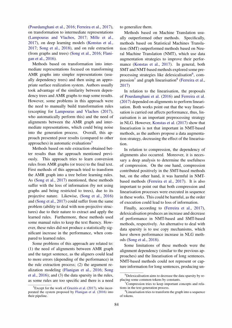
(Pourdamghani et al., 2016; Ferreira et al., 2017),on transformation to intermediate representations(Lampouras and Vlachos, 2017; Mille et al.,2017), on deep learning models (Konstas et al.,2017; Song et al., 2018), and on rule extraction(from graphs and trees) (Song et al., 2016; Flani-gan et al., 2016).

Methods based on transformation into inter-mediate representations focused on transformingAMR graphs into simpler representations (usu-ally dependency trees) and then using an appro-priate surface realization system. Authors usuallytook advantage of the similarity between depen-dency trees and AMR graphs to map some results.However, some problems in this approach werethe need to manually build transformation rules(excepting for Lampouras and Vlachos (2017),who automatically perform this) and the need ofalignments between the AMR graph and inter-mediate representations, which could bring noiseinto the generation process. Overall, this ap-proach presented poor results (compared to otherapproaches) in automatic evaluations5

Methods based on rule extraction obtained bet-ter results than the approach mentioned previ-ously. This approach tries to learn conversionrules from AMR graphs (or trees) to the final text.First methods of this approach tried to transformthe AMR graph into a tree before learning rules.As (Song et al., 2017) mentioned, these methodssuffer with the loss of information (by not usinggraphs and being restricted to trees), due to itsprojective nature. Likewise, (Song et al., 2016)and (Song et al., 2017) could suffer from the sameproblem (ability to deal with non-projective struc-tures) due to their nature to extract and apply thelearned rules. Furthermore, these methods usedsome manual rules to keep the text fluency. How-ever, these rules did not produce a statistically sig-nificant increase in the performance, when com-pared to learned rules.

Some problems of this approach are related to:(1) the need of alignments between AMR graphand the target sentence, as the aligners could leadto more errors (depending of the performance) inthe rule extraction process; (2) the argument re-alization modeling (Flanigan et al., 2016; Songet al., 2016); and (3) the data sparsity in the rules,as some rules are too specific and there is a need

5Except for the work of Gruzitis et al. (2017), who incor-porated the system proposed by Flanigan et al. (2016) intotheir pipeline.

to generalize them.Methods based on Machine Translation usu-

ally outperformed other methods. Specifically,methods based on Statistical Machines Transla-tion (SMT) outperformed methods based on Neu-ral Machine Translation (NMT), which use dataaugmentation strategies to improve their perfor-mance (Konstas et al., 2017). In general, bothSMT and NMT-based methods explored some pre-processing strategies like delexicalisation6, com-pression7 and graph linearisation8 (Ferreira et al.,2017)

In relation to the linearisation, the proposalsof Pourdamghani et al. (2016) and Ferreira et al.(2017) depended on alignments to perform lineari-sation. Both works point out that the way lineari-sation is carried out affects performance, thus, lin-earisation is an important preprocessing strategyin NLG. However, Konstas et al. (2017) show thatlinearisation is not that important in NMT-basedmethods, as the authors propose a data augmenta-tion strategy, decreasing the effect of the linearisa-tion.

In relation to compression, the dependency ofalignments also occurred. Moreover, it is neces-sary a deep analysis to determine the usefulnessof compression. On the one hand, compressioncontributed positively in the SMT-based methodsbut, on the other hand, it was harmful in NMT-based methods (Ferreira et al., 2017). It is alsoimportant to point out that both compression andlinearisation processes were executed in sequencein these works. This could be harmful, as the orderof execution could lead to loss of information.

Finally, according to (Ferreira et al., 2017),delexicalisation produces an increase and decreaseof performance in NMT-based and SMT-basedmethods, respectively. An alternative to deal withdata sparsity is to use copy mechanisms, whichhave shown performance increase in NLG meth-ods (Song et al., 2018).

Some limitations of these methods were thealignment dependency (similar to the previous ap-proaches) and the linearisation of long sentences.NMT-based methods could not represent or cap-ture information for long sentences, producing un-

6Delexicalisation aims to decrease the data sparsity by re-placing some common tokens by constants.

7Compression tries to keep important concepts and rela-tions in the text generation process.

8Linearisation tries to transform the graph into a sequenceof tokens.

84

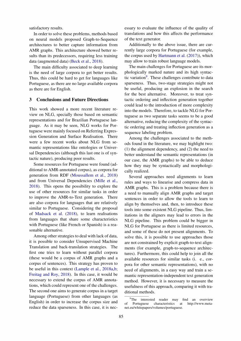
satisfactory results.In order to solve these problems, methods based

on neural models proposed Graph-to-Sequencearchitectures to better capture information fromAMR graphs. This architecture showed better re-sults than its predecessors, requiring less trainingdata (augmented data) (Beck et al., 2018).

The main difficulty associated to deep learningis the need of large corpora to get better results.Thus, this could be hard to get for languages likePortuguese, as there are no large available corporaas there are for English.

3 Conclusions and Future Directions

This work showed a more recent literature re-view on NLG, specially those based on semanticrepresentations and for Brazilian Portuguese lan-guage. As it may be seen, NLG works for Por-tuguese were mainly focused on Referring Expres-sion Generation and Surface Realisation. Therewere a few recent works about NLG from se-mantic representations like ontologies or Univer-sal Dependencies (although this last one is of syn-tactic nature), producing poor results.

Some resources for Portuguese were found (ad-ditional to AMR-annotated corpus), as corpora forgeneration from RDF (Moussallem et al., 2018)and from Universal Dependencies (Mille et al.,2018). This opens the possibility to explore theuse of other resources for similar tasks in orderto improve the AMR-to-Text generation. Thereare also corpora for languages that are relativelysimilar to Portuguese. Considering the proposalof Madsack et al. (2018), to learn realisationsfrom languages that share some characteristicswith Portuguese (like French or Spanish) is a rea-sonable alternative.

Among other strategies to deal with lack of data,it is possible to consider Unsupervised MachineTranslation and back-translation strategies. Thefirst one tries to learn without parallel corpora(these would be a corpus of AMR graphs and acorpus of sentences). This strategy has proven tobe useful in this context (Lample et al., 2018a,b;Freitag and Roy, 2018). In this case, it would benecessary to extend the corpus of AMR annota-tions, which could represent one of the challenges.The second one aims to generate corpus in a targetlanguage (Portuguese) from other languages (asEnglish) in order to increase the corpus size andreduce the data sparseness. In this case, it is nec-

essary to evaluate the influence of the quality oftranslations and how this affects the performanceof the text generator.

Additionally to the above issue, there are cur-rently large corpora for Portuguese (for example,the corpus used by Hartmann et al. (2017)), whichmay allow to train robust language models.

The main challenges for Portuguese are its mor-phologically marked nature and its high syntac-tic variation9. These challenges contribute to datasparseness. Thus, two-stage strategies might notbe useful, producing an explosion in the searchfor the best alternative. Moreover, to treat syn-tactic ordering and inflection generation togethercould lead to the introduction of more complexityinto the models. Therefore, to tackle NLG for Por-tuguese as two separate tasks seems to be a goodalternative, reducing the complexity of the syntac-tic ordering and treating inflection generation as asequence labeling problem.

Among the challenges associated to the meth-ods found in the literature, we may highlight two:(1) the alignment dependency, and (2) the need tobetter understand the semantic representations (inour case, the AMR graphs) to be able to deducehow they may be syntactically and morphologi-cally realized.

Several approaches need alignments to learnrules and ways to linearise and compress data inAMR graphs. This is a problem because there isa need to manually align AMR graphs and targetsentences in order to allow the tools to learn toalign by themselves and, then, to introduce thesetools into some existent NLG pipeline. Thus, lim-itations in the aligners may lead to errors in theNLG pipeline. This problem could be bigger inNLG for Portuguese as there is limited resources,and some of these do not present alignments. Tosolve this, it is possible to use approaches thoseare not constrained by explicit graph-to-text align-ments (for example, graph-to-sequence architec-tures). Furthermore, this could help to join all theavailable resources for similar tasks (i. e., cor-pora for other semantic representations), with noneed of alignments, in a easy way and train a se-mantic representation-independent text generationmethod. However, it is necessary to measure theusefulness of this approach, comparing it with tra-ditional methods.

9The interested reader may find an overviewof Portuguese characteristics at http://www.meta-net.eu/whitepapers/volumes/portuguese.

85

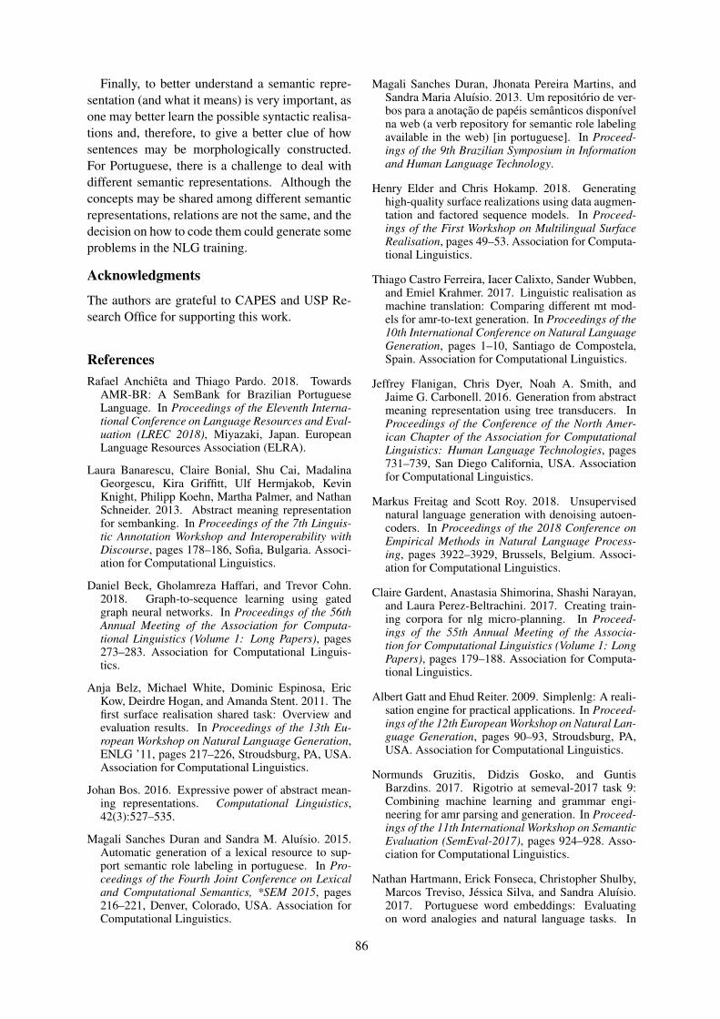
Finally, to better understand a semantic repre-sentation (and what it means) is very important, asone may better learn the possible syntactic realisa-tions and, therefore, to give a better clue of howsentences may be morphologically constructed.For Portuguese, there is a challenge to deal withdifferent semantic representations. Although theconcepts may be shared among different semanticrepresentations, relations are not the same, and thedecision on how to code them could generate someproblems in the NLG training.

Acknowledgments

The authors are grateful to CAPES and USP Re-search Office for supporting this work.

ReferencesRafael Anchieta and Thiago Pardo. 2018. Towards

AMR-BR: A SemBank for Brazilian PortugueseLanguage. In Proceedings of the Eleventh Interna-tional Conference on Language Resources and Eval-uation (LREC 2018), Miyazaki, Japan. EuropeanLanguage Resources Association (ELRA).

Laura Banarescu, Claire Bonial, Shu Cai, MadalinaGeorgescu, Kira Griffitt, Ulf Hermjakob, KevinKnight, Philipp Koehn, Martha Palmer, and NathanSchneider. 2013. Abstract meaning representationfor sembanking. In Proceedings of the 7th Linguis-tic Annotation Workshop and Interoperability withDiscourse, pages 178–186, Sofia, Bulgaria. Associ-ation for Computational Linguistics.

Daniel Beck, Gholamreza Haffari, and Trevor Cohn.2018. Graph-to-sequence learning using gatedgraph neural networks. In Proceedings of the 56thAnnual Meeting of the Association for Computa-tional Linguistics (Volume 1: Long Papers), pages273–283. Association for Computational Linguis-tics.

Anja Belz, Michael White, Dominic Espinosa, EricKow, Deirdre Hogan, and Amanda Stent. 2011. Thefirst surface realisation shared task: Overview andevaluation results. In Proceedings of the 13th Eu-ropean Workshop on Natural Language Generation,ENLG ’11, pages 217–226, Stroudsburg, PA, USA.Association for Computational Linguistics.

Johan Bos. 2016. Expressive power of abstract mean-ing representations. Computational Linguistics,42(3):527–535.

Magali Sanches Duran and Sandra M. Aluısio. 2015.Automatic generation of a lexical resource to sup-port semantic role labeling in portuguese. In Pro-ceedings of the Fourth Joint Conference on Lexicaland Computational Semantics, *SEM 2015, pages216–221, Denver, Colorado, USA. Association forComputational Linguistics.

Magali Sanches Duran, Jhonata Pereira Martins, andSandra Maria Aluısio. 2013. Um repositorio de ver-bos para a anotacao de papeis semanticos disponıvelna web (a verb repository for semantic role labelingavailable in the web) [in portuguese]. In Proceed-ings of the 9th Brazilian Symposium in Informationand Human Language Technology.

Henry Elder and Chris Hokamp. 2018. Generatinghigh-quality surface realizations using data augmen-tation and factored sequence models. In Proceed-ings of the First Workshop on Multilingual SurfaceRealisation, pages 49–53. Association for Computa-tional Linguistics.

Thiago Castro Ferreira, Iacer Calixto, Sander Wubben,and Emiel Krahmer. 2017. Linguistic realisation asmachine translation: Comparing different mt mod-els for amr-to-text generation. In Proceedings of the10th International Conference on Natural LanguageGeneration, pages 1–10, Santiago de Compostela,Spain. Association for Computational Linguistics.

Jeffrey Flanigan, Chris Dyer, Noah A. Smith, andJaime G. Carbonell. 2016. Generation from abstractmeaning representation using tree transducers. InProceedings of the Conference of the North Amer-ican Chapter of the Association for ComputationalLinguistics: Human Language Technologies, pages731–739, San Diego California, USA. Associationfor Computational Linguistics.

Markus Freitag and Scott Roy. 2018. Unsupervisednatural language generation with denoising autoen-coders. In Proceedings of the 2018 Conference onEmpirical Methods in Natural Language Process-ing, pages 3922–3929, Brussels, Belgium. Associ-ation for Computational Linguistics.

Claire Gardent, Anastasia Shimorina, Shashi Narayan,and Laura Perez-Beltrachini. 2017. Creating train-ing corpora for nlg micro-planning. In Proceed-ings of the 55th Annual Meeting of the Associa-tion for Computational Linguistics (Volume 1: LongPapers), pages 179–188. Association for Computa-tional Linguistics.

Albert Gatt and Ehud Reiter. 2009. Simplenlg: A reali-sation engine for practical applications. In Proceed-ings of the 12th European Workshop on Natural Lan-guage Generation, pages 90–93, Stroudsburg, PA,USA. Association for Computational Linguistics.

Normunds Gruzitis, Didzis Gosko, and GuntisBarzdins. 2017. Rigotrio at semeval-2017 task 9:Combining machine learning and grammar engi-neering for amr parsing and generation. In Proceed-ings of the 11th International Workshop on SemanticEvaluation (SemEval-2017), pages 924–928. Asso-ciation for Computational Linguistics.

Nathan Hartmann, Erick Fonseca, Christopher Shulby,Marcos Treviso, Jessica Silva, and Sandra Aluısio.2017. Portuguese word embeddings: Evaluatingon word analogies and natural language tasks. In

86

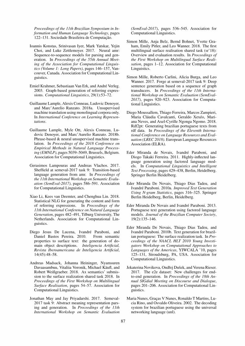
Proceedings of the 11th Brazilian Symposium in In-formation and Human Language Technology, pages122–131. Sociedade Brasileira de Computacao.

Ioannis Konstas, Srinivasan Iyer, Mark Yatskar, YejinChoi, and Luke Zettlemoyer. 2017. Neural amr:Sequence-to-sequence models for parsing and gen-eration. In Proceedings of the 55th Annual Meet-ing of the Association for Computational Linguis-tics (Volume 1: Long Papers), pages 146–157, Van-couver, Canada. Association for Computational Lin-guistics.

Emiel Krahmer, Sebastiaan Van Erk, and Andre Verleg.2003. Graph-based generation of referring expres-sions. Computational Linguistics, 29(1):53–72.

Guillaume Lample, Alexis Conneau, Ludovic Denoyer,and Marc’Aurelio Ranzato. 2018a. Unsupervisedmachine translation using monolingual corpora only.In International Conference on Learning Represen-tations.

Guillaume Lample, Myle Ott, Alexis Conneau, Lu-dovic Denoyer, and Marc’Aurelio Ranzato. 2018b.Phrase-based & neural unsupervised machine trans-lation. In Proceedings of the 2018 Conference onEmpirical Methods in Natural Language Process-ing (EMNLP), pages 5039–5049, Brussels, Belgium.Association for Computational Linguistics.

Gerasimos Lampouras and Andreas Vlachos. 2017.Sheffield at semeval-2017 task 9: Transition-basedlanguage generation from amr. In Proceedings ofthe 11th International Workshop on Semantic Evalu-ation (SemEval-2017), pages 586–591. Associationfor Computational Linguistics.

Xiao Li, Kees van Deemter, and Chenghua Lin. 2018.Statistical NLG for generating the content and formof referring expressions. In Proceedings of the11th International Conference on Natural LanguageGeneration, pages 482–491, Tilburg University, TheNetherlands. Association for Computational Lin-guistics.

Diego Jesus De Lucena, Ivandre Paraboni, andDaniel Bastos Pereira. 2010. From semanticproperties to surface text: the generation of do-main object descriptions. Inteligencia Artificial,Revista Iberoamericana de Inteligencia Artificial,14(45):48–58.

Andreas Madsack, Johanna Heininger, NyamsurenDavaasambuu, Vitaliia Voronik, Michael Kaufl, andRobert Weißgraeber. 2018. Ax semantics’ submis-sion to the surface realization shared task 2018. InProceedings of the First Workshop on MultilingualSurface Realisation, pages 54–57. Association forComputational Linguistics.

Jonathan May and Jay Priyadarshi. 2017. Semeval-2017 task 9: Abstract meaning representation pars-ing and generation. In Proceedings of the 11thInternational Workshop on Semantic Evaluation

(SemEval-2017), pages 536–545. Association forComputational Linguistics.

Simon Mille, Anja Belz, Bernd Bohnet, Yvette Gra-ham, Emily Pitler, and Leo Wanner. 2018. The firstmultilingual surface realisation shared task (sr’18):Overview and evaluation results. In Proceedings ofthe First Workshop on Multilingual Surface Reali-sation, pages 1–12. Association for ComputationalLinguistics.

Simon Mille, Roberto Carlini, Alicia Burga, and LeoWanner. 2017. Forge at semeval-2017 task 9: Deepsentence generation based on a sequence of graphtransducers. In Proceedings of the 11th Interna-tional Workshop on Semantic Evaluation (SemEval-2017), pages 920–923. Association for Computa-tional Linguistics.

Diego Moussallem, Thiago Ferreira, Marcos Zampieri,Maria Claudia Cavalcanti, Geraldo Xexeo, Mari-ana Neves, and Axel-Cyrille Ngonga Ngomo. 2018.Rdf2pt: Generating brazilian portuguese texts fromrdf data. In Proceedings of the Eleventh Interna-tional Conference on Language Resources and Eval-uation (LREC 2018). European Language ResourcesAssociation (ELRA).

Eder Miranda de Novais, Ivandre Paraboni, andDiogo Takaki Ferreira. 2011. Highly-inflected lan-guage generation using factored language mod-els. In Computational Linguistics and IntelligentText Processing, pages 429–438, Berlin, Heidelberg.Springer Berlin Heidelberg.

Eder Miranda De Novais, Thiago Dias Tadeu, andIvandre Paraboni. 2010a. Improved Text GenerationUsing N-gram Statistics, pages 316–325. SpringerBerlin Heidelberg, Berlin, Heidelberg.

Eder Miranda De Novais and Ivandre Paraboni. 2013.Portuguese text generation using factored languagemodels. Journal of the Brazilian Computer Society,19(2):135–146.

Eder Miranda De Novais, Thiago Dias Tadeu, andIvandre Paraboni. 2010b. Text generation for brazil-ian portuguese: The surface realization task. In Pro-ceedings of the NAACL HLT 2010 Young Investi-gators Workshop on Computational Approaches toLanguages of the Americas, YIWCALA ’10, pages125–131, Stroudsburg, PA, USA. Association forComputational Linguistics.

Jekaterina Novikova, Ondrej Dusek, and Verena Rieser.2017. The e2e dataset: New challenges for end-to-end generation. In Proceedings of the 18th An-nual SIGdial Meeting on Discourse and Dialogue,pages 201–206. Association for Computational Lin-guistics.

Maria Nunes, Gracas V Nunes, Ronaldo T Martins, Lu-cia Rino, and Osvaldo Oliveira. 2002. The decodingsystem for brazilian portuguese using the universalnetworking language (unl).

87

Rodrigo De Oliveira and Somayajulu Sripada. 2014.Adapting simplenlg for brazilian portuguese real-isation. In Proceedings of the Eighth Interna-tional Natural Language Generation Conference,Including Proceedings of the INLG and SIGDIAL,pages 93–94, Philadelphia, PA, USA. Associationfor Computational Linguistics.

Martha Palmer, Daniel Gildea, and Paul Kingsbury.2005. The proposition bank: An annotated cor-pus of semantic roles. Computational Linguistics.,31(1):71–106.

Daniel Bastos Pereira and Ivandre Paraboni. 2008. Sta-tistical surface realisation of portuguese referringexpressions. In Proceedings of the 6th InternationalConference on Advances in Natural Language Pro-cessing, pages 383–392, Gothenburg, Sweden.

JC Pereira, A Teixeira, and JS Pinto. 2015. Towards aHybrid Nlg System for Data2Text in Portuguese. InProceedings of the 10th Iberian Conference on In-formation Systems and Technologies (CISTI), pages1–6, Aveiro, Portugal. IEEE.

Jose Casimiro Pereira, Antonio JS Teixeira, andJoaquim Sousa Pinto. 2012. Natural language gen-eration in the context of multimodal interactionin portuguese. Electronica e Telecomunicacoes,5(4):400–409.

Nima Pourdamghani, Kevin Knight, and Ulf Her-mjakob. 2016. Generating english from abstractmeaning representations. In Proceedings of theNinth International Natural Language GenerationConference, pages 21–25, Edinburgh, UK.

Yevgeniy Puzikov and Iryna Gurevych. 2018a. Binlin:A simple method of dependency tree linearization.In Proceedings of the First Workshop on Multilin-gual Surface Realisation, pages 13–28. Associationfor Computational Linguistics.

Yevgeniy Puzikov and Iryna Gurevych. 2018b. E2e nlgchallenge: Neural models vs. templates. In Proceed-ings of the 11th International Conference on NaturalLanguage Generation, pages 463–471. Associationfor Computational Linguistics.

Ehud Reiter and Robert Dale. 2000. Building NaturalLanguage Generation Systems. Cambridge Univer-sity Press, New York, NY, USA.

Douglas Fernandes Pereira Da Silva, Eder Miranda DeNovais, and Ivandre Paraboni. 2013. Um sistema derealizacao superficial para geracao de textos em por-tugues. Revista de Informatica Teorica e Aplicada,20(3):31–48.

Marco Antonio Sobrevilla Cabezudo and ThiagoPardo. 2018. Nilc-swornemo at the surface real-ization shared task: Exploring syntax-based wordordering using neural models. In Proceedings ofthe First Workshop on Multilingual Surface Reali-sation, pages 58–64. Association for ComputationalLinguistics.

Linfeng Song, Xiaochang Peng, Yue Zhang, ZhiguoWang, and Daniel Gildea. 2017. Amr-to-text gener-ation with synchronous node replacement grammar.In Proceedings of the 55th Annual Meeting of theAssociation for Computational Linguistics, pages 7–13. Association for Computational Linguistics.

Linfeng Song, Yue Zhang, Xiaochang Peng, ZhiguoWang, and Daniel Gildea. 2016. Amr-to-text gener-ation as a traveling salesman problem. In Proceed-ings of the 2016 Conference on Empirical Methodsin Natural Language Processing, pages 2084–2089,Austin, Texas. Association for Computational Lin-guistics.

Linfeng Song, Yue Zhang, Zhiguo Wang, and DanielGildea. 2018. A graph-to-sequence model for amr-to-text generation. In Proceedings of the 56th An-nual Meeting of the Association for ComputationalLinguistics, pages 1616–1626. Association for Com-putational Linguistics.

88

Proceedings of the 57th Annual Meeting of the Association for Computational Linguistics: Student Research Workshop, pages 89–99Florence, Italy, July 28 - August 2, 2019. c©2019 Association for Computational Linguistics

Long-Distance Dependencies don’t have to be Long:Simplifying through Provably (Approximately) Optimal Permutations

Rishi BommasaniDepartment of Computer Science

Cornell Universityrb724@cornell.edu

Abstract

Neural models at the sentence level often op-erate on the constituent words/tokens in a waythat encodes the inductive bias of processingthe input in a similar fashion to how humansdo. However, there is no guarantee that thestandard ordering of words is computationallyefficient or optimal. To help mitigate this, weconsider a dependency parse as a proxy forthe inter-word dependencies in a sentence andsimplify the sentence with respect to combi-natorial objectives imposed on the sentence-parse pair. The associated optimization re-sults in permuted sentences that are provably(approximately) optimal with respect to min-imizing dependency parse lengths and thatare demonstrably simpler. We evaluate ourgeneral-purpose permutations within a fine-tuning schema for the downstream task of sub-jectivity analysis. Our fine-tuned baselines re-flect a new state of the art for the SUBJ datasetand the permutations we introduce lead to fur-ther improvements with a 2.0% increase inclassification accuracy (absolute) and a 45%reduction in classification error (relative) overthe previous state of the art.

1 Introduction

Natural language processing systems that operateat the sentence level often need to model the in-teraction between different words in a sentence.This kind of modelling has been shown to be nec-essary not only in explicit settings where we con-sider the relationships between words (GuoDonget al., 2005; Fundel et al., 2006) but also in opinionmining (Joshi and Penstein-Rose, 2009), questionanswering (Cui et al., 2005), and semantic role la-belling (Hacioglu, 2004). A standard roadblockin this process has been trying to model long-distance dependencies between words. Neuralmodels for sentence-level tasks, for example, haveleveraged recurrent neural networks (Sutskever

et al., 2014) and attention mechanisms (Bahdanauet al., 2015; Luong et al., 2015) as improvementsin addressing this challenge. LSTMs (Hochreiterand Schmidhuber, 1997) in particular have beentouted as being well-suited for capturing thesekinds of dependencies but recent work suggeststhat the modelling may be insufficient to vari-ous extents (Linzen et al., 2016; Liu et al., 2018;Dangovski et al., 2019). Fundamentally, theseneural components do not restructure the chal-lenge of learning long-distance dependencies butinstead introduce computational expressiveness asa means to represent and retain inter-word rela-tionships efficiently (Kuncoro et al., 2018).

Models that operate at the sentence level in nat-ural language processing generally process sen-tences word-by-word in a left-to-right fashion.Some models, especially recurrent models, con-sider the right-to-left traversal (Sutskever et al.,2014) or a bidirectional traversal that combinesboth the left-to-right and right-to-left traversals(Schuster and Paliwal, 1997). Other modelsweaken the requirement of sequential processingby incorporating position embeddings to retain thesequential nature of the data and then use self-attentive mechanisms that don’t explicitly modelthe sequential nature of the input (Vaswani et al.,2017). All such approaches encode the prior thatcomputational processing of sentences should ap-peal to a cognitively plausible ordering of words.

Nevertheless in machine translation, re-orderings of both the input and output sequenceshave been considered for the purpose of im-proving alignment between the source and targetlanguages. Specifically, preorders, or permutingthe input sequence, and postorders, or permutingthe output sequence, have been well-studied instatistical machine translation (Xia and McCord,2004; Goto et al., 2012) and have been recently in-tegrated towards fully neural machine translation

89

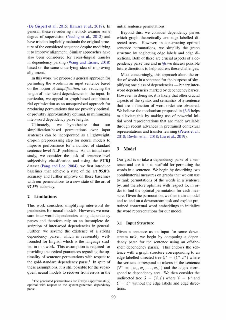
(De Gispert et al., 2015; Kawara et al., 2018). Ingeneral, these re-ordering methods assume somedegree of supervision (Neubig et al., 2012) andhave tried to implicitly maintain the original struc-ture of the considered sequence despite modifyingit to improve alignment. Similar approaches havealso been considered for cross-lingual transferin dependency parsing (Wang and Eisner, 2018)based on the same underlying idea of improvingalignment.

In this work, we propose a general approach forpermuting the words in an input sentence basedon the notion of simplification, i.e. reducing thelength of inter-word dependencies in the input. Inparticular, we appeal to graph-based combinato-rial optimization as an unsupervised approach forproducing permutations that are provably optimal,or provably approximately optimal, in minimizinginter-word dependency parse lengths.

Ultimately, we hypothesize that oursimplification-based permutations over inputsentences can be incorporated as a lightweight,drop-in preprocessing step for neural models toimprove performance for a number of standardsentence-level NLP problems. As an initial casestudy, we consider the task of sentence-levelsubjectivity classification and using the SUBJdataset (Pang and Lee, 2004), we first introducebaselines that achieve a state of the art 95.8%accuracy and further improve on these baselineswith our permutations to a new state of the art of97.5% accuracy.

2 Limitations

This work considers simplifying inter-word de-pendencies for neural models. However, we mea-sure inter-word dependencies using dependencyparses and therefore rely on an incomplete de-scription of inter-word dependencies in general.Further, we assume the existence of a strongdependency parser, which is reasonably well-founded for English which is the language stud-ied in this work. This assumption is required forproviding theoretical guarantees regarding the op-timality of sentence permutations with respect tothe gold-standard dependency parse.1 In spite ofthese assumptions, it is still possible for the subse-quent neural models to recover from errors in the

1The generated permutations are always (approximately)optimal with respect to the system-generated dependencyparse.

initial sentence permutations.Beyond this, we consider dependency parses

which graph theoretically are edge-labelled di-rected trees. However, in constructing optimalsentence permutations, we simplify the graphstructure by neglecting edge labels and edge di-rections. Both of these are crucial aspects of a de-pendency parse tree and in §6 we discuss possiblefuture directions to help address these challenges.

Most concerningly, this approach alters the or-der of words in a sentence for the purpose of sim-plifying one class of dependencies — binary inter-word dependencies marked by dependency parses.However, in doing so, it is likely that other crucialaspects of the syntax and semantics of a sentencethat are a function of word order are obscured.We believe the mechanism proposed in §3.3 helpsto alleviate this by making use of powerful ini-tial word representations that are made availablethrough recent advances in pretrained contextualrepresentations and transfer learning (Peters et al.,2018; Devlin et al., 2018; Liu et al., 2019).

3 Model

Our goal is to take a dependency parse of a sen-tence and use it is as scaffold for permuting thewords in a sentence. We begin by describing twocombinatorial measures on graphs that we can useto rank permutations of the words in a sentenceby, and therefore optimize with respect to, in or-der to find the optimal permutation for each mea-sure. Given the permutation, we then train a modelend-to-end on a downstream task and exploit pre-trained contextual word embeddings to initializethe word representations for our model.

3.1 Input Structure

Given a sentence as an input for some down-stream task, we begin by computing a depen-dency parse for the sentence using an off-the-shelf dependency parser. This endows the sen-tence with a graph structure corresponding to anedge-labelled directed tree G∗ = (V∗, E∗) wherethe vertices correspond to tokens in the sentence(V∗ = w1, w2, . . . , wn) and the edges corre-spond to dependency arcs. We then consider theundirected tree G = (V, E) where V = V∗ andE = E∗ without the edge labels and edge direc-tions.

90

3.2 Combinatorial Objectives

We begin by defining a linear layout on G to be abijective, i.e. one-to-one, ordering on the verticesπ : V → 1, 2, . . . , n. For a graph associatedwith a sentence, we consider the identity linearlayout πI to be given by πI(wi) = i: the linearlayout of vertices is based on the word order in theinput sentence. For any given linear layout π wecan further associate each edge (u, v) ∈ E with anedge distance du,v = |π(u)− π(v)|.2

By considering the modified dependency parseG alongside the sentence, we recognize that acomputational model of the sentence may needto model any given dependency arc (wi, wj) ∈E . As a result, for a model that processes sen-tences word-by-word, information regarding thisarc must be stored for a number of time-stepsgiven by dwi,wj = |πI(wi) − πI(wj)| = |j − i|.This implies that a model may need to store adependency for a large number of time-steps (along-distance dependency) and we instead con-sider finding an optimal linear layout π∗ (that islikely not to be the identity) to minimize theseedge distances with respect to two well-studiedobjectives on linear layouts.

Bandwidth Problem The bandwidth problemon graphs corresponds to finding an optimal lin-ear layout π∗ under the objective:

argminπ∈Π

max(u,v)∈E

du,v (1)

The bandwidth problem is a well known prob-lem dealing with linear layouts with applicationsin sparse matrix computation (Gibbs et al., 1976)and information retrieval (Botafogo, 1993) and hasbeen posed in equivalent ways for graphs and ma-trices (Chinn et al., 1982). For dependency parses,it corresponds to finding a linear layout that min-imizes the length of the longest dependency. Pa-padimitriou (1976) proved the problem was NP-hard and the problem was further shown to re-main NP-hard for trees and even restricted classesof trees (Unger, 1998; Garey et al., 1978). Inthis work, we use the better linear layout of thoseproduced by the guaranteed O(log n) approxima-tion of Haralambides and Makedon (1997) and theheuristic of Cuthill and McKee (1969) and refer tothe resulting linear layout as π∗b .

2Refer to Dıaz et al. (2002) for a survey of linear layouts,related problems, and their applications.

Minimum Linear Arrangement ProblemSimilar to the bandwidth problem, the minimumlinear arrangement (minLA) problem considersfinding a linear layout given by:

argminπ∈Π

∑

(u,v)∈Edu,v (2)

While less studied than the bandwidth problem,the minimum linear arrangement problem con-siders minimizing the sum of the edge lengthsof the dependency arcs which may more closelyresemble how models need to not only handlethe longest dependency well, as in the bandwidthproblem, but also need to handle the other de-pendencies. Although the problem is NP-hard forgeneral graphs (Garey et al., 1974), it admits poly-nomial time exact solutions for trees (Shiloach,1979). We use the algorithm of Chung (1984),which runs in O(n1.585), to find the optimal lay-out π∗m.

3.3 Downstream Integration

Given a linear layout π, we can define the associ-ated permuted sentence s′ of the original sentences = w1 w2 . . . wn where the position of wi ins′ is given by π(wi). We can then train modelsend-to-end taking the permuted sentences as di-rect replacements for the original input sentences.However, this approach suffers from the facts that(a) the resulting sentences may have lost syntac-tic/semantic qualities of the original sentences dueto the permutations and (b) existing pretrainedembedding methods would need to be re-trainedwith these new word orders, which is computa-tionally expensive, and pretraining objectives likelanguage modelling may be less sensible given theproblems noted in (a). To reconcile this, we lever-age a recent three-step pattern for many NLP tasks(Peters et al., 2019):

1. Pretrained Word Representations: Repre-sent each word in the sentence using a pre-trained contextualizer (Peters et al., 2018;Devlin et al., 2018).

2. Fine-tuned Sentence Representation:Learn a task-specific encoding of the sen-tence using a task-specific encoder as afine-tuning step on top of the pretrained wordrepresentations.

3. Task Predictions: Generate a prediction forthe task using the fine-tuned representation.

91

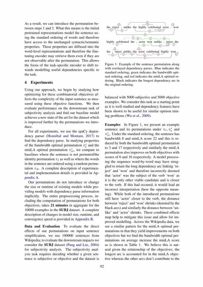
As a result, we can introduce the permutation be-tween steps 1 and 2. What this means is the initialpretrained representations model the sentence us-ing the standard ordering of words and thereforehave access to the unchanged syntactic/semanticproperties. These properties are diffused into theword-level representations and therefore the fine-tuning encoder may retrieve them even if they arenot observable after the permutation. This allowsthe focus of the task-specific encoder to shift to-wards modelling useful dependencies specific tothe task.

4 Experiments

Using our approach, we begin by studying howoptimizing for these combinatorial objectives af-fects the complexity of the input sentence as mea-sured using these objective functions. We thenevaluate performance on the downstream task ofsubjectivity analysis and find our baseline modelachieves a new state of the art for the dataset whichis improved further by the permutations we intro-duce.

For all experiments, we use the spaCy depen-dency parser (Honnibal and Montani, 2017) tofind the dependency parse. In studying propertiesof the bandwidth optimal permutation π∗b and theminLA optimal permutation π∗m, we compare tobaselines where the sentence is not permuted/theidentity permutation πI as well as where the wordsin the sentence are ordered using a random permu-tation πR. A complete description of experimen-tal and implementation details is provided in Ap-pendix A.

Our permutations do not introduce or changethe size or runtime of existing models while pro-viding models with dependency parse informationimplicitly. The entire preprocessing process, in-cluding the computation of permutations for bothobjectives, takes 21 minutes in aggregate for the10000 examples in the SUBJ dataset. A completedescription of changes in model size, runtime, andconvergence speed is provided in Appendix B.

Data and Evaluation To evaluate the directeffects of our permutations on input sentencesimplification, we use 100000 sentences fromWikipedia; to evaluate the downstream impacts weconsider the SUBJ dataset (Pang and Lee, 2004)for subjectivity analysis. The subjectivity anal-ysis task requires deciding whether a given sen-tence is subjective or objective and the dataset is

the reject , unlike the highly celebrated actor , won.

.

.

..

..

.

.

highly celebrated the , actor won unlike , reject the.

. .

.

.

.

.

. .

the , reject unlike the actor celebrated highly won ,.

.

. . .

.

..

.

Figure 1: Example of the sentence permutation alongwith overlayed dependency parses. Blue indicates thestandard ordering, green indicates the bandwidth opti-mal ordering, and red indicates the minLA optimal or-dering. Black indicates the longest dependency arc inthe original ordering.

balanced with 5000 subjective and 5000 objectiveexamples. We consider this task as a starting pointas it is well-studied and dependency features havebeen shown to be useful for similar opinion min-ing problems (Wu et al., 2009).

Examples In Figure 1, we present an examplesentence and its permutations under πI , π∗b andπ∗m. Under the standard ordering, the sentence hasbandwidth 8 and minLA score 22 and this is re-duced by both the bandwidth optimal permutationto 3 and 17 respectively and similarly the minLApermutation also improves on both objectives withscores of 6 and 16 respectively. A model process-ing the sequence word-by-word may have strug-gled to retain the long dependency arc linking ‘re-ject’ and ‘won’ and therefore incorrectly deemedthat ‘actor’ was the subject of the verb ‘won’ asit is the only other viable candidate and is closerto the verb. If this had occured, it would lead anincorrect interpretation (here the opposite mean-ing). While both of the introduced permutationsstill have ‘actor’ closer to the verb, the distancebetween ‘reject’ and ‘won’ shrinks (denoted by theblack arcs) and similarly the distance between ‘un-like’ and ‘actor’ shrinks. These combined effectsmap help to mitigate this issue and allow for im-proved modelling. Across the Wikipedia data, wesee a similar pattern for the minLA optimal per-mutations in that they yield improvements on bothobjectives but we find the bandwidth optimal per-mutations on average increase the minLA scoreas is shown in Table 1. We believe this is nat-ural given the relationship of the objectives; thelongest arc is accounted for in the minLA objec-tive whereas the other arcs don’t contribute to the

92

Bandwidth minLAπI (Standard) 17.64 82.39πR (Random) 20.94 294.43π∗b (Bandwidth) 6.75 101.23π∗m (minLA) 9.43 54.57

Table 1: Bandwidth and minimum linear arrange-ment scores for the specified permutation type averagedacross 100000 Wikipedia sentences.

AccuracyπI (Standard) 95.8πR (Random) 94.8π∗b (Bandwidth) 96.2π∗m (minLA) 97.5AdaSent (Zhao et al., 2015)† 95.5CNN+MCFA (Amplayo et al., 2018)† 94.8

Table 2: Accuracy on the SUBJ dataset using the spec-ified ordering of pretrained representations for the fine-tuning LSTM. † indicates prior models that were evalu-ated using 10-fold cross validation instead of a held-outtest set.

bandwidth cost. We also find the comparison ofthe standard and random orderings to be evidencethat human orderings of words to form sentences(at least in English) are correlated with these ob-jectives, as they are significantly better with re-spect to these objectives as compared to randomorderings. Refer to Figure 3 for a larger example.

Downstream Performance In Table 2, wepresent the results on the downstream task. De-spite the fact that the random permutation LSTMencoder cannot learn from the word order and im-plicitly is restrained to permutation-invariant fea-tures, the associated model performs comparablywith previous state of the art systems, indicatingthe potency of current pretrained embeddings andspecifically ELMo. When there is a deterministicordering, we find that the standard ordering is theleast helpful of the three orderings considered. Wesee a particularly significant spike in performancewhen using permutations that are minLA optimaland we conjecture that this may be because minLApermutations improve on both objectives on aver-age and empirically we observe they better main-tain the order of the original sentence (as can beseen in Figure 1).

5 Related Work

This work draws upon inspiration from the liter-ature on psycholinguistics and cognitive science.Specifically, dependency lengths and the existingminimization in natural language has been studiedunder the dependency length minimization (DLM)hypothesis (Liu, 2008) which posits a bias in hu-man languages towards constructions with shorterdependency lengths.3

In particular, the relationship described betweenrandom and natural language orderings of wordsto form sentences as in Table 1 has been stud-ied more broadly across 37 natural languages inFutrell et al. (2015). This work, alongside Gildeaand Temperley (2010); Liu et al. (2017); Futrellet al. (2017) helps to validate the extent and per-vasiveness of DLM in natural languages. Moregenerally, this literature body has proposed a num-ber of reasons for this behavior, many of whichcenter around the related notions of efficiency(Gibson et al., 2019) and memory constraints(Gulordava et al., 2015) for humans. Recentresearch at the intersection of psycholinguisticsand NLP that has tried to probe for dependency-oriented understanding in neural networks (pri-marily RNNs) does indicate relationships withspecific dependency-types and RNN understand-ing. This includes research considering specificdependency types (Wilcox et al., 2018, 2019a),word-order effects (Futrell and Levy, 2019), andstructural supervision (Wilcox et al., 2019b).

Prompted by this, the permutations consideredin this work can alternatively be seen as lin-earizations (Langkilde and Knight, 1998; Filip-pova and Strube, 2009; Futrell and Gibson, 2015;Puzikov and Gurevych, 2018) of a dependencyparse in a minimal fashion which is closely relatedto Gildea and Temperley (2007); Temperley andGildea (2018). While such linearizations have notbeen well-studied for downstream impacts, the us-age of dependency lengths as a constraint has beenstudied for dependency parsing itself. Towardsthis end, Eisner and Smith (2010) showed that us-ing dependency length can be a powerful heuristictool in dependency parsing (by either enforcing astrict preference or favoring a soft preference forshorter dependencies).

3In this work, we partially deviate from this linguistic ter-minology, which primarily deals with the measure definedin Equation 2, and prefer algorithmic terminology to accom-modate the measure defined in Equation 1 and disambiguatethese related measures more clearly.

93

6 Future Directions

Graph Structure Motivated by recent work ongraph convolutional networks that began withundirected unlabelled graphs (Kipf and Welling,2016; Zhang et al., 2018) that was extended toinclude edge direction and edge labels (Marcheg-giani and Titov, 2017), we consider whether thesefeatures of a dependency parse can also lever-aged in computing an optimal permutation. Weargue that bidirectionally traversing the permutedsequence may be sufficient to address edge direc-tion. A natural approach to encode edge labelswould be to define a mapping (either learned on anauxiliary objective or tuned as a hyperparameter)from categorical edge labels to numericals edgeweights and then consider the weighted analoguesof the objectives in Equation 1 and Equation 2.

Improved Objective The objectives introducedin Equation 1 and Equation 2 can be unified byconsidering the family of cost functions:

fp(π) =∑

(u,v)∈E|π(u)− π(v)|p (3)

Here, minLA correspond to p = 1 and the band-width problem corresponds to p = ∞. We canthen propose a generalized objective that is theconvex combination of the individual objectives,i.e. finding a permutation that minimizes:

fα1,∞(π) = αf1(π) + (1− α)f∞(π) (4)Setting α to 0 or 1 reduces to the original objec-tives. This form of the new objective is reminis-cent of Elastic Net regularization in statistical op-timization (Zou and Hastie, 2005). Inspired bythis parallel, a Lagrangian relaxation of one of theobjectives as a constraint may be an approach to-wards (approximate) optimization.

Task-specific Permutations The permutationsproduced by these models are invariant with re-spect to the downstream task. However, differ-ent tasks may benefit from different sentence or-ders that go beyond task-agnostic simplification.A natural way to model this in neural models isto learn the permutation in a differentiable fashionand train the permutation model end-to-end withinthe overarching model for the task. Refer to Ap-pendix C for further discussion.

7 Conclusion

In this work, we propose approaches that permutethe words in a sentence to provably minimize com-

binatorial objectives related to the length of depen-dency arcs. We find that this is a lightweight pro-cedure that helps to simplify input sentences fordownstream models and that it leads to improvedperformance and state of the art results (97.5%classification accuracy) for subjectivity analysisusing the SUBJ dataset.

Acknowledgements

I thank Bobby Kleinberg for his tremendous in-sight into the present and future algorithmic chal-lenges of layout-based optimization problems,Tianze Shi for his pointers towards the depen-dency length minimization literature in psycholin-guistics and cognitive science, and Arzoo Katiyarfor her advice on comparing against random se-quence orderings and considering future work to-wards soft/differentiable analogues. I also thankthe anonymous reviewers for their perceptive andconstructive feedback. Finally, I thank ClaireCardie for her articulate concerns and actionablesuggestions with regards to this work and, morebroadly, for her overarching guidance and warmmentoring as an adviser.

ReferencesReinald Kim Amplayo, Kyungjae Lee, Jinyoung Yeo,

and Seung won Hwang. 2018. Translations as addi-tional contexts for sentence classification. In IJCAI.

Dzmitry Bahdanau, Kyunghyun Cho, and Yoshua Ben-gio. 2015. Neural machine translation by jointlylearning to align and translate. In 3rd Inter-national Conference on Learning Representations,ICLR 2015, San Diego, CA, USA, May 7-9, 2015,Conference Track Proceedings.

Rodrigo A Botafogo. 1993. Cluster analysis for hyper-text systems. In Proceedings of the 16th annual in-ternational ACM SIGIR conference on Research anddevelopment in information retrieval, pages 116–125. ACM.

P. Z. Chinn, J. Chvtalov, A. K. Dewdney, and N. E.Gibbs. 1982. The bandwidth problem for graphsand matricesa survey. Journal of Graph Theory,6(3):223–254.

FRK Chung. 1984. On optimal linear arrangements oftrees. Computers & mathematics with applications,10(1):43–60.

Hang Cui, Renxu Sun, Keya Li, Min-Yen Kan, and Tat-Seng Chua. 2005. Question answering passage re-trieval using dependency relations. In Proceedingsof the 28th annual international ACM SIGIR confer-ence on Research and development in informationretrieval, pages 400–407. ACM.

94

E. Cuthill and J. McKee. 1969. Reducing the band-width of sparse symmetric matrices. In Proceedingsof the 1969 24th National Conference, ACM ’69,pages 157–172, New York, NY, USA. ACM.

Rumen Dangovski, Li Jing, Preslav Nakov, Mico Tat-alovic, and Marin Soljacic. 2019. Rotational unit ofmemory: A novel representation unit for rnns withscalable applications. Transactions of the Associa-tion for Computational Linguistics, 7:121–138.

Adria De Gispert, Gonzalo Iglesias, and Bill Byrne.2015. Fast and accurate preordering for smt usingneural networks. In Proceedings of the 2015 Con-ference of the North American Chapter of the Asso-ciation for Computational Linguistics: Human Lan-guage Technologies, pages 1012–1017.

Jacob Devlin, Ming-Wei Chang, Kenton Lee, andKristina Toutanova. 2018. Bert: Pre-training of deepbidirectional transformers for language understand-ing. arXiv preprint arXiv:1810.04805.

Josep Dıaz, Jordi Petit, and Maria Serna. 2002. A sur-vey of graph layout problems. ACM Computing Sur-veys (CSUR), 34(3):313–356.

Jason Eisner and Noah A Smith. 2010. Favor short de-pendencies: Parsing with soft and hard constraintson dependency length. In Trends in Parsing Tech-nology, pages 121–150. Springer.

Katja Filippova and Michael Strube. 2009. Tree lin-earization in english: Improving language modelbased approaches. In Proceedings of Human Lan-guage Technologies: The 2009 Annual Conferenceof the North American Chapter of the Associationfor Computational Linguistics, Companion Volume:Short Papers, NAACL-Short ’09, pages 225–228,Stroudsburg, PA, USA. Association for Computa-tional Linguistics.

Katrin Fundel, Robert Kuffner, and Ralf Zimmer.2006. Relexrelation extraction using dependencyparse trees. Bioinformatics, 23(3):365–371.

Richard Futrell and Edward Gibson. 2015. Experi-ments with generative models for dependency treelinearization. In Proceedings of the 2015 Confer-ence on Empirical Methods in Natural LanguageProcessing, pages 1978–1983.

Richard Futrell, Roger Levy, and Edward Gibson.2017. Generalizing dependency distance: Commenton dependency distance: A new perspective on syn-tactic patterns in natural languages by haitao liu etal. Physics of life reviews, 21:197–199.

Richard Futrell and Roger P. Levy. 2019. Do RNNslearn human-like abstract word order preferences?In Proceedings of the Society for Computation inLinguistics (SCiL) 2019, pages 50–59.

Richard Futrell, Kyle Mahowald, and Edward Gibson.2015. Large-scale evidence of dependency lengthminimization in 37 languages. Proceedings of

the National Academy of Sciences, 112(33):10336–10341.

Michael R Garey, Ronald L Graham, David S Johnson,and Donald Ervin Knuth. 1978. Complexity resultsfor bandwidth minimization. SIAM Journal on Ap-plied Mathematics, 34(3):477–495.

Michael R Garey, David S Johnson, and Larry Stock-meyer. 1974. Some simplified np-complete prob-lems. In Proceedings of the sixth annual ACMsymposium on Theory of computing, pages 47–63.ACM.

Norman E. Gibbs, William G. Poole, and Paul K.Stockmeyer. 1976. An algorithm for reducing thebandwidth and profile of a sparse matrix. SIAMJournal on Numerical Analysis, 13(2):236–250.

Edward Gibson, Richard Futrell, Steven T Piandadosi,Isabelle Dautriche, Kyle Mahowald, Leon Bergen,and Roger Levy. 2019. How efficiency shapes hu-man language. Trends in cognitive sciences.

Daniel Gildea and David Temperley. 2007. Optimizinggrammars for minimum dependency length. In Pro-ceedings of the 45th Annual Meeting of the Associa-tion of Computational Linguistics, pages 184–191.

Daniel Gildea and David Temperley. 2010. Do gram-mars minimize dependency length? Cognitive Sci-ence, 34(2):286–310.

Isao Goto, Masao Utiyama, and Eiichiro Sumita. 2012.Post-ordering by parsing for japanese-english statis-tical machine translation. In 50th Annual Meeting ofthe Association for Computational Linguistics, page311.

Kristina Gulordava, Paola Merlo, and Benoit Crabbe.2015. Dependency length minimisation effects inshort spans: a large-scale analysis of adjective place-ment in complex noun phrases. In Proceedingsof the 53rd Annual Meeting of the Association forComputational Linguistics and the 7th InternationalJoint Conference on Natural Language Processing(Volume 2: Short Papers), volume 2, pages 477–482.

Zhou GuoDong, Su Jian, Zhang Jie, and Zhang Min.2005. Exploring various knowledge in relation ex-traction. In Proceedings of the 43rd Annual Meetingon Association for Computational Linguistics, ACL’05, pages 427–434, Stroudsburg, PA, USA. Associ-ation for Computational Linguistics.

Kadri Hacioglu. 2004. Semantic role labeling usingdependency trees. In Proceedings of the 20th inter-national conference on Computational Linguistics,page 1273. Association for Computational Linguis-tics.

J. Haralambides and F. Makedon. 1997. Approxi-mation algorithms for the bandwidth minimizationproblem for a large class of trees. Theory of Com-puting Systems, 30(1):67–90.

95

Sepp Hochreiter and Jurgen Schmidhuber. 1997.Long short-term memory. Neural computation,9(8):1735–1780.

Matthew Honnibal and Ines Montani. 2017. spacy 2:Natural language understanding with bloom embed-dings, convolutional neural networks and incremen-tal parsing. To appear.

Jeremy Howard and Sebastian Ruder. 2018. Universallanguage model fine-tuning for text classification. InProceedings of the 56th Annual Meeting of the As-sociation for Computational Linguistics (Volume 1:Long Papers), pages 328–339.

Mahesh Joshi and Carolyn Penstein-Rose. 2009. Gen-eralizing dependency features for opinion mining.In Proceedings of the ACL-IJCNLP 2009 conferenceshort papers, pages 313–316.

Yuki Kawara, Chenhui Chu, and Yuki Arase. 2018.Recursive neural network based preordering forenglish-to-japanese machine translation. In Pro-ceedings of ACL 2018, Student Research Workshop,pages 21–27, Melbourne, Australia. Association forComputational Linguistics.

Diederik P. Kingma and Jimmy Ba. 2014. Adam:A method for stochastic optimization. CoRR,abs/1412.6980.

Thomas N Kipf and Max Welling. 2016. Semi-supervised classification with graph convolutionalnetworks. arXiv preprint arXiv:1609.02907.

Adhiguna Kuncoro, Chris Dyer, John Hale, Dani Yo-gatama, Stephen Clark, and Phil Blunsom. 2018.Lstms can learn syntax-sensitive dependencies well,but modeling structure makes them better. In Pro-ceedings of the 56th Annual Meeting of the Associa-tion for Computational Linguistics (Volume 1: LongPapers), pages 1426–1436.

Irene Langkilde and Kevin Knight. 1998. Gener-ation that exploits corpus-based statistical knowl-edge. In Proceedings of the 36th Annual Meet-ing of the Association for Computational Linguis-tics and 17th International Conference on Compu-tational Linguistics-Volume 1, pages 704–710. As-sociation for Computational Linguistics.

Tal Linzen, Emmanuel Dupoux, and Yoav Goldberg.2016. Assessing the ability of lstms to learn syntax-sensitive dependencies. Transactions of the Associ-ation for Computational Linguistics, 4:521–535.

Haitao Liu. 2008. Dependency distance as a metric oflanguage comprehension difficulty. Journal of Cog-nitive Science, 9(2):159–191.

Haitao Liu, Chunshan Xu, and Junying Liang. 2017.Dependency distance: a new perspective on syntac-tic patterns in natural languages. Physics of life re-views, 21:171–193.

Nelson F. Liu, Matt Gardner, Yonatan Belinkov,Matthew Peters, and Noah A. Smith. 2019. Lin-guistic knowledge and transferability of contextualrepresentations. CoRR, abs/1903.08855.

Nelson F Liu, Omer Levy, Roy Schwartz, ChenhaoTan, and Noah A Smith. 2018. Lstms exploit lin-guistic attributes of data. In Proceedings of TheThird Workshop on Representation Learning forNLP, pages 180–186.

Thang Luong, Hieu Pham, and Christopher D Man-ning. 2015. Effective approaches to attention-basedneural machine translation. In Proceedings of the2015 Conference on Empirical Methods in NaturalLanguage Processing, pages 1412–1421.

Diego Marcheggiani and Ivan Titov. 2017. Encodingsentences with graph convolutional networks for se-mantic role labeling. In Proceedings of the 2017Conference on Empirical Methods in Natural Lan-guage Processing, pages 1506–1515.

Graham Neubig, Taro Watanabe, and Shinsuke Mori.2012. Inducing a discriminative parser to optimizemachine translation reordering. In Proceedings ofthe 2012 Joint Conference on Empirical Methodsin Natural Language Processing and ComputationalNatural Language Learning, pages 843–853, JejuIsland, Korea. Association for Computational Lin-guistics.

Bo Pang and Lillian Lee. 2004. A sentimental educa-tion: Sentiment analysis using subjectivity summa-rization based on minimum cuts. In Proceedings ofthe 42nd annual meeting on Association for Compu-tational Linguistics, page 271. Association for Com-putational Linguistics.

Christos H. Papadimitriou. 1976. The np-completenessof the bandwidth minimization problem. Comput-ing, 16:263–270.

Adam Paszke, Sam Gross, Soumith Chintala, Gre-gory Chanan, Edward Yang, Zachary DeVito, Zem-ing Lin, Alban Desmaison, Luca Antiga, and AdamLerer. 2017. Automatic differentiation in pytorch.

Matthew Peters, Mark Neumann, Mohit Iyyer, MattGardner, Christopher Clark, Kenton Lee, and LukeZettlemoyer. 2018. Deep contextualized word rep-resentations. In Proceedings of the 2018 Confer-ence of the North American Chapter of the Associ-ation for Computational Linguistics: Human Lan-guage Technologies, Volume 1 (Long Papers), pages2227–2237.

Matthew Peters, Sebastian Ruder, and Noah A. Smith.2019. To tune or not to tune? adapting pretrainedrepresentations to diverse tasks.

Yevgeniy Puzikov and Iryna Gurevych. 2018. BinLin:A simple method of dependency tree linearization.In Proceedings of the First Workshop on Multilin-gual Surface Realisation, pages 13–28, Melbourne,Australia. Association for Computational Linguis-tics.

96

Rodrigo Santa Cruz, Basura Fernando, Anoop Cherian,and Stephen Gould. 2017. Deeppermnet: Visualpermutation learning. In Proceedings of the IEEEConference on Computer Vision and Pattern Recog-nition, pages 3949–3957.

Mike Schuster and Kuldip K Paliwal. 1997. Bidirec-tional recurrent neural networks. IEEE Transactionson Signal Processing, 45(11):2673–2681.

Yossi Shiloach. 1979. A minimum linear arrangementalgorithm for undirected trees. SIAM Journal onComputing, 8(1):15–32.

Ilya Sutskever, Oriol Vinyals, and Quoc V Le. 2014.Sequence to sequence learning with neural net-works. In Advances in neural information process-ing systems, pages 3104–3112.

David Temperley and Daniel Gildea. 2018. Min-imizing syntactic dependency lengths: Typologi-cal/cognitive universal? Annual Reviews of Linguis-tics.

Walter Unger. 1998. The complexity of the approxi-mation of the bandwidth problem. In Proceedings39th Annual Symposium on Foundations of Com-puter Science (Cat. No. 98CB36280), pages 82–91.IEEE.

Ashish Vaswani, Noam Shazeer, Niki Parmar, JakobUszkoreit, Llion Jones, Aidan N Gomez, ŁukaszKaiser, and Illia Polosukhin. 2017. Attention is allyou need. In Advances in neural information pro-cessing systems, pages 5998–6008.

Dingquan Wang and Jason Eisner. 2018. Synthetic datamade to order: The case of parsing. In Proceed-ings of the 2018 Conference on Empirical Methodsin Natural Language Processing, pages 1325–1337,Brussels, Belgium. Association for ComputationalLinguistics.

Ethan Wilcox, Roger Levy, Takashi Morita, andRichard Futrell. 2018. What do rnn language mod-els learn about filler–gap dependencies? In Pro-ceedings of the 2018 EMNLP Workshop Black-boxNLP: Analyzing and Interpreting Neural Net-works for NLP, pages 211–221.

Ethan Wilcox, Roger P. Levy, and Richard Futrell.2019a. What syntactic structures block dependen-cies in rnn language models? In Proceedings of the41st Annual Meeting of the Cognitive Science Soci-ety.

Ethan Wilcox, Peng Qian, Richard Futrell, MiguelBallesteros, and Roger Levy. 2019b. Structural su-pervision improves learning of non-local grammat-ical dependencies. In Proceedings of the 18th An-nual Conference of the North American Chapter ofthe Association for Computational Linguistics: Hu-man Language Technologies.

Yuanbin Wu, Qi Zhang, Xuanjing Huang, and Lide Wu.2009. Phrase dependency parsing for opinion min-ing. In Proceedings of the 2009 Conference on Em-pirical Methods in Natural Language Processing:Volume 3-Volume 3, pages 1533–1541. Associationfor Computational Linguistics.

Fei Xia and Michael McCord. 2004. Improving a sta-tistical mt system with automatically learned rewritepatterns. In Proceedings of the 20th internationalconference on Computational Linguistics, page 508.Association for Computational Linguistics.

Yuhao Zhang, Peng Qi, and Christopher D Manning.2018. Graph convolution over pruned dependencytrees improves relation extraction. In Proceedings ofthe 2018 Conference on Empirical Methods in Nat-ural Language Processing, pages 2205–2215.

Han Zhao, Zhengdong Lu, and Pascal Poupart. 2015.Self-adaptive hierarchical sentence model. InTwenty-Fourth International Joint Conference onArtificial Intelligence.

Hui Zou and Trevor Hastie. 2005. Regularization andvariable selection via the elastic net. Journal of theroyal statistical society: series B (statistical method-ology), 67(2):301–320.

A Implementation Details

We implement our models in PyTorch (Paszkeet al., 2017) using the Adam optimizer (Kingmaand Ba, 2014) with its default parameters in Py-Torch. We split the dataset using a 80/10/10split and the results in Table 2 are on the testset whereas those in Figure 2 are on the devel-opment set. We use ELMo embeddings (Peterset al., 2018)4, for the initial pretrained word repre-sentations by concatenating the two 1024 dimen-sional pretrained vectors, yielding a 2048 dimen-sional initial pretrained representation for each to-ken. These representations are frozen based on theresults of Peters et al. (2019) and passed througha single-layer bidirectional LSTM with output di-mensionality 256. The outputs of the forward andbackward LSTMs at position i are concatenatedand a sentence representation is produced by max-pooling as was found to be effective in Howardand Ruder (2018) and Peters et al. (2019). Thesentence representation is passed through a linearclassifier M ∈ R512×2 and the entire model istrained to minimize cross entropy loss. All mod-els are trained for 13 epochs with a batch size of

4Specifically, we use embeddings available at:https://s3-us-west-2.amazonaws.com/allennlp/models/elmo/2x4096_512_2048cnn_2xhighway/elmo_2x4096_512_2048cnn_2xhighway_options.json

97

Figure 2: Development set performance for each or-dering. Values are reported beginning at epoch 1 inintervals of 3 epochs.

16 with the test set results reported being fromthe model checkpoint after epoch 13. We also ex-perimented with changing the LSTM task-specificencoder to be unidirectional but found the resultswere strictly worse.

B Efficiency Analysis

Model Size The changes we introduce only im-pact the initial preprocessing and ordering of thepretrained representations for the model. As a re-sult, we make no changes to the number of modelparameters and the only contribution to the modelfootprint is we need to store the permutation on aper example basis. This can actually be avoidedin the case where we have frozen pretrained em-beddings as the permutation can be computed inadvance. Therefore, for the results in this paper,the model size is entirely unchanged.

Runtime The wall-clock training time, i.e. thewall-clock time for a fixed number of epochs, andinference time are unchanged as we do not changethe underlying model in any way and the permuta-tions can be precomputed. As noted in the paper,on a single CPU it takes 21 minutes to completethe entire preprocessing process and 25% of thistime is a result of computing bandwidth optimalpermutations and 70% of this time is a result ofcomputing minLA optimal permutations. The pre-processing time scales linearly in the number ofexamples and we verify this as it takes 10 minutesto process only the subjective examples (and thedataset is balanced). Figure 2 shows the develop-ment set performance for each of the permutationtypes over the course of the fine-tuning process.

C End-to-End Permutations

In order to approach differentiable optimizationfor permutations, we must specify a representa-tion. A standard choice that is well-suited for lin-ear algebraic manipulation is a permutation ma-trix, i.e Pπ ∈ Rn×n, where Pπ[i, j] = 1 if π(i) =j and 0 otherwise. As a result, permutation matri-ces are discrete, and therefore sparse, in the spaceof real matrices. As such they are poorly suitedfor the gradient-based optimization that supportsmost neural models. A recent approach from vi-sion has considered a generalization of permu-tation matrices to the associated class of doublystochastic matrices and then considered optimiza-tion with respect to the manifold they define (theSinkhorn Manifold) to find a discrete permutation(Santa Cruz et al., 2017). This approach cannotbe immediately applied for neural models for sen-tences since the algorithms exploits that images,and therefore permutations of the pixels in an im-age, are of fixed size between examples. That be-ing said we ultimately see this as being an impor-tant direction of study given the shift from discreteoptimization to soft/differentiable alternatives forsimilar problems in areas such as structured pre-diction.

98

She , among others excentricities5 , talks to a small rock , Gertrude , like if she was alive BW:8 MinLA: 51.

.

.

. .

. .

.

.

.

. .

.

. .

.

. .

alive she if Gertrude , small a others was rock excentricities like to among , , , talks She BW: 8 MinLA: 73..

...

.

.

..

.

.....

...

others excentricities among , She , talks , to a rock , Gertrude small like if was she alive BW: 8 MinLA: 38.. ...

. ..

.

. ..

. .

. . . .

Figure 3: Addition example sentence with sentence permutations and overlayed dependency parses. Blue indi-cates the standard ordering, green indicates the bandwidth optimal ordering, and red indicates the minLA optimalordering. Black indicates the longest dependency arc in the original ordering.

99

Proceedings of the 57th Annual Meeting of the Association for Computational Linguistics: Student Research Workshop, pages 100–105Florence, Italy, July 28 - August 2, 2019. c©2019 Association for Computational Linguistics

Predicting the Outcome of Deliberative Democracy: A Research Proposal

Conor McKillopSchool of Science and Engineering

University of DundeeDundee, United Kingdom

c.z.mckillop@dundee.ac.uk

Abstract

As liberal states across the world face a declinein political participation by citizens, deliber-ative democracy is a promising solution forthe publics decreasing confidence and apathytowards the democratic process (Dahl et al.,2017). Deliberative dialogue is method ofpublic interaction that is fundamental to theconcept of deliberative democracy. The abil-ity to identify and predict consensus in the di-alogues could bring greater accessibility andtransparency to the face-to-face participatoryprocess. The paper sets out a research planfor the first steps at automatically identifyingand predicting consensus in a corpus of Ger-man language debates on hydraulic fracking.It proposes the use of a unique combinationof lexical, sentiment, durational and furtherderivative features of adjacency pairs to traintraditional classification models. In additionto this, the use of deep learning techniques toimprove the accuracy of the classification andprediction tasks is also discussed. Preliminaryresults at the classification of utterances arealso presented, with an F1 between 0.61 and0.64 demonstrating that the task of recognis-ing agreement is demanding but possible.

1 Introduction

Liberal states across the world are facing a signif-icant decline in political participation by citizens.The global voter turnout rate has dropped by morethan 10% over the last 25 years (Groupe de laBanque mondiale, 2017), and this trend does notappear to be slowing down. The public have re-ported decreasing confidence and apathy towardsthe democratic process (Dahl et al., 2017). De-liberative Democracy represents a potential solu-tion to these problems. Through the evaluationof different policy proposals using a process oftruthful and rational discussion between citizensand authority, Deliberative democracy can enable

consensual, well-justified, decision making. It canimprove the political competence of citizens by;facilitating the exchange of arguments and shar-ing of ideas on proposals from authority (Estlundet al., 1989); reconfiguring democracy as a pro-cess of ‘public reasoning’ and connecting citizenswith each other and with their governing institu-tions (Parkinson and Mansbridge, 2012; Dryzek,2012).

Deliberative Dialogue is a structured, face-to-face method of public interaction. As a formof participatory process, it is fundamental to theconcept of Deliberative Democracy (McCoy andScully, 2002). There are many different forms ofdeliberative dialogue, including, but not limited to:citizens’ assemblies, citizens’ juries and planningcells. The European Commission’s ‘Future of Eu-rope debates’ (Directorate-General for Communi-cation, 2017b) are an exemplar of hosting deliber-ative dialogue successfully at large scale.

The ‘Future of Europe debates’ are due to cometo their natural conclusion after a two year longprocess that started with the release of the ‘Whitepaper on the future of Europe’ in March of 2017(ibid.). This white paper set out the main chal-langes and opportunities facing the 27 EuropeanUnion (EU) member states for the next decade. Toencourage citizens’ participation, the Commissionhosted a series of debates across cities and regionswithin Europe (Directorate-General for Commu-nication, 2017a). At the debates, all members ofthe Commission engaged in dialogue with citizensand listened to their views and expectations con-cerning the future of Europe. The debates werewell received, with 129 debates in more than 80towns, attended by over 21,000 citizens (ibid.).

In the deliberative democratic process, one ofthe main aims is for informed agreement to bereached among all involved parties. However, indialogues with larger citizenry, it is less likely that

100

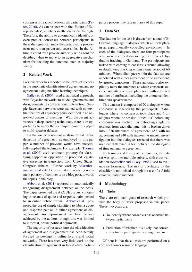
consensus is reached between all participants (Pe-ter, 2016). As can be seen with the ‘Future of Eu-rope debates’, numbers in attendance can be high.Therefore, the ability to automatically identify, oreven predict, consensus between participants inthese dialogues can make the participatory processeven more transparent and accessible. In the fu-ture, it could even provide authority with a tool fordeciding when to move to an aggregative mecha-nism for deciding the outcome, such as majorityvoting.

2 Related Work

Previous work has reported some levels of successin the automatic classification of agreement and noagreement using machine learning techniques.

Galley et al. (2004) used a statistical approach,with Bayesian networks to model agreements anddisagreements in conversational interaction. Sim-ple Bayesian networks were trained with contex-tual features of adjacency pairs identified in an an-notated corpus of meetings. With the recent ad-vances in deep learning techniques, there is an op-portunity to apply the techniques from this paperto multi-speaker debates

On the use of sentiment analysis to aid in thedetection of agreement, as employed in this pa-per, a number of previous works have success-fully applied the technique. For example, Thomaset al. (2006) used sentiment property for classi-fying support or opposition of proposed legisla-tive speeches in transcripts from United States’Congress debates. Further work by Balasubra-manyan et al. (2011) investigated classifying senti-ment polarity of comments on a blog post, towardsthe topics in the blog.

Abbott et al. (2011) reported on automaticallyrecognising disagreement between online posts.The paper presented the ARGUE corpus, contain-ing thousands of quote and response pairs postedto an online debate forum. Abbott et al. pro-posed the use of simple classifiers to label a quoteand response pair as in either agreement or dis-agreement. An improvement over baseline wasachieved by the authors, though this was limitedto informal, online political arguments.

The majority of research into the classificationof agreement and disagreement has been heavilyfocused on postings in online forums and socialnetworks. There has been very little work on theclassification of agreement in face-to-face partici-

patory process; the research area of this paper.

3 Data Set

The data set for the task is drawn from a total of 34German language dialogues which all took placein an experimentally controlled environment. Ineach of the dialogues, there are four participantswho were recorded discussing the topic of hy-draulic fracking in Germany. The participants aretasked with coming to consensus around allowingor disallowing fracking within a time period of 60minutes. Whole dialogues within the data set areannotated with either agreement or no agreement,by trusted annotators. These annotators also ex-plicitly mark the utterance at which consensus oc-curs. All utterances are plain text, with a limitednumber of attributes, including the utterance iden-tifier and speaker name.

This data set is composed of 20 dialogues whereconsensus is reached by the participants, 9 dia-logues where no consensus took place and 5 di-alogues where the session ‘timed out’ before anyconsensus was reached. By extracting single ut-terances from each dialogue, this is broken downinto 1,376 utterances of agreement, 458 with noagreement and 240 with timeout. A manual inves-tigation into the dialogues revealed that there wasno clear difference in text between the dialoguesof time out and no agreement.

For training and testing of the classifier, the dataset was split into multiple subsets, with cross val-idation (Mosteller and Tukey, 1968) used to eval-uate performance. The risk of overfitting by theclassifier is minimised through the use of a 5-foldcross validation method.

4 Methodology

4.1 Tasks

There are two main goals of research which pro-vide the body of work proposed in this paper.These two goals are:

• To identify where consensus has occurred be-tween participants

• Prediction of whether it is likely that consen-sus between participants is going to occur

Of note is that these tasks are performed on acorpus of lower resource language.

101

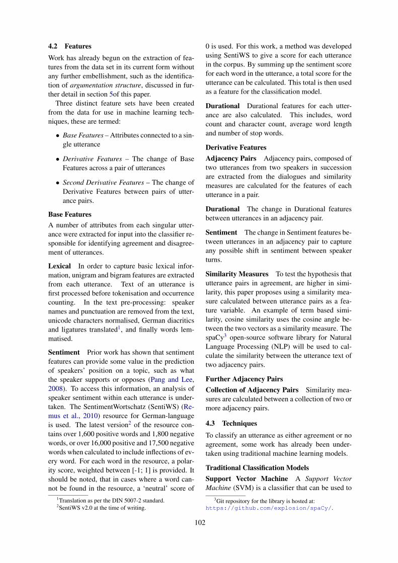
4.2 FeaturesWork has already begun on the extraction of fea-tures from the data set in its current form withoutany further embellishment, such as the identifica-tion of argumentation structure, discussed in fur-ther detail in section 5of this paper.

Three distinct feature sets have been createdfrom the data for use in machine learning tech-niques, these are termed:

• Base Features – Attributes connected to a sin-gle utterance

• Derivative Features – The change of BaseFeatures across a pair of utterances

• Second Derivative Features – The change ofDerivative Features between pairs of utter-ance pairs.

Base FeaturesA number of attributes from each singular utter-ance were extracted for input into the classifier re-sponsible for identifying agreement and disagree-ment of utterances.

Lexical In order to capture basic lexical infor-mation, unigram and bigram features are extractedfrom each utterance. Text of an utterance isfirst processed before tokenisation and occurrencecounting. In the text pre-processing: speakernames and punctuation are removed from the text,unicode characters normalised, German diacriticsand ligatures translated1, and finally words lem-matised.

Sentiment Prior work has shown that sentimentfeatures can provide some value in the predictionof speakers’ position on a topic, such as whatthe speaker supports or opposes (Pang and Lee,2008). To access this information, an analysis ofspeaker sentiment within each utterance is under-taken. The SentimentWortschatz (SentiWS) (Re-mus et al., 2010) resource for German-languageis used. The latest version2 of the resource con-tains over 1,600 positive words and 1,800 negativewords, or over 16,000 positive and 17,500 negativewords when calculated to include inflections of ev-ery word. For each word in the resource, a polar-ity score, weighted between [-1; 1] is provided. Itshould be noted, that in cases where a word can-not be found in the resource, a ‘neutral’ score of

1Translation as per the DIN 5007-2 standard.2SentiWS v2.0 at the time of writing.

0 is used. For this work, a method was developedusing SentiWS to give a score for each utterancein the corpus. By summing up the sentiment scorefor each word in the utterance, a total score for theutterance can be calculated. This total is then usedas a feature for the classification model.

Durational Durational features for each utter-ance are also calculated. This includes, wordcount and character count, average word lengthand number of stop words.

Derivative FeaturesAdjacency Pairs Adjacency pairs, composed oftwo utterances from two speakers in successionare extracted from the dialogues and similaritymeasures are calculated for the features of eachutterance in a pair.

Durational The change in Durational featuresbetween utterances in an adjacency pair.

Sentiment The change in Sentiment features be-tween utterances in an adjacency pair to captureany possible shift in sentiment between speakerturns.

Similarity Measures To test the hypothesis thatutterance pairs in agreement, are higher in simi-larity, this paper proposes using a similarity mea-sure calculated between utterance pairs as a fea-ture variable. An example of term based simi-larity, cosine similarity uses the cosine angle be-tween the two vectors as a similarity measure. ThespaCy3 open-source software library for NaturalLanguage Processing (NLP) will be used to cal-culate the similarity between the utterance text oftwo adjacency pairs.

Further Adjacency PairsCollection of Adjacency Pairs Similarity mea-sures are calculated between a collection of two ormore adjacency pairs.

4.3 Techniques

To classify an utterance as either agreement or noagreement, some work has already been under-taken using traditional machine learning models.

Traditional Classification ModelsSupport Vector Machine A Support VectorMachine (SVM) is a classifier that can be used to

3Git repository for the library is hosted at:https://github.com/explosion/spaCy/.

102

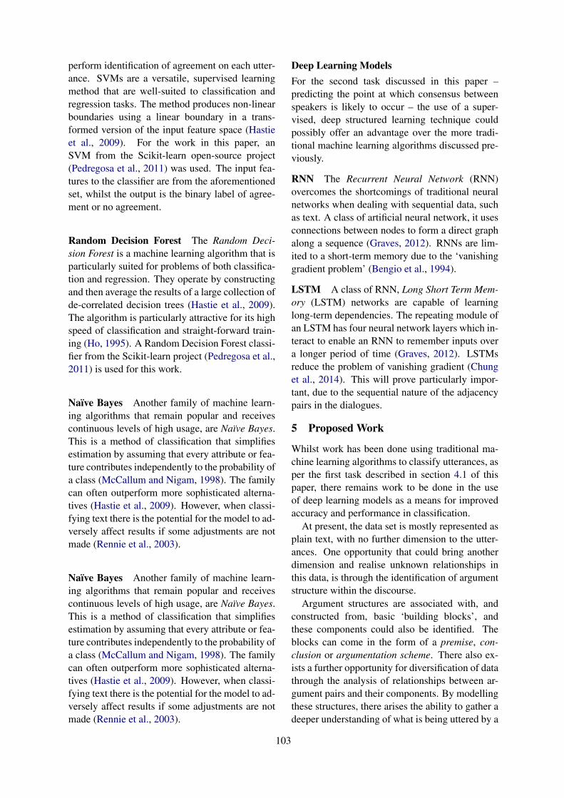
perform identification of agreement on each utter-ance. SVMs are a versatile, supervised learningmethod that are well-suited to classification andregression tasks. The method produces non-linearboundaries using a linear boundary in a trans-formed version of the input feature space (Hastieet al., 2009). For the work in this paper, anSVM from the Scikit-learn open-source project(Pedregosa et al., 2011) was used. The input fea-tures to the classifier are from the aforementionedset, whilst the output is the binary label of agree-ment or no agreement.

Random Decision Forest The Random Deci-sion Forest is a machine learning algorithm that isparticularly suited for problems of both classifica-tion and regression. They operate by constructingand then average the results of a large collection ofde-correlated decision trees (Hastie et al., 2009).The algorithm is particularly attractive for its highspeed of classification and straight-forward train-ing (Ho, 1995). A Random Decision Forest classi-fier from the Scikit-learn project (Pedregosa et al.,2011) is used for this work.

Naıve Bayes Another family of machine learn-ing algorithms that remain popular and receivescontinuous levels of high usage, are Naıve Bayes.This is a method of classification that simplifiesestimation by assuming that every attribute or fea-ture contributes independently to the probability ofa class (McCallum and Nigam, 1998). The familycan often outperform more sophisticated alterna-tives (Hastie et al., 2009). However, when classi-fying text there is the potential for the model to ad-versely affect results if some adjustments are notmade (Rennie et al., 2003).

Naıve Bayes Another family of machine learn-ing algorithms that remain popular and receivescontinuous levels of high usage, are Naıve Bayes.This is a method of classification that simplifiesestimation by assuming that every attribute or fea-ture contributes independently to the probability ofa class (McCallum and Nigam, 1998). The familycan often outperform more sophisticated alterna-tives (Hastie et al., 2009). However, when classi-fying text there is the potential for the model to ad-versely affect results if some adjustments are notmade (Rennie et al., 2003).

Deep Learning ModelsFor the second task discussed in this paper –predicting the point at which consensus betweenspeakers is likely to occur – the use of a super-vised, deep structured learning technique couldpossibly offer an advantage over the more tradi-tional machine learning algorithms discussed pre-viously.

RNN The Recurrent Neural Network (RNN)overcomes the shortcomings of traditional neuralnetworks when dealing with sequential data, suchas text. A class of artificial neural network, it usesconnections between nodes to form a direct graphalong a sequence (Graves, 2012). RNNs are lim-ited to a short-term memory due to the ‘vanishinggradient problem’ (Bengio et al., 1994).

LSTM A class of RNN, Long Short Term Mem-ory (LSTM) networks are capable of learninglong-term dependencies. The repeating module ofan LSTM has four neural network layers which in-teract to enable an RNN to remember inputs overa longer period of time (Graves, 2012). LSTMsreduce the problem of vanishing gradient (Chunget al., 2014). This will prove particularly impor-tant, due to the sequential nature of the adjacencypairs in the dialogues.

5 Proposed Work

Whilst work has been done using traditional ma-chine learning algorithms to classify utterances, asper the first task described in section 4.1 of thispaper, there remains work to be done in the useof deep learning models as a means for improvedaccuracy and performance in classification.

At present, the data set is mostly represented asplain text, with no further dimension to the utter-ances. One opportunity that could bring anotherdimension and realise unknown relationships inthis data, is through the identification of argumentstructure within the discourse.

Argument structures are associated with, andconstructed from, basic ‘building blocks’, andthese components could also be identified. Theblocks can come in the form of a premise, con-clusion or argumentation scheme. There also ex-ists a further opportunity for diversification of datathrough the analysis of relationships between ar-gument pairs and their components. By modellingthese structures, there arises the ability to gather adeeper understanding of what is being uttered by a

103

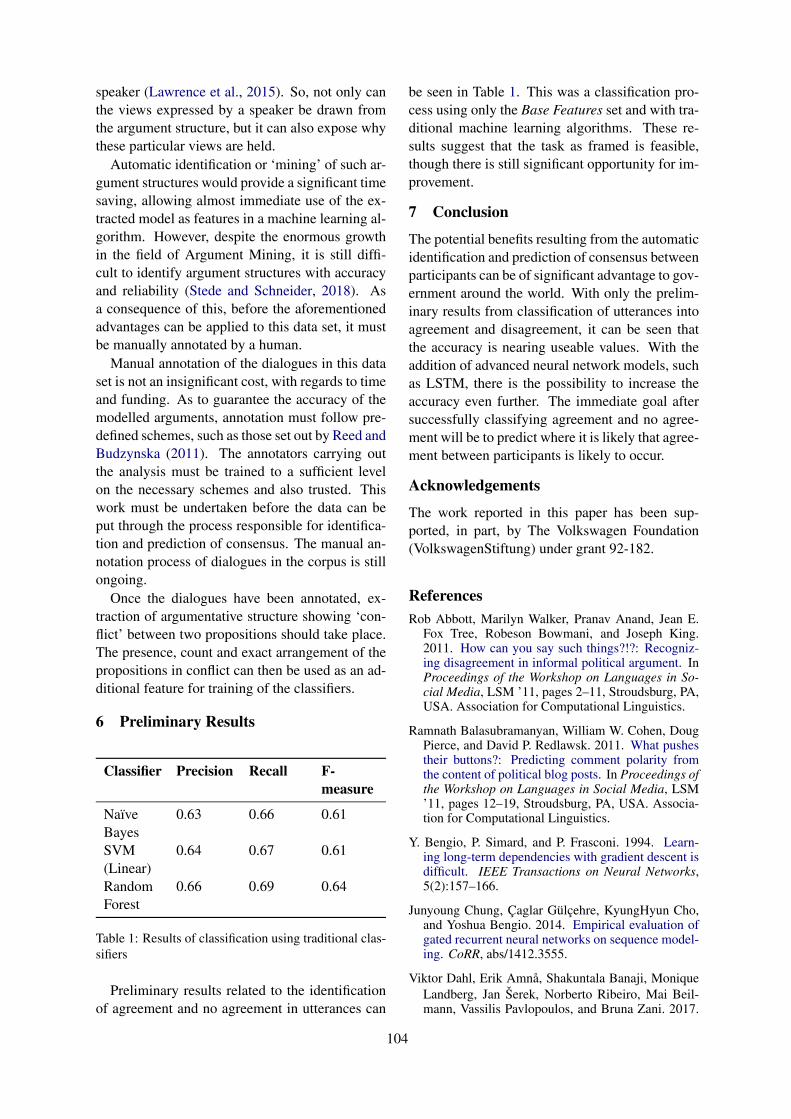
speaker (Lawrence et al., 2015). So, not only canthe views expressed by a speaker be drawn fromthe argument structure, but it can also expose whythese particular views are held.

Automatic identification or ‘mining’ of such ar-gument structures would provide a significant timesaving, allowing almost immediate use of the ex-tracted model as features in a machine learning al-gorithm. However, despite the enormous growthin the field of Argument Mining, it is still diffi-cult to identify argument structures with accuracyand reliability (Stede and Schneider, 2018). Asa consequence of this, before the aforementionedadvantages can be applied to this data set, it mustbe manually annotated by a human.

Manual annotation of the dialogues in this dataset is not an insignificant cost, with regards to timeand funding. As to guarantee the accuracy of themodelled arguments, annotation must follow pre-defined schemes, such as those set out by Reed andBudzynska (2011). The annotators carrying outthe analysis must be trained to a sufficient levelon the necessary schemes and also trusted. Thiswork must be undertaken before the data can beput through the process responsible for identifica-tion and prediction of consensus. The manual an-notation process of dialogues in the corpus is stillongoing.

Once the dialogues have been annotated, ex-traction of argumentative structure showing ‘con-flict’ between two propositions should take place.The presence, count and exact arrangement of thepropositions in conflict can then be used as an ad-ditional feature for training of the classifiers.

6 Preliminary Results

Classifier Precision Recall F-measure

NaıveBayes

0.63 0.66 0.61

SVM(Linear)

0.64 0.67 0.61

RandomForest

0.66 0.69 0.64

Table 1: Results of classification using traditional clas-sifiers

Preliminary results related to the identificationof agreement and no agreement in utterances can

be seen in Table 1. This was a classification pro-cess using only the Base Features set and with tra-ditional machine learning algorithms. These re-sults suggest that the task as framed is feasible,though there is still significant opportunity for im-provement.

7 Conclusion

The potential benefits resulting from the automaticidentification and prediction of consensus betweenparticipants can be of significant advantage to gov-ernment around the world. With only the prelim-inary results from classification of utterances intoagreement and disagreement, it can be seen thatthe accuracy is nearing useable values. With theaddition of advanced neural network models, suchas LSTM, there is the possibility to increase theaccuracy even further. The immediate goal aftersuccessfully classifying agreement and no agree-ment will be to predict where it is likely that agree-ment between participants is likely to occur.

Acknowledgements

The work reported in this paper has been sup-ported, in part, by The Volkswagen Foundation(VolkswagenStiftung) under grant 92-182.

ReferencesRob Abbott, Marilyn Walker, Pranav Anand, Jean E.

Fox Tree, Robeson Bowmani, and Joseph King.2011. How can you say such things?!?: Recogniz-ing disagreement in informal political argument. InProceedings of the Workshop on Languages in So-cial Media, LSM ’11, pages 2–11, Stroudsburg, PA,USA. Association for Computational Linguistics.

Ramnath Balasubramanyan, William W. Cohen, DougPierce, and David P. Redlawsk. 2011. What pushestheir buttons?: Predicting comment polarity fromthe content of political blog posts. In Proceedings ofthe Workshop on Languages in Social Media, LSM’11, pages 12–19, Stroudsburg, PA, USA. Associa-tion for Computational Linguistics.

Y. Bengio, P. Simard, and P. Frasconi. 1994. Learn-ing long-term dependencies with gradient descent isdifficult. IEEE Transactions on Neural Networks,5(2):157–166.

Junyoung Chung, Caglar Gulcehre, KyungHyun Cho,and Yoshua Bengio. 2014. Empirical evaluation ofgated recurrent neural networks on sequence model-ing. CoRR, abs/1412.3555.

Viktor Dahl, Erik Amna, Shakuntala Banaji, MoniqueLandberg, Jan Serek, Norberto Ribeiro, Mai Beil-mann, Vassilis Pavlopoulos, and Bruna Zani. 2017.

104

Apathy or alienation? political passivity amongyouths across eight european union countries.European Journal of Developmental Psychology,15(3):284–301.

Directorate-General for Communication. 2017a. Citi-zens’ dialogues on the future of europe. White PaperNA-01-17-787-EN-N, European Union, Brussels.

Directorate-General for Communication. 2017b.White paper on the future of europe. White PaperNA-02-17-345-EN-N, European Union, Brussels.

John S Dryzek. 2012. Foundations and frontiers of de-liberative governance. Oxford University Press.

David M. Estlund, Jeremy Waldron, Bernard Grof-man, and Scott L. Feld. 1989. Democratic the-ory and the public interest: Condorcet and rousseaurevisited. American Political Science Review,83(4):13171340.

Michel Galley, Kathleen McKeown, Julia Hirschberg,and Elizabeth Shriberg. 2004. Identifying agree-ment and disagreement in conversational speech:Use of bayesian networks to model pragmatic de-pendencies. In Proceedings of the 42nd AnnualMeeting on Association for Computational Linguis-tics, page 669. Association for Computational Lin-guistics.

Alex Graves. 2012. Supervised Sequence Labellingwith Recurrent Neural Networks, volume 385 ofStudies in Computational Intelligence. Springer.

Groupe de la Banque mondiale. 2017. World develop-ment report 2017: Governance and the law. WorldBank Group.

Trevor Hastie, Robert Tibshirani, and Jerome H. Fried-man. 2009. The Elements of Statistical Learn-ing, second edition. Springer Series in Statistics.Springer-Verlag, New York.

Tin Kam Ho. 1995. Random decision forests. In Pro-ceedings of 3rd International Conference on Doc-ument Analysis and Recognition, volume 1, pages278–282 vol.1.

J. Lawrence, M. Janier, and C. Reed. 2015. Workingwith open argument corpora. In Proceedings of the1st European Conference on Argumentation (ECA2015), Lisbon. College Publications.

Andrew McCallum and Kamal Nigam. 1998. A com-parison of event models for naive bayes text classi-fication. In Proceedings of the AAAI-98 Workshopon Learning for Text Categorization, pages 41–48.AAAI Press.

Martha L. McCoy and Patrick L. Scully. 2002. Delib-erative dialogue to expand civic engagement: Whatkind of talk does democracy need? National CivicReview, 91(2):117–135.

F. Mosteller and J Tukey. 1968. Data analysis, includ-ing statistics. In G. Lindzey and E. Aronson, editors,Revised Handbook of Social Psychology, volume 2,pages 80–203. Addison Wesley.

Bo Pang and Lillian Lee. 2008. Opinion mining andsentiment analysis. Foundations and Trends in In-formation Retrieval, 2(12):1–135.

John Parkinson and Jane Mansbridge. 2012. Deliber-ative systems: Deliberative democracy at the largescale. Cambridge University Press.

F. Pedregosa, G. Varoquaux, A. Gramfort, V. Michel,B. Thirion, O. Grisel, M. Blondel, P. Pretten-hofer, R. Weiss, V. Dubourg, J. Vanderplas, A. Pas-sos, D. Cournapeau, M. Brucher, M. Perrot, andE. Duchesnay. 2011. Scikit-learn: Machine learningin Python. Journal of Machine Learning Research,12:2825–2830.

Fabienne Peter. 2016. The Epistemology of Delibera-tive Democracy, chapter 6. John Wiley & Sons, Ltd.

Chris Reed and Katarzyna Budzynska. 2011. How di-alogues create arguments. In Proceedings of the 7thConference of the International Society for the Studyof Argumentation (ISSA), pages 1633–1645. SicSat.

Robert Remus, Uwe Quasthoff, and Gerhard Heyer.2010. Sentiws - a publicly available german-language resource for sentiment analysis. In Pro-ceedings of the Seventh International Conferenceon Language Resources and Evaluation (LREC’10),Valletta, Malta. European Language Resources As-sociation (ELRA).

Jason D. M. Rennie, Lawrence Shih, Jaime Teevan,and David R. Karger. 2003. Tackling the poor as-sumptions of naive bayes text classifiers. In Pro-ceedings of the Twentieth International Conferenceon International Conference on Machine Learning,ICML’03, pages 616–623, Washington, D.C. AAAIPress.

Manfred Stede and Jodi Schneider. 2018. Argumen-tation mining. Synthesis Lectures on Human Lan-guage Technologies, 11(2):1–191.

Matt Thomas, Bo Pang, and Lillian Lee. 2006. Get outthe vote: Determining support or opposition fromCongressional floor-debate transcripts. In Proceed-ings of EMNLP, pages 327–335.

105

Proceedings of the 57th Annual Meeting of the Association for Computational Linguistics: Student Research Workshop, pages 106–112Florence, Italy, July 28 - August 2, 2019. c©2019 Association for Computational Linguistics

Active Reading Comprehension: A dataset for learning theQuestion-Answer Relationship strategy

Diana GalvanTohoku University

Graduate School of Information SciencesSendai, Japan

dianags@ecei.tohoku.ac.jp

Abstract

Reading comprehension (RC) through ques-tion answering is a useful method for evaluat-ing if a reader understands a text. Standard ac-curacy metrics are used for evaluation, where ahigh accuracy is taken as indicative of a goodunderstanding. However, literature in qualitylearning suggests that task performance shouldalso be evaluated on the undergone process toanswer. The Question-Answer Relationship(QAR) is one of the strategies for evaluatinga reader’s understanding based on their abilityto select different sources of information de-pending on the question type. We propose thecreation of a dataset to learn the QAR strategywith weak supervision. We expect to comple-ment current work on reading comprehensionby introducing a new setup for evaluation.

1 Introduction

Computer system researchers have long been try-ing to imitate human cognitive skills like mem-ory (Hochreiter and Schmidhuber, 1997; Chunget al., 2014) and attention (Vaswani et al., 2017).These skills are essential for a number of NaturalLanguage Processing (NLP) tasks including read-ing comprehension (RC). Until now, the methodfor evaluating a system’s understanding imitatedthe common classroom setting where students areevaluated based on their number of correct an-swers. In the educational assessment literaturethis is known as product-based evaluation and isone of the performance-based assessments types(McTighe and Ferrara, 1994). However, thereis an alternative form: process-based evaluation.Process-based evaluation does not emphasize theoutput of the activity. This assessment aims toknow the step-by-step procedure followed to re-solve a given task.

When a reading comprehension system is notable to identify the correct answer, product-based

evaluation can result in the false impression ofweak understanding (i.e., misunderstanding of thetext, the question, or both) or the absence of re-quired knowledge. However, the system couldhave failed to arrive at the correct answer for someother reasons. For example, consider the readingcomprehension task shown in Figure 1. For thequestion “What were the consequences of Eliza-beth Choy's parents and grandparents being ‘moreadvanced for their times’?” the correct answeris in the text but it is located in different sen-tences. If the system only identifies “They wantedtheir daughters to be educated” as an answer, itwould be judged to be incorrect when it did notfail at finding the answer, it failed at connectingit with the fact “we were sent to schools awayfrom home” (linking problem). Similarly, any an-swer the system infers from the text for the ques-tion “What do you think are the qualities of a warheroine?” would be wrong because the answer isnot in the text, it relies exclusively on backgroundknowledge (wrong choice of information source).We propose to adopt the thesis that reading is nota passive process by which readers soak up wordsand information from the text, but an active pro-cess1 by which they predict, sample, and confirmor correct their hypotheses about the text (Weaver,1988). One of these hypotheses is which sourceof information the question requires. The readermight think it is necessary to look in the text tothen realize she could have answered without evenreading or, on the contrary, try to think of an an-swer even though it is directly in the text. Forthis reason, Raphael (1982) devised the Question-Answer Relation (QAR) strategy, a technique tohelp the reader decide the most suitable sourceof information as well as the level of reasoning

1Not to be confused with active learning, a machine learn-ing concept for a series of methods that actively participate inthe collection of training examples. (Thompson et al., 1999)

106

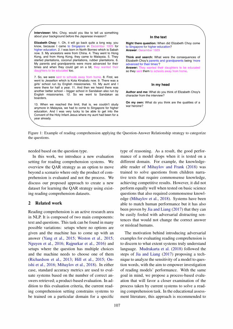
Interviewer: Mrs. Choy, would you like to tell us somethingabout your background before the Japanese invasion?

Elizabeth Choy: 1. Oh, it will go back quite a long way, youknow, because I came to Singapore in December 1929 forhigher education. 2. I was born in North Borneo which is Sabahnow. 3. My ancestors were from China. 4. They went to HongKong, and from Hong Kong, they came to Malaysia. 5. Theystarted plantations, coconut plantations, rubber plantations. 6.My parents and grandparents were more advanced for theirtimes and when they could get on a bit, they wanted theirdaughters to be educated too.

7. So, we were sent to schools away from home. 8. First, wewent to Jesselton which is Kota Kinabalu now. 9. There was agirls’ school run by English missionaries. 10. My aunt and Iwere there for half a year. 11. And then we heard there wasanother better school – bigger school in Sandakan also run byEnglish missionaries. 12. So we went to Sandakan asboarders.

13. When we reached the limit, that is, we couldn’t studyanymore in Malaysia, we had to come to Singapore for highereducation. And I was very lucky to be able to get into theConvent of the Holy Infant Jesus where my aunt had been for ayear already.

Right there question: When did Elizabeth Choy cometo Singapore for higher education?Answer: December 1929

Think and search: What were the consequences ofElizabeth Choy’s parents and grandparents being ‘moreadvanced for their times’? Answer: They wanted their daughters to be educatedso they sent them to schools away from home.

Author and me: What do you think of Elizabeth Choy'scharacter from the interview?

On my own: What do you think are the qualities of awar heroine?

In the text

In my head

Figure 1: Example of reading comprehension applying the Question-Answer Relationship strategy to categorizethe questions.

needed based on the question type.In this work, we introduce a new evaluation

setting for reading comprehension systems. Weoverview the QAR strategy as an option to movebeyond a scenario where only the product of com-prehension is evaluated and not the process. Wediscuss our proposed approach to create a newdataset for learning the QAR strategy using exist-ing reading comprehension datasets.

2 Related work

Reading comprehension is an active research areain NLP. It is composed of two main components:text and questions. This task can be found in manypossible variations: setups where no options aregiven and the machine has to come up with ananswer (Yang et al., 2015; Weston et al., 2015;Nguyen et al., 2016; Rajpurkar et al., 2016) andsetups where the question has multiple choicesand the machine needs to choose one of them(Richardson et al., 2013; Hill et al., 2015; On-ishi et al., 2016; Mihaylov et al., 2018). In eithercase, standard accuracy metrics are used to eval-uate systems based on the number of correct an-swers retrieved; a product-based evaluation. In ad-dition to this evaluation criteria, the current read-ing comprehension setting constrains systems tobe trained on a particular domain for a specific

type of reasoning. As a result, the good perfor-mance of a model drops when it is tested on adifferent domain. For example, the knowledge-able reader of Mihaylov and Frank (2018) wastrained to solve questions from children narra-tive texts that require commonsense knowledge,achieving competitive results. However, it did notperform equally well when tested on basic sciencequestions that also required commonsense knowl-edge (Mihaylov et al., 2018). Systems have beenable to match human performance but it has alsobeen proven by Jia and Liang (2017) that they canbe easily fooled with adversarial distracting sen-tences that would not change the correct answeror mislead humans.

The motivation behind introducing adversarialexamples for evaluating reading comprehension isto discern to what extent systems truly understandlanguage. Mudrakarta et al. (2018) followed thesteps of Jia and Liang (2017) proposing a tech-nique to analyze the sensitivity of a model to ques-tion words, with the aim to empower investigationof reading models’ performance. With the samegoal in mind, we propose a process-based evalu-ation that will favor a closer examination of theprocess taken by current systems to solve a read-ing comprehension task. In the educational assess-ment literature, this approach is recommended to

107

identify the weaknesses of a student. If we trans-fer this concept to computers, we would be ableto focus on the comprehension tasks a computer isweak in, regardless of the data in which the systemhas been trained.

3 Question-answer relationship

Raphael (1982) devised the Question-Answer Re-lationship as a way of improving children readingperformance across grades and subject areas. Thisapproach reflects the current concept of reading asan active process influenced by characteristics ofthe reader, the text, and the context within whichthe reading happens (McIntosh and Draper, 1995).Since its publication, several studies have exploredits positive effects (Benito et al., 1993; McIntoshand Draper, 1995; Ezell et al., 1996; Thuy andHuan, 2018; Apriani, 2019).

QAR states that an answer and its source of in-formation are directly related to the type of ques-tion being asked. It emphasizes the importanceof being able to locate this source to then identifythe level of reasoning the question requires. QARdefines four type of questions categorized in twobroad sources of information:In the text

• Right There questions: The answer can beliterally found in the text.

• Think and Search questions: The answercan be found in several sentences in the textthat need to be pieced together.

In my head

• Author and Me questions: The answer isnot directly stated in the text. It is neces-sary to fit text information with backgroundknowledge.

• On My Own questions: The answer can begiven without reading the text. The answerrelies solely on background knowledge.

Each one of the QAR categories requires a dif-ferent level of reasoning. For Right there ques-tions, the reader only needs to match the ques-tion with one of the sentences within the text.Think and search requires simple inference to re-late pieces of information contained in differentparts of the text. In my head questions introducethe use of background knowledge. Thus, deeper

thinking is required to relate the information pro-vided in the text with background information. Fi-nally, On my own questions ask the reader to onlyuse their background knowledge to come up withan answer. Figure 1 shows how QAR is appliedto a reading comprehension task. Note that forboth In the text questions, one can easily match thewords in the question with the words in the text.However, Think and search goes beyond matchingability; the reader should be able to conclude thatthe information in sentences 6 and 7 are equally re-quired to answer the question being asked. Thus,the correct answer is a combination of these two.For the Author and me question, the readers needto merge the information given in the text withtheir own background knowledge since the ques-tion explicitly asks for an opinion “from the inter-view.” Without this statement, the question couldbe considered as On my own if the reader is alreadyfamiliar with Elizabeth Choy. This is not the casein the last question, where even though the topicof the interview is related, the qualities of a warheroine are not in the text. The readers need to usetheir own background knowledge about heroes.

In the case of computers, In my head questionscan be understood as In a knowledge base. We hy-pothesize that once the system establishes that thesource of information is not in the text, it couldtrigger a connection to a knowledge base. Forthe time being, the type of knowledge needed isfixed for RC datasets by design (e.g., general do-main, commonsense, elementary science) and thesource is chosen accordingly in advance by the au-thor (e.g., Wikipedia, ConceptNet). Automaticallyselecting the appropriate external resource for areading comprehension task is a problem that wewould like to explore in the future.

3.1 QAR use cases

As a process-based evaluation strategy, QAR canbe used to understand a reader's ability in terms ofthe reasoning level applied and the elected sourceof information to answer a given question. In thecase of humans, this outcome is later used as feed-back to improve performance on a particular pro-cess. The incorporation of general reading strate-gies to a RC system has been recently proven ef-fective by Sun et al. (2018) and we aim to exploreQAR in the same way. However, our short-termobjective is to test the QAR strategy as a comple-mentary evaluation method for existing machine

108

1 Mary moved to the bathroom.2 John went to the hallway3 Where is Mary? bathroom 14 Daniel went back to the hallway.5 Sandra moved to the garden.6 Where is Daniel? hallway 47 John moved to the office.8 Sandra journeyed to the bathroom.9 Where is Daniel? hallway 4

Sentence Answer Sentenceneeded

1 Mary moved to the bathroom.2 Sandra journeyed to the bedroom.3 John went to the kitchen.4 Mary took the football there.5 How many objects is Mary carrying? one 46 Sandra went back to the office.7 How many objects is Mary carrying? one 4 8 Mary dropped the football. 9 How many objects is Mary carrying? none 4 8

Sentence Answer Sentenceneeded

1 Mary moved to the bathroom.2 John went to the hallway3 Where is Mary? bathroom 14 Daniel went back to the hallway.5 Sandra moved to the garden.6 Where is Daniel? hallway 17 John moved to the office.8 Sandra journeyed to the bathroom.9 Where is Daniel? hallway 1

Sentence Answer QARcategory

1 Mary moved to the bathroom.2 Sandra journeyed to the bedroom.3 John went to the kitchen.4 Mary took the football there.5 How many objects is Mary carrying? one 16 Sandra went back to the office.7 How many objects is Mary carrying? one 1 8 Mary dropped the football. 9 How many objects is Mary carrying? none 2

Sentence AnswerQARcategory

Figure 2: Example of bAbI annotations for the single supportive fact task (left) and the counting task (right).Below, our proposed annotations with QAR category.

reading comprehension models, somewhat simi-lar to PROTEST (Guillou and Hardmeier, 2016),a test suite for the evaluation of pronoun transla-tion by Machine Translation systems.

In the next section, we discuss how the QARstrategy can be imported from the educational lit-erature to the NLP domain by using existing read-ing comprehension datasets to create a new re-source for active reading comprehension evalua-tion.

4 Research plan

4.1 Dataset

We propose to model QAR learning as a mul-ticlass classification task with weak supervision.The dataset would contain labels corresponding toeach one of the QAR categories and the annotationprocess will depend on the two sources of infor-mation Raphael (1982) defined.

In recent years, we have seen a lot of effortfrom the NLP community in creating datasets totest different aspects of RC, like bAbI (Westonet al., 2015), SQuAD (Rajpurkar et al., 2016),NarrativeQA (Kocisky et al., 2018), QAngaroo(Welbl et al., 2018), HotpotQA (Yang et al., 2018),MCScript (Ostermann et al., 2018), MultiRC(Khashabi et al., 2018) and CommonsenseQA(Talmor et al., 2018). In the following sections,we will briefly overview these datasets and explainhow they can be adapted for our proposed task.

4.1.1 In the text questionsFor this type of questions, we can rely on the bAbIdataset (Weston et al., 2015), a set of synthetically

generated, simple narratives for testing text under-standing. The dataset has several tasks with 1000questions each for training and 1000 for testing.For our purposes, we will focus on the annotationsof Task 8 and 7. Task 8 is a “single supportingfact” task that shows a small passage in which eachsentence describes the location of a character (e.g.“Mary moved to the bathroom. John went to thehallway.”). After some sentences, there is a ques-tion asking where the character is (e.g. “Where isMary?”) and the goal is to give a single word an-swer to it (e.g. “bathroom”). Task 7 is a “count-ing” task describing the same situation, but it ag-gregates a sentence where one of the characters ei-ther takes (e.g. “Mary took the football there.”) ordrops (e.g. “Mary dropped the football.”) an ob-ject. This time, the question asks how many ob-jects is the character carrying and the answer isalso a single word (e.g. “none”). As shown inFigure 2, bAbI annotations enumerate each one ofthe sentences. The number next to the single wordanswer is the number of the sentence needed toanswer the question. Instead of the number of thesentence, we will use as label the number of theQAR category. This can be done following thisrule:

QARcategory =

1, for n = 12, for n > 1

Where n is the number of sentences and the cat-egories 1, 2 correspond to Right there and Thinkand Search, respectively. The bottom of Figure 2shows how the new annotations will look like.This annotations can be generated automatically

109

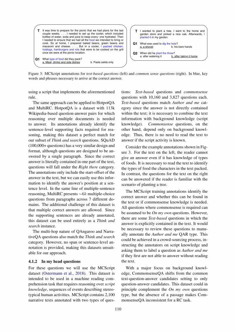
T It was time to prepare for the picnic that we had plans for the lastcouple weeks. . . . I needed to set up the cooler, which includedbottles of water, soda and juice to keep every- one hydrated. ThenI needed to ensure that we had all the food we intended to bring orcook. So at home, I prepared baked beans, green beans andmacaroni and cheese. . . . But in a cooler, I packed chicken,hotdogs, hamburgers and rots that were to be cooked on the grillonce we were at the picnic location. What type of food did they pack?a. Meat, drinks and side dishes b. Pasta salda only

Q1

T I wanted to plant a tree. I went to the home andgarden store and picked a nice oak. Afterwards, Iplanted it in my garden. What was used to dig the hole?a. a shovel b. his bare hands When did he plant the three?a. after watering it b. after taking it home

Q1

Q2

Figure 3: MCScript annotations for text-based questions (left) and common sense questions (right). In blue, keywords and phrases necessary to arrive at the correct answer.

using a script that implements the aforementionedrule.

The same approach can be applied to HotpotQAand MultiRC. HotpotQA is a dataset with 113kWikipedia-based question-answer pairs for whichreasoning over multiple documents is neededto answer. Its annotations already identify thesentence-level supporting facts required for rea-soning, making this dataset a perfect match forour subset of Think and search questions. SQuAD(100,000+ questions) has a very similar design andformat, although questions are designed to be an-swered by a single paragraph. Since the correctanswer is literally contained in one part of the text,questions will fall under the Right there category.The annotations only include the start-offset of theanswer in the text, but we can easily use this infor-mation to identify the answer's position at a sen-tence level. In the same line of multiple-sentencereasoning, MultiRC presents∼6k multiple-choicequestions from paragraphs across 7 different do-mains. The additional challenge of this dataset isthat multiple correct answers are allowed. Sincethe supporting sentences are already annotated,this dataset can be used entirely as a Think andsearch instance.

The multi-hop nature of QAngaroo and Narra-tiveQA questions also match the Think and searchcategory. However, no span or sentence-level an-notation is provided, making this datasets unsuit-able for our approach.

4.1.2 In my head questionsFor these questions we will use the MCScriptdataset (Ostermann et al., 2018). This dataset isintended to be used in a machine reading com-prehension task that requires reasoning over scriptknowledge, sequences of events describing stereo-typical human activities. MCScript contains 2,100narrative texts annotated with two types of ques-

tions: Text-based questions and commonsensequestions with 10,160 and 3,827 questions each.Text-based questions match Author and me cat-egory since the answer is not directly containedwithin the text; it is necessary to combine the textinformation with background knowledge (scriptknowledge). Commonsense questions, on theother hand, depend only on background knowl-edge. Thus, there is no need to read the text toanswer if the script activity is known.

Consider the example annotations shown in Fig-ure 3. For the text on the left, the reader cannotgive an answer even if it has knowledge of typesof foods. It is necessary to read the text to identifythe types of food the characters in the text packed.In contrast, the questions for the text on the rightcan be answered if the reader is familiar with thescenario of planting a tree.

The MCScript training annotations identify thecorrect answer and whether this can be found inthe text or if commonsense knowledge is needed.All questions where commonsense is required canbe assumed to be On my own questions. However,there are some Text-based questions in which theanswer is explicitly contained in the text. It wouldbe necessary to review these questions to manu-ally annotate the Author and me QAR type. Thiscould be achieved in a crowd-sourcing process, in-structing the annotators on script knowledge andasking them to label a question as Author and meif they first are not able to answer without readingthe text.

With a major focus on background knowl-edge, CommonsenseQA shifts from the commontext-question-answer candidates setting to onlyquestion-answer candidates. This dataset could inprinciple complement the On my own questionstype, but the absence of a passage makes Com-monsenseQA inconsistent for a RC task.

110

To ensure the integrity of our resulting dataset,we will take a subset for manual inspection.

5 Summary

We introduced process-based evaluation as a newsetting to evaluate systems in reading comprehen-sion. We propose to model QAR learning as aweak supervision classification task and discussedhow existing RC datasets can be used to generatenew data for this purpose. Our work is inspiredby the findings of the educational assessment fieldand we expect it to complement current work inreading comprehension. We will leave the detailson how to use the QAR classification task for a RCmodel’s evaluation performance to future work.

Acknowledgements

I would like to thank my supervisors Jun Suzuki,Koji Matsuda and Kentaro Inui for their feedback,support and helpful discussions. I am also thank-ful to Benjamin Heinzerling, Kyosuke Nishida andthe anonymous reviewers for their insightful com-ments. This work was supported by JST CRESTGrant Number JPMJCR1513, Japan.

ReferencesLuthfiyah Apriani. 2019. The use of question-answer

relationship to improve students’ reading compre-hension. In International Seminar and AnnualMeeting BKS-PTN Wilayah Barat, volume 1.

Yolande M Benito, Christy L Foley, Craig D Lewis,and Perry Prescott. 1993. The effect of instruction inquestion-answer relationships and metacognition onsocial studies comprehension. Journal of Researchin Reading, 16(1):20–29.

Junyoung Chung, Caglar Gulcehre, KyungHyun Cho,and Yoshua Bengio. 2014. Empirical evaluation ofgated recurrent neural networks on sequence model-ing. arXiv preprint arXiv:1412.3555.

Helen K Ezell, Stacie A Hunsicker, Maria M Quinque,and Elizabeth Randolph. 1996. Maintenance andgeneralization of qar reading comprehension strate-gies. Literacy Research and Instruction, 36(1):64–81.

Liane Guillou and Christian Hardmeier. 2016. Protest:A test suite for evaluating pronouns in machinetranslation. In LREC.

Felix Hill, Antoine Bordes, Sumit Chopra, and JasonWeston. 2015. The goldilocks principle: Readingchildren’s books with explicit memory representa-tions. arXiv preprint arXiv:1511.02301.

Sepp Hochreiter and Jurgen Schmidhuber. 1997.Long short-term memory. Neural computation,9(8):1735–1780.

Robin Jia and Percy Liang. 2017. Adversarial exam-ples for evaluating reading comprehension systems.arXiv preprint arXiv:1707.07328.

Daniel Khashabi, Snigdha Chaturvedi, Michael Roth,Shyam Upadhyay, and Dan Roth. 2018. Lookingbeyond the surface: A challenge set for reading com-prehension over multiple sentences. In Proceed-ings of the 2018 Conference of the North AmericanChapter of the Association for Computational Lin-guistics: Human Language Technologies, Volume 1(Long Papers), pages 252–262.

Tomas Kocisky, Jonathan Schwarz, Phil Blunsom,Chris Dyer, Karl Moritz Hermann, Gaabor Melis,and Edward Grefenstette. 2018. The narrativeqareading comprehension challenge. Transactionsof the Association of Computational Linguistics,6:317–328.

Margaret E McIntosh and Roni Jo Draper. 1995. Ap-plying the question-answer relationship strategy inmathematics. Journal of Adolescent & Adult Liter-acy, 39(2):120–131.

Jay McTighe and Steven Ferrara. 1994. Performance-based assessment in the classroom. PennsylvaniaEducational Leadership, pages 4–16.

Todor Mihaylov, Peter Clark, Tushar Khot, and AshishSabharwal. 2018. Can a suit of armor conduct elec-tricity? a new dataset for open book question an-swering. In Proceedings of the 2018 Conference onEmpirical Methods in Natural Language Process-ing, pages 2381–2391, Brussels, Belgium. Associ-ation for Computational Linguistics.

Todor Mihaylov and Anette Frank. 2018. Knowledge-able reader: Enhancing cloze-style reading com-prehension with external commonsense knowledge.arXiv preprint arXiv:1805.07858.

Pramod Kaushik Mudrakarta, Ankur Taly, MukundSundararajan, and Kedar Dhamdhere. 2018. Didthe model understand the question? arXiv preprintarXiv:1805.05492.

Tri Nguyen, Mir Rosenberg, Xia Song, Jianfeng Gao,Saurabh Tiwary, Rangan Majumder, and Li Deng.2016. Ms marco: A human generated machinereading comprehension dataset. arXiv preprintarXiv:1611.09268.

Takeshi Onishi, Hai Wang, Mohit Bansal, Kevin Gim-pel, and David McAllester. 2016. Who did what:A large-scale person-centered cloze dataset. arXivpreprint arXiv:1608.05457.

Simon Ostermann, Ashutosh Modi, Michael Roth,Stefan Thater, and Manfred Pinkal. 2018. Mc-script: a novel dataset for assessing machine com-prehension using script knowledge. arXiv preprintarXiv:1803.05223.

111

Pranav Rajpurkar, Jian Zhang, Konstantin Lopyrev, andPercy Liang. 2016. Squad: 100,000+ questionsfor machine comprehension of text. arXiv preprintarXiv:1606.05250.

Taffy E Raphael. 1982. Question-answering strategiesfor children. Reading Teacher.

Matthew Richardson, Christopher JC Burges, and ErinRenshaw. 2013. Mctest: A challenge dataset forthe open-domain machine comprehension of text.In Proceedings of the 2013 Conference on Empiri-cal Methods in Natural Language Processing, pages193–203.

Kai Sun, Dian Yu, Dong Yu, and Claire Cardie.2018. Improving machine reading comprehensionwith general reading strategies. arXiv preprintarXiv:1810.13441.

Alon Talmor, Jonathan Herzig, Nicholas Lourie, andJonathan Berant. 2018. Commonsenseqa: A ques-tion answering challenge targeting commonsenseknowledge. arXiv preprint arXiv:1811.00937.

Cynthia A Thompson, Mary Elaine Califf, and Ray-mond J Mooney. 1999. Active learning for natu-ral language parsing and information extraction. InICML, pages 406–414. Citeseer.

Nguyen Thi Bich Thuy and Nguyen Buu Huan. 2018.The effects of question-answer relationship strategyon efl high school studentsreading comprehension.European Journal of English Language Teaching.

Ashish Vaswani, Noam Shazeer, Niki Parmar, JakobUszkoreit, Llion Jones, Aidan N Gomez, ŁukaszKaiser, and Illia Polosukhin. 2017. Attention is allyou need. In Advances in neural information pro-cessing systems, pages 5998–6008.

Constance Weaver. 1988. Reading process and prac-tice: From socio-psycholinguistics to whole lan-guage. ERIC.

Johannes Welbl, Pontus Stenetorp, and SebastianRiedel. 2018. Constructing datasets for multi-hopreading comprehension across documents. Transac-tions of the Association of Computational Linguis-tics, 6:287–302.

Jason Weston, Antoine Bordes, Sumit Chopra, Alexan-der M Rush, Bart van Merrienboer, Armand Joulin,and Tomas Mikolov. 2015. Towards ai-completequestion answering: A set of prerequisite toy tasks.arXiv preprint arXiv:1502.05698.

Yi Yang, Wen-tau Yih, and Christopher Meek. 2015.Wikiqa: A challenge dataset for open-domain ques-tion answering. In Proceedings of the 2015 Con-ference on Empirical Methods in Natural LanguageProcessing, pages 2013–2018.

Zhilin Yang, Peng Qi, Saizheng Zhang, Yoshua Ben-gio, William Cohen, Ruslan Salakhutdinov, andChristopher D. Manning. 2018. HotpotQA: A

dataset for diverse, explainable multi-hop questionanswering. In Proceedings of the 2018 Conferenceon Empirical Methods in Natural Language Pro-cessing, pages 2369–2380, Brussels, Belgium. As-sociation for Computational Linguistics.

112

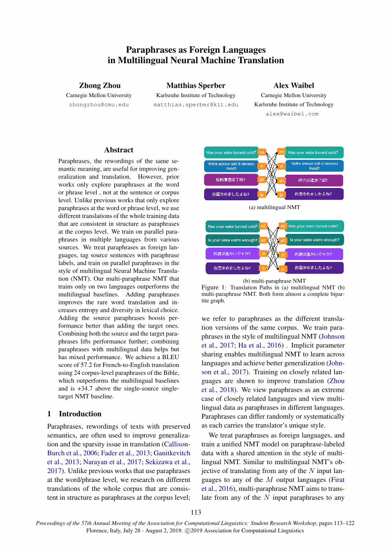
Proceedings of the 57th Annual Meeting of the Association for Computational Linguistics: Student Research Workshop, pages 113–122Florence, Italy, July 28 - August 2, 2019. c©2019 Association for Computational Linguistics

Paraphrases as Foreign Languagesin Multilingual Neural Machine Translation

Zhong ZhouCarnegie Mellon University

zhongzhou@cmu.edu

Matthias SperberKarlsruhe Institute of Technology

matthias.sperber@kit.edu

Alex WaibelCarnegie Mellon University

Karlsruhe Institute of Technology

alex@waibel.com

AbstractParaphrases, the rewordings of the same se-mantic meaning, are useful for improving gen-eralization and translation. However, priorworks only explore paraphrases at the wordor phrase level , not at the sentence or corpuslevel. Unlike previous works that only exploreparaphrases at the word or phrase level, we usedifferent translations of the whole training datathat are consistent in structure as paraphrasesat the corpus level. We train on parallel para-phrases in multiple languages from varioussources. We treat paraphrases as foreign lan-guages, tag source sentences with paraphraselabels, and train on parallel paraphrases in thestyle of multilingual Neural Machine Transla-tion (NMT). Our multi-paraphrase NMT thattrains only on two languages outperforms themultilingual baselines. Adding paraphrasesimproves the rare word translation and in-creases entropy and diversity in lexical choice.Adding the source paraphrases boosts per-formance better than adding the target ones.Combining both the source and the target para-phrases lifts performance further; combiningparaphrases with multilingual data helps buthas mixed performance. We achieve a BLEUscore of 57.2 for French-to-English translationusing 24 corpus-level paraphrases of the Bible,which outperforms the multilingual baselinesand is +34.7 above the single-source single-target NMT baseline.

1 IntroductionParaphrases, rewordings of texts with preservedsemantics, are often used to improve generaliza-tion and the sparsity issue in translation (Callison-Burch et al., 2006; Fader et al., 2013; Ganitkevitchet al., 2013; Narayan et al., 2017; Sekizawa et al.,2017). Unlike previous works that use paraphrasesat the word/phrase level, we research on differenttranslations of the whole corpus that are consis-tent in structure as paraphrases at the corpus level;

(a) multilingual NMT

(b) multi-paraphrase NMTFigure 1: Translation Paths in (a) multilingual NMT (b)multi-paraphrase NMT. Both form almost a complete bipar-tite graph.

we refer to paraphrases as the different transla-tion versions of the same corpus. We train para-phrases in the style of multilingual NMT (Johnsonet al., 2017; Ha et al., 2016) . Implicit parametersharing enables multilingual NMT to learn acrosslanguages and achieve better generalization (John-son et al., 2017). Training on closely related lan-guages are shown to improve translation (Zhouet al., 2018). We view paraphrases as an extremecase of closely related languages and view multi-lingual data as paraphrases in different languages.Paraphrases can differ randomly or systematicallyas each carries the translator’s unique style.

We treat paraphrases as foreign languages, andtrain a unified NMT model on paraphrase-labeleddata with a shared attention in the style of multi-lingual NMT. Similar to multilingual NMT’s ob-jective of translating from any of the N input lan-guages to any of the M output languages (Firatet al., 2016), multi-paraphrase NMT aims to trans-late from any of the N input paraphrases to any

113

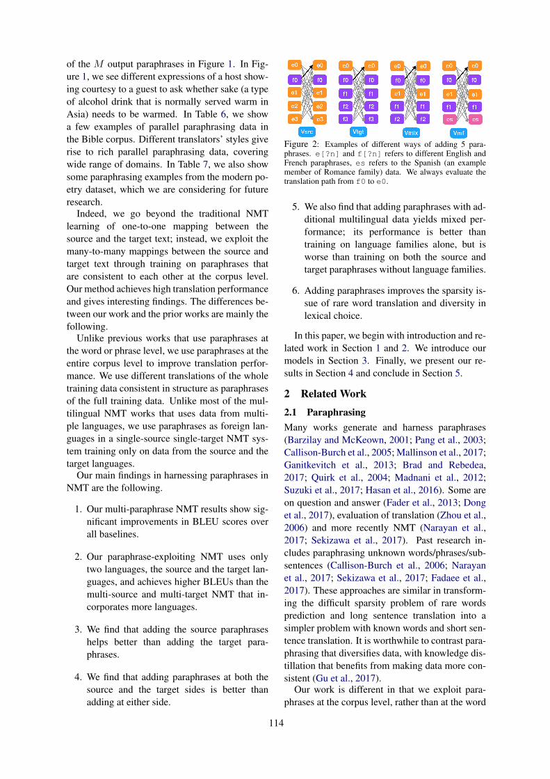
of the M output paraphrases in Figure 1. In Fig-ure 1, we see different expressions of a host show-ing courtesy to a guest to ask whether sake (a typeof alcohol drink that is normally served warm inAsia) needs to be warmed. In Table 6, we showa few examples of parallel paraphrasing data inthe Bible corpus. Different translators’ styles giverise to rich parallel paraphrasing data, coveringwide range of domains. In Table 7, we also showsome paraphrasing examples from the modern po-etry dataset, which we are considering for futureresearch.

Indeed, we go beyond the traditional NMTlearning of one-to-one mapping between thesource and the target text; instead, we exploit themany-to-many mappings between the source andtarget text through training on paraphrases thatare consistent to each other at the corpus level.Our method achieves high translation performanceand gives interesting findings. The differences be-tween our work and the prior works are mainly thefollowing.

Unlike previous works that use paraphrases atthe word or phrase level, we use paraphrases at theentire corpus level to improve translation perfor-mance. We use different translations of the wholetraining data consistent in structure as paraphrasesof the full training data. Unlike most of the mul-tilingual NMT works that uses data from multi-ple languages, we use paraphrases as foreign lan-guages in a single-source single-target NMT sys-tem training only on data from the source and thetarget languages.

Our main findings in harnessing paraphrases inNMT are the following.

1. Our multi-paraphrase NMT results show sig-nificant improvements in BLEU scores overall baselines.

2. Our paraphrase-exploiting NMT uses onlytwo languages, the source and the target lan-guages, and achieves higher BLEUs than themulti-source and multi-target NMT that in-corporates more languages.

3. We find that adding the source paraphraseshelps better than adding the target para-phrases.

4. We find that adding paraphrases at both thesource and the target sides is better thanadding at either side.

Figure 2: Examples of different ways of adding 5 para-phrases. e[?n] and f[?n] refers to different English andFrench paraphrases, es refers to the Spanish (an examplemember of Romance family) data. We always evaluate thetranslation path from f0 to e0.

5. We also find that adding paraphrases with ad-ditional multilingual data yields mixed per-formance; its performance is better thantraining on language families alone, but isworse than training on both the source andtarget paraphrases without language families.

6. Adding paraphrases improves the sparsity is-sue of rare word translation and diversity inlexical choice.

In this paper, we begin with introduction and re-lated work in Section 1 and 2. We introduce ourmodels in Section 3. Finally, we present our re-sults in Section 4 and conclude in Section 5.

2 Related Work

2.1 ParaphrasingMany works generate and harness paraphrases(Barzilay and McKeown, 2001; Pang et al., 2003;Callison-Burch et al., 2005; Mallinson et al., 2017;Ganitkevitch et al., 2013; Brad and Rebedea,2017; Quirk et al., 2004; Madnani et al., 2012;Suzuki et al., 2017; Hasan et al., 2016). Some areon question and answer (Fader et al., 2013; Donget al., 2017), evaluation of translation (Zhou et al.,2006) and more recently NMT (Narayan et al.,2017; Sekizawa et al., 2017). Past research in-cludes paraphrasing unknown words/phrases/sub-sentences (Callison-Burch et al., 2006; Narayanet al., 2017; Sekizawa et al., 2017; Fadaee et al.,2017). These approaches are similar in transform-ing the difficult sparsity problem of rare wordsprediction and long sentence translation into asimpler problem with known words and short sen-tence translation. It is worthwhile to contrast para-phrasing that diversifies data, with knowledge dis-tillation that benefits from making data more con-sistent (Gu et al., 2017).

Our work is different in that we exploit para-phrases at the corpus level, rather than at the word

114

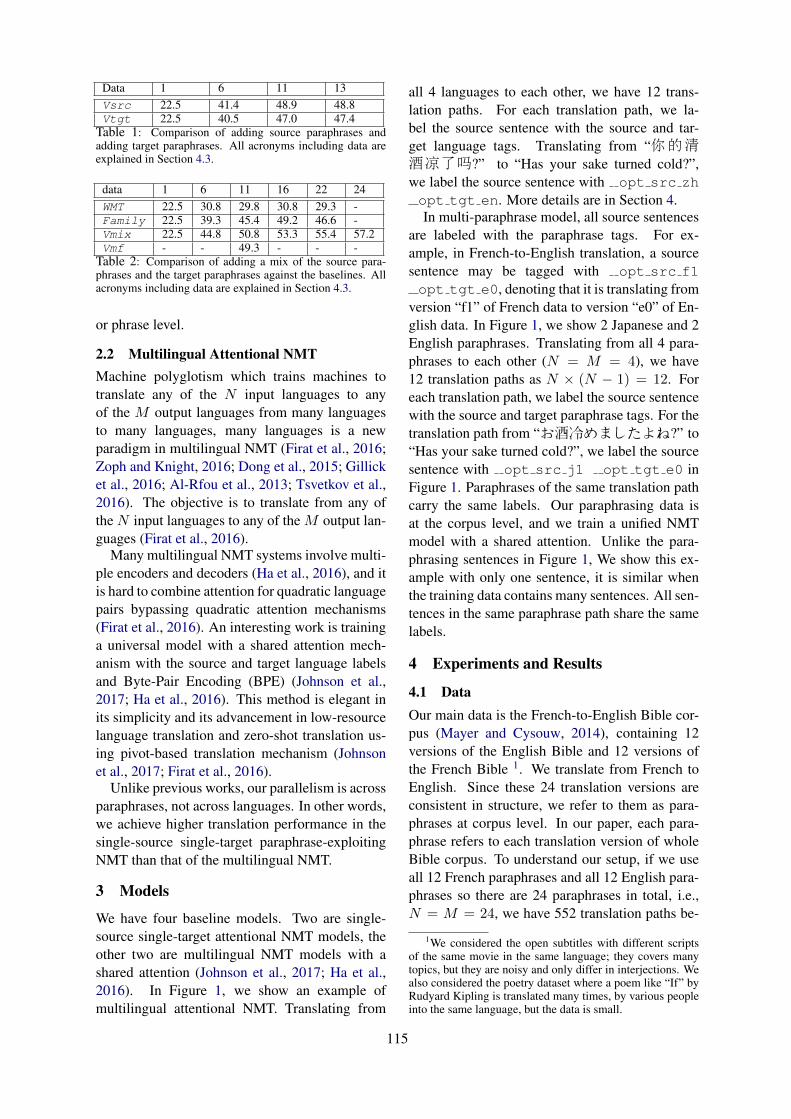
Data 1 6 11 13Vsrc 22.5 41.4 48.9 48.8Vtgt 22.5 40.5 47.0 47.4

Table 1: Comparison of adding source paraphrases andadding target paraphrases. All acronyms including data areexplained in Section 4.3.

data 1 6 11 16 22 24WMT 22.5 30.8 29.8 30.8 29.3 -Family 22.5 39.3 45.4 49.2 46.6 -Vmix 22.5 44.8 50.8 53.3 55.4 57.2Vmf - - 49.3 - - -

Table 2: Comparison of adding a mix of the source para-phrases and the target paraphrases against the baselines. Allacronyms including data are explained in Section 4.3.

or phrase level.

2.2 Multilingual Attentional NMTMachine polyglotism which trains machines totranslate any of the N input languages to anyof the M output languages from many languagesto many languages, many languages is a newparadigm in multilingual NMT (Firat et al., 2016;Zoph and Knight, 2016; Dong et al., 2015; Gillicket al., 2016; Al-Rfou et al., 2013; Tsvetkov et al.,2016). The objective is to translate from any ofthe N input languages to any of the M output lan-guages (Firat et al., 2016).

Many multilingual NMT systems involve multi-ple encoders and decoders (Ha et al., 2016), and itis hard to combine attention for quadratic languagepairs bypassing quadratic attention mechanisms(Firat et al., 2016). An interesting work is traininga universal model with a shared attention mech-anism with the source and target language labelsand Byte-Pair Encoding (BPE) (Johnson et al.,2017; Ha et al., 2016). This method is elegant inits simplicity and its advancement in low-resourcelanguage translation and zero-shot translation us-ing pivot-based translation mechanism (Johnsonet al., 2017; Firat et al., 2016).

Unlike previous works, our parallelism is acrossparaphrases, not across languages. In other words,we achieve higher translation performance in thesingle-source single-target paraphrase-exploitingNMT than that of the multilingual NMT.

3 Models

We have four baseline models. Two are single-source single-target attentional NMT models, theother two are multilingual NMT models with ashared attention (Johnson et al., 2017; Ha et al.,2016). In Figure 1, we show an example ofmultilingual attentional NMT. Translating from

all 4 languages to each other, we have 12 trans-lation paths. For each translation path, we la-bel the source sentence with the source and tar-get language tags. Translating from “你的清酒凉了吗?” to “Has your sake turned cold?”,we label the source sentence with opt src zhopt tgt en. More details are in Section 4.In multi-paraphrase model, all source sentences

are labeled with the paraphrase tags. For ex-ample, in French-to-English translation, a sourcesentence may be tagged with opt src f1opt tgt e0, denoting that it is translating from

version “f1” of French data to version “e0” of En-glish data. In Figure 1, we show 2 Japanese and 2English paraphrases. Translating from all 4 para-phrases to each other (N = M = 4), we have12 translation paths as N × (N − 1) = 12. Foreach translation path, we label the source sentencewith the source and target paraphrase tags. For thetranslation path from “お酒冷めましたよね?” to“Has your sake turned cold?”, we label the sourcesentence with opt src j1 opt tgt e0 inFigure 1. Paraphrases of the same translation pathcarry the same labels. Our paraphrasing data isat the corpus level, and we train a unified NMTmodel with a shared attention. Unlike the para-phrasing sentences in Figure 1, We show this ex-ample with only one sentence, it is similar whenthe training data contains many sentences. All sen-tences in the same paraphrase path share the samelabels.

4 Experiments and Results

4.1 DataOur main data is the French-to-English Bible cor-pus (Mayer and Cysouw, 2014), containing 12versions of the English Bible and 12 versions ofthe French Bible 1. We translate from French toEnglish. Since these 24 translation versions areconsistent in structure, we refer to them as para-phrases at corpus level. In our paper, each para-phrase refers to each translation version of wholeBible corpus. To understand our setup, if we useall 12 French paraphrases and all 12 English para-phrases so there are 24 paraphrases in total, i.e.,N = M = 24, we have 552 translation paths be-

1We considered the open subtitles with different scriptsof the same movie in the same language; they covers manytopics, but they are noisy and only differ in interjections. Wealso considered the poetry dataset where a poem like “If” byRudyard Kipling is translated many times, by various peopleinto the same language, but the data is small.

115

Source Sentence Machine Translation Correct Target TranslationComme de l’eau fraıche pour une per-sonne fatigue, Ainsi est une bonnenouvelle venant d’une terre lointaine.

As cold waters to a thirsty soul, so isgood news from a distant land.

Like cold waters to a weary soul, so isa good report from a far country.

Lorsque tu seras invite par quelqu’un ades noces, ne te mets pas a la premiereplace, de peur qu’il n’y ait parmi lesinvites une personne plus considerableque toi,

When you are invited to one to thewedding, do not be to the first place,lest any one be called greater than you.

When you are invited by anyone towedding feasts, do not recline at thechief seat lest one more honorable thanyou be invited by him,

Car chaque arbre se connaıt a son fruit.On ne cueille pas des figues sur desepines, et l’on ne vendange pas desraisins sur des ronces.

For each tree is known by its own fruit.For from thorns they do not gather figs,nor do they gather grapes from a bram-ble bush.

For each tree is known from its ownfruit. For they do not gather figs fromthorns, nor do they gather grapes froma bramble bush.

Vous tous qui avez soif, venez auxeaux, Meme celui qui n’a pas d’argent!Venez, achetez et mangez, Venez,achetez du vin et du lait, sans argent,sans rien payer!

Come, all you thirsty ones, come to thewaters; come, buy and eat. Come, buyfor wine, and for nothing, for withoutmoney.

Ho, everyone who thirsts, come to thewater; and he who has no silver, comebuy grain and eat. Yes, come buygrain, wine and milk without silver andwith no price.

Oui , vous sortirez avec joie , Et vousserez conduits en paix ; Les montagneset les collines eclateront d’allegressedevant vous , Et tous les arbres de lacampagne battront des mains .

When you go out with joy , you shallgo in peace ; the mountains shall re-joice before you , and the trees of thefield shall strike all the trees of the field.

For you shall go out with joy and be ledout with peace . The mountains and thehills shall break out into song beforeyou , and all the trees of the field shallclap the palm .

Table 3: Examples of French-to-English translation trained using 12 French paraphrases and 12 English paraphrases.

cause N × (N − 1) = 552. The original cor-pus contains missing or extra verses for differentparaphrases; we clean and align 24 paraphrases ofthe Bible corpus and randomly sample the train-ing, validation and test sets according to the 0.75,0.15, 0.10 ratio. Our training set contains only23K verses, but is massively parallel across para-phrases.

For all experiments, we choose a specific En-glish corpus as e0 and a specific French corpusas f0 which we evaluate across all experiments toensure consistency in comparison, and we evalu-ate all translation performance from f0 to e0.

4.2 Training ParametersIn all our experiments, we use a minibatch size of64, dropout rate of 0.3, 4 RNN layers of size 1000,a word vector size of 600, number of epochs of13, a learning rate of 0.8 that decays at the rate of0.7 if the validation score is not improving or it ispast epoch 9 across all LSTM-based experiments.Byte-Pair Encoding (BPE) is used at preprocess-ing stage (Ha et al., 2016). Our code is built onOpenNMT (Klein et al., 2017) and we evaluate ourmodels using BLEU scores (Papineni et al., 2002),entropy (Shannon, 1951), F-measure and qualita-tive evaluation.

4.3 BaselinesWe introduce a few acronyms for our four base-lines to describe the experiments in Table 1,Table 2 and Figure 3. Firstly, we have twosingle-source single-target attentional NMT mod-

els, Single and WMT. Single trains on f0 ande0 and gives a BLEU of 22.5, the starting point forall curves in Figure 3. WMT adds the out-domainWMT’14 French-to-English data on top of f0 ande0; it serves as a weak baseline that helps us toevaluate all experiments’ performance discountingthe effect of increasing data.

Moreover, we have two multilingual baselines2

built on multilingual attentional NMT, Familyand Span (Zhou et al., 2018). Family refers tothe multilingual baseline by adding one languagefamily at a time, where on top of the French cor-pus f0 and the English corpus e0, we add upto 20 other European languages. Span refers tothe multilingual baseline by adding one span ata time, where a span is a set of languages thatcontains at least one language from all the fami-lies in the data; in other words, span is a sparserepresentation of all the families. Both Familyand Span trains on the Bible in 22 Europeanslanguages trained using multilingual NMT. SinceSpan is always suboptimal to Family in our re-sults, we only show numerical results for Familyin Table 1 and 2, and we plot both Family andSpan in Figure 3. The two multilingual baselinesare strong baselines while the fWMT baseline is aweak baseline that helps us to evaluate all exper-iments’ performance discounting the effect of in-creasing data. All baseline results are taken from

2 For multilingual baselines, we use the additional Biblecorpus in 22 European languages that are cleaned and alignedto each other.

116

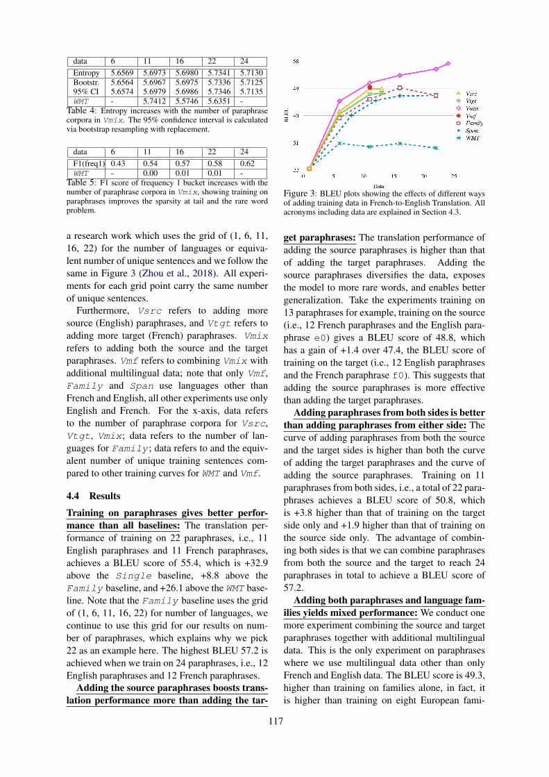
data 6 11 16 22 24Entropy 5.6569 5.6973 5.6980 5.7341 5.7130Bootstr.95% CI

5.65645.6574

5.69675.6979

5.69755.6986

5.73365.7346

5.71255.7135

WMT - 5.7412 5.5746 5.6351 -Table 4: Entropy increases with the number of paraphrasecorpora in Vmix. The 95% confidence interval is calculatedvia bootstrap resampling with replacement.

data 6 11 16 22 24F1(freq1) 0.43 0.54 0.57 0.58 0.62WMT - 0.00 0.01 0.01 -

Table 5: F1 score of frequency 1 bucket increases with thenumber of paraphrase corpora in Vmix, showing training onparaphrases improves the sparsity at tail and the rare wordproblem.

a research work which uses the grid of (1, 6, 11,16, 22) for the number of languages or equiva-lent number of unique sentences and we follow thesame in Figure 3 (Zhou et al., 2018). All experi-ments for each grid point carry the same numberof unique sentences.

Furthermore, Vsrc refers to adding moresource (English) paraphrases, and Vtgt refers toadding more target (French) paraphrases. Vmixrefers to adding both the source and the targetparaphrases. Vmf refers to combining Vmix withadditional multilingual data; note that only Vmf,Family and Span use languages other thanFrench and English, all other experiments use onlyEnglish and French. For the x-axis, data refersto the number of paraphrase corpora for Vsrc,Vtgt, Vmix; data refers to the number of lan-guages for Family; data refers to and the equiv-alent number of unique training sentences com-pared to other training curves for WMT and Vmf.

4.4 Results

Training on paraphrases gives better perfor-mance than all baselines: The translation per-formance of training on 22 paraphrases, i.e., 11English paraphrases and 11 French paraphrases,achieves a BLEU score of 55.4, which is +32.9above the Single baseline, +8.8 above theFamily baseline, and +26.1 above the WMT base-line. Note that the Family baseline uses the gridof (1, 6, 11, 16, 22) for number of languages, wecontinue to use this grid for our results on num-ber of paraphrases, which explains why we pick22 as an example here. The highest BLEU 57.2 isachieved when we train on 24 paraphrases, i.e., 12English paraphrases and 12 French paraphrases.

Adding the source paraphrases boosts trans-lation performance more than adding the tar-

Figure 3: BLEU plots showing the effects of different waysof adding training data in French-to-English Translation. Allacronyms including data are explained in Section 4.3.

get paraphrases: The translation performance ofadding the source paraphrases is higher than thatof adding the target paraphrases. Adding thesource paraphrases diversifies the data, exposesthe model to more rare words, and enables bettergeneralization. Take the experiments training on13 paraphrases for example, training on the source(i.e., 12 French paraphrases and the English para-phrase e0) gives a BLEU score of 48.8, whichhas a gain of +1.4 over 47.4, the BLEU score oftraining on the target (i.e., 12 English paraphrasesand the French paraphrase f0). This suggests thatadding the source paraphrases is more effectivethan adding the target paraphrases.

Adding paraphrases from both sides is betterthan adding paraphrases from either side: Thecurve of adding paraphrases from both the sourceand the target sides is higher than both the curveof adding the target paraphrases and the curve ofadding the source paraphrases. Training on 11paraphrases from both sides, i.e., a total of 22 para-phrases achieves a BLEU score of 50.8, whichis +3.8 higher than that of training on the targetside only and +1.9 higher than that of training onthe source side only. The advantage of combin-ing both sides is that we can combine paraphrasesfrom both the source and the target to reach 24paraphrases in total to achieve a BLEU score of57.2.

Adding both paraphrases and language fam-ilies yields mixed performance: We conduct onemore experiment combining the source and targetparaphrases together with additional multilingualdata. This is the only experiment on paraphraseswhere we use multilingual data other than onlyFrench and English data. The BLEU score is 49.3,higher than training on families alone, in fact, itis higher than training on eight European fami-

117

lies altogether. However, it is lower than trainingon English and French paraphrases alone. Indeed,adding paraphrases as foreign languages is effec-tive, however, when there is a lack of data, mixingthe paraphrases with multilingual data is helpful.

Adding paraphrases increases entropy anddiversity in lexical choice, and improves thesparsity issue of rare words: We use bootstrapresampling and construct 95% confidence inter-vals for entropies (Shannon, 1951) of all models ofVmix, i.e., models adding paraphrases at both thesource and the target sides. We find that the moreparaphrases, the higher the entropy, the more di-versity in lexical choice as shown in Table 4. Fromthe word F-measure shown in Table 5, we findthat the more paraphrases, the better the modelhandles the sparsity of rare words issue. Addingparaphrases not only achieves much higher BLEUscore than the WMT baseline, but also handles thesparsity issue much better than the WMT baseline.

Adding paraphrases helps rhetoric transla-tion and increases expressiveness: Qualitativeevaluation shows many cases where rhetoric trans-lation is improved by training on diverse sets ofparaphrases. In Table 3, Paraphrases help NMTto use a more contemporary synonym of “silver”,“money”, which is more direct and easier to un-derstand. Paraphrases simplifies the rhetorical orsubtle expressions, for example, our model uses“rejoice” to replace “break out into song”, a per-sonification device of mountains to describe joy,which captures the essence of the meaning beingconveyed. However, we also observe that NMTwrongly translates “clap the palm” to “strike”.We find the quality of rhetorical translation tiesclosely with the diversity of parallel paraphrasesdata. Indeed, the use of paraphrases to improverhetoric translation is a good future research ques-tion. Please refer to the Table 3 for more qualita-tive examples.

5 ConclusionWe train on paraphrases as foreign languagesin the style of multilingual NMT. Adding para-phrases improves translation quality, the rare wordissue, and diversity in lexical choice. Adding thesource paraphrases helps more than adding thetarget ones, while combining both boosts perfor-mance further. Adding multilingual data to para-phrases yields mixed performance. We would liketo explore the common structure and terminologyconsistency across different paraphrases. Since

structure and terminology are shared across para-phrases, we are interested in a building an ex-plicit representation of the paraphrases and extendour work for better translation, or translation withmore explicit and more explainable hidden states,which is very important in all neural systems.

We are interested in broadening our dataset inour future experiments. We hope to use other par-allel paraphrasing corpora like the poetry datasetas shown in Table 7. There are very few poemsthat are translated multiple times into the samelanguage, we therefore need to train on extremelysmall dataset. Rhetoric in paraphrasing is impor-tant in poetry dataset, which again depends on thetraining paraphrases. The limited data issue is alsorelevant to the low-resource setting.

We would like to effectively train on extremelysmall low-resource paraphrasing data. As dis-cussed above about the potential research poetrydataset, dataset with multiple paraphrases is typi-cally small and yet valuable. If we can train us-ing extremely small amount of data, especially inthe low-resource scenario, we would exploit thepower of multi-paraphrase NMT further.

Cultural-aware paraphrasing and subtle expres-sions are vital (Levin et al., 1998; Larson, 1984).Rhetoric in paraphrasing is a very important too.In Figure 1, “is your sake warm enough?” in Asianculture is an implicit way of saying “would youlike me to warm the sake for you?”. We wouldlike to model the culture-specific subtlety throughmulti-paraphrase training.

ReferencesRami Al-Rfou, Bryan Perozzi, and Steven Skiena.

2013. Polyglot: Distributed word representationsfor multilingual nlp. In Proceedings of the 17thConference on Computational Natural LanguageLearning, pages 183–192, Sofia, Bulgaria. Associ-ation for Computational Linguistics.

Regina Barzilay and Kathleen R McKeown. 2001. Ex-tracting paraphrases from a parallel corpus. In Pro-ceedings of the 39th Annual Meeting on Associationfor Computational Linguistics, pages 50–57. Asso-ciation for Computational Linguistics.

Florin Brad and Traian Rebedea. 2017. Neural para-phrase generation using transfer learning. In Pro-ceedings of the 10th International Conference onNatural Language Generation, pages 257–261.

Chris Callison-Burch, Colin Bannard, and JoshSchroeder. 2005. Scaling phrase-based statisticalmachine translation to larger corpora and longer

118

phrases. In Proceedings of the 43rd Annual Meet-ing on Association for Computational Linguistics,pages 255–262. Association for Computational Lin-guistics.

Chris Callison-Burch, Philipp Koehn, and Miles Os-borne. 2006. Improved statistical machine trans-lation using paraphrases. In Proceedings of NorthAmerican Chapter of the Association for Compu-tational Linguistics on Human Language Technolo-gies, pages 17–24. Association for ComputationalLinguistics.

Daxiang Dong, Hua Wu, Wei He, Dianhai Yu, andHaifeng Wang. 2015. Multi-task learning for mul-tiple language translation. In Proceedings of the53rd Annual Meeting of the Association for Com-putational Linguistics, pages 1723–1732.

Li Dong, Jonathan Mallinson, Siva Reddy, and MirellaLapata. 2017. Learning to paraphrase for questionanswering. In Proceedings of the 22nd Conferenceon Empirical Methods in Natural Language Pro-cessing, pages 875–886.

Marzieh Fadaee, Arianna Bisazza, and ChristofMonz. 2017. Data augmentation for low-resource neural machine translation. arXiv preprintarXiv:1705.00440.

Anthony Fader, Luke Zettlemoyer, and Oren Etzioni.2013. Paraphrase-driven learning for open questionanswering. In Proceedings of the 51st Annual Meet-ing of the Association for Computational Linguis-tics, pages 1608–1618.

Orhan Firat, Kyunghyun Cho, and Yoshua Bengio.2016. Multi-way, multilingual neural machinetranslation with a shared attention mechanism. InProceedings of the 15th Conference of the NorthAmerican Chapter of the Association for Compu-tational Linguistics on Human Language Technolo-gies, pages 866–875.

Juri Ganitkevitch, Benjamin Van Durme, and ChrisCallison-Burch. 2013. Ppdb: The paraphrasedatabase. In Proceedings of the 12th Conferenceof the North American Chapter of the Associationfor Computational Linguistics on Human LanguageTechnologies, pages 758–764.

Dan Gillick, Cliff Brunk, Oriol Vinyals, and AmarnagSubramanya. 2016. Multilingual language process-ing from bytes. In Proceedings of the 15th Confer-ence of the North American Chapter of the Associa-tion for Computational Linguistics on Human Lan-guage Technologies, pages 1296–1306.

Jiatao Gu, James Bradbury, Caiming Xiong, Vic-tor OK Li, and Richard Socher. 2017. Non-autoregressive neural machine translation. arXivpreprint arXiv:1711.02281.

Thanh-Le Ha, Jan Niehues, and Alexander Waibel.2016. Toward multilingual neural machine trans-lation with universal encoder and decoder. arXivpreprint arXiv:1611.04798.

Sadid A Hasan, Bo Liu, Joey Liu, Ashequl Qadir,Kathy Lee, Vivek Datla, Aaditya Prakash, andOladimeji Farri. 2016. Neural clinical paraphrasegeneration with attention. In Proceedings of theClinical Natural Language Processing Workshop,pages 42–53.

Melvin Johnson, Mike Schuster, Quoc V Le, MaximKrikun, Yonghui Wu, Zhifeng Chen, Nikhil Thorat,Fernanda Viegas, Martin Wattenberg, Greg Corrado,et al. 2017. Google’s multilingual neural machinetranslation system: Enabling zero-shot translation.Transactions of the Association for ComputationalLinguistics, 5:339–351.

Guillaume Klein, Yoon Kim, Yuntian Deng, JeanSenellart, and Alexander Rush. 2017. Opennmt:Open-source toolkit for neural machine translation.Proceedings of the 55th annual meeting of theAssociation for Computational Linguistics, SystemDemonstrations, pages 67–72.

Mildred L Larson. 1984. Meaning-based translation:A guide to cross-language equivalence. Universitypress of America Lanham.

Lori Levin, Donna Gates, Alon Lavie, and AlexWaibel. 1998. An interlingua based on domain ac-tions for machine translation of task-oriented dia-logues. In Proceedings of the 5th International Con-ference on Spoken Language Processing.

Nitin Madnani, Joel Tetreault, and Martin Chodorow.2012. Re-examining machine translation metrics forparaphrase identification. In Proceedings of the 11thConference of the North American Chapter of theAssociation for Computational Linguistics on Hu-man Language Technologies, pages 182–190. Asso-ciation for Computational Linguistics.

Jonathan Mallinson, Rico Sennrich, and Mirella Lap-ata. 2017. Paraphrasing revisited with neural ma-chine translation. In Proceedings of the 15th Con-ference of the European Chapter of the Associationfor Computational Linguistics, pages 881–893.

Thomas Mayer and Michael Cysouw. 2014. Creat-ing a massively parallel bible corpus. Oceania,135(273):40.

Shashi Narayan, Claire Gardent, Shay Cohen, andAnastasia Shimorina. 2017. Split and rephrase. InProceedings of the 22nd Conference on EmpiricalMethods in Natural Language Processing, pages617–627.

Bo Pang, Kevin Knight, and Daniel Marcu. 2003.Syntax-based alignment of multiple translations:Extracting paraphrases and generating new sen-tences. In Proceedings of North American Chapterof the Association for Computational Linguistics onHuman Language Technologies.

Kishore Papineni, Salim Roukos, Todd Ward, and Wei-Jing Zhu. 2002. Bleu: a method for automatic eval-uation of machine translation. In Proceedings of

119

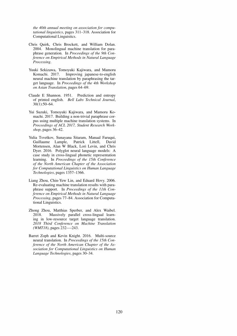
the 40th annual meeting on association for compu-tational linguistics, pages 311–318. Association forComputational Linguistics.

Chris Quirk, Chris Brockett, and William Dolan.2004. Monolingual machine translation for para-phrase generation. In Proceedings of the 9th Con-ference on Empirical Methods in Natural LanguageProcessing.

Yuuki Sekizawa, Tomoyuki Kajiwara, and MamoruKomachi. 2017. Improving japanese-to-englishneural machine translation by paraphrasing the tar-get language. In Proceedings of the 4th Workshopon Asian Translation, pages 64–69.

Claude E Shannon. 1951. Prediction and entropyof printed english. Bell Labs Technical Journal,30(1):50–64.

Yui Suzuki, Tomoyuki Kajiwara, and Mamoru Ko-machi. 2017. Building a non-trivial paraphrase cor-pus using multiple machine translation systems. InProceedings of ACL 2017, Student Research Work-shop, pages 36–42.

Yulia Tsvetkov, Sunayana Sitaram, Manaal Faruqui,Guillaume Lample, Patrick Littell, DavidMortensen, Alan W Black, Lori Levin, and ChrisDyer. 2016. Polyglot neural language models: Acase study in cross-lingual phonetic representationlearning. In Proceedings of the 15th Conferenceof the North American Chapter of the Associationfor Computational Linguistics on Human LanguageTechnologies, pages 1357–1366.

Liang Zhou, Chin-Yew Lin, and Eduard Hovy. 2006.Re-evaluating machine translation results with para-phrase support. In Proceedings of the 11th Con-ference on Empirical Methods in Natural LanguageProcessing, pages 77–84. Association for Computa-tional Linguistics.

Zhong Zhou, Matthias Sperber, and Alex Waibel.2018. Massively parallel cross-lingual learn-ing in low-resource target language translation.2018 Third Conference on Machine Translation(WMT18), pages 232—-243.

Barret Zoph and Kevin Knight. 2016. Multi-sourceneural translation. In Proceedings of the 15th Con-ference of the North American Chapter of the As-sociation for Computational Linguistics on HumanLanguage Technologies, pages 30–34.

120

Appendix A Supplemental Materials

We show a few examples of parallel paraphras-ing data in the Bible corpus. We also show someparaphrasing examples from the modern poetrydataset, which we are considering for future re-search.

121

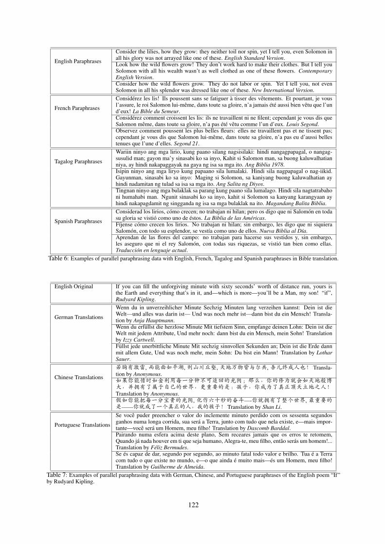
English Paraphrases

Consider the lilies, how they grow: they neither toil nor spin, yet I tell you, even Solomon inall his glory was not arrayed like one of these. English Standard Version.Look how the wild flowers grow! They don’t work hard to make their clothes. But I tell youSolomon with all his wealth wasn’t as well clothed as one of these flowers. ContemporaryEnglish Version.Consider how the wild flowers grow. They do not labor or spin. Yet I tell you, not evenSolomon in all his splendor was dressed like one of these. New International Version.

French Paraphrases

Considerez les lis! Ils poussent sans se fatiguer a tisser des vetements. Et pourtant, je vousl’assure, le roi Salomon lui-meme, dans toute sa gloire, n’a jamais ete aussi bien vetu que l’und’eux! La Bible du Semeur.Considerez comment croissent les lis: ils ne travaillent ni ne filent; cependant je vous dis queSalomon meme, dans toute sa gloire, n’a pas ete vetu comme l’un d’eux. Louis Segond.Observez comment poussent les plus belles fleurs: elles ne travaillent pas et ne tissent pas;cependant je vous dis que Salomon lui-meme, dans toute sa gloire, n’a pas eu d’aussi bellestenues que l’une d’elles. Segond 21.

Tagalog Paraphrases

Wariin ninyo ang mga lirio, kung paano silang nagsisilaki: hindi nangagpapagal, o nangag-susulid man; gayon ma’y sinasabi ko sa inyo, Kahit si Salomon man, sa buong kaluwalhatianniya, ay hindi nakapaggayak na gaya ng isa sa mga ito. Ang Biblia 1978.Isipin ninyo ang mga liryo kung papaano sila lumalaki. Hindi sila nagpapagal o nag-iikid.Gayunman, sinasabi ko sa inyo: Maging si Solomon, sa kaniyang buong kaluwalhatian ayhindi nadamitan ng tulad sa isa sa mga ito. Ang Salita ng Diyos.Tingnan ninyo ang mga bulaklak sa parang kung paano sila lumalago. Hindi sila nagtatrabahoni humahabi man. Ngunit sinasabi ko sa inyo, kahit si Solomon sa kanyang karangyaan ayhindi nakapagdamit ng singganda ng isa sa mga bulaklak na ito. Magandang Balita Biblia.

Spanish Paraphrases

Considerad los lirios, como crecen; no trabajan ni hilan; pero os digo que ni Salomon en todasu gloria se vistio como uno de estos. La Biblia de las Americas.Fıjense como crecen los lirios. No trabajan ni hilan; sin embargo, les digo que ni siquieraSalomon, con todo su esplendor, se vestıa como uno de ellos. Nueva Biblia al Dıa.Aprendan de las flores del campo: no trabajan para hacerse sus vestidos y, sin embargo,les aseguro que ni el rey Salomon, con todas sus riquezas, se vistio tan bien como ellas.Traduccion en lenguaje actual.

Table 6: Examples of parallel paraphrasing data with English, French, Tagalog and Spanish paraphrases in Bible translation.

English Original If you can fill the unforgiving minute with sixty seconds’ worth of distance run, yours isthe Earth and everything that’s in it, and—which is more—you’ll be a Man, my son! “if”,Rudyard Kipling.

German Translations

Wenn du in unverzeihlicher Minute Sechzig Minuten lang verzeihen kannst: Dein ist dieWelt—und alles was darin ist— Und was noch mehr ist—dann bist du ein Mensch! Transla-tion by Anja Hauptmann.Wenn du erfullst die herzlose Minute Mit tiefstem Sinn, empfange deinen Lohn: Dein ist dieWelt mit jedem Attribute, Und mehr noch: dann bist du ein Mensch, mein Sohn! Translationby Izzy Cartwell.Fullst jede unerbittliche Minute Mit sechzig sinnvollen Sekunden an; Dein ist die Erde dannmit allem Gute, Und was noch mehr, mein Sohn: Du bist ein Mann! Translation by LotharSauer.

Chinese Translations

若胸有激雷,而能面如平湖,则山川丘壑,天地万物皆与尔共,吾儿终成人也！ Transla-tion by Anonymous.如果你能惜时如金利用每一分钟不可追回的光阴；那么，你的修为就会如天地般博大，并拥有了属于自己的世界，更重要的是：孩子，你成为了真正顶天立地之人！Translation by Anonymous.假如你能把每一分宝贵的光阴, 化作六十秒的奋斗—-你就拥有了整个世界,最重要的是——你就成了一个真正的人，我的孩子！ Translation by Shan Li.

Portuguese Translations

Se voce puder preencher o valor do inclemente minuto perdido com os sessenta segundosganhos numa longa corrida, sua sera a Terra, junto com tudo que nela existe, e—mais impor-tante—voce sera um Homem, meu filho! Translation by Dascomb Barddal.Pairando numa esfera acima deste plano, Sem receares jamais que os erros te retomem,Quando ja nada houver em ti que seja humano, Alegra-te, meu filho, entao seras um homem!...Translation by Feliz Bermudes.Se es capaz de dar, segundo por segundo, ao minuto fatal todo valor e brilho. Tua e a Terracom tudo o que existe no mundo, e—o que ainda e muito mais—es um Homem, meu filho!Translation by Guilherme de Almeida.

Table 7: Examples of parallel paraphrasing data with German, Chinese, and Portuguese paraphrases of the English poem “If”by Rudyard Kipling.

122

Proceedings of the 57th Annual Meeting of the Association for Computational Linguistics: Student Research Workshop, pages 123–129Florence, Italy, July 28 - August 2, 2019. c©2019 Association for Computational Linguistics

Improving Mongolian-Chinese Neural Machine Translation withMorphological Noise

Yatu JI*jiyatu0@126.com

Hongxu HOU*†cshhx@imu.edu.cn

*Computer Science dept, Inner Mongolia University / Hohhot, China

Nier WU*wunier04@126.com

Junjie CHEN*chenjj@imau.edu.cn

Abstract

For the translation of agglutinative languagesuch as typical Mongolian, unknown (UN-K) words not only come from the quiterestricted vocabulary, but also mostly frommisunderstanding of the translation modelto the morphological changes. In this s-tudy, we introduce a new adversarial train-ing model to alleviate the UNK problemin Mongolian→Chinese machine translation.The training process can be described asthree adversarial sub models (generator, val-ue screener and discriminator), playing awin−win game. In this game, the addedscreener plays the role of emphasizing thatthe discriminator pays attention to the addedMongolian morphological noise1 in the formof pseudo-data and improving the training effi-ciency. The experimental results show that thenewly emerged Mongolian→Chinese task isstate-of-the-art. Under this premise, the train-ing time is greatly shortened.

1 Introduction

The dominant neural machine translation (NMT)(Sutskever et al., 2014) models are based on recur-rent (RNN, (Mikolov et al., 2011)), convolution-al neural networks (CNN, (Gehring et al., 2017))or entirely eliminates recurrent connections andrelies instead on a repeated attention mechanism(Transformer, (Vaswani et al., 2017)) which areachieved by an attention mechanism (Bahdanauet al., 2014). A considerable weakness in theseNMT systems is their inability to correctly trans-late very rare words: end-to-end NMTs tend tohave relatively small vocabularies with a single< unk > symbol that represents every possible

1These morphological noises exist in most agglutinativelanguages in the form of appended stem, which are used todetermine the presentation or tense of words. Some typicalnoises, such as suffixes and cases in Mongolian, Korean andJapanese.

out-of-vocabulary (OOV) word. The problem ismore prominent in agglutinative language tasks,because the varied morphology brings great confu-sion to model decoding. The change of suffix andcomponent case2 in Mongolian largely deceivesthe translation model directly resulting in a largeamount of OOV during decoding. This OOV isthen crudely considered the same as an < unk >symbol.

Generally, there are three ways to solve thisproblem. A usual practice is to speed up training(Morin and Bengio, 2005; Jean et al., 2015; Mnihet al., 2013), these approaches can maintain a verylarge vocabulary. However, it works well whenthere are only a few unknown words in the targetsentence. These approaches have been observedthat the translation performance degrades rapidlyas the number of unknown words increases. An-other aspect is the information in context (Luonget al., 2015; Hermann et al., 2015; Gulcehre et al.,2016), they motivate their work from a psycholog-ical evidence that humans naturally have a tenden-cy to point towards objects in the context. The lastaspect is the input/output change, these approach-es change to a smaller resolution, such as char-acters (Graves, 2013a) and bytecodes (Sennrichet al., 2016). However, it is worth thinking thatthe training process usually becomes much hard-er because of the length of sequences considerableincreases.

For NLP tasks, generative adversarial network(GAN) is immature. Some studies, such as (Chenet al., 2016; Zhang et al., 2017), used GAN forsemantic analysis and domain adaptation. (Yuet al., 2016; Zhen et al., 2018; Wu et al., 2018)successfully applied GAN to sequence generationtasks. (Zhang Y, 2017) propose matching thehigh-dimensional latent feature distributions of re-

2Mongolian-case is a special suffix used to determine itsrelationship to other words in a sentence.

123

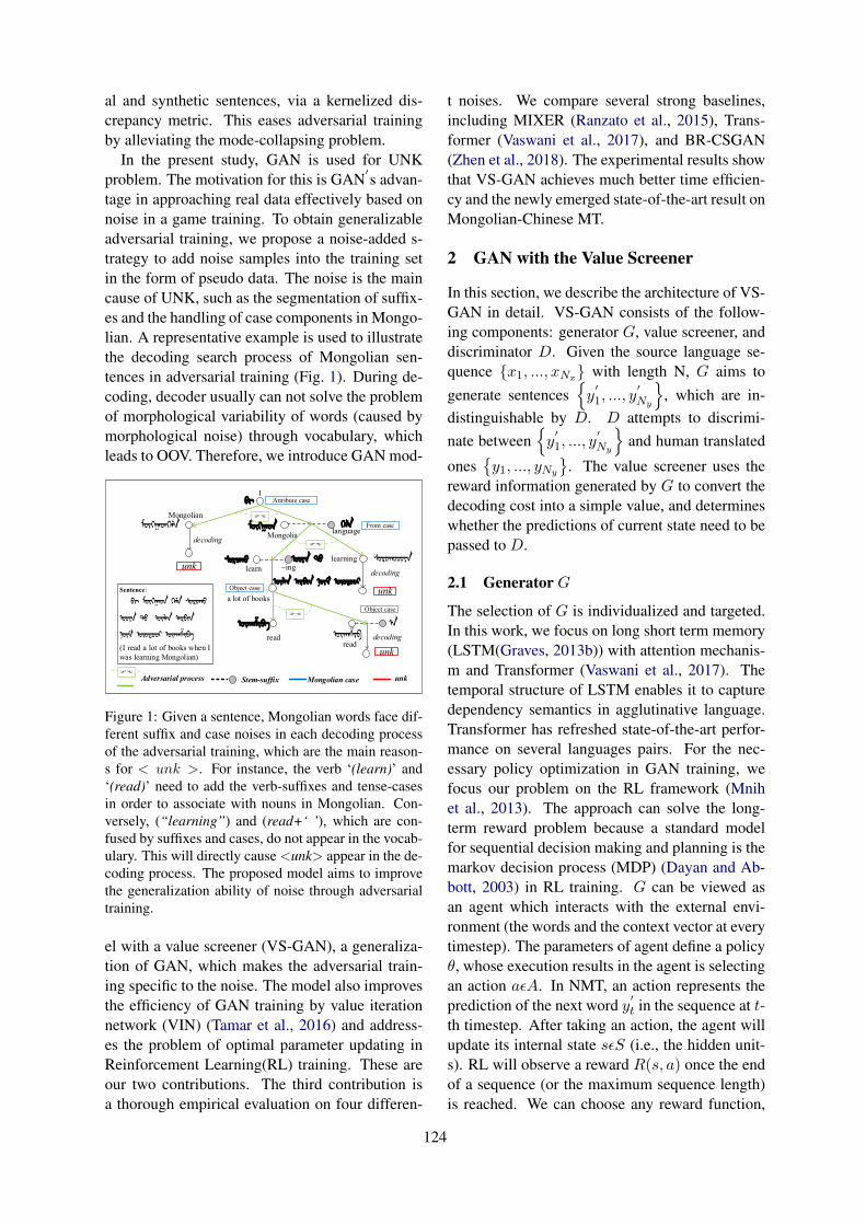
al and synthetic sentences, via a kernelized dis-crepancy metric. This eases adversarial trainingby alleviating the mode-collapsing problem.

In the present study, GAN is used for UNKproblem. The motivation for this is GAN

′s advan-

tage in approaching real data effectively based onnoise in a game training. To obtain generalizableadversarial training, we propose a noise-added s-trategy to add noise samples into the training setin the form of pseudo data. The noise is the maincause of UNK, such as the segmentation of suffix-es and the handling of case components in Mongo-lian. A representative example is used to illustratethe decoding search process of Mongolian sen-tences in adversarial training (Fig. 1). During de-coding, decoder usually can not solve the problemof morphological variability of words (caused bymorphological noise) through vocabulary, whichleads to OOV. Therefore, we introduce GAN mod-

I

Mongolian

unk

Mongolialanguage

learn ~inglearning

unka lot of books

readread

unk

Attribute case

From case

Object case

Object case

unkMongolian caseStem-suffixAdversarial process

Sentence:

(I read a lot of books when I

was learning Mongolian)

decoding

decoding

decoding

FE

FE

FE

FE

Figure 1: Given a sentence, Mongolian words face dif-ferent suffix and case noises in each decoding processof the adversarial training, which are the main reason-s for < unk >. For instance, the verb ‘(learn)’ and‘(read)’ need to add the verb-suffixes and tense-casesin order to associate with nouns in Mongolian. Con-versely, (“learning”) and (read+‘ ’), which are con-fused by suffixes and cases, do not appear in the vocab-ulary. This will directly cause <unk> appear in the de-coding process. The proposed model aims to improvethe generalization ability of noise through adversarialtraining.

el with a value screener (VS-GAN), a generaliza-tion of GAN, which makes the adversarial train-ing specific to the noise. The model also improvesthe efficiency of GAN training by value iterationnetwork (VIN) (Tamar et al., 2016) and address-es the problem of optimal parameter updating inReinforcement Learning(RL) training. These areour two contributions. The third contribution isa thorough empirical evaluation on four differen-

t noises. We compare several strong baselines,including MIXER (Ranzato et al., 2015), Trans-former (Vaswani et al., 2017), and BR-CSGAN(Zhen et al., 2018). The experimental results showthat VS-GAN achieves much better time efficien-cy and the newly emerged state-of-the-art result onMongolian-Chinese MT.

2 GAN with the Value Screener

In this section, we describe the architecture of VS-GAN in detail. VS-GAN consists of the follow-ing components: generator G, value screener, anddiscriminator D. Given the source language se-quence x1, ..., xNx with length N, G aims togenerate sentences

y′1, ..., y

′Ny

, which are in-

distinguishable by D. D attempts to discrimi-nate between

y′1, ..., y

′Ny

and human translated

onesy1, ..., yNy

. The value screener uses the

reward information generated by G to convert thedecoding cost into a simple value, and determineswhether the predictions of current state need to bepassed to D.

2.1 Generator G

The selection of G is individualized and targeted.In this work, we focus on long short term memory(LSTM(Graves, 2013b)) with attention mechanis-m and Transformer (Vaswani et al., 2017). Thetemporal structure of LSTM enables it to capturedependency semantics in agglutinative language.Transformer has refreshed state-of-the-art perfor-mance on several languages pairs. For the nec-essary policy optimization in GAN training, wefocus our problem on the RL framework (Mnihet al., 2013). The approach can solve the long-term reward problem because a standard modelfor sequential decision making and planning is themarkov decision process (MDP) (Dayan and Ab-bott, 2003) in RL training. G can be viewed asan agent which interacts with the external envi-ronment (the words and the context vector at everytimestep). The parameters of agent define a policyθ, whose execution results in the agent is selectingan action aεA. In NMT, an action represents theprediction of the next word y

′t in the sequence at t-

th timestep. After taking an action, the agent willupdate its internal state sεS (i.e., the hidden unit-s). RL will observe a reward R(s, a) once the endof a sequence (or the maximum sequence length)is reached. We can choose any reward function,

124

and in this case, we choose BLEU because it is themetric we used at the test time.

2.2 Value Screener

So far, the constructed G is still confused by noisebecause the effect of noise has not been fully u-tilized due to the lack of attention from D. Tosolve this problem, we add a VIN implementedvalue screener between G and D to enhance thegeneralization ability of G to the noise. In VIN,the < unk > symbol corresponds to a low train-ing reward, whereas the low training reward cor-responds to a low value. This is what the screenerwants to emphasize.

To achieve VIN, we introduce an interpretationof an approximate VI algorithm as a particular for-m of a standard CNN. Specifically, VI in this form,which makes learning the MDP (R., 1957; Bert-sekas., 2012) parameters and reward function nat-ural by backpropagation through the network. Wecan train the entire policy end-to-end on the ba-sis of its simplification by backpropagation. Forthe training process, each iteration of VI algorithmcan be seen as passing the previous value of Vt−1and reward R by a convolution layer and max-pooling layer. In this analogy, the active functionin the convolution layer corresponds to theQ func-tion. We can formulate the value iteration as:

yt = maxaQ(s, a)

= max

[R(s, a) +

N∑

t=1

P (s|st−1, a)Vt−1]

(1)

where Q(s,a) indicates the value of action a understate s at t-th timestep, the rewardR(s, a) and dis-counted transition probabilities P (s|st−1, a) areobtained from G which mentioned in Section 2.1.N denotes the length of the sequence. Thus,the value of sequence Vn will be produced byapplying the convolution layer recurrently sev-eral times according to the length of the sen-tence, and for a batch, n is valued between 1and batchsize of training. The optimal valueVupdate = Average(V1, ..., Vbatchsize) is the av-erage long-term return possible from a state. Thevalue of current predictions represents the cost ofdecoding at current state. We select the value ofoptimal pre-training model as the initial V ∗andcompare it with Vupdate. Subsequently, we ob-serve the decoding effect of the current batch;thus, we can decide the necessity of taking the neg-ative example as an input of D. The conditions of

screening are as follows:

direct input to D if Vupdate < V ∗

screening and V ∗ = Vupdate if Vupdate > V ∗

(2)Since VIN is simply a form of CNN, once a VIN

design is selected, implementing the screener is s-traightforward. The networks in the experimentsall require only several lines of Tensor code.

2.3 Discriminator D

We implementD on the basis of CNN. The reasonfor this is that CNN has advantages in dealing withvariable length sequences. The CNN padding isused to transform the sentences to sequences withfixed length. A source matrix X1:N and a targetmatrix Y1:N are created to represent x1, ..., xNxand

y′1, ..., y

′Ny

. We concatenate every k di-

mensional word embedding into the final matrixx1:N and y1:N respectively. A kernel wjεRl×k ap-plies a convolutional operation to a window sizeof l words to produce a series of feature maps:

cji = a(wj ⊕Xi:i+l−1 + b), (3)

where b is a bias term and ⊕ is the summation ofelement production. We use Relu as the functionto implement the nonlinear activation function a.Then a max-pooling operation is leveraged overthe feature maps:

cj∼max = max(cj1 , ..., cjN−l+1). (4)

For different window sizes, we set the corre-sponding kernel to extract the valid features, andthen we concatenate them to form the source sen-tence representation cx for D. And the target sen-tence representation cy can be extracted from thetarget matrix Y1:N . Then given the source sen-tence, the probability that the target sentence is be-ing real can be computed as:

pD = sigmoid(T [cx; cy]), (5)

where T is the transform matrix which transformsthe concatenation of cx and cy into a 2-dimensionembedding. We can get the final probability if weuse the matrix of 2-dimensional mapping as theinput of the sigmoid function.

2.4 Training Process

We present a standard VS-GAN training processin the form of data flow directions (Fig. 2):• Pre-training G with RL algorithm. Note that

we pre-train G to ensure that an optimal parame-ter is directly involved in training, and provides a

125

good search space for beam search.• Observe the reinforcement reward. Once the

end of sentence (or the maximum sequence length)is reached, a cumulative reward matrix R is gener-ated. The observed reward can measure the cumu-lative value of agent (G) in the prediction process(action) of a set of sequences.• Value screening. The reward R is fed into a

convolutional layer and a linear activation func-tion. This layer corresponds to a particular actionQ. The next-iteration value is then stacked withthe reward and fed back into the convolutional lay-er N times, where N depends on the length of thesequence. Subsequently, a long-term value Vupdateis generated by decoding a sentence. The batch isscreened by the set conditions, as shown in Eq.( 2).• Stay awake. D is dedicated to differentiat-

ing the screened negative result with the human-translated sentences, which provide the probabili-ty pD.• Adversarial game. When a win-win situation

is achieved, adversarial training will converge toan optimal state. That is,G can generate confusingnegative samples, and D has an efficient discrimi-nation ability for negative and human translations.Thus, the training objective is as follows:

Jθ = E(x,y)[logpD(x, y)]+E(x,y′ )[log(1−pD(x, y′))],

(6)where (x, y) is the ground truth sentence pair,(x, y

′) is the sampled translation pair, as positive

and negative training data respectively. pD(., .)represents a probability which mentioned in Dabout the similarity. Jθ can be regard as a gameprocess between maximum and minimum expec-tations. That is, the maximum expectation for thegeneration G, and the minimum expectation forD.

A common shortcoming of adversarial trainingin NLP applications is that it is non-trivial to de-sign the training process, i.e., texts (Huszr, 2015).Given that the discretely sampled y

′makes it dif-

ficult to back-propagate the error signals from Dto G directly, making Jθ nondifferentiable w.r.t.G′s model parameters θ. To solve this problem,

the Monte Carlo search under the policy of G isapplied to sample the unknown tokens for the es-timation of the signals. The objective of trainingG can be described as minimizing the followingloss:

Loss = E(x,y′ )[log(1− pD(x, y′))]. (7)

We use log(1− pD(x, y′) as a Monte-Carlo es-

timation of the signals. By simple derivation, wecan get the corresponding gradient of θ:∂Loss∂θ∼G

= Ey′ [log(1− pD(x, y′))

∂

∂θ∼GlogG(y

′ |x)],(8)

where ∂∂θ∼G logG(y

′ |x) represents the gradientsspecified with parameters of the translation mod-el based on RL. Therefore, the gradient update ofparameters can be described as:

θ∼G ← θ∼G + l∂

∂θ∼G, (9)

where l is the learning rate, and we back propagatethe gradient along negative direction. Note that wehave not observed a high variance is accompaniedby such a computation.

Figure 2: Presentation of VS-GAN model, in whichdifferent colors represent each component in VS-GAN.

3 Experiment and Analysis

3.1 Dataset and Noise Addition

We verify the effectiveness of our model on a lan-guage pair where one of the languages involved isagglutinative: Mongolian-Chinese(M-C). We usethe data from CLDC and CWMT2017 evaluationcampaign. To avoid allocating excessive trainingtime on long sentences, all sentence pairs longerthan 50 words either on the source or target sideare discarded. Finally, by adding noise, we di-vide the training data of Mongolian into five cat-egories3:Original, BPE4, Original&Suffixes, O-riginal&Case, Original&Suffixes&Case. For thetarget Chinese besides BPE processing, we adoptcharacter granularity to provide a smaller unit cor-responding to the morphological noise. Some ef-fective work on morphological segmentation (Ata-man D, 2017; ThuyLinh Nguyen, 2010) can be ap-

3(Original&*) represents a mixed sample of the originaldata and the * segmentation of the original data.

4Note that BPE can only represent an open vocabularythrough the variable-length character sequence, it is insensi-tive to morphological noise.

126

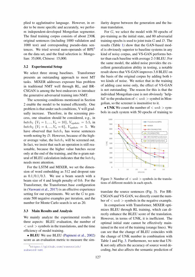
plied to agglutinative language. However, in or-der to be more specific and accurately, we perfor-m independent-developed Mongolian segmenter.The final training corpus consists of about 230Koriginal sentences (including 1000 validation and1000 test) and corresponding pseudo-data sen-tences. We tried several num-operands of BPE5

on the data set, and the final selection is: Mongo-lian: 35,000, Chinese: 15,000.

3.2 Experimental Setup

We select three strong baselines. Transformerpresents an outstanding approach to most MTtasks. MIXER addresses exposure bias problemin traditional NMT well through RL, and BR-CSGAN is among the best endeavors to introducethe generative adversarial training into NMT.

The screening conditions mentioned in Section2 enable the model to be trained efficiently. Oneproblem is that under such conditions, V will grad-ually increase. Therefore, in the screening pro-cess, one situation should be considered, e.g., inbatch1 V1 = 1, ..., Vn = 10, Vupdate = 5.5, inbatch2 V1 = 4, ..., Vn = 6, Vupdate = 5. Wehave observed that batch1 has worse sentencesworth noting byD. However, because of the high-er average value, the batch1 will be screened out.In fact, we insist that such an operation is still rea-sonable, because the higher value batches occuronly at the end of the training, and the n-gram nat-ural of BLEU calculation indicates that the batch2needs more attention.

For the LSTM and MIXER, we set the dimen-sion of word embedding as 512 and dropout rateas 0.1/0.1/0.3. We use a beam search with abeam size of 4 and length penalty of 0.6. For theTransformer, the Transformer base configurationin (Vaswani et al., 2017) is an effective experiencesetting for our experiments. We set the G to gen-erate 500 negative examples per iteration, and thenumber for Monte Carlo search is set as 20.

3.3 Main Results and Analysis

We mainly analyze the experimental results inthree aspects: BLEU evaluation, the number of< unk > symbols in the translations, and the timeefficiency of model training.• BLEU We use BLEU (Papineni et al., 2002)

score as an evaluation metric to measure the sim-5https://github.com/rsennrich/

subword-nmt

ilarity degree between the generation and the hu-man translation.

For G, we select the model with 50 epochs ofpre-training as the initial state, and 80 adversarialtraining epochs is used to joint trainG andD. Theresults (Table 1) show that the GAN-based mod-el is obviously superior to baseline systems in anykind of noisy corpus, and VS-GAN performs bet-ter than each baseline with average 2-3 BLEU. Forthe same model, the added noise provides the ex-cellent generalization ability in testing, a notableresult shows that VS-GAN improves 3.8 BLEU onthe basis of the original corpus by adding both t-wo kinds of noise. We notice that in the trainingof adding case noise only, the effect of VS-GANis not outstanding. The reason for this is that theindividual Mongolian-case is not obviously ’help-ful’ to the production of< unk > symbol in Mon-golian, so the screener is insensitive to it.• UNK We count the number of < unk > sym-

bols in each system with 50 epochs of training to

0

100

200

300

400

500

600

700

800

900

1000

1 10 20 30 40 50

UNK

EPOCHS

Transformer(BPE)

MIXER

BR-CSGAN(LSTM)

VS-GAN(LSTM)

BR-CSGAN(Transformer)

VS-GAN(Transformer)

Figure 3: Number of < unk > symbols in the transla-tions of different models in each epoch.

translate the source sentences (Fig. 3). For BR-CSGAN and VS-GAN, we directly count the num-ber of < unk > symbols in the negative example.

In comparison with Transformer, MIXER opti-mizes BLEU through RL training, which can di-rectly enhance the BLEU score of the translation.However, in terms of UNK, it is inefficient. Theoptimal initial state cannot be effectively main-tained in the rest of the training (orange lines). Wecan see that the change of BLEU coincides withthe change of UNK number in combination withTable 1 and Fig. 3. Furthermore, we note that UN-K not only affects the accuracy of source word de-coding, but also affects the semantic prediction of

127

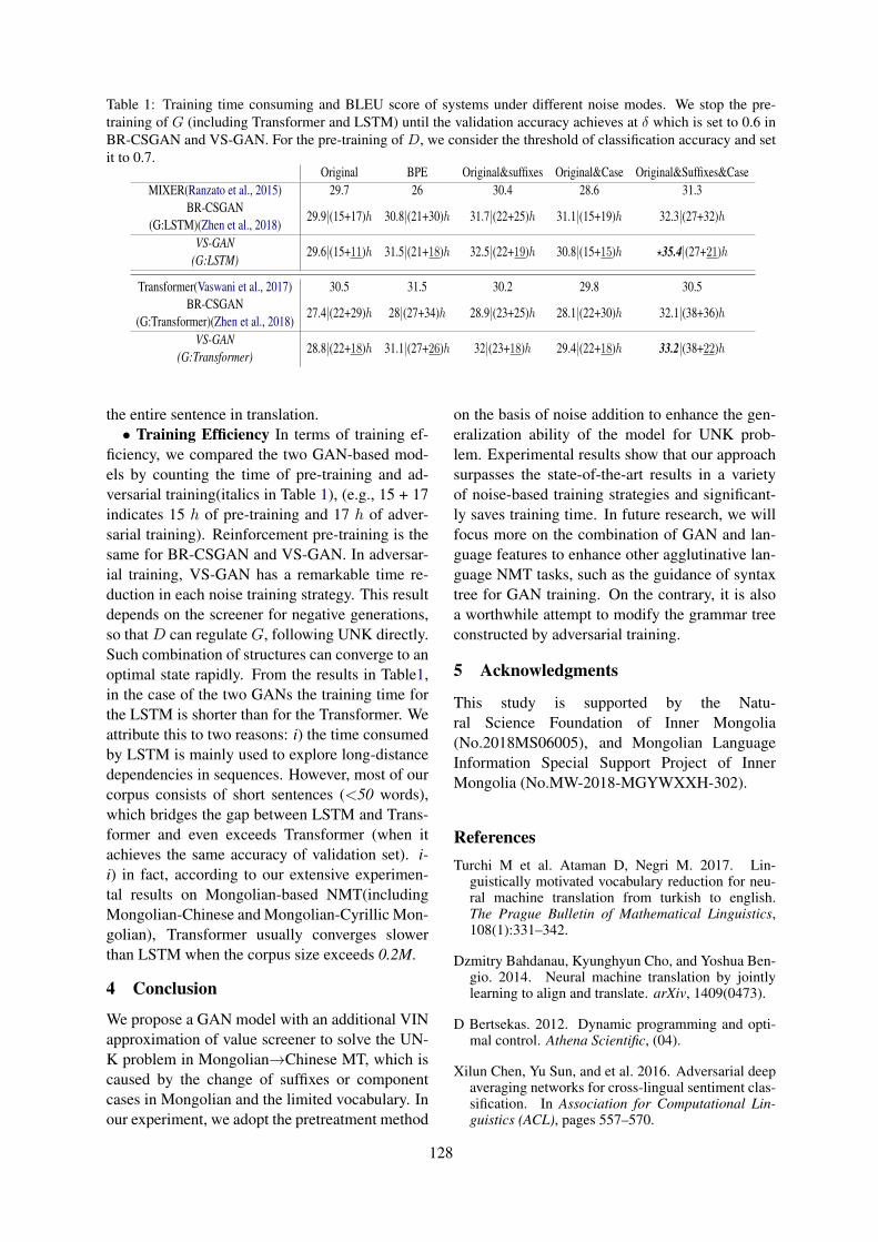
Table 1: Training time consuming and BLEU score of systems under different noise modes. We stop the pre-training of G (including Transformer and LSTM) until the validation accuracy achieves at δ which is set to 0.6 inBR-CSGAN and VS-GAN. For the pre-training of D, we consider the threshold of classification accuracy and setit to 0.7.

Original BPE Original&suffixes Original&Case Original&Suffixes&CaseMIXER(Ranzato et al., 2015) 29.7 26 30.4 28.6 31.3

BR-CSGAN(G:LSTM)(Zhen et al., 2018)

29.9|(15+17)h 30.8|(21+30)h 31.7|(22+25)h 31.1|(15+19)h 32.3|(27+32)h

VS-GAN(G:LSTM)

29.6|(15+11)h 31.5|(21+18)h 32.5|(22+19)h 30.8|(15+15)h ?35.4|(27+21)h

Transformer(Vaswani et al., 2017) 30.5 31.5 30.2 29.8 30.5BR-CSGAN

(G:Transformer)(Zhen et al., 2018)27.4|(22+29)h 28|(27+34)h 28.9|(23+25)h 28.1|(22+30)h 32.1|(38+36)h

VS-GAN(G:Transformer)

28.8|(22+18)h 31.1|(27+26)h 32|(23+18)h 29.4|(22+18)h 33.2|(38+22)h

the entire sentence in translation.• Training Efficiency In terms of training ef-

ficiency, we compared the two GAN-based mod-els by counting the time of pre-training and ad-versarial training(italics in Table 1), (e.g., 15 + 17indicates 15 h of pre-training and 17 h of adver-sarial training). Reinforcement pre-training is thesame for BR-CSGAN and VS-GAN. In adversar-ial training, VS-GAN has a remarkable time re-duction in each noise training strategy. This resultdepends on the screener for negative generations,so that D can regulate G, following UNK directly.Such combination of structures can converge to anoptimal state rapidly. From the results in Table1,in the case of the two GANs the training time forthe LSTM is shorter than for the Transformer. Weattribute this to two reasons: i) the time consumedby LSTM is mainly used to explore long-distancedependencies in sequences. However, most of ourcorpus consists of short sentences (<50 words),which bridges the gap between LSTM and Trans-former and even exceeds Transformer (when itachieves the same accuracy of validation set). i-i) in fact, according to our extensive experimen-tal results on Mongolian-based NMT(includingMongolian-Chinese and Mongolian-Cyrillic Mon-golian), Transformer usually converges slowerthan LSTM when the corpus size exceeds 0.2M.

4 Conclusion

We propose a GAN model with an additional VINapproximation of value screener to solve the UN-K problem in Mongolian→Chinese MT, which iscaused by the change of suffixes or componentcases in Mongolian and the limited vocabulary. Inour experiment, we adopt the pretreatment method

on the basis of noise addition to enhance the gen-eralization ability of the model for UNK prob-lem. Experimental results show that our approachsurpasses the state-of-the-art results in a varietyof noise-based training strategies and significant-ly saves training time. In future research, we willfocus more on the combination of GAN and lan-guage features to enhance other agglutinative lan-guage NMT tasks, such as the guidance of syntaxtree for GAN training. On the contrary, it is alsoa worthwhile attempt to modify the grammar treeconstructed by adversarial training.

5 Acknowledgments

This study is supported by the Natu-ral Science Foundation of Inner Mongolia(No.2018MS06005), and Mongolian LanguageInformation Special Support Project of InnerMongolia (No.MW-2018-MGYWXXH-302).

ReferencesTurchi M et al. Ataman D, Negri M. 2017. Lin-

guistically motivated vocabulary reduction for neu-ral machine translation from turkish to english.The Prague Bulletin of Mathematical Linguistics,108(1):331–342.

Dzmitry Bahdanau, Kyunghyun Cho, and Yoshua Ben-gio. 2014. Neural machine translation by jointlylearning to align and translate. arXiv, 1409(0473).

D Bertsekas. 2012. Dynamic programming and opti-mal control. Athena Scientific, (04).

Xilun Chen, Yu Sun, and et al. 2016. Adversarial deepaveraging networks for cross-lingual sentiment clas-sification. In Association for Computational Lin-guistics (ACL), pages 557–570.

128

P. Dayan and L F Abbott. 2003. Theoretical neu-roscience: Computational and mathematical mod-elling of neural systems. Journal of Cognitive Neu-roscience, 15(1):154–155.

Jonas Gehring, Michael Auli, David Grangier, andet al. 2017. Convolutional sequence to sequencelearning. In International conference on machinelearning(ICML), pages 1243–1252.

Alex Graves. 2013a. Generating sequences with re-current neural networks. arXiv preprint arXiv,1308(0850).

Alex Graves. 2013b. Generating sequences with re-current neural networks. arXiv preprint arXiv,1308(0850).

Caglar Gulcehre, Sungjin Ahn, and et al. 2016. Point-ing the unknown words. In Association for compu-tational linguistics (ACL), pages 140–149.

Karl Moritz Hermann, Tom Kocisk, and et al. 2015.Teaching machines to read and comprehend. InNeural Information Processing Systems (NIPS),pages 1693–1701.

Ferenc Huszr. 2015. How (not) to train your generativemodel: Scheduled sampling, likelihood, adversary?Computer Science, 1511(05101).

Sbastien Jean, Kyunghyun Cho, Roland Memisevic,and Yoshua Bengio. 2015. On using very large tar-get vocabulary for neural machine translation. InInternational joint conference on natural languageprocessing (IJCNLP), pages 1–10.

Minh-Thang Luong, Ilya Sutskever, and et al. 2015.Addressing the rare word problem in neural machinetranslation. In International joint conference on nat-ural language processing (IJCNLP), pages 11–19.

Tom Mikolov, Stefan Kombrink, Luk Burget, and et al.2011. Extensions of recurrent neural network lan-guage model. In International conference on acous-tics, speech, and signal processing, pages 5528–5531.

Volodymyr Mnih, Koray Kavukcuoglu, David Silver,and et al. 2013. Playing atari with deep reinforce-ment learning. arXiv, 1312(5602).

Frederic Morin and Yoshua Bengio. 2005. Hierarchicalprobabilistic neural network language model. In In-ternational conference on artificial intelligence andstatistics (Aistats), volume 5, pages 246–252.

Kishore Papineni, Salim Roukos, Todd Ward, and Wei-Jing Zhu. 2002. Bleu: a method for automatic e-valuation of machine translation. In Proceedings ofthe 40th annual meeting on association for compu-tational linguistics(ACL), pages 311–318.

Bellman R. 1957. Terminal control, time lags, and dy-namic programming. National Academy of Sciencesof the United States of America, 43(10):927–930.

Marc’Aurelio Ranzato, Sumit Chopra, and et al. 2015.Sequence level training with recurrent neural net-works. arXiv, 1511(06732).

Rico Sennrich, Barry Haddow, and Alexandra Birch.2016. Neural machine translation of rare words withsubword units. In Association for computational lin-guistics (ACL), pages 1715–1725.

Ilya Sutskever, Oriol Vinyals, and Quoc V. Le. 2014.Sequence to sequence learning with neural network-s. In Conference and Workshop on Neural Informa-tion Processing Systems (NIPS), pages 3104–3112.

A Tamar, Y Wu, G Thomas, and et al. 2016. Value it-eration networks. In Neural Information ProcessingSystems (NIPS), pages 2154–2162.

Noah A.Smith. ThuyLinh Nguyen, Stephan Vogel.2010. Nonparametric word segmentation for ma-chine translation. In Proceedings of the Internation-al Conference on Computational Linguistics, (COL-ING10), pages 815–823.

Ashish Vaswani, Noam Shazeer, and et al. 2017. Atten-tion is all you need. In Conference and Workshopon Neural Information Processing Systems (NIPS),pages 5998–6008.

L Wu, Y Xia, L Zhao, and et al. 2018. Adversarialneural machine translation. In Asian Conference onMachine Learning (ACML), pages 374–385.

Lantao Yu, Weinan Zhang, Jun Wang, and Yong Yu.2016. Seqgan: Sequence generative adversarial net-s with policy gradient. In The Association for theAdvancement of Artificial Intelligence (AAAI), pages2852–2858.

Yuan Zhang, Regina Barzilay, and Tommi Jaakkola.2017. Aspect-augmented adversarial networks fordomain adaptation. Transactions of the Associationfor Computational Linguistics, 5(1):515–528.

Fan K et al. Zhang Y, Gan Z. 2017. Adversarial fea-ture matching for text generation. In Proceedings ofthe International conference on machine learning,(ICML17), pages 4006–4015.

Yang Zhen, Chen Wei, Wang Feng, and Xu Bo. 2018.Improving neural machine translation with condi-tional sequence generative adversarial nets. InThe North American Chapter of the Association forComputational Linguistics (NAACL), pages 1346–1355.

129

Proceedings of the 57th Annual Meeting of the Association for Computational Linguistics: Student Research Workshop, pages 130–135Florence, Italy, July 28 - August 2, 2019. c©2019 Association for Computational Linguistics

Unsupervised Pretraining for Neural Machine TranslationUsing Elastic Weight Consolidation

Dusan VarisCharles University,

Faculty of Mathematics and PhysicsMalostranske namestı 25

118 00 Prague, Czech Republicvaris@ufal.mff.cuni.cz

Ondrej BojarCharles University,

Faculty of Mathematics and PhysicsMalostranske namestı 25

118 00 Prague, Czech Republicbojar@ufal.mff.cuni.cz

Abstract

This work presents our ongoing research ofunsupervised pretraining in neural machinetranslation (NMT). In our method, we initial-ize the weights of the encoder and decoderwith two language models that are trained withmonolingual data and then fine-tune the modelon parallel data using Elastic Weight Consoli-dation (EWC) to avoid forgetting of the orig-inal language modeling tasks. We comparethe regularization by EWC with the previouswork that focuses on regularization by lan-guage modeling objectives.

The positive result is that using EWC with thedecoder achieves BLEU scores similar to theprevious work. However, the model converges2-3 times faster and does not require the orig-inal unlabeled training data during the fine-tuning stage.

In contrast, the regularization using EWC isless effective if the original and new tasks arenot closely related. We show that initializingthe bidirectional NMT encoder with a left-to-right language model and forcing the modelto remember the original left-to-right languagemodeling task limits the learning capacity ofthe encoder for the whole bidirectional con-text.

1 Introduction

Neural machine translation (NMT) using sequenceto sequence architectures (Sutskever et al., 2014;Bahdanau et al., 2014; Vaswani et al., 2017) hasbecome the dominant approach to automatic ma-chine translation. While being able to approachhuman-level performance (Popel, 2018), it still re-quires a huge amount of parallel data, otherwise itcan easily overfit. Such data, however, might notalways be available. At the same time, it is gener-ally much easier to gather large amounts of mono-lingual data, and therefore, it is interesting to findways of making use of such data. The simplest

strategy is to use backtranslation (Sennrich et al.,2016), but it can be rather costly since it requirestraining a model in the opposite translation direc-tion and then translating the monolingual corpus.

It was suggested by Lake et al. (2017) that dur-ing the development of a general human-like AIsystem, one of the desired characteristics of sucha system is the ability to learn in a continuousmanner using previously learned tasks as build-ing blocks for mastering new, more complex tasks.Until recently, continuous learning of neural net-works was problematic, among others, due to thecatastrophic forgetting (McCloskey and Cohen,1989). Several methods were proposed (Li andHoiem, 2016; Aljundi et al., 2017; Zenke et al.,2017), however, they mainly focus only on adapt-ing the whole network (not just its parts) to newtasks while maintaining good performance on thepreviously learned tasks.

In this work, we present an unsupervised pre-training method for NMT models using ElasticWeight Consolidation (Kirkpatrick et al., 2017).First, we initialize both encoder and decoder withsource and target language models respectively.Then, we fine-tune the NMT model using the par-allel data. To prevent the encoder and decoderfrom forgetting the original language modeling(LM) task, we regularize their weights individu-ally using Elastic Weight Consolidation based ontheir importance to that task. Our hypothesis is thefollowing: by forcing the network to remember theoriginal LM tasks we can reduce overfitting of theNMT model on the limited parallel data.

We also provide a comparison of our approachwith the method proposed by Ramachandran et al.(2017). They also suggest initialization of the en-coder and decoder with a language model. How-ever, during the fine-tuning phase they use theoriginal language modeling objectives as an ad-ditional training loss in place of model regular-

130

ization. Their approach has two main drawbacks:first, during the fine-tuning phase, they still requirethe original monolingual data which might not beavailable anymore in a life-long learning scenario.Second, they need to compute both machine trans-lation and language modeling losses which in-creases the number of operations performed dur-ing the update slowing down the fine-tuning pro-cess. Our proposed method addresses both prob-lems: it requires only a small held-out set to esti-mate the EWC regularization term and converges2-3 times faster than the previous method.1

2 Related Work

Several other approaches towards exploiting theavailable monolingual data for NMT have beenpreviously proposed.

Currently, the most common method is creat-ing synthetic parallel data by backtranslating thetarget language monolingual corpora using ma-chine translation (Sennrich et al., 2016). Whilebeing consistently beneficial, this method requiresa pretrained model to prepare the backtranslations.Additionally, Ramachandran et al. (2017) showedthat the unsupervised pretraining approach reachesat least similar performance to the backtranslationapproach.

Recently, Lample and Conneau (2019) sug-gested using a single cross-lingual language modeltrained on multiple monolingual corpora as an ini-tialization for various NLP tasks, including ma-chine translation. While our work focuses strictlyon a monolingual language model pretraining, webelieve that our work can further benefit from us-ing cross-lingual language models.

Another possible approach is to introduce anadditional reordering (Zhang and Zong, 2016) orde-noising objectives, the latter being recentlyemployed in the unsupervised NMT scenarios(Artetxe et al., 2018; Lample et al., 2017). Theseapproaches try to force the NMT model to learnuseful features by presenting it with either shuf-fled or noisy sentences teaching it to reconstructthe original input.

Furthermore, Khayrallah et al. (2018) show howto prevent catastrophic forgeting during domainadaptation scenarios. They fine-tune the general-domain NMT model using in-domain data adding

1The speedup is with regard to the wall-clock time. Inour experiments both EWC and the LM-objective methodsrequire similar number of training examples to converge.

an additional cross-entropy objective to restrict thedistribution of the fine-tuned model to be similarto the distribution of the original general-domainmodel.

3 Elastic Weight Consolidation

Elastic Weight Consolidation (Kirkpatrick et al.,2017) is a simple, statistically motivated methodfor selective regularization of neural network pa-rameters. It was proposed to counteract catas-trophic forgetting in neural networks during a life-long continuous training. The previous work de-scribed the method in the context of adapting thewhole network for each new task. In this section,we show that EWC can be also used to preserveonly parts of the network that were relevant forthe previous task, thus being potentially useful forcompositional learning.

To justify the choice of the parameter con-straints, Kirkpatrick et al. (2017) approach theneural network training as a Bayesian inferenceproblem. To put it into the context of NMT, wewould like to find the most probable network pa-rameters θ, given a parallel data Dmt and mono-lingual data Dsrc and Dtgt for source and targetlanguages, respectively:

p(θ|Dmt ∪Dsrc ∪Dtgt) =p(Dmt|θ)p(θ|Dsrc ∪Dtgt)

p(Dmt)(1)

Equation 1 holds, assuming datasets Dmt, Dsrc

and Dtgt being mutually exclusive. The probabil-ity p(Dmt|θ) is the negative of the MT loss func-tion and p(θ|Dsrc ∪ Dtgt) is the result of the un-supervised pretraining. We can assume that dur-ing the unsupervised pretraining, the parametersθsrc of the encoder are independent of the param-eters θtgt of the decoder. Furthermore, we as-sume that the parameters of the encoder are in-dependent of the target-side monolingual data andthe parameters of the decoder are independent ofthe source-side monolingual data. Given these as-sumptions, we can express the posterior probabil-ity p(θ|Dsrc ∪Dtgt) in the following way:

p(θ|Dsrc∪Dtgt) = p(θsrc|Dsrc)p(θtgt|Dtgt) (2)

Probabilities p(θsrc|Dsrc) and p(θtgt|Dtgt) aregiven by the pretrained source and target lan-guage models respectively. The true posteriorprobabilities given by the language models are in-tractable during fine-tuning, however, similarly to

131

the work of Kirkpatrick et al. (2017), we can es-timate p(θsrc|Dsrc) as Gaussian distribution us-ing Laplace approximation (MacKay, 1992), withmean given by the pretrained parameters θsrc andvariance given by a diagonal of the Fisher informa-tion matrix Fsrc. Then, we can add the followingregularization term to our loss function:

Lewc−src(θ) =∑

i,θi⊂θsrc

λ

2Fsrc,i(θi − θ?src,i)2 (3)

The model parameters not present during thelanguage model pretraining are ignored by theregularization term. Analogically, the same canbe applied for the target-side posterior probabil-ity p(θtgt|Dtgt) giving a target-side regularizationterm Lewc−tgt.

In the following section, we show that these reg-ularization terms can be useful in a low-resourcemachine translation scenario. Since we do notnecessarily need to preserve the knowledge of theoriginal language modeling tasks, we focus on us-ing them only as prior knowledge to prevent over-fitting during the fine-tuning.

4 Experiments

In this section, we present the results of our ex-periments with EWC regularization and comparethem with the previously proposed regularizationby language modeling objectives.

4.1 Model DescriptionIn all experiments, we use the self-attentive Trans-former network (Vaswani et al., 2017) because it isthe current state-of-the-art NMT architecture, pro-viding us with a strong baseline. In general, it fol-lows the standard encoder-decoder paradigm, withencoder creating hidden representations of the in-put tokens based on their surrounding context anddecoder generating the output tokens autoregres-sively while attending to the source sentence to-ken representations and tokens it generated in theprevious decoding steps.2

We use Transformer with 6 layers in both en-coder and decoder. We set the dimension of thehidden states to 512 and the dimension of the feed-forward layer to 2048. We use multi-head at-tention with 16 attention heads. To simplify thepretraining process, we use a separate vocabulary

2For more details about the architecture, see the originalpaper.

for source and target languages, each containingaround 32k subwords. We use separate embed-dings in the encoder and decoder. In the decoder,we tie the embeddings with the output softmaxlayer (Press and Wolf, 2017). During both pre-training and fine tuning, we use Adam optimizer(Kingma and Ba, 2014) and gradient clipping. Weset the initial learning rate to 3.1, use a linearwarm-up for 33500 training steps and then decaythe learning rate exponentially. We set the train-ing batch size to a maximum of 2048 tokens perbatch together with sentence bucketing for moreefficient training. We set dropout to 0.1. Duringthe final evaluation, we use beam search decodingwith beam size of 8 and length normalization setto 1.0.

When pretraining the encoder and decoder, weuse identical network parameters. We train eachlanguage model to maximize the probability ofeach word in a sentence using its leftward context.To pretrain the decoder, we use the decoder archi-tecture from Transformer with encoder-attentionsub-layer removed due to the lack of source sen-tences. Later, we initialize the NMT decoderwith the language model weights and the encoder-attention weights by a normal distribution. Wereset all training-related variables (learning rate,Adam moments) during the NMT initialization.

For simplicity, we apply the same approach forthe encoder pretraining. In Section 4.2, we discussthe drawbacks of our encoder pretraining and sug-gest possible improvements. In all experiments,we set the weight λ of each EWC regularizationterm to 0.02.

The model implementation is available in Neu-ral Monkey3 (Helcl and Libovicky, 2017) frame-work for sequence-to-sequence modeling.

4.2 Dataset and Evaluation

In our experiments, we focused on the low-resource Basque-to-English machine translationtask featured in IWSLT 2018.4 We used the par-allel data provided by IWSLT organizers, con-sisting of 5,600 in-domain sentence pairs (TEDTalks) and around 940,000 general-domain sen-tence pairs. During pretraining, we used BasqueWikipedia for source language model and News-

3https://github.com/ufal/neuralmonkey4https://sites.google.com/site/

iwsltevaluation2018/TED-tasks

132

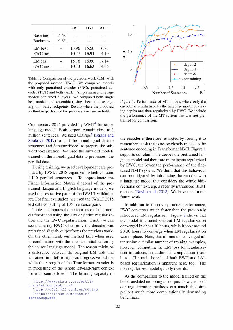
SRC TGT ALL

Baseline 15.68 – – –Backtrans. 19.65 – – –

LM best – 13.96 15.56 16.83EWC best – 10.77 15.91 14.10

LM ens. – 15.16 16.60 17.14EWC ens. – 10.73 16.63 14.66

Table 1: Comparison of the previous work (LM) withthe proposed method (EWC). We compared modelswith only pretrained encoder (SRC), pretrained de-coder (TGT) and both (ALL). All pretrained languagemodels contained 3 layers. We compared both singlebest models and ensemble (using checkpoint averag-ing) of 4 best checkpoints. Results where the proposedmethod outperformed the previous work are in bold.

Commentary 2015 provided by WMT5 for targetlanguage model. Both corpora contain close to 3million sentences. We used UDPipe6 (Straka andStrakova, 2017) to split the monolingual data tosentences and SentencePiece7 to prepare the sub-word tokenization. We used the subword modelstrained on the monolingual data to preprocess theparallel data.

During training, we used development data pro-vided by IWSLT 2018 organizers which contains1,140 parallel sentences. To approximate theFisher Information Matrix diagonal of the pre-trained Basque and English language models, weused the respective parts of the IWSLT validationset. For final evaluation, we used the IWSLT 2018test data consisting of 1051 sentence pairs.

Table 1 compares the performance of the mod-els fine-tuned using the LM objective regulariza-tion and the EWC regularization. First, we cansee that using EWC when only the decoder waspretrained slightly outperforms the previous work.On the other hand, our method fails when usedin combination with the encoder initialization bythe source language model. The reason might bea difference between the original LM task thatis trained in a left-to-right autoregressive fashionwhile the strength of the Transformer encoder isin modelling of the whole left-and-right contextfor each source token. The learning capacity of

5http://www.statmt.org/wmt18/translation-task.html

6http://ufal.mff.cuni.cz/udpipe7https://github.com/google/

sentencepiece

0.5 1 1.5 2 2.5·107

5

10

15

Number of Sentences

BL

EU

depth-2depth-4depth-6

no pretraining

Figure 1: Performance of MT models where only theencoder was initialized by the language model of vary-ing depths and then regularized by EWC. We includethe performance of the MT system that was not pre-trained for comparison.

the encoder is therefore restricted by forcing it toremember a task that is not so closely related to thesentence encoding in Transformer NMT. Figure 1supports our claim: the deeper the pretrained lan-guage model and therefore more layers regularizedby EWC, the lower the performance of the fine-tuned NMT system. We think that this behaviourcan be mitigated by initializing the encoder witha language model that considers the whole bidi-rectional context, e.g. a recently introduced BERTencoder (Devlin et al., 2018). We leave this for ourfuture work.

In addition to improving model performance,EWC converges much faster than the previouslyintroduced LM regularizer. Figure 2 shows thatthe model fine-tuned without LM regularizationconverged in about 10 hours, while it took around20-30 hours to converge when LM regularizationwas in place. Note, that all models converged af-ter seeing a similar number of training examples,however, computing the LM loss for regulariza-tion introduces an additional computation over-head. The main benefit of both EWC and LM-based regularization is apparent here, too. Thenon-regularized model quickly overfits.

As the comparison to the model trained on thebacktranslated monolingual corpus shows, none ofour regularization methods can match this sim-ple but much more computationally demandingbenchmark.

133

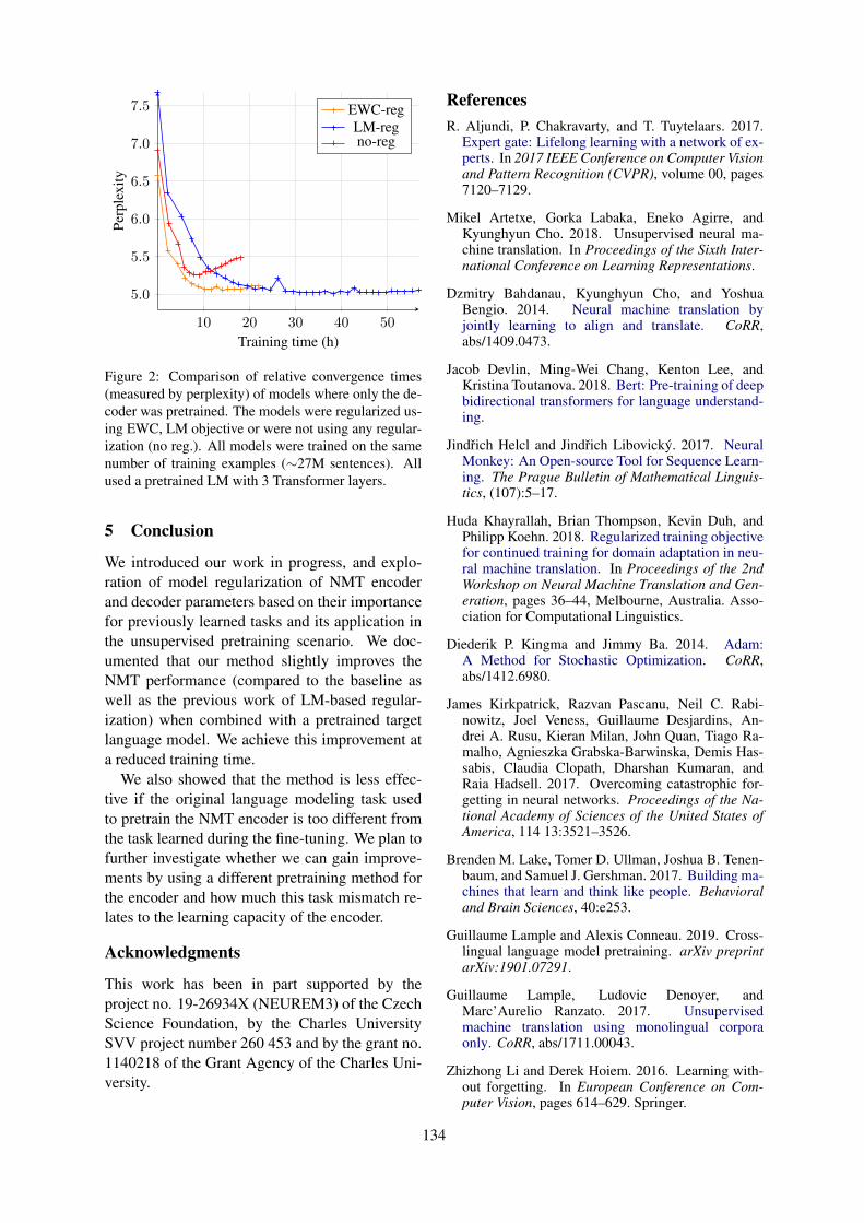
10 20 30 40 50

5.0

5.5

6.0

6.5

7.0

7.5

Training time (h)

Perp

lexi

tyEWC-regLM-regno-reg

Figure 2: Comparison of relative convergence times(measured by perplexity) of models where only the de-coder was pretrained. The models were regularized us-ing EWC, LM objective or were not using any regular-ization (no reg.). All models were trained on the samenumber of training examples (∼27M sentences). Allused a pretrained LM with 3 Transformer layers.

5 Conclusion

We introduced our work in progress, and explo-ration of model regularization of NMT encoderand decoder parameters based on their importancefor previously learned tasks and its application inthe unsupervised pretraining scenario. We doc-umented that our method slightly improves theNMT performance (compared to the baseline aswell as the previous work of LM-based regular-ization) when combined with a pretrained targetlanguage model. We achieve this improvement ata reduced training time.

We also showed that the method is less effec-tive if the original language modeling task usedto pretrain the NMT encoder is too different fromthe task learned during the fine-tuning. We plan tofurther investigate whether we can gain improve-ments by using a different pretraining method forthe encoder and how much this task mismatch re-lates to the learning capacity of the encoder.

Acknowledgments

This work has been in part supported by theproject no. 19-26934X (NEUREM3) of the CzechScience Foundation, by the Charles UniversitySVV project number 260 453 and by the grant no.1140218 of the Grant Agency of the Charles Uni-versity.

ReferencesR. Aljundi, P. Chakravarty, and T. Tuytelaars. 2017.

Expert gate: Lifelong learning with a network of ex-perts. In 2017 IEEE Conference on Computer Visionand Pattern Recognition (CVPR), volume 00, pages7120–7129.

Mikel Artetxe, Gorka Labaka, Eneko Agirre, andKyunghyun Cho. 2018. Unsupervised neural ma-chine translation. In Proceedings of the Sixth Inter-national Conference on Learning Representations.

Dzmitry Bahdanau, Kyunghyun Cho, and YoshuaBengio. 2014. Neural machine translation byjointly learning to align and translate. CoRR,abs/1409.0473.

Jacob Devlin, Ming-Wei Chang, Kenton Lee, andKristina Toutanova. 2018. Bert: Pre-training of deepbidirectional transformers for language understand-ing.

Jindrich Helcl and Jindrich Libovicky. 2017. NeuralMonkey: An Open-source Tool for Sequence Learn-ing. The Prague Bulletin of Mathematical Linguis-tics, (107):5–17.

Huda Khayrallah, Brian Thompson, Kevin Duh, andPhilipp Koehn. 2018. Regularized training objectivefor continued training for domain adaptation in neu-ral machine translation. In Proceedings of the 2ndWorkshop on Neural Machine Translation and Gen-eration, pages 36–44, Melbourne, Australia. Asso-ciation for Computational Linguistics.

Diederik P. Kingma and Jimmy Ba. 2014. Adam:A Method for Stochastic Optimization. CoRR,abs/1412.6980.

James Kirkpatrick, Razvan Pascanu, Neil C. Rabi-nowitz, Joel Veness, Guillaume Desjardins, An-drei A. Rusu, Kieran Milan, John Quan, Tiago Ra-malho, Agnieszka Grabska-Barwinska, Demis Has-sabis, Claudia Clopath, Dharshan Kumaran, andRaia Hadsell. 2017. Overcoming catastrophic for-getting in neural networks. Proceedings of the Na-tional Academy of Sciences of the United States ofAmerica, 114 13:3521–3526.

Brenden M. Lake, Tomer D. Ullman, Joshua B. Tenen-baum, and Samuel J. Gershman. 2017. Building ma-chines that learn and think like people. Behavioraland Brain Sciences, 40:e253.

Guillaume Lample and Alexis Conneau. 2019. Cross-lingual language model pretraining. arXiv preprintarXiv:1901.07291.

Guillaume Lample, Ludovic Denoyer, andMarc’Aurelio Ranzato. 2017. Unsupervisedmachine translation using monolingual corporaonly. CoRR, abs/1711.00043.

Zhizhong Li and Derek Hoiem. 2016. Learning with-out forgetting. In European Conference on Com-puter Vision, pages 614–629. Springer.

134

David J. C. MacKay. 1992. A practical bayesian frame-work for backpropagation networks. Neural Com-putation, 4(3):448–472.

Michael McCloskey and Neil J. Cohen. 1989. Catas-trophic interference in connectionist networks: Thesequential learning problem. The Psychology ofLearning and Motivation, 24:104–169.

Martin Popel. 2018. CUNI transformer neural MT sys-tem for WMT18. In Proceedings of the Third Con-ference on Machine Translation, Volume 2: SharedTasks, volume 2, pages 486–491, Stroudsburg, PA,USA. Association for Computational Linguistics,Association for Computational Linguistics.

Ofir Press and Lior Wolf. 2017. Using the output em-bedding to improve language models. In Proceed-ings of the 15th Conference of the European Chap-ter of the Association for Computational Linguistics:Volume 2, Short Papers, pages 157–163, Valencia,Spain. Association for Computational Linguistics.

Prajit Ramachandran, Peter J. Liu, and Quoc V. Le.2017. Unsupervised pretraining for sequence to se-quence learning. In Proceedings of the 2017 Con-ference on Empirical Methods in Natural LanguageProcessing, EMNLP 2017, Copenhagen, Denmark,September 9-11, 2017, pages 383–391.

Rico Sennrich, Barry Haddow, and Alexandra Birch.2016. Improving neural machine translation mod-els with monolingual data. In Proceedings of the54th Annual Meeting of the Association for Compu-tational Linguistics (Volume 1: Long Papers), pages86–96, Berlin, Germany. Association for Computa-tional Linguistics.

Milan Straka and Jana Strakova. 2017. Tokenizing,pos tagging, lemmatizing and parsing ud 2.0 withudpipe. In Proceedings of the CoNLL 2017 SharedTask: Multilingual Parsing from Raw Text to Univer-sal Dependencies, pages 88–99, Vancouver, Canada.Association for Computational Linguistics.

Ilya Sutskever, Oriol Vinyals, and Quoc V Le. 2014.Sequence to sequence learning with neural net-works. In Advances in neural information process-ing systems, pages 3104–3112.

Ashish Vaswani, Noam Shazeer, Niki Parmar, JakobUszkoreit, Llion Jones, Aidan N Gomez, LukaszKaiser, and Illia Polosukhin. 2017. Attention is allyou need. In I. Guyon, U. V. Luxburg, S. Bengio,H. Wallach, R. Fergus, S. Vishwanathan, and R. Gar-nett, editors, Advances in Neural Information Pro-cessing Systems 30, pages 6000–6010. Curran As-sociates, Inc.

Friedemann Zenke, Ben Poole, and Surya Ganguli.2017. Continual learning through synaptic intel-ligence. In Proceedings of the 34th InternationalConference on Machine Learning, ICML 2017, Syd-ney, NSW, Australia, 6-11 August 2017, pages 3987–3995.

Jiajun Zhang and Chengqing Zong. 2016. Exploit-ing source-side monolingual data in neural machinetranslation. In Proceedings of the 2016 Conferenceon Empirical Methods in Natural Language Pro-cessing, pages 1535–1545. Association for Compu-tational Linguistics.

135

Proceedings of the 57th Annual Meeting of the Association for Computational Linguistics: Student Research Workshop, pages 136–142Florence, Italy, July 28 - August 2, 2019. c©2019 Association for Computational Linguistics

Maori Loanwords: A Corpus of New Zealand English TweetsDavid Trye

Computing and Mathematical SciencesUniversity of Waikato, New Zealand

dgt12@students.waikato.ac.nz

Andreea S. CaludeSchool of General and Applied Linguistics

University of Waikato, New Zealandandreea.calude@waikato.ac.nz

Felipe Bravo-MarquezDepartment of Computer Science

University of Chile & IMFDfbravo@dcc.uchile.cl

Te Taka KeeganComputing and Mathematical Sciences

University of Waikato, New Zealandtetaka.keegan@waikato.ac.nz

Abstract

Maori loanwords are widely used in NewZealand English for various social functionsby New Zealanders within and outside of theMaori community. Motivated by the lack oflinguistic resources for studying how Maoriloanwords are used in social media, we presenta new corpus of New Zealand English tweets.We collected tweets containing selected Maoriwords that are likely to be known by NewZealanders who do not speak Maori. Sinceover 30% of these words turned out to be ir-relevant (e.g., mana is a popular gaming term,Moana is a character from a Disney movie),we manually annotated a sample of our tweetsinto relevant and irrelevant categories. Thisdata was used to train machine learning mod-els to automatically filter out irrelevant tweets.

1 Introduction

One of the most salient features of New ZealandEnglish (NZE) is the widespread use of Maoriwords (loanwords), such as aroha (love), kai(food) and Aotearoa (New Zealand). See ex. (1)specifically from Twitter (note the informal, con-versational style and the Maori loanwords empha-sised in bold).

(1) Led the waiata for the manuhiri at thepowhiri for new staff for induction week.Was told by the kaumatua I did it with manaand integrity.

The use of Maori words has been studied inten-sively over the past thirty years, offering a com-prehensive insight into the evolution of one ofthe youngest dialects of English – New ZealandEnglish (Calude et al., 2017; Daly, 2007, 2016;Davies and Maclagan, 2006; De Bres, 2006;Degani and Onysko, 2010; Kennedy and Ya-mazaki, 1999; Macalister, 2009, 2006a; Onyskoand Calude, 2013). One aspect which is missing in

this body of work is the online discourse presenceof the loanwords - almost all studies come from(collaborative) written language (highly edited, re-vised and scrutinised newspaper language, Daviesand Maclagan 2006; Macalister 2009, 2006a,b;Onysko and Calude 2013, and picture-books, Daly2007, 2016), or from spoken language collected inthe late 1990s (Kennedy and Yamazaki, 1999).

In this paper, we build a corpus of NewZealand English tweets containing Maori loan-words. Building such a corpus has its challenges(as discussed in Section 3.1). Before we discussthese, it is important to highlight the uniquenessof the language contact situation between Maoriand (NZ) English.

The language contact situation in New Zealandprovides a unique case-study for loanwords be-cause of a number of factors. We list three partic-ularly relevant here. First, the direction of lexicaltransfer is highly unusual, namely, from an endan-gered indigenous language (Maori) into a domi-nant lingua franca (English). The large-scale lex-ical transfer of this type has virtually never beendocumented elsewhere, to the best of our knowl-edge (see summary of current language contactsituations in Stammers and Deuchar 2012, partic-ularly Table 1, p. 634).

Secondly, because Maori loanwords are “NewZealand’s and New Zealand’s alone” (Deverson,1991, p. 18-19), and above speakers’ conscious-ness, their ardent study over the years provides afruitful comparison of the use of loanwords acrossgenres, contexts and time.

Finally, the aforementioned body of previousresearch on the topic is rich and detailed, and stillrapidly changing, with loanword use being an in-creasing trend (Macalister, 2006a; Kennedy andYamazaki, 1999). However, the jury is still outregarding the reasons for the loanword use (somehypotheses have been put forward), and the pat-

136

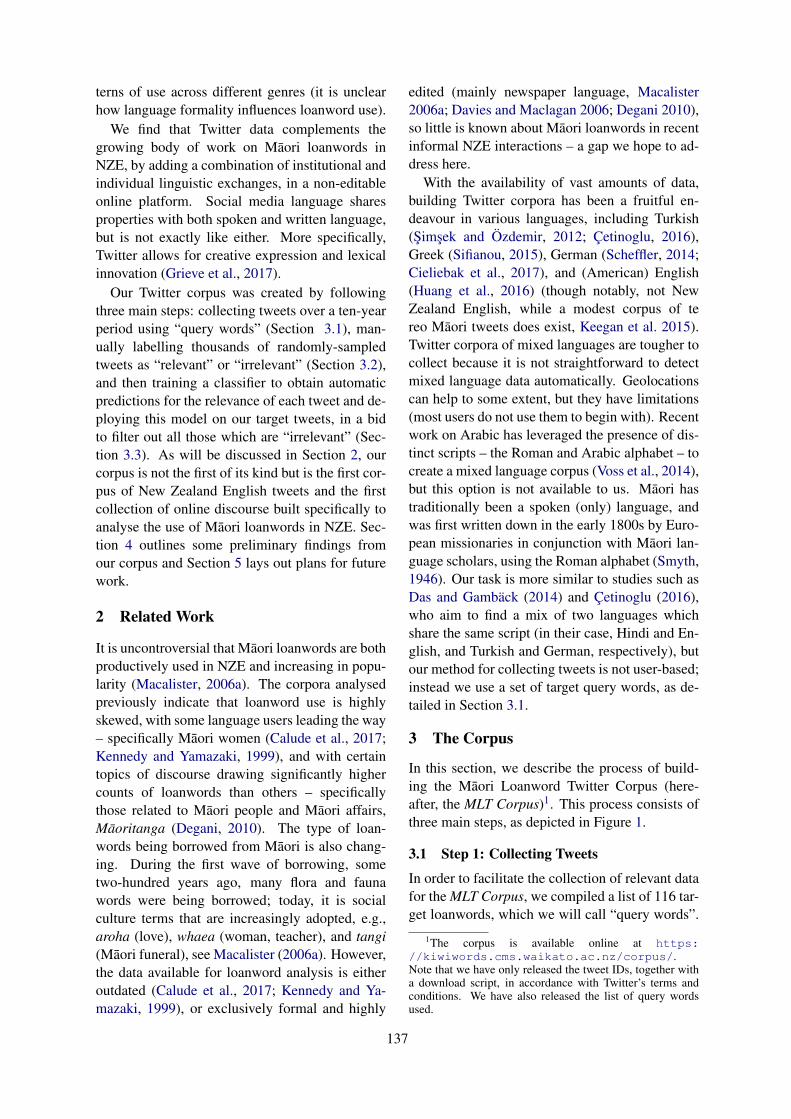
terns of use across different genres (it is unclearhow language formality influences loanword use).

We find that Twitter data complements thegrowing body of work on Maori loanwords inNZE, by adding a combination of institutional andindividual linguistic exchanges, in a non-editableonline platform. Social media language sharesproperties with both spoken and written language,but is not exactly like either. More specifically,Twitter allows for creative expression and lexicalinnovation (Grieve et al., 2017).

Our Twitter corpus was created by followingthree main steps: collecting tweets over a ten-yearperiod using “query words” (Section 3.1), man-ually labelling thousands of randomly-sampledtweets as “relevant” or “irrelevant” (Section 3.2),and then training a classifier to obtain automaticpredictions for the relevance of each tweet and de-ploying this model on our target tweets, in a bidto filter out all those which are “irrelevant” (Sec-tion 3.3). As will be discussed in Section 2, ourcorpus is not the first of its kind but is the first cor-pus of New Zealand English tweets and the firstcollection of online discourse built specifically toanalyse the use of Maori loanwords in NZE. Sec-tion 4 outlines some preliminary findings fromour corpus and Section 5 lays out plans for futurework.

2 Related Work

It is uncontroversial that Maori loanwords are bothproductively used in NZE and increasing in popu-larity (Macalister, 2006a). The corpora analysedpreviously indicate that loanword use is highlyskewed, with some language users leading the way– specifically Maori women (Calude et al., 2017;Kennedy and Yamazaki, 1999), and with certaintopics of discourse drawing significantly highercounts of loanwords than others – specificallythose related to Maori people and Maori affairs,Maoritanga (Degani, 2010). The type of loan-words being borrowed from Maori is also chang-ing. During the first wave of borrowing, sometwo-hundred years ago, many flora and faunawords were being borrowed; today, it is socialculture terms that are increasingly adopted, e.g.,aroha (love), whaea (woman, teacher), and tangi(Maori funeral), see Macalister (2006a). However,the data available for loanword analysis is eitheroutdated (Calude et al., 2017; Kennedy and Ya-mazaki, 1999), or exclusively formal and highly

edited (mainly newspaper language, Macalister2006a; Davies and Maclagan 2006; Degani 2010),so little is known about Maori loanwords in recentinformal NZE interactions – a gap we hope to ad-dress here.

With the availability of vast amounts of data,building Twitter corpora has been a fruitful en-deavour in various languages, including Turkish(Simsek and Ozdemir, 2012; Cetinoglu, 2016),Greek (Sifianou, 2015), German (Scheffler, 2014;Cieliebak et al., 2017), and (American) English(Huang et al., 2016) (though notably, not NewZealand English, while a modest corpus of tereo Maori tweets does exist, Keegan et al. 2015).Twitter corpora of mixed languages are tougher tocollect because it is not straightforward to detectmixed language data automatically. Geolocationscan help to some extent, but they have limitations(most users do not use them to begin with). Recentwork on Arabic has leveraged the presence of dis-tinct scripts – the Roman and Arabic alphabet – tocreate a mixed language corpus (Voss et al., 2014),but this option is not available to us. Maori hastraditionally been a spoken (only) language, andwas first written down in the early 1800s by Euro-pean missionaries in conjunction with Maori lan-guage scholars, using the Roman alphabet (Smyth,1946). Our task is more similar to studies such asDas and Gamback (2014) and Cetinoglu (2016),who aim to find a mix of two languages whichshare the same script (in their case, Hindi and En-glish, and Turkish and German, respectively), butour method for collecting tweets is not user-based;instead we use a set of target query words, as de-tailed in Section 3.1.

3 The Corpus

In this section, we describe the process of build-ing the Maori Loanword Twitter Corpus (here-after, the MLT Corpus)1. This process consists ofthree main steps, as depicted in Figure 1.

3.1 Step 1: Collecting Tweets

In order to facilitate the collection of relevant datafor the MLT Corpus, we compiled a list of 116 tar-get loanwords, which we will call “query words”.

1The corpus is available online at https://kiwiwords.cms.waikato.ac.nz/corpus/.Note that we have only released the tweet IDs, together witha download script, in accordance with Twitter’s terms andconditions. We have also released the list of query wordsused.

137

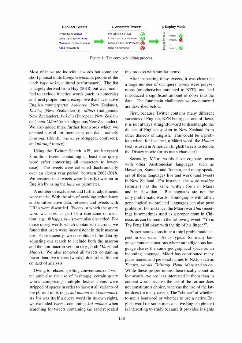
Proud to be a kiwi

haka ne kuma fa

Love my crazy whanau Proud to be a kiwi

Moana is my fav Princess haka ne kuma fa

tweet1

tweet2

...

tweetm

2. Annotate Tweets

Love my crazy whanau Moana is my fav Princess

3. Deploy Model 1. Collect Tweets

Target Tweets

Figure 1: The corpus-building process.

Most of these are individual words but some areshort phrasal units (tangata whenua, people of theland; kapa haka, cultural performance). The listis largely derived from Hay (2018) but was modi-fied to exclude function words (such as numerals)and most proper nouns, except five that have nativeEnglish counterparts: Aotearoa (New Zealand),Kiwi(s) (New Zealander(s)), Maori (indigenousNew Zealander), Pakeha (European New Zealan-der), non-Maori (non-indigenous New Zealander).We also added three further loanwords which wedeemed useful for increasing our data, namelyhaurangi (drunk), wairangi (drugged, confused),and porangi (crazy).

Using the Twitter Search API, we harvested8 million tweets containing at least one queryword (after converting all characters to lower-case). The tweets were collected diachronicallyover an eleven year period, between 2007-2018.We ensured that tweets were (mostly) written inEnglish by using the lang:en parameter.

A number of exclusions and further adjustmentswere made. With the aim of avoiding redundancyand uninformative data, retweets and tweets withURLs were discarded. Tweets in which the queryword was used as part of a username or men-tion (e.g., @happy kiwi) were also discarded. Forthose query words which contained macrons, wefound that users were inconsistent in their macronuse. Consequently, we consolidated the data byadjusting our search to include both the macronand the non-macron version (e.g., both Maori andMaori). We also removed all tweets containingfewer than five tokens (words), due to insufficientcontext of analysis.

Owing to relaxed spelling conventions on Twit-ter (and also the use of hashtags), certain querywords comprising multiple lexical items werestripped of spaces in order to harvest all variants ofthe phrasal units (e.g., kai moana and kaimoana).As kai was itself a query word (in its own right),we excluded tweets containing kai moana whensearching for tweets containing kai (and repeated

this process with similar items).

After inspecting these tweets, it was clear thata large number of our query words were polyse-mous (or otherwise unrelated to NZE), and hadintroduced a significant amount of noise into thedata. The four main challenges we encounteredare described below.

First, because Twitter contains many differentvarieties of English, NZE being just one of these,it is not always straightforward to disentangle thedialect of English spoken in New Zealand fromother dialects of English. This could be a prob-lem when, for instance, a Maori word like Moana(sea) is used in American English tweets to denotethe Disney movie (or its main character).

Secondly, Maori words have cognate formswith other Austronesian languages, such asHawaiian, Samoan and Tongan, and many speak-ers of these languages live and work (and tweet)in New Zealand. For instance, the word wahine(woman) has the same written form in Maoriand in Hawaiian. But cognates are not theonly problematic words. Homographs with other,genealogically-unrelated languages can also poseproblems. For instance, the Maori word hui (meet-ing) is sometimes used as a proper noun in Chi-nese, as can be seen in the following tweet: “Yo isTay Peng Hui okay with the tip of his finger?”.

Proper nouns constitute a third problematic as-pect in our data. As is typical for many lan-guage contact situations where an indigenous lan-guage shares the same geographical space as anincoming language, Maori has contributed manyplace names and personal names to NZE, such asTimaru, Aoraki, Titirangi, Hemi, Mere and so on.While these proper nouns theoretically count asloanwords, we are less interested in them than incontent words because the use of the former doesnot constitute a choice, whereas the use of the lat-ter does (in many cases). The “choice” of whetherto use a loanword or whether to use a native En-glish word (or sometimes a native English phrase)is interesting to study because it provides insights

138

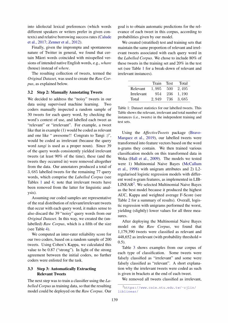
into idiolectal lexical preferences (which wordsdifferent speakers or writers prefer in given con-texts) and relative borrowing success rates (Caludeet al., 2017; Zenner et al., 2012).

Finally, given the impromptu and spontaneousnature of Twitter in general, we found that cer-tain Maori words coincided with misspelled ver-sions of intended native English words, e.g., whare(house) instead of where.

The resulting collection of tweets, termed theOriginal Dataset, was used to create the Raw Cor-pus, as explained below.

3.2 Step 2: Manually Annotating TweetsWe decided to address the “noisy” tweets in ourdata using supervised machine learning. Twocoders manually inspected a random sample of30 tweets for each query word, by checking theword’s context of use, and labelled each tweet as“relevant” or “irrelevant”. For example, a tweetlike that in example (1) would be coded as relevantand one like “ awesome!! Congrats to Tangi :)”,would be coded as irrelevant (because the queryword tangi is used as a proper noun). Since 39of the query words consistently yielded irrelevanttweets (at least 90% of the time), these (and thetweets they occurred in) were removed altogetherfrom the data. Our annotators produced a total of3, 685 labelled tweets for the remaining 77 querywords, which comprise the Labelled Corpus (seeTables 1 and 4; note that irrelevant tweets havebeen removed from the latter for linguistic anal-ysis).

Assuming our coded samples are representativeof the real distribution of relevant/irrelevant tweetsthat occur with each query word, it makes sense toalso discard the 39 “noisy” query words from ourOriginal Dataset. In this way, we created the (un-labelled) Raw Corpus, which is a fifth of the size(see Table 4).

We computed an inter-rater reliability score forour two coders, based on a random sample of 200tweets. Using Cohen’s Kappa, we calculated thisvalue to be 0.87 (“strong”). In light of the strongagreement between the initial coders, no furthercoders were enlisted for the task.

3.3 Step 3: Automatically ExtractingRelevant Tweets

The next step was to train a classifier using the La-belled Corpus as training data, so that the resultingmodel could be deployed on the Raw Corpus. Our

goal is to obtain automatic predictions for the rel-evance of each tweet in this corpus, according toprobabilities given by our model.

We created (stratified) test and training sets thatmaintain the same proportion of relevant and irrel-evant tweets associated with each query word inthe Labelled Corpus. We chose to include 80% ofthese tweets in the training set and 20% in the testset (see Table 1 for a break-down of relevant andirrelevant instances).

Train Test TotalRelevant 1, 995 500 2, 495Irrelevant 954 236 1, 190Total 2, 949 736 3, 685

Table 1: Dataset statistics for our labelled tweets. ThisTable shows the relevant, irrelevant and total number ofinstances (i.e., tweets) in the independent training andtest sets.

Using the AffectiveTweets package (Bravo-Marquez et al., 2019), our labelled tweets weretransformed into feature vectors based on the wordn-grams they contain. We then trained variousclassification models on this transformed data inWeka (Hall et al., 2009). The models we testedwere 1) Multinomial Naive Bayes (McCallumet al., 1998) with unigram attributes and 2) L2-regularised logistic regression models with differ-ent word n-gram features, as implemented in LIB-LINEAR2. We selected Multinomial Naive Bayesas the best model because it produced the highestAUC, Kappa and weighted average F-Score (seeTable 2 for a summary of results). Overall, logis-tic regression with unigrams performed the worst,yielding (slightly) lower values for all three mea-sures.

After deploying the Multinomial Naive Bayesmodel on the Raw Corpus, we found that1,179,390 tweets were classified as relevant and448,652 as irrelevant (with probability threshold =0.5).

Table 3 shows examples from our corpus ofeach type of classification. Some tweets werefalsely classified as “irrelevant” and some werefalsely classified as “relevant”. A short explana-tion why the irrelevant tweets were coded as suchis given in brackets at the end of each tweet.

We removed all tweets classified as irrelevant,

2https://www.csie.ntu.edu.tw/˜cjlin/liblinear/

139

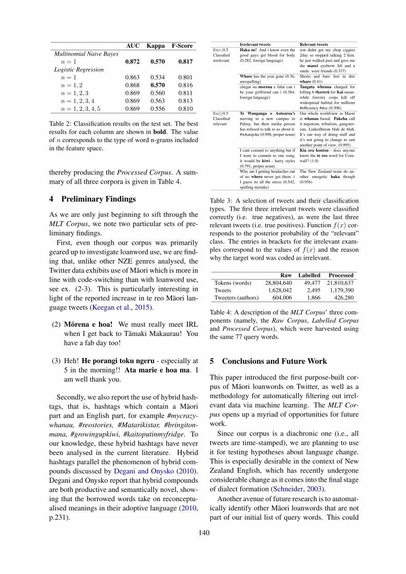
AUC Kappa F-ScoreMultinomial Naive Bayes

n = 1 0.872 0.570 0.817Logistic Regression

n = 1 0.863 0.534 0.801n = 1, 2 0.868 0.570 0.816n = 1, 2, 3 0.869 0.560 0.811n = 1, 2, 3, 4 0.869 0.563 0.813n = 1, 2, 3, 4, 5 0.869 0.556 0.810

Table 2: Classification results on the test set. The bestresults for each column are shown in bold. The valueof n corresponds to the type of word n-grams includedin the feature space.

thereby producing the Processed Corpus. A sum-mary of all three corpora is given in Table 4.

4 Preliminary Findings

As we are only just beginning to sift through theMLT Corpus, we note two particular sets of pre-liminary findings.

First, even though our corpus was primarilygeared up to investigate loanword use, we are find-ing that, unlike other NZE genres analysed, theTwitter data exhibits use of Maori which is more inline with code-switching than with loanword use,see ex. (2-3). This is particularly interesting inlight of the reported increase in te reo Maori lan-guage tweets (Keegan et al., 2015).

(2) Morena e hoa! We must really meet IRLwhen I get back to Tamaki Makaurau! Youhave a fab day too!

(3) Heh! He porangi toku ngeru - especially at5 in the morning!! Ata marie e hoa ma. Iam well thank you.

Secondly, we also report the use of hybrid hash-tags, that is, hashtags which contain a Maoripart and an English part, for example #mycrazy-whanau, #reostories, #Matarikistar, #bringiton-mana, #growingupkiwi, #kaitoputinmyfridge. Toour knowledge, these hybrid hashtags have neverbeen analysed in the current literature. Hybridhashtags parallel the phenomenon of hybrid com-pounds discussed by Degani and Onysko (2010).Degani and Onysko report that hybrid compoundsare both productive and semantically novel, show-ing that the borrowed words take on reconceptu-alised meanings in their adoptive language (2010,p.231).

Irrelevant tweets Relevant tweetsf(x)<0.5Classifiedirrelevant

Haka ne! And i know even thegood guys get blood for body(0.282, foreign language)

son didnt get my chop ciggies2day so stopped talking 2 him.he just walked past and gave methe maori eyebrow lift and asmile. were friends (0.337)

Whare has the year gone (0.36,misspelling)

Shorts and bare feet in thiswhare (0.41)

chegar na morena e falar can ibe your girlfriend can i (0.384,foreign language)

Tangata whenua charged forkilling 6 #kereru for Kai mean-while forestry corps kill offwidespread habitat for millions#efficiency #doc (0.306)

f(x)≥0.5Classifiedrelevant

Te Wanganga o Aotearoa’smoving to a new campus inPalmy, but their media personhas refused to talk to us about it.#whatajoke (0.998, proper noun)

Our whole worldview as Maoriis whanau based. Pakeha callit nepotism, tribalism, gangster-ism, LinkedInism blah de blah.It’s our way of doing stuff andit’s not going to change to suitanother point of view. (0.995)

I cant commit to anything but ifI were to commit to one song,it would be kiwi - harry styles(0.791, proper noun)

Kia ora koutou - does anyoneknow the te reo word for Corn-wall? (1.0)

Why am I getting headaches outof no whero never get them :(I guess its all the stress (0.542,spelling mistake)

The New Zealand team do an-other energetic haka though(0.956)

Table 3: A selection of tweets and their classificationtypes. The first three irrelevant tweets were classifiedcorrectly (i.e. true negatives), as were the last threerelevant tweets (i.e. true positives). Function f(x) cor-responds to the posterior probability of the “relevant”class. The entries in brackets for the irrelevant exam-ples correspond to the values of f(x) and the reasonwhy the target word was coded as irrelevant.

Raw Labelled ProcessedTokens (words) 28,804,640 49,477 21,810,637Tweets 1,628,042 2,495 1,179,390Tweeters (authors) 604,006 1,866 426,280

Table 4: A description of the MLT Corpus’ three com-ponents (namely, the Raw Corpus, Labelled Corpusand Processed Corpus), which were harvested usingthe same 77 query words.

5 Conclusions and Future Work

This paper introduced the first purpose-built cor-pus of Maori loanwords on Twitter, as well as amethodology for automatically filtering out irrel-evant data via machine learning. The MLT Cor-pus opens up a myriad of opportunities for futurework.

Since our corpus is a diachronic one (i.e., alltweets are time-stamped), we are planning to useit for testing hypotheses about language change.This is especially desirable in the context of NewZealand English, which has recently undergoneconsiderable change as it comes into the final stageof dialect formation (Schneider, 2003).

Another avenue of future research is to automat-ically identify other Maori loanwords that are notpart of our initial list of query words. This could

140

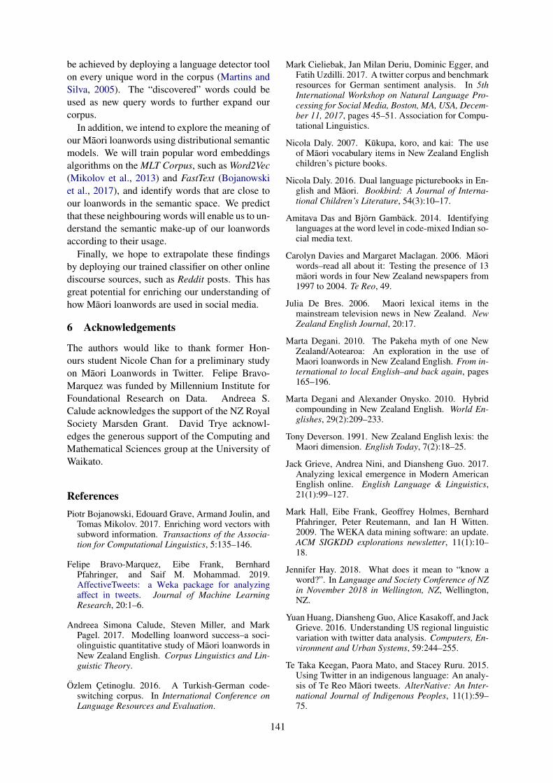
be achieved by deploying a language detector toolon every unique word in the corpus (Martins andSilva, 2005). The “discovered” words could beused as new query words to further expand ourcorpus.

In addition, we intend to explore the meaning ofour Maori loanwords using distributional semanticmodels. We will train popular word embeddingsalgorithms on the MLT Corpus, such as Word2Vec(Mikolov et al., 2013) and FastText (Bojanowskiet al., 2017), and identify words that are close toour loanwords in the semantic space. We predictthat these neighbouring words will enable us to un-derstand the semantic make-up of our loanwordsaccording to their usage.

Finally, we hope to extrapolate these findingsby deploying our trained classifier on other onlinediscourse sources, such as Reddit posts. This hasgreat potential for enriching our understanding ofhow Maori loanwords are used in social media.

6 Acknowledgements

The authors would like to thank former Hon-ours student Nicole Chan for a preliminary studyon Maori Loanwords in Twitter. Felipe Bravo-Marquez was funded by Millennium Institute forFoundational Research on Data. Andreea S.Calude acknowledges the support of the NZ RoyalSociety Marsden Grant. David Trye acknowl-edges the generous support of the Computing andMathematical Sciences group at the University ofWaikato.

ReferencesPiotr Bojanowski, Edouard Grave, Armand Joulin, and

Tomas Mikolov. 2017. Enriching word vectors withsubword information. Transactions of the Associa-tion for Computational Linguistics, 5:135–146.

Felipe Bravo-Marquez, Eibe Frank, BernhardPfahringer, and Saif M. Mohammad. 2019.AffectiveTweets: a Weka package for analyzingaffect in tweets. Journal of Machine LearningResearch, 20:1–6.

Andreea Simona Calude, Steven Miller, and MarkPagel. 2017. Modelling loanword success–a soci-olinguistic quantitative study of Maori loanwords inNew Zealand English. Corpus Linguistics and Lin-guistic Theory.

Ozlem Cetinoglu. 2016. A Turkish-German code-switching corpus. In International Conference onLanguage Resources and Evaluation.

Mark Cieliebak, Jan Milan Deriu, Dominic Egger, andFatih Uzdilli. 2017. A twitter corpus and benchmarkresources for German sentiment analysis. In 5thInternational Workshop on Natural Language Pro-cessing for Social Media, Boston, MA, USA, Decem-ber 11, 2017, pages 45–51. Association for Compu-tational Linguistics.

Nicola Daly. 2007. Kukupa, koro, and kai: The useof Maori vocabulary items in New Zealand Englishchildren’s picture books.

Nicola Daly. 2016. Dual language picturebooks in En-glish and Maori. Bookbird: A Journal of Interna-tional Children’s Literature, 54(3):10–17.

Amitava Das and Bjorn Gamback. 2014. Identifyinglanguages at the word level in code-mixed Indian so-cial media text.

Carolyn Davies and Margaret Maclagan. 2006. Maoriwords–read all about it: Testing the presence of 13maori words in four New Zealand newspapers from1997 to 2004. Te Reo, 49.

Julia De Bres. 2006. Maori lexical items in themainstream television news in New Zealand. NewZealand English Journal, 20:17.

Marta Degani. 2010. The Pakeha myth of one NewZealand/Aotearoa: An exploration in the use ofMaori loanwords in New Zealand English. From in-ternational to local English–and back again, pages165–196.

Marta Degani and Alexander Onysko. 2010. Hybridcompounding in New Zealand English. World En-glishes, 29(2):209–233.

Tony Deverson. 1991. New Zealand English lexis: theMaori dimension. English Today, 7(2):18–25.

Jack Grieve, Andrea Nini, and Diansheng Guo. 2017.Analyzing lexical emergence in Modern AmericanEnglish online. English Language & Linguistics,21(1):99–127.

Mark Hall, Eibe Frank, Geoffrey Holmes, BernhardPfahringer, Peter Reutemann, and Ian H Witten.2009. The WEKA data mining software: an update.ACM SIGKDD explorations newsletter, 11(1):10–18.

Jennifer Hay. 2018. What does it mean to “know aword?”. In Language and Society Conference of NZin November 2018 in Wellington, NZ, Wellington,NZ.

Yuan Huang, Diansheng Guo, Alice Kasakoff, and JackGrieve. 2016. Understanding US regional linguisticvariation with twitter data analysis. Computers, En-vironment and Urban Systems, 59:244–255.

Te Taka Keegan, Paora Mato, and Stacey Ruru. 2015.Using Twitter in an indigenous language: An analy-sis of Te Reo Maori tweets. AlterNative: An Inter-national Journal of Indigenous Peoples, 11(1):59–75.

141

Graeme Kennedy and Shunji Yamazaki. 1999. The in-fluence of Maori on the Nw Zealand English lexicon.LANGUAGE AND COMPUTERS, 30:33–44.

John Macalister. 2006a. The Maori lexical presencein New Zealand English: Constructing a corpus fordiachronic change. Corpora, 1(1):85–98.

John Macalister. 2006b. the Maori presence in theNew Zealand English lexicon, 1850–2000: Evi-dence from a corpus-based study. English World-Wide, 27(1):1–24.

John Macalister. 2009. Investigating the changing useof Te Reo. NZ Words, 13:3–4.

Bruno Martins and Mario J Silva. 2005. Languageidentification in web pages. In Proceedings of the2005 ACM symposium on Applied computing, pages764–768. ACM.

Andrew McCallum, Kamal Nigam, et al. 1998. A com-parison of event models for naive Bayes text classi-fication. In AAAI-98 workshop on learning for textcategorization, volume 752, pages 41–48. Citeseer.

Tomas Mikolov, Ilya Sutskever, Kai Chen, Greg S Cor-rado, and Jeff Dean. 2013. Distributed representa-tions of words and phrases and their compositional-ity. In Advances in neural information processingsystems, pages 3111–3119.

Alexander Onysko and Andreea Calude. 2013. Com-paring the usage of Maori loans in spoken and writ-ten New Zealand English: A case study of Maori,Pakeha, and Kiwi. New perspectives on lexicalborrowing: Onomasiological, methodological, andphraseological innovations, pages 143–170.

Tatjana Scheffler. 2014. A German twitter snapshot. InLREC, pages 2284–2289. Citeseer.

Edgar W Schneider. 2003. The dynamics of New En-glishes: From identity construction to dialect birth.Language, 79(2):233–281.

Maria Sifianou. 2015. Conceptualizing politeness inGreek: Evidence from twitter corpora. Journal ofPragmatics, 86:25–30.

Mehmet Ulvi Simsek and Suat Ozdemir. 2012. Analy-sis of the relation between Turkish twitter messagesand stock market index. In 2012 6th InternationalConference on Application of Information and Com-munication Technologies (AICT), pages 1–4. IEEE.

Patrick Smyth. 1946. Maori Pronunciation and theEvolution of Written Maori. Whitcombe & TombsLimited.

Jonathan R Stammers and Margaret Deuchar. 2012.Testing the nonce borrowing hypothesis: Counter-evidence from English-origin verbs in Welsh. Bilin-gualism: Language and Cognition, 15(3):630–643.

Clare R Voss, Stephen Tratz, Jamal Laoudi, and Dou-glas M Briesch. 2014. Finding Romanized Arabicdialect in code-mixed tweets. In LREC, pages 2249–2253.

Eline Zenner, Dirk Speelman, and Dirk Geeraerts.2012. Cognitive Sociolinguistics meets loan-word research: Measuring variation in the suc-cess of anglicisms in Dutch. Cognitive Linguistics,23(4):749–792.

142

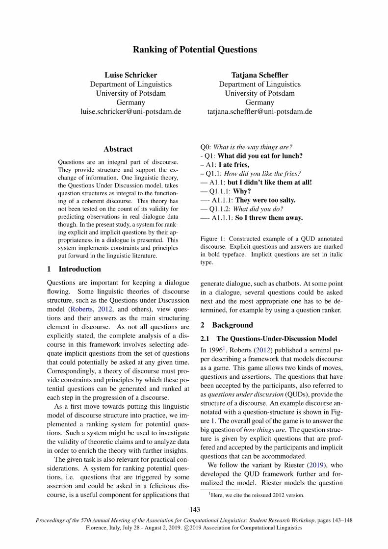
Proceedings of the 57th Annual Meeting of the Association for Computational Linguistics: Student Research Workshop, pages 143–148Florence, Italy, July 28 - August 2, 2019. c©2019 Association for Computational Linguistics

Ranking of Potential Questions

Luise SchrickerDepartment of Linguistics

University of PotsdamGermany

luise.schricker@uni-potsdam.de

Tatjana SchefflerDepartment of Linguistics

University of PotsdamGermany

tatjana.scheffler@uni-potsdam.de

AbstractQuestions are an integral part of discourse.They provide structure and support the ex-change of information. One linguistic theory,the Questions Under Discussion model, takesquestion structures as integral to the function-ing of a coherent discourse. This theory hasnot been tested on the count of its validity forpredicting observations in real dialogue datathough. In the present study, a system for rank-ing explicit and implicit questions by their ap-propriateness in a dialogue is presented. Thissystem implements constraints and principlesput forward in the linguistic literature.

1 Introduction

Questions are important for keeping a dialogueflowing. Some linguistic theories of discoursestructure, such as the Questions under Discussionmodel (Roberts, 2012, and others), view ques-tions and their answers as the main structuringelement in discourse. As not all questions areexplicitly stated, the complete analysis of a dis-course in this framework involves selecting ade-quate implicit questions from the set of questionsthat could potentially be asked at any given time.Correspondingly, a theory of discourse must pro-vide constraints and principles by which these po-tential questions can be generated and ranked ateach step in the progression of a discourse.

As a first move towards putting this linguisticmodel of discourse structure into practice, we im-plemented a ranking system for potential ques-tions. Such a system might be used to investigatethe validity of theoretic claims and to analyze datain order to enrich the theory with further insights.

The given task is also relevant for practical con-siderations. A system for ranking potential ques-tions, i.e. questions that are triggered by someassertion and could be asked in a felicitous dis-course, is a useful component for applications that

Q0: What is the way things are?- Q1: What did you eat for lunch?– A1: I ate fries,– Q1.1: How did you like the fries?— A1.1: but I didn’t like them at all!— Q1.1.1: Why?—- A1.1.1: They were too salty.— Q1.1.2: What did you do?—- A1.1.1: So I threw them away.

Figure 1: Constructed example of a QUD annotateddiscourse. Explicit questions and answers are markedin bold typeface. Implicit questions are set in italictype.

generate dialogue, such as chatbots. At some pointin a dialogue, several questions could be askednext and the most appropriate one has to be de-termined, for example by using a question ranker.

2 Background

2.1 The Questions-Under-Discussion ModelIn 19961, Roberts (2012) published a seminal pa-per describing a framework that models discourseas a game. This game allows two kinds of moves,questions and assertions. The questions that havebeen accepted by the participants, also referred toas questions under discussion (QUDs), provide thestructure of a discourse. An example discourse an-notated with a question-structure is shown in Fig-ure 1. The overall goal of the game is to answer thebig question of how things are. The question struc-ture is given by explicit questions that are prof-fered and accepted by the participants and implicitquestions that can be accommodated.

We follow the variant by Riester (2019), whodeveloped the QUD framework further and for-malized the model. Riester models the question

1Here, we cite the reissued 2012 version.

143

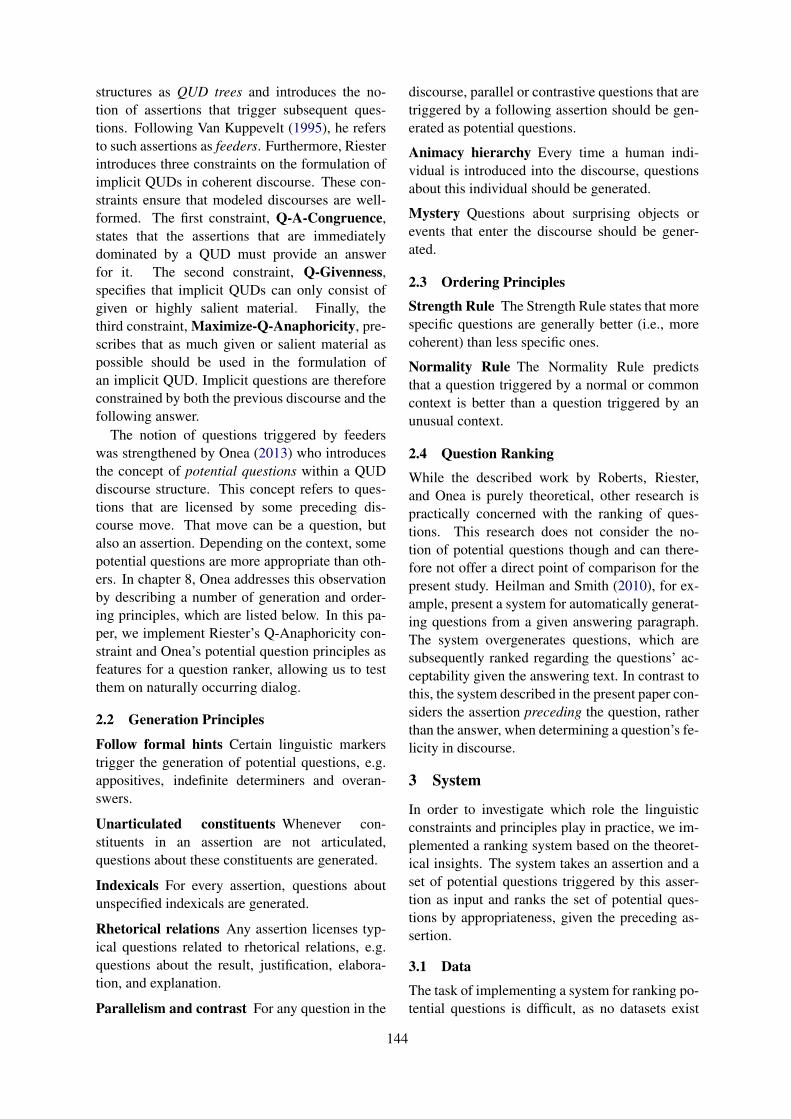
structures as QUD trees and introduces the no-tion of assertions that trigger subsequent ques-tions. Following Van Kuppevelt (1995), he refersto such assertions as feeders. Furthermore, Riesterintroduces three constraints on the formulation ofimplicit QUDs in coherent discourse. These con-straints ensure that modeled discourses are well-formed. The first constraint, Q-A-Congruence,states that the assertions that are immediatelydominated by a QUD must provide an answerfor it. The second constraint, Q-Givenness,specifies that implicit QUDs can only consist ofgiven or highly salient material. Finally, thethird constraint, Maximize-Q-Anaphoricity, pre-scribes that as much given or salient material aspossible should be used in the formulation ofan implicit QUD. Implicit questions are thereforeconstrained by both the previous discourse and thefollowing answer.

The notion of questions triggered by feederswas strengthened by Onea (2013) who introducesthe concept of potential questions within a QUDdiscourse structure. This concept refers to ques-tions that are licensed by some preceding dis-course move. That move can be a question, butalso an assertion. Depending on the context, somepotential questions are more appropriate than oth-ers. In chapter 8, Onea addresses this observationby describing a number of generation and order-ing principles, which are listed below. In this pa-per, we implement Riester’s Q-Anaphoricity con-straint and Onea’s potential question principles asfeatures for a question ranker, allowing us to testthem on naturally occurring dialog.

2.2 Generation Principles

Follow formal hints Certain linguistic markerstrigger the generation of potential questions, e.g.appositives, indefinite determiners and overan-swers.

Unarticulated constituents Whenever con-stituents in an assertion are not articulated,questions about these constituents are generated.

Indexicals For every assertion, questions aboutunspecified indexicals are generated.

Rhetorical relations Any assertion licenses typ-ical questions related to rhetorical relations, e.g.questions about the result, justification, elabora-tion, and explanation.

Parallelism and contrast For any question in the

discourse, parallel or contrastive questions that aretriggered by a following assertion should be gen-erated as potential questions.

Animacy hierarchy Every time a human indi-vidual is introduced into the discourse, questionsabout this individual should be generated.

Mystery Questions about surprising objects orevents that enter the discourse should be gener-ated.

2.3 Ordering Principles

Strength Rule The Strength Rule states that morespecific questions are generally better (i.e., morecoherent) than less specific ones.

Normality Rule The Normality Rule predictsthat a question triggered by a normal or commoncontext is better than a question triggered by anunusual context.

2.4 Question Ranking

While the described work by Roberts, Riester,and Onea is purely theoretical, other research ispractically concerned with the ranking of ques-tions. This research does not consider the no-tion of potential questions though and can there-fore not offer a direct point of comparison for thepresent study. Heilman and Smith (2010), for ex-ample, present a system for automatically generat-ing questions from a given answering paragraph.The system overgenerates questions, which aresubsequently ranked regarding the questions’ ac-ceptability given the answering text. In contrast tothis, the system described in the present paper con-siders the assertion preceding the question, ratherthan the answer, when determining a question’s fe-licity in discourse.

3 System

In order to investigate which role the linguisticconstraints and principles play in practice, we im-plemented a ranking system based on the theoret-ical insights. The system takes an assertion and aset of potential questions triggered by this asser-tion as input and ranks the set of potential ques-tions by appropriateness, given the preceding as-sertion.

3.1 Data

The task of implementing a system for ranking po-tential questions is difficult, as no datasets exist

144

that fulfils the requirements of the input. To cir-cumvent this problem, the required data was ap-proximated by different data extraction schemes.We used two corpora: the test set was extractedfrom a small manually annotated corpus of inter-view fragments. The training set was mined fromthe Switchboard Dialog Act corpus.

The test corpus consists of eight short texts. Thetexts are copies of a segment of an interview withEdward Snowden2 that was annotated with a QUDstructure like the one in Figure 1 by students of theclass Questions and Models of Discourse, held atthe University of Potsdam in 2018.3 Some pre-processing, manual and automatic, had to be donein order to ensure a consistent structure amongstthe texts. The interviews were segmented into as-sertions and explicit and implicit questions. As-sertions are often not complete sentences and thesegmentation differs between the individual texts.

We extracted every assertion that was followedby a question, explicit or implicit, together withthe following question. The three preceding andthree next questions were saved as an approxima-tion of the set of alternative potential questions.4

We deemed this acceptable because it is likelythat the immediately surrounding questions will beabout similar topics as the assertion. The questionimmediately following the assertion was regardedas the correct label, i.e. the question that shouldbe ranked highest by the system. Items that con-tained the same assertions were merged, which re-sulted in several correct labels, and a larger set ofalternative potential questions per assertion.

As the test set was not sufficiently big to usefor training in a machine learning setting, a sec-ond dataset was extracted from the SwitchboardDialog Act corpus (SWDA)5 (Stolcke et al.,2000). The SWDA corpus contains spontaneoustelephone conversations that are annotated with di-alog acts. The reasoning behind using this corpuswas that a question following an assertion in a dia-log can be interpreted as the highest ranked poten-

2https://edwardsnowden.com/2014/01/27/video-ard-interview-with-edward-snowden/

3The raw annotated files can be accessed un-der: https://github.com/QUD-comp/analysis-of-QUD-structures/tree/master/Snowden

4Incomplete datapoints from the start and end of a docu-ment, which were followed or preceded by fewer than threequestions, were excluded.

5The version distributed by Christopher Potts (https://github.com/cgpotts/swda) was used, as well asthe code he provided for better accessibility of the corpus.

tial question available at that point.Similar to the extraction of the test set, asser-

tions directly followed by a question were ex-tracted along with the question. We consideredonly prototypical types of assertions and ques-tions6, excluding for example rhetorical questions,to avoid inconsistent items. For each item, threequestions were randomly picked from the set ofall questions in the corpus to arrive at a set ofapproximate alternative potential questions. Theindividual questions and assertions were cleanedfrom disfluency annotation. The resulting trainingset consists of 2777 items.

3.2 Feature Extraction

In this work, we implemented a subset ofOnea’s (2013) generation and ordering principlesand Riester’s (2019) QUD constraints as featuresfor ranking a question following a preceding as-sertion. For linguistic processing spaCy (Honni-bal and Montani, 2019) (e.g. dependency pars-ing, named entity recognition and POS tagging),NLTK (Bird et al., 2009) (wordnet, stopwords)and neuralcoref7 (coreference resolution) wereused. For features using word embeddings, apretrained Word2vec model8 (Mikolov et al.,2013a,b) was used, the model was handled via thegensim package (Rehurek and Sojka, 2010). Be-low, the implemented features are described.

Indefinite Determiners This feature detects in-definite noun phrases in the assertion that arecoreferent to some mention in the question.

Indexicals This feature analyzes whether thequestion is about a time or a place by searchingfor question phrases that inquire about a time or aplace (e.g. when, where etc.).

Explanation Following Onea (2019), who drawsparallels between certain patterns in discoursetrees with question structures and rhetorical re-lations, the rhetorical relation Explanation is de-tected by searching for why-questions.

Elaboration The rhetorical relation Elaborationis linked by Onea (2019) to questions that ask

6List of considered assertion tags: [’s’, ’sd’, ’sv’] (state-ments with or without opinions); list of considered questiontags: [’qy’, ’qw’, ’ˆd’, ’qo’, ’qr’, ’qwˆd’] (different syntacticsub-types of questions).

7https://github.com/huggingface/neuralcoref

8https://code.google.com/archive/p/word2vec/

145

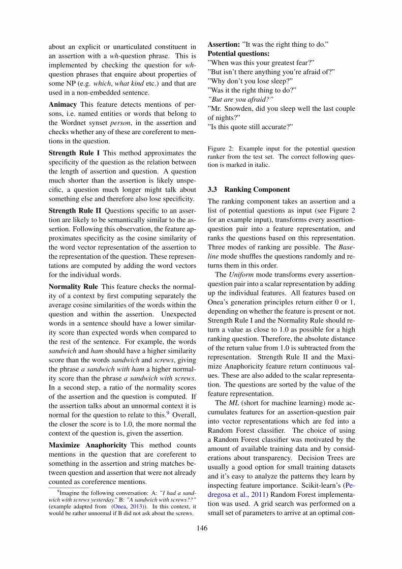
about an explicit or unarticulated constituent inan assertion with a wh-question phrase. This isimplemented by checking the question for wh-question phrases that enquire about properties ofsome NP (e.g. which, what kind etc.) and that areused in a non-embedded sentence.

Animacy This feature detects mentions of per-sons, i.e. named entities or words that belong tothe Wordnet synset person, in the assertion andchecks whether any of these are coreferent to men-tions in the question.

Strength Rule I This method approximates thespecificity of the question as the relation betweenthe length of assertion and question. A questionmuch shorter than the assertion is likely unspe-cific, a question much longer might talk aboutsomething else and therefore also lose specificity.

Strength Rule II Questions specific to an asser-tion are likely to be semantically similar to the as-sertion. Following this observation, the feature ap-proximates specificity as the cosine similarity ofthe word vector representation of the assertion tothe representation of the question. These represen-tations are computed by adding the word vectorsfor the individual words.

Normality Rule This feature checks the normal-ity of a context by first computing separately theaverage cosine similarities of the words within thequestion and within the assertion. Unexpectedwords in a sentence should have a lower similar-ity score than expected words when compared tothe rest of the sentence. For example, the wordssandwich and ham should have a higher similarityscore than the words sandwich and screws, givingthe phrase a sandwich with ham a higher normal-ity score than the phrase a sandwich with screws.In a second step, a ratio of the normality scoresof the assertion and the question is computed. Ifthe assertion talks about an unnormal context it isnormal for the question to relate to this.9 Overall,the closer the score is to 1.0, the more normal thecontext of the question is, given the assertion.

Maximize Anaphoricity This method countsmentions in the question that are coreferent tosomething in the assertion and string matches be-tween question and assertion that were not alreadycounted as coreference mentions.

9Imagine the following conversation: A: ”I had a sand-wich with screws yesterday.” B: ”A sandwich with screws??”(example adapted from (Onea, 2013)). In this context, itwould be rather unnormal if B did not ask about the screws.

Assertion: ”It was the right thing to do.”Potential questions:”When was this your greatest fear?””But isn’t there anything you’re afraid of?””Why don’t you lose sleep?””Was it the right thing to do?””But are you afraid?””Mr. Snowden, did you sleep well the last coupleof nights?””Is this quote still accurate?”

Figure 2: Example input for the potential questionranker from the test set. The correct following ques-tion is marked in italic.

3.3 Ranking ComponentThe ranking component takes an assertion and alist of potential questions as input (see Figure 2for an example input), transforms every assertion-question pair into a feature representation, andranks the questions based on this representation.Three modes of ranking are possible. The Base-line mode shuffles the questions randomly and re-turns them in this order.

The Uniform mode transforms every assertion-question pair into a scalar representation by addingup the individual features. All features based onOnea’s generation principles return either 0 or 1,depending on whether the feature is present or not.Strength Rule I and the Normality Rule should re-turn a value as close to 1.0 as possible for a highranking question. Therefore, the absolute distanceof the return value from 1.0 is subtracted from therepresentation. Strength Rule II and the Maxi-mize Anaphoricity feature return continuous val-ues. These are also added to the scalar representa-tion. The questions are sorted by the value of thefeature representation.

The ML (short for machine learning) mode ac-cumulates features for an assertion-question pairinto vector representations which are fed into aRandom Forest classifier. The choice of usinga Random Forest classifier was motivated by theamount of available training data and by consid-erations about transparency. Decision Trees areusually a good option for small training datasetsand it’s easy to analyze the patterns they learn byinspecting feature importance. Scikit-learn’s (Pe-dregosa et al., 2011) Random Forest implementa-tion was used. A grid search was performed on asmall set of parameters to arrive at an optimal con-

146

Mode Top-1 Top-3 Top-5Baseline 19.23 46.15 65.38Uniform 38.46 61.54 88.46

ML 50.00 73.08 80.77

Table 1: Results on test set. Top-N signi-fies the stage of evaluation.

figuration, results for the best configuration10 aredetailed in Table 1.

4 Evaluation

The different ranking modes and classifier configswere evaluated on the test set extracted from theannotated Snowden interview. In order to get amore detailed insight into the performance of theranking system, evaluations were done in threestages. To this end, the Top-N accuracy measurewas used. As a result of the merging of itemsdescribed in section 3.1, the average number ofquestions that are correct if ranked in first place isthree per item, and the average number of poten-tial questions available for ranking is 21 per item.Results are listed in Table 1.

Interestingly, the uniform mode works quitewell, providing the best result in the easiest eval-uation setting with an accuracy score of almost90%. The overall best ranking system (ML mode)achieves an accuracy of 50% for ranking a correctlabel highest and a score of 73% for placing a cor-rect label amongst the top three ranks. These num-bers show improvements of over 30 and over 25points compared to the random baseline.

It should be noted that the data in the train-ing and test sets have different properties. Whilethe training data is built from spontaneous dia-logue, the test set contains QUD annotations thatwere added in hindsight and that are sometimesnot phrased like natural speech. Training and testsets that are more similar might therefore providebetter results. This experiment should be repeatedin the future if a reasonably sized QUD-annotatedcorpus becomes available.

Furthermore, the random baseline is quite sim-ple and might be too easy to beat. An anonymousreviewer suggested implementing a deep learn-ing model trained for next sentence prediction asan additional baseline. While we agree that thiswould be worthwhile, we have to leave it for fu-

10The best configuration has min samples leaf = 5,max depth = 10, and class weight = 0:0.5, 1:1.

Type UtteranceAssertion There are significant threatsQuestion Are there significant threats?Assertion ”The greatest fear I have,” and I

quote you, ”regarding these dis-closures is nothing will change.”

Question But isn’t there anythingyou’re afraid of?

Table 2: Examples of questions incorrectly ranked intop place that the assertion already answers

ture work due to time constraints.An additional inspection of the best perform-

ing Random Forest model’s features by impor-tance showed the three ordering constraint fea-tures, Strength Rule II, the Normality Rule andStrength Rule I in top position. This confirmsthe theoretic background: the ordering principlesshould be more important for ranking potentialquestions than the generation principles.

4.1 Error AnalysisIn order to better understand the failings of theranking system, the best configuration was in-spected more closely in an error analysis. Themost prominent error by far is ranking a questionthat the assertion already answers highest, insteadof one that is triggered by the assertion. Some ex-amples of this type of error are listed in Table 2.

This can be explained by the nature of the train-ing data. As alternative potential questions weresampled randomly from the data during training,they are more likely to be about a different topicthan the assertion compared to the correct ques-tion, which would enhance the importance of sim-ilarity features like Strength Rule II. An answerto a question can be as similar to the question asthe assertion directly preceding a question. In areal application, questions that are answered bythe preceding assertion should not be part of theset of potential questions that are fed into the sys-tem, though.

5 Conclusion

Potential questions are a concept stemming fromtheories that organize discourse around questions.A ranking system11 based on these theories was

11The code and data presented here have beenmade available for public use under a GPL-3.0 li-cense: https://github.com/QUD-comp/ranking-potential-questions.

147

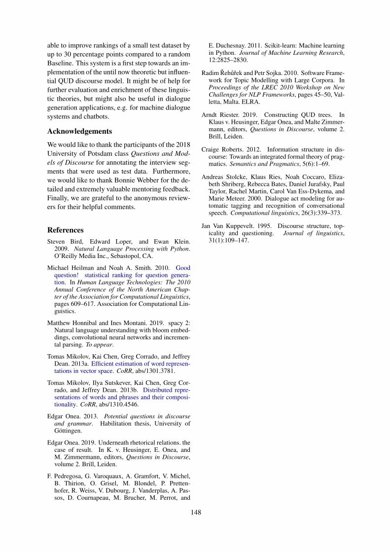
able to improve rankings of a small test dataset byup to 30 percentage points compared to a randomBaseline. This system is a first step towards an im-plementation of the until now theoretic but influen-tial QUD discourse model. It might be of help forfurther evaluation and enrichment of these linguis-tic theories, but might also be useful in dialoguegeneration applications, e.g. for machine dialoguesystems and chatbots.

Acknowledgements

We would like to thank the participants of the 2018University of Potsdam class Questions and Mod-els of Discourse for annotating the interview seg-ments that were used as test data. Furthermore,we would like to thank Bonnie Webber for the de-tailed and extremely valuable mentoring feedback.Finally, we are grateful to the anonymous review-ers for their helpful comments.

ReferencesSteven Bird, Edward Loper, and Ewan Klein.

2009. Natural Language Processing with Python.O’Reilly Media Inc., Sebastopol, CA.

Michael Heilman and Noah A. Smith. 2010. Goodquestion! statistical ranking for question genera-tion. In Human Language Technologies: The 2010Annual Conference of the North American Chap-ter of the Association for Computational Linguistics,pages 609–617. Association for Computational Lin-guistics.

Matthew Honnibal and Ines Montani. 2019. spacy 2:Natural language understanding with bloom embed-dings, convolutional neural networks and incremen-tal parsing. To appear.

Tomas Mikolov, Kai Chen, Greg Corrado, and JeffreyDean. 2013a. Efficient estimation of word represen-tations in vector space. CoRR, abs/1301.3781.

Tomas Mikolov, Ilya Sutskever, Kai Chen, Greg Cor-rado, and Jeffrey Dean. 2013b. Distributed repre-sentations of words and phrases and their composi-tionality. CoRR, abs/1310.4546.

Edgar Onea. 2013. Potential questions in discourseand grammar. Habilitation thesis, University ofGottingen.

Edgar Onea. 2019. Underneath rhetorical relations. thecase of result. In K. v. Heusinger, E. Onea, andM. Zimmermann, editors, Questions in Discourse,volume 2. Brill, Leiden.

F. Pedregosa, G. Varoquaux, A. Gramfort, V. Michel,B. Thirion, O. Grisel, M. Blondel, P. Pretten-hofer, R. Weiss, V. Dubourg, J. Vanderplas, A. Pas-sos, D. Cournapeau, M. Brucher, M. Perrot, and

E. Duchesnay. 2011. Scikit-learn: Machine learningin Python. Journal of Machine Learning Research,12:2825–2830.

Radim Rehurek and Petr Sojka. 2010. Software Frame-work for Topic Modelling with Large Corpora. InProceedings of the LREC 2010 Workshop on NewChallenges for NLP Frameworks, pages 45–50, Val-letta, Malta. ELRA.

Arndt Riester. 2019. Constructing QUD trees. InKlaus v. Heusinger, Edgar Onea, and Malte Zimmer-mann, editors, Questions in Discourse, volume 2.Brill, Leiden.

Craige Roberts. 2012. Information structure in dis-course: Towards an integrated formal theory of prag-matics. Semantics and Pragmatics, 5(6):1–69.

Andreas Stolcke, Klaus Ries, Noah Coccaro, Eliza-beth Shriberg, Rebecca Bates, Daniel Jurafsky, PaulTaylor, Rachel Martin, Carol Van Ess-Dykema, andMarie Meteer. 2000. Dialogue act modeling for au-tomatic tagging and recognition of conversationalspeech. Computational linguistics, 26(3):339–373.

Jan Van Kuppevelt. 1995. Discourse structure, top-icality and questioning. Journal of linguistics,31(1):109–147.

148

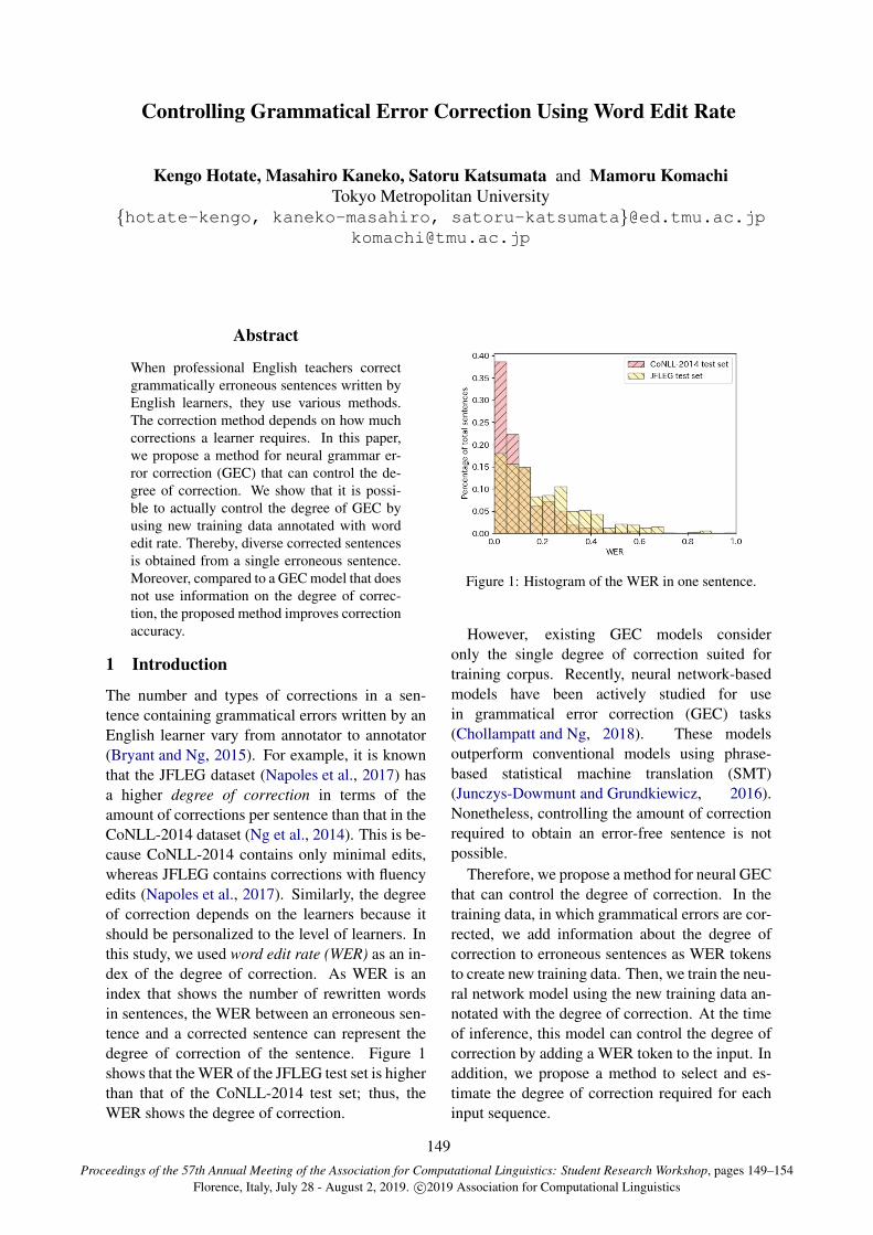
Proceedings of the 57th Annual Meeting of the Association for Computational Linguistics: Student Research Workshop, pages 149–154Florence, Italy, July 28 - August 2, 2019. c©2019 Association for Computational Linguistics

Controlling Grammatical Error Correction Using Word Edit Rate

Kengo Hotate, Masahiro Kaneko, Satoru Katsumata and Mamoru KomachiTokyo Metropolitan University

hotate-kengo, kaneko-masahiro, satoru-katsumata@ed.tmu.ac.jpkomachi@tmu.ac.jp

Abstract

When professional English teachers correctgrammatically erroneous sentences written byEnglish learners, they use various methods.The correction method depends on how muchcorrections a learner requires. In this paper,we propose a method for neural grammar er-ror correction (GEC) that can control the de-gree of correction. We show that it is possi-ble to actually control the degree of GEC byusing new training data annotated with wordedit rate. Thereby, diverse corrected sentencesis obtained from a single erroneous sentence.Moreover, compared to a GEC model that doesnot use information on the degree of correc-tion, the proposed method improves correctionaccuracy.

1 Introduction

The number and types of corrections in a sen-tence containing grammatical errors written by anEnglish learner vary from annotator to annotator(Bryant and Ng, 2015). For example, it is knownthat the JFLEG dataset (Napoles et al., 2017) hasa higher degree of correction in terms of theamount of corrections per sentence than that in theCoNLL-2014 dataset (Ng et al., 2014). This is be-cause CoNLL-2014 contains only minimal edits,whereas JFLEG contains corrections with fluencyedits (Napoles et al., 2017). Similarly, the degreeof correction depends on the learners because itshould be personalized to the level of learners. Inthis study, we used word edit rate (WER) as an in-dex of the degree of correction. As WER is anindex that shows the number of rewritten wordsin sentences, the WER between an erroneous sen-tence and a corrected sentence can represent thedegree of correction of the sentence. Figure 1shows that the WER of the JFLEG test set is higherthan that of the CoNLL-2014 test set; thus, theWER shows the degree of correction.

Figure 1: Histogram of the WER in one sentence.

However, existing GEC models consideronly the single degree of correction suited fortraining corpus. Recently, neural network-basedmodels have been actively studied for usein grammatical error correction (GEC) tasks(Chollampatt and Ng, 2018). These modelsoutperform conventional models using phrase-based statistical machine translation (SMT)(Junczys-Dowmunt and Grundkiewicz, 2016).Nonetheless, controlling the amount of correctionrequired to obtain an error-free sentence is notpossible.

Therefore, we propose a method for neural GECthat can control the degree of correction. In thetraining data, in which grammatical errors are cor-rected, we add information about the degree ofcorrection to erroneous sentences as WER tokensto create new training data. Then, we train the neu-ral network model using the new training data an-notated with the degree of correction. At the timeof inference, this model can control the degree ofcorrection by adding a WER token to the input. Inaddition, we propose a method to select and es-timate the degree of correction required for eachinput sequence.

149

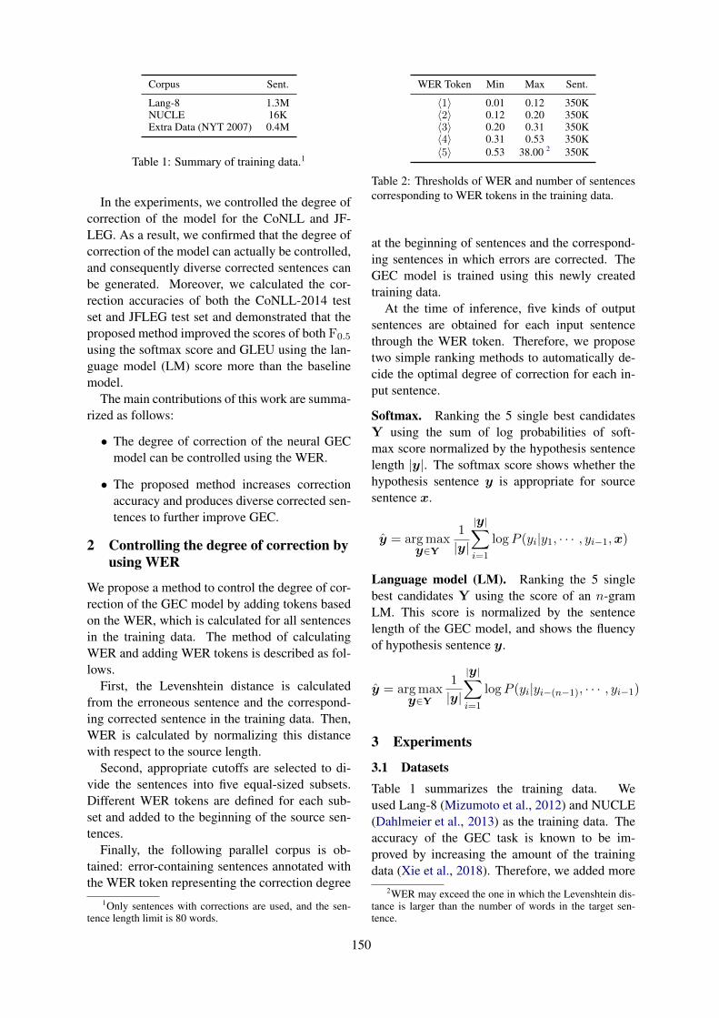
Corpus Sent.

Lang-8 1.3MNUCLE 16KExtra Data (NYT 2007) 0.4M

Table 1: Summary of training data.1

In the experiments, we controlled the degree ofcorrection of the model for the CoNLL and JF-LEG. As a result, we confirmed that the degree ofcorrection of the model can actually be controlled,and consequently diverse corrected sentences canbe generated. Moreover, we calculated the cor-rection accuracies of both the CoNLL-2014 testset and JFLEG test set and demonstrated that theproposed method improved the scores of both F0.5

using the softmax score and GLEU using the lan-guage model (LM) score more than the baselinemodel.

The main contributions of this work are summa-rized as follows:

• The degree of correction of the neural GECmodel can be controlled using the WER.

• The proposed method increases correctionaccuracy and produces diverse corrected sen-tences to further improve GEC.

2 Controlling the degree of correction byusing WER

We propose a method to control the degree of cor-rection of the GEC model by adding tokens basedon the WER, which is calculated for all sentencesin the training data. The method of calculatingWER and adding WER tokens is described as fol-lows.

First, the Levenshtein distance is calculatedfrom the erroneous sentence and the correspond-ing corrected sentence in the training data. Then,WER is calculated by normalizing this distancewith respect to the source length.

Second, appropriate cutoffs are selected to di-vide the sentences into five equal-sized subsets.Different WER tokens are defined for each sub-set and added to the beginning of the source sen-tences.

Finally, the following parallel corpus is ob-tained: error-containing sentences annotated withthe WER token representing the correction degree

1Only sentences with corrections are used, and the sen-tence length limit is 80 words.

WER Token Min Max Sent.

⟨1⟩ 0.01 0.12 350K⟨2⟩ 0.12 0.20 350K⟨3⟩ 0.20 0.31 350K⟨4⟩ 0.31 0.53 350K⟨5⟩ 0.53 38.00 2 350K

Table 2: Thresholds of WER and number of sentencescorresponding to WER tokens in the training data.

at the beginning of sentences and the correspond-ing sentences in which errors are corrected. TheGEC model is trained using this newly createdtraining data.

At the time of inference, five kinds of outputsentences are obtained for each input sentencethrough the WER token. Therefore, we proposetwo simple ranking methods to automatically de-cide the optimal degree of correction for each in-put sentence.

Softmax. Ranking the 5 single best candidatesY using the sum of log probabilities of soft-max score normalized by the hypothesis sentencelength |y|. The softmax score shows whether thehypothesis sentence y is appropriate for sourcesentence x.

y = arg maxy∈Y

1

|y|

|y|∑

i=1

log P (yi|y1, · · · , yi−1,x)

Language model (LM). Ranking the 5 singlebest candidates Y using the score of an n-gramLM. This score is normalized by the sentencelength of the GEC model, and shows the fluencyof hypothesis sentence y.

y = arg maxy∈Y

1

|y|

|y|∑

i=1

log P (yi|yi−(n−1), · · · , yi−1)

3 Experiments

3.1 DatasetsTable 1 summarizes the training data. Weused Lang-8 (Mizumoto et al., 2012) and NUCLE(Dahlmeier et al., 2013) as the training data. Theaccuracy of the GEC task is known to be im-proved by increasing the amount of the trainingdata (Xie et al., 2018). Therefore, we added more

2WER may exceed the one in which the Levenshtein dis-tance is larger than the number of words in the target sen-tence.

150

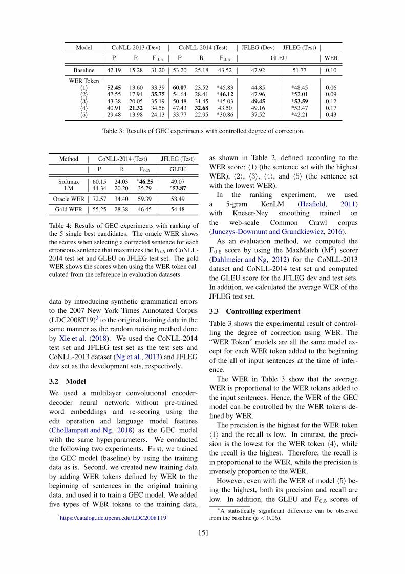
Model CoNLL-2013 (Dev) CoNLL-2014 (Test) JFLEG (Dev) JFLEG (Test)

P R F0.5 P R F0.5 GLEU WER

Baseline 42.19 15.28 31.20 53.20 25.18 43.52 47.92 51.77 0.10

WER Token⟨1⟩ 52.45 13.60 33.39 60.07 23.52 *45.83 44.85 *48.45 0.06⟨2⟩ 47.55 17.94 35.75 54.64 28.41 *46.12 47.96 *52.01 0.09⟨3⟩ 43.38 20.05 35.19 50.48 31.45 *45.03 49.45 *53.59 0.12⟨4⟩ 40.91 21.32 34.56 47.43 32.68 43.50 49.16 *53.47 0.17⟨5⟩ 29.48 13.98 24.13 33.77 22.95 *30.86 37.52 *42.21 0.43

Table 3: Results of GEC experiments with controlled degree of correction.

Method CoNLL-2014 (Test) JFLEG (Test)

P R F0.5 GLEU

Softmax 60.15 24.03 ∗46.25 49.07LM 44.34 20.20 35.79 ∗53.87

Oracle WER 72.57 34.40 59.39 58.49

Gold WER 55.25 28.38 46.45 54.48

Table 4: Results of GEC experiments with ranking ofthe 5 single best candidates. The oracle WER showsthe scores when selecting a corrected sentence for eacherroneous sentence that maximizes the F0.5 on CoNLL-2014 test set and GLEU on JFLEG test set. The goldWER shows the scores when using the WER token cal-culated from the reference in evaluation datasets.

data by introducing synthetic grammatical errorsto the 2007 New York Times Annotated Corpus(LDC2008T19)3 to the original training data in thesame manner as the random noising method doneby Xie et al. (2018). We used the CoNLL-2014test set and JFLEG test set as the test sets andCoNLL-2013 dataset (Ng et al., 2013) and JFLEGdev set as the development sets, respectively.

3.2 ModelWe used a multilayer convolutional encoder-decoder neural network without pre-trainedword embeddings and re-scoring using theedit operation and language model features(Chollampatt and Ng, 2018) as the GEC modelwith the same hyperparameters. We conductedthe following two experiments. First, we trainedthe GEC model (baseline) by using the trainingdata as is. Second, we created new training databy adding WER tokens defined by WER to thebeginning of sentences in the original trainingdata, and used it to train a GEC model. We addedfive types of WER tokens to the training data,

3https://catalog.ldc.upenn.edu/LDC2008T19

as shown in Table 2, defined according to theWER score: ⟨1⟩ (the sentence set with the highestWER), ⟨2⟩, ⟨3⟩, ⟨4⟩, and ⟨5⟩ (the sentence setwith the lowest WER).

In the ranking experiment, we useda 5-gram KenLM (Heafield, 2011)with Kneser-Ney smoothing trained onthe web-scale Common Crawl corpus(Junczys-Dowmunt and Grundkiewicz, 2016).

As an evaluation method, we computed theF0.5 score by using the MaxMatch (M2) scorer(Dahlmeier and Ng, 2012) for the CoNLL-2013dataset and CoNLL-2014 test set and computedthe GLEU score for the JFLEG dev and test sets.In addition, we calculated the average WER of theJFLEG test set.

3.3 Controlling experimentTable 3 shows the experimental result of control-ling the degree of correction using WER. The“WER Token” models are all the same model ex-cept for each WER token added to the beginningof the all of input sentences at the time of infer-ence.

The WER in Table 3 show that the averageWER is proportional to the WER tokens added tothe input sentences. Hence, the WER of the GECmodel can be controlled by the WER tokens de-fined by WER.

The precision is the highest for the WER token⟨1⟩ and the recall is low. In contrast, the preci-sion is the lowest for the WER token ⟨4⟩, whilethe recall is the highest. Therefore, the recall isin proportional to the WER, while the precision isinversely proportion to the WER.

However, even with the WER of model ⟨5⟩ be-ing the highest, both its precision and recall arelow. In addition, the GLEU and F0.5 scores of

∗A statistically significant difference can be observedfrom the baseline (p < 0.05).

151

Source Disadvantage is parking their car is very difficult . WER

Reference The disadvantage is that parking their car is very difficult . 0.33

Baseline Disadvantage is parking their car is very difficult . 0.00

WER Token⟨1⟩ Disadvantage is parking ; their car is very difficult . 0.11⟨2⟩ Disadvantages are parking their car is very difficult . 0.22⟨3⟩ The disadvantage is parking their car is very difficult . 0.22⟨4⟩ The disadvantage is that parking their car is very difficult . 0.33⟨5⟩ The disadvantage is that their car parking lot is very difficult . 0.56

Table 5: Example of outputs on the JFLEG test set.

model ⟨5⟩ are the lowest. Table 2 shows the WERof the training data with WER token ⟨5⟩ is morethan 0.5. The manual inspection of this trainingdata revealed that it includes noisy data, for exam-ple, very short source sentences or very long targetsentences with inserted comments not related tocorrections. Consequently, the score is consideredto decrease because the training fails.

The degree of correction differs between theCoNLL and JFLEG sets, as described in Section1. In this result, the WER token with the high-est score differs in CoNLL and JFLEG. Moreover,these scores are higher than the baseline scores.

The correction accuracies of both the CoNLLand JFLEG differ for each WER token. Hence,the proposed model can generate diverse correctedsentences by using the WER token.

3.4 Ranking experiment

In the controlling experiment, we obtained the 5single best candidates with different degrees ofcorrection. Table 4 shows the experimental resultsof GEC with the ranking of the 5 single best can-didates. As shown, these simple ranking methodscan decide the best WER token.

The row of softmax in Table 4 shows the resultof the ranking of the 5 single best using the soft-max score for each sentence. The result shows thatthe F0.5 score of CoNLL-2014 test set is higherthan the scores of the baseline. In contrast, theGLEU score of JFLEG test set is low. The WERin Table 3 shows that the GEC model does not cor-rect much. Hence, the softmax score of the GECmodel tends to be high when there are few correc-tions.

The result of ranking the 5 single best sentencesusing the LM score is shown in the LM row ofTable 4. The GLEU score of JFLEG contain-ing fluency corrections is higher than the scoresof the baseline model; however, the F0.5 score of

CoNLL-2014 test set containing minimal correc-tions is low. This outcome is plausible becauseLM prefers fluency in a sentence regardless of theinput.

Table 4 shows the scores of “Oracle WER”when selecting the corrected sentence, which hasa higher evaluation score than any other correctedsentences for each input sentence. As a result, F0.5

achieves a score of 59.39 on the CoNLL-2014 testset and GLEU achieves a score of 58.49 on theJFLEG test set. These scores significantly outper-form the baseline scores. This could be becausethe proposed model can generate diverse sentencesby controlling the degree of correction. These re-sults imply that the proposed model can be im-proved by selecting the best corrected sentences.

3.5 Example

Table 5 illustrates outputs of the GEC model withthe addition of different WER tokens to the inputsentences. This example is obtained from the out-puts on the JFLEG test set for each WER token.The bold words represent the parts changed fromthe source sentence.

This example shows several gold edits to correctgrammatical errors in the source sentence. Model⟨3⟩ corrects only two of these errors, whereasmodel ⟨4⟩ covers all the parts to be corrected.Model ⟨5⟩ makes further changes although theseedits are termed as erroneous corrections. This ex-ample confirms that the proposed method correctserrors with different degrees of correction. Al-though the output of the baseline is not corrected,the proposed method could be used to correct allthe errors by performing substantial corrections byusing the WER token.

3.6 Analysis

Effect of the WER token. We confirmed howaccurately the WER token could control the de-

152

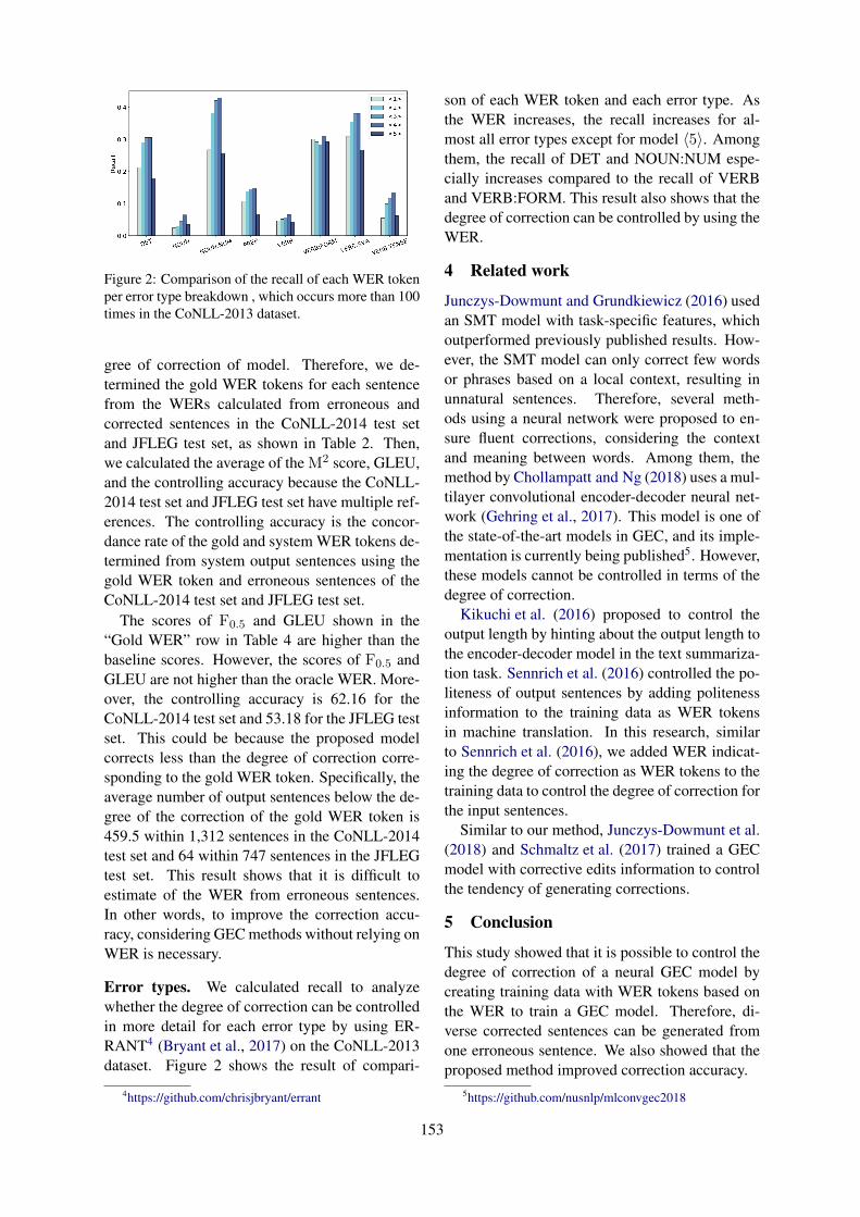
Figure 2: Comparison of the recall of each WER tokenper error type breakdown , which occurs more than 100times in the CoNLL-2013 dataset.

gree of correction of model. Therefore, we de-termined the gold WER tokens for each sentencefrom the WERs calculated from erroneous andcorrected sentences in the CoNLL-2014 test setand JFLEG test set, as shown in Table 2. Then,we calculated the average of the M2 score, GLEU,and the controlling accuracy because the CoNLL-2014 test set and JFLEG test set have multiple ref-erences. The controlling accuracy is the concor-dance rate of the gold and system WER tokens de-termined from system output sentences using thegold WER token and erroneous sentences of theCoNLL-2014 test set and JFLEG test set.

The scores of F0.5 and GLEU shown in the“Gold WER” row in Table 4 are higher than thebaseline scores. However, the scores of F0.5 andGLEU are not higher than the oracle WER. More-over, the controlling accuracy is 62.16 for theCoNLL-2014 test set and 53.18 for the JFLEG testset. This could be because the proposed modelcorrects less than the degree of correction corre-sponding to the gold WER token. Specifically, theaverage number of output sentences below the de-gree of the correction of the gold WER token is459.5 within 1,312 sentences in the CoNLL-2014test set and 64 within 747 sentences in the JFLEGtest set. This result shows that it is difficult toestimate of the WER from erroneous sentences.In other words, to improve the correction accu-racy, considering GEC methods without relying onWER is necessary.

Error types. We calculated recall to analyzewhether the degree of correction can be controlledin more detail for each error type by using ER-RANT4 (Bryant et al., 2017) on the CoNLL-2013dataset. Figure 2 shows the result of compari-

4https://github.com/chrisjbryant/errant

son of each WER token and each error type. Asthe WER increases, the recall increases for al-most all error types except for model ⟨5⟩. Amongthem, the recall of DET and NOUN:NUM espe-cially increases compared to the recall of VERBand VERB:FORM. This result also shows that thedegree of correction can be controlled by using theWER.

4 Related work

Junczys-Dowmunt and Grundkiewicz (2016) usedan SMT model with task-specific features, whichoutperformed previously published results. How-ever, the SMT model can only correct few wordsor phrases based on a local context, resulting inunnatural sentences. Therefore, several meth-ods using a neural network were proposed to en-sure fluent corrections, considering the contextand meaning between words. Among them, themethod by Chollampatt and Ng (2018) uses a mul-tilayer convolutional encoder-decoder neural net-work (Gehring et al., 2017). This model is one ofthe state-of-the-art models in GEC, and its imple-mentation is currently being published5. However,these models cannot be controlled in terms of thedegree of correction.

Kikuchi et al. (2016) proposed to control theoutput length by hinting about the output length tothe encoder-decoder model in the text summariza-tion task. Sennrich et al. (2016) controlled the po-liteness of output sentences by adding politenessinformation to the training data as WER tokensin machine translation. In this research, similarto Sennrich et al. (2016), we added WER indicat-ing the degree of correction as WER tokens to thetraining data to control the degree of correction forthe input sentences.

Similar to our method, Junczys-Dowmunt et al.(2018) and Schmaltz et al. (2017) trained a GECmodel with corrective edits information to controlthe tendency of generating corrections.

5 Conclusion

This study showed that it is possible to control thedegree of correction of a neural GEC model bycreating training data with WER tokens based onthe WER to train a GEC model. Therefore, di-verse corrected sentences can be generated fromone erroneous sentence. We also showed that theproposed method improved correction accuracy.

5https://github.com/nusnlp/mlconvgec2018

153

In the future, we would like to work on selectingthe best sentence from a wide variety of correctedsentences generated by a model varying the degreeof correction.

Acknowledgments

We thank Yangyang Xi of Lang-8, Inc. for kindlyallowing us to use the Lang-8 learner corpus.

ReferencesChristopher Bryant, Mariano Felice, and Ted Briscoe.

2017. Automatic annotation and evaluation of errortypes for grammatical error correction. In Proc. ofACL.

Christopher Bryant and Hwee Tou Ng. 2015. How farare we from fully automatic high quality grammati-cal error correction? In Proc. of ACL.

Shamil Chollampatt and Hwee Tou Ng. 2018. A multi-layer convolutional encoder-decoder neural networkfor grammatical error correction. In Proc. of AAAI.

Daniel Dahlmeier and Hwee Tou Ng. 2012. Bet-ter evaluation for grammatical error correction. InProc. of NAACL-HLT.

Daniel Dahlmeier, Hwee Tou Ng, and Siew Mei Wu.2013. Building a large annotated corpus of learnerEnglish: The NUS corpus of learner English. InProc. of BEA.

Jonas Gehring, Michael Auli, David Grangier, DenisYarats, and Yann N. Dauphin. 2017. Convolutionalsequence to sequence learning. In Proc. of ICML.

Kenneth Heafield. 2011. Kenlm: Faster and smallerlanguage model queries. In Proc. of WMT.

Marcin Junczys-Dowmunt and Roman Grundkiewicz.2016. Phrase-based machine translation is state-of-the-art for automatic grammatical error correction.In Proc. of EMNLP.

Marcin Junczys-Dowmunt, Roman Grundkiewicz,Shubha Guha, and Kenneth Heafield. 2018. Ap-proaching neural grammatical error correction as alow-resource machine translation task. In Proc. ofNAACL-HLT.

Yuta Kikuchi, Graham Neubig, Ryohei Sasano, HiroyaTakamura, and Manabu Okumura. 2016. Control-ling output length in neural encoder-decoders. InProc. of EMNLP.

Tomoya Mizumoto, Yuta Hayashibe, Mamoru Ko-machi, Masaaki Nagata, and Yuji Matsumoto. 2012.The effect of learner corpus size in grammatical er-ror correction of ESL writings. In Proc. of COLING.

Courtney Napoles, Keisuke Sakaguchi, and JoelTetreault. 2017. JFLEG: A fluency corpus andbenchmark for grammatical error correction. InProc. of EACL.

Hwee Tou Ng, Siew Mei Wu, Ted Briscoe, ChristianHadiwinoto, Raymond Hendy Susanto, and Christo-pher Bryant. 2014. The CoNLL-2014 shared task ongrammatical error correction. In Proc. of CoNLL.

Hwee Tou Ng, Siew Mei Wu, Yuanbin Wu, ChristianHadiwinoto, and Joel Tetreault. 2013. The CoNLL-2013 shared task on grammatical error correction.In Proc. of CoNLL.

Allen Schmaltz, Yoon Kim, Alexander Rush, and Stu-art Shieber. 2017. Adapting sequence models forsentence correction. In Proc. of EMNLP.

Rico Sennrich, Barry Haddow, and Alexandra Birch.2016. Controlling politeness in neural machinetranslation via side constraints. In Proc. of NAACL-HLT.

Ziang Xie, Guillaume Genthial, Stanley Xie, AndrewNg, and Dan Jurafsky. 2018. Noising and denoisingnatural language: Diverse backtranslation for gram-mar correction. In Proc. of NAACL-HLT.

154

Proceedings of the 57th Annual Meeting of the Association for Computational Linguistics: Student Research Workshop, pages 155–161Florence, Italy, July 28 - August 2, 2019. c©2019 Association for Computational Linguistics

From brain space to distributional space:the perilous journeys of fMRI decoding

Gosse Minnema and Aurelie HerbelotCenter for Mind/Brain Sciences

University of Trentogosseminnema@gmail.com

aurelie.herbelot@unitn.it

Abstract

Recent work in cognitive neuroscience hasintroduced models for predicting distribu-tional word meaning representations frombrain imaging data. Such models have greatpotential, but the quality of their predictionshas not yet been thoroughly evaluated from acomputational linguistics point of view. Dueto the limited size of available brain imagingdatasets, standard quality metrics (e.g. similar-ity judgments and analogies) cannot be used.Instead, we investigate the use of several al-ternative measures for evaluating the predicteddistributional space against a corpus-deriveddistributional space. We show that a state-of-the-art decoder, while performing impres-sively on metrics that are commonly usedin cognitive neuroscience, performs unexpect-edly poorly on our metrics. To address this, wepropose strategies for improving the model’sperformance. Despite returning promising re-sults, our experiments also demonstrate thatmuch work remains to be done before distribu-tional representations can reliably be predictedfrom brain data.

1 Introduction

Over the last decade, there has been a growingbody of research on the relationship between neu-ral and distributional representations of seman-tics (e.g., Mitchell et al., 2008; Anderson et al.,2013; Xu et al., 2016). This type of research isrelevant for cognitive neuroscientists interested inhow semantic information is represented in thebrain, as well as to computational linguists in-terested in the cognitive plausibility of distribu-tional models (Murphy et al., 2012). So far, moststudies investigated the correlation between neu-ral and distributional representations either by pre-dicting brain activity patterns from distributionalrepresentations (Mitchell et al., 2008; Abnar et al.,2018), or by using more direct correlation analyses

like Representational Similarity Analysis (RSA;introduced in Kriegeskorte et al. 2008) or simi-lar techniques (Anderson et al., 2013; Xu et al.,2016). Recently, however, a new model has beenproposed (Pereira et al., 2018) for decoding distri-butional representations from brain images.

This new approach is different from the earlierapproaches in a number of interesting ways. Firstof all, whereas predicting brain images from dis-tributional vectors tells us something about howmuch neurally relevant information is present indistributional representations, doing the predic-tion in the opposite way could tell us somethingabout how much of the textual co-occurrence in-formation that distributional models are based onis present in the brain. Brain decoding is also in-teresting from an NLP point of view: the output ofthe model is a word embedding that could, at leastin principle, be used in downstream tasks. Ulti-mately, a sufficiently accurate model for predict-ing distributional representations would amount toa sophisticated ‘mind reading’ device with numer-ous theoretical and practical applications.

Interestingly, despite being an early model andbeing trained on a (for NLP standards) very smalldataset, Pereira et al. (2018) already report im-pressively high accuracy scores for their decoder.However, despite these positive results, there arereasons to doubt whether it is really possible to de-code distributional representations from brain im-ages. Given the high-dimensional nature of bothneural and distributional representations, it is rea-sonable to expect that the mapping function be-tween the two spaces, if it indeed exists, is po-tentially very complicated, and, given the inher-ent noisiness of fMRI data, could be very hard tolearn, especially from a small dataset.

Moreover, we believe that the evaluation met-rics used in Pereira et al. (2018) are too limited.Both of these metrics, pairwise accuracy and rank

155

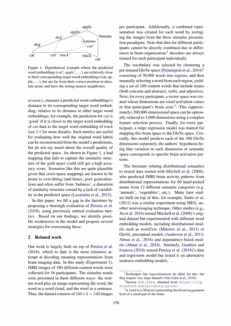
dog

cat truckcar

banana

apple

dog’

cat’ truck’

car’banana’

apple’

Figure 1: Hypothetical example where the predictedword embeddings (cat’, apple’, . . . ) are relatively closeto their corresponding target word embeddings (cat, ap-ple, . . . ), but are far from their correct position in abso-lute terms and have the wrong nearest neighbours.

accuracy, measure a predicted word embeddings’sdistance to its corresponding target word embed-ding, relative to its distance to other target wordembeddings; for example, the prediction for cat is‘good’ if it is closer to the target word embeddingof cat than to the target word embedding of truck(see 3.1 for more details). Such metrics are usefulfor evaluating how well the original word labelscan be reconstructed from the model’s predictions,but do not say much about the overall quality ofthe predicted space. As shown in Figure 1, a badmapping that fails to capture the similarity struc-ture of the gold space could still get a high accu-racy score. Scenarios like this are quite plausiblegiven that cross-space mappings are known to beprone to over-fitting (and hence, poor generaliza-tion) and often suffer from ‘hubness’, a distortionof similarity structure caused by a lack of variabil-ity in the predicted space (Lazaridou et al., 2015).

In this paper, we fill a gap in the literature byproposing a thorough evaluation of Pereira et al.(2018), using previously untried evaluation met-rics. Based on our findings, we identify possi-ble weaknesses in the model and propose severalstrategies for overcoming these.

2 Related work

Our work is largely built on top of Pereira et al.(2018), which to date is the most extensive at-tempt at decoding meaning representations frombrain imaging data. In this study (Experiment 1),fMRI images of 180 different content words werecollected for 16 participants. The stimulus wordswere presented in three different ways: the writ-ten word plus an image representing the word, theword in a word cloud, and the word in a sentence.Thus, the dataset consists of 180×3 = 540 images

per participant. Additionally, a combined repre-sentation was created for each word by averag-ing the images from the three stimulus presenta-tion paradigms. Note that data for different partic-ipants cannot be directly combined due to differ-ences in brain organization;1 decoders are alwaystrained for each participant individually.

The vocabulary was selected by clustering apre-trained GloVe space (Pennington et al., 2014)2

consisting of 30,000 words into regions, and thenmanually selecting a word from each region, yield-ing a set of 180 content words that include nouns(both concrete and abstract), verbs, and adjectives.Next, for every participant, a vector space was cre-ated whose dimensions are voxel activation valuesin that participant’s brain scan.3 This (approxi-mately) 200,000-dimensional space can be option-ally reduced to 5,000 dimensions using a complexfeature selection process. Finally, for every par-ticipant, a ridge regression model was trained formapping this brain space to the GloVe space. Cru-cially, this model predicts each of the 300 GloVedimensions separately, the authors’ hypothesis be-ing that variation in each dimension of semanticspace corresponds to specific brain activation pat-terns.

The literature relating distributional semanticsto neural data started with Mitchell et al. (2008),who predicted fMRI brain activity patterns fromdistributional representations for 60 hand-pickednouns from 12 different semantic categories (e.g.‘animals’, ‘vegetables’, etc.). Many later stud-ies built on top of this; for example, Sudre et al.(2012) was a similar experiment using MEG, an-other neuroimaging technique. Other studies (e.g.,Xu et al. 2016) reused Mitchell et al. (2008)’s orig-inal dataset but experimented with different wordembedding models, including distributional mod-els such as word2vec (Mikolov et al., 2013) orGloVe, perceptual models (Anderson et al., 2013;Abnar et al., 2018) and dependency-based mod-els (Abnar et al., 2018). Similarly, Gauthier andIvanova (2018) reused Pereira et al. (2018)’s dataand regression model but tested it on alternativesentence embedding models.

1Techniques like hyperalignment do allow for this, butthey require very large datasets (Van Uden et al., 2018).

2Version 42B.300d, obtained from https://nlp.stanford.edu/projects/glove/.

3A voxel is a 3D pixel representing the blood oxygenationlevel of a small part of the brain.

156

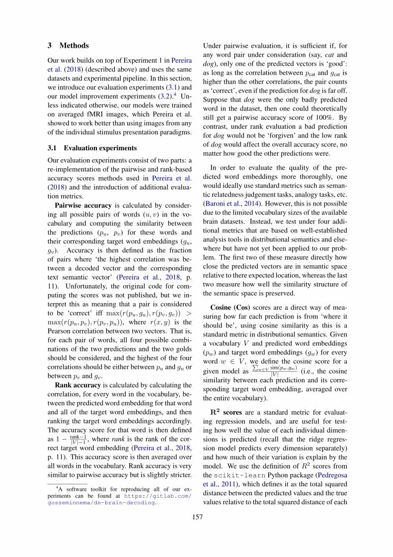
3 Methods

Our work builds on top of Experiment 1 in Pereiraet al. (2018) (described above) and uses the samedatasets and experimental pipeline. In this section,we introduce our evaluation experiments (3.1) andour model improvement experiments (3.2).4 Un-less indicated otherwise, our models were trainedon averaged fMRI images, which Pereira et al.showed to work better than using images from anyof the individual stimulus presentation paradigms.

3.1 Evaluation experiments

Our evaluation experiments consist of two parts: are-implementation of the pairwise and rank-basedaccuracy scores methods used in Pereira et al.(2018) and the introduction of additional evalua-tion metrics.

Pairwise accuracy is calculated by consider-ing all possible pairs of words (u, v) in the vo-cabulary and computing the similarity betweenthe predictions (pu, pv) for these words andtheir corresponding target word embeddings (gu,gv). Accuracy is then defined as the fractionof pairs where ‘the highest correlation was be-tween a decoded vector and the correspondingtext semantic vector’ (Pereira et al., 2018, p.11). Unfortunately, the original code for com-puting the scores was not published, but we in-terpret this as meaning that a pair is consideredto be ‘correct’ iff max(r(pu, gu), r(pv, gv)) >max(r(pu, pv), r(pv, pu)), where r(x, y) is thePearson correlation between two vectors. That is,for each pair of words, all four possible combi-nations of the two predictions and the two goldsshould be considered, and the highest of the fourcorrelations should be either between pu and gu orbetween pv and gv.

Rank accuracy is calculated by calculating thecorrelation, for every word in the vocabulary, be-tween the predicted word embedding for that wordand all of the target word embeddings, and thenranking the target word embeddings accordingly.The accuracy score for that word is then definedas 1 − rank−1

|V |−1 , where rank is the rank of the cor-rect target word embedding (Pereira et al., 2018,p. 11). This accuracy score is then averaged overall words in the vocabulary. Rank accuracy is verysimilar to pairwise accuracy but is slightly stricter.

4A software toolkit for reproducing all of our ex-periments can be found at https://gitlab.com/gosseminnema/ds-brain-decoding.

Under pairwise evaluation, it is sufficient if, forany word pair under consideration (say, cat anddog), only one of the predicted vectors is ‘good’:as long as the correlation between pcat and gcat ishigher than the other correlations, the pair countsas ‘correct’, even if the prediction for dog is far off.Suppose that dog were the only badly predictedword in the dataset, then one could theoreticallystill get a pairwise accuracy score of 100%. Bycontrast, under rank evaluation a bad predictionfor dog would not be ‘forgiven’ and the low rankof dog would affect the overall accuracy score, nomatter how good the other predictions were.

In order to evaluate the quality of the pre-dicted word embeddings more thoroughly, onewould ideally use standard metrics such as seman-tic relatedness judgement tasks, analogy tasks, etc.(Baroni et al., 2014). However, this is not possibledue to the limited vocabulary sizes of the availablebrain datasets. Instead, we test under four addi-tional metrics that are based on well-establishedanalysis tools in distributional semantics and else-where but have not yet been applied to our prob-lem. The first two of these measure directly howclose the predicted vectors are in semantic spacerelative to there expected location, whereas the lasttwo measure how well the similarity structure ofthe semantic space is preserved.

Cosine (Cos) scores are a direct way of mea-suring how far each prediction is from ‘where itshould be’, using cosine similarity as this is astandard metric in distributional semantics. Givena vocabulary V and predicted word embeddings(pw) and target word embeddings (gw) for everyword w ∈ V , we define the cosine score for agiven model as

∑w∈V sim(pw,gw)

|V | (i.e., the cosinesimilarity between each prediction and its corre-sponding target word embedding, averaged overthe entire vocabulary).

R2 scores are a standard metric for evaluat-ing regression models, and are useful for test-ing how well the value of each individual dimen-sions is predicted (recall that the ridge regres-sion model predicts every dimension separately)and how much of their variation is explain by themodel. We use the definition of R2 scores fromthe scikit-learn Python package (Pedregosaet al., 2011), which defines it as the total squareddistance between the predicted values and the truevalues relative to the total squared distance of each

157

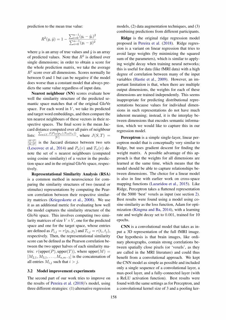
prediction to the mean true value:

R2(y, y) = 1−∑n−1

i=0 (yi − yi)2

∑n−1i=0 (yi − y)2

where y is an array of true values and y is an arrayof predicted values. Note that R2 is defined oversingle dimensions; in order to obtain a score forthe whole prediction matrix, we take the averageR2 score over all dimensions. Scores normally liebetween 0 and 1 but can be negative if the modeldoes worse than a constant model that always pre-dicts the same value regardless of input data.

Nearest neighbour (NN) scores evaluate howwell the similarity structure of the predicted se-mantic space matches that of the original GloVespace. For each word in V , we take its predictedand target word embeddings, and then compare theten nearest neighbours of these vectors in their re-spective spaces. The final score is the mean Jac-card distance computed over all pairs of neighbourlists:

∑w∈V J(P10(pw),T10(tw))

|V | , where J(S, T ) =|S∩T ||S∪T | is the Jaccard distance between two sets(Lescovec et al., 2014) and Pn(v) and Tn(v) de-note the set of n nearest neighbours (computedusing cosine similarity) of a vector in the predic-tion space and in the original GloVe space, respec-tively.

Representational Similarity Analysis (RSA)is a common method in neuroscience for com-paring the similarity structures of two (neural orstimulus) representations by computing the Pear-son correlation between their respective similar-ity matrices (Kriegeskorte et al., 2008). We useit as an additional metric for evaluating how wellthe model captures the similarity structure of theGloVe space. This involves computing two simi-larity matrices of size V ×V , one for the predictedspace and one for the target space, whose entriesare defined as Pi,j = r(pi, pj) and Ti,j = r(ti, tj),respectively. Then, the representational similarityscore can be defined as the Pearson correlation be-tween the two upper halves of each similarity ma-trix: r(upper(P ), upper(T )), where upper(M) =[M2,1,M3,1, . . . ,Mn,m−1] is the concatenation ofall entries Mi,j such that i > j.

3.2 Model improvement experiments

The second part of our work tries to improve onthe results of Pereira et al. (2018)’s model, usingthree different strategies: (1) alternative regression

models, (2) data augmentation techniques, and (3)combining predictions from different participants.

Ridge is the original ridge regression modelproposed in Pereira et al. (2018). Ridge regres-sion is a variant on linear regression that tries toavoid large weights (by minimizing the squaredsum of the parameters), which is similar to apply-ing weight decay when training neural networks;this is useful for data (like fMRI data) with a highdegree of correlation between many of the inputvariables (Hastie et al., 2009). However, an im-portant limitation is that, when there are multipleoutput dimensions, the weights for each of thesedimensions are trained independently. This seemsinappropriate for predicting distributional repre-sentations because values for individual dimen-sions in such representations do not have muchinherent meaning; instead, it is the interplay be-tween dimensions that encodes semantic informa-tion, which we would like to capture this in ourregression model.

Perceptron is a simple single-layer, linear per-ceptron model that is conceptually very similar toRidge, but uses gradient descent for finding theweight matrix. A possible advantage of this ap-proach is that the weights for all dimensions arelearned at the same time, which means that themodel should be able to capture relationships be-tween dimensions. The choice for a linear modelis also in line with earlier work on cross-spacemapping functions (Lazaridou et al., 2015). LikeRidge, Perceptron takes a flattened representationof the 5000 ‘best’ voxels as input (see section 2).Best results were found using a model using co-sine similarity as the loss function, Adam for opti-mization (Kingma and Ba, 2014), with a learningrate and weight decay set to 0.001, trained for 10epochs.

CNN is a convolutional model that takes as in-put a 3D representation of the full fMRI image.Our hypothesis is that brain images, like ordi-nary photographs, contain strong correlations be-tween spatially close pixels (or ‘voxels’, as theyare called in the MRI literature) and could thusbenefit from a convolutional approach. We keptthe CNN model as simple as possible and includedonly a single sequence of a convolutional layer, amax-pool layer, and a fully-connected layer (witha ReLU activation function). Best results werefound with the same settings as for Perceptron, anda convolutional kernel size of 3 and a pooling ker-

158

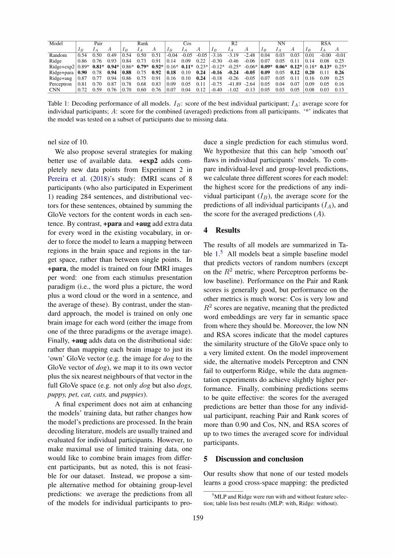
Model Pair Rank Cos R2 NN RSAIB IA A IB IA A IB IA A IB IA A IB IA A IB IA A

Random 0.54 0.50 0.49 0.54 0.50 0.51 -0.04 -0.05 -0.05 -3.16 -3.19 -2.48 0.04 0.03 0.03 0.01 -0.00 -0.01Ridge 0.86 0.76 0.93 0.84 0.73 0.91 0.14 0.09 0.22 -0.30 -0.46 -0.06 0.07 0.05 0.11 0.14 0.08 0.25Ridge+exp2 0.89* 0.81* 0.94* 0.86* 0.79* 0.92* 0.16* 0.11* 0.23* -0.12* -0.25* -0.06* 0.09* 0.06* 0.12* 0.18* 0.13* 0.25*Ridge+para 0.90 0.78 0.94 0.88 0.75 0.92 0.18 0.10 0.24 -0.16 -0.24 -0.05 0.09 0.05 0.12 0.20 0.11 0.26Ridge+aug 0.87 0.77 0.94 0.86 0.75 0.91 0.16 0.10 0.24 -0.18 -0.26 -0.05 0.07 0.05 0.11 0.16 0.09 0.25Perceptron 0.81 0.70 0.87 0.78 0.68 0.83 0.09 0.05 0.11 -0.75 -41.89 -2.64 0.05 0.04 0.07 0.09 0.05 0.16CNN 0.72 0.59 0.76 0.70 0.60 0.76 0.07 0.04 0.12 -0.40 -1.02 -0.13 0.05 0.03 0.05 0.08 0.03 0.13

Table 1: Decoding performance of all models. IB : score of the best individual participant; IA: average score forindividual participants; A: score for the combined (averaged) predictions from all participants. ‘*’ indicates thatthe model was tested on a subset of participants due to missing data.

nel size of 10.We also propose several strategies for making

better use of available data. +exp2 adds com-pletely new data points from Experiment 2 inPereira et al. (2018)’s study: fMRI scans of 8participants (who also participated in Experiment1) reading 284 sentences, and distributional vec-tors for these sentences, obtained by summing theGloVe vectors for the content words in each sen-tence. By contrast, +para and +aug add extra datafor every word in the existing vocabulary, in or-der to force the model to learn a mapping betweenregions in the brain space and regions in the tar-get space, rather than between single points. In+para, the model is trained on four fMRI imagesper word: one from each stimulus presentationparadigm (i.e., the word plus a picture, the wordplus a word cloud or the word in a sentence, andthe average of these). By contrast, under the stan-dard approach, the model is trained on only onebrain image for each word (either the image fromone of the three paradigms or the average image).Finally, +aug adds data on the distributional side:rather than mapping each brain image to just its‘own’ GloVe vector (e.g. the image for dog to theGloVe vector of dog), we map it to its own vectorplus the six nearest neighbours of that vector in thefull GloVe space (e.g. not only dog but also dogs,puppy, pet, cat, cats, and puppies).

A final experiment does not aim at enhancingthe models’ training data, but rather changes howthe model’s predictions are processed. In the braindecoding literature, models are usually trained andevaluated for individual participants. However, tomake maximal use of limited training data, onewould like to combine brain images from differ-ent participants, but as noted, this is not feasi-ble for our dataset. Instead, we propose a sim-ple alternative method for obtaining group-levelpredictions: we average the predictions from allof the models for individual participants to pro-

duce a single prediction for each stimulus word.We hypothesize that this can help ‘smooth out’flaws in individual participants’ models. To com-pare individual-level and group-level predictions,we calculate three different scores for each model:the highest score for the predictions of any indi-vidual participant (IB), the average score for thepredictions of all individual participants (IA), andthe score for the averaged predictions (A).

4 Results

The results of all models are summarized in Ta-ble 1.5 All models beat a simple baseline modelthat predicts vectors of random numbers (excepton the R2 metric, where Perceptron performs be-low baseline). Performance on the Pair and Rankscores is generally good, but performance on theother metrics is much worse: Cos is very low andR2 scores are negative, meaning that the predictedword embeddings are very far in semantic spacefrom where they should be. Moreover, the low NNand RSA scores indicate that the model capturesthe similarity structure of the GloVe space only toa very limited extent. On the model improvementside, the alternative models Perceptron and CNNfail to outperform Ridge, while the data augmen-tation experiments do achieve slightly higher per-formance. Finally, combining predictions seemsto be quite effective: the scores for the averagedpredictions are better than those for any individ-ual participant, reaching Pair and Rank scores ofmore than 0.90 and Cos, NN, and RSA scores ofup to two times the averaged score for individualparticipants.

5 Discussion and conclusion

Our results show that none of our tested modelslearns a good cross-space mapping: the predicted

5MLP and Ridge were run with and without feature selec-tion; table lists best results (MLP: with, Ridge: without).

159

semantic vectors are far from their expected loca-tion and fail to capture the target space’s similar-ity structure. Meanwhile, excellent performance isachieved on pairwise and rank-based classificationtasks, which implies that the predictions containsufficient information for reconstructing stimulusword labels. These contradictory results suggesta situation not unlike the one sketched in Fig. 1.This means that from a linguistic point of view,early claims about the success of brain decodingtechniques should be taken cautiously.

Two obvious questions are how such a situa-tion can arise and how it can be prevented. Firstof all, it seems likely that there is simply notenough training data to learn a precise mapping;the results of our experiments with adding ‘ex-tra’ data are in line with this hypothesis. More-over, the fact that all vocabulary words are rela-tively far from each other could make the mappingproblem harder. For example, the ‘correct’ near-est neighbours of dog are pig, toy, and bear; themodel might predict fish, play and bird, which are‘wrong’ but intuitively do not seem much worse.We speculate that using a dataset with a more di-verse similarity structure (i.e. where each word isvery close to some words and further from oth-ers) could help the model learn a better map-ping. Yet another issue is contextuality: stan-dard GloVe embeddings are context-independent(i.e. a given word always has the same repre-sentation regardless of its word sense and syntac-tic position in the sentence), whereas the brainimages are not because they were obtained us-ing contextualized stimuli (e.g. a word in a sen-tence). Hence, an interesting question is whethertrying to predict contextualized word embeddings,obtained using more traditional distributional ap-proaches (e.g. Erk and Pado, 2010; Thater et al.,2011) or deep neural language models (e.g. De-vlin et al., 2018), would be an easier task. Fi-nally, the success of our experiment with com-bining participants suggests that using group-leveldata can help overcome the challenges inherent inpredicting corpus-based (GloVe) representationsfrom individual-level (brain) representations.

Acknowledgments

The first author of this paper (GM) was enrolledin the European Master Program in Language andCommunication Technologies (LCT) while writ-ing the paper, and was supported by the European

Union Erasmus Mundus program.

ReferencesSamira Abnar, Rasyan Ahmed, Max Mijnheer, and

Willem Zuidema. 2018. Experiential, distributionaland dependency-based word embeddings have com-plementary roles in decoding brain activity. In Pro-ceedings of the 8th Workshop on Cognitive Modelingand Computational Linguistics (CMCL 2018), pages57–66.

Andrew J. Anderson, Elia Bruni, Ulisse Bordignon,Massimo Poesio, and Marco Baroni. 2013. Ofwords, eyes and brains: Correlating image-baseddistributional semantic models with neural represen-tations of concepts. In Proceedings of the 2013 Con-ference on Empirical Methods in Natural LanguageProcessing, pages 1960–1970.

Marco Baroni, Georgiana Dinu, and GermanKruszewski. 2014. Don’t count, predict! asystematic comparison of context-counting vs.context-predicting semantic vectors. In Proceedingsof the 52nd Annual Meeting of the Associationfor Computational Linguistics (Volume 1: LongPapers), volume 1, pages 238–247.

Jacob Devlin, Ming-Wei Chang, Kenton Lee, andKristina Toutanova. 2018. BERT: pre-training ofdeep bidirectional transformers for language under-standing. CoRR, abs/1810.04805.

Katrin Erk and Sebastian Pado. 2010. Examplar-basedmodels for word meaning in context. In Proceedingsof the ACL 2010 Conference Short Papers, pages92–97.

Jon Gauthier and Anna Ivanova. 2018. Doesthe brain represent words? an evaluation ofbrain decoding studies of language understanding.CoRR, abs/1806.00591. ArXiv preprint, http://arxiv.org/abs/1806.00591.

Trevor Hastie, Robert Tibshirani, and J. H. Friedman.2009. The Elements of Statistical Learning: DataMining, Inference, and Prediction., second edition,corrected 7th printing edition. Springer Series inStatistics. Springer.

Diederik P. Kingma and Jimmy Lei Ba. 2014. Adam:A method for stochastic optimization. CoRR,abs/1412.6980. ArXiv preprint, http://arxiv.org/abs/1412.6980.

Nikolaus Kriegeskorte, Marieke Mur, and Peter Ban-dettini. 2008. Representational similarity analysis:connecting the branches of systems neuroscience.Frontiers in Systems Neuroscience, 2.

Angeliki Lazaridou, Georgina Dinu, and Marco Ba-roni. 2015. Hubness and polution: Delving into

160

cross-space mapping for zero-shot learning. In Pro-ceedings of the 53rd Annual Meeting of the Associ-ation for Computational Linguistics and the 7th In-ternational Joint Conference on Natural LanguageProcessing, pages 270–280.

Jure Lescovec, Anand Rajaraman, and Jeffrey DavidUllman. 2014. Mining of Massive Datasets, 2nd edi-tion. Cambridge University Press. Online version,http://www.mmds.org/#ver21.

Tomas Mikolov, Kai Chen, Greg Corrado, and JeffreyDean. 2013. Efficient estimation of word repre-sentations in vector space. CoRR, abs/1301.3781.http://arxiv.org/abs/1301.3781.

Tom M. Mitchell, Svetlana V. Shinkareva, AndrewCarlson, Kai-Min Chang, Vicente L. Malave,Robert A. Mason, and Marcel Adam Just. 2008.Predicting human brain activity associated with themeanings of nouns. Science, 320(5880):1191–1195.

Brian Murphy, Partha Talukdar, and Tom Mitchell.2012. Selecting corpus-semantic models for neu-rolinguistic decoding. In Proceedings of the FirstJoint Conference on Lexical and ComputationalSemantics-Volume 1: Proceedings of the main con-ference and the shared task, and Volume 2: Pro-ceedings of the Sixth International Workshop on Se-mantic Evaluation, pages 114–123. Association forComputational Linguistics.

Fabian Pedregosa, Gael Varoquaux, Alexandre Gram-fort, Vincent Michel, Bertrand Thirion, OlivierGrisel, Mathieu Blondel, Peter Prettenhofer, RonWeiss, Vincent Dubourg, Jake Vanderplas, Alexan-dre Passos, David Cournapeau, Matthieu Brucher,Matthieu Perrot, and Edouard Duchesnay. 2011.Scikit-learn: Machine learning in Python. Journalof Machine Learning Research, 12:2825–2830.

Jeffrey Pennington, Richard Socher, and Christo-pher D. Manning. 2014. Glove: Global vectors forword representation. In Proceedings of the 2014Conference on Empirical Methods in Natural Lan-guage Processing (EMNLP), pages 1532–1543.

Francisco Pereira, Bin Lou, Brianna Pritchett, SamuelRitter, Samuel J. Gershman, Nancy Kanwisher,Matthew Botvinick, and Evelina Fedorenko. 2018.Toward a universal decoder of linguistic meaningfrom brain activation. Nature Communications,9(963).

Gustavo Sudre, Dean Pomerleau, Palatucci Mark, LeilaWehbe, Alona Fyshe, Riita Salmelin, and TomMitchell. 2012. Tracking neural coding of percep-tual and semantic features of concrete nouns. Neu-roImage, 62:451–463.

Stefan Thater, Hagen Furstenau, and Manfred Pinkel.2011. Word meaning in context: A simple and ef-fective vector model. In Proceedings of the 5th In-ternational Joint Conference on Natural LanguageProcessing, pages 1134–1143.

Cara E. Van Uden, Samuel A. Nastase, Andrew C. Con-nolly, Ma Feilong, Isabella Hansen, M. Ida Gobbini,and James V. Haxby. 2018. Modeling semantic en-coding in a common neural representational space.Frontiers in Neuroscience, 12.

Haoyan Xu, Brian Murphy, and Alona Fyshe. 2016.Brainbench: A brain-image test suite for distribu-tional semantic models. In Proceedings of the 2016Conference on Empirical Methods in Natural Lan-guage Processing, pages 2017–2021.

161

Proceedings of the 57th Annual Meeting of the Association for Computational Linguistics: Student Research Workshop, pages 162–168Florence, Italy, July 28 - August 2, 2019. c©2019 Association for Computational Linguistics

Towards incremental learning of word embeddings using contextinformativeness

Alexandre KabbachDept. of LinguisticsUniversity of Geneva

Center for Mind/Brain SciencesUniversity of Trento

Kristina GulordavaDept. of Translation

and Language SciencesUniversitat Pompeu Fabra

firstname.lastname@unige.ch;upf.edu;unitn.it

Aurelie HerbelotCenter for Mind/Brain Sciences,

Dept. of Information Engineeringand Computer ScienceUniversity of Trento

Abstract

In this paper, we investigate the task of learn-ing word embeddings from very sparse data inan incremental, cognitively-plausible way. Wefocus on the notion of informativeness, that is,the idea that some content is more valuableto the learning process than other. We fur-ther highlight the challenges of online learn-ing and argue that previous systems fall shortof implementing incrementality. Concretely,we incorporate informativeness in a previouslyproposed model of nonce learning, using it forcontext selection and learning rate modulation.We test our system on the task of learning newwords from definitions, as well as on the taskof learning new words from potentially unin-formative contexts. We demonstrate that infor-mativeness is crucial to obtaining state-of-the-art performance in a truly incremental setup.

1 Introduction

Distributional semantics models such as word em-beddings (Bengio et al., 2003; Collobert et al.,2011; Huang et al., 2012; Mikolov et al., 2013b)notoriously require exposure to a large amount ofcontextual data in order to generate high qualityvector representations of words. This poses prac-tical challenges when the available training datais scarce, or when distributional models are in-tended to mimic humans’ word learning abilitiesby constructing reasonable word representationsfrom limited observations (Lazaridou et al., 2017).In recent work, various approaches have been pro-posed to tackle these problems, ranging from task-specific auto-encoders generating word embed-dings from dictionary definitions only (Bosc andVincent, 2017, 2018), to Bayesian models used foracquiring definitional properties of words via one-shot learning (Wang et al., 2017), or recursive neu-ral network models making use of morphologicalstructure (Luong et al., 2013).

Arguing that the ideal model should rely onan all-purpose architecture able to learn fromany amount of data, Herbelot and Baroni (2017)proposed a model called Nonce2Vec (N2V), de-signed as a modification of Word2Vec (W2V;Mikolov et al., 2013b), refactored to allow in-cremental learning. The model was tested ontwo datasets: a) the newly introduced defini-tional dataset, where the task is to learn a nonceword from its Wikipedia definition; and b) thechimera dataset of Lazaridou et al. (2017), wherethe task is to reproduce human similarity judge-ments related to a novel word observed in 2-6 ran-domly extracted sentences. The N2V model per-formed much better than W2V on both datasetsbut failed to outperform a basic additive model onthe chimera dataset, leading the authors to hypoth-esise that their system would need to perform con-tent selection to deal with the potentially uninfor-mative chimera sentences.

There are two motivations to the present work.The first is to provide a formal definition of thenotion of informativeness applied to both senten-tial context (as a whole) and context words (takenindividually). To do so, we rely on the intuitionthat an informative context is a context that is morespecific to a given target, and that this notion ofcontext specificity can be quantified by computingthe entropy of the probability distribution gener-ated by a language model over a set of vocabularywords, given the context.

The secondary motivation of this work lays inconsiderations over incrementality. We show thatN2V itself did not fully implement its ideal of‘online’ concept learning. We also point out thatarchitectures that have outperformed N2V sinceits inception actually move even further from thisideal. In contrast, we attempt to make our architec-ture as close as possible to a realistic belief updatesystem, and we demonstrate that informativeness

162

is an essential part of retaining acceptable perfor-mance in such a challenging setting.

2 Related work

The original Nonce2Vec (N2V) model is designedto simulate new word acquisition by an adultspeaker who already masters a substantial vocab-ulary. The system uses some ‘background’ lexicalknowledge in the shape of a distributional spaceacquired over a large text corpus. A novel word isthen learnt by using information present in its con-text sentence. To achieve its goal, N2V proposessome modifications to the original Word2Vec ar-chitecture to make it suitable for novel word learn-ing. Three main changes are suggested: a) thelearning rate should be greatly heightened to allowfor learning via backpropagation using only thelimited amount of data; b) random subsamplingshould be reduced to a minimum so that all avail-able data is used; and c) embeddings in the back-ground should be ‘frozen’ so that the high learn-ing rate is prevented from ‘unlearning’ old lexicalknowledge in favour of the scarce, and potentiallyuninformative, new context information.

Recent work outperforms N2V on thechimera (Khodak et al., 2018; Schick andSchutze, 2019a) and the definitional (Schick andSchutze, 2018) datasets (see §1 for a descriptionof the datasets). However, they both deviate fromthe original motivation of N2V which is to learnword representations incrementally from anyamount of data. Instead, those state-of-the-artmodels rely—at least in part—on a learned linearregression matrix which is fixed for a given corpusand thus does not lend itself well to incrementallearning.

Our work follows the philosophy of N2V butpushes the notion of incrementality further byidentifying aspects of the original system that infact do not play well with true online learning. Fora start, the original model is not fully incrementalas it adopts a one-shot evaluation setup where eachtest instance is considered individually and wherethe background model is reloaded from scratch ateach test iteration. This does not test how the sys-tem would react to learning multiple nonces oneafter the other (as humans do in the course oftheir lives). Related to this, whilst ‘freezing’ back-ground vectors makes sense as a safety net whenusing very high learning rates, it similarly goesagainst the notion of incrementality. In any re-

alistic setup, indeed, we would like newly learntwords to inform our background lexical knowl-edge and become part of that background them-selves, being refined over time and contributingto acquiring the next nonce. Following this phi-losophy, the system we present in this paper doesaway with freezing previously learnt embeddingsand does not reload the background model at eachtest iteration.

We should further note that our work on in-formativeness echoes recent research on the useof attention mechanisms. Vaswani et al. (2017),followed by Devlin et al. (2018) and Schick andSchutze (2019b), have shown that such mecha-nisms can provide very powerful tools to buildsentence and contextualised word embeddingswhich are amenable to transfer learning tasks.However, we note that from our point of view,these systems suffer from the same problem as thepreviously mentioned architectures: the underly-ing model consists of a large set of parameterswhich can be used to learn a task-specific regres-sion. It is not designed to be updated with eachnew encountered experience.

3 Model

Let us consider context to be defined as a win-dow of ±n words around a given target. We de-fine two specific functions: context informative-ness (CI) which characterises how informative anentire context is with respect to its correspondingtarget; and context word informativeness (CWI)which characterises how informative a particularcontext item is with respect to the target. For in-stance, if target chases is seen in context c = the,cat, the, mouse, the context informativeness is theinformativeness of c, and the context word infor-mativeness can be computed for each element in c,with the expectation, in this case, that the might beless informative than cat or mouse. The CWI mea-sure is dependent on CI, as we proceed to show.

3.1 Context informativenessLet us consider a sequence c of n context itemsc = c1 . . . cn. We define the context informative-ness of a context sequence c as:

CI(c) = 1 +1

ln(|V|)∑

w∈Vp(w|c) ln p(w|c) (1)

CI is a slight modification of the Shannon en-tropy H = −∑w∈V p(w|c) ln p(w|c), normalised

163

over the cardinality of the vocabulary |V| to out-put values in [0, 1]. In this work, we use a CBOWmodel (Mikolov et al., 2013a) to obtain the proba-bility distribution p(w|c). We use CBOW becauseit is the simplest word-generation model whichtakes the relation between context words into ac-count, i.e., in contrast to skipgram.

A context will be considered maximally infor-mative (CI = 1) if only a single vocabulary itemis predicted to occur in context c with a non-nullprobability. Conversely, a context will be consid-ered minimally informative (CI = 0) if all vocab-ulary items are predicted to occur in context cwithequal probability. CI should therefore quantifyhow specific a given context is regarding a giventarget.

3.2 Context word informativenessLet us consider c6=i = c1 . . . ci−1, ci+1 . . . cn tobe the sequence of context items taken from c towhich the ith item has been removed. We definethe context word informativeness of a context itemci in a context sequence c as:

CWI(ci) = CI(c)− CI(c6=i) (2)

CWI outputs values in [−1, 1]: a context wordci will be considered maximally informative(CWI = 1) if removing it from a maximally in-formative context leads to a minimally informativeone. Conversely, a context word ci will be con-sidered minimally informative (CWI = −1) ifremoving it from a minimally informative contextleads to a maximally informative one.

3.3 CWI-augmented Nonce2VecAs explained in §2, N2V introduces several high-level changes to the W2V architecture to achievelearning from very sparse data. In practice, thistranslates into the following design choices: a)nonces are initialised by summing context wordembeddings (after subsampling); and b) noncesare trained with an adapted skipgram function in-corporating decaying window size, sampling andlearning rates at each iteration, while all other vec-tors remain frozen. The learning rate is computedvia α = α0e

−λt with a high α0.The modifications we propose are as follows:

i) we incorporate informativeness into the initial-isation phase by summing over the set of contextwords with positive CWI only; ii) we train on theentire context without subsampling and window

decay; and iii) we remove freezing and computethe learning rate as a function of CWI for eachcontext item ci via:

α(ci) = αmaxetanh(β∗CWI(ci))+1 − 1

e2 − 1(3)

The purpose of equation 3 is to modulate the learn-ing rate depending on the context word informa-tiveness for a context–target pair: α should bemaximal (α = αmax, where αmax is a hyper-parameter) when context is maximally informa-tive (CWI = 1) and minimal (α = 0) when con-text is minimally informative (CWI = −1). Thefunction x 7→ ex+1−1

e2−1 is therefore designed as a lo-gistic “S-shape” function with domain [−1, 1] →[0, 1]. In practice, CWI values are highly depen-dant on the language model used and may end upall being close to 0 (±0.01 with our CBOW modelfor instance). The tanh function and the β param-eter are therefore added to compensate for this ef-fect that would otherwise produce identical learn-ing rates for all target-context pairs, regardless ofCWI values.

4 Experimental setup and evaluation

To test the robustness of the results of Herbelotand Baroni (2017), we retrain a skipgram back-ground model with the same hyperparameters butfrom the more recent Wikipedia snapshot of Jan-uary 2019, and obtain a similar correlation ratioon the MEN similarity dataset (Bruni et al., 2014):ρ = 0.74 vs ρ = 0.75 for Herbelot and Baroni(2017). Probability distributions used for com-puting CI and CWI are generated with a CBOWmodel trained with gensim (Rehurek and Sojka,2010) on the same Wikipedia snapshot as our skip-gram background model, and with the same hy-perparameters. For the CWI-based learning ratecomputation, we set αmax = 1, chosen accordingto α0 in the original N2V for fair comparison; andβ = 1000, chosen given min and max CWI val-ues output by CBOW to produce tanh(β ∗ x) val-ues distributed across [−1, 1] and apply a learningrate αmax = 1 to maximally informative contextwords.

We report results on the definitional and thechimera datasets (see §1). The definitional datasetcontains first sentences from Wikipedia for 1000words: e.g. Insulin is a peptide hormone pro-duced by beta cells of the pancreatic islets, where

164

the task is to learn the nonce insulin. Evalua-tion is performed on 300 test instances in termsof Median Rank (MR) and Mean ReciprocalRank (MRR). That is, for each instance, the Recip-rocal Rank of the gold vector (the one that wouldbe obtained by training standard W2V over theentire corpus) is computed over the sorted list ofneighbours of the predicted representation.

The chimera dataset simulates a nonce situationwhere speaker encounters words for the first timein naturally-occurring (and not necessarily infor-mative) sentences. Each nonce instance in the datais associated with 2 (L2), 4 (L4) or 6 (L6) sen-tences showing the nonce in context, and a set ofsix word probes human-annotated for similarityto the nonce. For instance, the nonce VALTUORis shown in Canned sardines and VALTUOR be-tween two slices of wholemeal bread and thinlyspread Flora Original [...], and its similarity as-sessed with respect to rhubarb, onion, pear, straw-berry, limousine and cushion. Evaluation is per-formed on 110 test instances by computing theSpearman correlation between the similarities out-put by the system for each nonce-probe pair andthe similarities from the human subjects.

We evaluate both datasets using a one-shotsetup, as per the original N2V paper: each nonceword in considered individually and the back-ground model is reloaded at each test iteration. Wefurther propose an incremental evaluation setupwhere the background model is loaded only onceat the beginning of testing, keeping its word vec-tors modifiable during subsequent learning, andwhere each newly learned nonce representation isadded to the background model. As performancein the incremental setup proved to be dependenton the order of the test items, we report averageand standard deviation scores computed from 10test runs where the test set is shuffled each time.

5 Results

5.1 Improving additive modelsHerbelot and Baroni (2017) show that a simple ad-ditive model provides an extremely strong base-line for nonce learning. So we first measure thecontribution of our notion of informativeness tothe context filtering module of a sum model. Com-parison takes place across four settings: a) nofilter, where all words are retained; b) random,which applies standard subsampling with a sam-ple rate of 10,000, following the original N2V ap-

proach; c) self, where all items found in trainingwith a frequency above a given threshold are dis-carded;1 and d) CWI, which only retains contextitems with a positive CWI value.

Our results on the definitional dataset, displayedin Table 1, show a consistent hierarchy of filterswith the SUM CWI model outperforming all otherSUM models, in both one-shot and incrementalevaluation setups. Results on the chimera dataset,displayed in Table 2, are not as clear-cut, althoughthey do exhibit a similar trend on both L4 andL6 test sets, with the notable result of achievingstate-of-the-art performances with our SUM CWImodel on the L4 and L6 test sets in incrementalsetup, and near state-of-the-art performance on theL6 test set in one-shot setup. This confirms onceagain that additive models can provide very robustbaselines.

Qualitatively, the contribution of each filter onthe definitional dataset can be exemplified onthe following sentence, with nonce word Honey-well: “Honeywell International Inc is an Amer-ican multinational conglomerate company thatproduces [...] aerospace systems for a wide va-riety of customers from private consumers to ma-jor corporations and governments.”. The no-filteradditive model outputs a rank of 383 (the gold vec-tor for honeywell is found to be the 383th clos-est neighbour of the predicted vector). The ran-dom model randomly removes most (but not all)high frequency words before summing, outputtinga rank of 192 (filtered-out words include also con-tent words like international or company). Theself -information model reduces the size of thecontext words set even further by removing allhigh-frequency words left over by the random pro-cess (rank 170). Finally, the CWI model outputsthe best rank at 85, removing all function wordswhile keeping some useful high-frequency wordssuch as international or company.

5.2 Improving neural models in one-shotsettings

Our results for neural models are also displayedin Table 1 and Table 2: as-is refers to the orig-inal N2V system; CWI init is N2V as-is withCWI-based context filtering instead of subsam-pling; and CWI alpha is a model with a CWI-based

1We take the log of the sample int values computed bygensim for each word during training, keeping only itemswith log values above 22, which gave us the best perfor-mances overall.

165

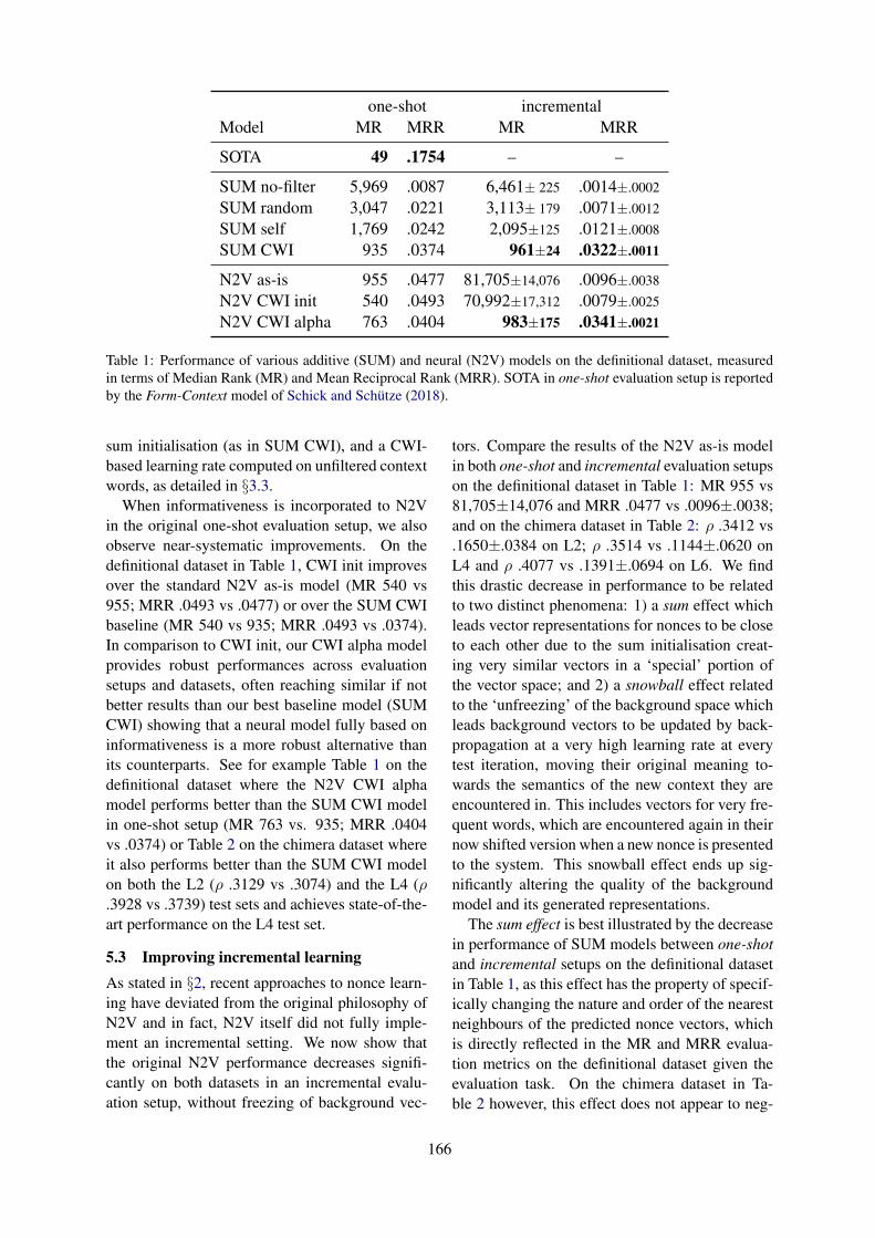
one-shot incrementalModel MR MRR MR MRR

SOTA 49 .1754 – –

SUM no-filter 5,969 .0087 6,461± 225 .0014±.0002

SUM random 3,047 .0221 3,113± 179 .0071±.0012

SUM self 1,769 .0242 2,095±125 .0121±.0008

SUM CWI 935 .0374 961±24 .0322±.0011

N2V as-is 955 .0477 81,705±14,076 .0096±.0038

N2V CWI init 540 .0493 70,992±17,312 .0079±.0025

N2V CWI alpha 763 .0404 983±175 .0341±.0021

Table 1: Performance of various additive (SUM) and neural (N2V) models on the definitional dataset, measuredin terms of Median Rank (MR) and Mean Reciprocal Rank (MRR). SOTA in one-shot evaluation setup is reportedby the Form-Context model of Schick and Schutze (2018).

sum initialisation (as in SUM CWI), and a CWI-based learning rate computed on unfiltered contextwords, as detailed in §3.3.

When informativeness is incorporated to N2Vin the original one-shot evaluation setup, we alsoobserve near-systematic improvements. On thedefinitional dataset in Table 1, CWI init improvesover the standard N2V as-is model (MR 540 vs955; MRR .0493 vs .0477) or over the SUM CWIbaseline (MR 540 vs 935; MRR .0493 vs .0374).In comparison to CWI init, our CWI alpha modelprovides robust performances across evaluationsetups and datasets, often reaching similar if notbetter results than our best baseline model (SUMCWI) showing that a neural model fully based oninformativeness is a more robust alternative thanits counterparts. See for example Table 1 on thedefinitional dataset where the N2V CWI alphamodel performs better than the SUM CWI modelin one-shot setup (MR 763 vs. 935; MRR .0404vs .0374) or Table 2 on the chimera dataset whereit also performs better than the SUM CWI modelon both the L2 (ρ .3129 vs .3074) and the L4 (ρ.3928 vs .3739) test sets and achieves state-of-the-art performance on the L4 test set.

5.3 Improving incremental learningAs stated in §2, recent approaches to nonce learn-ing have deviated from the original philosophy ofN2V and in fact, N2V itself did not fully imple-ment an incremental setting. We now show thatthe original N2V performance decreases signifi-cantly on both datasets in an incremental evalu-ation setup, without freezing of background vec-

tors. Compare the results of the N2V as-is modelin both one-shot and incremental evaluation setupson the definitional dataset in Table 1: MR 955 vs81,705±14,076 and MRR .0477 vs .0096±.0038;and on the chimera dataset in Table 2: ρ .3412 vs.1650±.0384 on L2; ρ .3514 vs .1144±.0620 onL4 and ρ .4077 vs .1391±.0694 on L6. We findthis drastic decrease in performance to be relatedto two distinct phenomena: 1) a sum effect whichleads vector representations for nonces to be closeto each other due to the sum initialisation creat-ing very similar vectors in a ‘special’ portion ofthe vector space; and 2) a snowball effect relatedto the ‘unfreezing’ of the background space whichleads background vectors to be updated by back-propagation at a very high learning rate at everytest iteration, moving their original meaning to-wards the semantics of the new context they areencountered in. This includes vectors for very fre-quent words, which are encountered again in theirnow shifted version when a new nonce is presentedto the system. This snowball effect ends up sig-nificantly altering the quality of the backgroundmodel and its generated representations.

The sum effect is best illustrated by the decreasein performance of SUM models between one-shotand incremental setups on the definitional datasetin Table 1, as this effect has the property of specif-ically changing the nature and order of the nearestneighbours of the predicted nonce vectors, whichis directly reflected in the MR and MRR evalua-tion metrics on the definitional dataset given theevaluation task. On the chimera dataset in Ta-ble 2 however, this effect does not appear to neg-

166

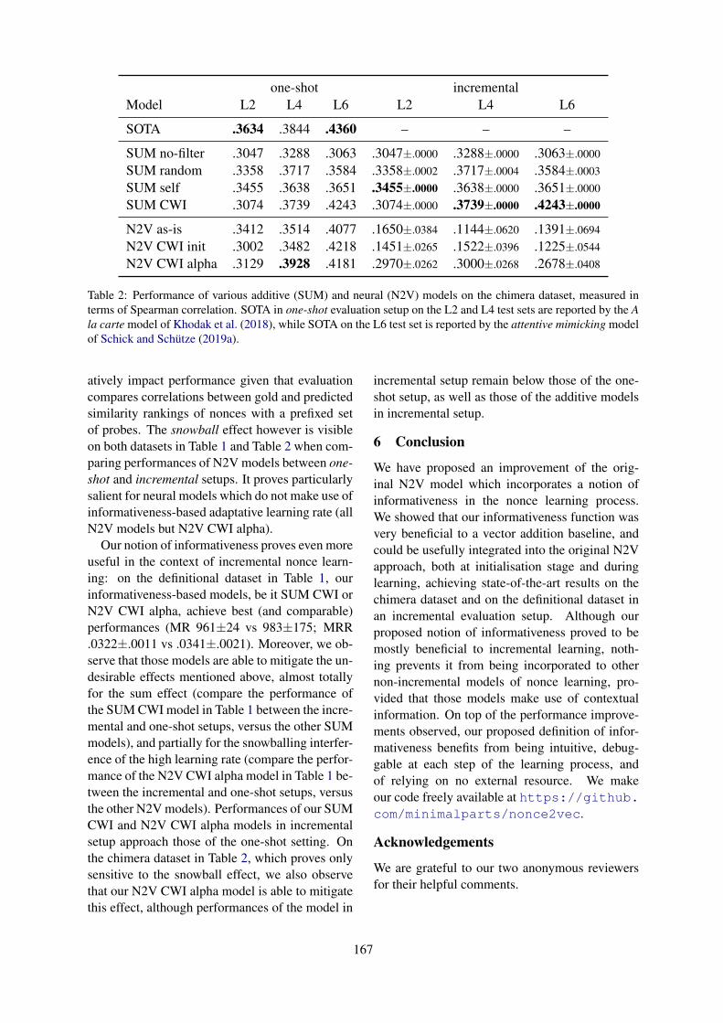
one-shot incrementalModel L2 L4 L6 L2 L4 L6

SOTA .3634 .3844 .4360 – – –

SUM no-filter .3047 .3288 .3063 .3047±.0000 .3288±.0000 .3063±.0000

SUM random .3358 .3717 .3584 .3358±.0002 .3717±.0004 .3584±.0003

SUM self .3455 .3638 .3651 .3455±.0000 .3638±.0000 .3651±.0000

SUM CWI .3074 .3739 .4243 .3074±.0000 .3739±.0000 .4243±.0000

N2V as-is .3412 .3514 .4077 .1650±.0384 .1144±.0620 .1391±.0694

N2V CWI init .3002 .3482 .4218 .1451±.0265 .1522±.0396 .1225±.0544

N2V CWI alpha .3129 .3928 .4181 .2970±.0262 .3000±.0268 .2678±.0408

Table 2: Performance of various additive (SUM) and neural (N2V) models on the chimera dataset, measured interms of Spearman correlation. SOTA in one-shot evaluation setup on the L2 and L4 test sets are reported by the Ala carte model of Khodak et al. (2018), while SOTA on the L6 test set is reported by the attentive mimicking modelof Schick and Schutze (2019a).

atively impact performance given that evaluationcompares correlations between gold and predictedsimilarity rankings of nonces with a prefixed setof probes. The snowball effect however is visibleon both datasets in Table 1 and Table 2 when com-paring performances of N2V models between one-shot and incremental setups. It proves particularlysalient for neural models which do not make use ofinformativeness-based adaptative learning rate (allN2V models but N2V CWI alpha).

Our notion of informativeness proves even moreuseful in the context of incremental nonce learn-ing: on the definitional dataset in Table 1, ourinformativeness-based models, be it SUM CWI orN2V CWI alpha, achieve best (and comparable)performances (MR 961±24 vs 983±175; MRR.0322±.0011 vs .0341±.0021). Moreover, we ob-serve that those models are able to mitigate the un-desirable effects mentioned above, almost totallyfor the sum effect (compare the performance ofthe SUM CWI model in Table 1 between the incre-mental and one-shot setups, versus the other SUMmodels), and partially for the snowballing interfer-ence of the high learning rate (compare the perfor-mance of the N2V CWI alpha model in Table 1 be-tween the incremental and one-shot setups, versusthe other N2V models). Performances of our SUMCWI and N2V CWI alpha models in incrementalsetup approach those of the one-shot setting. Onthe chimera dataset in Table 2, which proves onlysensitive to the snowball effect, we also observethat our N2V CWI alpha model is able to mitigatethis effect, although performances of the model in

incremental setup remain below those of the one-shot setup, as well as those of the additive modelsin incremental setup.

6 Conclusion

We have proposed an improvement of the orig-inal N2V model which incorporates a notion ofinformativeness in the nonce learning process.We showed that our informativeness function wasvery beneficial to a vector addition baseline, andcould be usefully integrated into the original N2Vapproach, both at initialisation stage and duringlearning, achieving state-of-the-art results on thechimera dataset and on the definitional dataset inan incremental evaluation setup. Although ourproposed notion of informativeness proved to bemostly beneficial to incremental learning, noth-ing prevents it from being incorporated to othernon-incremental models of nonce learning, pro-vided that those models make use of contextualinformation. On top of the performance improve-ments observed, our proposed definition of infor-mativeness benefits from being intuitive, debug-gable at each step of the learning process, andof relying on no external resource. We makeour code freely available at https://github.com/minimalparts/nonce2vec.

Acknowledgements

We are grateful to our two anonymous reviewersfor their helpful comments.

167

ReferencesYoshua Bengio, Rejean Ducharme, Pascal Vincent, and

Christian Janvin. 2003. A neural probabilistic lan-guage model. Journal of Machine Learning Re-search, 3:1137–1155.

Tom Bosc and Pascal Vincent. 2017. Learning wordembeddings from dictionary definitions only. InProceedings of the NIPS 2017 Workshop on Meta-Learning.

Tom Bosc and Pascal Vincent. 2018. Auto-encodingdictionary definitions into consistent word embed-dings. In Proceedings of the 2018 Conference onEmpirical Methods in Natural Language Process-ing, pages 1522–1532, Brussels, Belgium. Associ-ation for Computational Linguistics.

Elia Bruni, Nam-Khanh Tran, and Marco Baroni. 2014.Multimodal distributional semantics. Journal of Ar-tificial Intelligence Research, 49:1–47.

Ronan Collobert, Jason Weston, Leon Bottou, MichaelKarlen, Koray Kavukcuoglu, and Pavel Kuksa.2011. Natural language processing (almost) fromscratch. Journal of Machine Learning Research,12:2493–2537.

Jacob Devlin, Ming-Wei Chang, Kenton Lee, andKristina Toutanova. 2018. BERT: pre-training ofdeep bidirectional transformers for language under-standing. CoRR, abs/1810.04805.

Aurelie Herbelot and Marco Baroni. 2017. High-risklearning: acquiring new word vectors from tiny data.In Proceedings of the 2017 Conference on Empiri-cal Methods in Natural Language Processing, pages304–309, Copenhagen, Denmark. Association forComputational Linguistics.

Eric Huang, Richard Socher, Christopher Manning,and Andrew Ng. 2012. Improving word represen-tations via global context and multiple word proto-types. In Proceedings of the 50th Annual Meeting ofthe Association for Computational Linguistics (Vol-ume 1: Long Papers), pages 873–882, Jeju Island,Korea. Association for Computational Linguistics.

Mikhail Khodak, Nikunj Saunshi, Yingyu Liang,Tengyu Ma, Brandon Stewart, and Sanjeev Arora.2018. A la carte embedding: Cheap but effectiveinduction of semantic feature vectors. In Proceed-ings of the 56th Annual Meeting of the Associationfor Computational Linguistics (Volume 1: Long Pa-pers), pages 12–22, Melbourne, Australia. Associa-tion for Computational Linguistics.

Angeliki Lazaridou, Marco Marelli, and Marco Baroni.2017. Multimodal word meaning induction fromminimal exposure to natural text. Cognitive Science,41(S4):677–705.

Thang Luong, Richard Socher, and Christopher Man-ning. 2013. Better word representations with recur-sive neural networks for morphology. In Proceed-ings of the Seventeenth Conference on Computa-tional Natural Language Learning, pages 104–113,Sofia, Bulgaria. Association for Computational Lin-guistics.

Tomas Mikolov, Kai Chen, Greg Corrado, and JeffreyDean. 2013a. Efficient estimation of word represen-tations in vector space. CoRR, abs/1301.3781.

Tomas Mikolov, Ilya Sutskever, Kai Chen, Greg Cor-rado, and Jeffrey Dean. 2013b. Distributed repre-sentations of words and phrases and their composi-tionality. In Proceedings of the 26th InternationalConference on Neural Information Processing Sys-tems - Volume 2, NIPS’13, pages 3111–3119, USA.Curran Associates Inc.

Radim Rehurek and Petr Sojka. 2010. Software Frame-work for Topic Modelling with Large Corpora. InProceedings of the LREC 2010 Workshop on NewChallenges for NLP Frameworks, pages 45–50, Val-letta, Malta. ELRA.

Timo Schick and Hinrich Schutze. 2018. Learning se-mantic representations for novel words: Leveragingboth form and context. CoRR, abs/1811.03866.

Timo Schick and Hinrich Schutze. 2019a. Attentivemimicking: Better word embeddings by attendingto informative contexts. CoRR, abs/1904.01617.

Timo Schick and Hinrich Schutze. 2019b. Rare words:A major problem for contextualized embeddingsand how to fix it by attentive mimicking. CoRR,abs/1904.06707.

Ashish Vaswani, Noam Shazeer, Niki Parmar, JakobUszkoreit, Llion Jones, Aidan N. Gomez, ŁukaszKaiser, and Illia Polosukhin. 2017. Attention is allyou need. In Advances in neural information pro-cessing systems, pages 5998–6008.

Su Wang, Stephen Roller, and Katrin Erk. 2017. Distri-butional Modeling on a Diet: One-shot Word Learn-ing from Text Only. In Proceedings of the Eighth In-ternational Joint Conference on Natural LanguageProcessing (Volume 1: Long Papers), pages 204–213. Asian Federation of Natural Language Process-ing.

168

Proceedings of the 57th Annual Meeting of the Association for Computational Linguistics: Student Research Workshop, pages 169–176Florence, Italy, July 28 - August 2, 2019. c©2019 Association for Computational Linguistics

A Strong and Robust Baseline for Text-Image Matching

Fangyu LiuUniversity of Waterloo

fangyu.liu@uwaterloo.ca

Rongtian YeAalto University

rongtian7@gmail.com

Abstract

We review the current schemes of text-imagematching models and propose improvementsfor both training and inference. First, we em-pirically show limitations of two popular loss(sum and max-margin loss) widely used intraining text-image embeddings and proposea trade-off: a kNN-margin loss which 1) uti-lizes information from hard negatives and 2)is robust to noise as all K-most hardest sam-ples are taken into account, tolerating pseudonegatives and outliers. Second, we advocatethe use of Inverted Softmax (IS) and Cross-modal Local Scaling (CSLS) during inferenceto mitigate the so-called hubness problem inhigh-dimensional embedding space, enhanc-ing scores of all metrics by a large margin.

1 Introduction

In recent years, deep eural models have gained asignificant edge over shallow1 models in cross-modal matching tasks. Text-image matching hasbeen one of the most popular ones among them.Most methods involve two phases: 1) training:two neural networks (one image encoder and onetext encoder) are learned end-to-end, mappingtexts and images into a joint space, where vectors(either texts or images) with similar meanings areclose to each other; 2) inference: for a query inmodality A, after being encoded into a vector, anearest neighbor search is performed to match thevector against all vector representations of items2

in modality B. As the embedding space is learnedthrough jointly modeling vision and language, it isoften referred to as Visual Semantic Embeddings(VSE).

While the state-of-the-art architectures beingconsistently advanced (Nam et al., 2017; You

1shallow means non-neural methods.2In this paper, we refer to vectors used for searching as

“queries” and vectors in the searched space as “items”.

et al., 2018; Wehrmann et al., 2018; Wu et al.,2019), few works have focused on the more fun-damental problem of text-image matching - thatis, the optimization objectives during training andinference. And that is what this paper focuseson. In the following of the paper, we will dis-cuss 1) the optimization objective during training,i.e., loss function, and 2) the objective used in in-ference (how should a text-image correspondencegraph be predicted).

Loss function. Faghri et al. (2018) brought themost notable improvement on loss function usedfor training VSE. They proposed a max-margintriplet ranking loss that emphasizes on the hard-est negative sample within a min-batch. The max-margin loss has gained significant popularity andis used by a big set of recent works (Engilbergeet al., 2018; Faghri et al., 2018; Lee et al., 2018;Wu et al., 2019). We, however, point out that themax-margin loss is very sensitive to label noiseand encoder performance, and also easily over-fits. Through experiments, we show that it onlyachieves the best performance under a careful se-lection of model architecture and dataset. BeforeFaghri et al. (2018), a pairwise ranking loss hasbeen usually adopted for text-image model train-ing. The only difference is that, instead of onlyusing the hardest negative sample, it sums over allnegative samples (we thus refer to it as the sum-margin loss). Though sum-margin loss yields sta-ble and consistent performance under all datasetand architecture conditions, it does not make useinformation from hard samples but treats all sam-ples equally by summing the margins up. BothFaghri et al. (2018) and our own experiments pointto a clear trend that, more and cleaner data thereis, the higher quality the encoders have, the betterperformance the max-margin loss has; while thesmaller and less clean the data is, the less pow-erful the encoders are, the better sum-margin loss

169

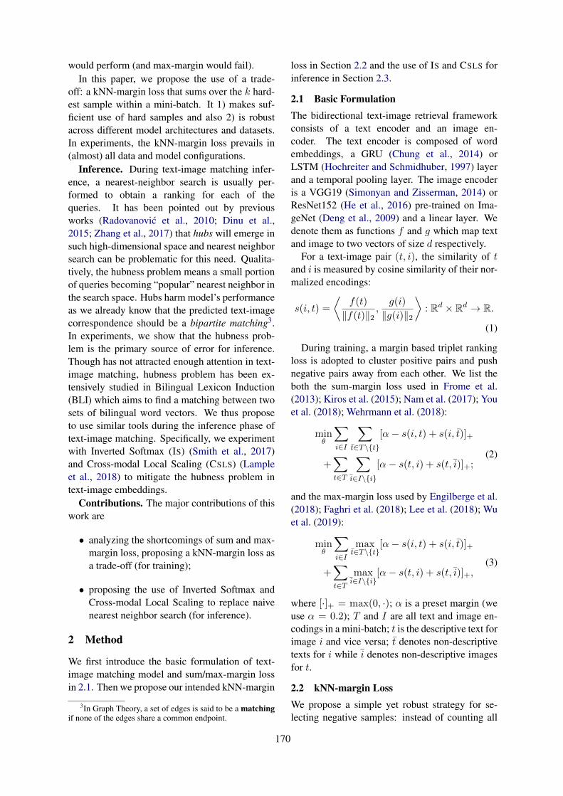
would perform (and max-margin would fail).In this paper, we propose the use of a trade-

off: a kNN-margin loss that sums over the k hard-est sample within a mini-batch. It 1) makes suf-ficient use of hard samples and also 2) is robustacross different model architectures and datasets.In experiments, the kNN-margin loss prevails in(almost) all data and model configurations.

Inference. During text-image matching infer-ence, a nearest-neighbor search is usually per-formed to obtain a ranking for each of thequeries. It has been pointed out by previousworks (Radovanovic et al., 2010; Dinu et al.,2015; Zhang et al., 2017) that hubs will emerge insuch high-dimensional space and nearest neighborsearch can be problematic for this need. Qualita-tively, the hubness problem means a small portionof queries becoming “popular” nearest neighbor inthe search space. Hubs harm model’s performanceas we already know that the predicted text-imagecorrespondence should be a bipartite matching3.In experiments, we show that the hubness prob-lem is the primary source of error for inference.Though has not attracted enough attention in text-image matching, hubness problem has been ex-tensively studied in Bilingual Lexicon Induction(BLI) which aims to find a matching between twosets of bilingual word vectors. We thus proposeto use similar tools during the inference phase oftext-image matching. Specifically, we experimentwith Inverted Softmax (IS) (Smith et al., 2017)and Cross-modal Local Scaling (CSLS) (Lampleet al., 2018) to mitigate the hubness problem intext-image embeddings.

Contributions. The major contributions of thiswork are

• analyzing the shortcomings of sum and max-margin loss, proposing a kNN-margin loss asa trade-off (for training);

• proposing the use of Inverted Softmax andCross-modal Local Scaling to replace naivenearest neighbor search (for inference).

2 Method

We first introduce the basic formulation of text-image matching model and sum/max-margin lossin 2.1. Then we propose our intended kNN-margin

3In Graph Theory, a set of edges is said to be a matchingif none of the edges share a common endpoint.

loss in Section 2.2 and the use of IS and CSLS forinference in Section 2.3.

2.1 Basic FormulationThe bidirectional text-image retrieval frameworkconsists of a text encoder and an image en-coder. The text encoder is composed of wordembeddings, a GRU (Chung et al., 2014) orLSTM (Hochreiter and Schmidhuber, 1997) layerand a temporal pooling layer. The image encoderis a VGG19 (Simonyan and Zisserman, 2014) orResNet152 (He et al., 2016) pre-trained on Ima-geNet (Deng et al., 2009) and a linear layer. Wedenote them as functions f and g which map textand image to two vectors of size d respectively.

For a text-image pair (t, i), the similarity of tand i is measured by cosine similarity of their nor-malized encodings:

s(i, t) =

⟨f(t)

‖f(t)‖2,g(i)

‖g(i)‖2

⟩: Rd × Rd → R.

(1)

During training, a margin based triplet rankingloss is adopted to cluster positive pairs and pushnegative pairs away from each other. We list theboth the sum-margin loss used in Frome et al.(2013); Kiros et al. (2015); Nam et al. (2017); Youet al. (2018); Wehrmann et al. (2018):

minθ

∑

i∈I

∑

t∈T\t[α− s(i, t) + s(i, t)]+

+∑

t∈T

∑

i∈I\i[α− s(t, i) + s(t, i)]+;

(2)

and the max-margin loss used by Engilberge et al.(2018); Faghri et al. (2018); Lee et al. (2018); Wuet al. (2019):

minθ

∑

i∈Imaxt∈T\t

[α− s(i, t) + s(i, t)]+

+∑

t∈Tmaxi∈I\i

[α− s(t, i) + s(t, i)]+,(3)

where [·]+ = max(0, ·); α is a preset margin (weuse α = 0.2); T and I are all text and image en-codings in a mini-batch; t is the descriptive text forimage i and vice versa; t denotes non-descriptivetexts for i while i denotes non-descriptive imagesfor t.

2.2 kNN-margin LossWe propose a simple yet robust strategy for se-lecting negative samples: instead of counting all

170

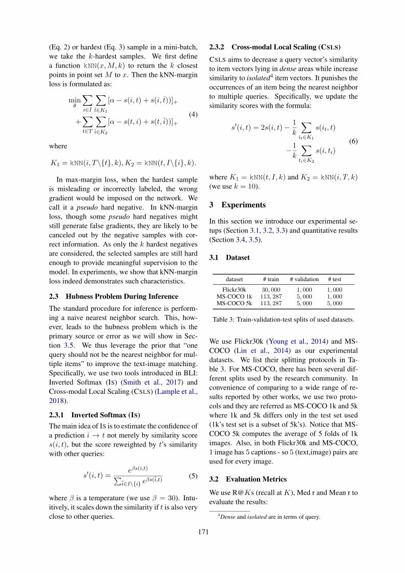
(Eq. 2) or hardest (Eq. 3) sample in a mini-batch,we take the k-hardest samples. We first definea function kNN(x,M, k) to return the k closestpoints in point set M to x. Then the kNN-marginloss is formulated as:

minθ

∑

i∈I

∑

t∈K1

[α− s(i, t) + s(i, t))]+

+∑

t∈T

∑

i∈K2

[α− s(t, i) + s(t, i))]+(4)

where

K1 = kNN(i, T\t, k),K2 = kNN(t, I\i, k).

In max-margin loss, when the hardest sampleis misleading or incorrectly labeled, the wronggradient would be imposed on the network. Wecall it a pseudo hard negative. In kNN-marginloss, though some pseudo hard negatives mightstill generate false gradients, they are likely to becanceled out by the negative samples with cor-rect information. As only the k hardest negativesare considered, the selected samples are still hardenough to provide meaningful supervision to themodel. In experiments, we show that kNN-marginloss indeed demonstrates such characteristics.

2.3 Hubness Problem During InferenceThe standard procedure for inference is perform-ing a naive nearest neighbor search. This, how-ever, leads to the hubness problem which is theprimary source or error as we will show in Sec-tion 3.5. We thus leverage the prior that “onequery should not be the nearest neighbor for mul-tiple items” to improve the text-image matching.Specifically, we use two tools introduced in BLI:Inverted Softmax (IS) (Smith et al., 2017) andCross-modal Local Scaling (CSLS) (Lample et al.,2018).

2.3.1 Inverted Softmax (IS)The main idea of IS is to estimate the confidence ofa prediction i → t not merely by similarity scores(i, t), but the score reweighted by t’s similaritywith other queries:

s′(i, t) =eβs(i,t)∑

i∈I\i eβs(i,t)

(5)

where β is a temperature (we use β = 30). Intu-itively, it scales down the similarity if t is also veryclose to other queries.

2.3.2 Cross-modal Local Scaling (CSLS)

CSLS aims to decrease a query vector’s similarityto item vectors lying in dense areas while increasesimilarity to isolated4 item vectors. It punishes theoccurrences of an item being the nearest neighborto multiple queries. Specifically, we update thesimilarity scores with the formula:

s′(i, t) = 2s(i, t)− 1

k

∑

it∈K1

s(it, t)

−1

k

∑

ti∈K2

s(i, ti)(6)

where K1 = kNN(t, I, k) and K2 = kNN(i, T, k)(we use k = 10).

3 Experiments

In this section we introduce our experimental se-tups (Section 3.1, 3.2, 3.3) and quantitative results(Section 3.4, 3.5).

3.1 Dataset

dataset # train # validation # test

Flickr30k 30, 000 1, 000 1, 000MS-COCO 1k 113, 287 5, 000 1, 000MS-COCO 5k 113, 287 5, 000 5, 000

Table 3: Train-validation-test splits of used datasets.

We use Flickr30k (Young et al., 2014) and MS-COCO (Lin et al., 2014) as our experimentaldatasets. We list their splitting protocols in Ta-ble 3. For MS-COCO, there has been several dif-ferent splits used by the research community. Inconvenience of comparing to a wide range of re-sults reported by other works, we use two proto-cols and they are referred as MS-COCO 1k and 5kwhere 1k and 5k differs only in the test set used(1k’s test set is a subset of 5k’s). Notice that MS-COCO 5k computes the average of 5 folds of 1kimages. Also, in both Flickr30k and MS-COCO,1 image has 5 captions - so 5 (text,image) pairs areused for every image.

3.2 Evaluation Metrics

We use R@Ks (recall at K), Med r and Mean r toevaluate the results:

4Dense and isolated are in terms of query.

171

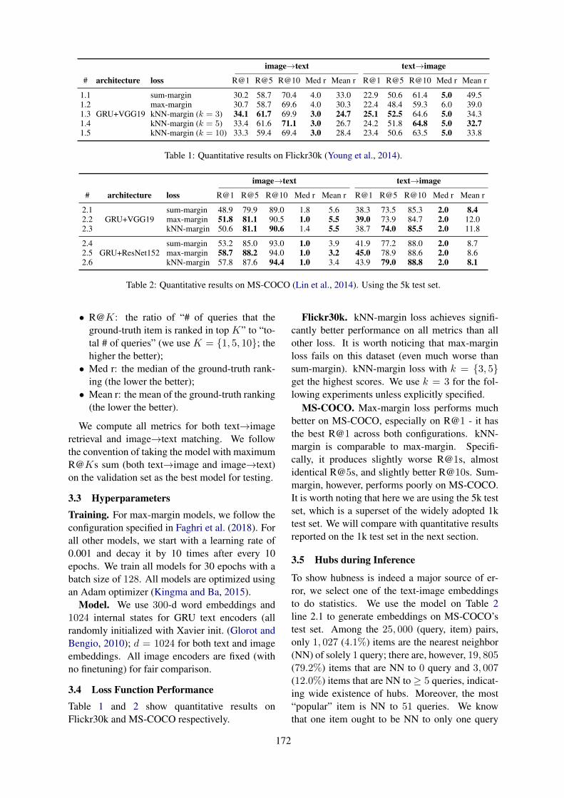
image→text text→image

# architecture loss R@1 R@5 R@10 Med r Mean r R@1 R@5 R@10 Med r Mean r

1.1

GRU+VGG19

sum-margin 30.2 58.7 70.4 4.0 33.0 22.9 50.6 61.4 5.0 49.51.2 max-margin 30.7 58.7 69.6 4.0 30.3 22.4 48.4 59.3 6.0 39.01.3 kNN-margin (k = 3) 34.1 61.7 69.9 3.0 24.7 25.1 52.5 64.6 5.0 34.31.4 kNN-margin (k = 5) 33.4 61.6 71.1 3.0 26.7 24.2 51.8 64.8 5.0 32.71.5 kNN-margin (k = 10) 33.3 59.4 69.4 3.0 28.4 23.4 50.6 63.5 5.0 33.8

Table 1: Quantitative results on Flickr30k (Young et al., 2014).

image→text text→image

# architecture loss R@1 R@5 R@10 Med r Mean r R@1 R@5 R@10 Med r Mean r

2.1GRU+VGG19

sum-margin 48.9 79.9 89.0 1.8 5.6 38.3 73.5 85.3 2.0 8.42.2 max-margin 51.8 81.1 90.5 1.0 5.5 39.0 73.9 84.7 2.0 12.02.3 kNN-margin 50.6 81.1 90.6 1.4 5.5 38.7 74.0 85.5 2.0 11.8

2.4GRU+ResNet152

sum-margin 53.2 85.0 93.0 1.0 3.9 41.9 77.2 88.0 2.0 8.72.5 max-margin 58.7 88.2 94.0 1.0 3.2 45.0 78.9 88.6 2.0 8.62.6 kNN-margin 57.8 87.6 94.4 1.0 3.4 43.9 79.0 88.8 2.0 8.1

Table 2: Quantitative results on MS-COCO (Lin et al., 2014). Using the 5k test set.

• R@K: the ratio of “# of queries that theground-truth item is ranked in top K” to “to-tal # of queries” (we use K = 1, 5, 10; thehigher the better);• Med r: the median of the ground-truth rank-

ing (the lower the better);• Mean r: the mean of the ground-truth ranking

(the lower the better).

We compute all metrics for both text→imageretrieval and image→text matching. We followthe convention of taking the model with maximumR@Ks sum (both text→image and image→text)on the validation set as the best model for testing.

3.3 HyperparametersTraining. For max-margin models, we follow theconfiguration specified in Faghri et al. (2018). Forall other models, we start with a learning rate of0.001 and decay it by 10 times after every 10epochs. We train all models for 30 epochs with abatch size of 128. All models are optimized usingan Adam optimizer (Kingma and Ba, 2015).

Model. We use 300-d word embeddings and1024 internal states for GRU text encoders (allrandomly initialized with Xavier init. (Glorot andBengio, 2010); d = 1024 for both text and imageembeddings. All image encoders are fixed (withno finetuning) for fair comparison.

3.4 Loss Function PerformanceTable 1 and 2 show quantitative results onFlickr30k and MS-COCO respectively.

Flickr30k. kNN-margin loss achieves signifi-cantly better performance on all metrics than allother loss. It is worth noticing that max-marginloss fails on this dataset (even much worse thansum-margin). kNN-margin loss with k = 3, 5get the highest scores. We use k = 3 for the fol-lowing experiments unless explicitly specified.

MS-COCO. Max-margin loss performs muchbetter on MS-COCO, especially on R@1 - it hasthe best R@1 across both configurations. kNN-margin is comparable to max-margin. Specifi-cally, it produces slightly worse R@1s, almostidentical R@5s, and slightly better R@10s. Sum-margin, however, performs poorly on MS-COCO.It is worth noting that here we are using the 5k testset, which is a superset of the widely adopted 1ktest set. We will compare with quantitative resultsreported on the 1k test set in the next section.

3.5 Hubs during Inference

To show hubness is indeed a major source of er-ror, we select one of the text-image embeddingsto do statistics. We use the model on Table 2line 2.1 to generate embeddings on MS-COCO’stest set. Among the 25, 000 (query, item) pairs,only 1, 027 (4.1%) items are the nearest neighbor(NN) of solely 1 query; there are, however, 19, 805(79.2%) items that are NN to 0 query and 3, 007(12.0%) items that are NN to ≥ 5 queries, indicat-ing wide existence of hubs. Moreover, the most“popular” item is NN to 51 queries. We knowthat one item ought to be NN to only one query

172

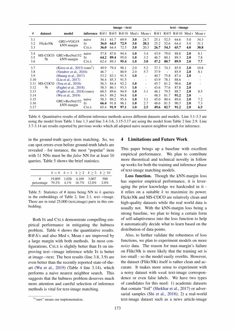
image→text text→image

# dataset model inference R@1 R@5 R@10 Med r Mean r R@1 R@5 R@10 Med r Mean r

3.1Flickr30k GRU+VGG19

kNN-margin

naive 34.1 61.7 69.9 3.0 24.7 25.1 52.5 64.6 5.0 34.33.2 IS 36.0 64.5 72.9 3.0 20.1 25.2 52.6 64.4 5.0 31.13.3 CSLS 36.0 64.4 72.5 3.0 20.3 26.7 54.3 65.7 4.0 30.8

3.4 MS-COCO5k

GRU+ResNet152kNN-margin

naive 57.8 87.6 94.4 1.0 3.4 43.9 79.0 88.8 2.0 8.13.5 IS 64.2 89.4 95.0 1.0 3.2 46.7 80.1 89.3 2.0 7.83.6 CSLS 62.4 89.3 95.4 1.0 3.0 47.2 80.7 89.9 2.0 7.7

3.7

MS-COCO1k

(Kiros et al., 2015) (ours5) 49.9 79.4 90.1 2.0 5.2 37.3 74.3 85.9 2.0 10.83.8 (Vendrov et al., 2016) 46.7 - 88.9 2.0 5.7 37.9 - 85.9 2.0 8.13.9 (Huang et al., 2017) 53.2 83.1 91.5 1.0 - 40.7 75.8 87.4 2.0 -

3.10 (Liu et al., 2017) 56.4 85.3 91.5 - - 43.9 78.1 88.6 - -3.11 (You et al., 2018) 56.3 84.4 92.2 1.0 - 45.7 81.2 90.6 2.0 -3.12 (Faghri et al., 2018) 58.3 86.1 93.3 1.0 - 43.6 77.6 87.8 2.03.13 (Faghri et al., 2018) (ours) 60.5 89.6 94.9 1.0 3.1 46.1 79.5 88.7 2.0 8.53.14 (Wu et al., 2019) 64.3 89.2 94.8 1.0 - 48.3 81.7 91.2 2.0 -3.15 GRU+ResNet152

kNN-margin

naive 58.3 89.2 95.4 1.0 3.1 45.0 80.4 89.6 2.0 7.23.16 IS 66.4 91.8 96.1 1.0 2.7 48.6 81.5 90.3 2.0 7.33.17 CSLS 65.4 91.9 97.1 1.0 2.5 49.6 82.7 91.2 2.0 6.5

Table 4: Quantitative results of different inference methods across different datasets and models. Line 3.1-3.3 areusing the model from Table 1 line 1.3 and line 3.4-3.6, 3.15-3.17 are using the model from Table 2 line 2.9. Line3.7-3.14 are results reported by previous works which all adopted naive nearest neighbor search for inference.

in the ground-truth query-item matching. So, wecan spot errors even before ground-truth labels arerevealed - for instance, the most “popular” itemwith 51 NNs must be the false NN for at least 50queries. Table 5 shows the brief statistics.

k = 0 k = 1 k ≥ 2 k ≥ 5 k ≥ 10

# 19,805 1,026 4,169 3,007 500percentage 79.2% 4.1% 16.7% 12.0% 2.0%

Table 5: Statistics of # items being NN to k queriesin the embeddings of Table 2, line 2.1, text→image.There are in total 25,000 (text,image) paris in this em-bedding.

Both IS and CSLS demonstrate compelling em-pirical performance in mitigating the hubnessproblem. Table 4 shows the quantitative results.R@Ks and also Med r, Mean r are improved bya large margin with both methods. In most con-figurations, CSLS is slightly better than IS on im-proving text→image inference while IS is betterat image→text. The best results (line 3.8, 3.9) areeven better than the recently reported state-of-the-art (Wu et al., 2019) (Table 4 line 3.14), whichperforms a naive nearest neighbor search. Thissuggests that the hubness problem deserves muchmore attention and careful selection of inferencemethods is vital for text-image matching.

5“ours” means our implementation.

4 Limitations and Future Work

This paper brings up a baseline with excellentempirical performance. We plan to contributemore theoretical and technical novelty in followup works for both the training and inference phaseof text-image matching models.

Loss function. Though the kNN-margin losshas superior empirical performance, it is lever-aging the prior knowledge we hardcoded in it -it relies on a suitable k to maximize its power.Flickr30k and MS-COCO are relatively clean andhigh-quality datasets while the real world data isusually not. With the kNN-margin loss being astrong baseline, we plan to bring a certain formof self-adaptiveness into the loss function to helpit automatically decide what to learn based on thedistribution of data points.

Also, to further validate the robustness of lossfunctions, we plan to experiment models on morenoisy data. The reason for max-margin’s failureon Flikr30k is more likely that the training set istoo small - so the model easily overfits. However,the dataset (Flikr30k) itself is rather clean and ac-curate. It makes more sense to experiment witha noisy dataset with weak text-image correspon-dence or even false labels. We have two typesof candidates for this need: 1) academic datasetsthat contain “foil” (Shekhar et al., 2017) or adver-sarial samples (Shi et al., 2018); 2) a real-worldtext-image dataset such as a news article-image

173

dataset (Elliott and Kleppe, 2016; Biten et al.,2019).

Inference. Both IS and CSLS are soft criteria.If we do have the strong prior that the final text-image correspondence is a bipartite matching, wemight as well make use of that information and im-pose a hard constraint on it. The task of text-imagematching, after all, is also a form of assignmentproblem in Combinatorial Optimization (CO). Wethus plan to investigate tools from the CO lit-erature such as the Hungarian Algorithm (Kuhn,1955), which is the best-known algorithm for pro-ducing a maximum weight bipartite matching; theMurty’s Algorithm (Murty, 1968), which general-izes the Hungarian Algorithm into producing theK-best matching - so that rankings are availablefor computing R@K scores.

5 Related Work

In this section, we introduce works from twofields which are highly-related to our work: 1)text-image matching and VSE; 2) Bilingual Lexi-con Induction (BLI) in the context of cross-modalmatching.

5.1 Text-image Matching

Since the dawn of deep learning, works haveemerged using a two-branch structure to connectboth language and vision. Frome et al. (2013)brought up the idea of VSE, which is to embedpairs of (text, image) data and compare them ina joint space. Later works extended VSE for thetask of text-image matching (Hodosh et al., 2013;Kiros et al., 2015; Gong et al., 2014; Vendrovet al., 2016; Hubert Tsai et al., 2017; Faghri et al.,2018; Wang et al., 2019), which is also our task ofinterest. It is worth noting that there are other linesof works which also jointly model language andvision. The closest one might be image captioning(Lebret et al., 2015; Karpathy and Fei-Fei, 2015).But image captioning aims to generate novel cap-tions while text-image matching retrieves existingdescriptive texts or images in a database.

5.2 Bilingual Lexicon Induction (BLI)

We specifically talk about BLI as the tools weused to improve inference performance come fromthis literature. BLI is the task of inducing wordtranslations from monolingual corpora in two lan-guages (Irvine and Callison-Burch, 2017). Wordsare usually represented by vectors trained from

Distributional Semantics, eg. Mikolov et al.(2013). So, the word translation problem convertsto finding the appropriate matching among twosets of vectors which makes it similar to our task ofinterest. Smith et al. (2017); Lample et al. (2018)proposed to first conduct a direct Procrustes Anal-ysis (Schonemann, 1966) between two sets of vec-tors, then use criteria that heavily punish hubs dur-ing inference to avoid the hubness problem. Weexperimented with both methods in our task.

6 Conclusion

We discuss the pros and cons of prevalent lossfunctions used in text-image matching and pro-pose a kNN-margin loss as a trade-off whichyields strong and robust performance across dif-ferent model architectures and datasets. Instead ofusing naive nearest neighbor search, we advocateto adopt more polished inference strategies suchas Inverted Softmax (IS) and Cross-modal LocalScaling (CSLS), which can significantly improvescores of all metrics.

We also analyze the limitations of this work andindicate the next step for improving both the lossfunction and the inference method.

7 Acknowledgement

We thank the reviewers for their careful and in-sightful comments. We thank our family mem-bers who have both spiritually and financiallysupported our independent research. The authorFangyu Liu thanks Remi Lebret for introducinghim this interesting problem and many of the re-lated works.

ReferencesAli Furkan Biten, Lluis Gomez, Marcal Rusinol, and

Dimosthenis Karatzas. 2019. Good news, everyone!context driven entity-aware captioning for news im-ages. CVPR.

Junyoung Chung, Caglar Gulcehre, KyungHyun Cho,and Yoshua Bengio. 2014. Empirical evaluation ofgated recurrent neural networks on sequence model-ing. arXiv preprint arXiv:1412.3555.

J. Deng, W. Dong, R. Socher, L.-J. Li, K. Li, andL. Fei-Fei. 2009. Imagenet: A large-scale hierar-chical image database. In Proceedings of the IEEEconference on computer vision and pattern recogni-tion (CVPR), pages 248–255. IEEE.

Georgiana Dinu, Angeliki Lazaridou, and Marco Ba-roni. 2015. Improving zero-shot learning by miti-gating the hubness problem. ICLR worshop.

174

Desmond Elliott and Martijn Kleppe. 2016. 1 millioncaptioned dutch newspaper images.

Martin Engilberge, Louis Chevallier, Patrick Perez, andMatthieu Cord. 2018. Finding beans in burgers:Deep semantic-visual embedding with localization.In Proceedings of the IEEE Conference on Com-puter Vision and Pattern Recognition, pages 3984–3993.

F. Faghri, D. J. Fleet, J. R. Kiros, and S. Fidler.2018. Vse++: Improving visual-semantic embed-dings with hard negatives.

A. Frome, G. S. Corrado, J. Shlens, S. Bengio, J. Dean,and T. Mikolov. 2013. Devise: A deep visual-semantic embedding model. In NIPS, pages 2121–2129.

Xavier Glorot and Yoshua Bengio. 2010. Understand-ing the difficulty of training deep feedforward neu-ral networks. In Proceedings of the thirteenth in-ternational conference on artificial intelligence andstatistics, pages 249–256.

Yunchao Gong, Liwei Wang, Micah Hodosh, JuliaHockenmaier, and Svetlana Lazebnik. 2014. Im-proving image-sentence embeddings using largeweakly annotated photo collections. In EuropeanConference on Computer Vision (ECCV), pages529–545. Springer.

Kaiming He, Xiangyu Zhang, Shaoqing Ren, and JianSun. 2016. Deep residual learning for image recog-nition. In Proceedings of the IEEE conference oncomputer vision and pattern recognition, pages 770–778.

S. Hochreiter and J. Schmidhuber. 1997. Long short-term memory. Neural computation, 9(8):1735–1780.

Micah Hodosh, Peter Young, and Julia Hockenmaier.2013. Framing image description as a ranking task:Data, models and evaluation metrics. Journal of Ar-tificial Intelligence Research, 47:853–899.

Yan Huang, Wei Wang, and Liang Wang. 2017.Instance-aware image and sentence matching withselective multimodal lstm. In Proceedings of theIEEE Conference on Computer Vision and PatternRecognition, pages 2310–2318.

Yao-Hung Hubert Tsai, Liang-Kang Huang, and Rus-lan Salakhutdinov. 2017. Learning robust visual-semantic embeddings. In Proceedings of theIEEE International Conference on Computer Vision(ICCV), pages 3571–3580.

Ann Irvine and Chris Callison-Burch. 2017. A com-prehensive analysis of bilingual lexicon induction.Computational Linguistics, 43(2):273–310.

Andrej Karpathy and Li Fei-Fei. 2015. Deep visual-semantic alignments for generating image descrip-tions. In Proceedings of the IEEE conference

on computer vision and pattern recognition, pages3128–3137.

Diederik P Kingma and Jimmy Ba. 2015. Adam: Amethod for stochastic optimization. ICLR.

R. Kiros, R. Salakhutdinov, and R. S. Zemel. 2015.Unifying visual-semantic embeddings with multi-modal neural language models. Transactions of theAssociation for Computational Linguistics (TACL).

Harold W Kuhn. 1955. The hungarian method for theassignment problem. Naval research logistics quar-terly, 2(1-2):83–97.

Guillaume Lample, Alexis Conneau, Marc’AurelioRanzato, Ludovic Denoyer, and Herv Jgou. 2018.Word translation without parallel data. In Interna-tional Conference on Learning Representations.

Remi Lebret, Pedro O Pinheiro, and Ronan Collobert.2015. Phrase-based image captioning. In Proceed-ings of the 32nd International Conference on Inter-national Conference on Machine Learning-Volume37 (ICML), pages 2085–2094. JMLR. org.

Kuang-Huei Lee, Xi Chen, Gang Hua, Houdong Hu,and Xiaodong He. 2018. Stacked cross attentionfor image-text matching. In Proceedings of theEuropean Conference on Computer Vision (ECCV),pages 201–216.

T.-Y. Lin, M. Maire, S. Belongie, J. Hays, P. Perona,D. Ramanan, P. Dollar, and L. Zitnick. 2014. Mi-crosoft coco: Common objects in context. In Euro-pean conference on computer vision (ECCV), pages740–755. Springer.

Yu Liu, Yanming Guo, Erwin M Bakker, and Michael SLew. 2017. Learning a recurrent residual fusion net-work for multimodal matching. In Proceedings ofthe IEEE International Conference on Computer Vi-sion, pages 4107–4116.

Tomas Mikolov, Ilya Sutskever, Kai Chen, Greg S Cor-rado, and Jeff Dean. 2013. Distributed representa-tions of words and phrases and their compositional-ity. In Advances in neural information processingsystems, pages 3111–3119.

Katta G Murty. 1968. Letter to the editoran algorithmfor ranking all the assignments in order of increasingcost. Operations research, 16(3):682–687.

Hyeonseob Nam, Jung-Woo Ha, and Jeonghee Kim.2017. Dual attention networks for multimodal rea-soning and matching. In Proceedings of the IEEEConference on Computer Vision and Pattern Recog-nition, pages 299–307.

Milos Radovanovic, Alexandros Nanopoulos, and Mir-jana Ivanovic. 2010. Hubs in space: Popular nearestneighbors in high-dimensional data. Journal of Ma-chine Learning Research, 11(Sep):2487–2531.

175

Peter H Schonemann. 1966. A generalized solution ofthe orthogonal procrustes problem. Psychometrika,31(1):1–10.

Ravi Shekhar, Sandro Pezzelle, Yauhen Klimovich,Aurelie Herbelot, Moin Nabi, Enver Sangineto, andRaffaella Bernardi. 2017. ”foil it! find one mis-match between image and language caption”. InProceedings of the 55th Annual Meeting of the As-sociation for Computational Linguistics (ACL) (Vol-ume 1: Long Papers), pages 255–265.

Haoyue Shi, Jiayuan Mao, Tete Xiao, Yuning Jiang,and Jian Sun. 2018. Learning visually-groundedsemantics from contrastive adversarial samples. InProceedings of the 27th International Conference onComputational Linguistics, pages 3715–3727.

K. Simonyan and A. Zisserman. 2014. Very deep con-volutional networks for large-scale image recogni-tion. CoRR, abs/1409.1556.

Samuel L Smith, David HP Turban, Steven Hamblin,and Nils Y Hammerla. 2017. Offline bilingual wordvectors, orthogonal transformations and the invertedsoftmax. ICLR.

I. Vendrov, R. Kiros, S. Fidler, and R/ Urtasun. 2016.Order-embeddings of images and language. ICLR.

Liwei Wang, Yin Li, Jing Huang, and Svetlana Lazeb-nik. 2019. Learning two-branch neural networksfor image-text matching tasks. IEEE Transac-tions on Pattern Analysis and Machine Intelligence,41(2):394–407.

Jonatas Wehrmann et al. 2018. Bidirectional retrievalmade simple. In Proceedings of the IEEE Confer-ence on Computer Vision and Pattern Recognition,pages 7718–7726.

Hao Wu, Jiayuan Mao, Yufeng Zhang, Yuning Jiang,Lei Li, Weiwei Sun, and Wei-Ying Ma. 2019. Uni-fied visual-semantic embeddings: Bridging visionand language with structured meaning representa-tions. In The IEEE Conference on Computer Visionand Pattern Recognition (CVPR).

Quanzeng You, Zhengyou Zhang, and Jiebo Luo. 2018.End-to-end convolutional semantic embeddings. InThe IEEE Conference on Computer Vision and Pat-tern Recognition (CVPR).

Peter Young, Alice Lai, Micah Hodosh, and JuliaHockenmaier. 2014. From image descriptions tovisual denotations: New similarity metrics for se-mantic inference over event descriptions. Transac-tions of the Association for Computational Linguis-tics, 2:67–78.

Li Zhang, Tao Xiang, and Shaogang Gong. 2017.Learning a deep embedding model for zero-shotlearning. In Proceedings of the IEEE Conferenceon Computer Vision and Pattern Recognition, pages2021–2030.

176

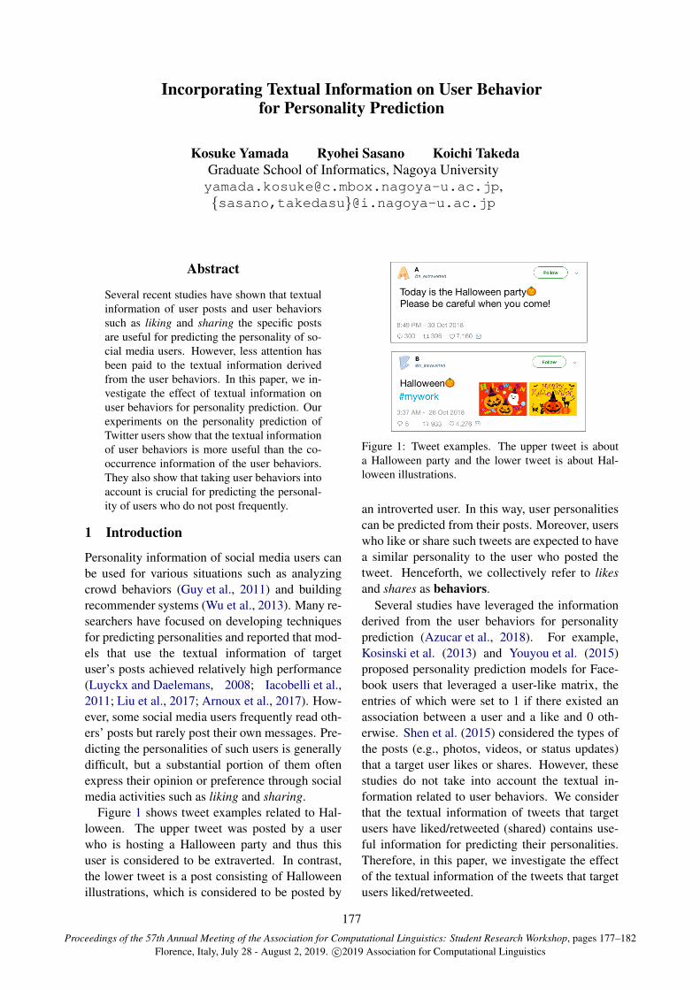
Proceedings of the 57th Annual Meeting of the Association for Computational Linguistics: Student Research Workshop, pages 177–182Florence, Italy, July 28 - August 2, 2019. c©2019 Association for Computational Linguistics

Incorporating Textual Information on User Behaviorfor Personality Prediction

Kosuke Yamada Ryohei Sasano Koichi TakedaGraduate School of Informatics, Nagoya Universityyamada.kosuke@c.mbox.nagoya-u.ac.jp,sasano,takedasu@i.nagoya-u.ac.jp

Abstract

Several recent studies have shown that textualinformation of user posts and user behaviorssuch as liking and sharing the specific postsare useful for predicting the personality of so-cial media users. However, less attention hasbeen paid to the textual information derivedfrom the user behaviors. In this paper, we in-vestigate the effect of textual information onuser behaviors for personality prediction. Ourexperiments on the personality prediction ofTwitter users show that the textual informationof user behaviors is more useful than the co-occurrence information of the user behaviors.They also show that taking user behaviors intoaccount is crucial for predicting the personal-ity of users who do not post frequently.

1 Introduction

Personality information of social media users canbe used for various situations such as analyzingcrowd behaviors (Guy et al., 2011) and buildingrecommender systems (Wu et al., 2013). Many re-searchers have focused on developing techniquesfor predicting personalities and reported that mod-els that use the textual information of targetuser’s posts achieved relatively high performance(Luyckx and Daelemans, 2008; Iacobelli et al.,2011; Liu et al., 2017; Arnoux et al., 2017). How-ever, some social media users frequently read oth-ers’ posts but rarely post their own messages. Pre-dicting the personalities of such users is generallydifficult, but a substantial portion of them oftenexpress their opinion or preference through socialmedia activities such as liking and sharing.

Figure 1 shows tweet examples related to Hal-loween. The upper tweet was posted by a userwho is hosting a Halloween party and thus thisuser is considered to be extraverted. In contrast,the lower tweet is a post consisting of Halloweenillustrations, which is considered to be posted by

Figure 1: Tweet examples. The upper tweet is abouta Halloween party and the lower tweet is about Hal-loween illustrations.

an introverted user. In this way, user personalitiescan be predicted from their posts. Moreover, userswho like or share such tweets are expected to havea similar personality to the user who posted thetweet. Henceforth, we collectively refer to likesand shares as behaviors.

Several studies have leveraged the informationderived from the user behaviors for personalityprediction (Azucar et al., 2018). For example,Kosinski et al. (2013) and Youyou et al. (2015)proposed personality prediction models for Face-book users that leveraged a user-like matrix, theentries of which were set to 1 if there existed anassociation between a user and a like and 0 oth-erwise. Shen et al. (2015) considered the types ofthe posts (e.g., photos, videos, or status updates)that a target user likes or shares. However, thesestudies do not take into account the textual in-formation related to user behaviors. We considerthat the textual information of tweets that targetusers have liked/retweeted (shared) contains use-ful information for predicting their personalities.Therefore, in this paper, we investigate the effectof the textual information of the tweets that targetusers liked/retweeted.

177

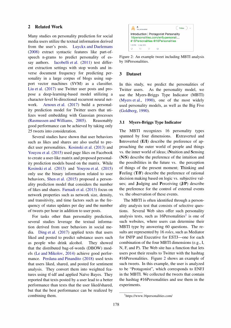
2 Related Work

Many studies on personality prediction for socialmedia users utilize the textual information derivedfrom the user’s posts. Luyckx and Daelemans(2008) extract syntactic features like part-of-speech n-grams to predict personality of es-say authors. Iacobelli et al. (2011) test differ-ent extraction settings with stop words and in-verse document frequency for predicting per-sonality in a large corpus of blogs using sup-port vector machines (SVM) as a classifier.Liu et al. (2017) use Twitter user posts and pro-pose a deep-learning-based model utilizing acharacter-level bi-directional recurrent neural net-work. Arnoux et al. (2017) build a personal-ity prediction model for Twitter users that uti-lizes word embedding with Gaussian processes(Rasmussen and Williams, 2005). Reasonablygood performance can be achieved by taking only25 tweets into consideration.

Several studies have shown that user behaviorssuch as likes and shares are also useful to pre-dict user personalities. Kosinski et al. (2013) andYouyou et al. (2015) used page likes on Facebookto create a user-like matrix and proposed personal-ity prediction models based on the matrix. WhileKosinski et al. (2013) and Youyou et al. (2015)only use the binary information related to userbehaviors, Shen et al. (2015) proposed a person-ality prediction model that considers the numberof likes and shares. Farnadi et al. (2013) focus onnetwork properties such as network size, density,and transitivity, and time factors such as the fre-quency of status updates per day and the numberof tweets per hour in addition to user posts.

For tasks other than personality prediction,several studies leverage the textual informa-tion derived from user behaviors in social me-dia. Ding et al. (2017) applied texts that usersliked and posted to predict substance users suchas people who drink alcohol. They showedthat the distributed bag-of-words (DBOW) mod-els (Le and Mikolov, 2014) achieve good perfor-mance. Perdana and Pinandito (2018) used textsthat users liked, shared, and posted for sentimentanalysis. They convert them into weighted fea-tures using tf-idf and applied Naıve Bayes. Theyreported that texts posted by a user lead to a betterperformance than texts that the user liked/shared,but that the best performance can be realized bycombining them.

Figure 2: An example tweet including MBTI analysisby 16Personalities.

3 Dataset

In this study, we predict the personalities ofTwitter users. As the personality model, weuse the Myers-Briggs Type Indicator (MBTI)(Myers et al., 1990), one of the most widelyused personality models, as well as the Big Five(Goldberg, 1990).

3.1 Myers-Briggs Type Indicator

The MBTI recognizes 16 personality typesspanned by four dimensions. Extraverted andIntroverted (E/I) describe the preference of ap-proaching the outer world of people and thingsvs. the inner world of ideas; iNtuition and Sensing(N/S) describe the preference of the intuition andthe possibilities in the future vs. the perceptionof things of the present moment; Thinking andFeeling (T/F) describe the preference of rationaldecision making based on logic vs. subjective val-ues; and Judging and Perceiving (J/P) describethe preference for the control of external eventsvs. the observation of these events.

The MBTI is often identified through a person-ality analysis test that consists of selective ques-tions. Several Web sites offer such personalityanalysis tests, such as 16Personalities1 is one ofsuch websites, where users can determine theirMBTI type by answering 60 questions. The re-sults are represented by 16 roles, such as Mediatorfor INFP and Executive for ESTJ—one for eachcombination of the four MBTI dimensions (e.g., I,N, F, and P). The Web site has a function that letsusers post their results to Twitter with the hashtag#16Personalities. Figure 2 shows an example ofsuch tweets. In this example, the user is analyzedto be “Protagonist”, which corresponds to ENFJin the MBTI. We collected the tweets that containthe hashtag #16Personalities and use them in theexperiments.

1https://www.16personalities.com/

178

UsersE / I 4,483 / 15,881N / S 13,733 / 6,631T / F 6,498 / 13,866J / P 7,008 / 13,356Total 20,364

Table 1: The number of users in each dimension.

No. of collected tweets Likes Retweets0 157 1621–255 2,076 6,836256–511 1,331 4,903512–1,023 2,065 5,3261,024 14,735 3,137

Table 2: Distribution of users based on number of likesor retweets.

3.2 Data Collection from Twitter

We collected tweets written in Japanese. Twit-ter Premium search APIs2 were used to find thetweets containing the hashtag #16personalities andlisted 72,847 users who posted such tweets in 2017and 2018. We refer to a tweet with #16personali-ties as the gold standard tweet. Next, we collectedthe latest 3,200 tweets for each user and then dis-carded the tweets that were posted after the goldstandard tweet. Only the users with 1,024 or moretweets were used in this study. The number ofsuch users was 20,364. Table 1 lists the statis-tics of users for each personality dimension. Wecan confirm that there are biases in the number ofusers for all dimensions and that the bias for theE/I dimension is particularly noticeable.

To build a model based on the text relatedto user behaviors such as like and retweet, wecollected up to 1,024 liked tweets and 1,024retweeted tweets for each user. Table 2 showsthe distribution of users based on the number oflikes or retweets. 14,735 out of 20,364 users likedmore than 1,023 tweets and 157 users liked notweets. Only 3,137 users retweeted more than1,023 tweets and 162 users retweeted no tweets.

4 Personality Prediction Models

We treat personality prediction as a set of binaryclassification tasks and build four binary classifiersindependently for each dimension of the MBTI.We regard the personality of the users shown in

2https://developer.twitter.com/en/docs/tweets/search/api-reference/premium-search.html

...

...

...

...

up to1,024

SVM classifier

Gold standard tweet

Target user’s tweets

Target user

up to1,024

Target user’s behaviors

Older tweets

Liked tweets

Retweeted tweets

1,024posts

Predicted personality

Figure 3: Overview of the personality predictionmodel.

the tweets with #16personalities as the gold stan-dard personality and attempt to predict it using theSVM classifier. Figure 3 shows an overview ofthe model. Specifically, we use linear SVM forclassification with two types of features: those de-rived from the tweets that the target user likes orretweets and those derived from the tweets that thetarget user posts.

4.1 Features derived from User Behaviors

Use of co-occurrence information We build amodel similar to Kosinski et al. (2013). Theyleveraged a co-occurrence matrix of users andlikes, the entries of which were set to 1 if there ex-isted an association between a user and a like and0 otherwise. Similarly, we create the binary matrixof users and behaviors, the entries of which wereset to 1 if the user liked/retweeted a tweet, 0 oth-erwise. For the sake of computational efficiency,we consider tweets that are liked or retweeted byat least ten users. Then, we apply singular valuedecomposition (SVD) to the matrix and use thedimension-reduced vectors as the features of theSVM classifier.

Use of textual information We propose threemodels that consider the textual information onuser behavior. All three models use MeCab3

with the IPA dictionary4 to perform morpholog-

3http://taku910.github.io/mecab/4mecab-ipadic-2.7.0-20070801

179

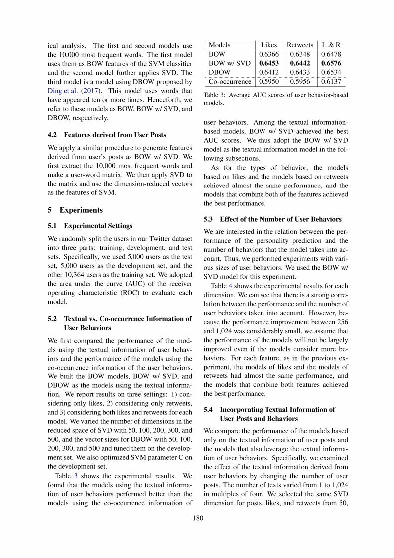
ical analysis. The first and second models usethe 10,000 most frequent words. The first modeluses them as BOW features of the SVM classifierand the second model further applies SVD. Thethird model is a model using DBOW proposed byDing et al. (2017). This model uses words thathave appeared ten or more times. Henceforth, werefer to these models as BOW, BOW w/ SVD, andDBOW, respectively.

4.2 Features derived from User Posts

We apply a similar procedure to generate featuresderived from user’s posts as BOW w/ SVD. Wefirst extract the 10,000 most frequent words andmake a user-word matrix. We then apply SVD tothe matrix and use the dimension-reduced vectorsas the features of SVM.

5 Experiments

5.1 Experimental Settings

We randomly split the users in our Twitter datasetinto three parts: training, development, and testsets. Specifically, we used 5,000 users as the testset, 5,000 users as the development set, and theother 10,364 users as the training set. We adoptedthe area under the curve (AUC) of the receiveroperating characteristic (ROC) to evaluate eachmodel.

5.2 Textual vs. Co-occurrence Information ofUser Behaviors

We first compared the performance of the mod-els using the textual information of user behav-iors and the performance of the models using theco-occurrence information of the user behaviors.We built the BOW models, BOW w/ SVD, andDBOW as the models using the textual informa-tion. We report results on three settings: 1) con-sidering only likes, 2) considering only retweets,and 3) considering both likes and retweets for eachmodel. We varied the number of dimensions in thereduced space of SVD with 50, 100, 200, 300, and500, and the vector sizes for DBOW with 50, 100,200, 300, and 500 and tuned them on the develop-ment set. We also optimized SVM parameter C onthe development set.

Table 3 shows the experimental results. Wefound that the models using the textual informa-tion of user behaviors performed better than themodels using the co-occurrence information of

Models Likes Retweets L & RBOW 0.6366 0.6348 0.6478BOW w/ SVD 0.6453 0.6442 0.6576DBOW 0.6412 0.6433 0.6534Co-occurrence 0.5950 0.5956 0.6137

Table 3: Average AUC scores of user behavior-basedmodels.

user behaviors. Among the textual information-based models, BOW w/ SVD achieved the bestAUC scores. We thus adopt the BOW w/ SVDmodel as the textual information model in the fol-lowing subsections.

As for the types of behavior, the modelsbased on likes and the models based on retweetsachieved almost the same performance, and themodels that combine both of the features achievedthe best performance.

5.3 Effect of the Number of User Behaviors

We are interested in the relation between the per-formance of the personality prediction and thenumber of behaviors that the model takes into ac-count. Thus, we performed experiments with vari-ous sizes of user behaviors. We used the BOW w/SVD model for this experiment.

Table 4 shows the experimental results for eachdimension. We can see that there is a strong corre-lation between the performance and the number ofuser behaviors taken into account. However, be-cause the performance improvement between 256and 1,024 was considerably small, we assume thatthe performance of the models will not be largelyimproved even if the models consider more be-haviors. For each feature, as in the previous ex-periment, the models of likes and the models ofretweets had almost the same performance, andthe models that combine both features achievedthe best performance.

5.4 Incorporating Textual Information ofUser Posts and Behaviors

We compare the performance of the models basedonly on the textual information of user posts andthe models that also leverage the textual informa-tion of user behaviors. Specifically, we examinedthe effect of the textual information derived fromuser behaviors by changing the number of userposts. The number of texts varied from 1 to 1,024in multiples of four. We selected the same SVDdimension for posts, likes, and retweets from 50,

180

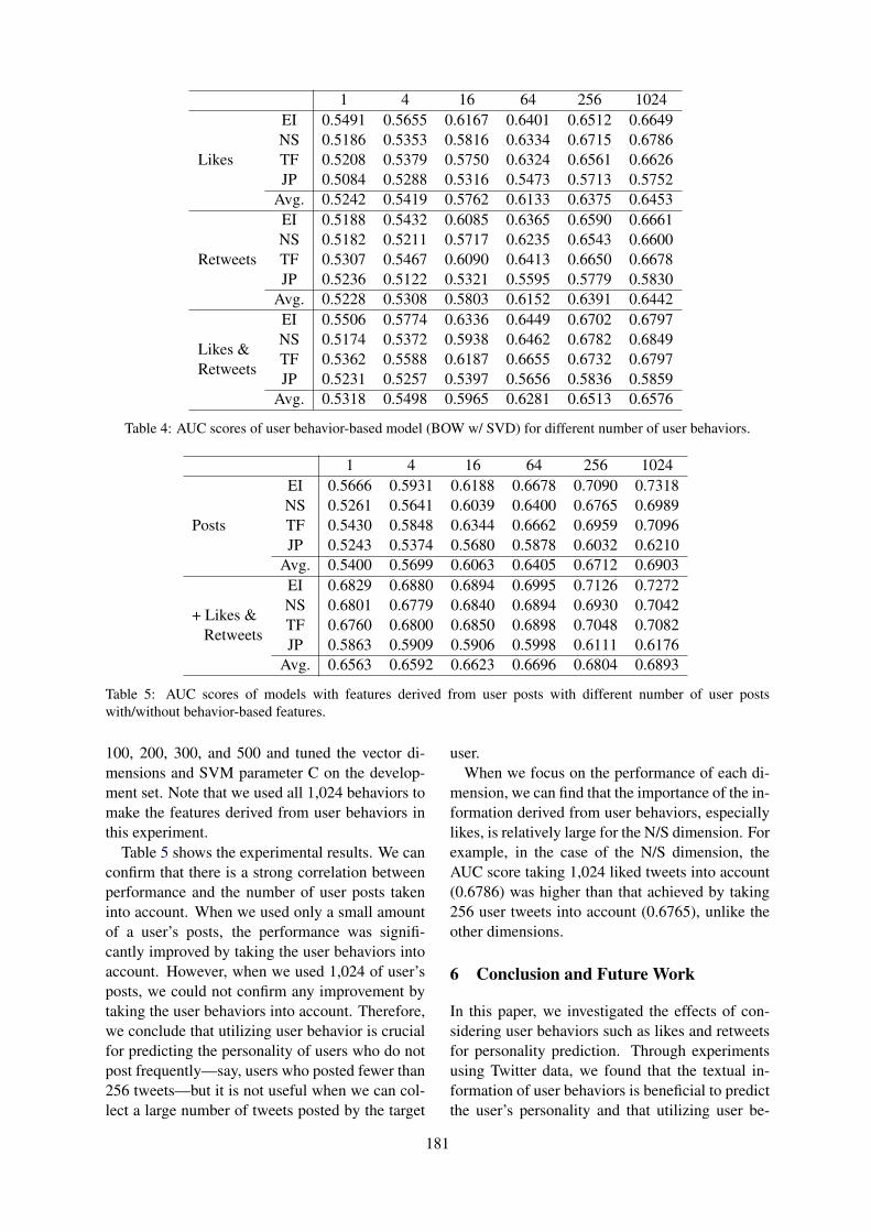
1 4 16 64 256 1024EI 0.5491 0.5655 0.6167 0.6401 0.6512 0.6649NS 0.5186 0.5353 0.5816 0.6334 0.6715 0.6786

Likes TF 0.5208 0.5379 0.5750 0.6324 0.6561 0.6626JP 0.5084 0.5288 0.5316 0.5473 0.5713 0.5752

Avg. 0.5242 0.5419 0.5762 0.6133 0.6375 0.6453EI 0.5188 0.5432 0.6085 0.6365 0.6590 0.6661NS 0.5182 0.5211 0.5717 0.6235 0.6543 0.6600

Retweets TF 0.5307 0.5467 0.6090 0.6413 0.6650 0.6678JP 0.5236 0.5122 0.5321 0.5595 0.5779 0.5830

Avg. 0.5228 0.5308 0.5803 0.6152 0.6391 0.6442EI 0.5506 0.5774 0.6336 0.6449 0.6702 0.6797

Likes &NS 0.5174 0.5372 0.5938 0.6462 0.6782 0.6849

RetweetsTF 0.5362 0.5588 0.6187 0.6655 0.6732 0.6797JP 0.5231 0.5257 0.5397 0.5656 0.5836 0.5859

Avg. 0.5318 0.5498 0.5965 0.6281 0.6513 0.6576

Table 4: AUC scores of user behavior-based model (BOW w/ SVD) for different number of user behaviors.

1 4 16 64 256 1024EI 0.5666 0.5931 0.6188 0.6678 0.7090 0.7318NS 0.5261 0.5641 0.6039 0.6400 0.6765 0.6989

Posts TF 0.5430 0.5848 0.6344 0.6662 0.6959 0.7096JP 0.5243 0.5374 0.5680 0.5878 0.6032 0.6210

Avg. 0.5400 0.5699 0.6063 0.6405 0.6712 0.6903EI 0.6829 0.6880 0.6894 0.6995 0.7126 0.7272

+ Likes &NS 0.6801 0.6779 0.6840 0.6894 0.6930 0.7042

RetweetsTF 0.6760 0.6800 0.6850 0.6898 0.7048 0.7082JP 0.5863 0.5909 0.5906 0.5998 0.6111 0.6176

Avg. 0.6563 0.6592 0.6623 0.6696 0.6804 0.6893

Table 5: AUC scores of models with features derived from user posts with different number of user postswith/without behavior-based features.

100, 200, 300, and 500 and tuned the vector di-mensions and SVM parameter C on the develop-ment set. Note that we used all 1,024 behaviors tomake the features derived from user behaviors inthis experiment.

Table 5 shows the experimental results. We canconfirm that there is a strong correlation betweenperformance and the number of user posts takeninto account. When we used only a small amountof a user’s posts, the performance was signifi-cantly improved by taking the user behaviors intoaccount. However, when we used 1,024 of user’sposts, we could not confirm any improvement bytaking the user behaviors into account. Therefore,we conclude that utilizing user behavior is crucialfor predicting the personality of users who do notpost frequently—say, users who posted fewer than256 tweets—but it is not useful when we can col-lect a large number of tweets posted by the target

user.When we focus on the performance of each di-

mension, we can find that the importance of the in-formation derived from user behaviors, especiallylikes, is relatively large for the N/S dimension. Forexample, in the case of the N/S dimension, theAUC score taking 1,024 liked tweets into account(0.6786) was higher than that achieved by taking256 user tweets into account (0.6765), unlike theother dimensions.

6 Conclusion and Future Work

In this paper, we investigated the effects of con-sidering user behaviors such as likes and retweetsfor personality prediction. Through experimentsusing Twitter data, we found that the textual in-formation of user behaviors is beneficial to predictthe user’s personality and that utilizing user be-

181

haviors is crucial for predicting the personality ofusers who do not post many tweets, e.g., less than256, but that the effect of taking user behaviorsinto account is very limited when we can collectmany tweets posted by the target user.

In the future, we plan to explore other use-ful textual information for personality prediction,such as text in a web page to which the target userlinked and public comments directed to the user(as reported by Jurgens et al. (2017)). We can alsoinclude replies to the target user’s tweets to see ifwe can improve personality prediction.

Acknowledgements

This work was partly supported by JSPS KAK-ENHI Grant Number 16K16110.

ReferencesPierre Arnoux, Anbang Xu, Neil Boyette, Jalal Mah-

mud, Rama Akkiraju, and Vibha Sinha. 2017. 25tweets to know you: A new model to predict person-ality with social media. In Proceedings of the 11thInternational AAAI Conference on Web and SocialMedia (ICWSM’17), pages 472–475.

Danny Azucar, Davide Marengo, and Michele Settanni.2018. Predicting the big 5 personality traits fromdigital footprints on social media: A meta-analysis.Personality and Individual Differences, 124:150–159.

Tao Ding, Warren K. Bickel, and Shimei Pan. 2017.Multi-view unsupervised user feature embeddingfor social media-based substance use prediction.In Proceedings of the 2017 Conference on Em-pirical Methods in Natural Language Processing(EMNLP’17), pages 2275–2284.

Golnoosh Farnadi, Susana Zoghbi, Marie-FrancineMoens, and Martine De Cock. 2013. Recognisingpersonality traits using facebook status updates. InProceedings of the Workshop on Computational Per-sonality Recognition (WCPR’13) at the 7th Interna-tional AAAI Conference on Weblogs and Social Me-dia (ICWSM’13), pages 14–18.

Lewis R Goldberg. 1990. An alternative “descrip-tion of personality”: the big-five factor struc-ture. Journal of personality and social psychology,59(6):1216–1229.

Stephen J Guy, Sujeong Kim, Ming C Lin, andDinesh Manocha. 2011. Simulating heteroge-neous crowd behaviors using personality trait the-ory. In Proceedings of the 2011 ACM SIG-GRAPH/Eurographics Symposium on Computer An-imation (SCA’11), pages 43–52.

Francisco Iacobelli, Alastair J Gill, Scott Nowson, andJon Oberlander. 2011. Large scale personality clas-sification of bloggers. In Proceedings of the 4th in-ternational conference on Affective Computing andIntelligent Interaction (ACII’11), pages 568–577.

David Jurgens, Yulia Tsvetkov, and Dan Jurafsky.2017. Writer profiling without the writer’s text. InProceedings of the 9th International Conference onSocial Informatics (SocInfo’17), pages 537–558.

Michal Kosinski, David Stillwell, and Thore Grae-pel. 2013. Private traits and attributes are pre-dictable from digital records of human behavior.Proceedings of the National Academy of Sciences,110(15):5802–5805.

Quoc Le and Tomas Mikolov. 2014. Distributed repre-sentations of sentences and documents. In Proceed-ings of the 31st International Conference on Ma-chine Learning (ICML’14), pages 1188–1196.

Fei Liu, Julien Perez, and Scott Nowson. 2017. Alanguage-independent and compositional model forpersonality trait recognition from short texts. In Pro-ceedings of the 15th Conference of the EuropeanChapter of the Association for Computational Lin-guistics (EACL’17), pages 754–764.

Kim Luyckx and Walter Daelemans. 2008. Per-sonae: a corpus for author and personality predictionfrom text. In Proceedings of the 6th InternationalConference on Language Resources and Evaluation(LREC’08), pages 2981–2987.

Isabel Briggs Myers, Mary H McCaulley, and Allen LHammer. 1990. Introduction to Type: A descriptionof the theory and applications of the Myers-Briggstype indicator. Consulting Psychologists Press.

Rizal Setya Perdana and Aryo Pinandito. 2018. Com-bining likes-retweet analysis and naive bayes classi-fier within twitter for sentiment analysis. Journal ofTelecommunication, Electronic and Computer Engi-neering (JTEC), 10(1-8):41–46.

Carl Edward Rasmussen and Christopher KI Williams.2005. Gaussian processes for machine learning.The MIT Press.

Jianqiang Shen, Oliver Brdiczka, and Juan Liu. 2015.A study of facebook behavior: What does it tellabout your neuroticism and extraversion? Comput-ers in Human Behavior, 45:32–38.

Wen Wu, Li Chen, and Liang He. 2013. Using person-ality to adjust diversity in recommender systems. InProceedings of the 24th ACM Conference on Hyper-text and Social Media (HT’13), pages 225–229.

Wu Youyou, Michal Kosinski, and David Stillwell.2015. Computer-based personality judgments aremore accurate than those made by humans. Pro-ceedings of the National Academy of Sciences,112(4):1036–1040.

182

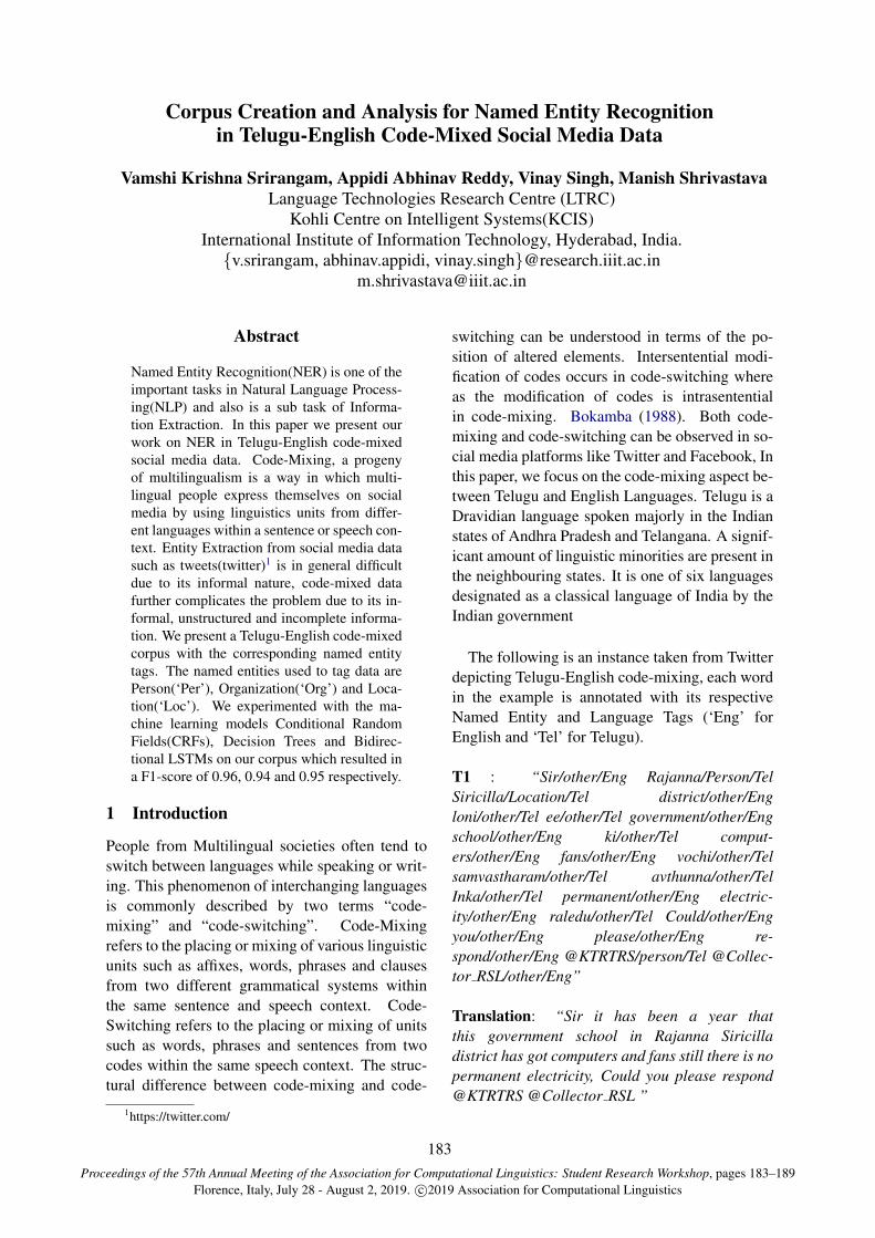
Proceedings of the 57th Annual Meeting of the Association for Computational Linguistics: Student Research Workshop, pages 183–189Florence, Italy, July 28 - August 2, 2019. c©2019 Association for Computational Linguistics

Corpus Creation and Analysis for Named Entity Recognitionin Telugu-English Code-Mixed Social Media Data

Vamshi Krishna Srirangam, Appidi Abhinav Reddy, Vinay Singh, Manish ShrivastavaLanguage Technologies Research Centre (LTRC)

Kohli Centre on Intelligent Systems(KCIS)International Institute of Information Technology, Hyderabad, India.v.srirangam, abhinav.appidi, vinay.singh@research.iiit.ac.in

m.shrivastava@iiit.ac.in

Abstract

Named Entity Recognition(NER) is one of theimportant tasks in Natural Language Process-ing(NLP) and also is a sub task of Informa-tion Extraction. In this paper we present ourwork on NER in Telugu-English code-mixedsocial media data. Code-Mixing, a progenyof multilingualism is a way in which multi-lingual people express themselves on socialmedia by using linguistics units from differ-ent languages within a sentence or speech con-text. Entity Extraction from social media datasuch as tweets(twitter)1 is in general difficultdue to its informal nature, code-mixed datafurther complicates the problem due to its in-formal, unstructured and incomplete informa-tion. We present a Telugu-English code-mixedcorpus with the corresponding named entitytags. The named entities used to tag data arePerson(‘Per’), Organization(‘Org’) and Loca-tion(‘Loc’). We experimented with the ma-chine learning models Conditional RandomFields(CRFs), Decision Trees and Bidirec-tional LSTMs on our corpus which resulted ina F1-score of 0.96, 0.94 and 0.95 respectively.

1 Introduction

People from Multilingual societies often tend toswitch between languages while speaking or writ-ing. This phenomenon of interchanging languagesis commonly described by two terms “code-mixing” and “code-switching”. Code-Mixingrefers to the placing or mixing of various linguisticunits such as affixes, words, phrases and clausesfrom two different grammatical systems withinthe same sentence and speech context. Code-Switching refers to the placing or mixing of unitssuch as words, phrases and sentences from twocodes within the same speech context. The struc-tural difference between code-mixing and code-

1https://twitter.com/

switching can be understood in terms of the po-sition of altered elements. Intersentential modi-fication of codes occurs in code-switching whereas the modification of codes is intrasententialin code-mixing. Bokamba (1988). Both code-mixing and code-switching can be observed in so-cial media platforms like Twitter and Facebook, Inthis paper, we focus on the code-mixing aspect be-tween Telugu and English Languages. Telugu is aDravidian language spoken majorly in the Indianstates of Andhra Pradesh and Telangana. A signif-icant amount of linguistic minorities are present inthe neighbouring states. It is one of six languagesdesignated as a classical language of India by theIndian government

The following is an instance taken from Twitterdepicting Telugu-English code-mixing, each wordin the example is annotated with its respectiveNamed Entity and Language Tags (‘Eng’ forEnglish and ‘Tel’ for Telugu).

T1 : “Sir/other/Eng Rajanna/Person/TelSiricilla/Location/Tel district/other/Engloni/other/Tel ee/other/Tel government/other/Engschool/other/Eng ki/other/Tel comput-ers/other/Eng fans/other/Eng vochi/other/Telsamvastharam/other/Tel avthunna/other/TelInka/other/Tel permanent/other/Eng electric-ity/other/Eng raledu/other/Tel Could/other/Engyou/other/Eng please/other/Eng re-spond/other/Eng @KTRTRS/person/Tel @Collec-tor RSL/other/Eng”

Translation: “Sir it has been a year thatthis government school in Rajanna Siricilladistrict has got computers and fans still there is nopermanent electricity, Could you please respond@KTRTRS @Collector RSL ”

183

2 Background and Related work

There has been a significant amount of researchdone in Named Entity Recognition(NER) of re-source rich languages Finkel et al. (2005), En-glish Sarkar (2015), German Tjong Kim Sang andDe Meulder (2003), French Azpeitia et al. (2014)and Spanish Zea et al. (2016) while the same isnot true for code-mixed Indian languages. TheFIRE(Forum for Information Retrieval and Ex-traction)2 tasks have shed light on NER in Indianlanguages as well as code-mixed data. The fol-lowing are some works in code-mixed Indian lan-guages. Bhargava et al. (2016) proposed an algo-rithm which uses a hybrid approach of a dictionarycum supervised classification approach for identi-fying entities in Code Mixed Text of Indian Lan-guages such as Hindi- English and Tamil-English.

Nelakuditi et al. (2016) reported work on anno-tating code mixed English-Telugu data collectedfrom social media site Facebook and creatingautomatic POS Taggers for this corpus, Singhet al. (2018a) presented an exploration of auto-matic NER of Hindi-English code-mixed data,Singh et al. (2018b) presented a corpus for NERin Hindi-English Code-Mixed along with experi-ments on their machine learning models. To thebest of our knowledge the corpus we created isthe first Telugu-English code-mixed corpus withnamed entity tags.

3 Corpus and Annotation

The corpus created consists of code-mixedTelugu-English tweets from Twitter. The tweetswere scrapped from Twitter using the TwitterPython API3 which uses the advanced search op-tion of Twitter. The mined tweets are from thepast 2 years and belong to topics such as politics,movies, sports, social events etc.. The Hashtagsused for tweet mining are shown in the appendi-cies section. Extensive Pre-processing of tweetsis done. The tweets which are noisy and uselessi.e contain only URL’s and hash-tags are removed.Tokenization of tweets is done using Tweet Tok-enizer. Tweets which are written only in Englishor in Telugu Script are removed too. Finally thetweets which contain linguistic units from bothTelugu and English language are considered. Thisway we made sure that the tweets are Telugu-English code-mixed. We have retrieved a total of

2http://fire.irsi.res.in/fire/2018/home3https://pypi.python.org/pypi/twitterscraper/0.2.7

2,16,800 tweets using the python twitter API andafter the extensive cleaning we are left with 3968code-mixed Telugu-English Tweets. The corpuswill be made available online soon. The followingexplains the mapping of tokens with their respec-tive tags.

3.1 Annotation: Named Entity Tagging

We used the following three Named Entities(NE)tags “Person”, “Organization“ and “Location”to tag the data. The Annotation of the corpusfor Named Entity tags was manually done bytwo persons with linguistic background whoare well proficient in both Telugu and English.Each of three tags(“Person”, “Organization“ and“Location”) is divided into B-tag (Beginner tag)and I-tag (Intermediate tag) according to the BIOstandard. Thus we have now a total of six tagsand an ’Other’ tag to indicate if it does not belongto any of the six tags. The B-tag is used to taga word which is the Beginning word of a NamedEntity. I-tag is used if a Named Entity is splitinto multiple continuous and I-tag is assigned tothe words which follow the Beginning word. Thefollowing explains each of the six tags used forannotation.

The ‘Per’ tag refers to the ‘Person’ entitywhich is the name of the Person, twitter handlesand nicknames of people. The ‘B-Per’ tag is givento the Beginning word of a Person name and‘I-Per’ tag is given to the Intermediate word if thePerson name is split into multiple continuous.

The ‘Org’ tag refers to ‘Organization’ entitywhich is the name of the social and political or-ganizations like ‘Hindus’, ‘Muslims’, ‘BharatiyaJanatha Party’, ‘BJP’, ‘TRS’ and governmentinstitutions like ‘Reserve Bank of India’. Socialmedia organizations and companies like ‘Twitter’,‘facebook’, ‘Google’. The ‘B-Org’ tag is given tothe beginning word of a Organization name andthe ‘I-Org’ tag is given to the Intermediate wordof the Organization name, if the Organizationname is split into multiple continuous.

The ‘Loc’ tag refers to ‘Location’ entity which isthe name of the places like ‘Hyderabad’, ‘USA’,‘Telangana’, ‘India’. The ‘B-Loc’ tag is given tothe Beginning word of the Location name and‘I-Loc’ tag is given to the Intermediate word of a

184

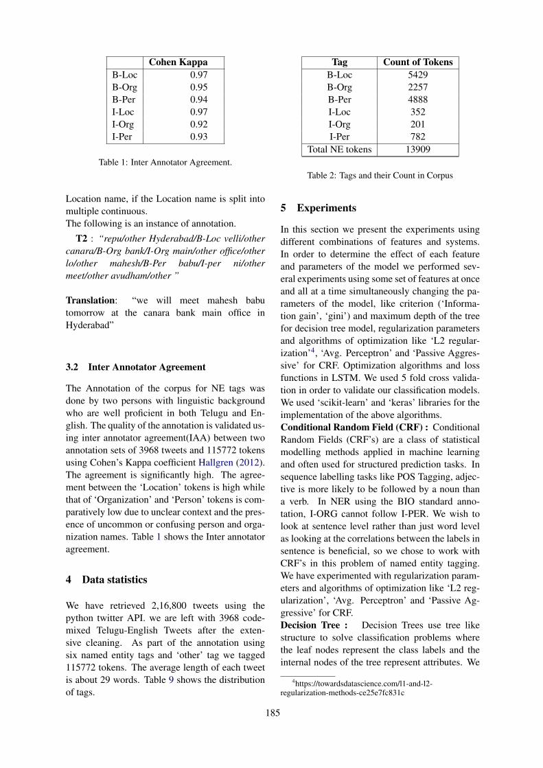
Cohen KappaB-Loc 0.97B-Org 0.95B-Per 0.94I-Loc 0.97I-Org 0.92I-Per 0.93

Table 1: Inter Annotator Agreement.

Location name, if the Location name is split intomultiple continuous.The following is an instance of annotation.

T2 : “repu/other Hyderabad/B-Loc velli/othercanara/B-Org bank/I-Org main/other office/otherlo/other mahesh/B-Per babu/I-per ni/othermeet/other avudham/other ”

Translation: “we will meet mahesh babutomorrow at the canara bank main office inHyderabad”

3.2 Inter Annotator Agreement

The Annotation of the corpus for NE tags wasdone by two persons with linguistic backgroundwho are well proficient in both Telugu and En-glish. The quality of the annotation is validated us-ing inter annotator agreement(IAA) between twoannotation sets of 3968 tweets and 115772 tokensusing Cohen’s Kappa coefficient Hallgren (2012).The agreement is significantly high. The agree-ment between the ‘Location’ tokens is high whilethat of ‘Organization’ and ‘Person’ tokens is com-paratively low due to unclear context and the pres-ence of uncommon or confusing person and orga-nization names. Table 1 shows the Inter annotatoragreement.

4 Data statistics

We have retrieved 2,16,800 tweets using thepython twitter API. we are left with 3968 code-mixed Telugu-English Tweets after the exten-sive cleaning. As part of the annotation usingsix named entity tags and ‘other’ tag we tagged115772 tokens. The average length of each tweetis about 29 words. Table 9 shows the distributionof tags.

Tag Count of TokensB-Loc 5429B-Org 2257B-Per 4888I-Loc 352I-Org 201I-Per 782

Total NE tokens 13909

Table 2: Tags and their Count in Corpus

5 Experiments

In this section we present the experiments usingdifferent combinations of features and systems.In order to determine the effect of each featureand parameters of the model we performed sev-eral experiments using some set of features at onceand all at a time simultaneously changing the pa-rameters of the model, like criterion (‘Informa-tion gain’, ‘gini’) and maximum depth of the treefor decision tree model, regularization parametersand algorithms of optimization like ‘L2 regular-ization’4, ‘Avg. Perceptron’ and ‘Passive Aggres-sive’ for CRF. Optimization algorithms and lossfunctions in LSTM. We used 5 fold cross valida-tion in order to validate our classification models.We used ‘scikit-learn’ and ‘keras’ libraries for theimplementation of the above algorithms.Conditional Random Field (CRF) : ConditionalRandom Fields (CRF’s) are a class of statisticalmodelling methods applied in machine learningand often used for structured prediction tasks. Insequence labelling tasks like POS Tagging, adjec-tive is more likely to be followed by a noun thana verb. In NER using the BIO standard anno-tation, I-ORG cannot follow I-PER. We wish tolook at sentence level rather than just word levelas looking at the correlations between the labels insentence is beneficial, so we chose to work withCRF’s in this problem of named entity tagging.We have experimented with regularization param-eters and algorithms of optimization like ‘L2 reg-ularization’, ‘Avg. Perceptron’ and ‘Passive Ag-gressive’ for CRF.Decision Tree : Decision Trees use tree likestructure to solve classification problems wherethe leaf nodes represent the class labels and theinternal nodes of the tree represent attributes. We

4https://towardsdatascience.com/l1-and-l2-regularization-methods-ce25e7fc831c

185

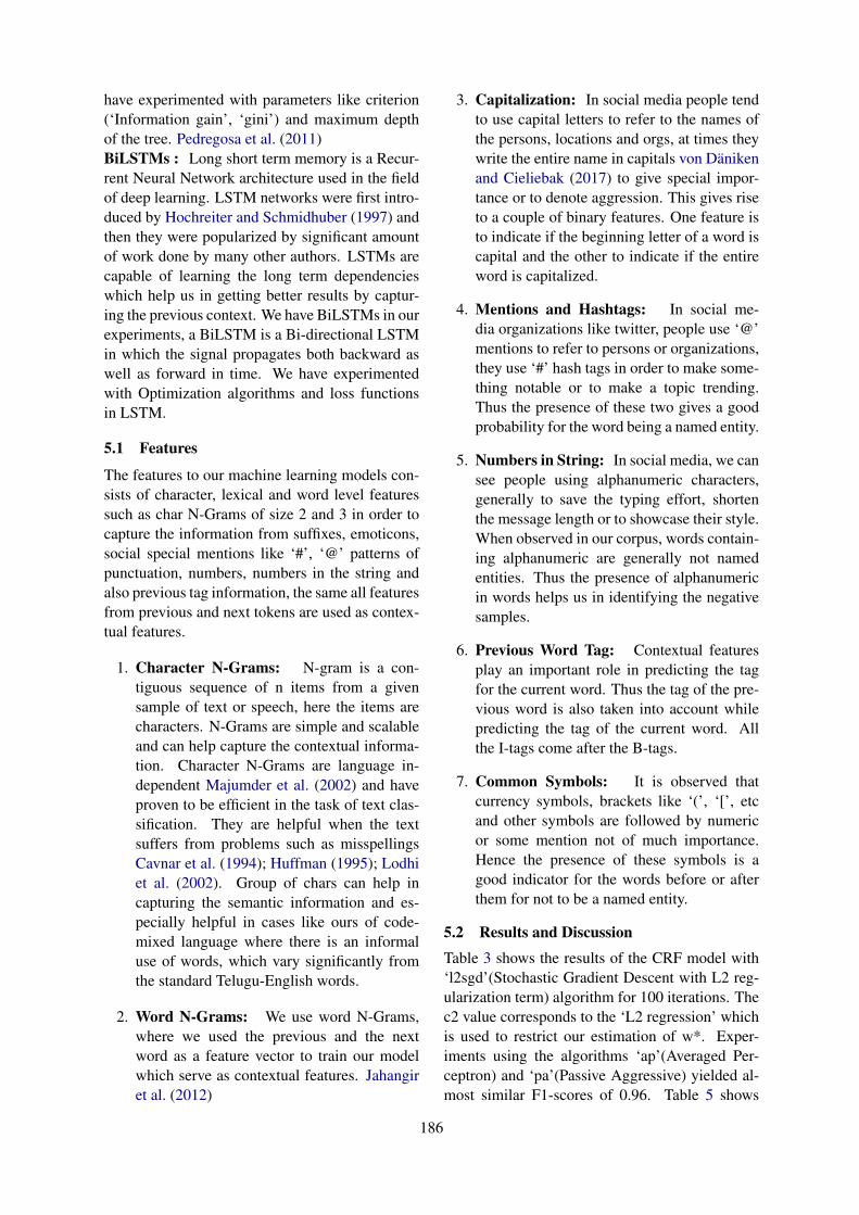
have experimented with parameters like criterion(‘Information gain’, ‘gini’) and maximum depthof the tree. Pedregosa et al. (2011)BiLSTMs : Long short term memory is a Recur-rent Neural Network architecture used in the fieldof deep learning. LSTM networks were first intro-duced by Hochreiter and Schmidhuber (1997) andthen they were popularized by significant amountof work done by many other authors. LSTMs arecapable of learning the long term dependencieswhich help us in getting better results by captur-ing the previous context. We have BiLSTMs in ourexperiments, a BiLSTM is a Bi-directional LSTMin which the signal propagates both backward aswell as forward in time. We have experimentedwith Optimization algorithms and loss functionsin LSTM.

5.1 Features

The features to our machine learning models con-sists of character, lexical and word level featuressuch as char N-Grams of size 2 and 3 in order tocapture the information from suffixes, emoticons,social special mentions like ‘#’, ‘@’ patterns ofpunctuation, numbers, numbers in the string andalso previous tag information, the same all featuresfrom previous and next tokens are used as contex-tual features.

1. Character N-Grams: N-gram is a con-tiguous sequence of n items from a givensample of text or speech, here the items arecharacters. N-Grams are simple and scalableand can help capture the contextual informa-tion. Character N-Grams are language in-dependent Majumder et al. (2002) and haveproven to be efficient in the task of text clas-sification. They are helpful when the textsuffers from problems such as misspellingsCavnar et al. (1994); Huffman (1995); Lodhiet al. (2002). Group of chars can help incapturing the semantic information and es-pecially helpful in cases like ours of code-mixed language where there is an informaluse of words, which vary significantly fromthe standard Telugu-English words.

2. Word N-Grams: We use word N-Grams,where we used the previous and the nextword as a feature vector to train our modelwhich serve as contextual features. Jahangiret al. (2012)

3. Capitalization: In social media people tendto use capital letters to refer to the names ofthe persons, locations and orgs, at times theywrite the entire name in capitals von Danikenand Cieliebak (2017) to give special impor-tance or to denote aggression. This gives riseto a couple of binary features. One feature isto indicate if the beginning letter of a word iscapital and the other to indicate if the entireword is capitalized.

4. Mentions and Hashtags: In social me-dia organizations like twitter, people use ‘@’mentions to refer to persons or organizations,they use ‘#’ hash tags in order to make some-thing notable or to make a topic trending.Thus the presence of these two gives a goodprobability for the word being a named entity.

5. Numbers in String: In social media, we cansee people using alphanumeric characters,generally to save the typing effort, shortenthe message length or to showcase their style.When observed in our corpus, words contain-ing alphanumeric are generally not namedentities. Thus the presence of alphanumericin words helps us in identifying the negativesamples.

6. Previous Word Tag: Contextual featuresplay an important role in predicting the tagfor the current word. Thus the tag of the pre-vious word is also taken into account whilepredicting the tag of the current word. Allthe I-tags come after the B-tags.

7. Common Symbols: It is observed thatcurrency symbols, brackets like ‘(’, ‘[’, etcand other symbols are followed by numericor some mention not of much importance.Hence the presence of these symbols is agood indicator for the words before or afterthem for not to be a named entity.

5.2 Results and Discussion

Table 3 shows the results of the CRF model with‘l2sgd’(Stochastic Gradient Descent with L2 reg-ularization term) algorithm for 100 iterations. Thec2 value corresponds to the ‘L2 regression’ whichis used to restrict our estimation of w*. Exper-iments using the algorithms ‘ap’(Averaged Per-ceptron) and ‘pa’(Passive Aggressive) yielded al-most similar F1-scores of 0.96. Table 5 shows

186

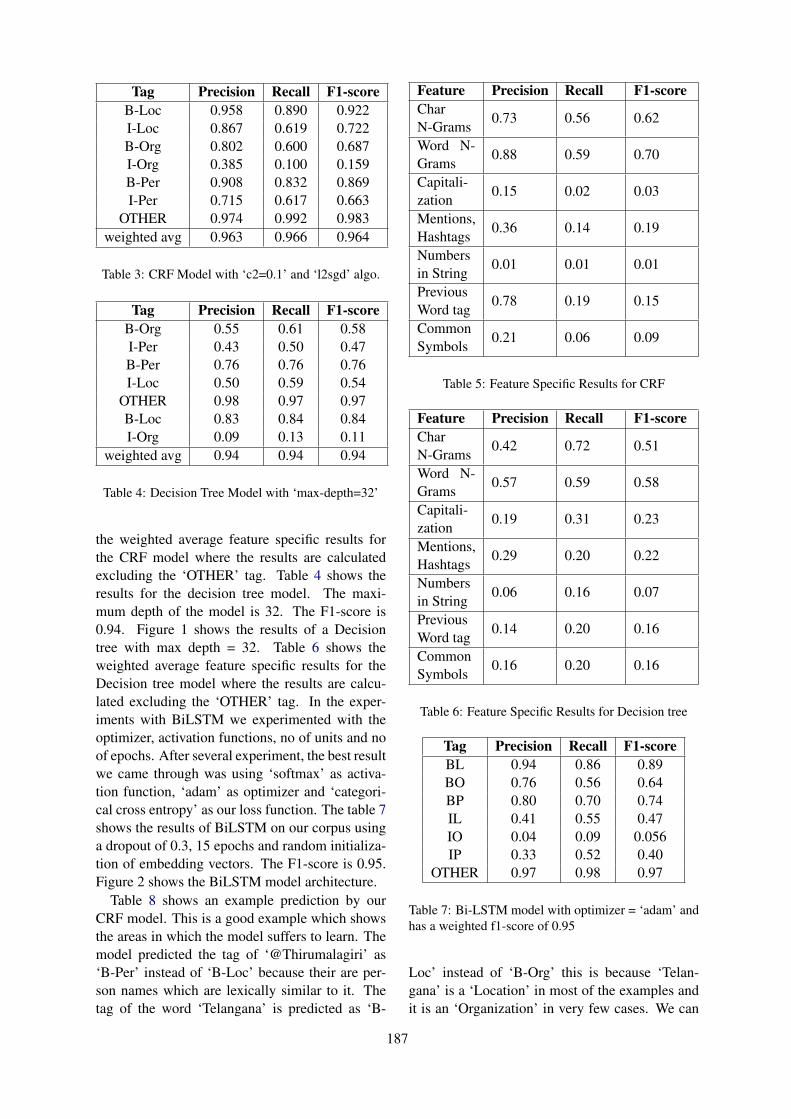
Tag Precision Recall F1-scoreB-Loc 0.958 0.890 0.922I-Loc 0.867 0.619 0.722B-Org 0.802 0.600 0.687I-Org 0.385 0.100 0.159B-Per 0.908 0.832 0.869I-Per 0.715 0.617 0.663

OTHER 0.974 0.992 0.983weighted avg 0.963 0.966 0.964

Table 3: CRF Model with ‘c2=0.1’ and ‘l2sgd’ algo.

Tag Precision Recall F1-scoreB-Org 0.55 0.61 0.58I-Per 0.43 0.50 0.47B-Per 0.76 0.76 0.76I-Loc 0.50 0.59 0.54

OTHER 0.98 0.97 0.97B-Loc 0.83 0.84 0.84I-Org 0.09 0.13 0.11

weighted avg 0.94 0.94 0.94

Table 4: Decision Tree Model with ‘max-depth=32’

the weighted average feature specific results forthe CRF model where the results are calculatedexcluding the ‘OTHER’ tag. Table 4 shows theresults for the decision tree model. The maxi-mum depth of the model is 32. The F1-score is0.94. Figure 1 shows the results of a Decisiontree with max depth = 32. Table 6 shows theweighted average feature specific results for theDecision tree model where the results are calcu-lated excluding the ‘OTHER’ tag. In the exper-iments with BiLSTM we experimented with theoptimizer, activation functions, no of units and noof epochs. After several experiment, the best resultwe came through was using ‘softmax’ as activa-tion function, ‘adam’ as optimizer and ‘categori-cal cross entropy’ as our loss function. The table 7shows the results of BiLSTM on our corpus usinga dropout of 0.3, 15 epochs and random initializa-tion of embedding vectors. The F1-score is 0.95.Figure 2 shows the BiLSTM model architecture.

Table 8 shows an example prediction by ourCRF model. This is a good example which showsthe areas in which the model suffers to learn. Themodel predicted the tag of ‘@Thirumalagiri’ as‘B-Per’ instead of ‘B-Loc’ because their are per-son names which are lexically similar to it. Thetag of the word ‘Telangana’ is predicted as ‘B-

Feature Precision Recall F1-scoreCharN-Grams

0.73 0.56 0.62

Word N-Grams

0.88 0.59 0.70

Capitali-zation

0.15 0.02 0.03

Mentions,Hashtags

0.36 0.14 0.19

Numbersin String

0.01 0.01 0.01

PreviousWord tag

0.78 0.19 0.15

CommonSymbols

0.21 0.06 0.09

Table 5: Feature Specific Results for CRF

Feature Precision Recall F1-scoreCharN-Grams

0.42 0.72 0.51

Word N-Grams

0.57 0.59 0.58

Capitali-zation

0.19 0.31 0.23

Mentions,Hashtags

0.29 0.20 0.22

Numbersin String

0.06 0.16 0.07

PreviousWord tag

0.14 0.20 0.16

CommonSymbols

0.16 0.20 0.16

Table 6: Feature Specific Results for Decision tree

Tag Precision Recall F1-scoreBL 0.94 0.86 0.89BO 0.76 0.56 0.64BP 0.80 0.70 0.74IL 0.41 0.55 0.47IO 0.04 0.09 0.056IP 0.33 0.52 0.40

OTHER 0.97 0.98 0.97

Table 7: Bi-LSTM model with optimizer = ‘adam’ andhas a weighted f1-score of 0.95

Loc’ instead of ‘B-Org’ this is because ‘Telan-gana’ is a ‘Location’ in most of the examples andit is an ‘Organization’ in very few cases. We can

187

Figure 1: Results from a Decision Tree

Figure 2: BiLSTM model architecture

also see ‘@MedayRajeev’ is predicted as ‘B-Org’instead of ‘B-Per’. The model performs well for‘OTHER’ and ‘Location’ tags. Lexically similarwords having different tags and insufficient datamakes it difficult for the model to train at times asa result of which we can see some incorrect pre-dictions of tags.

6 Conclusion and future work

The following are our contributions in this paper.

1. Presented an annotated code-mixed Telugu-English corpus for named entity recognitionwhich is to the best of our knowledge is thefirst corpus. The corpus will be made avail-able online soon.

2. Experimented with the machine learningmodels Conditional Random Fields(CRF),

Word Truth PredictedToday OTHER OTHERpaper OTHER OTHER

clippings OTHER OTHERmanam B-Org OTHERvartha I-Org OTHER

@Thirumalagiri B-Loc B-Per@Nagaram B-Loc B-PerTelangana B-Org B-LocJagruthi I-Org OTHER

Thungathurthy B-Loc B-LocNiyojakavargam OTHER OTHER@MedayRajeev B-Per B-Org@JagruthiFans B-Org B-Org

Table 8: An Example Prediction of our CRF Model

Decision tree, BiLSTM on our corpus, theF1-score for which is 0.96, 0.94 and 0.95 re-spectively. Which is looking good consider-ing the amount of research done in this newdomain.

3. Introducing and addressing named entityrecognition of Telugu-English code-mixedcorpus as a research problem.

As part of the future work, the corpus can beenriched by also giving the respective POS tagsfor each token. The size of the corpus can be in-creased with more NE tags.The problem can beextended for NER identification in code-mixedtext containing more than two languages frommultilingual societies.

ReferencesAndoni Azpeitia, Montse Cuadros, Sean Gaines, and

German Rigau. 2014. Nerc-fr: supervised namedentity recognition for french. In International Con-ference on Text, Speech, and Dialogue, pages 158–165. Springer.

Rupal Bhargava, Bapiraju Vamsi, and YashvardhanSharma. 2016. Named entity recognition for codemixing in indian languages using hybrid approach.Facilities, 23(10).

Eyamba G Bokamba. 1988. Code-mixing, languagevariation, and linguistic theory:: Evidence frombantu languages. Lingua, 76(1):21–62.

William B Cavnar, John M Trenkle, et al. 1994. N-gram-based text categorization. Ann arbor mi,48113(2):161–175.

188

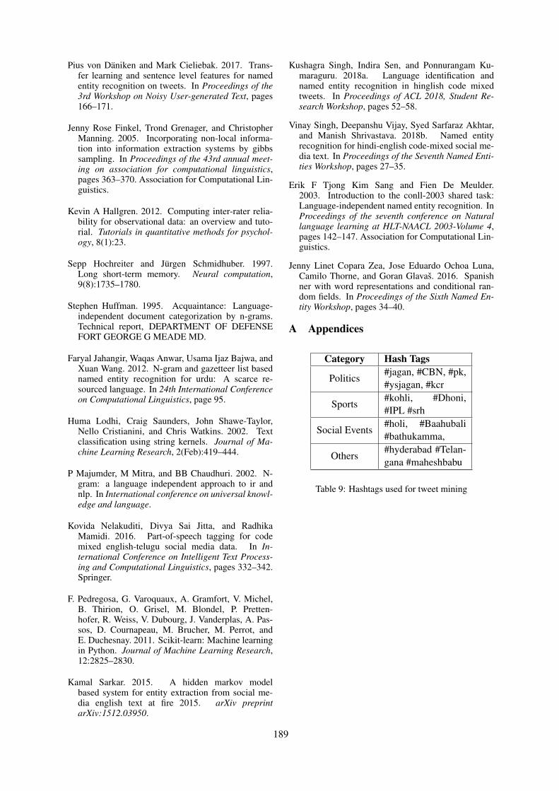
Pius von Daniken and Mark Cieliebak. 2017. Trans-fer learning and sentence level features for namedentity recognition on tweets. In Proceedings of the3rd Workshop on Noisy User-generated Text, pages166–171.

Jenny Rose Finkel, Trond Grenager, and ChristopherManning. 2005. Incorporating non-local informa-tion into information extraction systems by gibbssampling. In Proceedings of the 43rd annual meet-ing on association for computational linguistics,pages 363–370. Association for Computational Lin-guistics.

Kevin A Hallgren. 2012. Computing inter-rater relia-bility for observational data: an overview and tuto-rial. Tutorials in quantitative methods for psychol-ogy, 8(1):23.

Sepp Hochreiter and Jurgen Schmidhuber. 1997.Long short-term memory. Neural computation,9(8):1735–1780.

Stephen Huffman. 1995. Acquaintance: Language-independent document categorization by n-grams.Technical report, DEPARTMENT OF DEFENSEFORT GEORGE G MEADE MD.

Faryal Jahangir, Waqas Anwar, Usama Ijaz Bajwa, andXuan Wang. 2012. N-gram and gazetteer list basednamed entity recognition for urdu: A scarce re-sourced language. In 24th International Conferenceon Computational Linguistics, page 95.

Huma Lodhi, Craig Saunders, John Shawe-Taylor,Nello Cristianini, and Chris Watkins. 2002. Textclassification using string kernels. Journal of Ma-chine Learning Research, 2(Feb):419–444.

P Majumder, M Mitra, and BB Chaudhuri. 2002. N-gram: a language independent approach to ir andnlp. In International conference on universal knowl-edge and language.

Kovida Nelakuditi, Divya Sai Jitta, and RadhikaMamidi. 2016. Part-of-speech tagging for codemixed english-telugu social media data. In In-ternational Conference on Intelligent Text Process-ing and Computational Linguistics, pages 332–342.Springer.

F. Pedregosa, G. Varoquaux, A. Gramfort, V. Michel,B. Thirion, O. Grisel, M. Blondel, P. Pretten-hofer, R. Weiss, V. Dubourg, J. Vanderplas, A. Pas-sos, D. Cournapeau, M. Brucher, M. Perrot, andE. Duchesnay. 2011. Scikit-learn: Machine learningin Python. Journal of Machine Learning Research,12:2825–2830.

Kamal Sarkar. 2015. A hidden markov modelbased system for entity extraction from social me-dia english text at fire 2015. arXiv preprintarXiv:1512.03950.

Kushagra Singh, Indira Sen, and Ponnurangam Ku-maraguru. 2018a. Language identification andnamed entity recognition in hinglish code mixedtweets. In Proceedings of ACL 2018, Student Re-search Workshop, pages 52–58.

Vinay Singh, Deepanshu Vijay, Syed Sarfaraz Akhtar,and Manish Shrivastava. 2018b. Named entityrecognition for hindi-english code-mixed social me-dia text. In Proceedings of the Seventh Named Enti-ties Workshop, pages 27–35.

Erik F Tjong Kim Sang and Fien De Meulder.2003. Introduction to the conll-2003 shared task:Language-independent named entity recognition. InProceedings of the seventh conference on Naturallanguage learning at HLT-NAACL 2003-Volume 4,pages 142–147. Association for Computational Lin-guistics.

Jenny Linet Copara Zea, Jose Eduardo Ochoa Luna,Camilo Thorne, and Goran Glavas. 2016. Spanishner with word representations and conditional ran-dom fields. In Proceedings of the Sixth Named En-tity Workshop, pages 34–40.

A Appendices

Category Hash Tags

Politics#jagan, #CBN, #pk,#ysjagan, #kcr

Sports#kohli, #Dhoni,#IPL #srh

Social Events#holi, #Baahubali#bathukamma,

Others#hyderabad #Telan-gana #maheshbabu

Table 9: Hashtags used for tweet mining

189

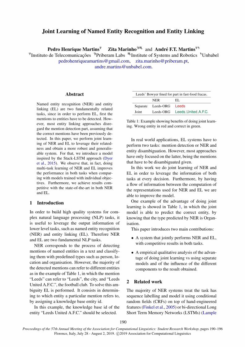
Proceedings of the 57th Annual Meeting of the Association for Computational Linguistics: Student Research Workshop, pages 190–196Florence, Italy, July 28 - August 2, 2019. c©2019 Association for Computational Linguistics

Joint Learning of Named Entity Recognition and Entity Linking

Pedro Henrique MartinsÈ Zita MarinhoÁç and Andre F.T. MartinsÈÆÈInstituto de Telecomunicacoes ÁPriberam Labs çInstitute of Systems and Robotics ÆUnbabel

pedrohenriqueamartins@gmail.com, zita.marinho@priberam.pt,andre.martins@unbabel.com.

Abstract

Named entity recognition (NER) and entitylinking (EL) are two fundamentally relatedtasks, since in order to perform EL, first thementions to entities have to be detected. How-ever, most entity linking approaches disre-gard the mention detection part, assuming thatthe correct mentions have been previously de-tected. In this paper, we perform joint learn-ing of NER and EL to leverage their related-ness and obtain a more robust and generalis-able system. For that, we introduce a modelinspired by the Stack-LSTM approach (Dyeret al., 2015). We observe that, in fact, doingmulti-task learning of NER and EL improvesthe performance in both tasks when compar-ing with models trained with individual objec-tives. Furthermore, we achieve results com-petitive with the state-of-the-art in both NERand EL.

1 Introduction

In order to build high quality systems for com-plex natural language processing (NLP) tasks, itis useful to leverage the output information oflower level tasks, such as named entity recognition(NER) and entity linking (EL). Therefore NERand EL are two fundamental NLP tasks.

NER corresponds to the process of detectingmentions of named entities in a text and classify-ing them with predefined types such as person, lo-cation and organisation. However, the majority ofthe detected mentions can refer to different entitiesas in the example of Table 1, in which the mention“Leeds” can refer to “Leeds”, the city, and “LeedsUnited A.F.C.”, the football club. To solve this am-biguity EL is performed. It consists in determin-ing to which entity a particular mention refers to,by assigning a knowledge base entity id.

In this example, the knowledge base id of theentity “Leeds United A.F.C.” should be selected.

Leeds’ Bowyer fined for part in fast-food fracas.

NER EL

Separate Leeds-ORG Leeds

Joint Leeds-ORG Leeds United A.F.C.

Table 1: Example showing benefits of doing joint learn-ing. Wrong entity in red and correct in green.

In real world applications, EL systems have toperform two tasks: mention detection or NER andentity disambiguation. However, most approacheshave only focused on the latter, being the mentionsthat have to be disambiguated given.

In this work we do joint learning of NER andEL in order to leverage the information of bothtasks at every decision. Furthermore, by havinga flow of information between the computation ofthe representations used for NER and EL we areable to improve the model.

One example of the advantage of doing jointlearning is showed in Table 1, in which the jointmodel is able to predict the correct entity, byknowing that the type predicted by NER is Organ-isation.

This paper introduces two main contributions:

• A system that jointly performs NER and EL,with competitive results in both tasks.

• A empirical qualitative analysis of the advan-tage of doing joint learning vs using separatemodels and of the influence of the differentcomponents to the result obtained.

2 Related work

The majority of NER systems treat the task hassequence labelling and model it using conditionalrandom fields (CRFs) on top of hand-engineeredfeatures (Finkel et al., 2005) or bi-directional LongShort Term Memory Networks (LSTMs) (Lample

190

Action Buffer Stack Output Entity[Obama, met, Donald, Trump] [] []

Shift [met, Donald, Trump] [Obama] []Reduce-PER [met, Donald, Trump] [] [(Obama)-PER] Barack ObamaOut [Donald, Trump] [] [(Obama)-PER, met] Barack ObamaShift [Trump] [Donald] [(Obama)-PER, met] Barack ObamaShift [] [Donald, Trump] [(Obama)-PER, met] Barack ObamaReduce-PER [] [] [(Obama)-PER, met, Barack Obama,

(Donald Trump)-PER] Donald Trump

Table 2: Actions and stack states when processing sentence “Obama met Donald Trump”. The predicted types anddetected mentions are contained in the Output and the entities the mentions refer to in the Entity.

et al., 2016; Chiu and Nichols, 2016). Recently,NER systems have been achieving state-of-the-artresults by using word contextual embeddings, ob-tained with language models (Peters et al., 2018;Devlin et al., 2018; Akbik et al., 2018).

Most EL systems discard mention detection,performing only entity disambiguation of previ-ously detected mentions. Thus, in these cases thedependency between the two tasks is ignored. ELstate-of-the-art methods often correspond to localmethods which use as main features a candidateentity representation, a mention representation,and a representation of the mention’s context (Sunet al., 2015; Yamada et al., 2016, 2017; Ganea andHofmann, 2017). Recently, there has also beenan increasing interest in attempting to improve ELperformance by leveraging knowledge base infor-mation (Radhakrishnan et al., 2018) or by allyinglocal and global features, using information aboutthe neighbouring mentions and respective entities(Le and Titov, 2018; Cao et al., 2018; Yang et al.,2018). However, these approaches involve know-ing the surrounding mentions which can be im-practical in a real case because we might not haveinformation about the following sentences. It alsoadds extraneous complexity that might implicate alonger time to process.

Some works, as in this paper, perform end-to-end EL trying to leverage the relatedness ofmention detection or NER and EL, and obtainedpromising results. Kolitsas et al. (2018) proposeda model that performs mention detection instead ofNER, not identifying the type of the detected men-tions, as in our approach. Sil and Yates (2013),Luo et al. (2015), and Nguyen et al. (2016) in-troduced models that do joint learning of NERand EL using hand-engineered features. (Durrettand Klein, 2014) performed joint learning of en-

tity typing, EL, and coreference using a structuredCRF, also with hand-engineered features. In con-trast, in our model we perform multi-task learning(Caruana, 1997; Evgeniou and Pontil, 2004), us-ing learned features.

3 Model Description

In this section firstly, we briefly explain the Stack-LSTM (Dyer et al., 2015; Lample et al., 2016),model that inspired our system. Then we will givea detailed explanation of our modifications and ofhow we extended it to also perform EL, as showedin the diagram of Figure 1. An example of howthe model processes a sentence can be viewed inTable 2.

3.1 Stack-LSTM

The Stack-LSTM corresponds to an action-basedsystem which is composed by LSTMs augmentedwith a stack pointer. In contrast to the most com-mon approaches which detect the entity mentionsfor a whole sequence, with Stack-LSTMs the en-tity mentions are detected and classified on the fly.This is a fundamental property to our model, sincewe perform EL when a mention is detected.

This model is composed by four stacks: theStack, that contains the words that are being pro-cessed, the Output, that is filled with the com-pleted chunks, the Action stack, which containsthe previous actions performed during the process-ing of the current document, and the Buffer, thatcontains the words to be processed.

For NER, in the Stack-LSTM there are threepossible types of actions:

• Shift, that pops a word off the Buffer andpushes it into the Stack. It means that the lastword of the Buffer is part of a named entity.

191

Buffer LSTM Output LSTM Stack LSTM Action LSTM

affineNER

bi-LSTM1

bi-LSTM2

Action (ŷt NER) c0

ce0 cp0

c1

ce1 cp1m et at

...

affineELEntity (ŷt EL) Mention

m

at

et

st ot bt

Type

pt

rt

Attention (αt)

Ht

qt

at et

Figure 1: Simplified diagram of our model. The dashed arrows only occur when the action is Reduce. The blocks inblue correspond to our extensions to the Stack-LSTM and the green blocks correspond to the model’s predictions.The grey blocks correspond to the stack-LSTM, the blue blocks to our extensions, and the green ones to the outputs.

• Out, that pops a word off the buffer and in-serts it into the Output. It means that the lastword of the Buffer is not part of a named en-tity.

• Reduce, that pops all the words in the Stackand pushes them into the Output. Thereis one action Reduce for each possible typeof named entities, e.g. Reduce-PER andReduce-LOC.

Moreover, the actions that can be performed ateach step are controlled: the action Out can onlyoccur if the stack is empty and the actions Reduceare only available when the Stack is not empty.

3.2 Our modelNER. To better capture the context, we comple-ment the Stack-LSTM with a representation vt ofthe sentence being processed, for each action stept. For that the sentence x1, . . . ,x|w| is passedthrough a bi-directional LSTM, being h1

w the hid-den state of its 1st layer (bi-LSTM1 in Figure 1),that corresponds to the word with index w:

h11, . . . ,h

1|w| = BiLSTM1(x1, . . . ,x|w|).

We compute a representation of the words con-tained in the Stack, qt, by doing the mean of thehidden states of the 1st layer of the bi-LSTM thatcorrespond to the words contained in the stack ataction step t, set St,:

qt =

∑k∈St

h1k

|St|.

This is used to compute the attention scores αt:

ztw = u>(W 1h1w +W 2 qt)

αt = softmax(zt),

where W 1, W 2, and u are trainable parameters.The representation vt is then obtained by doingthe weighted average of the bi-LSTM 1st layer’shidden states:

vt =

|w|∑

w=1

h1w αtw.

To predict the action to be performed, we imple-ment an affine transformation (affineNER in Fig-ure 1) whose input is the concatenation of the lasthidden states of the Buffer LSTM bt, Stack LSTMst, Action LSTM at, and Output LSTM ot, as wellas the sentence representation vt.

dt = [bt; st; at; ot; vt]

Then, for each step t, we use these representationsto compute the probability distribution pt over theset of possible actions A, and select the actionytNER

with the highest probability:

pt = softmax(affine(dt))

ytNER= arg max

a ∈ A(pt(a)).

192

The NER loss function is the cross entropy, withthe gold action for step t being represented by theone-hot vector ytNER

:

LNER = −T∑

t=1

y>tNERlog(pt).

where T is the total number of action steps for thecurrent document.

EL. When the action predicted is Reduce, amention is detected and classified. This mention isthen disambiguated by selecting its respective en-tity knowledge base id. The disambiguation stepis performed by ranking the mention’s candidateentities.

The candidate entities c ∈ C for the presentmention are represented by their entity embeddingce and their prior probability cp. The prior prob-abilities were previously computed based on theco-occurrences between mentions and candidatesin Wikipedia.

To represent the mention detected the 2nd layerof the sentence bi-LSTM (bi-LSTM2 in Figure 1),is used, being the representation m obtained byaveraging the hidden states h2

w that correspond tothe words contained in the mention, setM:

h21, . . . ,h

2|w| = BiLSTM2(h1

1, . . . ,h1|w|)

m =

∑w∈M h2

w

|M| .

These features are concatenated with the represen-tation of the sentence vt, and the last hidden stateof the Action stack-LSTM at:

ci = [cei; cpi; m; vt; at].

We compute a score for each candidate with affinetransformations (affineEL in Figure 1) that have cas input, and select the candidate entity with thehighest score, ytEL

:

lt = affine(tanh(affine(ci, . . . , cn)))

rt = softmax(lt)

ytEL= arg max

c ∈ C(rt(c)).

The EL loss function is the cross entropy, with thegold entity for step t being represented by the one-hot vector ytEL

:

LEL = −T∑

t=1

y>tELlog(rt)).

where T is the total number of mention that corre-spond to entities in the knowledge base.

Due to the fact that not every mention detectedhas a corresponding entity in the knowledge base,we first classify whether this mention contains anentry in the knowledge base using an affine trans-formation followed by a sigmoid. The affine’s in-put is the stack LSTM last hidden state st:

d = sigmoid(affine(st)).

The NIL loss function, binary cross-entropy, isgiven by:

LNIL =−(yNIL log(d)+(1− yNIL) log(1− d)),

where yNIL corresponds to the gold label, 1 ifmention should be linked and 0 otherwise.

During training we perform teacher forcing, i.e.we use the gold labels for NER and the NIL classi-fication, only performing EL when the gold actionis Reduce and the mention has a corresponding idin the knowledge base. The multi-task learningloss is then obtained by summing the individuallosses:

L = LNER + LEL + LNIL.

4 Experiments

4.1 Datasets and metricsWe trained and evaluated our model on the biggestNER-EL English dataset, the AIDA/CoNLLdataset (Hoffart et al., 2011). It is a collection ofnews wire articles from Reuters, composed by atraining set of 18,448 linked mentions in 946 doc-uments, a validation set of 4,791 mentions in 216documents, and a test set of 4,485 mentions in 231

193

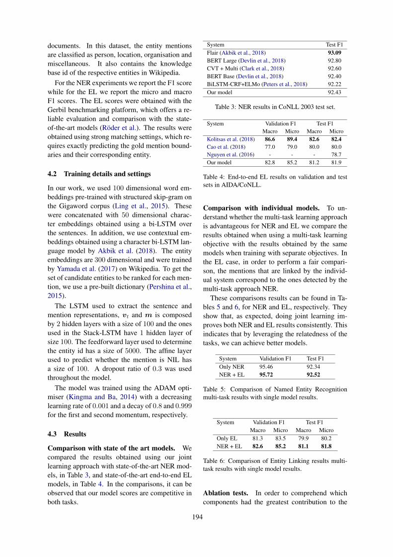
documents. In this dataset, the entity mentionsare classified as person, location, organisation andmiscellaneous. It also contains the knowledgebase id of the respective entities in Wikipedia.

For the NER experiments we report the F1 scorewhile for the EL we report the micro and macroF1 scores. The EL scores were obtained with theGerbil benchmarking platform, which offers a re-liable evaluation and comparison with the state-of-the-art models (Roder et al.). The results wereobtained using strong matching settings, which re-quires exactly predicting the gold mention bound-aries and their corresponding entity.

4.2 Training details and settings

In our work, we used 100 dimensional word em-beddings pre-trained with structured skip-gram onthe Gigaword corpus (Ling et al., 2015). Thesewere concatenated with 50 dimensional charac-ter embeddings obtained using a bi-LSTM overthe sentences. In addition, we use contextual em-beddings obtained using a character bi-LSTM lan-guage model by Akbik et al. (2018). The entityembeddings are 300 dimensional and were trainedby Yamada et al. (2017) on Wikipedia. To get theset of candidate entities to be ranked for each men-tion, we use a pre-built dictionary (Pershina et al.,2015).

The LSTM used to extract the sentence andmention representations, vt and m is composedby 2 hidden layers with a size of 100 and the onesused in the Stack-LSTM have 1 hidden layer ofsize 100. The feedforward layer used to determinethe entity id has a size of 5000. The affine layerused to predict whether the mention is NIL hasa size of 100. A dropout ratio of 0.3 was usedthroughout the model.

The model was trained using the ADAM opti-miser (Kingma and Ba, 2014) with a decreasinglearning rate of 0.001 and a decay of 0.8 and 0.999for the first and second momentum, respectively.

4.3 Results

Comparison with state of the art models. Wecompared the results obtained using our jointlearning approach with state-of-the-art NER mod-els, in Table 3, and state-of-the-art end-to-end ELmodels, in Table 4. In the comparisons, it can beobserved that our model scores are competitive inboth tasks.

System Test F1Flair (Akbik et al., 2018) 93.09BERT Large (Devlin et al., 2018) 92.80CVT + Multi (Clark et al., 2018) 92.60BERT Base (Devlin et al., 2018) 92.40BiLSTM-CRF+ELMo (Peters et al., 2018) 92.22Our model 92.43

Table 3: NER results in CoNLL 2003 test set.

System Validation F1 Test F1Macro Micro Macro Micro

Kolitsas et al. (2018) 86.6 89.4 82.6 82.4Cao et al. (2018) 77.0 79.0 80.0 80.0Nguyen et al. (2016) - - - 78.7Our model 82.8 85.2 81.2 81.9

Table 4: End-to-end EL results on validation and testsets in AIDA/CoNLL.

Comparison with individual models. To un-derstand whether the multi-task learning approachis advantageous for NER and EL we compare theresults obtained when using a multi-task learningobjective with the results obtained by the samemodels when training with separate objectives. Inthe EL case, in order to perform a fair compari-son, the mentions that are linked by the individ-ual system correspond to the ones detected by themulti-task approach NER.

These comparisons results can be found in Ta-bles 5 and 6, for NER and EL, respectively. Theyshow that, as expected, doing joint learning im-proves both NER and EL results consistently. Thisindicates that by leveraging the relatedness of thetasks, we can achieve better models.

System Validation F1 Test F1Only NER 95.46 92.34NER + EL 95.72 92.52

Table 5: Comparison of Named Entity Recognitionmulti-task results with single model results.

System Validation F1 Test F1Macro Micro Macro Micro

Only EL 81.3 83.5 79.9 80.2NER + EL 82.6 85.2 81.1 81.8

Table 6: Comparison of Entity Linking results multi-task results with single model results.

Ablation tests. In order to comprehend whichcomponents had the greatest contribution to the

194

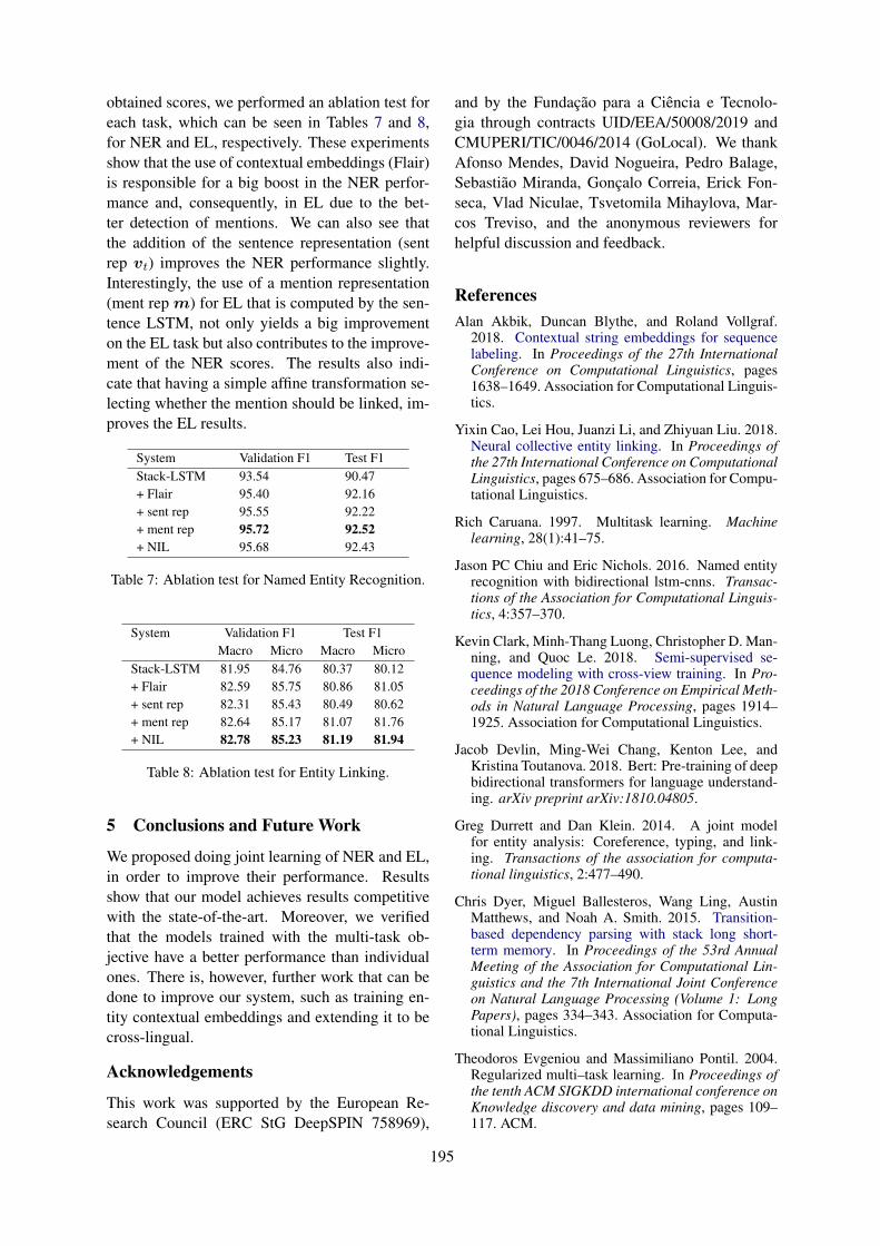
obtained scores, we performed an ablation test foreach task, which can be seen in Tables 7 and 8,for NER and EL, respectively. These experimentsshow that the use of contextual embeddings (Flair)is responsible for a big boost in the NER perfor-mance and, consequently, in EL due to the bet-ter detection of mentions. We can also see thatthe addition of the sentence representation (sentrep vt) improves the NER performance slightly.Interestingly, the use of a mention representation(ment rep m) for EL that is computed by the sen-tence LSTM, not only yields a big improvementon the EL task but also contributes to the improve-ment of the NER scores. The results also indi-cate that having a simple affine transformation se-lecting whether the mention should be linked, im-proves the EL results.

System Validation F1 Test F1Stack-LSTM 93.54 90.47+ Flair 95.40 92.16+ sent rep 95.55 92.22+ ment rep 95.72 92.52+ NIL 95.68 92.43

Table 7: Ablation test for Named Entity Recognition.

System Validation F1 Test F1Macro Micro Macro Micro

Stack-LSTM 81.95 84.76 80.37 80.12+ Flair 82.59 85.75 80.86 81.05+ sent rep 82.31 85.43 80.49 80.62+ ment rep 82.64 85.17 81.07 81.76+ NIL 82.78 85.23 81.19 81.94

Table 8: Ablation test for Entity Linking.

5 Conclusions and Future Work

We proposed doing joint learning of NER and EL,in order to improve their performance. Resultsshow that our model achieves results competitivewith the state-of-the-art. Moreover, we verifiedthat the models trained with the multi-task ob-jective have a better performance than individualones. There is, however, further work that can bedone to improve our system, such as training en-tity contextual embeddings and extending it to becross-lingual.

Acknowledgements

This work was supported by the European Re-search Council (ERC StG DeepSPIN 758969),

and by the Fundacao para a Ciencia e Tecnolo-gia through contracts UID/EEA/50008/2019 andCMUPERI/TIC/0046/2014 (GoLocal). We thankAfonso Mendes, David Nogueira, Pedro Balage,Sebastiao Miranda, Goncalo Correia, Erick Fon-seca, Vlad Niculae, Tsvetomila Mihaylova, Mar-cos Treviso, and the anonymous reviewers forhelpful discussion and feedback.

ReferencesAlan Akbik, Duncan Blythe, and Roland Vollgraf.

2018. Contextual string embeddings for sequencelabeling. In Proceedings of the 27th InternationalConference on Computational Linguistics, pages1638–1649. Association for Computational Linguis-tics.

Yixin Cao, Lei Hou, Juanzi Li, and Zhiyuan Liu. 2018.Neural collective entity linking. In Proceedings ofthe 27th International Conference on ComputationalLinguistics, pages 675–686. Association for Compu-tational Linguistics.

Rich Caruana. 1997. Multitask learning. Machinelearning, 28(1):41–75.

Jason PC Chiu and Eric Nichols. 2016. Named entityrecognition with bidirectional lstm-cnns. Transac-tions of the Association for Computational Linguis-tics, 4:357–370.

Kevin Clark, Minh-Thang Luong, Christopher D. Man-ning, and Quoc Le. 2018. Semi-supervised se-quence modeling with cross-view training. In Pro-ceedings of the 2018 Conference on Empirical Meth-ods in Natural Language Processing, pages 1914–1925. Association for Computational Linguistics.

Jacob Devlin, Ming-Wei Chang, Kenton Lee, andKristina Toutanova. 2018. Bert: Pre-training of deepbidirectional transformers for language understand-ing. arXiv preprint arXiv:1810.04805.

Greg Durrett and Dan Klein. 2014. A joint modelfor entity analysis: Coreference, typing, and link-ing. Transactions of the association for computa-tional linguistics, 2:477–490.

Chris Dyer, Miguel Ballesteros, Wang Ling, AustinMatthews, and Noah A. Smith. 2015. Transition-based dependency parsing with stack long short-term memory. In Proceedings of the 53rd AnnualMeeting of the Association for Computational Lin-guistics and the 7th International Joint Conferenceon Natural Language Processing (Volume 1: LongPapers), pages 334–343. Association for Computa-tional Linguistics.

Theodoros Evgeniou and Massimiliano Pontil. 2004.Regularized multi–task learning. In Proceedings ofthe tenth ACM SIGKDD international conference onKnowledge discovery and data mining, pages 109–117. ACM.

195

Jenny Rose Finkel, Trond Grenager, and ChristopherManning. 2005. Incorporating non-local informa-tion into information extraction systems by gibbssampling. In Proceedings of the 43rd annual meet-ing on association for computational linguistics,pages 363–370. Association for Computational Lin-guistics.

Octavian-Eugen Ganea and Thomas Hofmann. 2017.Deep joint entity disambiguation with local neuralattention. In Proceedings of the 2017 Conference onEmpirical Methods in Natural Language Process-ing, pages 2619–2629.

Johannes Hoffart, Mohamed Amir Yosef, Ilaria Bor-dino, Hagen Furstenau, Manfred Pinkal, Marc Span-iol, Bilyana Taneva, Stefan Thater, and GerhardWeikum. 2011. Robust disambiguation of namedentities in text. In Proceedings of the Conference onEmpirical Methods in Natural Language Process-ing, pages 782–792. Association for ComputationalLinguistics.

Diederik Kingma and Jimmy Ba. 2014. Adam:A method for stochastic optimization.arXiv:1412.6980 [cs.LG], pages 1–13.

Nikolaos Kolitsas, Octavian-Eugen Ganea, andThomas Hofmann. 2018. End-to-end neural entitylinking. In Proceedings of the 22nd Conferenceon Computational Natural Language Learning,pages 519–529. Association for ComputationalLinguistics.

Guillaume Lample, Miguel Ballesteros, Sandeep Sub-ramanian, Kazuya Kawakami, and Chris Dyer. 2016.Neural architectures for named entity recognition.arXiv preprint arXiv:1603.01360.

Phong Le and Ivan Titov. 2018. Improving entity link-ing by modeling latent relations between mentions.In Proceedings of the 56th Annual Meeting of theAssociation for Computational Linguistics (Volume1: Long Papers), pages 1595–1604.

Wang Ling, Chris Dyer, Alan W Black, and IsabelTrancoso. 2015. Two/too simple adaptations ofword2vec for syntax problems. In Proceedings ofthe 2015 Conference of the North American Chap-ter of the Association for Computational Linguistics:Human Language Technologies, pages 1299–1304.Association for Computational Linguistics.

Gang Luo, Xiaojiang Huang, Chin-Yew Lin, and Za-iqing Nie. 2015. Joint entity recognition and disam-biguation. In Proceedings of the 2015 Conferenceon Empirical Methods in Natural Language Pro-cessing, pages 879–888.

Dat Ba Nguyen, Martin Theobald, and GerhardWeikum. 2016. J-nerd: joint named entity recogni-tion and disambiguation with rich linguistic features.Transactions of the Association for ComputationalLinguistics, 4:215–229.

Maria Pershina, Yifan He, and Ralph Grishman. 2015.Personalized page rank for named entity disam-biguation. In Proceedings of the 2015 Conference ofthe North American Chapter of the Association forComputational Linguistics: Human Language Tech-nologies, pages 238–243.

Matthew E Peters, Mark Neumann, Mohit Iyyer, MattGardner, Christopher Clark, Kenton Lee, and LukeZettlemoyer. 2018. Deep contextualized word rep-resentations. In Proceedings of NAACL-HLT, pages2227–2237, New Orleans, Louisiana.

Priya Radhakrishnan, Partha Talukdar, and VasudevaVarma. 2018. Elden: Improved entity linking us-ing densified knowledge graphs. In Proceedings ofthe 2018 Conference of the North American Chap-ter of the Association for Computational Linguistics:Human Language Technologies, Volume 1 (Long Pa-pers), pages 1844–1853.

Michael Roder, Ricardo Usbeck, and Axel-CyrilleNgonga Ngomo. Gerbil–benchmarking named en-tity recognition and linking consistently. SemanticWeb, (Preprint):1–21.

Avirup Sil and Alexander Yates. 2013. Re-ranking forjoint named-entity recognition and linking. In Pro-ceedings of the 22nd ACM international conferenceon Information & Knowledge Management, pages2369–2374. ACM.

Yaming Sun, Lei Lin, Duyu Tang, Nan Yang, Zhen-zhou Ji, and Xiaolong Wang. 2015. Modeling men-tion, context and entity with neural networks for en-tity disambiguation. In Twenty-Fourth InternationalJoint Conference on Artificial Intelligence.

Ikuya Yamada, Hiroyuki Shindo, Hideaki Takeda, andYoshiyasu Takefuji. 2016. Joint learning of the em-bedding of words and entities for named entity dis-ambiguation. In Proceedings of The 20th SIGNLLConference on Computational Natural LanguageLearning, pages 250–259.

Ikuya Yamada, Hiroyuki Shindo, Hideaki Takeda, andYoshiyasu Takefuji. 2017. Learning distributed rep-resentations of texts and entities from knowledgebase. TACL, 5:397–411.

Yi Yang, Ozan Irsoy, and Kazi Shefaet Rahman.2018. Collective entity disambiguation with struc-tured gradient tree boosting. In Proceedings of the2018 Conference of the North American Chapter ofthe Association for Computational Linguistics: Hu-man Language Technologies, Volume 1 (Long Pa-pers), pages 777–786.

196

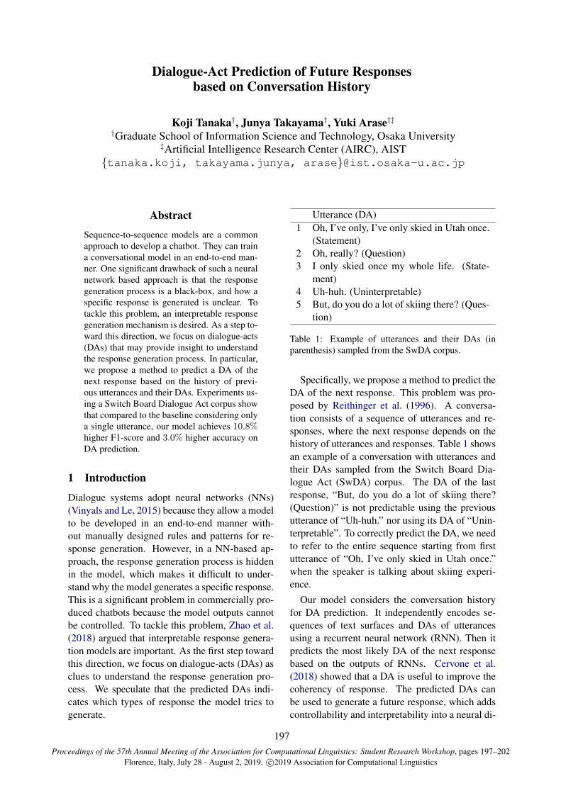
Proceedings of the 57th Annual Meeting of the Association for Computational Linguistics: Student Research Workshop, pages 197–202Florence, Italy, July 28 - August 2, 2019. c©2019 Association for Computational Linguistics

Dialogue-Act Prediction of Future Responsesbased on Conversation History

Koji Tanaka†, Junya Takayama†, Yuki Arase†‡†Graduate School of Information Science and Technology, Osaka University

‡Artificial Intelligence Research Center (AIRC), AISTtanaka.koji, takayama.junya, arase@ist.osaka-u.ac.jp

Abstract

Sequence-to-sequence models are a commonapproach to develop a chatbot. They can traina conversational model in an end-to-end man-ner. One significant drawback of such a neuralnetwork based approach is that the responsegeneration process is a black-box, and how aspecific response is generated is unclear. Totackle this problem, an interpretable responsegeneration mechanism is desired. As a step to-ward this direction, we focus on dialogue-acts(DAs) that may provide insight to understandthe response generation process. In particular,we propose a method to predict a DA of thenext response based on the history of previ-ous utterances and their DAs. Experiments us-ing a Switch Board Dialogue Act corpus showthat compared to the baseline considering onlya single utterance, our model achieves 10.8%higher F1-score and 3.0% higher accuracy onDA prediction.

1 Introduction

Dialogue systems adopt neural networks (NNs)(Vinyals and Le, 2015) because they allow a modelto be developed in an end-to-end manner with-out manually designed rules and patterns for re-sponse generation. However, in a NN-based ap-proach, the response generation process is hiddenin the model, which makes it difficult to under-stand why the model generates a specific response.This is a significant problem in commercially pro-duced chatbots because the model outputs cannotbe controlled. To tackle this problem, Zhao et al.(2018) argued that interpretable response genera-tion models are important. As the first step towardthis direction, we focus on dialogue-acts (DAs) asclues to understand the response generation pro-cess. We speculate that the predicted DAs indi-cates which types of response the model tries togenerate.

Utterance (DA)1 Oh, I’ve only, I’ve only skied in Utah once.

(Statement)2 Oh, really? (Question)3 I only skied once my whole life. (State-

ment)4 Uh-huh. (Uninterpretable)5 But, do you do a lot of skiing there? (Ques-

tion)

Table 1: Example of utterances and their DAs (inparenthesis) sampled from the SwDA corpus.

Specifically, we propose a method to predict theDA of the next response. This problem was pro-posed by Reithinger et al. (1996). A conversa-tion consists of a sequence of utterances and re-sponses, where the next response depends on thehistory of utterances and responses. Table 1 showsan example of a conversation with utterances andtheir DAs sampled from the Switch Board Dia-logue Act (SwDA) corpus. The DA of the lastresponse, “But, do you do a lot of skiing there?(Question)” is not predictable using the previousutterance of “Uh-huh.” nor using its DA of “Unin-terpretable”. To correctly predict the DA, we needto refer to the entire sequence starting from firstutterance of “Oh, I’ve only skied in Utah once.”when the speaker is talking about skiing experi-ence.

Our model considers the conversation historyfor DA prediction. It independently encodes se-quences of text surfaces and DAs of utterancesusing a recurrent neural network (RNN). Then itpredicts the most likely DA of the next responsebased on the outputs of RNNs. Cervone et al.(2018) showed that a DA is useful to improve thecoherency of response. The predicted DAs canbe used to generate a future response, which addscontrollability and interpretability into a neural di-

197

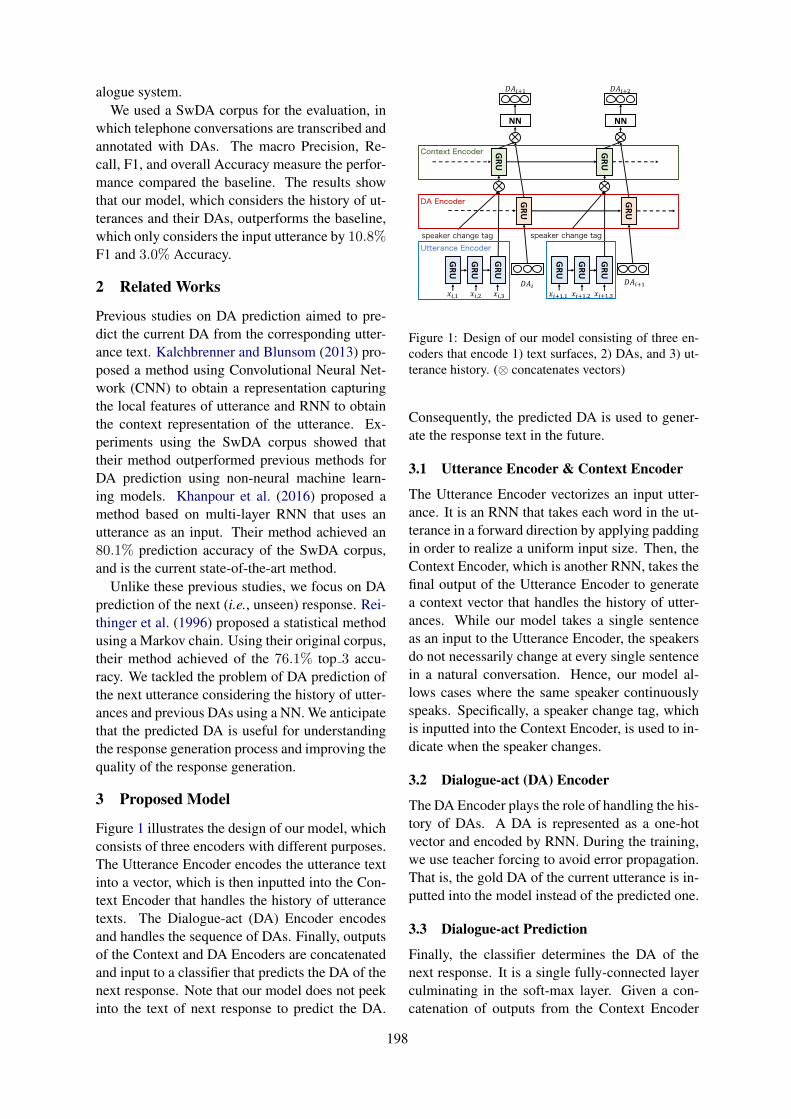
alogue system.We used a SwDA corpus for the evaluation, in

which telephone conversations are transcribed andannotated with DAs. The macro Precision, Re-call, F1, and overall Accuracy measure the perfor-mance compared the baseline. The results showthat our model, which considers the history of ut-terances and their DAs, outperforms the baseline,which only considers the input utterance by 10.8%F1 and 3.0% Accuracy.

2 Related Works

Previous studies on DA prediction aimed to pre-dict the current DA from the corresponding utter-ance text. Kalchbrenner and Blunsom (2013) pro-posed a method using Convolutional Neural Net-work (CNN) to obtain a representation capturingthe local features of utterance and RNN to obtainthe context representation of the utterance. Ex-periments using the SwDA corpus showed thattheir method outperformed previous methods forDA prediction using non-neural machine learn-ing models. Khanpour et al. (2016) proposed amethod based on multi-layer RNN that uses anutterance as an input. Their method achieved an80.1% prediction accuracy of the SwDA corpus,and is the current state-of-the-art method.

Unlike these previous studies, we focus on DAprediction of the next (i.e., unseen) response. Rei-thinger et al. (1996) proposed a statistical methodusing a Markov chain. Using their original corpus,their method achieved of the 76.1% top 3 accu-racy. We tackled the problem of DA prediction ofthe next utterance considering the history of utter-ances and previous DAs using a NN. We anticipatethat the predicted DA is useful for understandingthe response generation process and improving thequality of the response generation.

3 Proposed Model

Figure 1 illustrates the design of our model, whichconsists of three encoders with different purposes.The Utterance Encoder encodes the utterance textinto a vector, which is then inputted into the Con-text Encoder that handles the history of utterancetexts. The Dialogue-act (DA) Encoder encodesand handles the sequence of DAs. Finally, outputsof the Context and DA Encoders are concatenatedand input to a classifier that predicts the DA of thenext response. Note that our model does not peekinto the text of next response to predict the DA.

GRU!",$ !",%!",& !"'$,&!"'$,$ !"'$,%

()" ()"'$

()"'$ ()"'&

GRU

GRU

GRU

GRU

GRU

GRU

GRU

GRU

GRU

speaker change tag speaker change tag

NN NN

Utterance Encoder

DA Encoder

Context Encoder

Figure 1: Design of our model consisting of three en-coders that encode 1) text surfaces, 2) DAs, and 3) ut-terance history. (⊗ concatenates vectors)

Consequently, the predicted DA is used to gener-ate the response text in the future.

3.1 Utterance Encoder & Context Encoder

The Utterance Encoder vectorizes an input utter-ance. It is an RNN that takes each word in the ut-terance in a forward direction by applying paddingin order to realize a uniform input size. Then, theContext Encoder, which is another RNN, takes thefinal output of the Utterance Encoder to generatea context vector that handles the history of utter-ances. While our model takes a single sentenceas an input to the Utterance Encoder, the speakersdo not necessarily change at every single sentencein a natural conversation. Hence, our model al-lows cases where the same speaker continuouslyspeaks. Specifically, a speaker change tag, whichis inputted into the Context Encoder, is used to in-dicate when the speaker changes.

3.2 Dialogue-act (DA) Encoder

The DA Encoder plays the role of handling the his-tory of DAs. A DA is represented as a one-hotvector and encoded by RNN. During the training,we use teacher forcing to avoid error propagation.That is, the gold DA of the current utterance is in-putted into the model instead of the predicted one.

3.3 Dialogue-act Prediction

Finally, the classifier determines the DA of thenext response. It is a single fully-connected layerculminating in the soft-max layer. Given a con-catenation of outputs from the Context Encoder

198

Tag # of tags in the corpusStatement 576, 005Uninterpretable 93, 238Understanding 241, 008Agreement 55, 375Directive 3, 685Greeting 6, 618Question 54, 498Apology 11, 446Other 19, 882

Table 2: Distribution of DA tags in the preprocessedSwDA corpus.

and DA Encoder, the classifier conducts a multi-class classification and identifies the most likelyDA of the next response.

4 Experiment

4.1 Switch Board Dialogue Act Corpus(SwDA)

We evaluate the accuracy of our model to pre-dict the DA of the next response using the SwDAcorpus, which transcribes telephone conversationand annotates DAs of utterances. The SwDA cor-pus conforms to the damsl tag schema.1 We as-sembled the tag sets referring to easy damsl (Iso-mura et al., 2009) into 9 tags (Table 2) in orderto consolidate tags with a significantly low fre-quency. The SwDA corpus provides transcriptionsof 1, 155 conversations with 219, 297 utterances.One conversation contains 189 utterances on aver-age. Because the average length of utterance se-quences is large, we use a sliding window with asize of 5 to cut a sequence into several conversa-tions.

The number of conversations increases to212, 367 with 1, 061, 835 utterances. Table 2shows the distribution of DAs in the processed cor-pus. We randomly divide the conversations in thecorpus into 80%, 10%, and 10% for training, de-velopment, and testing, respectively.

4.2 Model Settings

We apply a Gated Recurrent Unit (GRU) (Choet al., 2014) to each RNN in our model. We set thedimensions of word embedding to 300 and thoseof the DA embedding to 100. The dimensions ofthe GRU hidden unit of the Utterance Encoder are

1https://web.stanford.edu/˜jurafsky/ws97/manual.august1.html

Figure 2: Conditional Probabilities of DA transitions.“Greeting” has a clear pattern, which is followed by a“Greeting”. Other DAs tend to be followed by a “State-ment”.

set to 512, while those the Context Encoder areset to 513 (one element is for the speaker changetag) and those of the DA Encoder are set to 128.Hence, the dimensions of an input into the clas-sifier are 641. The dimensions of the hidden unitof the fully-connected layer are set to 100. Thecross-entropy error is used for the loss function,and the Adam (Kingma and Ba, 2014) optimizerwith a learning rate of 5e− 5 is used for optimiza-tion. The number of epochs is set to 30. We use themodel with the lowest development loss for test-ing.

We use teacher forcing for training and simi-lar setting for testing by inputting the gold DA ofthe previous time step into the DA Encoder. Thismeans that the evaluation results here show theperformance when the predictions of the previoustime steps are all correct.

As Table 2 shows, the numbers of DAs arehighly diverse. To avoid frequent tags dominatingthe results, we measure the macro averages of pre-cision, recall, and F1-score of each DA. We alsomeasure the overall accuracy.

4.3 Baselines

To investigate the effects of each encoder in ourmodel, we compare our model to the baseline (Ta-ble 3). The second and third rows are simple meth-ods. Max-Probability is another non-neural base-line that outputs the DA with highest conditionalprobability from the input DA. Figure 2 showsthe conditional probability of DA transitions com-puted in our training set. “Greeting” has a no-

199

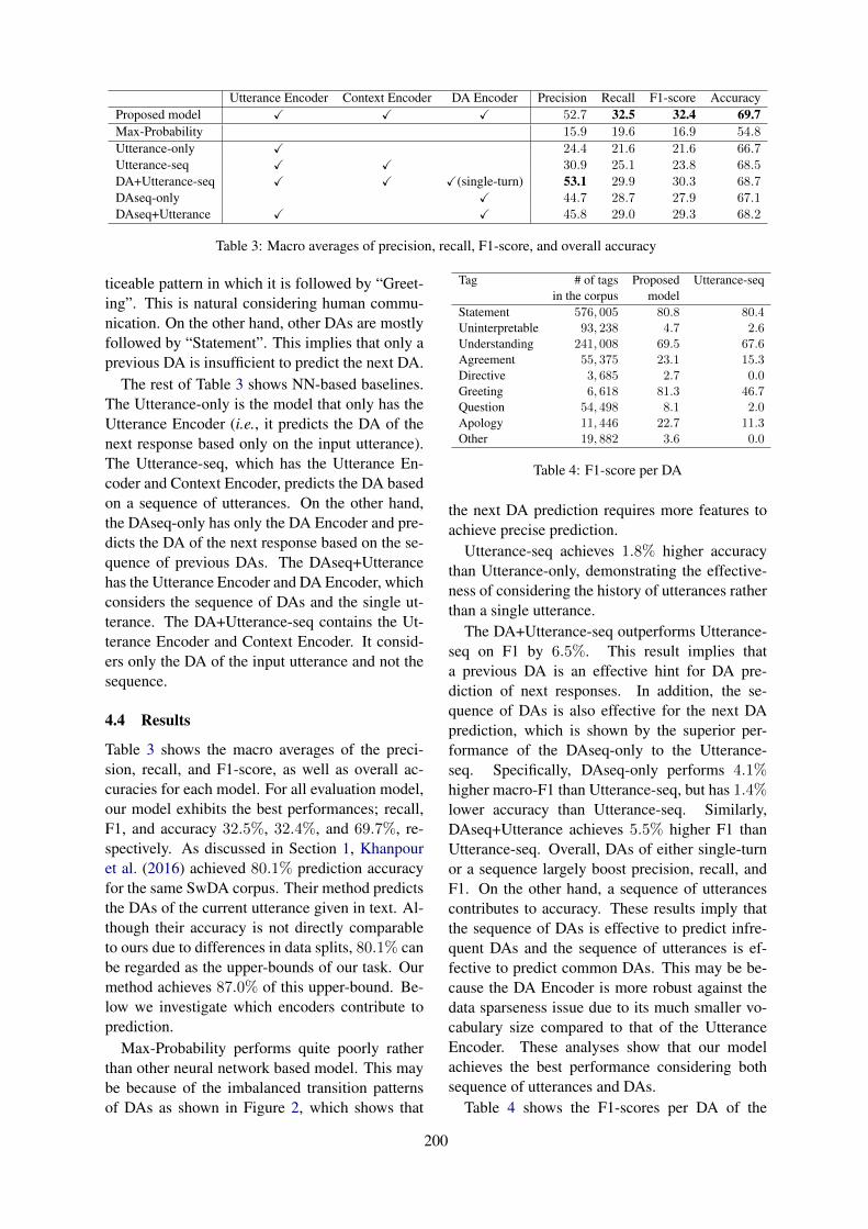
Utterance Encoder Context Encoder DA Encoder Precision Recall F1-score AccuracyProposed model 52.7 32.5 32.4 69.7Max-Probability 15.9 19.6 16.9 54.8

Utterance-only 24.4 21.6 21.6 66.7Utterance-seq 30.9 25.1 23.8 68.5DA+Utterance-seq (single-turn) 53.1 29.9 30.3 68.7DAseq-only 44.7 28.7 27.9 67.1DAseq+Utterance 45.8 29.0 29.3 68.2

Table 3: Macro averages of precision, recall, F1-score, and overall accuracy

ticeable pattern in which it is followed by “Greet-ing”. This is natural considering human commu-nication. On the other hand, other DAs are mostlyfollowed by “Statement”. This implies that only aprevious DA is insufficient to predict the next DA.

The rest of Table 3 shows NN-based baselines.The Utterance-only is the model that only has theUtterance Encoder (i.e., it predicts the DA of thenext response based only on the input utterance).The Utterance-seq, which has the Utterance En-coder and Context Encoder, predicts the DA basedon a sequence of utterances. On the other hand,the DAseq-only has only the DA Encoder and pre-dicts the DA of the next response based on the se-quence of previous DAs. The DAseq+Utterancehas the Utterance Encoder and DA Encoder, whichconsiders the sequence of DAs and the single ut-terance. The DA+Utterance-seq contains the Ut-terance Encoder and Context Encoder. It consid-ers only the DA of the input utterance and not thesequence.

4.4 Results

Table 3 shows the macro averages of the preci-sion, recall, and F1-score, as well as overall ac-curacies for each model. For all evaluation model,our model exhibits the best performances; recall,F1, and accuracy 32.5%, 32.4%, and 69.7%, re-spectively. As discussed in Section 1, Khanpouret al. (2016) achieved 80.1% prediction accuracyfor the same SwDA corpus. Their method predictsthe DAs of the current utterance given in text. Al-though their accuracy is not directly comparableto ours due to differences in data splits, 80.1% canbe regarded as the upper-bounds of our task. Ourmethod achieves 87.0% of this upper-bound. Be-low we investigate which encoders contribute toprediction.

Max-Probability performs quite poorly ratherthan other neural network based model. This maybe because of the imbalanced transition patternsof DAs as shown in Figure 2, which shows that

Tag # of tags Proposed Utterance-seqin the corpus model

Statement 576, 005 80.8 80.4Uninterpretable 93, 238 4.7 2.6Understanding 241, 008 69.5 67.6Agreement 55, 375 23.1 15.3Directive 3, 685 2.7 0.0Greeting 6, 618 81.3 46.7Question 54, 498 8.1 2.0Apology 11, 446 22.7 11.3Other 19, 882 3.6 0.0

Table 4: F1-score per DA

the next DA prediction requires more features toachieve precise prediction.

Utterance-seq achieves 1.8% higher accuracythan Utterance-only, demonstrating the effective-ness of considering the history of utterances ratherthan a single utterance.

The DA+Utterance-seq outperforms Utterance-seq on F1 by 6.5%. This result implies thata previous DA is an effective hint for DA pre-diction of next responses. In addition, the se-quence of DAs is also effective for the next DAprediction, which is shown by the superior per-formance of the DAseq-only to the Utterance-seq. Specifically, DAseq-only performs 4.1%higher macro-F1 than Utterance-seq, but has 1.4%lower accuracy than Utterance-seq. Similarly,DAseq+Utterance achieves 5.5% higher F1 thanUtterance-seq. Overall, DAs of either single-turnor a sequence largely boost precision, recall, andF1. On the other hand, a sequence of utterancescontributes to accuracy. These results imply thatthe sequence of DAs is effective to predict infre-quent DAs and the sequence of utterances is ef-fective to predict common DAs. This may be be-cause the DA Encoder is more robust against thedata sparseness issue due to its much smaller vo-cabulary size compared to that of the UtteranceEncoder. These analyses show that our modelachieves the best performance considering bothsequence of utterances and DAs.

Table 4 shows the F1-scores per DA of the

200

Utterance (DA) Gold DA Proposed model Utterance-seq1 What are they , (Uninterpretable) Statement Statement Statement2 the , (Statement) Statement Statement Statement3 I know , (Statement) Statement Statement Statement4 a Rabbit ’s one , diesel (Statement) Agreement Understanding Understanding5 Uh-huh , (Agreement) Agreement Agreement Statement1 I hope so too . (Statement) Statement Statement Statement2 You know . Right now there ’s a lot on the

market for sale because of people havinglost Yes . (Statement)

Understanding Understanding Understanding

3 Yes . (Understanding) Statement Statement Statement4 and everything (Statement) Statement Statement Statement5 so that ’s , you know , that keeps prices

down (Statement)Understanding Understanding Understanding

1 It does n’t seem like , (Statement) Statement Statement Statement2 but I guess when you think of it everybody

has some sort of aerosol in their home(Statement)

Understanding Understanding Understanding

3 Yeah . (Understanding) Statement Statement Statement4 You know , (Statement) Statement Statement Statement5 and it ’s kind of dangerous . (Statement) Agreement Understanding Understanding

Table 5: Examples of predicted DAs by the proposed model and Utterance-seq. DA in a parenthesis shows thatof the input utterance, while “Gold DA” shows the DAs of the next responses. The column of “Proposed Model”column shows the predicted DAs of the next responses by the proposed model, and the column of “Utterance-seq”shows the predicted DAs of the next responses by Utterance-seq.

proposed model and Utterance-seq. The pro-posed model outperforms Utterance-seq on all theDAs. In particular, infrequent tags of “Agree-ment”, “Greeting”, “Question” and “Apology”show significant improvements between 6.1%and 34.6%. Furthermore, the proposed modelcorrectly predicts “Directive” and “Other” eventhough Utterance-seq does not predict any of thesecorrectly.

4.5 Examples of Predicted DAs

Table 5 shows examples of the predicted DAs bythe proposed model and Utterance-seq. The firstexample shows that the proposed model correctlypredicts “Agreement”, which only has 5.2% oc-currence in the training set, whereas Utterance-seqmost frequently predicts it as “Statement”.

The second and third examples demonstratethe difficulty of DA prediction of the next re-sponse. The input utterances of these exampleshave the same DA sequences, but the DAs ofthe final responses differ (“Understanding” and“Agreement”). While both the proposed modeland Utterance-seq correctly predict the final DA ofthe second example, both fail in the third example.

The third conversation is about an aerosol, and theresponse to the final utterance of “and it’s kind ofdangerous.” depends on if one of the speakers un-derstands the danger of the aerosol. To correctlypredict DAs in such a case, a much longer con-versation sequence and/or personalize the predic-tion model must be considered based on profilesor knowledge of speakers. This is the direction ofour future work.

5 Conclusion

We propose a method to predict a DA of the nextresponse considering the sequences of utterancesand DAs. The evaluation results using the SwDAcorpus show that the proposed model achieves69.7% accuracy and 32.4% macro-F1. Addition-ally, the results show that the sequence of DAs sig-nificantly helps the prediction of infrequent DAs.

In the future, we plan to develop a response gen-eration model using the predicted DAs.

Acknowledgements

This project is funded by Microsoft ResearchAsia, Microsoft Japan Co., Ltd., and JSPS KAK-ENHI Grant Number JP18K11435.

201

ReferencesAlessandra Cervone, Evgeny Stepanov, and Giuseppe

Riccardi. 2018. Coherence models for dialogue. InProceedings of the Interspeech, pages 1011–1015.

Kyunghyun Cho, Bart Van Merrienboer, Caglar Gul-cehre, Dzmitry Bahdanau, Fethi Bougares, Hol-ger Schwenk, and Yoshua Bengio. 2014. Learn-ing Phrase Representations using RNN Encoder-Decoder for Statistical Machine Translation. In Pro-ceedings of the EMNLP, pages 1724–1734.

Naoki Isomura, Fujio Toriumi, and Kenichiro Ishii.2009. Evaluation method of non-task-oriented di-alogue system by HMM. The IEICE transac-tions on information and systems (Japanese edition),92(4):542–551.

Nal Kalchbrenner and Phil Blunsom. 2013. Recurrentconvolutional neural networks for discourse com-positionality. In Proceedings of the Workshop onCVSC, pages 119–126.

Hamed Khanpour, Nishitha Guntakandla, and Rod-ney Nielsen. 2016. Dialogue act classification indomain-independent conversations using a deep re-current neural network. In Proceedings of the COL-ING, pages 2012–2021.

Diederik Kingma and Jimmy Ba. 2014. Adam: Amethod for stochastic optimization. In Proceedingsof the ICLR.

Norbert Reithinger, Ralf Engel, Michael Kipp, andMartin Klesen. 1996. Predicting dialogue acts for aspeech-to-speech translation system. In Proceedingof the ICSLP, pages 654–657 vol.2.

Oriol Vinyals and Quoc V Le. 2015. A Neural Conver-sational Model. In Proceedings of the ICML.

Tiancheng Zhao, Kyusong Lee, and Maxine Eskenazi.2018. Unsupervised discrete sentence representa-tion learning for interpretable neural dialog gener-ation. In Proceedings of the ACL, pages 1098–1107.

202

Proceedings of the 57th Annual Meeting of the Association for Computational Linguistics: Student Research Workshop, pages 203–209Florence, Italy, July 28 - August 2, 2019. c©2019 Association for Computational Linguistics

Computational ad hominem detection

Pieter Delobelle, Murilo Cunha, Eric Massip Cano,Jeroen Peperkamp and Bettina Berendt

KU Leuven, Department of Computer ScienceCelestijnenlaan 200A, 3000 Leuven, Belgium

pieter.delobelle,murilo.cunha, eric.massipcano@student.kuleuven.beand jeroen.peperkamp, bettina.berendt@kuleuven.be

Abstract

Fallacies like the personal attack—also knownas the ad hominem attack—are introduced indebates as an easy win, even though they pro-vide no rhetorical contribution. Although theirimportance in argumentation mining is ac-knowledged, automated mining and analysis isstill lacking. We show TF-IDF approaches areinsufficient to detect the ad hominem attack.Therefore we present a machine learning ap-proach for information extraction, which has arecall of 80% for a social media data source.We also demonstrate our approach with an ap-plication that uses online learning.

1 Introduction

Debates are shaping our world, with them happen-ing online more than ever. But for these debates—and their offline variants as well—to be valuable,their argumentation needs to be solid. As Stedeand Schneider (2018, Sec. 1.3) recognize, study-ing fallacies is crucial for the understanding of ar-guments and their validity. The ad hominem fal-lacy, the personal attack, is one of the more preva-lent fallacies. Despite its common occurrence, apersonal attack can be quite effective and mightshape the course of debates.

In online discussion fora, these attacks are oftenunwanted for their low rhetorical quality. Thesedebates are watched by dedicated members ofthose fora, so-called moderators. They followentire discussion threads and flag any unwantedposts; which can take up a lot of their time and thediscussion might have already panned out. Au-tomated flagging could significantly improve thequality of debates and save moderators a lot oftime.

When developing such an automated system,the variety and ambiguity of ad hominem attackscan be difficult to cope with. These attacks rangefrom simple name calling (i.e. “You’re stupid”),abusive attacks (i.e. “He’s dishonest”) to more

complex circumstantial attacks (i.e. “You smokeyourself!”) (Walton, 1998). Detecting all these va-rieties is quite challenging, since there can even bediscussion about some of those labels amongst hu-mans.

We hereby focus in this paper on detectingmainly two variants of the ad hominem fallacy:name calling and abusive attacks. To realize thisautomated system, we present a recurrent neuralmodel to detect ad hominem attack in a paragraph,and we experiment with various other models tocompare them. Finally, we look into the issues re-lated to crowd sourcing of additional labeled para-graphs through an application as a web demo.

This article is structured as follows: Section 2covers related work on ad hominem fallacies, de-tecting those fallacies, and crowd sourcing datasets. Section 3 will then review the componentsused in our approach, which is then further dis-cussed in Section 4. Section 5 outlines the useddata set, the training setup, and baseline mod-els; afterwards the results are discussed in Sub-section 5.3. Finally, Section 6 concludes this workand discusses future improvements.

2 Related work

The study of argumentations has a long history,with Rethoric by Aristotle being one of the moretraditional works. In the second book, he dis-cussed the concept of Logos, the argument or rea-soning pattern in a debate. More recently, reason-ing and argumentations are studied in the field ofnatural language processing (NLP). The subfieldof argumentation mining focusses on extractingarguments and their relations (i.e. graphs) fromtexts (Stede and Schneider, 2018).

Ad hominem attacks The work of Walton(1998) describes at the structure of ad hominemattacks in great depth, from a non-computationalview. In addition to this, the work also analyzes

203

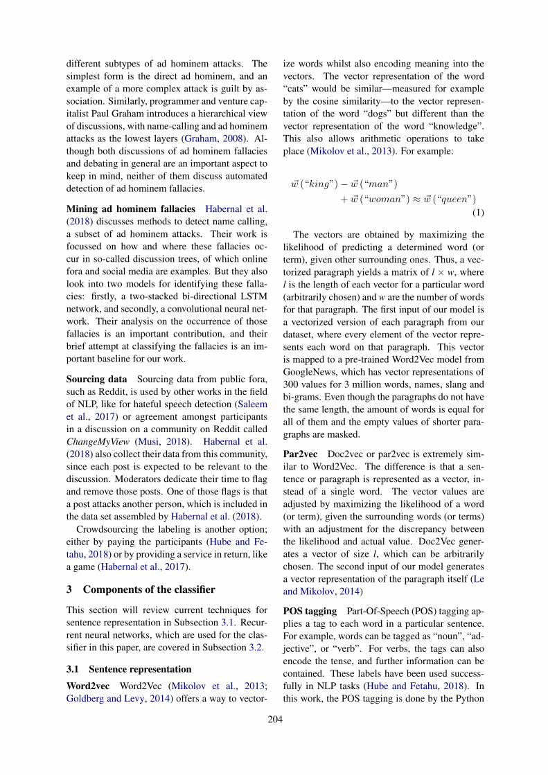
different subtypes of ad hominem attacks. Thesimplest form is the direct ad hominem, and anexample of a more complex attack is guilt by as-sociation. Similarly, programmer and venture cap-italist Paul Graham introduces a hierarchical viewof discussions, with name-calling and ad hominemattacks as the lowest layers (Graham, 2008). Al-though both discussions of ad hominem fallaciesand debating in general are an important aspect tokeep in mind, neither of them discuss automateddetection of ad hominem fallacies.

Mining ad hominem fallacies Habernal et al.(2018) discusses methods to detect name calling,a subset of ad hominem attacks. Their work isfocussed on how and where these fallacies oc-cur in so-called discussion trees, of which onlinefora and social media are examples. But they alsolook into two models for identifying these falla-cies: firstly, a two-stacked bi-directional LSTMnetwork, and secondly, a convolutional neural net-work. Their analysis on the occurrence of thosefallacies is an important contribution, and theirbrief attempt at classifying the fallacies is an im-portant baseline for our work.

Sourcing data Sourcing data from public fora,such as Reddit, is used by other works in the fieldof NLP, like for hateful speech detection (Saleemet al., 2017) or agreement amongst participantsin a discussion on a community on Reddit calledChangeMyView (Musi, 2018). Habernal et al.(2018) also collect their data from this community,since each post is expected to be relevant to thediscussion. Moderators dedicate their time to flagand remove those posts. One of those flags is thata post attacks another person, which is included inthe data set assembled by Habernal et al. (2018).

Crowdsourcing the labeling is another option;either by paying the participants (Hube and Fe-tahu, 2018) or by providing a service in return, likea game (Habernal et al., 2017).

3 Components of the classifier

This section will review current techniques forsentence representation in Subsection 3.1. Recur-rent neural networks, which are used for the clas-sifier in this paper, are covered in Subsection 3.2.

3.1 Sentence representation

Word2vec Word2Vec (Mikolov et al., 2013;Goldberg and Levy, 2014) offers a way to vector-

ize words whilst also encoding meaning into thevectors. The vector representation of the word“cats” would be similar—measured for exampleby the cosine similarity—to the vector represen-tation of the word “dogs” but different than thevector representation of the word “knowledge”.This also allows arithmetic operations to takeplace (Mikolov et al., 2013). For example:

~w (“king”)− ~w (“man”)

+ ~w (“woman”) ≈ ~w (“queen”)

(1)

The vectors are obtained by maximizing thelikelihood of predicting a determined word (orterm), given other surrounding ones. Thus, a vec-torized paragraph yields a matrix of l × w, wherel is the length of each vector for a particular word(arbitrarily chosen) and w are the number of wordsfor that paragraph. The first input of our model isa vectorized version of each paragraph from ourdataset, where every element of the vector repre-sents each word on that paragraph. This vectoris mapped to a pre-trained Word2Vec model fromGoogleNews, which has vector representations of300 values for 3 million words, names, slang andbi-grams. Even though the paragraphs do not havethe same length, the amount of words is equal forall of them and the empty values of shorter para-graphs are masked.

Par2vec Doc2vec or par2vec is extremely sim-ilar to Word2Vec. The difference is that a sen-tence or paragraph is represented as a vector, in-stead of a single word. The vector values areadjusted by maximizing the likelihood of a word(or term), given the surrounding words (or terms)with an adjustment for the discrepancy betweenthe likelihood and actual value. Doc2Vec gener-ates a vector of size l, which can be arbitrarilychosen. The second input of our model generatesa vector representation of the paragraph itself (Leand Mikolov, 2014)

POS tagging Part-Of-Speech (POS) tagging ap-plies a tag to each word in a particular sentence.For example, words can be tagged as “noun”, “ad-jective”, or “verb”. For verbs, the tags can alsoencode the tense, and further information can becontained. These labels have been used success-fully in NLP tasks (Hube and Fetahu, 2018). Inthis work, the POS tagging is done by the Python

204

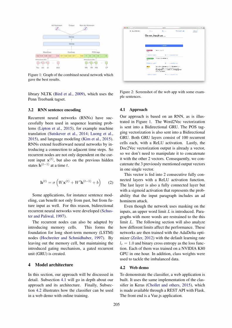
0.1 0.2 0.3 0.1 … 0.50.1 0.2 0.3 0.1 … 0.5 0.1 0.4 0.5 … 0.41 0 0 0 … 00.4 0.8 0.5 … 0.40.5 … 0.40.5 … 0.40.2 0.5 …

…

0.4

Word2vec Doc2vec POS tags

Dense

Dense

Output Non-Ad HominemAd Hominem

You are an idiot

…

NN VB NN CP

Bidirectional GRU Bidirectional GRU

Figure 1: Graph of the combined neural network whichgave the best results.

library NLTK (Bird et al., 2009), which uses thePenn Treebank tagset.

3.2 RNN sentence encoding

Recurrent neural networks (RNNs) have suc-cessfully been used in sequence learning prob-lems (Lipton et al., 2015), for example machinetranslation (Sutskever et al., 2014; Luong et al.,2015), and language modeling (Kim et al., 2015).RNNs extend feedforward neural networks by in-troducing a connection to adjacent time steps. Sorecurrent nodes are not only dependent on the cur-rent input x(t), but also on the previous hiddenstates h(t−1) at a time t.

h(t) = σ(Wx(t) +W ′h(t−1) + b

)(2)

Some applications, for instance sentence mod-eling, can benefit not only from past, but from fu-ture input as well. For this reason, bidirectionalrecurrent neural networks were developed (Schus-ter and Paliwal, 1997).

The recurrent nodes can also be adapted byintroducing memory cells. This forms thefoundation for long short-term memory (LSTM)nodes (Hochreiter and Schmidhuber, 1997). Byleaving out the memory cell, but maintaining theintroduced gating mechanism, a gated recurrentunit (GRU) is created.

4 Model architecture

In this section, our approach will be discussed indetail. Subsection 4.1 will go in depth about ourapproach and its architecture. Finally, Subsec-tion 4.2 illustrates how the classifier can be usedin a web demo with online training.

Figure 2: Screenshot of the web app with some exam-ple sentences.

4.1 ApproachOur approach is based on an RNN, as is illus-trated in Figure 1. The Word2Vec vectorizationis sent into a Bidirectional GRU. The POS tag-ging vectorization is also sent into a BidirectionalGRU. Both GRU layers consist of 100 recurrentcells each, with a ReLU activation. Lastly, theDoc2Vec vectorization output is already a vector,so we don’t need to manipulate it to concatenateit with the other 2 vectors. Consequently, we con-catenate the 3 previously mentioned output vectorsin one single vector.

This vector is fed into 2 consecutive fully con-nected layers with a ReLU activation function.The last layer is also a fully connected layer butwith a sigmoid activation that represents the prob-ability that the input paragraph includes an adhominem attack.

Even though the network uses masking on theinputs, an upper word limit L is introduced. Para-graphs with more words are restrained to the thislimit L. The following section will also analyzehow different limits affect the performance. Thesenetworks are then trained with the AdaDelta opti-mizer (Zeiler, 2012) with the default learning ratelr = 1.0 and binary cross entropy as the loss func-tion. Each of them was trained on a NVIDIA K80GPU in one hour. In addition, class weights wereused to tackle the imbalanced data.

4.2 Web demoTo demonstrate the classifier, a web application isbuilt. It uses the same implementation of the clas-sifier in Keras (Chollet and others, 2015), whichis made available through a REST API with Flask.The front end is a Vue.js application.

205

Table 1: Illustration of how fallacies in the middle of a paragraph are contributing less to the overall output of themodel, even though the attack itself is the same.

Sentence Confidence

Augmented recurrent neural networks, and the underlying technique of attention, are in-credibly exciting. You’re so wrong and a f*cking idiot! We look forward to seeing whathappens next.

0.39

You’re so wrong and a f*cking idiot! Augmented recurrent neural networks, and the un-derlying technique of attention, are incredibly exciting. We look forward to seeing whathappens next.

0.79

The web application also supports online learn-ing and labeling of paragraphs. Each queried para-graph has two buttons to label the input, afterwhich the backend saves the feedback and option-ally retrains the network. However, as will be dis-cussed in Section 5.3, this approach can actuallyworsen the accuracy of the classifier.

5 Evaluation

To correctly compare different models, the dataset is split into a training and test set. All mod-els are evaluated on a withheld test set (Flach,2012). In this case, the test set contains over 8klabeled paragraphs. In two instances, memory is-sues forced us to train and evaluate on a smallerdata set. These issues can be mitigated by stream-ing smaller batches of data, but this was made lessof a priority since the provisional results were infavor of the RNN network. A further breakdownof the data collection and processing is discussedin Subsection 5.1.

Our model is compared to different baselines,which are reviewed in Subsection 5.2.

5.1 Data set

Our models were trained on a data set that was ini-tially collected by Habernal et al. (2018). This dataset is in essence a database dump of a Reddit com-munity called Change My View, which focusseson online debating. In this context, ad hominemattacks are unwelcome and thus removed by mod-erators. The data set contains these labels amongstother things. The authors analyzed this data setextensively to make sure the labels were correct,in part by relabeling a subset by crowd-sourcedworkers.

However, our goal is different than thatof Habernal et al. (2018): we classify each postindividually, without taking any context about the

discussion into account. Habernal et al. (2018) fo-cusses on what this context—which they call a dis-cussion tree—means for the occurrence of an at-tack. For this reason, we decided to not use thefiltered dataset with only discussing trees that endup in ad hominem attacks. Instead we used thedatabase dump and applied our own data cleaning.

Reddit allows the use of text formatting withMarkdown (i.e. *bold* or italics ). These werefiltered, and more complex tags like links were re-moved, while still preserving the text associatedwith the link. Finally, the Markdown format alsoallows citations, which were commonly used toquote sentences of other posts. Since these cita-tions could contain ad hominem attacks, they areremoved as well.

5.2 BaselinesWe compare our approach to multiple baselines.One of them is a CNN approach by Habernal et al.(2018), whilst the others are baselines we considerwithout recurrent layers.

1. SVMa: our first model is based on a TF-IDF vectorizer and an SVM classifier (Flach,2012). The TF-IDF vectorizer uses the top3000 words from the test set. The SVM clas-sifier is a linear SVM.

2. SVMb: this model also uses a linear clas-sifier, but the features are based on wordrepresentations. Instead of the TF-IDF vec-tors for a paragraph, the 300 most occurringwords from the training set are used. Foreach of these 300 words, the TF-IDF valueis replaced by a weighted word embedding.So for words that don’t occur in a sentenceor paragraph, all elements of this vector arezero. Otherwise the word representation isscaled by the TF-IDF value of that word. Intotal, this yields an array of 300 words by 300

206

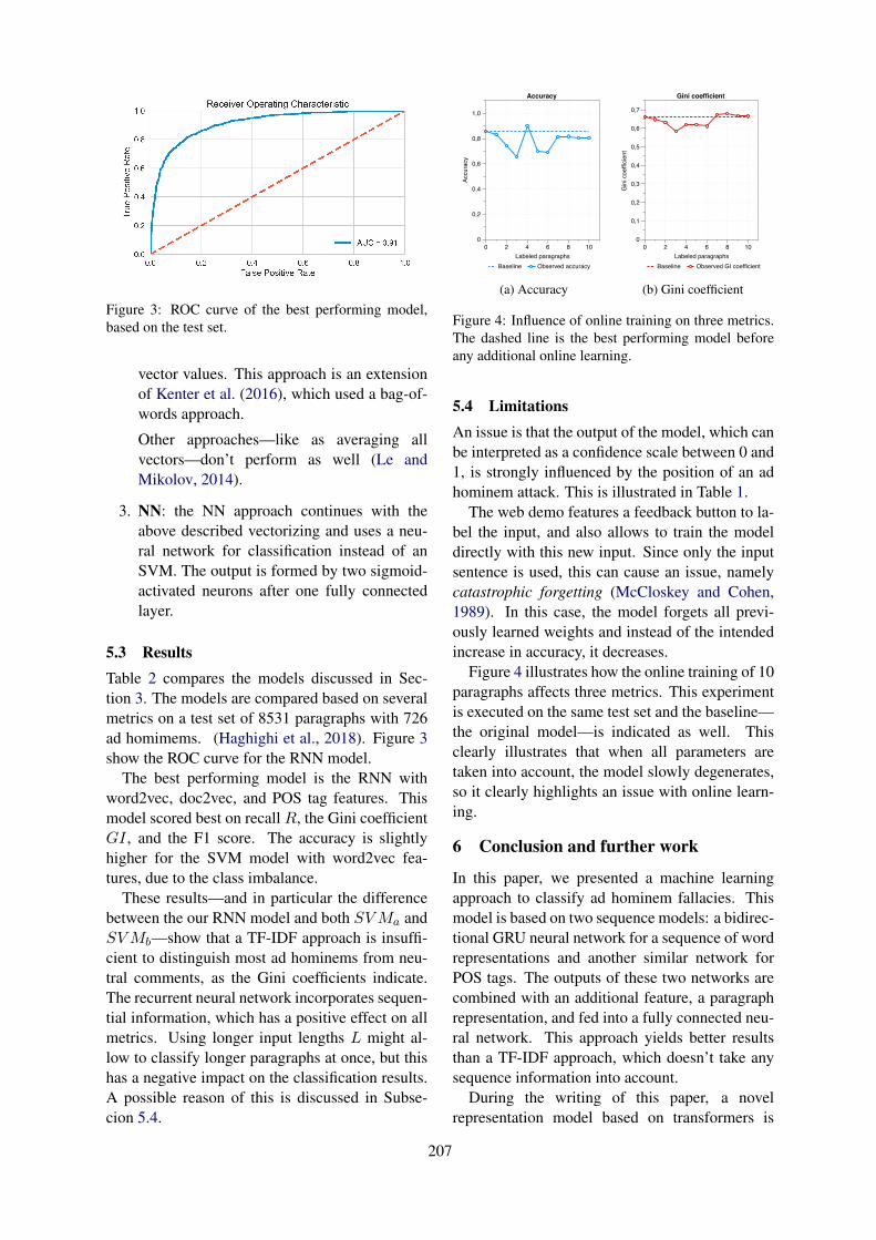
Figure 3: ROC curve of the best performing model,based on the test set.

vector values. This approach is an extensionof Kenter et al. (2016), which used a bag-of-words approach.

Other approaches—like as averaging allvectors—don’t perform as well (Le andMikolov, 2014).

3. NN: the NN approach continues with theabove described vectorizing and uses a neu-ral network for classification instead of anSVM. The output is formed by two sigmoid-activated neurons after one fully connectedlayer.

5.3 ResultsTable 2 compares the models discussed in Sec-tion 3. The models are compared based on severalmetrics on a test set of 8531 paragraphs with 726ad homimems. (Haghighi et al., 2018). Figure 3show the ROC curve for the RNN model.

The best performing model is the RNN withword2vec, doc2vec, and POS tag features. Thismodel scored best on recall R, the Gini coefficientGI , and the F1 score. The accuracy is slightlyhigher for the SVM model with word2vec fea-tures, due to the class imbalance.

These results—and in particular the differencebetween the our RNN model and both SVMa andSVMb—show that a TF-IDF approach is insuffi-cient to distinguish most ad hominems from neu-tral comments, as the Gini coefficients indicate.The recurrent neural network incorporates sequen-tial information, which has a positive effect on allmetrics. Using longer input lengths L might al-low to classify longer paragraphs at once, but thishas a negative impact on the classification results.A possible reason of this is discussed in Subse-cion 5.4.

Baseline Observed accuracy

Accu

racy

0

0,2

0,4

0,6

0,8

1,0

Labeled paragraphs0 2 4 6 8 10

Accuracy

(a) Accuracy

Baseline Observed GI coefficient

Gin

i coe

ffici

ent

0

0,1

0,2

0,3

0,4

0,5

0,6

0,7

Labeled paragraphs0 2 4 6 8 10

Gini coefficient

(b) Gini coefficient

Figure 4: Influence of online training on three metrics.The dashed line is the best performing model beforeany additional online learning.

5.4 LimitationsAn issue is that the output of the model, which canbe interpreted as a confidence scale between 0 and1, is strongly influenced by the position of an adhominem attack. This is illustrated in Table 1.

The web demo features a feedback button to la-bel the input, and also allows to train the modeldirectly with this new input. Since only the inputsentence is used, this can cause an issue, namelycatastrophic forgetting (McCloskey and Cohen,1989). In this case, the model forgets all previ-ously learned weights and instead of the intendedincrease in accuracy, it decreases.

Figure 4 illustrates how the online training of 10paragraphs affects three metrics. This experimentis executed on the same test set and the baseline—the original model—is indicated as well. Thisclearly illustrates that when all parameters aretaken into account, the model slowly degenerates,so it clearly highlights an issue with online learn-ing.

6 Conclusion and further work

In this paper, we presented a machine learningapproach to classify ad hominem fallacies. Thismodel is based on two sequence models: a bidirec-tional GRU neural network for a sequence of wordrepresentations and another similar network forPOS tags. The outputs of these two networks arecombined with an additional feature, a paragraphrepresentation, and fed into a fully connected neu-ral network. This approach yields better resultsthan a TF-IDF approach, which doesn’t take anysequence information into account.

During the writing of this paper, a novelrepresentation model based on transformers is

207

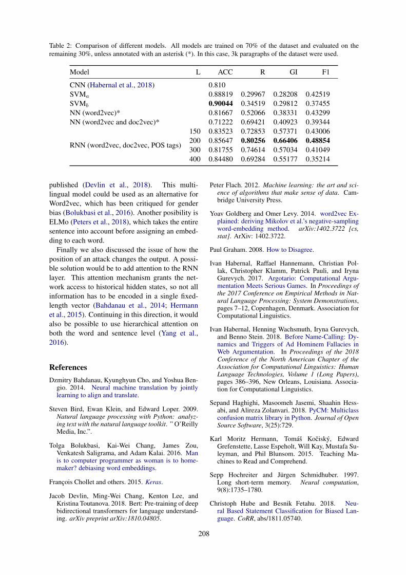
Table 2: Comparison of different models. All models are trained on 70% of the dataset and evaluated on theremaining 30%, unless annotated with an asterisk (*). In this case, 3k paragraphs of the dataset were used.

Model L ACC R GI F1

CNN (Habernal et al., 2018) 0.810SVMa 0.88819 0.29967 0.28208 0.42519SVMb 0.90044 0.34519 0.29812 0.37455NN (word2vec)* 0.81667 0.52066 0.38331 0.43299NN (word2vec and doc2vec)* 0.71222 0.69421 0.40923 0.39344

RNN (word2vec, doc2vec, POS tags)

150 0.83523 0.72853 0.57371 0.43006200 0.85647 0.80256 0.66406 0.48854300 0.81755 0.74614 0.57034 0.41049400 0.84480 0.69284 0.55177 0.35214

published (Devlin et al., 2018). This multi-lingual model could be used as an alternative forWord2vec, which has been critiqued for genderbias (Bolukbasi et al., 2016). Another posibility isELMo (Peters et al., 2018), which takes the entiresentence into account before assigning an embed-ding to each word.

Finally we also discussed the issue of how theposition of an attack changes the output. A possi-ble solution would be to add attention to the RNNlayer. This attention mechanism grants the net-work access to historical hidden states, so not allinformation has to be encoded in a single fixed-length vector (Bahdanau et al., 2014; Hermannet al., 2015). Continuing in this direction, it wouldalso be possible to use hierarchical attention onboth the word and sentence level (Yang et al.,2016).

ReferencesDzmitry Bahdanau, Kyunghyun Cho, and Yoshua Ben-

gio. 2014. Neural machine translation by jointlylearning to align and translate.

Steven Bird, Ewan Klein, and Edward Loper. 2009.Natural language processing with Python: analyz-ing text with the natural language toolkit. ” O’ReillyMedia, Inc.”.

Tolga Bolukbasi, Kai-Wei Chang, James Zou,Venkatesh Saligrama, and Adam Kalai. 2016. Manis to computer programmer as woman is to home-maker? debiasing word embeddings.

Francois Chollet and others. 2015. Keras.

Jacob Devlin, Ming-Wei Chang, Kenton Lee, andKristina Toutanova. 2018. Bert: Pre-training of deepbidirectional transformers for language understand-ing. arXiv preprint arXiv:1810.04805.

Peter Flach. 2012. Machine learning: the art and sci-ence of algorithms that make sense of data. Cam-bridge University Press.

Yoav Goldberg and Omer Levy. 2014. word2vec Ex-plained: deriving Mikolov et al.’s negative-samplingword-embedding method. arXiv:1402.3722 [cs,stat]. ArXiv: 1402.3722.

Paul Graham. 2008. How to Disagree.

Ivan Habernal, Raffael Hannemann, Christian Pol-lak, Christopher Klamm, Patrick Pauli, and IrynaGurevych. 2017. Argotario: Computational Argu-mentation Meets Serious Games. In Proceedings ofthe 2017 Conference on Empirical Methods in Nat-ural Language Processing: System Demonstrations,pages 7–12, Copenhagen, Denmark. Association forComputational Linguistics.

Ivan Habernal, Henning Wachsmuth, Iryna Gurevych,and Benno Stein. 2018. Before Name-Calling: Dy-namics and Triggers of Ad Hominem Fallacies inWeb Argumentation. In Proceedings of the 2018Conference of the North American Chapter of theAssociation for Computational Linguistics: HumanLanguage Technologies, Volume 1 (Long Papers),pages 386–396, New Orleans, Louisiana. Associa-tion for Computational Linguistics.

Sepand Haghighi, Masoomeh Jasemi, Shaahin Hess-abi, and Alireza Zolanvari. 2018. PyCM: Multiclassconfusion matrix library in Python. Journal of OpenSource Software, 3(25):729.

Karl Moritz Hermann, Tomas Kocisky, EdwardGrefenstette, Lasse Espeholt, Will Kay, Mustafa Su-leyman, and Phil Blunsom. 2015. Teaching Ma-chines to Read and Comprehend.

Sepp Hochreiter and Jurgen Schmidhuber. 1997.Long short-term memory. Neural computation,9(8):1735–1780.

Christoph Hube and Besnik Fetahu. 2018. Neu-ral Based Statement Classification for Biased Lan-guage. CoRR, abs/1811.05740.

208

Tom Kenter, Alexey Borisov, and Maarten de Rijke.2016. Siamese cbow: Optimizing word embed-dings for sentence representations. arXiv preprintarXiv:1606.04640.

Yoon Kim, Yacine Jernite, David Sontag, and Alexan-der M. Rush. 2015. Character-Aware Neural Lan-guage Models. arXiv:1508.06615 [cs, stat]. ArXiv:1508.06615.

Quoc Le and Tomas Mikolov. 2014. Distributed rep-resentations of sentences and documents. In Inter-national Conference on Machine Learning, pages1188–1196.

Zachary C. Lipton, John Berkowitz, and Charles Elkan.2015. A Critical Review of Recurrent Neural Net-works for Sequence Learning. arXiv:1506.00019[cs]. ArXiv: 1506.00019.

Minh-Thang Luong, Hieu Pham, and Christo-pher D. Manning. 2015. Effective Approachesto Attention-based Neural Machine Translation.arXiv:1508.04025 [cs]. ArXiv: 1508.04025.

Michael McCloskey and Neal J Cohen. 1989. Catas-trophic interference in connectionist networks: Thesequential learning problem. In Psychology oflearning and motivation, volume 24, pages 109–165. Elsevier.

Tomas Mikolov, Kai Chen, Greg Corrado, and Jef-frey Dean. 2013. Efficient estimation of wordrepresentations in vector space. arXiv preprintarXiv:1301.3781.

Elena Musi. 2018. How did you change my view?A corpus-based study of concessions’ argumentativerole. Discourse Studies, 20(2):270–288.

Matthew E. Peters, Mark Neumann, Mohit Iyyer, MattGardner, Christopher Clark, Kenton Lee, and LukeZettlemoyer. 2018. Deep contextualized word rep-resentations. In Proc. of NAACL.

Haji Mohammad Saleem, Kelly P. Dillon, Susan Be-nesch, and Derek Ruths. 2017. A Web of Hate:Tackling Hateful Speech in Online Social Spaces.arXiv:1709.10159 [cs]. ArXiv: 1709.10159.

M. Schuster and K.K. Paliwal. 1997. Bidirectional re-current neural networks. IEEE Transactions on Sig-nal Processing, 45(11):2673–2681.

Manfeld Stede and Jodi Schneider. 2018. Argumenta-tion Mining. Morgan & Claypool Publishers, SanRafael, United States.

Ilya Sutskever, Oriol Vinyals, and Quoc V. Le. 2014.Sequence to Sequence Learning with Neural Net-works. arXiv:1409.3215 [cs]. ArXiv: 1409.3215.

Douglas Walton. 1998. Ad Hominem Arguments (Stud-ies in Rhetoric & Communication). The Universityof Alabama Press, Alabama.

Zichao Yang, Diyi Yang, Chris Dyer, Xiaodong He,Alex Smola, and Eduard Hovy. 2016. Hierarchi-cal attention networks for document classification.In Proceedings of the 2016 Conference of the NorthAmerican Chapter of the Association for Computa-tional Linguistics: Human Language Technologies,pages 1480–1489.

Matthew D Zeiler. 2012. Adadelta: an adaptive learn-ing rate method. arXiv preprint arXiv:1212.5701.

209

Proceedings of the 57th Annual Meeting of the Association for Computational Linguistics: Student Research Workshop, pages 210–216Florence, Italy, July 28 - August 2, 2019. c©2019 Association for Computational Linguistics

Multiple Character Embeddings for Chinese Word Segmentation

Jingkang Wang∗ Jianing Zhou∗ Jie Zhou Gongshen Liu†

The Lab of Information Content Intelligent Analysis, Shanghai, ChinaSchool of Cyber Science and Engineering, Shanghai Jiao Tong University

wangjksjtu,zhjjn1919@gmail.com, sanny02,lgshen@sjtu.edu.cn

Abstract

Chinese word segmentation (CWS) is often re-garded as a character-based sequence label-ing task in most current works which haveachieved great success with the help of pow-erful neural networks. However, these worksneglect an important clue: Chinese charactersincorporate both semantic and phonetic mean-ings. In this paper, we introduce multiple char-acter embeddings including Pinyin Romaniza-tion and Wubi Input, both of which are easilyaccessible and effective in depicting semanticsof characters. We propose a novel shared Bi-LSTM-CRF model to fuse linguistic featuresefficiently by sharing the LSTM network dur-ing the training procedure. Extensive experi-ments on five corpora show that extra embed-dings help obtain a significant improvement inlabeling accuracy. Specifically, we achieve thestate-of-the-art performance in AS and CityUcorpora with F1 scores of 96.9 and 97.3, re-spectively without leveraging any external lex-ical resources.

1 Introduction

Chinese is written without explicit word delim-iters so word segmentation (CWS) is a preliminaryand essential pre-processing step for most naturallanguage processing (NLP) tasks in Chinese, suchas part-of-speech tagging (POS) and named-entityrecognition (NER). The representative approachesare treating CWS as a character-based sequencelabeling task following Xu (2003) and Peng et al.(2004).

Although not relying on hand-crafted features,most of the neural network models rely heavily onthe embeddings of characters. Since Mikolov et al.(2013) proposed word2vec technique, the vectorrepresentation of words or characters has become

∗ Equal contribution (alphabetical order).† Corresponding author.

a prerequisite for neural networks to solve NLPtasks in different languages.

However, existing approaches neglect an im-portant fact that Chinese characters contain bothsemantic and phonetic meanings - there are vari-ous representations of characters designed for cap-turing these features. The most intuitive one isPinyin Romanization (拼音) that keeps many-to-one relationship with Chinese characters - for onecharacter, different meanings in specific contextmay lead to different pronunciations. This phe-nomenon called Polyphony (and Polysemy) in lin-guistics is very common and crucial to word seg-mentation task. Apart from Pinyin Romanization,Wubi Input (五笔) is another effective represen-tation which absorbs semantic meanings of Chi-nese characters. Compared to Radical (偏旁) (Sunet al., 2014; Dong et al., 2016; Shao et al., 2017),Wubi includes more comprehensive graphical andstructural information that is highly relevant to thesemantic meanings and word boundaries, due toplentiful pictographic characters in Chinese andeffectiveness of Wubi in embedding the structures.

This paper will thoroughly study how impor-tant the extra embeddings are and what schol-ars can achieve by combining extra embeddingswith representative models. To leverage extra pho-netic and semantic information efficiently, we pro-pose a shared Bi-LSTMs-CRF model, which feedsembeddings into three stacked LSTM layers withshared parameters and finally scores with CRFlayer. We evaluate the proposed approach on fivecorpora and demonstrate that our method producesstate-of-the-art results and is highly efficient asprevious single-embedding scheme.

Our contributions are summarized as follows:1) We firstly propose to leverage both seman-tic and phonetic features of Chinese charactersin NLP tasks by introducing Pinyin Romaniza-tion and Wubi Input embeddings, which are easily

210

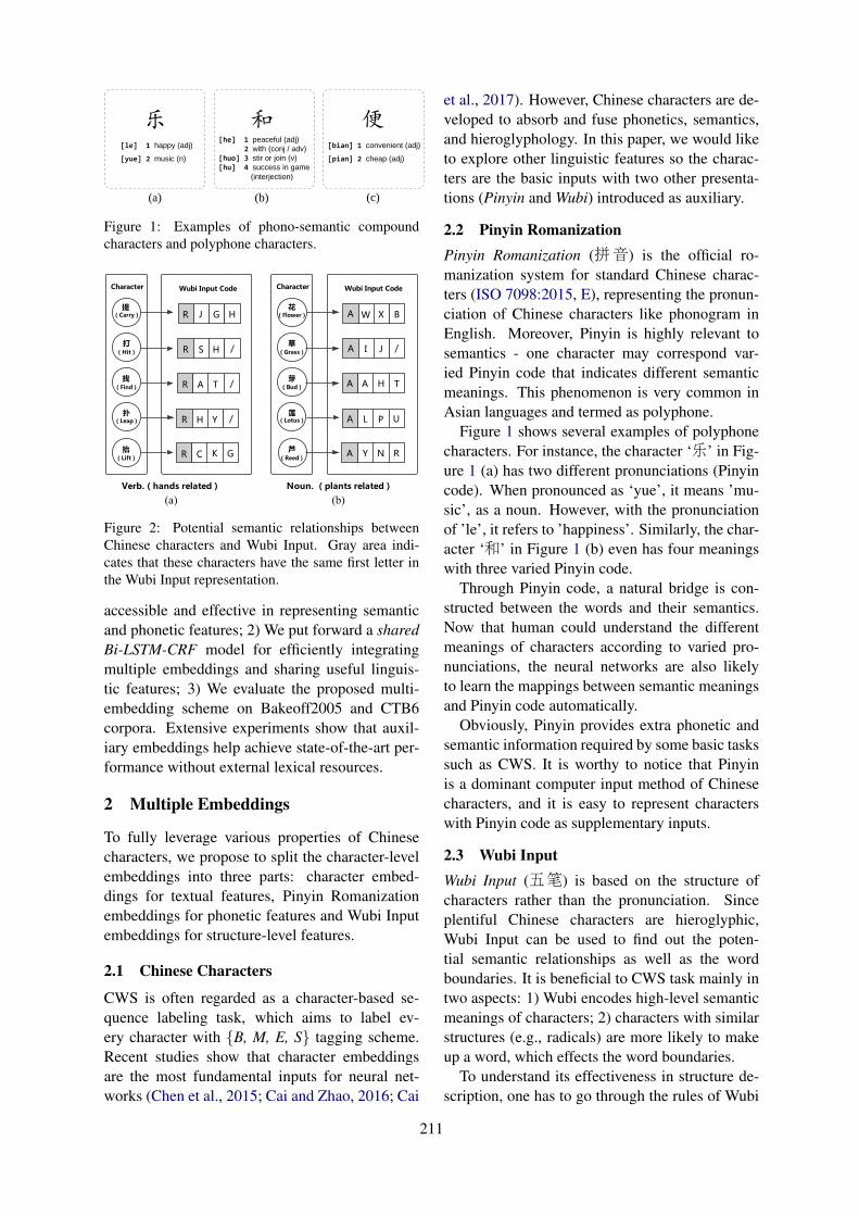
和 便[he] 1 peaceful (adj)

2 with (conj / adv)

[huo] 3 stir or join (v)

[hu] 4 success in game

(interjection)

[bian] 1 convenient (adj)

[pian] 2 cheap (adj)

乐[le] 1 happy (adj)

[yue] 2 music (n)

(a) (b) (c)

Figure 1: Examples of phono-semantic compoundcharacters and polyphone characters.

Character

R J G H

R S H /

R A T /

R H Y /

R C K G

Wubi Input Code

Verb.（hands related）

（Carry）提

打（Hit）

找（Find）

扑（Leap）

抬（Lift）

Character

W X B

A A H T

Wubi Input Code

Noun. （plants related）

（Flower）花

草（Grass）

芽（Bud）

莲（Lotus）

芦（Reed）

J /

A

A

A

L P U

A

I

Y N R

(a) (b)

Figure 2: Potential semantic relationships betweenChinese characters and Wubi Input. Gray area indi-cates that these characters have the same first letter inthe Wubi Input representation.

accessible and effective in representing semanticand phonetic features; 2) We put forward a sharedBi-LSTM-CRF model for efficiently integratingmultiple embeddings and sharing useful linguis-tic features; 3) We evaluate the proposed multi-embedding scheme on Bakeoff2005 and CTB6corpora. Extensive experiments show that auxil-iary embeddings help achieve state-of-the-art per-formance without external lexical resources.

2 Multiple Embeddings

To fully leverage various properties of Chinesecharacters, we propose to split the character-levelembeddings into three parts: character embed-dings for textual features, Pinyin Romanizationembeddings for phonetic features and Wubi Inputembeddings for structure-level features.

2.1 Chinese Characters

CWS is often regarded as a character-based se-quence labeling task, which aims to label ev-ery character with B, M, E, S tagging scheme.Recent studies show that character embeddingsare the most fundamental inputs for neural net-works (Chen et al., 2015; Cai and Zhao, 2016; Cai

et al., 2017). However, Chinese characters are de-veloped to absorb and fuse phonetics, semantics,and hieroglyphology. In this paper, we would liketo explore other linguistic features so the charac-ters are the basic inputs with two other presenta-tions (Pinyin and Wubi) introduced as auxiliary.

2.2 Pinyin RomanizationPinyin Romanization (拼音) is the official ro-manization system for standard Chinese charac-ters (ISO 7098:2015, E), representing the pronun-ciation of Chinese characters like phonogram inEnglish. Moreover, Pinyin is highly relevant tosemantics - one character may correspond var-ied Pinyin code that indicates different semanticmeanings. This phenomenon is very common inAsian languages and termed as polyphone.

Figure 1 shows several examples of polyphonecharacters. For instance, the character ‘乐’ in Fig-ure 1 (a) has two different pronunciations (Pinyincode). When pronounced as ‘yue’, it means ’mu-sic’, as a noun. However, with the pronunciationof ’le’, it refers to ’happiness’. Similarly, the char-acter ‘和’ in Figure 1 (b) even has four meaningswith three varied Pinyin code.

Through Pinyin code, a natural bridge is con-structed between the words and their semantics.Now that human could understand the differentmeanings of characters according to varied pro-nunciations, the neural networks are also likelyto learn the mappings between semantic meaningsand Pinyin code automatically.

Obviously, Pinyin provides extra phonetic andsemantic information required by some basic taskssuch as CWS. It is worthy to notice that Pinyinis a dominant computer input method of Chinesecharacters, and it is easy to represent characterswith Pinyin code as supplementary inputs.

2.3 Wubi InputWubi Input (五笔) is based on the structure ofcharacters rather than the pronunciation. Sinceplentiful Chinese characters are hieroglyphic,Wubi Input can be used to find out the poten-tial semantic relationships as well as the wordboundaries. It is beneficial to CWS task mainly intwo aspects: 1) Wubi encodes high-level semanticmeanings of characters; 2) characters with similarstructures (e.g., radicals) are more likely to makeup a word, which effects the word boundaries.

To understand its effectiveness in structure de-scription, one has to go through the rules of Wubi

211

FC Layer

Bi-LSTM

CRF

Tag

Bi-LSTM1

CRF CRF

Pinyin Wubi

TagTag

Bi-LSTM

Bi-LSTM

Bi-LSTM

Char Pinyin Wubi Char Pinyin Wubi

Bi-LSTM2 Bi-LSTM3

Char

Shared Parameters

(a) Model-I

FC Layer

Bi-LSTM

CRF

Tag

Bi-LSTM1

CRF CRF

Pinyin Wubi

TagTag

Bi-LSTM

Bi-LSTM

Bi-LSTM

Char Pinyin Wubi Char Pinyin Wubi

Bi-LSTM2 Bi-LSTM3

Char

Shared Parameters

(b) Model-II

FC Layer

Bi-LSTM

CRF

Tag

Bi-LSTM1

CRF CRF

Pinyin Wubi

TagTag

Bi-LSTM

Bi-LSTM

Bi-LSTM

Char Pinyin Wubi Char Pinyin Wubi

Bi-LSTM2 Bi-LSTM3

Char

Shared Parameters

(c) Model-III

Figure 3: Network architecture of three multi-embedding models. (a) Model-I: Multi-Bi-LSTMs-CRF Model. (b)Model-II: FC-Layer Bi-LSTMs-CRF Model. (c) Model-III: Shared Bi-LSTMs-CRF Model.

Input method. It is an efficient encoding systemwhich represents each Chinese character with atmost four English letters. Specifically, these let-ters are divided into five regions, each of whichrepresents a type of structure (stroke, 笔画) inChinese characters.

Figure 2 provides some examples of Chinesecharacters and their corresponding Wubi code(four letters). For instance, ‘提’ (carry), ‘打’ (hit)and ‘抬’ (lift) in Figure 2 (a) are all verbs relatedto hands and correspond different spellings in En-glish. On the contrary, in Chinese, these charactersare all left-right symbols and have the same radical(‘R’ in Wubi code). That is to say, Chinese char-acters that are highly semantically relevant usuallyhave similar structures which could be perfectlycaptured by Wubi. Besides, characters with simi-lar structures are more likely to make up a word.For example, ‘花’ (flower), ‘草’ (grass) and ‘芽’(bud) in Figure 2 (b) are nouns and represent dif-ferent plants. Whereas, they are all up-down sym-bols and have the same radical (‘A’ in Wubi code).These words usually make up new words such as‘花草’ (flowers and grasses) and ‘花芽’ (the budsof flowers).

In addition, the sequence in Wubi code is oneapproach to interpret the relationships betweenChinese characters. In Figure 2, it is easy to findsome interesting component rules. For instance,we can conclude: 1) the sequence order impliesthe order of character components (e.g., ‘IA’ vs‘AI’ and ‘IY’ vs ‘YI’); 2) some code has practicalmeanings (e.g., ‘I’ denotes water). Consequently,Wubi is an efficient encoding of Chinese charac-ters so incorporated as a supplementary input likePinyin in our multi-embedding model.

2.4 Multiple Embeddings

To fully utilize various properties of Chinese char-acters, we construct the Pinyin and Wubi embed-dings as two supplementary character-level fea-tures. We firstly pre-process the characters andobtain the basic character embedding followingthe strategy in Lample et al. (2016); Shao et al.(2017). Then we use the Pypinyin Library1 toannotate Pinyin code, and an official transforma-tion table2 to translate characters to Wubi code.Finally, we retrieve multiple embeddings usingword2vec tool (Mikolov et al., 2013).

For simplicity, we treat Pinyin and Wubi codeas units like characters processed by canonicalword2vec, which may discard some semanticaffinities. It is worth noticing that the sequenceorder in Wubi code is an intriguing property con-sidering the fact that structures of characters areencoded by the order of letters (see Sec 2.3). Thispoint merits further study. Finally, we remark thatgenerating Pinyin code relies on the external re-sources (statistics prior). Nontheless, Wubi codeis converted under a transformation table so doesnot introduce any external resources.

3 Multi-Embedding Model Architecture

We adopt the popular Bi-LSTMs-CRF as our base-line model (Figure 4 without Pinyin and Wubi in-put), similar to the architectures proposed by Lam-ple et al. (2016) and Dong et al. (2016). To ob-tain an efficient fusion and sharing mechanism formultiple features, we design three varied architec-tures (see Figure 3). In what follows, we will pro-vide detailed explanations and analysis.

1https://pypi.python.org/pypi/pypinyin2http://wubi.free.fr/index_en.html

212

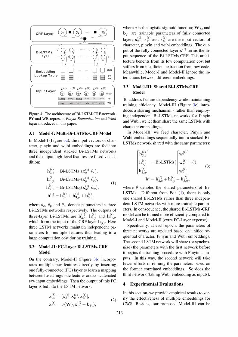
Input Layer

Embedding Lookup Table

Bi-LSTMsLayer

长 江 长 满 绿 藻

… … …

… … …

.... .. ..

char

PYWB

……

……

CRF Layer ……

char

WB

chang jiang zhang man lv zao PY

XVIY AIKSIAGWTAYIIAG/TAYI

Figure 4: The architecture of Bi-LSTM-CRF network.PY and WB represent Pinyin Romanization and WubiInput introduced in this paper.

3.1 Model-I: Multi-Bi-LSTMs-CRF ModelIn Model-I (Figure 3a), the input vectors of char-acter, pinyin and wubi embeddings are fed intothree independent stacked Bi-LSTMs networksand the output high-level features are fused via ad-dition:

h(t)3,c = Bi-LSTMs1(x(t)

c , θc),

h(t)3,p = Bi-LSTMs2(x(t)

p , θp),

h(t)3,w = Bi-LSTMs3(x(t)

w , θw),

h(t) = h(t)3,c + h

(t)3,p + h

(t)3,w,

(1)

where θc, θp and θw denote parameters in threeBi-LSTMs networks respectively. The outputs ofthree-layer Bi-LSTMs are h

(t)3,c, h

(t)3,p and h

(t)3,w,

which form the input of the CRF layer h(t). Herethree LSTM networks maintain independent pa-rameters for multiple features thus leading to alarge computation cost during training.

3.2 Model-II: FC-Layer Bi-LSTMs-CRFModel

On the contrary, Model-II (Figure 3b) incorpo-rates multiple raw features directly by insertingone fully-connected (FC) layer to learn a mappingbetween fused linguistic features and concatenatedraw input embeddings. Then the output of this FClayer is fed into the LSTM network:

x(t)in = [x(t)

c ;x(t)p ;x(t)

w ],

x(t) = σ(Wfcx(t)in + bfc),

(2)

where σ is the logistic sigmoid function; Wfc andbfc are trainable parameters of fully connectedlayer; x(t)

c , x(t)p and x

(t)w are the input vectors of

character, pinyin and wubi embeddings. The out-put of the fully connected layer x(t) forms the in-put sequence of the Bi-LSTMs-CRF. This archi-tecture benefits from its low computation cost butsuffers from insufficient extraction from raw code.Meanwhile, Model-I and Model-II ignore the in-teractions between different embeddings.

3.3 Model-III: Shared Bi-LSTMs-CRFModel

To address feature dependency while maintainingtraining efficiency, Model-III (Figure 3c) intro-duces a sharing mechanism - rather than employ-ing independent Bi-LSTMs networks for Pinyinand Wubi, we let them share the same LSTMs withcharacter embeddings.

In Model-III, we feed character, Pinyin andWubi embeddings sequentially into a stacked Bi-LSTMs network shared with the same parameters:

h(t)3,c

h(t)3,p

h(t)3,w

= Bi-LSTMs(

w(t)c

w(t)p

w(t)w

, θ),

ht = h(t)3,c + h

(t)3,p + h

(t)3,w,

(3)

where θ denotes the shared parameters of Bi-LSTMs. Different from Eqn (1), there is onlyone shared Bi-LSTMs rather than three indepen-dent LSTM networks with more trainable param-eters. In consequence, the shared Bi-LSTMs-CRFmodel can be trained more efficiently compared toModel-I and Model-II (extra FC-Layer expense).

Specifically, at each epoch, the parameters ofthree networks are updated based on unified se-quential character, Pinyin and Wubi embeddings.The second LSTM network will share (or synchro-nize) the parameters with the first network beforeit begins the training procedure with Pinyin as in-puts. In this way, the second network will takefewer efforts in refining the parameters based onthe former correlated embeddings. So does thethird network (taking Wubi embedding as inputs).

4 Experimental Evaluations

In this section, we provide empirical results to ver-ify the effectiveness of multiple embeddings forCWS. Besides, our proposed Model-III can be

213

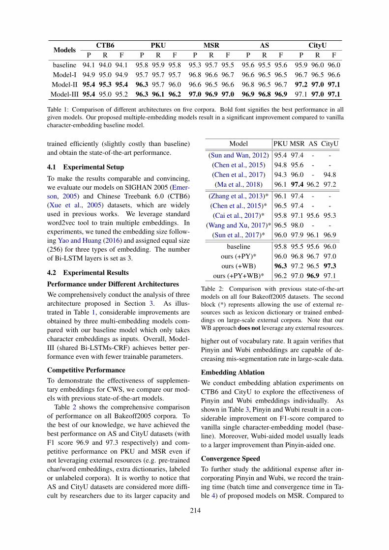
ModelsCTB6 PKU MSR AS CityU

P R F P R F P R F P R F P R Fbaseline 94.1 94.0 94.1 95.8 95.9 95.8 95.3 95.7 95.5 95.6 95.5 95.6 95.9 96.0 96.0Model-I 94.9 95.0 94.9 95.7 95.7 95.7 96.8 96.6 96.7 96.6 96.5 96.5 96.7 96.5 96.6Model-II 95.4 95.3 95.4 96.3 95.7 96.0 96.6 96.5 96.6 96.8 96.5 96.7 97.2 97.0 97.1Model-III 95.4 95.0 95.2 96.3 96.1 96.2 97.0 96.9 97.0 96.9 96.8 96.9 97.1 97.0 97.1

Table 1: Comparison of different architectures on five corpora. Bold font signifies the best performance in allgiven models. Our proposed multiple-embedding models result in a significant improvement compared to vanillacharacter-embedding baseline model.

trained efficiently (slightly costly than baseline)and obtain the state-of-the-art performance.

4.1 Experimental SetupTo make the results comparable and convincing,we evaluate our models on SIGHAN 2005 (Emer-son, 2005) and Chinese Treebank 6.0 (CTB6)(Xue et al., 2005) datasets, which are widelyused in previous works. We leverage standardword2vec tool to train multiple embeddings. Inexperiments, we tuned the embedding size follow-ing Yao and Huang (2016) and assigned equal size(256) for three types of embedding. The numberof Bi-LSTM layers is set as 3.

4.2 Experimental ResultsPerformance under Different ArchitecturesWe comprehensively conduct the analysis of threearchitecture proposed in Section 3. As illus-trated in Table 1, considerable improvements areobtained by three multi-embedding models com-pared with our baseline model which only takescharacter embeddings as inputs. Overall, Model-III (shared Bi-LSTMs-CRF) achieves better per-formance even with fewer trainable parameters.

Competitive PerformanceTo demonstrate the effectiveness of supplemen-tary embeddings for CWS, we compare our mod-els with previous state-of-the-art models.

Table 2 shows the comprehensive comparisonof performance on all Bakeoff2005 corpora. Tothe best of our knowledge, we have achieved thebest performance on AS and CityU datasets (withF1 score 96.9 and 97.3 respectively) and com-petitive performance on PKU and MSR even ifnot leveraging external resources (e.g. pre-trainedchar/word embeddings, extra dictionaries, labeledor unlabeled corpora). It is worthy to notice thatAS and CityU datasets are considered more diffi-cult by researchers due to its larger capacity and

Model PKU MSR AS CityU

(Sun and Wan, 2012) 95.4 97.4 - -(Chen et al., 2015) 94.8 95.6 - -(Chen et al., 2017) 94.3 96.0 - 94.8(Ma et al., 2018) 96.1 97.4 96.2 97.2

(Zhang et al., 2013)* 96.1 97.4 - -(Chen et al., 2015)* 96.5 97.4 - -(Cai et al., 2017)* 95.8 97.1 95.6 95.3

(Wang and Xu, 2017)* 96.5 98.0 - -(Sun et al., 2017)* 96.0 97.9 96.1 96.9

baseline 95.8 95.5 95.6 96.0ours (+PY)* 96.0 96.8 96.7 97.0ours (+WB) 96.3 97.2 96.5 97.3

ours (+PY+WB)* 96.2 97.0 96.9 97.1

Table 2: Comparison with previous state-of-the-artmodels on all four Bakeoff2005 datasets. The secondblock (*) represents allowing the use of external re-sources such as lexicon dictionary or trained embed-dings on large-scale external corpora. Note that ourWB approach does not leverage any external resources.

higher out of vocabulary rate. It again verifies thatPinyin and Wubi embeddings are capable of de-creasing mis-segmentation rate in large-scale data.

Embedding AblationWe conduct embedding ablation experiments onCTB6 and CityU to explore the effectiveness ofPinyin and Wubi embeddings individually. Asshown in Table 3, Pinyin and Wubi result in a con-siderable improvement on F1-score compared tovanilla single character-embedding model (base-line). Moreover, Wubi-aided model usually leadsto a larger improvement than Pinyin-aided one.

Convergence SpeedTo further study the additional expense after in-corporating Pinyin and Wubi, we record the train-ing time (batch time and convergence time in Ta-ble 4) of proposed models on MSR. Compared to

214

ModelsCTB6 CityU

P R F P R Fbaseline 94.1 94.0 94.1 95.9 96.0 96.0IO + PY 94.6 94.9 94.8 96.8 96.4 96.6IO + WB 95.3 95.4 95.3 97.3 97.3 97.3Model-II 95.4 95.3 95.4 97.2 97.0 97.1

Table 3: Feature ablation on CTB6 and CityU. IO +PY and IO + WB denote injecting Pinyin and Wubiembeddings separately under Model-II.

Model Time (batch) Time (P-95%)baseline 1 × 1 ×Model-I 2.61 × 2.51 ×Model-II 1.03 × 1.50 ×Model-III 1.07 × 1.04 ×

Table 4: Relative training time on MSR. (a) averagedtraining time per batch; (b) convergence time, whereabove 95% precision is considered as convergence.

the baseline model, it almost takes the same train-ing time (1.07×) per batch and convergence time(1.04×) for Model-III. By contrast, Model-II leadsto slower convergence (1.50×) in spite of its lowerbatch-training cost. In consequence, we recom-mend Model-III in practice for its high efficiency.

5 Related Work

Since Xu (2003), researchers have mostly treatedCWS as a sequence labeling problem. Followingthis idea, great achievements have been reached inthe past few years with the effective embeddingsintroduced and powerful neural networks armed.

In recent years, there are plentiful works ex-ploiting different neural network architectures inCWS. Among these architectures, there are sev-eral models most similar to our model: Bi-LSTM-CRF (Huang et al., 2015), Bi-LSTM-CRF (Lam-ple et al., 2016; Dong et al., 2016), and Bi-LSTM-CNNs-CRF (Ma and Hovy, 2016).

Huang et al. (2015) was the first to adopt Bi-LSTM network for character representations andCRF for label decoding. Lample et al. (2016)and Dong et al. (2016) exploited the Bi-LSTM-CRF model for named entity recognition in west-ern languages and Chinese, respectively. More-over, Dong et al. (2016) introduced radical-levelinformation that can be regarded as a special caseof Wubi code in our model.

Ma and Hovy (2016) proposed to combine Bi-LSTM, CNN and CRF, which results in faster con-vergence speed and better performance on POS

and NER tasks. In addition, their model leveragesboth the character-level and word-level informa-tion.

Our work distinguishes itself by utilizing multi-ple dimensions of features in Chinese characters.With phonetic and semantic meanings taken intoconsideration, three proposed models achieve bet-ter performance on CWS and can be also adaptedto POS and NER tasks. In particular, comparedto radical-level information in (Dong et al., 2016),Wubi Input encodes richer structure details andpotentially semantic relationships.

Recently, researchers propose to treat CWS asa word-based sequence labeling problem, whichalso achieves competitive performance (Zhanget al., 2016; Cai and Zhao, 2016; Cai et al., 2017;Yang et al., 2017). Other works try to introducevery deep networks (Wang and Xu, 2017) or treatCWS as a gap-filling problem (Sun et al., 2017).We believe that proposed linguistic features canalso be transferred into word-level sequence la-beling and correct the error. In a nutshell, multi-ple embeddings are generic and easily accessible,which can be applied and studied further in theseworks.

6 Conclusion

In this paper, we firstly propose to leverage pho-netic, structured and semantic features of Chinesecharacters by introducing multiple character em-beddings (Pinyin and Wubi). We conduct a com-prehensive analysis on why Pinyin and Wubi em-beddings are so essential in CWS task and couldbe translated to other NLP tasks such as POSand NER. Besides, we design three generic mod-els to fuse the multi-embedding and produce thestart-of-the-art performance in five public corpora.In particular, the shared Bi-LSTM-CRF models(Model III in Figure 3) could be trained effi-ciently and produce the best performance on ASand CityU corpora. In future, the effective ways ofleveraging hierarchical linguistic features to otherlanguages, NLP tasks (e.g., POS and NER) andrefining mis-labeled sentences merit further study.

Acknowledgement

This research work has been partially funded bythe National Natural Science Foundation of China(Grant No.61772337, U1736207), and the Na-tional Key Research and Development Program ofChina NO.2016QY03D0604.

215

ReferencesDeng Cai and Hai Zhao. 2016. Neural word segmen-

tation learning for chinese. In ACL (1), Berlin, Ger-many. The Association for Computer Linguistics.

Deng Cai, Hai Zhao, Zhisong Zhang, Yuan Xin,Yongjian Wu, and Feiyue Huang. 2017. Fast andaccurate neural word segmentation for chinese. InACL (2), pages 608–615. Association for Computa-tional Linguistics.

Xinchi Chen, Xipeng Qiu, Chenxi Zhu, Pengfei Liu,and Xuanjing Huang. 2015. Long short-term mem-ory neural networks for chinese word segmentation.In EMNLP, pages 1197–1206. The Association forComputational Linguistics.

Xinchi Chen, Zhan Shi, Xipeng Qiu, and XuanjingHuang. 2017. Adversarial multi-criteria learningfor chinese word segmentation. In ACL (1), pages1193–1203. Association for Computational Linguis-tics.

Chuanhai Dong, Jiajun Zhang, Chengqing Zong,Masanori Hattori, and Hui Di. 2016. Character-based LSTM-CRF with radical-level featuresfor chinese named entity recognition. InNLPCC/ICCPOL, volume 10102 of Lecture Notesin Computer Science, pages 239–250. Springer.

Thomas Emerson. 2005. The second international chi-nese word segmentation bakeoff. In Proceedings ofthe Fourth SIGHAN Workshop on Chinese LanguageProcessing, SIGHAN@IJCNLP 2005, Jeju Island,Korea, 14-15, 2005.

Zhiheng Huang, Wei Xu, and Kai Yu. 2015. Bidi-rectional LSTM-CRF models for sequence tagging.CoRR, abs/1508.01991.

ISO 7098:2015(E). 2015. Information and documen-tation – Romanization of Chinese. Standard, Inter-national Organization for Standardization, Geneva,CH.

Guillaume Lample, Miguel Ballesteros, Sandeep Sub-ramanian, Kazuya Kawakami, and Chris Dyer. 2016.Neural architectures for named entity recognition.In HLT-NAACL, pages 260–270. The Associationfor Computational Linguistics.

Ji Ma, Kuzman Ganchev, and David Weiss. 2018.State-of-the-art chinese word segmentation with bi-lstms. In EMNLP, pages 4902–4908. Associationfor Computational Linguistics.

Xuezhe Ma and Eduard H. Hovy. 2016. End-to-end se-quence labeling via bi-directional lstm-cnns-crf. InACL (1). The Association for Computer Linguistics.

Tomas Mikolov, Ilya Sutskever, Kai Chen, Greg Cor-rado, and Jeffrey Dean. 2013. Distributed represen-tations of words and phrases and their composition-ality. CoRR, abs/1310.4546.

Fuchun Peng, Fangfang Feng, and Andrew McCallum.2004. Chinese segmentation and new word detec-tion using conditional random fields. In Proceedingsof the 20th International Conference on Computa-tional Linguistics, COLING ’04, Stroudsburg, PA,USA. Association for Computational Linguistics.

Yan Shao, Christian Hardmeier, Jorg Tiedemann, andJoakim Nivre. 2017. Character-based joint segmen-tation and POS tagging for chinese using bidirec-tional RNN-CRF. In IJCNLP(1), pages 173–183.Asian Federation of Natural Language Processing.

Weiwei Sun and Xiaojun Wan. 2012. Reducing ap-proximation and estimation errors for chinese lexicalprocessing with heterogeneous annotations. In ACL(1), pages 232–241. The Association for ComputerLinguistics.

Yaming Sun, Lei Lin, Nan Yang, Zhenzhou Ji, andXiaolong Wang. 2014. Radical-enhanced chinesecharacter embedding. In ICONIP (2), volume 8835of Lecture Notes in Computer Science, pages 279–286. Springer.

Zhiqing Sun, Gehui Shen, and Zhi-Hong Deng. 2017.A gap-based framework for chinese word segmenta-tion via very deep convolutional networks. CoRR,abs/1712.09509.

Chunqi Wang and Bo Xu. 2017. Convolutional neu-ral network with word embeddings for chinese wordsegmentation. In IJCNLP(1), pages 163–172. AsianFederation of Natural Language Processing.

Nianwen Xu. 2003. Chinese word segmentation ascharacter tagging. Computational Linguistics andChinese Language Processing, 8(1):29–48.

Naiwen Xue, Fei Xia, Fu-Dong Chiou, and MarthaPalmer. 2005. The penn chinese treebank: Phrasestructure annotation of a large corpus. Natural Lan-guage Engineering, 11(2):207–238.

Jie Yang, Yue Zhang, and Fei Dong. 2017. Neuralword segmentation with rich pretraining. In ACL(1), pages 839–849. Association for ComputationalLinguistics.

Yushi Yao and Zheng Huang. 2016. Bi-directionalLSTM recurrent neural network for chinese wordsegmentation. In ICONIP (4), volume 9950 of Lec-ture Notes in Computer Science, pages 345–353.

Longkai Zhang, Houfeng Wang, Xu Sun, and MairgupMansur. 2013. Exploring representations from un-labeled data with co-training for chinese word seg-mentation. In EMNLP, pages 311–321. ACL.

Meishan Zhang, Yue Zhang, and Guohong Fu. 2016.Transition-based neural word segmentation. In Pro-ceedings of the 54th Annual Meeting of the Associ-ation for Computational Linguistics, ACL 2016, Au-gust 7-12, 2016, Berlin, Germany, Volume 1: LongPapers.

216

Proceedings of the 57th Annual Meeting of the Association for Computational Linguistics: Student Research Workshop, pages 217–222Florence, Italy, July 28 - August 2, 2019. c©2019 Association for Computational Linguistics

Attention over Heads:A Multi-Hop Attention for Neural Machine Translation

Shohei Iida†, Ryuichiro Kimura†, Hongyi Cui†, Po-Hsuan Hung†,Takehito Utsuro† and Masaaki Nagata‡

†Graduate School of Systems and Information Engineering, University of Tsukuba, Japan‡NTT Communication Science Laboratories, NTT Corporation, Japan

Abstract

In this paper, we propose a multi-hop attentionfor the Transformer. It refines the attention foran output symbol by integrating that of eachhead, and consists of two hops. The first hopattention is the scaled dot-product attentionwhich is the same attention mechanism used inthe original Transformer. The second hop at-tention is a combination of multi-layer percep-tron (MLP) attention and head gate, which ef-ficiently increases the complexity of the modelby adding dependencies between heads. Wedemonstrate that the translation accuracy ofthe proposed multi-hop attention outperformsthe baseline Transformer significantly, +0.85BLEU point for the IWSLT-2017 German-to-English task and +2.58 BLEU point for theWMT-2017 German-to-English task. We alsofind that the number of parameters required fora multi-hop attention is smaller than that forstacking another self-attention layer and theproposed model converges significantly fasterthan the original Transformer.

1 Introduction

Multi-hop attention was first proposed in end-to-end memory networks (Sukhbaatar et al., 2015)for machine comprehension. In this paper, we de-fine a hop as a computational step which couldbe performed for an output symbol many times.By “multi-hop attention”, we mean that somekind of attention is calculated many times forgenerating an output symbol. Previous multi-hop attention can be classified into “recurrent at-tention” (Sukhbaatar et al., 2015) and “hierarchi-cal attention” (Libovicky and Helcl, 2017). Theformer repeats the calculation of attention manytimes to refine the attention itself while the latterintegrates attentions for multiple input informationsources. The proposed multi-hop attention for theTransformer is different from previous recurrentattentions because the mechanism for the first hopattention and that for the second hop attention is

different. It is also different from previous hierar-chical attention because it is designed to integrateattentions from different heads for the same infor-mation source.

In neural machine translation, hier-archical attention (Bawden et al., 2018;Libovicky and Helcl, 2017) can be thoughtof a multi-hop attention because it repeats atten-tion calculation to integrate the information frommultiple source encoders. On the other hand, inthe Transformer (Vaswani et al., 2017), the state-of-the-art model for neural machine translation,feed-forward neural network (FFNN) integratesinformation from multiple heads. In this paper,we propose a multi-hop attention mechanism as apossible alternative to integrate information frommulti-head attention in the Transformer.

We find that the proposed Transformer withmulti-hop attention converges faster than the orig-inal Transformer. This is likely because all headslearn to influence each other, through a head gatemechanism, in the second hop attention (Fig-ure 1). Recently, many Transformer-based pre-trained language models such as BERT have beenproposed and take about a month for training. Thespeed at which the proposed model converges maybe even more important than the fact that its accu-racy is slightly better.

2 Multi-Hop Multi-Head Attention forthe Transformer

2.1 Multi-Head AttentionOne of the Transformer’s major successes is multi-head attention, which allows each head to capturedifferent features and achieve better results com-pared to a single-head case.

a(h) = softmax(Q(h)K(h)T

√d

)V (h) (1)

m = Concat(a(1), ..., a(h))WO (2)

217

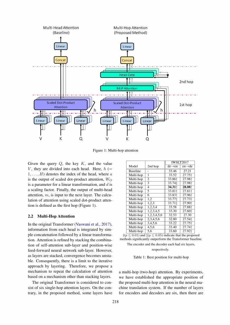
Figure 1: Multi-hop attention

Given the query Q, the key K, and the valueV , they are divided into each head. Here, h (=1, . . . ,H) denotes the index of the head, where ais the output of scaled dot-product attention, WO

is a parameter for a linear transformation, and d isa scaling factor. Finally, the output of multi-headattention, m, is input to the next layer. The calcu-lation of attention using scaled dot-product atten-tion is defined as the first hop (Figure 1).

2.2 Multi-Hop Attention

In the original Transformer (Vaswani et al., 2017),information from each head is integrated by sim-ple concatenation followed by a linear transforma-tion. Attention is refined by stacking the combina-tion of self-attention sub-layer and position-wisefeed-forward neural network sub-layer. However,as layers are stacked, convergence becomes unsta-ble. Consequently, there is a limit to the iterativeapproach by layering. Therefore, we propose amechanism to repeat the calculation of attentionbased on a mechanism other than stacking layers.

The original Transformer is considered to con-sist of six single-hop attention layers. On the con-trary, in the proposed method, some layers have

IWSLT2017Model 2nd hop de→en en→deBaseline - 33.46 27.21Multi-hop 1 33.52 27.75†Multi-hop 2 33.86† 27.98†Multi-hop 3 33.74‡ 27.98†Multi-hop 4 34.31† 28.08†Multi-hop 5 33.81† 27.81†Multi-hop 6 33.83† 27.96†Multi-hop 1,2 33.77‡ 27.73†Multi-hop 1,2,3 33.71‡ 27.90†Multi-hop 1,2,3,4 33.58 27.88†Multi-hop 1,2,3,4,5 33.30 27.60†Multi-hop 1,2,3,4,5,6 32.53 27.30Multi-hop 2,3,4,5,6 32.80 27.54‡Multi-hop 3,4,5,6 33.22 27.75†Multi-hop 4,5,6 33.40 27.74†Multi-hop 5,6 33.60 27.92†

†(p ≤ 0.01) and ‡(p ≤ 0.05) indicate that the proposedmethods significantly outperform the Transformer baseline.

The encoder and the decoder each had six layers,

respectively.

Table 1: Best position for multi-hop

a multi-hop (two-hop) attention. By experiments,we have established the appropriate position ofthe proposed multi-hop attention in the neural ma-chine translation system. If the number of layersfor encoders and decoders are six, then there are

218

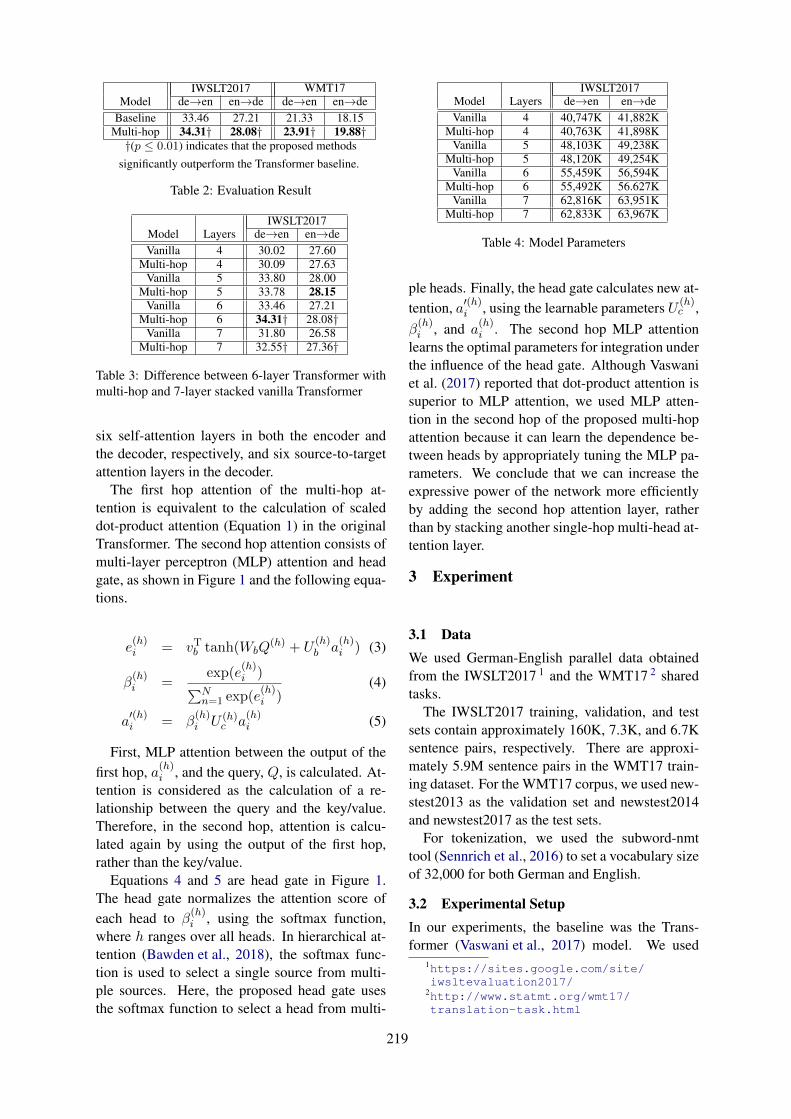
IWSLT2017 WMT17Model de→en en→de de→en en→de

Baseline 33.46 27.21 21.33 18.15Multi-hop 34.31† 28.08† 23.91† 19.88†

†(p ≤ 0.01) indicates that the proposed methods

significantly outperform the Transformer baseline.

Table 2: Evaluation Result

IWSLT2017Model Layers de→en en→deVanilla 4 30.02 27.60

Multi-hop 4 30.09 27.63Vanilla 5 33.80 28.00

Multi-hop 5 33.78 28.15Vanilla 6 33.46 27.21

Multi-hop 6 34.31† 28.08†Vanilla 7 31.80 26.58

Multi-hop 7 32.55† 27.36†

Table 3: Difference between 6-layer Transformer withmulti-hop and 7-layer stacked vanilla Transformer

six self-attention layers in both the encoder andthe decoder, respectively, and six source-to-targetattention layers in the decoder.

The first hop attention of the multi-hop at-tention is equivalent to the calculation of scaleddot-product attention (Equation 1) in the originalTransformer. The second hop attention consists ofmulti-layer perceptron (MLP) attention and headgate, as shown in Figure 1 and the following equa-tions.

e(h)i = vT

b tanh(WbQ(h) + U

(h)b a

(h)i ) (3)

β(h)i =

exp(e(h)i )

∑Nn=1 exp(e

(h)i )

(4)

a′(h)i = β

(h)i U (h)

c a(h)i (5)

First, MLP attention between the output of thefirst hop, a

(h)i , and the query, Q, is calculated. At-

tention is considered as the calculation of a re-lationship between the query and the key/value.Therefore, in the second hop, attention is calcu-lated again by using the output of the first hop,rather than the key/value.

Equations 4 and 5 are head gate in Figure 1.The head gate normalizes the attention score ofeach head to β

(h)i , using the softmax function,

where h ranges over all heads. In hierarchical at-tention (Bawden et al., 2018), the softmax func-tion is used to select a single source from multi-ple sources. Here, the proposed head gate usesthe softmax function to select a head from multi-

IWSLT2017Model Layers de→en en→deVanilla 4 40,747K 41,882K

Multi-hop 4 40,763K 41,898KVanilla 5 48,103K 49,238K

Multi-hop 5 48,120K 49,254KVanilla 6 55,459K 56,594K

Multi-hop 6 55,492K 56.627KVanilla 7 62,816K 63,951K

Multi-hop 7 62,833K 63,967K

Table 4: Model Parameters

ple heads. Finally, the head gate calculates new at-tention, a′(h)

i , using the learnable parameters U(h)c ,

β(h)i , and a

(h)i . The second hop MLP attention

learns the optimal parameters for integration underthe influence of the head gate. Although Vaswaniet al. (2017) reported that dot-product attention issuperior to MLP attention, we used MLP atten-tion in the second hop of the proposed multi-hopattention because it can learn the dependence be-tween heads by appropriately tuning the MLP pa-rameters. We conclude that we can increase theexpressive power of the network more efficientlyby adding the second hop attention layer, ratherthan by stacking another single-hop multi-head at-tention layer.

3 Experiment

3.1 DataWe used German-English parallel data obtainedfrom the IWSLT2017 1 and the WMT17 2 sharedtasks.

The IWSLT2017 training, validation, and testsets contain approximately 160K, 7.3K, and 6.7Ksentence pairs, respectively. There are approxi-mately 5.9M sentence pairs in the WMT17 train-ing dataset. For the WMT17 corpus, we used new-stest2013 as the validation set and newstest2014and newstest2017 as the test sets.

For tokenization, we used the subword-nmttool (Sennrich et al., 2016) to set a vocabulary sizeof 32,000 for both German and English.

3.2 Experimental SetupIn our experiments, the baseline was the Trans-former (Vaswani et al., 2017) model. We used

1https://sites.google.com/site/iwsltevaluation2017/

2http://www.statmt.org/wmt17/translation-task.html

219

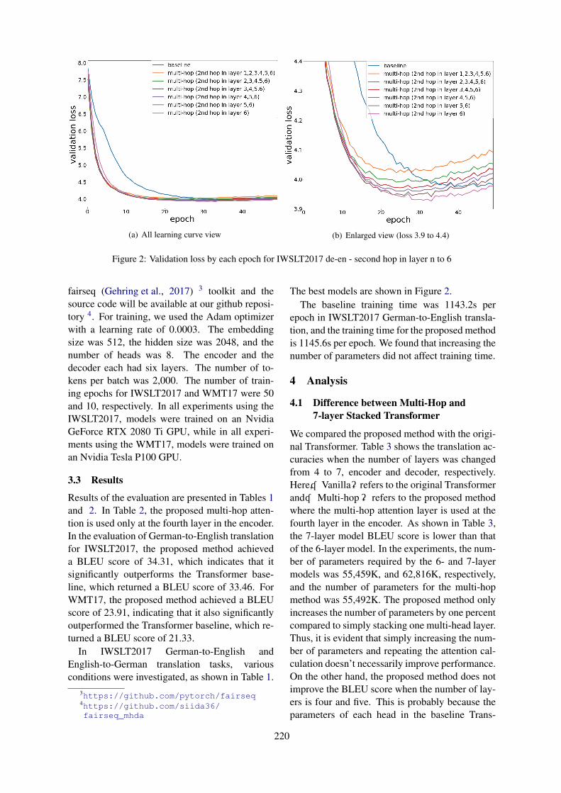
(a) All learning curve view (b) Enlarged view (loss 3.9 to 4.4)

Figure 2: Validation loss by each epoch for IWSLT2017 de-en - second hop in layer n to 6

fairseq (Gehring et al., 2017) 3 toolkit and thesource code will be available at our github reposi-tory 4. For training, we used the Adam optimizerwith a learning rate of 0.0003. The embeddingsize was 512, the hidden size was 2048, and thenumber of heads was 8. The encoder and thedecoder each had six layers. The number of to-kens per batch was 2,000. The number of train-ing epochs for IWSLT2017 and WMT17 were 50and 10, respectively. In all experiments using theIWSLT2017, models were trained on an NvidiaGeForce RTX 2080 Ti GPU, while in all experi-ments using the WMT17, models were trained onan Nvidia Tesla P100 GPU.

3.3 Results

Results of the evaluation are presented in Tables 1and 2. In Table 2, the proposed multi-hop atten-tion is used only at the fourth layer in the encoder.In the evaluation of German-to-English translationfor IWSLT2017, the proposed method achieveda BLEU score of 34.31, which indicates that itsignificantly outperforms the Transformer base-line, which returned a BLEU score of 33.46. ForWMT17, the proposed method achieved a BLEUscore of 23.91, indicating that it also significantlyoutperformed the Transformer baseline, which re-turned a BLEU score of 21.33.

In IWSLT2017 German-to-English andEnglish-to-German translation tasks, variousconditions were investigated, as shown in Table 1.

3https://github.com/pytorch/fairseq4https://github.com/siida36/fairseq_mhda

The best models are shown in Figure 2.The baseline training time was 1143.2s per

epoch in IWSLT2017 German-to-English transla-tion, and the training time for the proposed methodis 1145.6s per epoch. We found that increasing thenumber of parameters did not affect training time.

4 Analysis

4.1 Difference between Multi-Hop and7-layer Stacked Transformer

We compared the proposed method with the origi-nal Transformer. Table 3 shows the translation ac-curacies when the number of layers was changedfrom 4 to 7, encoder and decoder, respectively.Here,“Vanilla”refers to the original Transformerand“Multi-hop”refers to the proposed methodwhere the multi-hop attention layer is used at thefourth layer in the encoder. As shown in Table 3,the 7-layer model BLEU score is lower than thatof the 6-layer model. In the experiments, the num-ber of parameters required by the 6- and 7-layermodels was 55,459K, and 62,816K, respectively,and the number of parameters for the multi-hopmethod was 55,492K. The proposed method onlyincreases the number of parameters by one percentcompared to simply stacking one multi-head layer.Thus, it is evident that simply increasing the num-ber of parameters and repeating the attention cal-culation doesn’t necessarily improve performance.On the other hand, the proposed method does notimprove the BLEU score when the number of lay-ers is four and five. This is probably because theparameters of each head in the baseline Trans-

220

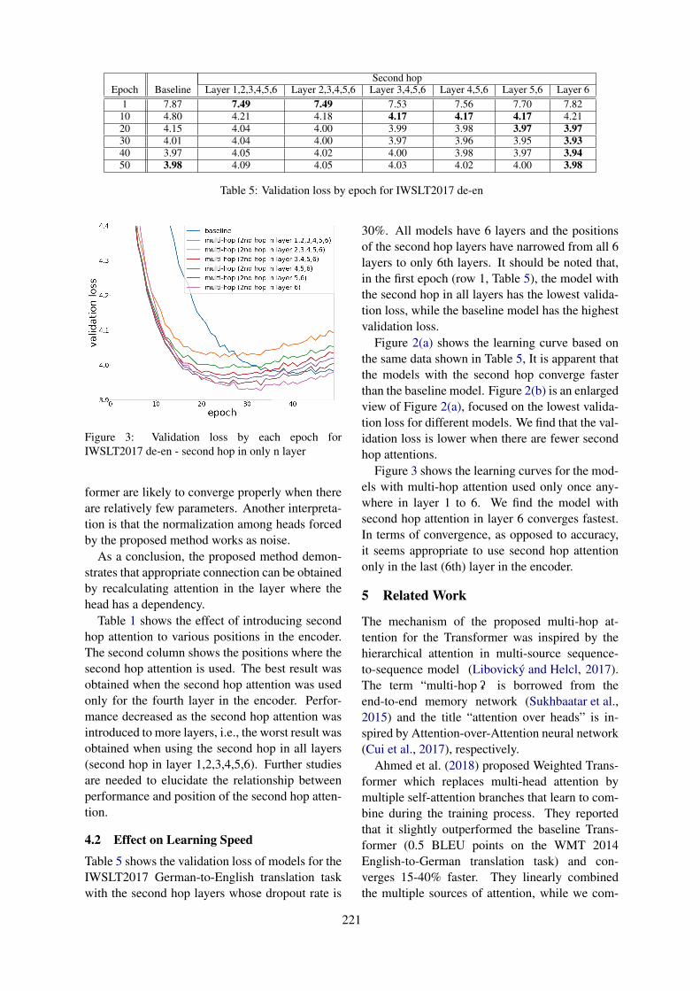
Second hopEpoch Baseline Layer 1,2,3,4,5,6 Layer 2,3,4,5,6 Layer 3,4,5,6 Layer 4,5,6 Layer 5,6 Layer 6

1 7.87 7.49 7.49 7.53 7.56 7.70 7.8210 4.80 4.21 4.18 4.17 4.17 4.17 4.2120 4.15 4.04 4.00 3.99 3.98 3.97 3.9730 4.01 4.04 4.00 3.97 3.96 3.95 3.9340 3.97 4.05 4.02 4.00 3.98 3.97 3.9450 3.98 4.09 4.05 4.03 4.02 4.00 3.98

Table 5: Validation loss by epoch for IWSLT2017 de-en

Figure 3: Validation loss by each epoch forIWSLT2017 de-en - second hop in only n layer

former are likely to converge properly when thereare relatively few parameters. Another interpreta-tion is that the normalization among heads forcedby the proposed method works as noise.

As a conclusion, the proposed method demon-strates that appropriate connection can be obtainedby recalculating attention in the layer where thehead has a dependency.

Table 1 shows the effect of introducing secondhop attention to various positions in the encoder.The second column shows the positions where thesecond hop attention is used. The best result wasobtained when the second hop attention was usedonly for the fourth layer in the encoder. Perfor-mance decreased as the second hop attention wasintroduced to more layers, i.e., the worst result wasobtained when using the second hop in all layers(second hop in layer 1,2,3,4,5,6). Further studiesare needed to elucidate the relationship betweenperformance and position of the second hop atten-tion.

4.2 Effect on Learning Speed

Table 5 shows the validation loss of models for theIWSLT2017 German-to-English translation taskwith the second hop layers whose dropout rate is

30%. All models have 6 layers and the positionsof the second hop layers have narrowed from all 6layers to only 6th layers. It should be noted that,in the first epoch (row 1, Table 5), the model withthe second hop in all layers has the lowest valida-tion loss, while the baseline model has the highestvalidation loss.

Figure 2(a) shows the learning curve based onthe same data shown in Table 5, It is apparent thatthe models with the second hop converge fasterthan the baseline model. Figure 2(b) is an enlargedview of Figure 2(a), focused on the lowest valida-tion loss for different models. We find that the val-idation loss is lower when there are fewer secondhop attentions.

Figure 3 shows the learning curves for the mod-els with multi-hop attention used only once any-where in layer 1 to 6. We find the model withsecond hop attention in layer 6 converges fastest.In terms of convergence, as opposed to accuracy,it seems appropriate to use second hop attentiononly in the last (6th) layer in the encoder.

5 Related Work

The mechanism of the proposed multi-hop at-tention for the Transformer was inspired by thehierarchical attention in multi-source sequence-to-sequence model (Libovicky and Helcl, 2017).The term “multi-hop” is borrowed from theend-to-end memory network (Sukhbaatar et al.,2015) and the title “attention over heads” is in-spired by Attention-over-Attention neural network(Cui et al., 2017), respectively.

Ahmed et al. (2018) proposed Weighted Trans-former which replaces multi-head attention bymultiple self-attention branches that learn to com-bine during the training process. They reportedthat it slightly outperformed the baseline Trans-former (0.5 BLEU points on the WMT 2014English-to-German translation task) and con-verges 15-40% faster. They linearly combinedthe multiple sources of attention, while we com-

221

bined multiple attention non-linearly using soft-max function in the second hop.

It is well known that the Transformer is diffi-cult to train (Popel and Bojar, 2018). As it has alarge number of parameters, it takes time to con-verge and sometimes it does not do so at all with-out appropriate hyper parameter tuning. Consid-ering the experimental results of our multi-hop at-tention experiments, and that of the Weight Trans-former, an appropriate design of the network tocombine multi-head attention could result in fasterand more stable convergence of the Transformer.As the Transformer is used as a building block forthe recently proposed pre-trained language modelssuch as BERT (Devlin et al., 2019) which takesabout a month for training, we think it is worth-while to pursue this line of research including theproposed multi-hop attention.

Universal Transformer (Dehghani et al., 2019)can be thought of variable-depth recurrent at-tention. It obtained Turing-complete expressivepower in exchange for a vast increase in the num-ber of parameters and training time. As shown inTable 4, we have proposed an efficient method toincrease the depth of recurrence in terms of thenumber of parameters and training time. Recently,Voita et al. (2019) and Michel et al. (2019) inde-pendently reported that only a certain subset of theheads plays an important role in the Transformer.They performed analyses by pruning heads froman already trained model, while we have proposeda method to assign weights to heads automati-cally. We assume our method (multi-hop attentionor attention-over-heads) selects important heads inthe early stage of training, which results in fasterconvergence than the original Transformer.

6 Conclusion

In this paper, we have proposed a multi-hop atten-tion mechanism for a Transformer model in whichall heads depend on each other repeatedly. Wefound that the proposed method significantly out-performs the original Transformer in accuracy andconverges faster with little increase in the numberof parameters. In future work, we would like toimplement a multi-hop attention mechanism to thedecoder side and investigate other language pairs.

ReferencesK. Ahmed, N. S. Keskar, and R.Socher. 2018.

Weighted transformer network for machine transla-

tion. arXiv preprint arXiv:1711.02132.

R. Bawden, R. Sennrich, A. Birch, and B. Haddow.2018. Evaluating discourse phenomena in neuralmachine translation. In Proc. NAACL-HLT, pages1304–1313.

Y. Cui, Z. Chen, S. Wei, S. Wang, T. Liu, and G. Hu.2017. Attention-over-attention neural networks forreading comprehension. In Proc. 55th ACL, pages593–602.

M. Dehghani, S. Gouws, O. Vinyals, J. Uszkoreit, andŁ. Kaiser. 2019. Universal transformers. In Proc.7th ICLR.

J. Devlin, M.-W. Chang, K. Lee, and K. Toutanova.2019. BERT: Pre-training of deep bidirectionaltransformers for language understanding. In Proc.NAACL-HLT, volume abs/1810.04805.

J. Gehring, M. Auli, D. Grangier, D. Yarats, and Y. N.Dauphin. 2017. Convolutional Sequence to Se-quence Learning. In Proc. 34th ICML.

J. Libovicky and J. Helcl. 2017. Attention strategiesfor multi-source sequence-to-sequence learning. InProc. 55th ACL, pages 196–202.

P. Michel, O. Levy, and G. Neubig. 2019. Are six-teen heads really better than one? arXiv preprintarXiv:1905.10650.

M. Popel and O. Bojar. 2018. Training tips for thetransformer model. The Prague Bulletin of Math-ematical Linguistics, 110(1):43–70.

R. Sennrich, B. Haddow, and A. Birch. 2016. Neu-ral machine translation of rare words with subwordunits. In Proc. 54th ACL, pages 1715–1725.

S. Sukhbaatar, A. Szlam, J. Weston, and R. Fergus.2015. End-to-end memory networks. In Proc. 28thNIPS, pages 2440–2448.

A. Vaswani, N. Shazeer, N. Parmar, J. Uszkoreit,L. Jones, A. Gomez, L. Kaiser, and I. Polosukhin.2017. Attention is all you need. In Proc. 30th NIPS,pages 5998–6008.

E. Voita, D. Talbot, F. Moiseev, R. Sennrich, andI. Titov. 2019. Analyzing multi-head self-attention:Specialized heads do the heavy lifting, the rest canbe pruned. arXiv preprint arXiv:1905.09418.

222

Proceedings of the 57th Annual Meeting of the Association for Computational Linguistics: Student Research Workshop, pages 223–228Florence, Italy, July 28 - August 2, 2019. c©2019 Association for Computational Linguistics

Reducing Gender Bias in Word-Level Language Models with aGender-Equalizing Loss Function

Yusu Qian∗Tandon Schoolof Engineering

New York University6 MetroTech Center

Brooklyn, NY, 11201yq729@nyu.edu

Urwa Muaz∗Tandon Schoolof Engineering

New York University6 MetroTech Center

Brooklyn, NY, 11201um367@nyu.edu

Ben ZhangCenter for

Data ScienceNew York University

60 Fifth AvenueNew York, NY, 10012bz957@nyu.edu

Jae Won HyunDepartment of

Computer ScienceNew York University

251 Mercer StNew York, NY, 10012jaewhyun@nyu.edu

Abstract

Gender bias exists in natural language datasetswhich neural language models tend to learn,resulting in biased text generation. In thisresearch, we propose a debiasing approachbased on the loss function modification. Weintroduce a new term to the loss functionwhich attempts to equalize the probabilities ofmale and female words in the output. Usingan array of bias evaluation metrics, we provideempirical evidence that our approach success-fully mitigates gender bias in language mod-els without increasing perplexity by much. Incomparison to existing debiasing strategies,data augmentation, and word embedding de-biasing, our method performs better in sev-eral aspects, especially in reducing gender biasin occupation words. Finally, we introduce acombination of data augmentation and our ap-proach, and show that it outperforms existingstrategies in all bias evaluation metrics.

1 Introduction

Natural Language Processing (NLP) models areshown to capture unwanted biases and stereotypesfound in the training data which raise concernsabout socioeconomic, ethnic and gender discrimi-nation when these models are deployed for publicuse (Lu et al., 2018; Zhao et al., 2018).

There are numerous studies that identify al-gorithmic bias in NLP applications. Lapowsky(2018) showed ethnic bias in Google autocom-plete suggestions whereas Lambrecht and Tucker(2018) found gender bias in advertisement deliv-ery systems. Additionally, Zhao et al. (2018)demonstrated that coreference resolution systemsexhibit gender bias.

Language modelling is a pivotal task in NLPwith important downstream applications such astext generation (Sutskever et al., 2011). Recent

∗Yusu Qian and Urwa Muaz contributed equally to thepaper.

studies by Lu et al. (2018) and Bordia and Bow-man (2019) have shown that this task is vulnerableto gender bias in the training corpus. Two priorworks focused on reducing bias in language mod-elling by data preprocessing (Lu et al., 2018) andword embedding debiasing (Bordia and Bowman,2019). In this study, we investigate the efficacyof bias reduction during training by introducing anew loss function which encourages the languagemodel to equalize the probabilities of predictinggendered word pairs like he and she. Although werecognize that gender is non-binary, for the pur-pose of this study, we focus on female and malewords.

Our main contributions are summarized as fol-lows: i) to our best knowledge, this study is thefirst one to investigate bias alleviation in text gen-eration by direct modification of the loss func-tion; ii) our new loss function effectively reducesgender bias in the language models during train-ing by equalizing the probabilities of male andfemale words in the output; iii) we show thatend-to-end debiasing of the language model canachieve word embedding debiasing; iv) we pro-vide an interpretation of our results and draw acomparison to other existing debiasing methods.We show that our method, combined with an ex-isting method, counterfactual data augmentation,achieves the best result and outperforms all exist-ing methods.

2 Related Work

Recently, the study of bias in NLP applicationshas received increasing attention from researchers.Most relevant work in this domain can be broadlydivided into two categories: word embedding de-biasing and data debiasing by preprocessing.

Word Embedding Debiasing Bolukbasi et al.(2016) introduced the idea of gender subspace aslow dimensional space in an embedding that cap-

223

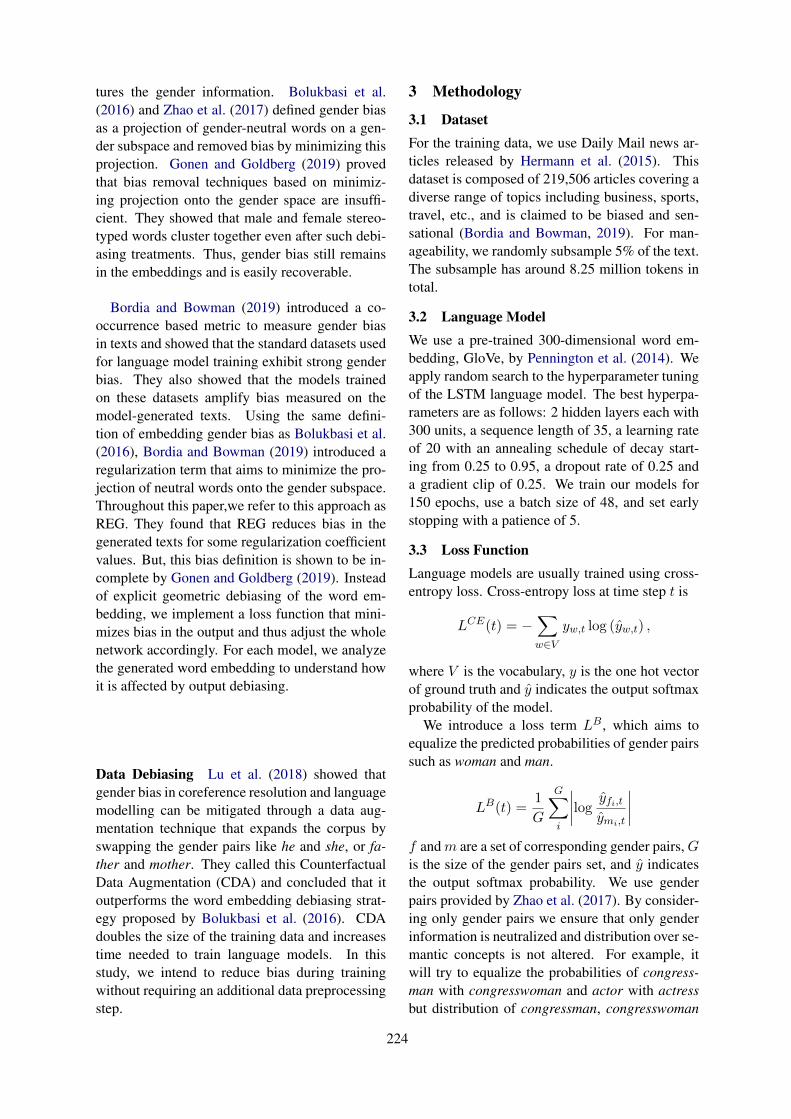
tures the gender information. Bolukbasi et al.(2016) and Zhao et al. (2017) defined gender biasas a projection of gender-neutral words on a gen-der subspace and removed bias by minimizing thisprojection. Gonen and Goldberg (2019) provedthat bias removal techniques based on minimiz-ing projection onto the gender space are insuffi-cient. They showed that male and female stereo-typed words cluster together even after such debi-asing treatments. Thus, gender bias still remainsin the embeddings and is easily recoverable.

Bordia and Bowman (2019) introduced a co-occurrence based metric to measure gender biasin texts and showed that the standard datasets usedfor language model training exhibit strong genderbias. They also showed that the models trainedon these datasets amplify bias measured on themodel-generated texts. Using the same defini-tion of embedding gender bias as Bolukbasi et al.(2016), Bordia and Bowman (2019) introduced aregularization term that aims to minimize the pro-jection of neutral words onto the gender subspace.Throughout this paper,we refer to this approach asREG. They found that REG reduces bias in thegenerated texts for some regularization coefficientvalues. But, this bias definition is shown to be in-complete by Gonen and Goldberg (2019). Insteadof explicit geometric debiasing of the word em-bedding, we implement a loss function that mini-mizes bias in the output and thus adjust the wholenetwork accordingly. For each model, we analyzethe generated word embedding to understand howit is affected by output debiasing.

Data Debiasing Lu et al. (2018) showed thatgender bias in coreference resolution and languagemodelling can be mitigated through a data aug-mentation technique that expands the corpus byswapping the gender pairs like he and she, or fa-ther and mother. They called this CounterfactualData Augmentation (CDA) and concluded that itoutperforms the word embedding debiasing strat-egy proposed by Bolukbasi et al. (2016). CDAdoubles the size of the training data and increasestime needed to train language models. In thisstudy, we intend to reduce bias during trainingwithout requiring an additional data preprocessingstep.

3 Methodology

3.1 DatasetFor the training data, we use Daily Mail news ar-ticles released by Hermann et al. (2015). Thisdataset is composed of 219,506 articles covering adiverse range of topics including business, sports,travel, etc., and is claimed to be biased and sen-sational (Bordia and Bowman, 2019). For man-ageability, we randomly subsample 5% of the text.The subsample has around 8.25 million tokens intotal.

3.2 Language ModelWe use a pre-trained 300-dimensional word em-bedding, GloVe, by Pennington et al. (2014). Weapply random search to the hyperparameter tuningof the LSTM language model. The best hyperpa-rameters are as follows: 2 hidden layers each with300 units, a sequence length of 35, a learning rateof 20 with an annealing schedule of decay start-ing from 0.25 to 0.95, a dropout rate of 0.25 anda gradient clip of 0.25. We train our models for150 epochs, use a batch size of 48, and set earlystopping with a patience of 5.

3.3 Loss FunctionLanguage models are usually trained using cross-entropy loss. Cross-entropy loss at time step t is

LCE(t) = −∑

w∈Vyw,t log (yw,t) ,

where V is the vocabulary, y is the one hot vectorof ground truth and y indicates the output softmaxprobability of the model.

We introduce a loss term LB , which aims toequalize the predicted probabilities of gender pairssuch as woman and man.

LB(t) =1

G

G∑

i

∣∣∣∣logyfi,tymi,t

∣∣∣∣

f andm are a set of corresponding gender pairs,Gis the size of the gender pairs set, and y indicatesthe output softmax probability. We use genderpairs provided by Zhao et al. (2017). By consider-ing only gender pairs we ensure that only genderinformation is neutralized and distribution over se-mantic concepts is not altered. For example, itwill try to equalize the probabilities of congress-man with congresswoman and actor with actressbut distribution of congressman, congresswoman

224

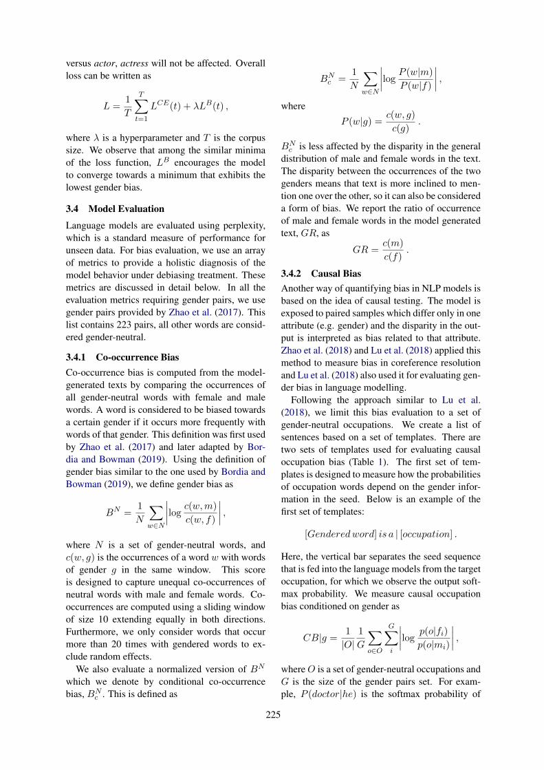
versus actor, actress will not be affected. Overallloss can be written as

L =1

T

T∑

t=1

LCE(t) + λLB(t) ,

where λ is a hyperparameter and T is the corpussize. We observe that among the similar minimaof the loss function, LB encourages the modelto converge towards a minimum that exhibits thelowest gender bias.

3.4 Model Evaluation

Language models are evaluated using perplexity,which is a standard measure of performance forunseen data. For bias evaluation, we use an arrayof metrics to provide a holistic diagnosis of themodel behavior under debiasing treatment. Thesemetrics are discussed in detail below. In all theevaluation metrics requiring gender pairs, we usegender pairs provided by Zhao et al. (2017). Thislist contains 223 pairs, all other words are consid-ered gender-neutral.

3.4.1 Co-occurrence BiasCo-occurrence bias is computed from the model-generated texts by comparing the occurrences ofall gender-neutral words with female and malewords. A word is considered to be biased towardsa certain gender if it occurs more frequently withwords of that gender. This definition was first usedby Zhao et al. (2017) and later adapted by Bor-dia and Bowman (2019). Using the definition ofgender bias similar to the one used by Bordia andBowman (2019), we define gender bias as

BN =1

N

∑

w∈N

∣∣∣∣logc(w,m)

c(w, f)

∣∣∣∣ ,

where N is a set of gender-neutral words, andc(w, g) is the occurrences of a word w with wordsof gender g in the same window. This scoreis designed to capture unequal co-occurrences ofneutral words with male and female words. Co-occurrences are computed using a sliding windowof size 10 extending equally in both directions.Furthermore, we only consider words that occurmore than 20 times with gendered words to ex-clude random effects.

We also evaluate a normalized version of BN

which we denote by conditional co-occurrencebias, BN

c . This is defined as

BNc =

1

N

∑

w∈N

∣∣∣∣logP (w|m)

P (w|f)

∣∣∣∣ ,

where

P (w|g) = c(w, g)

c(g).

BNc is less affected by the disparity in the general

distribution of male and female words in the text.The disparity between the occurrences of the twogenders means that text is more inclined to men-tion one over the other, so it can also be considereda form of bias. We report the ratio of occurrenceof male and female words in the model generatedtext, GR, as

GR =c(m)

c(f).

3.4.2 Causal BiasAnother way of quantifying bias in NLP models isbased on the idea of causal testing. The model isexposed to paired samples which differ only in oneattribute (e.g. gender) and the disparity in the out-put is interpreted as bias related to that attribute.Zhao et al. (2018) and Lu et al. (2018) applied thismethod to measure bias in coreference resolutionand Lu et al. (2018) also used it for evaluating gen-der bias in language modelling.

Following the approach similar to Lu et al.(2018), we limit this bias evaluation to a set ofgender-neutral occupations. We create a list ofsentences based on a set of templates. There aretwo sets of templates used for evaluating causaloccupation bias (Table 1). The first set of tem-plates is designed to measure how the probabilitiesof occupation words depend on the gender infor-mation in the seed. Below is an example of thefirst set of templates:

[Genderedword] is a | [occupation] .

Here, the vertical bar separates the seed sequencethat is fed into the language models from the targetoccupation, for which we observe the output soft-max probability. We measure causal occupationbias conditioned on gender as

CB|g =1

|O|1

G

∑

o∈O

G∑

i

∣∣∣∣logp(o|fi)p(o|mi)

∣∣∣∣ ,

whereO is a set of gender-neutral occupations andG is the size of the gender pairs set. For exam-ple, P (doctor|he) is the softmax probability of

225

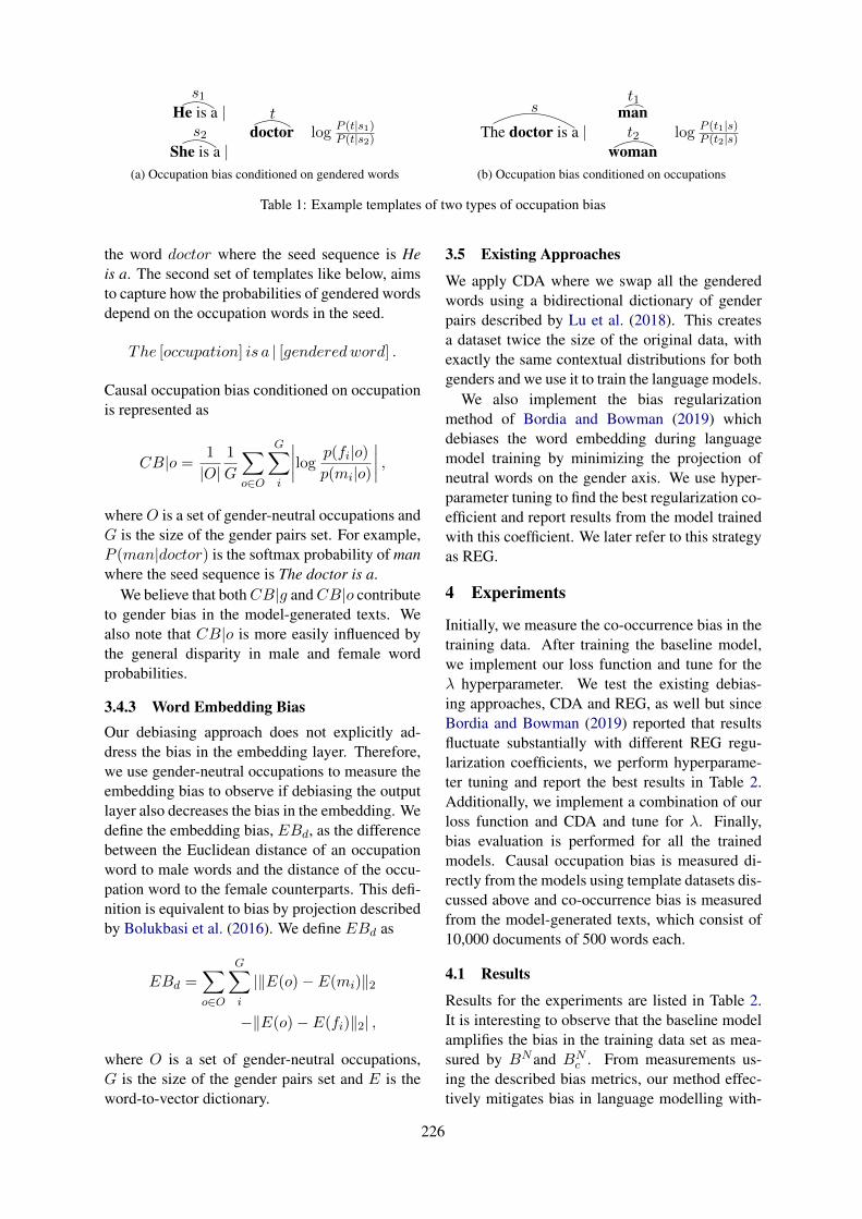
He is a |doctor log P (t|s1)

P (t|s2)She is a |

s1

s2

t

(a) Occupation bias conditioned on gendered words

The doctor is a |man

log P (t1|s)P (t2|s)

woman

st1

t2

(b) Occupation bias conditioned on occupations

Table 1: Example templates of two types of occupation bias

the word doctor where the seed sequence is Heis a. The second set of templates like below, aimsto capture how the probabilities of gendered wordsdepend on the occupation words in the seed.

The [occupation] is a | [genderedword] .

Causal occupation bias conditioned on occupationis represented as

CB|o = 1

|O|1

G

∑

o∈O

G∑

i

∣∣∣∣logp(fi|o)p(mi|o)

∣∣∣∣ ,

whereO is a set of gender-neutral occupations andG is the size of the gender pairs set. For example,P (man|doctor) is the softmax probability of manwhere the seed sequence is The doctor is a.

We believe that bothCB|g andCB|o contributeto gender bias in the model-generated texts. Wealso note that CB|o is more easily influenced bythe general disparity in male and female wordprobabilities.

3.4.3 Word Embedding BiasOur debiasing approach does not explicitly ad-dress the bias in the embedding layer. Therefore,we use gender-neutral occupations to measure theembedding bias to observe if debiasing the outputlayer also decreases the bias in the embedding. Wedefine the embedding bias, EBd, as the differencebetween the Euclidean distance of an occupationword to male words and the distance of the occu-pation word to the female counterparts. This defi-nition is equivalent to bias by projection describedby Bolukbasi et al. (2016). We define EBd as

EBd =∑

o∈O

G∑

i

|‖E(o)− E(mi)‖2

−‖E(o)− E(fi)‖2| ,

where O is a set of gender-neutral occupations,G is the size of the gender pairs set and E is theword-to-vector dictionary.

3.5 Existing Approaches

We apply CDA where we swap all the genderedwords using a bidirectional dictionary of genderpairs described by Lu et al. (2018). This createsa dataset twice the size of the original data, withexactly the same contextual distributions for bothgenders and we use it to train the language models.

We also implement the bias regularizationmethod of Bordia and Bowman (2019) whichdebiases the word embedding during languagemodel training by minimizing the projection ofneutral words on the gender axis. We use hyper-parameter tuning to find the best regularization co-efficient and report results from the model trainedwith this coefficient. We later refer to this strategyas REG.

4 Experiments

Initially, we measure the co-occurrence bias in thetraining data. After training the baseline model,we implement our loss function and tune for theλ hyperparameter. We test the existing debias-ing approaches, CDA and REG, as well but sinceBordia and Bowman (2019) reported that resultsfluctuate substantially with different REG regu-larization coefficients, we perform hyperparame-ter tuning and report the best results in Table 2.Additionally, we implement a combination of ourloss function and CDA and tune for λ. Finally,bias evaluation is performed for all the trainedmodels. Causal occupation bias is measured di-rectly from the models using template datasets dis-cussed above and co-occurrence bias is measuredfrom the model-generated texts, which consist of10,000 documents of 500 words each.

4.1 Results

Results for the experiments are listed in Table 2.It is interesting to observe that the baseline modelamplifies the bias in the training data set as mea-sured by BNand BN

c . From measurements us-ing the described bias metrics, our method effec-tively mitigates bias in language modelling with-

226

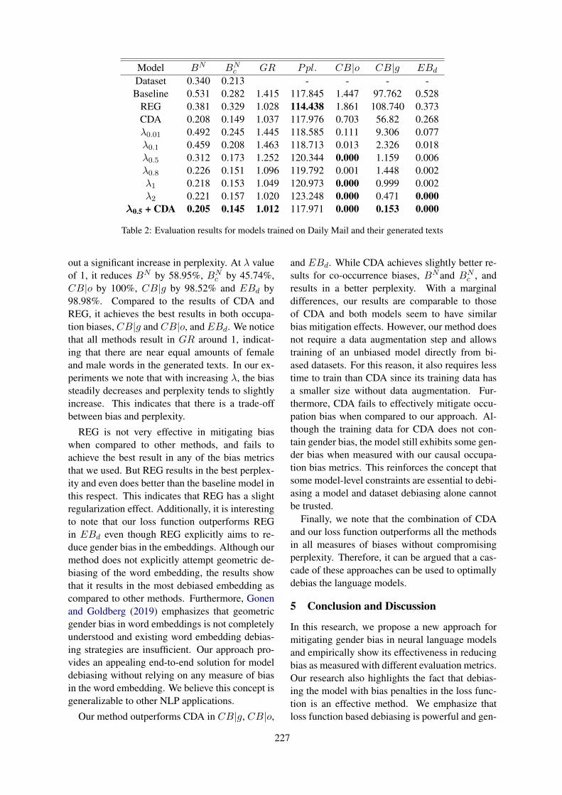
Model BN BNc GR Ppl. CB|o CB|g EBd

Dataset 0.340 0.213 - - - -Baseline 0.531 0.282 1.415 117.845 1.447 97.762 0.528

REG 0.381 0.329 1.028 114.438 1.861 108.740 0.373CDA 0.208 0.149 1.037 117.976 0.703 56.82 0.268λ0.01 0.492 0.245 1.445 118.585 0.111 9.306 0.077λ0.1 0.459 0.208 1.463 118.713 0.013 2.326 0.018λ0.5 0.312 0.173 1.252 120.344 0.000 1.159 0.006λ0.8 0.226 0.151 1.096 119.792 0.001 1.448 0.002λ1 0.218 0.153 1.049 120.973 0.000 0.999 0.002λ2 0.221 0.157 1.020 123.248 0.000 0.471 0.000

λ0.5 + CDA 0.205 0.145 1.012 117.971 0.000 0.153 0.000

Table 2: Evaluation results for models trained on Daily Mail and their generated texts

out a significant increase in perplexity. At λ valueof 1, it reduces BN by 58.95%, BN

c by 45.74%,CB|o by 100%, CB|g by 98.52% and EBd by98.98%. Compared to the results of CDA andREG, it achieves the best results in both occupa-tion biases, CB|g and CB|o, and EBd. We noticethat all methods result in GR around 1, indicat-ing that there are near equal amounts of femaleand male words in the generated texts. In our ex-periments we note that with increasing λ, the biassteadily decreases and perplexity tends to slightlyincrease. This indicates that there is a trade-offbetween bias and perplexity.

REG is not very effective in mitigating biaswhen compared to other methods, and fails toachieve the best result in any of the bias metricsthat we used. But REG results in the best perplex-ity and even does better than the baseline model inthis respect. This indicates that REG has a slightregularization effect. Additionally, it is interestingto note that our loss function outperforms REGin EBd even though REG explicitly aims to re-duce gender bias in the embeddings. Although ourmethod does not explicitly attempt geometric de-biasing of the word embedding, the results showthat it results in the most debiased embedding ascompared to other methods. Furthermore, Gonenand Goldberg (2019) emphasizes that geometricgender bias in word embeddings is not completelyunderstood and existing word embedding debias-ing strategies are insufficient. Our approach pro-vides an appealing end-to-end solution for modeldebiasing without relying on any measure of biasin the word embedding. We believe this concept isgeneralizable to other NLP applications.

Our method outperforms CDA in CB|g, CB|o,

and EBd. While CDA achieves slightly better re-sults for co-occurrence biases, BNand BN

c , andresults in a better perplexity. With a marginaldifferences, our results are comparable to thoseof CDA and both models seem to have similarbias mitigation effects. However, our method doesnot require a data augmentation step and allowstraining of an unbiased model directly from bi-ased datasets. For this reason, it also requires lesstime to train than CDA since its training data hasa smaller size without data augmentation. Fur-thermore, CDA fails to effectively mitigate occu-pation bias when compared to our approach. Al-though the training data for CDA does not con-tain gender bias, the model still exhibits some gen-der bias when measured with our causal occupa-tion bias metrics. This reinforces the concept thatsome model-level constraints are essential to debi-asing a model and dataset debiasing alone cannotbe trusted.

Finally, we note that the combination of CDAand our loss function outperforms all the methodsin all measures of biases without compromisingperplexity. Therefore, it can be argued that a cas-cade of these approaches can be used to optimallydebias the language models.

5 Conclusion and Discussion

In this research, we propose a new approach formitigating gender bias in neural language modelsand empirically show its effectiveness in reducingbias as measured with different evaluation metrics.Our research also highlights the fact that debias-ing the model with bias penalties in the loss func-tion is an effective method. We emphasize thatloss function based debiasing is powerful and gen-

227

eralizable to other downstream NLP applications.The research also reinforces the idea that geomet-ric debiasing of the word embedding is not a com-plete solution for debiasing the downstream appli-cations but encourages end-to-end approaches todebiasing.

All the debiasing techniques experimented inthis paper rely on a predefined set of gender pairsin some way. CDA used gender pairs for flipping,REG uses it for gender space definition and ourtechnique uses them for computing loss. This re-liance on pre-defined set of gender pairs can beconsidered a limitation of these methods. It alsoresults in another concern. There are gender asso-ciated words which do not have pairs, like preg-nant. These words are not treated properly bytechniques relying on gender pairs.

Future work includes designing a context-awareversion of our loss function which can distinguishbetween the unbiased and biased mentions of thegendered words and only penalize the biased ver-sion. Another interesting direction is exploring theapplication of this method in mitigating racial biaswhich brings more challenges.

6 Acknowledgment

We are grateful to Sam Bowman for helpful ad-vice, Shikha Bordia, Cuiying Yang, Gang Qian,Xiyu Miao, Qianyi Fan, Tian Liu, and StanislavSobolevsky for discussions, and reviewers for de-tailed feedback.

ReferencesTolga Bolukbasi, Kai-Wei Chang, James Zou,

Venkatesh Saligrama, and Adam Kalai. 2016. Manis to computer programmer as woman is to home-maker? debiasing word embeddings. In NIPS’16Proceedings of the 30th International Conferenceon Neural Information Processing Systems, pages4356–4364.

Shikha Bordia and Samuel R. Bowman. 2019. Iden-tifying and reducing gender bias in word-level lan-guage models. ArXiv:1904.03035.

Hila Gonen and Yoav Goldberg. 2019. Lipstick on apig: Debiasing methods cover up systematic genderbiases in word embeddings but do not remove them.ArXiv:1903.03862.

Karl Hermann, Tom Koisk, Edward Grefenstette, LasseEspeholt, Will Kay, Mustafa Suleyman, and PhilBlunsom. 2015. Teaching machines to read andcomprehend. In NIPS’15 Proceedings of the 28th

International Conference on Neural InformationProcessing Systems, pages 1693–1701.

Anja Lambrecht and Catherine E. Tucker. 2018. Al-gorithmic bias? an empirical study into apparentgender-based discrimination in the display of stemcareer ads.

Issie Lapowsky. 2018. Google autocomplete stillmakes vile suggestions.

Kaiji Lu, Piotr Mardziel, Fangjing Wu, PreetamAmancharla, and Anupam Datta. 2018. Gen-der bias in neural natural language processing.ArXiv:1807.11714v1.

Jeffrey Pennington, Richard Socher, and ChristopherManning. 2014. Glove: Global vectors for wordrepresentation. In Proceedings of the 2014 Con-ference on Empirical Methods in Natural LanguageProcessing, pages 1532–1543. Association for Com-putational Linguistics.

Ilya Sutskever, James Martens, and Geoffrey Hinton.2011. Generating text with recurrent neural net-works. In ICML’11 Proceedings of the 28th Inter-national Conference on International Conference onMachine Learning, pages 1017–1024.

Jieyu Zhao, Tianlu Wang, Mark Yatskar, Vicente Or-donez, and Kai-Wei Chag. 2017. Men also likeshopping: Reducing gender bias amplification usingcorpus-level constraints. In Conference on Empiri-cal Methods in Natural Language Processing.

Jieyu Zhao, Yichao Zhou, Zeyu Li, Wei Wang, andChang Kaiwei. 2018. Learning gender-neutral wordembeddings. In Proceedings of the 2018 Confer-ence on Empirical Methods in Natural LanguageProcessing, pages 4847–4853. Association for Com-putational Linguistics.

228

Proceedings of the 57th Annual Meeting of the Association for Computational Linguistics: Student Research Workshop, pages 229–235Florence, Italy, July 28 - August 2, 2019. c©2019 Association for Computational Linguistics

Automatic Generation of Personalized Comment Based on User Profile

Wenhuan Zeng1∗, Abulikemu Abuduweili2∗, Lei Li3, Pengcheng Yang4

1School of Mathematical Sciences, Peking University2State Key Lab of Advanced Optical Communication System and Networks,

School of EECS, Peking University3School of Computer Science and Technology, Xidian University

4MOE Key Lab of Computational Linguistics, School of EECS, Peking Universityzengwenhuan, abduwali@pku.edu.cn

tobiaslee@foxmail.com, yang pc@pku.edu.cn

Abstract

Comments on social media are very diverse, interms of content, style and vocabulary, whichmake generating comments much more chal-lenging than other existing natural languagegeneration (NLG) tasks. Besides, since dif-ferent user has different expression habits, itis necessary to take the user’s profile into con-sideration when generating comments. In thispaper, we introduce the task of automatic gen-eration of personalized comment (AGPC) forsocial media. Based on tens of thousands ofusers’ real comments and corresponding userprofiles on weibo, we propose PersonalizedComment Generation Network (PCGN) forAGPC. The model utilizes user feature embed-ding with a gated memory and attends to userdescription to model personality of users. Inaddition, external user representation is takeninto consideration during the decoding to en-hance the comments generation. Experimentalresults show that our model can generate natu-ral, human-like and personalized comments.1

1 Introduction

Nowadays, social media is gradually becoming amainstream communication tool. People tend toshare their ideas with others by commenting, re-posting or clicking like on posts in social media.Among these behaviors, comment plays a signif-icant role in the communication between postersand readers. Automatically generate personalizedcomments (AGPC) can be useful due to the fol-lowing reasons. First, AGPC helps readers expresstheir ideas more easily, thus make them engagemore actively in the platform. Second, bloggerscan capture different attitudes to the event frommultiple users with diverse backgrounds. Lastly,

∗Equal Contribution.1Source codes of this paper are available at

https://github.com/Walleclipse/AGPC

the platform can also benefit from the increasinginteractive rate.

Despite its great applicability, the AGPC taskfaces two important problems: whether can weachieve it and how to implement it? The SocialDifferentiation Theory proposed by Riley and Ri-ley (1959) proved the feasibility of building a uni-versal model to automatically generate personal-ized comments based on part of users’ data. TheIndividual Differences Theory pointed by Hovlandet al. (1953) answers the second question by in-troducing the significance of users’ background,which inspires us to incorporating user profileinto comments generation process. More specifi-cally, the user profile consists of demographic fea-tures (for example, where does the user live), in-dividual description and the common word dic-tionary extracted from user’s comment history.There are few works exploring the comments gen-eration problem. Zheng et al. (2017) first paidattention to generating comments for news arti-cles by proposing a gated attention neural net-work model (GANN) to address the contextual rel-evance and the diversity of comments. Similarly,Qin et al. (2018) introduced the task of automaticnews article commenting and released a large scaleChinese corpus. Nevertheless, AGPC is a morechallenging task, since it not only requires gener-ating relevant comments given the blog text, butalso needs the consideration of the diverse users’background.

In this paper, we propose a novel task, automat-ically generating personalized comment based onuser profile. We build the bridge between userprofiles and social media comments based on alarge-scale and high-quality Chinese dataset. Weelaborately design a generative model based onsequence-to-sequence (Seq2Seq) framework. Agated memory module is utilized to model the userpersonality. Besides, during the decoding process,

229

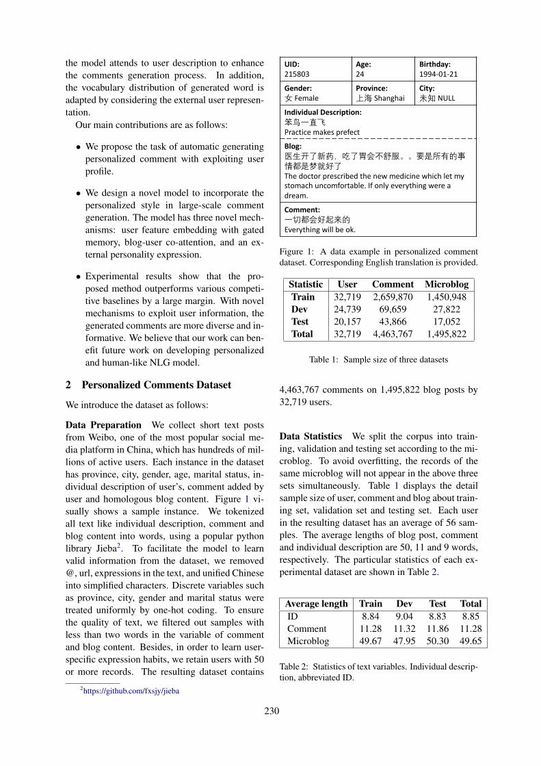
the model attends to user description to enhancethe comments generation process. In addition,the vocabulary distribution of generated word isadapted by considering the external user represen-tation.

Our main contributions are as follows:

• We propose the task of automatic generatingpersonalized comment with exploiting userprofile.

• We design a novel model to incorporate thepersonalized style in large-scale commentgeneration. The model has three novel mech-anisms: user feature embedding with gatedmemory, blog-user co-attention, and an ex-ternal personality expression.

• Experimental results show that the pro-posed method outperforms various competi-tive baselines by a large margin. With novelmechanisms to exploit user information, thegenerated comments are more diverse and in-formative. We believe that our work can ben-efit future work on developing personalizedand human-like NLG model.

2 Personalized Comments Dataset

We introduce the dataset as follows:

Data Preparation We collect short text postsfrom Weibo, one of the most popular social me-dia platform in China, which has hundreds of mil-lions of active users. Each instance in the datasethas province, city, gender, age, marital status, in-dividual description of user’s, comment added byuser and homologous blog content. Figure 1 vi-sually shows a sample instance. We tokenizedall text like individual description, comment andblog content into words, using a popular pythonlibrary Jieba2. To facilitate the model to learnvalid information from the dataset, we removed@, url, expressions in the text, and unified Chineseinto simplified characters. Discrete variables suchas province, city, gender and marital status weretreated uniformly by one-hot coding. To ensurethe quality of text, we filtered out samples withless than two words in the variable of commentand blog content. Besides, in order to learn user-specific expression habits, we retain users with 50or more records. The resulting dataset contains

2https://github.com/fxsjy/jieba

UID:215803

Age:24

Birthday:1994-01-21

Gender: Female

Province: Shanghai

City: NULL

Individual Description:%$Practice makes prefect

Blog: &!# The doctor prescribed the new medicine which let mystomach uncomfortable. If only everything were a dream.

Comment:#"Everything will be ok.

Figure 1: A data example in personalized commentdataset. Corresponding English translation is provided.

Statistic User Comment MicroblogTrain 32,719 2,659,870 1,450,948Dev 24,739 69,659 27,822Test 20,157 43,866 17,052Total 32,719 4,463,767 1,495,822

Table 1: Sample size of three datasets

4,463,767 comments on 1,495,822 blog posts by32,719 users.

Data Statistics We split the corpus into train-ing, validation and testing set according to the mi-croblog. To avoid overfitting, the records of thesame microblog will not appear in the above threesets simultaneously. Table 1 displays the detailsample size of user, comment and blog about train-ing set, validation set and testing set. Each userin the resulting dataset has an average of 56 sam-ples. The average lengths of blog post, commentand individual description are 50, 11 and 9 words,respectively. The particular statistics of each ex-perimental dataset are shown in Table 2.

Average length Train Dev Test TotalID 8.84 9.04 8.83 8.85Comment 11.28 11.32 11.86 11.28Microblog 49.67 47.95 50.30 49.65

Table 2: Statistics of text variables. Individual descrip-tion, abbreviated ID.

230

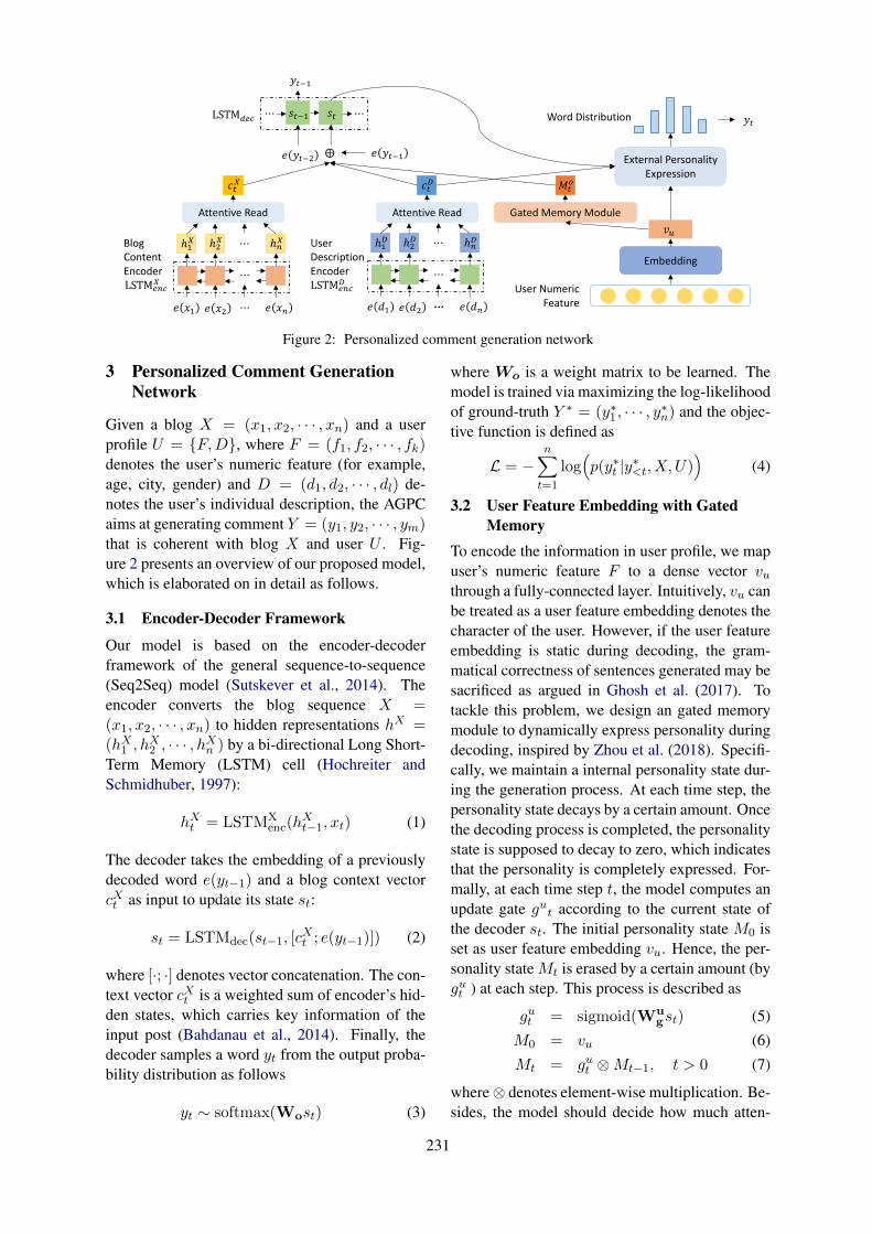
User NumericFeature

Embedding

:;BlogContentEncoderLSTM%&'(

ℎ*( ℎ+( ℎ&(

, -* , -+ , -&⋯

⋯

⋯

Attentive Read

/0( /01

UserDescriptionEncoderLSTM%&'1

ℎ*1 ℎ+1 ℎ&1

⋯

⋯

⋯

Attentive Read

, 2* , 2+ , 2&⋯

Gated Memory Module

304

506* 50 ⋯⋯

, 706+ , 706*

706*

LSTM8%'

⨁ External Personality Expression

Word Distribution 70

Figure 2: Personalized comment generation network

3 Personalized Comment GenerationNetwork

Given a blog X = (x1, x2, · · · , xn) and a userprofile U = F,D, where F = (f1, f2, · · · , fk)denotes the user’s numeric feature (for example,age, city, gender) and D = (d1, d2, · · · , dl) de-notes the user’s individual description, the AGPCaims at generating comment Y = (y1, y2, · · · , ym)that is coherent with blog X and user U . Fig-ure 2 presents an overview of our proposed model,which is elaborated on in detail as follows.

3.1 Encoder-Decoder Framework

Our model is based on the encoder-decoderframework of the general sequence-to-sequence(Seq2Seq) model (Sutskever et al., 2014). Theencoder converts the blog sequence X =(x1, x2, · · · , xn) to hidden representations hX =(hX1 , h

X2 , · · · , hXn ) by a bi-directional Long Short-

Term Memory (LSTM) cell (Hochreiter andSchmidhuber, 1997):

hXt = LSTMXenc(h

Xt−1, xt) (1)

The decoder takes the embedding of a previouslydecoded word e(yt−1) and a blog context vectorcXt as input to update its state st:

st = LSTMdec(st−1, [cXt ; e(yt−1)]) (2)

where [·; ·] denotes vector concatenation. The con-text vector cXt is a weighted sum of encoder’s hid-den states, which carries key information of theinput post (Bahdanau et al., 2014). Finally, thedecoder samples a word yt from the output proba-bility distribution as follows

yt ∼ softmax(Wost) (3)

where Wo is a weight matrix to be learned. Themodel is trained via maximizing the log-likelihoodof ground-truth Y ∗ = (y∗1, · · · , y∗n) and the objec-tive function is defined as

L = −n∑

t=1

log(p(y∗t |y∗<t, X, U)

)(4)

3.2 User Feature Embedding with GatedMemory

To encode the information in user profile, we mapuser’s numeric feature F to a dense vector vuthrough a fully-connected layer. Intuitively, vu canbe treated as a user feature embedding denotes thecharacter of the user. However, if the user featureembedding is static during decoding, the gram-matical correctness of sentences generated may besacrificed as argued in Ghosh et al. (2017). Totackle this problem, we design an gated memorymodule to dynamically express personality duringdecoding, inspired by Zhou et al. (2018). Specifi-cally, we maintain a internal personality state dur-ing the generation process. At each time step, thepersonality state decays by a certain amount. Oncethe decoding process is completed, the personalitystate is supposed to decay to zero, which indicatesthat the personality is completely expressed. For-mally, at each time step t, the model computes anupdate gate gut according to the current state ofthe decoder st. The initial personality state M0 isset as user feature embedding vu. Hence, the per-sonality stateMt is erased by a certain amount (bygut ) at each step. This process is described as

gut = sigmoid(Wugst) (5)

M0 = vu (6)

Mt = gut ⊗Mt−1, t > 0 (7)

where⊗ denotes element-wise multiplication. Be-sides, the model should decide how much atten-

231

tion should be paid to the personality state at eachtime step. Thus, output gate got is introduced tocontrol the information flow by considering theprevious decoder state st−1, previous target worde(yt−1) and the current context vector cXt

got = sigmoid(Wog[st−1; e(yt−1); c

Xt ]). (8)

By an element-wise multiplication of got and Mt,we can obtain adequate personality informationMo

t for current decoding step

Mot = got ⊗Mt. (9)

3.3 Blog-User Co-Attention

Individual description is another important infor-mation source when generating personalized com-ments. For example, a user with individual de-scription “只爱朱一龙” (I only love Yilong Zhu3),tends to writes a positive and adoring commentson the microblog related to Zhu. Motivated bythis, we propose Blog-user co-attention to modelthe interactions between user description and blogcontent. More specifically, we encode the user’sindividual descriptionD = (d1, d2, · · · , dl) to hid-den states (hD1 , h

D2 , · · · , hDl ) via another LSTM

hDt = LSTMDenc(h

Dt−1, dt) (10)

We can obtain a description context vector cDt byattentively reading the hidden states of user de-scription,

cDt =∑

j

αtjhDj (11)

αtj = softmax(etj) (12)

etj = st−1WahDj (13)

where etj is a alignment score (Bahdanau et al.,2014). Similarly, we can get the blog content vec-tor cXt . Finally, the context vector ct is a concate-nation of cXt and cDt , in order provide more com-prehensive information of user’s personality

ct = [cXt ; cDt ] (14)

Therefore, the state update mechanism in Eq.(2) ismodified to

st = LSTMdec(st−1, [ct; e(yt−1);Mot ]) (15)

3A famous Chinese star.

3.4 External Personality Expression

In the gated memory module, the correlation be-tween the change of the internal personality stateand selection of a word is implicit. To fully ex-ploit the user information when selecting wordsfor generation, we first compute a user representa-tion rut with user feature embedding and user de-scription context.

rut = Wr[vu; cDt ] (16)

where Wr is a weight matrix to align user repre-sentation dimention.

The final word is then sampled from output dis-tribution based on the concatenation of decoderstate st and rut as

yt ∼ softmax(Wot [st; rut ]) (17)

where Wot is a learnable weight matrix.

4 Experiments

4.1 Implementation

The blog content encoder and comment decoderare both 2-layer bi-LSTM with 512 hidden unitsfor each layer. The user’s personality descriptionencoder is a single layer bi-LSTM with 200 hiddenunits. The word embedding size is set to 300 andvocabulary size is set to 40,000. The embeddingsize of user’s numeric feature is set to 100.

We adopted beam search and set beam size to 10to promote diversity of generated comments. Weused SGD optimizer with batch size set to 128 andthe learning rate is 0.001.

To further enrich the information provided byuser description, we collected most common kwords in user historical comments (k = 20 in ourexperiment). We concatenate the common wordswith the user individual description. Therefore,we can obtain more information about users’ ex-pression style. The model using concatenated userdescription is named PCGN with common words(PCGN+ComWord).

4.2 Baseline

We implemented a general Seq2Seq model(Sutskever et al., 2014) and a user embeddingmodel (Seq2Seq+Emb) proposed by Li et al.(2016) as our baselines. The latter model embedsuser numeric features into a dense vector and feedsit as extra input into decoder at every time step.

232

Method PPL B-2 METEOR

Seq2Seq 32.47 0.071 0.070Seq2Seq+Emb 31.13 0.084 0.079

PCGN 27.94 0.162 0.132PCGN+ComWord 24.48 0.193 0.151

Table 3: Automatic evaluation results of differentmethods. PPL denotes perplexity and B-2 denotesBLEU-2. Best results are shown in bold.

Method PPL B-2

Seq2Seq 32.47 0.071+ Mem 30.73 (-1.74) 0.099 (+0.028)+ CoAtt 27.12 (-3.61) 0.147 (+0.078)+ External 27.94 (+0.82) 0.162 (+0.015)

Table 4: Incremental experiment results of proposedmodel. Performance on METEOR is similar to B-2.Mem denotes gated memory, CoAtt denotes blog-userco-attention and External denotes external personalityexpression

4.3 Evaluation Result

Metrics: We use BLEU-2 (Papineni et al.,2002) and METEOR (Banerjee and Lavie, 2005)to evaluate overlap between outputs and refer-ences. Besides, perplexity is also provided.

Results: The results are shown in Table 3.As can be seen, PCGN model with commonwords obtains the best performance on perplex-ity, BLEU-2 and METEOR. Note that the per-formance of Seq2Seq is extremely low, since theuser profile is not taken into consideration duringthe generation, resulting repetitive responses. Incontrast, with the help of three proposed mecha-nism (gated memory, blog-user co-attention andexternal personality expression), our model canutilize user information effectively, thus is capableof generating diverse and relevant comments forthe same blog. Further, we conducted incrementalexperiments to study the effect of proposed mech-anisms by adding them incrementally, as shown inTable 4. It can be found that all three mechanismhelp generate more diverse comments, while blog-user co-attention mechanism contributes most im-provements. An interesting finding is that externalpersonality expression mechanism causes the de-cay on perplexity. We speculate that the modifica-tion on word distribution by personality influencethe fluency of generated comments.

5 Related Work

This paper focuses on comments generation task,which can be further divided into generating acomment according to the structure data (Meiet al., 2015), text data (Qin et al., 2018), im-age (Vinyal et al., 2015) and video (Ma et al.,2018a), separately.

There are many works exploring the problemof text-based comment generation. Qin et al.(2018) contributed a high-quality corpus for ar-ticle comment generation problem. Zheng et al.(2017) proposed a gated attention neural networkmodel (GANN) to generate comments for newsarticle, which addressed the contextual relevanceand the diversity of comments. To alleviate thedependence on large parallel corpus, Ma et al.(2018b) designed an unsupervised neural topicmodel based on retrieval technique. However,these works focus on generating comments onnews text, while comments on social media aremuch more diverse and personal-specific.

In terms of the technique for modeling usercharacter, the existing works on machine com-menting only utilized part of users’ information.Ni and McAuley (2018) proposed to learn a latentrepresentation of users by utilizing history infor-mation. Lin et al. (2018) acquired readers’ gen-eral attitude to event mentioned by article throughits upvote count. Compared to the indirection in-formation obtained from history or indicator, userfeatures in user profile, like demographic factors,can provide more comprehensive and specific in-formation, and thus should be paid more attentionto when generating comments. Sharing the sameidea that user personality counts, Luo et al. (2018)proposed personalized MemN2N to explore per-sonalized goal-oriented dialog systems. Equippedwith a profile model to learn user representationand a preference model learning user preferences,the model is capable of generating high quality re-sponses. In this paper, we focus on modeling per-sonality in a different scenario, where the gener-ated comments is supposed to be general and di-verse.

6 Conclusion

In this paper, we introduce the task of auto-matic generating personalized comment. We alsopropose Personality Comment Generation Net-work (PCGN) to model the personality influencein comment generation. The PCGN model utilized

233

gated memory for user feature embedding, blog-user co-attention, and external personality repre-sentation to generate comments in personalizedstyle. Evaluation results show that PCGN outpe-forms baseline models by a large margin. With thehelp of three proposed mechanisms, the generatedcomments are more fluent and diverse.

ReferencesDzmitry Bahdanau, Kyunghyun Cho, and Yoshua Ben-

gio. 2014. Neural machine translation by jointlylearning to align and translate. arXiv preprintarXiv:1409.0473.

Satanjeev Banerjee and Alon Lavie. 2005. Meteor: Anautomatic metric for mt evaluation with improvedcorrelation with human judgments. In Proceedingsof the acl workshop on intrinsic and extrinsic evalu-ation measures for machine translation and/or sum-marization, pages 65–72.

Sayan Ghosh, Mathieu Chollet, Eugene Laksana,Louis-Philippe Morency, and Stefan Scherer. 2017.Affect-lm: A neural language model for customiz-able affective text generation. arXiv preprintarXiv:1704.06851.

Sepp Hochreiter and Jurgen Schmidhuber. 1997.Long short-term memory. Neural computation,9(8):1735–1780.

Carl I. Hovland, Irving L. Janis, and Harold H.Kelley. 1953. Communication and Persua-sion:Psychological Studies of Opinion Change.Yale University Press.

Jiwei Li, Michel Galley, Chris Brockett, Georgios PSpithourakis, Jianfeng Gao, and Bill Dolan. 2016.A persona-based neural conversation model. arXivpreprint arXiv:1603.06155.

Zhaojiang Lin, Genta Indra Winata, and Pascale Fung.2018. Learning comment generation by leveraginguser-generated data. CoRR, abs/1810.12264.

Liangchen Luo, Wenhao Huang, Qi Zeng, Zaiqing Nie,and Xu Sun. 2018. Learning personalized end-to-end goal-oriented dialog.

Shuming Ma, Lei Cui, Damai Dai, Furu Wei, andXu Sun. 2018a. Livebot: Generating live videocomments based on visual and textual contexts.CoRR, abs/1809.04938.

Shuming Ma, Lei Cui, Furu Wei, and Xu Sun.2018b. Unsupervised machine commenting withneural variational topic model. arXiv preprintarXiv:1809.04960.

Hongyuan Mei, Mohit Bansal, and Matthew R. Walter.2015. What to talk about and how? selective gen-eration using lstms with coarse-to-fine alignment.arXiv preprint arXiv:1509.00838.

Jianmo Ni and Julian McAuley. 2018. Personalized re-view generation by expanding phrases and attendingon aspect-aware representations. In In Proceedingsof the 56th Annual Meeting of the Association forComputational Linguistics, pages 706–711.

Kishore Papineni, Salim Roukos, Todd Ward, and Wei-Jing Zhu. 2002. Bleu: a method for automatic eval-uation of machine translation. In Proceedings ofthe 40th annual meeting on association for compu-tational linguistics, pages 311–318. Association forComputational Linguistics.

Lianhui Qin, Lemao Liu, Wei Bi, Yan Wang, XiaojiangLiu, Zhiting Hu, Hai Zhao, and Shuming Shi. 2018.Automatic article commenting: the task and dataset.In Proceedings of the 56th Annual Meeting of the As-sociation for Computational Linguistics, ACL 2018,Melbourne, Australia, July 15-20, 2018, Volume 2:Short Papers, pages 151–156.

J. W. Riley and Matilda White Riley. 1959. Mass com-munication and the social system.

Ilya Sutskever, Oriol Vinyals, and Quoc V Le. 2014.Sequence to sequence learning with neural net-works. In Advances in neural information process-ing systems, pages 3104–3112.

Oriol Vinyal, Alexander Toshev, Samy Bengio, andDumitru Erhan. 2015. Show and tell: A neural im-age caption generator. In Proceedings of the IEEEconference on computer vision and pattern recogni-tion, pages 3156–3164.

Hai-Tao Zheng, Wei Wang, Wang Chen, and Arun Ku-mar Sangaiah. 2017. Automatic generation of newscomments based on gated attention neural networks.6.

Hao Zhou, Minlie Huang, Tianyang Zhang, XiaoyanZhu, and Bing Liu. 2018. Emotional chatting ma-chine: Emotional conversation generation with in-ternal and external memory. In Thirty-Second AAAIConference on Artificial Intelligence.

A Case Study

We present some generated cases in Figure 4, 5.There are multiple users (corresponding profilesare shown in Figure 3) that are suitable for gen-erating comments. Seq2Seq generates same com-ments for the same blog, while PCGN can gen-erate personalized comment conditioned on givenuser. According to the user profile, U1 adores Yi-long Zhu very much. Therefore, U1 tends to ex-press her affection in comments when responsesto blogs related to Yilong Zhu. For users whoseindividual descriptions can not offer helpful infor-mation or there is missing value for individual de-scription, the PCGN model pays more attentionto numeric features and learns representation fromsimilar seen users.

234

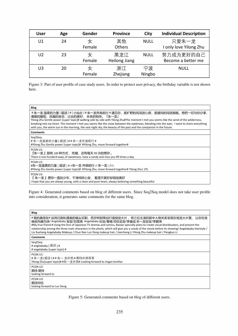
User Age Gender Province City Individual Description

U1 24 女Female

其他Others

NULL 只爱朱一龙I only love Yilong Zhu

U2 23 女Female

黑龙江Heilong Jiang

NULL 努力成为更好的自己Become a better me

U3 20 女Female

浙江Zhejiang

宁波Ningbo

NULL

Figure 3: Part of user profile of case study users. In order to protect user privacy, the birthday variable is not shownhere.

Blog# PLYx [ nm ] # [ 0+ ] # 4h # uiEwY~zr7=E\Yzr_9?OYF|Y'aoYg,JKY[Yilong Zhu Gentle power [super topic]# walking side by side with Yilong Zhu#The moment I met you seems like the wind of the wilderness, breaking into my heart. The moment I met you seems like the snow between the eyebrows, blending into the eyes. I want to share everything with you, the warm sun in the morning, the vast night sky, the beauty of the past and the companion in the future.

CommentsSeq2Seq:# *F3+7C [ A? ] # # *F:= ##Yilong Zhu Gentle power [super topic]# #Yilong Zhu, move forward together#

PCGN U1:G 100 `A5"dqGN) 99 MY9There is one hunderd ways of sweetness, have a candy and miss you 99 times a day.

PCGN U2:#PLYx OInm PI# J4h JI QINML#Yilong Zhu Gentle power [super topic]# #Yilong Zhu, move forward together# Yilong Zhu| ZYL

PCGN U3::Z-132fc7.]sg,[g,I hope that you are always young, with a clean and pure heart, always believing something beautiful

Figure 4: Generated comments based on blog of different users. Since Seq2Seq model does not take user profileinto consideration, it generates same comments for the same blog.

Blog# <Y^H #pWB$RXYy*Ub>tjk(S/ QYTe#V%jk(Svl%@C8! Angelababy!&/ Angelababy/D!/;!/#My true friend # Using the lens of Japanese TV dramas and comics, Bazaar specially plans to create visual blockbusters, and present the relationship among the three main characters in the photo, which will give you a sneak of the movie before its showing! Angelababy Hairstyle / Liu Xueliang Angelababy Makeup / Chun Nan Lun Deng makeup hair / Jiancheng Li Yilong Zhu makeup hair / Pengkun Li

CommentsSeq2Seq:# angelababy [ A? ] ## angelababy [super topic] #

PCGN U1:# *F[ A? ] # # *F4 # ) 4Yilong Zhu[super topic]# #*F4# Looking forward to Jingan brother

PCGN U2:I6I6looking forward to

PCGN U3:I6looking forward to Lun Deng

Figure 5: Generated comments based on blog of different users.

235

Proceedings of the 57th Annual Meeting of the Association for Computational Linguistics: Student Research Workshop, pages 236–242Florence, Italy, July 28 - August 2, 2019. c©2019 Association for Computational Linguistics

From Bilingual to Multilingual Neural Machine Translation byIncremental Training

Carlos Escolano, Marta R. Costa-jussa, Jose A. R. Fonollosa,carlos.escolano,marta.ruiz,jose.fonollosa@upc.edu

TALP Research CenterUniversitat Politecnica de Catalunya, Barcelona

Abstract

Multilingual Neural Machine Translation ap-proaches are based on the use of task-specificmodels and the addition of one more lan-guage can only be done by retraining thewhole system. In this work, we propose anew training schedule that allows the systemto scale to more languages without modifi-cation of the previous components based onjoint training and language-independent en-coder/decoder modules allowing for zero-shottranslation. This work in progress shows closeresults to the state-of-the-art in the WMT task.

1 Introduction

In recent years, neural machine translation (NMT)has had an important improvement in perfor-mance. Among the different neural architectures,most approaches are based in an encoder-decoderstructure and the use of attention-based mecha-nisms (Cho et al., 2014; Bahdanau et al., 2014;Vaswani et al., 2017). The main objective is com-puting a representation of the source sentence thatis weighted with attention-based mechanisms tocompute the conditional probability of the tokensof the target sentence and the previously decodedtarget tokens. Same principles have been success-fully applied to multilingual NMT, where the sys-tem is able to translate to and from several differ-ent languages.

Two main approaches have been proposedfor this task, language independent or sharedencoder-decoders. Language independent archi-tectures(Firat et al., 2016a,b; Schwenk and Douze,2017) in which each language has its own encoderand some additional mechanism is added to pro-duce shared representations, as averaging of thecontext vectors or sharing the attention mecha-nism. These architectures have the flexibility thateach language can be trained with its own vocab-

ulary all languages are trained in parallel. Re-cent work (Lu et al., 2018) show how to per-form many to many translations with indepen-dent encoders and decoders just by sharing ad-ditional language-specific layers that transformedthe language-specific representations into a sharedone without the need of a pivot language,

On the other hand, architectures that share pa-rameters between all languages (Johnson et al.,2017) by using a single encoder and decodertrained to be able to translate from and to anyof the languages of the system. This approachpresents the advantage that no further mechanismsare required to produced shared representation ofthe languages as they all share the same vocabu-lary and parameters, and by training all languageswithout distinction they allow low resources lan-guages to take benefit of other languages in thesystem improving their performance. Even thoughby sharing vocabulary between all languages thenumber of required tokens grows as more lan-guages are included in the system, especially whenlanguages employ different scripts in the system,such as Chinese or Russian. Recent work pro-poses a new approach to add new languages to asystem by adapting the vocabulary (Lakew et al.,2018), relying on the shared tokens between thelanguages to share model parameters, showingthat the amount of shared tokens between the lan-guages had an impact in the model performance.This could limit the capability of the system toadapt to languages with a different script.

These approaches can be further explored intounsupervised machine translation where the sys-tem learns to translate between languages withoutparallel data just by enforcing the generation andrepresentation of the tokens to be similar (Artetxeet al., 2017; Lample et al., 2018).

Also related to our method, recent work hasexplored transfer learning for NMT (Zoph et al.,

236

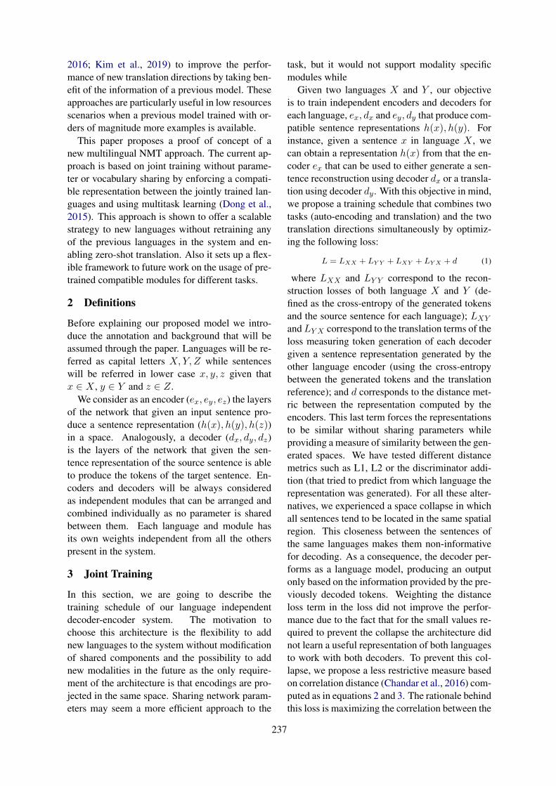
2016; Kim et al., 2019) to improve the perfor-mance of new translation directions by taking ben-efit of the information of a previous model. Theseapproaches are particularly useful in low resourcesscenarios when a previous model trained with or-ders of magnitude more examples is available.

This paper proposes a proof of concept of anew multilingual NMT approach. The current ap-proach is based on joint training without parame-ter or vocabulary sharing by enforcing a compati-ble representation between the jointly trained lan-guages and using multitask learning (Dong et al.,2015). This approach is shown to offer a scalablestrategy to new languages without retraining anyof the previous languages in the system and en-abling zero-shot translation. Also it sets up a flex-ible framework to future work on the usage of pre-trained compatible modules for different tasks.

2 Definitions

Before explaining our proposed model we intro-duce the annotation and background that will beassumed through the paper. Languages will be re-ferred as capital letters X,Y, Z while sentenceswill be referred in lower case x, y, z given thatx ∈ X , y ∈ Y and z ∈ Z.

We consider as an encoder (ex, ey, ez) the layersof the network that given an input sentence pro-duce a sentence representation (h(x), h(y), h(z))in a space. Analogously, a decoder (dx, dy, dz)is the layers of the network that given the sen-tence representation of the source sentence is ableto produce the tokens of the target sentence. En-coders and decoders will be always consideredas independent modules that can be arranged andcombined individually as no parameter is sharedbetween them. Each language and module hasits own weights independent from all the otherspresent in the system.

3 Joint Training

In this section, we are going to describe thetraining schedule of our language independentdecoder-encoder system. The motivation tochoose this architecture is the flexibility to addnew languages to the system without modificationof shared components and the possibility to addnew modalities in the future as the only require-ment of the architecture is that encodings are pro-jected in the same space. Sharing network param-eters may seem a more efficient approach to the

task, but it would not support modality specificmodules while

Given two languages X and Y , our objectiveis to train independent encoders and decoders foreach language, ex, dx and ey, dy that produce com-patible sentence representations h(x), h(y). Forinstance, given a sentence x in language X , wecan obtain a representation h(x) from that the en-coder ex that can be used to either generate a sen-tence reconstruction using decoder dx or a transla-tion using decoder dy. With this objective in mind,we propose a training schedule that combines twotasks (auto-encoding and translation) and the twotranslation directions simultaneously by optimiz-ing the following loss:

L = LXX + LY Y + LXY + LY X + d (1)

where LXX and LY Y correspond to the recon-struction losses of both language X and Y (de-fined as the cross-entropy of the generated tokensand the source sentence for each language); LXY

and LY X correspond to the translation terms of theloss measuring token generation of each decodergiven a sentence representation generated by theother language encoder (using the cross-entropybetween the generated tokens and the translationreference); and d corresponds to the distance met-ric between the representation computed by theencoders. This last term forces the representationsto be similar without sharing parameters whileproviding a measure of similarity between the gen-erated spaces. We have tested different distancemetrics such as L1, L2 or the discriminator addi-tion (that tried to predict from which language therepresentation was generated). For all these alter-natives, we experienced a space collapse in whichall sentences tend to be located in the same spatialregion. This closeness between the sentences ofthe same languages makes them non-informativefor decoding. As a consequence, the decoder per-forms as a language model, producing an outputonly based on the information provided by the pre-viously decoded tokens. Weighting the distanceloss term in the loss did not improve the perfor-mance due to the fact that for the small values re-quired to prevent the collapse the architecture didnot learn a useful representation of both languagesto work with both decoders. To prevent this col-lapse, we propose a less restrictive measure basedon correlation distance (Chandar et al., 2016) com-puted as in equations 2 and 3. The rationale behindthis loss is maximizing the correlation between the

237

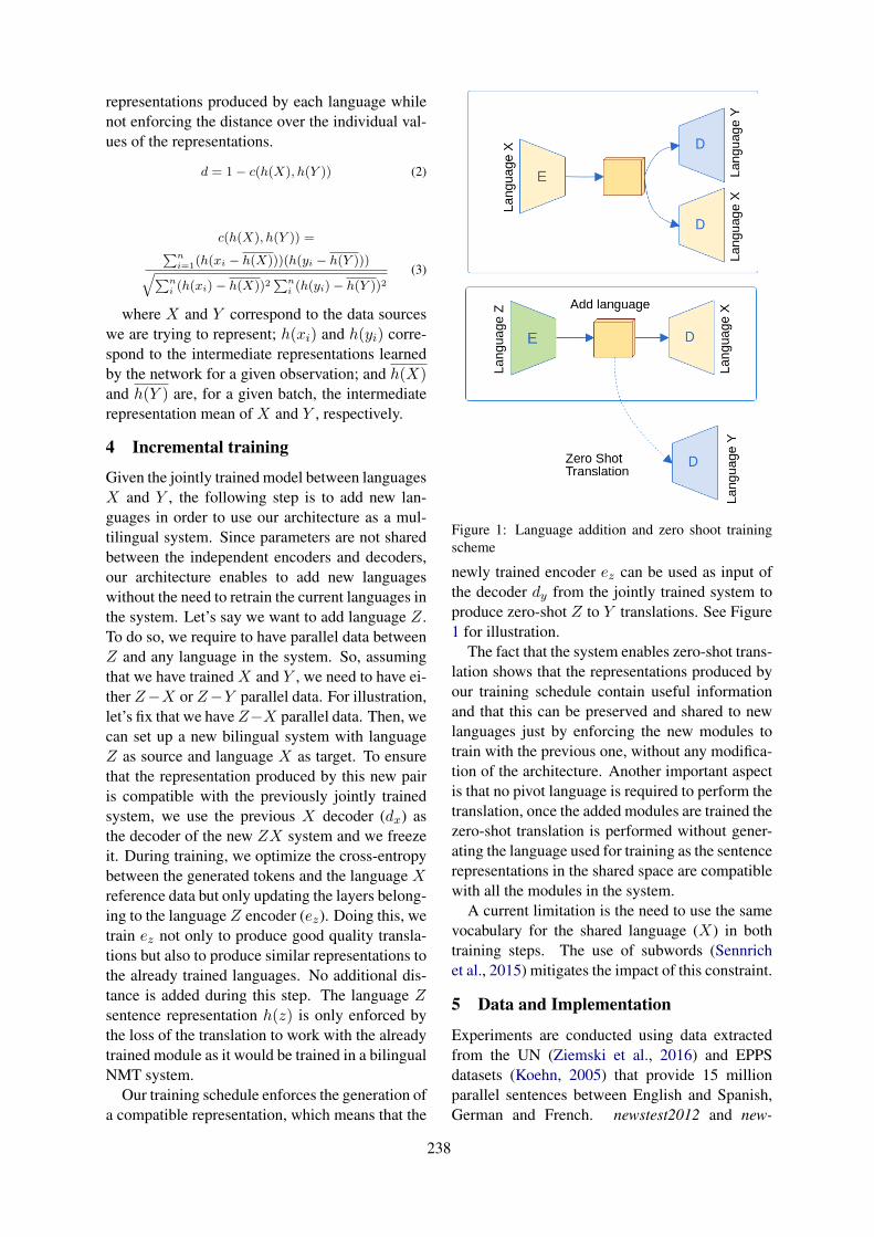
representations produced by each language whilenot enforcing the distance over the individual val-ues of the representations.

d = 1− c(h(X), h(Y )) (2)

c(h(X), h(Y )) =∑n

i=1(h(xi − h(X)))(h(yi − h(Y )))√∑ni (h(xi)− h(X))2

∑ni (h(yi)− h(Y ))2

(3)

where X and Y correspond to the data sourceswe are trying to represent; h(xi) and h(yi) corre-spond to the intermediate representations learnedby the network for a given observation; and h(X)and h(Y ) are, for a given batch, the intermediaterepresentation mean of X and Y , respectively.

4 Incremental training

Given the jointly trained model between languagesX and Y , the following step is to add new lan-guages in order to use our architecture as a mul-tilingual system. Since parameters are not sharedbetween the independent encoders and decoders,our architecture enables to add new languageswithout the need to retrain the current languages inthe system. Let’s say we want to add language Z.To do so, we require to have parallel data betweenZ and any language in the system. So, assumingthat we have trained X and Y , we need to have ei-ther Z−X or Z−Y parallel data. For illustration,let’s fix that we have Z−X parallel data. Then, wecan set up a new bilingual system with languageZ as source and language X as target. To ensurethat the representation produced by this new pairis compatible with the previously jointly trainedsystem, we use the previous X decoder (dx) asthe decoder of the new ZX system and we freezeit. During training, we optimize the cross-entropybetween the generated tokens and the language Xreference data but only updating the layers belong-ing to the language Z encoder (ez). Doing this, wetrain ez not only to produce good quality transla-tions but also to produce similar representations tothe already trained languages. No additional dis-tance is added during this step. The language Zsentence representation h(z) is only enforced bythe loss of the translation to work with the alreadytrained module as it would be trained in a bilingualNMT system.

Our training schedule enforces the generation ofa compatible representation, which means that the

Figure 1: Language addition and zero shoot trainingscheme

newly trained encoder ez can be used as input ofthe decoder dy from the jointly trained system toproduce zero-shot Z to Y translations. See Figure1 for illustration.

The fact that the system enables zero-shot trans-lation shows that the representations produced byour training schedule contain useful informationand that this can be preserved and shared to newlanguages just by enforcing the new modules totrain with the previous one, without any modifica-tion of the architecture. Another important aspectis that no pivot language is required to perform thetranslation, once the added modules are trained thezero-shot translation is performed without gener-ating the language used for training as the sentencerepresentations in the shared space are compatiblewith all the modules in the system.

A current limitation is the need to use the samevocabulary for the shared language (X) in bothtraining steps. The use of subwords (Sennrichet al., 2015) mitigates the impact of this constraint.

5 Data and Implementation

Experiments are conducted using data extractedfrom the UN (Ziemski et al., 2016) and EPPSdatasets (Koehn, 2005) that provide 15 millionparallel sentences between English and Spanish,German and French. newstest2012 and new-

238

System ES-EN EN-ES FR-EN DE-ENBaseline 32.60 32.90 31.81 28.96Joint 29.70 30.74 - -Added lang - - 30.93 27.63

Table 1: Experiment results measured in BLEU score.All blank positions are not tested or not viable combi-nations with our data.

System FR-ES DE-ESPivot 29.09 21.74Zero-shot 19.10 10.92

Table 2: Zero-shot results measured in BLEU score

stest2013 were used as validation and test sets,respectively. These sets provide parallel data be-tween the four languages that allow for zero-shotevaluation. Preprocessing consisted of a pipelineof punctuation normalization, tokenization, cor-pus filtering of longer sentences than 80 wordsand true-casing. These steps were performed us-ing the scripts available from Moses (Koehn et al.,2007). Preprocessed data is later tokenized intoBPE subwords (Sennrich et al., 2015) with a vo-cabulary size of 32000 tokens. We ensure that thevocabularies are independent and reusable whennew languages were added by creating vocabular-ies monolingually, i.e. without having access toother languages during the code generation.

6 Experiments

Our first experiment consists in comparing the per-formance of the jointly trained system to the stan-dard Transformer. As explained in previous sec-tions, this joint model is trained to perform twodifferent tasks, auto-encoding and translation inboth directions. In our experiments, these direc-tions are Spanish-English and English-Spanish. Inauto-encoding, both languages provide good re-sults at 98.21 and 97.44 BLEU points for Englishand Spanish, respectively. In translation, we ob-serve a decrease in performance. Table 1 showsthat for both directions the new training performsmore than 2 BLEU points below the baseline sys-tem. This difference suggests that even though theencoders and decoders of the system are compati-ble they still present some differences in the inter-nal representation.

Note that the languages chosen for the jointtraining seem relevant to the final system perfor-mance because they are used to define the repre-sentations of additional languages. Further exper-imentation is required to understand such impact.

Our second experiment consists of incremen-tally adding different languages to the system, inthis case, German and French. Note that, since wefreeze the weights while adding the new language,the order in which we add new languages does nothave any impact on performance. Table 1 showsthat French-English performs 0.9 BLEU points be-low the baseline and German-English performs1.33 points below the baseline. French-English iscloser to the baseline performance and this maybe due to its similarity to Spanish, one of the lan-guages of the initial system languages.

The added languages have better performancethan the jointly trained languages (Spanish-English from the previous section). This may beto the fact that the auto-encoding task may have anegative impact on the translation task.

Finally, another relevant aspect of the proposedarchitecture is enabling zero-shot translation. Toevaluate it, we compare the performance of eachof the added languages compared to a pivot sys-tem based on cascade. Such a system consists oftranslating from French (German) to English andfrom English to Spanish with the standard Trans-former. Results show that the zero shot translationprovides a consistent decrease in performance forboth cases of zero-shot translation.

7 Visualization

Our training schedule is based on training modulesto produce compatible representations, in this sec-tion we want to analyze this similarity at the lastattention block of encoders, where we are forcingthe similarity. In order to graphically show the pre-sentation a UMAP (McInnes et al., 2018) modelwas trained to combine the representations of alllanguages. Figures show 130 sentences extractedfrom the test set. These sentences have been se-lected to have a similar length to minimize theamount of padding required.

Figure 2 (A) shows the representations of alllanguages created by their encoders. Languagesare represented in clusters and no overlapping be-tween languages occurs, similarly to what (Luet al., 2018) reported in their multilingual ap-proach, the language dependent features of thesentences have a great impact in their representa-tions.

However, since our encoder/decoders are com-patible and produce competitive translations, wedecided to explore the representations generated

239

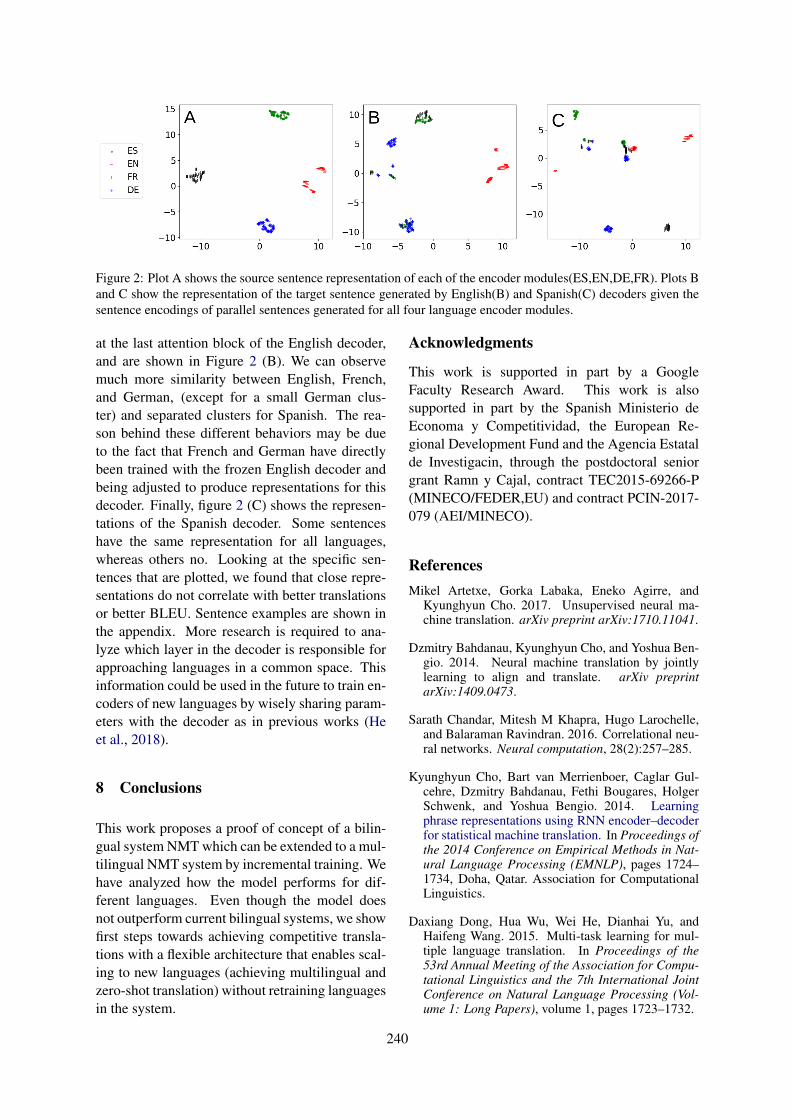
Figure 2: Plot A shows the source sentence representation of each of the encoder modules(ES,EN,DE,FR). Plots Band C show the representation of the target sentence generated by English(B) and Spanish(C) decoders given thesentence encodings of parallel sentences generated for all four language encoder modules.

at the last attention block of the English decoder,and are shown in Figure 2 (B). We can observemuch more similarity between English, French,and German, (except for a small German clus-ter) and separated clusters for Spanish. The rea-son behind these different behaviors may be dueto the fact that French and German have directlybeen trained with the frozen English decoder andbeing adjusted to produce representations for thisdecoder. Finally, figure 2 (C) shows the represen-tations of the Spanish decoder. Some sentenceshave the same representation for all languages,whereas others no. Looking at the specific sen-tences that are plotted, we found that close repre-sentations do not correlate with better translationsor better BLEU. Sentence examples are shown inthe appendix. More research is required to ana-lyze which layer in the decoder is responsible forapproaching languages in a common space. Thisinformation could be used in the future to train en-coders of new languages by wisely sharing param-eters with the decoder as in previous works (Heet al., 2018).

8 Conclusions

This work proposes a proof of concept of a bilin-gual system NMT which can be extended to a mul-tilingual NMT system by incremental training. Wehave analyzed how the model performs for dif-ferent languages. Even though the model doesnot outperform current bilingual systems, we showfirst steps towards achieving competitive transla-tions with a flexible architecture that enables scal-ing to new languages (achieving multilingual andzero-shot translation) without retraining languagesin the system.

Acknowledgments

This work is supported in part by a GoogleFaculty Research Award. This work is alsosupported in part by the Spanish Ministerio deEconoma y Competitividad, the European Re-gional Development Fund and the Agencia Estatalde Investigacin, through the postdoctoral seniorgrant Ramn y Cajal, contract TEC2015-69266-P(MINECO/FEDER,EU) and contract PCIN-2017-079 (AEI/MINECO).

ReferencesMikel Artetxe, Gorka Labaka, Eneko Agirre, and

Kyunghyun Cho. 2017. Unsupervised neural ma-chine translation. arXiv preprint arXiv:1710.11041.

Dzmitry Bahdanau, Kyunghyun Cho, and Yoshua Ben-gio. 2014. Neural machine translation by jointlylearning to align and translate. arXiv preprintarXiv:1409.0473.

Sarath Chandar, Mitesh M Khapra, Hugo Larochelle,and Balaraman Ravindran. 2016. Correlational neu-ral networks. Neural computation, 28(2):257–285.

Kyunghyun Cho, Bart van Merrienboer, Caglar Gul-cehre, Dzmitry Bahdanau, Fethi Bougares, HolgerSchwenk, and Yoshua Bengio. 2014. Learningphrase representations using RNN encoder–decoderfor statistical machine translation. In Proceedings ofthe 2014 Conference on Empirical Methods in Nat-ural Language Processing (EMNLP), pages 1724–1734, Doha, Qatar. Association for ComputationalLinguistics.

Daxiang Dong, Hua Wu, Wei He, Dianhai Yu, andHaifeng Wang. 2015. Multi-task learning for mul-tiple language translation. In Proceedings of the53rd Annual Meeting of the Association for Compu-tational Linguistics and the 7th International JointConference on Natural Language Processing (Vol-ume 1: Long Papers), volume 1, pages 1723–1732.

240

Orhan Firat, Kyunghyun Cho, and Yoshua Bengio.2016a. Multi-way, multilingual neural machinetranslation with a shared attention mechanism. InProceedings of the 2016 Conference of the NorthAmerican Chapter of the Association for Computa-tional Linguistics: Human Language Technologies,pages 866–875, San Diego, California. Associationfor Computational Linguistics.

Orhan Firat, Baskaran Sankaran, Yaser Al-Onaizan,Fatos T. Yarman Vural, and Kyunghyun Cho. 2016b.Zero-resource translation with multi-lingual neuralmachine translation. In Proceedings of the 2016Conference on Empirical Methods in Natural Lan-guage Processing, pages 268–277, Austin, Texas.Association for Computational Linguistics.

Tianyu He, Xu Tan, Yingce Xia, Di He, Tao Qin,Zhibo Chen, and Tie-Yan Liu. 2018. Layer-wisecoordination between encoder and decoder for neu-ral machine translation. In S. Bengio, H. Wallach,H. Larochelle, K. Grauman, N. Cesa-Bianchi, andR. Garnett, editors, Advances in Neural InformationProcessing Systems 31, pages 7955–7965. CurranAssociates, Inc.

Melvin Johnson, Mike Schuster, Quoc V Le, MaximKrikun, Yonghui Wu, Zhifeng Chen, Nikhil Thorat,Fernanda Viegas, Martin Wattenberg, Greg Corrado,et al. 2017. Googles multilingual neural machinetranslation system: Enabling zero-shot translation.Transactions of the Association for ComputationalLinguistics, 5:339–351.

Yunsu Kim, Yingbo Gao, and Hermann Ney. 2019.Effective cross-lingual transfer of neural machinetranslation models without shared vocabularies.arXiv preprint arXiv:1905.05475.

Philipp Koehn. 2005. Europarl: A parallel corpus forstatistical machine translation. In MT summit, vol-ume 5, pages 79–86.

Philipp Koehn, Hieu Hoang, Alexandra Birch, ChrisCallison-Burch, Marcello Federico, Nicola Bertoldi,Brooke Cowan, Wade Shen, Christine Moran,Richard Zens, et al. 2007. Moses: Open sourcetoolkit for statistical machine translation. In Pro-ceedings of the 45th annual meeting of the associ-ation for computational linguistics companion vol-ume proceedings of the demo and poster sessions,pages 177–180.

Surafel M. Lakew, Aliia Erofeeva, Matteo Negri, Mar-cello Federico, and Marco Turchi. 2018. Transferlearning in multilingual neural machine translationwith dynamic vocabulary. In Proceedings of the15th International Workshop on Spoken LanguageTranslation, pages 54–61, Belgium, Bruges.

Guillaume Lample, Alexis Conneau, Ludovic De-noyer, and Marc’Aurelio Ranzato. 2018. Unsuper-vised machine translation using monolingual cor-pora only. In International Conference on LearningRepresentations.

Yichao Lu, Phillip Keung, Faisal Ladhak, Vikas Bhard-waj, Shaonan Zhang, and Jason Sun. 2018. A neu-ral interlingua for multilingual machine translation.In Proceedings of the Third Conference on MachineTranslation: Research Papers, pages 84–92, Bel-gium, Brussels. Association for Computational Lin-guistics.

Leland McInnes, John Healy, Nathaniel Saul, andLukas Grossberger. 2018. Umap: Uniform mani-fold approximation and projection. The Journal ofOpen Source Software, 3(29):861.

Holger Schwenk and Matthijs Douze. 2017. Learn-ing joint multilingual sentence representationswith neural machine translation. arXiv preprintarXiv:1704.04154.

Rico Sennrich, Barry Haddow, and Alexandra Birch.2015. Neural machine translation of rare words withsubword units. arXiv preprint arXiv:1508.07909.

Ashish Vaswani, Noam Shazeer, Niki Parmar, JakobUszkoreit, Llion Jones, Aidan N Gomez, ŁukaszKaiser, and Illia Polosukhin. 2017. Attention is allyou need. In Advances in Neural Information Pro-cessing Systems, pages 5998–6008.

Michal Ziemski, Marcin Junczys-Dowmunt, and BrunoPouliquen. 2016. The united nations parallel corpusv1. 0. In Lrec.

Barret Zoph, Deniz Yuret, Jonathan May, and KevinKnight. 2016. Transfer learning for low-resourceneural machine translation. In Proceedings of the2016 Conference on Empirical Methods in Natu-ral Language Processing, pages 1568–1575, Austin,Texas. Association for Computational Linguistics.

A Examples

This appendix shows some examples of sentencesvisualized in Figure 2 in order to further analysethe visualization. Table 1 reports outputs producedby the Spanish decoder given encoding represen-tations produced by the Spanish, English, Frenchand German encoder. The first two sentences havesimilar representations between the languages inFigure 2 (right) (in the Spanish decoder visualiza-tion). While the first one keeps the meaning ofthe sentence, the second one produces meaning-less translations. The third sentence produces dis-joint representations but the meaning is preservedin the translations. Therefore, since close repre-sentations may imply different translation perfor-mance, further research is required to understandthe correlation between representations and trans-lation quality.

Table 2 shows outputs produced by the Englishdecoder given encoding representations produced

241

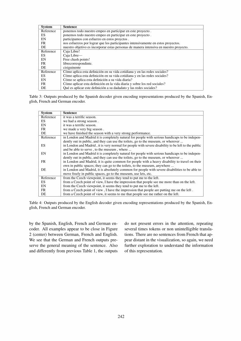
System SentenceReference ponemos todo nuestro empeo en participar en este proyecto .ES ponemos todo nuestro empeo en participar en este proyecto .EN participamos con esfuerzo en estos proyctos .FR nos esfuerzos por lograr que los participantes intensivamente en estos proyectos.DE nuestro objetivo es incorporar estas personas de manera intensiva en nuestro proyecto.Reference Caja Libre!ES Caja Libre—EN Free chash points!FR librecorrespondinte.DE cisiguinenteReference Como aplica esta definicion en su vida cotidiana y en las redes sociales?ES Como aplica esta definicion en su vida cotidiana y en las redes sociales?EN Como se aplica esta definicion a su vida diaria?FR Como aplicar esta definicion en la vida diaria y sobre los red sociales?DE Que es aplicar este definicion a su dadadato y las redes sociales?

Table 3: Outputs produced by the Spanish decoder given encoding representations produced by the Spanish, En-glish, French and German encoder.

System SentenceReference it was a terrific season.ES we had a strong season .EN it was a terrific season.FR we made a very big season .DE we have finished the season with a very strong performance.Reference in London and Madrid it is completely natural for people with serious handicaps to be indepen-

dently out in public, and they can use the toilets, go to the museum, or wherever ...ES in London and Madrid , it is very normal for people with severe disability to be left to the public

and be able to serve , to the museum , where ...EN in London and Madrid it is completely natural for people with serious handicaps to be indepen-

dently out in public, and they can use the toilets, go to the museum, or wherever ...FR in London and Madrid, it is quite common for people with a heavy disability to travel on their

own in public spaces; they can go to the toilets, to the museum, anywhere ...DE in London and Madrid, it is absolutely common for people with severe disabilities to be able to

move freely in public spaces, go to the museum, use lets, etc.Reference from the Czech viewpoint, it seems they tend to put me to the left.ES from a Czech point of view, I have the impression that people see me more than on the left.EN from the Czech viewpoint, it seems they tend to put me to the left.FR from a Czech point of view , I have the impression that people are putting me on the left .DE from a Czech point of view, it seems to me that people see me rather on the left.

Table 4: Outputs produced by the English decoder given encoding representations produced by the Spanish, En-glish, French and German encoder.

by the Spanish, English, French and German en-coder. All examples appear to be close in Figure2 (center) between German, French and English.We see that the German and French outputs pre-serve the general meaning of the sentence. Alsoand differently from previous Table 1, the outputs

do not present errors in the attention, repeatingseveral times tokens or non unintelligible transla-tions. There are no sentences from French that ap-pear distant in the visualization, so again, we needfurther exploration to understand the informationof this representation.

242

Proceedings of the 57th Annual Meeting of the Association for Computational Linguistics: Student Research Workshop, pages 243–252Florence, Italy, July 28 - August 2, 2019. c©2019 Association for Computational Linguistics

STRASS: A Light and Effective Method for Extractive SummarizationBased on Sentence Embeddings

Leo Bouscarrat, Antoine Bonnefoy, Thomas Peel, Cecile PereiraEURA NOVA

Marseille, Franceleo.bouscarrat,antoine.bonnefoy,

thomas.peel,cecile.pereira@euranova.eu

Abstract

This paper introduces STRASS: Summariza-tion by TRAnsformation Selection and Scor-ing. It is an extractive text summarizationmethod which leverages the semantic infor-mation in existing sentence embedding spaces.Our method creates an extractive summary byselecting the sentences with the closest embed-dings to the document embedding. The modellearns a transformation of the document em-bedding to minimize the similarity betweenthe extractive summary and the ground truthsummary. As the transformation is only com-posed of a dense layer, the training can bedone on CPU, therefore, inexpensive. More-over, inference time is short and linear ac-cording to the number of sentences. As asecond contribution, we introduce the FrenchCASS dataset, composed of judgments fromthe French Court of cassation and their corre-sponding summaries. On this dataset, our re-sults show that our method performs similarlyto the state of the art extractive methods witheffective training and inferring time.

1 Introduction

Summarization remains a field of interest asnumerous industries are faced with a growingamount of textual data that they need to process.Creating summary by hand is a costly and time-demanding task, thus automatic methods to gen-erate them are necessary. There are two ways ofsummarizing a document: abstractive and extrac-tive summarization.

In abstractive summarization, the goal is to cre-ate new textual elements to summarize the text.Summarization can be modeled as a sequence-to-sequence problem. For instance, Rush et al.(2015) tried to generate a headline from an article.However, when the system generates longer sum-maries, redundancy can be a problem. See et al.

(2017) introduce a pointer-generator model (PGN)that generates summaries by copying words fromthe text or generating new words. Moreover, theyadded a coverage loss as they noticed that othermodels made repetitions on long summaries. Evenif it provides state of the art results, the PGN isslow to learn and generate. Paulus et al. (2017)added a layer of reinforcement learning on anencoder-decoder architecture but their results canpresent fluency issues.

In extractive summarization, the goal is to ex-tract part of the text to create a summary. Thereare two standard ways to do that: a sequence la-beling task, where the goal is to select the sen-tences labeled as being part of the summary, anda ranking task, where the most salient sentencesare ranked first. It is hard to find datasets forthese tasks as most summaries written by humansare abstractive.Nallapati et al. (2016a) introducea way to train an extractive summarization modelwithout labels by applying a Recurrent NeuralNetwork (RNN) and using a greedy matching ap-proach based on ROUGE. Recently, Narayan et al.(2018b) combined reinforcement learning (to ex-tract sentences) and an encoder-decoder architec-ture (to select the sentences).

Some models combine extractive and abstrac-tive summarization, using an extractor to selectsentences and then an abstractor to rewrite them(Chen and Bansal, 2018; Cao et al., 2018; Hsuet al., 2018). They are generally faster than modelsusing only abstractors as they filter the input whilemaintaining or even improving the quality of thesummaries.

This paper presents two main contributions.First, we propose an inexpensive, scalable, CPU-trainable and efficient method of extractive textsummarization based on the use of sentence em-beddings. Our idea is that similar embeddingsare semantically similar, and so by looking at the

243

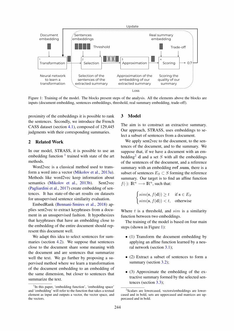
Document embedding

Sentences embeddings

Neural network to learn a

transformation

Real summary embedding

0.7

Selection of the sentences of the

extracted summary

Selection ScoringApproximationTransformation

Approximation of the embedding of our

extracted summary

Scoring the quality of our

summary

Trade-offThreshold

1 2 3 4

Loss

Update

Figure 1: Training of the model. The blocks present steps of the analysis. All the elements above the blocks areinputs (document embedding, sentences embeddings, threshold, real summary embedding, trade-off).

proximity of the embeddings it is possible to rankthe sentences. Secondly, we introduce the FrenchCASS dataset (section 4.1), composed of 129,445judgments with their corresponding summaries.

2 Related Work

In our model, STRASS, it is possible to use anembedding function 1 trained with state of the artmethods.

Word2vec is a classical method used to trans-form a word into a vector (Mikolov et al., 2013a).Methods like word2vec keep information aboutsemantics (Mikolov et al., 2013b). Sent2vec(Pagliardini et al., 2017) create embedding of sen-tences. It has state-of-the-art results on datasetsfor unsupervised sentence similarity evaluation.

EmbedRank (Bennani-Smires et al., 2018) ap-plies sent2vec to extract keyphrases from a docu-ment in an unsupervised fashion. It hypothesizesthat keyphrases that have an embedding close tothe embedding of the entire document should rep-resent this document well.

We adapt this idea to select sentences for sum-maries (section 4.2). We suppose that sentencesclose to the document share some meaning withthe document and are sentences that summarizewell the text. We go further by proposing a su-pervised method where we learn a transformationof the document embedding to an embedding ofthe same dimension, but closer to sentences thatsummarize the text.

1In this paper, ‘embedding function’, ‘embedding space’and ‘embedding’ will refer to the function that takes a textualelement as input and outputs a vector, the vector space, andthe vectors.

3 Model

The aim is to construct an extractive summary.Our approach, STRASS, uses embeddings to se-lect a subset of sentences from a document.

We apply sent2vec to the document, to the sen-tences of the document, and to the summary. Wesuppose that, if we have a document with an em-bedding2 d and a set S with all the embeddingsof the sentences of the document, and a referencesummary with an embedding ref sum, there is asubset of sentences ES ⊂ S forming the referencesummary. Our target is to find an affine functionf(·): IRn −→ IRn , such that:

sim(s, f(d)) ≥ t if s ∈ ES

sim(s, f(d)) < t, otherwise

Where t is a threshold, and sim is a similarityfunction between two embeddings.

The training of the model is based on four mainsteps (shown in Figure 1):

• (1) Transform the document embedding byapplying an affine function learned by a neu-ral network (section 3.1);

• (2) Extract a subset of sentences to form asummary (section 3.2);

• (3) Approximate the embedding of the ex-tractive summary formed by the selected sen-tences (section 3.3);

2Scalars are lowercased, vectors/embeddings are lower-cased and in bold, sets are uppercased and matrices are up-percased and in bold.

244

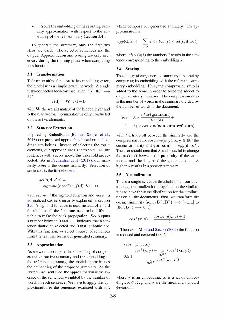
• (4) Score the embedding of the resulting sum-mary approximation with respect to the em-bedding of the real summary (section 3.4).

To generate the summary, only the first twosteps are used. The selected sentences are theoutput. Approximation and scoring are only nec-essary during the training phase when computingloss function.

3.1 TransformationTo learn an affine function in the embedding space,the model uses a simple neural network. A singlefully-connected feed-forward layer. f(·): IRn −→IRn :

f(d) = W × d+ b

with W the weight matrix of the hidden layer andb the bias vector. Optimization is only conductedon these two elements.

3.2 Sentence ExtractionInspired by EmbedRank (Bennani-Smires et al.,2018) our proposed approach is based on embed-dings similarities. Instead of selecting the top nelements, our approach uses a threshold. All thesentences with a score above this threshold are se-lected. As in Pagliardini et al. (2017), our simi-larity score is the cosine similarity. Selection ofsentences is the first element:

sel(s,d, S, t) =

sigmoid(ncos+(s, f(d), S)− t)

with sigmoid the sigmoid function and ncos+ anormalized cosine similarity explained in section3.5. A sigmoid function is used instead of a hardthreshold as all the functions need to be differen-tiable to make the back-propagation. Sel outputsa number between 0 and 1. 1 indicates that a sen-tence should be selected and 0 that it should not.With this function, we select a subset of sentencesfrom the text that forms our generated summary.

3.3 ApproximationAs we want to compare the embedding of our gen-erated extractive summary and the embedding ofthe reference summary, the model approximatesthe embedding of the proposed summary. As thesystem uses sent2vec, the approximation is the av-erage of the sentences weighted by the number ofwords in each sentence. We have to apply this ap-proximation to the sentences extracted with sel,

which compose our generated summary. The ap-proximation is:

app(d, S, t) =∑

s∈Ss× nb w(s)× sel(s,d, S, t)

where, nb w(s) is the number of words in the sen-tence corresponding to the embedding s.

3.4 Scoring

The quality of our generated summary is scored bycomparing its embedding with the reference sum-mary embedding. Here, the compression ratio isadded to the score in order to force the model tooutput shorter summaries. The compression ratiois the number of words in the summary divided bythe number of words in the document.

loss = λ× nb w(gen sum)

nb w(d)+

(1− λ)× cos sim(gen sum, ref sum)

with λ a trade-off between the similarity and thecompression ratio, cos sim(x,y), x,y ∈ IRn thecosine similarity and gen sum = app(d, S, t).The user should note that λ is also useful to changethe trade-off between the proximity of the sum-maries and the length of the generated one. Ahigher λ results in a shorter summary.

3.5 Normalization

To use a single selection threshold on all our doc-uments, a normalization is applied on the similar-ities to have the same distribution for the similari-ties on all the documents. First, we transform thecosine similarity from (IRn, IRn) −→ [−1, 1] to(IRn, IRn) −→ [0, 1]:

cos+(x,y) =cos sim(x,y) + 1

2

Then as in Mori and Sasaki (2002) the functionis reduced and centered in 0.5:

rcos+(x,y, X) =

0.5 +

cos+(x,y)− µxk∈X

(cos+(xk,y))

σxk∈X

(cos+(xk,y))

where y is an embedding, X is a set of embed-dings, x ∈ X , µ and σ are the mean and standarddeviation.

245

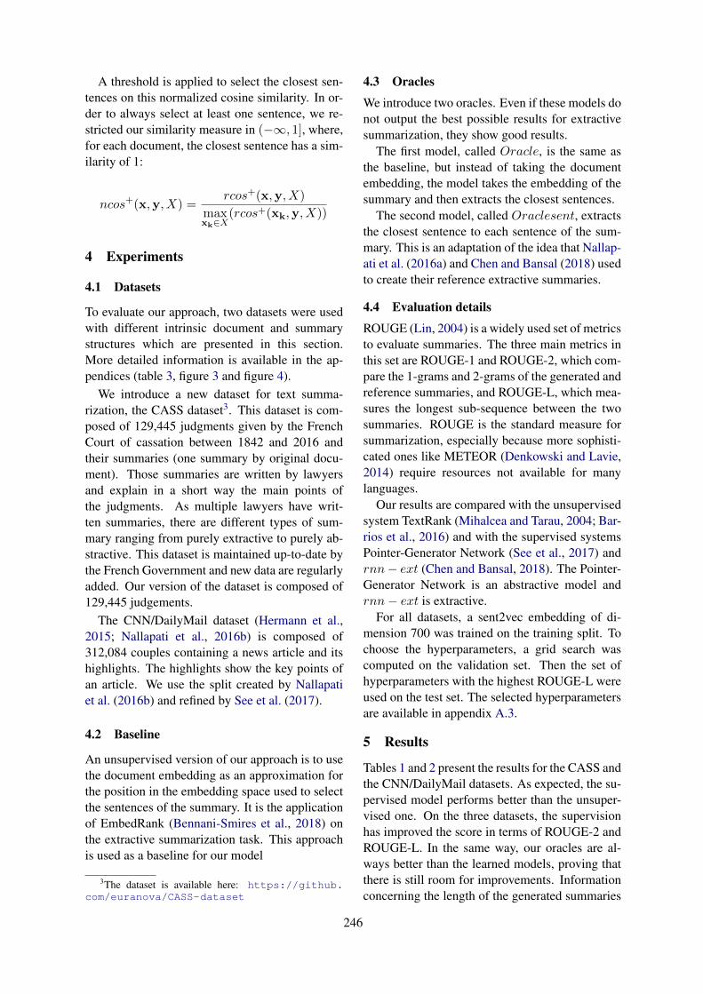
A threshold is applied to select the closest sen-tences on this normalized cosine similarity. In or-der to always select at least one sentence, we re-stricted our similarity measure in (−∞, 1], where,for each document, the closest sentence has a sim-ilarity of 1:

ncos+(x,y, X) =rcos+(x,y, X)

maxxk∈X

(rcos+(xk,y, X))

4 Experiments

4.1 Datasets

To evaluate our approach, two datasets were usedwith different intrinsic document and summarystructures which are presented in this section.More detailed information is available in the ap-pendices (table 3, figure 3 and figure 4).

We introduce a new dataset for text summa-rization, the CASS dataset3. This dataset is com-posed of 129,445 judgments given by the FrenchCourt of cassation between 1842 and 2016 andtheir summaries (one summary by original docu-ment). Those summaries are written by lawyersand explain in a short way the main points ofthe judgments. As multiple lawyers have writ-ten summaries, there are different types of sum-mary ranging from purely extractive to purely ab-stractive. This dataset is maintained up-to-date bythe French Government and new data are regularlyadded. Our version of the dataset is composed of129,445 judgements.

The CNN/DailyMail dataset (Hermann et al.,2015; Nallapati et al., 2016b) is composed of312,084 couples containing a news article and itshighlights. The highlights show the key points ofan article. We use the split created by Nallapatiet al. (2016b) and refined by See et al. (2017).

4.2 Baseline

An unsupervised version of our approach is to usethe document embedding as an approximation forthe position in the embedding space used to selectthe sentences of the summary. It is the applicationof EmbedRank (Bennani-Smires et al., 2018) onthe extractive summarization task. This approachis used as a baseline for our model

3The dataset is available here: https://github.com/euranova/CASS-dataset

4.3 Oracles

We introduce two oracles. Even if these models donot output the best possible results for extractivesummarization, they show good results.

The first model, called Oracle, is the same asthe baseline, but instead of taking the documentembedding, the model takes the embedding of thesummary and then extracts the closest sentences.

The second model, called Oraclesent, extractsthe closest sentence to each sentence of the sum-mary. This is an adaptation of the idea that Nallap-ati et al. (2016a) and Chen and Bansal (2018) usedto create their reference extractive summaries.

4.4 Evaluation details

ROUGE (Lin, 2004) is a widely used set of metricsto evaluate summaries. The three main metrics inthis set are ROUGE-1 and ROUGE-2, which com-pare the 1-grams and 2-grams of the generated andreference summaries, and ROUGE-L, which mea-sures the longest sub-sequence between the twosummaries. ROUGE is the standard measure forsummarization, especially because more sophisti-cated ones like METEOR (Denkowski and Lavie,2014) require resources not available for manylanguages.

Our results are compared with the unsupervisedsystem TextRank (Mihalcea and Tarau, 2004; Bar-rios et al., 2016) and with the supervised systemsPointer-Generator Network (See et al., 2017) andrnn− ext (Chen and Bansal, 2018). The Pointer-Generator Network is an abstractive model andrnn− ext is extractive.

For all datasets, a sent2vec embedding of di-mension 700 was trained on the training split. Tochoose the hyperparameters, a grid search wascomputed on the validation set. Then the set ofhyperparameters with the highest ROUGE-L wereused on the test set. The selected hyperparametersare available in appendix A.3.

5 Results

Tables 1 and 2 present the results for the CASS andthe CNN/DailyMail datasets. As expected, the su-pervised model performs better than the unsuper-vised one. On the three datasets, the supervisionhas improved the score in terms of ROUGE-2 andROUGE-L. In the same way, our oracles are al-ways better than the learned models, proving thatthere is still room for improvements. Informationconcerning the length of the generated summaries

246

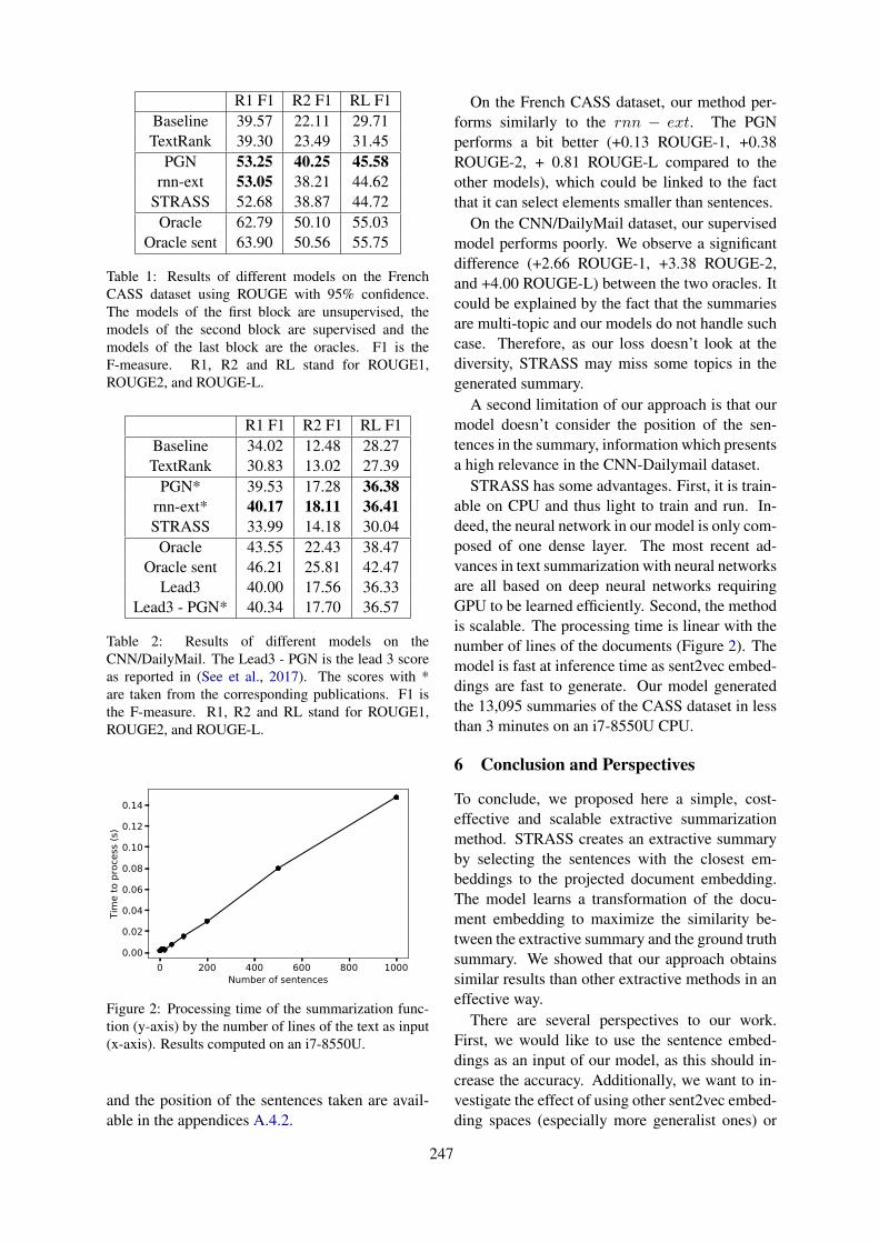
R1 F1 R2 F1 RL F1Baseline 39.57 22.11 29.71TextRank 39.30 23.49 31.45

PGN 53.25 40.25 45.58rnn-ext 53.05 38.21 44.62

STRASS 52.68 38.87 44.72Oracle 62.79 50.10 55.03

Oracle sent 63.90 50.56 55.75

Table 1: Results of different models on the FrenchCASS dataset using ROUGE with 95% confidence.The models of the first block are unsupervised, themodels of the second block are supervised and themodels of the last block are the oracles. F1 is theF-measure. R1, R2 and RL stand for ROUGE1,ROUGE2, and ROUGE-L.

R1 F1 R2 F1 RL F1Baseline 34.02 12.48 28.27TextRank 30.83 13.02 27.39

PGN* 39.53 17.28 36.38rnn-ext* 40.17 18.11 36.41STRASS 33.99 14.18 30.04

Oracle 43.55 22.43 38.47Oracle sent 46.21 25.81 42.47

Lead3 40.00 17.56 36.33Lead3 - PGN* 40.34 17.70 36.57

Table 2: Results of different models on theCNN/DailyMail. The Lead3 - PGN is the lead 3 scoreas reported in (See et al., 2017). The scores with *are taken from the corresponding publications. F1 isthe F-measure. R1, R2 and RL stand for ROUGE1,ROUGE2, and ROUGE-L.

0 200 400 600 800 1000Number of sentences

0.00

0.02

0.04

0.06

0.08

0.10

0.12

0.14

Time to proce

ss (s

)

Figure 2: Processing time of the summarization func-tion (y-axis) by the number of lines of the text as input(x-axis). Results computed on an i7-8550U.

and the position of the sentences taken are avail-able in the appendices A.4.2.

On the French CASS dataset, our method per-forms similarly to the rnn − ext. The PGNperforms a bit better (+0.13 ROUGE-1, +0.38ROUGE-2, + 0.81 ROUGE-L compared to theother models), which could be linked to the factthat it can select elements smaller than sentences.

On the CNN/DailyMail dataset, our supervisedmodel performs poorly. We observe a significantdifference (+2.66 ROUGE-1, +3.38 ROUGE-2,and +4.00 ROUGE-L) between the two oracles. Itcould be explained by the fact that the summariesare multi-topic and our models do not handle suchcase. Therefore, as our loss doesn’t look at thediversity, STRASS may miss some topics in thegenerated summary.

A second limitation of our approach is that ourmodel doesn’t consider the position of the sen-tences in the summary, information which presentsa high relevance in the CNN-Dailymail dataset.

STRASS has some advantages. First, it is train-able on CPU and thus light to train and run. In-deed, the neural network in our model is only com-posed of one dense layer. The most recent ad-vances in text summarization with neural networksare all based on deep neural networks requiringGPU to be learned efficiently. Second, the methodis scalable. The processing time is linear with thenumber of lines of the documents (Figure 2). Themodel is fast at inference time as sent2vec embed-dings are fast to generate. Our model generatedthe 13,095 summaries of the CASS dataset in lessthan 3 minutes on an i7-8550U CPU.

6 Conclusion and Perspectives

To conclude, we proposed here a simple, cost-effective and scalable extractive summarizationmethod. STRASS creates an extractive summaryby selecting the sentences with the closest em-beddings to the projected document embedding.The model learns a transformation of the docu-ment embedding to maximize the similarity be-tween the extractive summary and the ground truthsummary. We showed that our approach obtainssimilar results than other extractive methods in aneffective way.

There are several perspectives to our work.First, we would like to use the sentence embed-dings as an input of our model, as this should in-crease the accuracy. Additionally, we want to in-vestigate the effect of using other sent2vec embed-ding spaces (especially more generalist ones) or

247

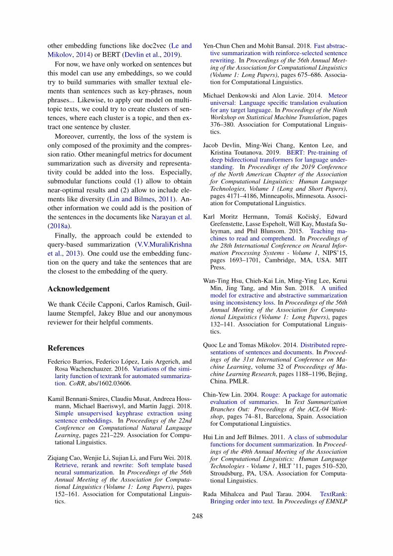
other embedding functions like doc2vec (Le andMikolov, 2014) or BERT (Devlin et al., 2019).

For now, we have only worked on sentences butthis model can use any embeddings, so we couldtry to build summaries with smaller textual ele-ments than sentences such as key-phrases, nounphrases... Likewise, to apply our model on multi-topic texts, we could try to create clusters of sen-tences, where each cluster is a topic, and then ex-tract one sentence by cluster.

Moreover, currently, the loss of the system isonly composed of the proximity and the compres-sion ratio. Other meaningful metrics for documentsummarization such as diversity and representa-tivity could be added into the loss. Especially,submodular functions could (1) allow to obtainnear-optimal results and (2) allow to include ele-ments like diversity (Lin and Bilmes, 2011). An-other information we could add is the position ofthe sentences in the documents like Narayan et al.(2018a).

Finally, the approach could be extended toquery-based summarization (V.V.MuraliKrishnaet al., 2013). One could use the embedding func-tion on the query and take the sentences that arethe closest to the embedding of the query.

Acknowledgement

We thank Cecile Capponi, Carlos Ramisch, Guil-laume Stempfel, Jakey Blue and our anonymousreviewer for their helpful comments.

References

Federico Barrios, Federico Lopez, Luis Argerich, andRosa Wachenchauzer. 2016. Variations of the simi-larity function of textrank for automated summariza-tion. CoRR, abs/1602.03606.

Kamil Bennani-Smires, Claudiu Musat, Andreea Hoss-mann, Michael Baeriswyl, and Martin Jaggi. 2018.Simple unsupervised keyphrase extraction usingsentence embeddings. In Proceedings of the 22ndConference on Computational Natural LanguageLearning, pages 221–229. Association for Compu-tational Linguistics.

Ziqiang Cao, Wenjie Li, Sujian Li, and Furu Wei. 2018.Retrieve, rerank and rewrite: Soft template basedneural summarization. In Proceedings of the 56thAnnual Meeting of the Association for Computa-tional Linguistics (Volume 1: Long Papers), pages152–161. Association for Computational Linguis-tics.

Yen-Chun Chen and Mohit Bansal. 2018. Fast abstrac-tive summarization with reinforce-selected sentencerewriting. In Proceedings of the 56th Annual Meet-ing of the Association for Computational Linguistics(Volume 1: Long Papers), pages 675–686. Associa-tion for Computational Linguistics.

Michael Denkowski and Alon Lavie. 2014. Meteoruniversal: Language specific translation evaluationfor any target language. In Proceedings of the NinthWorkshop on Statistical Machine Translation, pages376–380. Association for Computational Linguis-tics.

Jacob Devlin, Ming-Wei Chang, Kenton Lee, andKristina Toutanova. 2019. BERT: Pre-training ofdeep bidirectional transformers for language under-standing. In Proceedings of the 2019 Conferenceof the North American Chapter of the Associationfor Computational Linguistics: Human LanguageTechnologies, Volume 1 (Long and Short Papers),pages 4171–4186, Minneapolis, Minnesota. Associ-ation for Computational Linguistics.

Karl Moritz Hermann, Tomas Kocisky, EdwardGrefenstette, Lasse Espeholt, Will Kay, Mustafa Su-leyman, and Phil Blunsom. 2015. Teaching ma-chines to read and comprehend. In Proceedings ofthe 28th International Conference on Neural Infor-mation Processing Systems - Volume 1, NIPS’15,pages 1693–1701, Cambridge, MA, USA. MITPress.

Wan-Ting Hsu, Chieh-Kai Lin, Ming-Ying Lee, KeruiMin, Jing Tang, and Min Sun. 2018. A unifiedmodel for extractive and abstractive summarizationusing inconsistency loss. In Proceedings of the 56thAnnual Meeting of the Association for Computa-tional Linguistics (Volume 1: Long Papers), pages132–141. Association for Computational Linguis-tics.

Quoc Le and Tomas Mikolov. 2014. Distributed repre-sentations of sentences and documents. In Proceed-ings of the 31st International Conference on Ma-chine Learning, volume 32 of Proceedings of Ma-chine Learning Research, pages 1188–1196, Bejing,China. PMLR.

Chin-Yew Lin. 2004. Rouge: A package for automaticevaluation of summaries. In Text SummarizationBranches Out: Proceedings of the ACL-04 Work-shop, pages 74–81, Barcelona, Spain. Associationfor Computational Linguistics.

Hui Lin and Jeff Bilmes. 2011. A class of submodularfunctions for document summarization. In Proceed-ings of the 49th Annual Meeting of the Associationfor Computational Linguistics: Human LanguageTechnologies - Volume 1, HLT ’11, pages 510–520,Stroudsburg, PA, USA. Association for Computa-tional Linguistics.

Rada Mihalcea and Paul Tarau. 2004. TextRank:Bringing order into text. In Proceedings of EMNLP

248

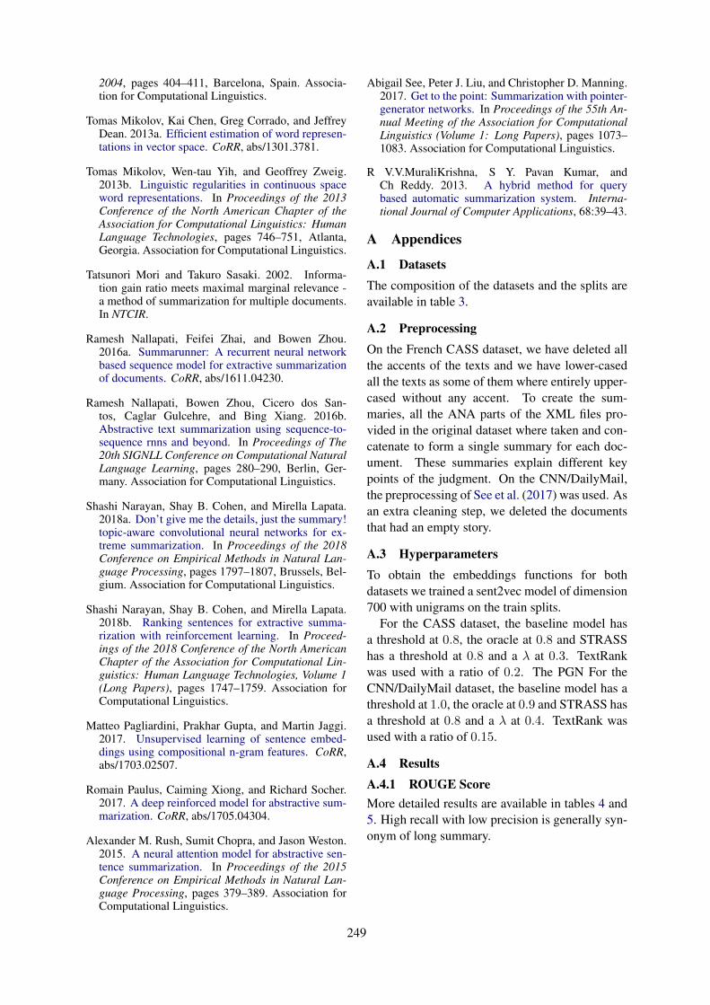
2004, pages 404–411, Barcelona, Spain. Associa-tion for Computational Linguistics.

Tomas Mikolov, Kai Chen, Greg Corrado, and JeffreyDean. 2013a. Efficient estimation of word represen-tations in vector space. CoRR, abs/1301.3781.

Tomas Mikolov, Wen-tau Yih, and Geoffrey Zweig.2013b. Linguistic regularities in continuous spaceword representations. In Proceedings of the 2013Conference of the North American Chapter of theAssociation for Computational Linguistics: HumanLanguage Technologies, pages 746–751, Atlanta,Georgia. Association for Computational Linguistics.

Tatsunori Mori and Takuro Sasaki. 2002. Informa-tion gain ratio meets maximal marginal relevance -a method of summarization for multiple documents.In NTCIR.

Ramesh Nallapati, Feifei Zhai, and Bowen Zhou.2016a. Summarunner: A recurrent neural networkbased sequence model for extractive summarizationof documents. CoRR, abs/1611.04230.

Ramesh Nallapati, Bowen Zhou, Cicero dos San-tos, Caglar Gulcehre, and Bing Xiang. 2016b.Abstractive text summarization using sequence-to-sequence rnns and beyond. In Proceedings of The20th SIGNLL Conference on Computational NaturalLanguage Learning, pages 280–290, Berlin, Ger-many. Association for Computational Linguistics.

Shashi Narayan, Shay B. Cohen, and Mirella Lapata.2018a. Don’t give me the details, just the summary!topic-aware convolutional neural networks for ex-treme summarization. In Proceedings of the 2018Conference on Empirical Methods in Natural Lan-guage Processing, pages 1797–1807, Brussels, Bel-gium. Association for Computational Linguistics.

Shashi Narayan, Shay B. Cohen, and Mirella Lapata.2018b. Ranking sentences for extractive summa-rization with reinforcement learning. In Proceed-ings of the 2018 Conference of the North AmericanChapter of the Association for Computational Lin-guistics: Human Language Technologies, Volume 1(Long Papers), pages 1747–1759. Association forComputational Linguistics.

Matteo Pagliardini, Prakhar Gupta, and Martin Jaggi.2017. Unsupervised learning of sentence embed-dings using compositional n-gram features. CoRR,abs/1703.02507.

Romain Paulus, Caiming Xiong, and Richard Socher.2017. A deep reinforced model for abstractive sum-marization. CoRR, abs/1705.04304.

Alexander M. Rush, Sumit Chopra, and Jason Weston.2015. A neural attention model for abstractive sen-tence summarization. In Proceedings of the 2015Conference on Empirical Methods in Natural Lan-guage Processing, pages 379–389. Association forComputational Linguistics.

Abigail See, Peter J. Liu, and Christopher D. Manning.2017. Get to the point: Summarization with pointer-generator networks. In Proceedings of the 55th An-nual Meeting of the Association for ComputationalLinguistics (Volume 1: Long Papers), pages 1073–1083. Association for Computational Linguistics.

R V.V.MuraliKrishna, S Y. Pavan Kumar, andCh Reddy. 2013. A hybrid method for querybased automatic summarization system. Interna-tional Journal of Computer Applications, 68:39–43.

A Appendices

A.1 DatasetsThe composition of the datasets and the splits areavailable in table 3.

A.2 PreprocessingOn the French CASS dataset, we have deleted allthe accents of the texts and we have lower-casedall the texts as some of them where entirely upper-cased without any accent. To create the sum-maries, all the ANA parts of the XML files pro-vided in the original dataset where taken and con-catenate to form a single summary for each doc-ument. These summaries explain different keypoints of the judgment. On the CNN/DailyMail,the preprocessing of See et al. (2017) was used. Asan extra cleaning step, we deleted the documentsthat had an empty story.

A.3 HyperparametersTo obtain the embeddings functions for bothdatasets we trained a sent2vec model of dimension700 with unigrams on the train splits.

For the CASS dataset, the baseline model hasa threshold at 0.8, the oracle at 0.8 and STRASShas a threshold at 0.8 and a λ at 0.3. TextRankwas used with a ratio of 0.2. The PGN For theCNN/DailyMail dataset, the baseline model has athreshold at 1.0, the oracle at 0.9 and STRASS hasa threshold at 0.8 and a λ at 0.4. TextRank wasused with a ratio of 0.15.

A.4 ResultsA.4.1 ROUGE ScoreMore detailed results are available in tables 4 and5. High recall with low precision is generally syn-onym of long summary.

249

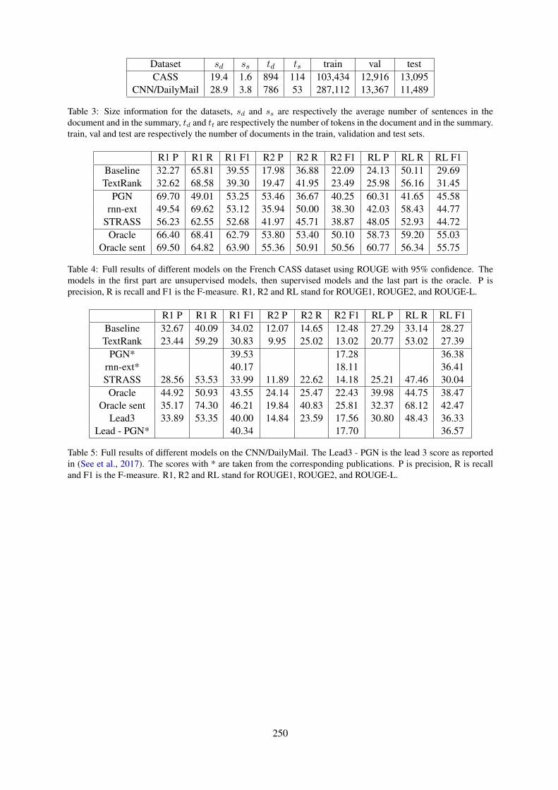
Dataset sd ss td ts train val testCASS 19.4 1.6 894 114 103,434 12,916 13,095

CNN/DailyMail 28.9 3.8 786 53 287,112 13,367 11,489

Table 3: Size information for the datasets, sd and ss are respectively the average number of sentences in thedocument and in the summary, td and tt are respectively the number of tokens in the document and in the summary.train, val and test are respectively the number of documents in the train, validation and test sets.

R1 P R1 R R1 F1 R2 P R2 R R2 F1 RL P RL R RL F1Baseline 32.27 65.81 39.55 17.98 36.88 22.09 24.13 50.11 29.69TextRank 32.62 68.58 39.30 19.47 41.95 23.49 25.98 56.16 31.45

PGN 69.70 49.01 53.25 53.46 36.67 40.25 60.31 41.65 45.58rnn-ext 49.54 69.62 53.12 35.94 50.00 38.30 42.03 58.43 44.77

STRASS 56.23 62.55 52.68 41.97 45.71 38.87 48.05 52.93 44.72Oracle 66.40 68.41 62.79 53.80 53.40 50.10 58.73 59.20 55.03

Oracle sent 69.50 64.82 63.90 55.36 50.91 50.56 60.77 56.34 55.75

Table 4: Full results of different models on the French CASS dataset using ROUGE with 95% confidence. Themodels in the first part are unsupervised models, then supervised models and the last part is the oracle. P isprecision, R is recall and F1 is the F-measure. R1, R2 and RL stand for ROUGE1, ROUGE2, and ROUGE-L.

R1 P R1 R R1 F1 R2 P R2 R R2 F1 RL P RL R RL F1Baseline 32.67 40.09 34.02 12.07 14.65 12.48 27.29 33.14 28.27TextRank 23.44 59.29 30.83 9.95 25.02 13.02 20.77 53.02 27.39

PGN* 39.53 17.28 36.38rnn-ext* 40.17 18.11 36.41STRASS 28.56 53.53 33.99 11.89 22.62 14.18 25.21 47.46 30.04

Oracle 44.92 50.93 43.55 24.14 25.47 22.43 39.98 44.75 38.47Oracle sent 35.17 74.30 46.21 19.84 40.83 25.81 32.37 68.12 42.47

Lead3 33.89 53.35 40.00 14.84 23.59 17.56 30.80 48.43 36.33Lead - PGN* 40.34 17.70 36.57

Table 5: Full results of different models on the CNN/DailyMail. The Lead3 - PGN is the lead 3 score as reportedin (See et al., 2017). The scores with * are taken from the corresponding publications. P is precision, R is recalland F1 is the F-measure. R1, R2 and RL stand for ROUGE1, ROUGE2, and ROUGE-L.

250

Model s w w/s

Reference 1.6 117 73.1STRASS 2.0 151 75.5

Oracle 1.7 138 81.2Oracle sent 1.5 112 74.7

(a) Size information for the generated summary on thetest split of the CASS dataset, s, w, w/s are respectivelythe average number of sentences, the average number ofwords and the average number of words per sentences.

1 2 3 4 5 6 7 8 9 10 11 12 13 14 15 16 17 18 19 20

Pos sentence

0.000

0.025

0.050

0.075

0.100

0.125

0.150

Percen

tage

take

n in su

mmaries

STRASSoracleoracle sent

(b) Percentage of times that a sentence is taken in a gen-erated summary in function of their position in the docu-ment on the CASS dataset.

0.0 2.5 5.0 7.5 10.0 12.5 15.0Nb sentences

0.0

0.1

0.2

0.3

0.4

0.5

Percen

tage

in th

e results

Density of the number of sentencesSTRASSoracleoracle sentreference

(c) Density of the number of sentences in the generatedsummaries for several models and the reference on theCASS dataset.

0 100 200 300 400Nb words

0.0000

0.0025

0.0050

0.0075

0.0100

0.0125

Percentage in th

e results

Density of the number of wordsSTRASSoracleoracle sentreference

(d) Density of the number of words in the generated sum-maries for several models and the reference on the CASSdataset.

Figure 3: Information about the length of the generated summaries for the CASS dataset.

A.4.2 Words and sentences

On the French CASS dataset the summaries gen-erated by the models are generally close in termsof length (number of words, number of sentencesand number of words per sentences (figure 3a, 3c,3d)). All the tested extractive methods tend to se-lect sentences at the beginning of the documents.The first sentence make an exception to that rule(figure 3b). We observe that this sentence can havethe list of the lawyers and judges that were presentat the case. STRASS tends to generate longersummaries with more sentences. The discrepancyin the average number of sentences between thereference and Oraclesent is due to sentences thatare extracted multiple times.

On the CNN/DailyMail dataset, STRASS tendsto extract less sentences but longer ones compar-ing to the Oraclesent (figure 4a, 4c, 4d). Onthe figure 4b we can see that the three modelstend to extract different sentences. Oraclesentwhich is the best performing model tends to ex-tract the 4 first sentences,Oracle extracts more of-

ten the fourth sentences than the first three and stillhave better results than the Lead3, which meansthat the fourth sentences could have some interest.With STRASS the first three sentences have a dif-ferent tendency than the rest of the text, showingthat the first three sentences may have a differentstructure than the rest. Then, the farther a sentenceis in the text, the lower the probability to take it.

251

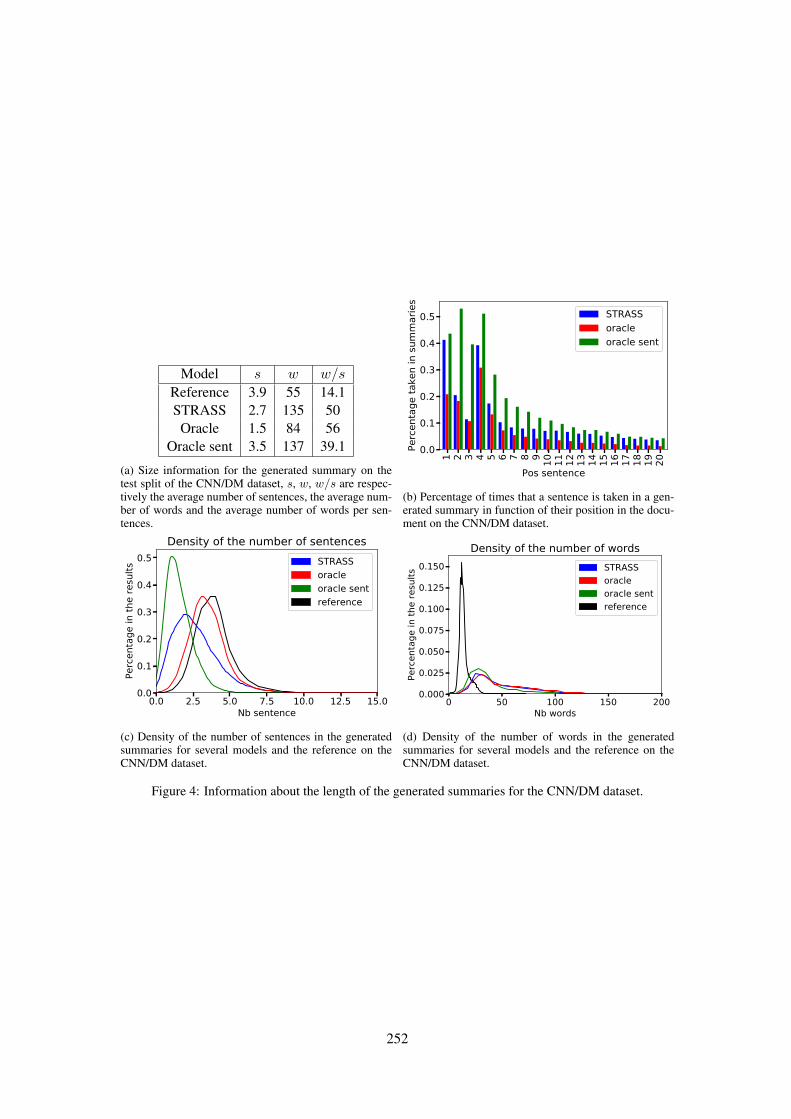
Model s w w/s

Reference 3.9 55 14.1STRASS 2.7 135 50

Oracle 1.5 84 56Oracle sent 3.5 137 39.1

(a) Size information for the generated summary on thetest split of the CNN/DM dataset, s, w, w/s are respec-tively the average number of sentences, the average num-ber of words and the average number of words per sen-tences.

1 2 3 4 5 6 7 8 9 10 11 12 13 14 15 16 17 18 19 20

Pos sentence

0.0

0.1

0.2

0.3

0.4

0.5

Percen

tage

take

n in su

mmaries

STRASSoracleoracle sent

(b) Percentage of times that a sentence is taken in a gen-erated summary in function of their position in the docu-ment on the CNN/DM dataset.

0.0 2.5 5.0 7.5 10.0 12.5 15.0Nb sentence

0.0

0.1

0.2

0.3

0.4

0.5

Percen

tage

in th

e results

Density of the number of sentencesSTRASSoracleoracle sentreference

(c) Density of the number of sentences in the generatedsummaries for several models and the reference on theCNN/DM dataset.

0 50 100 150 200Nb words

0.000

0.025

0.050

0.075

0.100

0.125

0.150

Percen

tage

in th

e results

Density of the number of wordsSTRASSoracleoracle sentreference

(d) Density of the number of words in the generatedsummaries for several models and the reference on theCNN/DM dataset.

Figure 4: Information about the length of the generated summaries for the CNN/DM dataset.

252

Proceedings of the 57th Annual Meeting of the Association for Computational Linguistics: Student Research Workshop, pages 253–259Florence, Italy, July 28 - August 2, 2019. c©2019 Association for Computational Linguistics

Attention and Lexicon Regularized LSTM for Aspect-based SentimentAnalysis

Lingxian BaoUniversitat Pompeu Fabra

lingxian.bao@upf.edu

Patrik LambertUniversitat Pompeu Fabrapatrik.lambert

@upf.edu

Toni BadiaUniversitat Pompeu Fabratoni.badia@upf.edu

AbstractAttention based deep learning systems havebeen demonstrated to be the state of the artapproach for aspect-level sentiment analysis,however, end-to-end deep neural networkslack flexibility as one can not easily adjust thenetwork to fix an obvious problem, especiallywhen more training data is not available: e.g.when it always predicts positive when seeingthe word disappointed. Meanwhile, it is lessstressed that attention mechanism is likely to“over-focus” on particular parts of a sentence,while ignoring positions which provide keyinformation for judging the polarity. In thispaper, we describe a simple yet effective ap-proach to leverage lexicon information so thatthe model becomes more flexible and robust.We also explore the effect of regularizing at-tention vectors to allow the network to have abroader “focus” on different parts of the sen-tence. The experimental results demonstratethe effectiveness of our approach.

1 Introduction

Sentiment analysis (also called opinion mining)has been one of the most active fields in NLP dueto its important value to business and society. Itis the field of study that tries to extract opinion(positive, neutral, negative) expressed in naturallanguages. Most sentiment analysis works havebeen carried out at document level (Pang et al.,2002; Turney, 2002) and sentence level (Wilsonet al., 2004), but as opinion expressed by words ishighly context dependent, one word may expressopposite sentiment under different circumstances.Thus aspect-level sentiment analysis (ABSA) wasproposed to address this problem. It finds the po-larity of an opinion associated with a certain as-pect, such as food, ambiance, service, or price in arestaurant domain.

Although deep neural networks yield significantimprovement across a variety of tasks compared to

previous state of the art methods, end-to-end deeplearning systems lack flexibility as one cannot eas-ily adjust the network to fix an obvious problem:e.g. when the network always predicts positivewhen seeing the word disappointed, or when thenetwork is not able to recognize the word dun-geon as an indication of negative polarity. It couldbe even trickier in a low-resource scenario wheremore labeled training data is simply not avail-able. Moreover, it is less stressed that attentionmechanism is likely to over-fit and force the net-work to “focus” too much on a particular part ofa sentence, while in some cases ignoring positionswhich provide key information for judging the po-larity. In recent studies, both Niculae and Blon-del (2017) and Zhang et al. (2019) proposed ap-proaches to make the attention vector more sparse,however, it would only encourage the over-fittingeffect in such scenario.

In this paper, we describe a simple yet effec-tive approach to merge lexicon information withan attention LSTM model for ABSA in order toleverage both the power of deep neural networksand existing linguistic resources, so that the frame-work becomes more flexible and robust withoutrequiring additional labeled data. We also explorethe effect of regularizing attention vectors by in-troducing an attention regularizer to allow the net-work to have a broader “focus” on different partsof the sentence.

2 Related works

ABSA is a fine-grained task which requires themodel to be able to produce accurate predictiongiven different aspects. As it is common thatone sentence may contain opposite polarities as-sociated to different aspects at the same time,attention-based LSTM (Wang et al., 2016) wasfirst proposed to allow the network to be able to as-

253

sign higher weights to more relevant words givendifferent aspects. Following this idea, a number ofresearches have been carried out to keep improv-ing the attention network for ABSA (Ma et al.,2017; Tay et al., 2017; Cheng et al., 2017; He et al.,2018; Zhu and Qian, 2018).

On the other hand, a lot of works have beendone focusing on leveraging existing linguistic re-sources such as sentiment to enhance the perfor-mance; however, most works are performed atdocument and sentence level. For instance, atdocument level, Teng et al. (2016) proposed aweighted-sum model which consists of represent-ing the final prediction as a weighted sum of thenetwork prediction and the polarities provided bythe lexicon. Zou et al. (2018) described a frame-work to assign higher weights to opinion wordsfound in the lexicon by transforming lexicon po-larity to sentiment degree.

At sentence level, Shin et al. (2017) used twoconvolutional neural networks to separately pro-cess sentence and lexicon inputs. Lei et al. (2018)described a multi-head attention network wherethe attention weights are jointly learned with lexi-con inputs. Wu et al. (2018) proposed a new label-ing strategy which breaks a sentence into clausesby punctuation to produce more lower-level ex-amples, inputs are then processed at different lev-els with linguistic information such as lexicon andPOS, and finally merged back to perform sentencelevel prediction. Meanwhile, some other similarworks that incorporate linguistic resources for sen-timent analysis have been carried out (Rouvier andFavre, 2016; Qian et al., 2017).

Regarding the attention regularization, insteadof using softmax and sparesmax, Niculae andBlondel (2017) proposed fusemax as a regularizedattention framework to learn the attention weights;Zhang et al. (2019) introducedLmax andEntropyas regularization terms to be jointly optimizedwith the loss. However, both approaches share thesame idea of shaping the attention weights to besharper and more sparse so that the advantage ofthe attention mechanism is maximized.

In our work, different from the previously men-tioned approaches, we incorporate polarities ob-tained from lexicons directly into the attention-based LSTM network to perform aspect-level sen-timent analysis, so that the model improves interms of robustness without requiring extra train-ing examples. Additionally, we find that the at-

tention vector is likely to over-fit which forces thenetwork to “focus” on particular words while ig-noring positions that provide key information forjudging the polarity; and that by adding lexicalfeatures, it is possible to reduce this effect. Fol-lowing this idea, we also experimented reducingthe over-fitting effect by introducing an attentionregularizer. Unlike previously mentioned ideas,we want the attention weights to be less sparse.Details of our approach are in following sections.

3 Methodology

3.1 Baseline AT-LSTMIn our experiments, we replicate AT-LSTM pro-posed by Wang et al. (2016) as our baseline sys-tem. Comparing with a traditional LSTM network(Hochreiter and Schmidhuber, 1997), AT-LSTM isable to learn the attention vector and at the sametime to take into account the aspect embeddings.Thus the network is able to assign higher weightsto more relevant parts of a given sentence with re-spect to a specific aspect.

Formally, given a sentence S, letw1, w2, ..., wN be the word vectors of eachword where N is the length of the sentence;va ∈ Rda represents the aspect embeddings whereda is its dimension; let H ∈ Rd×N be a matrix ofthe hidden states h1, h2, ..., hN ∈ Rd producedby LSTM where d is the number of neurons ofthe LSTM cell. Thus the attention vector α iscomputed as follows:

M = tanh(

[WhH

Wvva ⊗ eN

])

α = softmax(wTM)

r = HαT

where, M ∈ R(d+da)×N , α ∈ RN , r ∈ Rd,Wh ∈Rd×d,Wv ∈ Rda×da , w ∈ Rd+da . α is a vectorconsisting of attention weights and r is a weightedrepresentation of the input sentence with respectto the input aspect. va⊗ eN = [va, va, ..., va], thatis, the operator repeatedly concatenates va for Ntimes. Then, the final representation is obtainedand fed to the output layer as below:

h∗ = tanh(Wpr +WxhN )

y = softmax(Wsh∗ + bs)

where, h∗ ∈ Rd, Wp and Wx are projection pa-rameters to be learned during training; Ws and bs

254

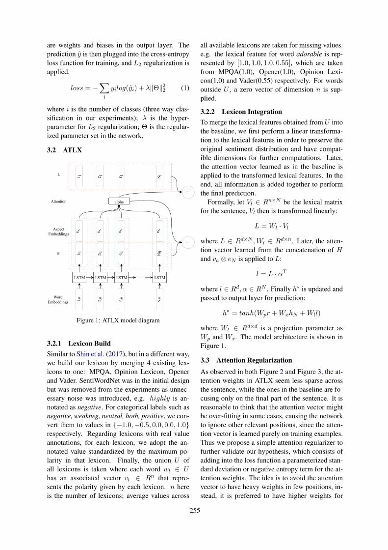
are weights and biases in the output layer. Theprediction y is then plugged into the cross-entropyloss function for training, and L2 regularization isapplied.

loss = −∑

i

yilog(yi) + λ‖Θ‖22 (1)

where i is the number of classes (three way clas-sification in our experiments); λ is the hyper-parameter for L2 regularization; Θ is the regular-ized parameter set in the network.

3.2 ATLX

LSTM

w1

h1va

LSTM

w2

h2va

LSTM

w3

h3va

LSTM

wN

hNva

...

alpha

l1 l2 l3 lN

rl

WordEmbeddings

H

AspectEmbeddings

Attention

L

Figure 1: ATLX model diagram

3.2.1 Lexicon BuildSimilar to Shin et al. (2017), but in a different way,we build our lexicon by merging 4 existing lex-icons to one: MPQA, Opinion Lexicon, Openerand Vader. SentiWordNet was in the initial designbut was removed from the experiments as unnec-essary noise was introduced, e.g. highly is an-notated as negative. For categorical labels such asnegative, weakneg, neutral, both, positive, we con-vert them to values in −1.0,−0.5, 0.0, 0.0, 1.0respectively. Regarding lexicons with real valueannotations, for each lexicon, we adopt the an-notated value standardized by the maximum po-larity in that lexicon. Finally, the union U ofall lexicons is taken where each word wl ∈ Uhas an associated vector vl ∈ Rn that repre-sents the polarity given by each lexicon. n hereis the number of lexicons; average values across

all available lexicons are taken for missing values.e.g. the lexical feature for word adorable is rep-resented by [1.0, 1.0, 1.0, 0.55], which are takenfrom MPQA(1.0), Opener(1.0), Opinion Lexi-con(1.0) and Vader(0.55) respectively. For wordsoutside U , a zero vector of dimension n is sup-plied.

3.2.2 Lexicon IntegrationTo merge the lexical features obtained from U intothe baseline, we first perform a linear transforma-tion to the lexical features in order to preserve theoriginal sentiment distribution and have compat-ible dimensions for further computations. Later,the attention vector learned as in the baseline isapplied to the transformed lexical features. In theend, all information is added together to performthe final prediction.

Formally, let Vl ∈ Rn×N be the lexical matrixfor the sentence, Vl then is transformed linearly:

L = Wl · Vl

where L ∈ Rd×N ,Wl ∈ Rd×n. Later, the atten-tion vector learned from the concatenation of Hand va ⊗ eN is applied to L:

l = L · αT

where l ∈ Rd, α ∈ RN . Finally h∗ is updated andpassed to output layer for prediction:

h∗ = tanh(Wpr +WxhN +Wll)

where Wl ∈ Rd×d is a projection parameter asWp and Wx. The model architecture is shown inFigure 1.

3.3 Attention RegularizationAs observed in both Figure 2 and Figure 3, the at-tention weights in ATLX seem less sparse acrossthe sentence, while the ones in the baseline are fo-cusing only on the final part of the sentence. It isreasonable to think that the attention vector mightbe over-fitting in some cases, causing the networkto ignore other relevant positions, since the atten-tion vector is learned purely on training examples.Thus we propose a simple attention regularizer tofurther validate our hypothesis, which consists ofadding into the loss function a parameterized stan-dard deviation or negative entropy term for the at-tention weights. The idea is to avoid the attentionvector to have heavy weights in few positions, in-stead, it is preferred to have higher weights for

255

more positions. Formally, the attention regular-ized loss is computed as:

loss = −∑

i

yilog(yi) + λ‖Θ‖22 + ε ·R(α) (2)

compared to equation (1), a second regularizationterm is added, where ε is the hyper-parameter forthe attention regularizer; R stands for the regular-ization term defined in (3) or (4); and α is the dis-tribution of attention weights. Note that duringimplementation, the attention weights for batchpadding positions are excluded from α.

We experiment two different regularizers, oneuses standard deviation of α defined in equation(3); the other one uses the negative entropy of αdefined in equation (4).

R(α) = σ(α) (3)

R(α) = −[−N∑

i

αi · log(αi)] (4)

4 Experiments

Figure 2: Comparison of attention weights betweenbaseline and ATLX; The rows annotated as ”Lexicon”indicates the average polarity per word given by U .

4.1 DatasetSame as Wang et al. (2016), we experiment onSemEval 2014 Task 4, restaurant domain dataset.The data consists of reviews of restaurants withaspects: food, price, service, ambience, miscel-laneous and associated polarities: positive, neu-tral, negative. The objective is to predict the po-larity given a sentence and an aspect. There are

Pos Neu Neg In CorpusMPQA 2298 440 4148 908OL 2004 3 4780 732Opener 2298 440 4147 908Vader 3333 0 4170 656Merged U 5129 404 7764 1234

Table 1: Lexicon statistics of positive, neutral, negativewords and number of words covered in corpus.

3,518 training examples and 973 test examples inthe corpus. To initialize word vectors with pre-trained word embeddings, the 300 dimensionalGlove vectors trained on 840b tokens are used, asdescribed in the original paper.

4.2 Lexicons

As shown in Table 1, we merge four existing andonline available lexicons into one. The mergedlexicon U as described in section 3.2.1 is usedfor our experiments. After the union, the fol-lowing postprocess is carried out: bar, try, tooare removed from U since they are unreason-ably annotated as negative by MPQA and Opener;n′t, not are added to U with −1 polarity fornegation.

4.3 Evaluation

Cross validation is applied to measure the perfor-mance of each model. In all experiments, the train-ing set is randomly shuffled and split into 6 foldswith a fixed random seed. According to the codereleased by Wang et al. (2016), a development setcontaining 528 examples is used, which is roughly16 of the training corpus. In order to remain faithfulto the original implementation, we thus evaluateour model with a cross validation of 6 folds.

As shown in Table 2, compared to the baselinesystem, ATLX is not only able to improve in termsof accuracy, but also the variance of the perfor-mance across different sets gets significantly re-duced. On the other hand, by adding attentionregularization to the baseline system without in-troducing lexical features, both the standard devi-ation regularizer (basestd) and the negative entropyregularizer (baseent) are able to contribute posi-tively; where baseent yields largest improvement.By combining attention regularization and lexicalfeatures together, although the model is able to fur-ther improve, the difference is too small to drawstrong conclusion.

256

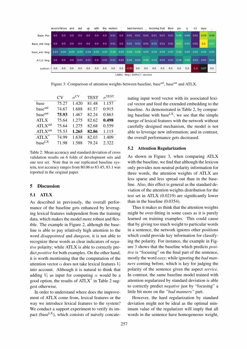
Figure 3: Comparison of attention weights between baseline, basestd, baseent and ATLX.

CV σCV TEST σTEST

base 75.27 1.420 81.48 1.157basestd 74.67 1.688 81.57 0.915baseent 75.93 1.467 82.24 0.863ATLX 75.64 1.275 82.62 0.498ATLXstd 75.64 1.275 82.68 0.559ATLXent 75.53 1.265 82.86 1.115ATLX* 74.99 1.638 82.03 1.409baseLX 71.98 1.588 79.24 2.322

Table 2: Mean accuracy and standard deviation of crossvalidation results on 6 folds of development sets andone test set. Note that in our replicated baseline sys-tem, test accuracy ranges from 80.06 to 83.45; 83.1 wasreported in the original paper.

5 Discussion

5.1 ATLXAs described in previously, the overall perfor-mance of the baseline gets enhanced by leverag-ing lexical features independent from the trainingdata, which makes the model more robust and flex-ible. The example in Figure 2, although the base-line is able to pay relatively high attention to theword disappointed and dungeon, it is not able torecognize these words as clear indicators of nega-tive polarity; while ATLX is able to correctly pre-dict positive for both examples. On the other hand,it is worth mentioning that the computation of theattention vector α does not take lexical features Vlinto account. Although it is natural to think thatadding Vl as input for computing α would be agood option, the results of ATLX* in Table 2 sug-gest otherwise.

In order to understand where does the improve-ment of ATLX come from, lexical features or theway we introduce lexical features to the system?We conduct a support experiment to verify its im-pact (baseLX), which consists of naively concate-

nating input word vector with its associated lexi-cal vector and feed the extended embedding to thebaseline. As demonstrated in Table 2, by compar-ing baseline with baseLX, we see that the simplemerge of lexical features with the network withoutcarefully designed mechanism, the model is notable to leverage new information; and in contrast,the overall performance gets decreased.

5.2 Attention Regularization

As shown in Figure 3, when comparing ATLXwith the baseline, we find that although the lexicononly provides non-neutral polarity information forthree words, the attention weights of ATLX areless sparse and less spread out than in the base-line. Also, this effect is general as the standard de-viation of the attention weights distribution for thetest set in ATLX (0.0219) are significantly lowerthan in the baseline (0.0354).

Thus it makes us think that the attention weightsmight be over-fitting in some cases as it is purelylearned on training examples. This could causethat by giving too much weight to particular wordsin a sentence, the network ignores other positionswhich could provide key information for classify-ing the polarity. For instance, the example in Fig-ure 3 shows that the baseline which predicts posi-tive is “focusing” on the final part of the sentence,mostly the word easy; while ignoring the bad man-ners coming before, which is key for judging thepolarity of the sentence given the aspect service.In contrast, the same baseline model trained withattention regularized by standard deviation is ableto correctly predict negative just by “focusing” alittle bit more on the ”bad manners” part.

However, the hard regularization by standarddeviation might not be ideal as the optimal min-imum value of the regularizer will imply that allwords in the sentence have homogeneous weight,

257

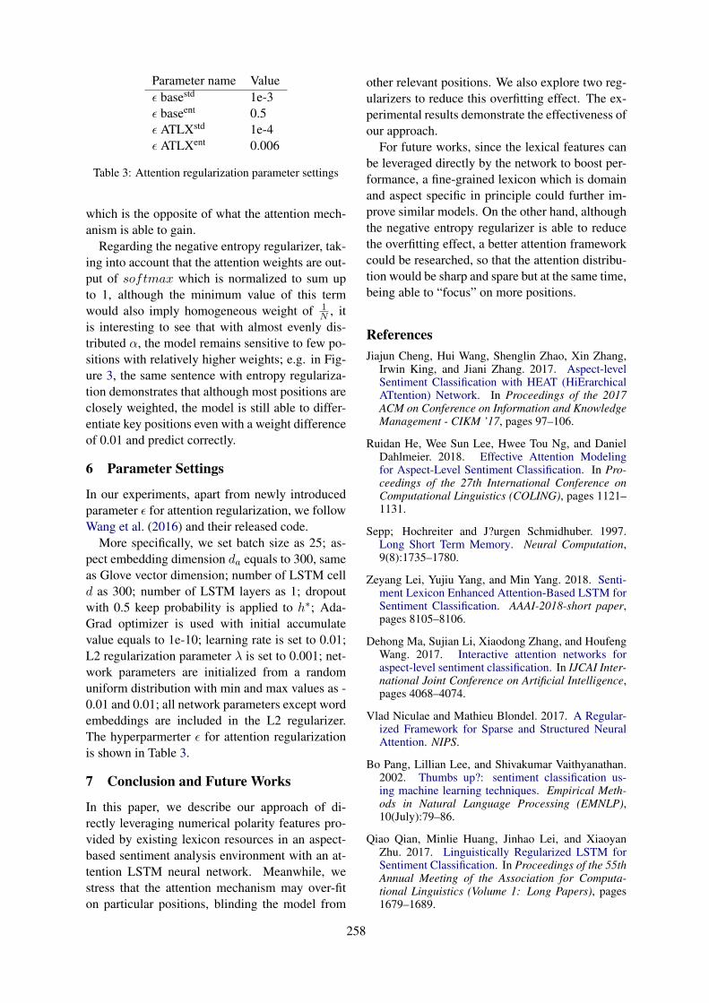
Parameter name Valueε basestd 1e-3ε baseent 0.5ε ATLXstd 1e-4ε ATLXent 0.006

Table 3: Attention regularization parameter settings

which is the opposite of what the attention mech-anism is able to gain.

Regarding the negative entropy regularizer, tak-ing into account that the attention weights are out-put of softmax which is normalized to sum upto 1, although the minimum value of this termwould also imply homogeneous weight of 1

N , itis interesting to see that with almost evenly dis-tributed α, the model remains sensitive to few po-sitions with relatively higher weights; e.g. in Fig-ure 3, the same sentence with entropy regulariza-tion demonstrates that although most positions areclosely weighted, the model is still able to differ-entiate key positions even with a weight differenceof 0.01 and predict correctly.

6 Parameter Settings

In our experiments, apart from newly introducedparameter ε for attention regularization, we followWang et al. (2016) and their released code.

More specifically, we set batch size as 25; as-pect embedding dimension da equals to 300, sameas Glove vector dimension; number of LSTM celld as 300; number of LSTM layers as 1; dropoutwith 0.5 keep probability is applied to h∗; Ada-Grad optimizer is used with initial accumulatevalue equals to 1e-10; learning rate is set to 0.01;L2 regularization parameter λ is set to 0.001; net-work parameters are initialized from a randomuniform distribution with min and max values as -0.01 and 0.01; all network parameters except wordembeddings are included in the L2 regularizer.The hyperparmerter ε for attention regularizationis shown in Table 3.

7 Conclusion and Future Works

In this paper, we describe our approach of di-rectly leveraging numerical polarity features pro-vided by existing lexicon resources in an aspect-based sentiment analysis environment with an at-tention LSTM neural network. Meanwhile, westress that the attention mechanism may over-fiton particular positions, blinding the model from

other relevant positions. We also explore two reg-ularizers to reduce this overfitting effect. The ex-perimental results demonstrate the effectiveness ofour approach.

For future works, since the lexical features canbe leveraged directly by the network to boost per-formance, a fine-grained lexicon which is domainand aspect specific in principle could further im-prove similar models. On the other hand, althoughthe negative entropy regularizer is able to reducethe overfitting effect, a better attention frameworkcould be researched, so that the attention distribu-tion would be sharp and spare but at the same time,being able to “focus” on more positions.

ReferencesJiajun Cheng, Hui Wang, Shenglin Zhao, Xin Zhang,

Irwin King, and Jiani Zhang. 2017. Aspect-levelSentiment Classification with HEAT (HiErarchicalATtention) Network. In Proceedings of the 2017ACM on Conference on Information and KnowledgeManagement - CIKM ’17, pages 97–106.

Ruidan He, Wee Sun Lee, Hwee Tou Ng, and DanielDahlmeier. 2018. Effective Attention Modelingfor Aspect-Level Sentiment Classification. In Pro-ceedings of the 27th International Conference onComputational Linguistics (COLING), pages 1121–1131.

Sepp; Hochreiter and J?urgen Schmidhuber. 1997.Long Short Term Memory. Neural Computation,9(8):1735–1780.

Zeyang Lei, Yujiu Yang, and Min Yang. 2018. Senti-ment Lexicon Enhanced Attention-Based LSTM forSentiment Classification. AAAI-2018-short paper,pages 8105–8106.

Dehong Ma, Sujian Li, Xiaodong Zhang, and HoufengWang. 2017. Interactive attention networks foraspect-level sentiment classification. In IJCAI Inter-national Joint Conference on Artificial Intelligence,pages 4068–4074.

Vlad Niculae and Mathieu Blondel. 2017. A Regular-ized Framework for Sparse and Structured NeuralAttention. NIPS.

Bo Pang, Lillian Lee, and Shivakumar Vaithyanathan.2002. Thumbs up?: sentiment classification us-ing machine learning techniques. Empirical Meth-ods in Natural Language Processing (EMNLP),10(July):79–86.

Qiao Qian, Minlie Huang, Jinhao Lei, and XiaoyanZhu. 2017. Linguistically Regularized LSTM forSentiment Classification. In Proceedings of the 55thAnnual Meeting of the Association for Computa-tional Linguistics (Volume 1: Long Papers), pages1679–1689.

258

Mickael Rouvier and Benoit Favre. 2016. SENSEI-LIF at SemEval-2016 Task 4 : Polarity embeddingfusion for robust sentiment analysis. In Proceed-ings of the 10th International Workshop on SemanticEvaluation (SemEval-2016), pages 207–213.

Bonggun Shin, Timothy Lee, and Jinho D Choi. 2017.Lexicon Integrated CNN Models with Attention forSentiment Analysis. ACL, pages 149–158.

Yi Tay, Luu Anh Tuan, and Siu Cheung Hui. 2017.Dyadic Memory Networks for Aspect-based Senti-ment Analysis. In Proceedings of the 2017 ACMon Conference on Information and Knowledge Man-agement - CIKM ’17, pages 107–116.

Zhiyang Teng, Duy-Tin Vo, and Yue Zhang. 2016.Context-Sensitive Lexicon Features for Neural Sen-timent Analysis. EMNLP, pages 1629–1638.

Peter D Turney. 2002. Thumbs up or thumbs down?Semantic Orientation applied to Unsupervised Clas-sification of Reviews. Proceedings of the 40th An-nual Meeting of the Association for ComputationalLinguistics (ACL), (July):417–424.

Yequan Wang, Minlie Huang, Li Zhao, and XiaoyanZhu. 2016. Attention-based LSTM for Aspect-levelSentiment Classification. Proceedings of the 2016Conference on Empirical Methods in Natural Lan-guage Processing (EMNLP), pages 606–615.

Theresa Wilson, Theresa Wilson, Janyce Wiebe,Janyce Wiebe, Rebecca Hwa, and Rebecca Hwa.2004. Just how mad are you? Finding strong andweak opinion clauses. Proceedings of the NationalConference on Artificial Intelligence, pages 761–769.

Ou Wu, Tao Yang, Mengyang Li, and Ming Li. 2018.$$-hot Lexicon Embedding-based Two-level LSTMfor Sentiment Analysis.

Jiajun Zhang, Yang Zhao, Haoran Li, and ChengqingZong. 2019. Attention with sparsity regularizationfor neural machine translation and summarization.IEEE/ACM Transactions on Audio Speech and Lan-guage Processing, 27(3):507–518.

Peisong Zhu and Tieyun Qian. 2018. Enhanced AspectLevel Sentiment Classification with Auxiliary Mem-ory. In COLING, pages 1077–1087.

Yicheng Zou, Tao Gui, Qi Zhang, and XuanjingHuang. 2018. A Lexicon-Based Supervised Atten-tion Model for Neural Sentiment Analysis. In COL-ING, pages 868–877.

A Supplemental Material

A.1 Resource DetailsLexical resources: MPQA1, Opinion Lexicon2,Opener3, and Vader4. Glove vectors5. Code6 re-leased by Wang et al. (2016). Experiments de-scribed in this paper are implemented with Ten-sorFlow7.

1http://mpqa.cs.pitt.edu/#subj lexicon2https://www.cs.uic.edu/liub/FBS/sentiment-

analysis.html#lexicon3https://github.com/opener-project/VU-sentiment-

lexicon/tree/master/VUSentimentLexicon/EN-lexicon4https://github.com/cjhutto/vaderSentiment5https://nlp.stanford.edu/projects/glove/6https://www.wangyequan.com/publications/7https://www.tensorflow.org/

259

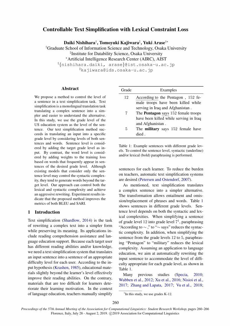
Proceedings of the 57th Annual Meeting of the Association for Computational Linguistics: Student Research Workshop, pages 260–266Florence, Italy, July 28 - August 2, 2019. c©2019 Association for Computational Linguistics

Controllable Text Simplification with Lexical Constraint Loss

Daiki Nishihara†, Tomoyuki Kajiwara‡, Yuki Arase†∗†Graduate School of Information Science and Technology, Osaka University

‡Institute for Datability Science, Osaka University∗Artificial Intelligence Research Center (AIRC), AIST

†nishihara.daiki, arase@ist.osaka-u.ac.jp‡kajiwara@ids.osaka-u.ac.jp

Abstract

We propose a method to control the level ofa sentence in a text simplification task. Textsimplification is a monolingual translation tasktranslating a complex sentence into a sim-pler and easier to understand the alternative.In this study, we use the grade level of theUS education system as the level of the sen-tence. Our text simplification method suc-ceeds in translating an input into a specificgrade level by considering levels of both sen-tences and words. Sentence level is consid-ered by adding the target grade level as in-put. By contrast, the word level is consid-ered by adding weights to the training lossbased on words that frequently appear in sen-tences of the desired grade level. Althoughexisting models that consider only the sen-tence level may control the syntactic complex-ity, they tend to generate words beyond the tar-get level. Our approach can control both thelexical and syntactic complexity and achievean aggressive rewriting. Experiment results in-dicate that the proposed method improves themetrics of both BLEU and SARI.

1 Introduction

Text simplification (Shardlow, 2014) is the taskof rewriting a complex text into a simpler formwhile preserving its meaning. Its applications in-clude reading comprehension assistance and lan-guage education support. Because each target userhas different reading abilities and/or knowledge,we need a text simplification system that translatesan input sentence into a sentence of an appropriatedifficulty level for each user. According to the in-put hypothesis (Krashen, 1985), educational mate-rials slightly beyond the learner’s level effectivelyimprove their reading abilities. On the contrary,materials that are too difficult for learners dete-riorate their learning motivation. In the contextof language education, teachers manually simplify

Grade Examples

12 According to the Pentagon , 152 fe-male troops have been killed whileserving in Iraq and Afghanistan .

7 The Pentagon says 152 female troopshave been killed while serving in Iraqand Afghanistan .

5 The military says 152 female havedied .

Table 1: Example sentences with different grade lev-els. To control the sentence level, syntactic (underline)and/or lexical (bold) paraphrasing is performed.

sentences for each learner. To reduce the burdenon teachers, automatic text simplification systemsare desired (Petersen and Ostendorf, 2007).

As mentioned, text simplification translatesa complex sentence into a simpler alternative.The transformation allows entailment and omis-sion/replacement of phrases and words. Table 1shows sentences in different grade levels. Sen-tence level depends on both the syntactic and lex-ical complexities. When simplifying a sentenceof grade level 12 into grade level 71, paraphrasing“According to ∼ ,” to “∼ says” reduces the syntac-tic complexity. In addition, when simplifying thesentence from the grade levels 12 to 5, paraphras-ing “Pentagon” to “military” reduces the lexicalcomplexity. Assuming an application to languageeducation, we aim at automatically rewriting theinput sentence to accommodate the level of diffi-culty appropriate for each grade level, as shown inTable 1.

Many previous studies (Specia, 2010;Wubben et al., 2012; Xu et al., 2016; Nisioi et al.,2017; Zhang and Lapata, 2017; Vu et al., 2018;

1In this study, we use grades K-12.

260

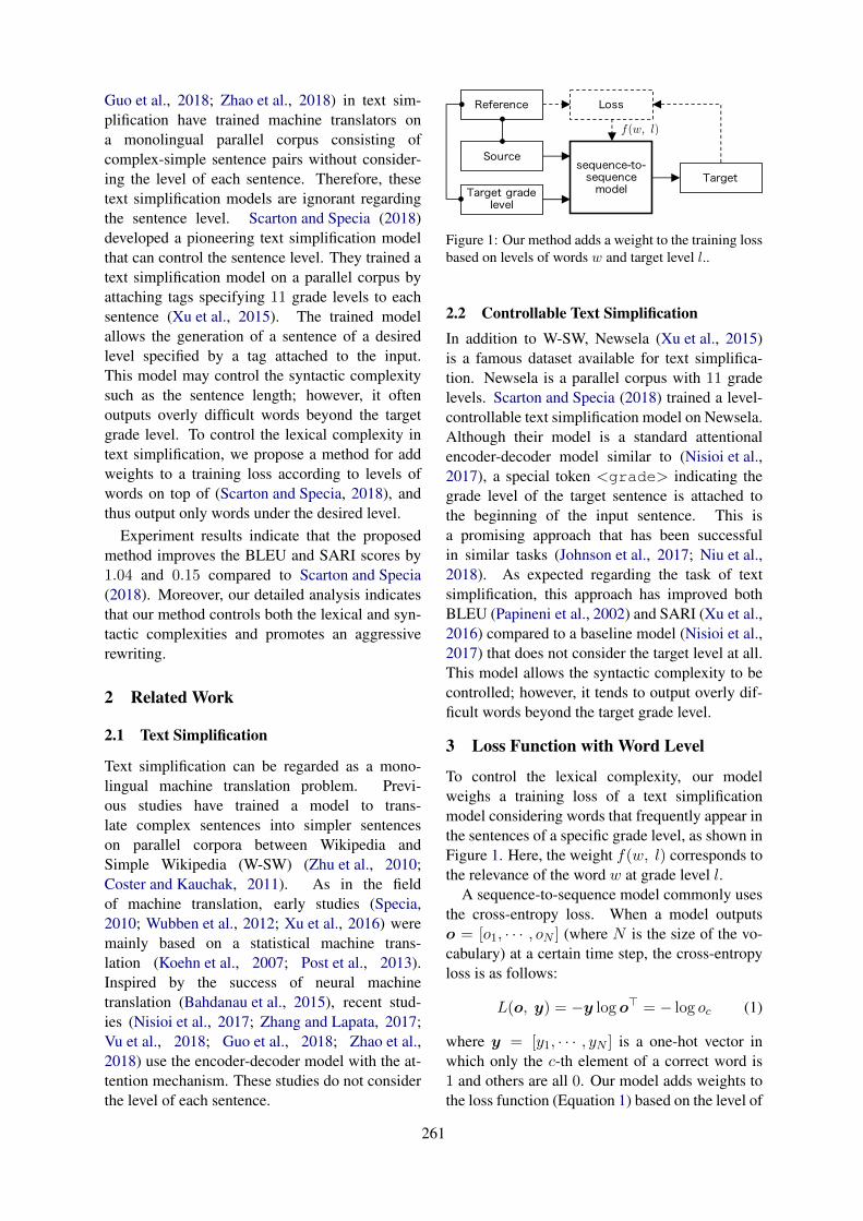
Guo et al., 2018; Zhao et al., 2018) in text sim-plification have trained machine translators ona monolingual parallel corpus consisting ofcomplex-simple sentence pairs without consider-ing the level of each sentence. Therefore, thesetext simplification models are ignorant regardingthe sentence level. Scarton and Specia (2018)developed a pioneering text simplification modelthat can control the sentence level. They trained atext simplification model on a parallel corpus byattaching tags specifying 11 grade levels to eachsentence (Xu et al., 2015). The trained modelallows the generation of a sentence of a desiredlevel specified by a tag attached to the input.This model may control the syntactic complexitysuch as the sentence length; however, it oftenoutputs overly difficult words beyond the targetgrade level. To control the lexical complexity intext simplification, we propose a method for addweights to a training loss according to levels ofwords on top of (Scarton and Specia, 2018), andthus output only words under the desired level.

Experiment results indicate that the proposedmethod improves the BLEU and SARI scores by1.04 and 0.15 compared to Scarton and Specia(2018). Moreover, our detailed analysis indicatesthat our method controls both the lexical and syn-tactic complexities and promotes an aggressiverewriting.

2 Related Work

2.1 Text Simplification

Text simplification can be regarded as a mono-lingual machine translation problem. Previ-ous studies have trained a model to trans-late complex sentences into simpler sentenceson parallel corpora between Wikipedia andSimple Wikipedia (W-SW) (Zhu et al., 2010;Coster and Kauchak, 2011). As in the fieldof machine translation, early studies (Specia,2010; Wubben et al., 2012; Xu et al., 2016) weremainly based on a statistical machine trans-lation (Koehn et al., 2007; Post et al., 2013).Inspired by the success of neural machinetranslation (Bahdanau et al., 2015), recent stud-ies (Nisioi et al., 2017; Zhang and Lapata, 2017;Vu et al., 2018; Guo et al., 2018; Zhao et al.,2018) use the encoder-decoder model with the at-tention mechanism. These studies do not considerthe level of each sentence.

Source

Reference

Target

Loss

sequence-to-sequence modelTarget grade

level

Figure 1: Our method adds a weight to the training lossbased on levels of words w and target level l..

2.2 Controllable Text SimplificationIn addition to W-SW, Newsela (Xu et al., 2015)is a famous dataset available for text simplifica-tion. Newsela is a parallel corpus with 11 gradelevels. Scarton and Specia (2018) trained a level-controllable text simplification model on Newsela.Although their model is a standard attentionalencoder-decoder model similar to (Nisioi et al.,2017), a special token <grade> indicating thegrade level of the target sentence is attached tothe beginning of the input sentence. This isa promising approach that has been successfulin similar tasks (Johnson et al., 2017; Niu et al.,2018). As expected regarding the task of textsimplification, this approach has improved bothBLEU (Papineni et al., 2002) and SARI (Xu et al.,2016) compared to a baseline model (Nisioi et al.,2017) that does not consider the target level at all.This model allows the syntactic complexity to becontrolled; however, it tends to output overly dif-ficult words beyond the target grade level.

3 Loss Function with Word Level

To control the lexical complexity, our modelweighs a training loss of a text simplificationmodel considering words that frequently appear inthe sentences of a specific grade level, as shown inFigure 1. Here, the weight f(w, l) corresponds tothe relevance of the word w at grade level l.

A sequence-to-sequence model commonly usesthe cross-entropy loss. When a model outputso = [o1, · · · , oN ] (where N is the size of the vo-cabulary) at a certain time step, the cross-entropyloss is as follows:

L(o, y) = −y log o⊤ = − log oc (1)

where y = [y1, · · · , yN ] is a one-hot vector inwhich only the c-th element of a correct word is1 and others are all 0. Our model adds weights tothe loss function (Equation 1) based on the level of

261

words such that the model learns to output wordsof the desired level:

L′(o, y, w, l) = −f(w, l) · log oc. (2)

As f(·, ·), we use TFIDF or PPMI assuming thatwords frequently appear in sentences of level l alsohave the same level l.

TFIDF We compute the TFIDF regarding sen-tences of the same level as a document:

TFIDF(w, l) = P (w | l) · logD

DF(w)(3)

where P (w | l) is a probability that word wappears in a set of sentences of grade level l,D is the number of grade levels2, and DF(w)is the number of grade levels in which w ap-pears. By so doing, TFIDF provides moreweights to words that uniquely appear in thesentences of a specific level.

PPMI Pointwise mutual information (PMI) al-lows estimating the strength of a co-occurrence between w and l:

PMI(w, l) = logP (w | l)

P (w). (4)

where P (w) is a probability of word w be-ing within the entire training corpus, whereasP (w | l) is the same as Equation 3. Wordswith negative PMI scores have a negative cor-relation against l that means w tends to ap-pear across different sentence levels. Hence,we ignore w with a negative PMI using apositive-PMI (PPMI) function:

PPMI(w, l) = max(PMI(w, l), 0). (5)

Both TFIDF and PPMI have a range of [0, ∞),and thus we apply the Laplace smoothing:

f(w, l) = Func(w, l) + 1 (6)

Func ∈ PPMI, TFIDF (7)

4 Experiment

4.1 DatasetWe evaluated whether our method can controlthe grade levels in a text simplification using theNewsela corpus. The Newsela corpus provides

2Here, D = 11 because we use grade levels 2 to 12.

Grade #Sentences #Words S-length

2 953 9, 882 10.373 3, 865 47, 211 12.224 43, 971 618, 184 14.065 31, 918 526, 769 16.506 19, 535 367, 319 18.807 17, 322 356, 307 20.578 15, 446 376, 678 24.399 7, 897 200, 242 25.3610 1, 018 30, 693 30.1511 104 2, 844 27.3512 50, 799 1, 484, 625 29.23

All 192, 828 4, 020, 754 20.85

Table 2: Statistics for the Newsela corpus, where S-length shows the average number of words in a sen-tence.

news articles of different levels, which have beenmanually rewritten by human experts. It conformsto the grade levels in the US education system,where the levels range from 2 to 12.

We use the publicly available version of theNewsela corpus3 that has been sentence-alignedby Xu et al. (2015) and divided into 94k, 1k, and1k sentences for the training, development, andtest, respectively, by Zhang and Lapata (2017).As in previous studies, we regard each sen-tence in an article as sharing the same levelas the entire article. Zhang and Lapata (2017)first divided the set of articles and then ex-tracted sentence pairs to avoid the same sen-tences appearing in both the training and testsets. Note that the Newsela corpus used in(Scarton and Specia, 2018) is different from thepresent corpus, and is preprocessed differently.Due to these differences, the training, develop-ment, and test sets used in (Scarton and Specia,2018) are unreproducible. Therefore, we reimple-mented (Scarton and Specia, 2018) and comparedit to our method using our public corpus.

Table 2 shows statistics for the Newsela cor-pus, which clearly present the tendency that lowergrade sentences are significantly shorter than thoseof higher grades. This indicates that aggressiveomission of phrases is required to simplify sen-tences of grade 8 to 12 into those of grade 2 to 7.

3https://newsela.com/data/

262

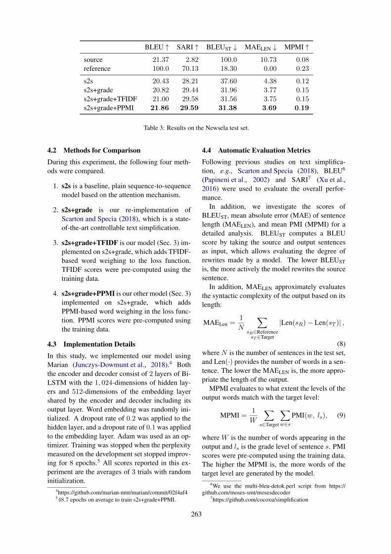
BLEU ↑ SARI ↑ BLEUST ↓ MAELEN ↓ MPMI ↑source 21.37 2.82 100.0 10.73 0.08reference 100.0 70.13 18.30 0.00 0.23

s2s 20.43 28.21 37.60 4.38 0.12s2s+grade 20.82 29.44 31.96 3.77 0.15s2s+grade+TFIDF 21.00 29.58 31.56 3.75 0.15s2s+grade+PPMI 21.86 29.59 31.38 3.69 0.19

Table 3: Results on the Newsela test set.

4.2 Methods for ComparisonDuring this experiment, the following four meth-ods were compared.

1. s2s is a baseline, plain sequence-to-sequencemodel based on the attention mechanism.

2. s2s+grade is our re-implementation ofScarton and Specia (2018), which is a state-of-the-art controllable text simplification.

3. s2s+grade+TFIDF is our model (Sec. 3) im-plemented on s2s+grade, which adds TFIDF-based word weighing to the loss function.TFIDF scores were pre-computed using thetraining data.

4. s2s+grade+PPMI is our other model (Sec. 3)implemented on s2s+grade, which addsPPMI-based word weighing in the loss func-tion. PPMI scores were pre-computed usingthe training data.

4.3 Implementation DetailsIn this study, we implemented our model usingMarian (Junczys-Dowmunt et al., 2018).4 Boththe encoder and decoder consist of 2 layers of Bi-LSTM with the 1, 024-dimensions of hidden lay-ers and 512-dimensions of the embedding layershared by the encoder and decoder including itsoutput layer. Word embedding was randomly ini-tialized. A dropout rate of 0.2 was applied to thehidden layer, and a dropout rate of 0.1 was appliedto the embedding layer. Adam was used as an op-timizer. Training was stopped when the perplexitymeasured on the development set stopped improv-ing for 8 epochs.5 All scores reported in this ex-periment are the averages of 3 trials with randominitialization.

4https://github.com/marian-nmt/marian/commit/02f4af4548.7 epochs on average to train s2s+grade+PPMI.

4.4 Automatic Evaluation MetricsFollowing previous studies on text simplifica-tion, e.g., Scarton and Specia (2018), BLEU6

(Papineni et al., 2002) and SARI7 (Xu et al.,2016) were used to evaluate the overall perfor-mance.

In addition, we investigate the scores ofBLEUST, mean absolute error (MAE) of sentencelength (MAELEN), and mean PMI (MPMI) for adetailed analysis. BLEUST computes a BLEUscore by taking the source and output sentencesas input, which allows evaluating the degree ofrewrites made by a model. The lower BLEUSTis, the more actively the model rewrites the sourcesentence.

In addition, MAELEN approximately evaluatesthe syntactic complexity of the output based on itslength:

MAELen =1

N

∑

sR∈ReferencesT ∈Target

|Len(sR) − Len(sT )| ,

(8)where N is the number of sentences in the test set,and Len(·) provides the number of words in a sen-tence. The lower the MAELEN is, the more appro-priate the length of the output.

MPMI evaluates to what extent the levels of theoutput words match with the target level:

MPMI =1

W

∑

s∈Target

∑

w∈s

PMI(w, ls), (9)

where W is the number of words appearing in theoutput and ls is the grade level of sentence s. PMIscores were pre-computed using the training data.The higher the MPMI is, the more words of thetarget level are generated by the model.

6We use the multi-bleu-detok.perl script from https://github.com/moses-smt/mosesdecoder

7https://github.com/cocoxu/simplification

263

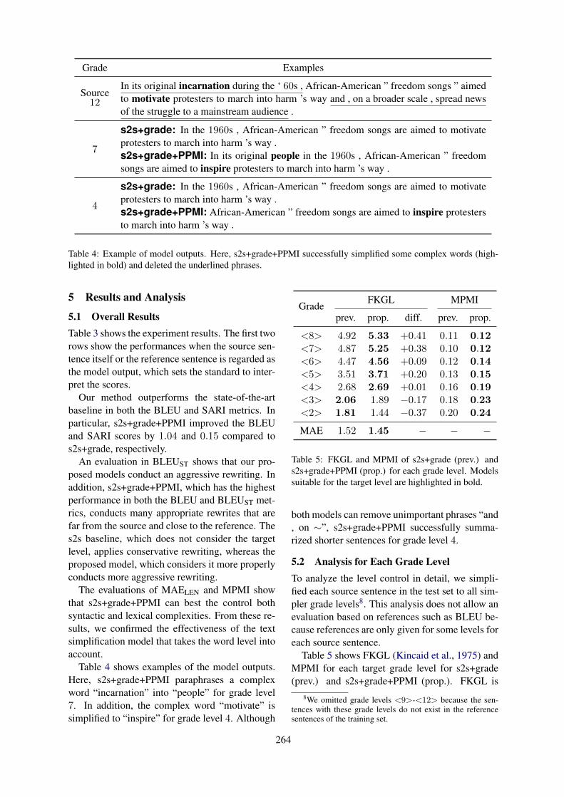
Grade Examples

Source12

In its original incarnation during the ‘ 60s , African-American ” freedom songs ” aimedto motivate protesters to march into harm ’s way and , on a broader scale , spread newsof the struggle to a mainstream audience .

7

s2s+grade: In the 1960s , African-American ” freedom songs are aimed to motivateprotesters to march into harm ’s way .s2s+grade+PPMI: In its original people in the 1960s , African-American ” freedomsongs are aimed to inspire protesters to march into harm ’s way .

4

s2s+grade: In the 1960s , African-American ” freedom songs are aimed to motivateprotesters to march into harm ’s way .s2s+grade+PPMI: African-American ” freedom songs are aimed to inspire protestersto march into harm ’s way .

Table 4: Example of model outputs. Here, s2s+grade+PPMI successfully simplified some complex words (high-lighted in bold) and deleted the underlined phrases.

5 Results and Analysis

5.1 Overall ResultsTable 3 shows the experiment results. The first tworows show the performances when the source sen-tence itself or the reference sentence is regarded asthe model output, which sets the standard to inter-pret the scores.

Our method outperforms the state-of-the-artbaseline in both the BLEU and SARI metrics. Inparticular, s2s+grade+PPMI improved the BLEUand SARI scores by 1.04 and 0.15 compared tos2s+grade, respectively.

An evaluation in BLEUST shows that our pro-posed models conduct an aggressive rewriting. Inaddition, s2s+grade+PPMI, which has the highestperformance in both the BLEU and BLEUST met-rics, conducts many appropriate rewrites that arefar from the source and close to the reference. Thes2s baseline, which does not consider the targetlevel, applies conservative rewriting, whereas theproposed model, which considers it more properlyconducts more aggressive rewriting.

The evaluations of MAELEN and MPMI showthat s2s+grade+PPMI can best the control bothsyntactic and lexical complexities. From these re-sults, we confirmed the effectiveness of the textsimplification model that takes the word level intoaccount.

Table 4 shows examples of the model outputs.Here, s2s+grade+PPMI paraphrases a complexword “incarnation” into “people” for grade level7. In addition, the complex word “motivate” issimplified to “inspire” for grade level 4. Although

GradeFKGL MPMI

prev. prop. diff. prev. prop.

<8> 4.92 5.33 +0.41 0.11 0.12<7> 4.87 5.25 +0.38 0.10 0.12<6> 4.47 4.56 +0.09 0.12 0.14<5> 3.51 3.71 +0.20 0.13 0.15<4> 2.68 2.69 +0.01 0.16 0.19<3> 2.06 1.89 −0.17 0.18 0.23<2> 1.81 1.44 −0.37 0.20 0.24

MAE 1.52 1.45 − − −

Table 5: FKGL and MPMI of s2s+grade (prev.) ands2s+grade+PPMI (prop.) for each grade level. Modelssuitable for the target level are highlighted in bold.

both models can remove unimportant phrases “and, on ∼”, s2s+grade+PPMI successfully summa-rized shorter sentences for grade level 4.

5.2 Analysis for Each Grade LevelTo analyze the level control in detail, we simpli-fied each source sentence in the test set to all sim-pler grade levels8. This analysis does not allow anevaluation based on references such as BLEU be-cause references are only given for some levels foreach source sentence.

Table 5 shows FKGL (Kincaid et al., 1975) andMPMI for each target grade level for s2s+grade(prev.) and s2s+grade+PPMI (prop.). FKGL is

8We omitted grade levels <9>-<12> because the sen-tences with these grade levels do not exist in the referencesentences of the training set.

264

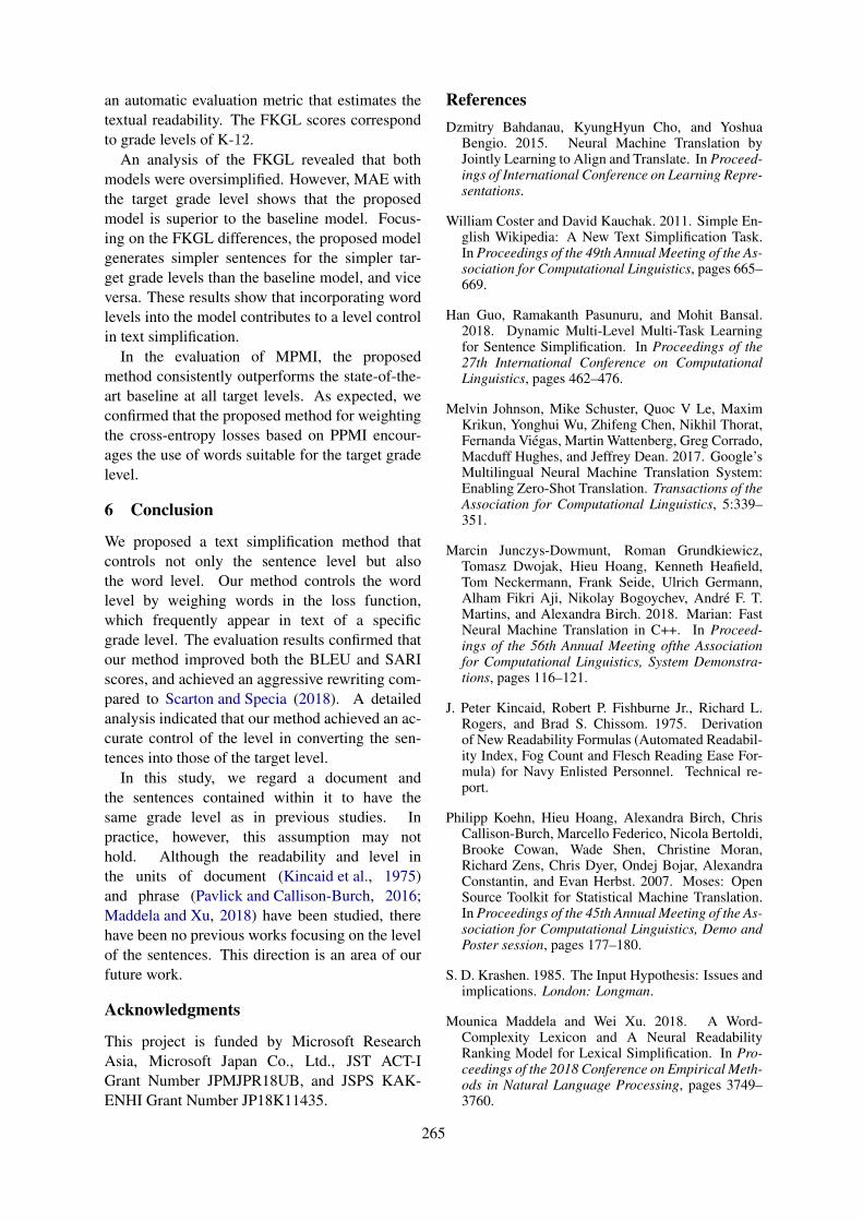
an automatic evaluation metric that estimates thetextual readability. The FKGL scores correspondto grade levels of K-12.

An analysis of the FKGL revealed that bothmodels were oversimplified. However, MAE withthe target grade level shows that the proposedmodel is superior to the baseline model. Focus-ing on the FKGL differences, the proposed modelgenerates simpler sentences for the simpler tar-get grade levels than the baseline model, and viceversa. These results show that incorporating wordlevels into the model contributes to a level controlin text simplification.

In the evaluation of MPMI, the proposedmethod consistently outperforms the state-of-the-art baseline at all target levels. As expected, weconfirmed that the proposed method for weightingthe cross-entropy losses based on PPMI encour-ages the use of words suitable for the target gradelevel.

6 Conclusion

We proposed a text simplification method thatcontrols not only the sentence level but alsothe word level. Our method controls the wordlevel by weighing words in the loss function,which frequently appear in text of a specificgrade level. The evaluation results confirmed thatour method improved both the BLEU and SARIscores, and achieved an aggressive rewriting com-pared to Scarton and Specia (2018). A detailedanalysis indicated that our method achieved an ac-curate control of the level in converting the sen-tences into those of the target level.

In this study, we regard a document andthe sentences contained within it to have thesame grade level as in previous studies. Inpractice, however, this assumption may nothold. Although the readability and level inthe units of document (Kincaid et al., 1975)and phrase (Pavlick and Callison-Burch, 2016;Maddela and Xu, 2018) have been studied, therehave been no previous works focusing on the levelof the sentences. This direction is an area of ourfuture work.

Acknowledgments

This project is funded by Microsoft ResearchAsia, Microsoft Japan Co., Ltd., JST ACT-IGrant Number JPMJPR18UB, and JSPS KAK-ENHI Grant Number JP18K11435.

ReferencesDzmitry Bahdanau, KyungHyun Cho, and Yoshua

Bengio. 2015. Neural Machine Translation byJointly Learning to Align and Translate. In Proceed-ings of International Conference on Learning Repre-sentations.

William Coster and David Kauchak. 2011. Simple En-glish Wikipedia: A New Text Simplification Task.In Proceedings of the 49th Annual Meeting of the As-sociation for Computational Linguistics, pages 665–669.

Han Guo, Ramakanth Pasunuru, and Mohit Bansal.2018. Dynamic Multi-Level Multi-Task Learningfor Sentence Simplification. In Proceedings of the27th International Conference on ComputationalLinguistics, pages 462–476.

Melvin Johnson, Mike Schuster, Quoc V Le, MaximKrikun, Yonghui Wu, Zhifeng Chen, Nikhil Thorat,Fernanda Viegas, Martin Wattenberg, Greg Corrado,Macduff Hughes, and Jeffrey Dean. 2017. Google’sMultilingual Neural Machine Translation System:Enabling Zero-Shot Translation. Transactions of theAssociation for Computational Linguistics, 5:339–351.

Marcin Junczys-Dowmunt, Roman Grundkiewicz,Tomasz Dwojak, Hieu Hoang, Kenneth Heafield,Tom Neckermann, Frank Seide, Ulrich Germann,Alham Fikri Aji, Nikolay Bogoychev, Andre F. T.Martins, and Alexandra Birch. 2018. Marian: FastNeural Machine Translation in C++. In Proceed-ings of the 56th Annual Meeting ofthe Associationfor Computational Linguistics, System Demonstra-tions, pages 116–121.

J. Peter Kincaid, Robert P. Fishburne Jr., Richard L.Rogers, and Brad S. Chissom. 1975. Derivationof New Readability Formulas (Automated Readabil-ity Index, Fog Count and Flesch Reading Ease For-mula) for Navy Enlisted Personnel. Technical re-port.

Philipp Koehn, Hieu Hoang, Alexandra Birch, ChrisCallison-Burch, Marcello Federico, Nicola Bertoldi,Brooke Cowan, Wade Shen, Christine Moran,Richard Zens, Chris Dyer, Ondej Bojar, AlexandraConstantin, and Evan Herbst. 2007. Moses: OpenSource Toolkit for Statistical Machine Translation.In Proceedings of the 45th Annual Meeting of the As-sociation for Computational Linguistics, Demo andPoster session, pages 177–180.

S. D. Krashen. 1985. The Input Hypothesis: Issues andimplications. London: Longman.

Mounica Maddela and Wei Xu. 2018. A Word-Complexity Lexicon and A Neural ReadabilityRanking Model for Lexical Simplification. In Pro-ceedings of the 2018 Conference on Empirical Meth-ods in Natural Language Processing, pages 3749–3760.

265

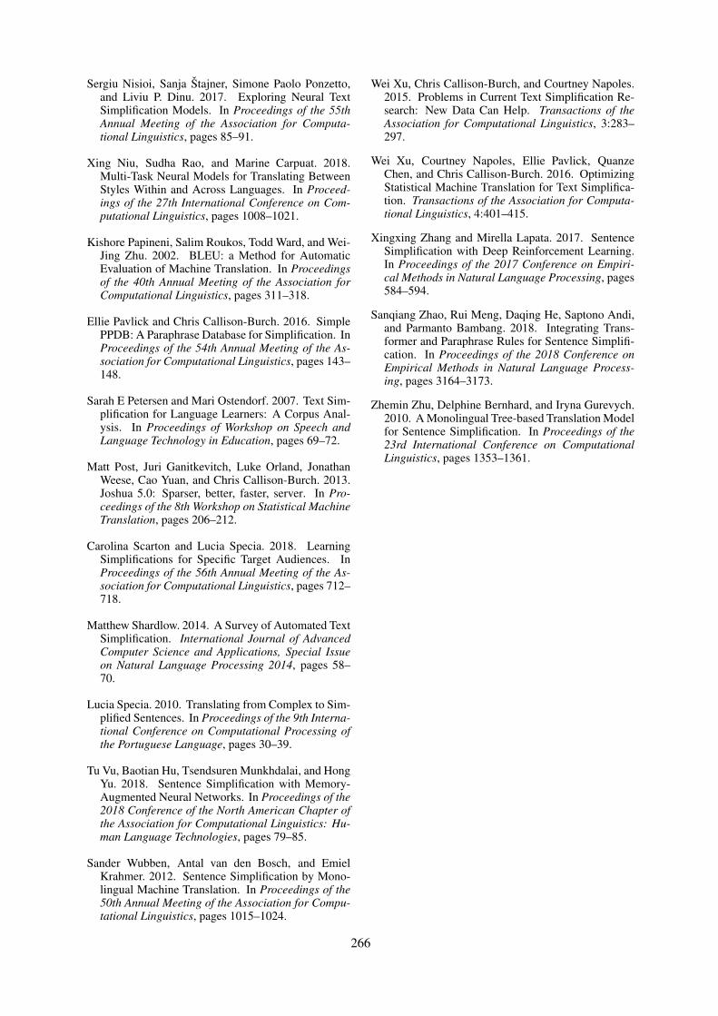
Sergiu Nisioi, Sanja Stajner, Simone Paolo Ponzetto,and Liviu P. Dinu. 2017. Exploring Neural TextSimplification Models. In Proceedings of the 55thAnnual Meeting of the Association for Computa-tional Linguistics, pages 85–91.

Xing Niu, Sudha Rao, and Marine Carpuat. 2018.Multi-Task Neural Models for Translating BetweenStyles Within and Across Languages. In Proceed-ings of the 27th International Conference on Com-putational Linguistics, pages 1008–1021.

Kishore Papineni, Salim Roukos, Todd Ward, and Wei-Jing Zhu. 2002. BLEU: a Method for AutomaticEvaluation of Machine Translation. In Proceedingsof the 40th Annual Meeting of the Association forComputational Linguistics, pages 311–318.

Ellie Pavlick and Chris Callison-Burch. 2016. SimplePPDB: A Paraphrase Database for Simplification. InProceedings of the 54th Annual Meeting of the As-sociation for Computational Linguistics, pages 143–148.

Sarah E Petersen and Mari Ostendorf. 2007. Text Sim-plification for Language Learners: A Corpus Anal-ysis. In Proceedings of Workshop on Speech andLanguage Technology in Education, pages 69–72.

Matt Post, Juri Ganitkevitch, Luke Orland, JonathanWeese, Cao Yuan, and Chris Callison-Burch. 2013.Joshua 5.0: Sparser, better, faster, server. In Pro-ceedings of the 8th Workshop on Statistical MachineTranslation, pages 206–212.

Carolina Scarton and Lucia Specia. 2018. LearningSimplifications for Specific Target Audiences. InProceedings of the 56th Annual Meeting of the As-sociation for Computational Linguistics, pages 712–718.

Matthew Shardlow. 2014. A Survey of Automated TextSimplification. International Journal of AdvancedComputer Science and Applications, Special Issueon Natural Language Processing 2014, pages 58–70.

Lucia Specia. 2010. Translating from Complex to Sim-plified Sentences. In Proceedings of the 9th Interna-tional Conference on Computational Processing ofthe Portuguese Language, pages 30–39.

Tu Vu, Baotian Hu, Tsendsuren Munkhdalai, and HongYu. 2018. Sentence Simplification with Memory-Augmented Neural Networks. In Proceedings of the2018 Conference of the North American Chapter ofthe Association for Computational Linguistics: Hu-man Language Technologies, pages 79–85.

Sander Wubben, Antal van den Bosch, and EmielKrahmer. 2012. Sentence Simplification by Mono-lingual Machine Translation. In Proceedings of the50th Annual Meeting of the Association for Compu-tational Linguistics, pages 1015–1024.

Wei Xu, Chris Callison-Burch, and Courtney Napoles.2015. Problems in Current Text Simplification Re-search: New Data Can Help. Transactions of theAssociation for Computational Linguistics, 3:283–297.

Wei Xu, Courtney Napoles, Ellie Pavlick, QuanzeChen, and Chris Callison-Burch. 2016. OptimizingStatistical Machine Translation for Text Simplifica-tion. Transactions of the Association for Computa-tional Linguistics, 4:401–415.

Xingxing Zhang and Mirella Lapata. 2017. SentenceSimplification with Deep Reinforcement Learning.In Proceedings of the 2017 Conference on Empiri-cal Methods in Natural Language Processing, pages584–594.

Sanqiang Zhao, Rui Meng, Daqing He, Saptono Andi,and Parmanto Bambang. 2018. Integrating Trans-former and Paraphrase Rules for Sentence Simplifi-cation. In Proceedings of the 2018 Conference onEmpirical Methods in Natural Language Process-ing, pages 3164–3173.

Zhemin Zhu, Delphine Bernhard, and Iryna Gurevych.2010. A Monolingual Tree-based Translation Modelfor Sentence Simplification. In Proceedings of the23rd International Conference on ComputationalLinguistics, pages 1353–1361.

266

Proceedings of the 57th Annual Meeting of the Association for Computational Linguistics: Student Research Workshop, pages 267–272Florence, Italy, July 28 - August 2, 2019. c©2019 Association for Computational Linguistics

Normalizing Non-canonical Turkish TextsUsing Machine Translation Approaches

Talha ColakogluIstanbul Technical University

Istanbul, Turkeycolakoglut@itu.edu.tr

Umut SulubacakUniversity of Helsinki

Helsinki, Finlandumut.sulubacak@helsinki.fi

A. Cuneyd TantugIstanbul Technical University

Istanbul, Turkeytantug@itu.edu.tr

AbstractWith the growth of the social web, user-generated text data has reached unprecedentedsizes. Non-canonical text normalization pro-vides a way to exploit this as a practicalsource of training data for language process-ing systems. The state of the art in Turk-ish text normalization is composed of a token-level pipeline of modules, heavily dependenton external linguistic resources and manually-defined rules. Instead, we propose a fully-automated, context-aware machine translationapproach with fewer stages of processing. Ex-periments with various implementations of ourapproach show that we are able to surpass thecurrent best-performing system by a large mar-gin.

1 Introduction

Supervised machine learning methods such asCRFs, SVMs, and neural networks have come todefine standard solutions for a wide variety of lan-guage processing tasks. These methods are typ-ically data-driven, and require training on a sub-stantial amount of data to reach their potential.This kind of data often has to be manually anno-tated, which constitutes a bottleneck in develop-ment. This is especially marked in some tasks,where quality or structural requirements for thedata are more constraining. Among the exam-ples are text normalization and machine transla-tion (MT), as both tasks require parallel data withlimited natural availability.

The success achieved by data-driven learn-ing methods brought about an interest in user-generated data. Collaborative online platformssuch as social media are a great source of largeamounts of text data. However, these texts typi-cally contain non-canonical usages, making themhard to leverage for systems sensitive to training

data bias. Non-canonical text normalization is thetask of processing such texts into a canonical for-mat. As such, normalizing user-generated data hasthe capability of producing large amounts of ser-viceable data for training data-driven systems.

As a denoising task, text normalization can beregarded as a translation problem between closelyrelated languages. Statistical machine translation(SMT) methods dominated the field of MT for awhile, until neural machine translation (NMT) be-came more popular. The modular composition ofan SMT system makes it less susceptible to datascarcity, and allows it to better exploit unaligneddata. In contrast, NMT is more data-hungry, with asuperior capacity for learning from data, but oftenfaring worse when data is scarce. Both translationmethods are very powerful in generalization.

In this study, we investigate the potential ofusing MT methods to normalize non-canonicaltexts in Turkish, a morphologically-rich, aggluti-native language, allowing for a very large numberof common word forms. Following in the foot-steps of unsupervised MT approaches, we auto-matically generate synthetic parallel data from un-aligned sources of “monolingual” canonical andnon-canonical texts. Afterwards, we use thesedatasets to train character-based translation sys-tems to normalize non-canonical texts1. We de-scribe our methodology in contrast with the stateof the art in Section 3, outline our data and empir-ical results in Sections 4 and 5, and finally presentour conclusions in Section 6.

2 Related Work

Non-canonical text normalization has been rela-tively slow to catch up with purely data-driven

1We have released the source code of the project athttps://github.com/talha252/tur-text-norm

267

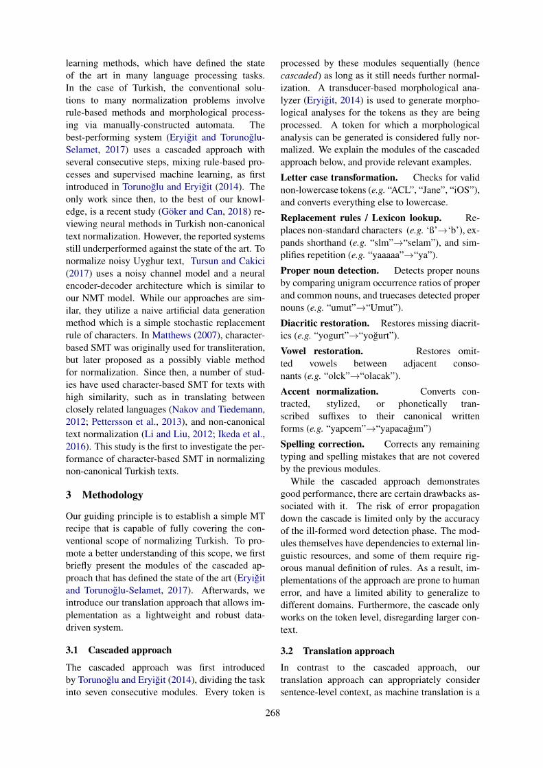
learning methods, which have defined the stateof the art in many language processing tasks.In the case of Turkish, the conventional solu-tions to many normalization problems involverule-based methods and morphological process-ing via manually-constructed automata. Thebest-performing system (Eryigit and Torunoglu-Selamet, 2017) uses a cascaded approach withseveral consecutive steps, mixing rule-based pro-cesses and supervised machine learning, as firstintroduced in Torunoglu and Eryigit (2014). Theonly work since then, to the best of our knowl-edge, is a recent study (Goker and Can, 2018) re-viewing neural methods in Turkish non-canonicaltext normalization. However, the reported systemsstill underperformed against the state of the art. Tonormalize noisy Uyghur text, Tursun and Cakici(2017) uses a noisy channel model and a neuralencoder-decoder architecture which is similar toour NMT model. While our approaches are sim-ilar, they utilize a naive artificial data generationmethod which is a simple stochastic replacementrule of characters. In Matthews (2007), character-based SMT was originally used for transliteration,but later proposed as a possibly viable methodfor normalization. Since then, a number of stud-ies have used character-based SMT for texts withhigh similarity, such as in translating betweenclosely related languages (Nakov and Tiedemann,2012; Pettersson et al., 2013), and non-canonicaltext normalization (Li and Liu, 2012; Ikeda et al.,2016). This study is the first to investigate the per-formance of character-based SMT in normalizingnon-canonical Turkish texts.

3 Methodology

Our guiding principle is to establish a simple MTrecipe that is capable of fully covering the con-ventional scope of normalizing Turkish. To pro-mote a better understanding of this scope, we firstbriefly present the modules of the cascaded ap-proach that has defined the state of the art (Eryigitand Torunoglu-Selamet, 2017). Afterwards, weintroduce our translation approach that allows im-plementation as a lightweight and robust data-driven system.

3.1 Cascaded approach

The cascaded approach was first introducedby Torunoglu and Eryigit (2014), dividing the taskinto seven consecutive modules. Every token is

processed by these modules sequentially (hencecascaded) as long as it still needs further normal-ization. A transducer-based morphological ana-lyzer (Eryigit, 2014) is used to generate morpho-logical analyses for the tokens as they are beingprocessed. A token for which a morphologicalanalysis can be generated is considered fully nor-malized. We explain the modules of the cascadedapproach below, and provide relevant examples.

Letter case transformation. Checks for validnon-lowercase tokens (e.g. “ACL”, “Jane”, “iOS”),and converts everything else to lowercase.

Replacement rules / Lexicon lookup. Re-places non-standard characters (e.g. ‘ß’→‘b’), ex-pands shorthand (e.g. “slm”→“selam”), and sim-plifies repetition (e.g. “yaaaaa”→“ya”).

Proper noun detection. Detects proper nounsby comparing unigram occurrence ratios of properand common nouns, and truecases detected propernouns (e.g. “umut”→“Umut”).

Diacritic restoration. Restores missing diacrit-ics (e.g. “yogurt”→“yogurt”).

Vowel restoration. Restores omit-ted vowels between adjacent conso-nants (e.g. “olck”→“olacak”).

Accent normalization. Converts con-tracted, stylized, or phonetically tran-scribed suffixes to their canonical writtenforms (e.g. “yapcem”→“yapacagım”)

Spelling correction. Corrects any remainingtyping and spelling mistakes that are not coveredby the previous modules.

While the cascaded approach demonstratesgood performance, there are certain drawbacks as-sociated with it. The risk of error propagationdown the cascade is limited only by the accuracyof the ill-formed word detection phase. The mod-ules themselves have dependencies to external lin-guistic resources, and some of them require rig-orous manual definition of rules. As a result, im-plementations of the approach are prone to humanerror, and have a limited ability to generalize todifferent domains. Furthermore, the cascade onlyworks on the token level, disregarding larger con-text.

3.2 Translation approach

In contrast to the cascaded approach, ourtranslation approach can appropriately considersentence-level context, as machine translation is a

268

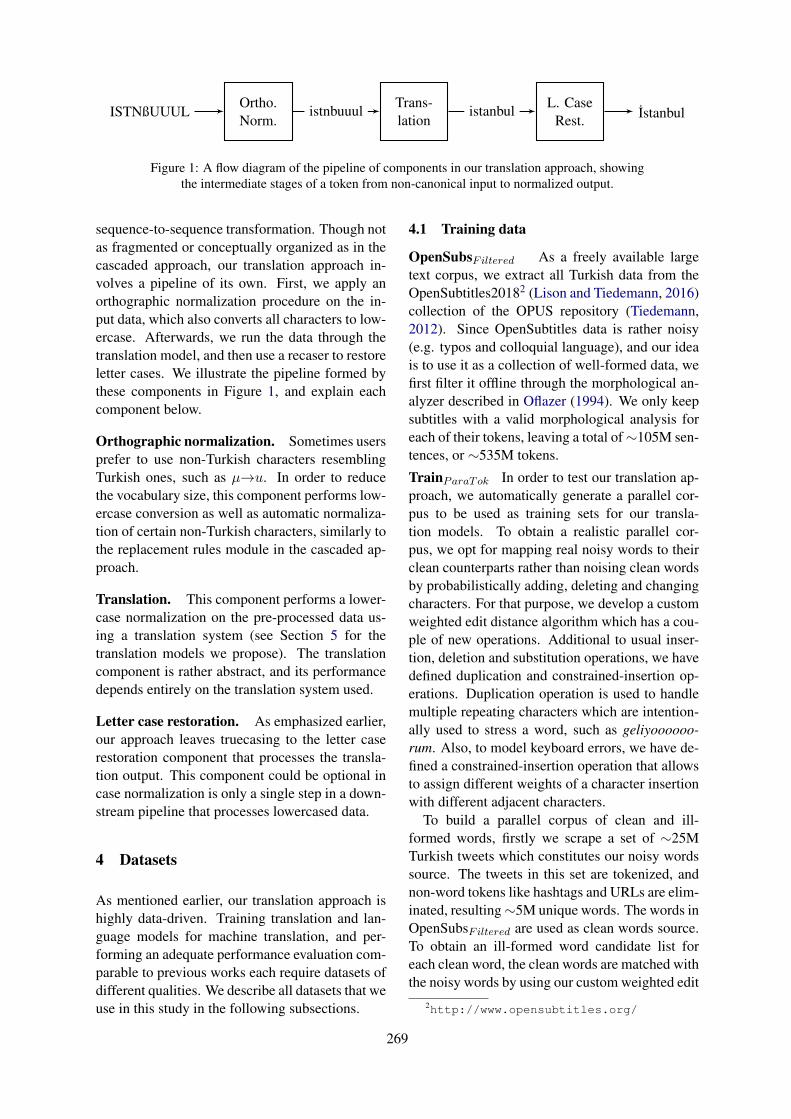
ISTNßUUULOrtho.Norm.

Trans-lation

L. CaseRest. Istanbulistnbuuul istanbul

Figure 1: A flow diagram of the pipeline of components in our translation approach, showingthe intermediate stages of a token from non-canonical input to normalized output.

sequence-to-sequence transformation. Though notas fragmented or conceptually organized as in thecascaded approach, our translation approach in-volves a pipeline of its own. First, we apply anorthographic normalization procedure on the in-put data, which also converts all characters to low-ercase. Afterwards, we run the data through thetranslation model, and then use a recaser to restoreletter cases. We illustrate the pipeline formed bythese components in Figure 1, and explain eachcomponent below.

Orthographic normalization. Sometimes usersprefer to use non-Turkish characters resemblingTurkish ones, such as µ→u. In order to reducethe vocabulary size, this component performs low-ercase conversion as well as automatic normaliza-tion of certain non-Turkish characters, similarly tothe replacement rules module in the cascaded ap-proach.

Translation. This component performs a lower-case normalization on the pre-processed data us-ing a translation system (see Section 5 for thetranslation models we propose). The translationcomponent is rather abstract, and its performancedepends entirely on the translation system used.

Letter case restoration. As emphasized earlier,our approach leaves truecasing to the letter caserestoration component that processes the transla-tion output. This component could be optional incase normalization is only a single step in a down-stream pipeline that processes lowercased data.

4 Datasets

As mentioned earlier, our translation approach ishighly data-driven. Training translation and lan-guage models for machine translation, and per-forming an adequate performance evaluation com-parable to previous works each require datasets ofdifferent qualities. We describe all datasets that weuse in this study in the following subsections.

4.1 Training data

OpenSubsFiltered As a freely available largetext corpus, we extract all Turkish data from theOpenSubtitles20182 (Lison and Tiedemann, 2016)collection of the OPUS repository (Tiedemann,2012). Since OpenSubtitles data is rather noisy(e.g. typos and colloquial language), and our ideais to use it as a collection of well-formed data, wefirst filter it offline through the morphological an-alyzer described in Oflazer (1994). We only keepsubtitles with a valid morphological analysis foreach of their tokens, leaving a total of∼105M sen-tences, or ∼535M tokens.

TrainParaTok In order to test our translation ap-proach, we automatically generate a parallel cor-pus to be used as training sets for our transla-tion models. To obtain a realistic parallel cor-pus, we opt for mapping real noisy words to theirclean counterparts rather than noising clean wordsby probabilistically adding, deleting and changingcharacters. For that purpose, we develop a customweighted edit distance algorithm which has a cou-ple of new operations. Additional to usual inser-tion, deletion and substitution operations, we havedefined duplication and constrained-insertion op-erations. Duplication operation is used to handlemultiple repeating characters which are intention-ally used to stress a word, such as geliyoooooo-rum. Also, to model keyboard errors, we have de-fined a constrained-insertion operation that allowsto assign different weights of a character insertionwith different adjacent characters.

To build a parallel corpus of clean and ill-formed words, firstly we scrape a set of ∼25MTurkish tweets which constitutes our noisy wordssource. The tweets in this set are tokenized, andnon-word tokens like hashtags and URLs are elim-inated, resulting∼5M unique words. The words inOpenSubsFiltered are used as clean words source.To obtain an ill-formed word candidate list foreach clean word, the clean words are matched withthe noisy words by using our custom weighted edit

2http://www.opensubtitles.org/

269

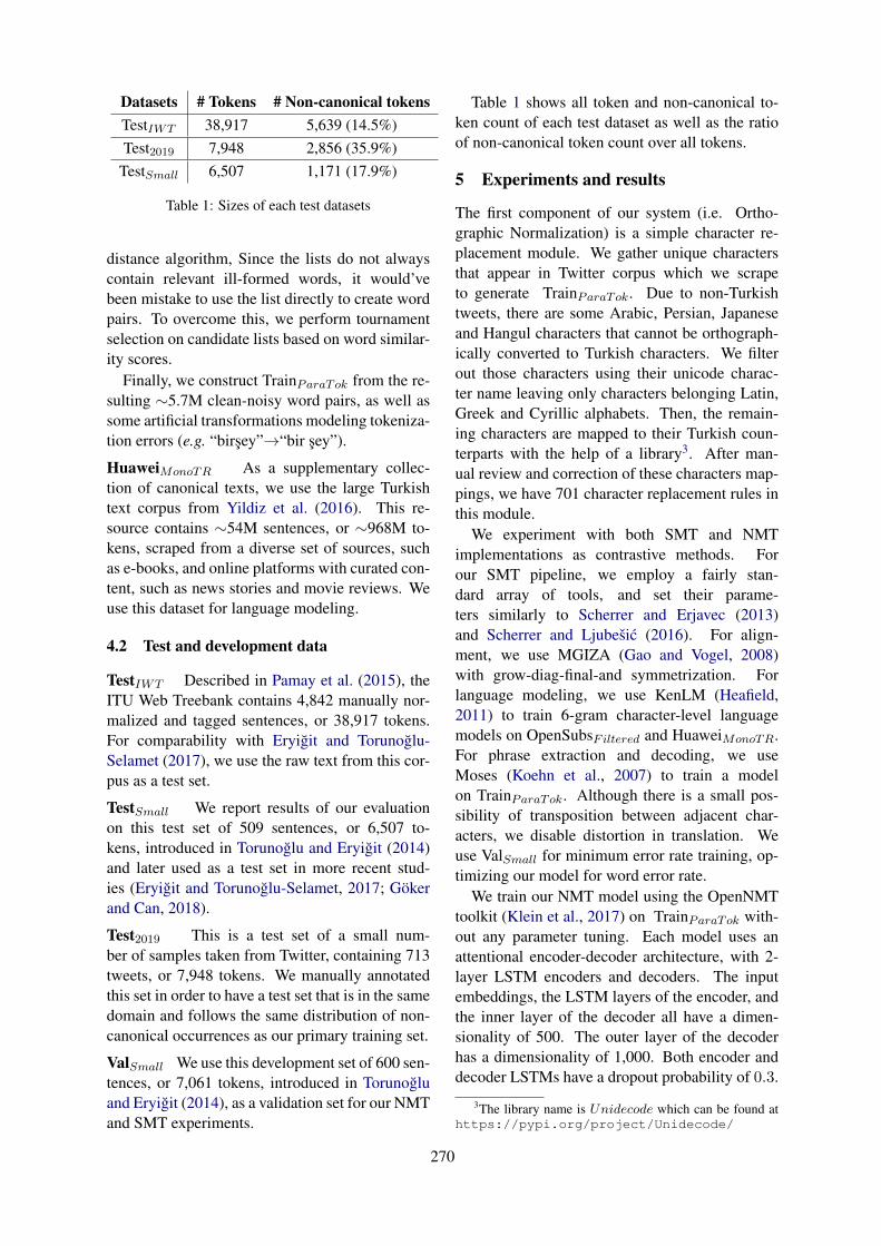
Datasets # Tokens # Non-canonical tokensTestIWT 38,917 5,639 (14.5%)Test2019 7,948 2,856 (35.9%)

TestSmall 6,507 1,171 (17.9%)

Table 1: Sizes of each test datasets

distance algorithm, Since the lists do not alwayscontain relevant ill-formed words, it would’vebeen mistake to use the list directly to create wordpairs. To overcome this, we perform tournamentselection on candidate lists based on word similar-ity scores.

Finally, we construct TrainParaTok from the re-sulting ∼5.7M clean-noisy word pairs, as well assome artificial transformations modeling tokeniza-tion errors (e.g. “birsey”→“bir sey”).

HuaweiMonoTR As a supplementary collec-tion of canonical texts, we use the large Turkishtext corpus from Yildiz et al. (2016). This re-source contains ∼54M sentences, or ∼968M to-kens, scraped from a diverse set of sources, suchas e-books, and online platforms with curated con-tent, such as news stories and movie reviews. Weuse this dataset for language modeling.

4.2 Test and development data

TestIWT Described in Pamay et al. (2015), theITU Web Treebank contains 4,842 manually nor-malized and tagged sentences, or 38,917 tokens.For comparability with Eryigit and Torunoglu-Selamet (2017), we use the raw text from this cor-pus as a test set.

TestSmall We report results of our evaluationon this test set of 509 sentences, or 6,507 to-kens, introduced in Torunoglu and Eryigit (2014)and later used as a test set in more recent stud-ies (Eryigit and Torunoglu-Selamet, 2017; Gokerand Can, 2018).

Test2019 This is a test set of a small num-ber of samples taken from Twitter, containing 713tweets, or 7,948 tokens. We manually annotatedthis set in order to have a test set that is in the samedomain and follows the same distribution of non-canonical occurrences as our primary training set.

ValSmall We use this development set of 600 sen-tences, or 7,061 tokens, introduced in Torunogluand Eryigit (2014), as a validation set for our NMTand SMT experiments.

Table 1 shows all token and non-canonical to-ken count of each test dataset as well as the ratioof non-canonical token count over all tokens.

5 Experiments and results

The first component of our system (i.e. Ortho-graphic Normalization) is a simple character re-placement module. We gather unique charactersthat appear in Twitter corpus which we scrapeto generate TrainParaTok. Due to non-Turkishtweets, there are some Arabic, Persian, Japaneseand Hangul characters that cannot be orthograph-ically converted to Turkish characters. We filterout those characters using their unicode charac-ter name leaving only characters belonging Latin,Greek and Cyrillic alphabets. Then, the remain-ing characters are mapped to their Turkish coun-terparts with the help of a library3. After man-ual review and correction of these characters map-pings, we have 701 character replacement rules inthis module.

We experiment with both SMT and NMTimplementations as contrastive methods. Forour SMT pipeline, we employ a fairly stan-dard array of tools, and set their parame-ters similarly to Scherrer and Erjavec (2013)and Scherrer and Ljubesic (2016). For align-ment, we use MGIZA (Gao and Vogel, 2008)with grow-diag-final-and symmetrization. Forlanguage modeling, we use KenLM (Heafield,2011) to train 6-gram character-level languagemodels on OpenSubsFiltered and HuaweiMonoTR.For phrase extraction and decoding, we useMoses (Koehn et al., 2007) to train a modelon TrainParaTok. Although there is a small pos-sibility of transposition between adjacent char-acters, we disable distortion in translation. Weuse ValSmall for minimum error rate training, op-timizing our model for word error rate.

We train our NMT model using the OpenNMTtoolkit (Klein et al., 2017) on TrainParaTok with-out any parameter tuning. Each model uses anattentional encoder-decoder architecture, with 2-layer LSTM encoders and decoders. The inputembeddings, the LSTM layers of the encoder, andthe inner layer of the decoder all have a dimen-sionality of 500. The outer layer of the decoderhas a dimensionality of 1,000. Both encoder anddecoder LSTMs have a dropout probability of 0.3.

3The library name is Unidecode which can be found athttps://pypi.org/project/Unidecode/

270

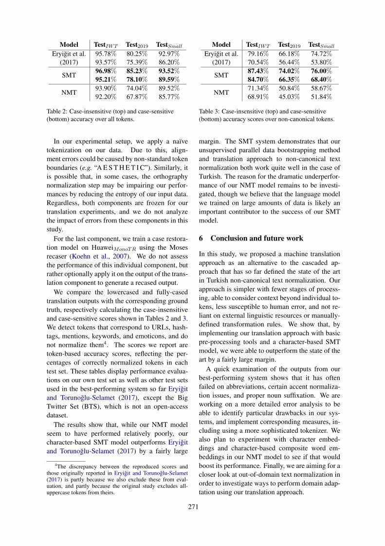
Model TestIWT Test2019 TestSmall

Eryigit et al.(2017)

95.78%93.57%

80.25%75.39%

92.97%86.20%

SMT96.98%95.21%

85.23%78.10%

93.52%89.59%

NMT93.90%92.20%

74.04%67.87%

89.52%85.77%

Table 2: Case-insensitive (top) and case-sensitive(bottom) accuracy over all tokens.

Model TestIWT Test2019 TestSmall

Eryigit et al.(2017)

79.16%70.54%

66.18%56.44%

74.72%53.80%

SMT87.43%84.70%

74.02%66.35%

76.00%68.40%

NMT71.34%68.91%

50.84%45.03%

58.67%51.84%

Table 3: Case-insensitive (top) and case-sensitive(bottom) accuracy scores over non-canonical tokens.

In our experimental setup, we apply a naıvetokenization on our data. Due to this, align-ment errors could be caused by non-standard tokenboundaries (e.g. “A E S T H E T I C”). Similarly, itis possible that, in some cases, the orthographynormalization step may be impairing our perfor-mances by reducing the entropy of our input data.Regardless, both components are frozen for ourtranslation experiments, and we do not analyzethe impact of errors from these components in thisstudy.

For the last component, we train a case restora-tion model on HuaweiMonoTR using the Mosesrecaser (Koehn et al., 2007). We do not assessthe performance of this individual component, butrather optionally apply it on the output of the trans-lation component to generate a recased output.

We compare the lowercased and fully-casedtranslation outputs with the corresponding groundtruth, respectively calculating the case-insensitiveand case-sensitive scores shown in Tables 2 and 3.We detect tokens that correspond to URLs, hash-tags, mentions, keywords, and emoticons, and donot normalize them4. The scores we report aretoken-based accuracy scores, reflecting the per-centages of correctly normalized tokens in eachtest set. These tables display performance evalua-tions on our own test set as well as other test setsused in the best-performing system so far Eryigitand Torunoglu-Selamet (2017), except the BigTwitter Set (BTS), which is not an open-accessdataset.

The results show that, while our NMT modelseem to have performed relatively poorly, ourcharacter-based SMT model outperforms Eryigitand Torunoglu-Selamet (2017) by a fairly large

4The discrepancy between the reproduced scores andthose originally reported in Eryigit and Torunoglu-Selamet(2017) is partly because we also exclude these from eval-uation, and partly because the original study excludes all-uppercase tokens from theirs.

margin. The SMT system demonstrates that ourunsupervised parallel data bootstrapping methodand translation approach to non-canonical textnormalization both work quite well in the case ofTurkish. The reason for the dramatic underperfor-mance of our NMT model remains to be investi-gated, though we believe that the language modelwe trained on large amounts of data is likely animportant contributor to the success of our SMTmodel.

6 Conclusion and future work

In this study, we proposed a machine translationapproach as an alternative to the cascaded ap-proach that has so far defined the state of the artin Turkish non-canonical text normalization. Ourapproach is simpler with fewer stages of process-ing, able to consider context beyond individual to-kens, less susceptible to human error, and not re-liant on external linguistic resources or manually-defined transformation rules. We show that, byimplementing our translation approach with basicpre-processing tools and a character-based SMTmodel, we were able to outperform the state of theart by a fairly large margin.

A quick examination of the outputs from ourbest-performing system shows that it has oftenfailed on abbreviations, certain accent normaliza-tion issues, and proper noun suffixation. We areworking on a more detailed error analysis to beable to identify particular drawbacks in our sys-tems, and implement corresponding measures, in-cluding using a more sophisticated tokenizer. Wealso plan to experiment with character embed-dings and character-based composite word em-beddings in our NMT model to see if that wouldboost its performance. Finally, we are aiming for acloser look at out-of-domain text normalization inorder to investigate ways to perform domain adap-tation using our translation approach.

271

Acknowledgments

The authors would like to thank Yves Scherrer forhis valuable insights, and the Faculty of Arts at theUniversity of Helsinki for funding a research visit,during which this study has materialized.

ReferencesGulsen Eryigit. 2014. ITU Turkish NLP web service.

In Proceedings of the Demonstrations at the 14thConference of the European Chapter of the Associa-tion for Computational Linguistics, pages 1–4.

Gulsen Eryigit and Dilara Torunoglu-Selamet. 2017.Social media text normalization for Turkish. Nat-ural Language Engineering, 23(6):835–875.

Qin Gao and Stephan Vogel. 2008. Parallel implemen-tations of word alignment tool. Software engineer-ing, testing, and quality assurance for natural lan-guage processing, pages 49–57.

Sinan Goker and Burcu Can. 2018. Neural text normal-ization for turkish social media. In 2018 3rd Inter-national Conference on Computer Science and En-gineering (UBMK), pages 161–166. IEEE.

Kenneth Heafield. 2011. KenLM: Faster and smallerlanguage model queries. In Proceedings of the sixthworkshop on statistical machine translation, pages187–197. Association for Computational Linguis-tics.

Taishi Ikeda, Hiroyuki Shindo, and Yuji Matsumoto.2016. Japanese text normalization with encoder-decoder model. In Proceedings of the 2nd Workshopon Noisy User-generated Text (WNUT), pages 129–137.

Guillaume Klein, Yoon Kim, Yuntian Deng, JeanSenellart, and Alexander M. Rush. 2017. Open-NMT: Open-source toolkit for neural machine trans-lation. In Proc. ACL.

Philipp Koehn, Hieu Hoang, Alexandra Birch, ChrisCallison-Burch, Marcello Federico, Nicola Bertoldi,Brooke Cowan, Wade Shen, Christine Moran,Richard Zens, et al. 2007. Moses: Open sourcetoolkit for statistical machine translation. In Pro-ceedings of the 45th annual meeting of the associ-ation for computational linguistics companion vol-ume proceedings of the demo and poster sessions,pages 177–180.

Chen Li and Yang Liu. 2012. Normalization of textmessages using character- and phone-based machinetranslation approaches. In Thirteenth Annual Con-ference of the International Speech CommunicationAssociation.

Pierre Lison and Jorg Tiedemann. 2016. OpenSub-titles2016: Extracting large parallel corpora frommovie and TV subtitles.

David Matthews. 2007. Machine transliteration ofproper names. Master’s Thesis, University of Ed-inburgh, Edinburgh, United Kingdom.

Preslav Nakov and Jorg Tiedemann. 2012. Combin-ing word-level and character-level models for ma-chine translation between closely-related languages.In Proceedings of the 50th Annual Meeting of theAssociation for Computational Linguistics: ShortPapers-Volume 2, pages 301–305. Association forComputational Linguistics.

Kemal Oflazer. 1994. Two-level description of turk-ish morphology. Literary and linguistic computing,9(2):137–148.

Tugba Pamay, Umut Sulubacak, Dilara Torunoglu-Selamet, and Gulsen Eryigit. 2015. The annotationprocess of the itu web treebank. In Proceedings ofthe 9th Linguistic Annotation Workshop, pages 95–101.

Eva Pettersson, Beata Megyesi, and Jorg Tiedemann.2013. An smt approach to automatic annotation ofhistorical text. In Proceedings of the workshop oncomputational historical linguistics at NODALIDA2013; May 22-24; 2013; Oslo; Norway. NEALTProceedings Series 18, 087, pages 54–69. LinkopingUniversity Electronic Press.

Yves Scherrer and Tomaz Erjavec. 2013. Moderniz-ing historical Slovene words with character-basedSMT. In BSNLP 2013-4th Biennial Workshop onBalto-Slavic Natural Language Processing.

Yves Scherrer and Nikola Ljubesic. 2016. Automaticnormalisation of the Swiss German ArchiMob cor-pus using character-level machine translation. InProceedings of the 13th Conference on Natural Lan-guage Processing (KONVENS 2016), pages 248–255.

Jorg Tiedemann. 2012. Parallel data, tools and inter-faces in opus. In Proceedings of the Eight Interna-tional Conference on Language Resources and Eval-uation (LREC’12), Istanbul, Turkey. European Lan-guage Resources Association (ELRA).

Dilara Torunoglu and Gulsen Eryigit. 2014. A cas-caded approach for social media text normalizationof turkish. In Proceedings of the 5th Workshop onLanguage Analysis for Social Media (LASM), pages62–70.

Osman Tursun and Ruket Cakici. 2017. Noisy uyghurtext normalization. In Proceedings of the 3rd Work-shop on Noisy User-generated Text, pages 85–93.

Eray Yildiz, Caglar Tirkaz, H Bahadır Sahin,Mustafa Tolga Eren, and Omer Ozan Sonmez. 2016.A morphology-aware network for morphologicaldisambiguation. In Thirtieth AAAI Conference onArtificial Intelligence.

272

Proceedings of the 57th Annual Meeting of the Association for Computational Linguistics: Student Research Workshop, pages 273–280Florence, Italy, July 28 - August 2, 2019. c©2019 Association for Computational Linguistics

ARHNet - Leveraging Community Interaction For Detection Of ReligiousHate Speech In Arabic

Arijit Ghosh Chowdhury∗Manipal Institute of Technologyarijit10@gmail.com

Aniket Didolkar∗Manipal Institute of Technologyadidolkar123@gmail.com

Ramit SawhneyNetaji Subhas Institute of Technology

ramits.co@nsit.net.in

Rajiv Ratn ShahMIDAS, IIIT-Delhi

rajivratn@iiitd.ac.in

AbstractThe rapid widespread of social media has ledto some undesirable consequences like therapid increase of hateful content and offen-sive language. Religious Hate Speech, in par-ticular, often leads to unrest and sometimesaggravates to violence against people on thebasis of their religious affiliations. The rich-ness of the Arabic morphology and the lim-ited available resources makes this task espe-cially challenging. The current state-of-the-art approaches to detect hate speech in Ara-bic rely entirely on textual (lexical and seman-tic) cues. Our proposed methodology con-tends that leveraging Community-Interactioncan better help us profile hate speech con-tent on social media. Our proposed ARHNet(Arabic Religious Hate Speech Net) model in-corporates both Arabic Word Embeddings andSocial Network Graphs for the detection of re-ligious hate speech.

1 Introduction

Hate speech was a major tool employed to pro-mote slavery in Colonial America, to aggravatetensions in Bosnia and in the rise of the Third Re-ich. The aim of such speech is to ridicule victims,to humiliate them and represent their grievancesas less serious (Gelashvili, 2018). The relation-ship between religion and hate speech is com-plex and has been central to recent discussionsof hate speech directed at religious people, espe-cially members of religious minorities (Bonotti,2017). This makes it important to develop auto-mated tools to detect messages that use inflamma-tory sectarian language to promote hatred and vi-olence against people.

Our work extends on the work done by (Al-badi et al., 2018) in terms of exploring the mer-

its of introducing community interaction as a fea-ture in the detection of religious hate speech inArabic. Most previous work in the area of hatespeech detection has targeted mainly English con-tent (Davidson et al., 2017) (Djuric et al., 2015)(Badjatiya et al., 2017). Author profiling usingcommunity graphs has been explored by (Mishraet al., 2018) for abuse detection on Twitter. Wepropose a novel Cyber Hate Detection approachusing multiple twitter graphs and traditional wordembeddings.

Social network graphs are increasingly beingused as a powerful tool for NLP applications(Mahata et al., 2018; Shah et al., 2016b), lead-ing to substantial improvement in performance fortasks like text categorization, sentiment analysis,and author attribute identification ((Hovy, 2015);(Yang and Eisenstein, 2015); (Yang et al., 2016).The idea of using this type of information is bestexplained by the concept of homophily, i.e., thephenomenon that people, both in real life as wellas on the Internet, tend to associate more withthose who appear similar. Here, similarity can bedefined based on various parameters like location,age, language, etc. The basic idea behind leverag-ing community interaction is that if we have infor-mation about members of a community defined bysome similarity measure, then we can infer infor-mation about a person based on which communitythey belong to. For our study, knowing that mem-bers of a particular community are prone to prolif-erating religious hate speech content, and know-ing that the user is connected to this community,we can use this information beyond linguistic cuesand more accurately predict the use of hateful/non-hateful language. Our work seeks to address twomain questions:

273

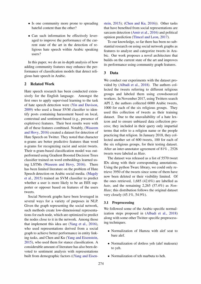
• Is one community more prone to spreadinghateful content than the other?

• Can such information be effectively lever-aged to improve the performance of the cur-rent state of the art in the detection of re-ligious hate speech within Arabic speakingusers?

In this paper, we do an in-depth analysis of howadding community features may enhance the per-formance of classification models that detect reli-gious hate speech in Arabic.

2 Related Work

Hate speech research has been conducted exten-sively for the English language. Amongst thefirst ones to apply supervised learning to the taskof hate speech detection were (Yin and Davison,2009) who used a linear SVM classifier to iden-tify posts containing harassment based on local,contextual and sentiment-based (e.g., presence ofexpletives) features. Their best results were withall of these features combined. Notably, (Waseemand Hovy, 2016) created a dataset for detection ofHate Speech on Twitter. They noted that charactern-grams are better predictive features than wordn-grams for recognizing racist and sexist tweets.Their n-gram-based classification model was out-performed using Gradient Boosted Decision Treesclassifier trained on word embeddings learned us-ing LSTMs (Waseem and Hovy, 2016). Therehas been limited literature on the problem of HateSpeech detection on Arabic social media. (Magdyet al., 2015) trained an SVM classifier to predictwhether a user is more likely to be an ISIS sup-porter or opposer based on features of the userstweets.

Social Network graphs have been leveraged inseveral ways for a variety of purposes in NLP.Given the graph representing the social network,such methods create low-dimensional representa-tions for each node, which are optimized to predictthe nodes close to it in the network. Among thosethat implement this idea are (Yang et al., 2016),who used representations derived from a socialgraph to achieve better performance in entity link-ing tasks, and Chen and Ku (Yang and Eisenstein,2015), who used them for stance classification. Aconsiderable amount of literature has also been de-voted to sentiment analysis with representationsbuilt from demographic factors ((Yang and Eisen-

stein, 2015); (Chen and Ku, 2016)). Other tasksthat have benefited from social representations aresarcasm detection (Amir et al., 2016) and politicalopinion prediction (Tlmcel and Leon, 2017).

To our knowledge, so far there has been no sub-stantial research on using social network graphs asfeatures to analyze and categorize tweets in Ara-bic. Our work proposes a novel architecture thatbuilds on the current state of the art and improvesits performance using community graph features.

3 Data

We conduct our experiments with the dataset pro-vided by (Albadi et al., 2018). The authors col-lected the tweets referring to different religiousgroups and labeled them using crowdsourcedworkers. In November 2017, using Twitters searchAPI 2, the authors collected 6000 Arabic tweets,1000 for each of the six religious groups. Theyused this collection of tweets as their trainingdataset. Due to the unavailability of a hate lex-icon and to ensure unbiased data collection pro-cess; they included in their query only impartialterms that refer to a religion name or the peoplepracticing that religion. In January 2018, they col-lected another set of 600 tweets, 100 for each ofthe six religious groups, for their testing dataset.After an inter-annotator agreement of 81% , 2526tweets were labeled as Hate.

The dataset was released as a list of 5570 tweetIDs along with their corresponding annotations.Using the python Twarc library, we could only re-trieve 3950 of the tweets since some of them havenow been deleted or their visibility limited. Ofthe ones retrieved, 1,685 (42.6%) are labelled ashate, and the remaining 2,265 (57.4%) as Non-Hate; this distribution follows the original datasetvery closely (45.1%, 54.9%).

3.1 Preprocessing

We followed some of the Arabic-specific normal-ization steps proposed in (Albadi et al., 2018)along with some other Twitter-specific preprocess-ing techniques.

• Normalization of Hamza with alef seat tobare alef.

• Normalization of dotless yeh (alef maksura)to yeh.

• Normalization of teh marbuta to heh.

274

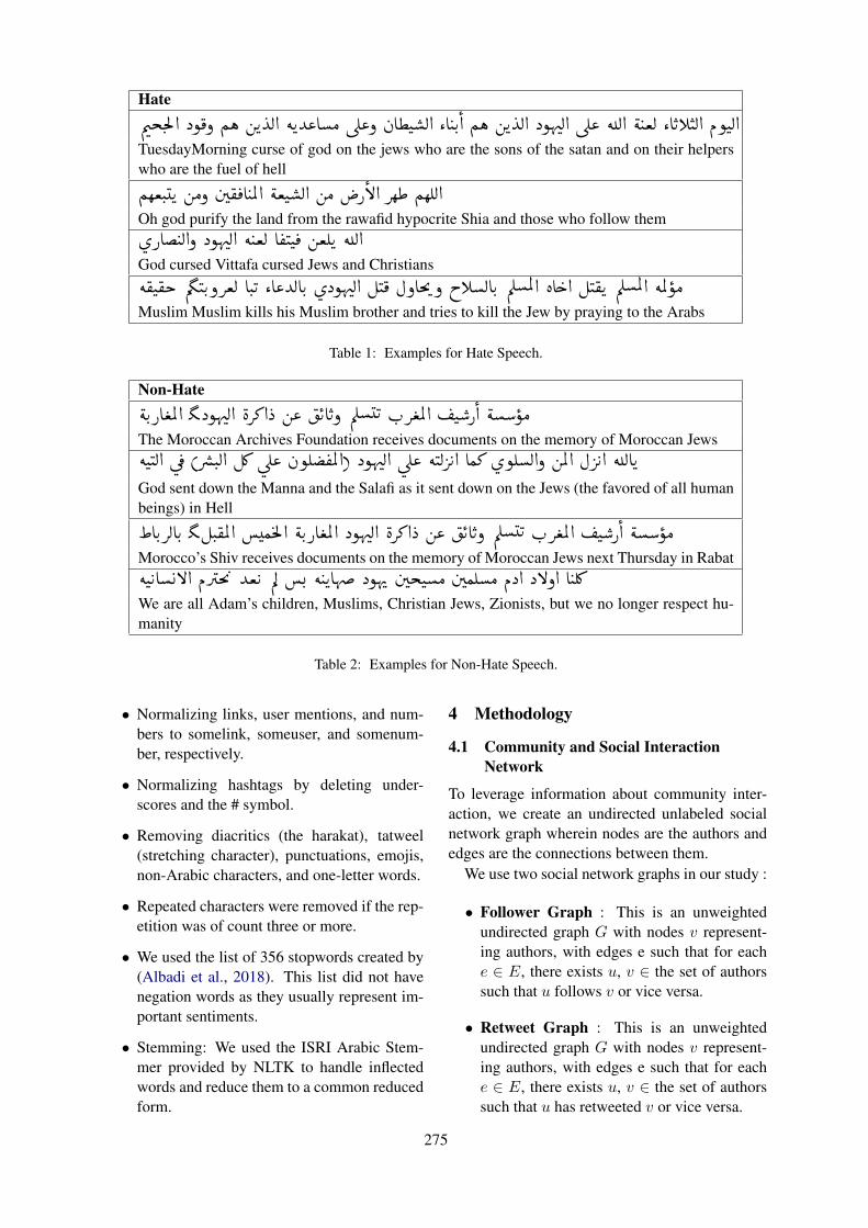
HateÕæjm.Ì'@ Xñð Ñë áK

YË@ éKY«AÓ úΫð àA¢J Ë@ ZA JK. @ Ñë áK

YË@ XñîDË @ úΫ é<Ë @ é JªË ZAKCJË @ ÐñJË @TuesdayMorning curse of god on the jews who are the sons of the satan and on their helperswho are the fuel of hell

ÑêªJ. K áÓð á® A JÖÏ @ éªJ Ë@ áÓ P B@ Qê£ ÑêÊË @

Oh god purify the land from the rawafid hypocrite Shia and those who follow themø PAJË @ð XñîDË @ é JªË A ®JJ áªÊK é<Ë @God cursed Vittafa cursed Jews and Christiansé®J®k ÕÂJK. ðQªË AJ. K ZA«YËAK. ø XñîDË @ ÉJ ÈðAm'ð hCËAK. ÕÎÖÏ @ è A g@ ÉJ®K ÕÎÖÏ @ éÖÏ ñÓMuslim Muslim kills his Muslim brother and tries to kill the Jew by praying to the Arabs

Table 1: Examples for Hate Speech.

Non-HateéK. PA ªÖÏ @ Â XñîDË @ èQ» @ X á« KAKð ÕÎK H. Q ªÖÏ @ ­J P

@ é ñÓ

The Moroccan Archives Foundation receives documents on the memory of Moroccan JewséJJË @ ú

(QåJ. Ë @ É¿ úΫ àñÊ ®ÖÏ @) XñîDË @ úΫ éJË Q K @ AÒ» ø ñÊË@ð áÖÏ @ È Q K @ é<ËAKGod sent down the Manna and the Salafi as it sent down on the Jews (the favored of all humanbeings) in Hell

AK. QËAK. Â ÉJ. ®ÖÏ @ ÒmÌ'@ éK. PA ªÖÏ @ XñîDË @ èQ» @ X á« KAKð ÕÎK H. Q ªÖÏ @ ­J P @ é ñÓ

Morocco’s Shiv receives documents on the memory of Moroccan Jews next Thursday in RabatéJ K AB@ ÐQm ' YªK ÕË . é JKAîD XñîE ájJÓ áÒÊÓ ÐX@ XBð@ A JÊ¿We are all Adam’s children, Muslims, Christian Jews, Zionists, but we no longer respect hu-manity

Table 2: Examples for Non-Hate Speech.

• Normalizing links, user mentions, and num-bers to somelink, someuser, and somenum-ber, respectively.

• Normalizing hashtags by deleting under-scores and the # symbol.

• Removing diacritics (the harakat), tatweel(stretching character), punctuations, emojis,non-Arabic characters, and one-letter words.

• Repeated characters were removed if the rep-etition was of count three or more.

• We used the list of 356 stopwords created by(Albadi et al., 2018). This list did not havenegation words as they usually represent im-portant sentiments.

• Stemming: We used the ISRI Arabic Stem-mer provided by NLTK to handle inflectedwords and reduce them to a common reducedform.

4 Methodology

4.1 Community and Social InteractionNetwork

To leverage information about community inter-action, we create an undirected unlabeled socialnetwork graph wherein nodes are the authors andedges are the connections between them.

We use two social network graphs in our study :

• Follower Graph : This is an unweightedundirected graph G with nodes v represent-ing authors, with edges e such that for eache ∈ E, there exists u, v ∈ the set of authorssuch that u follows v or vice versa.

• Retweet Graph : This is an unweightedundirected graph G with nodes v represent-ing authors, with edges e such that for eache ∈ E, there exists u, v ∈ the set of authorssuch that u has retweeted v or vice versa.

275

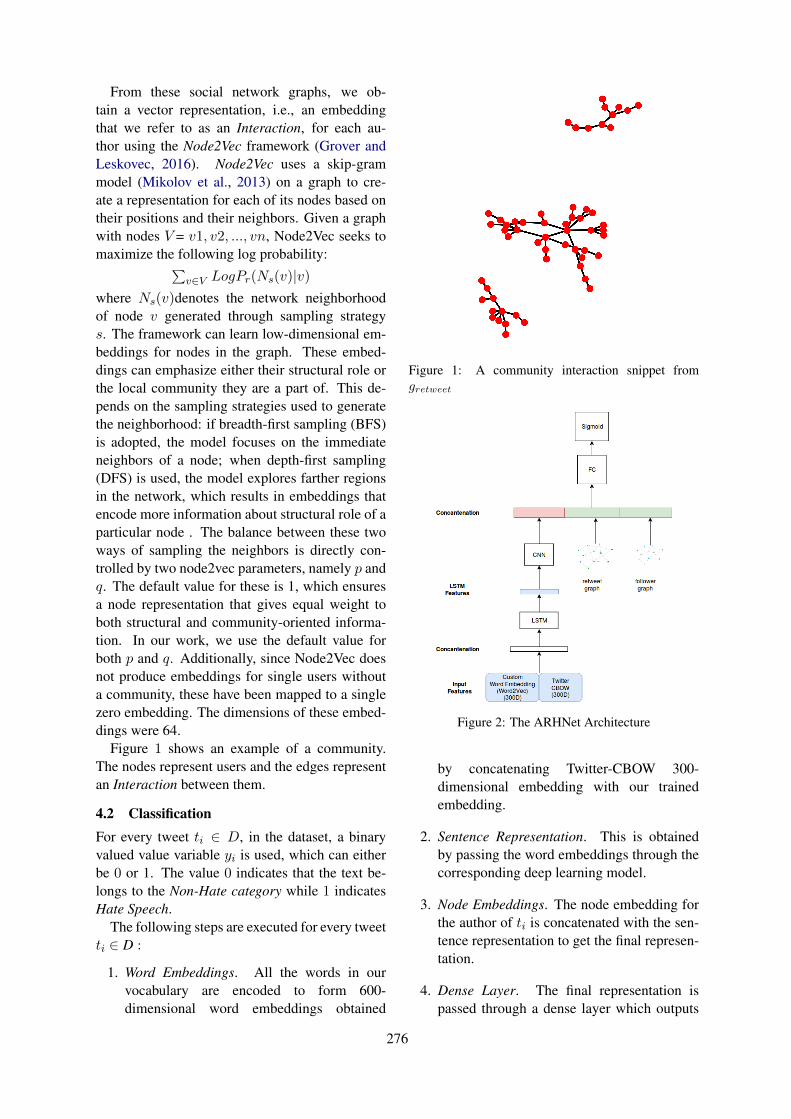
From these social network graphs, we ob-tain a vector representation, i.e., an embeddingthat we refer to as an Interaction, for each au-thor using the Node2Vec framework (Grover andLeskovec, 2016). Node2Vec uses a skip-grammodel (Mikolov et al., 2013) on a graph to cre-ate a representation for each of its nodes based ontheir positions and their neighbors. Given a graphwith nodes V = v1, v2, ..., vn, Node2Vec seeks tomaximize the following log probability:

∑v∈V LogPr(Ns(v)|v)

where Ns(v)denotes the network neighborhoodof node v generated through sampling strategys. The framework can learn low-dimensional em-beddings for nodes in the graph. These embed-dings can emphasize either their structural role orthe local community they are a part of. This de-pends on the sampling strategies used to generatethe neighborhood: if breadth-first sampling (BFS)is adopted, the model focuses on the immediateneighbors of a node; when depth-first sampling(DFS) is used, the model explores farther regionsin the network, which results in embeddings thatencode more information about structural role of aparticular node . The balance between these twoways of sampling the neighbors is directly con-trolled by two node2vec parameters, namely p andq. The default value for these is 1, which ensuresa node representation that gives equal weight toboth structural and community-oriented informa-tion. In our work, we use the default value forboth p and q. Additionally, since Node2Vec doesnot produce embeddings for single users withouta community, these have been mapped to a singlezero embedding. The dimensions of these embed-dings were 64.

Figure 1 shows an example of a community.The nodes represent users and the edges representan Interaction between them.

4.2 ClassificationFor every tweet ti ∈ D, in the dataset, a binaryvalued value variable yi is used, which can eitherbe 0 or 1. The value 0 indicates that the text be-longs to the Non-Hate category while 1 indicatesHate Speech.

The following steps are executed for every tweetti ∈ D :

1. Word Embeddings. All the words in ourvocabulary are encoded to form 600-dimensional word embeddings obtained

Figure 1: A community interaction snippet fromgretweet

Figure 2: The ARHNet Architecture

by concatenating Twitter-CBOW 300-dimensional embedding with our trainedembedding.

2. Sentence Representation. This is obtainedby passing the word embeddings through thecorresponding deep learning model.

3. Node Embeddings. The node embedding forthe author of ti is concatenated with the sen-tence representation to get the final represen-tation.

4. Dense Layer. The final representation ispassed through a dense layer which outputs

276

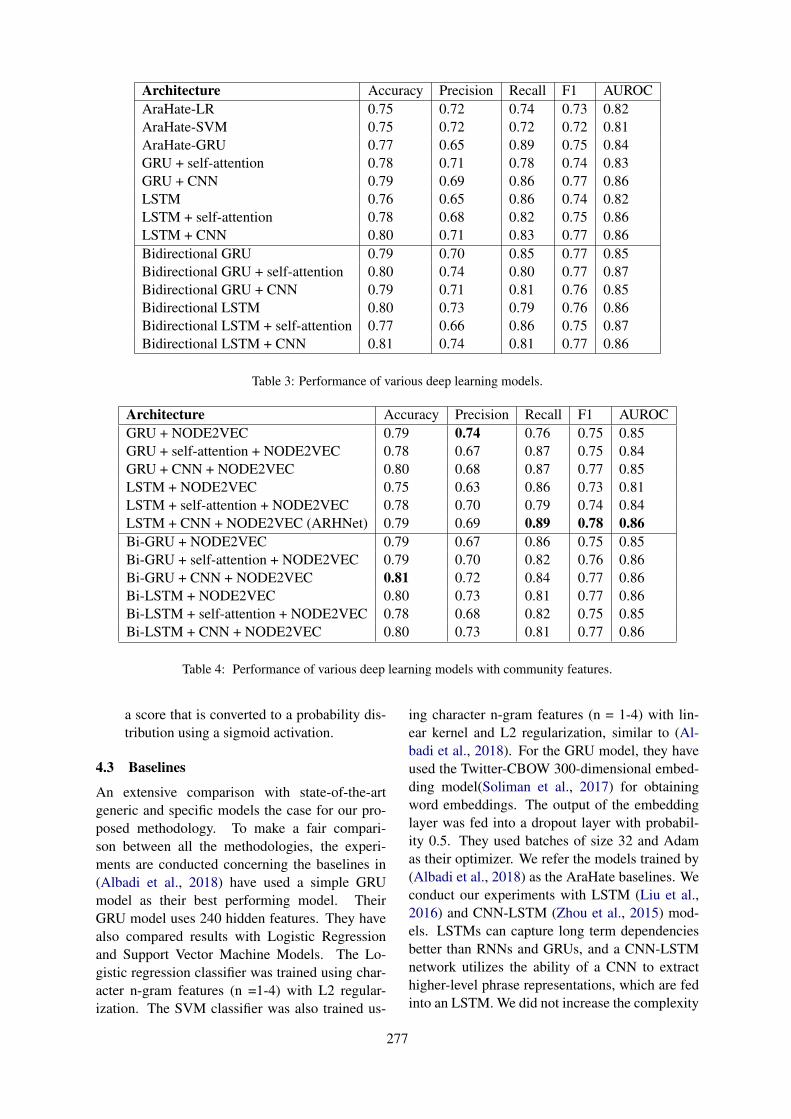
Architecture Accuracy Precision Recall F1 AUROCAraHate-LR 0.75 0.72 0.74 0.73 0.82AraHate-SVM 0.75 0.72 0.72 0.72 0.81AraHate-GRU 0.77 0.65 0.89 0.75 0.84GRU + self-attention 0.78 0.71 0.78 0.74 0.83GRU + CNN 0.79 0.69 0.86 0.77 0.86LSTM 0.76 0.65 0.86 0.74 0.82LSTM + self-attention 0.78 0.68 0.82 0.75 0.86LSTM + CNN 0.80 0.71 0.83 0.77 0.86Bidirectional GRU 0.79 0.70 0.85 0.77 0.85Bidirectional GRU + self-attention 0.80 0.74 0.80 0.77 0.87Bidirectional GRU + CNN 0.79 0.71 0.81 0.76 0.85Bidirectional LSTM 0.80 0.73 0.79 0.76 0.86Bidirectional LSTM + self-attention 0.77 0.66 0.86 0.75 0.87Bidirectional LSTM + CNN 0.81 0.74 0.81 0.77 0.86

Table 3: Performance of various deep learning models.

Architecture Accuracy Precision Recall F1 AUROCGRU + NODE2VEC 0.79 0.74 0.76 0.75 0.85GRU + self-attention + NODE2VEC 0.78 0.67 0.87 0.75 0.84GRU + CNN + NODE2VEC 0.80 0.68 0.87 0.77 0.85LSTM + NODE2VEC 0.75 0.63 0.86 0.73 0.81LSTM + self-attention + NODE2VEC 0.78 0.70 0.79 0.74 0.84LSTM + CNN + NODE2VEC (ARHNet) 0.79 0.69 0.89 0.78 0.86Bi-GRU + NODE2VEC 0.79 0.67 0.86 0.75 0.85Bi-GRU + self-attention + NODE2VEC 0.79 0.70 0.82 0.76 0.86Bi-GRU + CNN + NODE2VEC 0.81 0.72 0.84 0.77 0.86Bi-LSTM + NODE2VEC 0.80 0.73 0.81 0.77 0.86Bi-LSTM + self-attention + NODE2VEC 0.78 0.68 0.82 0.75 0.85Bi-LSTM + CNN + NODE2VEC 0.80 0.73 0.81 0.77 0.86

Table 4: Performance of various deep learning models with community features.

a score that is converted to a probability dis-tribution using a sigmoid activation.

4.3 Baselines

An extensive comparison with state-of-the-artgeneric and specific models the case for our pro-posed methodology. To make a fair compari-son between all the methodologies, the experi-ments are conducted concerning the baselines in(Albadi et al., 2018) have used a simple GRUmodel as their best performing model. TheirGRU model uses 240 hidden features. They havealso compared results with Logistic Regressionand Support Vector Machine Models. The Lo-gistic regression classifier was trained using char-acter n-gram features (n =1-4) with L2 regular-ization. The SVM classifier was also trained us-

ing character n-gram features (n = 1-4) with lin-ear kernel and L2 regularization, similar to (Al-badi et al., 2018). For the GRU model, they haveused the Twitter-CBOW 300-dimensional embed-ding model(Soliman et al., 2017) for obtainingword embeddings. The output of the embeddinglayer was fed into a dropout layer with probabil-ity 0.5. They used batches of size 32 and Adamas their optimizer. We refer the models trained by(Albadi et al., 2018) as the AraHate baselines. Weconduct our experiments with LSTM (Liu et al.,2016) and CNN-LSTM (Zhou et al., 2015) mod-els. LSTMs can capture long term dependenciesbetter than RNNs and GRUs, and a CNN-LSTMnetwork utilizes the ability of a CNN to extracthigher-level phrase representations, which are fedinto an LSTM. We did not increase the complexity

277

of the baselines beyond this to not risk overfittingon a small dataset.

4.4 Models and Hyperparameters

First, we prepared the vocabulary by assigninginteger indexes to unique words in our dataset.Tweets were then converted into sequences of in-teger indexes. These sequences were padded withzeros so that the tweets in each batch have thesame length during training. They were then fedinto an embedding layer which maps word in-dexes to word embeddings. We trained our wordembeddings using GenSim 1. We also used theTwitter-CBOW 300-dimension embedding modelprovided by AraVec (Soliman et al., 2017) whichcontains over 331k word vectors that have beentrained on about 67M Arabic tweets. We concate-nated our own trained embeddings with the Ar-aVec embeddings to obtain 600-dimensional em-beddings Similar to (Albadi et al., 2018), The out-put of the embedding layer was fed into a dropoutlayer with a rate of 0.5 to prevent overfitting.

For both LSTM and GRU, the word embed-dings were passed to both unidirectional and bidi-rectional LSTM with 240 features each. In theGRU-CNN/LSTM-CNN models, we used 2 Con-volutional Layers with a Kernel Size of 3 and ReluActivation in the middle. We obtained the finalrepresentation by taking the maximum along thetemporal dimension. For self-attention, the outputof the GRU/LSTM was passed to a self-attentionlayer. For the self-attention models, we used 240features.

We compared each of these models with theircounterparts obtained by concatenating Node2Vecembeddings to the representations obtained by theabove deep learning models. The final represen-tation was then passed into a Sigmoid Layer. Weperformed training in batches of size 32, and weused Adam as our optimizer for all experiments.

5 Results And Discussion

In our experiments, we have beaten the scoresof (Albadi et al., 2018) in all 5 metrics. Weobtained a highest f1-score of 0.78 as com-pared to 0.77 in (Albadi et al., 2018). This isachieved in our LSTM + CNN + CISNet model.The ARHNet model outperforms baselines interms of Recall, F1 and AUROC metrics while

1radimrehurek.com/gensim/models/word2vec.html

GRU-NODE2VEC demonstrates the highest pre-cision, and the Bi-GRU-CNN-NODE2VEC modelachieves the highest accuracy. Our methodol-ogy effectively improves upon the current state ofthe art and is successful in demonstration of howcommunity interaction can be leveraged to tackledownstream NLP tasks like detection of religioushate speech. Albadi et al. (2018) reached an 0.81agreement score between annotators. Our method-ology, therefore, matches human performance interms of unambiguously categorizing texts thatcontain religious hate speech from texts that don’t.

To summarize, our approach highlights the va-lidity of using Community Interaction Graphs asfeatures of classification in Arabic. Despite hav-ing a sparse representation of users, our proposedmethodology has shown improvements on Accu-racy and F1 over previously state of the art modelson a reduced dataset.

6 Conclusion

In this paper, we explored the effectiveness ofcommunity-interaction information about authorsfor the purpose of categorizing religious hatespeech in the Arabic Twittersphere and build uponexisting work in the linguistic aspects of socialmedia (Shah et al., 2016c,a; Mahata et al., 2015).Working with a dataset of 3950 tweets annotatedfor Hate and Non-Hate, we first comprehensivelyreplicated three established and currently best-performing hate speech detection methods basedon character n-grams and GRUs as our baselines.We then constructed a graph of all the authors oftweets in our dataset and extracted community-based information in the form of dense low-dimensional embeddings for each of them usingNode2Vec. We showed that the inclusion of com-munity graph embeddings significantly improvessystem performance over the baselines and ad-vances the state of the art in this task. Users proneto proliferate hate do tend to form social groupsonline, and this stresses the importance of utilizingcommunity-based information for automatic reli-gious hate speech detection.

References

N. Albadi, M. Kurdi, and S. Mishra. 2018. Are theyour brothers? analysis and detection of religioushate speech in the arabic twittersphere. In 2018IEEE/ACM International Conference on Advances

278

in Social Networks Analysis and Mining (ASONAM),pages 69–76.

Silvio Amir, Byron C. Wallace, Hao Lyu, Paula Car-valho, and Mario J. Silva. 2016. Modelling contextwith user embeddings for sarcasm detection in socialmedia. CoRR, abs/1607.00976.

Pinkesh Badjatiya, Shashank Gupta, Manish Gupta,and Vasudeva Varma. 2017. Deep learning for hatespeech detection in tweets. CoRR, abs/1706.00188.

Matteo Bonotti. 2017. Religion, hate speech and non-domination. Ethnicities, 17:259–274.

Wei-Fan Chen and Lun-Wei Ku. 2016. UTCNN: adeep learning model of stance classification on so-cial media text. In Proceedings of COLING 2016,the 26th International Conference on ComputationalLinguistics: Technical Papers, pages 1635–1645,Osaka, Japan. The COLING 2016 Organizing Com-mittee.

Thomas Davidson, Dana Warmsley, Michael W. Macy,and Ingmar Weber. 2017. Automated hate speechdetection and the problem of offensive language.CoRR, abs/1703.04009.

Nemanja Djuric, Jing Zhou, Robin Morris, Mihajlo Gr-bovic, Vladan Radosavljevic, and Narayan Bhamidi-pati. 2015. Hate speech detection with commentembeddings. In Proceedings of the 24th Interna-tional Conference on World Wide Web, WWW ’15Companion, pages 29–30, New York, NY, USA.ACM.

Teona Gelashvili. 2018. Hate speech on social media:Implications of private regulation and governancegaps. Student Paper.

Aditya Grover and Jure Leskovec. 2016. node2vec:Scalable feature learning for networks. CoRR,abs/1607.00653.

Dirk Hovy. 2015. Demographic factors improve clas-sification performance. In Proceedings of the 53rdAnnual Meeting of the Association for Computa-tional Linguistics and the 7th International JointConference on Natural Language Processing (Vol-ume 1: Long Papers), pages 752–762, Beijing,China. Association for Computational Linguistics.

Pengfei Liu, Xipeng Qiu, and Xuanjing Huang. 2016.Recurrent neural network for text classification withmulti-task learning. CoRR, abs/1605.05101.

Walid Magdy, Kareem Darwish, and Ingmar We-ber. 2015. #failedrevolutions: Using twitter tostudy the antecedents of ISIS support. CoRR,abs/1503.02401.

Debanjan Mahata, Jasper Friedrichs, Rajiv Ratn Shah,and Jing Jiang. 2018. Detecting personal intake ofmedicine from twitter. IEEE Intelligent Systems,33(4):87–95.

Debanjan Mahata, John R Talburt, and Vivek KumarSingh. 2015. From chirps to whistles: discover-ing event-specific informative content from twitter.In Proceedings of the ACM web science conference,page 17. ACM.

Tomas Mikolov, Ilya Sutskever, Kai Chen, Greg Cor-rado, and Jeffrey Dean. 2013. Distributed represen-tations of words and phrases and their composition-ality. CoRR, abs/1310.4546.

Pushkar Mishra, Marco Del Tredici, Helen Yan-nakoudakis, and Ekaterina Shutova. 2018. Authorprofiling for abuse detection. In COLING.

Rajiv Ratn Shah, Anupam Samanta, Deepak Gupta,Yi Yu, Suhua Tang, and Roger Zimmermann. 2016a.Prompt: Personalized user tag recommendation forsocial media photos leveraging personal and socialcontexts. In 2016 IEEE International Symposiumon Multimedia (ISM), pages 486–492. IEEE.

Rajiv Ratn Shah, Yi Yu, Suhua Tang, Shin’ichi Satoh,Akshay Verma, and Roger Zimmermann. 2016b.Concept-level multimodal ranking of flickr phototags via recall based weighting. In Proceedingsof the 2016 ACM Workshop on Multimedia COM-MONS, pages 19–26. ACM.

Rajiv Ratn Shah, Yi Yu, Akshay Verma, Suhua Tang,Anwar Dilawar Shaikh, and Roger Zimmermann.2016c. Leveraging multimodal information forevent summarization and concept-level sentimentanalysis. Knowledge-Based Systems, 108:102–109.

Abu Bakr Soliman, Kareem Eissa, and Samhaa R. El-Beltagy. 2017. Aravec: A set of arabic word embed-ding models for use in arabic nlp. Procedia Com-puter Science, 117:256 – 265. Arabic Computa-tional Linguistics.

C. Tlmcel and F. Leon. 2017. Predicting political opin-ions in social networks with user embeddings. In2017 13th IEEE International Conference on In-telligent Computer Communication and Processing(ICCP), pages 213–219.

Zeerak Waseem and Dirk Hovy. 2016. Hateful sym-bols or hateful people? predictive features for hatespeech detection on twitter. In Proceedings of theNAACL Student Research Workshop, pages 88–93,San Diego, California. Association for Computa-tional Linguistics.

Yi Yang, Ming-Wei Chang, and Jacob Eisenstein.2016. Toward socially-infused information extrac-tion: Embedding authors, mentions, and entities.CoRR, abs/1609.08084.

Yi Yang and Jacob Eisenstein. 2015. Puttingthings in context: Community-specific embed-ding projections for sentiment analysis. CoRR,abs/1511.06052.

Dawei Yin and Brian D. Davison. 2009. Detection ofharassment on web 2.0.

279

Chunting Zhou, Chonglin Sun, Zhiyuan Liu, and Fran-cis C. M. Lau. 2015. A C-LSTM neural network fortext classification. CoRR, abs/1511.08630.

280

Proceedings of the 57th Annual Meeting of the Association for Computational Linguistics: Student Research Workshop, pages 281–287Florence, Italy, July 28 - August 2, 2019. c©2019 Association for Computational Linguistics

Investigating Political Herd Mentality: A Community Sentiment BasedApproach

Anjali Bhavan∗

Delhi Technological Universityanjalibhavan98@gmail.com

Rohan Mishra∗

Delhi Technological Universityrohan.mishra1997@gmail.com

Pradyumna Prakhar Sinha∗

Delhi Technological Universitypradyumna014@gmail.com

Ramit SawhneyNetaji Subhash Institute of Technology

ramits.co@nsit.net.in

Rajiv Ratn ShahMIDAS, IIIT-Delhi

rajivratn@iiitd.ac.in

Abstract

Analyzing polarities and sentiments inherentin political speeches and debates poses an im-portant problem today. This experiment aimsto address this issue by analyzing publicly-available Hansard transcripts of the debatesconducted in the UK Parliament. Our pro-posed approach, which uses community-basedgraph information to augment hand-craftedfeatures based on topic modeling and emo-tion detection on debate transcripts currentlysurpasses the benchmark results on the samedataset. Such sentiment classification systemscould prove to be of great use in today’s po-litically turbulent times, for public knowledgeof politicians stands on various relevant is-sues proves vital for good governance and cit-izenship. The experiments also demonstratethat continuous feature representations learnedfrom graphs can improve performance on sen-timent classification tasks significantly.

1 Introduction

One of the key aspects of a functional, free soci-ety is being presented with comprehensive optionsin electing government representatives. The deci-sion is aided by the positions politicians take onrelevant issues like water, housing, etc. Hence,it becomes important to relay political standingsto the general public in a comprehensible manner.The Hansard transcripts of speeches delivered inthe UK Parliament are one such source of informa-tion. However, owing to the voluminous quantity,

* Indicates equal contribution.

esoteric language and opaque procedural jargon ofParliament, it is tougher for the non-expert citizento assess the standings of their elected represen-tative. Therefore, conducting stance classificationstudies on such data is a challenging task with po-tential benefits. However, the documents tend tobe highly tedious and difficult to comprehend, andthus become a barrier to information about politi-cal issues and leanings.

Sentiment analysis of data from various relevantsources (social media, newspapers, transcripts,etc.) has often given several insights about publicopinion, issues of contention, general trendsand so on (Carvalho et al., 2011; Loukis et al.,2014). Such techniques have even been used forpurposes like predicting election outcomes andthe reception of newly-launched products. Sincethese insights have wide-ranging consequences, itbecomes imperative to develop rigorous standardsand state-of-the-art techniques for them.One aspect that helps with analyzing such patternsand sentiments is studying about the inter-connections and networks underlying such data.Homophily, or the tendency of people to associatewith like-minded individuals, is the fundamentalaspect of depicting relationships between usersof a social network (for instance). Constructinggraphs to map such complex relationships andattributes in data could help one arrive at readyinsights and conclusions. This comes particularlyuseful when studying parliamentary debatesand sessions; connecting speakers according tofactors like party or position affiliations pro-

281

vides information on how a speaker is likely torespond to an issue being presented. Attemptsto analyze social media data based on such ap-proaches have been made (Deitrick and Hu, 2013).

2 Related Work

The analysis of political content and parliamentarydebates have opened an exciting line of researchin recent years and has shown promising results intasks of stance classification (Hasan and Ng, 2013)and opinion mining (Karami et al., 2018). A largepart of the work initially concentrated on legisla-tive speeches, but the focus has shifted to socialmedia content analysis in recent times. This shiftin focus has been particularly rapid with the pro-liferation of social media data and research (?Shahand Zimmermann, 2017; Shah et al., 2016b; Ma-hata et al., 2018; Shah et al., 2016c,a).

Lauderdale and Herzog (2016) presented theirmethod of determining political positions fromlegislative speech. The datasets were sourcedfrom Irish and US Senate debates. Rheault et al.(2016) examined the emotional polarity variationsin speeches delivered in the British parliamentover a hundred years. They observed a correlationbetween the variations in emotional states ofa particular period of time and the nationaleconomic situation. Thomas et al. (2006) studiedthe relationships between segments of speechesdelivered in the Congress and the overall tone:of opposition or support. A significant amountof research exists on the political temperamentacross social media websites like Facebook andTwitter. Stieglitz and Dang-Xuan (2012) studiedthe relationship between the inherent sentimentof politically relevant tweets and the retweetactivity. Ceron et al. (2014) proposed methods fordetermining the political alignments of citizensand tested them on French and Italian-contextdatasets. Many new findings based on the con-temporary political landscape continue to bedeveloped and presented. Wang and Liu (2018)analyzed US President Donald Trump’s speechesdelivered during his 2016 election campaign.Rudkowsky et al. (2018) proposed the usage ofword embeddings in the place of the traditionalBag-of-Words (BOW) approach for text analy-sis, and demonstrated experiments on Austrianparliamentary speeches. There have been someapproaches to model interactions among members

of a network to help in the task of sentimentanalysis. Moreover, there have been applicationsthat extract information about each user by rep-resenting them as a node in the social graph andcreating low dimensional representation usuallyinduced by neural architectures (Grover andLeskovec, 2016). Mishra et al. (2018) and Qianet al. (2018) use such social graph-based featuresto gain considerable improvement in the task ofabuse detection in social media. However therehas been no work done to model the interactionbetween the members of the Parliament for thetask of stance classification.For studying transcripts of speeches delivered inthe House of Commons in the UK Parliament,Abercrombie and Batista-Navarro (2018b) curateda dataset consisting of parliamentary motions anddebates as provided in the Hansard transcripts,along with other information like party affiliationsand polarities of the motions being discussed.This was followed by carrying out studies on thedataset and developing a sentiment analysis modelwhich also demonstrated the results of motion-independent (one-step) and motion-dependentclassification of polarities Abercrombie andBatista-Navarro (2018a). This dataset is used forfurther analysis in our experiments.

3 Dataset

In the UK, transcripts of parliamentary debates arepublicly available along with information relatedto division votes as well as manually annotatedsentiment labels. To investigate the effectivenessof our pipeline, experiments were conducted us-ing the HanDeSeT dataset as created by (Aber-crombie and Batista-Navarro, 2018b). The datasetconsists of 607 politicians and their speeches overvarious motions, with a total of 1251 samples. Thespeeches are divided into five utterances, and otherfeatures such as Debate ID, Debate title, Motionsubject with polarities: manual annotation andruling-opposing-based, Motion and Speaker partyaffiliations, Speech Polarities: manual and vote-based, Rebellion percentage.

Sentiment polarity is present in both speechesand motions. Hence labels are provided for mo-tion polarities as well. Two label types are pro-vided for motions: a manually-annotated one pre-dicting positive or negative polarity, and a gov-ernment/opposition one decided as follows: if the

282

speaker who proposes the motion belongs to theruling government, the polarity is positive; if thespeaker belongs to the opposition then the polar-ity is negative. Two label types are provided forspeeches as well: one manually-annotated, and theother a speaker-vote label extracted from the divi-sion related to the corresponding debate.

4 Methodology

The models described in Abercrombie andBatista-Navarro (2018a) extracted n-gram features(uni-grams, bi-grams, tri-grams, and their combi-nations) from the utterances for sentiment classi-fication. The stance-based relationships betweenthe members are modeled, and their effectivenessis analyzed. This study aims to develop on the lim-itations of using only text-based features and bydoing so present a sound, coherent model for sen-timent classification for parliamentary speeches.The methodology consists of the following sub-sections: preprocessing, to describe the initialdata preprocessing methods undertaken; featureextraction, which discusses the feature sets usedfor our model, and model description and training,to elaborate on our model and training procedures.

4.1 PreprocessingThe dataset was preprocessed for further analysis.This was required so unnecessary words; charac-ters etc. could be removed and not add furthernoise to the dataset. The text was lower-cased,and all punctuation marks and other special char-acters were removed. Following this, stopword re-moval was done using NLTK. Finally, a few cus-tom stopwords specific to the parliamentary pro-cedure were removed. These were taken fromAbercrombie and Batista-Navarro (2018b). Fi-nally, the utterances were concatenated and pre-pared for feature extraction and model training.

4.2 Feature Extraction4.2.1 Textual FeaturesVarious textual features were extracted for classi-fication and normalized using the L2 norm. Theseare listed below.

• TF-IDF: Term Frequency-inverse DocumentFrequency (TF-IDF) features were extractedfrom n-grams (upto 3) in the text. N-gramfeatures are immensely useful for factoringin contextual information surrounding thecomponents of a text (whether characters or

words) and are widely used for text analysis,language processing, etc.

• LDA-based topic modeling: Topic model-ing is used to derive information related tothe underlying ”topics” contained in a text.In order to extract such topic-based featuresfrom the utterances, the Latent Dirichlet Al-location (LDA) (Blei et al., 2003) model wasused. The probability distribution over themost commonly occurring 30 topics was usedas features for each speech.

• NRC Emotion: The NRC Emotion Lexicon(Mohammad and Turney, 2013) is a publiclyavailable lexicon that contains commonly oc-curring words along with their affect category(anger, fear, anticipation, trust, surprise, sad-ness, joy, or disgust) and two polarities (neg-ative or positive). The score along these 10features was computed for the utterances.

4.2.2 Graph-based featuresFor our analysis, two graphs were constructedfrom the dataset. The graph consists of nodes thatrepresent the members who participate in the pro-ceedings of the Parliament. The edges among themembers are conditioned upon their accord or dis-cord on debates regarding policies. Two membersof the same or varying political parties either agreeon a policy or differ on it. Therefore, the twographs are constructed.

• simGraph: In order to model the similarityon stances among members, Gsim(v, e) isa weighted undirected graph induced on thedataset with vertices v corresponding to themembers m of political parties where an edgee between two vertices v and u is defined asweight(e) =| f(v) ∩ f(u) | where f(v) isthe set of stances taken by the member that isrepresented by node v.

• oppGraph: Similarly, to model the differ-ences among the members, Gopp(v, e) is in-duced on the dataset such that an edge ebetween two vertices v and u is defined asweight(e) =| (f(v)\f(u))∩(f(u)\f(v)) |where f(v) is the set of stances taken by themember that is represented by node v.

node2vec: To obtain community based em-beddings, feature representations were generatedusing node2vec (Grover and Leskovec, 2016).

283

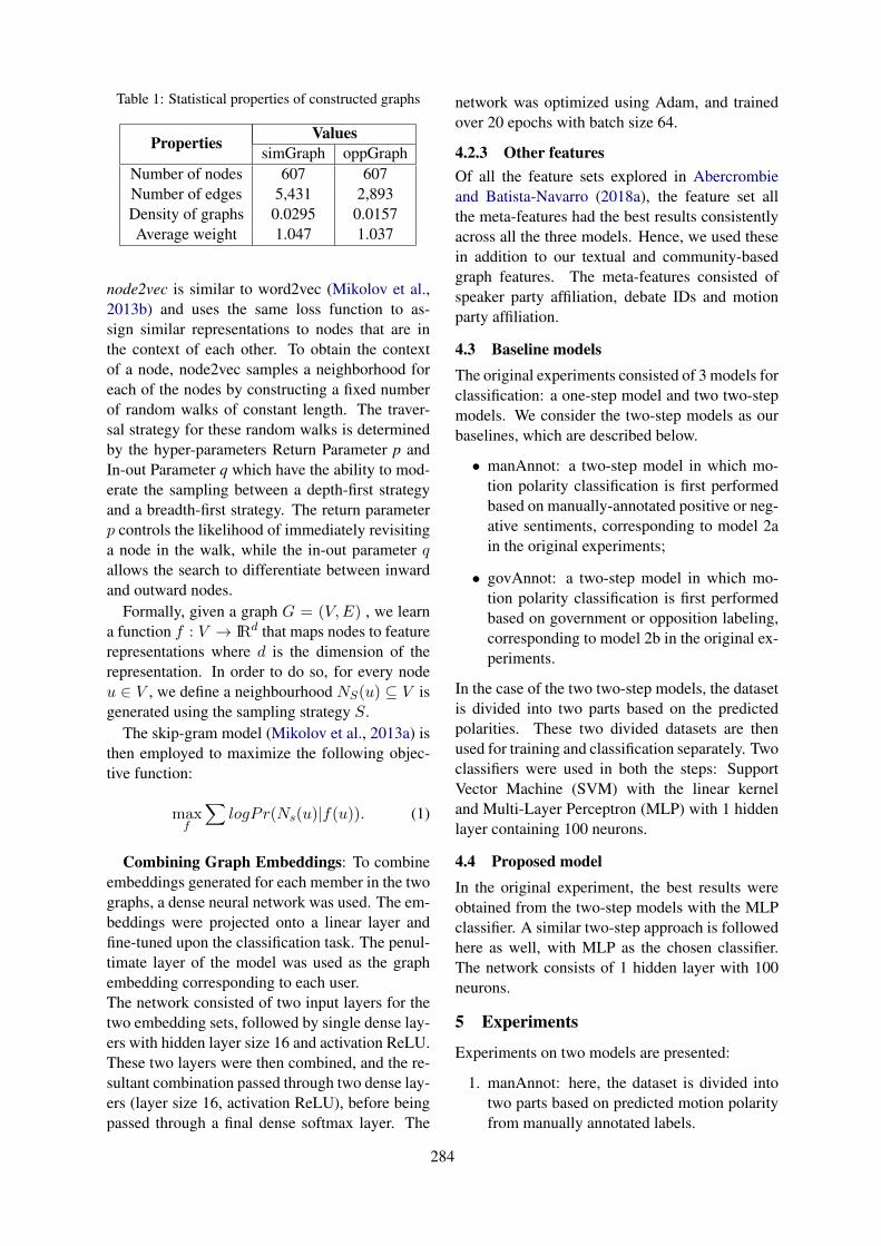
Table 1: Statistical properties of constructed graphs

Properties ValuessimGraph oppGraph

Number of nodes 607 607Number of edges 5,431 2,893Density of graphs 0.0295 0.0157Average weight 1.047 1.037

node2vec is similar to word2vec (Mikolov et al.,2013b) and uses the same loss function to as-sign similar representations to nodes that are inthe context of each other. To obtain the contextof a node, node2vec samples a neighborhood foreach of the nodes by constructing a fixed numberof random walks of constant length. The traver-sal strategy for these random walks is determinedby the hyper-parameters Return Parameter p andIn-out Parameter q which have the ability to mod-erate the sampling between a depth-first strategyand a breadth-first strategy. The return parameterp controls the likelihood of immediately revisitinga node in the walk, while the in-out parameter qallows the search to differentiate between inwardand outward nodes.

Formally, given a graph G = (V,E) , we learna function f : V → IRd that maps nodes to featurerepresentations where d is the dimension of therepresentation. In order to do so, for every nodeu ∈ V , we define a neighbourhood NS(u) ⊆ V isgenerated using the sampling strategy S.

The skip-gram model (Mikolov et al., 2013a) isthen employed to maximize the following objec-tive function:

maxf

∑logPr(Ns(u)|f(u)). (1)

Combining Graph Embeddings: To combineembeddings generated for each member in the twographs, a dense neural network was used. The em-beddings were projected onto a linear layer andfine-tuned upon the classification task. The penul-timate layer of the model was used as the graphembedding corresponding to each user.The network consisted of two input layers for thetwo embedding sets, followed by single dense lay-ers with hidden layer size 16 and activation ReLU.These two layers were then combined, and the re-sultant combination passed through two dense lay-ers (layer size 16, activation ReLU), before beingpassed through a final dense softmax layer. The

network was optimized using Adam, and trainedover 20 epochs with batch size 64.

4.2.3 Other featuresOf all the feature sets explored in Abercrombieand Batista-Navarro (2018a), the feature set allthe meta-features had the best results consistentlyacross all the three models. Hence, we used thesein addition to our textual and community-basedgraph features. The meta-features consisted ofspeaker party affiliation, debate IDs and motionparty affiliation.

4.3 Baseline modelsThe original experiments consisted of 3 models forclassification: a one-step model and two two-stepmodels. We consider the two-step models as ourbaselines, which are described below.

• manAnnot: a two-step model in which mo-tion polarity classification is first performedbased on manually-annotated positive or neg-ative sentiments, corresponding to model 2ain the original experiments;

• govAnnot: a two-step model in which mo-tion polarity classification is first performedbased on government or opposition labeling,corresponding to model 2b in the original ex-periments.

In the case of the two two-step models, the datasetis divided into two parts based on the predictedpolarities. These two divided datasets are thenused for training and classification separately. Twoclassifiers were used in both the steps: SupportVector Machine (SVM) with the linear kerneland Multi-Layer Perceptron (MLP) with 1 hiddenlayer containing 100 neurons.

4.4 Proposed modelIn the original experiment, the best results wereobtained from the two-step models with the MLPclassifier. A similar two-step approach is followedhere as well, with MLP as the chosen classifier.The network consists of 1 hidden layer with 100neurons.

5 Experiments

Experiments on two models are presented:

1. manAnnot: here, the dataset is divided intotwo parts based on predicted motion polarityfrom manually annotated labels.

284

Table 2: Observations for manModel

Feature Combinations without graph-based features with graph-based featuresAcc.(%) Prec. Recall F1 Acc.(%) Prec. Recall F1

TF-IDF+meta 89.38 0.897 0.887 0.884 92.26 0.920 0.917 0.917LDA+meta 86.34 0.875 0.839 0.850 92.34 0.930 0.902 0.915NRC+meta 86.43 0.860 0.859 0.858 92.25 0.932 0.903 0.916TF-IDF+LDA+meta 88.59 0.885 0.867 0.874 91.70 0.915 0.910 0.912TF-IDF+NRC+meta 88.73 0.896 0.867 0.879 91.94 0.918 0.914 0.914LDA+NRC+meta 85.86 0.861 0.828 0.842 92.66 0.938 0.905 0.920TF-IDF+LDA+NRC+meta 90.89 0.908 0.900 0.908 91.78 0.917 0.909 0.919

Table 3: Observations for govModel

Feature Combinations without graph-based features with graph-based featuresAcc.(%) Prec. Recall F1 Acc.(%) Prec. Recall F1

TF-IDF+meta 90.25 0.902 0.900 0.898 92.72 0.927 0.924 0.923LDA+meta 88.42 0.879 0.880 0.877 92.09 0.917 0.923 0.918NRC+meta 86.91 0.875 0.848 0.858 92.73 0.927 0.919 0.921TF-IDF+LDA+meta 89.06 0.887 0.882 0.883 92.33 0.920 0.925 0.920TF-IDF+NRC+meta 88.97 0.892 0.883 0.885 92.80 0.923 0.911 0.914LDA+NRC+meta 86.35 0.864 0.851 0.855 92.41 0.923 0.922 0.920TF-IDF+LDA+NRC+meta 89.22 0.896 0.876 0.883 92.33 0.920 0.922 0.918

2. govAnnot: Here, the dataset is separated intotwo parts based on the speaker’s affiliation: ifthe speaker presenting the motion belongs tothe ruling government, then the motion polar-ity is positive, or otherwise negative.

The hyperparameters (for each of the feature setsand the classifier) were tuned using grid search. L-BFGS (Liu and Nocedal, 1989) was used for op-timization in the neural network. Model trainingand evaluation was carried out using stratified 10-fold cross-validation. Stratification was performedto account for the slight imbalance in the dataset.Two types of labels are presented in the dataset:vote-based and manually-annotated. We use themanually-annotated labels for our experiments.For the graph-based features, a grid search wasperformed which yielded the following parametersfor generating embeddings:

• simGraph: p = 10, q = 1, walk length = 15,number of walks = 15, window size = 10. Thefeature vector obtained from these parame-ters yielded an accuracy of 79.51%.

• oppGraph: p = 0.1, q = 10, walk length = 5,number of walks = 10, window size = 10. Thefeature vector obtained from these parame-ters yielded an accuracy of 69.53%.

6 Results and Discussion

Table 2 and Table 3 present the results on the twomodels respectively. The values of accuracy, pre-

cision, recall, and F1-score are presented on fea-ture sets with and without graph-based features.In the case of both models, the usage of graph-based features outperforms the results obtainedwithout using them. The difference is large in thecase of the feature set comprising of LDA, NRC,and meta-features in the model with manually-annotated labels: the F1 scores obtained with andwithout graph features differ by 7.8%.It can be observed that by using graph-based fea-tures The baselines for both have been surpassedby using graph-based features along with the othertextual and meta-features. Our best results formanAnnot are obtained by using the combinationof LDA, NRC, and graph-based features alongwith meta-features. The best results for gov-Annot are obtained by using the combination ofTF-IDF and meta-features along with graph-basedfeatures.

7 Conclusion

We presented a method for sentiment analysis ofparliamentary debate transcripts, which could goa long way in helping determine the position anelected representative might assume on issues ofgreat importance to the general public. The exper-iments were carried out on the Hansard parliamen-tary debates dataset (Abercrombie and Batista-Navarro, 2018b). We performed experiments ona variety of textual analysis methods (e.g. topicmodeling, emotion classification, n-grams), and

285

combined them with community-based graph fea-tures obtained by representational learning on thedataset using node2vec. Our results surpass thestate-of-the-art results using both govAnnot andmanAnnot. Also, the F1 and accuracy values ofthe models using graph-based features are higherthan those without graph-based features, the dif-ference being considerable in some cases. Thisgives sufficient demonstration for the ability ofrepresentational learning to enhance performanceson tasks like sentiment analysis.

8 Future Work

Future work in this area could involve the follow-ing aspects:

• Application of the proposed approach totasks other than sentiment classification, forinstance analysis of mental health and suicideideation on social media.

• Constructing different graphs and analyzingother training and feature extraction methodsfor enhancing performance and deriving bet-ter inferences.

• Application of the proposed approach for an-alyzing data in different contexts; an exam-ple could be the analysis of the recently-conducted elections in India.

• Extend the proposed methodology to otherproblems (Mahata and Talburt, 2015; Mahataet al., 2015a,b) based on social media.

ReferencesGavin Abercrombie and Riza Batista-Navarro. 2018a.

’aye’or’no’? speech-level sentiment analysis ofhansard uk parliamentary debate transcripts. In Pro-ceedings of the Eleventh International Conferenceon Language Resources and Evaluation (LREC-2018), pages 33–40.

Gavin Abercrombie and Riza Theresa Batista-Navarro.2018b. Identifying opinion-topics and polarity ofparliamentary debate motions. In Proceedings ofthe 9th Workshop on Computational Approaches toSubjectivity, Sentiment and Social Media Analysis,pages 280–285.

David M Blei, Andrew Y Ng, and Michael I Jordan.2003. Latent dirichlet allocation. Journal of ma-chine Learning research, 3(Jan):993–1022.

Paula Carvalho, Luıs Sarmento, Jorge Teixeira, andMario J Silva. 2011. Liars and saviors in a senti-ment annotated corpus of comments to political de-bates. In Proceedings of the 49th Annual Meeting ofthe Association for Computational Linguistics: Hu-man Language Technologies: short papers-Volume2, pages 564–568. Association for ComputationalLinguistics.

Andrea Ceron, Luigi Curini, Stefano M Iacus, andGiuseppe Porro. 2014. Every tweet counts? howsentiment analysis of social media can improve ourknowledge of citizens political preferences with anapplication to italy and france. New media & soci-ety, 16(2):340–358.

William Deitrick and Wei Hu. 2013. Mutually enhanc-ing community detection and sentiment analysis ontwitter networks. Journal of Data Analysis and In-formation Processing, 1(03):19.

Aditya Grover and Jure Leskovec. 2016. node2vec:Scalable feature learning for networks. In Proceed-ings of the 22nd ACM SIGKDD international con-ference on Knowledge discovery and data mining,pages 855–864. ACM.

Kazi Saidul Hasan and Vincent Ng. 2013. Stanceclassification of ideological debates: Data, mod-els, features, and constraints. In Proceedings ofthe Sixth International Joint Conference on NaturalLanguage Processing, pages 1348–1356.

Amir Karami, London S Bennett, and Xiaoyun He.2018. Mining public opinion about economic is-sues: Twitter and the us presidential election. In-ternational Journal of Strategic Decision Sciences(IJSDS), 9(1):18–28.

Benjamin E Lauderdale and Alexander Herzog.2016. Measuring political positions from legislativespeech. Political Analysis, 24(3):374–394.

Dong C Liu and Jorge Nocedal. 1989. On the limitedmemory bfgs method for large scale optimization.Mathematical programming, 45(1-3):503–528.

Euripides Loukis, Yannis Charalabidis, and AggelikiAndroutsopoulou. 2014. An analysis of multiple so-cial media consultations in the european parliamentfrom a public policy perspective.

Debanjan Mahata, Jasper Friedrichs, Rajiv Ratn Shah,and Jing Jiang. 2018. Detecting personal intake ofmedicine from twitter. IEEE Intelligent Systems,33(4):87–95.

Debanjan Mahata and John R Talburt. 2015. A frame-work for collecting, extracting and managing eventidentity information from twitter. In ICIQ.

Debanjan Mahata, John R Talburt, and Vivek KumarSingh. 2015a. From chirps to whistles: Discover-ing event-specific informative content from twitter.In Proceedings of the ACM web science conference,page 17. ACM.

286

Debanjan Mahata, John R Talburt, and Vivek KumarSingh. 2015b. Identification and ranking of event-specific entity-centric informative content from twit-ter. In International Conference on Applicationsof Natural Language to Information Systems, pages275–281. Springer.

Tomas Mikolov, Kai Chen, Greg Corrado, and Jef-frey Dean. 2013a. Efficient estimation of wordrepresentations in vector space. arXiv preprintarXiv:1301.3781.

Tomas Mikolov, Ilya Sutskever, Kai Chen, Greg S Cor-rado, and Jeff Dean. 2013b. Distributed representa-tions of words and phrases and their compositional-ity. In Advances in neural information processingsystems, pages 3111–3119.

Pushkar Mishra, Marco Del Tredici, Helen Yan-nakoudakis, and Ekaterina Shutova. 2018. Authorprofiling for abuse detection. In Proceedings ofthe 27th International Conference on ComputationalLinguistics, pages 1088–1098.

Saif M Mohammad and Peter D Turney. 2013. Nrcemotion lexicon. National Research Council,Canada.

Jing Qian, Mai ElSherief, Elizabeth M Belding, andWilliam Yang Wang. 2018. Leveraging intra-user and inter-user representation learning for au-tomated hate speech detection. arXiv preprintarXiv:1804.03124.

Ludovic Rheault, Kaspar Beelen, ChristopherCochrane, and Graeme Hirst. 2016. Measuringemotion in parliamentary debates with automatedtextual analysis. PloS one, 11(12):e0168843.

Elena Rudkowsky, Martin Haselmayer, Matthias Was-tian, Marcelo Jenny, Stefan Emrich, and MichaelSedlmair. 2018. More than bags of words: Senti-ment analysis with word embeddings. Communica-tion Methods and Measures, 12(2-3):140–157.

Rajiv Shah and Roger Zimmermann. 2017. Multi-modal analysis of user-generated multimedia con-tent. Springer.

Rajiv Ratn Shah, Anupam Samanta, Deepak Gupta,Yi Yu, Suhua Tang, and Roger Zimmermann. 2016a.Prompt: Personalized user tag recommendation forsocial media photos leveraging personal and socialcontexts. In 2016 IEEE International Symposiumon Multimedia (ISM), pages 486–492. IEEE.

Rajiv Ratn Shah, Yi Yu, Suhua Tang, Shin’ichi Satoh,Akshay Verma, and Roger Zimmermann. 2016b.Concept-level multimodal ranking of flickr phototags via recall based weighting. In Proceedingsof the 2016 ACM Workshop on Multimedia COM-MONS, pages 19–26. ACM.

Rajiv Ratn Shah, Yi Yu, Akshay Verma, Suhua Tang,Anwar Dilawar Shaikh, and Roger Zimmermann.2016c. Leveraging multimodal information for

event summarization and concept-level sentimentanalysis. Knowledge-Based Systems, 108:102–109.

Stefan Stieglitz and Linh Dang-Xuan. 2012. Politicalcommunication and influence through microblog-ging – an empirical analysis of sentiment in twit-ter messages and retweet behavior. In 2012 45thHawaii International Conference on System Sci-ences, pages 3500–3509. IEEE.

Matt Thomas, Bo Pang, and Lillian Lee. 2006. Get outthe vote: Determining support or opposition fromcongressional floor-debate transcripts. In Proceed-ings of the 2006 conference on empirical methods innatural language processing, pages 327–335. Asso-ciation for Computational Linguistics.

Yaqin Wang and Haitao Liu. 2018. Is trump alwaysrambling like a fourth-grade student? an analysisof stylistic features of donald trumps political dis-course during the 2016 election. Discourse & Soci-ety, 29(3):299–323.

287

Proceedings of the 57th Annual Meeting of the Association for Computational Linguistics: Student Research Workshop, pages 288–294Florence, Italy, July 28 - August 2, 2019. c©2019 Association for Computational Linguistics

Transfer Learning Based Free-Form Speech Command Classification forLow-Resource Languages

Yohan KarunanayakeUniversity of Moratuwa

Sri Lankayohan.13@cse.mrt.ac.lk

Uthayasanker ThayasivamUniversity of Moratuwa

Sri Lankartuthaya@uom.lk

Surangika RanathungaUniversity of Moratuwa

Sri Lankasurangikar@uom.lk

Abstract

Current state-of-the-art speech-based user in-terfaces use data intense methodologies to rec-ognize free-form speech commands. However,this is not viable for low-resource languages,which lack speech data. This restricts the us-ability of such interfaces to a limited num-ber of languages. In this paper, we proposea methodology to develop a robust domain-specific speech command classification systemfor low-resource languages using speech dataof a high-resource language. In this transferlearning-based approach, we used a Convolu-tion Neural Network (CNN) to identify a fixedset of intents using an ASR-based characterprobability map. We were able to achieve sig-nificant results for Sinhala and Tamil datasetsusing an English based ASR, which attests therobustness of the proposed approach.

.

1 Introduction

Speech command recognizable user interfaces arebecoming popular since they are more naturalfor end-users to interact with. Google Assis-tant1, and Amazon Alexa2 can be highlighted asfew such commercial services, which are rang-ing from smartphones to home automation. Theseare capable of identifying the intent of free-formspeech commands given by the user. To enablethis kind of service, Automatic Speech Recogni-tion (ASR) systems and Natural Language Under-standing (NLU) systems work together with a veryhigh level of accuracy (Ram et al., 2018).

If ASR or NLU components have suboptimalresults, it directly affects the final output (Yamanet al., 2008; Rao et al., 2018). Hence, to getgood results in ASR systems, it is common to use

1https://assistant.google.com2https://developer.amazon.com/alexa

very large speech corpora (Hannun et al., 2014;Amodei et al., 2016; Chiu et al., 2018). How-ever, low-resource languages (LRL) do not havethis luxury. Here, languages that have a lim-ited presence on the Internet and those that lackelectronic resources for speech and/or languageprocessing are referred to as low-resource lan-guages (LRLs) (Besacier et al., 2014). Because ofthis reason despite the applicability, speech-baseduser interfaces are limited to common languages.For LRLs researchers have focused on narrowerscopes such as recognition of digits or keywords(Manamperi et al., 2018; Chen et al., 2015). How-ever, free-form commands are difficult to managein this way since there can be overlappings be-tween commands.

Buddhika et al. (2018); Chen et al. (2018) showsome direct speech classification approaches to itsintents. In particular, Buddhika et al. (2018) havegiven some attention for the low resource setting.Additionally, Transfer learning is used to exploitthe issue of limited data in some of the ASR basedresearch (Huang et al., 2013; Kunze et al., 2017).

In this paper, we present an improved and effec-tive methodology to classify domain-specific free-form speech commands while utilizing this directclassification and transfer learning approaches.Here, we use a character probability map from anASR model trained on English to identify intents.Performance of this methodology is evaluated us-ing Sinhala (Buddhika et al., 2018) and newly col-lected Tamil datasets. The proposed approach canreach to a reasonable accuracy using limited train-ing data.

Rest of the paper is organized as follows. Sec-tion 2 presents related work, section 3 describesmethodology used. Section 4 and 5 provides de-tails of the datasets and experiments. Section 6presents a detailed analysis of the obtained results.Finally Section 7 concludes the paper.

288

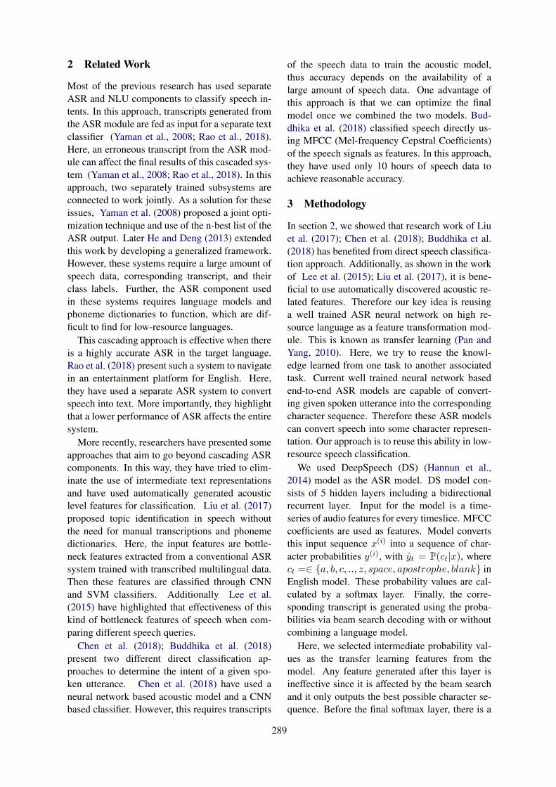
2 Related Work

Most of the previous research has used separateASR and NLU components to classify speech in-tents. In this approach, transcripts generated fromthe ASR module are fed as input for a separate textclassifier (Yaman et al., 2008; Rao et al., 2018).Here, an erroneous transcript from the ASR mod-ule can affect the final results of this cascaded sys-tem (Yaman et al., 2008; Rao et al., 2018). In thisapproach, two separately trained subsystems areconnected to work jointly. As a solution for theseissues, Yaman et al. (2008) proposed a joint opti-mization technique and use of the n-best list of theASR output. Later He and Deng (2013) extendedthis work by developing a generalized framework.However, these systems require a large amount ofspeech data, corresponding transcript, and theirclass labels. Further, the ASR component usedin these systems requires language models andphoneme dictionaries to function, which are dif-ficult to find for low-resource languages.

This cascading approach is effective when thereis a highly accurate ASR in the target language.Rao et al. (2018) present such a system to navigatein an entertainment platform for English. Here,they have used a separate ASR system to convertspeech into text. More importantly, they highlightthat a lower performance of ASR affects the entiresystem.

More recently, researchers have presented someapproaches that aim to go beyond cascading ASRcomponents. In this way, they have tried to elim-inate the use of intermediate text representationsand have used automatically generated acousticlevel features for classification. Liu et al. (2017)proposed topic identification in speech withoutthe need for manual transcriptions and phonemedictionaries. Here, the input features are bottle-neck features extracted from a conventional ASRsystem trained with transcribed multilingual data.Then these features are classified through CNNand SVM classifiers. Additionally Lee et al.(2015) have highlighted that effectiveness of thiskind of bottleneck features of speech when com-paring different speech queries.

Chen et al. (2018); Buddhika et al. (2018)present two different direct classification ap-proaches to determine the intent of a given spo-ken utterance. Chen et al. (2018) have used aneural network based acoustic model and a CNNbased classifier. However, this requires transcripts

of the speech data to train the acoustic model,thus accuracy depends on the availability of alarge amount of speech data. One advantage ofthis approach is that we can optimize the finalmodel once we combined the two models. Bud-dhika et al. (2018) classified speech directly us-ing MFCC (Mel-frequency Cepstral Coefficients)of the speech signals as features. In this approach,they have used only 10 hours of speech data toachieve reasonable accuracy.

3 Methodology

In section 2, we showed that research work of Liuet al. (2017); Chen et al. (2018); Buddhika et al.(2018) has benefited from direct speech classifica-tion approach. Additionally, as shown in the workof Lee et al. (2015); Liu et al. (2017), it is bene-ficial to use automatically discovered acoustic re-lated features. Therefore our key idea is reusinga well trained ASR neural network on high re-source language as a feature transformation mod-ule. This is known as transfer learning (Pan andYang, 2010). Here, we try to reuse the knowl-edge learned from one task to another associatedtask. Current well trained neural network basedend-to-end ASR models are capable of convert-ing given spoken utterance into the correspondingcharacter sequence. Therefore these ASR modelscan convert speech into some character represen-tation. Our approach is to reuse this ability in low-resource speech classification.

We used DeepSpeech (DS) (Hannun et al.,2014) model as the ASR model. DS model con-sists of 5 hidden layers including a bidirectionalrecurrent layer. Input for the model is a time-series of audio features for every timeslice. MFCCcoefficients are used as features. Model convertsthis input sequence x(i) into a sequence of char-acter probabilities y(i), with yt = P(ct|x), wherect =∈ a, b, c, .., z, space, apostrophe, blank inEnglish model. These probability values are cal-culated by a softmax layer. Finally, the corre-sponding transcript is generated using the proba-bilities via beam search decoding with or withoutcombining a language model.

Here, we selected intermediate probability val-ues as the transfer learning features from themodel. Any feature generated after this layer isineffective since it is affected by the beam searchand it only outputs the best possible character se-quence. Before the final softmax layer, there is a

289

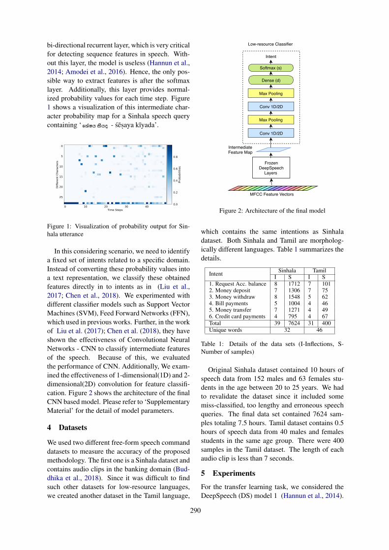
bi-directional recurrent layer, which is very criticalfor detecting sequence features in speech. With-out this layer, the model is useless (Hannun et al.,2014; Amodei et al., 2016). Hence, the only pos-sible way to extract features is after the softmaxlayer. Additionally, this layer provides normal-ized probability values for each time step. Figure1 shows a visualization of this intermediate char-acter probability map for a Sinhala speech querycontaining ‘ ෙෂය යද - ses.aya kıyada’.

0 10 20 30 40Time Steps

0

5

10

15

20

25

Diffe

rent

Cha

ract

ers

0.0

0.2

0.4

0.6

0.8

Prob

abilit

ies

Figure 1: Visualization of probability output for Sin-hala utterance

In this considering scenario, we need to identifya fixed set of intents related to a specific domain.Instead of converting these probability values intoa text representation, we classify these obtainedfeatures directly in to intents as in (Liu et al.,2017; Chen et al., 2018). We experimented withdifferent classifier models such as Support VectorMachines (SVM), Feed Forward Networks (FFN),which used in previous works. Further, in the workof Liu et al. (2017); Chen et al. (2018), they haveshown the effectiveness of Convolutional NeuralNetworks - CNN to classify intermediate featuresof the speech. Because of this, we evaluatedthe performance of CNN. Additionally, We exam-ined the effectiveness of 1-dimensional(1D) and 2-dimensional(2D) convolution for feature classifi-cation. Figure 2 shows the architecture of the finalCNN based model. Please refer to ‘SupplementaryMaterial’ for the detail of model parameters.

4 Datasets

We used two different free-form speech commanddatasets to measure the accuracy of the proposedmethodology. The first one is a Sinhala dataset andcontains audio clips in the banking domain (Bud-dhika et al., 2018). Since it was difficult to findsuch other datasets for low-resource languages,we created another dataset in the Tamil language,

FrozenDeepSpeech

Layers

Conv 1D/2D

Max Pooling

Conv 1D/2D

Max Pooling

Dense (d)

Intent

IntermediateFeature Map

MFCC Feature Vectors

Low-resource Classifier

Softmax (s)

Figure 2: Architecture of the final model

which contains the same intentions as Sinhaladataset. Both Sinhala and Tamil are morpholog-ically different languages. Table 1 summarizes thedetails.

Intent Sinhala TamilI S I S

1. Request Acc. balance 8 1712 7 1012. Money deposit 7 1306 7 753. Money withdraw 8 1548 5 624. Bill payments 5 1004 4 465. Money transfer 7 1271 4 496. Credit card payments 4 795 4 67Total 39 7624 31 400Unique words 32 46

Table 1: Details of the data sets (I-Inflections, S-Number of samples)

Original Sinhala dataset contained 10 hours ofspeech data from 152 males and 63 females stu-dents in the age between 20 to 25 years. We hadto revalidate the dataset since it included somemiss-classified, too lengthy and erroneous speechqueries. The final data set contained 7624 sam-ples totaling 7.5 hours. Tamil dataset contains 0.5hours of speech data from 40 males and femalesstudents in the same age group. There were 400samples in the Tamil dataset. The length of eachaudio clip is less than 7 seconds.

5 Experiments

For the transfer learning task, we considered theDeepSpeech (DS) model 1 (Hannun et al., 2014).

290

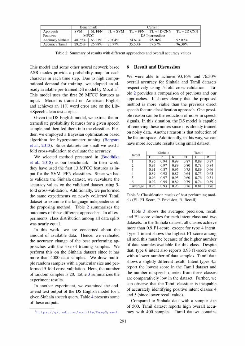
Benchmark CurrentApproach SVM 6L FFN TL + SVM TL + FFN TL + 1D CNN TL + 2D CNNFeatures MFCC DS IntermediateAccuracy Sinhala 48.79% 63.23% 70.04% 74.67% 93.16% 92.09%Accuracy Tamil 29.25% 26.98% 23.77% 35.50% 37.57% 76.30%

Table 2: Summary of results with different approaches and overall accuracy values

This model and some other neural network basedASR modes provide a probability map for eachcharacter in each time step. Due to high compu-tational demand for training, we adopted an al-ready available pre-trained DS model by Mozilla3.This model uses the first 26 MFCC features asinput. Model is trained on American Englishand achieves an 11% word error rate on the Lib-riSpeech clean test corpus.

Given the DS English model, we extract the in-termediate probability features for a given speechsample and then fed them into the classifier. Fur-ther, we employed a Bayesian optimization basedalgorithm for hyperparameter tuining (Bergstraet al., 2013). Since datasets are small we used 5fold cross-validation to evaluate the accuracy.

We selected method presented in (Buddhikaet al., 2018) as our benchmark. In their work,they have used the first 13 MFCC features as in-put for the SVM, FFN classifiers. Since we hadto validate the Sinhala dataset, we reevaluate theaccuracy values on the validated dataset using 5-fold cross-validation. Additionally, we performedthe same experiments on newly collected Tamildataset to examine the language independence ofthe proposing method. Table 2 summarizes theoutcomes of these different approaches. In all ex-periments, class distribution among all data splitswas nearly equal.

In this work, we are concerned about theamount of available data. Hence, we evaluatedthe accuracy change of the best performing ap-proaches with the size of training samples. Weperform this on the Sinhala dataset since it hasmore than 4000 data samples. We drew multi-ple random samples with a particular size and per-formed 5-fold cross-validation. Here, the numberof random samples is 20. Table 3 summarizes theexperiment results.

In another experiment, we examined the end-to-end text output of the DS English model for agiven Sinhala speech query. Table 4 presents someof these outputs.

3https://github.com/mozilla/DeepSpeech

6 Result and Discussion

We were able to achieve 93.16% and 76.30%overall accuracy for Sinhala and Tamil datasetsrespectively using 5-fold cross-validation. Ta-ble 2 provides a comparison of previous and ourapproaches. It shows clearly that the proposedmethod is more viable than the previous directspeech feature classification approach. One possi-ble reason can be the reduction of noise in speechsignals. In this situation, the DS model is capableof removing these noises since it is already trainedon noisy data. Another reason is that reduction ofthe feature space. Additionally, in this way, we canhave more accurate results using small dataset.

Intent Sinhala TamilF1 P R F1 P R

1 0.96 0.94 0.99 0.87 0.89 0.872 0.93 0.97 0.89 0.80 0.78 0.843 0.91 0.87 0.95 0.75 0.89 0.664 0.89 0.93 0.87 0.64 0.75 0.635 0.96 0.97 0.95 0.60 0.76 0.516 0.92 0.95 0.89 0.79 0.74 0.89Average 0.93 0.93 0.93 0.76 0.81 0.76

Table 3: Classification results of best performing mod-els (F1- F1-Score, P- Precision, R- Recall)

Table 3 shows the averaged precision, recalland F1-score values for each intent class and twodatasets. In the Sinhala dataset, all classes achievemore than 0.9 F1-score, except for type 4 intent.Type 1 intent shows the highest F1-score amongall and, this must be because of the higher numberof data samples available for this class. Despitethat, type 6 intent also reports 0.93 f1-score evenwith a lower number of data samples. Tamil datashows a slightly different result. Intent types 4,5report the lowest score in the Tamil dataset andthe number of speech queries from these classesare comparatively low in the dataset. Further, wecan observe that the Tamil classifier is incapableof accurately identifying positive intent classes 4and 5 (since lower recall value).

Compared to Sinhala data with a sample sizeof 500, Tamil dataset reports high overall accu-racy with 400 samples. Tamil dataset contains

291

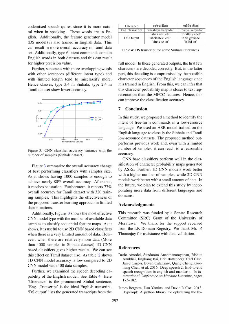
codemixed speech quires since it is more natu-ral when in speaking. These words are in En-glish. Additionally, the feature generator model(DS model) is also trained in English data. Thiscan result in more overall accuracy in Tamil dataset. Additionally, type 6 intent commands containEnglish words in both datasets and this can resultfor higher precision value.

Further, sentences with more overlapping wordswith other sentences (different intent type) andwith limited length tend to misclassify more.Hence classes, type 3,4 in Sinhala, type 2,4 inTamil dataset show lower accuracy.

1000 2000 3000 4000 5000Number of Data Samples

0.5

0.6

0.7

0.8

0.9

Accu

racy 1D CNN

2D CNN

Figure 3: CNN classifier accuracy variance with thenumber of samples (Sinhala dataset)

Figure 3 summarize the overall accuracy changeof best performing classifiers with samples size.As it shows having 1000 samples is enough toachieve nearly 80% overall accuracy. After that,it reaches saturation. Furthermore, it reports 77%overall accuracy for Tamil dataset with 320 train-ing samples. This highlights the effectiveness ofthe proposed transfer learning approach in limiteddata situations.

Additionally, Figure 3 shows the most effectiveCNN model type with the number of available datasamples to classify sequential feature maps. As itshows, it is useful to use 2D CNN based classifierswhen there is a very limited amount of data. How-ever, when there are relatively more data (Morethan 4000 samples in Sinhala dataset) 1D CNNbased classifiers gives higher results. We can seethis effect on Tamil dataset also. As table 2 shows1D CNN model accuracy is low compared to 2DCNN model with 400 data samples.

Further, we examined the speech decoding ca-pability of the English model. See Table 4. Here‘Utterance’ is the pronounced Sinhal sentence,‘Eng. Transcript’ is the ideal English transcript.‘DS output’ lists the generated transcripts from the

Utterance ෙෂය යද ඉය යද

Eng. Transcript ’sheshaya keeyada’ ’ithiriya keeyada’

DS Output’she s reci ete’ ’it cillety edet’

’sheis heki edit’ ’it tia gaviade’’sheis ae an’ ’it lid en’

Table 4: DS transcript for some Sinhala utterances

full model. In these generated outputs, the first fewcharacters are decoded correctly. But, in the latterpart, this decoding is compromised by the possiblecharacter sequences of the English language sinceit is trained in English. From this, we can infer thatthis character probability map is closer to text rep-resentation than the MFCC features. Hence, thiscan improve the classification accuracy.

7 Conclusion

In this study, we proposed a method to identify theintent of free-form commands in a low-resourcelanguage. We used an ASR model trained on theEnglish language to classify the Sinhala and Tamillow-resource datasets. The proposed method out-performs previous work and, even with a limitednumber of samples, it can reach to a reasonableaccuracy.

CNN base classifiers perform well in the clas-sification of character probability maps generatedby ASRs. Further, 1D CNN models work betterwith a higher number of samples, while 2D CNNmodels work better with a small amount of data. Inthe future, we plan to extend this study by incor-porating more data from different languages anddomains.

Acknowledgments

This research was funded by a Senate ResearchCommittee (SRC) Grant of the University ofMoratuwa. We thank for the support receivedfrom the LK Domain Registry. We thank Mr. P.Thananjay for assistance with data validation.

ReferencesDario Amodei, Sundaram Ananthanarayanan, Rishita

Anubhai, Jingliang Bai, Eric Battenberg, Carl Case,Jared Casper, Bryan Catanzaro, Qiang Cheng, Guo-liang Chen, et al. 2016. Deep speech 2: End-to-endspeech recognition in english and mandarin. In In-ternational Conference on Machine Learning, pages173–182.

James Bergstra, Dan Yamins, and David D Cox. 2013.Hyperopt: A python library for optimizing the hy-

292

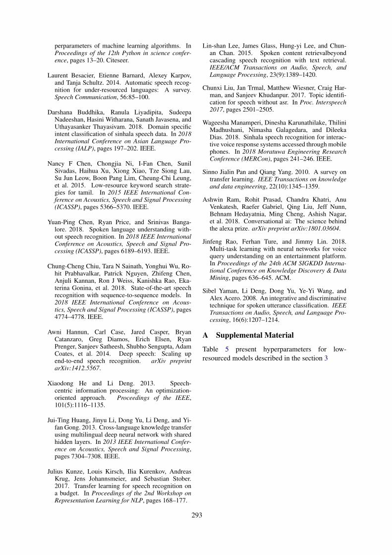
perparameters of machine learning algorithms. InProceedings of the 12th Python in science confer-ence, pages 13–20. Citeseer.

Laurent Besacier, Etienne Barnard, Alexey Karpov,and Tanja Schultz. 2014. Automatic speech recog-nition for under-resourced languages: A survey.Speech Communication, 56:85–100.

Darshana Buddhika, Ranula Liyadipita, SudeepaNadeeshan, Hasini Witharana, Sanath Javasena, andUthayasanker Thayasivam. 2018. Domain specificintent classification of sinhala speech data. In 2018International Conference on Asian Language Pro-cessing (IALP), pages 197–202. IEEE.

Nancy F Chen, Chongjia Ni, I-Fan Chen, SunilSivadas, Haihua Xu, Xiong Xiao, Tze Siong Lau,Su Jun Leow, Boon Pang Lim, Cheung-Chi Leung,et al. 2015. Low-resource keyword search strate-gies for tamil. In 2015 IEEE International Con-ference on Acoustics, Speech and Signal Processing(ICASSP), pages 5366–5370. IEEE.

Yuan-Ping Chen, Ryan Price, and Srinivas Banga-lore. 2018. Spoken language understanding with-out speech recognition. In 2018 IEEE InternationalConference on Acoustics, Speech and Signal Pro-cessing (ICASSP), pages 6189–6193. IEEE.

Chung-Cheng Chiu, Tara N Sainath, Yonghui Wu, Ro-hit Prabhavalkar, Patrick Nguyen, Zhifeng Chen,Anjuli Kannan, Ron J Weiss, Kanishka Rao, Eka-terina Gonina, et al. 2018. State-of-the-art speechrecognition with sequence-to-sequence models. In2018 IEEE International Conference on Acous-tics, Speech and Signal Processing (ICASSP), pages4774–4778. IEEE.

Awni Hannun, Carl Case, Jared Casper, BryanCatanzaro, Greg Diamos, Erich Elsen, RyanPrenger, Sanjeev Satheesh, Shubho Sengupta, AdamCoates, et al. 2014. Deep speech: Scaling upend-to-end speech recognition. arXiv preprintarXiv:1412.5567.

Xiaodong He and Li Deng. 2013. Speech-centric information processing: An optimization-oriented approach. Proceedings of the IEEE,101(5):1116–1135.

Jui-Ting Huang, Jinyu Li, Dong Yu, Li Deng, and Yi-fan Gong. 2013. Cross-language knowledge transferusing multilingual deep neural network with sharedhidden layers. In 2013 IEEE International Confer-ence on Acoustics, Speech and Signal Processing,pages 7304–7308. IEEE.

Julius Kunze, Louis Kirsch, Ilia Kurenkov, AndreasKrug, Jens Johannsmeier, and Sebastian Stober.2017. Transfer learning for speech recognition ona budget. In Proceedings of the 2nd Workshop onRepresentation Learning for NLP, pages 168–177.

Lin-shan Lee, James Glass, Hung-yi Lee, and Chun-an Chan. 2015. Spoken content retrievalbeyondcascading speech recognition with text retrieval.IEEE/ACM Transactions on Audio, Speech, andLanguage Processing, 23(9):1389–1420.

Chunxi Liu, Jan Trmal, Matthew Wiesner, Craig Har-man, and Sanjeev Khudanpur. 2017. Topic identifi-cation for speech without asr. In Proc. Interspeech2017, pages 2501–2505.

Wageesha Manamperi, Dinesha Karunathilake, ThiliniMadhushani, Nimasha Galagedara, and DileekaDias. 2018. Sinhala speech recognition for interac-tive voice response systems accessed through mobilephones. In 2018 Moratuwa Engineering ResearchConference (MERCon), pages 241–246. IEEE.

Sinno Jialin Pan and Qiang Yang. 2010. A survey ontransfer learning. IEEE Transactions on knowledgeand data engineering, 22(10):1345–1359.

Ashwin Ram, Rohit Prasad, Chandra Khatri, AnuVenkatesh, Raefer Gabriel, Qing Liu, Jeff Nunn,Behnam Hedayatnia, Ming Cheng, Ashish Nagar,et al. 2018. Conversational ai: The science behindthe alexa prize. arXiv preprint arXiv:1801.03604.

Jinfeng Rao, Ferhan Ture, and Jimmy Lin. 2018.Multi-task learning with neural networks for voicequery understanding on an entertainment platform.In Proceedings of the 24th ACM SIGKDD Interna-tional Conference on Knowledge Discovery & DataMining, pages 636–645. ACM.

Sibel Yaman, Li Deng, Dong Yu, Ye-Yi Wang, andAlex Acero. 2008. An integrative and discriminativetechnique for spoken utterance classification. IEEETransactions on Audio, Speech, and Language Pro-cessing, 16(6):1207–1214.

A Supplemental Material

Table 5 present hyperparameters for low-resourced models described in the section 3

293

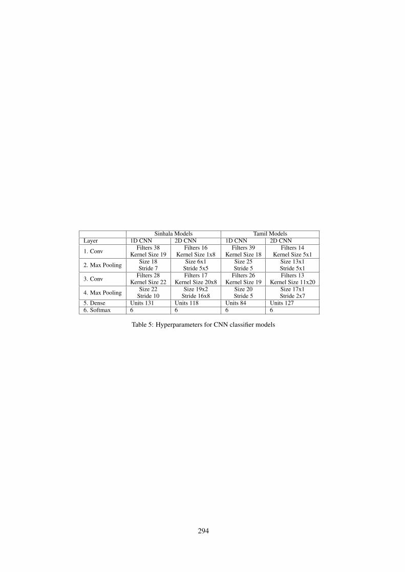
Sinhala Models Tamil ModelsLayer 1D CNN 2D CNN 1D CNN 2D CNN

1. Conv Filters 38Kernel Size 19

Filters 16Kernel Size 1x8

Filters 39Kernel Size 18

Filters 14Kernel Size 5x1

2. Max Pooling Size 18Stride 7

Size 6x1Stride 5x5

Size 25Stride 5

Size 13x1Stride 5x1

3. Conv Filters 28Kernel Size 22

Filters 17Kernel Size 20x8

Filters 26Kernel Size 19

Filters 13Kernel Size 11x20

4. Max Pooling Size 22Stride 10

Size 19x2Stride 16x8

Size 20Stride 5

Size 17x1Stride 2x7

5. Dense Units 131 Units 118 Units 84 Units 1276. Softmax 6 6 6 6

Table 5: Hyperparameters for CNN classifier models

294

Proceedings of the 57th Annual Meeting of the Association for Computational Linguistics: Student Research Workshop, pages 295–301Florence, Italy, July 28 - August 2, 2019. c©2019 Association for Computational Linguistics

Embedding Strategies for Specialized Domains: Application to ClinicalEntity Recognition

Hicham El Boukkouri1,2, Olivier Ferret3, Thomas Lavergne1,2, Pierre Zweigenbaum1

1LIMSI, CNRS, Universite Paris-Saclay, Orsay, France,2Univ. Paris-Sud,

3CEA, LIST, Gif-sur-Yvette, F-91191 France.elboukkouri,lavergne,pz@limsi.fr, olivier.ferret@cea.fr

Abstract

Using pre-trained word embeddings in con-junction with Deep Learning models has be-come the de facto approach in Natural Lan-guage Processing (NLP). While this usuallyyields satisfactory results, off-the-shelf wordembeddings tend to perform poorly on textsfrom specialized domains such as clinical re-ports. Moreover, training specialized wordrepresentations from scratch is often either im-possible or ineffective due to the lack of largeenough in-domain data. In this work, we focuson the clinical domain for which we study em-bedding strategies that rely on general-domainresources only. We show that by combiningoff-the-shelf contextual embeddings (ELMo)with static word2vec embeddings trained ona small in-domain corpus built from the taskdata, we manage to reach and sometimes out-perform representations learned from a largecorpus in the medical domain.1

1 Introduction

Today, the NLP community can enjoy an ever-growing list of embedding techniques that includefactorization methods (e.g. GloVe (Penningtonet al., 2014)), neural methods (e.g. word2vec(Mikolov et al., 2013), fastText (Bojanowski et al.,2017)) and more recently dynamic methods thattake into account the context (e.g. ELMo (Peterset al., 2018), BERT (Devlin et al., 2018)).

The success of these methods can be arguablyattributed to the availability of large general-domain corpora like Wikipedia, Gigaword (Graffet al., 2003) or the BooksCorpus (Zhu et al., 2015).Unfortunately, similar corpora are often unavail-able for specialized domains, leaving the NLPpractitioner with only two choices: either using

1Python code for reproducing our experiments isavailable at: https://github.com/helboukkouri/acl_srw_2019

general-domain word embeddings that are prob-ably not fit for the task at hand or training newembeddings on the available in-domain corpus,which may probably be too small and result inpoor performance.

In this paper, we focus on the clinical domainand explore several ways to improve pre-trainedembeddings built from a small corpus in this do-main by using different kinds of general-domainembeddings. More specifically, we make the fol-lowing contributions:

• we show that word embeddings trained ona small in-domain corpus can be improvedusing off-the-shelf contextual embeddings(ELMo) from the general domain. We alsoshow that this combination performs betterthan the contextual embeddings alone andimproves upon static embeddings trained ona large in-domain corpus;

• we define two ways of combining contextualand static embeddings and conclude that thenaive concatenation of vectors is consistentlyoutperformed by the addition of the staticrepresentation directly into the internal linearcombination of ELMo;

• finally, we show that ELMo models can besuccessfully fine-tuned on a small in-domaincorpus, bringing significant improvements tostrategies involving contextual embeddings.

2 Related Work

Former work by Roberts (2016) analyzed thetrade-off between corpus size and similarity whentraining word embeddings for a clinical entityrecognition task. The author’s conclusion was thatwhile embeddings trained with word2vec on in-domain texts performed generally better, a combi-nation of both in-domain and general domain em-

295

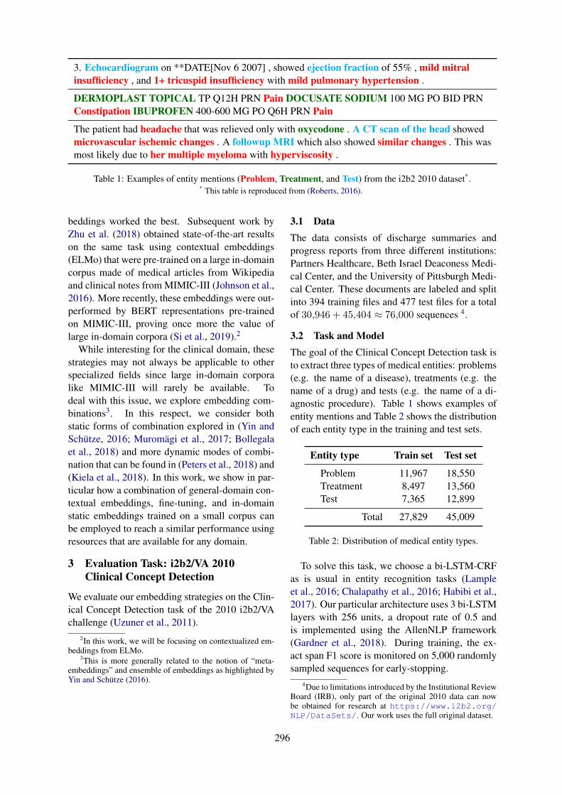
3. Echocardiogram on **DATE[Nov 6 2007] , showed ejection fraction of 55% , mild mitralinsufficiency , and 1+ tricuspid insufficiency with mild pulmonary hypertension .

DERMOPLAST TOPICAL TP Q12H PRN Pain DOCUSATE SODIUM 100 MG PO BID PRNConstipation IBUPROFEN 400-600 MG PO Q6H PRN Pain

The patient had headache that was relieved only with oxycodone . A CT scan of the head showedmicrovascular ischemic changes . A followup MRI which also showed similar changes . This wasmost likely due to her multiple myeloma with hyperviscosity .

Table 1: Examples of entity mentions (Problem, Treatment, and Test) from the i2b2 2010 dataset*.* This table is reproduced from (Roberts, 2016).

beddings worked the best. Subsequent work byZhu et al. (2018) obtained state-of-the-art resultson the same task using contextual embeddings(ELMo) that were pre-trained on a large in-domaincorpus made of medical articles from Wikipediaand clinical notes from MIMIC-III (Johnson et al.,2016). More recently, these embeddings were out-performed by BERT representations pre-trainedon MIMIC-III, proving once more the value oflarge in-domain corpora (Si et al., 2019).2

While interesting for the clinical domain, thesestrategies may not always be applicable to otherspecialized fields since large in-domain corporalike MIMIC-III will rarely be available. Todeal with this issue, we explore embedding com-binations3. In this respect, we consider bothstatic forms of combination explored in (Yin andSchutze, 2016; Muromagi et al., 2017; Bollegalaet al., 2018) and more dynamic modes of combi-nation that can be found in (Peters et al., 2018) and(Kiela et al., 2018). In this work, we show in par-ticular how a combination of general-domain con-textual embeddings, fine-tuning, and in-domainstatic embeddings trained on a small corpus canbe employed to reach a similar performance usingresources that are available for any domain.

3 Evaluation Task: i2b2/VA 2010Clinical Concept Detection

We evaluate our embedding strategies on the Clin-ical Concept Detection task of the 2010 i2b2/VAchallenge (Uzuner et al., 2011).

2In this work, we will be focusing on contextualized em-beddings from ELMo.

3This is more generally related to the notion of “meta-embeddings” and ensemble of embeddings as highlighted byYin and Schutze (2016).

3.1 DataThe data consists of discharge summaries andprogress reports from three different institutions:Partners Healthcare, Beth Israel Deaconess Medi-cal Center, and the University of Pittsburgh Medi-cal Center. These documents are labeled and splitinto 394 training files and 477 test files for a totalof 30,946 + 45,404 76,000 sequences 4.

3.2 Task and ModelThe goal of the Clinical Concept Detection task isto extract three types of medical entities: problems(e.g. the name of a disease), treatments (e.g. thename of a drug) and tests (e.g. the name of a di-agnostic procedure). Table 1 shows examples ofentity mentions and Table 2 shows the distributionof each entity type in the training and test sets.

Entity type Train set Test set

Problem 11,967 18,550Treatment 8,497 13,560Test 7,365 12,899

Total 27,829 45,009

Table 2: Distribution of medical entity types.

To solve this task, we choose a bi-LSTM-CRFas is usual in entity recognition tasks (Lampleet al., 2016; Chalapathy et al., 2016; Habibi et al.,2017). Our particular architecture uses 3 bi-LSTMlayers with 256 units, a dropout rate of 0.5 andis implemented using the AllenNLP framework(Gardner et al., 2018). During training, the ex-act span F1 score is monitored on 5,000 randomlysampled sequences for early-stopping.

4Due to limitations introduced by the Institutional ReviewBoard (IRB), only part of the original 2010 data can nowbe obtained for research at https://www.i2b2.org/NLP/DataSets/. Our work uses the full original dataset.

296

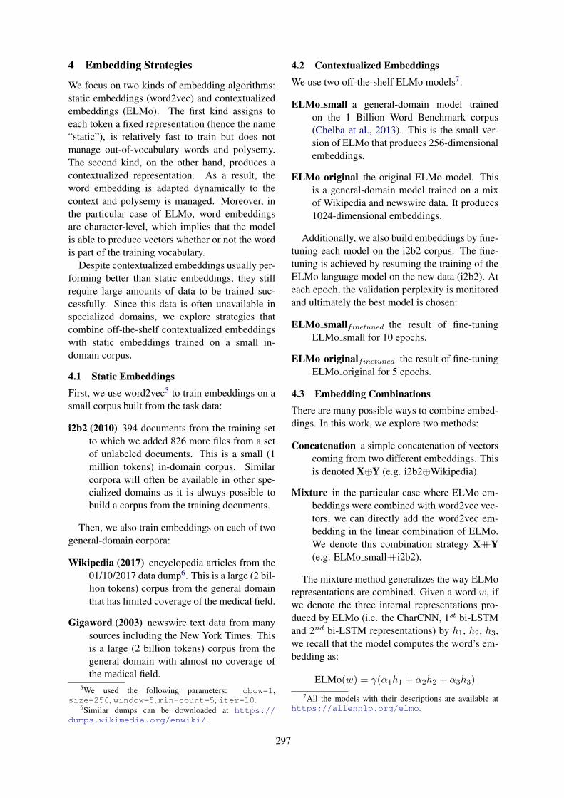
4 Embedding Strategies

We focus on two kinds of embedding algorithms:static embeddings (word2vec) and contextualizedembeddings (ELMo). The first kind assigns toeach token a fixed representation (hence the name“static”), is relatively fast to train but does notmanage out-of-vocabulary words and polysemy.The second kind, on the other hand, produces acontextualized representation. As a result, theword embedding is adapted dynamically to thecontext and polysemy is managed. Moreover, inthe particular case of ELMo, word embeddingsare character-level, which implies that the modelis able to produce vectors whether or not the wordis part of the training vocabulary.

Despite contextualized embeddings usually per-forming better than static embeddings, they stillrequire large amounts of data to be trained suc-cessfully. Since this data is often unavailable inspecialized domains, we explore strategies thatcombine off-the-shelf contextualized embeddingswith static embeddings trained on a small in-domain corpus.

4.1 Static EmbeddingsFirst, we use word2vec5 to train embeddings on asmall corpus built from the task data:

i2b2 (2010) 394 documents from the training setto which we added 826 more files from a setof unlabeled documents. This is a small (1million tokens) in-domain corpus. Similarcorpora will often be available in other spe-cialized domains as it is always possible tobuild a corpus from the training documents.

Then, we also train embeddings on each of twogeneral-domain corpora:

Wikipedia (2017) encyclopedia articles from the01/10/2017 data dump6. This is a large (2 bil-lion tokens) corpus from the general domainthat has limited coverage of the medical field.

Gigaword (2003) newswire text data from manysources including the New York Times. Thisis a large (2 billion tokens) corpus from thegeneral domain with almost no coverage ofthe medical field.

5We used the following parameters: cbow=1,size=256, window=5, min-count=5, iter=10.

6Similar dumps can be downloaded at https://dumps.wikimedia.org/enwiki/.

4.2 Contextualized EmbeddingsWe use two off-the-shelf ELMo models7:

ELMo small a general-domain model trainedon the 1 Billion Word Benchmark corpus(Chelba et al., 2013). This is the small ver-sion of ELMo that produces 256-dimensionalembeddings.

ELMo original the original ELMo model. Thisis a general-domain model trained on a mixof Wikipedia and newswire data. It produces1024-dimensional embeddings.

Additionally, we also build embeddings by fine-tuning each model on the i2b2 corpus. The fine-tuning is achieved by resuming the training of theELMo language model on the new data (i2b2). Ateach epoch, the validation perplexity is monitoredand ultimately the best model is chosen:

ELMo smallfinetuned the result of fine-tuningELMo small for 10 epochs.

ELMo originalfinetuned the result of fine-tuningELMo original for 5 epochs.

4.3 Embedding CombinationsThere are many possible ways to combine embed-dings. In this work, we explore two methods:

Concatenation a simple concatenation of vectorscoming from two different embeddings. Thisis denoted XY (e.g. i2b2Wikipedia).

Mixture in the particular case where ELMo em-beddings were combined with word2vec vec-tors, we can directly add the word2vec em-bedding in the linear combination of ELMo.We denote this combination strategy X++Y(e.g. ELMo small++i2b2).

The mixture method generalizes the way ELMorepresentations are combined. Given a word w, ifwe denote the three internal representations pro-duced by ELMo (i.e. the CharCNN, 1st bi-LSTMand 2nd bi-LSTM representations) by h1, h2, h3,we recall that the model computes the word’s em-bedding as:

ELMo(w) = (↵1h1 + ↵2h2 + ↵3h3)

7All the models with their descriptions are available athttps://allennlp.org/elmo.

297

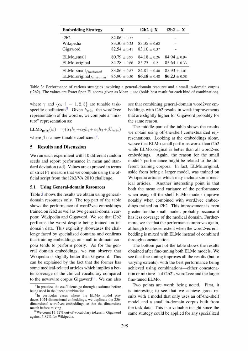
Embedding Strategy X i2b2 X i2b2 ++ X

i2b2 82.06 ± 0.32 - -Wikipedia 83.30 ± 0.25 83.35 ± 0.62 -Gigaword 82.54 ± 0.41 83.10 ± 0.37 -

ELMo small 80.79 ± 0.95 84.18 ± 0.26 84.94 ± 0.94

ELMo original 84.28 ± 0.66 85.25 ± 0.21 85.64 ± 0.33

ELMo smallfinetuned 83.86 ± 0.87 84.81 ± 0.40 85.93 ± 1.01

ELMo originalfinetuned 85.90 ± 0.50 86.18 ± 0.48 86.23 ± 0.58

Table 3: Performance of various strategies involving a general-domain resource and a small in-domain corpus(i2b2). The values are Exact Span F1 scores given as Mean ± Std (bold: best result for each kind of combination).

where and ↵i, i = 1, 2, 3 are tunable task-specific coefficients8. Given hw2v, the word2vecrepresentation of the word w, we compute a “mix-ture” representation as:

ELMomix(w) = (↵1h1+↵2h2+↵3h3+hw2v)

where is a new tunable coefficient9.

5 Results and Discussion

We run each experiment with 10 different randomseeds and report performance in mean and stan-dard deviation (std). Values are expressed in termsof strict F1 measure that we compute using the of-ficial script from the i2b2/VA 2010 challenge.

5.1 Using General-domain ResourcesTable 3 shows the results we obtain using general-domain resources only. The top part of the tableshows the performance of word2vec embeddingstrained on i2b2 as well as two general-domain cor-pora: Wikipedia and Gigaword. We see that i2b2performs the worst despite being trained on in-domain data. This explicitly showcases the chal-lenge faced by specialized domains and confirmsthat training embeddings on small in-domain cor-pora tends to perform poorly. As for the gen-eral domain embeddings, we can observe thatWikipedia is slightly better than Gigaword. Thiscan be explained by the fact that the former hassome medical-related articles which implies a bet-ter coverage of the clinical vocabulary comparedto the newswire corpus Gigaword10. We can also

8In practice, the coefficients go through a softmax beforebeing used in the linear combination.

9In particular cases where the ELMo model pro-duces 1024-dimensional embeddings, we duplicate the 256-dimensional word2vec embeddings so that the dimensionsmatch before mixing.

10We count 14.42% out-of-vocabulary tokens in Gigawordagainst 5.82% for Wikipedia.

see that combining general-domain word2vec em-beddings with i2b2 results in weak improvementsthat are slightly higher for Gigaword probably forthe same reason.

The middle part of the table shows the resultswe obtain using off-the-shelf contextualized rep-resentations. Looking at the embeddings alone,we see that ELMo small performs worse than i2b2while ELMo original is better than all word2vecembeddings. Again, the reason for the smallmodel’s performance might be related to the dif-ferent training corpora. In fact, ELMo original,aside from being a larger model, was trained onWikipedia articles which may include some med-ical articles. Another interesting point is thatboth the mean and variance of the performancewhen using off-the-shelf ELMo models improvenotably when combined with word2vec embed-dings trained on i2b2. This improvement is evengreater for the small model, probably because ithas less coverage of the medical domain. Further-more, we see that the performance improves again,although to a lesser extent when the word2vec em-bedding is mixed with ELMo instead of combinedthrough concatenation.

The bottom part of the table shows the resultsobtained after fine-tuning both ELMo models. Wesee that fine-tuning improves all the results (but tovarying extents), with the best performance beingachieved using combinations—either concatena-tion or mixture—of i2b2’s word2vec and the largerfine-tuned ELMo.

Two points are worth being noted. First, itis interesting to see that we achieve good re-sults with a model that only uses an off-the-shelfmodel and a small in-domain corpus built fromthe task data. This is a valuable insight since thesame strategy could be applied for any specialized

298

domain. Second, we see that the smaller 256-dimensional ELMo model, which initially per-formed very poorly ( 80 F1), improved dras-tically ( +6 F1) using our best strategy anddoes not lag very far behind the original 1024-dimensional model. This is also valuable sincemany practitioners do not have the computationalresources that are required for using the larger ver-sions of recent models like ELMo or BERT.

5.2 Using In-domain ResourcesIt is natural to wonder how our results fare againstmodels trained on large in-domain corpora. For-tunately, there are two such corpora in the clinicaldomain:

MIMIC III (2016) a collection of medical notesfrom a large database of Intensive Care Unitencounters at a large hospital (Johnson et al.,2016)11. This is a large (1 billion tokens) in-domain corpus.

PubMed (2018) a collection of scientific articleabstracts in the biomedical domain12. This isa large (4 billion tokens) corpus from a closebut somewhat different domain.

Both Zhu et al. (2018) and Si et al. (2019)trained the ELMo (original) on MIMIC, with theformer resorting to only a part of MIMIC mixedwith some curated Wikipedia articles. Table 4 re-ports their results, to which we add the perfor-mance of strategies using word2vec embeddingstrained on MIMIC and PubMed, and an open-source ELMo model trained on PubMed13.

We can see yet again that word2vec embed-dings perform less well than ELMo models trainedon the same corpora. We also see that combin-ing the two kinds of embeddings still brings someimprovement (see ELMo (PubMed) ++ MIMIC).And more importantly, we observe that by usingonly general-domain resources, we perform veryclose to the ELMo models trained on a large in-domain corpus (MIMIC) with a maximum differ-ence in F1 measure of 1.5 points.

11The MIMIC-III corpus can be downloaded at https://mimic.physionet.org/gettingstarted/access/.

12 The PubMed-MEDLINE corpus can be down-loaded at https://www.nlm.nih.gov/databases/download/pubmed_medline.html.

13Since we did not train this model ourselves, we are notsure whether the training corpus is equivalent to the PubMedcorpus we use for training word2vec embeddings.

Embedding Strategy F1

MIMIC 84.29 ± 0.30

PubMed 84.06 ± 0.14

ELMo (PubMed) 86.29 ± 0.61

ELMo (PubMed) ++ MIMIC 87.17 ± 0.54

ELMo originalfinetuned ++ i2b2 86.23 ± 0.58

ELMo (Clinical) (Zhu et al., 2018) 86.84 ± 0.16

ELMo (MIMIC) (Si et al., 2019) 87.80

Table 4: Comparison of strategies using large in-domain corpora with the best strategy using a smallin-domain corpus and general-domain resources. Thevalues are Exact Span F1 scores.

5.3 Using GloVe and fastTextIn order to make sure that the observed phenomenaare not the result of using the word2vec methodin particular, we reproduce the same experimentsusing GloVe and fastText14. The correspondingresults are reported in Table 5 and Table 6.

We can see that GloVe and fastText are alwaysoutperformed by word2vec when trained on a sin-gle corpus only. This is not true anymore whencombining these embeddings with representationsfrom ELMo. In fact, in this case, the results aremostly comparable to the performance obtainedwhen using word2vec, with a slight improvementwhen using fastText. This small improvement maybe explained by the fact that the fastText methodis able to manage Out-Of-Vocabulary tokens whileGloVe and word2vec are not.

More importantly, these additional experimentsvalidate the initial results obtained with word2vec:static embeddings pre-trained on a small in-domain corpus (i2b2) can be combined withgeneral domain contextual embeddings (ELMo),through either one of the proposed methods, toreach a performance that is comparable to thestate-of-the-art15.

5.4 LimitationsWe can list the following limitations for this work:

• we tested only one specialized domain on onetask using one NER architecture. Although

14We used the following parameters: (GloVe) size=256,window=15, min-count=5, iter=10; (fastText)skipgram, size=256, window=5, min-count=5,neg=5, loss=ns, minn=3, maxn=6, iter=10.

15Our single best model gets a F1 score of 87.10.

299

Embedding Strategy X i2b2 X i2b2 ++ X

i2b2 80.21 ± 0.37 - -Wikipedia 81.82 ± 0.52 81.29 ± 0.42 -Gigaword 81.38 ± 0.33 81.47 ± 0.18 -

ELMo small 80.79 ± 0.95 83.04 ± 1.03 84.30 ± 0.72

ELMo original 84.28 ± 0.66 85.00 ± 0.32 85.12 ± 0.26

ELMo smallfinetuned 83.86 ± 0.87 84.42 ± 0.75 85.19 ± 0.75

ELMo originalfinetuned 85.90 ± 0.50 86.05 ± 0.16 86.46 ± 0.36

Table 5: Performance of the strategies from Table 3 using GloVe instead of word2vec (bold: GloVe > word2vec)

Embedding Strategy X i2b2 X i2b2 ++ X

i2b2 81.98 ± 0.41 - -Wikipedia 82.32 ± 0.37 81.84 ± 1.48 -Gigaword 81.77 ± 0.36 82.40 ± 0.32 -

ELMo small 80.79 ± 0.95 84.44 ± 0.42 85.47 ± 0.61

ELMo original 84.28 ± 0.66 85.57 ± 0.46 85.77 ± 0.47

ELMo smallfinetuned 83.86 ± 0.87 85.18 ± 0.67 86.27 ± 0.35

ELMo originalfinetuned 85.90 ± 0.50 86.49 ± 0.28 86.82 ± 0.29

Table 6: Performance of the strategies from Table 3 using fastText instead of word2vec (bold: fastText > word2vec)

the results look promising, they should bevalidated by a wider set of experiments;

• our best strategies use the task corpus (i2b2)to adapt general off-the-shelf embeddings tothe target domain, then combine two differ-ent types of embeddings as an ensemble toboost performance. This may not work if thetask corpus is really small (we recall that ourcorpus is 1 million tokens).

6 Conclusion and Future Work

While embedding methods are improving on aregular basis, specialized domains still lack largeenough corpora to train these embeddings success-fully. We address this issue and propose embed-ding strategies that only require general-domainresources and a small in-domain corpus. In partic-ular, we show that using a combination of general-domain ELMo, fine-tuning and word2vec embed-dings trained on a small in-domain corpus, weachieve a performance that is not very far behindthat of models trained on large in-domain corpora.Future work may investigate other contextualizedrepresentations such as BERT, which has provento be superior to ELMo—at least on our task—inthe recent work by Si et al. (2019). Another inter-

esting research direction could be exploiting exter-nal knowledge (e.g. ontologies) that may be easierto find in specialized fields than large corpora.

Acknowledgments

This work has been funded by the French Na-tional Research Agency (ANR) and is under theADDICTE project (ANR-17-CE23-0001). We arealso thankful to Kirk Roberts for having kindlyprovided assistance regarding his 2016 paper.

ReferencesPiotr Bojanowski, Edouard Grave, Armand Joulin, and

Tomas Mikolov. 2017. Enriching word vectors withsubword information. Transactions of the Associa-tion for Computational Linguistics, 5:135–146.

Danushka Bollegala, Koheu Hayashi, and Ken ichiKawarabayashi. 2018. Think globally, embed lo-cally — locally linear meta-embedding of words. InProceedings of IJCAI-ECAI, pages 3970–3976.

Raghavendra Chalapathy, Ehsan Zare Borzeshi, andMassimo Piccardi. 2016. Bidirectional LSTM-CRFfor clinical concept extraction. In Proceedings ofthe Clinical Natural Language Processing Work-shop (ClinicalNLP), pages 7–12, Osaka, Japan. TheCOLING 2016 Organizing Committee.

300

Ciprian Chelba, Tomas Mikolov, Mike Schuster, Qi Ge,Thorsten Brants, Phillipp Koehn, and Tony Robin-son. 2013. One billion word benchmark for measur-ing progress in statistical language modeling. arXivpreprint arXiv:1312.3005.

Jacob Devlin, Ming-Wei Chang, Kenton Lee, andKristina Toutanova. 2018. Bert: Pre-training of deepbidirectional transformers for language understand-ing. arXiv preprint arXiv:1810.04805.

Matt Gardner, Joel Grus, Mark Neumann, OyvindTafjord, Pradeep Dasigi, Nelson F. Liu, Matthew Pe-ters, Michael Schmitz, and Luke Zettlemoyer. 2018.AllenNLP: A deep semantic natural language pro-cessing platform. In Proceedings of Workshop forNLP Open Source Software (NLP-OSS), pages 1–6, Melbourne, Australia. Association for Computa-tional Linguistics.

David Graff, Junbo Kong, Ke Chen, and KazuakiMaeda. 2003. English gigaword. Linguistic DataConsortium, Philadelphia, 4(1):34.

Maryam Habibi, Leon Weber, Mariana Neves,David Luis Wiegandt, and Ulf Leser. 2017. Deeplearning with word embeddings improves biomed-ical named entity recognition. Bioinformatics,33(14):i37–i48.

Alistair EW Johnson, Tom J Pollard, Lu Shen,H Lehman Li-wei, Mengling Feng, Moham-mad Ghassemi, Benjamin Moody, Peter Szolovits,Leo Anthony Celi, and Roger G Mark. 2016.MIMIC-III, a freely accessible critical care database.Scientific data, 3:160035.

Douwe Kiela, Changhan Wang, and Kyunghyun Cho.2018. Dynamic meta-embeddings for improvedsentence representations. In Proceedings of the2018 Conference on Empirical Methods in NaturalLanguage Processing (EMNLP 2018), pages 1466–1477, Brussels, Belgium.

Guillaume Lample, Miguel Ballesteros, Sandeep Sub-ramanian, Kazuya Kawakami, and Chris Dyer. 2016.Neural architectures for named entity recognition.In Proceedings of the 2016 Conference of the NorthAmerican Chapter of the Association for Computa-tional Linguistics: Human Language Technologies,pages 260–270, San Diego, California. Associationfor Computational Linguistics.

Tomas Mikolov, Kai Chen, Greg Corrado, and JeffreyDean. 2013. Efficient estimation of word represen-tations in vector space. In International Conferenceon Learning Representations (ICLR 20013), work-shop track.

Avo Muromagi, Kairit Sirts, and Sven Laur. 2017.Linear ensembles of word embedding models. In21st Nordic Conference on Computational Linguis-tics (NoDaLiDa 2017), pages 96–104, Gothenburg,Sweden.

Jeffrey Pennington, Richard Socher, and ChristopherManning. 2014. Glove: Global vectors for wordrepresentation. In Proceedings of the 2014 confer-ence on empirical methods in natural language pro-cessing (EMNLP), pages 1532–1543.

Matthew E. Peters, Mark Neumann, Mohit Iyyer, MattGardner, Christopher Clark, Kenton Lee, and LukeZettlemoyer. 2018. Deep contextualized word rep-resentations. In Proc. of NAACL.

Kirk Roberts. 2016. Assessing the corpus size vs.similarity trade-off for word embeddings in clinicalNLP. In Proceedings of the Clinical Natural Lan-guage Processing Workshop (ClinicalNLP), pages54–63.

Yuqi Si, Jingqi Wang, Hua Xu, and Kirk Roberts. 2019.Enhancing clinical concept extraction with contex-tual embedding. arXiv preprint arXiv:1902.08691.

Ozlem Uzuner, Brett R South, Shuying Shen, andScott L DuVall. 2011. 2010 i2b2/VA challenge onconcepts, assertions, and relations in clinical text.Journal of the American Medical Informatics Asso-ciation, 18(5):552–556.

Wenpeng Yin and Hinrich Schutze. 2016. Learningword meta-embeddings. In Proceedings of the 54thAnnual Meeting of the Association for Computa-tional Linguistics (ACL 2016), pages 1351–1360,Berlin, Germany.

Henghui Zhu, Ioannis Ch. Paschalidis, and Amir Tah-masebi. 2018. Clinical concept extraction with con-textual word embedding. In Proceedings of theMachine Learning for Health (ML4H) Workshop atNeurIPS 2018.

Yukun Zhu, Ryan Kiros, Rich Zemel, Ruslan Salakhut-dinov, Raquel Urtasun, Antonio Torralba, and SanjaFidler. 2015. Aligning books and movies: Towardsstory-like visual explanations by watching moviesand reading books. In Proceedings of the IEEEinternational conference on computer vision, pages19–27.

301

Proceedings of the 57th Annual Meeting of the Association for Computational Linguistics: Student Research Workshop, pages 302–308Florence, Italy, July 28 - August 2, 2019. c©2019 Association for Computational Linguistics

Enriching Neural Models with Targeted Features for Dementia Detection

Flavio Di Palo and Natalie PardeDepartment of Computer ScienceUniversity of Illinois at Chicagofdipal2, parde@uic.edu

Abstract

Alzheimer’s disease (AD) is an irreversiblebrain disease that can dramatically reducequality of life, most commonly manifestingin older adults and eventually leading to theneed for full-time care. Early detection is fun-damental to slowing its progression; however,diagnosis can be expensive, time-consuming,and invasive. In this work we develop a neu-ral model based on a CNN-LSTM architecturethat learns to detect AD and related dementiasusing targeted and implicitly-learned featuresfrom conversational transcripts. Our approachestablishes the new state of the art on the De-mentiaBank dataset, achieving an F1 score of0.929 when classifying participants into ADand control groups.

1 Introduction

Older adults constitute a growing subset of thepopulation. In the United States, adults overage 65 are expected to comprise one-fifth ofthe population by 2030, and a larger proportionof the population than those under 18 by 2035(United States Census Bureau, 2018). In Japan—perhaps the most extreme example of shifting agedemographics—42.4% of the population is ex-pected to be aged 60 or over by 2050 (United Na-tions, 2017). This will necessitate that age-relatedphysical and cognitive health issues become aforemost concern not only because they will im-pact such a large population, but because there willbe a proportionally smaller number of human care-givers available to diagnose, monitor, and remedi-ate those conditions. Artificial intelligence offersthe potential to fill many of these deficits, and al-ready, elder-focused research is underway to testintelligent systems that monitor and assist with ac-tivities of daily living (Lotfi et al., 2012), supportmental health (Wada et al., 2004), promote physi-cal well-being (Sarma et al., 2014), and encourage

cognitive exercise (Parde and Nielsen, 2019).Perhaps some of the most pressing issues belea-

guering an aging population are Alzheimer’s dis-ease (AD) and other age-related dementias. Ourinterest lies in fostering early diagnosis of theseconditions. Although there are currently no cures,with early diagnosis the symptoms can be man-aged and their impact on quality of life may beminimal. However, there can be many barriers toearly diagnosis, including cost, location, mobility,and time.

Here, we present preliminary work towards au-tomatically detecting whether individuals sufferfrom AD using only conversational transcripts.This solution addresses the above barriers by pro-viding a diagnosis technique that could eventuallybe employed free of cost and in the comfort ofone’s home, at whatever time works best. Our con-tributions are as follows:

1. We introduce a hybrid Convolutional NeuralNetwork (CNN) and Long Short Term Mem-ory Network (LSTM) approach to dementiadetection that takes advantage of both tar-geted and implicitly learned features to per-form classification.

2. We explore the effects of a bi-directionalLSTM and attention mechanism on both ourmodel and the current state-of-the-art for de-mentia detection.

3. We empirically demonstrate that our tech-nique outperforms the current state of the art,and suggest directions for future work that weexpect to further improve performance.

2 Related Work

The task of automatically detecting dementia inconversational transcripts is not new. In Fraseret al. (2016), the authors tackled the task using

302

features associated with many linguistic phenom-ena, including part of speech tags, syntactic com-plexity, psycholinguistic characteristics, vocabu-lary richness, and many others. They trained alogistic regression model to distinguish betweendementia-affected and healthy patients, achievingan accuracy of 81%. In our work here we considersome of the features found to be informative in thiswork; in particular, psycholinguistic features.

Habash et al. (2012) studied Alzheimer’s-related dementia (AD) specifically. The authorsselected 14 linguistic features to perform syntac-tic, semantic, and disfluency modeling. In doingso, they checked for the presence of filler words,repetitions, and incomplete words, and addition-ally incorporated counts indicating the number ofsyllables used per minute. Using this feature set,the authors trained a decision tree classifier tomake predictions for 80 conversational samplesfrom 31 AD and 57 non-AD patients. Their modelachieved an accuracy of 79.5%.

Orimaye et al. (2014) considered syntactic fea-tures, computed from syntactic tree structures, andvarious lexical features to evaluate four machinelearning algorithms for dementia detection. Thealgorithms considered included a decision tree,naıve Bayes, SVM with a radial basis kernel, anda neural network. On a dataset containing 242 ADand 242 healthy individuals, they found that com-pared to other algorithms, SVM exhibited the bestperformance with an accuracy score of 74%, a re-call of 73%, and a precision of 75%.

Yancheva and Rudzicz (2016) usedautomatically-generated topic models to ex-tract a small number of semantic features (12),which they then used to train a random forestclassifier. Their approach achieved an F1 Scoreof 0.74 in binary classification of control patientsversus dementia-affected patients. This is com-parable to results (F1 Score=0.72) obtained witha much larger set of lexicosyntactic and acousticfeatures. Ultimately, Yancheva and Rudziczfound that combining these varied feature typesimproved their F1 Score to 0.80.

Finally, Karlekar et al. (2018) proposed a CNN-LSTM neural language model and explored theeffectiveness of part-of-speech (POS) tagging theconversational transcript to improve classificationaccuracy for AD patients. They divided patientinterviews into single utterances, and rather thanclassifying at the patient level, they made their

predictions at the utterance level. Their modelachieved an accuracy of 91%. Unfortunately, thedataset on which their classifier was trained is im-balanced, and no other performance metrics werereported. This makes it difficult to fully under-stand the capabilities of their model. Here, in ad-dition to our other contributions, we extend theirwork by considering a full-interview classificationscenario and providing more detailed classifica-tion metrics to assess the classifier’s quality.

3 Data

We use a subset of DementiaBank (Becker et al.,1994) for our work here. DementiaBank is adataset gathered as part of a protocol administeredby the Alzheimer and Related Dementias Study atthe University of Pittsburgh School of Medicine.It contains spontaneous speech from individualswho do (AD group) and do not (control group)present different kinds of dementia. Participantsin the dataset performed several different tasks:

• Fluency: Participants were asked to namewords belonging to a given category or thatstart with a given letter.

• Recall: Participants were asked to recall astory from their past experience.

• Sentence: Participants were asked to con-struct a simple sentence with a given word, orwere asked if a given sentence made sense.

• Cookie Theft: Participants were askedto verbally describe an eventful image illus-trating, among other elements, a child at-tempting to steal a cookie. For this task,the participant’s and interviewer’s speech ut-terances were recorded and manually tran-scribed according to the TalkBank CHATprotocol (MacWhinney, 1992).

Of these tasks, Cookie Theft provides thelargest source of unstructured text. Thus, it is thedata subset that we use for our work here. In total,the Cookie Theft sub-corpus consists of 1049 tran-scripts from 208 patients suffering from dementia(AD group) and 243 transcripts from 104 healthyelderly patients (control, or CT, group), for a totalof 1229 transcripts. Dataset statistics are providedin Table 1. For each participant, DementiaBankalso provides demographic information including

303

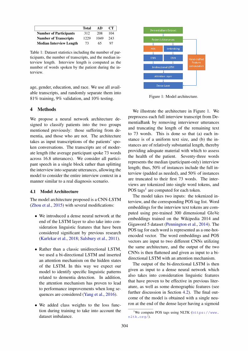
Total AD CTNumber of Participants 312 208 104Number of Transcripts 1229 1049 243Median Interview Length 73 65 97

Table 1: Dataset statistics including the number of par-ticipants, the number of transcripts, and the median in-terview length. Interview length is computed as thenumber of words spoken by the patient during the in-terview.

age, gender, education, and race. We use all avail-able transcripts, and randomly separate them into81% training, 9% validation, and 10% testing.

4 Methods

We propose a neural network architecture de-signed to classify patients into the two groupsmentioned previously: those suffering from de-mentia, and those who are not. The architecturetakes as input transcriptions of the patients’ spo-ken conversations. The transcripts are of moder-ate length (the average participant spoke 73 wordsacross 16.8 utterances). We consider all partici-pant speech in a single block rather than splittingthe interview into separate utterances, allowing themodel to consider the entire interview context in amanner similar to a real diagnosis scenario.

4.1 Model Architecture

The model architecture proposed is a CNN-LSTM(Zhou et al., 2015) with several modifications:

• We introduced a dense neural network at theend of the LSTM layer to also take into con-sideration linguistic features that have beenconsidered significant by previous research(Karlekar et al., 2018; Salsbury et al., 2011).

• Rather than a classic unidirectional LSTM,we used a bi-directional LSTM and insertedan attention mechanism on the hidden statesof the LSTM. In this way we expect ourmodel to identify specific linguistic patternsrelated to dementia detection. In addition,the attention mechanism has proven to leadto performance improvements when long se-quences are considered (Yang et al., 2016).

• We added class weights to the loss func-tion during training to take into account thedataset imbalance.

Figure 1: Model architecture.

We illustrate the architecture in Figure 1. Wepreprocess each full interview transcript from De-mentiaBank by removing interviewer utterancesand truncating the length of the remaining textto 73 words. This is done so that (a) each in-stance is of a uniform text size, and (b) the in-stances are of relatively substantial length, therebyproviding adequate material with which to assessthe health of the patient. Seventy-three wordsrepresents the median (participant-only) interviewlength; thus, 50% of instances include the full in-terview (padded as needed), and 50% of instancesare truncated to their first 73 words. The inter-views are tokenized into single word tokens, andPOS tags1 are computed for each token.

The model takes two inputs: the tokenized in-terview, and the corresponding POS tag list. Wordembeddings for the interview text tokens are com-puted using pre-trained 300 dimensional GloVeembeddings trained on the Wikipedia 2014 andGigaword 5 dataset (Pennington et al., 2014). ThePOS tag for each word is represented as a one-hot-encoded vector. The word embeddings and POSvectors are input to two different CNNs utilizingthe same architecture, and the output of the twoCNNs is then flattened and given as input to a bi-directional LSTM with an attention mechanism.

The output of the bi-directional LSTM is thengiven as input to a dense neural network whichalso takes into consideration linguistic featuresthat have proven to be effective in previous liter-ature, as well as some demographic features (seefurther discussion in Section 4.2). The final out-come of the model is obtained with a single neu-ron at the end of the dense layer having a sigmoid

1We compute POS tags using NLTK (https://www.nltk.org/).

304

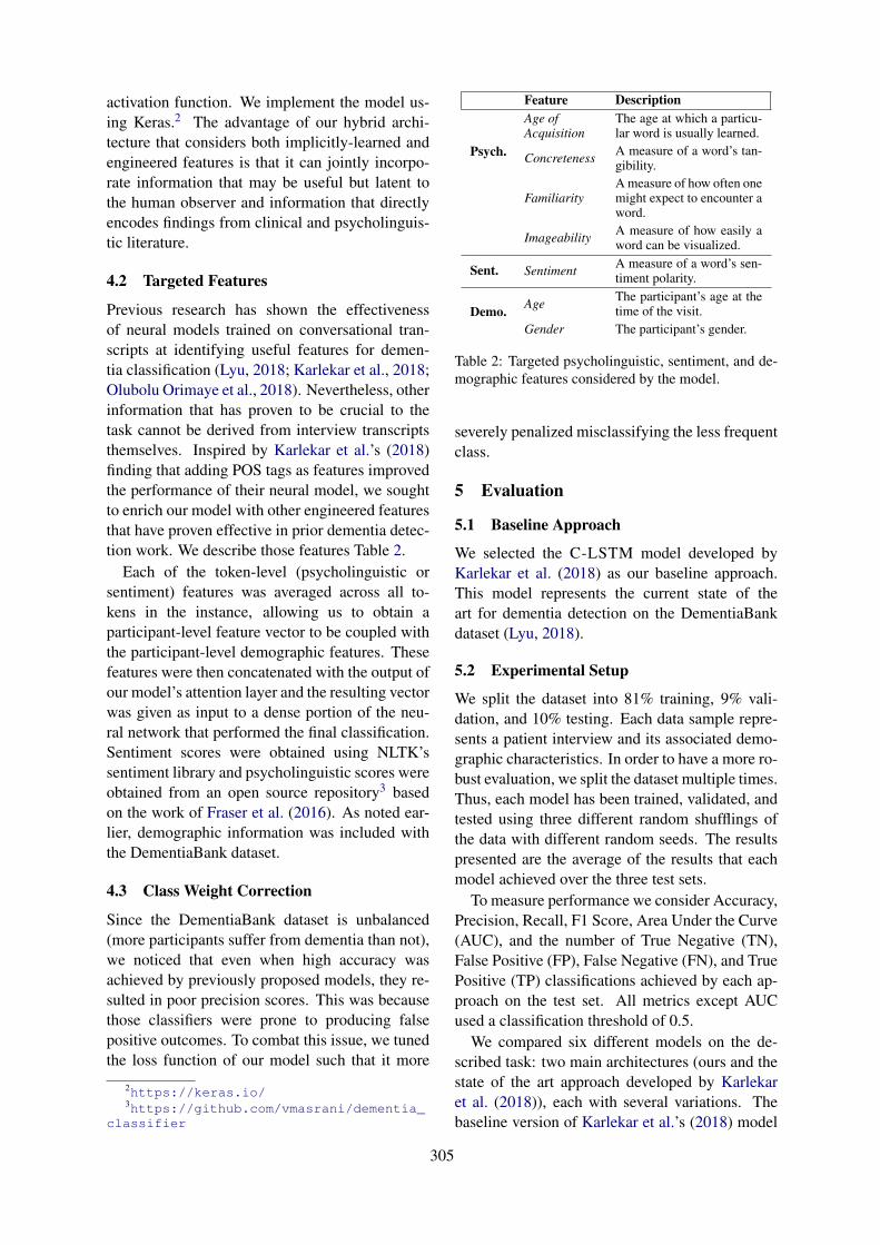
activation function. We implement the model us-ing Keras.2 The advantage of our hybrid archi-tecture that considers both implicitly-learned andengineered features is that it can jointly incorpo-rate information that may be useful but latent tothe human observer and information that directlyencodes findings from clinical and psycholinguis-tic literature.

4.2 Targeted Features

Previous research has shown the effectivenessof neural models trained on conversational tran-scripts at identifying useful features for demen-tia classification (Lyu, 2018; Karlekar et al., 2018;Olubolu Orimaye et al., 2018). Nevertheless, otherinformation that has proven to be crucial to thetask cannot be derived from interview transcriptsthemselves. Inspired by Karlekar et al.’s (2018)finding that adding POS tags as features improvedthe performance of their neural model, we soughtto enrich our model with other engineered featuresthat have proven effective in prior dementia detec-tion work. We describe those features Table 2.

Each of the token-level (psycholinguistic orsentiment) features was averaged across all to-kens in the instance, allowing us to obtain aparticipant-level feature vector to be coupled withthe participant-level demographic features. Thesefeatures were then concatenated with the output ofour model’s attention layer and the resulting vectorwas given as input to a dense portion of the neu-ral network that performed the final classification.Sentiment scores were obtained using NLTK’ssentiment library and psycholinguistic scores wereobtained from an open source repository3 basedon the work of Fraser et al. (2016). As noted ear-lier, demographic information was included withthe DementiaBank dataset.

4.3 Class Weight Correction

Since the DementiaBank dataset is unbalanced(more participants suffer from dementia than not),we noticed that even when high accuracy wasachieved by previously proposed models, they re-sulted in poor precision scores. This was becausethose classifiers were prone to producing falsepositive outcomes. To combat this issue, we tunedthe loss function of our model such that it more

2https://keras.io/3https://github.com/vmasrani/dementia_

classifier

Feature Description

Psych.

Age ofAcquisition

The age at which a particu-lar word is usually learned.

Concreteness A measure of a word’s tan-gibility.

FamiliarityA measure of how often onemight expect to encounter aword.

Imageability A measure of how easily aword can be visualized.

Sent. Sentiment A measure of a word’s sen-timent polarity.

Demo. Age The participant’s age at thetime of the visit.

Gender The participant’s gender.

Table 2: Targeted psycholinguistic, sentiment, and de-mographic features considered by the model.

severely penalized misclassifying the less frequentclass.

5 Evaluation

5.1 Baseline Approach

We selected the C-LSTM model developed byKarlekar et al. (2018) as our baseline approach.This model represents the current state of theart for dementia detection on the DementiaBankdataset (Lyu, 2018).

5.2 Experimental Setup

We split the dataset into 81% training, 9% vali-dation, and 10% testing. Each data sample repre-sents a patient interview and its associated demo-graphic characteristics. In order to have a more ro-bust evaluation, we split the dataset multiple times.Thus, each model has been trained, validated, andtested using three different random shufflings ofthe data with different random seeds. The resultspresented are the average of the results that eachmodel achieved over the three test sets.

To measure performance we consider Accuracy,Precision, Recall, F1 Score, Area Under the Curve(AUC), and the number of True Negative (TN),False Positive (FP), False Negative (FN), and TruePositive (TP) classifications achieved by each ap-proach on the test set. All metrics except AUCused a classification threshold of 0.5.

We compared six different models on the de-scribed task: two main architectures (ours and thestate of the art approach developed by Karlekaret al. (2018)), each with several variations. Thebaseline version of Karlekar et al.’s (2018) model

305

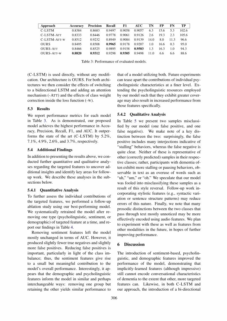
Approach Accuracy Precision Recall F1 AUC TN FP FN TPC-LSTM 0.8384 0.8683 0.9497 0.9058 0.9057 6.3 15.6 5.3 102.6C-LSTM-ATT 0.8333 0.8446 0.9778 0.9061 0.9126 2.6 19.3 2.3 105.6C-LSTM-ATT-W 0.8512 0.9232 0.8949 0.9084 0.9139 14.0 8.0 11.3 96.6OURS 0.8495 0.8508 0.9965 0.9178 0.9207 1.0 16.6 0.3 95.0OURS-ATT 0.8466 0.8525 0.9895 0.9158 0.9503 1.3 16.3 1.0 94.3OURS-ATT-W 0.8820 0.9312 0.9298 0.9305 0.9498 11.0 6.6 6.6 88.6

Table 3: Performance of evaluated models.

(C-LSTM) is used directly, without any modifi-cation. Our architecture is OURS. For both archi-tectures we then consider the effects of switchingto a bidirectional LSTM and adding an attentionmechanism (-ATT) and the effects of class weightcorrection inside the loss function (-W).

5.3 ResultsWe report performance metrics for each modelin Table 3. As is demonstrated, our proposedmodel achieves the highest performance in Accu-racy, Precision, Recall, F1, and AUC. It outper-forms the state of the art (C-LSTM) by 5.2%,7.1%, 4.9%, 2.6%, and 3.7%, respectively.

5.4 Additional FindingsIn addition to presenting the results above, we con-ducted further quantitative and qualitative analy-ses regarding the targeted features to uncover ad-ditional insights and identify key areas for follow-up work. We describe these analyses in the sub-sections below.

5.4.1 Quantitative AnalysisTo further assess the individual contributions ofthe targeted features, we performed a follow-upablation study using our best-performing model.We systematically retrained the model after re-moving one type (psycholinguistic, sentiment, ordemographic) of targeted feature at a time, and re-port our findings in Table 4.

Removing sentiment features left the modelmostly unchanged in terms of AUC. However, itproduced slightly fewer true negatives and slightlymore false positives. Reducing false positives isimportant, particularly in light of the class im-balance; thus, the sentiment features give riseto a small but meaningful contribution to themodel’s overall performance. Interestingly, it ap-pears that the demographic and psycholinguisticfeatures inform the model in similar and perhapsinterchangeable ways: removing one group butretaining the other yields similar performance to

that of a model utilizing both. Future experimentscan tease apart the contributions of individual psy-cholinguistic characteristics at a finer level. Ex-tending the psycholinguistic resources employedby our model such that they exhibit greater cover-age may also result in increased performance fromthose features specifically.

5.4.2 Qualitative AnalysisIn Table 5 we present two samples misclassi-fied by our model (one false positive, and onefalse negative). We make note of a key dis-tinction between the two: surprisingly, the falsepositive includes many interjections indicative of“stalling” behaviors, whereas the false negative isquite clear. Neither of these is representative ofother (correctly predicted) samples in their respec-tive classes; rather, participants with dementia of-ten exhibit more stalling or pausing behaviors, ob-servable in text as an overuse of words such as“uh,” “um,” or “oh.” We speculate that our modelwas fooled into misclassifying these samples as aresult of this style reversal. Follow-up work in-corporating stylistic features (e.g., syntactic vari-ation or sentence structure patterns) may reduceerrors of this nature. Finally, we note that manyprosodic distinctions between the two classes thatpass through text mostly unnoticed may be moreeffectively encoded using audio features. We planto experiment with these as well as features fromother modalities in the future, in hopes of furtherimproving performance.

6 Discussion

The introduction of sentiment-based, psycholin-guistic, and demographic features improved theperformance of the model, demonstrating thatimplicitly-learned features (although impressive)still cannot encode conversational characteristicsof dementia to the extent that other, more targetedfeatures can. Likewise, in both C-LSTM andour approach, the introduction of a bi-directional

306

Approach Accuracy Precision Recall F1 AUC TN FP FN TPOURS-ATT-W NO PSYCH. 0.8790 0.8870 0.9825 0.9319 0.9499 12.0 5.6 1.6 93.6OURS-ATT-W NO SENT. 0.8970 0.9239 0.9615 0.9321 0.9501 7.6 10.0 3.6 91.6OURS-ATT-W NO DEMO. 0.8908 0.9005 0.9789 0.9308 0.9473 10.33 7.33 2 93.3

Table 4: Ablation study performed using our best-performing model (OURS-ATT-W).

False Positive

Uh, oh I can oh you don’t want me to memorize it.Oh okay, the the little girl is asking for the cookie from the boy who is about to fall on his headAnd she is going I guess “shush” or give me oneThe mother laughs we don’t think she might be on drugs because uh laughsshe is off someplace because the sink is running overand uh it is summer outside because the window is openand the grasses or the bushes look healthy. And uh that’s it.

False Negative

Oh, the water is running off the sinkMother is calmly drying a dishThe uh stool is going to fall over and the little boy is on top of it getting in the cookie jar.And the little girl is reaching for a cookie.She has her hands to her her finger to her lip as if she is telling the boy not to tell.The curtains seem to be waving a bit, the water is running. that’s it.

Table 5: Samples misclassified by our model. False Positives are control patients classified as AD patients, whileFalse Negatives are AD-patients classified as control patients.

LSTM with an attention mechanism led to perfor-mance improvements on classifier AUC. This im-provement suggests that these additions allowedthe model to better focus on specific patterns in-dicative of participants suffering from dementia.

In contrast, the benefits of adding class weightsto the model’s loss function were less clear. We in-troduced this correction as a mechanism to encour-age our classifier to make fewer false positive pre-dictions, and although this worked, the model alsobecame less capable of identifying true positives.Given the nature of our classification problem, thistrade-off is rather undesirable, and additionallythis correction did not improve the general qual-ity of the classifier—the AUC for both our modeland C-LSTM remained almost unchanged. How-ever, regardless of the inclusion of class weightsfor the loss function, our measures regarding theAUC, Precision, Recall, F1 Score, and Accuracyshow that overall our model is able to outperformthe previous state of the art (C-LSTM) at predict-ing whether or not participants are suffering fromdementia based on their conversational transcripts.

7 Conclusion

In this work we introduced a new approach to clas-sify conversational transcripts as belonging to in-dividuals with or without dementia. Our contribu-tions were as follows:

1. We introduced a hybrid architecture that al-lowed us to take advantage of both engi-neered features and deep-learning techniqueson conversational transcripts.

2. We explored the effects of a bi-directionalLSTM and attention mechanism on both ourmodel and the current state of the art for de-mentia detection.

3. We examined the effects of loss func-tion modification to take into considerationthe class imbalance in the DementiaBankdataset.

Importantly, the model that we present in thiswork represents the new state of the art for AD de-tection on the DementiaBank dataset. Our sourcecode is available publicly online.4 In the fu-ture, we plan to explore additional psycholinguis-tic, sentiment-based, and stylistic features for thistask, as well as to experiment with features fromother modalities. Finally, we plan to work towardsinterpreting the neural features implicitly learnedby the model, in order to understand some of thelatent characteristics it captures in AD patients’conversational transcripts.

4https://github.com/flaviodipalo/AlzheimerDetection

307

ReferencesJames T Becker, Francois Boiler, Oscar L Lopez, Ju-

dith Saxton, and Karen L McGonigle. 1994. Thenatural history of alzheimer’s disease: description ofstudy cohort and accuracy of diagnosis. Archives ofNeurology, 51(6):585–594.

Kathleen C. Fraser, Jed A. Meltzer, and Frank Rudz-icz. 2016. Linguistic features identify alzheimer’sdisease in narrative speech. Journal of Alzheimer’sdisease: JAD, 49 2:407–22.

Anthony Habash, Curry Guinn, Doug Kline, and Lau-rie Patterson. 2012. Language Analysis of Speakerswith Dementia of the Alzheimer’s Type. Ph.D. thesis,University of North Carolina Wilmington.

Sweta Karlekar, Tong Niu, and Mohit Bansal. 2018.Detecting linguistic characteristics of alzheimer’sdementia by interpreting neural models. In Proceed-ings of the 2018 Conference of the North AmericanAssociation for Computational Linguistics (NAACL2018).

Ahmad Lotfi, Caroline Langensiepen, Sawsan M. Mah-moud, and M. J. Akhlaghinia. 2012. Smart homesfor the elderly dementia sufferers: identificationand prediction of abnormal behaviour. Journal ofAmbient Intelligence and Humanized Computing,3(3):205–218.

G. Lyu. 2018. A review of alzheimer’s disease classi-fication using neuropsychological data and machinelearning. In 2018 11th International Congress onImage and Signal Processing, BioMedical Engineer-ing and Informatics (CISP-BMEI), pages 1–5.

Brian MacWhinney. 1992. The childes project: toolsfor analyzing talk. Child Language Teaching andTherapy, 8(2):217–218.

Sylvester Olubolu Orimaye, Jojo Wong, and Chee PiauWong. 2018. Deep language space neuralnetwork for classifying mild cognitive impair-ment and alzheimer-type dementia. PLOS ONE,13:e0205636.

Sylvester Olubolu Orimaye, Jojo Sze-Meng Wong, andKaren Jennifer Golden. 2014. Learning predictivelinguistic features for Alzheimer’s disease and re-lated dementias using verbal utterances. In Proceed-ings of the Workshop on Computational Linguisticsand Clinical Psychology: From Linguistic Signal toClinical Reality, pages 78–87, Baltimore, Maryland,USA. Association for Computational Linguistics.

Natalie Parde and Rodney D. Nielsen. 2019. AI meetsAusten: Towards human-robot discussions of liter-ary metaphor. In Artificial Intelligence in Educa-tion, Cham. Springer International Publishing.

Jeffrey Pennington, Richard Socher, and Christo-pher D. Manning. 2014. Glove: Global vectors forword representation. In Empirical Methods in Nat-ural Language Processing (EMNLP), pages 1532–1543.

Tom Salsbury, Scott A. Crossley, and Danielle S. Mc-Namara. 2011. Psycholinguistic word informationin second language oral discourse. Second Lan-guage Research, 27(3):343–360.

Bandita Sarma, Amitava Das, and Rodney Nielsen.2014. A framework for health behavior change us-ing companionable robots. In Proceedings of the 8thInternational Natural Language Generation Confer-ence (INLG), pages 103–107, Philadelphia, Pennsyl-vania, U.S.A. Association for Computational Lin-guistics.

United Nations. 2017. World population ageing. De-partment of Economic and Social Affairs, Popula-tion Division.

United States Census Bureau. 2018. Older people pro-jected to outnumber children for first time in U.S.history. Public Information Office.

K. Wada, T. Shibata, T. Saito, and K. Tanie. 2004. Ef-fects of robot-assisted activity for elderly people andnurses at a day service center. Proceedings of theIEEE, 92(11):1780–1788.

Maria Yancheva and Frank Rudzicz. 2016. Vector-space topic models for detecting Alzheimer’s dis-ease. In Proceedings of the 54th Annual Meeting ofthe Association for Computational Linguistics (Vol-ume 1: Long Papers), pages 2337–2346, Berlin,Germany. Association for Computational Linguis-tics.

Zichao Yang, Diyi Yang, Chris Dyer, Xiaodong He,Alexander J. Smola, and Eduard H. Hovy. 2016. Hi-erarchical attention networks for document classifi-cation. In Proceedings of the 2016 Conference ofthe North American Association for ComputationalLinguistics (NAACL 2016).

Chunting Zhou, Chonglin Sun, Zhiyuan Liu, and Fran-cis Chi-Moon Lau. 2015. A c-lstm neural networkfor text classification. CoRR, abs/1511.08630.

308

Proceedings of the 57th Annual Meeting of the Association for Computational Linguistics: Student Research Workshop, pages 309–314Florence, Italy, July 28 - August 2, 2019. c©2019 Association for Computational Linguistics

English-Indonesian Neural Machine Translation for Spoken LanguageDomains

Meisyarah DwiastutiCharles University, Faculty of Mathematics and Physics

Prague, Czech Republicmeisyarah.dwiastuti@gmail.com

Abstract

In this work, we conduct a study on Neu-ral Machine Translation (NMT) for English-Indonesian (EN-ID) and Indonesian-English(ID-EN). We focus on spoken language do-mains, namely colloquial and speech lan-guages. We build NMT systems using theTransformer model for both translation direc-tions and implement domain adaptation, inwhich we train our pre-trained NMT systemson speech language (in-domain) data. More-over, we conduct an evaluation on how thedomain-adaptation method in our EN-ID sys-tem can result in more formal translation out-puts.

1 Introduction

Neural machine translation (NMT) has becomethe state-of-the-art method in the research area ofmachine translation (MT) in the past few years(Bojar et al., 2018). As a data-driven method,NMT suffers from the need of a big amount ofdata to build a robust translation model (Koehnand Knowles, 2017). The lack of parallel cor-pora for some languages is one of the reasonswhy the research of NMT for these languages hasnot grown. Indonesian is one of the examples ofsuch under-researched language. Despite the hugenumber of speakers (more than 200 million peo-ple), there have been only a few works on Indone-sian MT, even towards the heavily researched lan-guage like English. While the lack of data wasan issue for NMT research in this language (Trieuet al., 2017; Adiputra and Arase, 2017), the recentrelease of OpenSubtitles2018 corpus (Lison et al.,2018) containing more than 9 millions Indonesian-English sentence pairs gives us an opportunity tobroaden the study of Indonesian NMT systems.

One of interesting linguistic problems is lan-guage style, which is the way a language is useddepending on some circumstances, such as when

and where it is spoken, who is speaking, or towhom it is addressed. We are interested in study-ing the formality of MT output, focusing on spo-ken language domains. Given a small dataset ofspeech-styled language and a significantly largerdataset of less formal language, we would like toinvestigate the effect of domain adaptation methodin learning the formality level of MT output.Learning formality level through domain adap-tation will help MT systems generate formality-specific translations.

In this paper, we conduct a study of NMTfor English-Indonesian (EN-ID) and Indonesian-English (ID-EN) directions. This study has thefollowing objectives:

1. to present a set of baseline results for EN-ID and ID-EN NMT systems on spoken lan-guage domains.

2. to examine the effectiveness of domain adap-tation in:

(a) boosting the performance of the NMTsystems for both directions.

(b) learning the formality change in spokenlanguage EN-ID NMT systems.

To accomplish both objectives, we build theNMT systems for both EN-ID and ID-EN direc-tions using the Transformer model (Vaswani et al.,2017). This model relies on self-attention to com-pute the representation of the sequence. To thebest of our knowledge, there has not been anywork on building NMT for those language pairsusing the Transformer model.

We perform experiments using domain adap-tation. We consider formal speech languageas our in-domain data, and colloquial dialogue-styled language from movie subtitles as our out-of-domain data. We adopt the domain-adaptation

309

method used by Luong and Manning (2015) tofine-tune the trained model using in-domain data.For each translation direction, we run five experi-ments: three in which we do not perform domainadaptation and two when we do. We evaluate theeffectiveness of the domain adaptation method us-ing automatic evaluation, BLEU (Papineni et al.,2002), and report the score obtained from eachexperiment on in-domain test set. Moreover, weanalyze how domain adaptation affects formalitychange in the translations of EN-ID NMT systemsby performing a human evaluation.

2 Background

In this section, we provide background informa-tion on Indonesian language and the approachesused in our experiments.

2.1 Indonesian language

Similarly to English, Indonesian’s writing systemuses the Latin alphabet without any diacritics. Thetypical word order in Indonesian is Subject-Verb-Object (SVO). The language does not make use ofany grammatical case nor gender. The grammat-ical tenses do not change the form of the verbs.Most of the word constructions are derivationalmorphology. The complexity of its morphologyincludes affixation, clitics, and reduplication.

In spoken language, while formal speech issimilar to written language, people tend to usenon-standard spelling in colloquial language bychanging the word forms or simply using infor-mal words. For example, ’bagaimana’ (how) →’gimana’ or ’tidak’ (no) → ’nggak’. Althoughthe measure of formality level can be relative tosome people depending on their culture, thereare words that are only used in formal situation.For example, the use of pronouns like saya’ (I),’Anda’ (you), or certain words like ’dapat’ (can)or ’mengkehendaki’ (would like).

2.2 Neural Machine Translation

Neural machine translation (NMT) uses anencoder-decoder architecture, in which the en-coder encodes the source sentence x =(x1, ..., xn) to a continuous representation se-quence z = (z1, ..., zk) and the decoder trans-lates the representation z into a sentence y =(y1, ..., ym) in the target language.

Several previous works implemented recurrentneural networks (RNN) in their encoder-decoder

architecture (Sutskever et al., 2014; Cho et al.,2014; Bahdanau et al., 2015; Luong and Manning,2015). While Bahdanau et al. (2015) used bidirec-tional RNN for their encoder and Luong and Man-ning (2015) used multilayer RNN in their architec-ture, both works implemented an attention mech-anism in their decoder, which was able to handlethe problem in translating long sentences.

The model that we use in this paper is Trans-former model (Vaswani et al., 2017), which getsrid of all the recurrent operations found in the pre-vious approach. Instead, it relies on self-attentionmechanism to compute the continuous represen-tation on both the encoder and the decoder. Inorder to keep track of the token order within thesequence, the model appends positional-encodingof the tokens to the input and output embed-dings. Both of the encoder and the decoder arecomposed of stacked multi-head self-attention andfully-connected layers.

Our choice of the Transformer model is moti-vated by its good performance reported recentlyin various translation tasks, such as bilingualtranslation of various language directions (Bojaret al., 2018), multilingual translation (Lakew et al.,2018), and also for the low-resource with multi-source setting (Tubay and Costa-jussa, 2018).While some works empirically compare the per-formance of Transformer and RNN-based models(Vaswani et al., 2017; Lakew et al., 2018; Tanget al., 2018), this is not the aim of this paper. Weleave the comparison of both methods for EN-IDand ID-EN NMT as future research.

2.3 Domain-adaptation

One of the challenges in translation is that wordscan be translated differently depending on the con-text or domain (Koehn and Knowles, 2017). Whilein-domain data is limited, we expect using avail-able large amounts of out-of-domain data to trainour model and implementing a domain-adaptationmethod will give the model a robust performance.Therefore, we implement the method of Luongand Manning (2015). First, we train our modelon general domain data consisting of around 9millions parallel sentences. After that we fine-tune the model using in-domain data, which meansthe model training is continued on only in-domaindata for a few more steps.

310

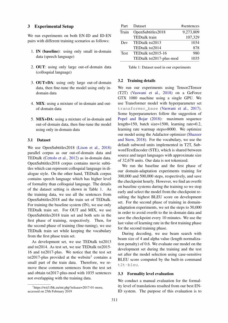
3 Experimental Setup

We run experiments on both EN-ID and ID-ENpairs with different training scenarios as follows:

1. IN (baseline): using only small in-domaindata (speech language)

2. OUT: using only large out-of-domain data(colloquial language)

3. OUT+DA: using only large out-of-domaindata, then fine-tune the model using only in-domain data

4. MIX: using a mixture of in-domain and out-of-domain data

5. MIX+DA: using a mixture of in-domain andout-of-domain data, then fine-tune the modelusing only in-domain data

3.1 Dataset

We use OpenSubtitles2018 (Lison et al., 2018)parallel corpus as our out-of-domain data andTEDtalk (Cettolo et al., 2012) as in-domain data.OpenSubtitles2018 corpus contains movie subti-tles which can represent colloquial language in di-alogue style. On the other hand, TEDtalk corpuscontains speech language which has higher levelof formality than colloquial language. The detailsof the dataset setting is shown in Table 1. Asthe training data, we use all the sentences fromOpenSubtitles2018 and the train set of TEDtalk.For training the baseline system (IN), we use onlyTEDtalk train set. For OUT and MIX, we useOpenSubtitles2018 train set and both sets in thefirst phase of training, respectively. Then, forthe second phase of training (fine-tuning), we useTEDtalk train set while keeping the vocabularyfrom the first phase train set.

As development set, we use TEDtalk tst2013and tst2014. As test set, we use TEDtalk tst2015-16 and tst2017-plus. We notice that the test settst2017-plus provided at the website1 contains asmall part of the train data. Therefore, we re-move these common sentences from the test setand obtain tst2017-plus-mod with 1035 sentencesnot overlapping with the training data.

1https://wit3.fbk.eu/mt.php?release=2017-01-more,accessed on 25th February 2019

Part Dataset #sentencesTrain OpenSubtitles2018 9,273,809

TEDtalk train 107,329Dev TEDtalk tst2013 1034

TEDtalk tst2014 878Test TEDtalk tst2015-16 980

TEDtalk tst2017-plus-mod 1035

Table 1: Dataset used in our experiments

3.2 Training details

We run our experiments using Tensor2Tensor(T2T) (Vaswani et al., 2018) on a GeForceGTX 1080 machine using a single GPU. Weuse Transformer model with hyperparameter settransformer_base (Vaswani et al., 2017).Some hyperparameters follow the suggestion ofPopel and Bojar (2018): maximum sequencelength=150, batch size=1500, learning rate=0.2,learning rate warmup steps=8000. We optimizeour model using the Adafactor optimizer (Shazeerand Stern, 2018). For the vocabulary, we use thedefault subword units implemented in T2T, Sub-wordTextEncoder (STE), which is shared betweensource and target languages with approximate sizeof 32,678 units. Our data is not tokenized.

We run the baseline and the first phase ofour domain-adaptation experiments training for300,000 and 500,000 steps, respectively, and savethe checkpoint hourly. However, we find an overfiton baseline systems during the training so we stopearly and select the model from the checkpoint re-sulting the highest BLEU score on developmentset. For the second phase of training in domain-adaptation experiments, we set the steps to 50,000in order to avoid overfit to the in-domain data andsave the checkpoint every 10 minutes. We use thelast value of learning rate in the first training phasefor the second training phase.

During decoding, we use beam search withbeam size of 4 and alpha value (length normaliza-tion penalty) of 0.6. We evaluate our model on thedevelopment set during the training and the testset after the model selection using case-sensitiveBLEU score computed by the built-in commandt2t-bleu.

3.3 Formality level evaluation

We conduct a manual evaluation for the formal-ity level of translations resulted from our best EN-ID system. The purpose of this evaluation is to

311

System EN-ID ID-ENIN 22.03 23.06OUT 20.75 22.81OUT+DA 27.47 26.93MIX 24.84 25.18MIX+DA 29.10 28.18

Table 2: BLEU scores of our English-Indonesian (EN-ID) and Indonesian-English (ID-EN) NMT systems ontest set. The bold texts mark the best scores.

see whether the domain-adapted system generatesmore formal translation based on human evalua-tion. The evaluation is inspired by human assess-ment of Niu et al. (2017). We randomly select50 translation pairs from the test set generated bythe first and second phases of our EN-ID system.We make sure each pair does not consist of thesame sentences. Then 48 Indonesian native speak-ers vote which sentence is more formal betweentwo of them. An option of ”neutral or difficult todistinguish” is also available. The voters are notaware that the sentence pairs are generated by MTsystems in order to keep the purity of the evalua-tion based on formality level and not biased to thetranslation quality.

4 Result

4.1 NMT performance

Table 2 shows the BLEU evaluation of our sys-tems. For both EN-ID and ID-EN directions, theresult shows similar patterns: (1) System trainedwith only in-domain data (IN) works better thanwith only out-of-domain data (OUT) although thetraining-data sizes are significantly different. (2)Domain adaptation (fine-tuning) helps to improvethe BLEU score in both cases when the modelis first trained without and with in-domain data(OUT and MIX respectively). Despite the bestperformance of our mixture system, the domainadaptation method has higher impact on the out-of-domain system.

While IN systems suffer from overfit, bothtraining and evaluation loss in OUT and MIX sys-tems still slightly decrease in the end of the train-ing which indicates the training steps still can beincreased.

4.2 Formality level

We use the evaluation approach described in Sub-section 3.3 on translation output of MIX and

Sentence 1Source You have to listen to one another.MIX Kau harus mendengarkan satu sama lain.MIX+DA Anda harus mendengarkan satu sama lain.Sentence 2Source I enjoy fashion magazines and pretty things.MIX Aku menikmati majalah fashion dan hal-hal

cantik.MIX+DA Saya menikmati majalah adibusana dan hal-

hal yang cukup.Sentence 3Source It could even be disseminated intentionally.MIX Itu bahkan bisa dibubarkan secara sengaja.MIX+DA Hal ini bahkan dapat diabaikan dengan sen-

gaja.Sentence 4Source They come from these cells.MIX Mereka datang dari sel-sel ini.MIX+DA Mereka berasal dari sel-sel ini.

Figure 1: Sample outputs of our EN-ID non-adapted(MIX) and domain-adapted (MIX+DA) systems, inwhich more than 50% of human assessors vote trans-lation by the domain-adapted system as more formal.

MIX+DA from the test set. Out of 50 pairs,35 MIX+DA sentences are voted by the majority(>50% of the voters) as more formal than theirpairs. For the remaining pairs, the majority eitherselect MIX sentences as more formal (12 pairs) orthe MIX+DA sentences are still the most selectedbut the frequency is less than 50% of the voters(3 pairs). We consider the latter condition has nodifference to being indistinct, although none of thepairs with ”difficult to distinguish” option are se-lected by the majority,

Among those 35 MIX+DA sentence pairs, weanalyze 13 pairs that are voted by more than 85%voters to observe which segment of the sentencesmight trigger the voters to label them as moreformal. Figure 1 shows sample output sentencepairs with such condition. Interestingly, 9 of thosepairs show similar pattern, namely they containthe change of pronouns to the formal one. Forinstance, ”kau” → ”Anda” or ”aku” → ”saya” inSentence 1 and 2, respectively, in the figure. Notethat English does not use honorifics that can givesuch context change in the translation.

Among 2015 translation pairs from the test set,we find 316 translations which change the pro-nouns to be more formal, 448 translations whichalready use formal pronouns before domain-adapted thus do not change, and, surprisingly, notranslation that still uses informal pronouns afterbeing domain-adapted. This indicates the style of

312

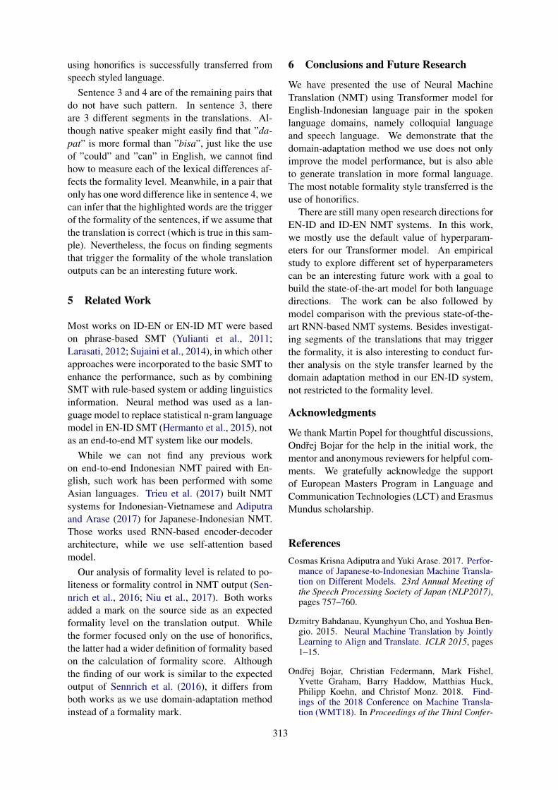
using honorifics is successfully transferred fromspeech styled language.

Sentence 3 and 4 are of the remaining pairs thatdo not have such pattern. In sentence 3, thereare 3 different segments in the translations. Al-though native speaker might easily find that ”da-pat” is more formal than ”bisa”, just like the useof ”could” and ”can” in English, we cannot findhow to measure each of the lexical differences af-fects the formality level. Meanwhile, in a pair thatonly has one word difference like in sentence 4, wecan infer that the highlighted words are the triggerof the formality of the sentences, if we assume thatthe translation is correct (which is true in this sam-ple). Nevertheless, the focus on finding segmentsthat trigger the formality of the whole translationoutputs can be an interesting future work.

5 Related Work

Most works on ID-EN or EN-ID MT were basedon phrase-based SMT (Yulianti et al., 2011;Larasati, 2012; Sujaini et al., 2014), in which otherapproaches were incorporated to the basic SMT toenhance the performance, such as by combiningSMT with rule-based system or adding linguisticsinformation. Neural method was used as a lan-guage model to replace statistical n-gram languagemodel in EN-ID SMT (Hermanto et al., 2015), notas an end-to-end MT system like our models.

While we can not find any previous workon end-to-end Indonesian NMT paired with En-glish, such work has been performed with someAsian languages. Trieu et al. (2017) built NMTsystems for Indonesian-Vietnamese and Adiputraand Arase (2017) for Japanese-Indonesian NMT.Those works used RNN-based encoder-decoderarchitecture, while we use self-attention basedmodel.

Our analysis of formality level is related to po-liteness or formality control in NMT output (Sen-nrich et al., 2016; Niu et al., 2017). Both worksadded a mark on the source side as an expectedformality level on the translation output. Whilethe former focused only on the use of honorifics,the latter had a wider definition of formality basedon the calculation of formality score. Althoughthe finding of our work is similar to the expectedoutput of Sennrich et al. (2016), it differs fromboth works as we use domain-adaptation methodinstead of a formality mark.

6 Conclusions and Future Research

We have presented the use of Neural MachineTranslation (NMT) using Transformer model forEnglish-Indonesian language pair in the spokenlanguage domains, namely colloquial languageand speech language. We demonstrate that thedomain-adaptation method we use does not onlyimprove the model performance, but is also ableto generate translation in more formal language.The most notable formality style transferred is theuse of honorifics.

There are still many open research directions forEN-ID and ID-EN NMT systems. In this work,we mostly use the default value of hyperparam-eters for our Transformer model. An empiricalstudy to explore different set of hyperparameterscan be an interesting future work with a goal tobuild the state-of-the-art model for both languagedirections. The work can be also followed bymodel comparison with the previous state-of-the-art RNN-based NMT systems. Besides investigat-ing segments of the translations that may triggerthe formality, it is also interesting to conduct fur-ther analysis on the style transfer learned by thedomain adaptation method in our EN-ID system,not restricted to the formality level.

Acknowledgments

We thank Martin Popel for thoughtful discussions,Ondrej Bojar for the help in the initial work, thementor and anonymous reviewers for helpful com-ments. We gratefully acknowledge the supportof European Masters Program in Language andCommunication Technologies (LCT) and ErasmusMundus scholarship.

ReferencesCosmas Krisna Adiputra and Yuki Arase. 2017. Perfor-

mance of Japanese-to-Indonesian Machine Transla-tion on Different Models. 23rd Annual Meeting ofthe Speech Processing Society of Japan (NLP2017),pages 757–760.

Dzmitry Bahdanau, Kyunghyun Cho, and Yoshua Ben-gio. 2015. Neural Machine Translation by JointlyLearning to Align and Translate. ICLR 2015, pages1–15.

Ondrej Bojar, Christian Federmann, Mark Fishel,Yvette Graham, Barry Haddow, Matthias Huck,Philipp Koehn, and Christof Monz. 2018. Find-ings of the 2018 Conference on Machine Transla-tion (WMT18). In Proceedings of the Third Confer-

313

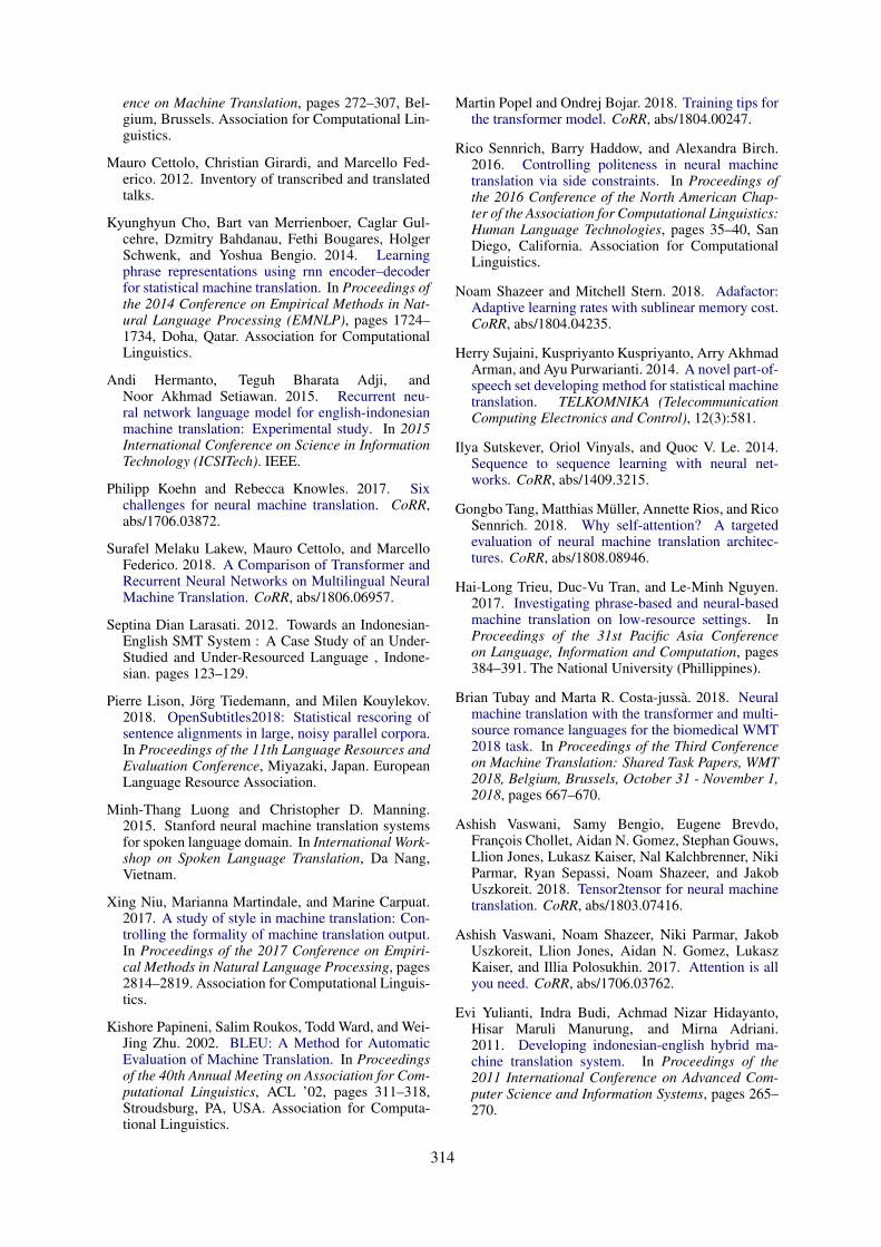
ence on Machine Translation, pages 272–307, Bel-gium, Brussels. Association for Computational Lin-guistics.

Mauro Cettolo, Christian Girardi, and Marcello Fed-erico. 2012. Inventory of transcribed and translatedtalks.

Kyunghyun Cho, Bart van Merrienboer, Caglar Gul-cehre, Dzmitry Bahdanau, Fethi Bougares, HolgerSchwenk, and Yoshua Bengio. 2014. Learningphrase representations using rnn encoder–decoderfor statistical machine translation. In Proceedings ofthe 2014 Conference on Empirical Methods in Nat-ural Language Processing (EMNLP), pages 1724–1734, Doha, Qatar. Association for ComputationalLinguistics.

Andi Hermanto, Teguh Bharata Adji, andNoor Akhmad Setiawan. 2015. Recurrent neu-ral network language model for english-indonesianmachine translation: Experimental study. In 2015International Conference on Science in InformationTechnology (ICSITech). IEEE.

Philipp Koehn and Rebecca Knowles. 2017. Sixchallenges for neural machine translation. CoRR,abs/1706.03872.

Surafel Melaku Lakew, Mauro Cettolo, and MarcelloFederico. 2018. A Comparison of Transformer andRecurrent Neural Networks on Multilingual NeuralMachine Translation. CoRR, abs/1806.06957.

Septina Dian Larasati. 2012. Towards an Indonesian-English SMT System : A Case Study of an Under-Studied and Under-Resourced Language , Indone-sian. pages 123–129.

Pierre Lison, Jorg Tiedemann, and Milen Kouylekov.2018. OpenSubtitles2018: Statistical rescoring ofsentence alignments in large, noisy parallel corpora.In Proceedings of the 11th Language Resources andEvaluation Conference, Miyazaki, Japan. EuropeanLanguage Resource Association.

Minh-Thang Luong and Christopher D. Manning.2015. Stanford neural machine translation systemsfor spoken language domain. In International Work-shop on Spoken Language Translation, Da Nang,Vietnam.

Xing Niu, Marianna Martindale, and Marine Carpuat.2017. A study of style in machine translation: Con-trolling the formality of machine translation output.In Proceedings of the 2017 Conference on Empiri-cal Methods in Natural Language Processing, pages2814–2819. Association for Computational Linguis-tics.

Kishore Papineni, Salim Roukos, Todd Ward, and Wei-Jing Zhu. 2002. BLEU: A Method for AutomaticEvaluation of Machine Translation. In Proceedingsof the 40th Annual Meeting on Association for Com-putational Linguistics, ACL ’02, pages 311–318,Stroudsburg, PA, USA. Association for Computa-tional Linguistics.

Martin Popel and Ondrej Bojar. 2018. Training tips forthe transformer model. CoRR, abs/1804.00247.

Rico Sennrich, Barry Haddow, and Alexandra Birch.2016. Controlling politeness in neural machinetranslation via side constraints. In Proceedings ofthe 2016 Conference of the North American Chap-ter of the Association for Computational Linguistics:Human Language Technologies, pages 35–40, SanDiego, California. Association for ComputationalLinguistics.

Noam Shazeer and Mitchell Stern. 2018. Adafactor:Adaptive learning rates with sublinear memory cost.CoRR, abs/1804.04235.

Herry Sujaini, Kuspriyanto Kuspriyanto, Arry AkhmadArman, and Ayu Purwarianti. 2014. A novel part-of-speech set developing method for statistical machinetranslation. TELKOMNIKA (TelecommunicationComputing Electronics and Control), 12(3):581.

Ilya Sutskever, Oriol Vinyals, and Quoc V. Le. 2014.Sequence to sequence learning with neural net-works. CoRR, abs/1409.3215.

Gongbo Tang, Matthias Muller, Annette Rios, and RicoSennrich. 2018. Why self-attention? A targetedevaluation of neural machine translation architec-tures. CoRR, abs/1808.08946.

Hai-Long Trieu, Duc-Vu Tran, and Le-Minh Nguyen.2017. Investigating phrase-based and neural-basedmachine translation on low-resource settings. InProceedings of the 31st Pacific Asia Conferenceon Language, Information and Computation, pages384–391. The National University (Phillippines).

Brian Tubay and Marta R. Costa-jussa. 2018. Neuralmachine translation with the transformer and multi-source romance languages for the biomedical WMT2018 task. In Proceedings of the Third Conferenceon Machine Translation: Shared Task Papers, WMT2018, Belgium, Brussels, October 31 - November 1,2018, pages 667–670.

Ashish Vaswani, Samy Bengio, Eugene Brevdo,Francois Chollet, Aidan N. Gomez, Stephan Gouws,Llion Jones, Lukasz Kaiser, Nal Kalchbrenner, NikiParmar, Ryan Sepassi, Noam Shazeer, and JakobUszkoreit. 2018. Tensor2tensor for neural machinetranslation. CoRR, abs/1803.07416.

Ashish Vaswani, Noam Shazeer, Niki Parmar, JakobUszkoreit, Llion Jones, Aidan N. Gomez, LukaszKaiser, and Illia Polosukhin. 2017. Attention is allyou need. CoRR, abs/1706.03762.

Evi Yulianti, Indra Budi, Achmad Nizar Hidayanto,Hisar Maruli Manurung, and Mirna Adriani.2011. Developing indonesian-english hybrid ma-chine translation system. In Proceedings of the2011 International Conference on Advanced Com-puter Science and Information Systems, pages 265–270.

314

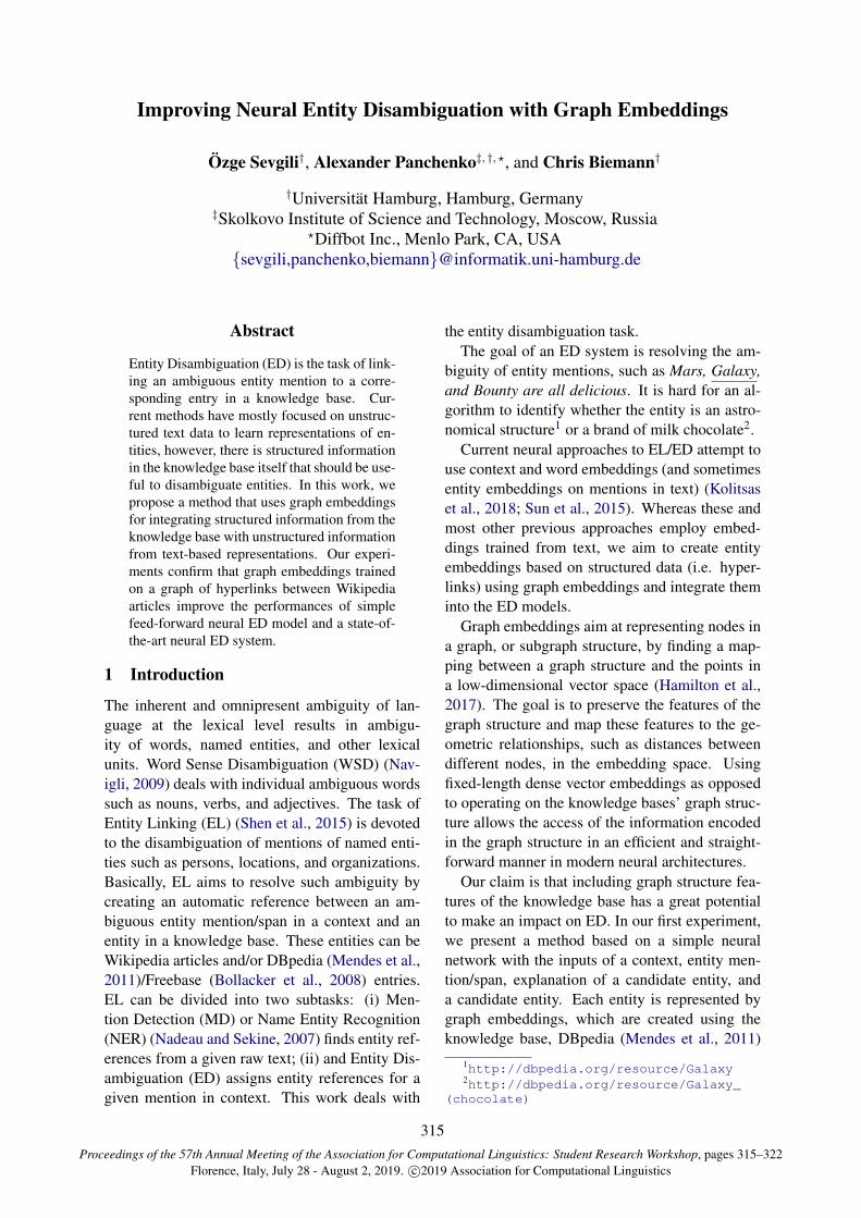
Proceedings of the 57th Annual Meeting of the Association for Computational Linguistics: Student Research Workshop, pages 315–322Florence, Italy, July 28 - August 2, 2019. c©2019 Association for Computational Linguistics

Improving Neural Entity Disambiguation with Graph Embeddings

Ozge Sevgili†, Alexander Panchenko‡, †, ?, and Chris Biemann†

†Universitat Hamburg, Hamburg, Germany‡Skolkovo Institute of Science and Technology, Moscow, Russia

?Diffbot Inc., Menlo Park, CA, USAsevgili,panchenko,biemann@informatik.uni-hamburg.de

Abstract

Entity Disambiguation (ED) is the task of link-ing an ambiguous entity mention to a corre-sponding entry in a knowledge base. Cur-rent methods have mostly focused on unstruc-tured text data to learn representations of en-tities, however, there is structured informationin the knowledge base itself that should be use-ful to disambiguate entities. In this work, wepropose a method that uses graph embeddingsfor integrating structured information from theknowledge base with unstructured informationfrom text-based representations. Our experi-ments confirm that graph embeddings trainedon a graph of hyperlinks between Wikipediaarticles improve the performances of simplefeed-forward neural ED model and a state-of-the-art neural ED system.

1 Introduction

The inherent and omnipresent ambiguity of lan-guage at the lexical level results in ambigu-ity of words, named entities, and other lexicalunits. Word Sense Disambiguation (WSD) (Nav-igli, 2009) deals with individual ambiguous wordssuch as nouns, verbs, and adjectives. The task ofEntity Linking (EL) (Shen et al., 2015) is devotedto the disambiguation of mentions of named enti-ties such as persons, locations, and organizations.Basically, EL aims to resolve such ambiguity bycreating an automatic reference between an am-biguous entity mention/span in a context and anentity in a knowledge base. These entities can beWikipedia articles and/or DBpedia (Mendes et al.,2011)/Freebase (Bollacker et al., 2008) entries.EL can be divided into two subtasks: (i) Men-tion Detection (MD) or Name Entity Recognition(NER) (Nadeau and Sekine, 2007) finds entity ref-erences from a given raw text; (ii) and Entity Dis-ambiguation (ED) assigns entity references for agiven mention in context. This work deals with

the entity disambiguation task.The goal of an ED system is resolving the am-

biguity of entity mentions, such as Mars, Galaxy,and Bounty are all delicious. It is hard for an al-gorithm to identify whether the entity is an astro-nomical structure1 or a brand of milk chocolate2.

Current neural approaches to EL/ED attempt touse context and word embeddings (and sometimesentity embeddings on mentions in text) (Kolitsaset al., 2018; Sun et al., 2015). Whereas these andmost other previous approaches employ embed-dings trained from text, we aim to create entityembeddings based on structured data (i.e. hyper-links) using graph embeddings and integrate theminto the ED models.

Graph embeddings aim at representing nodes ina graph, or subgraph structure, by finding a map-ping between a graph structure and the points ina low-dimensional vector space (Hamilton et al.,2017). The goal is to preserve the features of thegraph structure and map these features to the ge-ometric relationships, such as distances betweendifferent nodes, in the embedding space. Usingfixed-length dense vector embeddings as opposedto operating on the knowledge bases’ graph struc-ture allows the access of the information encodedin the graph structure in an efficient and straight-forward manner in modern neural architectures.

Our claim is that including graph structure fea-tures of the knowledge base has a great potentialto make an impact on ED. In our first experiment,we present a method based on a simple neuralnetwork with the inputs of a context, entity men-tion/span, explanation of a candidate entity, anda candidate entity. Each entity is represented bygraph embeddings, which are created using theknowledge base, DBpedia (Mendes et al., 2011)

1http://dbpedia.org/resource/Galaxy2http://dbpedia.org/resource/Galaxy_

(chocolate)

315

containing hyperlinks between entities. We per-form ablation tests on the types of inputs, whichallows us to judge the impact of the single inputsas well as their interplay. In a second experiment,we enhance a state-of-the-art neural entity disam-biguation system called end2end (Kolitsas et al.,2018) with our graph embeddings: The originalsystem relies on character, word and entity embed-dings; we replace respectively complement thesewith our graph embeddings. Both experimentsconfirm the hypothesis that structured informationin the form of graph embeddings are an efficientand effective way of improving ED.

Our main contribution is a creation of a simpletechnique for integration of structured informationinto an ED system with graph embeddings. Thereis no obvious way to use large structured knowl-edge bases directly in a neural ED system. Weprovide a simple solution based on graph embed-dings and confirm experimentally its effectiveness.

2 Related Work

Entity Linking Traditional approaches to ELfocus on defining the similarity measurement be-tween a mention and a candidate entity (Mihal-cea and Csomai, 2007; Strube and Ponzetto, 2006;Bunescu and Pasca, 2006). Similarly, Milne andWitten (2008) define a measurement of entity-entity relatedness. Current state-of-the-art ap-proaches are based on neural networks (Huanget al., 2015; Ganea and Hofmann, 2017; Kolitsaset al., 2018; Sun et al., 2015), where are based oncharacter, word and/or entity embeddings createdby a neural network with a motivation of their ca-pability to automatically induce features, as op-posed to hand-crafting them. Then, they all usethese embeddings in neural EL/ED.

Yamada et al. (2016) and Fang et al. (2016) uti-lize structured data modelling entities and wordsin the same space and mapping spans to entitiesbased on the similarity in this space. They ex-pand the objective function of word2vec (Mikolovet al., 2013a,b) and use both text and structured in-formation. Radhakrishnan et al. (2018) extend thework of Yamada et al. (2016) by creating their owngraph based on co-occurrences statistics instead ofusing the knowledge graph directly. Contrary tothem, our model learns a mapping of spans andentities, which reside in different spaces and usegraph embeddings trained on the knowledge graphfor representing structured information.

Kolitsas et al. (2018) address both MD and EDin their end2end system. They build a context-aware neural network based on character, word,and entity embeddings coupled with attention andglobal voting mechanisms. Their entity embed-dings, proposed by Ganea and Hofmann (2017),are computed by the empirical conditional word-entity distribution based on the co-occurrencecounts on Wikipedia pages and hyperlinks.

Graph Embeddings There are various meth-ods to create graph embedding, which can begrouped into the methods based on matrix factor-ization, random walks, and deep learning (Goyaland Ferrara, 2018). Factorization-based modelsdepend on the node adjacency matrix and dimen-sionality reduction method (Belkin and Niyogi,2001; Roweis and Saul, 2000; Tang et al., 2015).Random-walk-based methods aim to preservemany properties of graph (Perozzi et al., 2014;Grover and Leskovec, 2016). Deep-learning-based ones reduce dimensionality automaticallyand model non-linearity (Wang et al., 2016; Kipfand Welling, 2017). In our case, efficiency is cru-cial and time complexity of factorization-basedmodels is high. The disadvantage of the deep-learning-based models is that they require exten-sive hyperparameter optimization. To keep it sim-ple, efficient, and to minimize the numbers of hy-perparameters to tune, yet still effective, we selectrandom-walk-based methods, where two promi-nent representatives are DeepWalk (Perozzi et al.,2014) and node2vec (Grover and Leskovec, 2016).

3 Learning Graph-based Entity Vectors

In order to make information from a semanticgraph available for an entity linking system, wemake use of graph embeddings. We use DeepWalk(Perozzi et al., 2014) to create the representationof entities in the DBPedia. DeepWalk is scalable,which makes it applicable on a large graph. It usesrandom walks to learn latent representations andprovides a representation of each node on the ba-sis of the graph structure.

First, we created a graph whose nodes areunique entities; attributes are explanations of en-tities, i.e. long abstracts; edges are the page linksbetween entities with the information from DB-pedia. Second, a vector representation per en-tity is generated by training DeepWalk on theedges of this graph. For this, we used all de-fault hyper-parameters of DeepWalk, e.g. number-

316

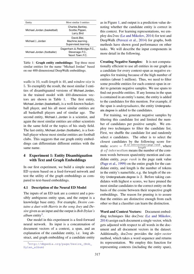
Entity Most similar 3 entities

Michael Jordan (basketball)Charles Barkley,Scottie Pippen,

Larry Bird

Michael I. JordanDavid Blei,

Machine learning ,Supervised learning

Michael Jordan (footballer)Dagenham & Redbridge F.C.,

Stevenage F.C.,Yeovil Town F.C.

Table 1: Graph entity embeddings: Top three mostsimilar entities for the name “Michael Jordan” basedon our 400-dimensional DeepWalk embeddings.

walks is 10, walk-length is 40, and window-size is5. To exemplify the result, the most similar 3 enti-ties of disambiguated versions of Michael Jordan,in the trained model with 400-dimension vec-tors are shown in Table 1. The first entity,Michael Jordan (basketball), is a well-known basket-ball player, and his all most similar entities areall basketball players and of similar age. Thesecond entity, Michael I. Jordan is a scientist, andagain the most similar entities are either scientistsin the same field or the topics of his study field.The last entity, Michael Jordan (footballer), is a foot-ball player whose most similar entities are footballclubs. This suggests that our graph entity embed-dings can differentiate different entities with thesame name.

4 Experiment 1: Entity Disambiguationwith Text and Graph Embeddings

In our first experiment, we build a simple neuralED system based on a feed-forward network andtest the utility of the graph embeddings as com-pared to text-based embeddings.

4.1 Description of the Neural ED ModelThe inputs of an ED task are a context and a pos-sibly ambiguous entity span, and the output is aknowledge base entry. For example, Desire con-tains a duet with Harris in the song Joey and De-sire given as an input and the output is Bob Dylan’salbum entity3.

Our model in this experiment is a feed-forwardneural network. Its input is a concatenation ofdocument vectors of a context, a span, and anexplanation of the candidate entity, i.e. long ab-stract, and graph embedding of a candidate entity

3http://dbpedia.org/page/Desire_(Bob_Dylan_album)

as in Figure 1, and output is a prediction value de-noting whether the candidate entity is correct inthis context. For learning representations, we em-ploy doc2vec (Le and Mikolov, 2014) for text andDeepWalk (Perozzi et al., 2014) for graphs, bothmethods have shown good performance on othertasks. We will describe the input components inmore detail in the following.

Creating Negative Samples: It is not computa-tionally efficient to use all entities in our graph asa candidate for every context-span as negative ex-amples for training because of the high number ofentities (about 5 million). Thus, we need to filtersome possible entities for each context-span in or-der to generate negative samples. We use spans tofind out possible entities. If any lemma in the spanis contained in an entity’s name, the entity is addedto the candidates for this mention. For example, ifthe span is undergraduates, the entity Undergradu-ate degree is added to the candidates.

For training, we generate negative samples byfiltering this candidate list and limited the num-ber of candidates per positive sample. We em-ploy two techniques to filter the candidate list.First, we shuffle the candidate list and randomlyselect n candidates. The other is to select theclosest candidates by the following score for-mula: score = # of intersection×page rank

length , where# of intersection means the number of the com-mon words between span/entity mention and can-didate entity, page rank is the page rank value(Page et al., 1999) on the entire graph for the can-didate entity, and length is the number of tokensin the entity’s name/title, e.g. the length of the en-tity Undergraduate degree is 2. Before taking can-didates with highest n scores, we have pruned themost similar candidates to the correct entity on thebasis of the cosine between their respective graphembeddings. The reason for pruning is to assurethat the entities are distinctive enough from eachother so that a classifier can learn the distinction.

Word and Context Vectors: Document embed-ding techniques like doc2vec (Le and Mikolov,2014) assign each document a single vector, whichgets adjusted with respect to all words in the doc-ument and all document vectors in the dataset.Additionally, doc2vec provides the infer vectormethod, which takes a word sequence and returnsits representation. We employ this function forrepresenting contexts (including the entity span),

317

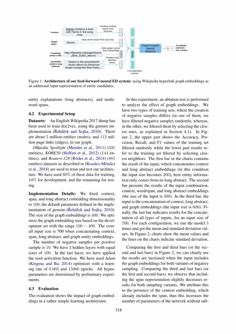
Creates context vector from

doc2vec

Creates long abstract vector

Gets word vector from doc2vec

Gets graph vector from DeepWalk

Concatenates vectors

Feed-Forward Neural

Network 0 - 1

Candidate matches the context

Desire

http://dbpedia.org/page/Desire_(Bob_Dylan_album)

Desire is the seventeenth studio album by American

singer-songwriter Bob Dylan,...

Context

Target Span

Candidate entity’s URL

Desire contains a duet with Harris in the song

Joey

Candidate entity’s long

abstract

Figure 1: Architecture of our feed-forward neural ED system: using Wikipedia hyperlink graph embeddings asan additional input representation of entity candidates.

entity explanations (long abstracts), and multi-word spans.

4.2 Experimental SetupDatasets: An English Wikipedia 2017 dump hasbeen used to train doc2vec, using the gensim im-plementation (Rehurek and Sojka, 2010). Thereare about 5 million entities (nodes), and 112 mil-lion page links (edges), in our graph.

DBpedia Spotlight (Mendes et al., 2011) (331entities), KORE50 (Hoffart et al., 2012) (144 en-tities), and Reuters-128 (Roder et al., 2014) (881entities) datasets as described in (Rosales-Mendezet al., 2018) are used to train and test our architec-ture. We have used 80% of these data for training,10% for development, and the remaining for test-ing.

Implementation Details: We fixed context,span, and long abstract embedding dimensionalityto 100, the default parameter defined in the imple-mentation of gensim (Rehurek and Sojka, 2010).The size of the graph embeddings is 400. We opti-mize the graph embedding size based on the devel-opment set with the range 100 − 400. The over-all input size is 700 when concatenating context,span, long abstract, and graph entity embeddings.

The number of negative samples per positivesample is 10. We have 3 hidden layers with equalsizes of 100. In the last layer, we have appliedthe tanh activation function. We have used Adam(Kingma and Ba, 2014) optimizer with a learn-ing rate of 0.005 and 15000 epochs. All hyper-parameters are determined by preliminary experi-ments.

4.3 EvaluationThe evaluation shows the impact of graph embed-dings in a rather simple learning architecture.

In this experiment, an ablation test is performedto analyze the effect of graph embeddings. Wehave two types of training sets, where the creationof negative samples differs (in one of them, wehave filtered negative samples randomly, whereas,in the other, we filtered them by selecting the clos-est ones, as explained in Section 4.1). In Fig-ure 2, the upper part shows the Accuracy, Pre-cision, Recall, and F1 values of the training setfiltered randomly while the lower part results re-fer to the training set filtered by selecting clos-est neighbors. The first bar in the charts containsthe result of the input, which concatenates contextand long abstract embeddings (in this conditionthe input size becomes 200), here entity informa-tion only comes from its long abstract. The secondbar presents the results of the input combination,context, word/span, and long abstract embeddings(the size of the input is 300). In the third bar, theinput is the concatenation of context, long abstract,and graph embeddings (the input size is 600). Fi-nally, the last bar indicates results for the concate-nation of all types of inputs, for an input size of700. For each configuration, we run the model 5times and get the mean and standard deviation val-ues. In Figure 2, charts show the mean values andthe lines on the charts indicate standard deviation.

Comparing the first and third bars (or the sec-ond and last bars) in Figure 2, we can clearly seethe results are increased when the input includesthe graph embeddings for both variants of negativesampling. Comparing the third and last bars (orthe first and second bars), we observe that includ-ing the span representation slightly decreases re-sults for both sampling variants. We attribute thisto the presence of the context embedding, whichalready includes the span, thus this increases thenumber of parameters of the network without sub-

318

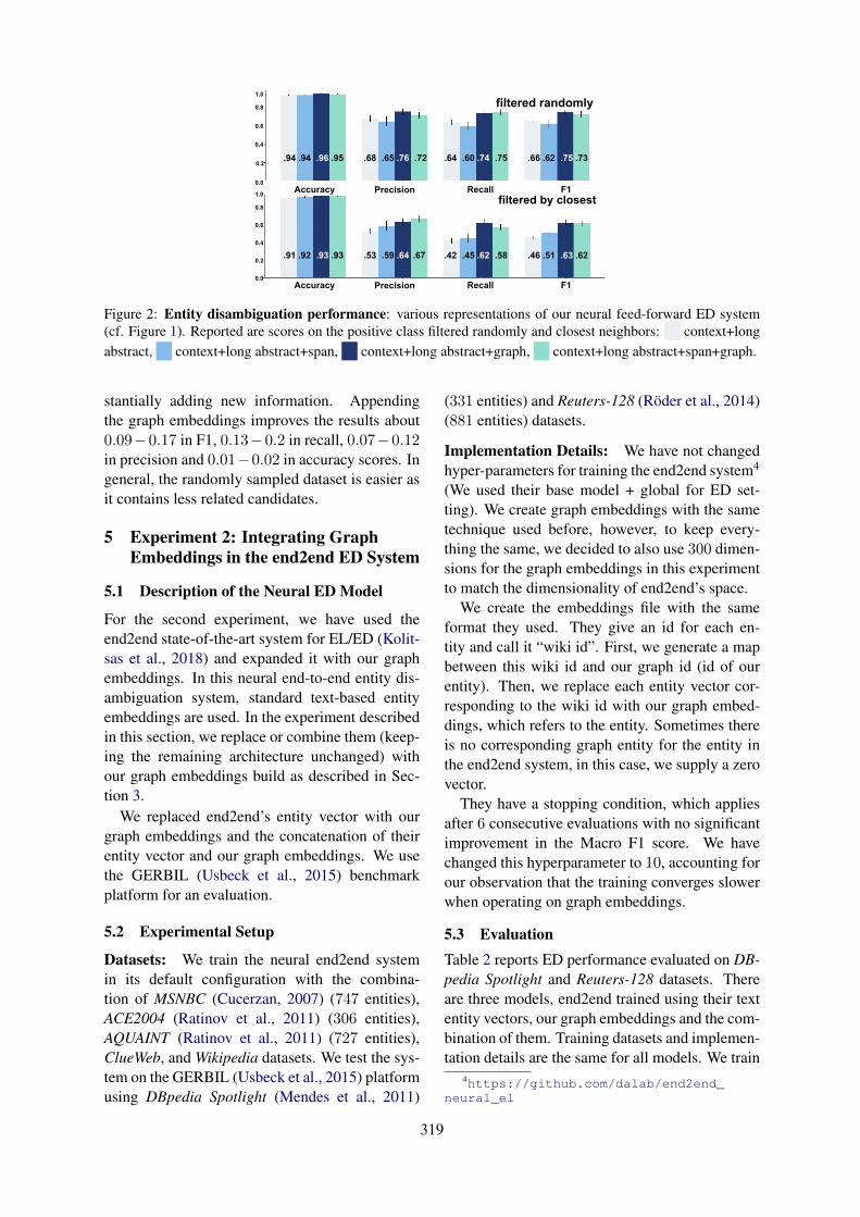
.94 .94 .96 .95 .68 .65 .76 .72 .64 .60 .74 .75 .66 .62 .75 .73

.91 .92 .93 .93 .53 .59 .64 .67 .42 .45 .62 .58 .46 .51 .63 .62

Accuracy Precision Recall

Accuracy Precision Recall F1

filtered randomly

filtered by closest

0.0

0.2

0.4

0.6

0.8

1.0

0.0

0.2

0.4

0.6

0.8

1.0

F1

Figure 2: Entity disambiguation performance: various representations of our neural feed-forward ED system(cf. Figure 1). Reported are scores on the positive class filtered randomly and closest neighbors: 0 context+longabstract, 0 context+long abstract+span, 0 context+long abstract+graph, 0 context+long abstract+span+graph.

stantially adding new information. Appendingthe graph embeddings improves the results about0.09−0.17 in F1, 0.13−0.2 in recall, 0.07−0.12in precision and 0.01−0.02 in accuracy scores. Ingeneral, the randomly sampled dataset is easier asit contains less related candidates.

5 Experiment 2: Integrating GraphEmbeddings in the end2end ED System

5.1 Description of the Neural ED Model

For the second experiment, we have used theend2end state-of-the-art system for EL/ED (Kolit-sas et al., 2018) and expanded it with our graphembeddings. In this neural end-to-end entity dis-ambiguation system, standard text-based entityembeddings are used. In the experiment describedin this section, we replace or combine them (keep-ing the remaining architecture unchanged) withour graph embeddings build as described in Sec-tion 3.

We replaced end2end’s entity vector with ourgraph embeddings and the concatenation of theirentity vector and our graph embeddings. We usethe GERBIL (Usbeck et al., 2015) benchmarkplatform for an evaluation.

5.2 Experimental Setup

Datasets: We train the neural end2end systemin its default configuration with the combina-tion of MSNBC (Cucerzan, 2007) (747 entities),ACE2004 (Ratinov et al., 2011) (306 entities),AQUAINT (Ratinov et al., 2011) (727 entities),ClueWeb, and Wikipedia datasets. We test the sys-tem on the GERBIL (Usbeck et al., 2015) platformusing DBpedia Spotlight (Mendes et al., 2011)

(331 entities) and Reuters-128 (Roder et al., 2014)(881 entities) datasets.

Implementation Details: We have not changedhyper-parameters for training the end2end system4

(We used their base model + global for ED set-ting). We create graph embeddings with the sametechnique used before, however, to keep every-thing the same, we decided to also use 300 dimen-sions for the graph embeddings in this experimentto match the dimensionality of end2end’s space.

We create the embeddings file with the sameformat they used. They give an id for each en-tity and call it “wiki id”. First, we generate a mapbetween this wiki id and our graph id (id of ourentity). Then, we replace each entity vector cor-responding to the wiki id with our graph embed-dings, which refers to the entity. Sometimes thereis no corresponding graph entity for the entity inthe end2end system, in this case, we supply a zerovector.

They have a stopping condition, which appliesafter 6 consecutive evaluations with no significantimprovement in the Macro F1 score. We havechanged this hyperparameter to 10, accounting forour observation that the training converges slowerwhen operating on graph embeddings.

5.3 EvaluationTable 2 reports ED performance evaluated on DB-pedia Spotlight and Reuters-128 datasets. Thereare three models, end2end trained using their textentity vectors, our graph embeddings and the com-bination of them. Training datasets and implemen-tation details are the same for all models. We train

4https://github.com/dalab/end2end_neural_el

319

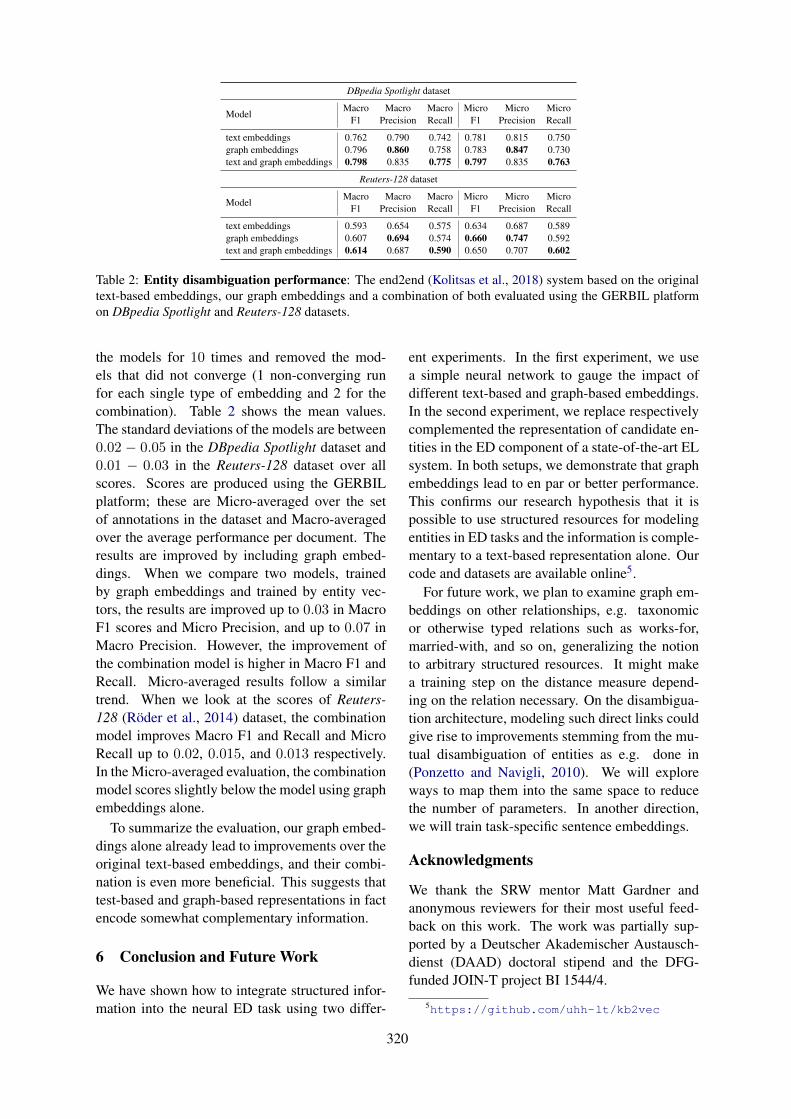
DBpedia Spotlight dataset

ModelMacro

F1Macro

PrecisionMacroRecall

MicroF1

MicroPrecision

MicroRecall

text embeddings 0.762 0.790 0.742 0.781 0.815 0.750graph embeddings 0.796 0.860 0.758 0.783 0.847 0.730text and graph embeddings 0.798 0.835 0.775 0.797 0.835 0.763

Reuters-128 dataset

ModelMacro

F1Macro

PrecisionMacroRecall

MicroF1

MicroPrecision

MicroRecall

text embeddings 0.593 0.654 0.575 0.634 0.687 0.589graph embeddings 0.607 0.694 0.574 0.660 0.747 0.592text and graph embeddings 0.614 0.687 0.590 0.650 0.707 0.602

Table 2: Entity disambiguation performance: The end2end (Kolitsas et al., 2018) system based on the originaltext-based embeddings, our graph embeddings and a combination of both evaluated using the GERBIL platformon DBpedia Spotlight and Reuters-128 datasets.

the models for 10 times and removed the mod-els that did not converge (1 non-converging runfor each single type of embedding and 2 for thecombination). Table 2 shows the mean values.The standard deviations of the models are between0.02 − 0.05 in the DBpedia Spotlight dataset and0.01 − 0.03 in the Reuters-128 dataset over allscores. Scores are produced using the GERBILplatform; these are Micro-averaged over the setof annotations in the dataset and Macro-averagedover the average performance per document. Theresults are improved by including graph embed-dings. When we compare two models, trainedby graph embeddings and trained by entity vec-tors, the results are improved up to 0.03 in MacroF1 scores and Micro Precision, and up to 0.07 inMacro Precision. However, the improvement ofthe combination model is higher in Macro F1 andRecall. Micro-averaged results follow a similartrend. When we look at the scores of Reuters-128 (Roder et al., 2014) dataset, the combinationmodel improves Macro F1 and Recall and MicroRecall up to 0.02, 0.015, and 0.013 respectively.In the Micro-averaged evaluation, the combinationmodel scores slightly below the model using graphembeddings alone.

To summarize the evaluation, our graph embed-dings alone already lead to improvements over theoriginal text-based embeddings, and their combi-nation is even more beneficial. This suggests thattest-based and graph-based representations in factencode somewhat complementary information.

6 Conclusion and Future Work

We have shown how to integrate structured infor-mation into the neural ED task using two differ-

ent experiments. In the first experiment, we usea simple neural network to gauge the impact ofdifferent text-based and graph-based embeddings.In the second experiment, we replace respectivelycomplemented the representation of candidate en-tities in the ED component of a state-of-the-art ELsystem. In both setups, we demonstrate that graphembeddings lead to en par or better performance.This confirms our research hypothesis that it ispossible to use structured resources for modelingentities in ED tasks and the information is comple-mentary to a text-based representation alone. Ourcode and datasets are available online5.

For future work, we plan to examine graph em-beddings on other relationships, e.g. taxonomicor otherwise typed relations such as works-for,married-with, and so on, generalizing the notionto arbitrary structured resources. It might makea training step on the distance measure depend-ing on the relation necessary. On the disambigua-tion architecture, modeling such direct links couldgive rise to improvements stemming from the mu-tual disambiguation of entities as e.g. done in(Ponzetto and Navigli, 2010). We will exploreways to map them into the same space to reducethe number of parameters. In another direction,we will train task-specific sentence embeddings.

Acknowledgments

We thank the SRW mentor Matt Gardner andanonymous reviewers for their most useful feed-back on this work. The work was partially sup-ported by a Deutscher Akademischer Austausch-dienst (DAAD) doctoral stipend and the DFG-funded JOIN-T project BI 1544/4.

5https://github.com/uhh-lt/kb2vec

320

ReferencesMikhail Belkin and Partha Niyogi. 2001. Laplacian

eigenmaps and spectral techniques for embeddingand clustering. In Proceedings of the 14th Interna-tional Conference on Neural Information Process-ing Systems: Natural and Synthetic, NIPS’01, pages585–591, Cambridge, MA, USA. MIT Press.

Kurt Bollacker, Colin Evans, Praveen Paritosh, TimSturge, and Jamie Taylor. 2008. Freebase: A col-laboratively created graph database for structuringhuman knowledge. In Proceedings of the 2008ACM SIGMOD International Conference on Man-agement of Data, SIGMOD ’08, pages 1247–1250,New York, NY, USA. ACM.

Razvan Bunescu and Marius Pasca. 2006. Using en-cyclopedic knowledge for named entity disambigua-tion. In 11th Conference of the European Chap-ter of the Association for Computational Linguistics,pages 9–16, Trento, Italy. Association for Computa-tional Linguistics.

Silviu Cucerzan. 2007. Large-scale named entity dis-ambiguation based on Wikipedia data. In Proceed-ings of the 2007 Joint Conference on EmpiricalMethods in Natural Language Processing and Com-putational Natural Language Learning (EMNLP-CoNLL), pages 708–716, Prague, Czech Republic.Association for Computational Linguistics.

Wei Fang, Jianwen Zhang, Dilin Wang, Zheng Chen,and Ming Li. 2016. Entity disambiguation byknowledge and text jointly embedding. In Proceed-ings of The 20th SIGNLL Conference on Compu-tational Natural Language Learning, pages 260–269, Berlin, Germany. Association for Computa-tional Linguistics.

Octavian-Eugen Ganea and Thomas Hofmann. 2017.Deep joint entity disambiguation with local neuralattention. In Proceedings of the 2017 Conference onEmpirical Methods in Natural Language Process-ing, pages 2619–2629, Copenhagen, Denmark. As-sociation for Computational Linguistics.

Palash Goyal and Emilio Ferrara. 2018. Graph embed-ding techniques, applications, and performance: Asurvey. Knowledge-Based Systems, 151(1 July):78–94.

Aditya Grover and Jure Leskovec. 2016. Node2vec:Scalable feature learning for networks. In Proceed-ings of the 22Nd ACM SIGKDD International Con-ference on Knowledge Discovery and Data Mining,KDD ’16, pages 855–864, New York, NY, USA.ACM.

William L. Hamilton, Rex Ying, and Jure Leskovec.2017. Representation learning on graphs: Methodsand applications. IEEE Data Eng. Bull., 40:52–74.

Johannes Hoffart, Stephan Seufert, Dat Ba Nguyen,Martin Theobald, and Gerhard Weikum. 2012.

KORE: keyphrase overlap relatedness for entity dis-ambiguation. In Proceedings of the 21st ACM In-ternational Conference on Information and Knowl-edge Management, CIKM ’12, pages 545–554, NewYork, NY, USA. ACM.

Hongzhao Huang, Larry P. Heck, and Heng Ji.2015. Leveraging deep neural networks and knowl-edge graphs for entity disambiguation. CoRR,abs/1504.07678.

Diederik P. Kingma and Jimmy Ba. 2014. Adam: Amethod for stochastic optimization. Proceedings ofthe 3rd International Conference for Learning Rep-resentations (ICLR), San Diego, CA, USA, 2015.

Thomas N. Kipf and Max Welling. 2017. Semi-supervised classification with graph convolutionalnetworks. In Proceedings of the 5th InternationalConference on Learning Representations, (ICLR),Toulon, France.

Nikolaos Kolitsas, Octavian-Eugen Ganea, andThomas Hofmann. 2018. End-to-end neural entitylinking. In Proceedings of the 22nd Conferenceon Computational Natural Language Learning,pages 519–529, Brussels, Belgium. Association forComputational Linguistics.

Quoc Le and Tomas Mikolov. 2014. Distributed repre-sentations of sentences and documents. In Proceed-ings of the 31st International Conference on Inter-national Conference on Machine Learning - Volume32, ICML’14, pages II–1188–II–1196. JMLR.org.

Pablo N. Mendes, Max Jakob, Andres Garcıa-Silva,and Christian Bizer. 2011. DBpedia spotlight: Shed-ding light on the web of documents. In Proceedingsof the 7th International Conference on Semantic Sys-tems, I-Semantics ’11, pages 1–8, New York, NY,USA. ACM.

Rada Mihalcea and Andras Csomai. 2007. Wikify!:Linking documents to encyclopedic knowledge. InProceedings of the Sixteenth ACM Conference onConference on Information and Knowledge Man-agement, CIKM ’07, pages 233–242, New York,NY, USA. ACM.

Tomas Mikolov, Kai Chen, Greg Corrado, and JeffreyDean. 2013a. Efficient estimation of word represen-tations in vector space. In Workshop Proceedings ofthe International Conference on Learning Represen-tations (ICLR). 2013, Scottsdale, AZ, USA.

Tomas Mikolov, Ilya Sutskever, Kai Chen, Greg S. Cor-rado, and Jeffrey Dean. 2013b. Distributed repre-sentations of words and phrases and their composi-tionality. In Proceedings of the 26th InternationalConference on Neural Information Processing Sys-tems - Volume 2, NIPS’13, pages 3111–3119, LakeTahoe, NV, USA. Curran Associates Inc.

David Milne and Ian H. Witten. 2008. Learning to linkwith Wikipedia. In Proceedings of the 17th ACM

321

Conference on Information and Knowledge Man-agement, CIKM ’08, pages 509–518, New York,NY, USA. ACM.

David Nadeau and Satoshi Sekine. 2007. A surveyof named entity recognition and classification. Lin-guisticae Investigationes, 30(1):3–26.

Roberto Navigli. 2009. Word sense disambiguation:A survey. ACM Computing Surveys, 41(2):10:1–10:69.

Lawrence Page, Sergey Brin, Rajeev Motwani, andTerry Winograd. 1999. The PageRank citation rank-ing: Bringing order to the web. Technical Re-port 1999-66, Stanford InfoLab. Previous number= SIDL-WP-1999-0120.

Bryan Perozzi, Rami Al-Rfou, and Steven Skiena.2014. DeepWalk: Online learning of social rep-resentations. In Proceedings of the 20th ACMSIGKDD International Conference on KnowledgeDiscovery and Data Mining, KDD ’14, pages 701–710, New York, NY, USA. ACM.

Simone P. Ponzetto and Roberto Navigli. 2010.Knowledge-rich word sense disambiguation rival-ing supervised systems. In Proceedings of the 48thAnnual Meeting of the Association for Computa-tional Linguistics, pages 1522–1531, Uppsala, Swe-den. Association for Computational Linguistics.

Priya Radhakrishnan, Partha Talukdar, and VasudevaVarma. 2018. ELDEN: Improved entity linking us-ing densified knowledge graphs. In Proceedings ofthe 2018 Conference of the North American Chap-ter of the Association for Computational Linguistics:Human Language Technologies, Volume 1 (Long Pa-pers), pages 1844–1853, New Orleans, LA, USA.Association for Computational Linguistics.

Lev Ratinov, Dan Roth, Doug Downey, and Mike An-derson. 2011. Local and global algorithms for dis-ambiguation to Wikipedia. In Proceedings of the49th Annual Meeting of the Association for Com-putational Linguistics: Human Language Technolo-gies - Volume 1, HLT ’11, pages 1375–1384, Port-land, OR, USA. Association for Computational Lin-guistics.

Radim Rehurek and Petr Sojka. 2010. Software Frame-work for Topic Modelling with Large Corpora. InProceedings of the LREC 2010 Workshop on NewChallenges for NLP Frameworks, pages 45–50, Val-letta, Malta. European Language Resources Associ-ation (ELRA).

Michael Roder, Ricardo Usbeck, Sebastian Hellmann,Daniel Gerber, and Andreas Both. 2014. N3 - A col-lection of datasets for named entity recognition anddisambiguation in the NLP interchange format. InProceedings of the Ninth International Conferenceon Language Resources and Evaluation (LREC’14),pages 3529–3533, Reykjavik, Iceland. EuropeanLanguage Resources Association (ELRA).

Henry Rosales-Mendez, Aidan Hogan, and BarbaraPoblete. 2018. VoxEL: A benchmark dataset formultilingual entity linking. In International Seman-tic Web Conference (2), volume 11137 of LectureNotes in Computer Science, pages 170–186, Mon-terey, CA, USA. Springer.

Sam T. Roweis and Lawrence K. Saul. 2000. Nonlin-ear dimensionality reduction by locally linear em-bedding. Science, 290:2323–2326.

Wei Shen, Jianyong Wang, and Jiawei Han. 2015. En-tity linking with a knowledge base: Issues, tech-niques, and solutions. IEEE Trans. Knowl. DataEng., 27(2):443–460.

Michael Strube and Simone P. Ponzetto. 2006.WikiRelate! Computing semantic relatedness us-ing Wikipedia. In Proceedings of the 21st Na-tional Conference on Artificial Intelligence - Volume2, AAAI’06, pages 1419–1424, Boston, MA, USA.AAAI Press.

Yaming Sun, Lei Lin, Duyu Tang, Nan Yang, Zhen-zhou Ji, and Xiaolong Wang. 2015. Modelingmention, context and entity with neural networksfor entity disambiguation. In Proceedings of the24th International Conference on Artificial Intelli-gence, IJCAI’15, pages 1333–1339, Buenos Aires,Argentina. AAAI Press.

Jian Tang, Meng Qu, Mingzhe Wang, Ming Zhang, JunYan, and Qiaozhu Mei. 2015. LINE: Large-scale in-formation network embedding. In Proceedings ofthe 24th International Conference on World WideWeb, WWW ’15, pages 1067–1077, Republic andCanton of Geneva, Switzerland. International WorldWide Web Conferences Steering Committee.

Ricardo Usbeck, Michael Roder, Axel-CyrilleNgonga Ngomo, Ciro Baron, Andreas Both, Mar-tin Brummer, Diego Ceccarelli, Marco Cornolti,Didier Cherix, Bernd Eickmann, Paolo Ferragina,Christiane Lemke, Andrea Moro, Roberto Navigli,Francesco Piccinno, Giuseppe Rizzo, Harald Sack,Rene Speck, Raphael Troncy, Jorg Waitelonis, andLars Wesemann. 2015. GERBIL: General entityannotator benchmarking framework. In Proceed-ings of the 24th International Conference on WorldWide Web, WWW ’15, pages 1133–1143, Florence,Italy. International World Wide Web ConferencesSteering Committee.

Daixin Wang, Peng Cui, and Wenwu Zhu. 2016. Struc-tural deep network embedding. In Proceedings ofthe 22Nd ACM SIGKDD International Conferenceon Knowledge Discovery and Data Mining, KDD’16, pages 1225–1234, New York, NY, USA. ACM.

Ikuya Yamada, Hiroyuki Shindo, Hideaki Takeda, andYoshiyasu Takefuji. 2016. Joint learning of the em-bedding of words and entities for named entity dis-ambiguation. In Proceedings of The 20th SIGNLLConference on Computational Natural LanguageLearning, pages 250–259, Berlin, Germany. Asso-ciation for Computational Linguistics.

322

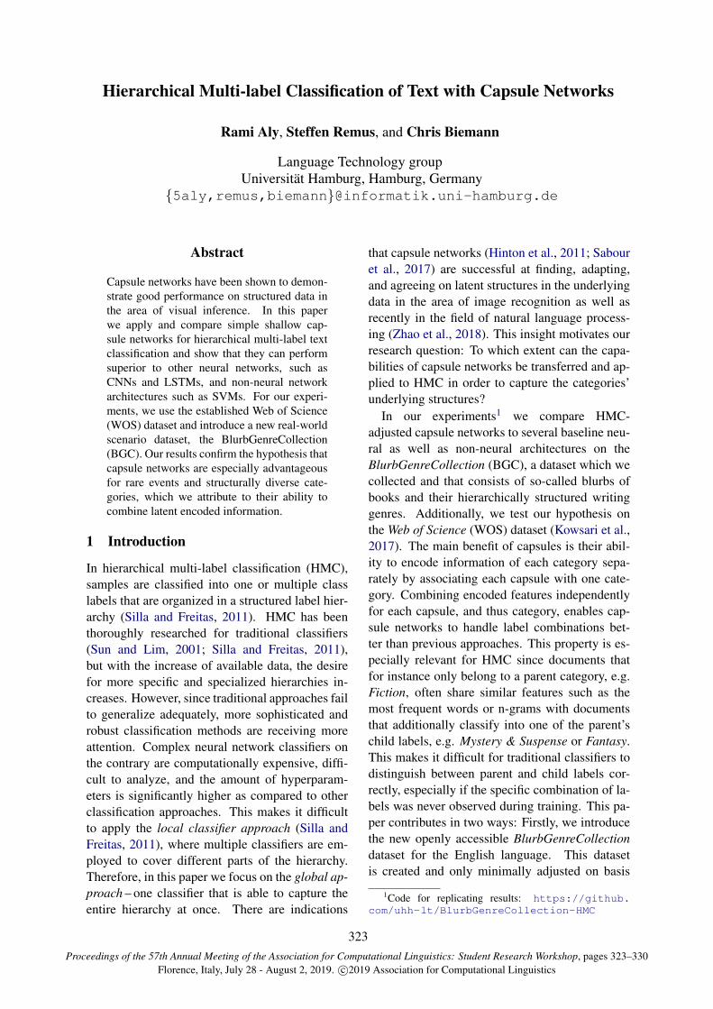
Proceedings of the 57th Annual Meeting of the Association for Computational Linguistics: Student Research Workshop, pages 323–330Florence, Italy, July 28 - August 2, 2019. c©2019 Association for Computational Linguistics

Hierarchical Multi-label Classification of Text with Capsule Networks

Rami Aly, Steffen Remus, and Chris Biemann

Language Technology groupUniversitat Hamburg, Hamburg, Germany

5aly,remus,biemann@informatik.uni-hamburg.de

Abstract

Capsule networks have been shown to demon-strate good performance on structured data inthe area of visual inference. In this paperwe apply and compare simple shallow cap-sule networks for hierarchical multi-label textclassification and show that they can performsuperior to other neural networks, such asCNNs and LSTMs, and non-neural networkarchitectures such as SVMs. For our experi-ments, we use the established Web of Science(WOS) dataset and introduce a new real-worldscenario dataset, the BlurbGenreCollection(BGC). Our results confirm the hypothesis thatcapsule networks are especially advantageousfor rare events and structurally diverse cate-gories, which we attribute to their ability tocombine latent encoded information.

1 Introduction

In hierarchical multi-label classification (HMC),samples are classified into one or multiple classlabels that are organized in a structured label hier-archy (Silla and Freitas, 2011). HMC has beenthoroughly researched for traditional classifiers(Sun and Lim, 2001; Silla and Freitas, 2011),but with the increase of available data, the desirefor more specific and specialized hierarchies in-creases. However, since traditional approaches failto generalize adequately, more sophisticated androbust classification methods are receiving moreattention. Complex neural network classifiers onthe contrary are computationally expensive, diffi-cult to analyze, and the amount of hyperparam-eters is significantly higher as compared to otherclassification approaches. This makes it difficultto apply the local classifier approach (Silla andFreitas, 2011), where multiple classifiers are em-ployed to cover different parts of the hierarchy.Therefore, in this paper we focus on the global ap-proach – one classifier that is able to capture theentire hierarchy at once. There are indications

that capsule networks (Hinton et al., 2011; Sabouret al., 2017) are successful at finding, adapting,and agreeing on latent structures in the underlyingdata in the area of image recognition as well asrecently in the field of natural language process-ing (Zhao et al., 2018). This insight motivates ourresearch question: To which extent can the capa-bilities of capsule networks be transferred and ap-plied to HMC in order to capture the categories’underlying structures?

In our experiments1 we compare HMC-adjusted capsule networks to several baseline neu-ral as well as non-neural architectures on theBlurbGenreCollection (BGC), a dataset which wecollected and that consists of so-called blurbs ofbooks and their hierarchically structured writinggenres. Additionally, we test our hypothesis onthe Web of Science (WOS) dataset (Kowsari et al.,2017). The main benefit of capsules is their abil-ity to encode information of each category sepa-rately by associating each capsule with one cate-gory. Combining encoded features independentlyfor each capsule, and thus category, enables cap-sule networks to handle label combinations bet-ter than previous approaches. This property is es-pecially relevant for HMC since documents thatfor instance only belong to a parent category, e.g.Fiction, often share similar features such as themost frequent words or n-grams with documentsthat additionally classify into one of the parent’schild labels, e.g. Mystery & Suspense or Fantasy.This makes it difficult for traditional classifiers todistinguish between parent and child labels cor-rectly, especially if the specific combination of la-bels was never observed during training. This pa-per contributes in two ways: Firstly, we introducethe new openly accessible BlurbGenreCollectiondataset for the English language. This datasetis created and only minimally adjusted on basis

1Code for replicating results: https://github.com/uhh-lt/BlurbGenreCollection-HMC

323

of a vertical search webpage for books and thuspresents a real-world scenario task. Secondly, wethoroughly analyze the properties of capsule net-works for HMC. To the best of our knowledge,capsule networks have not yet been applied andtested in the HMC domain.

2 Related Work

Neural networks for HMC: In hierarchicalmulti-label classification (HMC) samples are as-signed one or multiple class labels, which areorganized in a structured label hierarchy (Sillaand Freitas, 2011). For text classification (TC),we treat a document as a sample and its cate-gories as labels. Convolutional Neural Networks(CNNs) and different types of Recurrent Neu-ral Networks (RNNs) (Goodfellow et al., 2016;Kim, 2014), most notably long short-term mem-ory units (LSTMs, Hochreiter and Schmidhuber,1997) have shown to be highly efficient in TCtasks. For HMC, Cerri et al. (2014) use concate-nated multi-layer perceptrons (MLP), where eachMLP is associated to one level of the class hierar-chy. Kowsari et al. (2017) use multiple concate-nated deep learning architectures (CNN, LSTM,and MLP) to HMC on a dataset with a rather shal-low hierarchy with only two levels. Similar toKiritchenko et al. (2005), Baker and Korhonen(2017) treat the HMC task as a multi-label clas-sification problem that considers every label in thehierarchy, but they additionally leverage the co-occurrence of labels within the hierarchy to initial-ize the weights of their CNN’s final layer (Kurataet al., 2016).

Capsule Networks: Capsule networks encap-sulate features into groups of neurons, so-calledcapsules (Hinton et al., 2011; Sabour et al., 2017).Originally introduced for a handwritten digit im-age classification task where each digit has beenassociated with a capsule, capsules have shown tolearn more robust representations for each class asthey capture parent-child relationships more ac-curately. They reached on-par performance withmore complex CNN architectures, even outper-forming them in several classification tasks suchas the affNIST and MultiMNIST dataset (Sabouret al., 2017). First attempts to use capsules for sen-timent analysis were carried out by (Wang et al.,2018) on the basis of an RNN, however, theydid not employ the routing algorithm, thus highlylimiting the capabilities of capsules. Zhao et al.

(2018) show that capsule networks can outperformtraditional neural networks for TC by a great mar-gin when training on single-labeled and testingon multi-labeled documents of the Reuters-21578dataset since the routing of capsules behaves like aparallel attention mechanism regarding the selec-tion of categories. By connecting a BiLSTM toa capsule network for relation extraction, Zhanget al. (2018) show that capsule networks improveat extracting n-ary relations, with n > 2, per sen-tence and thus confirm the observation of (Zhaoet al., 2018) in a different context. For multi-tasklearning, Xiao et al. (2018) use capsule networksto improve the differentiation between tasks. Theyencapsulate features in different capsules and usethe routing algorithm to cluster features for eachtask. Further applications to NLP span aggression,toxicity and emotion detection (Srivastava et al.,2018; Rathnayaka et al., 2018), embedding cre-ation for knowledge graph completion (Nguyenet al., 2019), and knowledge transfer of user in-tents (Xia et al., 2018). Despite the suitable prop-erties of capsule networks to classify into hierar-chical structured categories, they have not yet beenapplied to HMC. This work aims to fill the gapby applying and thoroughly analyzing capsules’properties at HMC.

3 Capsule Network for HMC

For each category in the hierarchy, an associatedcapsule outputs latent information of the categoryin form of a vector as opposed to a single scalarvalue used in traditional neural networks. Thevector is equivariant with its length defining thepseudo-probability of its activation and its orien-tation representing different cases of a category’sexistence. This distributional representation in theform of a vector instead of a scalar makes cap-sules exponentially more informative than tradi-tional perceptrons (Sabour et al., 2017).

The input of capsules in the first capsule layerof a capsule network is called primary capsulesand can be of arbitrary dimension, typically com-ing from a convolutional layer or from the hid-den state of a recurrent network. The output vec-tor of a primary capsule represents latent informa-tion such as local order and semantic representa-tions of words (Zhao et al., 2018). Each capsulej in the next layer, called classification capsules,take as input the weighted sum sj =

∑i cj|iuj|i

of the prediction vectors of all primary capsules

324

i. A capsule’s prediction vector uj|i is generatedby multiplying the output uj|i by a weight matrixWij . Since the length of a vector of a classificationcapsule should be interpreted as the probability ofthe corresponding category, a squashing functionvj = squash(sj) is applied, which scales the out-put of each classification capsule non-linearly be-tween zero and one. The coupling coefficients cj|ithat determine the contribution of each primarycapsule’s output to a classification capsule are cal-culated using a dynamic routing heuristic (Sabouret al., 2017). It iteratively decides the routes ofcapsules and thus how to cluster features for eachcategory. The pseudocode for the full routing al-gorithm is written in Algorithm 1.

Routing algorithmResult: vjInitialization: ∀i ∈ Primary.∀j ∈Classification : bj|i ← 0.

for r iterations do∀i ∈ Primary : ci ← softmax(bi)∀j ∈ Clas. : vj ← squash(

∑i cj|iuj|i)

∀i ∈ Primary.∀j ∈ Clas. : bj|i ←bj|i + uj|i · vj

endAlgorithm 1: Routing algorithm as described in(Sabour et al., 2017)

The coupling coefficients are generated by ap-plying the softmax function to the log prior proba-bilities that primary capsule i should be coupled toclassification capsule j. The probability is higherwhen the primary capsule’s prediction vector ismore similar to the classification capsule’s output.Therefore, primary capsules try to predict the out-put of the capsule in the subsequent layer. Since vjis partially determined by uj|i, their similarity in-creases for the next iteration. Thus a convergenceis guaranteed.

This routing algorithm is superior regardingits ability to combine and generalize informationcompared to primitive routing algorithms such asmax-pooling layers, as the latter only stores themost prominent features while the others are ig-nored. This leads to CNNs having more difficultydifferentiating between classes with highly similarfeatures (Sabour et al., 2017), but since most labelcombinations appear rarely and categories oftenshare features with their parents, it is a desirableproperty to exploit for hierarchical classification.

Architecture: The HMC task is converted to a

300

Primary Capsules Classification Capsules

FlattenRouting

EmbeddingConvolutional

Reshape

h

d x q

s

1q

Cp Cc

=d-dimension

l

l

Figure 1: Architecture of our capsule network with dbeing the dimensionality of a capsule’s output.

multi-label classification task using the hierarchyof labels: All explicitly labeled classes must alsoinclude all ancestor labels of the hierarchy. Thearchitecture of our capsule network is shown inFigure 1 and consists of four layers. We designeda minimal capsule network, similar to CapsNet-1 in (Xiao et al., 2018) in order to benefit fromcapsules and dynamic routing while maintaininghigh comparability to a similarly simple CNN. Inour network, the primary capsules take as input theoutput created by a preceding convolutional layer.For each classification capsule, the routing algo-rithm is then used to cluster the outputs of all cpprimary capsules. The pseudo-probability ||vj || isthen assigned to the category associated with theeffective classification capsule. We follow Sabouret al. (2017), and use their margin loss function.

Leveraging Label Co-occurrence: We fur-ther follow the layer weight initialization in-troduced by (Kurata et al., 2016) in order toleverage label co-occurrences during the learn-ing process of a neural network. Since labelco-occurrences such as Fiction, Mystery & Sus-pense or Fiction, Fantasy naturally occur inHMC because of parent-child relationships be-tween categories, we aim to bias the learning pro-cess of the capsule network in respect to the co-occurrences in the dataset by initializing W withlabel co-occurrences. Weights between a primarycapsule and the co-occurring classification cap-sules are initialized using a uniform distributionwhile all other values are set to zero.

Label Correction: A classifier may assign la-bels to classes that do not conform with the under-lying hierarchy of the categories as the activationfunction as well as the routing algorithm look ateach category separately. For instance, if the cap-sule network only assigns the label Fantasy thenthe prediction is inconsistent with the hierarchy asits parent Fiction has not been labeled. Inconsis-tencies with respect to the hierarchical structure ofcategories are corrected by a post-processing step.

325

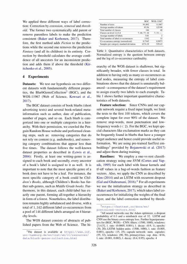
We applied three different ways of label correc-tion: Correction by extension, removal and thresh-old. The former two systematically add parent orremove parentless labels to make the predictionconsistent (Baker and Korhonen, 2017). There-fore, the first method adds Fiction to the predic-tions while the second one removes the predictionFantasy (and all its children) in its entirety. Cor-rection by threshold calculates the average confi-dence of all ancestors for an inconsistent predic-tion and adds them if above the threshold (Kir-itchenko et al., 2005).

4 Experiments

Datasets: We test our hypothesis on two differ-ent datasets with fundamentally different proper-ties, the BlurbGenreCollection2 (BGC), and theWOS-11967 (Web of Science, Kowsari et al.,2017).

The BGC dataset consists of book blurbs (shortadvertising texts) and several book-related meta-information such as author, date of publication,number of pages, and so on. Each blurb is cate-gorized into one or multiple categories in a hier-archy. With their permission, we crawled the Pen-guin Random House website and performed clean-ing steps, such as: removing categories that donot rely on content (e.g. audiobooks), and remov-ing category combinations that appear less thanfive times. The dataset follows the well-knowndataset properties as described in (Lewis et al.,2004): Firstly, at least one writing-genre is as-signed to each book and secondly, every ancestorof a book’s label is assigned to it as well. It isimportant to note that the most specific genre of abook does not have to be a leaf. For instance, themost specific category of a book could be Chil-dren’s Books, although Children’s Books has fur-ther sub-genres, such as Middle Grade books. Fur-thermore, in this dataset, each child-label has ex-actly one parent, forming all-together a hierarchyin form of a forest. Nonetheless, the label distribu-tion remains highly unbalanced and diverse, with atotal of 1, 342 different label co-occurrences froma pool of 146 different labels arranged on 4 hierar-chy levels.

The WOS dataset consists of abstracts of pub-lished papers from the Web of Science. The hi-

2The dataset is available at https://www.inf.uni-hamburg.de/en/inst/ab/lt/resources/data/blurb-genre-collection.html

BGC WOS-11967Number of texts 91,892 11,967Average number of tokens 93.56 125.90Total number of classes 146 40Classes on level 1;2;3;4 7; 46; 77; 16 7; 33; -; -Average number of labels 3.01 2Total number of label co-occurrences 1342 33Co-occurrence entropy (normalized) 0.7345 0.9973Samples per category standard deviation 4374.19 529.43

Table 1: Quantitative characteristics of both datasets.Normalized entropy is the quotient between entropyand the log of co-occurrence cardinality.

erarchy of the WOS dataset is shallower, but sig-nificantly broader, with fewer classes in total. Inaddition to having only as many co-occurrences asleaf nodes, measuring the entropy of label com-binations shows that the dataset is unnaturally bal-anced – a consequence of the dataset’s requirementto assign exactly two labels to each example. Ta-ble 1 shows further important quantitative charac-teristics of both datasets.

Feature selection: Since CNNs and our cap-sule network require a fixed input length, we limitthe texts to the first 100 tokens, which covers thecomplete input for over 90% of the dataset. Weremove stop-words, most punctuation and low-frequency words (< 2). For the BGC, we kept spe-cial characters like exclamation marks as they canbe frequently found in blurbs that have a youngertarget audience and hence could provide useful in-formation. We are using pre-trained fastText em-beddings3 provided by Bojanowski et al. (2017)and adjust them during training.

Baselines: We employ a one-vs-rest classifi-cation strategy using one SVM (Cortes and Vap-nik, 1995) for each label with linear kernels andtf-idf values in a bag-of-words fashion as featurevectors. Also, we apply the CNN as described byKim (2014) and an LSTM with recurrent dropout(Gal and Ghahramani, 2016).4 For all experimentswe use the initialization strategy as described in(Baker and Korhonen, 2017), which takes label co-occurrences for initializing the weights of the finallayer, and the label correction method by thresh-

3https://fasttext.cc/docs/en/pretrained-vectors.html

4All neural networks use the Adam optimizer, a dropoutprobability of 0.5 and a minibatch size of 32. LSTM andCNN use the binary cross entropy loss. Further hyperparame-ters for (BGC, WOS) – CNN: filters: (1500, 1000), windows:3,4,5, l. rate: (0.0005, 0.001), l. decay: (0.9, 1), epochs:(30, 20); LSTM: hidden units: (1500, 1000), l. rate: (0.005,0.001), epochs: (15, 25); capsule network: num. capsules:(55, 32), windows: (90, 50), primary/class. cap. dim.: 8/16,l. rate: (0.001, 0.002), l. decay: (0.4, 0.95), epochs: 4

326

BGC WOS-11967Model Recall Precision F1 Subset Acc. Recall Precision F1 Subset Acc.SVM 61.11 85.37 71.23 35.79 72.43 89.84 80.20 56.47CNN 64.75± 0.41 83.87± 0.09 73.08± 0.27 37.26± 0.52 84.06± 0.93 91.68± 1.00 87.71± 0.58 75.16± 1.66

LSTM 69.12± 1.24 75.49± 3.54 72.16± 1.01 37.99± 1.52 83.78± 1.69 87.56± 1.04 85.63± 1.22 76.80± 2.15Caps. Network 71.73± 0.63 77.21± 0.54 74.37± 0.35 37.70± 0.68 80.67± 1.27 82.75± 2.42 81.69± 0.70 64.97± 0.49

Table 2: All results with their corresponding 95% confidence intervals, measured across three runs.

old with a confidence value of 0.2.5 The datasetis split into 64% train, 16% validation and 20%test. For evaluation, we measure subset accuracy,micro-averaged recall, precision, and F1 as definedin (Sorower, 2010; Silla and Freitas, 2011).

5 Results

Results are shown in Table 2. Regarding the BGCdataset, the capsule network yields the highest F1

and recall, the SVM the highest precision, whilethe LSTM showed the best result in subset accu-racy. On WOS, all neural network architecturesbeat the baseline SVM model by a substantial mar-gin. However, both, the SVM and the capsule net-work, are substantially outperformed by the CNNand LSTM. In Figure 2 we further observe a per-formance decline for deeper levels of the hierar-chy. On BGC, the capsule network performs beston every level of the hierarchy with an increasingmargin for more specific labels.

5.1 Identification of label co-occurrences

We argue that the pronounced performance differ-ence between the datasets is due to the ability ofcapsules to handle label combinations better thanthe CNN and LSTM. We observe, as shown in Fig-ure 4, that capsule networks are beneficial for ex-amples with many label assignments. While thecapsule network performs worse on BGC for a la-bel set cardinality of 1 and 2, it starts to performbetter at a cardinality of 3 and almost doubles theF1 of all baselines for 9 and 11. The number of ex-amples decreases exponentially with the label setcardinality, so that the ability of networks to com-bine labels is becoming increasingly important.

In contrast, in the WOS dataset, exactly oneparent-child label combination is assigned to eachexample, resulting in a label set cardinality of twofor the whole dataset. There are comparably fewlabel combinations, which occur with a high fre-quency in the dataset (cf. Table 1). The benefit ofcapsules can thus not apply here.

5These options consistently performed well in prelimi-nary experiments.

(a) BGC

(b) WOS

Figure 2: Scores on different levels for the BGC (a) andWOS (b). The lines are the cumulative scores.

To verify this hypothesis, we conduct a fur-ther test exclusively on BGC examples with labelcombinations that have not been observed duringtraining (5, 943 samples). As shown in Table 3,the capsule network again achieves the highestF1 score, outperforming the other networks, es-pecially in terms of recall. In order to create hi-erarchical inconsistencies in the WOS dataset, wetest two modifications on the training data whilethe test data is kept the same: a) 50% of all childlabels are removed, and b) for each sample, eitherthe child or the parent label is kept. Results of thisstudy are shown in Table 4. Removing 50% of thechildren labels results in the capsule network be-ing more similar to the CNN and LSTM in termsof subset accuracy. However, for the second modi-fication, where label combinations are completelyomitted for training, the capsule network signifi-cantly outperforms both networks. Figure 3 showsthat different primary capsules are routed to theclassification capsule representing the parent cat-

327

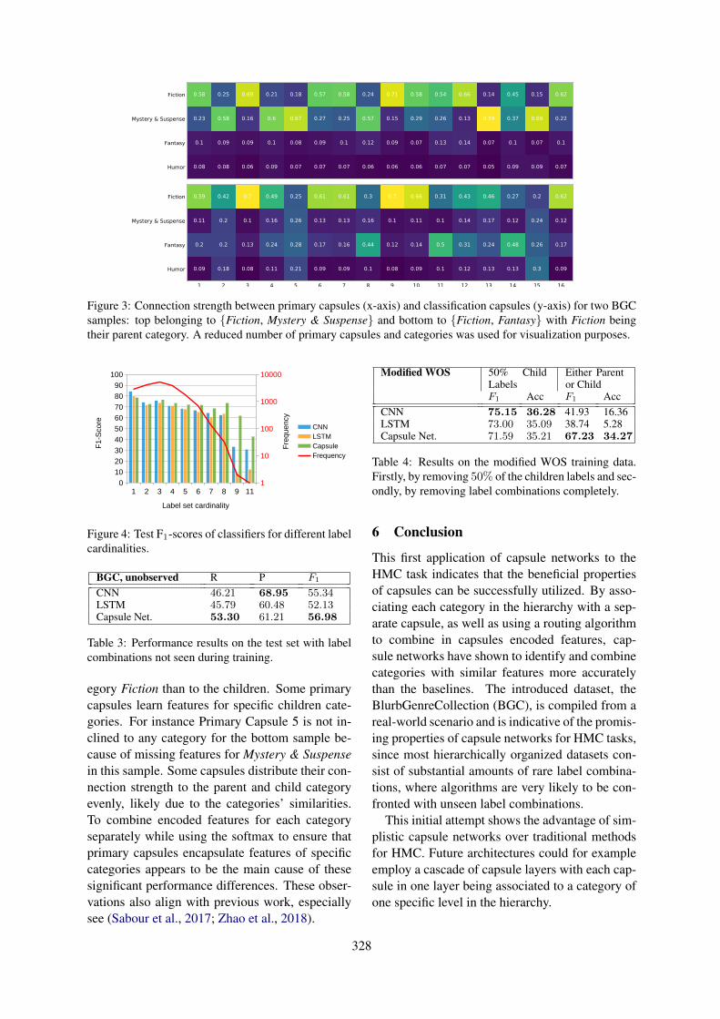
Fiction

Mystery & Suspense

Fantasy

Humor

0.58 0.25 0.69 0.21 0.18 0.57 0.58 0.24 0.71 0.58 0.54 0.66 0.14 0.45 0.15 0.62

0.23 0.58 0.16 0.6 0.67 0.27 0.25 0.57 0.15 0.29 0.26 0.13 0.74 0.37 0.69 0.22

0.1 0.09 0.09 0.1 0.08 0.09 0.1 0.12 0.09 0.07 0.13 0.14 0.07 0.1 0.07 0.1

0.08 0.08 0.06 0.09 0.07 0.07 0.07 0.06 0.06 0.06 0.07 0.07 0.05 0.09 0.09 0.07

1 2 3 4 5 6 7 8 9 10 11 12 13 14 15 16

Fiction

Mystery & Suspense

Fantasy

Humor

0.59 0.42 0.7 0.49 0.25 0.61 0.61 0.3 0.7 0.66 0.31 0.43 0.46 0.27 0.2 0.62

0.11 0.2 0.1 0.16 0.26 0.13 0.13 0.16 0.1 0.11 0.1 0.14 0.17 0.12 0.24 0.12

0.2 0.2 0.13 0.24 0.28 0.17 0.16 0.44 0.12 0.14 0.5 0.31 0.24 0.48 0.26 0.17

0.09 0.18 0.08 0.11 0.21 0.09 0.09 0.1 0.08 0.09 0.1 0.12 0.13 0.13 0.3 0.09

Figure 3: Connection strength between primary capsules (x-axis) and classification capsules (y-axis) for two BGCsamples: top belonging to Fiction, Mystery & Suspense and bottom to Fiction, Fantasy with Fiction beingtheir parent category. A reduced number of primary capsules and categories was used for visualization purposes.

1 2 3 4 5 6 7 8 9 110

10

20

30

40

50

60

70

80

90

100

1

10

100

1000

10000

CNNLSTMCapsuleFrequency

Label set cardinality

F1-

Sco

re

Fre

quen

cy

Figure 4: Test F1-scores of classifiers for different labelcardinalities.

BGC, unobserved R P F1

CNN 46.21 68.95 55.34LSTM 45.79 60.48 52.13Capsule Net. 53.30 61.21 56.98

Table 3: Performance results on the test set with labelcombinations not seen during training.

egory Fiction than to the children. Some primarycapsules learn features for specific children cate-gories. For instance Primary Capsule 5 is not in-clined to any category for the bottom sample be-cause of missing features for Mystery & Suspensein this sample. Some capsules distribute their con-nection strength to the parent and child categoryevenly, likely due to the categories’ similarities.To combine encoded features for each categoryseparately while using the softmax to ensure thatprimary capsules encapsulate features of specificcategories appears to be the main cause of thesesignificant performance differences. These obser-vations also align with previous work, especiallysee (Sabour et al., 2017; Zhao et al., 2018).

Modified WOS 50% ChildLabels

Either Parentor Child

F1 Acc F1 AccCNN 75.15 36.28 41.93 16.36LSTM 73.00 35.09 38.74 5.28Capsule Net. 71.59 35.21 67.23 34.27

Table 4: Results on the modified WOS training data.Firstly, by removing 50% of the children labels and sec-ondly, by removing label combinations completely.

6 Conclusion

This first application of capsule networks to theHMC task indicates that the beneficial propertiesof capsules can be successfully utilized. By asso-ciating each category in the hierarchy with a sep-arate capsule, as well as using a routing algorithmto combine in capsules encoded features, cap-sule networks have shown to identify and combinecategories with similar features more accuratelythan the baselines. The introduced dataset, theBlurbGenreCollection (BGC), is compiled from areal-world scenario and is indicative of the promis-ing properties of capsule networks for HMC tasks,since most hierarchically organized datasets con-sist of substantial amounts of rare label combina-tions, where algorithms are very likely to be con-fronted with unseen label combinations.

This initial attempt shows the advantage of sim-plistic capsule networks over traditional methodsfor HMC. Future architectures could for exampleemploy a cascade of capsule layers with each cap-sule in one layer being associated to a category ofone specific level in the hierarchy.

328

ReferencesSimon Baker and Anna Korhonen. 2017. Initializ-

ing neural networks for hierarchical multi-label textclassification. In Proceedings of the 16th Biomedi-cal Natural Language Processing Workshop, pages307–315, Vancouver, Canada.

Piotr Bojanowski, Edouard Grave, Armand Joulin, andTomas Mikolov. 2017. Enriching word vectors withsubword information. Transactions of the Associa-tion for Computational Linguistics, 5(1):135–146.

Ricardo Cerri, Rodrigo C. Barros, and Andre C.P.L.F.de Carvalho. 2014. Hierarchical multi-label classifi-cation using local neural networks. Journal of Com-puter and System Sciences, 80(1):39 – 56.

Corinna Cortes and Vladimir Vapnik. 1995. Support-vector networks. Machine learning, 20(3):273–297.

Yarin Gal and Zoubin Ghahramani. 2016. A theo-retically grounded application of dropout in recur-rent neural networks. In Advances in neural infor-mation processing systems 2016, pages 1019–1027,Barcelona, Spain.

Ian Goodfellow, Yoshua Bengio, and Aaron Courville.2016. Deep Learning. MIT Press. http://www.deeplearningbook.org.

Geoffrey E. Hinton, Alex Krizhevsky, and Sida D.Wang. 2011. Transforming auto-encoders. In Inter-national Conference on Artificial Neural Networks,pages 44–51, Espoo, Finland.

Sepp Hochreiter and Jurgen Schmidhuber. 1997.Long short-term memory. Neural computation,9(8):1735–1780.

Yoon Kim. 2014. Convolutional neural networksfor sentence classification. In Proceedings of the2014 Conference on Empirical Methods in NaturalLanguage Processing (EMNLP), pages 1746–1751,Doha, Qatar.

Svetlana Kiritchenko, Stan Matwin, and A. FazelFamili. 2005. Functional annotation of genes usinghierarchical text categorization. In BioLINK SIG:Linking Literature, Information and Knowledge forBiology, Detroit, MI, USA. Workshop track.

Kamran Kowsari, Donald E. Brown, Mojtaba Hei-darysafa, Kiana Jafari Meimandi, Matthew S. Ger-ber, and Laura E. Barnes. 2017. HDLTex: Hierar-chical deep learning for text classification. In IEEEInternational Conference on Machine Learning andApplications, pages 364–371, Cancun, Mexico.

Gakuto Kurata, Bing Xiang, and Bowen Zhou. 2016.Improved neural network-based multi-label classifi-cation with better initialization leveraging label co-occurrence. In Proceedings of the 2016 Confer-ence of the North American Chapter of the Associ-ation for Computational Linguistics: Human Lan-guage Technologies, pages 521–526, New Orleans,LA, USA.

David D. Lewis, Yiming Yang, Tony G. Rose, and FanLi. 2004. RCV1: A new benchmark collection fortext categorization research. Journal of MachineLearning Research, 5(Apr):361–397.

Dai Quoc Nguyen, Thanh Vu, Tu Dinh Nguyen,Dat Quoc Nguyen, and Dinh Q. Phung. 2019. Acapsule network-based embedding model for knowl-edge graph completion and search personalization.In Proceedings of the 2019 Conference of the NorthAmerican Chapter of the Association for Computa-tional Linguistics: Human Language Technologies,Minneapolis, MN, USA.

Prabod Rathnayaka, Supun Abeysinghe, ChamodSamarajeewa, Isura Manchanayake, and MalakaWalpola. 2018. Sentylic at IEST 2018: Gated re-current neural network and capsule network basedapproach for implicit emotion detection. In Pro-ceedings of the 9th Workshop on Computational Ap-proaches to Subjectivity, Sentiment and Social Me-dia Analysis, pages 254–259, Brussels, Belgium.

Sara Sabour, Nicholas Frosst, and Geoffrey E. Hinton.2017. Dynamic routing between capsules. In Ad-vances in Neural Information Processing Systems30, pages 3856–3866, Long Beach, CA, USA.

Carlos N. Silla and Alex A. Freitas. 2011. A surveyof hierarchical classification across different appli-cation domains. Data Mining and Knowledge Dis-covery, 22(1-2):31–72.

Mohammad S. Sorower. 2010. A literature survey onalgorithms for multi-label learning. Oregon StateUniversity, Corvallis, OR, USA.

Saurabh Srivastava, Prerna Khurana, and VartikaTewari. 2018. Identifying aggression and toxicity incomments using capsule network. In Proceedings ofthe First Workshop on Trolling, Aggression and Cy-berbullying (TRAC-2018), pages 98–105, Santa Fe,NM, USA.

Aixin Sun and Ee-Peng Lim. 2001. Hierarchical textclassification and evaluation. In Proceedings of the2001 IEEE International Conference on Data Min-ing, ICDM ’01, pages 521–528, San Jose, CA, USA.

Yequan Wang, Aixin Sun, Jialong Han, Ying Liu, andXiaoyan Zhu. 2018. Sentiment analysis by capsules.In Proceedings of the 2018 World Wide Web Confer-ence, pages 1165–1174, Lyon, France.

Congying Xia, Chenwei Zhang, Xiaohui Yan,Yi Chang, and Philip Yu. 2018. Zero-shot userintent detection via capsule neural networks. InProceedings of the 2018 Conference on EmpiricalMethods in Natural Language Processing, pages3090–3099, Brussels, Belgium.

Liqiang Xiao, Honglun Zhang, Wenqing Chen,Yongkun Wang, and Yaohui Jin. 2018. MCapsNet:Capsule network for text with multi-task learning.In Proceedings of the 2018 Conference on Empiri-cal Methods in Natural Language Processing, page4565–4574, Brussels, Belgium.

329

Ningyu Zhang, Shumin Deng, Zhanlin Sun, Xi Chen,Wei Zhang, and Huajun Chen. 2018. Attention-based capsule networks with dynamic routing for re-lation extraction. In Proceedings of the 2018 Con-ference on Empirical Methods in Natural LanguageProcessing, page 986–992, Brussels, Belgium.

Wei Zhao, Jianbo Ye, Min Yang, Zeyang Lei, SuofeiZhang, and Zhou Zhao. 2018. Investigating capsulenetworks with dynamic routing for text classifica-tion. In Proceedings of the 2018 Conference on Em-pirical Methods in Natural Language, pages 3110 –3119, Brussels, Belgium.

330

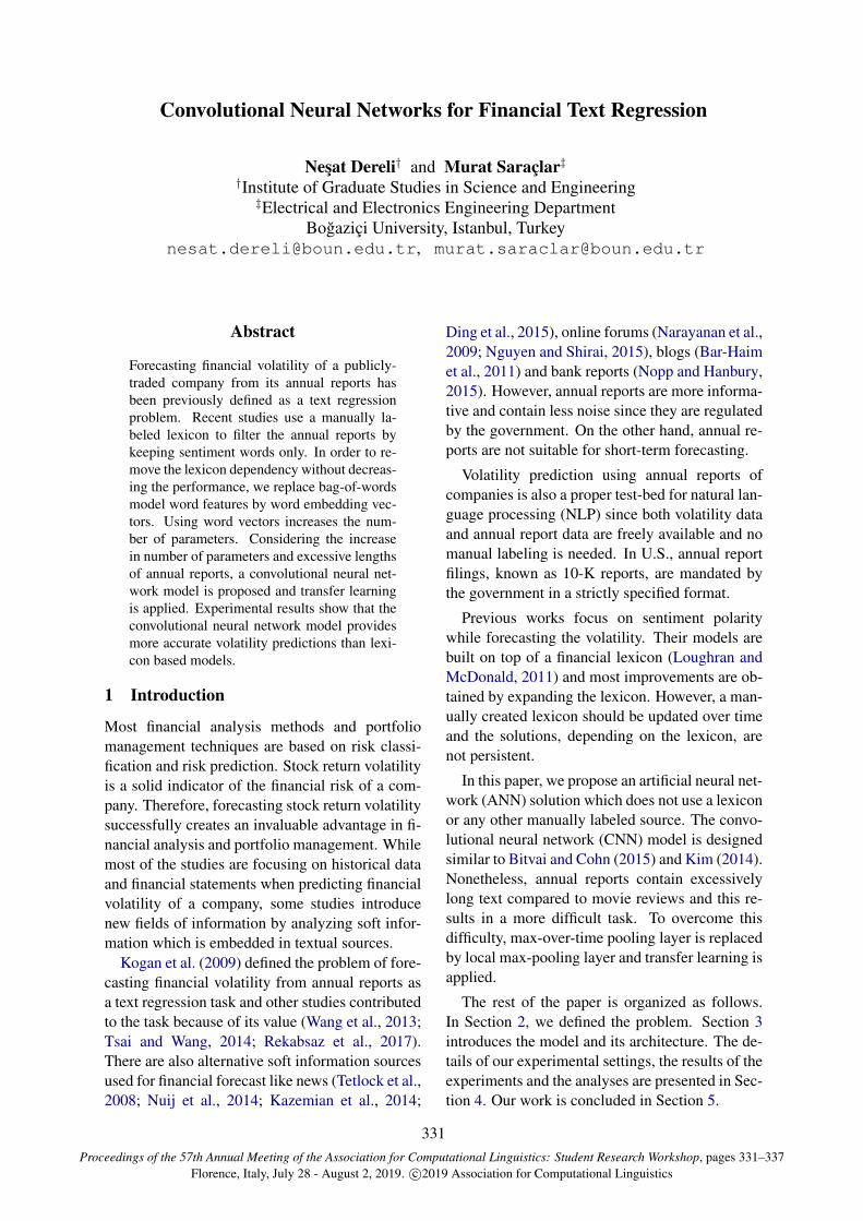
Proceedings of the 57th Annual Meeting of the Association for Computational Linguistics: Student Research Workshop, pages 331–337Florence, Italy, July 28 - August 2, 2019. c©2019 Association for Computational Linguistics

Convolutional Neural Networks for Financial Text Regression

Nesat Dereli† and Murat Saraclar‡†Institute of Graduate Studies in Science and Engineering‡Electrical and Electronics Engineering Department

Bogazici University, Istanbul, Turkeynesat.dereli@boun.edu.tr, murat.saraclar@boun.edu.tr

Abstract

Forecasting financial volatility of a publicly-traded company from its annual reports hasbeen previously defined as a text regressionproblem. Recent studies use a manually la-beled lexicon to filter the annual reports bykeeping sentiment words only. In order to re-move the lexicon dependency without decreas-ing the performance, we replace bag-of-wordsmodel word features by word embedding vec-tors. Using word vectors increases the num-ber of parameters. Considering the increasein number of parameters and excessive lengthsof annual reports, a convolutional neural net-work model is proposed and transfer learningis applied. Experimental results show that theconvolutional neural network model providesmore accurate volatility predictions than lexi-con based models.

1 Introduction

Most financial analysis methods and portfoliomanagement techniques are based on risk classi-fication and risk prediction. Stock return volatilityis a solid indicator of the financial risk of a com-pany. Therefore, forecasting stock return volatilitysuccessfully creates an invaluable advantage in fi-nancial analysis and portfolio management. Whilemost of the studies are focusing on historical dataand financial statements when predicting financialvolatility of a company, some studies introducenew fields of information by analyzing soft infor-mation which is embedded in textual sources.

Kogan et al. (2009) defined the problem of fore-casting financial volatility from annual reports asa text regression task and other studies contributedto the task because of its value (Wang et al., 2013;Tsai and Wang, 2014; Rekabsaz et al., 2017).There are also alternative soft information sourcesused for financial forecast like news (Tetlock et al.,2008; Nuij et al., 2014; Kazemian et al., 2014;

Ding et al., 2015), online forums (Narayanan et al.,2009; Nguyen and Shirai, 2015), blogs (Bar-Haimet al., 2011) and bank reports (Nopp and Hanbury,2015). However, annual reports are more informa-tive and contain less noise since they are regulatedby the government. On the other hand, annual re-ports are not suitable for short-term forecasting.

Volatility prediction using annual reports ofcompanies is also a proper test-bed for natural lan-guage processing (NLP) since both volatility dataand annual report data are freely available and nomanual labeling is needed. In U.S., annual reportfilings, known as 10-K reports, are mandated bythe government in a strictly specified format.

Previous works focus on sentiment polaritywhile forecasting the volatility. Their models arebuilt on top of a financial lexicon (Loughran andMcDonald, 2011) and most improvements are ob-tained by expanding the lexicon. However, a man-ually created lexicon should be updated over timeand the solutions, depending on the lexicon, arenot persistent.

In this paper, we propose an artificial neural net-work (ANN) solution which does not use a lexiconor any other manually labeled source. The convo-lutional neural network (CNN) model is designedsimilar to Bitvai and Cohn (2015) and Kim (2014).Nonetheless, annual reports contain excessivelylong text compared to movie reviews and this re-sults in a more difficult task. To overcome thisdifficulty, max-over-time pooling layer is replacedby local max-pooling layer and transfer learning isapplied.

The rest of the paper is organized as follows.In Section 2, we defined the problem. Section 3introduces the model and its architecture. The de-tails of our experimental settings, the results of theexperiments and the analyses are presented in Sec-tion 4. Our work is concluded in Section 5.

331

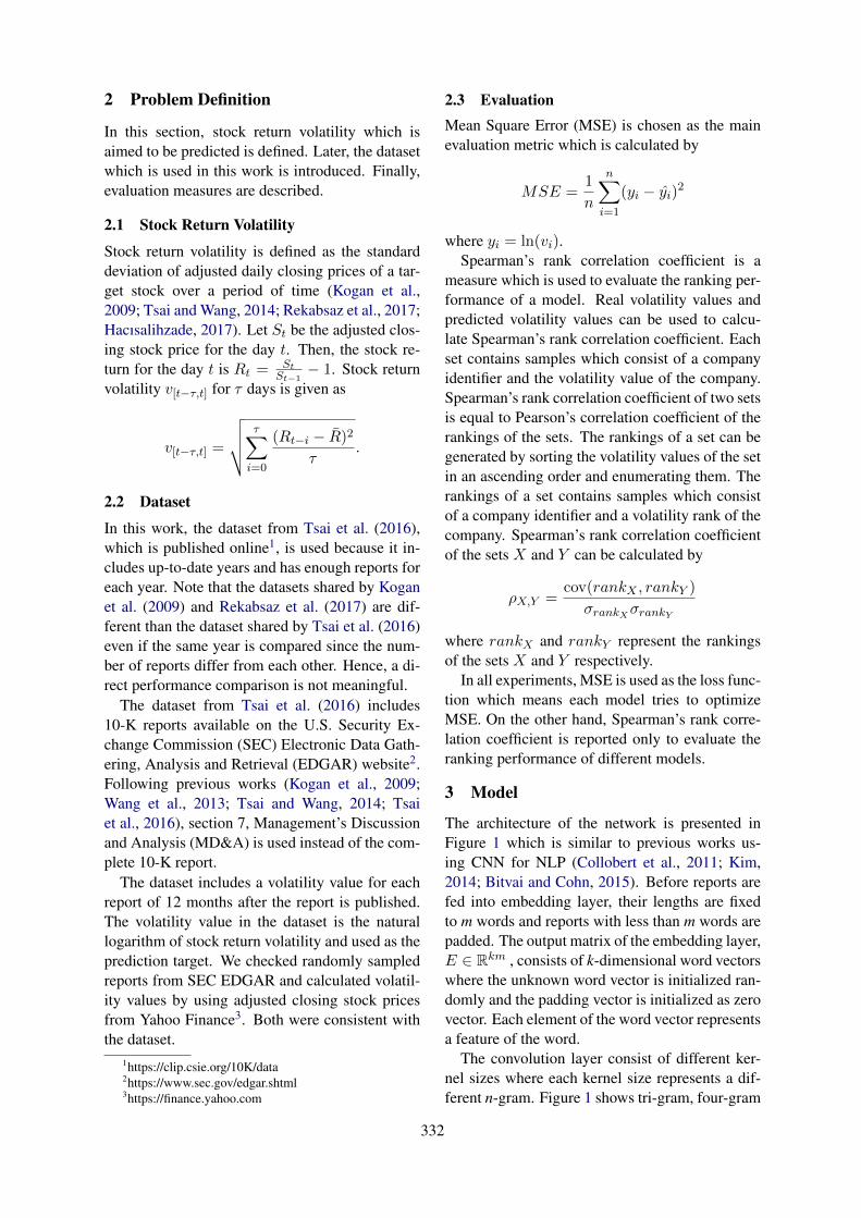
2 Problem Definition

In this section, stock return volatility which isaimed to be predicted is defined. Later, the datasetwhich is used in this work is introduced. Finally,evaluation measures are described.

2.1 Stock Return Volatility

Stock return volatility is defined as the standarddeviation of adjusted daily closing prices of a tar-get stock over a period of time (Kogan et al.,2009; Tsai and Wang, 2014; Rekabsaz et al., 2017;Hacısalihzade, 2017). Let St be the adjusted clos-ing stock price for the day t. Then, the stock re-turn for the day t is Rt = St

St−1− 1. Stock return

volatility v[t−τ,t] for τ days is given as

v[t−τ,t] =

√√√√τ∑

i=0

(Rt−i − R)2

τ.

2.2 Dataset

In this work, the dataset from Tsai et al. (2016),which is published online1, is used because it in-cludes up-to-date years and has enough reports foreach year. Note that the datasets shared by Koganet al. (2009) and Rekabsaz et al. (2017) are dif-ferent than the dataset shared by Tsai et al. (2016)even if the same year is compared since the num-ber of reports differ from each other. Hence, a di-rect performance comparison is not meaningful.

The dataset from Tsai et al. (2016) includes10-K reports available on the U.S. Security Ex-change Commission (SEC) Electronic Data Gath-ering, Analysis and Retrieval (EDGAR) website2.Following previous works (Kogan et al., 2009;Wang et al., 2013; Tsai and Wang, 2014; Tsaiet al., 2016), section 7, Management’s Discussionand Analysis (MD&A) is used instead of the com-plete 10-K report.

The dataset includes a volatility value for eachreport of 12 months after the report is published.The volatility value in the dataset is the naturallogarithm of stock return volatility and used as theprediction target. We checked randomly sampledreports from SEC EDGAR and calculated volatil-ity values by using adjusted closing stock pricesfrom Yahoo Finance3. Both were consistent withthe dataset.

1https://clip.csie.org/10K/data2https://www.sec.gov/edgar.shtml3https://finance.yahoo.com

2.3 EvaluationMean Square Error (MSE) is chosen as the mainevaluation metric which is calculated by

MSE =1

n

n∑

i=1

(yi − yi)2

where yi = ln(vi).Spearman’s rank correlation coefficient is a

measure which is used to evaluate the ranking per-formance of a model. Real volatility values andpredicted volatility values can be used to calcu-late Spearman’s rank correlation coefficient. Eachset contains samples which consist of a companyidentifier and the volatility value of the company.Spearman’s rank correlation coefficient of two setsis equal to Pearson’s correlation coefficient of therankings of the sets. The rankings of a set can begenerated by sorting the volatility values of the setin an ascending order and enumerating them. Therankings of a set contains samples which consistof a company identifier and a volatility rank of thecompany. Spearman’s rank correlation coefficientof the sets X and Y can be calculated by

ρX,Y =cov(rankX , rankY )

σrankXσrankY

where rankX and rankY represent the rankingsof the sets X and Y respectively.

In all experiments, MSE is used as the loss func-tion which means each model tries to optimizeMSE. On the other hand, Spearman’s rank corre-lation coefficient is reported only to evaluate theranking performance of different models.

3 Model

The architecture of the network is presented inFigure 1 which is similar to previous works us-ing CNN for NLP (Collobert et al., 2011; Kim,2014; Bitvai and Cohn, 2015). Before reports arefed into embedding layer, their lengths are fixedto m words and reports with less than m words arepadded. The output matrix of the embedding layer,E ∈ Rkm , consists of k-dimensional word vectorswhere the unknown word vector is initialized ran-domly and the padding vector is initialized as zerovector. Each element of the word vector representsa feature of the word.

The convolution layer consist of different ker-nel sizes where each kernel size represents a dif-ferent n-gram. Figure 1 shows tri-gram, four-gram

332

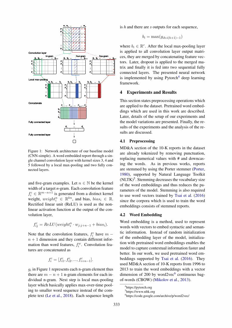
Figure 1: Network architecture of our baseline model(CNN-simple). A word embedded report through a sin-gle channel convolution layer with kernel sizes 3, 4 and5 followed by a local max-pooling and two fully con-nected layers.

and five-gram examples. Let n ∈ N be the kernelwidth of a target n-gram. Each convolution featuref ci ∈ Rm−n+1 is generated from a distinct kernelweight, weightni ∈ Rkn, and bias, biasi ∈ R.Rectified linear unit (ReLU) is used as the non-linear activation function at the output of the con-volution layer,

f cij = ReLU(weightni · wj:j+n−1 + biasi).

Note that the convolution features, f ci have m −n + 1 dimension and they contain different infor-mation than word features, fwi . Convolution fea-tures are concatenated as

f ci = [f ci1, fci2, ..., f

ci+n−1].

gi in Figure 1 represents each n-gram element thusthere are m− n+ 1 n-gram elements for each in-dividual n-gram. Next step is local max-poolinglayer which basically applies max-over-time pool-ing to smaller word sequence instead of the com-plete text (Le et al., 2018). Each sequence length

is h and there are s outputs for each sequence,

bi = max(gih:i(h+1)−1)

where bi ∈ Rr. After the local max-pooling layeris applied to all convolution layer output matri-ces, they are merged by concatenating feature vec-tors. Later, dropout is applied to the merged ma-trix and finally it is fed into two sequential fullyconnected layers. The presented neural networkis implemented by using Pytorch4 deep learningframework.

4 Experiments and Results

This section states preprocessing operations whichare applied to the dataset. Pretrained word embed-dings which are used in this work are described.Later, details of the setup of our experiments andthe model variations are presented. Finally, the re-sults of the experiments and the analysis of the re-sults are discussed.

4.1 PreprocessingMD&A section of the 10-K reports in the datasetare already tokenized by removing punctuation,replacing numerical values with # and downcas-ing the words. As in previous works, reportsare stemmed by using the Porter stemmer (Porter,1980), supported by Natural Language Toolkit(NLTK)5. Stemming decreases the vocabulary sizeof the word embeddings and thus reduces the pa-rameters of the model. Stemming is also requiredto use word vectors trained by Tsai et al. (2016)since the corpora which is used to train the wordembeddings consists of stemmed reports.

4.2 Word EmbeddingWord embedding is a method, used to representwords with vectors to embed syntactic and seman-tic information. Instead of random initializationof the embedding layer of the model, initializa-tion with pretrained word embeddings enables themodel to capture contextual information faster andbetter. In our work, we used pretrained word em-beddings supported by Tsai et al. (2016). Theyused MD&A section of 10-K reports from 1996 to2013 to train the word embeddings with a vectordimension of 200 by word2vec6 continuous bag-of-words (CBOW) (Mikolov et al., 2013).

4https://pytorch.org5https://www.nltk.org6https://code.google.com/archive/p/word2vec/

333

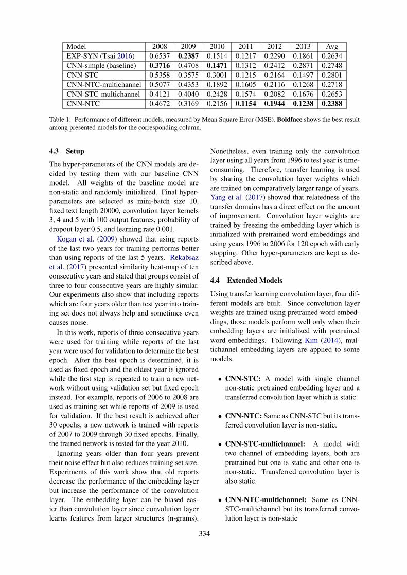
Model 2008 2009 2010 2011 2012 2013 AvgEXP-SYN (Tsai 2016) 0.6537 0.2387 0.1514 0.1217 0.2290 0.1861 0.2634CNN-simple (baseline) 0.3716 0.4708 0.1471 0.1312 0.2412 0.2871 0.2748CNN-STC 0.5358 0.3575 0.3001 0.1215 0.2164 0.1497 0.2801CNN-NTC-multichannel 0.5077 0.4353 0.1892 0.1605 0.2116 0.1268 0.2718CNN-STC-multichannel 0.4121 0.4040 0.2428 0.1574 0.2082 0.1676 0.2653CNN-NTC 0.4672 0.3169 0.2156 0.1154 0.1944 0.1238 0.2388

Table 1: Performance of different models, measured by Mean Square Error (MSE). Boldface shows the best resultamong presented models for the corresponding column.

4.3 Setup

The hyper-parameters of the CNN models are de-cided by testing them with our baseline CNNmodel. All weights of the baseline model arenon-static and randomly initialized. Final hyper-parameters are selected as mini-batch size 10,fixed text length 20000, convolution layer kernels3, 4 and 5 with 100 output features, probability ofdropout layer 0.5, and learning rate 0.001.

Kogan et al. (2009) showed that using reportsof the last two years for training performs betterthan using reports of the last 5 years. Rekabsazet al. (2017) presented similarity heat-map of tenconsecutive years and stated that groups consist ofthree to four consecutive years are highly similar.Our experiments also show that including reportswhich are four years older than test year into train-ing set does not always help and sometimes evencauses noise.

In this work, reports of three consecutive yearswere used for training while reports of the lastyear were used for validation to determine the bestepoch. After the best epoch is determined, it isused as fixed epoch and the oldest year is ignoredwhile the first step is repeated to train a new net-work without using validation set but fixed epochinstead. For example, reports of 2006 to 2008 areused as training set while reports of 2009 is usedfor validation. If the best result is achieved after30 epochs, a new network is trained with reportsof 2007 to 2009 through 30 fixed epochs. Finally,the trained network is tested for the year 2010.

Ignoring years older than four years preventtheir noise effect but also reduces training set size.Experiments of this work show that old reportsdecrease the performance of the embedding layerbut increase the performance of the convolutionlayer. The embedding layer can be biased eas-ier than convolution layer since convolution layerlearns features from larger structures (n-grams).

Nonetheless, even training only the convolutionlayer using all years from 1996 to test year is time-consuming. Therefore, transfer learning is usedby sharing the convolution layer weights whichare trained on comparatively larger range of years.Yang et al. (2017) showed that relatedness of thetransfer domains has a direct effect on the amountof improvement. Convolution layer weights aretrained by freezing the embedding layer which isinitialized with pretrained word embeddings andusing years 1996 to 2006 for 120 epoch with earlystopping. Other hyper-parameters are kept as de-scribed above.

4.4 Extended Models

Using transfer learning convolution layer, four dif-ferent models are built. Since convolution layerweights are trained using pretrained word embed-dings, those models perform well only when theirembedding layers are initialized with pretrainedword embeddings. Following Kim (2014), mul-tichannel embedding layers are applied to somemodels.

• CNN-STC: A model with single channelnon-static pretrained embedding layer and atransferred convolution layer which is static.

• CNN-NTC: Same as CNN-STC but its trans-ferred convolution layer is non-static.

• CNN-STC-multichannel: A model withtwo channel of embedding layers, both arepretrained but one is static and other one isnon-static. Transferred convolution layer isalso static.

• CNN-NTC-multichannel: Same as CNN-STC-multichannel but its transferred convo-lution layer is non-static

334

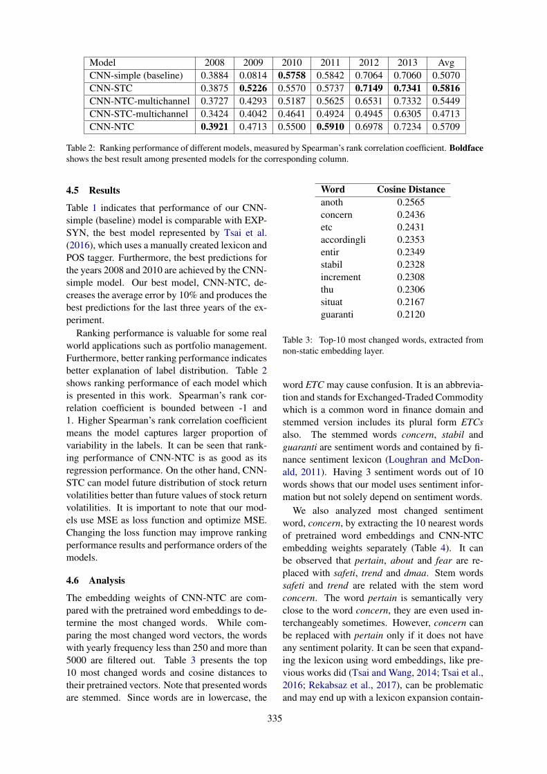
Model 2008 2009 2010 2011 2012 2013 AvgCNN-simple (baseline) 0.3884 0.0814 0.5758 0.5842 0.7064 0.7060 0.5070CNN-STC 0.3875 0.5226 0.5570 0.5737 0.7149 0.7341 0.5816CNN-NTC-multichannel 0.3727 0.4293 0.5187 0.5625 0.6531 0.7332 0.5449CNN-STC-multichannel 0.3424 0.4042 0.4641 0.4924 0.4945 0.6305 0.4713CNN-NTC 0.3921 0.4713 0.5500 0.5910 0.6978 0.7234 0.5709

Table 2: Ranking performance of different models, measured by Spearman’s rank correlation coefficient. Boldfaceshows the best result among presented models for the corresponding column.

4.5 Results

Table 1 indicates that performance of our CNN-simple (baseline) model is comparable with EXP-SYN, the best model represented by Tsai et al.(2016), which uses a manually created lexicon andPOS tagger. Furthermore, the best predictions forthe years 2008 and 2010 are achieved by the CNN-simple model. Our best model, CNN-NTC, de-creases the average error by 10% and produces thebest predictions for the last three years of the ex-periment.

Ranking performance is valuable for some realworld applications such as portfolio management.Furthermore, better ranking performance indicatesbetter explanation of label distribution. Table 2shows ranking performance of each model whichis presented in this work. Spearman’s rank cor-relation coefficient is bounded between -1 and1. Higher Spearman’s rank correlation coefficientmeans the model captures larger proportion ofvariability in the labels. It can be seen that rank-ing performance of CNN-NTC is as good as itsregression performance. On the other hand, CNN-STC can model future distribution of stock returnvolatilities better than future values of stock returnvolatilities. It is important to note that our mod-els use MSE as loss function and optimize MSE.Changing the loss function may improve rankingperformance results and performance orders of themodels.

4.6 Analysis

The embedding weights of CNN-NTC are com-pared with the pretrained word embeddings to de-termine the most changed words. While com-paring the most changed word vectors, the wordswith yearly frequency less than 250 and more than5000 are filtered out. Table 3 presents the top10 most changed words and cosine distances totheir pretrained vectors. Note that presented wordsare stemmed. Since words are in lowercase, the

Word Cosine Distanceanoth 0.2565concern 0.2436etc 0.2431accordingli 0.2353entir 0.2349stabil 0.2328increment 0.2308thu 0.2306situat 0.2167guaranti 0.2120

Table 3: Top-10 most changed words, extracted fromnon-static embedding layer.

word ETC may cause confusion. It is an abbrevia-tion and stands for Exchanged-Traded Commoditywhich is a common word in finance domain andstemmed version includes its plural form ETCsalso. The stemmed words concern, stabil andguaranti are sentiment words and contained by fi-nance sentiment lexicon (Loughran and McDon-ald, 2011). Having 3 sentiment words out of 10words shows that our model uses sentiment infor-mation but not solely depend on sentiment words.

We also analyzed most changed sentimentword, concern, by extracting the 10 nearest wordsof pretrained word embeddings and CNN-NTCembedding weights separately (Table 4). It canbe observed that pertain, about and fear are re-placed with safeti, trend and dmaa. Stem wordssafeti and trend are related with the stem wordconcern. The word pertain is semantically veryclose to the word concern, they are even used in-terchangeably sometimes. However, concern canbe replaced with pertain only if it does not haveany sentiment polarity. It can be seen that expand-ing the lexicon using word embeddings, like pre-vious works did (Tsai and Wang, 2014; Tsai et al.,2016; Rekabsaz et al., 2017), can be problematicand may end up with a lexicon expansion contain-

335

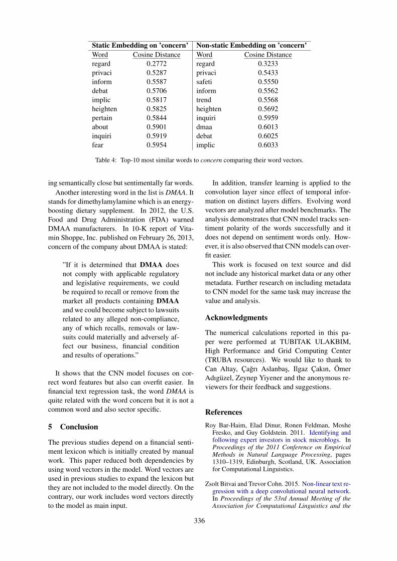
Static Embedding on ’concern’ Non-static Embedding on ’concern’Word Cosine Distance Word Cosine Distanceregard 0.2772 regard 0.3233privaci 0.5287 privaci 0.5433inform 0.5587 safeti 0.5550debat 0.5706 inform 0.5562implic 0.5817 trend 0.5568heighten 0.5825 heighten 0.5692pertain 0.5844 inquiri 0.5959about 0.5901 dmaa 0.6013inquiri 0.5919 debat 0.6025fear 0.5954 implic 0.6033

Table 4: Top-10 most similar words to concern comparing their word vectors.

ing semantically close but sentimentally far words.Another interesting word in the list is DMAA. It

stands for dimethylamylamine which is an energy-boosting dietary supplement. In 2012, the U.S.Food and Drug Administration (FDA) warnedDMAA manufacturers. In 10-K report of Vita-min Shoppe, Inc. published on February 26, 2013,concern of the company about DMAA is stated:

”If it is determined that DMAA doesnot comply with applicable regulatoryand legislative requirements, we couldbe required to recall or remove from themarket all products containing DMAAand we could become subject to lawsuitsrelated to any alleged non-compliance,any of which recalls, removals or law-suits could materially and adversely af-fect our business, financial conditionand results of operations.”

It shows that the CNN model focuses on cor-rect word features but also can overfit easier. Infinancial text regression task, the word DMAA isquite related with the word concern but it is not acommon word and also sector specific.

5 Conclusion

The previous studies depend on a financial senti-ment lexicon which is initially created by manualwork. This paper reduced both dependencies byusing word vectors in the model. Word vectors areused in previous studies to expand the lexicon butthey are not included to the model directly. On thecontrary, our work includes word vectors directlyto the model as main input.

In addition, transfer learning is applied to theconvolution layer since effect of temporal infor-mation on distinct layers differs. Evolving wordvectors are analyzed after model benchmarks. Theanalysis demonstrates that CNN model tracks sen-timent polarity of the words successfully and itdoes not depend on sentiment words only. How-ever, it is also observed that CNN models can over-fit easier.

This work is focused on text source and didnot include any historical market data or any othermetadata. Further research on including metadatato CNN model for the same task may increase thevalue and analysis.

Acknowledgments

The numerical calculations reported in this pa-per were performed at TUBITAK ULAKBIM,High Performance and Grid Computing Center(TRUBA resources). We would like to thank toCan Altay, Cagrı Aslanbas, Ilgaz Cakın, OmerAdıguzel, Zeynep Yiyener and the anonymous re-viewers for their feedback and suggestions.

ReferencesRoy Bar-Haim, Elad Dinur, Ronen Feldman, Moshe

Fresko, and Guy Goldstein. 2011. Identifying andfollowing expert investors in stock microblogs. InProceedings of the 2011 Conference on EmpiricalMethods in Natural Language Processing, pages1310–1319, Edinburgh, Scotland, UK. Associationfor Computational Linguistics.

Zsolt Bitvai and Trevor Cohn. 2015. Non-linear text re-gression with a deep convolutional neural network.In Proceedings of the 53rd Annual Meeting of theAssociation for Computational Linguistics and the

336

7th International Joint Conference on Natural Lan-guage Processing (Volume 2: Short Papers), pages180–185, Beijing, China. Association for Computa-tional Linguistics.

Ronan Collobert, Jason Weston, Leon Bottou, MichaelKarlen, Koray Kavukcuoglu, and Pavel Kuksa.2011. Natural language processing (almost) fromscratch. J. Mach. Learn. Res., 12:2493–2537.

Xiao Ding, Yue Zhang, Ting Liu, and Junwen Duan.2015. Deep learning for event-driven stock predic-tion. In Proceedings of the 24th International Con-ference on Artificial Intelligence, IJCAI’15, pages2327–2333. AAAI Press.

S.S. Hacısalihzade. 2017. Control Engineering andFinance, Lecture Notes in Control and InformationSciences, page 49. Springer International Publish-ing.

Siavash Kazemian, Shunan Zhao, and Gerald Penn.2014. Evaluating sentiment analysis evaluation: Acase study in securities trading. In Proceedings ofthe 5th Workshop on Computational Approaches toSubjectivity, Sentiment and Social Media Analysis,pages 119–127, Baltimore, Maryland. Associationfor Computational Linguistics.

Yoon Kim. 2014. Convolutional neural networksfor sentence classification. In Proceedings of the2014 Conference on Empirical Methods in NaturalLanguage Processing (EMNLP), pages 1746–1751,Doha, Qatar. Association for Computational Lin-guistics.

Shimon Kogan, Dimitry Levin, Bryan R. Routledge,Jacob S. Sagi, and Noah A. Smith. 2009. Pre-dicting risk from financial reports with regression.In Proceedings of Human Language Technologies:The 2009 Annual Conference of the North AmericanChapter of the Association for Computational Lin-guistics, pages 272–280, Boulder, Colorado. Asso-ciation for Computational Linguistics.

Hoa Le, Christophe Cerisara, and Alexandre Denis.2018. Do convolutional networks need to be deepfor text classification ?

Tim Loughran and Bill McDonald. 2011. When is aliability not a liability? textual analysis, dictionaries,and 10-ks. The Journal of Finance, 66(1):35–65.

Tomas Mikolov, Ilya Sutskever, Kai Chen, Greg S Cor-rado, and Jeff Dean. 2013. Distributed representa-tions of words and phrases and their composition-ality. In C. J. C. Burges, L. Bottou, M. Welling,Z. Ghahramani, and K. Q. Weinberger, editors, Ad-vances in Neural Information Processing Systems26, pages 3111–3119. Curran Associates, Inc.

Ramanathan Narayanan, Bing Liu, and Alok Choud-hary. 2009. Sentiment analysis of conditional sen-tences. In Proceedings of the 2009 Conferenceon Empirical Methods in Natural Language Pro-cessing, pages 180–189, Singapore. Association forComputational Linguistics.

Thien Hai Nguyen and Kiyoaki Shirai. 2015. Topicmodeling based sentiment analysis on social mediafor stock market prediction. In Proceedings of the53rd Annual Meeting of the Association for Compu-tational Linguistics and the 7th International JointConference on Natural Language Processing (Vol-ume 1: Long Papers), pages 1354–1364, Beijing,China. Association for Computational Linguistics.

Clemens Nopp and Allan Hanbury. 2015. Detectingrisks in the banking system by sentiment analysis.In Proceedings of the 2015 Conference on Empiri-cal Methods in Natural Language Processing, pages591–600, Lisbon, Portugal. Association for Compu-tational Linguistics.

Wijnand Nuij, Viorel Milea, Frederik Hogenboom,Flavius Frasincar, and Uzay Kaymak. 2014. Anautomated framework for incorporating news intostock trading strategies. IEEE Trans. on Knowl. andData Eng., 26(4):823–835.

MF Porter. 1980. An algorithm for suffix stripping.Program: Electronic Library and Information Sys-tems, 14.

Navid Rekabsaz, Mihai Lupu, Artem Baklanov,Alexander Dur, Linda Andersson, and Allan Han-bury. 2017. Volatility prediction using financial dis-closures sentiments with word embedding-based irmodels. In Proceedings of the 55th Annual Meet-ing of the Association for Computational Linguistics(Volume 1: Long Papers), pages 1712–1721, Van-couver, Canada. Association for Computational Lin-guistics.

Paul C. Tetlock, Maytal Saar-Tsechansky, and SofusMacskassy. 2008. More than words: Quantifyinglanguage to measure firms’ fundamentals. The Jour-nal of Finance, 63(3):1437–1467.

Ming-Feng Tsai and Chuan-Ju Wang. 2014. Financialkeyword expansion via continuous word vector rep-resentations. In Proceedings of the 2014 Conferenceon Empirical Methods in Natural Language Pro-cessing (EMNLP), pages 1453–1458, Doha, Qatar.Association for Computational Linguistics.

Ming-Feng Tsai, Chuan-Ju Wang, and Po-ChuanChien. 2016. Discovering finance keywords viacontinuous-space language models. ACM Trans.Manage. Inf. Syst., 7(3):7:1–7:17.

Chuan-Ju Wang, Ming-Feng Tsai, Tse Liu, and Chin-Ting Chang. 2013. Financial sentiment analysis forrisk prediction. In Proceedings of the Sixth Interna-tional Joint Conference on Natural Language Pro-cessing, pages 802–808, Nagoya, Japan. Asian Fed-eration of Natural Language Processing.

Zhilin Yang, Ruslan Salakhutdinov, and WilliamW. Cohen. 2017. Transfer learning for sequence tag-ging with hierarchical recurrent networks.

337

Proceedings of the 57th Annual Meeting of the Association for Computational Linguistics: Student Research Workshop, pages 338–343Florence, Italy, July 28 - August 2, 2019. c©2019 Association for Computational Linguistics

Sentiment Analysis on Naija-Tweets

Abstract

Examining sentiments in social media poses a challenge to natural language processing because of the intricacy and variability in the dialect articulation, noisy terms in form of slang, abbreviation, acronym, emoticon, and spelling error coupled with the availability of real-time content. Moreover, most of the knowledge-based approaches for resolving slang, abbreviation, and acronym do not consider the issue of ambiguity that evolves in the usage of these noisy terms. This research work proposes an improved framework for social media feed pre-processing that leverages on the combination of integrated local knowledge bases and adapted Lesk algorithm to facilitate pre-processing of social media feeds. The results from the experimental evaluation revealed an improvement over existing methods when applied to supervised learning algorithms in the task of extracting sentiments from Nigeria-origin tweets with an accuracy of 99.17%.

1 Introduction

Sentiment Analysis is being used to automatically detect speculations, emotions, opinions, and evaluations in social media content (Thakkar and Patel, 2015). Unlike carefully created news and other literary web contents, social media streams present various difficulties for analytics algorithms because of their extensive scale, short nature,

slang, abbreviation, grammatical and spelling errors (Asghar et al., 2017). Most of the knowledge-based approaches for resolving these noisy terms do not consider the issue of ambiguity that evolves in their usage (Sabbir et al., 2017). These challenges, which inform this research work, make it necessary to seek improvement on the performance of existing solutions for pre-processing of social media streams (Carter et al., 2013; Ghosh et al., 2017; Kuflik et al., 2017).

Due to language complexity, analysing sentiments in social media presents a challenge to natural language processing (Vyas and Uma, 2018). Moreover, social media content is characterized with a short length of messages, use of dynamically evolving, irregular, informal, and abbreviated words. These make it difficult for techniques that build on them to perform effectively and efficiently (Singh and Kumari, 2016; Zhan and Dahal, 2017).

The short nature of social media streams coupled with no restriction in the choice of language has informed the usage of abbreviation, slang, and acronym (Atefeh and Khreich, 2015; Kumar, 2016). These noisy but useful terms have their implicit meanings and form part of the rich context that needs to be addressed in order to fully make sense of social media streams (Bontcheva and Rout, 2014). Just like there is ambiguity in the use of normal language there is also ambiguity in the usage of slang/abbreviation/acronym because they often have context-based meanings, which must be rightly interpreted in order to improve the

Taiwo Kolajo* Covenant University, Ota, Nigeria taiwo.kolajo@stu.cu.edu.ng

Federal University Lokoja, Kogi State, Nigeria taiwo.kolajo@fulokoja.edu.ng

Olawande Daramola CPUT, Cape Town, South Africa

daramolaj@cput.ac.za

Ayodele Adebiyi Covenant University, Ota, Nigeria

ayo.adebiyi@covenantuniversity.edu.ng

Landmark University, Omu-Aran, Nigeria ayo.adebiyi@lmu.edu.ng

338

results of social media analysis. There is a dearth of social media streams preprocessing geared at resolving slang, abbreviation and acronym as well as ambiguity issues that erupt as a result of their usage (Mihanovic et al., 2014; Matsumoto et al., 2016).

2 Related Work

Many researchers have studied the effect and impact of pre-processing (which ranges from tokenization, removal of stop-words, lemmatization, fixing of slangs, redundancy elimination) on the accuracy of result of techniques building on them for sentiment analysis and unanimously agreed that when social media stream data are well interpreted and represented, it leads to significant improvement of sentiment analysis result.

Haddi et al. (2013) presented the role of text pre-processing in sentiment analysis. The pre-processing stages include removal of HTML tags, stop word removal, negation handling, stemming, and expansion of abbreviation using pattern recognition and regular expression techniques. The problem here is that representing abbreviation based on co-occurrence does not take care of ambiguity. The impact of pre-processing methods on Twitter sentiment classification was explored by Bao et al. (2014) by using the Stanford Twitter Sentiment Dataset. The result of the study showed an improvement in accuracy when negation transformation, URLs feature reservation and repeated letters normalization is employed while lemmatization and stemming reduce the accuracy of sentiment classification. In the same vein, Uysal and Gunal (2014) and Singh and Kumari (2016) investigated the role of text pre-processing and found out that an appropriate combination of pre-processing tasks improves classification accuracy.

Smailovic et al. (2014) and Ansari et al. (2017) investigated sentiments analysis on twitter dataset. Their pre-processing method along with tokenization, stemming and lemmatization includes replacement of user mention, URLs, negation, exclamation, and question marks with tokens. Letter repetition was replaced with one or two occurrences of the letter. From the result of their experiments, it was concluded that pre-processing twitter data improves techniques building on them.

The pre-processing method adopted by Ouyang et al. (2017) and Ramadhan et al. (2017) includes

deletion of URLs, mentions, stop-words, punctuation, and stemming. Ramadhan et al. (2017) added the handling of slang conversion in their work although the authors did not state how the slang conversion was done. Jianqiang and Xiaolin (2017) discussed the effect of pre-processing and found that expanding acronyms and replacing negation improve classification while removal of stop-words, numbers or URLs do not yield any significant improvement. On the contrary, Symeonidis et al. (2018) evaluated classification accuracy based on pre-processing techniques and found out that removing numbers, lemmatization, and replacing negation improve accuracy. Zhang et al. (2017) presented Arc2Vec framework for learning acronyms in twitter using three embedding models. However, the authors did not take care of contextual information. From the review, most research efforts have not been directed towards the handling all of slang/abbreviation/acronym as well as resolving ambiguity in the usage of noisy terms based on contextual information.

3 Methodology

3.1 Data Collection

The dataset (referred to as Naija-tweets in this paper) was extracted from tweets of Nigeria origin. The dataset focused on politics in Nigeria. A user interface was built around an underlying API provided by Twitter to collect tweets based on politics-related keywords such as “politics”, “governments”, “policy”, “policymaking”, and “legislation”. The total tweets extracted was 10,000. These were manually classified into positive (1) or negative (0) by three experts in sentiment analysis. 80% was used as training data while 10% was used as test data and 10% for dev set. The general preprocessing method (GTPM), Arc2Vec Framework and the proposed preprocessing method (PTPM) are depicted in figure 1 (a), (b) and (c) respectively.

3.2 Data Preprocessing From the data stream collected, Tags, URLs, mentions and non-ASCII characters were automatically removed using a regular expression. This was followed by tokenization and normalization. Thereafter, slangs, abbreviation, acronyms, and emoticons were filtered from the tweets using corpora of English words in natural language toolkit (NLTK). The filtered

339

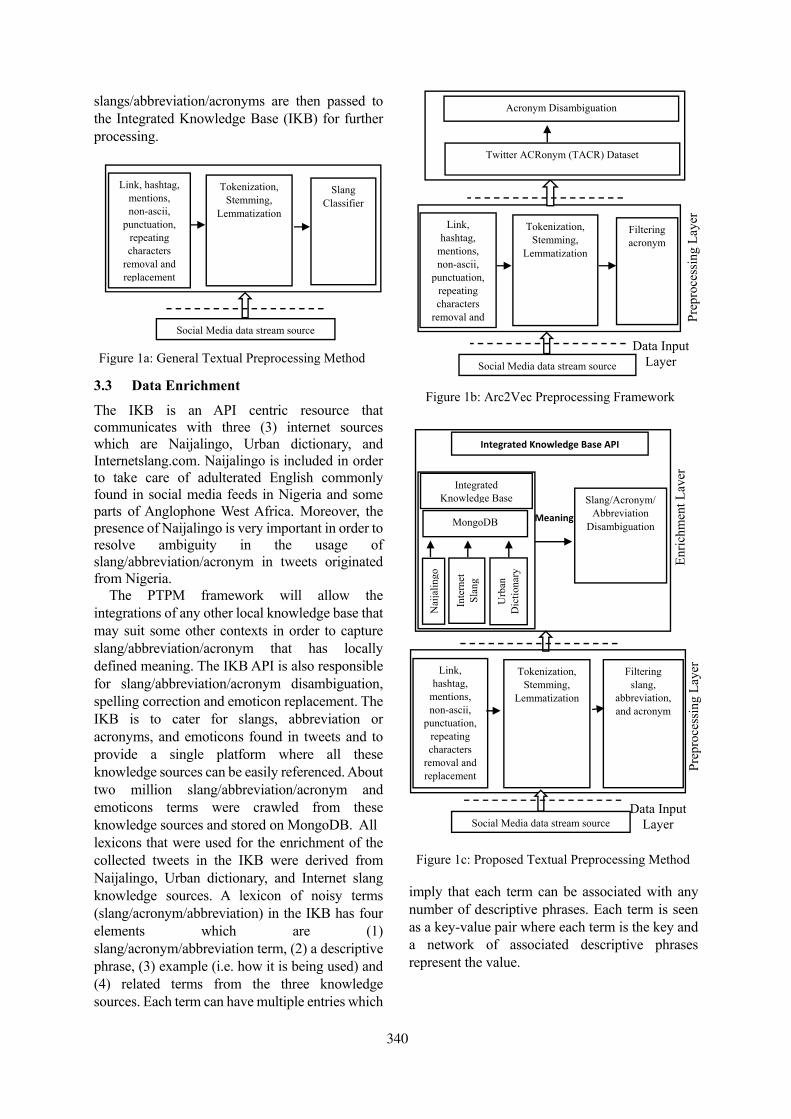
slangs/abbreviation/acronyms are then passed to the Integrated Knowledge Base (IKB) for further processing.

3.3 Data Enrichment The IKB is an API centric resource that communicates with three (3) internet sources which are Naijalingo, Urban dictionary, and Internetslang.com. Naijalingo is included in order to take care of adulterated English commonly found in social media feeds in Nigeria and some parts of Anglophone West Africa. Moreover, the presence of Naijalingo is very important in order to resolve ambiguity in the usage of slang/abbreviation/acronym in tweets originated from Nigeria.

The PTPM framework will allow the integrations of any other local knowledge base that may suit some other contexts in order to capture slang/abbreviation/acronym that has locally defined meaning. The IKB API is also responsible for slang/abbreviation/acronym disambiguation, spelling correction and emoticon replacement. The IKB is to cater for slangs, abbreviation or acronyms, and emoticons found in tweets and to provide a single platform where all these knowledge sources can be easily referenced. About two million slang/abbreviation/acronym and emoticons terms were crawled from these knowledge sources and stored on MongoDB. All lexicons that were used for the enrichment of the collected tweets in the IKB were derived from Naijalingo, Urban dictionary, and Internet slang knowledge sources. A lexicon of noisy terms (slang/acronym/abbreviation) in the IKB has four elements which are (1) slang/acronym/abbreviation term, (2) a descriptive phrase, (3) example (i.e. how it is being used) and (4) related terms from the three knowledge sources. Each term can have multiple entries which

imply that each term can be associated with any number of descriptive phrases. Each term is seen as a key-value pair where each term is the key and a network of associated descriptive phrases represent the value.

Link, hashtag, mentions, non-ascii,

punctuation, repeating characters

removal and replacement

Tokenization, Stemming,

Lemmatization

Social Media data stream source

Slang Classifier

Figure 1a: General Textual Preprocessing Method

Twitter ACRonym (TACR) Dataset

Acronym Disambiguation

Link, hashtag,

mentions, non-ascii,

punctuation, repeating characters

removal and

Tokenization, Stemming,

Lemmatization

Filtering acronym

Social Media data stream source

Data Input Layer

Figure 1b: Arc2Vec Preprocessing Framework

Prep

roce

ssin

g La

yer

Figure 1c: Proposed Textual Preprocessing Method

Integrated Knowledge Base API

Slang/Acronym/Abbreviation

Disambiguation

Integrated Knowledge Base

MongoDB

Inte

rnet

Sl

ang

Urb

an

Dic

tiona

ry

Nai

jalin

go

Meaning

Enric

hmen

t Lay

er

Link, hashtag,

mentions, non-ascii,

punctuation, repeating characters

removal and replacement

Tokenization, Stemming,

Lemmatization

Filtering slang,

abbreviation, and acronym

Prep

roce

ssin

g La

yer

Social Media data stream source Data Input

Layer

340

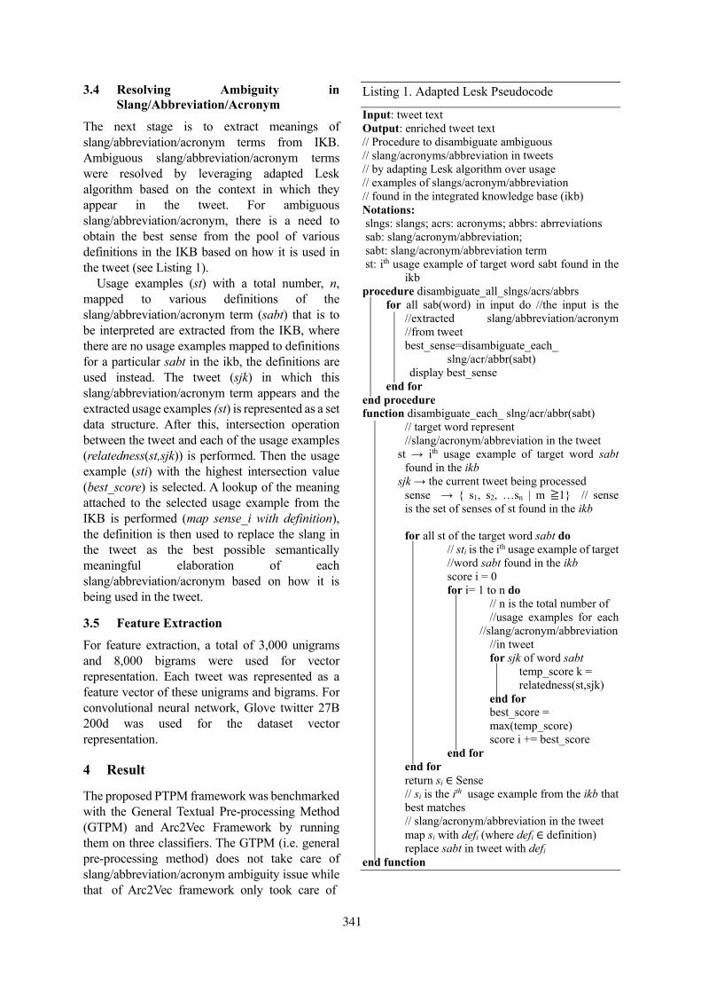
3.4 Resolving Ambiguity in Slang/Abbreviation/Acronym

The next stage is to extract meanings of slang/abbreviation/acronym terms from IKB. Ambiguous slang/abbreviation/acronym terms were resolved by leveraging adapted Lesk algorithm based on the context in which they appear in the tweet. For ambiguous slang/abbreviation/acronym, there is a need to obtain the best sense from the pool of various definitions in the IKB based on how it is used in the tweet (see Listing 1).

Usage examples (st) with a total number, n, mapped to various definitions of the slang/abbreviation/acronym term (sabt) that is to be interpreted are extracted from the IKB, where there are no usage examples mapped to definitions for a particular sabt in the ikb, the definitions are used instead. The tweet (sjk) in which this slang/abbreviation/acronym term appears and the extracted usage examples (st) is represented as a set data structure. After this, intersection operation between the tweet and each of the usage examples (relatedness(st,sjk)) is performed. Then the usage example (sti) with the highest intersection value (best_score) is selected. A lookup of the meaning attached to the selected usage example from the IKB is performed (map sense_i with definition), the definition is then used to replace the slang in the tweet as the best possible semantically meaningful elaboration of each slang/abbreviation/acronym based on how it is being used in the tweet.

3.5 Feature Extraction For feature extraction, a total of 3,000 unigrams and 8,000 bigrams were used for vector representation. Each tweet was represented as a feature vector of these unigrams and bigrams. For convolutional neural network, Glove twitter 27B 200d was used for the dataset vector representation.

4 Result

The proposed PTPM framework was benchmarked with the General Textual Pre-processing Method (GTPM) and Arc2Vec Framework by running them on three classifiers. The GTPM (i.e. general pre-processing method) does not take care of slang/abbreviation/acronym ambiguity issue while that of Arc2Vec framework only took care of

Listing 1. Adapted Lesk Pseudocode

Input: tweet text Output: enriched tweet text // Procedure to disambiguate ambiguous // slang/acronyms/abbreviation in tweets // by adapting Lesk algorithm over usage // examples of slangs/acronym/abbreviation // found in the integrated knowledge base (ikb) Notations: slngs: slangs; acrs: acronyms; abbrs: abrreviations sab: slang/acronym/abbreviation; sabt: slang/acronym/abbreviation term st: ith usage example of target word sabt found in the ikb procedure disambiguate_all_slngs/acrs/abbrs for all sab(word) in input do //the input is the //extracted slang/abbreviation/acronym //from tweet best_sense=disambiguate_each_ slng/acr/abbr(sabt) display best_sense end for end procedure function disambiguate_each_ slng/acr/abbr(sabt)

// target word represent //slang/acronym/abbreviation in the tweet

st → ith usage example of target word sabt found in the ikb sjk → the current tweet being processed sense → s1, s2, …sn | m ≧1 // sense is the set of senses of st found in the ikb

for all st of the target word sabt do

// sti is the ith usage example of target //word sabt found in the ikb

score i = 0 for i= 1 to n do // n is the total number of //usage examples for each //slang/acronym/abbreviation //in tweet for sjk of word sabt temp_score k = relatedness(st,sjk) end for best_score = max(temp_score) score i += best_score end for

end for return si ∈ Sense // si is the ith usage example from the ikb that best matches // slang/acronym/abbreviation in the tweet map si with defi (where defi ∈ definition) replace sabt in tweet with defi

end function

341

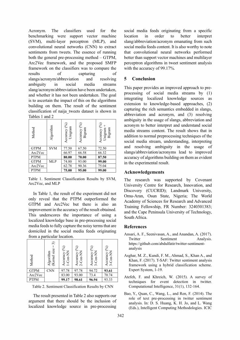
Acronym. The classifiers used for the benchmarking were support vector machine (SVM), multi-layer perceptron (MLP), and convolutional neural networks (CNN) to extract sentiments from tweets. The essence of running both the general pre-processing method – GTPM, Arc2Vec framework, and the proposed SMFP framework on the classifiers was to compare the results of capturing of slangs/acronym/abbreviation and resolving ambiguity in social media streams slang/acronym/abbreviation have been undertaken, and whether it has not been undertaken. The goal is to ascertain the impact of this on the algorithms building on them. The result of the sentiment classification of naija_tweets dataset is shown in Tables 1 and 2

Met

hod

Alg

orith

m

Acc

urac

y (%

) U

nigr

am

Acc

urac

y (%

) Bi

gram

Acc

urac

y (%

) U

nigr

am +

Bi

gram

GTPM SVM 77.50 67.50 72.50 Arc2Vec 66.97 66.58 66.32 PTPM 80.00 70.00 87.50 GTPM MLP 74.80 93.00 99.00Arc2Vec 62.78 90.36 75.04 PTPM 75.00 95.00 99.00

In Table 1, the result of the experiment did not

only reveal that the PTPM outperformed the GTPM and Arc2Vec but there is also an improvement in the accuracy of the result obtained. This underscores the importance of using a localized knowledge base in pre-processing social media feeds to fully capture the noisy terms that are domiciled in the social media feeds originating from a particular location.

Met

hod

Alg

orith

m

(Ker

nel s

ize =

3)

Acc

urac

y (%

) 1-

Con-

NN

Acc

urac

y (%

) 2-

Con-

NN

Acc

urac

y (%

) 3-

Con-

NN

Acc

urac

y (%

) 3-

Con-

NN

GTPM CNN 97.78 97.78 94.72 93.61 Arc2Vec 83.00 93.00 73.4 70.74 PTPM 99.17 98.61 96.94 93.33

The result presented in Table 2 also supports our

argument that there should be the inclusion of localized knowledge source in pre-processing

social media feeds originating from a specific location in order to better interpret slang/abbreviation/acronym emanating from such social media feeds content. It is also worthy to note that convolutional neural networks performed better than support vector machines and multilayer perceptron algorithms in tweet sentiment analysis with the accuracy of 99.17%.

5 Conclusion

This paper provides an improved approach to pre-processing of social media streams by (1) integrating localized knowledge sources as extension to knowledge-based approaches, (2) capturing the rich semantics embedded in slangs, abbreviation and acronym, and (3) resolving ambiguity in the usage of slangs, abbreviation and acronym to better interpret and understand social media streams content. The result shows that in addition to normal preprocessing techniques of the social media stream, understanding, interpreting and resolving ambiguity in the usage of slangs/abbreviation/acronyms lead to improved accuracy of algorithms building on them as evident in the experimental result.

Acknowledgements The research was supported by Covenant University Centre for Research, Innovation, and Discovery (CUCRID); Landmark University, Omu-Aran, Osun State, Nigeria; The World Academy of Sciences for Research and Advanced Training Fellowship, FR Number: 3240301383; and the Cape Peninsula University of Technology, South Africa.

References Ansari, A. F., Seenivasan, A., and Anandan, A. (2017).

Twitter Sentiment Analysis. https://github.com/abdulfatir/twitter-sentiment-analysis

Asghar, M. Z., Kundi, F. M., Ahmad, S., Khan A., and Khan, F. (2017). T-SAF: Twitter sentiment analysis framework using a hybrid classification scheme. Expert System, 1-19.

Atefeh, F. and Khreich, W. (2015). A survey of techniques for event detection in twitter. Computational Intelligence, 31(1), 132-164.

Bao, Y., Quan, C., Wang, L., and Ren, F. (2014). The role of text pre-processing in twitter sentiment analysis. In: D. S. Huang, K. H. Jo, and L. Wang (Eds.), Intelligent Computing Methodologies. ICIC

Table 2. Sentiment Classification Results by CNN

Table 1. Sentiment Classification Results by SVM, Arc2Vec, and MLP

342

2014. Lecture Notes in Computer Science 8589, 615-629. Taiyuan, China: Springer.

Bontcheva, K. and Rout, D. (2014). Making sense of social media streams through semantics: A survey. Semantic Web, 5(5), 373-403. Available from: semantic-web-journal.org>swj303_0.pdf

Carter, S., Weerkamp, W., and Tsagkias, E. (2013). Microblog language identification: Overcoming the limitations of short, unedited and idiomatic text. Language Resources and Evaluation Journal, 47(1), 195-215.

Ghosh, S., Ghosh, S., and Das, D. (2017). Sentiment identification in code-mixed social media text. https://arxiv.org/pdf/1707.01184.pdf

Haddi, E., Liu, X., and Shi, Y. (2013). The role of text pre-processing in sentiment analysis. Procedia Computer Science, 17, 26-32.

Jianqiang, Z., and Xiaolin, G. (2017). Comparison research on text pre-processing methods on twitter sentiment analysis. IEEE Access, 5, 2870-2879.

Kuflik, T., Minkov, E., Nocera, S., Grant-Muller, S., Gal-Tzur, A., and Shoor I. (2017). Automating a framework to extract and analyse transport related social media content: the potential and challenges. Transport Research Part C, 275-291.

Kumar, M.G.M. (2016). Review on event detection techniques in social multimedia. Online Information Review, 40(3), 347-361.

Matsumoto, K., Yoshida, M., Tsuchiya, S., Kita, K., and Ren, F. (2016). Slang Analysis Based on Variant Information Extraction Focusing on the Time Series Topics. International Journal of Advanced Intelligence, 8(1), 84-98.

Mihanovic, A., Gabelica, H., and Kristic, Z. (2014). Big Data and Sentiment Analysis using KNIME: Online reviews vs. social media. MIPRO 2014, 26-30 May, Opatija, Croatia, (pp. 1464-1468).

Ouyang, Y., Guo, B., Zhang, J., Yu, Z., and Zhou, X. (2017). Senti-story: Multigrained sentiment analysis and event summarization with crowdsourced social media data. Personal and Ubiquitous Computing, 21(1), 97-111.

Ramadhan, W. P., Novianty, A., and Setianingsih, C. (2017, September). Sentiment analysis using multinomial logistic regression. Proceedings of the 2017 International Conference on Control, Electronics, Renewable Energy and Communications (ICCEREC) (pp.46-49). Yogyakarta, Indonesia: IEEE.

Sabbir, A. K. M., Jimeno-Yepes, A., and Kavuluru, R. (2017, October). Knowledge-based biomedical word sense disambiguation with neural concept embeddings. 2017 IEEE 17th International

Conference on Bioinformatics and Bioengineering (BIBE). Washington, DC, USA: IEEE.

Singh, T., and Kumari, M. (2016). Role of text pre-processing in twitter sentiment analysis. Procedia Computer Science 89, 549-554. Available from: https://doi.org/10.1016/j.procs.2016.06.095

Smailovic, J., Grcar, M., Lavrac, N. Znidarsic, M. (2014). Stream-based active learning for sentiment analysis. Information Sciences, 285, 181-203.

Symeonidis, S., Effrosynidis, D., and Arampatzis, A. (2018). A comparative evaluation of pre-processing techniques and their interactions for twitter sentiment analysis. Expert Systems with Applications, 110, 298-310.

Thakkar, H., and Patel, D. (2015). Approaches for sentiment analysis on twitter: A state-of-art study. arXuv preprint arXiv:1512.01043, 1-8.

Uysal, A. K., and Gunal, S. (2014). The impact of pre-processing on text classification. Information Processing and Management, 50(1), 104-112.

Vyas, V., and Uma, V. (2018). An extensive study of sentiment analysis tools and binary classification of tweets using rapid miner. Procedia Computer Science, 125, 329-335.

Zhan, J., and Dahal, B. (2017). Using deep learning for short text understanding. Journal of Big Data, 4:34. doi: 10.1186/s40537-017-0095-2

Zhang, Z., Luo, S., and Ma, S. (2017). Arc2Vec: Learning acronym representations in twitter. In: L. Polkowski et al. (Eds.) IJCRS 2017, Part I, LNAI 10313, 280-288

343

Proceedings of the 57th Annual Meeting of the Association for Computational Linguistics: Student Research Workshop, pages 344–350Florence, Italy, July 28 - August 2, 2019. c©2019 Association for Computational Linguistics

Fact or Factitious? Contextualized Opinion Spam Detection

Stefan Kennedy, Niall Walsh∗, Kirils Sloka, Andrew McCarren and Jennifer FosterSchool of Computing

Dublin City University15902803,15384141,13405888@mail.dcu.ieAndrew McCarren,Jennifer.Foster@dcu.ie

Abstract

In recent years, it has been shown that falsifi-cation of online reviews can have a substantial,quantifiable effect on the success of the sub-ject. This creates a large enticement for sellersto participate in review deception to boost theirown success, or hinder the competition. Mostcurrent efforts to detect review deception arebased on supervised classifiers trained on syn-tactic and lexical patterns. However, recentneural approaches to classification have beenshown to match or outperform state-of-the-artmethods. In this paper, we perform an ana-lytic comparison of these methods, and intro-duce our own results. By fine-tuning Google’srecently published transformer-based architec-ture, BERT, on the fake review detection task,we demonstrate near state-of-the-art perfor-mance, achieving over 90% accuracy on awidely used deception detection dataset.

1 Introduction

Online reviews of products and services have be-come significantly more important over the lasttwo decades. Reviews influence customer pur-chasing decisions through review score and vol-ume of reviews (Maslowska et al., 2017). It is es-timated that as many as 90% of consumers read re-views before a purchase (Kumar et al., 2018) andthat the conversion rate of a product increases byup to 270% as it gains reviews. For high priceproducts, reviews can increase conversion rate by380% (Askalidis and Malthouse, 2016).

With the rise of consumer reviews comes theproblem of deceptive reviews. It has been shownthat in competitive, ranked conditions it is worth-while for unlawful merchants to create fake re-views. For TripAdvisor, in 80% of cases, a hotelcould become more visible than another hotel us-ing just 50 deceptive reviews (Lappas et al., 2016).Fake reviews are an established problem – 20% of

∗Joint first author with Stefan Kennedy

Yelp reviews are marked as fake by Yelp’s algo-rithm (Luca and Zervas, 2016).

First introduced by Jindal and Liu (2007), theproblem of fake review detection has been tack-led from the perspectives of opinion spam de-tection and deception detection. It is usuallytreated as a binary classification problem using tra-ditional text classification features such as wordand part-of-speech n-grams, structural features ob-tained from syntactic parsing (Feng et al., 2012),topic models (Hernandez-Castaneda et al., 2017),psycho-linguistic features obtained using the Lin-guistic Inquiry and Word Count (Ott et al., 2011;Hernandez-Castaneda et al., 2017; Pennebakeret al., 2015) and non-verbal features related to re-viewer behaviour (You et al., 2018; Wang et al.,2017; Aghakhani et al., 2018; Stanton and Irissap-pane, 2019)

We revisit the problem of fake review detectionby comparing the performance of a variety of neu-ral and non-neural approaches on two freely avail-able datasets, a small set of hotel reviews wherethe deceptive subset has been obtained via crowd-sourcing (Ott et al., 2011) and a much larger set ofYelp reviews obtained automatically (Rayana andAkoglu, 2015). We find that features based on re-viewer characteristics can be used to boost the ac-curacy of a strong bag-of-words baseline. We alsofind that neural approaches perform at about thesame level as the traditional non-neural ones. Per-haps counter-intuitively, the use of pretrained non-contextual word embeddings do not tend to leadto improved performance in most of our experi-ments. However, our best performance is achievedby fine-tuning BERT embeddings (Devlin et al.,2018) on this task. On the hotel review dataset,bootstrap validation accuracy is 90.5%, just be-hind the 91.2% reported by Feng et al. (2012)who combine bag-of-words with constituency treefragments.

344

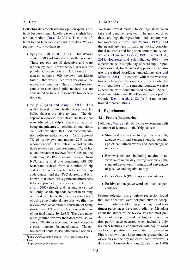
2 Data

Collecting data for classifying opinion spam is dif-ficult because human labelling is only slightly bet-ter than random (Ott et al., 2011). Thus, it is dif-ficult to find large-scale ground truth data. We ex-periment with two datasets:

• OpSpam (Ott et al., 2011): This datasetcontains 800 gold-standard, labelled reviews.These reviews are all deceptive and werewritten by paid, crowd-funded workers forpopular Chicago hotels. Additionally thisdataset contains 800 reviews consideredtruthful, that were mined from various onlinereview communities. These truthful reviewscannot be considered gold-standard, but areconsidered to have a reasonably low decep-tion rate.

• Yelp (Rayana and Akoglu, 2015): Thisis the largest ground truth, deceptively la-belled dataset available to date. The de-ceptive reviews in this dataset are those thatwere filtered by Yelp’s review software forbeing manufactured, solicited or malicious.Yelp acknowledges that their recommenda-tion software makes errors1. Yelp removed7% of its reviews and marked 22% as notrecommended2. This dataset is broken intothree review sets, one containing 67,395 ho-tel and restaurant reviews from Chicago, onecontaining 359,052 restaurant reviews fromNYC and a final one containing 608,598restaurant reviews from a number of zipcodes. There is overlap between the zipcode dataset and the NYC dataset, and it isknown that there are significant differencesbetween product review categories (Blitzeret al., 2007) (hotels and restaurants) so wewill only use the zip code dataset in trainingour models. Due to the memory restrictionsof using convolutional networks, we filter thereviews with an additional constraint of beingshorter than 321 words. This reduces the sizeof our final dataset by 2.63%. There are manymore genuine reviews than deceptive, so weextract 78,346 each of genuine and deceptiveclasses to create a balanced dataset. The en-tire dataset contains 451,906 unused reviews.

1https://www.yelpblog.com/2010/03/yelp-review-filter-explained

2https://www.yelp.com/factsheet

3 Methods

We train several models to distinguish betweenfake and genuine reviews. The non-neural ofthese are logistic regression, and support vec-tor machines (Cortes and Vapnik, 1995), andthe neural are feed-forward networks, convolu-tional networks and long short-term memory net-works (LeCun and Bengio, 1998; Jacovi et al.,2018; Hochreiter and Schmidhuber, 1997). Weexperiment with simple bag-of-word input repre-sentations and, for the neural approaches, we alsouse pre-trained word2vec embeddings (Le andMikolov, 2014). In contrast with word2vec vec-tors which provide the same vector for a particularword regardless of its sentential context, we alsoexperiment with contextualised vectors. Specif-ically, we utilize the BERT model developed byGoogle (Devlin et al., 2018) for fine-tuning pre-trained representations.

4 Experiments

4.1 Feature Engineering

Following Wang et al. (2017), we experiment witha number of features on the Yelp dataset:

• Structural features including review length,average word and sentence length, percent-age of capitalized words and percentage ofnumerals.

• Reviewer features including maximum re-view count in one day, average review length,standard deviation of ratings, and percentageof positive and negative ratings.

• Part-of-Speech (POS) tags as percentages.

• Positive and negative word sentiment as per-centages.

Feature selection using logistic regression foundthat some features were not predictive of decep-tion. In particular POS tag percentages and sen-timent percentages were not predictive. Metadataabout the author of the review was the most pre-dictive of deception, and the highest classifica-tion performance occurred when including onlyreviewer features in conjunction with bag-of-wordvectors. Separation of these features displayed inFigure 1 shows that a large number (greater than 2)of reviews in one day indicates that a reviewer isdeceptive. Conversely a long (greater than 1000)

345

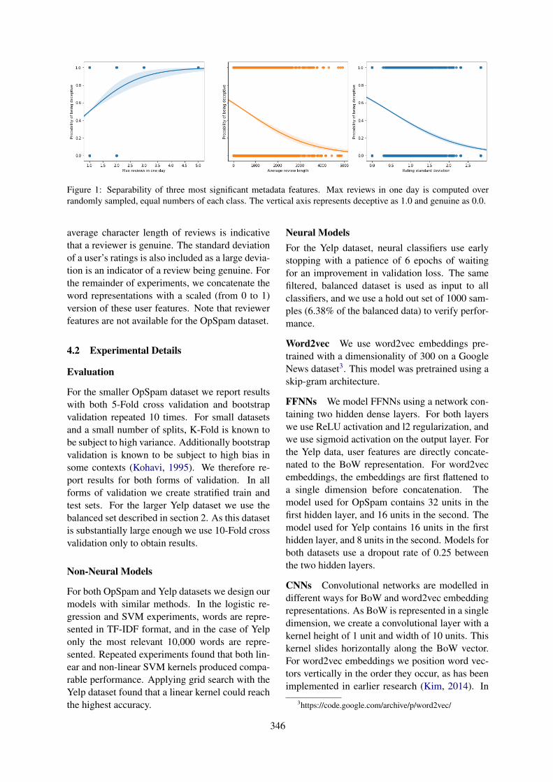
Figure 1: Separability of three most significant metadata features. Max reviews in one day is computed overrandomly sampled, equal numbers of each class. The vertical axis represents deceptive as 1.0 and genuine as 0.0.

average character length of reviews is indicativethat a reviewer is genuine. The standard deviationof a user’s ratings is also included as a large devia-tion is an indicator of a review being genuine. Forthe remainder of experiments, we concatenate theword representations with a scaled (from 0 to 1)version of these user features. Note that reviewerfeatures are not available for the OpSpam dataset.

4.2 Experimental Details

Evaluation

For the smaller OpSpam dataset we report resultswith both 5-Fold cross validation and bootstrapvalidation repeated 10 times. For small datasetsand a small number of splits, K-Fold is known tobe subject to high variance. Additionally bootstrapvalidation is known to be subject to high bias insome contexts (Kohavi, 1995). We therefore re-port results for both forms of validation. In allforms of validation we create stratified train andtest sets. For the larger Yelp dataset we use thebalanced set described in section 2. As this datasetis substantially large enough we use 10-Fold crossvalidation only to obtain results.

Non-Neural Models

For both OpSpam and Yelp datasets we design ourmodels with similar methods. In the logistic re-gression and SVM experiments, words are repre-sented in TF-IDF format, and in the case of Yelponly the most relevant 10,000 words are repre-sented. Repeated experiments found that both lin-ear and non-linear SVM kernels produced compa-rable performance. Applying grid search with theYelp dataset found that a linear kernel could reachthe highest accuracy.

Neural ModelsFor the Yelp dataset, neural classifiers use earlystopping with a patience of 6 epochs of waitingfor an improvement in validation loss. The samefiltered, balanced dataset is used as input to allclassifiers, and we use a hold out set of 1000 sam-ples (6.38% of the balanced data) to verify perfor-mance.

Word2vec We use word2vec embeddings pre-trained with a dimensionality of 300 on a GoogleNews dataset3. This model was pretrained using askip-gram architecture.

FFNNs We model FFNNs using a network con-taining two hidden dense layers. For both layerswe use ReLU activation and l2 regularization, andwe use sigmoid activation on the output layer. Forthe Yelp data, user features are directly concate-nated to the BoW representation. For word2vecembeddings, the embeddings are first flattened toa single dimension before concatenation. Themodel used for OpSpam contains 32 units in thefirst hidden layer, and 16 units in the second. Themodel used for Yelp contains 16 units in the firsthidden layer, and 8 units in the second. Models forboth datasets use a dropout rate of 0.25 betweenthe two hidden layers.

CNNs Convolutional networks are modelled indifferent ways for BoW and word2vec embeddingrepresentations. As BoW is represented in a singledimension, we create a convolutional layer with akernel height of 1 unit and width of 10 units. Thiskernel slides horizontally along the BoW vector.For word2vec embeddings we position word vec-tors vertically in the order they occur, as has beenimplemented in earlier research (Kim, 2014). In

3https://code.google.com/archive/p/word2vec/

346

this case the kernel has a width equal to the di-mensionality of the word vectors and slides verti-cally along the word axis. We use a kernel heightof 10, containing 10 words in each kernel posi-tion. Both BoW and word2vec embedding mod-els use 50 filters. Following the convolutions theresult is passed through a pooling layer, and adropout rate of 0.5 is applied before the result isflattened. In the case of Yelp this flattened resultis concatenated with the user features of the re-view. Two hidden dense layers follow this, bothusing ReLU activation and l2 regularization. Bothhidden layers contain 8 units and are followed byan output layer that uses sigmoid activation. Forthe OpSpam dataset, the BoW model uses a poolsize of (1, 10) and the word2vec embedding im-plementation uses a pool size of (5, 1). For theYelp dataset both BoW and word2vec embeddingmodels use global max pooling.

LSTMs In the implementation of LSTMs, mod-els for both BoW and word2vec embeddings di-rectly input word representations to an LSTMlayer. Numerous repeated runs with differentnumbers of LSTM layers and units found thatthe optimal accuracy occurs at just one layer of10 units. We model implementations for bothOpSpam and Yelp datasets using this number oflayers and units. In the case of the Yelp dataset,the output of the LSTM layer is concatenated withuser features. This is followed by 2 hidden denselayers using ReLU activation and l2 regulariza-tion, each containing 8 units, followed by an out-put layer using sigmoid activation.

BERT We fine-tune thebert-base-uncased model on theOpSpam dataset and perform stratified vali-dation using both 5-Fold validation and bootstrapvalidation repeated 10 times. For fine-tuning weuse a learning rate of 2e-5, batch size of 16 and 3training epochs.

Two implementations of fine-tuning are used toverify results. One implementation is the BERTimplementation published by Google alongsidethe pretrained models, and the other uses the‘op-for-op’ reimplementation of BERT created byHugging Face4.

4https://github.com/huggingface/pytorch-pretrained-BERT

4.3 Results

The results of performing validation on these mod-els are shown in Tables 1, 2 and 3. Table 1 showsthat SVMs slightly outperform logistic regression,and that the Yelp dataset represents a much harderchallenge than the OpSpam one.

Contrary to expectations, Table 2 shows thatpretrained word2vec embeddings do not improveperformance, and in the case of OpSpam BoWcan substantially outperform them. We do not yetknow why this might be case.

The BERT results in Table 3 show thatthe Google TensorFlow implementation performssubstantially better than PyTorch in our case. Thisis an unexpected result and more research needsto be carried out to understand the differences. Wealso report that Google’s TensorFlow implemen-tation outperforms all other classifiers tested onthe OpSpam dataset, providing tentative evidenceof contextualized embeddings outperforming allnon-contextual pre-trained word2vec embeddingsand BoW approaches.

By inspecting the results of evaluation on a sin-gle 5-Fold test set split for the BERT experiments,we see that there are an approximately equal num-ber of false negatives (15), and false positives (14).There appears to be a slight tendency for the modelto perform better when individual sentences arelonger, and when the review is long. In the caseof our 29 incorrect classifications the number ofwords in a sentence was 16.0 words, comparedto 18.4 for correct classifications. Entire reviewstend to be longer in correct classifications with anaverage length of 149.0 words, compared to 117.6for incorrect classifications. Meanwhile the av-erage word length is approximately 4.25 for bothcorrect and incorrect classifications.

5 Application of Research

We have developed a frontend which retrievesbusiness information from Yelp and utilizes ourmodels to analyze reviews. Results are displayedin an engaging fashion using data visualizationand explanations of our prediction. We display adeception distribution of all reviews for the prod-uct. This includes how many reviews are clas-sified as deceptive or genuine, shown in bucketsat 10% intervals of confidence. This allows usersto quickly determine if the distribution is differentto a typical, expected one. This tool also enablesusers to view frequency and average rating of re-

347

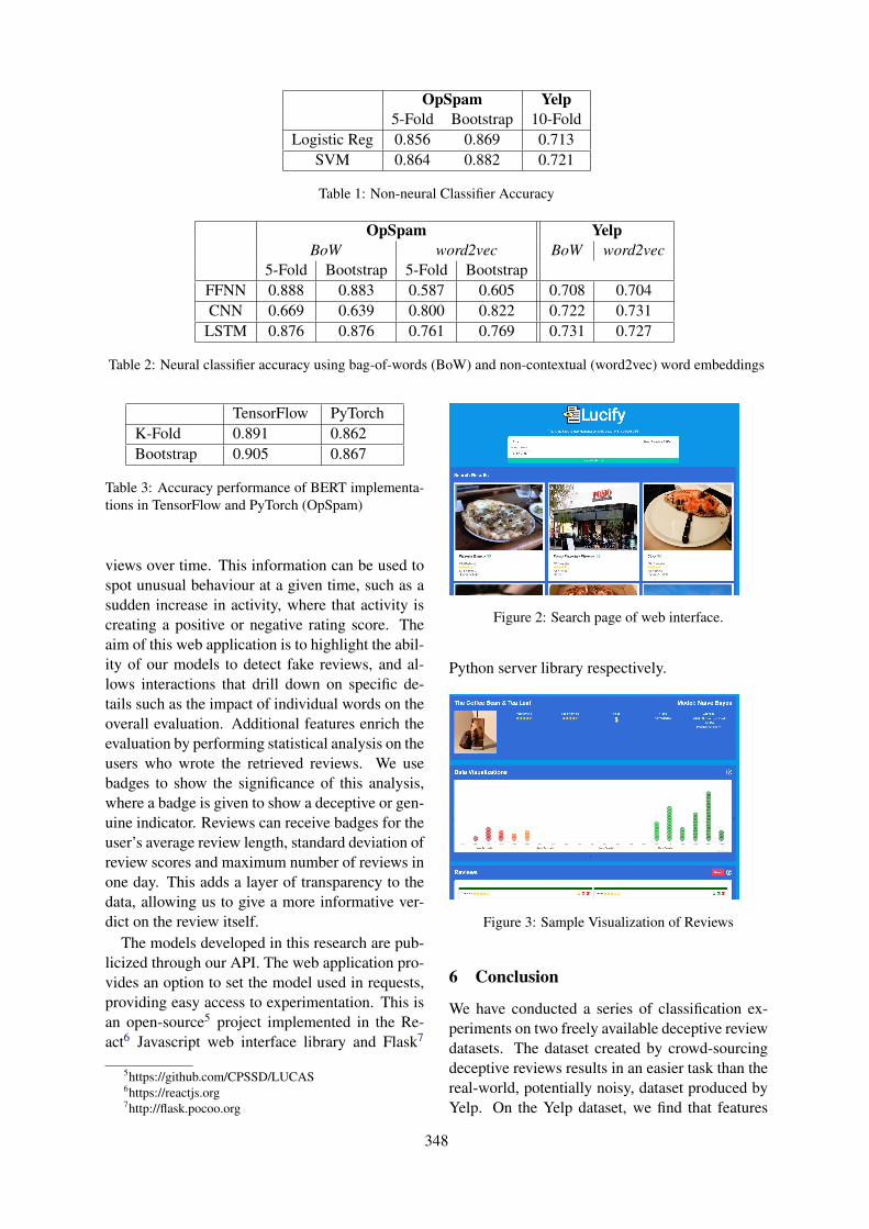
OpSpam Yelp5-Fold Bootstrap 10-Fold

Logistic Reg 0.856 0.869 0.713SVM 0.864 0.882 0.721

Table 1: Non-neural Classifier Accuracy

OpSpam YelpBoW word2vec BoW word2vec

5-Fold Bootstrap 5-Fold BootstrapFFNN 0.888 0.883 0.587 0.605 0.708 0.704CNN 0.669 0.639 0.800 0.822 0.722 0.731

LSTM 0.876 0.876 0.761 0.769 0.731 0.727

Table 2: Neural classifier accuracy using bag-of-words (BoW) and non-contextual (word2vec) word embeddings

TensorFlow PyTorchK-Fold 0.891 0.862Bootstrap 0.905 0.867

Table 3: Accuracy performance of BERT implementa-tions in TensorFlow and PyTorch (OpSpam)

views over time. This information can be used tospot unusual behaviour at a given time, such as asudden increase in activity, where that activity iscreating a positive or negative rating score. Theaim of this web application is to highlight the abil-ity of our models to detect fake reviews, and al-lows interactions that drill down on specific de-tails such as the impact of individual words on theoverall evaluation. Additional features enrich theevaluation by performing statistical analysis on theusers who wrote the retrieved reviews. We usebadges to show the significance of this analysis,where a badge is given to show a deceptive or gen-uine indicator. Reviews can receive badges for theuser’s average review length, standard deviation ofreview scores and maximum number of reviews inone day. This adds a layer of transparency to thedata, allowing us to give a more informative ver-dict on the review itself.

The models developed in this research are pub-licized through our API. The web application pro-vides an option to set the model used in requests,providing easy access to experimentation. This isan open-source5 project implemented in the Re-act6 Javascript web interface library and Flask7

5https://github.com/CPSSD/LUCAS6https://reactjs.org7http://flask.pocoo.org

Figure 2: Search page of web interface.

Python server library respectively.

Figure 3: Sample Visualization of Reviews

6 Conclusion

We have conducted a series of classification ex-periments on two freely available deceptive reviewdatasets. The dataset created by crowd-sourcingdeceptive reviews results in an easier task than thereal-world, potentially noisy, dataset produced byYelp. On the Yelp dataset, we find that features

348

that encode reviewer behaviour are important inboth a neural and non-neural setting. The best per-formance on the OpSpam dataset, which is com-petitive with the state-of-the-art, is achieved byfine-tuning with BERT. Future work involves un-derstanding the relatively poor performance of thepretrained non-contextual embeddings, and exper-imenting with conditional, more efficient genera-tive adversarial networks.

Acknowledgments

We thank the reviewers for their helpful com-ments. The work presented in this paper is the finalyear project of the first three authors, conductedas part of their undergraduate degree in Compu-tational Problem Solving and Software Develop-ment in Dublin City University. We thank theADAPT Centre for Digital Content Technologyfor providing computing resources. The ADAPTCentre for Digital Content Technology is fundedunder the Science Foundation Ireland ResearchCentres Programme (Grant 13/RC/2106) and isco-funded under the European Regional Develop-ment Fund.

ReferencesH. Aghakhani, A. Machiry, S. Nilizadeh, C. Kruegel,

and G. Vigna. 2018. Detecting deceptive reviews us-ing generative adversarial networks. In 2018 IEEESecurity and Privacy Workshops (SPW), pages 89–95.

Georgios Askalidis and Edward Malthouse. 2016. Thevalue of online customer reviews. In Proceedings ofthe ACM conference on Recommender Systems.

John Blitzer, Mark Dredze, and Fernando Pereira.2007. Biographies, bollywood, boom-boxes andblenders: Domain adaptation for sentiment classifi-cation. In Proceedings of the 45th annual meeting ofthe association of computational linguistics, pages440–447.

Corinna Cortes and Vladimir Vapnik. 1995. Support-vector networks. Machine Learning, 20(3):273–297.

Jacob Devlin, Ming-Wei Chang, Kenton Lee, andKristina Toutanova. 2018. BERT: pre-training ofdeep bidirectional transformers for language under-standing. CoRR, abs/1810.04805.

Song Feng, Ritwik Banerjee, and Yejin Choi. 2012.Syntactic stylometry for deception detection. InProceedings of the 50th Annual Meeting of the As-sociation for Computational Linguistics (Volume 2:Short Papers), pages 171–175, Jeju Island, Korea.Association for Computational Linguistics.

Angel Hernandez-Castaneda, Hiram Calvo, AlexanderGelbukh, and Jorge J. Flores. 2017. Cross-domaindeception detection using support vector networks.Soft Comput., 21(3):585–595.

Sepp Hochreiter and Jurgen Schmidhuber. 1997. Longshort-term memory. Neural Comput., 9(8):1735–1780.

Alon Jacovi, Oren Sar Shalom, and Yoav Goldberg.2018. Understanding convolutional neural networksfor text classification. pages 56–65.

Nitin Jindal and Bing Liu. 2007. Review spam de-tection. In Proceedings of the 16th InternationalConference on World Wide Web, WWW ’07, pages1189–1190, New York, NY, USA. ACM.

Yoon Kim. 2014. Convolutional neural networksfor sentence classification. In Proceedings of the2014 Conference on Empirical Methods in NaturalLanguage Processing (EMNLP), pages 1746–1751,Doha, Qatar. Association for Computational Lin-guistics.

Ron Kohavi. 1995. A study of cross-validation andbootstrap for accuracy estimation and model selec-tion. In Proceedings of the 14th International JointConference on Artificial Intelligence - Volume 2,IJCAI’95, pages 1137–1143, San Francisco, CA,USA. Morgan Kaufmann Publishers Inc.

Naveen Kumar, Deepak Venugopal, Liangfei Qiu, andSubodha Kumar. 2018. Detecting review manipula-tion on online platforms with hierarchical supervisedlearning. Journal of Management Information Sys-tems, 35(1):350–380.

Theodoros Lappas, Gaurav Sabnis, and GeorgiosValkanas. 2016. The impact of fake reviews on on-line visibility: A vulnerability assessment of the ho-tel industry. Information Systems Research, 27:940–961.

Quoc V. Le and Tomas Mikolov. 2014. Distributed rep-resentations of sentences and documents. In Pro-ceedings of the 31th International Conference onMachine Learning, ICML 2014, Beijing, China, 21-26 June 2014, pages 1188–1196.

Yann LeCun and Yoshua Bengio. 1998. Convolutionalnetworks for images, speech, and time series. pages255–258. MIT Press, Cambridge, MA, USA.

Michael Luca and Georgios Zervas. 2016. Fake it tillyou make it: Reputation, competition, and yelp re-view fraud. Management Science, 62:3412–3427.

Ewa Maslowska, Edward C. Malthouse, and VijayViswanathan. 2017. Do customer reviews drive pur-chase decisions? the moderating roles of review ex-posure and price. Decis. Support Syst., 98(C):1–9.

Myle Ott, Yejin Choi, Claire Cardie, and Jeffrey T.Hancock. 2011. Finding deceptive opinion spamby any stretch of the imagination. In Proceedings

349

of the 49th Annual Meeting of the Association forComputational Linguistics: Human Language Tech-nologies, pages 309–319, Portland, Oregon, USA.Association for Computational Linguistics.

James W Pennebaker, Ryan L Boyd, Kayla Jordan, andKate Blackburn. 2015. The development and psy-chometric properties of liwc2015. Technical report.

Shebuti Rayana and Leman Akoglu. 2015. Collec-tive opinion spam detection: Bridging review net-works and metadata. In Proceedings of the 21thACM SIGKDD International Conference on Knowl-edge Discovery and Data Mining, KDD ’15, pages985–994, New York, NY, USA. ACM.

Gray Stanton and Athirai Aravazhi Irissappane. 2019.Gans for semi-supervised opinion spam detection.CoRR, abs/1903.08289.

Zehui Wang, Yuzhu Zhang, and Tianpei Qian. 2017.Fake review detection on yelp.

Zhenni You, Tieyun Qian, and Bing Liu. 2018. An at-tribute enhanced domain adaptive model for cold-start spam review detection. In Proceedings ofthe 27th International Conference on ComputationalLinguistics, pages 1884–1895, Santa Fe, New Mex-ico, USA. Association for Computational Linguis-tics.

350

Proceedings of the 57th Annual Meeting of the Association for Computational Linguistics: Student Research Workshop, pages 351–356Florence, Italy, July 28 - August 2, 2019. c©2019 Association for Computational Linguistics

Scheduled Sampling for Transformers

Tsvetomila MihaylovaInstituto de Telecomunicacoes

Lisbon, Portugaltsvetomila.mihaylova@lx.it.pt

Andre F. T. MartinsInstituto de Telecomunicacoes & Unbabel

Lisbon, Portugalandre.martins@unbabel.com

AbstractScheduled sampling is a technique for avoid-ing one of the known problems in sequence-to-sequence generation: exposure bias. It con-sists of feeding the model a mix of the teacherforced embeddings and the model predictionsfrom the previous step in training time. Thetechnique has been used for improving themodel performance with recurrent neural net-works (RNN). In the Transformer model, un-like the RNN, the generation of a new wordattends to the full sentence generated so far,not only to the last word, and it is not straight-forward to apply the scheduled sampling tech-nique. We propose some structural changesto allow scheduled sampling to be applied toTransformer architecture, via a two-pass de-coding strategy. Experiments on two languagepairs achieve performance close to a teacher-forcing baseline and show that this techniqueis promising for further exploration.

1 Introduction

Recent work in Neural Machine Translation(NMT) relies on a sequence-to-sequence modelwith global attention (Sutskever et al., 2014; Bah-danau et al., 2014), trained with maximum like-lihood estimation (MLE). These models are typ-ically trained by teacher forcing, in which themodel makes each decision conditioned on thegold history of the target sequence. This tends tolead to quick convergence but is dissimilar to theprocedure used at decoding time, when the goldtarget sequence is not available and decisions areconditioned on previous model predictions.

Ranzato et al. (2015) point out the problem thatusing teacher forcing means the model has neverbeen trained on its own errors and may not berobust to them—a phenomenon called exposurebias. This has the potential to cause problems attranslation time, when the model is exposed to itsown (likely imperfect) predictions.

A common approach for addressing the prob-lem with exposure bias is using a scheduled strat-egy for deciding when to use teacher forcing andwhen not to (Bengio et al., 2015). For a recur-rent decoder, applying scheduled sampling is triv-ial: for generation of each word, the model decideswhether to condition on the gold embedding fromthe given target (teacher forcing) or the model pre-diction from the previous step.

In the Transformer model (Vaswani et al.,2017), the decoding is still autoregressive, but un-like the RNN decoder, the generation of each wordconditions on the whole prefix sequence and notonly on the last word. This makes it non-trivial toapply scheduled sampling directly for this model.Since the Transformer achieves state-of-the-art re-sults and has become a default choice for manynatural language processing problems, it is inter-esting to adapt and explore the idea of scheduledsampling for it, and, to our knowledge, no way ofdoing this has been proposed so far.

Our contributions in this paper are:

• We propose a new strategy for using sched-uled sampling in Transformer models bymaking two passes through the decoder intraining time.

• We compare several approaches for condi-tioning on the model predictions when theyare used instead of the gold target.

• We test the scheduled sampling with trans-formers in a machine translation task on twolanguage pairs and achieve results close toa teacher forcing baseline (with a slight im-provement of up to 1 BLEU point for somemodels).

2 Related Work

Bengio et al. (2015) proposed scheduled sampling

351

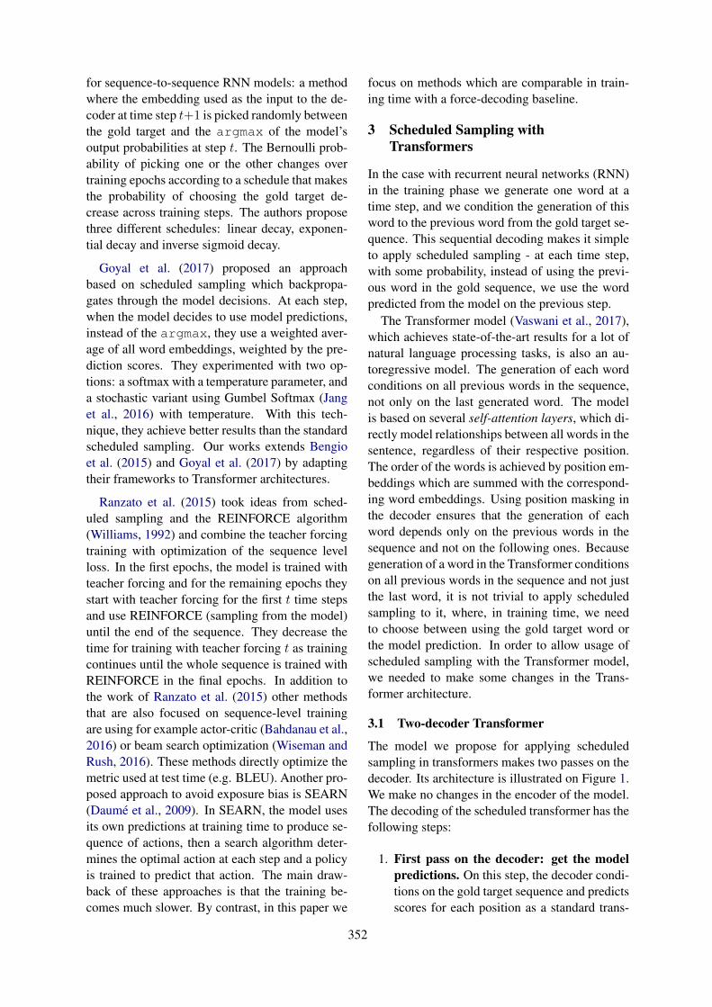
for sequence-to-sequence RNN models: a methodwhere the embedding used as the input to the de-coder at time step t+1 is picked randomly betweenthe gold target and the argmax of the model’soutput probabilities at step t. The Bernoulli prob-ability of picking one or the other changes overtraining epochs according to a schedule that makesthe probability of choosing the gold target de-crease across training steps. The authors proposethree different schedules: linear decay, exponen-tial decay and inverse sigmoid decay.

Goyal et al. (2017) proposed an approachbased on scheduled sampling which backpropa-gates through the model decisions. At each step,when the model decides to use model predictions,instead of the argmax, they use a weighted aver-age of all word embeddings, weighted by the pre-diction scores. They experimented with two op-tions: a softmax with a temperature parameter, anda stochastic variant using Gumbel Softmax (Janget al., 2016) with temperature. With this tech-nique, they achieve better results than the standardscheduled sampling. Our works extends Bengioet al. (2015) and Goyal et al. (2017) by adaptingtheir frameworks to Transformer architectures.

Ranzato et al. (2015) took ideas from sched-uled sampling and the REINFORCE algorithm(Williams, 1992) and combine the teacher forcingtraining with optimization of the sequence levelloss. In the first epochs, the model is trained withteacher forcing and for the remaining epochs theystart with teacher forcing for the first t time stepsand use REINFORCE (sampling from the model)until the end of the sequence. They decrease thetime for training with teacher forcing t as trainingcontinues until the whole sequence is trained withREINFORCE in the final epochs. In addition tothe work of Ranzato et al. (2015) other methodsthat are also focused on sequence-level trainingare using for example actor-critic (Bahdanau et al.,2016) or beam search optimization (Wiseman andRush, 2016). These methods directly optimize themetric used at test time (e.g. BLEU). Another pro-posed approach to avoid exposure bias is SEARN(Daume et al., 2009). In SEARN, the model usesits own predictions at training time to produce se-quence of actions, then a search algorithm deter-mines the optimal action at each step and a policyis trained to predict that action. The main draw-back of these approaches is that the training be-comes much slower. By contrast, in this paper we

focus on methods which are comparable in train-ing time with a force-decoding baseline.

3 Scheduled Sampling withTransformers

In the case with recurrent neural networks (RNN)in the training phase we generate one word at atime step, and we condition the generation of thisword to the previous word from the gold target se-quence. This sequential decoding makes it simpleto apply scheduled sampling - at each time step,with some probability, instead of using the previ-ous word in the gold sequence, we use the wordpredicted from the model on the previous step.

The Transformer model (Vaswani et al., 2017),which achieves state-of-the-art results for a lot ofnatural language processing tasks, is also an au-toregressive model. The generation of each wordconditions on all previous words in the sequence,not only on the last generated word. The modelis based on several self-attention layers, which di-rectly model relationships between all words in thesentence, regardless of their respective position.The order of the words is achieved by position em-beddings which are summed with the correspond-ing word embeddings. Using position masking inthe decoder ensures that the generation of eachword depends only on the previous words in thesequence and not on the following ones. Becausegeneration of a word in the Transformer conditionson all previous words in the sequence and not justthe last word, it is not trivial to apply scheduledsampling to it, where, in training time, we needto choose between using the gold target word orthe model prediction. In order to allow usage ofscheduled sampling with the Transformer model,we needed to make some changes in the Trans-former architecture.

3.1 Two-decoder Transformer

The model we propose for applying scheduledsampling in transformers makes two passes on thedecoder. Its architecture is illustrated on Figure 1.We make no changes in the encoder of the model.The decoding of the scheduled transformer has thefollowing steps:

1. First pass on the decoder: get the modelpredictions. On this step, the decoder condi-tions on the gold target sequence and predictsscores for each position as a standard trans-

352

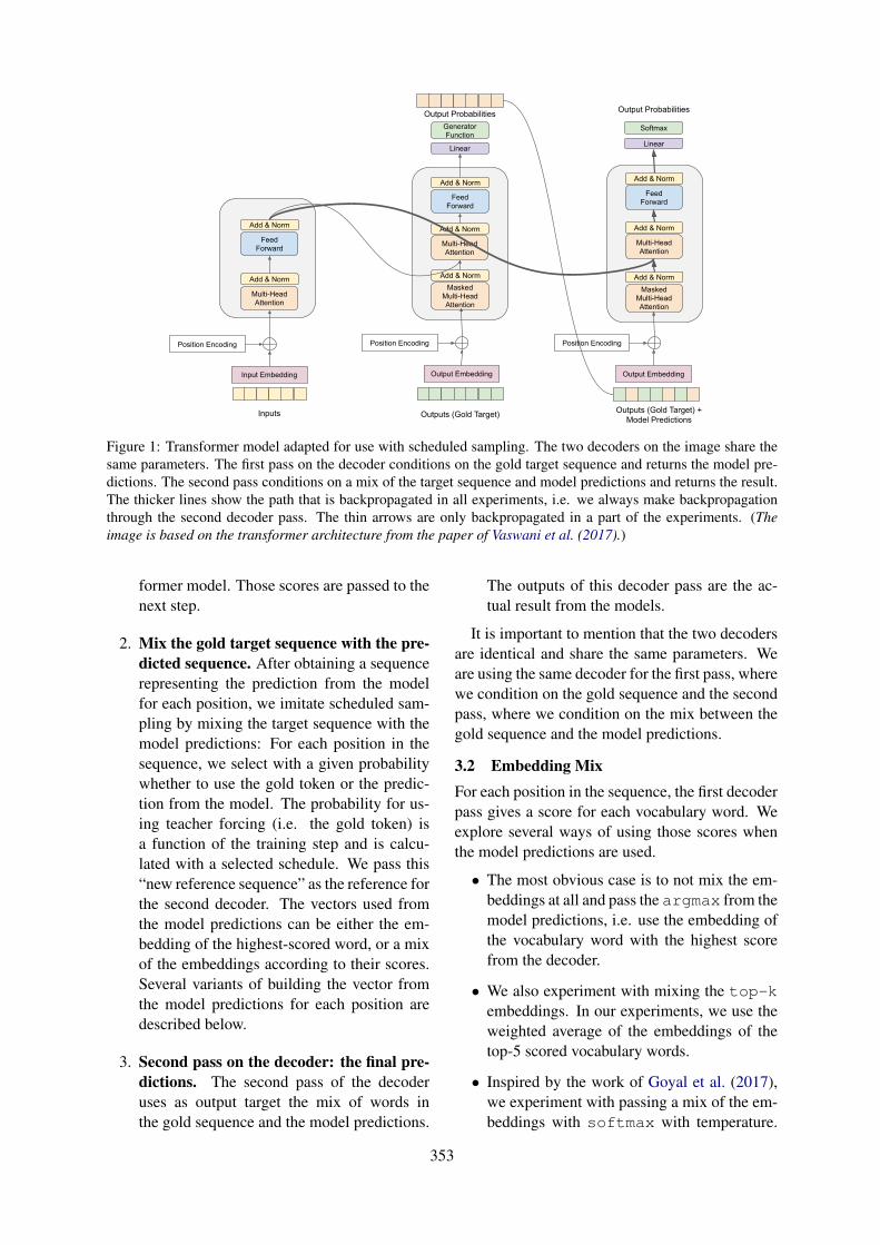
Masked Multi-Head Attention

Add & Norm

Feed Forward

Add & Norm

Masked Multi-Head Attention

Add & Norm

Feed Forward

Add & Norm

Multi-Head Attention

Add & Norm

Output Embedding

Multi-Head Attention

Add & Norm

Feed Forward

Add & Norm

Input Embedding

Position Encoding

Output Embedding

Position Encoding

Inputs Outputs (Gold Target) Outputs (Gold Target) + Model Predictions

Linear

Generator Function

Output Probabilities

Linear

Softmax

Output Probabilities

Position Encoding

Add & Norm

Multi-Head Attention

Figure 1: Transformer model adapted for use with scheduled sampling. The two decoders on the image share thesame parameters. The first pass on the decoder conditions on the gold target sequence and returns the model pre-dictions. The second pass conditions on a mix of the target sequence and model predictions and returns the result.The thicker lines show the path that is backpropagated in all experiments, i.e. we always make backpropagationthrough the second decoder pass. The thin arrows are only backpropagated in a part of the experiments. (Theimage is based on the transformer architecture from the paper of Vaswani et al. (2017).)

former model. Those scores are passed to thenext step.

2. Mix the gold target sequence with the pre-dicted sequence. After obtaining a sequencerepresenting the prediction from the modelfor each position, we imitate scheduled sam-pling by mixing the target sequence with themodel predictions: For each position in thesequence, we select with a given probabilitywhether to use the gold token or the predic-tion from the model. The probability for us-ing teacher forcing (i.e. the gold token) isa function of the training step and is calcu-lated with a selected schedule. We pass this“new reference sequence” as the reference forthe second decoder. The vectors used fromthe model predictions can be either the em-bedding of the highest-scored word, or a mixof the embeddings according to their scores.Several variants of building the vector fromthe model predictions for each position aredescribed below.

3. Second pass on the decoder: the final pre-dictions. The second pass of the decoderuses as output target the mix of words inthe gold sequence and the model predictions.

The outputs of this decoder pass are the ac-tual result from the models.

It is important to mention that the two decodersare identical and share the same parameters. Weare using the same decoder for the first pass, wherewe condition on the gold sequence and the secondpass, where we condition on the mix between thegold sequence and the model predictions.

3.2 Embedding MixFor each position in the sequence, the first decoderpass gives a score for each vocabulary word. Weexplore several ways of using those scores whenthe model predictions are used.

• The most obvious case is to not mix the em-beddings at all and pass the argmax from themodel predictions, i.e. use the embedding ofthe vocabulary word with the highest scorefrom the decoder.

• We also experiment with mixing the top-kembeddings. In our experiments, we use theweighted average of the embeddings of thetop-5 scored vocabulary words.

• Inspired by the work of Goyal et al. (2017),we experiment with passing a mix of the em-beddings with softmax with temperature.

353

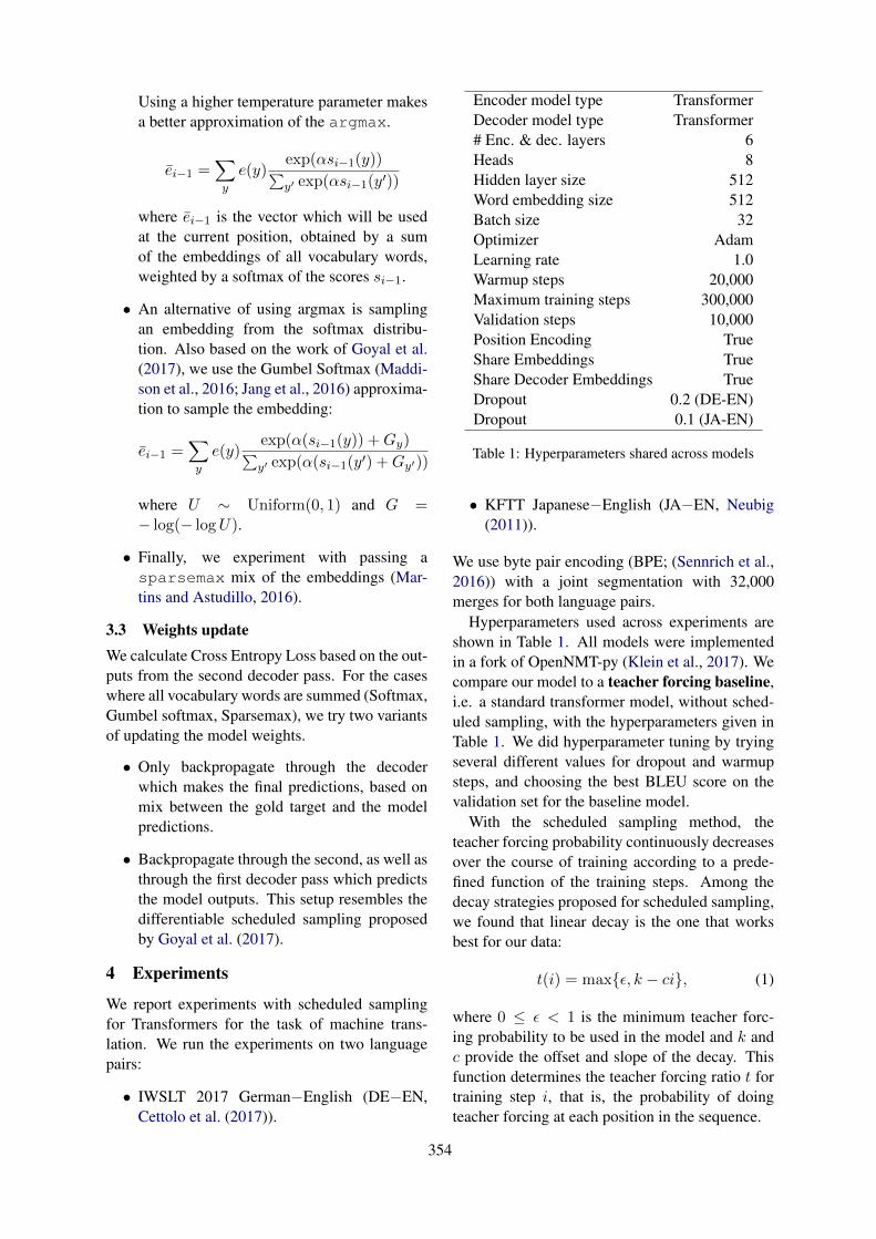
Using a higher temperature parameter makesa better approximation of the argmax.

ei−1 =∑

y

e(y)exp(αsi−1(y))∑y′ exp(αsi−1(y′))

where ei−1 is the vector which will be usedat the current position, obtained by a sumof the embeddings of all vocabulary words,weighted by a softmax of the scores si−1.

• An alternative of using argmax is samplingan embedding from the softmax distribu-tion. Also based on the work of Goyal et al.(2017), we use the Gumbel Softmax (Maddi-son et al., 2016; Jang et al., 2016) approxima-tion to sample the embedding:

ei−1 =∑

y

e(y)exp(α(si−1(y)) +Gy)∑y′ exp(α(si−1(y′) +Gy′))

where U ∼ Uniform(0, 1) and G =− log(− logU).

• Finally, we experiment with passing asparsemax mix of the embeddings (Mar-tins and Astudillo, 2016).

3.3 Weights updateWe calculate Cross Entropy Loss based on the out-puts from the second decoder pass. For the caseswhere all vocabulary words are summed (Softmax,Gumbel softmax, Sparsemax), we try two variantsof updating the model weights.

• Only backpropagate through the decoderwhich makes the final predictions, based onmix between the gold target and the modelpredictions.

• Backpropagate through the second, as well asthrough the first decoder pass which predictsthe model outputs. This setup resembles thedifferentiable scheduled sampling proposedby Goyal et al. (2017).

4 Experiments

We report experiments with scheduled samplingfor Transformers for the task of machine trans-lation. We run the experiments on two languagepairs:

• IWSLT 2017 German−English (DE−EN,Cettolo et al. (2017)).

Encoder model type TransformerDecoder model type Transformer# Enc. & dec. layers 6Heads 8Hidden layer size 512Word embedding size 512Batch size 32Optimizer AdamLearning rate 1.0Warmup steps 20,000Maximum training steps 300,000Validation steps 10,000Position Encoding TrueShare Embeddings TrueShare Decoder Embeddings TrueDropout 0.2 (DE-EN)Dropout 0.1 (JA-EN)

Table 1: Hyperparameters shared across models

• KFTT Japanese−English (JA−EN, Neubig(2011)).

We use byte pair encoding (BPE; (Sennrich et al.,2016)) with a joint segmentation with 32,000merges for both language pairs.

Hyperparameters used across experiments areshown in Table 1. All models were implementedin a fork of OpenNMT-py (Klein et al., 2017). Wecompare our model to a teacher forcing baseline,i.e. a standard transformer model, without sched-uled sampling, with the hyperparameters given inTable 1. We did hyperparameter tuning by tryingseveral different values for dropout and warmupsteps, and choosing the best BLEU score on thevalidation set for the baseline model.

With the scheduled sampling method, theteacher forcing probability continuously decreasesover the course of training according to a prede-fined function of the training steps. Among thedecay strategies proposed for scheduled sampling,we found that linear decay is the one that worksbest for our data:

t(i) = maxε, k − ci, (1)

where 0 ≤ ε < 1 is the minimum teacher forc-ing probability to be used in the model and k andc provide the offset and slope of the decay. Thisfunction determines the teacher forcing ratio t fortraining step i, that is, the probability of doingteacher forcing at each position in the sequence.

354

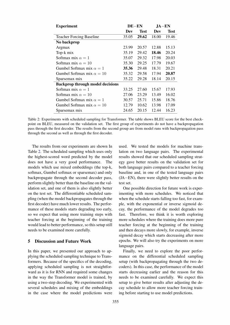
Experiment DE−EN JA−ENDev Test Dev Test

Teacher Forcing Baseline 35.05 29.62 18.00 19.46No backpropArgmax 23.99 20.57 12.88 15.13Top-k mix 35.19 29.42 18.46 20.24Softmax mix α = 1 35.07 29.32 17.98 20.03Softmax mix α = 10 35.30 29.25 17.79 19.67Gumbel Softmax mix α = 1 35.36 29.48 18.31 20.21Gumbel Softmax mix α = 10 35.32 29.58 17.94 20.87Sparsemax mix 35.22 29.28 18.14 20.15Backprop through model decisionsSoftmax mix α = 1 33.25 27.60 15.67 17.93Softmax mix α = 10 27.06 23.29 13.49 16.02Gumbel Softmax mix α = 1 30.57 25.71 15.86 18.76Gumbel Softmax mix α = 10 12.79 10.62 13.98 17.09Sparsemax mix 24.65 20.15 12.44 16.23

Table 2: Experiments with scheduled sampling for Transformer. The table shows BLEU score for the best check-point on BLEU, measured on the validation set. The first group of experiments do not have a backpropagationpass through the first decoder. The results from the second group are from model runs with backpropagation passthrough the second as well as through the first decoder.

The results from our experiments are shown InTable 2. The scheduled sampling which uses onlythe highest-scored word predicted by the modeldoes not have a very good performance. Themodels which use mixed embeddings (the top-k,softmax, Gumbel softmax or sparsemax) and onlybackpropagate through the second decoder pass,perform slightly better than the baseline on the val-idation set, and one of them is also slightly betteron the test set. The differentiable scheduled sam-pling (when the model backpropagates through thefirst decoder) have much lower results. The perfor-mance of these models starts degrading too early,so we expect that using more training steps withteacher forcing at the beginning of the trainingwould lead to better performance, so this setup stillneeds to be examined more carefully.

5 Discussion and Future Work

In this paper, we presented our approach to ap-plying the scheduled sampling technique to Trans-formers. Because of the specifics of the decoding,applying scheduled sampling is not straightfor-ward as it is for RNN and required some changesin the way the Transformer model is trained, byusing a two-step decoding. We experimented withseveral schedules and mixing of the embeddingsin the case where the model predictions were

used. We tested the models for machine trans-lation on two language pairs. The experimentalresults showed that our scheduled sampling strat-egy gave better results on the validation set forboth language pairs compared to a teacher forcingbaseline and, in one of the tested language pairs(JA−EN), there were slightly better results on thetest set.

One possible direction for future work is exper-imenting with more schedules. We noticed thatwhen the schedule starts falling too fast, for exam-ple, with the exponential or inverse sigmoid de-cay, the performance of the model degrades toofast. Therefore, we think it is worth exploringmore schedules where the training does more pureteacher forcing at the beginning of the trainingand then decays more slowly, for example, inversesigmoid decay which starts decreasing after moreepochs. We will also try the experiments on morelanguage pairs.

Finally, we need to explore the poor perfor-mance on the differential scheduled samplingsetup (with backpropagating through the two de-coders). In this case, the performance of the modelstarts decreasing earlier and the reason for thisneeds to be examined carefully. We expect thissetup to give better results after adjusting the de-cay schedule to allow more teacher forcing train-ing before starting to use model predictions.

355

Acknowledgments

This work was supported by the European Re-search Council (ERC StG DeepSPIN 758969),and by the Fundacao para a Ciencia e Tecnolo-gia through contracts UID/EEA/50008/2019 andCMUPERI/TIC/0046/2014 (GoLocal). We wouldlike to thank Goncalo Correia and Ben Petersfor their involvement on an earlier stage of thisproject.

ReferencesDzmitry Bahdanau, Philemon Brakel, Kelvin Xu,

Anirudh Goyal, Ryan Lowe, Joelle Pineau, AaronCourville, and Yoshua Bengio. 2016. An actor-criticalgorithm for sequence prediction. arXiv preprintarXiv:1607.07086.

Dzmitry Bahdanau, Kyunghyun Cho, and Yoshua Ben-gio. 2014. Neural machine translation by jointlylearning to align and translate. arXiv preprintarXiv:1409.0473.

Samy Bengio, Oriol Vinyals, Navdeep Jaitly, andNoam Shazeer. 2015. Scheduled sampling for se-quence prediction with recurrent neural networks.In Advances in Neural Information Processing Sys-tems, pages 1171–1179.

Mauro Cettolo, Marcello Federico, Luisa Bentivogli,Niehues Jan, Stuker Sebastian, Sudoh Katsuitho,Yoshino Koichiro, and Federmann Christian. 2017.Overview of the iwslt 2017 evaluation campaign. InInternational Workshop on Spoken Language Trans-lation, pages 2–14.

Hal Daume, John Langford, and Daniel Marcu. 2009.Search-based structured prediction. Machine learn-ing, 75(3):297–325.

Kartik Goyal, Chris Dyer, and Taylor Berg-Kirkpatrick. 2017. Differentiable scheduledsampling for credit assignment. arXiv preprintarXiv:1704.06970.

Eric Jang, Shixiang Gu, and Ben Poole. 2016. Categor-ical reparameterization with gumbel-softmax. arXivpreprint arXiv:1611.01144.

G. Klein, Y. Kim, Y. Deng, J. Senellart, and A. M.Rush. 2017. OpenNMT: Open-Source Toolkit forNeural Machine Translation. ArXiv e-prints.

Chris J Maddison, Andriy Mnih, and Yee Whye Teh.2016. The concrete distribution: A continuousrelaxation of discrete random variables. arXivpreprint arXiv:1611.00712.

Andre Martins and Ramon Astudillo. 2016. From soft-max to sparsemax: A sparse model of attention andmulti-label classification. In International Confer-ence on Machine Learning, pages 1614–1623.

Graham Neubig. 2011. The kyoto free translation task.

Marc’Aurelio Ranzato, Sumit Chopra, Michael Auli,and Wojciech Zaremba. 2015. Sequence level train-ing with recurrent neural networks. arXiv preprintarXiv:1511.06732.

Rico Sennrich, Barry Haddow, and Alexandra Birch.2016. Neural machine translation of rare words withsubword units. arXiv preprint arXiv:1508.07909.

Ilya Sutskever, Oriol Vinyals, and Quoc V Le. 2014.Sequence to sequence learning with neural net-works. In Advances in neural information process-ing systems, pages 3104–3112.

Ashish Vaswani, Noam Shazeer, Niki Parmar, JakobUszkoreit, Llion Jones, Aidan N Gomez, ŁukaszKaiser, and Illia Polosukhin. 2017. Attention is allyou need. In Advances in Neural Information Pro-cessing Systems, pages 5998–6008.

Ronald J Williams. 1992. Simple statistical gradient-following algorithms for connectionist reinforce-ment learning. Machine learning, 8(3-4):229–256.

Sam Wiseman and Alexander M Rush. 2016.Sequence-to-sequence learning as beam-search opti-mization. In Proceedings of the 2016 Conference onEmpirical Methods in Natural Language Process-ing, pages 1296–1306.

356

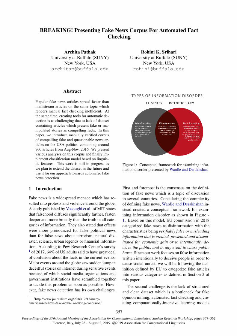
Proceedings of the 57th Annual Meeting of the Association for Computational Linguistics: Student Research Workshop, pages 357–362Florence, Italy, July 28 - August 2, 2019. c©2019 Association for Computational Linguistics

BREAKING! Presenting Fake News Corpus For Automated FactChecking

Archita PathakUniversity at Buffalo (SUNY)

New York, USAarchitap@buffalo.edu

Rohini K. SrihariUniversity at Buffalo (SUNY)

New York, USArohini@buffalo.edu

Abstract

Popular fake news articles spread faster thanmainstream articles on the same topic whichrenders manual fact checking inefficient. Atthe same time, creating tools for automatic de-tection is as challenging due to lack of datasetcontaining articles which present fake or ma-nipulated stories as compelling facts. In thispaper, we introduce manually verified corpusof compelling fake and questionable news ar-ticles on the USA politics, containing around700 articles from Aug-Nov, 2016. We presentvarious analyses on this corpus and finally im-plement classification model based on linguis-tic features. This work is still in progress aswe plan to extend the dataset in the future anduse it for our approach towards automated fakenews detection.

1 Introduction

Fake news is a widespread menace which has re-sulted into protests and violence around the globe.A study published by Vosoughi et al. of MIT statesthat falsehood diffuses significantly farther, faster,deeper and more broadly than the truth in all cate-gories of information. They also stated that effectswere more pronounced for false political newsthan for false news about terrorism, natural dis-aster, science, urban legends or financial informa-tion. According to Pew Research Center’s survey1 of 2017, 64% of US adults said to have great dealof confusion about the facts in the current events.Major events around the globe saw sudden jump indeceitful stories on internet during sensitive eventsbecause of which social media organizations andgovernment institutions have scrambled togetherto tackle this problem as soon as possible. How-ever, fake news detection has its own challenges.

1http://www.journalism.org/2016/12/15/many-americans-believe-fake-news-is-sowing-confusion/

Figure 1: Conceptual framework for examining infor-mation disorder presented by Wardle and Derakhshan

First and foremost is the consensus on the defini-tion of fake news which is a topic of discussionin several countries. Considering the complexityof defining fake news, Wardle and Derakhshan in-stead created a conceptual framework for exam-ining information disorder as shown in Figure -1. Based on this model, EU commission in 2018categorized fake news as disinformation with thecharacteristics being verifiably false or misleadinginformation that is created, presented and dissem-inated for economic gain or to intentionally de-ceive the public, and in any event to cause publicharm. Since our work focuses on false informationwritten intentionally to deceive people in order tocause social unrest, we will be following the def-inition defined by EU to categorize fake articlesinto various categories as defined in Section 3 ofthis paper.

The second challenge is the lack of structuredand clean dataset which is a bottleneck for fakeopinion mining, automated fact checking and cre-ating computationally-intensive learning models

357

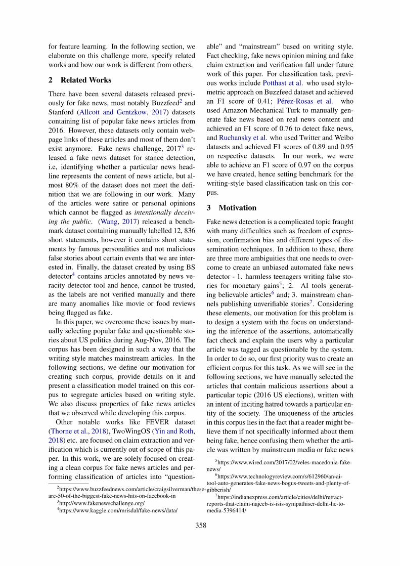
for feature learning. In the following section, weelaborate on this challenge more, specify relatedworks and how our work is different from others.

2 Related Works

There have been several datasets released previ-ously for fake news, most notably Buzzfeed2 andStanford (Allcott and Gentzkow, 2017) datasetscontaining list of popular fake news articles from2016. However, these datasets only contain web-page links of these articles and most of them don’texist anymore. Fake news challenge, 20173 re-leased a fake news dataset for stance detection,i.e, identifying whether a particular news head-line represents the content of news article, but al-most 80% of the dataset does not meet the defi-nition that we are following in our work. Manyof the articles were satire or personal opinionswhich cannot be flagged as intentionally deceiv-ing the public. (Wang, 2017) released a bench-mark dataset containing manually labelled 12, 836short statements, however it contains short state-ments by famous personalities and not maliciousfalse stories about certain events that we are inter-ested in. Finally, the dataset created by using BSdetector4 contains articles annotated by news ve-racity detector tool and hence, cannot be trusted,as the labels are not verified manually and thereare many anomalies like movie or food reviewsbeing flagged as fake.

In this paper, we overcome these issues by man-ually selecting popular fake and questionable sto-ries about US politics during Aug-Nov, 2016. Thecorpus has been designed in such a way that thewriting style matches mainstream articles. In thefollowing sections, we define our motivation forcreating such corpus, provide details on it andpresent a classification model trained on this cor-pus to segregate articles based on writing style.We also discuss properties of fake news articlesthat we observed while developing this corpus.

Other notable works like FEVER dataset(Thorne et al., 2018), TwoWingOS (Yin and Roth,2018) etc. are focused on claim extraction and ver-ification which is currently out of scope of this pa-per. In this work, we are solely focused on creat-ing a clean corpus for fake news articles and per-forming classification of articles into “question-

2https://www.buzzfeednews.com/article/craigsilverman/these-are-50-of-the-biggest-fake-news-hits-on-facebook-in

3http://www.fakenewschallenge.org/4https://www.kaggle.com/mrisdal/fake-news/data/

able” and “mainstream” based on writing style.Fact checking, fake news opinion mining and fakeclaim extraction and verification fall under futurework of this paper. For classification task, previ-ous works include Potthast et al. who used stylo-metric approach on Buzzfeed dataset and achievedan F1 score of 0.41; Perez-Rosas et al. whoused Amazon Mechanical Turk to manually gen-erate fake news based on real news content andachieved an F1 score of 0.76 to detect fake news,and Ruchansky et al. who used Twitter and Weibodatasets and achieved F1 scores of 0.89 and 0.95on respective datasets. In our work, we wereable to achieve an F1 score of 0.97 on the corpuswe have created, hence setting benchmark for thewriting-style based classification task on this cor-pus.

3 Motivation

Fake news detection is a complicated topic fraughtwith many difficulties such as freedom of expres-sion, confirmation bias and different types of dis-semination techniques. In addition to these, thereare three more ambiguities that one needs to over-come to create an unbiased automated fake newsdetector - 1. harmless teenagers writing false sto-ries for monetary gains5; 2. AI tools generat-ing believable articles6 and; 3. mainstream chan-nels publishing unverifiable stories7. Consideringthese elements, our motivation for this problem isto design a system with the focus on understand-ing the inference of the assertions, automaticallyfact check and explain the users why a particulararticle was tagged as questionable by the system.In order to do so, our first priority was to create anefficient corpus for this task. As we will see in thefollowing sections, we have manually selected thearticles that contain malicious assertions about aparticular topic (2016 US elections), written withan intent of inciting hatred towards a particular en-tity of the society. The uniqueness of the articlesin this corpus lies in the fact that a reader might be-lieve them if not specifically informed about thembeing fake, hence confusing them whether the arti-cle was written by mainstream media or fake news

5https://www.wired.com/2017/02/veles-macedonia-fake-news/

6https://www.technologyreview.com/s/612960/an-ai-tool-auto-generates-fake-news-bogus-tweets-and-plenty-of-gibberish/

7https://indianexpress.com/article/cities/delhi/retract-reports-that-claim-najeeb-is-isis-sympathiser-delhi-hc-to-media-5396414/

358

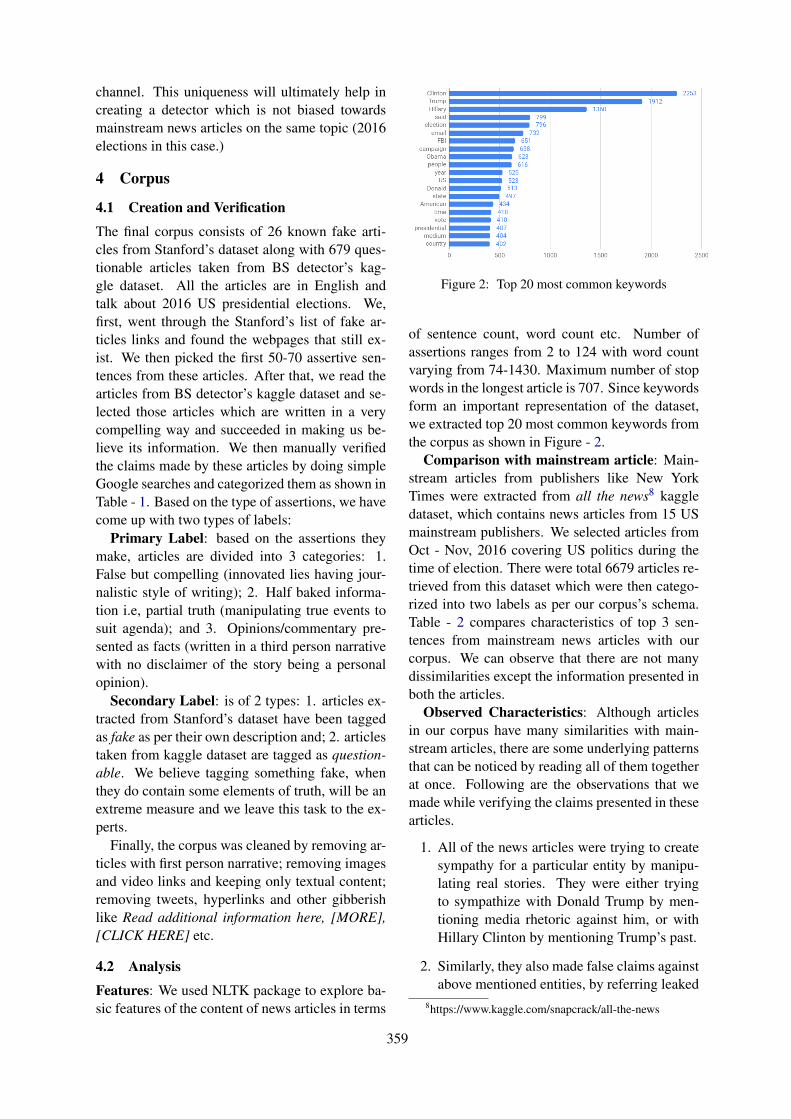
channel. This uniqueness will ultimately help increating a detector which is not biased towardsmainstream news articles on the same topic (2016elections in this case.)

4 Corpus

4.1 Creation and Verification

The final corpus consists of 26 known fake arti-cles from Stanford’s dataset along with 679 ques-tionable articles taken from BS detector’s kag-gle dataset. All the articles are in English andtalk about 2016 US presidential elections. We,first, went through the Stanford’s list of fake ar-ticles links and found the webpages that still ex-ist. We then picked the first 50-70 assertive sen-tences from these articles. After that, we read thearticles from BS detector’s kaggle dataset and se-lected those articles which are written in a verycompelling way and succeeded in making us be-lieve its information. We then manually verifiedthe claims made by these articles by doing simpleGoogle searches and categorized them as shown inTable - 1. Based on the type of assertions, we havecome up with two types of labels:

Primary Label: based on the assertions theymake, articles are divided into 3 categories: 1.False but compelling (innovated lies having jour-nalistic style of writing); 2. Half baked informa-tion i.e, partial truth (manipulating true events tosuit agenda); and 3. Opinions/commentary pre-sented as facts (written in a third person narrativewith no disclaimer of the story being a personalopinion).

Secondary Label: is of 2 types: 1. articles ex-tracted from Stanford’s dataset have been taggedas fake as per their own description and; 2. articlestaken from kaggle dataset are tagged as question-able. We believe tagging something fake, whenthey do contain some elements of truth, will be anextreme measure and we leave this task to the ex-perts.

Finally, the corpus was cleaned by removing ar-ticles with first person narrative; removing imagesand video links and keeping only textual content;removing tweets, hyperlinks and other gibberishlike Read additional information here, [MORE],[CLICK HERE] etc.

4.2 Analysis

Features: We used NLTK package to explore ba-sic features of the content of news articles in terms

Figure 2: Top 20 most common keywords

of sentence count, word count etc. Number ofassertions ranges from 2 to 124 with word countvarying from 74-1430. Maximum number of stopwords in the longest article is 707. Since keywordsform an important representation of the dataset,we extracted top 20 most common keywords fromthe corpus as shown in Figure - 2.

Comparison with mainstream article: Main-stream articles from publishers like New YorkTimes were extracted from all the news8 kaggledataset, which contains news articles from 15 USmainstream publishers. We selected articles fromOct - Nov, 2016 covering US politics during thetime of election. There were total 6679 articles re-trieved from this dataset which were then catego-rized into two labels as per our corpus’s schema.Table - 2 compares characteristics of top 3 sen-tences from mainstream news articles with ourcorpus. We can observe that there are not manydissimilarities except the information presented inboth the articles.

Observed Characteristics: Although articlesin our corpus have many similarities with main-stream articles, there are some underlying patternsthat can be noticed by reading all of them togetherat once. Following are the observations that wemade while verifying the claims presented in thesearticles.

1. All of the news articles were trying to createsympathy for a particular entity by manipu-lating real stories. They were either tryingto sympathize with Donald Trump by men-tioning media rhetoric against him, or withHillary Clinton by mentioning Trump’s past.

2. Similarly, they also made false claims againstabove mentioned entities, by referring leaked

8https://www.kaggle.com/snapcrack/all-the-news

359

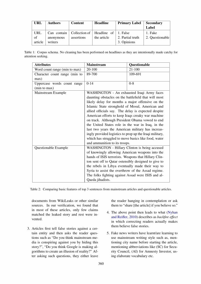
URL Authors Content Headline Primary Label SecondaryLabel

URLofarticle

Can containanonymouswriters

Collection ofassertions

Headline ofthe article

1. False2. Partial truth3. Opinions

1. Fake2. Questionable

Table 1: Corpus schema. No cleaning has been performed on headlines as they are intentionally made catchy forattention seeking.

Attributes Mainstream QuestionableWord count range (min to max) 20-100 21-100Character count range (min tomax)

89-700 109-691

Uppercase words count range(min to max)

0-14 0-8

Mainstream Example WASHINGTON - An exhausted Iraqi Army facesdaunting obstacles on the battlefield that will mostlikely delay for months a major offensive on theIslamic State stronghold of Mosul, American andallied officials say. The delay is expected despiteAmerican efforts to keep Iraqs creaky war machineon track. Although President Obama vowed to endthe United States role in the war in Iraq, in thelast two years the American military has increas-ingly provided logistics to prop up the Iraqi military,which has struggled to move basics like food, waterand ammunition to its troops.

Questionable Example WASHINGTON - Hillary Clinton is being accusedof knowingly allowing American weapons into thehands of ISIS terrorists. Weapons that Hillary Clin-ton sent off to Qatar ostensibly designed to give tothe rebels in Libya eventually made their way toSyria to assist the overthrow of the Assad regime.The folks fighting against Assad were ISIS and al-Qaeda jihadists.

Table 2: Comparing basic features of top 3 sentences from mainstream articles and questionable articles.

documents from WikiLeaks or other similarsources. In our verification, we found thatin most of these articles, only few claimsmatched the leaked story and rest were in-vented.

3. Articles first tell false stories against a cer-tain entity and then asks the reader ques-tions such as “Do you think mainstream me-dia is conspiring against you by hiding thisstory?”, “Do you think Google is making al-gorithms to create an illusion of reality?” Af-ter asking such questions, they either leave

the reader hanging in contemplation or askthem to “share [the article] if you believe so.”

4. The above point then leads to what (Nyhanand Reifler, 2010) describes as backfire effectin which correcting readers actually makesthem believe false stories.

5. Fake news writers have learnt/are learning touse mainstream writing style such as, men-tioning city name before starting the article,mentioning abbreviations like (SC) for Secu-rity Council, (AI) for Amnesty Investor, us-ing elaborate vocabulary etc.

360

SplitRandom K-Fold

Questionable (1) Mainstream (0) Questionable (1) Mainstream (0)

Train 406 5334 396 5343Test 90 1345 100 1336

Table 3: To meet the real world scenario, train data and test data have been split with an approximate ratio of 1:10.

Figure 3: Bi-directional architecture

5 Classification Task

5.1 Model

After creating this corpus, we trained a classifi-cation model on the content to see if it can learnany writing patterns which are not visible to hu-man eye and create benchmark results. Our model,as shown in Figure - 3, is inspired by the works of(Anand et al., 2016) and uses bi-directional LSTMand character embedding to classify articles intoquestionable (1) and mainstream (0) by learningwriting style. We have not performed any pre-processing like removing punctuation, stop wordsetc. to make sure the model learns every contextof the content. 1-D CNN has been used to cre-ate character embedding which has been proven tobe very efficient in learning orthographic and mor-phological features of text (Zhang et al., 2015).This layer takes one-hot vector of each characterand uses filter size of [196, 196, 300]. We haveused 3 layers of 1-D CNN with pool size 2 andkernel stride of 3. Finally, we have performedmaxpooling across the sequence to identify fea-tures that produces strong sentiments. This layeris then connected to bi-directional LSTM whichcontains one forward and one backward layer with128 units each.

This model was trained with top 3 sentences,containing 20-100 words, and retrieved from total

7175 articles. As per the example shown in Ta-ble - 2, it can be assumed that top 3 sentences areenough for a normal reader to understand what thearticle is talking about. Dataset splitting for train-ing and testing was inspired by the findings in thestudy conducted by (Guess et al., 2019) of Prince-ton and NYU earlier this year which stated thatAmericans who shared false stories during 2016Presidential elections were far more likely to beover 65. Current US age demographic suggeststhat 15% of the population are over 65 9. There-fore, we have decided to have the ratio of question-able to mainstream news articles approximately1:10, as shown in Table - 3.

5.2 Training and Results

We first trained our model by randomly splittingour dataset into training, validation and test set ofsizes 4592, 1148 and 1435 respectively. However,since the dataset is unbalanced, stratified k-foldcross-validation mechanism is also implementedwith 5 folds. (Kohavi, 1995) states that stratifica-tion, which ensures that each fold represents theentire dataset, is generally a better scheme bothin terms of bias and variance. The model wastrained on an average number of 2, 296, 000 char-acters. We have evaluated our models on variousmetrics as shown in Figure - 4. For this prob-lem, we will be majorly focused on ROC and F1scores. In both the cases, stratified k-fold out-performs random sampling significantly. Trainingwith only random sampling resulted into under-representation of data points leading to many falsepositives. This can also be because writing styleof questionable and mainstream articles are verysimilar. On the other hand, 5-fold cross validationperformed significantly well in learning the pat-terns and avoiding the problems of false positives.

9https://www.census.gov/quickfacts/fact/table/US/PST045217

361

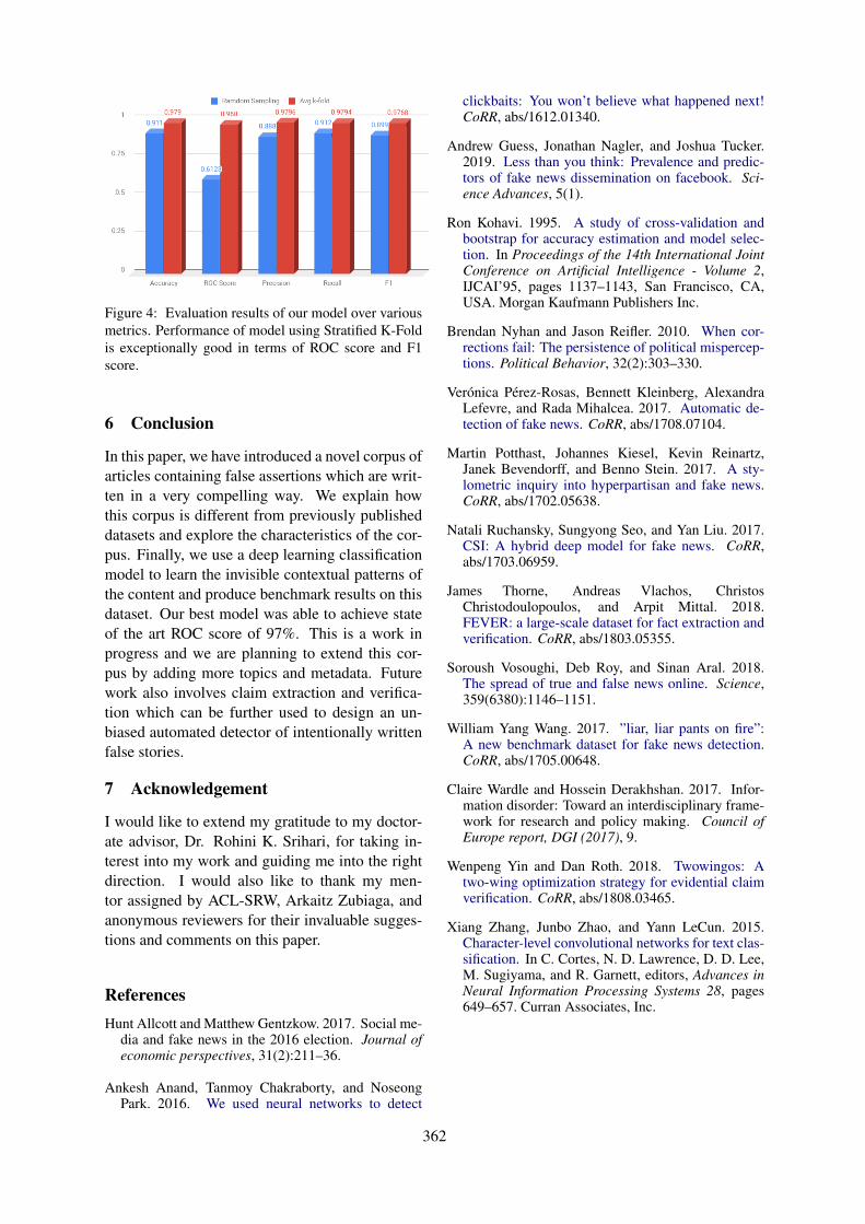
Figure 4: Evaluation results of our model over variousmetrics. Performance of model using Stratified K-Foldis exceptionally good in terms of ROC score and F1score.

6 Conclusion

In this paper, we have introduced a novel corpus ofarticles containing false assertions which are writ-ten in a very compelling way. We explain howthis corpus is different from previously publisheddatasets and explore the characteristics of the cor-pus. Finally, we use a deep learning classificationmodel to learn the invisible contextual patterns ofthe content and produce benchmark results on thisdataset. Our best model was able to achieve stateof the art ROC score of 97%. This is a work inprogress and we are planning to extend this cor-pus by adding more topics and metadata. Futurework also involves claim extraction and verifica-tion which can be further used to design an un-biased automated detector of intentionally writtenfalse stories.

7 Acknowledgement

I would like to extend my gratitude to my doctor-ate advisor, Dr. Rohini K. Srihari, for taking in-terest into my work and guiding me into the rightdirection. I would also like to thank my men-tor assigned by ACL-SRW, Arkaitz Zubiaga, andanonymous reviewers for their invaluable sugges-tions and comments on this paper.

ReferencesHunt Allcott and Matthew Gentzkow. 2017. Social me-

dia and fake news in the 2016 election. Journal ofeconomic perspectives, 31(2):211–36.

Ankesh Anand, Tanmoy Chakraborty, and NoseongPark. 2016. We used neural networks to detect

clickbaits: You won’t believe what happened next!CoRR, abs/1612.01340.

Andrew Guess, Jonathan Nagler, and Joshua Tucker.2019. Less than you think: Prevalence and predic-tors of fake news dissemination on facebook. Sci-ence Advances, 5(1).

Ron Kohavi. 1995. A study of cross-validation andbootstrap for accuracy estimation and model selec-tion. In Proceedings of the 14th International JointConference on Artificial Intelligence - Volume 2,IJCAI’95, pages 1137–1143, San Francisco, CA,USA. Morgan Kaufmann Publishers Inc.

Brendan Nyhan and Jason Reifler. 2010. When cor-rections fail: The persistence of political mispercep-tions. Political Behavior, 32(2):303–330.

Veronica Perez-Rosas, Bennett Kleinberg, AlexandraLefevre, and Rada Mihalcea. 2017. Automatic de-tection of fake news. CoRR, abs/1708.07104.

Martin Potthast, Johannes Kiesel, Kevin Reinartz,Janek Bevendorff, and Benno Stein. 2017. A sty-lometric inquiry into hyperpartisan and fake news.CoRR, abs/1702.05638.

Natali Ruchansky, Sungyong Seo, and Yan Liu. 2017.CSI: A hybrid deep model for fake news. CoRR,abs/1703.06959.

James Thorne, Andreas Vlachos, ChristosChristodoulopoulos, and Arpit Mittal. 2018.FEVER: a large-scale dataset for fact extraction andverification. CoRR, abs/1803.05355.

Soroush Vosoughi, Deb Roy, and Sinan Aral. 2018.The spread of true and false news online. Science,359(6380):1146–1151.

William Yang Wang. 2017. ”liar, liar pants on fire”:A new benchmark dataset for fake news detection.CoRR, abs/1705.00648.

Claire Wardle and Hossein Derakhshan. 2017. Infor-mation disorder: Toward an interdisciplinary frame-work for research and policy making. Council ofEurope report, DGI (2017), 9.

Wenpeng Yin and Dan Roth. 2018. Twowingos: Atwo-wing optimization strategy for evidential claimverification. CoRR, abs/1808.03465.

Xiang Zhang, Junbo Zhao, and Yann LeCun. 2015.Character-level convolutional networks for text clas-sification. In C. Cortes, N. D. Lawrence, D. D. Lee,M. Sugiyama, and R. Garnett, editors, Advances inNeural Information Processing Systems 28, pages649–657. Curran Associates, Inc.

362

Proceedings of the 57th Annual Meeting of the Association for Computational Linguistics: Student Research Workshop, pages 363–370Florence, Italy, July 28 - August 2, 2019. c©2019 Association for Computational Linguistics

Cross-domain and Cross-lingual Abusive Language Detection:a Hybrid Approach with Deep Learning and a Multilingual Lexicon

Endang Wahyu Pamungkas, Viviana PattiDipartimento di Informatica

University of Turin, Italypamungka,patti@di.unito.it

Abstract

The development of computational methods todetect abusive language in social media withinvariable and multilingual contexts has recentlygained significant traction. The growing inter-est is confirmed by the large number of bench-mark corpora for different languages devel-oped in the latest years. However, abusive lan-guage behaviour is multifaceted and availabledatasets are featured by different topical fo-cuses. This makes abusive language detectiona domain-dependent task, and building a ro-bust system to detect general abusive contenta first challenge. Moreover, most resourcesare available for English, which makes de-tecting abusive language in low-resource lan-guages a further challenge. We address bothchallenges by considering ten publicly avail-able datasets across different domains and lan-guages. A hybrid approach with deep learn-ing and a multilingual lexicon to cross-domainand cross-lingual detection of abusive contentis proposed and compared with other simplermodels. We show that training a system ongeneral abusive language datasets will producea cross-domain robust system, which can beused to detect other more specific types of abu-sive content. We also found that using thedomain-independent lexicon HurtLex is usefulto transfer knowledge between domains andlanguages. In the cross-lingual experiment,we demonstrate the effectiveness of our joint-learning model also in out-domain scenarios.

1 Introduction

Detecting online abusive language in social me-dia messages is gaining increasing attention fromscholars and stakeholders, such as governments,social media platforms and citizens. The spread ofonline abusive content negatively affects the tar-geted victims, has a chilling effect on the demo-cratic discourse on social networking platforms

and negatively impacts those who speak for free-dom and non-discrimination. Abusive language isusually used as an umbrella term (Waseem et al.,2017), covering several sub-categories, such as cy-berbullying (Van Hee et al., 2015; Sprugnoli et al.,2018), hate speech (Waseem and Hovy, 2016;Davidson et al., 2017), toxic comments (Wulczynet al., 2017), offensive language (Zampieri et al.,2019a) and online aggression (Kumar et al., 2018).Several datasets have been proposed having dif-ferent topical focuses and specific targets, e.g.,misogyny or racism. This diversity makes the taskto detect general abusive language difficult. Somestudies attempted to bridge some of these subtasksby proposing cross-domain classification of abu-sive content (Wiegand et al., 2018a; Karan andSnajder, 2018; Waseem et al., 2018).

Another prominent challenge in abusive lan-guage detection is the multilinguality issue. Evenif in the last year abusive language datasets weredeveloped for other languages, including Italian(Bosco et al., 2018; Fersini et al., 2018b), Span-ish (Fersini et al., 2018b), and German (Wiegandet al., 2018b), most studies so far focused on En-glish. Since most popular social media such asTwitter and Facebook goes multilingual, fosteringtheir users to interact in their primary language,there is a considerable urgency to develop a robustapproach for abusive language detection in a mul-tilingual environment, also for guaranteeing a bet-ter compliance to governments demands for coun-teracting the phenomenon (see, e.g., the recentlyissued EU commission Code of Conduct on coun-tering illegal hate speech online (EU Commis-sion, 2016). Cross-lingual classification is an ap-proach to transfer knowledge from resource-richlanguages to resource-poor ones. It has been ap-plied to sentiment analysis (Zhou et al., 2016), arelated task to abusive language detection. How-ever, there is still not much work focused on cross-

363

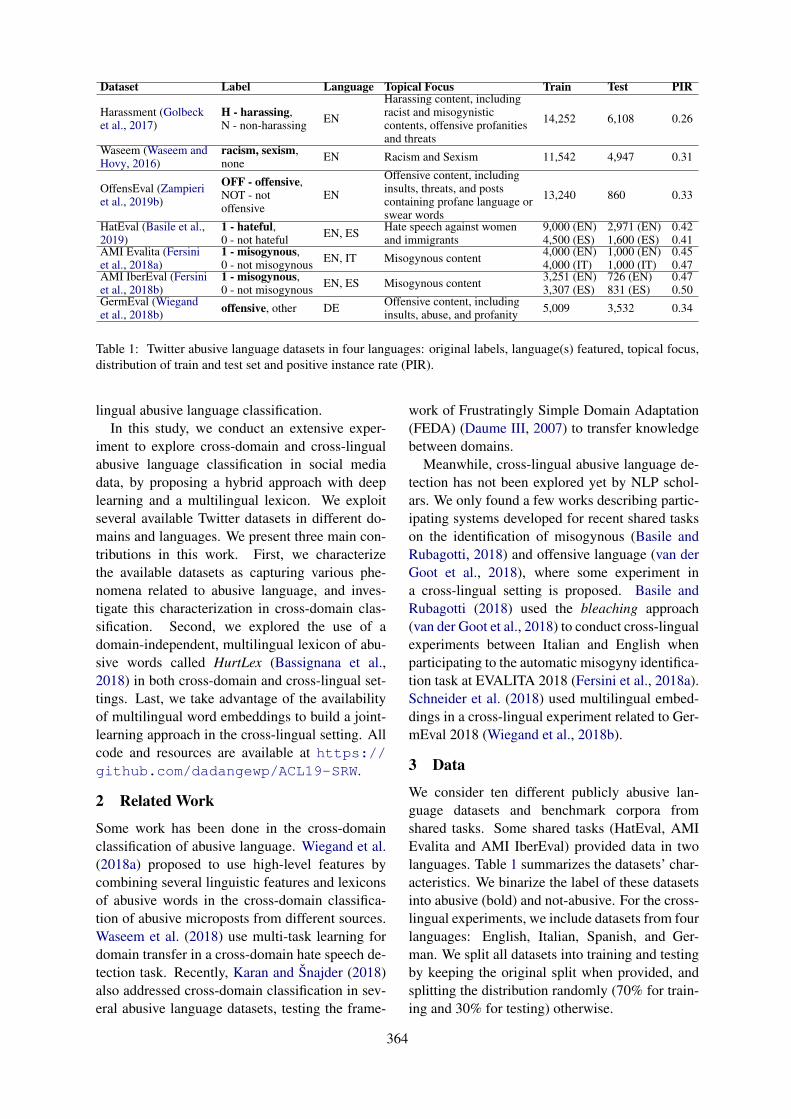
Dataset Label Language Topical Focus Train Test PIR

Harassment (Golbecket al., 2017)

H - harassing,N - non-harassing EN

Harassing content, includingracist and misogynisticcontents, offensive profanitiesand threats

14,252 6,108 0.26

Waseem (Waseem andHovy, 2016)

racism, sexism,none EN Racism and Sexism 11,542 4,947 0.31

OffensEval (Zampieriet al., 2019b)

OFF - offensive,NOT - notoffensive

EN

Offensive content, includinginsults, threats, and postscontaining profane language orswear words

13,240 860 0.33

HatEval (Basile et al.,2019)

1 - hateful,0 - not hateful EN, ES Hate speech against women

and immigrants9,000 (EN)4,500 (ES)

2,971 (EN)1,600 (ES)

0.420.41

AMI Evalita (Fersiniet al., 2018a)

1 - misogynous,0 - not misogynous EN, IT Misogynous content 4,000 (EN)

4,000 (IT)1,000 (EN)1,000 (IT)

0.450.47

AMI IberEval (Fersiniet al., 2018b)

1 - misogynous,0 - not misogynous EN, ES Misogynous content 3,251 (EN)

3,307 (ES)726 (EN)831 (ES)

0.470.50

GermEval (Wiegandet al., 2018b) offensive, other DE Offensive content, including

insults, abuse, and profanity 5,009 3,532 0.34

Table 1: Twitter abusive language datasets in four languages: original labels, language(s) featured, topical focus,distribution of train and test set and positive instance rate (PIR).

lingual abusive language classification.In this study, we conduct an extensive exper-

iment to explore cross-domain and cross-lingualabusive language classification in social mediadata, by proposing a hybrid approach with deeplearning and a multilingual lexicon. We exploitseveral available Twitter datasets in different do-mains and languages. We present three main con-tributions in this work. First, we characterizethe available datasets as capturing various phe-nomena related to abusive language, and inves-tigate this characterization in cross-domain clas-sification. Second, we explored the use of adomain-independent, multilingual lexicon of abu-sive words called HurtLex (Bassignana et al.,2018) in both cross-domain and cross-lingual set-tings. Last, we take advantage of the availabilityof multilingual word embeddings to build a joint-learning approach in the cross-lingual setting. Allcode and resources are available at https://github.com/dadangewp/ACL19-SRW.

2 Related Work

Some work has been done in the cross-domainclassification of abusive language. Wiegand et al.(2018a) proposed to use high-level features bycombining several linguistic features and lexiconsof abusive words in the cross-domain classifica-tion of abusive microposts from different sources.Waseem et al. (2018) use multi-task learning fordomain transfer in a cross-domain hate speech de-tection task. Recently, Karan and Snajder (2018)also addressed cross-domain classification in sev-eral abusive language datasets, testing the frame-

work of Frustratingly Simple Domain Adaptation(FEDA) (Daume III, 2007) to transfer knowledgebetween domains.

Meanwhile, cross-lingual abusive language de-tection has not been explored yet by NLP schol-ars. We only found a few works describing partic-ipating systems developed for recent shared taskson the identification of misogynous (Basile andRubagotti, 2018) and offensive language (van derGoot et al., 2018), where some experiment ina cross-lingual setting is proposed. Basile andRubagotti (2018) used the bleaching approach(van der Goot et al., 2018) to conduct cross-lingualexperiments between Italian and English whenparticipating to the automatic misogyny identifica-tion task at EVALITA 2018 (Fersini et al., 2018a).Schneider et al. (2018) used multilingual embed-dings in a cross-lingual experiment related to Ger-mEval 2018 (Wiegand et al., 2018b).

3 Data

We consider ten different publicly abusive lan-guage datasets and benchmark corpora fromshared tasks. Some shared tasks (HatEval, AMIEvalita and AMI IberEval) provided data in twolanguages. Table 1 summarizes the datasets’ char-acteristics. We binarize the label of these datasetsinto abusive (bold) and not-abusive. For the cross-lingual experiments, we include datasets from fourlanguages: English, Italian, Spanish, and Ger-man. We split all datasets into training and testingby keeping the original split when provided, andsplitting the distribution randomly (70% for train-ing and 30% for testing) otherwise.

364

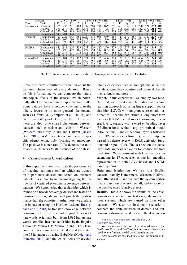
Dataset LSVC + BoW LSVC + BoW + HL LSTM + WE LSTM + WE + HLTest Train P R F1 ∆ P R F1 ∆ P R F1 ∆ P R F1 ∆Harassment Waseem .325 .233 .271 .103 .337 .264 .296 .079 .291 .467 .359 .033 .290 .524 .373 .045

HatEval .389 .119 .183 .191 .374 .116 .177 .198 .341 .308 .324 .068 .332 .379 .354 .064OffensEval .320 .508 .393 -.019 .322 .516 .396 -.021 .333 .443 .380 .012 .314 .567 .404 .014Harassment .547 .284 .374 .540 .288 .375 .510 .319 .392 .464 .380 .418

Waseem Harassment .729 .022 .043 .688 .720 .034 .065 .669 .464 .111 .179 .587 .491 .149 .229 .520HatEval .620 .109 .186 .545 .672 .113 .194 .540 .496 .213 .299 .467 .453 .318 .374 .375OffensEval .461 .390 .422 .309 .453 .391 .420 .314 .444 .282 .345 .421 .419 .411 .415 .334Waseem .817 .662 .731 .819 .665 .734 .760 .771 .766 .711 .790 .749

HatEval Harassment .485 .181 .264 .339 .513 .229 .317 .290 .523 .308 .387 .216 .514 .394 .446 .158Waseem .505 .490 .497 .106 .477 .558 .514 .093 .481 .636 .548 .055 .494 .609 .546 .058OffensEval .450 .646 .531 .072 .451 .656 .534 .073 .452 .603 .516 .087 .457 .704 .554 .050HatEval .449 .919 .603 .453 .919 .607 .444 .939 .603 .441 .955 .604

OffensEval Harassment .301 .104 .155 .422 .321 .113 .167 .406 .525 .133 .213 .395 .406 .179 .249 .349Waseem .440 .246 .316 .261 .462 .254 .328 .245 .403 .225 .289 .319 .400 .175 .244 .354HatEval .372 .225 .281 .296 .381 .233 .289 .284 .392 .371 .381 .227 .371 .529 .436 .162OffensEval .616 .542 .577 .626 .529 .573 .667 .558 .608 .551 .654 .598

Table 2: Results on cross-domain abusive language identification (only in English).

We also provide further information about thecaptured phenomena of every dataset. Basedon this information, we can compare the natureand topical focus of the dataset, which poten-tially affect the cross-domain experimental results.Some datasets have a broader coverage than theothers, focussing on more general phenomena,such as OffensEval (Zampieri et al., 2019b), andGermEval (Wiegand et al., 2018b). However,there are also some shared phenomena betweendatasets, such as racism and sexism in Waseem(Waseem and Hovy, 2016) and HatEval (Basileet al., 2019). AMI datasets contain the most spe-cific phenomenon, only focusing on misogyny.The positive instance rate (PIR) denotes the ratioof abusive instances to all instances of the dataset.

4 Cross-domain Classification

In this experiment, we investigate the performanceof machine learning classifiers which are trainedon a particular dataset and tested on differentdatasets ones. We focus on investigating the in-fluence of captured phenomena coverage betweendatasets. We hypothesize that a classifier which istrained on a broader coverage dataset and tested onnarrower coverage dataset will give better perfor-mance than the opposite. Furthermore, we analysethe impact of using the HurtLex lexicon (Bassig-nana et al., 2018) to transfer knowledge betweendomains. HurtLex is a multilingual lexicon ofhate words, originally built from 1,082 Italian hatewords compiled in a manual fashion by the linguistTullio De Mauro (De Mauro, 2016). This lexi-con is semi-automatically extended and translatedinto 53 languages by using BabelNet (Navigli andPonzetto, 2012), and the lexical items are divided

into 17 categories such as homophobic slurs, eth-nic slurs, genitalia, cognitive and physical disabil-ities, animals and more1.Model. In this experiment, we employ two mod-els. First, we exploit a simple traditional machinelearning approach by using linear support vectorclassifier (LSVC) with unigram representation asa feature. Second, we utilize a long short-termmemory (LSTM) neural model consisting of sev-eral layers, starting with a word embedding layer(32-dimensions) without any pre-trained modelinitialization2. This embedding layer is followedby LSTM networks (16-units), whose output ispassed to a dense layer with ReLU activation func-tion and dropout (0.4). The last section is a denselayer with sigmoid activation to produce the finalprediction. We experiment with HurtLex by con-catenating its 17 categories as one hot encodingrepresentation to both LSVC-based and LSTM-based systems.Data and Evaluation We use four Englishdatasets, namely Harassment, Waseem, HatEval,and OffensEval 3. We evaluate the system perfor-mance based on precision, recall, and F -score onthe positive class (abusive class).Results. Table 2 shows the results of the cross-domain experiment. We test every dataset withthree systems which are trained on three otherdatasets. We also run in-domain scenario tocompare the delta between in-domain and out-domain performance and measure the drop in per-

1http://hatespeech.di.unito.it/resources.html

2We experimented the use of pre-trained models (i.e.GloVe, word2vec, and FastText), but the result is lower com-pared to a self-trained model based on training set.

3AMI datasets are excluded due to the low number of in-stances.

365

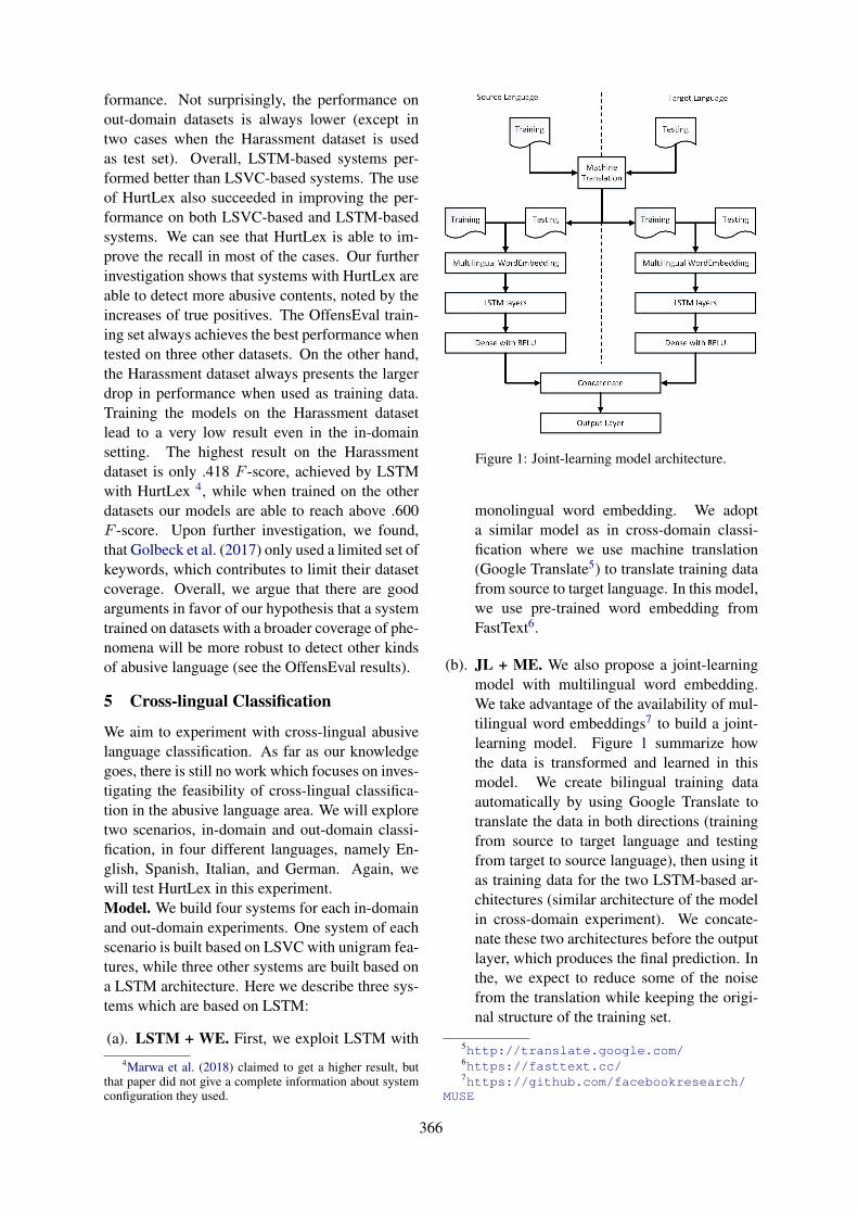
formance. Not surprisingly, the performance onout-domain datasets is always lower (except intwo cases when the Harassment dataset is usedas test set). Overall, LSTM-based systems per-formed better than LSVC-based systems. The useof HurtLex also succeeded in improving the per-formance on both LSVC-based and LSTM-basedsystems. We can see that HurtLex is able to im-prove the recall in most of the cases. Our furtherinvestigation shows that systems with HurtLex areable to detect more abusive contents, noted by theincreases of true positives. The OffensEval train-ing set always achieves the best performance whentested on three other datasets. On the other hand,the Harassment dataset always presents the largerdrop in performance when used as training data.Training the models on the Harassment datasetlead to a very low result even in the in-domainsetting. The highest result on the Harassmentdataset is only .418 F -score, achieved by LSTMwith HurtLex 4, while when trained on the otherdatasets our models are able to reach above .600F -score. Upon further investigation, we found,that Golbeck et al. (2017) only used a limited set ofkeywords, which contributes to limit their datasetcoverage. Overall, we argue that there are goodarguments in favor of our hypothesis that a systemtrained on datasets with a broader coverage of phe-nomena will be more robust to detect other kindsof abusive language (see the OffensEval results).

5 Cross-lingual Classification

We aim to experiment with cross-lingual abusivelanguage classification. As far as our knowledgegoes, there is still no work which focuses on inves-tigating the feasibility of cross-lingual classifica-tion in the abusive language area. We will exploretwo scenarios, in-domain and out-domain classi-fication, in four different languages, namely En-glish, Spanish, Italian, and German. Again, wewill test HurtLex in this experiment.Model. We build four systems for each in-domainand out-domain experiments. One system of eachscenario is built based on LSVC with unigram fea-tures, while three other systems are built based ona LSTM architecture. Here we describe three sys-tems which are based on LSTM:

(a). LSTM + WE. First, we exploit LSTM with4Marwa et al. (2018) claimed to get a higher result, but

that paper did not give a complete information about systemconfiguration they used.

Figure 1: Joint-learning model architecture.

monolingual word embedding. We adopta similar model as in cross-domain classi-fication where we use machine translation(Google Translate5) to translate training datafrom source to target language. In this model,we use pre-trained word embedding fromFastText6.

(b). JL + ME. We also propose a joint-learningmodel with multilingual word embedding.We take advantage of the availability of mul-tilingual word embeddings7 to build a joint-learning model. Figure 1 summarize howthe data is transformed and learned in thismodel. We create bilingual training dataautomatically by using Google Translate totranslate the data in both directions (trainingfrom source to target language and testingfrom target to source language), then using itas training data for the two LSTM-based ar-chitectures (similar architecture of the modelin cross-domain experiment). We concate-nate these two architectures before the outputlayer, which produces the final prediction. Inthe, we expect to reduce some of the noisefrom the translation while keeping the origi-nal structure of the training set.

5http://translate.google.com/6https://fasttext.cc/7https://github.com/facebookresearch/

MUSE

366

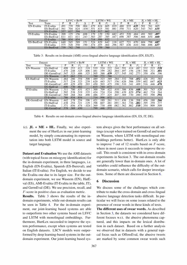
Dataset LSVC + BoW LSTM + WE JL + ME JL + ME + HLTest Train P R F1 ∆ P R F1 ∆ P R F1 P R F1

EN-Evalita IT-Evalita .491 .739 .590 .004 .479 .824 .605 .019 .480 .935 .635 .501 .761 .605ES-IberEval .561 .704 .624 -.030 .551 .615 .581 .081 .550 .711 .620 .543 .763 .635EN-Evalita .557 .637 .594 .518 .917 .662 - - - - - -

IT-Evalita EN-Evalita .209 .125 .156 .698 .179 .129 .150 .682 .453 .520 .484 .491 .502 .497ES-IberEval .611 .611 .611 .243 .583 .287 .385 .447 .698 .387 .506 .666 .654 .660IT-Evalita .786 .934 .854 .714 .996 .832 - - - - - -

ES-IberEval EN-Evalita .640 .545 .589 .151 .524 .829 .642 .118 .627 .721 .670 .604 .798 .687IT-Evalita .575 .528 .550 .190 .474 .455 .464 .296 .587 .636 .610 .586 .696 .637ES-IberEval .739 .742 .740 .761 .759 .760 - - - - - -

Table 3: Results on in-domain (AMI) cross-lingual abusive language identification (EN, ES,IT).

Dataset LSVC + BoW LSTM + WE JL + ME JL + ME + HLTest Train P R F1 ∆ P R F1 ∆ P R F1 P R F1

EN-Waseem ES-HatEval .498 .353 .413 .318 .519 .524 .522 .244 .591 .414 .487 .532 .523 .528IT-Evalita .470 .248 .325 .406 .481 .199 .282 .484 .497 .156 .238 .566 .311 .401DE-GermEval .547 .323 .406 .325 .505 .388 .439 .327 .545 .182 .273 .350 .456 .396EN-Waseem .817 .662 .731 .760 .771 .766 - - - - - -

ES-HatEval EN-Waseem .464 .286 .354 .308 .489 .323 .389 .284 .332 .708 .452 .426 .351 .384IT-Evalita .517 .234 .323 .239 .620 .443 .517 .156 .626 .506 .559 .602 .647 .623DE-GermEval .495 .429 .459 .203 .450 .503 .475 .198 .510 .341 .409 .516 .446 .478ES-HatEval .606 .730 .662 .615 .744 .673 - - - - - -

IT-Evalita EN-Waseem .311 .700 .431 .423 .300 .709 .422 .410 .306 .836 .448 .301 .743 .428ES-HatEval .502 .538 .519 .335 .424 .724 .534 .298 .439 .829 .574 .462 .724 .564DE-GermEval .569 .268 .364 .490 .486 .377 .425 .407 .369 .730 .490 .593 .590 .592IT-Evalita .786 .934 .854 .714 .996 .832 - - - - - -

DE-GermEval EN-Waseem .442 .178 .254 .196 .421 .189 .261 .311 .436 .136 .208 .456 .188 .266ES-HatEval .438 .254 .321 .129 .398 .607 .481 .091 .361 .726 .482 .395 .359 .377IT-Evalita .371 .656 .474 -.024 .369 .730 .490 .082 .362 .862 .510 .354 .909 .509DE-GermEval .578 .369 .450 .799 .446 .572 - - - - - -

Table 4: Results on out-domain cross-lingual abusive language identification (EN, ES, IT, DE).

(c). JL + ME + HL. Finally, we also experi-ment the use of HurtLex in our joint-learningmodel, by simply concatenating its represen-tation into both LSTM model in source andtarget language.

Dataset and Evaluation We use the AMI datasets(with topical focus on misogyny identification) forthe in-domain experiment, in three languages, i.e.English (EN-Evalita), Spanish (ES-Ibereval), andItalian (IT-Evalita). For English, we decide to usethe Evalita one due to its larger size. For the out-domain experiment, we use Waseem (EN), HatE-val (ES), AMI-Evalita (IT-Evalita in the table, IT),and GermEval (DE). We use precision, recall, andF -score in positive class as evaluation metric.Results. Table 3 shows the results of the in-domain experiments, while out-domain results canbe seen in Table 4. For the in-domain experi-ment, our joint-learning based systems are ableto outperform two other systems based on LSVCand LSTM with monolingual embeddings. Fur-thermore, HurtLex succeeded to improve the sys-tem performance, except when systems are testedon English datasets. LSCV models were outper-formed by deep learning-based systems in the out-domain experiment. Our joint-learning based sys-

tem always gives the best performance on all set-tings (except when trained on GermEval and testedon Waseem, where LSTM with monolingual em-beddings performs better). HurtLex is only ableto improve 7 out of 12 results based on F -score,where in most cases it succeeds to improve the re-call. This result is consistent with in cross-domainexperiments in Section 3. The out-domain resultsare generally lower than in-domain ones. A lot ofvariables could influence the difficulty of the out-domain scenario, which calls for deeper investiga-tions. Some of them are discussed in Section 6.

6 Discussion

We discuss some of the challenges which con-tribute to make the cross-domain and cross-lingualabusive language detection tasks difficult. In par-ticular we will focus on some issues related to thepresence of swear words in these kinds of texts.The different uses of swear words. As describedin Section 3, the datasets we considered have dif-ferent focuses w.r.t. the abusive phenomena cap-tured, and this impacts on the lexical distribu-tion in each dataset. Based on a further analysiswe observed that in datasets with a general topi-cal focus such as OffensEval, the abusive tweetsare marked by some common swear words such

367

as “fuck”, “shit”, and “ass”. While in datasetsfeatured by a specific hate target, such as theAMI dataset (misogyny), the lexical keywords inabusive tweets are dominated by specific sexistslurs such as “bitch”, “cunt”, and “whore”. Thisfinding is consistent with the study of (ElSheriefet al., 2018), which conducted an analysis on hatespeech in social media based on its target. Fur-thermore, the pragmatics of swearing could alsochange from one dataset to another, depending onthe topical features.Translation issues. As we expected, the use ofautomatic machine translation (via Google Trans-late) in our pipeline can give rise to errors inthe cross-lingual setting. In particular, we ob-served errors in translations from English to otherlanguages (Italian and Spanish) on some swearwords, which are usually important clues to de-tect abusive content. See for instance the follow-ing cases from the EN-AMI Evalita dataset:

Original tweet (EN):Punch that girl right in the skankTranslated tweet (IT):Pugno quella ragazza proprio nellaSkank

Original tweet (EN):Apparently, you can turn a hoe into ahousewifeTranslated tweet (ES):Aparentemente, puedes convertir unaazada en una ama de casa.

Translating swearing is indeed challenging. In thefirst example, Google Translate is unable to pro-vide an Italian translation for the English word“skank” (a proper translation could be “sciac-quetta” or “sciattona”, which means “slut”). Wefound 134 occurrences of the word “skank” in EN-AMI Evalita and 185 in the EN-HatEval dataset.The second example shows, instead, a problemrelated to context and disambiguation issues. In-deed, the word “hoe” here is used informally inits derogatory sense, meaning “A woman whoengages in sexual intercourse for money” (syn-onyms: slut, whore, floozy)8. But, disregardingthe context, it is translated in Spanish by relyingon a different conventional meaning (hoe as agri-cultural and horticultural hand tool). The term

8https://www.urbandictionary.com/define.php?term=Hoe

“hoe” is also very frequent in the EN-AMI Evalita(292 occurrences) and EN-HatEval dataset (348occurrences).

7 Conclusion and Future Work

In this study, we conduct an exploratory exper-iment on abusive language detection in cross-domain and cross-lingual classification scenarios.We focus on social media data, exploiting severaldatasets across different domains and languages.Based on the cross-domain experiments, we foundthat training a system on datasets featured bymore general abusive phenomena will produce amore robust system to detect other more specifickinds of abusive languages. We also observed thatHurtLex is able to transfer knowledge between do-mains by improving the number of true positives.In the cross-lingual experiment, our joint-learningsystems outperformed the other systems in mostcases also in the out-domain setting. The resultspresented here succeed to shed some light regard-ing the issues and difficulties of this research di-rection. As future work, we aim at exploring moredeeply the issue related to different coverage, top-ical focuses and abusive phenomena characteriz-ing the datasets in this field, taking a semanticontology-based approach to clearly represent therelations between concepts and linguistic phenom-ena involved. This will allow us to further exploreand refine the idea that combining some datasetscan produce a more robust system to detect abu-sive language across different domains. We alsofound that detecting out-domain abusive contentcross-lingual is really challenging, and the use ofdomain-independent resources to transfer knowl-edge between domains and languages an interest-ing issue to be further explored. Finally, we willfurther investigate the different uses and contextsof swearing, which seems to play a key role inthe abusive language detection task (Holgate et al.,2018), with impact also on experiments in cross-domain and cross-lingual settings.

Acknowledgements

We would like to deeply thank Valerio Basilefor his valuable and useful feedback on earlierversions of this paper. The work of EndangW. Pamungkas and Viviana Patti was partiallyfunded by Progetto di Ateneo/CSP 2016 (Im-migrants, Hate and Prejudice in Social Media,S1618 L2 BOSC 01).

368

ReferencesAngelo Basile and Chiara Rubagotti. 2018. Crotone-

milano for AMI at evalita2018. A performant, cross-lingual misogyny detection system. In Proceedingsof the Sixth Evaluation Campaign of Natural Lan-guage Processing and Speech Tools for Italian. Fi-nal Workshop (EVALITA 2018) co-located with theFifth Italian Conference on Computational Linguis-tics (CLiC-it 2018), Turin, Italy, December 12-13,2018.

Valerio Basile, Cristina Bosco, Elisabetta Fersini,Debora Nozza, Viviana Patti, Francisco ManuelRangel Pardo, Paolo Rosso, and Manuela San-guinetti. 2019. SemEval-2019 task 5: Multilin-gual detection of hate speech against immigrants andwomen in twitter. In Proceedings of the 13th Inter-national Workshop on Semantic Evaluation, pages54–63, Minneapolis, Minnesota, USA. ACL.

Elisa Bassignana, Valerio Basile, and Viviana Patti.2018. Hurtlex: A multilingual lexicon of wordsto hurt. In Proceedings of the Fifth Italian Confer-ence on Computational Linguistics (CLiC-it 2018),Torino, Italy, December 10-12, 2018.

Cristina Bosco, Felice Dell’Orletta, Fabio Poletto,Manuela Sanguinetti, and Maurizio Tesconi. 2018.Overview of the EVALITA 2018 hate speech de-tection task. In Proceedings of the Sixth Eval-uation Campaign of Natural Language Process-ing and Speech Tools for Italian. Final Workshop(EVALITA 2018) co-located with the Fifth ItalianConference on Computational Linguistics (CLiC-it2018), Turin, Italy, December 12-13, 2018., vol-ume 2263 of CEUR Workshop Proceedings. CEUR-WS.org.

Hal Daume III. 2007. Frustratingly easy domain adap-tation. In Proceedings of the 45th Annual Meeting ofthe Association of Computational Linguistics, pages256–263, Prague, Czech Republic. Association forComputational Linguistics.

Thomas Davidson, Dana Warmsley, Michael W. Macy,and Ingmar Weber. 2017. Automated hate speechdetection and the problem of offensive language.In Proceedings of the Eleventh International Con-ference on Web and Social Media, ICWSM 2017,Montreal, Quebec, Canada, May 15-18, 2017.,pages 512–515. AAAI Press.

Tullio De Mauro. 2016. Le parole per ferire. Inter-nazionale. 27 settembre 2016.

Mai ElSherief, Vivek Kulkarni, Dana Nguyen,William Yang Wang, and Elizabeth M. Belding.2018. Hate lingo: A target-based linguistic analy-sis of hate speech in social media. In Proceedingsof the Twelfth International Conference on Web andSocial Media, ICWSM 2018, Stanford, California,USA, June 25-28, 2018., pages 42–51. AAAI Press.

EU Commission. 2016. Code of conduct on counteringillegal hate speech online.

Elisabetta Fersini, Debora Nozza, and Paolo Rosso.2018a. Overview of the evalita 2018 task on auto-matic misogyny identification (AMI). In Proceed-ings of the Sixth Evaluation Campaign of NaturalLanguage Processing and Speech Tools for Italian.Final Workshop (EVALITA 2018) co-located withthe Fifth Italian Conference on Computational Lin-guistics (CLiC-it 2018), Turin, Italy, December 12-13, 2018., volume 2263 of CEUR Workshop Pro-ceedings. CEUR-WS.org.

Elisabetta Fersini, Paolo Rosso, and Maria Anzovino.2018b. Overview of the task on automatic misog-yny identification at ibereval 2018. In Proceed-ings of the Third Workshop on Evaluation of Hu-man Language Technologies for Iberian Languages(IberEval 2018) co-located with 34th Conference ofthe Spanish Society for Natural Language Process-ing (SEPLN 2018), Sevilla, Spain, September 18th,2018., volume 2150 of CEUR Workshop Proceed-ings, pages 214–228. CEUR-WS.org.

Jennifer Golbeck, Zahra Ashktorab, Rashad O. Banjo,Alexandra Berlinger, Siddharth Bhagwan, CodyBuntain, Paul Cheakalos, Alicia A. Geller, QuintGergory, Rajesh Kumar Gnanasekaran, Raja Ra-jan Gunasekaran, Kelly M. Hoffman, Jenny Hot-tle, Vichita Jienjitlert, Shivika Khare, Ryan Lau,Marianna J. Martindale, Shalmali Naik, Heather L.Nixon, Piyush Ramachandran, Kristine M. Rogers,Lisa Rogers, Meghna Sardana Sarin, Gaurav Sha-hane, Jayanee Thanki, Priyanka Vengataraman, Zi-jian Wan, and Derek Michael Wu. 2017. A largelabeled corpus for online harassment research. InProceedings of the 2017 ACM on Web Science Con-ference, WebSci 2017, Troy, NY, USA, June 25 - 28,2017, pages 229–233. ACM.

Rob van der Goot, Nikola Ljubesic, Ian Matroos, Malv-ina Nissim, and Barbara Plank. 2018. Bleachingtext: Abstract features for cross-lingual gender pre-diction. In Proceedings of the 56th Annual Meet-ing of the Association for Computational Linguis-tics, ACL 2018, Melbourne, Australia, July 15-20,2018, Volume 2: Short Papers, pages 383–389. As-sociation for Computational Linguistics.

Eric Holgate, Isabel Cachola, Daniel Preotiuc-Pietro,and Junyi Jessy Li. 2018. Why swear? analyz-ing and inferring the intentions of vulgar expres-sions. In Proceedings of the 2018 Conference onEmpirical Methods in Natural Language Process-ing, pages 4405–4414, Brussels, Belgium. Associ-ation for Computational Linguistics.

Mladen Karan and Jan Snajder. 2018. Cross-domaindetection of abusive language online. In Proceed-ings of the 2nd Workshop on Abusive Language On-line (ALW2), pages 132–137, Brussels, Belgium.Association for Computational Linguistics.

Ritesh Kumar, Atul Kr. Ojha, Shervin Malmasi, andMarcos Zampieri. 2018. Benchmarking aggressionidentification in social media. In Proceedings of the

369

First Workshop on Trolling, Aggression and Cyber-bullying (TRAC-2018), pages 1–11, Santa Fe, NewMexico, USA. Association for Computational Lin-guistics.

Tolba Marwa, Ouadfel Salima, and Meshoul Souham.2018. Deep learning for online harassment detec-tion in tweets. In 2018 3rd International Conferenceon Pattern Analysis and Intelligent Systems (PAIS),pages 1–5. IEEE.

Roberto Navigli and Simone Paolo Ponzetto. 2012.Babelnet: The automatic construction, evaluationand application of a wide-coverage multilingual se-mantic network. Artificial Intelligence, 193:217–250.

Julian Moreno Schneider, Roland Roller, Peter Bour-gonje, Stefanie Hegele, and Georg Rehm. 2018. To-wards the automatic classification of offensive lan-guage and related phenomena in german tweets. In14th Conference on Natural Language ProcessingKONVENS 2018, page 95.

Rachele Sprugnoli, Stefano Menini, Sara Tonelli, Fil-ippo Oncini, and Enrico Piras. 2018. Creating aWhatsApp dataset to study pre-teen cyberbullying.In Proceedings of the 2nd Workshop on Abusive Lan-guage Online (ALW2), pages 51–59, Brussels, Bel-gium. Association for Computational Linguistics.

Cynthia Van Hee, Els Lefever, Ben Verhoeven, JulieMennes, Bart Desmet, Guy De Pauw, Walter Daele-mans, and Veronique Hoste. 2015. Detection andfine-grained classification of cyberbullying events.In Proceedings of the International Conference Re-cent Advances in Natural Language Processing,pages 672–680, Hissar, Bulgaria. INCOMA Ltd.Shoumen, BULGARIA.

Zeerak Waseem, Thomas Davidson, Dana Warmsley,and Ingmar Weber. 2017. Understanding abuse:A typology of abusive language detection subtasks.In Proceedings of the First Workshop on AbusiveLanguage Online, pages 78–84, Vancouver, BC,Canada. Association for Computational Linguistics.

Zeerak Waseem and Dirk Hovy. 2016. Hateful sym-bols or hateful people? predictive features for hatespeech detection on twitter. In Proceedings of theNAACL Student Research Workshop, pages 88–93,San Diego, California. Association for Computa-tional Linguistics.

Zeerak Waseem, James Thorne, and Joachim Bingel.2018. Bridging the gaps: Multi task learning for do-main transfer of hate speech detection. Online Ha-rassment, page 29.

Michael Wiegand, Josef Ruppenhofer, Anna Schmidt,and Clayton Greenberg. 2018a. Inducing a lexiconof abusive words – a feature-based approach. InProceedings of the 2018 Conference of the NorthAmerican Chapter of the Association for Computa-tional Linguistics: Human Language Technologies,

Volume 1 (Long Papers), pages 1046–1056, NewOrleans, Louisiana. Association for ComputationalLinguistics.

Michael Wiegand, Melanie Siegel, and Josef Ruppen-hofer. 2018b. Overview of the germeval 2018 sharedtask on the identification of offensive language. In14th Conference on Natural Language ProcessingKONVENS 2018, page 1.

Ellery Wulczyn, Nithum Thain, and Lucas Dixon.2017. Ex machina: Personal attacks seen at scale.In Proceedings of the 26th International Conferenceon World Wide Web, pages 1391–1399. InternationalWorld Wide Web Conferences Steering Committee.

Marcos Zampieri, Shervin Malmasi, Preslav Nakov,Sara Rosenthal, Noura Farra, and Ritesh Kumar.2019a. Predicting the type and target of offen-sive posts in social media. In Proceedings of the2019 Conference of the North American Chapter ofthe Association for Computational Linguistics: Hu-man Language Technologies, Volume 1 (Long andShort Papers), pages 1415–1420, Minneapolis, Min-nesota. Association for Computational Linguistics.

Marcos Zampieri, Shervin Malmasi, Preslav Nakov,Sara Rosenthal, Noura Farra, and Ritesh Kumar.2019b. SemEval-2019 task 6: Identifying and cat-egorizing offensive language in social media (Of-fensEval). In Proceedings of the 13th Interna-tional Workshop on Semantic Evaluation, pages 75–86, Minneapolis, Minnesota, USA. Association forComputational Linguistics.

Xinjie Zhou, Xiaojun Wan, and Jianguo Xiao. 2016.Cross-lingual sentiment classification with bilingualdocument representation learning. In Proceedingsof the 54th Annual Meeting of the Association forComputational Linguistics (Volume 1: Long Pa-pers), pages 1403–1412, Berlin, Germany. Associ-ation for Computational Linguistics.

370

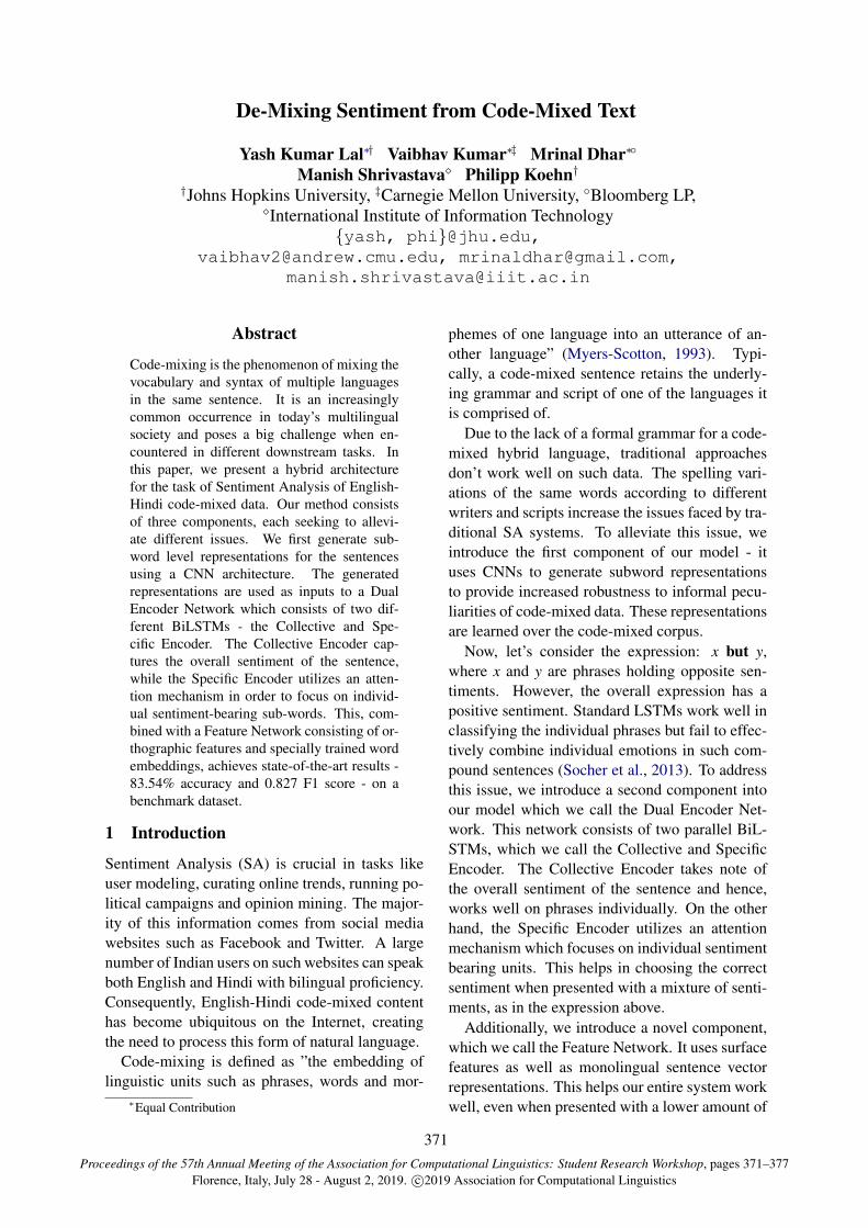
Proceedings of the 57th Annual Meeting of the Association for Computational Linguistics: Student Research Workshop, pages 371–377Florence, Italy, July 28 - August 2, 2019. c©2019 Association for Computational Linguistics

De-Mixing Sentiment from Code-Mixed Text

Yash Kumar Lal∗† Vaibhav Kumar∗‡ Mrinal Dhar∗Manish Shrivastava Philipp Koehn†

†Johns Hopkins University, ‡Carnegie Mellon University, Bloomberg LP,International Institute of Information Technology

yash, phi@jhu.edu,vaibhav2@andrew.cmu.edu, mrinaldhar@gmail.com,

manish.shrivastava@iiit.ac.in

Abstract

Code-mixing is the phenomenon of mixing thevocabulary and syntax of multiple languagesin the same sentence. It is an increasinglycommon occurrence in today’s multilingualsociety and poses a big challenge when en-countered in different downstream tasks. Inthis paper, we present a hybrid architecturefor the task of Sentiment Analysis of English-Hindi code-mixed data. Our method consistsof three components, each seeking to allevi-ate different issues. We first generate sub-word level representations for the sentencesusing a CNN architecture. The generatedrepresentations are used as inputs to a DualEncoder Network which consists of two dif-ferent BiLSTMs - the Collective and Spe-cific Encoder. The Collective Encoder cap-tures the overall sentiment of the sentence,while the Specific Encoder utilizes an atten-tion mechanism in order to focus on individ-ual sentiment-bearing sub-words. This, com-bined with a Feature Network consisting of or-thographic features and specially trained wordembeddings, achieves state-of-the-art results -83.54% accuracy and 0.827 F1 score - on abenchmark dataset.

1 Introduction

Sentiment Analysis (SA) is crucial in tasks likeuser modeling, curating online trends, running po-litical campaigns and opinion mining. The major-ity of this information comes from social mediawebsites such as Facebook and Twitter. A largenumber of Indian users on such websites can speakboth English and Hindi with bilingual proficiency.Consequently, English-Hindi code-mixed contenthas become ubiquitous on the Internet, creatingthe need to process this form of natural language.

Code-mixing is defined as ”the embedding oflinguistic units such as phrases, words and mor-

∗Equal Contribution

phemes of one language into an utterance of an-other language” (Myers-Scotton, 1993). Typi-cally, a code-mixed sentence retains the underly-ing grammar and script of one of the languages itis comprised of.

Due to the lack of a formal grammar for a code-mixed hybrid language, traditional approachesdon’t work well on such data. The spelling vari-ations of the same words according to differentwriters and scripts increase the issues faced by tra-ditional SA systems. To alleviate this issue, weintroduce the first component of our model - ituses CNNs to generate subword representationsto provide increased robustness to informal pecu-liarities of code-mixed data. These representationsare learned over the code-mixed corpus.

Now, let’s consider the expression: x but y,where x and y are phrases holding opposite sen-timents. However, the overall expression has apositive sentiment. Standard LSTMs work well inclassifying the individual phrases but fail to effec-tively combine individual emotions in such com-pound sentences (Socher et al., 2013). To addressthis issue, we introduce a second component intoour model which we call the Dual Encoder Net-work. This network consists of two parallel BiL-STMs, which we call the Collective and SpecificEncoder. The Collective Encoder takes note ofthe overall sentiment of the sentence and hence,works well on phrases individually. On the otherhand, the Specific Encoder utilizes an attentionmechanism which focuses on individual sentimentbearing units. This helps in choosing the correctsentiment when presented with a mixture of senti-ments, as in the expression above.

Additionally, we introduce a novel component,which we call the Feature Network. It uses surfacefeatures as well as monolingual sentence vectorrepresentations. This helps our entire system workwell, even when presented with a lower amount of

371

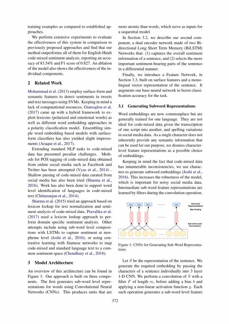
training examples as compared to established ap-proaches.

We perform extensive experiments to evaluatethe effectiveness of this system in comparison topreviously proposed approaches and find that ourmethod outperforms all of them for English-Hindicode-mixed sentiment analysis, reporting an accu-racy of 83.54% and F1 score of 0.827. An ablationof the model also shows the effectiveness of the in-dividual components.

2 Related Work

Mohammad et al. (2013) employ surface-form andsemantic features to detect sentiments in tweetsand text messages using SVMs. Keeping in mind alack of computational resources, Giatsoglou et al.(2017) came up with a hybrid framework to ex-ploit lexicons (polarized and emotional words) aswell as different word embedding approaches ina polarity classification model. Ensembling sim-ple word embedding based models with surface-form classifiers has also yielded slight improve-ments (Araque et al., 2017).

Extending standard NLP tasks to code-mixeddata has presented peculiar challenges. Meth-ods for POS tagging of code-mixed data obtainedfrom online social media such as Facebook andTwitter has been attempted (Vyas et al., 2014) .Shallow parsing of code-mixed data curated fromsocial media has also been tried (Sharma et al.,2016). Work has also been done to support wordlevel identification of languages in code-mixedtext (Chittaranjan et al., 2014).

Sharma et al. (2015) tried an approach based onlexicon lookup for text normalization and senti-ment analysis of code-mixed data. Pravalika et al.(2017) used a lexicon lookup approach to per-form domain specific sentiment analysis. Otherattempts include using sub-word level composi-tions with LSTMs to capture sentiment at mor-pheme level (Joshi et al., 2016), or using con-trastive learning with Siamese networks to mapcode-mixed and standard language text to a com-mon sentiment space (Choudhary et al., 2018).

3 Model Architecture

An overview of this architecture can be found inFigure 3. Our approach is built on three compo-nents. The first generates sub-word level repre-sentations for words using Convolutional NeuralNetworks (CNNs). This produces units that are

more atomic than words, which serve as inputs fora sequential model.

In Section 3.2, we describe our second com-ponent, a dual encoder network made of two Bi-directional Long Short Term Memory (BiLSTM)Networks that: (1) captures the overall sentimentinformation of a sentence, and (2) selects the moreimportant sentiment-bearing parts of the sentencein a differential manner.

Finally, we introduce a Feature Network, inSection 3.3, built on surface features and a mono-lingual vector representation of the sentence. Itaugments our base neural network to boost classi-fication accuracy for the task.

3.1 Generating Subword Representations

Word embeddings are now commonplace but aregenerally trained for one language. They are notideal for code-mixed data given the transcriptionof one script into another, and spelling variationsin social media data. As a single character does notinherently provide any semantic information thatcan be used for our purpose, we dismiss character-level feature representations as a possible choiceof embeddings.

Keeping in mind the fact that code-mixed datahas innumerable inconsistencies, we use charac-ters to generate subword embeddings (Joshi et al.,2016). This increases the robustness of the model,which is important for noisy social media data.Intermediate sub-word feature representations arelearned by filters during the convolution operation.

sw1 sw2 swt

Sub-wordRepresentations

Max Pooling

Sub-word LevelConvolutions

sw3

Figure 1: CNNs for Generating Sub-Word Representa-tions

Let S be the representation of the sentence. Wegenerate the required embedding by passing thecharacters of a sentence individually into 3 layer1-D CNN. We perform a convolution of S with afilter F of length m, before adding a bias b andapplying a non-linear activation function g. Eachsuch operation generates a sub-word level feature

372

map fsw.

fsw[i] = g((S[:, i : i+m− 1] ∗ F ) + b) (1)

Here, S[:, i : i + m − 1] is a matrix of (i)th to(i +m − 1)th character embeddings and g is theReLU activation function. Thereafter, a final max-pooling operation over p feature maps generates arepresentation for individual subwords:

swi = max(fsw[p ∗ (i : i+ p− 1)]) (2)

A graphical representation of the architecturecan be seen in Figure 1

3.2 Dual Encoder

We utilize a combination of two different encodersin our model.

3.2.1 Collective EncoderThe collective encoder, built over a BiLSTM, aimsto learn a representation for the overall sentimentof the sentence. A graphical representation of thisencoder is in Figure 2(A). It takes as input thesubword representation of the sentence. The lasthidden state of the BiLSTM i.e. ht, encapsulatesthe overall summary of the sentence’s sentiment,which is denoted by cmrc.

3.2.2 Specific EncoderThe specific encoder is similar to the collective en-coder, in that it takes as input a subword repre-sentation of the sentence and is built over LSTMs,with one caveat - an affixed attention mechanism.This allows for selection of subwords which con-tribute the most towards the sentiment of the inputtext. It can be seen in Figure 2(B).

Identifying which subwords play a significantrole in deciding the sentiment is crucial. The spe-cific encoder generates a context vector cmrs tothis end. We first concatenate the forward andbackward states to obtain a combined annotation(k1, k2, . . . , kt). Taking inspiration from (Yanget al., 2016), we quantify the significance of a sub-word by measuring the similarity of an additionalhidden representation ui of each sub-word againsta sub-word level context vector X . Then, a nor-malized significance weight αi is obtained.

ui = tanh(Wiki + bi) (3)

αi =exp(uTi X)∑exp(uTi X)

(4)

The context vectorX can be looked at as a high-level representation of the question ”is it a signif-icant sentiment-bearing unit” evaluated across thesub-words. It is initialized randomly and learnedjointly during training. Finally, we calculate a vec-tor cmrs as a weighted sum of the sub-word anno-tations.

cmrs =∑

αiki (5)

Using such a mechanism helps our model to adap-tively select the more important sub-words fromthe less important ones.

3.2.3 Fusion of the EncodersWe concatenate the outputs obtained from boththese encoders and use it as inputs to further fullyconnected layers. Information obtained from boththe encoders is utilized to come up with a unifiedrepresentation of sentiment present in a sentence,

cmrsent = [cmrc; cmrs] (6)

where cmrsent represents the unified representa-tion of the sentiment. A representation of the samecan be found in Figure 3.

3.3 Feature NetworkWe also use linguistic features to augment the neu-ral network framework of our model.

• Capital words: Number of words that haveonly capital letters

• Extended words: Number of words with mul-tiple contiguous repeating characters.

• Aggregate positive and negative sentiments:Using SentiWordNet (Esuli and Sebastiani,2006) for every word bar articles and con-junctions, and combining the sentiment po-larity values into net positive aggregate andnet negative aggregate features.

• Repeated exclamations and other punctua-tion: Number of sets of two or more contigu-ous punctuation.

• Exclamation at end of sentence: Booleanvalue.

• Monolingual Sentence Vectors: Bojanowskiet al. (2017)’s method is used to train wordvectors for Hindi words in the code-mixedsentences.

373

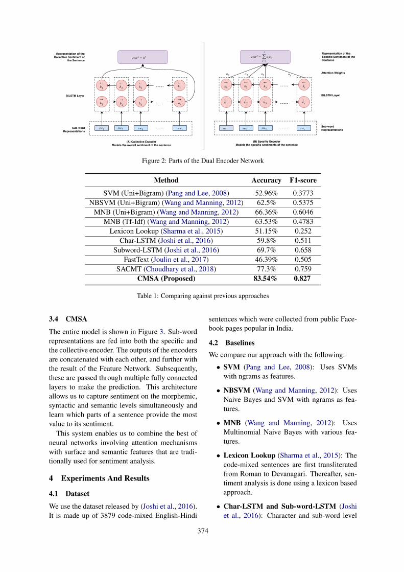
sw1 sw2 sw3 swt

←ht

cmrc = ht

←h1

←h2

←h3

Sub-wordRepresentations

BiLSTM Layer

sw1 sw2 sw3 swt

cmrs =t

∑i=1

αiki

←k1

Sub-wordRepresentations

BiLSTM Layer

Representation of theSpecific Sentiment of theSentence

α1 α2 αtα3Attention Weights

(A) Collective Encoder Models the overall sentiment of the sentence

(B) Specific Encoder Models the specific sentiments of the sentence

→ht

→h1

→h2

→h3

Representation of theCollective Sentiment of

the Sentence

←k2

←k3

←kt

→k 1

→k 2

→k 3

→k t

Figure 2: Parts of the Dual Encoder Network

Method Accuracy F1-score

SVM (Uni+Bigram) (Pang and Lee, 2008) 52.96% 0.3773NBSVM (Uni+Bigram) (Wang and Manning, 2012) 62.5% 0.5375

MNB (Uni+Bigram) (Wang and Manning, 2012) 66.36% 0.6046MNB (Tf-Idf) (Wang and Manning, 2012) 63.53% 0.4783

Lexicon Lookup (Sharma et al., 2015) 51.15% 0.252Char-LSTM (Joshi et al., 2016) 59.8% 0.511

Subword-LSTM (Joshi et al., 2016) 69.7% 0.658FastText (Joulin et al., 2017) 46.39% 0.505

SACMT (Choudhary et al., 2018) 77.3% 0.759CMSA (Proposed) 83.54% 0.827

Table 1: Comparing against previous approaches

3.4 CMSA

The entire model is shown in Figure 3. Sub-wordrepresentations are fed into both the specific andthe collective encoder. The outputs of the encodersare concatenated with each other, and further withthe result of the Feature Network. Subsequently,these are passed through multiple fully connectedlayers to make the prediction. This architectureallows us to capture sentiment on the morphemic,syntactic and semantic levels simultaneously andlearn which parts of a sentence provide the mostvalue to its sentiment.

This system enables us to combine the best ofneural networks involving attention mechanismswith surface and semantic features that are tradi-tionally used for sentiment analysis.

4 Experiments And Results

4.1 Dataset

We use the dataset released by (Joshi et al., 2016).It is made up of 3879 code-mixed English-Hindi

sentences which were collected from public Face-book pages popular in India.

4.2 BaselinesWe compare our approach with the following:

• SVM (Pang and Lee, 2008): Uses SVMswith ngrams as features.

• NBSVM (Wang and Manning, 2012): UsesNaive Bayes and SVM with ngrams as fea-tures.

• MNB (Wang and Manning, 2012): UsesMultinomial Naive Bayes with various fea-tures.

• Lexicon Lookup (Sharma et al., 2015): Thecode-mixed sentences are first transliteratedfrom Roman to Devanagari. Thereafter, sen-timent analysis is done using a lexicon basedapproach.

• Char-LSTM and Sub-word-LSTM (Joshiet al., 2016): Character and sub-word level

374

Text

TextText

16

32

64

128

Concatenate

Specific Encoder Collective Encoder

Sub-word level CNN

Prediction

Features

cmrsent = [cmrc; cmrs]

Figure 3: Complete Architecture of CMSA.

embeddings are passed to LSTM for classifi-cation.

• FastText (Joulin et al., 2017): Word Embed-dings utilized for classification. It has theability to handle OoV words as well.

• SACMT (Choudhary et al., 2018): Siamesenetworks are used to map code-mixed andstandard sentences to a common sentimentspace.

5 Results and Analysis

From Table 1, it is clear that that CMSA outper-forms the state-of-the-art techniques by 6.24% inaccuracy and 0.068 in F1-score. We observe thatsentence vectors (FastText) alone are not suitablefor this task. A possible reason for this is the pres-ence of two different languages.

There is a significant difference in accuracy be-tween Subword-LSTM and Char-LSTM, as seenin Table 1, which confirms our assumption aboutsubword-level representations being better for thistask as compared to character-level embeddings.Amongst the baselines, SACMT performed thebest. However, mapping two sentences into a com-mon space does not seem to be enough for senti-ment classification. With a combination of differ-

ent components, our proposed method is able toovercome the shortcomings of each of these base-lines and achieve significant gains.

5.1 Effect of different Encoders

Method Accuracy F1-scoreSpecific Encoder 80.2% 0.801

Collective Encoder 77.3% 0.795Specific + Collective (CMSA) 83.54% 0.827

Table 2: Different encoding mechanisms with FeatureNetwork

We experiment with different encoders used inthe dual encoder network. From Table 2, we cansee that CMSA > Collective Encoder > SpecificEncoder, for both accuracy and F1 score. A com-bination of the two encoders provides a better sen-timent classification model which validates ourinitial hypothesis of using two separate encoders.

5.2 Effect of Different Model Components

System Accuracy F1-scoreDual Encoder 75.74% 0.705

Feature Network only 57.9% 0.381CMSA 83.54% 0.827

Table 3: Effect of different model components

From Table 3, we see the performance trend asfollows: CMSA > Dual Encoder > Feature Net-work. Although the feature network alone doesnot result in better overall performance, it is stillcomparable to Char-LSTM (Table 2). However,the combination of feature network with dual en-coder helps in boosting the overall performance.

5.3 Effect of Training Examples

Figure 4: Performance on varying training data size

375

We experimented with varying numbers oftraining examples used for learning the model pa-rameters. Different models were trained on 500,1000, 1500 and 2000 examples. We observedthat the performance of CMSA was greater thanSubword-LSTM and SACMT at each point. Thiscan be seen in Figure 4. One of the reasons for thesame is the feature network in CMSA which helpsin better performance even with lesser number oftraining examples.

6 Conclusion

We propose a hybrid approach that combines re-current neural networks utilizing attention mech-anisms, with surface features, yielding a unifiedrepresentation that can be trained to classify sen-timents. We conduct extensive experiments on areal world code-mixed social media dataset, anddemonstrate that our system is able to achieve anaccuracy of 83.54% and an F1-score of 0.827,outperforming state-of-the-art approaches for thistask. In the future, we’d like to look at varying theattention mechanism in the model, and evaluatinghow it performs with a larger training set.

ReferencesOscar Araque, Ignacio Corcuera-Platas, J. Fernando

Snchez-Rada, and Carlos A. Iglesias. 2017. Enhanc-ing deep learning sentiment analysis with ensembletechniques in social applications. Expert Systemswith Applications, 77:236 – 246.

Piotr Bojanowski, Edouard Grave, Armand Joulin, andTomas Mikolov. 2017. Enriching word vectors withsubword information. Transactions of the Associa-tion for Computational Linguistics, 5:135–146.

Gokul Chittaranjan, Yogarshi Vyas, Kalika Bali, andMonojit Choudhury. 2014. Word-level languageidentification using crf: Code-switching shared taskreport of msr india system.

Nurendra Choudhary, Rajat Singh, Ishita Bindlish, andManish Shrivastava. 2018. Sentiment analysis ofcode-mixed languages leveraging resource rich lan-guages.

Andrea Esuli and Fabrizio Sebastiani. 2006. Sen-tiwordnet: A publicly available lexical resourcefor opinion mining. In In Proceedings of the 5thConference on Language Resources and Evaluation(LREC06, pages 417–422.

Maria Giatsoglou, Manolis G. Vozalis, KonstantinosDiamantaras, Athena Vakali, George Sarigiannidis,

and Konstantinos Ch. Chatzisavvas. 2017. Senti-ment analysis leveraging emotions and word embed-dings. Expert Systems with Applications, 69:214 –224.

Aditya Joshi, Ameya Prabhu, Manish Shrivastava, andVasudeva Varma. 2016. Towards sub-word levelcompositions for sentiment analysis of hindi-englishcode mixed text. In Proceedings of the 26th Inter-national Conference on Computational Linguistics(COLING).

Armand Joulin, Edouard Grave, Piotr Bojanowski, andTomas Mikolov. 2017. Bag of tricks for efficienttext classification. In Proceedings of the 15th Con-ference of the European Chapter of the Associationfor Computational Linguistics: Volume 2, Short Pa-pers, pages 427–431.

Saif M. Mohammad, Svetlana Kiritchenko, and Xiao-dan Zhu. 2013. Nrc-canada: Building the state-of-the-art in sentiment analysis of tweets. CoRR,abs/1308.6242.

Carol Myers-Scotton. 1993. Common and uncommonground: Social and structural factors in codeswitch-ing. Language in society, 22(4):475–503.

Bo Pang and Lillian Lee. 2008. Opinion mining andsentiment analysis. Found. Trends Inf. Retr., 2(1-2):1–135.

A. Pravalika, V. Oza, N. P. Meghana, and S. S. Ka-math. 2017. Domain-specific sentiment analysis ap-proaches for code-mixed social network data. In2017 8th International Conference on Computing,Communication and Networking Technologies (IC-CCNT), pages 1–6.

A. Sharma, S. Gupta, R. Motlani, P. Bansal, M. Srivas-tava, R. Mamidi, and D. M. Sharma. 2016. ShallowParsing Pipeline for Hindi-English Code-Mixed So-cial Media Text.

Shashank Sharma, PYKL Srinivas, and Rakesh Chan-dra Balabantaray. 2015. Text normalization of codemix and sentiment analysis. 2015 InternationalConference on Advances in Computing, Commu-nications and Informatics (ICACCI), pages 1468–1473.

Richard Socher, Alex Perelygin, Jean Wu, JasonChuang, Christopher D Manning, Andrew Ng, andChristopher Potts. 2013. Recursive deep modelsfor semantic compositionality over a sentiment tree-bank. In Proceedings of the 2013 conference onempirical methods in natural language processing,pages 1631–1642.

Yogarshi Vyas, Spandana Gella, Jatin Sharma, Ka-lika Bali, and Monojit Choudhury. 2014. Pos tag-ging of english-hindi code-mixed social media con-tent. In Proceedings of the 2014 Conference onEmpirical Methods in Natural Language Processing(EMNLP).

376

Sida Wang and Christopher D. Manning. 2012. Base-lines and bigrams: Simple, good sentiment and topicclassification. In Proceedings of the 50th AnnualMeeting of the Association for Computational Lin-guistics: Short Papers - Volume 2, ACL ’12.

Zichao Yang, Diyi Yang, Chris Dyer, Xiaodong He,Alexander J. Smola, and Eduard H. Hovy. 2016. Hi-erarchical attention networks for document classifi-cation. In HLT-NAACL.

377

Proceedings of the 57th Annual Meeting of the Association for Computational Linguistics: Student Research Workshop, pages 378–385Florence, Italy, July 28 - August 2, 2019. c©2019 Association for Computational Linguistics

Unsupervised Learning ofDiscourse-Aware Text Representation for Essay Scoring

Farjana Sultana Mim1 Naoya Inoue1,2 Paul Reisert2,1Hiroki Ouchi2,1 Kentaro Inui1,2

1Tohoku University 2RIKEN Center for Advanced Intelligence Project (AIP)mim, naoya-i, inui @ecei.tohoku.ac.jppaul.reisert, hiroki.ouchi @riken.jp

Abstract

Existing document embedding approachesmainly focus on capturing sequences of wordsin documents. However, some document clas-sification and regression tasks such as essayscoring need to consider discourse structure ofdocuments. Although some prior approachesconsider this issue and utilize discourse struc-ture of text for document classification, theseapproaches are dependent on computationallyexpensive parsers. In this paper, we proposean unsupervised approach to capture discoursestructure in terms of coherence and cohesionfor document embedding that does not requireany expensive parser or annotation. Extrin-sic evaluation results show that the documentrepresentation obtained from our approach im-proves the performance of essay Organizationscoring and Argument Strength scoring.

1 Introduction

Document embedding is important for many NLPtasks such as document classification (e.g., es-say scoring and sentiment classification) (Le andMikolov, 2014; Liu et al., 2017; Wu et al.,2018; Tang et al., 2015) and summarization.While embedding approaches can be supervised,semi-supervised and unsupervised, recent studieshave largely focused on unsupervised and semi-supervised approaches in order to utilize largeamounts of unlabeled text and avoid expensive an-notation procedures.

In general, a document is a discourse wheresentences are logically connected to each other toprovide comprehensive meaning. Discourse hastwo important properties: coherence and cohesion(Halliday, 1994). Coherence refers to the seman-tic relatedness among sentences and logical orderof concepts and meanings in a text. For example,“I saw Jill on the street. She was going home.” iscoherent whereas “I saw Jill on the street. She hastwo sisters.” is incoherent. Cohesion refers to the

use of linguistic devices that hold a text together.Example of these linguistic devices include con-junctions such as discourse indicators (DIs) (e.g.,“because” and “for example”), coreference (e.g.,“he” and “they”), substitution, ellipsis etc.

Some text classification and regression tasksneed to consider discourse structure of text inaddition to dependency relations and predicate-argument structures. One example of such tasksis essay scoring, where discourse structure (e.g.,coherence and cohesion) plays a crucial role, es-pecially when considering Organization and Argu-ment Strength criteria, since they refer to logical-sequence awareness in texts. Organization refersto how good an essay structure is, where well-structured essays logically develop arguments andstate positions by supporting them (Persing et al.,2010). Argument Strength means how strongly anessay argues in favor of its thesis to persuade thereaders (Persing and Ng, 2015).

An example of the relation between coherenceand an essay’s Organization is shown in Figure 1.The high-scored essay (i.e., Organization score of4) first states its position regarding the promptand then provides several reasons to strengthen theclaim. It is considered coherent because it followsa logical order. However, the low-scored essayis not clear on its position and what it is arguingabout. Therefore, it can be considered incoherentsince it lacks logical sequencing.

Previous studies on document embedding haveprimarily focused on capturing word similarity,word dependencies and semantic information ofdocuments (Le and Mikolov, 2014; Liu et al.,2017; Wu et al., 2018; Tang et al., 2015). How-ever, less attention has been paid to capturing dis-course structure for document embedding in anunsupervised manner and no prior work appliesunsupervised document representation learning toessay scoring. In short, it has not yet been ex-plored how some of the discourse properties can

378

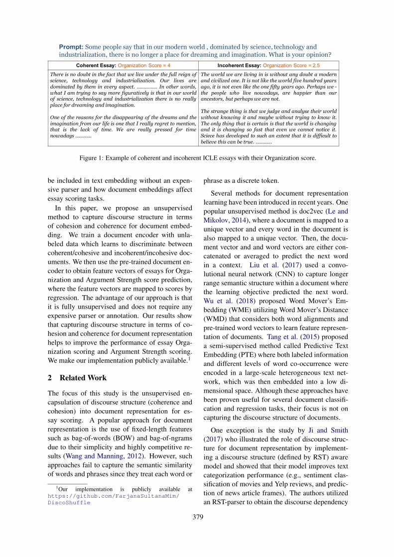
Coherent Essay: Organization Score = 4 Incoherent Essay: Organization Score = 2.5

There is no doubt in the fact that we live under the full reign ofscience, technology and industrialization. Our lives aredominated by them in every aspect. …………… In other words,what I am trying to say more figuratively is that in our worldof science, technology and industrialization there is no reallyplace for dreaming and imagination.

One of the reasons for the disappearing of the dreams and theimagination from our life is one that I really regret to mention,that is the lack of time. We are really pressed for timenowadays …………

The world we are living in is without any doubt a modernand civilized one. It is not like the world five hundred yearsago, it is not even like the one fifty years ago. Perhaps we -the people who live nowadays, are happier than ourancestors, but perhapswe are not.

The strange thing is that we judge and analyse their worldwithout knowing it and maybe without trying to know it.The only thing that is certain is that the world is changingand it is changing so fast that even we cannot notice it.Sciece has developed to such an extent that it is difficult tobelieve this can be true. …………

Prompt: Some people say that in our modern world , dominated by science, technology and industrialization, there is no longer a place for dreaming and imagination. What is your opinion?

Figure 1: Example of coherent and incoherent ICLE essays with their Organization score.

be included in text embedding without an expen-sive parser and how document embeddings affectessay scoring tasks.

In this paper, we propose an unsupervisedmethod to capture discourse structure in termsof cohesion and coherence for document embed-ding. We train a document encoder with unla-beled data which learns to discriminate betweencoherent/cohesive and incoherent/incohesive doc-uments. We then use the pre-trained document en-coder to obtain feature vectors of essays for Orga-nization and Argument Strength score prediction,where the feature vectors are mapped to scores byregression. The advantage of our approach is thatit is fully unsupervised and does not require anyexpensive parser or annotation. Our results showthat capturing discourse structure in terms of co-hesion and coherence for document representationhelps to improve the performance of essay Orga-nization scoring and Argument Strength scoring.We make our implementation publicly available.1

2 Related Work

The focus of this study is the unsupervised en-capsulation of discourse structure (coherence andcohesion) into document representation for es-say scoring. A popular approach for documentrepresentation is the use of fixed-length featuressuch as bag-of-words (BOW) and bag-of-ngramsdue to their simplicity and highly competitive re-sults (Wang and Manning, 2012). However, suchapproaches fail to capture the semantic similarityof words and phrases since they treat each word or

1Our implementation is publicly available athttps://github.com/FarjanaSultanaMim/DiscoShuffle

phrase as a discrete token.

Several methods for document representationlearning have been introduced in recent years. Onepopular unsupervised method is doc2vec (Le andMikolov, 2014), where a document is mapped to aunique vector and every word in the document isalso mapped to a unique vector. Then, the docu-ment vector and and word vectors are either con-catenated or averaged to predict the next wordin a context. Liu et al. (2017) used a convo-lutional neural network (CNN) to capture longerrange semantic structure within a document wherethe learning objective predicted the next word.Wu et al. (2018) proposed Word Mover’s Em-bedding (WME) utilizing Word Mover’s Distance(WMD) that considers both word alignments andpre-trained word vectors to learn feature represen-tation of documents. Tang et al. (2015) proposeda semi-supervised method called Predictive TextEmbedding (PTE) where both labeled informationand different levels of word co-occurrence wereencoded in a large-scale heterogeneous text net-work, which was then embedded into a low di-mensional space. Although these approaches havebeen proven useful for several document classifi-cation and regression tasks, their focus is not oncapturing the discourse structure of documents.

One exception is the study by Ji and Smith(2017) who illustrated the role of discourse struc-ture for document representation by implement-ing a discourse structure (defined by RST) awaremodel and showed that their model improves textcategorization performance (e.g., sentiment clas-sification of movies and Yelp reviews, and predic-tion of news article frames). The authors utilizedan RST-parser to obtain the discourse dependency

379

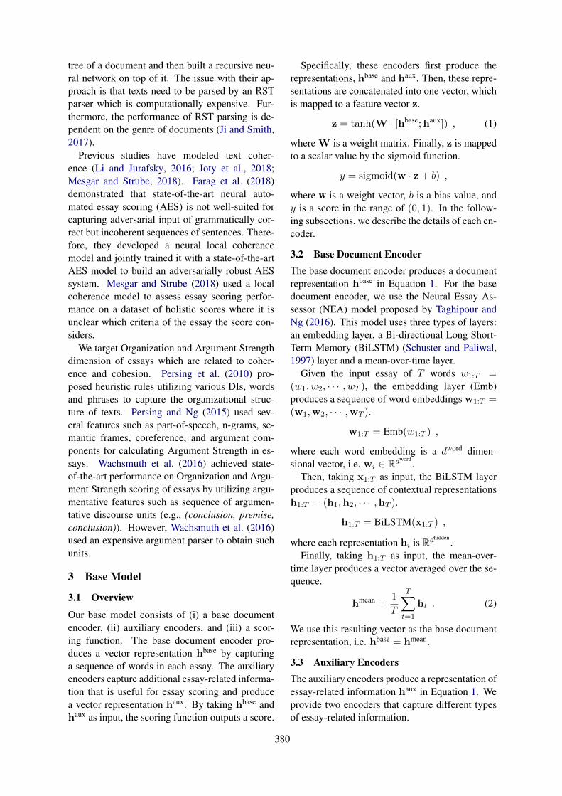
tree of a document and then built a recursive neu-ral network on top of it. The issue with their ap-proach is that texts need to be parsed by an RSTparser which is computationally expensive. Fur-thermore, the performance of RST parsing is de-pendent on the genre of documents (Ji and Smith,2017).

Previous studies have modeled text coher-ence (Li and Jurafsky, 2016; Joty et al., 2018;Mesgar and Strube, 2018). Farag et al. (2018)demonstrated that state-of-the-art neural auto-mated essay scoring (AES) is not well-suited forcapturing adversarial input of grammatically cor-rect but incoherent sequences of sentences. There-fore, they developed a neural local coherencemodel and jointly trained it with a state-of-the-artAES model to build an adversarially robust AESsystem. Mesgar and Strube (2018) used a localcoherence model to assess essay scoring perfor-mance on a dataset of holistic scores where it isunclear which criteria of the essay the score con-siders.

We target Organization and Argument Strengthdimension of essays which are related to coher-ence and cohesion. Persing et al. (2010) pro-posed heuristic rules utilizing various DIs, wordsand phrases to capture the organizational struc-ture of texts. Persing and Ng (2015) used sev-eral features such as part-of-speech, n-grams, se-mantic frames, coreference, and argument com-ponents for calculating Argument Strength in es-says. Wachsmuth et al. (2016) achieved state-of-the-art performance on Organization and Argu-ment Strength scoring of essays by utilizing argu-mentative features such as sequence of argumen-tative discourse units (e.g., (conclusion, premise,conclusion)). However, Wachsmuth et al. (2016)used an expensive argument parser to obtain suchunits.

3 Base Model

3.1 Overview

Our base model consists of (i) a base documentencoder, (ii) auxiliary encoders, and (iii) a scor-ing function. The base document encoder pro-duces a vector representation hbase by capturinga sequence of words in each essay. The auxiliaryencoders capture additional essay-related informa-tion that is useful for essay scoring and producea vector representation haux. By taking hbase andhaux as input, the scoring function outputs a score.

Specifically, these encoders first produce therepresentations, hbase and haux. Then, these repre-sentations are concatenated into one vector, whichis mapped to a feature vector z.

z = tanh(W · [hbase;haux]) , (1)

where W is a weight matrix. Finally, z is mappedto a scalar value by the sigmoid function.

y = sigmoid(w · z+ b) ,

where w is a weight vector, b is a bias value, andy is a score in the range of (0, 1). In the follow-ing subsections, we describe the details of each en-coder.

3.2 Base Document EncoderThe base document encoder produces a documentrepresentation hbase in Equation 1. For the basedocument encoder, we use the Neural Essay As-sessor (NEA) model proposed by Taghipour andNg (2016). This model uses three types of layers:an embedding layer, a Bi-directional Long Short-Term Memory (BiLSTM) (Schuster and Paliwal,1997) layer and a mean-over-time layer.

Given the input essay of T words w1:T =(w1, w2, · · · , wT ), the embedding layer (Emb)produces a sequence of word embeddings w1:T =(w1,w2, · · · ,wT ).

w1:T = Emb(w1:T ) ,

where each word embedding is a dword dimen-sional vector, i.e. wi ∈ Rdword

.Then, taking x1:T as input, the BiLSTM layer

produces a sequence of contextual representationsh1:T = (h1,h2, · · · ,hT ).

h1:T = BiLSTM(x1:T ) ,

where each representation hi is Rdhidden.

Finally, taking h1:T as input, the mean-over-time layer produces a vector averaged over the se-quence.

hmean =1

T

T∑

t=1

ht . (2)

We use this resulting vector as the base documentrepresentation, i.e. hbase = hmean.

3.3 Auxiliary EncodersThe auxiliary encoders produce a representation ofessay-related information haux in Equation 1. Weprovide two encoders that capture different typesof essay-related information.

380

Large-scaleUnlabeledEssays

Pre-training(Section 4.2)

Labeled Essays

Auxiliary Encoder

Base DocumentEncoder

Scoring Function

Binary Classifier

(Sentence shuffled, incoherent)

(Paragraph shuffled, incoherent)

Label = 1: original documents(coherent/cohesive)

The majority … instead of activities.I believe that … because the students ...

Moreover, some are … percentage.They are only … for they pass exams.

Cross Entropy Loss

CrossEntropy

Loss

Label = 0: corrupted documents (incoherent/incohesive)

Moreover, some are … percentage.They are only … for they pass exams.I believe that … because the students ...The majority … instead of activities.

(DI shuffled, incohesive)

The majority … instead of activities.I believe that … because the students ...

Moreover, some are … percentage.They are only … for they pass exams.

The majority … for activities.I believe that … Moreover the students ...

instead of, some are … percentage.They are only … because they pass exams.

The majority … instead of activities.I believe that … because the students ...

Moreover, some are … percentage.They are only … for they pass exams.

Moreover, some are … percentage.They are only … for they pass exams.

The majority … instead of activities.I believe that … because the students ...

Figure 2: Proposed method for unsupervised learning of discourse-aware text representation utilizing coher-ent/incoherent and cohesive/incohesive texts and use of the discourse-aware text embeddings for essay scoring.

Paragraph Function Encoder (PFE). Eachparagraph in an essay plays a different role. Forinstance, the first paragraph tends to introduce thetopic of the essay, and the last paragraph tends tosum up the whole content and make some conclu-sions. Here, we capture such paragraph functions.

Specifically, we obtain paragraph function la-bels of essays using Persing et al. (2010)’s heuris-tic rules.2 Persing et al. (2010) specified fourparagraph function labels: Introduction (I), Body(B), Rebuttal (R) and Conclusion (C). We repre-sent these labels as vectors and incorporate theminto the base model. The paragraph function labelencoder consists of two modules, an embeddinglayer and a BiLSTM layer.

We assume that an essay consists of M para-graphs, and the i-th paragraph has already beenassigned a function label pi. Given the sequenceof paragraph function labels of an essay p1:M =(p1, p2, ..., pM ), the embedding layer (Embpara)produces a sequence of label embeddings, i.e.p1:M = Embpara(p1:M ), where each embeddingpi is Rdpara

. Then, taking p1:M as input, the BiL-STM layer produces a sequence of contextual rep-resentations h1:M = BiLSTM(p1:M ), where hi

is RdPFE. We use the last hidden state hM as the

paragraph function label sequence representation,i.e. haux = hM .

Prompt Encoder (PE). As shown in Figure 1,essays are written for a given prompt, where theprompt itself can be useful for essay scoring.

2See http://www.hlt.utdallas.edu/˜persingq/ICLE/orgDataset.html for furtherdetails.

Based on this intuition, we incorporate prompt in-formation.

The prompt encoder uses an embed-ding layer and a Long Short-Term Memory(LSTM) (Hochreiter, Sepp and Schmidhuber,Jurgen, 1997) layer to produce a prompt repre-sentation. Formally, we assume that the input is aprompt of N words, w1:N = (w1, w2, · · · , wN ).First, the embedding layer maps the input promptw1:N to a sequence of word embeddings, w1:N ,where wi is Rdprompt

. Then, taking w1:N as input,the LSTM layer produces a sequence of hiddenstates, h1:N = (h1,h2, · · · ,hN ), where hi isRdPE

. The last hidden state is regarded as theresulting representation, i.e. haux = hN .

4 Proposed Method

4.1 Overview

Figure 2 summarizes the proposed method. First,we pre-train a base document encoder (Sec-tion 3.2) in an unsupervised manner. The pretrain-ing is motivated by the following hypotheses: (i)artificially corrupted incoherent/incohesive docu-ments lack logical sequencing, and (ii) training abase document encoder to differentiate betweenthe original and incoherent/incohesive documentsmakes the encoder logical sequence-aware.

The pre-training is done in two steps. First, wepre-train the document encoder with large-scaleunlabeled essays. Second, we pre-train the en-coder using only the unlabeled essays of targetcorpus used for essay scoring. We expect thatthis fine-tuning alleviates the domain mismatchbetween the large-scale essays and target essays

381

(e.g., essay length). Finally, the pre-trained en-coder is then re-trained on the annotations of essayscoring tasks in a supervised manner.

4.2 Pre-training

We artificially create incoherent/incohesive docu-ments by corrupting them with random shufflingmethods: (i) sentences, (ii) only DIs and (iii) para-graphs. Figure 2 shows examples of original andcorrupted documents. We shuffle DIs since theyare important for representing the logical connec-tion between sentences. For example, “Mary didwell although she was ill” is logically connected,but “Mary did well but she was ill.” and “Marydid well. She was ill.” lack logical sequencing be-cause of improper and lack of DI usage, respec-tively. Paragraph shuffling is also important sincecoherent essays have sequences like Introduction-Body-Conclusion to provide a logically consistentmeaning of the text.

Specifically, we treat the pre-training as a bi-nary classification task where the encoder classi-fies documents as coherent/cohesive or not.

P (y(d) = 1|d) = σ(wunsup · hmean) ,

where y is a binary function mapping from a doc-ument d to 0, 1, in which 1 represents the doc-ument is coherent/cohesive and 0 represents not.The base document representation hmean (Eq. 2)is multiplied with a weight vector wunsup, and thesigmoid function σ returns a probability that thegiven document d is coherent/cohesive.

To train the model parameters, we minimize thebinary cross-entropy loss function,

L = −N∑

i=1

yilog(P (y(di) = 1|di)) +

(1− yi)log(1− P (y(di) = 1|di)) ,

where yi is a gold-standard label of coher-ence/cohesion of di and N is the total number ofdocuments. Note that yi is automatically assignedin the corruption process where an original docu-ment has a label of 1 and an artificially corrupteddocument has a label of 0.

5 Experiments

5.1 Setup

We use five-fold cross-validation for evaluatingour models with the same split as Persing et al.

(2010); Persing and Ng (2015) and Wachsmuthet al. (2016). The reported results are aver-aged over five folds. However, our results arenot directly comparable since our training data issmaller as we reserve a development set (100 es-says) for model selection while they do not. Weuse the mean squared error as an evaluation mea-sure.

Data We use the International Corpus of LearnerEnglish (ICLE) (Granger et al., 2009) for essayscoring which contains 6,085 essays and 3.7 mil-lion words. Most of the ICLE essays (91%) areargumentative and vary in length, having 7.6 para-graphs and 33.8 sentences on average (Wachsmuthet al., 2016). Some essays have been anno-tated with different criteria among which 1,003essays are annotated with Organization scoresand 1,000 essays are annotated with ArgumentStrength scores. Both scores range from 1 to 4at half-point increments. For our scoring task, weutilize the 1,003 essays.

To pre-train the document encoder, we use35,222 essays from four datasets, (i) the Kaggle’sAutomated Student Assessment Prize (ASAP)dataset3 (12,976) (ii) TOEFL11 (Blanchard et al.,2013) dataset (12,100), (iii) The International Cor-pus Network of Asian Learners of English (IC-NALE) (Ishikawa, 2013) dataset (5,600), and (iv)the ICLE essays not used for Organization and Ar-gument Strength scoring (4,546).4

See Appendix A and B for further details on thehyperparameters and preprocessing.

5.2 Results and Discussion

From two baseline models, we report the bestmodel for each task (Base+PFE for Organization,Base+PE for Argument Strength).

Table 1 indicates that the proposed unsuper-vised pre-training improves the performance ofOrganization and Argument Strength scoring.These results support our hypothesis that trainingwith random corruption of documents helps a doc-ument encoder learn logical sequence-aware textrepresentations. In most cases, fine-tuning the en-coder for each scoring task again helps to improvethe performance.

The results indicate that paragraph shuffling

3https://www.kaggle.com/c/asap-aes4During pre-training with paragraph shuffled essays, we

use only 16,646 essays (TOEFL11 and ICLE essays) sinceASAP and ICNALE essays have a single paragraph.

382

Model Shuffle Type Fine-tuning Mean Squared ErrorOrganization Argument Strength

Baseline - - 0.182 0.248

Proposed

Sentence 0.187 0.244Sentence X 0.186 0.244*

Discourse Indicator 0.187 0.242Discourse Indicator X 0.193 0.246Paragraph 0.172* 0.236*

Paragraph X 0.169* 0.231*

Persing et al. (2010) 0.175 -Persing et al. (2015) - 0.244Wachsmuth et al. (2016) 0.164 0.226

Table 1: Performance of essay scoring. ‘*’ indicates a statistical significance (Wilcoxon signed-rank test, p < 0.05)against the baseline model. Base+PFE and Base+PE are used in Organization and Argument Strength, respectively.

is the most effective in both scoring tasks (sta-tistically significant by Wilcoxon’s signed ranktest, p < 0.05). This could be attributed tothe fact that paragraph sequences create a moreclear organizational and argumentative structure.Suppose that an essay first introduces a topic,states their position, supports their position andthen concludes. Then, the structure of the essaywould be regarded as “well-organized”. More-over, the argument of the essay would be con-sidered “strong” since it provides support fortheir position. The results suggest that such lev-els of abstractions (e.g., Introduction-Body-Body-Conclusion) are well captured at a paragraph-level, but not at a sentence-level or DI-level alone.

Furthermore, a manual inspection of DIs identi-fied by the system suggest room for improvementin DI shuffling. First, the identification of DIs isnot always reliable. Almost half of DIs identifiedby our simple pattern matching algorithm (see Ap-pendix B) were not actually DIs (e.g., we have sur-vived so far only external difficulties). Second, wealso found that some DI-shuffled documents aresometimes cohesive. This happens when originaldocument counterparts have two or more DIs withthe more or less same meaning (e.g., since and be-cause). We speculate that this confuses the docu-ment encoder in the pre-training process.

6 Conclusion and Future Work

We proposed an unsupervised strategy to capturediscourse structure (i.e., coherence and cohesion)for document embedding. We train a documentencoder with coherent/cohesive and randomly cor-rupted incoherent/incohesive documents to makeit logical-sequence aware. Our method does notrequire any expensive annotation or parser. The

experimental results show that the proposed learn-ing strategy improves the performance of essayOrganization and Argument Strength scoring.

Our future work includes adding more unanno-tated data for pre-training and trying other unsu-pervised objectives such as swapping clauses be-fore and after DIs (e.g., A because B→ B becauseA). We also intend to perform intrinsic evaluationof the learned document embedding space. More-over, we plan to evaluate the effectiveness of ourapproach on more document regression or classi-fication tasks.

7 Acknowledgements

This work was supported by JST CREST GrantNumber JPMJCR1513 and JSPS KAKENHIGrant Number 19K20332. We would like to thankthe anonymous ACL reviewers for their insightfulcomments. We also thank Ekaterina Kochmar forher profound and useful feedback.

ReferencesDaniel Blanchard, Joel Tetreault, Derrick Hig-

gins, Aoife Cahill, and Martin Chodorow. 2013.TOEFL11: A corpus of non-native English. ETSResearch Report Series, 2013(2):i–15.

Youmna Farag, Helen Yannakoudakis, and TedBriscoe. 2018. Neural automated essay scoring andcoherence modeling for adversarially crafted input.arXiv preprint arXiv:1804.06898.

Sylviane Granger, Estelle Dagneaux, Fanny Meunier,and Magali Paquot. 2009. International corpus oflearner English.

Miochael AK Halliday. 1994. An introduction to func-tional grammar 2nd edition. London: Arnold.

383

Hochreiter, Sepp and Schmidhuber, Jurgen. 1997.Long short-term memory. Neural computation,9(8):1735–1780.

S Ishikawa. 2013. ICNALE: the international corpusnetwork of Asian learners of English. Retrieved onNovember, 21:2014.

Yangfeng Ji and Noah Smith. 2017. Neural discoursestructure for text categorization. arXiv preprintarXiv:1702.01829.

Shafiq Joty, Muhammad Tasnim Mohiuddin, andDat Tien Nguyen. 2018. Coherence modeling ofasynchronous conversations: A neural entity gridapproach. In Proceedings of the 56th Annual Meet-ing of the Association for Computational Linguistics(Volume 1: Long Papers), volume 1, pages 558–568.

Quoc Le and Tomas Mikolov. 2014. Distributed rep-resentations of sentences and documents. In Inter-national Conference on Machine Learning, pages1188–1196.

Jiwei Li and Dan Jurafsky. 2016. Neural net models foropen-domain discourse coherence. arXiv preprintarXiv:1606.01545.

Chundi Liu, Shunan Zhao, and Maksims Volkovs.2017. Unsupervised Document Embedding WithCNNs. arXiv preprint arXiv:1711.04168.

Mohsen Mesgar and Michael Strube. 2018. A Neu-ral Local Coherence Model for Text Quality Assess-ment. In Proceedings of the 2018 Conference onEMNLP, pages 4328–4339.

Isaac Persing, Alan Davis, and Vincent Ng. 2010.Modeling organization in student essays. In Pro-ceedings of the 2010 Conference on EMNLP, pages229–239. ACL.

Isaac Persing and Vincent Ng. 2015. Modeling argu-ment strength in student essays. In Proceedings ofthe 53rd Annual Meeting of the ACL the 7th Interna-tional Joint Conference on Natural Language Pro-cessing, volume 1, pages 543–552.

Mike Schuster and Kuldip K Paliwal. 1997. Bidirec-tional recurrent neural networks. IEEE Transactionson Signal Processing, 45(11):2673–2681.

Kaveh Taghipour and Hwee Tou Ng. 2016. A neu-ral approach to automated essay scoring. In Pro-ceedings of the 2016 Conference on EMNLP, pages1882–1891.

Jian Tang, Meng Qu, and Qiaozhu Mei. 2015. Pte: Pre-dictive text embedding through large-scale hetero-geneous text networks. In Proceedings of the 21thACM SIGKDD International Conference on Knowl-edge Discovery and Data Mining, pages 1165–1174.ACM.

Henning Wachsmuth, Khalid Al Khatib, and BennoStein. 2016. Using argument mining to assess theargumentation quality of essays. In Proceedingsof COLING 2016, the 26th International Confer-ence on Computational Linguistics: Technical Pa-pers, pages 1680–1691.

Sida Wang and Christopher D Manning. 2012. Base-lines and bigrams: Simple, good sentiment and topicclassification. In Proceedings of the 50th AnnualMeeting of the ACL: Short Papers-Volume 2, pages90–94. Association for Computational Linguistics.

Lingfei Wu, Ian EH Yen, Kun Xu, Fangli Xu, AvinashBalakrishnan, Pin-Yu Chen, Pradeep Ravikumar,and Michael J Witbrock. 2018. Word Mover’s Em-bedding: From Word2Vec to Document Embedding.arXiv preprint arXiv:1811.01713.

Will Y Zou, Richard Socher, Daniel Cer, and Christo-pher D Manning. 2013. Bilingual word embed-dings for phrase-based machine translation. In Pro-ceedings of the 2013 Conference on EMNLP, pages1393–1398.

A Hyperparameters

We use BiLSTM with 200 hidden units in eachlayer for the base document encoder (dhidden =200). For the paragraph function encoder, weuse a BiLSTM with hidden units of 200 in eachlayer (dPFE = 200). For the prompt encoder, anLSTM with an output dimension of 300 is used(dPE = 300). We use the 50-dimensional pre-trained word embeddings released by Zou et al.(2013) in our base document encoder (dword =50, dprompt = 50).

We use the Adam optimizer with a learning rateof 0.001 and a batch size of 32. We use early stop-ping with patience 15 (5 for pre-training), and trainthe network for 100 epochs. The vocabulary con-sists of the 90,000 and 15,000 most frequent wordsfor pre-training and essay scoring, respectively.Out-of-vocabulary words are mapped to specialtokens. We perform hyperparameter tuning andchoose the best model. We tuned norm clippingmaximum values (3,5,7) and dropout rates (0.3,0.5, 0.7, 0.9) for all models on the developmentset.

B Preprocessing

We lowercase the tokens and specify an essay’sparagraph boundaries with special tokens. Duringsentence/DI shuffling for pre-training, paragraphboundaries are not used. We collect 847 DIs from

384

the Web.5 We exclude the DI “and” since it is notalways used for initiating logic (e.g milk, bananaand tea). In essay scoring data, we found 176 DIsand average DIs per essay is around 24. In thepre-training data, the number of DIs found is 204and the average DIs per essay is around 13. Weidentified DIs by simple string-pattern matching.

5http://www.studygs.net/wrtstr6.htm,http://home.ku.edu.tr/˜doregan/Writing/Cohesion.html etc.

385

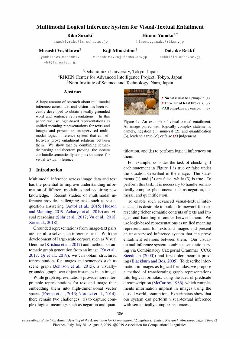
Proceedings of the 57th Annual Meeting of the Association for Computational Linguistics: Student Research Workshop, pages 386–392Florence, Italy, July 28 - August 2, 2019. c©2019 Association for Computational Linguistics

Multimodal Logical Inference System for Visual-Textual EntailmentRiko Suzuki1

suzuki.riko@is.ocha.ac.jp

Hitomi Yanaka1,2

hitomi.yanaka@riken.jp

Masashi Yoshikawa3

yoshikawa.masashi.

yh8@is.naist.jp

Koji Mineshima1

mineshima.koji@ocha.ac.jp

Daisuke Bekki1bekki@is.ocha.ac.jp

1Ochanomizu University, Tokyo, Japan2RIKEN Center for Advanced Intelligence Project, Tokyo, Japan

3Nara Institute of Science and Technology, Nara, Japan

Abstract

A large amount of research about multimodalinference across text and vision has been re-cently developed to obtain visually groundedword and sentence representations. In thispaper, we use logic-based representations asunified meaning representations for texts andimages and present an unsupervised multi-modal logical inference system that can ef-fectively prove entailment relations betweenthem. We show that by combining seman-tic parsing and theorem proving, the systemcan handle semantically complex sentences forvisual-textual inference.

1 Introduction

Multimodal inference across image data and texthas the potential to improve understanding infor-mation of different modalities and acquiring newknowledge. Recent studies of multimodal in-ference provide challenging tasks such as visualquestion answering (Antol et al., 2015; Hudsonand Manning, 2019; Acharya et al., 2019) and vi-sual reasoning (Suhr et al., 2017; Vu et al., 2018;Xie et al., 2018).

Grounded representations from image-text pairsare useful to solve such inference tasks. With thedevelopment of large-scale corpora such as VisualGenome (Krishna et al., 2017) and methods of au-tomatic graph generation from an image (Xu et al.,2017; Qi et al., 2019), we can obtain structuredrepresentations for images and sentences such asscene graph (Johnson et al., 2015), a visually-grounded graph over object instances in an image.

While graph representations provide more inter-pretable representations for text and image thanembedding them into high-dimensional vectorspaces (Frome et al., 2013; Norouzi et al., 2014),there remain two challenges: (i) to capture com-plex logical meanings such as negation and quan-

7 No cat is next to a pumpkin. (1)7 There are at least two cats. (2)3All pumpkins are orange. (3)

Figure 1: An example of visual-textual entailment.An image paired with logically complex statements,namely, negation (1), numeral (2), and quantification(3), leads to a true (3) or false (7) judgement.

tification, and (ii) to perform logical inferences onthem.

For example, consider the task of checking ifeach statement in Figure 1 is true or false underthe situation described in the image. The state-ments (1) and (2) are false, while (3) is true. Toperform this task, it is necessary to handle seman-tically complex phenomena such as negation, nu-meral, and quantification.

To enable such advanced visual-textual infer-ences, it is desirable to build a framework for rep-resenting richer semantic contents of texts and im-ages and handling inference between them. Weuse logic-based representations as unified meaningrepresentations for texts and images and presentan unsupervised inference system that can proveentailment relations between them. Our visual-textual inference system combines semantic pars-ing via Combinatory Categorial Grammar (CCG;Steedman (2000)) and first-order theorem prov-ing (Blackburn and Bos, 2005). To describe infor-mation in images as logical formulas, we proposea method of transforming graph representationsinto logical formulas, using the idea of predicatecircumscription (McCarthy, 1986), which comple-ments information implicit in images using theclosed world assumption. Experiments show thatour system can perform visual-textual inferencewith semantically complex sentences.

386

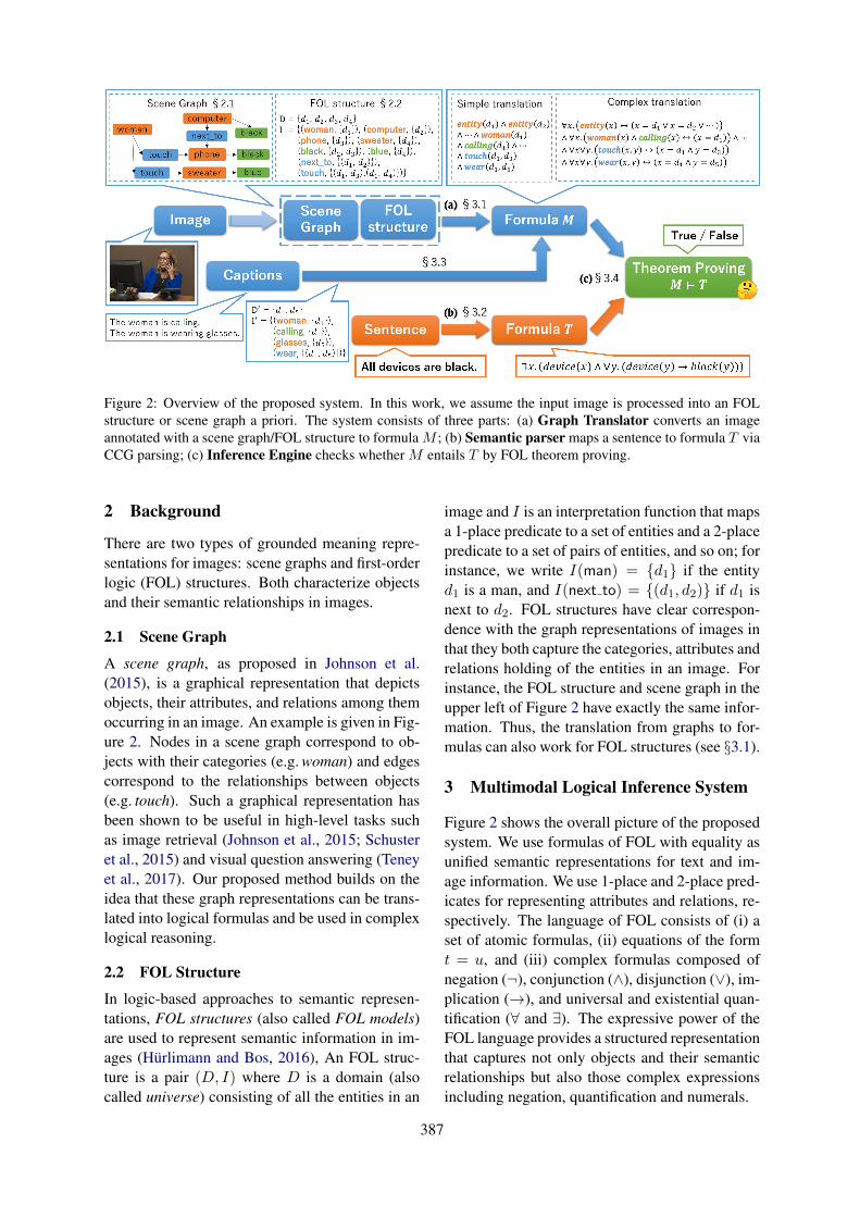
Figure 2: Overview of the proposed system. In this work, we assume the input image is processed into an FOLstructure or scene graph a priori. The system consists of three parts: (a) Graph Translator converts an imageannotated with a scene graph/FOL structure to formula M ; (b) Semantic parser maps a sentence to formula T viaCCG parsing; (c) Inference Engine checks whether M entails T by FOL theorem proving.

2 Background

There are two types of grounded meaning repre-sentations for images: scene graphs and first-orderlogic (FOL) structures. Both characterize objectsand their semantic relationships in images.

2.1 Scene Graph

A scene graph, as proposed in Johnson et al.(2015), is a graphical representation that depictsobjects, their attributes, and relations among themoccurring in an image. An example is given in Fig-ure 2. Nodes in a scene graph correspond to ob-jects with their categories (e.g. woman) and edgescorrespond to the relationships between objects(e.g. touch). Such a graphical representation hasbeen shown to be useful in high-level tasks suchas image retrieval (Johnson et al., 2015; Schusteret al., 2015) and visual question answering (Teneyet al., 2017). Our proposed method builds on theidea that these graph representations can be trans-lated into logical formulas and be used in complexlogical reasoning.

2.2 FOL Structure

In logic-based approaches to semantic represen-tations, FOL structures (also called FOL models)are used to represent semantic information in im-ages (Hurlimann and Bos, 2016), An FOL struc-ture is a pair (D, I) where D is a domain (alsocalled universe) consisting of all the entities in an

image and I is an interpretation function that mapsa 1-place predicate to a set of entities and a 2-placepredicate to a set of pairs of entities, and so on; forinstance, we write I(man) = d1 if the entityd1 is a man, and I(next to) = (d1, d2) if d1 isnext to d2. FOL structures have clear correspon-dence with the graph representations of images inthat they both capture the categories, attributes andrelations holding of the entities in an image. Forinstance, the FOL structure and scene graph in theupper left of Figure 2 have exactly the same infor-mation. Thus, the translation from graphs to for-mulas can also work for FOL structures (see §3.1).

3 Multimodal Logical Inference System

Figure 2 shows the overall picture of the proposedsystem. We use formulas of FOL with equality asunified semantic representations for text and im-age information. We use 1-place and 2-place pred-icates for representing attributes and relations, re-spectively. The language of FOL consists of (i) aset of atomic formulas, (ii) equations of the formt = u, and (iii) complex formulas composed ofnegation (¬), conjunction (∧), disjunction (∨), im-plication (→), and universal and existential quan-tification (∀ and ∃). The expressive power of theFOL language provides a structured representationthat captures not only objects and their semanticrelationships but also those complex expressionsincluding negation, quantification and numerals.

387

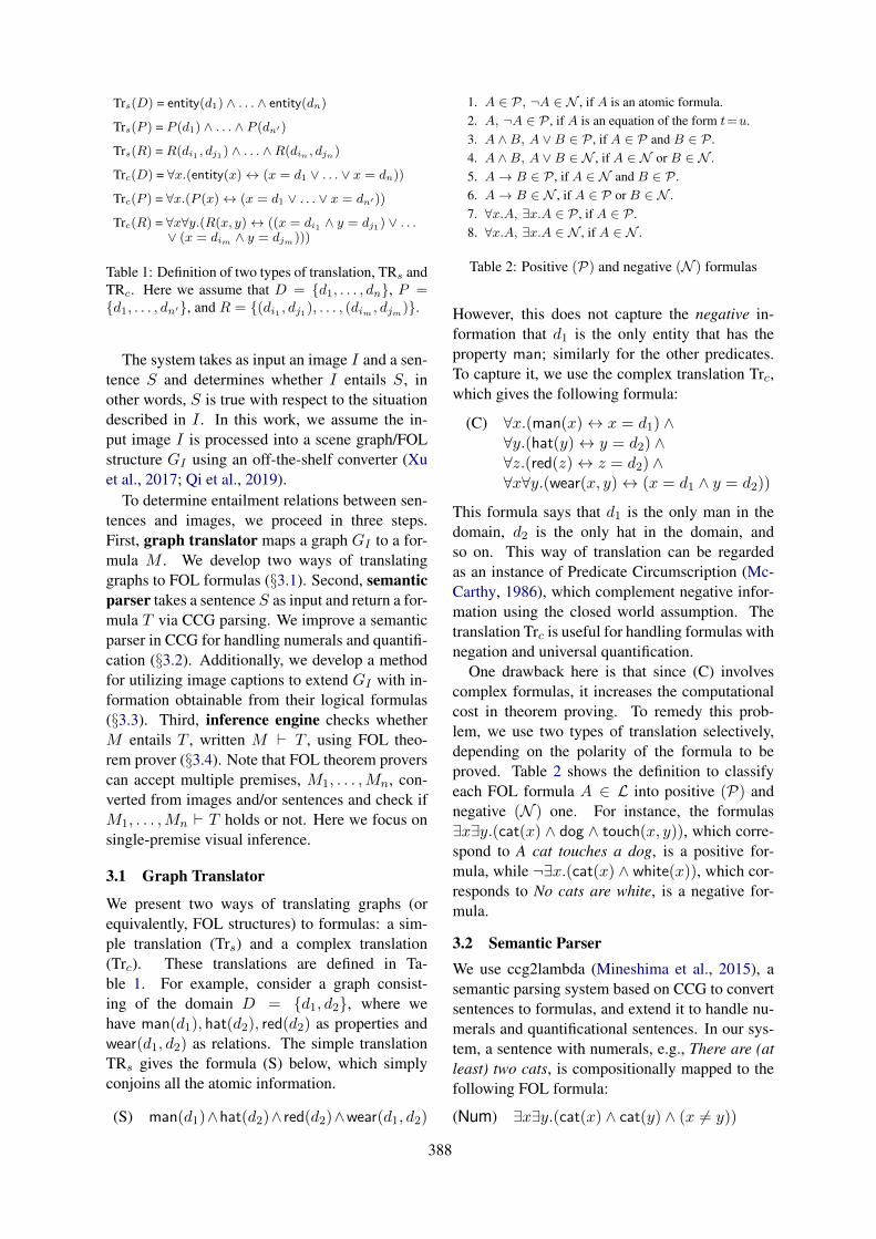
Trs(D) = entity(d1) ∧ . . . ∧ entity(dn)

Trs(P ) = P (d1) ∧ . . . ∧ P (dn′)

Trs(R) = R(di1 , dj1) ∧ . . . ∧ R(din , djn)

Trc(D) = ∀x.(entity(x) ↔ (x = d1 ∨ . . . ∨ x = dn))

Trc(P ) = ∀x.(P (x) ↔ (x = d1 ∨ . . . ∨ x = dn′))

Trc(R) = ∀x∀y.(R(x, y) ↔ ((x = di1 ∧ y = dj1) ∨ . . .∨ (x = dim ∧ y = djm)))

Table 1: Definition of two types of translation, TRs andTRc. Here we assume that D = d1, . . . , dn, P =d1, . . . , dn′, and R = (di1 , dj1), . . . , (dim , djm).

The system takes as input an image I and a sen-tence S and determines whether I entails S, inother words, S is true with respect to the situationdescribed in I . In this work, we assume the in-put image I is processed into a scene graph/FOLstructure GI using an off-the-shelf converter (Xuet al., 2017; Qi et al., 2019).

To determine entailment relations between sen-tences and images, we proceed in three steps.First, graph translator maps a graph GI to a for-mula M . We develop two ways of translatinggraphs to FOL formulas (§3.1). Second, semanticparser takes a sentence S as input and return a for-mula T via CCG parsing. We improve a semanticparser in CCG for handling numerals and quantifi-cation (§3.2). Additionally, we develop a methodfor utilizing image captions to extend GI with in-formation obtainable from their logical formulas(§3.3). Third, inference engine checks whetherM entails T , written M ⊢ T , using FOL theo-rem prover (§3.4). Note that FOL theorem proverscan accept multiple premises, M1, . . . , Mn, con-verted from images and/or sentences and check ifM1, . . . , Mn ⊢ T holds or not. Here we focus onsingle-premise visual inference.

3.1 Graph Translator

We present two ways of translating graphs (orequivalently, FOL structures) to formulas: a sim-ple translation (Trs) and a complex translation(Trc). These translations are defined in Ta-ble 1. For example, consider a graph consist-ing of the domain D = d1, d2, where wehave man(d1), hat(d2), red(d2) as properties andwear(d1, d2) as relations. The simple translationTRs gives the formula (S) below, which simplyconjoins all the atomic information.

(S) man(d1)∧hat(d2)∧ red(d2)∧wear(d1, d2)

1. A ∈ P, ¬A ∈ N , if A is an atomic formula.2. A, ¬A ∈ P , if A is an equation of the form t=u.3. A ∧ B, A ∨ B ∈ P , if A ∈ P and B ∈ P .4. A ∧ B, A ∨ B ∈ N , if A ∈ N or B ∈ N .5. A → B ∈ P , if A ∈ N and B ∈ P .6. A → B ∈ N , if A ∈ P or B ∈ N .7. ∀x.A, ∃x.A ∈ P , if A ∈ P .8. ∀x.A, ∃x.A ∈ N , if A ∈ N .

Table 2: Positive (P) and negative (N ) formulas

However, this does not capture the negative in-formation that d1 is the only entity that has theproperty man; similarly for the other predicates.To capture it, we use the complex translation Trc,which gives the following formula:

(C) ∀x.(man(x) ↔ x = d1) ∧∀y.(hat(y) ↔ y = d2) ∧∀z.(red(z) ↔ z = d2) ∧∀x∀y.(wear(x, y) ↔ (x = d1 ∧ y = d2))

This formula says that d1 is the only man in thedomain, d2 is the only hat in the domain, andso on. This way of translation can be regardedas an instance of Predicate Circumscription (Mc-Carthy, 1986), which complement negative infor-mation using the closed world assumption. Thetranslation Trc is useful for handling formulas withnegation and universal quantification.

One drawback here is that since (C) involvescomplex formulas, it increases the computationalcost in theorem proving. To remedy this prob-lem, we use two types of translation selectively,depending on the polarity of the formula to beproved. Table 2 shows the definition to classifyeach FOL formula A ∈ L into positive (P) andnegative (N ) one. For instance, the formulas∃x∃y.(cat(x) ∧ dog ∧ touch(x, y)), which corre-spond to A cat touches a dog, is a positive for-mula, while ¬∃x.(cat(x) ∧ white(x)), which cor-responds to No cats are white, is a negative for-mula.

3.2 Semantic ParserWe use ccg2lambda (Mineshima et al., 2015), asemantic parsing system based on CCG to convertsentences to formulas, and extend it to handle nu-merals and quantificational sentences. In our sys-tem, a sentence with numerals, e.g., There are (atleast) two cats, is compositionally mapped to thefollowing FOL formula:

(Num) ∃x∃y.(cat(x) ∧ cat(y) ∧ (x = y))

388

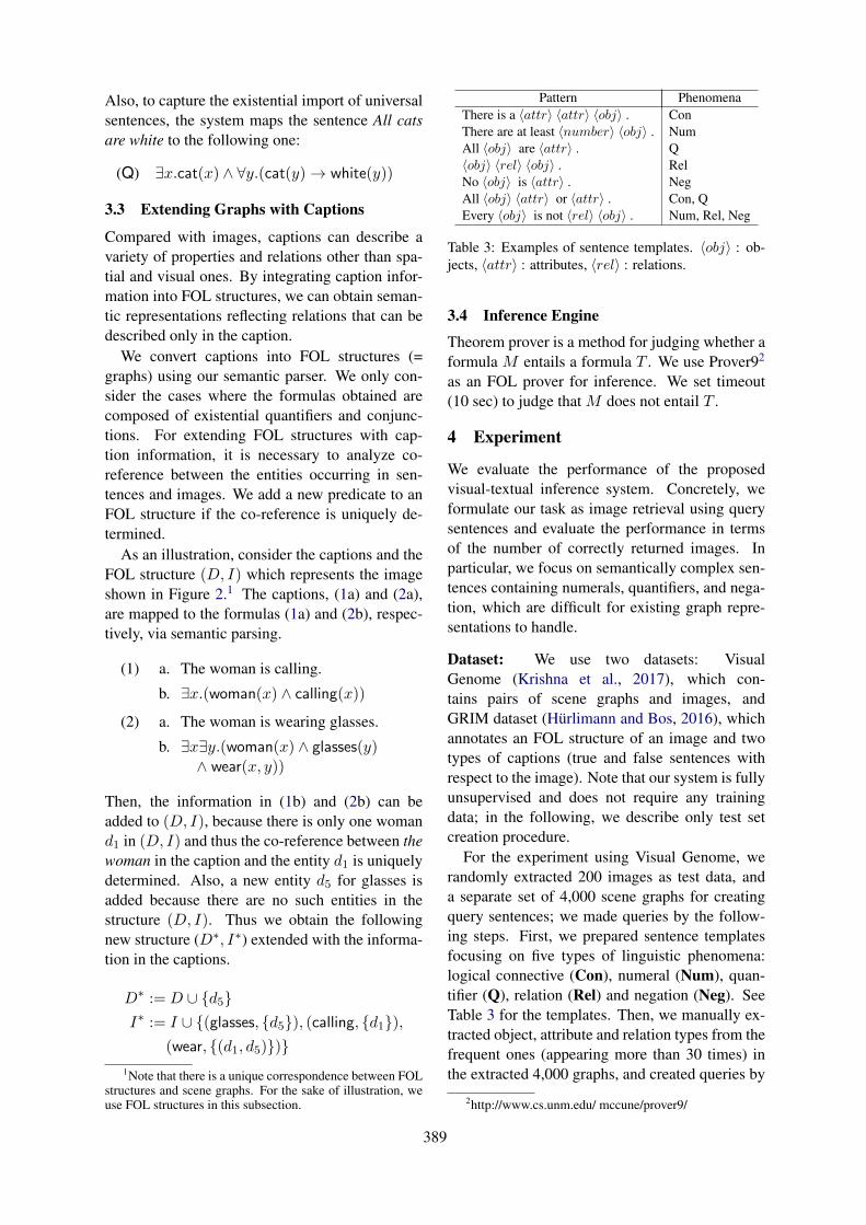
Also, to capture the existential import of universalsentences, the system maps the sentence All catsare white to the following one:

(Q) ∃x.cat(x) ∧ ∀y.(cat(y) → white(y))

3.3 Extending Graphs with Captions

Compared with images, captions can describe avariety of properties and relations other than spa-tial and visual ones. By integrating caption infor-mation into FOL structures, we can obtain seman-tic representations reflecting relations that can bedescribed only in the caption.

We convert captions into FOL structures (=graphs) using our semantic parser. We only con-sider the cases where the formulas obtained arecomposed of existential quantifiers and conjunc-tions. For extending FOL structures with cap-tion information, it is necessary to analyze co-reference between the entities occurring in sen-tences and images. We add a new predicate to anFOL structure if the co-reference is uniquely de-termined.

As an illustration, consider the captions and theFOL structure (D, I) which represents the imageshown in Figure 2.1 The captions, (1a) and (2a),are mapped to the formulas (1a) and (2b), respec-tively, via semantic parsing.

(1) a. The woman is calling.

b. ∃x.(woman(x) ∧ calling(x))

(2) a. The woman is wearing glasses.

b. ∃x∃y.(woman(x) ∧ glasses(y)∧ wear(x, y))

Then, the information in (1b) and (2b) can beadded to (D, I), because there is only one womand1 in (D, I) and thus the co-reference between thewoman in the caption and the entity d1 is uniquelydetermined. Also, a new entity d5 for glasses isadded because there are no such entities in thestructure (D, I). Thus we obtain the followingnew structure (D∗, I∗) extended with the informa-tion in the captions.

D∗ := D ∪ d5I∗ := I ∪ (glasses, d5), (calling, d1),

(wear, (d1, d5))1Note that there is a unique correspondence between FOL

structures and scene graphs. For the sake of illustration, weuse FOL structures in this subsection.

Pattern PhenomenaThere is a ⟨attr⟩ ⟨attr⟩ ⟨obj⟩ . ConThere are at least ⟨number⟩ ⟨obj⟩ . NumAll ⟨obj⟩ are ⟨attr⟩ . Q⟨obj⟩ ⟨rel⟩ ⟨obj⟩ . RelNo ⟨obj⟩ is ⟨attr⟩ . NegAll ⟨obj⟩ ⟨attr⟩ or ⟨attr⟩ . Con, QEvery ⟨obj⟩ is not ⟨rel⟩ ⟨obj⟩ . Num, Rel, Neg

Table 3: Examples of sentence templates. ⟨obj⟩ : ob-jects, ⟨attr⟩ : attributes, ⟨rel⟩ : relations.

3.4 Inference Engine

Theorem prover is a method for judging whether aformula M entails a formula T . We use Prover92

as an FOL prover for inference. We set timeout(10 sec) to judge that M does not entail T .

4 Experiment

We evaluate the performance of the proposedvisual-textual inference system. Concretely, weformulate our task as image retrieval using querysentences and evaluate the performance in termsof the number of correctly returned images. Inparticular, we focus on semantically complex sen-tences containing numerals, quantifiers, and nega-tion, which are difficult for existing graph repre-sentations to handle.

Dataset: We use two datasets: VisualGenome (Krishna et al., 2017), which con-tains pairs of scene graphs and images, andGRIM dataset (Hurlimann and Bos, 2016), whichannotates an FOL structure of an image and twotypes of captions (true and false sentences withrespect to the image). Note that our system is fullyunsupervised and does not require any trainingdata; in the following, we describe only test setcreation procedure.

For the experiment using Visual Genome, werandomly extracted 200 images as test data, anda separate set of 4,000 scene graphs for creatingquery sentences; we made queries by the follow-ing steps. First, we prepared sentence templatesfocusing on five types of linguistic phenomena:logical connective (Con), numeral (Num), quan-tifier (Q), relation (Rel) and negation (Neg). SeeTable 3 for the templates. Then, we manually ex-tracted object, attribute and relation types from thefrequent ones (appearing more than 30 times) inthe extracted 4,000 graphs, and created queries by

2http://www.cs.unm.edu/ mccune/prover9/

389

Sentences Phenomena CountThere is a long red bus. Con 3There are at least three men. Num 32All windows are closed. Q 53Every green tree is tall. Q 18A man is wearing a hat. Rel 12No umbrella is colorful. Neg 197There is a train which is not red. Neg 6There are two cups or three cups. Con, Num 5All hairs are black or brown. Con, Q 46A gray or black pole has two signs. Con, Num, Rel 6Three cars are not red. Num, Neg 28All women wear a hat. Q, Rel 2A man is not walking on a street. Rel, Neg 76A clock on a tower is not black. Rel, Neg 7Two women aren’t having black hair. Num, Rel, Neg 10Every man isn’t eating anything. Q, Rel, Neg 67

Table 4: Examples of query sentences In §4.1; Countshows the number of images describing situations un-der which each sentence is true.

replacing ⟨obj⟩ , ⟨attr⟩ and ⟨rel⟩ in the templateswith them. As a result, we obtained 37 semanti-cally complex queries as shown in Table 4. To as-sign correct images to each query, two annotatorsjudged whether each of the test images entails thequery sentence. If the two judgments disagreed,the first author decided the correct label.

In the experiment using GRIM, we adopted thesame procedure to create a test dataset and ob-tained 19 query sentences and 194 images.

One of the issues in this dataset is that annotatedFOL structures contain only spatial relations suchas next to and near; to handle queries containinggeneral relations such as play and sing, our sys-tem needs to utilize annotated captions (§3.3). Toevaluate if our system can effectively extract infor-mation from captions, we split Rel of above lin-guistic phenomena into spatial relation (Spa-Rel;relations about spatial information) and general re-lation (Gen-Rel; other relations), and report thescores separately in terms of these categories.

4.1 Experimental Results on Visual Genome

Firstly, we evaluate the performance in terms ofour Graph translator’s conversion algorithm. Asdescribed in §3.1, there are two translation algo-rithms; simple one that conjunctively enumeratesall relation in a graph (SIMPLE in the following),and one that selectively employs translation basedon Predicate Circumscription (HYBRID).

Table 5 shows image retrieval scores per lin-guistic phenomenon, macro averages of F1 scoresof queries labeled with the respective phenomena.

Phenomena (#) SIMPLE HYBRID

Con (17) 36.40 41.66Num (9) 43.07 45.45

Q (9) 8.59 28.18Rel (11) 25.13 35.10Neg (11) 66.38 73.39

Table 5: Experimental results on Visual Genome (F1).“#” stands for the number of query sentences catego-rized into that phenomenon.

HYBRID shows better performance for all phe-nomena than SIMPLE one, improving by 19.59%on Q, 9.97% on Rel and 7.01% on Neg, over SIM-PLE, suggesting that the proposed complex trans-lation is useful for inference using semanticallycomplex sentences including quantifier and nega-tion. Figure 3 shows retrieved results for a query(a) Every green tree is tall and (b) No umbrella iscolorful, each containing universal quantifier andnegation, respectively. Our system successfullyperforms inference on these queries, returning thecorrect images, while excluding wrong ones (notethat the third picture in (a) contains short trees).

(a) Every green tree is tall.

(b) No umbrella is colorful.

Figure 3: Predicted images of our system; Images ingreen entail the queries, while those in red do not.

Error Analysis: One of the reasons for thelower F1 of Q is the gap of annotation rule be-tween Visual Genome and our test set. Quan-tifiers in natural language often involve vague-ness (Pezzelle et al., 2018). for example, the in-terpretation of everyone depends on what countsas an entity in the domain. Difficulties in fixingthe interpretation of quantifiers caused the lowerperformance.

The low F1 in Rel is primarily due to lexicalgaps between formulas of a query and an image.For example, sentences All women wear a hat andAll women have a hat are the same in their mean-ing. However, if a scene graph contains only wear

390

relation, our system can handle the former query,while not the other. In future work, we will ex-tend our system with a knowledge insertion mech-anism (Martınez-Gomez et al., 2017).

4.2 Experimental Results on GRIM

We test our system on GRIM dataset. As notedabove, the main issue on this dataset is the lack ofrelations other than spatial ones. We evaluate ifour system can be enhanced using the informationcontained in captions. The F1 scores of the Hybridsystem with captions are the same with the onewithout captions on the sets except for Gen-Rel;3on the subset, the F1 score of the former improvesby 60% compared to the latter, which suggests thatcaptions can be integrated into FOL structures forthe improved performance.

5 Conclusion

We have proposed a logic-based system to achieveadvanced visual-textual inference, demonstratingthe importance of building a framework for rep-resenting the richer semantic content of texts andimages. In the experiment, we have shown that ourCCG-based pipeline system, consisting of graphtranslator, semantic parser and inference engine,can perform visual-textual inference with seman-tically complex sentences, without requiring anysupervised data.

Acknowledgement

We thank the two anonymous reviewers for theirencouragement and insightful comments. Thiswork was partially supported by JST CRESTGrant Number JPMJCR1301, Japan.

ReferencesManoj Acharya, Kushal Kafle, and Christopher Kanan. 2019.

TallyQA: Answering complex counting questions. In TheAssociation for the Advancement of Artificial Intelligence(AAAI2019).

Stanislaw Antol, Aishwarya Agrawal, Jiasen Lu, MargaretMitchell, Dhruv Batra, C. Lawrence Zitnick, and DeviParikh. 2015. VQA: Visual Question Answering. In In-ternational Conference on Computer Vision.

Patrick Blackburn and Johan Bos. 2005. Representation andInference for Natural Language: A First Course in Com-putational Semantics. Center for the Study of Languageand Information, Stanford, CA, USA.

3Con: 91.41%, Num: 95.24%, Q: 78.84%, Spa-Rel:88.57%, Neg: 62.57%.

Andrea Frome, Greg S Corrado, Jon Shlens, Samy Bengio,Jeff Dean, Marc Aurelio Ranzato, and Tomas Mikolov.2013. DeViSE: A Deep Visual-Semantic EmbeddingModel. In Neural Information Processing Systems con-ference, pages 2121–2129.

Drew A. Hudson and Christopher D. Manning. 2019. Gqa:A new dataset for real-world visual reasoning and compo-sitional question answering. In The IEEE Conference onComputer Vision and Pattern Recognition (CVPR).

Manuela Hurlimann and Johan Bos. 2016. Combining lexicaland spatial knowledge to predict spatial relations betweenobjects in images. In Proceedings of the 5th Workshop onVision and Language, pages 10–18. Association for Com-putational Linguistics.

Justin Johnson, Ranjay Krishna, Michael Stark, Li-Jia Li,David A. Shamma, Michael S. Bernstein, and Li Fei-Fei.2015. Image retrieval using scene graphs. In IEEE/ CVFInternational Conference on Computer Vision and PatternRecognition, pages 3668–3678. IEEE Computer Society.

Ranjay Krishna, Yuke Zhu, Oliver Groth, Justin Johnson,Kenji Hata, Joshua Kravitz, Stephanie Chen, YannisKalantidis, Li-Jia Li, David A Shamma, Michael Bern-stein, and Li Fei-Fei. 2017. Visual genome: Connect-ing language and vision using crowdsourced dense imageannotations. International Journal of Computer Vision,123(1):32–73.

Pascual Martınez-Gomez, Koji Mineshima, Yusuke Miyao,and Daisuke Bekki. 2017. On-demand Injection of Lex-ical Knowledge for Recognising Textual Entailment. InProceedings of The European Chapter of the Associationfor Computational Linguistics, pages 710–720.

John McCarthy. 1986. Applications of circumscription toformalizing common-sense knowledge. Artificial Intelli-gence, 28(1):89–116.

Koji Mineshima, Pascual Martınez-Gomez, Yusuke Miyao,and Daisuke Bekki. 2015. Higher-order logical inferencewith compositional semantics. In Proceedings of the 2015Conference on Empirical Methods in Natural LanguageProcessing, pages 2055–2061. Association for Computa-tional Linguistics.

Mohammad Norouzi, Tomas Mikolov, Samy Bengio, YoramSinger, Jonathon Shlens, Andrea Frome, Greg Corrado,and Jeffrey Dean. 2014. Zero-Shot Learning by ConvexCombination of Semantic Embeddings. In InternationalConference on Learning Representations.

Sandro Pezzelle, Ionut-Teodor Sorodoc, and RaffaellaBernardi. 2018. Comparatives, quantifiers, proportions:a multi-task model for the learning of quantities from vi-sion. In Proceedings of the 2018 Conference of the NorthAmerican Chapter of the Association for ComputationalLinguistics: Human Language Technologies, pages 419–430. Association for Computational Linguistics.

Mengshi Qi, Weijian Li, Zhengyuan Yang, Yunhong Wang,and Jiebo Luo. 2019. Attentive relational networks formapping images to scene graphs. In The IEEE Conferenceon Computer Vision and Pattern Recognition.

Sebastian Schuster, Ranjay Krishna, Angel Chang, Li Fei-Fei, and Christopher D. Manning. 2015. Generating se-mantically precise scene graphs from textual descriptionsfor improved image retrieval. In Proceedings of the FourthWorkshop on Vision and Language, pages 70–80. Associ-ation for Computational Linguistics.

391

Mark Steedman. 2000. The Syntactic Process. MIT Press,Cambridge, MA, USA.

Alane Suhr, Mike Lewis, James Yeh, and Yoav Artzi. 2017.A corpus of natural language for visual reasoning. In Pro-ceedings of the 55th Annual Meeting of the Associationfor Computational Linguistics (Volume 2: Short Papers),pages 217–223, Vancouver, Canada. Association for Com-putational Linguistics.

Damien Teney, Lingqiao Liu, and Anton van den Hengel.2017. Graph-structured representations for visual ques-tion answering. In The IEEE Conference on ComputerVision and Pattern Recognition, pages 3233–3241.

Hoa Trong Vu, Claudio Greco, Aliia Erofeeva, Somayeh Ja-faritazehjan, Guido Linders, Marc Tanti, Alberto Testoni,Raffaella Bernardi, and Albert Gatt. 2018. Grounded tex-tual entailment. In Proceedings of the 27th InternationalConference on Computational Linguistics, pages 2354–2368.

Ning Xie, Farley Lai, Derek Doran, and Asim Kadav. 2018.Visual entailment task for visually-grounded languagelearning. arXiv preprint arXiv:1811.10582.

Danfei Xu, Yuke Zhu, Christopher B. Choy, and Li Fei-Fei.2017. Scene Graph Generation by Iterative Message Pass-ing. In The IEEE Conference on Computer Vision andPattern Recognition.

392

Proceedings of the 57th Annual Meeting of the Association for Computational Linguistics: Student Research Workshop, pages 393–399Florence, Italy, July 28 - August 2, 2019. c©2019 Association for Computational Linguistics

Deep Neural Models for Medical Concept Normalization inUser-Generated Texts

Zulfat MiftahutdinovKazan Federal University,

Kazan, Russiazulfatmi@gmail.com

Elena TutubalinaKazan Federal University,

Kazan, RussiaSamsung-PDMI Joint AI Center,

PDMI RAS, St. Petersburg, Russiaelvtutubalina@kpfu.ru

Abstract

In this work, we consider the medical con-cept normalization problem, i.e., the prob-lem of mapping a health-related entity men-tion in a free-form text to a concept in a con-trolled vocabulary, usually to the standard the-saurus in the Unified Medical Language Sys-tem (UMLS). This is a challenging task sincemedical terminology is very different whencoming from health care professionals or fromthe general public in the form of social mediatexts. We approach it as a sequence learningproblem with powerful neural networks suchas recurrent neural networks and contextual-ized word representation models trained to ob-tain semantic representations of social mediaexpressions. Our experimental evaluation overthree different benchmarks shows that neuralarchitectures leverage the semantic meaningof the entity mention and significantly outper-form an existing state of the art models.

1 Introduction

User-generated texts (UGT) on social mediapresent a wide variety of facts, experiences, andopinions on numerous topics, and this treasuretrove of information is currently severely under-explored. We consider the problem of discoveringmedical concepts in UGTs with the ultimate goalof mining new symptoms, adverse drug reactions(ADR), and other information about a disorder ora drug.

An important part of this problem is to translatea text from “social media language” (e.g., “can’tfall asleep all night” or “head spinning a little”)to “formal medical language” (e.g., “insomnia”and “dizziness” respectively). This is necessaryto match user-generated descriptions with medicalconcepts, but it is more than just a simple matchingof UGTs against a vocabulary. We call the task ofmapping the language of UGTs to medical termi-

nology medical concept normalization. It is espe-cially difficult since in social media, patients dis-cuss different concepts of illness and a wide arrayof drug reactions. Moreover, UGTs from socialnetworks are typically ambiguous and very noisy,containing misspelled words, incorrect grammar,hashtags, abbreviations, smileys, different varia-tions of the same word, and so on.

Traditional approaches for concept normaliza-tion utilized lexicons and knowledge bases withstring matching. The most popular knowledge-based system for mapping texts to UMLS identi-fiers is MetaMap (Aronson, 2001). This linguistic-based system uses lexical lookup and variants byassociating a score with phrases in a sentence. Thestate-of-the-art baseline for clinical and scientifictexts is DNorm (Leaman et al., 2013). DNormadopts a pairwise learning-to-rank technique usingvectors of query mentions and candidate conceptterms. This model outperforms MetaMap signif-icantly, increasing the macro-averaged F-measureby 25% on an NCBI disease dataset. However,while these tools have proven to be effective forpatient records and research papers, they achievemoderate results on social media texts (Nikfarjamet al., 2015; Limsopatham and Collier, 2016).

Recent works go beyond string matching: theseworks have tried to view the problem of matchinga one- or multi-word expression against a knowl-edge base as a supervised sequence labeling prob-lem. Limsopatham and Collier (2016) utilizedconvolutional neural networks (CNNs) for phrasenormalization in user reviews, while Tutubalinaet al. (2018), Han et al. (2017), and Belousov et al.(2017) applied recurrent neural networks (RNNs)to UGTs, achieving similar results. These workswere among the first applications of deep learningtechniques to medical concept normalization.

The goal of this work is to study the use of deepneural models, i.e., contextualized word represen-

393

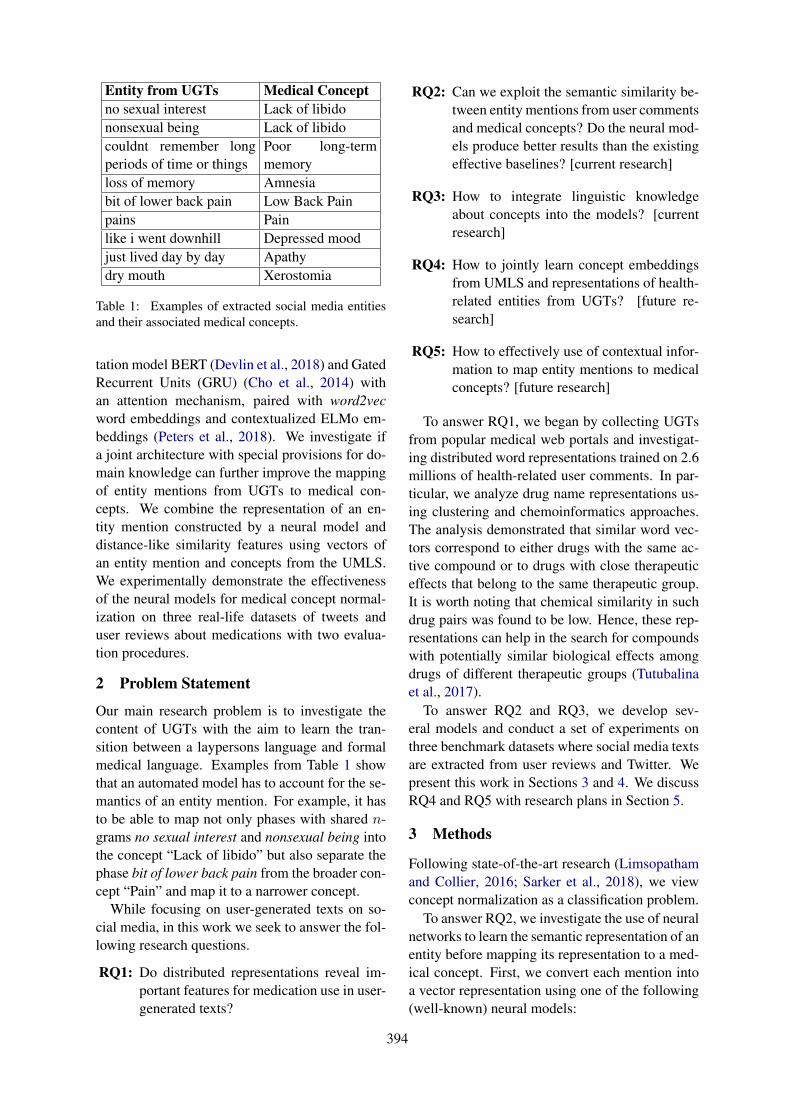
Entity from UGTs Medical Conceptno sexual interest Lack of libidononsexual being Lack of libidocouldnt remember longperiods of time or things

Poor long-termmemory

loss of memory Amnesiabit of lower back pain Low Back Painpains Painlike i went downhill Depressed moodjust lived day by day Apathydry mouth Xerostomia

Table 1: Examples of extracted social media entitiesand their associated medical concepts.

tation model BERT (Devlin et al., 2018) and GatedRecurrent Units (GRU) (Cho et al., 2014) withan attention mechanism, paired with word2vecword embeddings and contextualized ELMo em-beddings (Peters et al., 2018). We investigate ifa joint architecture with special provisions for do-main knowledge can further improve the mappingof entity mentions from UGTs to medical con-cepts. We combine the representation of an en-tity mention constructed by a neural model anddistance-like similarity features using vectors ofan entity mention and concepts from the UMLS.We experimentally demonstrate the effectivenessof the neural models for medical concept normal-ization on three real-life datasets of tweets anduser reviews about medications with two evalua-tion procedures.

2 Problem Statement

Our main research problem is to investigate thecontent of UGTs with the aim to learn the tran-sition between a laypersons language and formalmedical language. Examples from Table 1 showthat an automated model has to account for the se-mantics of an entity mention. For example, it hasto be able to map not only phases with shared n-grams no sexual interest and nonsexual being intothe concept “Lack of libido” but also separate thephase bit of lower back pain from the broader con-cept “Pain” and map it to a narrower concept.

While focusing on user-generated texts on so-cial media, in this work we seek to answer the fol-lowing research questions.

RQ1: Do distributed representations reveal im-portant features for medication use in user-generated texts?

RQ2: Can we exploit the semantic similarity be-tween entity mentions from user commentsand medical concepts? Do the neural mod-els produce better results than the existingeffective baselines? [current research]

RQ3: How to integrate linguistic knowledgeabout concepts into the models? [currentresearch]

RQ4: How to jointly learn concept embeddingsfrom UMLS and representations of health-related entities from UGTs? [future re-search]

RQ5: How to effectively use of contextual infor-mation to map entity mentions to medicalconcepts? [future research]

To answer RQ1, we began by collecting UGTsfrom popular medical web portals and investigat-ing distributed word representations trained on 2.6millions of health-related user comments. In par-ticular, we analyze drug name representations us-ing clustering and chemoinformatics approaches.The analysis demonstrated that similar word vec-tors correspond to either drugs with the same ac-tive compound or to drugs with close therapeuticeffects that belong to the same therapeutic group.It is worth noting that chemical similarity in suchdrug pairs was found to be low. Hence, these rep-resentations can help in the search for compoundswith potentially similar biological effects amongdrugs of different therapeutic groups (Tutubalinaet al., 2017).

To answer RQ2 and RQ3, we develop sev-eral models and conduct a set of experiments onthree benchmark datasets where social media textsare extracted from user reviews and Twitter. Wepresent this work in Sections 3 and 4. We discussRQ4 and RQ5 with research plans in Section 5.

3 Methods

Following state-of-the-art research (Limsopathamand Collier, 2016; Sarker et al., 2018), we viewconcept normalization as a classification problem.

To answer RQ2, we investigate the use of neuralnetworks to learn the semantic representation of anentity before mapping its representation to a med-ical concept. First, we convert each mention intoa vector representation using one of the following(well-known) neural models:

394

(1) bidirectional LSTM (Hochreiter and Schmid-huber, 1997) or GRU (Cho et al., 2014)with an attention mechanism and a hyper-bolic tangent activation function on top of200-dimensional word embeddings obtainedto answer RQ1;

(2) a bidirectional layer with attention on topof deep contextualized word representationsELMo (Peters et al., 2018);

(3) a contextualized word representation modelBERT (Devlin et al., 2018), which is a multi-layer bidirectional Transformer encoder.

We omit technical explanations of the neural net-work architectures due to space constraints and re-fer to the studies above.

Next, the learned representation is concate-nated with a number of semantic similarity fea-tures based on prior knowledge from the UMLSMetathesaurus. Lastly, we add a softmax layer toconvert values to conditional probabilities.

The most attractive feature of the biomedicaldomain is that domain knowledge is prevailing inthis domain for dozens of languages. In particular,UMLS is undoubtedly the largest lexico-semanticresource for medicine, containing more than 150lexicons with terms from 25 languages. To answerRQ3, we extract a set of features to enhance therepresentation of phrases. These features containcosine similarities between the vectors of an inputphrase and a concept in a medical terminology dic-tionary. We use the following strategy, which wecall TF-IDF (MAX), to construct representationsof a concept and a mention: represent a medicalcode as a set of terms; for each term, compute thecosine distance between its TF-IDF representationand the entity mention; then choose the term withthe largest similarity.

4 Experiments

We perform an extensive evaluation of neu-ral models on three datasets of UGTs, namelyCADEC (Karimi et al., 2015), PsyTAR (Zolnooriet al., 2019), and SMM4H 2017 (Sarker et al.,2018). The basic task is to map a social mediaphrase to a relevant medical concept.

4.1 Data

CADEC. CSIRO Adverse Drug Event Corpus(CADEC) (Karimi et al., 2015) is the first richly

annotated and publicly available corpus of med-ical forum posts taken from AskaPatient1. Thisdataset contains 1253 UGTs about 12 drugs di-vided into two categories: Diclofenac and Lipi-tor. All posts were annotated manually for 5 typesof entities: ADR, Drug, Disease, Symptom, andFinding. The annotators performed terminologyassociation using the Systematized NomenclatureOf Medicine Clinical Terms (SNOMED CT). Weremoved “conceptless” or ambiguous mentions forthe purposes of evaluation. There were 6,754 en-tities and 1,029 unique codes in total.

PsyTAR. Psychiatric Treatment Adverse Reac-tions (PsyTAR) corpus (Zolnoori et al., 2019) isthe second open-source corpus of user-generatedposts taken from AskaPatient. This dataset in-cludes 887 posts about four psychiatric medica-tions from two classes: (i) Zoloft and Lexaprofrom the Selective Serotonin Reuptake Inhibitor(SSRI) class and (ii) Effexor and Cymbaltafrom the Serotonin Norepinephrine Reuptake In-hibitor (SNRI) class. All posts were anno-tated manually for 4 types of entities: ADR,withdrawal symptoms, drug indications, andsign/symptoms/illness. The corpus consists of6556 phrases mapped to 618 SNOMED codes.

SMM4H 2017. In 2017, Sarker et al. (2018)organized the Social Media Mining for Health(SMM4H) shared task which introduced a datasetwith annotated ADR expressions from Twitter.Tweets were collected using 250 keywords suchas generic and trade names for medications alongwith misspellings. Manually extracted ADR ex-pressions were mapped to Preferred Terms (PTs)of the Medical Dictionary for Regulatory Activi-ties (MedDRA). The training set consists of 6650phrases mapped to 472 PTs. The test set consistsof 2500 mentions mapped to 254 PTs.

4.2 Evaluation Details

We evaluate our models based on classificationaccuracy, averaged across randomly divided fivefolds of the CADEC and PsyTAR corpora. ForSMM4H 2017 data, we adopted the official train-ing and test sets (Sarker et al., 2018). Analy-sis of randomly split folds shows that RandomKFolds create a high overlap of expressions inexact matching between subsets (see the base-line results in Table 2). Therefore, we set up a

1https://www.askapatient.com

395

specific train/test split procedure for 5-fold cross-validation on the CADEC and PsyTAR corpora:we removed duplicates of mentions and groupedmedical records we are working with into sets re-lated to specific medical codes. Then, each set hasbeen split independently into k folds, and all foldshave been merged into the final k folds namedCustom KFolds. Random folds of CADEC areadopted from (Limsopatham and Collier, 2016)for a fair comparison. Custom folds of CADECare adopted from our previous work (Tutubalinaet al., 2018). PsyTAR folds are available on Zen-odo.org2. We have also implemented a simplebaseline approach that uses exact lexical match-ing with lowercased annotations from the trainingset.

4.3 Results

Table 2 shows our results for the concept normal-ization task on the Random and Custom KFolds ofthe CADEC, PsyTAR, and SMM4H 2017 corpora.

To answer RQ2, we compare the performanceof examined neural models with the baselineand state-of-the-art methods in terms of accuracy.Attention-based GRU with ELMo embeddingsshowed improvement over GRU with word2vecembeddings, increasing the average accuracy to77.85 (+3.65). The semantic information of anentity mention learned by BERT helps to im-prove the mapping abilities, outperforming othermodels (avg. accuracy 83.67). Our experimentswith recurrent units showed that GRU consistentlyoutperformed LSTM on all subsets, and atten-tion mechanism provided further quality improve-ments for GRU. From the difference in accuracyon the Random and Custom KFolds, we concludethat future research should focus on developingextrinsic test sets for medical concept normaliza-tion. In particular, the BERT model’s accuracy onthe CADEC Custom KFolds decreased by 9.23%compared to the CADEC Random KFolds.

To answer RQ3, we compare the performanceof models with additional similarity features(marked by “w/”) with others. Indeed, joint mod-els based on GRU and similarity features gain 2-5% improvement on sets with Custom KFolds.The joint model based on BERT and similarityfeatures stays roughly on par with BERT on allsets. We also tested different strategies for con-

2https://doi.org/10.5281/zenodo.3236318

structing representations using word embeddingsand TF-IDF for all synonyms’ tokens that led tosimilar improvements for GRU.

5 Future Directions

RQ4. Future research might focus on develop-ing an embedding method that jointly maps ex-tracted entity mentions and UMLS concepts intothe same continuous vector space. The methodscould help us to easily measure the similarity be-tween words and concepts in the same space. Re-cently, Yamada et al. (2016) demonstrated that co-trained vectors improve the quality of both wordand entity representations in entity linking (EL)which is a task closely related to concept nor-malization. We note that most of the recent ELmethods focus on the disambiguation sub-task, ap-plying simple heuristics for candidate generation.The latter is especially challenging in medical con-cept normalization due to a significant languagedifference between medical terminology and pa-tient vocabulary.

RQ5. Error analysis has confirmed that mod-els often misclassify closely related concepts(e.g., “Emotionally detached” and “Apathy”) andantonymous concepts (e.g., “Hypertension” and“Hypotension”). We suggest to take into accountnot only the distance-like similarity between en-tity mentions and concepts but the mention’s con-text, which is not used directly in recent studies onconcept normalization. The context can be repre-sented by the set of adjacent words or entities. Asan alternative, one can use a conditional randomfield (CRF) to output the most likely sequence ofmedical concepts discussed in a review.

6 Related Work

In 2004, the research community started to addressthe needs to automatically detect biomedical en-tities in free texts through shared tasks. Huangand Lu (2015) survey the work done in the orga-nization of biomedical NLP (BioNLP) challengeevaluations up to 2014. These tasks are devoted tothe normalization of (1) genes from scientific arti-cles (BioCreative I-III in 2005-2011); (2) chemicalentity mentions (BioCreative IV CHEMDNER in2014); (3) disorders from abstracts (BioCreativeV CDR Task in 2015); (4) diseases from clini-cal reports (ShARe/CLEF eHealth 2013; SemEval2014 task 7). Similarly, the CLEF Health 2016

396

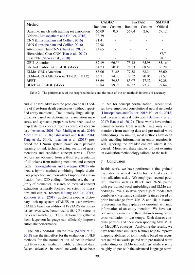
Method CADEC PsyTAR SMM4HRandom Custom Random Custom Official

Baseline: match with training set annotation 66.09 0.0 56.04 2.63 67.12DNorm (Limsopatham and Collier, 2016) 73.39 - - - -CNN (Limsopatham and Collier, 2016) 81.41 - - - -RNN (Limsopatham and Collier, 2016) 79.98 - - - -Attentional Char-CNN (Niu et al., 2018) 84.65 - - - -Hierarchical Char-CNN (Han et al., 2017) - - - - 87.7Ensemble (Sarker et al., 2018) - - - - 88.7GRU+Attention 82.19 66.56 73.12 65.98 83.16GRU+Attention w/ TF-IDF (MAX) 84.23 70.05 75.53 68.59 86.28ELMo+GRU+Attention 85.06 71.68 77.58 68.34 86.60ELMo+GRU+Attention w/ TF-IDF (MAX) 85.71 74.70 79.52 70.05 87.52BERT 88.69 79.83 83.07 77.52 89.28BERT w/ TF-IDF (MAX) 88.84 79.25 82.37 77.33 89.64

Table 2: The performance of the proposed models and the state-of-the-art methods in terms of accuracy.

and 2017 labs addressed the problem of ICD cod-ing of free-form death certificates (without speci-fied entity mentions). Traditionally, linguistic ap-proaches based on dictionaries, association mea-sures, and syntactic properties have been used tomap texts to a concept from a controlled vocabu-lary (Aronson, 2001; Van Mulligen et al., 2016;Mottin et al., 2016; Ghiasvand and Kate, 2014;Tang et al., 2014). Leaman et al. (2013) pro-posed the DNorm system based on a pairwiselearning-to-rank technique using vectors of querymentions and candidate concept terms. Thesevectors are obtained from a tf-idf representationof all tokens from training mentions and conceptterms. Zweigenbaum and Lavergne (2016) uti-lized a hybrid method combining simple dictio-nary projection and mono-label supervised classi-fication from ICD coding. Nevertheless, the ma-jority of biomedical research on medical conceptextraction primarily focused on scientific litera-ture and clinical records (Huang and Lu, 2015).Zolnoori et al. (2019) applied a popular dictio-nary look-up system cTAKES on user reviews.cTAKES based on additional PsyTAR’s dictionar-ies achieves twice better results (0.49 F1 score onthe exact matching). Thus, dictionaries gatheredfrom layperson language can efficiently improveautomatic performance.

The 2017 SMM4H shared task (Sarker et al.,2018) was the first effort for the evaluation of NLPmethods for the normalization of health-relatedtext from social media on publicly released data.Recent advances in neural networks have been

utilized for concept normalization: recent stud-ies have employed convolutional neural networks(Limsopatham and Collier, 2016; Niu et al., 2018)and recurrent neural networks (Belousov et al.,2017; Han et al., 2017). These works have trainedneural networks from scratch using only entitymentions from training data and pre-trained wordembeddings. To sum up, most methods have dealtwith encoding information an entity mention it-self, ignoring the broader context where it oc-curred. Moreover, these studies did not examinean evaluation methodology tailored to the task.

7 Conclusion

In this work, we have performed a fine-grainedevaluation of neural models for medical conceptnormalization tasks. We employed several pow-erful models such as BERT and RNNs pairedwith pre-trained word embeddings and ELMo em-beddings. We also developed a joint model thatcombines (i) semantic similarity features based onprior knowledge from UMLS and (ii) a learnedrepresentation that captures extensional semanticinformation of an entity mention. We have car-ried out experiments on three datasets using 5-foldcross-validation in two setups. Each dataset con-tains phrases and their corresponding SNOMEDor MedDRA concepts. Analyzing the results, wehave found that similarity features help to improvemapping abilities of joint models based on recur-rent neural networks paired with pre-trained wordembeddings or ELMo embeddings while stayingroughly on par with the advanced language repre-

397

sentation model BERT in terms of accuracy. Dif-ferent setups of evaluation procedures affect theperformance of models significantly: the accu-racy of BERT is 7.25% higher on test sets witha simple random split than on test sets with theproposed custom split. Moreover, we have dis-cussed some interesting future research directionsand challenges to be overcome.

Acknowledgments

We thank Sergey Nikolenko for helpful discus-sions. This research was supported by the RussianScience Foundation grant no. 18-11-00284.

ReferencesAlan R Aronson. 2001. Effective mapping of biomed-

ical text to the UMLS Metathesaurus: the MetaMapprogram. In Proceedings of the AMIA Symposium,page 17. American Medical Informatics Associa-tion.

M. Belousov, W. Dixon, and G. Nenadic. 2017. Usingan ensemble of generalised linear and deep learn-ing models in the smm4h 2017 medical conceptnormalisation task. CEUR Workshop Proceedings,1996:54–58.

Kyunghyun Cho, Bart van Merrienboer, CaglarGulcehre, Fethi Bougares, Holger Schwenk, andYoshua Bengio. 2014. Learning phrase representa-tions using RNN encoder-decoder for statistical ma-chine translation. CoRR, abs/1406.1078.

Jacob Devlin, Ming-Wei Chang, Kenton Lee, andKristina Toutanova. 2018. Bert: Pre-training of deepbidirectional transformers for language understand-ing. arXiv preprint arXiv:1810.04805.

Omid Ghiasvand and Rohit J Kate. 2014. Uwm: Disor-der mention extraction from clinical text using crfsand normalization using learned edit distance pat-terns. In SemEval@ COLING, pages 828–832.

S. Han, T. Tran, A. Rios, and R. Kavuluru. 2017. Teamuknlp: Detecting adrs, classifying medication intakemessages, and normalizing adr mentions on twitter.CEUR Workshop Proceedings, 1996:49–53.

S. Hochreiter and J. Schmidhuber. 1997. Long Short-Term Memory. Neural Computation, 9(8):1735–1780. Based on TR FKI-207-95, TUM (1995).

Chung-Chi Huang and Zhiyong Lu. 2015. Communitychallenges in biomedical text mining over 10 years:success, failure and the future. Briefings in bioinfor-matics, 17(1):132–144.

Sarvnaz Karimi, Alejandro Metke-Jimenez, MadonnaKemp, and Chen Wang. 2015. Cadec: A corpus ofadverse drug event annotations. Journal of biomed-ical informatics, 55:73–81.

Robert Leaman, Rezarta Islamaj Dogan, and Zhiy-ong Lu. 2013. DNorm: disease name normaliza-tion with pairwise learning to rank. Bioinformatics,29(22):2909–2917.

Nut Limsopatham and Nigel Collier. 2016. Normal-ising Medical Concepts in Social Media Texts byLearning Semantic Representation. In ACL.

Luc Mottin, Julien Gobeill, Anaıs Mottaz, EmiliePasche, Arnaud Gaudinat, and Patrick Ruch. 2016.Bitem at clef ehealth evaluation lab 2016 task2: Multilingual information extraction. In CLEF(Working Notes), pages 94–102.

Azadeh Nikfarjam, Abeed Sarker, Karen OConnor,Rachel Ginn, and Graciela Gonzalez. 2015. Phar-macovigilance from social media: mining adversedrug reaction mentions using sequence labelingwith word embedding cluster features. Journalof the American Medical Informatics Association,22(3):671–681.

Jinghao Niu, Yehui Yang, Siheng Zhang, Zhengya Sun,and Wensheng Zhang. 2018. Multi-task character-level attentional networks for medical concept nor-malization. Neural Processing Letters, pages 1–18.

Matthew E. Peters, Mark Neumann, Mohit Iyyer, MattGardner, Christopher Clark, Kenton Lee, and LukeZettlemoyer. 2018. Deep contextualized word rep-resentations. In Proc. of NAACL.

Abeed Sarker, Maksim Belousov, Jasper Friedrichs,Kai Hakala, Svetlana Kiritchenko, FarrokhMehryary, Sifei Han, Tung Tran, Anthony Rios,Ramakanth Kavuluru, et al. 2018. Data and sys-tems for medication-related text classification andconcept normalization from twitter: insights fromthe social media mining for health (smm4h)-2017shared task. Journal of the American MedicalInformatics Association, 25(10):1274–1283.

Yaoyun Zhang1 Jingqi Wang1 Buzhou Tang, YonghuiWu1 Min Jiang, and Yukun Chen3 Hua Xu. 2014.Uth ccb: a report for semeval 2014–task 7 analysisof clinical text. SemEval 2014, page 802.

Elena Tutubalina, Zulfat Miftahutdinov, SergeyNikolenko, and Valentin Malykh. 2018. Medicalconcept normalization in social media posts withrecurrent neural networks. Journal of biomedicalinformatics, 84:93–102.

EV Tutubalina, Z Sh Miftahutdinov, RI Nugmanov,TI Madzhidov, SI Nikolenko, IS Alimova, andAE Tropsha. 2017. Using semantic analysis oftexts for the identification of drugs with similartherapeutic effects. Russian Chemical Bulletin,66(11):2180–2189.

E Van Mulligen, Zubair Afzal, Saber A Akhondi, DangVo, and Jan A Kors. 2016. Erasmus MC at CLEFeHealth 2016: Concept recognition and coding inFrench texts. CLEF.

398

Ikuya Yamada, Hiroyuki Shindo, Hideaki Takeda, andYoshiyasu Takefuji. 2016. Joint learning of the em-bedding of words and entities for named entity dis-ambiguation. In Proceedings of The 20th SIGNLLConference on Computational Natural LanguageLearning, pages 250–259.

Maryam Zolnoori, Kin Wah Fung, Timothy B Patrick,Paul Fontelo, Hadi Kharrazi, Anthony Faiola,Yi Shuan Shirley Wu, Christina E Eldredge, JakeLuo, Mike Conway, et al. 2019. A systematic ap-proach for developing a corpus of patient reportedadverse drug events: A case study for ssri and snrimedications. Journal of biomedical informatics,90:103091.

Pierre Zweigenbaum and Thomas Lavergne. 2016. Hy-brid methods for icd-10 coding of death certificates.EMNLP 2016, page 96.

399

Proceedings of the 57th Annual Meeting of the Association for Computational Linguistics: Student Research Workshop, pages 400–406Florence, Italy, July 28 - August 2, 2019. c©2019 Association for Computational Linguistics

Using Semantic Similarity as Reward forReinforcement Learning in Sentence Generation

Go Yasui1 Yoshimasa Tsuruoka1 Masaaki Nagata2

1The University of Tokyo7-3-1 Hongo, Bunkyo-ku, Tokyo, Japan

gyasui,tsuruoka@logos.t.u-tokyo.ac.jp

2NTT Communication Science Laboratories, NTT Corporation2-4 Hikaridai, Seika-cho, Soraku-gun, Kyoto, 619-0237 Japan

masaaki.nagata.et@hco.ntt.co.jp

Abstract

Traditional model training for sentence gener-ation employs cross-entropy loss as the lossfunction. While cross-entropy loss has con-venient properties for supervised learning, itis unable to evaluate sentences as a whole,and lacks flexibility. We present the approachof training the generation model using the es-timated semantic similarity between the out-put and reference sentences to alleviate theproblems faced by the training with cross-entropy loss. We use the BERT-based scorerfine-tuned to the Semantic Textual Similarity(STS) task for semantic similarity estimation,and train the model with the estimated scoresthrough reinforcement learning (RL). Our ex-periments show that reinforcement learningwith semantic similarity reward improves theBLEU scores from the baseline LSTM NMTmodel.

1 Introduction

Sentence generation using neural networks hasbecome a vital part of various natural lan-guage processing tasks including machine transla-tion (Sutskever et al., 2014) and abstractive sum-marization (Rush et al., 2015). Most previ-ous work on sentence generation employ cross-entropy loss between the model outputs and theground-truth sentence to guide the maximum-likelihood training on the token-level. Differentia-bility of cross-entropy loss is useful for computinggradients in supervised learning; however, it lacksflexibility and may penalize the generation modelfor a slight shift or change in token sequence evenif the sequence retains the meaning.

For instance, consider the sentence pair, “Iwatched a movie last night.” and “I saw a film last

night.”. As the simple cross-entropy loss lacks theability to properly assess semantically similar to-kens, these sentences are penalized for having twotoken mismatches. As another example, the sen-tence pair “He often walked to school.” and “Hewalked to school often.” would be severely pun-ished by the token misalignment, despite havingidentical meanings.

To tackle the inflexible nature of model eval-uation during training, we propose an approachof using semantic similarity between the outputsequence and the ground-truth sequence to trainthe generation model. In the proposed framework,semantic similarity of sentence pairs is estimatedby a BERT-based (Devlin et al., 2018) regressionmodel fine-tuned against Semantic Textual Simi-larity (Agirre et al., 2012) dataset, and the result-ing score is passed back to the model using rein-forcement learning strategies.

Our experiment on translation datasets suggeststhat the proposed method is better at improvingthe BLEU score than the traditional cross-entropylearning. However, since the model outputs hadlimited paraphrastic variations, the results are alsoinconclusive in supporting the effectiveness of ap-plying the proposed method to sentence genera-tion.

2 Related Work

2.1 Sentence Generation

Recurrent neural networks have become pop-ular models of choice for sentence genera-tion (Sutskever et al., 2014). These sentence gen-eration models are generally implemented as anarchitecture known as an Encoder-Decoder model.

The decoder model, the portion of Encoder-

400

Decoder responsible for generating tokens, is usu-ally an RNN. For an intermediate representationX , output token distribution at time t yt for theRNN decoder πθ can be written as

st+1 = Φθ (yt, st, X) (1)

yt+1 ∼ πθ (yt | yt, st, X) (2)

where st is the hidden state of the decoder at timet, Φθ is the state update function, and θ is themodel parameter. Since a simple RNN is knownto lack the ability to handle long-term dependen-cies, recurrent models with more sophisticated up-date mechanisms such as Long Short-term Mem-ory (LSTM) (Hochreiter and Schmidhuber, 1997)and Gate Recurrent Unit (GRU) (Cho et al., 2014)are used in more recent works.

Sentence generation models are typicallytrained using cross-entropy loss as follows:

LCE = −T∑

t=1

log πθ (yt | yt−1, st, X) , (3)

where Y = y1, y2, ..., yT is the ground-truth se-quence.

While cross-entropy loss is an effective lossfunction for multi-class classification problemssuch as sentence generation, there are a few draw-backs. Cross-entropy loss is computed by compar-ing the output distribution and the target distribu-tion on every timestep, and this token-wise natureis intolerant of slight shift or reordering in outputtokens. As the ground-truth distributions Y areusually one-hot distributions cross-entropy loss isalso intolerant to distribution mismatch even whenthe two distributions represent similar but differenttokens.

2.2 Reinforcement Learning for SentenceGeneration

One way to avoid the problems of cross-entropyloss is to use a different criterion during the modeltraining. Reinforcement learning, a framework inwhich the agent must choose a series of discreteactions to maximize the reward returned fromits surrounding environment, is one of such ap-proaches. The advantages of using RL are that thereward for an action does not have to be returnedspontaneously and that the reward function doesnot have to be differentiable by the parameter ofthe agent model.

Because of these advantages, RL has of-ten been used as a means to train sentence

generation model against sentence-level met-rics (Pasunuru and Bansal, 2018; Ranzato et al.,2015). Sentence-level metrics commonly used inRL settings, such as BLEU, ROUGE and ME-TEOR, are typically not differentiable, and thusare not usable under the regular supervised train-ing.

One of the common RL algorithms used insentence generation is REINFORCE (Williams,1992). REINFORCE is a relatively simple pol-icy gradient algorithm. In the context of sentencegeneration, the goal of the agent is to maximize theexpectation of the reward provided as the functionr as in the following:

Maximize Ey1,...,yT ∼πθ(y1,...,yT ) [r (y1, ..., yT )] ,(4)

where Y = y1, y2, ..., yT is a series of decoderoutput tokens.

The loss function is the negative of the rewardexpectation, but the expectation is typically ap-proximated by a single sample sequence as fol-lows:

LRL =∑

t

log πθ (yt | yt−1, st) (r (y1,...,T ) − rb) ,

(5)where rb is the baseline reward which counters thelarge variance of reward caused by sampling. rbcan be any function that does not contain the pa-rameter of the sentence generation model, but usu-ally is kept to a simple model or function to nothinder the training.

2.3 Semantic Textual SimilaritySemantic Textual Similarity (STS) (Agirre et al.,2012; Cer et al., 2017) is an NLP task of evalu-ating the degree of similarity between two giventexts. Similarity scores must be given as continu-ous real values from 0 (completely dissimilar) and5 (completely equivalent), and the model perfor-mance is measured by computing the Pearson cor-relation between the machine score and the humanscore. As STS scores are assigned as similarityscores between whole sentences and not tokens,slight token differences can lower the STS scoredrastically. For example, the first sentence pairshown in Table 1, “A man is playing a guitar.” and“A girl is playing a guitar.”, only has a single tokenmismatch, “man” and “girl”. However, the scoregiven to the pair is 2.8, because that single mis-match causes clear contrasts in meanings betweenthe sentences.

401

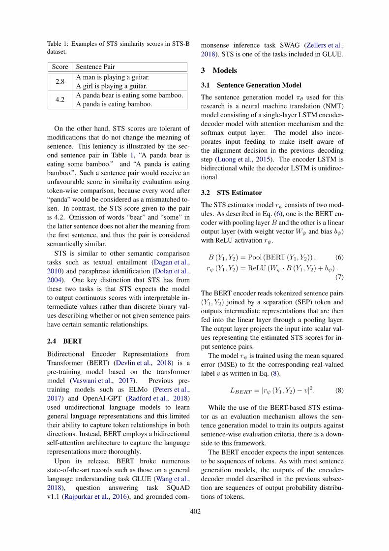
Table 1: Examples of STS similarity scores in STS-Bdataset.

Score Sentence Pair

2.8A man is playing a guitar.A girl is playing a guitar.

4.2A panda bear is eating some bamboo.A panda is eating bamboo.

On the other hand, STS scores are tolerant ofmodifications that do not change the meaning ofsentence. This leniency is illustrated by the sec-ond sentence pair in Table 1, “A panda bear iseating some bamboo.” and “A panda is eatingbamboo.”. Such a sentence pair would receive anunfavourable score in similarity evaluation usingtoken-wise comparison, because every word after“panda” would be considered as a mismatched to-ken. In contrast, the STS score given to the pairis 4.2. Omission of words “bear” and “some” inthe latter sentence does not alter the meaning fromthe first sentence, and thus the pair is consideredsemantically similar.

STS is similar to other semantic comparisontasks such as textual entailment (Dagan et al.,2010) and paraphrase identification (Dolan et al.,2004). One key distinction that STS has fromthese two tasks is that STS expects the modelto output continuous scores with interpretable in-termediate values rather than discrete binary val-ues describing whether or not given sentence pairshave certain semantic relationships.

2.4 BERT

Bidirectional Encoder Representations fromTransformer (BERT) (Devlin et al., 2018) is apre-training model based on the transformermodel (Vaswani et al., 2017). Previous pre-training models such as ELMo (Peters et al.,2017) and OpenAI-GPT (Radford et al., 2018)used unidirectional language models to learngeneral language representations and this limitedtheir ability to capture token relationships in bothdirections. Instead, BERT employs a bidirectionalself-attention architecture to capture the languagerepresentations more thoroughly.

Upon its release, BERT broke numerousstate-of-the-art records such as those on a generallanguage understanding task GLUE (Wang et al.,2018), question answering task SQuADv1.1 (Rajpurkar et al., 2016), and grounded com-

monsense inference task SWAG (Zellers et al.,2018). STS is one of the tasks included in GLUE.

3 Models

3.1 Sentence Generation Model

The sentence generation model πθ used for thisresearch is a neural machine translation (NMT)model consisting of a single-layer LSTM encoder-decoder model with attention mechanism and thesoftmax output layer. The model also incor-porates input feeding to make itself aware ofthe alignment decision in the previous decodingstep (Luong et al., 2015). The encoder LSTM isbidirectional while the decoder LSTM is unidirec-tional.

3.2 STS Estimator

The STS estimator model rψ consists of two mod-ules. As described in Eq. (6), one is the BERT en-coder with pooling layer B and the other is a linearoutput layer (with weight vector Wψ and bias bψ)with ReLU activation rψ.

B (Y1, Y2) = Pool (BERT (Y1, Y2)) , (6)

rψ (Y1, Y2) = ReLU (Wψ · B (Y1, Y2) + bψ) .(7)

The BERT encoder reads tokenized sentence pairs(Y1, Y2) joined by a separation (SEP) token andoutputs intermediate representations that are thenfed into the linear layer through a pooling layer.The output layer projects the input into scalar val-ues representing the estimated STS scores for in-put sentence pairs.

The model rψ is trained using the mean squarederror (MSE) to fit the corresponding real-valuedlabel v as written in Eq. (8).

LBERT = |rψ (Y1, Y2) − v|2. (8)

While the use of the BERT-based STS estima-tor as an evaluation mechanism allows the sen-tence generation model to train its outputs againstsentence-wise evaluation criteria, there is a down-side to this framework.

The BERT encoder expects the input sentencesto be sequences of tokens. As with most sentencegeneration models, the outputs of the encoder-decoder model described in the previous subsec-tion are sequences of output probability distribu-tions of tokens.

402

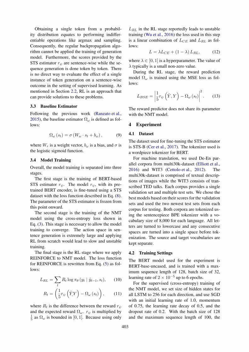
Obtaining a single token from a probabil-ity distribution equates to performing indiffer-entiable operations like argmax and sampling.Consequently, the regular backpropagation algo-rithm cannot be applied the training of generationmodel. Furthermore, the scores provided by theSTS estimator rψ are sentence-wise while the se-quence generation is done token by token. Thereis no direct way to evaluate the effect of a singleinstance of token generation on a sentence-wiseoutcome in the setting of supervised learning. Asmentioned in Section 2.2, RL is an approach thatcan provide solutions to these problems.

3.3 Baseline EstimatorFollowing the previous work (Ranzato et al.,2015), the baseline estimator Ωω is defined as fol-lows:

Ωω (st) = σ (Wω · st + bω) , (9)

where Wr is a weight vector, bω is a bias, and σ isthe logistic sigmoid function.

3.4 Model TrainingOverall, the model training is separated into threestages.

The first stage is the training of BERT-basedSTS estimator rψ. The model rψ, with its pre-trained BERT encoder, is fine-tuned using a STSdataset with the loss function described in Eq. (8).The parameter of the STS estimator is frozen fromthis point onward.

The second stage is the training of the NMTmodel using the cross-entropy loss shown inEq. (3). This stage is necessary to allow the modeltraining to converge. The action space in sen-tence generation is extremely large and applyingRL from scratch would lead to slow and unstabletraining.

The final stage is the RL stage where we applyREINFORCE to NMT model. The loss functionfor REINFORCE is rewritten from Eq. (5) as fol-lows:

LRL =∑

t

Rt log πθ (yt | yt−1, st), (10)

Rt =

(1

5rψ

(Y,Y

)− Ωω (st)

), (11)

where Rt is the difference between the reward rψand the expected reward Ωω. rψ is multiplied by15 as Ωω is bounded in [0, 1]. Because using only

LRL in the RL stage reportedly leads to unstabletraining (Wu et al., 2016) the loss used in this stepis a linear combination of LCE and LRL as fol-lows:

L = λLCE + (1 − λ) LRL, (12)

where λ ∈ [0, 1] is a hyperparameter. The value ofλ typically is a small non-zero value.

During the RL stage, the reward predictionmodel Ωω is trained using the MSE loss as fol-lows:

LBSE =

∣∣∣∣1

5rψ

(Y , Y

)− Ωω (st)

∣∣∣∣2

. (13)

The reward predictor does not share its parameterwith the NMT model.

4 Experiment

4.1 Dataset

The dataset used for fine-tuning the STS estimatoris STS-B (Cer et al., 2017). The tokenizer used isa wordpiece tokenizer for BERT.

For machine translation, we used De-En par-allel corpora from multi30k-dataset (Elliott et al.,2016) and WIT3 (Cettolo et al., 2012). Themulti30k-dataset is comprised of textual descrip-tions of images while the WIT3 consists of tran-scribed TED talks. Each corpus provides a singlevalidation set and multiple test sets. We chose thebest models based on their scores for the validationsets and used the two newest test sets from eachcorpus for testing. Both corpora are tokenized us-ing the sentencepiece BPE tokenizer with a vo-cabulary size of 8,000 for each language. All let-ters are turned to lowercase and any consecutivespaces are turned into a single space before tok-enization. The source and target vocabularies arekept separate.

4.2 Training Settings

The BERT model used for the experiment isBERT-base-uncased, and is trained with a max-imum sequence length of 128, batch size of 32,learning rate of 2 × 10−5 up to 6 epochs.

For the supervised (cross-entropy) training ofthe NMT model, we set size of hidden states forall LSTM to 256 for each direction, and use SGDwith an initial learning rate of 1.0, momentumof 0.75, the learning rate decay of 0.5, and thedropout rate of 0.2. With the batch size of 128and the maximum sequence length of 100, the

403

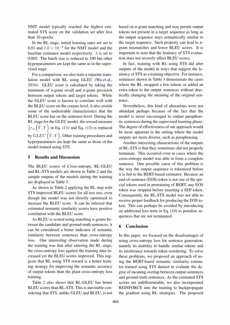
NMT model typically reached the highest esti-mated STS score on the validation set after lessthan 10 epochs.

In the RL stage, initial learning rates are set to0.01 and 1.0 × 10−3 for the NMT model and thebaseline estimator model respectively. λ is set to0.005. The batch size is reduced to 100 but otherhyperparameters are kept the same as in the super-vised stage.

For a comparison, we also train a separate trans-lation model with RL using GLEU (Wu et al.,2016). GLEU score is calculated by taking theminimum of n-gram recall and n-gram precisionbetween output tokens and target tokens. Whilethe GLEU score is known to correlate well withthe BLEU score on the corpus-level, it also avoidssome of the undesirable characteristics that theBLEU score has on the sentence-level. During theRL stage for the GLEU model, the reward measure15rψ

(Y , Y

)in Eq. (11) and Eq. (13) is replaced

by GLEU(Y , Y

). Other training procedures and

hyperparameters are kept the same as those of themodel trained using STS.

5 Results and Discussion

The BLEU scores of Cross-entropy, RL-GLEUand RL-STS models are shown in Table 2 and thesample outputs of the models during the trainingare displayed in Table 3.

As shown in Table 2 applying the RL step withSTS improved BLEU scores for all test sets, eventhough the model was not directly optimized toincrease the BLEU score. It can be inferred thatestimated semantic similarity scores have positivecorrelation with the BLEU score.

As BLEU is scored using matching n-grams be-tween the candidate and ground-truth sentences, itcan be considered a better indicator of semanticsimilarity between sentences than cross-entropyloss. One interesting observation made duringthe training was that after entering the RL stage,the cross-entropy loss against the training data in-creased yet the BLEU scores improved. This sug-gests that RL using STS reward is a better train-ing strategy for improving the semantic accuracyof output tokens than the plain cross-entropy losstraining.

Table 2 also shows that RL-GLEU has betterBLEU scores than RL-STS. This is inevitable con-sidering that STS, unlike GLEU and BLEU, is not

based on n-gram matching and may permit outputtokens not present in a target sequence as long asthe output sequence stays semantically similar tothe target sequence. Such property can lead to n-gram mismatches and lower BLEU scores. It isimportant to note that the leniency of STS evalua-tion does not severely affect BLEU scores.

In fact, training with RL using STS did alteroutputs of the model in ways that suggest the le-niency of STS as a training objective. For instance,sentences shown in Table 3 demonstrate the caseswhere the RL swapped a few tokens or added anextra token to the output sentences without dras-tically changing the meaning of the original sen-tence.

Nevertheless, this kind of alterations were notabundant perhaps because of the fact that themodel is never encouraged to output paraphras-tic sentences during the supervised learning phase.The degree of effectiveness of our approach wouldbe more apparent in the setting where the modeloutputs are more diverse, such as paraphrasing.

Another interesting characteristic of the outputsof RL-STS is that they sometimes did not properlyterminate. This occurred even in cases where thecross-entropy model was able to form a completesentence. One possible cause of this problem isthe way the output sequence is tokenized beforeit is fed to the BERT-based estimator. Because anend-of-sentence (EOS) token is not one of the spe-cial tokens used in pretraining of BERT, any EOStoken was stripped before inserting a SEP token.Consequently, the RL-STS model was not able toreceive proper feedback for producing the EOS to-ken. This can perhaps be avoided by introducingan additional loss term in Eq. (10) to penalize se-quences that are not terminated.

6 Conclusion

In this paper, we focused on the disadvantages ofusing cross-entropy loss for sentence generation,namely its inability to handle similar tokens andits intolerance towards token reordering. To solvethese problems, we proposed an approach of us-ing the BERT-based semantic similarity estima-tor trained using STS dataset to evaluate the de-gree of meaning overlap between output sentencesand ground-truth sentences. As the estimated STSscores are indifferentiable, we also incorporatedREINFORCE into the training to backpropagatethe gradient using RL strategies. The proposed

404

Table 2: BLEU and estimated STS scores for test sets in multi30k-dataset and WIT3. mscoco2017 and flickr2017are test sets for multi30k-dataset, while TED2014 and TED2015 are test sets for WIT3. RL-GLEU and RL-STSdenote models trained with REINFORCE using GLEU reward and STS reward respectively.

mscoco2017 flickr2017 TED2014 TED2015Model BLEU STS BLEU STS BLEU STS BLEU STSCross-entropy 16.44 2.76 22.22 3.03 12.54 2.63 13.43 2.80RL-GLEU 20.13 2.93 25.83 3.15 13.97 2.71 14.59 2.89RL-STS 18.31 2.96 24.70 3.21 13.58 2.87 14.56 2.99

Table 3: Sample outputs of the models for the training set

Model Output SentencesGround-truth I’ll show you what I mean. So how do we solve?Cross-entropy I’ll show you what I mean. So how do we solve?RL-GLEU I’ll show you what I mean. So how do we solve?RL-STS I’m going to show you what I mean. So how do we solve problems?

method proved successful in improving the BLEUscore over the baseline model trained using onlythe cross-entropy loss. The findings from the com-parison of model outputs suggest that the STS al-lows lenient evaluation without severely degrad-ing BLEU scores. However, the extent of effec-tiveness of the proposed method is yet to be deter-mined. Further analysis of the method using dif-ferent datasets such as those for abstractive sum-marization and paraphrasing, as well as humanevaluation are necessary to reach a proper conclu-sion.

Acknowledgments

We would like to thank Kazuma Hashimoto andanonymous reviewers for helpful comments andsuggestions.

ReferencesEneko Agirre, Mona Diab, Daniel Cer, and Aitor

Gonzalez-Agirre. 2012. Semeval-2012 task 6: A pi-lot on semantic textual similarity. In SemEval.

Daniel Cer, Mona Diab, Eneko Agirre, Inigo Lopez-Gazpio, and Lucia Specia. 2017. SemEval-2017Task 1: Semantic Textual Similarity Multilingualand Crosslingual Focused Evaluation. In SemEval.

Mauro Cettolo, Christian Girardi, and Marcello Fed-erico. 2012. Wit3: Web inventory of transcribed andtranslated talks. In EAMT.

Kyunghyun Cho, Bart van Merrienboer, Caglar Gul-cehre, Dzmitry Bahdanau, Fethi Bougares, HolgerSchwenk, and Yoshua Bengio. 2014. Learning

Phrase Representations using RNN EncoderDecoderfor Statistical Machine Translation. In EMNLP.

Ido Dagan, Bill Dolan, Bernardo Magnini, and DanRoth. 2010. Recognizing textual entailment: Ra-tional, evaluation and approaches–erratum. NaturalLanguage Engineering, 16(1).

Jacob Devlin, Ming-Wei Chang, Kenton Lee, andKristina Toutanova. 2018. BERT: Pre-training ofDeep Bidirectional Transformers for Language Un-derstanding. arXiv:1810.04805 [cs].

Bill Dolan, Chris Quirk, and Chris Brockett. 2004.Unsupervised construction of large paraphrase cor-pora: Exploiting massively parallel news sources. InCOLING.

Desmond Elliott, Stella Frank, Khalil Sima’an, and Lu-cia Specia. 2016. Multi30k: Multilingual english-german image descriptions. In VL.

Sepp Hochreiter and Jrgen Schmidhuber. 1997.Long Short-Term Memory. Neural Computation,9(8):1735–1780.

Thang Luong, Hieu Pham, and Christopher D. Man-ning. 2015. Effective Approaches to Attention-based Neural Machine Translation. In EMNLP.

Ramakanth Pasunuru and Mohit Bansal. 2018. Multi-reward reinforced summarization with saliency andentailment. In NAACL.

Matthew Peters, Waleed Ammar, Chandra Bhagavat-ula, and Russell Power. 2017. Semi-supervised se-quence tagging with bidirectional language models.In ACL.

Alec Radford, Karthik Narasimhan, Time Salimans,and Ilya Sutskever. 2018. Improving language un-derstanding with unsupervised learning. Technicalreport, Technical report, OpenAI.

405

Pranav Rajpurkar, Jian Zhang, Konstantin Lopyrev, andPercy Liang. 2016. Squad: 100,000+ questionsfor machine comprehension of text. arXiv preprintarXiv:1606.05250.

Marc’Aurelio Ranzato, Sumit Chopra, MichaelAuli, and Wojciech Zaremba. 2015. SequenceLevel Training with Recurrent Neural Networks.arXiv:1511.06732 [cs]. ArXiv: 1511.06732.

Alexander M Rush, Sumit Chopra, and Jason Weston.2015. A neural attention model for abstractive sen-tence summarization. In EMNLP.

Ilya Sutskever, Oriol Vinyals, and Quoc V Le. 2014.Sequence to Sequence Learning with Neural Net-works. In NIPS.

Ashish Vaswani, Noam Shazeer, Niki Parmar, JakobUszkoreit, Llion Jones, Aidan N Gomez, Ł ukaszKaiser, and Illia Polosukhin. 2017. Attention is allyou need. In NIPS.

Alex Wang, Amanpreet Singh, Julian Michael, Fe-lix Hill, Omer Levy, and Samuel Bowman. 2018.GLUE: A Multi-Task Benchmark and Analysis Plat-form for Natural Language Understanding. InEMNLP Workshop BlackboxNLP.

Ronald J. Williams. 1992. Simple statistical gradient-following algorithms for connectionist reinforce-ment learning. Machine Learning, 8(3):229–256.

Yonghui Wu, Mike Schuster, Zhifeng Chen, Quoc V.Le, Mohammad Norouzi, Wolfgang Macherey,Maxim Krikun, Yuan Cao, Qin Gao, KlausMacherey, Jeff Klingner, Apurva Shah, MelvinJohnson, Xiaobing Liu, ukasz Kaiser, StephanGouws, Yoshikiyo Kato, Taku Kudo, HidetoKazawa, Keith Stevens, George Kurian, NishantPatil, Wei Wang, Cliff Young, Jason Smith, JasonRiesa, Alex Rudnick, Oriol Vinyals, Greg Corrado,Macduff Hughes, and Jeffrey Dean. 2016. Google’sneural machine translation system: Bridging the gapbetween human and machine translation. CoRR.

Rowan Zellers, Yonatan Bisk, Roy Schwartz, andYejin Choi. 2018. Swag: A large-scale adversarialdataset for grounded commonsense inference. arXivpreprint arXiv:1808.05326.

406

Proceedings of the 57th Annual Meeting of the Association for Computational Linguistics: Student Research Workshop, pages 407–414Florence, Italy, July 28 - August 2, 2019. c©2019 Association for Computational Linguistics

Sentiment Classification using Document Embeddings trained withCosine Similarity

Tan ThongtanDepartment of Computer Engineering

Mahidol University International CollegeMahidol University

Thailandtan.thongtan1@gmail.com

Tanasanee PhienthrakulDepartment of Computer Engineering

Faculty of EngineeringMahidol University

Thailandtanasanee.phi@mahidol.ac.th

Abstract

In document-level sentiment classification,each document must be mapped to a fixedlength vector. Document embedding mod-els map each document to a dense, low-dimensional vector in continuous vectorspace. This paper proposes training docu-ment embeddings using cosine similarity in-stead of dot product. Experiments on theIMDB dataset show that accuracy is im-proved when using cosine similarity com-pared to using dot product, while using fea-ture combination with Naıve Bayes weightedbag of n-grams achieves a new state ofthe art accuracy of 97.42%. Code toreproduce all experiments is available athttps://github.com/tanthongtan/dv-cosine.

1 Introduction

In document classification tasks such as sentimentclassification (in this paper we focus on binarysentiment classification of long movie reviews, i.e.determining whether each review is positive ornegative), the choice of document representationis usually more important than the choice of clas-sifier. The task of text representation aims at map-ping variable length texts into fixed length vec-tors, as to be valid inputs to a classifier. Documentembedding models achieve this by mapping eachdocument to a dense, real-valued vector.

This paper aims to improve existing documentembedding models (Le and Mikolov, 2014; Liet al., 2016a) by training document embeddingsusing cosine similarity instead of dot product. Forexample, in the basic model of trying to predict -given a document - the words/n-grams in the doc-ument, instead of trying to maximize the dot prod-uct between a document vector and vectors of thewords/n-grams in the document over the trainingset, we’ll be trying to maximize the cosine simi-larity instead.

The motivation behind this is twofold. Firstly,cosine similarity serves as a regularization mech-anism; by ignoring vector magnitudes, there isless incentive to increase the magnitudes of theinput and output vectors, whereas in the case ofdot product, vectors of frequent document-n-grampairs can be made to have a high dot product sim-ply by increasing the magnitudes of each vector.The weights learned should be smaller overall.

Secondly, as cosine similarity is widely usedto measure document similarity (Singhal, 2001;Dai et al., 2015), we believe our method shouldmore directly maximize the cosine similarity be-tween similar document vectors. The angle be-tween similar documents should be lower, and thatmay encode useful information for distinguishingbetween different types of documents. We’ll com-pare the performance of our model on the IMDBdataset (Maas et al., 2011) with dot product andto determine if our model serves anything beyondsimple regularization, we’ll also compare it to dotproduct using L2 regularization.

2 Related Work

Here we review methods of text representation,in which there are two main categories: bag ofwords models and neural embedding models.

The bag of words model (Joachims, 1998) rep-resents text as a fixed length vector of length equalto the number of distinct n-grams in the vocab-ulary. Naive Bayes - Support Vector Machine(NB-SVM) (Wang and Manning, 2012) utilizesnaıve bayes weighted bag of n-grams vectors forrepresenting texts, feeding these vectors into a lo-gistic regression or support vector machine classi-fier.

The first example of a neural embeddingmodel is word embeddings which was proposedby Bengio et al. in 2003, while objective functions

407

utilizing the negative sampling technique for effi-cient training of word embeddings were proposedin 2013 by Mikolov et al. (word2vec). The aimof word embeddings is to map each word to a realvector, whereby the dot product between two vec-tors represents the amount of similarity in meaningbetween the words they represent. There are twoversions of word2vec: continuous bag of words(CBOW), in which a neural network is trained topredict the next word in a piece of text given theword’s context, and skip-gram, where it will try topredict a word’s context given the word itself.

In a 2017 paper Arora et al. produce SentenceEmbeddings by computing the weighted averageof word vectors, where each word is weighted us-ing smooth inverse frequency, and removing thefirst principle component.

Paragraph Vector (Le and Mikolov, 2014)may be seen as a modification to word embed-dings in order to embed as vectors paragraphs asopposed to words. Paragraph vector comes intwo flavors: the Distributed Memory Model ofParagraph Vectors (PV-DM), and the DistributedBag of Words version of Paragraph Vector (PV-DBOW). PV-DM is basically the same as CBOWexcept that a paragraph vector is additionally av-eraged or concatenated along with the context andthat whole thing is used to predict the next word.In the PV-DBOW model a paragraph vector aloneis used/trained to predict the words in the para-graph.

Document Vector by predicting n-grams(DV-ngram) (Li et al., 2016a) trains paragraphvectors to predict not only the words in the para-graph, but n-grams in the paragraph as well.Weighted Neural Bag of n-grams (W-Neural-BON) (Li et al., 2016b) uses an objective functionsimilar to the one in DV-ngram, except that eachlog probability term is weighted using a weighingscheme which is similar to taking the absolute val-ues of naive bayes weights.

In (Li et al., 2017), they introduce three mainmethods of embedding n-grams. The first is con-text guided n-gram representation (CGNR), whichis training n-gram vectors to predict its context n-grams. The second is label guided n-gram rep-resentation (LGNR), which is predicting given ann-gram the label of the document to which it be-longs. The last is text guided n-gram representa-tion (TGNR), which is predicting given an n-gramthe document to which it belongs.

Embeddings from Language Models (ELMo)(Peters et al., 2018) learns contextualized wordembeddings by training a bidirectional LSTM(Hochreiter and Schmidhuber, 1997) on the lan-guage modelling task of predicting the next wordas well as the previous word. BidirectionalEncoder Representations from Transformers(BERT) (Devlin et al., 2018) uses the masked lan-guage model objective, which is predicting themasked word given the left and right context, inorder to pre-train a multi-layer bidirectional Trans-former (Vaswani et al., 2017). BERT also jointlypre-trains text-pair representations by using a nextsentence prediction objective.

For the rest of this section we’ll look at otherresearch which replaces dot product with cosinesimilarity. In the context of fully-connected neuralnetworks and convolutional neural networks, (Luoet al., 2017) uses cosine similarity instead of dotproduct in computing a layer’s pre-activation as aregularization mechanism. Using a special datasetwhere each instance is a paraphrase pair, (Wietinget al., 2015) trains word vectors in such a way thatthe cosine similarity between the resultant docu-ment vectors of a paraphrase pair is directly max-imized.

3 Proposed Model

In learning neural n-gram and document embed-dings, a dot product between the input vector andthe output vector is generally used to compute thesimilarity measure between the two vectors, i.e.‘similar’ vectors should have a high dot product.In this paper we explore using cosine similarityinstead of dot product in computing the similar-ity measure between the input and output vectors.More specifically we focus on modifications tothe PV-DBOW and the similar DV-ngram models.The cosine similarity between a paragraph vectorand vectors of n-grams in the paragraph is maxi-mized over the training set.

3.1 ArchitectureA neural network is trained to be useful in pre-dicting, given a document, the words and n-gramsin the document, in the process of doing so learn-ing useful document embeddings. Formally, theobjective function to be minimized is defined asfollows:

∑

d∈D

∑

wo∈Wd

− log p(wo|d) (1)

408

where d is a document, D is the set of all docu-ments in the dataset, wo is an n-gram and Wd isthe set of all n-grams in the document d. p(wo|d)is defined using softmax:

p(wo|d) =eα cos θwo

∑w∈W eα cos θw

(2)

= softmax(α cos θwo) (3)

We have cos θw defined as follows:

cos θw =vTd vw‖vd‖‖vw‖

(4)

where vd and vw are vector representations of thedocument d and the word/n-gram w respectivelyand are parameters to be learned. α is a hyperpa-rameter. W is the set of all n-grams in the vocab-ulary.

Normally, the softmax of the dot product be-tween the input and output vector is used to modelthe conditional probability term as follows:

p(wo|d) =ev

Td vwo

∑w∈W ev

Td vw

(5)

Whereas dot product ranges from negative infinityto positive infinity, since cosine similarity rangesfrom -1 to 1, using the cosine similarity term aloneas an input to the softmax function may not besufficient in modeling the conditional probabilitydistribution. Therefore, we add a scaling hyperpa-rameter α to increase the range of possible proba-bility values for each conditional probability term.6/12/2019 architecture.drawio

1/1

nodes inhidden layerN

M|D|×NM ′

|W|×N

nodes inoutput layer|W |

vd vw

d vd

softmax for

(α cos )θw

w ∈ W

Figure 1: Proposed Architecture.

Figure 1 shows the architecture of the neuralnetwork used in learning the document embed-dings. There is a hidden layer with N nodes cor-responding to the dimensionality of the paragraphvectors and an output layer with |W | nodes corre-sponding to the number of distinct n-grams foundin the dataset. There are two weight parameter ma-trices to be learned: M , which may be seen as a

collection of |D| document vectors each havingNdimensions, and M ′, which is a collection of |W |n-gram vectors each also having N dimensions.

An input document id d is used to select itsvector representation vd which is exactly outputthrough the N nodes of the first hidden layer. Theoutput of each node in the output layer representsthe probability p(w|d) of its corresponding n-gramw, and is calculated as in (2) using softmax.

3.2 Negative SamplingSince the weight update equations for minimizing(1) implies that we must update each output vec-tor corresponding to each feature in the feature setW , with extremely large vocabularies, this com-putation is impractical. In (Mikolov et al., 2013),the negative sampling technique is introduced as ameans to speed up the learning process and it canbe shown that the updates for the negative sam-pling version of (1) as shown in (6) approximatesthe weight updates carried out in minimizing (1).Therefore in practice, the document embeddingsare obtained by minimizing the following objec-tive function with stochastic gradient descent andbackpropagation (Rumelhart et al., 1986):∑

d∈D

∑

wo∈Wd

[− log σ (α cos θwo)

−∑

wn∈Wneg

log σ (−α cos θwn)

](6)

where Wneg is a set of negatively sampled words;the size of the set or the negative sampling sizeas well as the distribution used to draw negativelysampled words/n-grams are hyperparameters. σ isthe sigmoid function.

By contrast, in the case of dot product the ob-jective function is:∑

d∈D

∑

wo∈Wd

[− log σ

(vTd vwo

)

−∑

wn∈Wneg

log σ(−vTd vwn

)](7)

while in the case of L2R dot product, the objectivefunction used is:∑

d∈D

∑

wo∈Wd

[− log σ

(vTd vwo

)+λ

2‖vd‖2 +

λ

2‖vwo‖2

−∑

wn∈Wneg

(log σ

(−vTd vwn

)+λ

2‖vwn‖2

)]

(8)

409

Features Dot Product Dot Product Cosine(DV-ngram) with L2R Similarity

(%) (%) (%)

Unigrams 89.60 87.15 (-2.45) 90.75 (+1.15)Unigrams+Bigrams 91.27 91.72 (+0.45) 92.56 (+1.29)Unigrams+Bigrams+Trigrams 92.14 92.45 (+0.31) 93.13 (+0.99)

Table 1: Experimental Results.

where λ is the regularization strength.

4 Experiments

The models are benchmarked on the IMDB dataset(Maas et al., 2011), which contains 25,000 train-ing documents, 25,000 test documents, and 50,000unlabeled documents. The IMDB dataset is a bi-nary sentiment classification dataset consisting ofmovie reviews retrieved from IMDB; training doc-uments in the dataset are highly polar. For labeleddocuments, there is a 1:1 ratio between negativeand positive documents. The document vectorsare learned using all the documents in the dataset(train, test and unlabeled documents). The datasetconsists of mainly long movie reviews.

In order to train the document vectors on un-igrams to trigrams, the reviews are preprocessedin such a way that tokens representing bigramsand trigrams are simply appended to the originalunigrams of the review itself. An L2-regularizedlogistic regression (LR) classifier is used to clas-sify the documents at the end of each epoch us-ing the predefined train-test split. However, theresults reported in this paper include only the ac-curacy obtained from classifying documents inthe final epoch. For any java implementations ofthe LR classifier we use the LIBLINEAR library(Fan et al., 2008) while for python implementa-tions we use Sci-kit learn (Pedregosa et al., 2011).Code to reproduce all experiments is available athttps://github.com/tanthongtan/dv-cosine.

4.1 Optimal Hyperparameters

Grid search was performed using 20% of the train-ing data as a validation set in order to determinethe optimal hyperparameters as well as whether touse a constant learning rate or learning rate an-nealing. Table 2 shows the optimal hyperparam-eters for the models on the IMDB dataset. Wedid not tune the N hyperparameter or the nega-tive sampling size and left it the same as in (Liet al., 2016a) and (Lau and Baldwin, 2016). Wedid however tune the number of iterations from

[10, 20, 40, 80, 120], learning rate from [0.25,0.025, 0.0025, 0.001] and α from [4, 6, 8]. A sen-sible value of α should be around 6, since lookingat the graph of the sigmoid function, for input val-ues greater than 6 and less than -6, the sigmoidfunction doesn’t change much and has values ofclose to 1 and 0, respectively. In the case of us-ing L2 regularized dot product, λ (regularizationstrength) was chosen from [1, 0.1, 0.01].

Hyperparameter Dot L2R Dot Cos.Prod. Prod. Sim.

N (dimensionality) 500 500 500Neg. Sampling Size 5 5 5Iterations 10 20 120Learning Rate 0.25 0.025 0.001α - - 6λ - 0.01 -LR annealing true false false

Table 2: Optimal Hyperparameters.

The optimal learning rate in the case of cosinesimilarity is extremely small, suggesting a chaoticerror surface. Since the learning rate is alreadysmall to begin with, no learning rate annealing isused. The model in turn requires a larger numberof epochs for convergence. For the distribution forsampling negative words, we used the n-gram dis-tribution raised to the 3/4th power in accordancewith (Mikolov et al., 2013). The weights of thenetworks were initialized from a uniform distribu-tion in the range of [-0.001, 0.001].

4.2 Results

Each experiment was carried out 5 times and themean accuracy is reported in Table 1. This is toaccount for random factors such as shuffling doc-ument and word ids, and random initialization.From here we see that using cosine similarity in-stead of dot product improves accuracy across theboard. The results are most apparent in the caseof unigrams + bigrams. However it is not to sug-gest that switching from dot product to cosine sim-ilarity alone improves accuracy as other minor ad-

410

Figure 2: PCA visualization of embeddings trained with (a) dot product, (b) L2R dot product and (c) cos. similarity.

justments and hyperparameter tuning as explainedwas done. However it may imply that using cosinesimilarity allows for a higher potential accuracy aswas achieved in these experiments.

Regardless, we believe the comparisons are fairsince each model is using its own set of optimalhyperparameters, but for the full sake of compari-son, leaving everything the same and only switch-ing out dot product for cosine similarity (α = 1) aswell as switching it out and using a sensible valueof α at α = 6 both achieve an accuracy of around50%. This is because our model fails wheneverthe learning rate is too large. As seen during gridsearch, whenever the initial learning rate was 0.25,accuracy was always poor.

Introducing L2 regularization to dot product im-proves accuracy for all cases except a depreciationin the case of using unigrams only, lucikily cosinesimilarity does not suffer from this same depreci-ation.

4.3 Discussion

From table 3, the mean Euclidean norm of embed-dings trained with cosine similarity is lower thanthat of L2R dot product which is in turn lower thanin the case of using dot product; this suggests thatthe method employing cosine similarity acts as aregularization mechanism, preventing the weightsfrom getting too large. Large magnitudes of doc-ument vectors may be harder for the end classifierto fit in such a way that generalizes well, whichmay be why cosine similarity and L2R dot prod-uct perform better than dot product on the IMDBdataset.

As predicted, the mean cosine similarity be-tween all pairs of vectors in the same class (SameMean Cos. Sim.) is higher in the case of cosinesimilarity than the other two models. Unfortu-

nately, the mean for all pairs in different classes(Diff. Mean Cos. Sim.) is higher as well. Fur-ther analysis and hopefully some formalism as towhy cosine similarity performs better is a plannedfuture work.

Embedding Dot L2R Dot Cos.Statistic Prod. Prod. Sim.

Same Mean Cos. Sim. 0.23 0.20 0.35Diff. Mean Cos. Sim. 0.21 0.17 0.32Mean Norm 8.91 6.30 5.35

Table 3: Embedding statistics.

Figure 2 shows the projection of the embed-dings along their first two principle components,different colors corresponding to different classes.Cosine similarity shows slightly better seperabil-ity between the two classes, while dot product andL2R dot product are quite similar.

4.4 Feature CombinationAnother contribution of this paper is demonstrat-ing the effectiveness of concatenating naive bayesweighted bag of n-grams with DV-ngram, L2R dotproduct, or document vectors trained with cosinesimilarity, the last achieving state of the art accu-racy on the IMDB dataset. We note that all modelsutilize unigrams to trigrams and additional unla-beled data if possible. Table 4 shows a compari-son between our proposed models (shown in bold)and previous state of the arts and other publishedresults.

5 Conclusion and Future Work

Our proposed model trains document embeddingsusing cosine similarity as the similarity measureand we show that sentiment classification perfor-mance on the IMDB dataset is improved when

411

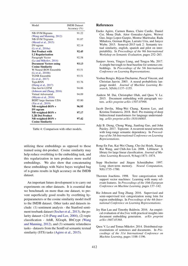
Model IMDB DatasetAccuracy (%)

NB-SVM Bigrams 91.22(Wang and Manning, 2012)NB-SVM Trigrams 91.87(Mesnil et al., 2015)DV-ngram 92.14(Li et al., 2016a)Dot Product with 92.45L2 RegularizationParagraph Vector 92.58(Le and Mikolov, 2014)Document Vectors using 93.13Cosine SimilarityW-Neural-BON Ensemble 93.51(Li et al., 2016b)TGNR Ensemble 93.51(Li et al., 2017)TopicRNN 93.76(Dieng et al., 2017)One-hot bi-LSTM 94.06(Johnson and Zhang, 2016)Virtual Adversarial 94.09(Miyato et al., 2016)BERT large finetune UDA 95.80(Xie et al., 2019)NB-weighted-BON + 96.95DV-ngramNB-weighted-BON + 97.17L2R Dot ProductNB-weighted-BON + 97.42Cosine Similarity

Table 4: Comparison with other models.

utilizing these embeddings as opposed to thosetrained using dot-product. Cosine similarity mayhelp reduce overfitting to the embedding task, andthis regularization in turn produces more usefulembeddings. We also show that concatenatingthese embeddings with Naıve bayes weighed bagof n-grams results in high accuracy on the IMDBdataset.

An important future development is to carry outexperiments on other datasets. It is essential thatwe benchmark on more than one dataset, to pre-vent superficially good results by overfitting hy-perparameters or the cosine similarity model itselfto the IMDB dataset. Other tasks and datasets in-clude: (1) sentiment analysis - the Stanford senti-ment treebank dataset (Socher et al., 2013), the po-larity dataset v2.0 (Pang and Lee, 2004), (2) topicclassification - AthR, XGraph, BbCrypt (Wangand Manning, 2012), and (3) semantic relatednesstasks - datasets from the SemEval semantic textualsimilarity (STS) tasks (Agirre et al., 2015).

ReferencesEneko Agirre, Carmen Banea, Claire Cardie, Daniel

Cer, Mona Diab, Aitor Gonzalez-Agirre, WeiweiGuo, Inigo Lopez-Gazpio, Montse Maritxalar, RadaMihalcea, German Rigau, Larraitz Uria, and JanyceWiebe. 2015. Semeval-2015 task 2: Semantic tex-tual similarity, english, spanish and pilot on inter-pretability. In Proceedings of the 9th InternationalWorkshop on Semantic Evaluation, pages 252–263.

Sanjeev Arora, Yingyu Liang, and Tengyu Ma. 2017.A simple but tough-to-beat baseline for sentence em-beddings. In Proceedings of the 5th InternationalConference on Learning Representations.

Yoshua Bengio, Rejean Ducharme, Pascal Vincent, andChristian Jauvin. 2003. A neural probabilistic lan-guage model. Journal of Machine Learning Re-search, 3(Feb):1137–1155.

Andrew M. Dai, Christopher Olah, and Quoc V. Le.2015. Document embedding with paragraph vec-tors. arXiv preprint arXiv:1507.07998.

Jacob Devlin, Ming-Wei Chang, Kenton Lee, andKristina Toutanova. 2018. Bert: Pre-training of deepbidirectional transformers for language understand-ing. arXiv preprint arXiv:1810.04805.

Adji B. Dieng, Chong Wang, Jianfeng Gao, and JohnPaisley. 2017. Topicrnn: A recurrent neural networkwith long-range semantic dependency. In Proceed-ings of the 5th International Conference on LearningRepresentations.

Rong-En Fan, Kai-Wei Chang, Cho-Jui Hsieh, Xiang-Rui Wang, and Chih-Jen Lin. 2008. Liblinear: Alibrary for large linear classification. Journal of Ma-chine Learning Research, 9(Aug):1871–1874.

Sepp Hochreiter and Jurgen Schmidhuber. 1997.Long short-term memory. Neural Computation,9(8):1735–1780.

Thorsten Joachims. 1998. Text categorization withsupport vector machines: Learning with many rel-evant features. In Proceedings of the 10th EuropeanConference on Machine Learning, pages 137–142.

Rie Johnson and Tong Zhang. 2016. Supervised andsemi-supervised text categorization using lstm forregion embeddings. In Proceedings of the 4th Inter-national Conference on Learning Representations.

Jey Han Lau and Timothy Baldwin. 2016. An empiri-cal evaluation of doc2vec with practical insights intodocument embedding generation. arXiv preprintarXiv:1607.05368.

Quoc V. Le and Tomas Mikolov. 2014. Distributed rep-resentations of sentences and documents. In Pro-ceedings of the 31st International Conference onMachine Learning, pages 1188–1196.

412

Bofang Li, Tao Liu, Xiaoyong Du, Deyuan Zhang, andZhe Zhao. 2016a. Learning document embeddingsby predicting n-grams for sentiment classification oflong movie reviews. In Proceedings of the 4th Inter-national Workshop on Learning Representations.

Bofang Li, Tao Liu, Zhe Zhao, Puwei Wang, and Xi-aoyong Du. 2017. Neural bag-of-ngrams. In Pro-ceedings of the 31st AAAI Conference on ArtificialIntelligence, pages 3067–3074.

Bofang Li, Zhe Zhao, Tao Liu, Puwei Wang, and Xi-aoyong Du. 2016b. Weighted neural bag-of-n-gramsmodel: New baselines for text classification. In Pro-ceedings of the 26th International Conference onComputational Linguistics, pages 1591–1600.

Chunjie Luo, Jianfeng Zhan, Lei Wang, and QiangYang. 2017. Cosine normalization: Using cosinesimilarity instead of dot product in neural networks.arXiv preprint arXiv:1702.05870.

Andrew L. Maas, Raymond E. Daly, Peter T. Pham,Dan Huang, Andrew Y. Ng, and Christopher Potts.2011. Learning word vectors for sentiment analysis.In Proceedings of the 49th Annual Meeting of the As-sociation for Computational Linguistics, pages 142–150.

Gregoire Mesnil, Tomas Mikolov, Marc’Aurelio Ran-zato, and Yoshua Bengio. 2015. Ensemble of gen-erative and discriminative techniques for sentimentanalysis of movie reviews. In Proceedings of the3rd International Workshop on Learning Represen-tations.

Tomas Mikolov, Ilya Sutskever, Kai Chen, Greg S. Cor-rado, and Jeff Dean. 2013. Distributed representa-tions of words and phrases and their compositional-ity. In Proceedings of the 26th International Con-ference on Neural Information Processing Systems,pages 3111–3119.

Takeru Miyato, Andrew M. Dai, and Ian Goodfel-low. 2016. Adversarial training methods for semi-supervised text classification. In Proceedings of the4th International Conference on Learning Represen-tations.

Bo Pang and Lillian Lee. 2004. A sentimental edu-cation: Sentiment analysis using subjectivity sum-marization based on minimum cuts. In Proceedingsof the 42nd Annual Meeting of the Association forComputational Linguistics, page 271.

Fabian Pedregosa, Gael Varoquaux, Alexandre Gram-fort, Vincent Michel, Bertrand Thirion, OlivierGrisel, Mathieu Blondel, Peter Prettenhofer, RonWeiss, Vincent Dubourg, et al. 2011. Scikit-learn:Machine learning in python. Journal of MachineLearning Research, 12(Oct):2825–2830.

Matthew E. Peters, Mark Neumann, Mohit Iyyer, MattGardner, Christopher Clark, Kenton Lee, and LukeZettlemoyer. 2018. Deep contextualized word repre-sentations. In Proceedings of the 2018 Conference

of the North American Chapter of the Associationfor Computational Linguistics: Human LanguageTechnologies, pages 2227–2237.

David E. Rumelhart, Geoffrey E. Hinton, and Ronald J.Williams. 1986. Learning representations by back-propagating errors. Nature, 323(6088):533–536.

Amit Singhal. 2001. Modern information retrieval: Abrief overview. IEEE Data Engineering Bulletin,24(4):35–43.

Richard Socher, Alex Perelygin, Jean Wu, JasonChuang, Christopher D. Manning, Andrew Ng, andChristopher Potts. 2013. Recursive deep modelsfor semantic compositionality over a sentiment tree-bank. In Proceedings of the 2013 Conference onEmpirical Methods in Natural Language Process-ing, pages 1631–1642.

Ashish Vaswani, Noam Shazeer, Niki Parmar, JakobUszkoreit, Llion Jones, Aidan N. Gomez, Ł ukaszKaiser, and Illia Polosukhin. 2017. Attention is allyou need. In Proceedings of the 31st InternationalConference on Neural Information Processing Sys-tems, pages 5998–6008.

Sida Wang and Christopher D. Manning. 2012. Base-lines and bigrams: Simple, good sentiment and topicclassification. In Proceedings of the 50th AnnualMeeting of the Association for Computational Lin-guistics, pages 90–94.

John Wieting, Mohit Bansal, Kevin Gimpel, and KarenLivescu. 2015. Towards universal paraphrastic sen-tence embeddings. In Proceedings of the 4th Inter-national Conference on Learning Representations.

Qizhe Xie, Zihang Dai, Eduard Hovy, Minh-Thang Lu-ong, and Quoc V. Le. 2019. Unsupervised data aug-mentation. arXiv preprint arXiv:1904.12848.

A Obtaining the weight update equationsin the case of cosine similarity

To obtain the weight update equations for the inputand output vectors of our model in each iterationof stochastic gradient descent, we must find thegradient of the error function at a given trainingexample, which may be considered a document,n-gram pair.

Let:

E =− log σ (α cos θwo)

−∑

wn∈Wneg

log σ (−α cos θwn) (9)

where:

cos θw =vTd vw‖vd‖‖vw‖

(10)

413

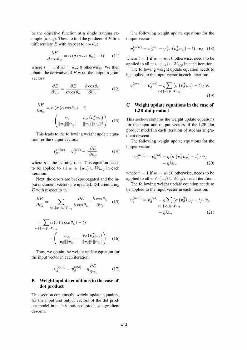
be the objective function at a single training ex-ample (d,wo). Then, to find the gradient of E firstdifferentiate E with respect to cos θw:

∂E

∂ cos θw= α (σ (α cos θw)− t) (11)

where t = 1 if w = wo; 0 otherwise. We thenobtain the derivative of E w.r.t. the output n-gramvectors:

∂E

∂vw=

∂E

∂ cos θw· ∂ cos θw

∂vw(12)

∂E

∂vw= α (σ (α cos θw)− t)

·(

vd‖vd‖‖vw‖

− vw(vTd vw

)

‖vd‖‖vw‖3

)(13)

This leads to the following weight update equa-tion for the output vectors:

v(new)w = v(old)

w − η ∂E∂vw

(14)

where η is the learning rate. This equation needsto be applied to all w ∈ wo ∪ Wneg in eachiteration.

Next, the errors are backpropagated and the in-put document vectors are updated. DifferentiatingE with respect to vd:

∂E

∂vd=

∑

w∈wo∪Wneg

∂E

∂ cos θw· ∂ cos θw

∂vd(15)

=∑

w∈wo∪Wneg

α (σ (α cos θw)− t)

·(

vw‖vd‖‖vw‖

− vd(vTd vw

)

‖vd‖3‖vw‖

)(16)

Thus, we obtain the weight update equation forthe input vector in each iteration:

v(new)d = v

(old)d − η ∂E

∂vd(17)

B Weight update equations in the case ofdot product

This section contains the weight update equationsfor the input and output vectors of the dot prod-uct model in each iteration of stochastic gradientdescent.

The following weight update equations for theoutput vectors:

v(new)w = v(old)

w − η(σ(vTd vw

)− t)· vd (18)

where t = 1 if w = wo; 0 otherwise, needs to beapplied to all w ∈ wo ∪Wneg in each iteration.

The following weight update equation needs tobe applied to the input vector in each iteration:

v(new)d = v

(old)d − η

∑

w∈wo∪Wneg

(σ(vTd vw

)− t)· vw

(19)

C Weight update equations in the case ofL2R dot product

This section contains the weight update equationsfor the input and output vectors of the L2R dotproduct model in each iteration of stochastic gra-dient descent.

The following weight update equations for theoutput vectors:

v(new)w = v(old)

w − η(σ(vTd vw

)− t)· vd

− ηλvw (20)

where t = 1 if w = wo; 0 otherwise, needs to beapplied to all w ∈ wo ∪Wneg in each iteration.

The following weight update equation needs tobe applied to the input vector in each iteration:

v(new)d = v

(old)d − η

∑

w∈wo∪Wneg

(σ(vTd vw

)− t)· vw

− ηλvd (21)

414

Proceedings of the 57th Annual Meeting of the Association for Computational Linguistics: Student Research Workshop, pages 415–421Florence, Italy, July 28 - August 2, 2019. c©2019 Association for Computational Linguistics

Detecting Adverse Drug Reactions from Biomedical Texts With NeuralNetworks

Ilseyar AlimovaKazan Federal University,

Kazan, RussiaISAlimova@kpfu.ru

Elena TutubalinaKazan Federal University,

Kazan, RussiaSamsung-PDMI Joint AI Center,

PDMI RAS, St. Petersburg, Russiaelvtutubalina@kpfu.ru

Abstract

Detection of adverse drug reactions in post-approval periods is a crucial challenge forpharmacology. Social media and electronicclinical reports are becoming increasinglypopular as a source for obtaining health-related information. In this work, we focus onextraction information of adverse drug reac-tions from various sources of biomedical text-based information, including biomedical liter-ature and social media. We formulate the prob-lem as a binary classification task and com-pare the performance of four state-of-the-artattention-based neural networks in terms of theF-measure. We show the effectiveness of thesemethods on four different benchmarks.

1 Introduction

Detection of adverse drug reactions (ADRs) in thepost-marketing period is becoming increasinglypopular, as evidenced by the growth of ADR mon-itoring systems (Singh et al., 2017; Shareef et al.,2017; Hou et al., 2016). Information about ad-verse drug reactions can be found in the texts ofsocial media, health-related forums, and electronichealth records. We formulated the problem as abinary classification task. The ADR classifica-tion task addresses two sub-tasks: (a) detecting thepresence of ADRs in a textual message (message-level task) and (b) detecting the class of an entitywithin a message (entity-level task). In this pa-per, we focus on the latter task. Different fromthe message-level classification task, which aimsto determine whether a textual fragment such astweet or an abstract of a paper includes an ADRmention or not, the objective of the entity-leveltask is to detect whether a given entity (a singleword or a multi-word expression) conveys adversedrug effect in the context of a message. For exam-ple, in “He was unable to sleep last night because

of pain”, the health condition ‘pain’ trigger insom-nia. Meanwhile, in “after 3 days on this drug I wasunable to sleep due to symptoms like a very badattack of RLS”, there is an entity ‘unable to sleep’associated with drug use and can be classified asADR.

Inspired by recent successful methods, we in-vestigated various deep neural network models forentity-level ADR classification (Alimova and Tu-tubalina, 2018). Our previous experiments showedthat Interactive Attention Neural network (IAN)(Ma et al., 2017) outperforms other models basedon LSTM (Hochreiter and Schmidhuber, 1997).In this paper, we continue our study and com-pare IAN with the following attention-based neu-ral networks for entity-level ADR classification:(i) Attention-over-Attention (AOA) model (Huanget al., 2018); (ii) Attentional Encoder Network(AEN) (Song et al., 2019); (iii) Attention-basedLSTM with Aspect Embedding (ATAE-LSTM)(Wang et al., 2016). We conduct extensive experi-ments on four benchmarks which consist of scien-tific abstracts and user-generated texts about drugtherapy.

2 Related Work

Different approaches are utilized to identify ad-verse drug reactions (Sarker et al., 2015; Guptaet al., 2018b; Harpaz et al., 2010). First workswere limited in the number of study drugs andtargeted ADRs due to limitations of traditionallexicon-based approaches (Benton et al., 2011;Liu and Chen, 2013). In order to eliminate theseshortcomings, rule-based methods have been pro-posed (Nikfarjam and Gonzalez, 2011; Na et al.,2012). These methods capture the underlyingsyntactic and semantic patterns from social me-dia posts. Third group of works utilized popu-lar machine learning models, such as support vec-

415

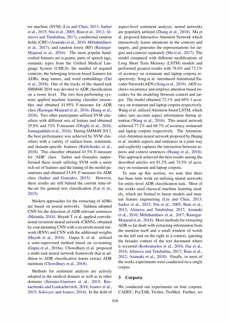
tor machine (SVM) (Liu and Chen, 2013; Sarkeret al., 2015; Niu et al., 2005; Bian et al., 2012; Al-imova and Tutubalina, 2017), conditional randomfields (CRF) (Aramaki et al., 2010; Miftahutdinovet al., 2017), and random forest (RF) (Rastegar-Mojarad et al., 2016). The most popular hand-crafted features are n-grams, parts of speech tags,semantic types from the Unified Medical Lan-guage System (UMLS), the number of negatedcontexts, the belonging lexicon based features forADRs, drug names, and word embeddings (Daiet al., 2016). One of the tracks of the shared taskSMM4H 2016 was devoted to ADR classificationon a tweet level. The two best-performing sys-tems applied machine learning classifier ensem-bles and obtained 41.95% F-measure for ADRclass (Rastegar-Mojarad et al., 2016; Zhang et al.,2016). Two other participants utilized SVM clas-sifiers with different sets of feature and obtained35.8% and 33% F-measure (Ofoghi et al., 2016;Jonnagaddala et al., 2016). During SMM4H 2017,the best performance was achieved by SVM clas-sifiers with a variety of surface-form, sentiment,and domain-specific features (Kiritchenko et al.,2018). This classifier obtained 43.5% F-measurefor ‘ADR’ class. Sarker and Gonsales outper-formed these result utilizing SVM with a morerich set of features and the tuning of the model pa-rameters and obtained 53.8% F-measure for ADRclass (Sarker and Gonzalez, 2015). However,these results are still behind the current state-of-the-art for general text classification (Lai et al.,2015).

Modern approaches for the extracting of ADRsare based on neural networks. Saldana adoptedCNN for the detection of ADR relevant sentences(Miranda, 2018). Huynh T. et al. applied convolu-tional recurrent neural network (CRNN), obtainedby concatenating CNN with a recurrent neural net-work (RNN) and CNN with the additional weights(Huynh et al., 2016). Gupta S. et al. utilizeda semi-supervised method based on co-training(Gupta et al., 2018a). Chowdhury et al. proposeda multi-task neural network framework that in ad-dition to ADR classification learns extract ADRmentions (Chowdhury et al., 2018).

Methods for sentiment analysis are activelyadopted in the medical domain as well as in otherdomains (Serrano-Guerrero et al., 2015; Rus-nachenko and Loukachevitch, 2018; Ivanov et al.,2015; Solovyev and Ivanov, 2014). In the field of

aspect-level sentiment analysis, neural networksare popularly utilized (Zhang et al., 2018). Ma etal. proposed Interactive Attention Network whichinteractively learns attentions in the contexts andtargets, and generates the representations for tar-gets and contexts separately (Ma et al., 2017). Themodel compared with different modifications ofLong Short Term Memory (LSTM) models andperformed greatest results with 78.6% and 72.1%of accuracy on restaurant and laptop corpora re-spectively. Song et al. introduced Attentional En-coder Network(AEN) (Song et al., 2019). AEN es-chews recurrence and employs attention based en-coders for the modeling between context and tar-get. The model obtained 72.1% and 69% f accu-racy on restaurant and laptop corpora respectively.Wang et al. utilized Attention-based LSTM, whichtakes into account aspect information during at-tention (Wang et al., 2016). This neural networkachieved 77.2% and 68.7% of accuracy restaurantand laptop corpora respectively. The Attention-over-Attention neural network proposed by Huanget al. models aspects and sentences in a joint wayand explicitly captures the interaction between as-pects and context sentences (Huang et al., 2018).This approach achieved the best results among thedescribed articles wit 81.2% and 74.5% of accu-racy on restaurant and laptop corpora.

To sum up this section, we note that therehas been little work on utilizing neural networksfor entity-level ADR classification task. Most ofthe works used classical machine learning mod-els, which are limited to linear models and man-ual feature engineering (Liu and Chen, 2013;Sarker et al., 2015; Niu et al., 2005; Bian et al.,2012; Alimova and Tutubalina, 2017; Aramakiet al., 2010; Miftahutdinov et al., 2017; Rastegar-Mojarad et al., 2016). Most methods for extractingADR so far dealt with extracting information fromthe mention itself and a small window of wordson the left and on the right as a context, ignoringthe broader context of the text document whereit occurred (Korkontzelos et al., 2016; Dai et al.,2016; Alimova and Tutubalina, 2017; Bian et al.,2012; Aramaki et al., 2010). Finally, in most ofthe works experiments were conducted on a singlecorpus.

3 Corpora

We conducted our experiments on four corpora:CADEC, PsyTAR, Twitter, TwiMed. Further, we

416

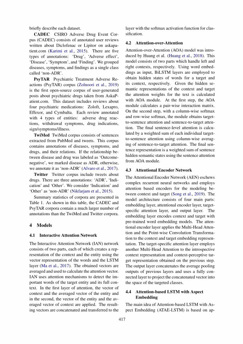
briefly describe each dataset.CADEC CSIRO Adverse Drug Event Cor-

pus (CADEC) consists of annotated user reviewswritten about Diclofenac or Lipitor on askapa-tient.com (Karimi et al., 2015). There are fivetypes of annotations: ‘Drug’, ‘Adverse effect’,‘Disease’, ‘Symptom’, and ‘Finding’. We groupeddiseases, symptoms, and findings as a single classcalled ‘non-ADR’.

PsyTAR Psychiatric Treatment Adverse Re-actions (PsyTAR) corpus (Zolnoori et al., 2019)is the first open-source corpus of user-generatedposts about psychiatric drugs taken from AskaP-atient.com. This dataset includes reviews aboutfour psychiatric medications: Zoloft, Lexapro,Effexor, and Cymbalta. Each review annotatedwith 4 types of entities: adverse drug reac-tions, withdrawal symptoms, drug indications,sign/symptoms/illness.

TwiMed TwiMed corpus consists of sentencesextracted from PubMed and tweets. This corpuscontains annotations of diseases, symptoms, anddrugs, and their relations. If the relationship be-tween disease and drug was labeled as ‘Outcome-negative’, we marked disease as ADR, otherwise,we annotate it as ‘non-ADR’ (Alvaro et al., 2017).

Twitter Twitter corpus include tweets aboutdrugs. There are three annotations: ‘ADR’, ‘Indi-cation’ and ‘Other’. We consider ‘Indication’ and‘Other’ as ‘non-ADR’ (Nikfarjam et al., 2015).

Summary statistics of corpora are presented inTable 1. As shown in this table, the CADEC andPsyTAR corpora contain a much larger number ofannotations than the TwiMed and Twitter corpora.

4 Models

4.1 Interactive Attention Network

The Interactive Attention Network (IAN) networkconsists of two parts, each of which creates a rep-resentation of the context and the entity using thevector representation of the words and the LSTMlayer (Ma et al., 2017). The obtained vectors areaveraged and used to calculate the attention vector.IAN uses attention mechanisms to detect the im-portant words of the target entity and its full con-text. In the first layer of attention, the vector ofcontext and the averaged vector of the entity andin the second, the vector of the entity and the av-eraged vector of context are applied. The result-ing vectors are concatenated and transferred to the

layer with the softmax activation function for clas-sification.

4.2 Attention-over-AttentionAttention-over-Attention (AOA) model was intro-duced by Huang et al. (Huang et al., 2018). Thismodel consists of two parts which handle left andright contexts, respectively. Using word embed-dings as input, BiLSTM layers are employed toobtain hidden states of words for a target andits context, respectively. Given the hidden se-mantic representations of the context and targetthe attention weights for the text is calculatedwith AOA module. At the first step, the AOAmodule calculates a pair-wise interaction matrix.On the second step, with a column-wise softmaxand row-wise softmax, the module obtains target-to-sentence attention and sentence-to-target atten-tion. The final sentence-level attention is calcu-lated by a weighted sum of each individual target-to-sentence attention using column-wise averag-ing of sentence-to-target attention. The final sen-tence representation is a weighted sum of sentencehidden semantic states using the sentence attentionfrom AOA module.

4.3 Attentional Encoder NetworkThe Attentional Encoder Network (AEN) eschewscomplex recurrent neural networks and employsattention based encoders for the modeling be-tween context and target (Song et al., 2019). Themodel architecture consists of four main parts:embedding layer, attentional encoder layer, target-specific attention layer, and output layer. Theembedding layer encodes context and target withpre-trained word embedding models. The atten-tional encoder layer applies the Multi-Head Atten-tion and the Point-wise Convolution Transforma-tion to the context and target embedding represen-tation. The target-specific attention layer employsanother Multi-Head Attention to the introspectivecontext representation and context-perceptive tar-get representation obtained on the previous step.The output layer concatenates the average poolingoutputs of previous layers and uses a fully con-nected layer to project the concatenated vector intothe space of the targeted classes.

4.4 Attention-based LSTM with AspectEmbedding

The main idea of Attention-based LSTM with As-pect Embedding (ATAE-LSTM) is based on ap-

417

Table 1: Summary statistics of corpora.

Corpus Documents ADR non-ADR Max sentence lengthCADEC (Karimi et al., 2015) 1231 5770 550 236PsyTAR (Zolnoori et al., 2019) 891 4525 2987 264TwiMed-Pubmed (Alvaro et al., 2017) 1000 264 983 150TwiMed-Twitter (Alvaro et al., 2017) 637 329 308 42Twitter (Nikfarjam et al., 2015) 645 569 76 37

pending the input aspect embedding into each con-text word input vector (Wang et al., 2016). Theconcatenated vectors are fed to the LSTM layerin order to obtain the hidden semantic represen-tations. With the resulting hidden states and theaspect embedding, the attention mechanism pro-duces an attention weight vector and a weightedhidden representation, which is applied for finalclassification.

5 Experiments

In this section, we compare the performance of thediscussed neural networks with Interactive Atten-tion Neural Network.

5.1 SettingsWe utilized vector representation trained on so-cial media posts from (Miftahutdinov et al., 2017).Word embedding vectors were obtained usingword2vec trained on a Health corpus consists of2.5 million reviews written in English. We usedan embedding size of 200, local context length of10, the negative sampling of 5, vocabulary cutoffof 10, Continuous Bag of Words model. Coveragestatistics of word embedding model vocabulary:CADEC – 93.5%, Twitter – 80.4%, PsyTAR –54%, TwiMed-Twitter – 81.2%, TwiMed-Pubmed– 76.4%. For the out of vocabulary words, therepresentations were uniformly sampled from therange of embedding weights. We used a maximumof 15 epochs to train IAN and ATAE-LSTM and30 epochs to train AEN and AOA on each dataset.We set the batch size to 32 for each corpus. Thenumber of hidden units for LSTM layer is 300, thelearning rate is 0.01, l2 regularization is 0.001. Weapplied the implementation of the model from thisrepository1.

5.2 Experiments and ResultsAll models were evaluated by 5-fold cross-validation. We utilized the F-measure to evaluate

1https://github.com/songyouwei/ABSA-PyTorch

the quality of the classification.The results are presented in Table 2. The re-

sults show that IAN outperformed other modelson all corpora. IAN obtained the most signifi-cant increase in results compared to other modelson Cadec and Twitter-Pubmed corpora with 81.5%and 87.4% of the macro F-measures, respectively.We assume that the superiority of the IAN resultsin comparison with other models is due to thesmall number of parameters being trained and thesmall size of the corpora.

The AOA model achieved the second-place re-sult on all corpora except Twitter. The AOA re-sults for PsyTAR (81.5%) and Twimed-Twitter(79.5%) corpora state on par with IAN model,while for the rest corpora, the results are signifi-cantly lower. This leads to the conclusion that themodel is unstable for highly imbalanced corpora.

The ATAE-LSTM model with 78.6% of macroF-measure outperformed AEN and AOA modelsresults on Twitter corpora and achieved compara-ble with AOA results on Twimed-Pubmed corpora(80.1%). This result shows that ATAE-LSTM ap-plicable to a small size imbalanced corpora.

The AEN model achieved comparable withother models results on PsyTAR (80.2%) corporaand significantly lower results on Twitter (66.7%),Cadec (49%) and Twimed-Pubmed (74.3%) cor-pora. 72.4% of F-measure on Twimed-Twitter cor-pus states on par with the ATAE-LSTM model(73.5%). This leads to the conclusion that the pres-ence of multiple attention layers did not give theimprovement in results.

6 Conclusion and Feature ResearchDirections

We have performed a fine-grained evaluationof state-of-the-art attention-based neural networkmodels for entity-level ADR classification task.We have conducted extensive experiments on fourbenchmarks. Analyzing the results, we have foundthat that increasing the number of attention layers

418

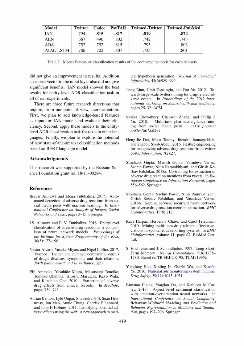
Model Twitter Cadec PsyTAR Twimed-Twitter Twimed-PubMedIAN .794 .815 .817 .819 .874AEN .667 .490 .802 .742 .743AOA .752 .752 .815 .795 .803ATAE-LSTM .786 .702 .807 .735 .801

Table 2: Macro F-measure classification results of the compared methods for each datasets.

did not give an improvement in results. Additionan aspect vector to the input layer also did not givesignificant benefits. IAN model showed the bestresults for entity-level ADR classification task inall of our experiments.

There are three future research directions thatrequire, from our point of view, more attention.First, we plan to add knowledge-based featuresas input for IAN model and evaluate their effi-ciency. Second, apply these models to the entity-level ADR classification task for texts in other lan-guages. Finally, we plan to explore the potentialof new state-of-the-art text classification methodsbased on BERT language model.

Acknowledgments

This research was supported by the Russian Sci-ence Foundation grant no. 18-11-00284.

ReferencesIlseyar Alimova and Elena Tutubalina. 2017. Auto-

mated detection of adverse drug reactions from so-cial media posts with machine learning. In Inter-national Conference on Analysis of Images, SocialNetworks and Texts, pages 3–15. Springer.

I.S. Alimova and E. V. Tutubalina. 2018. Entity-levelclassification of adverse drug reactions: a compar-ison of neural network models. Proceedings ofthe Institute for System Programming of the RAS,30(5):177–196.

Nestor Alvaro, Yusuke Miyao, and Nigel Collier. 2017.Twimed: Twitter and pubmed comparable corpusof drugs, diseases, symptoms, and their relations.JMIR public health and surveillance, 3(2).

Eiji Aramaki, Yasuhide Miura, Masatsugu Tonoike,Tomoko Ohkuma, Hiroshi Masuichi, Kayo Waki,and Kazuhiko Ohe. 2010. Extraction of adversedrug effects from clinical records. In MedInfo,pages 739–743.

Adrian Benton, Lyle Ungar, Shawndra Hill, Sean Hen-nessy, Jun Mao, Annie Chung, Charles E Leonard,and John H Holmes. 2011. Identifying potential ad-verse effects using the web: A new approach to med-

ical hypothesis generation. Journal of biomedicalinformatics, 44(6):989–996.

Jiang Bian, Umit Topaloglu, and Fan Yu. 2012. To-wards large-scale twitter mining for drug-related ad-verse events. In Proceedings of the 2012 inter-national workshop on Smart health and wellbeing,pages 25–32. ACM.

Shaika Chowdhury, Chenwei Zhang, and Philip SYu. 2018. Multi-task pharmacovigilance min-ing from social media posts. arXiv preprintarXiv:1801.06294.

Hong-Jie Dai, Musa Touray, Jitendra Jonnagaddala,and Shabbir Syed-Abdul. 2016. Feature engineeringfor recognizing adverse drug reactions from twitterposts. Information, 7(2):27.

Shashank Gupta, Manish Gupta, Vasudeva Varma,Sachin Pawar, Nitin Ramrakhiyani, and Girish Ke-shav Palshikar. 2018a. Co-training for extraction ofadverse drug reaction mentions from tweets. In Eu-ropean Conference on Information Retrieval, pages556–562. Springer.

Shashank Gupta, Sachin Pawar, Nitin Ramrakhiyani,Girish Keshav Palshikar, and Vasudeva Varma.2018b. Semi-supervised recurrent neural networkfor adverse drug reaction mention extraction. BMCbioinformatics, 19(8):212.

Rave Harpaz, Herbert S Chase, and Carol Friedman.2010. Mining multi-item drug adverse effect asso-ciations in spontaneous reporting systems. In BMCbioinformatics, volume 11, page S7. BioMed Cen-tral.

S. Hochreiter and J. Schmidhuber. 1997. Long Short-Term Memory. Neural Computation, 9(8):1735–1780. Based on TR FKI-207-95, TUM (1995).

Yongfang Hou, Xinling Li, Guizhi Wu, and XiaofeiYe. 2016. National adr monitoring system in china.Drug Safety, 39(11):1043–1051.

Binxuan Huang, Yanglan Ou, and Kathleen M Car-ley. 2018. Aspect level sentiment classificationwith attention-over-attention neural networks. InInternational Conference on Social Computing,Behavioral-Cultural Modeling and Prediction andBehavior Representation in Modeling and Simula-tion, pages 197–206. Springer.

419

Trung Huynh, Yulan He, Alistair Willis, and StefanRuger. 2016. Adverse drug reaction classificationwith deep neural networks. In Proceedings of COL-ING 2016, the 26th International Conference onComputational Linguistics: Technical Papers, pages877–887.

V Ivanov, E Tutubalina, N Mingazov, and I Alimova.2015. Extracting aspects, sentiment and categoriesof aspects in user reviews about restaurants and cars.In Proceedings of International Conference Dialog,volume 2, pages 22–34.

Jitendra Jonnagaddala, Toni Rose Jue, and Hong-JieDai. 2016. Binary classification of twitter posts foradverse drug reactions. In Proceedings of the SocialMedia Mining Shared Task Workshop at the PacificSymposium on Biocomputing, Big Island, HI, USA,pages 4–8.

Sarvnaz Karimi, Alejandro Metke-Jimenez, MadonnaKemp, and Chen Wang. 2015. Cadec: A corpus ofadverse drug event annotations. Journal of biomed-ical informatics, 55:73–81.

Svetlana Kiritchenko, Saif M Mohammad, JasonMorin, and Berry de Bruijn. 2018. Nrc-canada atsmm4h shared task: Classifying tweets mentioningadverse drug reactions and medication intake. arXivpreprint arXiv:1805.04558.

Ioannis Korkontzelos, Azadeh Nikfarjam, MatthewShardlow, Abeed Sarker, Sophia Ananiadou, andGraciela H Gonzalez. 2016. Analysis of the effectof sentiment analysis on extracting adverse drug re-actions from tweets and forum posts. Journal ofbiomedical informatics, 62:148–158.

Siwei Lai, Liheng Xu, Kang Liu, and Jun Zhao. 2015.Recurrent convolutional neural networks for textclassification. In AAAI, volume 333, pages 2267–2273.

Xiao Liu and Hsinchun Chen. 2013. Azdrugminer:an information extraction system for mining patient-reported adverse drug events in online patient fo-rums. In International Conference on Smart Health,pages 134–150. Springer.

Dehong Ma, Sujian Li, Xiaodong Zhang, and HoufengWang. 2017. Interactive attention networks foraspect-level sentiment classification. arXiv preprintarXiv:1709.00893.

Z.Sh. Miftahutdinov, E.V. Tutubalina, and A.E. Trop-sha. 2017. Identifying disease-related expressionsin reviews using conditional random fields. Com-putational Linguistics and Intellectual Technolo-gies: Papers from the Annual conference Dialogue,1(16):155–166.

Diego Saldana Miranda. 2018. Automated detec-tion of adverse drug reactions in the biomedi-cal literature using convolutional neural networksand biomedical word embeddings. arXiv preprintarXiv:1804.09148.

Jin-Cheon Na, Wai Yan Min Kyaing, Christopher SGKhoo, Schubert Foo, Yun-Ke Chang, and Yin-LengTheng. 2012. Sentiment classification of drug re-views using a rule-based linguistic approach. In In-ternational Conference on Asian Digital Libraries,pages 189–198. Springer.

Azadeh Nikfarjam and Graciela H Gonzalez. 2011.Pattern mining for extraction of mentions of adversedrug reactions from user comments. In AMIA An-nual Symposium Proceedings, volume 2011, page1019. American Medical Informatics Association.

Azadeh Nikfarjam, Abeed Sarker, Karen OConnor,Rachel Ginn, and Graciela Gonzalez. 2015. Phar-macovigilance from social media: mining adversedrug reaction mentions using sequence labelingwith word embedding cluster features. Journalof the American Medical Informatics Association,22(3):671–681.

Yun Niu, Xiaodan Zhu, Jianhua Li, and Graeme Hirst.2005. Analysis of polarity information in medicaltext. In AMIA annual symposium proceedings, vol-ume 2005, page 570. American Medical InformaticsAssociation.

BAHADORREZA Ofoghi, SAMIN Siddiqui, andKARIN Verspoor. 2016. Read-biomed-ss: Ad-verse drug reaction classification of microblogs us-ing emotional and conceptual enrichment. In Pro-ceedings of the Social Media Mining Shared TaskWorkshop at the Pacific Symposium on Biocomput-ing.

Majid Rastegar-Mojarad, Ravikumar KomandurElayavilli, Yue Yu, and Hongfang Liu. 2016.Detecting signals in noisy data-can ensembleclassifiers help identify adverse drug reaction intweets. In Proceedings of the Social Media MiningShared Task Workshop at the Pacific Symposium onBiocomputing.

N. Rusnachenko and N. Loukachevitch. 2018. Usingconvolutional neural networks for sentiment attitudeextraction from analytical texts. In Proceedings ofCEUR Workshop, CLLS-2018 Conference.

Abeed Sarker, Rachel Ginn, Azadeh Nikfarjam, KarenOConnor, Karen Smith, Swetha Jayaraman, TejaswiUpadhaya, and Graciela Gonzalez. 2015. Utilizingsocial media data for pharmacovigilance: a review.Journal of biomedical informatics, 54:202–212.

Abeed Sarker and Graciela Gonzalez. 2015. Portableautomatic text classification for adverse drug reac-tion detection via multi-corpus training. Journal ofbiomedical informatics, 53:196–207.

Jesus Serrano-Guerrero, Jose A Olivas, Francisco PRomero, and Enrique Herrera-Viedma. 2015. Sen-timent analysis: A review and comparative analysisof web services. Information Sciences, 311:18–38.

420

SM Shareef, CDM Naidu, Shrinivas R Raikar,Y Venkata Rao, and U Devika. 2017. Develop-ment, implementation, and analysis of adverse drugreaction monitoring system in a rural tertiary careteaching hospital in narketpally, telangana. Interna-tional Journal of Basic & Clinical Pharmacology,4(4):757–760.

Preeti Singh, Manju Agrawal, Rajesh Hishikar, UshaJoshi, Basant Maheshwari, and Ajay Halwai. 2017.Adverse drug reactions at adverse drug reactionmonitoring center in raipur: Analysis of sponta-neous reports during 1 year. Indian journal of phar-macology, 49(6):432.

V. Solovyev and V. Ivanov. 2014. Dictionary-basedproblem phrase extraction from user reviews. Lec-ture Notes in Computer Science (including subseriesLecture Notes in Artificial Intelligence and LectureNotes in Bioinformatics), 8655 LNAI:225–232.

Youwei Song, Jiahai Wang, Tao Jiang, Zhiyue Liu, andYanghui Rao. 2019. Attentional encoder networkfor targeted sentiment classification. arXiv preprintarXiv:1902.09314.

Yequan Wang, Minlie Huang, Li Zhao, et al. 2016.Attention-based lstm for aspect-level sentiment clas-sification. In Proceedings of the 2016 conference onempirical methods in natural language processing,pages 606–615.

Lei Zhang, Shuai Wang, and Bing Liu. 2018. Deeplearning for sentiment analysis: A survey. Wiley In-terdisciplinary Reviews: Data Mining and Knowl-edge Discovery, page e1253.

Zhifei Zhang, JY Nie, and Xuyao Zhang. 2016. Anensemble method for binary classification of adversedrug reactions from social media. In Proceedings ofthe Social Media Mining Shared Task Workshop atthe Pacific Symposium on Biocomputing.

Maryam Zolnoori, Kin Wah Fung, Timothy B Patrick,Paul Fontelo, Hadi Kharrazi, Anthony Faiola,Yi Shuan Shirley Wu, Christina E Eldredge, JakeLuo, Mike Conway, et al. 2019. A systematic ap-proach for developing a corpus of patient reportedadverse drug events: A case study for ssri and snrimedications. Journal of biomedical informatics,90:103091.

421

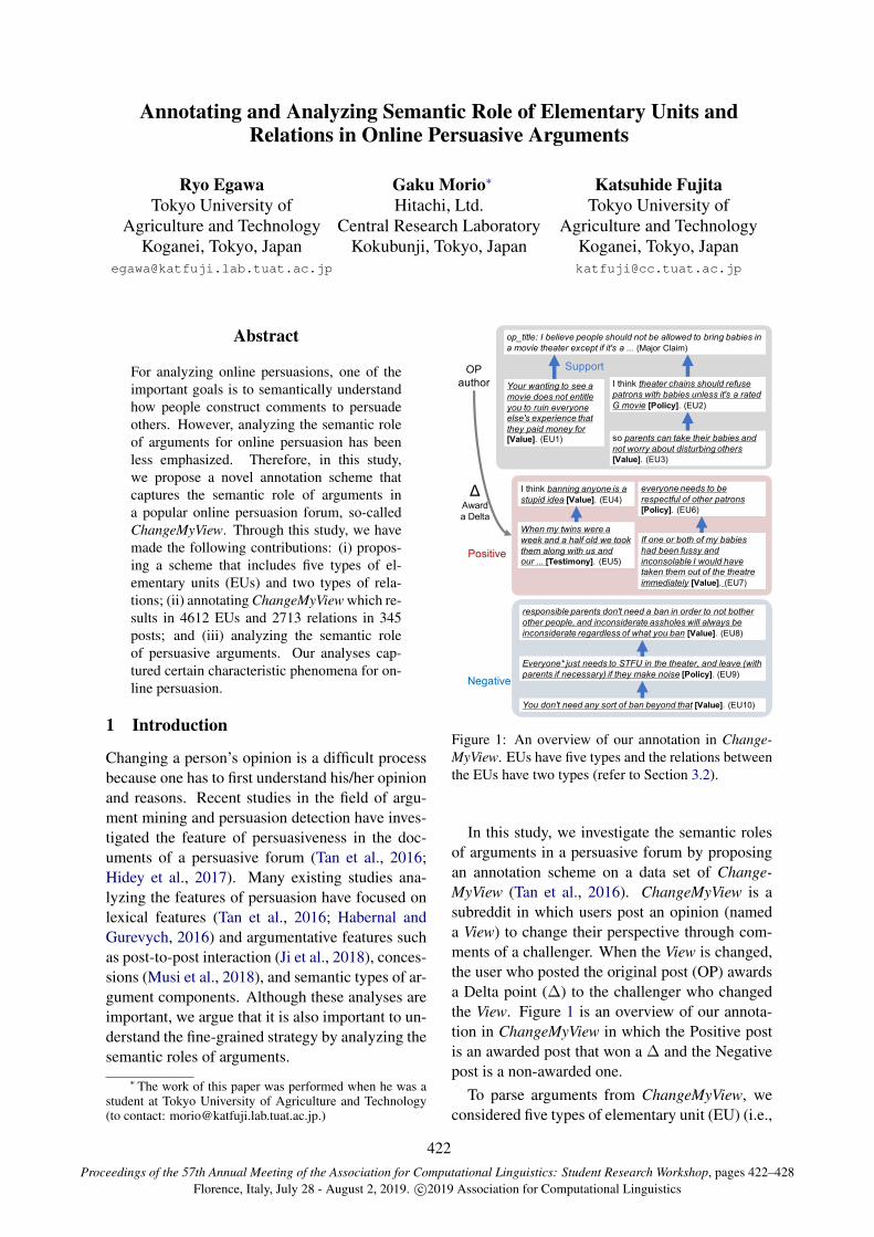
Proceedings of the 57th Annual Meeting of the Association for Computational Linguistics: Student Research Workshop, pages 422–428Florence, Italy, July 28 - August 2, 2019. c©2019 Association for Computational Linguistics

Annotating and Analyzing Semantic Role of Elementary Units andRelations in Online Persuasive Arguments

Ryo EgawaTokyo University of

Agriculture and TechnologyKoganei, Tokyo, Japan

egawa@katfuji.lab.tuat.ac.jp

Gaku Morio∗

Hitachi, Ltd.Central Research Laboratory

Kokubunji, Tokyo, Japan

Katsuhide FujitaTokyo University of

Agriculture and TechnologyKoganei, Tokyo, Japankatfuji@cc.tuat.ac.jp

Abstract

For analyzing online persuasions, one of theimportant goals is to semantically understandhow people construct comments to persuadeothers. However, analyzing the semantic roleof arguments for online persuasion has beenless emphasized. Therefore, in this study,we propose a novel annotation scheme thatcaptures the semantic role of arguments ina popular online persuasion forum, so-calledChangeMyView. Through this study, we havemade the following contributions: (i) propos-ing a scheme that includes five types of el-ementary units (EUs) and two types of rela-tions; (ii) annotating ChangeMyView which re-sults in 4612 EUs and 2713 relations in 345posts; and (iii) analyzing the semantic roleof persuasive arguments. Our analyses cap-tured certain characteristic phenomena for on-line persuasion.

1 Introduction

Changing a person’s opinion is a difficult processbecause one has to first understand his/her opinionand reasons. Recent studies in the field of argu-ment mining and persuasion detection have inves-tigated the feature of persuasiveness in the doc-uments of a persuasive forum (Tan et al., 2016;Hidey et al., 2017). Many existing studies ana-lyzing the features of persuasion have focused onlexical features (Tan et al., 2016; Habernal andGurevych, 2016) and argumentative features suchas post-to-post interaction (Ji et al., 2018), conces-sions (Musi et al., 2018), and semantic types of ar-gument components. Although these analyses areimportant, we argue that it is also important to un-derstand the fine-grained strategy by analyzing thesemantic roles of arguments.

∗ The work of this paper was performed when he was astudent at Tokyo University of Agriculture and Technology(to contact: morio@katfuji.lab.tuat.ac.jp.)

!"#

$%&'()

*+,$)-

$#./0&$

1#&'234#!"#$!#%&'"$()*&*"+,-.&%#/,*#&

0$!%+)*&1(!"&2$2(#*&,)-#**&(!3*&$&%$!#.&

4&5+6(# !"#$%&'(5#6789:

;(#0$%#)!*&'$)&!$7#&!"#(%&2$2(#*&$).&

)+!&1+%%8&$2+,!&.(*!,%2()9&+!"#%*

!)*$+,(5#678<:

:+,%&1$)!()9&!+&*##&$&

5+6(#&.+#*&)+!&#)!(!-#&

8+,&!+&%,()&#6#%8+)#&

#-*#3*&#;0#%(#)'#&!"$!&

!"#8&0$(.&5+)#8&/+%!)*$+,(5#678=:

+0<!(!-#=&>&2#-(#6#&0#+0-#&*"+,-.&)+!&2#&$--+1#.&!+&2%()9&2$2(#*&()&

$&5+6(#&!"#$!#%&#;'#0!&(/&(!3*&$&???&6>$?()#@0$2A:

"(;2&2B/

1#&'234#2$))()9&$)8+)#&(*&$&

*!,0(.&(.#$ !)*$+,(5#678C:

@"#)&58&!1()*&1#%#&$&

1##7&$).&$&"$-/&+-.&1#&!++7&

!"#5&$-+)9&1(!"&,*&$).&

+,%&???&!-,./%0#1'(5# 678D:

#6#%8+)#&)##.*&!+&2#&

%#*0#'!/,-&+/&+!"#%&0$!%+)*

!"#$%&'(5#678E:

>/&+)#&+%&2+!"&+/&58&2$2(#*&

"$.&2##)&/,**8&$).&

()'+)*+-$2-#&>&1+,-.&"$6#&

!$7#)&!"#5&+,!&+/&!"#&!"#$!%#&

(55#.($!#-8 !)*$+,(5 678F:

G/H$&2B/

%#*0+)*(2-#&0$%#)!*&.+)3!&)##.&$&2$)&()&+%.#%&!+&)+!&2+!"#%&

+!"#%&0#+0-#A&$).&()'+)*(.#%$!#&$**"+-#*&1(--&$-1$8*&2#&

()'+)*(.#%$!#&%#9$%.-#**&+/&1"$!&8+,&2$) !)*$+,(5#678I:

B6#%8+)#C&D,*!&)##.*&!+&EFGH&()&!"#&!"#$!#%A&$).&-#$6#&I1(!"&

0$%#)!*&(/&)#'#**$%8J&(/&!"#8&5$7#&)+(*# !"#$%&'(5#678J:

:+,&.+)3!&)##.&$)8&*+%!&+/&2$)&2#8+).&!"$! !)*$+,(5#678=K:

L%MM()&

Figure 1: An overview of our annotation in Change-MyView. EUs have five types and the relations betweenthe EUs have two types (refer to Section 3.2).

In this study, we investigate the semantic rolesof arguments in a persuasive forum by proposingan annotation scheme on a data set of Change-MyView (Tan et al., 2016). ChangeMyView is asubreddit in which users post an opinion (nameda View) to change their perspective through com-ments of a challenger. When the View is changed,the user who posted the original post (OP) awardsa Delta point (∆) to the challenger who changedthe View. Figure 1 is an overview of our annota-tion in ChangeMyView in which the Positive postis an awarded post that won a ∆ and the Negativepost is a non-awarded one.

To parse arguments from ChangeMyView, weconsidered five types of elementary unit (EU) (i.e.,

422

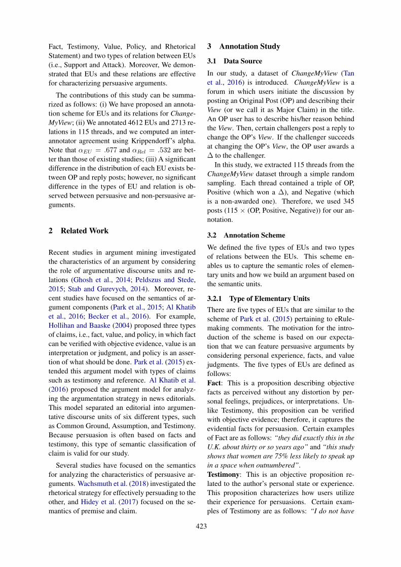
Fact, Testimony, Value, Policy, and RhetoricalStatement) and two types of relation between EUs(i.e., Support and Attack). Moreover, We demon-strated that EUs and these relations are effectivefor characterizing persuasive arguments.

The contributions of this study can be summa-rized as follows: (i) We have proposed an annota-tion scheme for EUs and its relations for Change-MyView; (ii) We annotated 4612 EUs and 2713 re-lations in 115 threads, and we computed an inter-annotator agreement using Krippendorff’s alpha.Note that αEU = .677 and αRel = .532 are bet-ter than those of existing studies; (iii) A significantdifference in the distribution of each EU exists be-tween OP and reply posts; however, no significantdifference in the types of EU and relation is ob-served between persuasive and non-persuasive ar-guments.

2 Related Work

Recent studies in argument mining investigatedthe characteristics of an argument by consideringthe role of argumentative discourse units and re-lations (Ghosh et al., 2014; Peldszus and Stede,2015; Stab and Gurevych, 2014). Moreover, re-cent studies have focused on the semantics of ar-gument components (Park et al., 2015; Al Khatibet al., 2016; Becker et al., 2016). For example,Hollihan and Baaske (2004) proposed three typesof claims, i.e., fact, value, and policy, in which factcan be verified with objective evidence, value is aninterpretation or judgment, and policy is an asser-tion of what should be done. Park et al. (2015) ex-tended this argument model with types of claimssuch as testimony and reference. Al Khatib et al.(2016) proposed the argument model for analyz-ing the argumentation strategy in news editorials.This model separated an editorial into argumen-tative discourse units of six different types, suchas Common Ground, Assumption, and Testimony.Because persuasion is often based on facts andtestimony, this type of semantic classification ofclaim is valid for our study.

Several studies have focused on the semanticsfor analyzing the characteristics of persuasive ar-guments. Wachsmuth et al. (2018) investigated therhetorical strategy for effectively persuading to theother, and Hidey et al. (2017) focused on the se-mantics of premise and claim.

3 Annotation Study

3.1 Data Source

In our study, a dataset of ChangeMyView (Tanet al., 2016) is introduced. ChangeMyView is aforum in which users initiate the discussion byposting an Original Post (OP) and describing theirView (or we call it as Major Claim) in the title.An OP user has to describe his/her reason behindthe View. Then, certain challengers post a reply tochange the OP’s View. If the challenger succeedsat changing the OP’s View, the OP user awards a∆ to the challenger.

In this study, we extracted 115 threads from theChangeMyView dataset through a simple randomsampling. Each thread contained a triple of OP,Positive (which won a ∆), and Negative (whichis a non-awarded one). Therefore, we used 345posts (115 × (OP, Positive, Negative)) for our an-notation.

3.2 Annotation Scheme

We defined the five types of EUs and two typesof relations between the EUs. This scheme en-ables us to capture the semantic roles of elemen-tary units and how we build an argument based onthe semantic units.

3.2.1 Type of Elementary UnitsThere are five types of EUs that are similar to thescheme of Park et al. (2015) pertaining to eRule-making comments. The motivation for the intro-duction of the scheme is based on our expecta-tion that we can feature persuasive arguments byconsidering personal experience, facts, and valuejudgments. The five types of EUs are defined asfollows:Fact: This is a proposition describing objectivefacts as perceived without any distortion by per-sonal feelings, prejudices, or interpretations. Un-like Testimony, this proposition can be verifiedwith objective evidence; therefore, it captures theevidential facts for persuasion. Certain examplesof Fact are as follows: “they did exactly this in theU.K. about thirty or so years ago” and “this studyshows that women are 75% less likely to speak upin a space when outnumbered”.Testimony: This is an objective proposition re-lated to the author’s personal state or experience.This proposition characterizes how users utilizetheir experience for persuasions. Certain exam-ples of Testimony are as follows: “I do not have

423

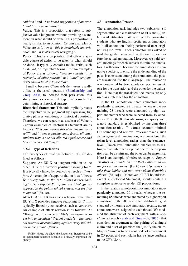
children” and “I’ve heard suggestions of an exor-bitant tax on ammunition”.Value: This is a proposition that refers to sub-jective value judgments without providing a state-ment on what should be done. This proposition isnearly similar to an opinion. Certain examples ofValue are as follows: “this is completely unwork-able” and “it is absolutely terrifying”.Policy: This is a proposition that offers a spe-cific course of action to be taken or what shouldbe done. It typically contains modal verbs, suchas should, or imperative forms. Certain examplesof Policy are as follows: “everyone needs to berespectful of other patrons” and “intelligent stu-dents should be able to see that”.

Finally, because ChangeMyView users usuallyutilize a rhetorical question (Blankenship andCraig, 2006) to increase their persuasion, thisstudy provides a novel EU type that is useful fordetermining a rhetorical strategy.Rhetorical Statement: This unit implicitly statesthe subjective value judgment by expressing fig-urative phrases, emotions, or rhetorical questions.Therefore, we can regard it as a subset of Value 1.Certain examples of Rhetorical Statement are asfollows: “You can observe this phenomenon your-self!” and “if one is paying equal fees to all otherstudents why is one not allowed equal access andhow is this a good thing?”.

3.2.2 Type of RelationsThe two types of relations between EUs are de-fined as follows:Support: An EU X has support relation to theother EU Y if X provides positive reasoning for Y.It is typically linked by connectives such as there-fore. An example of support relation is as follows:X: “Every state in the U.S. allows homeschool-ing” (Fact) support Y: “if you are ideologicallyopposed to the public school system, you are freeto opt out” (Value).Attack: An EU X has attack relation to the otherEU Y if X provides negative reasoning for Y. It istypically linked by connectives such as however.An example of attack relation is as follows: X:“Young men are the most likely demographic toget into an accident” (Value) attack Y: “that doesnot warrant discriminating against every individ-ual in the group” (Value).

1Unlike Value, we allow the Rhetorical Statement to bean incomplete sentence because it is usually expressed im-plicitly.

3.3 Annotation Process

The annotation task includes two subtasks: (1)segmentation and classification of EUs and (2) re-lation identification. We recruited 19 non-nativestudents who are English proficient as annotatorswith all annotations being performed over origi-nal English texts. Each annotator was asked toread the guideline as well as the entire post be-fore the actual annotation. Moreover, we held sev-eral meetings for each subtask to train the annota-tors. Furthermore, because the annotators are non-native speakers, to ensure the understanding of theposts is consistent among the annotators, the postsare translated into their language. The translationwas conducted by two annotators per document:one for the translation and the other for the valida-tion. Note that the translated documents are onlyused as a reference for the annotators.

In the EU annotation, three annotators inde-pendently annotated 87 threads, whereas the re-maining 28 threads were annotated by eight ex-pert annotators who were selected from 19 anno-tators. From the 87 threads, using a majority vote,a gold standard is established by merging threeannotation results. To extract accurate minimalEU boundary and remove irrelevant tokens, suchas therefore and punctuation, we considered thetoken-level annotation rather than the sentence-level. Token-level annotation enables us to dis-tinguish an inference step that one of the proposi-tions can be a claim and the other can be a premise.Here is an example of inference step: <“EmpireTheatres in Canada has a ”Reel Babies” show-ing for certain movies” [Fact]> so <“parents cantake their babies and not worry about disturbingothers” [Value]>. Moreover, all EU boundaries,except a Rhetorical Statement, should contain acomplete sentence to render EU propositions.

In the relation annotation, two annotators inde-pendently annotated 50 threads, whereas the re-maining 65 threads were annotated by eight expertannotators. In the 50 threads, to establish the goldstandard by merging two annotation results, expertannotators were assigned to each thread. We mod-eled the structure of each argument with a one-claim approach (Stab and Gurevych, 2016) thatconsiders an argument as the pairing of a singleclaim and a set of premises that justify the claim.Major Claim has to be a root node of an argumentin OP posts, and each claim has a stance attributeto the OP’s View.

424

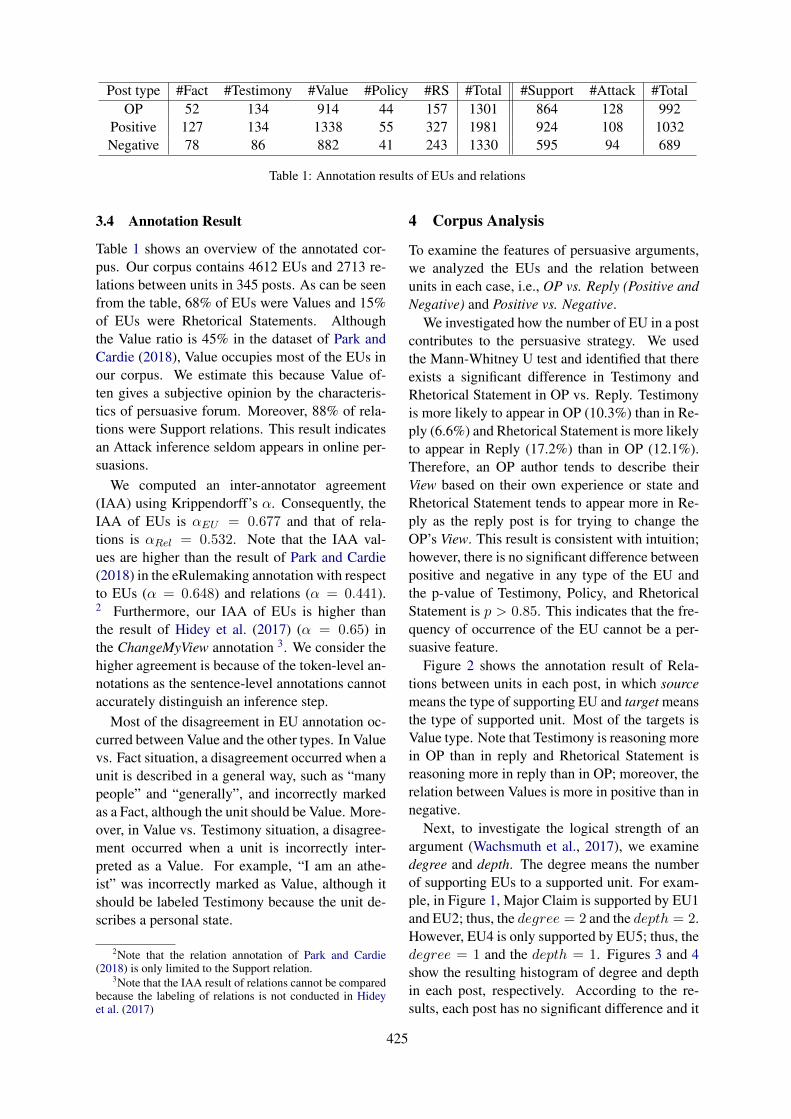
Post type #Fact #Testimony #Value #Policy #RS #Total #Support #Attack #TotalOP 52 134 914 44 157 1301 864 128 992

Positive 127 134 1338 55 327 1981 924 108 1032Negative 78 86 882 41 243 1330 595 94 689

Table 1: Annotation results of EUs and relations

3.4 Annotation Result

Table 1 shows an overview of the annotated cor-pus. Our corpus contains 4612 EUs and 2713 re-lations between units in 345 posts. As can be seenfrom the table, 68% of EUs were Values and 15%of EUs were Rhetorical Statements. Althoughthe Value ratio is 45% in the dataset of Park andCardie (2018), Value occupies most of the EUs inour corpus. We estimate this because Value of-ten gives a subjective opinion by the characteris-tics of persuasive forum. Moreover, 88% of rela-tions were Support relations. This result indicatesan Attack inference seldom appears in online per-suasions.

We computed an inter-annotator agreement(IAA) using Krippendorff’s α. Consequently, theIAA of EUs is αEU = 0.677 and that of rela-tions is αRel = 0.532. Note that the IAA val-ues are higher than the result of Park and Cardie(2018) in the eRulemaking annotation with respectto EUs (α = 0.648) and relations (α = 0.441).2 Furthermore, our IAA of EUs is higher thanthe result of Hidey et al. (2017) (α = 0.65) inthe ChangeMyView annotation 3. We consider thehigher agreement is because of the token-level an-notations as the sentence-level annotations cannotaccurately distinguish an inference step.

Most of the disagreement in EU annotation oc-curred between Value and the other types. In Valuevs. Fact situation, a disagreement occurred when aunit is described in a general way, such as “manypeople” and “generally”, and incorrectly markedas a Fact, although the unit should be Value. More-over, in Value vs. Testimony situation, a disagree-ment occurred when a unit is incorrectly inter-preted as a Value. For example, “I am an athe-ist” was incorrectly marked as Value, although itshould be labeled Testimony because the unit de-scribes a personal state.

2Note that the relation annotation of Park and Cardie(2018) is only limited to the Support relation.

3Note that the IAA result of relations cannot be comparedbecause the labeling of relations is not conducted in Hideyet al. (2017)

4 Corpus Analysis

To examine the features of persuasive arguments,we analyzed the EUs and the relation betweenunits in each case, i.e., OP vs. Reply (Positive andNegative) and Positive vs. Negative.

We investigated how the number of EU in a postcontributes to the persuasive strategy. We usedthe Mann-Whitney U test and identified that thereexists a significant difference in Testimony andRhetorical Statement in OP vs. Reply. Testimonyis more likely to appear in OP (10.3%) than in Re-ply (6.6%) and Rhetorical Statement is more likelyto appear in Reply (17.2%) than in OP (12.1%).Therefore, an OP author tends to describe theirView based on their own experience or state andRhetorical Statement tends to appear more in Re-ply as the reply post is for trying to change theOP’s View. This result is consistent with intuition;however, there is no significant difference betweenpositive and negative in any type of the EU andthe p-value of Testimony, Policy, and RhetoricalStatement is p > 0.85. This indicates that the fre-quency of occurrence of the EU cannot be a per-suasive feature.

Figure 2 shows the annotation result of Rela-tions between units in each post, in which sourcemeans the type of supporting EU and target meansthe type of supported unit. Most of the targets isValue type. Note that Testimony is reasoning morein OP than in reply and Rhetorical Statement isreasoning more in reply than in OP; moreover, therelation between Values is more in positive than innegative.

Next, to investigate the logical strength of anargument (Wachsmuth et al., 2017), we examinedegree and depth. The degree means the numberof supporting EUs to a supported unit. For exam-ple, in Figure 1, Major Claim is supported by EU1and EU2; thus, the degree = 2 and the depth = 2.However, EU4 is only supported by EU5; thus, thedegree = 1 and the depth = 1. Figures 3 and 4show the resulting histogram of degree and depthin each post, respectively. According to the re-sults, each post has no significant difference and it

425

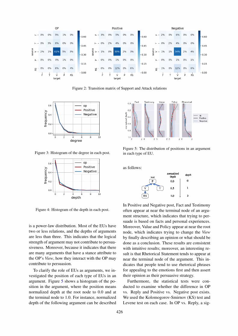
Figure 2: Transition matrix of Support and Attack relations

Figure 3: Histogram of the degree in each post.

Figure 4: Histogram of the depth in each post.

is a power-law distribution. Most of the EUs havetwo or less relations, and the depths of argumentsare less than three. This indicates that the logicalstrength of argument may not contribute to persua-siveness. Moreover, because it indicates that thereare many arguments that have a stance attribute tothe OP’s View, how they interact with the OP maycontribute to persuasion.

To clarify the role of EUs as arguments, we in-vestigated the position of each type of EUs in anargument. Figure 5 shows a histogram of the po-sition in the argument, where the position meansnormalized depth at the root node to 0.0 and atthe terminal node to 1.0. For instance, normalizeddepth of the following argument can be described

Figure 5: The distribution of positions in an argumentin each type of EU.

as follows:

In Positive and Negative post, Fact and Testimonyoften appear at near the terminal node of an argu-ment structure, which indicates that trying to per-suade is based on facts and personal experiences.Moreover, Value and Policy appear at near the rootnode, which indicates trying to change the Viewby finally describing an opinion or what should bedone as a conclusion. These results are consistentwith intuitive results; moreover, an interesting re-sult is that Rhetorical Statement tends to appear atnear the terminal node of the argument. This in-dicates that people tend to use rhetorical phrasesfor appealing to the emotions first and then asserttheir opinion as their persuasive strategy.

Furthermore, the statistical tests were con-ducted to examine whether the difference in OPvs. Reply and Positive vs. Negative post exists.We used the Kolomogorov-Smirnov (KS) test andLevene test on each case. In OP vs. Reply, a sig-

426

nificant difference exists in the position distribu-tion of Fact by KS test (p < 0.05), and Policy byLevene test (p < 0.01). This indicates that peopletend to make an assertion based on objective factsas a persuasion strategy.

5 Conclusion

In this study, we proposed an annotation schemefor capturing the semantic role of EUs and re-lations in online persuasions. We annotated fivetypes of EUs and two types of relations that re-sulted in 4612 EU and 2713 relation annotations.The analyses revealed that the existence of Rhetor-ical Statement and the position of Fact in an argu-ment structure characterizes the persuasive poststhat try to change the View. In future studies, wewill focus on the following: (i) the expansion ofour corpus data by annotating the post-to-post in-teraction and (ii) the application of our data totraining sets of machine learning, i.e., automat-ically identifying the argument structure and de-tecting the persuasive posts.

Acknowledgment

This work was supported by JST AIP-PRISM(JPMJCR18ZL) and JST CREST (JPMJCR15E1),Japan.

ReferencesKhalid Al Khatib, Henning Wachsmuth, Johannes

Kiesel, Matthias Hagen, and Benno Stein. 2016.A news editorial corpus for mining argumentationstrategies. In Proceedings of COLING 2016, the26th International Conference on ComputationalLinguistics: Technical Papers, pages 3433–3443,Osaka, Japan. The COLING 2016 Organizing Com-mittee.

Maria Becker, Alexis Palmer, and Anette Frank. 2016.Argumentative texts and clause types. In Proceed-ings of the Third Workshop on Argument Mining(ArgMining2016), pages 21–30, Berlin, Germany.Association for Computational Linguistics.

Kevin L. Blankenship and Traci Y. Craig. 2006.Rhetorical question use and resistance to persuasion:An attitude strength analysis. Journal of Languageand Social Psychology, 25(2):111–128.

Debanjan Ghosh, Smaranda Muresan, Nina Wacholder,Mark Aakhus, and Matthew Mitsui. 2014. Ana-lyzing argumentative discourse units in online in-teractions. In Proceedings of the First Workshopon Argumentation Mining, pages 39–48, Baltimore,Maryland. Association for Computational Linguis-tics.

Ivan Habernal and Iryna Gurevych. 2016. Which ar-gument is more convincing? analyzing and predict-ing convincingness of web arguments using bidirec-tional lstm. In Proceedings of the 54th Annual Meet-ing of the Association for Computational Linguistics(Volume 1: Long Papers), pages 1589–1599, Berlin,Germany. Association for Computational Linguis-tics.

Christopher Hidey, Elena Musi, Alyssa Hwang,Smaranda Muresan, and Kathy McKeown. 2017.Analyzing the semantic types of claims andpremises in an online persuasive forum. In Proceed-ings of the 4th Workshop on Argument Mining, pages11–21. Association for Computational Linguistics.

T.A. Hollihan and K.T. Baaske. 2004. Arguments andArguing: The Products and Process of Human De-cision Making, Second Edition. Waveland Press.

Lu Ji, Zhongyu Wei, Xiangkun Hu, Yang Liu,Qi Zhang, and Xuanjing Huang. 2018. Incorporat-ing argument-level interactions for persuasion com-ments evaluation using co-attention model. In Pro-ceedings of the 27th International Conference onComputational Linguistics, pages 3703–3714, SantaFe, New Mexico, USA. Association for Computa-tional Linguistics.

Elena Musi, Debanjan Ghosh, and Smaranda Mure-san. 2018. Changemyview through concessions:Do concessions increase persuasion? CoRR,abs/1806.03223.

Joonsuk Park, Cheryl Blake, and Claire Cardie. 2015.Toward machine-assisted participation in erulemak-ing: An argumentation model of evaluability. InProceedings of the 15th International Conference onArtificial Intelligence and Law, ICAIL ’15, pages206–210, New York, NY, USA. ACM.

Joonsuk Park and Claire Cardie. 2018. A corpus oferulemaking user comments for measuring evalu-ability of arguments. In Proceedings of the 11thLanguage Resources and Evaluation Conference,Miyazaki, Japan. European Language Resource As-sociation.

Andreas Peldszus and Manfred Stede. 2015. Joint pre-diction in mst-style discourse parsing for argumen-tation mining. In Proceedings of the 2015 Confer-ence on Empirical Methods in Natural LanguageProcessing, pages 938–948, Lisbon, Portugal. As-sociation for Computational Linguistics.

Christian Stab and Iryna Gurevych. 2014. Annotatingargument components and relations in persuasive es-says. In COLING 2014, 25th International Con-ference on Computational Linguistics, Proceedingsof the Conference: Technical Papers, August 23-29,2014, Dublin, Ireland, pages 1501–1510.

Christian Stab and Iryna Gurevych. 2016. Parsing ar-gumentation structures in persuasive essays. CoRR,abs/1604.07370.

427

Chenhao Tan, Vlad Niculae, Cristian Danescu-Niculescu-Mizil, and Lillian Lee. 2016. Winningarguments: Interaction dynamics and persuasionstrategies in good-faith online discussions. CoRR,abs/1602.01103.

Henning Wachsmuth, Nona Naderi, Ivan Habernal,Yufang Hou, Graeme Hirst, Iryna Gurevych, andBenno Stein. 2017. Argumentation quality assess-ment: Theory vs. practice. In Proceedings of the55th Annual Meeting of the Association for Compu-tational Linguistics (Volume 2: Short Papers), pages250–255. Association for Computational Linguis-tics.

Henning Wachsmuth, Manfred Stede, RoxanneEl Baff, Khalid Al Khatib, Maria Skeppstedt,and Benno Stein. 2018. Argumentation synthesisfollowing rhetorical strategies. In Proceedingsof the 27th International Conference on Compu-tational Linguistics, pages 3753–3765, Santa Fe,New Mexico, USA. Association for ComputationalLinguistics.

428

Proceedings of the 57th Annual Meeting of the Association for Computational Linguistics: Student Research Workshop, pages 429–435Florence, Italy, July 28 - August 2, 2019. c©2019 Association for Computational Linguistics

A Japanese Word Segmentation Proposal

Stalin AguirreNational Polytechnic School of Ecuador

Faculty of Systems Engineeringstalin.aguirre@epn.edu.ec

Josafa de Jesus Aguiar PontesNational Polytechnic School of Ecuador

Faculty of Systems Engineeringjosafa.aguiar@epn.edu.ec

Abstract

Current Japanese word segmentation methods,that use a morpheme-based approach, mayproduce different segmentations for the samestrings. This occurs when these strings appearin different sentences. The cause is the influ-ence of different contexts around these stringsaffecting the probabilistic models used in seg-mentation algorithms. This paper presentsan alternative to the current morpheme-basedscheme for Japanese word segmentation. Theproposed scheme focuses on segmenting in-flections as single words instead of separat-ing the auxiliary verbs and other morphemesfrom the stems. Some morphological segmen-tation rules are presented for each type of wordand these rules are implemented in a programwhich is properly described. The program isused to generate a segmentation of a sentencecorpus, whose consistency is calculated andcompared with the current morpheme-basedsegmentation of the same corpus. The ex-periments show that this method produces amuch more consistent segmentation than themorpheme-based one.

1 Introduction

In computational linguistics, the first step in text-processing tasks is segmenting an input text intowords. Most languages make use of white spacesas word boundaries, facilitating this segmentationstep. However, Japanese is one of the few lan-guages that does not use a word delimiter. Thisparticular problem has been the focus of many re-searchers because its solution is key to subsequentprocessing tasks, such as Part-of-Speech (PoS)tagging, machine translation or file indexing.

Segmenting a text requires the definition ofa segmentation unit (Indurkhya and Damerau,2010). This unit must be strictly defined to de-scribe all the elements in a language. But lan-guages are not perfect and have changed abruptly

throughout the years, making it difficult or nearlyimpossible to define such a unit. The consensushas been that the unit to be used was the word, be-cause it defines the majority of the elements in alanguage, elements that have a meaning and canstand by themselves (Katamba, 1994).

Even though there still are some constructionsthat do not fit in the word definition (Bauer, 1983),this segmentation unit is useful in languages thatuse spaces because they separate the majority ofwords in a text. For Japanese, however, this is notthe case. It is a language that does not use spacesin its written form.

私たちの性格はまったく異なる。

(Our personalities are completely different.)

Furthermore, Japanese is an agglutinative lan-guage, which means that some constructions (spe-cially inflected words) are formed by consecu-tively attaching morphemes to a stem (Kamer-mans, 2010). These long words are very importantbecause they can work as full sentences withoutthe need to add context that was previously stated,as illustrated in the following example:

待たされていました。

(I have been kept waiting.)

待つ (wait)待たされる (be kept waiting)待たされている (being kept waiting)待たされています (being kept waiting) (*P)1

待たされていました (been kept waiting) (*P)

Given the nature of the language and the lackof a need for native speakers to explicitly sepa-rate words, there is no standard on how to seg-ment a written text. Because of this, the segmenta-tion unit and rules for text processing tasks are setby each researcher, although most of them have

1*P: Polite form

429

chosen a morpheme-based approach (Matsumotoet al., 1991; Kudo, 2005; Matsumoto et al., 2007).

The downside about this morpheme approach isthat, in many cases, there is no consistency whensegmenting the same string. The cause seems tobe the influence of different contexts on the prob-abilistic models used in segmentation algorithms.In other words, by producing short morphemes ascandidates, there are many segmentation possibil-ities from which the final one may change due tothe context. This inconsistency problem is visi-ble in n-gram data produced by Kudo and Kazawa(2009) and Yata (2010). Within these files, thereare various entries of the same string as result ofdifferent segmentations, as shown in Table 1. Thisproblem directly affects any later processing taskthat relies on the resulting segmentation. In ma-chine translation, for example, different segmen-tations for the same word would produce differentincorrect translations.

File N-gram Frequency3gm-0034 行き　まし　た 26814864gm-0056 行　き　まし　た 2904gm-0056 行き　ま　し　た 384

Table 1: The word行きました (went) (*P) as found inn-gram data files produced by Yata (2010).

Inflected words follow a limited set of rules.These rules properly define all possible inflections(Kamermans, 2010). As such, they can only leadto one possible correct segmentation. Taking thispremise, the Proposed approach aims for a moreconsistent segmentation by focusing on the treat-ment of inflected words to limit their segmentationpossibilities to a single one in all cases. Thus, re-ducing word segmentation inconsistency errors.

The present work is structured as follows: Sec-tion 2 describes the rules that lead the Proposedsegmentation method. Section 3 describes the im-plementation of the algorithm that applies theserules; Section 4 introduces the evaluation param-eters and the results obtained with the Proposedmethod, a comparison of these metrics with amorpheme-based method and discussion of the re-sults; and Section 5 presents the conclusions of thework.

2 Segmentation Definition

Most Japanese constructions are created by di-rectly connecting an affix to a word. A few

of these constructions are considered separatedwords when translating them into English, suchas: 日本式 (Japan style, from 日本 Japan and式 style) or 外国語 (foreign language, from 外国 foreign and語 language). Other constructionshave a single word as translation, such as: 日本語 (Japanese (language) from日本 Japan and語language). However, this word construction rulein Japanese can be found in ”basic” words as well.For example: 大人 (adult, from 大 great and 人person) or 女子 (girl, from 女 woman and 子child), which are kept as single words in both lan-guages. This means that we cannot generalize howthese constructions should always get segmented,either as single words or multiple words.

As such, we have established a few segmenta-tion rules where some affixes were connected tothe words they modify by the use of symbols, re-gardless of the number of words it forms whentranslating them into English. For prefix concate-nation, the backtick symbol (`) was used, on theother hand, for suffix concatenation, the hyphensymbol (-) was used. In general, the words thatwere considered for these affix concatenation ruleswere nouns and verbs.

Overall, the base of the segmentation for thiswork was the IPADIC (Asahara and Matsumoto,2003) dictionary. This means that what was con-sidered as word was each entry in this dictionary,with the exception of the verb and adjective en-tries. For these inflectional words, what was con-sidered as word were the union of the inflectionalword stems and the morphemes or auxiliary verbsthat form the inflection, as described by Pontes(2013). In the case of the inflectional words, onlythe most common inflections are shown below 2.

Based on this word definition, the followingrules were set:

2.1 Nouns

Most regular nouns were kept as single words ac-cording to the entries that belonged to this tagwithin the IPADIC. Some PoS included in thiscategory were: common nouns, proper names,pronouns, pronoun contractions, adverbial nouns,verbal nouns (nouns that can be followed by する or related verbs), adjectival nouns (nouns thatcan be followed byな), Arabic numbers (wide andshort length), counters and Chinese numbers.

2When mentioning an inflection based on an auxiliaryverb, it also refers to all the inflections of such auxiliary.

430

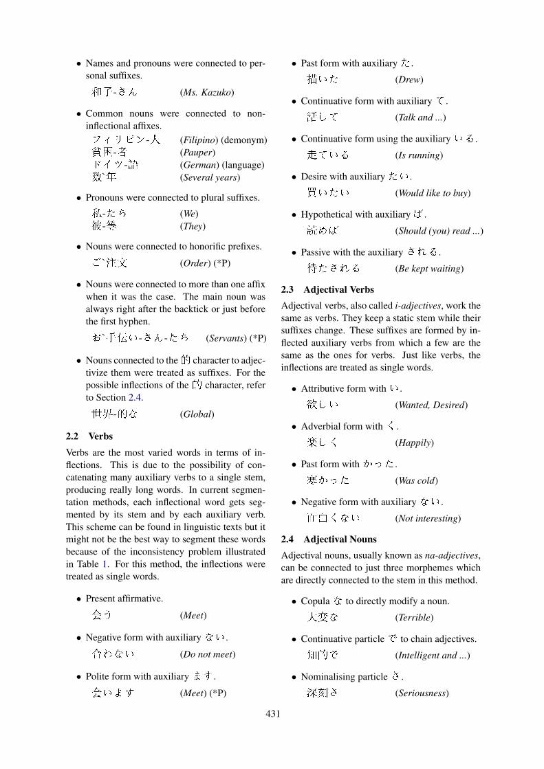
• Names and pronouns were connected to per-sonal suffixes.

和子-さん (Ms. Kazuko)

• Common nouns were connected to non-inflectional affixes.フィリピン-人 (Filipino) (demonym)貧困-者 (Pauper)ドイツ-語 (German) (language)数`年 (Several years)

• Pronouns were connected to plural suffixes.

私-たち (We)彼-等 (They)

• Nouns were connected to honorific prefixes.

ご`注文 (Order) (*P)

• Nouns were connected to more than one affixwhen it was the case. The main noun wasalways right after the backtick or just beforethe first hyphen.

お`手伝い-さん-たち (Servants) (*P)

• Nouns connected to the的 character to adjec-tivize them were treated as suffixes. For thepossible inflections of the的 character, referto Section 2.4.

世界-的な (Global)

2.2 Verbs

Verbs are the most varied words in terms of in-flections. This is due to the possibility of con-catenating many auxiliary verbs to a single stem,producing really long words. In current segmen-tation methods, each inflectional word gets seg-mented by its stem and by each auxiliary verb.This scheme can be found in linguistic texts but itmight not be the best way to segment these wordsbecause of the inconsistency problem illustratedin Table 1. For this method, the inflections weretreated as single words.

• Present affirmative.

会う (Meet)

• Negative form with auxiliaryない.

合わない (Do not meet)

• Polite form with auxiliaryます.

会います (Meet) (*P)

• Past form with auxiliaryた.

描いた (Drew)

• Continuative form with auxiliaryて.

話して (Talk and ...)

• Continuative form using the auxiliaryいる.

走ている (Is running)

• Desire with auxiliaryたい.

買いたい (Would like to buy)

• Hypothetical with auxiliaryば.

読めば (Should (you) read ...)

• Passive with the auxiliaryされる.

待たされる (Be kept waiting)

2.3 Adjectival VerbsAdjectival verbs, also called i-adjectives, work thesame as verbs. They keep a static stem while theirsuffixes change. These suffixes are formed by in-flected auxiliary verbs from which a few are thesame as the ones for verbs. Just like verbs, theinflections are treated as single words.

• Attributive form withい.

欲しい (Wanted, Desired)

• Adverbial form withく.

楽しく (Happily)

• Past form withかった.

寒かった (Was cold)

• Negative form with auxiliaryない.

面白くない (Not interesting)

2.4 Adjectival NounsAdjectival nouns, usually known as na-adjectives,can be connected to just three morphemes whichare directly connected to the stem in this method.

• Copulaな to directly modify a noun.

大変な (Terrible)

• Continuative particleで to chain adjectives.

知的で (Intelligent and ...)

• Nominalising particleさ.

深刻さ (Seriousness)

431

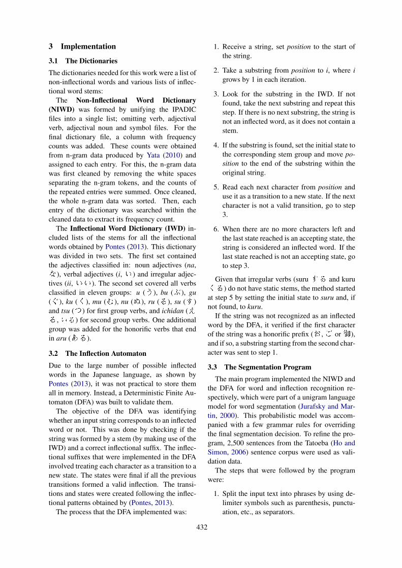
3 Implementation

3.1 The DictionariesThe dictionaries needed for this work were a list ofnon-inflectional words and various lists of inflec-tional word stems:

The Non-Inflectional Word Dictionary(NIWD) was formed by unifying the IPADICfiles into a single list; omitting verb, adjectivalverb, adjectival noun and symbol files. For thefinal dictionary file, a column with frequencycounts was added. These counts were obtainedfrom n-gram data produced by Yata (2010) andassigned to each entry. For this, the n-gram datawas first cleaned by removing the white spacesseparating the n-gram tokens, and the counts ofthe repeated entries were summed. Once cleaned,the whole n-gram data was sorted. Then, eachentry of the dictionary was searched within thecleaned data to extract its frequency count.

The Inflectional Word Dictionary (IWD) in-cluded lists of the stems for all the inflectionalwords obtained by Pontes (2013). This dictionarywas divided in two sets. The first set containedthe adjectives classified in: noun adjectives (na,な), verbal adjectives (i, い) and irregular adjec-tives (ii,いい). The second set covered all verbsclassified in eleven groups: u (う), bu (ぶ), gu(ぐ), ku (く), mu (む), nu (ぬ), ru (る), su (す)and tsu (つ) for first group verbs, and ichidan (える,いる) for second group verbs. One additionalgroup was added for the honorific verbs that endin aru (ある).

3.2 The Inflection AutomatonDue to the large number of possible inflectedwords in the Japanese language, as shown byPontes (2013), it was not practical to store themall in memory. Instead, a Deterministic Finite Au-tomaton (DFA) was built to validate them.

The objective of the DFA was identifyingwhether an input string corresponds to an inflectedword or not. This was done by checking if thestring was formed by a stem (by making use of theIWD) and a correct inflectional suffix. The inflec-tional suffixes that were implemented in the DFAinvolved treating each character as a transition to anew state. The states were final if all the previoustransitions formed a valid inflection. The transi-tions and states were created following the inflec-tional patterns obtained by (Pontes, 2013).

The process that the DFA implemented was:

1. Receive a string, set position to the start ofthe string.

2. Take a substring from position to i, where igrows by 1 in each iteration.

3. Look for the substring in the IWD. If notfound, take the next substring and repeat thisstep. If there is no next substring, the string isnot an inflected word, as it does not contain astem.

4. If the substring is found, set the initial state tothe corresponding stem group and move po-sition to the end of the substring within theoriginal string.

5. Read each next character from position anduse it as a transition to a new state. If the nextcharacter is not a valid transition, go to step3.

6. When there are no more characters left andthe last state reached is an accepting state, thestring is considered an inflected word. If thelast state reached is not an accepting state, goto step 3.

Given that irregular verbs (suruする and kuruくる) do not have static stems, the method startedat step 5 by setting the initial state to suru and, ifnot found, to kuru.

If the string was not recognized as an inflectedword by the DFA, it verified if the first characterof the string was a honorific prefix (お,ご or御),and if so, a substring starting from the second char-acter was sent to step 1.

3.3 The Segmentation ProgramThe main program implemented the NIWD and

the DFA for word and inflection recognition re-spectively, which were part of a unigram languagemodel for word segmentation (Jurafsky and Mar-tin, 2000). This probabilistic model was accom-panied with a few grammar rules for overridingthe final segmentation decision. To refine the pro-gram, 2,500 sentences from the Tatoeba (Ho andSimon, 2006) sentence corpus were used as vali-dation data.

The steps that were followed by the programwere:

1. Split the input text into phrases by using de-limiter symbols such as parenthesis, punctu-ation, etc., as separators.

432

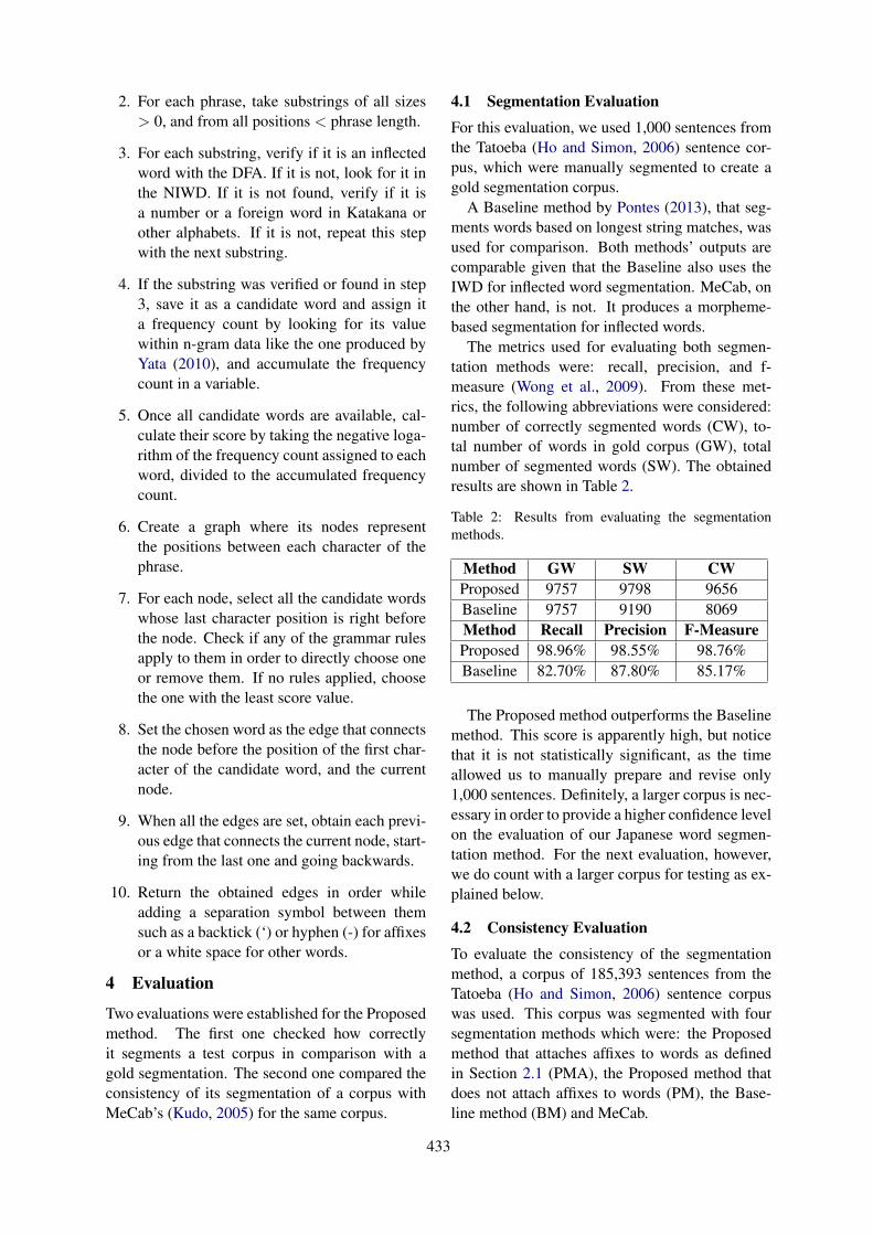
2. For each phrase, take substrings of all sizes> 0, and from all positions < phrase length.

3. For each substring, verify if it is an inflectedword with the DFA. If it is not, look for it inthe NIWD. If it is not found, verify if it isa number or a foreign word in Katakana orother alphabets. If it is not, repeat this stepwith the next substring.

4. If the substring was verified or found in step3, save it as a candidate word and assign ita frequency count by looking for its valuewithin n-gram data like the one produced byYata (2010), and accumulate the frequencycount in a variable.

5. Once all candidate words are available, cal-culate their score by taking the negative loga-rithm of the frequency count assigned to eachword, divided to the accumulated frequencycount.

6. Create a graph where its nodes representthe positions between each character of thephrase.

7. For each node, select all the candidate wordswhose last character position is right beforethe node. Check if any of the grammar rulesapply to them in order to directly choose oneor remove them. If no rules applied, choosethe one with the least score value.

8. Set the chosen word as the edge that connectsthe node before the position of the first char-acter of the candidate word, and the currentnode.

9. When all the edges are set, obtain each previ-ous edge that connects the current node, start-ing from the last one and going backwards.

10. Return the obtained edges in order whileadding a separation symbol between themsuch as a backtick (‘) or hyphen (-) for affixesor a white space for other words.

4 Evaluation

Two evaluations were established for the Proposedmethod. The first one checked how correctlyit segments a test corpus in comparison with agold segmentation. The second one compared theconsistency of its segmentation of a corpus withMeCab’s (Kudo, 2005) for the same corpus.

4.1 Segmentation Evaluation

For this evaluation, we used 1,000 sentences fromthe Tatoeba (Ho and Simon, 2006) sentence cor-pus, which were manually segmented to create agold segmentation corpus.

A Baseline method by Pontes (2013), that seg-ments words based on longest string matches, wasused for comparison. Both methods’ outputs arecomparable given that the Baseline also uses theIWD for inflected word segmentation. MeCab, onthe other hand, is not. It produces a morpheme-based segmentation for inflected words.

The metrics used for evaluating both segmen-tation methods were: recall, precision, and f-measure (Wong et al., 2009). From these met-rics, the following abbreviations were considered:number of correctly segmented words (CW), to-tal number of words in gold corpus (GW), totalnumber of segmented words (SW). The obtainedresults are shown in Table 2.

Table 2: Results from evaluating the segmentationmethods.

Method GW SW CWProposed 9757 9798 9656Baseline 9757 9190 8069Method Recall Precision F-MeasureProposed 98.96% 98.55% 98.76%Baseline 82.70% 87.80% 85.17%

The Proposed method outperforms the Baselinemethod. This score is apparently high, but noticethat it is not statistically significant, as the timeallowed us to manually prepare and revise only1,000 sentences. Definitely, a larger corpus is nec-essary in order to provide a higher confidence levelon the evaluation of our Japanese word segmen-tation method. For the next evaluation, however,we do count with a larger corpus for testing as ex-plained below.

4.2 Consistency Evaluation

To evaluate the consistency of the segmentationmethod, a corpus of 185,393 sentences from theTatoeba (Ho and Simon, 2006) sentence corpuswas used. This corpus was segmented with foursegmentation methods which were: the Proposedmethod that attaches affixes to words as definedin Section 2.1 (PMA), the Proposed method thatdoes not attach affixes to words (PM), the Base-line method (BM) and MeCab.

433

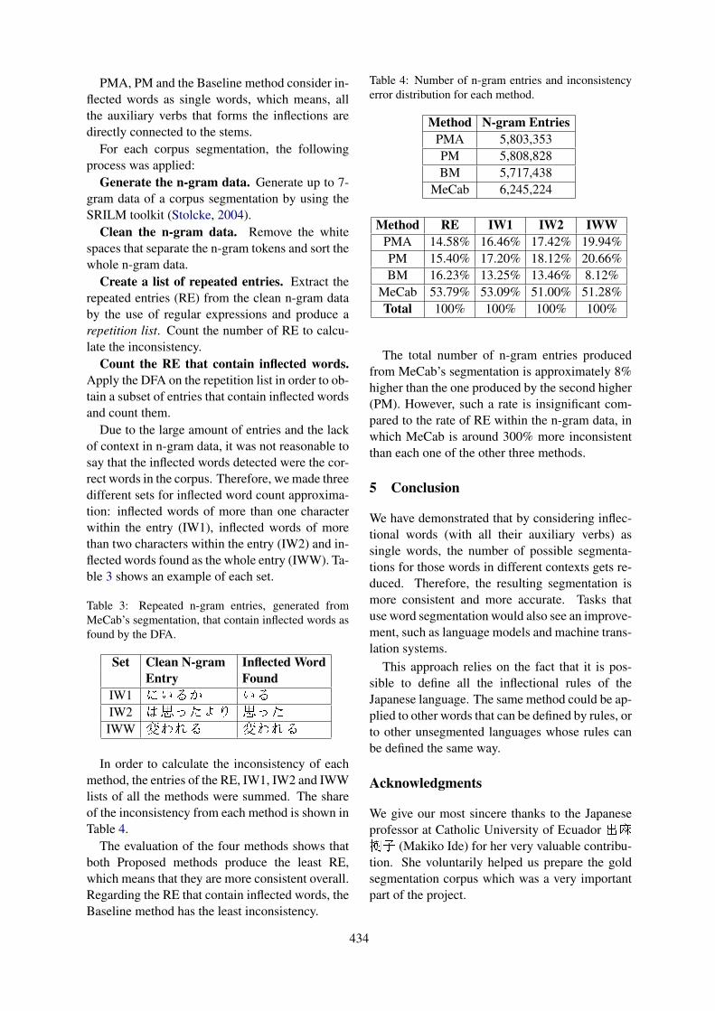
PMA, PM and the Baseline method consider in-flected words as single words, which means, allthe auxiliary verbs that forms the inflections aredirectly connected to the stems.

For each corpus segmentation, the followingprocess was applied:

Generate the n-gram data. Generate up to 7-gram data of a corpus segmentation by using theSRILM toolkit (Stolcke, 2004).

Clean the n-gram data. Remove the whitespaces that separate the n-gram tokens and sort thewhole n-gram data.

Create a list of repeated entries. Extract therepeated entries (RE) from the clean n-gram databy the use of regular expressions and produce arepetition list. Count the number of RE to calcu-late the inconsistency.

Count the RE that contain inflected words.Apply the DFA on the repetition list in order to ob-tain a subset of entries that contain inflected wordsand count them.

Due to the large amount of entries and the lackof context in n-gram data, it was not reasonable tosay that the inflected words detected were the cor-rect words in the corpus. Therefore, we made threedifferent sets for inflected word count approxima-tion: inflected words of more than one characterwithin the entry (IW1), inflected words of morethan two characters within the entry (IW2) and in-flected words found as the whole entry (IWW). Ta-ble 3 shows an example of each set.

Table 3: Repeated n-gram entries, generated fromMeCab’s segmentation, that contain inflected words asfound by the DFA.

Set Clean N-gram Inflected WordEntry Found

IW1 にいるか いる

IW2 は思ったより 思った

IWW 変われる 変われる

In order to calculate the inconsistency of eachmethod, the entries of the RE, IW1, IW2 and IWWlists of all the methods were summed. The shareof the inconsistency from each method is shown inTable 4.

The evaluation of the four methods shows thatboth Proposed methods produce the least RE,which means that they are more consistent overall.Regarding the RE that contain inflected words, theBaseline method has the least inconsistency.

Table 4: Number of n-gram entries and inconsistencyerror distribution for each method.

Method N-gram EntriesPMA 5,803,353PM 5,808,828BM 5,717,438

MeCab 6,245,224

Method RE IW1 IW2 IWWPMA 14.58% 16.46% 17.42% 19.94%PM 15.40% 17.20% 18.12% 20.66%BM 16.23% 13.25% 13.46% 8.12%

MeCab 53.79% 53.09% 51.00% 51.28%Total 100% 100% 100% 100%

The total number of n-gram entries producedfrom MeCab’s segmentation is approximately 8%higher than the one produced by the second higher(PM). However, such a rate is insignificant com-pared to the rate of RE within the n-gram data, inwhich MeCab is around 300% more inconsistentthan each one of the other three methods.

5 Conclusion

We have demonstrated that by considering inflec-tional words (with all their auxiliary verbs) assingle words, the number of possible segmenta-tions for those words in different contexts gets re-duced. Therefore, the resulting segmentation ismore consistent and more accurate. Tasks thatuse word segmentation would also see an improve-ment, such as language models and machine trans-lation systems.

This approach relies on the fact that it is pos-sible to define all the inflectional rules of theJapanese language. The same method could be ap-plied to other words that can be defined by rules, orto other unsegmented languages whose rules canbe defined the same way.

Acknowledgments

We give our most sincere thanks to the Japaneseprofessor at Catholic University of Ecuador出麻樹子 (Makiko Ide) for her very valuable contribu-tion. She voluntarily helped us prepare the goldsegmentation corpus which was a very importantpart of the project.

434

ReferencesMasayuki Asahara and Yuji Matsumoto. 2003.

Ipadic version 2.7.0 user’s manual. [online]Open Source Development Network. Available at:https://ja.osdn.net/projects/ipadic/docs/ipadic-2.7.0-manual-en.pdf [Accessed 25 Apr. 2019].

Laurie Bauer. 1983. Some basic concepts, CambridgeTextbooks in Linguistics, page 7–41. CambridgeUniversity Press.

Trang Ho and Allan Simon. 2006. Tatoeba. [online]Tatoeba: Collection of Sentences and Translations.Available at: https://tatoeba.org [Accessed 25 Apr.2019].

Nitin Indurkhya and Fred J. Damerau. 2010. Hand-book of Natural Language Processing, 2nd edition.Chapman & Hall/CRC.

Daniel Jurafsky and James H. Martin. 2000. Speechand Language Processing: An Introduction to Nat-ural Language Processing, Computational Linguis-tics, and Speech Recognition, 1st edition. PrenticeHall PTR, Upper Saddle River, NJ, USA.

Michiel Kamermans. 2010. An Introduction toJapanese - Syntax, Grammar and Language. SJGRPublishing.

Francis Katamba. 1994. English Words. Routledge.

Taisei Kudo. 2005. Mecab : Yet another part-of-speechand morphological analyzer.

Taku Kudo and Hideto Kazawa. 2009. Japaneseweb n-gram version 1 ldc2009t08. [online]Linguistic Data Consortium. Available at:https://catalog.ldc.upenn.edu/LDC2009T08 [Ac-cessed 25 Apr. 2019].

Yuji Matsumoto, Sadao Kurohashi, Yutaka Nyoki, Hi-toshi Shinho, and Makoto Nagao. 1991. User’sguide for the juman system, a user-extensible mor-phological analyzer for Japanese. Nagao Labora-tory, Kyoto University.

Yuji Matsumoto, Kazuma Takaoka, and Masayuki Asa-hara. 2007. Chasen morphological analyzer version2.4. 0 user’s manual. Nara Institute of Science andTechnology.

Josafa Pontes. 2013. A corpus of inflected japaneseverbs and adjectives. [Unpublished].

Andreas Stolcke. 2004. Srilm — an extensible lan-guage modeling toolkit. Proceedings of the 7th In-ternational Conference on Spoken Language Pro-cessing (ICSLP 2002), 2.

Kam-Fai Wong, Wenjie Li, Ruifeng Xu, and Zheng-sheng Zhang. 2009. Introduction to Chinese NaturalLanguage Processing, volume 2.

Susumu Yata. 2010. N-gram corpus - japanese webcorpus 2010. [online] S-yata.jp. Available at:http://www.s-yata.jp/corpus/nwc2010/ngrams/ [Ac-cessed 25 Apr. 2019].

435

Author Index

Abuduweili, Abulikemu, 229Adebiyi, Ayodele, 338Aguiar, Josafá, 429Aguirre, Stalin, 429Alimova, Ilseyar, 415Aly, Rami, 323Arase, Yuki, 197, 260Azin, Zahra, 43

Badia, Toni, 253Bao, Lingxian, 253Bekki, Daisuke, 386Berendt, Bettina, 203Bhavan, Anjali, 281Biemann, Chris, 315, 323Bojar, Ondrej, 130Bommasani, Rishi, 89Bonnefoy, Antoine, 243Bouscarrat, Léo, 243Bravo-Marquez, Felipe, 136

Calude, Andreea, 136Chen, Emily, 27Çolakoglu, Talha, 267Costa-jussà, Marta R., 236Cui, Hongyi, 217Cunha, Murilo, 203

Daramola, Olawande, 338Delobelle, Pieter, 203Dereli, Nesat, 331Dhar, Mrinal, 371Di Palo, Flavio, 302Didolkar, Aniket, 273Dirkson, Anne, 64Dwiastuti, Meisyarah, 309

Egawa, Ryo, 422El Boukkouri, Hicham, 295Eryigit, Gülsen, 43Escolano, Carlos, 236

Ferret, Olivier, 295Fonollosa, José A. R., 236Foster, Jennifer, 344

Fujita, Katsuhide, 422

Galván-Sosa, Diana, 106Ghosh Chowdhury, Arijit, 273Gulordava, Kristina, 162

Herbelot, Aurélie, 155, 162Hosseini-Kivanani, Nina, 74Hotate, Kengo, 149Hou, Hongxu, 123Hung, Po-Hsuan, 217Hyun, Jae Won, 223

Iida, Shohei, 217Inoue, Naoya, 378Inui, Kentaro, 378

Jagfeld, Glorianna, 17Ji, Yatu, 123Junjie, Chen, 123

Kabbach, Alexandre, 162Kajiwara, Tomoyuki, 260Kaneko, Masahiro, 149Karunanayake, Yohan, 288Katsumata, Satoru, 149Kaur, Rajvir, 1Keegan, Te Taka, 136Kennedy, Stefan, 344Kimura, Ryuichiro, 217Koehn, Philipp, 371Kolajo, Taiwo, 338Komachi, Mamoru, 149Kumar, Vaibhav, 371

Lal, Yash Kumar, 371Lambert, Patrik, 253Lavergne, Thomas, 295Li, Lei, 229Liu, Fangyu, 169Liu, Gongshen, 210

Malykh, Valentin, 10Marinho, Zita, 190Martins, André F. T., 190, 351Martins, Pedro Henrique, 190

437

Massip Cano, Eric, 203McCarren, Andrew, 344McKillop, Conor, 100Miftahutdinov, Zulfat, 393Mihaylova, Tsvetomila, 351Mim, Farjana Sultana, 378Mineshima, Koji, 386Minnema, Gosse, 155Mishra, Rohan, 281Morio, Gaku, 422Muaz, Urwa, 223

Nagata, Masaaki, 217, 400Nguyen, Vincent, 54Nishihara, Daiki, 260Nöth, Elmar, 74

Ouchi, Hiroki, 378

Pamungkas, Endang Wahyu, 363Panchenko, Alexander, 315Parde, Natalie, 302Pardo, Thiago, 81Pathak, Archita, 357Patti, Viviana, 363Peel, Thomas, 243Peperkamp, Jeroen, 203Pereira, Cécile, 243Phienthrakul, Tanasanee, 407

Qian, Yusu, 48, 223

Ranathunga, Surangika, 288Reddy, Appidi Abhinav, 183Reisert, Paul, 378Remus, Steffen, 323

Saraclar, Murat, 331Sasano, Ryohei, 177Sawhney, Ramit, 273, 281Scheffler, Tatjana, 143Schricker, Luise, 143Sevgili, Özge, 315Shah, Rajiv Ratn, 273, 281Shrivastava, Manish, 183, 371Singh, Vinay, 183Sinha, Pradyumna Prakhar, 281Sloka, Kirils, 344Sobrevilla Cabezudo, Marco Antonio, 81Sperber, Matthias, 113Srihari, Rohini, 357Srirangam, Vamshi Krishna, 183Stede, Manfred, 74

Sulubacak, Umut, 267Suzuki, Riko, 386

Takayama, Junya, 197Takeda, Koichi, 177Tanaka, Koji, 197Tantug, Ahmet Cüneyd, 267Tay, Wenyi, 34Thayasivam, Uthayasanker, 288Thongtan, Tan, 407Trye, David, 136Tsuruoka, Yoshimasa, 400Tutubalina, Elena, 393, 415

Utsuro, Takehito, 217

Variš, Dušan, 130Vásquez-Correa, Juan Camilo, 74

Waibel, Alexander, 113Walsh, Niall, 344Wang, Jingkang, 210Wu, Nier, 123

Yamada, Kosuke, 177Yanaka, Hitomi, 386Yang, Pengcheng, 229Yasui, Go, 400Ye, Rongtian, 169Yoshikawa, Masashi, 386

Zeng, Wenhuan, 229Zhang, Ben, 223Zhou, Jianing, 210Zhou, Zhong, 113Zweigenbaum, Pierre, 295