Proceedings of the 2019 EMNLP Workshop W-NUT - ACL ...

W-NUT 2019

The Fifth Workshop onNoisy User-generated Text

(W-NUT 2019)

Proceedings of the Workshop

Nov 4, 2019Hong Kong, China

c©2019 The Association for Computational Linguistics

Order copies of this and other ACL proceedings from:

Association for Computational Linguistics (ACL)209 N. Eighth StreetStroudsburg, PA 18360USATel: +1-570-476-8006Fax: [email protected]

ISBN 978-1-950737-84-0

ii

Introduction

The W-NUT 2019 workshop focuses on a core set of natural language processing tasks on top ofnoisy user-generated text, such as that found on social media, web forums and online reviews. Recentyears have seen a significant increase of interest in these areas. The internet has democratized contentcreation leading to an explosion of informal user-generated text, publicly available in electronic format,motivating the need for NLP on noisy text to enable new data analytics applications.

We received 89 long and short paper submissions this year. There are two invited speakers, IsabelleAugenstein (University of Copenhagen) and Jing Jiang (Singapore Management University) with eachof their talks covering a different aspect of NLP for user-generated text. We have the best paperaward(s) sponsored by Google this year, for which we are thankful. We would like to thank the ProgramCommittee members who reviewed the papers this year. We would also like to thank the workshopparticipants.

Wei Xu, Alan Ritter, Tim Baldwin and Afshin RahimiCo-Organizers

iii

Organizers:

Wei Xu, Ohio State UniversityAlan Ritter, Ohio State UniversityTim Baldwin, University of MelbourneAfshin Rahimi, University of Melbourne

Program Committee:

Mostafa Abdou (University of Copenhagen)Muhammad Abdul-Mageed (University of British Columbia)Željko Agic (Corti)Gustavo Aguilar (University of Houston)Hadi Amiri (Harvard University)Rahul Aralikatte (University of Copenhagen)Eiji Aramaki (NAIST)Roy Bar-Haim (IBM)Francesco Barbieri (UPF Barcelona)Cosmin Bejan (Vanderbilt University)Eric Bell (PNNL)Adrian Benton (JHU)Eduardo Blanco (University of North Texas)Su Lin Blodgett (UMass Amherst)Matko Bošnjak (University College London)Julian Brooke (University of British Columbia)Annabelle Carrell (JHU)Xilun Chen (Cornell University)Anne Cocos (University of Pennsylvania)Arman Cohan (AI2)Nigel Collier (University of Cambridge)Paul Cook (University of New Brunswick)Marina Danilevsky (IBM Research)Leon Derczynski (IT University of Copenhagen)Seza Dogruöz (Tilburg University)Jay DeYoung (Northeastern University)Eduard Dragut (Temple University)Xinya Du (Cornell University)Heba Elfardy (Amazon)Micha Elsner (Ohio State University)Sindhu Kiranmai Ernala (Georgia Tech)Manaal Faruqui (Google Research)Lisheng Fu (New York University)Yoshinari Fujinuma (University of Colorado, Boulder)Dan Garrette (Google Research)Kevin Gimpel (TTIC)Dan Goldwasser (Purdue University)Amit Goyal (Criteo)Nizar Habash (NYU Abu Dhabi)Masato Hagiwara (Duolingo) v

Bo Han (Kaplan)Abe Handler (University of Massachusetts Amherst)Shudong Hao (University of Colorado, Boulder)Devamanyu Hazarika (National University of Singapore)Jack Hessel (Cornell University)Dirk Hovy (Bocconi University)Xiaolei Huang (University of Colorado, Boulder)Sarthak Jain (Northeastern University)Kenny Joseph (University at Buffalo)David Jurgens (University of Michigan)Nobuhiro Kaji (Yahoo! Research)Pallika Kanani (Oracle)Dongyeop Kang (Carnegie Mellon University)Emre Kiciman (Microsoft Research)Svetlana Kiritchenko (National Research Council Canada)Roman Klinger (University of Stuttgart)Ekaterina Kochmar (University of Cambridge)Vivek Kulkarni (University of California Santa Barbara)Jonathan Kummerfeld (University of Michigan)Ophélie Lacroix (Siteimprove)Wuwei Lan (Ohio State University)Chen Li (Tencent)Jing Li (Tencent AI)Jessy Junyi Li (University of Texas Austin)Yitong Li (University of Melbourne)Nut Limsopatham (University of Glasgow)Patrick Littell (National Research Council Canada)Zhiyuan Liu (Tsinghua University)Fei Liu (University of Melbourne)Nikola Ljubešic (University of Zagreb)Wei-Yun Ma (Academia Sinica)Mounica Maddela (Ohio State University)Suraj Maharjan (University of Houston)Aaron Masino (The Children’s Hospital of Philadelphia)Paul Michel (CMU)Shachar Mirkin (Xerox Research)Saif M. Mohammad (National Research Council Canada)Ahmed Mourad (RMIT University)Günter Neumann (DFKI)Vincent Ng (University of Texas at Dallas)Eric Nichols (Honda Research Institute)Xing Niu (University of Maryland, College Park)Benjamin Nye (Northeastern University)Alice Oh (KAIST)Naoki Otani (CMU)Patrick Pantel (Microsoft Research)Umashanthi Pavalanathan (Georgia Tech)Yuval Pinter (Georgia Tech)Barbara Plank (IT University of Copenhagen)Christopher Potts (Stanford University)Daniel Preotiuc-Pietro (Bloomberg)

vi

Chris Quirk (Microsoft Research)Ella Rabinovich (University of Toronto)Dianna Radpour (University of Colorado Boulder)Preethi Raghavan (IBM Research)Revanth Rameshkumar (Microsoft)Sudha Rao (Microsoft Research)Marek Rei (University of Cambridge)Roi Reichart (Technion)Adithya Renduchintala (JHU)Carolyn Penstein Rose (CMU)Alla Rozovskaya (City University of New York)Koustuv Saha (Georgia Tech)Keisuke Sakaguchi (Allen Institute for Artificial Intelligence)Maarten Sap (University of Washington)Natalie Schluter (IT University of Copenhagen)Andrew Schwartz (Stony Brook University)Djamé Seddah (University Paris-Sorbonne)Amirreza Shirani (University of Houston)Dan Simonson (BlackBoiler)Evangelia Spiliopoulou (Carnegie Mellon University)Jan Šnajder (University of Zagreb)Gabriel Stanovsky (Allen Institute for Artificial Intelligence)Ian Stewart (Georgia Tech)Jeniya Tabassum (Ohio State University)Joel Tetreault (Grammarly)Sara Tonelli (FBK)Rob van der Goot (University of Groningen)Rob Voigt (Stanford University)Byron Wallace (Northeastern University)Xiaojun Wan (Peking University)Zeerak Waseem (University of Sheffield)Zhongyu Wei (Fudan University)Diyi Yang (Georgia Tech)Yi Yang (ASAPP)Guido Zarrella (MITRE)Justine Zhang (Cornell University)Jason Shuo Zhang (University of Colorado, Boulder)Shi Zong (Ohio State University)

Invited Speakers:

Isabelle Augenstein (University of Copenhagen)Jing Jiang (Singapore Management University)

vii

Table of Contents

Weakly Supervised Attention Networks for Fine-Grained Opinion Mining and Public HealthGiannis Karamanolakis, Daniel Hsu and Luis Gravano . . . . . . . . . . . . . . . . . . . . . . . . . . . . . . . . . . . . . . .1

Formality Style Transfer for Noisy, User-generated Conversations: Extracting Labeled, Parallel Datafrom Unlabeled Corpora

Isak Czeresnia Etinger and Alan W Black . . . . . . . . . . . . . . . . . . . . . . . . . . . . . . . . . . . . . . . . . . . . . . . . . 11

Multilingual Whispers: Generating Paraphrases with TranslationChristian Federmann, Oussama Elachqar and Chris Quirk . . . . . . . . . . . . . . . . . . . . . . . . . . . . . . . . . . .17

Personalizing Grammatical Error Correction: Adaptation to Proficiency Level and L1Maria Nadejde and Joel Tetreault . . . . . . . . . . . . . . . . . . . . . . . . . . . . . . . . . . . . . . . . . . . . . . . . . . . . . . . . . 27

Exploiting BERT for End-to-End Aspect-based Sentiment AnalysisXin Li, Lidong Bing, Wenxuan Zhang and Wai Lam. . . . . . . . . . . . . . . . . . . . . . . . . . . . . . . . . . . . . . . .34

Training on Synthetic Noise Improves Robustness to Natural Noise in Machine Translationvladimir karpukhin, Omer Levy, Jacob Eisenstein and Marjan Ghazvininejad . . . . . . . . . . . . . . . . . 42

Character-Based Models for Adversarial Phone Extraction: Preventing Human Sex TraffickingNathanael Chambers, Timothy Forman, Catherine Griswold, Kevin Lu, Yogaish Khastgir and

Stephen Steckler . . . . . . . . . . . . . . . . . . . . . . . . . . . . . . . . . . . . . . . . . . . . . . . . . . . . . . . . . . . . . . . . . . . . . . . . . . . . 48

Tkol, Httt, and r/radiohead: High Affinity Terms in Reddit CommunitiesAbhinav Bhandari and Caitrin Armstrong . . . . . . . . . . . . . . . . . . . . . . . . . . . . . . . . . . . . . . . . . . . . . . . . . 57

Large Scale Question Paraphrase Retrieval with Smoothed Deep Metric LearningDaniele Bonadiman, Anjishnu Kumar and Arpit Mittal . . . . . . . . . . . . . . . . . . . . . . . . . . . . . . . . . . . . . 68

Hey Siri. Ok Google. Alexa: A topic modeling of user reviews for smart speakersHanh Nguyen and Dirk Hovy . . . . . . . . . . . . . . . . . . . . . . . . . . . . . . . . . . . . . . . . . . . . . . . . . . . . . . . . . . . . 76

Predicting Algorithm Classes for Programming Word Problemsvinayak athavale, aayush naik, rajas vanjape and Manish Shrivastava . . . . . . . . . . . . . . . . . . . . . . . . . 84

Automatic identification of writers’ intentions: Comparing different methods for predicting relationshipgoals in online dating profile texts

Chris van der Lee, Tess van der Zanden, Emiel Krahmer, Maria Mos and Alexander Schouten . . 94

Contextualized Word Representations from Distant Supervision with and for NERAbbas Ghaddar and Phillippe Langlais . . . . . . . . . . . . . . . . . . . . . . . . . . . . . . . . . . . . . . . . . . . . . . . . . . . 101

Extract, Transform and Filling: A Pipeline Model for Question Paraphrasing based on TemplateYunfan Gu, yang yuqiao and Zhongyu Wei . . . . . . . . . . . . . . . . . . . . . . . . . . . . . . . . . . . . . . . . . . . . . . . 109

An In-depth Analysis of the Effect of Lexical Normalization on the Dependency Parsing of Social MediaRob van der Goot . . . . . . . . . . . . . . . . . . . . . . . . . . . . . . . . . . . . . . . . . . . . . . . . . . . . . . . . . . . . . . . . . . . . . . 115

Who wrote this book? A challenge for e-commerceBéranger Dumont, Simona Maggio, Ghiles Sidi Said and Quoc-Tien Au . . . . . . . . . . . . . . . . . . . . 121

Mining Tweets that refer to TV programs with Deep Neural NetworksTakeshi Kobayakawa, Taro Miyazaki, Hiroki Okamoto and Simon Clippingdale . . . . . . . . . . . . . 126

ix

Normalising Non-standardised Orthography in Algerian Code-switched User-generated DataWafia Adouane, Jean-Philippe Bernardy and Simon Dobnik . . . . . . . . . . . . . . . . . . . . . . . . . . . . . . . . 131

Dialect Text Normalization to Normative Standard FinnishNiko Partanen, Mika Hämäläinen and Khalid Alnajjar . . . . . . . . . . . . . . . . . . . . . . . . . . . . . . . . . . . . . 141

A Cross-Topic Method for Supervised Relevance ClassificationJiawei Yong . . . . . . . . . . . . . . . . . . . . . . . . . . . . . . . . . . . . . . . . . . . . . . . . . . . . . . . . . . . . . . . . . . . . . . . . . . . 147

Exploring Multilingual Syntactic Sentence RepresentationsChen Liu, Anderson De Andrade and Muhammad Osama . . . . . . . . . . . . . . . . . . . . . . . . . . . . . . . . . 153

FASPell: A Fast, Adaptable, Simple, Powerful Chinese Spell Checker Based On DAE-Decoder ParadigmYuzhong Hong, Xianguo Yu, Neng He, Nan Liu and Junhui Liu . . . . . . . . . . . . . . . . . . . . . . . . . . . . 160

Latent semantic network induction in the context of linked example sensesHunter Heidenreich and Jake Williams . . . . . . . . . . . . . . . . . . . . . . . . . . . . . . . . . . . . . . . . . . . . . . . . . . . 170

SmokEng: Towards Fine-grained Classification of Tobacco-related Social Media TextKartikey Pant, Venkata Himakar Yanamandra, Alok Debnath and Radhika Mamidi . . . . . . . . . . . 181

Modelling Uncertainty in Collaborative Document Quality AssessmentAili Shen, Daniel Beck, Bahar Salehi, Jianzhong Qi and Timothy Baldwin . . . . . . . . . . . . . . . . . . 191

Conceptualisation and Annotation of Drug Nonadherence Information for Knowledge Extraction fromPatient-Generated Texts

Anja Belz, Richard Hoile, Elizabeth Ford and Azam Mullick . . . . . . . . . . . . . . . . . . . . . . . . . . . . . . . 202

Dataset Analysis and Augmentation for Emoji-Sensitive Irony DetectionShirley Anugrah Hayati, Aditi Chaudhary, Naoki Otani and Alan W Black . . . . . . . . . . . . . . . . . . 212

Geolocation with Attention-Based Multitask Learning ModelsTommaso Fornaciari and Dirk Hovy . . . . . . . . . . . . . . . . . . . . . . . . . . . . . . . . . . . . . . . . . . . . . . . . . . . . . 217

Dense Node Representation for GeolocationTommaso Fornaciari and Dirk Hovy . . . . . . . . . . . . . . . . . . . . . . . . . . . . . . . . . . . . . . . . . . . . . . . . . . . . . 224

Identifying Linguistic Areas for GeolocationTommaso Fornaciari and Dirk Hovy . . . . . . . . . . . . . . . . . . . . . . . . . . . . . . . . . . . . . . . . . . . . . . . . . . . . . 231

Robustness to Capitalization Errors in Named Entity RecognitionSravan Bodapati, Hyokun Yun and Yaser Al-Onaizan. . . . . . . . . . . . . . . . . . . . . . . . . . . . . . . . . . . . . .237

Extending Event Detection to New Types with Learning from KeywordsViet Dac Lai and Thien Nguyen . . . . . . . . . . . . . . . . . . . . . . . . . . . . . . . . . . . . . . . . . . . . . . . . . . . . . . . . . 243

Distant Supervised Relation Extraction with Separate Head-Tail CNNRui Xing and Jie Luo . . . . . . . . . . . . . . . . . . . . . . . . . . . . . . . . . . . . . . . . . . . . . . . . . . . . . . . . . . . . . . . . . . 249

Discovering the Functions of Language in Online ForumsYoumna Ismaeil, Oana Balalau and Paramita Mirza . . . . . . . . . . . . . . . . . . . . . . . . . . . . . . . . . . . . . . . 259

Incremental processing of noisy user utterances in the spoken language understanding taskStefan Constantin, Jan Niehues and Alex Waibel . . . . . . . . . . . . . . . . . . . . . . . . . . . . . . . . . . . . . . . . . . 265

x

Benefits of Data Augmentation for NMT-based Text Normalization of User-Generated ContentClaudia Matos Veliz, Orphee De Clercq and Veronique Hoste . . . . . . . . . . . . . . . . . . . . . . . . . . . . . . 275

Contextual Text Denoising with Masked Language ModelYifu Sun and Haoming Jiang . . . . . . . . . . . . . . . . . . . . . . . . . . . . . . . . . . . . . . . . . . . . . . . . . . . . . . . . . . . 286

Towards Automated Semantic Role Labelling of Hindi-English Code-Mixed TweetsRiya Pal and Dipti Sharma. . . . . . . . . . . . . . . . . . . . . . . . . . . . . . . . . . . . . . . . . . . . . . . . . . . . . . . . . . . . . .291

Enhancing BERT for Lexical NormalizationBenjamin Muller, Benoit Sagot and Djamé Seddah . . . . . . . . . . . . . . . . . . . . . . . . . . . . . . . . . . . . . . . . 297

No, you’re not alone: A better way to find people with similar experiences on RedditZhilin Wang, Elena Rastorgueva, Weizhe Lin and Xiaodong Wu . . . . . . . . . . . . . . . . . . . . . . . . . . . . 307

Improving Multi-label Emotion Classification by Integrating both General and Domain-specific Knowl-edge

Wenhao Ying, Rong Xiang and Qin Lu . . . . . . . . . . . . . . . . . . . . . . . . . . . . . . . . . . . . . . . . . . . . . . . . . . 316

Adapting Deep Learning Methods for Mental Health Prediction on Social MediaIvan Sekulic and Michael Strube . . . . . . . . . . . . . . . . . . . . . . . . . . . . . . . . . . . . . . . . . . . . . . . . . . . . . . . . 322

Improving Neural Machine Translation Robustness via Data Augmentation: Beyond Back-TranslationZhenhao Li and Lucia Specia . . . . . . . . . . . . . . . . . . . . . . . . . . . . . . . . . . . . . . . . . . . . . . . . . . . . . . . . . . . 328

An Ensemble of Humour, Sarcasm, and Hate Speechfor Sentiment Classification in Online ReviewsRohan Badlani, Nishit Asnani and Manan Rai . . . . . . . . . . . . . . . . . . . . . . . . . . . . . . . . . . . . . . . . . . . . 337

Grammatical Error Correction in Low-Resource ScenariosJakub Náplava and Milan Straka . . . . . . . . . . . . . . . . . . . . . . . . . . . . . . . . . . . . . . . . . . . . . . . . . . . . . . . . 346

Minimally-Augmented Grammatical Error CorrectionRoman Grundkiewicz and Marcin Junczys-Dowmunt . . . . . . . . . . . . . . . . . . . . . . . . . . . . . . . . . . . . . 357

A Social Opinion Gold Standard for the Malta Government Budget 2018Keith Cortis and Brian Davis . . . . . . . . . . . . . . . . . . . . . . . . . . . . . . . . . . . . . . . . . . . . . . . . . . . . . . . . . . . 364

The Fallacy of Echo Chambers: Analyzing the Political Slants of User-Generated News Comments inKorean Media

Jiyoung Han, Youngin Lee, Junbum Lee and Meeyoung Cha . . . . . . . . . . . . . . . . . . . . . . . . . . . . . . . 370

Y’all should read this! Identifying Plurality in Second-Person Personal Pronouns in English TextsGabriel Stanovsky and Ronen Tamari . . . . . . . . . . . . . . . . . . . . . . . . . . . . . . . . . . . . . . . . . . . . . . . . . . . . 375

An Edit-centric Approach for Wikipedia Article Quality AssessmentEdison Marrese-Taylor, Pablo Loyola and Yutaka Matsuo . . . . . . . . . . . . . . . . . . . . . . . . . . . . . . . . . . 381

Additive Compositionality of Word VectorsYeon Seonwoo, Sungjoon Park, Dongkwan Kim and Alice Oh . . . . . . . . . . . . . . . . . . . . . . . . . . . . . 387

Contextualized context2vecKazuki Ashihara, Tomoyuki Kajiwara, Yuki Arase and Satoru Uchida . . . . . . . . . . . . . . . . . . . . . . 397

Phonetic Normalization for Machine Translation of User Generated ContentJosé Carlos Rosales Núñez, Djamé Seddah and Guillaume Wisniewski . . . . . . . . . . . . . . . . . . . . . . 407

xi

Normalization of Indonesian-English Code-Mixed Twitter DataAnab Maulana Barik, Rahmad Mahendra and Mirna Adriani . . . . . . . . . . . . . . . . . . . . . . . . . . . . . . . 417

Unsupervised Neologism Normalization Using Embedding Space MappingNasser Zalmout, Kapil Thadani and Aasish Pappu . . . . . . . . . . . . . . . . . . . . . . . . . . . . . . . . . . . . . . . . 425

Lexical Features Are More Vulnerable, Syntactic Features Have More Predictive PowerJekaterina Novikova, Aparna Balagopalan, Ksenia Shkaruta and Frank Rudzicz . . . . . . . . . . . . . . 431

Towards Actual (Not Operational) Textual Style Transfer Auto-EvaluationRichard Yuanzhe Pang . . . . . . . . . . . . . . . . . . . . . . . . . . . . . . . . . . . . . . . . . . . . . . . . . . . . . . . . . . . . . . . . . 444

CodeSwitch-Reddit: Exploration of Written Multilingual Discourse in Online Discussion ForumsElla Rabinovich, Masih Sultani and Suzanne Stevenson . . . . . . . . . . . . . . . . . . . . . . . . . . . . . . . . . . . 446

xii

Conference Program

Monday, November, 4, 2019

9:00–9:05 Opening

9:05–9:50 Invited Talk: Isabelle Augenstein

9:50–10:35 Oral Session I

9:50–10:05 Weakly Supervised Attention Networks for Fine-Grained Opinion Mining and Pub-lic HealthGiannis Karamanolakis, Daniel Hsu and Luis Gravano

10:05–10:20 Formality Style Transfer for Noisy, User-generated Conversations: Extracting La-beled, Parallel Data from Unlabeled CorporaIsak Czeresnia Etinger and Alan W Black

10:20–10:35 Multilingual Whispers: Generating Paraphrases with TranslationChristian Federmann, Oussama Elachqar and Chris Quirk

10:35–11:00 Coffee Break

11:00–12:15 Oral Session II

11:00–11:15 Personalizing Grammatical Error Correction: Adaptation to Proficiency Level andL1Maria Nadejde and Joel Tetreault

11:15–11:30 Exploiting BERT for End-to-End Aspect-based Sentiment AnalysisXin Li, Lidong Bing, Wenxuan Zhang and Wai Lam

11:30–11:45 Training on Synthetic Noise Improves Robustness to Natural Noise in MachineTranslationvladimir karpukhin, Omer Levy, Jacob Eisenstein and Marjan Ghazvininejad

11:45–12:00 Character-Based Models for Adversarial Phone Extraction: Preventing Human SexTraffickingNathanael Chambers, Timothy Forman, Catherine Griswold, Kevin Lu, YogaishKhastgir and Stephen Steckler

xiii

Monday, November, 4, 2019 (continued)

12:00–12:15 Tkol, Httt, and r/radiohead: High Affinity Terms in Reddit CommunitiesAbhinav Bhandari and Caitrin Armstrong

12:30–2:00 Lunch

2:00–3:00 Lightning Talks

Large Scale Question Paraphrase Retrieval with Smoothed Deep Metric LearningDaniele Bonadiman, Anjishnu Kumar and Arpit Mittal

Hey Siri. Ok Google. Alexa: A topic modeling of user reviews for smart speakersHanh Nguyen and Dirk Hovy

Predicting Algorithm Classes for Programming Word Problemsvinayak athavale, aayush naik, rajas vanjape and Manish Shrivastava

Automatic identification of writers’ intentions: Comparing different methods forpredicting relationship goals in online dating profile textsChris van der Lee, Tess van der Zanden, Emiel Krahmer, Maria Mos and AlexanderSchouten

Contextualized Word Representations from Distant Supervision with and for NERAbbas Ghaddar and Phillippe Langlais

Extract, Transform and Filling: A Pipeline Model for Question Paraphrasing basedon TemplateYunfan Gu, yang yuqiao and Zhongyu Wei

An In-depth Analysis of the Effect of Lexical Normalization on the Dependency Pars-ing of Social MediaRob van der Goot

Who wrote this book? A challenge for e-commerceBéranger Dumont, Simona Maggio, Ghiles Sidi Said and Quoc-Tien Au

Mining Tweets that refer to TV programs with Deep Neural NetworksTakeshi Kobayakawa, Taro Miyazaki, Hiroki Okamoto and Simon Clippingdale

xiv


Normalising Non-standardised Orthography in Algerian Code-switched User-generated DataWafia Adouane, Jean-Philippe Bernardy and Simon Dobnik

Dialect Text Normalization to Normative Standard FinnishNiko Partanen, Mika Hämäläinen and Khalid Alnajjar

A Cross-Topic Method for Supervised Relevance ClassificationJiawei Yong

Exploring Multilingual Syntactic Sentence RepresentationsChen Liu, Anderson De Andrade and Muhammad Osama

FASPell: A Fast, Adaptable, Simple, Powerful Chinese Spell Checker Based OnDAE-Decoder ParadigmYuzhong Hong, Xianguo Yu, Neng He, Nan Liu and Junhui Liu

Latent semantic network induction in the context of linked example sensesHunter Heidenreich and Jake Williams

SmokEng: Towards Fine-grained Classification of Tobacco-related Social MediaTextKartikey Pant, Venkata Himakar Yanamandra, Alok Debnath and Radhika Mamidi

Modelling Uncertainty in Collaborative Document Quality AssessmentAili Shen, Daniel Beck, Bahar Salehi, Jianzhong Qi and Timothy Baldwin

Conceptualisation and Annotation of Drug Nonadherence Information for Knowl-edge Extraction from Patient-Generated TextsAnja Belz, Richard Hoile, Elizabeth Ford and Azam Mullick

Dataset Analysis and Augmentation for Emoji-Sensitive Irony DetectionShirley Anugrah Hayati, Aditi Chaudhary, Naoki Otani and Alan W Black

Geolocation with Attention-Based Multitask Learning ModelsTommaso Fornaciari and Dirk Hovy

Dense Node Representation for GeolocationTommaso Fornaciari and Dirk Hovy

xv


Identifying Linguistic Areas for GeolocationTommaso Fornaciari and Dirk Hovy

Robustness to Capitalization Errors in Named Entity RecognitionSravan Bodapati, Hyokun Yun and Yaser Al-Onaizan

Extending Event Detection to New Types with Learning from KeywordsViet Dac Lai and Thien Nguyen

Distant Supervised Relation Extraction with Separate Head-Tail CNNRui Xing and Jie Luo

Discovering the Functions of Language in Online ForumsYoumna Ismaeil, Oana Balalau and Paramita Mirza

Incremental processing of noisy user utterances in the spoken language understand-ing taskStefan Constantin, Jan Niehues and Alex Waibel

Benefits of Data Augmentation for NMT-based Text Normalization of User-Generated ContentClaudia Matos Veliz, Orphee De Clercq and Veronique Hoste

Contextual Text Denoising with Masked Language ModelYifu Sun and Haoming Jiang

Towards Automated Semantic Role Labelling of Hindi-English Code-Mixed TweetsRiya Pal and Dipti Sharma

Enhancing BERT for Lexical NormalizationBenjamin Muller, Benoit Sagot and Djamé Seddah

No, you’re not alone: A better way to find people with similar experiences on RedditZhilin Wang, Elena Rastorgueva, Weizhe Lin and Xiaodong Wu

Improving Multi-label Emotion Classification by Integrating both General andDomain-specific KnowledgeWenhao Ying, Rong Xiang and Qin Lu

xvi


Adapting Deep Learning Methods for Mental Health Prediction on Social MediaIvan Sekulic and Michael Strube

Improving Neural Machine Translation Robustness via Data Augmentation: BeyondBack-TranslationZhenhao Li and Lucia Specia

An Ensemble of Humour, Sarcasm, and Hate Speechfor Sentiment Classification inOnline ReviewsRohan Badlani, Nishit Asnani and Manan Rai

Grammatical Error Correction in Low-Resource ScenariosJakub Náplava and Milan Straka

Minimally-Augmented Grammatical Error CorrectionRoman Grundkiewicz and Marcin Junczys-Dowmunt

A Social Opinion Gold Standard for the Malta Government Budget 2018Keith Cortis and Brian Davis

The Fallacy of Echo Chambers: Analyzing the Political Slants of User-GeneratedNews Comments in Korean MediaJiyoung Han, Youngin Lee, Junbum Lee and Meeyoung Cha

Y’all should read this! Identifying Plurality in Second-Person Personal Pronouns inEnglish TextsGabriel Stanovsky and Ronen Tamari

An Edit-centric Approach for Wikipedia Article Quality AssessmentEdison Marrese-Taylor, Pablo Loyola and Yutaka Matsuo

Additive Compositionality of Word VectorsYeon Seonwoo, Sungjoon Park, Dongkwan Kim and Alice Oh

Contextualized context2vecKazuki Ashihara, Tomoyuki Kajiwara, Yuki Arase and Satoru Uchida

Phonetic Normalization for Machine Translation of User Generated ContentJosé Carlos Rosales Núñez, Djamé Seddah and Guillaume Wisniewski

xvii


Normalization of Indonesian-English Code-Mixed Twitter DataAnab Maulana Barik, Rahmad Mahendra and Mirna Adriani

Unsupervised Neologism Normalization Using Embedding Space MappingNasser Zalmout, Kapil Thadani and Aasish Pappu

Lexical Features Are More Vulnerable, Syntactic Features Have More PredictivePowerJekaterina Novikova, Aparna Balagopalan, Ksenia Shkaruta and Frank Rudzicz

Simple Discovery of Aliases from User CommentsAbram Handler and Brian Clifton

Towards Actual (Not Operational) Textual Style Transfer Auto-EvaluationRichard Yuanzhe Pang

CodeSwitch-Reddit: Exploration of Written Multilingual Discourse in Online Dis-cussion ForumsElla Rabinovich, Masih Sultani and Suzanne Stevenson

3:00–4:30 Poster Session (all papers above)

4:30–4:55 Coffee Break

xviii


5:00–5:45 Invited Talk: Jing Jiang

5:45–6:00 Closing and Best Paper Awards

xix

Proceedings of the 2019 EMNLP Workshop W-NUT: The 5th Workshop on Noisy User-generated Text, pages 1–10Hong Kong, Nov 4, 2019. c©2019 Association for Computational Linguistics

Weakly Supervised Attention Networksfor Fine-Grained Opinion Mining and Public Health

Giannis Karamanolakis, Daniel Hsu, Luis GravanoColumbia University, New York, NY 10027, USA

{gkaraman, djhsu, gravano}@cs.columbia.edu

AbstractIn many review classification applications, afine-grained analysis of the reviews is desir-able, because different segments (e.g., sen-tences) of a review may focus on different as-pects of the entity in question. However, train-ing supervised models for segment-level clas-sification requires segment labels, which maybe more difficult or expensive to obtain thanreview labels. In this paper, we employ Mul-tiple Instance Learning (MIL) and use onlyweak supervision in the form of a single la-bel per review. First, we show that when inap-propriate MIL aggregation functions are used,then MIL-based networks are outperformedby simpler baselines. Second, we propose anew aggregation function based on the sig-moid attention mechanism and show that ourproposed model outperforms the state-of-the-art models for segment-level sentiment clas-sification (by up to 9.8% in F1). Finally, wehighlight the importance of fine-grained pre-dictions in an important public-health applica-tion: finding actionable reports of foodborneillness. We show that our model achieves48.6% higher recall compared to previousmodels, thus increasing the chance of identify-ing previously unknown foodborne outbreaks.

1 Introduction

Many applications of text review classification,such as sentiment analysis, can benefit from a fine-grained understanding of the reviews. Considerthe Yelp restaurant review in Figure 1. Some seg-ments (e.g., sentences or clauses) of the review ex-press positive sentiment towards some of the itemsconsumed, service, and ambience, but other seg-ments express a negative sentiment towards theprice and food. To capture the nuances expressedin such reviews, analyzing the reviews at the seg-ment level is desirable.

In this paper, we focus on segment classifica-tion when only review labels—but not segment

Figure 1: A Yelp review discussing both positive and nega-tive aspects of a restaurant, as well as food poisoning.

labels—are available. The lack of segment labelsprevents the use of standard supervised learningapproaches. While review labels, such as user-provided ratings, are often available, they are notdirectly relevant for segment classification, thuspresenting a challenge for supervised learning.

Existing weakly supervised learning frame-works have been proposed for training modelssuch as support vector machines (Andrews et al.,2003; Yessenalina et al., 2010; Gartner et al.,2002), logistic regression (Kotzias et al., 2015),and hidden conditional random fields (Tackstromand McDonald, 2011). The most recent state-of-the-art approaches employ the Multiple InstanceLearning (MIL) framework (Section 2.2) in hi-erarchical neural networks (Pappas and Popescu-Belis, 2014; Kotzias et al., 2015; Angelidis andLapata, 2018; Pappas and Popescu-Belis, 2017;Ilse et al., 2018). MIL-based hierarchical net-works combine the (unknown) segment labelsthrough an aggregation function to form a singlereview label. This enables the use of ground-truthreview labels as a weak form of supervision fortraining segment-level classifiers. However, it re-mains unanswered whether performance gains incurrent models stem from the hierarchical struc-

1

ture of the models or from the representationalpower of their deep learning components. Also,as we will see, the current modeling choices forthe MIL aggregation function might be problem-atic for some applications and, in turn, might hurtthe performance of the resulting classifiers.

As a first contribution of this paper, we showthat non-hierarchical, deep learning approachesfor segment-level sentiment classification —withonly review-level labels— are strong, and theyequal or exceed in performance hierarchical net-works with various MIL aggregation functions.

As a second contribution of this paper, wesubstantially improve previous hierarchical ap-proaches for segment-level sentiment classifica-tion and propose the use of a new MIL aggrega-tion function based on the sigmoid attention mech-anism to jointly model the relative importance ofeach segment as a product of Bernoulli distribu-tions. This modeling choice allows multiple seg-ments to contribute with different weights to thereview label, which is desirable in many applica-tions, including segment-level sentiment classifi-cation. We demonstrate that our MIL approachoutperforms all of the alternative techniques.

As a third contribution, we experiment beyondsentiment classification and apply our approachto a critical public health application: the dis-covery of foodborne illness incidents in onlinerestaurant reviews. Restaurant patrons increas-ingly turn to social media—rather than officialpublic health channels—to discuss food poison-ing incidents (see Figure 1). As a result, publichealth authorities need to identify such rare inci-dents among the vast volumes of content on socialmedia platforms. We experimentally show thatour MIL-based network effectively detects seg-ments discussing food poisoning and has a higherchance than all previous models to identify un-known foodborne outbreaks.

2 Background and Problem Definition

We now summarize relevant work on fully super-vised (Section 2.1) and weakly supervised models(Section 2.2) for segment classification. We alsodescribe a public health application for our modelevaluation (Section 2.3). Finally, we define ourproblem of focus (Section 2.4).

2.1 Fully Supervised Models

State-of-the-art supervised learning methods forsegment classification use segment embeddingtechniques followed by a classification model.During segment encoding, a segment si =(xi1, xi2, . . . , xiNi) composed of Ni words is en-coded as a fixed-size real vector hi ∈ R` us-ing transformations such as the average of wordembeddings (Wieting et al., 2015; Arora et al.,2017), Recurrent Neural Networks (RNNs) (Wi-eting and Gimpel, 2017; Yang et al., 2016), Con-volutional Neural Networks (CNNs) (Kim, 2014),or self-attention blocks (Devlin et al., 2019; Rad-ford et al., 2018). We refer to the whole seg-ment encoding procedure as hi = ENC(si). Dur-ing segment classification, the segment si is as-signed to one of C predefined classes [C] :={1, 2, . . . , C}. To provide a probability distribu-tion pi = 〈p1i , . . . , pCi 〉 over the C classes, the seg-ment encoding hi is fed to a classification model:pi = CLF(hi). Supervised approaches requireground-truth segment labels for training.

2.2 Weakly Supervised Models

State-of-the-art weakly supervised approaches forsegment and review classification employ the Mul-tiple Instance Learning (MIL) framework (Zhouet al., 2009; Pappas and Popescu-Belis, 2014;Kotzias et al., 2015; Pappas and Popescu-Belis,2017; Angelidis and Lapata, 2018). In contrast totraditional supervised learning, where segment la-bels are required to train segment classifiers, MIL-based models can be trained using review labels asa weak source of supervision, as we describe next.

MIL is employed for problems where data arearranged in groups (bags) of instances. In our set-ting, each review is a group of segments: r =(s1, s2, . . . , sM ). The key assumption followed byMIL is that the observed review label is an aggre-gation function of the unobserved segment labels:p = AGG(p1, . . . , pM ). Hierarchical MIL-basedmodels (Figure 2) work in three main steps: (1)encode the review segments into fixed-size vec-tors hi = ENC(si), (2) provide segment predic-tions pi = CLF(hi), and (3) aggregate the pre-dictions to get a review-level probability estimatep = AGG(p1, . . . , pM ). Supervision during train-ing is provided in the form of review labels.

Different modeling choices have been taken foreach part of the MIL hierarchical architecture.Kotzias et al. (2015) encoded sentences as the in-

2

Figure 2: MIL-based hierarchical models.

ternal representations of a hierarchical CNN thatwas pre-trained for document-level sentiment clas-sification (Denil et al., 2014). For sentence-levelclassification, they used logistic regression, whilethe aggregation function was the uniform aver-age. Pappas and Popescu-Belis (2014, 2017) em-ployed Multiple Instance Regression, evaluatedvarious models for segment encoding, includingfeed forward neural networks and Gated RecurrentUnits (GRUs) (Bahdanau et al., 2015), and usedthe weighted average for the aggregation function,where the weights were computed by linear re-gression or a one-layer neural network. Ange-lidis and Lapata (2018) proposed an end-to-endMultiple Instance Learning Network (MILNET),which outperformed previous models for senti-ment classification using CNNs for segment en-coding, a softmax layer for segment classification,and GRUs with attention (Bahdanau et al., 2015)to aggregate segment predictions as a weighted av-erage. Our proposed model (Section 4) also fol-lows the MIL hierarchical structure of Figure 2for both sentiment classification and an importantpublic health application, which we discuss next.

2.3 Foodborne Illness Discovery in OnlineRestaurant Reviews

Health departments nationwide have started toanalyze social media content (e.g., Yelp re-views, Twitter messages) to identify foodborneillness outbreaks originating in restaurants. InChicago (Harris et al., 2014), New York City (Ef-fland et al., 2018), Nevada (Sadilek et al., 2016),and St. Louis (Harris et al., 2018), text classifica-tion systems have been successfully deployed forthe detection of social media documents mention-ing foodborne illness. (Figure 1 shows a Yelp re-

view discussing a food poisoning incident.) Af-ter such social media documents are flagged bythe classifiers, they are typically examined man-ually by epidemiologists, who decide if further in-vestigation (e.g., interviewing the restaurant pa-trons who became ill, inspecting the restaurant)is warranted. This manual examination is time-consuming, and hence it is critically important to(1) produce accurate review-level classifiers, toidentify foodborne illness cases while not showingepidemiologists large numbers of false-positivecases; and (2) annotate the flagged reviews to helpthe epidemiologists in their decision-making.

We propose to apply our segment classificationapproach to this important public health applica-tion. By identifying which review segments dis-cuss food poisoning, epidemiologists could focuson the relevant portions of the review and safelyignore the rest. As we will see, our evaluationwill focus on Yelp restaurant reviews. Discoveringfoodborne illness is fundamentally different fromsentiment classification, because the mentions offood poisoning incidents in Yelp are rare. Further-more, even reviews mentioning foodborne illnessoften include multiple sentences unrelated to food-borne illness (see Figure 1).

2.4 Problem Definition

Consider a text review for an entity, with M con-tiguous segments r = (s1, . . . , sM ). Segmentsmay have a variable number of words and differ-ent reviews may have a different number of seg-ments. A discrete label yr ∈ [C] is providedfor each review but the individual segment labelsare not provided. Our goal is to train a segment-level classifier that, given an unseen test reviewrt = (st1, s

t2, . . . , s

tMt

), predicts a label pi ∈ [C]for each segment and then aggregates the segmentlabels to infer the review label ytr ∈ [C] for rt.

3 Non-Hierarchical Baselines

We can address the problem described in Sec-tion 2.4 without using hierarchical approachessuch as MIL. In fact, the hierarchical structure ofFigure 2 for the MIL-based deep networks adds alevel of complexity that has not been empiricallyjustified, giving rise to the following question: doperformance gains in current MIL-based modelsstem from their hierarchical structure or just fromthe representational power of their deep learningcomponents?

3

We explore this question by evaluating a classof simpler non-hierarchical baselines: deep neuralnetworks trained at the review level (without en-coding and classifying individual segments) andapplied at the segment level by treating each testsegment as if it were a short “review.” Whilethe distribution of input length is different duringtraining and testing, we will show that this class ofnon-hierarchical models is quite competitive andsometime outperforms MIL-based networks withinappropriate modeling choices.

4 Hierarchical Sigmoid AttentionNetworks

We now describe the details of our MIL-basedhierarchical approach, which we call Hierarchi-cal Sigmoid Attention Network (HSAN). HSANworks in three steps to process a review, follow-ing the general architecture in Figure 2: (1) eachsegment si in the review is encoded as a fixed-sizevector using word embeddings and CNNs (Kim,2014): hi = CNN(si) ∈ R`; (2) each seg-ment encoding hi is classified using a softmaxclassifier with parameters W ∈ R` and b ∈ R:pi = softmax(Whi + b); and (3) a review predic-tion p is computed as an aggregation function ofthe segment predictions p1, . . . , pM from the pre-vious step. A key contribution of our work is themotivation, definition, and evaluation of a suitableaggregation function for HSAN, a critical designissue for MIL-based models.

The choice of aggregation function has a sub-stantial impact on the performance of MIL-basedmodels and should depend on the specific assump-tions about the relationship between bags and in-stances (Carbonneau et al., 2018). Importantly, theperformance of MIL algorithms depends on thewitness rate (WR), which is defined as the propor-tion of positive instances in positive bags. For ex-ample, when WR is very low (which is the case inour public health application), using the uniformaverage as an aggregation function in MIL is notan appropriate modeling choice, because the con-tribution of the few positive instances to the bag la-bel is outweighed by that of the negative instances.

The choice of the uniform average of segmentpredictions (Kotzias et al., 2015) is also problem-atic because particular segments of reviews mightbe more informative than other segments for thetask at hand and thus should contribute with higherweights to the computation of the review label.

For this reason, we opt for the weighted aver-age (Pappas and Popescu-Belis, 2014; Angelidisand Lapata, 2018):

p =

∑Mi=1 αi · pi∑M

i=1 αi

. (1)

The weights α1, . . . , αM ∈ [0, 1] define the rel-ative contribution of the corresponding segmentss1, . . . , sM to the review label. To estimate thesegment weights, we adopt the attention mecha-nism (Bahdanau et al., 2015). In contrast to MIL-NET (Angelidis and Lapata, 2018), which uses thetraditional softmax attention, we propose to usethe sigmoid attention. Sigmoid attention is bothfunctionally and semantically different from soft-max attention and is more suitable for our prob-lem, as we show next.

The probabilistic interpretation of softmax at-tention is that of a categorical latent variable z ∈{1, . . . ,M} that represents the index of the seg-ment to be selected from the M segments (Kimet al., 2017). The attention probability distributionis:

p(z = i | e1, . . . , eM ) =exp(ei)∑Mi=1 exp(ei)

, (2)

where:

ei = uTa tanh(Wah′i + ba), (3)

where h′i are context-dependent segment vectorscomputed using bi-directional GRUs (Bi-GRUs),Wa ∈ Rm×n and ba ∈ Rn are the attentionmodel’s weight and bias parameter, respectively,and ua ∈ Rm is the “attention query” vector pa-rameter. The probabilistic interpretation of Equa-tion 2 suggests that, when using the softmax at-tention, exactly one segment should be consideredimportant under the constraint that the weights ofall segments sum to one. This property of the soft-max attention to prioritize one instance explainsthe successful application of the mechanism forproblems such as machine translation (Bahdanauet al., 2015), where the role of attention is to aligneach target word to (usually) one of the M wordsfrom the source language. However, softmax at-tention is not well suited for estimating the aggre-gation function weights for our problem, wheremultiple segments usually affect the review-levelprediction.

We hence propose using the sigmoid attentionmechanism to compute the weights α1, . . . , αM .

4

Figure 3: Our Hierarchical Sigmoid Attention Net-work.

In particular, we replace softmax in Equation (2)with the sigmoid (logistic) function:

αi = σ(ei) =1

1 + exp(−ei). (4)

With sigmoid attention, the computation of the at-tention weight αi does not depend on scores ejfor j 6= i. Indeed, the probabilistic interpre-tation of sigmoid attention is a vector z of dis-crete latent variables z = [z1, . . . , zM ], wherezi ∈ {0, 1} (Kim et al., 2017). In other words,the relative importance of each segment is mod-eled as a Bernoulli distribution. The sigmoid at-tention probability distribution is:

p(zi = 1 | e1, . . . , eM ) = σ(ei). (5)

This probabilistic model indicates that z1, . . . , zMare conditionally independent given e1, . . . , eM .Therefore, sigmoid attention allows multiple seg-ments, or even no segments, to be selected. Thisproperty of sigmoid attention explains why it ismore appropriate for our problem. Also, as wewill see in the next sections, using the sigmoid at-tention is the key modeling change needed in MIL-based hierarchical networks to outperform non-hierarchical baselines for segment-level classifica-tion. Attention mechanisms using sigmoid acti-vation have also been recently applied for tasksdifferent than segment-level classification of re-views (Shen and Lee, 2016; Kim et al., 2017; Reiand Søgaard, 2018). Our work differs from theseapproaches in that we use the sigmoid attention

mechanism for the MIL aggregation function ofEquation 1, i.e., we aggregate segment labels pi(instead of segment vectors hi) into a single re-view label p (instead of review vectors h).

We summarize our HSAN architecture in Fig-ure 3. HSAN follows the MIL framework and thusit does not require segment labels for training. In-stead, we only use ground-truth review labels andjointly learn the model parameters by minimizingthe negative log-likelihood of the model parame-ters. Even though a single label is available foreach review, our model allows different segmentsof the review to receive different labels. Thus, wecan appropriately handle reviews such as that inFigure 1 and assign a mix of positive and negativesegment labels, even when the review as a wholehas a negative (2-star) rating.

5 Experiments

We now turn to another key contribution of our pa-per, namely, the evaluation of critical aspects ofhierarchical approaches and also our HSAN ap-proach. For this, we focus on two important andfundamentally different, real-world applications:segment-level sentiment classification and the dis-covery of foodborne illness in restaurant reviews.

5.1 Experimental Settings

For segment-level sentiment classification, we usethe Yelp’13 corpus with 5-star ratings (Tang et al.,2015) and the IMDB corpora with 10-star rat-ings (Diao et al., 2014). We do not use segmentlabels for training any models except the fully su-pervised Seg-* baselines (see below). For evalu-ating the segment-level classification performanceon Yelp’13 and IMDB, we use the SPOT-Yelp andSPOT-IMDB datasets, respectively (Angelidis andLapata, 2018), annotated at two levels of gran-ularity, namely, sentences (SENT) and Elemen-tary Discourse Units (EDUs)1 (see Table 1). Fordataset statistics and implementation details, seethe supplementary material.

For the discovery of foodborne illness, we usea dataset of Yelp restaurant reviews, manually la-beled by epidemiologists in the New York CityDepartment of Health and Mental Hygiene. Eachreview is assigned a binary label (“Sick” vs. “NotSick”). To test the models at the sentence level,epidemiologists have manually annotated each

1The use of EDUs for sentiment classification is moti-vated in (Angelidis and Lapata, 2018).

5

SPOT-Yelp SPOT-IMDBStatistic SENT EDU SENT EDU# Segments 1,065 2,110 1,029 2,398Positive segments (%) 39.9 32.9 37.9 25.6Neutral segments (%) 21.7 34.3 29.2 47.7Negative segments (%) 38.4 32.8 32.9 26.7Witness positive (# segs) 7.9 12.1 6.0 8.5Witness negative (# segs) 7.3 11.6 6.6 11.2Witness salient (# segs) 8.5 14.0 7.6 12.6WR positive 0.74 0.58 0.55 0.36WR negative 0.68 0.53 0.63 0.43WR salient 0.80 0.65 0.76 0.55

Table 1: Label statistics for the SPOT datasets. “WR(x)” is the witness rate, meaning the proportion of seg-ments with label x in a review with label x. “Witness(x)” is the average number of segments with label xin a review with label x. “Salient” is the union of the“positive” and “negative” classes.

sentence for a subset of the test reviews (see thesupplementary material). In this sentence-leveldataset, the WR of the “Sick” class is 0.25, whichis significantly lower than the WR on sentimentclassification datasets (Table 1). In other words,the proportion of “Sick” segments in “Sick” re-views is relatively low; in contrast, in sentimentclassification the proportion of positive (or neg-ative) segments is relatively high in positive (ornegative) reviews.

For a robust evaluation of our approach(HSAN), we compare against state-of-the-artmodels and baselines:

• Rev-*: non-hierarchical models, trained atthe review level and applied at the segmentlevel (see Section 3); this family includesa logistic regression classifier trained on re-view embeddings, computed as the element-wise average of word embeddings (“Rev-LR-EMB”), a CNN (“Rev-CNN”) (Kim,2014), and a Bi-GRU with attention (“Rev-RNN”) (Bahdanau et al., 2015). For food-borne classification we also report a logis-tic regression classifier trained on bag-of-words review vectors (“Rev-LR-BoW”), be-cause it is the best performing model in pre-vious work (Effland et al., 2018).

• MIL-*: MIL-based hierarchical deep learn-ing models with different aggregation func-tions. “MIL-avg” computes the review labelas the average of the segment-level predic-tions (Kotzias et al., 2015). “MIL-softmax”uses the softmax attention mechanism –this is

the best performing MILNET model reportedin (Angelidis and Lapata, 2018) (“MIL-NETgt”). “MIL-sigmoid” uses the sigmoidattention mechanism as we propose in Sec-tion 4 (HSAN model). All MIL-* modelshave the hierarchical structure of Figure 2and for comparison reasons we use the samefunctions for segment encoding (ENC) andsegment classification (CLF), namely, a CNNand a softmax classifier, respectively.

For the evaluation of hierarchical non-MIL net-works such as the hierarchical classifier of Yanget al. (2016), see Angelidis and Lapata (2018).Here, we ignore this class of models as they havebeen outperformed by MILNET.

The above models require only review-level la-bels for training, which is the scenario of focus ofthis paper. For comparison purposes, we also eval-uate a family of fully supervised baselines trainedat the segment level:

• Seg-*: fully supervised baselines usingSPOT segment labels for training. “Seg-LR”is a logistic regression classifier trained onsegment embeddings, which are computedas the element-wise average of the corre-sponding word embeddings. We also reportthe CNN baseline (“Seg-CNN”), which wasevaluated in Angelidis and Lapata (2018).Seg-* baselines are evaluated using 10-foldcross-validation on the SPOT dataset.

For sentiment classification, we evaluate the mod-els using the macro-averaged F1 score. Forfoodborne classification, we report both macro-averaged F1 and recall scores (for more metrics,see the supplementary material).

5.2 Experimental ResultsSentiment Classification: Table 2 reports theevaluation results on SPOT datasets for bothsentence- and EDU-level classification.

The Seg-* baselines are not directly comparablewith other models, as they are trained at the seg-ment level on the (relatively small) SPOT datasetswith segment labels. The more complex Seg-CNNmodel does not significantly improve over the sim-pler Seg-LR, perhaps due to the small training setavailable at the segment level.

Rev-CNN outperforms Seg-CNN in three out ofthe four datasets. Although Rev-CNN is trainedat the review level (but is applied at the segment

6

SPOT-Yelp SPOT-IMDBMethod SENT EDU SENT EDUSeg-LR 55.6 59.2 60.5 62.8Seg-CNN 56.2 60.0 58.3 63.0Rev-LR-EMB 51.2 49.3 52.7 48.6Rev-CNN 60.6 61.5 60.8 60.1Rev-RNN 58.5 53.9 55.3 50.8MIL-avg 51.8 46.8 45.7 38.4MIL-softmax 63.4 59.9 64.0 59.9MIL-sigmoid 64.6 63.3 66.2 65.7

Table 2: F1 score for segment-level sentiment classifi-cation.

level), it is trained with 10 times as many ex-amples as Seg-CNN. This suggests that, for thenon-hierarchical CNN models, review-level train-ing may be advantageous with more training ex-amples. In addition, Rev-CNN outperforms Rev-LR-EMB, indicating that the fine-tuned featuresextracted by the CNN are an improvement over thepre-trained embeddings used by Rev-LR-EMB.

Rev-CNN outperforms MIL-avg and hascomparable performance to MILNET: non-hierarchical deep learning models trained at thereview level and applied at the segment level arestrong baselines, because of their representationalpower. Thus, the Rev-* model class should beevaluated and compared with MIL-based hier-archical models for applications where segmentlabels are not available.

Interestingly, MIL-sigmoid (HSAN) consis-tently outperforms all models, including MIL-avg,MIL-softmax (MILNET), and the Rev-* base-lines. This shows that:

1. the choice of aggregation function of MIL-based classifiers heavily impacts classificationperformance; and

2. MIL-based hierarchical networks can indeedoutperform non-hierarchical networks whenthe appropriate aggregation function is used.

We emphasize that we use the same ENC andCLF functions across all MIL-based models toshow that performance gains stem solely from thechoice of aggregation function. Given that HSANconsistently outperforms MILNET in all datasetsfor segment-level sentiment classification, we con-clude that the choice of sigmoid attention for ag-gregation is a better fit than softmax for this task.

The difference in performance between HSANand MILNET is especially pronounced on the *-

EDU datasets. We explain this behavior with thestatistics of Table 1: “Witness (Salient)” is higherin *-EDU datasets compared to *-SENT datasets.In other words, *-EDU datasets contain more seg-ments that should be considered important than*-SENT datasets. This implies that the attentionmodel needs to “attend” to more segments in thecase of *-EDU datasets: as we argued in Section 4,this is best modeled by sigmoid attention.

Foodborne Illness Discovery: Table 3 reportsthe evaluation results for both review- andsentence-level foodborne classification.2 For moredetailed results, see the supplementary material.Rev-LR-EMB has significantly lower F1 scorethan Rev-CNN and Rev-RNN: representing a re-view as the uniform average of the word embed-dings is not an appropriate modeling choice forthis task, where only a few segments in each re-view are relevant to the positive class.

MIL-sigmoid (HSAN) achieves the highest F1score among all models for review-level classifi-cation. MIL-avg has lower F1 score compared toother models: as discussed in Section 2.2, in appli-cations where the value of WR is very low (hereWR=0.25), the uniform average is not an appro-priate aggregation function for MIL.

Applying the best classifier reported in Efflandet al. (2018) (Rev-LR-BoW) for sentence-levelclassification leads to high precision but very lowrecall. On the other hand, the MIL-* models out-perform the Rev-* models in F1 score (with theexception of MIL-avg, which has lower F1 scorethan Rev-RNN): the MIL framework is appropri-ate for this task, especially when the weighted av-erage is used for the aggregation function. Thesignificant difference in recall and F1 score be-tween different MIL-based models highlights onceagain the importance of choosing the appropriateaggregation function. MIL-sigmoid consistentlyoutperforms MIL-softmax in all metrics, showingthat the sigmoid attention properly encodes the hi-erarchical structure of reviews. MIL-sigmoid alsooutperforms all other models in all metrics. Also,MIL-sigmoid’s recall is 48.6% higher than that ofRev-LR-BoW. In other words, MIL-sigmoid de-tects more sentences relevant to foodborne illnessthan Rev-LR-BoW, which is especially desirable

2We report review-level classification results because epi-demiologists rely on the review-level predictions to decidewhether to investigate restaurants; in turn, segment-level pre-dictions help epidemiologists focus on the relevant portionsof positively labeled reviews.

7

REV SENTMethod F1 Prec Rec F1 AUPRRev-LR-BoW 86.7 82.1 58.8 68.6 80.9Rev-LR-EMB 63.3 50.0 84.3 62.8 48.9Rev-CNN 84.8 79.3 59.4 67.9 24.7Rev-RNN 86.7 81.0 74.5 77.6 11.3MIL-avg 59.8 75.0 78.0 76.5 73.6MIL-softmax 87.6 75.5 83.3 79.2 81.6MIL-sigmoid 89.6 76.4 87.4 81.5 84.0

Table 3: Review-level (left) and sentence-level (right)evaluation results for discovering foodborne illness.

for this application, as discussed next.

Important Segment Highlighting Fine-grainedpredictions could potentially help epidemiologiststo quickly focus on the relevant portions of the re-views and safely ignore the rest. Figure 4 showshow the segment predictions and attention scorespredicted by HSAN —with the highest recall andF1 score among all models that we evaluated—could be used to highlight important sentences ofa review. We highlight sentences in red if the cor-responding attention scores exceed a pre-definedthreshold. In this example, high attention scoresare assigned by HSAN to sentences that mentionfood poisoning or symptoms related to food poi-soning. (For more examples, see the supplemen-tary material.) This is particularly important be-cause reviews on Yelp and other platforms can belong, with many irrelevant sentences surroundingthe truly important ones for the task at hand. Thefine-grained predictions produced by our modelcould inform a graphical user interface in healthdepartments for the inspection of candidate re-views. Such an interface would allow epidemi-ologists to examine reviews more efficiently and,ultimately, more effectively.

6 Conclusions and Future Work

We presented a Multiple Instance Learning-basedmodel for fine-grained text classification that re-quires only review-level labels for training butproduces both review- and segment-level labels.Our first contribution is the observation that non-hierarchical deep networks trained at the reviewlevel and applied at the segment level (by treat-ing each test segment as if it were a short “re-view”) are surprisingly strong and perform com-parably or better than MIL-based hierarchical net-works with a variety of aggregation functions. Oursecond contribution is a new MIL aggregation

Figure 4: HSAN’s fine-grained predictions for a Yelpreview: for each sentence, HSAN provides one binarylabel (Pred) and one attention score (Att). A sentenceis highlighted if its attention score is greater than 0.1.

function based on the sigmoid attention mecha-nism, which explicitly allows multiple segmentsto contribute to the review-level classification de-cision with different weights. We experimentallyshowed that the sigmoid attention is the key mod-eling change needed for MIL-based hierarchicalnetworks to outperform the non-hierarchical base-lines for segment-level sentiment classification.Our third contribution is the application of ourweakly supervised approach to the important pub-lic health application of foodborne illness discov-ery in online restaurant reviews. We showed thatour MIL-based approach has a higher chance thanall previous models to identify unknown food-borne outbreaks, and demonstrated how its fine-grained segment annotations can be used to high-light the segments that were considered importantfor the computation of the review-level label.

In future work, we plan to consider alterna-tive techniques for segment encoding (ENC), suchas pre-trained transformer-based language mod-els (Devlin et al., 2019; Radford et al., 2018),which we expect to further boost our method’s per-formance. We also plan to quantitatively evaluatethe extent to which the fine-grained predictions ofour model help epidemiologists to efficiently ex-amine candidate reviews and to interpret classi-fication decisions. Indeed, choosing segments ofthe review text that explain the review-level de-cisions can help interpretability (Lei et al., 2016;Yessenalina et al., 2010; Biran and Cotton, 2017).Another important direction for future work isto study if minimal supervision at the fine-grain

8

level, either in the form of expert labels or ratio-nales (Bao et al., 2018), could effectively guide theweakly supervised models. This kind of supervi-sion is especially desirable to satisfy prior beliefsabout the intended role of fine-grained predictionsin downstream applications. We believe that build-ing this kind of fine-grained models is particularlydesirable when model predictions are used by hu-mans to take concrete actions in the real world.

AcknowledgmentsWe thank the anonymous reviewers for their con-structive feedback. This material is based uponwork supported by the National Science Founda-tion under Grant No. IIS-15-63785.

ReferencesStuart Andrews, Ioannis Tsochantaridis, and Thomas

Hofmann. 2003. Support vector machines formultiple-instance learning. In Advances in NeuralInformation Processing Systems, pages 577–584.

Stefanos Angelidis and Mirella Lapata. 2018. Multi-ple instance learning networks for fine-grained sen-timent analysis. Transactions of the Association forComputational Linguistics, 6:17–31.

Sanjeev Arora, Yingyu Liang, and Tengyu Ma. 2017.A simple but tough-to-beat baseline for sentence em-beddings. In Proceedings of the 5th InternationalConference on Learning Representations.

Dzmitry Bahdanau, Kyunghyun Cho, and Yoshua Ben-gio. 2015. Neural machine translation by jointlylearning to align and translate. In Proceedings ofthe 3rd International Conference on Learning Rep-resentations.

Yujia Bao, Shiyu Chang, Mo Yu, and Regina Barzilay.2018. Deriving machine attention from human ra-tionales. In Proceedings of the 2018 Conference onEmpirical Methods in Natural Language Process-ing.

Or Biran and Courtenay Cotton. 2017. Explanationand justification in machine learning: A survey. InIJCAI-17 Workshop on Explainable AI (XAI).

Marc-Andre Carbonneau, Veronika Cheplygina, EricGranger, and Ghyslain Gagnon. 2018. Multiple in-stance learning: A survey of problem characteristicsand applications. Pattern Recognition, 77:329–353.

Misha Denil, Alban Demiraj, and Nando de Freitas.2014. Extraction of salient sentences from labelleddocuments. Technical report, University of Oxford.

Jacob Devlin, Ming-Wei Chang, Kenton Lee, andKristina Toutanova. 2019. Bert: Pre-training ofdeep bidirectional transformers for language under-standing. In Proceedings of the 2019 Conference of

the North American Chapter of the Association forComputational Linguistics: Human Language Tech-nologies.

Qiming Diao, Minghui Qiu, Chao-Yuan Wu, Alexan-der J Smola, Jing Jiang, and Chong Wang. 2014.Jointly modeling aspects, ratings and sentiments formovie recommendation (JMARS). In Proceedingsof the 20th ACM SIGKDD International Conferenceon Knowledge Discovery and Data Mining, pages193–202.

Thomas Effland, Anna Lawson, Sharon Balter, Kate-lynn Devinney, Vasudha Reddy, HaeNa Waechter,Luis Gravano, and Daniel Hsu. 2018. Discoveringfoodborne illness in online restaurant reviews. Jour-nal of the American Medical Informatics Associa-tion.

Thomas Gartner, Peter A Flach, Adam Kowalczyk, andAlexander J Smola. 2002. Multi-instance kernels.In Proceedings of the International Conference onMachine Learning, volume 2, pages 179–186.

Jenine K Harris, Leslie Hinyard, Kate Beatty, Jared BHawkins, Elaine O Nsoesie, Raed Mansour, andJohn S Brownstein. 2018. Evaluating the imple-mentation of a Twitter-based foodborne illness re-porting tool in the City of St. Louis Department ofHealth. International Journal of Environmental Re-search and Public Health, 15(5).

Jenine K Harris, Raed Mansour, Bechara Choucair, JoeOlson, Cory Nissen, and Jay Bhatt. 2014. Healthdepartment use of social media to identify foodborneillness-Chicago, Illinois, 2013-2014. Morbidity andMortality Weekly Report, 63(32):681–685.

Maximilian Ilse, Jakub M Tomczak, and Max Welling.2018. Attention-based deep multiple instance learn-ing. In Proceedings of the 36th International Con-ference on Machine Learning.

Yoon Kim. 2014. Convolutional neural networks forsentence classification. In Proceedings of the 2014Conference on Empirical Methods in Natural Lan-guage Processing, pages 1746–1751.

Yoon Kim, Carl Denton, Luong Hoang, and Alexan-der M Rush. 2017. Structured attention networks.In Proceedings of the 5th International Conferenceon Learning Representations.

Dimitrios Kotzias, Misha Denil, Nando De Freitas, andPadhraic Smyth. 2015. From group to individual la-bels using deep features. In Proceedings of the 21stACM SIGKDD International Conference on Knowl-edge Discovery and Data Mining, pages 597–606.

Tao Lei, Regina Barzilay, and Tommi Jaakkola. 2016.Rationalizing neural predictions. In Proceedings ofthe 2016 Conference on Empirical Methods in Nat-ural Language Processing, pages 107–117.

9

Nikolaos Pappas and Andrei Popescu-Belis. 2014. Ex-plaining the stars: Weighted multiple-instance learn-ing for aspect-based sentiment analysis. In Proceed-ings of the 2014 Conference on Empirical Methodsin Natural Language processing, pages 455–466.

Nikolaos Pappas and Andrei Popescu-Belis. 2017.Explicit document modeling through weightedmultiple-instance learning. Journal of Artificial In-telligence Research, 58:591–626.

Alec Radford, Karthik Narasimhan, Tim Salimans,and Ilya Sutskever. 2018. Improving lan-guage understanding by generative pre-training.https://blog.openai.com/language-unsupervised.

Marek Rei and Anders Søgaard. 2018. Zero-shot se-quence labeling: transferring knowledge from sen-tences to tokens. In Proceedings of the 2018 Con-ference of the North American Chapter of the Asso-ciation for Computational Linguistics: Human Lan-guage Technologies, volume 1, pages 293–302.

Adam Sadilek, Henry A Kautz, Lauren DiPrete, BrianLabus, Eric Portman, Jack Teitel, and Vincent Silen-zio. 2016. Deploying nEmesis: Preventing food-borne illness by data mining social media. In Pro-ceedings of the AAAI Conference on Artificial Intel-ligence, pages 3982–3990.

Sheng-syun Shen and Hung-yi Lee. 2016. Neural at-tention models for sequence classification: Analysisand application to key term extraction and dialogueact detection. In Proceedings of INTERSPEECH,pages 2716–2720.

Oscar Tackstrom and Ryan McDonald. 2011. Dis-covering fine-grained sentiment with latent variablestructured prediction models. In European Confer-ence on Information Retrieval, pages 368–374.

Duyu Tang, Bing Qin, and Ting Liu. 2015. Documentmodeling with gated recurrent neural network forsentiment classification. In Proceedings of the 2015Conference on Empirical Methods in Natural Lan-guage Processing, pages 1422–1432.

John Wieting, Mohit Bansal, Kevin Gimpel, and KarenLivescu. 2015. Towards universal paraphrastic sen-tence embeddings. In Proceedings of the 3rd Inter-national Conference on Learning Representations.

John Wieting and Kevin Gimpel. 2017. Revisiting re-current networks for paraphrastic sentence embed-dings. In Proceedings of the 55th Annual Meeting ofthe Association for Computational Linguistics, vol-ume 1, pages 2078–2088.

Zichao Yang, Diyi Yang, Chris Dyer, Xiaodong He,Alex Smola, and Eduard Hovy. 2016. Hierarchi-cal attention networks for document classification.In Proceedings of the 2016 Conference of the NorthAmerican Chapter of the Association for Computa-tional Linguistics: Human Language Technologies,pages 1480–1489.

Ainur Yessenalina, Yisong Yue, and Claire Cardie.2010. Multi-level structured models for document-level sentiment classification. In Proceedings of the2010 Conference on Empirical Methods in NaturalLanguage Processing, pages 1046–1056.

Zhi-Hua Zhou, Yu-Yin Sun, and Yu-Feng Li. 2009.Multi-instance learning by treating instances as non-IID samples. In Proceedings of the 26th Inter-national Conference on Machine Learning, pages1249–1256.

10


Formality Style Transfer for Noisy Text: Leveraging Out-of-DomainParallel Data for In-Domain Training via POS Masking

Isak Czeresnia Etinger Alan W. BlackLanguage Technologies Institute

Carnegie Mellon University{ice,awb}@cs.cmu.edu

Abstract

Typical datasets used for style transfer in NLPcontain aligned pairs of two opposite extremesof a style. As each existing dataset is sourcedfrom a specific domain and context, mostuse cases will have a sizable mismatch fromthe vocabulary and sentence structures of anydataset available. This reduces the perfor-mance of the style transfer, and is particularlysignificant for noisy, user-generated text. Tosolve this problem, we show a technique to de-rive a dataset of aligned pairs (style-agnosticvs stylistic sentences) from an unlabeled cor-pus by using an auxiliary dataset, allowingfor in-domain training. We test the techniquewith the Yahoo Formality Dataset and 6 noveldatasets we produced, which consist of scriptsfrom 5 popular TV-shows (Friends, Futurama,Seinfeld, Southpark, Stargate SG-1) and theSlate Star Codex online forum. We gather1080 human evaluations, which show that ourmethod produces a sizable change in formal-ity while maintaining fluency and context; andthat it considerably outperforms OpenNMT’sSeq2Seq model directly trained on the YahooFormality Dataset. Additionally, we publishthe full pipeline code and our novel datasets 1.

1 Introduction

Typical datasets used for style transfer in NLPcontain aligned pairs of two opposite extremes of astyle (Hughes et al., 2012; Xu et al., 2012; Jham-tani et al., 2017; Carlson et al., 2017; Xu, 2017;Rao and Tetreault, 2018). Those datasets are use-ful for training neural networks that perform styletransfer on text that is similar (both in vocabularyand structure) to the text in the datasets. However,as each of those datasets is sourced from a specificdomain and context, in most use cases there is not

1https:/github.com/ICEtinger/StyleTransfer

an available dataset of parallel data with vocabu-lary and structure similar to the one requested.

This is especially significant for style transferwith noisy/user-generated text, where a mismatchis common even when the training dataset is alsonoisy/user-generated. We explore formality trans-fer specifically for noisy/user-generated text. Tothe best of our knowledge, the best dataset for thisis currently the Yahoo Formality Dataset (Rao andTetreault, 2018). However, this dataset is limitedto few domains and to the context of Yahoo an-swers instead of other websites or in-person chat.

To overcome this problem, we propose a tech-nique to derive a dataset of aligned pairs from anunlabeled corpus by using an auxiliary dataset;and we apply this technique to the task of formal-ity transfer on noisy/user-generated conversations.

2 Related Work

Textual style transfer has been a large topic ofresearch in NLP. Early research directly fed la-beled, parallel data to train generic Seq2Seq mod-els. Jhamtani et al. (2017) employed this tech-nique on Shakespeare and modern literature. Carl-son et al. (2017) employed it on bible translations.

More recent methods have tackled the problemof training models with unlabeled corpora. Theyseek to obtain latent representations that wouldcorrespond to stylistics and semantics separately,then change the stylistic representation whilemaintaining the semantic one. This can be doneby one of 3 ways (Tikhonov and Yamshchikov,2018): employing back-translation; training astylistic discriminator; or embedding words orsentences and segmenting embedding state-spaceinto semantic and stylistic sections. Our methoddiffers from those works in many aspects.

Artetxe et al. (2017) worked on unsupervisedmachine translation. It differs from our objective

11

because it is translation instead of style transfer.Our work employs POS tags as a latent sharedrepresentation of syntactic structures and style-free semantics across sentences of different styles.This is not possible (or much less direct) acrossdifferent languages.

Han et al. (2017) presented a Seq2Seq modelthat uses two switches with tensor product to con-trol the style transfer in the encoding and decod-ing processes. Fu et al. (2018) proposed adver-sarial networks for the task of textual style trans-fer. Yang et al. (2018) presented a new techniquethat uses a target domain language model as thediscriminator to improve training. Our method ismodular with respect to the main Seq2Seq neuralmodel, so it can more easily leverage state-of-the-art (Merity et al., 2017) new models, e.g. mostrecent versions of OpenNMT (Klein et al., 2017).

Shen et al. (2017) proposed a model that as-sumes a shared latent content distribution acrossdifferent text corpora, and leverages refined align-ment of latent representations to perform styletransfer. Our method does not assume such sharedlatent content distribution across different corpora.We instead leverage shared latent content distribu-tion across different styles of a same corpus.

Zhang et al. (2018) presented a Seq2Seq modelarchitecture using shared and private model pa-rameters to better train a model from multiple cor-pora of different domains. Our method is modularwith respect to the main Seq2Seq neural model,and is trained with a single corpus each time.

Li et al. (2018) proposed a method that uses re-trieval of training sentences (after a deletion oper-ation) during inference time to improve sentencegeneration. Our method uses a similar inspira-tion of selecting the “deleted” terms, but insteadof being deleted, they are replaced by a latentshared representation of syntactic structures andstyle-free semantics in the form of POS tags. Ad-ditionally, we employ a modular Seq2Seq neuralmodel with the replaced representation instead ofretrieving training sentences.

Prabhumoye et al. (2018) presented a methodthat uses back-translation in French to obtain a la-tent representation of sentences with less stylis-tic characteristics. That technique requires thatthe French translation be trained on a dataset withsimilar vocabulary and structure as the data onwhich style transfer is applied. Our work doesnot have this requirement. Additionally, that work

fixes the encoder and decoder in order to employthe back-translation, while our work employs amodular Seq2Seq neural model to leverage state-of-the-art Seq2Seq neural models.

3 Technique for Dataset Generation

Consider an unlabeled corpus A and a labeled, par-allel dataset B. We show a technique that uses Bto derive a dataset A′ of aligned pairs from A.

If B contains aligned pairs of sentences withstyles s1 and s2, then one technique to generateA′ is to train a classifier between s1 and s2 on B,then to use the classifier to select subsets A1 andA2 from A following each style, i.e:

Ai = {x ∈ A|P (class(x) = si) > t}, t constant

Then, to create parallel data from {A1, A2}, usethe classifier to select the terms that have the mostweight in determining the style of sentences (e.g.:if Logistic Regression, use term coefficients, se-lect term with coefficients above a certain thresh-old). Call the set of those terms T . For each sen-tence x ∈ A1∪A2, map x with an altered sentencex′ which is equal to x when all terms in x that arein T are replaced by their POS tags in x. The setof pairs {(x, x′)} = A′ is now parallel data.

POS tags are employed as a latent shared repre-sentation of syntactic structures and style-free se-mantics across sentences of different styles.

4 Neural Network Models

After obtaining the dataset in the format {(x, x′)}as described in Section 3, we train a typicalSeq2Seq model to predict x from x′. Then, oninference time, we apply the same transformationdescribed in Section 3 to the test set (that may havedifferent styles from the training set), and applythe model on that transformed test set.

For example, consider we have a classifier oftwo styles: formal and informal. We usethe classifier to produce datasets Aformal andAinformal from an unlabeled corpus A. FromAformal, we produce {(x, x′)}, and use it to traina model that predicts {x} from {x′}. Recall thatx′ is equal to x when all terms in x that are themost characteristic of formality are replaced bytheir POS tags in x. During inference time, wewant to transform a neutral or an informal sentencey to formal. We derive a y′ from y at the same waywe did for x′, but now we replace the terms mostcharacteristic of informality by their POS tags. We

12

Figure 1: Pipeline for generating data, training Seq2Seq models, and applying style transfer.

feed this transformed y′ to the model, and it pre-dicts y, which should be formal because the modellearned to replace POS tags by words that are for-mal and are suited to the other words in the sen-tence. The full pipeline is shown in Figure 1.

5 Datasets

We used multiple datasets, existing and novel.The Yahoo Formality Dataset was obtained

from (Rao and Tetreault, 2018), and it contains106k formal-informal pairs of sentences. Infor-mal sentences were extracted from Yahoo An-swers (“Entertainment & Music” and “Family &Relationships” categories). Formal (parallel) sen-tences were produced with mechanical turks.

The TV-Shows Datasets are the scripts of 5popular TV-shows from the 1990’s and 2000’s(Friends, Futurama, Seinfeld, Southpark, StargateSG-1), with 420k sentences in total. The datasetsare novel: we produced them by crawling a web-site that contains scripts of TV-shows and movies(IMS); except for Friends, obtained from (Fri).

The Slate Star Codex is a novel dataset we pro-duced in this work. It is comprised of 3.2 mil-lion sentences from comments in the online forumSlate Star Codex(SSC), which contains very for-mal language in the areas of science and philoso-phy. It was obtained by crawling the website, andcontains posts from 2013 to 2019.

6 Experimental Setup

We applied the techniques explained in Sections 3and 4. We used the Yahoo Formality Dataset aslabeled dataset B and either a TV-show dataset,all TV-shows together, or the Slate Star Codex

dataset as unlabeled corpus A. A Logistic Regres-sion model was employed as the classifier 2 , andOpenNMT as the Seq2Seq models 3.

The hyperparameters of the Seq2Seq modelsare shown in Table 1.

Hyper-parameter ValueEncoder

type LSTMrnn hidden size 100

layers 1Decoder

type LSTMrnn hidden size 100

layers 1General

word vec size 200optimizer Adam

learning rate 1e−3

train/validation split 90/10

vocabulary size30k for SSC, TV merged10k for single TV-shows

Table 1: Hyperparameters.

2Scikit-learn’s model was used. Terms were stemmedwith Porter Stemming before being fed to the model, and onlyterms with frequency ≥2 in the dataset were fed.

3To derive formal and informal datasets from each of ouroriginal unlabeled corpora, we applied our logistic regressionmodel on each sentence in each corpus. Sentences with infor-mality scores ≤ 0.6 were considered formal, scores ≥ 0.65were considered informal, and others were ignored for beingneutral. Terms were replaced by POS tags in the followingmanner: the N terms in each sentence with the highest abso-lute weight (from the Log-Reg model) are replaced by POStags, provided they pass a certain threshold (−0.001 for for-mal terms, and 0.2 for informal terms). N is the floor of thenumber of terms in the sentence divided by 5.

13

Dataset Targetformality

Avg. formalityscore (1–5)

Avg. suitabilityscore (1–5)

Total # ofsentences

Friendsformal

informal2.25→ 3.43 (+1.2)3.91→ 1.63 (−2.3)

3.44→ 3.43 (−0.0)3.18→ 3.53 (+0.4)

105k

Futuramaformal

informal2.04→ 3.43 (+1.4)4.41→ 1.85 (−2.6)

3.39→ 2.29 (−1.1)3.71→ 3.00 (−0.7) 27k

Seinfeldformal

informal1.84→ 3.18 (+1.3)3.62→ 1.71 (−1.9)

3.58→ 2.82 (−0.8)4.00→ 3.41 (−0.6) 94k

Southparkformal

informal1.92→ 3.47 (+1.6)3.92→ 1.59 (−2.3)

3.00→ 3.18 (+0.2)3.69→ 3.06 (−0.6) 77k

Stargate-SG1formal

informal2.17→ 4.06 (+1.9)4.59→ 1.77 (−2.8)

3.50→ 3.17 (−0.3)3.41→ 3.30 (−0.1) 117k

All TV-Showsformal

informal2.38→ 4.18 (+1.8)3.94→ 1.92 (−2.0)

3.77→ 3.76 (−0.0)4.24→ 3.92 (−0.3) 420k

Slate Star Codexformal

informal3.53→ 4.40 (+0.9)4.75→ 2.86 (−1.9)

3.67→ 3.93 (+0.3)4.19→ 3.93 (−0.3) 3.2M

Yahoo (baseline)formal

informal2.45→ 2.80 (+0.4)3.89→ 3.33 (−0.6)

3.85→ 3.05 (−0.8)4.33→ 2.79 (−1.5) 218k

Table 2: Results of experiments on formality and sentence suitability.

Numbers and proper names were replaced bysymbols <NUMBER> and <NAME> respectively, inorder to greatly reduce data sparcity.

After splitting each corpus in formal and infor-mal sentences (according to our logistic regres-sion model), we randomly selected 60 sentencesfrom each corpus (30 formal and 30 informal) asheld-out test sets, and transformed them to oppo-site styles. Sentences were assigned evenly splitto 3 human evaluators. To avoid bias, each sen-tence was randomly shown either original or trans-formed with equal probabilities (without evalua-tors’ knowledge). Each sentence was shown ac-companied with a context: preceding sentence inthe TV-show (or SSC post), character speakingand TV-show name. Evaluators rated each sen-tence formality and suitability (how fluent and ap-propriate it is for the context) in a 1–5 scale4.

Additionally, to serve as baseline, we trainedtwo Seq2Seq models (formal-to-informal and

41: The sentence does not form any grammatical struc-ture, or the evaluator cannot understand its meaning. 2: Thesentence forms segments of grammatical structures, and theevaluator can barely understand the intended meaning. 3:The sentence is a few words away from perfect English, andthe evaluator probably understands its meaning; or meaningis clear, but not appropriate for the context. 4: The sentenceis in almost perfect English (usually only missing a word ora comma, which is common in informal oral speech) and themeaning is clear; or the English is perfect but the meaning orwords used are not perfectly appropriate for the context. 5:The sentence is in perfect English and perfectly appropriatefor the context.

informal-to-formal) on OpenNMT directly on thepairs of parallel sentences of the Yahoo FormalityDataset. We used the same hyper-parameters asthe other experiments. Then we applied the modelon the All TV-Shows corpus and performed thesame human evaluation as described above, but wedoubled the number of sentences analyzed to 120.

7 Results

Results are presented in Table 2. The averagescores show the differences between the scores ofthe original and transformed sentences.

The technique produced a sizable change informality while maintaining fluency and context.When transforming informal sentences to formal,the average formality score increased by ∼1.5points (in a 5-point scale) for TV shows, and 0.9point for SSC. In the formal-to-informal transfor-mation, the formality score decreased by ∼2.2.The absolute changes in formality seem to corre-late with the formality scores of the original sen-tences. They do not seem to correlate with the totalnumber of sentences in each dataset.

Average suitability scores suffered a small de-crease for corpora with a low number of sentences.The biggest decrease was for Futurama, whosetraining datasets contained only ∼10k sentences(after splitting the 27k total in the corpus). Otherdatasets contained smaller decreases in suitability,or even small improvements over the original sen-

14

tences. The largest corpora (All TV-Shows andSSC) maintained suitability scores approximatelyunchanged (∈ [−0.3,+0.3]).

In general, all datasets showed sizable differ-ences of formality when the formal or informaltransformation was applied, and showed smalldecreases in suitability for small datasets (e.g.10k training sentences for Futurama) and approxi-mately no changes in suitability for larger datasets.Note that the suitability scores for the originalsentences were not 5, because many sentences inthe conversations employed in the datasets are inoral (“wrong”) English, had small typos, or do notseem appropriate for the context.

The baseline (directly training the OpenNMTmodel with the Yahoo Formality Dataset) onlyshowed small absolute changes in formality(∼0.5) and lost a sizable amount of average suit-ability score (−0.8 or −1.5). We suspect the mainreason for the loss of average suitability is the mis-match of the data used to train the model with thedata on which the style transfer was applied, bothin terms of vocabulary and in structure. The mainreason for the smaller absolute change in formalityscores, we suspect, is the model being conserva-tive on making changes when it encountered sen-tences with many new terms. For many sentencesgenerated by the model, the generated sentencewas equal to the original sentence, which did notoccurred as frequently in the other models (prob-ably because of a greater match between trainingdata and inference data).

On the All TV-Shows dataset, our method out-performs the baseline by 1.4 points in absoluteformality change (both formal and informal trans-fers), and by 0.8 and 1.2 in average suitability.

8 Conclusion

In this work we presented a technique to derivea dataset of aligned pairs from an unlabeled cor-pus by using an auxiliary dataset. The techniqueis particularly important for noisy/user-generatedtext, which often lack datasets of matching vocab-ulary and structure. We tested the technique withthe Yahoo Formality Dataset and 7 novel datasetswe produced by web-crawling, which consists ofscripts from 5 TV-shows, all TV-shows together,and the SSC online forum. We gathered 1080 hu-man evaluations on the formality and suitability ofsentences, and showed that our method produced asizable change in formality while maintaining flu-

ency and context; and that it considerably outper-formed OpenNMT’s Seq2Seq model trained di-rectly on the Yahoo Formality Dataset.

A possible application of this technique in in-dustry is to use large standard datasets as auxil-iary to build style transformers based on specificcorpora relevant to the industry. For example, acompany wishing to change the formality of com-ments in its website could use the Yahoo FormalityDataset as the auxiliary dataset and use the logsof comments in its own website as the main cor-pus. This would enable them to create style trans-fers that are suited to the vocabulary and structuresthey use, improving style-transfer and fluency.

For future work, we plan to research differentmodels for selecting the words most characteris-tic of formality instead of the logistic regressionmodel used, such as neural models.

We make available the full pipelinecode (ready-to-run) and our novel datasets:https:/github.com/ICEtinger/StyleTransfer

ReferencesFriends dataset. https://github.com/npow/friends-chatbot/tree/master/data.

IMSDB. https://www.imsdb.com/.

Slate Star Codex online forum. https://slatestarcodex.com/.

Mikel Artetxe, Gorka Labaka, Eneko Agirre, andKyunghyun Cho. 2017. Unsupervised neural ma-chine translation. arXiv preprint arXiv:1710.11041.

Keith Carlson, Allen Riddell, and Daniel Rockmore.2017. Zero-shot style transfer in text using recurrentneural networks. arXiv preprint arXiv:1711.04731.

Zhenxin Fu, Xiaoye Tan, Nanyun Peng, DongyanZhao, and Rui Yan. 2018. Style transfer in text:Exploration and evaluation. In Thirty-Second AAAIConference on Artificial Intelligence.

Mengqiao Han, Ou Wu, and Zhendong Niu. 2017. Un-supervised automatic text style transfer using lstm.In National CCF Conference on Natural LanguageProcessing and Chinese Computing, pages 281–292.Springer.

James M Hughes, Nicholas J Foti, David C Krakauer,and Daniel N Rockmore. 2012. Quantitative pat-terns of stylistic influence in the evolution of liter-ature. Proceedings of the National Academy of Sci-ences, 109(20):7682–7686.

15

Harsh Jhamtani, Varun Gangal, Eduard Hovy, and EricNyberg. 2017. Shakespearizing modern languageusing copy-enriched sequence-to-sequence models.arXiv preprint arXiv:1707.01161.

Guillaume Klein, Yoon Kim, Yuntian Deng, JeanSenellart, and Alexander M Rush. 2017. Opennmt:Open-source toolkit for neural machine translation.arXiv preprint arXiv:1701.02810.

Juncen Li, Robin Jia, He He, and Percy Liang. 2018.Delete, retrieve, generate: A simple approach to sen-timent and style transfer. CoRR, abs/1804.06437.

Stephen Merity, Nitish Shirish Keskar, and RichardSocher. 2017. Regularizing and optimizing lstm lan-guage models. arXiv preprint arXiv:1708.02182.

Shrimai Prabhumoye, Yulia Tsvetkov, RuslanSalakhutdinov, and Alan W. Black. 2018.Style transfer through back-translation. CoRR,abs/1804.09000.

Sudha Rao and Joel R. Tetreault. 2018. Dear sir ormadam, may I introduce the YAFC corpus: Corpus,benchmarks and metrics for formality style transfer.CoRR, abs/1803.06535.

Tianxiao Shen, Tao Lei, Regina Barzilay, and TommiJaakkola. 2017. Style transfer from non-parallel textby cross-alignment. In Advances in neural informa-tion processing systems, pages 6830–6841.

Alexey Tikhonov and Ivan P Yamshchikov. 2018.What is wrong with style transfer for texts? arXivpreprint arXiv:1808.04365.

Wei Xu. 2017. From shakespeare to twitter: What arelanguage styles all about? In Proceedings of theWorkshop on Stylistic Variation, pages 1–9.

Wei Xu, Alan Ritter, Bill Dolan, Ralph Grishman, andColin Cherry. 2012. Paraphrasing for style. Pro-ceedings of COLING 2012, pages 2899–2914.

Zichao Yang, Zhiting Hu, Chris Dyer, Eric P Xing, andTaylor Berg-Kirkpatrick. 2018. Unsupervised textstyle transfer using language models as discrimina-tors. In Advances in Neural Information ProcessingSystems, pages 7287–7298.

Ye Zhang, Nan Ding, and Radu Soricut. 2018. Shaped:Shared-private encoder-decoder for text style adap-tation. arXiv preprint arXiv:1804.04093.

16


Multilingual Whispers: Generating Paraphrases with Translation

Christian Federmann, Oussama Elachqar, Chris QuirkMicrosoft

One Microsoft WayRedmond, WA 98052 USA

{chrife,ouelachq,chrisq}@microsoft.com

Abstract

Naturally occurring paraphrase data, such asmultiple news stories about the same event, is auseful but rare resource. This paper comparestranslation-based paraphrase gathering usinghuman, automatic, or hybrid techniques tomonolingual paraphrasing by experts and non-experts. We gather translations, paraphrases,and empirical human quality assessments ofthese approaches. Neural machine translationtechniques, especially when pivoting throughrelated languages, provide a relatively robustsource of paraphrases with diversity compara-ble to expert human paraphrases. Surprisingly,human translators do not reliably outperformneural systems. The resulting data release willnot only be a useful test set, but will also allowadditional explorations in translation and para-phrase quality assessments and relationships.

1 Introduction

Humans naturally paraphrase. These paraphrasesare often a byproduct: when we can’t recall theexact words, we can often generate approximatelythe same meaning with a different surface realiza-tion. Recognizing and generating paraphrases arekey challenges in many tasks, including transla-tion, information retrieval, question answering, andsemantic parsing. Large collections of sententialparaphrase corpora could benefit such systems.1

Yet when we ask humans to generate paraphrasesof a given task, they are often a bit stuck. Howmuch should be changed? Annotators tend to pre-serve the reference expression: a safe choice, asthe only truly equivalent representation is to leavethe text unchanged. Each time we replace a wordwith a synonym, some shades of meaning change,some connotations or even denotations shift.

1Expanding beyond the sentence boundary is also very im-portant, though we do not explore cross-sentence phenomenain this paper.

Figure 1: Generating broad-coverage paraphrasesthrough pivot translation.

One path around the obstacle of reference bias isto provide a non-linguistic input, then ask humansto describe this input in language. For instance,crowd-sourced descriptions of videos provide arich source of paraphrase data that is grounded invisual phenomena (Chen and Dolan, 2011). Suchvisual grounding helps users focus on a clear andspecific activity without imparting a bias towardparticular lexical realizations. Unfortunately, theseparaphrases are limited to phenomena that can berealized visually. Another path is to find multi-ple news stories describing the same event (Dolanet al., 2004), or multiple commentaries about thesame news story (Lan et al., 2017). Although thisprovides a rich and growing set of paraphrases, thelanguage is again biased, this time toward eventscommonly reported in the news.

An alternative is to provide input in a foreign lan-guage. Nearly anything expressible in one humanlanguage can be written in another language. Whenusers translate content, some variation in lexicalrealization occurs. To gather monolingual para-phrases, we can first translate a source sentenceinto a variety of target languages, then translateback into the source language, using either humansor machines. This provides naturalistic variation inlanguage, centered around a common yet relativelyunconstrained starting point. Although several re-search threads have explored this possibility (e.g.,(Wieting and Gimpel, 2018)), we have seen few ifany comparative evaluations of the quality of thisapproach.

17

Our primary contribution is to evaluate variousmethods of constructing paraphrase corpora, in-cluding monolingual methods with experts and non-experts as well as automated, semi-automated, andmanual translation-based approaches. Each para-phrasing method is evaluated for fluency (“doesthe resulting paraphrase sound not only grammati-cal but natural?”) and adequacy (“does the para-phrase accurately convey the original meaningof the source?”) using human direct assessment,inspired by effective techniques in machine trans-lation evaluation (Federmann, 2018).

In addition, we measure the degree of changebetween the original and rewritten sentence us-ing both edit distance and BLEU (Papineni et al.,2002). Somewhat surprisingly, fully automatic neu-ral machine translation actually outperforms man-ual human translation in terms of adequacy. Thesemi-automatic method of post-editing neural ma-chine translation output with human editors leadsto fluency improvements while retaining diversityand adequacy. Although none of the translation-based approaches outperform monolingual rewritesin terms of adequacy or fluency, they do producegreater diversity. Human editors, particularly non-experts, tend toward small edits rather than substan-tial rewrites. We conclude that round-tripping withneural machine translation is a cheap and effectivemeans of gathering diverse paraphrases.

Our second contribution is a unique data release.As a byproduct of this evaluation, we have com-piled a data set consisting of paraphrases gatheredusing monolingual rewrites and translation para-phrases generated through human translation, neu-ral machine translation, and human post-editedneural machine translation. These 500 sourcesentences—together with all rewrites and interme-diate translations—comprise a rare and interestingmultilingual data set, useful for both monolingualand translation tasks. We include all human qualityassessments for adequacy (semantic equivalence)and fluency of paraphrases, as well as translationadequacy assessments. Data is publicly availableat https://aka.ms/MultilingualWhispers.

2 Related Work

Translation as a means of generating paraphraseshas been explored for decades. Paraphrase cor-pora can be extracted from multiple translationsof the same source material (Barzilay and McK-eown, 2001). Sub-sentential paraphrases (mostly

phrasal replacements) can be gathered from thesemultiple translations. Alternatively, one can createa large body of phrasal replacements from by pivot-ing on the phrase-tables used by phrase-based sta-tistical machine translation (Bannard and Callison-Burch, 2005; Ganitkevitch et al., 2013; Pavlicket al., 2015).

Recent work has also explored using neural ma-chine translation to generate paraphrases via pivot-ing (Prakash et al., 2016; Mallinson et al., 2017).One can also use neural MT systems to generatelarge monolingual paraphrase corpora. Anotherline of work has translated the Czech side of aCzech-English parallel corpus into English, thusproducing 50 million words of English paraphrasedata (Wieting and Gimpel, 2018). Not only canthe system generate interesting paraphrases, butembeddings trained on the resulting data set proveuseful in sentence similarity tasks. When addedto a paraphrase system, constraints obtained froma semantic parser can reduce the semantic driftencountered during rewrites (Wang et al., 2018).Adding lexical constraints to the output can alsoincrease diversity (Hu et al., 2019).

Past research has also explored effectivemethods for gathering paraphrases from thecrowd (Jiang et al., 2017). However, to the best ofour knowledge, no prior work has compared theefficacy of human experts, crowd-workers, humanpost-editing approaches and machine translationsystems on gathering paraphrase quality.

3 MethodologyTo run a comprehensive evaluation of paraphrasetechniques, we create many paraphrases of a com-mon data set using multiple methods, then evaluateusing human direct assessment as well as automaticdiversity measurements.

3.1 DataInput data was sampled from two sources: Redditprovides volumes of casual online conversations;the Enron email corpus represents communicationin the professional world.2 Both are noisier thanusual NMT training data; traditionally, such noisehas been challenging for NMT systems (Micheland Neubig, 2018) and should provide a lower-bound on their performance. It would definitely bevaluable, albeit expensive, to rerun our experimentson a cleaner data source.

2However, the Enron emails often contain conversationsabout casual and personal matters.

18

Tokens per segment

Segments Types Tokens median mean min max

500 2,370 9,835 19 19.67 4 46

Table 1: Key characteristics of the source sentences.

As an initial filtering step, we ran automaticgrammar and spell-checking, in order to select sen-tences that exhibit some disfluency or clear error.Additionally, we asked crowd workers to discardsentences that contain any personally identifiableinformation, URLs, code, XML, Markdown, andnon-English sentences. The crowd workers werealso encouraged to select noisy sentences contain-ing slang, run-ons, contractions, and other behaviorobserved in informal communications.

3.2 Paraphrase techniquesExpert human monolingual paraphrase. Wehired trained linguists (who are native speakersof English) to provide paraphrases of the givensource sentences, targeting highest quality rewrites.These linguists were also encouraged to fix anymisspellings, grammatical errors, or disfluencies.

Crowd-worker monolingual paraphrase. Asa less expensive and more realistic setting, weasked English native speaking crowd workers whopassed a qualification test to perform the same task.

Human round-trip translation. For the firstset of translation-based paraphrases, we employedhuman translators who translated the source textfrom English into some pivot language and backagain. The translations were provided by a humantranslation service, potentially using multiple dif-ferent translators (though the exact number was notvisible to us). In our experiments we focused ona diverse set of pivot languages, namely: Arabic,Chinese, French, German, Japanese, and Russian.

While French and German seem like a betterchoice for translation from and back into English,due to the close proximity of English as part of theGermanic language family and its shared vocabu-lary with French, we hypothesize that the use ofmore distant pivot languages may result in a greaterdiversity of the back translation output.

We employed professional translators—native inthe chosen target language—who were instructedto generate translations from scratch, without theuse of any online translation tools. Translationfrom English into the pivot languages and backinto English were conducted in separate phases, bydifferent translators.

Tokens per segment

Segments Types Tokens median mean min max

14,500 7,196 285,833 19 19.72 1 68

Table 2: Key characteristics of collected paraphrases.

Post-edited round-trip translation. Second,we created round-trip translation output based onhuman post-editing of neural machine translationoutput. Given the much lower post-editing cost,we hypothesize that results contain only minimaledits, mostly improving fluency but not necessarilyfixing problems with translation adequacy.

Neural machine translation. We kept theNMT output used to generate post-editing-basedparaphrases, without further human modification.Given the unsupervized nature of machine trans-lation, we hypothesize that resulting output maybe closer to the source syntactically (and hopefullymore diverse lexically), especially those sourcesentences which a human editor would considerincomplete or low quality.

Crowd-worker monolingual paraphrasegrounded by translation. Finally, we also usea variant of the Crowd-worker monolingualparaphrase technique where the crowd worker isgrounded by a translation-based paraphrase output.The crowd worker is then asked to modify thetranslation-based paraphrase to make it more fluentthan the source, and as adequate.

Intuitively, one assumes that human translationoutput should achieve both highest adequacy andfluency scores, while post-editing should result inhigher adequacy than raw neural machine transla-tion output.

Considering translation fluency scores, NMToutput should be closer to both post-editing andhuman translation output, as neural MT modelsusually achieve high levels of fluency (Bojar et al.,2016; Castilho et al., 2017; Laubli et al., 2018).

We hypothesize that translation helps to increasediversity of the resulting back translation output,irrespective of the specific method.

3.3 Assessments

We measure four dimensions of quality:

1. Paraphrase adequacy;2. Paraphrase relative fluency;3. Translation adequacy;4. Paraphrase diversity.

19

Eval mode Priming question used

ParA How accurately does candidate text B convey the original semantics of candidate text A?Slider ranges from Not at all (left) to Perfectly (right).

ParF Which of the two candidate texts is more fluent?Slider marks preference for Candidate A (left), no difference (middle) or preference for Candidate B (right).

NMTA How accurately does the above candidate text convey the original semantics of the source text?Slider ranges from Not at all (left) to Perfectly (right).

Table 3: Priming questions used for human evaluation of paraphrase adequacy (ParA), paraphrase fluency (ParF ),and translation adequacy (NMTA). Paraphrase evaluation campaigns referred to source and candidate text as“candidate A” and “B”, respectively. Translation evaluation campaigns used “source” and “candidate text” instead.

Paraphrase adequacy For adequacy, we askannotators to assess semantic similarity betweensource and candidate text, labeled as “candidateA” and “B”, respectively. The annotation interfaceimplements a slider widget to encode perceivedsimilarity as a value x ∈ [0, 100]. Note that theexact value is hidden from the human, and canonly be guessed based on the positioning of theslider. Candidates are displayed in random order,preventing bias.

Paraphrase fluency For fluency, we use a differ-ent priming question, implicitly asking the humanannotators to assess fluency for candidate “B” rel-ative to that of candidate “A”. We collect scoresx ∈ [−50, 50], with −50 encoding that candidate“A” is much more fluent than “B”, while a valueof 50 denotes the polar opposite. Intuitively, themiddle value 0 encodes that the annotator couldnot determine a meaningful difference in fluencybetween both candidates. Note that this may meantwo things:

1. candidates are semantically equivalent butsimilarly fluent or non-fluent; or

2. candidates have different semantics.

We observe that annotators have a tendency to fallback to “neutral” x = 0 scoring whenever they areconfused, e.g., when semantic similarity of bothcandidates is considered low.

Translation Adequacy We measure translationadequacy using our own implementation of source-based direct assessment. Annotators do not knowthat the source text shown might be translated con-tent, and they do not know about the actual goal ofusing back-translated output for paraphrase genera-tion. Except for the labels for source and candidatetext, the priming question is identical to the oneused for paraphrase adequacy evaluation. Notably,we have to employ bilingual annotators to collectthese assessments. Scores for translation adequacyagain are collected as x ∈ [0, 100].

Paraphrase diversity Additionally, we measurediversity of all paraphrases (both monolingual andbased on translation) by computing the averagenumber of token edits between source and can-didate texts. To focus our attention on meaning-ful changes as opposed to minor function wordrewrites, we normalize both source and candidateby lower-casing and excluding any punctuation andstop words using NLTK (Bird et al., 2009).

We adopt source-based direct assessment(src-DA) for human evaluation of adequacy andfluency. The original DA approach (Graham et al.,2013, 2014) is reference-based and, thus, needs tobe adapted for use in our paraphrase assessmentand translation scoring scenarios. In both cases, wecan use the source sentence to guide annotators intheir assessment. Of course, this makes translationevaluation more difficult, as we require bilingualannotators. Src-DA has previously been used, e.g.,in (Cettolo et al., 2017; Bojar et al., 2018).

Direct assessment initializes mental context forannotators by asking a priming question. The userinterface shows two sentences:

- the source (src-DA, reference otherwise); and- the candidate output.

Annotators read the priming question and bothsentences and then assign a score x ∈ [0, 100] tothe candidate shown. The interpretation of thisscore considers the context defined by the primingquestion, effectively allowing us to use the sameannotation method to collect human assessmentswith respect to the different dimensions of qualitya defined above. Our priming questions are shownabove in Table 3.

3.4 Profanity handlingSome source segments from Reddit contain profan-ities, which may have affected results reported inthis paper. While a detailed investigation of sucheffects is outside the scope of this work, we want

20

Method ParA ↑ ParF ↑ ParD ↑ NMTA ↑Expert 83.20 11.80 3.48 –HT 63.13 -7.13 5.98 88.8NMT 64.62 -8.60 3.58 85.1Non-Expert 87.10 9.40 1.11 –Post-Edited NMT 67.57 -4.20 4.43 90.0Multi-Hop NMT 42.05 -20.65 6.18 50.7

Table 4: Results by paraphrasing method. Adequacy(ParA) and fluency (ParF ) are human assessments ofparaphrases; paraphrase diversity (ParD) is measuredby the average string-edit-distance between source andparaphrase (higher means greater diversity); NMTA isa human assessment of translation quality.

to highlight two potential issues which could beintroduced by profanity in the source text:

1. Profanity may have caused additionalmonolingual rewrites (in an attempt to cleanthe resulting paraphrase), possibly inflatingdiversity scores;

2. Human translators may have performed simi-lar cleanup, increasing the likelihood of backtranslations having a lower adequacy score.

4 Results

In total, we collect 14,500 paraphrases from 29different systems, as described below:

- Expert paraphrase;- Non-Expert paraphrase;- Human translation (HT), for 6 languages;- Human Post-editing (PE), for 6 languages;- Neural MT (NMT), for 6 languages;- Neural “multi-hop” NMT, for 2 languages;- Grounded Non-Expert (GNE), with grounding

from 7 translation methods.

All data collected in this work is publicly re-leased. This includes paraphrases as well as as-sessments of adequacy, fluency, and translationadequacy. Human scores are based on two eval-uation campaigns—one for adequacy, the other forfluency—with t = 27 annotation tasks, a = 54human annotators, r = 4 redundancy, and tpa = 2tasks per annotator, resulting in a total of t ∗ r =a ∗ tpa = 108 annotated tasks—equivalent to atleast 9, 504 assessments per campaign (more incase of duplicates in the set of paraphrases to beevaluated), based on the alternate HIT structurewith 88 : 12 candidates-vs-controls setting as de-scribed in (Bojar et al., 2018).

Language ParA ↑ ParF ↑ ParD ↑ NMTA ↑Arabic 58.33 -12.57 4.96 81.6Chinese 61.57 -7.67 5.70 71.3Chinese-Japanese 40.60 -22.30 6.42 53.9French 71.50 -1.80 3.68 84.2German 70.90 -2.77 3.80 87.5Japanese 59.67 -9.33 5.38 69.5Japanese-Chinese 43.50 -19.00 5.95 47.4Russian 68.67 -5.73 4.47 81.4

Table 5: Results by pivot language.

Table 4 presents empirical results organized byparaphrasing method, while Table 5 organizes bypivot languages used. “Multi-Hop NMT” refersto an experiment in which we created paraphrasestranslating via two non-English pivot languages,namely Chinese and Japanese. French and Germanperform best as pivot languages, while Chinese-Japanese achieves best diversity.

Table 6 shows results from our grounded para-phrasing experiment in which we compared howdifferent translation methods affect monolingualrewriting quality. Based on results in Tables 5, wefocus on French and German as our pivot languages.We also keep Chinese-Japanese “Two-Pivot NMT”to see how additional pivot languages may affectresulting paraphrase diversity.

Figure 2 shows convergence of adequacy scoresfor the grounded paraphrasing experiment, overtime. Figure 3 shows convergence of relative flu-ency scores. Note how clustering reported in Ta-ble 6 appears after a few hundred annotations only.The clusters denote sets of systems that are notstatistically significantly different.

4.1 Error Analysis

While neural machine translation based para-phrases achieve surprising results in terms of diver-sity compared to paraphrases generated by humanNon-Experts, NMT does not reach the adequacy orfluency level provided by Expert paraphrases. Theexamples in Table 7 provides a flavor of the outputsfrom each method and demonstrates some of theerror cases.

Partially paraphrasing entities and common ex-pressions. NMT systems often mangle multi-word units, rewriting parts of non-compositionalphrases that change meaning (“Material Design”→ “hardware design”) or decrease fluency.

Informal language. Inadequate or disfluent para-phrases are also caused by typos, slang and

21

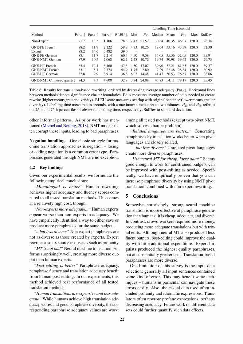
Labelling Time [seconds]

Method ParA ↑ ParF ↑ ParD ↑ BLEU ↓ Min P25 Median Mean P75 Max StdDev

Non-Expert 91.7 13.3 1.106 78.8 7.47 21.52 30.84 40.35 48.07 120.0 28.34

GNE-PE French 88.2 11.9 2.222 59.9 4.73 10.26 18.64 33.16 43.39 120.0 32.30Expert 88.2 14.6 3.482 39.0 – – – – – – –GNE-PE German 88.1 11.7 2.214 60.5 4.50 9.58 15.05 35.36 52.05 120.0 35.91GNE-NMT German 87.9 10.5 2.068 62.2 2.28 10.72 19.74 30.98 39.62 120.0 29.73

GNE-HT French 85.4 12.4 3.160 47.3 4.50 17.07 39.90 52.21 81.65 120.0 39.37GNE-NMT French 83.1 5.1 2.374 54.9 1.75 2.80 7.29 22.48 28.64 120.0 30.92GNE-HT German 82.8 9.9 3.914 36.8 6.02 14.48 41.47 50.53 76.67 120.0 38.66

GNE-NMT Chinese-Japanese 74.3 4.3 4.608 32.8 3.84 24.08 45.83 54.11 79.17 120.0 35.45

Table 6: Results for translation-based rewriting, ordered by decreasing average adequacy (ParA). Horizontal linesbetween methods denote significance cluster boundaries. Edits measures average number of edits needed to createrewrite (higher means greater diversity). BLEU score measures overlap with original sentence (lower means greaterdiversity). Labelling time measured in seconds, with a maximum timeout set to two minutes. P25 and P75 refer tothe 25th and 75th percentiles of observed labelling time, respectively; StdDev to standard deviation.

other informal patterns. As prior work has men-tioned (Michel and Neubig, 2018), NMT models of-ten corrupt these inputs, leading to bad paraphrases.

Negation handling. One classic struggle for ma-chine translation approaches is negation – losingor adding negation is a common error type. Para-phrases generated through NMT are no exception.

4.2 Key findings

Given our experimental results, we formulate thefollowing empirical conclusions:

“Monolingual is better” Human rewritingachieves higher adequacy and fluency scores com-pared to all tested translation methods. This comesat a relatively high cost, though.

“Non-experts more adequate...” Human expertsappear worse than non-experts in adequacy. Wehave empirically identified a way to either save orproduce more paraphrases for the same budget.

“...but less diverse” Non-expert paraphrases arenot as diverse as those created by experts. Expertrewrites also fix source text issues such as profanity.

“MT is not bad” Neural machine translation per-forms surprisingly well, creating more diverse out-put than human experts.

“Post-editing is better” Paraphrase adequacy,paraphrase fluency and translation adequacy benefitfrom human post-editing. In our experiments, thismethod achieved best performance of all testedtranslation methods.

“Human translations are expensive and less ade-quate” While humans achieve high translation ade-quacy scores and good paraphrase diversity, the cor-responding paraphrase adequacy values are worst

among all tested methods (except two-pivot NMT,which solves a harder problem).

“Related languages are better...” Generatingparaphrases by translation works better when pivotlanguages are closely related.

“...but less diverse” Unrelated pivot languagescreate more diverse paraphrases.

“Use neural MT for cheap, large data!” Seemsgood enough to work for constrained budgets, canbe improved with post-editing as needed. Specif-ically, we have empirically proven that you canincrease paraphrase diversity by using NMT pivottranslation, combined with non-expert rewriting.

5 Conclusions

Somewhat surprisingly, strong neural machinetranslation is more effective at paraphrase genera-tion than humans: it is cheap, adequate, and diverse.In contrast, crowd workers required more money,producing more adequate translations but with triv-ial edits. Although neural MT also produced lessfluent outputs, post-editing could improve the qual-ity with little additional expenditure. Expert lin-guists produced the highest quality paraphrases,but at substantially greater cost. Translation-basedparaphrases are more diverse.

One limitation of this survey is the input dataselection: generally all input sentences containedsome kind of error. This may benefit some tech-niques – humans in particular can navigate theseerrors easily. Also, the casual data used often in-cluded profanity and idiomatic expressions. Trans-lators often rewrote profane expressions, perhapsdecreasing adequacy. Future work on different datasets could further quantify such data effects.

22

Method Text

ORIGINAL Rick, It was really great visiting with you the other day.EXPERT Rick, it was really great visiting with you the other day.

NMT CHINESE-JAPANESE Rick, the visit with you a few days ago was great.

PE GERMAN Rick, it was really great visiting with you the other day.

PE FRENCH Rick, It was really fantastic visiting with you the other day.HT FRENCH Rick, it was really good to visit you the other day.

HT GERMAN Rick, it was really great to visit you recently.

NON-EXPERT Rick, it was really great visiting with you the other day.NMT FRENCH Rick, it was really great to visit with you the other day.NMT GERMAN Rick, It was really great to visit with you the other day.

ORIGINAL Yeah exactly, btw how did u manage to update ur nvidia driver ?EXPERT Yes, exactly. How did you update your Nvidia driver?

NMT CHINESE-JAPANESE Yes, exactly. By the way, how were you able to update your NVIDIA drivers?

PE GERMAN Yes, exactly - how did you update your Nvidia driver?

PE FRENCH Yes exactly, by the way how did you manage to update your Nvidia driver ?

HT FRENCH Yeah, exactly, by the way, how did you manage to update your NVIDIA driver?

HT GERMAN Yes exactly, moreover, how did you manage to update your NVIDIA driver?

NON-EXPERT Yes, exactly. By the way, did you manage to update your Nvidia driver?

NMT FRENCH Yes exactly, BTW How did you manage to update your NVIDIA driver?

NMT GERMAN Yes, exactly, btw how did you manage to update your nvidia driver?

ORIGINAL Is it actually more benefitial/safe to do this many exercises a day?EXPERT Is it actually more beneficial and safe to do so many exercises in a day?

NMT CHINESE-JAPANESE Tell me if daily practice is good?

PE GERMAN Is it actually more safe and important to do this many exercises a day?PE FRENCH Is it actually more benefitial/safe to do as many exercises a day?HT FRENCH Is it really more beneficial/safe to do so much exercise per day?

HT GERMAN Is it really more beneficial / safer to do so many exercises per day?

NON-EXPERT Is it actually more beneficial and safe to do this many exercises a day?NMT FRENCH Is it actually more benefitial/safe to do this many exercises per day?

NMT GERMAN Is it actually beneditialat/sure to do these many exercises a day?

ORIGINAL The cold and rain couldn’t effect my enjoyment.EXPERT The cold and rain could not affect my enjoyment.NMT CHINESE-JAPANESE Cold and rain can not detract from my enjoyment.PE GERMAN The cold and rain will not affect my enjoyment.PE FRENCH The cold and rain could not effect my enjoyment.HT FRENCH Cold and rain dont satisfy me.

HT GERMAN The cold and rain couldnt spoil my enjoyment.

NON-EXPERT The cold and the rain couldn’t affect my happiness.

NMT FRENCH The cold and the rain could not affect my pleasure.

NMT GERMAN The cold and rain couldn’t affect my enjoyment.

Table 7: Example paraphrases generated by several monolingual and bilingual methods. Changed regions arehighlighted – insertions are presented in green , and deleted phrases from the original sentence are highlighted in

red and strikethrough . Note how Non-Expert translations tend to be the most conservative, except when clearlyinformal language is rewritten or corrected.

23

Figure 2: Convergence of adequacy scores over time. Despite the lack of an absolute standard of system assessment,a diverse set of judges rapidly converge to a consistent ranking of system quality. Within a 100 to 200 judgements,the rating has basically stabilized, though we continue to assess the whole set for greatest stability and confidencein ranking. We note, however, that readers should take caution in an absolute reading of these ratings – instead, itshould reflect a relative quality assessment among the approaches under consideration.

Figure 3: Convergence of relative fluency scores over time. These assessments reflect the same trends as adequacy– raters rapidly converge on a relative assessment of distinct systems.

24

Acknowledgments

The authors thank the three anonymous reviewersfor their feedback and valuable suggestions, whichwe have addressed in the final version of this paper.

ReferencesColin Bannard and Chris Callison-Burch. 2005. Para-

phrasing with Bilingual Parallel Corpora. In Pro-ceedings of the 43rd Annual Meeting of the As-sociation for Computational Linguistics (ACL’05),pages 597–604, Ann Arbor, Michigan. Associationfor Computational Linguistics.

Regina Barzilay and Kathleen R. McKeown. 2001. Ex-tracting Paraphrases from a Parallel Corpus. InProceedings of 39th Annual Meeting of the Associ-ation for Computational Linguistics, pages 50–57,Toulouse, France. Association for ComputationalLinguistics.

Steven Bird, Ewan Klein, and Edward Loper.2009. Natural Language Processing with Python.O’Reilly Media.

Ondrej Bojar, Rajen Chatterjee, Christian Federmann,Yvette Graham, Barry Haddow, Matthias Huck,Antonio Jimeno Yepes, Philipp Koehn, VarvaraLogacheva, Christof Monz, Matteo Negri, Aure-lie Neveol, Mariana Neves, Martin Popel, MattPost, Raphael Rubino, Carolina Scarton, Lucia Spe-cia, Marco Turchi, Karin Verspoor, and MarcosZampieri. 2016. Findings of the 2016 Conferenceon Machine Translation. In Proceedings of theFirst Conference on Machine Translation, pages131–198, Berlin, Germany. Association for Compu-tational Linguistics.

Ondrej Bojar, Christian Federmann, Mark Fishel,Yvette Graham, Barry Haddow, Matthias Huck,Philipp Koehn, and Christof Monz. 2018. Find-ings of the 2018 Conference on Machine Transla-tion (WMT18). In Proceedings of the Third Con-ference on Machine Translation, Volume 2: SharedTask Papers, pages 272–307, Belgium, Brussels. As-sociation for Computational Linguistics.

Sheila Castilho, Joss Moorkens, Federico Gaspari,Iacer Calixto, John Tinsley, and Andy Way. 2017.Is Neural Machine Translation the New State of theArt? The Prague Bulletin of Mathematical Linguis-tics, 108:109–120.

Mauro Cettolo, Marcello Federico, Luisa Bentivogli,Jan Niehues, Sebastian Stuker, Katsuhito Sudoh,Koichiro Yoshino, and Christian Federmann. 2017.Overview of the IWSLT 2017 Evaluation Campaign.In International Workshop on Spoken LanguageTranslation, pages 2–14, Tokyo, Japan.

David Chen and William Dolan. 2011. CollectingHighly Parallel Data for Paraphrase Evaluation. In

Proceedings of the 49th Annual Meeting of the Asso-ciation for Computational Linguistics: Human Lan-guage Technologies, pages 190–200. Association forComputational Linguistics.

Bill Dolan, Chris Quirk, and Chris Brockett. 2004. Un-supervised Construction of Large Paraphrase Cor-pora: Exploiting Massively Parallel News Sources.In Proceedings of the 20th International Confer-ence on Computational Linguistics, COLING ’04,Stroudsburg, PA, USA. Association for Computa-tional Linguistics.

Christian Federmann. 2018. Appraise EvaluationFramework for Machine Translation. In Proceed-ings of the 27th International Conference on Compu-tational Linguistics: System Demonstrations, pages86–88, Santa Fe, New Mexico. Association for Com-putational Linguistics.

Juri Ganitkevitch, Benjamin Van Durme, and ChrisCallison-Burch. 2013. PPDB: The ParaphraseDatabase. In Proceedings of the 2013 Conference ofthe North American Chapter of the Association forComputational Linguistics: Human Language Tech-nologies, pages 758–764, Atlanta, Georgia. Associa-tion for Computational Linguistics.

Yvette Graham, Timothy Baldwin, Alistair Moffat,and Justin Zobel. 2013. Continuous MeasurementScales in Human Evaluation of Machine Transla-tion. In Proceedings of the 7th Linguistic Annota-tion Workshop and Interoperability with Discourse,pages 33–41. Association for Computational Lin-guistics.

Yvette Graham, Timothy Baldwin, Alistair Moffat, andJustin Zobel. 2014. Is Machine Translation GettingBetter over Time? In Proceedings of the 14th Con-ference of the European Chapter of the Associationfor Computational Linguistics, pages 443–451. As-sociation for Computational Linguistics.

J. Edward Hu, Rachel Rudinger, Matt Post, and Ben-jamin Van Durme. 2019. ParaBank: Monolingualbitext generation and sentential paraphrasing vialexically-constrained neural machine translation. InProceedings of AAAI.

Youxuan Jiang, Jonathan K. Kummerfeld, and Walter S.Lasecki. 2017. Understanding Task Design Trade-offs in Crowdsourced Paraphrase Collection. In Pro-ceedings of the 55th Annual Meeting of the Associa-tion for Computational Linguistics (Volume 2: ShortPapers), pages 103–109, Vancouver, Canada. Asso-ciation for Computational Linguistics.

Wuwei Lan, Siyu Qiu, Hua He, and Wei Xu. 2017. AContinuously Growing Dataset of Sentential Para-phrases. In Proceedings of The 2017 Conference onEmpirical Methods on Natural Language Process-ing (EMNLP), pages 1224–1234, Copenhagen, Den-mark. Association for Computational Linguistics.

25

Samuel Laubli, Rico Sennrich, and Martin Volk. 2018.Has Machine Translation Achieved Human Parity?A Case for Document-level Evaluation. In Proceed-ings of the 2018 Conference on Empirical Methodsin Natural Language Processing, pages 4791–4796.Association for Computational Linguistics.

Jonathan Mallinson, Rico Sennrich, and Mirella Lap-ata. 2017. Paraphrasing Revisited with Neural Ma-chine Translation. In Proceedings of the 15th Con-ference of the European Chapter of the Associationfor Computational Linguistics: Volume 1, Long Pa-pers, pages 881–893, Valencia, Spain. Associationfor Computational Linguistics.

Paul Michel and Graham Neubig. 2018. MTNT: ATestbed for Machine Translation of Noisy Text. InProceedings of the 2018 Conference on EmpiricalMethods in Natural Language Processing, pages543–553, Brussels, Belgium. Association for Com-putational Linguistics.

Kishore Papineni, Salim Roukos, Todd Ward, and Wei-Jing Zhu. 2002. Bleu: a Method for Automatic Eval-uation of Machine Translation. In Proceedings ofthe 40th Annual Meeting of the Association for Com-putational Linguistics, pages 311–318, Philadelphia,Pennsylvania, USA. Association for ComputationalLinguistics.

Ellie Pavlick, Pushpendre Rastogi, Juri Ganitkevich,Benjamin Van Durme, and Chris Callison-Burch.2015. PPDB 2.0: Better Paraphrase Ranking, fine-grained Entailment Relations, Word Embeddings,and Style Classification. In Proceedings of the53rd Annual Meeting of the Association for Compu-tational Linguistics and the 7th International JointConference on Natural Language Processing (Vol-ume 2: Short Papers), pages 425–430, Beijing,China. Association for Computational Linguistics.

Aaditya Prakash, Sadid A. Hasan, Kathy Lee, VivekDatla, Ashequl Qadir, Joey Liu, and Oladimeji Farri.2016. Neural Paraphrase Generation with StackedResidual LSTM Networks. In Proceedings of COL-ING 2016, the 26th International Conference onComputational Linguistics: Technical Papers, pages2923–2934, Osaka, Japan. The COLING 2016 Orga-nizing Committee.

Su Wang, Rahul Gupta, Nancy Chang, and JasonBaldridge. 2018. A task in a suit and a tie:paraphrase generation with semantic augmentation.CoRR, abs/1811.00119.

John Wieting and Kevin Gimpel. 2018. ParaNMT-50M: Pushing the Limits of Paraphrastic SentenceEmbeddings with Millions of Machine Translations.In Proceedings of the 56th Annual Meeting of the As-sociation for Computational Linguistics (Volume 1:Long Papers), pages 451–462. Association for Com-putational Linguistics.

26


Personalizing Grammatical Error Correction:Adaptation to Proficiency Level and L1

Maria NadejdeGrammarly

[email protected]

Joel Tetreault∗Dataminr

[email protected]

AbstractGrammar error correction (GEC) systems havebecome ubiquitous in a variety of softwareapplications, and have started to approachhuman-level performance for some datasets.However, very little is known about how toefficiently personalize these systems to theuser’s characteristics, such as their proficiencylevel and first language, or to emerging do-mains of text. We present the first results onadapting a general purpose neural GEC systemto both the proficiency level and the first lan-guage of a writer, using only a few thousandannotated sentences. Our study is the broad-est of its kind, covering five proficiency levelsand twelve different languages, and compar-ing three different adaptation scenarios: adapt-ing to the proficiency level only, to the firstlanguage only, or to both aspects simultane-ously. We show that tailoring to both scenariosachieves the largest performance improvement(3.6 F0.5) relative to a strong baseline.

1 Introduction

Guides for English teachers have extensively doc-umented how grammatical errors made by learn-ers are influenced by their native language (L1).Swan and Smith (2001) attribute some of the er-rors to “transfer” or “interference” between lan-guages. For example, German native speakers aremore likely to incorrectly use a definite article withgeneral purpose nouns or omit the indefinite articlewhen defining people’s professions. Other errorsare attributed to the absence of a certain linguisticfeature in the native language. For example, Chi-nese and Russian speakers make more errors in-volving articles, since these languages do not havearticles.

A few grammatical error correction (GEC) sys-tems have incorporated knowledge about L1. Ro-

∗This research was conducted while the author was atGrammarly.

zovskaya and Roth (2011) use a different prior foreach of five L1s to adapt a Naive Bayes classi-fier for preposition correction. Rozovskaya et al.(2017) expand on this work to eleven L1s andthree error types. Mizumoto et al. (2011) showedfor the first time that a statistical machine transla-tion (SMT) system applied to GEC performs bet-ter when the training and test data have the sameL1. Chollampatt et al. (2016) extend this work byadapting a neural language model to three differ-ent L1s and use it as a feature in SMT-based GECsystem. However, we are not aware of prior workaddressing the impact of both proficiency level andnative language on the performance of GEC sys-tems. Furthermore, neural GEC systems, whichhave become state-of-the-art (Gehring et al., 2017;Junczys-Dowmunt et al., 2018; Grundkiewicz andJunczys-Dowmunt, 2018), are general purposeand domain agnostic.

We believe the future of GEC lies in providingusers with feedback that is personalized to theirproficiency level and native language (L1). In thiswork, we present the first results on adapting ageneral purpose neural GEC system for English toboth of these characteristics by using fine-tuning,a transfer learning method for neural networks,which has been extensively explored for domainadaptation of machine translation systems (Lu-ong and Manning, 2015; Freitag and Al-Onaizan,2016; Chu et al., 2017; Miceli Barone et al., 2017;Thompson et al., 2018). We show that a modeladapted to both L1 and proficiency level outper-forms models adapted to only one of these charac-teristics. Our contributions also include the firstresults on adapting GEC systems to proficiencylevels and the broadest study of adapting GEC toL1 which includes twelve different languages.

27

0 500 1000 1500 2000 2500 3000

C2

C1

A2

B2

B1

0 250 500 750 1000 1250 1500Japanese

UrduThai

KoreanCzech

CatalanGreek

TurkishArabicPolish

RussianFrench

SwissGermanGerman

PortugueseItalian

ChineseSpanish

0 200 400 600 800Korean-B2Polish-B2

Chinese-A2Russian-B2French-B1

Spanish-C1French-B2

German-B2Italian-A2

Chinese-C1German-B1

Portuguese-A2SwissGerman-B1

Chinese-B1Spanish-B2

Portuguese-B1Chinese-B2

Italian-B1Spanish-A2Spanish-B1

Figure 1: Corpus Distributions for CEFR Level, L1 and L1-Level.

2 Personalizing GEC

Data In this work, we adapt a general purposeneural GEC system, initially trained on two mil-lion sentences written by both native and non-native speakers and covering a variety of topicsand styles. All the sentences have been correctedfor grammatical errors by professional editors.1

Adaptation of the model to proficiency leveland L1 requires a corpus annotated with thesefeatures. We use the Cambridge Learner Corpus(CLC) (Nicholls, 2003) comprising examinationessays written by English learners with six profi-ciency levels2 and more than 100 different nativelanguages. Each essay is corrected by one anno-tator, who also identifies the minimal error spansand labels them using about 80 error types. Fromthis annotated corpus we extract a parallel corpuscomprising of source sentences with grammaticalerrors and the corresponding corrected target sen-tences.

We do note the proprietary nature of the CLCwhich makes reproducibility difficult, though ithas been used in prior research, such as Rei andYannakoudakis (2016). It was necessary for thisstudy as the other GEC corpora available are notannotated for both L1 and level. The Lang-8 Learner Corpora (Mizumoto et al., 2011) alsoprovides information about L1, but it has no in-formation about proficiency levels. The FCEdataset (Yannakoudakis et al., 2011) is a subsetof the CLC, however, it only covers one profi-ciency level and there are not enough sentencesfor each L1 for our experiments. Previous workon adapting GEC classifiers to L1 (Rozovskayaet al., 2017) used the FCE corpus, and thus did not

1To maintain anonymity, we do not include more details.2The CLC uses levels defined by the Common European

Framework of Reference for Languages: A1 - Beginner, A2 -Elementary, B1 - Intermediate, B2 - Upper intermediate, C1- Advanced, C2 - Proficiency.

address adaptation to different proficiency levels.One of our future goals is to create a public corpusfor this type of work.

Experimental Setup Our baseline neural GECsystem is an RNN-based encoder-decoder neu-ral network with attention and LSTM units (Bah-danau et al., 2015). The system takes as inputan English sentence which may contain gram-matical errors and decodes the corrected sen-tence. We train the system on the parallel cor-pus extracted from the CLC with the OpenNMT-py toolkit (Klein et al., 2018) using the hyper-parameters listed in the Appendix. To increase thecoverage of the neural network’s vocabulary, with-out hurting efficiency, we break source and targetwords into sub-word units. The segmentation intosub-word units is learned from unlabeled data us-ing the Byte Pair Encoding (BPE) algorithm (Sen-nrich et al., 2016). The vocabulary, consisting of20,000 BPE sub-units, is shared between the en-coder and decoder.3 We truncate sentences longerthan 60 BPE sub-units and train the baseline sys-tem with early stopping on a development set sam-pled from the base dataset.4

To train and evaluate the adapted models, weextract subsets of sentences from the CLC thathave been written by learners having a particularLevel, L1, or L1-Level combination. We considerall subsets having at least 11,000 sentences, suchthat we can allocate 8,000 sentences for training,1,000 for tuning and 2,000 for testing. We com-pare adapted models trained and evaluated on thesame subset of the data. For example, we adapta model using the Chinese training data and thenevaluate it on the Chinese test set.

Since our base dataset and CLC are differentdomains, we wanted to make sure that improve-

3Although the source and target vocabularies are thesame, the embeddings are not tied.

4Performance did not improve after 15 epochs.

28

ments by fine-tuning by Level or L1 were notdue to simply being in-domain with the test data,which is also from the CLC. To control for this, weconstruct another baseline system (“Random”) byadapting the general purpose GEC system to a ran-dom sample of learner data drawn from the CLC.In Figure 1 we show the distribution of Level, L1and L1-Level sentences in a random CLC sam-ple, for the subsets having at least 100 sentences.B1 is the most frequent level, while A2, the low-est proficiency level included in this study, is halfas frequent in the random sample. The L1 dis-tribution is dominated by Spanish, with Chinesesecond with half as many sentences. Among theL1-Level subsets, Spanish-B2 is the most frequentwith Spanish-A2 covering half as many sentences.

Fine-tuning We build adapted GEC models us-ing fine-tuning, a transfer learning method for neu-ral networks. We continue training the parametersof the general purpose model on the “in-domain”subset of the data covering a particular Level, L1,or L1-Level. Thompson et al. (2018) showed thatadapting only a single component of the encoder-decoder network is almost as effective as adaptingthe entire set of parameters. In this work, we fine-tune the parameters of the source embeddings andencoder, while keeping the other parameters fixed.

To avoid quickly over-fitting to the smaller“in-domain” training data, we reduce the batchsize (Thompson et al., 2018) and continue us-ing the dropout regularization (Miceli Baroneet al., 2017). We apply dropout to all the lay-ers and to the source words, as well as varia-tional dropout (Gal and Ghahramani, 2016) oneach step, all with probability 0.1. We also re-duce the learning rate by four times and use thestart decay at option which halves the learn-ing rate after each epoch. Consequently, the up-dates become small after a few epochs. To en-able the comparison between different adaptationscenarios, all fine-tuned models are trained for 10epochs on 8,000 sentences of “in-domain” data.

3 Results

We report the results for the three adaptation sce-narios: adapting to Level only, adapting to L1only, and adapting to both L1 and Level. We sum-marize the results by showing the average M2 F0.5

score (Dahlmeier and Ng, 2012) across all the testsets included in the respective scenario.

We first note that the strong baseline (“Ran-dom”), which is a model adapted to a random sam-ple of CLC , achieves improvements between 11 to13 F0.5 points on average on all scenarios. Whilenot the focus of the paper, this large improvementshows the performance gains by simply adaptingto a new domain (in this case CLC data). Second,we note that the models adapted only by Level orby L1 are on average better than the “Random”model by 2.1 and 2.3 F0.5 points respectively. Fi-nally, the models adapted to both Level and L1outperform all others, beating the “Random” base-line on average by 3.6 F0.5 points.

On all adaptation scenarios we report the per-formance of the single best model released byJunczys-Dowmunt et al. (2018). Their model,which we call JD single, was trained on Englishlearner data of comparable size to our base datasetand optimized using the CoNLL14 training andtest data.

Adaptation by Proficiency Level We adaptGEC models to five of the CEFR proficiency lev-els: A2, B1, B2, C1, C2. The results in Ta-ble 1 show that performance improves for all lev-els compared to the “Random” baseline. Thelargest improvement, 5.2 F0.5 points, is achievedfor A2, the lowest proficiency level. We attributethe large improvement to this level having a highererror rate, a lower lexical diversity and being lessrepresented in the random sample on which thebaseline is trained on. In contrast, for the B1 andB2 levels, the most frequent in the random sample,improvements are more modest: 0.7 and 0.2 F0.5

points respectively. Our adapted models are betterthan the JD single model on all levels, and with alarge margin on the A2 and C1 levels.

Adapt A2 B1 B2 C1 C2 Avg.No 30.4 34.9 33.1 32.5 33.0 32.8Rand. 48.4 47.9 42.5 41.4 39.2 43.8Level 53.6 48.6 42.7 43.3 41.1 45.9

JD single 44.1 47.1 41.7 37.8 35.0 44.1

Table 1: Adaptation to Proficiency Level in F0.5

Adaptation by L1 We adapt GEC models totwelve L1s: Arabic, Chinese, French, German,Greek, Italian, Polish, Portuguese, Russian, Span-ish, Swiss-German and Turkish. The results inTable 2 (top) show that all L1-adapted modelsare better than the baseline, with improvementsranging from 1.2 F0.5 for Chinese and French, up

29

Adapt AR CN FR DE GR IT PL PT RU ES CH TR AvgNo 37.5 36.2 32.7 31.4 32.7 29.3 36.0 31.7 35.8 32.1 31.1 35.4 33.5Random 46.3 45.0 44.9 44.7 46.4 44.9 46.2 45.2 45.3 47.6 44.2 47.0 45.6L1 48.3 46.2 46.1 47.1 49.0 46.8 48.4 47.6 47.8 49.8 47.1 50.6 47.9

JD single 47.0 44.7 44.2 41.4 44.1 40.7 46.0 44.6 43.7 44.8 40.7 47.5 44.1

Adapt CN-B2 CN-C1 FR-B1 DE-B1 IT-B1 PT-B1 ES-A2 ES-B1 ES-B2 Avg.No 36.1 32.5 31.8 31.2 28.1 31.4 28.9 31.9 33.7 31.8Random 42.7 39.1 45.3 46.1 43.5 45.2 50.2 46.4 44.1 44.7Level 43.4 41.0 46.5 46.9 45.3 46.1 56.6 47.5 43.7 46.3L1 44.1 40.9 46.5 48.1 46.5 46.2 53.8 47.6 44.4 46.5L1 & Level 45.5 43.1 48.1 50.2 47.3 47.9 58.2 48.8 45.6 48.3

JD single 43.0 35.8 46.9 43.8 41.6 46.7 43.4 45.0 41.0 43.0

Table 2: Top: Adaptation to L1 Only. Bottom: Adaptation to Level and L1. Eval metric: F0.5

to 3.6 F0.5 for Turkish. For the languages thatare less frequent in the random sample of CLC(Greek, Turkish, Arabic, Polish and Russian) wesee consistent improvements of over 2 F0.5 points.Our adapted models are better than the JD singlemodel on all L1s, and with a margin larger than5 F0.5 points on German, Swiss-German, Italian,Greek and Spanish.

Adaptation by L1 and Proficiency Level Fi-nally, we adapt GEC models to the followingnine L1 – Level subsets: Chinese-B2, Chinese-C1,French-B1, German-B1, Italian-B1, Portuguese-B1, Spanish-A2, Spanish-B1 and Spanish-B2. Weinclude these subsets in our study because theymeet the requirement of having at least 8,000 sen-tences for training. All the models adapted to bothLevel and L1 outperform the models adapted toonly one of these features, as shown in Table 2(bottom). Focusing on the two levels for Chinesenative speakers, we see the model adapted to C1achieves a larger improvement over the baseline,4.1 F0.5 points, compared to 2.7 F0.5 points for theB2 level. Again, this is explained by the lower fre-quency of the C1 level in the random sample ofCLC, which is also reflected by the lowest F0.5

score for the baseline model. Similarly, amongthe models adapted to different levels of Spanishnative speakers, the one adapted to Spanish-A2achieves the largest gains of 8 F0.5 points. TheSpanish-A2 testset has the highest number of er-rors per 100 words among all the L1-Level test-sets, as shown in Table 1 in the Appendix. Fur-thermore, the A2 level is only half as frequent asthe B1 level in the random sample of CLC. Finally,our adapted models are better than the JD singlemodel on all L1–Level subsets, with a margin of 5

F0.5 points on average.

Adapted P R F0.5Random 61.9 35.6 54.0CN-C1 61.1 37.0 54.1CN-B2 62.4 37.5 55.1+ spellcheck 63.6 40.3 57.0

JD single 59.1 40.4 54.1JD ensemble 63.1 42.6 57.5

Table 3: Results on the CoNLL14 testsets for Chinesemodels.

CoNLL14 Evaluation We compare our adaptedmodels on the CoNLL14 testset (Ng et al., 2014)in Table 3. The model adapted to Chinese-B2improves the most over the baseline, achieving55.1 F0.5. This result aligns with how the testset was constructed: it consists of essays writ-ten by university students, mostly Chinese na-tive speakers. When we pre-process the eval-uation set before decoding with a commercialspellchecker5, our adapted model scores 57.0which places it near other leading models, trainedon a similar amount of data, such as Chollam-patt and Ng (2018) (56.52) and Junczys-Dowmuntet al. (2018)6 (57.53) even though we do not usethe CoNLL14 in-domain training data. We notethat the most recent state-of-the-art models (Zhaoet al., 2019; Grundkiewicz et al., 2019), are trainedon up to one hundred million additional syntheticparallel sentences, while we adapt models withonly eight thousand parallel sentences.

5Details removed for anonymity.6We call their ensemble of four models with language

model re-scoring JD ensemble and their single best modelwithout language model re-scoring JD single

30

Adapt Det Prep Verb Tense NNum Noun PronCN-C1 3.53 5.90 2.99 1.77 8.28 8.02 22.78FR-B1 2.34 1.99 12.54 5.16 9.16 3.48 1.13DE-B1 8.85 1.77 2.04 2.37 3.86 7.18 22.75IT-B1 2.37 5.32 12.48 6.74 4.40 3.29 8.99ES-A2 6.06 12.52 7.51 8.54 8.73 12.39 10.57

Table 4: L1-Level breakdown by error type in relative improvements in F0.5 over the “Random” baseline.

Error-type Analysis We conclude our study byreporting improvements on the most frequent errortypes, excluding punctuation, spelling and orthog-raphy errors. We identify the error types in eachevaluation set with Errant, a rule-based classi-fier (Bryant et al., 2017). Table 4 shows the resultsfor the systems adapted to both L1 and Level thatimproved the most in overall F0.5. The adaptedsystems consistently outperform the “Random”baseline on most error types. For Chinese-C1, theadapted model achieves the largest gains on pro-noun (Pron) and noun number agreement errors(NNum). The Spanish-A2 adapted model achievesnotable gains on preposition (Prep), noun and pro-noun errors. Both the French-B1 and Italian-B1adapted models gain the most on verb errors. ForGerman-B1, the adapted model improves the moston pronoun (Pron) and determiner (Det) errors.The large improvement of 22.75 F0.5 points forthe pronoun category is in part an artefact of thesmall error counts. The adapted model corrects35 pronouns (P=67.3) while the baseline correctsonly 15 pronouns (P=46.9). We leave an in depthanalysis by error type to future work.

Below, we give an example of a confused aux-iliary verb that the French-B1 adapted model cor-rects. The verb phrase corresponding to “go shop-ping” in French is “faire des achats”, where theverb “faire” would translate to “make/do”.

Orig He told me that celebrity can be badbecause he can’t do shopping nor-mally.

Rand He told me that the celebrity can bebad because he can’t do shoppingnormally.

FR-B1 He told me that celebrity can be badbecause he can’t go shopping nor-mally.

Ref He told me that celebrity can be badbecause he can’t go shopping nor-mally.

4 Conclusions

We present the first results on adapting a neuralGEC system to proficiency level and L1 of lan-guage learners. This is the broadest study of itskind, covering five proficiency levels and twelvedifferent languages. While models adapted to ei-ther proficiency level or L1 are on average betterthan the baseline by over 2 F0.5 points and thelargest improvement (3.6 F0.5) is achieved whenadapting to both characteristics simultaneously.

We envision building a single model that com-bines knowledge across L1s and proficiency lev-els using a mixture-of-experts approach. Adaptedmodels could also be improved by using the mixedfine tuning approach which uses a mix of in-domain and out-of-domain data (Chu et al., 2017).

Acknowledgements

The authors would like to thank the anonymousreviewers for their feedback. We are also gratefulto our colleagues for their assistance and insights:Dimitrios Alikaniotis, Claudia Leacock, DmitryLider, Courtney Napoles, Jimmy Nguyen, VipulRaheja and Igor Tytyk.

ReferencesDzmitry Bahdanau, Kyunghyun Cho, and Yoshua Ben-

gio. 2015. Neural machine translation by jointlylearning to align and translate. In Proceedings ofthe International Conference on Learning Represen-tations (ICLR).

Christopher Bryant, Mariano Felice, and Ted Briscoe.2017. Automatic annotation and evaluation of errortypes for grammatical error correction. In Proceed-ings of the 55th Annual Meeting of the Associationfor Computational Linguistics (Volume 1: Long Pa-pers), pages 793–805, Vancouver, Canada. Associa-tion for Computational Linguistics.

Shamil Chollampatt, Duc Tam Hoang, and Hwee TouNg. 2016. Adapting grammatical error correctionbased on the native language of writers with neu-ral network joint models. In Proceedings of the

31

2016 Conference on Empirical Methods in NaturalLanguage Processing, pages 1901–1911. Associa-tion for Computational Linguistics.

Shamil Chollampatt and Hwee Tou Ng. 2018. Neu-ral quality estimation of grammatical error correc-tion. In Proceedings of the 2018 Conference onEmpirical Methods in Natural Language Process-ing, pages 2528–2539, Brussels, Belgium. Associ-ation for Computational Linguistics.

Chenhui Chu, Raj Dabre, and Sadao Kurohashi. 2017.An empirical comparison of domain adaptationmethods for neural machine translation. In Pro-ceedings of the 55th Annual Meeting of the Associa-tion for Computational Linguistics (Volume 2: ShortPapers), pages 385–391. Association for Computa-tional Linguistics.

Daniel Dahlmeier and Hwee Tou Ng. 2012. Betterevaluation for grammatical error correction. In Pro-ceedings of the 2012 Conference of the North Amer-ican Chapter of the Association for ComputationalLinguistics: Human Language Technologies, pages568–572, Montreal, Canada. Association for Com-putational Linguistics.

Markus Freitag and Yaser Al-Onaizan. 2016. Fastdomain adaptation for neural machine translation.CoRR, abs/1612.06897.

Yarin Gal and Zoubin Ghahramani. 2016. A theoret-ically grounded application of dropout in recurrentneural networks. In Proceedings of the 30th Interna-tional Conference on Neural Information ProcessingSystems, NIPS’16, pages 1027–1035, USA. CurranAssociates Inc.

Jonas Gehring, Michael Auli, David Grangier, DenisYarats, and Yann N. Dauphin. 2017. Convolutionalsequence to sequence learning. In Proceedingsof the 34th International Conference on MachineLearning, volume 70 of Proceedings of MachineLearning Research, pages 1243–1252, InternationalConvention Centre, Sydney, Australia. PMLR.

Roman Grundkiewicz and Marcin Junczys-Dowmunt.2018. Near human-level performance in grammati-cal error correction with hybrid machine translation.In Proceedings of the 2018 Conference of the NorthAmerican Chapter of the Association for Computa-tional Linguistics: Human Language Technologies,Volume 2 (Short Papers), pages 284–290. Associa-tion for Computational Linguistics.

Roman Grundkiewicz, Marcin Junczys-Dowmunt, andKenneth Heafield. 2019. Neural grammatical errorcorrection systems with unsupervised pre-trainingon synthetic data. In Proceedings of the FourteenthWorkshop on Innovative Use of NLP for BuildingEducational Applications, pages 252–263, Florence,Italy. Association for Computational Linguistics.

Marcin Junczys-Dowmunt, Roman Grundkiewicz,Shubha Guha, and Kenneth Heafield. 2018. Ap-proaching neural grammatical error correction as a

low-resource machine translation task. In Proceed-ings of the 2018 Conference of the North AmericanChapter of the Association for Computational Lin-guistics: Human Language Technologies, Volume1 (Long Papers), pages 595–606. Association forComputational Linguistics.

Guillaume Klein, Yoon Kim, Yuntian Deng, VincentNguyen, Jean Senellart, and Alexander Rush. 2018.Opennmt: Neural machine translation toolkit. InProceedings of the 13th Conference of the Associ-ation for Machine Translation in the Americas (Vol-ume 1: Research Papers), pages 177–184. Associa-tion for Machine Translation in the Americas.

Minh-Thang Luong and Christopher D. Manning.2015. Stanford neural machine translation systemsfor spoken language domain. In International Work-shop on Spoken Language Translation.

Antonio Valerio Miceli Barone, Barry Haddow, UlrichGermann, and Rico Sennrich. 2017. Regularizationtechniques for fine-tuning in neural machine trans-lation. In Proceedings of the 2017 Conference onEmpirical Methods in Natural Language Process-ing, pages 1489–1494. Association for Computa-tional Linguistics.

Tomoya Mizumoto, Mamoru Komachi, Masaaki Na-gata, and Yuji Matsumoto. 2011. Mining revisionlog of language learning sns for automated japaneseerror correction of second language learners. InProceedings of 5th International Joint Conferenceon Natural Language Processing, pages 147–155.Asian Federation of Natural Language Processing.

Hwee Tou Ng, Siew Mei Wu, Ted Briscoe, ChristianHadiwinoto, Raymond Hendy Susanto, and Christo-pher Bryant. 2014. The CoNLL-2014 shared taskon grammatical error correction. In Proceedings ofthe Eighteenth Conference on Computational Nat-ural Language Learning: Shared Task, pages 1–14, Baltimore, Maryland. Association for Compu-tational Linguistics.

Diane Nicholls. 2003. The Cambridge Learner Cor-pus: Error coding and analysis for lexicography andELT. In Proceedings of the Corpus Linguistics 2003conference, volume 16, pages 572–581.

Marek Rei and Helen Yannakoudakis. 2016. Composi-tional sequence labeling models for error detectionin learner writing. In Proceedings of the 54th An-nual Meeting of the Association for ComputationalLinguistics (Volume 1: Long Papers), pages 1181–1191, Berlin, Germany. Association for Computa-tional Linguistics.

Alla Rozovskaya and Dan Roth. 2011. Algorithm se-lection and model adaptation for esl correction tasks.In Proceedings of the 49th Annual Meeting of theAssociation for Computational Linguistics: HumanLanguage Technologies - Volume 1, HLT ’11, pages924–933, Stroudsburg, PA, USA. Association forComputational Linguistics.

32

Alla Rozovskaya, Dan Roth, and Mark Sammons.2017. Adapting to learner errors with minimal su-pervision. Computational Linguistics, 43(4):723–760.

Rico Sennrich, Barry Haddow, and Alexandra Birch.2016. Neural machine translation of rare words withsubword units. In Proceedings of the 54th AnnualMeeting of the Association for Computational Lin-guistics (Volume 1: Long Papers), Berlin, Germany.Association for Computational Linguistics.

Michael Swan and Bernard Smith. 2001. Learner En-glish: A Teacher’s Guide to Interference and otherProblems. Second Edition. Cambridge UniversityPress.

Brian Thompson, Huda Khayrallah, Antonios Anasta-sopoulos, Arya D. McCarthy, Kevin Duh, RebeccaMarvin, Paul McNamee, Jeremy Gwinnup, Tim An-derson, and Philipp Koehn. 2018. Freezing sub-networks to analyze domain adaptation in neuralmachine translation. In Proceedings of the ThirdConference on Machine Translation, Volume 1: Re-search Papers, pages 124–132, Belgium, Brussels.Association for Computational Linguistics.

Helen Yannakoudakis, Ted Briscoe, and Ben Medlock.2011. A new dataset and method for automaticallygrading ESOL texts. In Proceedings of the 49th An-nual Meeting of the Association for ComputationalLinguistics: Human Language Technologies, pages180–189, Portland, Oregon, USA. Association forComputational Linguistics.

Wei Zhao, Liang Wang, Kewei Shen, Jia Ruoyu, andJingming Liu. 2019. Better evaluation for gram-matical error correctionimproving grammatical er-ror correction via pre-training a copy-augmented ar-chitecture with unlabeled data. In Proceedings ofthe 2019 Conference of the North American Chap-ter of the Association for Computational Linguistics:Human Language Technologies, Minneapolis, MN,USA. Association for Computational Linguistics.

33


Exploiting BERT for End-to-End Aspect-based Sentiment Analysis∗

Xin Li1, Lidong Bing2, Wenxuan Zhang1 and Wai Lam1

1Department of Systems Engineering and Engineering ManagementThe Chinese University of Hong Kong, Hong Kong

2R&D Center Singapore, Machine Intelligence Technology, Alibaba DAMO Academy{lixin,wxzhang,wlam}@se.cuhk.edu.hk

[email protected]

Abstract

In this paper, we investigate the modelingpower of contextualized embeddings from pre-trained language models, e.g. BERT, on theE2E-ABSA task. Specifically, we build aseries of simple yet insightful neural base-lines to deal with E2E-ABSA. The experimen-tal results show that even with a simple lin-ear classification layer, our BERT-based archi-tecture can outperform state-of-the-art works.Besides, we also standardize the comparativestudy by consistently utilizing a hold-out de-velopment dataset for model selection, whichis largely ignored by previous works. There-fore, our work can serve as a BERT-basedbenchmark for E2E-ABSA.1

1 Introduction

Aspect-based sentiment analysis (ABSA) is to dis-cover the users’ sentiment or opinion towards anaspect, usually in the form of explicitly men-tioned aspect terms (Mitchell et al., 2013; Zhanget al., 2015) or implicit aspect categories (Wanget al., 2016), from user-generated natural languagetexts (Liu, 2012). The most popular ABSA bench-mark datasets are from SemEval ABSA chal-lenges (Pontiki et al., 2014, 2015, 2016) where afew thousand review sentences with gold standardaspect sentiment annotations are provided.

Table 1 summarizes three existing researchproblems related to ABSA. The first one is theoriginal ABSA, aiming at predicting the senti-ment polarity of the sentence towards the givenaspect. Compared to this classification problem,the second one and the third one, namely, Aspect-oriented Opinion Words Extraction (AOWE) (Fan

∗The work described in this paper is substantially sup-ported by a grant from the Research Grant Council of theHong Kong Special Administrative Region, China (ProjectCode: 14204418).

1Our code is open-source and available at: https://github.com/lixin4ever/BERT-E2E-ABSA

et al., 2019) and End-to-End Aspect-based Sen-timent Analysis (E2E-ABSA) (Ma et al., 2018a;Schmitt et al., 2018; Li et al., 2019a; Li and Lu,2017, 2019), are related to a sequence taggingproblem. Precisely, the goal of AOWE is to ex-tract the aspect-specific opinion words from thesentence given the aspect. The goal of E2E-ABSAis to jointly detect aspect terms/categories and thecorresponding aspect sentiments.

Many neural models composed of a task-agnostic pre-trained word embedding layer andtask-specific neural architecture have been pro-posed for the original ABSA task (i.e. the aspect-level sentiment classification) (Tang et al., 2016;Wang et al., 2016; Chen et al., 2017; Liu andZhang, 2017; Ma et al., 2017, 2018b; Majumderet al., 2018; Li et al., 2018; He et al., 2018;Xue and Li, 2018; Wang et al., 2018; Fan et al.,2018; Huang and Carley, 2018; Lei et al., 2019;Li et al., 2019b)2, but the improvement of thesemodels measured by the accuracy or F1 scorehas reached a bottleneck. One reason is that thetask-agnostic embedding layer, usually a linearlayer initialized with Word2Vec (Mikolov et al.,2013) or GloVe (Pennington et al., 2014), onlyprovides context-independent word-level features,which is insufficient for capturing the complex se-mantic dependencies in the sentence. Meanwhile,the size of existing datasets is too small to trainsophisticated task-specific architectures. Thus,introducing a context-aware word embedding3

layer pre-trained on large-scale datasets with deepLSTM (McCann et al., 2017; Peters et al., 2018;Howard and Ruder, 2018) or Transformer (Rad-ford et al., 2018, 2019; Devlin et al., 2019; Lample

2Due to the limited space, we can not list all of the existingworks here, please refer to the survey (Zhou et al., 2019) formore related papers.

3In this paper, we generalize the concept of “word em-bedding” as a mapping between the word and the low-dimensional word representations.

34

Sentence:<Great> [food]P but the[::::::service]N is <

:::::::::::dreadful>.

Settings Input Output1. ABSA sentence, aspect aspect sentiment2. AOWE sentence, aspect opinion words3. E2E-ABSA sentence aspect, aspect sentiment

Table 1: Different problem settings in ABSA. Goldstandard aspects and opinions are wrapped in [] and<> respectively. The subscripts N and P refer to aspectsentiment. Underline

:* or * indicates the association

between the aspect and the opinion.

and Conneau, 2019; Yang et al., 2019; Dong et al.,2019) for fine-tuning a lightweight task-specificnetwork using the labeled data has good potentialfor further enhancing the performance.

Xu et al. (2019); Sun et al. (2019); Song et al.(2019); Yu and Jiang (2019); Rietzler et al. (2019);Huang and Carley (2019) have conducted someinitial attempts to couple the deep contextualizedword embedding layer with downstream neuralmodels for the original ABSA task and establishthe new state-of-the-art results. It encourages usto explore the potential of using such contextual-ized embeddings to the more difficult but practi-cal task, i.e. E2E-ABSA (the third setting in Ta-ble 1).4 Note that we are not aiming at developinga task-specific architecture, instead, our focus isto examine the potential of contextualized embed-ding for E2E-ABSA, coupled with various simplelayers for prediction of E2E-ABSA labels.5

In this paper, we investigate the modeling powerof BERT (Devlin et al., 2019), one of the mostpopular pre-trained language model armed withTransformer (Vaswani et al., 2017), on the taskof E2E-ABSA. Concretely, inspired by the inves-tigation of E2E-ABSA in Li et al. (2019a), whichpredicts aspect boundaries as well as aspect sen-timents using a single sequence tagger, we builda series of simple yet insightful neural baselinesfor the sequence labeling problem and fine-tunethe task-specific components with BERT or deemBERT as feature extractor. Besides, we standard-ize the comparative study by consistently utiliz-ing the hold-out development dataset for modelselection, which is ignored in most of the existing

4Both of ABSA and AOWE assume that the aspects in asentence are given. Such setting makes them less practicalin real-world scenarios since manual annotation of the fine-grained aspect mentions/categories is quite expensive.

5Hu et al. (2019) introduce BERT to handle the E2E-ABSA problem but their focus is to design a task-specificarchitecture rather than exploring the potential of BERT.

The AMD Turin Processor seems to perform better than Intel

E1 E2 E3 E4 E5 E6 E7 E8 E9 E10

Ex1Ex2

Ex3Ex4

Ex5Ex6

Ex7Ex8

Ex9Ex10

EA EA EA EA EA EA EA EA EA EA

PositionEmbedding

SegmentEmbedding

Token Embedding

1-st Transformer Layer

L-th Transformer Layer

⋯

hL

1hL

2hL

3hL

4hL

5hL

6hL

7hL

8hL

9hL

10

BERT

E2E-ABSA Layer

O B-POS I-POS E-POS O O O O O S-NEG

X

y

Figure 1: Overview of the designed model.

ABSA works (Tay et al., 2018).

2 Model

In this paper, we focus on the aspect term-level End-to-End Aspect-Based Sentiment Analy-sis (E2E-ABSA) problem setting. This task canbe formulated as a sequence labeling problem.The overall architecture of our model is depictedin Figure 1. Given the input token sequencex = {x1, · · · , xT } of length T , we firstly em-ploy BERT component with L transformer lay-ers to calculate the corresponding contextualizedrepresentations HL = {hL1 , · · · , hLT } ∈ RT×dimh

for the input tokens where dimh denotes the di-mension of the representation vector. Then, thecontextualized representations are fed to the task-specific layers to predict the tag sequence y ={y1, · · · , yT }. The possible values of the tag ytare B-{POS,NEG,NEU}, I-{POS,NEG,NEU},E-{POS,NEG,NEU}, S-{POS,NEG,NEU} or O,denoting the beginning of aspect, inside of aspect,end of aspect, single-word aspect, with positive,negative or neutral sentiment respectively, as wellas outside of aspect.

2.1 BERT as Embedding Layer

Compared to the traditional Word2Vec- or GloVe-based embedding layer which only provides a sin-gle context-independent representation for eachtoken, the BERT embedding layer takes the sen-tence as input and calculates the token-level rep-resentations using the information from the entiresentence. First of all, we pack the input featuresas H0 = {e1, · · · , eT }, where et (t ∈ [1, T ]) is

35

the combination of the token embedding, positionembedding and segment embedding correspond-ing to the input token xt. Then L transformerlayers are introduced to refine the token-level fea-tures layer by layer. Specifically, the representa-tions H l = {hl1, · · · , hlT } at the l-th (l ∈ [1, L])layer are calculated below:

H l = Transformerl(H l−1) (1)

We regard HL as the contextualized representa-tions of the input tokens and use them to performthe predictions for the downstream task.

2.2 Design of Downstream ModelAfter obtaining the BERT representations, we de-sign a neural layer, called E2E-ABSA layer inFigure 1, on top of BERT embedding layer forsolving the task of E2E-ABSA. We investigateseveral different design for the E2E-ABSA layer,namely, linear layer, recurrent neural networks,self-attention networks, and conditional randomfields layer.

Linear Layer The obtained token representa-tions can be directly fed to linear layer with soft-max activation function to calculate the token-level predictions:

P (yt|xt) = softmax(WohLt + bo) (2)

where Wo ∈ Rdimh×|Y| is the learnable parame-ters of the linear layer.

Recurrent Neural Networks Considering itssequence labeling formulation, Recurrent NeuralNetworks (RNN) (Elman, 1990) is a natural so-lution for the task of E2E-ABSA. In this paper,we adopt GRU (Cho et al., 2014), whose superior-ity compared to LSTM (Hochreiter and Schmid-huber, 1997) and basic RNN has been verifiedin Jozefowicz et al. (2015). The computationalformula of the task-specific hidden representationhTt ∈ Rdimh at the t-th time step is shown below:

[rtzt

]= σ(LN(Wxh

Lt ) + LN(Whh

Tt−1))

nt = tanh(LN(WxnhLt ) + rt ∗ LN(Whnh

Tt−1))

hTt = (1− zt) ∗ nt + zt ∗ hTt−1

(3)

where σ is the sigmoid activation function andrt, zt, nt respectively denote the reset gate, up-date gate and new gate. Wx,Wh ∈ R2dimh×dimh ,Wxn,Whn ∈ Rdimh×dimh are the parameters of

GRU. Since directly applying RNN on the out-put of transformer, namely, the BERT represen-tation hLt , may lead to unstable training (Chenet al., 2018; Liu, 2019), we add additional layer-normalization (Ba et al., 2016), denoted as LN,when calculating the gates. Then, the predictionsare obtained by introducing a softmax layer:

p(yt|xt) = softmax(WohTt + bo) (4)

Self-Attention Networks With the help of selfattention (Cheng et al., 2016; Lin et al., 2017),Self-Attention Network (Vaswani et al., 2017;Shen et al., 2018) is another effective feature ex-tractor apart from RNN and CNN. In this pa-per, we introduce two SAN variants to buildthe task-specific token representations HT ={hT1 , · · · , hTT }. One variant is composed of asimple self-attention layer and residual connec-tion (He et al., 2016), dubbed as “SAN”. The com-putational process of SAN is below:

HT = LN(HL + SLF-ATT(Q,K, V ))

Q,K, V = HLWQ, HLWK , HLW V(5)

where SLF-ATT is identical to the self-attentivescaled dot-product attention (Vaswani et al.,2017). Another variant is a transformer layer(dubbed as “TFM”), which has the same archi-tecture with the transformer encoder layer in theBERT. The computational process of TFM is asfollows:

HL = LN(HL + SLF-ATT(Q,K, V ))

HT = LN(HL + FFN(HL))(6)

where FFN refers to the point-wise feed-forwardnetworks (Vaswani et al., 2017). Again, a linearlayer with softmax activation is stacked on the de-signed SAN/TFM layer to output the predictions(same with that in Eq(4)).

Conditional Random Fields Conditional Ran-dom Fields (CRF) (Lafferty et al., 2001) is effec-tive in sequence modeling and has been widelyadopted for solving the sequence labeling taskstogether with neural models (Huang et al., 2015;Lample et al., 2016; Ma and Hovy, 2016). Inthis paper, we introduce a linear-chain CRF layeron top of the BERT embedding layer. Differentfrom the above mentioned neural models max-imizing the token-level likelihood p(yt|xt), theCRF-based model aims to find the globally most

36

ModelLAPTOP REST

P R F1 P R F1

Existing Models(Li et al., 2019a)\ 61.27 54.89 57.90 68.64 71.01 69.80(Luo et al., 2019)\ - - 60.35 - - 72.78(He et al., 2019)\ - - 58.37 - - -

LSTM-CRF(Lample et al., 2016)] 58.61 50.47 54.24 66.10 66.30 66.20(Ma and Hovy, 2016)] 58.66 51.26 54.71 61.56 67.26 64.29(Liu et al., 2018)] 53.31 59.40 56.19 68.46 64.43 66.38

BERT Models

BERT+Linear 62.16 58.90 60.43 71.42 75.25 73.22BERT+GRU 61.88 60.47 61.12 70.61 76.20 73.24BERT+SAN 62.42 58.71 60.49 72.92 76.72 74.72BERT+TFM 63.23 58.64 60.80 72.39 76.64 74.41BERT+CRF 62.22 59.49 60.78 71.88 76.48 74.06

Table 2: Main results. The symbol \ denotes the numbers are officially reported ones. The results with ] areretrieved from Li et al. (2019a).

Dataset Train Dev Test Total

LAPTOP# sent 2741 304 800 4245# aspect 2041 256 634 2931

REST# sent 3490 387 2158 6035# aspect 3893 413 2287 6593

Table 3: Statistics of datasets.

probable tag sequence. Specifically, the sequence-level scores s(x,y) and likelihood p(y|x) of y ={y1, · · · , yT } are calculated as follows:

s(x,y) =T∑

t=0

MAyt,yt+1

+T∑

t=1

MPt,yt

p(y|x) = softmax(s(x,y))

(7)

where MA ∈ R|Y|×|Y| is the randomly initializedtransition matrix for modeling the dependency be-tween the adjacent predictions and MP ∈ RT×|Y|

denote the emission matrix linearly transformedfrom the BERT representations HL. The softmaxhere is conducted over all of the possible tag se-quences. As for the decoding, we regard the tagsequence with the highest scores as output:

y∗ = argmaxy

s(x,y) (8)

where the solution is obtained via Viterbi search.

3 Experiment

3.1 Dataset and SettingsWe conduct experiments on two review datasetsoriginating from SemEval (Pontiki et al., 2014,2015, 2016) but re-prepared in Li et al. (2019a).The statistics are summarized in Table 3. Weuse the pre-trained “bert-base-uncased” model6,

6https://github.com/huggingface/transformers

0 500 1000 1500 2000 2500 3000Steps

0.40

0.45

0.50

0.55

0.60

0.65

0.70

F1 sc

ore

BERT-GRUBERT-TFMBERT-CRF

Figure 2: Performances on the Dev set of REST.

where the number of transformer layers L = 12and the hidden size dimh is 768. For the down-stream E2E-ABSA component, we consistentlyuse the single-layer architecture and set the dimen-sion of task-specific representation as dimh. Thelearning rate is 2e-5. The batch size is set as 25 forLAPTOP and 16 for REST. We train the model upto 1500 steps. After training 1000 steps, we con-duct model selection on the development set forvery 100 steps according to the micro-averaged F1score. Following these settings, we train 5 modelswith different random seeds and report the averageresults.

We compare with Existing Models, includingtailor-made E2E-ABSA models (Li et al., 2019a;Luo et al., 2019; He et al., 2019), and competitiveLSTM-CRF sequence labeling models (Lampleet al., 2016; Ma and Hovy, 2016; Liu et al., 2018).

3.2 Main Results

From Table 2, we surprisingly find that only in-troducing a simple token-level classifier, namely,BERT-Linear, already outperforms the existing

37

BERT-GRU BERT-TFM BERT-CRF0

20

40

60

80

100

F1 sc

ore

46.5851.83

47.64

73.24 74.41 74.06

w/o fine-tuningw/ fine-tuning

Figure 3: Effect of fine-tuning BERT.

works without using BERT, suggesting that BERTrepresentations encoding the associations betweenarbitrary two tokens largely alleviate the issue ofcontext independence in the linear E2E-ABSAlayer. It is also observed that slightly more pow-erful E2E-ABSA layers lead to much better per-formance, verifying the postulation that incorpo-rating context helps to sequence modeling.

3.3 Over-parameterization Issue

Although we employ the smallest pre-trainedBERT model, it is still over-parameterized for theE2E-ABSA task (110M parameters), which natu-rally raises a question: does BERT-based modeltend to overfit the small training set? Followingthis question, we train BERT-GRU, BERT-TFMand BERT-CRF up to 3000 steps on REST and ob-serve the fluctuation of the F1 measures on the de-velopment set. As shown in Figure 2, F1 scores onthe development set are quite stable and do not de-crease much as the training proceeds, which showsthat the BERT-based model is exceptionally robustto overfitting.

3.4 Finetuning BERT or Not

We also study the impact of fine-tuning on the fi-nal performances. Specifically, we employ BERTto calculate the contextualized token-level repre-sentations but kept the parameters of BERT com-ponent unchanged in the training phase. Fig-ure 3 illustrate the comparative results betweenthe BERT-based models and those keeping BERTcomponent fixed. Obviously, the general purposeBERT representation is far from satisfactory forthe downstream tasks and task-specific fine-tuningis essential for exploiting the strengths of BERT toimprove the performance.

4 Conclusion

In this paper, we investigate the effectiveness ofBERT embedding component on the task of End-to-End Aspect-Based Sentiment Analysis (E2E-ABSA). Specifically, we explore to couple theBERT embedding component with various neu-ral models and conduct extensive experiments ontwo benchmark datasets. The experimental resultsdemonstrate the superiority of BERT-based mod-els on capturing aspect-based sentiment and theirrobustness to overfitting.

ReferencesJimmy Lei Ba, Jamie Ryan Kiros, and Geoffrey E Hin-

ton. 2016. Layer normalization. arXiv preprintarXiv:1607.06450.

Mia Xu Chen, Orhan Firat, Ankur Bapna, MelvinJohnson, Wolfgang Macherey, George Foster, LlionJones, Mike Schuster, Noam Shazeer, Niki Parmar,Ashish Vaswani, Jakob Uszkoreit, Lukasz Kaiser,Zhifeng Chen, Yonghui Wu, and Macduff Hughes.2018. The best of both worlds: Combining recentadvances in neural machine translation. In ACL,pages 76–86.

Peng Chen, Zhongqian Sun, Lidong Bing, and WeiYang. 2017. Recurrent attention network on mem-ory for aspect sentiment analysis. In EMNLP, pages452–461.

Jianpeng Cheng, Li Dong, and Mirella Lapata. 2016.Long short-term memory-networks for machinereading. In EMNLP, pages 551–561.

Kyunghyun Cho, Bart van Merrienboer, Caglar Gul-cehre, Dzmitry Bahdanau, Fethi Bougares, HolgerSchwenk, and Yoshua Bengio. 2014. Learningphrase representations using RNN encoder–decoderfor statistical machine translation. In EMNLP, pages1724–1734.

Jacob Devlin, Ming-Wei Chang, Kenton Lee, andKristina Toutanova. 2019. BERT: Pre-training ofdeep bidirectional transformers for language under-standing. In NAACL, pages 4171–4186.

Li Dong, Nan Yang, Wenhui Wang, Furu Wei,Xiaodong Liu, Yu Wang, Jianfeng Gao, MingZhou, and Hsiao-Wuen Hon. 2019. Unifiedlanguage model pre-training for natural languageunderstanding and generation. arXiv preprintarXiv:1905.03197.

Jeffrey L Elman. 1990. Finding structure in time. Cog-nitive science, 14(2):179–211.

Feifan Fan, Yansong Feng, and Dongyan Zhao. 2018.Multi-grained attention network for aspect-levelsentiment classification. In EMNLP, pages 3433–3442.

38

Zhifang Fan, Zhen Wu, Xin-Yu Dai, Shujian Huang,and Jiajun Chen. 2019. Target-oriented opinionwords extraction with target-fused neural sequencelabeling. In NAACL, pages 2509–2518.

Kaiming He, Xiangyu Zhang, Shaoqing Ren, and JianSun. 2016. Deep residual learning for image recog-nition. In CVPR, pages 770–778.

Ruidan He, Wee Sun Lee, Hwee Tou Ng, and DanielDahlmeier. 2018. Exploiting document knowledgefor aspect-level sentiment classification. In ACL,pages 579–585.

Ruidan He, Wee Sun Lee, Hwee Tou Ng, and DanielDahlmeier. 2019. An interactive multi-task learningnetwork for end-to-end aspect-based sentiment anal-ysis. In ACL, pages 504–515.

Sepp Hochreiter and Jurgen Schmidhuber. 1997.Long short-term memory. Neural computation,9(8):1735–1780.

Jeremy Howard and Sebastian Ruder. 2018. Universallanguage model fine-tuning for text classification. InACL, pages 328–339.

Minghao Hu, Yuxing Peng, Zhen Huang, DongshengLi, and Yiwei Lv. 2019. Open-domain targeted sen-timent analysis via span-based extraction and classi-fication. In ACL, pages 537–546.

Binxuan Huang and Kathleen Carley. 2018. Parameter-ized convolutional neural networks for aspect levelsentiment classification. In EMNLP, pages 1091–1096.

Binxuan Huang and Kathleen M Carley. 2019.Syntax-aware aspect level sentiment classificationwith graph attention networks. arXiv preprintarXiv:1909.02606.

Zhiheng Huang, Wei Xu, and Kai Yu. 2015. Bidirec-tional lstm-crf models for sequence tagging. arXivpreprint arXiv:1508.01991.

Rafal Jozefowicz, Wojciech Zaremba, and IlyaSutskever. 2015. An empirical exploration of recur-rent network architectures. In ICML, pages 2342–2350.

John D Lafferty, Andrew McCallum, and Fernando CNPereira. 2001. Conditional random fields: Prob-abilistic models for segmenting and labeling se-quence data. In ICML, pages 282–289.

Guillaume Lample, Miguel Ballesteros, Sandeep Sub-ramanian, Kazuya Kawakami, and Chris Dyer. 2016.Neural architectures for named entity recognition.In NAACL, pages 260–270.

Guillaume Lample and Alexis Conneau. 2019. Cross-lingual language model pretraining. arXiv preprintarXiv:1901.07291.

Zeyang Lei, Yujiu Yang, Min Yang, Wei Zhao, JunGuo, and Yi Liu. 2019. A human-like semantic cog-nition network for aspect-level sentiment classifica-tion. In AAAI, pages 6650–6657.

Hao Li and Wei Lu. 2017. Learning latent sentimentscopes for entity-level sentiment analysis. In AAAI,pages 3482–3489.

Hao Li and Wei Lu. 2019. Learning explicit andimplicit structures for targeted sentiment analysis.arXiv preprint arXiv:1909.07593.

Xin Li, Lidong Bing, Wai Lam, and Bei Shi. 2018.Transformation networks for target-oriented senti-ment classification. In ACL, pages 946–956.

Xin Li, Lidong Bing, Piji Li, and Wai Lam. 2019a. Aunified model for opinion target extraction and targetsentiment prediction. In AAAI, pages 6714–6721.

Zheng Li, Ying Wei, Yu Zhang, Xiang Zhang, and XinLi. 2019b. Exploiting coarse-to-fine task transfer foraspect-level sentiment classification. In AAAI, pages4253–4260.

Zhouhan Lin, Minwei Feng, Cicero Nogueira dos San-tos, Mo Yu, Bing Xiang, Bowen Zhou, and YoshuaBengio. 2017. A structured self-attentive sentenceembedding. In ICLR.

Bing Liu. 2012. Sentiment analysis and opinion min-ing. Synthesis lectures on human language tech-nologies, 5(1):1–167.

Jiangming Liu and Yue Zhang. 2017. Attention mod-eling for targeted sentiment. In EACL, pages 572–577.

Liyuan Liu, Jingbo Shang, Xiang Ren, Frank F Xu,Huan Gui, Jian Peng, and Jiawei Han. 2018. Em-power sequence labeling with task-aware neural lan-guage model. In AAAI, pages 5253–5260.

Yang Liu. 2019. Fine-tune bert for extractive summa-rization. arXiv preprint arXiv:1903.10318.

Huaishao Luo, Tianrui Li, Bing Liu, and Junbo Zhang.2019. DOER: Dual cross-shared RNN for aspectterm-polarity co-extraction. In ACL, pages 591–601.

Dehong Ma, Sujian Li, and Houfeng Wang. 2018a.Joint learning for targeted sentiment analysis. InEMNLP, pages 4737–4742.

Dehong Ma, Sujian Li, Xiaodong Zhang, and HoufengWang. 2017. Interactive attention networks foraspect-level sentiment classification. In IJCAI,pages 4068–4074.

Xuezhe Ma and Eduard Hovy. 2016. End-to-endsequence labeling via bi-directional LSTM-CNNs-CRF. In ACL, pages 1064–1074.

39

Yukun Ma, Haiyun Peng, and Erik Cambria. 2018b.Targeted aspect-based sentiment analysis via em-bedding commonsense knowledge into an attentivelstm. In AAAI.

Navonil Majumder, Soujanya Poria, Alexander Gel-bukh, Md. Shad Akhtar, Erik Cambria, and Asif Ek-bal. 2018. IARM: Inter-aspect relation modelingwith memory networks in aspect-based sentimentanalysis. In EMNLP, pages 3402–3411.

Bryan McCann, James Bradbury, Caiming Xiong, andRichard Socher. 2017. Learned in translation: Con-textualized word vectors. In NeurIPS, pages 6294–6305.

Tomas Mikolov, Ilya Sutskever, Kai Chen, Greg S Cor-rado, and Jeff Dean. 2013. Distributed representa-tions of words and phrases and their compositional-ity. In NeurIPS, pages 3111–3119.

Margaret Mitchell, Jacqui Aguilar, Theresa Wilson,and Benjamin Van Durme. 2013. Open domain tar-geted sentiment. In EMNLP, pages 1643–1654.

Jeffrey Pennington, Richard Socher, and ChristopherManning. 2014. Glove: Global vectors for wordrepresentation. In EMNLP, pages 1532–1543.

Matthew Peters, Mark Neumann, Mohit Iyyer, MattGardner, Christopher Clark, Kenton Lee, and LukeZettlemoyer. 2018. Deep contextualized word rep-resentations. In NAACL, pages 2227–2237.

Maria Pontiki, Dimitris Galanis, Haris Papageorgiou,Ion Androutsopoulos, Suresh Manandhar, Moham-mad AL-Smadi, Mahmoud Al-Ayyoub, YanyanZhao, Bing Qin, Orphee De Clercq, VeroniqueHoste, Marianna Apidianaki, Xavier Tannier, Na-talia Loukachevitch, Evgeniy Kotelnikov, Nuria Bel,Salud Marıa Jimenez-Zafra, and Gulsen Eryigit.2016. SemEval-2016 task 5: Aspect based senti-ment analysis. In SemEval, pages 19–30.

Maria Pontiki, Dimitris Galanis, Haris Papageorgiou,Suresh Manandhar, and Ion Androutsopoulos. 2015.SemEval-2015 task 12: Aspect based sentimentanalysis. In SemEval, pages 486–495.

Maria Pontiki, Dimitris Galanis, John Pavlopoulos,Harris Papageorgiou, Ion Androutsopoulos, andSuresh Manandhar. 2014. SemEval-2014 task 4:Aspect based sentiment analysis. In SemEval, pages27–35.

Alec Radford, Karthik Narasimhan, Tim Salimans, andIlya Sutskever. 2018. Improving language under-standing by generative pre-training.

Alec Radford, Jeffrey Wu, Rewon Child, David Luan,Dario Amodei, and Ilya Sutskever. 2019. Languagemodels are unsupervised multitask learners. OpenAIBlog, 1(8).

Alexander Rietzler, Sebastian Stabinger, Paul Opitz,and Stefan Engl. 2019. Adapt or get left behind:Domain adaptation through bert language modelfinetuning for aspect-target sentiment classification.arXiv preprint arXiv:1908.11860.

Martin Schmitt, Simon Steinheber, Konrad Schreiber,and Benjamin Roth. 2018. Joint aspect and polar-ity classification for aspect-based sentiment analysiswith end-to-end neural networks. In EMNLP, pages1109–1114.

Tao Shen, Tianyi Zhou, Guodong Long, Jing Jiang,Shirui Pan, and Chengqi Zhang. 2018. Disan: Di-rectional self-attention network for rnn/cnn-free lan-guage understanding. In AAAI.

Youwei Song, Jiahai Wang, Tao Jiang, Zhiyue Liu, andYanghui Rao. 2019. Attentional encoder networkfor targeted sentiment classification. arXiv preprintarXiv:1902.09314.

Chi Sun, Luyao Huang, and Xipeng Qiu. 2019. Uti-lizing BERT for aspect-based sentiment analysis viaconstructing auxiliary sentence. In NAACL, pages380–385.

Duyu Tang, Bing Qin, and Ting Liu. 2016. Aspectlevel sentiment classification with deep memory net-work. In EMNLP, pages 214–224.

Yi Tay, Luu Anh Tuan, and Siu Cheung Hui. 2018.Learning to attend via word-aspect associative fu-sion for aspect-based sentiment analysis. In Thirty-Second AAAI Conference on Artificial Intelligence.

Ashish Vaswani, Noam Shazeer, Niki Parmar, JakobUszkoreit, Llion Jones, Aidan N Gomez, ŁukaszKaiser, and Illia Polosukhin. 2017. Attention is allyou need. In NeurIPS, pages 5998–6008.

Shuai Wang, Sahisnu Mazumder, Bing Liu, MianweiZhou, and Yi Chang. 2018. Target-sensitive mem-ory networks for aspect sentiment classification. InACL, pages 957–967.

Yequan Wang, Minlie Huang, Xiaoyan Zhu, andLi Zhao. 2016. Attention-based LSTM for aspect-level sentiment classification. In EMNLP, pages606–615.

Hu Xu, Bing Liu, Lei Shu, and Philip Yu. 2019. BERTpost-training for review reading comprehension andaspect-based sentiment analysis. In NAACL, pages2324–2335.

Wei Xue and Tao Li. 2018. Aspect based sentimentanalysis with gated convolutional networks. In ACL,pages 2514–2523.

Zhilin Yang, Zihang Dai, Yiming Yang, Jaime Car-bonell, Ruslan Salakhutdinov, and Quoc V Le.2019. Xlnet: Generalized autoregressive pretrain-ing for language understanding. arXiv preprintarXiv:1906.08237.

40

Jianfei Yu and Jing Jiang. 2019. Adapting bert fortarget-oriented multimodal sentiment classification.In IJCAI, pages 5408–5414.

Meishan Zhang, Yue Zhang, and Duy-Tin Vo. 2015.Neural networks for open domain targeted senti-ment. In EMNLP, pages 612–621.

Jie Zhou, Jimmy Xiangji Huang, Qin Chen, Qin-min Vivian Hu, Tingting Wang, and Liang He. 2019.Deep learning for aspect-level sentiment classifica-tion: Survey, vision and challenges. IEEE Access.

41


Training on Synthetic NoiseImproves Robustness to Natural Noise in Machine Translation

Vladimir Karpukhin Omer Levy Jacob Eisenstein∗ Marjan Ghazvininejad

Facebook Artificial Intelligence ResearchSeattle, WA

AbstractContemporary machine translation systemsachieve greater coverage by applying sub-word models such as BPE and character-levelCNNs, but these methods are highly sensitiveto orthographical variations such as spellingmistakes. We show how training on a mildamount of random synthetic noise can dra-matically improve robustness to these vari-ations, without diminishing performance onclean text. We focus on translation perfor-mance on natural typos, and show that robust-ness to such noise can be achieved using a bal-anced diet of simple synthetic noises at train-ing time, without access to the natural noisedata or distribution.

1 Introduction

Machine translation systems are generally trainedon clean data, without spelling errors. Yet manytranslation scenarios require robustness to such er-rors: for example, social media text in which thereis little emphasis on standard spelling (Michel andNeubig, 2018), and interactive settings in whichusers must enter text on a mobile device. Systemstrained on clean data generally perform poorlywhen faced with such errors at test time (Heigoldet al., 2017; Belinkov and Bisk, 2018).

One potential solution is to introduce noiseat training time, similar in spirit to the use ofadversarial examples (Goodfellow et al., 2014;Ebrahimi et al., 2018). So far, using syntheticnoise at training time has been found to im-prove performance only on test data with exactlythe same kind of synthetic noise, while at thesame time impairing performance on clean testdata (Heigold et al., 2017; Belinkov and Bisk,2018). We desire methods that perform well onboth clean text and naturally-occurring noise, butthis is beyond the current state of the art.

∗Jacob Eisenstein is now at Google Research.

Drawing inspiration from dropout and noise-based regularization methods, we explore thespace of random noising methods at training time,and evaluate performance on both clean text andtext corrupted by “natural noise” found in realspelling errors. We find that by feeding our trans-lation models a balanced diet of several types ofsynthetic noise at training time (random charac-ter deletions, insertions, substitutions, and swaps),it is possible to obtain substantial improvementson such naturally noisy data, with minimal impacton the performance on clean data, and without ac-cessing the test noise data or even its distribution.

Our method substantially improves the robust-ness of a transformer-based machine translationmodel with CNN character encoders to spellingerrors across multiple input languages (German,French, and Czech). Of the different noise typeswe use at training, we find that random charac-ter deletions are particularly useful, followed bycharacter insertions. However, noisy training doesnot improve translations of social media text, asindicated by performance on the MTNT datasetof Reddit posts (Michel and Neubig, 2018). Thisfinding aligns with previous work arguing that thedistinctive feature of social media text is not noiseor orthographical errors, but rather, variation inwriting style and vocabulary (Eisenstein, 2013).

2 Noise Models

We focus on orthographical noise; character-levelnoise that affects the spelling of individual terms.Orthographical noise is problematic for machinetranslation systems that operate on token-level em-beddings because noised terms are usually out-of-vocabulary, even when divided into subwords us-ing techniques such as byte pair encoding (BPE;Sennrich et al., 2015). Interestingly, orthograph-ical noise can also pose problems for character-

42

Deletion A character is deleted. whale→ whleInsertion A character is inserted into a random position. whale→ wxhaleSubstitution A character is replaced with a random character. whale→ whalzSwap Two adjacent characters change position. whale→ wahle

Table 1: The synthetic noise types applied during training. Noise is applied on a random character, selected froma uniform distribution. The right column illustrates the application of each noise type on the word “whale.”

level encoding models, which are based on mod-els such as convolutional neural networks (CNNs;Kim et al., 2016). These models learn to matchfilters against specific character n-grams, so whenn-grams are disrupted by orthographical noise, theresulting encoding may radically differ from theencoding of a “clean” version of the same text. Be-linkov and Bisk (2018) report significant degrada-tions in performance after applying noise to only asmall fraction of input tokens.

Synthetic Noise Table 1 describes the four typesof synthetic noise we used during training. Substi-tutions and swaps were experimented with exten-sively in previous work (Heigold et al., 2017; Be-linkov and Bisk, 2018), but deletion and insertionwere not. Deletion and insertion pose a differentchallenge to character encoders, because they al-ter the distances between character sequences inthe word, as well as the overall word length.

During training, we noised each token by sam-pling from a multinomial distribution of 60%clean (no noise) and 10% probability for each ofthe four noise types. The noise was added dynam-ically, allowing for different mutations of the sameexample over different epochs.

Natural Noise We evaluate our models on nat-ural noise from edit histories of Wikipedia (forFrench and German; Max and Wisniewski, 2010;Zesch, 2012) and manually-corrected essays (forCzech; Sebesta et al., 2017). These authors haveobtained a set of likely spelling error pairs, eachinvolving a clean spelling and a candidate error.We used that set to replace correct words withtheir misspelled versions for each evaluation sam-ple text in the source language. When there aremultiple error forms for a single word, an error isselected randomly. Not all words have errors, andso even with maximal noise, only 20-50% of thetokens are noised.

Natural noise is more representative of whatmight actually be encountered by a deployed ma-chine translation system, so we reserve it for testdata. While it is possible, in theory, to use nat-

ural noise for training, it is not always realistic.Significant engineering effort is required to obtainsuch noise examples, making it difficult to buildnaturally-noised training sets for any source lan-guage. Furthermore, orthography varies across de-mographics and periods, so it is unrealistic to an-ticipate the exact distribution of noise at test time.

3 Experiment

Data Following Belinkov and Bisk (2018), weevaluated our method on the IWSLT 2016 ma-chine translation benchmark (Cettolo et al., 2016).We translated from three source languages (Ger-man, French, Czech) to English, each with a train-ing set of approximately 200K sentence pairs.Synthetic noise was added only to the trainingdata, and natural noise was added only to the testdata; the validation data remained untouched.

Model We used a transformer-based translationmodel (Vaswani et al., 2017) with a CNN-basedcharacter encoder (Kim et al., 2016).

Hyperparameters We followed the base con-figuration of the transformer (Vaswani et al., 2017)with 6 encoder and decoder layers of 512/2048model/hidden dimensions and 8 attention heads.Character embeddings had 256 dimensions andthe character CNN followed the specifications ofKim et al. (2016). We optimized the model withAdam and used the inverse square-root learningrate schedule typically used for transformers, butwith a peek learning rate of 0.001. Each batchcontained a maximum of 8,000 tokens. We useda dropout rate of 0.2. We generated the transla-tions with beam search (5 beams), and computedBLEU scores to measure test set performance.

Results Table 2 shows the model’s performanceon data with varying amounts of natural errors. Asobserved in prior art (Heigold et al., 2017; Be-linkov and Bisk, 2018), when there are signifi-cant amounts of natural noise, the model’s perfor-mance drops significantly. However, training onour synthetic noise cocktail greatly improves per-formance, regaining between 19% and 54% of the

43

BLEU

Dataset Noise Probability Noised Tokens Clean Training Data + Synthetic Noise ∆ %Recovered

de-en 0.00% 0.00% 34.20 33.53 –0.67 –de-en 25.00% 9.72% 27.93 31.32 3.39 54.1%de-en 100.00% 39.36% 12.49 23.34 10.85 50.0%

fr-en 0.00% 0.00% 39.61 39.94 0.33 –fr-en 25.00% 13.47% 30.48 34.07 3.59 39.3%fr-en 100.00% 53.74% 11.48 19.43 7.95 28.3%

cs-en 0.00% 0.00% 27.48 27.09 –0.39 –cs-en 25.00% 6.14% 24.31 24.91 0.60 18.9%cs-en 100.00% 24.53% 16.64 18.91 2.27 20.9%

Table 2: Performance on the IWSLT 2016 translation task with varying rates of natural noise in the test set. NoiseProbability is the probability of attempting to apply natural noise to a test token, while Noised Tokens is thefraction of tokens that were noised in practice; not every word in the vocabulary has a corresponding misspelling.

Training Noise BLEU ∆

No Training Noise 12.49+ Deletion 17.39 4.90+ Insertion 15.00 2.51+ Substitution 11.99 –0.50+ Swap 14.04 1.55

All Training Noise 23.34− Deletion 14.96 –8.38− Insertion 18.81 -4.53− Substitution 20.23 –3.11− Swap 23.07 –0.27

Table 3: Performance on IWSLT 2016 de-en test withmaximal natural noise when training with one noisetype (top) and three noise types (bottom).

BLEU score that was lost to natural noise. More-over, this training regime has minimal impact onclean text translations, with negative and positivefluctuations that are smaller than 1 BLEU point.

To determine the ceiling performance of noise-based training, we split the set of natural typosand used one part for training and the other fortest. However, we observed that training on natu-ral noise behaves very similarly to training with-out noise at all (not shown), perhaps because thenatural typos did not have enough variance to en-courage the model to generalize well.

Ablation Analysis To determine the individualcontribution of each type of synthetic noise, weconduct an ablation study. We first add only onetype of synthetic noise at 10% (i.e. 90% of thetraining data is clean), and measure performance.We then take the full set of noise types, and re-move a single type at each time to see how impor-tant it is given the other noises.

Table 3 shows the model’s performance on theGerman dataset when training with various mix-tures of noise. We find that deletion is by far

Dataset Del Ins Sub Swap

de-en 16.6% 26.5% 17.0% 6.0%fr-en 11.8% 11.4% 9.7% 2.6%cs-en 6.6% 6.1% 41.7% 0.4%

Table 4: The proportion of natural errors causedby deleting/inserting/substituting a single character orswapping two adjacent characters.

the most effective synthetic noise in preparingour model for natural errors, followed by inser-tion. We observe the same trend for French andCzech. This result could explain why our experi-ments show a significant improvement when train-ing on synthetic noise, while previous work, whichtrained only on synthetic substitutions and swaps,did not observe similar improvements.

Natural Noise Analysis Finally, we analyzehow well our synthetic noise covers the distribu-tion of natural noise. Table 4 shows the percentageof noised tokens that can be covered by a singlenoising operation. With the exception of substitu-tions in Czech, higher overlap between syntheticand natural noise appears to correlate with higherrecovery rate in Table 2. One possible explanationfor this outlier is that random synthetic substitu-tions might be less effective at imitating real sub-stitutions, and that perhaps a more informed modelis needed for simulating synthetic substitutions.

4 Translating Social Media Text

We also apply our synthetic noise training proce-dure to social media, using the recently-releasedMTNT dataset of Reddit posts (Michel and Neu-big, 2018), focusing on the English-French trans-lation pair. Note that no noise was inserted into thetest data in this case; the only source of noise is the

44

Dataset Clean Train + Synthetic Noise

en-fr 21.1 20.6fr-en 23.6 24.1

Table 5: The performance of a machine translationmodel on the MTNT task.

non-standard spellings inherent to the dataset.As shown in Table 5, noised training has min-

imal impact on performance. We did not ex-haustively explore the space of possible noisingstrategies, and so these negative results should betaken only as a preliminary finding. Nonetheless,there are reasons to believe that synthetic train-ing noise may not help in this case. Michel andNeubig (2018) note that the rate of spelling errors,as reported by a spell check system, is not espe-cially high in MTNT; other differences from stan-dard corpora include the use of entirely new wordsand names, terms from other languages (especiallyEnglish), grammar differences, and paralinguis-tic phenomena such as emoticons. These findingsalign with prior work showing that social mediadoes not feature high rates of misspellings (Relloand Baeza-Yates, 2012). Furthermore, many of thespelling variants in MTNT have very high edit dis-tance (e.g., catholique→ catho [Fr]). It is unlikelythat training with mild synthetic noise would yieldrobustness to these variants, which reflect well-understood stylistic patterns rather than randomvariation at the character level.1

5 Related work

The use of noise to improve robustness in ma-chine learning has a long history (e.g., Holm-strom and Koistinen, 1992; Wager et al., 2013),with early work by Bishop (1995) demonstrating aconnection between additive noise and regulariza-tion. To achieve robustness to orthographical er-rors, we require noise that operates at the characterlevel. Heigold et al. (2017) demonstrated that syn-thetic noising operations such as random swapsand replacements can degrade performance wheninserted at test time; they also show that some ro-bustness can be obtained by inserting the samenoise at training time. Similarly, Sperber et al.(2017) explore the impact of speech-like noise.

1 Contemporaneous work shows that MTNT performancecan be improved by a domain-specific noising distributionthat includes character insertions and deletions, as well asthe random insertion of emoticons, stopwords, and profan-ity (Vaibhav et al., 2019). The specific impact of spellingnoise is not evaluated, nor is the impact on clean text.

Most relevant for us is the work of Belinkovand Bisk (2018), who evaluated on natural noiseobtained from Wikipedia edit histories (e.g., Maxand Wisniewski, 2010). They find that robustnessto natural noise can be obtained by training on thesame noise model, but that (a) training on syn-thetic noise does not yield robustness to naturalnoise at test time, and (b) training on natural noisesignificantly impairs performance on clean text. Incontrast, we show that training on the right blendof synthetic noise can yield substantial improve-ments on natural noise at test time, without signif-icantly impairing performance on clean data. Ourablation results suggest that deletion and insertionnoise (not included by Belinkov and Bisk) are es-sential to achieving robustness to natural noise.

An alternative to noise infusion is to buildcharacter-level encoders that are robust to noise bydesign. Belinkov and Bisk (2018) experiment witha bag of characters, while Sakaguchi et al. (2017)use character-level recurrent neural networks com-bined with special representations for the first andlast characters of each token. These models areparticularly suited for specific types of swappingand scrambling noises, but are not robust to natu-ral noise. We conducted preliminary experimentswith noise-invariant encoders, but obtained betterresults by adding noise at training time. A re-lated idea is to optimize an adversarial objective,in which a discriminator tries to distinguish noisedand clean examples from their encoded represen-tations (Cheng et al., 2018). This improves per-formance on clean data, but it makes optimizationunstable, which is a well-known defect of adver-sarial learning (Arjovsky et al., 2017). Cheng et al.(2018) do not evaluate on natural noise.

6 Conclusion

This work takes a step towards making machinetranslation robust to character-level noise. Weshow how training on synthetic character-levelnoise, similar in spirit to dropout, can significantlyimprove a translation model’s robustness to natu-ral spelling mistakes. In particular, we find thatdeleting and inserting random characters play akey role in preparing the model for test-time typos.While our method works well on misspellings, itdoes not appear to generalize to non-standard textin social media. We conjecture that spelling mis-takes constitute a small part of the deviations fromstandard text, and that the main challenges in this

45

domain stem from other linguistic phenomena.

Acknowledgments Thanks to the anonymousreviewers for their feedback. We also thank LukeZettlemoyer and our colleagues at FAIR for valu-able feedback. Specifically, we thank Abdelrah-man Mohamed for sharing his expertise on non-autoregressive models.

ReferencesMartin Arjovsky, Soumith Chintala, and Leon Bottou.

2017. Wasserstein generative adversarial networks.In International Conference on Machine Learning,pages 214–223.

Yonatan Belinkov and Yonatan Bisk. 2018. Syntheticand natural noise both break neural machine transla-tion. In ICLR.

Chris M Bishop. 1995. Training with noise is equiva-lent to tikhonov regularization. Neural computation,7(1):108–116.

Mauro Cettolo, Niehues Jan, Stuker Sebastian, LuisaBentivogli, Roldano Cattoni, and Marcello Federico.2016. The IWSLT 2016 evaluation campaign. In In-ternational Workshop on Spoken Language Transla-tion.

Yong Cheng, Zhaopeng Tu, Fandong Meng, JunjieZhai, and Yang Liu. 2018. Towards robust neuralmachine translation. In Proceedings of the 56th An-nual Meeting of the Association for ComputationalLinguistics (Volume 1: Long Papers), pages 1756–1766, Melbourne, Australia. Association for Com-putational Linguistics.

Javid Ebrahimi, Anyi Rao, Daniel Lowd, and DejingDou. 2018. Hotflip: White-box adversarial exam-ples for text classification. In Proceedings of the56th Annual Meeting of the Association for Compu-tational Linguistics (Volume 2: Short Papers), pages31–36, Melbourne, Australia. Association for Com-putational Linguistics.

Jacob Eisenstein. 2013. What to do about bad languageon the internet. In Proceedings of the 2013 confer-ence of the North American Chapter of the associa-tion for computational linguistics: Human languagetechnologies, pages 359–369.

Ian J Goodfellow, Jonathon Shlens, and ChristianSzegedy. 2014. Explaining and harnessing adver-sarial examples. arXiv preprint arXiv:1412.6572.

Georg Heigold, Gunter Neumann, and Josef vanGenabith. 2017. How robust are character-basedword embeddings in tagging and mt against wrodscramlbing or randdm nouse? arXiv preprintarXiv:1704.04441.

Lasse Holmstrom and Petri Koistinen. 1992. Usingadditive noise in back-propagation training. IEEETransactions on Neural Networks, 3(1):24–38.

Yoon Kim, Yacine Jernite, David Sontag, and Alexan-der M Rush. 2016. Character-aware neural languagemodels. In AAAI, pages 2741–2749.

Aurelien Max and Guillaume Wisniewski. 2010. Min-ing naturally-occurring corrections and paraphrasesfrom wikipedia’s revision history. In LREC.

Paul Michel and Graham Neubig. 2018. Mtnt: Atestbed for machine translation of noisy text. InEMNLP.

Luz Rello and Ricardo A Baeza-Yates. 2012. Socialmedia is not that bad! the lexical quality of socialmedia. In ICWSM.

Keisuke Sakaguchi, Kevin Duh, Matt Post, and Ben-jamin Van Durme. 2017. Robsut wrod reocgini-ton via semi-character recurrent neural network. InAAAI, pages 3281–3287.

Karel Sebesta, Zuzanna Bedrichova, KaterinaSormova, Barbora Stindlova, Milan Hrdlicka,Tereza Hrdlickova, Jirı Hana, Vladimır Petkevic,Tomas Jelınek, Svatava Skodova, Petr Janes,Katerina Lundakova, Hana Skoumalova, SimonSladek, Piotr Pierscieniak, Dagmar Toufarova,Milan Straka, Alexandr Rosen, Jakub Naplava,and Marie Polackova. 2017. CzeSL grammaticalerror correction dataset (CzeSL-GEC). LIN-DAT/CLARIN digital library at the Institute ofFormal and Applied Linguistics (UFAL), Faculty ofMathematics and Physics, Charles University.

Rico Sennrich, Barry Haddow, and Alexandra Birch.2015. Neural machine translation of rare words withsubword units. arXiv preprint arXiv:1508.07909.

Matthias Sperber, Jan Niehues, and Alex Waibel. 2017.Toward robust neural machine translation for noisyinput sequences. In International Workshop on Spo-ken Language Translation (IWSLT), Tokyo, Japan.

Vaibhav, Sumeet Singh, Craig Stewart, and GrahamNeubig. 2019. Improving robustness of machinetranslation with synthetic noise. arXiv preprintarXiv:1902.09508.

Ashish Vaswani, Noam Shazeer, Niki Parmar, JakobUszkoreit, Llion Jones, Aidan N Gomez, ŁukaszKaiser, and Illia Polosukhin. 2017. Attention is allyou need. In Advances in Neural Information Pro-cessing Systems, pages 5998–6008.

Stefan Wager, Sida Wang, and Percy S Liang. 2013.Dropout training as adaptive regularization. In Ad-vances in neural information processing systems,pages 351–359.

Torsten Zesch. 2012. Measuring contextual fitness us-ing error contexts extracted from the wikipedia revi-sion history. In Proceedings of the 13th Conference

46

of the European Chapter of the Association for Com-putational Linguistics, pages 529–538. Associationfor Computational Linguistics.

47


Character-Based Models for Adversarial Phone Number Extraction:Preventing Human Sex Trafficking

Nathanael Chambers Timothy Forman Catherine GriswoldYogaish Khastgir Kevin Lu Stephen Steckler

Department of Computer ScienceUnited States Naval [email protected]

Abstract

Illicit activity on the Web often uses noisytext to obscure information between client andseller, such as the seller’s phone number. Thispresents an interesting challenge to languageunderstanding systems; how do we model ad-versarial noise in a text extraction system?This paper addresses the sex trafficking do-main, and proposes some of the first neu-ral network architectures to learn and extractphone numbers from noisy text. We createa new adversarial advertisement dataset, pro-pose several RNN-based models to solve theproblem, and most notably propose a visualcharacter language model to interpret unseenunicode characters. We train a CRF jointlywith a CNN to improve number recognition by89% over just a CRF. Through data augmenta-tion in this unique model, we present the firstresults on characters never seen in training.

1 Introduction

One reason people intentionally obscure textualcontent is to evade automatic extraction systems.There are good reasons for wanting to do this, pri-vacy being at the forefront. However, illicit activ-ity is another reason, and human sex trafficking isone of the most egregious uses. We draw inspi-ration from this domain, but extracting informa-tion from adversarial noisy text is a more generalchallenge for the NLP community. It is a languageunderstanding task that humans can easily do, butwhich presents difficulty for automated methods.This paper presents the first deep learning modelsfor adversarial phone number extraction, and re-leases new datasets for future experimentation.

An obscured example number is shown here:

(9I4) Too.46-callme-ÖÖ1/4

The true phone number is 914-246-0014, butthis breaks even the most comprehensive rule-

based extractors. It contains examples of visualsubstitution (I for 1 and unicode for 0), word sub-stitution (“Too” for 2), and character confounders(separators ‘.’, ‘-’, ‘/’ and other words). Any onechallenge might be solvable in isolation, but theyoften combine together:

n1ne0one 7n1ne3 n1ne351

Rather than swapping letters for digits (I for1), this example swaps digits for letters (1 for i)which are also part of a word swap (‘nine’ for 9).There are four ‘1’ characters in the string, but onlyone of them maps to one of the two 1 digits inthe number 901-793-9351. Beyond this, the mostchallenging noise occurs when unicode is injected,thus rendering finite character models ineffectivesince they’ve never seen these characters in train-ing. This paper proposes to model all of this noisewith several neural network architectures.

The domain of focus for our study is human sextrafficking, although our proposed models apply toany domain with obscured information (social me-dia, for instance, often mixes unusual characters,confounding normal language models). This topicis important in terms of global need, but it also hasattractive language properties for research. Sinceour datasets come from people who need to postcontact information, they can’t obscure the text toomuch, or nobody could call them. This results inan interesting cognitive challenge that humans cansolve, but state-of-the-art extraction struggles.

The main contributions in this paper are (1) thefirst neural models for noisy phone number extrac-tion, (2) a visual language model over images ofcharacters, (3) a combined CRF with CNN input,(4) a data augmentation technique for training thathelps recognize unseen unicode, and (5) state-of-the-art extraction results on new datasets.

48

2 Previous Work

A number of papers have looked into the sex traf-ficking domain. Some focus on classifying entireads as trafficking or not (Alvari et al., 2016, 2017),while others build knowledge graphs of mentionedentities (Szekely et al., 2015) or focus on normal-izing attributes like geolocations (Kapoor et al.,2017; Kejriwal and Szekely, 2017; Kejriwal et al.,2017). Most of these use phone numbers as fea-tures, and several found them to be among themost important input (Dubrawski et al., 2015;Nagpal et al., 2017; Li et al., 2018). In fact, phonenumbers are used as gold truth to connect simi-lar ads or link traffickers (Rabbany et al., 2018;Li et al., 2018). Phone numbers have also beenshown to be some of the most stable links to enti-ties (Costin et al., 2013), so are important for en-tity linking tasks. Almost all of these threads as-sume correct phone extraction and ignore the dif-ficulty of ads with obscured numbers. Althoughsometimes unspecified, they all appear to use rule-based extractors.

Most relevant to this paper is TJBatchEx-tractor, a rule-based regular expression system(Dubrawski et al., 2015) which is still state-of-the-art for extraction, and is used by other workon trafficking ID (Nagpal et al., 2017). We em-ploy TJBatchExtractor to identify the ads with ob-scured text from which it fails to extract a number.Our paper thus focuses on only the difficult adswith noisy phone numbers.

Most language models use words or charactersas their base inputs. One of our contributionsis a visual model of characters. We use an im-age database of 65k unicode characters developedby BBVA Next Security Lab1 for phishing pre-vention. Most similar is Liu et al. (2017) whouse CNNs for Asian-language classification. Theyaren’t addressing noise like our paper, but ratherthe semantics inherent to their visual characters.

Finally, we employ data augmentation (Dinget al., 2016; Xu et al., 2016) during training of ourvisual character model. This is commonly used inthe visual community (Salamon and Bello, 2017;Zhong et al., 2017) and we adopt their overall ideato randomly perturb our character images to learna robust character recognizer.

1https://github.com/next-security-lab

3 Data and Attributes

3.1 Noisy and Obscured DataWe begin by highlighting the main methods peo-ple use for adversarial noise in written text. Thisis not an exhaustive list, but it covers the vast ma-jority of cases observed in this paper’s datasets.

1. Digits as Lexemes. The most basic approachto obscuring numbers is to substitute lexemes(words) for digits. These are often easy to iden-tify, and regular expressions with a dictionary areusually sufficient for detection. Words might becapitalized (FOUR) or camel case (foUr), such asin the text, “threeoh2FOUR070six22”.

2. Homophones. This method replaces digitswith homophones or near-rhymes, thereby confus-ing dictionary approaches as in “337 9twennyfo06juan9”. Tokens “twenny” and “juan” sharephonological similarities with the digit pronunci-ation. Regular expressions cannot capture thesewithout complex phoneme modeling.

3. Letters as Digits. This method substitutesASCII letters for their digit lookalikes (e.g., 6I5093 93B6). The ‘I’ and ‘B’ are representing 1 and8 respectively. These substitutions can grow morecomplicated with things like ‘()’ for 0 and whatwas popularized as leetspeak in the 1980’s with‘E’ for ‘3’ and other such inversions.

4. Visual Deception and Unicode. This is avariant of ‘Letters as Digits’ above, but goes be-yond ASCII substitution to use Unicode charac-ters. Unicode presents a huge challenge to extrac-tion as these rely entirely on visual similarities inthe character images. Below are just some unicodeoptions that resemble the ASCII character ‘8’:

8 ! ! ! ! ! Ȣ ȣ " # $ %A rule-based approach would have to manually

map all possible characters to their digits, an im-possible task for 138k current unicode characters(with future room for 1mil). This would also failon the larger problem of capturing visually am-biguous close-matches. For instance, an emoticonsmiley face can be used for the ASCII letter ‘o’:

(4 !! 2) 456 9412

We are the first to our knowledge to model vi-sual noise with a language model architecture.

49

5. Confounding Separators. Another commonnoise tactic is to insert arbitrary characters as sep-arators. For example: –270**1tree&&822==31–.The noise in this obscured text is meant to con-fuse a pattern matcher as to when a digit’s sub-string begins and ends. Other difficult versions ofthis method uses digit characters themselves as theseparators: 111 410 111 897 111 3245 111

6. Human Reasoning. The most difficult classof obscured text is that which requires reason-ing to solve. For instance, including arithmetic(3+1) or instructions to invert digits. This type isa small minority in obscured phone numbers, butthey prove most challenging.

Some of these challenges have rule-based so-lutions in isolation, but combined together, theyoverlap and build on each other for an exponen-tial number of noisy combinations. This paper ad-dresses all of these challenges except for homo-phones and human reasoning. We leave phonememodeling to future work, and reasoning requiresa different approach than discriminative classi-fiers. The most significant challenge this paperaddresses is that of the visual deceptions (lettersas digits, unicode, and visual sim). We proposethe first neural model for visual similarity detec-tion with a unique visual model based on a CNN.

4 Corpora

4.1 Real-World Noisy AdvertisementsOur initial corpus started from a 250k advertise-ment crawl of Backpage and Craigslist escort sec-tions, shared with us by the Global EmancipationNetwork. The majority of these ads (180k) are oneline with a standard phone number and no actualtext. We filtered these out to focus on ads withwritten descriptions.

After removing one-liners, we ran the state-of-the-art extractor (Dubrawski et al., 2015) to iden-tify all ads where the extractor failed to extractanything. This remaining subset contains ads thateither don’t have a phone number, or they containan obscured number that fooled the rule-based ex-tractor. Figure 1 shows one such explicit ad.

Undergraduate volunteers manually inspectedthe remaining ads, removed those without num-bers, and identified minimal text spans that en-compassed any obscured phone numbers. Theseannotations resulted in approximately 200 real-world obscured ads with their obscured text spans.

Ad for Phone 555-584-4630

Sexy Slim 555 Ready for fun let me 584 sat-isfy your 4630 every desire no disappointments..!!**IF YOUR NOT SERIOUS PLEASE DON’TCALL ME..!!Kik Me-censored ****CARPLAY ONLY****

Figure 1: An example advertisement from the escortsection of Backpage. Phone and username changed foranonymity. This ad illustrates an obscured number withnormal digits, but text is interspersed in between.

Desiring a larger test set for evaluation, we cre-ated an adversarial data collection environment forundergrads to try and “beat” the TJBatchExtractor.This small-scale collection resulted in about 200more obscured phone examples.

Merging the crawl with these adversarial ob-scured numbers, we had 390 real-world examples.We split into 250 test numbers and 140 for devel-opment (dev). The dev set was used for model im-provement and parameter tuning, and the test setonly for final results. Two examples from the devset are given here:

Gold Phone Ad Text3189481720 tree1ate nein 48-one7 twenty4177015067 4!7 70! fifty6svn

Due to the nature of this domain, training datais difficult to obtain so neural models are stymied.We instead chose to “fake” the training data, cre-ating our own computer-based adversarial dataset.Though training data is artificial, all experimentsuse the above real-world data annotations.

4.2 Artificial Noisy Adversarial Data

A core research question is now whether artificialtraining data can train this real-world task. Thissection describes our approach.

The generation algorithm starts with a 10 digitnumber string (randomly selected2), and thentransforms the string with a sequence of obfusca-tion operations. Space prevents a full descriptionof this process and its details, but we will releasethe code upon publication. Example transforma-tions are as follows:

1. Insert separator ASCII chars between digits.2. Replace a digit with an ASCII lookalike.

2We used a US area code dictionary, and followed the con-straint that the 4th digit must be [2-9] whereas the 5th to 10thdigits are [0-9]. Numbers were then chosen randomly.

50

Artificial Obscured Phone Numbers2 1tree\6-zero0###33\˜15778cinco7five688 PaRtyGiRL 6*forejuan*for 55!826ate5 1290 si&te4 ˜˜˜˜˜˜˜˜˜˜135ate0 5 ***2 08–88 8nine

Figure 2: Examples from the artificial phone numbertraining set.

3. Replace a digit with its English, Spanish, orhomonym (2 to ‘two’)

4. Capitalize letters or replace with an ASCIIlookalike (C to ‘(’)

5. Replace two digits with its English word(‘18’ to ‘eighteen’)

6. Insert random English words as separators

These occur in sequence, each with randomchance, so the original digit ‘2’ might become‘too’ which then becomes ‘To0’ after characterconversion. The output of this process is arguablymore difficult than many real-world examples. SeeFigure 2 for generated examples. We ultimatelytrained on 100k of these.

5 Models for Obscured Extraction

5.1 Baseline ModelsWe use two baselines: one from prior work andanother with a basic RNN model.

5.1.1 Rule-Based BaselineThe state-of-the-art for phone number extractionis the TJBatchExtractor from Debrawski et al.(2015). This is a large set of regular expressionsdesigned to capture phone numbers even with vari-ation and noise, mostly focused on what we’venamed “Digits as Lexemes” and “Letters as Dig-its”. Their previous results showed 99% extractionaccuracy, however, we found that 72% of ads areone line with just unobscured digits, so their resultmasks a more challenging subset.

5.1.2 RNN BaselineOur baseline neural architecture is a character-based bi-directional LSTM. Input is a 70 charac-ter span of obscured text, and each character ismapped to its embedding vector. The embeddingsare randomly initialized and learned during train-ing. Each embedding is fed into the biLSTM, andthe final hidden state of the biLSTM is treated asthe representation of the obscured text. The hid-den state is then passed to 10 independent dense

layers, one for each of the 10 digits in the phonenumber. A softmax is then used on the output ofeach dense layer to predict the digit in that positionof the 10-digit phone number.

We also tested GRUs instead of LSTMs, butperformance did not significantly change.

5.2 Obscured Models

5.2.1 RNN with Positional AttentionThe RNN baseline transforms the input text to asingle vector from the biLSTM, and then predictsthe digits in the phone number from this vector.We found that the model quickly learns to pre-dict the first digits and the last digits, but learningfor the middle digits is hindered. This intuitivelymakes sense because the vector represents the en-tire text without directed guidance on identifyingwhere in the text the digits exist. How does thefinal dense layer know where the 4th and 5th dig-its begin? The initial digit, in contrast, is easier toidentify because it leads the string.

Our solution to this deficiency was to add po-sitional attention to the LSTM. Instead of usingits final LSTM state, the vector is a weighted sumof all hidden states. The weight vector α is thelearned positional attention. Formally, the ith digitin the 10 digit phone number is predicted by adense layer over context vector input Wi:

Wi =

N∑

j=0

αij ∗ Vj (1)

where N is the length of the LSTM, Vj is the jthLSTM hidden state, i is the ith digit in the phone,and αi is the ith digit’s positional attention vector.This allows the network to learn which part of thetext is relevant for each digit. The first digit inthe number should learn a weight vector α0 thatweights the front of the LSTM more than the end,and vice versa for α9. Figure 3 shows this model.

We experimented with individual attention(each digit i has its own learned αi) and a singleshared attention (all digits use the same learnedα). We only report on individual attention since itoutperformed shared attention.

We also tested multiple stacked LSTM layers.Stacking showed no further improvement.

5.2.2 RNN with Conditioned PredictionOne characteristic of our task is that each digitprediction is mostly independent from the previ-ous digit. Unlike many domains in NLP, this is

51

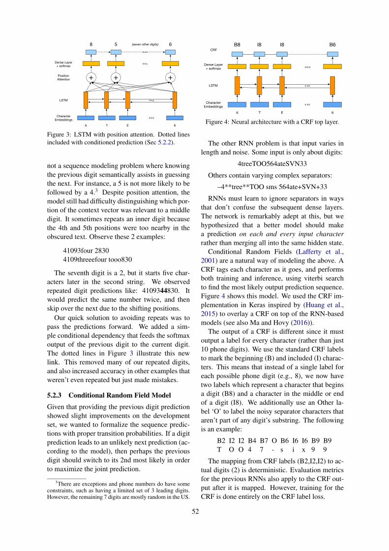
A T E 6

+

8 5 (seven other digits) 6

LSTM

CharacterEmbeddings

+ +PositionAttention

Dense Layer+ softmax

Figure 3: LSTM with position attention. Dotted linesincluded with conditioned prediction (Sec 5.2.2).

not a sequence modeling problem where knowingthe previous digit semantically assists in guessingthe next. For instance, a 5 is not more likely to befollowed by a 4.3 Despite position attention, themodel still had difficulty distinguishing which por-tion of the context vector was relevant to a middledigit. It sometimes repeats an inner digit becausethe 4th and 5th positions were too nearby in theobscured text. Observe these 2 examples:

41093four 28304109threeefour tooo830

The seventh digit is a 2, but it starts five char-acters later in the second string. We observedrepeated digit predictions like: 4109344830. Itwould predict the same number twice, and thenskip over the next due to the shifting positions.

Our quick solution to avoiding repeats was topass the predictions forward. We added a sim-ple conditional dependency that feeds the softmaxoutput of the previous digit to the current digit.The dotted lines in Figure 3 illustrate this newlink. This removed many of our repeated digits,and also increased accuracy in other examples thatweren’t even repeated but just made mistakes.

5.2.3 Conditional Random Field ModelGiven that providing the previous digit predictionshowed slight improvements on the developmentset, we wanted to formalize the sequence predic-tions with proper transition probabilities. If a digitprediction leads to an unlikely next prediction (ac-cording to the model), then perhaps the previousdigit should switch to its 2nd most likely in orderto maximize the joint prediction.

3There are exceptions and phone numbers do have someconstraints, such as having a limited set of 3 leading digits.However, the remaining 7 digits are mostly random in the US.

A T E 6

B8 B6

LSTM

CharacterEmbeddings


I8 I8CRF

Figure 4: Neural architecture with a CRF top layer.

The other RNN problem is that input varies inlength and noise. Some input is only about digits:

4treeTOO564ateSVN33

Others contain varying complex separators:

–4**tree**TOO sms 564ate+SVN+33

RNNs must learn to ignore separators in waysthat don’t confuse the subsequent dense layers.The network is remarkably adept at this, but wehypothesized that a better model should makea prediction on each and every input characterrather than merging all into the same hidden state.

Conditional Random Fields (Lafferty et al.,2001) are a natural way of modeling the above. ACRF tags each character as it goes, and performsboth training and inference, using viterbi searchto find the most likely output prediction sequence.Figure 4 shows this model. We used the CRF im-plementation in Keras inspired by (Huang et al.,2015) to overlay a CRF on top of the RNN-basedmodels (see also Ma and Hovy (2016)).

The output of a CRF is different since it mustoutput a label for every character (rather than just10 phone digits). We use the standard CRF labelsto mark the beginning (B) and included (I) charac-ters. This means that instead of a single label foreach possible phone digit (e.g., 8), we now havetwo labels which represent a character that beginsa digit (B8) and a character in the middle or endof a digit (I8). We additionally use an Other la-bel ‘O’ to label the noisy separator characters thataren’t part of any digit’s substring. The followingis an example:

B2 I2 I2 B4 B7 O B6 I6 I6 B9 B9T O O 4 7 - s i x 9 9

The mapping from CRF labels (B2,I2,I2) to ac-tual digits (2) is deterministic. Evaluation metricsfor the previous RNNs also apply to the CRF out-put after it is mapped. However, training for theCRF is done entirely on the CRF label loss.

52

A T E 6

+

8 5 (seven other digits) 6

LSTM

CharacterEmbeddings

+ +PositionAttention


A T E 6Character

Images

CNN

CNN

Max pool +Flatten

Figure 5: CNN architecture for visual image input tothe LSTM model.

5.2.4 Visual Characters with CNNsAs with most NLP tasks, out of vocabulary (OOV)input is an issue. Our adversarial task is even moresevere because visual substitutions are intentional,and often OOV as there are 138k current unicodeoptions. If the character is unseen in training, onlycontext can try to guess the digit. Below are ex-amples of such replacement:

Digits ASCII Unicode

410 41o 41!Why are these easy for humans to decipher? It’s

purely due to visual similarity. In a “normal” NLPneural model, each character (or token) is mappedto an embedding, so unseen characters have norepresentation. We might use the default approachof mapping all unknowns to a shared ‘UNK’ em-bedding, but this loses the different visual charac-teristics of each character.

All of this motivates our new Visual-BasedCharacter RNN. Our model does not learn a dic-tionary of character embeddings, but instead usesa series of CNN layers that transform 34x34 im-ages of the characters. The transformations thenfeed into our above models. This is now a modelthat can interpret unseen (in training) characters.

Figure 5 shows the CNN combined with our po-sitional attention RNN. We use two 3x3 convolu-tion layers with 4 and 8 filters respectively. Eachlayer is followed by a relu layer and a batch nor-

malization layer (not shown in the figure). Theconvolutions are followed by a max pooling layerand then flattened. A dense layer with softmaxthen reduces the flattened vector. We experi-mented with up to 3 convolution layers, up to 32filters, and varied the size of the dense layer.

Visual input changes the model significantly. Itis no longer learning an NLP-style character em-bedding, but rather learning CNN parameters totransform an image input into that embedding.Our first models ran into problems because theysimply memorized each 34x34 image. Since allASCII ‘3’ characters map to the same flattenedrepresentation, the model memorizes it, and uni-code variations fail no matter how similar. Wethus introduced data augmentation during train-ing. Each 34x34 input is ‘jiggled’ with ran-dom transformations: (1) translation of the im-age up/down or right/left, (2) darken/lighten theimage, (3) stretch or widen, and (4) rotate up to20 degrees. This provided different inputs for thesame ASCII chars, so the CNN was encouraged tolearn key visual features across all variants. Dataaugmentation led to our most significant improve-ments on unseen unicode character input.

6 Experiments

All models were trained on the 100k artificial ob-scured phone dataset (Section 4.2). 90k was usedfor training and 10k to determine convergence.The RNNs were set to N = 70 in length, and in-puts were padded to that length. The rare input textlonger than 70 is cropped. Embedding size N=100and LSTM internal dimensions M=200 were cho-sen for all RNNs based on dev set performance.The CRFs performed best at N=200. We also ap-plied dropout of 0.2 for the LSTMs and 0.5 CRF.

We report results with three metrics: digit ac-curacy, Levenshtein edit distance, and perfect ac-curacy. Digit accuracy is the simple alignment ofpredicted digit with gold digit (# correct / 10). Ifa predicted phone number is longer than 10 dig-its (CRFs are not bound to strictly 10 predictions),digit accuracy is computed only over the first 10predicted digits.

Digit accuracy is flawed because a model mightinsert one extra digit, but still guess correct for theremainder. For example:

Gold: 4109342309Guess: 41109342309

The CRF inserted an extra 1 digit, just one mis-take, but digit accuracy is now a very low 0.2.

53

Development Set Test SetModel Digit Lev Perfect Digit Lev PerfectTJBatch Rules 0.0 0.0 0.0 0.0 0.0 0.0LSTM (5.1.2) 77.0 79.7 48.1 74.4 78.2 40.3LSTM-2 77.5 79.4 49.7 74.8 77.6 40.6LSTM +att (5.2.1) 78.5 80.5 48.6 76.6 78.9 43.5LSTM +cond (5.2.2) 79.7 81.6 48.5 76.5 79.5 39.8LSTM +att +cond 79.1 81.2 48.3 77.2 79.8 42.3CRF with LSTM (5.2.3) 72.9 84.0 58.1 67.7 83.4 48.2

Table 1: Results on dev and test. Though flawed, digit accuracy is included for completeness. The +att and +condoptions are not compatible with the CRF which does not need attention since it predicts at every input character.

We thus use the Levenshtein edit distance to bet-ter evaluate performance. Levenshtein’s measurejudges string similarity based on the minimumnumber of “edits” required to transform the pre-diction into the gold: (1.0 − edits/10). In theabove case, one deletion is required to make thestrings the same, so the score is (1− 1/10) = 0.9.

Finally, perfect accuracy is the number of per-fect phone numbers (all 10 digits) that were cor-rectly guessed, divided by the size of the test set.

Real-world Test: We report results only on thereal-world test set from Section 4.1. The artifi-cial data was solely used for training. We did notrun models on the test set until the very end afterchoosing our best settings (on the dev set).

Real-world Challenge Test: To further illustratethe challenge of noisy text, we enhanced the real-world test set with unicode injections. Using ahand-created character lookup of visually similarunicode characters, we replaced 10% of the char-acters with randomly chosen unicode lookalikesnot in the training data. This results in a very chal-lenging test set to further benchmark the models.

Finally, all results in the next section are the av-erage of 4 train/test runs of the same model.

7 Results

Table 1 contains results without CNNs for thebaselines, RNNs, and CRF. The models listed arethose that showed consistent improvement on de-velopment, and the test set columns were run onlyat the end for publication results. Adding positionattention and conditional dependence each showedimprovements of 1-2% Levenshtein. Stacking twoLSTMs showed little gain. The CRF excelled witha 11% relative gain (on test) for perfect predictionover the best LSTM setup.

CNN Comparison (Perfect Acc)

Test ChallengeLev Perf Lev Perf

Best LSTM (no CNN) 81.2 48.3 72.9 22.1CNN-LSTM 77.3 42.1 65.5 15.6CNN-LSTM +aug 79.7 39.8 75.2 27.3Best CRF (no CNN) 84.0 58.1 74.9 17.6CNN-CRF 82.8 54.2 73.4 14.6CNN-CRF +aug 83.3 56.1 79.7 33.3

Table 2: Results of the CNN models. Challenge has10% unseen unicode injected. +aug used visual dataaugmentation during training.

For CNN results, Table 2 shows test set perfor-mance. Adding just the CNNs does not improverecognition, but in fact are slightly worse. How-ever, more compelling is the challenge set withinjected unicode confounders. Recall the impor-tance of data augmentation during training so themodels learn real visual features. These “+aug”results show why it is needed with a 89% rela-tive improvement in perfect phone accuracy (from17.6% to 33.3%). The non-CNN LSTM and CRFstruggle at 17-22%. They simply cannnot repre-sent unseen characters.

Our new CRF model (no CNN) outperforms theRNNs on the test set by 10% absolute. When com-paring challenge test performance, the best CRF-CNN outperforms the best non-CNN LSTM by11% absolute. To further illustrate the effect ofunicode confounders, we varied how much we in-jected and graphed performance in Figure 3. TheCNN models consistently outperform.

8 Full Ad Extraction

We wrapup with a pilot for full ad extraction. Themodels presented so far extract from one span oftext (it assumes a phone number exists). This for-

54

Table 3: Phone accuracy as a higher % of unicode sub-stitutions are made for lookalike ASCII characters.

mulation is a well-defined task for research, butwe also propose how one might apply these ex-tractors to the more difficult task of full documentextraction when the location of the phone numberis unknown. We briefly describe initial tests.

The most straightforward way to extract froma document is to split it into text windows(spans) and try all possible extractions. Sincethese are probabilistic models, we can computeP (phone|span), and find the window span thatmaximizes the probability.

best = maxspanP (phone|span) (2)

P (phone|span) =9∏

i=0

maxjP (di = j|span) (3)

The phone number extracted from the best span isthe phone number in the text.

We collected a set of real advertisements thatdon’t have phone numbers, and artificially insertedan obscured number from our artificial dataset.This allows us to track which span contains thephone number, and then evaluate an extractor.

The difficulty with this task is that our mod-els are trained on precise text spans, whereas thisfull document dataset contains lots of non-phone-related text. To address this difference, we stoppedpadding our snippet input with null values (up tothe length of the RNN), and instead pad with ran-domly selected text snippets from real ads. Themodels are exactly the same, we just change howpadding works when the training text is shorterthan length 70. We refer to this as the “ad pad”.

Datum: 6I5 093 93B6Null-Pad: 6I5 093 93B6Ad-Pad: 6I5 093 93B6always in town call

To be clear, no models were changed, just howtraining input is padded. Can the models iden-tify the correct text span that contains a phonenumber? Table 4 shows these results for standard

Text Span ID of Phone NumbersFull Full+Partial

Zero pad 70.3% 92.1%Craigslist ad pad 99.3% 99.7%Backpage ad pad 98.0% 99.6%

Table 4: Results of choosing text spans with the fullphone number, or a partial match. Partial matches con-tained on average 7-8 of the 10 digits.

null-padding versus ad-padding, as well as cross-domain tests. We trained on Craigslist and Back-page separately, then tested on only Backpage ads.

Window identification works very well as longas training padded its input with real ad text. Thisis encouraging in that it seems these models canreliably identify where a phone number is present.

Finally, we tested how the models also extractfrom these spans after identifying them. Extrac-tion showed 80% accuracy on full numbers, com-pared to 98% when train/test only on artificialphone snippets. We attribute the drop to the diffi-cult task - window spans contain more noise thana precise text span. Future work will focus on thisfull document task with real-world numbers.

9 Discussion

This is the first work to model noisy phone num-ber extraction with neural models. Most notably,our CNNs explore how to use visual characteris-tics of the characters, rather than standard NLP-style models with trained embeddings. To the bestof our knowledge, this is the first proposal for a vi-sual language model in an extraction architecture.

We showed results on new challenge datasetswith injected unicode. These results illustrate thechallenge for extractors, but also the usefulness ofCNN recognizers. In fact, current rule-based ex-tractors cannot extract any of the numbers in ourtest sets. Our CRF outperformed an LSTM-onlymodel by 10% absolute, and data augmentationimproved on unicode tests by a relative 89% gain.

Possible future work could investigate a Gen-erative Adversarial Network (GAN) (Goodfellowet al., 2014). GANs have become popular in visiontasks, but the normal GAN setup requires trainingdata to start from, and this sparse domain prohibitsits straightforward use.

Data from this work’s training and evaluationare available online4, and we hope this spurs fur-ther work on this important societal challenge.

4www.usna.edu/Users/cs/nchamber/data/phone/

55

10 Acknowledgments

This work would not be possible without thehelp of the Global Emancipation Network. Manythanks also to Jeff Kosseff for bringing this issueto our attention in the first place. We recognizeand appreciate the support of the DoD HPC Mod-ernization Office for enhancing our undergradu-ate education and research. Finally, thanks to Re-becca Hwa for helpful conversations early on inthis work.

ReferencesHamidreza Alvari, Paulo Shakarian, and J. E. Kelly

Snyder. 2017. Semi-supervised learning for detect-ing human trafficking. In Semi-supervised learningfor detecting human trafficking.

Hamidreza Alvari, Paulo Shakarian, and J.E. KellySnyder. 2016. A non-parametric learning approachto identify online human trafficking. In IEEE Con-ference on Intelligence and Security Informatics(ISI).

Andrei Costin, Jelena Isacenkova, Marco Balduzzi,Aurelien Francillon, and Davide Balzarotti. 2013.The role of phone numbers in understanding cyber-crime schemes. In 2013 Eleventh Annual Confer-ence on Privacy, Security and Trust, pages 213–220.IEEE.

Jun Ding, Bo Chen, Hongwei Liu, and MengyuanHuang. 2016. Convolutional neural network withdata augmentation for sar target recognition. IEEEGeoscience and remote sensing letters, 13(3):364–368.

Artur Dubrawski, Kyle Miller, Matthew Barnes,Benedikt Boecking, and Emily Kennedy. 2015.Leveraging publicly available data to discern pat-terns of human-trafficking activity. Journal of Hu-man Trafficking, 1.

Ian Goodfellow, Jean Pouget-Abadie, Mehdi Mirza,Bing Xu, David Warde-Farley, Sherjil Ozair, AaronCourville, and Yoshua Bengio. 2014. Generative ad-versarial nets. In Advances in neural informationprocessing systems, pages 2672–2680.


Rahul Kapoor, Mayank Kejriwal, and Pedro Szekely.2017. Using contexts and constraints for improvedgeotagging of human trafficking webpages. In Pro-ceedings of the Fourth International ACM Workshopon Managing and Mining Enriched Geo-SpatialData.

Mayank Kejriwal, Jiayuan Ding, Runqi Shao, AnoopKumar, and Pedro Szekely. 2017. Flagit: A systemfor minimally supervised human trafficking indica-tor mining.

Mayank Kejriwal and Pedro Szekely. 2017. Informa-tion extraction in illicit web domains. In WWW.

John Lafferty, Andrew McCallum, and Fernando CNPereira. 2001. Conditional random fields: Prob-abilistic models for segmenting and labeling se-quence data.

Lin Li, Olga Simek, Angela Lai, Matthew P. Daggett,Charlie K. Dagli, and Cara Jones. 2018. Detectionand characterization of human trafficking networksusing unsupervised scalable text template matching.In IEEE International Conference on Big Data (BigData).

Frederick Liu, Han Lu, Chieh Lo, and Graham Neu-big. 2017. Learning character-level compositional-ity with visual features. In ACL.

Xuezhe Ma and Eduard Hovy. 2016. End-to-endsequence labeling via bi-directional lstm-cnns-crf.arXiv preprint arXiv:1603.01354.

C. Nagpal, K. Miller, B. Boecking, and A. Dubrawski.2017. An entity resolution approach to isolate in-stances of human trafficking online.

Reihaneh Rabbany, David Bayani, and ArturDubrawski. 2018. Active search of connec-tions for case building and combating humantrafficking. In KDD.

Justin Salamon and Juan Pablo Bello. 2017. Deep con-volutional neural networks and data augmentationfor environmental sound classification. IEEE SignalProcessing Letters, 24(3):279–283.

Pedro Szekely, Craig Knoblock, Jason Slepickz, An-drew Philpot, et al. 2015. Building and using aknowledge graph to combat human trafficking. InInternational Conference on Semantic Web (ICSW).

Yan Xu, Ran Jia, Lili Mou, Ge Li, Yunchuan Chen,Yangyang Lu, and Zhi Jin. 2016. Improved re-lation classification by deep recurrent neural net-works with data augmentation. arXiv preprintarXiv:1601.03651.

Zhun Zhong, Liang Zheng, Guoliang Kang, Shaozi Li,and Yi Yang. 2017. Random erasing data augmen-tation. arXiv preprint arXiv:1708.04896.

56


Community Characteristics and Semantic Shift ofHigh Affinity Terms on Reddit

Abhinav Bhandari† ‡ Caitrin Armstrong†

†School of Computer Science, McGill University‡Agoop Corp, 3-35-8 Jingumae, Shibuya City, Tokyo

abhinav.bhandari,caitrin.armstrong{@mail.mcgill.ca}

Abstract

Language is an important marker of a culturalgroup, large or small. One aspect of languagevariation between communities is the employ-ment of highly specialized terms with uniquesignificance to the group. We study these highaffinity terms across a wide variety of commu-nities by leveraging the rich diversity of Red-dit.com. We provide a systematic explorationof high affinity terms, the often rapid semanticshifts they undergo, and their relationship tosubreddit characteristics across 2600 diversesubreddits. Our results show that high affin-ity terms are effective signals of loyal commu-nities, they undergo more semantic shift thanlow affinity terms, and that they are partialbarrier to entry for new users. We concludethat Reddit is a robust and valuable data sourcefor testing further theories about high affinityterms across communities.

1 Introduction

The evolution and semantic change of human lan-guage has been studied extensively, both in a his-torical context (Garg et al., 2017) and, increas-ingly, in the online context (Jaidka et al., 2018).However, few studies have explored the evolutionof words across different online communities thatallow a comparison between community charac-teristics and terms that have high affinity to a com-munity.

The banning of r/CoonTown and r/fatpeoplehatein 2015, as analyzed by Saleem et al., providesgood motivation for our work. r/CoonTown wasa racist subreddit with a short life span of 8months (November 2014 - June 2015)(Saleemet al., 2017). During this time, as shownby Saleem (2017), these subreddits underwentrapid semantic development through which newwords, such as “dindu”, “tbi” and “nuffin” werenot only created, but increasingly became more

context-specific (accumulated in meaning). Inr/fatpeoplehate existing words such as “moo”,“xxl” and “whale” underwent localized seman-tic shift such that their meanings transformed toderogatory terms (Saleem et al., 2017).

These two cases demonstrate that not only arenew words conceived within subreddits, existingwords undergo localized transition. They also sug-gest that this phenomenon likely takes place in ashort time period for high affinity words. In or-der to evaluate whether such trends are consistentacross subreddits, we study semantic shift and theroles high affinity terms play in 2600 different sub-reddits between November 2014 to June 2015.

Our aim is to provide a characterization of highaffinity terms by mapping their relationship to dif-ferent types of online communities and the seman-tic shifts they undergo in comparison to general-ized terms (low affinity terms). We leverage datacurated from the multi-community social networkReddit and the types of subreddit characteristicswe study are loyalty, dedication, number of usersand number of comments. Our paper explores thefollowing research questions:

1. Do certain community characteristics corre-late with the presence of high affinity terms?

2. Do high affinity terms undergo greater se-mantic shift than low affinity terms?

3. Do high affinity terms and community char-acteristics function as a barriers to entry fornew users to participate?

Some key findings include:

1. Loyalty is strongly correlated to the presenceof high affinity terms in a community.

2. High affinity terms undergo greater seman-tic shift than generalized terms (low affinityterms) in a short interval of time.

57

3. High affinity terms, and dedication values ofa subreddit strongly correlate to the numberof new users that participate, indicating thatthe degree of high affinity terms establishes alexical barrier to entry to a community.

2 Related Work and Concepts

2.1 Understanding Community SpecificTerms

Before defining high affinity terms, we examinethe traits observed in community specific termsfrom past literature.

Studies have shown that words specific toa community have qualities of cultural carriers(Goddard, 2015). While culture is “somethinglearned, transmitted, passed down from one gener-ation to the next, through human actions,” (Durantiet al., 1997) these transmissions through languageaffect a culture’s system of “classifications, spe-cialized lexicons, metaphors, and reference forms”in communities (Cuza, 2011). Pierre Bourdieu ar-gues that language is not only grammar and sys-tematic arrangemennt of words, but it is symbolicof cultural ideas for each community. To speaka certain language, is to view the world in a par-ticular way. To Bourdieu, through language peo-ple are members of a community of unique ideasand practices (Bourdieu et al., 1991). As such,community specific terms are usually not easilytranslatable across different communities. For ex-ample, in Hungarian “life” is metaphorically de-scribed as “life is a war” and “life is a com-promise”, whereas in American English “life” ismetaphorically represented as “life is a preciousposesssion”, or “life is a game” (KA, 2010). Thesedefinitions of similar entities vary due to differentcultural outlooks in communities.

Besides words that are cultural carriers, slang isalso a form of terminology specific to a commu-nity. While there is no standard operational defini-tion of slang, many philosophical linguists defineslang as terms that are vulgar (Green, 2016; Al-lens, 1993), encapsulate local cultural value and atype of insider speech that roots from subcultures(Partridge and Beale, 2002). Morphological prop-erties of slang are defined as “extra-grammatical”,and these morphological properties in slang areshown to be distinguishable from morphologicalproperties of standard words in English (Mat-tiello, 2013). There has been an increase of slangin online spaces (Eble, 2012), with many terms

falling under the extra-grammatical classifica-tions of abbreviation (‘DIY’, ‘hmu’, ‘lol’), blends(‘brangelina’, ‘brunch’), and clippings (‘doc (doc-tor)’, ‘fam (family)’) (Mattiello, 2013; Kulkarniand Wang, 2018).

By extracting terms that have a high affinity to acommunity, we approximate words that are eithercultural carriers or slang.

2.2 Measuring Affinity of Terms

Measurements for affinity of terms to a commu-nity have been explored in research, where the fre-quency of a word is compared to some backgrounddistribution to extract linguistic variations that aremore likely in one setting (Monroe et al.; Zhanget al., 2018). Most helpful to our approach is apast study that computed a term’s specificity spcto a subreddit through the pointwise mutual infor-mation (PMI) of a wordw in one community c rel-ative to all other communities C in Reddit (Zhanget al., 2017).

spc(w) = logPc(w)

PC(w)

An issue with this metric is that terms withequal specificity can differ in their frequency.Specificity does not show which term is moredominant within a community by frequency, asshow in Table 1. Due to this, we compute the affin-ity value of a term by measuring its locality anddominance to a community. Locality is the likeli-hood of a term belonging to some community, anddominance captures the presence of the term in thesaid community by its frequency.

We therefore calculate the locality l of a wordwj in subreddit si through the conditional proba-bility of a word occurring in si, relative to it oc-curring in all other subreddits S.

lsi(wj) =Psi(wj)

PS(wj)

We then calculate dominance d in two steps.First we calculate an intermediate value r, whichis the difference between the count of word wj insi subtracted by the sum of all terms W in si mul-tiplied by constant ε, which in our work was suf-ficient as 0.0001. If the value of r is negative, wedisregard it, as it is likely to be an infrequent wordof little semantic significance, such as a typo.

rsi(wj) = Countsi(wj)− Countsi(W )× ε

58

mccoy slowmo ducati bleacher takahashi motogpspc 0.000 0.000 -0.004 0.000 0.000 -0.004asi 0.942 0.666 0.987 0.500 0.833 0.987

Table 1: Affinity and Specificity of terms found inr/motogp calculated on the word distributions of 10sample subreddits. This shows that less frequently oc-curring words and frequently occurring words can havethe same specificity value, however the affinity valuetakes into account the degree of frequency of each termin a community.

where

rsi(wj) =

{rsi(wj) rsi(wj) > 1

1 rsi(wj) ≤ 1

Then, we calculate the dominance d as a neg-ative hyperbolic function of each word’s occur-rence:

dsi(wj) = 1− 1

rsi(wj)

Finally, we compute the affinity value of a wordto a subreddit as a product of a word’s dominanceand locality:

asi(wj) = dsi(wj)× lsi(wj)

After extracting affinity values of each word rel-ative to a subreddit, we partition the sets of wordsinto high affinity terms and low affinity terms.

High Affinity Terms: For each subreddit, weextract 50 terms with the highest affinity values,and we categorize them as high affinity terms. Theaverage of high affinity terms is denoted as highaffinity average.

Low Affinity Terms: For each subreddit, weextract 50 terms with the lowest affinity values,and we categorize them as low affinity terms. Theaverage of low affinity terms is denoted as lowaffinity average.

2.3 How Semantic Shift Can CaptureCultural Shifts

As previously stated, high affinity terms are ap-proximations for words that are either cultural car-riers or slang.

Research has shown that shifts of local neigh-borhoods across embeddings are more effective incapturing cultural shifts than to calculate distancesof a word across aligned embeddings, which isused to measure structural shifts (Hamilton et al.,2016; Eger and Mehler, 2016). Studies have repre-sented k-nearest neighbors n of a word w through

second-order vectors V |n| that are made of thecosine similarities between n and w, then cal-culate the difference between these second-ordervectors to identify shifts (Hamilton et al., 2016;Eger and Mehler, 2016). Recent works have alsomodeled shifts in words through the change incommon neighbors across different embeddings(Wendlandt et al., 2018; Eger and Mehler, 2016).

2.4 Measuring Semantic Change

Our measurement of semantic shift is based onthe concepts of semantic narrowing of words, aprocess in which words become more specializedto a context, and semantic broadening of words,a process in which words become more gener-alized from a context (Bloomfield, 1933; Blankand Koch, 1999). We capture this contextual in-formation by constructing 300 dimensional wordembeddings (word2vec) for each subreddit us-ing skip-gram with negative sampling algorithms,where a distributional model is trained on wordspredicting their context words (Mikolov et al.,2013). For each word, we measure narrowing asan increase in co-occurrence of a word’s nearestneighbors, and broadening as a decrease in co-occurrence of a word’s nearest neighbors (Crow-ley and Bowern, 2010).

To measure semantic shift, we extract commonvocabulary V = (w1, ..., wm) across all time in-tervals t ∈ T . Then, for some t and t+ n, we takea word wj’s set of k nearest-neighbors (accord-ing to cosine similarity). These neighbor sets aredenoted as At

k(wj) and At+nk (wj). We then cal-

culate the neighbours co-occurrence value CO asthe Jaccard similarity of neighbours sets (Hamil-ton et al., 2016), in subreddit si:

Atk(wj) = cos-sim(wt

j , k)

At+nk (wj) = cos-sim(wt+n

j , k)

COsi(wtj , w

t+nj ) =

|Atk(wj) ∩At+n

k (wj)||At

k(wj) ∪At+nk (wj)|

Then, we calculate the difference of CO acrosssuccessive embeddings in T . We label, chrono-logically, the first time interval (t1) as initial pointand the last time interval (tp) as terminal point,across which narrowing and broadening are mea-sured. We used k = 10 for all computations.

Broadening Measurement: We measurebroadening as the sum of the difference of COsi

59

Figure 1: This figure provides a visual representa-tion of our methodology of semantic shift measure-ment. The initial point embedding is trained on 2014-11/12 dataset. The terminal point embedding is trainedon 2015-05/06. All semantic shift measurements fol-low a chronological order of comparison, such thatnarrowing and broadening are both measurements ofembeddingt+1 - embeddingt.

between initial point embedding and all successiveembeddings. This is defined as:

bsi(wj) =

p−1∑

t=2

(COsi(w1j , w

t+1j )−COsi(w

1j , w

tj))

By comparing an embedding to its future em-beddings, we are able to see which contexts arelost as a word’s meaning becomes more broad.

Narrowing Measurement: Similarly, we mea-sure narrowing by calculating the sum of the dif-ference of CO between terminal point embeddingand all previous embeddings.

nsi(wj) =

p−2∑

t=1

(COsi(wpj , w

t+1j )−COsi(w

pj , w

tj))

By comparing an embedding to its previous em-beddings, we are able to see which contexts as-sociated with a word have increased in specificityover time.

A visual representation of the metrics are pro-vided in Figure 1.

2.5 Extracting Rate of Change of FrequencyMany past works have also modelled relationshipsbetween frequency and semantic shift (Lancia,2007; Hilpert and Gries, 2016; Lijffijt et al., 2014).

One study shows that an increase in frequency ofa term across decades results in a semantic broad-ening, while a decrease in frequency causes it tonarrow (Feltgen et al., 2017). For example an in-crease in frequency of the word “dog” evolved itsmeaning from a breed to an entire species, andthe decrease in frequency of “deer” localized itsmeaning from “animal” to a specific animal (un-dergoing narrowing) (Hilpert and Gries, 2016).

Very few studies have modelled narrowing andbroadening of terms in the short term. As such, weare interested in the frequency patterns of termsthat go through short-term cultural shifts. Onestudy showed the effect of frequency on learn-ing new words, and how it affects the use ofnew words in their correct context. They con-ducted their experiments in a physical capacity onchildren of five years old who were made famil-iar with new words (Abbot-Smith and Tomasello,2010) in a short time period. Their results demon-strate that familiarizing children with new wordsallowed them to use the word in correct grammat-ical contexts, and greater frequency of exposure tonew words resulted in more narrowed and correctuse of the word to a context. This pattern of teach-ing is categorized as lexically-based learning.

Due to this, we assess whether in the short-termin subreddits, narrowing and broadening of termscorrelates to the rate of change of frequencies.

We calculate rate of change of frequency acrosstime periods T for a subreddit si as such, where nis the size of T :

∆fsi(wj) =n−1∑

t=1

ft+1(wj)− ft(wj)

ft+1(wj)

A positive value shows an increasing rate of fre-quency, and a negative value shows a decreasingrate of frequency.

2.6 Characteristics of SubredditsWe introduce four quantifiers that describe subred-dit networks based on existing typology. Usingthese quantitative chararacteristics we can evalu-ate and identify systemic patterns that exist be-tween types of subreddits and high affinity terms.The four quantifiers are loyalty, dedication, num-ber of comments, and number of users.

Loyalty: Previous work on subreddit character-istics has defined community loyalty as a percent-age of users that demonstrate both preference andcommitment, over other communities in multiple

60

SubredditsHigh Aff.

Avg. High Aff. TermsLow Aff.

Avg. Low Aff. Terms

Top 1% bravefrontier 0.999‘sbb’, ‘zelnite’, ‘darvanshel’,

‘tridon’, ‘ulkina’ 0.000‘food’, ‘drive’, ‘park’,

‘episode’, ‘photo’

chess 0.999‘pgn’, ‘bxc’, ‘nxe’,

‘nxd’, ‘bxf’ 0.000’character’, ‘compose’,

‘pack’, ‘message’, ‘damage’

Arbitrary radiohead 0.732‘cuttooth’, ‘backdrifts’, ‘tkol’,

‘crushd’, ‘htdc’ , 0.000’willing’, ‘phone’, ‘gain’,

‘sell’, ‘provide’

fatpeoplehate 0.357‘pco’, ‘tubblr’, ‘fatshion’,

‘fatkini’, ‘feedee’ 0.000

’application’, ‘network’,‘engine’, ‘element’,

‘cable’

Bottom 1% Wellthatsucks 0.002‘helmet’, ‘shoe’, ‘brake’,

‘truck’, ‘tire’ 0.000‘help’, ‘team’, ‘love’,‘include’, ‘question’

gif 0.002‘gif’, ‘prank’, ‘repost’,

‘swim’, ‘ftfy’ 0.000‘subreddit’, ‘order’,

‘account’, ‘game’, ‘issue’

Table 2: A sample presentation of high affinity terms and low affinity terms from subreddits with high high affinityaverages (top 1%), and low high affinity averages (bottom 1%).

time periods (Hamilton et al., 2017). Preference isdemonstrated by more than half of a user’s com-ments contributing to subreddit si ∈ S, and com-mitment is measured by a user commenting in siin multiple time periods t ∈ T . It has been shownthat community wide loyalty impacts usage of lin-guistic features such as singular (“I”) and plural(“We”) pronoun (Hamilton et al., 2017). Commu-nities with greater loyalty have a higher usage ofplural pronouns than communities with low loy-alty which have a heavier usage of singular pro-nouns. Following this finding, we investigate re-lationships between loyal communities and highaffinity terms, to gauge whether loyal communi-ties are also strongly correlated to use of othertypes of terms.

Dedication: Other studies have also shownthat user retention correlates to increased use ofsubreddit specific terms (similar to high affinityterms) (Zhang et al., 2017). We calculate userretention to measure a community characteristicsimilar to commitment as defined in a past study(Hamilton et al., 2017), by extracting users thatcomment in subreddit si ∈ S a minimum of nnumber of times across all time periods t ∈ T andlabel this retention value as dedication. A key dif-ference between dedication and loyalty is that auser does not have to contribute more than 50%of their comments to a particular subreddit to bededicated, which is a requirement for loyalty. Thismeans that a user can be dedicated to multiple sub-reddits, while a user is loyal to only one group at aparticular time. The comparison between loyaltyand dedication allows us to explore whether pref-erence is a strong factor in the linguistic evolutionof high affinity terms in online communities.

Number of Comments and Number of Users:Lastly, we measure raw metadata of subredditswhich are the number of comments made, and thenumber of users that participated in a subreddit.

Existing work has shown that areas with largepopulations experience a larger introduction ofnew words, whereas areas with small populationsexperience a greater rate of word loss (Bromhamet al., 2015). Furthermore, words in larger popu-lations are suspect to greater language evolution.While this is a correlation found in physical com-munities, we assess whether this remains consis-tent in online communities. As a proxy for pop-ulation we consider both the number of users andthe number of comments.

3 Description of Data

Our dataset consists of all subreddits betweenNovember 2014 to June 2015 with more than10000 comments in that period. We performed ourmeasures on the curated data in time intervals of 2months. We manually removed communities thatare mostly in non-ascii or run by bots. This re-sulted in a dataset of 2626 subreddits.

4 Qualitative Overview of High Affinityand Low Affinity Terms

We examine high and low affinity terms acrosssubreddits. Our results, as shown in Table 2,demonstrate that high affinity terms have differentcharacteristics across communities.

Certain high affinity terms exist independent ofonline communications. For example in r/chess,the high affinity terms “bxc”, “bxf”, “nxe” areall numerical representations used to communi-cate game moves. Similarly in r/bravefrontier,

61

Figure 2: This figure shows the relationship between community characteristics and high affinity averages. Eachcommunity characteristics is binned into intervals of 20% by percentile. Loyalty most strongly correlates withhigh affinity averages.

the terms ”zelnite” and ”darvanshel” are gamecharacters. However in r/fatpeoplehate, there arehigh affinity terms that originate online. Termsin r/fatpeoplehate demonstrate extra-grammaticalqualities of slang, such as “fatkini”, which is ablend of “fat” + “bikini”, and “feedee”, whichis clipping of “feeder”, signalling word devel-opment through online communication (Kulkarniand Wang, 2018).

Interestingly, across the topically different sub-reddits, abbreviations are common form of highaffinity terms. For instance, “pgn” in r/chessstands for ”portable game notation”, “tkol” inr/radiohead stand for “The king of Limbs”, “ftfy”in r/gif stands for ”fixed that for you”. The useof abbreviations illustrates the transformation of“gibberish” into collective meaning within a com-munity. It is only with the context of domain andculture, that one can attribute meaning to theseterms.

Named Entity Recognition (NER) of Top 100and Bottom 100 subreddits by high affinity av-erages: We performed NER using bablefy on thenames of the top 100 and bottom 100 subreddits byhigh affinity averages. Through this analysis, weobserve that 82 of the top 100 are named entities,whereas only 18 of bottom 100 are named entities.Of the 82, 33 subreddits are videogames, 19 areregional subreddits and 11 are sports subreddits.This shows that communities with high affinity av-erages are likely to be strongly linked with a phys-ical counterpart. Whereas the bottom 100 subred-dits consisted of discussion and generalized sub-reddits such as r/TrueReddit, r/Showerthoughts,r/blackpeoplegifs whose creation and culture candirectly be attributed to online communities rather

than physical counterparts. This provides anexplanation for subreddits with low high affin-ity averages having extremely generalized highaffinity terms, such as “helmet” and “shoe” inr/Wellthatsucks.

5 Impact of Community Characteristicson Affinity of Terms

We conducted prediction tasks using communitycharacteristics to demonstrate meaningful rela-tionships between high affinity terms. We treatedeach of the community characteristics as features(log-transformed), and perform linear regressions,with five cross-validation, to predict the high affin-ity average (log-transformed) of a subreddit.

5.1 Prediction of High Affinity Terms fromCommunity Characteristics

We find that loyalty of a subreddit is remarkablycorrelated to the high affinity average of subred-dits. A linear model trained on loyalty to predicthigh affinity average of a subreddit achieves anR2

of 0.364 (p-value < 0.001). Compared to this, alinear model trained on dedication results in anR2

value of 0.274 (p-value < 0.001). This impliesthat preference is a strong factor in the likelihoodof high affinity terms in communities.

In contrast, models trained on number of com-ments and number of users resulted in an R2 of0.071 and 0.004. Loyalty is therefore a much moreeffective measure than most standard communitymeasures at least when measured on a linear scale.This finding supports existing work, which showsthat distinctiveness of a community is strongly re-lated to its rate of user retention (Zhang et al.,2017).

62

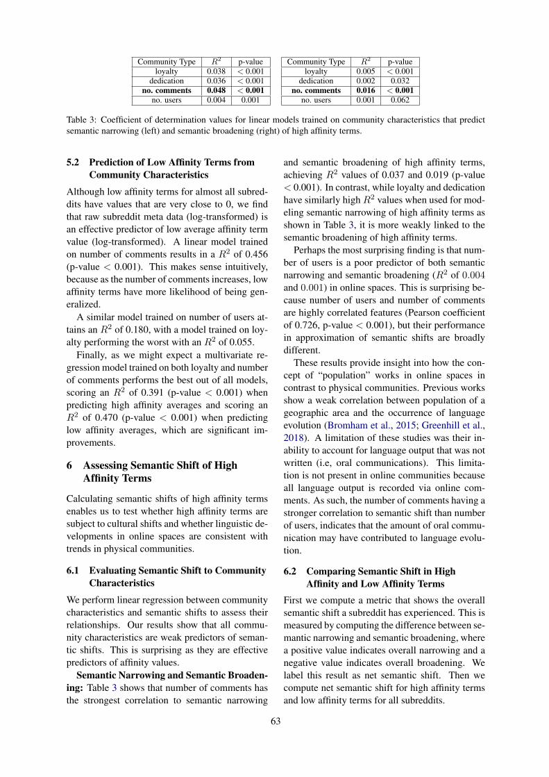
Community Type R2 p-valueloyalty 0.038 < 0.001

dedication 0.036 < 0.001no. comments 0.048 < 0.001

no. users 0.004 0.001

Community Type R2 p-valueloyalty 0.005 < 0.001

dedication 0.002 0.032no. comments 0.016 < 0.001

no. users 0.001 0.062

Table 3: Coefficient of determination values for linear models trained on community characteristics that predictsemantic narrowing (left) and semantic broadening (right) of high affinity terms.

5.2 Prediction of Low Affinity Terms fromCommunity Characteristics

Although low affinity terms for almost all subred-dits have values that are very close to 0, we findthat raw subreddit meta data (log-transformed) isan effective predictor of low average affinity termvalue (log-transformed). A linear model trainedon number of comments results in a R2 of 0.456(p-value < 0.001). This makes sense intuitively,because as the number of comments increases, lowaffinity terms have more likelihood of being gen-eralized.

A similar model trained on number of users at-tains an R2 of 0.180, with a model trained on loy-alty performing the worst with an R2 of 0.055.

Finally, as we might expect a multivariate re-gression model trained on both loyalty and numberof comments performs the best out of all models,scoring an R2 of 0.391 (p-value < 0.001) whenpredicting high affinity averages and scoring anR2 of 0.470 (p-value < 0.001) when predictinglow affinity averages, which are significant im-provements.

6 Assessing Semantic Shift of HighAffinity Terms

Calculating semantic shifts of high affinity termsenables us to test whether high affinity terms aresubject to cultural shifts and whether linguistic de-velopments in online spaces are consistent withtrends in physical communities.

6.1 Evaluating Semantic Shift to CommunityCharacteristics

We perform linear regression between communitycharacteristics and semantic shifts to assess theirrelationships. Our results show that all commu-nity characteristics are weak predictors of seman-tic shifts. This is surprising as they are effectivepredictors of affinity values.

Semantic Narrowing and Semantic Broaden-ing: Table 3 shows that number of comments hasthe strongest correlation to semantic narrowing

and semantic broadening of high affinity terms,achieving R2 values of 0.037 and 0.019 (p-value< 0.001). In contrast, while loyalty and dedicationhave similarly high R2 values when used for mod-eling semantic narrowing of high affinity terms asshown in Table 3, it is more weakly linked to thesemantic broadening of high affinity terms.

Perhaps the most surprising finding is that num-ber of users is a poor predictor of both semanticnarrowing and semantic broadening (R2 of 0.004and 0.001) in online spaces. This is surprising be-cause number of users and number of commentsare highly correlated features (Pearson coefficientof 0.726, p-value < 0.001), but their performancein approximation of semantic shifts are broadlydifferent.

These results provide insight into how the con-cept of “population” works in online spaces incontrast to physical communities. Previous worksshow a weak correlation between population of ageographic area and the occurrence of languageevolution (Bromham et al., 2015; Greenhill et al.,2018). A limitation of these studies was their in-ability to account for language output that was notwritten (i.e, oral communications). This limita-tion is not present in online communities becauseall language output is recorded via online com-ments. As such, the number of comments having astronger correlation to semantic shift than numberof users, indicates that the amount of oral commu-nication may have contributed to language evolu-tion.

6.2 Comparing Semantic Shift in HighAffinity and Low Affinity Terms

First we compute a metric that shows the overallsemantic shift a subreddit has experienced. This ismeasured by computing the difference between se-mantic narrowing and semantic broadening, wherea positive value indicates overall narrowing and anegative value indicates overall broadening. Welabel this result as net semantic shift. Then wecompute net semantic shift for high affinity termsand low affinity terms for all subreddits.

63

Figure 3: The sum of semantic narrowing and semanticbroadening from all subreddits by high affinity and lowaffinity terms. High affinity terms are more volatile andsensitive to cultural shifts.

We find that out of 2626 subreddits, 1638 (62%)subreddits demonstrate a positive net semanticshift in high affinity terms, whereas, 1529 (58%)subreddits demonstrate a positive net semanticshift in low affinity terms.

In Figure 3, we show that across all subred-dits, the sum of net semantic shift in high affinityterms is 20.462 (50.253-29.791), whereas the sumof net semantic shift in low affinity terms is 4.402(17.878-13.476). This implies that high affinityterms in general are more likely to attain quali-ties that are defining of neologisms, and are morelikely to be narrowed in communities across Red-dit.

This is explained by our results which showthat the rate of decrease of semantic broadeningis slower than the rate of increase of semantic nar-rowing (Pearson coefficient of -0.192, p-value <0.001), as demonstrated by a regression coefficientof -0.148. This trend is consistent when modelingsemantic narrowing and semantic broadening withother community characteristics.

Interestingly, in communities with very highaffinity averages, we observe several cases wherethe semantic narrowing and semantic broadeningare close to 0. Examples of such subreddits arer/kpop, r/chess, and r/Cricket. We notice that thesegroups contain terms that are essential and almostexclusive to the domain of that community. How-ever, these terms do not undergo extraordinary cul-tural impetus that causes a shift in meaning. Forinstance in r/chess there is little motivation to use“bxe”, “cdf” outside of the context of game moves.

Additionally, we observe highest semanticshifts in groups that are mostly video games, tv-

Figure 4: This figure illustrates the relationship be-tween net semantic shift of subreddits and their averagerate of change of frequency for high-affinity terms.

shows and sports communities, with high affinityaverages being less than 0.5 in most cases - the av-erage high affinity score of top 100 semantic nar-rowing groups is 0.367. These lower scores thattend away from the possible extremes, show thatniche terms that shift the most are also slightlydistributed in few other communities, but clearlydominant in one. Terms that are likely to undergohigh levels of semantic shift have potential of be-ing cross-cultural and adopted by a different groupof people. Study of external influence of highaffinity terms in other communities is an area offuture research, and may reveal factors that makesome high affinity terms more likely to evolve in ashort period of time.

6.3 Mapping of Frequency

Past studies show that in the long term words thatnarrow decrease in frequency (Feltgen et al., 2017;Hilpert and Gries, 2016). However, our results, asshown in Figure 4, indicate that in the short termnet semantic shift is strongly correlated with in-crease in frequency.

By testing the relationship between ∆fsi andnet semantic shift, we discovered a strong linearrelationship (Pearson coefficient of 0.429, p-value< 0.001).

Language adoption studies have shown that in-creased familiarization with a word in the shortterm - measured through frequency - actually en-ables a person to use the word more accuratelyand precisely. This is achieved, in both adults andchildren through lexically-based learning (Abbot-Smith and Tomasello, 2010). Our results indicatethat online communities also employ lexically-

64

CommunityCharacteristic R2 p-value

loyalty 0.340 < 0.001dedication 0.518 < 0.001

High Aff. Avg. 0.201 < 0.001

Community Characteristic R2 p-valueloyalty + dedication 0.503 < 0.001loyalty + High Aff. 0.377 < 0.001

dedication + High Aff. 0.539 < 0.001

Table 4: Coefficient of determination values for linear and multivariate models trained on community characteris-tics that predict rate of new users (δu(si)).

based learning in the short term, and may factorinto linguistic culture adoption and development.We derive this finding from the fact that increasein frequency is strongly correlated with semanticnarrowing.

7 Barriers to Entry

In this section, we evaluate the impact high affinityvalues have on the rate of new users participatingin each time period.

We calculate the rate of new users δu(si) as:

δu(si) =n−1∑

t=1

Ut+1(si)− Ut(si)

Ut+1(si)

where U is the set of users in subreddit si attime period t.

In Table 4 we present our results of regressionand correlation testing. We find that dedicationshows the strongest correlation to the rate of newusers in a community. This insinuates that abso-lute preference is an unlikely indicator of δu(si).

Although weaker, high affinity terms also showa correlation to δu(si). However, as shown in Ta-ble 4, it is remarkable that dedication and highaffinity averages outperform the combination ofloyalty and dedication in predicting the value ofδu(si). This is because loyalty has a stronger cor-relation with δu(si) than high affinity averages.Due to this, a model trained on loyalty and ded-ication should perform better. However not onlydoes it not perform better than a model trained ondedication and high affinity averages, it performsworse than a model trained only on dedication.This suggests that loyalty likely captures barriersto entry similar to dedication but more poorly. Italso suggests that high affinity terms and dedica-tion capture different types of barriers to entry.

Furthermore, we observe that communitieswhich show the least δu(si), are mostly topics thatoriginate outside of Reddit, such as r/NASCAR(sports) and r/SburbRP (sexual roleplay).

These results indicate that there are linguis-tic and non-linguistic barriers that prevent peo-

ple from engaging in certain online communi-ties. While this may not be concerning for in-nocuous topics such as r/Chess, issues may arisefor ideologically-themed subreddits. In the age ofpolitical polarization, hate groups and infamousecho chambers, further research could be con-ducted into barriers to entry and the role high affin-ity terms play.

8 Conclusion and Future Work

Through several analyses we have shown there tobe a strong relationship between online commu-nity behaviour and several aspects of high affin-ity terms. We found correlations with subredditcharacteristics related to collective user behaviour,especially loyalty. The high affinity terms under-went semantic shift at a high rate given our verycondensed timescale. Finally, we showed a rela-tionship between user retention and the presenceof these terms.

All three conclusions, and the secondary anal-yses conducted alongside them, show that highaffinity terms have strong potential for further elu-cidating online community behaviour, and likelyare correlated with further characteristics moredifficult to measure than subreddit loyalty suchas community cohesion (the strength and salienceof group identity (Rogers and Lea, 2004)) or be-haviour leading to the formation of extremist hategroups. Finally, our results and further investiga-tion can contribute to the literature surrounding therelationship between vocabulary and social mobil-ity between groups.

References

Kirsten Abbot-Smith and Michael Tomasello. 2010.The influence of frequency and semantic similarityon how children learn grammar. First Language,30(1):79–101.

Irving Lewis Allens. 1993. The city in slang : NewYork life and popular speech, 1 edition, volume 1 of1. Oxford University Press. An optional note.

65

A. Blank and P. Koch. 1999. Historical Semantics andCognition. Cognitive linguistics research. Moutonde Gruyter.

Leonard Bloomfield. 1933. Language. Holt, NewYork.

P. Bourdieu, J.B. Thompson, G. Raymond, andM. Adamson. 1991. Language and Symbolic Power.Social theory. Harvard University Press.

Lindell Bromham, Xia Hua, Thomas Fitzpatrick, andSimon Greenhill. 2015. Rate of language evolutionis affected by population size. Proceedings of theNational Academy of Sciences of the United Statesof America, 112.

T. Crowley and C. Bowern. 2010. An Introductionto Historical Linguistics. Oxford University PressUSA - OSO.

Alexandru Ioan Cuza. 2011. Translation of culturalterms : Possible or impossible ?

A. Duranti, Cambridge University Press, S.R. An-derson, J. Bresnan, B. Comrie, W. Dressler, andC.J. Ewen. 1997. Linguistic Anthropology. Cam-bridge Textbooks in Linguistics. Cambridge Univer-sity Press.

C. Eble. 2012. Slang and Sociability: In-Group Lan-guage Among College Students. University of NorthCarolina Press.

Steffen Eger and Alexander Mehler. 2016. On the lin-earity of semantic change: Investigating meaningvariation via dynamic graph models. In Proceed-ings of the 54th Annual Meeting of the Associationfor Computational Linguistics (Volume 2: Short Pa-pers), pages 52–58, Berlin, Germany. Associationfor Computational Linguistics.

Quentin Feltgen, Benjamin Fagard, and Jean-PierreNadal. 2017. Frequency patterns of semanticchange: Corpus-based evidence of a near-critical dy-namics in language change. Royal Society Open Sci-ence, 4.

Nikhil Garg, Londa Schiebinger, Dan Jurafsky, andJames Zou. 2017. Word embeddings quantify 100years of gender and ethnic stereotypes. CoRR,abs/1711.08412.

Cliff Goddard. 2015. Words as Carriers of CulturalMeaning, pages 380–400.

J. Green. 2016. Slang: A Very Short Introduction. Veryshort introductions. Oxford University Press.

Simon J. Greenhill, Xia Hua, Caela F. Welsh, HildeSchneemann, and Lindell Bromham. 2018. Popu-lation size and the rate of language evolution: A testacross indo-european, austronesian, and bantu lan-guages. Frontiers in Psychology, 9:576.

William L. Hamilton, Jure Leskovec, and Dan Jurafsky.2016. Cultural shift or linguistic drift? comparingtwo computational measures of semantic change.CoRR, abs/1606.02821.

William L. Hamilton, Justine Zhang, Cristian Danescu-Niculescu-Mizil, Dan Jurafsky, and Jure Leskovec.2017. Loyalty in online communities. CoRR,abs/1703.03386.

Martin Hilpert and Stefan Th. Gries. 2016. Quanti-tative approaches to diachronic corpus linguistics,Cambridge Handbooks in Language and Linguistics,page 36–53. Cambridge University Press.

Kokil Jaidka, Niyati Chhaya, and Lyle Ungar. 2018.Diachronic degradation of language models: In-sights from social media. In Proceedings of the56th Annual Meeting of the Association for Compu-tational Linguistics (Volume 2: Short Papers), pages195–200. Association for Computational Linguis-tics.

ZoltA¡n KA. 2010. Metaphor, language, and culture.DELTA: DocumentaA§Ade Estudos em LingAAsticaTeAe Aplicada, 26:739 – 757.

Vivek Kulkarni and William Yang Wang. 2018. Simplemodels for word formation in english slang. CoRR,abs/1804.02596.

Franco Lancia. 2007. Word co-occurrence and similar-ity in meaning.

Jefrey Lijffijt, Terttu Nevalainen, Tanja Saily, Panagi-otis Papapetrou, Kai Puolamaki, and Heikki Man-nila. 2014. Significance testing of word frequenciesin corpora. Digital Scholarship in the Humanities,31(2):374–397.

E. Mattiello. 2013. Extra-grammatical Morphology inEnglish: Abbreviations, Blends, Reduplicatives, andRelated Phenomena. Topics in English Linguistics[TiEL]. De Gruyter.

Tomas Mikolov, Ilya Sutskever, Kai Chen, Greg Cor-rado, and Jeffrey Dean. 2013. Distributed represen-tations of words and phrases and their composition-ality. In Proceedings of the 26th International Con-ference on Neural Information Processing Systems -Volume 2, NIPS’13, pages 3111–3119, USA. CurranAssociates Inc.

Burt L. Monroe, Michael P. Colaresi, and Kevin M.Quinn. Fightin’ words: Lexical feature selectionand evaluation for identifying the content of polit-ical conflict. Political Analysis, 16(4):372–403.

E. Partridge and P. Beale. 2002. A Dictionary of Slangand Unconventional English: Colloquialisms andCatch Phrases, Fossilised Jokes and Puns, GeneralNicknames, Vulgarisms and Such Americanisms asHave Been Naturalised. Dictionary of Slang andUnconvetional English. Routledge.

66

P Rogers and M Lea. 2004. Cohesion in online groups.WIT Transactions on Information and Communica-tion Technologies, 31.

Haji Mohammad Saleem, Kelly P. Dillon, Susan Be-nesch, and Derek Ruths. 2017. A web of hate: Tack-ling hateful speech in online social spaces. CoRR,abs/1709.10159.

Laura Wendlandt, Jonathan K. Kummerfeld, and RadaMihalcea. 2018. Factors influencing the sur-prising instability of word embeddings. CoRR,abs/1804.09692.

Jason Shuo Zhang, Chenhao Tan, and Qin Lv. 2018.”this is why we play”: Characterizing onlinefan communities of the NBA teams. CoRR,abs/1809.01170.

Justine Zhang, William L. Hamilton, Cristian Danescu-Niculescu-Mizil, Dan Jurafsky, and Jure Leskovec.2017. Community identity and user engage-ment in a multi-community landscape. CoRR,abs/1705.09665.

67


Large Scale Question Paraphrase Retrieval withSmoothed Deep Metric Learning

Daniele BonadimanUniversity of Trento

Trento, [email protected]

Anjishnu KumarAmazon AlexaSeattle, USA

[email protected]

Arpit MittalAmazon AlexaCambridge, UK

[email protected]

Abstract

The goal of a Question Paraphrase Retrieval(QPR) system is to retrieve similar questionsthat result in the same answer as the orig-inal question. Such a system can be usedto understand and answer rare and noisy re-formulations of common questions by map-ping them to a set of canonical forms. Thistask has large-scale applications for commu-nity Question Answering (cQA) and open-domain spoken language question-answeringsystems. In this paper, we describe a newQPR system implemented as a Neural Infor-mation Retrieval (NIR) system consisting of aneural network sentence encoder and an ap-proximate k-Nearest Neighbour index for ef-ficient vector retrieval. We also describe ourmechanism to generate an annotated datasetfor question paraphrase retrieval experimentsautomatically from question-answer logs viadistant supervision. We show that the standardloss function in NIR, triplet loss, does not per-form well with noisy labels. We propose thesmoothed deep metric loss (SDML), and withour experiments on two QPR datasets we showthat it significantly outperforms triplet loss inthe noisy label setting.

1 Introduction

In this paper, we propose a Question ParaphraseRetrieval (QPR) (Bernhard and Gurevych, 2008)system that can operate at industrial scale whentrained on noisy training data that contains somenumber of false-negative samples. A QPR sys-tem retrieves a set of paraphrase questions for agiven input, enabling existing question answeringsystems to answer rare formulations present in in-coming questions. QPR finds natural applicationsin open-domain question answering systems, andis especially relevant to the community QuestionAnswering (cQA) systems.

Open-domain QA systems provide answers to a

user’s questions with or without human interven-tion. These systems are employed by virtual as-sistants such as Alexa, Siri, Cortana and GoogleAssistant. Most virtual assistants use noisy chan-nels, such as speech, to interact with users. Ques-tions that are the output of an Automated SpeechRecognition (ASR) system could contain errorssuch as truncations and misinterpretations. Tran-scription errors are more likely to occur for rareror grammatically non-standard formulations of aquestion. For example ‘Where Michael Jordanat?’ could be a reformulation for ‘Where isMichael Jordan?’. QPR systems mitigate the im-pact of this noise by identifying an answerableparaphrase of the noisy query and hence improvesthe overall performance of the system.

Another use of QPR is with cQA websites suchas Quora or Yahoo Answers. These websitesare platforms in which users interact by askingquestions to the community and answering ques-tions that have been posted by other users. Thecommunity-driven nature of these platforms leadsto problems such as question duplication. There-fore, having a way to identify paraphrases canreduce clutter and improve the user experience.Question duplication can be prevented by present-ing users a set of candidate paraphrase questionsby retrieving them from the set of questions thathave been already answered.

Despite some similarities, QPR task differsfrom the better known Paraphrase Identification(PI) task. In order to retrieve the most similarquestion to a new question, QPR system needsto compare the new question with all other ques-tions in the dataset. Paraphrase Identification (Mi-halcea et al., 2006; Islam and Inkpen, 2009; Heet al., 2015) is a related task where the objec-tive is to recognize whether a pair of sentencesare paraphrases. The largest dataset for this task

68

was released by Quora.com1. State-of-the-art ap-proaches on this dataset use neural architectureswith attention mechanisms across both the queryand candidate questions. (Parikh et al., 2016;Wang et al., 2017; Devlin et al., 2019). However,these systems are increasingly impractical whenscaled to millions of candidates as in the QPR set-ting, since they involve a quadratic number of vec-tor comparisons per question pair, which are non-trivial to parallelize efficiently.

Information Retrieval (IR) systems have beenvery successful to operate at scale for such tasks.However, standard IR systems, such as BM25(Robertson et al., 2004), are based on lexical over-lap rather than on a deep semantic understandingof the questions (Robertson et al., 2009), mak-ing them unable to recognize paraphrases that lacksignificant lexical overlap. In recent years, thefocus of the IR community has moved towardsneural network-based systems that can provide abetter representation of the object to be retrievedwhile maintaining the performance of the standardmodel. Neural representations can capture latentsyntactic and semantic information from the text,overcoming the shortcomings of systems basedpurely on lexical information. Moreover, repre-sentations trained using a neural network can betask-specific, allowing them to encode domain-specific information that helps them outperformgeneric systems. The major components of a Neu-ral Information Retrieval (NIR) system are a neu-ral encoder and a k-Nearest Neighbour (kNN) in-dex (Mitra and Craswell, 2017). The encoder is aneural network capable of transforming an inputexample, in our case a question, to a fixed sizevector representation. In a standard setting, theencoder is trained via triplet loss (Schroff et al.,2015; Rao et al., 2016) to reduce the distance be-tween a paraphrase vector when compared to aparaphrase vector with respect to a non-paraphrasevector. After being trained for this task, the en-coder is used to embed the questions that can belater retrieved at inference time. The encodedquestions are added to the kNN index for efficientretrieval. The input question is encoded and usedas a query to the index, returning the top k mostsimilar questions

Public datasets, such as Quora Question Pairs,are built to train and evaluate classifiers to iden-

1https://data.quora.com/First-Quora-Dataset-Release-Question-Pairs

tify paraphrases rather than evaluating retrievalsystems. Additionally, the Quora dataset is notmanually curated, thus resulting in a dataset thatcontains false-negative question paraphrases. Thisproblem introduces noise in the training procedurewhen minimizing the triplet loss, since each ques-tion is compared with a positive and a negativeexample, that could be a false negative, at eachtraining step. This noise is further exacerbatedin approaches for training that exploit the conceptof hard negatives, i.e., mining the non-paraphrasesamples that are close to paraphrase samples in thevector space (Manmatha et al., 2017; Rao et al.,2016). Rather than treating these false negativesas a quirk of our data generation process, we rec-ognize that false negatives are unavoidable in alllarge scale information retrieval scenarios with or-ders of millions or billions of documents - it is notfeasible to get complete annotations as that wouldbe of quadratic complexity in the number of doc-uments. Usually, in these settings, randomly se-lected documents are treated as negative examples- thus the presence of noisy annotations with a biastowards false negatives is a recurring phenomenonin machine-learning based information retrieval.

In this work, we propose a loss function thatminimizes the effect of false negatives in the train-ing data. The proposed loss function trains themodel to identify the valid paraphrase in a setof randomly sampled questions and uses labelsmoothing to assign some probability mass to neg-ative examples, thus mitigating the impact of falsenegatives.

The proposed technique is evaluated on twodatasets: a distantly supervised dataset of ques-tions collected from a popular virtual assistant sys-tem, and a modified version of the Quora datasetthat allows models to be evaluated in a retrievalsetting. The effect of our proposed loss and theimpact of the smoothing parameters are analyzedin Section 4.

2 Question Paraphrase Retrieval

In QPR the task is to retrieve a set of candidateparaphrases for a given query. Formally, given anew query qnew, the task is to retrieve k-questions,Qk (|Qk| = k), that are more likely to be para-phrases of the original question. The questionsneed to be retrieved from a given set of questionsQall such that Qk ⊆ Qall, e.g., questions alreadyanswered in a cQA website.

69

2.1 System overviewThe QPR system described in this paper is madeof two core components: a neural encoder and anindex. The encoder φ is a function (φ : Q → Rn)that takes as input a question q ∈ Q and mapsit to a dense n-dimensional vector representation.The index is defined as the encoded set of all thequestions that can be retrieved {φ(q′)|q′ ∈ Qall}using the standard kNN search mechanism.

2.1.1 EncoderThe encoder φ used by our system is a neuralnetwork that transforms the input question to afixed size vector representation. To this end, weuse a convolutional encoder since it scales bet-ter (is easily parallelizable) compared to a re-current neural network encoder and transformers(Vaswani et al., 2017), that have quadratic com-parisons while maintaining good performance onsentence matching tasks (Yin et al., 2017). Addi-tionally, convolutional encoders are less sensitiveto the global structure of the sentence then recur-rent neural network thus being more resilient tonoisy nature of user-generated text The encoderuses a three-step process:

1. An embedding layer maps each word wi inthe question q to its corresponding word em-bedding xi ∈ Redim and thereby generatinga sentence matrix Xq ∈ Rl×edim , where l isnumber of words in the question. We also usethe hashing trick of (Weinberger et al., 2009)to map rare words to m bins via random pro-jection to reduce the number of false matchesat the retrieval time.

2. A convolutional layer (Kim, 2014) takesthe question embedding matrix Xq as in-put and applies a trained convolutional filterW ∈ Redimwin iteratively by taking at eachtimestep i a set of win word embeddings.This results in the output:

hwini = σ(Wxi−win2

:i+win2

+ b) (1)

, where σ is a non linearity function, tanh inour case, and b ∈ R is the bias parameter. Byiterating over the whole sentence it producesa feature map hwin = [hwin1 , .., hwinl ].

3. A global max pooling operation is appliedover the feature map (hwin = max(hwin))to reduce it into a single feature value. The

convolutional and global max pooling stepsdescribed above are applied multiple times(cdim times) with varying window size withresultant h values concatenated to get a fea-ture vector h ∈ Rcdim which is then lin-early projected to an n-dimensional outputvector using a learned weight matrix Wp ∈Rn×cdim .

2.1.2 kNN IndexDespite there is no restriction on the type of kNNindex that can be used, for performance reasons,we use FAISS2 (Johnson et al., 2017) as an ap-proximate kNN index3. All the questions (Qall)are encoded offline using the encoder φ and addedto the index. At retrieval time a new question is en-coded and used as a query to the index. The kNNindex uses a predefined distance function (e.g. Eu-clidean distance) to retrieve the nearest questionsin the vector space.

3 Training

Typical approaches for training the encoder usetriplet loss (Schroff et al., 2015; Rao et al., 2016).This loss attempts to minimize the distance be-tween positive examples while maximizing thedistance between positive and negative examples.

The loss is formalized as follows:

N∑

i

[‖φ(qai )− φ(qpi )‖22−‖φ(qai )− φ(qni )‖22 +α]+

(2)where qai is a positive (anchor) question, qpi is a

positive match to the anchor (a valid paraphrase),qni is a negative match (i.e. a non-paraphrase), αis a margin parameter and N is the batch size.

In a recent work by Manmatha et al. 2017 theauthors found that better results could be obtainedby training the above objective with hard nega-tive samples. These hard negatives are samplesfrom the negative class that are the closest in vec-tor space to the positive samples, hence most likelyto be misclassified.

However, in our case, and in other cases withnoisy training data, this technique negatively im-pacts the performance of the model since it startsfocusing disproportionately on any false-negativesamples in the data (i.e. positive examples labelled

2https://github.com/facebookresearch/faiss

3FAISS provides efficient implementations of various ap-proximated kNN search algorithms for both CPU and GPU

70

Encoder

Who is Obama?

ParaphraseVector Indexing

Encoder

What is a Car?

Encoder

Define Car

Training

Encoder

Where is Rome?

Index

Inference

......

Top KparaphrasesEncodingIndexingEncoding

Figure 1: System

as negative due to noise) making the learning pro-cess faulty. For example in the Quora dataset pos-itive examples are marked as paraphrase, dupli-cate, by users using the website however there isno manual check for the negative examples, thusleading to a number of false negatives that hap-pens to be close in the vector space.

3.1 Smoothed Deep Metric Learning

In this paper, we propose a new loss function thatovercomes the limitation of triplet loss in the noisysetting. Instead of minimizing the distance be-tween positive examples with respect to negativeexamples, we view the problem as a classifica-tion problem. Ideally, we would like to classifythe paraphrases of the original question amongstall other questions in the dataset. This processis infeasible due to time and memory constraints.We can, however, approximate this general loss byidentifying a valid paraphrase in a set of randomlysampled questions (Kannan et al., 2016). We mapvector distances into probabilities similar to Gold-berger et al. 2005 by applying a softmax operationover the negative squared euclidean distance:

p(a, i) =e−‖φ(q

a)−φ(qi)‖22∑N

j e−‖φ(qa)−φ(qj)‖22

(3)

where qa is an anchor question and qj and qi

are questions belonging in a batch of size N con-taining one paraphrase and N − 1 randomly sam-pled non-paraphrases. The network is then trainedto assign a higher probability, hence a shorter dis-tance, to pair of questions that are paraphrases.

Additionally, we apply the label smoothing reg-ularization technique (Szegedy et al., 2016) to re-duce impact of false negatives. This techniquereduces the probability of the ground truth by a

smoothing factor ε and redistributes it uniformlyacross all other values, i.e.,

p′(k|a) = (1− ε)p(k|a) +ε

N(4)

where p(k|a) is the probability for the gold label.The new smoothed labels computed in this wayare used to train the network using Cross-Entropy(CE) or Kullback-Leibler (KL) divergence loss4.In our setting, the standard cross-entropy loss triesto enforce the euclidean distance between all ran-dom points to become infinity, which may notbe feasible and could lead to noisy training andslow convergence. Instead, assigning a constantprobability to random interactions tries to positionrandom points onto the surface of a hyperspherearound the anchor which simplifies the learningproblem.

The sampling required for this formulation canbe easily implemented in frameworks like Py-Torch (Paszke et al., 2017) or MxNet (Chen et al.,2015) using a batch of positive pairs< q1,j , q2,j >derived from a shuffled dataset, as depicted in Fig-ure 2. In this setting, each question q1,i would haveexactly one paraphrase, i.e., q2,i andN−1 all otherquestions q2,j when j 6= i would serve as counter-examples. This batched implementation reducestraining time and makes sampling tractable byavoiding sampling N questions for each example,reducing the number of forward passes required toencode the questions in a batch from O(N2) in anaive implementation to O(2N).

4In this setting, CE loss and KL divergence loss are equiv-alent in expected values. However, we use the KL divergenceloss for performance reasons.

71

0.8 0.1 0.1

0.1 0.8 0.1

0.1 0.1 0.8

q2,1 q2,2 q2,3

q1,1

q1,2

q1,3

Figure 2: Batched implementation of the loss withsmoothing parameter ε = 0.3 and batch size N = 3.Each paraphrase pair< q1,j , q2,j > in the batch is com-pared with all the others questions in the batch.

4 Experiments

In this section, we present the experimental setupused to validate our approach for QPR using theSmoothed Deep Metric Learning (SDML) tech-nique.

4.1 Datasets

In order to generate a dataset for question para-phrase retrieval, we propose a technique that usesdistant supervision to create it automatically fromhigh-precision question-answer (QA) logs. Addi-tionally, due to the proprietary nature of our in-ternal dataset, we tested our approach on a modi-fied version of the Quora paraphrase identificationdataset that has been adapted for the paraphraseretrieval task.

4.1.1 Open Domain QA datasetOur open domain Q&A dataset is created by weaksupervision method using high precision QA logsof a large scale industrial virtual assistant. Fromthe logs, we retrieve ‘clusters’ of questions thatare mapped to the same answer. However, wenotice that this may generate clusters where un-related questions are mapped to a generic answer.For instance, many different math questions maymap to the same answer; e.g. a given number. Tofurther refine these clusters, the data is filtered us-ing a heuristic based on an intra-cluster similaritymetric that we call cluster coherence, denoted as c.We define this metric as the mean Jaccard similar-ity (Levandowsky and Winter, 1971) of each ques-tion in a cluster to the cluster taken as the whole.

Mathematically, for a given cluster A ={q1, q2...qn} and defining Tqi = {wi1 , wi2 , ...wik}as shorthand for the set of unique tokens present

in a given question, the coherence of the cluster isdefined as:

S =

n⋃

i=1

Tqi (5)

c =1

nΣni=1

|Tqi ∩ S||S| (6)

In practice, we found that even a small coher-ence filter (c < 0.1) can eliminate all incoherentquestion clusters. Our approach to weak supervi-sion can be considered as a generalized instance ofthe candidate-generation noise-removal pipelineparadigm used by Kim et al. 2018. Once the in-coherent clusters are removed from the dataset,the remaining clusters are randomly split in an80:10:10 ratio into training, validation and test setsand question pairs are generated from them5. Asecond filter is applied to remove questions in thevalidation and test sets that overlap with questionsin the training set. The final output of the weak su-pervision process is a set of silver labelled clusterswith > 99% accuracy based on spot-checking, arandom sample of 200 clusters.

4.1.2 Quora datasetWe introduce a variant of the Quora dataset forQPR task. The original dataset consists of pairsof questions with a positive label if they are para-phrases, and a negative label if they are not. Simi-larly to Haponchyk et al. (2018), we identify ques-tion clusters in the dataset by exploiting the transi-tive property of the paraphrase relation in the orig-inal pairs, i.e., if q1 and q2 are paraphrases, and q2and q3 are paraphrases then q1 and q3 are also para-phrases, hence q1, q2, and q3 belong to the samecluster. After iterating over the entire dataset, weidentified 60, 312 question clusters. The questionclusters are split into the training, validation andtest sets such that the resulting validation and testset contains roughly 5, 000 question pairs each,and the training set contains 219, 369 questionpairs6. The kNN index is composed of all thequestions in the original Quora datasets (includ-ing questions that appear only as negative, thus notbeing part of any cluster) for a total of 556, 107questions.

5The open-domain QA dataset contains on order of 100k- 1M training clusters, 10k - 100k clusters each for validationand testing, and a search index of size ≈ 10M .

6The code to generate the splits will be released upon ac-ceptance.

72

4.2 Experimental setup

We described the architecture of our encoder pre-viously in section 2.1.1. For experimentation, werandomly initialized word embeddings. The sizeof vocabulary for Quora dataset is fixed at 50,000whereas for the bigger open-domain QA datasetwe used a vocabulary of size 100,000. To maprare words we use the hashing trick (Weinbergeret al., 2009) with 5,000 bins for the Quora datasetand 10,000 bins for the QA dataset.

We set the dimensionality of word embeddingsat 300 (i.e., edim = 300); the convolutional layeruses a window size of 5 (i.e., win = 5) and the en-coder outputs a vector of size n = 300. For tripletloss the network is trained with margin α = 0.5.The default batch size for all the experiments is512 (i.e., N = 512) and the smoothing factorfor SDML, ε, is 0.3. For all experiments train-ing is performed using the Adam optimizer withlearning rate λ = 0.001 until the model stops im-proving on the validation test, using early stop-ping (Prechelt, 1998) on the ROC AUC metric(Bradley, 1997).

4.3 Evaluation

We use IVF2000, Flat configuration of the FAISSlibrary as our index, which is a hierarchical in-dex consisting of an index of k-means centroidsas the top-level index. For evaluation, we re-trieve 20 questions with 10 probes into the in-dex each returning a pair of paraphrase questions,with an average query time of < 10 ms. Thesequestions are used to measure the system per-formance via standard information retrieval met-rics, Hits@N (H@N ) and Mean Reciprocal Rank(MRR). H@N measures if at least one questionin the first N that are retrieved is a paraphraseand MRR is the mean reciprocal rank (position)at which the first retrieved paraphrase is encoun-tered.

4.4 Results

In the first set of experiments, we measured theimpact of varying the smoothing factor ε. The re-sults for the Quora validation set are presented inTable 1. We observe that the presence of smooth-ing leads to a significant increase over the baseline(simple cross-entropy loss) and increasing this pa-rameter has a positive impact up to ε = 0.3.

In our second experiment, we hold the ε con-stant at 0.3 and experiment with varying the num-

ε H@1 H@10 MRR0 0.5568 0.7381 0.62170.1 0.5901 0.7841 0.65910.2 0.6030 0.8090 0.67620.3 0.6133 0.8113 0.68370.4 0.6107 0.8144 0.6815

Table 1: Impact of smoothing factor ε on the Quoravalidation set.

N H@1 H@10 MRR32 0.5389 0.7444 0.610364 0.5710 0.7726 0.6410128 0.6093 0.8085 0.6777256 0.6112 0.8141 0.6833512 0.6133 0.8113 0.68371024 0.6081 0.8008 0.6764

Table 2: Impact of the batch size N on the Quoravalidation set. For computing SDML a batch consistsof a paraphrase and N − 1 negative examples.

ber of negative samples. Table 2 shows the effectof an increase in the number of negative examplesin a batch. The model’s performance reaches itsmaximum value at N = 512, i.e., with 511 nega-tive samples for each positive sample. We want topoint out that we limited our exploration to 1024due to memory constraints. However, better per-formance may be achieved by further increasingthe number of examples, since the batch becomesa better approximation of the real distribution.

Table 3 and 4 compare the proposed loss withthe triplet loss with random sampling, TL(Rand).We compared the proposed approach with twovariants of triplet loss that uses different distancefunctions Euclidean Distance (EUC) and Sum ofSquared Differences (SSD). The Euclidean dis-tance is the standard distance function for tripletloss implementation present in popular deep learn-ing frameworks, PyTorch and Mxnet, whereasSSD is the distance function used in the originalpaper of Schroff et al. 2015. Our approach im-proves over the original triplet loss considerablyon both datasets. The SSD distance also outper-forms the EUC implementation of the loss.

Tables 5 and 6 show the results on the open do-main QA dataset validation and test set. TL(Rand)is the triplet loss with random sampling of nega-tive examples, whereas TL(Hard) is a variant withhard negative mining. In both cases, the SDMLoutperforms triplet loss by a considerable mar-

73

Loss Dist H@1 H@10 MRRTL (Rand) EUC 0.4742 0.6509 0.5359TL (Rand) SSD 0.5763 0.7640 0.6421SDML SSD 0.6133 0.8113 0.6837

Table 3: Comparison of different loss functions onQuora validation set.

Loss Dist H@1 H@10 MRRTL (Rand) EUC 0.4641 0.6523 0.5297TL (Rand) SSD 0.5507 0.7641 0.6265SDML SSD 0.6043 0.8179 0.6789

Table 4: Comparison of different loss functions onQuora test set.

Loss Dist H@1 H@10 MRRTL (Rand) EUC 0.5738 0.7684 0.6428TL (Rand) SSD 0.6506 0.8579 0.7252TL (Hard) EUC 0.5549 0.7534 0.6256TL (Hard) SSD 0.5233 0.7077 0.5870SDML EUC 0.6526 0.8832 0.7361SDML SSD 0.6745 0.8817 0.7491

Table 5: Comparison of different loss functions onopen domain QA dataset validation set.

Loss Dist H@1 H@10 MRRTL (Rand) EUC 0.5721 0.7695 0.6431TL (Rand) SSD 0.6538 0.8610 0.7271TL (Hard) EUC 0.5593 0.7593 0.6304TL (Hard) SSD 0.5201 0.7095 0.5863SDML EUC 0.6545 0.8846 0.7382SDML SSD 0.6718 0.8830 0.7480

Table 6: Comparison of different loss functions onopen domain QA dataset test set.

gin. It is important to note that, since our datasetcontains noisy examples, triplet loss with randomsampling outperforms hard sampling setting, incontrast with the results presented in Manmathaet al. 2017.

The results presented in this section are consis-tent with our expectations based on the design ofthe loss function.

5 Conclusion

We investigated a variant of the paraphrase identi-fication task - large scale question paraphrase re-trieval, which is of particular importance in indus-trial question answering applications. We devised

a weak supervision algorithm to generate trainingdata from the logs of an existing high precisionquestion-answering system and introduced a vari-ant of the popular Quora dataset for this task. Inorder to solve this task efficiently, we developeda neural information retrieval system consisting ofa convolutional neural encoder and a fast approxi-mate nearest neighbour search index.

Triplet loss, a standard baseline for learning-to-rank setting, tends to overfit to noisy examplesin training. To deal with this issue, we designeda new loss function inspired by label smooth-ing, which assigns a small constant probability torandomly paired question utterances in a trainingmini-batch resulting in a model that demonstratessuperior performance. We believe that our batch-wise smoothed loss formulation will be applicableto a variety of metric learning and information re-trieval problems for which triplet loss is currentlywidespread. The loss function framework we de-scribe is also flexible enough to experiment withdifferent priors - for e.g. allocating probabilitymasses based on the distances between the points.

ReferencesDelphine Bernhard and Iryna Gurevych. 2008. An-

swering learners’ questions by retrieving questionparaphrases from social q&a sites. In Proceedingsof the third workshop on innovative use of NLP forbuilding educational applications, pages 44–52. As-sociation for Computational Linguistics.

Andrew P Bradley. 1997. The use of the area underthe roc curve in the evaluation of machine learningalgorithms. Pattern recognition, 30(7):1145–1159.

Tianqi Chen, Mu Li, Yutian Li, Min Lin, Naiyan Wang,Minjie Wang, Tianjun Xiao, Bing Xu, ChiyuanZhang, and Zheng Zhang. 2015. Mxnet: A flex-ible and efficient machine learning library for het-erogeneous distributed systems. arXiv preprintarXiv:1512.01274.

Jacob Devlin, Ming-Wei Chang, Kenton Lee, andKristina Toutanova. 2019. Bert: Pre-training ofdeep bidirectional transformers for language under-standing. In Proceedings of the 2019 Conference ofthe North American Chapter of the Association forComputational Linguistics: Human Language Tech-nologies, Volume 1 (Long and Short Papers), pages4171–4186.

Jacob Goldberger, Geoffrey E Hinton, Sam T Roweis,and Ruslan R Salakhutdinov. 2005. Neighbourhoodcomponents analysis. In Advances in neural infor-mation processing systems, pages 513–520.

74

Iryna Haponchyk, Antonio Uva, Seunghak Yu, OlgaUryupina, and Alessandro Moschitti. 2018. Super-vised clustering of questions into intents for dialogsystem applications. In Proceedings of the 2018Conference on Empirical Methods in Natural Lan-guage Processing, pages 2310–2321.

Hua He, Kevin Gimpel, and Jimmy Lin. 2015. Multi-perspective sentence similarity modeling with con-volutional neural networks. In Proceedings of the2015 Conference on Empirical Methods in NaturalLanguage Processing, pages 1576–1586.

Aminul Islam and Diana Inkpen. 2009. Semantic sim-ilarity of short texts. Recent Advances in NaturalLanguage Processing V, 309:227–236.

Jeff Johnson, Matthijs Douze, and Herve Jegou. 2017.Billion-scale similarity search with gpus. arXivpreprint arXiv:1702.08734.

Anjuli Kannan, Karol Kurach, Sujith Ravi, TobiasKaufmann, Andrew Tomkins, Balint Miklos, GregCorrado, Laszlo Lukacs, Marina Ganea, PeterYoung, et al. 2016. Smart reply: Automated re-sponse suggestion for email. In Proceedings of the22nd ACM SIGKDD International Conference onKnowledge Discovery and Data Mining, pages 955–964. ACM.

Yoon Kim. 2014. Convolutional neural networks forsentence classification. In Proceedings of the 2014Conference on Empirical Methods in Natural Lan-guage Processing (EMNLP), pages 1746–1751.

Young-Bum Kim, Dongchan Kim, Anjishnu Kumar,and Ruhi Sarikaya. 2018. Efficient large-scale neu-ral domain classification with personalized attention.In Proceedings of the 56th Annual Meeting of the As-sociation for Computational Linguistics (Volume 1:Long Papers), volume 1, pages 2214–2224.

Michael Levandowsky and David Winter. 1971. Dis-tance between sets. Nature, 234(5323):34.

R Manmatha, Chao-Yuan Wu, Alexander J Smola,and Philipp Krahenbuhl. 2017. Sampling mattersin deep embedding learning. In Computer Vision(ICCV), 2017 IEEE International Conference on,pages 2859–2867. IEEE.

Rada Mihalcea, Courtney Corley, Carlo Strapparava,et al. 2006. Corpus-based and knowledge-basedmeasures of text semantic similarity.

Bhaskar Mitra and Nick Craswell. 2017. Neuralmodels for information retrieval. arXiv preprintarXiv:1705.01509.

Ankur P Parikh, Oscar Tackstrom, Dipanjan Das, andJakob Uszkoreit. 2016. A decomposable attentionmodel for natural language inference. arXiv preprintarXiv:1606.01933.

Adam Paszke, Sam Gross, Soumith Chintala, Gre-gory Chanan, Edward Yang, Zachary DeVito, Zem-ing Lin, Alban Desmaison, Luca Antiga, and AdamLerer. 2017. Automatic differentiation in pytorch.In NIPS-W.

Lutz Prechelt. 1998. Early stopping-but when? InNeural Networks: Tricks of the trade, pages 55–69.Springer.

Jinfeng Rao, Hua He, and Jimmy Lin. 2016. Noise-contrastive estimation for answer selection withdeep neural networks. In Proceedings of the 25thACM International on Conference on Informationand Knowledge Management, pages 1913–1916.ACM.

Stephen Robertson, Hugo Zaragoza, and Michael Tay-lor. 2004. Simple bm25 extension to multipleweighted fields. In Proceedings of the ThirteenthACM International Conference on Information andKnowledge Management, CIKM ’04.

Stephen Robertson, Hugo Zaragoza, et al. 2009. Theprobabilistic relevance framework: Bm25 and be-yond. Foundations and Trends R© in Information Re-trieval, 3(4):333–389.

Florian Schroff, Dmitry Kalenichenko, and JamesPhilbin. 2015. Facenet: A unified embedding forface recognition and clustering. In Proceedings ofthe IEEE conference on computer vision and patternrecognition, pages 815–823.

Christian Szegedy, Vincent Vanhoucke, Sergey Ioffe,Jon Shlens, and Zbigniew Wojna. 2016. Rethink-ing the inception architecture for computer vision.In Proceedings of the IEEE conference on computervision and pattern recognition, pages 2818–2826.

Ashish Vaswani, Noam Shazeer, Niki Parmar, JakobUszkoreit, Llion Jones, Aidan N Gomez, ŁukaszKaiser, and Illia Polosukhin. 2017. Attention is allyou need. In Advances in neural information pro-cessing systems, pages 5998–6008.

Zhiguo Wang, Wael Hamza, and Radu Florian. 2017.Bilateral multi-perspective matching for natural lan-guage sentences. In Proceedings of the 26th Inter-national Joint Conference on Artificial Intelligence,pages 4144–4150. AAAI Press.

Kilian Weinberger, Anirban Dasgupta, Josh Attenberg,John Langford, and Alex Smola. 2009. Featurehashing for large scale multitask learning. arXivpreprint arXiv:0902.2206.

Wenpeng Yin, Katharina Kann, Mo Yu, and HinrichSchutze. 2017. Comparative study of cnn and rnnfor natural language processing. arXiv preprintarXiv:1702.01923.

75


Hey Siri. Ok Google. Alexa:A topic modeling of user reviews for smart speakers

Hanh NguyenBocconi [email protected]

Dirk HovyBocconi University

[email protected]

Abstract

User reviews provide a significant source ofinformation for companies to understand theirmarket and audience. In order to discoverbroad trends in this source, researchers havetypically used topic models such as LatentDirichlet Allocation (LDA). However, whilethere are metrics to choose the “best” num-ber of topics, it is not clear whether the re-sulting topics can also provide in-depth, ac-tionable product analysis. Our paper exam-ines this issue by analyzing user reviews fromthe Best Buy US website for smart speakers.Using coherence scores to choose topics, wetest whether the results help us to understanduser interests and concerns. We find that whilecoherence scores are a good starting point toidentify a number of topics, it still requiresmanual adaptation based on domain knowl-edge to provide market insights. We show thatthe resulting dimensions capture brand perfor-mance and differences, and differentiate themarket into two distinct groups with differentproperties.

1 Introduction

The Internet has provided a platform for people toexpress their opinions on a wide range of issues,including reviews for products they buy. Listen-ing to what users say is critical to understandingthe product usage, helpfulness, and opportunitiesfor further product development to deliver betteruser experience. User reviews – despite some po-tentially inherent biases1 – have quickly becomean invaluable (and cheap) form of information forproduct managers and analysts (Dellarocas, 2006).However, the speed, amount, and varying formatof user feedback also creates a need to effectivelyextract the most important insights.

1People tend to over-report negative experiences, whilesome positive reviews are bought (Hovy, 2016).

Topic models, especially LDA (Blei et al.,2003), are one of the most widely used tools forthese purposes. However, due to their stochas-tic nature, they can present a challenge for in-terpretability (McAuliffe and Blei, 2008; Changet al., 2009). This is less problematic when theanalysis is exploratory, but proves difficult if it isto result in actionable changes, for example prod-uct development. The main dimension of freedomin LDA is the number of topics: while there aremetrics to assess the optimal number accordingto a criterion, it is unclear whether the resultingtopics provide us with a useful discrimination forproduct and market analysis. The question is “Canwe derive market-relevant information from topicmodeling of reviews?”

We use smart speakers as a test case to studyLDA topic models for both high-level and in-depthanalyses. We are interested in to answer the fol-lowing research questions:

• What are the main dimensions of concernswhen people talk about smart speakers?

• Can the LDA topic mixtures be used to di-rectly compare smart speakers by Amazon,Google, Apple, and Sonos?

Smart speakers are a type of wireless speakerthat provides a voice interface for people to usespoken input to control household devices and ap-pliances. While still relatively new, smart speak-ers are rapidly growing in popularity. As theEconomist (2017) put it: “voice has the powerto transform computing, by providing a naturalmeans of interaction.” We use a dataset of smartspeaker reviews and coherence scores as a met-ric to choose the number of topics, and evaluatethe resulting model both in terms of human judge-ment and in its ability to meaningfully discrimi-nate brands in the market.

76

Raw dataAfter

pre-processing

# reviews 53,273# words 1,724,842 529,035# unique words 25,007 10,102

Table 1: Summary of dataset.

Contributions We show that LDA can be avaluable tool for user insights: 1) basic user con-cerns can be distinguished with LDA by using co-herence scores (Roder et al., 2015) to determinethe best number of topics, but an additional stepis still needed for consolidation; 2) human judge-ment correlates strongly with the model findings;3) the extracted topic mixture distributions accu-rately reflect the qualitative dimensions to com-pare products and distinguish brands.

2 Dataset

2.1 Data collection

From the Best Buy US website, we collect adataset of 53,273 reviews for nine products fromfour brands: Amazon (Echo, Echo Dot, EchoSpot), Google (Home, Home Mini, Home Max),Apple (HomePod) and Sonos (One, Beam). Eachreview includes a review text and the brand as-sociated with it. Our collection took place inNovember 2018. Due to their later market entriesand significantly smaller market sizes, the num-ber of available Apple and Sonos reviews is lim-ited. Amazon, Google, Apple, and Sonos reviewsaccount for 53.9%, 41.1%, 3.5% and 1.5% of thedataset, respectively.

2.2 Review text pre-processing

We pre-process the review text as follows: First,we convert all text to lowercase and tokenize it.We then remove punctuation and stop words. Webuild bigrams and remove any remaining wordswith 2 or fewer characters. Finally, we lemma-tize the data. The statistics of the resulting bag-of-words representation are described in Table 1.

3 Methodology

3.1 Topic extraction

The main issue in LDA is choosing the optimalnumber of topics. To address this issue, we use

the coherence score (Roder et al., 2015) of the re-sulting topics. This metric is more useful for in-terpretability than choosing the number of topicson held-out data likelihood, which is a proxy andcan still result in semantically meaningless topics(Chang et al., 2009).

The question is: what is coherent? A set of topicdescriptors are said to be coherent if they sup-port each other and refer to the same topic or con-cept. For example, “music, subscription, stream-ing, spotify, pandora” are more coherent than “mu-sic, machine, nlp, yelp, love.” While this differ-ence is obvious to human observers, we need away to quantify it algorithmically.

Coherence scores are a way to do this. Severalversions exist, but the one used here has the high-est correlation with human ratings (Roder et al.,2015). It takes the topic descriptors and combinesfour measures of them that capture different as-pects of “coherence”: 1) a segmentationn Soneset ,2) a boolean sliding window Psw(110), 3) the in-direct cosine measure with normalized pointwisemutual information (NPMI) mcos(nlr), and 4) thearithmetic mean of the cosine similarities σa.

The input to the scoring function is a set W ofthe N top words describing a topic, derived fromthe fitted model. The first step is their segmenta-tion Soneset . It measures how strongly W ∗ supportsW ′ by quantifying the similarity of W ∗ and W ′ inrelation to all the words in W :{(W ′,W ∗)|W ′ = {wi};wi ∈W ;W ∗ =W

}

In order to so do,W ′ andW ∗ are represented ascontext vectors ~v(W ′) and ~v(W ∗) by pairing themwith all words in W :

~v(W ′) =

∑

wi∈W ′NPMI(wi, wj)

γ

j=1,...,|W |

The same applies for ~v(W ∗). In addition:

NPMI(wi, wj)γ =

log

P (wi,wj)+εP (wi)·P (wj)

− log(P (wi, wj) + ε

γ

An increase of γ gives higher NPMI valuesmore weight. ε is set to a small value to pre-vent logarithm of zero. We choose γ = 1 andε = 10−12.

Second, the probability Psw(110) captures prox-imity between word tokens. It is the boolean slid-ing window probability, i.e., the number of doc-

77

Figure 1: Example of word intrusion task in the survey

Figure 2: Example of topic intrusion task in the survey

uments in which the word occurs, divided by thenumber of sliding windows of size s = 110.

Third, given context vectors ~u = ~v(W ′) and~w = ~v(W ∗) for the word sets of a pair Si =(W ′,W ∗), the similarity of W ′ and W ∗ is the co-sine vector similarity between all context vectors.

scos(~u, ~w) =

∑|W |i=1 ui · wi‖~u‖2 · ‖~w‖2

Finally, the cosine similarity measures are aver-aged, giving us a single coherence score for eachmodel (each model has a different number of top-ics).

We fit LDA models, using Gensim library inPython, with the number of topics ranging from2 to 20 to calculate the coherence score. For eachmodel, we choose the top 20 words of each topicas inputs to calculate the model’s coherence score.We move forward with the model with the highestcoherence score (13 topics) for validation, and usethe document-topic distributions and topic-worddistributions from that model in the subsequentsteps.

3.2 LDA validationTo evaluate the semantic interpretability of the re-sulting LDA model from the coherence score se-lection, we run a human judgment survey usingword intrusion and topic intrusion. We used 125human judges. Each of 125 human subjects re-sponds to 10 questions (5 questions for word in-trusion, and 5 questions for topic intrusion), whichare randomly selected from a collection of 20questions.

For the word intrusion task, each subject isasked to choose which word they think does notbelong to the topic (Fig. 1). Each question is com-prised of the 5 words with the highest probabili-

ties in that topic, and one random word with lowprobability in that topic but high probability (top 5most frequent words) in another topic. The wordthat does not belong to the topic is called the trueintruder word. The hypothesis of word intrusion isthat if the topics are interpretable, they are coher-ent, and subjects will consistently choose the trueintruder words.

For topic k, letwk be the true intruder word, ik,sbe the intruder selected by the subject s. S is thenumber of subjects. The model precision for topick is defined as the fraction of subjects agreeingwith the model:

MPk =

∑s |(ik,s = wk)|

S

The model precision ranges from 0 to 1, withhigher value indicating a better model.

For the topic intrusion task, each survey sub-ject is shown a short review text and is asked tochoose a group of words which they think do notdescribe the review (Fig. 2). Each group of wordsrepresents a topic. Each question is comprised of 3topics with the highest probabilities LDA assignedto that review, and 1 random topic with low proba-bility. The topic with low probability is called thetrue intruder topic. The hypothesis of topic intru-sion is that if the association of topics to a doc-ument is interpretable, subjects will consistentlychoose the true intruder topic.

For review r, let jr be the true intruder topic,jr,s be the intruding topic selected by subject s. θris the probability that the review r belongs to eachtopic. The topic log odds for a review r are definedas the log ratio of a) the probability mass assignedto the true intruder to b) the probability mass as-signed to the intruder selected by the subject:

TLOr =

∑s (log θr,jr− log θr,jr,s)

S

The topic log odds have an upper bound of 0,which indicates the perfect match between judg-ments of the model and the subjects. This met-ric is preferred for the topic intrusion task ratherthan the model precision, which only takes intoaccount right or wrong answers, because eachtopic has a probability of generating the review.Thus, the topic log odds serve as an error function(Lukasiewicz et al., 2018).

78

Figure 3: Coherence score for each model. Modelswith 7, 13, and 14 topics have highest coherence score.

4 Results and discussion

4.1 Topic extractionFor each model, we compute topic coherencebased on the top 20 words in each topic. The topiccoherence plot (Fig. 3) shows three candidates forthe best number of topics, 7, 13, and 14, all witha score of 0.62. We manually examine the top20 words for each. The 7-topic model has somemixed and chained topics e.g., “easy, use, great,setup, gift, christmas.” The 14-topic model doesnot provide any more meaningful topics comparedto 13 topics. Thus, we choose the 13-topic model.

4.2 LDA validation and consolidationWe extract document-topic and topic-word distri-butions for 13 topics and evaluate them in a hu-man judgment survey on word and topic intrusion.The mean of the word intrusion precision is 0.85(standard deviation 0.086), and the mean of thetopic log odds is -1.66 (standard deviation 1.58).Fig. 4 shows the box plots for the results of bothtasks. Model precision and topic log odds are ondifferent scales, see section 3.2. Model precisionis sufficiently good, while topic log odds are ac-ceptable, but with higher variance. They are on apar with the best models in (Chang et al., 2009;Arnold et al., 2016).

Reviews dominated by few topics show moreagreement between model and human judges, re-views with many topics show a greater diver-gence. For example, for the review with the lowestlevel of agreement (lowest topic log odds): “OnceI managed to get all the apps synced with thisspeaker, I was blown away by the sound quality.Using Alexa’s voice recognition is great, even fromthe other side of the room.”, LDA assigns fairlyequal proportions to the top 3 topics (23%, 25%,

Figure 4: Model precision with word intrusion (left)and topic log odds with topic intrusion (right).

and 32%). For the review with the highest levelof agreement (highest topic log odds): “I get mymorning facts and news all in one easy to use sys-tem.”, LDA assigns 48% to a dominant topic, and15% and 26% to the next two topics.

After running the intrusion tests with the 13-topic model, we manually merge some topics thatwere similar to each other. This process results in8 dimensions (we call them “dimensions” to dif-ferentiate them from the 13-topic model of the pre-vious steps). We use these 8 dimensions to mea-sure brand performance.

As (Boyd-Graber et al., 2014) pointed out, dif-ferent researchers might combine topics differ-ently. Here, the merging step is based on ourdomain knowledge in the smart speaker market.We group topics with similar top words into onedimension. For topics that we cannot label, wegroup them to the most similar topics based on thetop words. Doing so, we aim to make the topicsmaximally distinguished from each other, and tobe able to label the topics appropriately.

Table 2 shows the respective top keywords. Thefollowing describes the resulting 8 dimensions.

1. Price: price and worthiness, especially asgifts. Example: “Love my Echo Dot, greatpurchase! Made a great Christmas gift.”(Amazon)

2. Integration: ability to connect, and controldevices/household appliances (e.g., lighting,thermostat) in a smart home. Bedroom andkitchen are the two rooms in which peopleput their smart speakers most often. Exam-ple:“I use these in several rooms in my hometo control lights and my AV system. They in-tegrate with my Samsung Smart Things Hub

79

Label Top keywords

Price price, buy, gift, christmas, worth, black friday, money, sale, deal, itemIntegration light, control, command, system, integration, thermostat, room, ecosystem, connectSound quality speaker, sound, quality, small, music, loud, great, room, bluetooth, volumeAccuracy question, answer, time, response, quick, issue, problem, work, search, goodSkills music, weather, news, alarm, timer, kitchen, morning, reminder, shopping listFun fun, family, kid, useful, helpful, great, friend, game, information, questionEase of use easy, use, set, setup, simple, install, recommend, connect, quick, workPlaying music music, play, song, playlist, favorite, pandora, prime, stream, subscription, beam

Table 2: 8 merged dimensions and the keywords reveal how people use smart speakers and their perceptions.

and Harmony Hub.” (Amazon)

3. Sound quality: ability to provide high-quality sound. Example: “Can’t believe thislittle device has such great sound quality”(Apple). “This is a great speaker! The soundis just WOW! And the speaker doesn’t take upmuch space.” (Sonos)

4. Accuracy: ability to respond accurately tothe users voice commands, provide answersto questions, and to issues they might en-counter. Example: “It is amazing how manysimple questions stump Alexa. Too frequentlythe response I hear is “I don’t understand”or “Sorry, I can’t find the answer.”” (Ama-zon)

5. Skills: variety of applications that the smartspeaker provides. They are referred to as“skills” in Amazon Alexa, and as “actions” inGoogle Assistant. I.e., music, weather fore-cast, news, alarms, setting kitchen timers, re-minders, and shopping lists. Example: “Youcan ask Alexa anything. Find informationabout the weather, sports, or the news. Also,ask her to play your favorite music. All youhave to do is ask.” (Amazon)

6. Fun: pleasure to interact with smart speak-ers, especially with/for kids and family. Ex-ample: “Lots of fun and lots of great infor-mation. It was fun to ask it all kinds of ques-tions.” (Google)

7. Ease of use: ease of setup and connecting toan existing internet connection via the mobileapp to use voice commands. Example: “Funand easy to operate. Connects to your Wi-Fiin a simple and quick manner.” (Amazon)

Figure 5: % of reviews based on dominant dimensions.

8. Playing music: ability to play music, con-nect with music services, like Amazon Musicand Pandora. Example: “Upload all of yourmusic for free to Google Play Music and thentell the Mini what to play from your musicand it will!” (Google)

Since the LDA model can assign a review tomultiple topics, it is more difficult to see the pro-portion of reviews for each. We define the domi-nant dimension for each review as the topic withthe highest probability for the review. The mostfrequently mentioned dominant dimensions (Fig.5) are price (27% of total reviews), integration(25%), sound quality (14%), and accuracy (13%).

4.3 Brand performance along dimensions

Brand performance measures how frequently eachdimension was mentioned in user reviews.

As described in section 2.1, the amount of avail-able data across companies is highly imbalanced.Thus, in order to compare the relative performanceof brands along the 8 dimensions, we normalizethe amount of data for each company. We definea relative dimension score for a brand b (Ama-

80

Figure 6: Company profiles along 8 dimensions form 2groups with similar positioning.

zon, Google, Apple Sonos) along a dimensiondk (k ∈ [1, 8]) as the normalized topic probabil-ity:

DSb,dk =

1/Nb

Nb∑r=1

pr,dk

1/N

N∑r=1

pr,dk

pr,dk is the probability that review r belongs todimension dk. Nb is the number of reviews forbrand b. N is the total number of reviews for allbrands.

The line plot in Fig. 6 reveals some interestingdifferences between the brands’ relative strengthsand weaknesses.

Amazon and Google speakers are similar toeach other, with a balanced performance on all di-mensions. On the other hand, Apple and Sonosspeakers are also similar to each other, but with afocus on sound quality. This suggests a segmenta-tion of the smart speaker market into two groupsalong those lines.

Apple and Sonos clearly outperform Amazonand Google speakers in terms of sound quality.Indeed, both Apple and Sonos speakers are high-end products, arguably the best sounding smartspeakers on the market, using, e.g., adaptive audio(beamforming) to determine the position of a userand adjust its microphones accordingly. Sonos hasdigital amplifiers, a tweeter, a woofer, and a 6-microphone array, and an adaptive noise suppres-sion algorithm.

Interestingly, Amazon and Google users men-tion using their speakers to listen to music as muchas Apple and Sonos users do. This is most likelydue to the fact that playing music is the most pop-ular task on every smart speaker. However, it does

suggest that only a few people are willing to payextra for better sound quality, and that they dogreatly appreciate sound quality and mention it of-ten.

Amazon performs best in term of price, fol-lowed by Google. Users mention that prices arereasonable, and many people buy it as a gift forChristmas or during sales such as Black Friday.Amazon speakers do have the lowest prices amongthe 4 brands (Amazon: $49.99, Echo 2nd Gen:$99.99, Echo Spot: $129.99). Google’s high-endspeaker, the HomeMax ($399.00) is much lesspopular than its Home Mini ($49.00) and Home($129.00). The main competition in terms of priceand gift is between Amazon Echo Dot ($49.99)and Google Home Mini ($49).

For skills, Amazon/Google perform better thanApple/Sonos. Siri is strictly limited to Apple’secosystem (e.g., users can only stream music fromApple Music, not from Spotify). This is poten-tially interesting for Sonos to distinguish them-selves, as the speakers are Alexa-enabled (as ofNovember 2018 when the reviews were collected),so users could exploit its skills just like Ama-zon users. One possible explanation could be thatSonos users focus more on music and sound qual-ity, and that other skills become less important tothem so they mention other skills less often.

5 Related work

Several topic models have been proposed, such asLatent Semantic Indexing (LSI) (Deerwester et al.,1990), Probabilistic LSI (pLSI) (Hofmann, 1999),and the most commonly used, Latent Dirichlet Al-location (Blei et al., 2003). LDA assumes thata document is comprised of mixtures over latenttopics, and each topic is a distribution over words.

LDA has some limitations. The main limita-tions are the assumption that the number of topicsis known and fixed, together with the validity ofthe assignments, and the interpretability of topics.LDA evaluation schemes can be categorized intointrinsic evaluation (holdout-log likelihood/ per-plexity (Blei et al., 2003; Wallach et al., 2009),topic coherence (Newman et al., 2010; Roderet al., 2015), human-in-the-loop (word or topic in-trusion (Chang et al., 2009; Lau et al., 2014)), andextrinsic evaluation (e.g., document clustering (Ja-garlamudi et al., 2012), information retrieval (Weiand Croft, 2006)). Those work mainly focus onextracting meaningful high-level topic descriptors.

81

In this paper, we show that those techniques, whencombined appropriately together, are useful in notonly high-level topics but also in-depth insightsfrom data. In order to do so, we address LDA lim-itations with topic coherence, human-in-the-loop,and incorporating human knowledge to merge top-ics for better quality (Boyd-Graber et al., 2014).

6 Conclusion

In this paper, we use the coherence score by Roderet al. (2015) as a guide to choose the optimal num-ber of topics, and evaluate this choice with respectto human judgement and its ability to provide mar-ket insights. While coherence scores are judgedmeaningful (in word intrusion and topic intrusion)and provide a good starting point, they require andadditional merging step based on domain knowl-edge to provide market insights. We merge the op-timal choice of 13 topics into 8 dimensions for eas-ier interpretation. We show that the topic mixtureproportions are useful to give more insights aboutbrand performance and market structure, separat-ing the brands into two distinct camps with sim-ilar properties. Further research directions couldassess the generalizability of the methodology onother datasets and tasks.

Acknowledgments

Hanh Nguyen is grateful to Raffaella Piccarretafor the inspiration that led to this work. The au-thors would like to thank Barbara Plank for usefulfeedback, as well as the reviewers for their helpfulcomments to make the paper clearer. Dirk Hovy isa member of the Bocconi Institute for Data Sci-ence and Analytics (BIDSA) and the Data andMarketing Insights (DMI) unit.

ReferencesCorey W. Arnold, Andrea Oh, Shawn Chen, and

William Speier. 2016. Evaluating topic model in-terpretability from a primary care physician per-spective. Computer Methods and Programs inBiomedicine, 124:67–75.

David M Blei, Andrew Y Ng, and Michael I Jordan.2003. Latent dirichlet allocation. Journal of Ma-chine Learning Research, 3(Jan):993–1022.

Jordan Boyd-Graber, David Mimno, and David New-man. 2014. Care and feeding of topic models: Prob-lems, diagnostics, and improvements. Handbook ofMixed Membership Models and Their Applications,225255.

Jonathan Chang, Sean Gerrish, Chong Wang, Jordan LBoyd-Graber, and David M Blei. 2009. Reading tealeaves: How humans interpret topic models. In Ad-vances in Neural Information Processing Systems,pages 288–296.

Scott Deerwester, Susan T Dumais, George W Fur-nas, Thomas K Landauer, and Richard Harshman.1990. Indexing by latent semantic analysis. Journalof the American Ssociety for Information Science,41(6):391–407.

Chrysanthos Dellarocas. 2006. Strategic manipu-lation of internet opinion forums: Implicationsfor consumers and firms. Management Science,52(10):1577–1593.

Economist. 2017. How voice technology is transform-ing computing - now we are talking. The Economist,422(Jan):7.

Thomas Hofmann. 1999. Probabilistic latent seman-tic analysis. In Proceedings of the 15th ConferenceConference on Uncertainty in Artificial Intelligence,pages 289–296. Morgan Kaufmann Publishers Inc.

Dirk Hovy. 2016. The enemy in your own camp: Howwell can we detect statistically-generated fake re-views – an adversarial study. In Proceedings of the54th Annual Meeting of the Association for Compu-tational Linguistics (Volume 2: Short Papers), pages351–356, Berlin, Germany. Association for Compu-tational Linguistics.

Jagadeesh Jagarlamudi, Hal Daume III, and Raghaven-dra Udupa. 2012. Incorporating lexical priors intotopic models. In Proceedings of the 13th Confer-ence of the European Chapter of the Association forComputational Linguistics, pages 204–213. Associ-ation for Computational Linguistics.

Jey Han Lau, David Newman, and Timothy Baldwin.2014. Machine reading tea leaves: Automaticallyevaluating topic coherence and topic model quality.In Proceedings of the 14th Conference of the Euro-pean Chapter of the Association for ComputationalLinguistics. Association for Computational Linguis-tics.

Wojciech Lukasiewicz, Alexandru Todor, and AdrianPaschke. 2018. Human perception of enriched topicmodels. In Business Information Systems, pages 15–29. Springer International Publishing.

Jon D. McAuliffe and David M. Blei. 2008. Supervisedtopic models. In J. C. Platt, D. Koller, Y. Singer,and S. T. Roweis, editors, Advances in Neural Infor-mation Processing Systems, pages 121–128. CurranAssociates, Inc.

David Newman, Jey Han Lau, Karl Grieser, and Tim-othy Baldwin. 2010. Automatic evaluation of topiccoherence. In Human Language Technologies: The2010 Annual Conference of the North AmericanChapter of the Association for Computational Lin-guistics, pages 100–108. Association for Computa-tional Linguistics.

82

Michael Roder, Andreas Both, and Alexander Hinneb-urg. 2015. Exploring the space of topic coherencemeasures. In Proceedings of the 8th ACM Interna-tional Conference on Web Search and Data Mining.ACM Press.

Hanna M. Wallach, Iain Murray, Ruslan Salakhutdinov,and David Mimno. 2009. Evaluation methods fortopic models. In Proceedings of the 26th Annual In-ternational Conference on Machine Learning. ACMPress.

Xing Wei and W. Bruce Croft. 2006. LDA-based docu-ment models for ad-hoc retrieval. In Proceedings ofthe 29th Annual International ACM SIGIR Confer-ence on Research and Development in InformationRetrieval. ACM Press.

83


Predicting Algorithm Classes for Programming Word Problems

Vinayak Athavale ∗1 Aayush Naik ∗2 Rajas Vanjape 1 Manish Shrivastava 1

(vinayak.athavale, rajas.vanjape)@research.iiit.ac.in, [email protected], [email protected] Language Technologies Research Center, IIIT Hyderabad

2 IIIT Hyderabad

Abstract

We introduce the task of algorithm class pre-diction for programming word problems. Aprogramming word problem is a problem writ-ten in natural language, which can be solvedusing an algorithm or a program. We defineclasses of various programming word prob-lems which correspond to the class of algo-rithms required to solve the problem. Wepresent four new datasets for this task, twomulticlass datasets with 550 and 1159 prob-lems each and two multilabel datasets having3737 and 3960 problems each. We pose theproblem as a text classification problem andtrain neural network and non-neural networkbased models on this task. Our best perform-ing classifier gets an accuracy of 62.7 per-cent for the multiclass case on the five classclassification dataset, Codeforces Multiclass-5(CFMC5). We also do some human-level anal-ysis and compare human performance withthat of our text classification models. Our bestclassifier has an accuracy only 9 percent lowerthan that of a human on this task. To the bestof our knowledge, these are the first reportedresults on such a task. We make our code anddatasets publicly available.

1 Introduction

In this paper we introduce and work on the prob-lem of predicting algorithms classes for program-ming word problems (PWPs). A PWP is a prob-lem written in natural language which can besolved using a computer program. These prob-lems generally map to one or more classes of al-gorithms, which are used to solve them. Binarysearch, disjoint-set union, and dynamic program-ming are some examples. In this paper, our aimis to automatically map programming word prob-lems to the relevant classes of algorithms. We ap-

∗* denotes equal contribution

Figure 1: An example programming word problem.Note that the example shown here is one of theeasy Codeforces problems – most problems are muchharder.

proach this problem by treating it as a classifica-tion task.

Programming word problems A program-ming word problem (PWP) requires the solver todesign correct and efficient programs. The cor-rectness and efficiency is checked by various test-cases provided by the problem writer. A PWPusually consists of three parts – the problem state-ment, a well-defined input and output format, andtime and memory constraints. An example PWPcan be seen in Figure 1.

Solving PWPs is difficult for several reasons.One reason is, the problems are often embeddedin a narrative, that is, they are described as quasireal-world situations in the form of short stories orriddles. The solver must first decode the intent ofthe problem, or understand what the problem is.Then the solver needs to apply their knowledge ofalgorithms to write a solution program. Anotherreason is that, the solution programs must be effi-

84

cient with respect to the given time and memoryconstraints. An outgrowth of this is that, the al-gorithm required to solve a particular problem notonly depends on the problem statement, but alsothe constraints. Consider that there may be twodifferent algorithms which will generate the cor-rect output, for example, linear search, and binarysearch, but only one of those will abide by the timeand memory constraints.

With the growing popularity of these prob-lems, various competitions like ACM-ICPC, andGoogle CodeJam have emerged. Additionally,several companies including Google, Facebook,and Amazon evaluate problem-solving skills ofcandidates for software-related jobs (McDowell,2016) using PWPs. Consequently, as noted byForisek (2010), programming problems have beenbecoming more difficult over time. To solve aPWP, humans get information from all its parts,not just the the problem statement. Thus, we pre-dict algorithms from the entire text of a PWP. Wealso try to identify which parts of a PWP con-tribute the most towards predicting algorithms.

Significance of the Problem Many interestingreal-world problems can be solved and optimisedusing standard algorithms. Time spent groceryshopping can be optimised by posing it as a graphtraversal problem (Gertin, 2012). Arranging andretrieving items like mail, or books in a librarycan be done more efficiently using sorting andsearching algorithms. Solving problems using al-gorithms can be scaled by using computers, trans-forming the algorithms into programs. A programis an algorithm that has been customised to solve aspecific task under a specific set of circumstancesusing a specific language. Converting textual de-scriptions of such real-world problems into algo-rithms, and then into programs has largely beena human endeavour. An AI agent that could au-tomatically generate programs from natural lan-guage problem descriptions could greatly increasethe rate of technological advancement by quicklyproviding efficient solutions to the said real-worldproblems. A subsystem that could identify algo-rithm classes from natural language would signif-icantly narrow down the search space of possibleprograms. Consequently, such a subsystem wouldbe a useful feature for, or likely be even part of,such an agent. Therefore, building a system topredict algorithms from programming word prob-lems is potentially an important first step toward

an automatic program generating AI. More imme-diately, such a system could serve as an applica-tion to help people in improving their algorithmicproblem-solving skills for software job interviews,competitive programming, and other uses.

As per our knowledge, this task has not beenaddressed in the literature before. Hence, thereis no standard dataset available for this task. Wegenerate and introduce new datasets by extractingproblems from Codeforces1, a sport programmingplatform. We release the datasets and our experi-ment code at 2.

Contribution The major contributions of thispaper are: Four datasets on programming wordproblems - two multiclass3 datasets having 5 and10 classes and two multilabel4 datasets having 10and 20 classes. Evaluation of Classifiers on var-ious multiclass and multilabel classifiers that canpredict classes for programming word problemson our datasets along with the human baseline.We define our problem more clearly in section 2.Then we explain our datasets – their generationand format along with human evaluation in sec-tion 3. We describe the models we use for mul-ticlass and multilabel classification in section 4.We delineate our experiments, models, and eval-uation metrics in section 5. We report our clas-sification results in section 6. We analyse somedataset nuances in section 7. Finally, we discussrelated work and the conclusion in sections 8 and9 respectively.

2 Problem Definition

The focus of this paper is the problem of mappinga PWP to one or more classes of algorithms. Aclass of algorithms is a set containing more spe-cific algorithms. For example, breadth-first search,and Dijkstra’s algorithm belong to the class ofgraph algorithms. A PWP can be solved using oneof the algorithms in the class it is mapped to. Prob-lems on the Codeforces platform have tags thatcorrespond to the class of algorithms.

Thus, our aim is to find a tagging function, f∗ :S → P(T ) which maps a PWP string, s ∈ S, to aset of tags, {t1, t2, ...} ∈ P(T ). We also consideranother variant of the problem. For the PWPs thatonly have one tag, we focus on finding a tagging

1codeforces.com2https://github.com/aayn/codeforces-clean3each problem belongs to only one class4each problem belongs to one or more classes

85

Dataset Size Vocab classes Avg. words Class percentageCFMC5 550 9326 5 504

greedy: 20%, implementation:20%, data struc-tures: 20%, dp: 20%, math: 20%

CFMC10 1159 14691 10 485implementation: 34.94%, dp: 12.42%, math:11.38%, greedy: 10.44%, data structures:9.49%, brute force: 5.60%, geometry: 4.22%,constructive algorithms: 5.52%, dfs and simi-lar: 3.10%, strings: 2.84%

Table 1: Dataset statistics for multiclass datasets. CFMC5 has 550 problems with a balanced class distribution.CFMC10 has 1159 problems and has a class imbalance. CFMC5 is a subset of CFMC10. Red classes belong tothe solution category; blue classes belong to the problem category.

Dataset Size Vocab N classes Avg. len Label card Label den Label subsetsCFML10 3737 28178 10 494 1.69 0.169 231CFML20 3960 29433 20 495 2.1 0.105 808

Table 2: Dataset statistics for multilabel datasets. The problems of the CFML10 dataset are a subset of those in theCFML20 dataset.

function, f∗1 : S → T , which maps a PWP string,s ∈ S, to a tag, t ∈ T . We approximate f∗ and f∗1by training models on data.

3 Dataset

3.1 Data Collection

We collected the data from a popular sport pro-gramming platform called Codeforces. Code-forces was founded in 2010, and now has over43000 active registered participants5. We first col-lected a total of 4300 problems from this platform.Each problem has associated tags, with most ofthe problems having more than one tag. Thesetags correspond to the algorithm or class of al-gorithms that can be used to solve that particularproblem. The tags for a problem are given by theproblem writer and they can only be edited only byhigh-rated (expert) contestants who have solvedthe problem. Next, we performed basic filteringon the data – removing the problems which hadnon-algorithmic tags, problems with no tags as-signed to them, and also the problems wherein theproblem statement was not extracted completely.After this filtering, we got 4019 problems with 35different tags. This forms the Codeforces dataset.The label (tag) cardinality (average number of la-bels/tags per problem) was 2.24. Since the Code-forces dataset is the first dataset generated for anew problem, we select different subsets of this

5http://codeforces.com/ratings/page/219

dataset with differing properties. This is to checkif classification models are robust to different vari-ations of the problem.

3.2 Multilabel Datasets

We found that a large number of tags had a verylow frequency. Hence, we removed those prob-lems and tags from the Codeforces dataset as fol-lows. First, we got the list of 20 most frequentlyoccurring tags, ordered by decreasing frequency.We observed that the 20th tag in this list had a fre-quency of 98, in other words, 98 problems had thistag. Next, for each problem, we removed the tagsthat are not in this list. After that, all problems thatdid not have any tags left were removed.

This led to the formation of the CodeforcesMultilabel-20 (CFML20) dataset, which has 20tags. We used the same procedure for the 10 mostfrequently occurring tags to get the CodeforcesMultilabel-10 (CFML10) dataset. The CFML20has 98.53 (3960 problems) percent of the prob-lems of the original dataset and the label (tag) car-dinality only reduces from 2.24 to 2.21. CFML10on the other hand has 92.9 percent of the problemswith label (tag) cardinality 1.69. Statistics aboutboth these multilabel datasets are given in Table 2.

3.3 Multiclass Datasets

To generate the multiclass datasets, first, we ex-tracted the problems from the CFML20 datasetthat only had one tag. There were about 1300

86

such problems. From those, we selected the prob-lems whose tags occur in the list of 10 most com-mon tags. These problems formed the CodeforcesMulticlass-10 (CFMC10) dataset which contains1159 examples. We found that the CFMC10dataset has a class (tag) imbalance. We alsomake a balanced dataset, Codeforces Multiclass-5(CFMC5), in which the prior class (tag) distribu-tion is uniform. The CFMC5 dataset has five tags,each having 110 problems. To make CFMC5, firstwe extracted the problems whose tags are amongthe five most common tags. The fifth most com-mon tag occurs 110 times. We sampled 110 ran-dom problems corresponding to the other four tagsto give a total of 550 problems. Statistics aboutboth the multiclass datasets are given in Table 1.

3.4 Dataset FormatEach problem in the datasets follows the same for-mat (refer to Figure 1 for an example problem).The header contains the problem title, and the timeand memory constraints for a program running onthe problem testcases. The problem statement isthe natural language description of the problemframed as a real world scenario. The input andoutput format describe the input to, and the out-put from a valid solution program. It also containsconstraints that will be put on the size of inputs(for example, max size of input array, max size of2 input values). The tags associated with the prob-lem are the algorithm classes that we are trying topredict using the above information.

3.5 Class Categories in the DatasetThe classes for PWPs can be divided into two cat-egories: Problem category classes tell us whatkind of broad class of problem the PWP belongsto. For instance, math, and string are two suchclasses. Solution category classes tell us whatkind of algorithm can solve a particular PWP. Forexample, a PWP of class dp or binary searchwould need a dynamic programming or binarysearch based algorithm to solve it.

Problem category PWPs are easier to classifybecause, in some cases, simple keyword mappingmay lead to the classification (an equation in theproblem is a strong indicator that a problem is ofmath type). Whereas, for solution category PWPs,a deeper understanding of the problem is required.

The classes belong to problem and solution cat-egories for CFML20 are mentioned in the supple-mentary material.

3.6 Human Evaluation

In this section, we evaluate and analyze the per-formance of an average competitor on the task ofpredicting an algorithm for a PWP. The tags fora given PWP are added by its problem setter orother high-rated contestants who have solved it.Our test participants were recent computer sciencegraduates with some experience in algorithms andcompetitive programming. We gave 5 participantsthe problem text along with all the constraints, andthe input and output format. We also providedthem with a list of all the tags and a few exam-ple problems for each tag. We randomly sample120 problems from the CFML20 dataset and splitthem into two parts – containing 20 and 100 prob-lems respectively. The 20 problems were givenalong with their tags to familiarize the participantswith the task. For the remaining 100 problems,the participants were asked to predict the tags (oneor more) for each problem. We chose to samplethe problems from the CFML20 dataset as it is theclosest to a real-world scenario of predicting algo-rithms for solving problems. We find that there issome variation in the accuracy reported by differ-ent humans with the highest F1 micro score being11 percent greater than that of the the lowest. (seesupplementary material for more details). The F1micro score averaged over all 5 participants was51.8 while the averaged F1 Macro was 42.7. Theresults are not surprising since this task is like anyother problem solving task, and people based ontheir proficiency would get different results. Thisshows us that the problem is hard even for humanswith a computer science education.

4 Classification Models

To test the compatibility of our problem with textclassification paradigm, we apply to it some stan-dard text classification models from recent litera-ture.

4.1 Multiclass Classification

To approximate the optimal tagging function f∗1(see section 2) we use the following models.

Multinomial Naive Bayes (MNB) and Sup-port Vector Machine (SVM) Wang and Man-ning (2012) proposed several simple and effec-tive baselines for text classification. An MNB is anaive Bayes classifier for multinomial models. AnSVM is a discriminative hyperplane-based classi-fier (Hearst et al., 1998). These baselines use uni-

87

grams and bigrams as features. We also try apply-ing TF-IDF to these features.

Multi-layer Perceptron (MLP) An MLP is aclass of artificial neural network that uses back-propagation for training in a supervised setting(Rumelhart et al., 1986). MLP-based models arestandard for text classification baselines (Glorotet al., 2011).

Convolutional Neural Network (CNN) Wealso train a Convolutional Neural Network (CNN)based model, similar to the one used by Kim(2014) in their paper, to classify the prob-lems. We use the model both with and withoutpre-trained GloVe word-embeddings (Penningtonet al., 2014).

CNN ensemble Hansen and Salamon (1990)introduce neural network ensemble learning, inwhich many neural networks are trained and theirpredictions combined. These neural network sys-tems show greater generalization ability and pre-dictive power. We train five CNN networks andcombine their predictions using the majority vot-ing system.

4.2 Multilabel Classifiers

To approximate, f∗ (see section 2), we apply thefollowing augmentations to the models describedabove.

Multinomial Naive Bayes (MNB) and Sup-port Vector Machine (SVM) For applying thesemodels to the multilabel case, we use the one-vs-rest (or, one-vs-all) strategy. This strategy involvestraining a single classifier for each class, with thesamples of that class as positive samples and allother samples as negatives (Bishop, 2006).

Multi-layer Perceptron (MLP) Nam et al.(2014) use MLP-based models for multilabel textclassification. We use similar models, but use theMSE loss instead of the cross-entropy loss.

Convolutional Neural Network (CNN) Formultilabel classification we use a CNN based fea-ture extractor similar to the one used in (Kim,2014). The output is passed through a sigmoidactivation function, σ(x) = 1

1+e−x . The labelswhich have a corresponding activation greater than0.5 are considered (Liu et al., 2017). Similar tothe multiclass case, we train the model both withand without pre-trained GloVe (Pennington et al.,2014) word-embeddings.

CNN ensemble We train five CNNs and addtheir output linear activation values. We pass this

sum through a sigmoid function and consider thelabels (tags) with activation greater than 0.5.

5 Experiment setup

All hyperparameter tuning experiments were per-formed with 10-fold cross validation. For the non-neural network-based methods, we first vector-ize each problem using a bag-of-words vectorizer,scikit-learn’s (Pedregosa et al., 2011) CountVec-torizer. We also experiment with TF-IDF featuresfor each problem. In the multiclass case, we usethe LIBSVM (chung Chang and Lin, 2001) im-plementation of the SVM classifier and we gridsearch over different kernels. However, the LIB-SVM implementation is not compatible with theone-vs-rest strategy (complexity O(n) where n isthe number of classes), but only the one-vs-one(complexity O(n2)). This becomes prohibitivelyslow and thus, we use the LIBLINEAR (Fan et al.,2008) implementation for the multilabel case. Forhyperparameter tuning, we applied a grid searchover the parameters of the vectorizers, classifiers,and other components. The exact parameterstuned can be seen in our code repository. For theneural network-based methods, we tokenize eachproblem using the spaCy tokenizer (Honnibal andMontani, 2017). We only use words appearing 2or more times in building the vocabulary and re-place the words that appear fewer times with a spe-cial UNK token. Our CNN network architecture issimilar to that used by Kim (2014). The batch sizeused is 32. We apply 512 one-dimensional con-volution filters of size 3, 4, and 5 on each prob-lem. The rectifier, R(x) = max(x, 0), is usedas the activation function. We concatenate thesefilters, apply a global max-pooling followed by afully-connected layer with output size equal to thenumber of classes. We use the PyTorch frame-work (Paszke et al., 2017) to build this model.For the word embedding we use two approaches- a vanilla PyTorch trainable embedding layer anda 300-dimensional GloVe embedding (Penningtonet al., 2014). The networks were initialized us-ing the Xavier method (Glorot and Bengio, 2010)at the beginning of each fold. We use the Adamoptimization algorithm (Kingma and Ba, 2014) aswe observe that it converges faster than vanillastochastic gradient descent.

88

Classifier CFMC5 CFMC10Acc F1 W Acc F1 W

CNN Random 25.0 22.1 35.2 19.2MNB 47.6 47.5 43.9 37.4SVM BoW 49.3 49.1 47.9 43.2SVM TFIDF 47.8 47.6 45.7 41.2MLP 47.8 47.6 49.3 46.2CNN 61.7 61.3 54.7 51.3CNN Ensemble 62.7 62.2 53.5 50.5CNN GloVe 62.2 61.3 54.5 51.4

Table 3: Classification Accuracy for single label classi-fication. Note that all results were obtained on 10-foldcross validation. CNN Random refers to a CNN trainedon a random labelling of the dataset. F1 W stands forweighted macro F1-score.

6 Results

6.1 Multiclass Results

We see that the classification accuracy of thebest performing classifier, CNN ensemble, for theCFMC5 dataset is 62.7 %. The highest accu-racy for the CFMC10 dataset was achieved by theCNN classifer which does not use any pretrainedembeddings. For all the multiclass classificationresults refer to table 3. We observe that CNN-based classifiers perform better than other classi-fiers – MLP, MNB, and SVM for both CFMC5and CFMC10 datasets. Since these are the firstlearning results on the task of algorithm predictionfor PWPs, we train a CNN classifier on a randomlabelling of the dataset. The results are given inthe row called CNN random. To obtain this ran-dom labelling we shuffle the current mapping fromproblem to tag randomly. This ensures that theclass distribution of the datasets remain the same.We see that all the classifiers significantly outper-form the performance on the random dataset. Wealso observe that the classification accuracy is notthe same for every class. We get the highest ac-curacy (see Fig. 2) for the class, data structures,at 90%, while, the lowest accuracy is for the class,greedy, at 40%. These results are on the CFMC5dataset.

6.2 Multilabel Results

We see that CNN-based classifiers give the best re-sults for the CFML10 and CFML20 datasets. Thebest F1 micro and macro scores for the CFML10dataset were 45.32, 38.9 respectively. These wereobtained by the CNN Ensemble model. For com-

plete results see table 4. The best performingmodel on the CFML20 dataset was also the CNNensemble. As we did in the multiclass case, wetrain a CNN model on the randomly shuffled la-belling for both CFML10, CFML20 datasets. Wefind that all the classifers significantly outperformthe model trained on a shuffled labelling. Thehuman-level F1 micro and macro scores on a sub-set of the CFML20 dataset were 51.2 and 40.5. Incomparison, our best performing classifier on theCMFL20 dataset, CNN Ensemble, got F1 macroand micro scores of 42.75, 37.29 respectively. Wesee that the performance of our best classifiers trailaverage human performance by about 8.45% and3.21% on F1 micro and F1 macro scores respec-tively.

7 Analysis

7.1 Experiments with various subsets of theproblem

As described in section 1, a PWP consists of threecomponents – the problem statement, input andoutput format, and time and memory constraints.We seek to answer the following questions. Doesone component contribute to the accuracy morethan any other? Does the contribution of differentcomponents vary over the problem class? We per-formed some experiments to address these ques-tions. We split the problem into two parts – 1)the problem statement, and 2) the input and out-put format, and time and memory constraints. Wetrain an SVM, and a CNN on these two compo-nents independently.

Multiclass PWP component analysis We findclassifier accuracies on the CFMC5 dataset. Wechoose the CFMC5 dataset out of the two multi-class datasets because it has a balanced class dis-tribution. We find that the classifiers perform quitewell on only the input and output format, and timeand memory constraints – the best classifier get-ting an accuracy of 56.4 percent (only 5.3 percentlower than the accuracy of CNN with the wholeproblem). Classification using only the problemstatement gives worse results than using the for-mat and constraints, with a classification accuracyof 45.2 percent for the best classifier CNN (16.5percent lower than the accuracy of a CNN trainedon the whole problem). Complete results are givenin table 5. We also see that the performance acrossdifferent classes varies when trained on differentinputs. We find that the class dp performs better

89

Classifier CFML10 CFML20hamming loss F1 micro F1 macro hamming loss F1 micro F1 macro

CNN Random TWE 0.2158 15.98 9.39 0.1207 12.07 4.02MNB BoW 0.1706 30.57 25.73 0.1067 29.67 23.41SVM BoW 0.1713 36.08 31.09 0.1056 34.93 30.70SVM BoW + TF-IDF 0.1723 38.20 33.68 0.1059 38.55 34.70MLP BoW 0.1879 39.13 34.92 0.1167 38.12 31.37CNN TWE 0.1671 39.20 32.59 0.1023 38.44 30.38CNN Ensemble TWE 0.1703 45.32 38.93 0.1093 42.75 37.29CNN GloVe 0.1676 39.22 33.77 0.1052 37.56 30.29Human - - - - 51.8 42.7

Table 4: Classification Accuracy for multi-label classification. TWE stands for trainable word embeddings ini-tialized with a normal distribution. Note that all results were obtained on 10-fold cross validation. CNN Randomrefers to a CNN trained on a random labelling of the dataset.

when trained on the problem statement, whereasthe other classes perform much better on the for-mat and constraints. For each class except greedy,we see an additive trend – the accuracy is im-proved by combining both these features. Referto figure 2 for more details.

Multilabel partial problem results We alsotabulate the classifier accuracies on the CFML20dataset by training it only on the format and con-straints, and the problem statement. Even here,we observe similar trends as the multiclass par-tial problem experiments. We find that classifiersare more accurate when trained only on the formatand constraints than only on the problem state-ment. Again, the accuracy is improved by combin-ing both these features. Refer to table 5 for moredetails.

7.2 Problem category and Solution categoryresults

We find that correctly classifying PWPs of the so-lution category is harder than correctly classify-ing PWPs of the problem category (table 5). Forinstance, take a look at the row corresponding toCFMC5 dataset and ”all prob” feature. The ac-curacy for solution category is 54.24% as com-pared to 71.36% for the problem category. Thistrend is followed for both CFMC5 and CFML20datasets and also when using different features ofthe PWPs. In spite of the difficulty, the classifi-cation scores for the solution category are signifi-cantly better than random.

8 Related Work

Our work is related to three major topics of re-search, math word problem solving, text document

classification and program synthesis.Math word problem solving In the recent

years, many models have been built to solve dif-ferent kinds of math word problems. Some mod-els solve only arithmetic problems (Hosseini et al.,2014), while others solve algebra word prob-lems (Kushman et al., 2014). There are somerecent solvers which solve a wide range pre-university level math word problems (Matsuzakiet al., 2017), (Hopkins et al., 2017). Wang et al.(2017), and Mehta et al. (2017) have built deepneural network based solvers for math word prob-lems. Program synthesis Work related to thetask of converting natural language descriptionto code comes under the research areas of pro-gram synthesis and natural language understand-ing. This work is still in its nascent stage. Zhonget al. (2017) worked on generating SQL queriesautomatically from natural language descriptions.Lin et al. (2017) worked on automatically gener-ating bash commands from natural language de-scriptions. Iyer et al. (2016) worked on summa-rizing source code. Sudha et al. (2017) use aCNN based model to classify the algorithm usedin a programming problem using the C++ code.Our model tries to accomplish this task by usingthe natural language problem description. Gul-wani et al. (2017) is a comprehensive treatise onprogram synthesis. Document classification Theproblem of classifying a programming word prob-lem in natural language is similar to the task ofdocument classification. The state-of-the-art ap-proach currently for single label classification is touse a hierarchical attention network based model(Yang et al., 2016). This model is improved by us-ing transfer learning (Howard and Ruder, 2018).

90

Dataset Features Classifier Soln. category Prob. category allF1 Mi F1 Ma F1 Mi F1 Ma F1 Mi F1 Ma

CFMC5 only statement cnn 42.73 46.14 51.32 64.35 46.13 45.20CFMC5 only i/o cnn 44.24 51.73 74.73 81.31 56.42 55.41CFMC5 all prob cnn 54.24 59.91 71.36 78.32 61.71 61.32CFML20 only statement cnn 30.83 17.32 38.64 41.82 33.59 28.34CFML20 only i/o cnn 34.63 19.59 44.49 44.34 38.44 30.38CFML20 all prob cnn 34.39 19.23 45.36 44.02 39.20 32.59

Table 5: Performance on different categories of PWPs for different parts of the PWPs. The rows with ”onlystatement” features use only the problem description part of the PWP, the rows with ”only i/o” use only the I/O andconstraint information, and ”all prob” use the entire PWP. The results under the ”Soln category”, ”Prob category”columns are for the problems which have the label under problem, solution category respectively. ”All” is for theentire dataset. So, for example, the F1 Micro score using only I/O and constraint for solution category problems ofCFML20 is 34.63. Note that for CFMC5, F1 Mi (F1 Micro) is the same as accuracy, and F1 Ma (F1 Macro) scoreis a weighted Macro F1-score.

Figure 2: Confusion matrices for different parts of the problem on CFMC5. Whole problem text (left), only formatand constraints information (center), and only problem statement (right). Perfomance on the whole problem is thehighest, followed by only format and constraints information. Performance across different classes (except greedy)is additive, which shows that features extracted from both the parts are of importance

Other approaches include a Recurrent Convolu-tional Neural Network based approach (Lai et al.,2015) or the fasttext model (Joulin et al., 2016)which uses bag-of-words features and a hierarchi-cal softmax. Nam et al. (2014) use a feed-forwardneural network with binary cross entropy per la-bel to perform multilabel document classification.Kurata et al. (2016) leverage label co-occurrenceto improve multilabel classification. Liu et al.(2017) use a CNN based architecture to performextreme multilabel classification.

9 Conclusion

We introduced a new problem of predicting the al-gorithm classes for programming word problems.For this task we generated four datasets – two mul-ticlass (CFMC5 and CFMC10), having five and 10classes respectively, and two multilabel (CFML10and CFML20), having 10 and 20 classes respec-

tively. Our classifiers are falling short only byabout 9 percent of the human score. We alsodid some experiments which show that increasingthe size of the train dataset improves the accuracy(see supplementary material). These problems aremuch harder than high school math word problemsas they require a good knowledge of various com-puter science algorithms and an ability to reduce aproblem to these known algorithms. Even our hu-man analysis shows that trained computer sciencegraduates only get an F1 of 51.8. Based on theseresults, we see that algorithm class prediction iscompatible with and can be solved using text clas-sification.

References

Christopher M. Bishop. 2006. Pattern Recognition andMachine Learning (Information Science and Statis-tics). Springer-Verlag, Berlin, Heidelberg.

91

Chih chung Chang and Chih-Jen Lin. 2001. Libsvm: alibrary for support vector machines.

Rong-En Fan, Kai-Wei Chang, Cho-Jui Hsieh, Xiang-Rui Wang, and Chih-Jen Lin. 2008. LIBLINEAR:A library for large linear classification. Journal ofMachine Learning Research, 9:1871–1874.

Michal Forisek. 2010. The difficulty of program-ming contests increases. In International Confer-ence on Informatics in Secondary Schools-Evolutionand Perspectives, pages 72–85. Springer.

Thomas Gertin. 2012. Maximizing the cost of short-est paths between facilities through optimal productcategory locations. Ph.D. thesis.

Xavier Glorot and Yoshua Bengio. 2010. Understand-ing the difficulty of training deep feedforward neu-ral networks. In In Proceedings of the InternationalConference on Artificial Intelligence and Statistics(AISTATS10). Society for Artificial Intelligence andStatistics.

Xavier Glorot, Antoine Bordes, and Yoshua Bengio.2011. Domain adaptation for large-scale sentimentclassification: A deep learning approach. In Pro-ceedings of the 28th international conference on ma-chine learning (ICML-11), pages 513–520.

Sumit Gulwani, Oleksandr Polozov, Rishabh Singh,et al. 2017. Program synthesis. Foundations andTrends R© in Programming Languages, 4(1-2):1–119.

L. K. Hansen and P. Salamon. 1990. Neural networkensembles. IEEE Transactions on Pattern Analysisand Machine Intelligence, 12(10):993–1001.

Marti A. Hearst, Susan T Dumais, Edgar Osuna, JohnPlatt, and Bernhard Scholkopf. 1998. Support vec-tor machines. IEEE Intelligent Systems and their ap-plications, 13(4):18–28.

Matthew Honnibal and Ines Montani. 2017. spacy 2:Natural language understanding with bloom embed-dings, convolutional neural networks and incremen-tal parsing. To appear.

Mark Hopkins, Cristian Petrescu-Prahova, Roie Levin,Ronan Le Bras, Alvaro Herrasti, and Vidur Joshi.2017. Beyond sentential semantic parsing: Tack-ling the math sat with a cascade of tree transducers.In Proceedings of the 2017 Conference on Empiri-cal Methods in Natural Language Processing, pages795–804.

Mohammad Javad Hosseini, Hannaneh Hajishirzi,Oren Etzioni, and Nate Kushman. 2014. Learningto solve arithmetic word problems with verb catego-rization. In Proceedings of the 2014 Conference onEmpirical Methods in Natural Language Processing(EMNLP), pages 523–533.

Jeremy Howard and Sebastian Ruder. 2018. Universallanguage model fine-tuning for text classification. InProceedings of the 56th Annual Meeting of the As-sociation for Computational Linguistics (Volume 1:Long Papers), volume 1, pages 328–339.

Srinivasan Iyer, Ioannis Konstas, Alvin Cheung, andLuke Zettlemoyer. 2016. Summarizing source codeusing a neural attention model. In Proceedings ofthe 54th Annual Meeting of the Association for Com-putational Linguistics (Volume 1: Long Papers),volume 1, pages 2073–2083.

Armand Joulin, Edouard Grave, Piotr Bojanowski, andTomas Mikolov. 2016. Bag of tricks for efficient textclassification. arXiv preprint arXiv:1607.01759.

Yoon Kim. 2014. Convolutional neural net-works for sentence classification. arXiv preprintarXiv:1408.5882.

Diederik P Kingma and Jimmy Ba. 2014. Adam: Amethod for stochastic optimization. arXiv preprintarXiv:1412.6980.

Gakuto Kurata, Bing Xiang, and Bowen Zhou. 2016.Improved neural network-based multi-label classifi-cation with better initialization leveraging label co-occurrence. In Proceedings of the 2016 Conferenceof the North American Chapter of the Associationfor Computational Linguistics: Human LanguageTechnologies, pages 521–526.

Nate Kushman, Yoav Artzi, Luke Zettlemoyer, andRegina Barzilay. 2014. Learning to automaticallysolve algebra word problems. In Proceedings of the52nd Annual Meeting of the Association for Compu-tational Linguistics (Volume 1: Long Papers), vol-ume 1, pages 271–281.

Siwei Lai, Liheng Xu, Kang Liu, and Jun Zhao. 2015.Recurrent convolutional neural networks for textclassification. In AAAI, volume 333, pages 2267–2273.

Xi Victoria Lin, Chenglong Wang, Deric Pang, KevinVu, Luke Zettlemoyer, and Michael D Ernst. 2017.Program synthesis from natural language using re-current neural networks. University of WashingtonDepartment of Computer Science and Engineering,Seattle, WA, USA, Tech. Rep. UW-CSE-17-03-01.

Jingzhou Liu, Wei-Cheng Chang, Yuexin Wu, andYiming Yang. 2017. Deep learning for extrememulti-label text classification. In Proceedings of the40th International ACM SIGIR Conference on Re-search and Development in Information Retrieval,pages 115–124. ACM.

Takuya Matsuzaki, Takumi Ito, Hidenao Iwane, Hi-rokazu Anai, and Noriko H Arai. 2017. Semanticparsing of pre-university math problems. In Pro-ceedings of the 55th Annual Meeting of the Associa-tion for Computational Linguistics (Volume 1: LongPapers), volume 1, pages 2131–2141.

92

Gayle Laakmann McDowell. 2016. Cracking the Cod-ing Interview: 189 Programming Questions and So-lutions. CareerCup, LLC.

Purvanshi Mehta, Pruthwik Mishra, Vinayak Athavale,Manish Shrivastava, and Dipti Sharma. 2017. Deepneural network based system for solving arithmeticword problems. Proceedings of the IJCNLP 2017,System Demonstrations, pages 65–68.

Jinseok Nam, Jungi Kim, Eneldo Loza Mencıa, IrynaGurevych, and Johannes Furnkranz. 2014. Large-scale multi-label text classificationrevisiting neuralnetworks. In Joint european conference on machinelearning and knowledge discovery in databases,pages 437–452. Springer.

Adam Paszke, Sam Gross, Soumith Chintala, Gre-gory Chanan, Edward Yang, Zachary DeVito, Zem-ing Lin, Alban Desmaison, Luca Antiga, and AdamLerer. 2017. Automatic differentiation in pytorch.In NIPS-W.

F. Pedregosa, G. Varoquaux, A. Gramfort, V. Michel,B. Thirion, O. Grisel, M. Blondel, P. Pretten-hofer, R. Weiss, V. Dubourg, J. Vanderplas, A. Pas-sos, D. Cournapeau, M. Brucher, M. Perrot, andE. Duchesnay. 2011. Scikit-learn: Machine learningin Python. Journal of Machine Learning Research,12:2825–2830.

Jeffrey Pennington, Richard Socher, and Christo-pher D. Manning. 2014. Glove: Global vectors forword representation. In In EMNLP.

David E. Rumelhart, Geoffrey E. Hinton, and Ronald J.Williams. 1986. Learning internal representationsby error propagation. In David E. Rumelhart andJames L. Mcclelland, editors, Parallel DistributedProcessing: Explorations in the Microstructure ofCognition, Volume 1: Foundations, pages 318–362.MIT Press, Cambridge, MA.

S Sudha, A Arun Kumar, M Muthu Nagappan, andR Suresh. 2017. Classification and recommendationof competitive programming problems using cnn. InInternational Conference on Intelligent InformationTechnologies, pages 262–272. Springer.

Sida Wang and Christopher D. Manning. 2012. Base-lines and bigrams: Simple, good sentiment andtopic classification. In Proceedings of the 50th An-nual Meeting of the Association for ComputationalLinguistics: Short Papers - Volume 2, ACL ’12,pages 90–94, Stroudsburg, PA, USA. Associationfor Computational Linguistics.

Yan Wang, Xiaojiang Liu, and Shuming Shi. 2017.Deep neural solver for math word problems. In Pro-ceedings of the 2017 Conference on Empirical Meth-ods in Natural Language Processing, pages 845–854.

Zichao Yang, Diyi Yang, Chris Dyer, Xiaodong He,Alex Smola, and Eduard Hovy. 2016. Hierarchi-cal attention networks for document classification.

In Proceedings of the 2016 Conference of the NorthAmerican Chapter of the Association for Computa-tional Linguistics: Human Language Technologies,pages 1480–1489.

Victor Zhong, Caiming Xiong, and Richard Socher.2017. Seq2sql: Generating structured queriesfrom natural language using reinforcement learning.arXiv preprint arXiv:1709.00103.

93


Automatic identification of writers’ intentions: Comparing differentmethods for predicting relationship goals in online dating profile texts

Chris van der Lee, Tess van der Zanden, Emiel Krahmer, Maria Mos, and Alexander SchoutenTilburg center for Cognition and Communication (TiCC),

School of Humanities and Digital Sciences, Tilburg University{c.vdrlee,t.vdrzanden}@tilburguniversity.edu

{maria.mos,a.p.schouten,e.j.krahmer}@tilburguniversity.edu

Abstract

Psychologically motivated, lexicon-based textanalysis methods such as LIWC (Pennebakeret al., 2015) have been criticized by compu-tational linguists for their lack of adaptabil-ity, but they have not often been systemati-cally compared with either human evaluationsor machine learning approaches. The goal ofthe current study was to assess the effective-ness and predictive ability of LIWC on a rela-tionship goal classification task. In this paper,we compared the outcomes of (1) LIWC, (2)machine learning, and (3) a human baseline.A newly collected corpus of online dating pro-file texts (a genre not explored before in theACL anthology) was used, accompanied bythe profile writers’ self-selected relationshipgoal (long-term versus date). These three ap-proaches were tested by comparing their per-formance on identifying both the intended re-lationship goal and content-related text labels.Results show that LIWC and machine learningmodels both correlate with humans in termsof content-related label assignment. Further-more, LIWC’s content-related labels corre-sponded more strongly to humans than thoseof the machine learning model. Moreover, allapproaches were similarly accurate in predict-ing the relationship goal.

1 Introduction

When investigating large textual datasets, it is of-tentimes necessary to use (automated) tools in or-der to make sense of the texts. Such tools canhelp expose properties of texts or of the texts’ au-thor (Riffe et al., 2014). A distinction in thesetools can be made between predefined lexicon-based approaches and more content-specific ma-chine learning approaches. One commonly usedlexicon-based approach is the Linguistic Inquiryand Word Count program (LIWC; Pennebakeret al., 2015). This approach assigns words to

one or more (psychologically validated) labels as-sociated with the word. These labels might re-veal more about a writer’s thought processes, emo-tional states, and intentions (Tausczik and Pen-nebaker, 2010).

Text analysis tools such as LIWC have becomemore popular with the surge of social media: re-searchers want to assess, for instance, the sen-timent of social media users on various matters,and lexicon-based text analysis tools can providehelp with that. At the same time, these toolshave also garnered criticism, for example, becausethey do not differentiate between domains andcannot deal with non-literal language use (e.g.,irony), or out-of-vocabulary terms frequently seenwithin noisy text (e.g., typos or (internet) slang)(Panger, 2016; Franklin, 2015; Schwartz et al.,2013). This is something that machine learn-ing methods might be better suited for as theycan be trained on specific content, thus are ableto analyze more complex language. Yet, notmuch is known about the effectiveness of lexicon-based compared to machine learning methods ora ground truth: comparative research is scarce,with few exceptions like Hartmann et al. (2019).Thus, outcomes of lexicon-based approaches areoften taken at face value, without knowing howthey compare to human attributions. While someresearchers dispute the effectiveness of lexicon-based approaches (Kross et al., 2019; Johnson andGoldwasser, 2018), there are others who foundthat such approaches are helpful on their own (Doand Choi, 2015), or that classification performanceincreases with the addition of features from suchapproaches (Sawhney et al., 2018; Pamungkas andPatti, 2018). Additionally, most work on writer’sintentions focuses on basic emotions only (Yanget al., 2018; Chen et al., 2018; Yu et al., 2018).Thus, LIWC’s wide range of psychology-relatedlabel detection is presently not matched by others.

94

The social media domain, which the online dat-ing domain (hereafter: dating profiles) is part of,might be challenging for LIWC, since these textsoften contain non-standard language and noise.LIWC may nevertheless be a viable tool for ana-lyzing dating profiles. Previous research has foundthat intended relationship goals are related to psy-chological traits (Feeney and Noller, 1990; Peterand Valkenburg, 2007), and that dating profilescan contain information about a writer’s psycho-logical and mental states (Ellison et al., 2006).This underlying psychological layer is somethingthat may be exploited by LIWC, since previous re-search found that the tool can expose such psycho-logical and mental states from linguistic behavior(Tausczik and Pennebaker, 2010; Van der Zandenet al., 2019).

The goal of the current study was to assess theeffectiveness and predictive ability of LIWC ona relationship goal classification task. For this,LIWC was compared to human judgment and ma-chine learning approaches in three steps. First, thequality of LIWC’s content-related labels was as-sessed by comparing the values given to content-related labels to those of humans and a regressionmodel. Second, the meaningfulness of LIWC’sdictionary was investigated by using the label val-ues as features for a classification model that pre-dicts relationship type, contrasting these resultswith the predictions of humans and a classifica-tion model using word features. Third, a quali-tative evaluation based on topic models, Gini Im-portance scores, and log-likelihood ratios was con-ducted to find limitations of LIWC’s lexicon.

2 Method

2.1 Corpus

Corpus Long-term DateTexts Tokens Types Texts Tokens Types

Full 10,696 863,227 32,020 1,634 127,644 11,274Train+val 1,464 117,947 9,973 1,464 115,227 10,540Test 150 11,886 2,383 150 11,738 2,592

Table 1: Descriptives of the dating profile corpus

A total sample of 12,310 dating profiles togetherwith the indicated desired relationship goal wascollected from a popular Dutch dating site (seeTable 1). These profiles were anonymized aftercollection, and were between 50 and 100 words,written in Dutch (M = 80.36 words, SD = 14.56).

Ethical clearance was obtained from the universityfor the collection of the dating profiles and the usefor further text analysis. The (anonymized) corpusitself and the results from the human evaluationare available upon request.

2.2 LIWCLIWC 2015 (Pennebaker et al., 2015) was usedfor the experiments, with the Dutch lexicon byVan Wissen and Boot (2017). This Dutch versionof LIWC is of similar size as the English versionand the scores have been found to correlate wellwith those of its English counterpart when testedon parallel corpora (Van Wissen and Boot, 2017).LIWC works by iterating over all words and multi-word phrases in a text and checking whether theword or phrase is in the predefined lexicon of oneor more labels. There are 70 labels in total. LIWCoutputs percentage scores. For example, if 8%of words are an I-reference, the I-reference scorewould be 8.

2.3 Human EvaluationIn this study, 152 university students participated(68% female, mean age = 21.8 years). Fortheir voluntary participation they received coursecredit. Altogether, these participants rated a ran-dom sample of 300 profile texts (test set in Ta-ble 1). Each participant judged six texts in to-tal: 3 texts where the indicated goal was a long-term relationship, and 3 texts where this goal wasa date. Approximately three judgments for each ofthe 300 profile texts were obtained.

Participants rated the degree to which the pro-file writer discussed six topics which were deemedimportant for dating profiles based on previous re-search (status, physical appearance, positive emo-tion, I-references, you-references, we-references;see Appendix A) (Davis and Fingerman, 2016;Groom and Pennebaker, 2005; Van der Zandenet al., 2019). These ratings were done on sixitems, all 7-point Likert scales (“To what degree isthe writer of the text talking about: status relatedqualities (e.g., job, achievements), physical quali-ties (e.g., height, build), positive emotions, them-self (use of ‘I’), the reader (use of ‘you’), a groupthe writer belongs to (use of ‘we’)”, ranging from“low degree” to “high degree”). The judgmentswere used as a baseline for the label assignmenttask. Furthermore, participants indicated whetherthey thought the profile text writer sought for along-term relationship or a date (Krippendorff’s α

95

Method Status Physical Positive I You Weappearance emotion

LIWC .42** .20** .30** .45** .44** .36**Regression .51** .13* .13* .31** .37** .29**

Table 2: Pearson’s r compared to humans. Verti-cally aligned bold values differ significantly.* p < .05, ** p < .001.

Metric Human LIWC Word Meta

Precision 0.55 0.54 0.61 0.61Recall 0.67 0.87 0.65 0.65F1 0.60 0.67 0.63 0.63Accuracy 0.57 0.56 0.62 0.62

Table 3: Accuracy scores by humans and classifica-tion models. Bold indicates highest score on metric.

= 0.24). These predictions were used as a baselinefor the relationship goal classification task. Ad-ditionally, participants were asked to highlight thewords in the text on which they based their long-term or date prediction. All marked words werethen collected and counted for the qualitative anal-ysis.

2.4 Label Assignment Task

The goal of this task was to evaluate the similarityof labels from lexicon-based and machine learningapproaches compared to a human baseline. Theoutput of LIWC was limited to the six labels dis-cussed in Section 2.3. The 300 dating profilesevaluated in the human evaluation task were ratedby LIWC for fair comparison.

The same 300 texts were also used (with ran-dom ten-fold cross-validation) for the regressionmodel. This model was trained to give continuousscores on the six text labels. Word features werechosen for fair comparison, since LIWC is word-based and humans also tend to analyze texts atword, phrase, or sentence level (Marsi and Krah-mer, 2005). TheilSenRegressor was the regressionalgorithm used (see Appendix B for details).

2.5 Relationship Goal Identification Task

With this task, the meaningfulness of the lexi-cons used by LIWC to capture writers’ relation-ship goals was investigated and compared to thefeature sets that humans and machine learning ap-proaches use. To do so, three classification modelswere used. One classification model used LIWC’slabel scores on the aforementioned six labels asfeatures. The second classification model usedword features. Furthermore, a meta-classifier wastrained on the probability scores of the classifi-cation model with LIWC features and the modelwith word features. This was done to investigateif LIWC and word features use different facets ofa text to distinguish between relationship goals. Ifso, pooling them together could achieve some kindof synergy, resulting in higher accuracy scores.

A total of 3,228 texts (1,614 texts for each re-lationship group; see Table 1) was used for train-ing and testing. This sample was randomly strat-ified on gender, age and education level basedon the distribution of the group of date seek-ers. For the classification models, the text wastrained using 2,635 texts and validated on 293texts. Finally, to enable fair comparison betweenmethods, the model was tested on the 300 textsrated by humans. While this test dataset is rel-atively small, only minor differences were foundbetween accuracy scores when trained on the fulldataset using ten-fold cross-validation (approxi-mately 1-2%). Thus, the test set was sufficientlylarge to obtain relatively stable results. Further-more, a test was done using Dutch word2vecword-embeddings pre-trained on the COW corpus(Rehurek and Sojka, 2010; Tulkens et al., 2016)for the classification model with word features, butthis did not lead to an increase of accuracy scores.For all classification models, an LSTM networkwith eight layers was used (see Appendix B fordetails).

2.6 Qualitative analysisA qualitative analysis of the output on the re-lationship goal identification task was performedto analyze possible shortcomings of LIWC’s lexi-con. Indicative words for identification accordingto Gini Importance scores obtained with XGBoostwere compared to LIWC’s lexicon (Breiman et al.,1984). Furthermore, LIWC’s lexicon was com-pared to indicative words according to humans andaccording to log-likelihood ratio scores (Dunning,1993). Labels from LIWC were also comparedwith topics obtained by topic modeling (see Ap-pendix B).

3 Results

3.1 Label Assignment TaskFor the label assignment task, the performance ofLIWC and the regression model were measuredusing (two-tailed) Pearson’s r. Results show that

96

Topic name Words

Person characteristics I, humor, good, man, honest, sportive, like, social, sometimes, sweet, spontaneous, woman, positive, little bit, open, stubborn,especially, reliable, human, happy

Self-disclosure I, you, none, much, say, come, good, something, myself, human, find, become, we, think, sit, always, see, sometime, otherBeing together I, you, want, woman, someone, together, man, sweet, find, know, with, you, good, each other, relationship, spontaneous,

cozy, go, where, comeFamily and I, LOCATION, PERSON, reside, year, name, visit, ORGANISATION, work, child, you, come, MISCELLANEOUS, go,occupation time, since, like, oldNamed entities, pro, MISCELLANEOUS, LOCATION, PERSON, you, the, ORGANIZATION, to, a, none, and, a, what, I, one, life,English, and Misc. rather, music, EVENT, myNature and hobbies I, like, find, nice, go, friend, eat, movie, cozy, time, watch, couch, delightful, walk, evening, day, good, make, enjoy, music

Table 4: Translated topic models with assigned topic names.

both LIWC and the regression model correlate sig-nificantly with human behavior for all six inves-tigated labels. This suggests that LIWC and aregression model can obtain label scores similarto humans. However, it should be noted that thecorrelation coefficients are relatively low (rangingfrom .13 to .51), which indicates a weak to mod-erate relationship between the regression modelsand human judgments.

Fishers r to z transformation was employed toinvestigate whether the strength of the correlationwith humans differed significantly between LIWCscores and word-based regression scores. Over-all, LIWC performed better on this task: the cor-relation for LIWC on positive emotions (p = .03)as well as I-references (p = .05) was significantlystronger than the correlation scores for the regres-sion model on these labels (see Table 2). This in-dicates that LIWC scores are more similar to thelabel scores of human annotators (at least for pos-itive emotions and I-references) than the scores ofthe regression model.

3.2 Relationship Goal Identification Task

For the intended relationship goal identificationtask, chi-square tests were performed on the pre-dictions for all different methods, to compare themto chance and to each other. All methods turnedout to perform better than chance (humans: χ2(1)= 17.58, p < .001; word-based classifier: χ2(1)= 17.28, p < .001; classifier with LIWC features:χ2(1) = 5.33, p = .02; meta-classifier: χ2(1) =17.28, p < .001). These results suggest that hu-mans, LIWC, and a word-based regression modelare similarly accurate in identifying a writer’s rela-tionship goal. This was further corroborated by a4 (text analysis method) x 2 (correct vs. incorrectjudgments) not significant chi-square test (χ2(3) =4.22, p = .24), meaning that there was no methodthat performed significantly better than any other

method (see Table 3).Accuracy for the meta-classifiers did not in-

crease for the relationship goal identification task.The accuracy score of the meta-classifier was thesame as the word-based classifier, which suggeststhat LIWC features and word features pick up onthe same aspects of the text. Since the classifica-tion model with word features performed slightlybetter, the meta-classifier likely learns to focus onthe probability scores of that model.

3.3 Qualitative Analysis

With all 70 labels, LIWC manages to captureonly 15% of the types in the dating profile texts,which suggests that a substantial amount of infor-mation is not captured by the approach. Infor-mation that is missing are words such as ‘date’,‘profile’, ‘click’, and ‘friendship’ (all χ2(1) >=5.39, and p <= .02): important relationship-related words, and good discriminators accord-ing to the word-based classification model, hu-mans, and log-likelihood ratio. This illustrates thatLIWC was not necessarily built with dating pro-files in mind.

Distinctive words like ‘spontaneous’ (χ2(1) =0.13, p = .72, but distinctive according to humansand Gini Importances), ‘caring’, ‘quiet’, ‘honest’,and ‘sweet’ (all χ2(1) >= 7.18, and p <= .007)show that LIWC is missing a person characteris-tics category. Topic modeling also found a per-sonality traits topic, further emphasizing the im-portance of this label. Similarly, words like ‘sea’and ‘nature’ (both χ2(1)>= 5.99 and p = .01), anda nature-related topic model shows that a nature-focused label is important to distinguish relation-ship goals, which LIWC is currently lacking (seeTable 4 and Table 5).

However, while there are some systematic pat-terns to be found regarding what LIWC is not cap-turing, do note that LIWC’s scores on the two

97

tasks were similar to machine learning and to hu-mans. This suggests that the relatively small per-centage of word types that LIWC is processingis meaningful. The top 100 most important fea-tures according to log likelihood ratios, humans,and Gini Importances corroborates this sugges-tion. 62% of the top 100 most important wordsaccording to log likelihood ratios are found inLIWC, 81% of the top 100 most important wordsaccording to humans, and 90% of the top 100 mostimportant words according to Gini Importances.

Method Important features

Human seek, date, nice, know, people, undertake, spontaneous,sweet, terrace, pretty, enjoy, child wish, family person

Classifier date, spontaneous, let, live, nature, sociable, send, build,exercise, nice, independent, again, friendship, sea, girl,terrace

LLR quiet, sweet, nothing, nature, fetch, again, profile,click, feel free, weekend, sea, people, visit, caring

Table 5: Translated words not in LIWC’s lexicon or-dered by importance for relationship goal identifica-tion. Blue is indicative of long-term, red is indicativeof date

4 Discussion

In this study, a lexicon-based text analysis method(LIWC) was compared to machine learning ap-proaches (regression, classification model), withhuman judgment scores as a baseline. Lexicon-based methods are criticized because they may notcapture complex elements of language and do notdiscriminate between domains. Still, research of-ten takes the outcomes of these approaches at facevalue without assessing whether they accuratelyreflect reality. This study aimed to address theseissues using three tasks: (1) assigning content-related labels to texts, (2) predicting intended re-lationship goals, and (3) comparing the output ofthe different approaches with a qualitative study.While (1) was used to investigate if LIWC’s la-bels reflect reality, (2) and (3) aimed to elucidateif LIWC’s labels are sufficient to highlight differ-ences in intended relationship goals. The threetasks were conducted on a newly collected corpusof online dating profiles.

The results of this study show that LIWC is a vi-able text analysis method for these tasks. Despitethe fact that it uses a fixed word list and there-fore might miss context and out-of-vocabularywords, it performed similarly to machine learn-ing methods and humans. The label assignment

task showed that the labels of LIWC and the re-gression model both correlated with the labels as-signed by humans. Furthermore, for some labels,LIWC’s scores corresponded more to human judg-ments than those of the regression model. Thissuggests that LIWC’s lexicon was chosen mean-ingfully and that despite its limitations, it seems tobe good at exposing textual themes. This is cor-roborated by the fact that most of the importantwords according to Gini Importances, log likeli-hood ratio, and humans were in LIWC’s lexicon.

However, it should be noted that the sample sizefor this task was small (300 texts), and that re-sults could be different if there was more trainingdata. Relationship goal prediction turned out to bea difficult task (low accuracy scores overall, andlow inter-rater agreement). Thus, future researchshould look into extending the human evaluationdataset with more texts and judgments per text.Nevertheless, humans and all classification modelsscored similarly on accuracy and performed abovechance, suggesting that LIWC does cover cate-gorical differences between long-term relationshipand date seekers, although LIWC seems to pick upon the same signal as the word-based classificationmodel. Results from the qualitative analysis showthat the categories in LIWC might not be sufficientto cover the full range of categorical linguistic dif-ferences between the two groups. These short-comings might be addressed by novel approachesthat aim to combine dictionaries with neural textanalysis methods, such as Empath (Fast et al.,2016). Or by extending neural Emotion Classifi-cation and Emotion Cause Detection systems like(Yang et al., 2018; Chen et al., 2018; Yu et al.,2018) to cover more psychology-relevant cate-gories. Using novel pre-trained word-embeddingssuch as BERT (Devlin et al., 2019) could alsoboost the results for the current approach, as thishas improved results for many tasks.

The focus of this study on the intended relation-ship goals of online daters was a challenge that hadnot been investigated in previous computationallinguistics research. We must note that this is justone example of a task for which LIWC could beused. Studies have shown that LIWC may be lesssuited for some tasks, such as sentiment analysis(Hartmann et al., 2019). However, the current re-sults indicate that it can be a viable method fortasks that tend to look at other, deeper, psycholog-ical constructs.

98

Acknowledgements

We received support from RAAK-PRO SIA(2014-01-51PRO) and The Netherlands Organiza-tion for Scientific Research (NWO 360-89-050),which is gratefully acknowledged. We would alsolike to thank the anonymous reviewers for theirvaluable and insightful comments.

ReferencesBing Bai. 2017. LSTM with word2vec embeddings.

L. Breiman, J. H. Friedman, R. A. Olshen, and C. J.Stone. 1984. Classification and Regression Trees.Wadsworth and Brooks, Monterey, CA.

Ying Chen, Wenjun Hou, Xiyao Cheng, and ShoushanLi. 2018. Joint learning for emotion classificationand emotion cause detection. In Proceedings of the2018 Conference on Empirical Methods in NaturalLanguage Processing, pages 646–651.

Francois Chollet et al. 2015. Keras.

Xin Dang, Hanxiang Peng, Xueqin Wang, and HepingZhang. 2008. Theil-sen estimators in a multiple lin-ear regression model. Olemiss Edu.

Eden M Davis and Karen L Fingerman. 2016. Digitaldating: Online profile content of older and youngeradults. Journals of Gerontology Series B: Psycho-logical Sciences and Social Sciences, 71(6):959–967.

Jacob Devlin, Ming-Wei Chang, Kenton Lee, andKristina Toutanova. 2019. BERT: Pre-training ofdeep bidirectional transformers for language under-standing. In Proceedings of the 2019 Conferenceof the North American Chapter of the Associationfor Computational Linguistics: Human LanguageTechnologies, Volume 1 (Long and Short Papers),pages 4171–4186, Minneapolis, Minnesota. Associ-ation for Computational Linguistics.

Hyo Jin Do and Ho-Jin Choi. 2015. Korean Twit-ter emotion classification using automatically builtemotion lexicons and fine-grained features. In Pro-ceedings of the 29th Pacific Asia Conference onLanguage, Information and Computation: Posters,pages 142–150.

Ted Dunning. 1993. Accurate methods for the statisticsof surprise and coincidence. Computational Lin-guistics, 19(1):61–74.

Nicole Ellison, Rebecca Heino, and Jennifer Gibbs.2006. Managing impressions online: Self-presentation processes in the online dating environ-ment. Journal of Computer-Mediated Communica-tion, 11(2):415–441.

Ethan Fast, Binbin Chen, and Michael S Bernstein.2016. Empath: Understanding topic signals in large-scale text. In Proceedings of the 2016 CHI Con-ference on Human Factors in Computing Systems,pages 4647–4657. ACM.

Judith A Feeney and Patricia Noller. 1990. Attach-ment style as a predictor of adult romantic relation-ships. Journal of Personality and Social Psychol-ogy, 58(2):281–291.

Emma Franklin. 2015. Some theoretical considerationsin off-the-shelf text analysis software. In Proceed-ings of the Student Research Workshop associatedwith RANLP 2015, pages 8–15.

Carla J Groom and James W Pennebaker. 2005. Thelanguage of love: Sex, sexual orientation, and lan-guage use in online personal advertisements. SexRoles, 52(7-8):447–461.

Jochen Hartmann, Juliana Huppertz, ChristinaSchamp, and Mark Heitmann. 2019. Comparingautomated text classification methods. InternationalJournal of Research in Marketing, 36(1):20–38.

Sepp Hochreiter and Jurgen Schmidhuber. 1997.Long short-term memory. Neural Computation,9(8):1735–1780.

Kristen Johnson and Dan Goldwasser. 2018. Classi-fication of moral foundations in microblog politicaldiscourse. In Proceedings of the 56th Annual Meet-ing of the Association for Computational Linguistics(Volume 1: Long Papers), pages 720–730.

Ethan Kross, Philippe Verduyn, Margaret Boyer, Brit-tany Drake, Izzy Gainsburg, Brian Vickers, Os-car Ybarra, and John Jonides. 2019. Does count-ing emotion words on online social networks pro-vide a window into peoples subjective experienceof emotion? A case study on Facebook. Emotion,19(1):97–107.

Erwin Marsi and Emiel Krahmer. 2005. Classifica-tion of semantic relations by humans and machines.In Proceedings of the ACL workshop on EmpiricalModeling of Semantic Equivalence and Entailment,pages 1–6. Association for Computational Linguis-tics.

Andrew K McCallum. 2002. MALLET: Amachine learning for language toolkit.http://mallet.cs.umass.edu.

Endang Wahyu Pamungkas and Viviana Patti. 2018.Exploiting emojis and affective content for irony de-tection in English tweets. In International Workshopon Semantic Evaluation, pages 649–654. Associa-tion for Computational Linguistics.

Galen Panger. 2016. Reassessing the Facebook exper-iment: Critical thinking about the validity of BigData research. Information, Communication & So-ciety, 19(8):1108–1126.

99

James W Pennebaker, Roger J Booth, and Martha EFrancis. 2015. Linguistic Inquiry and Word Count:LIWC2015. http://www.liwc.net Pennebaker Con-glomerates, Austin, TX.

Jochen Peter and Patti M Valkenburg. 2007. Who looksfor casual dates on the internet? A test of the com-pensation and the recreation hypotheses. New Me-dia & Society, 9(3):455–474.

Radim Rehurek and Petr Sojka. 2010. Software Frame-work for Topic Modelling with Large Corpora. InProceedings of the LREC 2010 Workshop on NewChallenges for NLP Frameworks, pages 45–50, Val-letta, Malta. ELRA.

Daniel Riffe, Stephen Lacy, and Frederick Fico. 2014.Analyzing media messages: Using quantitative con-tent analysis in research. Routledge.

Ramit Sawhney, Prachi Manchanda, Raj Singh, andSwati Aggarwal. 2018. A computational approachto feature extraction for identification of suicidalideation in tweets. In Proceedings of ACL 2018, Stu-dent Research Workshop, pages 91–98.

Hansen Andrew Schwartz, Johannes Eichstaedt, Ed-uardo Blanco, Lukasz Dziurzynski, Margaret LKern, Stephanie Ramones, Martin Seligman, andLyle Ungar. 2013. Choosing the right words: Char-acterizing and reducing error of the word count ap-proach. In Proceedings of the Second Joint Confer-ence on Lexical and Computational Semantics, vol-ume 1, pages 296–305.

Jasper Snoek, Hugo Larochelle, and Ryan P Adams.2012. Practical bayesian optimization of machinelearning algorithms. In Advances in neural informa-tion processing systems, pages 2951–2959.

Yla R Tausczik and James W Pennebaker. 2010. Thepsychological meaning of words: LIWC and com-puterized text analysis methods. Journal of Lan-guage and Social Psychology, 29(1):24–54.

Laure Thompson and David Mimno. 2018. Author-less topic models: Biasing models away from knownstructure. In Proceedings of the 27th InternationalConference on Computational Linguistics, pages3903–3914.

Stephan Tulkens, Chris Emmery, and Walter Daele-mans. 2016. Evaluating unsupervised Dutch wordembeddings as a linguistic resource. In Proceedingsof the 10th International Conference on LanguageResources and Evaluation, Paris, France. EuropeanLanguage Resources Association.

Leon Van Wissen and Peter Boot. 2017. An electronictranslation of the LIWC dictionary into Dutch. InProceedings of eLex 2017 conference, pages 703–715.

Yang Yang, Zhou Deyu, and Yulan He. 2018. An in-terpretable neural network with topical informationfor relevant emotion ranking. In Proceedings of the

2018 Conference on Empirical Methods in NaturalLanguage Processing, pages 3423–3432.

Jianfei Yu, Luis Marujo, Jing Jiang, Pradeep Karu-turi, and William Brendel. 2018. Improving multi-label emotion classification via sentiment classifica-tion with dual attention transfer network. In Pro-ceedings of the 2018 Conference on Empirical Meth-ods in Natural Language Processing, pages 1097–1102.

Tess Van der Zanden, Alexander P Schouten, MariaMos, Chris Van der Lee, and Emiel Krahmer. 2019.Effects of relationship goal on linguistic behaviorin online dating profiles: A multi-method approach.Frontiers in Communication, pages 1–30.

100


Contextualized Word Representations from Distant Supervisionwith and for NER

Abbas GhaddarRALI-DIRO

Universite de MontrealMontreal, Canada

[email protected]

Philippe LanglaisRALI-DIRO

Universite de MontrealMontreal, Canada

[email protected]

Abstract

We describe a special type of deep contex-tualized word representation that is learnedfrom distant supervision annotations and dedi-cated to named entity recognition. Our exten-sive experiments on 7 datasets show system-atic gains across all domains over strong base-lines, and demonstrate that our representationis complementary to previously proposed em-beddings. We report new state-of-the-art re-sults on CONLL and ONTONOTES datasets.

1 Introduction

Contextualized word representations are nowa-days a resource of choice for most NLP tasks (Pe-ters et al., 2018). These representations are trainedwith unsupervised language modelling (Jozefow-icz et al., 2016), masked-word prediction (Devlinet al., 2018), or supervised objectives like ma-chine translation (McCann et al., 2017). Despitetheir strength, best performances on downstreamtasks (Akbik et al., 2018; Lee et al., 2018; Heet al., 2018) are always obtained when these rep-resentations are stacked with traditional (classic)word embeddings (Mikolov et al., 2013; Penning-ton et al., 2014).

Our main contribution in this work is to re-visit the work of Ghaddar and Langlais (2018a)that explores distant supervision for learning clas-sic word representations, used later as features forNamed Entity Recognition (NER). Motivated bythe recent success of pre-trained language modelembeddings, we propose a contextualized wordrepresentation trained on the distant supervisionmaterial made available by the authors. We do soby training a model to predict the entity type ofeach word in a given sequence (e.g. paragraph).

We run extensive experiments feeding our rep-resentation, along side with previously proposedtraditional and contextualized ones, as features to

a vanilla Bi-LSTM-CRF (Ma and Hovy, 2016).Results shows that our contextualized represen-tation leads to significant boost in performanceson 7 NER datasets of various sizes and domains.The proposed representation surpasses the oneof Ghaddar and Langlais (2018a) and is com-plementary to popular contextualized embeddingslike ELMo (Peters et al., 2018).

By simply stacking various representations,we report new state-of the-art performances onCONLL-2003 (Tjong Kim Sang and De Meulder,2003) and ONTONOTES 5.0 (Pradhan et al., 2013)with a F1 score of 93.22 and 89.95 respectively.

2 Related Work

Pre-trained contextualized word-embeddings haveshown great success in NLP due to their abilityto capture both syntactic and semantic properties.ELMo representations (Peters et al., 2018) arebuilt from internal states of forward and backwardword-level language models. Akbik et al. (2018)showed that pure character-level language mod-els can also be used. Also, McCann et al. (2017)used the encoder of a machine translation model tocompute contextualized representations. Recently,(Devlin et al., 2018) proposed BERT, an encoderbased on the Transformer architecture (Vaswaniet al., 2017). To overcome the unidirectionality ofthe language model objective, the authors proposetwo novel tasks for unsupervised learning: maskedwords and next sentence prediction.

Ghaddar and Langlais (2018a) applied distantsupervision (Mintz et al., 2009) in order to in-duce traditional word representations. They usedWiFiNE1 (Ghaddar and Langlais, 2018b, 2017),a Wikipedia dump with massive amount of auto-matically annotated entities, using the fine-grained

1http://rali.iro.umontreal.ca/rali/en/wikipedia-lex-sim

101

tagset proposed in (Ling and Weld, 2012). Mak-ing use of Fasttext (Bojanowski et al., 2016), theyembedded words and (noisy) entity types in thisresource into the same space from which theyinduced a 120-dimensional word-representation,where each dimension encodes the similarity of aword with one of the 120 types they considered.While the authors claim the resulting representa-tion captures contextual information, they do notspecifically train it to do so. Our work revisits pre-cisely this.

3 Data and Preprocessing

We leverage the entity type annotations in WiFiNEwhich consists of 1.3B tokens annotated with159.4M mentions, which cover 15% of the to-kens. A significant amount of named enti-ties such as person names and countries canactually be resolved via their mention tokensonly (Ghaddar and Langlais, 2016a,b). With thehope to enforce context, we use the fine-grainedtype annotation available in the resource (e.g./person/politician). Also, inspired by therecent success of masked-word prediction (Devlinet al., 2018), we further apply preprocessing to theoriginal annotations by (a) replacing an entity bya special token [MASK] with a probability of 0.2,and (b) replacing primary entity mentions, e.g. allmentions of Barack Obama within its dedicatedarticle, by the special mask token with a probabil-ity of 0.5. In WiFiNE, named-entities that do nothave a Wikipedia article (e.g. Malia Ann in Fig-ure 2) are left unannotated, which introduces falsenegatives. Therefore, we mask non-entity wordswhen we calculate the loss.

Although contextualized representation learn-ing has access to arbitrary large contexts (e.g.the document), in practice representations mainlydepend on sentence level context (Chang et al.,2019). To overcome this limitation to some extent,we use the Wikipedia layout provided in WiFiNEto concatenate sentences of the same paragraphs,sections and document up to a maximum size of512 tokens.

An illustration of the preprocessing is depictedin Figure 2 where for the sake of space, a singlesentence is being showed. Masked entities encour-age the model to learn good representations fornon-entity words even if they do not participatein the final loss. Because our examples are sec-tions and paragraphs, the model will be forced to

encode sentence- as well as document-based con-text. In addition, training on (longer) paragraphsis much faster and memory efficient than batchingsentences.

4 Learning our Representation

We use a model (Figure 1) composed of a multi-layer bidirectional encoder that produces hiddenstates for each token in the input sequence. Atthe output layer, the last hidden states are fed intoa softmax layer for predicting entity types. Fol-lowing (Strubell et al., 2017), we used as our en-coder the Dilated Convolutional Neural Network(DCNN) with an exponential increasing dilatedwidth. DCNN was first proposed by (Yu andKoltun, 2015) for image segmentation, and wassuccessfully deployed for NER by (Strubell et al.,2017). The authors show that stacked layers ofDCNN that incorporate document context havecomparable performance to Bi-LSTM while be-ing 8 times faster. DCNN with a size 3 convolu-tion window needs 8 stacked layers to incorporatethe entire input context of a sequence of 512 to-kens, compared to 255 layers using a regular CNN.This greatly reduces the number of parameters andmakes training more scalable and efficient. Be-cause our examples are paragraphs rather than sen-tences, we employ a self-attention mechanism ontop of DCNN output with the aim to encourage themodel to focus on salient global information. Inthis paper, we adopt the multi-head self-attentionformulation by Vaswani et al. (2017). Compar-atively, Transformer-based architectures (Devlinet al., 2018) require a much larger2 amount of re-sources and computations. To improve the han-dling of rare and unknown words, our input se-quence consists of WordPiece embeddings (Wuet al., 2016) as used by Devlin et al. (2018); Rad-ford et al. (2018). We use the same vocabulary dis-tributed by the authors, as it was originally learnedon Wikipedia. Model parameters and training de-tails are provided in Appendix A.1.

5 Experiments on NER

5.1 Datasets

To compare with state-of-the-art models, weconsider two well-established NER benchmarks:CONLL-2003 (Tjong Kim Sang and De Meulder,2003) and ONTONOTES 5.0 (Pradhan et al., 2012).

2Actually prohibitive with our single GPU computer.

102

E1 E2 E3 E4 ....... E509 E510 E511 E512

D-CNN Encoder

hcnn hcnn hcnn hcnn hcnn hcnn

Self-attention Layerhsa hsa hsa hsa hsa hsa

EnType EnType EnType EnType EnType EnType

Figure 1: Illustration of the architecture of the model used for learning our representation. It consists ofstacked layers of dilated convolutional neural network followed by a self-attention layer. The input isa sequence of tokens with a maximum length of 512, where the output is the associated entity type se-quence. We use the hidden state of the last DCNN layer and the self-attention layer as our representation.

before [Obama] first daughter, Malia Ann, wasborn in [July 1998] at [Chicago], [Illinois].

after [MASK] first daughter, Malia Ann, wasborn in [July 1998] at [Chicago], [Illinois].

tags /person/politician X X X X X X X

X X /date /date X /location/cityX /location/province X

Figure 2: Sequence before and after masking,along with output tags. X indicates that no pre-diction is made for the corresponding token.

To further determine how useful our learned repre-sentation is on other domains, we also consideredthree additional datasets: WNUT17 (Derczyn-ski et al., 2017) (social media), I2B2 (Stubbs andUzuner, 2015) (biomedical), and FIN (Alvaradoet al., 2015) (financial). In addition, we per-form an out-domain evaluation for models trainedon CONLL-2003 and tested on WIKIGOLD (Bal-asuriya et al., 2009) (wikipedia) and WEB-PAGES (Ratinov and Roth, 2009) (web pages).Statistics of the datasets are provided in Ap-pendix A.2.

5.2 Input RepresentationsOur NER model is a vanilla Bi-LSTM-CRF (Maand Hovy, 2016) that we feed with various repre-sentations (hereafter described) at the input layer.

Model parameters and training details are pro-vided in Appendix A.3.

5.2.1 Word-Shape FeaturesWe use 7 word-shape features: allUpper,allLower, upperFirst, upperNotFirst,numeric, punctuation or noAlphaNum.We randomly allocate a 25-dimensional vector foreach feature, and learn them during training.

5.2.2 Traditional Word EmbeddingsWe use the 100-dimensional case sensitiveSSKIP (Ling et al., 2015) word embeddings. Wealso compare with the previously described 120-dimensional vector representation of (Ghaddarand Langlais, 2018a), they call it LS.

5.2.3 Contextualized Word EmbeddingsWe tested 3 publicly available contextualizedword representations: ELMo (Peters et al., 2018):dim = 1024, layers = 3; FLAIR (Akbik et al.,2018): d = 2048, l = 1; and BERT (Devlinet al., 2018): d = 1024, l = 4. For the latter,we use the hidden state of the 4 last layers of theLarge model. For the proposed representation,we use the hidden state of the last DCNN layer andthe self-attention layer as feature input (d = 384,l = 2). Following Peters et al. (2018), each rep-resentation (including ours) is the weighted sumof the hidden layers, where weights are learned

103

Conll OntonotesX LS ours X LS ours

ws+sskip 90.37 91.23 (+0.9) 91.76 (+1.4) 86.44 87.95 (+0.9) 88.13 (+0.9)ws+sskip+elmo 92.47 92.49 (+0.0) 92.82 (+0.4) 89.37 89.44 (+0.1) 89.68 (+0.3)ws+sskip+elmo+flair 92.69 92.75 (+0.1) 93.22 (+0.5) 89.55 89.59 (+0.0) 89.73 (+0.2)ws+sskip+elmo+flair+bert 92.91 92.87 (+0.0) 93.01 (+0.1) 89.66 89.70 (+0.0) 89.95 (+0.3)(Peters et al., 2018) 92.20 -(Clark et al., 2018) 92.61 88.81(Devlin et al., 2018) 92.80 -

Table 1: F1 scores over five runs on CONLL and ONTONOTES test set of ablation experiments. Weevaluate 4 baselines without additional embeddings (column X ) and with LS embeddings (Ghaddar andLanglais, 2018a) or ours. Figures in parenthesis indicate the gain over the baselines.

during training. We use concatenation to stackthe resulting representations in the input layer ofour vanilla Bi-LSTM-CRF model, since Coatesand Bollegala (2018) show that concatenation per-forms reasonably well in many NLP tasks.

6 Experiments

6.1 Comparison to LS embeddings

Since we used the very same distant supervisionmaterial for training our contextual representation,we compare it to the one of Ghaddar and Langlais(2018a). We concentrate on CONLL-2003 andONTONOTES 5.0, the datasets most often used forbenchmarking NER systems.

Table 1 reports results of 4 strong baselinesthat use popular embeddings (column X ), furtheradding either the LS representation (Ghaddar andLanglais, 2018a) or ours. In all experiments, wereport the results on the test portion of models per-forming the best on the official development set ofeach dataset. As a point of comparison, we alsoreport 2018 state-of-the-art systems.

First we observe that adding our representationto all baseline models leads to systematic improve-ments, even for the very strong baseline which ex-ploits all three contextual representations (fourthline). The LS representation does not deliver suchgains, which demonstrates that our way of ex-ploiting the very same distant supervision mate-rial is more efficient. Second, we see that addingour representation to the weakest baseline (line 1),while giving a significant boost, does not deliveras good performance as when adding other contex-tual embeddings. Nevertheless, combining all em-beddings yields state-of-the-art on both CONLLand ONTONOTES.

6.2 Comparing Contextualized Embeddings

Table 2 reports F1 scores on the test portion ofthe 7 datasets we considered, for models trainedwith different embedding combinations. Our base-line is composed of word-shape and traditional(SSKIP) embeddings. Then, contextualized wordrepresentations are added greedily, that is, the rep-resentation that yields the largest gain when con-sidered is added first and so forth.

Expectedly, ELMo is the best representation toadd to the baseline configuration, with significantF1 gains for all test sets. We are pleased to ob-serve that the next best representation to consideris ours, significantly outperforming FLAIR. This islikely due to the fact that both FLAIR and ELMoembeddings are obtained by training a languagemodel, therefore encoding similar information.

Continuously aggregating other contextual em-beddings (FLAIR and BERT) leads to some im-provements on some datasets, and degradations onothers. In particular, stacking all representationsleads to the best performance on 2 datasets only:ONTONOTES and I2B2. Those datasets are large,domain diversified, and have more tags than otherones. In any case, stacking word-shapes, SSKIP,ELMo and our representation leads to a strongconfiguration across all datasets. Adding our rep-resentation to ELMo, actually brings noticeablegains (over 2 absolute F1 points) in out-domainsettings, a very positive outcome.

Surprisingly, BERT did not perform as we ex-pected, since they bring minor (ONTONOTES) orno (CONLL) improvement. We tried to repro-duce the results of fine-tuned and feature-basedapproaches reported by the authors on CONLL,

104

In Domain Out DomainConll Onto WNUT FIN I2B2 WikiGold WebPage

WS+SSKIP 90.73 86.44 32.30 81.82 86.41 66.03 45.13+ELMo 92.47 89.37 44.15 82.03 94.47 76.34 54.45

+Ours 92.96 89.68 47.40 83.00 94.75 78.51 57.23+FLAIR 93.22 89.73 46.80 83.11 94.79 77.77 56.20

+BERT 93.02 89.97 46.47 81.94 94.92 78.06 56.84

Table 2: Mention-level F1 scores. The baseline (first line) uses word shape and traditional (classic)embeddings. Variants stacking various representations are presented in decreasing order of F1 return. Sofor instance, ELMo is the best representation to add to the baseline one.

but as many others,3 our results were disappoint-ing.

6.3 Analysis

We suspect one reason for the success of our repre-sentation is that it captures document wise context.We inspected the words the most attended accord-ing to the the self-attention layer of some docu-ments, an excerpt of which is reported in Figure 3.We observe that attended words in the documentare often related to the topic of the document.

84 economic Stock, mark, Wall, Treasury, bond148 sport World, team, record, game, win201 news truck, Fire, store, hospital, arms

Figure 3: top 5 attended words for some randomlypicked documents in the dev set of CONLL. Col-umn 1 indicate document number, while column 2is our appreciation of the document topic.

We further checked whether the gain could beimputable to the fact that WiFiNE contains thementions that appear in the test sets we consid-ered. While this of course happens (for instance38% of the test mentions in ONTONOTES are inthe resource), the performance on those mentionswith our representation is no better than the per-formance on other mentions.


We have explored the idea of generating a contex-tualized word representation from distant super-vision annotations coming from Wikipedia, im-proving over the static representation of Ghad-dar and Langlais (2018a). When combined with

3https://github.com/google-research/bert/issues?utf8=%E2%9C%93&q=NER

popular contextual ones, our representation leadsto state-of-the-art performance on both CONLLand ONTONOTES. We are currently analyzing thecomplementarity of our representation to others.

We plan to investigate tasks such as coref-erence resolution and non-extractive machinereading comprehension, where document levelcontext and entity type information is crucial.The source code and the pre-trained modelswe used in this work are publicly availableat http://rali.iro.umontreal.ca/rali/en/wikipedia-ds-cont-emb

Acknowledgments

We gratefully acknowledge the support ofNVIDIA Corporation with the donation of the Ti-tan Xp and Titan V GPUs used for this research.We thank the anonymous reviewers for their in-sightful comments.

ReferencesMartın Abadi, Ashish Agarwal, Paul Barham, Eugene

Brevdo, Zhifeng Chen, Craig Citro, Greg S Corrado,Andy Davis, Jeffrey Dean, Matthieu Devin, et al.2016. Tensorflow: Large-scale machine learning onheterogeneous distributed systems. arXiv preprintarXiv:1603.04467.

Alan Akbik, Duncan Blythe, and Roland Vollgraf.2018. Contextual string embeddings for sequencelabeling. In Proceedings of the 27th InternationalConference on Computational Linguistics, pages1638–1649.

Julio Cesar Salinas Alvarado, Karin Verspoor, andTimothy Baldwin. 2015. Domain adaption of namedentity recognition to support credit risk assessment.In Proceedings of the Australasian Language Tech-nology Association Workshop 2015, pages 84–90.

Dominic Balasuriya, Nicky Ringland, Joel Nothman,Tara Murphy, and James R Curran. 2009. Named

105

Entity Recognition in Wikipedia. In Proceed-ings of the 2009 Workshop on The People’s WebMeets NLP: Collaboratively Constructed SemanticResources, pages 10–18. Association for Computa-tional Linguistics.

Piotr Bojanowski, Edouard Grave, Armand Joulin,and Tomas Mikolov. 2016. Enriching Word Vec-tors with Subword Information. arXiv preprintarXiv:1607.04606.

Ming-Wei Chang, Kristina Toutanova, Kenton Lee, andJacob Devlin. 2019. Language Model Pre-trainingfor Hierarchical Document Representations. arXivpreprint arXiv:1901.09128.

Kevin Clark, Minh-Thang Luong, Christopher D Man-ning, and Quoc V Le. 2018. Semi-supervised se-quence modeling with cross-view training. arXivpreprint arXiv:1809.08370.

Joshua Coates and Danushka Bollegala. 2018. Frus-tratingly easy meta-embedding–computing meta-embeddings by averaging source word embeddings.arXiv preprint arXiv:1804.05262.

Leon Derczynski, Eric Nichols, Marieke van Erp,and Nut Limsopatham. 2017. Results of theWNUT2017 shared task on novel and emerging en-tity recognition. In Proceedings of the 3rd Workshopon Noisy User-generated Text, pages 140–147.

Jacob Devlin, Ming-Wei Chang, Kenton Lee, andKristina Toutanova. 2018. Bert: Pre-training of deepbidirectional transformers for language understand-ing. arXiv preprint arXiv:1810.04805.

Abbas Ghaddar and Philippe Langlais. 2016a. Wiki-Coref: An English Coreference-annotated Corpus ofWikipedia Articles. In Proceedings of the Tenth In-ternational Conference on Language Resources andEvaluation (LREC 2016), Portoroz, Slovenia.

Abbas Ghaddar and Phillippe Langlais. 2016b. Coref-erence in Wikipedia: Main concept resolution. InProceedings of The 20th SIGNLL Conference onComputational Natural Language Learning, pages229–238.

Abbas Ghaddar and Phillippe Langlais. 2017. WiNER:A Wikipedia Annotated Corpus for Named EntityRecognition. In Proceedings of the Eighth Interna-tional Joint Conference on Natural Language Pro-cessing (Volume 1: Long Papers), volume 1, pages413–422.

Abbas Ghaddar and Phillippe Langlais. 2018a. Ro-bust Lexical Features for Improved Neural NetworkNamed-Entity Recognition. In COLING 2018, 27thInternational Conference on Computational Lin-guistics, pages 1896–1907.

Abbas Ghaddar and Phillippe Langlais. 2018b. Trans-forming Wikipedia into a Large-Scale Fine-GrainedEntity Type Corpus. In Proceedings of the EleventhInternational Conference on Language Resourcesand Evaluation (LREC-2018).

Luheng He, Kenton Lee, Omer Levy, and Luke Zettle-moyer. 2018. Jointly predicting predicates and ar-guments in neural semantic role labeling. arXivpreprint arXiv:1805.04787.

Rafal Jozefowicz, Oriol Vinyals, Mike Schuster, NoamShazeer, and Yonghui Wu. 2016. Exploringthe limits of language modeling. arXiv preprintarXiv:1602.02410.

Diederik Kingma and Jimmy Ba. 2014. Adam: Amethod for stochastic optimization. arXiv preprintarXiv:1412.6980.

Kenton Lee, Luheng He, and Luke Zettlemoyer. 2018.Higher-order coreference resolution with coarse-to-fine inference. arXiv preprint arXiv:1804.05392.

Wang Ling, Yulia Tsvetkov, Silvio Amir, Ramon Fer-mandez, Chris Dyer, Alan W Black, Isabel Tran-coso, and Chu-Cheng Lin. 2015. Not all contextsare created equal: Better word representations withvariable attention. In Proceedings of the 2015 Con-ference on Empirical Methods in Natural LanguageProcessing, pages 1367–1372.

Xiao Ling and Daniel S Weld. 2012. Fine-Grained En-tity Recognition. In AAAI.


Bryan McCann, James Bradbury, Caiming Xiong, andRichard Socher. 2017. Learned in translation: Con-textualized word vectors. In Advances in Neural In-formation Processing Systems, pages 6297–6308.

Tomas Mikolov, Ilya Sutskever, Kai Chen, Greg S Cor-rado, and Jeff Dean. 2013. Distributed representa-tions of words and phrases and their compositional-ity. In Advances in neural information processingsystems, pages 3111–3119.

Mike Mintz, Steven Bills, Rion Snow, and Dan Juraf-sky. 2009. Distant supervision for relation extrac-tion without labeled data. In Proceedings of theJoint Conference of the 47th Annual Meeting of theACL and the 4th International Joint Conference onNatural Language Processing of the AFNLP: Vol-ume 2-Volume 2, pages 1003–1011. Association forComputational Linguistics.

Jeffrey Pennington, Richard Socher, and Christopher DManning. 2014. Glove: Global Vectors for WordRepresentation. In EMNLP, volume 14, pages1532–1543.

Matthew E Peters, Mark Neumann, Mohit Iyyer, MattGardner, Christopher Clark, Kenton Lee, and LukeZettlemoyer. 2018. Deep contextualized word rep-resentations. arXiv preprint arXiv:1802.05365.

Sameer Pradhan, Alessandro Moschitti, Nianwen Xue,Hwee Tou Ng, Anders Bjorkelund, Olga Uryupina,Yuchen Zhang, and Zhi Zhong. 2013. Towards

106

Robust Linguistic Analysis using OntoNotes. InCoNLL, pages 143–152.

Sameer Pradhan, Alessandro Moschitti, Nianwen Xue,Olga Uryupina, and Yuchen Zhang. 2012. CoNLL-2012 shared task: Modeling multilingual unre-stricted coreference in OntoNotes. In Joint Confer-ence on EMNLP and CoNLL-Shared Task, pages 1–40.

Alec Radford, Karthik Narasimhan, Tim Salimans, andIlya Sutskever. 2018. Improving language under-standing by generative pre-training. URL https://s3-us-west-2. amazonaws. com/openai-assets/research-covers/languageunsupervised/language under-standing paper. pdf.

Lev Ratinov and Dan Roth. 2009. Design challengesand misconceptions in named entity recognition. InProceedings of the Thirteenth Conference on Com-putational Natural Language Learning, pages 147–155. Association for Computational Linguistics.

Nitish Srivastava, Geoffrey E Hinton, Alex Krizhevsky,Ilya Sutskever, and Ruslan Salakhutdinov. 2014.Dropout: a simple way to prevent neural networksfrom overfitting. Journal of machine learning re-search, 15(1):1929–1958.

Emma Strubell, Patrick Verga, David Belanger, andAndrew McCallum. 2017. Fast and Accurate En-tity Recognition with Iterated Dilated Convolutions.In Proceedings of the 2017 Conference on Empiri-cal Methods in Natural Language Processing, pages2660–2670.

Amber Stubbs and Ozlem Uzuner. 2015. Annotatinglongitudinal clinical narratives for de-identification:The 2014 i2b2/UTHealth corpus. Journal ofbiomedical informatics, 58:S20–S29.

Erik F Tjong Kim Sang and Fien De Meulder.2003. Introduction to the CoNLL-2003 shared task:Language-independent named entity recognition. InProceedings of the seventh conference on Naturallanguage learning at HLT-NAACL 2003-Volume 4,pages 142–147. Association for Computational Lin-guistics.


Yonghui Wu, Mike Schuster, Zhifeng Chen, Quoc VLe, Mohammad Norouzi, Wolfgang Macherey,Maxim Krikun, Yuan Cao, Qin Gao, KlausMacherey, et al. 2016. Google’s neural ma-chine translation system: Bridging the gap betweenhuman and machine translation. arXiv preprintarXiv:1609.08144.

Fisher Yu and Vladlen Koltun. 2015. Multi-scale con-text aggregation by dilated convolutions. arXivpreprint arXiv:1511.07122.

107

A Appendices

A.1 Training RepresentationWe use 8 stacked layers of DCNN to encode inputsequences of maximum length of 512. WordPieceand position embeddings, number of filters in eachdilated layer and self-attention hidden units wereall set to 384. For self-attention, we use 6 attentionheads and set intermediate hidden unit to 512. Weapply a dropout mask (Srivastava et al., 2014) witha probability of 0.3 at the end of each DCNN layer,and at the input and output of the self-attentionlayer. We adopt the Adam (Kingma and Ba, 2014)optimization algorithm, set the initial learning rateto 1e−4, and use an exponential decay. We trainour model up to 1.5 millions steps with mini-batchsize of 64. We implemented our system using theTensorflow (Abadi et al., 2016) library, and train-ing requires about 5 days on a single TITAN XPGPU.

A.2 DatasetTable 3 list the dataset used in this study do-main, label size, and number of mentions intrain/dev/test portions.

# entitiesDataset Domain Types train dev testCONLL news 4 23499 5942 5648ONTONOTES news 18 81828 11066 11257WNUT17 tweet 6 1975 836 1079I2B2 bio 23 11791 5453 11360FIN finance 4 460 - 120WIKIGOLD wikipedia 4 - - 3558WEBPAGES web 4 - - 783

Table 3: Statistics on the datasets used in our ex-periments.

We used the last 2 datasets to perform an out-of-domain evaluation of CONLL models. Those aresmall datasets extracted from Wikipedia articlesand web pages respectively, and manually anno-tated following CONLL-2003 annotation scheme.

A.3 NER Model TrainingOur system is a single Bi-LSTM layer with a CRFdecoder, with 128 hidden units for all datasetsexcept for ONTONOTES and I2B2 where we use256 hidden units. For each learned representa-tions (ours, ELMo, FLAIR, BERT), we use theweighted sum of all layers as input, where weightsare learned during training. For each word, we

stack the embeddings by concatenating them toform the input feature of the encoder.

Training is carried out by mini-batch of stochas-tic gradient descent (SGD) with a momentum of0.9 and a gradient clipping of 5.0. To mitigateover-fitting, we apply a dropout mask with a prob-ability of 0.7 on the input and output vectors of theBi-LSTM layer. The mini-batch is 10 and learningrate is 0.011 for all datasets. We trained the mod-els up to 63 epochs and use early stopping basedon the official development set. For FIN, we ran-domly sampled 10% of the train set for develop-ment.

108


Extract, Transform and Fill: A Pipeline Model for Question ParaphrasingBased on Templates

Yufan Gu12, Yuqiao Yang13, Zhongyu Wei1*

1School of Data Science, Fudan University2Alibaba Group, China

3Department of Information and Communication, School of Engineering, Tokyo institute of [email protected], [email protected], [email protected]

Abstract

Question paraphrasing aims to restate a givenquestion with different expressions but keepthe original meaning. Recent approaches aremostly based on neural networks following asequence-to-sequence fashion, however, thesemodels tend to generate unpredictable results.To overcome this drawback, we propose apipeline model based on templates. It fol-lows three steps, a) identifies template fromthe input question, b) retrieves candidate tem-plates, c) fills candidate templates with orig-inal topic words. Experiment results on twoself-constructed datasets show that our modeloutperforms the sequence-to-sequence modelin a large margin and the advantage is morepromising when the size of training sample issmall.

1 Introduction

Paraphrase means sentences or phrases that con-vey the same meaning with different expressions.Popular tasks about paraphrases are paraphraseidentification (Yin and Schutze, 2015), paraphrasegeneration (Li et al., 2018; Gupta et al., 2018),sentence rewriting (Barzilay and Lee, 2003), etc.As a special case of paraphrase generation, ques-tion paraphrasing (McKeown, 1983) aims to re-state an input question. It can be applied in a ques-tion answering system for the expansion of ques-tion set to enhance the coverage of candidate an-swers. Besides, it is able to probe the need of userswithin an interactive system by rephrasing ques-tions.

Traditional approaches for paraphrase genera-tion are mostly based on external knowledge, in-cluding manually constructed templates (McKe-own, 1983), or external thesaurus (Hassan et al.,

* Corresponding author

Original Question请帮我查一下卡片的开户行Please help me check the card’s bank.Paraphrase Questions我想知道卡片的开户行I would like to know the card’s bank您好,请帮我查询一下卡片的开户行Hi, please help me checkthe card’s bank卡片的开户行请帮我查询一下The card’s bank, please help me check it卡片的开户行能帮我查询一下吗？The card’s bank, can you help me check it?

Table 1: Example of an question and its paraphrases.Underlined phrases are topic words and others are tem-plates.

2007). The generated paraphrases are usually flu-ent and informative. However, it is very time-consuming to construct templates by human andexternal thesaurus are always absent for somelanguages. Recently, researchers start to useneural network based approaches by formulatingthe generation task in a fashion of sequence-to-sequence (Sutskever et al., 2014; Bahdanau et al.,2014; Prakash et al., 2016). However, these mod-els tend to “lose control” generating some unpre-dictable results.

In order to alleviate the uncertainty in sequence-to-sequence model, Cao et al. (2018) propose tosearch for similar sentences as soft template toback up the neural generation model in the sce-nario of text summarization. With this inspira-tion, we also try to bridge neural-based modelsand template-based approaches for question para-phrasing. An example of question paraphrasingcan be seen in Table 1. We have two observations.First, words in a question can be easily dividedinto two types, namely, topic words and templatewords. Template words define the informationneed of the question while topic words are relatedto some specific entities or events. Second, for apair of paraphrase questions, they tend to share the

109

same topic words while template words are differ-ent. Motivated by these two observations, we tryto identify template and topic words in the origi-nal question and construct paraphrase questions byconsidering these two parts separately.

In this paper, we propose a template-basedframework to generate question paraphrase in apipeline. The framework mainly includes threecomponents, namely template extraction, templatetransforming and template filling. The contribu-tion of our paper is three-fold.

• First, we propose a pipeline model to identifytemplate and topic words from a question andgenerate the question paraphrases via tem-plate transforming and filling.

• Second, we construct two datasets for ques-tion paraphrasing collected from two do-mains, namely financial domain and automo-tive domain. All topic words are labeled inquestions. The dataset is available here 1

• Third, extensive experiments are performedon the self-constructed dataset to evaluate theeffectiveness of our pipeline model. Resultsshow that our model outperforms the state-of-the-art approach in a large margin.

2 Datasets Description

Two datasets are collected and annotated for ques-tion paraphrasing, including banking service ques-tions from the financial domain and sales servicequestions from the automotive domain. The an-notation consists of two parts. First, we classifyquestions into different clusters so that questionsin each cluster share the same meaning. Second,we label template and topic words in each ques-tion. The number of question clusters for the fi-nancial domain and automotive domain are 2,589and 526 respectively. Note that, for each clusterin financial dataset, we have 5 paraphrasing ques-tions and for each cluster in automotive dataset,we have 4 paraphrasing questions.

The annotation of question cluster is performedby experts in the two domains, while two studentannotators are hired for the labeling of the tem-plates. For the template identification, annotatorsare instructed that the template part should be gen-eralized, which means that the question will be

1http://www.sdspeople.fudan.edu.cn/zywei/data/paraphrase.zip

readable if we replace the topic words with othersimilar content.

The agreement between annotators for templateidentification is 0.558 and 0.568 for the domainof finance and automotive respectively. Furtherobservations on the annotation results of templateidentification show that even if templates identi-fied by the two annotators are different, both tem-plates can be reasonable. We therefore constructtwo versions of datasets for experiments. Onekeeps both annotations (union) and the other in-cludes questions with same labels from annotators(intersection). The statistics of our datasets can beseen in Table 2.

Statistics financial automotiveinter. union inter. union

# of questions 7,218 12,938 1,195 2,103# of templates 6,574 17,300 1,184 2,998

# of vocab. 908 1,100 656 907# of template vocab. 325 528 144 303

# of topic vocab. 869 1,063 620 873

Table 2: Statistics of annotated datasets for questionparaphrasing. inter. is short for intersection; vocab.is short for vocabulary; vocabulary here means uniquetokens.

3 Proposed Model

Given the input question q, question paraphrasingsystem aims to generate questions with the samemeaning but different expressions. Our proposedtemplate-based model follows a pipeline fashion.It includes three main components, namely, tem-plate extraction, template transforming and tem-plate filling. The template extraction module clas-sifies words in the input question into templatepart and topic part. Template transforming modulesearches for candidate templates for paraphrasing.Finally template filling module fills in the slots ofthe retrieved templates with topic words. And wetake two training approaches, one is separate train-ing and the other is joint training. A running ex-ample can be seen in Figure 1.

3.1 Template Extraction

Take a question as input, template extraction mod-ule classifies words into template and topic ones.We treat the problem as a supervised sequence la-beling task and modify the classical BIO taggingstrategy to fit our scenario. Specifically, we use“O” to specify the template part, and treat “B”and “I” as the topic part. As Bi-LSTM has been

110

Figure 1: The overview of the proposed framework.

proved to be effective for the task of sequence la-beling (Ma and Hovy, 2016), we also utilize suchstructure for template extraction. Cross-entropy(CE) is used for training and the loss is JTE .

3.2 Template TransformingTake the extracted template from previous moduleas input, template transforming module searchesfor candidate templates for paraphrasing. We uti-lize a retrieval-based approach to search for can-didate templates. We first build an index for allthe templates in our dataset. Then we use a scorefunction (e.g. cosine similarity) to evaluate thesimilarity between original template and candidatetemplates to find out the most similar template.

To better represent our template, we train asequence-to-sequence model with attention fortemplate transforming. For each template, the hid-den state resulted from the encoder is used as itsrepresentation. Note that, we also tried the gen-eration results directly, however, preliminary ex-periment results showed the model performs poor.The loss for training seq-to-seq model is JTT .

3.3 Template FillingTake a candidate template and topic words as in-put, template filling module fills each slot in thetemplate with topic words to form a new question.In practice, we use two encoders to encode sub-sequence of topic part and candidate template sep-arately. Then we concatenate topic representationand candidate representation, and put them into aclassifier to predict the position of the slot for theparticular topic word. Cross-entropy is used herefor training and loss is denoted by JTF .

3.4 TrainingWe study two different approaches for the train-ing of our pipeline model, namely separate train-ing and joint training. For separate training, wetrain three modules (template extraction, templatetransforming and template filling) separately andcombine them together for the whole framework.

We can also train them together to ease the errorpropagation problem resulted from separate train-ing. The loss function here is the sum of eachmodule.

J(θ) = JTE(θ) + JTT (θ) + JTF (θ) (1)

4 Experiments

4.1 Experimental Setup

We test our model on datasets described in Sec-tion 2. Both datasets are divided into training,validation and test with split ratio of 7:2:1. Weuse Adam as our optimization method and set thelearning rate as 0.0001. We set the dimensionof hidden state as 128. For padding, we set themax length as 64. We use BERT-Chinese tok-enizer(Devlin et al., 2018) to separate characters.

For the general evaluation, we evaluate the qual-ity of the generated paraphrase questions. BLEU-1, BLEU-2, BLEU-3, BLEU-4((Papineni et al.,2002)) are used as evaluation measures. Threemodels are compared.

seq2seq (Bahdanau et al., 2014) uses anencoder-decoder structure with attention for gen-eration.

ours (separate) this is our pipeline model con-sisting of three modules. Each module is trainedseparately.

ours (joint) this is our pipeline model consist-ing of three modules and joint training is used.

4.2 Overall Evaluation

The overall experiment results can be seen in Ta-ble 3. Both of our pipeline models based on tem-plate outperform sequence-to-sequence model in alarge margin on all the four datasets in terms of allthe four metrics. The performance of ours (joint)is better than that of ours (separate) which indi-cates that joint training is effective for the pipelinemodel. The performances of all three models onthe union set are better than their counter-part on

111

Dataset Model BLEU-1 BLEU-2 BLEU-3 BLEU-4intersection union intersection union intersection union intersection union

Financialseq2seq 0.658 0.803 0.577 0.741 0.504 0.683 0.444 0.630

ours (separate) 0.863 0.892 0.808 0.832 0.753 0.772 0.698 0.716ours (joint) 0.873 0.902 0.827 0.857 0.782 0.812 0.739 0.770

Automotiveseq2seq 0.581 0.771 0.526 0.723 0.482 0.684 0.441 0.648

ours (separate) 0.826 0.850 0.757 0.777 0.701 0.713 0.650 0.654ours (joint) 0.859 0.849 0.808 0.790 0.763 0.738 0.720 0.690

Table 3: The overall performance of different models on four datasets from two domains (bold number in eachcolumn is the best performance on that dataset).

the intersection set. This is probably because thesize of training samples are larger in the unionset. Moreover, the sequence-to-sequence modelis more sensitive to the size of training set, whileour template-based model can achieve comparableperformance on both sets.

4.3 Further Analysis for Transfer Learning

In addition to the overall performance of ourpipeline model, we also analyze its performancefor transfer learning. Since we have datasets fromtwo domains, and the financial one is much biggerthan the one from automotive domain. It is nat-ural to train the model in the bigger dataset andtransfer it to the domain with less training data.We thus report the experiment results for transferlearning from financial domain to the automotiveone. Here, we compare three settings for the train-ing of our model.

f2a: Model is trained on the financial dataset.a2a: Model is trained on the automotive dataset

only. It is the same joint model as we used in theprevious section.

f+a2a: Model is pre-trained on the financialdataset and then fine-tuned on the automotivedataset.

Model BLEU-1 BLEU-2 BLEU-3 BLEU-4Seq2Seq(f2a) 0.251 0.167 0.110 0.085Seq2Seq(a2a) 0.581 0.526 0.482 0.441

Seq2Seq(f+a2a) 0.715 0.661 0.619 0.580ours (f2a) 0.796 0.722 0.656 0.598ours (a2a) 0.859 0.808 0.763 0.720

ours (f+a2a) 0.881 0.835 0.791 0.747

Table 4: Transfer learning performance of our pipelinemodel on the intersection datasets (bold number ineach column is the best performance on that dataset).

Performance for transfer learning can be seenin Table 4. The performance of ours (f2a) thatdirectly applies the model trained on financialdomain to automotive domain is better than theperformance of Seq2Seq. This indicates thattemplate-based model is easier to be transferred

from one domain to the other. ours (f2a) is worsethan our (a2a), this is reasonable because there isa gap between dataset, such as different vocabu-laries and different templates. The performanceof ours (f+a2a) is better than ours (a2a). Thisshows that fine-tuning on the target domain canfurther improve the model. The results on Seq2Seq(f2a), Seq2Seq (a2a) and Seq2Seq (f+a2a) showthe same trend. The experiment we have done inthis part also gives us a new way to improve theperformance of our model when the size of targetdataset is limited.

5 Related Work

There are two lines of research for paraphrase gen-eration including knowledge based ones and neu-ral network based ones. Some researchers pro-vide rules (Bhagat and Hovy, 2013) or corpus in-cluding knowledge (Fader et al., 2013; Ganitke-vitch et al., 2013; Pavlick et al., 2015). Other re-searchers try to make use of templates (Berant andLiang, 2014), semantic information (Kozlowskiet al., 2003) and thesaurus (Hassan et al., 2007)for paraphrase generation.

Rush (2015) have applied Seq2Seq modelwith attention mechanism for text summarization.Prakash (2016) employ a residual net in Seq2Seqmodel to generate paraphrases. Cao (2017) com-bine a copying decoder and a generative decoderfor paraphrase generation. Cao(2018) try to uti-lize template information to help text summariza-tion, however, the template is vague in that paper.We hope to utilize the special structure of questionand extract the template explicitly from questions.

6 Conclusion

In this paper, we proposed a template-basedframework for paraphrase question generation in-cluding three components, template extraction,template transforming and template filling. Weidentify template and topic words via template

112

extraction and generate paraphrase questions viatemplate transforming and filling. Experiment re-sults on two self-constructed datasets from two do-mains showed that our pipeline model outperformsseq2seq model in a large margin.

Acknowledgments

Thanks for the constructive comments fromanonymous reviewers. This work is partiallyfunded by National Natural Science Foundationof China (No. 61751201), National Natural Sci-ence Foundation of China (No. 61702106) andShanghai Science and Technology Commission(No. 17JC1420200, No. 17YF1427600 and No.16JC1420401).


gio. 2014. Neural machine translation by jointlylearning to align and translate. arXiv preprintarXiv:1409.0473.

Regina Barzilay and Lillian Lee. 2003. Learningto paraphrase: an unsupervised approach usingmultiple-sequence alignment. In Proceedings of the2003 Conference of the North American Chapterof the Association for Computational Linguistics onHuman Language Technology-Volume 1, pages 16–23. Association for Computational Linguistics.

Jonathan Berant and Percy Liang. 2014. Semanticparsing via paraphrasing. In Proceedings of the52nd Annual Meeting of the Association for Compu-tational Linguistics (Volume 1: Long Papers), vol-ume 1, pages 1415–1425.

Rahul Bhagat and Eduard Hovy. 2013. What is a para-phrase? Computational Linguistics, 39(3):463–472.

Ziqiang Cao, Wenjie Li, Sujian Li, and Furu Wei.2018. Retrieve, rerank and rewrite: Soft templatebased neural summarization. In Proceedings of the56th Annual Meeting of the Association for Compu-tational Linguistics (Volume 1: Long Papers), vol-ume 1, pages 152–161.

Ziqiang Cao, Chuwei Luo, Wenjie Li, and Sujian Li.2017. Joint copying and restricted generation forparaphrase. In Thirty-First AAAI Conference on Ar-tificial Intelligence.


Anthony Fader, Luke Zettlemoyer, and Oren Etzioni.2013. Paraphrase-driven learning for open questionanswering. In Proceedings of the 51st Annual Meet-ing of the Association for Computational Linguistics

(Volume 1: Long Papers), volume 1, pages 1608–1618.

Juri Ganitkevitch, Benjamin Van Durme, and ChrisCallison-Burch. 2013. Ppdb: The paraphrasedatabase. In Proceedings of the 2013 Conference ofthe North American Chapter of the Association forComputational Linguistics: Human Language Tech-nologies, pages 758–764.

Ankush Gupta, Arvind Agarwal, Prawaan Singh, andPiyush Rai. 2018. A deep generative framework forparaphrase generation. In Thirty-Second AAAI Con-ference on Artificial Intelligence.

Samer Hassan, Andras Csomai, Carmen Banea, RaviSinha, and Rada Mihalcea. 2007. Unt: Subfinder:Combining knowledge sources for automatic lex-ical substitution. In Proceedings of the FourthInternational Workshop on Semantic Evaluations(SemEval-2007), pages 410–413.

Raymond Kozlowski, Kathleen F McCoy, and K Vijay-Shanker. 2003. Generation of single-sentence para-phrases from predicate/argument structure usinglexico-grammatical resources. In Proceedings of thesecond international workshop on Paraphrasing-Volume 16, pages 1–8. Association for Computa-tional Linguistics.

Zichao Li, Xin Jiang, Lifeng Shang, and Hang Li.2018. Paraphrase generation with deep reinforce-ment learning. In Proceedings of the 2018 Con-ference on Empirical Methods in Natural LanguageProcessing, pages 3865–3878. Association for Com-putational Linguistics.


Kathleen R McKeown. 1983. Paraphrasing questionsusing given and new information. ComputationalLinguistics, 9(1):1–10.

Kishore Papineni, Salim Roukos, Todd Ward, and Wei-Jing Zhu. 2002. Bleu: a method for automatic eval-uation of machine translation. In Proceedings ofthe 40th annual meeting on association for compu-tational linguistics, pages 311–318. Association forComputational Linguistics.

Ellie Pavlick, Pushpendre Rastogi, Juri Ganitkevitch,Benjamin Van Durme, and Chris Callison-Burch.2015. Ppdb 2.0: Better paraphrase ranking, fine-grained entailment relations, word embeddings, andstyle classification. In Proceedings of the 53rd An-nual Meeting of the Association for ComputationalLinguistics and the 7th International Joint Confer-ence on Natural Language Processing (Volume 2:Short Papers), volume 2, pages 425–430.

Aaditya Prakash, Sadid A Hasan, Kathy Lee, VivekDatla, Ashequl Qadir, Joey Liu, and OladimejiFarri. 2016. Neural paraphrase generation withstacked residual lstm networks. arXiv preprintarXiv:1610.03098.

113

Alexander M Rush, Sumit Chopra, and Jason We-ston. 2015. A neural attention model for ab-stractive sentence summarization. arXiv preprintarXiv:1509.00685.

Ilya Sutskever, Oriol Vinyals, and Quoc V Le. 2014.Sequence to sequence learning with neural net-works. In Advances in neural information process-ing systems, pages 3104–3112.

Wenpeng Yin and Hinrich Schutze. 2015. Convolu-tional neural network for paraphrase identification.In Proceedings of the 2015 Conference of the NorthAmerican Chapter of the Association for Computa-tional Linguistics: Human Language Technologies,pages 901–911.

114


An In-depth Analysis of the Effect of Lexical Normalization on theDependency Parsing of Social Media

Rob van der GootCenter for Language and Cognition Department of Computer Science

University of Groningen IT University of [email protected]

Abstract

Existing natural language processing systemshave often been designed with standard textsin mind. However, when these tools are usedon the substantially different texts from socialmedia, their performance drops dramatically.One solution is to translate social media datato standard language before processing, thisis also called normalization. It is well-knownthat this improves performance for many nat-ural language processing tasks on social me-dia data. However, little is known about whichtypes of normalization replacements have themost effect. Furthermore, it is unknown whatthe weaknesses of existing lexical normaliza-tion systems are in an extrinsic setting. In thispaper, we analyze the effect of manual as wellas automatic lexical normalization for depen-dency parsing. After our analysis, we con-clude that for most categories, automatic nor-malization scores close to manually annotatednormalization and that small annotation differ-ences are important to take into considerationwhen exploiting normalization in a pipelinesetup.

1 Introduction

It is well known that many traditional natural lan-guage processing systems are focused on standardtexts, and their performance drops when used onanother domain. This is also called the problemof domain adaptation. Recently, much focus hasbeen on the notoriously noisy domain of socialmedia. The hasty and informal nature of com-munication on social media results in highly non-standard texts, including a variety of phenomenanot seen in standard texts, like phrasal abbrevi-ations, slang, typos, lengthening, etc. One ap-proach to adapt natural language processing toolsto the social media domain is to ‘translate’ in-put to standard text before processing it, this isalso referred to as normalization. In this ap-

proach, the input data is made more similar tothe type of data the tool is expecting. Previouswork has shown that normalization improves per-formance on social media data for tasks like POStagging, parsing, lemmatization and named en-tity tagging (Baldwin and Li, 2015; Schulz et al.,2016; Zhang et al., 2013), however, it often re-mains unknown which types of replacements aremost influential and which type of replacementsstill have potential to improve the usefulness of anautomatic normalization system.

Baldwin and Li (2015) already investigated thiseffect in detail. They evaluate the effect of man-ual normalization beyond the word-level (includ-ing insertion and deletion of words). To the best ofour knowledge, no automatic systems are availableto obtain such a normalization, which is why Bald-win and Li (2015) focused only on the theoreticaleffect (i.e. manually annotated normalization). Inthis work, we will instead focus on lexical normal-ization, which is normalization on the word level.For this task, publicly available datasets and au-tomatic systems are available (Han and Baldwin,2011; Baldwin et al., 2015).

Recently, multiple English social media tree-banks were released (Blodgett et al., 2018; Liuet al., 2018; van der Goot and van Noord, 2018) inUniversal Depencies format (Nivre et al., 2017), aswell as novel categorizations of phenomena occur-ring in lexical normalization (van der Goot et al.,2018). In this work, we combine both of thesetasks into one dataset, which allows us not only toevaluate the theoretical effect of lexical normaliza-tion for dependency parsing, but also a real-worldsituation with automatic normalization.

The main contributions of this paper are:

• We add a layer of annotation to a social mediatreebank to also include normalization cate-gories.

115

Orig. text Oo yeaa ii hear thunda ! Rainnn kum onnnnnnPOS INTJ INTJ PRON VERB NOUN PUNCT NOUN VERB ADPGold norm. Oh yeah I hear thunder ! rain come onAut. norm. Oo yeah i hear thunder ! Rainn kum onNorm. cat. 11 12 7 0 11 0 7 12 7

DISCOURSE

DISCOURSE

NSUBJ

ROOT

OBJ

PUNCT

NSUBJ

PARATAXIS

COMPOUND:PRT

Figure 1: Example annotation for the sentence “Oo yeaa ii hear thunda ! Rainnn kum onnnnnn”

• We analyze the theoretical effect of lexicalnormalization for dependency parsing by us-ing manually annotated normalization.

• We analyze the effect of an automatic lexicalnormalization model for dependency parsing,thereby showing which type of replacementsstill require attention.

2 Data

In this section we shortly discuss our choices fordatasets and annotation formats, starting with thetreebank data, followed by the lexical normaliza-tion categories annotation and automatic normal-ization. See Figure 1 for a fully annotated exampleinstance from our development data.

2.1 Treebank

In 2018, three research groups simultaneously an-notated dependency trees in the Universal Depen-dencies format on tweets: Liu et al. (2018) fo-cussed on training a better parser by using an en-semble strategy, Blodgett et al. (2018) improveda dependency parser by using several adaptationmethods, whereas van der Goot and van Noord(2018) focused on the use of normalization. Be-cause the treebank created by van der Goot andvan Noord (2018) is already annotated for lexicalnormalization, we will use this treebank.

The data from the treebank is taken from Li andLiu (2015), where van der Goot and van Noord(2018) only kept the tweets that were still avail-able at the time of writing. The data from Li andLiu (2015) was in turn taken from two differentsources: the LexNorm dataset (Han and Baldwin,2011), originally annotated with lexical normal-ization and the dataset by Owoputi et al. (2013),originally annotated with POS tags. Li and Liu

(2015) complemented this annotation so that bothsets contain normalization as well as POS tags,to which van der Goot and van Noord (2018)added Universal Dependency structures. Simi-lar to van der Goot and van Noord (2018) weuse the English Web Treebank treebank (Silveiraet al., 2014) for training, and Owoputi (develop-ment data) for the analysis. The test split is notused in this work, since our aim is not to improvethe parser.

2.2 Normalization Categories

We choose to use the taxonomy of van der Gootet al. (2018) for three main reasons: 1) to the bestof our knowledge, this is the most detailed catego-rization for lexical normalization 2) annotation forthe same source data as the treebanks is availablefrom Reijngoud (2019) 3) systems are available toautomatically perform this type of normalization,as opposed to the taxonomy used by Baldwin andLi (2015). The existing annotation is edited to fitthe treebank tokenization; if a word is split in thetreebank, the normalization is split accordingly,and both resulting words are annotated in the samecategory. (Reijngoud, 2019) added one categoryto the taxonomy: informal contractions, which in-cludes splitting of words like ‘gonna’ and ‘wanna’.The frequencies of the categories in the devel-opment data are shown in Table 1. The ‘split’,‘merge’ and ‘phrasal abbreviations’ categories arevery infrequent, because the original annotationonly included 1-1 replacements, these categorieshave been added when transforming the annota-tion to treebank tokenization.

2.3 Automatic Lexical Normalization

We use the state-of-the-art model for lexical nor-malization: MoNoise (van der Goot, 2019), which

116

Typo

Missing

apo.

Spelli

ng er

r.Sp

litMerg

e

Phras

al ab

br.

Repeti

tion

Short

. vow

.

Short

. end

Short

. othe

r

Reg. tr

ans

Other tr

ans.

Slang

Inf. C

ontra

ct. Unk0.5

0.0

0.5

1.0

1.5

2.0

Diffe

renc

e in

LAS Isolation

Ablation

Figure 2: The effect of the categories when using manually annotated normalization. Isolation is the increasein performance when using only one category compared to using no normalization. Ablation is the loss whendisabling only one category (higher is better).

Category Freq. % Category Freq. %

No norm. 3,743 81.76 Short. vow. 22 0.48Typo 30 0.66 Short. end 64 1.40Missing apo. 176 3.84 Short. other 35 0.76Spelling err. 44 0.96 Reg. trans. 66 1.44Split 0 0.0 Other trans. 18 4.06Merge 10 0.22 Slang 42 0.92Phrasal abbr. 2 0.04 Inf. Contr. 56 1.22Repetition 90 1.97 Unk 12 0.26

Table 1: Distribution of the replacement categoriesin the development data, ‘No norm.’ refers to wordswhich are not normalized. For a detailed description ofthe categories we refer to (van der Goot et al., 2018).

is a modular normalization model, consisting oftwo steps; candidate generation and candidateranking. For the generation, the most importantmodules are a lookup list based on the trainingdata, the Aspell spell-checker1 and word embed-dings. For the ranking of candidates, featuresfrom the generation are complemented with n-gram probabilities and used as input to a randomforest classifier, which predicts the confidence thata candidate is the correct replacement.

We train MoNoise on data from (Li and Liu,2014), because it is most similar in annotationstyle to our development and test sets. Perfor-mance on the normalization task is slightly lowercompared to the reported results (Error reduc-tion rate (van der Goot, 2019) on the word leveldropped from 60.61 to 45.38), because of differ-

1http://aspell.net/

ences in tokenization required for Universal De-pendencies annotation. Also, the model clearlyhas issues with capitalization (see for exampleFigure 1) because capitalization is not correctedin the normalization training data.

3 Effect of Manual Normalization

We use the UUparser(de Lhoneux et al., 2017) forour experiments, with similar settings as van derGoot and van Noord (2018), including a heuris-tic to correctly parse a sentence starting with aretweet token or a username. All results reportedin this paper are obtained with the official UDevaluation script2 and are the average of 10 runswith different random seeds for the parser. Forboth settings (manual/automatic) we inspected theLAS graphs as well as the UAS graphs, but be-cause the UAS scores showed very similar trendsthey are not reported here. The parser scores 52.56LAS on the original input data, which improves to57.83 when using the full gold normalization.

To evaluate the effect of each category, we mea-sure performance twofold: in isolation, and in anablation setting. For the isolation, we look atthe difference between the baseline parser (with-out normalization) and a parser which only hasaccess to normalization replacements of one cat-egory. For the ablation setting, we look at the losswhen removing one category from the full model.

2http://universaldependencies.org/conll18/conll18_ud_eval.py

117

Typo

Missing

apo.

Spelli

ng er

r.Sp

litMerg

e

Phras

al ab

br.

Repeti

tion

Short

. vow

.

Short

. end

Short

. othe

r

Reg. tr

ans

Other tr

ans.

Slang

Inf. C

ontra

ct. UnkOthe

r0.5

0.0

0.5

1.0

1.5

2.0Di

ffere

nce

in L

AS IsolationAblation

0.0

0.2

0.4

0.6

0.8

Norm

aliza

tion

Reca

ll

Norm.Rec.

Figure 3: The effect of the categories when using automatic normalization. On the right y-axis the performance ofthe normalization model on this category is plotted (recall). The ‘Other’ category shows the effect of normalizationreplacements that were not annotated (but are still replaced by MoNoise).

The results for each category with gold normal-ization are shown in Figure 2. From these results,it becomes clear that some categories have a muchlarger effect compared to other categories. Notsurprisingly, there is a correlation visible with thefrequencies (Table 1). The categories going be-yond the 1-1 normalization have only very littleeffect since they are very rare in this dataset3. Themost important category is ‘other transformation’,this is mainly due to very frequent short words(e.g. 27→to, u7→you). Other important categoriesare ‘shortening end’ and ‘regular transformations’.This can be explained by the fact that they repairthe suffixes, which often contain important syntac-tic clues.

It also becomes clear that differences in to-kenization guidelines play a large role; one ofthe most frequent categories ‘missing apostrophe’seems to be not useful for parsing; a manual in-spection showed that this is because these alsooccur in the training data in their not-normalizedform (e.g. ’ll 7→ will), thereby normalizing themcreates more diversity. For the same reason, infor-mal contractions (e.g. wanna, gonna) also have arelatively small effect.

4 Effect of Automatic Normalization

When using the full normalization model, theparser achieves a LAS of 56.32 when using all

3they were not annotated in their original releases, butwere added when used in the treebank

normalization categories, which is 72% of the gainthat can be achieved with gold normalization com-pared to the baseline setting (52.56). Similar tothe previous section, we run an isolation as wellas an ablation experiment. In this setting, we onlyallow the normalization to replace words that areannotated as the category under evaluation (for theablation experiments the inverse).

The parser performance as well as the recallof the normalization model on each category areplotted in Figure 3. Results show that the ‘othertransformations’ and ‘slang’ category have themost room for improvement in LAS compared togold normalization, even though they are not theworst categories with respect to the normaliza-tion performance. Furthermore, trends are rathersimilar compared to the gold normalization, eventhough there are differences in normalization per-formance. As expected from the gold normaliza-tion, the ‘missing apostrophe’ category is not help-ful.

Interestingly, the ‘other’ category, which in-cludes normalization replacements that were notannotated in the gold normalization, shows asmall increase in performance. This category in-cludes replacements like ‘supp’ 7→‘support’ and‘da’7→‘the’, which were overlooked by the anno-tator. This could also be due to differences in thescope of annotation between the training data anddevelopment data.

118

5 Conclusion

We have introduced a novel annotation layer foran existing treebank with normalization annota-tion, which indicates which types of replacementsare made. This allowed us to evaluate the effectof lexical normalization on the dependency pars-ing of tweets, both with manual normalization an-notation and automatically predicted normaliza-tion. The automatic normalization obtained over70% of the performance increase that could be ob-tained with gold normalization. The most influen-tial categories were ‘other transformation’, whichincludes many replacements for very short words,and the categories with a high frequency that re-pair a words’ suffix: ‘shortening end’ and ‘regulartransformation’. The categories which have themost potential for improvement in parser perfor-mance are the ‘other transformation’ and ‘slang’categories. Furthermore, we saw that some pre-dicted normalization replacements which were notannotated in the gold data also led to an increase inperformance. Our results suggest that care shouldbe taken when taking out-of-the-box annotation,because differences in annotation and the scope ofthe normalization task (i.e. tokenization, missednormalization) could lead to sub-optimal perfor-mance.

The dataset and code for the analysis isavailable on: https://bitbucket.org/robvanderg/taxeval/.

6 Acknowledgments

I would like to thank Wessel Reijngoud for pro-viding the annotation of the normalization cate-gories and Gertjan van Noord and the anonymousreviewers for their feedback.

ReferencesTimothy Baldwin, Marie-Catherine de Marneffe,

Bo Han, Young-Bum Kim, Alan Ritter, and Wei Xu.2015. Shared tasks of the 2015 workshop on noisyuser-generated text: Twitter lexical normalizationand named entity recognition. In Proceedings of theWorkshop on Noisy User-generated Text, pages 126–135, Beijing, China. Association for ComputationalLinguistics.

Tyler Baldwin and Yunyao Li. 2015. An in-depthanalysis of the effect of text normalization in socialmedia. In Proceedings of the 2015 Conference ofthe North American Chapter of the Association forComputational Linguistics: Human Language Tech-

nologies, pages 420–429, Denver, Colorado. Asso-ciation for Computational Linguistics.

Su Lin Blodgett, Johnny Wei, and Brendan O’Connor.2018. Twitter universal dependency parsing forAfrican-American and mainstream American En-glish. In Proceedings of the 56th Annual Meeting ofthe Association for Computational Linguistics (Vol-ume 1: Long Papers), pages 1415–1425, Melbourne,Australia. Association for Computational Linguis-tics.

Rob van der Goot. 2019. MoNoise: A multi-lingualand easy-to-use lexical normalization tool. In Pro-ceedings of the 57th Annual Meeting of the Associa-tion for Computational Linguistics: System Demon-strations, pages 201–206, Florence, Italy. Associa-tion for Computational Linguistics.

Rob van der Goot and Gertjan van Noord. 2018. Mod-eling input uncertainty in neural network depen-dency parsing. In Proceedings of the 2018 Con-ference on Empirical Methods in Natural LanguageProcessing, pages 4984–4991, Brussels, Belgium.Association for Computational Linguistics.

Rob van der Goot, Rik van Noord, and Gertjan van No-ord. 2018. A taxonomy for in-depth evaluation ofnormalization for user generated content. In Pro-ceedings of the Eleventh International Conferenceon Language Resources and Evaluation (LREC-2018), Miyazaki, Japan. European Languages Re-sources Association (ELRA).

Bo Han and Timothy Baldwin. 2011. Lexical normal-isation of short text messages: Makn sens a #twit-ter. In Proceedings of the 49th Annual Meeting ofthe Association for Computational Linguistics: Hu-man Language Technologies, pages 368–378, Port-land, Oregon, USA. Association for ComputationalLinguistics.

Miryam de Lhoneux, Sara Stymne, and Joakim Nivre.2017. Arc-hybrid non-projective dependency pars-ing with a static-dynamic oracle. In Proceedings ofthe The 15th International Conference on ParsingTechnologies (IWPT)., Pisa, Italy.

Chen Li and Yang Liu. 2014. Improving text normal-ization via unsupervised model and discriminativereranking. In Proceedings of the ACL 2014 StudentResearch Workshop, pages 86–93, Baltimore, Mary-land, USA. Association for Computational Linguis-tics.

Chen Li and Yang Liu. 2015. Joint POS tagging andtext normalization for informal text. In Proceedingsof the Twenty-Fourth International Joint Conferenceon Artificial Intelligence, IJCAI 2015, Buenos Aires,Argentina, July 25-31, 2015, pages 1263–1269.

Yijia Liu, Yi Zhu, Wanxiang Che, Bing Qin, NathanSchneider, and Noah A. Smith. 2018. Parsing tweetsinto universal dependencies. In Proceedings of the2018 Conference of the North American Chapter of

119

the Association for Computational Linguistics: Hu-man Language Technologies, Volume 1 (Long Pa-pers), pages 965–975, New Orleans, Louisiana. As-sociation for Computational Linguistics.

Joakim Nivre, Zeljko Agic, Lars Ahrenberg, Maria Je-sus Aranzabe, Masayuki Asahara, Aitziber Atutxa,Miguel Ballesteros, John Bauer, Kepa Ben-goetxea, Riyaz Ahmad Bhat, Eckhard Bick, CristinaBosco, Gosse Bouma, Sam Bowman, Marie Can-dito, Gulsen Cebiroglu Eryigit, Giuseppe G. A.Celano, Fabricio Chalub, Jinho Choi, CagrıColtekin, Miriam Connor, Elizabeth Davidson,Marie-Catherine de Marneffe, Valeria de Paiva,Arantza Diaz de Ilarraza, Kaja Dobrovoljc, Tim-othy Dozat, Kira Droganova, Puneet Dwivedi,Marhaba Eli, Tomaz Erjavec, Richard Farkas, Jen-nifer Foster, Claudia Freitas, Katarına Gajdosova,Daniel Galbraith, Marcos Garcia, Filip Ginter, IakesGoenaga, Koldo Gojenola, Memduh Gokırmak,Yoav Goldberg, Xavier Gomez Guinovart, BertaGonzales Saavedra, Matias Grioni, NormundsGruzıtis, Bruno Guillaume, Nizar Habash, JanHajic, Linh Ha My, Dag Haug, Barbora Hladka,Petter Hohle, Radu Ion, Elena Irimia, Anders Jo-hannsen, Fredrik Jorgensen, Huner Kasıkara, Hi-roshi Kanayama, Jenna Kanerva, Natalia Kot-syba, Simon Krek, Veronika Laippala, PhuongLe H`ong, Alessandro Lenci, Nikola Ljubesic, OlgaLyashevskaya, Teresa Lynn, Aibek Makazhanov,Christopher Manning, Catalina Maranduc, DavidMarecek, Hector Martınez Alonso, Andre Mar-tins, Jan Masek, Yuji Matsumoto, Ryan McDon-ald, Anna Missila, Verginica Mititelu, YusukeMiyao, Simonetta Montemagni, Amir More, Shun-suke Mori, Bohdan Moskalevskyi, Kadri Muis-chnek, Nina Mustafina, Kaili Muurisep, LuongNguy˜en Thi., Huy`en Nguy˜en Thi. Minh, VitalyNikolaev, Hanna Nurmi, Stina Ojala, Petya Osen-ova, Lilja Ovrelid, Elena Pascual, Marco Passarotti,Cenel-Augusto Perez, Guy Perrier, Slav Petrov,Jussi Piitulainen, Barbara Plank, Martin Popel,Lauma Pretkalnina, Prokopis Prokopidis, Tiina Puo-lakainen, Sampo Pyysalo, Alexandre Rademaker,Loganathan Ramasamy, Livy Real, Laura Rituma,Rudolf Rosa, Shadi Saleh, Manuela Sanguinetti,Baiba Saulıte, Sebastian Schuster, Djame Seddah,Wolfgang Seeker, Mojgan Seraji, Lena Shakurova,Mo Shen, Dmitry Sichinava, Natalia Silveira, MariaSimi, Radu Simionescu, Katalin Simko, MariaSimkova, Kiril Simov, Aaron Smith, Alane Suhr,Umut Sulubacak, Zsolt Szanto, Dima Taji, TakaakiTanaka, Reut Tsarfaty, Francis Tyers, Sumire Ue-matsu, Larraitz Uria, Gertjan van Noord, ViktorVarga, Veronika Vincze, Jonathan North Washing-ton, Zdenek Zabokrtsky, Amir Zeldes, Daniel Ze-man, and Hanzhi Zhu. 2017. Universal dependen-cies 2.0. LINDAT/CLARIN digital library at the In-stitute of Formal and Applied Linguistics (UFAL),Faculty of Mathematics and Physics, Charles Uni-versity.

Olutobi Owoputi, Brendan O’Connor, Chris Dyer,Kevin Gimpel, Nathan Schneider, and Noah A.

Smith. 2013. Improved part-of-speech tagging foronline conversational text with word clusters. InProceedings of the 2013 Conference of the NorthAmerican Chapter of the Association for Computa-tional Linguistics: Human Language Technologies,pages 380–390, Atlanta, Georgia. Association forComputational Linguistics.

Wessel Reijngoud. 2019. Automatic classification ofnormalisation replacement categories: within cor-pus and cross corpora. Master’s thesis, Universityof Groningen.

Sarah Schulz, Guy De Pauw, Orphee De Clercq, BartDesmet, Veronique Hoste, Walter Daelemans, andLieve Macken. 2016. Multimodular text normaliza-tion of Dutch user-generated content. ACM Trans-actions on Intelligent Systems Technology, 7(4):1–22.

Natalia Silveira, Timothy Dozat, Marie-Catherinede Marneffe, Samuel Bowman, Miriam Connor,John Bauer, and Christopher D. Manning. 2014. Agold standard dependency corpus for English. InProceedings of the Ninth International Conferenceon Language Resources and Evaluation (LREC-2014).

Congle Zhang, Tyler Baldwin, Howard Ho, BennyKimelfeld, and Yunyao Li. 2013. Adaptive parser-centric text normalization. In Proceedings of the51st Annual Meeting of the Association for Compu-tational Linguistics (Volume 1: Long Papers), pages1159–1168, Sofia, Bulgaria. Association for Com-putational Linguistics.

120


Who wrote this book? A challenge for e-commerce

Beranger Dumont, Simona Maggio, Ghiles Sidi Said & Quoc-Tien AuRakuten Institute of Technology Paris

{beranger.dumont,simona.maggio}@rakuten.com,{ts-ghiles.sidisaid,quoctien.au}@rakuten.com

Abstract

Modern e-commerce catalogs contain millionsof references, associated with textual and vi-sual information that is of paramount impor-tance for the products to be found via searchor browsing. Of particular significance is thebook category, where the author name(s) fieldposes a significant challenge. Indeed, bookswritten by a given author might be listed withdifferent authors’ names due to abbreviations,spelling variants and mistakes, among others.To solve this problem at scale, we design a com-posite system involving open data sources forbooks, as well as deep learning components,such as approximate match with Siamese net-works and name correction with sequence-to-sequence networks. We evaluate this approachon product data from the e-commerce websiteRakuten France, and find that the top proposalof the system is the normalized author namewith 72% accuracy.

1 Introduction

Unlike brick-and-mortar stores, e-commerce websitescan list hundreds of millions of products, with thousandsof new products entering their catalogs every day. Theavailability and the reliability of the information on theproducts, or product data, is crucial for the products tobe found by the users via textual or visual search, orusing faceted navigation.

Books constitute a prominent part of many large e-commerce catalogs. Relevant book properties include:title, author(s), format, edition, and publication date,among others. In this work, we focus on the names ofbook authors, as they are found to be extremely relevantto the user and are commonly used in search queries one-commerce websites, but suffer from considerable vari-ability and noise. To the best of our knowledge, there isno large-scale public dataset for books that captures thevariability arising on e-commerce marketplaces fromuser-generated input. Thus, in this work we use productdata from Rakuten France (RFR).1

1https://fr.shopping.rakuten.com

The variability and noise is evident in the RFR dataset.For example, books written by F. Scott Fitzgerald arealso listed with the following author’s names: “Fran-cis Scott Fitzgerald” (full name), “Fitzgerald, F. Scott”(inversion of the first and last name), “Fitzgerald” (lastname only), “F. Scott Fitgerald” (misspelling of the lastname), “F SCOTT FITZGERALD” (capitalization anddifferent typological conventions), as well as severalcombinations of those variations. The variability of thepossible spellings for an author’s name is very hard tocapture using rules, even more so for names which arenot primarily written in latin alphabet (such as arabic orasian names), for names containing titles (such as “Dr.”or “Pr.”), and for pen names which may not follow theusual conventions. This motivated us to explore auto-mated techniques for normalizing the authors’ names totheir best known (“canonical”) spellings.

Fortunately, a wealth of open databases exist forbooks, making it possible to match a significant frac-tion of the books listed in e-commerce catalogs. Whilenot always clean and unambiguous, this information isextremely valuable and enables us to build datasets ofname variants, used to train machine learning systems tonormalize authors’ names. To this end, in addition to thematch with open databases, we will explore two differ-ent approaches: approximate match with known authors’names using Siamese neural networks, and direct cor-rection of the provided author’s name using sequence-to-sequence learning with neural networks. Then, anadditional machine learning component is used to rankthe results.

The rest of the paper is organized as follows: wepresent the data from RFR and from the open databasesin Section 2, before turning to the experimental setup forthe overall system and for each of its components in Sec-tion 3. Finally, we give results in Section 4, we presentrelated works in Section 5, and conclude in Section 6.

2 Book data2.1 Rakuten France dataThe RFR dataset contains 12 million book references2.The most relevant product data for normalization is:

2The RFR dataset is publicly available at https://rit.rakuten.co.jp/data_release.

121

F. S. Fitzgerald

Match with open bibliographic sources Siamese approx. name matching Seq2seq name correction

a l d

F r a

Fitzgerald, F. Scott F. Scott Fitzgerald Frank S. Fitzgerald

F. Scott Fitzgerald

Ranking

ISBN NAME

Figure 1: Overview of the system for normalizing author names. Each component is detailed in Section 3.

Table 1: Performances of the external bibliographic re-sources used for matching books on RFR via ISBN.

Source URL % of ISBNsOpen Library openlibrary.org 24.9%ISBNdb isbndb.com 36.3%Goodreads www.goodreads.com 64.7%Google Books books.google.com 51.2%OCLC www.oclc.org 52.2%BnF www.bnf.fr 7.4%Sudoc www.sudoc.abes.fr 29.0%Babelio www.babelio.com 7.9%

• ISBN3 in 10 digit or 13 digit format;

• product title, which includes the book title, oftensupplemented with extra information in free text;

• author(s) of the book as the input catalog nameprovided by the seller.

In particular, the ISBN is a worldwide unique iden-tifier for books, which makes it a prime candidate forunambiguous matching with external sources. In thisdataset, an ISBN is present for about 70% of the books.Among the books with no ISBN, 30% are ancient bookswhich are not expected to be associated an ISBN.

2.2 External bibliographic resourcesThere is no central authority providing consistent infor-mation on books associated with an ISBN. However,there is a wealth of bibliographic resources and opendatabases for books. In order to retrieve the author’sname(s) associated with the books in the RFR dataset,we perform ISBN matching using public APIs on eightof them, listed in Table 1 along with the fraction offound ISBNs from this dataset. We find the sources tobe highly complementary and that 75% of the bookswith an ISBN are matched with at least one source. Thematch via ISBN on external bibliographic resources isthe first component of the system depicted in Fig. 1.

2.3 Dataset of name entitiesIn order to train and evaluate machine learning systemsto match or correct authors’ names, a dataset of name en-

3International Standard Book Number, see https://www.isbn-international.org

tities containing the different surface forms (or variants)of authors’ names is required. The entities should reflectas well as possible the variability that can be found inthe RFR dataset, as was illustrated in the case of F. ScottFitzgerald in Section 1.

For each entity, a canonical name should be electedand correspond to the name that should be preferred forthe purpose of e-commerce. Instead of setting these goldspellings by following some predefined rules (i.e. familyname in the first position, initial of first name, etc. ), fore-commerce applications it is more appropriate that thedisplayed authors names have the most popular spellingsamong readers. In agreement with Rakuten catalog ana-lysts we set the most popular spelling of an author nameas the one found on Wikipedia4 or DBpedia (Lehmannet al., 2015).

While Wikipedia seems more pertinent to selectcanonical names matching the e-commerce user expec-tations, specialized librarian data services, such as theLibrary of Congress Name Authority5, could be used infuture research to enrich the dataset of name entities.

Name entities are collected in three distinct ways:

1. ISBN matching: for each book the different authornames found via ISBN search on external sourcesand the RFR author name field build up an entity.The canonical form is the one that is matched withWikipedia or DBpedia; else the one provided bythe greatest number of sources.

2. Matching of Rakuten authors: we build entitiesusing fuzzy search on the author name field onDBpedia and consider the DBpedia value to becanonical. We limit the number of false positives infuzzy search by tokenizing both names, and keep-ing only the names where at least one token fromthe name on RFR is approximately found in theexternal resource (Levenshtein distance < 2).

3. Name variants: DBpedia, BnF, and JRC-names (Steinberger et al., 2011; Maud et al., 2016)directly provide data about people (not limited tobook authors) and their name variants.

4https://www.wikipedia.org5id.loc.gov/authorities/names.html

122

As an example, by using the wikiPageRedirects fieldin DBpedia we can build a large entity for the canoni-cal name “Anton Tchekhov”, containing “Anton Tche-chov”, “Anton Pavlovic Chechov”, “Checkhov”, “AntonChekov”, and many more.

After creating the name entity dataset, we normalizeall names to latin-1. We obtain about 750,000 entities,for a total of 2.1 million names.

2.4 Annotated Rakuten France dataIn order to evaluate the overall system, we need productdata from RFR for which the canonical author name hasbeen carefully annotated and can be considered as theground truth. To this end, we have considered a subsetof 1000 books from the RFR dataset, discarding bookswritten by more than one author for simplicity.6 We findthat 467 books have a canonical author name that differsfrom RFR’s original (unnormalized) author name. Also,310 do not have an ISBN or do not match on any ofthe bibliographic resources listed in Section 2.2. Amongthem, 208 books have a canonical name that differs fromthe input catalog name provided by the seller.

3 Experimental setupThe overview of the system can be found in Fig. 1. Itsfirst component, the matching via ISBN against externaldatabases, has already been presented in Section 2.2. Inthe rest of this section, we will shed light on the threemachine learning components of the system.

3.1 Siamese approximate name matchingWe want to learn a mapping that assigns a similarityscore to a pair of author names such that name variantsof the same entity will have high similarity, and namesthat belong to different entities will have low similarity.Once learned, this mapping will enable us to assign anentity to any given name.

To this end, we might use a classical string metricsuch as the Levenshtein distance or the n-gram dis-tance (Kondrak, 2005). However, those are not specificto people’s names, and might return a large distance (lowsimilarity) in cases such as the inversion between firstname and last name or the abbreviation of the first nameto an initial. Thus, we want to use the dataset of nameentities to learn a specialized notion of similarity—thisis known as distance metric learning (Kulis et al., 2013).

To this purpose, we use a pair of neural networkswith shared weights, or Siamese neural network (Brom-ley et al., 1994). Each network is a recurrent neuralnetwork (RNN) composed of a character-level embed-ding layer with 256 units, a bidirectional long short-term memory (LSTM) (Hochreiter and Schmidhuber,1997) with 2 × 128 units, and a dense layer with 256units. Each network takes a name as input and outputs arepresentation—the two representations are then com-pared using cosine similarity with a target value equal to

6The annotated RFR dataset is publicly available athttps://rit.rakuten.co.jp/data_release.

1 for name variants of the same entity, and to 0 otherwise.We preprocess the input by representing all charactersin ASCII and lowercase. We consider a sequence lengthof 32 using zero padding.

The Siamese network is trained with contrastiveloss (Hadsell et al., 2006) in order to push the similaritytowards 1 for similar pairs, and below a certain margin(that we set to 0) for dissimilar pairs. The optimizationis done using Adam (Kingma and Ba, 2014), with alearning rate of 10−3 and a gradient clipping value of 5.We use batches of 512 samples, consider a negative topositive pairs ratio of 4 : 1, and randomly generate newnegative pairs at every epoch.

At test time, we search for the canonical name whoserepresentation is closest to that of the query, using onlythe high-quality name entities from DBpedia, BnF, andJRC-names. To this end, we do approximate nearestneighbor search using Annoy7.

3.2 Name correction with seq2seq networksWe use a generative model to correct and normalizeauthors’ names directly. The dataset of name entitiesis again employed to train a sequence-to-sequence(seq2seq) model (Sutskever et al., 2014) to produce thecanonical form of a name from one of its variants. Thedataset is further augmented by including additionalvariants where the first name is abbreviated to an initial.

The seq2seq model is an encoder-decoder usingRNNs, with a character embedding layer, as in the caseof the Siamese network. The encoder is a bi-directionalLSTM with 2× 256 units, while the decoder is a plainLSTM with 512 units connected to a softmax layer thatcomputes a probability distribution over the characters.

The training is performed by minimizing the categor-ical cross-entropy loss, using teacher forcing (Williamsand Zipser, 1989). The optimization setting is identicalto that of the Siamese nework, with batches of 1024 sam-ples. For inference, we collect the 10 output sequenceswith highest probability using beam search.

3.3 Ranking of the proposalsFor any given book with an ISBN and an author’s name,all three techniques shown in Fig. 1 provide one or sev-eral candidate canonical names. As we aim at providingan automated tool to enhance the quality of the bookproducts, the final system should provide a ranked listof candidates with a calibrated confidence level. Forthis purpose we train a logistic regression to estimatethe probability that a proposal is the canonical form foran author’s name. This information is then used as aconfidence score to rank the different candidate namesreturned by the three normalization approaches.

Specifically, we represent a proposal with a set of 12features: 11 indicating whether it is found in the bib-liographic sources, generated from the seq2seq model,matched with the Siamese network or equal to the inputname, and one last feature corresponding to the cosine

7https://github.com/spotify/annoy

123

distance between the representation of the proposal andthat of the input name. The selected features reflect thatthe confidence of the global system should increase with(i) the consensus among the different sources, and (ii)the similarity of the candidate to the input name.

For this component we use the annotated dataset in-troduced in Section 2.4, splitting the books betweentraining and test sets, with a ratio of 50% : 50%, gener-ating a total of 11185 proposals.

4 ResultsThe three machine learning components discussed inthe previous section have been individually evaluatedon their specific task. Furthermore the final system hasbeen evaluated in terms of correctly normalized bookauthors in a real case scenario.

Siamese approximate name matching We evaluatethe Siamese network on a held out test set, and compareit to an n-gram distance, by checking that the nearestneighbor of a name variant is the canonical name ofthe entity to which it belongs. We find an accuracy of79.8% for the Siamese network, against 71.1% for then-gram baseline with n = 3. We have also checkedmetrics when introducing a threshold distance abovewhich we consider that no matching entity is found, andfound systematic improvement over the baseline. In thefinal system, we set the threshold to infinity.

Siamese networks are more effective than simplerrule-based approaches and more specifically they per-form better than the n-gram baseline on the followingcases:

• Vittorio Hugo → Victor Hugo: capturing namevariants in different languages;

• Bill Shakespeare→William Shakespeare: captur-ing common nicknames

Name correction with seq2seq networks Similarlyto the previous approach, the seq2seq network is evalu-ated on a held out test set by checking that one of the gen-erated name variants is the canonical name of the entityto which it belongs. As expected, name normalizationusing seq2seq network gives poorer performances thanapproximate matching within a dataset of known au-thors, but constitutes a complementary approach that isuseful in case of formatting issues or incomplete names.This approach alone reaches a top-10 accuracy of 42%on the entire test set, 26% on a test set containing onlynames with initials, and 53% on a test set containingonly minor spelling mistakes.

Some examples where seq2seq performs better thanthe other methods are as follows:

• V. Hugo→ Victor Hugo: first name prediction forauthors we don’t have in the canonical database;

• Vicor Hugo→Victor Hugo: misspelling correctionfor authors we don’t have in the canonical database.

Table 2: Global system top-k accuracy at the book level.

Type of books #samples acc@1 acc@3all 500 72% 85%unnorm. input author 235 49% 67%no ISBN match 151 50% 64%unnorm. + no ISBN 109 35% 49%

Ranking of the proposals With a decision thresholdof p = 0.5, the trained classifier has an accuracy of 93%for both positive and negative candidates in the test set.The coefficients of the estimator reveal the importanceof the features and, thus, of the related components. Thethree most important contributions are the match withthe Siamese network, the match via ISBN in Babelio,and the similarity with the input catalog name, confirm-ing the relevance of a multi-approach design choice.

Global system In order to reflect the actual use ofthe global system on e-commerce catalog data, the finalevaluation is performed at the book level, by consideringall the proposals provided by the different componentsfor a given book. The metric used is the top-k accuracyon the ranked list of proposals for each book; resultsare summarized in Table 2. We find that 72% of thebooks have the author’s name normalized by the highestranked proposal. Excluding from the evaluation bookswhere the ground truth for the author’s name equals thecatalog value, this accuracy drops to 49%. In the caseof books without ISBN or that do not match on any ofthe bibliographic resources, thus relying on machinelearning-based components only, we find that 50% ofthe books are normalized by the top proposal. Finally,for the combination of the above two restrictions, wefind a top-1 accuracy of 35%.

5 Related works

There is a long line of work on author name disambigua-tion for the case of bibliographic citation records (Hus-sain and Asghar, 2017). While related, this problem dif-fers from the one of book authors. Indeed, unlike mostbooks, research publications usually have several au-thors, each of them having published papers with otherresearchers. The relationships among authors, whichcan be represented as a graph, may be used to help dis-ambiguate the bibliographic citations.

Named entity linking (Shen et al., 2015), where oneaims at determining the identity of entities (such as aperson’s name) mentioned in text, is another relatedproblem. The crucial difference with the disambiguationof book authors is that entity linking systems leveragethe context of the named entity mention to link unam-biguously to an entity in a pre-populated knowledgebase.

The conformity of truth in web resources is alsoa related problem, addressed in the literature byTruthFinder (Yin et al., 2008) algorithms. Similarly, theproposed global model in which we combine sourceslearns to some extent the level of trust of the different

124

sources. Unlike our technique, the TruthFinder approachneeds to start from a book we can unambiguously iden-tify in several sources and, thus, needs its ISBN.

Distance metric learning with neural networks hasbeen used for merging datasets on names (Srinivas et al.,2018), for normalizing job titles (Neculoiu et al., 2016),and for the disambiguation of researchers (Zhang et al.,2018). Sequence-to-sequence learning has been usedfor the more general task of text normalization (Sproatand Jaitly, 2016), and for sentence-level grammar erroridentification (Schmaltz et al., 2016).

To the best of our knowledge, the problem of normal-ization of book authors name has not been tackled in theprevious literature, except for a work on named entitylinking for French writers (Frontini et al., 2015).

6 ConclusionsWe provided a first attempt at solving the problem of au-thor name normalization in the context of books sold one-commerce websites. To this end, we used a compositesystem involving open data sources for books, approx-imate match with Siamese networks, name correctionwith sequence-to-sequence networks, and ranking of theproposals. We find that 72% of the books have the au-thor’s name normalized by the highest ranked proposal.

In order to facilitate future research, we are releasingdata from Rakuten France: a large dataset containingproduct information, and a subset of it with expert hu-man annotation for the authors’ names. They are acces-sible at rit.rakuten.co.jp/data_release.

Multiple challenges remain and are left for future re-search. First, the system should be extended to handlethe case of books with multiple authors. In addition, thebook title could be used to help disambiguate betweenauthors and to query external bibliographic resources.This work can also be seen as an intermediate step to-wards a knowledge base for book author names withname variants, extending public ones such as BnF, usingthe ISNI8 for easier record linkage whenever available.

AcknowledgmentsWe thank Raphael Ligier-Tirilly for his help with thedeployment of the system as microservices, and LaurentAch for his support.

ReferencesJ. Bromley et al. 1994. Signature verification using a

“siamese” time delay neural network. pages 737–744.

F. Frontini et al. 2015. Semantic web based namedentity linking for digital humanities and heritage texts.

R. Hadsell, S. Chopra, and Y. LeCun. 2006. Dimension-ality reduction by learning an invariant mapping.

S. Hochreiter and J. Schmidhuber. 1997. Long short-term memory. Neural computation 9(8):1735–1780.8International Standard Name Identifier, isni.org

I. Hussain and S. Asghar. 2017. A survey of authorname disambiguation techniques: 2010 to 2016. TheKnowledge Engineering Review 32.

D. P. Kingma and J. Ba. 2014. Adam: A method forstochastic optimization .

G. Kondrak. 2005. N-gram similarity and distance.Springer, pages 115–126.

B. Kulis et al. 2013. Metric learning: A survey. Founda-tions and Trends in Machine Learning 5(4):287–364.

J. Lehmann et al. 2015. DBpedia - a large-scale, mul-tilingual knowledge base extracted from wikipedia.Semantic Web Journal 6(2):167–195.

E. Maud et al. 2016. Jrc-names: Multilingual entityname variants and titles as linked data. Semantic WebJournal 8(2):283–295.

P. Neculoiu et al. 2016. Learning text similarity withsiamese recurrent networks.

A. Schmaltz et al. 2016. Sentence-level grammatical er-ror identification as sequence-to-sequence correction.

W. Shen, J. Wang, and J. Han. 2015. Entity linking witha knowledge base: Issues, techniques, and solutions.IEEE TKDE .

R. Sproat and N. Jaitly. 2016. Rnn approaches to textnormalization: A challenge .

K. Srinivas, A. Gale, and J. Dolby. 2018. Mergingdatasets through deep learning .

R. Steinberger et al. 2011. Jrc-names: A freely available,highly multilingual named entity resource.

I. Sutskever, O. Vinyals, and Q. V. Le. 2014. Sequenceto sequence learning with neural networks.

R. J. Williams and D. Zipser. 1989. A learning algo-rithm for continually running fully recurrent neuralnetworks. Neural computation 1(2):270–280.

X. Yin et al. 2008. Truth discovery with multiple con-flicting information providers on the web. IEEETransactions on Knowledge and Data Engineering .

Y. Zhang et al. 2018. Name disambiguation in aminer:Clustering, maintenance, and human in the loop.

125


Mining Tweets that refer to TV programs with Deep Neural Networks

Takeshi S. Kobayakawa Taro Miyazaki Hiroki Okamoto Simon Clippingdale{kobayakawa.t-ko,miyazaki.t-jw,okamoto.h-iw,simon.c-fe}@nhk.or.jp

NHK (Japan Broadcasting Corporation)1-10-11 Kinuta, Setagaya-ku, Tokyo 157-8510, JAPAN

Abstract

The automatic analysis of expressions of opin-ion has been well studied in the opinion min-ing area, but a remaining problem is robustnessfor user-generated texts. Although consumer-generated texts are valuable since they containa great number and wide variety of user eval-uations, spelling inconsistency and the varietyof expressions make analysis difficult. In orderto tackle such situations, we applied a modelthat is reported to handle context in many nat-ural language processing areas, to the problemof extracting references to the opinion targetfrom text. Experiments on tweets that refer totelevision programs show that the model canextract such references with more than 90%accuracy.

1 Introduction

For some decades, opinion mining has beenamong the more extensively studied naturallanguage applications, as plenty of consumer-generated texts have become widely available onthe Internet. Consumer-generated texts in the realworld are not always ”clean” in the sense thatvocabulary not in dictionaries is frequently used,so some measures for handling out-of-vocabulary(OOV) words are required. (Turney, 2002) gave asolution to this problem in the form of a semanticorientation measure, defined by pointwise mutualinformation, to automatically calculate the polar-ity of words.

However, these kinds of measures, usuallycalled sentiment analysis, are only one aspect ofopinion mining; another big problem to be tackledis the detection of the target of the opinion. Unlikeanalyzing opinions about, say, a well-known prod-uct that is referred to by name without many vari-ations, analyzing opinions about an inconcrete ob-ject such as media content requires the extractionof the opinion target. Real tweets that refer to tele-vision (TV) programs frequently do not explicitly

mention the proper full name of the program. Al-though official hashtags supplied by broadcastersare sometimes used, unofficial hashtags may alsoappear, and on occasion, paraphrased versions ofthe content may be used without either hashtags orthe program name. Thus some method for findingparaphrases in that context is required in order toextract the target of such tweets.

Following the advent of Deep Neural Networks(DNNs), many context processing models havebeen proposed. One of the most successful modelsis Long Short-term Memory (LSTM) (Hochreiterand Schmidhuber, 1997), which we adopt as thebasis for context processing. The recurrent archi-tecture of LSTM is thought to handle long-termdependencies.

Our task is to detect references to TV programsas described in section 3. Viewers of TV programsgenerate many tweets, and broadcasters pay muchattention to what viewers say, including what spe-cific part of a program is being discussed. Produc-ers and directors want to know as specifically aspossible what viewers talk about, in order to as-sess in detail the impact that their programs haveon audiences.

Formally, our task is to extract relevant partsfrom a sentence, which is similar to named en-tity recognition (NER) in the sense that it is a se-quence detection problem, but rather more seman-tic. Our motivation is to clarify how well variousNER models work on our task. The contributionof this paper is the performance comparison, onour task, of three NER methods that are reportedto perform at state-of-the-art levels. We also con-ducted the same experiment on the CoNLL 2003NER task, to allow comparison against our task.

2 Related Work

Related to our task in this study is the extrac-tion of opinion targets in sentiment analysis thatwas conducted as a shared task in SemEval 2016,

126

called aspect-based sentiment analysis (Pontikiet al., 2016), where opinion target extraction wasone measure of performance for a sentence-levelsubtask. Unlike other sentiment analysis tasks,such a task requires the extraction of entity typesincluding the opinion target and attribute labelsas aspects of the opinion. However, entities tobe extracted remain at the word level, and thecandidates are given, such as “RESTAURANT”,“FOOD”, etc. Aspects to be extracted are similarin that one word can be chosen among given can-didates, such as “PRICE”, “QUALITY” and so on.In our task, the opinion target to be extracted is notrestricted to a word but rather can be a phrase, andis not in general specified in advance. There havebeen many studies related to paraphrases, one ofwhich was a shared task in SemEval 2015, knownas paraphrase identification (Xu et al., 2015).

As regards phrase extraction, NER has a longhistory from (Tjong Kim Sang and De Meulder,2003). The state-of-the-art models are thought tobe (Huang et al., 2015; Lample et al., 2016; Maand Hovy, 2016).

3 Task and Data

The task is to extract references to TV programsin the text part of tweets. We call such expressions”referers”. Figure 1 shows these notions with anexample. The referer part is not always the propername of the program or an officially-defined hash-tag, but can be a paraphrased reference to the pro-gram content.

Figure 1: Terminology with an example

The targeted TV program is a Japanese TVdrama, described in Table 1. We prepared a pop-ulation of tweets that refer to TV programs by se-lecting tweets manually in a best-effort manner:tweets that contain wider general terms are likelyto contain some portion of targeted data (includ-ing the broadcaster name NHK, for this study) iftransmitted during the broadcast time of the pro-gram. Tweets were then selected manually to pre-pare research data.

The referer parts in the text are annotated man-ually as a region, using the brat rapid annotationtool by (Stenetorp et al., 2012). Since such anno-

tations are performed at the character level beforethe tokenization process, labels for the sequencetagging problem are converted to the positions oftokens during the tokenization process. The cod-ing scheme for the region of the reference is IOBtags (Ramshaw and Marcus, 1995).

The tweets and targeted program names areboth in Japanese, and since Japanese has no spacesbetween words, a Japanese tokenizer is used toseparate words. We used SentencePiece (Kudo,2018), a kind of subword tokenizer that handlesOOVs and de-tokenization well. SentencePiece istrained with the same training data as the maintask. Raw data are as described in Table 2. Se-quence lengths in terms of words and charactersare given as averages and standard deviations. Ta-ble 3 shows the characteristics of annotated tags.The referer part is annotated more finely, i.e. sub-categorized by type of reference such as people,scene, music, etc., but for this study, we gatherthem into a single type of reference. Almost onethird of the tokens has some kind of reference tothe targeted program, and many chunks consistof more than one token, since there are many I-REFERENCE tags in the corpus. The data thusprepared are used for both training and evaluation.

Broadcast time 2019.4.1 8:00-8:15Broadcaster NHK (GTV channel)Program title Natsuzora1

Genre television drama series

Synopsis The story of an animatorwho decides to go to Tokyo.

Table 1: Targeted TV program

# tweets 3,745# chars per. tweet 30.1(ave.) 19.5(SD.)# words per. tweet 11.6(ave.) 9.4(SD.)# vocab of chars 1,693# vocab of words 7,727

Table 2: Statistics of Raw Data

# B-REFERENCE 7,871# I-REFERENCE 5,558# O 29,829

Table 3: Statistics of Reference Tags

1https://en.wikipedia.org/wiki/Natsuzora

127

4 Model and Training Procedure

We treat the extraction of referer sections as a se-quence tagging problem, and the state-of-the-artmodel for such a sequence tagging problem is aLSTM model combined with CRF, as reported in(Huang et al., 2015). We used a modified versionof LSTM-CRF 2, implemented by TensorFlow 3.

The models used have three types of layers. In-puts for the model are a sequence of tokenizedwords, and to deal with large vocabulary tasks,distributed representations are used. The firstlayer is a trainable embedding layer that inputs se-quences of words. The second layer is a recurrentlayer, LSTM, where contexts are handled. Thethird layer is a CRF layer. The Viterbi decodingbecomes the model output. For robustness pur-poses, a dropout (Hinton et al., 2012) layer is in-serted at each layer, and can be thought of as akind of regularizer.

Models are trained to maximize the f1 score(harmonic mean of precision and recall), and train-ing is stopped when there is no further improve-ment. We tried three variants of these models, de-tails of which are described as follows.

4.1 Bidirectional LSTM-CRFThe basic type of LSTM-CRF model was dis-cussed in (Huang et al., 2015). The model consistsgenerally of three layers: embedding, recurrent,and CRF.

Although several pre-trained models are avail-able for the embedding layer, such as GLoVE(Pennington et al., 2014) or Word2Vec (Mikolovet al., 2013), we elected to train the embedding it-self during the training procedure.

For the recurrent layer, contexts are handled bythe LSTM type cell, whose input is whole se-quence of words (distributed reps.) of a text, andwhose output is a sequence of the same length asthe input. The input is treated bi-directionally, sothat a reversed word order is equivalent, in order tohandle both forward and backward context depen-dencies. Forward and backward computations areperformed separately, and they are concatenatedjust before the next CRF layer.

At the CRF layer, the concatenated outputs fromthe preceding recurrent layer are input to a linear-chain CRF. Like the original CRF (Lafferty et al.,2001), output labels are also used in the estimationof subsequent outputs.

2https://github.com/guillaumegenthial/tf_ner

3TensorFlow: Large-Scale Machine Learning on Hetero-geneous Systems. http://tensorflow.org/

4.2 Character EmbeddingsGiven the sparsity problem with vocabularies,characters (the components of words) are used andcombined with words. Like (Lample et al., 2016),characters are fed into the embedding layer andtheir parameters are also trained like the word in-put layer. The embeddings of both words and char-acters are concatenated, for input to the followingrecurrent layer.

4.3 Character ConvolutionsThere is also a model that uses convolutions forcharacter inputs. (Ma and Hovy, 2016) used a con-volutional neural network for characters, whichthen performed max-pooling. We also evaluatedthis model.

5 Experiments

5.1 Data allocationData with referer tags, as described in section 3,were divided into sets for training, validation, andevaluation, in the proportions 90%, 5%, and 5%,respectively.

The three models described in the previous sec-tion were compared on two tasks. One task is theoriginal CoNLL 2003 Named Entity Recognitiontask (Tjong Kim Sang and De Meulder, 2003) inEnglish. Named entities here are persons, loca-tions, organizations, and names of miscellaneousentities, found in the Reuters news corpus. Thesecond task is the task for this study, described insection 3.

We used texts without part-of-speech tags. De-tails of the training parameters are given in Ta-ble 4. Character type parameters are only usedfor those models that include character-level mod-eling. The training took 10 to 20 minutes on alaptop computer. Training was stopped at around4,000 iterations.

Mini-batch size 20Char. embedding dims. 100Word embedding dims. 100

Char LSTM size 25Word LSTM size 100

Dims. of context representations 300Dropout rate 0.5

Table 4: Training Parameters

5.2 ResultsThe results are shown in Table 5. Figures for accu-racy, precision, and recall have the same meanings

128

Task Model Accuracy(%) Precision(%) Recall(%)

CoNLL 2003

Majority Voting 82.54 100.00 0.05LSTM-CRF 94.15 75.61 69.97

With char-emb. 95.92 80.35 77.90With conv. of char-emb. 96.19 81.00 79.76

Extraction of referer partfor TV program extraction

from tweets

Majority Voting 78.12 7.73 5.11LSTM-CRF 90.27 76.53 82.95

With char-emb. 91.23 77.38 82.70With conv. of char-emb. 91.06 76.71 82.95

Table 5: Results

as in CoNLL 2003. Accuracy is an overall correctratio including O tags (which means containing nokind of tags of interest). Precision is a measurefor extracted instances, while recall relates to rel-evant instances, as usual in information retrievalparlance. The three models described in section 4are compared together with majority voting as atrivial baseline model. The trivial model choosesthe most frequent output seen in the training dataas the trained output. Bold-faced figures are thebest results among the four models compared.

Figures for the CoNLL 2003 NER task are al-most the same as those given for the state-of-the-art models, so the implementation seems correct.On the CoNLL 2003 NER task, models that useconvolution of character embeddings were the bestperforming, as reported in (Ma and Hovy, 2016).The 100% precision attained by majority votingcomes at the price of extremely low recall, so it isnot of much use; majority voting works very con-servatively, only working when confident of theoccurrence.

Figures for our task are original, and first re-ported here as far as we know. Unlike the NERtask, the best performing model except for recallis LSTM-CRF with simple character embeddings,while simple word-level LSTM-CRF with convo-lutional character embeddings performed best forrecall. Convolution of character embeddings per-formed a little worse than the model without con-volutions. This may be due to over-modeling ofcharacters, when in fact they are not so impor-tant for this task, while character level modelingremains effective.

6 Discussions

The experiments showed that referer sections forTV programs were well extracted using the state-of-the-art models for sequence tagging. However,the performance on this task was somewhat dif-ferent than that on the NER task. This is be-

cause the extracted parts are longer than namedentities, and tend to form explanatory phrase ex-pressions. These expressions can be thought of asphrase-level coreferences, or paraphrases, whichare thought to relate linguistically to the high-level understanding of natural languages, such asrhetorical structures.

One possibility is to improve the embeddinglayer. Several phrase-level embeddings have beenstudied, and they may be useful for this kind oftask. As words and characters are combined,phrases can also be combined to represent inputsequences, and such models are probably worthtrying.

A second possibility is to improve the recurrentlayer. For deeper context handling, simply stack-ing LSTM layers is proposed. Techniques fromsemantic parsers may also help in capturing se-mantic chunks from the whole sentence. Whetherfurther handling of contexts is possible is of muchinterest.


We applied sequence tagging models to study theperformance of extracting referer sections fromrelevant tweets for a targeted TV program. Theextraction accuracy achieved by LSTM-CRF wassignificantly better than that attained by majorityvoting. Further treatment of deep contexts is sug-gested by comparisons of the experimental resultson NER tasks, which remains a topic for futurework. We suspect that some variations of deepneural networks may be able to solve this prob-lem, especially for this kind of domain, becausealthough noisy, large amounts of data addressingthe same topic are available.

AcknowledgmentThe authors would like to acknowledge the signif-icant contribution to this work made by the lateDr. Atsushi Matsui.

129

ReferencesGeoffrey E. Hinton, Nitish Srivastava, Alex

Krizhevsky, Ilya Sutskever, and Ruslan Salakhut-dinov. 2012. Improving neural networks bypreventing co-adaptation of feature detectors.CoRR, abs/1207.0580.

Sepp Hochreiter and Jurgen Schmidhuber. 1997. Longshort-term memory. Neural computation, 9:1735–80.

Zhiheng Huang, Wei Xu, and Kai Yu. 2015. Bidi-rectional LSTM-CRF models for sequence tagging.CoRR, abs/1508.01991.

Taku Kudo. 2018. Subword regularization: Improv-ing neural network translation models with multiplesubword candidates. In Proceedings of the 56th An-nual Meeting of the Association for ComputationalLinguistics (Volume 1: Long Papers), pages 66–75, Melbourne, Australia. Association for Compu-tational Linguistics.

John D. Lafferty, Andrew McCallum, and FernandoC. N. Pereira. 2001. Conditional random fields:Probabilistic models for segmenting and labeling se-quence data. In Proceedings of the Eighteenth Inter-national Conference on Machine Learning, ICML’01, pages 282–289, San Francisco, CA, USA. Mor-gan Kaufmann Publishers Inc.

Guillaume Lample, Miguel Ballesteros, Sandeep Sub-ramanian, Kazuya Kawakami, and Chris Dyer. 2016.Neural architectures for named entity recognition.In Proceedings of the 2016 Conference of the NorthAmerican Chapter of the Association for Computa-tional Linguistics: Human Language Technologies,pages 260–270, San Diego, California. Associationfor Computational Linguistics.

Xuezhe Ma and Eduard Hovy. 2016. End-to-endsequence labeling via bi-directional LSTM-CNNs-CRF. In Proceedings of the 54th Annual Meeting ofthe Association for Computational Linguistics (Vol-ume 1: Long Papers), pages 1064–1074, Berlin,Germany. Association for Computational Linguis-tics.

Tomas Mikolov, Wen-tau Yih, and Geoffrey Zweig.2013. Linguistic regularities in continuous spaceword representations. In HLT-NAACL, pages 746–751.

Jeffrey Pennington, Richard Socher, and Christo-pher D. Manning. 2014. Glove: Global vectors forword representation. In Empirical Methods in Nat-ural Language Processing (EMNLP), pages 1532–1543.

Maria Pontiki, Dimitris Galanis, Haris Papageorgiou,Ion Androutsopoulos, Suresh Manandhar, Moham-mad AL-Smadi, Mahmoud Al-Ayyoub, YanyanZhao, Bing Qin, Orphee De Clercq, VeroniqueHoste, Marianna Apidianaki, Xavier Tannier, Na-talia Loukachevitch, Evgeniy Kotelnikov, Nuria Bel,

Salud Marıa Jimenez-Zafra, and Gulsen Eryigit.2016. SemEval-2016 task 5: Aspect based senti-ment analysis. In Proceedings of the 10th Interna-tional Workshop on Semantic Evaluation (SemEval-2016), pages 19–30, San Diego, California. Associ-ation for Computational Linguistics.

Lance Ramshaw and Mitch Marcus. 1995. Text chunk-ing using transformation-based learning. In ThirdWorkshop on Very Large Corpora.

Pontus Stenetorp, Sampo Pyysalo, Goran Topic,Tomoko Ohta, Sophia Ananiadou, and Jun’ichi Tsu-jii. 2012. brat: a web-based tool for NLP-assistedtext annotation. In Proceedings of the Demonstra-tions Session at EACL 2012, Avignon, France. As-sociation for Computational Linguistics. Availablefrom http://brat.nlplab.org.

Erik F. Tjong Kim Sang and Fien De Meulder.2003. Introduction to the conll-2003 shared task:Language-independent named entity recognition. InProceedings of CoNLL-2003, pages 142–147. Ed-monton, Canada.

Peter Turney. 2002. Thumbs up or thumbs down? se-mantic orientation applied to unsupervised classifi-cation of reviews. In Proceedings of the 40th AnnualMeeting of the Association for Computational Lin-guistics, pages 417–424, Philadelphia, Pennsylva-nia, USA. Association for Computational Linguis-tics.

Wei Xu, Chris Callison-Burch, and Bill Dolan. 2015.SemEval-2015 task 1: Paraphrase and semantic sim-ilarity in twitter (PIT). In Proceedings of the 9th In-ternational Workshop on Semantic Evaluation (Se-mEval 2015), pages 1–11, Denver, Colorado. Asso-ciation for Computational Linguistics.

130


Normalising Non-standardised Orthography inAlgerian Code-switched User-generated Data

Wafia Adouane, Jean-Philippe Bernardy and Simon DobnikDepartment of Philosophy, Linguistics and Theory of Science (FLoV),

Centre for Linguistic Theory and Studies in Probability (CLASP), University of [email protected]

Abstract

We work with Algerian, an under-resourcednon-standardised Arabic variety, for whichwe compile a new parallel corpus consist-ing of user-generated textual data matchedwith normalised and corrected human annota-tions following data-driven and our linguisti-cally motivated standard. We use an end-to-end deep neural model designed to deal withcontext-dependent spelling correction and nor-malisation. Results indicate that a modelwith two CNN sub-network encoders and anLSTM decoder performs the best, and thatword context matters. Additionally, pre-processing data token-by-token with an edit-distance based aligner significantly improvesthe performance. We get promising results forthe spelling correction and normalisation, as apre-processing step for downstream tasks, ondetecting binary Semantic Textual Similarity.

1 Introduction

Natural language processing (NLP) research hasachieved impressive results, notably thanks to theuse of deep neural networks (DNNs) which haspushed the field forward, achieving unprecedentedperformance for various tasks. However, researchis often focused on large, standardised, monolin-gual and well-edited corpora that exist for a fewwell-resourced languages. We believe that suchcorpora will not generalise to all languages anddomains, particularly regarding the colloquial va-rieties used in new communication channels. Infact, the large unstructured data coming from suchchannels is not only unedited, it also poses seriouschallenges to the current NLP processing pipelinesand approaches as a whole.

Traditionally, the standard language ideologyhas dominated linguistic studies: it has been fre-quently assumed that languages are naturally uni-form and monolingual. Nevertheless, the new

online data reveals that standardisation is nei-ther natural nor universal, it is rather a humaninvention (Milroy, 2001), and variation is thenorm. This variation presents several challengesto studying and processing dialects in social me-dia (Jørgensen et al., 2015). These challengesare even more pronounced in multilingual soci-eties where people use more than one languageor language variety at the same time. We con-sider the case of the colloquial language used inAlgeria (hereafter referred to as ALG) which com-bines both linguistic challenges mentioned above:(i) it is non-standardised, and (ii) it is a mixture oflanguages which involves code-switching betweenModern Standard Arabic (MSA) and local Arabic,French, Berber, and English. (We refer the inter-ested reader to the work of Adouane et al. (2018),who provides an overview of the linguistic land-scape in Algeria.)

In interactive scenarios, people usually usespoken-like language and spontaneous orthogra-phy which reflects local variations. Our observa-tions confirm those of Eisenstein (2013), namelythat speakers have some-kind of tacit knowledgeof spelling which is not completely arbitrary.However, it is hard to distinguish between localvarieties and draw a clear borderline between themdue to the free mobility of people, their ability tointeract online, and the fact that these varieties areclosely related and therefore hard to describe for-mally. Therefore, we find that using location tomap dialectal variation (Doyle, 2014) is not use-ful. In many cases, the spelling is not consistenteven by a single person within the same conversa-tion. There is nothing intrinsically wrong with thisinconsistency for there is no standard form to takeas a reference. Besides, spelling variation does nothinder mutual understanding.

Current NLP approaches based on learning un-derlying regularities from data is not suitable to

131

sparse noisy data. Furthermore, the data written inArabic script is already rich in orthographic am-biguity because vowels are not written, except invery specific settings. Our focus is to process suchuser-generated textual data, reflecting the real useof a language. Therefore, for computational pur-poses, we want to automatically reduce the datasparsity caused by spelling inconsistency by nor-malising it based on spelling decisions that we de-signed, and build a tool that can be used for pre-processing such texts for other NLP tasks.

This paper is an attempt to take advantage ofDNNs to reduce spelling inconsistency by per-forming several transformations (normalisation,disambiguation, etc.) detailed in Section 3 as asingle machine-learning task. It is significantlydifferent from the well-established spelling errorcorrection mainly because we have to deal with anon-standardised code-switched language. In ad-dition to the fact that ALG is an under-resourcedlanguage with respect to the size, quality and thediversity of the available labelled data, it suf-fers from the absence of other tools and linguis-tic resources required by current NLP techniquessuch as tokenisers, syntactic parsers, morphologi-cal taggers, lexicons, etc.

As contributions, (i) we introduce a new user-generated corpus for ALG with its parallel spellingnormalised and corrected version produced by hu-man annotators. (ii) We describe our spelling de-cisions aiming to reduce orthographic ambiguityand inconsistency for NLP tasks. These decisionsare not the only possible ones, and can be debatedand further refined. (iii) We propose a generalend-to-end model for context sensitive text nor-malisation of non-standardised languages. We optfor end-to-end deep learning approach (with onlya simple automatic pre-processing) because it isnot only expensive and time consuming to buildequivalent rule-based tools from bottom up, but itis also hard to exhaustively define spelling normsgiven the high linguistic variation.

The paper is organised as follows. In Sec-tion 2 we survey related work. In Section 3, wepresent our newly compiled parallel corpus andexplain our data processing decisions. In Sec-tion 4, we give information about data statisticsand data alignment. In Section 5, we describe ourmodels. In Section 6, we describe our experimentsand discuss the results. We conclude in Section 7with potential future improvements.

2 Related Work

The task of normalising user-generated non-standardised data is closely related to the one ofhistorical text normalisation (Pettersson, 2016),namely they present similar challenges for the cur-rent NLP – little sparse data. While the latter hasa standardised spelling as a reference, the formerdoes not because many colloquial languages havenot undergone the standardisation process. Boll-mann (2019) surveys the approaches used for his-torical text normalization for a set of languages.Both tasks are mainly framed as (statistical/neural)machine translation mostly at a token level wherethe source and the target language are the same ora standardised version of one another.

Similarly to the previous work, we formu-late our task as a sequence-to-sequence (seq2seq)learning problem, but in contrast we take wordcontext into account. A large body of work hasbeen done to address the problem of seq2seqprediction and has achieved impressive resultsfor diverse NLP tasks. Encoder-decoder mod-els are most frequently used for seq2seq predic-tion with varying the architectures of the encoderlike Recurrent Neural Network (RNN) in (Choet al., 2014; Sutskever et al., 2014), bidirectionalLong Short-Term Memory (LSTM) (Hochreiterand Schmidhuber, 1997) in (Bahdanau et al.,2014), Convolutional Neural Networks (CNN) in(Vinyals et al., 2015).

Our CNN-based architecture (see Section 5) isreminiscent of what has been proposed for ma-chine translation by Gehring et al. (2017) but in-stead they use CNN for both encoder and de-coder with multi-step attention. A differencewith our model is that we use two sub-networks(LSTM/CNN and CNN/CNN) as an encoder,jointly trained to learn contextual representationsof words. Then we use an LSTM as decoder in-stead of a CNN. Compared to the model of Bah-danau et al. (2014), an important difference is thatwe do not jointly train alignment and seq2seq pre-diction. Instead we perform alignment separatelyas a pre-processing step using edit-distance.

None of the mentioned models have been testedon the same prediction task as ours or on a re-lated language. As the most closely related workfor spell checking, Ghosh and Kristensson (2017)propose a seq2seq neural attention network sys-tem for automatic text correction and comple-tion. They combine a character-based CNN and

132

a Gated Recurrent Unit (GRU) (Cho et al., 2014)as encoder and a word-based GRU as decoderusing a 12 million word English corpus. Re-cently, Sooraj et al. (2018) employed a character-based LSTM language model to detect and cor-rect spelling errors for Malayalam. In the sameline of research, Etoori et al. (2018) propose anattention model with a bidirectional character-based LSTM encoder-decoder trained end-to-endfor Hindi and Telugu spelling correction usingsynthetic datasets.

Contrary to the task we are trying to address inthis paper, the mentioned work deals either withspelling correction for monolingual standardisedlanguages or historical text normalisation for stan-dardised languages. This makes our task linguisti-cally more challenging because our data includesmore languages hence the model has to find thecorrect spelling of a word not only based on itscontext but also based on its language.

There has been work done for Arabic automaticerror correction mainly for MSA including thework of Shaalan et al. (2012) and others includedin the Arabic shared task (Mohit et al., 2014). Stillthey are inadequate to process non-standardisedArabic varieties given the significant phonolog-ical, morphological and lexicon differences be-tween MSA and Arabic dialects (Watson, 2007).To the best of our knowledge, this is the first effortto process user-generated non-standardised dialec-tal Arabic textual data end-to-end.

3 Data Preparation

3.1 Corpus creation

As a basis we take the extended version of theunlabelled dataset of Adouane et al. (2018). Ourextended version of it consists of 408,832 auto-matically pre-processed user-generated short textsfrom social media, such as forum discussions, andcontains more than 6 million words. The auto-matic pre-processing involves removal of punctu-ation, emoticons and reduction of repeated lettersto a maximum of two. Indeed, Arabic orthogra-phy does not use more than two adjacent occur-rences of the same letter, and repeats in socialmedia texts are mainly typos or emphasis. Forthis work, we further pre-processed this datasetby removing any existing diacritics representingshort vowels because they are used rarely and in-consistently, even in the texts generated by thesame user. We assume that such idiosyncratic

variation will not affect our task in terms of se-mantics and bring about more robustness to lan-guage processing, especially because diacritics arenot commonly used outside of the formal regis-ter. We also normalised many commonly used(often french-based) Latin script abbreviations totheir full versions using the most frequent spellingin Arabic script including psk/because, r7/recipe,bnj/good morning, b1/well, 2m1/see you tomor-row, dsl/sorry, on+/moreover, tj/always, etc.

All texts are written in Arabic script and dis-play spelling variations, typos and misspellingswrt. MSA, diglossic code-switching betweenMSA and local colloquial Arabic varieties, bilin-gual code-switching between Arabic varieties;French; Berber and English. From this further pre-processed unlabelled dataset, we created a paral-lel corpus of manually normalised texts. For thispurpose, we randomly selected 185,219 texts andhad 5 human annotators, who are native speak-ers with (computational) linguistics background,to edit and process them. The process took 6months mainly working on lexical and syntacticambiguities which require linguistically informa-tive decisions, and all annotators checked the an-notations of each other. We give here a few exam-ples of spelling variation, but the corpus contains50,456 words and 26,199 types to be normalisedor corrected. Note that we will use word to re-fer to lexical words and tokens to refer to lexicalwords plus digits and interjections.

3.2 Annotation standardIn order to guide the annotators in producing par-allel normalised text, we designed the followingannotation standard which involves (i) spellingcorrection and (ii) spelling normalisation tasks.3.2.1 Spelling correction for MSAMisspelled MSA words are corrected using MSAorthography based on their context. , éKZ @ Y « , J � �é �� A JÓ ,PZ@ Qk. (clean, nutritional, Algeria, discussion)

are corrected as �é �� A JÓ ,Q K @ Qk. , �éJ K @ Y « , J ¢�.3.2.2 Typographical error correctionThe texts have been written on different kinds ofkeyboards resulting in lot of typos which mainlyinclude missing spaces like in ñ k. Q j�J ��A ëñ Ê m×ð or

additional spaces like in �é Ê K Aª Ë which have been

respectively corrected as ð h. Q m��' ��AëñÊ gAÓð (and

they did not let her to go out and) and �é Ê KAª Ë (thefamily). There are also keyboard related typos like

133

reversing the order of letters or substituting oneletter by another like in ø YJ. Ëð where H. should be

replaced by ø to get the correct intended wordø YJËð (my son).

These typos can be detected from their context bymanual checking. Usually they are not valid wordsand tend to be consistently generated by the sameuser which suggests that they may be related totheir typing style and conditions. In AîDJ ª AîDJ k the

user used the same wrong letter ø twice instead of

P and the correct form is AëQ� ª AëQ� g (the better isin something else).

3.2.3 Spelling normalisation

Non-MSA words including local Arabic vari-eties, French, Berber, English and neologisms arespelled spontaneously in Arabic script where usersuse improvised phonetically-based orthography.

A. Local Arabic varieties To deal with thespelling variation in colloquial varieties, a conven-tional orthography for dialectal Arabic (CODA)has been proposed for Egyptian (Eskander et al.,2013) and has been extended for Algerian(Saadane and Habash, 2015) and recently for sev-eral other Arabic varieties (Habash et al., 2018).We share the overall goals with the authors ofCODA that a conventional orthography for de-veloping NLP tools should preserve phonological,morphological and syntactic information of di-alectal texts, should not diverge substantially fromthe existing forms, and should be easy to learn andwrite by the annotators.

However, CODA is primarily a recommenda-tion of guidelines with several open questions re-lated to how these guidelines could be imple-mented in new scenarios. In our case the mostrelevant open question is how to deal with mul-tilingual code-switched data found in ALG. Usingthe existing recommendations from CODA wouldbe in several cases impractical because severalphonological distinctions required by the varietiesin ALG could not be encoded and would have tobe listed as exceptions. In other cases, the appli-cation of CODA would also require a substantialrewriting of the original user-generated text. In-stead we use data statistics as heuristics to find thecanonical forms.

We first train word embeddings using FastText(Joulin et al., 2016) on the entire unlabelled data.We collect a list of all words in the corpus and foreach word we use FastText to predict the 10 mostsimilar words and their frequencies. This normallyreturns the spelling variations of that word. A hu-man annotator then decides whether the returnedcluster should be considered as a spelling varia-tion and assigns the most frequent spelling as thecanonical form for all word occurrences in thiscluster.

This is not a trivial task to be performed fullyautomatically because the model often returns un-related words for less frequent words (case of themajority of words in the dataset). Hence a humanexpertise is needed. Contrary to CODA whereevery word has a single orthographic rendering,if a word has more than one frequently occur-ring spelling we keep such variations because theyreflect local lexical or phonological differenceswhich may be useful for sociolinguistic studies.For example, we keep both spelling variations ofquestion words è @Y � , ��@Y� and èC«ð , ��C« (whenand why) because they occurred very frequentlyand could be mapped to the same form if needed.

In cases where the difference between MSA andlocal Arabic spelling of a word is based on phonet-ically close sounds such as the sounds � [s] and

� [sQ] as in �éªÖÞ� , �éªÖÞ� (reputation) or between �H

[t] and [tQ] as in ��KQ£ , ��KQ�K (road), and the mean-ing is preserved, MSA spelling is used. Thesecases are hard to identify automatically and re-quire human expertise. Making spelling MSA-likeas practically as possible will facilitate the reuseof existing MSA resources. Nevertheless, in caseswhere a word does not exist in MSA and has sev-eral different spellings, the most frequent one isused provided that it is not homonymous with an-other existing word. Such words include frequentlocal Arabic words like BAÓ@ , ½ � , ÈAg. C« (so,now, for) with 27, 59 and 39 spellings respectively,along with the newly created words like � �Q K (I

practise sports) and á �ÓQK (I fast).B. Non-Arabic words The dataset includes

French, Berber and English words, and the limi-tation of the Arabic script creates more ambiguityregrading how to spell non-existing sounds like /g,p, v/. The most frequent spelling with long vowelsis used. For example, the French word “journal”

134

(newspaper) occurs with 6 spellings all mapped toÈA KPñk. which is the most frequent spelling.

3.2.4 Word sense disambiguationUsing various languages with spelling variationat the same time creates considerable ambiguity,especially when all the varieties are written inthe Arabic script. One particular frequent sourceof lexical ambiguity concerns the spelling of theFrench definite articles (le, la, les) spelled as , úÍñ Ë , B , either separated or concatenated to theword they associate with. However, the Arabicspelling is ambiguous because each of the abovewords means something else in MSA or local Ara-bic. For instance, úÍ when written as a separateword could either be a prepositional phrase (forme) in MSA or a relative pronoun (who / that /which) in local Arabic. For this reason we decidedto spell French definite articles attached as prefixeslike the Arabic definite article È@ . This allows

disambiguation of cases like: ��AÓ úÍ (hair stranddyeing) in French and (who is not) in local Arabic.

The Berber word for “window” is spelt as �é � A£which means energy in MSA. Since Berber doesnot have a standardised spelling in Arabic script1,we decided to change the spelling to �é � A �K whichis another spelling found in the dataset. Further-more, lexical ambiguity is caused by the absenceof sounds (and corresponding graphemes) in Ara-bic like /g,v,p/. “Group” is spelled : , H. ððQ �

H. ðQ « , H. ñ ª � , H. ðQ � , H. ðQk. where H. ðQ « andH. ðQ � mean “sunset” and “closeness” in MSA. To

disambiguate these senses H. ñ ª � is used for“group”.

3.2.5 Negation particle

The various spellings of the word A Ó cause sig-nificant lexical and syntactic ambiguity. Whenwritten separately, it could be a relative pronounor an interjection in MSA, a feminine possessivepronoun in French, ’mother’, ’water’ or a nega-tive particle in local Arabic. We decided to spellthis negation particle as a proclitic with a long Alifwhen used with verbs ( A Ó instead of Ð). This re-moves ambiguity for cases like the local Arabicnegated verb àA¿ AÓ (there was not) from the MSA

noun àA¾Ó (place) and the local Arabic àA¿ AÓ @Yë(that’s it). All negated verbs in local Arabic are

1Berber has its own script called Tifinagh and a standard-ised Latin spelling.

spelled with AÓ as proclitic and �� as enclitic. Asa result it is easier to get the non-negated form bystripping off the negation clitics. By removing theinitial AÓ and the final �� from ��¢J«AÓ (he did not

call) we get ¡J« (he called).

3.2.6 Word segmentation and tokenisation

Users tend to spell prepositions, reduced questionwords and conjunctions as proclitics. This createsan unnecessary sparse and large vocabulary. Toreduce the size of the vocabulary, we write suchproclitics as separate full forms, among others: ��ð, ¼ , , A �� , ��@ð , ¬ , ð@ , ú» , ú

, Ð , h ,

Bð , è , É« , ¨ , ©�K , CK. . We split úÍ and AÓ when

they occur as relative pronouns attached to a verb.àñ º J ��ð (who is him) is tokenised to àñ º K ��@ð ,�éÓ PBAÓ (from the crisis) as �éÓ PB@ áÓ , ñËQKY Jk (I will

make him) ñËQKY K h@P, and split relative pronouns

in ø A JÒ�J�KAÓ (what you wish) as ø A JÒ�J�K AÓ and àA¾J Ë

(who was) as àA¿ úÍ. Other ambiguous cases in-

clude A K @Pð which could be either A K @P áKð (where are

we) or A K @P ð (and we are) or A KZ @Pð (behind us)depending on the context.

3.2.7 Abbreviations and acronyms

We collapse acronyms written as several tokensto a single token and extend abbreviated words totheir full form based on their context. For instance,

�@ Ð @ �B is collapsed to �AÓA�B (SMS), and ¼ Ð

is extended to �èQ�J.»¬Q ªÓ (tablespoon).

4 Data Statistics and Alignment

4.1 Data statistics

The final processed parallel corpus, described inSection 3 consists of 185,219 unique (input, out-put) text pairs where the input is from the automat-ically pre-processed data and the output is fromthe manually corrected and normalised data. Theinput corpus has 3,175,788 words, and 272,421types (unique words) where 90.20% of them oc-curred less than 10 times and 59.60% occurredonly once in the entire corpus. These figures serveto give an idea about how sparse the data is. The

135

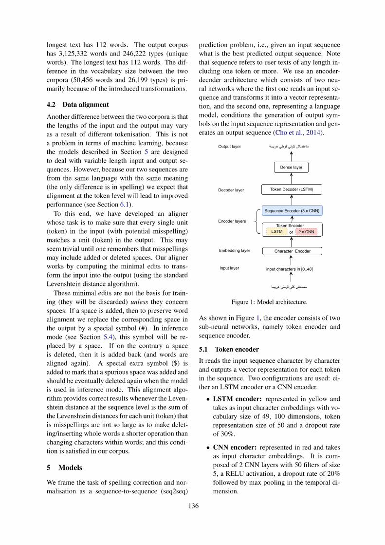
longest text has 112 words. The output corpushas 3,125,332 words and 246,222 types (uniquewords). The longest text has 112 words. The dif-ference in the vocabulary size between the twocorpora (50,456 words and 26,199 types) is pri-marily because of the introduced transformations.

4.2 Data alignment

Another difference between the two corpora is thatthe lengths of the input and the output may varyas a result of different tokenisation. This is nota problem in terms of machine learning, becausethe models described in Section 5 are designedto deal with variable length input and output se-quences. However, because our two sequences arefrom the same language with the same meaning(the only difference is in spelling) we expect thatalignment at the token level will lead to improvedperformance (see Section 6.1).

To this end, we have developed an alignerwhose task is to make sure that every single unit(token) in the input (with potential misspelling)matches a unit (token) in the output. This mayseem trivial until one remembers that misspellingsmay include added or deleted spaces. Our alignerworks by computing the minimal edits to trans-form the input into the output (using the standardLevenshtein distance algorithm).

These minimal edits are not the basis for train-ing (they will be discarded) unless they concernspaces. If a space is added, then to preserve wordalignment we replace the corresponding space inthe output by a special symbol (#). In inferencemode (see Section 5.4), this symbol will be re-placed by a space. If on the contrary a spaceis deleted, then it is added back (and words arealigned again). A special extra symbol ($) isadded to mark that a spurious space was added andshould be eventually deleted again when the modelis used in inference mode. This alignment algo-rithm provides correct results whenever the Leven-shtein distance at the sequence level is the sum ofthe Levenshtein distances for each unit (token) thatis misspellings are not so large as to make delet-ing/inserting whole words a shorter operation thanchanging characters within words; and this condi-tion is satisfied in our corpus.

5 Models

We frame the task of spelling correction and nor-malisation as a sequence-to-sequence (seq2seq)

prediction problem, i.e., given an input sequencewhat is the best predicted output sequence. Notethat sequence refers to user texts of any length in-cluding one token or more. We use an encoder-decoder architecture which consists of two neu-ral networks where the first one reads an input se-quence and transforms it into a vector representa-tion, and the second one, representing a languagemodel, conditions the generation of output sym-bols on the input sequence representation and gen-erates an output sequence (Cho et al., 2014).

Sequence Encoder (3 x CNN)

or

Token Decoder (LSTM)

Dense layer

معندناش كلي قوطى ھریسا

ماعندناش كولي قوطي ھریسة

Input layer

Embedding layer

Encoder layers

Decoder layer

Output layer

input characters in [0..48]

LSTM 2 x CNNToken Encoder

Character Encoder

Figure 1: Model architecture.

As shown in Figure 1, the encoder consists of twosub-neural networks, namely token encoder andsequence encoder.

5.1 Token encoderIt reads the input sequence character by characterand outputs a vector representation for each tokenin the sequence. Two configurations are used: ei-ther an LSTM encoder or a CNN encoder.

• LSTM encoder: represented in yellow andtakes as input character embeddings with vo-cabulary size of 49, 100 dimensions, tokenrepresentation size of 50 and a dropout rateof 30%.

• CNN encoder: represented in red and takesas input character embeddings. It is com-posed of 2 CNN layers with 50 filters of size5, a RELU activation, a dropout rate of 20%followed by max pooling in the temporal di-mension.

136

5.2 Sequence encoder

Represented in blue and consists of 3 CNN lay-ers with 200 filters for the two first layers and 100for the third layer, all filters have size 3, a RELUactivation and dropout rate of 5%.

5.3 Token decoder

It is composed of one character-based LSTM layerwith the same hyper-parameters as the LSTM en-coder, followed by a dense layer.

5.4 Training and inference

All models are trained end-to-end to maximise thelikelihood of the output sequence conditioned onthe input sequence for 150 epochs using a batchsize of 64 and Adam optimiser. Gradients with anorm greater than 5 are clipped.

For inference (generating an output charactersequence), we use beam-search with a size of 20.Note that beam-search is used only to generatean output sequence and does not influence nei-ther model training nor validation. The modelsgenerate characters starting from the start symbol(<) and stop at the end symbol (>) or at a prede-fined sequence length given as a hyper-parameter,whichever comes first.

6 Experiments and Results

In order to test our models and the gain from thealigner (see Section 4.2), we experiment with bothversions of data: the non-aligned and the aligneddata. It is worth mentioning that the only differ-ence between them is that the aligned one containsextra symbols (# and $) marking missing or extraspaces. An extra space – thus word– is also addedfor every dollar sign. Moreover, to measure the ef-fect of the context, we feed the data either token-by-token or sentence by sentence.

We split both the datasets into 75% (138,917samples) for training, 5% (9,261 samples) for de-velopment, and 20% (37,041 samples) for valida-tion. The reported hyper-parameters in Section 5were fine-tuned on the development set.

We conduct two evaluations: (i) how well thesuggested models perform on the seq2seq task,and (ii) how good is the best performing modelfor spelling correction and normalisation task, andwhat is its effect as a pre-processing step ondownstream tasks like Semantic Textual Similarity(STS). We evaluate (i) using character-level accu-racy, and we evaluate (ii) by calculating Precision,

Recall and the F-score for the class of tokens thatshould be changed. Hence, Recall is the ratio ofthe correctly changed tokens to the number of to-kens that should be changed, and Precision is theratio of the correctly changed tokens to the num-ber of tokens that are changed. F-score is the har-monic average of both.6.1 Comparing models on Seq2seq task

In Table 1 we report the overall character level ac-curacy of the 4 best performing models for eachconfiguration and experiment: (1) LSTM-Token-seq: the model with the Token LSTM + Sequenceencoder (yellow and blue parts of Figure 1) andToken decoder, (2) CNN-Token-seq: the modelwith the Token CNN + Sequence encoder (redand blue parts of Figure 1) and Token decoder.Both (1) and (2) are trained and evaluated on non-aligned data with a sequence of tokens as input.(3) CNN-Token-seq-alig the same as model (2) buttrained and evaluated on aligned data. (4) CNN-Token-token-alig: the same as (3) but with one to-ken as input (token-by-token).

Results indicate that the LSTM encoder in (1)does not suit our task / data and fails to learnthe sequential representations with an overall char-acter accuracy of only 23.90%. This could bebecause of the high sparsity of the data whichmakes it hard to learn regularities. In contrast, theCNN encoder in (2) performs much better, withan overall character accuracy of 89.20%, suggest-ing that learning sequences of patterns throughconvolutions suits better our task / data than se-quence modelling with LSTM. This is in line withwhat has been reported for machine translation in(Gehring et al., 2017).

The CNN encoder performs even better withthe aligned data in (3). The difference can be at-tributed to the positive effect of the aligner whichboosts the accuracy by 7%. The 9.1% drop in theaccuracy in (4) compared to (3) is due to the lackof word context. This indicates that word contextis essential, especially for word sense disambigua-tion in such highly varied data.

6.2 Quality and effect

• Quality We use the best performing model (3)and run the inference mode, (see Section 5.4),on the validation set which contains 567,308words of which 507,429 words are alreadycorrectly spelled and 59,880 words must bechanged, either corrected or normalised. We

137

Models Input Data Validation1 LSTM-Token-seq sequence of tokens non-aligned 23.902 CNN-Token-seq sequence of tokens non-aligned 89.203 CNN-Token-seq-alig sequence of tokens aligned 96.204 CNN-Token-token-alig one token aligned 87.10

Table 1: Accuracy of models (%) on Seq2seq task.

perform quantitative and qualitative analysisof the generated sequences in terms of thechanged spellings at a word level. Model (3)achieves an overall F-score of 64.74%, Recall of88.58% and Precision of 51.02% on the wordsto change. It correctly spells 53,041 wordsfrom the total words to change and fails to cor-rectly change 6,839 words. However, it in-troduces 50,914 incorrect changes (newly mis-spelled words or infelicitous corrections).

• Error analysis Examining the generated se-quences shows that most errors are at the levelof one character (duplicating or substituting onecharacter) and the generated words are verysimilar to the reference. This is similar to theconclusion of Tiedemann (2009) that many er-rors of a character level phrase-based statisticalmachine translation for Norwegian and Swedishare of small length. Furthermore, we find thatmost of the not properly corrected words ac-tually do not have enough representative in-stances, i.e., most of them occurred only oncein the validation data and were not seen duringthe training. The high sparsity of the data is aninteresting challenge for the current neural net-works for which more research is needed.

With the settings of our experiments, the highRecall of the model at a word level indicates thatit can be used for detecting errors and words tonormalise but not for automatically fixing thembecause of its low Precision. Actually the re-ported low Precision is not that dramatic as itmight seem because it is aggressive, i.e., a sin-gle wrong character means the entire word iswrong. Besides improving our inference set-tings, a better metric for evaluating such casesis needed.

• Effect We evaluate the effect of spelling correc-tion and normalisation, as a pre-processing stepfor downstream tasks, on detecting binary Se-mantic Textual Similarity. We chose this taskbecause it is one of the few available tasks for

ALG we are aware of. We apply our spellingcorrection and normalisation on the ALG datareported by (Adouane et al., 2019). We repli-cate the best performing model for which theauthors report an accuracy of 92.76%, and weget an accuracy of 94.40% with the same set-tings. The gain indicates that the spelling cor-rection and normalisation is potentially a usefulpre-processing step for downstream tasks.


We compiled a new parallel corpus for ALG withlinguistically motivated decisions for spelling cor-rection and normalisation. Considerations such asbeing practical to implement and suitability for ourgoals are taken into account. We designed, imple-mented and tested 2 deep neural network architec-tures trained end-to-end to capture the knowledgeencoded in the corrected and normalised corpus.The results showed that a CNN token-sequenceencoder and an LSTM decoder performed the bestwhen including context information. Additionally,applying a token aligner on the input data yieldedbetter performance compared to the non-aligneddata. Even though, with the current inference set-tings, the model generated some errors at a charac-ter level mainly due to the data sparsity, it is gen-eral and does not require extra resources except aparallel corpus. Hence it could be applied to otherlanguages with the same settings.

In future work, we plan to improve the currentinference mode by investigating other settings, im-prove the decoder by pre-training on the correctedand normalised data and a large MSA corpus toavoid generating incorrect character sequences.Moreover, we will evaluate the model extrinsicallyby using it to pre-process data for tasks such ascode-switch detection, and topic detection to seehow much it helps or hinders attempts to tacklethese tasks.

138

Acknowledgement

The research reported in this paper was supportedby a grant from the Swedish Research Council(VR project 2014-39) for the establishment of theCentre for Linguistic Theory and Studies in Prob-ability (CLASP) at the University of Gothenburg.We are grateful to the annotators and all peoplewho helped collecting the data. We also thank theanonymous reviewers for their useful comments.

ReferencesWafia Adouane, Jean-Philippe Bernardy, and Simon

Dobnik. 2018. Improving Neural Network Perfor-mance by Injecting Background Knowledge: De-tecting Code-switching and Borrowing in Alge-rian Texts. In Proceedings of the Third Workshopon Computational Approaches to Linguistic Code-Switching, pages 20–28. Association for Computa-tional Linguistics (ACL).

Wafia Adouane, Jean-Philippe Bernardy, and SimonDobnik. 2019. Neural Models for Detecting Bi-nary Semantic Textual Similarity for Algerian andMSA. In Proceedings of the Fourth Arabic NaturalLanguage Processing Workshop, pages 78–87, Flo-rence, Italy. Association for Computational Linguis-tics (ACL).

Dzmitry Bahdanau, Kyunghyun Cho, and YoshuaBengio. 2014. Neural Machine Translation byJointly Learning to Align and Translate. arXiv,arXiv:1409.0473.

Marcel Bollmann. 2019. A Large-scale Comparison ofHistorical Text Normalization Systems. In Proceed-ings of the 2019 Conference of the North AmericanChapter of the Association for Computational Lin-guistics: Human Language Technologies, Volume 1(Long and Short Papers), pages 3885–3898. Associ-ation for Computational Linguistics (ACL).

Kyunghyun Cho, Bart Van Merrienboer, Caglar Gul-cehre, Dzmitry Bahdanau, Fethi Bougares, Hol-ger Schwenk, and Yoshua Bengio. 2014. Learn-ing Phrase Representations using RNN Encoder–Decoder for Statistical Machine Translation. In Pro-ceedings of the 2014 Conference on Empirical Meth-ods in Natural Language Processing (EMNLP),pages 1724–1734, Doha, Qatar. Association forComputational Linguistics (ACL).

Gabriel Doyle. 2014. Mapping Dialectal Variation byQuerying Social Media. In Proceedings of the 14thConference of the European Chapter of the Associ-ation for Computational Linguistics, pages 98–106.Association for Computational Linguistics (ACL).

Jacob Eisenstein. 2013. Phonological Factors in SocialMedia Writing. In Proceedings of the Workshop onLanguage Analysis in Social Media, pages 11–19,Atlanta.

Ramy Eskander, Nizar Habash, Owen Rambow, andNadi Tomeh. 2013. Processing Spontaneous Or-thography. In Proceedings of the 2013 Conferenceof the North American Chapter of the Associationfor Computational Linguistics: Human LanguageTechnologies, pages 585–595. Association for Com-putational Linguistics (ACL).

Pravallika Etoori, Manoj Chinnakotla, and RadhikaMamidi. 2018. Automatic Spelling Correction forResource-scarce Languages Using Deep Learning.In Proceedings of Association for ComputationalLinguistics 2018, Student Research Workshop, pages146–152. Association for Computational Linguistics(ACL).

Jonas Gehring, Michael Auli, David Grangier, DenisYarats, and Yann N. Dauphin. 2017. ConvolutionalSequence to Sequence Learning. In Proceedingsof the 34th International Conference on MachineLearning, volume 70 of Proceedings of MachineLearning Research, pages 1243–1252, InternationalConvention Centre, Sydney, Australia. PMLR.

Shaona Ghosh and Per Ola Kristensson. 2017. Neu-ral Networks for Text Correction and Completion inKeyboard Decoding. arXiv, arXiv: 1709.06429.

Nizar Habash, Fadhl Eryani, Salam Khalifa, OwenRambow, Dana Abdulrahim, Alexander Erdmann,Reem Faraj, Wajdi Zaghouani, Houda Bouamor,Nasser Zalmout, Sara Hassan, Faisal Al shargi,Sakhar Alkhereyf, Basma Abdulkareem, Ramy Es-kander, Mohammad Salameh, and Hind Saddiki.2018. Unified Guidelines and Resources for Ara-bic Dialect Orthography. In Proceedings of theEleventh International Conference on Language Re-sources and Evaluation (LREC 2018), Miyazaki,Japan. European Language Resources Association(ELRA).

Sepp Hochreiter and Jurgen Schmidhuber. 1997.Long Short-Term Memory. Neural Computation,9(8):1735–1780.

Anna Jørgensen, Dirk Hovy, and Anders Søgaard.2015. Challenges of Studying and Processing Di-alects in Social Media. In Proceedings of the Work-shop on Noisy User-generated Text, pages 9–18. As-sociation for Computational Linguistics (ACL).

Armand Joulin, Edouard Grave, Piotr Bojanowski, andTomas Mikolov. 2016. Bag of Tricks for EfficientText Classification. arXiv, arXiv:1607.01759.

James Milroy. 2001. Language Ideologies and theConsequence of Standardization. Journal of Soci-olinguistics, 5:530 – 555.

Behrang Mohit, Alla Rozovskaya, Nizar Habash, Wa-jdi Zaghouani, and Ossama Obeid. 2014. The FirstQALB Shared Task on Automatic Text Correctionfor Arabic. In Proceedings of the EMNLP 2014Workshop on Arabic Natural Langauge Processing(ANLP), pages 39–47, Doha, Qatar.

139

Eva Pettersson. 2016. Spelling Normalisation and Lin-guistic Analysis of Historical Text for InformationExtraction. PhD thesis, Studia Liguistica Upsalien-sia 17, Uppsala: Acta Universitatis Upsaliensis.

Houda Saadane and Nizar Habash. 2015. A Conven-tional Orthography for Algerian Arabic. In Proceed-ings of the Second Workshop on Arabic Natural Lan-guage Processing, ANLP, ACL 2015, Beijing, China,July 30, 2015, pages 69–79. Association for Compu-tational Linguistics (ACL).

Khaled Shaalan, Mohammed Attia, Pavel Pecina,Younes Samih, and Josef van Genabith. 2012.Arabic Word Generation and Modelling for SpellChecking. In Proceedings of the Eight InternationalConference on Language Resources and Evaluation(LREC’12), Istanbul, Turkey. European LanguageResources Association (ELRA).

S. Sooraj, K. Manjusha, M. Kumar, and K.P. So-man. 2018. Deep Learning Based Spell Checkerfor Malayalam Language. Journal of Intelligent &Fuzzy Systems, 34:1427–1434.

Ilya Sutskever, Oriol Vinyals, and Quoc V. Le. 2014.Sequence to Sequence Learning with Neural Net-works. In Advances in Neural Information Process-ing Systems 27: Annual Conference on Neural In-formation Processing Systems 2014, December 8-13 2014, Montreal, Quebec, Canada, pages 3104–3112.

Jorg Tiedemann. 2009. Character-based PSMT forClosely Related Languages. In Proceedings of 13thAnnual Conference of the European Associationfor Machine Translation, pages 12–19, Barcelona,Spain.

Oriol Vinyals, Alexander Toshev, Samy Bengio, andDumitru Erhan. 2015. Show and Tell: A NeuralImage Caption Generator. In Computer Vision andPattern Recognition.

Janet C. E. Watson. 2007. The Phonology and Mor-phology of Arabic. The Phonology of the World’sLanguages. OUP Oxford.

140


Dialect Text Normalization to Normative Standard Finnish

Niko PartanenDepartment of Finnish,

Finno-Ugrianand Scandinavian Studies

University of Helsinki

Mika HamalainenDepartment of Digital

HumanitiesUniversity of Helsinki

[email protected]

Khalid AlnajjarDepartment of Computer Science

University of Helsinki

AbstractWe compare different LSTMs and transformermodels in terms of their effectiveness in nor-malizing dialectal Finnish into the normativestandard Finnish. As dialect is the commonway of communication for people online inFinnish, such a normalization is a necessarystep to improve the accuracy of the existingFinnish NLP tools that are tailored for norma-tive Finnish text. We work on a corpus consist-ing of dialectal data from 23 distinct Finnishdialect varieties. The best functioning BRNNapproach lowers the initial word error rate ofthe corpus from 52.89 to 5.73.

1 Introduction

Normalization is one of the possible pre-processing steps that can be applied to various texttypes in order to increase their compatibility withtools designed for the standard language. This ap-proach can be taken in an essentially similar man-ner with dialectal texts, historical texts or collo-quial written genres, and can be beneficial alsoas one processing step with many types of spokenlanguage materials.

Our study focuses to the normalization of di-alect texts, especially within the format of tran-scribed dialectal audio recordings, published pri-marily for linguistic research use. However, thedialectal correspondences in this kind of materialare comparable to phenomena in other texts wheredialectal features occur, the results are expected tobe generally applicable.

This paper introduces a method for dialect tran-script normalization, which enables the possibilityto use existing NLP tools targeted for normativeFinnish on these materials. Previous work con-ducted in English data indicates that normaliza-tion is a viable way of improving the accuracy ofNLP methods such as POS tagging (van der Gootet al., 2017). This is an important motivation as the

non-standard colloquial Finnish is the de facto lan-guage of communication on a multitude of internetplatforms ranging from social media to forums andblogs. In its linguistic form, the colloquial dialec-tal Finnish deviates greatly from the standard nor-mative Finnish, a fact that lowers the performanceof the existing NLP tools for processing Finnishon such text.

2 Related work

Automated normalization has been tackled in thepast many times especially in the case of histori-cal text normalization. A recent meta-analysis onthe topic (Bollmann, 2019) divides the contempo-rary approaches into five categories: substitutionlists like VARD (Rayson et al., 2005) and Norma(Bollmann, 2012), rule-based methods (Baronand Rayson, 2008; Porta et al., 2013), edit dis-tance based approaches (Hauser and Schulz, 2007;Amoia and Martinez, 2013), statistical methodsand most recently neural methods.

For statistical methods, the most prominent re-cent ones have been different statistical machinetranslation (SMT) based methods. These methodsoften assimilate the normalization process with aregular translation process by training an SMTmodel on a character level. Such methods havebeen used for historical text (Pettersson et al.,2013; Hamalainen et al., 2018) and contemporarydialect normalization (Samardzic et al., 2015).

Recently, many normalization methods utilizedneural machine translation (NMT) analogously tothe previous SMT based approaches on a char-acter level due to its considerable ability in ad-dressing the task. Bollmann and Søgaard (2016)have used a bidirectional long short-term mem-ory (bi-LSTM) deep neural network to normalizehistorical German on a character level. The au-thors have also tested the efficiency of the model

141

when additional auxiliary data is used during thetraining phase (i.e. multi-task learning). Based ontheir benchmarks, normalizations using the neuralnetwork approach outperformed the ones by con-ditional random fields (CRF) and Norma, wheremodels trained with the auxiliary data generallyhad the best accuracy.

Tursun and Cakici (2017) test out LSTM andnoisy channel model (NCM), a method commonlyused for spell-checking text, to normalize Uyghurtext. In addition to the base dataset (≈ 200sentences obtained from social networks, auto-matically and manually normalized), the authorshave generated synthetic data by crawling newswebsites and introducing noise in it by substitut-ing characters with their corresponding corruptedcharacters at random. Both of the methods havenormalized the text with high accuracy which il-lustrates the their effectiveness. Similarly, Man-dal and Nanmaran (2018) had employed an LSTMnetwork and successfully normalized code-mixeddata with an accuracy of 90.27%.

A recent study on historical English letters(Hamalainen et al., 2019) compares differentLSTM architectures finding that bi-directional re-current neural networks (BRNN) work better thanone-directional RNNs, however different attentionmodels or deeper architecture do not have a posi-tive effect on the results. Also providing additionaldata such as social metadata or century informa-tion makes the accuracy worse. Their findingssuggest that post-processing is the most effectiveway of improving a character level NMT normal-ization model. The same method has been suc-cessfully applied in OCR post-correction as well(Hamalainen and Hengchen, 2019).

3 Data

Finnish dialect materials have been collected sys-tematically since late 1950s. These materials arecurrently stored in the Finnish Dialect Archivewithin Institute for the Languages of Finland, andthey amount all in all 24,000 hours. The ini-tial goal was to record 30 hours of speech fromeach pre-war Finnish municipality. This goal wasreached in the 70s, and the work evolved towardmaking parts of the materials available as pub-lished text collections. Another approach that wasinitiated in the 80s was to start follow-up record-ings in the same municipalities that were the tar-gets of earlier recording activity.

Later the work on these published materials hasresulted in multiple electronic corpora that are cur-rently available. Although they represent only atiny fraction of the entire recorded material, theyreach remarkable coverage of different dialectsand varieties of spoken Finnish. Some of thesecorpora contain various levels of manual annota-tion, while others are mainly plain text with as-sociated metadata. Materials of this type can becharacterized by an explicit attempt to representdialects in linguistically accurate manner, havingbeen created primarily by linguists with formaltraining in the field. These transcriptions are usu-ally written with a transcription systems specificfor each research tradition. The result of this typeof work is not simply a text containing some di-alectal features, but a systematic and scientifictranscription of the dialectal speech.

The corpus we have used in training and testingis the Samples of Spoken Finnish corpus (Institutefor the Languages of Finland, 2014). It is one ofthe primary traditional Finnish dialect collections,and one that is accompanied with hand-annotatednormalization into standard Finnish. The size ofcorpus is 696,376 transcribed words, of which684,977 have been normalized. The corpus cov-ers 50 municipalities, and each municipality hastwo dialect samples. The materials were originallypublished in a series between 1978-2000. Thegoal was to include various dialects systematicallyand equally into the collection. The modern dig-ital corpus is released under CC-BY license, andis available with its accompanying materials anddocumentation in the Language Bank of Finland.1

The data has been tokenized and the normativespellings have been aligned with the dialectal tran-scriptions on a token level. This makes our taskwith normalization model easier as no preprocess-ing is required. We randomly sort the sentences inthe data and split them into a training (70% of thesentences), validation (15% of the sentences) andtest (15% of the sentences) sets.

4 Dialect normalization

Our approach consists of a character level NMTmodel that learns to translate the dialectal Finnishto normative spelling. We experiment with twodifferent model types, one being an LSTM basedBRNN (bi-directional recurrent neural network)approach as taken by many in the past, and the

1http://urn.fi/urn:nbn:fi:lb-201407141

142

other is a transformer model as it has been reportedto outperform LSTMs in many other sequence-to-sequence tasks.

For the BRNN model, we use mainly the Open-NMT (Klein et al., 2017) defaults. This means thatthere are two layers both in the encoder and the de-coder and the attention model is the general globalattention presented by Luong et al. (2015). Thetransformer model is that of Vaswani et al. (2017).Both models are trained for the default 100,000training steps.

We experiment with three different ways oftraining the models. We train a set of models ona word level normalization, which means that thesource and target consist of single words split intocharacters by white spaces. In order to make themodels more aware of the context, we also train aset of models on chunked data. This means thatwe train the models by feeding in 3 words at atime; the words are split into characters and theword boundaries are indicated with an underscorecharacter ( ). Lastly we train one set of modelson a sentence level. In this case the models aretrained to normalize full sentences of words splitinto characters and separated by underscores.

In terms of the size of the training data, the wordlevel data consists of 590k, the chunk level of 208kand the sentence level of 35k parallel rows. All ofthe models use the same split of training, testingand validation datasets as described earlier. Theonly difference is in how the data is fed into themodels.

5 Results & Evaluation

We evaluate the methods by counting the word er-ror rate2 (WER) of their output in comparison withthe test dataset. WER is a commonly used metricto assess the accuracy of text normalization.

Table 1 shows the WERs of the different meth-ods. The initial WER of the non normalized di-alectal text in comparison with the normalized textis shown in the column No normalization. As wecan see from this number, the dialectal text is verydifferent from the standardized spelling. Both theword level and chunk level normalization methodsreach to a very high drop in the WER meaning thatthey manage to normalize the text rather well. Outof these, the chunk level BRNN achieves the bestresults. The performance is the worst in the sen-

2We use the implementation provided inhttps://github.com/nsmartinez/WERpp

tence level models, even to a degree that the trans-former model manages to make the WER higherthan the original.

5.1 Error analysis

Table 2 illustrates the general performance of themodel, with errors marked in bold. The examplesentence fragments are chosen by individual fea-tures they exhibit, as well as by how well they rep-resent the corpus data.

Since the model accuracy is rather high, the er-rors are not very common in the output. We canalso see clearly that the chunk model is able to pre-dict the right form even when form is reduced toone character, as on line 5.

Since the dialectal variants often match the stan-dard Finnish, over half of the forms need nochanges. The model learns this well. Vast ma-jority of needed changes are individual insertions,replacements or deletions in the word end, as il-lustrated in Table 2 at lines 2, 4, 6, 7, 15, 16, 17and 18. However, also word-internal changes arecommon, as shown at lines 11 and 12. Some dis-tinct types of common errors can be detected, andthey are discussed below.

In some cases the errors are clearly connectedto the vowel lengthening that does not mark or-dinary phonological contrast. Line 3 shows howthe dialectal pronoun variant of he ‘he / she’, het,is occasionally present in dialect material as heet,possibly being simply emphasized in a way thatsurfaces with an unexpected long vowel. This kindof sporadic vowel lengthening is rare, but seems tolead regularly to a wrong prediction, as these pro-cesses are highly irregular. This example also il-lustrates that when the model is presented a rare orunusual form, it seems to have a tendency to returnprediction that has overgone no changes at all.

The model seems to learn relatively well thephonotactics of literary Finnish words. However,especially with compounds it shows a trait to clas-sify word boundaries incorrectly. A good exam-ple of this is ratapolokyntervaau

ˇs””kon ‘railroad

tie treatment machine’, for which the correct anal-ysis would be ‘rata#polkyn#tervaus#kone’3, butthe model proposes ‘rata#polkyn#terva#uskoinen’which roughly translates as ‘railroad tie creosotebeliever’. The latter variant is semantically quiteawkward, but morphologically possible. This

3Here # is used for the illustrative purpose to indicateword boundaries within the compound

143

No normalization Words Chunks of 3 SentencesBRNN Transformer BRNN Transformer BRNN Transformer

WER 52.89 6.44 6.34 5.73 6.1 46.52 53.23

Table 1: The word error rates of the different models in relation to the test set

source correct target prediction1 joo joo joo2 ettE etta etta3 heet he heet4 uskovah uskovat uskovat5 n niin niin6 <ettE etta etta7 sinn sinne sinne8 <ei ei ei9 ole ole ole

10 , , ,11 kukhaan kukaan kukaan12 ymmartanny ymmartanyt ymmartanyt13 menna menna menna14 . . .15 ArtjarveN Artjarven Artjarven16 kirkolt kirkolta kirkolta17 mennah mennaan mennaan18 sinneh sinne sinne19 Hiitelah Hiitelaan Hiitelassa

Table 2: Examples from input, output and prediction

phonotactic accuracy makes selection of correctanalysis from multiple predicted variants more dif-ficult, as it is not possible to easily detect mor-phologically valid and invalid forms. The longerwords such as this also have more environmentswhere normalization related changes have to bedone, which likely makes their correct predictionincreasingly difficult.

In word level model there are various errors re-lated to morphology that has eroded from the di-alectal realizations of the words, or correspond toa more complicated sequences. Long vowel se-quences in standard Finnish often correspond todiphthongs or word internal -h- characters, andthese multiple correspondence patterns may bechallenging for the model to learn. Chunk modelperforms few percentages better than word modelin predictions where long vowel sequences arepresent, which could hint that the model bene-fits from wider syntactic window the neighbouringwords can provide. On line 19 a case of wronglyselected spatial case is illustrated.

There are cases where dialectal wordforms areambiguous without context, i.e. standard Finnishcases adessive (-lla) and allative (-lle) are bothmarked with single character (-l). Various sandhi-phenomena at the word boundary also blurren thepicture by introducing even more possible inter-pretations, such as vuoristol laitaa, where the cor-rect underlying form of the first element wouldbe vuoriston ‘mountain-GEN’. The decision aboutcorrect form cannot be done with information pro-vided only by single forms in isolation. The chunklevel model shows small but consistent improve-ments in these cases. This is expected, as the wordlevel model simply has no context to make the cor-rect prediction.

It is important to note that since the modelis trained on linguistic transcriptions, its perfor-mance is also limited to this context. For example,in the transcriptions all numbers, such as years anddates, are always written out as words. Therebythe model has never seen a number, and is doesn’tprocess them either. Improving the model withadditional training data that accounts this phe-nomena should, on the other hand, be relativelystraightforward. Similarly the model has had onlyvery limited exposure to upper case characters andsome of the punctuation characters used in ordi-nary literary language, which should all be takeninto account when attempting to use the modelwith novel datasets.

6 Conclusion & Future work

The normalization method we have proposedreaches remarkable accuracy with this dialectaltranscription dataset of spoken Finnish. The er-ror rate is so low that even if manual normaliza-tion would be the ultimate target, doing this incombination with our approach would make thework manifold faster. We have tested the resultswith large enough material that we assume simi-lar method would work in other conditions wheresame preliminary conditions are met. These aresufficiently large amount of training data and sys-tematic transcription system used to represent thedialectal speech.

144

Future work needs to be carried out to evaluatethe results on different dialectal Finnish datasets,many of which have been created largely withinthe activities described earlier, but which are alsocontinuously increasing as research on Finnish is avery vibrant topic in Finland and elsewhere. Thismethod could also be a very efficient in increas-ing the possibilities for natural language process-ing of other contemporary spoken Finnish texts.Our method could also be easily used within OCRcorrection workflows, for example, as a step afterautomatic error correction.

Situation is essentially similar, to our knowl-edge, also in other countries with comparable his-tory of dialectal text collection. Already withinFinnish archives there are large collections of di-alectal transcriptions in Swedish, as well as in theendangered Karelian and Sami languages. Apply-ing our method into these resources would also di-rectly improve their usability. However, it has tobe kept in mind that our work has been carried outin a situation where the manually annotated train-ing data is exceptionally large. In order to under-stand how widely applicable our method is for anendangered language setting, it would be impor-tant to test further how well the model performswith less data.

The performance with less data is especiallycrucial with low-resource languages. Many en-dangered languages around the world have textcollections published in the last centuries, which,however, customarily use a linguistic transcriptionsystem that deviates systematically from the cur-rent standard orthography. Such a legacy data canbe highly useful in language documentation workand enrich modern corpora, but there are chal-lenges in normalization and further processing ofthis data (Blokland et al., 2019). The approachpresented in our paper could be applicable intosuch data in various language documentation sit-uations, and the recent interest the field has dis-played toward language technology creates goodconditions for further integration of these methods(Gerstenberger et al., 2016).

We have released the chunk-level BRNN nor-malization model openly on GitHub as a part of anopen-source library called Murre4. We hope thatthe normalization models developed in this paperare useful for other researchers dealing with a va-riety of downstream Finnish NLP tasks.

4https://github.com/mikahama/murre

7 Acknowledgements

Niko Partanen’s work has been conducted withinthe project Language Documentation meets Lan-guage Technology: The Next Step in the Descrip-tion of Komi, funded by the Kone Foundation.

ReferencesMarilisa Amoia and Jose Manuel Martinez. 2013. Us-

ing comparable collections of historical texts forbuilding a diachronic dictionary for spelling normal-ization. In Proceedings of the 7th workshop on lan-guage technology for cultural heritage, social sci-ences, and humanities, pages 84–89.

Alistair Baron and Paul Rayson. 2008. VARD2: A toolfor dealing with spelling variation in historical cor-pora. In Postgraduate conference in corpus linguis-tics.

Rogier Blokland, Niko Partanen, Michael Rießler, andJoshua Wilbur. 2019. Using computational ap-proaches to integrate endangered language legacydata into documentation corpora: Past experiencesand challenges ahead. In Workshop on Computa-tional Methods for Endangered Languages, Hon-olulu, Hawai’i, USA, February 26–27, 2019, vol-ume 2, pages 24–30. University of Colorado.

Marcel Bollmann. 2012. (Semi-)automatic normaliza-tion of historical texts using distance measures andthe Norma tool. In Proceedings of the Second Work-shop on Annotation of Corpora for Research in theHumanities (ACRH-2), Lisbon, Portugal.

Marcel Bollmann. 2019. A large-scale comparison ofhistorical text normalization systems. In Proceed-ings of the 2019 Conference of the North AmericanChapter of the Association for Computational Lin-guistics: Human Language Technologies, Volume 1(Long and Short Papers), pages 3885–3898, Min-neapolis, Minnesota. Association for ComputationalLinguistics.

Marcel Bollmann and Anders Søgaard. 2016. Im-proving historical spelling normalization with bi-directional LSTMs and multi-task learning. In Pro-ceedings of COLING 2016, the 26th InternationalConference on Computational Linguistics: Techni-cal Papers, pages 131–139, Osaka, Japan. The COL-ING 2016 Organizing Committee.

Ciprian Gerstenberger, Niko Partanen, MichaelRießler, and Joshua Wilbur. 2016. Utilizinglanguage technology in the documentation ofendangered Uralic languages. Northern EuropeanJournal of Language Technology, 4:29–47.

Rob van der Goot, Barbara Plank, and Malvina Nis-sim. 2017. To normalize, or not to normalize: Theimpact of normalization on Part-of-Speech tagging.In Proceedings of the 3rd Workshop on Noisy User-generated Text, pages 31–39.

145

Mika Hamalainen and Simon Hengchen. 2019. Fromthe Paft to the Fiiture: a fully automatic NMTand Word Embeddings Method for OCR Post-Correction. In Recent Advances in Natural Lan-guage Processing, pages 432–437. INCOMA.

Mika Hamalainen, Tanja Saily, Jack Rueter, JorgTiedemann, and Eetu Makela. 2018. Normalizingearly English letters to present-day English spelling.In Proceedings of the Second Joint SIGHUM Work-shop on Computational Linguistics for CulturalHeritage, Social Sciences, Humanities and Litera-ture, pages 87–96.

Mika Hamalainen, Tanja Saily, Jack Rueter, JorgTiedemann, and Eetu Makela. 2019. RevisitingNMT for normalization of early English letters. InProceedings of the 3rd Joint SIGHUM Workshopon Computational Linguistics for Cultural Heritage,Social Sciences, Humanities and Literature, pages71–75, Minneapolis, USA. Association for Compu-tational Linguistics.

Andreas W Hauser and Klaus U Schulz. 2007. Unsu-pervised learning of edit distance weights for retriev-ing historical spelling variations. In Proceedings ofthe First Workshop on Finite-State Techniques andApproximate Search, pages 1–6.

Institute for the Languages of Finland. 2014.Suomen kielen naytteita - Samples of Spo-ken Finnish [online-corpus], version 1.0.http://urn.fi/urn:nbn:fi:lb-201407141.

Guillaume Klein, Yoon Kim, Yuntian Deng, JeanSenellart, and Alexander M. Rush. 2017. Open-NMT: Open-Source Toolkit for Neural MachineTranslation. In Proc. ACL.

Minh-Thang Luong, Hieu Pham, and Christopher DManning. 2015. Effective approaches to attention-based neural machine translation. arXiv preprintarXiv:1508.04025.

Soumil Mandal and Karthick Nanmaran. 2018. Nor-malization of transliterated words in code-mixeddata using Seq2Seq model & Levenshtein distance.In Proceedings of the 2018 EMNLP Workshop W-NUT: The 4th Workshop on Noisy User-generatedText, pages 49–53, Brussels, Belgium. Associationfor Computational Linguistics.

Eva Pettersson, Beata Megyesi, and Jorg Tiedemann.2013. An SMT approach to automatic annotationof historical text. In Proceedings of the workshopon computational historical linguistics at NODAL-IDA 2013; May 22-24; 2013; Oslo; Norway. NEALTProceedings Series 18, 087, pages 54–69. LinkopingUniversity Electronic Press.

Jordi Porta, Jose-Luis Sancho, and Javier Gomez.2013. Edit transducers for spelling variation in OldSpanish. In Proceedings of the workshop on compu-tational historical linguistics at NODALIDA 2013;

May 22-24; 2013; Oslo; Norway. NEALT Proceed-ings Series 18, 087, pages 70–79. Linkoping Univer-sity Electronic Press.

Paul Rayson, Dawn Archer, and Nicholas Smith. 2005.VARD versus WORD: a comparison of the UCRELvariant detector and modern spellcheckers on en-glish historical corpora. Corpus Linguistics 2005.

Tanja Samardzic, Yves Scherrer, and Elvira Glaser.2015. Normalising orthographic and dialectal vari-ants for the automatic processing of Swiss German.In Proceedings of the 7th Language and TechnologyConference. ID: unige:82397.

Osman Tursun and Ruket Cakici. 2017. Noisy Uyghurtext normalization. In Proceedings of the 3rd Work-shop on Noisy User-generated Text, pages 85–93,Copenhagen, Denmark. Association for Computa-tional Linguistics.


146


Abstract

In relevance classification, we hope to

judge whether some utterances expressed

on a topic are relevant or not. A usual

method is to train a specific classifier

respectively for each topic. However, in

that way, it easily causes an underfitting

problem in supervised learning model,

since annotated data can be insufficient for

every single topic. In this paper, we explore

the common features beyond different

topics and propose our cross-topic

relevance embedding aggregation

methodology (CREAM) that can expand

the range of training data and apply what

has been learned from source topics to a

target topic. In our experiment, we show

that our proposal could capture common

features within a small amount of

annotated data and improve the

performance of relevance classification

compared with other baselines.

1 Introduction

Relevance classification is a task of automatically

distinguishing relevant information for a specific

topic (Kimura et al., 2019). It can be regarded as a

preprocessing task of stance detection, since

potential stances should be refined into relevant

ones to improve accuracy and efficiency. In Table

1, we show a simple example of relevance

classification task in NTCIR-14.

Here utterance1 is relevant to the topic not only

for the contained topic words but also for its related

semantics, and then we could leverage its features

available for further stance detection. On the

contrary, utterance2 is irrelevant to the topic, and

its further calculation of stance detection is

meaningless. Previously, the relevance task could

be approached in an unsupervised way by

calculating pairwise semantic distances between

topic and utterance (Achananuparp et al., 2008;

Kusner et al., 2015). However, in most instances,

their performance is not as good as a supervised

approach. As to the supervised method,

traditionally, a specific topic-oriented classifier

could be trained for prediction on a single topic

(Hasan and Ng, 2013; Y Wang et al., 2017), but this

method actually builds up an isolation among

different topics and wastes existing annotated data

for new predictions.

Cross-topic classification, which enables the

classifier to adapt different topics even in different

domains, is an alternative to a supervised approach

(Augenstein et al., 2016; Xu et al., 2018). It allows

the model to assimilate the common features from

existing topics and make inferences for a new topic.

For example, in the NTCIR-14 relevance

classification task, we could start with an existing

classifier containing a well-prepared set of ground-

truth data from some other Tsukiji Market history

or economic topics, to give a prediction about

Tsukiji Market relocation topic.

In this paper, aiming to alleviate insufficient

annotated data problems for a specific topic, we

have concentrated on cross-topic relevance

classification by our novel CREAM proposal. The

basic idea of the CREAM method is to capture the

common pairwise features between existing topic

and utterance, and then apply them to relevance

prediction on a target topic. By analyzing F1-

scores in experiment results, we have known that

CREAM has shown its better performance on a

known topic’s relevance classification compared

with baselines. In addition, an associated value to

A Cross-Topic Method for Supervised Relevance Classification

Jiawei Yong

[email protected]

Ricoh Company, Ltd.

Topic: we should move Tsukiji Market to Toyosu.

Utterance1: I do not agree to move Tsukiji Market

because of its long history. Relevance: relevant

Utterance2: The number of foreign tourists to Japan

has been on the rise. Relevance: irrelevant

Table 1: An example of relevance classification.

147

the unknown topic relevance has also been

evaluated.

2 Related Work

To establish a cross-topic relevance classification

model for supervised learning, here we regard it as

a two-step procedure including pairwise text

embedding and binary text classifier. Besides, the

literatures around stance detection bright us

inspiration as well.

2.1 Text Embedding

There are 3 well-known embedding methods

named Word2Vec (Mikolov et al., 2013), GloVe

(Pennington et al., 2014) and fastText (Joulin et al.,

2016) for word-level representation. Although

GloVe and fastText show higher performance on

some specific aspects, there's no escaping the fact

that Word2Vec (CBOW, Skip-Gram) is most

popular and widely used among different

languages. As to sentence-level embeddings, the Word2Vec

inventor Mikolov proposed doc2vec (Quoc et al.,

2014), as its name implies, to learn sentence or

document embeddings. What’s more, averaged

word embeddings (Han and Baldwin, 2016) is also

a common sentence-level embedding method.

2.2 Text Classifier

There are several classical ML/DL models utilized

for text classification such as Support Vector

Machine (SVM) (Vapnik, 1998; Vapnik, 2013),

and an RNN variant Long Short-term Memory

(LSTM) (Hochreiter and Schmidhuber, 1997). It is

noteworthy that SVM has an advantage in

processing low-resource data.

Besides, nowadays we also could utilize a pre-

trained model such as BERT (Devlin et al., 2018)

or ELMO (Matthew et al., 2018) as a contextual

text classifier. However, note that they are always

pre-trained by a tremendous amount of open data

(E.X. Wikipedia), we still need fine-tuning data on

a large scale for root domain recognition.

2.3 Stance Detection

Stance detection, which is the task of classifying

the attitude expressed in text towards a target, also

provides us with valuable inspiration on text

classification. For example, Augenstein

(Augenstein et al., 2016) tried to utilize conditional

LSTM encoding to build a representation for

stance and target independently, and an end-to-end

memory network (Mohtarami et al., 2018), which

integrates CNN with LSTM, has also been

presented to solve this classification task. What’s

more, a simple but tough-to-beat baseline (Riedel

et al., 2017) shows the potential of TF-IDF and

cosine similarity on this pairwise classification

task. Note that relevance classification can be

regarded as a preprocessing of stance detection,

since irrelevant stances should be excluded before

being classified into support, against or even a

neutral stance.

3 Methodology

In this section, we would like to give a

comprehensive introduction about our proposed

cross-topic method CREAM, for supervised

relevance classification. The overall architecture of

CREAM is depicted in Figure 1. As described in

the previous section, we briefly divide the whole

model into 2 parts including text embedding and

text classifier. In the text embedding part, we have

implemented Word Embedding Layer and

Sentence Aggregation Layer, and as to the text

classifier, the SVM Layer and Prediction Layer

would achieve their functions. The expected input

includes a pair of topic text and topic-oriented

utterance in the same domain, and the output

would be predicted binary relevance label. In the

following, we would illustrate the implementation

details of each layer in CREAM.

3.1 Word Embedding Layer

Here we adopt pre-trained Word2Vec embeddings

to represent each word of two inputs (a topic text T

containing n words and a topic-oriented utterance

U, e.g., topic and utterance1 in Table 1). Note that

utterance could be much longer than topic text, so

here we select the same number of words as topic

T from utterance U. For each selected word of T,

Figure 1: The overall architecture of CREAM.

148

we select one word with the highest Word2Vec

similarity from U. The outputs of this layer are two

sequences of word vectors with the same length

1{ ,...., }nT t t→ →

= and 1{ ,..., }nU u u→ →

= .

3.2 Sentence Aggregation Layer

The sentence aggregation layer is the key to our

cross-topic method CREAM. Here we manage to

aggregate topic and utterance vectors by two steps

to represent common features.

Separated Aggregation: In this step, we aim to

provide a sentence-level embedding for T and U

respectively. Here we separately aggregate T

word vectors for topic and utterance by averaged

word embeddings:

n

iit

Tn

→

→

=

n

iiu

Un

→

→

= (1)

Topic-Utterance Aggregation: Here we further

concentrate on applying an aggregation between

topic and utterance to represent the common

features of relevance. As we have known there

exists a classical conclusion from Word2Vec:

king man woman queen→ → → →

− + = , we could get an inference

that there exist some common features between

word pairs (king, man) and (queen, woman) since king man queen woman→ → → →

− = − is still workable.

As to sentence-level relevance classification,

here we also conduct a vector subtraction between

topic T→

and utterance U→

to represent relevance

vector R→

as below.

T UR

T

→ →→ −= (2)

It is noteworthy that here we normalize each

dimension value of relevance vector R→

by

dividing T to limit the subtraction result in the

same range. Therefore, assuming that we have a

relevance vector 1R→

(topic1) and 2R→

(topic2), they

would be treated equally for the same cross-topic

training if they all denote the same relevant

relationship (e.g., 1R→

represents a utterance is

relevant to topic1, 2R→

represents another utterance

is relevant to topic2).

3.3 Cross-Topic SVM Layer

In this layer, we decide to adopt a supervised

learning model SVM for cross-topic binary

classification. The reason is because of low-

resource data we have stated in chapter 2.2. In our

case, SVM can efficiently perform a non-linear

classification using kernel function (Mark et al.,

1964) to fit the maximum-margin hyperplane in a

transformed feature space. Here the following

sigmoid kernel function for relevance vectors 1R

→

and 2R

→ makes SVM acted as multi-layer neural

networks even they are different topics.

1 2 1 2( , ) tanh( )K R R a R R b

→→ → →= − (3)

After applying the kernel function, the target

function of maximum-margin hyperplane could be

written in:

* *( ( , ) )i i i

i S

y sign t K R x h→

= − (4)

Here ℎ∗, 𝛼∗ are optimal parameters to distinguish

binary hyperplane, and t is the correct class label

for training.

3.4 Prediction Layer

We predict the relevance label of each topic-

utterance pair via sigmoid-fitting method:

1

1 exp( + )i

i

pAy B

=+ (5)

Where we apply the sigmoid operation to get the

predicted probability for relevant and irrelevant

classes with parameters A and B.

4 Experiments

In this section, we would introduce the evaluation

results of our proposed methodology. We have

evaluated our CREAM on the NTCIR-14 QALab

dataset (Kimura et al., 2019). Note that NTCIR-14

QALab dataset maybe is the first dataset focusing

on relevance classification besides fact-check and

stance detection. Besides our own method, we

have also taken three baseline approaches to cross-

topic relevance classification.

Word Mover’s Distance (WMD): this classical

unsupervised learning method is often utilized to

calculate a word travel cost between two

documents. Here we predict the relevance label

based on switch cost boundary from utterance to its

topic.

Bidirectional LSTM (BiLSTM): this approach

receives encoded-word sequences (topic and

utterance) and makes a concatenation to merge

them into one sequence. Finally, the concatenated

vector would be fed into its prediction layer to give

a relevance label prediction.

BERT: There is no doubt that BERT is the state-

of-the-art model to solve NLP issues such as text

classification. It is well-known that BERT could

receive pairwise texts as inputs and output the label

between them. Therefore, BERT is also applicable

to this relevance classification theoretically. Here

149

we beforehand input labelled topic and utterance

separately into pre-trained BERT for fine-tuning.

4.1 Experiment dataset

NTCIR-14 QALab: This dataset is a Japanese

collection for the relevance classification task,

which contains around 10000 topic-oriented

utterances on 14 different topics. Although task

organizers do manual labeling by crowdsourcing,

it is still difficult to provide an even larger amount

of labeled dataset for each topic. Therefore, the

traditional method with low-resource data would

easily cause an underfitting problem.

4.2 Experiment Setup

Our initial word embeddings are obtained from the

pre-trained Wikipedia word vectors (Suzuki et al.,

2016).

In experiment 1, we divide our dataset into

training data (1620) and test data (180) with the

proportion 9:1. Note that there is no new topic in

test data of experiment 1 since all topics have been

included for training in the learning phase.

In experiment 2, we hope to verify the

performance of our method compared with others

on unknown topic relevance prediction. Therefore,

we extract 13 topics’ data for training to predict the

last one topic in cross-validation.

4.3 Experiment Results

We mainly use F1-score to evaluate classification

performance. Figure 2 illustrates the F1-score and

averaged precision/recall as well among four

methods in experiment 1, and the averaged

evaluation results of cross-validation in

experiment 2 have been summarized in Figure 3.

Furthermore, the relationship between the

threshold of word mover’s distance and F1 score is

shown as an example in Figure 4. We just go

through all the potential thresholds to find out the

optimal one on the peak point to give a prediction

for test data.

5 Discussion

As shown in Figure 2, we have known our

CREAM has improved performance of relevance

classification through experiment 1 since its F1-

score is higher than others. The potential reasons

of improvement are listed in the below.

• The sentence aggregation layer could extract

common features between topic-utterance

pairs and demonstrate the pairwise relevance

degree by sentence aggregation processing.

• The cross-topic SVM layer shows high

performance especially in low-resource data

even compared with BiLSTM and BERT

model. The BERT model pre-trained with

open data perhaps is limited by the fine-

tuning need for larger-scale data.

As to the unknown topic’s relevance prediction

in experiment 2, the result of our method is close

to the unsupervised WMD method which shows a

Figure 2: The averaged precision recall and F1-

score of CREAM and baselines in experiment 1.

Figure 3: The averaged precision recall and F1-

score of CREAM and baselines in experiment 2.

Figure 4: The relationship between the threshold

of word mover’s distance and F1 score.

150

powerful predictive power to new data. We believe

our CREAM method has an associated value on

relevance prediction for unknown topics since the

impact of a specific topic has been deducted by

topic-utterance aggregation across different topics.


In this paper, we have proposed a novel cross-topic

aggregation model named CREAM to generalize

the common features for solving low-resource data

problems in relevance classification. Experiment

results show its excellent performance on a known

topic’s relevance classification by F1-score over

baselines. Meanwhile, we have also known that

CREAM has an associated value to the unknown

topic relevance prediction.

In the future, CREAM for relevance

classification deserves more experiments with

different datasets. For example, we could evaluate

our methodology on multilingual datasets, in order

to make it more impressive. Moreover, we could

also input extern synonyms from the domain-based

thesaurus to expand topic texts. Finally, self-

attention mechanisms can be a promising

improvement for imbalance length problems

between topic and utterance instead of Word2Vec-

style extraction.

Acknowledgments

Thanks to all relevant members of Ricoh System

research center and NLU research group for their

advices. Also, we would like to thank the

anonymous reviewers and chairs for valuable

feedback and discussions.

References

Isabelle Augenstein, Tim Rocktaschel, Andreas Vla- ¨

chos, and Kalina Bontcheva. 2016. Stance detection

with bidirectional conditional encoding. In

Proceedings of the Conference on Empirical

Methods in Natural Language Processing (EMNLP).

pages 876–885.

Xu Chang et al. Cross-Target Stance Classification with

Self-Attention Networks. arXiv preprint arXiv:

1805.06593 (2018).

Sepp Hochreiter and J¨urgen Schmidhuber. 1997. Long

Short-term Memory. Neural computation, 9(8): pages

1735–1780.

Devlin Jacob et al. Bert: Pre-training of deep

bidirectional transformers for language

understanding. arXiv preprint arXiv:1810.04805

(2018).

Lau Jey Han and Baldwin Timothy. 2016. An empirical

evaluation of doc2vec with practical insights into

document embedding generation. Computing

Research Repository, arXiv preprint

arXiv:1607.05368.

Armand Joulin, Edouard Grave, Piotr Bojanowski and

Tomas Mikolov. 2016. Bag of Tricks for Efficient Text

Classification. Computing Research Repository,

arXiv:1607.01759.

Aizerman Mark A, Braverman, Emmanuel M, and

Rozonoer, Lev I. 1964. Theoretical foundations of

the potential function method in pattern recognition

learning. Automation and Remote Control. 25: pages

821–837.

Peters Matthew E et al. Deep contextualized word

representations. arXiv preprint arXiv:1802.05365

(2018).

Kusner Matt, Sun Yu, Kolkin Nicholas, and Weinberger

Kilian. 2015. From word embeddings to document

distances. In Proceedings of International

Conference on Machine Learning, pages 957-966.

Tomas Mikolov, Ilya Sutskever, Kai Chen, Greg S

Corrado and Jeff Dean. 2013. Distributed

Representations of Words and Phrases and Their

Compositionality. Advances in Neural Information

Processing Systems, pages 3111-3119.

Mohtarami Mitra et al. Automatic stance detection using

end-to-end memory networks. arXiv preprint

arXiv:1804.07581 (2018).

Achananuparp Palakorn, Hu Xiaohua and Shen

Xiajiong. 2008. The Evaluation of Sentence

Similarity Measures. In Proceedings of Data

Warehousing and Knowledge Discovery, pages 305-

316.

Jeffrey Pennington, Richard Socher and Christopher

Manning. 2014. Glove: Global vectors for word

representation. In Proceedings of the 2014

conference on empirical methods in natural

language processing (EMNLP), pages 1532-1543.

Le Quoc and Tomas Mikolov. 2014. Distributed

representations of sentences and documents. In

proceedings of International conference on machine

learning, pages 1188-1196.

Benjamin Riedel et al. A simple but tough-to-beat

baseline for the Fake News Challenge stance

detection task. arXiv preprint arXiv:1707.03264

(2017).

Kazi Saidul Hasan and Vincent Ng. 2013. Stance

classification of ideological debates: Data, models,

features, and constraints. In Proceedings of the 6th

151

International Joint Conference on Natural Language

Processing. pages 1348–1356.

Masatoshi Suzuki, Koji Matsuda, Satoshi Sekine,

Naoaki Okazaki and Kentaro Inui. 2016. Neural Joint

Learning for Classifying Wikipedia Articles into

Fine-grained Named Entity Types. In Proceedings of

the 30th Pacific Asia Conference on Language,

Information and Computation, pages 535-544.

Vapnik Vladimir. 1998. Statistical learning theory.

Wiley, New York.

Vapnik Vladimir. 2013. The Nature of Statistical

Learning theory. Springer Science & Business Media.

Yue Wang, Jidong Ge, Yemao Zhou, Yi Feng, Chuanyi

Li, Zhongjin Li, Xiaoyu Zhou and Bin Luo. 2017.

Topic Model Based Text Similarity Measure for

Chinese Judgment Document. In Proceedings of

ICPCSEE, vol 728.

Kimura Yasumoto et al. 2019. Overview of the NTCIR-

14 QA Lab-PoliInfo task. In Proceedings of the 14th

NTCIR Conference.

152


Exploring Multilingual Syntactic Sentence Representations

Chen Liu, Anderson de Andrade, Muhammad OsamaWattpad

Toronto, ON, Canadacecilia, anderson, [email protected]

Abstract

We study methods for learning sentence em-beddings with syntactic structure. We focuson methods of learning syntactic sentence-embeddings by using a multilingual parallel-corpus augmented by Universal Parts-of-Speech tags. We evaluate the quality of thelearned embeddings by examining sentence-level nearest neighbours and functional dis-similarity in the embedding space. We alsoevaluate the ability of the method to learn syn-tactic sentence-embeddings for low-resourcelanguages and demonstrate strong evidence fortransfer learning. Our results show that syntac-tic sentence-embeddings can be learned whileusing less training data, fewer model parame-ters, and resulting in better evaluation metricsthan state-of-the-art language models.

1 Introduction

Recent success in language modelling and repre-sentation learning have largely focused on learn-ing the semantic structures of language (Devlinet al., 2018). Syntactic information, such as part-of-speech (POS) sequences, is an essential partof language and can be important for tasks suchas authorship identification, writing-style analysis,translation, etc. Methods that learn syntactic rep-resentations have received relatively less attention,with focus mostly on evaluating the semantic in-formation contained in representations producedby language models.

Multilingual embeddings have been shown toachieve top performance in many downstreamtasks (Conneau et al., 2017; Artetxe and Schwenk,2018). By training over large corpora, these mod-els have shown to generalize to similar but unseencontexts. However, words contain multiple typesof information: semantic, syntactic, and morpho-logic. Therefore, it is possible that syntacticallydifferent passages have similar embeddings due

to their semantic properties. On tasks like theones mentioned above, discriminating using pat-terns that include semantic information may resultin poor generalization, specially when datasets arenot sufficiently representative.

In this work, we study methods that learnsentence-level embeddings that explicitly capturesyntactic information. We focus on variationsof sequence-to-sequence models (Sutskever et al.,2014), trained using a multilingual corpus withuniversal part-of-speech (UPOS) tags for the tar-get languages only. By using target-languageUPOS tags in the training process, we are ableto learn sentence-level embeddings for source lan-guages that lack UPOS tagging data. This prop-erty can be leveraged to learn syntactic embed-dings for low-resource languages.

Our main contributions are: to study whethersentence-level syntactic embeddings can belearned efficiently, to evaluate the structure ofthe learned embedding space, and to explore thepotential of learning syntactic embeddings forlow-resource languages.

We evaluate the syntactic structure ofsentence-level embeddings by performingnearest-neighbour (NN) search in the embeddingspace. We show that these embeddings exhibitproperties that correlate with similarities betweenUPOS sequences of the original sentences.We also evaluate the embeddings produced bylanguage models such as BERT (Devlin et al.,2018) and show that they contain some syntacticinformation.

We further explore our method in the few-shotsetting for low-resource source languages withoutlarge, high quality treebank datasets. We show itstransfer-learning capabilities on artificial and reallow-resource languages.

Lastly, we show that training on multilingualparallel corpora significantly improves the learned

153

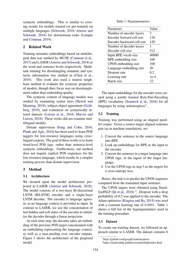
syntactic embeddings. This is similar to exist-ing results for models trained (or pre-trained) onmultiple languages (Schwenk, 2018; Artetxe andSchwenk, 2018) for downstream tasks (Lampleand Conneau, 2019).

2 Related Work

Training semantic embeddings based on multilin-gual data was studied by MUSE (Conneau et al.,2017) and LASER (Artetxe and Schwenk, 2018) atthe word and sentence levels respectively. Multi-task training for disentangling semantic and syn-tactic information was studied in (Chen et al.,2019). This work also used a nearest neigh-bour method to evaluate the syntactic propertiesof models, though their focus was on disentangle-ment rather than embedding quality.

The syntactic content of language models wasstudied by examining syntax trees (Hewitt andManning, 2019), subject-object agreement (Gold-berg, 2019), and evaluation on syntactically al-tered datasets (Linzen et al., 2016; Marvin andLinzen, 2018). These works did not examine mul-tilingual models.

Distant supervision (Fang and Cohn, 2016;Plank and Agic, 2018) has been used to learn POStaggers for low-resource languages using cross-lingual corpora. The goal of these works is to learnword-level POS tags, rather than sentence-levelsyntactic embeddings. Furthermore, our methoddoes not require explicit POS sequences for thelow-resource language, which results in a simplertraining process than distant supervision.

3 Method

3.1 ArchitectureWe iterated upon the model architecture pro-posed in LASER (Artetxe and Schwenk, 2018).The model consists of a two-layer Bi-directionalLSTM (BiLSTM) encoder and a single-layerLSTM decoder. The encoder is language agnos-tic as no language context is provided as input. Incontrast to LASER, we use the concatenation oflast hidden and cell states of the encoder to initial-ize the decoder through a linear projection.

At each time-step, the decoder takes an embed-ding of the previous POS target concatenated withan embedding representing the language context,as well as a max-pooling over encoder outputs.Figure 1 shows the architecture of the proposedmodel.

Table 1: Hyperparameters

Parameter ValueNumber of encoder layers 2Encoder forward cell size 128Encoder backward cell size 128Number of decoder layers 1Decoder cell size 512Input BPE vocab size 40000BPE embedding size 100UPOS embedding size 100Language embedding size 20Dropout rate 0.2Learning rate 1e-4Batch size 32

The input embeddings for the encoder were cre-ated using a jointly learned Byte-Pair-Encoding(BPE) vocabulary (Sennrich et al., 2016) for alllanguages by using sentencepiece1.

3.2 Training

Training was performed using an aligned paral-lel corpus. Given a source-target aligned sentencepair (as in machine translation), we:

1. Convert the sentence in the source languageinto BPE

2. Look up embeddings for BPE as the input tothe encoder

3. Convert the sentence in a target language intoUPOS tags, in the tagset of the target lan-guage.

4. Use the UPOS tags in step 3 as the targets fora cross-entropy loss.

Hence, the task is to predict the UPOS sequencecomputed from the translated input sentence.

The UPOS targets were obtained using Stand-fordNLP (Qi et al., 2018) 2. Dropout with a dropprobability of 0.2 was applied to the encoder. TheAdam optimizer (Kingma and Ba, 2015) was usedwith a constant learning rate of 0.0001. Table 1shows a full list of the hyperparameters used inthe training procedure.

3.3 Dataset

To create our training dataset, we followed an ap-proach similar to LASER. The dataset contains 6

1https://github.com/google/sentencepiece2https://stanfordnlp.github.io/stanfordnlp/index.html

154

X1 X2 X3 Xn X</s>

Sentence Embedding (Max Pooling)

BiLSTM(Encoder)

BiLSTM(Encoder)

BPE Emb.

Linear Projection

P<s>

Language Embedding

Softmax Softmax Softmax Softmax Softmax

Pemb1

P1 P2 P3 Pn </s>

Pemb2 Pemb3 Pembn

LSTM(Decoder)

Output

UPOSEmbedding

Last Hidden StatesLast Cell States

Concatenate

...

...

...

...

...

...

...

Figure 1: Proposed architecture.

languages: English, Spanish, German, Dutch, Ko-rean and Chinese Mandarin. These languages use3 different scripts, 2 different language orderings,and belong to 4 language families.

English, Spanish, German, and Dutch use aLatin-based script. However, Spanish is a Roman-tic language while the others are Germanic lan-guages. Chinese Mandarin and Korean are in-cluded because they use non-latin based scriptsand originate from language families distinct fromthe other languages. Although the grammaticalrules vary between the selected languages, theyshare a number of key characteristics such asthe Subject-Verb-Object ordering, except Korean(which mainly follows the Subject-Object-Verb or-der). We hope to extend our work to other lan-guages with different scripts and sentence struc-tures, such as Arabic, Japanese, Hindi, etc. in thefuture.

The dataset was created by using translationsprovided by Tatoeba3 and OpenSubtitles4 (Lisonand Tiedemann, 2016). They were chosen for theirhigh availability in multiple languages.

Statistics of the final training dataset are shownin Table 2. Rows and columns correspond tosource and target languages respectively.

3.3.1 Tatoeba

Tatoeba is a freely available crowd-annotateddataset for language learning. We selected all sen-tences in English, Spanish, German, Dutch, andKorean. We pruned the dataset to contain onlysentences with at least one translation to any ofthe other languages. The final training set contains1.36M translation sentence pairs from this source.

3https://tatoeba.org/eng/4http://opus.nlpl.eu/OpenSubtitles-v2018.php

3.3.2 OpenSubtitlesWe augmented our training data by using the 2018OpenSubtitles dataset. OpenSubtitles is a publiclyavailable dataset based on movie subtitles (Lisonand Tiedemann, 2016). We created our trainingdataset from selected aligned subtitles by takingthe unique translations among the first million sen-tences, for each aligned parallel corpus. We fur-ther processed the data by pruning to remove sam-ples with less than 3 words, multiple sentences,or incomplete sentences. The resulting datasetcontains 1.9M translation sentence pairs from thissource.

4 Experiments

We aim to address the following questions:

1. Can syntactic structures be embedded? Formultiple languages?

2. Can parallel corpora be used to learn syntac-tic structure for low-resource languages?

3. Does multilingual pre-training improve syn-tactic embeddings?

We address question 1 in Secs. 4.1 and 4.2 byevaluating the quality of syntactic and semanticembeddings in several ways. Questions 2 and 3are addressed in Sec. 4.3 by studying the transfer-learning performance of syntactic embeddings.

4.1 Quality of Syntactic Embeddings

We studied the quality of the learned syntacticembeddings by using a nearest-neighbour (NN)method.

First, we calculated the UPOS sequence of allsentences in the Tatoeba dataset by using a tagger.Sentences were then assigned to distinct groupsaccording to their UPOS sequence, i.e., all sen-tences belonging to the same group had the same

155

Table 2: Training Dataset Statistics

English German Spanish Chinese Korean DutchEnglish - 521.87k 194.51k 41.33k 31.81k 190.86kGerman 520.64k - 217.96k 5.67k 0.21k 12.20kSpanish 193.01k 217.46k - 159.67k 28.68k 144.82kChinese 40.79k 5.62k 159.73k - 0.05k 0.32kKorean 31.05k 1.37k 28.89k 0.07k - 56.93kDutch 215.18k 25.75k 155.35k 0.66k 56.92k -

UPOS sequence.For all languages except Korean, a held-out test

set was created by randomly sampling groups thatcontained at least 6 sentences. For Korean, allgroups containing at least 6 sentences were keptas the test set since the dataset is small.

During evaluation, we applied max-pooling tothe outputs of the encoder to obtain the syntacticembeddings of the held-out sentences5.

For each syntactic embedding, we find its topnearest neighbour (1-NN) and top-5 nearest neigh-bours (5-NN) in the embedding space for the held-out sentences, based on their UPOS group.

Given n sentences S = {s0, . . . , sn−1} andtheir embeddings E = {e0, . . . , en−1}, for eachsi there is a set of k gold nearest neighboursG(i, k) = {g0, . . . , gk−1}, G(i, k) ⊆ S such thatd(si, g) ≤ d(si, s) for all g ∈ G(i, k) and s ∈S \G(i, k), where d(·, ·) is the cosine distance.

Given embedding ei, we calculate cosine dis-tances {d(ei, ej) for ej ∈ E, ej 6= ei} and sortthem into non-decreasing order dj0 ≤ dj1 ≤ · · · ≤djn−2 . We consider the ordering to be unique asthe probability of embedding cosine distances be-ing equal is very small.

The set of embedded k-nearest neighbours of siis defined as

N(i, k) = {sj for j ∈ {j0, . . . , jk−1}}.

Finally, the k-nearest neighbours accuracy for siis given by

|N(i, k) ∩G(i, k)|k

.

A good embedding model should cluster theembeddings for similar inputs in the embeddingspace. Hence, the 5-NN test can be seen as an in-dicator of how cohesive the embedding space is.

5Evaluation data will be hosted athttps://github.com/ccliu2/syn-emb

Table 3: Syntactic Nearest-Neighbour Accuracy (%)

ISO 1-NN/5-NN Total/GroupsEnglish en 97.27/93.36 2784/160German de 93.45/86.77 1282/91Spanish es 93.81/86.24 1503/81Chinese zh 71.26/61.44 167/22Korean ko 28.27/18.40 527/40Dutch nl 74.17/51.71 3171/452

The results are shown in Table 3. The differ-ences in the number of groups in each languageare due to different availabilities of sentences andsentence-types in the Tatoeba dataset.

The high nearest neighbours accuracy indicatesthat syntax information was successfully capturedby the embeddings. Table 3 also shows that thesyntactic information of multiple languages wascaptured by a single embedding model.

4.1.1 Language ModelA number of recent works (Hewitt and Man-ning, 2019; Goldberg, 2019) have probed lan-guage models to determine if they contain syn-tactic information. We applied the same nearestneighbours experiment (with the same test sets)on a number of existing language models: Uni-versal Sentence Encoder (USE) (Cer et al., 2018),LASER, and BERT. For USE we used modelsavailable from TensorHub6. For LASER we usedmodels and created embeddings from the officialrepository 7.

For BERT, we report the results using max(BERTmax) and average-pooling (BERTavg), ob-tained from the BERT embedding toolkit8 withthe multilingual cased model (104 languages, 12-layers, 768-hidden units, 12-heads), and ‘pooled-output’ (BERToutput) from the TensorHub version

6https://www.tensorflow.org/hub7https://github.com/facebookresearch/LASER8https://github.com/imgarylai/bert-embedding

156

of the model with the same parameters.We computed the nearest neighbours experi-

ment for all languages in the training data forthe above models. The results are shown in Ta-ble 4. The results show that general purposelanguage models do capture syntax information,which varies greatly across languages and models.

The nearest neighbours accuracy of our syn-tactic embeddings in Table 3 significantly outper-forms the general purpose language models. Ar-guably these language models were trained usingdifferent training data. However, this is a reason-able comparison because many real-world appli-cations rely on released pre-trained language mod-els for syntactically related information. Hence,we want to show that we can use much smallermodels trained with direct supervision, to obtainsyntactic embeddings with similar or better qual-ity. Nonetheless, the training method used in thiswork can certainly be extended to architecturessimilar to BERT or USE.

4.2 Functional Dissimilarity

The experiments in the previous section showedthat the proposed syntactic embeddings formedcohesive clusters in the embedding space, basedon UPOS sequence similarities. We further stud-ied the spatial relationships within the embed-dings.

Word2Vec (Mikolov et al., 2013) examined spa-tial relationships between embeddings and com-pared them to the semantic relationships betweenwords. Operations on vectors in the embeddingspace such as King−Man+Woman = Queencreated vectors that also correlated with similaroperations in semantics. Such semantic compar-isons do not directly translate to syntactic embed-dings. However, syntax information shifts withedits on POS sequences. Hence, we examinedthe spatial relationships between syntactic embed-dings by comparing their cosine similarities withthe edit distances between UPOS sequence pairs.

Given n UPOS sequences U = {u0, ..., un−1},we compute the matrix L ∈ Rn×n, where lij =l(ui, uj), the complement of the normalized Lev-enshtein distance between ui and uj .

Given the set of embedding vectors{e0, ..., en−1} where ei is the embedding forsentence si, we also compute D ∈ Rn×n, wheredij = d(ei, ej). We further normalize dij to bewithin [0, 1] by min-max normalization to obtain

D = minMax(D).Following (Yin and Shen, 2018), we define the

functional dissimilarity score by

‖L− D‖Fn

.

Intuitively, UPOS sequences that are similar(smaller edit distance) should be embedded closeto each other in the embedding space, and embed-dings that are further away should have dissimilarUPOS sequences. Hence, the functional dissimi-larity score is low if the relative changes in UPOSsequences are reflected in the embedding space.The score is high if such changes are not reflected.

The functional dissimilarity score was com-puted using sentences from the test set in CoNLL2017 Universal Dependencies task (Nivre et al.,2017) for the relevant languages with the providedUPOS sequences. Furthermore, none of the evalu-ated models, including the proposed method, weretrained with CoNLL2017 data.

We compared the functional dissimilarity scoresof our syntactic representations against embed-dings obtained from BERT and LASER, to furtherdemonstrate that simple network structures withexplicit supervision may be sufficient to capturesyntactic structure. All the results are shown inTable 5. We only show the best (lowest) resultsfrom BERT.

4.3 Transfer Performance of SyntacticEmbeddings

Many NLP tasks utilize POS as features, but hu-man annotated POS sequences are difficult and ex-pensive to obtain. Thus, it is important to know ifwe can learn sentences-level syntactic embeddingsfor low-sources languages without treebanks.

We performed zero-shot transfer of the syntac-tic embeddings for French, Portuguese and In-donesian. French and Portuguese are simulatedlow-resource languages, while Indonesian is a truelow-resource language. We reported the 1-NN and5-NN accuracies for all languages using the sameevaluation setting as described in the previous sec-tion. The results are shown in Table 6 (top).

We also fine-tuned the learned syntactic embed-dings on the low-resource language for a varyingnumber of training data and languages. The resultsare shown in Table 6 (bottom). In this table, thelow-resource language is denoted as the ‘source’,while the high-resource language(s) is denoted asthe ‘target’. With this training method, no UPOS

157

Table 4: Syntactic Nearest-Neighbour for Language Models (%)

English German Spanish Chinese Korean DutchModel 1-NN/5-NN 1-NN/5-NN 1-NN/5-NN 1-NN/5-NN 1-NN/5-NN 1-NN/5-NNUSE 71.83/55.68 59.87/44.26 53.05/38.06 39.23/30.18 21.22/12.43 28.66/12.77BERTmax 90.19/86.36 83.66/77.63 83.89/79.92 67.96/68.40 20.30/11.92 37.67/19.51BERTavg 89.06/84.70 79.54/74.82 78.24/75.61 65.75/67.07 20.30/11.47 37.04/19.46BERToutput 77.75/63.44 66.20/51.89 65.21/50.41 52.49/46.34 16.39/10.98 24.27/10.67LASER 86.33/76.66 76.56/62.88 72.49/59.72 56.89/45.15 26.63/15.90 50.75/31.00

Table 5: Functional Dissimilarity Scores (Lower is Better)

Model English German Spanish Chinese Korean DutchBERTavg 0.3463 0.3131 0.2955 0.2935 0.3001 0.3131LASER 0.1602 0.1654 0.2074 0.3099 0.2829 0.1654Proposed Work 0.1527 0.1588 0.1588 0.2267 0.2533 0.1588

tag information was provided to the model forthe ‘source’ languages, where supervising infor-mation comes solely from parallel sentences andUPOS tags in high-resource languages.

The results show that for a new language(French and Portuguese) that is similar to the fam-ily of pre-training languages, there are two waysto achieve higher 1-NN accuracy. If the num-ber of unique sentences in the new language issmall, accuracy can be improved by increasing thesize of the parallel corpora used to fine-tune. Ifonly one parallel corpus is available, accuracy canbe improved by increasing the number of uniquesentence-pairs used to fine-tune.

For a new language that is dissimilar to the fam-ily of pre-training languages, e.g. Indonesian inTable 6, the above methods only improved nearestneighbours accuracy slightly. This may be causedby differing data distribution or by tagger inaccu-racies. The results for Indonesian do indicate thatsome syntactic structure can be learned by usingour method, even for a dissimilar language.

A future direction is to conduct a rigorous anal-ysis of transfer learning between languages fromthe same versus different language families.

5 Conclusion

We examined the possibility of creating syntacticembeddings by using a multilingual method basedon sequence-to-sequence models. In contrast toprior work, our method only requires parallel cor-pora and UPOS tags in the target language.

We studied the quality of learned embeddingsby examining nearest neighbours in the embed-

Table 6: Syntactic Nearest-Neighbour on New lan-guages (%)

Lang (ISO) 1-NN/5-NN Total/GroupFrench (fr) 35.86/22.11 6816/435Protuguese (pt) 48.29/23.15 4608/922Indonesian (id) 21.00/35.92 657/59

Number of Parallel Sentence PairsSource -Target(s) 2k 10kISO 1-NN/5-NN 1-NN/5-NNfr-en 47.37/32.18 58.41/42.87fr-(en,es) 46.82/31.92 58.01/42.65pt-en 56.75/30.14 64.52/36.94pt-(en,es) 57.94/30.63 65.00/37.06id-en 27.09/47.64 31.35/56.01

ding space and investigating their functional dis-similarity. These results were compared againstrecent state-of-the-art language models. We alsoshowed that pre-training with a parallel corpusallowed the syntactic embeddings to be trans-ferred to low-resource languages via few-shotfine-tuning.

Our evaluations indicated that syntactic struc-ture can be learnt by using simple network archi-tectures and explicit supervision. Future direc-tions include improving the transfer performancefor low-resource languages, disentangling seman-tic and syntactic embeddings, and analyzing theeffect of transfer learning between languages be-long to the same versus different language fami-lies.

158

ReferencesMikel Artetxe and Holger Schwenk. 2018. Mas-

sively multilingual sentence embeddings for zero-shot cross-lingual transfer and beyond. arXivpreprint arXiv:1812.10464.

Daniel Cer, Yinfei Yang, Sheng yi Kong, Nan Hua,Nicole Limtiaco, Rhomni St. John, Noah Con-stant, Mario Guajardo-Cespedes, Steve Yuan, ChrisTar, Yun-Hsuan Sung, Brian Strope, and RayKurzweil. 2018. Universal sentence encoder. CoRR,abs/1803.11175.

Mingda Chen, Qingming Tang, Sam Wiseman, andKevin Gimpel. 2019. A multi-task approach for dis-entangling syntax and semantics in sentence repre-sentations. In NAACL2019.

Alexis Conneau, Guillaume Lample, Marc’AurelioRanzato, Ludovic Denoyer, and Herve Jegou. 2017.Word translation without parallel data. arXivpreprint arXiv:1710.04087.


Meng Fang and Trevor Cohn. 2016. Learning whento trust distant supervision: An application to low-resource POS tagging using cross-lingual projection.In Proceedings of the 20th SIGNLL Conference onComputational Natural Language Learning.

Yoav Goldberg. 2019. Assessing bert’s syntactic abili-ties. arXiv preprint arXiv:1901.05287.

John Hewitt and Christopher D. Manning. 2019. Astructural probe for finding syntax in word represen-tations. In NAACL2019.

Diederik P. Kingma and Jimmy Ba. 2015. Adam:A method for stochastic optimization. CoRR,abs/1412.6980.

Guillaume Lample and Alexis Conneau. 2019. Cross-lingual language model pretraining. CoRR,abs/1901.07291.

Tal Linzen, Emmanuel Dupoux, and Yoav Goldberg.2016. Assessing the ability of lstms to learn syntax-sensitive dependencies. Transactions of the Associ-ation for Computational Linguistics.

Pierre Lison and Jorg Tiedemann. 2016. Opensub-titles2016: Extracting large parallel corpora frommovie and tv subtitles.

Rebecca Marvin and Tal Linzen. 2018. Targetedsyntactic evaluation of language models. InEMNLP2018.

Tomas Mikolov, Ilya Sutskever, Kai Chen, Gregory S.Corrado, and James A. Dean. 2013. Distributed rep-resentations of words and phrases and their compo-sitionality. In NIPS.

Joakim Nivre, Zeljko Agic, Lars Ahrenberg, et al.2017. Universal dependencies 2.0. lindat/clarin dig-ital library at the institute of formal and applied lin-guistics, charles university, prague.

Barbara Plank and Zeljko Agic. 2018. Distant super-vision from disparate sources for low-resource part-of-speech tagging. In EMNLP2018.

Peng Qi, Timothy Dozat, Yuhao Zhang, and Christo-pher D. Manning. 2018. Universal dependency pars-ing from scratch. In Proceedings of the CoNLL 2018Shared Task: Multilingual Parsing from Raw Textto Universal Dependencies, pages 160–170, Brus-sels, Belgium. Association for Computational Lin-guistics.

Holger Schwenk. 2018. Filtering and mining paralleldata in a joint multilingual space. In ACL.

Rico Sennrich, Barry Haddow, and Alexandra Birch.2016. Neural machine translation of rare wordswith subword units. In Proceedings of the 54th An-nual Meeting of the Association for ComputationalLinguistics (Volume 1: Long Papers), pages 1715–1725, Berlin, Germany. Association for Computa-tional Linguistics.

Ilya Sutskever, Oriol Vinyals, and Quoc V. Le. 2014.Sequence to sequence learning with neural net-works. In NIPS.

Zi Yin and Yuanyuan Shen. 2018. On the dimension-ality of word embedding. In Advances in Neural In-formation Processing Systems, pages 887–898.

159


FASPell: A Fast, Adaptable, Simple, Powerful Chinese Spell CheckerBased On DAE-Decoder Paradigm

Yuzhong Hong, Xianguo Yu, Neng He, Nan Liu, Junhui LiuIntelligent Platform Division, iQIYI, Inc.

{hongyuzhong, yuxianguo, heneng, liunan, liujunhui}@qiyi.com

Abstract

We propose a Chinese spell checker – FASPellbased on a new paradigm which consists ofa denoising autoencoder (DAE) and a de-coder. In comparison with previous state-of-the-art models, the new paradigm allowsour spell checker to be Faster in computa-tion, readily Adaptable to both simplified andtraditional Chinese texts produced by eitherhumans or machines, and to require muchSimpler structure to be as much Powerful inboth error detection and correction. These fourachievements are made possible because thenew paradigm circumvents two bottlenecks.First, the DAE curtails the amount of Chi-nese spell checking data needed for super-vised learning (to <10k sentences) by lever-aging the power of unsupervisedly pre-trainedmasked language model as in BERT, XLNet,MASS etc. Second, the decoder helps to elim-inate the use of confusion set that is deficientin flexibility and sufficiency of utilizing thesalient feature of Chinese character similarity.

1 Introduction

There has been a long line of research on detect-ing and correcting spelling errors in Chinese textssince some trailblazing work in the early 1990s(Shih et al., 1992; Chang, 1995). However, de-spite the spelling errors being reduced to substitu-tion errors in most researches1 and efforts of mul-tiple recent shared tasks (Wu et al., 2013; Yu et al.,2014; Tseng et al., 2015; Fung et al., 2017), Chi-nese spell checking remains a difficult task. More-over, the methods for languages like English canhardly be directly used for the Chinese languagebecause there are no delimiters between words,whose lack of morphological variations makes thesyntactic and semantic interpretations of any Chi-nese character highly dependent on its context.

1Likewise, this paper only covers substitution errors.

1.1 Related work and bottlenecksAlmost all previous Chinese spell checking mod-els deploy a common paradigm where a fixed setof similar characters of each Chinese character(called confusion set) is used as candidates, and afilter selects the best candidates as substitutions fora given sentence. This naive design is subjected totwo major bottlenecks, whose negative impact hasbeen unsuccessfully mitigated:

• overfitting to under-resourced Chinesespell checking data. Since Chinese spellchecking data require tedious professionalmanual work, they have always been under-resourced. To prevent the filter from over-fitting, Wang et al. (2018) propose an auto-matic method to generate pseudo spell check-ing data. However, the precision of their spellchecking model ceases to improve when thegenerated data reaches 40k sentences. Zhaoet al. (2017) use an extensive amount of adhoc linguistic rules to filter candidates, onlyto achieve worse performance than ours eventhough our model does not leverage any lin-guistic knowledge.

• inflexibility and insufficiency of confusionset in utilizing character similarity. Thefeature of Chinese character similarity is verysalient as it is related to the main cause ofspelling errors (see subsection 2.2). How-ever, the idea of confusion set is troublesomein utilizing it:

1. inflexibility to address the issue thatconfusing characters in one scenariomay not be confusing in another. Thedifference between simplified and tradi-tional Chinese shown in Table 1 is anexample. Wang et al. (2018) also sug-gest that confusing characters for ma-

160

chines are different from those for hu-mans. Therefore, in practice, it is verylikely that the correct candidates for sub-stitution do not exist in a given confu-sion set, which harms recall. Also, con-sidering more similar characters to pre-serve recall will risk lowering precision.

2. insufficiency in utilizing character simi-larity. Since a cut-off threshold of quan-tified character similarity (Liu et al.,2010; Wang et al., 2018) is used to pro-duce the confusion set, similar charac-ters are actually treated indiscriminatelyin terms of their similarity. This meansthe information of character similarityis not sufficiently utilized. To compen-sate this, Zhang et al. (2015) propose aspell checker that has to consider manyless salient features such as word seg-mentation, which add more unnecessarynoises to their model.

1.2 Motivation and contributions

The motivation of this paper is to circumvent thetwo bottlenecks in subsection 1.1 by changing theparadigm for Chinese spell checking.

As a major contribution and as exemplified byour proposed Chinese spell checking model in Fig-ure 1, the most general form of the new paradigmconsists of a denoising autoencoder2 (DAE) and adecoder. To prove that it is indeed a novel contri-bution, we compare it with two similar paradigmsand show their differences as follows:

1. Similar to the old paradigm used in previousChinese spell checking models, a model un-der the DAE-decoder paradigm also producescandidates (by DAE) and then filters the can-didates (by the decoder). However, candi-dates are produced on the fly based on con-texts. If the DAE is powerful enough, weshould expect that all contextually suitablecandidates are recalled, which prevent the in-flexibility issue caused by using confusionset. The DAE will also prevent the overfit-ting issue because it can be trained unsuper-visedly using a large number of natural texts.Moreover, character similarity can be used bythe decoder without losing any information.

2the term denoising autoencoder follows the same senseused by Yang et al. (2019), which is arguably more generalthan the one used by Vincent et al. (2008).

2. The DAE-decoder paradigm is sequence-to-sequence, which makes it resemble theencoder-decoder paradigm in tasks like ma-chine translation, grammar checking, etc.However, in the encoder-decoder paradigm,the encoder extracts semantic information,and the decoder generates texts that embodythe information. In contrast, in the DAE-decoder paradigm, the DAE provides candi-dates to reconstruct texts from the corruptedones based on contextual feature, and the de-coder3 selects the best candidates by incorpo-rating other features.

Besides the new paradigm per se, there are twoadditional contributions in our proposed Chinesespell checking model:

• we propose a more precise quantificationmethod of character similarity than the onesproposed by Liu et al. (2010) and Wang et al.(2018) (see subsection 2.2);

• we propose an empirically effective decoderto filter candidates under the principle of get-ting the highest possible precision with mini-mal harm to recall (see subsection 2.3).

1.3 AchievementsThanks to our contributions mentioned in subsec-tion 1.2, our model can be characterized by the fol-lowing achievements relative to previous state-of-the-art models, and thus is named FASPell.

• Our model is Fast. It is shown (subsection3.3) to be faster in filtering than previousstate-of-the-art models either in terms of ab-solute time consumption or time complexity.

• Our model is Adaptable. To demonstrate this,we test it on texts from different scenarios– texts by humans, such as learners of Chi-nese as a Foreign Language (CFL), and bymachines, such as Optical Character Recog-nition (OCR). It can also be applied to bothsimplified Chinese and traditional Chinese,despite the challenging issue that some er-roneous usages of characters in traditionaltexts are considered valid usages in simpli-fied texts (see Table 1). To the best of ourknowledge, all previous state-of-the-art mod-els only focus on human errors in traditionalChinese texts.

3The term decoder here is analogous as in Viterbi decoderin the sense of finding the best path along candidates.

161

Table 1: Examples on the left are considered validusages in simplified Chinese (SC). Notes on the rightare about how they are erroneous in traditional Chi-nese (TC) and suggested corrections. This inconsis-tency is because multiple traditional characters weremerged into identical characters in the simplificationprocess. Our model makes corrections for this type oferrors only in traditional texts. In simplified texts, theyare not detected as errors.

SC Examples Notes on TC usage

周末 (weekend)旅游 (trip)制造 (make)

周→週周 only in周到, etc.游→遊游 only in游泳, etc.制→製制 only in制度, etc.

• Our model is Simple. As shown in Fig-ure 1, it has only a masked language modeland a filter as opposed to multiple feature-producing models and filters being used inprevious state-of-the-art proposals. More-over, only a small training set and a set ofvisual and phonological features of charac-ters are required in our model. No extra dataare necessary, including confusion set. Thismakes our model even simpler.

• Our model is Powerful. On benchmarkdata sets, it achieves similar F1 performances(subsection 3.2) to those of previous state-of-the-art models on both detection and correc-tion level. It also achieves arguably high pre-cision (78.5% in detection and 73.4% in cor-rection) on our OCR data set.

2 FASPell

As shown in Figure 1, our model uses masked lan-guage model (see subsection 2.1) as the DAE toproduce candidates and confidence-similarity de-coder (see subsection 2.2 and 2.3) to filter can-didates. In practice, doing several rounds of thewhole process is also proven to be helpful (sub-section 3.4).

2.1 Masked language modelMasked language model (MLM) guesses the to-kens that are masked in a tokenized sentence. Itis intuitive to use MLM as the DAE to detect andcorrect Chinese spelling errors because it is in linewith the task of Chinese spell checking. In theoriginal training process of MLM in BERT (De-vlin et al., 2018), the errors are the random masks,which are the special token [MASK] 80% of the

国际电台苦名丰持人

国际电台知名主持人

听话著音广目者

世家节视报台演主手

台界讲播冠闻支节持

國際0.9994 0.9999 0.9999 0.9999 0.2878 0.9626 0.9994 0.9981 0.9999

0.0002 0.0000 0.0000 0.0000 0.1999 0.0019 0.0002 0.0002 0.0000

0.0000 0.0000 0.0000 0.0000 0.0429 0.0015 0.0000 0.0001 0.0000

0.0000 0.0000 0.0000 0.0000 0.0252 0.0014 0.0000 0.0001 0.0000

Masked Language Model

国际电台著名主持人

rank=1

rank=2

rank=3

rank=4

✓ ✓

✖ ✖

Confidence-Similarity Decoder

Figure 1: A real example of how an erroneous sentencewhich is supposed to have the meaning of "A famousinternational radio broadcaster" is successfully spell-checked with two erroneous characters苦 and丰 beingdetected and corrected using FASPell. Note that withour proposed confidence-similarity decoder, the finalchoice for substitution is not necessarily the candidateranked the first.

time, a random token in the vocabulary 10% ofthe time and the original token 10% of the time. Incases where a random token is used as the mask,the model actually learns how to correct an erro-neous character; in cases where the original tokensare kept, the model actually learns how to detect ifa character is erroneous or not. For simplicity pur-poses, FASPell adopts the architecture of MLM asin BERT (Devlin et al., 2018). Recent variants –XLNet (Yang et al., 2019), MASS (Song et al.,2019) have more complex architectures of MLM,but they are also suitable.

However, just using a pre-trained MLM raisesthe issue that the errors introduced by randommasks may be very different from the actual errorsin spell checking data. Therefore, we propose thefollowing method to fine-tune the MLM on spellchecking training sets:

• For texts that have no errors, we follow theoriginal training process as in BERT;

• For texts that have errors, we create two typesof training examples by:

162

1. given a sentence, we mask the erroneoustokens with themselves and set their tar-get labels as their corresponding correctcharacters;

2. to prevent overfitting, we also mask to-kens that are not erroneous with them-selves and set their target labels as them-selves, too.

The two types of training examples are bal-anced to have roughly similar quantity.

Fine-tuning a pre-trained MLM is proven to bevery effective in many downstream tasks (Devlinet al., 2018; Yang et al., 2019; Song et al., 2019),so one would argue that this is where the power ofFASPell mainly comes from. However, we wouldlike to emphasize that the power of FASPell shouldnot be biasedly attributed to MLM. In fact, weshow in our ablation studies (subsection 3.2) thatMLM itself can only serve as a very weak Chinesespell checker (its performance can be as poor asF1 being only 28.9%), and the decoder that uti-lizes character similarity (see subsection 2.2 and2.3) is also significantly indispensable to produc-ing a strong Chinese spell checker.

2.2 Character similarity

Erroneous characters in Chinese texts by humansare usually either visually (subsection 2.2.1) orphonologically similar (subsection 2.2.2) to corre-sponding correct characters, or both (Chang, 1995;Liu et al., 2010; Yu and Li, 2014). It is also truethat erroneous characters produced by OCR pos-sess visual similarity (Tong and Evans, 1996).

We base our similarity computation on twoopen databases: Kanji Database Project4 and Uni-han Database5 because they provide shape andpronunciation representations for all CJK UnifiedIdeographs in all CJK languages.

2.2.1 Visual similarityThe Kanji Database Project uses the Unicodestandard – Ideographic Description Sequence(IDS) to represent the shape of a character.

As illustrated by examples in Figure 2, the IDSof a character is formally a string, but it is essen-tially the preorder traversal path of an ordered tree.

4http://kanji-database.sourceforge.net/

5https://unicode.org/charts/unihan.html

／＼／＼

/" /"

／＼

／＼／＼

/"/\/"/"

贫 :

分贝八刀人冂

⿱⿱⿰丿乁⿹𠃌丿⿵⿰丨𠃌⿰丿乁

⿱

⿱⿱

⿱

⿱

⿵

⿵

⿰ ⿰⿰⿹

丿丿丿乁乁𠃌𠃌丨

① ②

③

--------------------------------------------------

Figure 2: The IDS of a character can be given in dif-ferent granularity levels as shown in the tree forms in¬-® for the simplified character 贫 (meaning poor).In FASPell, we only use stroke-level IDS in the formof a string, like the one above the dashed ruling line.Unlike using only actual strokes (Wang et al., 2018),the Unicode standard Ideographic Description Charac-ters (e.g., the non-leaf nodes in the trees) describe thelayout of a character. They help us to model the sub-tle nuances in different characters that are composed ofidentical strokes (see examples in Table 2). Therefore,IDS gives us a more precise shape representation of acharacter.

In our model, we only adopt the string-formIDS. We define the visual similarity between twocharacters as one minus normalized6 Levenshteinedit distance between their IDS representations.The reason for normalization is twofold. Firstly,we want the similarity to range from 0 to 1 for theconvenience of later filtering. Secondly, if a pairof more complex characters have the same edit dis-tance as a pair of less complex characters, we wantthe similarity of the more complex characters to beslightly higher than that of the less complex char-acters (see examples in Table 2).

We do not use the tree-form IDS for two rea-sons even as it seems to make more sense intu-itively. Firstly, even with the most efficient algo-rithm (Pawlik and Augsten, 2015, 2016) so far, treeedit distance (TED) has far greater time complex-ity than edit distance of strings (O(mn(m + n))vs. O(mn)). Secondly, we did try TED in prelimi-nary experiments, but there was no significant dif-ference from using edit distance of strings in termsof spell checking performance.

6Since the maximal value of Levenshtein edit distance isthe maximum of the lengths of the two strings in question, wenormalize it simply by dividing it by the maximum length.

163

Table 2: Examples of the computation of character similarities. IDS is used to compute visual similarity (V-sim)and pronunciation representations in Mandarin Chinese (MC), Cantonese Chinese (CC), Japanese On’yomi (JO),Korean (K) and Vietnamese (V) are used to compute phonological similarity (P-sim). Note that the normalizationof edit distance gives us the desired fact that less complex character pair (午,牛) has smaller visual similarity thanmore complex character pair (田, 由) even though both of their IDS edit distances are 1. Also, note that 午 and牛 have more similar pronunciations in some languages than in others; the combination of the pronunciations inmultiple languages gives us a more continuous phonological similarity.

IDS MC CC JO K V V-sim P-sim

午 (noon)牛 (cow)

⿱⿰丿一⿻一丨⿻⿰丿一⿻一丨

wu3niu2

ng5ngau4

gogyuu

owu

ngọngưu

0.857 0.280

田 (field)由 (from)

⿵⿰丨𠃌⿱⿻一丨一

⿻⿰丨𠃌⿱⿻一丨一tian2you2

tin4jau4

denyuu

cenyu

điềndo

0.889 0.090

2.2.2 Phonological similarityDifferent Chinese characters sharing identical pro-nunciation is very common (Yang et al., 2012),which is the case for any CJK language. Thus, Ifwe were to use character pronunciations in onlyone CJK language, the phonological similarity ofcharacter pairs would be limited to a few discretevalues. However, a more continuous phonologi-cal similarity is preferred because it can make thecurve used for filtering candidates smoother (seesubsection 2.3).

Therefore, we utilize character pronunciationsof all CJK languages (see examples in Table 2),which are provided by the Unihan Database. Tocompute the phonological similarity of two char-acters, we first calculate one minus normalizedLevenshtein edit distance between their pronunci-ation representations in all CJK languages (if ap-plicable). Then, we take the mean of the results.Hence, the similarity should range from 0 to 1.

2.3 Confidence-Similarity Decoder

Candidate filters in many previous models arebased on setting various thresholds and weights formultiple features of candidate characters. Insteadof this naive approach, we propose a method thatis empirically effective under the principle of get-ting the highest possible precision with minimalharm to recall. Since the decoder utilizes contex-tual confidence and character similarity, we referto it as the confidence-similarity decoder (CSD).The mechanism of CSD is explained, and its ef-fectiveness is justified as follows:

First, consider the simplest case where only onecandidate character is provided for each originalcharacter. For those candidates that are the sameas their original characters, we do not substitute

the original characters. For those that are dif-ferent, we can draw a confidence-similarity scat-ter graph. If we compare the candidates with theground truths, the graph will resemble the plot¬ of Figure 3. We can observe that the true-detection-and-correction candidates are denser to-ward the upper-right corner; false-detection candi-dates toward the lower-left corner; true-detection-and-false-correction candidates in the middle area.If we draw a curve to filter out false-detectioncandidates (plot of Figure 3) and use the restas substitutions, we can optimize character-levelprecision with minimal harm to character-levelrecall for detection; if true-detection-and-false-correction candidates are also filtered out (plot ®

of Figure 3), we can get the same effect for cor-rection. In FASPell, we optimize correction per-formance and manually find the filtering curve us-ing a training set, assuming its consistency with itscorresponding testing set. But in practice, we haveto find two curves – one for each type of similarity,and then take the union of the filtering results.

Now, consider the case where there are c > 1candidates. To reduce it into the previously de-scribed simplest case, we rank the candidates foreach original character according to their contex-tual confidence and put candidates that have thesame rank into the same group (i.e., c groups intotal). Thus, we can find a filter as previously de-scribed for each group of candidates. All c filterscombined further alleviate the harm to recall be-cause more candidates are taken into account.

In the example of Figure 1, there are c = 4groups of candidates. We get a correct substitution丰→主 from the group whose rank = 1, anotherone苦→著 from the group whose rank = 2, andno more from the other two groups.

164

0 0.2 0.4 0.6 0.8 10

0.2

0.4

0.6

0.8

1

Confidence

Sim

ilarity

¬

0 0.2 0.4 0.6 0.8 10

0.2

0.4

0.6

0.8

1

Confidence

Sim

ilarity

T-d&T-c

T-d&F-c

F-d

filtering curve

filtered-out

0 0.2 0.4 0.6 0.8 10

0.2

0.4

0.6

0.8

1

Confidence

Sim

ilarity

®

0 0.2 0.4 0.6 0.8 10

0.2

0.4

0.6

0.8

1

Confidence

Sim

ilarity

¯

Figure 3: All four plots show the same confidence-similarity graph of candidates categorized by being true-detection-and-true-correction (T-d&T-c), true-detection-and-false-correction (T-d&F-c) and false-detection (F-d).But, each plot shows a different way of filtering candidates: in plot ¬, no candidates are filtered; in plot , thefiltering optimizes detection performance; in plot ®, as adopted in FASPell, the filtering optimizes correctionperformance; in plot ¯, as adopted by previous models, candidates are filtered out by setting a threshold forweighted confidence and similarity (0.8× confidence+0.2× similarity < 0.8 as an example in the plot). Notethat the four plots use the actual first-rank candidates (using visual similarity) for our OCR data (Trnocr) exceptthat we randomly sampled only 30% of the candidates to make the plots more viewable on paper.

3 Experiments and results

We first describe the data, metrics and model con-figurations adopted in our experiments in subsec-tion 3.1. Then, in subsection 3.2, we show the per-formance on spell checking texts written by hu-mans to compare FASPell with previous state-of-the-art models; we also show the performance ondata that are harvested from OCR results to provethe adaptability of the model. In subsection 3.3,we compare the speed of FASPell and three state-of-the-art models. In subsection 3.4, we investi-gate how hyper-parameters affect the performanceof FASPell.

3.1 Data, metrics and configurationsWe adopt the benchmark datasets (all in traditionalChinese) and sentence-level7 accuracy, precision,

7Note that although we do not use character-level metrics(Fung et al., 2017) in evaluation, they are actually importantin the justification of the effectiveness of the CSD as in sub-section 2.3

Table 3: Statistics of datasets.

Dataset # erroneous sent # sent Avg. length

Trn13

Trn14

Trn15

Tst13Tst14Tst15

35034322339

996529550

70034352339100010621100

41.849.631.374.350.030.6

Trnocr

Tstocr

35751000

35751000

10.110.2

recall and F1 given by SIGHAN13 - 15 sharedtasks on Chinese spell checking (Wu et al., 2013;Yu et al., 2014; Tseng et al., 2015). We also har-vested 4575 sentences (4516 are simplified Chi-nese) from OCR results of Chinese subtitles invideos. We used the OCR method by Shi et al.(2017). Detailed data statistics are in Table 3.

We use the pre-trained masked language

165

Table 4: Configurations of FASPell. FT means thetraining set for fine-tuning; CSD means the training setfor CSD; r means the number of rounds and c meansthe number of candidates for each character. U is theunion of all the spell checking data from SIGHAN13 -15.

FT CSD Test set r c FT steps

U − Tst13U − Tst14U − Tst15

Trn13

Trn14

Trn15

Tst13Tst14Tst15

133

444

10k10k10k

(-) Trnocr Tstocr 2 4 (-)

model8 provided by Devlin et al. (2018). Set-tings of its hyper-parameters and pre-trainingare available at https://github.com/google-research/bert. Other configura-tions of FASPell used in our major experiments(subsection 3.2 - 3.3) are given in Table 4. Forablation experiments, the same configurations areused except when CSD is removed, we take thecandidates ranked the first as default outputs. Notethat we do not fine-tune the mask language modelfor OCR data because we learned in preliminaryexperiments that fine-tuning worsens performancefor this type of data9.

3.2 Performance

As shown in Table 6, FASPell achieves state-of-the-art F1 performance on both detection level andcorrection level. It is better in precision than themodel by Wang et al. (2018) and better in recallthan the model by Zhang et al. (2015). In compar-ison with Zhao et al. (2017), It is better by any met-ric. It also reaches comparable precision on OCRdata. The lower recall on OCR data is partially be-cause many OCR errors are harder to correct evenfor humans (Wang et al., 2018).

Table 6 also shows that all the components ofFASPell contribute effectively to its good perfor-mance. FASPell without both fine-tuning andCSD is essentially the pre-trained mask languagemodel. Fine-tuning it improves recall becauseFASPell can learn about common errors and howthey are corrected. CSD improves its precisionwith minimal harm to recall because this is the un-

8https://storage.googleapis.com/bert_models/2018_11_03/chinese_L-12_H-768_A-12.zip

9 It is probably because OCR errors are subject to randomnoise in source pictures rather than learnable patterns as inhuman errors. However, since the paper is not about OCR,we do not elaborate on this here.

Table 5: Speed comparison (ms/sent). Note that thespeed of FASPell is the average in several rounds.

Test set FASPell Wang et al. (2018)

Tst13Tst14Tst15

446284177

680745566

derlying principle of the design of CSD.

3.3 Filtering Speed10

First, we measure the filtering speed of Chinesespell checking in terms of absolute time consump-tion per sentence (see Table 5). We compare thespeed of FASPell with the model by Wang et al.(2018) in this manner because they have reportedtheir absolute time consumption11. Table 5 clearlyshows that FASPell is much faster.

Second, to compare FASPell with models(Zhang et al., 2015; Zhao et al., 2017) whose ab-solute time consumption has not been reported,we analyze the time complexity. The time com-plexity of FASPell is O(scmn + sc log c), wheres is the sentence length, c is the number of can-didates, mn accounts for computing edit distanceand c log c for ranking candidates. Zhang et al.(2015) use more features than just edit distance, sothe time complexity of their model has additionalfactors. Moreover, since we do not use confusionset, the number of candidates for each character oftheir model is practically larger than ours: x × 10vs. 4. Thus, FASPell is faster than their model.Zhao et al. (2017) filter candidates by finding thesingle-source shortest path (SSSP) in a directedgraph consisting of all candidates for every tokenin a sentence. The algorithm they used has a timecomplexity of O(|V |+ |E|) where |V | is the num-ber of vertices and |E| is the number of edges inthe graph (Eppstein, 1998). Translating it in termsof s and c, the time complexity of their model isO(sc+ cs). This implies that their model is expo-nentially slower than FASPell for long sentences.

10Considering only the filtering speed is because theTransformer, the Bi-LSTM and language models used by pre-vious state-of-the-art models or us before filtering are alreadywell studied in the literature.

11 We have no access to the 4-core Intel Core i5-7500 CPUused by Wang et al. (2018). To minimize the difference ofspeed caused by hardware, we only use 4 cores of a 12-coreIntel(R) Xeon(R) CPU E5-2650 in the experiments.

166

Table 6: This table shows spell checking performances on both detection and correction level. Our model –FASPell achieves similar performance to that of previous state-of-the-art models. Note that fine-tuning and CSDboth contribute effectively to its performance according to the results of ablation experiments. (− FT meansremoving fine-tuning; − CSD means removing CSD.)

Test set Models Detection Level Correction Level

Acc. (%) Prec. (%) Rec. (%) F1 (%) Acc. (%) Prec. (%) Rec. (%) F1 (%)

Tst13

Wang et al. (2018)Yeh et al. (2013)FASPellFASPell − FTFASPell − CSDFASPell − FT − CSD

(-)(-)

63.140.941.047.9

54.0(-)

76.275.542.365.2

69.3(-)

63.240.941.147.8

60.7(-)

69.153.041.655.2

(-)62.560.539.631.335.6

(-)70.373.173.232.248.4

(-)62.560.539.631.335.4

52.166.266.251.431.840.9

Tst14

Zhao et al. (2017)Wang et al. (2018)FASPellFASPell − FTFASPell − CSDFASPell − FT − CSD

(-)(-)

70.057.849.056.3

(-)51.961.054.531.038.4

(-)66.253.518.142.326.8

(-)58.257.027.235.831.6

(-)(-)

69.357.744.952.1

55.5(-)

59.453.725.026.0

39.1(-)

52.017.834.218.0

45.956.155.426.728.921.3

Tst15

Zhang et al. (2015)Wang et al. (2018)FASPellFASPell − FTFASPell − CSDFASPell − FT − CSD

70.1(-)

74.261.565.563.7

80.356.667.674.149.359.1

53.369.460.025.559.135.3

64.062.363.537.953.844.2

69.2(-)

73.761.360.057.6

79.7(-)

66.672.540.238.3

51.5(-)

59.124.948.222.7

62.557.162.637.143.828.5

TstocrFASPellFASPell − CSD

18.634.5

78.565.8

18.634.5

30.145.3

17.418.9

73.436.1

17.418.9

28.124.8

3.4 Exploring hyper-parametersFirst, we only change the number of candidatesin Table 4 to see its effect on spell checking per-formance. As illustrated in Figure 4, when morecandidates are taken into account, additional de-tections and corrections are recalled while max-imizing precision. Thus, increase in the numberof candidates always results in the improvement ofF1. The reason we set the number of candidatesc = 4 in Table 4 and no larger is because there is atrade-off with time consumption.

Second, we do the same thing to the number ofrounds of spell checking in Table 4. We can ob-serve in Figure 4 that the correction performanceon Tst14 and Tst15 reaches its peak when thenumber of rounds is 3. For Tst13 and Tstocr, thatnumber is 1 and 2, respectively. A larger num-ber of rounds sometimes helps because FASPellcan achieve high precision in detection in eachround, so undiscovered errors in last round may bedetected and corrected in the next round withoutfalsely detecting too many non-errors.

4 Conclusion

We propose a Chinese spell checker – FASPell thatreaches state-of-the-art performance. It is basedon DAE-decoder paradigm that requires only a

small amount of spell checking data and gives upthe troublesome notion of confusion set. WithFASPell as an example, each component of theparadigm is shown to be effective. We make ourcode and data publically available at https://github.com/iqiyi/FASPell.

Future work may include studying if the DAE-decoder paradigm can be used to detect and cor-rect grammatical errors or other less frequentlystudied types of Chinese spelling errors such asdialectical colloquialism (Fung et al., 2017) andinsertion/deletion errors.

0 1 2 3 4 50.5

0.55

0.6

0.65

0.7

Tst13

0 1 2 3 4 50.5

0.55

0.6

0.65

0.7

Tst14

0 1 2 3 4 50.5

0.55

0.6

0.65

0.7

Tst15

0 1 2 3 4 50.2

0.25

0.3

0.35

0.4

Tstocr

0 1 2 3 4 5 60.5

0.55

0.6

0.65

0.7

Tst13

0 1 2 3 4 5 60.5

0.55

0.6

0.65

0.7

Tst14

0 1 2 3 4 5 60.5

0.55

0.6

0.65

0.7

Tst15

0 1 2 3 4 5 60.2

0.25

0.3

0.35

0.4

Tstocr

Detection

Correction

F1

Number of candidates

F1

Number of rounds

Figure 4: The four plots in the first row show howthe number of candidates for each character affects F1performances. The four in the second row show theimpact of the number of rounds of spell checking.

167

Acknowledgments

The authors would like to thank the anonymousreviewers for their comments. We also thank ourcolleagues from the IT Infrastructure team ofiQIYI, Inc. for the hardware support. Specialthanks go to Prof. Yves Lepage from GraduateSchool of IPS, Waseda University for his insight-ful advice about the paper.

References

Chao-Huang Chang. 1995. A new approach for auto-matic chinese spelling correction. In Proceedingsof Natural Language Processing Pacific Rim Sym-posium, volume 95, pages 278–283. Citeseer.

Jacob Devlin, Ming-Wei Chang, Kenton Lee, andKristina Toutanova. 2018. BERT: pre-training ofdeep bidirectional transformers for language under-standing. CoRR, abs/1810.04805.

David Eppstein. 1998. Finding the k shortest paths.SIAM Journal on computing, 28(2):652–673.

Gabriel Fung, Maxime Debosschere, Dingmin Wang,Bo Li, Jia Zhu, and Kam-Fai Wong. 2017. Nlptea2017 shared task – Chinese spelling check. InProceedings of the 4th Workshop on Natural Lan-guage Processing Techniques for Educational Appli-cations (NLPTEA 2017), pages 29–34, Taipei, Tai-wan. Asian Federation of Natural Language Process-ing.

Chao-Lin Liu, Min-Hua Lai, Yi-Hsuan Chuang, andChia-Ying Lee. 2010. Visually and phonologi-cally similar characters in incorrect simplified chi-nese words. In Proceedings of the 23rd Inter-national Conference on Computational Linguistics:Posters, pages 739–747, Beijing, China. Associationfor Computational Linguistics.

Mateusz Pawlik and Nikolaus Augsten. 2015. Efficientcomputation of the tree edit distance. ACM Trans.Database Syst., 40(1):3:1–3:40.

Mateusz Pawlik and Nikolaus Augsten. 2016. Tree editdistance: Robust and memory-efficient. Informa-tion Systems, 56:157 – 173.

Baoguang Shi, Xiang Bai, and Cong Yao. 2017. Anend-to-end trainable neural network for image-basedsequence recognition and its application to scenetext recognition. IEEE transactions on pattern anal-ysis and machine intelligence, 39(11):2298–2304.

DS Shih et al. 1992. A statistical method for locatingtypo in Chinese sentences. CCL Research Journal,pages 19–26.

Kaitao Song, Xu Tan, Tao Qin, Jianfeng Lu, and Tie-Yan Liu. 2019. Mass: Masked sequence to sequencepre-training for language generation. arXiv preprintarXiv:1905.02450.

Xiang Tong and David A. Evans. 1996. A statisticalapproach to automatic OCR error correction in con-text. In Fourth Workshop on Very Large Corpora.

Yuen-Hsien Tseng, Lung-Hao Lee, Li-Ping Chang, andHsin-Hsi Chen. 2015. Introduction to SIGHAN2015 bake-off for Chinese spelling check. In Pro-ceedings of the Eighth SIGHAN Workshop on Chi-nese Language Processing, pages 32–37.

Pascal Vincent, Hugo Larochelle, Yoshua Bengio, andPierre-Antoine Manzagol. 2008. Extracting andcomposing robust features with denoising autoen-coders. In Proceedings of the 25th internationalconference on Machine learning, pages 1096–1103.ACM.

Dingmin Wang, Yan Song, Jing Li, Jialong Han, andHaisong Zhang. 2018. A hybrid approach to auto-matic corpus generation for Chinese spelling check.In Proceedings of the 2018 Conference on Em-pirical Methods in Natural Language Processing,pages 2517–2527, Brussels, Belgium. Associationfor Computational Linguistics.

Shih-Hung Wu, Chao-Lin Liu, and Lung-Hao Lee.2013. Chinese spelling check evaluation atSIGHAN bake-off 2013. In Proceedings of the Sev-enth SIGHAN Workshop on Chinese Language Pro-cessing, pages 35–42, Nagoya, Japan. Asian Federa-tion of Natural Language Processing.

Shaohua Yang, Hai Zhao, Xiaolin Wang, and Bao liangLu. 2012. Spell checking for Chinese. In Proceed-ings of the Eight International Conference on Lan-guage Resources and Evaluation (LREC’12), Istan-bul, Turkey. European Language Resources Associ-ation (ELRA).


Jui-Feng Yeh, Sheng-Feng Li, Mei-Rong Wu, Wen-Yi Chen, and Mao-Chuan Su. 2013. Chinese wordspelling correction based on n-gram ranked invertedindex list. In Proceedings of the Seventh SIGHANWorkshop on Chinese Language Processing, pages43–48, Nagoya, Japan. Asian Federation of NaturalLanguage Processing.

Junjie Yu and Zhenghua Li. 2014. Chinese spellingerror detection and correction based on languagemodel, pronunciation, and shape. In Proceedings ofThe Third CIPS-SIGHAN Joint Conference on Chi-nese Language Processing, pages 220–223.

168

Liang-Chih Yu, Lung-Hao Lee, Yuen-Hsien Tseng, andHsin-Hsi Chen. 2014. Overview of SIGHAN 2014bake-off for Chinese spelling check. In Proceed-ings of The Third CIPS-SIGHAN Joint Conferenceon Chinese Language Processing, pages 126–132,Wuhan, China. Association for Computational Lin-guistics.

Shuiyuan Zhang, Jinhua Xiong, Jianpeng Hou, QiaoZhang, and Xueqi Cheng. 2015. HANSpeller++: Aunified framework for Chinese spelling correction.In Proceedings of the Eighth SIGHAN Workshop onChinese Language Processing, pages 38–45, Bei-jing, China. Association for Computational Linguis-tics.

Hai Zhao, Deng Cai, Yang Xin, Yuzhu Wang, andZhongye Jia. 2017. A hybrid model for Chinesespelling check. ACM Trans. Asian Low-Resour.Lang. Inf. Process., 16(3):21:1–21:22.

169


Latent semantic network induction in the context of linked example senses

Hunter Scott HeidenreichDepartment of Computer Science

College of Computing and [email protected]

Jake Ryland WilliamsDepartment of Information Science

College of Computing and [email protected]

Abstract

The Princeton WordNet is a powerful toolfor studying language and developing nat-ural language processing algorithms. Withsignificant work developing it further, oneline considers its extension through aligningits expert-annotated structure with other lex-ical resources. In contrast, this work ex-plores a completely data-driven approach tonetwork construction, forming a wordnet us-ing the entirety of the open-source, noisy, user-annotated dictionary, Wiktionary. Compar-ing baselines to WordNet, we find compellingevidence that our network induction processconstructs a network with useful semanticstructure. With thousands of semantically-linked examples that demonstrate sense usagefrom basic lemmas to multiword expressions(MWEs), we believe this work motivates fu-ture research.

1 Introduction

Wiktionary is a free and open-source collaborativedictionary1 (Wikimedia). With the ability for any-one to add or edit lemmas, definitions, relations,and examples, Wiktionary has the potential to belarger and more diverse than any printable dic-tionary. Wiktionary features a rich set of exam-ples of sense usage for many of its lemmas which,when converted to a usable format, supports lan-guage processing tasks such as sense disambigua-tion (Meyer and Gurevych, 2010a; Matuschekand Gurevych, 2013; Miller and Gurevych, 2014)and MWE identification (Muzny and Zettlemoyer,2013; Salehi et al., 2014; Hosseini et al., 2016).With natural alignment to other languages, Wik-tionary can likewise be used as a resource for ma-chine translation tasks (Matuschek et al., 2013;Borin et al., 2014; Gohring, 2014). With theseuses in mind, this work introduces the creation

1https://www.wiktionary.org/

of a network—much like the Princeton Word-Net (Miller, 1995; Fellbaum, 1998)—that is con-structed solely from the semi-structured data ofWiktionary. This relies on the noisy annotationsof the editors of Wiktionary to naturally induce anetwork over the entirety of the English portion ofWiktionary. In doing so, the development of thiswork produces:

• an induced network over Wiktionary, en-riched with semantically linked examples,forming a directed acyclic graph (DAG);

• an exploration of the task of relationship dis-ambiguation as a means to induce networkconstruction; and

• an outline for directions of expansion, includ-ing increasing precision in disambiguation,cross-linking example usages, and aligningEnglish Wiktionary with other languages.

We make our code freely available2, which in-cludes code to download data, to disambiguaterelationships between lemmas, to construct net-works from disambiguation output, and to interactwith networks produced through this work.

2 Related work

2.1 WordNet

The Princeton WordNet, or WordNet as it’s morecommonly referred to, is a lexical database orig-inally created for the English language (Miller,1995; Fellbaum, 1998). It consists of expert-annotated data, and has been more or less contin-ually updated since its creation (Harabagiu et al.,1999; Miller and Hristea, 2006). WordNet is builtup of synsets, collections of lexical items that all

2 Code will be available at https://github.com/hunter-heidenreich/lsni-paper

170

have the same meaning. For each synset, a def-inition is provided, and for some synsets, usageexamples are also presented. If extracted and at-tributed properly, the example usages present onWiktionary could critically enhance WordNet byfilling gaps. While significant other work has beendone in utilizing Wiktionary to enhance WordNetfor purposes like this (discussed in the next sec-tions), this work takes a novel step by constructinga wordnet through entirely computational means,i.e. under the framing of a machine learning taskbased on Wiktionary’s data.

2.2 WiktionaryWiktionary is an open-source, Wiki-based, opencontent dictionary organized by the WikiMediaFoundation (Wikimedia). It has a large and activevolunteer editorial community, and from its noisy,crowd-sourced nature, includes many MWEs, col-loquial terms, and their example usages, whichcould ultimately fill difficult-to-resolve gaps leftin other linguistic resources, such as WordNet.

Thus, Wiktionary has a significant history of ex-ploration for the enhancement of WordNet, includ-ing efforts that extend WordNet for better domaincoverage of word senses (Meyer and Gurevych,2011; Gurevych et al., 2012; Miller and Gurevych,2014), automatically derive new lemmas (Jurgensand Pilehvar, 2015; Rusert and Pedersen, 2016),and develop the creation of multilingual word-nets (de Melo and Weikum, 2009; Gurevych et al.,2012; Bond and Foster, 2013). While these worksconstitute important steps in the usage of extractedWiktionary contents for the development of Word-Net, none before this effort has attempted to utilizethe entirety of Wiktionary alone for the construc-tion of such a network.

Most similarly, Wiktionary has been usedin a sense-disambiguated fashion (Meyer andGurevych, 2012b) and to construct an ontology(Meyer and Gurevych, 2012a). Our work doesnot create an ontology, but instead attempts tocreate a semantic wordnet. In this context, ourwork can be viewed as building on notions ofsense-disambiguating Wiktionary to construct aWordNet-like resource.

2.3 Relation DisambiguationThe task of taking definitions, a semantic relation-ship, and sub-selecting the definitions that belongto that relationship is one of critical importance toour work. Sometimes called sense linking or rela-

tionship anchoring, this task has been previouslyexplored in the creation of machine-readable dic-tionaries (Krovetz, 1992), ontology learning (Pan-tel and Pennacchiotti, 2006, 2008), and GermanWikitionary (Meyer and Gurevych, 2010b).

As mentioned above, Meyer and Gurevych ex-plore relationship disambiguation in the contextof Wiktionary, motivating a sense-disambiguatedWiktionary as a powerful resource (Meyer andGurevych, 2012a,b). This task is frequentlyviewed as a binary classification: Given two linkedlemmas, do these pairs of definitions belong to therelationship? While easier to model, this fram-ing can suffer from a combinatorial explosion asall pairs of definitions must be compared. Thiswork attempts to model the task differently, dis-ambiguating all definitions in the context of a re-lationship and its lemmas.

3 Model

3.1 Framework

This work starts by identifying a set of lemmas,W , and a set of senses, S. It then proceeds, as-suming that S forms the vertex set of a DirectedAcyclic Graph (DAG) with edge set E, organizingS by refinement of specificity. That is, if sensess, t ∈ S have a link (t, s) ∈ E—to s—then s isone degree of refinement more specific than t.

Next, we suppose a lemma u ∈ W has relation∼ (e.g., synonymy) indicated to another lemmav ∈W . Assuming∼ is recorded from u to v (e.g.,from u’s page), we call u the source and v thesink. Working along these lines, the model thenassumes a given indicated relation ∼ is qualifiedby a sense s; this semantic equivalence is denotedu

s∼ v.Like others (Landauer and Dumais, 1997; Blei

et al., 2003; Bengio et al., 2003), this work as-sumes senses exist in a latent semantic space. Pro-cessing a dictionary, one can empirically discoverrelationships like u s∼ v and v t∼ w. But for alarger network structure one must know if s = t—that is, do s and t refer to the same relationship—and often neither s nor t are known, explicitly.Hence, this work sets up approximations of s andt for comparison. Given a lemma, u ∈ W , sup-pose a set of definitions, Du, exists and form thebasis for disambiguation of a lemma’s senses. Wethen assume that for any d ∈ Du there exists oneor more senses, s ∈ S, such that d =⇒ s, that is,the definition d conveys the sense s.

171

Having assumed a DAG structure for S, thiswork denotes specificity of sense by using the for-malism of a partial order, �, which, for sensess, t ∈ S having s � t, indicates that the sense sis comparable to t and more specific. Note that—as with any partial order—senses can be, and areoften non-comparable.

Intuitively, a given definition d might conveymultiple senses d =⇒ s, t of differing speci-ficities, s � t. So for a given definition d, themodel’s goal is to find the sense t that is least spe-cific in being conveyed. Satisfying this goal im-plies resolving the sense identification function,f : D → S, for which any lemma u ∈ W anddefinition d ∈ Du with d =⇒ s ∈ S, it is as-sured that s � f(d). Since no direct knowledge ofany s ∈ S is assumed known for any annotated re-lationship between lemmas, systems must approx-imate senses according to the available resources,e.g., definitions or example usages.

3.2 Task development

On Wiktionary, every lemma has its own page.Each page is commonly broken down into sec-tions such as languages, etymologies, and parts-of-speech (POS). Under each POS, a lemma fea-tures a set of definitions that can be automaticallyextracted. An example of the word induce on En-glish Wiktionary can be seen in Figure 1.

A significant benefit of using Wiktionary as aresource to build a wordnet lies in the wealth ofexamples it offers. Examples come in two fla-vors: basic usage and usage from reference mate-rial. Currently, each example is linked to its orig-ination definition and lemma, however, in futureworks, these examples could be segmented andsense disambiguated, offering new network linksand densely connected example usages.

For each lemma, Wiktionary may offer relation-ship annotations between lemmas. These relation-ships span many categories including acronyms,alternative forms, anagrams, antonyms, com-pounds, conjugations, derived terms, descendants,holonyms, hypernyms, hyponyms, meronyms, re-lated terms, and synonyms. For this work’s pur-poses, only antonyms and synonyms are consid-ered, exploiting their more typical structure onWiktionary and clear theoretical basis in semanticequivalence to induce a network. Exploring moreof these relationships is of interest in future work.

Additionally, a minority of annotations present

‘gloss’ labels, which indicate the definitions thatapply to relationships. So from the data there issome knowledge of exact matching, but due totheir limited, noisy, and crowd-sourced nature, thelabelings may not cover all definitions that belong.

We assume annotations exhibit relationships be-tween lemmas. Finding one: u

s∼ v, if u isthe source, we assume there exists some defini-tion d ∈ Du that implies the appropriate sense:d =⇒ s. This good practice assumption mod-els editor behavior as a response to exposure to aparticular definition on the source page. Providedthis, an editor won’t necessarily annotate the rela-tionship on the sink page—even if the sink pagehas a definition that implies the sense s. Thus, ourtask doesn’t require identification of a definitionon the sink’s page. More precisely, no d ∈ Dv

might exist that implies s (d =⇒ s) for an anno-tated relationship, u s∼ v.

Altogether, for an annotated relationship thetask aims to identify the sense-conveying subset:

Du

s∼v = {d ∈ Du ∪Dv | d =⇒ s}

for which at least one definition must be drawnfrom Du. Note that the model does not assumethat arbitrary d, d ∈ D

us∼v map through the sense

identification function to the same most generalsense. Presently, these details are resolved by aseparate algorithm (developed below), leaving di-rect modeling of the sense identification functionto future work.3

3.3 Semantic hierarchy induction

This section outlines preliminary work inferring asemantic hierarchy from pairwise relationships. IfA is the set of relationships, a model’s output, C,will be a collection of sense-conveying subsets,Du

s∼v, in one-to-one correspondence: A ↔ C.So, for all D ∈ P(C), one has a covering of(some) senses by pairwise relationships, D

us∼v ∈

D.Under our assumptions, any collection of sense

conveying subsets D ∈ P(C) with non-empty in-tersection restricts to a set of definitions that mustconvey at least one common sense, s′. Notably,s′ must be at least as general as any qualifyinga particular annotated relationship, i.e., s � s′

for any s (implicitly) defining any Du

s∼v ∈ D.

3 A major challenge to this approach is the increased com-plexity required for the development of evaluation data.

172

Figure 1: The Verb section of the induce page on English Wiktionary. Definitions are enumerated, with exampleusages as sub-elements or drop-down quotations. Relationships for this page are well annotated, with gloss labelsto indicate the definition that prompted annotation.

So this work induces the sense-identification func-tion, f , through pre-images: for D ∈ P(C), an im-plicit sense, s, is assumed such that that f−1(s) ⊆⋂

DDus∼v. Now, if a covering D′ ⊃ D exists with

non-empty intersection, then its (smaller) intersec-tion comprises definitions that convey a sense, s′

which is more-general than s. So to precisely re-solve f through pre-images the model must ‘holepunch’ the more-general definitions, constructingthe hierarchy by allocating the more general defi-nitions in the intersection of D′ to the more generalsenses:

f−1(t) =

(⋂

DDu

s∼v

)\( ⋂

D′⊃D

⋂

D′Du′s

′∼v′

).

This allocates each definition to exactly one im-plicit sense approximation, t, which is the mostgeneral sense indicated by the definition. Addi-tionally, all senses then fall under a DAG hierarchy(excepting the singletons, addressed below) as setinclusion, D′ ⊃ D defines a partial order. Thisdeterministic algorithm for hierarchy induction ispresented in Algorithm 1.

Considering the output of a model, C, if d isnot covered by C the model assumes a singletonsense. These include definitions not selected dur-ing relationship disambiguation as well as the def-initions of lemmas that feature no relationship an-notations. Singletons are then placed in the DAGat the lowest level, disconnected from all othersenses. Figure 2 visually represents this full se-mantic hierarchy.

Algorithm 1 Construction of semantic hierarchythrough pairwise collection.Require: C: Collection of D

us∼v

levels← List()prev ← Cwhile prev 6= ∅ donext← List()defs← ∅for p, p′ ∈ prev do

if p 6= p′ and p ∩ p′ 6= ∅ thenAppend(next, p ∩ p′)Union(defs, p ∩ p′)

end ifend forfiltered← List()for p ∈ prev doAppend(filtered, p \ defs)

end forAppend(levels, filtered)prev ← next

end whilereturn levels

173

Figure 2: A visualization of 3 lemmas intersecting tocreate a semantic hierarchy.

4 Evaluation

4.1 Characteristics of Wiktionary data

Data was downloaded from Wiktionary on 1/23/19using the Wikimedia Rest API4. To evaluate per-formance, a ‘gold’ dataset was created to com-pare modeling strategies. In totality, 298,377synonym and 44,758 antonym links were gener-ated from Wiktionary. ‘Gold’ links were ran-domly sampled, selecting 400 synonym and 100antonym links. For each link, source and sinklemmas were considered independently. Defini-tions were included if they could plausibly referto the other lemma. This process is supportedby the available examples, testing if one lemmacan replace the other lemma in the example us-ages. This dataset was constructed in contrastto other Wiktionary relationship disambiguationtasks due to the modeling differences and desirefor more synonym- and antonym-specific evalua-tions (Meyer and Gurevych, 2012a,b).

4.2 Evaluation strategy

This work’s evaluation considers precision, recall,and variants of the Fβ score (biasing averages ofprecision and recall). As there is selection on bothsource and sink sides, we consider several averag-ing schemes. For a final evaluation, each sampleis averaged at the side-level and averaged acrossall relationships. Macro-averages compute an un-weighted average, while micro-averages weight

4 https://en.wikipedia.org/api/rest_v1/

performance based on the number of definitionsinvolved in the selection process. Intuitively, mi-cro metrics weight based on size, while macrometrics ignore size (treating all potential links andsides as equal).

4.3 Setting up baselinesFor baselines, we present two types of models,which we refer to as return all and vector simi-larity. The return all baseline model assumes thatfor a given relationship link, all definitions be-long. This is not intended as a model that couldproduce a useful network as many definitions andlemmas would be linked that clearly do not belongtogether. This achieves maximum recall at the ex-pense of precision, demonstrating a base level ofprecision that must be exceeded.

The vector similarity baseline model takesadvantage of semantic vector representationsfor computing similarity (Bengio et al., 2003;Mikolov et al., 2013; Pennington et al., 2014;Joulin et al., 2017). It computes the similarity be-tween lemmas and definitions, utilizing thresholdsthat flag to either retain similarities above (max),below (min), or with magnitude above the thresh-old (abs).

Wiktionary features many MWEs and uncom-mon lemmas requiring use of a vectorization strat-egy that allows for handling of lemmas not ob-served in the representation’s training. Thus, Fast-Text was selected for its ability to represent out-of-vocabulary lemmas through its bag-of-character n-gram modeling (Bojanowski et al., 2017). To com-pute similarity between lemmas and definitions,this model aggregates word vectors of the individ-ual tokens present in a definition. Following otherwork (Lilleberg et al., 2015; Wu et al., 2018), TF-IDF weighted averages of word vectors were uti-lized in a very simple averaging scheme.

Initial results indicated that a simple cosine sim-ilarity with a linear kernel performed marginallyabove the return all baseline5. Thus, kernel tricks(Cristianini and Shawe-Taylor, 2000) were ex-plored (to positive effect). The Gaussian kernelis often recommended as a good initial kernel totry as a baseline (Scholkopf et al., 1995; Joachims,

5 This is interesting to note, since previous work has foundthat word embeddings like GloVe and word2vec contain asurprising amount of word frequency effects that pollute sim-ple cosine similarity (Schnabel et al., 2015). This may ex-plain why vanilla cosine similarity performed poorly withFastText vectors here and provides more evidence against us-ing it as the default similarity measure.

174

1998). It is formulated using a radial basis func-tion (RBF), only dependent on a measure of dis-tance. The Laplacian kernel is a slight variation ofthe Gaussian kernel, measuring distance as the L1distance where the Gaussian measures distance asL2 distance. Both kernels fall in the RBF categorywith a single regularization parameter, γ, and wereused in comparison to cosine similarity.

For these kernels, a grid search over γ was con-ducted from 10−3 to 103 at steps of powers of 10.Similarly, similarity comparison thresholds wereconsidered from −1.0 to 1.0 at steps of 0.05 forall 3 thresholding schemes (min, max, abs).

When selecting a final model, F1 scores werenot considered as recall scores outweighed preci-sion under a simple harmonic mean. This resultedin models with identical performance to the returnall model or worse. Instead, models were consid-ered against full-precision and F0.1 scores.

4.4 Semantic Structure Correlation

Creating a wordnet solely from Wiktionary’snoisy, crowd-sourced data begs the question:Does the generated network structure resemblethe structure present in Princeton’s WordNet? Toget a sense of this, we compare the capacitiesof each of these resources as a basis for seman-tic similarity modeling (using Pearson correlation(Pearson, 1895)). This work considers three no-tions of graph-based semantic similarity that arepresent in WordNet: path similarity (PS), Lea-cock Chodorow similarity (LCH) (Leacock andChodorow, 1998), and Wu Palmer similarity (WP)(Wu and Palmer, 1994).

The point of this experiment is not to enforcea notion that this network should mirror the struc-ture of WordNet. Given Wiktionary’s size, it likelypossesses a great deal of information not repre-sented by WordNet (resolved our other experimenton word similarity, Sec. 5.3). But if there is someassociation between the semantic representationcapacities of these two networks we may possi-bly draw some insight into a more basic question:“has this model produced some relevant semanticstructure?”

For this experiment, only nouns and verbs areconsidered as they are the only POS for whichWordNet defines these metrics. Additionally,these metrics are defined at the synset level. Thereis no direct mapping between synsets in our net-work and WordNet, therefore, scores are consid-

ered at a lemma level. By computing values ofall pairs of synsets between lemmas, three valuesper metric are generated: minimum, maximum,and average. Additionally, only lemmas that differin minimum and maximum similarity are retained,restricting the experiment to the most polysemousportions of the networks.

5 Results

5.1 Baseline model performance

Table 1 shows baseline model performance on therelationship disambiguation task and highlightsmodel parameters. During evaluation, the Lapla-cian kernel was found to consistently outperformthe Gaussian kernel. For this reason, this workpresents the scores from the return all baseline andtwo variants of the Laplacian kernel model—oneoptimized for precision and the other for F0.1.

Note that in the synonym case, max-thresholdselection performed best, while in the antonymcase min- and abs-threshold fared better. Thisaligns well with the notion that while synonymsare semantically similar, antonyms are seman-tically anti-similar—an interesting considerationfor future model development.

Overall, from the scores in Table 1 one can seethat the vector similarity models improve over thereturn all, but that there is much work to be doneto further improve precision and recall.

5.2 Comparison against WordNet

WordNet publishes several statistics6 that one canuse for quantitative comparison with the networkconstructed herein. Reviewing the count statis-tics shows that Wiktionary is an order of magni-tude larger than WordNet and that Wiktionary fea-tures 344,789 linked example usages to WordNet’s68,411.

Polysemy. Table 2 report polysemy statistics.Despite the difference in creation processes, theinduced networks do not have polysemy averagesdrastically different from WordNet.

In comparing the three networks induced, thereis a common theme of increase in polysemy whenshifting from recall to precision. This makes sensedue to the fact that the return all model will mergeall possible lemmas that overlap in relationship an-notations resulting in lower polysemy statistics,

6 Statistics are taken from WordNet’s website for Word-Net 3.0, last accessed on 8/11/2019: https://wordnet.princeton.edu/documentation/wnstats7wn

175

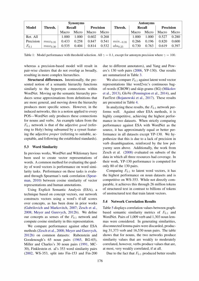
ModelSynonyms Antonyms

Thresh. Recall Precision Thresh. Recall PrecisionMacro Micro Macro Micro Macro Micro Macro Micro

Ret. All 1.000 1.000 0.602 0.268 1.000 1.000 0.527 0.280Precision max0.35 0.433 0.258 0.847 0.541 min−0.35 0.266 0.196 0.820 0.600F0.1 max0.30 0.535 0.404 0.814 0.532 abs0.25 0.730 0.763 0.619 0.397

Table 1: Model performance with threshold selection. All γ = 0.1, except for antonym precision where γ = 100.

whereas a precision-based model will result inpair-wise clusters that do not overlap as broadly,resulting in more complex hierarchies.

Structural differences. Intentionally, the pre-sented notion of a semantic hierarchy functionssimilarly to the hypernym connections withinWordNet. Moving up the semantic hierarchy pro-duces sense approximations from definitions thatare more general, and moving down the hierarchyproduces more specific senses. However, in theinduced networks, this is a notion applied to everyPOS—WordNet only produces these connectionsfor nouns and verbs. An example taken from theF0.1 network is that of the adjective good (refer-ring to Holy) being subsumed by a synset featur-ing the adjective proper (referring to suitable, ac-ceptable, and following the established standards).

5.3 Word Similarity

In previous works, WordNet and Wiktionary havebeen used to create vector representations ofwords. A common method for evaluating the qual-ity of word vectors is performance on word simi-larity tasks. Performance on these tasks is evalu-ated through Spearman’s rank correlation (Spear-man, 2010) between cosine similarity of vectorrepresentations and human annotations.

Using Explicit Semantic Analysis (ESA), atechnique based on concept vectors, our networkconstructs vectors using a word’s tf-idf scoresover concepts, as has been done in prior works(Gabrilovich and Markovitch, 2007; Zesch et al.,2008; Meyer and Gurevych, 2012b). We defineour concepts as senses of the F0.1 network andcompute cosine similarity in this representation.

We compare performance against other ESAmethods (Zesch et al., 2008; Meyer and Gurevych,2012b) on common datasets: Rubenstein andGoodenough’s 65 noun pairs (1965, RG-65),Miller and Charles’s 30 noun pairs (1991, MC-30), Finklestein et. al’s 353 word similarity pairs(2002, WS-353, split into Fin-153 and Fin-200

due to different annotators), and Yang and Pow-ers’s 130 verb pairs (2006, YP-130). Our resultsare summarized in Table 3.

We also compare F0.1 against latent word vectorrepresentations like word2vec’s continuous bag-of-words (CBOW) and skip-grams (SG) (Mikolovet al., 2013), GloVe (Pennington et al., 2014), andFastText (Bojanowski et al., 2017). These resultsare presented in Table 4.

In analyzing these results, the F0.1 network per-forms well. Against other ESA methods, it ishighly competitive, achieving the highest perfor-mance in two datasets. When strictly comparingperformance against ESA with WordNet as thesource, it has approximately equal or better per-formance in all datasets except YP-130. We hy-pothesize that this is due to a lack of precision inverb disambiguation, reinforced by the low pol-ysemy seen above. Additionally, the work fromZesch et al. (2008) evaluated on subsets of thedata in which all three resources had coverage. Intheir work, YP-130 performance is computed foronly 80 of the 130 pairs.

Comparing F0.1 to latent word vectors, it hasthe highest performance on noun datasets and iscompetitive on WS-353. While not directly com-parable, it achieves this through 26 million tokensof structured text in contrast to billions of tokensof unstructured text that train latent vectors.

5.4 Network Correlation Results

Table 5 displays correlation values between graph-based semantic similarity metrics of F0.1 andWordNet. Pairs of 1,009 verb and 1,303 noun lem-mas were considered. In generating similarities,disconnected lemma pairs were discarded, produc-ing 31,373 verb and 16,530 noun pairs. The tableshows that for nouns, the two networks producesimilarity values that are weakly to moderatelycorrelated, however, verbs produce values that are,at most, very weakly correlated, if at all.

Due to the fact that F0.1 produced better results

176

With Monosemous Words Without Monosemous WordsPOS WordNet F0.01 Precision Return All WordNet F0.01 Precision Return AllNoun 1.24 1.17 1.18 1.10 2.79 2.94 2.99 2.66Verb 2.17 1.20 1.22 1.10 3.57 3.18 3.33 2.78Adjective 1.18 1.18 1.18 1.10 2.71 2.59 2.62 2.33Adverb 1.25 1.11 1.12 1.08 2.50 2.34 2.36 2.25

Table 2: Average polysemy statistics.

Dataset RG-65 MC-30 Fin-153 Fin-200 YP-130F0.1 0.831 0.849 0.723 0.557 0.687WordNet* (Zesch et al., 2008) 0.82 0.78 0.61 0.56 0.71Wikipedia* (Zesch et al., 2008) 0.76 0.68 0.70 0.50 0.29Wiktionary* (Zesch et al., 2008) 0.84 0.84 0.70 0.60 0.65Wiktionary (Meyer and Gurevych, 2012b) - - - - 0.73

Table 3: Spearman’s rank correlation coefficients on word similarity tasks. Best values are in bold.

Dataset RG-65 MC-30 WS-353F0.1 0.831 0.849 0.669FastText - - 0.73CBOW (6B) 0.682 0.656 0.572SG (6B) 0.697 0.652 0.628GloVe (6B) 0.778 0.727 0.658GloVe (42B) 0.829 0.836 0.759CBOW (100B) 0.754 0.796 0.684

Table 4: Spearman’s correlation on word similaritytasks. Best values are in bold. Number of tokens intraining data is featured in parentheses, if reported.FastText is reported from (Bojanowski et al., 2017),and all others are from (Pennington et al., 2014).

Noun VerbPS min 0.266 0.132PS max 0.495 0.189PS avg 0.448 0.082LCH min 0.207 0.120LCH max 0.384 0.056LCH avg 0.359 -0.013WP min 0.116 0.090WP max 0.219 0.005WP avg 0.226 -0.025

Table 5: Correlations between F0.1 and WordNet simi-larity metrics: path similarity (PS), Leacock Chodorowsimilarity (LCH), and Wu Palmer similarity (WP).

on noun similarity tasks, we hypothesize that thisindicates better semantic structure for nouns thanfor verbs, further emphasizing that a possible lim-itation of the current baseline produced is its lack

of precision when it comes to polysemous verbs.However, the positive correlation values seen fornouns, coupled with noun similarity performance,offer strong indications that the F0.1 does provideuseful semantic structure that can be further in-creased through better modeling.

6 Future work

Here, several directions are highlighted alongwhich we see this work being extended.

Better models. The development of more accu-rate models for predicting definitions involved inthe pair-wise relations will produce more interest-ing and useful networks, especially with the mag-nitude of examples of sense usage. Precision ofverb relations seems to be a critical component ofa better model.

Supervision. Relationship prediction is cur-rently unsupervised. While it is an interesting taskto model in this fashion, crowd sourcing the an-notation of this data would be possible throughservices like Amazon Mechanical Turk. Thiswould allow for the potential of exploring su-pervised models for predicting relationship links,particularly for relationships like synonymy andantonymy which are familiar concepts for a broadcommunity of potential annotators.

WordNet semi-supervision. Another logicaltransformation of this task would be to use Word-Net to inform the induction of a network in a semi-supervised fashion. There are many ways to goabout this such as using statistics from WordNetto create a loss function, or using the structure of

177

WordNet as a base. As this work aimed to create anetwork solely from the data of Wiktionary, theseideas were not explored. However, using WordNetin this fashion is one of the directions of greatestinterest for exploration in the future.

Sense usage examples. The examples presentin Wiktionary have only begun to be used in thiswork. When examples are pulled, the source def-inition and lemma are linked. However, these ex-amples have the potential to be linked to othersenses and lemmas. This would an immenseamount of structured, sense-usage data that couldbe used for many machine learning tasks.

Multilingual networks Wiktionary has beenexplored as a multilingual resource in previousworks (de Melo and Weikum, 2009; Gurevychet al., 2012; Meyer and Gurevych, 2012b; Bondand Foster, 2013) largely due to the natural align-ment across languages. Extending this approach toa multilingual setting could prove to be extremelyuseful for machine translation, and could allowlow resource languages to benefit from alignmentwith other languages that have more annotations.

7 Conclusion

This paper introduced the idea of constructing awordnet solely using the data from Wiktionary.Wiktionary is a powerful resource, featuring mil-lions of pages that describe lemmas, their senses,example usages, and the relationships betweenthem. Previous work has explored aligning re-sources like this with other networks like thePrinceton WordNet. However, no work has fullyexplored the idea of building an entire networkfrom the ground up using just Wiktionary.

This work explores simple baselines for con-structing a network from Wiktionary throughantonym and synonym relationships and com-pares induced networks with WordNet to find sim-ilar structures and statistics that appear to high-light strong future directions of particular inter-est, including but not limited to improving net-work modeling, linking more semantic exam-ples, and reinforcing network construction usingexpert-annotated networks, like WordNet.

As conducted, this work is an initial step intransforming Wikitionary from an open-sourcedictionary into a powerful tool, dataset, and frame-work, with the hope of driving and motivating fur-ther work at endeavors studying languages and de-veloping language processing systems.

ReferencesYoshua Bengio, Rjean Ducharme, Pascal Vincent, and

Christian Jauvin. 2003. A neural probabilistic lan-guage model. Journal of machine learning research,3:1137–1155.

David M. Blei, Andrew Y. Ng, and Michael I. Jordan.2003. Latent dirichlet allocation. Journal of ma-chine learning research, 3:993–1022.

Piotr Bojanowski, Edouard Grave, Armand Joulin, andTomas Mikolov. 2017. Enriching word vectors withsubword information. Transactions of the Associa-tion for Computational Linguistics, 5:135–146.

Francis Bond and Ryan Foster. 2013. Linking and ex-tending an open multilingual wordnet. In Proceed-ings of the 51st Annual Meeting of the Associationfor Computational Linguistics (Volume 1: Long Pa-pers), pages 1352–1362, Sofia, Bulgaria. Associa-tion for Computational Linguistics.

Lars Borin, Jens Allwood, and Gerard de Melo. 2014.Bring vs. mtroget: Evaluating automatic thesaurustranslation. In Proceedings of the Ninth Interna-tional Conference on Language Resources and Eval-uation (LREC’14), pages 2115–2121, Reykjavik,Iceland. European Language Resources Association(ELRA).

Nello Cristianini and John Shawe-Taylor. 2000. An in-troduction to Support Vector Machines: and otherkernel-based learning methods. Cambridge Univer-sity Press, New York, NY, USA.

Christiane Fellbaum. 1998. WordNet: An ElectronicLexical Database. MIT Press, Cambridge, MA,USA.

Lev Finkelstein, Evgeniy Gabrilovich, Yossi Matias,Ehud Rivlin, Zach Solan, Gadi Wolfman, and EytanRuppin. 2002. Placing search in context: The con-cept revisited. ACM Trans. Inf. Syst., 20:116–131.

Evgeniy Gabrilovich and Shaul Markovitch. 2007.Computing semantic relatedness using wikipedia-based explicit semantic analysis. In Proceedings ofthe 20th International Joint Conference on ArtificalIntelligence, IJCAI’07, pages 1606–1611, San Fran-cisco, CA, USA. Morgan Kaufmann Publishers Inc.

Anne Gohring. 2014. Building a spanish-german dic-tionary for hybrid mt. In Proceedings of the 3rdWorkshop on Hybrid Approaches to Machine Trans-lation (HyTra), pages 30–35, Gothenburg, Sweden.Association for Computational Linguistics.

Iryna Gurevych, Judith Eckle-Kohler, Silvana Hart-mann, Michael Matuschek, Christian M. Meyer, andChristian Wirth. 2012. Uby - a large-scale unifiedlexical-semantic resource based on lmf. In Proceed-ings of the 13th Conference of the European Chap-ter of the Association for Computational Linguis-tics, pages 580–590, Avignon, France. Associationfor Computational Linguistics.

178

Sanda M. Harabagiu, George A. Miller, and Dan I.Moldovan. 1999. Wordnet 2 - a morphologicallyand semantically enhanced resource. In SIGLEX99:Standardizing Lexical Resources.

Mohammad Javad Hosseini, Noah A. Smith, and Su-InLee. 2016. Uw-cse at semeval-2016 task 10: De-tecting multiword expressions and supersenses us-ing double-chained conditional random fields. InProceedings of the 10th International Workshop onSemantic Evaluation (SemEval-2016), pages 931–936, San Diego, California. Association for Com-putational Linguistics.

Thorsten Joachims. 1998. Text categorization withsupport vector machines: Learning with many rel-evant features. In Machine Learning: ECML-98,pages 137–142, Berlin, Heidelberg. Springer BerlinHeidelberg.

Armand Joulin, Edouard Grave, Piotr Bojanowski, andTomas Mikolov. 2017. Bag of tricks for efficienttext classification. In Proceedings of the 15th Con-ference of the European Chapter of the Associationfor Computational Linguistics: Volume 2, Short Pa-pers, pages 427–431, Valencia, Spain. Associationfor Computational Linguistics.

David Jurgens and Mohammad Taher Pilehvar. 2015.Reserating the awesometastic: An automatic exten-sion of the wordnet taxonomy for novel terms. InProceedings of the 2015 Conference of the NorthAmerican Chapter of the Association for Computa-tional Linguistics: Human Language Technologies,pages 1459–1465, Denver, Colorado. Associationfor Computational Linguistics.

Robert Krovetz. 1992. Sense-linking in a machinereadable dictionary. In 30th Annual Meeting of theAssociation for Computational Linguistics, pages330–332, Newark, Delaware, USA. Association forComputational Linguistics.

Thomas K. Landauer and Susan T. Dumais. 1997. Asolution to plato’s problem: The latent semanticanalysis theory of acquisition, induction, and rep-resentation of knowledge. Psychological Review,104(2):211–240.

C. Leacock and M. Chodorow. 1998. Combining lo-cal context and WordNet similarity for word senseidentification. WordNet: An Electronic LexicalDatabase, pages 265–283.

J. Lilleberg, Y. Zhu, and Y. Zhang. 2015. Supportvector machines and word2vec for text classificationwith semantic features. In 2015 IEEE 14th Interna-tional Conference on Cognitive Informatics Cogni-tive Computing (ICCI*CC), pages 136–140.

Michael Matuschek and Iryna Gurevych. 2013.Dijkstra-wsa: A graph-based approach to wordsense alignment. Transactions of the Association forComputational Linguistics, 1:151–164.

Michael Matuschek, Christian M. Meyer, and IrynaGurevych. 2013. Multilingual knowledge in alignedwiktionary and omegawiki for translation applica-tions. Translation: Computation, Corpora, Cogni-tion, 3(1).

Gerard de Melo and Gerhard Weikum. 2009. Towardsa universal wordnet by learning from combined evi-dence. In Proceedings of the 18th ACM Conferenceon Information and Knowledge Management, CIKM’09, pages 513–522, New York, NY, USA. ACM.

Christian M. Meyer and Iryna Gurevych. 2010a. Howweb communities analyze human language: Wordsenses in wiktionary. Proceedings of the 2nd WebScience Conference.

Christian M. Meyer and Iryna Gurevych. 2010b. Worthits weight in gold or yet another resource–a com-parative study of wiktionary, openthesaurus and ger-manet. In Computational Linguistics and IntelligentText Processing, pages 38–49, Berlin, Heidelberg.Springer Berlin Heidelberg.

Christian M. Meyer and Iryna Gurevych. 2011. Whatpsycholinguists know about chemistry: Aligningwiktionary and wordnet for increased domain cov-erage. In Proceedings of 5th International JointConference on Natural Language Processing, pages883–892, Chiang Mai, Thailand. Asian Federationof Natural Language Processing.

Christian M. Meyer and Iryna Gurevych. 2012a. On-towiktionary — constructing an ontology from thecollaborative online dictionary wiktionary. In M. T.Pazienza and A. Stellato, editors, Semi-AutomaticOntology Development: Processes and Resources,pages 131—161. IGI Global, Hershey, PA.

Christian M. Meyer and Iryna Gurevych. 2012b. Toexhibit is not to loiter: A multilingual, sense-disambiguated Wiktionary for measuring verb sim-ilarity. In Proceedings of COLING 2012, pages1763–1780, Mumbai, India. The COLING 2012 Or-ganizing Committee.

Tomas Mikolov, Ilya Sutskever, Kai Chen, Greg S Cor-rado, and Jeff Dean. 2013. Distributed representa-tions of words and phrases and their composition-ality. In C. J. C. Burges, L. Bottou, M. Welling,Z. Ghahramani, and K. Q. Weinberger, editors, Ad-vances in Neural Information Processing Systems26, pages 3111–3119. Curran Associates, Inc.

George A. Miller. 1995. Wordnet: A lexicaldatabase for english. Communications of the ACM,38(11):39–31.

George A. Miller and Walter G. Charles. 1991. Con-textual correlates of semantic similarity. Languageand Cognitive Processes, 6(1):1–28.

George A. Miller and Florentina Hristea. 2006. Squibsand discussions: Wordnet nouns: Classes and in-stances. Computational Linguistics, 32(1):1–3.

179

Tristan Miller and Iryna Gurevych. 2014. Wordnet—wikipedia—wiktionary: Construction of a three-way alignment. In Proceedings of the Ninth Interna-tional Conference on Language Resources and Eval-uation (LREC’14), pages 2094–2100, Reykjavik,Iceland. European Language Resources Association(ELRA).

Grace Muzny and Luke Zettlemoyer. 2013. Automaticidiom identification in Wiktionary. In Proceedingsof the 2013 Conference on Empirical Methods inNatural Language Processing, pages 1417–1421,Seattle, Washington, USA. Association for Compu-tational Linguistics.

Patrick Pantel and Marco Pennacchiotti. 2006.Espresso: Leveraging generic patterns for automati-cally harvesting semantic relations. In Proceedingsof the 21st International Conference on Compu-tational Linguistics and 44th Annual Meeting ofthe Association for Computational Linguistics,pages 113–120, Sydney, Australia. Association forComputational Linguistics.

Patrick Pantel and Marco Pennacchiotti. 2008. Auto-matically harvesting and ontologizing semantic rela-tions. In Ontology Learning and Population: Bridg-ing the Gap between Text and Knowledge, pages171–198, Amsterdam, Netherlands. IOS Press.

Karl Pearson. 1895. Notes on regression and inheri-tance in the case of two parents. In Proceedings ofthe Royal Society of London, volume 58, pages 240–242. The Royal Society of London.

Jeffrey Pennington, Richard Socher, and ChristopherManning. 2014. Glove: Global vectors for wordrepresentation. In Proceedings of the 2014 Con-ference on Empirical Methods in Natural LanguageProcessing (EMNLP), pages 1532–1543, Doha,Qatar. Association for Computational Linguistics.

Herbert Rubenstein and John Goodenough. 1965. Con-textual correlates of synonymy. Communications ofthe ACM, 8:627–633.

Jon Rusert and Ted Pedersen. 2016. Umnduluthat semeval-2016 task 14: Wordnet’s missing lem-mas. In Proceedings of the 10th InternationalWorkshop on Semantic Evaluation (SemEval-2016),pages 1346–1350, San Diego, California. Associa-tion for Computational Linguistics.

Bahar Salehi, Paul Cook, and Timothy Baldwin.2014. Detecting non-compositional mwe compo-nents using wiktionary. In Proceedings of the2014 Conference on Empirical Methods in NaturalLanguage Processing (EMNLP), pages 1792–1797,Doha, Qatar. Association for Computational Lin-guistics.

Tobias Schnabel, Igor Labutov, David Mimno, andThorsten Joachims. 2015. Evaluation methods forunsupervised word embeddings. pages 298–307.

Bernhard Scholkopf, Chris Burges, and Vladimir Vap-nik. 1995. Extracting support data for a given task.In Proceedings of the First International Confer-ence on Knowledge Discovery and Data Mining,KDD’95, pages 252–257. AAAI Press.

C Spearman. 2010. The proof and measurement of as-sociation between two things. International Journalof Epidemiology, 39(5):1137–1150.

Wikimedia. Wiktionary, the free dictionary.

Lingfei Wu, Ian En-Hsu Yen, Kun Xu, FangliXu, Avinash Balakrishnan, Pin-Yu Chen, PradeepRavikumar, and Michael J. Witbrock. 2018. Wordmover’s embedding: From word2vec to documentembedding. In Proceedings of the 2018 Conferenceon Empirical Methods in Natural Language Pro-cessing, pages 4524–4534, Brussels, Belgium. As-sociation for Computational Linguistics.

Z. Wu and M. Palmer. 1994. Verbs semantics and lex-ical selection. Proceedings of the 32nd conferenceon Association for Computational Linguistics, pages133–138.

Dongqiang Yang and David Powers. 2006. Verb simi-larity on the taxonomy of wordnet. Proceedings ofthe 3rd International WordNet Conference (GWC),pages 121–128.

Torsten Zesch, Christof Muller, and Iryna Gurevych.2008. Using wiktionary for computing semantic re-latedness. In In Proceedings of AAAI, pages 861–867.

180


SmokEng: Towards Fine-grained Classification of Tobacco-related SocialMedia Text

Kartikey Pant, Venkata Himakar Yanamandra, Alok Debnath and Radhika MamidiInternational Institute of Information Technology

Hyderabad, Telangana, India{kartikey.pant, himakar.y, alok.debnath}@research.iiit.ac.in

[email protected]

Abstract

Contemporary datasets on tobacco consump-tion focus on one of two topics, either pub-lic health mentions and disease surveillance,or sentiment analysis on topical tobacco prod-ucts and services. However, two primary con-siderations are not accounted for, the languageof the demographic affected and a combina-tion of the topics mentioned above in a fine-grained classification mechanism. In this pa-per, we create a dataset of 3144 tweets, whichare selected based on the presence of collo-quial slang related to smoking and analyze itbased on the semantics of the tweet. Eachclass is created and annotated based on thecontent of the tweets such that further hierar-chical methods can be easily applied.

Further, we prove the efficacy of standard textclassification methods on this dataset, by de-signing experiments which do both binary aswell as multi-class classification. Our experi-ments tackle the identification of either a spe-cific topic (such as tobacco product promo-tion), a general mention (cigarettes and relatedproducts) or a more fine-grained classification.This methodology paves the way for furtheranalysis, such as understanding sentiment orstyle, which makes this dataset a vital contri-bution to both disease surveillance and tobaccouse research.

1 Introduction

As Twitter has grown in popularity to 330 millionmonthly active users, researchers have increas-ingly been using it as a source of data for tobaccosurveillance (Lienemann et al., 2017). Tobacco-related advertisements, tweets, awareness posts,and related information is most actively viewedby young adults (aged 18 to 29), who are ex-tensive users of social media and also representthe largest population of smokers in the US and

Canada 1. Furthermore, it allows us to understandpatterns in ethnically diverse and vulnerable au-diences (Lienemann et al., 2017). Social mediaprovides an active and useful platform for spread-ing awareness, especially dialog platforms, whichhave untapped potential for disease surveillance(Platt et al., 2016). These platforms are useful instimulating the discussion on societal roles in thedomain of public health (Platt et al., 2016). Sharpeet al. (2016) has shown the utility of social mediaby highlighting that the number of people usingsocial media channels for information about theirillnesses before seeking medical care.

Correlation studies have shown that the mostprobable leading cause of preventable death glob-ally is the consumption of tobacco and tobaccoproducts (Prochaska et al., 2012). The diseasemost commonly associated with tobacco con-sumption is lung cancer, with two million casesreported in 2018 alone 2. While cigarettes arecondemned on social media, this has been rivaledby the rising popularity and analysis of the sup-posed benefits of e-cigarettes (Dai and Hao, 2017).Information pertaining to new flavors and inno-vations in the industry and surrounding culturehave generated sizable traffic on social media aswell (Hilton et al., 2016). Studies show that so-cial acceptance is a leading factor to the use andproliferation of e-cigarettes, with some reportsclaiming as many as 2.39 million high school and0.63 million middle school students having usedan e-cigarette at least once (Malik et al., 2019;Mantey et al., 2019). However, there are strongclaims suggesting the use of e-cigarettes as a ’gate-way’ drug for other illicit substances (Unger et al.,

1https://www.cdc.gov/tobacco/data_statistics/fact_sheets/adult_data/cig_smoking/

2https://www.wcrf.org/dietandcancer/cancer-trends/lung-cancer-statistics

181

Figure 1: Procedure for Data Collection. We started out with approximately 7 million Tweets which were minedbased on 24 slang terms. These were pre-processed to select relevant tweets with decent traction on Twitter. Afinal cleaned dataset of 3144 tweets is presented.

2016).In this paper, we aim at classifying tweets relat-

ing to cigarettes, e-cigarettes, and other tobacco-related products into distinct classes. This classifi-cation is fine-grained in order to assist in the anal-ysis of the type of tweets which affect the usersthe most for each product or category. The exten-sive, manually annotated dataset of 3144 tweetspertains to tobacco use classification into adver-tisement, general information, personal informa-tion, and non-tobacco drug classes. Such classifi-cation provides insight into the type of tweet andassociated target audience. For example, presentcessation programs target users who are ready toquit rather than people who use it regularly, whichcan be solved using twitter and other online so-cial media (Prochaska et al., 2012). Unlike manyprevious studies, we also include common slangterms into the classification scheme so as to beable to work with the social media discourse ofthe target audience.

Finally, we present several text-classificationmodels for the fine-grained classification taskspertaining to tobacco-related tweets on the re-leased dataset3. In doing so, we extend the workin topical Twitter content analysis as well as thestudy of public health mentions on Twitter.

2 Related Work

Myslın et al. (2013) explored content and senti-3https://github.com/kartikeypant/

smokeng-tobacco-classification

ment analysis of Tobacco-related Twitter posts andperformed analysis using machine learning clas-sifiers for the detection of tobacco-relevant postswith a particular focus on emerging products likee-cigarettes and hookah. Their work depends on atriaxial classification along and uses basic statisti-cal classifiers. However, their feature-engineeredkeyword-based systems do not account for slangassociated with tobacco consumption.

Vandewater et al. (2018) performs a classifica-tion study based on identifying brand associatedwith a post using basic text analytics using key-words and image-based classifiers to determinethe brands that were most responsible to postingabout their brands on social media. Cortese et al.(2018) does a similar analysis on the consumerside, for female smokers on Instagram, targetingthe same age group, but based entirely on featureextraction on images, particularly selfies.

More recently, Malik et al. (2019) explored pat-terns of communication of e-cigarette companyJuul use on Twitter. They categorized 1008 ran-domly selected tweets across four dimensions,namely, user type, sentiment, genre, theme. How-ever, they explore the effects of only Juul, andnot other cigarettes or e-cigarettes, further limit-ing their experiment to only Juul-based analysisand inferences.

In the domain of Disease Surveillance, Aramakiet al. (2011) explored the problem of identifyinginfluenza epidemics using machine-learning basedtweet classifiers along with search engine trends

182

Name Label AnnotationClass

Mention of Non-Tobacco Drugs OD -1Unrelated or Ambiguous Mention UM 0Personal or Anecdotal Mention PM 1

Informative or Advisory Mention IM 2Advertisements AD 3

Table 1: Label and ID associated with each class.

for medical keywords and medical records for thedisease in a local environment. For doing so, theyuse SVM based classifiers for extracting tweetsthat mention actual influenza patients. However,since they use only SVM based classifiers, theyare limited in their accuracy in classification.

Dai et al. (2017) also focuses on public healthsurveillance, and uses word embeddings on a topicclassifier in order to identify and capture seman-tic similarities between medical tweets by diseaseand tweet type for a more robust yet very filteredclassification, not accounting for the variety of lin-guistic features in tweets such as slang, abbrevia-tions and the like in the keyword-based classifica-tion mechanism. Jiang et al. (2018) works on asimilar problem using machine learning solutionssuch as an LSTM classifier.

3 Dataset Creation

In this section, we explain the development of thedataset that we present along with this paper. Wesummarize the methods for collecting and filter-ing through the tweets to arrive at the final datasetand provide some examples of the types of tweetsand features we focused on. We also provide thedataset annotation schema and guidelines.

3.1 Data CollectionUsing the Twitter Application Programming Inter-face (API4), we collected a sample of tweets be-tween 1st October 2018 and 7th October 2018 thatrepresented 1% of the entire Twitter feed. This 1%sample consisted of an average 1,035,206 milliontweets per day. Out of the 7,246,442 tweets, onlytweets written in English and written by users withmore than 100 followers have selected for the nextstep in order to clear spam written by bots.

In order to extract tobacco related tweets fromthis dataset, we constructed a list of keywords rel-evant to general tobacco usage, including hookah

4https://developer.twitter.com/en/products/tweets/sample.html

and e-cigarettes. Our initial list consisted of 32such terms compiled from online slang dictionar-ies, but we pruned this list to 24 terms. Thesewere smoking, cigarette, e-cig*, cigar, tobacco,hookah, shisha, e-juice, e-liquid, vape, vaping,cheroot, cigarillo, roll-up, ashtray, baccy, rollies,claro, chain-smok*, vaper, ciggie, nicotine, non-smoker, non-smoking.

By taking the dataset for a full week, we thusavoided potential bias based on the day of theweek, which has been observed for alcohol relatedtweets, which spike in positive sentiment on Fri-days and Saturdays (Cavazos-Rehg et al., 2015).For each of the 7 days, all tweets matching anyof the listed keywords were included. Tweetsmatching these tobacco related keywords reflected0.00043% of all tweets in the Twitter API 1%sample. The resulting final dataset thus contained3144 tweets, with a mean of 449 tweets per day.

3.2 Data Annotation

The collected data was then annotated based on thecategories mentioned in Table 1. These categorieswere chosen on the basis of frequency of occur-rence, motivated by the general perception of to-bacco and non-tobacco drug related tweets. Theseincluded advertisements as well anecdotes, infor-mation and cautionary tweets. We further noticedthat a similar pattern was seen for e-cigarettes andalso pertained to some other drugs. While wehave explored e-cigarettes in this classification, wehave marked the mention of other drugs that weretagged with the same keywords.

A formal definition of each of the categories isgiven below.

• Unrelated or Ambiguous Mention: Thiscategory of tweets contain tweets containinginformation unrelated to tobacco or any otherdrug, or pertaining to ambiguity in the intentof the tweet, such as sarcasm.

183

Label Examples

UM”What are you smoking bruh ?””The smoking gun on Kavanaugh! URL ”

PM”im smoking and doing whats best for me””I haven’t had a cigarette in $NUMBER$ months why do I want one so bad now??”

IM”Obama puffed. Clinton did cigar feel.Churchill won major wars on whisky.””The FDA’s claim of a teen vaping addiction epidemic doesn’t add up. #ecigarette #health”

AD”Which ACID Kuba Kuba are you aiming for? #De4L #ExperienceAcid #cigar #cigars URL””Spookah Lounge: A concept - a year round Halloween-themed hookah lounge”

OD”Making my money and smoking my weed””Mobbin in da Bentley smoking moonrocks.”

Table 2: Examples for each category represented by its label.

• Personal or Anecdotal Mention: Tweets areclassified as containing a personal or anecdo-tal mention if they imply either personal useof tobacco products or e-cigarettes, or pro-vide instances of use of the products by them-selves or others.

• Informative or Advisory Mention: Thisclass of tweets consist of a broad range oftopics such as:

– mention or discussion on statistics of to-bacco and e-cigarette use or consump-tion

– mention associated health risks or bene-fits

– portray the use of tobacco products or e-cigarettes by a public figure

– emphasize social campaigns for anti-smoking, smoking cessation and relatedproducts such as patches

• Advertisements: All tweets written with theintent of the sale of tobacco products, e-cigarettes and associated products or servicesare marked advertisements. In this classifica-tion, intent is considered using the mention ofprice as an objective measure.

• Mention of Non-Tobacco Drugs: Tweetswhich mention the use, sale, anecdotesand information about drugs other than e-cigarettes or tobacco products are annotatedin this category.

3.3 Inter-annotator AgreementAnnotation of the dataset to detect the presence oftobacco substance use was carried out by two hu-man annotators having linguistic background and

proficiency in English. A sample annotation setconsisting of 10 tweets per class was selected ran-domly from all across the corpus. Both annota-tors were given the selected sample annotation set.These sample annotation set served as a referencebaseline of each category of the text.

In order to validate the quality of annotation, wecalculated the Inter-Annotator Agreement (IAA)for the fine-grain classification between the twoannotation sets of 3,144 tobacco-related tweets us-ing Cohen’s Kappa coefficient (Fleiss and Cohen,1973). The Kappa score of 0.791 indicates that thequality of the annotation and presented schema isproductive.

4 Methodology

In this section we describe the classifiers designedfor this task of fine grained classification. Theclassifier architecture is based upon a combina-tion of choosing word representations, along witha discriminator that is compatible with that rep-resentation. We use the TF-IDF for the suportvector machines and GloVe embeddings (Penning-ton et al., 2014) with our convolutional neuralnetwork architecture and recurrent architectures(LSTM and Bi-LSTM). We also used FastText andBERT embeddings (both base and large) with theirnative classifiers to note the change in the accura-cies.

4.1 Support Vector Machines (SVM)

The first learning model used for classificationin our experiment was Support Vector Machines(SVM) (Cortes and Vapnik, 1995). We used termfrequency-inverse document frequency (TF-IDF)as a feature to classify the annotated tweets in ourdata set (Salton and Buckley, 1988). TF-IDF cap-

184

tures the importance of the given the word in adocument, defined in Equation 1.

tfidf(t, d,D) = f(t, d)× logN

|{dεD : tεd}| (1)

where f(t, d) indicates the number of times term tappears in context, d and N is the total number ofdocuments |dεD : tεd| represents the total numberof documents where t occurs.

The SVM classifier finds the decision boundarythat maximizes the margin by minimizing ||w|| tofind the optimal hyperplane for all the classifica-tion tasks:

min f : 12‖w‖2

s.t. y(i)(wTx(i) + b

)≥ 1, i = 1, . . . ,m

(2)where w is the weight vector, x is the input vec-

tor and b is the bias.

4.2 Convolutional Neural Networks (CNN)

In this subsection, we outline the ConvolutionalNeural Networks (Fukushima, 1988) for classifi-cation and also provide the process description fortext classification in particular. Convolutional neu-ral networks are multistage trainable neural net-works architectures developed for classificationtasks (Lecun et al., 1998). Each of these stagesconsist of the types of layers described below:

• Embedding Layer: The purpose of an em-bedding layer is to transform the text inputsinto a form which can be used by the CNNmodel. Here, each word of a text document istransformed into a dense vector of fixed size.

• Convolutional Layers: A Convolutionallayer consists of multiple kernel matrices thatperform the convolution mathematical oper-ation on their input and produce an outputmatrix of features upon the addition of a biasvalue.

• Pooling Layers: The purpose of a poolinglayer is to perform dimensionality reductionof the input feature vectors. Pooling layersuse sub-sampling to the output of the convo-lutional layer matrices combing neighbour-ing elements. We have used the commonlyused max-pooling function for the pooling.

• Fully-Connected Layer: It is a classic fullyconnected neural network layer. It is con-nected to the Pooling layers via a Dropoutlayer in order to prevent overfitting. Softmaxactivation function is used for defining the fi-nal output of this layer.

The following objective function is commonlyused in the task:

Ew =1

n

P∑

p=1

NL∑

j=1

(oLj,p − yj,p)2 (3)

where P is the number of patterns, oLj,p is the out-put of jth neuron that belongs to Lth layer, NL isthe number of neurons in output of Lth layer, yj,pis the desirable target of jth neuron of pattern pand yi is the output associated with an input vec-tor xi to the CNN.

We use Adam Optimizer (Kingma and Ba,2014) to minimize the cost function Ew.

4.3 Recurrent Neural ArchitecturesRecurrent neural networks (RNN) have been em-ployed to produce promising results on a varietyof tasks, including language model and speechrecognition (Mikolov et al., 2010, 2011; Gravesand Schmidhuber, 2005). An RNN predicts thecurrent output conditioned on long-distance fea-tures by maintaining a memory based on historyinformation.

An input layer represents features at time t.One-hot vectors for words, dense vector featuressuch as word embeddings, or sparse features usu-ally represent an input layer. An input layer hasthe same dimensionality as feature size. An out-put layer represents a probability distribution overlabels at time t and has the same dimensionalityas the size of the labels. Compared to the feed-forward network, an RNN contains a connectionbetween the previous hidden state and current hid-den state. This connection is made through the re-current layer, which is designed to store history in-formation. The following equation is used to com-pute the values in the hidden, and output layers:

h(t) = f(Ux(t) + Wh(t− 1)). (4)

y(t) = g(Vh(t)), (5)

where U , W , and V are the connection weightsto be computed during training, and f(z) and g(z)

185

Model/Experiment Personal Health Mentions Tobacco-related MentionsSVM 82.17% 83.44%CNN 84.08% 82.48%LSTM 84.39% 83.32%BiLSTM 83.92% 82.97%FastText 83.76% 81.05%BERTBase 85.19% 85.50%BERTLarge 87.26% 85.67%

Table 3: Binary Classification accuracies for specific topic (Personal Health Mention) or general theme (Tobacco-related Mentions).

are sigmoid and softmax activation functions asfollows.

f(z) =1

1 + e−z, (6)

g(zm) =ezm∑k e

zk

(7)

In this paper, we apply Long Short Term Mem-ory (LSTM) and Bidirectional Long Short TermMemory(Bi-LSTM) to sequence tagging (Hochre-iter and Schmidhuber, 1997; Graves and Schmid-huber, 2005; Graves et al., 2013).

LSTM networks use purpose-built memorycells to update the hidden layer values. As a re-sult, they may be better at finding and exploitinglong-range dependencies in the data than a stan-dard RNN. The following equation implementsthe LSTM model:

it = σ(Wxixt +Whiht−1 +Wcict−1 + bi) (8)

ft = σ(Wxfxt+Whfht−1+Wcfct−1+ bf ) (9)

ot = σ(Wxoxt +Whoht−1 +Wcoct + bo) (10)

ht = ottanh(ct) (11)

In sequence tagging task, we have access toboth past and future input features for a given time.Thus, we can utilize a bidirectional LSTM net-work (Bi-LSTM) as proposed in (Graves et al.,2013).

4.4 FastText

FastText classifier has proven to be efficient fortext classification (Joulin et al., 2016). It is often at

par with deep learning classifiers in terms of accu-racy, and much faster for training and evaluation.FastText uses bag of words and bag of n-gramsas features for text classification. Bag of n-gramsfeature captures partial information about the lo-cal word order. FastText allows updating wordvectors through back-propagation during trainingallowing the model to fine-tune word representa-tions according to the task at hand (Bojanowskiet al., 2016). The model is trained using stochasticgradient descent and a linearly decaying learningrate.

4.5 BERT

While previous studies on word representationsfocused on learning context-independent repre-sentations, recent works have focused on learningcontextualized word representations. One of themore recent contextualized word representation isBERT (Devlin et al., 2019).

BERT is a contextualized word representationmodel, pre-trained using bidirectional transform-ers(Vaswani et al., 2017). It uses a masked lan-guage model that predicts randomly masked in asequence. It uses the task of next sentence predic-tion for learning the embeddings with a broadercontext. It outperforms many existing techniqueson most NLP tasks with minimal task-specific ar-chitectural changes. It is pretrained on 3.3B wordsfrom various sources including BooksCorpus andthe English Wikipedia.

Based on the transformer architecture used,BERT is classified into two types: BERTBase andBERTLarge. BERTBase uses a 12-layered trans-former with 110M parameters. BERTLarge usesa 24-layered transformer with 340M parameters.We use the cased variant of both models.

186

Methods Accuracy F1 Score RecallSVM 65.45% 0.678 0.657CNN 66.72% 0.668 0.599LSTM 64.97% 0.641 0.583BiLSTM 65.29% 0.643 0.597FastText 69.43% 0.696 0.669BERTBase 70.86% 0.708 0.709BERTLarge 71.34% 0.714 0.713

Table 4: Evaluation scores for the Fine-grained classification experiment.

5 Experiments

In this section, we describe three experiments onthe dataset created in the section above. The ex-periments are designed to show how well existingmodels perform on the naive binary classificationbased on this dataset as well as the fine-grainedfive-class classification system. The first experi-ment is based on detecting just personal or anec-dotal mentions. The second is based on identify-ing whether a tweet is about tobacco or not. Thelast experiment is a full fine-grained classificationexperiment.

The following experiments were conductedkeeping an 80-20 split between training and testdata, with 2517 tweets in the training dataset and629 tweets in the test dataset. All tweets wereshuffled randomly before the train-test split.BERTLarge was observed to perform the best

in all three experiments, followed closely byBERTBase in all the experiments that were con-ducted.

5.1 Experiment 1: Detecting PersonalMentions of Tobacco Use

The first experiment in the study was to detecttweets containing personal mentions of tobaccouse. Tweets containing personal mentions of to-bacco use are the ones marking implicit or ex-plicit use of a tobacco substance by the poster.The objective of this experiment is to analyze thebest method to identify tweets which talk abouttobacco in an anecdotal manner, which can beused to understand the semantic similarity be-tween such tweets. Table 3 illustrates the resultsfor this experiment.

5.2 Experiment 2: IdentifyingTobacco-related Mentions

The next experiment in the study was to detect alltobacco-related tweets related. These include the

following categories of tweets: personal mentionsof tobacco-use, general information about tobaccoor its use, advertisements. Thus, the experimentwas to determine whether the tweet belonged toone of the above categories or not. The objec-tive here is also to gauge semantic information intweets with mentions of tobacco, suggesting thattweets using the similar slang might be talkingabout other drugs or ambiguous or unrelated in-formation. Table 3 illustrates the results for thisexperiment.

5.3 Experiment 3: Performing Fine-grainedClassification of Tobacco-relatedMentions

The last experiment conducted in the study wasto classify the tweets into all five categories: UM,PM, IM, AD, OD. Table 4 illustrates the results ofthe experiment. This is essentially the fine grainedclassification experiment which relies on semanticinformation as well as lexical choice. We see thatmodels from all the three experiments perform dif-ferently given the type of task. Table 4 illustratesthe results for this experiment.

6 Discussion

In this section, we analyze our contributions fromthe perspective of advancing work in the fields oftopical content analysis as well as the study ofpublic health mentions in tweets, with regards totobacco products, as well as e-cigarettes and re-lated products. Given the effects of both as well asthe significant overlap in the demographic of con-sumers of tobacco products and Twitter users, wefound it necessary to understand the nature of thetweets produced and consumed by them.

Our dataset, a collection of 3144 tweets, ac-cumulated and filtered over the period of just aweek, implies that tobacco and related drugs aretweeted about and spoken of quite frequently, but

187

Figure 2: Distribution of tweets among different cate-gories

Category Retweets FavoritesUM 1079.05 0.794PM 12171.60 0.904IM 680.24 3.918AD 140.81 4.586OD 873.08 0.868

Table 5: Average retweets and favorites across classes

the linguistic cues common among these tweetswas not considered until now. The inclusion oftweets into the corpus based on slang terminologyis an attempt to analyze the Twitter landscape inthe language of the audience which most highlycorrelates with the demographic of consumers forthe aforementioned products. To the best of ourknowledge, using common slang as a basis ofdataset creation and filtration for this task has notbeen attempted before.

Contemporary methods in the field focus on twobasic characterizations, user based and sentimentbased. User based classification such as Maliket al. (2019) and Jo et al. (2016) are based onthe analyzing activity from a particular user or setof users, while sentiment based analyses such asPaul and Dredze (2011); Allem et al. (2018) andMyslın et al. (2013) are based on understandingthe sentiment of the users on the basis of a newproduct, category or a more generalized percep-tion of smoking in general. On the other hand,public health mention research such as Jawad et al.(2015) focuses on effect of a particular type oftweet, generally health campaigns. Fundamen-

tally, the classes we have chosen for the collecteddata are based on the same principle as the datacollection mechanism, with the aim to bridge thegap between the classification studies and the pub-lic health surveillance research. This is becauseour categories cover the breadth of the tweetsevenly, directed towards semantically understand-ing the nature of the tweets. This information isvital for addressing the validity and reach of cam-paigns, advertisements and other efforts.

Figure 2 shows the distribution of the numberof tweets in each class. We see that in the spanof a week, informative or advisory and personalmentions are the most widely posted. The tweetsthat provide general information about smokers orthe habits of smoking tobacco or e-cigarettes aregenerated the most, implying that a larger sectionof the population tweets of smoking in an anecdo-tal manner. Similarly, Table 5 shows an interest-ing trends for the favorites. Advertisements havea higher average favorite count than most otherclasses, while anecdotal and advisory tweets arethe most retweeted on average. This difference isan interesting observation, primarily because onfurther work such as sentiment analysis and do-ing short text style transfer (Luo et al., 2019) forthese categories may provide an effective strategyfor advertisers and campaigners alike.


In this paper, we created a dataset of tweets andclassified them in order to understand the socialmedia atmosphere around tobacco, e-cigarettesand other related products. Our schema for cat-egorization targets posts on public health as muchas tobacco related products, therefore allowing usto know the number and type of tweets used inpublic health surveillance for the above mentionedproducts. Most importantly, we consider slang as avery important aspect of our data collection mech-anism, which has allowed us to factor in the con-tent which is circulated and exposed to the major-ity of the consumers of social media and the afore-mentioned products both.

This contribution can be further extended byworking with other social media platforms, wherethe methods introduced above can be easily repli-cated. Social media specific slang can be takeninto account to make a more robust dataset for thistask. Furthermore, on the public health surveil-lance aspect, more metadata using the tweets can

188

be extracted, which gives an idea of the type oftweets or posts needed to grab the attention ofa wider audience on topics of public health andawareness for the grave topic of tobacco productsand e-cigarettes.

References

Jon-Patrick Allem, Likhit Dharmapuri, Adam Leven-thal, Jennifer Unger, and Tess Cruz. 2018. Hookah-related posts to twitter from 2017 to 2018: The-matic analysis. Journal of Medical Internet Re-search, 20:e11669.

Eiji Aramaki, Sachiko Maskawa, and Mizuki Morita.2011. Twitter catches the flu: detecting influenzaepidemics using twitter. In Proceedings of the con-ference on empirical methods in natural languageprocessing, pages 1568–1576. Association for Com-putational Linguistics.

Piotr Bojanowski, Edouard Grave, Armand Joulin, andTomas Mikolov. 2016. Enriching word vectors withsubword information. Transactions of the Associa-tion for Computational Linguistics, 5:135–146.

Patricia A. Cavazos-Rehg, Melissa J. Krauss, ShainaSowles, and Laura J. Bierut. 2015. ”hey everyone,i’m drunk.” an evaluation of drinking-related twitterchatter. Journal of studies on alcohol and drugs, 764:635–43.

Corinna Cortes and Vladimir Vapnik. 1995. Support-vector networks. Mach. Learn., 20(3):273–297.

Daniel K Cortese, Glen Szczypka, Sherry Emery, ShuaiWang, Elizabeth Hair, and Donna Vallone. 2018.Smoking selfies: using instagram to explore youngwomen’s smoking behaviors. Social Media+ Soci-ety, 4(3):2056305118790762.

Hongying Dai and Jianqiang Hao. 2017. Mining socialmedia data for opinion polarities about electroniccigarettes. Tobacco control, 26(2):175–180.

Xiangfeng Dai, Marwan Bikdash, and Bradley Meyer.2017. From social media to public health surveil-lance: Word embedding based clustering method fortwitter classification. In SoutheastCon 2017, pages1–7. IEEE.

Jacob Devlin, Ming-Wei Chang, Kenton Lee, andKristina Toutanova. 2019. BERT: pre-training ofdeep bidirectional transformers for language under-standing. In Proceedings of the 2019 Conferenceof the North American Chapter of the Associationfor Computational Linguistics: Human LanguageTechnologies, NAACL-HLT 2019, Minneapolis, MN,USA, June 2-7, 2019, Volume 1 (Long and Short Pa-pers), pages 4171–4186.

Joseph L. Fleiss and Jacob Cohen. 1973. The equiv-alence of weighted kappa and the intraclass corre-lation coefficient as measures of reliability. Educa-tional and Psychological Measurement, 33(3):613–619.

Kunihiko Fukushima. 1988. Neocognitron: A hier-archical neural network capable of visual patternrecognition. Neural Networks, 1(2):119 – 130.

Alex Graves, Abdel rahman Mohamed, and Geof-frey E. Hinton. 2013. Speech recognition with deeprecurrent neural networks. 2013 IEEE InternationalConference on Acoustics, Speech and Signal Pro-cessing, pages 6645–6649.

Alex Graves and Jurgen Schmidhuber. 2005. Frame-wise phoneme classification with bidirectional lstmand other neural network architectures. Neural net-works : the official journal of the International Neu-ral Network Society, 18 5-6:602–10.

Shona Hilton, Heide Weishaar, Helen Sweeting, Fil-ippo Trevisan, and Srinivasa Vittal Katikireddi.2016. E-cigarettes, a safer alternative for teenagers?a uk focus group study of teenagers’ views. BMJOpen, 6(11).

Sepp Hochreiter and Jurgen Schmidhuber. 1997. Longshort-term memory. Neural Computation, 9:1735–1780.

Mohammed Jawad, Jooman Abass, Ahmad Hariri, andElie A Akl. 2015. Social media use for public healthcampaigning in a low resource setting: the case ofwaterpipe tobacco smoking. BioMed research inter-national, 2015.

Keyuan Jiang, Shichao Feng, Qunhao Song, Ricardo ACalix, Matrika Gupta, and Gordon R Bernard. 2018.Identifying tweets of personal health experiencethrough word embedding and lstm neural network.BMC bioinformatics, 19(8):210.

Catherine L Jo, Rachel Kornfield, Yoonsang Kim,Sherry Emery, and Kurt M Ribisl. 2016. Price-related promotions for tobacco products on twitter.Tobacco control, 25(4):476–479.

Armand Joulin, Edouard Grave, Piotr Bojanowski, andTomas Mikolov. 2016. Bag of tricks for efficient textclassification. In EACL.

Diederik P. Kingma and Jimmy Ba. 2014. Adam:A method for stochastic optimization. Citearxiv:1412.6980Comment: Published as a confer-ence paper at the 3rd International Conference forLearning Representations, San Diego, 2015.

Yann Lecun, Leon Bottou, Yoshua Bengio, and PatrickHaffner. 1998. Gradient-based learning applied todocument recognition. In Proceedings of the IEEE,pages 2278–2324.

189

Brianna Lienemann, Jennifer Unger, Tess Cruz, andKar-Hai Chu. 2017. Methods for coding tobacco-related twitter data: A systematic review. Journal ofMedical Internet Research, 19:e91.

Fuli Luo, Peng Li, Pengcheng Yang, Jie Zhou, YutongTan, Baobao Chang, Zhifang Sui, and Xu Sun. 2019.Towards fine-grained text sentiment transfer. In Pro-ceedings of the 57th Conference of the Associationfor Computational Linguistics, pages 2013–2022.

Aqdas Malik, Yisheng Li, Habib Karbasian, JuhoHamari, and Aditya Johri. 2019. Live, love, juul:User and content analysis of twitter posts about juul.American Journal of Health Behavior, 43:326–336.

Dale S Mantey, Cristina S Barroso, Ben T Kelder, andSteven H Kelder. 2019. Retail access to e-cigarettesand frequency of e-cigarette use in high school stu-dents. Tobacco Regulatory Science, 5(3):280–290.

Tomas Mikolov, Anoop Deoras, Daniel Povey, LukasBurget, and Jan ernocky. 2011. Strategies for train-ing large scale neural network language models.2011 IEEE Workshop on Automatic Speech Recog-nition Understanding, pages 196–201.

Tomas Mikolov, Martin Karafiat, Lukas Burget, Jan er-nocky, and Sanjeev Khudanpur. 2010. Recurrentneural network based language model. In INTER-SPEECH.

Mark Myslın, Shu-Hong Zhu, Wendy Chapman, andMike Conway. 2013. Using twitter to examinesmoking behavior and perceptions of emerging to-bacco products. Journal of medical Internet re-search, 15:e174.

Michael J. Paul and Mark Dredze. 2011. You are whatyou tweet: Analyzing twitter for public health. InICWSM. The AAAI Press.

Jeffrey Pennington, Richard Socher, and ChristopherManning. 2014. Glove: Global vectors for wordrepresentation. In Proceedings of the 2014 confer-ence on empirical methods in natural language pro-cessing (EMNLP), pages 1532–1543.

Tevah Platt, Jodyn Platt, Daniel Thiel, and SharonL. R Kardia. 2016. Facebook advertising acrossan engagement spectrum: A case example for pub-lic health communication. JMIR Public Health andSurveillance, 2:e27.

Judith Prochaska, Cornelia Pechmann, Romina Kim,and James Leonhardt. 2012. Twitter = quitter? ananalysis of twitter quit smoking social networks. To-bacco Control, 21:447–449.

Gerard Salton and Christopher Buckley. 1988. Term-weighting approaches in automatic text retrieval.Inf. Process. Manage., 24(5):513–523.

Danielle Sharpe, Richard S Hopkins, Robert Cook, andCatherine Striley. 2016. Evaluating google, twit-ter, and wikipedia as tools for influenza surveillance

using bayesian change point analysis: A compara-tive analysis. JMIR Public Health and Surveillance,2:e161.

Jennifer Unger, Daniel Soto, and Adam Leventhal.2016. E-cigarette use and subsequent cigarette andmarijuana use among hispanic young adults. Drugand Alcohol Dependence, 163.

Elizabeth A Vandewater, Stephanie L Clendennen,Emily T Hebert, Galya Bigman, Christian D Jack-son, Anna V Wilkinson, and Cheryl L Perry. 2018.Whose post is it? predicting e-cigarette brand fromsocial media posts. Tobacco regulatory science,4(2):30–43.


190


Modelling Uncertainty in Collaborative Document Quality Assessment

Aili Shen Daniel Beck Bahar Salehi Jianzhong Qi Timothy BaldwinSchool of Computing and Information Systems

The University of MelbourneVictoria, Australia

[email protected]@unimelb.edu.au [email protected]@unimelb.edu.au [email protected]

Abstract

In the context of document quality assessment,previous work has mainly focused on predict-ing the quality of a document relative to a pu-tative gold standard, without paying attentionto the subjectivity of this task. To imitate peo-ple’s disagreement over inherently subjectivetasks such as rating the quality of a Wikipediaarticle, a document quality assessment systemshould provide not only a prediction of the ar-ticle quality but also the uncertainty over itspredictions. This motivates us to measure theuncertainty in document quality predictions, inaddition to making the label prediction. Ex-perimental results show that both Gaussianprocesses (GPs) and random forests (RFs)can yield competitive results in predicting thequality of Wikipedia articles, while provid-ing an estimate of uncertainty when there isinconsistency in the quality labels from theWikipedia contributors. We additionally eval-uate our methods in the context of a semi-automated document quality class assignmentdecision-making process, where there is asym-metric risk associated with overestimates andunderestimates of document quality. Our ex-periments suggest that GPs provide more reli-able estimates in this context.

1 Introduction

The volume of textual web content generated col-laboratively — through sites such as Wikipedia,or community question answering platforms suchas Stack Overflow — has been growing progres-sively. Such collaborative paradigms give rise toa problem in quality assessment: how to ensuredocuments are reliable and useful to end users.

Given the volume of such documents, andvelocity with which they are being produced,there has been recent interest in automatic qual-ity assessment using machine learning techniques(Dang and Ignat, 2016a; Dalip et al., 2017; Shen

Figure 1: A screenshot of the “Warden Head Light”Talk page. Wikipedia Project Lighthouses as-signs a B-class quality label to this article, whileWikipedia Project Australia assigns a Start-classquality label.

et al., 2017). However, previous work has treatedthis problem using off-the-shelf predictors, whichfail to take into account two key aspects. First,any quality rating is inherently subjective: differ-ent end users can heavily disagree on the quality ofa document. For example, as shown in Figure 1,the Wikipedia article Warden Head Light1 is as-signed to different labels from different WikipediaProjects:2 B (in the green block) by WikipediaProject Lighthouses, and Start (in the orangeblock) by Wikipedia Project Australia;3 among a30K datatset we collected, there are 7% such arti-cles (even including high-quality articles), wherecontributors disagree over the article quality. Sec-ond, previous work has ignored decision-making

1https://en.wikipedia.org/w/index.php?title=Warden_Head_Light&oldid=759074867

2A Wikipedia Project is a group of Wikipedia contributorswho work together to improve Wikipedia articles that they areinterested in.

3We return to describe the full label set in Section 2.

191

procedures (such as expert reviewing, and featur-ing articles on the Wikipedia main page) that areimpacted by the results of the prediction, whichcan vary in non-trivial ways.

In this work, we address these two gaps bymodelling the uncertainty in the quality labelsby treating predictions as probability distributions.In order to obtain these distributions, we experi-ment with both Bayesian models (Gaussian Pro-cesses, GPs, Rasmussen and Williams, 2006)and frequentist, ensemble-based methods (Ran-dom Forests, RFs, Breiman, 2001), applying themto English Wikipedia articles. Our results showthat these approaches are competitive with thestate-of-the-art in terms of predictive performance,while also providing estimates of uncertainty inthe form of predictive distributions.

As a case study on the utility of uncertainty es-timates, we analyse a typical Wikipedia scenario,where articles with predicted high quality are sentto expert reviewers to confirm their status. Suchreviewing procedures are costly: if a low-qualityarticle is predicted to be a featured article (thehighest quality in Wikipedia), the triggered man-ual review can substantially waste time and hu-man effort. Conversely, if a high-quality articleis predicted to be of a lower-quality class, there isno cost to the editor community.4 This is an ex-ample of asymmetric risk, where underestimatesand overestimates have different penalties. In thispaper, we show how to use uncertainty estimatesfrom predictions in order to make a quality pre-diction that minimises this asymmetric risk.

In summary, this paper makes the followingcontributions:

(i) We are the first to propose to measure theuncertainty of article quality assessment sys-tems. We find that both GPs and RFs canachieve performance competitive with thestate-of-the-art, while providing uncertaintyestimates over their predictions in the formof predictive distributions.

(ii) To model asymmetric risk scenarios inWikipedia, we propose to combine the pre-dictive distributions provided by our meth-ods with asymmetric cost functions. Experi-mental results show that GPs are superior toRFs under such scenarios.

(iii) We constructed a 30K Wikipedia article4Although there may be an opportunity cost (in terms of

not showcasing high-quality articles), and the potential de-motivation of the associated editors.

dataset containing both gold-standard la-bels and Wikipedia Project labels, whichwe release for public use along withall code associated with this paper athttps://github.com/AiliAili/measure_uncertainty.

2 Preliminaries

In this section, we detail the specific scenarioaddressed in this study: quality assessment ofWikipedia articles. We also describe the procedureto construct our dataset.

2.1 Problem DefinitionIn line with previous work (Warncke-Wang et al.,2015; Dang and Ignat, 2016a,b, 2017), we con-sider six quality classes of Wikipedia articles,ordered from highest to lowest: Featured Ar-ticle (“FA”), Good Article (“GA”), B-class Ar-ticle (“B”), C-class Article (“C”), Start Article(“Start”), and Stub Article (“Stub”). A descrip-tion of the quality grading criteria can be found inthe Wikipedia grading scheme page.5

The quality assessment process over aWikipedia article is done in a collaborativeway, through discussions on the correspondingarticle’s Talk page.6 Wikipedia contributorsalso carefully review articles that are GA and FAcandidates. In particular, FA articles are eligible toappear on the main page of the website. A reliableautomatic quality assessment model should takethese decision making aspects into account.

Problem statement. In this paper, our aim is topredict the quality of unseen Wikipedia articles,paired with an estimate of uncertainty over eachprediction, which we evaluate in a risk-aware deci-sion making scenario. Figure 2 summarises modelapplication and actions depending on the uncer-tainty: (1) quality-indicative features are first ex-tracted from a Wikipedia article; (2) a model pre-dicts the article quality and provides an indicationof how confident it is of its prediction; and (3)different actions are taken based on the predictedquality and confidence value, such as expert re-view and featuring on the Wikipedia main page ifan article is predicted to be FA/GA with high con-fidence.

5https://en.wikipedia.org/wiki/Template:Grading_scheme

6Such as the Talk page for the “Warden Head Light”article: https://en.wikipedia.org/wiki/Talk:Warden_Head_Light

192

Figure 2: Model application and decision-makingprocedure.

2.2 Data Collection

We constructed an evaluation dataset by collectingarticles from Wikipedia in a balanced way. Fromeach quality class, we crawled 5K articles from itscorresponding repository.7 As mentioned in Sec-tion 1, quality assessment is subjective and multi-ple editors/Wikipedia Projects may disagree whenassigning a quality label to an article. We can ob-serve this behaviour by inspecting an article’s cor-responding Talk page, which records quality labelsfrom different Wikipedia Projects.8 For roughly7% of the articles, there is a disagreement betweeneditors/Wikipedia Projects. Take Figure 1 in Sec-tion 1 as an example, although the primary la-bel of the Wikipedia article Warden Head Lightis B, two other quality labels are assigned to it:B class (in the green block) by Wikipedia ProjectLighthouses, and Start class (in the orange block)by Wikipedia Project Australia. Since we are in-terested in investigating how an automatic qual-ity assessment system performs when there is adisagreement, we also crawl these secondary la-bels when building our dataset. Finally, we re-move markup that relates to the document qualityclasses, such as {Featured Article} or {geo-start},to alleviate any overt indication of the quality labelin the text of the article.

The resulting dataset contains 29,097 Wikipediaarticles, which we partition into two subsets forseparate evaluation in Section 4: (1) consistent ar-ticles, where primary and secondary labels fullyagree; and (2) inconsistent articles, where thereis disagreement among secondary labels, with atleast one of them agreeing with the primary label.We emphasise that we keep all secondary labelsfor the latter, without performing any label aggre-gation (e.g., voting). Our aim is to make qual-

7For example, we obtain FA articles by crawling pagesfrom the FA repository: https://en.wikipedia.org/wiki/Category:Featured_articles

8Different Wikipedia articles can be rated by differentWikipedia Projects. And the number of quality labels in aTalk page depends on how many Wikipedia Projects rate thisarticle.

Train Dev Test Total

FAconsistent 3956 470 538

4998inconsistent 28 4 2

GAconsistent 3887 468 495


Bconsistent 3138 400 416


Cconsistent 3036 382 381


Startconsistent 3725 451 472


Stubconsistent 3863 470 492


Total — 23227 2845 3025 29097

Table 1: A breakdown of our Wikipedia dataset.

ity predictions as close as possible to the primarylabels while also providing uncertainty estimatesof such predictions: lower uncertainty over con-sistent articles and higher uncertainty over incon-sistent articles. The dataset is then stratified intotraining, development, and test sets, as detailed inTable 1.

3 Methods

A key aspect of the task is the ordinal nature ofthe quality labels, e.g., a Start article is close inquality to a C, but much worse than an FA. Sur-prisingly though, most previous studies (Dang andIgnat, 2016a,b, 2017; Shen et al., 2017) formu-late the problem as multi-class classification anduse accuracy as the evaluation metric. Such mod-elling and evaluation procedures completely disre-gard the ordinal nature of the labels, which in turndoes not correspond to real world scenarios: thecost of mispredicting a Start article as C is differ-ent to mispredicting it as an FA (standard classifi-cation metrics such as accuracy assume equal costfor all mispredictions).

To better address the scenarios we are inter-ested in, we treat quality assessment as a regres-sion problem, in terms of both modelling and eval-uation. In order to do this, we encode the qualityclass labels as real values by mapping them to theinterval [−2.5, 2.5] with increments of 1. Theselabels are −2.5, −1.5, −0.5, 0.5, 1.5, and 2.5,respectively, where higher values indicate higherquality.9 We perform this step to be able to useoff-the-shelf regression models, while also center-

9Having equal intervals is a heuristic: we discuss this lim-itation in Section 6.

193

ing the labels. The remainder of this section de-tails the regression methods we use, as well as twotypes of features we employ to represent each ar-ticle. Both methods provide uncertainty estimatesthrough predictive distributions (Gaussian distri-butions in our case).

3.1 Gaussian ProcessesA principled approach to obtain predictive distri-butions is to use GPs (Rasmussen and Williams,2006), a Bayesian non-parametric frameworkwidely considered the state-of-the-art for regres-sion (Hensman et al., 2013). Given a latent func-tion f , which explains the relationship between aninput vector x and its corresponding output valuey, the model assumes that f is distributed accord-ing to a GP, i.e.,

f(x) ˜ GP(m(x), k(x,x′)),

where m(x) is a mean function, and k(x,x′) is acovariance or kernel function.

Following common practice, we fix the meanfunction to zero, as our output values are centered.Most of the information obtained from the train-ing data can be encoded in the kernel function, ofwhich the most common one is the Radial BasisFunction (RBF), defined as

k(x,x′) = σv exp

−1

2

d∑

j=1

1

`2j(xj − x′j)2

,

where σv is the variance hyperparameter control-ling the scale of the labels, and `j is the lengthscalefor the jth dimension of the input. The length-scales are learned by maximising the marginallikelihood (Rasmussen and Williams, 2006), re-sulting in a feature selection procedure knownas Automatic Relevance Determination (ARD):lower lengthscales indicate features with higherdiscriminative power. We use this procedure toperform a feature analysis in Section 4.1. Besidesthe RBF, we also experiment with a range of otherkernels used in GP models: see Rasmussen andWilliams (2006, Chap. 4) for details.

Standard GP inference takesO(n3) time, wheren is the number of instances in the training data.As this is prohibitively expensive given the size ofour dataset, we employ Sparse GPs (Titsias, 2009;Gal et al., 2014), a scalable extension that approx-imates an exact GP by using a small set of latentinducing points. These are learned by maximising

a variational lower bound on the marginal likeli-hood: see Titsias (2009) for details.

3.2 Random Forests

As an alternative method to obtain predictive dis-tributions, we use RFs (Breiman, 2001), whichare ensembles of decision trees (regression treesin our case). Each tree is trained on a bootstrappedsample of the training set and within each tree, arandom subset of features is used when splittingnodes. To obtain predictive distributions, we as-sume that the individual tree predictions follow an“empirical” Gaussian distribution. The mean andthe variance are computed from the full set of pre-dictions obtained by the RF. While this approachis less principled — since there is no reason tobelieve the distribution over individual predictedvalues is Gaussian — it can work well in practice.For instance, RFs have been used before to obtainuncertainty estimates in the context of BayesianOptimisation (Hutter et al., 2011).

3.3 Features and Preprocessing

Following Dang and Ignat (2016a), we use hand-crafted features, in the form of 11 structuralfeatures and 10 readability scores, which arelisted in Dang and Ignat (2016a) and Shen et al.(2017).10 Structural features can reflect the qual-ity of Wikipedia articles in different ways. For ex-ample, References, Pagelinks, and Citation showhow the article content is supported by informa-tion from different sources, indicating whether thearticle is reliable and thus indicating higher/lowerquality, while features Level2, and Level3+ indi-cate how the content is organised, which is anotherquality indicator of Wikipedia articles. Readabil-ity scores reflect the usage of language and com-prehension difficulty of a Wikipedia article. Forexample, Difficult Words (Chall and Dale, 1995),Dale-Chall (Dale and Chall, 1948), and Gunning-Fog (Gunning, 1969) use the number or percent-age of difficult words to measure the comprehen-sion difficulty of a text, where a difficult word is aword not in a list of predefined words that fourth-grade American students can reliably understand.These hand-crafted features are extracted fromWikipedia articles using the open-source packages

10Dang and Ignat (2016a) explore nine readability scores,to which we add an extra readability score denoted Consen-sus. This score represents the estimated school grade levelrequired to understand the content.

194

wikiclass11 and textstat.12

As features from the revision history, such asthe number of revisions and the article–editor net-work, are indirect quality indicators, we only focuson direct quality indicators from the content itself.

4 Experimental Study

In this section, we detail four sets of experiments:(1) intrinsic comparison of our methods with re-spect to their predictive distributions; (2) com-parative experiments with the state-of-the-art withrespect to point estimates only; (3) experimentsmeasuring the performance of our methods in atransfer setting, where the goal is to predict sec-ondary labels; and (4) a case study where auto-matic labels are used to filter articles for manualrevisions and we use distributions to incorporaterisk in the quality predictions. All our models aretrained on the primary labels but we explicitly re-port our results on two different test sets: one withconsistent and one with inconsistent labels, as ex-plained in Section 2.2.

4.1 Intrinsic Evaluation

Our first set of experiments evaluates the perfor-mance of methods intrinsically, with respect totheir predictive distributions.

GP settings. We use GP models from theGPflow toolkit (Matthews et al., 2017). In particu-lar, we use a Sparse GP with 300 inducing points,which are initialised with k-means clusters learnedon the training set and we explore different kernels(RBF, Arccosine (Cho and Saul, 2009), Matern 32,Matern 52, Rational Quadratic (RQ)).

RF settings. We use the RF implementation inscikit-learn (Pedregosa et al., 2011), with 300trees and a maximum depth of 40, fine-tuning overthe development set. All other hyperparametersare set to default values.

Evaluation metrics. Standard metrics to evalu-ate regression models such as Root Mean SquaredError (RMSE) and Pearson’s correlation (r) areonly based on point estimate predictions. Theseare not ideal for our setting since we aim to as-sess predictive distributions instead. For such set-tings, Candela et al. (2005) proposed the Negative

11https://github.com/wiki-ai/wikiclass12https://pypi.python.org/pypi/

textstat/0.5.1

NLPD (consistent) NLPD (inconsistent)

RF 0.978† 1.642GPRBF 1.224 1.364†GParc0 1.280 1.460GParc1 1.266 1.428GParc2 1.286 1.426GPMatern32 1.275 1.427GPMatern52 1.275 1.425GPRQ 1.271 1.442

Table 2: Intrinsic evaluation results. GParc0,GParc1, and GParc2 denote GP using an Arcco-sine kernel with orders of 0, 1, and 2. GPMatern32,GPMatern52, and GPRQ denote GP using Matern32,Matern52, and RQ, respectively. The best result isindicated in bold, and marked with “†” if the im-provement is statistically significant (based on aone-tailed Wilcoxon signed-rank test; p < 0.05).

Log Predictive Density (“NLPD”) as an alterna-tive metric, which is commonly used in the lit-erature (Chalupka et al., 2013; Hernandez-Lobatoand Adams, 2015; Beck et al., 2016) to evaluateprobabilistic regression models.

Given a test set containing the input and its ref-erence score (xi, yi), NLPD is defined as

NLPD = − 1

n

n∑

i=1

log p(yi = yi|xi),

where n is the number of test samples and p(yi|xi)is the predictive distribution for input xi. ForGaussian distributions, NLPD penalises both over-confident wrong predictions and underconfidentcorrect predictions.

Results. Table 2 shows the average NLPD over10 runs on both test sets. Clearly, RFs outperformGPs on the consistent set while the opposite hap-pens on the inconsistent set. In general, this showsthat GPs tend to give more conservative predictivedistributions compared to RFs. This is beneficialwhen there is label disagreement, and therefore,high uncertainty over the labels. However, it alsotranslates into worse performance when labels areconsistent, where the higher confidence obtainedby RFs give better results. In terms of kernels, weobtained the best results using RBF for both testsets.

Feature Analysis. To find out which featurescontribute most to the performance of our mod-els, we analyse the lengthscales from GP and thefeature weigths from RF. Figure 3 shows the top

195

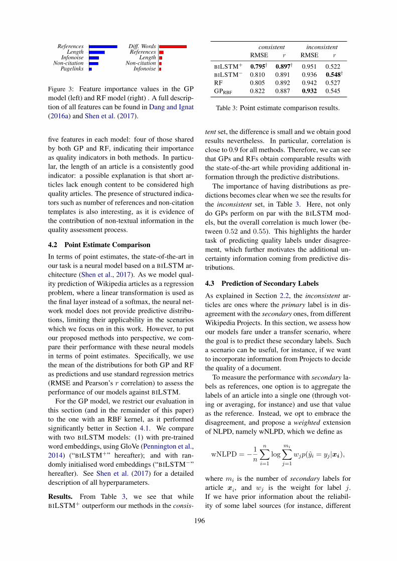
ReferencesLength

InfonoiseNon-citation

Pagelinks

Diff. WordsReferences

LengthNon-citation

Infonoise

Figure 3: Feature importance values in the GPmodel (left) and RF model (right) . A full descrip-tion of all features can be found in Dang and Ignat(2016a) and Shen et al. (2017).

five features in each model: four of those sharedby both GP and RF, indicating their importanceas quality indicators in both methods. In particu-lar, the length of an article is a consistently goodindicator: a possible explanation is that short ar-ticles lack enough content to be considered highquality articles. The presence of structured indica-tors such as number of references and non-citationtemplates is also interesting, as it is evidence ofthe contribution of non-textual information in thequality assessment process.

4.2 Point Estimate ComparisonIn terms of point estimates, the state-of-the-art inour task is a neural model based on a BILSTM ar-chitecture (Shen et al., 2017). As we model qual-ity prediction of Wikipedia articles as a regressionproblem, where a linear transformation is used asthe final layer instead of a softmax, the neural net-work model does not provide predictive distribu-tions, limiting their applicability in the scenarioswhich we focus on in this work. However, to putour proposed methods into perspective, we com-pare their performance with these neural modelsin terms of point estimates. Specifically, we usethe mean of the distributions for both GP and RFas predictions and use standard regression metrics(RMSE and Pearson’s r correlation) to assess theperformance of our models against BILSTM.

For the GP model, we restrict our evaluation inthis section (and in the remainder of this paper)to the one with an RBF kernel, as it performedsignificantly better in Section 4.1. We comparewith two BILSTM models: (1) with pre-trainedword embeddings, using GloVe (Pennington et al.,2014) (“BILSTM+” hereafter); and with ran-domly initialised word embeddings (“BILSTM−”hereafter). See Shen et al. (2017) for a detaileddescription of all hyperparameters.

Results. From Table 3, we see that whileBILSTM+ outperform our methods in the consis-

consistent inconsistentRMSE r RMSE r

BILSTM+ 0.795† 0.897† 0.951 0.522BILSTM− 0.810 0.891 0.936 0.548†RF 0.805 0.892 0.942 0.527GPRBF 0.822 0.887 0.932 0.545

Table 3: Point estimate comparison results.

tent set, the difference is small and we obtain goodresults nevertheless. In particular, correlation isclose to 0.9 for all methods. Therefore, we can seethat GPs and RFs obtain comparable results withthe state-of-the-art while providing additional in-formation through the predictive distributions.

The importance of having distributions as pre-dictions becomes clear when we see the results forthe inconsistent set, in Table 3. Here, not onlydo GPs perform on par with the BILSTM mod-els, but the overall correlation is much lower (be-tween 0.52 and 0.55). This highlights the hardertask of predicting quality labels under disagree-ment, which further motivates the additional un-certainty information coming from predictive dis-tributions.

4.3 Prediction of Secondary Labels

As explained in Section 2.2, the inconsistent ar-ticles are ones where the primary label is in dis-agreement with the secondary ones, from differentWikipedia Projects. In this section, we assess howour models fare under a transfer scenario, wherethe goal is to predict these secondary labels. Sucha scenario can be useful, for instance, if we wantto incorporate information from Projects to decidethe quality of a document.

To measure the performance with secondary la-bels as references, one option is to aggregate thelabels of an article into a single one (through vot-ing or averaging, for instance) and use that valueas the reference. Instead, we opt to embrace thedisagreement, and propose a weighted extensionof NLPD, namely wNLPD, which we define as

wNLPD = − 1

n

n∑

i=1

log

mi∑

j=1

wjp(yi = yj |xi),

where mi is the number of secondary labels forarticle xi, and wj is the weight for label j.If we have prior information about the reliabil-ity of some label sources (for instance, different

196

wNLPD wRMSE

RF 1.460 1.158GPRBF 1.412† 1.152†

Table 4: Results for prediction of secondary labels.

Wikipedia Projects), one can plug this informa-tion into the weights. Here we assume equal relia-bility and use uniform weights wj = freq(j)/mi,where freq is the count of label j among secondarylabels. The metric degrades to standard NLPDwhen labels are consistent. We also evaluate pointestimate performance using a similar weightingscheme for RMSE (which we denote as wRMSE).

Results. Table 4 summarises the results. Noticethat in this setting we only report results for the in-consistent test set, as the consistent one has no dis-agreement (and therefore, numbers would matchthe ones in Section 4.1). Here we also see thatGPs achieve significantly better performance thanRFs, although by a much lower margin comparedto the results on the primary labels (Table 2). Thisreflects the harder aspect of this setting. We hy-pothesize we can obtain better performance in thisscenario by incorporating the secondary labels attraining time, which we leave for future work.

4.4 Case Study: Quality Prediction asFiltering for Manual Revision

As mentioned in Section 1, one use for a qualityprediction system is to filter documents for man-ual revision. In the case of Wikipedia, such revi-sions are mandatory for articles to be assigned as aGood Article or a Featured Article. This incurs inan asymmetric risk: the cost of mispredicting anarticle as GA and FA is higher than other labels,as these trigger expensive, manual labour. Such ascenario can be modelled through asymmetric lossfunctions (Varian, 1975).

If a quality model provides predictive distribu-tions, one can obtain optimal quality decisionsunder an asymmetric loss function through theframework of Minimum Bayes Risk (MBR). Thissetting has been studied before by Christoffersenand Diebold (1997) and more recently applied byBeck et al. (2016) in the context of machine trans-lation post-editing. However, these assume a re-gression scenario. While we employ regressionmodels in our work for ease of modelling reasons,the final decisions in the pipeline are discrete (al-though still ordinal).

Figure 4: Discretisation of a continuous predictivedistribution. The shaded area shows the probabil-ity of quality label Start (−1.5).

To adapt the MBR framework into our case, wefirst define the risk δ(q) of predicting the qualitylabel q as

δ(q) =∑

q

L(q, q)p(q|x),

where L(q, q) is an (asymmetric) loss functionover the discrete quality labels and p(q|x) is thediscretised probability of quality label q for doc-ument x under one of our proposed models. Wedetail these two terms below.

Discretised distribution Given a predictive dis-tribution obtained by a regression model we candiscretise it by using the cumulative density func-tion (cdf). Define `(q) as the real value whichwe encode quality label q, as described in Sec-tion 3. With this, we obtain the discretised proba-bility mass function

p(q|x) =

1− cdf(`(q)− 0.5) if q = FAcdf(`(q) + 0.5) if q = Stubcdf(`(q) + 0.5)− cdf(`(q)− 0.5) otherwise,

where the cdf is obtained from the predictive dis-tribution. As we only consider Gaussian distri-butions for predictions, we can easily use off-the-shelf implementations to obtain the cdf. Figure 4gives an example of how to obtain the probabilityof an instance being predicted to be Start (−1.5).

Asymmetric loss function To incorporateasymmetry into the quality label prediction, wedefine it as

L(q, q) =

0 if q = qα if q 6= q, q /∈ S, q ∈ S1 otherwise

,

197

1 2 3 4 5 6 7 8 9 100.5

1

1.5

2

2.5

Varying values of α

Asy

mm

etri

cco

stGPcon

RFcon

GPinc

RFinc

Figure 5: Asymmetric risk vs. α (best viewedin color). Here, GPcon/RFcon denote risk val-ues achieved by GP/RF over consistent arti-cles, respectively; GPinc/RFinc denote risk valuesachieved by GP/RF over inconsistent articles.

where S is a high-risk label set and α > 1 is thepenalty associated with a higher risk prediction. Inour scenario, we set S = {GA,FA}, as these arethe labels we want to give larger penalties whenthere is a misprediction. Notice that this loss isonly an example tailored to our specific setting:other scenarios might warrant different definitions.

Evaluation Under a deployment scenario, onewould evaluate δ(q) for all possible 6 labels andchoose the one with minimum risk. However,since in our case we have access to true test setlabels, we can just average all δ(q) for the goldlabels q in order to assess the models we are inter-ested in (GPs and RFs). As in the previous sec-tions, we report average results over 10 runs forboth consistent and inconsistent test sets.

Results. In Figure 5 we plot the average riskwhile varying the penalty cost α. As in the in-trinsic evaluation result, we see that GPs tend toperform better in the inconsistent set. On the otherhand, the results in the consistent set are very sim-ilar, and no conclusions can be made about whichmethod performs best. Overall, the results arefavourable towards GPs but the inconclusive re-sults for consistent labels shows that there is roomfor improvements in uncertainty modelling, whichwe leave for future work.

5 Related Work

The quality assessment of Wikipedia articles is atask that assigns a quality label to a Wikipediaarticle, reflecting the quality assessment pro-cess carried out by the Wikipedia community.

Hand-crafted feature-based approaches use fea-tures from the article itself (e.g., article length),meta-data features (the number of revisions of anarticle), and a combination of these two. Variousfeatures derived from Wikipedia articles have beenused for assessing the quality of Wikipedia arti-cles (Blumenstock, 2008; Lipka and Stein, 2010;Warncke-Wang et al., 2013, 2015; Dang and Ig-nat, 2016a). For example, Blumenstock (2008)and Lipka and Stein (2010) use article length andwriting styles (represented by binarised charac-ter trigram features) to differentiate FA articlesfrom non-featured articles, respectively. Warncke-Wang et al. (2015) proposed 11 structural features(such as the number of references and whetherthere is an infobox or not) to assess the quality ofWikipedia articles. Dang and Ignat (2016a) fur-ther proposed nine readability scores (such as theFlesch reading-ease score (Kincaid et al., 1975))to assess the quality of Wikipedia articles. Basedon these last two studies, an online Objective Re-vision Evaluation Service has been built to mea-sure the quality of Wikipedia articles (Halfakerand Taraborelli, 2015). Features derived from themeta-data of Wikipedia articles — e.g., the num-ber of revisions a Wikipedia article has received— have been proposed to assess the quality ofWikipedia articles (Stvilia et al., 2005; Stein andHess, 2007; Adler et al., 2008; Dalip et al., 2009,2017, 2014). For example, Stein and Hess (2007)and Adler et al. (2008) use the authority of editorsto measure the quality of Wikipedia articles, as de-termined by the quality of articles they edited.

Different neural network architectures havebeen exploited to learn high-level representationsof Wikipedia articles. For example, Dang andIgnat (2016b) use a distributed memory versionof Paragraph Vector (Le and Mikolov, 2014) tolearn Wikipedia article representations, which areused to predict the quality of Wikipedia articles.Dang and Ignat (2017) and Shen et al. (2017) ex-ploit LSTMs (Hochreiter and Schmidhuber, 1997)to learn document-level representations to train aclassifier and predict the quality label of an un-seen Wikipedia article. Observing that the vi-sual rendering of a Wikipedia article can cap-ture implicit quality indicators (such as imagesand tables), Shen et al. (2019) use Inception V3(Szegedy et al., 2016) to capture visual represen-tations, which are used to classify Wikipedia arti-cles based on their quality. They further propose

198

a joint model, which combines textual representa-tions from bidirectional LSTM with visual repre-sentations from Inception V3, to predict the qual-ity of Wikipedia articles.

Beck et al. (2016) explore prediction uncer-tainty in machine translation quality estimation(QE), where post-editing rate is the dependentvariable. In QE, the post-editing rate — whichis computed by dividing the post-editing time bythe length of the translation hypothesis — is apositive real value. The performance of a GPmodel was studied in both underestimate and over-estimate scenarios. Beck and Cohn (2017); Beck(2017) employ GPs to model text representationnoise in emotion analysis, where Pearson’s corre-lation and NLPD are used as the evaluation met-rics. Our work is different from these two stud-ies as we model the subjectivity of quality assess-ment explicitly, which can mimic people’s differ-ent opinions over the quality of a document.

There is also a rich body of work on identify-ing trustworthy annotators and predicting the cor-rect underlying labels from multiple annotations(Hovy et al., 2013; Cohn and Specia, 2013; Pas-sonneau and Carpenter, 2014; Graham et al., 2017;Paun et al., 2018). For example, Hovy et al. (2013)propose an item-response model to identify trust-worthy annotators and predict the true labels ofinstances in an unsupervised way. However, ourtask is to measure the uncertainty of a model overits predictions (as distinct from attempting to learnthe “true” label for an instance from potentiallybiased/noisy annotations), in addition to correctlypredicting the gold label, in the context of as-sessing the quality of Wikipedia articles. Addi-tionally, we have a rich representation of the datapoint (i.e. document) that we are attempting tolabel, whereas in work on interpreting multiply-annotated data, there is little or no representationof each data point that has been annotated. Finally,we do not have access to the IDs of annotatorsacross documents, and thus cannot model anno-tator reliability or bias.


In this paper, we proposed to measure the un-certainty of Wikipedia article quality assessmentsystems using Gaussian processes and randomforests, utilising the NLPD evaluation metric tomeasure performance over consistent and incon-sistent articles. Experimental results show that

both GPs and RFs are less certain over inconsis-tent articles, where people tend to disagree overtheir quality, and GPs are more conservative intheir predictions over such articles. To imitate areal world scenario where decision-making pro-cesses based on model predictions can lead todifferent costs, we proposed an asymmetric cost,which takes the prediction uncertainty into consid-eration. Empirical results show that GPs are a bet-ter option if overestimates are heavily penalised.

In the future, we are interested in conducting auser study to find out how Wikipedians respond tothe utility of uncertainty information provided tothem. On the modelling side, having equal inter-vals between adjacent quality classes is a heuristic,which is potentially inappropriate in the case ofWikipedia. Thus we are also planning to model thequality assessment of Wikipedia articles as an or-dinal regression problem, where the gap betweenadjacent quality labels can vary.

ReferencesB. Thomas Adler, Krishnendu Chatterjee, Luca De Al-

faro, Marco Faella, Ian Pye, and Vishwanath Ra-man. 2008. Assigning trust to Wikipedia content.In Proceedings of the 4th International Symposiumon Wikis, pages 26:1–26:12.

Daniel Beck. 2017. Modelling representation noise inemotion analysis using Gaussian processes. In IJC-NLP, volume 2, pages 140–145.

Daniel Beck and Trevor Cohn. 2017. Learning kernelsover strings using Gaussian processes. In IJCNLP,pages 67–73.

Daniel Beck, Lucia Specia, and Trevor Cohn. 2016.Exploring prediction uncertainty in machine transla-tion quality estimation. In CoNLL, pages 208–218.

Joshua E. Blumenstock. 2008. Size matters: Wordcount as a measure of quality on Wikipedia. InWWW, pages 1095–1096.

Leo Breiman. 2001. Random forests. Mach. Learn.,45(1):5–32.

Joaquin Quinonero Candela, Carl Edward Rasmussen,Fabian H. Sinz, Olivier Bousquet, and BernhardScholkopf. 2005. Evaluating predictive uncertaintychallenge. In Machine Learning Challenges, vol-ume 3944, pages 1–27.

Jeanne Sternlicht Chall and Edgar Dale. 1995. Read-ability Revisited: The New Dale-Chall ReadabilityFormula. Brookline Books.

Krzysztof Chalupka, Christopher K. I. Williams, andIain Murray. 2013. A framework for evaluating

199

approximation methods for Gaussian process re-gression. Journal of Machine Learning Research,14(1):333–350.

Youngmin Cho and Lawrence K. Saul. 2009. Kernelmethods for deep learning. In NIPS, pages 342–350.

Peter F. Christoffersen and Francis X. Diebold.1997. Optimal Prediction Under Asymmetric Loss.Econometric Theory, 13(06):808–817.

Trevor Cohn and Lucia Specia. 2013. Modelling anno-tator bias with multi-task gaussian processes: An ap-plication to machine translation quality estimation.In ACL, pages 32–42.

Edgar Dale and Jeanne S. Chall. 1948. A formulafor predicting readability: Instructions. EducationalResearch Bulletin, 27(2):37–54.

Daniel H. Dalip, Marcos A. Goncalves, Marco Cristo,and Pavel Calado. 2009. Automatic quality assess-ment of content created collaboratively by web com-munities: A case study of Wikipedia. In JCDL,pages 295–304.

Daniel Hasan Dalip, Marcos Andre Goncalves, MarcoCristo, and Pavel Calado. 2017. A general multi-view framework for assessing the quality of collab-oratively created content on web 2.0. Journal ofthe Association for Information Science and Tech-nology, 68(2):286–308.

Daniel Hasan Dalip, Harlley Lima, Marcos AndreGoncalves, Marco Cristo, and Pavel Calado. 2014.Quality assessment of collaborative content withminimal information. In JCDL, pages 201–210.

Quang-Vinh Dang and Claudia-Lavinia Ignat. 2016a.Measuring quality of collaboratively edited docu-ments: The case of Wikipedia. In The 2nd IEEEInternational Conference on Collaboration and In-ternet Computing, pages 266–275.

Quang-Vinh Dang and Claudia-Lavinia Ignat. 2016b.Quality assessment of Wikipedia articles withoutfeature engineering. In JCDL, pages 27–30.

Quang-Vinh Dang and Claudia-Lavinia Ignat. 2017.An end-to-end learning solution for assessing thequality of Wikipedia articles. In The 13th Inter-national Symposium on Open Collaboration, pages4:1–4:10.

Yarin Gal, Mark van der Wilk, and Carl E. Ras-mussen. 2014. Distributed variational inference insparse Gaussian process regression and latent vari-able models. In NIPS, pages 3257–3265.

Yvette Graham, Timothy Baldwin, Alistair Moffat, andJustin Zobel. 2017. Can machine translation sys-tems be evaluated by the crowd alone? Natural Lan-guage Engineering, 23(1):3–30.

Robert Gunning. 1969. The fog index after twentyyears. International Journal of Business Commu-nication, 6(2):3–13.

Aaron Halfaker and Dario Taraborelli. 2015. Artificialintelligence service “ore” gives Wikipedians x-rayspecs to see through bad edits. [online] Available:https://blog.wikimedia.org/2015/11/30/artificial-intelligence-x-ray-specs.

James Hensman, Nicolo Fusi, and Neil D. Lawrence.2013. Gaussian processes for big data. In Proceed-ings of the Twenty-Ninth Conference on Uncertaintyin Artificial Intelligence.

Jose Miguel Hernandez-Lobato and Ryan P. Adams.2015. Probabilistic backpropagation for scalablelearning of Bayesian neural networks. In ICML,pages 1861–1869.

Sepp Hochreiter and Jurgen Schmidhuber. 1997.Long short-term memory. Neural Computation,9(8):1735–1780.

Dirk Hovy, Taylor Berg-Kirkpatrick, Ashish Vaswani,and Eduard H. Hovy. 2013. Learning whom to trustwith MACE. In NACCL-HLT, pages 1120–1130.

Frank Hutter, Holger H. Hoos, and Kevin Leyton-Brown. 2011. Sequential model-based optimizationfor general algorithm configuration. In 5th Interna-tional Conference on Learning and Intelligent Opti-mization, pages 507–523.

J. Peter Kincaid, Robert P. Fishburne Jr., Richard L.Rogers, and Brad S. Chissom. 1975. Derivation ofnew readability formulas (automated readability in-dex, Fog count and Flesch reading ease formula) fornavy enlisted personnel. Technical report, Institutefor Simulation and Training, University of CentralFlorida.

Quoc Le and Tomas Mikolov. 2014. Distributed rep-resentations of sentences and documents. In ICML,pages 1188–1196.

Nedim Lipka and Benno Stein. 2010. Identifying fea-tured articles in Wikipedia: Writing style matters. InWWW, pages 1147–1148.

Alexander G. de G. Matthews, Mark van der Wilk, TomNickson, Keisuke. Fujii, Alexis Boukouvalas, PabloLeon-Villagra, Zoubin Ghahramani, and JamesHensman. 2017. GPflow: A Gaussian process li-brary using TensorFlow. Journal of Machine Learn-ing Research, 18(40):1–6.

Rebecca J. Passonneau and Bob Carpenter. 2014. Thebenefits of a model of annotation. TACL, 2:311–326.

Silviu Paun, Bob Carpenter, Jon Chamberlain, DirkHovy, Udo Kruschwitz, and Massimo Poesio. 2018.Comparing bayesian models of annotation. TACL,6:571–585.

Fabian Pedregosa, Gael Varoquaux, Alexandre Gram-fort, Vincent Michel, Bertrand Thirion, OlivierGrisel, Mathieu Blondel, Peter Prettenhofer, RonWeiss, Vincent Dubourg, Jake Vanderplas, Alexan-dre Passos, David Cournapeau, Matthieu Brucher,

200

Matthieu Perrot, and Edouard Duchesnay. 2011.Scikit-learn: Machine learning in Python. Journalof Machine Learning Research, 12:2825–2830.

Jeffrey Pennington, Richard Socher, and Christo-pher D. Manning. 2014. GloVe: Global vectors forword representation. In EMNLP, volume 14, pages1532–1543.

Carl Edward Rasmussen and Christopher KI Williams.2006. Gaussian Process for Machine Learning.MIT press.

Aili Shen, Jianzhong Qi, and Timothy Baldwin. 2017.A hybrid model for quality assessment of Wikipediaarticles. In Australasian Language Technology As-sociation Workshop, pages 43–52.

Aili Shen, Bahar Salehi, Timothy Baldwin, andJianzhong Qi. 2019. A joint model for multimodaldocument quality assessment. In JCDL.

Klaus Stein and Claudia Hess. 2007. Does it matterwho contributes: A study on featured articles in theGerman Wikipedia. In Hypertext, pages 171–174.

Besiki Stvilia, Michael B. Twidale, Linda C. Smith,and Les Gasser. 2005. Assessing informationquality of a community-based encyclopedia. InThe 2005 International Conference on InformationQuality, pages 442–454.

Christian Szegedy, Vincent Vanhoucke, Sergey Ioffe,Jonathon Shlens, and Zbigniew Wojna. 2016. Re-thinking the Inception architecture for computer vi-sion. In CVPR, pages 2818–2826.

Michalis K. Titsias. 2009. Variational learning of in-ducing variables in sparse Gaussian processes. InInternational Conference on Artificial Intelligenceand Statistics, pages 567–574.

Hal Varian. 1975. A Bayesian Approach to Real EstateAssessment. Studies in Bayesian Econometrics andStatistics in Honor of Leonard J. Savage, pages 195–208.

Morten Warncke-Wang, Vladislav R. Ayukaev, BrentHecht, and Loren Terveen. 2015. The success andfailure of quality improvement projects in peer pro-duction communities. In The 18th ACM Conferenceon Computer-Supported Cooperative Work and So-cial Computing, pages 743–756.

Morten Warncke-Wang, Dan Cosley, and John Riedl.2013. Tell me more: An actionable quality modelfor Wikipedia. In The 9th International Symposiumon Open Collaboration, pages 8:1–8:10.

201


Conceptualisation and Annotation of Drug Nonadherence Informationfor Knowledge Extraction from Patient-Generated Texts

Anja BelzUniversity of Brighton, UK

[email protected]

Elizabeth FordBrighton and Sussex Medical School, UK

[email protected]

Richard HoileSussex Partnership NHS Foundation Trust, UK

[email protected]

Azam MullickUniversity of Brighton, UK

[email protected]

Abstract

Approaches to knowledge extraction (KE) inthe health domain often start by annotating textto indicate the knowledge to be extracted, andthen use the annotated text to train systems toperform the KE. This may work for annotat-ing named entities or other contiguous nounphrases (drugs, some drug effects), but be-comes increasingly difficult when items tendto be expressed across multiple, possibly non-contiguous, syntactic constituents (e.g. mostdescriptions of drug effects in user-generatedtext). Other issues include that it is not al-ways clear how annotations map to actionableinsights, or how they scale up to, or can formpart of, more complex KE tasks. This paperreports our efforts in developing an approachto extracting knowledge about drug nonadher-ence from health forums which led us to con-clude that development cannot proceed in sep-arate steps but that all aspects—from concep-tualisation to annotation scheme development,annotation, KE system training and knowl-edge graph instantiation—are interdependentand need to be co-developed. Our aim in thispaper is two-fold: we describe a generally ap-plicable framework for developing a KE ap-proach, and present a specific KE approach,developed with the framework, for the taskof gathering information about antidepressantdrug nonadherence. We report the conceptual-isation, the annotation scheme, the annotatedcorpus, and an analysis of annotated texts.

1 Introduction

Depression is experienced by 1 in 4 people in theUK. More than two thirds of patients are mostlymanaged with antidepressant medication, yet non-adherence rates are very high. One study foundthat 4.2% of patients who were prescribed antide-pressants did not take them at all, and 23.7% filledonly a single prescription (van Geffen et al., 2009).Nonadherence is a major obstacle in the effective

treatment of depression, but cannot currently bepredicted or explained adequately (van Dulmenet al., 2007). An influential WHO report (Sabateet al., 2003) concluded: “[i]ncreasing the effec-tiveness of adherence interventions may have a fargreater impact on the health of the population thanany improvement in specific medical treatments”.Nonadherence is hard to investigate via controlledstudies meaning alternative sources of informationare needed. Recent results indicate a strong sig-nal relating to usage of psychiatric medications onhealth forums and social media (Tregunno, 2017),and that social media users report nonadherenceand reasons for it (Onishi et al., 2018).

The work reported in this paper aimed (i) to de-velop a conceptualisation of the information spacearound drug nonadherence, defining the relevantconcepts, properties and relations; (ii) to developan annotation scheme based on the conceptualisa-tion; (iii) to annotate a corpus of depression healthforum posts with the scheme; and (iv) to use theannotated data to examine the prevalence, and co-occurrence, of different kinds of nonadherence in-formation (testing signal strength). We examinethe interdependent and mutually constraining re-lationship between conceptualisation, annotationscheme and knowledge extraction processes.

The ultimate goal is to perform automaticknowledge extraction (KE) in order to providevaluable non-adherence information from a largesample about why and how non-adherence occurs.We hope this will in turn lead to better prescribing,better adherence and more informed discussionsbetween patient and prescriber around medication.

2 Nonadherence and Health Forums

Different terms have been used to describe the“suboptimal taking of medicine by patients”(Hugtenburg et al., 2013). Among these, non-compliance and nonadherence both mean not tak-

202

Quitting your meds can be awful, for sure. I started trying to get off Zoloft by myself 5 years ago. I went coldturkey which was a complete disaster. Next I tried cutting down by large amounts which was slightly less of adisaster. Finally I tapered off very slowly. ONE WHOLE YEAR to get from 200mg to zero. With the tapering offthe brain zaps were much less severe. Simply takes a long time to wean yourself off these drugs.

I reduced my mirtazapine from 45mg first to 30mg, and then to 15mg, then stopped it altogether. After two weeksI was feeling awful so I decided to restart it at 15mg.

So I stopped Fluoxetine about a month ago sort of by accident. After I missed a few doses I just decided to keepgoing. So far I’ve only had rather minor symptoms. One of my symptoms has been an electric shock sensationfrom my brain down my spine/body. This happens especially when I get up, sit down or move suddenly.

Last week my doctor increased my Lamictol dosage to 200 MG. I am beginning to notice serious cognitive deficits.For example constantly losing/misplacing things.. Has anyone else experienced this situation?

Figure 1: Four example depression forum posts created to closely resemble real posts.

ing a drug as instructed (the intended meaningin the present context), but nonadherence is theterm now preferred as reflecting a more equalprescriber-patient relationship (Hugtenburg et al.,2013). Two types of nonadherence are distin-guished, intentional, where a patient “actively de-cides” not to follow instructions, and unintentionalnonadherence, including forgetting and not know-ing how to take a drug (Hugtenburg et al., 2013).

Consider the four example posts from healthforums for specific antidepressants in Figure 1.Some of the sentences contain explicit statementsthat the modifications described were instigated bythe patient (“I started trying to get off Zoloft bymyself 5 years ago”; “After two weeks I was feel-ing awful so I decided to restart it at 15mg”; “SoI stopped Fluoxetine about a month ago sort of byaccident”). Other modifications described in thefirst three posts (unlike in the fourth) are likely toalso have been instigated by the patient, but clini-cian involvement cannot be ruled out.

These are typical examples of how patients talkabout nonadherence in health forums: explicitstatements (‘my doctor told me to do one thing,but I did another’) are rare (7% of posts on thedepression forums we have been looking at, seealso Section 5). More typically, a drug modifica-tion is described along with the side effect and/orother reason(s) that gave rise to it, but the extent towhich the prescribing physician was involved indeciding to make the modification can only be in-ferred, with varying degrees of certainty, from thelanguage, or on the basis of medical knowledge(e.g. a modification is known to be dangerous).

3 Conceptualisation and KE Task

Posts like the ones in Figure 1 clearly contain in-formation about the why and how of drug nonad-

herence, but how can it be automatically extractedand rendered useful? In this section we discussthe main issues in developing a knowledge extrac-tion (KE) approach for a specific domain and aspecific KE task, nonadherence event extraction inour case. To introduce the different components indeveloping an approach to KE (overview see Fig-ure 2, we use as an illustrative running example thesimpler task of drug effect extraction which is—incontrast to the far more complex task of nonad-herent event extraction we are addressing here—already a well established research task1 (Leamanet al., 2010; Nikfarjam et al., 2015). Drug effectdetection is an important subtask of nonadherenceevent extraction, because drug effects as perceivedby the patient play an important role in nonadher-ence and are often the reason for it. The last post inFigure 1 is a typical example, containing a claimthat a drug referred to as “Lamictol”, is causing aneffect described as “cognitive deficits”.

3.1 From Text to MeaningSuppose that we have a method capable of iden-tifying drug and effect mentions in text and de-termining which ones are linked (i.e. which drugcauses which effect), and that we extract a linkeddrug and effect pair from the fourth post in Fig-ure 1 for which we could choose the followingnotation: cause(“Lamictol”,“cognitive deficits”).Suppose from this and other posts we extract fivesuch linked pairs as follows:

cause(“Lamictol”,“serious cognitive deficits”)cause(“Lamictol”,“constantly losing/misplacing

things”)cause(“Lamictal”,”uncoordinated”)cause(“lamotrigine”,”so forgetful”)cause(“Lamotrigene”,”keep losing my phone and

going upstairs and forgetting what for”)

(1)

1See e.g. Task 2 at this year’s SMM4H Shared Task event:https://healthlanguageprocessing.org/smm4h/challenge/

203

If this was the actual output of our method, itwould be nothing more than a list of drug-effectmentions in a given set of texts, possibly withcounts of multiple occurrences of identical men-tions (none in Example 1 above). One importanttype of knowledge would be entirely inaccessible,namely that the above five pairs in fact all claimthe same side effect for the same drug (lamot-rigine, a mood-stabilising medication sometimesprescribed for depression).2 In order to extractthat knowledge (crucial to be able e.g. to act uponside effect reports depending on novelty or reportfrequency), the identified word strings need to bemapped to a more abstract level of representationwhere knowledge is encoded in terms of concepts,rather than word strings. It is only once this pro-cess, known as entity linking3 (Han et al., 2011;Hachey et al., 2013; Rao et al., 2013; Smith et al.,2018), has been performed that the five linkedpairs above can be interpreted as five mentions ofthe same drug effect. In this crucial step, we movefrom extracting word strings (surface representa-tions) to extracting concept structures (meaningrepresentations); from something that can be com-pared in terms of string similarity and counted, tosomething that can be incorporated into a knowl-edge graph and reasoned about.

3.2 Concept Model and KE Template

In the case of drug effect extraction it is clearwhat we want to extract, and how it is struc-tured. A very simple conceptualisation suffices toexpress that understanding: a single parent con-cept, drug effect, consisting of a drug, an effectand a causal relation, possibly implicit. Depend-ing on application context, further concepts, suchas duration or severity, could also be added (thesewould be required e.g. if the application task wasautomatic completion of Yellow Card reports).One of many possible notations for this conceptu-alisation is the following (for a complete conceptmodel the range of possible values of the compo-nent concepts would also have to specified):

DRUG EFFECT [DRUG; EFFECT; SEVERITY; DURATION ] (2)

The above can be seen as providing both a conceptmodel representing a piece of domain knowledge,

2Whether they are considered the same depends on theconcept set linked to, in our case SIDER (Kuhn et al., 2015).

3A.k.a. normalisation, e.g. for adverse effect normalisa-tion see Task 3 at this year’s SMM4H Shared Task event:https://healthlanguageprocessing.org/sm m4h/challenge/

Figure 2: Components in developing KE approach.

and a template to be instantiated by a specific KEtool (depending on the application task, only sub-sets of concepts might be used for KE). A possibleinstantiation produced by a KE tool via entity de-tection and linking for the last post in Figure 1 isthe following (initial underscores indicating termi-nal concepts as opposed to word strings):

DRUG EFFECT [DRUG= lamotrigine;EFFECT= confusional state;SEVERITY= moderate;DURATION= continuous; ]

(3)

In order to produce the above we have to have cre-ated a suitable conceptualisation (concept model),a KE template, a KE task construal and methodsfor implementing it, here detecting word spanscorresponding to the above concepts and for map-ping the word spans to concepts. In order to beable to do the latter, we also need texts which havebeen labelled for entities such as drugs and effectsand the links between them. All these aspects areshown to the left of Figure 2 which provides anoverview of elements and steps involved in devel-oping a KE approach. In the next sections we lookat how conceptualisation and annotation schemeinteract with possible KE tasks (Section 3.3), fol-lowed by issues in determining the details of theannotation scheme (Section 3.4).

3.3 Text Annotation and KE TaskUseful one-off analysis can be conducted on thebasis of manual mark-up of text, but for knowl-edge extraction from large quantities of new texts,automatic processes are needed. Two commontypes of KE model are word sequence (post, sen-tence, phrase, etc.) classifiers and labellers. Thesetend to be supervised models, i.e. they require la-belled training data the creation of which, espe-cially initially, requires human annotation effort.

How the data is annotated limits what kind ofKE tasks and models it can be used for. Con-

204

versely, aiming for a particular KE task has im-plications for the kinds of annotations that areneeded. For the KE task described above, i.e.mapping from health forum posts (Figure 1) toinstantiated KE templates (Example 3), the moststraightforward way to interpret the annotationtask would be to annotate each post (as a whole)with an instantiated KE template for every men-tion of a drug effect contained in the post. How-ever, this would make the annotators’ task cog-nitively extremely challenging (requiring multiplejudgments to be made in conjunction), and verytime-intensive (involving look up of concepts indatabases and inventories). Moreover, it is not ob-vious how to define a corresponding KE modellingtask and training regime. It is also not feasible todefine one output class for each possible instanti-ated template, because that would lead to an un-manageable combinatorial explosion of classes.

In the relatively simple case of adverse drug ef-fect extraction, the divide-and-conquer approachthat tends to be used instead (Nikfarjam et al.,2015; Metke-Jimenez and Karimi, 2016) con-strues the task, as mentioned above, as a sequenceof subtasks, first identifying all mentions of drugsand effects in the text, then linking them to con-cepts and to each other. For the first step to be pos-sible, drug mentions and effect mentions need tobe identified in the text, for which correspondingmark-up needs to be available in the training data.Similarly, any links between the marked up enti-ties also need to be present in the annotations. Theidentified text strings can then be mapped (linked)in a separate step to drug (e.g. lamictol) and ef-fect (e.g. confusional state) concepts, potentiallywith separately retrained off-the-shelf tools.

The above discussion points to an annotationscheme involving a DRUG concept (but not con-cepts for individual drugs), and an EFFECT con-cept (but not concepts for specific effects), and forcorresponding labels to be inserted into texts asmark up. However, more issues arise when map-ping these conclusions to an annotation scheme.

3.4 Towards an Annotation Scheme

Some of the questions that arise in text annota-tion are (1) whether conceptually grounded anno-tations should attach to word strings (a) with themeaning ‘these words together express the givenconcept’, or (b) with the meaning ‘somewhere inthis text there is an occurrence of the concept’;

(2) whether labels should be (a) terminal concepts(e.g. lamictol) or (b) classes of terminal concepts(e.g. Drug); (3) how to treat instances where anentity or event is mentioned, but is not asserted tohave occurred or have been observed, which hap-pens e.g. with negation, questions or hypotheticalconsiderations; and (4) how to present the task toannotators in such a way that the cognitive load iswithin manageable limits and annotations can bereplicated with sufficient consistency.

Not all concepts can clearly and easily be asso-ciated with specific words in the text. While men-tions of a drug or effect entity always have cor-responding words in the text (entity annotationsfall under (1a) above), this is not necessarily thecase of concepts naturally seen as relations be-tween other concepts. Consider again the last postin Figure 1: there are no substrings that can be as-sociated with Lamictol causing cognitive deficits.Rather, it is the first two sentences in their en-tirety that imply (but do not state explicitly) thecausal link. It tends to be considered not appro-priate to mark up such relations in text, and theyattach instead to one or more already marked upword strings (meaning they fall under (1b) above).

Regarding (2) above, aside from the issuesraised in Section 3.3, available resources are adeciding factor: e.g. it would take annotators farlonger to determine the specific drug concept la-bel for a drug mention than it would to simply la-bel each such mention with a generic drug label.

Regarding (3), while KE would typically aimto extract information with factual status from text(e.g. all drug effects patients claim to have expe-rienced), far from all mentions of such informa-tion have factual status (drug effect mentions an benegated, part of a question, etc.). Simply treatinge.g. a negated drug effect as not a drug effect is un-likely to be helpful in a machine learning context,because negated and non-negated versions willlook identical except for a negation marker else-where in the text, potentially resulting in a largenumber of spurious negative examples. It is morelikely to help generalisation to treat all drug effectmentions identically, and to additionally mark upin annotations, and subsequently learn, the charac-teristics of negation. The same holds for generali-sations, questions and similar phenomena.

Regarding (4), it is virtually impossible toachieve perfect consistency between annotators,or even self-consistency, with mark-up annotation

205

DRUG NONADHERENCE [+DRUG MODIFICATION [ instigated by = patient

intentional || patient unintentional ] ]

DRUG MODIFICATION [drug : Drugschange : DOSE CHANGE || FORM CHANGE || PROD

UCT CHANGE+reason : DRUG EFFECT || DRUG PROPERTY ||

Other Reasoninstigated by : Instigator+mod effect : EFFECT || Other Outcome ]

DOSE CHANGE [?from dose : ( Numbers, Units, Time Span )?to dose : ( Numbers, Units, Time Span )dose mod type : DoseModTypes ]

FORM CHANGE [?from form : Form Types?to form : Form Types ]

PRODUCT CHANGE [?from product : Drug Products?to product : Drug Products ]

DRUG EFFECT [drug : DrugsmedDRA preferred term : MPTsduration : ( Numbers, Units )severity : Severity Levels ]

DRUG PROPERTY [drug : Drugsproperty : Drug Properties ]

Drugs = {x|x is a drug entry in SIDER}Drug Products = {x|x is a drug product entry in SIDER}MPTs = {x|x is an MPT entry in SIDER}Drug Properties = { effective, ineffective, like, dis-

like, cheap, expensive, ...}Numbers = {x|x ∈ IR}Units = { ml, mg, ...}Time Span = { halfday, day, week, ...}Form Types = { tablet, powder, solution, cream, ...}DoseModTypes = { start, stop, increase, decrease}Other Reason = { life event, insurance financial,

view belief, ...}Instigator = { patient intentional, patient unintentional,

clinician, both together, other}Other Outcome = { negative, positive, neutral}Severity Levels = { mild, moderate, severe}

Figure 3: Nonadherence concept model (UML-like no-tation). + = 1 or more; || = xor; ? = at least 1 of two.

schemes. For simpler concepts corresponding tofewer possible word strings, such as named enti-ties of type drug, issues are comparatively simple,and inter-annotator agreement (IAA, the extent towhich annotators agree where drug mentions be-gin/end) would be high. As is apparent even in thesimple example word strings in Example 1, thereis comparatively higher variation in word stringsdescribing side effects: if the last two examples

were extracted from the longer strings I’m beingso forgetful and I just keep losing my phone..., re-spectively, in our experience there tends to be con-siderable variation among annotators about whereto place the start of the effect mention.

One way to address this is to ensure that theconcepts underlying annotation labels are highlycoherent and crisply defined, so that there is highconcurrence among annotators in how to interpretand apply them. This underlines the need to co-develop conceptualisation and annotation scheme,because they provide the formal grounding thatcan help ensure coherence and crispness. For highIAA, the tasks annotators are asked to performneed to be focused and homogeneous, and the vi-sual interfaces as uncluttered as possible. If this isnot the case it can make the task too difficult, andalso quickly lead to frustration among annotators.

4 An Approach to Nonadherence KE

In this section, we scale up the insights from Sec-tion 3 to an approach to knowledge extraction(KE) in the nonadherence domain, a substantiallymore complex task than drug effect detection. Weadopt the definition of nonadherence as not takinga drug as instructed (Section 2), and assume thatthe relationship between a patient and a drug startswith a prescription and instructions issued by aclinician. We see nonadherence as one or moremodifications to the original prescription regimen,or to a previous modification, made without theapproval of the prescribing clinician. Our first taskthen is to model the concept of modification, afterwhich we can define nonadherence as modifica-tions instigated by the patient. Our goal is to de-sign a concept model, KE template and annotationscheme for nonadherence that support KE meth-ods that extract information about the how and whyof drug nonadherence.

4.1 Concept Model

Information about how and why nonadherent drugmodifications occur will necessarily involve a spe-cific drug. To address the how part, we needto know what type of modification was carriedout. Nonadherent modifications in all exampleswe have encountered involve some change to thedose that is taken, if stopping, starting and forget-ting to take a drug are considered dose modifica-tions. Other types of modifications also apply todrug form (tablet, capsule, etc.), or drug brand

206

(e.g. generic vs. branded). To address the why part,we also need to know the reason for the modifica-tion and its effect, because it often becomes thereason for a further modification. Our nonadher-ence concept model is shown in Figure 3. Startingfrom the top, it defines drug nonadherence as oneor more drug modifications instigated by the pa-tient either intentially or unintentionally. A drugmodification is composed of a drug, a change, op-tionally a reason and an effect, plus a specifica-tion of instigation. A reason is either a drug effect,drug property or another reason. A drug effect isas defined in Section 3; a drug property identifiesthe drug it relates to and covers non-effect proper-ties such as cost, how well it works and whetherthe patient likes it. Other reasons include reasonsrelating to life events, insurance issues and beliefsheld by the patient. Others are possible, and asindicated in the model, we have not defined a fi-nal set of terminal concepts for some of the preter-minals (preterminal concepts are indicated by ital-ics). In order to define the possible terminal con-cepts for the preterminal drugs, drug products andeffects concepts, we use the SIDER knowledgebase (Kuhn et al., 2015).

4.2 KE Template and TaskThe concept model in Figure 3 is task-agnostic.For the specific task of nonadherence event extrac-tion from health forum posts it needs to be mappedto a KE template, task specification and annotationscheme that are necessarily task-specific. Follow-ing inspection of about 200 random texts from ourcorpus of 150K posts (Section 5), and based onthe concept model above, we construe the nonad-herence KE task as follows:

1. Binary classification of posts into first person narration vs.others.

2. Binary classification of posts into containing modificationmentions vs. others.

3. Anaphora resolution: replace drug, drug form and drugdose anaphora with full references.

4. Entity detection: drug, dose, effect, modification.

5. Entity linking: drug, effect, modification (yielding modi-fication type); text normalisation: dose.

6. Topic segmentation: drug related, other.

7. NE relation detection via binary classification (applied todrug-related topic fields only):

• drug, dose, context→ dose of?• drug, effect, context→ drug effect?• dose, effect, context→ dose effect?• modification, drug, context→ drug modification?• modification, dose, context→ drug modification?

• drug modification, effect, context→ mod reason?• drug modification, context→ clinician, patient in

tentional, patient unintentional, both together,not stated?

• drug modification, context→ stop, start, increase,decrease, unclear?

Note that we do not currently include product orform changes in the task construal. Moreover, weare leaving identification of drug properties, andmodification reasons other than effects to futurework. While the first six tasks above would need tobe implemented, in this order, in a pipeline, thereis no intention to imply that the subtasks under (7)would be implemented separately and in a specificorder. Rather, there is likely to be benefit fromjointly modelling some or even all of them.

The above KE process is aimed at filling KEtemplates derived from the concept model in Fig-ure 3 (and the annotation scheme in the next sec-tion). Initially, we are using the following tem-plate for each drug modification identified by theKE process, here instantiated for the second andthird sentences in the first post in Figure 1:

DRUG MODIFICATION [DRUG= sertraline;DOSE= unknown;MOD REASON= unknown;MOD TYPE= stop;INSTIGATED BY= patient intentional; ]

(4)

Ideally we would also like to extract informationabout the severity and duration of drug effects, andthe order in which they occur, but have had to ex-clude those for the time being as infeasibly hardfrom health forum posts.

4.3 Nonadherence Annotation SchemeThe annotation scheme we have devised to matchthe concept model, KE task and KE templateabove, consists of 8 entities and 3 events, as shownin Figure 4. The entities are annotated as labels at-tached to identified word strings in the text, withthe meaning of (1a) in Section 3.4. Events are notassociated with word spans, but link two or moreentities; events also have sets of attributes.

In order to minimise cognitive load for ourannotators, we made several implementationalchoices that are not reflected in Figure 4, partlyinfluenced by the brat evaluation tool we are us-ing for annotating texts.4 E.g. we annotatedDRUG EFFECT and DRUG PROPERTY events in oneround, and DRUG MODIFICATION events in another,

4brat.nlplab.org

207

Entities:Drug, Drugs, Drug Dose, Drug Form, Drug Brand, Drug Effect, Drug Property, Other Reason.Events:DRUG EFFECT:

Argument 1: (Drug|Drugs|Drug Form|Drug Dose|Drug Brand)+Argument 2: Drug Effect.Attributes (binary, optional): Question, Negation, Generalisation, Speculation, ReducedCertainty.

DRUG PROPERTY:Argument 1: (Drug|Drugs|Drug Form|Drug Dose|Drug Brand)+Argument 2: Drug PropertyAttributes (binary, optional): Question, Negation, Generalisation, Speculation, ReducedCertainty.

DRUG MODIFICATION:Argument 1: Drug|Drug Form|Drug Dose|Drug BrandArgument 2 (reason(s) for modification): (DRUG EFFECT|DRUG PROPERTY|Other Reason)*Attributes (binary, optional): Question, Negation, Generalisation, Speculation, ReducedCertainty.Attributes (multiple valued, obligatory):

Instigated By = {not stated, clinician, patient intentional, patient unintentional, both together}.Mod Type = {increase, decrease, start, stop, unclear}.

Relations:antecedent: links pronouns and common noun references to their most recent antecedent (named reference).dose of, form of, brand of: link dose, form and brand mentions to the drugs they relate to.

Figure 4: Nonadherence annotation scheme.

separate round; we annotated antecedent links aschains of antecedent relations to the nearest fullreference, using all intervening anaphoric refer-ences, in order to minimise clutter in the interface.

4.4 Agreement among annotators

The scheme was developed in several iterations ofdevelopment /testing, each time improving con-cept model, scheme and Inter-Annotator Agree-ment (InterAA). For annotations with the final ver-sion of the scheme we allowed four hours per 50posts (average post length is 83 words). InterAAfor entities, as measured by averaged bratevalscores (F1 on combined label/span matches) com-puted on 50 random posts, between our two mainannotators, ranges from 0.74 for Drug Effect, and0.64 for Drug, to 0.39 for Drug Property. The cor-responding IntraAA scores are 0.85, 0.8 and 0.75for one annotator, and 0.75, 0.73, and 0.81 for theother (numbers for Drug Property indicate anno-tators are interpreting the guidance differently).

5 Data Collection and Analysis

We opted for arms-length data scraping and de-identification where a trusted third party scrapedhealth forum posts, and de-identified the texts,making available to us the masked version of thedataset only. The partner accessed and down-loaded all posts on the 11 drug-specific forums onwww.depressionforums.org at the end of 20 Dec2018, yielding 148,575 posts. The posts were pro-cessed and converted to text-only form, forum postIDs were removed and replaced with new dataset-

specific post IDs, and personally identifiable in-formation (PII) was masked, e.g. usernames werereplaced by the token [USER] and person namesby [NAME]. In addition, the partner performedadverse event (AE) (Nielsen, 2011) and sentimentscoring (Xu and Painter, 2016) for each post. AEscores express the probability p that the post con-tains mention of an adverse event (AE), thresh-olded at p=0.7. Sentiment scores range from -5 to5, with negative sentiment thresholded at -1, andpositive sentiment at 1, with scores from -1 to 1indicating neutral sentiment.

Post were distributed over the 11 forums asshown in Table 1 in terms of number of postsand percentage of total (columns 2 and 3); alsoshown are median post length, percentage of postswith AEs, and percentages of posts with posi-tive/negative/neutral sentiment. Some trends canbe observed in Table 1. Post length tends to go upas forum size increases. Some forums contain sub-stantially higher rates of AE mentions than others:prevalence ranges from 47.6% of posts for Abil-ify, to 63.9% for Citalopram. These correlate tosome extent with sentiment scores: e.g. 22.5% ofAbilify posts were classified as negative in senti-ment, compared to 28.1% for Citalopram. Thereis no correlation (Pearsons r=0.17) between % AEmention and % positive sentiment; there is a stronginverse correlation (r=-0.74) between % AE and% neutral sentiment, and some correlation (r=0.3)between % AE and % negative sentiment.

We have so far annotated 2,000 posts in Phase 1.In the annotated posts, there are 3,882 individual

208

Forum Posts %-age Median % AE % pos % neg % neuttokens mention sentim. sentim. sentim.

55-citalopram-celexa-lexapro-escitalopram 31,286 21.1% 87 63.9% 50.2% 21.7% 28.1%46-other-depression-and-anxiety-medications 21,408 14.4% 80 56.3% 47.7% 24.7% 27.6%56-wellbutrin-bupropion 20,098 13.5% 93.5 62.6% 51.0% 21.8% 27.2%53-zoloftlustral-sertraline 19,597 13.2% 87 64.4% 50.2% 21.2% 28.5%54-effexor-venlafaxine-pristiq-desvenlafaxine 15,014 10.1% 82 63.8% 46.5% 23.1% 30.4%50-cymbalta-duloxetine 12,439 8.4% 85 62.1% 49.0% 22.0% 28.9%52-prozac-fluoxetine 11,166 7.5% 80 54.3% 47.7% 23.2% 29.0%51-remeron-mirtazapine 8,142 5.5% 80 61.4% 51.7% 22.6% 25.7%57-paxilseroxat-paroxetine 4,476 3.0% 68 52.2% 45.9% 23.4% 30.7%103-abilify-aripiprazole 3,223 2.2% 56 47.6% 52.2% 25.3% 22.5%102-viibryd-vilazodone 1,726 1.2% 59 55.7% 42.9% 26.4% 30.7%Total 148,575 100.0% 83 60.9% 49.2% 22.6% 28.2%

Table 1: Data set statistics, adverse drug event (AE) and sentiment scores.

Drug Drugs Drug Dose Drug Form Drug Effect Drug Property Que. Neg. Gen. Spec. Red.2,320 216 615 51 2,845 1,037 137 360 313 169 308

Table 2: Occurrence counts for Phase 1 annotations (Que=Question, Neg=Negation, Gen=Generalisation, Spe=Speculation, Red=ReducedCertainty; see Section 4.3).

Drug Effect and Drug Property annotations alto-gether. 999 posts have at least one such annota-tion; 258 posts have exactly 1, 197 have 2, 151have 3, 108 have 4, and 285 have 5 or more (up to28). Table 2 presents occurrence counts for enti-ties and events from Phase 1.

6 Related Research

Structured information resources in health infor-matics range from ordered lists of terms, glos-saries and medical thesauri (MeSH5, UMLS (Bo-denreider, 2004)), to ontologies like SNOMEDCT (Donnelly, 2006) and BioPax (Demir et al.,2010). Such resources have underlying conceptmodels, from the very simple (e.g. in a drug listeach entry is a member of the class drug) to themuch more complex, e.g. ontologies incorporatingcomplex relations, properties and structures.

KE work in health informatics involves implicitor explicit underlying concept models. Exam-ples include adverse drug effect detection (Karimiet al., 2015; Yates et al., 2015), usually involvingtwo main stages—entity identification and entitylinking—although some simply classify posts ascontaining a drug-effect mention or not (Bollegalaet al., 2018). Others have applied further layersof interpretation such as sentiment extraction, e.g.headache is negative (Cameron et al., 2013).

Conceptualisations have been developed formore complex health domains. Mowery et al. clas-sify posts as containing evidence of depression to

5http://www.nlm.nih.gov/mesh/meshhome.html

yield a first layer of information which is then in-stantiated by either a specific symptom or psy-chosocial stressor (Mowery et al., 2015). Otherstudies have addressed suicide (Desmet and Hoste,2014; Huang et al., 2017), flu avoidance (Collieret al., 2011), cyber-bullying (Van Hee et al., 2015),and rumours (Zubiaga et al., 2016).

7 Conclusion

In this paper our aim has been to pin down andclarify the interdependent and mutually constrain-ing elements involved in developing an approachto knowledge extraction, encompassing the under-lying concept model, KE task construal and cor-responding KE template, as well as the annotationscheme. We have discussed the issues that arisewhen addressing each of the elements, the choicesthat need to be made and the trade-offs involved.

All this reflects our experience of developing anannotation scheme for drug nonadherence. Whilewe have discussed the steps involved in develop-ing a KE approach in the context of the nonadher-ence domain, we found that many of the steps andissues are not domain-specific, and are also appli-cable to KE in other domains.

Acknowledgments

The research reported here was carried out as partof the CoQuaND project funded by the EPSRCUK Healthcare Text Analytics Research Network(Healtex, EP/N027280).

209

References

Olivier Bodenreider. 2004. The unified medical lan-guage system (umls): integrating biomedical termi-nology. Nucleic acids research, 32(suppl 1):D267–D270.

Danushka Bollegala, Simon Maskell, Richard Sloane,Joanna Hajne, and Munir Pirmohamed. 2018.Causality patterns for detecting adverse drug re-actions from social media: Text mining approach.JMIR public health and surveillance, 4(2):e51.

Delroy Cameron, Gary A Smith, Raminta Daniulaityte,Amit P Sheth, Drashti Dave, Lu Chen, GaurishAnand, Robert Carlson, Kera Z Watkins, and RusselFalck. 2013. Predose: a semantic web platform fordrug abuse epidemiology using social media. Jour-nal of biomedical informatics, 46(6):985–997.

Nigel Collier, Nguyen Truong Son, and Ngoc MaiNguyen. 2011. Omg u got flu? analysis of sharedhealth messages for bio-surveillance. Journal ofbiomedical semantics, 2(5):S9.

Emek Demir, Michael P Cary, Suzanne Paley, KenFukuda, Christian Lemer, Imre Vastrik, GuanmingWu, Peter D’eustachio, Carl Schaefer, Joanne Lu-ciano, et al. 2010. The biopax community standardfor pathway data sharing. Nature biotechnology,28(9):935.

Bart Desmet and Veronique Hoste. 2014. Recognis-ing suicidal messages in dutch social media. In 9thinternational conference on language resources andevaluation (LREC), pages 830–835.

Kevin Donnelly. 2006. Snomed-ct: The advanced ter-minology and coding system for ehealth. Studies inhealth technology and informatics, 121:279.

Sandra van Dulmen, Emmy Sluijs, Liset Van Dijk,Denise de Ridder, Rob Heerdink, and Jozien Bens-ing. 2007. Patient adherence to medical treatment:A review of reviews. BMC health services research,7(1):55.

Erica CG van Geffen, Helga Gardarsdottir, Rolf vanHulten, Liset van Dijk, Antoine CG Egberts, andEibert R Heerdink. 2009. Initiation of antidepres-sant therapy: Do patients follow the gp’s prescrip-tion? Br J Gen Pract, 59(559):81–87.

Ben Hachey, Will Radford, Joel Nothman, MatthewHonnibal, and James R Curran. 2013. Evaluatingentity linking with wikipedia. Artificial intelligence,194:130–150.

Xianpei Han, Le Sun, and Jun Zhao. 2011. Collectiveentity linking in web text: a graph-based method. InProceedings of the 34th international ACM SIGIRconference on Research and development in Infor-mation Retrieval, pages 765–774. ACM.

Xiaolei Huang, Linzi Xing, Jed R Brubaker, andMichael J Paul. 2017. Exploring timelines of con-firmed suicide incidents through social media. In2017 IEEE International Conference on HealthcareInformatics (ICHI), pages 470–477. IEEE.

Jacqueline G Hugtenburg, Lonneke Timmers, Petra JMElders, Marcia Vervloet, and Liset van Dijk. 2013.Definitions, variants, and causes of nonadherencewith medication: A challenge for tailored interven-tions. Patient preference and adherence, 7:675.

Sarvnaz Karimi, Alejandro Metke-Jimenez, MadonnaKemp, and Chen Wang. 2015. Cadec: A corpus ofadverse drug event annotations. Journal of Biomed-ical Informatics, 55:73 – 81.

Michael Kuhn, Ivica Letunic, Lars Juhl Jensen,and Peer Bork. 2015. The sider database ofdrugs and side effects. Nucleic acids research,44(D1):D1075–D1079.

Robert Leaman, Laura Wojtulewicz, Ryan Sullivan,Annie Skariah, Jian Yang, and Graciela Gonzalez.2010. Towards internet-age pharmacovigilance: ex-tracting adverse drug reactions from user posts tohealth-related social networks. In Proceedings ofthe 2010 workshop on biomedical natural languageprocessing, pages 117–125. Association for Compu-tational Linguistics.

Alejandro Metke-Jimenez and Sarvnaz Karimi. 2016.Concept identification and normalisation for adversedrug event discovery in medical forums. In BM-DID@ ISWC.

Danielle Mowery, Craig Bryan, and Mike Conway.2015. Towards developing an annotation schemefor depressive disorder symptoms: A preliminarystudy using twitter data. In Proceedings of the 2ndWorkshop on Computational Linguistics and Clini-cal Psychology: From Linguistic Signal to ClinicalReality, pages 89–98.

Finn Arup Nielsen. 2011. A new anew: Evaluation of aword list for sentiment analysis in microblogs. arXivpreprint arXiv:1103.2903.

Azadeh Nikfarjam, Abeed Sarker, Karen Oconnor,Rachel Ginn, and Graciela Gonzalez. 2015. Phar-macovigilance from social media: mining adversedrug reaction mentions using sequence labelingwith word embedding cluster features. Journalof the American Medical Informatics Association,22(3):671–681.

Takeshi Onishi, Davy Weissenbacher, Ari Klein, KarenO’Connor, and Graciela Gonzalez-Hernandez. 2018.Dealing with medication non-adherence expressionsin twitter. In Proceedings of the 2018 EMNLPWorkshop SMM4H: The 3rd Social Media Miningfor Health Applications Workshop and Shared Task,pages 32–33, Brussels, Belgium. Association forComputational Linguistics.

210

Delip Rao, Paul McNamee, and Mark Dredze. 2013.Entity linking: Finding extracted entities in a knowl-edge base. In Multi-source, multilingual informa-tion extraction and summarization, pages 93–115.Springer.

Eduardo Sabate et al. 2003. Adherence to long-termtherapies: evidence for action. World Health Orga-nization.

Karen Smith, Su Golder, Abeed Sarker, Yoon Loke,Karen OConnor, and Graciela Gonzalez-Hernandez.2018. Methods to compare adverse events in twitterto faers, drug information databases, and systematicreviews: Proof of concept with adalimumab. Drugsafety, 41(12):1397–1410.

Phil Tregunno. 2017. Use of social media in pharma-covigilance. Report on WEB-RADR results to 2017Yellow Card Centre Conference, Wales.

Cynthia Van Hee, Ben Verhoeven, Els Lefever, GuyDe Pauw, Veronique Hoste, and Walter Daelemans.2015. Guidelines for the fine-grained analysis of cy-berbullying.

Yingzi Xu and Jeffery L Painter. 2016. Application ofclassification and clustering methods on mvoc (med-ical voice of customer) data for scientific engage-ment.

Andrew Yates, Nazli Goharian, and Ophir Frieder.2015. Extracting adverse drug reactions from socialmedia. In Twenty-Ninth AAAI Conference on Artifi-cial Intelligence.

Arkaitz Zubiaga, Maria Liakata, Rob Procter, Geral-dine Wong Sak Hoi, and Peter Tolmie. 2016.Analysing how people orient to and spread rumoursin social media by looking at conversational threads.PloS one, 11(3):e0150989.

211


What A Sunny Day :Toward Emoji-Sensitive Irony Detection

Aditi Chaudhary∗ Shirley Anugrah Hayati∗ Naoki Otani∗ Alan W BlackLanguage Technologies Institute

Carnegie Mellon University{aschaudh, shayati, notani, awb}@cs.cmu.edu

Abstract

Irony detection is an important task with ap-plications in identification of online abuse andharassment. With the ubiquitous use of non-verbal cues such as emojis in social media, inthis work we study the role of these structuresin irony detection. Since the existing irony de-tection datasets have <10% ironic tweets withemoji, classifiers trained on them are insen-sitive to emojis. We propose an automatedpipeline for creating a more balanced dataset.

1 Introduction

Social media text often contains non-verbal cues,such as emojis, for users to convey their inten-tion. Statistics have shown that more than 45%of internet users in the United States have used anemoji in social media1. Due to this prevalent usageof emoji, some works attempt to exploit the oc-curences of emoji for tackling NLP tasks, such assentiment analysis (Chen et al., 2019), emotion de-tection, and sarcasm detection (Felbo et al., 2017),as the presence of emoji can change the meaning atext as an emoji can have positive or negative tone.

We are interested in analyzing the role of emojiin irony since this specific linguistic phenomenonis related to sentiment analysis and opinion mining(Pang et al., 2008). Irony can also relate to moreserious issues, such as criticism (Hee et al., 2018)or online harassment (Van Hee et al., 2018). Basedon our analysis on existing irony dataset from Se-mEval 2018 (Van Hee et al., 2018), only 9.2% ofthe ironic tweets contain an emoji. Furthermore,they crawled tweets using irony-related hashtags(i.e. #irony, #sarcasm, #not). This does not cap-ture all variations of ironic occurrences, especiallythose caused by emojis.

∗ equal contributions1https://expandedramblings.com/index.php/interesting-

emoji-statistics/

How an emoji changes the meaning of ironytweets is illustrated by the following example. Ifwe have this tweet: “What a sunny day ”, it doesnot sound ironic. However, “What a sunny day ”is ironic. From these examples, we can see that wecannot ignore the importance of emoji to identifyirony.

Due to the sparcity of ironic tweets containingemoji, our goal is to augment the existing datasetsuch that the model requires both textual and emojicues for irony detection.

We first analyze the behavior of emojis in ironicand non-ironic expressions. We find that the pres-ence of emojis can convert a non-ironic text to anironic text by causing sentiment polarity contrasts.We develop heuristics for data augmentation andevaluate the results. Then, we propose a simplemethod for generating ironic/non-ironic texts us-ing sentiment polarities and emojis.

2 Related Work

A common definition of verbal irony is sayingthings opposite to what is meant (McQuarrie andMick, 1996; Curcó, 2007). Many studies have di-verse opinions regarding sarcasm and irony beingdifferent phenomenon (Sperber and Wilson, 1981;Grice, 1978, 1975) or being the same (Reyes et al.,2013; Attardo et al., 2003). In this work, we do notmake a distinction between sarcasm and irony.

Previous work on irony detection relied onhand-crafted features such as punctuation andsmiles (Veale and Hao, 2010) or lexical features,such as gap between rare and common words, in-tensity of adverbs and adjectives, sentiments, andsentence structure (Barbieri and Saggion, 2014).

More recently, Van Hee et al. (2016) exploreconstructions of verbal irony in social media texts,reporting that detection of contrasting polaritiesis a strong indicator and use sentiment analysis

212

Train All Ironic Non-IronicIrony 1 2 3# Tweets 3817 1901 1383 (73%) 316 (17%) 202 (10%) 1916# Tweets containing emoji 406 175 162 (93%) 7 (4%) 6 (3%) 231# Unique emojis 158 104 122Test# Tweets 784 311 164 (53%) 85 (27%) 62 (20%) 473# Tweets containing emoji 88 33 27 (82%) 3 (9%) 3 (9%) 55# Unique emojis 81 23 70

Table 1: Dataset statistics

Ironic Non-ironicEmoji Count Emoji Count

42 (29.0%) 49 (31.2%)26 (17.9%) 22 (14.0%)

12 (8.3%) 16 (10.2%)11 (7.6%) 14 (8.9%)10 (6.9%) 14 (8.9%)9 (6.2%) 11 (7.0%)9 (6.2%) 11 (7.0%)9 (6.2%) 11 (7.0%)9 (6.2%) 9 (5.5%)8 (5.5%) 8 (4.8%)

Table 2: Top 10 most frequent emojis in ironic tweets andnon-ironic tweets along with the count and percentage of eachemoji.

for the same. Machine learning algorithms suchas SVMs informed with sentiment features haveshown good performance gains in irony detection(Van Hee, 2017, 2018).

Some neural network-based methods have beenconducted. LSTM has proven to be successful forpredicting irony. Wu et al. (2018), that ranks firstfor SemEval 2018: Shared Task on Irony in En-glish Tweets Task A, utilizes multitask-learningdense LSTM network. The second-ranked par-ticipants, Baziotis et al. (2017), uses bidirectionalLSTM (biLSTM) and self-attention mechanismlayer. Ilic et al. (2018)’s architecture is based onEmbeddings from Language Model (ELMo) (Pe-ters et al., 2018) and passes the contextualized em-beddings to a biLSTM. Ilic et al. (2018)’s modelbecomes the state of the art for sarcasm and ironydetection in 6 out of 7 datasets from 3 differentdata sources (Twitter, dialog, Reddit).

3 Proposed Approach

3.1 Dataset Analysis

We analyze the SemEval 2018: Irony Detection inEnglish Tweets dataset (Van Hee et al., 2018). Ta-ble 1 shows the data statistics for both ironic andnon-ironic tweets. Row 2 shows the tweet distri-

bution with respect to the presence of emojis. Wecan see that only 11% of the all tweets containan emoji, out of which 46% are ironic. In orderto study the robustness of current irony detectionmodel to ironic text containing emoji, it is nec-essary to augment the existing dataset with addi-tional tweets containing emojis due to the limitedamount of ironic tweets with emojis.

We hypothesize that the emojis used for ironictweets may be different from the emojis used fornon-ironic tweets. Table 2 shows ten emojis thatmost frequently appear in ironic tweets and non-ironic tweets in the English dataset. appearsmost often in both ironic (42 times) tweets andnon-ironic (49 times) tweets. For other frequentemojis, except for , the emojis in ironic tweetsare different from the emojis in non-ironic tweets.Emojis in the ironic tweets mostly does not havepositive sentiment, if we do not want to say neg-ative, such as , , , , and while themost frequent emojis in the non-ironic tweets aredominated by positive emojis, such as , , ,

, and . Moreover, some tweets may containmultiple emojis. We found that out of 175 ironictweets that contain emoji, 45% of them containmultiple emojis. We consider to follow this distri-bution when we are building our ironic tweet gen-eration pipeline.

3.2 Manual Data Augmentation

To further analyze the role of emoji in ironic ex-pressions, we conduct qualitative analysis whilecontrolling the effect of the text content. Con-cretely, we generate ironic and non-ironic textsby manipulating emoji without changing the texts.The resulting texts give us an insight about emojiuse and can also be used as an evaluation resourcefor developing emoji-sensitive irony detection.

Our manual inspection focuses on the threecases of emoji manupulation below.

1. Case 1 - Irony with emoji→ non-irony: Werandomly sample 50 ironic tweets containing

213

Original Example Transformed Example

Case 1 My year is ending perfectly (Ironic) My year is ending perfectly (Non-Ironic)Case 2 Finally went to the doctor and feeling so much better. (Non-Ironic) Finally went to the doctor and feeling so much better . (Ironic)Case 3 Another day in paradise haha (Ironic) Another day in paradise haha (Non-Ironic)

Table 3: Examples of annotated tweets with respect to the different cases.

emojis from the original dataset and inspectwhether replacing/removing the emojis con-verts these ironic tweets to non-ironic tweets.

2. Case 2 - Non-irony without emoji →irony: We randomly sample 50 non-ironictweets without containing emojis and inspectwhether adding emoji turns these non-ironictweets to ironic tweets.

3. Case 3 - Irony without emoji→ non-irony:For another set of randomly sampled 50ironic tweets not containing any emojis orig-inally, we inspect whether addition of anyemojis converts these ironic tweets to non-ironic tweets.

For each original tweet in each case, three anno-tators assign a label ‘1‘ in case a conversion is pos-sible and ‘0‘ otherwise. Additionally, for tweetsthat can be converted, each of the annotators pro-vides one transformed tweet. Table 3 shows someexample tweets. After this annotation step, we ob-tained 171 transformed tweets in total.

We calculate the inter-annotator agreement foreach case in Table 4. Case 2 has the worst agree-ment. This is possibly because it is difficult toconvert non-ironic tweets to ironic tweets only byadding emoji.

For instance, two out of the three annotators feltthe following non-ironic tweet “@MiriamMock-bill must b in the #blood lol x” can be transformedinto an ironic tweet “@MiriamMockbill must b inthe #blood lol x ” by adding emojis, however theirony in the transformed tweet is not very evident.

Next, we validate the quality of the gener-ated texts. Each example of the generated textsis given to the two annotators. The annotatorsmust rate the given example as ’ironic’ or ’non-ironic’. The agreement was moderately high.We achieved 100% agreement on 100 out of 171tweets (58.4%). We call this dataset consistingof the generated 100 tweets plus their 60 origi-nal tweets Imoji dataset and use it in a subsequentanalysis. To the best of our knowledge, this isthe first dataset which contain multiple ironic/non-

Fleiss’ κ % Agreement

Case 1 0.49 62%Case 2 0.02 30%Case 3 0.23 52%

Table 4: Fleiss’ κ and percent agreement scores for calculat-ing inter-annotator agreement.

ironic expressions with the same text body and dif-ferent emojis.

3.3 Automatic Data AugmentationAnalysis of Imoji dataset suggests that emojistend to be used for causing “irony by clash” inmost cases. Positive emoji is likely to be pairedwith negative texts in ironic expressions, and viceversa.

3.3.1 MethodFollowing the insight drawn from Imoji dataset,we propose a simple data augmentation using sen-timent analysis dataset so that we can build anironic detector more robust to emoji.

1. We collected emoji-sentiment lexicon fromEmoji Sentiment Ranking (Kralj Novak et al.,2015). This resource contains the emojis’frequency and sentiment polarity. Then, wepreprocessed the emojis in from this EmojiSentiment Ranking, resulting in 48 stronglypositive 48 emojis and 48 strongly nega-tive emojis. We filter out low-frequencyemoji (bottom 50% frequency), ignore non-emotional symbols (e.g. arrows), and extracttop 10% emoji in terms of normalized senti-ment scores for each of positive and negativesentiments.

2. Collect tweets with positive and negativesentiments from SemEval 2018 Affect inTweets Task 3 dataset (Mohammad et al.,2018). This dataset contains total of 2,600tweets with negative emotions, such as sad-ness, anger and fear, joy tweets, and sarcastictweets. Crowdsourcers were asked to anno-tate them as positive or negative tweets.

3. Generate ironic/non-ironic tweets by addingemoji at the end of texts.

214

Text Tweet Emoji Labelnow that I have my future planned out, I feel so much happier + - Ironic (Yes)#goals #life #igotthis #yayNever let me see you frown - + Ironic (?)MC: what are you listen to these days?Bogum: these days I feel gloomy, - + Ironic (No)I listen to ccm (spiritual song) often. Church oppa mode. :)Love your new show @driverminnie + + Non-ironic (Yes)

Table 5: Generated ironic examples. Tweet refers to tweet sentiment and emoji refers to emoji sentiment

3.3.2 Evaluation of Automatic GenerationWe conduct manual analysis of the generatedtweets. Table 5 displays the generated ironic andnon-ironic tweets.

The first example is generated by combiningpositive sentiment tweet with negative sentimentemoji, and we agree that it is an ironic text. Forthe second example, it is quite unclear whether thetext is ironic or not. may not make the textironic if the writer’s purpose is really not to seethe other person frown even though the sentimentof the text without emoji itself is slightly negative.The third example is not ironic although it is gen-erated by combining negative tweet with positiveemoji. “Bogum” is a Korean actor and “oppa” iscommonly used by fangirls to call older Koreanmale. Thus, using in the text makes senseand does not make it ironic. The last exampleis a generated non-ironic text by adding positiveemoji to positive tweet. Based on this analysis,we decided to use only tweets with positive sen-timents as seeds to generate accurate ironic/non-ironic tweets.

4 Experiments

4.1 PreprocessingTo normalize special strings in tweets like URLs,mentions and hashtags, we run ekphrasis2 (Bazi-otis et al., 2017) to normalize texts. We alsocorrect non-standard spellings. We collect senti-ment analysis datasets for automatic data augmen-tation from SemEval 2018 Shared Task (Moham-mad et al., 2018). Then we obtained 768 addi-tional irony detection instances.

4.2 Baseline ModelWe use the NTUA-SLP system (Baziotis et al.,2018) from SemEval 2018. It uses standard two-layer biLSTMs and a self-attention mechanism toencode a tweet into a fixed-sized vector and makesa prediction by a logistic regression classifier tak-ing the encoded tweet as input. Embedding layers

2https://github.com/cbaziotis/ekphrasis

Acc Prec Rec F1 Acc Prec Rec F10.0

0.2

0.4

0.6

0.8

1.0

Emoji only

BaselineOursSE15

Figure 1: Result on irony detection in Imoji dataset. Base-line referes to SemEval 2018 train set, ours is baseline andour generated data (+767 instances), SE15 is baseline andSemEval 2015 dataset (+767 instances). Performances aremean averages over 10 trials, and error bars denote standarddeviations.

are initialized with 300D pre-trained word embed-dings, word2vec model trained on tweets for En-glish ((Baziotis et al., 2017)).

4.3 ResultWe train the model on our augmented data andtest it on the Imoji dataset as shown in Figure1. To make sure that the performance change byour augmented data (Ours) is not only from theincreased number of training instances, we alsocollect the same number of ironic detection in-stances as the generated instances from anotherdataset containing irony annotations (Ghosh et al.,2015). Interestingly, the classifier trained on ouraugmented dataset achieve much higher recall.

5 Conclusion

In this work, we presented an automatic pipelinefor generating ironic data using sentiment analy-sis. We observe that our method works well forthe irony based on polarity contrast. In summary,the experimental results show our augmented datahelped classifiers improve their sensitivity to emo-jis in irony detection tasks without damaging theoverall performance of irony detection on thewhole datasets. An interesting future direction isto apply our method to multilingual irony dataset.

215

ReferencesSalvatore Attardo, Jodi Eisterhold, Jennifer Hay, and

Isabella Poggi. 2003. Multimodal markers of ironyand sarcasm. Humor, 16(2):243–260.

Francesco Barbieri and Horacio Saggion. 2014. Mod-elling irony in twitter. In Proceedings of the StudentResearch Workshop at EACL, pages 56–64.

Christos Baziotis, Athanasiou Nikolaos, PinelopiPapalampidi, Athanasia Kolovou, GeorgiosParaskevopoulos, Nikolaos Ellinas, and AlexandrosPotamianos. 2018. Ntua-slp at semeval-2018 task3: Tracking ironic tweets using ensembles of wordand character level attentive rnns. In Proceedings ofSemEval, pages 613–621.

Christos Baziotis, Nikos Pelekis, and Christos Doulk-eridis. 2017. Datastories at semeval-2017 task4: Deep lstm with attention for message-level andtopic-based sentiment analysis. In Proceedings ofSemEval, pages 747–754.

Zhenpeng Chen, Sheng Shen, Ziniu Hu, Xuan Lu,Qiaozhu Mei, and Xuanzhe Liu. 2019. Emoji-powered representation learning for cross-lingualsentiment classification. In The World Wide WebConference, pages 251–262. ACM.

Carmen Curcó. 2007. Irony: Negation, Echo,and Metarepresentation. Irony in Language andThought, pages 269–296.

Bjarke Felbo, Alan Mislove, Anders Søgaard, IyadRahwan, and Sune Lehmann. 2017. Using millionsof emoji occurrences to learn any-domain represen-tations for detecting sentiment, emotion and sar-casm. In Conference on Empirical Methods in Nat-ural Language Processing (EMNLP).

Aniruddha Ghosh, Guofu Li, Tony Veale, Paolo Rosso,Ekaterina Shutova, John Barnden, and AntonioReyes. 2015. SemEval-2015 Task 11: SentimentAnalysis of Figurative Language in Twitter. In Pro-ceedings of SemEval, pages 470–478.

H Paul Grice. 1975. Logic and conversation. speechacts, ed. by peter cole and jerry morgan, 41-58.

H Paul Grice. 1978. Further notes on logic and conver-sation. 1978, 1:13–128.

Cynthia Van Hee, Els Lefever, and Véronique Hoste.2018. Exploring the fine-grained analysis and auto-matic detection of irony on twitter. Language Re-sources and Evaluation, 52(3):707–731.

Suzana Ilic, Edison Marrese-Taylor, Jorge A Bal-azs, and Yutaka Matsuo. 2018. Deep contextual-ized word representations for detecting sarcasm andirony. arXiv preprint arXiv:1809.09795.

Petra Kralj Novak, Jasmina Smailovic, Borut Sluban,and Igor Mozetic. 2015. Sentiment of emojis. PLoSONE, 10(12):e0144296.

Edward F McQuarrie and David Glen Mick. 1996. Fig-ures of rhetoric in advertising language. Journal ofConsumer Research, 22(4):424–438.

Saif Mohammad, Felipe Bravo-Marquez, Moham-mad Salameh, and Svetlana Kiritchenko. 2018.SemEval-2018 Task 1: Affect in Tweets. In Pro-ceedings of SemEval, pages 1–17.

Bo Pang, Lillian Lee, et al. 2008. Opinion mining andsentiment analysis. Foundations and Trends R© in In-formation Retrieval, 2(1–2):1–135.


Antonio Reyes, Paolo Rosso, and Tony Veale. 2013.A multidimensional approach for detecting ironyin twitter. Language Resources and Evaluation,47(1):239–268.

Dan Sperber and Deirdre Wilson. 1981. Irony and theuse-mention distinction. Philosophy, 3:143–184.

Cynthia Van Hee. 2017. Can machines sense irony?

Cynthia Van Hee. 2018. Exploring the fine-grainedanalysis and automatic detection of irony on twitter.In Proceedings of LREC.

Cynthia Van Hee, Els Lefever, and Véronique Hoste.2016. Exploring the realization of irony in twitterdata. In Proceedings of LREC.

Cynthia Van Hee, Els Lefever, and Véronique Hoste.2018. Semeval-2018 task 3: Irony detection in en-glish tweets. In Proceedings of SemEval, pages 39–50.

Tony Veale and Yanfen Hao. 2010. Detecting IronicIntent in Creative Comparisons. In Proceedings ofECAI, pages 765–770.

Chuhan Wu, Fangzhao Wu, Sixing Wu, JunxinLiu, Zhigang Yuan, and Yongfeng Huang. 2018.Thu_ngn at semeval-2018 task 3: Tweet irony de-tection with densely connected lstm and multi-tasklearning. In Proceedings of SemEval, pages 51–56.

216


Geolocation with Attention-Based Multitask Learning Models

Tommaso Fornaciari, Dirk HovyBocconi University, Milan, Italy

{fornaciari|dirk.hovy}@unibocconi.it

Abstract

Geolocation, predicting the location of a postbased on text and other information, has ahuge potential for several social media appli-cations. Typically, the problem is modeledas either multi-class classification or regres-sion. In the first case, the classes are geo-graphic areas previously identified; in the sec-ond, the models directly predict geographiccoordinates. The former requires discretiza-tion of the coordinates, but yields better perfor-mance. The latter is potentially more preciseand true to the nature of the problem, but of-ten results in worse performance. We proposeto combine the two approaches in an attention-based multitask convolutional neural networkthat jointly predicts both discrete locations andcontinuous geographic coordinates. We evalu-ate the multi-task (MTL) model against single-task models and prior work. We find that MTLsignificantly improves performance, reportinglarge gains on one data set, but also note thatthe correlation between labels and coordinateshas a marked impact on the effectiveness of in-cluding a regression task.

1 IntroductionKnowing the location of a social media post is use-ful for a variety of applications: from improvingcontent relevance for the socio-cultural environ-ment of a geographic area (Rakesh et al., 2013),to the understanding of demographic distributionsfor disaster relief (Lingad et al., 2013).

However, most social media posts do not in-clude location. On Twitter, one of the most stud-ied social media, geotagging is enabled for at most5% of the posts (Sloan and Morgan, 2015; Cebeil-lac and Rault, 2016). In order to address this issue,samples of geolocated data have been used to cre-ate corpora of geo-tagged texts. Those corpora al-low us to train supervised models to predict the ge-ographic location for a post, relying on the post’s

text and, possibly, users’ interaction informationand other meta-data provided by the social media.While a lot of work has gone into this problem, itis still far from solved.

The task is usually framed as a multi-class clas-sification problem, but actual location informationis normally given as a pair of continuous-valuedlatitude/longitude coordinates (e.g.: 51.5074◦ N,0.1278◦ W). Using these coordinates in classifi-cation requires translation into labels correspond-ing to a geographic area (e.g., cities, states, coun-tries). This translation is another non-trivial task(Wing and Baldridge, 2014), and necessarily losesinformation. Much less frequently, geolocationis framed as regression, i.e., direct prediction ofthe coordinates. While potentially more accurate,regression over geographic coordinates presentsa host of challenges (values are continuous butbounded, can be negative, and distances are non-Euclidean, due to the Earth’s curvature). It istherefore usually less effective than classification.

Ideally, we would like to combine the advan-tages of both approaches, i.e., let the regres-sion over continuous-valued coordinates guide thediscrete location classification. So far, how-ever, no work has tried to combine the two ap-proaches. With recent advances in multi-tasklearning (MTL), we have the opportunity to com-bine them. In this paper, we do exactly that.

We combine classification and regression ina multi-task attention-based convolutional neuralnetwork (MTL-Att-CNN), which jointly learns topredict the geographic labels and the relative co-ordinates. We evaluate on two data sets widelyused in the geolocation literature, TWITTER-USand TWITTER-WORLD (Section 3). In line withprior research on MTL (Alonso and Plank, 2017;Bingel and Søgaard, 2017), we do find that auxil-iary regression can indeed help classification per-formance, but under a somewhat surprising con-

217

dition: when there are enough classification la-bels. We show this by evaluating on two differ-ent schemes for discretizing coordinates into la-bels. The first (Rahimi et al., 2017b) identifies ir-regular areas via k-d trees, and is the most com-mon in the literature. The second (Fornaciari andHovy, 2019b) directly identifies towns of at least15K inhabitants and allows the evaluation of themethod in a more realistic scenario, but results in3–6 times more labels.

Contributions 1) We propose a novel multi-task CNN model, which learns geographic la-bel prediction and coordinate regression together.2) Based on Fornaciari and Hovy (2019b), wepropose an alternative coordinate discretization,which correlates more with geocoordinates (Sec-tion 3). We find that label granularity impacts theeffectiveness of MTL.

2 Related Work

Most successful recent approaches to geolocationuse Deep Learning architectures for the task (Liuand Inkpen, 2015; Iso et al., 2017; Han et al.,2016). Many authors (Miura et al., 2016; Baker-man et al., 2018; Rahimi et al., 2018; Ebrahimiet al., 2018; Do et al., 2018; Fornaciari and Hovy,2019a) follow a hybrid approach, combining thetext representation with network information andfurther meta-data. However, recent works explorethe effectiveness of purely textual data for geolo-cation (Tang et al., 2019).

Other researchers have directly predicted thegeographic coordinates associated with the texts.Eisenstein et al. (2010) was the first to formulatethe problem as a regression task predicting the co-ordinate values as numerical values. Lourentzouet al. (2017) use very simple labels, but create aneural model which separately performs both theclassification task and the prediction of the geo-graphic coordinates. They evaluate the relativeperformance of each approach.

Rahimi et al. (2017a) created a dense repre-sentation of bi-dimensional points using MixtureDensity Networks (Bishop, 1994). They motivatethe higher complexity of such multi-dimensionalrepresentations with the limits of the loss min-imization in uni-modal distributions for multi-target scenarios. In particular, they underline thatminimizing the squared loss is equivalent to po-sitioning the predicted point in the middle of thepossible outputs, when more flexible representa-

tions would be useful for geographic prediction:“a user who mentions content in both NYC andLA is predicted to be in the centre of the U.S.”.

We address this point with a model whichjointly solves the classification and regressionproblem, similar to the approach by Subrama-nian et al. (2018), who combine regression witha classification-like “ordinal regression” in orderto predict both the number of votes for a petitionas well as the voting threshold it reaches.

There is a rich literature on the use of multi-task learning (Caruana, 1996; Caruana et al., 1996;Caruana, 1997) in NLP, highlighting the impor-tance of choosing the right auxiliary tasks (Alonsoand Plank, 2017; Bingel and Søgaard, 2017; Ben-ton et al., 2017; Lamprinidis et al., 2018).

3 Data

Corpora We use two publicly available datasets commonly used for geolocation, known asTWITTER-US and TWITTER-WORLD. They werereleased by Roller et al. (2012) and Han et al.(2012) respectively. Both data sets consist of ge-olocated tweets written in English, coming fromNorth America and from everywhere in the World.Each instance consists of a set of tweets from a sin-gle user, associated with a pair of geographic coor-dinates (latitude and longitude). TWITTER-US has449 694 instances, TWITTER-WORLD 1 386 766.Both corpora have predefined development andtest sets of 10 000 records each. These corporawere used in the shared task of W-NUT 2016, pro-viding the basis for comparison with other modelsin the literature.

Labels Since the location is represented as coor-dinates, there is no single best solution for translat-ing them into meaningful labels (i.e., geographicareas). We follow two distinct discretizing ap-proaches, resulting in different label sets. First,to allow comparison with prior work, we imple-ment the coordinate clustering method proposedby Rahimi et al. (2017b). It relies on the k-d treeprocedure (Maneewongvatana and Mount, 1999)and led to the identification of 256 geographicareas for TWITTER-US and 930 for TWITTER-WORLD. These areas, however, are quite largeand do not always correspond to any meaningfulterritorial division (e.g., city, county, state, etc).

In order to create labels sets correspondingmore closely to existing geographic distinctions,we follow the Point2City - P2C, another algorithm

218

based on k-d tree with additional steps, proposedby Fornaciari and Hovy (2019b). This results inmore fine-grained geographic labels.

P2C clusters all points closer than 11 km (whichcorrespond to the first decimal point on the lon-gitude axis), then iteratively merges the centroidsuntil no centroids are closer than 11 km to eachother. Finally, these points are labeled with thename of the closest city of at least 15 000 inhab-itants, according to the information provided bythe free database GeoNames. We refer the readerto Fornaciari and Hovy (2019b) for more detailsof the method.

The mean distance between P2C labels and therespective actual city centers is less than 3.5 km.P2C results in 1 593 labels for TWITTER-US and2 975 for TWITTER-WORLD, a factor of respec-tively 6 and 3 greater than the method used byRahimi et al. (2017b). We provide our labels andour models on GitHub Bocconi-NLPLab.

Pre-processing and feature selection We pre-process the text by converting it to lowercase, re-moving URLs and stop-words. We reduce num-bers to 0, except for those appearing in mentions(e.g., @abc123). In order to make the vocabularysize computationally tractable, we restrict the al-lowed words to those with a minimum frequencyof 5 for each corpus. Since this removes about80% of the vocabulary, losing possibly relevant in-formation, we convert a part of the low-frequencywords into replacement tokens. In particular, con-sidering the training set only, we selected all thoseappearing uniquely in the same place according tothe P2C labels. We discarded the low frequencyterms found in more than one geographic area. Inthis way, the resulting vocabulary size is 1.470Mwords for TWITTER-US and 470K for TWITTER-WORLD.

We follow Han et al. (2014) and Forman (2003)in limiting both vocabularies to the same numberof tokens, i.e., 470K tokens, by filtering the termsaccording to their Information Gain Ratio (IGR).This is a measure of the degree of informativenessfor each term, according to its distribution amonga set of labels – geographic areas in our case.

4 MethodsWe train embeddings for both corpora, and usethem as input to the multi-task learning model.

Embeddings Since tweets are natively shorttexts further reduced by removing stop words,

we use a small context window size of 5 words.We trained our embeddings on the training setsof each corpus. As we are interested in poten-tially rare geographically informative words, weuse the skip-gram model, which is more sensi-tive to low-frequency terms than CBOW (Mikolovet al., 2013) and train for 50 epochs. We use anembedding size of 512, choosing a power of 2for memory efficiency, and the size as a compro-mise between a rich representation and the com-putational tractability of the embeddings matrix.For the same reason, we limit the length of eachinstance to 800 words for TWITTER-US and 400words for TWITTER-WORLD, which preserves theentire text for 99.5% of the instances in each cor-pus.

MTL-Att-CNN We implement a CNN with thefollowing structure. The input layer has theword indices of the text, converted via the em-bedding matrix into a matrix of shape words ×embeddings. We convolve two parallel channelswith max-pooling layers and convolutional win-dow sizes 4 and 8 over the input. The two windowsizes account for both short and relatively longpatterns in the texts. In both channels, the initialnumber of filters is 128 for the first convolution,and 256 in the second one. We join the outputof the convolutional channels and pass it throughan attention mechanism (Bahdanau et al., 2014;Vaswani et al., 2017) to emphasize the weight ofany meaningful pattern recognized by the convo-lutions. We use the implementation of Yang et al.(2016). The output consists of two independent,fully-connected layers for the predictions, respec-tively in the form of discrete labels for classifica-tion and of continuous latitude and longitude val-ues for regression.

Gradient Normalization Multi-task networksare quite sensitive to the choice of auxiliary tasksand the associated loss (Benton et al., 2017). Ifthe loss function outputs of different tasks differ inscale, backpropagation also involves errors at dif-ferent scales. This can imbalance the relative con-tributions of each task on the overall results: the“lighter” task can therefore be disadvantaged upto the point to become untrainable, since the back-propagation becomes dominated by the task withthe larger error scale. To prevent this problem,we first normalize the coordinates to the range0 − 1. Since coordinates include negative values,we transform them by adding 180 and dividing by

219

TWITTER-US

method model # labels Acc Acc@161 mean median

Han et al. (2014) NB + IGR 378 26% 45% - 260Rahimi et al. (2017b) MLP + k-means 256 - 55% 581 91

k-d labels STL-Att-CNN 256 21.06% 44.51% 845.23† 272.15MTL-Att-CNN 256 20.75% 44.35% 856.60 276.99

P2C labels STL-Att-CNN 1,593 31.22% 44.48% 944.89 304.99MTL-Att-CNN 1,593 31.36% 44.64% 889.98∗∗ 293.26

TWITTER-WORLD

Han et al. (2014) NB + IGR 3135 13% 26% - 913Rahimi et al. (2017b) MLP + k-means 930 - 36% 1417 373

k-d labels STL-Att-CNN 930 30.67% 48.13% 1656.06 202.68MTL-Att-CNN 930 30.70% 48.46% 1640.16 195.18

P2C labels STL-Att-CNN 2,975 35.67% 47.95% 1695.85 203.50MTL-Att-CNN 2,975 36.07% 48.48%∗ 1643.29∗∗ 195.54

Table 1: Performance of prior work and proposed model. NB= Naive Bayes, MLP=Multi-Layer Perceptron,CNN=Convolutional Neural Net, STL=Single Task, MTL=Multi Task. Significance on MTL vs. STL: ∗ : p ≤ 0.05, ∗∗ : p ≤ 0.01, † : p ≤ 0.005

360. As loss function, we compute the Euclideandistance between the predicted and the target coor-dinates.1 We rescale all distances to within 0−1 aswell, i.e., to the same scale as the softmax outputof the classification task.

For the main task (i.e., classification), we usethe Adam optimizer (Kingma and Ba, 2014). Thisgradient descent optimizer is widely used as it usesmoving averages of the parameters (i.e., the mo-mentum), in practice adjusting the step size duringthe training (Bengio, 2012). The Adam optimizer,though, requires a high number of parameter. Forthe auxiliary task (i.e., regression), we simply usedstandard gradient descent.

5 ExperimentsWe carry out 8 experiments, 4 on TWITTER-US and 4 on TWITTER-WORLD. For each dataset, we compare the performance of multi-task(MTL) and single-task (i.e., classification) mod-els (STL), both with the labels of Rahimi et al.(2017b) and our own label set. For each of the8 conditions, we report results averaged over threeruns to reduce the impact of the random initial-izations. For each condition, we compute sig-nificance between STL and MTL via bootstrapsampling (Berg-Kirkpatrick et al., 2012; Søgaardet al., 2014).

1We also experimented with incorporating radians into thedistance measure, but did not find any particular improve-ment, since it is learned directly during the training process.

TWITTER-US and TWITTER-WORLD are tworemarkably different data sets. Not only they ad-dress areas of different size, with different geo-graphic density of the entities to locate, they alsodiffer in vocabulary size (larger in TWITTER-US),even considering different pre-processing proce-dures. Therefore, the performance differencemany studies report is not surprising.

The outcomes are shown in Table 1. On bothdata sets, MTL yields the best results for exactaccuracy. On TWITTER-US, we outperform Hanet al. (2014) in exact accuracy, but cannot compareto Rahimi et al. (2017b), and do not reach theiracc@161 or distance measures. For TWITTER-WORLD, we report the best results for both typesof accuracy and median distance. Interestingly,mean distance is higher, suggesting a very long tailof far-away predictions.

The effectiveness of MTL increases with labelgranularity. This makes sense, since under a morefine-grained label scheme, the correlation betweencoordinates and labels is higher, which is exactlywhat we learn in the auxiliary task. Under thebroader labeling scheme by Rahimi et al. (2017b),label areas are of irregular size, and so the correla-tion with the coordinates varies. With the k-d treelabels, the mean distance between the coordinatesand the cluster centroids is 50 Km for TWITTER-US and 40 km for TWITTER-WORLD, while withour labels the mean distance is 16 and 7 km, re-

220

spectively. With highly granular P2C labels, MTLconsistently outperforms STL; in contrast, withwider areas, STL mean distance beats MTL inTWITTER-US. The auxiliary regression adds valu-able information to the classification task: MTLimproves significantly over STL.

6 Ablation studyIn order to verify the impact of the network com-ponents on the overall performance, we carry outa brief ablation study. In particular, we are in-terested in the attention mechanism, implementedfollowing Yang et al. (2016). To this end, we traina MTL model without attention mechanism. Wenote that they are not directly comparable to thoseshown in table 1, since they used different, ran-domly initialized embeddings, and should be in-terpreted with caution. The results do suggest,though, that we can expect the attention mecha-nism to increase performance by about 10 pointspercent (both for accuracy and for acc@161), andto increase median distance by about 150 km. Thiseffect holds for both multi-task and single-taskmodels.

7 ConclusionIN this paper, we propose a novel multi-tasklearning framework with attention for geoloca-tion, combining label classification with regres-sion over geo-coordinates.

We find that the granularity of the labels (andtheir correlation with the coordinates) has a directimpact on the effectiveness of MTL, with morelabels counter-intuitively resulting in higher exactaccuracy. Besides the labels commonly adopted inthe literature, we also evaluate with a greater num-ber and more specific locations (arguably a morerealistic way to evaluate the geolocation for manyreal life applications). This effect holds indepen-dent of whether the model is trained with attentionor not.

The auxiliary regression task is helpful for clas-sification when using more fine-grained labels,which address specific rather than broad areas.Our models are optimized for exact accuracy,rather than to Acc@161, and we report some of thebest accuracy measures for TWITTER-WORLD,and competitive results for TWITTER-US.

AcknowledgmentsThe authors would like to thank the reviewers ofthe various drafts for their comments. Both au-

thors are members of the Bocconi Institute forData Science and Analytics (BIDSA) and the Dataand Marketing Insights (DMI) unit. This researchwas supported by a GPU donation from Nvidia, aswell as a research grant from CERMES to set up aGPU server, which enabled us to run these experi-ments.

ReferencesHector Martınez Alonso and Barbara Plank. 2017.

When is multitask learning effective? Semantic se-quence prediction under varying data conditions. InProceedings of the 15th Conference of the EuropeanChapter of the Association for Computational Lin-guistics: Volume 1, Long Papers, volume 1, pages44–53.

Dzmitry Bahdanau, Kyunghyun Cho, and Yoshua Ben-gio. 2014. Neural machine translation by jointlylearning to align and translate. arXiv preprintarXiv:1409.0473.

Jordan Bakerman, Karl Pazdernik, Alyson Wilson, Ge-offrey Fairchild, and Rian Bahran. 2018. Twittergeolocation: A hybrid approach. ACM Transac-tions on Knowledge Discovery from Data (TKDD),12(3):34.

Yoshua Bengio. 2012. Practical recommendations forgradient-based training of deep architectures. InNeural networks: Tricks of the trade, pages 437–478. Springer.

Adrian Benton, Margaret Mitchell, and Dirk Hovy.2017. Multitask learning for mental health condi-tions with limited social media data. In Proceedingsof the 15th Conference of the European Chapter ofthe Association for Computational Linguistics: Vol-ume 1, Long Papers, volume 1, pages 152–162.

Taylor Berg-Kirkpatrick, David Burkett, and DanKlein. 2012. An empirical investigation of statisti-cal significance in NLP. In Proceedings of the 2012Joint Conference on Empirical Methods in NaturalLanguage Processing and Computational NaturalLanguage Learning, pages 995–1005. Associationfor Computational Linguistics.

Joachim Bingel and Anders Søgaard. 2017. Identify-ing beneficial task relations for multi-task learningin deep neural networks. In Proceedings of the 15thConference of the European Chapter of the Associa-tion for Computational Linguistics: Volume 2, ShortPapers, volume 2, pages 164–169.

Christopher M Bishop. 1994. Mixture density net-works. Technical report, Citeseer.

Rich Caruana. 1996. Algorithms and applications formultitask learning. In ICML, pages 87–95.

Rich Caruana. 1997. Multitask learning. Machinelearning, 28(1):41–75.

221

Rich Caruana, Shumeet Baluja, and Tom Mitchell.1996. Using the future to “sort out” the present:Rankprop and multitask learning for medical riskevaluation. In Advances in neural information pro-cessing systems, pages 959–965.

Alexandre Cebeillac and Yves-Marie Rault. 2016.Contribution of geotagged twitter data in the studyof a social group’s activity space. the case of the up-per middle class in delhi, india. Netcom. Reseaux,communication et territoires, 30(3/4):231–248.

Tien Huu Do, Duc Minh Nguyen, Evaggelia Tsili-gianni, Bruno Cornelis, and Nikos Deligiannis.2018. Twitter user geolocation using deep multi-view learning. In 2018 IEEE International Con-ference on Acoustics, Speech and Signal Processing(ICASSP), pages 6304–6308. IEEE.

Mohammad Ebrahimi, Elaheh ShafieiBavani, Ray-mond Wong, and Fang Chen. 2018. A unified neuralnetwork model for geolocating twitter users. In Pro-ceedings of the 22nd Conference on ComputationalNatural Language Learning, pages 42–53.

Jacob Eisenstein, Brendan O’Connor, Noah A Smith,and Eric P Xing. 2010. A latent variable model forgeographic lexical variation. In Proceedings of the2010 conference on empirical methods in naturallanguage processing, pages 1277–1287. Associationfor Computational Linguistics.

George Forman. 2003. An extensive empiricalstudy of feature selection metrics for text classi-fication. Journal of machine learning research,3(Mar):1289–1305.

Tommaso Fornaciari and Dirk Hovy. 2019a. DenseNode Representation for Geolocation. In Proceed-ings of the 5th Workshop on Noisy User-generatedText (WNUT).

Tommaso Fornaciari and Dirk Hovy. 2019b. Identify-ing Linguistic Areas for Geolocation. In Proceed-ings of the 5th Workshop on Noisy User-generatedText (WNUT).

Bo Han, Paul Cook, and Timothy Baldwin. 2012. Ge-olocation prediction in social media data by findinglocation indicative words. Proceedings of COLING2012, pages 1045–1062.

Bo Han, Paul Cook, and Timothy Baldwin. 2014. Text-based twitter user geolocation prediction. Journal ofArtificial Intelligence Research, 49:451–500.

Bo Han, Afshin Rahimi, Leon Derczynski, and Timo-thy Baldwin. 2016. Twitter Geolocation PredictionShared Task of the 2016 Workshop on Noisy User-generated Text. In Proceedings of the 2nd Workshopon Noisy User-generated Text (WNUT), pages 213–217.

Hayate Iso, Shoko Wakamiya, and Eiji Aramaki. 2017.Density estimation for geolocation via convolu-tional mixture density network. arXiv preprintarXiv:1705.02750.


Sotiris Lamprinidis, Daniel Hardt, and Dirk Hovy.2018. Predicting news headline popularity withsyntactic and semantic knowledge using multi-tasklearning. In Proceedings of the 2018 Conference onEmpirical Methods in Natural Language Process-ing, pages 659–664.

John Lingad, Sarvnaz Karimi, and Jie Yin. 2013. Loca-tion extraction from disaster-related microblogs. InProceedings of the 22nd international conference onworld wide web, pages 1017–1020. ACM.

Ji Liu and Diana Inkpen. 2015. Estimating user lo-cation in social media with stacked denoising auto-encoders. In Proceedings of the 1st Workshop onVector Space Modeling for Natural Language Pro-cessing, pages 201–210.

Ismini Lourentzou, Alex Morales, and ChengXiangZhai. 2017. Text-based geolocation prediction ofsocial media users with neural networks. In 2017IEEE International Conference on Big Data (BigData), pages 696–705. IEEE.

Songrit Maneewongvatana and David M Mount. 1999.It’s okay to be skinny, if your friends are fat. In Cen-ter for Geometric Computing 4th Annual Workshopon Computational Geometry, volume 2, pages 1–8.

Tomas Mikolov, Wen-tau Yih, and Geoffrey Zweig.2013. Linguistic regularities in continuous spaceword representations. In Proceedings of the 2013Conference of the North American Chapter of theAssociation for Computational Linguistics: HumanLanguage Technologies, pages 746–751.

Yasuhide Miura, Motoki Taniguchi, Tomoki Taniguchi,and Tomoko Ohkuma. 2016. A simple scalable neu-ral networks based model for geolocation predictionin twitter. In Proceedings of the 2nd Workshop onNoisy User-generated Text (WNUT), pages 235–239.

Afshin Rahimi, Timothy Baldwin, and Trevor Cohn.2017a. Continuous representation of location forgeolocation and lexical dialectology using mixturedensity networks. In Empirical Methods in Natu-ral Language Processing. Association for Computa-tional Linguistics.

Afshin Rahimi, Trevor Cohn, and Tim Baldwin.2018. Semi-supervised user geolocation viagraph convolutional networks. arXiv preprintarXiv:1804.08049, pages 2009–2019.

Afshin Rahimi, Trevor Cohn, and Timothy Baldwin.2017b. A neural model for user geolocation and lex-ical dialectology. arXiv preprint arXiv:1704.04008,pages 209–216.

Vineeth Rakesh, Chandan K Reddy, and DilpreetSingh. 2013. Location-specific tweet detection andtopic summarization in twitter. In Proceedings of

222

the 2013 IEEE/ACM International Conference onAdvances in Social Networks Analysis and Mining,pages 1441–1444. ACM.

Stephen Roller, Michael Speriosu, Sarat Rallapalli,Benjamin Wing, and Jason Baldridge. 2012. Super-vised text-based geolocation using language modelson an adaptive grid. In Proceedings of the 2012 JointConference on Empirical Methods in Natural Lan-guage Processing and Computational Natural Lan-guage Learning, pages 1500–1510. Association forComputational Linguistics.

Luke Sloan and Jeffrey Morgan. 2015. Who tweetswith their location? understanding the relationshipbetween demographic characteristics and the use ofgeoservices and geotagging on twitter. PloS one,10(11):e0142209.

Anders Søgaard, Anders Johannsen, Barbara Plank,Dirk Hovy, and Hector Martınez Alonso. 2014.What’s in a p-value in nlp? In Proceedings of theeighteenth conference on computational natural lan-guage learning, pages 1–10.

Shivashankar Subramanian, Timothy Baldwin, andTrevor Cohn. 2018. Content-based Popularity Pre-diction of Online Petitions Using a Deep RegressionModel. In Proceedings of the 56th Annual Meet-ing of the Association for Computational Linguistics(Volume 2: Short Papers), pages 182–188. Associa-tion for Computational Linguistics.

Haina Tang, Xiangpeng Zhao, and Yongmao Ren.2019. A multilayer recognition model for twitteruser geolocation. Wireless Networks, pages 1–6.


Benjamin Wing and Jason Baldridge. 2014. Hierar-chical discriminative classification for text-based ge-olocation. In Proceedings of the 2014 Conferenceon Empirical Methods in Natural Language Pro-cessing (EMNLP), pages 336–348.

Zichao Yang, Diyi Yang, Chris Dyer, Xiaodong He,Alex Smola, and Eduard Hovy. 2016. Hierarchi-cal attention networks for document classification.In Proceedings of the 2016 Conference of the NorthAmerican Chapter of the Association for Computa-tional Linguistics: Human Language Technologies,pages 1480–1489.

223


Dense Node Representation for Geolocation



Abstract

Prior research has shown that geolocation canbe substantially improved by including usernetwork information. While effective, it suf-fers from the curse of dimensionality, sincenetworks are usually represented as sparse ad-jacency matrices of connections, which growexponentially with the number of users. In or-der to incorporate this information, we there-fore need to limit the network size, in turnlimiting performance and risking sample bias.In this paper, we address these limitations byinstead using dense network representations.We explore two methods to learn continuousnode representations from either 1) the net-work structure with node2vec (Grover andLeskovec, 2016), or 2) textual user mentionsvia doc2vec (Le and Mikolov, 2014). Wecombine both methods with input from so-cial media posts in an attention-based convolu-tional neural network and evaluate the contri-bution of each component on geolocation per-formance. Our method enables us to incorpo-rate arbitrarily large networks in a fixed-lengthvector, without limiting the network size. Ourmodels achieve competitive results with sim-ilar state-of-the-art methods, but with muchfewer model parameters, while being applica-ble to networks of virtually any size.

1 Introduction

Current state-of-the-art methods for user geolo-cation in social media rely on a number of datasources. Text is the main source, since people uselocation-specific terms (Salehi et al., 2017). How-ever, research has shown that text should be aug-mented with network information, since people in-teract with other from their local social circles.Even though social media allows for worldwideconnections, most people have a larger number ofconnections with people who live close-by (fromtheir school, workplace, or friend network). The

most successful predictive models are therefore ar-chitectures that combine these different kinds ofinputs (Rahimi et al., 2018; Ebrahimi et al., 2018).

However, incorporating network information isthe computational bottleneck of these hybrid ap-proaches: we want to represent the whole network,but we have to do so efficiently. We show thatboth are possible with dense representations, andindeed improve performance over previous sparsegraph network representations. Following graphtheory (Bondy et al., 1976), networks are typicallyrepresented as connections between entities in asquare adjacency matrix, whose size correspondsto the number of users in the network. This means,though, that the matrix grows quadratically withthe number of nodes/users. For large-scale socialmedia analysis, where the number of users is of-ten in the millions, this property creates a com-putational bottleneck: Incorporating such a ma-trix in a neural architecture, for example throughgraph-convolution (Kipf and Welling, 2017), eas-ily increases the parameters by orders of magni-tude, making training more expensive and increas-ing the risk of overfitting.

Previous work has therefore usually resorted tosampling methods. While sampling addresses thespace issue, it necessarily loses a large amount ofinformation, especially in complex networks, andintroduces the risk of sampling biases.

Compounding the problem is the fact that adja-cency matrices, despite their size, are very sparse,and do not represent information efficiently. Thisproblem is analogous to sparse word and text rep-resentations, which were successfully replaced bydense embeddings (Mikolov et al., 2013a).

We show how to incorporate dense networkrepresentations in two ways: 1) with an existingword2vec-based method based on network struc-ture, node2vec (Grover and Leskovec, 2016), and2) with a new, doc2vec-based method of document

224

representations (Le and Mikolov, 2014) over theset of user mentions in the text of posts (M2V).Both allow us to represent mentions as dense vec-tors that encode the network interactions so thatsimilar users will have similar representations.However, they capture different aspects of inter-actions: people we are connected with vs. peoplewe mention.

We compare the geolocation performance ofmodels that combine a text view with the net-work views of both node2vec and the doc2vec-based method. We measure the contribution ofeach component to performance. Our results showthat dense network representations significantlyimprove over sparse network representations, butthat mention representations (M2V) are more im-portant than structure representations (node2vec).

Contributions The contributions of the studyare the following:

• We propose a document embeddings applica-tion that builds effective network representa-tions through dense vectors, with no need ofsampling procedures even in large networks;

• We show that the node representations canbe tuned via two parameters which model thewidth and strength of their interactions.

2 Related work

Different kinds of data sources and methods can beused for the geolocation of users in Social Media.The the most straightforward approach is to ex-ploit the geographic information conveyed by thelinguistic behavior of the user. The first studies re-lied on the idea of exploiting Location-IndicativeWords (LIW) (Han et al., 2012, 2014). More re-cently, neural models have been applied to thesame strategy (Rahimi et al., 2017; Tang et al.,2019), improving performance.

The problem, however, can be modeled in dif-ferent ways, including the different designs of thegeographic areas to predict, such as grids (Wingand Baldridge, 2011), hierarchical grids (Wingand Baldridge, 2014), or different kinds of clusters(Han et al., 2012, 2014). In this paper, we test ourmodels both on the set of geographic areas - i.e.,labels - used in the shared task of the Workshopon Noisy User-generated Text - W-NUT (Hanet al., 2016), and the more fine-grained clusters ob-tained through the method of Fornaciari and Hovy(2019b). Geographic coordinates themselves can

also be exploited, as Fornaciari and Hovy (2019a)showed in a multi-task model that jointly predictscontinuous geocoordinates and discrete labels.

In general, geolocation with multi-source mod-els is becoming more popular, as indicated by theirincreased use in state-of-the-art performances.Miura et al. (2016, 2017) considered text, meta-data and network information, modeling the lastas a combination user and city embeddings. Sim-ilarly to our study, Rahimi et al. (2015) exploitedthe mentions, even though they used them to buildundirected graphs. Ebrahimi et al. (2017, 2018)also used mentions to create an undirected graph,that they pruned and fed into an embedding layerfollowed by an attention mechanism, in order tocreate a network representation.

The study of Rahimi et al. (2018) is an exam-ple of network segmentation for use in a neuralmodel. They propose a Graph Convolutional Neu-ral Network (GCN), where network and text dataare vertically concatenated in a single channel,rather than employed as parallel channels into thesame model. Do et al. (2017, 2018) present theMulti-Entry Neural Network (MENET), a modelwhich, similarly to our study, employs node2vecand, separately, includes doc2vec as methods forextraction of document features.

These works represent the state-of-the-artbenchmark with respect to the implementationof network views in the models. Other models(Ebrahimi et al., 2017, 2018; Do et al., 2018) alsoinclude metadata or other source of information.

3 Methods

3.1 The data setsWe test our methods on three data sets: GEOTEXT

(Eisenstein et al., 2010), TWITTER-US (Rolleret al., 2012) and TWITTER-WORLD (Han et al.,2012). They contain English tweets, concate-nated by author, with geographic coordinates asso-ciated with each author. GEOTEXT contains 10Ktexts, TWITTER-US 450K and TWITTER-WORLD

1.390M. The corpora are each split into training,development and test sets.

3.2 Learning network representations3.2.1 node2vecGrover and Leskovec (2016) presented node2vec,a method to obtain dense node representationsthrough a skip-gram model. Those representa-tions, however, are obtained through a tiered sam-

225

pling procedure. While that allows node2vec toexplore large networks, by balancing the breadthand depth of the search for the neighbours’ iden-tification, it does introduce a random factor. Inaddition, since node2vec uses the word2vec skip-gram model (Mikolov et al., 2013c), the sequenceof the nodes does not carry any meaning, essen-tially functioning as a further random neighborsselection. In the geolocation scenario, though, net-work breadth is more important than depth, as sim-ilarity between entities grows with their proximity:we would like to preserve this is information en-tirely, even and especially in large networks. Forthis reason, we follow the authors settings for thedetection of nodes’ homophily, rather than theirstructural similarity in the network, and set thenode2vec parameters p = 1 and q = 0.5 (Groverand Leskovec, 2016, p. 11).

3.2.2 mentions2vec - M2V

We introduce a novel network representationmethod which does not depend on graph theory.We bypass the adjacency matrices and directlylearn the social interactions from the content ofsocial media messages. In many social media thisis straightforward, as the users’ mentions are in-troduced by the at sign ‘@’, but in general otherforms of Named Entity Recognition (NER) mightbe considered for the same purpose.

Concretely, we filter from the text everythingbut the user mentions and apply doc2vec to the re-sulting “texts” (Mikolov et al., 2013b). Basically,we are representing the users according to theircommunicative behavior directed at other users,in the temporal order these mentions appear in.Therefore, similarly to node2vec, M2V creates adense representation of the user interactions.

As pointed out earlier, node2vec is applied to asequence of nodes sampled form the whole net-work that does not account for temporal order-ing. In contrast, M2V does not address nodes,but mentions, which are themselves an evidenceof personal connection. The consequence of thischoice is two-fold. First, there is no need for asampling procedure: the whole set of interactionscan be considered, even for wide networks. Sec-ond, the order of the mentions in the texts reflectsthe time sequence of the interactions, possibly en-coding patterns of social behaviors.

Text M2V N2V

Conv/MaxPool Conv/MaxPool

Conv/MaxPool Conv/MaxPool

Attention

Dense Dense

Attention Attention

Dense

Output

Figure 1: The Multiview Attention-based Convolu-tional Model. The inputs are the texts, mentions2vec(M2V) and node2vec (N2V)

3.3 Labels

For our experiments we use two different sets oflabels: those used in the W-NUT 2016 task (Hanet al., 2016), and our own labels (Fornaciari andHovy, 2019b). Our label identification method,called point2city (P2C), clusters all points closerthan 25 km and associates each cluster with theclosest town of at least 15K people. For furtherdetails, see Fornaciari and Hovy (2019b). The re-sulting labels are highly granular and precise inthe identification of meaningful administrative re-gions.

3.4 Feature selection

The label sets were involved in the preprocess-ing as follows. Using only the training data, wefirst select the terms with frequency greater orequal to 10 and 5 for TWITTER-US and TWITTER-WORLD, respectively. This choice is motivated bythe different vocabulary size of the two data sets.Any term with frequency greater than 2, but belowthese thresholds, which is associated with onlyone label, we replace with label-representative to-kens. Low-frequency terms found in more thanone place are considered geographically ambigu-ous and discarded. This allows us to reduceremarkably the vocabulary size, maintaining theuseful geographic information of the huge amountof low frequency terms. Considering the terms’Zipf distribution (Powers, 1998), this procedureallows us to replace a small number of types, but agreat number of tokens.

Following Han et al. (2012), we further filterthe vocabulary by applying Information Gain Ra-tio (IGR), selecting the terms with the highest val-ues until we reach a manageable vocabulary size:750K and 470K for TWITTER-US and TWITTER-WORLD.

226

TWITTER-US

Authors, method + labels nr. labels Acc Acc@161 mean median

Han et al. (2014), NB + IGR 378 26% 45% - 260Wing and Baldridge (2014), HierLR k-d “fewer classes” - 48% 687 191Rahimi et al. (2017), MLP + k-tree 256 - 55% 581 91

AttCNN + k-d tree 256 27.86% 57.85% 565.64 64.25AttCNN-N2V + k-d tree 256 28.2% 56.99% 550.77 68.41AttCNN-M2V + k-d tree 256 29.84%∗ 56.77% 546.97 67.91AttCNN-M2V-N2V + k-d tree 256 29.12% 56.16% 563.52 77.63

AttCNN + P2C 914 51.22% 61.97% 523.42 0AttCNN-N2V + P2C 914 51.9% 62.36% 518.34 0AttCNN-M2V + P2C 914 53.04%∗∗ 63.64%∗∗ 483.09∗ 0AttCNN-M2V-N2V + P2C 914 52.93%∗∗ 62.91%∗∗ 510.98∗∗ 0

Table 1: Model performance and significance levels with respect to text-only models: ∗ : p ≤ 0.05, ∗∗ : p ≤ 0.01

TWITTER-WORLD

Authors, method + labels nr. labels Acc Acc@161 mean medianHan et al. (2014), NB + IGR 3135 13% 26% - 913Wing and Baldridge (2014), HierLR k-d “fewer classes” - 31% 1670 509Rahimi et al. (2017), MLP + k-tree 930 - 36% 1417 373

AttCNN + k-d tree 930 20.0% 36.39% 1458.63 414.29AttCNN-N2V + k-d tree 930 22.3%∗∗ 40.02%∗∗ 1363.11∗∗ 330.69∗∗

AttCNN-M2V + k-d tree 930 29.26%∗∗ 46.05%∗∗ 1155.5∗∗ 230.17∗∗

AttCNN-M2V-N2V + k-d tree 930 28.76%∗∗ 46.31%∗∗ 1191.19∗∗ 223.96∗∗

AttCNN + P2C 2818 28.39% 42.5% 1195.92 274.06AttCNN-N2V + P2C 2818 28.48% 42.18% 1220.02 280.66AttCNN-M2V + P2C 2818 34.58%∗∗ 47.91%∗∗ 1134.08∗∗ 194.03∗∗

AttCNN-M2V-N2V + P2C 2818 33.98%∗∗ 47.19%∗∗ 1180.21∗∗ 208.03∗∗

Table 2: Model performance and significance levels with respect to text-only model AttCNN: ∗ : p ≤ 0.05,∗∗ : p ≤ 0.01

3.5 Multiview Attention-based ConvolutionalModels

Our models are multi-view neural networks withthree input channels: the text view, node2vec, andmentions2vec. The text view, in turn, containstwo channels of convolutional/max pooling lay-ers (with window size 4 and 8) followed by anattention mechanism. Both node2vec and men-tions2vec are fed into a dense layer, followed byan attention mechanism. All the outputs are thenconcatenated and fed into a fully connected outputlayer. For a graphical representation, see Figure 1.

We report the performance metrics commonlyconsidered in the literature: accuracy, acc@161- i.e., the accuracy within 161 km, or 100 miles,from the target point. This allows us to mea-sure the accuracy of predictions within a reason-able distance from the target point. We also re-port mean and median distance between the pre-dicted and the target points. We evaluate signifi-cance via bootstrap sampling, following Søgaard

et al. (2014). The code for the methods describedin this paper are available at github.com/Bocconi-NLPLab.

4 Results

Tables 1 and 2 show the performance of our mod-els with and without N2V/M2V, in TWITTER-USand TWITTER-WORLD. Compared to the previ-ous studies using only textual features, our ba-sic model AttCNN shows comparable (TWITTER-WORLD) or better performance (TWITTER-US).

Therefore we consider our base AttCNN modelas baseline comparison for the hybrid modelsAttCNN-N2V, AttCNN-M2V and AttCNN-M2V-N2V. We test two label sets (k-d tree and P2C),and the significance level remarkably changes inthese two conditions.

In TWITTER-US, with coarse granularity la-bels, there is no performance improvement withdense node representations. In contrast, the mod-els with M2V show a significant effect with fine

227

(a) k-d tree (b) k-d tree

(c) P2C (d) P2C

Figure 2: Labels’ coordinates in TWITTER-USand TWITTER-WORLD

granularity labels. In TWITTER-WORLD, thedense node representations significantly improvethe models’ performance, with both kind of la-bels, even though AttCNN-N2V does not showimprovements with P2C labels.

5 Discussion

Mentions2vec is a computationally affordablemethod for dense network representations, de-signed to capture social interactions. It provesvery effective under most experimental conditions.The results suggest that dense users’ network rep-resentation enhance geolocation performance, inparticular when fine-grained labels identify spe-cific geographic areas, rather than when a smallnumber of labels refers to larger areas, where moredifferent social communities can be found. Figure2 shows the different density of labels identifiedby k-d tree and P2C. These settings are particu-larly useful for M2V, which considers the users’linguistic behavior. In contrast, Node2vec doesnot lead to significant improvement in TWITTER-US, presumably because the sampling procedureof node2vec does not allow to detect homophilywith sufficient clarity. Mentions2vec, which doesnot suffer from this limitation, appears to be moreeffective in that context. However, in general,the labels’ granularity affects the usefulness of themethods. In TWITTER-US, using labels whichcover large areas is detrimental for techniqueswhich address geographical homophily, that is,

relatively small cultural/linguistic areas. Evenso, it makes sense to use these techniques, as infavourable conditions (for example in TWITTER-WORLD), they lead to remarkable performanceimprovements.

Acknowledgments

The authors would like to thank the reviewers ofthe various drafts for their comments. Both au-thors are members of the Bocconi Institute forData Science and Analytics (BIDSA) and the Dataand Marketing Insights (DMI) unit. This researchwas supported by a GPU donation from Nvidia, aswell as a research grant from CERMES to set up aGPU server, which enabled us to run these experi-ments.

ReferencesJohn Adrian Bondy, Uppaluri Siva Ramachandra

Murty, et al. 1976. Graph theory with applications,volume 290. Citeseer.

Tien Huu Do, Duc Minh Nguyen, Evaggelia Tsili-gianni, Bruno Cornelis, and Nikos Deligiannis.2017. Multiview deep learning for predicting twitterusers’ location. arXiv preprint arXiv:1712.08091.

Tien Huu Do, Duc Minh Nguyen, Evaggelia Tsili-gianni, Bruno Cornelis, and Nikos Deligiannis.2018. Twitter user geolocation using deep multi-view learning. In 2018 IEEE International Con-ference on Acoustics, Speech and Signal Processing(ICASSP), pages 6304–6308. IEEE.

228

Mohammad Ebrahimi, Elaheh ShafieiBavani, Ray-mond Wong, and Fang Chen. 2017. Exploringcelebrities on inferring user geolocation in twitter.In Pacific-Asia Conference on Knowledge Discoveryand Data Mining, pages 395–406. Springer.


Jacob Eisenstein, Brendan O’Connor, Noah A Smith,and Eric P Xing. 2010. A latent variable model forgeographic lexical variation. In Proceedings of the2010 conference on empirical methods in naturallanguage processing, pages 1277–1287. Associationfor Computational Linguistics.

Tommaso Fornaciari and Dirk Hovy. 2019a. Geoloca-tion with Attention-Based Multitask Learning Mod-els. In Proceedings of the 5th Workshop on NoisyUser-generated Text (WNUT).

Tommaso Fornaciari and Dirk Hovy. 2019b. Identify-ing Linguistic Areas for Geolocation. In Proceed-ings of the 5th Workshop on Noisy User-generatedText (WNUT).

Aditya Grover and Jure Leskovec. 2016. node2vec:Scalable feature learning for networks. In Proceed-ings of the 22nd ACM SIGKDD international con-ference on Knowledge discovery and data mining,pages 855–864. ACM.




Thomas N Kipf and Max Welling. 2017. Semi-supervised classification with graph convolutionalnetworks. In Proceedings of the International Con-ference on Learning Representations (ICLR).

Quoc Le and Tomas Mikolov. 2014. Distributed rep-resentations of sentences and documents. In Inter-national Conference on Machine Learning, pages1188–1196.

Tomas Mikolov, Kai Chen, Greg Corrado, and Jef-frey Dean. 2013a. Efficient estimation of wordrepresentations in vector space. arXiv preprintarXiv:1301.3781.

Tomas Mikolov, Ilya Sutskever, Kai Chen, Greg S Cor-rado, and Jeff Dean. 2013b. Distributed representa-tions of words and phrases and their compositional-ity. In Advances in neural information processingsystems, pages 3111–3119.

Tomas Mikolov, Wen-tau Yih, and Geoffrey Zweig.2013c. Linguistic regularities in continuous spaceword representations. In Proceedings of the 2013Conference of the North American Chapter of theAssociation for Computational Linguistics: HumanLanguage Technologies, pages 746–751.


Yasuhide Miura, Motoki Taniguchi, Tomoki Taniguchi,and Tomoko Ohkuma. 2017. Unifying text, meta-data, and user network representations with a neu-ral network for geolocation prediction. In Proceed-ings of the 55th Annual Meeting of the Associationfor Computational Linguistics (Volume 1: Long Pa-pers), volume 1, pages 1260–1272.

David MW Powers. 1998. Applications and expla-nations of zipf’s law. In Proceedings of the jointconferences on new methods in language process-ing and computational natural language learning,pages 151–160. Association for Computational Lin-guistics.


Afshin Rahimi, Trevor Cohn, and Timothy Baldwin.2015. Twitter user geolocation using a unifiedtext and network prediction model. arXiv preprintarXiv:1506.08259.

Afshin Rahimi, Trevor Cohn, and Timothy Baldwin.2017. A neural model for user geolocation and lex-ical dialectology. arXiv preprint arXiv:1704.04008,pages 209–216.


Bahar Salehi, Dirk Hovy, Eduard Hovy, and AndersSøgaard. 2017. Huntsville, hospitals, and hockeyteams: Names can reveal your location. In Proceed-ings of the 3rd Workshop on Noisy User-generatedText, pages 116–121.

229




Benjamin P Wing and Jason Baldridge. 2011. Sim-ple supervised document geolocation with geodesicgrids. In Proceedings of the 49th annual meeting ofthe association for computational linguistics: Hu-man language technologies-volume 1, pages 955–964. Association for Computational Linguistics.

230


Identifying Linguistic Areas for Geolocation



Abstract

Geolocating social media posts relies on theassumption that language carries sufficient ge-ographic information. However, locations areusually given as continuous latitude/longitudetuples, so we first need to define discrete geo-graphic regions that can serve as labels. Moststudies use some form of clustering to dis-cretize the continuous coordinates (Han et al.,2016). However, the resulting regions do notalways correspond to existing linguistic areas.Consequently, accuracy at 100 miles tends tobe good, but degrades for finer-grained dis-tinctions, when different linguistic regions getlumped together. We describe a new algo-rithm, Point-to-City (P2C), an iterative k-dtree-based method for clustering geographiccoordinates and associating them with towns.We create three sets of labels at different levelsof granularity, and compare performance of astate-of-the-art geolocation model trained andtested with P2C labels to one with regular k-dtree labels. Even though P2C results in sub-stantially more labels than the baseline, modelaccuracy increases significantly over using tra-ditional labels at the fine-grained level, whilestaying comparable at 100 miles. The resultssuggest that identifying meaningful linguisticareas is crucial for improving geolocation at afine-grained level.

1 IntroductionPredicting the location of a Social Media postinvolves first and foremost ways to identify thewords that indicate geographic location. Secondly,and perhaps even more fundamentally, though, wealso need to determine an effective notion of whata “location” is, i.e., what do our labels represent:a state, a city, a neighborhood, a street? In manyNLP tasks, labels are ambiguous and open to inter-pretation (Plank et al., 2014). In geolocation, theinformation initially given is an unambiguous lati-tude/longitude pair, but this format captures a level

of detail (precise down to a centimeter) that is bothunnecessary and unrealistic for most practical ap-plications. Collapsing coordinates to geographiccategories is therefore a common step in geoloca-tion. However, this discretization step is open tointerpretation: what method should we choose?

Previous work includes three different ap-proaches to discretizing continuous values into lo-cation labels (see also Section 2):

1.) Geodesic grids are the most straightforward,but do not “lead to a natural representation ofthe administrative, population-based or languageboundaries in the region” (Han et al., 2012).

2.) Clustering coordinates prevents the iden-tification of (nearly) empty locations and keepspoints which are geographically close togetherin one location. Unfortunately, in crowded re-gions, clusters might be too close to each other,and therefore divide cultural/linguistic areas intomeaningless groups.

3.) Predefined administrative regions, likecities, can provide homogeneous interpretable ar-eas. However, mapping coordinates to the clos-est city can be ambiguous. Previous work typi-cally considered cities with a population of at least100K (Han et al., 2012, 2014). This approach hasthe opposite problem of clustering: different lin-guistic areas might be contained within a singleadministrative region.

Here, we propose Point-To-City (P2C), a newmethod mapping continuous coordinates to loca-tions. It combines the strengths of the last two ap-proaches, keeping coordinates which appear closeto each other in the same location, while also rep-resenting them in terms of meaningful administra-tive regions, with adjustable granularity. We showthat these two criteria also result in superior pre-diction performance for geolocation.

Relying on k-d trees (Maneewongvatana andMount, 1999), P2C iteratively clusters points

231

within a specified maximum distance d, and mapsthem to the coordinates of the closest town with aminimum population size.

We evaluate P2C on two data sets commonlyused for geolocation. We create three differentconditions by using three different values for d asmaximum distance between points, and comparethe results to those obtained using k-d tree labels(as used in the W-NUT shared task (Han et al.,2016)). For all four labeling schemes, we train anattention-based convolutional neural network, andevaluate mean and median distance between targetand predicted point, and accuracy within 161 km(Acc@161). We also show the standard accuracyscore relative to the specific labels, usually muchworse than Acc@161, and often not reported inthe literature.

Our results show that P2C reliably producesAcc@161 performance which is comparable withstate-of-the-art models. For exact accuracy, how-ever, P2C labels always result in substantially bet-ter performance than previous methods, in spiteof the larger set of classes. This suggests thatP2C captures more meaningful location distinc-tions (backed up by a qualitative analysis), and thatprevious labels capture only broader, linguisticallymixed areas. More generally, our results show thatlanguage reflects social and geographical distinc-tions in the world, and that more meaningful real-world labels help language-based prediction mod-els to perform their task more efficiently.

Contributions The contributions of this paperare the following: 1.) we propose P2C, a k-d treebased procedure to cluster geographic points as-sociated with existing towns within a certain dis-tance between town and cluster centroid. 2.) weshow that P2C produces more meaningful, inter-pretable cultural and linguistic locations 3.) weshow that P2C labels substantially improve modelperformance in exact, fine-grained classification

2 Related work

Geolocation prediction can, in principle, be mod-eled both as regression and as classification prob-lem. In practice, however, given the difficulty ofpredicting continuous coordinate values, regres-sion is often carried out in conjunction with theclassification (Eisenstein et al., 2010; Lourentzouet al., 2017; Fornaciari and Hovy, 2019b). In gen-eral, however, the task is considered a classifi-cation problem, which requires solutions for the

identification of geographic regions as labels.Geodesic grids were used for the geolocation of

posts on Flickr, Twitter and Wikipedia (Serdyukovet al., 2009; Wing and Baldridge, 2011).

Hulden et al. (2015) noticed that “using smallergrid sizes leads to an immediate sparse data prob-lem since very few features/words are [selectively]observed in each cell”.

In order to enhance the expressiveness of the ge-ographic cells, Wing and Baldridge (2014), con-structed both flat and hierarchical grids relying onk-d tree, and testing their methods at different lev-els of granularity. The same labels were used inthe study of Rahimi et al. (2018).

Han et al. (2012, 2014), who releasedTWITTER-WORLD, use the information providedby the Geoname dataset1 in order to identify a setof cities around the world with at least 100K in-habitants. Then they refer their geo-tagged textsto those cities, creating easily interpretable ge-ographic places. Cha et al. (2015) proposed avoting-based grid selection scheme, with the clas-sification referred to regions/states in US.

Most works use deep learning techniques forclassification (Miura et al., 2016). Often, theyinclude multi-view models, considering differ-ent sources (Miura et al., 2017; Lau et al.,2017; Ebrahimi et al., 2018; Fornaciari and Hovy,2019a). In particular, Lau et al. (2017) imple-mented a multi-channel convolutional network,structurally similar to our model. Rahimi et al.(2018) proposes a Graph-Convolutional neuralnetwork, though the text features are representedby a bag-of-words, while we rely on word embed-dings.

The ability of the labels to reflect real anthropo-logical areas, however, affects primarily the mod-els which rely on linguistic data. This is thecase of the studies of Han et al. (2012) and Hanet al. (2014) who based their predictions on theso-called Location-Indicative Words (LIW). Re-cently, neural models have been built with thesame purpose (Rahimi et al., 2017; Tang et al.,2019).

3 MethodsData sets We apply our method to two widelyused data sets for geolocation: TWITTER-US(Roller et al., 2012), and TWITTER-WORLD (Hanet al., 2012). They are all collections of En-

1http://www.geonames.org

232

glish tweets aggregated by author and labeledwith geographic coordinates. TWITTER-US andTWITTER-WORLD contain 450K and 1.39M texts,respectively. They are each divided into their owntraining, development, and test sets. Readers arereferred to the respective papers for additional de-tails. We round the coordinates to the second dec-imal number. A distance of 0.01 degrees corre-sponds to less than 1.1 km on the longitude axis(the distance is not constant on the latitude axis).Smaller distinctions are not relevant for any com-mon NLP task.

Data set d labels mean median

TW.-US .1 1554 7.07 3.81.25 914 9.10 5.64.5 418 15.54 12.21

W-NUT 256 – –

TW.-WORLD .1 3047 0.45 0.00.25 2818 1.77 0.00.5 2350 3.28 2.39

W-NUT 930 – –

Table 1: Number of labels and mean/median distancein km between instances and the cluster town center.For W-NUT, distance can not be computed, as cen-troids are not close to meaningful places

Point-To-City (P2C) For the classification, weneed to identify labels corresponding to existingcultural/linguistic areas, so that the geographic in-formation conveyed through language can be fullyexploited.To this end, P2C iteratively creates clus-ters of points, and afterwards associates the finalclusters with specific towns.

The parameter d controls the maximum spheri-cal distance we allow between points assigned tothe same cluster at the initialization step. We runP2C considering three values: 0.1, 0.25, and 0.5coordinate decimal points, which correspond to11.12 km (6.91 miles), 27.80 km (17.27 miles),and 55.60 km (34.55 miles) on the longitude axis.We use these values to explore the feasibilityof finer (and more challenging) predictions thanthose usually accepted in the literature.

One of the most popular metrics in previousstudies (see Section 2 and 4) is the accuracy ofthe predictions within 161 km, or 100 mi, fromthe target point. In contrast, we are interested inthe accuracy relative to the precise prediction ofthe labels, and we want labels representing pointsaggregated according to a distance much smallerthan 161 km/100 mi: even the highest value we

choose for d, 0.5, is about one third the distance ofaccuracy at 161 km (Acc@161). However, sinceP2C iteratively creates clusters of clusters, it ispossible that the original points belonging to dif-ferent clusters are further apart than the thresh-old of d. For this reason, we selected values of dwhich are about three to fifteen times smaller than161 km/100 mi.

Given d and a set of coordinate points/instancesin the data set, P2C iterates over the followingsteps until convergence:

1. for each point, apply k-d trees to find clustersof points where each pair has a reciprocal dis-tance less than d;

2. remove redundant clusters by ordering theirelements (e.g., (A,B) vs. (B,A));

3. remove subsets of larger clusters (e.g. (A,B)vs. (A,B,C));

4. compute clusters’ centroids as the averagecoordinates of all points belonging to thecluster;

5. assign the points which fall into more thanone cluster to the one with the nearest cen-troid;

6. substitute each instance’s coordinates withthe centroid coordinates of the correspondingcluster.

The algorithm converges when the final number ofpoints cannot be further reduced, since they all arefarther apart from each other than the maximumdistance d. After assigning each instance its newcoordinates, we follow Han et al. (2012, 2014) inusing the GeoNames data set to associate clus-ters with cities, by substituting the instance coordi-nates with those of the closest town center. In ourcase, however, rather than collecting cities with apopulation of at least 100K, we consider all townswith a population of at least 15K.

This last step further reduces the set of pointsassociated with our instances. Table 1 shows theresulting number of labels, and the mean distancein km between the new instance coordinates andthe respective town center.

This choice of 15K inhabitants is coherent withthe settings of d: we aim to account for lin-guistic/social environments more specific than thebroad and compound communities of densely pop-ulated cities. This is helpful for high resolution

233

method model # labels Acc Acc@161 mean median

TWITTER-US

Han et al. (2014) NB + IGR 378 26% 45% - 260Wing and Baldridge (2014) HierLR k-d “fewer classes” - 48% 687 191Rahimi et al. (2017) MLP + k-d tree 256 - 55% 581 91

Att-CNN + k-d tree 256 26.17% 55.27% 580.7 93.02Att-CNN + P2C .1 1554 44.04%∗ 59.76%∗ 544.35∗ 47.19∗

Att-CNN + P2C .25 914 49.08%∗ 60.4%∗ 537.0∗ 39.71∗

Att-CNN + P2C .5 418 54.73%∗ 58.56% 537.79∗ 0∗

TWITTER-WORLD

Han et al. (2014) NB + IGR 3135 13% 26% - 913Wing and Baldridge (2014) HierLR k-d “fewer classes” - 31% 1670 509Rahimi et al. (2017) MLP + k-d tree 930 - 36% 1417 373

Att-CNN + k-d tree 930 18.35% 33.85% 1506.33 469.48Att-CNN + P2C .1 3047 22.57%∗ 39.41%∗ 1372.3∗ 328.42∗

Att-CNN + P2C .25 2818 26.68%∗ 39.94%∗ 1269.13∗ 299.04∗

Att-CNN + P2C .5 2350 32.64%∗ 41.8%∗ 1257.36∗ 292.09∗

Table 2: Performance of prior work and of the proposed model with W-NUT and P2C labels. ∗ : p ≤ 0.01.

geolocation both in the case of crowded regionsand of areas with low density of inhabitants. How-ever, we found that in spite of qualified informa-tion, such as the annual Worlds Cities report ofthe United Nations, it is actually difficult to setan optimal threshold. In fact, not even that doc-ument provides a detailed profile of small towns ata global level. Therefore we rely on the format ofthe information offered by Geonames.

The code for computing P2C is available atgithub.com/Bocconi-NLPLab.

Feature selection The two corpora have verydifferent vocabulary sizes. Despite fewer in-stances, TWITTER-US contains a much richer vo-cabulary than TWITTER-WORLD: 14 vs. 6.5 mil-lions words. This size is computationally infeasi-ble. In order to maximize discrimination, we filterthe vocabulary with several steps.

In order not to waste the possible geographic in-formation carried by the huge amount of low fre-quency terms, we use replacement tokens as fol-lows: We again take only the training data intoaccount. First, we discard the hapax legomena,that is the words with frequency 1, as there is noevidence that these words could be found else-where. Then, we discard words with frequencygreater than 1, if they appear in more than oneplace. We replace low frequency terms which ap-pear uniquely in on place with a replacement tokenspecific for that place, i.e., label. Finally, we sub-stitute these words with their replacement token inthe whole corpus, including development and test

set. Since the word distribution follows the Zipfcurve (Powers, 1998) we are able to exploit thegeographic information of millions of words usingonly a small number of replacement tokens. Theuse of this information is fair, as it relies on the in-formation present in the training set only. In termsof performance, however, the effect of the replace-ment tokens is theoretically not different from thatresulting from the direct inclusion of the singlewords in the vocabulary.The benefit is in terms ofnoise reduction, for the selective removal of geo-graphically ambiguous words, and computationalaffordability.

Following Han et al. (2012), we further filterthe vocabulary via Information Gain Ratio (IGR),selecting the terms with the highest values untilwe reach a computationally feasible vocabularysize: here, 750K and 460K for TWITTER-US andTWITTER-WORLD.

Attention-based CNN For classification, weuse an attention-based convolutional neuralmodel. We first train our own word embeddingsfor each corpus, and feed the texts into two con-volutional channels (with window size 4 and 8)and max-pooling, followed by an overall attentionmechanism, and finally a fully-connected layerwith softmax activation for prediction.

For evaluation, as discussed in Section 3, weuse the common metrics considered in literature:acc@161, that is the accuracy within 161 km(100 mi) from the target point, and mean and me-dian distance between the predicted and the target

234

points. We are also interested in the exact accu-racy. This metric is often not shown in literature,but is important for the geolocation in real casescenarios. We evaluate significance via bootstrapsampling, following Søgaard et al. (2014).

(a) W-NUT labels

(b) P2C labels

Figure 1: Example of cumulative point accuracy withthe two label sets for gold label Washington DC (flag).Circles are predictions, diameter represents percentageof predictions on that point.

4 ResultsThe model performance is shown in table 2. Whenapplied to the W-NUT labels, our model repli-cates the results of Rahimi et al. (2017): inTWITTER-US the values correspond perfectly, inTWITTER-WORLD the Att-CNN performance isslightly lower. Compared to the W-NUT labels,the P2C labels are much more granular in everycondition and, in spite of their apparent greaterdifficulty, they help to reach better performance inall metrics, with very high levels of significance.Such differences are surprisingly wide with re-spect to the accuracy: in TWITTER-US, for P2Cwith d = .5, the performance is more than doubledcompared to the same model with the W-NUT k-d

tree labels (54% vs. 26%).Figure 1 shows the coordinates of the W-NUT

(1a) and of the P2C cluster centroids (1b). The di-ameter of the circles represent the rate correct pre-diction for those points. As can be seen, P2C iden-tifies a unique linguistic region around Washing-ton, while different W-NUT labels cover more orless the same area. P2C labels also allow a muchbetter concentration of predictions in the same ad-ministrative/linguistic area.

5 ConclusionP2C is a method for geographic labeling that dy-namically clusters points and links them to spe-cific towns. The aims are 1) to gather the pointsbelonging to the same linguistic areas; 2) to asso-ciate such areas with distinct, existing administra-tive regions; 3) to improve the models’ effective-ness, training them with texts showing consistentlinguistic patterns. Compared to the W-NUT k-dtree labels, P2C leads to remarkably higher per-formance in all metrics, and in particular in theaccuracy, even in spite of the higher number of la-bels identified. This suggests that techniques likeP2C might be particularly useful when high per-formance at high levels of granularity is required.

AcknowledgmentsThe authors would like to thank the reviewers ofthe various drafts for their comments. Both au-thors are members of the Bocconi Institute forData Science and Analytics (BIDSA) and the Dataand Marketing Insights (DMI) unit. This researchwas supported by a GPU donation from Nvidia, aswell as a research grant from CERMES to set up aGPU server, which enabled us to run these experi-ments.

ReferencesMiriam Cha, Youngjune Gwon, and HT Kung. 2015.

Twitter geolocation and regional classification viasparse coding. In Ninth International AAAI Confer-ence on Web and Social Media.


Jacob Eisenstein, Brendan O’Connor, Noah A Smith,and Eric P Xing. 2010. A latent variable model forgeographic lexical variation. In Proceedings of the2010 conference on empirical methods in natural

235

language processing, pages 1277–1287. Associationfor Computational Linguistics.

Tommaso Fornaciari and Dirk Hovy. 2019a. DenseNode Representation for Geolocation. In Proceed-ings of the 5th Workshop on Noisy User-generatedText (WNUT).

Tommaso Fornaciari and Dirk Hovy. 2019b. Geoloca-tion with Attention-Based Multitask Learning Mod-els. In Proceedings of the 5th Workshop on NoisyUser-generated Text (WNUT).




Mans Hulden, Miikka Silfverberg, and Jerid Francom.2015. Kernel density estimation for text-based ge-olocation. In Twenty-Ninth AAAI Conference on Ar-tificial Intelligence.

Jey Han Lau, Lianhua Chi, Khoi-Nguyen Tran, andTrevor Cohn. 2017. End-to-end network for twittergeolocation prediction and hashing. arXiv preprintarXiv:1710.04802, pages 744–753.

Ismini Lourentzou, Alex Morales, and ChengXiangZhai. 2017. Text-based geolocation prediction ofsocial media users with neural networks. In 2017IEEE International Conference on Big Data (BigData), pages 696–705. IEEE.

Songrit Maneewongvatana and David M Mount. 1999.It’s okay to be skinny, if your friends are fat. In Cen-ter for Geometric Computing 4th Annual Workshopon Computational Geometry, volume 2, pages 1–8.


Yasuhide Miura, Motoki Taniguchi, Tomoki Taniguchi,and Tomoko Ohkuma. 2017. Unifying text, meta-data, and user network representations with a neu-ral network for geolocation prediction. In Proceed-ings of the 55th Annual Meeting of the Associationfor Computational Linguistics (Volume 1: Long Pa-pers), volume 1, pages 1260–1272.

Barbara Plank, Dirk Hovy, and Anders Søgaard. 2014.Linguistically debatable or just plain wrong? InProceedings of the 52nd Annual Meeting of the As-sociation for Computational Linguistics (volume 2:Short Papers), pages 507–511.

David MW Powers. 1998. Applications and expla-nations of zipf’s law. In Proceedings of the jointconferences on new methods in language process-ing and computational natural language learning,pages 151–160. Association for Computational Lin-guistics.


Afshin Rahimi, Trevor Cohn, and Timothy Baldwin.2017. A neural model for user geolocation and lex-ical dialectology. arXiv preprint arXiv:1704.04008,pages 209–216.


Pavel Serdyukov, Vanessa Murdock, and RoelofVan Zwol. 2009. Placing flickr photos on a map. InProceedings of the 32nd international ACM SIGIRconference on Research and development in infor-mation retrieval, pages 484–491. ACM.




Benjamin P Wing and Jason Baldridge. 2011. Sim-ple supervised document geolocation with geodesicgrids. In Proceedings of the 49th annual meeting ofthe association for computational linguistics: Hu-man language technologies-volume 1, pages 955–964. Association for Computational Linguistics.

236


Robustness to Capitalization Errors in Named Entity Recognition

Sravan BodapatiAmazon.com

[email protected]

Hyokun YunAmazon.com

[email protected]

Yaser Al-OnaizanAmazon.com

[email protected]

Abstract

Robustness to capitalization errors is a highlydesirable characteristic of named entity recog-nizers, yet we find standard models for the taskare surprisingly brittle to such noise. Exist-ing methods to improve robustness to the noisecompletely discard given orthographic infor-mation, which significantly degrades their per-formance on well-formed text. We propose asimple alternative approach based on data aug-mentation, which allows the model to learnto utilize or ignore orthographic informationdepending on its usefulness in the context.It achieves competitive robustness to capital-ization errors while making negligible com-promise to its performance on well-formedtext and significantly improving generalizationpower on noisy user-generated text. Our ex-periments clearly and consistently validate ourclaim across different types of machine learn-ing models, languages, and dataset sizes.

1 Introduction

In the last two decades, substantial progress hasbeen made on the task of named entity recogni-tion (NER), as it has enjoyed the developmentof probabilistic modeling (Lafferty et al., 2001;Finkel et al., 2005), methodology (Ratinov andRoth, 2009), deep learning (Collobert et al., 2011;Huang et al., 2015; Lample et al., 2016) as wellas semi-supervised learning (Peters et al., 2017,2018). Evaluation of these developments, how-ever, has been mostly focused on their impact onglobal average metrics, most notably the micro-averaged F1 score (Chinchor, 1992).

For practical applications of NER, however,there can be other considerations for model eval-uation. While standard training data for thetask consists mainly of well-formed text (TjongKim Sang, 2002; Pradhan and Xue, 2009), modelstrained on such data are often applied on a broad

range of domains and genres by users who are notnecessarily NLP experts, thanks to the prolifera-tion of toolkits (Manning et al., 2014) and general-purpose machine learning services. Therefore,there is an increasing demand for the strong ro-bustness of models to unexpected noise.

In this paper, we tackle one of the most com-mon types of noise in applications of NER: unreli-able capitalization. Noisiness in capitalization is atypical characteristic of user-generated text (Ritteret al., 2011; Baldwin et al., 2015), but it is not un-common even in formal text. Headings, legal doc-uments, or emphasized sentences are often capi-talized. All-lowercased text, on the other hand,can be produced in large scale from upstream ma-chine learning models such as speech recogniz-ers and machine translators (Kubala et al., 1998),or processing steps in the data pipeline which arenot fully under the control of the practitioner. Al-though a text without correct capitalization is per-fectly legible for human readers (Cattell, 1886;Rayner, 1975) with only a minor impact on thereading speed (Tinker and Paterson, 1928; Arditiand Cho, 2007), we show that typical NER mod-els are surprisingly brittle to all-uppercasing orall-lowercasing of text. The lack of robustnessthese models show to such common types of noisemakes them unreliable, especially when character-istics of target text are not known a priori.

There are two standard treatments on the prob-lem in the literature. The first is to train a case-agnostic model (Kubala et al., 1998; Robinsonet al., 1999), and the second is to explicitly cor-rect the capitalization (Srihari et al., 2003; Litaet al., 2003; Ritter et al., 2011). One of the maincontributions of this paper is to empirically eval-uate the effectiveness of these techniques acrossmodels, languages, and dataset sizes. However,both approaches have clear conceptual limitations.Case-agnostic models discard orthographic infor-

237

Annotation O O O B-ORG I-ORG E-ORG(a) Original Sentence I live in New York City(b) Lower-cased Sentence i live in new york city(c) Upper-cased Sentence I LIVE IN NEW YORK CITY

Table 1: Example of Data Augmentation

mation (how the given text was capitalized), whichis considered to be highly useful (Robinson et al.,1999); our experimental results also support this.The second approach of correcting the capitaliza-tion of the text, on the other hand, requires an ac-cess to a high-quality truecasing model, and errorsfrom the truecasing model would cascade to finalnamed entity predictions.

We argue that an ideal approach should take afull advantage of orthographic information whenit is correctly present, but rather than assumingthe information to be always perfect, the modelshould be able to learn to ignore the orthographicinformation when it is unreliable. To this end, wepropose a novel approach based on data augmen-tation (Simard et al., 2003). In computer vision,data augmentation is a highly successful standardtechnique (Krizhevsky et al., 2012), and it hasfound adoptions in natural language processingtasks such as text classification (Zhang and Le-Cun, 2015), question-answering (Yu et al., 2018)and low-resource learning (Sahin and Steedman,2018). Consistently across a wide range of models(linear models, deep learning models to deep con-textualized models), languages (English, German,Dutch, and Spanish), and dataset sizes (CoNLL2003 and OntoNotes 5.0), the proposed methodshows strong robustness while making little com-promise to the performance on well-formed text.

2 Formulation

Let x = (x1, x2, . . . , xn) be a sequence of wordsin a sentence. We follow the standard approachof formulating NER as a sequence tagging task(Rabiner, 1989; Lafferty et al., 2001; Collins,2002). That is, we predict a sequence of tagsy = (y1, y2, . . . , yn) where each yi identifies thetype of the entity the word xi belongs to, as wellas the position of it in the surface form accordingto IOBES scheme (Uchimoto et al., 2000). SeeTable 1 (a) for an example annotated sentence.We train probabilistic models under the maximumlikelihood principle, which produce a probabilityscore P [y | x] for any possible output sequence y.

All-uppercasing and all-lowercasing are com-

mon types of capitalization errors. Let upper(xi)and lower(xi) be functions that lower-cases andupper-cases the word xi, respectively. Robust-ness of a probabilistic model to these types ofnoise can be understood as the quality of scor-ing function P[y | upper(x1), . . . , upper(xn)] andP[y | lower(x1), . . . , lower(xn)] in predicting thecorrect annotation y, which can still be quanti-fied with standard evaluation metrics such as themicro-F1 score.

3 Prior Work

There are two common strategies to improve ro-bustness to capitalization errors. The first is tocompletely ignore orthograhpic information by us-ing case-agnostic models (Kubala et al., 1998;Robinson et al., 1999). For linear models, this canbe achieved by restricting the choice of features tocase-agnostic ones. On the other hand, deep learn-ing models without hand-curated features (Lam-ple et al., 2016; Chiu and Nichols, 2016) can beeasily made case-agnostic by lower-casing everyinput to the model. The second strategy is to ex-plictly correct the capitalization by using anothermodel trained for this purpose, which is called“truecasing”(Srihari et al., 2003; Lita et al., 2003).Both methods, however, have the common limita-tion that they discard orthographic information inthe target text, which can be correct; this leads todegradation of performance on well-formed text.

4 Data Augmentation

Data augmentation refers to a technique of in-creasing the size of training data by adding label-preserving transformations of them (Simard et al.,2003). For example, in image classification, anobject inside of an image does not change if theimage is rotated, translated, or slightly skewed;most people would still recognize the same objectthey would find in the original image. By train-ing a model on transformed versions of trainingimages, the model becomes invariant to the trans-formations used (Krizhevsky et al., 2012).

In order to improve the robustness of NERmodels to capitalization errors, we appeal to the

238

Model Method CoNLL-2003 English OntoNotes 5.0 English Transfer to TwitterOriginal Lower Upper Original Lower Upper Original Lower Upper

Linear

Baseline 89.2 57.8 75.2 81.7 37.4 15.1 24.4 6.9 20.2Caseless 83.7 83.7 83.7 75.5 75.5 75.5 20.3 20.3 20.3

Truecasing 83.8 83.8 83.8 76.6 76.6 76.6 24.0 24.0 24.0DA 88.2 85.6 86.1 - - - 28.2 26.4 27.0

BiLSTM


Truecasing 84.6 84.6 84.6 81.7 81.7 81.7 18.7 18.7 18.7DA 90.4 85.3 83.8 87.5 83.2 82.6 21.2 17.7 18.4

ELMo


Truecasing 86.2 86.2 86.2 83.2 83.2 83.2 28.8 28.8 28.8DA 91.3 88.7 87.9 88.3 85.8 83.6 34.6 31.7 30.2

Table 2: F1 scores on original, lower-cased, and upper-cased test sets of English Datasets. Stanford Core NLPcould not be trained on the augmented dataset even with 512GB of RAM.

same idea. When a sentence is all-lowercasedor all-uppercased as in Table 1 (b) and (c), eachword would still correspond to the same en-tity. This implies such transformations are alsolabel-preserving ones: for a sentence x and itsground-truth annotation y, y would still be a cor-rect annotation for the all-uppercased sentence(upper(x1), . . . , upper(xn)) as well as the all-lowercased version (lower(x1), . . . , lower(xn)).Indeed, all three sentences (a), (b) and (c) in Ta-ble 1 would share the same annotation.

5 Experiments

We consider following three models, each ofwhich is state-of-the-art in their respective group:Linear: Linear CRF model (Finkel et al., 2005)from Stanford Core NLP (Manning et al., 2014),which is representative of feature engineeringapproaches. BiLSTM: Deep learning modelfrom Lample et al. (2016) which uses bidirec-tional LSTM for both character-level encoder andword-level encoder with CRF loss. This is thestate-of-the-art supervised deep learning approach(Reimers and Gurevych, 2017). ELMo: Bidirec-tional LSTM-CRF model which uses contextual-ized features from deep bidirectional LSTM lan-guage model (Peters et al., 2018). For all models,we used hyperparameters from original papers.

We compare four strategies: Baseline: Modelsare trained on unmodified training data. Caseless:We lower-case input data both at the training timeand at the test time. Truecasing: Models are stilltrained on unmodified training data, but every in-put to test data is “truecased” (Lita et al., 2003)using CRF truecasing model from Stanford CoreNLP (Manning et al., 2014), which ignores given

orthographic information in the text. Due to thelack of access to truecasing models in other lan-guages, this strategy was used only on English.DA (Data Augmentation): We augment the orig-inal training set with upper-cased and lower-casedversions of it, as discussed in Section 4.

We evaluate these models and methods on threeversions of the test set for each dataset: Original:Original test data. Upper: All words are upper-cased. Lower: All words are lower-cased. Notethat both Caseless and Truecasing method performequally on all three versions because they ignoreany original orthographic information in the testdataset. We focus on micro-averaged F1 scores.

We use CoNLL-2002 Spanish and Dutch (TjongKim Sang, 2002) and CoNLL-2003 English andGerman (Sang and De Meulder, 2003) to coverfour languages, all of which orthographic infor-mation is useful in idenfitying named entities, andupper or lower-casing of text is straightforward.We additionally evaluate on OntoNotes 5.0 En-glish (Pradhan and Xue, 2009), which is aboutfive times larger than CoNLL datasets and con-tains more diverse genres. F1 scores are shownin Table 2 and 3.

Question 1: How robust are NER modelsto capitalization errors? Models trained withthe standard Baseline strategy suffer from signif-icant loss of performance when the test sentenceis upper/lower-cased (compare ‘Original’ columnwith ‘Lower’ and ‘Upper’). For example, F1 scoreof BiLSTM on lower-cased CoNLL-2003 Englishis abysmal 0.4%, completely losing any predic-tive power. Linear and ELMo are more robustthan BiLSTM thanks to smaller capacity and semi-supervision respectively, but the degradation isstill strong, ranging 20pp to 60pp loss in F1.

239

Model Method CoNLL-2002 Spanish CoNLL-2002 Dutch CoNLL-2003 GermanOriginal Lower Upper Original Lower Upper Original Lower Upper

LinearBaseline 80.7 1.1 22.1 79.1 9.8 9.7 68.4 11.8 11.3Caseless 69.9 69.9 69.9 63.9 63.9 63.9 53.3 53.3 53.3

DA 77.3 70.9 73.2 74.4 68.5 68.5 61.8 57.8 62.8

BiLSTMBaseline 85.4 1.0 26.8 87.3 2.0 15.8 79.5 6.5 9.8Caseless 77.8 77.8 77.8 77.7 77.7 77.7 69.8 69.8 69.8

DA 85.3 78.4 76.5 84.8 75.0 75.9 76.8 69.7 69.7

Table 3: F1 scores on original, lower-cased, and upper-cased test sets of Non-English Datasets

Question 2: How effective Caseless, True-casing, and Data Augmentation approaches arein improving robustness of models? All meth-ods show similar levels of performance on lower-cased or uppercased text. Since Caseless and DataAugmentation strategy do not require additionallanguage-specifc resource as truecasing does, theyseem to be superior to the truecasing approach,at least on CoNLL-2003 English and OntoNotes5.0 datasets with the particular truecasing modelused. Across all datasets, the performance of Lin-ear model on lower-cased or upper-cased test setis consistently enhanced with data augmentation,compared with caseless models.

Question 3: How much performance on well-formed text is sacrificed due to robustness?Caseless and Truecasing methods are perfectly ro-bust to capitalization errors, but only at the cost ofsignificant degradation on well-formed text: case-less and truecasing strategy lose 5.1pp and 6.2pprespectively on the original test set of CoNLL-2003 English compared to Baseline strategy, andon non-English datasets the drop is even big-ger. On the other hand, data augmentation pre-serves most of the performance on the originaltest set: with BiLSTM, its F1 score drops by only0.4pp and 0.1pp respectively on CoNLL-2003 andOntoNotes 5.0 English. On non-English datasets,the drop is bigger (0.1pp on Spanish but 2.5pp onDutch and 2.7pp on German) but still data aug-mentation performs about 7pp higher than Case-less on original well-formed text across languages.

Question 4: How do models trained on well-formed text generalize to noisy user-generatedtext? The robustness of models is especiallyimportant when the characteristics of target textare not known at the training time and can devi-ate significantly from those of training data. Tothis end, we trained models on CoNLL 2003-English, and evaluated them on annotations ofTwitter data from Fromreide et al. (2014), whichexhibits natural errors of capitalization common

in user-generated text. ‘Transfer to Twitter’ col-umn of Table 2 reports results. In this experi-ment, Data Augmentation approach consistentlyand significantly improves upon Baseline strategyby 3.8pp, 3.1pp, and 3.0pp with Linear, BiLSTM,and ELMo models respectively on Original test setof Twitter, demonstrating much strengthened gen-eralization power when the test data is noisier thanthe training data.

In order to understand the results, we exam-ined some samples from the dataset. Indeed, ona sentence like ‘OHIO IS STUPID I HATE IT’,BiLSTM model trained with Baseline strategy wasunable to identify ‘OHIO’ as a location althoughthe state is mentioned fifteen times in the trainingdataset of CoNLL 2003-English as ‘Ohio’. BiL-STM models trained with all other strategies cor-rectly identified the state. On the other hand, onanother sample sentence ‘Someone come with meto Raging Waters on Monday’, BiLSTM modelsfrom Baseline and Data Augmentation strategieswere able to correctly identify ‘Raging Waters’as a location thanks to the proper capitalization,while the model from Caseless strategy failed onthe entity due to its ignorance of orthographic in-formation.

6 Conclusion

We proposed a data augmentation strategy forimproving robustness of NER models to capital-ization errors. Compared to previous methods,data augmentation provides competitive robust-ness while not sacrificing its performance on well-formed text, and improving generalization to noisytext. This is consistently observed across mod-els, languages, and dataset sizes. Also, data aug-mentation does not require additional language-specific resource, and is trivial to implement formany natural languages. Therefore, we recom-mend to use data augmentation by default fortraining NER models, especially when character-istics of test data are little known a priori.

240

ReferencesAries Arditi and Jianna Cho. 2007. Letter case and text

legibility in normal and low vision. Vision research,47(19):2499–2505.

Timothy Baldwin, Marie-Catherine de Marneffe,Bo Han, Young-Bum Kim, Alan Ritter, and WeiXu. 2015. Shared tasks of the 2015 workshop onnoisy user-generated text: Twitter lexical normal-ization and named entity recognition. In Proceed-ings of the Workshop on Noisy User-generated Text,pages 126–135.

James McKeen Cattell. 1886. The time it takes to seeand name objects. Mind, 11(41):63–65.

Nancy Chinchor. 1992. Muc-4 evaluation metrics. InProceedings of the 4th conference on Message un-derstanding, pages 22–29. Association for Compu-tational Linguistics.

Jason PC Chiu and Eric Nichols. 2016. Named entityrecognition with bidirectional lstm-cnns. Transac-tions of the Association for Computational Linguis-tics, 4:357–370.

Michael Collins. 2002. Discriminative training meth-ods for hidden markov models: Theory and exper-iments with perceptron algorithms. In Proceedingsof the ACL-02 conference on Empirical methods innatural language processing-Volume 10, pages 1–8.Association for Computational Linguistics.

Ronan Collobert, Jason Weston, Leon Bottou, MichaelKarlen, Koray Kavukcuoglu, and Pavel Kuksa.2011. Natural language processing (almost) fromscratch. Journal of machine learning research,12(Aug):2493–2537.

Jenny Rose Finkel, Trond Grenager, and ChristopherManning. 2005. Incorporating non-local informa-tion into information extraction systems by gibbssampling. In Proceedings of the 43rd annual meet-ing on association for computational linguistics,pages 363–370. Association for Computational Lin-guistics.

Hege Fromreide, Dirk Hovy, and Anders Søgaard.2014. Crowdsourcing and annotating ner for twit-ter# drift. In LREC, pages 2544–2547.


Alex Krizhevsky, Ilya Sutskever, and Geoffrey E Hin-ton. 2012. Imagenet classification with deep con-volutional neural networks. In Advances in neuralinformation processing systems, pages 1097–1105.

Francis Kubala, Richard Schwartz, Rebecca Stone, andRalph Weischedel. 1998. Named entity extractionfrom speech. In Proceedings of DARPA BroadcastNews Transcription and Understanding Workshop,pages 287–292. Citeseer.

John Lafferty, Andrew McCallum, and Fernando CNPereira. 2001. Conditional random fields: Prob-abilistic models for segmenting and labeling se-quence data.

Guillaume Lample, Miguel Ballesteros, Sandeep Sub-ramanian, Kazuya Kawakami, and Chris Dyer. 2016.Neural architectures for named entity recognition.arXiv preprint arXiv:1603.01360.

Lucian Vlad Lita, Abe Ittycheriah, Salim Roukos, andNanda Kambhatla. 2003. Truecasing. In Proceed-ings of the 41st Annual Meeting on Association forComputational Linguistics-Volume 1, pages 152–159. Association for Computational Linguistics.

Christopher Manning, Mihai Surdeanu, John Bauer,Jenny Finkel, Steven Bethard, and David McClosky.2014. The stanford corenlp natural language pro-cessing toolkit. In Proceedings of 52nd annualmeeting of the association for computational lin-guistics: system demonstrations, pages 55–60.

Matthew E Peters, Waleed Ammar, Chandra Bhagavat-ula, and Russell Power. 2017. Semi-supervised se-quence tagging with bidirectional language models.arXiv preprint arXiv:1705.00108.


Sameer S Pradhan and Nianwen Xue. 2009.Ontonotes: The 90% solution. In HLT-NAACL(Tutorial Abstracts), pages 11–12.

Lawrence R Rabiner. 1989. A tutorial on hiddenmarkov models and selected applications in speechrecognition. Proceedings of the IEEE, 77(2):257–286.

Lev Ratinov and Dan Roth. 2009. Design challengesand misconceptions in named entity recognition. InProceedings of the thirteenth conference on compu-tational natural language learning, pages 147–155.Association for Computational Linguistics.

Keith Rayner. 1975. The perceptual span and periph-eral cues in reading. Cognitive Psychology, 7(1):65–81.

Nils Reimers and Iryna Gurevych. 2017. Reportingscore distributions makes a difference: Performancestudy of lstm-networks for sequence tagging. arXivpreprint arXiv:1707.09861.

Alan Ritter, Sam Clark, Oren Etzioni, et al. 2011.Named entity recognition in tweets: an experimentalstudy. In Proceedings of the conference on empiri-cal methods in natural language processing, pages1524–1534. Association for Computational Linguis-tics.

241

Patricia Robinson, Erica Brown, John Burger, NancyChinchor, Aaron Douthat, Lisa Ferro, and LynetteHirschman. 1999. Overview: Information extrac-tion from broadcast news. In Proceedings of DARPABroadcast News Workshop, pages 27–30.

Gozde Gul Sahin and Mark Steedman. 2018. Data aug-mentation via dependency tree morphing for low-resource languages. In Proceedings of the 2018Conference on Empirical Methods in Natural Lan-guage Processing, pages 5004–5009.

Erik F Sang and Fien De Meulder. 2003. Intro-duction to the conll-2003 shared task: Language-independent named entity recognition. arXivpreprint cs/0306050.

Patrice Y Simard, Dave Steinkraus, and John C Platt.2003. Best practices for convolutional neural net-works applied to visual document analysis. In null,page 958. IEEE.

Rohini K Srihari, Cheng Niu, Wei Li, and Jihong Ding.2003. A case restoration approach to named entitytagging in degraded documents. In null, page 720.IEEE.

Miles A Tinker and Donald G Paterson. 1928. Influ-ence of type form on speed of reading. Journal ofApplied Psychology, 12(4):359.

Erik F. Tjong Kim Sang. 2002. Introduction tothe conll-2002 shared task: Language-independentnamed entity recognition. In Proceedings ofCoNLL-2002, pages 155–158. Taipei, Taiwan.

Kiyotaka Uchimoto, Qing Ma, Masaki Murata, HiromiOzaku, and Hitoshi Isahara. 2000. Named entityextraction based on a maximum entropy model andtransformation rules. In Proceedings of the 38th An-nual Meeting on Association for Computational Lin-guistics, pages 326–335. Association for Computa-tional Linguistics.

Adams Wei Yu, David Dohan, Minh-Thang Luong, RuiZhao, Kai Chen, Mohammad Norouzi, and Quoc VLe. 2018. Qanet: Combining local convolutionwith global self-attention for reading comprehen-sion. arXiv preprint arXiv:1804.09541.

Xiang Zhang and Yann LeCun. 2015. Text understand-ing from scratch. arXiv preprint arXiv:1502.01710.

242


Extending Event Detection to New Types with Learning from Keywords

Viet Dac Lai and Thien Huu NguyenDepartment of Computer and Information Science

University of Oregon, OR, USA{vietl,thien}@cs.uoregon.edu

Abstract

Traditional event detection classifies a word ora phrase in a given sentence for a set of prede-fined event types. The limitation of such pre-defined set is that it prevents the adaptation ofthe event detection models to new event types.We study a novel formulation of event detec-tion that describes types via several keywordsto match the contexts in documents. This fa-cilitates the operation of the models to newtypes. We introduce a novel feature-basedattention mechanism for convolutional neuralnetworks for event detection in the new for-mulation. Our extensive experiments demon-strate the benefits of the new formulation fornew type extension for event detection as wellas the proposed attention mechanism for thisproblem.

1 Introduction

Event detection (ED) is a task of information ex-traction that aims to recognize event instances(event mentions) in text and classify them into spe-cific types of interest. Event mentions are usu-ally associated with an event trigger/anchor in thesentence of the event mentions, functioning as themain word to evoke the event. For instance, in thesentence ”She is going to leave to become chair-man of Time Inc.”, an ED system should be ableto recognize that the word “leave” is triggering anevent of type “End-Position”.

There have been two major approaches for EDin the literature. The first approach focuses onthe development of linguistic features to feed intothe statistical models (i.e., MaxEnt) (Ahn, 2006;Ji and Grishman, 2008; Liao and Grishman, 2010;McClosky et al., 2011). The second approach, onthe other hand, relies on deep learning (i.e., con-volutional neural networks (CNN)) to automati-cally induce features from data (Chen et al., 2015;Nguyen et al., 2016a; Liu et al., 2017; Lu and

Nguyen, 2018), thus significantly improving theperformance for ED.

One limitation of the current approaches forED is the assumption of a predefined set of eventtypes for which data is manually annotated to trainthe models. For example, the popular benchmarkdataset ACE 2005 for ED annotates 8 types and33 subtypes of events. Once the models have beentrained in this way, they are unable to extract in-stances of new, yet related types (i.e., having zeroperformance on the new types). To extend the op-eration of these models into the new types, thecommon approach is to spend some effort anno-tating data for the new types to retrain the mod-els. Unfortunately, this is an expensive processas we might need to obtain a large amount oflabeled data to adequately represent various newevent types in practice. Such expensive annota-tion has hindered the application of ED systemson new types and calls for a better way to formu-late the ED problem to facilitate the extension ofthe models to new event types.

In this paper, we investigate a novel formu-lation of ED where the event types are definedvia several keywords instead of a large numberof examples for event types in the traditional ap-proaches (called the learning-from-keyword for-mulation (LFK)). These keywords involve thewords that can possibly trigger the event types inthe contexts. For instance, the event type End-Position can be specified by the keywords (“left,“fired”, “resigned”). Given the keywords to rep-resent event types, the ED problem becomes a bi-nary classification problem whose goal is to pre-dict whether a word in a sentence expresses theevent type specified by the keywords or not. Thisformulation enables the ED models to work withnew event types as long as the keywords to de-scribe the new types are provided, thus allowingthe ED models to be applicable on a wide range of

243

new event types and mitigating the needs for largeamounts of annotated data for the new types.

The goal of this paper is to evaluate the effec-tiveness of LFK in the new type extension settingfor ED where the models are trained on labeleddata from some types but applied to extract in-stances of unseen types. We would like to pro-mote this problem as a new task for ED for fu-ture research. To set the baselines for this prob-lem, we employ the ACE 2005 dataset and recastit into LFK. We examine the performance of thebaseline models for ED in the traditional formu-lation when they are adapted to LFK. The exper-iments show that with the new formulation, suchED models can actually recognize new event typesalthough their performance should be still furtherimproved in future research. Finally, we demon-strate one possibility to improve the performanceof the baseline ED models in LFK by present-ing a novel attention mechanism for CNNs basedon the feature space to fuse the representations ofthe keywords and contexts. We achieve the state-of-the-art performance for the new type extensionwith the proposed attention mechanism.

2 Related work

In the last decade, many machine learning sys-tems have been introduced to solve ED. Before theera of the deep neural networks, these systems aremainly based on supervised learning using exten-sive feature engineering with the machine learningframeworks (Ahn, 2006; Ji and Grishman, 2008;Hong et al., 2011; Riedel et al., 2009; Riedel andMcCallum, 2011a,b; Miwa et al., 2014; Li et al.,2014, 2015). Recently, many advanced deep learn-ing methods were introduced to enhance event de-tectors such as distributed word embedding (Chenet al., 2015; Nguyen et al., 2016b; Liu et al., 2017;Nguyen and Nguyen, 2019), convolutional neuralnetworks (Chen et al., 2015, 2017; Nguyen andGrishman, 2015; Nguyen et al., 2016b; Nguyenand Grishman, 2018), recurrent neural networks(Nguyen et al., 2016b; Sha et al., 2018), and the at-tention mechanism (Liu et al., 2017; Nguyen andNguyen, 2018b; Liu et al., 2018). However, themodels proposed in these work cannot extend theiroperation to new event types.

Regarding the new formulations for ED, pre-vious studies(Bronstein et al., 2015; Peng et al.,2016) also examine keywords to specify eventtypes. However, these studies do not investigate

the new type extension setting as we do in this.Recently, zero-shot learning is employed for newtypes in event extraction(Huang et al., 2018); how-ever, the event types are specified via the possibleroles of the arguments participating into the eventsin this work. It also uses complicated natural lan-guage processing toolkits, making it difficult toapply and replicate the settings. Our work em-phasizes the simplicity in the setting for new typeextension to facilitate future research. Finally, ex-tending ED to the new type is investigated usingreal examples as new event types (Nguyen et al.,2016c). However, it requires a large number of ex-amples to perform well. Our work instead requiresonly a few keywords to help the models achievereasonable performance on new types.

3 Learning-from-Keywords for ED

3.1 Task Definition

In the learning-from-keyword formulation for ED,the inputs include a context (i.e., an n-word sen-tence X = {x1, x2, . . . , xn} with an anchor wordlocated at position a (the word xa)) and a set ofkeywordsK. The words inK are the possible trig-ger words of some event type of interest. The goalis to predict whether the word xa in S expressesthe event type specified by K or not (i.e., a bi-nary classification problem to decide whether thecontext matches the event keywords or not). Anexample in LFK thus has the form (X,xa,K, Y )where Y is either 1 or 0 to indicate the match ofX and K.

3.2 Data Generation

To facilitate the evaluation of the ED models inLFK for the new type extension setting, we needto obtain training and test/development datasetsso the keyword sets of the examples in thetest/development datasets define event types thatare different from those specified by the keywordsets in the training datasets. To our best knowl-edge, there is no existing data following LFK set-ting, therefore, in this section, we present a pro-cess to automatically generate an ED dataset forLFK setting from an existing ED dataset.

We obtain these datasets by leveraging ACE2005, the popular benchmark datasets for ED.ACE 2005 dataset is annotated for 8 event typesT = {t1, t2, . . . , t8}, and 33 event subtypesS = {s1, s2, . . . , s33}. There is also a specialtype/subtype of “Other” indicating the non-event

244

instances (Other /∈ S) . As each event subtype inACE 2005 is associated with one event type, letCi be the set of subtypes corresponding to the typeti ∈ T . Also, let Kj be the set of trigger wordsfor the event mentions of the subtype sj ∈ S. K iscollected from training set of ACE 2005.

To generate the training and test/developmentdatasets, we first split the documents in ACE 2005into three parts Dtrain, Dtest and Ddev followingthe previous work on ED (Li et al., 2013). Theywould contain event mentions for all the possibleevent types and subtypes in T and S. Assume thatwe want to extend the system to a new event typettarget ∈ T , we need a train set without ttarget.So, we remove every event mention whose sub-type belongs to Ctarget from Dtrain. Whereas,samples with subtypes in Ctarget ∪ {Other} arekept in Dtest and Ddev. The results of this re-moval process are called as D′train, D′test andD′dev (from Dtrain, Dtest and Ddev, respectively).They will be used to generate the actual train-ing/test/development datasets for LFK, respec-tively.

Specifically, for each of these datasets (i.e.,D′train, D′test and D′dev), the goal is to producethe positive and negative examples in correspond-ing LFK datasets. Algorithm 1 shows the pseudo-code to generate the training dataset for LFK fromD′train. The same algorithm can be applied for thetest and development dastasets of LFK, but replaceD′train with D′test and D′dev respectively in line 2,and replace S \ Ctarget with Ctarget in line 10.

Since the number of positive examples in Dtest

set is small, we choose two event types (i.e., Con-flict and Life) that have the largest numbers of pos-itive examples in Dtest as the target types. Ap-plying the data generation procedure above, wegenerate a dataset in LFK for each of these targettypes.

4 Model

This section first presents the typical deep learningmodels in the traditional ED formulation adaptedto LFK. We then introduce a novel attention mech-anism to improve such models for LFK.

4.1 Baselines

As CNNs have been applied to the traditional for-mulation of ED since the early day (Chen et al.,2015; Nguyen and Grishman, 2015, 2016), we fo-cus on the CNN-based model in this work and

Algorithm 1 Training dataset generation for LFK1: D+

train, D−train← ∅, ∅ . Positive and negative

example sets2: for (X,xa, sj) ∈ D′train do . where X : a

sentence, xa ∈ X : the anchor word, sj ∈ S :the corresponding subtype

3: if sj 6= “Other” then4: for u = 1..5 do5: Ku

j ← A subset of Kj \ {xa}:|Ku

j | = 4

6: D+train ← D+

train ∪{(X,xa,Ku

j , 1)}7: end for8: else . s = “Other”9: sv ← Some subtype in S \ Ctarget

10: K ← A subset of Kv: |K| = 411: D−train← D−train ∪ {(X,xa,K, 0)}12: end if13: end for14: return D+

train and D−train

leave the other models for future research.Encoding Layer: To prepare the sentence S

and the anchor xa for the models, we first con-vert each word xi ∈ S into a concatenated vec-tor h0i = [pi, qi], in which pi ∈ Ru is the posi-tion embedding vector and qi ∈ Rd is the wordembedding of xi. We follow the settings for piand qi described in (Nguyen and Grishman, 2015).This step transforms S into a sequence of vectorH0 = (h01, h

02, . . . , h

0n).

Convolution Layers: Following (Chen et al.,2015; Nguyen and Grishman, 2015), we apply aconvolutional layers with multiple window sizesfor the filters W over H0, resulting in a sequenceof hidden vectors H1 = (h11, h

12, . . . , h

1n). Note

that we pad H0 with zero vectors to ensure thatH1 still has n vectors. We can essentially run mconvolutional layers in this way that would lead tom sequences of hidden vectors H1, H2, . . . ,Hm.

Keyword Representation: We generate therepresentation vector VK for the keyword setK bytaking the average of the embeddings of its words.

Given the keyword vectors VK and the hid-den vector sequences from CNNs for S (i.e.,H1, H2, . . . ,Hm), the goal is to produce the fi-nal representationR = G(VK , H

1, H2, . . . ,Hm),serving as the features to predict the matching be-tween (S, xa) and K (i.e., R would be fed into afeed-forward neural network with a softmax layer

245

in the end to perform classification). There are twoimmediate baselines to obtain R adapted from themodels for traditional ED:

(i) Concat: In this method, we apply the usualmax-pooling operation over the hidden vectors forthe last CNN layer Hm whose result is concate-nated with VK to produce R (Nguyen and Grish-man, 2015; Chen et al., 2015).

(ii) Attention: This method applies the popularattention method to aggregate the hidden vectorsin Hm using VK as the query (Bahdanau et al.,2015). The formulas for R are shown below:

ui = σ(Wuhmi + bu)

c = σ(Wc[VK , hma ] + bc)

αi =exp(c>ui)∑j exp(c>uj)

R =∑

i

αihmi

4.2 Conditional Feature-wise Attention

The interaction between the keywords and hiddenvectors in the baselines is only done in the lastlayer, letting the intermediate CNN layers to de-cide the computation themselves without consid-ering the information from the keywords.

To overcome this limitation, we propose to in-ject supervision signals for each CNN layer inthe modeling process. In particular, given the se-quence of hidden vectors H i = (hi1, h

i2, . . . , h

in)

obtained by the i-th CNN layer, instead of directlysending H i to the next layer, we use VK to gen-erate the representation vectors γi and βi, aimingto reveal the underlying information/constraintsfrom the keywords that the i-th CNN layer shouldreason about. Such representation vectors condi-tion and bias the hidden vectors in H i toward thekeywords based on the feature-wise affine trans-formation (Perez et al., 2018). The conditionedhidden vectors from this process (called H i =(hi1, h

i2, . . . , h

in)) would be sent to the next CNN

layer where the conditional process guided by thekeywords continues:

γi = σ(W iγVK + biγ)

βi = σ(W iβVK + biβ)

hij = γi ∗ hij + βi

where σ is a non-linear function whileW iγ , b

iγ ,W

iβ

and biβ are model parameters.

We call the operation described in this sectionthe Conditional Feature-wise Attention (CFA).The application of CFA into the two baselinesConcat and Attention leads to two new methodsConcat-CFA and Attention-CFA respectively.

5 Experiments

We use the datasets generated in Section 3.2 toevaluate the models in this section. Table 1 showsthe staticstics of our generated datasets. Thisdataset will be publicly available to the commu-nity.

Label Train Dev Test

Conflict+1 14,749 929 509-1 177,421 13,130 13,576

Life+1 17,434 354 154-1 177,421 13,130 13,576

Table 1: Numbers of the positive and negative samplesof the LFK datasets.

5.1 ParametersWe examine four deep learning models: baselines(i.e., Concat and Attention) and the proposed mod-els (i.e., Concat-CFA and Attention-CFA). Follow-ing (Nguyen and Grishman, 2015), we employthe word2vec word embeddings from (Mikolovet al., 2013) with 300 dimensions for the modelsin this work. The other parameters for the deeplearning models in this work are tuned on the de-velopment datasets. In particular, we employ mul-tiple window sizes (i.e., 2, 3, 4 and 5) in the CNNlayers, each has 100 filters. We use Adadelta asthe optimizer with the learning rate set to 1.0. Weapply a dropout with a rate of 0.5 to the final repre-sentation vector R. Finally, we optimize the num-ber of CNN layers for each deep learning model.

In addition, we investigate the typical feature-based models with the MaxEnt classifier in the tra-ditional ED formulation for LFK to constitute thebaselines for future research. In particular, we ex-amine four feature-based models for ED in LFK:

• Feature combines the state-of-the-art featureset for ED designed in (Li et al., 2013) forthe input context (S, xa) with the words in thekeyword set K to form its features

• Word2Vec utilizes the keyword representa-tion VK and the average of the embedding ofthe words in the window size of 5 for xa in Sas the features

246

ModelConflict Life

P R F1 P R F1Feature 21.7 9.8 13.5 14.4 25.8 18.5Word2Vec 20.6 72.4 32.1 4.4 61.9 8.2Feature + Word2vec 27.8 20.2 23.4 15.7 31.6 21.0Seed 11.9 36.1 17.9 9.5 71.0 16.7Concat 20.5 57.8 30.0 (4) 10.9 48.3 17.7 (2)Attention 21.5 59.1 31.4 (4) 12.8 45.0 19.1 (2)Concat-CFA 25.1 57.1 33.8 (4) 10.6 43.6 16.9 (1)Attention-CFA 22.5 74.2 34.1 (1) 18.5 38.7 25.0 (4)

Table 2: Model performance. The numbers in the brackets indicate the optimized numbers of CNN layers.

• Feature + word2vec uses the aggregated fea-tures from above models

• Seed employs the model with semantic fea-tures in (Bronstein et al., 2015).

5.2 Evaluation

Table 2 presents the performance of the modelson the test performance for different datasets (i.e.,with Conflict and Life as the target type). Amongthe features in the feature-based models, the em-bedding features in Word2Vec are very helpfulfor ED in LFK as the models with these featuresachieve the best performance (i.e., Word2Vec forConflict and Feature+Word2Vec for Life). Amongthe deep learning models, the CFA-based mod-els (i.e., Concat-CFA and Attention-CFA) are sig-nificantly better than their corresponding baselinemodels (i.e., Concat and Attention) over both Con-flict and Life with Attention. This confirms thebenefits of CFA for ED in LFK.

Comparing the deep learning and the feature-based models, it is interesting that the feature-based models with average word embedding fea-tures can perform better than the deep learningbaseline models (i.e., Concat and Attention) forConflict. However, when the deep learning modelsare integrated with both attention and CFA (i.e.,Attention-CFA), it achieves the best performanceover both datasets. This helps to testify to the ad-vantage of deep learning and CFA for ED in thenew type extension setting with LFK.

Finally, although the models can extract eventmentions of the new types, the performance isstill limited in general, illustrating the challengeof ED in this setting and leaving many rooms forfuture research (especially with deep learning) toimprove the performance. We hope that the set-ting in this work presents a new way to evaluate

the effectiveness of the ED models.

6 Conclusion

We investigate a new formulation for event detec-tion task that enables the operation of the modelsto new event types, featuring the use of keywordsto specify the event types on the fly for the mod-els. A novel feature-wise attention technique ispresented for the CNN models for ED in this for-mulation. Several models are evaluated to serve asthe baselines for future research on this problem.

ReferencesDavid Ahn. 2006. The stages of event extraction. In

Proceedings of the Workshop on Annotating andReasoning about Time and Events, pages 1–8.

Dzmitry Bahdanau, Kyunghyun Cho, and Yoshua Ben-gio. 2015. Neural machine translation by jointlylearning to align and translate. In ICLR.

Ofer Bronstein, Ido Dagan, Qi Li, Heng Ji, and AnetteFrank. 2015. Seed-based event trigger labeling:How far can event descriptions get us? In ACL-IJCNLP (Volume 2: Short Papers), volume 2, pages372–376.

Yubo Chen, Shulin Liu, Xiang Zhang, Kang Liu, andJun Zhao. 2017. Automatically labeled data genera-tion for large scale event extraction. In ACL.

Yubo Chen, Liheng Xu, Kang Liu, Daojian Zeng,and Jun Zhao. 2015. Event extraction via dynamicmulti-pooling convolutional neural networks. InACL-IJCNLP (Volume 1: Long Papers), volume 1,pages 167–176.

Yu Hong, Jianfeng Zhang, Bin Ma, Jianmin Yao,Guodong Zhou, and Qiaoming Zhu. 2011. Usingcross-entity inference to improve event extraction.In ACL.

Lifu Huang, Heng Ji, Kyunghyun Cho, and Clare RVoss. 2018. Zero-shot transfer learning for event ex-traction. In ACL, pages 2160–2170.

247

Heng Ji and Ralph Grishman. 2008. Refining event ex-traction through cross-document inference. In ACL.

Qi Li, Heng Ji, Yu Hong, and Sujian Li. 2014. Con-structing information networks using one singlemodel. In EMNLP.

Qi Li, Heng Ji, and Liang Huang. 2013. Joint eventextraction via structured prediction with global fea-tures. In ACL.

Xiang Li, Thien Huu Nguyen, Kai Cao, and Ralph Gr-ishman. 2015. Improving event detection with ab-stract meaning representation. In Proceedings of theFirst Workshop on Computing News Storylines.

Shasha Liao and Ralph Grishman. 2010. Using doc-ument level cross-event inference to improve eventextraction. In ACL.

Jian Liu, Yubo Chen, Kang Liu, and Jun Zhao. 2018.Event detection via gated multilingual attentionmechanism. In AAAI.

Shulin Liu, Yubo Chen, Kang Liu, and Jun Zhao. 2017.Exploiting argument information to improve eventdetection via supervised attention mechanisms. InACL.

Weiyi Lu and Thien Huu Nguyen. 2018. Similar butnot the same: Word sense disambiguation improvesevent detection via neural representation matching.In EMNLP.

David McClosky, Mihai Surdeanu, and ChristopherManning. 2011. Event extraction as dependencyparsing. In BioNLP Shared Task Workshop.

Tomas Mikolov, Ilya Sutskever, Kai Chen, Greg Cor-rado, and Jeffrey Dean. 2013. Distributed represen-tations of words and phrases and their composition-ality. In NIPS.

Makoto Miwa, Paul Thompson, Ioannis Korkontzelos,and Sophia Ananiadou. 2014. Comparable studyof event extraction in newswire and biomedical do-mains. In COLING.

Minh Nguyen and Thien Huu Nguyen. 2018b. Whois killed by police: Introducing supervised attentionfor hierarchical lstms. In COLING.

Thien Nguyen and Ralph Grishman. 2018. Graph con-volutional networks with argument-aware poolingfor event detection. In AAAI.

Thien Huu Nguyen, , Adam Meyers, and Ralph Gr-ishman. 2016a. New york university 2016 systemfor kbp event nugget: A deep learning approach. InTAC.

Thien Huu Nguyen, Kyunghyun Cho, and Ralph Gr-ishman. 2016b. Joint event extraction via recurrentneural networks. In NAACL.

Thien Huu Nguyen, Lisheng Fu, Kyunghyun Cho, andRalph Grishman. 2016c. A two-stage approach forextending event detection to new types via neuralnetworks. In Proceedings of the 1st ACL Workshopon Representation Learning for NLP (RepL4NLP).

Thien Huu Nguyen and Ralph Grishman. 2015. Eventdetection and domain adaptation with convolutionalneural networks. In ACL-IJCNLP.

Thien Huu Nguyen and Ralph Grishman. 2016. Mod-eling skip-grams for event detection with convolu-tional neural networks. In EMNLP.

Trung Minh Nguyen and Thien Huu Nguyen. 2019.One for all: Neural joint modeling of entities andevents. In AAAI.

Haoruo Peng, Yangqiu Song, and Dan Roth. 2016.Event detection and co-reference with minimal su-pervision. In EMNLP, pages 392–402.

Ethan Perez, Florian Strub, Harm De Vries, VincentDumoulin, and Aaron Courville. 2018. Film: Vi-sual reasoning with a general conditioning layer. InAAAI.

Sebastian Riedel, Hong-Woo Chun, Toshihisa Takagi,and Jun’ichi Tsujii. 2009. A markov logic approachto bio-molecular event extraction. In BioNLP 2009Workshop.

Sebastian Riedel and Andrew McCallum. 2011a. Fastand robust joint models for biomedical event extrac-tion. In EMNLP.

Sebastian Riedel and Andrew McCallum. 2011b. Ro-bust biomedical event extraction with dual decom-position and minimal domain adaptation. In BioNLPShared Task 2011 Workshop.

Lei Sha, Feng Qian, Baobao Chang, and Zhifang Sui.2018. Jointly extracting event triggers and argu-ments by dependency-bridge rnn and tensor-basedargument interaction. In AAAI.

248


Distant Supervised Relation Extraction with Separate Head-Tail CNN

Rui Xing, Jie Luo∗

State Key Laboratory of Software Development EnvironmentSchool of Computer Science and Engineering

Beihang University, China{xingrui,luojie}@nlsde.buaa.edu.cn

Abstract

Distant supervised relation extraction is an ef-ficient and effective strategy to find relationsbetween entities in texts. However, it in-evitably suffers from mislabeling problem andthe noisy data will hinder the performance.In this paper, we propose the Separate Head-Tail Convolution Neural Network (SHTCNN),a novel neural relation extraction framework toalleviate this issue. In this method, we applyseparate convolution and pooling to the headand tail entity respectively for extracting bet-ter semantic features of sentences, and coarse-to-fine strategy to filter out instances which donot have actual relations in order to alleviatenoisy data issues. Experiments on a widelyused dataset show that our model achieves sig-nificant and consistent improvements in re-lation extraction compared to statistical andvanilla CNN-based methods.

1 Introduction

Relation extraction is a fundamental task in infor-mation extraction, which aims to extract relationsbetween entities. For example, “Bill Gates is theCEO of Microsoft.” holds the relationship /busi-ness/company/founders between the head entityBill Gates and tail entity Microsoft.

Traditional supervised relation extraction sys-tems require a large amount of manually well-labeled relation data (Walker et al., 2005; Dod-dington et al., 2004; Gabor et al., 2018), whichis extremely labor intensive and time-consuming.(Mintz et al., 2009) instead proposes distant su-pervision which exploits relational facts in knowl-edge bases. Distant supervision aligns entity men-tions in plain texts with those in knowledge baseand assumes that if two entities have a relationthere, then all sentences containing these two en-tities will express that relation. If there is no re-

∗Corresponding author.

Bag Sentence Correct

b1Barack Obama was born inthe United States.

True

Barack Obama was the44th president of the UnitedStates.

False

b2Bill Gates is the CEO of Mi-crosoft.

True

Bill Gates announced that hewould be transitioning to apart-time role at Microsoftand full-time work in June2006.

False

Table 1: Examples of relations annotated by distantsupervision. Sentences in b1 are annotated with theplace of birth relation and sentences in b2 the busi-ness company founders relation.

lation link between a certain entity pair in knowl-edge base, the sentence will be labeled as a Not Arelation (NA) instance. Although distant supervi-sion is an efficient and effective strategy for auto-matically labeling large-scale training data, it in-evitably suffers from mislabeling problems due toits strong assumption. As a result, the dataset cre-ated by distant supervision is usually very noisy.According to (Riedel et al., 2010), the precisionof using distant supervision aligning Freebase toNew York Times corpus is about 70%, an exam-ple of labeled sentences in New York Times cor-pus is shown in Table 1. Therefore, many effortshave been devoted to alleviate noise in distant su-pervised relation extraction.

With the development of deep learning tech-niques (LeCun et al., 2015), large amount of workusing deep neural networks has been proposed fordistant supervised relation extraction (Zeng et al.,2014, 2015; Lin et al., 2016; Liu et al., 2017;Jat et al., 2018; Ji et al., 2017; Han et al., 2018;

249

Du et al., 2018; Vashishth et al., 2018; Lei et al.,2018; Qin et al., 2018a,b; Ye and Ling, 2019;Xu and Barbosa, 2019). Various previous workalso used well-designed attention mechanism (Linet al., 2016; Jat et al., 2018; Ji et al., 2017; Su et al.,2018; Du et al., 2018) which have achieved sig-nificant results. Besides, knowledge-based meth-ods (Lei et al., 2018; Han et al., 2018; Vashishthet al., 2018; Ren et al., 2018) incorporated exter-nal knowledge base information with deep neuralnetwork, obtaining impressive performance.

Most of previous work used vanilla ConvolutionNeural Network (CNN) or Piecewise Convolu-tion Neural Network (PCNN) as sentence encoder.CNN/PCNN adopted the same group of weight-sharing filters to extract semantic feature of sen-tences. Though effective and efficient, there is stillroom to improve if we look deeper into proper-ties of relations. We find that semantic propertiesof relations such as symmetry and asymmetry areoften overlooked when using CNN/PCNN. For ex-ample, “Bill Gates is the CEO of Microsoft.” holdsthe relationship /business/company/founders be-tween the head entity Bill Gates and tail entity Mi-crosoft. While in the sentence “The most famousman in Microsoft is Bill Gates.“ where the headentity Microsoft and the tail Bill Gates do notshare that relationship. It indicates that the rela-tion /business/company/founders is asymmetric.Most previous work use position embedding spec-ified by entity pairs and piecewise pooling (Zenget al., 2015; Lin et al., 2016; Liu et al., 2017; Hanet al., 2018) to predict relations. However, aboveexamples show that they share similar positionembeddings due to their similar position distancesto both entities. Vanilla CNN/PCNN is not suffi-cient to capture such semantic features because ittreats the head and tail entities equally. Thus, ittend to “memorize” certain entity pairs and maylearn similar context representation when dealingwith these noisy asymmetric instances.

In addition to relation properties, we also inves-tigate some noise source in distant supervised rela-tion extraction. NA instances usually account fora large portion in distant supervised datasets, mak-ing the data highly imbalanced. Similarly, in ob-jection detection task (Lin et al., 2017), extremeclass imbalance greatly hinders the performance.

In this paper, in order to deal with above de-ficiencies, we propose Separate Head-Tail CNN(SHTCNN) framework, an effective strategy for

distant supervised relation extraction. The frame-work is composed of two ideas. First, we em-ploy separate head-tail convolution and pooling toembed the semantics of sentences targeting headand tail entities respectively. By this means, wecan capture better semantic properties of relationsin the distant supervised data and further alleviatemislabeling problem. Second, relations are classi-fied from coarse to fine. In order to do this, an ex-tra auxiliary network is adopted for NA/Non-NAbinary classification, which is expected to filter asmany easy NA instances as possible while main-taining high recall of all non-NA relationships.Instances selected by binary network are treatedas non-NA examples for fine-grained multi-classclassification. Inspired by Retina (Lin et al.,2017), we make use of focal loss in binary classifi-cation. We evaluate our model on a real-world dis-tant supervised dataset. Experimental results showthat our model achieves significant and consistentimprovements in relation extraction compared toselected baselines.

2 Related Work

Relation extraction is a crucial task and heav-ily studied area in Natural Language Processing(NLP). Many efforts have been devoted, espe-cially in supervised paradigm. Conventional su-pervised methods require large amounts of human-annotated data, which is highly expensive andtime-consuming. To deal with this issue, (Mintzet al., 2009) proposed distant supervision, whichaligned Freebase relational facts with plain textsto automatically generate relation labels for en-tity pairs. Apparently, such assumption is toostrong that inevitably accompanies with mislabel-ing problem.

Plenty of studies have been done to allevi-ate such problem. (Riedel et al., 2010; Hoff-mann et al., 2011; Surdeanu et al., 2012) introducemulti-instance learning framework to the problem.(Riedel et al., 2010) and (Surdeanu et al., 2012)use a graphical model to select valid sentences inthe bag to predict relations. However, the maindisadvantage in conventional statistical and graph-ical methods is that using features explicitly de-rived from NLP tools will cause error propagationand low precision.

As deep learning techniques (Bengio, 2009; Le-Cun et al., 2015) have been widely used, plentyof work adopt deep neural network for distant su-

250

Figure 1: Separate Head-Tail CNN for distant supervised relation extraction

pervised relation extraction. (Zeng et al., 2015)proposed piecewise convolution neural networkto model sentence representations under multi in-stance learning framework while using piecewisepooling based on entity position to capture struc-tural information. (Lin et al., 2016) proposed sen-tence level attention, which is expected to dy-namically reduce the weights of those noisy in-stances. (Ji et al., 2017) adopted similar attentionstrategy and combined entity descriptions to cal-culate weights over sentences. (Liu et al., 2017)proposed a soft-label method to reduce the in-fluence of noisy instances on entity-level. (Jatet al., 2018) used word-level and entity-based at-tention for efficiently relation extraction. Dueto the effectiveness of self-attention mechanism,(Du et al., 2018) proposed a structured word-levelself-attention and sentence-level attention mecha-nism which are both 2-D matrix to learn rich as-pects of data. Also, plenty of knowledge basedstrategies for distant supervised relation extractionhave also been proposed. (Ji et al., 2017) useshierarchical information of relations for relationextraction and achieve significant performance.(Lei et al., 2018) proposed Cooperative Denois-ing framework, which consists two base networksleveraging text corpus and knowledge graph re-spectively. (Vashishth et al., 2018) proposed RE-SIDE, a distantly supervised neural relation ex-traction method which utilizes additional side in-formation from knowledge bases for improving re-lation extraction. (Han et al., 2018) aimed to incor-

porate the hierarchical information of relations fordistantly supervised relation extraction. Althoughthese methods achieved significant improvementin relation extraction, they tend to treat entities insentences equally or rely more or less on knowl-edge base information which may be unavailablein other domains.

In order to alleviate mislabeling problem andreduce the burden of integrating external knowl-edge and resource, we propose SHTCNN to pro-vide better sentence representation and reduce theimpact of NA instances.

3 Methodology

In this section, we introduce our SHTCNN model.The overall framework is shown in Figure 1.Our model is built under multi-instances learningframework. It splits the training set into multi-ple n bags {〈h1, t1〉, 〈h2, t2〉, · · · , 〈hn, tn〉}, eachof which contains m sentences {s1, s2, · · · , sm}mentioning same head entity hi and tail entityti. Note that sentence number m may not be thesame in each bag. Each sentence consists of a se-quence of k words {x1, x2, · · · , xk}. First, sen-tence representation si is acquired using our sep-arate head-tail convolution and pooling on words{x1, x2, · · · , xk}. Next, selective attention mech-anism is used to dynamically merge sentences toits bag representation bi = 〈hi, ti〉. On bag level,binary classifier filters out easy NA instances withfocal loss, leaving others to multi-class classifier

251

for further fine-grained classification.

3.1 Sentence EncoderWord RepresentationFirst, the i-th word xi in sentence is mapped intoa dw-dimensional word embedding ei. Then, tokeep track of head and tail entity position infor-mation, two dp-dimensional position embeddings(Zeng et al., 2014, 2015) are also adopted for eachword as p1i and p2i recording the distance to two en-tities respectively. Thus, the final word represen-tation is the concatenation of these three vectorswi = [ei, p

1i , p

2i ] of d = dw + 2pw dimensions.

Separate Head-Tail Convolution and PoolingConvolution layer are often utilized in relation ex-traction to capture local features in window formand then perform relation prediction globally. Indetail, convolution is an operation between a con-volution matrix W and a sequence of vector qi.We define qi ∈ Rl×d of w words in the sentencesi = {w1, w2, w3, · · · , wn} with word representa-tions defined above.

qi = wi−l+1:i, where 1 ≤ i ≤ m+ l − 1 (1)

Because the window may be out of the sentenceboundary when sliding along. We use wide convo-lution technique by adding special padding tokenson both sides of sentence boundaries. Thus the i-thconvolutional filter pi computes as follows:

pi = [Wq + b]i, (2)

where b is bias vector.Conventional PCNN uses piecewise pooling for

relation extraction which divided convolutionalfilter pi into three segments based on positions ofhead and tail entities. Piecewise pooling is definedas follows:

[x]ij = max(pij), where 1 ≤ j ≤ 3 (3)

where j indicates position of segments in sen-tence.

As mentioned in section, traditional methodsget representation of each sentence using samegroup of convolution filters, which focuses on bothhead entity and tail entity equally and ignores se-mantic difference between them. We use twoseparate groups of convolution filters W1,W2 ∈Rds×d, where ds is the sentence embedding size.Also, simply piecewise pooling can not well deal

with examples of which relations are similar butasymmetric. In detail, we utilize two groups ofseparate head-tail entity convolution W 1, W 2 torepresent the sentence si as p1i , p

2i .

p1i = [Wq + b]1i

p2i = [Wq + b]2i(4)

To exploit such semantic properties of relationsexpressed by entity pairs, we use separate head-tail entity pooling. Targeting head and tail enti-ties, head-entity pooling and tail-entity pooling areadopted on two convolution results respectively.p1i , p

2i are further segmented by positions of en-

tity pair for head-tail entity pooling. Head entitypooling is defined as:

hi = [max(p1i1);max([p1i2, p1i3])] (5)

Similarly, tail pooling is defined as:

ti = [max([p2i1, p2i2]);max(p2i3)] (6)

And i-th sentence vector si is the concatenationof hi and ti:

si = [hi; ti] (7)

Finally, we apply non-linear function such asReLU as activation on the output.

3.2 Selective AttentionBags contain sentences sharing the same entitypair. In order to alleviate mislabeling problemon sentence level, we adopted selective attentionwhich is widely used in many works (Lin et al.,2016; Liu et al., 2017; Ji et al., 2017; LeCun et al.,2015; Han et al., 2018; Du et al., 2018). The rep-resentation of the bag bi = 〈hi, ti〉 is the weightedsum of all sentence vectors in that bag.

bi =∑

i

αisi

αi =exp(siAr)∑j exp(sjAr)

(8)

where αi is the weight of sentence representationsi, A and r are diagonal matrix and relation query.

3.3 Coarse-to-Fine Relation ClassificationTraditional methods directly predict relationclasses for each bag after obtaining bag represen-tations. However, large amount of NA instancescontaining mixed semantic information will hin-der the performance. To alleviate such impact of

252

NA instances, we manually utilize a binary clas-sifier to filter out as many NA instances as pos-sible, while leaving hard NA instances for multi-class classification.

Binary classification can also be viewed as anauxiliary task about whether the input sentencehold an NA relation. In this method, NA is treatedas negative class while all other non-NA labelsare treated as positive class. In this method, weadopted focal loss (Lin et al., 2017) for NA/non-NA classification. Focal loss is designed to ad-dress class imbalance problem. When predictclass label y for binary task y ∈ {0, 1}, we firstdefine the prediction score pt for positive class:

pt =

{p, if y = 1,1− p, otherwise

(9)

Then traditional weighted cross-entropy losscan be defined as follows:

CE(pt) = −αlog(pt) (10)

where α is a hyper-parameter usually set as classratio.

Focal loss modifies it by changing α to (1−pt)γin order to dynamically adjust weights betweenwell-classified easy instances and hard instancesas:

CE(pt) = −(1− pt)γlog(pt) (11)

For easy instances, prediction score pt will behigh while the loss low and vise versa for hard in-stances. As a result, focal loss focuses on thosehard NA instances. Finally, instances which arepredicted as non-NA are selected for multi-classclassifier for fine-grained classification. Due to ex-istence of NA instances which are hard to handle,we also add a “NA class” in multi-class classifica-tion for further filtering those instances which donot hold an exact relationship.

3.4 OptimizationIn this section, we introduce the learning and op-timization details for our SHTCNN model. Asshown in Figure 1, binary and multi network shareonly same word representations. We define bi-nary and multi labels as br ∈ {0, 1} and mr ∈{0, 1, 2, · · · , n} respectively. Both 0 represent NAclass. In binary classification, 1 represents allnon-NA classes while in multi-class classification,each non-zero number represents a certain non-NA relation. Besides, we use Θ1,Θ2 to denote pa-rameters for binary and multi-class classification

network respectively. The objective function forour model is:

J(Θ1,Θ2) = −1∑

i=0

log(bri|bi,Θ1)

−n∑

j=0

log(mrj |bi,Θ2)

(12)

where n is the number of relation classes. Allmodels are optimized using Stochastic GradientDescent (SGD).

4 Experiments

In this section, we first introduce the dataset andevaluation metrics. Then we list our experimen-tal parameter settings. Afterwards, we comparethe performance of our method with feature-basedand selected neural-based methods. Besides, casestudy shows our SHTCNN is an effective methodto extract better semantic features.

4.1 Dataset and Evaluation Metrics

We evaluate our model on a widely used datasetNew York Times (NYT) released by (Riedel et al.,2010). The dataset was generated by aligningFreebase (Bollacker et al., 2008) relations withNew York Times Corpus. Sentences of year 2005and 2006 are used for training while sentences of2007 are used as testing. There are 52 actual rela-tions and a special NA which indicates there wasno relation between two entities. The training setcontains 522,611 sentences, 281,270 entity pairsand 18,152 relational facts. The testing set con-tains 172,448 sentences, 96,678 entity pairs and1950 relational facts.

4.2 Comparison with Baseline Methods

Following previous work (Mintz et al., 2009; Linet al., 2016; Ji et al., 2017; Liu et al., 2017; Hanet al., 2018; Du et al., 2018), we evaluate ourmodel in the held-out evaluation. It evaluatesmodels by comparing the relational facts discov-ered from the test articles with those in Freebase,which provides an approximate measure of pre-cision without requiring expensive human evalua-tion. We draw precision-recall curves for all mod-els and also report the Precision@N results to fur-ther verify the effort of our SHTCNN model.

For fair comparison with sentence encoders, weselected the following baselines:

253

• Mintz: Multi-class logistic regression modelused by (Mintz et al., 2009) for distant super-vision.

• MultiR: Probabilistic graphical model undermulti-instance learning framework proposedby (Hoffmann et al., 2011)

• MIMLRE: Graphical model jointly modelsmultiple instances and multiple labels pro-posed by (Surdeanu et al., 2012)

• PCNN: CNN based model under multi-instance learning framework for distant rela-tion extracion proposed by (Zeng et al., 2015)

• PCNN-ATT: CNN based model which usesadditional attention mechanism on sentencelevel for distant supervision proposed by (Linet al., 2016)

• SHTCNN: Framework proposed in this pa-per, please refer to Section 3 for more details.

4.3 Experimental SettingsWord and Position EmbeddingsOur model use pre-trained word embeddings forNYT corpus. Word embeddings of blank wordsare initialized with zero while unknown words areinitialized with the normal distribution of whichthe standard deviation is 0.05. Position embed-dings are initialized with Xavier initialization forall models. Two parts of our model share the sameword and position embeddings as inputs.

Parameter SettingsWe use cross-validation to determine the pa-rameters in our model. We also use a gridsearch to select learning rate λ for SGD among{0.5, 0.1, 0.01, 0.001}, sliding windows size lamong {1, 3, 5, 7}, sentence embedding size dsamong {100, 150, 200, 300, 350, 400} and batchsize among {64, 128, 256, 512}. Other parametersproved to have little effect on results. We show ouroptimal parameter settings in Table 2.

4.4 Overall PerformanceFigure 2 shows the overall performance of ourproposed SHTCNN against baselines mentionedabove. From results, we can observe that: (1)When recall is smaller than 0.05, all models havereasonable precision. When recall is higher, pre-cision of feature-based models decrease sharplycompared to neural-based methods, and the latter

Word Embedding Size 50Position Embedding Size 5Sentence Embedding Size 230Filter Window Size 3γ in Focal Loss 2Positive weight in Focal Loss 0.75Threshold for Selecting non-NA 0.3Batch Size 128Learning rate 0.1Dropout Probability 0.5

Table 2: Parameter Settings

outperform the former over the entire range of re-call. It demonstrates that human-designed featuresare limited and cannot concisely express seman-tic meaning of sentences in noisy data environ-ment. (2) SHTCNN outperforms PCNN/PCNN-ATT over the entire range of recall, It indicates thatSHTCNN is a more powerful sentence encoderwhich can better capture semantic features ofnoisy sentences. Further experimental results andcase study show the effectiveness of our model.

0.00 0.05 0.10 0.15 0.20 0.25 0.30 0.35 0.40Recall

0.3

0.4

0.5

0.6

0.7

0.8

0.9

1.0

Prec

ision

MintzMultiRMIMLREPCNNPCNN-ATTSHTCNN

Figure 2: Precision/Recall curves of our model and pre-vious baseline methods.

4.5 Top N PrecisionWe also conduct Precision@N tests on entity pairswith few instances. In our tests, three settings areused: ONE randomly select an instance in the bag;TWO randomly select two instances for each en-tity pair; ALL use all bag instances for evaluation.Table 3 shows the results on NYT dataset regard-ing P@100, P@200, P@300 and the mean of threesettings for each model. From the table we can seethat: (1) Performance of all methods improves as

254

Test Settings ONE TWO ALLP@N(%) 100 200 300 Mean 100 200 300 Mean 100 200 300 Mean

PCNN+AVE 71.3 63.7 57.8 64.3 73.3 65.2 62.1 66.9 73.3 66.7 62.8 67.6PCNN+ATT 73.3 69.2 60.8 67.8 77.2 71.6 66.1 71.6 76.2 73.1 67.4 72.2

SHTCNN+AVE 72.3 64.2 60.1 65.5 76.3 71.3 68.9 72.2 77.2 76.6 71.4 75.1Coarse-to-Fine 74.3 69.6 63.2 69.0 77.7 74.4 68.2 73.4 78.6 74.3 71.2 74.7

HT+ATT 75.3 74.3 65.1 71.6 79.2 75.6 72.3 75.7 80.4 76.2 74.9 77.2SHTCNN+ATT 78.2 77.1 70.1 75.1 80.0 76.2 73.2 76.5 86.1 79.1 75.4 80.2

Table 3: P@N for relation extraction in entity pairs with different number of sentences

0.00 0.05 0.10 0.15 0.20 0.25 0.30 0.35 0.40Recall

0.3

0.4

0.5

0.6

0.7

0.8

0.9

1.0

Prec

ision

PCNN-AVESHTCNN-AVEPCNN-ATTSHTCNN-ATT

Figure 3: Precision/Recall curves of our model andselected neural based methods. PCNN-AVE andSHTCNN-AVE use Average method (AVE) whilePCNN-ATT and SHTCNN-ATT use selective ATTen-tion method (ATT) described in section 3.2 to obtainbag representation from its sentences.

the instance number increases which shows thatmore sentences selected in the bag, more infor-mation can be utilized. (2) SHTCNN improvesprecision by over 8% for PCNN, PCNN-AVE andPCNN-ATT model. It indicates that in noisy tex-tual dataset, our SHTCNN is a more powerfulsentence encoder to capture better semantic fea-tures. (3) Average method improves slowly wheninstances number increases which indicates that itcan not effectively extract relations and be easilydistracted by noises in the bag.

4.6 Effectiveness of Separate Head-Tail CNN

To further verify the contribution and effectivenessof two phase of our SHTCNN, we conduct twoextra experiments. First, we evaluate the abilityof our model to capture better sentence semanticfeatures under different bag representation calcu-lation methods. PCNN-AVE (Average) assumesthat all sentences in the bag contribute equallyto the representation of the bag, which brings in

0.00 0.05 0.10 0.15 0.20 0.25 0.30 0.35 0.40Recall

0.3

0.4

0.5

0.6

0.7

0.8

0.9

1.0

Prec

ision

PCNN-ATTHT-ATTSHTCNN-ATTCoarse-to-Fine

Figure 4: Precision/Recall curves of separate parts ofour model. PCNN-ATT is the baseline method intro-duced in Section 4.2. HT-ATT replaces sentence en-coder of PCNN-ATT with separate Head-Tail convolu-tion and pooling (HT) proposed in section 3.1 withoutusing Coarse-to-fine strategy in section 3.3. Coarse-to-Fine solely classifies relation from coarse to finewithout using HT. SHTCNN-ATT is our full modelcombines HT and Coarse-to-Fine relation extraction to-gether.

more noise from mislabeling sentences. Com-pared to PCNN-ATT, PCNN-AVE hinders the per-formance of relation extraction as shown in Ta-ble 3. We evaluate our model using Average andAttention respectively. From results in Figure 3,we observe that: (1) Both SHTCNN-AVE andSHTCNN-ATT achieve significant performancethan their compared baselines, which proves thatSHTCNN offers better sentence semantic featuresfor bag representation with or without selective at-tention mechanism. (2) SHTCNN-AVE achievessimilar performance as PCNN-ATT when recall isbetween 0.15 and 0.35. (3) When recall is greaterthan 0.35, SHTCNN-AVE performs even betterthan PCNN-ATT. It demonstrates that SHTCNN isrelatively more robust and stable on dealing withnoisier sentences.

Second, we explore the effect of separate head-

255

tail convolution and pooling and contribution ofcoarse-to-fine relation extraction. From resultsshown in Figure 4, we can observe that: (1) BothHT-ATT and Coarse-to-Fine improve performanceof PCNN-ATT on a wide range of recall, whichindicates that separate head-tail convolution andpooling, and coarse-to-fine strategy perform bet-ter on predicting relations. (2) Figure 4 and Ta-ble 3 both show that separate head-tail convolu-tion and pooling achieve much better results thanonly using coarse-to-fine strategy, indicating that abetter sentence encoder is more important in noisyenvironment. (3) Our full model SHTCNN im-proves performance on the entire recall comparedto using separate parts (solely separate head-tailconvolution and pooling or only coarse-to-fine) ofour model which suggests that combining two pro-posed methods together can achieve better results.

/business/company/foundersThat may include the chairman and chiefsoftware architect of Microsoft, Bill Gates,an otherwise infrequent television viewer./business/company/founders→ NABill Gates and Steve Ballmer, for example,were roommates in college, joined forces atMicrosoft in 1980 and still work together to-day.NA→ /business/shopping center/ownerEarlier this week, the company said it ex-pected to sell Madrid Xanad and its half-interest in two other malls, Vaughan Mills inOntario and St. Enoch Centre in Glasgow, toIvanhoe Cambridge, a Montreal companythat is Mills’s partner in the Canadian andScottish properties .

Table 4: Some examples of Separate Head-Tail CNNcorrections compared to PCNN

4.7 Case Study

In Table 4, we show some of our SHTCNNmodel examples corrections compared to tradi-tional PCNN. Left of the arrow is PCNN predictedclass label on the below sentence while the right isour prediction. We can observe that the first sen-tence is labeled as /business/company/foundersby both PCNN and SHTCNN since closer entitiesbring similar position embeddings which benefitboth models. However, the second one is similarbut does not hold the relationship. PCNN failed to

recognize the relation but SHTCNN corrected thelabel. Finally, the last sentence is longer and enti-ties are not as close as those in first two sentences.Our model outperformed PCNN by successfullygiving correct label to the sentence. It indicatesthat SHTCNN perform better on modelling rela-tionship in relative long sentences.

5 Conclusion

In this paper, we propose SHTCNN, a novel neuralframework using separate head-tail convolutionand pooling for sentence encoding and classifiesrelations from coarse-to-fine. Various experimentsconducted show that, in our framework, separatehead-tail convolution and pooling can better cap-ture sentence semantic features compared to base-line methods, even in noisier environment. Be-sides, coarse-to-fine relation extraction strategycan further improve and stabilize the performanceof our model.

In the future, we will explore the following di-rections: (1) We will explore effective separatehead-tail convolution and pooling on other sen-tence encoders like RNN. (2) Coarse-to-fine clas-sification is an experimental method, we plan tofurther investigate noisy source in distant super-vised datasets. (3) It will be promising to incor-porate well-designed attention and self-attentionmechanisms with two parts of our frameworkto further improve the performance. All codesand data are available at: https://bit.ly/ds-shtcnn.

6 Acknowledgement

This work is supported by National Natural Sci-ence Foundation of China (Grant Nos. 61690202).We would like to thank the anonymous reviewersfor their insightful comments.

ReferencesYoshua Bengio. 2009. Learning deep architectures for

ai. Found. Trends Mach. Learn., 2(1):1–127.

Kurt Bollacker, Colin Evans, Praveen Paritosh, TimSturge, and Jamie Taylor. 2008. Freebase: A col-laboratively created graph database for structuringhuman knowledge. In Proceedings of the 2008ACM SIGMOD International Conference on Man-agement of Data, SIGMOD ’08, pages 1247–1250,New York, NY, USA. ACM.

George Doddington, Alexis Mitchell, Mark Przybocki,Lance Ramshaw, Stephanie Strassel, and Ralph

256

Weischedel. 2004. The automatic content extrac-tion (ACE) program – tasks, data, and evaluation. InProceedings of the Fourth International Conferenceon Language Resources and Evaluation (LREC’04),Lisbon, Portugal. European Language ResourcesAssociation (ELRA).

Jinhua Du, Jingguang Han, Andy Way, and DadongWan. 2018. Multi-level structured self-attentions fordistantly supervised relation extraction. In Proceed-ings of the 2018 Conference on Empirical Methodsin Natural Language Processing, pages 2216–2225,Brussels, Belgium. Association for ComputationalLinguistics.

Kata Gabor, Davide Buscaldi, Anne-Kathrin Schu-mann, Behrang QasemiZadeh, Haıfa Zargayouna,and Thierry Charnois. 2018. SemEval-2018 task7: Semantic relation extraction and classification inscientific papers. In Proceedings of The 12th Inter-national Workshop on Semantic Evaluation, pages679–688, New Orleans, Louisiana. Association forComputational Linguistics.

Xu Han, Pengfei Yu, Zhiyuan Liu, Maosong Sun, andPeng Li. 2018. Hierarchical relation extraction withcoarse-to-fine grained attention. In Proceedings ofthe 2018 Conference on Empirical Methods in Nat-ural Language Processing, pages 2236–2245, Brus-sels, Belgium. Association for Computational Lin-guistics.

Raphael Hoffmann, Congle Zhang, Xiao Ling,Luke Zettlemoyer, and Daniel S. Weld. 2011.Knowledge-based weak supervision for informationextraction of overlapping relations. In Proceedingsof the 49th Annual Meeting of the Association forComputational Linguistics: Human Language Tech-nologies, pages 541–550, Portland, Oregon, USA.Association for Computational Linguistics.

Sharmistha Jat, Siddhesh Khandelwal, and ParthaTalukdar. 2018. Improving Distantly SupervisedRelation Extraction using Word and Entity BasedAttention. arXiv e-prints, page arXiv:1804.06987.

Guoliang Ji, Kang Liu, Shizhu He, and Jun Zhao.2017. Distant supervision for relation extractionwith sentence-level attention and entity descriptions.In Proceedings of the Thirty-First AAAI Conferenceon Artificial Intelligence, February 4-9, 2017, SanFrancisco, California, USA., pages 3060–3066.

Yann LeCun, Yoshua Bengio, and Geoffrey E. Hinton.2015. Deep learning. Nature, 521(7553):436–444.

Kai Lei, Daoyuan Chen, Yaliang Li, Nan Du, MinYang, Wei Fan, and Ying Shen. 2018. Cooperativedenoising for distantly supervised relation extrac-tion. In Proceedings of the 27th International Con-ference on Computational Linguistics, pages 426–436, Santa Fe, New Mexico, USA. Association forComputational Linguistics.

Tsung-Yi Lin, Priya Goyal, Ross Girshick, Kaim-ing He, and Piotr Dollar. 2017. Focal Loss forDense Object Detection. arXiv e-prints, pagearXiv:1708.02002.

Yankai Lin, Shiqi Shen, Zhiyuan Liu, Huanbo Luan,and Maosong Sun. 2016. Neural relation extractionwith selective attention over instances. In Proceed-ings of the 54th Annual Meeting of the Associationfor Computational Linguistics (Volume 1: Long Pa-pers), pages 2124–2133, Berlin, Germany. Associa-tion for Computational Linguistics.

Tianyu Liu, Kexiang Wang, Baobao Chang, and Zhi-fang Sui. 2017. A soft-label method for noise-tolerant distantly supervised relation extraction. InProceedings of the 2017 Conference on EmpiricalMethods in Natural Language Processing, pages1790–1795, Copenhagen, Denmark. Association forComputational Linguistics.

Mike Mintz, Steven Bills, Rion Snow, and Dan Juraf-sky. 2009. Distant supervision for relation extrac-tion without labeled data. In Proceedings of theJoint Conference of the 47th Annual Meeting of theACL and the 4th International Joint Conference onNatural Language Processing of the AFNLP: Vol-ume 2 - Volume 2, ACL ’09, pages 1003–1011,Stroudsburg, PA, USA. Association for Computa-tional Linguistics.

Pengda Qin, Weiran XU, and William Yang Wang.2018a. DSGAN: Generative adversarial training fordistant supervision relation extraction. In Proceed-ings of the 56th Annual Meeting of the Associationfor Computational Linguistics (Volume 1: Long Pa-pers), pages 496–505, Melbourne, Australia. Asso-ciation for Computational Linguistics.

Pengda Qin, Weiran Xu, and William Yang Wang.2018b. Robust distant supervision relation extrac-tion via deep reinforcement learning. In Proceed-ings of the 56th Annual Meeting of the Associationfor Computational Linguistics (Volume 1: Long Pa-pers), pages 2137–2147, Melbourne, Australia. As-sociation for Computational Linguistics.

Feiliang Ren, Di Zhou, Zhihui Liu, Yongcheng Li,Rongsheng Zhao, Yongkang Liu, and Xiaobo Liang.2018. Neural relation classification with text de-scriptions. In Proceedings of the 27th InternationalConference on Computational Linguistics, pages1167–1177, Santa Fe, New Mexico, USA. Associ-ation for Computational Linguistics.

Sebastian Riedel, Limin Yao, and Andrew McCal-lum. 2010. Modeling relations and their men-tions without labeled text. In Proceedings of the2010 European Conference on Machine Learningand Knowledge Discovery in Databases: Part III,ECML PKDD’10, pages 148–163, Berlin, Heidel-berg. Springer-Verlag.

Sen Su, Ningning Jia, Xiang Cheng, Shuguang Zhu,and Ruiping Li. 2018. Exploring encoder-decoder

257

model for distant supervised relation extraction.In Proceedings of the Twenty-Seventh InternationalJoint Conference on Artificial Intelligence, IJCAI-18, pages 4389–4395. International Joint Confer-ences on Artificial Intelligence Organization.

Mihai Surdeanu, Julie Tibshirani, Ramesh Nallapati,and Christopher D. Manning. 2012. Multi-instancemulti-label learning for relation extraction. In Pro-ceedings of the 2012 Joint Conference on EmpiricalMethods in Natural Language Processing and Com-putational Natural Language Learning, pages 455–465, Jeju Island, Korea. Association for Computa-tional Linguistics.

Shikhar Vashishth, Rishabh Joshi, Sai Suman Prayaga,Chiranjib Bhattacharyya, and Partha Talukdar. 2018.RESIDE: Improving distantly-supervised neural re-lation extraction using side information. In Proceed-ings of the 2018 Conference on Empirical Methodsin Natural Language Processing, pages 1257–1266,Brussels, Belgium. Association for ComputationalLinguistics.

Christopher Walker, Stephanie Strassel, Julie Medero,and Kazuaki Maeda. 2005. Ace 2005 multilingualtraining corpus.

Peng Xu and Denilson Barbosa. 2019. ConnectingLanguage and Knowledge with Heterogeneous Rep-resentations for Neural Relation Extraction. arXive-prints, page arXiv:1903.10126.

Zhi-Xiu Ye and Zhen-Hua Ling. 2019. Distant supervi-sion relation extraction with intra-bag and inter-bagattentions. In Proceedings of the 2019 Conferenceof the North American Chapter of the Associationfor Computational Linguistics: Human LanguageTechnologies, Volume 1 (Long and Short Papers),pages 2810–2819, Minneapolis, Minnesota. Associ-ation for Computational Linguistics.

Daojian Zeng, Kang Liu, Yubo Chen, and Jun Zhao.2015. Distant supervision for relation extraction viapiecewise convolutional neural networks. In Pro-ceedings of the 2015 Conference on Empirical Meth-ods in Natural Language Processing, pages 1753–1762, Lisbon, Portugal. Association for Computa-tional Linguistics.

Daojian Zeng, Kang Liu, Siwei Lai, Guangyou Zhou,and Jun Zhao. 2014. Relation classification via con-volutional deep neural network. In Proceedings ofCOLING 2014, the 25th International Conferenceon Computational Linguistics: Technical Papers,pages 2335–2344, Dublin, Ireland. Dublin City Uni-versity and Association for Computational Linguis-tics.

258


Discovering the Functions of Language in Online Forums

Youmna Ismaeil, Oana Balalau, Paramita MirzaMax Planck Institute for Informatics

{yismaeil, obalalau, paramita}@mpi-inf.mpg.de

Abstract

In this work, we revisit the functions of lan-guage proposed by linguist Roman Jakobsonand we highlight their potential in analyzingonline forum conversations. We investigate therelation between functions and other proper-ties of comments, such as controversiality. Wepropose and evaluate a semi-supervised frame-work for predicting the functions of Redditcomments. To accommodate further research,we release a corpus of 165K comments anno-tated with their functions of language.

1 Introduction

Understanding human conversations has long beenan active area of research and has become evenmore important with the pervasiveness of intelli-gent assistants in our daily life. A vast amountof work has been dedicated to speech act (alsoreferred to as dialogue act or discourse act) cat-egorization for the purpose of characterizing thediscourse of conversations or discussions. Speechacts focus on the addresser’s intent in using lan-guage and were first introduced by Austin (1975).One of the most influential subsequent work bySearle (1976) focused on the addresser’s intent inusing language and proposed five categories forspeech acts: representatives, directives, commis-sives, expressives, and declarations.

With the rise of the internet and online commu-nication, recent works focus on utilizing dialogueacts for analyzing emails, online forums and livechats (Zhang et al., 2017; Joty and Hoque, 2016;Jeong et al., 2009; Forsyth, 2007; Wu et al., 2002).

However, even though they employed sets of di-alogue acts based on the Dialogue Act Markupin Several Layers (DAMSL) scheme (Core andAllen, 1997), each work proposed different sub-sets to annotate the data with, tailored for eachspecific purpose. Zhang et al. (2017) proposed 9

MESSAGEPOETIC

ADDRESSEREMOTIVE

ADDRESSEECONATIVE

CONTEXTREFERENTIAL

CONTACTPHATIC

CODEMETALINGUAL

Figure 1: Functions of language (in bold), each focuseson different elements of communication (in italic).

X: I am so happy, our paper got accepted! Emotive,Referential

Y: Seriously?? Congratz. Emotive, PhaticX: Well, the pen is mightier than the sword. PoeticY: What do you mean? MetalingualX: It’s a proverb, meaning to persuade Metalingual

reviewers with words instead of force.Y: I see. Phatic

Could you send me your paper? ConativeX: Sure, it’s here: <link> ReferentialY: Thanks! Phatic

Table 1: An example of a discussion where all func-tions of language are present.

speech acts for characterizing comments in Red-dit; Joty and Hoque (2016) utilized 5 coarserclasses from 12 acts used in Jeong et al. (2009);while Forsyth (2007) and Wu et al. (2002) defined15 dialogue acts based on Stolcke et al. (2000).The lack of formalism and the diversity of tax-onomies make it difficult to compare different an-notated datasets. It is also not clear if the proposedacts cover all kinds of utterances in various con-versation types. For instance, Zhang et al. (2017)labelled comments expressing disgust or anger asnegative reaction, however, the counterpart pos-itive reaction is not available as a label. Mean-while, Joty and Hoque (2016) acknowledge onlycertain positive reactions labelled as politeness.

In this work, we address these issues by adopt-

259

ing the theory of language functions proposed byJakobson (1960). One key difference betweenspeech acts and language functions is that the for-mer describes the meaning of utterances, while thelatter also explains why utterances have differentmeanings, through the dynamic relationship be-tween the elements of communication and theirfunctions. Hence, we argue that the functions oflanguage are a more comprehensive framework forcapturing the discourse of human communication.Jakobson’s model distinguishes six elements thatare necessary for communication to occur: a mes-sage sent by an addresser to an addressee re-quires (i) a certain context to be understood, (ii)a common code, i.e., common definitions under-stood by both addresser and addressee, as well as(iii) a contact, i.e., a physical and psychologicalconnection enabling both addresser and addresseeto stay in the communication. Figure 1 illustratesthe communicative functions of language in re-lation to those elements. In Table 1, we presentan anecdotal example where all functions are ex-pressed in the conversation.

There is a limited body of work exploring thisscheme for content analysis. Bonini and Sellas(2014) use the functions of language to study thebehavior of public radio channels on social me-dia. Morrison and Martens (2018) incorporate thephatic function in a dialog system that would fol-low social norms. We believe we are the first toinvestigate Jakobson’s functions of language forcharacterizing online forum discussions.

2 Jakobson’s Functions of Language

We expand the original definitions of languagefunctions (Jakobson, 1960) with further clarifi-cations from the literature, as well as examplesof how each function can be used to characterizemessages on online forums.

Referential. The referential function, which isthe most frequent one in communication, ismarked by a reference to the context of the dis-cussion, which can be a situation, a person, or anobject. The message is used to transmit informa-tion and the words most often carry literal defi-nitions (denotative). Instances of referential mes-sages include observations, opinions, and factualinformation.

Examples: factual information (“Trump wonthe election”), opinions (“He has a shot”).

Poetic. The poetic function appears when the fo-cus is on the message, marked in conversations bythe use of figurative language. Figurative languageconcerns the use of metaphor, alliteration, ono-matopoeia, idioms, irony and oxymorons, amongothers. Particularly in online forums, users oftenuse slang expressions, which can be considered aspoetic as well.

Examples: slang (“Thanks Obama1”), ono-matopoeia (“ding ding ding”).

Emotive. The emotive function reflects the atti-tude or mood of the addresser towards the infor-mation being communicated. The message canbe perceived as conveying emotion, such as anger,anticipation, joy and sadness. Emotive messagesfocus more attention on the addresser and less onthe information being sent. Despite the absenceof emotional tone and nonverbal cues, people candistinguish emotions in a text-based communica-tion (Hancock et al., 2007).

Examples: emotions are often expressed usingemojis or slang such as “lol” or “omg”, as well aswords bearing strong sentiment (“what a horriblehuman being”).

Conative. The conative function is marked by afocus on the addressee. A conative message wouldmake the addressee react by performing a verbalact (e.g., answering a question), a psychologicalact (e.g., changing a conviction), or a physical act(e.g., closing a door). More precisely, messageshave a conative function if they represent orders,demands, advice, or wishes, among others.

Examples: demands (“link please”,“Vote forBernie Sanders”), warnings (“don’t count on it”).

Phatic. Sometimes referred to as back-channelor small talk, the phatic function serves the pur-pose of preserving the physical and psychologicalcontact between speakers. The physical contact isrelated to the physical environment in which theconversation takes place and in the case of onlineforums, this will be a reference to the platform,e.g., “happy cake day!2”. The psychological con-tact refers to the personal relation between speak-ers and the involvement in the conversation.

Examples: involvement in the conversation(“I see”), agreement and disagreement between

1https://www.urbandictionary.com/define.php?term=Thanks%20Obama

2Reddit “Cake Day” is the yearly anniversary of when auser signed up on Reddit.

260

speakers (“good point”, “I don’t think so”).

Metalingual. The metalingual function corre-sponds to clarifications regarding the conceptsused in the conversation, which can be relatedto the language used (as the common code) orthe system/environment where the communicationtakes place. The metalingual function is often in-dicated by linguistic cues such as “what is a” or“what do you mean by”. The metalingual functionappears when we need definitions, as well as ambi-guity resolution. Examples: clarifying the vocab-ulary “what is a noob?”, or more general concepts“what does the Supreme Court do?”.

Relations between Functions. Messages willgenerally have more than one function of lan-guage. Jakobson (1960) highlights the relation be-tween referential and poetic functions. The au-thor argues that a poetic message will make refer-ential information ambiguous, however, it will notcompletely discard it. Klinkenberg (2000), on theother hand, justifies the relation between conativeand referential functions. The transfer of infor-mation between the addresser and the addresseemight determine a change in the behavior of theaddressee.

3 Functions of Language on Reddit

3.1 DatasetIn order to have a diverse tone of comments in longdiscussions, we consider the Politics3 subreddit,a popular forum for political U.S. news. We re-trieved 10.6M comments on the Politics subredditfor the year 2016, the year of the presidential elec-tion, using the Reddit API.

In this work, we focus on short comments, asthey are challenging for existing automatic con-tent analysis tools such as topic models. How-ever, they often carry clear language functions ontheir own and can be easily distinguished by hu-mans. We consider short comments to be the onesthat consist of at most two syntactic phrases orchunks4, e.g. “I see your point” (NP-VP), obtain-ing 165K comments. After removing punctuationand converting the text to lowercase, we have a fi-nal dataset of 4, 482 distinct utterances, which wewill refer to as messages. Each message mightrepresent several comments and be used in differ-ent contexts. Our intuition for removing punctua-

3https://www.reddit.com/r/politics/4We used OSU Twitter NLP by Ritter et al. (2011).

tion and uppercase is that the additional meaningcan be added using simple rules. For example, anexclamation mark or text in all caps may suggestsurprise or anger.

Manual Annotation. We set aside 920 (420most frequent and 500 randomly selected) mes-sages from the 4, 482 messages to be manuallyannotated. Each message was annotated by threehuman annotators, who are trained with the de-scriptions and examples of functions of languageas have been explained in Section 2. We ob-served that almost all messages strongly express,and hence, annotated with at most two languagefunctions, as we focus only on short comments.When a message is very ambiguous, the annota-tors were encouraged to give the label unclear. Amessage receives as a final label a function of lan-guage f if that function is assigned by at least twoannotators. The Krippendorff’s alpha agreementscore among annotators is 0.565. We remark thatthe agreement score which is comparable with re-sults reported for speech act labeling on Reddit (cf.Table 1 in Zhang et al. (2017)). Out of the 920labelled messages, the annotators disagree on 67messages, i.e. no label is voted more than once,which we exclude from our final dataset. We alsoremoved 10 messages that are consistently labeledunclear by three annotators, leaving 843 labeledmessages in our final dataset used for analysis, andlater for experiments with automatic methods. Thefinal label distribution is as follows: 352 referen-tial, 288 phatic, 147 emotive, 104 poetic, 71 cona-tive and 16 metalingual.

3.2 Analysis

We now analyze the properties of the annotatedmessages in relation to the functions of language.For each distinct message, we first retrieve the ini-tial comments containing it. For example, the text“thank you” appears in 2, 292 comments, with dif-ferent letter cases and punctuation. A commenthas several properties, including author, contro-versiality and parent comment. A comment re-ceives the tag controversial when it has a signif-icant amount of votes, and these votes are roughlyequally split between upvotes and downvotes. Theparent comment is the comment to which the cur-rent comment is replying. From the parent-childrelation of comments, we infer the number ofreplies of a given comment.

261

Controversiality. We first investigate whichlanguage functions commonly follow controver-sial comments. Our intuition is that emotive (e.g.,expressing surprise or anger) and conative mes-sages (e.g., asking users to behave or to provideevidence) will be written frequently in responseto controversial topics or controversial users. Thepercentage of controversial parent comments perfunction shown in Table 2 confirms our intuitionthat conative comments are used to reply to con-troversial content more often than the other com-ments. Emotive messages are also written morefrequently in reply to controversies, as well as ref-erential messages. For the latter, the user maybring more information about the topic, either toapprove or disprove the parent comment.

Function % controversial parents % receive reply

referential 15.87% 36.74%poetic 12.86% 18.17%emotive 16.59% 15.78%conative 20.14% 51.03%phatic 11.43% 14.61%metalingual 13.41% 26.51%

Table 2: Analysis per language function.

Replies. We also examine which language func-tions are often followed by at least one reply com-ment, shown in Table 2. The findings corroboratewith the definitions of the language functions, asconative comments, which put the focus on the ad-dressee, often receive replies. Referential and met-alingual are the other functions that often receivereplies, since they bring more information and nat-urally prolong the discussion. Meanwhile, the op-posite is observed for emotive and phatic com-ments. Emotive comments such as “lol”, “haha”representing joy usually require no follow-up inverbal conversations. Poetic comments receivealso relatively few replies. Drew and Holt (1998)found that figures of speech are used as transitionsbetween topics or as ending remarks on a topic.This phenomenon may also be present on Red-dit. On the subreddit Politics, users initiate discus-sions via an article or video, hence, phatic mes-sages mostly express involvement (e.g., “I see”)or (dis)agreement (e.g., “good point”), which re-quire no replies and serve the role of ending theconversation.

Applications. Given the definitions of languagefunctions and the previous observations, we illus-

trate two use cases for the analysis of languagefunctions in online forums. First, they can beused in combination with other features for the au-tomatic classification of comments or threads ascontroversial, in the absence of sufficient votingactivity. Controversial messages require the im-mediate attention of moderators as they might con-tain hate speech or false information. Secondly,understanding conversational patterns related tolanguage functions (e.g., a conative message asksfor a referential reply, while an emotive messagecalls for a thoughtful and empathetic response) arebeneficial for building smarter chatbots.

3.3 Semi-Supervised Inference of Labels

Annotating posts on social media with functionsof language, or any semantic or discourse label ingeneral, is a time-consuming and labor-intensivetask. To overcome this challenge, we investigatethe utility of a graph-based semi-supervised la-bel propagation framework with the Modified Ad-sorption (MAD) algorithm (Talukdar and Pereira,2010), which makes predictions by taking intoconsideration both labeled and unlabeled data.MAD was shown to perform the best when com-pared with other semi-supervised frameworks,such as the Label Propagation (LP-ZGL) algo-rithm and the Adsorption algorithm (Talukdar andPereira, 2010). MAD computes a soft assignmentof labels of the nodes in a graph, allowing multi-label classification. Graph-based semi-supervisedlearning is widely used by the NLP community,particularly for tasks where acquiring annotateddata is expensive, such as semantic parsing (Dasand Smith, 2011).

We construct a graph in the following way:the set of 4, 482 messages (e.g., “thank you”,“thanks”) is considered as the set of nodes and anedge is added between a message and its k-nearestneighbor in the embedding space. Cosine simi-larity between two messages embeddings5 is as-signed as the weight of the edge. We experimentwith different values for k and we find that the al-gorithm performs best for k = 4. For evaluation,we used 5-folds cross-validation on the annotateddataset (843 messages) and we report precision,recall, and F1-score per function of language inTable 4. Note that we exclude metalingual com-ments, as they were not sufficient for propagating

5Pre-trained embeddings from Google’s Universal Sen-tence Encoder (Cer et al., 2018).

262

referential phatic emotive poetic conative

she has a credible claim absolutely agree shameful feeltheburn mind explaining whywhat time was that I’m sorry barely even human inverted triple bern keep fooling yourselfit’s all marketing I upvoted you epic simply epic duality of man dude relax

Table 3: Example of predictions of our semi-supervised approach.

Function Precision Recall F1

referential 0.893 0.888 0.891phatic 0.905 0.889 0.897emotive 0.868 0.838 0.853poetic 0.680 0.798 0.734conative 0.822 0.890 0.855

Average 0.834 0.861 0.847

Table 4: Precision, recall and F1 score per function.

the labels. However, we hypothesize that one sureway to identify metalingual function is by lookingat the presence of linguistic cues such as “what isa” or “what do you mean by”. Apart from met-alingual, our approach performs well on all func-tions yielding around 0.734 − 0.897 F1-scores.The lowest F1-score is coined by poetic functionsdue to the high variation of figurative language.Users can make comparisons, metaphors or puns,among others, making the task at hand challengingand deserving of a focused effort.

Qualitative Analysis. We show in Table 3 ex-amples of the predictions for the unlabelled datasetmade by our approach. Even for the difficult taskof identifying figurative language, MAD can makegood predictions.

4 Conclusion

This paper revisits the functions of language intro-duced by Jakobson (1960) and investigates theirpotential in analyzing online forum conversations,specifically political discussions on Reddit. Wehighlight interesting relations between comments,their properties, and the language functions theyexpress. In addition, we present a graph-basedsemi-supervised approach for automatic annota-tion of language functions.

Dataset. For further research in this area, werelease a corpus6 of 165K comment IDs labeledwith their functions of language.

6https://github.com/nyxpho/jakobson

ReferencesJohn Langshaw Austin. 1975. How to do things with

words. Oxford university press.

Tiziano Bonini and Toni Sellas. 2014. Twitter as a pub-lic service medium? A content analysis of the Twit-ter use made by Radio RAI and RNE. Communica-tion & Society, 27(2):125–146.

Daniel Cer, Yinfei Yang, Sheng-yi Kong, Nan Hua,Nicole Limtiaco, Rhomni St John, Noah Constant,Mario Guajardo-Cespedes, Steve Yuan, Chris Tar,et al. 2018. Universal sentence encoder. arXivpreprint arXiv:1803.11175.

Mark G Core and James Allen. 1997. Coding dialogswith the DAMSL annotation scheme. In AAAI fallsymposium on communicative action in humans andmachines, volume 56. Boston, MA.

Dipanjan Das and Noah A. Smith. 2011. Semi-supervised frame-semantic parsing for unknownpredicates. In Proceedings of the 49th Annual Meet-ing of the Association for Computational Linguis-tics: Human Language Technologies, pages 1435–1444. Association for Computational Linguistics.

Paul Drew and Elizabeth Holt. 1998. Figures ofspeech: Figurative expressions and the managementof topic transition in conversation. Language in So-ciety, 27(04):495–522.

Eric N. Forsyth. 2007. Improving automated lexicaland discourse analysis of online chat dialog. In Mas-ters thesis, Naval Postgraduate School.

Jeffrey T. Hancock, Christopher Landrigan, and Court-ney Silver. 2007. Expressing emotion in text-basedcommunication. page 929.

Roman Jakobson. 1960. Linguistics and poetics. InStyle in language, pages 350–377. MA: MIT Press.

Minwoo Jeong, Chin-Yew Lin, and Gary Geunbae Lee.2009. Semi-supervised speech act recognition inemails and forums. In Proceedings of the 2009 Con-ference on Empirical Methods in Natural LanguageProcessing, pages 1250–1259, Singapore. Associa-tion for Computational Linguistics.

Shafiq Joty and Enamul Hoque. 2016. Speech ActModeling of Written Asynchronous Conversationswith Task-Specific Embeddings and ConditionalStructured Models. Proceedings of the 54th An-nual Meeting of the Association for ComputationalLinguistics (Volume 1: Long Papers), pages 1746–1756.

263

Jean-Marie Klinkenberg. 2000. Precis de semiotiquegenerale. Le Seuil.

Hannah Morrison and Chris Martens. 2018. ”HowWas Your Weekend?” A Generative Model of PhaticConversation. pages 74–79.

Alan Ritter, Sam Clark, Mausam, and Oren Etzioni.2011. Named entity recognition in tweets: An ex-perimental study. In Proceedings of the 2011 Con-ference on Empirical Methods in Natural LanguageProcessing, pages 1524–1534. Association for Com-putational Linguistics.

John R Searle. 1976. A classification of illocutionaryacts. Language in society, 5(1):1–23.

Andreas Stolcke, Noah Coccaro, Rebecca Bates, PaulTaylor, Carol Van Ess-Dykema, Klaus Ries, Eliza-beth Shriberg, Daniel Jurafsky, Rachel Martin, andMarie Meteer. 2000. Dialogue act modeling for au-

tomatic tagging and recognition of conversationalspeech. Computational Linguistics, 26(3).

Partha Pratim Talukdar and Fernando Pereira. 2010.Experiments in graph-based semi-supervised learn-ing methods for class-instance acquisition. In Pro-ceedings of the 48th Annual Meeting of the Asso-ciation for Computational Linguistics, pages 1473–1481. Association for Computational Linguistics.

Tianhao Wu, Faisal M. Khan, Todd A. Fisher, Lori A.Shuler, and William M. Pottenger. 2002. Postingact tagging using transformation-based learning. InFoundations of Data Mining and knowledge Discov-ery.

Amy Zhang, Bryan Culbertson, and Praveen Paritosh.2017. Characterizing online discussion using coarsediscourse sequences. In International AAAI Confer-ence on Web and Social Media (ICWSM’17).

264


Incremental processing of noisy user utterances in the spoken languageunderstanding task

Stefan Constantin∗ Jan Niehues+ Alex Waibel∗∗ Karlsruhe Institute of Technology

Institute for Anthropomatics and Robotic{stefan.constantin|waibel}@kit.edu

+ Maastricht UniversityDepartment of Data Science and Knowledge [email protected]

Abstract

The state-of-the-art neural network architec-tures make it possible to create spoken lan-guage understanding systems with high qual-ity and fast processing time. One major chal-lenge for real-world applications is the highlatency of these systems caused by triggeredactions with high executions times. If an ac-tion can be separated into subactions, the re-action time of the systems can be improvedthrough incremental processing of the user ut-terance and starting subactions while the utter-ance is still being uttered. In this work, wepresent a model-agnostic method to achievehigh quality in processing incrementally pro-duced partial utterances. Based on clean andnoisy versions of the ATIS dataset, we showhow to create datasets with our method to cre-ate low-latency natural language understand-ing components. We get improvements of upto 47.91 absolute percentage points in the met-ric F1-score.

1 Introduction

Dialog Systems are ubiquitous - they are used incustomer hotlines, at home (Amazon Alexa, Ap-ple Siri, Google Home, etc.), in cars, in robots(Asfour et al., 2018), and in smartphones (AppleSiri, Google Assistant, etc.). From a user experi-ence point of view, one of the main challenges ofstate-of-the-art dialog systems is the slow reactionof the assistants. Usually, these dialog systemswait for the completion of a user utterance and af-terwards process the utterance. The processed ut-terance can trigger a suitable action, e. g. ask forclarification, book a certain flight, or bring an ob-ject. Actions can have a high execution time, dueto which the dialog systems react slowly. If an ac-tion can be separated into subactions, the reactiontime of the dialog system can be improved throughincremental processing of the user utterance and

starting subactions while the utterance is still be-ing uttered. The action still has the same executiontime but the action is completed earlier because itwas started earlier and therefore the dialog systemcan react faster. In the domain of airplane travelinformation, database queries can be finished ear-lier if the system can execute subqueries before thecompletion of the user utterance, e. g. the utter-ance On next Wednesday flight from Kansas Cityto Chicago should arrive in Chicago around 7 pmcan be separated in the databases queries flightfrom Kansas City to Chicago on next Wednesdayand use result of the first query to find flights thatarrive in Chicago around 7 pm. In the domain ofhousehold robots, e. g. the user goal of the userutterance Bring me from the kitchen the cup that Ilike because it reminds me of my unforgettable va-cation in the United States can be fulfilled faster ifthe robot goes to the kitchen before the user utterswhat object the robot should bring.

Motivated by this approach to improve the re-action of dialog systems, our main contributionis a low-latency natural language understanding(NLU) component. We use the Transformer ar-chitecture (Vaswani et al., 2017) to build this low-latency NLU component, but the ingredient to un-derstand partial utterances and incrementally pro-cess user utterances is the model-agnostic trainingprocess presented in this work. Secondly, partialutterances are particularly affected by noise. Thisis due to the short context available in partial utter-ances and because automatic speech recognition(ASR) systems cannot utilize their complete lan-guage model and therefore potentially make moreerrors when transcribing short utterances. Weaddress the potential noisier inputs by includingnoisy inputs in the training process. Finally, wepresent two evaluation schemes for low-latencyNLU components.

265

2 Related Work

Gambino et al. (2018) described time buyingstrategies to avoid long pauses, e. g. by uttering anacknowledgement or echoing the user input. How-ever, the triggered actions are not finished earlierwith this approach, but in cases where long pausescannot be avoided, even with incremental process-ing, such time buying strategies can be applied.

The automatically generated backchannel de-scribed by Rude et al. (2017) gives feedback dur-ing the uttering of an utterance. However, onlyacoustic features are used and it does not reducethe latency of actions that can be triggered by theutterances.

Studies have been conducted on incrementalNLU. DeVault et al. (2009) used a maximum en-tropy classificator (Berger et al., 1996) to classifythe partial utterances. They optimized the max-imum entropy classificator for partial utterancesby using an individual classificator for every ut-terance length. The problem of this classifica-tion approach is that it is not suitable for taskswith a lot of different parameter combinations; forsuch tasks, a slot filling (sequence labeling task)or word by word approach (sequence to sequencetask) is more suitable. Such a more suitable ap-proach is described by Niehues et al. (2018) forincrementally updating machine translations. Theauthors used an attention-based encoder decoder(Bahdanau et al., 2015), which outputs a sequence.We described and evaluated in this work such amore suitable approach for incremental NLU.

Different approaches are available to handlenoisy input, such as general-purpose regulariza-tion techniques like dropout (Srivastava et al.,2014) and domain-specific regularization tech-niques e. g. data augmentation by inserting, delet-ing, and substituting words (Sperber et al., 2017).Our trained models in this work uses the general-purpose techniques and some of our trained mod-els are trained with such augmented data to have abetter performance on noisy data.

3 Low-latency NLU component

In this work, we present a model-agnostic methodto build an incremental processing low-latencyNLU component. The advantages of this model-agnostic method are that we can use state-of-the-art neural network architectures and reuse themethod for future state-of-the-art neural networkarchitectures. Our used architecture is described

in Section 3.1 and the used data is described inSection 3.2. Our method to include the informa-tion necessary to incrementally process user utter-ances with high quality in the training dataset isdescribed in Section 3.3 and our methods to in-clude noise to process noisy texts with high qualityare described in Section 3.4. In Sections 3.5 and3.6, we present our evaluation metrics and evalu-ation schemes respectively. The configuration ofthe used architecture is given in Section 3.7.

3.1 Architecture

We used the Transformer architecture in our exper-iments to demonstrate the model-agnostic method.The Transformer architecture, with its encoder anddecoder, was used as sequence to sequence ar-chitecture. The user utterances are the input se-quences and their corresponding triggered actionsare the output actions (this is described in moredetails in Section 3.2). We used the Transformerimplementation used by Pham et al. (2019) andadded the functionality for online translation. Theoriginal code1 and the added code are publiclyavailable2. The partial utterances and, in the end,the full utterance were fed successively and com-pletely into the Transformer architecture withoutusing information of the computation of the pre-vious partial utterances. Our proposed method ismodel-agnostic because of this separate treatmentand therefore an arbitrary model that can processsequences can be used to process the partial andfull utterances. The method is depicted in Figure1 for the utterance Flights to Pittsburgh.

3.2 Data

For our experiments, we used utterances fromthe Airline Travel Information System (ATIS)datasets. We used the utterances that are used byHakkani-Tur et al. (2016) and are publicly avail-able3. These utterances were cleaned and every ut-terance is labeled with its intents and for every to-ken, the corresponding slot is labeled with a tag (inthe IOB2 format (Sang and Veenstra, 1999) that isdepicted in Figure 2).

We converted the data from the IOB2 format toa sequence to sequence format (Constantin et al.,2019). The source sequence is a user utterance

1https://github.com/quanpn90/NMTGMinor/tree/DbMajor

2https://github.com/msc42/NMTGMinor/tree/DbMajor

3https://github.com/yvchen/JointSLU

266

atis flight atis flight atis flight toloc pittsburgh

model model model

Flights Flights to Flights to Pittsburgh

Figure 1: model-agnostic approach

utterance(source sequence)

Which flights go from New York to Pittsburgh

slots O O O O B-fromloc I-fromloc O B-tolocintents atis flighttarget sequence atis flight fromloc new york toloc pittsburgh

Figure 2: joint intents classification and slot filling approach to end-to-end target sequence

and the target sequence consists of the intents fol-lowed by the parameters. In this work, the slot tagand the corresponding slot tokens compose an in-tents parameter. An example of the conversion ofthe IOB2 format to the sequence to sequence for-mat is depicted in Figure 2. The sequence to se-quence format has the advantages that no rules areneeded for mapping the slot tokens to an API callor a database query and that this format is more ro-bust against noisy text like What is restriction apslash fifty seven, where the noise word slash is in-troduced (in the classical IOB2 format, the tokensap and fifty seven would not belong to the samechunk).

The publicly available utterances are partitionedin a training and test dataset. The training datasetis partitioned in a training (train-2) and valida-tion (dev-2) dataset. Hereinafter, original train-ing dataset refers to the utterances of the trainingdataset, training dataset refers to the utterances ofthe train-2 dataset, and validation dataset refers tothe utterances of the dev-2 dataset. We createda file that maps to every utterance in the trainingdataset the line number of the corresponding utter-ance in the original training dataset and a file thatmaps to every utterance in the validation datasetthe line number of the corresponding utterance inthe original training dataset. We published thesetwo files4. The training dataset has 4478 utter-ances, the validation dataset has 500 utterances,and the test dataset has 893 utterances.

The utterances were taken from the ATIS2dataset (Linguistic Data Consortium (LDC)catalog number LDC93S5), the ATIS3 train-

4https://github.com/msc42/ATIS-data

ing dataset (LDC94S19) and the ATIS3 testdataset (LDC94S26). The audio files of thespoken utterances and the uncleaned human tran-scribed transcripts are on the corresponding LDCCDs. For the original training dataset and the testdataset, we published5 in each case a file that mapsto every utterance the path of the correspondingaudio file and a file that maps to every utterancethe path of the corresponding transcript of thecorresponding LDC CD. One audio file is missingon the corresponding LDC CD (LDC94S19):atis3/17 2.1/atis3/sp trn/sri/tx0/2/tx0022ss.wav(corresponding to the training dataset). We usedthe tool sph2pipe6 to convert the SPH files (withextension .wav) of the LDC CDs to WAVE files.

The utterances have an average token lengthof 11.21 - 11.36 in the training dataset, 11.48in the validation dataset, and 10.30 in the testdataset. We tokenized the utterances with the de-fault English word tokenizer of the Natural Lan-guage Toolkit (NLTK)7 (Bird et al., 2009).

There are 19 unique intents in the ATIS data. Inthe training dataset, 22 utterances are labeled with2 intents and 1 utterance is labeled with 3 intents,in the validation dataset, there are 3 utteranceswith 2 intents and in the test dataset, there are 15utterances with 2 intents, the rest of the utterancesare labeled with 1 intent. The intents are separatedby the number sign in the target sequence. Theintents are unbalanced (more than 70 % of the ut-terances have the same intent, more than 90 % of

5see footnote 46https://www.ldc.upenn.edu/sites/www.

ldc.upenn.edu/files/ctools/sph2pipe_v2.5.tar.gz

7https://www.nltk.org/

267

the utterances belong to the 5 most used intents).More information about the intents distribution isgiven Table 7. There are 83 different parametersthat can parameterize the intents. On average, atarget has 3.35 (training dataset), 3.46 (validationdataset), and 3.19 (test dataset) parameters.

3.3 Training process to improve incrementalprocessing

We call our dataset, which contains the datasetdescribed in Section 3.2, cleaned full transcripts.Our model-agnostic method to achieve good qual-ity for partial utterances works in this manner: Weuse the dataset with the full utterances and cre-ate partial utterances from it. An utterance ofthe length n is split into n utterances, where thei-th utterance of these utterances has the lengthi. The target contains all information that can begotten from the source utterance of the length i.When only a part of a chunk is in the user utter-ance, only this part is integrated in the target utter-ances, e. g. I want a flight from New York to Sanhas the target atis flight fromloc.city name newyork toloc.city name san. Such partial informationcontains information and can accelerate databasequeries, for example. We created with this methodthe cleaned incremental transcripts dataset. An ar-bitrary model without modifications, in this workthe Transformer architecture, can be trained withthis dataset to have an improved incremental pro-cessing ability compared to a model trained onlywith full utterances. Since every partial utteranceis regarded as independent utterance, like the fullutterances, our approach is model-agnostic. Themodel-agnostic approach for the utterance Flightsto Pittsburgh is depicted in Figure 1.

3.4 Training process to improve robustness

In Section 3.3, the training process for improv-ing the incremental processing is described. How-ever, the described process does not consider thefact that the incremental data are noisier. We in-duced noise in the training by training with artifi-cial noise, human transcribed utterances that con-tain the noise of spoken utterances, and utterancestranscribed by an ASR system.

The dataset cleaned incremental transcriptswith artificial noise consists of the utterancesfrom the dataset cleaned incremental transcriptsto these artificial noise were added with the ap-proach described by Sperber et al. (2017). We

published the implementation8 of this approach.In this approach, random distributions are used tosubstitute, insert, and delete words. We sampledthe words for substitution and insertion based onacoustic similarity to the original input. As vocab-ulary for the substitutions and insertions, we usedthe tokens of the utterances of the training datasetof the cleaned incremental transcripts dataset andfilled the vocabulary with the most frequent tokensnot included in the used training dataset occurringin the source utterances of a subset of the Open-Subtitle corpus9 (Tiedemann, 2009) that is pub-licly available10 (Senellart, 2017). We chose theposition of the words to be substituted and deletedbased on the length. Shorter words are often moreexposed to errors in ASR systems and thereforeshould be substituted and deleted in the artificialnoise approach more frequently. Since substitu-tions are more probable in ASR systems, we re-flected this in the artificial noise generating by as-signing substitutions a 5-times higher probabilitythan insertions or deletions. For the value of thehyperparameter τ (the induced amount of noise),we used 0.08.

For the dataset human full transcripts, we usedthe human transcribed transcripts given by theLDC CDs. We mapped these utterances to thecorresponding targets of the datasets based on thecleaned full transcripts dataset. The utterances arenot cleaned and have some annotations like noiseand repeated words. The dataset human incre-mental transcripts, human incremental transcriptswith artificial noise, and human full transcriptswith artificial noise were generated analogous tothe described approaches before.

For the dataset automatic incremental tran-scripts, we automatically transcribed the audiofiles from the LDC CDs with the ASR systemJanus Recognition Toolkit (JRTk) (Nguyen et al.,2017, 2018). This ASR system is used as an out-of-domain ASR system - there is no adaption forthe ATIS utterances. We used the incrementalmode of the JRTk, which means that transcrip-tions are updated multiple times while transcrib-ing. It is not automatically possible to generatethe partial output targets to the partial utterances,because the ASR system makes errors and it is

8https://github.com/msc42/NLP-tools/blob/master/noise_adder.py

9based on http://www.opensubtitles.org/10https://s3.amazonaws.com/

opennmt-trainingdata/opensub_qa_en.tgz

268

impossible to map with 100 % accuracy automat-ically the wrong transcript to come up to the cor-rect transcript Tacoma, for example. We used aworkaround: We measured the length of a partialtranscript, searched the corresponding transcriptof the human incremental transcripts dataset thathas the same length, and used the target of thefound transcript. If there were only shorter tran-scripts, the target of the full transcript was used.This approach punishes insertions and deletionsof the ASR system. For the dataset automatic fulltranscripts, we used the last transcript of the incre-mental transcripts of the ASR system for the userutterance and the full target of the correspondingutterance of the human full transcripts dataset. Forthe mentioned missing audio file, we used the hu-man transcription of the corresponding LDC CD.

An arbitrary model without modifications, inthis work the Transformer architecture, is trainedwith one of the described noisy datasets to haveimproved robustness compared to a model trainedonly with clean utterances.

3.5 Evaluation metrics

We evaluated the quality of the models, trainedwith the different datasets, with the metric F1-score for which we used an adapted definition forthe precision and the recall in this work and themetric intents accuracy.

The adapted definitions for the precision and therecall consider the order of the classes in the targetsequence. The intents and the intents parametersare the classes. Intents parameters with the sameslot tag are considered as different classes. We callthe F1-score calculated with the adapted definitionof the precision and the recall considering ordermultiple classes F1-score (CO-MC F1-score). Or-der considering means that the predicted param-eters have to be in the correct order in the targetsequence. In the target sequence

atis flight fromloc.city name milwaukeetoloc.city name orlando depart date.day namewednesday depart time.period of day evening oror depart date.day name thursdaydepart time.period of day morning

the order is important. To calculate the true pos-itives, we adapted the Levenshtein distance (Lev-enshtein, 1966). The entities that are compared inthis adapted Levenshtein distance are the classes.The adapted Levenshtein distance is only changedby a match (incremented by one) and the maxi-

mum instead of the minimum function is used toselect the best operation. In Figure 3 the recur-sive definition of the adapted Levenshtein distance(ALD) is depicted. Let r be the reference and h thehypothesis and |r| and |h| the number of classesof the reference or hyptothesis respectively and riand hi the i-th class of the reference or hypothesisrespectively. L|h|,|r| is the resultant adapted Lev-enshtein distance and the number of true positives.

ALD0,0 = 0

ALDi,0 = i, 1 ≤ i ≤ |h|ALD0,j = j, 1 ≤ j ≤ |r|

ALDi,j = max

ALDi−1,j−1 + 1, ri = hj

ALDi−1,j−1, ri 6= hj

ALDi−1,jALDi,j−1

1 ≤ i ≤ |h|, 1 ≤ j ≤ |r|

Figure 3: adapted Levenshtein distance

With this approach, the given example targethas 7 instead of 9 true positives if the slot to-kens of the intents parameters with the slot tagdepart date.day name parameter are changed (inthis case both parameters are considered as substi-tutions in the Levenshtein distance). We countedall true positives for the different classes over theevaluated dataset and divided the counted true pos-itives by the reference lengths of all targets for therecall and by the hypothesis lengths for the pre-cision (micro-averaging). The CO-MC F1-score ismore strict than the vanilla F1-score because of theconsideration of the order.

The metric intents accuracy considers all intentsas whole. That means the intents accuracy of onetarget is 100 % if the intents of the reference andthe hypothesis are equivalent; otherwise, the in-tents accuracy is 0 %.

3.6 Evaluation schemes

We used for the evaluation of the models themodel version of the epoch with the best CO-MC F1-score on the following validation datasetswith only full utterances: For the models trainedwith the datasets based on the cleaned full tran-scripts dataset, we used the validation dataset ofthe cleaned full transcripts dataset, for models

269

trained with the datasets based on the human fulltranscripts dataset, we used the validation datasetof the human full transcripts dataset, and for mod-els trained with the datasets based on the auto-matic incremental transcripts dataset, we used thevalidation dataset of the automatic full transcribeddataset.

We evaluated our models with our evaluationmetrics in the following manner: First, we evalu-ated the models with partial utterances that containthe first 100 %, 75 %, 50 %, and 25 % of the to-kens of the full utterances. The number of tokensis rounded off to the next integer and this numberis called i in the following. For evaluating withthe cleaned and the human transcribed utterances,we used the first i tokens of the full utterances.For evaluating with automatically transcribed ut-terances, we used the first utterance in the auto-matic incremental transcripts dataset of the corre-sponding utterance that was equal than or greaterthan i, because the ASR system did not producepartial utterances for all numbers less than the to-ken length of the full utterance. In the following,this evaluation scheme is called partial utterancesprocessing.

In addition, we evaluated our models with themetric intents accuracy in the following manner:We predicted the intents incrementally and abortedthe incremental processing once a certain confi-dence for the intents prediction was reached. Weused 95 %, 90 %, 85 %, and 80 % as confidencethresholds. When the target confidence was neverreached, the full utterance was used to predict theintents, even if the confidence of the full utter-ance was under the confidence threshold. We usedfor those experiments the partial utterances suc-cessively for the cleaned and human transcribedutterances and the partial utterances successivelyof the automatically transcribed utterances. In theautomatically transcribed utterances, the last tran-script is the full utterance. In the following, thisevaluation scheme is called confidence based pro-cessing.

The models trained on the cleaned transcriptscannot be evaluated appropriately on the un-cleaned transcripts, because the numbers are writ-ten in Arabic numerals in the cleaned transcriptsand in words in the uncleaned transcripts. Theconversion is often ambiguous. The same appliesto the other direction.

3.7 System Setup

We optimized the Transformer architecture for thevalidation dataset of the cleaned full transcriptsdataset. The result of this optimization is a Trans-former architecture with a model and inner size of256, 4 layers, 4 heads, Adam (Kingma and Ba,2015) with the noam learning rate decay scheme(used by Vaswani et al. (2017) as learning rate de-cay scheme) as optimization algorithm, a dropoutof 40 %, an attention, embedding, and residualdropout of each 20 % and a label smoothing of15 %. We used 64 utterances as batch size. Thevocabulary of a trained model contains all wordsof the training dataset with which it was trained.We trained the models for 100 epochs.

4 Results

4.1 Partial utterances processing

In Tables 1, 3, and 5, the CO-MC F1-scores andthe intents accuracies are depicted for the eval-uation scheme partial hypothesis processing forthe cleaned, human transcribed, and automaticallytranscribed utterances respectively.

In the following, all percentage differences areabsolute percentage differences. The ranges referto the smallest and biggest improvements on theCO-MC F1-score. If no artificial noise is explicitlymentioned, the models without artificial noise aremeant.

The models that were trained only with full ut-terances have better results evaluated on the fullutterances than models trained with the partial andfull utterances (in the range from 1.3 % to 3.24 %).However, the models trained on the partial and fullutterances have better results when they are eval-uated on the first 75 % and 50 % of the tokens (inthe range from 0.81 % to 4.39 %). Evaluated onthe utterances of the first 25 % of the tokens, thereare even bigger improvements (in the range from14.44 % to 47.91 %). This means that our pro-posed training method improves the processing ofpartial utterances, especially if they are partial ut-terances produced incrementally at the beginningof the incremental processing of an utterance. Foran incremental processing capable NLU compo-nent, the best approach is to combine the two mod-els. The model trained on only full utterances isused for the full utterances and the model trainedon the partial and full utterances is used for theincrementally produced partial utterances.

270

With the combination described above, the per-formance of the models trained with the automat-ically transcribed utterances decreased less com-pared to the models trained on the human tran-scribed utterances, evaluated on the human tran-scribed utterances (in the range from 0.13 % to2.01 %) than the models trained with the humantranscribed utterances decreased compared to themodels trained on the automatically transcribedutterances, evaluated on the automatically tran-scribed utterances (in the range from 1.22 % to4 %). In our experiments, the result was conse-quently that it is better to train on noisier data.This is especially the case on evaluating the fullutterances.

We tried to simulate the noise of the automat-ically transcribed utterances with artificial noise.We used again the same combination describedabove. The performance of the models trainedwith the human transcribed utterances with arti-ficial noise decreased less compared to the modelstrained on the human transcripts, evaluated on thehuman transcribed utterances (in the range from-1.43 % to 2.5 %) than the models trained with thehuman transcribed utterances decreased comparedto the human transcribed utterances with artificialnoise, on the automatically transcribed utterances(in the range from -1.06 % to 5.21 %).

4.2 Confidence based processing

In Tables 2, 4, and 6, the intents accuracies andthe needed percentage of tokens on average are de-picted for the evaluation scheme confidence basedprocessing for the cleaned, human transcribed, andautomatically transcribed utterances respectively.

In the following, all percentage differences areabsolute percentage differences. The ranges referto the smallest and biggest improvements on theintents accuracy metric. If no artificial noise isexplicitly mentioned, the models without artificialnoise are meant.

The following statements apply to the incre-mentally trained models (the models trained onlyon the full utterances have only good results if theycan use nearly the full utterances and therefore itmakes no sense to use them for early predictingof intents). It is better to train on the automat-ically transcribed utterances. The decreasing isfrom 1.57 % to 2.58 % if they are evaluated on thehuman transcribed utterances, but they have an im-provement from 2.58 % to 4.25 % if they are eval-

uated on the automatically transcribed utterancescompared to the models trained on the human tran-scribed utterances. The human transcribed utter-ances with artificial noise decrease by -1.46 % to2.58 % if they are evaluated on the human tran-scribed utterances, but they have an improvementfrom 0.67 % to 3.69 % if they are evaluated on theautomatically transcribed utterances compared tothe models trained on the human transcribed utter-ances.

4.3 Computation time

Since the partial utterances are fed successivelyin the Transformer architecture, the computationmust be fast enough for the system to work offall partial utterances without latency. On a note-book with an Intel Core i5-8250U CPU - all com-putations were done only on the CPU and we lim-ited the usage to one thread (with the app taskset)so other component like the ASR system can runon the same system - it took 310 milliseconds tocompute the longest utterance (46 tokens) of thecleaned utterances and 293 milliseconds to com-pute the utterance (38 tokens) with the longesttarget sequence (41 tokens - one intent with 17parameters) of the cleaned utterances. We pro-cessed continually both utterances for 15 minutesand selected for both utterances the run with themaximum computation time. The model was themodel trained with the cleaned full utterances.This means that it is possible to process an utter-ance after every word because a normal user needson average more than these measured times to ut-ter a word or type a word with a keyboard.

5 Conclusions and Further Work

In this work, we report that the best approach foran incremental processing capable NLU compo-nent is to mix models. A model trained on partialand full utterances should be used for processingpartial utterances and a model trained only on fullutterances for processing full utterances. In par-ticular, the improvements are for the first incre-mentally produced utterances, which contain onlya small number of tokens, high if the model is notonly trained on full utterances.

Evaluated on the noisy human and even noisierautomatically transcribed utterances, we got bet-ter results with the models trained with the humantranscribed utterances with artificial noise and themodels trained with the automatically transcribed

271

training dataset first 100 % first 75 % first 50 % first 25 %cleaned, full 92.90 / 97.09 89.95 / 96.19 88.98 / 90.37 49.36 / 49.05cleaned, incremental 91.60 / 96.75 94.20 / 94.85 93.37 / 92.05 83.15 / 79.73cleaned, incremental, art. noise 91.97 / 96.19 94.65 / 94.85 93.22 / 91.83 81.75 / 78.61

Table 1: CO-MC F1-scores / intents accuracies of the first 100 %, 75 %, 50 %, and 25 % of the tokens of theutterances of the test dataset of the cleaned human transcribed full utterances

training dataset 95 % conf. 90 % conf. 85 % conf. 80 % conf.cleaned, full 96.98 / 96.36 80.29 / 74.14 72.56 / 30.62 70.66 / 29.93cleaned, incremental 96.42 / 97.27 95.97 / 92.16 92.83 / 34.74 89.47 / 30.56cleaned, incremental, art. noise 95.86 / 99.02 95.41 / 92.20 91.71 / 33.12 86.56 / 24.54

Table 2: Intents accuracies / percentages of the used tokens for predicting the intents using the smallest partialutterance of the test dataset of the cleaned human transcribed incremental utterances for which the system has aconfidence of more or equal than 95 %, 90 %, 85 %, and 80 %, if the confidence is not reached, the full utterance isused

training dataset first 100 % first 75 % first 50 % first 25 %human, full 90.44 / 94.85 87.91 / 94.51 87.75 / 89.14 34.86 / 48.38human, full, art. noise 87.94 / 95.30 85.77 / 94.74 89.51 / 91.27 67.71 / 68.65human, incremental 88.57 / 94.40 90.58 / 93.62 91.51 / 90.59 82.77 / 79.06human, incremental, art. noise 88.24 / 95.41 90.71 / 94.18 92.94 / 91.83 84.14 / 79.17automatic, full 88.43 / 93.39 86.18 / 93.62 89.24 / 90.37 56.80 / 70.66automatic, incremental 86.38 / 92.72 89.56 / 93.73 90.05 / 89.03 82.64 / 79.17

Table 3: CO-MC F1-scores / intents accuracies of the first 100 %, 75 %, 50 %, and 25 % of the tokens of theutterances of the test dataset of the human transcribed full utterances

training dataset 95 % conf. 90 % conf. 85 % conf. 80 % conf.human, full 94.51 / 96.51 90.82 / 85.59 77.60 / 32.52 76.37 / 30.22human, full, art. noise 95.41 / 96.33 90.71 / 81.50 77.72 / 30.58 76.04 / 28.13human, incremental 94.18 / 99.10 93.95 / 89.53 90.59 / 32.83 88.47 / 27.04human, incremental, art. noise 95.18 / 97.85 95.41 / 92.65 91.60 / 32.78 85.89 / 24.90automatic, full 88.58 / 91.51 88.35 / 83.19 76.82 / 30.85 75.36 / 28.79automatic, incremental 92.61 / 99.63 92.16 / 93.38 88.35 / 35.41 85.89 / 30.33

Table 4: Intents accuracies / percentages of the used tokens for predicting the intents using the smallest partialutterance of the test dataset of the human transcribed incremental utterances for which the system has a confidenceof more or equal than 95 %, 90 %, 85 %, and 80 %, if the confidence is not reached, the full utterance is used

training dataset first 100 % first 75 % first 50 % first 25 %human, full 83.87 / 91.49 80.26 / 91.04 83.13 / 85.78 42.06 / 51.74human, full, art. noise 81.93 / 91.15 78.94 / 90.71 83.76 / 88.35 74.98 / 68.31human, incremental 80.63 / 87.91 82.16 / 88.24 85.85 / 85.44 80.49 / 75.93human, incremental, art. noise 82.93 / 91.04 83.16 / 89.70 88.13 / 88.02 83.75 / 77.27automatic, full 87.14 / 93.39 82.06 / 92.61 85.15 / 90.03 70.05 / 72.45automatic, incremental 84.62 / 92.27 84.90 / 91.71 87.07 / 88.35 84.49 / 79.73

Table 5: CO-MC F1-scores / intents accuracies of the first partial automatically transcribed utterances that haveequal or more than the first 100 %, 75 %, 50 %, and 25 % of the tokens of the utterances of the test dataset of theautomatically transcribed full utterances

272

training dataset 95 % conf. 90 % conf. 85 % conf. 80 % conf.human, full 91.04 / 97.63 87.46 / 88.24 78.84 / 41.52 76.82 / 38.41human, full, art. noise 90.93 / 96.87 86.79 / 85.60 77.94 / 37.99 76.48 / 34.93human, incremental 87.68 / 99.18 87.35 / 91.23 86.56 / 42.35 83.99 / 36.96human, incremental, art. noise 90.59 / 98.29 90.37 / 93.58 88.47 / 40.33 82.98 / 31.53automatic, full 88.24 / 93.41 87.91 / 86.65 80.40 / 38.74 78.50 / 35.70automatic, incremental 91.83 / 99.16 91.60 / 94.29 89.14 / 39.67 86.67 / 34.54

Table 6: Intents accuracies / percentages of the used tokens for predicting the intents using the first partial utteranceof the test dataset of the automatically transcribed incremental utterances for which the system has a confidence ofmore or equal than 95 %, 90 %, 85 %, and 80 %, if the confidence is not reached, the full utterance is used

utterances. This is especially the case when eval-uating the full utterances. A reason for this couldbe that the partial utterances can be already con-sidered as noisier utterances.

The short computation time of the processing ofan utterance makes it possible to use the incremen-tal processing for spoken and written utterances.

In future work, it has to be evaluated whetherour results are also valid for other architecturesand other datasets. A balanced version of the ATISdatasets can also be seen as another dataset.

We got better performance with artificial noise.However, the results could be improved by opti-mizing the hyperparameter of the artificial noisegenerator.

In this work, we researched the performance us-ing incremental utterances. There should be re-search on how the results of the incremental pro-cessing can be separated into subactions and howmuch this can accelerate the processing of actionsin real-world scenarios.

In future work not only the acceleration, butalso other benefits of the incremental processing,like using semantic information for improving thebackchannel, could be researched.

Acknowledgement

This work has been conducted in the SecondHandsproject which has received funding from the Eu-ropean Union’s Horizon 2020 Research and Inno-vation programme (call:H2020- ICT-2014-1, RIA)under grant agreement No 643950.

ReferencesTamim Asfour, Lukas Kaul, Mirko Wachter, Si-

mon Ottenhaus, Pascal Weiner, Samuel Rader,Raphael Grimm, You Zhou, Markus Grotz, FabianPaus, Dmitriy Shingarey, and Hans Haubert. 2018.Armar-6: A collaborative humanoid robot for indus-

trial environments. In IEEE/RAS International Con-ference on Humanoid Robots (Humanoids), pages447–454.

Dzmitry Bahdanau, Kyunghyun Cho, and Yoshua Ben-gio. 2015. Neural machine translation by jointlylearning to align and translate. In Proceedings of theThird International Conference on Learning Repre-sentations (ICLR).

Adam L. Berger, Vincent J. Della Pietra, and StephenA. Della Pietra. 1996. A maximum entropy ap-proach to natural language processing. Comput.Linguist., 22(1):39–71.

Steven Bird, Ewan Klein, and Edward Loper. 2009.Natural Language Processing with Python, 1st edi-tion. O’Reilly Media, Inc.

Stefan Constantin, Jan Niehues, and Alex Waibel.2019. Multi-task learning to improve natural lan-guage understanding. In Proceedings of the TenthInternational Workshop on Spoken Dialogue Sys-tems (IWSDS).

David DeVault, Kenji Sagae, and David Traum. 2009.Can I finish? learning when to respond to incremen-tal interpretation results in interactive dialogue. InProceedings of the SIGDIAL 2009 Conference.

Soledad Lopez Gambino, Sina Zarrieß, Casey Ken-nington, and David Schlangen. 2018. Learning tobuy time: A data-driven model for avoiding silencewhile task-related information cannot yet be pre-sented. In Proceedings of 22nd Workshop on theSemantics and Pragmatics of Dialogue (Semdial).

Dilek Hakkani-Tur, Gokhan Tur, Asli Celikyilmaz,Yun-Nung Chen, Jianfeng Gao, Li Deng, and Ye-Yi Wang. 2016. Multi-domain joint semantic frameparsing using bi-directional rnn-lstm. In Proceed-ings of the 17th Annual Meeting of the InternationalSpeech Communication Association (Interspeech).

Diederik P. Kingma and Jimmy Ba. 2015. Adam : Amethod for stochastic optimization. In Proceedingsof the Third International Conference on LearningRepresentations (ICLR).

Vladimir I Levenshtein. 1966. Binary codes capable ofcorrecting deletions, insertions, and reversals. So-viet physics doklady, 10(8):707–710.

273

Thai-Son Nguyen, Markus Muller, Matthias Sperber,Thomas Zenkel, Sebastian Stuker, and Alex Waibel.2017. The 2017 kit iwslt speech-to-text systems forenglish and german. In Proceedings of the 14th In-ternational Workshop on Spoken Language Transla-tion (IWSLT).

Thai Son Nguyen, Matthias Sperber, Sebastian Stuker,and Alex Waibel. 2018. Building real-time speechrecognition without cmvn. In 20th InternationalConference on Speech and Computer (SPECOM).

Jan Niehues, Ngoc-Quan Pham, Thanh-Le Ha,Matthias Sperber, and Alex Waibel. 2018. Low-latency neural speech translation. In Proceedings ofthe 19th Annual Meeting of the International SpeechCommunication Association (Interspeech).

Ngoc-Quan Pham, Thai-Son Nguyen, Jan Niehues,Markus Muller, and Alex Waibel. 2019. Very deepself-attention networks for end-to-end speech recog-nition. In Proceedings of the 20th Annual Meetingof the International Speech Communication Associ-ation (Interspeech).

Robin Rude, Markus Muller, Sebastian Stuker, andAlex Waibel. 2017. Enhancing backchannel pre-diction using word embeddings. In Proceedings ofthe 18th Annual Meeting of the International SpeechCommunication Association (Interspeech).

Erik F. Tjong Kim Sang and Jorn Veenstra. 1999. Rep-resenting text chunks. In Proceedings of the NinthConference of the European Chapter of the Associa-tion for Computational Linguistics (EACL).

Jean Senellart. 2017. English chatbot model withopennmt. http://forum.opennmt.net/t/english-chatbot-model-with-opennmt/184.

Matthias Sperber, Jan Niehues, and Alex Waibel. 2017.Toward robust neural machine translation for noisyinput sequences. In Proceedings of the 14th Inter-national Workshop on Spoken Language Translation(IWSLT).

Nitish Srivastava, Geoffrey E. Hinton, AlexKrizhevsky, Ilya Sutskever, and Ruslan Salakhutdi-nov. 2014. Dropout: a simple way to prevent neuralnetworks from overfitting. Journal of MachineLearning Research, 15(1):1929–1958.

Jorg Tiedemann. 2009. News from OPUS - A collec-tion of multilingual parallel corpora with tools andinterfaces. In Recent Advances in Natural LanguageProcessing, volume V, pages 237–248. John Ben-jamins, Amsterdam/Philadelphia.

Ashish Vaswani, Noam Shazeer, Niki Parmar, JakobUszkoreit, Llion Jones, Aidan N Gomez, ŁukaszKaiser, and Illia Polosukhin. 2017. Attention is allyou need. In Advances in Neural Information Pro-cessing Systems 30, pages 5998–6008. Curran Asso-ciates, Inc.

A Supplemental Material

train valid test intent(s)73.89 71.4 70.77 atis flight8.6 7.6 5.38 atis airfare5.14 5.0 4.03 atis ground service3.1 3.6 4.26 atis airline2.9 3.4 3.7 atis abbreviation1.56 2.2 1.01 atis aircraft1.0 1.8 0.11 atis flight time0.92 2.0 0.34 atis quantity0.42 0.4 1.34 atis flight#atis airfare0.4 0.2 0.67 atis city0.38 0.6 1.12 atis distance0.38 0.6 2.02 atis airport0.33 0.6 0.78 atis ground fare0.33 0.2 2.35 atis capacity0.27 0 8 atis flight no0.13 0 0.67 atis meal0.11 0.2 0 atis restriction0.04 0 0 atis airline#

atis flight no0.02 0 0 atis ground service#

atis ground fare0.02 0 0 atis cheapest0.02 0 0 atis aircraft#atis flight#

atis flight no0 0.2 0 atis airfare#

atis flight time0 0 0.22 atis day name0 0 0.11 atis flight#atis airline0 0 0.11 atis airfare#atis flight0 0 0.11 atis flight no#

atis airline

Table 7: intents distribution (in percent) of the ATISutterances used in this work

274


Benefits of Data Augmentation for NMT-based Text Normalization ofUser-Generated Content

Claudia Matos Veliz, Orphee De Clercq and Veronique HosteLT3, Language and Translation Technology Team - Ghent Univeristy

Groot-Brittannielaan 45, 9000, Ghent, [email protected]

Abstract

One of the most persistent characteristics ofwritten user-generated content (UGC) is theuse of non-standard words. This character-istic contributes to an increased difficulty toautomatically process and analyze UGC. Textnormalization is the task of transforming lexi-cal variants to their canonical forms and is of-ten used as a pre-processing step for conven-tional NLP tasks in order to overcome the per-formance drop that NLP systems experiencewhen applied to UGC. In this work, we fol-low a Neural Machine Translation approach totext normalization. To train such an encoder-decoder model, large parallel training corporaof sentence pairs are required. However, ob-taining large data sets with UGC and their nor-malized version is not trivial, especially forlanguages other than English. In this paper,we explore how to overcome this data bottle-neck for Dutch, a low-resource language. Westart off with a small publicly available parallelDutch data set comprising three UGC genresand compare two different approaches. Thefirst is to manually normalize and add train-ing data, a money and time-consuming task.The second approach is a set of data augmen-tation techniques which increase data size byconverting existing resources into synthesizednon-standard forms. Our results reveal that,while the different approaches yield similar re-sults regarding the normalization issues in thetest set, they also introduce a large amount ofover-normalizations.

1 Introduction

Social media text are considered important lan-guage resources for several NLP tasks (Van Heeet al., 2017; Pinto et al., 2016; Zhu et al., 2014).However, one of their most persistent character-istics is the use non-standard words. Social me-dia texts are considered a type of written user-generated content (UGC) in which several lan-

guage variations can be found as people often tendto write as they speak and/or write as fast as pos-sible (Vandekerckhove and Nobels, 2010). For in-stance, it is typical to express emotions by the useof symbols or lexical variation. This can be donein the form of the repetition of characters or flood-ing (wooooow), capitalization (YEY!), and the pro-ductive use of emoticons. In addition, the useof homophonous graphemic variants of a word,abbreviations, spelling mistakes or letter transpo-sitions are also used regularly (Eisenstein et al.,2014).

Since NLP tools have originally been developedfor and trained on standard language, these non-standard forms adversely affect their performance.One of the computational approaches which hasbeen suggested to overcome this problem is textnormalization (Sproat et al., 2001). This approachenvisages transforming the lexical variants to theircanonical forms. In this way, standard NLP toolscan be applied in a next step after normalization(Aw et al., 2006). Please note that for some NLPapplications, e.g. sentiment analysis, it might bebeneficial to keep some ’noise’ in the data. For ex-ample, the use of flooding or capital letters couldbe a good indicator of the emotion present in thetext (Van Hee et al., 2017). However, for applica-tions aiming at information extraction from text,normalization is needed to help to improve theperformance of downstream NLP tasks (Schulzet al., 2016). Kobus et al. (2008) introducedthree metaphors to refer to these normalization ap-proaches: the spell checking, automatic speechrecognition and machine translation metaphors.

In this paper, the focus will be on the ma-chine translation metaphor. One of the mostconventional approaches is to use Statistical Ma-chine Translation (SMT) techniques (Kaufmann,2010; De Clercq et al., 2014; Junczys-Dowmuntand Grundkiewicz, 2016), in particular using

275

the Moses toolkit (Koehn et al., 2007). How-ever, neural networks have proven to outperformmany state-of-the-art systems in several NLP tasks(Young et al., 2018). Especially the encoder-decoder model with an attention mechanism (Bah-danau et al., 2014) for recurrent neural networks(RNN) has lead to a new paradigm in machinetranslation, i.e., Neural MT (NMT) (Sutskeveret al., 2014; Cho et al., 2014; Bahdanau et al.,2014; Luong et al., 2015; Sennrich et al., 2016a).

Many works have adopted and applied thesetechniques to the normalization task (Ikeda et al.,2016; Mandal and Nanmaran, 2018; Lusetti et al.,2018) some of them outperforming the SMT ap-proach. However, it is well-known that these neu-ral systems require a huge amount of data in orderto perform properly (Ikeda et al., 2016; Saito et al.,2017). When it comes to translation these dataeven have to be parallel and should thus consistof aligned source and target sentences. Unfortu-nately, when it comes to UGC text normalizationthere is a lack of parallel corpora in which UGCis considered the source language and its stan-dardized form the target language. Furthermore,the problem even exacerbates when working withlow-resourced languages.

In this work, we follow an NMT approach totackle text normalization of Dutch UGC and ex-plore how to overcome this parallel data bottle-neck for Dutch, a low-resource language. We startoff with a publicly available tiny parallel Dutchdata set comprising three UGC genres and com-pare two different approaches. The first one isto manually normalize and add training data, amoney and time-consuming task. The secondapproach consists in a set of data augmentationtechniques which increase data size by convertingexisting resources into synthesized non-standardforms. Our results reveal that the different setupsresolve most of the normalization issues and thatautomatic data augmentation mainly helps to re-duce the number of over-generalizations producedby the NMT approach.

In the following section, we discuss relatedwork on MT-based text normalization as well asdata augmentation techniques. In section 3, wediscuss the two approaches to augment the avail-able data: manual annotations of new sentencepairs and augmentation techniques. The data usedfor our experiments are also explained in detail.Section 4 gives an overview of the experiments

and results, whereas section 5 concludes this workand offers prospects for future work.

2 Related Work

Previous research on UGC text normalization hasbeen performed on diverse languages using dif-ferent techniques ranging from hand-crafted rules(Chua et al., 2018) to deep learning approaches(Ikeda et al., 2016; Sproat and Jaitly, 2016; Lusettiet al., 2018). Three different metaphors were in-troduced by Kobus et al. (2008) to refer to thesenormalization approaches. That is the automaticspeech recognition (ASR), spell checking, andtranslation metaphors. The ASR approach exploitsthe similarity between social media text and spo-ken language. Several works have followed thismethodology, mostly combining it with the others(Beaufort and Roekhaut, 2010; Xue et al., 2011;Han and Baldwin, 2011). In the spell checking ap-proach, corrections from noisy to standard wordsoccurs at the word level. Some approaches havetreated the problem by using dictionaries contain-ing standard and non-standard words (Clark andAraki, 2011). However, the success of this kind ofsystems highly depends on the coverage of the dic-tionary. Since social media language is highly pro-ductive and new terms constantly appear, it is verychallenging and expensive to continuously keepsuch a dictionary up to date.

In this work, we consider the normalization taskas a Machine Translation problem and treat noisyUGC text as the source language and its normal-ized form as the target language. In the past, sev-eral works have also used this approach and thereare two leading paradigms: Statistical and NeuralMachine Translation.

Statistical Machine Translation (SMT) models,especially those trained at the character-level, haveproven highly effective for the task because theycapture well intra-word transformations (Pennelland Liu, 2011). Besides, they have the advantageof being effective when small training data is pro-vided, thanks to their small vocabulary size. Kauf-mann (2010), for example, followed a two stepapproach for the normalization of English tweets.First, they pre-processed the tweets to remove asmuch noise as possible, and then they used Moses1

to convert them into standard English. Moses is astatistical machine translation package which canproduce high quality translations from one lan-

1http://statmt.org/moses/

276

Source Sentence Target Sentence English Translationiz da muzieksgool vnavnd ?kwt da niemr .

is dat muziekschool vanavond ?ik weet dat niet meer .

is that music school tonight? Idon’t know that anymore.

wa is je msn k en e nieuwe msnomda k er nie meer op graal .xxx

wat is je msn ik heb een nieuwemsn omdat ik er niet meer opgeraak . xx

what is your msn i have a newmsn because i can’t get it any-more. xx

@renskedemaessc dm me jegsmnummer eens ;-)

<user> doormail me je gsm-nummer eens <emoji>

<user> mail me your cell-phone number once <emoji>

Table 1: Source and target pairs as parallel data for a machine translation approach.

guage into another (Koehn et al., 2007). De Clercqet al. (2013) proposed a phrase-based method tonormalize Dutch UGC comprising various gen-res. In a preprocessing step they handled emoti-cons, hyperlinks, hashtags and so forth. Then theyworked in two steps: first at the word level andthen at the character level. This approach revealedgood results across various genres of UGC. How-ever, a high number of phonetic alternations re-mained unresolved.

Recently, neural networks have proven to out-perform many state-of-the-art systems in sev-eral NLP tasks (Young et al., 2018). Theencoder-decoder model for recurrent neural net-works (RNN) was developed in order to ad-dress the sequence-to-sequence nature of machinetranslation and obtains good results for this task(Sutskever et al., 2014; Cho et al., 2014; Bahdanauet al., 2014; Luong et al., 2015). The model consistof two neural networks: an encoder and a decoder.The encoder extracts a fixed-length representationfrom a variable-length input sentence, and the de-coder generates a correct translation from this rep-resentation. Some works on text normalizationhave followed the same approach (Lusetti et al.,2018; Cho et al., 2014).

In 2016, Sproat and Jaitly (Sproat and Jaitly,2016) presented a challenge to the research com-munity: given a large corpus of written textaligned to its normalized spoken form, train anRNN to learn the correct normalization function.Although their work focuses on the Text to Speech(TTS) use case of text normalization, they com-pared prior work of text normalization for TTS(Rao et al., 2015; William Chan, 2016) and alsodiscuss the problems that arise when using neuralnetworks for text normalization. They made clearthat although RNNs were often capable to producesurprisingly good results and learn some complexmappings, they are prone to make errors like read-

ing the wrong number, or substituting hours forgigabytes. This makes them risky to apply in aTTS system. Lusetti et al. (2018) performed NMTtext normalization over Swiss German WhatsAppmessages and compared it to a state-of-the-artSMT system. They revealed that integrating lan-guage models into an encoder-decoder frameworkcan outperform the character-level SMT methodsfor that language.

Although the encoder-decoder model hasshown its effectiveness in large datasets, it is muchless effective when only a small number of sen-tence pairs is available (Sennrich et al., 2016b;Zoph et al., 2016). Automatic data augmenta-tion is commonly used in vision and speech andcan help train more robust models, particularlywhen using smaller datasets (Chatfield et al., 2014;Taylor and Nitschke, 2017). Fadaee et al. (2017)present Translation Data Augmentation (TDA), amethod to improve the translation quality for lowresource pairs (English to German and German toEnglish). Their approach generates new sentencepairs containing rare words in new, syntheticallycreated contexts.

Data augmentation techniques have thereforealso been applied to outperform text normaliza-tion for low-resourced languages. For example,Ikeda et al. (2016) performed text normalizationat the character level for Japanese text and pro-posed a method for data augmentation using hand-crafted rules. Their method transformed exist-ing resources into synthesized non-standard formsusing the rules proposed in the work of Sasanoet al. (2015). They proved that the use of thesynthesized corpus improved the performance ofJapanese text normalization. Saito et al. (2017)also proposed two methods for data augmentationin order to improve text normalization. Unlike theprevious work, the proposed method did not useprior knowledge to generate synthetic data at the

277

character and morphological level. Instead, theyproposed a two-level data augmentation modelthat converted standard sentences to dialect sen-tences by using extracted morphological conver-sion patterns. Their experiments using an encoder-decoder model for Japanese, performed better thanSMT with Moses after the data augmentation.

3 Methodology

Our objective is to go from noisy to standard textand we tackle this normalization problem using anNMT approach. Sequence-to-Sequence (seq2seq)models have been used for a variety of NLP tasksincluding machine translation obtaining state-of-the-art results (Luong et al., 2015; Young et al.,2018). As in general MT, a translation model istrained on parallel data consisting of pairs (x, y) ofsource sentences/words (= social media text) andtheir corresponding target equivalents (= standardtext). Table 1 lists some examples of the noisy datawe are dealing with.

3.1 NMT Approach

In this approach, both input and output sentencesare going in and out of the model. As describedin the literature overview, the model consist oftwo neural networks: an encoder and decoder (SeeFigure 1).

Figure 1: Encoder-decoder architecture. The light-color nodes represent the encoder and the dark-colorones the decoder. Image taken from Luong et al.(2015).

The encoder extracts a fixed-length representa-tion from a variable-length input sentence (A B CD), and the decoder generates a correct transla-tion from this representation (X Y Z). In the figure,<eos> marks the end of a sentence. The encoder-decoder model is trained on a parallel corpus con-sisting of source sentences aligned with their nor-malized form.

We relied on OpenNMT2 to train our encoder-decoder model. OpenNMT is an open source(MIT) initiative for neural machine translation andneural sequence modeling (Klein et al., 2017).The main system is implemented in the Lua/Torchmathematical framework, and can easily be ex-tended using Torch’s internal standard neural net-work components. We used the version of the sys-tem with the basic architecture which consists ofan encoder using a simple LSTM recurrent neu-ral network. The decoder applies attention overthe source sequence and implements input feeding(Luong et al., 2015).

3.2 Evaluation MetricTo evaluate the results of the normalization, wecalculated Word Error Rate (WER) and Charac-ter Error Rate (CER) over the three genres. WERis a metric derived from the Levenshtein distance(Levenshtein, 1966), working at the word level.Character Error Rate (CER), instead, works at thecharacter level. These metrics take into accountthe number of insertions (INS), deletions (DEL)and substitutions (SUBS) that are needed to trans-form the suggested string into the manually nor-malized string. The metrics are computed as fol-lows:

WER =INSw +DELw + SUBSw

Nw

CER =INSc +DELc + SUBSc

Nc

where Nw is the number of words in the referenceand Nc represents the number of characters.

The higher the value, the higher the number ofnormalization operations needed to obtain the tar-get sentence.

3.3 Overcoming Data SparsitySince our focus is on Dutch, our starting point isan existing Dutch corpus comprising three UGCgenres, which were manually normalized (Schulzet al., 2016). The genres represented in this corpusare the following:

Tweets (TWE), which were randomly selectedfrom the social network.

Message board posts (SNS), which were sam-pled from the social network Netlog, which was

2http://opennmt.net

278

a Belgian social networking website targeted atyoungsters.

Text messages (SMS), which were sampledfrom the Flemish part of the SoNaR corpus(Treurniet et al., 2012).

This corpus is, to our knowledge, the only freelyavailable parallel normalization dataset for Dutch.

Table 2 presents the number of parallel sen-tences in each genre and the number of words be-fore and after normalization3. The WER and CERvalues computed between the original and targetparallel sentence pairs are also shown. These val-ues were calculated per sentence and averagedover the data set. As can be observed, the Dutchtweets (TWE) required hardly any normalization(a WER of 0.09 and a CER of 0.047). This can beexplained by the fact that this platform has mainlybeen mainly adopted by professionals in Belgiumwho write in a more formal style (Schulz et al.,2016).

Genre # Sent. # Words WER CERSrc Tgt

TWE 841 12951 12867 0.09 0.047SNS 770 11670 11913 0.25 0.116SMS 801 13063 13610 0.27 0.117

Table 2: Dutch parallel corpora data statistics.

On the other hand, we observe that the text mes-sages (SMS) required most normalization (witha WER and CER score of 0.27 and 0.117, re-spectively). Table 2 also reveals that the corpusamounts to only a few hundred parallel sentences.NMT models often fail when insufficient data isprovided (Ikeda et al., 2016; Saito et al., 2017).Because of that, we believe that the mentioneddata would not be enough to successfully train aRNN model.

Under these conditions, we decided to experi-mentally verify which approach works best in or-der to overcome this data sparsity problem. Ourobjective is to find out whether annotating moredata or using a set of data augmentation techniquesis more beneficial and leads to better results.

Collecting More DataFirst, we sampled and manually annotated tenthousand additional sentences for each of the threegenres. We sampled SMS from the Flemish partof the SoNaR corpus (Treurniet et al., 2012). For

3All data was normalized following the procedure de-scribed in Schulz et al. (2016)

the TWE genre, new data were retrieved by crawl-ing Twitter using the Twiqs software4, which wasspecifically designed to crawl Dutch tweets fromTwitter. We used emoticons as keyword for thecrawling process in order to collect text in whichnoisy words were present to some extent. For theSNS genre we relied on text collected from thesocial networking site ASKfm (Van Hee et al.,2018), where users can create profiles and askor answer questions, with the option of doing soanonymously. ASKfm data typically consists ofquestion-answer pairs published on a user’s pro-file.

For all genres we made sure that there wereno duplicates in the texts. Each message wasalso lowercased and tokenized using the NLTK to-kenizer5 prior to annotation, and the annotatorsalso had to check the tokenization of the sen-tences. Besides this, hashtags, usernames andemoticons were replaced with a placeholder. Alldata was then normalized following the proceduredescribed in Schulz et al. (2016). Table 3 showsthe size of the newly annotated data in terms ofthe number of sentences and tokens for each genre.The WER and CER values give an insight into thenormalization needed for each of the genres.

Genre # Sent. # Words WER CERSrc Tgt

TWE 5190 124578 122165 0.10 0.062SNS 8136 108127 110326 0.23 0.094SMS 7626 111393 113846 0.15 0.067

Table 3: Parallel corpora data statistics after new anno-tations.

As can be derived from Table 3, TWE remainsthe least noisy genre, whereas the SNS genre isnow the noisiest one with higher WER and CERvalues.

Applying Data Augmentation TechniquesA less time-consuming way to overcome datasparsity is to investigate the added value of dataaugmentation. A rudimentary way to augment theexisting data, is to simply add monolingual stan-dard data to both the source and target side of thecorpus. This implies providing a large number ofstandard Dutch sentences from which the modelcan learn the standard word use. This type ofdata augmentation, however, is very primitive and,although it could probably provide good training

4https://github.com/twinl/crawler5https://www.nltk.org/api/nltk.tokenize.html

279

data to learn the standard form of sentences, thenon-canonical form of the words would be heavily(and even more so than in the beginning) under-represented in the training data.

In order to address this problem, we took ourinitial parallel data as starting point for the dataaugmentation. Since we want to obtain moreinstances of non-canonical words and their cor-responding normalized forms, we first relied onpretrained embeddings to replace the standardwords by similar ones. These embeddings wheretrained on Flemish newspapers and magazinesdata collected from 1999 to 2014 in the MediargusArchives, which can be accessed through GoPressAcademic6.

SentencesSource jaaa sws toch <emoji> hij is echt leukTarget ja sowieso toch <emoji> hij is echt leukEmbed. jaaa sws toch <emoji> hijzelf is wel tof

jaaa sws toch <emoji> hij blijft echt leukjaaa sws maar <emoji> hij is gewoon leukjaaa sws dus <emoji> hij is inderdaad tof

English yes anyway but/so <emoji> he/himself isreally/just/indeed nice/cool

Table 4: Data augmentation using pretrained embed-dings.

Using this technique, we produced synthesizedsimilar sentences containing the original user-generated text in it. In Table 4, we illustrate thisaugmentation technique, starting from the user-generated text jaaa sws toch :) hij is echt leuk(yes anyway <emoji> he is really nice). It is im-portant to emphasize that we only replaced wordsthat were already in their standard form in both thesource and target side of the corpus. The replace-ments were made using the most similar wordsfrom the embeddings, using a similarity thresholdwith a value equal or greater than 0.5.

In the upper part of Table 4 the standard wordsin the source and target sentences are placedin cursive. In the middle and lower part, thebold words show the replacement for the stan-dard words based on the embeddings. Please notethat this replacement sometimes caused a (slight)change in the semantics of the sentence, as in jaaasws toch <emoji> hij blijft echt leuk. However,since we are only dealing with lexical normaliza-tion, we argue that this is not an issue for the task.

In a second step, we applied an additional dataaugmentation technique which produces new ab-

6https://bib.kuleuven.be/english/ub/searching/collections/belgian-press-database-gopress-academic

breviations on the source side of the parallel cor-pus. We made use of a dictionary of about 350frequent abbreviations appearing in social mediatexts, such as lol (laughing out loud) and aub foralstublieft (you are welcome) (Schulz et al., 2016).We went through every sentence in the newly aug-mented dataset and duplicated every sentence pairin which a standard word or phrase appeared in thedictionary. In the new source sentence, this stan-dard word was then replaced by its correspondingabbreviation. For those cases in which a standardword had several abbreviation forms, a new orig-inal sentence for each of the abbreviation formswas generated.

Table 5 exemplifies this technique. It first liststwo examples of newly generated sentences us-ing the embeddings after which the abbreviationsstep is applied, leading to two additional new sen-tences.

SentencesSource jaaa sws toch <emoji> hij is echt leukTarget ja sowieso toch <emoji> hij is echt leukEmbed. jaaa sws maar <emoji> hij is gewoon leuk

jaaa sws dus <emoji> hij is inderdaad tofAbbr. jaaa sws maar <emoji> hij is gwn leuk

jaaa sws dus <emoji> hij is idd tofEnglish yes anyway but/so <emoji> he is really/

just/indeed nice/cool

Table 5: Data augmentation using dictionary of abbre-viations.


To conduct the experiments, both approaches wereapplied in several steps and combinations.

The first round of experiments (Setup 0), whichwe will consider as the baseline system, consistedin applying the NMT architecture to the originalsmall Dutch parallel corpus, as presented in Ta-ble 2. We performed 10-fold cross validation ex-periments to ensure that each part of the datasetwould be used once as training and test set. Forthe remaining experiments (see Setup 1 to 3 be-low), this entire small dataset was used as held-outtest set in order to find out which approach worksbest for overcoming data sparsity.

INS DEL SUBS SUMTWE 1118 934 355 2407SNS 2483 2238 1021 5742SMS 4209 508 758 5475

Table 6: Operations needed at the character level tonormalize the test set for each genre.

280

Table 6 shows the number of insertions (INS),deletions (DEL) and substitutions (SUBS) that areneeded to transform the source sentences of thetest set into manually normalized ones. The lastcolumn of the table shows the overall number ofoperations that would need to be solved by the sys-tems.

The new annotations as presented in Table 3were used for training (Setup 1). In a next step,we trained the NMT model on the data obtainedby first applying the embeddings technique to thenewly annotated data (Setup 2) and then togetherwith the abbreviation step (Setup 3).

#Sent. # WordsTWE Src Tgt

1 5190 124578 1221652 697441 20692213 204164663 853465 26316110 26002836

SNS Src Tgt1 8136 108127 1103262 577281 21120858 214994653 835091 70337827 71257870

SMS Src Tgt1 7626 111393 1138462 615195 15356594 156696833 766946 22066532 22651464

Table 7: Parallel corpora data statistics for each exper-imental setup.

Table 7 shows the number of parallel trainingsentences and words in the original and targetsides of each setup for each genre.

4 Experiments

As we explained before, the goal of our work is toexperimentally verify which approach works bestto overcome the data sparsity problem for a low-resourced language such as Dutch UGC: annotat-ing more data or using data augmentation tech-niques.

Figure 2 presents the WER results for eachgenre with the different experimental setups andFigure 3 the CER results. As expected, the 10-fold cross validation experiments on the tiny orig-inal datasets (Setup 0) leads to bad results. Thesystem’s output consisted of sentences of the type<emoji> , de , , , . . . <emoji>. These are ran-dom repetitions of the most represented tokens inthe training data like ik (I in English), punctuationmarks or <emoji> labels. The system was thusunable to learn from such a small dataset.

Annotating more data (Setup 1) consistently re-sults in better WER scores, with a more than

50% WER and CER reduction for the SMS genre.The data augmentation techniques (Setup 2 and3) seem to further affect the normalization results.For the SNS and SMS genre, the WER and CERsignificantly decreases with the data augmentationtechnique relying on embeddings. However, whenmore noise is introduced to the data set (Setup 3)this adversely affects the WER and CER values forall genres.

However, these data augmentation techniquesonly seem to work when working with similardata. Recall that for the annotation of the newtraining data, similar data were collected for boththe SMS and SNS genre. However, given the lackof noise in the Twitter data, we opted for anotherstrategy to collect the tweets, viz. we used emoti-cons as keyword to query Twitter. This has re-sulted in a different style of Twitter corpus whichcomprises more noisy and longer tweets (see CERin Table 2 vs. Table 3). This difference in trainingdata seems to be amplified during data augmenta-tion. Whereas the use of more training data yieldsa large WER reduction (from 1.16 to 0.72 WERand 1.37 to 0.74 CER), this effect of adding moredata is undone when augmenting the training datawith similar data. However, the overall CER andWER results are still better than when just relyingon the small original dataset (Setup 0).

When comparing the results of Setups 2 and 3with the original WER values of our test set (seeTable 2) we observe that the normalization taskwas not solved at all as the WER values are al-most always higher. Only for the SMS genre, theresults are somewhat similar, with WERs of 0.25and 0.27 for setups 2 and 3 respectively.

4.1 Error Analysis

Table 8 shows some examples of sentences whichwere normalized using the proposed NMT ap-proach.

However, the approach still produces a largenumber of odd normalizations. For example, inthe second sentence in Table 8, the system wasunable to correctly normalize some of the words.For instance, the word byyyy (there) was incor-rectly normalized as the verb gedragen (behave).Furthermore, the system also produced odd trans-lations of words that already were in their stan-dard form. For example, the word tammy, whichis a proper name, is changed into toevallig (acci-dentally) and the word u (you) was duplicated in

281

Figure 2: Experimental WER results for each genre using the different setups.

Figure 3: Experimental CER results for each genre using the different setups.

src sent. haha zekr mdaje n vriend vn matti zyt !<emoji> x

norm sent. haha zeker omdat je een vriend van mattizijt ! <emoji> x

tgt sent. haha zeker omdat je een vriend van mattizijt ! <emoji> x

English haha certainly because you are a friend ofmatti !<emoji> x

src sent. eeh ik sta dr nie byyyy <emoji> l y mis jenorm sent. he ik sta er niet gedragen <emoji> love

you mis jetgt sent. he ik sta er niet bij <emoji> love you

mis jeEnglish hey i am not there <emoji> love you miss

yousrc sent. jonge tammy , k u

norm sent. jongen toevallig , ik u utgt sent. jongen tammy , ik uEnglish boy tammy, me you

Table 8: Examples of original (src), predicted (norm)and target (tgt) sentences using the NMT approach. AnEnglish translation is also provided.

the normalized sentence. So, while the k (I) wascorrectly normalized, two errors were introducedthrough normalization. This is a common issue

with encoder-decoder models (Sproat and Jaitly,2017).

TWE INS DEL SUBS SUMTest 1118 934 355 2407Setup 0 1101 930 351 2382Setup 1 1099 924 330 2353Setup 2 1105 917 326 2348Setup 3 1094 903 325 2322SNS INS DEL SUBS SUMTest 2483 2238 1021 5742Setup 0 2454 2225 992 5671Setup 1 2468 2220 995 5683Setup 2 2366 2092 968 5426Setup 3 2366 2141 971 5478SMS INS DEL SUBS SUMTest 4209 508 758 5475Setup 0 4107 505 727 5339Setup 1 4094 483 700 5277Setup 2 4099 470 709 5278Setup 3 4090 468 710 5268

Table 9: Number of solved operations at the characterlevel after normalization for each genre.

Ideally, the number of operations after normal-ization should be reduced to zero. As can be de-rived from the Table 9 many cases where correctly

282

normalized by the systems. However, we can alsoobserve that at the same time a large number ofover-normalizations is introduced (Figures 2 and3). Regarding data augmentation, we concludethat these techniques mainly help to reduce thenumber of over-normalizations.


In this article, we have applied text normalizationto Dutch written user-generated content from dif-ferent genres: text messages, message board postsand tweets. We followed a Neural Machine Trans-lation approach to solve the task and investigateddifferent data augmentation techniques to tacklethe problem of data sparsity. Results show that formost of the genres, augmenting the data by usingpretrained embeddings helped to reduce the errorsintroduced by the NMT approach. On the otherhand, for most of the genres Setup 0, i.e. trainingthe NMT system on the small in-domain data set,solved most of the normalization problems in thetest set.

Regarding the quality of the normalization,despite many of the non-standard words beingcorrectly normalized, the system also producedodd translations, which is a common error usingencoder-decoder architectures (Sproat and Jaitly,2016). This is reflected in the number of over-normalizations that are produced by the system.With respect to these errors, we believe that fol-lowing a modular approach that helps to solvethe remaining errors, instead of only using NMT,could lead to a better performance.

ReferencesAiTi Aw, Min Zhang, Juan Xiao, and Jian Su. 2006. A

phrase-based statistical model for SMS text normal-ization. Proceedings of the COLING/ACL on Mainconference poster sessions -, (July):33–40.

Dzmitry Bahdanau, Kyunghyun Cho, and Yoshua Ben-gio. 2014. Neural Machine Translation by JointlyLearning to Align and Translate. arXiv preprint,pages 1–15.

Richard Beaufort and Sophie Roekhaut. 2010. Ahybrid rule/model-based finite-state framework fornormalizing SMS messages. Proceedings of the48th Annual Meeting of the Association for Compu-tational Linguistics. Association for ComputationalLinguistics, 1(July):770–779.

Ken Chatfield, Karen Simonyan, Andrea Vedaldi, andAndrew Zisserman. 2014. Return of the devil in

the details: Delving deep into convolutional nets.BMVC 2014 - Proceedings of the British MachineVision Conference 2014, pages 1–11.

Kyunghyun Cho, Bart van Merrienboer, Caglar Gul-cehre, Dzmitry Bahdanau, Fethi Bougares, Hol-ger Schwenk, and Yoshua Bengio. 2014. Learn-ing Phrase Representations using RNN Encoder-Decoder for Statistical Machine Translation. Inter-national Conference on Learning RepresentationsICLR.

Mason Chua, Daan Van Esch, Noah Coccaro, EunjoonCho, Sujeet Bhandari, and Libin Jia. 2018. TextNormalization Infrastructure that Scales to Hun-dreds of Language Varieties. In Proceedings of theEleventh International Conference on Language Re-sources and Evaluation (LREC), pages 1353–1356,Miyazaki, Japan. European Language Resource As-sociation.

Eleanor Clark and Kenji Araki. 2011. Text normal-ization in social media: Progress, problems and ap-plications for a pre-processing system of casual En-glish. Procedia - Social and Behavioral Sciences,27(Pacling):2–11.

Orphee De Clercq, Sarah Schulz, Bart Desmet, andVeronique Hoste. 2014. Towards Shared Datasetsfor Normalization Research. Proceedings of theNinth International Conference on Language Re-sources and Evaluation (LREC’14), pages 1218–1223.

Orphee De Clercq, Sarah Schulz, Bart Desmet, ElsLefever, and Veronique Hoste. 2013. Normaliza-tion of Dutch User-Generated Content. Proceed-ings of the 9th International Conference on RecentAdvances in Natural Language Processing (RANLP2013), pages 179–188.

Jacob Eisenstein, Brendan O’Connor, Noah A. Smith,and Eric P. Xing. 2014. Diffusion of lexical changein social media. PLoS ONE, 9(11):1–13.

Marzieh Fadaee, Arianna Bisazza, and Christof Monz.2017. Data augmentation for low-Resource neuralmachine translation. ACL 2017 - 55th Annual Meet-ing of the Association for Computational Linguis-tics, Proceedings of the Conference (Long Papers),2:567–573.

Bo Han and Timothy Baldwin. 2011. Lexical Nor-malisation of Short Text Messages : Makn Sens a#twitter. Proceedings of the 49th Annual Meetingof the Association for Computational Linguistics,pages 368–378.

Taishi Ikeda, Hiroyuki Shindo, and Yuji Matsumoto.2016. Japanese Text Normalization with Encoder-Decoder Model. Proceedings of the 2nd Workshopon Noisy User-generated Text (WNUT), pages 129–137.

283

Marcin Junczys-Dowmunt and Roman Grundkiewicz.2016. Phrase-based Machine Translation is State-of-the-Art for Automatic Grammatical Error Correc-tion. pages 1546–1556.

Max Kaufmann. 2010. Syntactic Normalization ofTwitter Messages. International conference on nat-ural language processing, 2:1–7.

Guillaume Klein, Yoon Kim, Yuntian Deng, JosepCrego, Jean Senellart, and Alexander M. Rush.2017. OpenNMT: Open-source Toolkit for NeuralMachine Translation. arXiv preprint.

Catherine Kobus, Francois Yvon, and GeeraldineDamnati. 2008. Normalizing SMS: are twometaphors better than one? Proceedings of the22nd International Conference on ComputationalLinguistics, 1(August):441–448.

Philipp Koehn, Hiue Hoang, Alexandra Birch, ChrisCallison-Burch, Marcello Federico, Nicola Bertoldi,and Brooke Cowan. 2007. Moses: Open sourcetoolkit for statistical machine translation. Prague:Proceedings of 45th Annual Meeting of the Associa-tion for Computational Linguistics Companion Vol-ume Proceedings of the Demo and Poster Sessions.,(June):177–180.

Vladimir I. Levenshtein. 1966. Binary codes capa-ble of correcting deletions. Soviet physics doklady,10(8):707–710.

Minh-Thang Luong, Hieu Pham, and Christopher D.Manning. 2015. Effective Approaches to Attention-based Neural Machine Translation. arXiv preprint.

Massimo Lusetti, Tatyana Ruzsics, Anne Gohring,Tanja Samardi Samardzic, and Elisabeth Stark.2018. Encoder-Decoder Methods for Text Normal-ization. In Proceedings of the Fifth Workshop onNLP for Similar Languages, Varieties and Dialects(VarDial), pages 18–28.

Soumil Mandal and Karthick Nanmaran. 2018. Nor-malization of Transliterated Words in Code-MixedData Using Seq2Seq Model & Levenshtein Dis-tance. In Proceedings of the 2018 EMNLP Work-shop W-NUT: The 4th Workshop on Noisy User-generated Text, pages 49–53, Brussels, Belgium.Association for Computational Linguistics.

D Pennell and Y Liu. 2011. A Character-Level Ma-chine Translation Approach for Normalization ofSMS Abbreviations. Proceedings of the 5th Interna-tional Joint Conference on Natural Language Pro-cessing, pages 974–982.

Alexandre Pinto, Hugo Gonalo Oliveira, andAna Oliveira Alves. 2016. Comparing the per-formance of different NLP toolkits in formaland social media text. OpenAccess Series inInformatics, 51(3):31–316.

Kanishka Rao, Fuchun Peng, Hasim Sak, and Fran-coise Beaufays. 2015. Grapheme-to-phoneme con-version using Long Short-Term Memory recurrentneural networks. In 2015 IEEE International Con-ference on Acoustics, Speech and Signal Processing(ICASSP), volume 2015-Augus, pages 4225–4229.

Itsumi Saito, Jun Suzuki, Kyosuke Nishida, and Ku-gatsu Sadamitsu. 2017. Improving Neural Text Nor-malization with Data Augmentation at Character-and Morphological Levels. Proceedings of the The8th International Joint Conference on Natural Lan-guage Processing, pages 257–262.

Ryohei Sasano, Sadao Kurohashi, and Manabu Oku-mura. 2015. A Simple Approach to UnknownWord Processing in Japanese Morphological Anal-ysis. Journal of Natural Language Processing,21(6):1183–1205.

Sarah Schulz, Guy De Pauw, Orphee De Clercq, BartDesmet, Veronique Hoste, Walter Daelemans, andLieve Macken. 2016. Multimodular Text Normal-ization of Dutch User-Generated Content. ACMTransactions on Intelligent Systems and Technology,7(4):1–22.

Rico Sennrich, Barry Haddow, and Alexandra Birch.2016a. Improving Neural Machine TranslationModels with Monolingual Data. In Proceedings ofthe 54th Annual Meeting of the Association for Com-putational Linguistics, pages 86–96.

Rico Sennrich, Barry Haddow, and Alexandra Birch.2016b. Neural machine translation of rare wordswith subword units. 54th Annual Meeting of the As-sociation for Computational Linguistics, ACL 2016- Long Papers, 3:1715–1725.

Richard Sproat, Alan W. Black, Stanley Chen, ShankarKumar, Mari Ostendorf, and Christopher Richards.2001. Normalization of non-standard words. Com-puter Speech and Language, 15(3):287–333.

Richard Sproat and Navdeep Jaitly. 2016. RNN Ap-proaches to Text Normalization: A Challenge. Com-puting Research Repository (CoRR), abs/1611.0.

Richard Sproat and Navdeep Jaitly. 2017. An RNNmodel of text normalization. Proceedings of the An-nual Conference of the International Speech Com-munication Association, INTERSPEECH, 2017-Augus:754–758.

Ilya Sutskever, Oriol Vinyals, and Quoc V. Le. 2014.Sequence to Sequence Learning with Neural Net-works. In Advances in neural information process-ing systems, pages 3104–3112.

Luke Taylor and Geoff Nitschke. 2017. ImprovingDeep Learning using Generic Data Augmentation.arXiv preprint.

Maaske Treurniet, Henk van den Heuvel, Nelleke Oost-dijk, and Orphee De Clercq. 2012. Collection ofa corpus of Dutch SMS. Proceedings of the Eight

284

Conference of International Language Resourcesand Evaluation., pages 2268–2273.

Cynthia Van Hee, Gilles Jacobs, Chris Emmery, BartDesmet, Els Lefever, Ben Verhoeven, Guy De Pauw,Walter Daelemans, and Veronique Hoste. 2018. Au-tomatic detection of cyberbullying in social mediatext. Plos One, 13(10):1–21.

Cynthia Van Hee, Marjan Van De Kauter, OrpheeDe Clercq, Els Lefever, Bart Desmet, and VeroniqueHoste. 2017. Noise or music? Investigating the use-fulness of normalisation for robust sentiment analy-sis on social media data. Revue Traitement Automa-tique des Langues, 58(1):63–87.

Reinhild Vandekerckhove and Judith Nobels. 2010.Code eclecticism : Linguistic variation and code al-ternation in the chat language of Flemish teenagers.Journal of Sociolinguistics, 14(5):657–677.

Quoc Le Oriol Vinyals William Chan, Navdeep Jaitly.2016. Listen, attend and spell: A neural networkfor large vocabulary conversational speech recog-nition. IEEE International Conference on Acous-tics, Speech, and Signal Processing (ICASSP) 2016,pages 4960–4964.

Zhenzhen Xue, Dawei Yin, and Bd Davison. 2011.Normalizing Microtext. Analyzing Microtext, pages74–79.

Tom Young, Devamanyu Hazarika, Soujanya Poria,and Erik Cambria. 2018. Recent trends in deeplearning based natural language processing. ieeeComputational intelligenCe magazine, 13(3):55–75.

Linhong Zhu, Aram Galstyan, James Cheng, andKristina Lerman. 2014. Tripartite graph cluster-ing for dynamic sentiment analysis on social me-dia. Proceedings of the ACM SIGMOD Interna-tional Conference on Management of Data, pages1531–1542.

Barret Zoph, Deniz Yuret, Jonathan May, and KevinKnight. 2016. Transfer Learning for Low-ResourceNeural Machine Translation. pages 1568–1575.

285


Contextual Text Denoising with Masked Language Models

Yifu Sun ∗Tencent

[email protected]

Haoming JiangGeorgia Tech

[email protected]

AbstractRecently, with the help of deep learning mod-els, significant advances have been made indifferent Natural Language Processing (NLP)tasks. Unfortunately, state-of-the-art modelsare vulnerable to noisy texts. We propose anew contextual text denoising algorithm basedon the ready-to-use masked language model.The proposed algorithm does not require re-training of the model and can be integratedinto any NLP system without additional train-ing on paired cleaning training data. We evalu-ate our method under synthetic noise and natu-ral noise and show that the proposed algorithmcan use context information to correct noisetext and improve the performance of noisy in-puts in several downstream tasks.

1 IntroductionBased on our prior knowledge and contextual in-formation in sentences, humans can understandnoisy texts like misspelled words without diffi-culty. However, NLP systems break down fornoisy text. For example, Belinkov and Bisk(2017) showed that modern neural machine trans-lation (NMT) system could not even translate textswith moderate noise. An illustrative exampleof English-to-Chinese translation using GoogleTranslate 1 is presented in Table 1.

Text correction systems are widely used inreal-world scenarios to address noisy text inputsproblem. Simple rule-based and frequency-basedspell-checker are limited to complex language sys-tems. More recently, modern neural Grammati-cal Error Correction (GEC) systems are developedwith the help of deep learning (Zhao et al., 2019;Chollampatt and Ng, 2018). These GEC systemsheavily rely on annotated GEC corpora, such asCoNLL-2014 (Ng et al., 2014). The parallel GEC

∗ Work done at Georgia Tech.1https://translate.google.com; Access Date:

08/09/2019

corpora, however, are expansive, limited, and evenunavailable for many languages. Another line ofresearches focuses on training a robust model thatinherently deals with noise. For example, Be-linkov and Bisk (2017) train robust character-levelNMT models using noisy training datasets, in-cluding both synthetic and natural noise. On theother hand, Malykh et al. (2018) consider robustword vectors. These methods require retrainingthe model based on new word vectors or noisedata. Retraining is expensive and will affect theperformance of clean text. For example, in Be-linkov and Bisk (2017), the robustness scarifies theperformance of the clean text by about 7 BLEUscore on the EN-FR translation task.

In this paper, we propose a novel text denois-ing algorithm based on the ready-to-use maskedlanguage model (MLM, Devlin et al. (2018)). No-tice that we are using English Bert. For other lan-guages, We need to use MLM model pre-trainedon that specific language. The design follows thehuman cognitive process that humans can utilizethe context, the spell of the wrong word (Mayallet al., 1997), and even the location of the letterson the keyboard to correct noisy text. The MLMessentially mimics the process that the model pre-dicts the masked words based on their context.There are several benefits of the proposed method:• Our method can make accurate corrections

based on the context and semantic meaningof the whole sentence as Table 1 shows.• The pre-trained masked language model is

ready-to-use (Devlin et al., 2018; Liu et al.,2019). No extra training or data is required.• Our method makes use of Word Piece embed-

dings (Wu et al., 2016) to alleviate the out-of-vocabulary problem.

2 MethodOur denoising algorithm cleans the words in thesentence in sequential order. Given a word, the

286

Method Input Text Google TranslateClean Input there is a fat duck swimming in the lake 湖里有一只胖鸭子在游泳Noisy Input there is a fat dack swimming in the leake 在 leake里游泳时有一个胖子

Spell-Checker there is a fat sack swimming in the leak 在泄露处有一个肥胖袋在游泳Grammaly2 there is a fat dack swimming in the lake 湖里游泳很胖

Ours there is a fat duck swimming in the lake 湖里有一只胖鸭子在游泳

Table 1: Illustrative example of spell-checker and contextual denoising.

algorithm first generates a candidate list using theMLM and then further filter the list to select a can-didate from the list. In this section, we first brieflyintroduce the masked language model, and thendescribe the proposed denoising algorithm.

2.1 Masked Language ModelMasked language model (MLM) masks somewords from a sentence and then predicts themasked words based on the contextual informa-tion. Specifically, given a sentence x = {xi}Li=1

with L words, a MLM modelsp(xj |x1, ..., xj−1, [MASK], xj+1, ..., xL),

where [MASK] is a masking token over the j-thword. Actually, MLM can recover multiple maskstogether, here we only present the case with onemask for notation simplicity. In this way, unliketraditional language model that is in left-to-rightorder (i.e., p(xj |x1, ..., xj−1)), MLM is able touse both the left and right context. As a result,a more accurate prediction can be made by MLM.In the following, we use the pre-trained maskedlanguage model, BERT (Devlin et al., 2018). Sono training process is involved in developing ouralgorithm.

2.2 Denoising AlgorithmThe algorithm cleans every word in the sentencewith left-to-right order except for the punctuationand numbers by masking them in order. For eachword, MLM first provide a candidate list using atransformed sentence. Then the cleaned word isselected from the list. The whole process is sum-marized in Algorithm 1.Text Masking The first step is to convert the sen-tence x into a masked form x′. With the use ofWord Piece tokens, each word can be representedby several different tokens. Suppose the j-th word(that needs to be cleaned) is represented by the js-th token to the je-th token, we need to mask themout together. For the same reason, the number oftokens of the expected cleaned word is unknown.

2https://app.grammarly.com; Access Date:08/09/2019

So we use different number of masks to create themasked sentence {x′n}Nn=1, where x′n denotes themasked sentence with n-gram mask. Specifically,given x = x1, ..., xjs , ..., xje , ..., xL, the maskedform is x′n = x1, ..., [MASK] × n, ..., xL. Wemask each word in the noisy sentence by order.The number of masks N can not be too small ortoo large. The candidate list will fail to capture theright answer with a small N . However, the opti-mal answer would fit the noisy text perfectly witha large enough N . Empirically, we find out N = 4is sufficiently large to obtain decent performancewithout too much overfitting.Text Augmentation Since the wrong word is alsoinformative, so we augment each masked text x′nby concatenating the original text x. Specifically,the augmented text is xn = x′n[SEP ]x, where[SEP ] is a separation token.3

Compared with directly leaving the noisy wordin the original sentence, the masking and augmen-tation strategy are more flexible. It is benefitedfrom that the number of tokens of the expectedword does not necessarily equal to the noisy word.Besides, the model pays less attention to the noisywords, which may induce bias to the prediction ofthe clean word.Candidate Selection The algorithm then con-structs a candidate list using the MLM, which issemantically suitable for the masked position inthe sentence. We first construct candidate list V n

c

for each xn, and then combine them to obtainedthe final candidate list Vc = V 1

c ∪ · · · ∪ V Nc .

Note that we need to handle multiple masks whenn > 1. So we first find k most possible wordpieces for each mask and then enumerate all pos-sible combinations to construct the final candidatelist. Specifically,

V nc = Top-k{p([MASK]1 = w|xn)}w∈V

× · · · × Top-k{p([MASK]n = w|xn)}w∈V ,where V is the whole vocabulary and×means theCartesian product.

3In BERT convention, the input also needs to be embracedwith a [CLS] and a [SEP ] token.

287

There may be multiple words that make sensefor the replacement. In this case, the spellingof the wrong word is useful for finding the mostlikely correct word. We use the edit distance toselect the most likely correct word further.

wc = arg minw∈Vc

E(w, xj),

where E(w, xj) represent the edit distance be-tween w and the noisy word xj .

Algorithm 1: Denoising with MLM

Input: Noisy sentence x = {xi}Li=1

Output: Denoised sentence x = {xi}Li=1

for i = 1, 2, ..., L do{x′n}Nn=1 = Masking(x) ;{xn}Nn=1 = {Augment(x′n,x)}Nn=1 ;for n = 1, 2, ..., N do

V nc = Candidate(xn) ;

endVc = V 1

c ∪ · · · ∪ V Nc ;

wc = argminw∈Vc E(w, xj) ;xi = wc;

end

3 Experiment

We test the performance of the proposed text de-noising method on three downstream tasks: neuralmachine translation, natural language inference,and paraphrase detection. All experiments areconducted with NVIDIA Tesla V100 GPUs. Weuse the pretrained pytorch Bert-large (with wholeword masking) as the masked language model 4.For the denoising algorithm, we use at most N =4 masks for each word, and the detailed configu-ration of the size of the candidate list is shown inTable 2. We use a large candidate list for one wordpiece which covers the most cases. For multiplemasks, a smaller list would be good enough.

For all tasks, we train the task-specific modelon the original clean training set. Then we com-pare the model performance on the different testsets, including original test data, noise test data,and cleaned noise test data. We use a commercial-level spell-checker api 5 as our baseline method.

In this section, we first introduce how the noiseis generated, and then present experimental resultsof three NLP tasks.

4https://github.com/huggingface/pytorch-pretrained-BERT

5https://rapidapi.com/montanaflynn/api/spellcheck; Access Date: 08/09/2019

No. of [MASK] (n) Top k Size1 3000 30002 5 253 3 274 2 16

Total: 3068

Table 2: Size of the candidate list

3.1 NoiseTo control the noise level, we randomly pickwords from the testing data to be perturbed witha certain probability. For each selected word, weconsider two perturbation setting: artificial noiseand natural noise. Under artificial noise setting,we separately apply four kinds of noise: Swap,Delete, Replace, Insert with certain probability.Specifically,• Swap: We swap two letters per word.• Delete: We randomly delete a letter in the

middle of the word.• Replace: We randomly replace a letter in a

word with another.• Insert: We randomly insert a letter in the mid-

dle of the word.

Following the setting in (Belinkov and Bisk,2017), the first and the last character remains un-changed.

For the artificial noise, we follow the experi-ment of Belinkov and Bisk (2017) that harvest nat-urally occurring errors (typos, misspellings, etc.)from the edit histories of available corpora. It gen-erates a lookup table of all possible errors for eachword. We replace the selected words with the cor-responding noise in the lookup table according totheir settings.

3.2 Neural Machine TranslationWe conduct the English-to-German translation ex-periments on the TED talks corpus from IWSLT2014 dataset 6. The data contains about 160, 000sentence pairs for training, 6, 750 pairs for testing.

We first evaluate the performance using a 12-layer transformer implemented by fairseq (Ottet al., 2019). For all implementation details, wefollow the training recipe given by fairseq 7. Wealso evaluate the performance of Google Trans-late.

6https://wit3.fbk.eu/archive/2014-01/texts/en/de/en-de.tgz

7https://github.com/pytorch/fairseq/tree/master/examples/translation

288

For the artificial noise setting, we perturb 20%words and apply each noise with probability 25%.For that natural noise setting, we also perturb 20%words. All experiment results is summarized inTable 3, where we use BLEU score (Papineniet al., 2002) to evaluate the translation result.

Text Source Google FairseqOriginal 31.49 28.06

Artificial Noise 28.11 22.27+ Spell-Checker 26.28 21.15

+ Ours 28.96 25.80

Natural Noise 25.22 17.29+ Spell-Checker 20.90 15.04

+ Ours 25.49 21.40

Table 3: BLEU scores of EN-to-DE tranlsation

As can be seen, both fairseq model and GoogleTranslate suffer from a significant performancedrop on the noisy texts with both natural and syn-thetic noise. When using the spell-checker, theperformance even drops more. Moreover, our pur-posed method can alleviate the performance drop.

3.3 Natural Language InferenceWe test the algorithm on Natural Language Infer-ence (NLI) task, which is one of the most chal-lenge tasks related to the semantics of sentences.We establish our experiment based on the SNLI(the Stanford Natural Language Inference, Bow-man et al. (2015)) corpus. Here we use accuracyas the evaluation metric for SNLI.

Here we use state-of-the-art 400 dimensionalHierarchical BiLSTM with Max Pooling (HBMP)(Talman et al., 2019). The implementation followsthe publicly released code 8. We use the samenoise setting as the NMT experiments. All resultsare presented in Table 4. We observe performanceimprovement with our method. To see if the de-noising algorithm would induce noises to the cleantexts, we also apply the algorithm to the originalsentence and check if performance will degrade.It can be seen that, unlike the traditional robustmodel approach, applying a denoising algorithmon a clean sample has little influence on perfor-mance.

As shown in the Table4, the accuracy is veryclose to the original one under the artificial noise.Natural noises contain punctuations and are morecomplicated than artificial ones. As a result, infer-ence becomes much harder in this way.

8https://github.com/Helsinki-NLP/HBMP

Method OriginalArtificial Natural

Noise NoiseHBMP 84.0 75.0 74.0

+Spell-Checker 84.0∗ 63.0 68.0+Ours 83.0∗ 81.0 77.0

Table 4: SNLI classification accuracy with artificialnoise and natural noise. ∗: Applying denoising algo-rithm on original texts.

3.4 Paraphrase Detection

We conducted Paraphrase detection experimentson the Microsoft Research Paraphrase Corpus(MRPC, Dolan and Brockett (2005)) consisting of5800 sentence pairs extracted from news sourceson the web. It is manually labelled for pres-ence/absence of semantic equivalence.

We evaluate the performance using the state-of-the-art model: fine-tuned RoBERTa (Liu et al.,2019). For all implemented details follows thepublicly released code 9. All experiment resultsis summarized in Table 5. We increase the size ofthe candidate list to 10000+25+27+16 = 10068because there are a lot of proper nouns, which arehard to predict.

Method OriginalArtificial Natural

Noise NoiseRoBERTa 84.3 81.9 75.2

+Spell-Checker 82.6 81.3 75.4+Ours 83.6 82.7 76.4

Table 5: Classification F1 score on MRPC


In this paper, we present a novel text denois-ing algorithm using ready-to-use masked languagemodel. We show that the proposed method can re-cover the noisy text by the contextual informationwithout any training or data. We further demon-strate the effectiveness of the proposed method onthree downstream tasks, where the performancedrop is alleviated by our method. A promising fu-ture research topic is how to design a better can-didate selection rule rather than merely using theedit distance. We can also try to use GEC corpora,such as CoNLL-2014, to further fine-tune the de-noising model in a supervised way to improve theperformance.

9https://github.com/pytorch/fairseq/tree/master/examples/roberta

289

ReferencesYonatan Belinkov and Yonatan Bisk. 2017. Synthetic

and natural noise both break neural machine transla-tion. arXiv preprint arXiv:1711.02173.

Samuel R Bowman, Gabor Angeli, Christopher Potts,and Christopher D Manning. 2015. A large anno-tated corpus for learning natural language inference.arXiv preprint arXiv:1508.05326.

Shamil Chollampatt and Hwee Tou Ng. 2018. Neuralquality estimation of grammatical error correction.In Proceedings of the 2018 Conference on Empiri-cal Methods in Natural Language Processing, pages2528–2539.


William B Dolan and Chris Brockett. 2005. Automati-cally constructing a corpus of sentential paraphrases.In Proceedings of the Third International Workshopon Paraphrasing (IWP2005).

Yinhan Liu, Myle Ott, Naman Goyal, Jingfei Du, Man-dar Joshi, Danqi Chen, Omer Levy, Mike Lewis,Luke Zettlemoyer, and Veselin Stoyanov. 2019.Roberta: A robustly optimized bert pretraining ap-proach. arXiv preprint arXiv:1907.11692.

Valentin Malykh, Varvara Logacheva, and TarasKhakhulin. 2018. Robust word vectors: Context-informed embeddings for noisy texts. In Proceed-ings of the 2018 EMNLP Workshop W-NUT: The 4thWorkshop on Noisy User-generated Text, pages 54–63.

Kate Mayall, Glyn W Humphreys, and Andrew Olson.1997. Disruption to word or letter processing? theorigins of case-mixing effects. Journal of Experi-mental Psychology: Learning, Memory, and Cogni-tion, 23(5):1275.

Hwee Tou Ng, Siew Mei Wu, Ted Briscoe, ChristianHadiwinoto, Raymond Hendy Susanto, and Christo-pher Bryant. 2014. The conll-2014 shared task ongrammatical error correction. In Proceedings of theEighteenth Conference on Computational NaturalLanguage Learning: Shared Task, pages 1–14.

Myle Ott, Sergey Edunov, Alexei Baevski, AngelaFan, Sam Gross, Nathan Ng, David Grangier, andMichael Auli. 2019. fairseq: A fast, extensibletoolkit for sequence modeling. In Proceedings ofNAACL-HLT 2019: Demonstrations.

Kishore Papineni, Salim Roukos, Todd Ward, and Wei-Jing Zhu. 2002. Bleu: a method for automatic eval-uation of machine translation. In Proceedings ofthe 40th annual meeting on association for compu-tational linguistics, pages 311–318. Association forComputational Linguistics.

Aarne Talman, Anssi Yli-Jyra, and Jorg Tiedemann.2019. Sentence embeddings in nli with iterative re-finement encoders. Natural Language Engineering,25(4):467–482.

Yonghui Wu, Mike Schuster, Zhifeng Chen, Quoc VLe, Mohammad Norouzi, Wolfgang Macherey,Maxim Krikun, Yuan Cao, Qin Gao, KlausMacherey, et al. 2016. Google’s neural ma-chine translation system: Bridging the gap betweenhuman and machine translation. arXiv preprintarXiv:1609.08144.

Wei Zhao, Liang Wang, Kewei Shen, Ruoyu Jia, andJingming Liu. 2019. Improving grammatical er-ror correction via pre-training a copy-augmentedarchitecture with unlabeled data. arXiv preprintarXiv:1903.00138.

290


Towards Automated Semantic Role Labelling of Hindi-EnglishCode-Mixed Tweets

Riya Pal and Dipti Misra SharmaKohli Center on Intelligent Systems (KCIS)

International Institute of Information Technology, Hyderabad (IIIT-Hyderabad)Gachibowli, Hyderabad, Telangana - 500032, India

[email protected]@iiit.ac.in

Abstract

We present a system for automating SemanticRole Labelling of Hindi-English code-mixedtweets. We explore the issues posed by noisy,user generated code-mixed social media data.We also compare the individual effect of var-ious linguistic features used in our system.Our proposed model is a 2-step system for au-tomated labelling which gives an overall ac-curacy of 84% for Argument Classification,marking a 10% increase over the existing rule-based baseline model. This is the first attemptat building a statistical Semantic Role Labellerfor Hindi-English code-mixed data, to the bestof our knowledge.

1 Introduction

Semantic Role Labelling (SRL) deals with iden-tifying arguments of a given predicate or verb, ina sentence or utterance, and classifying them intovarious semantic roles. These labels give us infor-mation about the function played by the argumentwith respect to its predicate in the particular sen-tence.

With the growing popularity of social media,there is a lot of user generated data availableonline on forums such as Facebook, Twitter,Reddit, amongst many others. Subsequently, thereis an increasing need to develop tools to processthis text for its understanding. In multi-lingualcommunities, code-mixing is a largely observedphenomenon in colloquial usage as well as onsocial media. Code-mixing is described as “theembedding of linguistic units such as phrases,words and morphemes of one language into anutterance of another language” (Myers-Scotton,1997). Social media data, Code-mixed text inparticular, doesn’t strictly adhere to the syntax,morphology or structure of any of the involvedlanguages, which results in standard NLP toolsnot performing well with this data for a lot of

tasks (Solorio and Liu, 2008; Cetinoglu et al.,2016). T1 is an example from the corpus ofHindi-English code-mixed tweets (The Hindiwords are denoted in italics).

T1 : “My life is revolving around ‘bhook lagrihai’ and ‘zyada kha liya”’Translation: My life is revolving around ‘I amhungry’ and ‘I ate too much’

We present a 2-step system for automated Se-mantic Role Labelling of Hindi-English code-mixed tweets. The first step is to identify the argu-ments of the predicates in the sentence. The sec-ond step is to then classify these identified argu-ments into various semantic roles. We discuss theeffect of 14 linguistic features on our system, ofwhich 6 are derived from literature and rest arespecific to Hindi or to the nature of code-mixedtext. Semantic Role Labelling will aid in variousNLP tasks such as building question-answeringsystems (Shen and Lapata, 2007), co-referenceresolution (Ponzetto and Strube, 2006), documentsummarization (Khan et al., 2015), information re-trieval (Moschitti et al., 2003; Osman et al., 2012)and so on.

The structure of this paper is as follows. Wedescribe our data and the normalisation done forpre-processing of the text for our system in Section2. The features used and compared are explainedin detail in Section 3 along with the architectureof our system. We analyse the experiments and itsresults in Section 4. In Section 5, we conclude thepaper.

2 Data and Pre-Processing

We used a dataset of 1460 Hindi-English code-mixed tweets comprising of 20,949 tokens la-belled with their semantic roles (Pal and Sharma,

291

2019). This dataset is built on a dependency la-belled corpus by Bhat et al. (2018). The tokens areparsed and labelled with Proposition Bank (Prop-Bank) labels shown in table 1, depicting semanticroles of the arguments with respect to the predi-cates in the sentence (Palmer et al., 2005; Bhattet al., 2009).

Label DescriptionARGA CauserARG0 Agent or Experiencer or DoerARG1 Theme or PatientARG2 Benificiary

ARG2 ATTR Attribute or QualityARG2 LOC Physical LocationARG2 GOL Destination or GoalARG2 SOU Source

ARG3 InstrumentARGM DIR DirectionARGM LOC LocationARGM MNR MannerARGM EXT Extent or ComparisonARGM TMP TemporalARGM REC ReciprocalARGM PRP PurposeARGM CAU Cause or ReasonARGM DIS Discourse

ARGM ADV AdverbARGM NEG NegativeARGM PRX Complex Predicate

Table 1: PropBank Tagset

Social media data doesn’t conform to the rulesof spelling, grammar or punctuation. These needto be taken into account to maintain uniformityfor our system. We incorporated this in our pre-processing steps.

2.1 Misspelling

One of the most widely seen errors in social me-dia data is ‘typos’, which are errors in spelling,usually slangs or typing errors. These errors canbe broadly classified as follows:

• Misspelling leading to another word. Forexample, “thing”[NN]1 misspelled as“think”[VM].

• Omission of vowels - For example, the to-ken “hr” is a commonly used abbreviation for

1Part of Speech (POS) tag

the English word ‘hour’. In our corpus, itreferred to the Hindi word ‘har’ which is aquantifier and means ‘every’.

• Elongation - tokens such as “Loooonng”,“Heyyyyy”, “pyaaaar” and so on.

• Typing errors. For example, “saluet”, whichshould have been ‘salute’.

• Non-Uniformity in transliteration of Hinditokens (usually written in Devanagari script)using the Roman alphabet. For example, theHindi word for ‘no’ - “nahi” - had a lot ofvariation in its spelling in the corpus - ‘nai’,‘naee’, ‘nahi’, ‘nahee’, ‘nhi’ etc.

We were able to detect some of the other er-rors through automated methods, such as elonga-tion and some typing errors. Non-uniformity intransliteration was the most commonly found er-ror in our corpus. These were all normalised andcorrected manually to ensure a consistent spellingthroughout the corpus.

2.2 Word Sense Disambiguation

A word can have different meanings according tothe context in which it is used. T2 is an examplefrom the corpus. The token “dikhny” refers tothe Hindi verb ‘xeKa’2 which means to look.This verb can have different senses according toits context as shown in table 2. From contextwe know the relevant roleset here would be[xeKa.01]. Available Frame files are usedto identify rolesets for the verbs in the corpus(Vaidya et al., 2013; Bonial et al., 2014).

T2: “We are journilist and hmy sechae dikhnyse kiu rok ni skta”Translation: We are journalists and no one canstop us from seeing the truth.

Different senses for xeKaRoleset id MeaningxeKa.01 to see somethingxeKa.04 to see (without volition)xeKa.06 to show someone somethingxeKa.07 used as a light verb

Table 2: Rolesets and meanings for the Hindi verbxeKa.

2WX notation

292

T3: “Shane on you maine tuje pehle hi Warnekiya tha”Translation: Shane[NNP] on you, I hadWarne[NNP] you before.Implicit meaning: Shame[VM] on you, I hadwarned[VM] you before.

T3 is an interesting example from the corpus.The proper nouns ‘Shane’ and ‘Warne’ are usedas the verbs ‘shame’ and ‘warn’ respectively inthe sentence, due to their phonetic similarity. Thespeaker is possibly warning against the famouscricketer Shane Warne, and thus uses his name toconvey the same. This sort of word play is not un-common in social media data. These tokens aredetected as proper nouns. We added them as pred-icates, according to their context, manually.

3 Semantic Role Labeller

Our Semantic Role Labeller has a 2-step architec-ture. The first step is a binary classification taskwherein each token in the tweet is classified as‘Argument’ or ‘Not an Argument’. This step iscalled Argument Identification. In the secondstep, the identified arguments from the previousstep are classified into the various semantic roles.This is called Argument Classification.

We used Support Vector Models (SVM) for bi-nary classification. The identified arguments fromthis step are then classified into various seman-tic roles mentioned in Table 1. We used the Lin-ear SVC class of SVM (Pedregosa et al., 2011)for one-vs-rest multi-class classification. The datawas split in the ratio of 80:20 for training and test-ing respectively. All parameters of the LinearSVCwere set to default for training.

3.1 Features used

Hindi and English have very different grammaticalrules and vary greatly syntactically as well. We in-corporated linguistic features in our system whichmay take into account these differences and helpthe labeller attain higher accuracy in identifyingand classifying arguments.

3.1.1 Baseline FeaturesWe used 6 baseline features which have been usedextensively for the task of Semantic Role La-belling for English (Gildea and Jurafsky, 2002;Xue and Palmer, 2004). They are as follows:

• Predicate: Identified verb in the sentence

• Headword: Headword of the chunk

• HeadwordPOS: Part of Speech tag of theheadword

• Phrasetype: Syntactic category of the phrase(NP, VP, CCP etc.)

• Predicate + Phrasetype

• Predicate + Headword

Semantic Arguments are identified at a phraseor chunk level. Hence we used features such asHeadword of the chunk, phrasetype category, asbaseline features. We also saw the impact of thepart of speech (POS) tag of the Headword.

3.1.2 Features specific to Indian LanguagesPrevious work on Semantic Role Labelling haveused the following features for Hindi specifically(Anwar and Sharma, 2016):

• Dependency(karaka relation): Paninian de-pendency label

• Named Entities

• HeadwordPOS + Phrasetype

• Headword + Phrasetype

We used the same features in our system.Named Entities have previously been seen to bea critical feature for Argument Identification taskin English (Pradhan et al., 2004).

Vaidya et al. (2011) showed the strong co-relation between Paninian dependency (karta) la-bels and Propbank labels for Hindi. This featurewas also seen to give the best results for Hindi andUrdu monolingual corpus (Anwar and Sharma,2016). Universal Dependencies (UD) have gaineda lot of attention lately for cross-lingual parsing.Tandon et al. (2016) discussed and evaluatedUD scheme for Hindi and also compared themto Paninian dependency labels. We evaluated UDpart of speech(POS) tags and UD dependency la-bels as features in our system, as mentioned below.

• HeadwordPOS(UD) - UD part of speech tagof the headword

• UD dependency label

293

3.1.3 Features for code-mixed dataSince we are dealing with code-mixed text, wewanted to see the effect the identified language ofa token may have. We thus used the following fea-tures:

• Predicate + language: Predicate and its iden-tified language.

• Headword + language: The chunk headwordand its identified language.

4 Results and Analysis

We do a thorough analysis of the individual fea-tures and their performance for the tasks of Ar-gument identification and Argument Classificationseparately. Table 3 shows the precision, recall andF1 scores of the features for Argument Identifica-tion. Paninian Dependency labels give the highestF1-score of 78.

Named Entities also give good results for Argu-ment Identification. This is because Named En-tities are usually arguments of a predicate. How-ever, they by themselves don’t capture much in-formation about the role played by the argumentin the sentence. Hence, the score for ArgumentClassification isn’t that high, as can be seen in ta-ble 5.

FeatureArgument IdentificationP R f-score

Predicate 33 50 40Headword (HW) 52 47 49HeadwordPOS 33 50 40Phrasetype (PT) 41 34 37

Predicate-PT 42 65 51Predicate-HW 55 49 51Dependency 78 78 78

Named Entity 57 50 65HeadwordPOS-PT 41 34 37

Headword-PT 57 49 53HeadwordPOS(UD) 32 50 39

UD dependency 64 65 64Predicate-language 43 65 52Headword-language 55 47 51

Table 3: Individual feature performance for ArgumentIdentification.

We also see a significant increase in accu-racy when we use the combinational feature ofpredicate and its language, as compared to using

only predicate as a feature (Table 3). T4 is anexample from the corpus where the token “ban”is the Hindi verb [bana], ‘to become’. This canbe confused with the English verb ‘ban’ (legalprohibition). In such cases, the language of thepredicate token can play an important role.

T4: “Dear so called liberals, kabhi indian banke dekho”Translation: Dear so called liberals, try being anIndian some time.

FeatureArgument IdentificationP R f-score

Baseline 56 53 55with predicate-lang 57 54 55

+dependency 81 76 78

Table 4: Accuracy scores for Argument Identification.

Table 4 gives the accuracy scores for the systemusing baseline features. Here, the score doesn’tchange much when we use ‘predicate-language’as a part of our baseline. We are able to obtainthe highest F1-score of 78 for this step by addingdependency label to our baseline features. Therule-based baseline model gives a much higher ac-curacy of 96.74% (Pal and Sharma, 2019). Thebaseline model uses the dependency tree structureof the sentence and identifies direct dependents ofpredicates as their arguments. Auxiliary verbs,post-positions, symbols, amongst others, are notconsidered as Arguments.

As the Classification step is based on the iden-tified arguments from the first step, we chose toadopt a hybrid approach. We used the rule-basedbaseline system for Argument Identification, andused statistical approach with SVM for ArgumentClassification.

The precision, recall and F1 scores of the in-dividual features for Argument Classification aregiven in Table 5. The best F1-score of 83 is againgiven by Paninian dependency labels. UD depen-dency gives a score of 80 which is slightly lower.Paninian dependency labels have performed bet-ter for both tasks as seen in Tables 3 and 5.There isn’t much variation in performance be-tween ‘HeadwordPOS’ and ‘HeadwordPOS(UD)’for both steps.

The UD tagset is a coarser tagset. The UDPOS tagset has only 17 tags, compared to the POStagset developed for Indian languages which has

294

32 tags (Bharati et al., 2006). Similarly, in thePaninian dependency scheme, there are in total 82relations, whereas UD has only 40. From the ac-curacy scores, we can infer that Paninian depep-ndency labels capture more semantic informationthan UD dependency labels.

FeatureArgument ClassificationP R f-score

Predicate 06 09 06Headword (HW) 18 10 13HeadwordPOS 05 07 06Phrasetype (PT) 08 10 08

Predicate-PT 05 08 06Predicate-HW 05 06 06Dependency 81 86 83

Named Entity 20 14 16HeadwordPOS-PT 07 09 08

Headword-PT 12 09 10HeadwordPOS(UD) 08 11 09

UD dependency 77 83 80Predicate-language 06 10 07Headword-language 18 11 14

Table 5: Individual feature performance for ArgumentClassification.

FeatureArgument ClassificationP R f-score

Baseline 27 15 19+dependency 84 84 84

Table 6: Accuracy scores for Argument Classification.

Table 6 gives the accuracy scores for ArgumentClassification while using baseline features, andafter incorporating dependency labels. We ob-tained an F1 score of 84. This is a significant im-provement over the rule-based baseline model (Paland Sharma, 2019) which gives an overall accu-racy of 73.93% for Argument Classification.

5 Conclusion

In this work, we analyse the problems posed bycode-mixed social media data. We present a sys-tem for automatic Semantic Role Labelling ofHindi-English code-mixed tweets. We used a hy-brid approach of rule-based and statistical tech-niques for Argument Identification and ArgumentClassification respectively.

ReferencesMaaz Anwar and Dipti Misra Sharma. 2016. Towards

building semantic role labeler for indian languages.In Proceedings of the Tenth International Confer-ence on Language Resources and Evaluation (LREC2016), pages 4588–4595.

Akshar Bharati, Rajeev Sangal, Dipti Misra Sharma,and Lakshmi Bai. 2006. Anncorra: Annotating cor-pora guidelines for pos and chunk annotation for in-dian languages. LTRC-TR31, pages 1–38.

Irshad Ahmad Bhat, Riyaz Ahmad Bhat, Manish Shri-vastava, and Dipti Misra Sharma. 2018. Uni-versal dependency parsing for hindi-english code-switching. arXiv preprint arXiv:1804.05868.

Rajesh Bhatt, Bhuvana Narasimhan, Martha Palmer,Owen Rambow, Dipti Sharma, and Fei Xia. 2009.A multi-representational and multi-layered treebankfor hindi/urdu. In Proceedings of the Third Linguis-tic Annotation Workshop (LAW III), pages 186–189.

Claire Bonial, Julia Bonn, Kathryn Conger, Jena DHwang, and Martha Palmer. 2014. Propbank: Se-mantics of new predicate types. In LREC, pages3013–3019.

Ozlem Cetinoglu, Sarah Schulz, and Ngoc Thang Vu.2016. Challenges of computational processing ofcode-switching. arXiv preprint arXiv:1610.02213.

Daniel Gildea and Daniel Jurafsky. 2002. Automaticlabeling of semantic roles. Computational linguis-tics, 28(3):245–288.

Atif Khan, Naomie Salim, and Yogan Jaya Kumar.2015. A framework for multi-document abstrac-tive summarization based on semantic role labelling.Applied Soft Computing, 30:737–747.

Alessandro Moschitti, Paul Morarescu, Sanda MHarabagiu, et al. 2003. Open domain informa-tion extraction via automatic semantic labeling. InFLAIRS conference, volume 3, pages 397–401.

Carol Myers-Scotton. 1997. Duelling languages:Grammatical structure in codeswitching. OxfordUniversity Press.

Ahmed Hamza Osman, Naomie Salim, Mo-hammed Salem Binwahlan, Rihab Alteeb, andAlbaraa Abuobieda. 2012. An improved plagiarismdetection scheme based on semantic role labeling.Applied Soft Computing, 12(5):1493–1502.

Riya Pal and Dipti Misra Sharma. 2019. A dataset forsemantic role labelling of hindi-english code-mixedtweets. In Proceedings of the 13th Linguistic Anno-tation Workshop, pages 178–188.

Martha Palmer, Daniel Gildea, and Paul Kingsbury.2005. The proposition bank: An annotated cor-pus of semantic roles. Computational linguistics,31(1):71–106.

295

Fabian Pedregosa, Gael Varoquaux, Alexandre Gram-fort, Vincent Michel, Bertrand Thirion, OlivierGrisel, Mathieu Blondel, Peter Prettenhofer, RonWeiss, Vincent Dubourg, et al. 2011. Scikit-learn:Machine learning in python. Journal of machinelearning research, 12(Oct):2825–2830.

Simone Paolo Ponzetto and Michael Strube. 2006.Exploiting semantic role labeling, wordnet andwikipedia for coreference resolution. In Proceed-ings of the Human Language Technology Confer-ence of the NAACL, Main Conference.

Sameer S Pradhan, Wayne H Ward, Kadri Hacioglu,James H Martin, and Dan Jurafsky. 2004. Shal-low semantic parsing using support vector machines.In Proceedings of the Human Language TechnologyConference of the North American Chapter of theAssociation for Computational Linguistics: HLT-NAACL 2004, pages 233–240.

Dan Shen and Mirella Lapata. 2007. Using semanticroles to improve question answering. In Proceed-ings of the 2007 joint conference on empirical meth-ods in natural language processing and computa-tional natural language learning (EMNLP-CoNLL),pages 12–21.

Thamar Solorio and Yang Liu. 2008. Part-of-speechtagging for english-spanish code-switched text. InProceedings of the Conference on Empirical Meth-ods in Natural Language Processing, pages 1051–1060. Association for Computational Linguistics.

Juhi Tandon, Himani Chaudhry, Riyaz Ahmad Bhat,and Dipti Sharma. 2016. Conversion from paniniankarakas to universal dependencies for hindi depen-dency treebank. In Proceedings of the 10th Linguis-tic Annotation Workshop held in conjunction withACL 2016 (LAW-X 2016), pages 141–150.

Ashwini Vaidya, Jinho D Choi, Martha Palmer, andBhuvana Narasimhan. 2011. Analysis of the hindiproposition bank using dependency structure. InProceedings of the 5th Linguistic Annotation Work-shop, pages 21–29. Association for ComputationalLinguistics.

Ashwini Vaidya, Martha Palmer, and BhuvanaNarasimhan. 2013. Semantic roles for nominalpredicates: Building a lexical resource. In Proceed-ings of the 9th Workshop on Multiword Expressions,pages 126–131.

Nianwen Xue and Martha Palmer. 2004. Calibratingfeatures for semantic role labeling. In Proceedingsof the 2004 Conference on Empirical Methods inNatural Language Processing, pages 88–94.

296


Enhancing BERT for Lexical Normalization

Benjamin Muller Benoıt Sagot Djame SeddahInria

[email protected]

Abstract

Language model-based pre-trained representa-tions have become ubiquitous in natural lan-guage processing. They have been shown tosignificantly improve the performance of neu-ral models on a great variety of tasks. How-ever, it remains unclear how useful those gen-eral models can be in handling non-canonicaltext. In this article, focusing on User Gener-ated Content (UGC) in a resource-scarce sce-nario, we study the ability of BERT (Devlinet al., 2018) to perform lexical normalisation.Our contribution is simple: by framing lexicalnormalisation as a token prediction task, by en-hancing its architecture and by carefully fine-tuning it, we show that BERT can be a compet-itive lexical normalisation model without theneed of any UGC resources aside from 3,000training sentences. To the best of our knowl-edge, it is the first work done in adapting andanalysing the ability of this model to handlenoisy UGC data.1

1 Introduction

Pre-trained contextual language models(e.g. ELMo, Peters et al., 2018; BERT, De-vlin et al., 2018) have improved the performanceof a large number of state-of-the-art models onmany Natural Language Processing (NLP) tasks.In this article, we focus on BERT (BidirectionalEncoder Representations from Transformers), thecontextual language modelling architecture thatrecently had the greatest impact.

A major specificity of BERT is that it is trainedto jointly predict randomly masked tokens as wellas the consecutiveness of two sentences. Moreover,it takes as input WordPieces tokens which consistsin frequent sub-word units (Schuster and Nakajima,2012). Finally, available pre-trained models have

1The code is available in the following repositoryhttps://gitlab.inria.fr/bemuller/bert nomalizer

been trained on the concatenation of the Wikipediacorpus and the BookCorpus, which constitutesa large corpus of canonical (i.e. proper, edited)language.

Putting aside the efficiency of its transformer-based architecture, these three aspects respectivelyenable BERT to elegantly cope with out-of-vocabulary words and to include contextualinformation at the token and at the sentence levels,while fully taking advantage of a training corpuscontaining billions of words.

Without listing all of them, BERT successfullyimproved the state-of-the-art for a numberof tasks such as Name-Entity Recognition,Question Answering (Devlin et al., 2018) andMachine Translation (Lample and Conneau, 2019).Moreover, it has recently been shown to capturea rich set of syntactic information (Hewitt andManning, 2019; Jawahar et al., 2019), without theadded complexity of more complex syntax-basedlanguage models.

However, it remains unclear and, to the best ofour knowledge, unexplored, how well can BERTbe used in handling non-canonical text such asUser-Generated Content (UGC), especially in alow resource scenario. This question is the focusof this paper.

As described in (Foster, 2010; Seddah et al.,2012; Eisenstein, 2013; Baldwin et al., 2013),UGC is often characterized by the extensive useof abbreviations, slang, internet jargon, emojis,embedded metadata (such as hashtags, URLsor at mentions), and non standard syntacticconstructions and spelling errors.

This type of non-canonical text, which wecharacterize as noisy, negatively impacts NLPmodels performances on many tasks as shownin (van der Goot et al., 2017; van der Gootand van Noord, 2018; Moon et al., 2018;Michel and Neubig, 2018) on respectively Part-of-

297

Speech Tagging, Syntactic Parsing, Name-EntityRecognition and Machine Translation.

In this context and as impactful as BERT wasshown to be, its ability to handle noisy inputs is stillan open question2. Indeed, as highlighted above, itwas trained on highly edited texts, as expected fromWikipedia and BookCorpus sources, which differfrom UGC at many levels of linguistic descriptions,and which, of course, exhibit an important domaingap.

Based on those observations, we take lexicalnormalisation of UGC as a case study of howBERT can model noisy inputs. Briefly, lexicalnormalisation is the task of translating non-canonical words into canonical ones. It involvesa detection step in assessing if a word is alreadycanonical or not, followed by a normalisation step.All the experiments presented in this paper arecarried out on the dataset released by Baldwin et al.(2015), which is the only non-raw resource we use.This is because our goal is to study how well BERThandles noisy UGC by itself, which means that,unlike most previous work (e.g. van der Goot andvan Noord, 2017), we cannot make use of externalUGC-specific resources such as word embeddingsand language models trained on UGC or dedicatedlexicons.

Yet, building a lexical normalization model insuch a setting is a challenging endeavor. As wewill present, blindly fine-tuning BERT on such astask is not possible. It requires architectural andoptimization adaptations that constitute the core ofour contribution.

In summary, we show that BERT can be adaptedto perform lexical normalisation in a low resourcesetting without external data covering the sourceUGC domain, aside from 2950 aligned trainingexamples that include only 3928 noisy words. Inthis purpose, we make three contributions:

• We design a WordPiece tokenizer thatenforces alignment between canonical andnoisy tokens.• We enhance the BERT architecture so that the

model is able to add extra tokens or removethem when normalisation requires it.• We fine-tune the overall architecture with a

novel noise-specific strategy.

2The importance of this research question is furtherconfirmed by the very recent pre-publication of the work by(Gopalakrishnan et al., 2018) who study how BERT is affectedby synthetic noise

In a few words, our paper is the first attempt tosuccessfully design a domain transfer model basedon BERT in a low resource setting.

2 Related Work

There is an extensive literature on normalizing textfrom UGC.

The first systematic attempt was Han andBaldwin (2011). They released 549 tweets withtheir normalized word-aligned counterparts and thefirst result for a normalization system on tweets.Their model was a Support-Vector-Machine fordetecting noisy words. Then a lookup and n-gram based system would pick the best candidateamong the closest ones in terms of edit andphonetic distances. Following this work, theliterature explored different modelling frameworkto tackle the task, whether it is Statistical MachineTranslation (Li and Liu, 2012), purely unsupervisedapproach (Yang and Eisenstein, 2013), or syllableslevel model (Xu et al., 2015).

In 2015, on the occasion of the Workshop onNoisy User-Generated Text, a shared task on lexicalnormalization of English tweets was organized(Baldwin et al., 2015) for which a collection ofannotated tweets for training and evaluation wasreleased. We will refer it as the lexnorm15 dataset.A wide range of approaches competed. The bestapproach (Supranovich and Patsepnia, 2015) useda UGC feature-based CRF model for detection andnormalization.

In 2016, the MoNoise model (van der Goot andvan Noord, 2017) significantly improved the State-of-the-art with a feature-based Random Forest. Themodel ranks candidates provided by modules suchas a spelling checker (aspell), a n-gram basedlanguage model and word embeddings trained onmillions of tweets.

In summary, two aspects of the past literatureon UGC normalization are striking. First, all thepast work is based on UGC-specific resources suchas lexicons or large UGC corpora. Second, mostsuccessful models are modular in the sense thatthey combine several independent modules thatcapture different aspects of the problem.

3 Lexical Normalisation

3.1 TaskLexical normalisation is the task of translating noncanonical words into canonical ones.. We illustrateit with the following example (Table 1). Given a

298

noisy source sentence, our goal is to predict thegold canonical sentence.

Noisy yea... @beautifulloser8 im abt totype it uuup !!

Gold yeah... @beautifulloser8 i’m aboutto type it up !

Table 1: Noisy UGC example and its canonical form(Gold)

We make a few comments on this definition.First, lexical normalisation assumes a certaindegree of word level alignment between the non-canonical source text and the canonical one.

Second, language evolves. It varies acrossdomain, communities and time, specifically online(Jurafsky, 2018). There is therefore no universaldefinition of what is a canonical form and what isnot. In the context of NLP, this means that we haveto set conventions and define what we consideras canonical. In our case, the task is made lesscomplicated as we are tied to the conventions setby our training data set.

Finally, to grasp the complexity of such a task,we list and illustrate non exhaustively the sort oflinguistic phenomenons that lexical normalisationof UGC involves. Lexical normalisation involveshandling the following cases :

• spelling errors : makeing in making

• internet Slang : lmfao in laughing my f.ckingass off 3

• contraction : lil for little

• abbreviation : 2nite for tonight

• phonetics : dat for that

It also involves detecting that the following shouldbe untouched : :), @KhalilBrown, #Beyonce, rt

3.2 DataWe base all our experiments on the WNUT datareleased by Baldwin et al. (2015). This datasetincludes 2950 noisy tweets for training and 1967for test. Out of the 44,385 training tokens, 3,928require normalisation leading to an unbalanced dataset. Among those 3,928 noisy tokens, 1043 are 1-to-N (i.e. single noisy words that are normalized asseveral words) and 10 are N-to-1 cases (i.e. severalnoisy words that are normalized as single canonicalwords).

3Normalisation found in the lexnorm 2015 dataset

As highlighted before, our framework ismore challenging than the standard approach tonormalisation, illustrated by the 2015 shared task,that usually authorizes external UGC resources.As our goal is to test the ability of BERT, amodel trained on canonical data only, we restrainourselves to only using the training data asexamples of normalisation and nothing more.

Our work is therefore to build a domain transfermodel in a low resource setting.

4 Normalisation with BERT

4.1 BERT

We start by presenting the components of BERTthat are relevant for our normalisation model. Allour work is done on the released base version.

4.1.1 WordPiece TokenizationBERT takes as input sub-word units in the form ofWordPiece tokens originally introduced in Schusterand Nakajima (2012). The WordPiece vocabularyis computed based on the observed frequency ofeach sequence of characters of the corpus BERT ispre-trained on: Wikipedia and the BookCorpus. Itresults in a 30 thousand tokens vocabulary. Wewill refer to the process of getting WordPiecetokens from word tokens simply as tokenizationfor brievety.

Reusing BERT, in any way, requires to use itsoriginal WordPiece vocabulary. In the context ofhandling non canonical data, this is of primaryimportance. Indeed, frequent tokens in ournon canonical data set might not appear in thevocabulary of BERT and therefore will have tobe split. For example, the word lol appear morethan 222 times in the original lexnorm15 dataset(more than the word like that appears 187 times).Still, it is not in BERT-base WordPiece vocabulary.For tokenization of WordPieces, we follow theimplementation found in the huggingface pytorch-pretrained-BERT project 4. It is implemented as agreedy matching algorithm. We write it in pseudo-code in Algorithm 1.

4.1.2 Masked Language ModelWe now present one crucial aspect of BERTarchitecture. It was trained jointly on twoobjectives : On next sentence prediction on theone hand. On the other hand, it was trained on


299

Algorithm 1: Greedy WordPiece tokenizationVocabulary = Bert WordPiece Vocabulary;init start=0, string=word,wordPieceList = list();while string not empty do

substring:=string[start:]while substring not empty do

if substring in Vocabulary thenwordPieceList :=wordPieceList U [substring]break loop

elsesubstring := substring[:-1]

endendstart := start + length(substring)

endResult: wordPieceListNote : Tokenizing words into wordpiece tokens, by

matching in an iterative way from left to right, thelongest sub-string belonging to the wordpiecevocabulary

Masked Language Model (MLM). As we frame ournormalization task very closely to it, we describeMLM briefly.

For each input sequence, 15% of the WordPiecetokens are either replaced with the special token[MASK] (80% of the time), replaced by a randomtoken (10% of the time) or untouched (10% of thetime). BERT is trained by predicting this portionof token based on the surrounding context.

4.2 Fine-Tuning BERT for Normalisation

We now present the core of our contribution. Howto make BERT a competitive normalisation model?In a nutshell, there are many ways to do lexicalnormalisation. Neural models have establishedthe state-of-the-art in the related GrammaticalError Correction task using the sequence tosequence paradigm (Sutskever et al., 2014) at thecharacter level. Still, this framework requires alarge amount of parallel data. Our preliminaryexperiments showed that this was unusable forUGC normalisation. Even the use a powerfulpre-trained model such as BERT for initializingan encoder-decoder requires the decoder to learnan implicit mapping between noisy words andcanonical ones. This is not reachable with only3000 sentences.

We therefore adapted BERT in a direct way fornormalisation. As described in section 4, BERTMasked Language Model ability allows tokenprediction. Simply feeding the model with noisytokens on the input and fine-tuning on canonicaltoken labels transforms BERT into a normalisation

model. There are two critical points in doing sosuccessfully. The first is that it requires WordPiecealignment (cf. section 4.2.1). The second is that itrequires careful fine-tuning (cf. section 4.2.3).

4.2.1 Wordpiece AlignmentWe have in a majority of cases, as described insection 3.2, word level alignment between noncanonical and canonical text. Still, the datasetalso includes words that are not aligned. For 1-to-N cases we simply remove the spaces. As wework at the WordPiece level this does not bring anyissue. For N-to-1 cases (only 10 observations), byconsidering the special token ”|” of the lexnorm15dataset as any other token, we simply handle sourcemulti-words as a single one, and let the wordpiecetokenization splitting them.

We frame normalization as a 1-to-1 WordPiecetoken mapping. Based on the word level alignment,we present two methods to get WordPiecealignment : an Independent Alignment approachand a Parallel Alignment one.

Independent AlignmentWe tokenize noisy words and non noisy onesindependently (cf. algorithm 1). By doing so, foreach word we get non-aligned WordPiece tokens.We handle it in three ways :

• If it is the same number of WordPiece tokens,we keep the alignment as such• If there are more tokens on the target side,

we append the special token [MASK] on thesource side. This means that at training time,we force the model to predict a token.• If there are more tokens on the source side,

we introduce a new special token [SPACE].

An alignment example extracted fromlexnorm15 can be found in table 2. Briefly, wecan point some intuitive pros and cons of suchan alignment method. On the one hand, applyingtokenization that was used in pre-training BERTmeans that the sequence of tokens observed duringtraining should be modelled properly by BERT.This should help normalisation. On the other-hand,we understand that learning normalisation in thisway requires (as potentially many [MASK] willbe introduced) abstracting away from the rawtokens in understanding the surrounding context.This should make normalisation harder. We willsee in section 5 that despite its simplicity, such

300

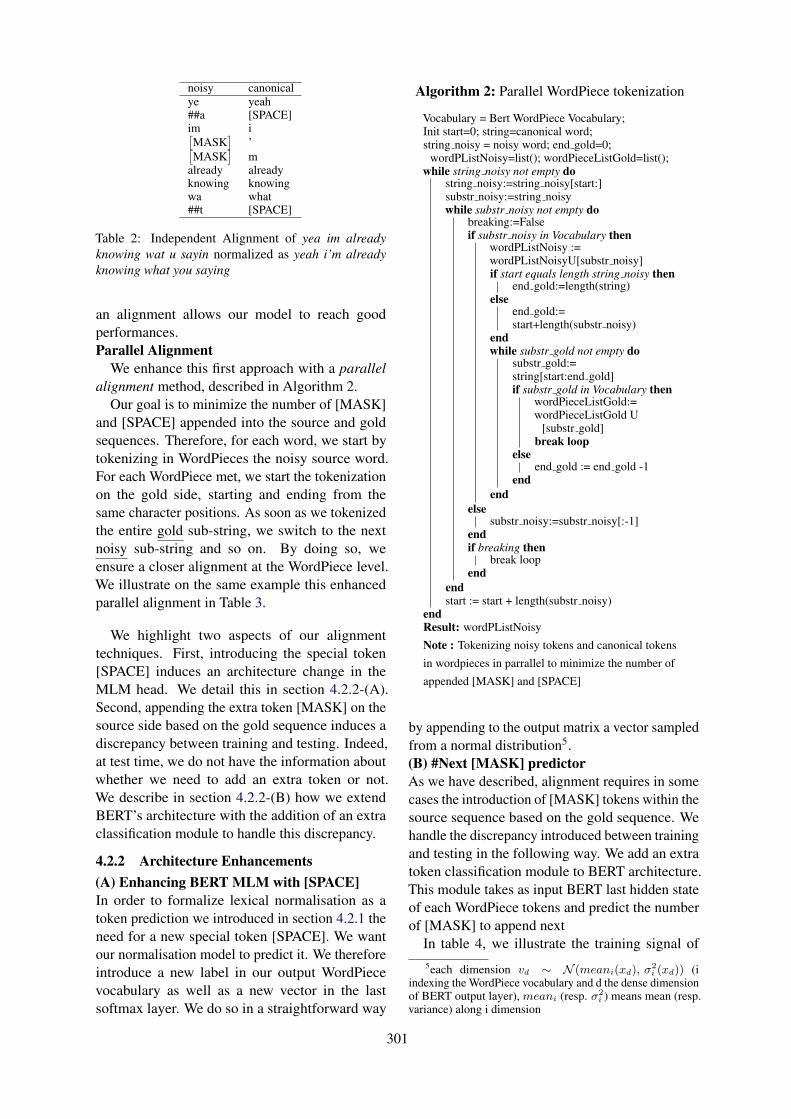
noisy canonicalye yeah##a [SPACE]im i[MASK

]’[

MASK]

malready alreadyknowing knowingwa what##t [SPACE]

Table 2: Independent Alignment of yea im alreadyknowing wat u sayin normalized as yeah i’m alreadyknowing what you saying

an alignment allows our model to reach goodperformances.Parallel Alignment

We enhance this first approach with a parallelalignment method, described in Algorithm 2.

Our goal is to minimize the number of [MASK]and [SPACE] appended into the source and goldsequences. Therefore, for each word, we start bytokenizing in WordPieces the noisy source word.For each WordPiece met, we start the tokenizationon the gold side, starting and ending from thesame character positions. As soon as we tokenizedthe entire gold sub-string, we switch to the nextnoisy sub-string and so on. By doing so, weensure a closer alignment at the WordPiece level.We illustrate on the same example this enhancedparallel alignment in Table 3.

We highlight two aspects of our alignmenttechniques. First, introducing the special token[SPACE] induces an architecture change in theMLM head. We detail this in section 4.2.2-(A).Second, appending the extra token [MASK] on thesource side based on the gold sequence induces adiscrepancy between training and testing. Indeed,at test time, we do not have the information aboutwhether we need to add an extra token or not.We describe in section 4.2.2-(B) how we extendBERT’s architecture with the addition of an extraclassification module to handle this discrepancy.

4.2.2 Architecture Enhancements(A) Enhancing BERT MLM with [SPACE]In order to formalize lexical normalisation as atoken prediction we introduced in section 4.2.1 theneed for a new special token [SPACE]. We wantour normalisation model to predict it. We thereforeintroduce a new label in our output WordPiecevocabulary as well as a new vector in the lastsoftmax layer. We do so in a straightforward way

Algorithm 2: Parallel WordPiece tokenization

Vocabulary = Bert WordPiece Vocabulary;Init start=0; string=canonical word;string noisy = noisy word; end gold=0;

wordPListNoisy=list(); wordPieceListGold=list();while string noisy not empty do

string noisy:=string noisy[start:]substr noisy:=string noisywhile substr noisy not empty do

breaking:=Falseif substr noisy in Vocabulary then

wordPListNoisy :=wordPListNoisyU[substr noisy]if start equals length string noisy then

end gold:=length(string)else

end gold:=start+length(substr noisy)

endwhile substr gold not empty do

substr gold:=string[start:end gold]if substr gold in Vocabulary then

wordPieceListGold:=wordPieceListGold U

[substr gold]break loop

elseend gold := end gold -1

endend

elsesubstr noisy:=substr noisy[:-1]

endif breaking then

break loopend

endstart := start + length(substr noisy)

endResult: wordPListNoisy

Note : Tokenizing noisy tokens and canonical tokens

in wordpieces in parrallel to minimize the number of

appended [MASK] and [SPACE]

by appending to the output matrix a vector sampledfrom a normal distribution5.(B) #Next [MASK] predictorAs we have described, alignment requires in somecases the introduction of [MASK] tokens within thesource sequence based on the gold sequence. Wehandle the discrepancy introduced between trainingand testing in the following way. We add an extratoken classification module to BERT architecture.This module takes as input BERT last hidden stateof each WordPiece tokens and predict the numberof [MASK] to append next

In table 4, we illustrate the training signal of5each dimension vd ∼ N (meani(xd), σ

2i (xd)) (i

indexing the WordPiece vocabulary and d the dense dimensionof BERT output layer), meani (resp. σ2

i ) means mean (resp.variance) along i dimension

301

Noisy Canonicalye ye##a ##ahim i[MASK

]’[

MASK]

malready alreadyknowing knowingwa wh##t ##at

Table 3: Parallel Alignment of yea im already knowingwat u sayin normalized as yeah i’m already knowingwhat you saying

Noisy Gold #next mask

ye ye 0##a ##ah 0im i 2[MASK

]’ -[

MASK]

m -already already 0knowing knowing 0wa wh 0##t ##at 0

Table 4: Parallel Alignment of yea im already knowingwat u sayin normalized as yeah i’m already knowingwhat you saying with gold number of next masks foreach source token

the overall architecture. It takes noisy WordPiecetokens as input. As gold labels, it takes on the oneside the gold WordPiece tokens and on the otherside the number of [MASK] to append next to eachsource WordPiece tokens.

At test time, we first predict the number of nextmasks to introduce in the noisy sequence. We thenpredict normalized tokens using the full sequence.

This #next mask prediction module exceedsthe context of normalisation. Indeed, itprovides a straightforward way of performingdata augmentation on any Masked LanguageModel architecture. We leave to future workthe investigation of its impact beyond lexicalnormalisation.

4.2.3 Fine-Tuning

We describe here how we fine-tune our architecturefor normalisation. Our goal is to learn lexicalnormalisation in a general manner. To do so,intuitively, our model needs to: on the one hand,preserve its language model ability that will allowgeneralization. On the other hand, the MLM needsto adjust itself to learn alignment between noisytokens and canonical tokens.

Based on those intuitions, we performe fine-tuningin the following way:

(i) Our first approach is to back-propagate on alltokens at each iteration. We also dropout 10% ofinput tokens by replacing them with the [MASK]as done during BERT pre-training. In this setting,all tokens are considered indifferently whether theyrequire normalisation or not .

(ii) The second approach that happens to performthe best is our Noise-focus fine-tuning. Theintuition is that it should be much easier for themodel to learn to predict already normalized tokensthan the ones that require normalization. For thisreason, we design the following strategy: For aspecific portion of batches noted pnoise we onlyback-propagate through noisy tokens. We foundthat having an increasing number of noise-specificbatch while training provides the best results.

Formally we describe our strategy as follows.For each mini-batch, we sample b followingthe distribution b ∼ Bernoulli(pnoise), withpnoise = min

(epoch

n epoch , 0.5)

, epoch being thecurrent number of epoch and n epoch the totalnumber of epochs.

If b equals 1 we back-propagate throughnoisy tokens, otherwise we back-propagate inthe standard way on all the tokens. In otherwords, while training, for an increasing portionof batches, we train on tokens that requirenormalization. We found that this dynamic strategywas much more efficient than applying a staticpnoise. Moreover, we highlight that the portionof noise specific update is capped at 50% (0.5 inthe equation). Above this value, we observed thatthe performances degraded in predicting non-noisytokens.

4.2.4 Optimization Details

Note that, excluding the fine-tuning strategy andthe alignment algorithm, the optimization hyper-parameters are shared to all the experiments wepresent next. Generally speaking, we found thatoptimizing BERT for lexical normalisation withWordPiece alignment is extremely sensitive tohyper-parameters. We managed to reach valuesthat work in all our following experiments. For theoptimization, we use the Adam algorithm (Kingmaand Ba, 2014). We found that 1e-5 provides themost stable and consistent convergence across allexperiments as evaluated on validation set. Wefound that a mini-batch of dimension 4 brings

302

the best performance also across all experiments.Finally, we kept a dropout value of 0.1 within theentire BERT model. We train the model for up to10 epochs and used performance as measured withthe F1-score (detailed in the next section) on thevalidation set as our early-stopping metric.

5 Experiments

All our experiments are run on the lexnorm15dataset. We do not use any other resources makingour problem falling under a low resource domaintransfer framework. As only pre-processing, welower-case all tokens whether they are on the noisysource side or on the canonical side.

We first present our analysis on the validationset that corresponds to the last 450 sentences of theoriginal training set of lexnorm15.

We define the three evaluation metrics onwhich we make our analysis. We distinguishbetween need norm words, words that require to benormalized and need no norm words that have tobe ”copied” by the model. We refer the wordsnormalized by our model (i.e our model gavea prediction different from the source word) aspred need norm. We refer to the number of TruePrediction of need norm words as TP. We thendefine recall and precision as:

recall =TP

#need norm

precision =TP

#pred need norm

Following previous works, we will focus onthe F1 score as our main evaluation metric. F1is simply the harmonic mean of the recall andprecision. For more fine grained analysis we alsoreport the recall on sub-sample of the evaluateddataset. Particularly, we distinguish between Out-of-Vocabulary (OOV) and In-Vocabulary words(InV) and report the recall on those subsets. Wedefine it formally as:

recall sample =TP ∩ sample

#need norm ∩ sample

5.1 Alignment algorithm

Does enforcing alignment in a greedy way asdescribed in Algorithm 2 help normalisation ?

As we compare in figure 1, our parallelalignment method provides a +0.5 F1 improvement

F1 recall-InV recall-OOVmetric

70.0

72.5

75.0

77.5

80.0

82.5

85.0

87.5

90.0independant alignementparrallel alignement

Figure 1: Impact of noisy/canonical alignmentmethod with a focus on generalization by comparingOut-of-Vocabulary (OOV) and In-Vocabulary (InV)performance (development set)

Standard Noise-focused Gain

78.1 79.28 +1.18

Table 5: Impact of our noise-specific strategy on the F1score (development set) reported with best alignmentsetting

(78.1 vs 77.6 F1). We also compare theperformance of our two models on OOV and InVwords. Indeed, normalising a seen word is mucheasier than a word unseen during training. As weobserve, the gain coming from our our alignmenttechnique come from a better generalization. Wegain +0.6 in recall on OOV thanks to this parallelalignment.

5.2 Fine-Tuning Strategy

As observed in table 5, our fine-tuning strategyfocused on noisy tokens improves with a largemargin the performance of our system. Weinterpret it in the following way: lexicalnormalisation is imbalanced. As seen in 3.2there are around 9 times more need no norm thanneed norm tokens. By specifically training onnoisy tokens we successfully manage to alleviatethis aspect of the data.

In conclusion, our best model is BERT trainedon parallel tokenized data with the noise-focus fine-tuning strategy. We reach 79.28 in F1 score. Thefollowing table illustrates how our model performsnormalization on a typical example:

Noisy @aijaee i hear you u knw betta to cross minetho

Norm @aijaee i hear you you know better to crossmine though

303

Model Accuracy

BERT noise-focused 97.5MoNoise 97.6

Table 6: Comparing our systems to the State-of-the-art system MoNoise (we report on same developmentdataset reported in MoNoise original paper (last 950sentences))

Model F1

Supranovich and Patsepnia, 2015 82.72Berend and Tasnadi, 2015 80.52

our best model 79.28Beckley, 2015 75.71

GIGO 72.64Ruiz et al., 2014 53.1

Table 7: Comparing our systems to WNUT 2015shared task that allowed UGC resources

6 Discussion

We now compare our system to previous works.As we see in Table 8, our non-UGC system is far

from the State-of-the-Art model MoNoise (van derGoot and van Noord, 2017) in terms of F1 score. Inorder to take into account detection in our metric,we also report the overall accuracy of the system intable 6. We are therefore 6.7 points below in termsof F1 score and 0.2 point below in terms of overallaccuracy on lexnorm15 dataset.

However, we emphasize that MoNoise is afeature-based Random Forest based on externalmodules. Among others, it makes use of a skip-gram model trained on 5 millions tweets, the Aspelltool and a n-gram model trained on more than 700millions tweets.

In order to have a more balanced comparison,we compare our system to the MoNoise modelafter removing the feature that has the most impact,according to the original paper: the n-gram module(referred as MoNoise no n-gram). In this setting,we significantly outperform the MoNoise model(+1.78 improvement) (Table 8).

Moreover, we based all our work on thelexnorm15 dataset released for the W-NUT 2015shared task (Baldwin et al., 2015). We compareour model to the competing systems (cf. table7). Briefly, the second best model (Berend andTasnadi, 2015) use a n-gram model trained on aEnglish tweet corpus. The best competing system(Supranovich and Patsepnia, 2015) is based on alexicon extracted from tweets. Still, we see thatour model is able to outperform models ranked 3,

Model F1 UGC resources speed

MoNoise 86.39 lex15+700Mtweets 57sour best model 79.28 lexnorm15 9.5sMoNoise NNG 77.5 lex15+5Mtweets -

Table 8: Comparing our systems to the State-of-the-artsystem MoNoise on lexnorm15 test. Speed is reportedas time to predict 1000 tokens (includes model loading).MoNoise No-Ngrams or MoNoise NNG is the scorereported in the original paper without the use of UGC-n-grams but with a UGC word2vec

4 and 5 that are all built using UGC resources.Finally, the state-of-the-art models we presented

are modular. They require features from externalmodules. This makes them extremely slow at testtime. We compare it in Table 8, demonstratinganother practical interest for our approach. Ourmodel is 6 times faster than MoNoise at predictiontime.

Following those observations, we claim thatBERT, enhanced to handle token introduction andtoken removal, fine-tuned in a precise way towardnoisy words, is a competitive lexical normalisationmodel.

This result exceeds the context of lexicalnormalization of noisy User Generated Content.Indeed, the success of BERT in improving NLPmodels on a diversity of tasks was, until now,restricted to canonical edited texts. In our work,we showed that it was possible to adapt such ageneral model to the extreme case of normalisingnoisy UGC in a low resource setting. We let forfuture work the adaptation of BERT to other tasksin out-of-domain non canonical context.

7 Conclusion

General pre-trained language model have demon-strated their ability to improve Natural LanguageProcessing systems for most tasks on canonicaldata. In our work, we demonstrated that they canalso be useful in non-canonical noisy text in low re-source setting. We hope that this work will pave theway for future research in modelling non-canonicaltextual data.

Acknowledgments

We thank the reviewers for their valuable feedbacks.This work was funded by the ANR projects ParSiTi(ANR-16-CE33-0021), SoSweet (ANR15-CE38-0011-01) and the French-Israeli PHC Maimonideprogram.

304

ReferencesTimothy Baldwin, Paul Cook, Marco Lui, Andrew

MacKinlay, and Li Wang. 2013. How noisysocial media text, how diffrnt social media sources?In Proceedings of the Sixth International JointConference on Natural Language Processing, pages356–364.

Timothy Baldwin, Marie-Catherine de Marneffe,Bo Han, Young-Bum Kim, Alan Ritter, and Wei Xu.2015. Shared tasks of the 2015 workshop on noisyuser-generated text: Twitter lexical normalizationand named entity recognition. In Proceedings of theWorkshop on Noisy User-generated Text, pages 126–135.

Russell Beckley. 2015. Bekli: A simple approach totwitter text normalization. In Proceedings of theWorkshop on Noisy User-generated Text, pages 82–86.

Gabor Berend and Ervin Tasnadi. 2015. Uszeged:correction type-sensitive normalization of englishtweets using efficiently indexed n-gram statistics.In Proceedings of the Workshop on Noisy User-generated Text, pages 120–125.

Jacob Devlin, Ming-Wei Chang, Kenton Lee, andKristina Toutanova. 2018. Bert: Pre-trainingof deep bidirectional transformers for languageunderstanding. arXiv preprint arXiv:1810.04805.

Jacob Eisenstein. 2013. What to do about bad languageon the internet. In HLT-NAACL, Atlanta, USA.

Jennifer Foster. 2010. “cba to check the spelling”:Investigating parser performance on discussionforum posts. In NAACL, Los Angeles, California.

Rob van der Goot and Gertjan van Noord. 2017.Monoise: modeling noise using a modular normal-ization system. arXiv preprint arXiv:1710.03476.

Rob van der Goot and Gertjan van Noord. 2018.Modeling input uncertainty in neural networkdependency parsing. In Proceedings of the2018 Conference on Empirical Methods in NaturalLanguage Processing, pages 4984–4991.

Rob van der Goot, Barbara Plank, and Malvina Nissim.2017. To normalize, or not to normalize: The impactof normalization on part-of-speech tagging. arXivpreprint arXiv:1707.05116.

Soorya Gopalakrishnan, Zhinus Marzi, UpamanyuMadhow, and Ramtin Pedarsani. 2018. Combatingadversarial attacks using sparse representations.

Bo Han and Timothy Baldwin. 2011. Lexicalnormalisation of short text messages: Makn sensa# twitter. In Proceedings of the 49th AnnualMeeting of the Association for ComputationalLinguistics: Human Language Technologies-Volume1, pages 368–378. Association for ComputationalLinguistics.

John Hewitt and Christopher D. Manning. 2019.A Structural Probe for Finding Syntax in WordRepresentations. In Proceedings of the 2019Conference of the North American Chapter ofthe Association for Computational Linguistics:Human Language Technologies. Association forComputational Linguistics.

Ganesh Jawahar, Benoıt Sagot, and Djame Seddah.2019. What does BERT learn about the structure oflanguage? In in proc. of the 57th Annual Meetingof the Association for Computational Linguistics(ACL), Florence, Italy.

Dan Jurafsky. 2018. Speech & language processing,3rd edition. Currently in draft.


Guillaume Lample and Alexis Conneau. 2019. Cross-lingual language model pretraining. arXiv preprintarXiv:1901.07291.

Chen Li and Yang Liu. 2012. Improving textnormalization using character-blocks based modelsand system combination. Proceedings of COLING2012, pages 1587–1602.

Paul Michel and Graham Neubig. 2018. Mtnt: Atestbed for machine translation of noisy text. arXivpreprint arXiv:1809.00388.

Seungwhan Moon, Leonardo Neves, and VitorCarvalho. 2018. Multimodal named entityrecognition for short social media posts. arXivpreprint arXiv:1802.07862.

Matthew E Peters, Mark Neumann, Mohit Iyyer, MattGardner, Christopher Clark, Kenton Lee, and LukeZettlemoyer. 2018. Deep contextualized wordrepresentations. arXiv preprint arXiv:1802.05365.

Pablo Ruiz, Montse Cuadros, and Thierry Etchegoyhen.2014. Lexical normalization of spanish tweetswith rule-based components and language models.Procesamiento del Lenguaje Natural, page 8.

Mike Schuster and Kaisuke Nakajima. 2012. Japaneseand korean voice search. In 2012 IEEEInternational Conference on Acoustics, Speech andSignal Processing (ICASSP), pages 5149–5152.IEEE.

Djame Seddah, Benoıt Sagot, Marie Candito, VirginieMouilleron, and Vanessa Combet. 2012. The FrenchSocial Media Bank: a Treebank of Noisy UserGenerated Content. In CoLing, Mumbai, India.

Dmitry Supranovich and Viachaslau Patsepnia. 2015.Ihs rd: Lexical normalization for english tweets.In Proceedings of the Workshop on Noisy User-generated Text, pages 78–81.

305

Ilya Sutskever, Oriol Vinyals, and Quoc V Le. 2014.Sequence to sequence learning with neural networks.In Advances in neural information processingsystems, pages 3104–3112.

Ke Xu, Yunqing Xia, and Chin-Hui Lee. 2015. Tweetnormalization with syllables. In Proceedings ofthe 53rd Annual Meeting of the Association forComputational Linguistics and the 7th InternationalJoint Conference on Natural Language Processing(Volume 1: Long Papers), volume 1, pages 920–928.

Yi Yang and Jacob Eisenstein. 2013. A log-linearmodel for unsupervised text normalization. InProceedings of the 2013 Conference on EmpiricalMethods in Natural Language Processing, pages 61–72.

306


No, you’re not alone: A better way to find people with similar experienceson Reddit

Zhilin Wang Elena Rastorgueva Weizhe Lin Xiaodong WuUniversity of Cambridge, United Kingdom{zw322, wl356, xw338}@cam.ac.uk,

[email protected]

Abstract

We present a probabilistic clustering algorithmthat can help Reddit users to find posts thatdiscuss experiences similar to their own. Thismodel is built upon the BERT Next SentencePrediction model and reduces the time com-plexity for clustering all posts in a corpus fromO(n2) to O(n) with respect to the number ofposts. We demonstrate that such probabilis-tic clustering can yield a performance betterthan baseline clustering methods based on La-tent Dirichlet Allocation (Blei et al., 2003)and Word2Vec (Mikolov et al., 2013). Fur-thermore, there is a high degree of coher-ence between our probabilistic clustering andthe exhaustive comparison O(n2) algorithmin which the similarity between every pair ofposts is found. This makes the use of theBERT Next Sentence Prediction model morepractical for unsupervised clustering tasks dueto the high runtime overhead of each BERTcomputation.

1 Introduction

On many subreddits within Reddit, such as r/Ad-vice1, users choose to share highly personal expe-riences that matter greatly in their lives in order toask for advice from other users. Relative to otherpopular social networking sites such as Facebook,Instagram and Twitter, Reddit offers a greater ex-tent of anonymity because there is no requirementfor users to register accounts with their real names.Users are therefore often more at ease to revealtheir experiences honestly and in full detail be-cause the risk of facing repercussion from theirreal-life social networks is minimal. An examplepost is shown in Figure 1. This offers a uniqueopportunity to use what users posted on these sub-reddits as a proxy for their real-life experiences,

1 https://www.reddit.com/r/Advice/

Title: “How do I get Vaccinated as a Minor?”Body: “I am a 16 year old female whosemother became anti-vax a couple of years agowhen she got Facebook. I don’t think I’vegotten a vaccine in 4-6 years at this point.Ireally want to get vaccinated ...”

Figure 1: An excerpt from a /r/Advice subreddit post.

and what they felt and thought about these experi-ences. Here, we attempt to cluster similar posts onthese subreddits. In this aspect, we are not only in-terested in the circumstances under which the indi-viduals encountered the experiences, but also howthey responded to the various situations in termsof their actions, thoughts and feelings.

To do so, we take advantage of recent im-provements in transformer-based mechanisms fortransfer learning, most prominently BERT (Devlinet al., 2019). This capacity allows a model to bepre-trained on a large corpus unrelated to our spe-cific task, in order to learn fundamental statisti-cal properties of language relating to syntax andsemantics. Specifically, we employ the model ofBERT that is pre-trained for the task of Next Sen-tence Prediction, which seeks to capture semanticcongruence between two paragraphs. While this isnot entirely similar with finding semantic similar-ities within Reddit posts (which often contain in-formal language), we hypothesize that some infor-mation encapsulated in the pre-trained model willbe transferable to our task. In this way, we cantrain a model using an extremely limited datasetof around 9000 posts. Currently, we have onlytrained our model using an English corpus, butgiven that the BERT model (Devlin et al., 2019)has multi-lingual capabilities, we believe that ourfindings can apply to languages other than En-glish.

Our key contribution lies in clustering all posts

307

into groups without needing to calculate the pair-wise Next Sentence Prediction likelihood for ev-ery pair of posts. This reduces the computationalcomplexity of this process from O(n2) to O(nm),where n is the number of posts, m is the numberof clusters and n � m. This is an important ad-vancement because an operation on each pair ofposts is in itself computationally intensive due tothe transformer architecture. Our design can en-able such clustering to be more scalable for largercorpora.

2 Related work

2.1 Deductive coding of individualexperiences

The first field of related work lies in attempts tocreate a standard for deductive coding of individ-ual experiences, typically based in the field of psy-chology. In this approach, trained individuals in-spect people’s writing of their experience and clas-sify each into a predefined category. The inspec-tion of each individual is then compared to thatof others to ensure consistency. Demorest et al.(1999) defined an individual experience in termsof a person’s wish, a response from another personand a response from the self in light of the otherperson’s response. At each stage, experiences canbe classified into categories such as wanting to berespected, being disliked by others and feeling dis-appointed because of the rejection. On the otherhand, Thorne and McLean (2001) defined experi-ences in terms of themes. These themes includeoccasions of life threatening events, relationship-related issues and a sense of mastery. Together,these can provide a basis for identifying the ele-ments within a post that can be used to compare toother posts.

2.2 Computational personality differences

The second field of related work lies in research onhow individuals differ in terms of their responsesto common life situations and how such differ-ences can be measured by analyzing their writing.The most popular measure is the Myers-BriggsType Indicator (Myers et al., 1990; Gjurkovicand Snajder, 2018), which classifies individualsinto 16 types based on their disposition. An-other common measure is the Big Five person-ality traits (Yarkoni, 2010), which gauges peoplein terms of five dimensions: Openness, Conscien-tiousness, Extraversion, Agreeableness and Neu-

roticism. Pennebaker (2011) also investigated howother personality attributes such as a focus on theself (as opposed to others) and differences in sta-tus can be predicted based on word choices. All ofthe above measures seek to group people into dis-tinct categories based on how they write. The rel-ative success of this field in doing so convinced usthat it is possible to capture individual differencesthrough a person’s writing. However, to help Red-dit users find other users with similar experiences,we are interested in not only the general responsepatterns of an individual but also their specific re-sponse to a specific situation. This means that wecannot directly adopt their methodology of per-forming a supervised classification task. Instead,we decided on unsupervised methodology becauseit would permit a wider range of situations and re-sponses.

2.3 Analysis of characters and plots in novelsand movies

The final field of related work comes from thecomputational analysis of characters and plots innovels and movies. Bamman et al. (2013, 2014)sought to classify characters into various proto-types in film and novels. Frermann and Szarvas(2017) and Iyyer et al. (2016) went a step furtherto classify the types of relationships that exist be-tween main characters in a novel, in addition tothe prototype of each character in novels. Theseworks inspired this paper on Reddit posts, becauseevents in many novels and movies are relatable tothe experiences of real-life individuals. Further-more, many posts also concern interactions be-tween the author and other people in the author’sreal-life social networks. However, Reddit postsare much shorter than movies and novels. Thismeans that the recurrent models designed to repre-sent how a character/relationship develops througha novel/movie in literature above is less applica-ble in our research. Moreover, unlike novels/-movies, which often use character names togetherwith personal pronouns, Reddit posts tend to usepersonal pronouns almost exclusively (in order topreserve anonymity). As a result, a popular coref-erence resolution framework2 would not work onReddit posts. Therefore, most of the methods de-scribed in literature above could not be adapted forour research and we had to look elsewhere for asuitable architecture.

2 https://github.com/huggingface/neuralcoref

308

Algorithm 11: procedure ONE-PROB-CLUSTERING(posts, m)2: unselected posts← posts; clusters← {}3: while unselected posts 6= [ ] do4: selected post← RANDOM-SELECTION(all unselected posts) . Without replacement5: for query post in all unselected posts do6: similarity←BERT-NEXT-SENTENCE-PREDICTION(selected post.title, query post.text)7: most similar← most similar bn/mc query posts8: clusters [selected post]← most similar9: for post in most similar do

10: unselected posts.remove(post)11: return clusters

3 Probabilistic Clustering

3.1 Data preprocessingWe downloaded 200 days of posts from the r/Ad-vice subreddit1 using the Pushshift API3. Afterthat, we filtered out posts with (i) scores lower than3 based on the number of upvotes, downvotes andcomments they received, which indicated that theymight not be pertinent to the users of the subred-dit, and (ii) no textual information in the post. Thisleft us with 8865 posts.

3.2 Generating similarities between two postsWe then used the BERT Next Sentence Predic-tion model4 to predict the likelihood that the titlefrom post A will be proceeded by the body textof post B. The model had been pre-trained on theBooksCorpus (800M words) (Zhu et al., 2015) andEnglish Wikipedia corpus (2,500M words). Dur-ing the pre-training process, half of the inputs con-sist of sentence B being the actual sentence fol-lowing sentence A (labeled as ‘IsNext’) while theother half consists of a random sentence from thecorpus that does not proceed sentence A (labeledas ‘NotNext’) (Devlin et al., 2019). We found thisto be a feasible method of deciphering the seman-tic similarity between the title of post A and thebody text of post B because in more than 97.7%of our posts, the text is predicted to follow its owntitle. This is likely because the pre-training taskof finding sentences that are likely to follow oneanother is highly similar to our task of findingtext of a post that is likely to be after the title ofthe same post. While the BERT Next-Sentence-Prediction model was pre-trained on a sentence-

3https://github.com/dmarx/psaw4The uncased small model on

https://github.com/huggingface/pytorch-transformers

level corpus, this result demonstrates that its ef-fects can translate to a paragraph-level task, whichwas also noted by Devlin et al. (2019).

Besides using the title of post A and the text ofpost B, we also experimented with the title of postA and the title of post B as well as the text of postA and the text of post B.

3.3 Clustering based on similarities

Intuitively, clustering can be done by comparingeach post with all other posts in the corpus. Thiswould be a O(n2) operation where n is num-ber of posts. However, due to the large numberof weights of the BERT model, each comparisontakes a long time to complete. Therefore, even fora small corpus of 8865 posts, it would be infeasi-ble to perform pairwise comparison of every pair.This makes the intuitive algorithm highly unscal-able with the number of posts.

To overcome this problem, we invented a proba-bilistic clustering architecture, described in Algo-rithm 1.

The computational complexity of this algo-rithm, ONE-PROBABILISTIC-CLUSTERING canbe calculated as follows. Given that themost runtime-intensive step is BERT-NEXT-SENTENCE-PREDICTION, we can choose tosolely focus our analysis on this step.

In each while-loop, we have to performthe BERT-NEXT-SENTENCE-PREDICTION pro-cess nunselected posts times. nunselected posts startsfrom n and decreases by bn/mc after each while-loop, where n is the number of posts and m is thenumber of clusters.

Therefore, S, the total number of timesthe BERT-NEXT-SENTENCE-PREDICTION pro-cess is carried out, follows an arithmetic progres-

309

Algorithm 21: procedure MERGE-MULTIPLE-PROB-CLUSTERING(p, m, posts)2: similarity table← {}3: for i← 0, n− 1 do4: similarity table[i] = [0, 0, ..., 0, 0] . Initialise with array of size n

5: for i← 0, p− 1 do6: one probabilistic clustering = ONE-PROBABILISTIC-CLUSTERING(posts, m)7: for j in one probabilistic clustering.keys() do8: One cluster = [j] + [one probabilistic clustering[j]]9: all similar pairs = PERMUTATIONS(one cluster, 2)

10: for k in all similar pairs do11: similarity table[k[0]][k[1]] += 112: return similarity table

Algorithm 31: procedure GENERATE-CLUSTERS-FROM-SIMILARITY(similarity table, m, n)2: unselected posts← posts; clusters← {}3: while unselected posts 6= [ ] do4: selected post = RANDOM-SELECTION(unselected posts) . Without replacement5: sort similarity table[selected post]6: most similar = most similar bn/mc posts in unselected posts7: clusters [selected post] = most similar8: for post in most similar do unselected posts.remove(post)9: return clusters

sion:

S = n+ (n− bn/mc) + (n− 2bn/mc)+...

(n− (m− 1) ∗ bn/mc) + (n−m ∗ bn/mc)≤ n ∗m

2(1)

Therefore the time complexity of ONE-PROBABLISTIC-CLUSTERING is O(nm).We chose m = 30 because initial experimentsusing a Gaussian Mixture Model to clusterBERT sentence embedding of Reddit post text(by average-pooling all tokens in the second-to-last layer)5 suggested that m = 30 is theoptimal choice because it scored lowest on theAkaike Information Criteria (Akaike, 1973).The absolute computational complexity forONE-PROBABLISTIC-CLUSTERING, taking intoconsideration the cost of sorting most similaris O(mnlogn). When n is small however, theconstant factor for BERT-NEXT-SENTENCE-PREDICTION is so great that it dominates therun-time, allowing the run-time to O(nm).

5 https://github.com/hanxiao/bert-as-service

The time complexity for Algorithm 2, MERGE-MULTIPLE-PROB-CLUSTERING, is O(n2) wheren is the number of posts used to generate ann-by-n matrix for the similarity table. How-ever, because the constant factor is so large,when n = 8865, it is the time complexity fromrunning ONE-PROBABILISTIC-CLUSTERING thatdominates. Therefore, the runtime complex-ity of MERGE-MULTIPLE-PROB-CLUSTERING iso(nmp), n = 8865 where n is the numberof posts, m is the number of clusters and p isthe number of times that ONE-PROBABILISTIC-CLUSTERING is run. A value of p = 5 is chosenbecause although a more informative similarity ta-ble will be constructed when p is higher, it alsorequires more computational resources.

GENERATE-CLUSTERS-FROM-SIMILARITY

has a time complexity O(mn log n) where nis the number of posts and m is the number ofclusters because the while-loop will run for miterations with each iteration taking O(n log n)for sorting. In practice however, the runtime isdominated by the previous MERGE-MULTIPLE-PROBALISTIC-CLUSTERING step due to its largeconstant factor.

310

3.4 Fine-tuning BERT Next SentencePrediction

Besides using the pre-trained Next Sentence Pre-diction model, we also fine-tuned the model usingposts from Reddit to better fit the classification toour corpus. We used not only 8865 posts fromr/Advice, but also over 300,000 posts from sim-ilar subreddits6. During the pre-training process,we focused on training the weights for the finalBERT pooling layer as well as the classificationlayer and froze the parameters in all other BERTlayers. We made this decision because our cor-pus was not sufficient for us to retrain the parame-ters for the layers beneath and doing so might leadto worse performance than using the default pre-trained parameters. Because fine-tuning requireslabeled data, we performed fine-tuning based onposts from the same author. In the subreddits thatwe used, some authors posted multiple times toshare about a similar experience. This is likely be-cause they did not receive adequate guidance fromthe Reddit community after their earlier post(s).Therefore, two posts from the same subreddit andthe same author are likely to discuss about similarthemes and topics. We used this tendency to gen-erate text-text pairs from the same author with alabel ‘IsNext’ and paired one text with a randomlyselected text from another post not from the sameauthor with a label ‘NotNext’.

4 Evaluation

4.1 Qualitative Evaluation

Table 1, shows the titles of 3 randomly chosenposts and the five most similar posts to them.There is a high degree of coherence, and the postsare not only similar thematically (in Post 1: preg-nant - pregnancy test - dating - hookups), but alsoemotionally (in Post 2: a sense of succorance) andat a word-level (in Post 3: ‘dog’).

4.2 Quantitative Evaluation

BaselinesBaseline measurements were done using LatentDirichlet Allocation (LDA) (Blei et al., 2003)and word2vec (Mikolov et al., 2013). LDAdocument-topic mappings were performed using

6r/depression, r/relationship advice, r/offmychest,r/IAmA, r/needadvice, r/tifu, r/confessions, r/confession,r/TrueOffMyChest, r/confidence, r/socialanxiety, r/Anxiety,r/socialskills.

Gensim7. Documents were first tokenized, re-moved of stopwords and lemmatized. A Bag ofWords (BoW) corpus was obtained before a termfrequency-inverse document frequency (TF-IDF)corpus was derived from it. Topic modeling wasthen performed on both the BoW corpus (there-after LDA-BoW) and TF-IDF corpus (thereafterLDA-TFIDF) with the number of topics set to 30,in line with the number of clusters used. Thedocument-topic mapping of each post is then usedfor computing cosine similarities with all otherposts.

Word2Vec embeddings were also used as abenchmark. Specifically, pre-trained word2vecembeddings of dimension 300 (Mikolov et al.,2013) were used to generate two forms of sentenceembeddings. The first (thereafter called W2V-Weighted) is calculated by weighing the contribu-tion of each word embedding by the inverse of itsrelative frequency to the final sentence embedding.In doing so, the contributions of the most com-mon words are minimized. The second (thereaftercalled W2V-SIF) is calculated by first taking theweighed sentence embedding before removing thefirst principal component from it. (Arora et al.,2017).

Generating similarities from baselinesCosine similarities were then calculated be-

tween all documents. The resulting cosine similar-ity matrix was be then entered in the GENERATE-CLUSTERS-FROM-SIMILARITY function (Algo-rithm 3) with the number of clusters (m) and num-ber of posts (n) kept the same as in the probabilis-tic clustering model.

Evaluation metricsTo determine if our clustering algorithm is bet-

ter than baselines, it is imperative to have eval-uation metrics. However, because our clusteringtasks do not have ground truth labels, we couldnot find common metrics to evaluate the effective-ness of our algorithm. Therefore, we designed twonovel extrinsic metrics for this purpose.

Evaluation Metric 1: Same author scoreWe designed this metric based on the observa-

tion that authors who post multiple times in ther/Advice subreddit tend to post about similar top-ics. Therefore, a good clustering algorithm mightbe more effective at clustering posts from the sameauthor in the same cluster. To measure this, wefound all pairs of posts with the same author and

7 https://github.com/RaRe-Technologies/gensim

311

Randomly chosen post titlesTitles of 5 most similar postsPost 1: I’m afraid I could be pregnant1. I bought pregnancy tests bc im paranoidddd2. What should I think of this convo between my ex and I? I felt guilty...3. Met an E-guy became really good friends, started ‘dating’. We joked sexually and I found it funny.4. My entire life I skipped school and just didn’t really care too much for it.5. I’m scared of hookups.Post 2: How do I help support my girlfriend who has been raped?1. Should this teacher get in trouble for making these comments about male students?2. How do I help my (severely?) mentally ill daughter?3. I’ve been avoiding my family for the past few months, I’m not sure what to do now.4. How to turn you life around after doing almost nothing for 3-4 years.5. An old tradition brought me into a rather messed up situation.Post 3: Neighbor is going nuts and wants to shoot my dog (or my sister, or all of us...)1. How long do I wait before calling the police for a welfare check?2. How to help my roommate - crying in his sleep.3. To dog or not to dog?4. All day every day my neighbors dog is on a 6-10 ft rope.5. Dog sitting disaster

Table 1: Each unshaded box shows the titles of a randomly chosen post and the 5 posts most similar to it

counted the proportion of them that are clusteredinto the same cluster. Finally we account for thelikelihood that they were arranged into the samecluster by chance, which is a constant equal to1m . This is described in Eq. 2, where I is thetotal number of authors and j represents possiblecombinations of pairs of posts by a single author(hence there are a total of Ji possible combina-tions for author i). j0 and j1 represent the firstand second post in the pair, respectively, and e.g.Cluster(j0) returns the i.d. of the cluster that j0

has been assigned to.

Ssame author =

I∑i=1

Ji∑j=1

1Cluster(j0)=Cluster(j1)

I∑i=1

J∑j=1

1

− 1

m(2)

Evaluation Metric 2: Jaccard score This met-ric was inspired by the observation that authorswho share similar interests tend to post about sim-ilar topics on r/Advice. In this case, we mea-sure how similar the interests of the authors are bycounting the number of subreddits they have bothposted and commented on divided by the num-ber of the union of subreddits they have posted

and commented on. In the case that they haveboth commented and posted in exactly the sameset of subreddits, their Jaccard scores will be 1. Ifthey have not posted or commented on any sub-reddits in common, their Jaccard score will be0. In our use case, however, the lower bound isstrictly higher than 0 because two authors wouldhave both posted in r/Advice. Furthermore, toprevent over-accounting for throwaway accounts,which are only used to post once, we set the Jac-card score of any pair of posts, which consists ofat least one that has only posted/commented in onesubreddit to 0.

Jaccard scores of all pairs of posts in the samecluster were then added together. The result wasthen multiplied by the number of clusters to ac-count for the difference in probability that twoposts will be put into the same cluster by chancealone, which varies inversely with the number ofclusters. Finally, the result is divided by the squareof the number of posts because the number ofposts in each cluster varies linearly with the totalnumber of posts and therefore the number of com-bination of two posts in the same category varieslinearly to the square of the number of posts.

The metric is described in Eq. 3 where I is thetotal number of clusters (referred to as m in therest of this paper) and Ji represents all possiblecombinations of pairs of posts in the same cluster.

312

Lpostedj0

represents the set of subreddits that the au-thor of the first post in the pair has posted to. Like-wise j1 refers to the second author and commented

refers to subreddits the author commented on.

SJaccard =

I∑

i=1

Ji∑

j=1

0.5

(Lpostedj0

∩ Lpostedj1

Lpostedj0

∪ Lpostedj1

+

Lcommentedj0 ∩ Lcommented

j1

Lcommentedj0

∪ Lcommentedj1

)∗ nclusters

n2posts

(3)

4.3 Effectiveness of probabilistic clustering

(a)

(b)

Figure 2: Same author (a) and Jaccard scores (b) forpre-trained probabilistic clustering compared to base-lines. Scores generated by performing 100 iterationsand finding the average. Error bars in (a) represent thestandard deviation. Error bars are not shown on (b) be-cause standard deviation is insignificant relative to thescale of the figure. Higher is better on both figures.

Figure 2 shows that probabilistic clustering per-forms better than all baseline embeddings. Thisis due to the model’s capability to learn complexrelationships between the two input sentences in-stead of using cosine distance as the measure ofsimilarity. In nearly all embeddings, using thebody text from two posts surpasses the perfor-mance of using the title from one post and thebody text from the second post, measured in bothmetrics. This is likely because the body text typ-ically contains more words, which can providemore information for sentence embeddings. A

review of the topic-word mapping for LDA sug-gests that words were not clearly resolved into dis-tinct topics. Words like “friends”, “dating” and“fun” appeared in nearly half of all topics, sug-gesting that LDA might be inadequate for captur-ing topics in such Reddit posts. This might be be-cause Reddit posts are mostly informal and usesa limited range of vocabulary with many commonwords used in different context with highly dis-tinct meanings. Using a transformer-based BERTarchitecture might be better able to capture suchcontextual information (Vaswani et al., 2017).

4.4 Fine-tuning

(a)

(b)

Figure 3: Same author (a) and Jaccard scores (b)for probabilistic clustering of BERT embeddings fine-tuned on subreddit(s) based on the same author selec-tion criteria. Scores generated by performing 100 itera-tions and finding the average, with error bars in (a) rep-resenting the standard deviation. Error bars not shownon (b) because standard deviation is insignificant rela-tive to the scale of the figure. Higher is better on bothfigures.

Figure 3b suggests that while some forms offine-tuning can perform better than the pre-trainedmodel, improvements are usually modest and in-consistent. In both Figures 3a and 3b, the modelfine-tuned using only the Advice subreddit per-formed worst in terms of both metrics suggestingthat pre-training on a highly limited corpus shouldbe avoided. Furthermore, its poor performance

313

also supports the hypothesis that the model doesnot simply memorize the seen corpus because thesame set of the corpus was used to train and totest the classifier. On the contrary, pre-training themodel with a large corpus, even one that does notcontain the testing sample, can lead to some im-provement in the Jaccard score, as in Figure 3b.This suggests a lack of over-fitting in our modeland correspondingly indicates a high possibility ofgeneralizing our model beyond our corpus.

4.5 Ablation experiments

(a)

(b)

Figure 4: (a) Jaccard Scores for the first 1000 posts,obtained from Probabilistic Clustering and ExhaustiveComparison. (b) Similarity scores between Probabilis-tic clustering and Exhaustive Comparison for the first1000 posts. Scores generated by performing 50 itera-tions and finding the average. Error bars represent stan-dard deviation. Higher is better on both figures.8

An ablation study was conducted to investi-gate the contribution of the probabilistic cluster-ing algorithm beyond the value of the BERT NextSentence Prediction task. In the exhaustive com-parison control, the likelihood that the post textof post A will follow the post text of post Bwas found for all combinations of pairs of posts.This allowed us to construct a complete similar-ity table that can be used to generate clusters us-ing the procedure GENERATE-CLUSTERS-FROM-SIMILARITY. The same parameters of 1,000 postsand 30 clusters were chosen for both probabilistic

clustering and the exhaustive comparison. Figure4a suggests that while exhaustive comparison ledto higher performance, the difference is typicallyless than a standard deviation. This means thatthe reduction in performance is relatively minimalcompared to the significant reduction in time com-plexity, which might make exhaustive comparisonincreasingly unfeasible as the number of posts in-creases.

In Figure 4b, Adjusted Rand score (Hubert andArabie, 1985) and Adjusted Mutual Information(Vinh et al., 2010) were used to measure for co-herence between exhaustive comparison and prob-abilistic clustering. Both scores suggest that theprobabilistic clustering of embeddings pre-trainedon all corpuses agree with the exhaustive compar-ison to a degree that is significantly higher thanchance would predict (when both scores wouldbe 0). Furthermore, the model pre-trained on thelarger corpora of (i) Multiple subreddits inc. Ad-vice and (ii) exc. Advice agree more with the ex-haustive comparison. This might be because themodels fine-tuned on those corpora are better ableto understand the use of language used on Red-dit and hence better able to accurately choose thetop bn/mc similar posts. However, this does nottranslate to higher Jaccard scores compared to thepre-trained model. This could be due to (i) theJaccard score metric (measuring the proportion ofsubreddits that two authors have posted or com-mented on in common) not being able to fullycapture all information that explain the similar-ity between posts, or (ii) the BERT Next SentencePrediction model (pre-trained and minimally fine-tuned) being unable to fully capture the relativesimilarities between posts, even though it is capa-ble of capturing absolute similarities between thetitle of a post and its post text.

5 Conclusion

In conclusion, we have presented a probabilisticclustering algorithm for clustering similar posts onmany subreddits on Reddit such as r/Advice. Thisalgorithm is built on top of the BERT Next Sen-tence Prediction model and reduces the time com-plexity of clustering posts from O(n2) to O(n)with respect to the number of posts. This algo-rithm can be helpful for users on Reddits to find

8 Only Jaccard scores were used to compare the extrin-sic performance of both methods because the low number ofpairs of post that share the same author makes the same au-thor score uninformative.

314

posts similar to those they have written themselves(about their own experiences) or others that theyare interested in. To further build on the contri-bution of this work, we encourage researchers toexperiment with alternative fine-tuning methodsas well as performing post-processing of similar-ity tables such as performing post-level normal-ization to reduce the occurrence of some posts be-ing highly similar to a great number of posts whileothers being similar to too few. Researchers mayalso consider incorporating other textual informa-tion such as comments on Reddit posts into themodel to improve its performance.

ReferencesHirotugu Akaike. 1973. Information theory and an ex-

tension of the maximum likelihood principle. Czaki,Akademiai Kiado, Budapest.

Sanjeev Arora, Yingyu Liang, and Tengyu Ma. 2017.A simple but tough-to-beat baseline for sentence em-beddings. In ICLR.

David Bamman, Brendan O’Connor, and Noah A.Smith. 2013. Learning latent personas of film char-acters. In Proceedings of the 51st Annual Meeting ofthe Association for Computational Linguistics (Vol-ume 1: Long Papers), pages 352–361, Sofia, Bul-garia. Association for Computational Linguistics.

David Bamman, Ted Underwood, and Noah A. Smith.2014. A Bayesian mixed effects model of literarycharacter. In Proceedings of the 52nd Annual Meet-ing of the Association for Computational Linguis-tics (Volume 1: Long Papers), pages 370–379, Bal-timore, Maryland. Association for ComputationalLinguistics.

David M. Blei, Andrew Y. Ng, and Michael I. Jordan.2003. Latent dirichlet allocation. J. Mach. Learn.Res., 3:993–1022.

Amy Demorest, Paul Crits-Christoph, Mary Hatch, andLester Luborsky. 1999. A comparison of interper-sonal scripts in clinically depressed versus nonde-pressed individuals. Journal of Research in Person-ality, 33(3):265 – 280.

Jacob Devlin, Ming-Wei Chang, Kenton Lee, andKristina Toutanova. 2019. Bert: Pre-training of deepbidirectional transformers for language understand-ing. In NAACL-HLT.

Lea Frermann and Gyorgy Szarvas. 2017. Inducingsemantic micro-clusters from deep multi-view rep-resentations of novels. In Proceedings of the 2017Conference on Empirical Methods in Natural Lan-guage Processing, pages 1873–1883, Copenhagen,Denmark. Association for Computational Linguis-tics.

Matej Gjurkovic and Jan Snajder. 2018. Reddit: Agold mine for personality prediction. In Proceed-ings of the Second Workshop on ComputationalModeling of People’s Opinions, Personality, andEmotions in Social Media, pages 87–97, New Or-leans, Louisiana, USA. Association for Computa-tional Linguistics.

Lawrence Hubert and Phipps Arabie. 1985. Compar-ing partitions. Journal of classification, 2(1):193–218.

Mohit Iyyer, Anupam Guha, Snigdha Chaturvedi, Jor-dan Boyd-Graber, and Hal Daume III. 2016. Feud-ing families and former Friends: Unsupervisedlearning for dynamic fictional relationships. In Pro-ceedings of the 2016 Conference of the North Amer-ican Chapter of the Association for ComputationalLinguistics: Human Language Technologies, pages1534–1544, San Diego, California. Association forComputational Linguistics.


Isabel Briggs Myers, Mary H.McCaulley, and Allen L.Hammer. 1990. Introduction to Type: a descriptionof the theory and applications of the Myers-Briggstype indicator. Consulting Psychologists Press.

James W. Pennebaker. 2011. The secret life of pro-nouns: What our words say about us. BloomsburyPress, New York, NY.

Avril Thorne and Kate C. McLean. 2001. Manual forcoding events in self-defining memories. Unpub-lished Manuscript.

Ashish Vaswani, Noam Shazeer, Niki Parmar, JakobUszkoreit, Llion Jones, Aidan N. Gomez, LukaszKaiser, and Illia Polosukhin. 2017. Attention is allyou need. In NIPS.

Nguyen Xuan Vinh, Julien Epps, and James Bailey.2010. Information theoretic measures for cluster-ings comparison: Variants, properties, normaliza-tion and correction for chance. J. Mach. Learn. Res.,11:2837–2854.

Tal Yarkoni. 2010. Personality in 100,000 words:A large-scale analysis of personality and word useamong bloggers. Journal of research in personality,44(3):363373.

Yukun Zhu, Jamie Ryan Kiros, Richard S. Zemel, Rus-lan Salakhutdinov, Raquel Urtasun, Antonio Tor-ralba, and Sanja Fidler. 2015. Aligning books andmovies: Towards story-like visual explanations bywatching movies and reading books. 2015 IEEE In-ternational Conference on Computer Vision (ICCV),pages 19–27.

315


Improving Multi-label Emotion Classification by Integrating bothGeneral and Domain Knowledge

Wenhao Ying Rong XiangThe Hong Kong Polytechnic University, Hong Kong, China

[email protected], {csrxiang,csluqin}@comp.polyu.edu.hk

Qin Lu

Abstract

Deep learning based general language mod-els have achieved state-of-the-art results inmany popular tasks such as sentiment analy-sis and QA tasks. Text in domains like so-cial media has its own salient characteristics.Domain knowledge should be helpful in do-main relevant tasks. In this work, we de-vise a simple method to obtain domain knowl-edge and further propose a method to inte-grate domain knowledge with general knowl-edge based on deep language models to im-prove performance of emotion classification.Experiments on Twitter data show that eventhough a deep language model fine-tuned bya target domain data has attained compara-ble results to that of previous state-of-the-artmodels, this fine-tuned model can still benefitfrom our extracted domain knowledge to ob-tain more improvement. This highlights theimportance of making use of domain knowl-edge in domain-specific applications.

1 Introduction

Deep language models (LM) have been very suc-cessful in recent years. In pre-training, a deep LMlearns to predict unseen words in the context athand in an unsupervised way, which enables theLM to make use of very large amount of unlabeleddata. By using deep structures and large amount oftraining data, these deep LMs can learn useful lin-guistic knowledge common to many natural lan-guage processing tasks. For example, BERT (De-vlin et al., 2019) has the ability to encode gram-matical knowledge in context in its representations(Hewitt and Manning, 2019). Deep LMs providegeneral knowledge of text to benefit downstreamtasks. To be adaptive to a target domain, they doneed to be fine-tuned by data of the target domain.

Obviously, every domain has its own character-istics which deserve special attention. A typical

example is Twitter data. In twitter, people can ex-press their thoughts online in real time. Due toits informal nature, people tend to pick whatevercomes to their mind to jot down their opinionseven if the writing does not conform to grammarrules. For example, Combinations of characters,such as ”:(” and ”:-)”, are often used to expressdifferent emotions. Deliberate irregular spellingsalso occur in Twitter to indicate authors’ attitude.Table 1 shows an example of an irregular expres-sion and how it can be preprocessed at word level,wordpiece level and at domain level. Many of

Snippet haaapppyyyy birthday best friend!!Love you lots #love

Word ‘haaapppyyyy’, ‘birthday’, ‘best’,‘friend’, ‘!’, ‘!’, ‘Love’, ‘you’,‘lots’, ‘#’, ‘love’

Wordpiece ‘ha’, ‘##aa’, ‘##pp’, ‘##py’, ‘##y’,‘##y’, ‘##y’, ‘birthday’, ‘best’,‘friend’, ‘!’, ‘!’, ‘Love’, ‘you’,‘lots’, ‘#’, ‘love’

Domain-specific

‘happy’, ‘<elongated>’, ‘birth-day’, ‘best’, ‘friend’, ‘!’, ‘<re-peated>’, ‘Love’, ‘you’, ‘lots’,‘</hashtag>’, ‘love’, ‘<hashtag>’

Table 1: Example of an real-world irregular expressionpreprocessed by methods at different levels. ‘##’ is asign of word pieces, and ‘<>’ is a special mark pro-duced by a Twitter-specific preprocessor.

these domain-specific expressions are strong indi-cators for affective analysis in Twitter, and thesecharacteristics are worthy of special consideration.Simply neglecting them would lose a lot of usefulinformation. Such information can be formulatedas domain knowledge by using Twitter prepro-cessor like (Baziotis et al., 2017). After Twitter-specific preprocessing, these expressions are an-notated automatically and we can find informa-

316

tive token patterns from preprocessed tweets. Inthe above example, a pattern ‘[+, <elongated>]’expresses more positive sentiment than a regularpositive word. Another pattern ‘[</hashtag>, *,</hashtag>]’ means it is a hashtag and usuallyhas an overall meaning for a tweet.

In this work, we select the popular BERT lan-guage model to provide general linguistic knowl-edge for modelling sentences. As a commonlyused deep LM, BERT is not intended to pay atten-tion to domain-specific details in Twitter. BERTactually use sub-word tokens as its inputs for gen-eralization, and a word is first divided into a num-ber of smaller units if necessary before being con-verted to embeddings. We design a token patterndetector that sifts through preprocessed tweets toobtain domain knowledge, and supplement BERTwith extracted domain-specific features. To inte-grate the domain knowledge with BERT, we firstfine-tune BERT to extract general features of Twit-ter data. Features from the fine-tuned BERT arethen integrated with domain-specific features toclassify tweets into target emotions. Performanceevaluations show that even though BERT was pre-trained on different source domains, the fine-tunedBERT using Twitter data indeed attains compa-rable results to that of the previous state-of-the-art models. Most importantly, even after BERTis tuned by Twitter data, integration of domainknowledge in our system still makes over onepercent improvement on the accuracy of emotionclassification compared to the previous state-of-the-art method using BERT only.

2 Related Work

Related works include both deep LMs especiallyBERT, a representative deep learning based LMand works on Twitter classification.

2.1 Deep Language Models

In contrast to n-gram LMs and early neural modelsfor learning word embeddings, recent LMs havedeeper structures. ELMo (Peters et al., 2018) usea stack of bi-directional LSTM to encode wordcontext either from left-to-right or from right-to-left. BERT (Devlin et al., 2019) has a bidirec-tional structure to learn context from both direc-tions. As a consequence of its bidirectionality,BERT is not trained by predicting words in se-quence either from left-to-right or from right-to-left. After masking a part of words in a sentence,

training predicts the masked and unseen wordswithin the remaining context. However, by cor-rupting inputs with masks, BERT neglects depen-dency between masked positions. XLNet (Yanget al., 2019) proposes to maximizes the likelihoodover all permutations of the factorization order ofconditional probability to learn bidirectional con-text without masking. Recently, RoBERTa (Liuet al., 2019) matches the previous state-of-the-artlanguage models by training BERT on even largerdata with optimized hyper-parameters.

In this work, we use BERT as our baseline, apopular deep language model. BERT has a stackof transformer layers (Vaswani et al., 2017). Thecentral part of a transformer is a multi-head atten-tion mechanism to include queries, keys, and val-ues as inputs, which makes scaled dot-product at-tention among all inputs. Let Q denote a querymatrix, K denote a key matrix, V denote a valuematrix, and Q = K = V in the case of BERT. Thescaled dot-product attention formula is then givenas follows:

Attention(Q,K, V ) = softmax(QKT

√dk

)V

where dk is the dimension of queries and keys. ForBERT, an input token has a positional embeddingand a segment embedding in addition to its reg-ular word embedding. Positional embeddings tellBERT relative positions of two words and segmentembeddings help BERT to differentiate two sen-tences of a pair. In each sentence fed into BERT,a special token [CLS] is inserted at the first placeand one uses its corresponding output as the over-all representation of this sentence for sentence-level tasks such as entailment or sentiment anal-ysis.

2.2 Twitter Affective AnalysisAs a platform to express everyday thoughts, Twit-ter has huge amount of affect-related text. ThusTwitter is a good source of research study on affec-tive analysis of people towards a topic. N-gramsand negative indicators are widely used in affec-tive analysis of Twitter (Mohammad et al., 2013;Miura et al., 2014). Affect-based lexicons are alsoincluded to provide general sentiment or emotioninformation (Hagen et al., 2015). (Go et al.) use:) and :( emoticons as natural labels and collecta pseudo-labeled training data to increase their n-gram classifier. Similarly, Wang et al (Wang et al.,

317

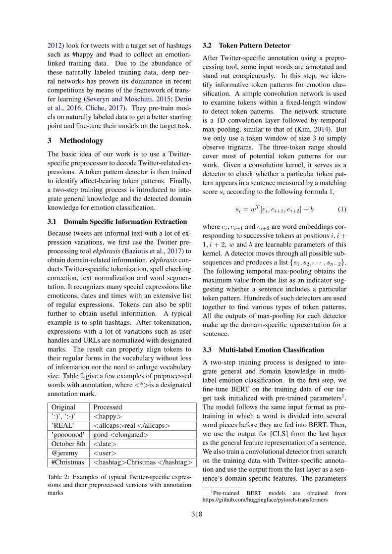
2012) look for tweets with a target set of hashtagssuch as #happy and #sad to collect an emotion-linked training data. Due to the abundance ofthese naturally labeled training data, deep neu-ral networks has proven its dominance in recentcompetitions by means of the framework of trans-fer learning (Severyn and Moschitti, 2015; Deriuet al., 2016; Cliche, 2017). They pre-train mod-els on naturally labeled data to get a better startingpoint and fine-tune their models on the target task.

3 Methodology

The basic idea of our work is to use a Twitter-specific preprocessor to decode Twitter-related ex-pressions. A token pattern detector is then trainedto identify affect-bearing token patterns. Finally,a two-step training process is introduced to inte-grate general knowledge and the detected domainknowledge for emotion classification.

3.1 Domain Specific Information ExtractionBecause tweets are informal text with a lot of ex-pression variations, we first use the Twitter pre-processing tool ekphrasis (Baziotis et al., 2017) toobtain domain-related information. ekphrasis con-ducts Twitter-specific tokenization, spell checkingcorrection, text normalization and word segmen-tation. It recognizes many special expressions likeemoticons, dates and times with an extensive listof regular expressions. Tokens can also be splitfurther to obtain useful information. A typicalexample is to split hashtags. After tokenization,expressions with a lot of variations such as userhandles and URLs are normalized with designatedmarks. The result can properly align tokens totheir regular forms in the vocabulary without lossof information nor the need to enlarge vocabularysize. Table 2 give a few examples of preprocessedwords with annotation, where <*>is a designatedannotation mark.

Original Processed’:)’, ’:-)’ <happy>’REAL’ <allcaps>real </allcaps>’gooooood’ good <elongated>October 8th <date>@jeremy <user>#Christmas <hashtag>Christmas </hashtag>

Table 2: Examples of typical Twitter-specific expres-sions and their preprocessed versions with annotationmarks

3.2 Token Pattern Detector

After Twitter-specific annotation using a prepro-cessing tool, some input words are annotated andstand out conspicuously. In this step, we iden-tify informative token patterns for emotion clas-sification. A simple convolution network is usedto examine tokens within a fixed-length windowto detect token patterns. The network structureis a 1D convolution layer followed by temporalmax-pooling, similar to that of (Kim, 2014). Butwe only use a token window of size 3 to simplyobserve trigrams. The three-token range shouldcover most of potential token patterns for ourwork. Given a convolution kernel, it serves as adetector to check whether a particular token pat-tern appears in a sentence measured by a matchingscore si according to the following formula 1,

si = wT [ei, ei+1, ei+2] + b (1)

where ei, ei+1 and ei+2 are word embeddings cor-responding to successive tokens at positions i, i+1, i + 2, w and b are learnable parameters of thiskernel. A detector moves through all possible sub-sequences and produces a list {s1, s2, · · · , sn−2}.The following temporal max-pooling obtains themaximum value from the list as an indicator sug-gesting whether a sentence includes a particulartoken pattern. Hundreds of such detectors are usedtogether to find various types of token patterns.All the outputs of max-pooling for each detectormake up the domain-specific representation for asentence.

3.3 Multi-label Emotion Classification

A two-step training process is designed to inte-grate general and domain knowledge in multi-label emotion classification. In the first step, wefine-tune BERT on the training data of our tar-get task initialized with pre-trained parameters1.The model follows the same input format as pre-training in which a word is divided into severalword pieces before they are fed into BERT. Then,we use the output for [CLS] from the last layeras the general feature representation of a sentence.We also train a convolutional detector from scratchon the training data with Twitter-specific annota-tion and use the output from the last layer as a sen-tence’s domain-specific features. The parameters

1Pre-trained BERT models are obtained fromhttps://github.com/huggingface/pytorch-transformers

318

of both models are fixed after this step and there-fore the representation produced by each modelwill not be changed in the next step. In the sec-ond step, the two types of representations are con-catenated and fed into a linear scoring layer foremotion class predication. For a target emotion iand the representation of a sentence x, its scoreis computed by y[i] = wTx. The layer is tunedon the training data so that general and Twitter-specific features can work collaboratively.

For the gold labels y and prediction scores y,their loss is given by

loss(x, y) =− 1

C

C∑

i

(y[i] ∗ log(1

1 + e−y[i])

+ (1− y[i]) ∗ log(e−y[i]

1 + e−y[i]))

(2)where y[i] and y[i] are for the ith emotion class,and C is the number of target emotion classes. Ifthe target emotion class is positive, that is y[i] = 1,the loss function requires the corresponding pre-diction to be as large as possible. When makingprediction of a target emotion for a sample, we as-sign it a positive label if y[i] ≥ 0.

4 Performance Evaluation

Performance evaluation is conducted on multi-label emotion classification of SemEval-2018Task 1 (Mohammad et al., 2018). Given a tweet,the task requires participants to classify text tozero or more of 11 target emotions.

4.1 Setup

SemEval-2018 dataset was already split into train-ing, development and testing sets by its organizer.We train and tune our models on the training anddevelopment sets, and report classification resultson the testing set. Word embeddings of our CNNdetector are learned from a corpus of 550M unla-beled tweets by word2vec (Mikolov et al., 2013)2. Multi-label accuracy, known as Jaccard Index,is used as the evaluation metric, defined as the sizeof the intersection divided by the size of the unionof the true label set and predicted label set. Macro-F1 and Micro-F1 are used as secondary evaluationmetrics following the same practice of SemEval-2018 Task 1. In the two-step training, we firsttrain our CNN detector and fine-tune BERT on the

2We use the pre-trained embeddings from (Baziotis et al.,2018)

training data 10 times and select the parameterswith the best performance on the development setto hopefully provide good representation of bothgeneral and domain-specific information. In thesecond step, the representation for a tweet remainsunchanged and only the parameters of a scoringlayer is learned.

4.2 Evaluation

Table 3 lists the results of multi-label emotionclassification on SemEval-2018. The first blocksare the state-of-the-art models on SemEval-2018Task 1, where we directly cite the results fromtheir papers. Two BERT models are used as ad-ditional baselines including BERTbase, which has12 layers of transformers with 768 dimension, andBERTlarge, which has 24 layers of transformerswith 1024 dimension. BERT using domain knowl-edge (DK) proposed by our work are appendedwith ‘+DK’. Another baselines include a biLSTMand our CNN detector. To randomize parame-ter initialization and learning algorithm, we trainCNN and BiLSTM from scratch, fine-tune BERTfrom the given initialized parameters, and learnthe weights of scoring layer 10 times, respectively.We report the average performance on the testingset for each model.

micro macroModel acc. F1 F1PlusEmo2Vec (Parket al., 2018)

57.6 69.2 49.7

TCS Research (Meish-eri and Dey, 2018)

58.2 69.3 53.0

NTUA-SLA (Baziotiset al., 2018)

58.8 70.1 52.8

CNN Detector 55.8 68.5 50.0BiLSTM 56.3 68.7 51.0BERTbase 58.4 70.4 54.2BERTlarge 58.8 70.7 55.2BERTbase+DK 59.1†‡ 71.3†‡ 54.9†BERTlarge+DK 59.5†‡ 71.6†‡ 56.3†

Table 3: Result of multi-label emotion classification onSemEval-2018. † means the result is statistically sig-nificant with p < 0.01 in contrast to the state-of-the-art NTUA-SLA. ‡ means the improvement by integrat-ing domain knowledge is statistically significant withp < 0.01 compared with its corresponding pure BERT,as BERTbase vs BERTbase+DK. For Macro-F1, theresults are statistically significant with p < 0.05.

As expected, the CNN detector has the worst

319

Emotion BERTlarge +DKanger 78.82 79.34 (+0.52)anticipation 23.60 23.60 (+0.00)disgust 75.00 76.28 (+1.28)fear 74.96 76.18 (+1.22)joy 85.22 86.39 (+1.17)love 61.52 63.94 (+2.42)optimism 73.41 73.73 (+0.32)pessimism 32.05 32.16 (+0.11)sadness 70.21 71.90 (+1.69)surprise 22.56 26.24 (+3.68)trust 9.56 9.03 (-0.53)

Table 4: F1 on binary classification for each emotionclass.

performance as this tri-gram model is too sim-ple to learn complex relationships such as long-distance negative relations. The CNN detector isto sift through domain-specific token patterns tosupplement the general knowledge of BERT. Bothof the fine-tuned pure BERTs are either compa-rable or slightly better than the performance ofthe previous state-of-the-art models. With theabundant pre-training data and their deep struc-ture, BERT models obtain a good starting pointfor a domain-specific task. More importantly,both BERT models benefit from domain knowl-edge supplied by the CNN detector to obtain per-formance improvement of 1.20% on major multi-label accuary for both models. Both BERT mod-els with domain knowledge outperform their cor-responding pure BERT and the state-of-the-artmodel statistically significantly with p < 0.01except for Macro-F1 where the results are statis-tically significant with p < 0.05. In the first-step training, the selected CNN, BERTbase andBERTlarge for providing tweet representation hasaccuracy of 56.7%, 59.0% and 58.9%, respec-tively. Table 3 shows that BERT integrating withTwitter-specific features outperforms both generaland domain-specific component model.

For more detailed investigation of the effect ofdomain knowledge, Table 4 shows the result ofbinary classification for each emotion class mea-sured by F1 score. Improvements are obtained innine out of eleven emotion classes. If excluding‘surprise’ and ‘trust’ which have low percentageof occurrence, salient improvements come mostlyfrom ‘disgust’, ‘fear’, ‘joy’, ‘love’ and ‘sadness’.Abundant domain-specific expressions in Twitter,

such as emoticons ‘:-)’ and ‘:-(’ and hashtags like‘#offended’, are useful affective indicators, whichare not used fully by BERT.

5 Conclusion

In this work, we leverage deep language models toprovide general sentence representations and inte-grate them with domain knowledge. We show thatintegration of both types of knowledge improvesmulti-label emotion classification of tweets. Eval-uation shows that a deep LM like BERT has thecapacity to perform well. Yet, its performance canstill be further improved by integrating elaboratedomain knowledge. Future works may investigateother deep LMs as well as data of other domains.

Acknowledgments

This work was partially supported by a GRF grantfrom HKUGC (PolyU 152006/16E).

ReferencesChristos Baziotis, Athanasiou Nikolaos, Alexan-

dra Chronopoulou, Athanasia Kolovou, Geor-gios Paraskevopoulos, Nikolaos Ellinas, ShrikanthNarayanan, and Alexandros Potamianos. 2018.Ntua-slp at semeval-2018 task 1: Predicting affec-tive content in tweets with deep attentive rnns andtransfer learning. In Proceedings of The 12th Inter-national Workshop on Semantic Evaluation, pages245–255.

Christos Baziotis, Nikos Pelekis, and Christos Doulk-eridis. 2017. Datastories at semeval-2017 task4: Deep lstm with attention for message-level andtopic-based sentiment analysis. In Proceedings ofthe 11th International Workshop on Semantic Eval-uation (SemEval-2017), pages 747–754, Vancouver,Canada. Association for Computational Linguistics.

Mathieu Cliche. 2017. Bb twtr at semeval-2017 task 4:Twitter sentiment analysis with cnns and lstms. InProceedings of the 11th International Workshop onSemantic Evaluation (SemEval-2017), pages 573–580.

Jan Deriu, Maurice Gonzenbach, Fatih Uzdilli, Au-relien Lucchi, Valeria De Luca, and Martin Jaggi.2016. Swisscheese at semeval-2016 task 4: Senti-ment classification using an ensemble of convolu-tional neural networks with distant supervision. InProceedings of the 10th international workshop onsemantic evaluation, CONF, pages 1124–1128.

Jacob Devlin, Ming-Wei Chang, Kenton Lee, andKristina Toutanova. 2019. Bert: Pre-training ofdeep bidirectional transformers for language under-standing. In Proceedings of the 2019 Conference of

320

the North American Chapter of the Association forComputational Linguistics: Human Language Tech-nologies, Volume 1 (Long and Short Papers), pages4171–4186.

Alec Go, Richa Bhayani, and Lei Huang. Twitter sen-timent classification using distant supervision.

Matthias Hagen, Martin Potthast, Michel Buchner, andBenno Stein. 2015. Webis: An ensemble for twittersentiment detection. In Proceedings of the 9th inter-national workshop on semantic evaluation (SemEval2015), pages 582–589.

John Hewitt and Christopher D Manning. 2019. Astructural probe for finding syntax in word represen-tations. In Proceedings of the 2019 Conference ofthe North American Chapter of the Association forComputational Linguistics: Human Language Tech-nologies, Volume 1 (Long and Short Papers), pages4129–4138.

Yoon Kim. 2014. Convolutional neural networks forsentence classification. In Proceedings of the 2014Conference on Empirical Methods in Natural Lan-guage Processing (EMNLP), pages 1746–1751.

Yinhan Liu, Myle Ott, Naman Goyal, Jingfei Du, Man-dar Joshi, Danqi Chen, Omer Levy, Mike Lewis,Luke Zettlemoyer, and Veselin Stoyanov. 2019.Roberta: A robustly optimized bert pretraining ap-proach. arXiv preprint arXiv:1907.11692.

Hardik Meisheri and Lipika Dey. 2018. Tcs researchat semeval-2018 task 1: Learning robust representa-tions using multi-attention architecture. In Proceed-ings of The 12th International Workshop on Seman-tic Evaluation, pages 291–299.


Yasuhide Miura, Shigeyuki Sakaki, Keigo Hattori, andTomoko Ohkuma. 2014. Teamx: A sentiment ana-lyzer with enhanced lexicon mapping and weightingscheme for unbalanced data. In Proceedings of the8th International Workshop on Semantic Evaluation(SemEval 2014), pages 628–632.

Saif Mohammad, Svetlana Kiritchenko, and XiaodanZhu. 2013. Nrc-canada: Building the state-of-the-art in sentiment analysis of tweets. In Second JointConference on Lexical and Computational Seman-tics (* SEM), Volume 2: Proceedings of the Sev-enth International Workshop on Semantic Evalua-tion (SemEval 2013), pages 321–327.

Saif M. Mohammad, Felipe Bravo-Marquez, Mo-hammad Salameh, and Svetlana Kiritchenko. 2018.Semeval-2018 Task 1: Affect in tweets. In Proceed-ings of International Workshop on Semantic Evalu-ation (SemEval-2018), New Orleans, LA, USA.

Ji Ho Park, Peng Xu, and Pascale Fung. 2018.Plusemo2vec at semeval-2018 task 1: Exploit-ing emotion knowledge from emoji and# hashtags.arXiv preprint arXiv:1804.08280.

Matthew Peters, Mark Neumann, Mohit Iyyer, MattGardner, Christopher Clark, Kenton Lee, and LukeZettlemoyer. 2018. Deep contextualized word rep-resentations. In Proceedings of the 2018 Confer-ence of the North American Chapter of the Associ-ation for Computational Linguistics: Human Lan-guage Technologies, Volume 1 (Long Papers), pages2227–2237.

Aliaksei Severyn and Alessandro Moschitti. 2015.Unitn: Training deep convolutional neural networkfor twitter sentiment classification. In Proceedingsof the 9th international workshop on semantic eval-uation (SemEval 2015), pages 464–469.


Wenbo Wang, Lu Chen, Krishnaprasad Thirunarayan,and Amit P Sheth. 2012. Harnessing twitter” bigdata” for automatic emotion identification. In 2012International Conference on Privacy, Security, Riskand Trust and 2012 International Confernece on So-cial Computing, pages 587–592. IEEE.


321


Adapting Deep Learning Methods forMental Health Prediction on Social Media

Ivan Sekulic and Michael StrubeHeidelberg Institute for Theoretical Studies gGmbH

{ivan.sekulic,michael.strube}@h-its.org

Abstract

Mental health poses a significant challengefor an individual’s well-being. Text analy-sis of rich resources, like social media, cancontribute to deeper understanding of illnessesand provide means for their early detection.We tackle a challenge of detecting social me-dia users’ mental status through deep learning-based models, moving away from traditionalapproaches to the task. In a binary classifica-tion task on predicting if a user suffers fromone of nine different disorders, a hierarchicalattention network outperforms previously setbenchmarks for four of the disorders. Further-more, we explore the limitations of our modeland analyze phrases relevant for classificationby inspecting the model’s word-level attentionweights.

1 Introduction

Mental health is a serious issue of the modern-dayworld. According to the World Health Organiza-tion’s 2017 report and Wykes et al. (2015) morethan a quarter of Europe’s adult population suf-fers from an episode of a mental disorder in theirlife. The problem grows bigger with the fact thatas much as 35–50% of those affected go undiag-nosed and receive no treatment for their illness. Inline with WHO’s Mental Health Action Plan (Sax-ena et al., 2013), the natural language processingcommunity helps the gathering of information andevidence on mental conditions, focusing on textanalysis of authors affected by mental illnesses.

Researchers can utilize large amounts of text onsocial media sites to get a deeper understanding ofmental health and develop models for early detec-tion of various mental disorders (De Choudhuryet al., 2013a; Coppersmith et al., 2014; Gkotsiset al., 2016; Benton et al., 2017; Sekulic et al.,2018; Zomick et al., 2019). In this work, weexperiment with the Self-reported Mental Health

Diagnoses (SMHD) dataset (Cohan et al., 2018),consisting of thousands of Reddit users diagnosedwith one or more mental illnesses. The contri-bution of our work is threefold. First, we adapta deep neural model, proved to be successful inlarge-scale document classification, for user clas-sification on social media, outperforming previ-ously set benchmarks for four out of nine disor-ders. In contrast to the majority of preceding stud-ies on mental health prediction in social media,which relied mostly on traditional classifiers, weemploy Hierarchical Attention Network (HAN)(Yang et al., 2016). Second, we explore the limita-tions of the model in terms of data needed for suc-cessful classification, specifically, the number ofusers and number of posts per user. Third, throughthe attention mechanism of the model, we analyzethe most relevant phrases for the classification andcompare them to previous work in the field. Wefind similarities between lexical features and n-grams identified by the attention mechanism, sup-porting previous analyses.

2 Dataset and the Model

2.1 Self-reported Mental Health DiagnosesDataset

The SMHD dataset (Cohan et al., 2018) is a large-scale dataset of Reddit posts from users with oneor multiple mental health conditions. The userswere identified by constructing patterns for dis-covering self-reported diagnoses of nine differentmental disorders. For example, if a user writes“I was officially diagnosed with depression lastyear”, she/he/other would be considered to sufferfrom depression.

Nine or more control users, which are meant torepresent general population, are selected for eachdiagnosed user by their similarity, i.e., by theirnumber of posts and the subreddits (sub-forums on

322

# users# postsper user

Depression 14,139 162.2 (84.2)ADHD 10,098 164.7 (83.6)Anxiety 8,783 159.7 (83.0)Bipolar 6,434 157.6 (82.4)PTSD 2,894 160.7 (84.7)Autism 2,911 168.3 (84.5)OCD 2,336 158.8 (81.4)Schizophrenia 1,331 157.3 (80.5)Eating 598 161.4 (81.0)

Table 1: Number of users in SMHD dataset per con-dition and the average number of posts per user (withstd.).

Reddit) they post in. Diagnosed users’ language isnormalized by removing posts with specific men-tal health signals and discussions, in order to an-alyze the language of general discussions and tobe more comparable to the control groups. Thenine disorders and the number of users per disor-der, as well as average number of posts per user,are shown in Table 1.

For each disorder, Cohan et al. (2018) analyzethe differences in language use between diagnosedusers and their respective control groups. Theyalso provide benchmark results for the binary clas-sification task of predicting whether the user be-longs to the diagnosed or the control group. Wereproduce their baseline models for each disorderand compare to our deep learning-based model,explained in Section 2.3.

2.2 Selecting the Control Group

Cohan et al. (2018) select nine or more controlusers for each diagnosed user and run their ex-periments with these mappings. With this exactmapping not being available, for each of the nineconditions, we had to select the control group our-selves. For each diagnosed user, we draw exactlynine control users from the pool of 335,952 con-trol users present in SMHD and proceed to trainand test our binary classifiers on the newly createdsub-datasets.

In order to create a statistically-fair comparison,we run the selection process multiple times, aswell as reimplement the benchmark models usedin Cohan et al. (2018). Multiple sub-datasets withdifferent control groups not only provide us withunbiased results, but also show how results of a

binary classification can differ depending on thecontrol group.

2.3 Hierarchical Attention Network

We adapt a Hierarchical Attention Network(HAN) (Yang et al., 2016), originally used fordocument classification, to user classification onsocial media. A HAN consists of a word se-quence encoder, a word-level attention layer, asentence encoder and a sentence-level attentionlayer. It employs GRU-based sequence encoders(Cho et al., 2014) on sentence and document level,yielding a document representation in the end.The word sequence encoder produces a represen-tation of a given sentence, which then is forwardedto a sentence sequence encoder that, given a se-quence of encoded sentences, returns a documentrepresentation. Both, word sequence and sentencesequence encoders, apply attention mechanismson top to help the encoder more accurately ag-gregate the representation of given sequence. Fordetails of the architecture we refer the interestedreaders to Yang et al. (2016).

In this work, we model a user as a document,enabling an intuitive adaptation of the HAN. Justas a document is a sequence of sentences, we pro-pose to model a social media user as a sequenceof posts. Similarly, we identify posts as sentences,both being a sequence of tokens. This interpreta-tion enables us to apply the HAN, which had greatsuccess in document classification, to user classi-fication on social media.

3 Results


The HAN uses two layers of bidirectional GRUunits with hidden size of 150, each of them fol-lowed by a 100 dimensional attention mechanism.The first layer encodes posts, while the secondone encodes a user as a sequence of encodedposts. The output layer is 50-dimensional fully-connected network, with binary cross entropy as aloss function. We initialize the input layer with300 dimensional GloVe word embeddings (Pen-nington et al., 2014). We train the model withAdam (Kingma and Ba, 2014), with an initiallearning rate of 10−4 and a batch size of 32 for50 epochs. The model that proves best on the de-velopment set is selected.

We implement the baselines as in Cohan et al.(2018). Logistic regression and the linear SVM

323

Depression ADHD Anxiety Bipolar PTSD Autism OCD Schizo Eating

Logistic Regression 59.00 51.02 62.34 61.87 69.34 55.57 59.49 56.31 70.71Linear SVM 58.64 50.08 61.69 61.30 69.91 55.35 58.56 57.43 70.91Supervised FastText 58.38 48.80 60.17 56.53 61.08 49.52 54.16 46.73 63.73HAN 68.28 64.27 69.24 67.42 68.59 53.09 58.51 53.68 63.94

Table 2: F1 measure averaged over five runs with different control groups.

were trained on tf-idf weighted bag-of-words fea-tures, where users’ posts are all concatenated andall the tokens lower-cased. Optimal parameterswere found on the development set, and modelswere evaluated on the test set. FastText (Joulinet al., 2016) was trained for 100 epochs, usingcharacter n-grams of size 3 to 6, with a 100 di-mensional hidden layer. We take diagnosed usersfrom predefined train-dev-test split, and select thecontrol group as described in Subsection 2.2. Toensure unbiased results and fair comparison to thebaselines, we repeat the process of selecting thecontrol group five times for each disorder and re-port the average of the runs.

3.2 Binary Classification per Disorder

We report the F1 measures per disorder in Ta-ble 2, in the task of binary classification of users,with the diagnosed class as a positive one. Ourmodel outperforms the baseline models for De-pression, ADHD, Anxiety, and Bipolar disorder,while it proves insufficient for PTSD, Autism,OCD, Schizophrenia, and Eating disorder. We hy-pothesize that the reason for this are the sizes ofparticular sub-datasets, which can be seen in Ta-ble 1. We observe higher F1 score for the HANin disorders with sufficient data, suggesting onceagain that deep neural models are data-hungry(Sun et al., 2017). Logistic regression and lin-ear SVM achieve higher scores where there is asmaller number of diagnosed users. In contrastto Cohan et al. (2018), supervised FastText yieldsworse results than tuned linear models.

We further investigate the impact of the size ofthe dataset on the final results of classification. Welimit the number of posts per user available to themodel to examine the amount needed for reason-able performance. The results for 50, 100, 150,200, and 250 posts per user available are presentedin Figure 1. Experiments were run three times foreach disorder and each number of available posts,every time with a different control group selected.We observe a positive correlation between the data

Figure 1: F1 scores for different number of posts perusers made available to HAN, averaged over three runsfor different control groups.

provided to the model and the performance, al-though we find an upper bound to this tendency.As the average number of posts per user is roughly160 (Table 1), it is reasonable to expect of a modelto perform well with similar amounts of data avail-able. However, further analysis is required to seeif the model reaches the plateau because a largeamount of data is not needed for the task, or dueto it not being expressive enough.

3.3 Attention Weights AnalysisThe HAN, through attention mechanism, providesa clear way to identify posts, and words or phrasesin those posts, relevant for classification. Weexamine attention weights on a word level andcompare the most attended words to prior re-search on depression. Depression is selected asthe most prevalent disorder in the SMHD datasetwith a number of studies in the field (Rude et al.,2004; Chung and Pennebaker, 2007; De Choud-hury et al., 2013b; Park et al., 2012). For eachpost, we extracted two words with the highest at-tention weight as being the most relevant for theclassification. If the two words are appearing nextto each other in a post we consider them as bigram.Some of the top 100 most common unigrams andbigrams are presented in Table 3, aggregated un-der the most common LIWC categories.

We observe similar patterns in features shown

324

unigrams bigrams

Pers. pronouns I, my, her, your, they I’ve never, your thoughtsAffective like, nice, love, bad I loveSocial friend, boyfriend, girl, guy my dad, my girlfriend, my exBiological pain, sex, skin, sleep, porn your pain, a doctor, a therapistInformal omg, lol, shit, fuck, cool tl dr, holy shitOther advice, please, reddit thank you, your advice

Table 3: Unigrams and bigrams most often given thehighest weight by attention mechanism in depressionclassification.

relevant by the HAN and previous research on sig-nals of depression in language. The importanceof personal pronouns in distinguishing depressedauthors from the control group is supported bymultiple studies (Rude et al., 2004; Chung andPennebaker, 2007; De Choudhury et al., 2013b;Cohan et al., 2018). In the categories Affectiveprocesses, Social processes, and Biological pro-cesses, Cohan et al. (2018) report significant dif-ferences between depressed and control group,similar to some other disorders. Except the abovementioned words and their abbreviations, amongmost commonly attended are swear words, as wellas other forms of informal language. The atten-tion mechanism’s weighting suggests that wordsand phrases proved important in previous studies,using lexical features and linear models, are rele-vant for the HAN as well.

4 Related Work

In recent years, social media has been a valu-able source for psychological research. Whilemost studies use Twitter data (Coppersmith et al.,2015a, 2014; Benton et al., 2017; Coppersmithet al., 2015b), a recent stream turns to Reddit asa richer source of high-volume data (De Choud-hury and De, 2014; Shen and Rudzicz, 2017;Gjurkovic and Snajder, 2018; Cohan et al., 2018;Sekulic et al., 2018; Zirikly et al., 2019). Previousapproaches to author’s mental health predictionusually relied on linguistic and stylistic features,e.g., Linguistic Inquiry and Word Count (LIWC)(Pennebaker et al., 2001) – a widely used fea-ture extractor for various studies regarding men-tal health (Rude et al., 2004; Coppersmith et al.,2014; Sekulic et al., 2018; Zomick et al., 2019).

Recently, Song et al. (2018) built a feature atten-tion network for depression detection on Reddit,showing high interpretability, but low improve-ment in accuracy. Orabi et al. (2018) concate-nate all the tweets of a Twitter user in a singledocument and experiment with various deep neu-

ral models for depression detection. Some of theprevious studies use deep learning methods on apost level to infer general information about a user(Kshirsagar et al., 2017; Ive et al., 2018; Ruderet al., 2016), or detect different mental health con-cepts in posts themselves (Rojas-Barahona et al.,2018), while we focus on utilizing all of the users’text. Yates et al. (2017) use a CNN on a post-level to extract features, which are then concate-nated to get a user representation used for self-harm and depression assessment. A CNN requiresa fixed length of posts, putting constraints on thedata available to the model, while a HAN utilizesall of the data from posts of arbitrary lengths.

A social media user can be modeled as collec-tion of their posts, so we look at neural modelsfor large-scale text classification. Liu et al. (2018)split a document into chunks and use a combina-tion of CNNs and RNNs for document classifica-tion. While this approach proves to be successfulfor scientific paper categorization, it is unintuitiveto use in social media text due to an unclear wayof splitting user’s data into equally sized chunks oftext. Yang et al. (2016) use a hierarchical attentionnetwork for document classification, an approachthat we adapt for Reddit. A step further wouldbe adding another hierarchy, similar to Jiang et al.(2019), who use a multi-depth attention-based hi-erarchical RNN to tackle the problem of long-length document semantic matching.

4.1 Ethical considerations

Acknowledging the social impact of NLP research(Hovy and Spruit, 2016), mental health analysismust be approached carefully as it is an extremelysensitive matter (Suster et al., 2017). In order toacquire the SMHD dataset, we comply to the DataUsage Agreement, made to protect the users’ pri-vacy. We do not attempt to contact the users in thedataset, nor identify or link them with other userinformation.

5 Conclusion

In this study, we experimented with hierarchicalattention networks for the task of predicting men-tal health status of Reddit users. For the disor-ders with a fair amount of diagnosed users, a HANproves to be better than the baselines. However,the results worsen as the data available decreases,suggesting that traditional approaches remain bet-ter for smaller datasets. The analysis of atten-

325

tion weights on word level suggested similaritiesto previous studies of depressed authors. Embed-ding mental health-specific insights from previ-ous work could benefit the model in general. Fu-ture work includes analysis of post-level attentionweights, with a goal of finding patterns in the rele-vance of particular posts, and, through them, timeperiods when a user is in distress. As some of thedisorders share similar symptoms, e.g., depressiveepisodes in bipolar disorder, exploiting correla-tions between labels through multi-task or transferlearning techniques might prove useful. In order toimprove the classification accuracy, a transformer-based model for encoding users’ posts should betested.

6 Acknowledgments

This work has been funded by the Erasmus+ pro-gramme of the European Union and the KlausTschira Foundation.

ReferencesAdrian Benton, Margaret Mitchell, and Dirk Hovy.

2017. Multi-task learning for mental health usingsocial media text. arXiv preprint arXiv:1712.03538.

Kyunghyun Cho, Bart Van Merrienboer, Dzmitry Bah-danau, and Yoshua Bengio. 2014. On the propertiesof neural machine translation: Encoder-decoder ap-proaches. arXiv preprint arXiv:1409.1259.

Cindy Chung and James W Pennebaker. 2007. Thepsychological functions of function words. Socialcommunication, 1:343–359.

Arman Cohan, Bart Desmet, Andrew Yates, Luca Sol-daini, Sean MacAvaney, and Nazli Goharian. 2018.Smhd: a large-scale resource for exploring onlinelanguage usage for multiple mental health condi-tions. In 27th International Conference on Compu-tational Linguistics, pages 1485–1497. ACL.

Glen Coppersmith, Mark Dredze, and Craig Harman.2014. Quantifying mental health signals in twitter.In Proceedings of the workshop on computationallinguistics and clinical psychology: From linguisticsignal to clinical reality, pages 51–60.

Glen Coppersmith, Mark Dredze, Craig Harman, andKristy Hollingshead. 2015a. From adhd to sad:Analyzing the language of mental health on twit-ter through self-reported diagnoses. In Proceedingsof the 2nd Workshop on Computational Linguisticsand Clinical Psychology: From Linguistic Signal toClinical Reality, pages 1–10.

Glen Coppersmith, Mark Dredze, Craig Harman,Kristy Hollingshead, and Margaret Mitchell. 2015b.

Clpsych 2015 shared task: Depression and ptsd ontwitter. In Proceedings of the 2nd Workshop onComputational Linguistics and Clinical Psychology:From Linguistic Signal to Clinical Reality, pages31–39.

Munmun De Choudhury, Scott Counts, and EricHorvitz. 2013a. Social media as a measurementtool of depression in populations. In Proceedings ofthe 5th Annual ACM Web Science Conference, pages47–56. ACM.

Munmun De Choudhury and Sushovan De. 2014.Mental health discourse on reddit: Self-disclosure,social support, and anonymity. In Eighth Interna-tional AAAI Conference on Weblogs and Social Me-dia.

Munmun De Choudhury, Michael Gamon, ScottCounts, and Eric Horvitz. 2013b. Predicting depres-sion via social media. In Seventh international AAAIconference on weblogs and social media.

Matej Gjurkovic and Jan Snajder. 2018. Reddit: A goldmine for personality prediction. In Proceedings ofthe Second Workshop on Computational Modelingof Peoples Opinions, Personality, and Emotions inSocial Media, pages 87–97.

George Gkotsis, Anika Oellrich, Tim Hubbard,Richard Dobson, Maria Liakata, Sumithra Velupil-lai, and Rina Dutta. 2016. The language of men-tal health problems in social media. In Proceedingsof the Third Workshop on Computational Linguisticsand Clinical Psychology, pages 63–73.

Dirk Hovy and Shannon L Spruit. 2016. The socialimpact of natural language processing. In Proceed-ings of the 54th Annual Meeting of the Associationfor Computational Linguistics (Volume 2: Short Pa-pers), pages 591–598.

Julia Ive, George Gkotsis, Rina Dutta, Robert Stewart,and Sumithra Velupillai. 2018. Hierarchical neuralmodel with attention mechanisms for the classifica-tion of social media text related to mental health.In Proceedings of the Fifth Workshop on Compu-tational Linguistics and Clinical Psychology: FromKeyboard to Clinic, pages 69–77.

Jyun-Yu Jiang, Mingyang Zhang, Cheng Li, MichaelBendersky, Nadav Golbandi, and Marc Najork.2019. Semantic text matching for long-form doc-uments. In The World Wide Web Conference, pages795–806. ACM.

Armand Joulin, Edouard Grave, Piotr Bojanowski,Matthijs Douze, Herve Jegou, and Tomas Mikolov.2016. Fasttext.zip: Compressing text classificationmodels. arXiv preprint arXiv:1612.03651.


326

Rohan Kshirsagar, Robert Morris, and Sam Bowman.2017. Detecting and explaining crisis. arXivpreprint arXiv:1705.09585.

Liu Liu, Kaile Liu, Zhenghai Cong, Jiali Zhao, YefeiJi, and Jun He. 2018. Long length document classi-fication by local convolutional feature aggregation.Algorithms, 11(8):109.

Ahmed Husseini Orabi, Prasadith Buddhitha, Mah-moud Husseini Orabi, and Diana Inkpen. 2018.Deep learning for depression detection of twitterusers. In Proceedings of the Fifth Workshop onComputational Linguistics and Clinical Psychology:From Keyboard to Clinic, pages 88–97.

Minsu Park, Chiyoung Cha, and Meeyoung Cha. 2012.Depressive moods of users portrayed in twitter.In Proceedings of the ACM SIGKDD Workshopon healthcare informatics (HI-KDD), volume 2012,pages 1–8.

James W Pennebaker, Martha E Francis, and Roger JBooth. 2001. Linguistic inquiry and word count:Liwc 2001. Mahway: Lawrence Erlbaum Asso-ciates, 71(2001):2001.

Jeffrey Pennington, Richard Socher, and ChristopherManning. 2014. Glove: Global vectors for wordrepresentation. In Proceedings of the 2014 confer-ence on empirical methods in natural language pro-cessing (EMNLP), pages 1532–1543.

Lina Rojas-Barahona, Bo-Hsiang Tseng, Yinpei Dai,Clare Mansfield, Osman Ramadan, Stefan Ultes,Michael Crawford, and Milica Gasic. 2018. Deeplearning for language understanding of mentalhealth concepts derived from cognitive behaviouraltherapy. arXiv preprint arXiv:1809.00640.

Stephanie Rude, Eva-Maria Gortner, and James Pen-nebaker. 2004. Language use of depressed anddepression-vulnerable college students. Cognition& Emotion, 18(8):1121–1133.

Sebastian Ruder, Parsa Ghaffari, and John G Breslin.2016. Character-level and multi-channel convolu-tional neural networks for large-scale authorship at-tribution. arXiv preprint arXiv:1609.06686.

Shekhar Saxena, Michelle Funk, and Dan Chisholm.2013. World health assembly adopts comprehensivemental health action plan 2013–2020. The Lancet,381(9882):1970–1971.

Ivan Sekulic, Matej Gjurkovic, and Jan Snajder. 2018.Not just depressed: Bipolar disorder prediction onreddit. In 9th Workshop on Computational Ap-proaches to Subjectivity, Sentiment and Social Me-dia Analysis.

Judy Hanwen Shen and Frank Rudzicz. 2017. Detect-ing anxiety through reddit. In Proceedings of theFourth Workshop on Computational Linguistics andClinical PsychologyFrom Linguistic Signal to Clini-cal Reality, pages 58–65.

Hoyun Song, Jinseon You, Jin-Woo Chung, and Jong CPark. 2018. Feature attention network: Interpretabledepression detection from social media. In Proceed-ings of the 32nd Pacific Asia Conference on Lan-guage, Information and Computation.

Chen Sun, Abhinav Shrivastava, Saurabh Singh, andAbhinav Gupta. 2017. Revisiting unreasonable ef-fectiveness of data in deep learning era. In Proceed-ings of the IEEE international conference on com-puter vision, pages 843–852.

Simon Suster, Stephan Tulkens, and Walter Daelemans.2017. A short review of ethical challenges in clinicalnatural language processing. In Proceedings of theFirst ACL Workshop on Ethics in Natural LanguageProcessing/Hovy, Dirk [edit.]; et al., pages 80–87.

Til Wykes, Josep Maria Haro, Stefano R Belli, CarlaObradors-Tarrago, Celso Arango, Jose Luis Ayuso-Mateos, Istvan Bitter, Matthias Brunn, KarineChevreul, Jacques Demotes-Mainard, et al. 2015.Mental health research priorities for europe. TheLancet Psychiatry, 2(11):1036–1042.

Zichao Yang, Diyi Yang, Chris Dyer, Xiaodong He,Alex Smola, and Eduard Hovy. 2016. Hierarchi-cal attention networks for document classification.In Proceedings of the 2016 conference of the NorthAmerican chapter of the association for computa-tional linguistics: human language technologies,pages 1480–1489.

Andrew Yates, Arman Cohan, and Nazli Goharian.2017. Depression and self-harm risk assessment inonline forums. arXiv preprint arXiv:1709.01848.

Ayah Zirikly, Philip Resnik, Ozlem Uzuner, and KristyHollingshead. 2019. CLPsych 2019 shared task:Predicting the degree of suicide risk in Reddit posts.In Proceedings of the Sixth Workshop on Compu-tational Linguistics and Clinical Psychology, pages24–33, Minneapolis, Minnesota. Association forComputational Linguistics.

Jonathan Zomick, Sarah Ita Levitan, and Mark Serper.2019. Linguistic analysis of schizophrenia in red-dit posts. In Proceedings of the Sixth Workshop onComputational Linguistics and Clinical Psychology,pages 74–83.

327


Improving Neural Machine Translation Robustness via DataAugmentation: Beyond Back Translation

Zhenhao LiDepartment of Computing

Imperial College London, [email protected]

Lucia SpeciaDepartment of Computing

Imperial College London, [email protected]

Abstract

Neural Machine Translation (NMT) modelshave been proved strong when translatingclean texts, but they are very sensitive to noisein the input. Improving NMT models robust-ness can be seen as a form of “domain” adap-tion to noise. The recently created MachineTranslation on Noisy Text task corpus pro-vides noisy-clean parallel data for a few lan-guage pairs, but this data is very limited in sizeand diversity. The state-of-the-art approachesare heavily dependent on large volumes ofback-translated data. This paper has two maincontributions: Firstly, we propose new dataaugmentation methods to extend limited noisydata and further improve NMT robustness tonoise while keeping the models small. Sec-ondly, we explore the effect of utilizing noisefrom external data in the form of speech tran-scripts and show that it could help robustness.

1 Introduction

Neural Machine Translation (NMT) modelstrained on large, clean parallel corpora havereached impressive performance in translatingclean texts following various architectures (Bah-danau et al., 2015; Gehring et al., 2017; Vaswaniet al., 2017).

Despite this success, NMT models still lack ro-bustness when applied to noisy sentences. Be-linkov and Bisk (2017) show that perturbationsin characters could cause a significant decreasein translation quality. They point out that train-ing on noisy data, which can be seen as adversar-ial training, might help to improve model robust-ness. Michel and Neubig (2018) propose the Ma-chine Translation on Noisy Text (MTNT) dataset,which contains parallel sentence pairs with com-ments crawled from Reddit1 and manual transla-tions. This dataset contains user-generated text

1www.reddit.com

with different kinds of noise, e.g., typos, grammat-ical errors, emojis, spoken languages, etc. for twolanguage pairs.

In the WMT19 Robustness Task2 (Li et al.,2019), improving NMT robustness is treated as adomain adaption problem. The MTNT dataset isused as in-domain data, where models are trainedwith clean data and adapted to noisy data. Do-main adaption is conducted in two main methods:fine tuning on in-domain data (Dabre and Sumita,2019; Post and Duh, 2019) and mixed trainingwith domain tags (Berard et al., 2019; Zheng et al.,2019). The size of the noisy data provided by theshared task is small, with only thousands of noisysentence pairs on each direction. Hence most ap-proaches participating in the task performed noisydata augmentation using back translation (Berardet al., 2019; Helcl et al., 2019; Zheng et al., 2019),with some approaches also directly adding syn-thetic noise (Berard et al., 2019). The robustnessof an NMT model can be seen as denoising sourcesentences (e.g. dealing with typos, etc.) whilekeeping a similar level of informal language inthe translations (e.g. keeping emojis/emoticons).Based on this assumption, we believe that backtranslation of clean texts, although providing alarge volume of extra data, is limited since it re-moves most types of noise from the translations.In addition to adapting models on noisy paral-lel data, other techniques have been used to im-prove performance, generally measured accordingto BLEU (Papineni et al., 2002) against clean ref-erences. For example, Berard et al. (2019) ap-ply inline-casing by adding special tokens beforeeach word to represent word casing. In (Murakamiet al., 2019), placeholders are used to help to trans-late sentences with emojis.

In this paper, we also explore data augmenta-2http://www.statmt.org/wmt19/

robustness.html

328

tion for robustness but focus on techniques otherthan back translation. We follow the WMT19Robustness Task and conduct experiments underconstrained and unconstrained data settings onFr↔En as language pairs. Under the constrainedsetting, we only use datasets provided by theshared task, and propose new data augmentationmethods to generate noise from this data. We com-pare back translation (BT) (Sennrich et al., 2016a)with forward translation (FT) on noisy texts andfind that pseudo-parallel data from forward trans-lation can help improve more robustness. We alsoadapt the idea of fuzzy matches from Bulte andTezcan (2019) to the MTNT case by finding sim-ilar sentences in a parallel corpus to augment thelimited noisy data. Results show that the fuzzymatch method can extend noisy parallel data andimprove model performance on both noisy andclean texts. The proposed techniques substan-tially outperform the baseline. While they stilllag behind the winning submission in the WMT19shared task, the resulting models are trained onmuch smaller clean data but augmented noisy data,leading to faster and more efficient training. Un-der the unconstrained setting, we propose for thefirst time the use of speech datasets, in two forms:(a) the IWSLT (Cettolo et al., 2012) and MuST-C (Di Gangi et al., 2019) human transcripts as asource of spontaneous, clean speech data, and (b)automatically generated transcripts for the MuST-C dataset as another source of noise. We show thatusing informal language from spoken languagedatasets can also help to increase NMT robustness.

This paper is structured as follows: Section 2 in-troduces the data augmentation methods for noisytexts, including the previously proposed methodsand our approaches to data augmentation. Sec-tion 3 describes our experimental settings, includ-ing the datasets we used, the augmented data andthe baseline model. Section 4 shows the results ofmodels built from different training and evaluatedon both clean and noisy test sets.

2 Noisy Data Augmentation

2.1 Previous Work

Considering the limited size of noisy parallel data,data augmentation methods are commonly used togenerate more noisy training materials.

Previous methods include back translation, in-jecting synthetic noise, and adversarial attacks.In the WMT19 Robustness Task, back translation

on monolingual data was used to generate noisyparallel sentences (Murakami et al., 2019; Zhouet al., 2019; Berard et al., 2019; Helcl et al., 2019).Zheng et al. (2019) proposed an extension of backtranslation that generates noisy translations fromclean monolingual data. Therefore, after revers-ing the direction, the noisy translations becomethe source, which would simulate the noisy sourcesentences from the MTNT parallel data. Syntheticnoise is injected into clean data to form noisy par-allel data in Belinkov and Bisk (2017); Karpukhinet al. (2019). However, rule-based synthetic noiseinjection is limited to certain types of noise. Ad-versarial methods are proposed to inject randomnoise into clean training data in Cheng et al. (2018,2019).

We explore the following new methods as alter-native ways to augment noisy parallel data.

2.2 Fuzzy MatchesWe adapted the method to augment data from par-allel corpus from Bulte and Tezcan (2019). Theoriginal method aims to find similar source sen-tences to those in a parallel corpus (S, T ) using amonolingual corpus, and then reuse the translationof the original source sentences as translations forthe similar source sentences found. We adaptedit to use only on the provided noisy training cor-pus. For each source sentence si ∈ S in the train-ing set, all other source sentences sj ∈ S(si 6=sj) are compared with this sentence by measur-ing string similarity Sim(si, sj). If the similarityof the two sentences is above a threshold λ, thetwo sentences are mapped to each other’s corre-sponding target sentence and the two new sentencepairs (si, tj), (sj , ti) are added into our augmentedtraining data. The similarity is measured with Lev-enshtein distance (Levenshtein, 1966) on the to-ken level. The similarity score is calculated as theedit distance divided by the minimum length of thetwo sentences (Equation 1). In addition to fuzzymatches in the parallel corpus, we experimentedwith the monolingual corpus by mapping sentencemi in monolingual corpus to its fuzzy match’s tar-get sentence tj (If Sim(mi, sj) > λ, we add newsentence pair (mi, tj) to the training augmenteddata).

Sim(Si, Sj) =editdistance(si, sj)

min(len(si), len(sj))(1)

To boost the speed of finding matches,we followed the approach in Bulte and

329

Tezcan (2019) and used a Python librarySetSimilaritySearch3 to select similarcandidates before calculating edit distance. Foreach source sentence, only the top 10 similarcandidates are selected to calculate the editdistance score.

2.3 Forward Translation

Back translation (Sennrich et al., 2016a) is a verypopular technique for in-domain data augmenta-tion. In the experiment, we back-translated MTNTmonolingual data using a model fine-tuned onMTNT parallel corpus. However, considering thatthe task of improving robustness is to produce lessnoisy output, data generated with back translationmight have noisy target translations (from mono-lingual data) and less noisy source texts (fromback translation). Since this might increase thenoise level of the output texts, we also exper-imented with forward translation using modelsfine-tuned on the noisy parallel corpus. Pseudoparallel data generated by forward translation isused for fine tuning models on the same languagedirection. To avoid overfitting, we merged thenoisy parallel data of both language directions toproduce noisy forward translations. The pseudoparallel data generated by back translation and for-ward translation is combined with noisy paralleldata and fine-tuned on the baseline model.

2.4 Automatic Speech Recognition

We used ASR systems and transcribed audio filesinto texts. In this case, we would expect noiseto be generated during the process of automaticspeech recognition. We selected a dataset withboth audio and human transcripts, namely theMuST-C dataset. In this dataset, audio files A, hu-man transcripts S and transcript translated into an-other language T are provided. We used GoogleSpeech-to-Text API4 and transcribed the audiofiles into automatic transcripts S′. The human andASR transcripts of the audio (S and S′) are treatedas the source texts while the translations T are tar-get texts. We formed a new set of parallel data(S′, T ) with ASR generated texts and the corre-sponding gold translations by humans.

Looking into the ASR transcripts, we found thatthe ASR system tends to skip some sentences due

3https://github.com/ekzhu/SetSimilaritySearch

4https://cloud.google.com/speech-to-text/

to the fast speaking speed, therefore we did somefiltering based on the length ratio of the humantranscripts and the ASR transcripts. We set a ratiothreshold λ. For each pair si, ti in the ASR par-allel data (S′, T ), we removed this sentence pairif the length of ti dividing by si is larger than thethreshold λ.

3 Experiments

3.1 Corpora

We used all parallel corpora from the WMT19Robustness Task on Fr↔En. For out-of-domaintraining, we used the WMT15 Fr↔En NewsTranslation Task data, including Europarl v7,Common Crawl, UN, News Commentary v10, andGigaword Corpora. In the following sections,we represent the combination of these corpora as“clean data". The MTNT dataset is used as our in-domain data for fine tuning. We also experimentedwith external corpora, namely the IWSLT20175

and MuST-C6 corpora7, to explore the effect ofinformal spoken languages in human transcriptsfrom speech. We also utilized monolingual data inthe MTNT dataset. The size of parallel and mono-lingual data is shown in Table 1.

We used the development set in MTNT and thenewsdiscussdev2015 for validation. Models withbest performance on the validation set are evalu-ated on both noisy (MTNT and MTNT2019) andclean (newstest2014 and newsdiscusstest2015) testsets.

For prepossessing, we first tokenized thedata with Moses tokenizer (Koehn et al., 2007)and applied Byte Pair Encoding (BPE) (Sen-nrich et al., 2016b) to segment words into sub-words. We experimented with a large vocab-ulary to include noisy as well as clean to-kens and applied 50k merge operations for BPE.Upon evaluation, we detokenized our hypoth-esis files with the Moses detokenizer. Weused multi-bleu-detok.perl to evaluatethe BLEU score on the test sets.

5https://wit3.fbk.eu/mt.php?release=2017-01-trnted

6https://ict.fbk.eu/must-c/7The data from IWSLT has the same sentences in both

translation directions, so we reversed the En→Fr data on theFr→En direction. The MuST-C data is only used on En→Frdirection.

330

Corpus Sentences Wordssource target

Gigaword 22.52M 575.67M 672.07MUN Corpus 12.89M 316.22M 353.92MCommon Crawl 3.24M 70.73M 76.69MEuroparl 2.01M 50.26M 52.35MNews Commentary 200k 4.46M 5.19MIWSLT 236k 4.16M 4.34MMuST-C(en-fr) 275k 5.09M 5.30MMTNT(en-fr) 36k 841k 965kMTNT(fr-en) 19k 661k 634kMTNT(en) 81k 3.41MMTNT(fr) 26k 1.27M

Table 1: Size of parallel and monolingual data. Sourcelanguage represents English unless specified in brack-ets. The last two rows are noisy monolingual datasetsin the MTNT dataset.

3.2 Augmented Data

Fuzzy Match Considering the large size of ourclean data, we only looked for noisy matcheswithin the MTNT parallel and monolingual data.The parallel data on both directions was mergedto get more combinations. With the similaritythreshold setting to 50%, we have 7,290 newsentence pairs in the En→Fr and 7,154 in theFr→En language directions.

Forward Translation We used noisy mono-lingual data to produce forward translations.Therefore, the number of parallel samples is thesame as the monolingual data in Table 1. Apartfrom tokenization and BPE, we did not do anyother preprocessing to the forward translation.

ASR We filtered the ASR parallel data by differentlength ratio thresholds (1.5 and 1.2). We measuredthe noise level of ASR transcripts S′ by evaluatingWord Error Rate (WER) and Word RecognitionRate (WRR) with asr_evaluation8 library,comparing it to the gold human transcripts S.

Data WER WRRASR(λ = 1.5) 36.41% 65.38%ASR(λ = 1.2) 31.70% 70.54%

Table 2: Noise level of ASR generated data filteredwith different length ratio thresholds.

8https://github.com/belambert/asr-evaluation

3.3 Model

Our baseline model, which only uses cleandata for training, is the standard Transformermodel (Vaswani et al., 2017) with default hyper-parameters. The batch size is 4096 tokens (sub-words). Our models are trained with OpenNMT-py (Klein et al., 2017) on a single GTX 1080 Tifor 5 epochs. We experimented with fine tuningon noisy data and mixed training with “domain”tags (Caswell et al., 2019; Kobus et al., 2016) in-dicating where the sentences are sourced from. Weused different tags for clean data, MTNT paralleldata, forward translation, back translation, ASRdata, and fuzzy match data. Tags are added at thebeginning of each source sentences.

During the fine tuning on in-domain data, wecontinued the learning rate and model parame-ters. We stop the fine tuning when the perplexityon noisy validation set does not improve after 3epochs. Best fine-tuned checkpoints are evaluatedon the test sets.

The MTNT dataset provides noisy parallel datain specific language pairs. We used models withtwo fine tuning strategies: Tune-S and Tune-B.The Tune-S model is fine-tuned only with thenoisy parallel data in the same direction while theTune-B model is fine-tuned with the combinationof both language directions (Fr→En and En→Fr).

4 Results

We evaluated the models fine-tuned on differentdatasets in terms of BLEU on both noisy and cleantest sets. We note that although both MTNT andMTNT2019 test sets are noisy, the MTNT2019 isless noisy and contains fewer occurrences of noisesuch as emojis. Similarly, since the newsdiscusstest set contains informal language, it is slightlynoisier than newstest test set. The evaluation re-sults for both directions are shown in Tables 3 and4.

4.1 Fine Tuning on Noisy Text

It can be seen that for both directions fine tun-ing on noisy data gives better performance for thenoisy test set. Although the size of training datain MTNT is only 19k and 36k sentences, by sim-ply fine tuning on it, the BLEU scores of Tune-S model increase by +5.65 and +6.03 on MTNTtest set, +5.44 and +2.68 on MTNT2019 test set(See the second row in the tables). It is also worthnoticing that although fine-tuned on noisy data, the

331

Models Fine-tune MTNT MTNT2019 newstest2014 newsdiscusstest2015Baseline None 34.41 36.14 36.51 34.43

Constrained

Tune-S 40.16 41.58 35.94 36.75+BT 37.93 39.19 34.03 34.00

Tune-B 38.25 40.12 35.36 35.15+FM 38.91 40.85 35.62 34.58+FT 39.38 41.82 35.56 35.00+FT+FM 40.13 42.80 35.82 35.88

+double tune 40.57 42.55 36.06 36.53

UnconstrainedIWSLT 34.22 38.28 35.96 32.95MTNT+IWSLT 37.52 41.22 36.33 34.07

Table 3: BLEU scores of models fine-tuned on different data in the Fr→En direction. The Tune-B model is fine-tuned with MTNT data merging both Fr→En and En→Fr directions while the Tune-S is fine-tuned only withFr→En data. BT and FT stand for back and forward translation, respectively. FM means fuzzy matching data. Bydouble tuning we mean we fine-tune the model a second time on the MTNT training data.

Models Fine-tune MTNT MTNT2019 newstest2014 newsdiscusstest2015Baseline None 30.12 29.57 35.51 35.93

Constrained

MTNT(Tune-S) 36.15 32.25 36.77 37.16+fix punctuation — 35.49 — —

MTNT∗(Tune-B) 35.64 31.27 36.67 37.21+FM 36.03 31.37 36.58 37.13+FT 35.98 31.37 36.30 37.91+FT+FM 36.21 31.25 36.37 37.76

+double tune 36.78 32.10 36.72 37.84+fix punctuation — 36.46 — —

Unconstrained

IWSLT 33.66 30.58 36.89 37.34MTNT+IWSLT 35.44 31.24 36.73 37.90ASR(λ = 1.5) 30.53 28.66 36.46 35.61ASR(λ = 1.2) 31.09 29.48 36.59 35.54MuST-C 34.15 31.09 36.27 37.61

Mixed training None 35.32 31.14 35.5 36.05

Table 4: BLEU scores of models fine-tuned on different data in the En→Fr direction. λ in ASR data represents thefiltering threshold, as mentioned in Section 2.4. The mixed-training model combines all data available and addsdomain tags in front of each sentence. Other notations are same as in Table 3.

performance on clean test sets increases as well.This shows that noisy parallel data could improvemodel robustness on both noisy and clean texts.

4.2 Data Augmentation

As it is common in the field, we experimentedwith back translation (third row in Table 3). Weused the target-to-source Tune-S model to back-translate monolingual data in MTNT corpus. Theback-translated data is combined with the noisyparallel data and used to fine-tune the base-line model. For Fr→En, by introducing back-translated data, the model performance drops byover 2 BLEU scores compared the simply tuningon parallel data. This would suggest that the back

translation data might break the noise level gap be-tween source and target texts, and hence the modelfine-tuned on back-translated data tends to outputnoisier translations and performs worse.

Since the size of the MTNT dataset is too small,we tried merging the data in both language direc-tions, resulting in 55k sentence pairs for fine tun-ing. For both directions, the models tuned on themerged MTNT data (Tune-B) show worse perfor-mance than the models tuned on single directiondata (Tune-S). This is due to the introduction ofopposite direction data would increase the noise intarget texts. We added the forward translation andfuzzy matches data separately and fine-tuned withthe merged MTNT data. Results show that the in-

332

troduction of either forward translation or fuzzymatch data would improve model performance onnoisy test sets, compared to the Tune-B model.However, with only forward translation or fuzzymatch data added, the model still lags behind theTune-S performance. Therefore, we mix the FT,FM, and merged MTNT data. After we use themixed data for fine tuning, models in both direc-tions scored better with the augmented data. TheFr→En model with forward translation and fuzzymatches data achieved a performance of 42.80BLEU score on the MTNT2019 test set, an im-provement of +1.32 BLEU points over the Tune-Smodel. The forward translation data is generatedusing the Tune-B model, which includes informa-tion on the opposite direction, and this might bene-fit forward translation and prevent the model fromoverfitting. Compared to back translation, forwardtranslation could keep the noise level differencebetween the source and target sentences9.

4.3 Double Fine Tuning

Considering that the opposite direction data fromthat of the MTNT dataset would harm the modelperformance, we applied double fine tuning tocompensate. We used the model which had al-ready been tuned on the combination of forwardtranslation data, fuzzy match data and mergedMTNT data, and fine-tuned it with the MTNT dataon the corresponding direction (e.g. Fr→En datafor Fr→En model). In this case, the MTNT datain the same language direction would fine-tune themodel twice, thus adapting the model to the spe-cific language direction domain. The second finetuning was able to further improve model robust-ness to noisy data and keep a similar performanceon clean data. In the En→Fr direction, the sec-ond fine tuning improves +0.57 and +0.85 BLEUpoints on MTNT and MTNT2019.

4.4 Punctuation Fixing

The MTNT2019 test set uses a different set ofpunctuation in French text as the MTNT datasetand clean training data. In the MTNT2019 testset, the French references use apostrophes (’) andangle quotes (« and »), instead of the single quotes(') and double quotes (") used in the MTNT train-ing data (Berard et al., 2019). Therefore, mod-

9We experimented with fuzzy matches plus MTNT data(not merged), but it does not improve performance, becausewithout the opposite direction information the model overfitsto the tuning data.

els fine-tuned with MTNT training data wouldshow an inconsistent performance for punctuationwhen evaluating on the MTNT2019 test set. Wefixed the punctuation in the En→Fr direction as apostprocessing step. This single replacement im-proves +4.36 BLEU score over the double fine-tuned model. For comparison, we also postpro-cessed the output from the Tune-S model. Thepunctuation fix results in an increase of +3.24BLEU score.

4.5 External Data

To explore the effect of other types of noise, wefine-tuned our baseline model on different externaldatasets (see the “Unconstrained" rows in Table 3and 4). We experimented with human transcriptand translation in IWSLT dataset. The BLEUscore (Fr→En) on MTNT2019 increases by +2.14over the baseline, while the results on the otherthree test sets decrease. In the En→Fr direction,fine tuning on IWSLT improves the model per-formance on all four test sets, and with MTNTdata added, the BLEU score on noisy data per-forms even better than the Tune-B model. Thebenefit of speech transcripts might come from in-formal languages such as slang, spoken language,and domain-related words. Apart from this, wealso kept the indicating words (e.g. “[laughter]"and “[applause]") in the transcripts, which couldalso play a role of noise.

When using ASR data generated from the au-dio files in the MuST-C dataset, we first filteredASR data by removing sentences where the origi-nal transcript length is over 1.5 times that of theASR transcript. The model fine-tuned on ASRdata shows a slight decrease in BLEU scores. Wefound that the ASR transcript often skips somephrases in a sentence. Therefore, we reduced thelength ratio threshold to 1.2, and with that themodel achieves similar performance as the base-line model. Evaluated on newstest, the ASR-tunedmodel improves +1.08 BLEU score over the base-line. Finally, we tried with the parallel texts fromhuman transcript and translation in MuST-C cor-pus, similar to IWSLT, the performance increaseson all test data. This suggests that the introductionof external data with different types of noise couldimprove model robustness, even without the use ofin-domain noisy data.

Finally, we conducted a domain-sensitive train-ing experiment by adding tags for different data.

333

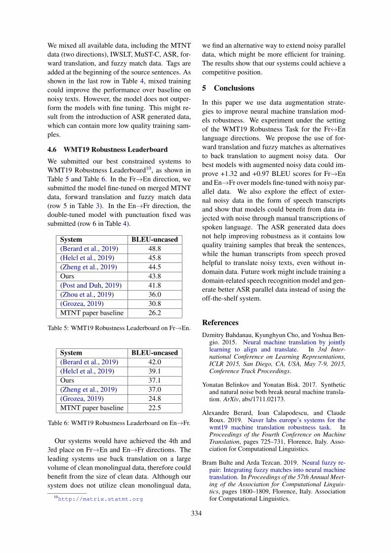
We mixed all available data, including the MTNTdata (two directions), IWSLT, MuST-C, ASR, for-ward translation, and fuzzy match data. Tags areadded at the beginning of the source sentences. Asshown in the last row in Table 4, mixed trainingcould improve the performance over baseline onnoisy texts. However, the model does not outper-form the models with fine tuning. This might re-sult from the introduction of ASR generated data,which can contain more low quality training sam-ples.

4.6 WMT19 Robustness Leaderboard

We submitted our best constrained systems toWMT19 Robustness Leaderboard10, as shown inTable 5 and Table 6. In the Fr→En direction, wesubmitted the model fine-tuned on merged MTNTdata, forward translation and fuzzy match data(row 5 in Table 3). In the En→Fr direction, thedouble-tuned model with punctuation fixed wassubmitted (row 6 in Table 4).

System BLEU-uncased(Berard et al., 2019) 48.8(Helcl et al., 2019) 45.8(Zheng et al., 2019) 44.5Ours 43.8(Post and Duh, 2019) 41.8(Zhou et al., 2019) 36.0(Grozea, 2019) 30.8MTNT paper baseline 26.2

Table 5: WMT19 Robustness Leaderboard on Fr→En.

System BLEU-uncased(Berard et al., 2019) 42.0(Helcl et al., 2019) 39.1Ours 37.1(Zheng et al., 2019) 37.0(Grozea, 2019) 24.8MTNT paper baseline 22.5

Table 6: WMT19 Robustness Leaderboard on En→Fr.

Our systems would have achieved the 4th and3rd place on Fr→En and En→Fr directions. Theleading systems use back translation on a largevolume of clean monolingual data, therefore couldbenefit from the size of clean data. Although oursystem does not utilize clean monolingual data,

10http://matrix.statmt.org

we find an alternative way to extend noisy paralleldata, which might be more efficient for training.The results show that our systems could achieve acompetitive position.

5 Conclusions

In this paper we use data augmentation strate-gies to improve neural machine translation mod-els robustness. We experiment under the settingof the WMT19 Robustness Task for the Fr↔Enlanguage directions. We propose the use of for-ward translation and fuzzy matches as alternativesto back translation to augment noisy data. Ourbest models with augmented noisy data could im-prove +1.32 and +0.97 BLEU scores for Fr→Enand En→Fr over models fine-tuned with noisy par-allel data. We also explore the effect of exter-nal noisy data in the form of speech transcriptsand show that models could benefit from data in-jected with noise through manual transcriptions ofspoken language. The ASR generated data doesnot help improving robustness as it contains lowquality training samples that break the sentences,while the human transcripts from speech provedhelpful to translate noisy texts, even without in-domain data. Future work might include training adomain-related speech recognition model and gen-erate better ASR parallel data instead of using theoff-the-shelf system.


gio. 2015. Neural machine translation by jointlylearning to align and translate. In 3rd Inter-national Conference on Learning Representations,ICLR 2015, San Diego, CA, USA, May 7-9, 2015,Conference Track Proceedings.

Yonatan Belinkov and Yonatan Bisk. 2017. Syntheticand natural noise both break neural machine transla-tion. ArXiv, abs/1711.02173.

Alexandre Berard, Ioan Calapodescu, and ClaudeRoux. 2019. Naver labs europe’s systems for thewmt19 machine translation robustness task. InProceedings of the Fourth Conference on MachineTranslation, pages 725–731, Florence, Italy. Asso-ciation for Computational Linguistics.

Bram Bulte and Arda Tezcan. 2019. Neural fuzzy re-pair: Integrating fuzzy matches into neural machinetranslation. In Proceedings of the 57th Annual Meet-ing of the Association for Computational Linguis-tics, pages 1800–1809, Florence, Italy. Associationfor Computational Linguistics.

334

Isaac Caswell, Ciprian Chelba, and David Grangier.2019. Tagged back-translation. In Proceedings ofthe Fourth Conference on Machine Translation (Vol-ume 1: Research Papers), pages 53–63, Florence,Italy. Association for Computational Linguistics.

Mauro Cettolo, Christian Girardi, and Marcello Fed-erico. 2012. Wit3: Web inventory of transcribed andtranslated talks. In Proceedings of the 16th Con-ference of the European Association for MachineTranslation (EAMT), pages 261–268, Trento, Italy.

Yong Cheng, Lu Jiang, and Wolfgang Macherey. 2019.Robust neural machine translation with doubly ad-versarial inputs. In Proceedings of the 57th AnnualMeeting of the Association for Computational Lin-guistics, pages 4324–4333, Florence, Italy. Associa-tion for Computational Linguistics.

Yong Cheng, Zhaopeng Tu, Fandong Meng, JunjieZhai, and Yang Liu. 2018. Towards robust neuralmachine translation. In Proceedings of the 56th An-nual Meeting of the Association for ComputationalLinguistics (Volume 1: Long Papers), pages 1756–1766, Melbourne, Australia. Association for Com-putational Linguistics.

Raj Dabre and Eiichiro Sumita. 2019. Nict’s super-vised neural machine translation systems for thewmt19 translation robustness task. In Proceed-ings of the Fourth Conference on Machine Transla-tion, pages 732–735, Florence, Italy. Association forComputational Linguistics.

Mattia A. Di Gangi, Roldano Cattoni, Luisa Bentivogli,Matteo Negri, and Marco Turchi. 2019. MuST-C:a Multilingual Speech Translation Corpus. In Pro-ceedings of the 2019 Conference of the North Amer-ican Chapter of the Association for ComputationalLinguistics: Human Language Technologies, Vol-ume 1 (Long and Short Papers), pages 2012–2017,Minneapolis, Minnesota. Association for Computa-tional Linguistics.

Jonas Gehring, Michael Auli, David Grangier, DenisYarats, and Yann N Dauphin. 2017. Convolutionalsequence to sequence learning. In Proceedingsof the 34th International Conference on MachineLearning-Volume 70, pages 1243–1252. JMLR. org.

Cristian Grozea. 2019. System description: The sub-mission of fokus to the wmt 19 robustness task. InProceedings of the Fourth Conference on MachineTranslation (Volume 2: Shared Task Papers, Day1), pages 537–538, Florence, Italy. Association forComputational Linguistics.

JindÅ™ich Helcl, JindÅ™ich LibovickÃ½, and Mar-tin Popel. 2019. Cuni system for the wmt19 robust-ness task. In Proceedings of the Fourth Conferenceon Machine Translation, pages 738–742, Florence,Italy. Association for Computational Linguistics.

Vladimir Karpukhin, Omer Levy, Jacob Eisenstein, andMarjan Ghazvininejad. 2019. Training on synthetic

noise improves robustness to natural noise in ma-chine translation. arXiv preprint arXiv:1902.01509.

Guillaume Klein, Yoon Kim, Yuntian Deng, JeanSenellart, and Alexander M. Rush. 2017. Open-NMT: Open-source toolkit for neural machine trans-lation. In Proc. ACL.

Catherine Kobus, Josep Crego, and Jean Senellart.2016. Domain control for neural machine transla-tion. arXiv preprint arXiv:1612.06140.

Philipp Koehn, Hieu Hoang, Alexandra Birch, ChrisCallison-Burch, Marcello Federico, Nicola Bertoldi,Brooke Cowan, Wade Shen, Christine Moran,Richard Zens, Chris Dyer, Ondrej Bojar, AlexandraConstantin, and Evan Herbst. 2007. Moses: Opensource toolkit for statistical machine translation. InProceedings of the 45th Annual Meeting of the As-sociation for Computational Linguistics CompanionVolume Proceedings of the Demo and Poster Ses-sions, pages 177–180, Prague, Czech Republic. As-sociation for Computational Linguistics.

Vladimir I Levenshtein. 1966. Binary codes capableof correcting deletions, insertions, and reversals. InSoviet physics doklady, volume 10, pages 707–710.

Xian Li, Paul Michel, Antonios Anastasopoulos,Yonatan Belinkov, Nadir Durrani, Orhan Firat,Philipp Koehn, Graham Neubig, Juan Pino, andHassan Sajjad. 2019. Findings of the first sharedtask on machine translation robustness. In Proceed-ings of the Fourth Conference on Machine Transla-tion, pages 218–229, Florence, Italy. Association forComputational Linguistics.

Paul Michel and Graham Neubig. 2018. MTNT: Atestbed for machine translation of noisy text. In Pro-ceedings of the 2018 Conference on Empirical Meth-ods in Natural Language Processing, pages 543–553, Brussels, Belgium. Association for Computa-tional Linguistics.

Soichiro Murakami, Makoto Morishita, Tsutomu Hi-rao, and Masaaki Nagata. 2019. NttâC™s machinetranslation systems for wmt19 robustness task. InProceedings of the Fourth Conference on MachineTranslation, pages 743–750, Florence, Italy. Asso-ciation for Computational Linguistics.

Kishore Papineni, Salim Roukos, Todd Ward, and Wei-Jing Zhu. 2002. Bleu: a method for automatic eval-uation of machine translation. In Proceedings of the40th Annual Meeting of the Association for Com-putational Linguistics, pages 311–318, Philadelphia,Pennsylvania, USA. Association for ComputationalLinguistics.

Matt Post and Kevin Duh. 2019. Jhu 2019 robust-ness task system description. In Proceedings of theFourth Conference on Machine Translation, pages751–757, Florence, Italy. Association for Computa-tional Linguistics.

335

Rico Sennrich, Barry Haddow, and Alexandra Birch.2016a. Improving neural machine translation mod-els with monolingual data. In Proceedings of the54th Annual Meeting of the Association for Compu-tational Linguistics (Volume 1: Long Papers), pages86–96, Berlin, Germany. Association for Computa-tional Linguistics.

Rico Sennrich, Barry Haddow, and Alexandra Birch.2016b. Neural machine translation of rare wordswith subword units. In Proceedings of the 54th An-nual Meeting of the Association for ComputationalLinguistics (Volume 1: Long Papers), pages 1715–1725, Berlin, Germany. Association for Computa-tional Linguistics.

Ashish Vaswani, Noam Shazeer, Niki Parmar, JakobUszkoreit, Llion Jones, Aidan N Gomez, Ł ukaszKaiser, and Illia Polosukhin. 2017. Attention is allyou need. In I. Guyon, U. V. Luxburg, S. Bengio,H. Wallach, R. Fergus, S. Vishwanathan, and R. Gar-nett, editors, Advances in Neural Information Pro-cessing Systems 30, pages 5998–6008. Curran As-sociates, Inc.

Renjie Zheng, Hairong Liu, Mingbo Ma, BaigongZheng, and Liang Huang. 2019. Robust machinetranslation with domain sensitive pseudo-sources:Baidu-osu wmt19 mt robustness shared task systemreport. In Proceedings of the Fourth Conferenceon Machine Translation, pages 758–763, Florence,Italy. Association for Computational Linguistics.

Shuyan Zhou, Xiangkai Zeng, Yingqi Zhou, AntoniosAnastasopoulos, and Graham Neubig. 2019. Im-proving robustness of neural machine translationwith multi-task learning. In Proceedings of theFourth Conference on Machine Translation (Volume2: Shared Task Papers, Day 1), pages 565–571, Flo-rence, Italy. Association for Computational Linguis-tics.

336


Disambiguating Sentiment: An Ensemble of Humour, Sarcasm,and Hate Speech Features for Sentiment Classification

Rohan Badlani ∗

Dept. of Computer ScienceStanford University

[email protected]

Nishit Asnani ∗


[email protected]

Manan Rai ∗


[email protected]

Abstract

Due to the nature of online user reviews,sentiment analysis on such data requires adeep semantic understanding of the text.Many online reviews are sarcastic, humorous,or hateful. Signals from such languagenuances may reinforce or completely alterthe sentiment of a review as predicted bya machine learning model that attempts todetect sentiment alone. Thus, having a modelthat is explicitly aware of these featuresshould help it perform better on reviewsthat are characterized by them. We proposea composite two-step model that extractsfeatures pertaining to sarcasm, humour, hatespeech, as well as sentiment, in the firststep, feeding them in conjunction to informsentiment classification in the second step.We show that this multi-step approach leads toa better empirical performance for sentimentclassification than a model that predictssentiment alone. A qualitative analysis revealsthat the conjunctive approach can bettercapture the nuances of sentiment as expressedin online reviews.

1 Introduction

Sentiment classification is one of the most widelystudied problems in natural language processing,partly since it is a complex problem from a linguis-tic point of view, and partly since it has huge com-mercial value for enterprises attempting to under-stand user behaviour. Online user review datasetshave contributed significantly to research in thisdirection, since they provide large sets of humangenerated commentary about real products andservices, which capture the nuances and complex-ity of the user-generated text (Zhang et al., 2015)(He and McAuley, 2016).

∗equal contribution

Traditionally, models developed for sentimentclassification have been used to solve other binaryor multi-class classification problems in naturallanguage, like intent detection, document tagging,etc. Sentiment classification has also been usedas a building block towards more complicated lan-guage understanding/generation tasks (Poria et al.,2016) (Hu et al., 2017). Given that sentiment is acomplex language attribute influenced by severalother features, this paper poses a question morefundamental to the nature of sentiment in humanlanguage: can models developed for other tasks,like sarcasm, humor, or hate speech detection, helpimprove sentiment classification models? Goingfurther, we also attempt to answer if the samemodel architecture can be used for these tasks, andthen be combined to yield higher performance onsentiment classification.

This line of thought is inspired by how hu-mans perceive sentiment in any piece of spokenor written language. Detection of elements ofsarcasm help us resolve seemingly contradictorystatements (“The restaurant was so clean that Icould barely avoid stepping into the puddle!”)into their intended sentiment. Similarly, humor(because it can get similarly confusing) and hatespeech (since specific offensive words may be theonly indicators of sentiment in a review) act as cru-cial indicators of the intended meaning of phrasesin a given utterance.

Since the sentiment model is not optimizing fordetecting these language attributes, it is likely toget confused by utterances having them unless itis sufficiently exposed to similar sentences duringtraining. We therefore believe that making sen-timent models explicitly aware of these languageattributes would help them become more robust tosarcastic, humorous or hateful utterances, and thusget better at classifying sentiment.

Thus, our research hypotheses are as follows:

337

Figure 1: CNN Based Binary Classification Model for embedding generation. We use a stride of 1 in our final CNNmodel. Different colors in the word embeddings represent different inputs to the convolutional neural network

• H1: Models individually learned on sarcasm,humor and hate speech detection, and thenused as subroutines to extract features, shouldboost the performance of a sentiment classi-fication model.

• H2: Given that the individual tasks are allbinary classification tasks, we believe thata single model architecture should providereasonable performance on these individualtasks and would make it easier to re-usethe same learned models for multiple down-stream classification tasks.

2 Related Work

Sentiment classification, sarcasm detection, hu-mor detection and hate speech detection have allseen varying levels of interest from the natural lan-guage research community, and have evolved overtime as better datasets and modeling techniqueshave come into the picture.

There has been quite a bit of work on sarcasmdetection, especially in the context of Twitter-based self-annotated data and Self-AnnotatedReddit Corpus. The seminal work in this areastarted with (Gonzalez-Ibanez et al., 2011) - theyused lexical and pragmatic features and found thatpragmatic features were more useful in detect-ing sarcasm. Addition of context-based featuresalong with text-based features in certain subse-quent models helped as well in improving perfor-

mance on sarcasm detection. There was a dra-matic shift with the introduction of deep learningas feature engineering took a back seat and deepmodels began to be used for learning task-specificrepresentations. (Hazarika et al., 2018) show thatusing context, user and text embedding providesstate of the art performance, which is challengedby Kolchinski (Kolchinski and Potts, 2018) (Westet al., 2014) through a more simplistic user embed-ding based approach that achieves similar perfor-mance without other context (like forum embed-dings as used by (Hazarika et al., 2018)).

Hate Speech in natural language research hastraditionally been a loosely-defined term, withone cause being the similarity with other catego-rizations of hateful utterances, such as offensivelanguage. In the context of online reviews, webroadly use hate speech to include any form ofoffensive language. (Davidson et al., 2017) in-troduce the seminal dataset in the field, and testa variety of models – Logistic Regression, NaiveBayes, decision trees, random forests, and SupportVector Machines (SVMs), each tested with 5-foldcross validation to find that the Logistic Regres-sion and Linear SVM tend to perform significantlybetter than other models. Models such as LSTMsand CNNs have also been tried in works such as(Badjatiya et al., 2017) and (de Gibert et al., 2018).

Humour Detection has seen a lot of work, withmodels being developed on several large-scalepublic datasets, such as the Pun of the Day, 16000

338

Figure 2: Full Sentiment Classification model with ensemble of features from sarcasm, humour, and hate speechdetection models

OneLiners, Short Jokes dataset, and the PTT jokesdataset. (Chen and Soo, 2018) use a Highway Net-work on top of a CNN on a combination of thesedatasets. (Kim, 2014) uses CNN for sentence clas-sification, and these models have also been testedon funny-labelled reviews from the Yelp dataset1.

Recent works have attempted to combine fea-ture extraction models trained on some tasks for adifferent task. (Poria et al., 2016), for instance,uses knowledge about sentiment, emotion, andpersonality to better detect sarcasm. This findsa parallel in our attempt here, with the differencethat these features include non-linguistic featuressuch as user personality, and we focus only on nat-ural language features to test the transferability ofknowledge about certain features to detecting oth-ers.

Sentiment classification is a text classificationtask with the objective to classify text according tothe sentimental polarities. This has been a widelyresearched area (Mantyla et al., 2016) and recentlythere has been a lot of success in this area. Thecurrent state of the art performance on this taskis using transformer (Vaswani et al., 2017) basedmodels like BERT (Devlin et al., 2018) and XL-

1https://github.com/srishti-1795/Humour-Detection

Net (Yang et al., 2019). These models achievevery high accuracy on the binary classificationtask of sentiment polarity detection but analyz-ing the failure modes of these models indicate thatthese models might fail in cases where there arehigher order language concepts like sarcasm, hu-mour and hate speech co-occur in the same utter-ance. Hence, through this paper, we investigatethe performance of sentiment classification whenprovided with representative features pertaining tothese language oriented concepts and at the sametime propose a generic approach to compute thesefeature so as to reuse for multiple downstreamtasks.

3 Methods

3.1 Datasets

We experiment with the following datasets corre-sponding to sentiment, sarcasm, hate speech, andhumour to test our hypotheses:

1. D1 - Sentiment: The Yelp Review Dataset(Zhang et al., 2015) consists of about 560,000reviews, with binary sentiment labels. For thepurposes of our analysis, we use 100,000 re-views for training and validation and 36,614

339

Review NLU Aspect CapturedI am a nurse and to characterize this office as nothing but a frustration isa compliment.

Sarcasm

It would have been faster if I would have grown, harvested, and brewedthe tea myself.

Sarcasm

If you want to get pastries while being yelled at by the staff and treatedlike dirt, this is the place for you.

Sarcasm

They are THE RUDEST people I’ve ever met! The lady with short hairhas a crappy attitude, so does the younger guy.

Hate Speech

Table 1: Examples where our combined model is able to predict correct label whereas the baseline sentimentmodel fails.

reviews for testing.

2. D2 - Sarcasm: The SARC (Self-AnnotatedReddit Comments) dataset (Khodak et al.,2017) consists of about 1.3 million Redditcomments. These comments have been selfannotated using the \s character. The datasethas a balanced set and an unbalanced set. Forthe purposes of our analysis, we focus onbalanced set and take 100,000 comments fortraining and validation and 20,000 commentsfor testing.

3. D3 - Humour: The Yelp Review Dataset hasa field called ‘funny.’ We consider a commentto be humorous (i.e positive label) when thecomment has a ‘funny’ score greater than 2.

4. D4 - Hate Speech: The hatebase.org TwitterDataset (Davidson et al., 2017) is a popularhate speech tweet dataset, which consists of28,000 tweets, each labelled as either havingoffensive content or not.

3.2 Validating Hypothesis H1

We conduct a quick initial evaluation of hypoth-esis H1 using well-performing models for senti-ment, sarcasm, humour, and hate speech. Thesemodels are discussed below:

1. M1 - Sentiment: For sentiment detection,the current state of the art model is BERTLarge (Devlin et al., 2018) which provides anaccuracy of about 98.11% (Xie et al., 2019).We use the BERT Base model which has asmaller architecture and therefore helps runa quick evaluation (12-layer, 768-hidden, 12-heads, 110M parameters).

2. M2 - Sarcasm: The CASCADE model (Haz-arika et al., 2018) is the current state of the arton the SARC dataset. This achieves a 77%balanced set accuracy and 79% unbalancedset accuracy. This model computes user-specific embeddings from their comments onother threads, thread embeddings from otheruser comments on the same thread, and theembeddings of the input text, and uses all ofthese for sarcasm detection. We use the CAS-CADE model but without the user and threadembeddings since they were not readily avail-able for this dataset. The CASCADE modelmodified as above provides reasonable per-formance for the task of sarcasm detection.

3. M3 - Humour: We use an SVM model withbag of words features for humour detection asused in pre-existing implementations2. Thisprovides an accuracy of 83% on the yelp re-views dataset.

4. M4 - Hate Speech: We use the implemen-tation provided by (Davidson et al., 2017)which is simple Logistic regression modelthat provides a F1 score of 0.90 on D4.

M2, M3, M4 models as described above predictthe probability of occurrence of sarcasm, humourand hate speech respectively on a given input text.These probabilities are then fed as features to ourBERT-base sentiment classification model as de-scribed in M1 above for the Yelp reviews dataset.We compare our modified model with BERT-baseand observe a small improvement in the sentimentdetection performance which positively supportsour hypothesis H1. This motivates us to consider

2https://github.com/srishti-1795/Humour-Detection

340

developing embeddings for each of these languagespecific features instead of using just the probabil-ity of their occurrence.

3.3 Validating hypothesis H2

In order to test hypothesis H2, we construct ageneral-purpose feature embedding model E forall the four tasks, along with a classifier C for clas-sification on the combined representation, as dis-cussed below.

3.3.1 Feature Embedding Model

Given a d-word sentence s, we initialize trainable128-dimensional word embeddings for each word,and create a d×128 embedding matrix for the sen-tence. In order to capture n-gram features, we usea word-level Convolutional Neural Network (Kim,2014) with f filters (n× 128) for n = 3, 4, 5. Foreach n, we compute the (d−n+1)×f output, anduse max pooling to get a f -dimensional vector. Weconcatenate these vectors for all three values of nand flatten them to get a 3f -dimensional embed-ding. With f = 100, we get a 300-dimensionalembedding for every sentence.

We use one such model for each of Sentiment(E1), Sarcasm (E2), Hate Speech (E3), and Hu-mour (E4).

3.3.2 Combination Classifier

Given a d-word sentence s and a set of mfeature embedding models (1 ≤ m ≤ 4)E ⊆ [E1,E2,E3,E4], we calculate a set of 300-dimensional embeddings per model, and concate-nate them into a single 300 ∗m-dimensional fea-ture vector v. This is used as input to a sentimentclassifier that predicts C(v) ∈ [0, 1] that representsthe probability of positive sentiment. This clas-sifier consists of two fully-connected layers withhidden size 50 and ReLU activation. This modelis trained and tested separately for several combi-nations E, and the results from these experimentsare discussed in section 4.

4 Experiments and Results

4.1 Results for Hypothesis H1

To test if our hypothesis H1 holds true, we con-catenated predictions from the sarcasm (M2) de-tection model to the BERT-base model embed-dings (M1) used for sentiment classification as de-scribed in section 3.2. We used the PyTorch im-

Model Accuracy (%)M1 95.13

M1 + M2 (P/L) 95.22

Table 2: Testing our hypothesis: Mi refers to the re-spective model, P and L indicate using predicted prob-abilities and labels respectively. Both of our augmentedmodels perform better than the sentiment model alone(M1), thus validating our hypothesis.

plementation of BERT Base3, and our results aretabulated in Table 2. We trained the models for 3epochs with a learning rate of 2e-5 and a batch sizeof 32.

This experiment validated our hypothesis thatthere is tangible sentiment information to begleaned from a sentence’s sarcasm features (andpotentially other features as well).

Attribute Combination Accuracy (%)Se 95.95

Se + Sc 96.02Se + Hu 95.93Se + Ha 95.69

Se + Sc + Hu 96.06Se + Sc + Hu + Ha 96.18

Table 3: Model Performances for various combina-tions of Sentiment Se (E1), Sarcasm Sc (E2), HumorHu (E3) and Hate Speech Ha (E4). We find that ourcombined model performs the best.

4.2 Results for Hypothesis H2

As described in 3.3.1, we used a single model ar-chitecture for training separate models on senti-ment, sarcasm, humor and hate speech. Due toclass imbalance and large dataset sizes, we modi-fied our datasets in the following ways:

• D1: We took a subset of the training set forYelp reviews which amounted to 100k re-views for training and validation combined,and included the entire test set of 36.6k re-views for reporting the performance of ourmodels.

• D2: To maintain consistency, we took a sam-ple of 100k comments for training our modelon sarcasm detection.


341

Attribute Combination Accuracy (%)Run 1 Run 2 Run 3

Se 95.95 95.76 95.85Se + Sc + Hu + Ha 96.18 96.08 96.40

Table 4: Model performances during several runs of the baseline and the combined (Se + Sc + Hu + Ha) models.

Review NLU Aspect Missed...The manager went around and asked the 2 waitressesworking all 4/5 tables surrounding us and none of themtook responsibility or seemed to want our table. Little didwe know this was a blessing in disguise...

Extended story line: the first half ofthe review is negative, and the modellikely misses the turning point towardspositive halfway through the review

Table 5: Examples where the combined model goes wrong and the baseline sentiment model predicts the correctsentiment.

Review NLU Aspect MissedSay it with me now: Blaaaaaaaaaand Indicative word missedThis place is closed, and for good reason. Flip in sentiment

Table 6: Examples where the combined and the baseline sentiment models both fail to predict the correct senti-ment.

Figure 3: Scatter plot for the various task-specific em-beddings (unit normalized) of the first 100 test reviewsfrom the Yelp dataset. It can be seen that sentiment,sarcasm, humor and hate predominantly occupy differ-ent regions of the embedding space when reduced to2D using tSNE.

• D3: Since this dataset had a ratio of 19:1for non-humorous to humorous reviews, wetook the entire set of humorous reviews fromthe original Yelp dataset, and added abouttwice the amount of randomly sampled non-humorous reviews to maintain a healthy ra-tio of 2:1. Final number of train/val reviewswere 40k and test reviews were 8,661.

• D4: The number of hateful tweets in this

dataset were 16 times the number of non-hateful tweets. We oversample the non-hateful tweets by 4x, and undersample thehateful tweets by 2x to obtain a ratio of 2:1 infavor of the positive class, for both the train-ing/val and the test datasets. The total num-ber of tweets in train/val are 16,854 and num-ber of test tweets are 3,521.

After training a model each on these datasetsfollowing the architecture described in 3.3.1, weobtain the sentiment, sarcasm, humor and hate em-beddings for each of the training and testing re-views from D1. For this model, we use CNN win-dow sizes of 3, 4 and 5 with 100 kernels each,batch size of 64, learning rate 0.001, and dropoutprobability 0.5.

Further, we train combined sentiment classifiers(3.3.2) on top of various combinations of subsetsof these embeddings for the training set, and thenevaluate performance on the test set. The perfor-mances of these combinations is reported in Ta-ble 3, and results from more runs comparing thebaseline against our combined model are shown in4. In order to test if the improvement of our pro-posed hybrid model is consistently better than thebaseline, we train our the combined and baselinemodels over fixed training set size multiple timesand evaluate the performance on the same held-out test set consisting of 36,614 reviews. Table

342

4 shows the results of the models on the test set.We observe a consistent improvement using sen-timent, sarcasm, humour and hate speech featuresas compared to just sentiment features.

5 Discussion and Analysis

Our hypothesis H1 is supported by the experi-ments in both 4.1 and 4.2, i.e. sarcasm, humorand hate speech are signals that boost the senti-ment classification performance on Yelp reviews.

5.1 Different natural language features addmutually exclusive information

As Figure 3 shows, the normalized task-specificembeddings occupy distinct regions of the 2Dspace (after dimensionality reduction using tSNE).Thus, the three additional models probably assistthe sentiment embeddings by combining informa-tion from the source review that the sentimentmodel may not have learned to catch, and thatmight, in certain cases, help the combined modelmake better decisions. Since these embeddingshave been obtained via a single model architecturetrained on different datasets, the increase in per-formance on sentiment classification validates ourhypothesis H2. This implies not only that a singlearchitecture might suit multiple natural languageproblem domains, which models like BERT havealready shown, but also that one or more of themcan help boost the performance of others, if thereasoning behind such a predicted improvement islinguistically sound.

5.2 Interpretibility of model’s success modes

We analyze the contribution of each of the indi-vidual models trained for sarcasm, humour andhate speech detection to the performance of senti-ment detection by comparing the predicted labelsagainst the ground truth. In each of the matricesin Figure 4, the value in cell (i, j) of category c(which can be TP, TN, FP or FN) denotes the re-spective fraction of predictions in model i that be-long to category c if the predictions of model j areassumed to be the ground truth.

As evident from Figure 4, we find that addingfeatures pertaining to sarcasm, hate speech, andhumour to a baseline sentiment classifier increasesthe number of true positives against the GroundTruth labels (the baseline model predicts 97% ofthe combined model’s positive labels). Since thefalse positive rate of the combined model (0.02) is

also less than that of the sentiment model (0.03)against the ground truth, this shows that the com-bined model has a higher precision. This obser-vation is also consistent with the reasoning thatsarcasm and hate speech are both likely to catchnegative reviews which may otherwise sound pos-itive to a naive model, and thus reduce the falsepositive rate.

Similarly, looking at the true negatives’ matrixshows that the combined (Sentiment + Sarcasm +Humour + Hate Speech) model predicts negativelabels better than the (Sentiment + Sarcasm + Hu-mour) model (0.97 against 0.95), which is consis-tent with the reasoning that Hate Speech is likelyto indicate a negative sentiment, and that knowl-edge of Hate Speech helps the model better under-stand what to look for in a review that is negativebecause of hateful language.

On looking at some reviews in the test datasetthat our combined model (Se + Sc + Hu + Ha)got right and that the baseline sentiment modelgot wrong, we observe that our model definitivelyhelps with identifying the right sentiment for sar-castic reviews (Table 1) and some hate reviews, al-though we couldn’t find many humorous reviewsin this context. Similarly, it seems that the reviewswhose sentiment has been classified wrongly bythe sentiment-only baseline and that don’t haveany sarcastic / hate intent don’t get classified cor-rectly by our combined model either (Table 6).

5.3 Error Analysis

Tables 5 and 6 present some analysis of the er-rors made by our model, and how they comparewith the baseline Sentiment model. As can beseen, our model doesn’t catch the elements of nat-ural language that it was not trained to detect,and while it is quite sensitive to catching negativesentiment, it doesn’t do as well when sentimentchanges halfway through the review.

6 Conclusions

In this paper we show that features from sarcasm,humor and hate speech help in improving senti-ment classification performance on the Yelp re-views dataset. We have also shown that a general-purpose model architecture for binary classifica-tion can be trained on each of these natural lan-guage tasks individually and that it provides aneasy way for end-to-end sentiment classificationthat combines the strengths of each of these mod-

343

Figure 4: Overlap of model predictions with one another. Adding features from Sarcasm, Hate Speech, andHumour to baseline Sentiment classifier improves its ability to predict True Positives against the Ground Truthlabels.

els.This work shows that natural language under-

standing problems need not be thought of in iso-lation of each other. When motivated by humaninsights on how language is perceived, solutionsto nuanced sub-problems might help solve moregeneral problems like sentiment classification.

Future Directions

An interesting future direction is to test the com-bination of features from sarcasm, humor and hatespeech for more fine-grained sentiment classifica-tion, as in Yelp (5-way classification) or StanfordSentiment Treebank (5-way classification). Webelieve that our formulation would help in thiscase, by distinguishing between 1-star and 2-starreviews based on offensive language for instance.

It would also be interesting to see if the samegeneric template achieves state of the art perfor-mance on other classification tasks like entailmentdetection, entity detection, etc.

Acknowledgements

The authors would like to thank Prof Christo-pher Potts from Stanford NLP Group for valu-able suggestions and discussion on experimentalevaluation and analysis. The authors would liketo thank Min Kim for his suggestions on the ex-perimental setup and the paper writeup. The au-thors would also like to thank the authors of CNNsentence classification (Kim, 2014) for provid-ing open-source implementations of their modelswhich allowed us to bootstrap our research ideas.

344

ReferencesPinkesh Badjatiya, Shashank Gupta, Manish Gupta,

and Vasudeva Varma. 2017. Deep learning for hatespeech detection in tweets. CoRR, abs/1706.00188.

Peng-Yu Chen and Von-Wun Soo. 2018. Humor recog-nition using deep learning. In Proceedings of the2018 Conference of the North American Chapter ofthe Association for Computational Linguistics: Hu-man Language Technologies, Volume 2 (Short Pa-pers), pages 113–117, New Orleans, Louisiana. As-sociation for Computational Linguistics.

Thomas Davidson, Dana Warmsley, Michael Macy,and Ingmar Weber. 2017. Automated hate speechdetection and the problem of offensive language. InProceedings of the 11th International AAAI Confer-ence on Web and Social Media, ICWSM ’17, pages512–515.

Jacob Devlin, Ming-Wei Chang, Kenton Lee, andKristina Toutanova. 2018. BERT: pre-training ofdeep bidirectional transformers for language under-standing. CoRR, abs/1810.04805.

Ona de Gibert, Naiara Perez, Aitor Garcıa Pablos, andMontse Cuadros. 2018. Hate speech dataset froma white supremacy forum. In Proceedings of the2nd Workshop on Abusive Language Online (ALW2),pages 11–20, Brussels, Belgium. Association forComputational Linguistics.

Roberto Gonzalez-Ibanez, Smaranda Muresan, andNina Wacholder. 2011. Identifying sarcasm in twit-ter: A closer look. In Proceedings of the 49thAnnual Meeting of the Association for Computa-tional Linguistics: Human Language Technologies:Short Papers - Volume 2, HLT ’11, pages 581–586,Stroudsburg, PA, USA. Association for Computa-tional Linguistics.

Devamanyu Hazarika, Soujanya Poria, Sruthi Gorantla,Erik Cambria, Roger Zimmermann, and Rada Mi-halcea. 2018. CASCADE: Contextual sarcasm de-tection in online discussion forums. In Proceedingsof the 27th International Conference on Computa-tional Linguistics, pages 1837–1848, Santa Fe, NewMexico, USA. Association for Computational Lin-guistics.

Ruining He and Julian McAuley. 2016. Ups anddowns: Modeling the visual evolution of fashiontrends with one-class collaborative filtering. Inproceedings of the 25th international conferenceon world wide web, pages 507–517. InternationalWorld Wide Web Conferences Steering Committee.

Zhiting Hu, Zichao Yang, Xiaodan Liang, RuslanSalakhutdinov, and Eric P Xing. 2017. Toward con-trolled generation of text. In Proceedings of the 34thInternational Conference on Machine Learning-Volume 70, pages 1587–1596. JMLR. org.

Mikhail Khodak, Nikunj Saunshi, and Kiran Vodra-halli. 2017. A large self-annotated corpus for sar-casm. CoRR, abs/1704.05579.

Yoon Kim. 2014. Convolutional neural networks forsentence classification. CoRR, abs/1408.5882.

Y. Alex Kolchinski and Christopher Potts. 2018. Rep-resenting social media users for sarcasm detection.CoRR, abs/1808.08470.

Mika Viking Mantyla, Daniel Graziotin, and MiikkaKuutila. 2016. The evolution of sentiment analysis- A review of research topics, venues, and top citedpapers. CoRR, abs/1612.01556.

Soujanya Poria, Erik Cambria, Devamanyu Hazarika,and Prateek Vij. 2016. A deeper look into sarcas-tic tweets using deep convolutional neural networks.CoRR, abs/1610.08815.

Ashish Vaswani, Noam Shazeer, Niki Parmar, JakobUszkoreit, Llion Jones, Aidan N. Gomez, LukaszKaiser, and Illia Polosukhin. 2017. Attention is allyou need. CoRR, abs/1706.03762.

Robert West, Hristo S. Paskov, Jure Leskovec, andChristopher Potts. 2014. Exploiting social networkstructure for person-to-person sentiment analysis.CoRR, abs/1409.2450.

Qizhe Xie, Zihang Dai, Eduard Hovy, Minh-Thang Lu-ong, and Quoc V Le. 2019. Unsupervised data aug-mentation. arXiv preprint arXiv:1904.12848.

Zhilin Yang, Zihang Dai, Yiming Yang, Jaime G.Carbonell, Ruslan Salakhutdinov, and Quoc V.Le. 2019. Xlnet: Generalized autoregressivepretraining for language understanding. CoRR,abs/1906.08237.

Xiang Zhang, Junbo Zhao, and Yann LeCun. 2015.Character-level convolutional networks for text clas-sification. In Advances in neural information pro-cessing systems, pages 649–657.

345


Grammatical Error Correction in Low-Resource Scenarios

Jakub Náplava and Milan StrakaCharles University,

Faculty of Mathematics and Physics,Institute of Formal and Applied Linguistics

{naplava,straka}@ufal.mff.cuni.cz

Abstract

Grammatical error correction in English isa long studied problem with many existingsystems and datasets. However, there has beenonly a limited research on error correction ofother languages. In this paper, we presenta new dataset AKCES-GEC on grammaticalerror correction for Czech. We then make ex-periments on Czech, German and Russian andshow that when utilizing synthetic parallel cor-pus, Transformer neural machine translationmodel can reach new state-of-the-art results onthese datasets. AKCES-GEC is published un-der CC BY-NC-SA 4.0 license at http://hdl.handle.net/11234/1-3057, andthe source code of the GEC model is avail-able at https://github.com/ufal/low-resource-gec-wnut2019.

1 Introduction

A great progress has been recently achieved ingrammatical error correction (GEC) in English.The performance of systems has since CoNLL2014 shared task (Ng et al., 2014) increased bymore than 60% on its test set (Bryant et al.,2019) and also a variety of new datasets appeared.Both rule-based models, single error-type classi-fiers and their combinations were due to largeramount of data surpassed by statistical and later byneural machine translation systems. These addressGEC as a translation problem from a language ofungrammatical sentences to a grammatically cor-rect ones.

Machine translation systems require largeamount of data for training. To cope with this is-sue, different approaches were explored, from ac-quiring additional corpora (e.g. from Wikipediaedits) to building a synthetic corpus from cleanmonolingual data. This was apparent on recentBuilding Educational Applications (BEA) 2019Shared Task on GEC (Bryant et al., 2019) when

top scoring teams extensively utilized syntheticcorpora.

The majority of research has been done in En-glish. Unfortunately, there is a limited progress onother languages. Namely, Boyd (2018) created adataset and presented a GEC system for German,Rozovskaya and Roth (2019) for Russian, Náplava(2017) for Czech and efforts to create annotatedlearner corpora were also done for Chinese (Yuet al., 2014), Japanese (Mizumoto et al., 2011) andArabic (Zaghouani et al., 2015).

Our contributions are as follows:• We introduce a new Czech dataset for

GEC. In comparison to dataset of Šebestaet al. (2017) it contains separated edits to-gether with their type annotations in M2 for-mat (Dahlmeier and Ng, 2012) and also hastwo times more sentences.• We extend the GEC model of Náplava and

Straka (2019) by utilizing synthetic trainingdata, and evaluate it on Czech, German andRussian, achieving state-of-the-art results.

2 Related Work

There are several main approaches to GEC in low-resource scenarios. The first one is based on anoisy channel model and consists of three com-ponents: a candidate model to propose (word) al-ternatives, an error model to score their likelihoodand a language model to score both candidate(word) probability and probability of a whole newsentence. Richter et al. (2012) consider for a givenword all its small modifications (up to characteredit distance 2) present in a morphological dictio-nary. The error model weights every character editby a trained weight, and three language models(for word forms, lemmas and POS tags) are usedto choose the most probable sequence of correc-tions. A candidate model of Bryant and Briscoe

346

(2018) contains for each word spell-checker pro-posals, its morphological variants (if found in Au-tomatically Generated Inflection Database) and, ifthe word is either preposition or article, also a setof predefined alternatives. They assign uniformprobability to all changes, but use strong languagemodel to re-rank all candidate sentences. Lacroixet al. (2019) also consider single word edits ex-tracted from Wikipedia revisions.

Other popular approach is to extract parallelsentences from Wikipedia revision histories. Agreat advantage of such an approach is that the re-sulting corpus is, especially for English, of greatsize. However, as Wikipedia edits are not hu-man curated specifically for GEC edits, the corpusis extremely noisy. Grundkiewicz and Junczys-Dowmunt (2014) filter this corpus by a set of regu-lar expressions derived from NUCLE training dataand report a performance boost in statistical ma-chine translation approach. Grundkiewicz et al.(2019) filter Wikipedia edits by a simple languagemodel trained on BEA 2019 development corpus.Lichtarge et al. (2019), on the other hand, re-ports that even without any sophisticated filtering,Transformer (Vaswani et al., 2017) can reach sur-prisingly good results when used iteratively.

The third approach is to create synthetic corpusfrom a clean monolingual corpus and use it as ad-ditional data for training. Noise is typically intro-duced either by rule-based substitutions or by us-ing a subset of the following operations: token re-placement, token deletion, token insertion, multi-token swap and spelling noise introduction. Yuanand Felice (2013) extract edits from NUCLE andapply them on a clean text. Choe et al. (2019)apply edits from W&I+Locness training set andalso define manual noising scenarios for prepo-sition, nouns and verbs. Zhao et al. (2019) usean unsupervised approach to synthesize noisy sen-tences and allow deleting a word, inserting a ran-dom word, replacing a word with random wordand also shuffling (rather locally). Grundkiewiczet al. (2019) improve this approach and replacea token with one of its spell-checker suggestions.They also introduce additional spelling noise.

3 Data

In this Section, we present existing corpora forGEC, together with newly released corpus forCzech.

3.1 AKCES-GEC

The AKCES (Czech Language Acquisition Cor-pora; Šebesta, 2010) is an umbrella project com-prising of several acquisition resources – CzeSL(learner corpus of Czech as a second language),ROMi (Romani ethnolect of Czech Romani chil-dren and teenagers) and SKRIPT and SCHOLA(written and spoken language collected from na-tive Czech pupils, respectively).

We present the AKCES-GEC dataset, whichis a grammar error correction corpus for Czechgenerated from a subset of AKCES resources.Concretely, the AKCES-GEC dataset is based onCzeSL-man corpus (Rosen, 2016) consisting ofmanually annotated transcripts of essays of non-native speakers of Czech. Apart from the releasedCzeSL-man, AKCES-GEC further utilizes addi-tional unreleased parts of CzeSL-man and also es-says of Romani pupils with Romani ethnolect ofCzech as their first language.

The CzeSL-man annotation consists of threeTiers – Tier 0 are transcribed inputs, followed bythe level of orthographic and morphemic correc-tions, where only word forms incorrect in any con-text are considered (Tier 1). Finally, the rest of er-rors is annotated at Tier 2. Forms at different Tiersare manually aligned and can be assigned one ormore error types (Jelínek et al., 2012). An exam-ple of the annotation is presented in Figure 1, andthe list of error types used in CzeSL-man annota-tion is listed in Table 1.

We generated AKCES-GEC dataset using thethree Tier annotation of the underlying corpus. Weemployed Tier 0 as source texts, Tier 2 as cor-rected texts, and created error edits according tothe manual alignments, keeping error annotationswhere available.1 Considering that the M2 format(Dahlmeier and Ng, 2012) we wanted to use doesnot support non-local error edits and therefore can-not efficiently encode word transposition on longdistances, we decided to consider word swaps overat most 2 correct words a single edit (with the con-stant 2 chosen according to the coverage of long-range transpositions in the data). For illustration,see Figure 2.

The AKCES-GEC dataset consists of an ex-plicit train/development/test split, with each set di-vided into foreigner and Romani students; for de-

1The error annotations are unfortunately not available inthe whole underlying corpus, and not all errors are annotatedwith at least one label.

347

Figure 1: Example of two-level annotation of a sentence in CzeSL corpus, reproduced from (Rosen, 2016).

original sentence

corrected sentence

A B C

C A B

A B C

CA B

D

D

Figure 2: Word swap over one or two correct words (on the left) is considered a single edit (A B C→ C A B). Wordswap over more than two correct words (on the right) is represented as two edits of deleting D and inserting D.

Error type Description Example OccincorInfl incorrect inflection [pracovají → pracují] v továrne 8 986incorBase incorrect word base musíš to [posvetlit → posvetit] 20 334fwFab non-emendable, „fabricated“ word pokud nechceš slyšet [smášky] 78fwNC foreign word váza je na [Tisch → stole] 166flex supplementary flag used with fwFab and jdu do [shopa → obchodu] 34

fwNC marking the presence of inflectionwbdPre prefix separated by a space or preposition w/o space musím to [pri pravit → pripravit] 817wbdComp wrongly separated compound [ceský anglický → cesko-anglický] slovník 92wbdOther other word boundary error [mocdobre → moc dobre]; [atak → a tak] 1326stylColl colloquial form [dobrej → dobrý] film 3 533stylOther bookish, dialectal, slang, hyper-correct form holka s [hnedými ocimi → hnedýma ocima] 156agr violated agreement rules to jsou [hezké → hezcí] chlapci; Jana [ctu → cte] 5 162dep error in valency bojí se [pes → psa]; otázka [cas → casu] 6 733ref error in pronominal reference dal jsem to jemu i [jejího → jeho] bratrovi 344vbx error in analytical verb form or compound predicate musíš [prijdeš → prijít]; kluci [jsou] behali 864rflx error in reflexive expression dívá [∅ → se] na televizi; Pavel [si → se] raduje 915neg error in negation [pujdu ne → nepujdu] do školy 111lex error in lexicon or phraseology dopadlo to [prírodne → prirozene] 3 967use error in the use of a grammar category pošta je [nejvíc blízko → nejblíže] 1 458sec secondary error (supplementary flag) stará se o [našich holcickách → naše holcicky] 866stylColl colloquial expression videli jsme [hezký → hezké] holky 3 533stylOther bookish, dialectal, slang, hyper-correct expression rozbil se mi [hadr] 156stylMark redundant discourse marker [no]; [teda]; [jo] 15disr disrupted construction známe [hodné spoustu → spoustu hodných] lidí 64problem supplementary label for problematic cases 175unspec unspecified error type 69 123

Table 1: Error types used in CzeSL corpus taken from (Jelínek et al., 2012), including number of occurrences inthe dataset being released. Tier 1 errors are in the upper part of the table, Tier 2 errors are in the lower part. ThestylColl and stylOther are annotated on both Tiers, but we do not distinguish on which one in the AKCES-GEC.

velopment and test sets, the foreigners are furthersplit into Slavic and non-Slavic speakers. Further-more, the development and test sets were anno-tated by two annotators, so we provide two refer-ences if the annotators utilized the same sentencesegmentation and produced different annotations.

The detailed statistics of the dataset are pre-sented in Table 2. The AKCES-GEC dataset isreleased under the CC BY-NC-SA 4.0 license at

http://hdl.handle.net/11234/1-3057.We note that there already exists a CzeSL-GEC

dataset (Šebesta et al., 2017). However, it consistsonly of a subset of data and does not contain errortypes nor M2 files with individual edits.

3.2 English

Probably the largest corpus for English GEC isthe Lang-8 Corpus of Learner English (Mizumoto

348

Train Dev TestDoc Sent Word Error r. Doc Sent Word Error r. Doc Sent Word Error r.

Foreign.Slavic

1 816 27 242 289 439 22.2 %70 1 161 14 243 21.8 % 69 1 255 14 984 18.8 %

Other 45 804 8 331 23.8 % 45 879 9 624 20.5 %Romani 1 937 14 968 157 342 20.4 % 80 520 5 481 21.0 % 74 542 5 831 17.8 %

Total 3 753 42 210 446 781 21.5 % 195 2 485 28 055 22.2 % 188 2 676 30 439 19.1 %

Table 2: Statistics of the AKCES-GEC dataset – number of documents, sentences, words and error rates.

et al., 2011; Tajiri et al., 2012). It comes froman online language learning website, where usersare able to post texts in language they are learn-ing. These texts then appear to native speakersfor correction. The corpus has over 100 000 rawEnglish entries comprising of more than 1M sen-tences. Due to the fact that texts are corrected byonline users, this corpus is also quite noisy.

Other corpora are corrected by trained annota-tors making them much cleaner but also signifi-cantly smaller. NUCLE (Dahlmeier et al., 2013)has 57 151 sentences originating from 1 400 es-says written by mainly Asian undergraduate stu-dents at the National University of Singapore.FCE (Yannakoudakis et al., 2011) is a subset ofthe Cambridge Learner Corpus (CLC) and has33 236 sentences from 1 244 written answers toFCE exam questions. Recent Write & Improve(W&I) and LOCNESS v2.1 (Bryant et al., 2019;Granger, 1998) datasets were annotated for differ-ent English proficiency levels and a part of themalso comes from texts written by native Englishspeakers. Altogether, it has 43 169 sentences.

To evaluate system performance, CoNLL-2014test set is most commonly used. It comprises of1 312 sentences written by 25 South-East Asianundergraduates. The gold annotations are matchedagainst system hypothesis using MaxMatch scoreroutputting F0.5 score. The other frequently useddataset is JFLEG (Napoles et al., 2017; Heilmanet al., 2014), which also tests systems for howfluent they sound by utilizing the GLEU met-ric (Napoles et al., 2015). Finally, recent W&I andLOCNESS v2.1 test set allows to evaluate systemson different levels of proficiency and also againstdifferent error types (utilizing ERRANT scorer).

3.3 GermanBoyd (2018) created GEC corpus for Germanfrom two German learner corpora: Falko andMERLIN (Boyd et al., 2014). The resultingdataset comprises of 24 077 sentences divided into

training, development and test set in the ratioof 80:10:10. To evaluate system performance,MaxMatch scorer is used.

Apart from creating the dataset, Boyd (2018)also extended ERRANT for German. She defined21 error types (15 based on POS tags) and ex-tended spaCy2 pipeline to classify them.

3.4 Russian

Rozovskaya and Roth (2019) introduced RULEC-GEC dataset for Russian GEC. To create thisdataset, a subset of RULEC corpus with foreignand heritage speakers was corrected. The finaldataset has 12 480 sentences annotated with 23 er-ror tags. The training, development and test setscontain 4 980, 2 500 and 5 000 sentence pairs, re-spectively.

3.5 Corpora Statistics

Table 3 indicates that there is a variety of Englishdatasets for GEC. As Náplava and Straka (2019)show, training Transformer solely using these an-notated data gives solid results. On the other hand,there is only limited number of data for Czech,German and Russian and also the existing systemsperform substantially worse. This motivates ourresearch in these low-resource languages.

Table 3 also presents an average error rate ofeach corpus. It is computed using maximum align-ment of original and annotated sentences as a ratioof non-matching alignment edges (insertion, dele-tion, and replacement). The highest error rate of21.4 % is on Czech dataset. This implies that circaevery fifth word contains an error. German is alsoquite noisy with an error rate of 16.8 %. The av-erage error rate on English ranges from 6.6 % to14.1 % and, finally, the Russian corpus containsthe least errors with an average error rate of 6.4%.

2https://spacy.io/

349

Language Corpus Sentences Err. r.

EnglishLang-8 1 147 451 14.1%NUCLE 57 151 6.6%FCE 33 236 11.5%W&I+LOCNESS 43 169 11.8%

Czech AKCES-GEC 42 210 21.4%German Falko-MERLIN 24 077 16.8%Russian RULEC-GEC 12 480 6.4%

Table 3: Statistics of available corpora for GrammaticalError Correction.

3.6 TokenizationThe most popular metric for benchmarking sys-tems are MaxMatch scorer (Dahlmeier and Ng,2012) and ERRANT scorer (Bryant et al., 2017).They both require data to be tokenized; therefore,most of the GEC datasets are tokenized.

To tokenize monolingual English and Germandata, we use spaCy v1.9.0 tokenizer utilizingen_core_web_sm-1.2.0 and de model. We use cus-tom tokenizers for Czech3 and Russian4.

4 System Overview

We use neural machine translation approachto GEC. Specifically, we utilize Transformermodel (Vaswani et al., 2017) to translate ungram-matical sentences to grammatically correct ones.We further follow Náplava and Straka (2019) andemploy source and target word dropouts, edit-weighted MLE and checkpoint averaging. We donot use iterative decoding in this work, becauseit substantially slows down decoding. Our mod-els are implemented in Tensor2Tensor frameworkversion 1.12.0.5

4.1 Pretraining on Synthetic DatasetDue to the limited number of annotated data inCzech, German and Russian we decided to createa corpus of synthetic parallel sentences. We werealso motivated by the fact that such approach wasshown to improve performance even in Englishwith substantially more annotated training data.

We follow Grundkiewicz et al. (2019), who usean unsupervised approach to create noisy inputsentences. Given a clean sentence, they samplea probability perr_word from a normal distribu-tion with a predefined mean and a standard de-

3A slight modification of MorphoDiTa tokenizer.4https://github.com/aatimofeev/spacy_russian_

tokenizer5https://github.com/tensorflow/tensor2tensor

viation. After multiplying perr_word by a num-ber of words in the sentence, as many sentencewords are selected for modification. For eachchosen word, one of the following operations isperformed with a predefined probability: substi-tuting the word with one of its ASpell6 propos-als, deleting it, swapping it with its right-adjacentneighbour or inserting a random word from dic-tionary after the current word. To make the systemmore robust to spelling errors, same operations arealso used on individual characters with perr_charsampled from a normal distribution with a differ-ent mean and standard deviation than perr_word

and (potentially) different probabilities of charac-ter operations.

When we inspected the results of a modeltrained on such dataset in Czech, we observed thatthe model often fails to correct casing errors andsometimes also errors in diacritics. Therefore, weextend word-level operations to also contain op-eration to change casing of a word. If a word ischosen for modification, it is with 50% probabil-ity whole converted to lower-case, or several in-dividual characters are chosen and their casing isinverted. To increase the number of errors in dia-critics, we add a new character-level noising oper-ation, which for a selected character either gener-ates one of its possible diacritized variants or re-moves diacritics. Note that this operation is per-formed only in Czech.

We generate synthetic corpus for each languagefrom WMT News Crawl monolingual trainingdata (Bojar et al., 2017). We set perr_word to 0.15,perr_char to 0.02 and estimate error distributionsof individual operations from development sets ofeach language. The constants used are presentedin Table 4. We limited amount of synthetic sen-tences to 10M in each language.

4.2 Finetuning

A model is (pre-)trained on a synthetic datasetuntil convergence. Afterwards, we finetune themodel on a mix of original language training dataand synthetic data. When finetuning the model, wepreserve all hyperparameters (e.g., learning rateand optimizer moments). In other words, the train-ing continues and only the data are replaced.

When finetuning, we found that it is crucialto preserve some portion of synthetic data in thetraining corpus. Finetuning with original training

6http://aspell.net/

350

Language Token-level operations Character-level operations

sub ins del swap recase sub ins del recase togglediacritics

English 0.6 0.2 0.1 0.05 0.05 0.25 0.25 0.25 0.25 0Czech 0.7 0.1 0.05 0.1 0.05 0.2 0.2 0.2 0.2 0.2German 0.64 0.2 0.1 0.01 0.05 0.25 0.25 0.25 0.25 0Russian 0.65 0.1 0.1 0.1 0.05 0.25 0.25 0.25 0.25 0

Table 4: Language specific constants for token- and character-level noising operations.

data leads to fast overfitting with worse results onall of Czech, German and Russian. We also foundout that it also slightly helps on English.

We ran a small grid-search to estimate the ra-tio of synthetic versus original sentences in thefinetuning phase. Although the ratio of 1:2 (5Moriginal oversampled training pairs and 10M syn-thetic pairs) still overfits, we found it to work bestfor English, Czech and German, and stop train-ing when the performance on the development setstarts deteriorating. For Russian, the ratio of 1:20(0.5M oversampled training pairs and 10M syn-thetic pairs) works the best.

The original sentences for English finetuningare concatenated sentences from Lang-8 Corpusof Learner English, FCE, NUCLE and W&I andLOCNESS. To better match domain of test data,we oversampled training set by adding W&I train-ing data 10 times, FCE data 5 times and NUCLEcorpus 5 times to the training set. The originalsentences in Czech, German and Russian are thetraining data of the corresponding languages.

4.3 Implementation Details

When running grid search for hyperparameter tun-ing, we use transformer_base_single_gpu config-uration, which uses only 1 GPU to train Trans-former Base model. After we select all hyperpa-rameter, we train Transformer Big architecture on4 GPUs. Hyperparameters described in followingparagraphs belong to both architectures.

We use Adafactor optimizer (Shazeer and Stern,2018), linearly increasing the learning rate from 0to 0.011 over the first 8000 steps, then decreaseit proportionally to the number of steps after that(using the rsqrt_decay schedule). Note thatthis only applies to the pre-training phase.

All systems are trained on Nvidia P5000 GPUs.The vocabulary consists of approximately 32kmost common word-pieces, the batch size is 2000word-pieces per each GPU and all sentences with

more than 150 word-pieces are discarded duringtraining. Model checkpoints are saved every hour.

At evaluation time, we decode using a beam sizeof 4. Beam-search length-balance decoding hyper-parameter alpha is set to 0.6.

5 Results

We present results of our model when trained onEnglish, Czech, German and Russian in this Sec-tion. As we are aware of only one system in Ger-man, Czech and Russian to compare with, we startwith English model discussion. We show that ourmodel is on par or even slightly better than currentstate-of-the-art systems in English when no en-sembles are allowed. We then discuss our resultson other languages, where our system exceeds allexisting systems by a large margin.

In all experiments, we report results of threesystems: synthetic pretrain, which is based onTransformer Big and is trained using syntheticdata only, and finetuned and finetuned base sin-gle GPU, which are based on Transformer Bigand Base, respectively, and are both pretrained andfinetuned. Note that even if the finetuned base sys-tem has 3 times less parameters than finetuned, itsresults on some languages are nearly identical.

We also tried training the system using anno-tated data only. With our model architecture, allbut English experiments (which contain substan-tially more data) starts overfitting quickly, yield-ing poor performance. The overfitting problemcould be possibly addressed as proposed by Sen-nrich and Zhang (2019). Nevertheless, given thatour best system on English is by circa 10 points inF0.5 score better than the system trained solely onannotated data, we focused primarily on the syn-thetic data experiments.

Apart from the W&I+L development and testsets, which are evaluated using ERRANT scorer,we use MaxMatch scorer in all experiments.

351

System W&I+L test W&I+L devCoNLL 14 test

No W&I+L With W&I+Lincluding ensembles

Lichtarge et al. (2019) – – 60.40 –Zhao et al. (2019) – – 61.15 –Xu et al. (2019) 67.21 55.37 – 63.20Choe et al. (2019) 69.06 52.79 57.50 –Grundkiewicz et al. (2019) 69.47 53.00 61.30 64.16

no ensemblesLichtarge et al. (2019) – – 56.80 –Xu et al. (2019) 63.94 52.29 – 60.90Choe et al. (2019) 63.05 47.75 – –Grundkiewicz et al. (2019) – 50.01 – –

no ensemblesOur work – synthetic pretrain 51.16 32.76 41.85 44.12Our work – finetuned base single GPU 67.18 52.80 59.87 –Our work – finetuned 69.00 53.30 60.76 63.40

Table 5: Comparison of systems on two English GEC datasets. CoNLL 2014 Test Set is divided into two systemgroups (columns): those who do not train on W&I+L training data and those who do.

System P R F0.5

Boyd (2018) 51.99 29.73 45.22Our work – synthetic pretrain 67.45 26.35 51.41Our work – finetuned base single GPU 78.11 59.13 73.40Our work – finetuned 78.21 59.94 73.71

Table 6: Results on on Falko-Merlin Test Set (German).

5.1 English

We provide comparison between our model andexisting systems on W&I+L test and developmentsets and on CoNLL 14 test set in Table 5. Evenif the results on the W&I+L development set areonly partially indicative of system performance,we report them due to the W&I+L test set beingblind. All mentioned papers do not train their sys-tems on the development set, but use it only formodel selection. Also note that we split the resultson CoNLL 14 test set into two groups: those whodo not use the W&I+L data for training, and thosewho do. This is to allow a fair comparison, giventhat the W&I+L data were not available before theBEA 2019 Shared Task on GEC.

The best performing systems are utilizing en-sembles. Table 5 shows an evident performanceboost (3.27-6.01 points) when combining multi-ple models into an ensemble. The best perform-ing system on English is an ensemble system ofGrundkiewicz et al. (2019).

The aim of this paper is to concentrate on low-resource languages rather than on English. There-fore, we report results of our single model. De-spite that our best system reaches 69.0 F0.5 score,which is comparable to the performance of bestsystems that employ ensembles. Although Grund-kiewicz et al. (2019) do not report their single sys-tem score, we can hypothesise that given develop-ment set scores, our system is on par with theirs oreven performs slightly better.

Note that there is a significant difference be-tween results reported on W&I+L dev and W&I+Ltest sets. This is caused by the fact that each sen-tence in the W&I+L test set was annotated by 10annotators, while there is only a single annotatorfor each sentence in the development set.

5.2 German

Boyd (2018) developed a GEC system for Ger-man based on multilayer convolutional encoder-decoder neural network (Chollampatt and Ng,2018). To account for the lack of annotated

352

System Test Subset P R F0.5

Richter et al. (2012) All 68.72 36.75 58.54Our work – synthetic pretrain All 80.32 39.55 66.59Our work – finetuned base single GPU All 84.21 66.67 80.00

Our work – finetuned

Foreigners – Slavic 84.34 71.55 81.43Foreigners – Other 81.03 62.36 76.45Romani 86.61 71.13 83.00All 83.75 68.48 80.17

Table 7: Results on on AKCES-GEC Test Set (Czech).

Figure 3: Recall for each error type in the test set of AKCES-GEC, computed using the first annotator (ID 0).

data, she generated additional training data fromWikipedia edits, which she filtered to match thedistribution of the original error types. As Table 6shows, her best system reaches 45.22 F0.5 score onFalko-Merlin test set. All our three systems out-perform it.

Compared to Boyd (2018), our system trainedsolely on synthetic data has lower recall, but sub-stantially higher precision. The main reason be-hind the lower recall is the unsupervised approachto synthetic data generation. Both our finetunedmodels outperform Boyd (2018) system by a largemargin.

5.3 Czech

We compare our system with Richter et al. (2012),who developed a statistical spelling corrector forCzech. Although their system can only make localchanges (e.g., cannot insert a new word or swaptwo nearby words), it achieves surprisingly solidresults. Nevertheless, all our three system perform

better in both precision, recall and F0.5 score. Pos-sibly due to already quite high precision of thepretrained model, the finetuning stage improvesmainly model recall.

We also evaluate performance of our best sys-tem on three subsets of the AKCES-GEC test set:Foreigners–Slavic, Foreigners–Other and Romani.As the name suggests, the first of them is a partof AKCES-GEC collected from essays of non-Czech Slavic people, the second from essays ofnon-Czech non-Slavic people and finally Romanicomes from essays of Romani pupils with Romaniethnolect of Czech as their first language. Thebest result is reached on Romani subset, while onForeigners–Other the F0.5 score is by more than 6points lower. We hypothesize this effect is causedby the fact, that Czech is the primary languageof Romani pupils. Furthermore, we presume thatforeigners with Slavic background should learnCzech faster than non-Slavic foreigners, becauseof the similarity between their mother tongue and

353

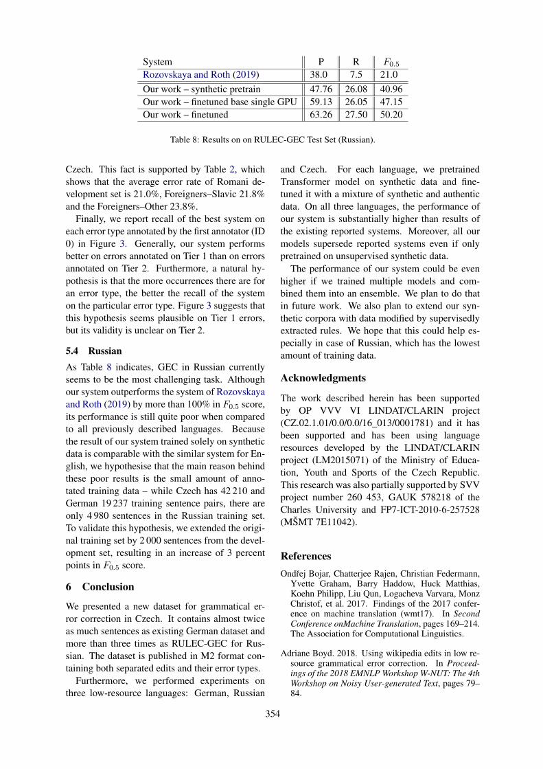
System P R F0.5

Rozovskaya and Roth (2019) 38.0 7.5 21.0Our work – synthetic pretrain 47.76 26.08 40.96Our work – finetuned base single GPU 59.13 26.05 47.15Our work – finetuned 63.26 27.50 50.20

Table 8: Results on on RULEC-GEC Test Set (Russian).

Czech. This fact is supported by Table 2, whichshows that the average error rate of Romani de-velopment set is 21.0%, Foreigners–Slavic 21.8%and the Foreigners–Other 23.8%.

Finally, we report recall of the best system oneach error type annotated by the first annotator (ID0) in Figure 3. Generally, our system performsbetter on errors annotated on Tier 1 than on errorsannotated on Tier 2. Furthermore, a natural hy-pothesis is that the more occurrences there are foran error type, the better the recall of the systemon the particular error type. Figure 3 suggests thatthis hypothesis seems plausible on Tier 1 errors,but its validity is unclear on Tier 2.

5.4 RussianAs Table 8 indicates, GEC in Russian currentlyseems to be the most challenging task. Althoughour system outperforms the system of Rozovskayaand Roth (2019) by more than 100% in F0.5 score,its performance is still quite poor when comparedto all previously described languages. Becausethe result of our system trained solely on syntheticdata is comparable with the similar system for En-glish, we hypothesise that the main reason behindthese poor results is the small amount of anno-tated training data – while Czech has 42 210 andGerman 19 237 training sentence pairs, there areonly 4 980 sentences in the Russian training set.To validate this hypothesis, we extended the origi-nal training set by 2 000 sentences from the devel-opment set, resulting in an increase of 3 percentpoints in F0.5 score.

6 Conclusion

We presented a new dataset for grammatical er-ror correction in Czech. It contains almost twiceas much sentences as existing German dataset andmore than three times as RULEC-GEC for Rus-sian. The dataset is published in M2 format con-taining both separated edits and their error types.

Furthermore, we performed experiments onthree low-resource languages: German, Russian

and Czech. For each language, we pretrainedTransformer model on synthetic data and fine-tuned it with a mixture of synthetic and authenticdata. On all three languages, the performance ofour system is substantially higher than results ofthe existing reported systems. Moreover, all ourmodels supersede reported systems even if onlypretrained on unsupervised synthetic data.

The performance of our system could be evenhigher if we trained multiple models and com-bined them into an ensemble. We plan to do thatin future work. We also plan to extend our syn-thetic corpora with data modified by supervisedlyextracted rules. We hope that this could help es-pecially in case of Russian, which has the lowestamount of training data.

Acknowledgments

The work described herein has been supportedby OP VVV VI LINDAT/CLARIN project(CZ.02.1.01/0.0/0.0/16_013/0001781) and it hasbeen supported and has been using languageresources developed by the LINDAT/CLARINproject (LM2015071) of the Ministry of Educa-tion, Youth and Sports of the Czech Republic.This research was also partially supported by SVVproject number 260 453, GAUK 578218 of theCharles University and FP7-ICT-2010-6-257528(MŠMT 7E11042).

ReferencesOndrej Bojar, Chatterjee Rajen, Christian Federmann,

Yvette Graham, Barry Haddow, Huck Matthias,Koehn Philipp, Liu Qun, Logacheva Varvara, MonzChristof, et al. 2017. Findings of the 2017 confer-ence on machine translation (wmt17). In SecondConference onMachine Translation, pages 169–214.The Association for Computational Linguistics.

Adriane Boyd. 2018. Using wikipedia edits in low re-source grammatical error correction. In Proceed-ings of the 2018 EMNLP Workshop W-NUT: The 4thWorkshop on Noisy User-generated Text, pages 79–84.

354

Adriane Boyd, Jirka Hana, Lionel Nicolas, DetmarMeurers, Katrin Wisniewski, Andrea Abel, KarinSchöne, Barbora Stindlová, and Chiara Vettori.2014. The merlin corpus: Learner language and thecefr. In LREC, pages 1281–1288.

Christopher Bryant and Ted Briscoe. 2018. Languagemodel based grammatical error correction withoutannotated training data. In Proceedings of the Thir-teenth Workshop on Innovative Use of NLP forBuilding Educational Applications, pages 247–253.

Christopher Bryant, Mariano Felice, Øistein E An-dersen, and Ted Briscoe. 2019. The bea-2019shared task on grammatical error correction. In Pro-ceedings of the Fourteenth Workshop on InnovativeUse of NLP for Building Educational Applications,pages 52–75.

Christopher Bryant, Mariano Felice, and Edward JohnBriscoe. 2017. Automatic annotation and evaluationof error types for grammatical error correction. As-sociation for Computational Linguistics.

Yo Joong Choe, Jiyeon Ham, Kyubyong Park, andYeoil Yoon. 2019. A neural grammatical er-ror correction system built on better pre-trainingand sequential transfer learning. arXiv preprintarXiv:1907.01256.

Shamil Chollampatt and Hwee Tou Ng. 2018. A multi-layer convolutional encoder-decoder neural networkfor grammatical error correction. In Proceedings ofthe Thirty-Second AAAI Conference on Artificial In-telligence.

Daniel Dahlmeier and Hwee Tou Ng. 2012. Betterevaluation for grammatical error correction. In Pro-ceedings of the 2012 Conference of the North Amer-ican Chapter of the Association for ComputationalLinguistics: Human Language Technologies, pages568–572. Association for Computational Linguis-tics.

Daniel Dahlmeier, Hwee Tou Ng, and Siew Mei Wu.2013. Building a large annotated corpus of learnerenglish: The nus corpus of learner english. In Pro-ceedings of the eighth workshop on innovative useof NLP for building educational applications, pages22–31.

Sylviane Granger. 1998. The computer learner corpus:A versatile new source of data for SLA research. InSylviane Granger, editor, Learner English on Com-puter, pages 3–18. Addison Wesley Longman, Lon-don and New York.

Roman Grundkiewicz and Marcin Junczys-Dowmunt.2014. The wiked error corpus: A corpus of correc-tive wikipedia edits and its application to grammat-ical error correction. In International Conferenceon Natural Language Processing, pages 478–490.Springer.

Roman Grundkiewicz, Marcin Junczys-Dowmunt, andKenneth Heafield. 2019. Neural grammatical errorcorrection systems with unsupervised pre-trainingon synthetic data. In Proceedings of the FourteenthWorkshop on Innovative Use of NLP for BuildingEducational Applications, pages 252–263.

Michael Heilman, Aoife Cahill, Nitin Madnani,Melissa Lopez, Matthew Mulholland, and JoelTetreault. 2014. Predicting grammaticality on anordinal scale. In Proceedings of the 52nd An-nual Meeting of the Association for ComputationalLinguistics (Volume 2: Short Papers), pages 174–180, Baltimore, Maryland. Association for Compu-tational Linguistics.

Tomáš Jelínek, Barbora Štindlová, Alexandr Rosen,and Jirka Hana. 2012. Combining manual and auto-matic annotation of a learner corpus. In Text, Speechand Dialogue, pages 127–134, Berlin, Heidelberg.Springer Berlin Heidelberg.

Ophélie Lacroix, Simon Flachs, and Anders Søgaard.2019. Noisy channel for low resource grammaticalerror correction. In Proceedings of the FourteenthWorkshop on Innovative Use of NLP for BuildingEducational Applications, pages 191–196.

Jared Lichtarge, Chris Alberti, Shankar Kumar, NoamShazeer, Niki Parmar, and Simon Tong. 2019. Cor-pora generation for grammatical error correction.arXiv preprint arXiv:1904.05780.

Tomoya Mizumoto, Mamoru Komachi, Masaaki Na-gata, and Yuji Matsumoto. 2011. Mining revisionlog of language learning sns for automated japaneseerror correction of second language learners. In Pro-ceedings of 5th International Joint Conference onNatural Language Processing, pages 147–155.

Jakub Náplava. 2017. Natural language correction.Diploma thesis, Univerzita Karlova, Matematicko-fyzikální fakulta.

Jakub Náplava and Milan Straka. 2019. Cuni sys-tem for the building educational applications 2019shared task: Grammatical error correction. In Pro-ceedings of the Fourteenth Workshop on InnovativeUse of NLP for Building Educational Applications,pages 183–190.

Courtney Napoles, Keisuke Sakaguchi, Matt Post, andJoel Tetreault. 2015. Ground truth for grammati-cal error correction metrics. In Proceedings of the53rd Annual Meeting of the Association for Compu-tational Linguistics and the 7th International JointConference on Natural Language Processing (Vol-ume 2: Short Papers), pages 588–593.

Courtney Napoles, Keisuke Sakaguchi, and JoelTetreault. 2017. Jfleg: A fluency corpus and bench-mark for grammatical error correction. In Proceed-ings of the 15th Conference of the European Chap-ter of the Association for Computational Linguistics:Volume 2, Short Papers, pages 229–234, Valencia,Spain. Association for Computational Linguistics.

355

Hwee Tou Ng, Siew Mei Wu, Ted Briscoe, ChristianHadiwinoto, Raymond Hendy Susanto, and Christo-pher Bryant. 2014. The conll-2014 shared task ongrammatical error correction. In Proceedings of theEighteenth Conference on Computational NaturalLanguage Learning: Shared Task, pages 1–14.

Michal Richter, Pavel Stranák, and Alexandr Rosen.2012. Korektor–a system for contextual spell-checking and diacritics completion. In Proceedingsof COLING 2012: Posters, pages 1019–1028.

Alexandr Rosen. 2016. Building and using corpora ofnon-native Czech. In Proceedings of the 16th ITAT:Slovenskoceský NLP workshop (SloNLP 2016), vol-ume 1649 of CEUR Workshop Proceedings, pages80–87, Bratislava, Slovakia. Comenius Universityin Bratislava, Faculty of Mathematics, Physics andInformatics, CreateSpace Independent PublishingPlatform.

Alla Rozovskaya and Dan Roth. 2019. Grammar errorcorrection in morphologically rich languages: Thecase of russian. Transactions of the Association forComputational Linguistics, 7:1–17.

Karel Šebesta, Zuzanna Bedrichová, KaterinaŠormová, Barbora Štindlová, Milan Hrdlicka,Tereza Hrdlicková, Jirí Hana, Vladimír Petkevic,Tomáš Jelínek, Svatava Škodová, Petr Janeš,Katerina Lundáková, Hana Skoumalová, ŠimonSládek, Piotr Pierscieniak, Dagmar Toufarová,Milan Straka, Alexandr Rosen, Jakub Náplava,and Marie Polácková. 2017. CzeSL gram-matical error correction dataset (CzeSL-GEC).http://hdl.handle.net/11234/1-2143LINDAT/CLARIN digital library at the Institute ofFormal and Applied Linguistics (ÚFAL), Faculty ofMathematics and Physics, Charles University.

Rico Sennrich and Biao Zhang. 2019. Revisiting low-resource neural machine translation: A case study.arXiv preprint arXiv:1905.11901.

Noam Shazeer and Mitchell Stern. 2018. Adafactor:Adaptive learning rates with sublinear memory cost.arXiv preprint arXiv:1804.04235.

Toshikazu Tajiri, Mamoru Komachi, and Yuji Mat-sumoto. 2012. Tense and aspect error correction foresl learners using global context. In Proceedingsof the 50th Annual Meeting of the Association forComputational Linguistics: Short Papers-Volume 2,pages 198–202. Association for Computational Lin-guistics.


Karel Šebesta. 2010. Korpusy cestiny a osvojováníjazyka [Corpora of Czech and language acquisition].In Studie z aplikované lingvistiky [Studies in AppliedLinguistics], volume 2010(2), pages 11–33.

Shuyao Xu, Jiehao Zhang, Jin Chen, and Long Qin.2019. Erroneous data generation for grammaticalerror correction. In Proceedings of the FourteenthWorkshop on Innovative Use of NLP for BuildingEducational Applications, pages 149–158.

Helen Yannakoudakis, Ted Briscoe, and Ben Medlock.2011. A new dataset and method for automaticallygrading esol texts. In Proceedings of the 49th An-nual Meeting of the Association for ComputationalLinguistics: Human Language Technologies-Volume1, pages 180–189. Association for ComputationalLinguistics.

Liang-Chih Yu, Lung-Hao Lee, and Li-Ping Chang.2014. Overview of grammatical error diagnosis forlearning chinese as a foreign language. In Proceed-ings of the 1st Workshop on Natural Language Pro-cessing Techniques for Educational Applications,pages 42–47.

Zheng Yuan and Mariano Felice. 2013. Constrainedgrammatical error correction using statistical ma-chine translation. In Proceedings of the Seven-teenth Conference on Computational Natural Lan-guage Learning: Shared Task, pages 52–61.

Wajdi Zaghouani, Behrang Mohit, Nizar Habash, Os-sama Obeid, Nadi Tomeh, Alla Rozovskaya, NouraFarra, Sarah Alkuhlani, and Kemal Oflazer. 2015.Large scale arabic error annotation: Guidelines andframework.

Wei Zhao, Liang Wang, Kewei Shen, Ruoyu Jia, andJingming Liu. 2019. Improving grammatical er-ror correction via pre-training a copy-augmentedarchitecture with unlabeled data. arXiv preprintarXiv:1903.00138.

356


Minimally-Augmented Grammatical Error Correction

Roman Grundkiewicz†‡ and Marcin Junczys-Dowmunt‡† University of Edinburgh, Edinburgh EH8 9AB, UK

‡ Microsoft, Redmond, WA 98052, [email protected], [email protected]

Abstract

There has been an increased interest in low-resource approaches to automatic grammati-cal error correction. We introduce Minimally-Augmented Grammatical Error Correction(MAGEC) that does not require any error-labelled data. Our unsupervised approach isbased on a simple but effective synthetic er-ror generation method based on confusion setsfrom inverted spell-checkers. In low-resourcesettings, we outperform the current state-of-the-art results for German and Russian GECtasks by a large margin without using any realerror-annotated training data. When combinedwith labelled data, our method can serve as anefficient pre-training technique.

1 Introduction

Most neural approaches to automatic grammati-cal error correction (GEC) require error-labelledtraining data to achieve their best performance.Unfortunately, such resources are not easily avail-able, particularly for languages other than English.This has lead to an increased interest in unsuper-vised and low-resource GEC (Rozovskaya et al.,2017; Bryant and Briscoe, 2018; Boyd, 2018; Ro-zovskaya and Roth, 2019), which recently culmi-nated in the low-resource track of the Building Ed-ucational Application (BEA) shared task (Bryantet al., 2019).1

We present Minimally-Augmented GrammaticalError Correction (MAGEC), a simple but effectiveapproach to unsupervised and low-resource GECwhich does not require any authentic error-labelledtraining data. A neural sequence-to-sequencemodel is trained on clean and synthetically noisedsentences alone. The noise is automatically createdfrom confusion sets. Additionally, if labelled data

1https://www.cl.cam.ac.uk/research/nl/bea2019st

is available for fine-tuning (Hinton and Salakhutdi-nov, 2006), MAGEC can also serve as an efficientpre-training technique.

The proposed unsupervised synthetic error gen-eration method does not require a seed corpus withexample errors as most other methods based on sta-tistical error injection (Felice and Yuan, 2014) orback-translation models (Rei et al., 2017; Kasewaet al., 2018; Htut and Tetreault, 2019). It also out-performs noising techniques that rely on randomword replacements (Xie et al., 2018; Zhao et al.,2019). Contrary to Ge et al. (2018) or Lichtargeet al. (2018), our approach can be easily used foreffective pre-training of full encoder-decoder mod-els as it is model-independent and only requiresclean monolingual data and potentially an availablespell-checker dictionary.2 In comparison to pre-training with BERT (Devlin et al., 2019), syntheticerrors provide more task-specific training exam-ples than masking. As an unsupervised approach,MAGEC is an alternative to recently proposed lan-guage model (LM) based approaches (Bryant andBriscoe, 2018; Stahlberg et al., 2019), but it doesnot require any amount of annotated sentences fortuning.

2 Minimally-augmented grammaticalerror correction

Our minimally-augmented GEC approach uses syn-thetic noise as its primary source of training data.We generate erroneous sentences from monolingualtexts via random word perturbations selected fromautomatically created confusion sets. These aretraditionally defined as sets of frequently confusedwords (Rozovskaya and Roth, 2010).

We experiment with three unsupervised methodsfor generating confusion sets:

2GNU Aspell supports more than 160 languages: http://aspell.net/man-html/Supported.html

357

Word Confusion set

had hard head hand gad has ha ad hatnight knight naught nought nights bight might nightiethen them the hen ten than thin thee thew

haben habend halben gaben habe habet hakenNacht Nachts Nascht Macht Naht Acht Nach Jacht Pachtdann sann dank denn dünn kann wann bannen kannst

имел им ел им-ел имела имели имело мел умелночь ночью ночи дочь мочь ноль новь точьзатем за тем за-тем затеем затеям зятем затеями

Table 1: Examples of spell-broken confusion sets forEnglish, German and Russian.

Edit distance Confusion sets consist of wordswith the shortest Levenshtein distance (Leven-shtein, 1966) to the selected confused word.

Word embeddings Confusion sets contain themost similar words to the confused wordbased on the cosine similarity of their wordembedding vectors (Mikolov et al., 2013).

Spell-breaking Confusion sets are composed ofsuggestions from a spell-checker; a sugges-tion list is extracted for the confused wordregardless of its actual correctness.

These methods can be used to build confusionsets for any alphabetic language.3 We find that con-fusion sets constructed via spell-breaking performbest (Section 4). Most context-free spell-checkerscombine a weighted edit distance and phonetic al-gorithms to order suggestions, which produces reli-able confusion sets (Table 1).

We synthesize erroneous sentences as follows:given a confusion set Ci = {ci1, ci2, ci3, ...}, and thevocabulary V , we sample word wj ∈ V from the in-put sentence with a probability approximated witha normal distribution N (pWER, 0.2), and performone of the following operations: (1) substitutionof wj with a random word cjk from its confusionset with probability psub, (2) deletion of wj withpdel, (3) insertion of a random word wk ∈ V atj + 1 with pins, and (4) swapping wj and wj+1

with pswp. When making a substitution, wordswithin confusion sets are sampled uniformly.

To improve the model’s capability of correctingspelling errors, inspired by Lichtarge et al. (2018);Xie et al. (2018), we randomly perturb 10% ofcharacters using the same edit operations as above.

3For languages with logosylabic writing system like Chi-nese, the edit distance can be calculated on transcribedtext, while word embeddings can be generated after word-segmentation.

Lang. Corpus Dev Test Train

EN W&I+LOCNESS 4,384 4,477 34,308DE Falco+MERLIN 2,503 2,337 18,7544

RU RULEC-GEC 2,500 5,000 4,980

Table 2: Sizes of labelled corpora in no. of sentences.

Character-level noise is introduced on top of thesynthetic errors generated via confusion sets.

A MAGEC model is trained solely on the syn-thetically noised data and then ensembled with alanguage model. Being limited only by the amountof clean monolingual data, this large-scale unsu-pervised approach can perform better than trainingon small authentic error corpora. A large amountof training examples increases the chance that syn-thetic errors resemble real error patterns and resultsin better language modelling properties.

If any small amount of error-annotated learnerdata is available, it can be used to fine-tune thepre-trained model and further boost its perfor-mance. Pre-training of decoders of GEC mod-els from language models has been introduced byJunczys-Dowmunt et al. (2018b), we pretrain thefull encoder-decoder models instead, as proposedby Grundkiewicz et al. (2019).

3 Experiments

Data and evaluation Our approach requires alarge amount of monolingual data that is used forgenerating synthetic training pairs. We use thepublicly available News crawl data5 released forthe WMT shared tasks (Bojar et al., 2018). ForEnglish and German, we limit the size of the datato 100 million sentences; for Russian, we use allthe available 80.5 million sentences.

As primary development and test data, we usethe following learner corpora (Table 2):

• English: the new W&I+LOCNESS corpus(Bryant et al., 2019; Granger, 1998) releasedfor the BEA 2019 shared task and representinga diverse cross-section of English language;

• German: the Falko-MERLIN GEC corpus(Boyd, 2018) that combines two Germanlearner corpora of all proficiency levels;

4The original training part of Falco+MERLIN consists of19,237 sentences, but is contaminated with some test sentences.We have removed training examples if their target sentencesoccur in the development or test set.

5http://data.statmt.org/news-crawl

358

System P R F0.5

Random 32.8 6.7 18.49Edit distance 39.9 9.5 24.27Word embeddings 39.7 9.0 23.56Spell-breaking 43.1 10.6 26.66+ OOV + Case 44.9 10.9 27.70

→ WER = 0.25 43.3 11.8 27.50→ Edit-weighted Λ = 2 43.0 12.6 28.99

Table 3: Performance for different confusion sets andedit weighting techniques on W&I+LOCNESS Dev.

• Russian: the recently introduced RULEC-GEC dataset (Alsufieva et al., 2012; Ro-zovskaya and Roth, 2019) containing Russiantexts from foreign and heritage speakers.

Unless explicitly stated, we do not use the train-ing parts of those datasets. For each languagewe follow the originally proposed preprocessingand evaluation settings. English and German dataare tokenized with Spacy6, while Russian is pre-processed with Mystem (Segalovich, 2003). Weadditionally normalise punctuation in monolingualdata using Moses scripts (Koehn et al., 2007). Dur-ing training, we limit the vocabulary size to 32,000subwords computed with SentencePiece using theunigram method (Kudo and Richardson, 2018).

English models are evaluated with ERRANT(Bryant et al., 2017) using F0.5; for German andRussian, the M2Scorer with the MaxMatch metric(Dahlmeier and Ng, 2012) is used.

Synthetic data Confusion sets are created foreach language for V = 96, 000 most frequent lex-ical word forms from monolingual data. We usethe Levenshtein distance to generate edit-distancebased confusion sets. The maximum considereddistance is 2. Word embeddings are computed withword2vec7 from monolingual data. To generatespell-broken confusion sets we use Enchant8 withAspell dictionaries.9 The size of confusion sets islimited to top 20 words.

Synthetic errors are introduced into monolingualtexts to mimic word error rate (WER) of about15%, i.e. pWER = 0.15, which resembles errorfrequency in common ESL error corpora. Whenconfusing a word, the probability psub is set to 0.7,other probabilities are set to 0.1.

6https://spacy.io7https://github.com/tmikolov/word2vec8https://abiword.github.io/enchant9ftp://ftp.gnu.org/gnu/aspell/dict

System Dev P R F0.5

Top BEA19 (Low-res.) 44.95 70.2 48.0 64.24Top BEA19 (Restricted) 53.00 72.3 60.1 69.47

Spell-checker 10.04 23.7 7.4 16.45Spell-checker w/ LM 12.00 41.5 6.8 20.52

MAGEC w/o LM 28.99 53.4 26.2 44.22MAGEC 31.87 49.1 37.5 46.22MAGEC Ens. 33.32 53.0 34.5 47.89

Fine-tuned (Real) 44.29 61.2 54.1 59.62Fine-tuned (Real+Synth.) 49.49 66.0 58.8 64.45

(a) English (W&I+LOCNESS)

System Dev P R M20.5

Boyd (2018) (Unsup.) — 30.0 14.0 24.37Boyd (2018) — 52.0 29.8 45.22




(b) German (Falko-MERLIN)

System Dev P R M20.5

Rozovskaya and Roth (2019) — 38.0 7.5 21.0




(c) Russian (RULEC-GEC)

Table 4: Unsupervised and fine-tuned MAGEC sys-tems for English, German and Russian, contrasted withsystems from related work and spell-checking base-lines.

Training settings We adapt the recent state-of-the-art GEC system by Junczys-Dowmunt et al.(2018b), an ensemble of sequence-to-sequenceTransformer models (Vaswani et al., 2017) and aneural language model.10

We use the training setting proposed by the au-thors11, but introduce stronger regularization: weincrease dropout probabilities of source words to0.3, add dropout on transformer self-attention andfilter layers of 0.1, and use larger mini-batches with

10Models and outputs are available from https://github.com/grammatical/magec-wnut2019

11https://github.com/grammatical/neural-naacl2018

359

~2,500 sentences. We do not pre-train the decoderparameters with a language model and train di-rectly on the synthetic data. We increase the sizeof language model used for ensembling to matchthe Transformer-big configuration (Vaswani et al.,2017) with 16-head self-attention, embeddings sizeof 1024 and feed-forward filter size size of 4096.In experiments with fine-tuning, the training hyper-parameters remain unchanged.

All models are trained with Marian (Junczys-Dowmunt et al., 2018a). The training is continuedfor at most 5 epochs or until early-stopping is trig-gered after 5 stalled validation steps. We found thatusing 10,000 synthetic sentences as validation sets,i.e. a fully unsupervised approach, is as effectiveas using the development parts of error corpora anddoes not decrease the final performance.

4 Results and analysis

Confusion sets On English data, all proposedconfusion set generation methods perform betterthan random word substitution (Table 3).Confu-sion sets based on word embeddings are the leasteffective, while spell-broken sets perform best at26.66 F0.5. We observe further gains of +1.04 fromkeeping out-of-vocabulary spell-checker sugges-tions (OOV) and preserving consistent letter casingwithin confusion sets (Case).

The word error rate of error corpora is an use-ful statistic that can be used to balance preci-sion/recall ratios (Rozovskaya and Roth, 2010;Junczys-Dowmunt et al., 2018b; Hotate et al.,2019). Increasing WER in the synthetic data from15% to 25% increases recall at the expense of preci-sion, but no overall improvement is observed. A no-ticeable recall gain that transfers to a higher F-scoreof 28.99 is achieved by increasing the importanceof edited fragments with the edit-weighted MLEobjective from Junczys-Dowmunt et al. (2018b)with Λ = 2. We use this setting for the rest of ourexperiments.

Main results We first compare the GEC systemswith simple baselines using a greedy and contextspell-checking (Table 4); the latter selects the bestcorrection suggestion based on the sentence per-plexity from a Transformer language model. Allsystems outperform the spell-checker baselines.

On German and Russian test sets, singleMAGEC models without ensembling with a lan-guage model already achieve better performancethan reported by Boyd (2018) and Rozovskaya and

System CoNLL JFLEG

Bryant and Briscoe (2018) ? 34.09 48.75Stahlberg et al. (2019) ? 44.43 52.61Stahlberg et al. (2019) (659K real data) 58.40 58.63

MAGEC Ens. ? 44.23 56.18MAGEC Fine-tuned (34K real data) 56.54 60.01

Table 5: Comparison with LM-based GEC on theCoNLL (M2) and JFLEG (GLEU) test sets for unsuper-vised (?) and supervised systems trained or fine-tunedon different amounts of labelled data.

0 116

18

14

12

1

28.0

32.0

36.0

40.0

44.0

33.3

37.1

39.240.7

43.6 44.3

F0.5

Ensemble w/ LMEnsembleAverage of 4 w/o LM

Figure 1: Improvements from fine-tuning on subsets ofW&I+LOCNESS Train. The smallest 1

16 part of thedataset contains 2,145 sentences. Averaged F-scoresover 4 runs trained on different subsets of the data.

Roth (2019) for their systems that use authenticerror-annotated data for training (Table 4b and 4c).Our best unsupervised ensemble systems that com-bine three Transformer models and a LM12 outper-form the state-of-the-art results for these languagesby +7.0 and +11.4 F0.5.

Our English models do not compete with thetop systems (Grundkiewicz et al., 2019) from theBEA shared task trained on publicly available error-annotated corpora (Table 4a). It is difficult tocompare with the top low-resource system fromthe shared task, because it uses additional paralleldata from Wikipedia (Grundkiewicz and Junczys-Dowmunt, 2014), larger ensemble, and n-best listre-ranking with right-to-left models, which can bealso implemented in this work.

MAGEC systems are generally on par with theresults achieved by a recent unsupervised contribu-tion based on finite state transducers by Stahlberget al. (2019) on the CoNLL-2014 (Dahlmeier et al.,2013) and JFLEG test sets (Napoles et al., 2017)(Table 5).

12The weight of the language model is grid-searched on thedevelopment set.

360

Spell.+punc. Other errorsLang. P R F0.5 P R F0.5

EN 28.8 24.1 27.68 33.5 16.8 27.93DE 54.8 71.4 57.43 63.6 55.8 61.83RU 26.7 75.0 30.70 14.6 19.7 15.37

Table 6: Performance of single MAGEC w/ LM modelson two groups of errors on respective development sets.

All unsupervised systems benefit from domain-adaptation via fine-tuning on authentic labelleddata (Miceli Barone et al., 2017). The more au-thentic high-quality and in-domain training datais used, the greater the improvement, but even asfew as ~2,000 sentences are helpful (Fig. 1). Wefound that fine-tuning on a 2:1 mixture of syntheticand oversampled authentic data prevents the modelfrom over-fitting. This is particularly visible for En-glish which has the largest fine-tuning set (34K sen-tences), and the difference of 5.2 F0.5 between fine-tuning with and without synthetic data is largest.

Spelling and punctuation errors The GEC taskinvolves detection and correction of all types of er-ror in written texts, including grammatical, lexicaland orthographical errors. Spelling and punctua-tion errors are among the most frequent error typesand also the easiest to synthesize.

To counter the argument that – mostly due tothe introduced character-level noise and strong lan-guage modelling – MAGEC can only correct these“simple” errors, we evaluate it against test sets thatcontain either spelling and punctuation errors orall other error types; with the complement errorscorrected (Table 6). Our systems indeed performbest on misspellings and punctuation errors, butare capable of correcting various error types. Thedisparity for Russian can be explained by the factthat it is a morphologically-rich language and wesuffer from generally lower performance.

5 Conclusions and future work

We have presented Minimally-Augmented Gram-matical Error Correction (MAGEC), which canbe effectively used in both unsupervised and low-resource scenarios. The method is model indepen-dent, requires easily available resources, and can beused for creating reliable baselines for supervisedtechniques or as an efficient pre-training methodfor neural GEC models with labelled data. We havedemonstrated the effectiveness of our method andoutperformed state-of-the-art results for German

and Russian benchmarks, trained with labelled data,by a large margin.

For future work, we plan to evaluate MAGECon more languages and experiment with more di-versified confusion sets created with additional un-supervised generation methods.

ReferencesAnna Alsufieva, Olesya Kisselev, and Sandra Freels.

2012. Results 2012: Using flagship data to developa Russian learner corpus of academic writing. Rus-sian Language Journal, 62:79–105.

Ondrej Bojar, Christian Federmann, Mark Fishel,Yvette Graham, Barry Haddow, Philipp Koehn, andChristof Monz. 2018. Findings of the 2018 con-ference on machine translation (WMT18). In Pro-ceedings of the Third Conference on Machine Trans-lation: Shared Task Papers, pages 272–303, Bel-gium, Brussels. Association for Computational Lin-guistics.

Adriane Boyd. 2018. Using Wikipedia edits in lowresource grammatical error correction. In Proceed-ings of the 2018 EMNLP Workshop W-NUT: The4th Workshop on Noisy User-generated Text, pages79–84, Brussels, Belgium. Association for Compu-tational Linguistics.

Christopher Bryant and Ted Briscoe. 2018. Languagemodel based grammatical error correction withoutannotated training data. In Proceedings of the Thir-teenth Workshop on Innovative Use of NLP for Build-ing Educational Applications, pages 247–253, NewOrleans, Louisiana. Association for ComputationalLinguistics.

Christopher Bryant, Mariano Felice, Øistein E. An-dersen, and Ted Briscoe. 2019. The BEA-2019shared task on grammatical error correction. In Pro-ceedings of the Fourteenth Workshop on InnovativeUse of NLP for Building Educational Applications,pages 52–75, Florence, Italy. Association for Com-putational Linguistics.

Christopher Bryant, Mariano Felice, and Ted Briscoe.2017. Automatic annotation and evaluation of errortypes for grammatical error correction. In Proceed-ings of the 55th Annual Meeting of the Associationfor Computational Linguistics (Volume 1: Long Pa-pers), pages 793–805, Vancouver, Canada. Associa-tion for Computational Linguistics.

Daniel Dahlmeier and Hwee Tou Ng. 2012. Betterevaluation for grammatical error correction. In Pro-ceedings of the 2012 Conference of the North Amer-ican Chapter of the Association for ComputationalLinguistics: Human Language Technologies, pages568–572, Montréal, Canada. Association for Com-putational Linguistics.

361

Daniel Dahlmeier, Hwee Tou Ng, and Siew Mei Wu.2013. Building a large annotated corpus of learnerEnglish: The NUS corpus of learner English. InProceedings of the Eighth Workshop on InnovativeUse of NLP for Building Educational Applications,pages 22–31.

Jacob Devlin, Ming-Wei Chang, Kenton Lee, andKristina Toutanova. 2019. BERT: Pre-training ofdeep bidirectional transformers for language under-standing. pages 4171–4186.

Mariano Felice and Zheng Yuan. 2014. Generating arti-ficial errors for grammatical error correction. In Pro-ceedings of the Student Research Workshop at the14th Conference of the European Chapter of the As-sociation for Computational Linguistics, pages 116–126, Gothenburg, Sweden. Association for Compu-tational Linguistics.

Tao Ge, Furu Wei, and Ming Zhou. 2018. Fluencyboost learning and inference for neural grammati-cal error correction. In Proceedings of the 56th An-nual Meeting of the Association for ComputationalLinguistics (Volume 1: Long Papers), pages 1055–1065, Melbourne, Australia. Association for Compu-tational Linguistics.

Sylviane Granger. 1998. The computer learner corpus:A versatile new source of data for SLA research. InSylviane Granger, editor, Learner English on Com-puter, pages 3–18. Addison Wesley Longman, Lon-don and New York.

Roman Grundkiewicz and Marcin Junczys-Dowmunt.2014. The WikEd error corpus: A corpus of correc-tive Wikipedia edits and its application to grammat-ical error correction. In Advances in Natural Lan-guage Processing — Lecture Notes in Computer Sci-ence, volume 8686, pages 478–490. Springer.

Roman Grundkiewicz, Marcin Junczys-Dowmunt, andKenneth Heafield. 2019. Neural grammatical errorcorrection systems with unsupervised pre-trainingon synthetic data. In Proceedings of the FourteenthWorkshop on Innovative Use of NLP for BuildingEducational Applications, pages 252–263, Florence,Italy. Association for Computational Linguistics.

Geoffrey E Hinton and Ruslan R Salakhutdinov. 2006.Reducing the dimensionality of data with neural net-works. science, 313(5786):504–507.

Kengo Hotate, Masahiro Kaneko, Satoru Katsumata,and Mamoru Komachi. 2019. Controlling grammat-ical error correction using word edit rate. In Pro-ceedings of the 57th Annual Meeting of the Asso-ciation for Computational Linguistics: Student Re-search Workshop, pages 149–154. Association forComputational Linguistics.

Phu Mon Htut and Joel Tetreault. 2019. The unbear-able weight of generating artificial errors for gram-matical error correction. In Proceedings of the Four-teenth Workshop on Innovative Use of NLP for Build-

ing Educational Applications, pages 478–483, Flo-rence, Italy. Association for Computational Linguis-tics.

Marcin Junczys-Dowmunt, Roman Grundkiewicz,Tomasz Dwojak, Hieu Hoang, Kenneth Heafield,Tom Neckermann, Frank Seide, Ulrich Germann, Al-ham Fikri Aji, Nikolay Bogoychev, André F. T. Mar-tins, and Alexandra Birch. 2018a. Marian: Fastneural machine translation in C++. In Proceedingsof ACL 2018, System Demonstrations, pages 116–121, Melbourne, Australia. Association for Compu-tational Linguistics.

Marcin Junczys-Dowmunt, Roman Grundkiewicz,Shubha Guha, and Kenneth Heafield. 2018b. Ap-proaching neural grammatical error correction as alow-resource machine translation task. In Proceed-ings of the 2018 Conference of the North Ameri-can Chapter of the Association for ComputationalLinguistics: Human Language Technologies, Vol-ume 1 (Long Papers), pages 595–606, New Orleans,Louisiana. Association for Computational Linguis-tics.

Sudhanshu Kasewa, Pontus Stenetorp, and SebastianRiedel. 2018. Wronging a right: Generating bet-ter errors to improve grammatical error detection.In Proceedings of the 2018 Conference on Em-pirical Methods in Natural Language Processing,pages 4977–4983, Brussels, Belgium. Associationfor Computational Linguistics.

Philipp Koehn, Hieu Hoang, Alexandra Birch, ChrisCallison-Burch, Marcello Federico, Nicola Bertoldi,Brooke Cowan, Wade Shen, Christine Moran,Richard Zens, Chris Dyer, Ondrej Bojar, AlexandraConstantin, and Evan Herbst. 2007. Moses: Opensource toolkit for statistical machine translation. InAnnual Meeting of the Association for Computa-tional Linguistics. The Association for ComputerLinguistics.

Taku Kudo and John Richardson. 2018. SentencePiece:A simple and language independent subword tok-enizer and detokenizer for neural text processing. InProceedings of the 2018 Conference on EmpiricalMethods in Natural Language Processing: SystemDemonstrations, pages 66–71, Brussels, Belgium.Association for Computational Linguistics.

Vladimir I Levenshtein. 1966. Binary codes capableof correcting deletions, insertions, and reversals. InSoviet physics doklady, volume 10, pages 707–710.

Jared Lichtarge, Christopher Alberti, Shankar Kumar,Noam Shazeer, and Niki Parmar. 2018. Weakly su-pervised grammatical error correction using iterativedecoding. CoRR, abs/1811.01710.

Antonio Valerio Miceli Barone, Barry Haddow, UlrichGermann, and Rico Sennrich. 2017. Regularizationtechniques for fine-tuning in neural machine trans-lation. In Proceedings of the 2017 Conference onEmpirical Methods in Natural Language Processing,

362

pages 1489–1494, Copenhagen, Denmark. Associa-tion for Computational Linguistics.


Courtney Napoles, Keisuke Sakaguchi, and JoelTetreault. 2017. JFLEG: A fluency corpus andbenchmark for grammatical error correction. In Pro-ceedings of the 2017 Conference of the EuropeanChapter of the Association for Computational Lin-guistics, Valencia, Spain. Association for Computa-tional Linguistics.

Marek Rei, Mariano Felice, Zheng Yuan, and TedBriscoe. 2017. Artificial error generation with ma-chine translation and syntactic patterns. In Proceed-ings of the 12th Workshop on Innovative Use of NLPfor Building Educational Applications, pages 287–292, Copenhagen, Denmark. Association for Com-putational Linguistics.

Alla Rozovskaya and Dan Roth. 2010. Generatingconfusion sets for context-sensitive error correction.In Proceedings of the 2010 Conference on Empiri-cal Methods in Natural Language Processing, pages961–970, Cambridge, MA. Association for Compu-tational Linguistics.

Alla Rozovskaya and Dan Roth. 2019. Grammar errorcorrection in morphologically-rich languages: Thecase of Russian. Transactions of the Association forComputational Linguistics, 7:1–17.

Alla Rozovskaya, Dan Roth, and Mark Sammons.2017. Adapting to learner errors with minimal su-pervision. Comput. Linguist., 43(4):723–760.

Ilya Segalovich. 2003. A fast morphological algorithmwith unknown word guessing induced by a dictio-nary for a web search engine. In MLMTA, pages273–280. CSREA Press.

Felix Stahlberg, Christopher Bryant, and Bill Byrne.2019. Neural grammatical error correction with fi-nite state transducers. In Proceedings of the 2018Conference of the North American Chapter of theAssociation for Computational Linguistics: HumanLanguage Technologies, Minneapolis, USA. Associ-ation for Computational Linguistics.

Ashish Vaswani, Noam Shazeer, Niki Parmar, JakobUszkoreit, Llion Jones, Aidan N Gomez, ŁukaszKaiser, and Illia Polosukhin. 2017. Attention is allyou need. In Advances in Neural Information Pro-cessing Systems 30, pages 5998–6008. Curran Asso-ciates, Inc.

Ziang Xie, Guillaume Genthial, Stanley Xie, AndrewNg, and Dan Jurafsky. 2018. Noising and denoising

natural language: Diverse backtranslation for gram-mar correction. In Proceedings of the 2018 Confer-ence of the North American Chapter of the Associ-ation for Computational Linguistics: Human Lan-guage Technologies, Volume 1 (Long Papers), pages619–628, New Orleans, Louisiana. Association forComputational Linguistics.

Wei Zhao, Liang Wang, Kewei Shen, Ruoyu Jia, andJingming Liu. 2019. Improving grammatical errorcorrection via pre-training a copy-augmented archi-tecture with unlabeled data. CoRR, abs/1903.00138.

363


A Social Opinion Gold Standard for the Malta Government Budget 2018

Keith CortisMaynooth University, Maynooth, Ireland

Malta Information Technology Agency, [email protected]

Brian DavisADAPT Centre,

Dublin City University,Glasnevin, Dublin 9, Ireland

[email protected]

Abstract

We present a gold standard of annotated so-cial opinion for the Malta Government Bud-get 2018. It consists of over 500 online postsin English and/or the Maltese less-resourcedlanguage, gathered from social media plat-forms, specifically, social networking servicesand newswires, which have been annotatedwith information about opinions expressed bythe general public and other entities, in termsof sentiment polarity, emotion, sarcasm/irony,and negation. This dataset is a resource foropinion mining based on social data, withinthe context of politics. It is the first opinionannotated social dataset from Malta, which hasvery limited language resources available.

1 Introduction

European usage trends show that Malta is the sec-ond highest user of social media, with around 90%of the adult population being online and activeon social media (Eurostat, 2017), whereas around80% of users read news online (Caruana, 2018).In terms of social media, this is not only used byindividuals, but is also increasingly being used byenterprises (Eurostat, 2018). In fact, governmentsand businesses are spreading their news via socialmedia and moving away from newswires (Grech,2019). This has increased the importance of socialopinions and the need to refine data mining tech-niques that are able to identify and classify opin-ions related to a particular aspect, e.g., entity ortopic, which can be beneficial.

This paper presents a dataset of opinion-annotated social online posts targeting the MaltaGovernment Budget for 20181 presented on 9thOctober 2017 by the Honourable Minister for Fi-nance, Edward Scicluna. It contains the opinionsand reactions (in terms of sentiment, emotions,

1https://mfin.gov.mt/en/The-Budget/Pages/The-Budget-2018.aspx

etc.) of the public and professionals towards thementioned budget as expressed over various socialchannels, specifically, social networking servicesand newswires, during and after the event. In addi-tion, it has the potential of identifying commenda-tions, regrets and other reactions concerning anypresented measure, such as tax matters, industryspecific initiatives, strategic initiatives and socialmeasures. This dataset can support governmentinitiatives for the development of opinion miningtools to better capture the public perception to-wards an upcoming/current/past budget presentedto the House of Representatives. Such valuableinsights can be taken in consideration within theupcoming budgets and/or any bills presented anddiscussed in Parliament.

2 Related Work

The Politics domain is one of the most popular ap-plication areas in the social media-based opinionmining domain, with such techniques being ap-plied on election, debate, referendum and otherpolitical events’ (such as uprisings and protests)datasets. However, applying such techniques ongovernment budgets is not common.

Kalampokis et al. (2011) proposed a methodthat integrates government and social data (fromsocial media platforms, such as Twitter and Face-book) to enable decision makers to understandpublic opinion and be able to predict public reac-tions on certain decisions. The methodology dis-cussed by Hubert et al. (2018), uses emotion anal-ysis to study government-citizen interactions onTwitter for five Latin American countries that havea mature e-Participation, namely Mexico, Colom-bia, Chile, Uruguay and Argentina. Similarly, thecity of Washington D.C. in the United States, usessentiment analysis to interpret and examine thecomments posted by citizens and businesses over

364

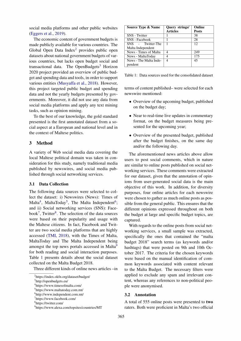
social media platforms and other public websites(Eggers et al., 2019).

The economic content of government budgets ismade publicly available for various countries. TheGlobal Open Data Index2 provides public opendatasets about national government budgets of var-ious countries, but lacks open budget social andtransactional data. The OpenBudgets3 Horizon2020 project provided an overview of public bud-get and spending data and tools, in order to supportvarious entities (Musyaffa et al., 2018). However,this project targeted public budget and spendingdata and not the yearly budgets presented by gov-ernments. Moreover, it did not use any data fromsocial media platforms and apply any text miningtasks, such as opinion mining.

To the best of our knowledge, the gold standardpresented is the first annotated dataset from a so-cial aspect at a European and national level and inthe context of Maltese politics.

3 Method

A variety of Web social media data covering thelocal Maltese political domain was taken in con-sideration for this study, namely traditional mediapublished by newswires, and social media pub-lished through social networking services.

3.1 Data Collection

The following data sources were selected to col-lect the dataset: i) Newswires (News): Times ofMalta4, MaltaToday5, The Malta Independent6;and ii) Social networking services (SNS): Face-book7, Twitter8. The selection of the data sourceswere based on their popularity and usage withthe Maltese citizens. In fact, Facebook and Twit-ter are two social media platforms that are highlyaccessed (TMI, 2018), with the Times of Malta,MaltaToday and The Malta Independent beingamongst the top news portals accessed in Malta9

for both reading and social interaction purposes.Table 1 presents details about the social datasetcollected on the Malta Budget 2018.

Three different kinds of online news articles –in2https://index.okfn.org/dataset/budget/3http://openbudgets.eu/4https://www.timesofmalta.com/5https://www.maltatoday.com.mt/6http://www.independent.com.mt/7https://www.facebook.com/8https://twitter.com/9https://www.alexa.com/topsites/countries/MT

Source Type & Name Query strings/Articles

OnlinePosts

SNS - Twitter 1 38SNS - Facebook 1 28SNS - Twitter-TheMalta Independent

1 12

News - Times of Malta 4 249News - MaltaToday 4 175News - The Malta Inde-pendent

4 45

Table 1: Data sources used for the consolidated dataset

terms of content published– were selected for eachnewswire mentioned:

• Overview of the upcoming budget, publishedon the budget day;

• Near to real-time live updates in commentaryformat, on the budget measures being pre-sented for the upcoming year;

• Overview of the presented budget, publishedafter the budget finishes, on the same dayand/or the following day.

The aforementioned news articles above allowusers to post social comments, which in natureare similar to online posts published on social net-working services. These comments were extractedfor our dataset, given that the annotation of opin-ions from user-generated social data is the mainobjective of this work. In addition, for diversitypurposes, four online articles for each newswirewere chosen to gather as much online posts as pos-sible from the general public. This ensures that thedifferent opinions expressed throughout on boththe budget at large and specific budget topics, arecaptured.

With regards to the online posts from social net-working services, a small sample was extracted,specifically the ones that contained the “maltabudget 2018” search terms (as keywords and/orhashtags) that were posted on 9th and 10th Oc-tober 2017. The criteria for the chosen keywordswere based on the manual identification of com-mon keywords associated with content relevantto the Malta Budget. The necessary filters wereapplied to exclude any spam and irrelevant con-tent, whereas any references to non-political peo-ple were anonymised.

3.2 AnnotationA total of 555 online posts were presented to tworaters. Both were proficient in Malta’s two official

365

languages - Maltese (Malti) –a Semitic languagewritten in the Latin script that is the national lan-guage of Malta– and English, which are equallyimportant10. Moreover, the raters worked in thetechnology domain, were given a lecture aboutopinion mining and provided with relevant readingmaterial and terminology for reference purposes.The following metatdata and annotation types (#6-13) were created for each online post:

1. Online Post Identifier: unique numericalidentifier for the online post;

2. Related Online Post Identifier: numericalidentifier for the parent online post (if any);

3. Source Identifier: numerical identifier refer-ring to the actual data source (e.g., website)of the online post;

4. Source Name: origin of the online post (e.g.,Twitter, MaltaToday);

5. Online Post: textual string of the online post;

6. Sentiment Polarity: a categorical value (3-levels) for the sentiment polarity of the onlinepost (negative, neutral, positive);

7. Sentiment Polarity Intensity: a categoricalvalue (5-levels) for the sentiment polarity in-tensity of the online post (very negative, neg-ative, neutral, positive, very positive);

8. Emotion (6-levels): a categorical value forthe emotion of the online post based onEkman’s (Ekman, 1992) six basic emotions(anger, disgust, fear, happiness, sadness, sur-prise);

9. Emotion (8-levels): a categorical value forthe emotion of the online post based onPlutchik’s (Plutchik, 1980) eight primaryemotions (joy, sadness, fear, anger, anticipa-tion, surprise, disgust, trust);

10. Sarcasm/Irony: binary value, with 1 refer-ring to sarcasm and irony in online posts11;

11. Negation: binary value, with 1 referring tonegated online posts12;

10In Malta both languages are used by the general public,especially English or a mix for transcription purposes, hencewhy it is important to collect online posts in both

11These are treated as one class for this study12A negated post refers to the opposite of what is conveyed

due to certain grammatical operations such as ‘not’

12. Off-topic: binary value, with 1 referring tooff-topic online posts that are political but notrelated to the budget;

13. Maltese: binary value, with 1 referring toonline posts (full text or majority of text) inMaltese, and 0 referring to posts in English.

The raters were advised to follow any weblinks present in their online posts, for example“Budget 2018: #Highlights and #Opportunitiescan be accessed here - https://lnkd.in/eQxeM7G#MaltaBudget18 #KPMG”, when required toreach a decision, especially for determining thesentiment polarity, sentiment polarity intensityand/or emotion.

The online post with textual content “TallinjaCard b’xejn ghal dawk bejn 16 u 20 sena.#maltabudget2018” (English translation: “freetransport card for people aged between 16-20years”) provides an example of the annotationtypes created for each collected post:

• Sentiment Polarity: Positive;

• Sentiment Polarity Intensity: Positive;

• Emotion (6-levels): Happiness;

• Emotion (8-levels): Joy;

• Sarcasm/Irony: 0;

• Negation: 0;

• Off-topic: 0;

• Maltese: 1.

3.3 Reliability and ConsolidationInter-rater reliability, that is, the level of agreementbetween the raters’ annotations was determined.The percent agreement (basic measure) was pri-marily calculated on the annotations performed bythe two raters. This was followed by the Cohen’sKappa (Cohen, 1960), a statistical measure thattakes chance agreement into consideration, whichis commonly used for categorical variables. More-over, this statistic is calculated when two ratersperform annotations on the same categorical val-ues and dataset. Table 2, shows the inter-rater reli-ability agreement scores for each annotation type.

A fair Kappa agreement was achieved for thesentiment polarity, sentiment polarity intensityand emotion (6-levels) annotations, with a slight

366

agreement obtained for the emotion (8-levels) an-notation13. The percent agreement highlights thechallenges behind these annotation tasks, espe-cially when an annotation type such as emotion,has several categorical values to choose from andcan convey multiple ones, e.g., anger and surprise.These annotation tasks are not trivial, where de-tecting emotion in text can be difficult for hu-mans due to the personal context of individualswhich can influence emotion interpretation, thusresulting in a low level of inter-rater agreement(Canales Zaragoza, 2018). Moreover, words usedin different senses can lead to different emotions,hence making emotion annotation more challeng-ing (Mohammad and Turney, 2013). This claimis also supported by Devillers et al. in (Dev-illers et al., 2005), who mention that categorisationand annotation of real-life emotions is a big chal-lenge given that they are context-dependent andalso highly person-dependent, whereas unambigu-ous emotions are only possible in a small portionof any real corpus. Therefore, the nature of rele-vant emotion data is too infrequent to provide ad-equate support for consistent annotation and mod-elling through fine-grained emotion labels.

Furthermore, a moderate agreement wasachieved for sarcasm/irony detection, whereasnegation obtained a chance agreement, whichunderlines how challenging such a task can be.Off-topic annotations achieved a fair level ofagreement, whereas detection of Maltese onlineposts resulted in a near perfect agreement.

Annotation Type % Agreement Cohen’sKappa

Sentiment Polarity 0.6015 0.3703Sentiment PolarityIntensity

0.4132 0.2182

Emotion (6-levels) 0.3985 0.2394Emotion (8-levels) 0.2669 0.119Sarcasm/Irony 0.7843 0.5027Negation 0.8940 0.0581Off-topic 0.7148 0.3494Maltese 0.9854 0.9669

Table 2: Inter-rater reliability measures for each anno-tation type

A third expert in the domain consolidated theannotations to create a final dataset. In caseswhere both raters agreed on the annotation thiswas selected, whereas in cases of non-agreement,

13Ekman’s 6-levels (Ekman, 1992) and Plutchik’s 8-levels(Plutchik, 1980) emotion categories were chosen due to thembeing the most popular for Emotion Analysis

the third expert selected the most appropriate oneto the best of their knowledge.

4 Dataset

The gold standard obtained through the methoddescribed in Section 3 consists of 547 online posts.This number was achieved after discarding irrele-vant posts and ones that consisted of images only.Moreover, some online posts that were originallycollected after the budget, were deleted from theoriginal data source at the time of rating, in whichcase they were also removed. The distribution ofthe dataset annotations are represented as follows:sentiment polarity in Table 3, sentiment polarityintensity in Table 4 and emotion in Tables 5 and 6,respectively.

Polarity Online Posts PercentagePositive 122 22.3%Neutral 145 26.5%Negative 280 51.2%

Table 3: Distribution of sentiment polarity annotations

Polarity Intensity Online Posts PercentageVery Positive 37 6.8%Positive 85 15.5%Neutral 145 26.5%Negative 193 35.3%Very Negative 87 15.9%

Table 4: Distribution of sentiment polarity intensityannotations

Emotion Online Posts PercentageAnger 131 23.9%Disgust 159 29.1%Fear 10 1.8%Happiness 132 24.1%Sadness 26 4.8%Surprise 89 16.3%

Table 5: Distribution of emotion (6-levels) annotations

Emotion Online Posts PercentageAnger 121 22.1%Anticipation 95 17.4%Disgust 154 28.2%Fear 5 0.9%Joy 50 9.1%Sadness 23 4.2%Surprise 39 7.1%Trust 60 11%

Table 6: Distribution of emotion (8-levels) annotations

The dataset annotation results displayed do notfully reflect the opinions portrayed by the writers,

367

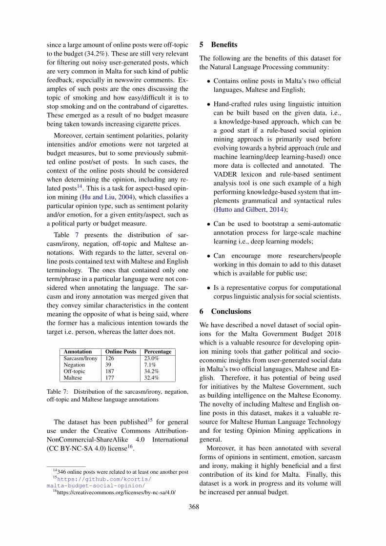
since a large amount of online posts were off-topicto the budget (34.2%). These are still very relevantfor filtering out noisy user-generated posts, whichare very common in Malta for such kind of publicfeedback, especially in newswire comments. Ex-amples of such posts are the ones discussing thetopic of smoking and how easy/difficult it is tostop smoking and on the contraband of cigarettes.These emerged as a result of no budget measurebeing taken towards increasing cigarette prices.

Moreover, certain sentiment polarities, polarityintensities and/or emotions were not targeted atbudget measures, but to some previously submit-ted online post/set of posts. In such cases, thecontext of the online posts should be consideredwhen determining the opinion, including any re-lated posts14. This is a task for aspect-based opin-ion mining (Hu and Liu, 2004), which classifies aparticular opinion type, such as sentiment polarityand/or emotion, for a given entity/aspect, such asa political party or budget measure.

Table 7 presents the distribution of sar-casm/irony, negation, off-topic and Maltese an-notations. With regards to the latter, several on-line posts contained text with Maltese and Englishterminology. The ones that contained only oneterm/phrase in a particular language were not con-sidered when annotating the language. The sar-casm and irony annotation was merged given thatthey convey similar characteristics in the contentmeaning the opposite of what is being said, wherethe former has a malicious intention towards thetarget i.e. person, whereas the latter does not.

Annotation Online Posts PercentageSarcasm/Irony 126 23.0%Negation 39 7.1%Off-topic 187 34.2%Maltese 177 32.4%

Table 7: Distribution of the sarcasm/irony, negation,off-topic and Maltese language annotations

The dataset has been published15 for generaluse under the Creative Commons Attribution-NonCommercial-ShareAlike 4.0 International(CC BY-NC-SA 4.0) license16.

14346 online posts were related to at least one another post15https://github.com/kcortis/

malta-budget-social-opinion/16https://creativecommons.org/licenses/by-nc-sa/4.0/

5 Benefits

The following are the benefits of this dataset forthe Natural Language Processing community:

• Contains online posts in Malta’s two officiallanguages, Maltese and English;

• Hand-crafted rules using linguistic intuitioncan be built based on the given data, i.e.,a knowledge-based approach, which can bea good start if a rule-based social opinionmining approach is primarily used beforeevolving towards a hybrid approach (rule andmachine learning/deep learning-based) oncemore data is collected and annotated. TheVADER lexicon and rule-based sentimentanalysis tool is one such example of a highperforming knowledge-based system that im-plements grammatical and syntactical rules(Hutto and Gilbert, 2014);

• Can be used to bootstrap a semi-automaticannotation process for large-scale machinelearning i.e., deep learning models;

• Can encourage more researchers/peopleworking in this domain to add to this datasetwhich is available for public use;

• Is a representative corpus for computationalcorpus linguistic analysis for social scientists.

6 Conclusions

We have described a novel dataset of social opin-ions for the Malta Government Budget 2018which is a valuable resource for developing opin-ion mining tools that gather political and socio-economic insights from user-generated social datain Malta’s two official languages, Maltese and En-glish. Therefore, it has potential of being usedfor initiatives by the Maltese Government, suchas building intelligence on the Maltese Economy.The novelty of including Maltese and English on-line posts in this dataset, makes it a valuable re-source for Maltese Human Language Technologyand for testing Opinion Mining applications ingeneral.

Moreover, it has been annotated with severalforms of opinions in sentiment, emotion, sarcasmand irony, making it highly beneficial and a firstcontribution of its kind for Malta. Finally, thisdataset is a work in progress and its volume willbe increased per annual budget.

368

References2018. Social media usage trends in malta in 2018. The

Malta Independent.

Lea Canales Zaragoza. 2018. Tackling the challenge ofemotion annotation in text.

Claire Caruana. 2018. Just 10 per cent of maltese arenot on social media. Times of Malta.

Jacob Cohen. 1960. A coefficient of agreement fornominal scales. Educational and psychologicalmeasurement, 20(1):37–46.

Laurence Devillers, Laurence Vidrascu, and LoriLamel. 2005. Challenges in real-life emotion anno-tation and machine learning based detection. NeuralNetworks, 18(4):407–422.

William D. Eggers, Neha Malik, and Matt Gracie.2019. Using ai to unleash the power of unstructuredgovernment data. Deloitte Insights.

Paul Ekman. 1992. An argument for basic emotions.Cognition & emotion, 6(3-4):169–200.

Eurostat. 2017. Living online: what the internet is usedfor.

Eurostat. 2018. Almost 75 % of enterprises in maltause social media.

Herman Grech. 2019. Here’s the bad news. Times ofMalta.

Minqing Hu and Bing Liu. 2004. Mining and summa-rizing customer reviews. In Proceedings of the tenthACM SIGKDD international conference on Knowl-edge discovery and data mining, pages 168–177.ACM.

Rocıo B Hubert, Elsa Estevez, Ana Maguitman, andTomasz Janowski. 2018. Examining government-citizen interactions on twitter using visual and senti-ment analysis. In Proceedings of the 19th Annual In-ternational Conference on Digital Government Re-search: Governance in the Data Age, page 55.ACM.

Clayton J Hutto and Eric Gilbert. 2014. Vader: A par-simonious rule-based model for sentiment analysisof social media text. In Eighth international AAAIconference on weblogs and social media.

Evangelos Kalampokis, Michael Hausenblas, and Kon-stantinos Tarabanis. 2011. Combining social andgovernment open data for participatory decision-making. In International Conference on ElectronicParticipation, pages 36–47. Springer.

Saif M Mohammad and Peter D Turney. 2013. Crowd-sourcing a word–emotion association lexicon. Com-putational Intelligence, 29(3):436–465.

Fathoni A Musyaffa, Lavdim Halilaj, Yakun Li, Fab-rizio Orlandi, Hajira Jabeen, Soren Auer, and Maria-Esther Vidal. 2018. Openbudgets. eu: A platformfor semantically representing and analyzing openfiscal data. In International Conference on Web En-gineering, pages 433–447. Springer.

Robert Plutchik. 1980. Chapter 1 - a general psycho-evolutionary theory of emotion. In Robert Plutchikand Henry Kellerman, editors, Theories of Emotion,pages 3 – 33. Academic Press.

369


The Fallacy of Echo Chambers: Analyzing the Political Slants ofUser-Generated News Comments in Korean MediaJiyoung Han1, Youngin Lee1, Junbum Lee2, Meeyoung Cha3 1

1Korea Advanced Institute of Science and Technology (KAIST), Daejeon, Korea2Seoul National Univ. of Education, Seoul, Korea3Institute for Basic Science (IBS), Daejeon, Korea

[email protected], [email protected],[email protected], [email protected]

Abstract

This study analyzes the political slants ofuser comments on Korean partisan media. Webuilt a BERT-based classifier to detect politicalleaning of short comments via the use of semi-unsupervised deep learning methods that pro-duced an F1 score of 0.83. As a result of clas-sifying 21.6K comments, we found the highpresence of conservative bias on both conser-vative and liberal news outlets. Moreover, thisstudy discloses an asymmetry across the par-tisan spectrum in that more liberals (48.0%)than conservatives (23.6%) comment not onlyon news stories resonating with their politi-cal perspectives but also on those challengingtheir viewpoints. These findings advance thecurrent understanding of online echo cham-bers.

1 Introduction

User-generated news comments manifest the in-teractive and participatory nature of online jour-nalism. Unlike letters to the editor, the commentssection allows readers to express their thoughtsand feelings in response to news stories theyread more publicly and instantaneously. Moreover,comments themselves generate subsequent userreactions from others. For example, in South Ko-rea, news portals wherein the vast majority con-sume news online displays the list of “most com-mented” articles along with the “most viewed”news stories. This aggregation of user responses isa major contributing factor toward news selection(KPF, 2018). As such, real-time user reactions,rather than the cover stories of newspapers, nowtell people what to read and think about, signify-ing the shift of the traditional direction of agenda-setting (Lee and Tandoc, 2017).

On a related note, about 63% of South Kore-ans getting news online reported they regularlyread the comments section (DMCReport, 2013)and consider them as a valid, direct cue to public

opinion (Lee and Tandoc, 2017). Much researchhas corroborated the role of comments on the for-mation of public opinion (Springer, Engelmann,and Pfaffinger, 2015; Waddell, 2018). Nonethe-less, diverging from the massive scholarly atten-tion paid to the role of hyper-partisan news me-dia, little research has analyzed political biases ofnews comments. This study aims to fill this voidin current literature by examining political slantsof news comments as well as the overlap of com-menters across the partisan spectrum. These exam-inations will contribute to advancing the currentunderstanding of the presence of echo chambersin the realm of online news comment sections.

To analyze comments on a million scale, wetook two different approaches. First, we traineda BERT model based on news stories publishedby both liberal and conservative news outlets. Sec-ond, we expanded the seed data of human-labelednews comments with the use of user informa-tion and built a comment-specific classifier. Next,based on the best performing model, the politicalslants of 21.6K news comments were analyzed.This allows us to examine the composition of thepolitical diversity of commenters within each lib-eral and conservative news outlet. For the identi-fied liberal- or conservative-leaning commenters,we also tracked whether they leave comments onnews stories resonating with their own politicalpreferences or do so to news stories challengingtheir political viewpoints.

2 Related Work

2.1 Partisan Media and Echo Chambers

The proliferation of partisan media has invitedmuch scholarly concern about the rise of echochambers (Sunstein, 2009). As more people tuneinto news outlets congenial to their politicalviewpoints, their existing preferences reinforceand, in turn, opinion polarization and social ex-

370

tremism become prevalent (Iyengar and Hahn,2009; Stroud, 2010). The recent employment ofweb tracking technologies, however, rebuts theecho chamber hypothesis with the observationaldata showing accidental or purposeful crosscut-ting news exposure (Gentzkow and Shapiro, 2011;Flaxman, Goel, and Rao, 2016).

However, in the realms of online discussion fo-rums including online news commenting sections,to date there is no evidence opposing the extantfindings such that people are more likely to leavecomments in alignment with the other posts, thusleaving user commenting sections homogeneous(Lee and Jang, 2010; Hsueh, Yogeeswaran, andMalinen, 2015). Interestingly, whereas user com-ments posted on news websites exerted consider-able power in the perceptions of individuals’ in-ference about public opinion (Lee and Jang, 2010,2010), no such effect emerged when it comes touser comments posted on news outlets’ Facebookpages (Winter, Bruckner, and Kramer, 2015).

2.2 Neural Network for Text Classification

User-contributed news comments are, by nature,informal, irregular, and erratic. To reduce the noiseof the dataset as such, many studies have adoptedvarious data cleaning methods. However, user gen-erated text is difficult to sanitize and the resultscould be misleading if we apply a naive statisticmethod. Recent NLP (natural language process-ing) research has shown that neural network ap-proaches outperform conventional statistical mod-els. For instance, TextCNN (Kim, 2014) gainedperformance in text classification tasks via intro-ducing convolutional layers and BERT (Devlin,Chang, Lee, and Toutanova, 2018) shows state-of-the-art results via its bidirectional transformernetwork, and it shows Modern text classificationmethods utilize pretrained models like BERT byfine-tuning them on the target NLP domain.

3 Data Collection

Using “minimum wage” as a keyword, we crawlednews stories and their associated user commentson NAVER, the top news portal site in South Ko-rea. The platform offers its own user comment-ing section and ten times more Internet usersare known to read news on NAVER comparedto individual news websites. From January toJuly of 2019, 1534 articles from three conser-vative news outlets–Chosun Ilbo, Joongang Ilbo,

and Donga Ilbo–and 765 from thee progres-sive ones–Hankyoreh, Kyunghyang Shinmun, andOhMyNews–were collected, with a total of 2299news stories.

We collected press releases of the two major po-litical parties in South Korea–the liberal Demo-cratic Party of Korea and the conservative Lib-erty Korea Party–containing the phrase “minimumwage.” This data serves as the basis for learn-ing partisan framing and for filtering out irrele-vant topics that might create noise in determin-ing the political stance of news comments. Weperformed part-of-speech tagging on the press re-leases and analyzed the frequency of nouns andbigrams. From the list of nouns and bigrams ap-pearing more than a hundred times, the authorscarefully examined and selected phrases that wererelevant. In this way, the list of related keywords(i.e., nouns and bigrams) on the minimum wagewas compiled for the liberal and conservative par-ties, respectively. This list includes a wide rangeof phrases relevant to politics in general, suchas inter-Korean summit, denuclearization, corrup-tion, flexible working hours, labor union, and un-employment rates.

Online news comments were also collectedfrom NAVER’s top “most commented” storieson each of seven major news sections includingnational, politics, economy, culture, world, andlifestyle, resulting in a total of 210 most com-mented news stories per day. These news storiesreceived around 38 million news comments by 1.8million unique users. This data contains text con-tent as well as user identifiers.

4 Language Models

4.1 Classification from News Articles

We first built a classifier trained on news articlesin order to observe how well news articles couldproxy comments in the task of political bias clas-sification. To compensate for the relatively smallnews article dataset, we spliced the news articlesinto individual sentences and then filtered in sen-tences that included at least one of the identifiedpartisan-specific keywords. Two hundred conser-vative and liberal articles (100 each) were set asidefor validation tests. The remaining 2,099 articleswere spliced sentences, resulting in 49.8K sen-tences. Each sentence was labeled as either con-servative or liberal based on the political leaningof the news outlets. The completed dataset con-

371

sists of 20.3K liberal and 29.5K conservative sen-tences.

Using the BERT-based pre-trained model forthe Korean language, KorBERT1, we trained aclassifier for binary classification task of news sen-tences. Test data composed of the 200 news ar-ticles mentioned above (i.e., 100 each from lib-eral and conservative news outlets). Test sets werefurther prepared in two different manners: (1)the HEADLINE representation includes headlinesonly of the labeled data and (2) the BODY-TEXTrepresentation includes only sentences containingpartisan-specific keywords in the news body text.The former representation was considered sincepolitical slant are known to be more apparent innews headlines.

4.2 Classification from News Comments

We also built another language model that istrained on the slants of news comments directly.To obtain labels, we randomly sampled 4,827 usercomments that had been posted to stories on theminimum wage and employed three coders. Thesecoders labeled each comment as liberal, conser-vative, or other (including nuetral). After a seriesof training sessions, coders could achieve an ac-ceptable inter-coder reliability (Krippendorff’s al-pha = .7015). Coders next independently labeledthe rest. This human-labeled dataset consisted of1,345 liberal (27.6%), 1,597 conservative (32.8%),and 1,930 other (39.6%) comments.

To ensure sufficient training data, we expandedthe comment labels by a semi-unsupervisedmethod. All online users who had authored at leasttwo comments in the human-labeled dataset wereidentified. The bias of each user was computed asthe mean of their comment labels, where scoresare -1 for a liberal comment and +1 for a conser-vative. We selected those users whose mean biasscore was below -0.8 or above 0.8 and identified250 such users, whose political leaning could berecognized. We then collected all comments au-thored by the 250 users from the entire news cor-pus of 6 months. Under the assumption that the po-litical stance of these users would be constant dur-ing this time period, we labeled these commentswith the author’s computed political bias. The fi-nal dataset contained a total of 93,565 comments,out of which 17,535 were liberal and 76,030 wereconservative.

1http://aiopen.etri.re.kr/

The expanded comment labels were used totrain two NLP models: TextCNN and BERT. Weundersampled 17,535 conservative comments tobalance the labels, resulting in a total of 35,070labels. We set aside 10% of labels as the test set,then split the remainder into 10% of the validationset and 90% of the train set to train the models.

The TextCNN-based model employed paddingup to 300 characters, which is the maximum lengthof comments on NAVER. Comments were tok-enized on character level and fed into an embed-ding layer of 300 dimensions. The model useda single-dimensional CNN with the channels ofsizes 5, 10, 15, and 20, respectively. Then the datawere fed into the max-pooling layer with a dropoutratio of 0.5 and classified through a linear layer.We used Adam optimizer with the default learningrate (1e-3) and trained six epochs, as validationloss did not converge. For the second model, weagain utilized the pretrained BERT model for theKorean language, KorBERT. Comments were tok-enized by words and padded to a size of 70. Themodel converged after two epochs with a higherlearning rate (1e-3), with the lowest loss.

5 Results

5.1 Bias ClassificationAfter training the BERT classifier on news sen-tence labels, we evaluated the model by classify-ing political slants of the HEADLINE and BODY-TEXT representations into liberal and conserva-tive labels. The performance of the classifiers wasmeasured in terms of Matthew’s correlation coef-ficient, accuracy, and F1-scores. Table 1 summa-rizes the results, which shows the BODY-TEXTrepresentation of the validation set showed the bestresult. The slant detection model trained on newsarticle data, however, was not effective in detect-ing slant of user-contributed comments, indicatedby the low F1 score of 0.3571.

Test set Matthew’s Accuracy F1

HEADLINE 0.7825 0.8900 0.8942BODY-TEXT 0.8202 0.9100 0.9109

Comments -0.0844 0.4600 0.3571

Table 1: Performance of Article Bias Classifier

When comment labels were utilized for train-ing, existing language models could success-fully detect the slant of news comments, as dis-

372

Figure 1: The proportion of liberal and conservative news comments within the progressive and conser-vative media’s comment sections

played in Table 2. BERT-based model outper-formed TextCNN model in this domain-specificlearning task.

Models Matthew’s Accuracy F1

TextCNN 0.5087 0.7516 0.7684BERT 0.6644 0.8322 0.8322

Table 2: Performance of Comment Bias Classifier

5.2 Bias Distribution in User Comments

We analyzed the distribution of political slantsin the comment sections. From the set of newsarticles on minimum wage, we inferred politi-cal bias labels for the comments of all articlespublished by the aforementioned major outletswith the best-performing model (i.e., BERT-basedmodel trained on comment labels) and used it toderive a statistic on bias distribution.

Fig 1 shows the percentage of liberal and con-servative comments for each news outlet based onthe labels inferred. The figure demonstrates a clearpresence of conservative bias in user commentsacross all partisan news media; Even for the bot-tom three liberal outlets, more news comments areconservative-leaning, as opposed to the widely ac-cepted echo chamber conjecture in digital media.

6 Discussion & Conclusion

The slant classifier trained on news articles relatedto the minimum wage issue performed well onsimilar news articles. However, the same modelperformed poorly in the comments section. Thismay be due to the unstructured nature of the user-generated data that is very different from editori-alized news content. The slant classifiers trainedon the labeled comment data, however, showedpromising performance on classifying the politicalbias of crowd-generated comments.

The analysis in this paper revealed that the ma-jority of user comments are pro-conservatives inKorean news outlets, although conservative par-tisan media attracted more congenial comments(71.1% conservative versus 28.9% liberal) thanliberal ones (46.4% liberal versus 53.6% conser-vative). This finding may suggest the fallacy of on-line echo chambers in Korean news media.

We do not, however, argue that the prominentcrossover, of news commenters in both liberal andconservative news stories, represents that onlineusers in South Korea have established a more bal-anced news reading habits nor have disrupted the“filter bubble.” Notably, because a recent study in-dicated that being exposed to opposing views cansometimes backfire and further increase polariza-tion (Bail et al., 2018).

Moreover, the auxiliary analyses tracking userIDs further showed that less than half of liberals

373

(48.0%) and conservatives (23.6%) commented onboth congenial and uncongenial partisan news out-lets. This finding provides imperative insights tothe current understanding of online political dis-cussions in the era of partisan media.

This work bares several limitations that can beimproved. First, the expanded comments datasetthat was built from human-labeled news com-ments could be validated further. While we as-sumed people’s slant remains consistent over ahalf a year, there is a chance that the political slantof commenters could differ by news topics. Sec-ond, while this paper utilized data from contrib-utors who post news comments frequently, futuremethods could also consider data from one-timecommenters. Such methods could reveal the politi-cal slant map of comments more comprehensively.

References

Bail, C. A., Argyle, L. P., Brown, T. W., Bum-pus, J. P., Chen, H., Hunzaker, M. B. F., . . .Volfovsky, A. (2018). Exposure to oppos-ing views on social media can increase po-litical polarization. Proceedings of the Na-tional Academy of Sciences.

Devlin, J., Chang, M.-W., Lee, K., & Toutanova,K. (2018). Bert: Pre-training of deep bidi-rectional transformers for language under-standing. arXiv preprint arXiv:1810.04805.

DMCReport. (2013). Online news consumption inkorea. DMC report 2013.

Flaxman, S., Goel, S., & Rao, J. M. (2016).Filter bubbles, echo chambers, and onlinenews consumption. Public opinion quar-terly, 80(S1), 298–320.

Gentzkow, M. & Shapiro, J. M. (2011). Ideo-logical segregation online and offline. TheQuarterly Journal of Economics, 126(4),1799–1839.

Hsueh, M., Yogeeswaran, K., & Malinen, S.(2015). ‘‘leave your comment below”: Canbiased online comments influence our ownprejudicial attitudes and behaviors? HumanCommunication Research, 41(4), 557–576.

Iyengar, S. & Hahn, K. S. (2009). Red media, bluemedia: Evidence of ideological selectivityin media use. Journal of Communication,59(1), 19–39.

Kim, Y. (2014). Convolutional neural networksfor sentence classification. arXiv preprintarXiv:1408.5882.

KPF. (2018). 2018 news consumer report. Seoul:Korea Press Foundation.

Lee, E.-J. & Jang, Y. J. (2010). What do others’reactions to news on internet portal sites tellus? effects of presentation format and read-ers’ need for cognition on reality perception.Communication Research, 37(6), 825–846.

Lee, E.-J. & Tandoc, E. C. (2017). When newsmeets the audience: How audience feed-back online affects news production andconsumption. Human Communication Re-search, 43(4), 436–449.

Springer, N., Engelmann, I., & Pfaffinger, C.(2015). User comments: Motives and in-hibitors to write and read. Information,Communication & Society, 18(7), 798–815.

Stroud, N. J. (2010). Polarization and partisanselective exposure. Journal of communica-tion, 60(3), 556–576.

Sunstein, C. R. (2009). Going to extremes: Howlike minds unite and divide. Oxford Univer-sity Press.

Waddell, T. F. (2018). What does the crowd think?how online comments and popularity met-rics affect news credibility and issue impor-tance. New Media & Society, 20(8), 3068–3083.

Winter, S., Bruckner, C., & Kramer, N. C. (2015).They came, they liked, they commented:Social influence on Facebook news chan-nels. Cyberpsychology, Behavior, and So-cial Networking, 18(8), 431–436.

374


Y’all should read this!Identifying Plurality in Second-Person Personal Pronouns in English Texts

Gabriel StanovskyUniversity of Washington

Allen Institute for Artificial [email protected]

Ronen Tamari∗Hebrew University of [email protected]

Abstract

Distinguishing between singular and plural“you” in English is a challenging task whichhas potential for downstream applications,such as machine translation or coreference res-olution. While formal written English doesnot distinguish between these cases, other lan-guages (such as Spanish), as well as other di-alects of English (via phrases such as “y’all”),do make this distinction. We make use ofthis to obtain distantly-supervised labels forthe task on a large-scale in two domains. Fol-lowing, we train a model to distinguish be-tween the single/plural ‘you’, finding that al-though in-domain training achieves reason-able accuracy (≥ 77%), there is still a lotof room for improvement, especially in thedomain-transfer scenario, which proves ex-tremely challenging. Our code and data arepublicly available.1

1 Introduction

The second-person personal pronoun (e.g., “you”in English) is used by a speaker when referring toactive participants in a dialog or an event. Variouslanguages, such as Spanish, Hebrew, or French,have different words to distinguish between sin-gular “you” (referring to a single participant) andplural “you” (for multiple participants). Tradi-tionally, English has made this distinction as well.The now archaic “thou” indicated singular second-person, while “you” was reserved for plural uses.The last several hundred years, however, have seenmodern formal written English largely abandoningthis distinction, conflating both meanings into anambiguous “all-purpose you” (Maynor, 2000).

In this work, we are interested in the following∗ Work done during an internship at the Allen Institute

for Artificial Intelligence.1https://github.com/gabrielStanovsky/

yall

Figure 1: We use two sources for distant-supervisionfor singular (marked in purple) versus plural (markedin blue) second person pronouns: (a) we find colloquialuses on Twitter, and (b) through alignment with Span-ish, which formally distinguishes between the cases.

research question: How can we automatically dis-ambiguate between singular and plural “you”?

While this topic has received much attention inlinguistic literature (Jochnowitz, 1983; Tillery andBailey, 1998; Maynor, 2000; Haspelmath, 2013;Molina, 2016), it has been largely unexplored inthe context of computational linguistics, despite itspotential benefits for downstream natural languageprocessing (NLP) tasks. For example, distinguish-ing between singular and plural “you” can serveas additional signal when translating between En-glish and a language which formally makes thisdistinction. See Figure 2 where an error in inter-preting a plural “you” in the source English textresults in a non-grammatical Hebrew translation.This example can be amended by replacing “you”with the informal “you guys”.

To tackle this task, we create two large-scalecorpora annotated with distantly-supervised bi-nary labels distinguishing between singular andplural “you” in two different domains (see Fig-ure 1). First, we regard Twitter as a noisy cor-pus for informal English and automatically iden-tify speakers who make use of an informal form ofthe English plural “you”, such as “y’all” or “you

375

Figure 2: An example translation from English to Hebrew (Google Translate, Aug. 21, 2019). The first sentencedepicts wrong interpretation of “you” resulting in a non-grammatical Hebrew translation, due to wrong inflectionsof pronoun and verb (marked in red). Both issues are fixed when changing “you” to “you guys” in English in thesecond example (marked in green).

Domain Example Plurality

Twitter # goodnight #twittersphere <3 I love y’all! Including @anonimized. Even ifshe hates me. <3

Plural

(masked) # goodnight #twittersphere <3 I love you! Including @anonimized. Even ifshe hates me. <3

Twitter ! @anonimized, Happy anniversary of entering the world! Look how much youhave done!

Singular

Europarl I am terribly sorry, Mr Hansch and Mr Cox. I did not see you asking to speak. Plural

Europarl I should be very grateful, Mrs Schroedter, if you would actually include thisproposed amendment in the part relating to subsidiarity in your positive delib-erations.

Singular

Table 1: Examples from our two domains. Twitter is informal, includes hashtags, mentions (anonymized here),and plural “you” (e.g., “y’all” in the first example), which we mask as a generic “you” as shown in the second row.In contrast, Europarl is formal and “you” is used for plural (third example), as well as singular uses (last example).

guys”, which are common in American Englishspeaking communities (Katz, 2016). We record aplurality binary label, and mask the tweet by re-placing these with the generic “you”. Second, weuse the Europarl English-Spanish parallel corpus(Koehn, 2005), and identify cases where the for-mal plural Spanish second-person pronoun alignswith “you” in the English text.

Finally, we fine-tune BERT (Devlin et al., 2018)on each of these corpora. We find that contextualcues indeed allow our model to recover the correctintended use in more than 77% of the instances,when tested in-domain. Out-of-domain perfor-mance drops significantly, doing only slightly bet-ter than a random coin toss. This could indicatethat models are learning surface cues which arehighly domain-dependent and do not generalizewell.

Future work can make use of our corpus andtechniques to collect more data for this task, aswell as incorporating similar predictors in down-

stream tasks.

2 Task Definition

Given the word “you” marked in an input text, thetask of plurality identification is to make a binarydecision whether this utterance refers to:

• A single entity, such as the examples in rows2 or 4 in Table 1.

• Multiple participants, such as those referredto in the third line in Table 1.

In the following sections we collect data for thistask and develop models for its automatic predic-tion.

3 Distant Supervision: The y’all Corpus

Manually collecting data for this task on a large-scale is an expensive and involved process. In-stead, we employ different techniques to obtaindistantly supervised labels in two domains, as

376

Twitter Europarl

Train 58963 11249Dev 7370 1405Test 7370 1405Total 73703 14059

Table 2: Number of instances in our two corpora. Eachof the partitions (train, dev, test) is equally split be-tween plural and singular second-person personal pro-nouns.

elaborated below. These are then randomly splitbetween train (80% of the data), development, andtest (10% each). See Table 2 for details about eachof these datasets, which we make publicly avail-able.

3.1 The Twitter DomainAs mentioned in the Introduction, English speak-ing communities tend to maintain the singular ver-sus plural “you” distinction by introducing id-iosyncratic phrases which specifically indicate aplural pronoun, while reserving “you” for the sin-gular use-case. We operationalize this observationon a large Twitter corpus (Cheng et al., 2010) inthe following manner:

• First, we identify speakers who use an infor-mal plural “you” at least once in any of theirtweets.2

• Following, we assume that these users speakan English dialect which distinguishes be-tween singular and plural second-person pro-nouns, interpreting their “you” as a singularpronoun. See the first two tweets in Table 1,for an example of these two uses by the sameuser.

• Finally, we mask out the plural pronoun ineach of their tweets by replacing it with ageneric “you” (see the second row in Table1). This allows us to test whether modelscan subsequently rely on contextual cues torecover the original intention.

This process yields about 36K plural instances,which we augment with 36K singular instancesfrom the same users, to obtain a corpus which isbalanced between the two classes.

2We use a fixed list of informal plural “you”, in-cluding you guys, y’all and youse. See https://en.wikipedia.org/wiki/You#Informal_plural_forms for the complete list.

Figure 3: Histogram distribution of informal plural“you” forms in the development partition of our Twittercorpus.

Figure 4: Variation in the most common phrase usedfor plural “you” in our Twitter corpus across states inthe continental United States.

Data analysis Our Twitter corpus was com-posed of U.S. based users, and included geo-locations for 36.8K of the plural tweets. This al-lows for several interesting observations. First,Figure 3 shows the distribution of informal plu-ral “you” phrases in our corpus (before masking).Second, using the tweets geo-location, we canplot the geographical variation in usage. Figure 4shows the most common term for plural “you” ineach state in the continental United States. Whilemost of the U.S. prefers “you guys”, southernstates (such as Texas or Louisiana) prefer “y’all”.Katz (2016) reached similar conclusions througha large-scale online survey. Interestingly, our sur-vey of Twitter usage differs from theirs for severalMidwestern states, such as Wyoming or Nebraska.

Quality estimation. We evaluate the assump-tion we made above (i.e., that users reserve “you”for the singular case) by asking an English native-speaker to annotate a sample of 100 singular “you”instances from our Twitter corpus. In 70% of theinstances, the annotator agreed that these indeed

377

represent a singular “you”, leaving the other 30%to either ambiguous or inconsistent usage (i.e.,sometimes “you” is used for a plural use-case).Overall, while there is a non-negligible amount ofnoise in the Twitter domain, in Section 5 we showthat the signal is strong enough for models to pickup on and achieve good accuracy.

3.2 The Europarl Domain

Another method to obtain distant supervision forthis task is through an alignment with a languagewhich distinguishes between the two usages ofthe pronoun. To that end, we use the Spanishand English parallel texts available as part of Eu-roparl (Koehn, 2005), a large corpus containingaligned sentences from meeting transcripts of theEuropean parliament.

As these texts originate from a formal setting,we expect to find much less colloquial phrases. In-deed, the term “y’all” does not appear at all, while“you guys” appears only twice in about 2 millionsentences. Instead, we rely on the gold alignmentwith Spanish sentences, which have a formal plu-ral “you” - ustedes or vosotros. We find Spanishsentences which have exactly one plural “you” andwhich aligns with an English sentence containingexactly one “you”. This process yields about 7Ksentences which we mark with a “plural” label.Similarly to the Twitter domain, we augment thesewith the same amount of singular “you”, foundin the same manner; by tracing a Spanish singu-lar “you” to a single English “you”. This processyields a balanced binary corpus.

Quality estimation We sampled 100 instancesfrom the Europarl domain to estimate the qualityof our binary labels. Unlike the Twitter domain, inEuroparl we rely on gold alignments and cleanertext. As a result, we found that about 90% of thelabels agree with a human annotator, while the re-maining 10% were ambiguous.

3.3 Discussion

The distinction between plural and singular “you”in English is an instance of a more general phe-nomenon. Namely, semantic features are ex-pressed in varying degrees of lexical or grammati-cal explicitness across different languages.

For instance, languages vary in grammati-cal tense-marking (Wolfram, 1985), from lan-guages with no morphological tense, such asMandarin (Wang and Sun, 2015), to languages

test→ Europarl Twittertrain ↓Europarl 77.1 56.8Twitter 56.3 83.1Joint 77.5 82.8

Table 3: Accuracy (percent of correct predictions) ofour fine-tuned BERT model, tested both in- and out-of-domain. Rows indicate train corpus, columns indicatetest corpus. Bold numbers indicate best performanceon test corpus.

with 9 different tense-marking morphological in-flections (Comrie, 1985). Similarly, languagesvary in gender-marking in pronouns, from gender-less Turkish, to languages with six genders ormore (Awde and Galaev, 1997).

The two data collection methods we presentedhere, finding colloquial explicit utterances on so-cial media, and alignment with another language,may also be applicable to some of these phenom-ena and present an interesting avenue for futurework.

4 Model

We fine-tune the BERT-large pretrained embed-dings (Devlin et al., 2018)3 on the training par-tition of each of our domains (Twitter and Eu-roparl), as well as on a concatenation of both do-mains (Joint). We then classify based on the [CLS]token in each of these instances. We use a fixedlearning rate of 2e − 5 and a batch size of 24.Training for 10 Epochs on a Titan X GPU tookabout 3 hours for the Twitter domain, 2 hours forthe Europarl domain and roughly 5 hours for theJoint model.

5 Evaluation

We test models trained both in and out of domainfor both parts of our dataset (Twitter and Europarl)as well as a joint model, trained on both partsof the dataset. We use accuracy (percent of cor-rect predictions), as our dataset is binary and bothclasses are symmetric and evenly distributed. Ourmain findings are shown in Table 3. Following,several observations can be made.

3Using Hugging Face’s implementation:https://github.com/huggingface/pytorch-transformers

378

In-domain performance does significantly bet-ter than chance. For both domains, BERTachieves more than 77% accuracy. Indicating thatthe contextual cues in both domains are meaning-ful enough to capture correlations with plural andsingular uses.

Out-of-domain performance is significantly de-graded. We see significant drop in performancewhen testing either model on the other part of thedataset. Both models do only slightly better thanchance. This may indicate that the cues for plural-ity are vastly different between the two domains,probably due to differences in vocabulary, tone, orformality.

Training jointly on the two domains maintainsgood performance, but does not improve uponit. A model trained on both the Twitter and Eu-roparl domains achieves the in-domain perfor-mance of each of the individual in-domain mod-els, but does not improve over them. This mayindicate that while BERT is expressive enough tomodel both domains, it only picks up on surfacecues in each and does not generalize across do-mains. As a result, robustness is questionable forout-of-domain instances.

6 Related Work

Several previous works have touched on relatedtopics. A few works developed models for under-standing the second-person pronoun within coref-erence resolution frameworks (Purver et al., 2009;Zhou and Choi, 2018). Perhaps most related toour work is Gupta et al. (2007), who have tack-led the orthogonal problem of disambiguation be-tween generic (or editorial) “you” and referential“you”.

To the best of our knowledge, we are the first todeal with plurality identification in second-personpersonal pronouns in English.


We presented the first corpus for the identificationof plurality in second-person personal pronouns inEnglish texts. Labels were collected on a largescale from two domains (Twitter and Europarl) us-ing different distant-supervision techniques.

Following, a BERT model was fine-tuned on thelabeled data, showing that while models achievereasonable in-domain performance, they signifi-cantly suffer from domain transfer, degrading per-

formance close to random chance. Interesting av-enues for future work may be to extend this data tonew domains, develop more complex models forthe task (which may achieve better cross-domainperformance), and integrating plurality models indownstream tasks, such as machine translation orcoreference resolution.

Acknowledgements

We thank the anonymous reviewers for their manyhelpful comments and suggestions.

ReferencesNicholas Awde and Muhammad Galaev. 1997.

Chechen-English English-Chechen: Dictionary andPhrasebook. Hippocrene Books.

Zhiyuan Cheng, James Caverlee, and Kyumin Lee.2010. You are where you tweet: a content-basedapproach to geo-locating twitter users. In CIKM.

Bernard Comrie. 1985. Tense, volume 17. Cambridgeuniversity press.

Jacob Devlin, Ming-Wei Chang, Kenton Lee, andKristina Toutanova. 2018. BERT: Pre-training ofdeep bidirectional transformers for language under-standing. In NAACL-HLT.

Surabhi Gupta, Matthew Purver, and Dan Jurafsky.2007. Disambiguating between generic and refer-ential you in dialog. In Proceedings of the 45th An-nual Meeting of the Association for ComputationalLinguistics Companion Volume Proceedings of theDemo and Poster Sessions, pages 105–108.

Martin Haspelmath. 2013. Politeness distinctions insecond-person pronouns. In The Atlas of Pidgin andCreole Language Structures, pages 68–71. OxfordUniv. Pr.

George Jochnowitz. 1983. Another view of you guys.American Speech, 58(1):68–70.

Josh Katz. 2016. Speaking American: How Y’all,Youse, and You Guys Talk: A Visual Guide.Houghton Mifflin Harcourt.

Philipp Koehn. 2005. Europarl: A parallel corpus forstatistical machine translation.

Natalie Maynor. 2000. Battle of the pronouns: Y’allversus you-guys. American speech, 75(4):416–418.

Ralph Molina. 2016. Y’all, This Paper Is Crazy Inter-esting: A Study of Variation in US English. Ph.D.thesis.

Matthew Purver, Raquel Fernandez, Matthew Framp-ton, and Stanley Peters. 2009. Cascaded lexicalisedclassifiers for second-person reference resolution.

379

In Proceedings of the SIGDIAL 2009 Conference:The 10th Annual Meeting of the Special InterestGroup on Discourse and Dialogue, pages 306–309.Association for Computational Linguistics.

Jan Tillery and Guy Bailey. 1998. Yall in oklahoma.

William SY Wang and Chaofen Sun. 2015. The Oxfordhandbook of Chinese linguistics. Oxford UniversityPress.

Walt Wolfram. 1985. Variability in tense mark-ing: A case for the obvious. Language Learning,35(2):229–253.

Ethan Zhou and Jinho D Choi. 2018. They exist! in-troducing plural mentions to coreference resolutionand entity linking. In Proceedings of the 27th Inter-national Conference on Computational Linguistics,pages 24–34.

380


An Edit-centric Approach for Wikipedia Article Quality Assessment

Edison Marrese-Taylor1, Pablo Loyola2, Yutaka Matsuo1

Graduate School of Engineering, The University of Tokyo, Japan1

{emarrese, matsuo}@weblab.t-utokyo.ac.jpIBM Research, Tokyo, Japan2

[email protected]

Abstract

We propose an edit-centric approach to as-sess Wikipedia article quality as a complemen-tary alternative to current full document-basedtechniques. Our model consists of a main clas-sifier equipped with an auxiliary generativemodule which, for a given edit, jointly pro-vides an estimation of its quality and gener-ates a description in natural language. We per-formed an empirical study to assess the fea-sibility of the proposed model and its cost-effectiveness in terms of data and quality re-quirements.

1 Introduction

Wikipedia is arguably the world’s most famousexample of crowd-sourcing involving natural lan-guage. Given its open-edit nature, article oftenend up containing passages that can be regardedas noisy. These may be the indirect result of be-nign edits that do not meet certain standards, ora more direct consequence of vandalism attacks.In this context, assessing the quality of the largeand heterogeneous stream of contributions is crit-ical for maintaining Wikipedia’s reputation andcredibility. To that end, the WikiMedia Foun-dation has deployed a tool named ORES (Hal-faker and Taraborelli, 2015) to help monitor articlequality, which treats quality assessment as a su-pervised multi-class classification problem. Thistool is static, works at the document-level, and isbased on a set of predefined hand-crafted features(Warncke-Wang et al., 2015).

While the ORES approach seems to work ef-fectively, considering the whole document couldhave negative repercussions. As seen on Figure1, article length naturally increases over time (seeAppendix A.1 for additional examples), whichcould lead to scalability issues and harm predic-tive performance, as compressing a large amount

2003 2005 2007 2009 2011 2013 2015Time

0

100000

200000

300000

Num

ber o

f cha

ract

ers

Length of United States's Articles/EditsEditVersion

Figure 1: Monthly average of the article/edits length(in number of characters) for the United States article.

of content into hand crafted features could dimin-ish their discriminative power. We conducted anexploratory analysis using a state-of-the-art (Dangand Ignat, 2016) document-level approach, findingthat there is a clear negative relationship betweendocument length and model accuracy (see detailson Appendix A.2).

In light of this, we are interested in exploringa complementary alternative for assessing articlequality in Wikipedia. We propose a model that re-ceives as input only the edit, computed as the dif-ference between two consecutive article versionsassociated to a contribution, and returns a measureof article quality. As seen on Figure 1, edit lengthsexhibit a more stable distribution over time.

Moreover, as edits are usually accompanied bya short description which clarifies their purposeand helps with the reviewing process (Guzmanet al., 2014), we explore whether this informa-tion could help improve quality assessment by alsoproposing a model that jointly predicts the qualityof a given edit and generates a description of itin natural language. Our hypothesis is that whileboth tasks may not be completely aligned, thequality aspect could be benefited by accounting forthe dual nature of the edit representation.

We performed an empirical study on a set ofWikipedia pages and their edit history, evaluatingthe feasibility of the approach. Our results showthat our edit-level model offers competitive re-

381

sults, benefiting from the proposed auxiliary task.In addition to requiring less content as input, webelieve our model offers a more natural approachby focusing on the actual parts of the documentsthat were modified, ultimately allowing us to tran-sition from a static, document-based approach,to an edit-based approach for quality assessment.Our code and data are available on GitHub1.

2 Related Work

In terms of quality assessment, the pioneer workof Hu et al. (2007) used the interaction betweenarticles and their editors to estimate quality, pro-posed as a classification task. Later, Kittur andKraut (2008) studied how the number of editorsand their coordination affects article quality, whileBlumenstock (2008) proposed to use word countfor measuring article quality.

Warncke-Wang et al. (2013, 2015) took the clas-sification approach and characterized an articleversion with several hand-crafted features, train-ing a SVM-based model whose updated versionwas deployed into the ORES system. More re-cent work has experimented with models basedon representation learning, such as Dang and Ig-nat (2016) who used a doc2vec-based approach,and Shen et al. (2017) who trained an RNN to en-code the article content. While all these modelsare inherently static, as they model the content ofa version, the work of Zhang et al. (2018) is, to thebest of our knowledge, the only one to propose ahistory-based approach.

On the other hand, Su and Liu (2015) tackledthe quality problem by using a psycho-lexical re-source, while Kiesel et al. (2017) aimed at auto-matically detecting vandalism utilizing change in-formation as a primary input. Gandon et al. (2016)also validated the importance of the editing historyof Wikipedia pages as a source of information.

In addition to quality assessment, our work isalso related to generative modeling on Wikipedia.Recent work includes approaches based on au-toencoders, such as Chisholm et al. (2017), whogenerate short biographies, and Yin et al. (2019)who directly learn diff representations. Otherworks include the approach by Zhang et al. (2017)which summarizes the discussion surrounding achange in the content, and by Boyd (2018) whoutilizes Wikipedia edits to augment a small datasetfor grammatical error correction in German.

1github.com/epochx/wikigen

3 Proposed Approach

Our goal is to model the quality assessment taskon Wikipedia articles from a dynamic perspective.Let v1, . . . , vT be the sequence of the time-sortedT revisions of a given article in Wikipedia. Givena pair of consecutive revisions (vt−1, vt), an editet = ∆t

t−1(v) is the result of applying the Unixdiff tool over the wikitext2 contents of the revisionpair, allowing us to recover the added and deletedlines on each edition.

Due to the line-based approach of the Unix difftool, small changes in wikitext may lead to bigchunks (or hunks) of differences in the resultingdiff file. Moreover, as changes usually occur at thesentence level, these chunks can contain a consid-erable amount of duplicated information. To moreaccurately isolate the introduced change, we seg-ment the added and removed lines on each hunkinto sentences, and eliminate the ones appearingboth in the added and removed lines. Whenevermultiple sentences have been modified, we usestring matching techniques to identify the before-after pairs. After this process, et can be charac-terized with a set of before-after sentence pairs(s−ti , s

+ti), where s+ti is an empty string in case of

full deletion, and vice-versa.Similarly to Yin et al. (2019), to obtain a fine-

grained characterization of the edit, we tokenizeeach sentence and then use a standard diff algo-rithm to compare each sequence pair. We thus ob-tain an alignment for each sentence pair, which inturn allows us to identify the tokens that have beenadded, removed, or remained unchanged. For eachcase, we build an edit-sentence based on the align-ment, containing added, deleted and unchangedtokens, where the nature of each is characterizedwith the token-level labels +, − and =, respec-tively.

For a given edit et we generate an edit represen-tation based on the contents of the associated diff,and then use it to predict the quality of the articlein that time. We follow previous work and treatquality assessment as a multi-class classificationtask, with labels Stub ≤ Start ≤ C ≤ B ≤ GA ≤FA. We consider a training corpus with T edits et,1 ≤ t ≤ T .

Our quality assessment model encodes the in-put edit-sentence using a BiLSTM. Concretely, weuse a token embedding matrix ET to represent theinput tokens, and another embedding matrix EL

2mediawiki.org/wiki/Wikitext

382

to represent the token-level labels. For a givenembedded token sequence Xt and embedded labelsequence Lt, we concatenate the vectors for eachposition and feed them into the BiLSTM to cap-ture context. We later use a max pooling layer toobtain a fixed-length edit representation, which isfed to the classifier module.

3.1 Incorporating Edit Message Information

When a user submits an edit, she can add a shortmessage describing or summarizing it. We are in-terested in studying how these messages can beused as an additional source to support quality as-sessment task. A natural, straightforward way toincorporate the message into our proposal is to en-code it into a feature vector using another BiLSTMwith pooling, and combine this with the featureslearned from the edit.

Furthermore, we note that the availability ofan edit message actually converts an edit into adual-nature entity. In that sense, we would liketo study whether the messages are representativeconstructs of the actual edits, and how this rela-tion, if it exists, could impact the quality assess-ment task. One way to achieve this is by learninga mapping between edits and their messages.

Therefore, we propose to incorporate the editmessages by adding an auxiliary task that consistsof generating a natural language description of agiven edit. The idea is to jointly train the clas-sification and the auxiliary task to see if the per-formance on quality assessment improves. Ourhypothesis is that while both tasks are not natu-rally aligned, the quality aspect could benefit byaccounting for the dual nature of the edit repre-sentation.

Our proposed generative auxiliary task is mod-eled using a sequence-to-sequence (Sutskeveret al., 2014; Cho et al., 2014) with global atten-tion (Bahdanau et al., 2015; Luong et al., 2015)approach, sharing the encoder with the classifier.During inference, we use beam search and let thedecoder run for a fixed maximum number of steps,or until the special end-of-sentence token is gener-ated. This task is combined with our main clas-sification task using a linear combination of theirlosses, where parameter λ weights the importanceof the classification loss. Figure 2 shows how themodel with the auxiliary task looks like.

E(1) E(2) E(3)

A

Changed his

NN

D(2) D(3)D(1)

NN NN

birthday

E(4)

== - +

inBorn 1978 1980

FA (Featured Article)

NN

Auxiliary Generative Task

max

Figure 2: Proposed model with the addition of the mod-ule for the auxiliary generative task.

4 Empirical Study

We collected historical dumps from Wikipedia,choosing some of the most edited articles for boththe English and German languages. Wikipediadumps contain every version of a given page inwikitext, along with metadata for every edit. Toobtain the content associated to each ∆t

t−1(v),we sorted the extracted edits chronologically andcomputed the diff of each pair of consecutive ver-sions using the Unix diff tool. We ignore ed-its with no accompanying message. For Englishsentence splitting we used the automatic approachby Kiss and Strunk (2006), and Somajo (Proisland Uhrig, 2016) for German. The quality la-bels are obtained using the ORES API, the officialplatform of the WikiMedia Foundation to performquality assessment. This platform is built upon arandom forest classifier with 100 trees (Warncke-Wang et al., 2015), which when trained on a smallcorpus of 2,272 random articles obtained an F1-Score of 0.425. The API gives us a probabilitydistribution over the quality labels for each revi-sion, which in this work we use as a silver stan-dard. We randomize and then split each datasetusing a 70/10/20 ratio.

For comparison, we also consider the Wi-kiclass dataset built by Warncke-Wang et al.(2015), which consists of 30K revisions of randomWikipedia articles paired with their manually-annotated quality classes. To use this dataset withour models, we identified and downloaded thepage revision immediately preceding each exam-ple using the Wikipedia API, to later apply theUnix diff tool and obtain the edits. We use thetrain/test splits provided and 20% of the trainingset as a validation. Other similar datasets are not

383

suitable for us as they do not include the revisionids which we require in order to obtain the edits.

4.1 Experimental SettingOn our collected datasets, the classification mod-els are trained using the Kullback-Leibler diver-gence as the loss function —which in our prelimi-nary experiments worked better than using the de-rived hard labels with cross entropy— while forthe Wikiclass dataset we used the cross entropywith the gold standard. In both cases we used ac-curacy on the validation set for hyper-parametertuning and evaluation, and also measured macro-averaged F1-Score. For the models with the auxil-iary task, we also evaluate our generated descrip-tions with sentence-level BLEU-4 (Papineni et al.,2002). All our models are trained with a maximuminput/output length of 300 tokens, a batch size of64 and a learning rate of 0.001 with Adam.

4.2 ResultsWe firstly conducted an ablation study to iden-tify the model components that have greater im-pact on the performance. We compare our edit-sentence encoder with a regular encoding mecha-nism, where the tokens from s−ti and s+ti are con-catenated (separated with a special marker token),and with a version that ignores the token-level la-bel embeddings.

Model F1 Acc BLEU

Regular 0.47 0.74 -+ edit-sentence 0.56 0.80 -

+ diff tags 0.62 0.78 -

+ Generation λ = 0.2 0.28 0.61 0.25+ Generation λ = 0.5 0.33 0.68 0.24+ Generation λ = 0.8 0.41 0.77 0.25+ Generation λ = 0.9 0.65 0.77 0.22

Only Generation (λ = 0) - - 0.23

Table 1: Impact of the parameters on validation perfor-mance for the WWII article history.

As seen on Table 1, when compared againstthe regular encoder, utilizing our edit-sentence ap-proach with token-level labels leads to a higherF1-Score and accuracy, showing the effectivenessof our proposed edit encoder. These results alsoshed some light on the trade-off between tasksfor different values of λ. We see that althougha higher value tends to give better classificationperformance both in terms of F1-Score and ac-curacy, it is also possible to see that there is asweet-spot that allows the classification to bene-fit from learning an edit-message mapping, sup-

porting our hypothesis. Moreover, this comes at anegligible variation in terms of BLEU scores, asseen when we compare against a pure message-generation task (Only Generation on the table).

On the other hand, when we tested the alter-native mechanism to combine the edit and mes-sage information simply combining their represen-tations and feeding them to the classifier, we ob-tained no performance improvements. This againsupports our choice to model the edit-messagemapping for the benefit of quality assessment.

Since we discarded edits that were not accom-panied by messages during pre-processing, it isdifficult to assess the impact that the absence ofthese messages may have on quality assessment.In those cases, we believe our model with the aux-iliary generative task could be used as a drop-inreplacement and thus help content reviewers.

DatasetModel

Validation Test

F1 Acc BL F1 Acc BL

BarackObama

C 0.50 0.92 - 0.62 0.91 -C+G 0.57 0.89 0.21 0.66 0.88 0.20

DonaldTrump

C 0.69 0.79 - 0.47 0.78 -C+G 0.69 0.76 0.22 0.47 0.77 0.20

Guns n’Roses

C 0.28 0.86 - 0.18 0.84 -C+G 0.31 0.79 0.23 0.30 0.81

Xbox 360 C 0.22 0.60 - 0.30 0.61 -C+G 0.37 0.62 0.34 0.32 0.63 0.31

Chicago C 0.36 0.71 - 0.38 0.72 -C+G 0.44 0.70 0.30 0.39 0.71 0.29

PinkFloyd

C 0.43 0.79 - 0.35 0.80 -C+G 0.46 0.80 0.34 0.37 0.80 0.35

ManchesterUnited F.

C 0.15 0.24 - 0.17 0.72 -C+G 0.29 0.79 0.43 0.39 0.77 0.43

Deutschland C 0.19 0.31 - 0.12 0.31 -C+G 0.22 0.38 0.31 0.17 0.33 0.36

ZweiterWeltkrieg

C 0.26 0.29 - 0.15 0.30 -C+G 0.29 0.32 0.35 0.18 0.30 0.28

Table 2: Summary of our results. C indicates modelsthat only perform classification, and C+G models withthe auxiliary generative task. BL is short for BLEU-4.

Table 2 summarizes our best results on each se-lected article. We see how the addition of the gen-erative task can improve the classification perfor-mance for both considered languages. In terms ofthe task trade-off, controlled with parameter λ, weempirically found that higher values tend to workbetter for datasets with more examples.

Regarding the Wikiclass dataset, we comparedour model against a state-of-the-art document-level approach (Dang and Ignat, 2016; Shen et al.,2017) based on on doc2vec (Le and Mikolov,2014). In this scenario, our model obtains an ac-

384

curacy of 0.40 on the test set, while the docu-ment level approach reaches 0.42. While the docu-ment level approach performed slightly better, ourmodel is able to obtain a reasonable performancein a more efficient manner as it requires an inputthat averages only 2K characters (the edits), whichcontrasts to the average 12K characters in the doc-uments. It is worth mentioning that the perfor-mance of the document-level approach reported byDang and Ignat (2016) significantly differs fromthe value reported here. By looking at their im-plementation3 we note that this value is obtainedwhen also using the test documents to train.

5 Conclusion and Future work

In this work we proposed a new perspective to theproblem of quality assessment in Wikipedia arti-cles, taking as central element the dynamic natureof the edits. Our results support our hypothesisand show the feasibly of the approach. We be-lieve the temporal view on the problem that theproposed approach provides could open the doorto incorporating behavioral aspects into the qualityestimation, such as user traces and reverting activ-ity, which are also critical to limit the amount ofnoise and ensure the reliability of Wikipedia.

We think our results could represent a concretecontribution in improving our understanding of theevolution knowledge bases, in terms of of bothsoftware and scientific documentation, from a lin-guistic perspective. We envision this as a toolthat could be useful for supporting documentationand quality-related tasks in collaborative environ-ments, where human supervision is insufficient ornot always available.


gio. 2015. Neural machine translation by jointlylearning to align and translate. In Proceedings of the2015 International Conference on Learning Repre-sentations, San Diego, California.

Joshua E Blumenstock. 2008. Size matters: wordcount as a measure of quality on wikipedia. InProceedings of the 17th international conference onWorld Wide Web, pages 1095–1096. ACM.

Adriane Boyd. 2018. Using Wikipedia Edits in LowResource Grammatical Error Correction. In Pro-ceedings of the 2018 EMNLP Workshop W-NUT:

3github.com/vinhqdang/doc2vec_dnn_wikipedia

The 4th Workshop on Noisy User-generated Text,pages 79–84, Brussels, Belgium. Association forComputational Linguistics.

Andrew Chisholm, Will Radford, and Ben Hachey.2017. Learning to generate one-sentence biogra-phies from wikidata. In Proceedings of the 15thConference of the European Chapter of the Associa-tion for Computational Linguistics: Volume 1, LongPapers, pages 633–642, Valencia, Spain. Associa-tion for Computational Linguistics.

Kyunghyun Cho, Bart van Merrienboer, Caglar Gul-cehre, Dzmitry Bahdanau, Fethi Bougares, HolgerSchwenk, and Yoshua Bengio. 2014. LearningPhrase Representations using RNN EncoderDecoderfor Statistical Machine Translation. In Proceed-ings of the 2014 Conference on Empirical Methodsin Natural Language Processing (EMNLP), pages1724–1734, Doha, Qatar. Association for Computa-tional Linguistics.

Q. Dang and C. Ignat. 2016. Quality assessment ofWikipedia articles without feature engineering. In2016 IEEE/ACM Joint Conference on Digital Li-braries (JCDL), pages 27–30.

F. Gandon, R. Boyer, O. Corby, and A. Monnin. 2016.Wikipedia editing history in dbpedia: Extractingand publishing the encyclopedia editing activity aslinked data. In 2016 IEEE/WIC/ACM InternationalConference on Web Intelligence (WI), pages 479–482.

Emitza Guzman, David Azocar, and Yang Li. 2014.Sentiment analysis of commit comments in github:An empirical study. In Proceedings of the 11thWorking Conference on Mining Software Reposito-ries, MSR 2014, pages 352–355, New York, NY,USA. ACM.

Aaron Halfaker and Dario Taraborelli. 2015. Artifi-cial intelligence service ores gives wikipedians x-rayspecs to see through bad edits.

Meiqun Hu, Ee-Peng Lim, Aixin Sun, Hady WirawanLauw, and Ba-Quy Vuong. 2007. Measuring articlequality in wikipedia: models and evaluation. In Pro-ceedings of the sixteenth ACM conference on Con-ference on information and knowledge management,pages 243–252. ACM.

Johannes Kiesel, Martin Potthast, Matthias Hagen, andBenno Stein. 2017. Spatio-temporal analysis of re-verted wikipedia edits.

Tibor Kiss and Jan Strunk. 2006. Unsupervised multi-lingual sentence boundary detection. Comput. Lin-guist., 32(4):485–525.

Aniket Kittur and Robert E Kraut. 2008. Harnessingthe wisdom of crowds in wikipedia: quality throughcoordination. In Proceedings of the 2008 ACM con-ference on Computer supported cooperative work,pages 37–46. ACM.

385

Quoc Le and Tomas Mikolov. 2014. Distributed rep-resentations of sentences and documents. In Inter-national Conference on Machine Learning, pages1188–1196.

Thang Luong, Hieu Pham, and Christopher D. Man-ning. 2015. Effective approaches to attention-basedneural machine translation. In Proceedings of the2015 Conference on Empirical Methods in Natu-ral Language Processing, pages 1412–1421, Lis-bon, Portugal. Association for Computational Lin-guistics.

Kishore Papineni, Salim Roukos, Todd Ward, and Wei-Jing Zhu. 2002. Bleu: a method for automatic eval-uation of machine translation. In Proceedings of40th Annual Meeting of the Association for Com-putational Linguistics, pages 311–318, Philadelphia,Pennsylvania, USA. Association for ComputationalLinguistics.

Thomas Proisl and Peter Uhrig. 2016. Somajo: State-of-the-art tokenization for german web and socialmedia texts. In Proceedings of the 9th Web as Cor-pus Workshop (WaC-X) and the EmpiriST SharedTask, pages 57–62, Berlin, Germany. Association forComputational Linguistics.

Aili Shen, Jianzhong Qi, and Timothy Baldwin.2017. A Hybrid Model for Quality Assessmentof Wikipedia Articles. In Proceedings of the Aus-tralasian Language Technology Association Work-shop 2017, pages 43–52. Event-place: Brisbane,Australia.

Q. Su and P. Liu. 2015. A psycho-lexical approach tothe assessment of information quality on wikipedia.In 2015 IEEE/WIC/ACM International Conferenceon Web Intelligence and Intelligent Agent Technol-ogy (WI-IAT), volume 3, pages 184–187.

Ilya Sutskever, Oriol Vinyals, and Quoc V Le. 2014.Sequence to sequence learning with neural net-works. In Advances in neural information process-ing systems, pages 3104–3112.

Morten Warncke-Wang, Vladislav R. Ayukaev, BrentHecht, and Loren G. Terveen. 2015. The Successand Failure of Quality Improvement Projects in PeerProduction Communities. In Proceedings of the18th ACM Conference on Computer Supported Co-operative Work & Social Computing, CSCW ’15,pages 743–756, New York, NY, USA. ACM.

Morten Warncke-Wang, Dan Cosley, and John Riedl.2013. Tell Me More: An Actionable Quality Modelfor Wikipedia. In Proceedings of the 9th Interna-tional Symposium on Open Collaboration, WikiSym’13, pages 8:1–8:10, New York, NY, USA. ACM.

Pengcheng Yin, Graham Neubig, Miltiadis Allamanis,Marc Brockschmidt, and Alexander L Gaunt. 2019.Learning to represent edits. In Proceedings of the2019 International Conference on Learning Repre-sentations.

Amy X. Zhang, Lea Verou, and David Karger. 2017.Wikum: Bridging discussion forums and wikis usingrecursive summarization. pages 2082–2096.

S. Zhang, Z. Hu, C. Zhang, and K. Yu. 2018. History-Based Article Quality Assessment on Wikipedia. In2018 IEEE International Conference on Big Dataand Smart Computing (BigComp), pages 1–8.

386


Additive Compositionality of Word Vectors

Yeon Seonwoo, Sungjoon Park, Dongkwan Kim, and Alice OhSchool of Computing, KAIST, Republic of Korea

{yeon.seonwoo, sungjoon.park, dongkwan.kim}@kaist.ac.kr,[email protected]

Abstract

Additive compositionality of word embeddingmodels has been studied from empirical andtheoretical perspectives. Existing research onjustifying additive compositionality of exist-ing word embedding models requires a ratherstrong assumption of uniform word distribu-tion. In this paper, we relax that assumptionand propose more realistic conditions for prov-ing additive compositionality, and we developa novel word and sub-word embedding modelthat satisfies additive compositionality underthose conditions. We then empirically showour model’s improved semantic representationperformance on word similarity and noisy sen-tence similarity.

1 Introduction

Previous word embedding studies have empiri-cally shown linguistic regularities represented aslinear translation in the word vector space, but theydo not explain these empirical results mathemat-ically (Mikolov et al., 2013b; Pennington et al.,2014; Bojanowski et al., 2017).

Recent studies present theoretical advances tointerpret these word embedding models. Levy andGoldberg (2014b) show that the global optimumof SGNS (Skip-Gram with Negative Sampling) isthe shifted PMI (PMI(i, j)−k). Arora et al. (2016)propose a generative model to explain PMI-baseddistributional models and presents a mathemati-cal explanation of the linguistic regularity in Skip-Gram (Mikolov et al., 2013a). Gittens et al. (2017)provide a theoretical justification of the additivecompositionality of Skip-Gram and shows that thelinguistic regularity of Skip-Gram is explained byadditive compositionality of Skip-Gram (Mikolovet al., 2013a). One property of the word vectorsthat equates to satisfying additive compositional-ity is the following:

~uc =

n∑

i=1

~uci

where word c is the paraphrase word of the set ofwords {c1, ..., cn}, and ~u is the vector representa-tion of a word. We explain additive composition-ality in more detail in section 3.3.

In this paper, we provide a more sound math-ematical explanation of linguistic regularity toovercome the limitations of previous theoreticalexplanations. For instance, Levy and Goldberg(2014b) do not provide a connection betweenshifted-PMI and linguistic regularity, and Aroraet al. (2016) and Gittens et al. (2017) requirestrong assumptions in their mathematical explana-tion about linguistic regularity. Arora et al. (2016)assume isotropy, a uniformly distributed word vec-tor space, and Gittens et al. (2017) assume a uni-form word frequency distribution within a corpus,p(w) = 1/|V |.

We propose a novel word/sub-word embeddingmodel which we call OLIVE that satisfies exactadditive compositionality. The objective functionof OLIVE consists of two parts. One is a globalco-occurrence term to capture the semantic simi-larity of words. The other is a regularization termto constrain the size of the inner product of co-occurring word pairs. We show that the globaloptimum point of OLIVE is the exact PMI ma-trix under certain condition unlike SGNS whoseoptimum approximates PMI due to the samplingprocess in training (Levy and Goldberg, 2014b).The source code and pre-trained word vectorsof OLIVE are publicly available 1. By being amore theoretically sound word embedding modelOLIVE shows improved empirical performancefor semantic representation of word vectors, andby eliminating sampling process in SGNS, OLIVEshows robustness on the size of the vocabulary

1https://github.com/yeonsw/OLIVE

387

and sentence representation performance on var-ious noisy settings. We evaluate the semantic rep-resentation performance with the word similaritytask, and we show the robustness of our model byconducting word similarity task on various vocab-ulary size and sentence similarity task on variousnoisy settings.

The contributions of our research are as follows:

• We present a novel mathematical explanationof additive compositionality of SGNS.

• We propose a word/sub-word embeddingmodel that theoretically satisfies additivecompositionality. We provide the code forthis model for reproducibility.

• In addition to theoretical justification, weshow the empirical performance of our modeland its robustness.

2 Related Work

Learning word co-occurrence distribution isknown as an effective method to capture the se-mantics of words (Baroni and Lenci, 2010; Har-ris, 1954; Miller and Charles, 1991; Bullinaria andLevy, 2007).

Based on this word co-occurrence distribution,two major types of word embedding research havebeen conducted. One is to use the local contextof words in a corpus to train a neural network(Mikolov et al., 2013a,b; Bojanowski et al., 2017;Xu et al., 2018; Khodak et al., 2018). The otheris to use the global statistics (Huang et al., 2012;Pennington et al., 2014). Aside from the generalpurpose embedding, some approaches are specificto a domain (Shi et al., 2018) or use extra humanlabeled information (Wang et al., 2018). In thispaper, we focus on the general purpose word em-bedding.

Among those, SGNS (Skip-Gram with NegativeSampling) (Mikolov et al., 2013b) and FastText(Bojanowski et al., 2017) are widely-used neu-ral network based word and sub-word embeddingmodels that use negative sampling (Gutmann andHyvarinen, 2012; Mnih and Kavukcuoglu, 2013).With the argument that global co-occurrencestatistics, overlooked in SGNS and FastText, areimportant in capturing the word semantics, Pen-nington et al. (2014) propose GloVe.

There were empirical studies of linguistic regu-larity in word embedding vector space (Levy and

Goldberg, 2014a; Socher et al., 2012; Botha andBlunsom, 2014; Mikolov et al., 2013c; Socheret al., 2013).

Although Skip-Gram and GloVe seem to cap-ture the linguistic regularity sufficiently, from thetheoretical perspective of additive compositional-ity of word vectors, both models are lacking be-cause they require extra and strong assumptions(Gittens et al., 2017; Arora et al., 2016).

Recently, (Allen and Hospedales, 2019) claimstrong assumptions in the previous word embed-ding studies (Gittens et al., 2017; Arora et al.,2016) and propose theoretical explanation aboutlinguistic regularity in SGNS based on paraphrasedefinition in (Gittens et al., 2017). Although theirtheory explains linguistic regularity in SGNS,there are remaining mathematical properties inSGNS: uniqueness of the paraphrase vector, andthe meaning of the negative sampling parameter.

In this paper, we recognize the importance ofadditive compositionality of word vectors whichconnects word vectors, and their linguistic regu-larity and we provide a novel mathematical expla-nation of SGNS’s additive compositionality anduniqueness property in additive compositionality.Further, we propose a novel word/sub-word em-bedding model that satisfies additive composition-ality based on our theory and show its capabilitiesin capturing the semantics of words.

3 Preliminaries

In this section, we describe three important con-cepts about word vectors and how they are usedin existing word embedding models. First, we de-scribe the PMI matrix which is an approximatedglobal optimum point of SGNS (Skip-Gram withNegative Sampling) (Levy and Goldberg, 2014b)and known to capture the semantic meaning ofwords in vector space (Arora et al., 2016). Second,we describe sub-sampling, a word frequency bal-ancing method to increase word embedding per-formance. Third, we describe additive composi-tionality, the notion that a paraphrase word vec-tor is a vector sum of its context word set (Gittenset al., 2017).

3.1 Objective Function

There are two major types of objective functionsused in word embedding models. One is used inSGNS and is based on the PMI; and the other isused in GloVe, based on the joint probability dis-

388

tribution of word pairs, p(w1, w2).

3.1.1 Skip-Gram with Negative SamplingSGNS iteratively trains word vectors for each co-occurring word pair in the same local context win-dow (Mikolov et al., 2013b). The objective func-tion for each word pair is as follows,

LSG(i, j) = log σ(~uTi ~vj)

+k∑

i=1

En∼p(w)[log σ(−~uTi ~vn)].(1)

By minimizing (1), we get the global optimumpoint of SGNS as follows, Levy and Goldberg(2014b)

~uTi ~vj = PMI(i, j)− log k,

where k is the number of negative samples.One problem of SGNS which trains word vec-

tors for each independent context window is thatit cannot utilize the global statistics of a corpus(Pennington et al., 2014).

3.1.2 GloVeTo capture the global co-occurrence statistics ofword pairs, Pennington et al. (2014) proposeGloVe with the following objective function,

LGloVe =∑

i,j∈Df(i, j)(~uTi ~vj + bi + bj−logXij)

2,

which learns the word vectors that capture theglobal co-occurrences of word pairs (Xij). Notethat this model does not result in the optimum be-ing the PMI statistic, which is the condition foradditive compositionality described in section 4.

3.2 Sub-sampling

Word embedding models such as SGNS, Fast-Text, and GloVe use various balancing methodsthat reduce the frequencies of very frequent words.These balancing methods are known to improvethe semantic structure learned by a word embed-ding model. GloVe uses a clipping method totheir weighting function that has an upper boundon the number of co-occurrences of word pairs.SGNS and FastText use a sub-sampling methodthat probabilistically discards frequent words dur-ing the learning procedure with the discard proba-bility of word i as follows (Mikolov et al., 2013b),

ps(i) = 1−(√ s

p(i)+

s

p(i)

). (2)

Here, p(i) is word frequency of word i in a cor-pus. s is a sub-sampling parameter. In this paper,we propose a statistical sub-sampling method thatis based on sub-sampling method in SGNS. Ourproposed method can be applied to a model thatuses global statistics.

3.3 Additive Compositionality of Gittenset al. (2017)

Gittens et al. (2017) provide a mathematical defi-nition of additive compositionality and a theoreti-cal framework to justify the additive composition-ality of Skip-Gram. They define additive compo-sitionality by formulating a link between a para-phrase word and its context words, where the def-inition of paraphrase words is,

c = argminw∈V

DKL(p(·|C)|p(·|w)). (3)

Here, c is a word and C = {c1, ..., cn} is a set ofwords. So, if a word c minimizes (3) for given setof wordsC, then we say the word c is a paraphraseof the word set, C. If paraphrase vector ~uc is cap-tured by vector addition of words {c1, ..., cn}, wecall the word vectors, ~u satisfy additive composi-tionality. Gittens et al. (2017) introduce two con-ditions of a paraphrase word vector c to be vectorsum of a set C, ~uc =

∑ni=1 ~uci .

• Given context word c, the probability thatword w occurs within the same window canbe calculated as follows,

p(w|c) = 1

Zcexp (~uTw~vc). (4)

• Given the set of words C, the probability dis-tribution of word w can be calculated as fol-lows,

p(w|C) = p(w)1−m

ZC

m∏

i=1

p(w|ci) (5)

where Zc and ZC are normalization vari-ables (Zc =

∑w∈V exp (~uTw~vc), ZC =∑

w∈V p(w)1−m∏m

i=1 p(w|ci)).

We are inspired by this mathematical definition ofadditive compositionality, and our work is basedon their problem definition.

4 Additive Compositionality

To prove additive compositionality of word vec-tors, i.e., (4) and (5) are satisfied, Gittens et al.

389

(2017) assume uniform word frequency distribu-tion, p(w) = 1/|V |. We know from Zipf’s lawthat this assumption is not realistic, so we proposeto replace (4) with the following such that the wordembedding model satisfies additive composition-ality without the uniform distribution assumption:

p(w|c) = p(w)

Zcexp (~uTw~vc) (6)

where Zc =∑

w∈V p(w) exp (~uTw~vc).

Theorem 1. If a word embedding model satisfies(5) and (6), then the embedding vector of a para-phrase word, ~uc can be represented by the vec-tor sum of its context word set, c1, ..., cm, ~uc =∑m

i=1 ~uci .

Proof. The KL divergence (3) between (5) and (6)is computed as follows,

DKL = −∑

w∈Vp(w) exp(~uTC~vw)

{(~uc − ~uC)T~vw

− log(∑

w′∈Vp(w′) exp(~uTc ~vw′)

)+ logZ

} 1Z.

(7)

Here, Z = ZC∏m

i=1 zci . ~uC =∑m

i=1 ~uci . Differ-entiating (7) by ~uc, we get

∂DKL

∂~uc=− 1

Z

∑

w∈Vp(w) exp(~vTw~uC)~vw

+1

Z

∑

w∈Vp(w) exp(~vTw~uc)~vw

×∑

w∈V p(w) exp(~vTw~uC)∑

w∈V p(w) exp(~vTw~uc)

(8)

Since (7) is convex and (8) becomes 0 when ~uc =~uC , a paraphrase word vector can be representedby the vector sum of its context words set, C. Weexplain the details of the proof about convexity of(7) in the Appendix.

From (4) and (6), we can show that SGNSapproximately satisfies additive compositionalitywithout the uniform word frequency distributionassumption.

Theorem 2. SGNS (Skip-Gram with NegativeSampling) approximately satisfies additive compo-sitionality.

Proof. The approximated global optimum pointof SGNS is shifted-PMI (Levy and Goldberg,

Symbol Description

V VocabularyGi Set of sub-words in word ii, j Index of a word in vocabularyD Set of co-occurring word pairsσ Sigmoid function~ui, ~vj Embedding vector of word i, j~gi,~hj Embedding vector of sub-word i, jk Regularization parameters Statistic sub-sampling parameter

SijRegularization coefficientof word pair (i, j)

Table 1: Summary of the symbols

2014b). We can rewrite the approximated globaloptimum point as follows,

p(i|j) = p(i)

k−1exp(~uTi ~vj). (9)

Since (9) is the same as (6) and we can prove (5)with Bayes’ theorem, we prove that SGNS approx-imately satisfies additive compositionality.

5 Model

In this section, we describe our word embeddingmodel OLIVE which satisfies additive composi-tionality described in section 4. We first describeour word level embedding model and its proper-ties, then we expand the model to the sub-wordlevel.

5.1 Word Level Embedding5.1.1 Loss FunctionThe loss function in OLIVE consists of two parts:1) a global co-occurrence term to capture the se-mantic similarity of co-occurring word pairs, and2) a regularization term with sigmoid function anda different coefficient value for each word pair.Here, we use the regularization term to control theglobal optimal point of our model. Our proposedloss function is

LOLIVE =

−∑

ij∈Dp(i, j) log σ(~uTi ~vj) +

∑

ij∈DSijσ(~u

Ti ~vj).

(10)

Here, D is the set of co-occurring word pairs,p(i, j) is the probability that the words (i, j) oc-cur in the same context window, ~u,~v are the word

390

embedding vectors, and Sij is the regularizationcoefficient for word pair (i, j). The notations usedin our model are summarized in Table 1. By mini-mizing this loss function, we get the word embed-ding vectors ~u and ~v.

5.1.2 PropertiesThe global optimum of (10) depends on the valueSij . When Sij is p(i, j)+p(i)p(j)k, our model hasa single local optimum – the global optimum pointwhich is the shifted PMI. Also, OLIVE satisfiesadditive compositionality when Sij = p(i, j) +p(i)p(j)k. We describe the theorem and the proofbelow.

Theorem 3. If Sij = p(i, j) + p(i)p(j)k andthe dimension of word embedding vector ~u,~v issufficiently large to get global optimum point ofLOLIV E , then LOLIVE has a unique local opti-mum with respect to ~uTi ~vj , and ~uTi ~vj becomesPMI(i, j)− log k at the local optimum.

Proof. Let r = ~uTi ~vj . First derivative of (10) is asfollows,

∂LOLIVE

∂r

= p(i)p(j)kσ(−r)σ(r)e−r × (er − p(i, j)

p(i)p(j)k)

(11)

Since p(i)p(j)kσ(−r)σ(r)e−r is always positive,∂LOLIVE

∂r is positive when r satisfies the followingcondition:

r ∈ (logp(i, j)

p(i)p(j)k,∞). (12)

Second derivative of LOLIVE is as follows,

∂LOLIVE

∂r2=− p(i)p(j)kσ(−r)σ(r)2e−r

× (er − (2p(i, j)

p(i)p(j)k+ 1))

(13)

Since p(i)p(j)kσ(−r)σ(r)2e−r is always posi-tive, ∂LOLIVE

∂r2is positive when r satisfies following

condition:

r ∈ (−∞, log( 2p(i, j)

p(i)p(j)k+ 1)) (14)

which leads to the following properties:

(a) ∂LOLIVE∂r2

> 0 if r ∈ (−∞, log( 2p(i,j)p(i)p(j)k + 1))

(b) ∂LOLIVE∂r > 0 if r ∈ (log( p(i,j)

p(i)p(j)k ),∞)

Since log( 2p(i,j)p(i)p(j)k + 1) > log( p(i,j)

p(i)p(j)k ), LOLIVE

has a unique local optimum with respect to ~uTi ~vj .By simply finding r that makes (11) 0, we canshow that the global optimum is PMI(i, j) −log k.

Theorem 4. If Sij = p(i, j) + p(i)p(j)k, thenLOLIVE satisfies additive compositionality.

Proof. From Theorem 1, we can prove Theorem 4by showing that LOLIVE satisfies (5) and (6).

(a) We can simply prove (5) with Bayes’ theo-rem.

(b) From Theorem 3, we can rewrite the globaloptimum of our model as

p(i|j) = p(i)

k−1exp(~uTi ~vj). (15)

Since (15) is the same as (6), we prove thatour model satisfies (6).

5.2 Sub-word Level Embedding

We can expand (10) to a sub-word level embed-ding model without losing the properties in sec-tion 5.1.2. Let ~ui =

∑x∈Gi ~gx/|Gi| and ~vj =∑

y∈Gj~hy/|Gj |. Then, the expanded sub-word

level model can be defined by the loss funtion

Lsub =

−∑

ij∈Dp(i, j) log σ((

1

|Gi|∑

x∈Gi~gx)

T (1

|Gj |∑

y∈Gj

~hy))

+∑

ij∈DSijσ((

1

|Gi|∑

x∈Gi~gx)

T (1

|Gj |∑

y∈Gj

~hy)),

(16)

where x, y are sub-word indicators in words i, j.~g,~h are sub-word embedding vectors, and Gi is theset of sub-words in word i.

5.3 Statistical Sub-sampling

Similar to SGNS and FastText, we apply sub-sampling to improve word embedding perfor-mance, but because SGNS sub-samples words ineach iteration of the learning process, we cannotdirectly apply it to OLIVE which uses the globalstatistics. Instead we propose a statistical sub-sampling based on the same discard probability

391

form as (2) but considering for each word whetherit needs to be sub-sampled, as follows:

ps(i) =

√s

p(i) +s

p(i) if p(i) > s · (√5+12 )2

1 otherwise(17)

Here, s is the sub-sampling parameter. By mul-tiplying the above probability to the frequency ofthe word, we can get the sub-sampled global statis-tic of a word. The statistics can be calculated by

N si = Ni ·ps(i), N s

i,j = Ni,j ·ps(i) ·ps(j) (18)

whereNi is the frequency of word i andNi,j is theco-occurrence frequency of word pair (i, j).

5.4 Updating RuleIn the learning process of (10) and (16), the wordvectors are updated by gradient descent, where thegradient of a word vector ~ui in (10) is

∂L

∂~ui=∑

j∈Di

p(i)p(j)k~vjσ(−~uTi ~vj)σ(~uTi ~vj)

−∑

j∈Di

p(i, j)σ(−~uTi ~vj)2~vj .

(19)

In (16), the gradient of the sub-word vector ~gx and~hy can be simply calculated by (19) as

∂L

∂~gx=

∑

{i|x∈Gi}

∂L

∂~ui,

∂L

∂~hy=

∑

{j|y∈Gj}

∂L

∂~vj. (20)

We update the word vectors with the normalizedgradient of the word vector. The updating rule is

~ui := ~ui − η ·∂L

∂~ui·∣∣∣∣∂L

∂~ui

∣∣∣∣−1

(21)

where η is the learning rate.

6 Experiment

In this section, we conduct three experiments toshow the empirical effects of theoretical improve-ment on OLIVE. First, we conduct an experimenton the word similarity task to verify the seman-tic representation performance of OLIVE. Sec-ond, we report the word similarity performanceof OLIVE on various vocabulary sizes and noisysentence representation performance to show therobustness of OLIVE.

6.1 Training SettingsWe train our model and baseline models with theWikipedia English corpus with 4 billion tokens.We preprocess the corpus with Matt Mahoney’sperl script 2. We use Skip-Gram, FastText, GloVe,and Probabilistic-FastText (Athiwaratkun et al.,2018) as baseline models. For all word and sub-word experiments, we set dimension = 300 andwindowsize = 5. To train our word/sub-wordmodel, we set s = 10−5, k = 50, the number ofiterations to 500, and the initial learning rate, η0 to0.5. For every iteration, we decrease the learningrate by the following formula:

ηt = η0 ×1

(t+ 1)0.25(22)

In Skip-Gram and FastText, we set the number ofnegative samples to 5, the sub-sampling parameterto 10−5 and the initial learning rate to 0.025. InGloVe, we set the parameter x max to 100 follow-ing their paper (Pennington et al., 2014). In Prob-FastText (Athiwaratkun et al., 2018), we set theparameters to the default settings in their code3.In the sub-word experiment, we extract sub-wordswhose length is in the range [2, 7].

6.2 Word SimilarityWe evaluate our word embedding performancewith the word similarity task using three wordsimilarity datasets: MTurk-(287, 771) (Radinskyet al., 2011), and SL-999 (Hill et al., 2015). Wecompare our model with four models: Skip-Gram,FastText, GloVe, and Probabilistic-FastText, amultisense sub-word embedding model (Athi-waratkun et al., 2018).

Table 3 shows the results of the word similar-ity experiment with words that occur two or moretimes in the corpus for a vocabulary size of 6.2million words. Table 2 shows the results for thesame experiment but with words that occur five ormore times in the corpus for a vocabulary size of2.8 million words. With both of these tables, wecan see that OLIVE outperforms all four compari-son models.

6.2.1 Effect of Vocabulary SizeWhen we compare tables 2 and 3 we see sig-nificant performance decreases in FastText, Skip-Gram, and Prob-FastText for the larger vocab-

2http://mattmahoney.net/dc/textdata3https://github.com/benathi/

multisense-prob-fasttext

392

FastText Skip-Gram GloVe Prob-FastText OLIVE-sub OLIVE-word

MTurk-287 64.73 66.30 60.62 66.49 65.69 66.54MTurk-771 63.92 65.32 62.30 65.81 65.43 66.31SL-999 35.09 36.01 32.53 36.54 34.86 36.18

Table 2: Spearman’s rank correlation coefficient of word similarity task on 2.8× 106 vocabulary size.

FastText Skip-Gram GloVe Prob-FastText OLIVE-sub OLIVE-word

MTurk-287 62.46 63.38 60.77 63.17 64.33 67.22MTurk-771 59.60 61.67 61.91 64.56 65.32 66.66SL-999 33.04 34.20 31.98 33.83 34.99 35.81

Table 3: Spearman’s rank correlation coefficient of word similarity task on 6.2× 106 vocabulary size.

2 106 3 106 4 106 5 106 6 106

Vocabulary size5456586062646668

Spea

rman

's ra

nk c

orre

latio

n

Our modelSkip-GramFastText

GloVeProb-FastText

Figure 1: Spearman correlation of our model, Skip-Gram, and FastText on various vocabulary size inMTurk-771 testset.

ulary size. On the other hand, our model andGloVe show consistent performance, and we in-terpret that as a result of using the global wordco-occurrence statistics. To visualize that moreclearly, we plot in Figure 1 the word similarityscores for the MTurk-771 dataset on various vo-cabulary sizes for the different models. This figureclearly shows the robustness of our model with re-spect to the vocabulary size.

6.3 Noisy Sentence Representation

In sections 4 and 5.1.2, we have shown thatour model satisfies additive compositionality andSGNS’s approximated additive compositionality.Theorem 1 implies equality between finding para-phrase vector of context words and finding sen-tence vector, which makes the sentence vector thatminimizes the KL divergence (7) to ~usentence =∑

w∈sentence ~uw. To see robustness on additivecompositionality of OLIVE that comes from re-moving the approximation in SGNS, we measuresentence similarity on various noise settings with

0.1 0.15 0.2 0.25 0.3 0.35 0.4Misspelling probability

510152025303540455055

Pears

on c

orr

ela

tion

OLIVE-word

OLIVE-sub

Skip-Gram

FastText

GloVe

Figure 2: Pearson correlation of OLIVE, SGNS,GloVe, and FastText on SICK-dataset. We misspellwords with probability between [0.1, 0.4].

the sentence vectors calculated by the sum of wordvectors in the sentence.

We use SICK dataset (Marelli et al., 2014) andall the STS-English dataset (Cer et al., 2017):STS-train, STS-dev, and STS-test. These datasetscontain sentence pairs and human-annotated simi-larity scores for each sentence pair. To make noisein a sentence, we use two types of noise settings:typo and omitted-word. We use misspelling gen-eration method proposed in Piktus et al. (2019) tomake typos in a sentence with probability p. Pik-tus et al. (2019) use query logs of a search engineto build probabilistic distribution of misspelledwords of a word, p(misspelled word|word). Inomitted-word setting, we randomly discard wordsin each sentence with probability p. In bothtypo/omitted-word settings, we measure sentencesimilarity on various noise probability settings,p ∈ [0.1, 0.15, 0.2, 0.25, 0.3, 0.35, 0.4].

To compute the similarity of a pair of sentences,we first calculate the sentence vector and take thecosine similarity of the sentence vector pair. Then

393

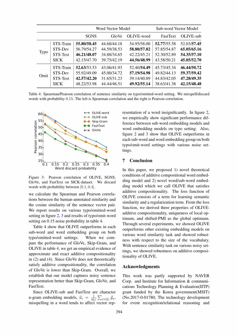
Word Vector Model Sub-word Vector Model

SGNS GloVe OLIVE-word FastText OLIVE-sub

Typo

STS-Train 55.80/58.45 44.68/44.18 54.95/58.00 52.77/55.58 52.03/57.45STS-Dev 56.79/54.27 44.59/38.53 58.80/57.82 57.85/54.87 65.05/65.16STS-Test 46.21/48.07 34.88/34.65 42.22/45.21 52.30/52.89 54.35/57.10SICK 42.15/47.70 39.75/42.19 44.56/48.99 43.58/50.21 45.05/52.70

Omit

STS-Train 52.63/53.53 43.06/41.93 52.40/54.49 45.73/45.34 46.44/50.72STS-Dev 55.92/49.09 45.00/34.72 57.19/54.98 49.82/44.13 59.37/59.42STS-Test 42.57/42.20 31.65/31.23 39.14/40.89 44.83/42.05 47.28/49.35SICK 48.22/53.98 44.44/46.51 49.92/55.14 38.63/41.38 42.15/48.48

Table 4: Spearman/Pearson correlation of sentence similarity on typo/omitted-word setting. We misspell/discardwords with probability 0.15. The left is Spearman correlation and the right is Pearson correlation.

0.1 0.15 0.2 0.25 0.3 0.35 0.4Word discard probability

25

30

35

40

45

50

55

60

Pears

on c

orr

ela

tion

OLIVE-word

OLIVE-sub

Skip-Gram

FastText

GloVe

Figure 3: Pearson correlation of OLIVE, SGNS,GloVe, and FastText on SICK-dataset. We discardwords with probability between [0.1, 0.4].

we calculate the Spearman and Pearson correla-tions between the human-annotated similarity andthe cosine similarity of the sentence vector pair.We report results on various typo/omitted-wordsetting in figure 2, 3 and results of typo/omit-wordsetting on 0.15 noise probability in table 4.

Table 4 show that OLIVE outperforms in eachsub-word and word embedding group on bothtypo/omitted-word settings. When we com-pare the performance of GloVe, Skip-Gram, andOLIVE in table 4, we get an empirical evidence ofapproximate and exact additive compositionalityin (2) and (4). Since GloVe does not theoreticallysatisfy additive compositionality, the correlationof GloVe is lower than Skip-Gram. Overall, weestablish that our model captures noisy sentencerepresentation better than Skip-Gram, GloVe, andFastText.

Since OLIVE-sub and FastText are charactern-gram embedding models, ~ui = 1

|Gi|∑

x∈Gi ~gx,misspelling in a word tends to affect vector rep-

resentation of a word insignificantly. In figure 2,we empirically show significant performance dif-ference between sub-word embedding models andword embedding models on typo setting. Also,figure 2 and 3 show that OLIVE outperforms ineach sub-word and word embedding group on bothtypo/omit-word settings with various noise set-tings.

7 Conclusion

In this paper, we proposed 1) novel theoreticalconditions of additive compositional word embed-ding model and 2) novel word/sub-word embed-ding model which we call OLIVE that satisfiesadditive compositionality. The loss function ofOLIVE consists of a term for learning semanticsimilarity and a regularization term. From the lossfunction, we derived three properties of OLIVE:additive compositionality, uniqueness of local op-timum, and shifted-PMI as the global optimum.Through several experiments, we showed OLIVEoutperforms other existing embedding models onvarious word similarity task and showed robust-ness with respect to the size of the vocabulary.With sentence similarity task on various noisy set-tings, we showed robustness on additive composi-tionality of OLIVE.

Acknowledgments

This work was partly supported by NAVERCorp. and Institute for Information & communi-cations Technology Planning & Evaluation(IITP)grant funded by the Korea government(MSIT)(No.2017-0-01780, The technology developmentfor event recognition/relational reasoning and

394

learning knowledge based system for video under-standing).

ReferencesCarl Allen and Timothy Hospedales. 2019. Analo-

gies explained: Towards understanding word em-beddings. In ICML.

Sanjeev Arora, Yuanzhi Li, Yingyu Liang, Tengyu Ma,and Andrej Risteski. 2016. A latent variable modelapproach to pmi-based word embeddings. Transac-tions of the Association for Computational Linguis-tics, 4:385–399.

Ben Athiwaratkun, Andrew Wilson, and AnimaAnandkumar. 2018. Probabilistic fasttext for multi-sense word embeddings. In ACL.

Marco Baroni and Alessandro Lenci. 2010. Dis-tributional memory: A general framework forcorpus-based semantics. Computational Linguis-tics, 36(4):673–721.

Piotr Bojanowski, Edouard Grave, Armand Joulin, andTomas Mikolov. 2017. Enriching word vectors withsubword information. Transactions of the Associa-tion of Computational Linguistics, 5(1):135–146.

Jan Botha and Phil Blunsom. 2014. Compositionalmorphology for word representations and languagemodelling. In ICML.

John A Bullinaria and Joseph P Levy. 2007. Extractingsemantic representations from word co-occurrencestatistics: A computational study. Behavior re-search methods, 39(3):510–526.

Daniel Cer, Mona Diab, Eneko Agirre, Inigo Lopez-Gazpio, and Lucia Specia. 2017. Semeval-2017task 1: Semantic textual similarity multilingual andcrosslingual focused evaluation. In SemEval.

Alex Gittens, Dimitris Achlioptas, and Michael W Ma-honey. 2017. Skip-gram-zipf+ uniform= vector ad-ditivity. In ACL.

Michael U Gutmann and Aapo Hyvarinen. 2012.Noise-contrastive estimation of unnormalized sta-tistical models, with applications to natural imagestatistics. Journal of Machine Learning Research,13(Feb):307–361.

Zellig S Harris. 1954. Distributional structure. Word,10(2-3):146–162.

Felix Hill, Roi Reichart, and Anna Korhonen. 2015.Simlex-999: Evaluating semantic models with (gen-uine) similarity estimation. Computational Linguis-tics, 41(4):665–695.

Eric H Huang, Richard Socher, Christopher D Man-ning, and Andrew Y Ng. 2012. Improving wordrepresentations via global context and multiple wordprototypes. In ACL.

Mikhail Khodak, Nikunj Saunshi, Yingyu Liang,Tengyu Ma, Brandon Stewart, and Sanjeev Arora.2018. A la carte embedding: Cheap but effectiveinduction of semantic feature vectors. In ACL.

Omer Levy and Yoav Goldberg. 2014a. Linguistic reg-ularities in sparse and explicit word representations.In CoNLL.

Omer Levy and Yoav Goldberg. 2014b. Neural wordembedding as implicit matrix factorization. In NIPS.

Marco Marelli, Luisa Bentivogli, Marco Baroni, Raf-faella Bernardi, Stefano Menini, and Roberto Zam-parelli. 2014. Semeval-2014 task 1: Evaluation ofcompositional distributional semantic models on fullsentences through semantic relatedness and textualentailment. In SemEval.

Tomas Mikolov, Kai Chen, Greg Corrado, and JeffreyDean. 2013a. Efficient estimation of word represen-tations in vector space. arXiv.

Tomas Mikolov, Ilya Sutskever, Kai Chen, Greg S Cor-rado, and Jeff Dean. 2013b. Distributed representa-tions of words and phrases and their compositional-ity. In NIPS.

Tomas Mikolov, Wen-tau Yih, and Geoffrey Zweig.2013c. Linguistic regularities in continuous spaceword representations. In NAACL-HLT.

George A Miller and Walter G Charles. 1991. Contex-tual correlates of semantic similarity. Language andcognitive processes, 6(1):1–28.

Andriy Mnih and Koray Kavukcuoglu. 2013. Learningword embeddings efficiently with noise-contrastiveestimation. In NIPS.

Jeffrey Pennington, Richard Socher, and ChristopherManning. 2014. Glove: Global vectors for wordrepresentation. In EMNLP.

Aleksandra Piktus, Necati Bora Edizel, Piotr Bo-janowski, Edouard Grave, Rui Ferreira, and FabrizioSilvestri. 2019. Misspelling oblivious word embed-dings. In NAACL.

Kira Radinsky, Eugene Agichtein, EvgeniyGabrilovich, and Shaul Markovitch. 2011. Aword at a time: computing word relatedness usingtemporal semantic analysis. In WWW.

Bei Shi, Zihao Fu, Lidong Bing, and Wai Lam.2018. Learning domain-sensitive and sentiment-aware word embeddings. In ACL.

Richard Socher, John Bauer, Christopher D Manning,et al. 2013. Parsing with compositional vector gram-mars. In ACL.

Richard Socher, Brody Huval, Christopher D Man-ning, and Andrew Y Ng. 2012. Semantic composi-tionality through recursive matrix-vector spaces. InEMNLP-CoNLL.

395

Guoyin Wang, Chunyuan Li, Wenlin Wang, YizheZhang, Dinghan Shen, Xinyuan Zhang, RicardoHenao, and Lawrence Carin. 2018. Joint embeddingof words and labels for text classification. In ACL.

Yang Xu, Jiawei Liu, Wei Yang, and Liusheng Huang.2018. Incorporating latent meanings of morpholog-ical compositions to enhance word embeddings. InACL.

A Convexity of (7)

The second derivative of DKL is as follows,

∂2DKL

∂~uc∂~uTc

=K∂

∂~uc

∑w∈V p(w) exp(~v

Tw~uc)~vw∑


=K


Tw~uc)~vw~v

Tw∑


−K∑

w∈V p(w) exp(~vTw~uc)~vw∑


×∑

w∈V p(w) exp(~vTw~uc)~v

Tw∑


,

where K is 1Z


Tw(∑m

i=1 ~uci)).To prove the second derivative of DKL is posi-

tive definite matrix, we multiply non-zero vector ~xto the Hessian matrix ( ∂

2DKL

∂~uc∂~uTc

).

~xT∂2DKL

∂~uc∂~uTc~x

= K


Tw~uc)~x

T~vw~vTw~x∑


−K∑

w∈V p(w) exp(~vTw~uc)~x

T~vw∑w∈V p(w) exp(~v

Tw~uc)

×∑

w∈V p(w) exp(~vTw~uc)~v

Tw~x∑


= K∑

w∈Vrwq

2w −K(

∑

w∈Vrwqw)

2

(23)

Where,

rw =p(w) exp(~vTw~uc)∑


, qw = ~xT~vw.

By Jensen’s inequality,

K∑

w∈Vrwq

2w > K(

∑

w∈Vrwqw)

2.

Now, we get

~xT∂2DKL

∂~uc∂~uTc~x > 0

for all non-zero vector ~x. So, the Hessian of DKLis positive definite matrix which leads to convexityof the DKL.

396


Contextualized context2vec

Kazuki AshiharaOsaka University

[email protected]

Yuki AraseOsaka University

[email protected]

Tomoyuki KajiwaraOsaka University

[email protected]

Satoru UchidaKyushu University

[email protected]

Abstract

Lexical substitution ranks substitution candi-dates from the viewpoint of paraphrasabilityfor a target word in a given sentence. Thereare two major approaches for lexical substitu-tion: (1) generating contextualized word em-beddings by assigning multiple embeddings toone word and (2) generating context embed-dings using the sentence. Herein we proposea method that combines these two approachesto contextualize word embeddings for lexi-cal substitution. Experiments demonstrate thatour method outperforms the current state-of-the-art method. We also create CEFR-LP, anew evaluation dataset for the lexical substi-tution task. It has a wider coverage of sub-stitution candidates than previous datasets andassigns English proficiency levels to all targetwords and substitution candidates.

1 Introduction

Lexical substitution (McCarthy and Navigli,2007) is the finest-level paraphrase problem.It determines if a word in a sentence can bereplaced by other words while preserving thesame meaning. It is important not only as a funda-mental paraphrase problem but also as a practicalapplication for language learning support suchas lexical simplification (Paetzold and Specia,2017) and acquisition (McCarthy, 2002). Table 1shows an example of the lexical substitution taskwith a sentence,1 the target word to replace, andwords of substitution candidates. The numbersin parentheses represent the paraphrasabilityof each candidate, where a larger value meansthe corresponding word is more appropriate tosubstitute the target word. The lexical substitutiontask ranks these candidates according to assigning

1In this paper, the terms context and sentence are usedinterchangeably wherever the context for the target refers tothe sentence.

context ... explain the basic concept andpurpose and get it going with min-imal briefing .

target gocandidate start (4), proceed (1), move (1) ...

Table 1: Example of the lexical substitution tasks

weights. The key technology to solve lexicalsubstitution tasks is to precisely capture wordsenses in a context.

There are mainly two approaches for lexicalsubstitution: (1) generating contextualized wordembeddings by assigning multiple embeddingsto one word and (2) generating context embed-dings using the sentence. The former realizesstatic embeddings as it pre-computes word em-beddings. One example of the first approachis DMSE (Dependency-based Multi-Sense Em-bedding), which was proposed by Ashihara et al.(2018) to contextualize word embeddings usingwords with dependency relations as a clue todistinguish senses. As an example of the sec-ond approach, context2vec (Melamud et al., 2016)generates a context embedding by inputting thesentence into bidirectional recurrent neural net-works. It combines context embedding and a sim-ple word embedding to generate a dynamic em-bedding. These two methods are current state-of-the-arts among methods of each approach.

We focus on the fact that these two methodshave a complementary nature. DMSE considersonly a single word as context, while context2vecuses a simple word embedding. Herein we com-bine DMSE and context2vec to take advantages ofboth contextualized word embeddings and contextembeddings. Specifically, we apply a contextual-ized word embedding generated by DMSE to re-place the word embedding used in context2vec.

397

In addition, we create a new evaluation datasetfor lexical substitution, named CEFR-LP. It is anextension of CEFR-LS (Uchida et al., 2018) andis created for lexical simplification to support sub-stitution tasks. The benefits of CEFR-LP are thatit expands the coverage of substitution candidatesand provides English proficiency levels. Thesefeatures are unavailable in previous evaluationdatasets such as LS-SE (McCarthy and Navigli,2007) and LS-CIC (Kremer et al., 2014).

The evaluation results on CEFR-LP, LS-SE,and LS-CIC confirm that our method effectivelystrengthens DMSE and context2vec. Addition-ally, our proposed method outperforms the currentstate-of-the-art methods. The contributions of thispaper are twofold:

• A method that takes advantages of contextu-alized word embedding and dynamic embed-ding generation from contexts is proposed.This method achieves a state-of-the-art per-formance on lexical substitution tasks.

• Creation and release2 of CEFR-LP, which isa new evaluation dataset for lexical substitu-tion with an expanded coverage of substitu-tion candidates and English proficiency lev-els.

2 Related Work

There are two major approaches to lexical sub-stitution. One approach generates contextualizedword embeddings by assigning multiple embed-dings to one word. Paetzold and Specia (2016)generated word embeddings per part-of-speech ofthe same word assuming that words with the samesurface have different senses for different part-of-speech. Fadaee et al. (2017) also generated mul-tiple word embeddings per topic represented ina sentence. For example, the word soft mayhave embeddings for topics of food when used likesoft cheese and that for music when used likesoft voice. To adequately distinguish theseword senses, both methods assign embeddings thatare too coarse. For example, the phrases softcheese and soft drink both use soft as anadjective and are related to the food topic. The for-mer has the sense of tender while the latter rep-resents the sense of non-alcoholic. To solvethis problem, DMSE generates finer-grained word

2http://www-bigdata.ist.osaka-u.ac.jp/arase/pj/CEFR-LP.zip

embeddings because it generates embeddings forwords with dependency relations based on theCBOW algorithm of word2vec (Mikolov et al.,2013). It concatenates words with dependent rela-tions within a specific window, which is a hyper-parameter in CBOW. Hence considered context inDMSE is bounded by the window size. DMSEachieves the highest performance for lexical sub-stitution tasks among the methods categorized intothe first approach.

The other approach dynamically generates con-textualized embeddings considering a sentence.Context2vec generates a context embedding usingbidirectional long short-term memory (biLSTM)networks (Schuster and Paliwal, 1997). Then itcombines the context embedding with a simpleword embedding. Context2vec is the current state-of-the-art method for representative lexical substi-tution tasks. Its advantage is that it can considerthe entire sentence as the context, while DMSEis bounded by a window size. However, DMSEcan use contextualized word embeddings, whereascontext2vec just uses a simple word embedding foreach word. The complementary nature of thesetwo methods inspired us to combine them. Morerecently, ELMo (Peters et al., 2018) showed a lan-guage modeling using biLSTM networks producescontextualized word embeddings, which are effec-tive for various NLP tasks such as named entityrecognition. Context2vec differs from ELMo whenexplicitly considering word embeddings of substi-tution targets. Our experiments empirically con-firm that context2vec outperforms ELMo in Sec-tion 6.

3 Proposed Method

We combine DMSE and context2vec to take ad-vantage of both fine-grained contextualized wordembeddings and context embeddings.

3.1 Overview

DMSE is designed to train its word embeddingsusing CBOW, which we replaced with biLSTMnetworks in context2vec. DMSE contextualizes aword using words with dependency relations (bothhead and dependents) in a given sentence. Here-after, words with dependency relations are referredto as dependency-words.3

There are numerous number of combinations3These are called as context-words in Ashihara et al.

(2018).

398

I drunk soft drink

LSTM LSTM

LSTM LSTM

MLP

soft

objectivefunction

LSTM

LSTM

context embedding

target wordembedding

(a) Pre-Training

(b) Post-Training

LSTM

LSTM

I drunk soft drink

MLP

soft_drink

objectivefunctioncontext

embeddingcontextualized

word embedding

biLSTM

Dependency relation

Figure 1: Design of the proposed method where softis the target to generate embedding.

of words and dependency-words. Similar toAshihara et al. (2018), we implement a two-stagetraining: pre-training and post-training for com-putational efficiency. In the pre-training, simpleword embeddings (one embedding per word) andparameters of biLSTM networks are trained bycontext2vec. In the post-training, only contextu-alized word embeddings are trained starting fromthe pre-trained word embeddings.

3.2 Pre-Training

Figure 1 (a) overviews pre-training, which corre-sponds to the training of context2vec. Word em-beddings and parameters of biLSTM networks areset.

First, the entire sentence is inputted into the biL-STM networks. At time step k, the forward net-work encodes words from the beginning to the k-th word. The backward network does the sameexcept in the opposite direction. Therefore, theoutputs of each LSTM network before and after atarget word represent the preceding and followingcontexts surrounding the target word, respectively.These outputs are concatenated and inputted intoa multi-layer perceptron to generate a unified con-text embedding for the target word. On the otherhand, the target word is represented by a word em-bedding that has the same dimensions as the con-

text embedding.The objective function is the negative sampling

proposed by Mikolov et al. (2013). A positive ex-ample is the target word and its context, whereasnegative examples are random words. Note thatword embeddings, forward LSTM network, andthe backward LSTM network each have their ownparameters.

3.3 Post-Training

Figure 1 (b) outlines post-training. Multiple wordembeddings are generated for words with the samesurface but with different dependency-words ascontextualized word embeddings.

First, the sentence is parsed to obtaindependency-words of the target. For eachdependency-word and target pair, its word em-bedding is trained. The process is simple. Thesewords are concatenated with an under-bar ( ) andtreated as a single word, whose embedding is usedas a contextualized word embedding of the targetword. The contextualized word embeddings aretrained in the same manner with pre-training.

The contextualized embeddings are initializedby assigning the pre-trained word embeddings inSection 3.2. The pre-trained word embeddingsand biLSTM networks are fixed, and only the con-textualized word embeddings are updated duringpost-training. This setting allows the contextual-ized embeddings to be trained in parallel.

3.4 Application to Lexical Substitution Task

This section describes how to tackle the lexicalsubstitution task using both contextualized wordembeddings and context embeddings obtained bythe proposed method.

Ranking Method As shown in Table 1, lexicalsubstitution ranks substitution candidates of thetarget word based on their paraphrasabilities undera given context. We use the same ranking methodwith context2vec, which assumes not only that agood substitution candidate is semantically simi-lar to the target word but also is suitable for a givencontext. This assumption is commonly used in re-cent lexical substitution models (Melamud et al.,2015; Roller and Erk, 2016).

Here we have target word t and its dependency-word d. The contextualized word embedding of tis noted as vd

t and the word embedding of a sub-stitution candidate s contextualized by d is vd

s . Fi-nally, the context embedding is denoted as vc. The

399

following scores are calculated for each substitu-tion candidate and ranked them in descending or-der.

S(vds |vd

t ,vc)

= (cos (vdt ,v

ds ) + 1)(cos (vd

s ,vc) + 1). (1)

Here, cos(·, ·) calculates the cosine similarity be-tween two vectors. If the word embedding doesnot exist in the vocabulary, the word embeddingof ⟨unk⟩ is used.

Dependency-word Selection When there aremultiple dependency-words to contextualize aword embedding, the most appropriate one mustbe selected to characterize the sense of the targetword in a given context. Ashihara et al. (2018)proposed the following dependency-word selec-tion method for the DMSE model.

Smaxc : d = arg maxd∈D

S(vds |vd

t ,vc),

where D is a set of dependency-words of the tar-get word in the context. If the contextualized wordembedding vd

s or vdt does not exist in the vocabu-

lary, the corresponding simple word embeddings(vs or vt) pre-trained for context2vec are used.

Smaxc uses the dependency-word that maxi-mizes the paraphrasability score, but there is noguarantee that this dependency-word best charac-terizes the sense of the word in the given context.Therefore, we propose the following dependency-word selection methods based on the similarity be-tween the target word or candidate words and thecontext.

Star : d = arg maxd∈D

cos(vdt ,vc),

Scan : d = arg maxd∈D

cos(vds ,vc).

These methods should select more appropriatedependency-word using both contextualized wordembeddings and context embeddings.

4 CEFR-LP: New Evaluation Dataset

In addition to proposing a method for lexical sub-stitution, we created CEFR-LP, which mitigateslimitations of previous evaluation datasets.

4.1 Principle of CEFR-LPLS-SE (McCarthy and Navigli, 2007) and LS-CIC (Kremer et al., 2014) are the standard eval-uation datasets for lexical substitution. However,

they have limited annotation coverage because theannotators provide substitution candidates manu-ally. Specifically, each annotator provides up tothree substitution candidates for LS-SE and upto five substitution candidates for LS-CIC. Thesecandidates are regarded as appropriate candidatesfor a target under a specific context. During anevaluation, these candidates are combined for thesame targets with different contexts. This leadsto two limitations. First, annotators may not de-rive all the appropriate candidates for the target.Second, some appropriate candidates for a targetamong the combined ones are regarded as inap-propriate because they were missed by the anasno-tators when annotating the target under the givencontext.

To mitigate these limitations, CEFR-LS (Uchida et al., 2018) was constructed toimprove the coverage. However, the target islexical simplification rather than substitution.Herein we extend CEFR-LS and build a newevaluation dataset called CEFR-LP for lexicalsubstitution tasks that:

1. Define the substitution candidates

2. Determine the paraphrasability label

3. Evaluate the number of annotators

The first extension adapts to lexical substitution.CEFR-LS only includes substitutions from com-plex words to simpler ones because it is specif-ically intended for simplification. On the otherhand, CEFR-LP includes not only complex tosimple substitutions but also simple to complexsubstitutions and substitutions between equivalentcomplexities. The substitution candidates are asynonym set of target words extracted from adictionary.4 The second extension generates fine-grained judgments for paraphrasability. CEFR-LS is annotated with binary labels, while CEFR-LP is annotated with continuous values represent-ing paraphrasability. This extension allows auto-matic evaluation via the Generalized Average Pre-cision (GAP) score (Kishida, 2005; Thater et al.,2009), which is common in recent lexical substi-tution studies. The last extension reduces poten-tial annotation biases. While CEFR-LS was an-notated by one expert, CEFR-LP employs morethan five annotators per target to reduce bias dueto annotator subjectivity. Following CEFR-LS,

4http://www.thesaurus.com/

400

context ..., and to create elixirs to cure disease and extend life . From alchemy came the his-torical progressions that led to modern chemistry : the isolation of drugs from naturalsources , metallurgy , and the dye industry . Today , chemistry continues to deepen ourunderstanding ...

target progressions [C1]candidate block [B1] (0), development [B1] (6), advancement [B2] (8), break [A2] (1), ...

context ... Competition would ensure that prices remained low and faulty goods disappeared fromthe market . In this way , businesses would reap profits , consumers would have theirneeds satisfied , and society as a whole would prosper . Smith discussed these ideas, ...

target prosper [B2]candidate thrive [C1] (8), blossom [B2] (6), yield [B2] (1), bear [A2] (0), flourish [C2] (8), ...

context ... That is , a member of the population may be chosen only once . Most samples are takenfrom large populations and the sample tends to be small in comparison to the population. Since this is the case , sampling without replacement is approximately ...

target large [A1]candidate substantial [B1] (8), giant [B1] (6), extravagant [C2] (0), wide [A2] (1), ...

Table 2: Examples of CEFR-LP. “Context” shows context sentences where the target word is presented in bold.“Target” shows the target and “candidate” lists the substitution candidates. Square brackets indicate CEFR levelsof targets and candidates. Round brackets indicate the weights of candidates.

CEFR-LP also provides CEFR (the Common Eu-ropean Framework of Reference for Languages)levels (A1 (lowest), A2, B1, B2, C1, and C2 (high-est)) for the target and candidates as English pro-ficiency levels.

4.2 Annotation

Following CEFR-LS, we use sentences extractedfrom textbooks publicly available at the OpenStaxwebsite5 initiated by Rice University. We hiredannotators on Amazon Mechanical Turk,6 who (1)possessed a degree from an accredited universityin the United States and (2) held the Mechani-cal Turk Masters qualification or a past acceptancerate above 98%.

Annotators were given a target word, its con-text, and a list of synonyms. They annotated eachsubstitution candidate in the synonym list withparaphrasability labels (“sure”, “maybe”, and “notpossible”) considering the given context. As thecontext, a sentence on which the target word ap-peared as well as two more sentences before andafter it were provided. To avoid overloading theannotator, target words with more than 30 syn-onyms were excluded.

Following CEFR-LS, we used the following an-notation criteria:

5https://cnx.org/6https://www.mturk.com/

Grammatical Reformation Stage When para-phrasing the target word into the substitutioncandidate, grammatical accuracy such asthe part-of-speech and the connection to thepreposition must be maintained. The mor-phology of the target word such as past tenseand third person singular are automaticallycorrected.

Definition Stage The target word and the substi-tution candidate have the same meaning.

Context Stage The candidate should retain thenuance of the target word in a given contextand not affect the meaning of the sentence.

If all of the above conditions were met, a labelof “sure” is assigned. If either condition was notmet, a label of “not possible” was assigned. If thejudgment was difficult, a label of “maybe” was as-signed.

Each annotation set was assigned to at least fiveannotators. To improve the reliability of annota-tion labels, we discarded the result from the anno-tator who had the lowest agreement with the oth-ers. Consequently, each set had four annotatorsand the average Fleiss’ kappa was 0.33.

To use CEFR-LP for a lexical substitution task,the assigned labels were consolidated as a weight.For example, LS-SE and LS-CIC were set suchthat a weight to the number of annotators produced

401

CEFR-LP LS-SE LS-CIC

number of target words 863 2, 010 15, 344number of substitution candidates 14, 259 34, 600 601, 257average number of substitution candidates per target 16.5 17.2 39.2average number of paraphrasable candidates per target 10.0 3.48 6.65

Table 3: Basic statistics in CEFR-LP compared to LS-SE and LS-CIC

CEFR level target candidate

all 863 14, 259

A1 300 2, 090A2 190 2, 856B1 110 4, 513B2 186 3, 201C1 30 648C2 47 951

Table 4: Distribution of CEFR levels in CEFR-LP

a certain candidate. A “sure”, “maybe”, and “notpossible” label were assigned values of 2, 1, and0 points, respectively. These values were summedto give the weight of the candidate. Because eachsubstitution candidate has four annotation labels,the weight ranged from 0 to 8. The larger thevalue, the higher the paraphrase possibility.

Table 2 shows examples sampled from CEFR-LP. “Context” gives sentences, including a targetword. “Target” is the target word with its CEFRlevel in a square bracket, which is represented bya bold style in the context sentences. “Candidate”lists substitution candidates with their CEFR lev-els in square brackets and weights computed basedon annotated labels in round brackets.

4.3 Analysis of CEFR-LP

Table 3 shows the basic statistics for CEFR-LPcompared to those in LS-SE and LS-CIC. CEFR-LP provides 14, 259 substitution candidates for863 target words. The average number of para-phrasable candidates per word is 10.0, which islarger than 3.48 of LS-SE and 6.65 of LS-CIC.Here, a paraphrasable candidate means substitu-tion candidates with a weight of 1 or more (i.e.,at least one annotator judged it can paraphrase thetarget in a given context). Compared to LS-SE andLS-CIC, CEFR-LP has an enhanced coverage ofsubstitution candidates.

Table 4 shows the distribution of CEFR levels

context embedding units 300LSTM hidden/output units 600MLP input units 1200MLP hidden units 1200sentential context units 600target word units 600number of negative samples 10negative sampling rate 0.75number of epochs 10

Table 5: Context2vec hyper-parameters that show thebest performance in (Melamud et al., 2016).

in CEFR-LP. Words at the C1 and C2 levels arenaturally less frequent than others in general docu-ments. The distribution reflects this tendency. Webelieve that these CEFR levels are useful when ap-plying lexical substitution technologies to educa-tional applications.

5 Evaluation Settings

This section describes the evaluation settings usedto investigate the performance of our method onlexical substitution tasks.

5.1 Training of Our Method

To train contextualized word embeddings by usingour method, we used 61.6M sentences7 extractedfrom the main contents of English Wikipedia8 arti-cles. We lemmatized each word using the StanfordParser (Manning et al., 2014) and replaced wordsless than or equal to ten frequency to ⟨unk⟩ tag toreduce the size of the vocabulary.

Pre-training used the same hyper-parameter set-tings of context2vec (Table 5). These settingsachieved the best performance on lexical substi-tution tasks in Melamud et al. (2016).

7To speed-up the training of context2vec, all sentencesconsisting of more than 25 words are discarded.

8https://dumps.wikimedia.org/enwiki/20170601/

402

For post-training, dependency relations werederived using the Stanford Parser. To avoid thedata sparseness problem, dependency-words werelimited to nouns, verbs, adjectives, and adverbs.The number of training epochs in the post-trainingwas set to one because our post-training aims tocontextualize word embeddings that have beenpre-trained. Hence, a long-time training does nothave to be assumed. In the future, we plan toinvestigate the effects of the number of trainingepochs in post-training.

5.2 Evaluation DatasetWe used the following datasets in the evaluation.

LS-SEThis is an official evaluation dataset in thelexical substitution task of SemEval-2007.For each target word, five annotators sug-gested up to three different substitutions. Asthe context, a sentence where a target wordappears is provided. Every target has ten con-text sentences. The number of targets is 201(types). Consequently, there are 2, 010 sets oftarget, candidates, and context sentences areavailable.

LS-CICThis is a large-scale dataset for a lexical sub-stitution task. For 15, 629 target words, sixannotators suggested up to five different sub-stitutions under a context. Unlike LS-SE,three sentences are provided as context: asentence containing the target word, its pre-ceding sentence, and its following sentences.

CEFR-LPOur new dataset for lexical substitution,which is described in Section 4.

5.3 Evaluation MetricsWe used GAP (Kishida, 2005; Thater et al., 2009)as an evaluation metric. GAP is a commonly usedmetric to evaluate lexical substitution tasks. GAPcalculates the ranking accuracy by considering theweight of correct examples:

pi =

∑ik=1 xk

i,

GAP =100

∑ni=1 I(xi)pi∑n

i=1 I(yi)yi,

where xi and yi represent the weight of the i-th substitution candidate ranked by an automatic

method and by the ideal ranking, respectively. nrepresents the number of substitution candidates.I(x) (x ∈ N) is a binary function that returns 1if x ≥ 1. Otherwise, it returns 0. In this ex-periment, we regarded the number of annotatorssuggesting a substitution candidate under a givencontext as the weight of the candidate for LS-SEand LS-CIC. For CEFR-LP, we used the weightof the candidate that was computed based on theannotated labels as described in Section 4.2.

5.4 Baseline Method

We used the following baselines for comparison.

DMSE (Smaxc)For dependency-word selection, Smaxc show-ing the highest performance is used herein.This is the best-performing model among themethods that generate contextualized wordembeddings.

Context2vecThis is the current state-of-the-art methodamong those proposed for lexical substitu-tion. Note that this corresponds to the pre-trained model of our method.

ELMoWe concatenate embeddings generated fromthree hidden layers in ELMo as contextual-ized word embeddings.9

DMSE and ELMo were trained using the sameWikipedia corpus as our method. These methodsrank the substitution candidates in descending or-der of the cosine similarity between embeddingsof the target and substitution candidate. For con-text2vec, the candidates are ranked in the samemanner using our method based on Equation (1).

5.5 Ideal Selection of Dependency-words

The performance of our method depends on howdependency-words are selected. We simulatethe performance when our method selects idealdependency-words that maximize the GAP score.This selection method of dependency-words is de-noted as Sbest.

9As a preliminary experiment, we compared methods togenerate contextualized word embeddings. One used one ofthree layers of embeddings, one summed these embeddings,and one concatenated these embeddings. The results con-firmed that concatenation performed best.

403

Model LS-SE LS-CIC CEFR-LP

DMSE (Smaxc) 49.3 46.5 71.1ELMo 47.6 48.1 74.9context2vec 51.1 50.0 75.3

context2vec + DMSE (Smaxc) 52.2 50.9 75.5context2vec + DMSE (Star) 52.3 50.9 75.6context2vec + DMSE (Scan) 52.3 51.0 75.6

context2vec + DMSE (Sbest) 55.6 52.9 77.2

Table 6: GAP scores on LS-SE, LS-CIC and CEFR-LP datasets, where bold denotes the highest scores.

A1 A2 B1 B2 C1 / C2

DMSE (Smaxc) 67.9 75.2 65.7 74.9 72.7context2vec 75.2 78.5 69.4 75.7 75.2context2vec+DMSE (Scan) 75.3 78.9 69.9 76.2 75.9

Table 7: GAP scores on different CEFR levels of target words in CEFR-LP

6 Results

Table 6 shows the GAP scores for LS-SE, LS-CICand CEFR-LS datasets. Our method is denoted ascontext2vec + DMSE where the dependency-wordselection method is represented in parenthesis asSmaxc, Star, or Scan.

When using Scan for dependency-word selec-tion, context2vec + DMSE outperformed DMSEby 3.0 points, 4.5 points, and 4.5 points for LS-SE,LS-CIC, and CEFR-LP, respectively. It even out-performed context2vec, the current state-of-the-artmethod, by 1.2 points, 1.0 points, and 0.3 pointson these datasets, respectively. These results con-firm the effectiveness of our method, which com-bines contextualized word embeddings and con-text embeddings to complement each other.

All dependency-word selection methods showfairly competitive performances, but Scan consis-tently achieved the highest GAP scores. Contextembedding may be effective to select dependency-words rather than comparing contextualized wordembeddings. The last row of Table 6 showsthe performance of our method with Sbest (i.e.,when the ideal dependency-word was selected).This best selection method outperformed 1.6 - 3.3points higher than our method with Scan, demon-strating the importance of dependency-word selec-tion. In the future, we will improve the selectionmethod.

CEFR-LP analyzes performances from the per-spective of the CEFR levels of target words. Ta-

ble 7 shows the GAP score of DMSE (Smaxc),context2vec, and context2vec+DMSE (Scan).Note that scores are not comparable across lev-els because the number of appropriate substitutioncandidates varies. Our method consistently out-performs DMSE (Smaxc) and context2vec. Suchan analysis is important when applying lexicalsubstitution to educational applications.

Table 8 lists the results where each row showsa ranking of substitution candidates by comparedmethods. The annotated weights of each candidateare presented in parentheses. Here, the outputsof context2vec+DMSE (Smaxc) to use the samedependency-words with DMSE (Smaxc).

Inputs (1) and (2) show the cases wherethe meanings of polysemous target words (goand tender) are successfully captured by ourmethod. It ranks start and soft first for eachtarget, respectively. On the other hand, DMSE(Smaxc) failed to rank correct candidates higher al-though it referred to the same dependency-words.Context2vec also failed, but it used context embed-dings. These results demonstrate that contextu-alized word embeddings and context embeddingscomplement each other. On Input (3), both DMSE(Smaxc) and our method failed while context2vecsuccessfully rank the correct candidate (grasp)on top. This is caused by incorrect dependency-word selection. In Input (3), there are two majordependency-words, sat and hands. In this con-text, hands should be useful as a clue to iden-

404

Input (1) To make these techniques work well , explain the basic concept andpurpose and get it going with minimal briefing .

DMSE (Smaxc) try (0), move (1), proceed (1), leave (0), ...context2vec proceed (1), run (0), start (4), move (1), ...

context2vec+DMSE (Smaxc) start (4), proceed (1), move (1), run (0), ...

Input (2) Rabbits often feed on young , tender perennial growth as it emergesin spring , or on young transplants .

DMSE (Smaxc) immature (0), young (0), great (1), soft (4), ...context2vec delicate (1), immature (0), soft (4), painful (0), ...

context2vec+DMSE (Smaxc) soft (4), delicate (1), immature (0), young (0), ...

Input (3) A doctor sat in front of me and held my hands .DMSE (Smaxc) put (0), lift (1), grasp (3), carry (0), ...

context2vec grasp (3), carry (0), take (1), keep (0), ...context2vec+DMSE (Smaxc) take (1), carry (0), keep (0), lift (1), ...

Table 8: Example outputs of each method. Target words in the input sentences are presented in bold and all of theirdependency-words are presented in italic. Outputs are ranked lists of candidates, where the numbers in parenthesesshow candidates’ weights. Our method ranks the appropriate candidates on top for the first two examples, but itfailed on the last example due to incorrect dependency-word selection.

tify target word’s sense but sat was mistakenlyselected as the dependency-word. This result sug-gests that dependency types matter when selectingdependency-words, which we will tackle in the fu-ture.

7 Conclusion

Herein we proposed a method that combinesDMSE and context2vec to simultaneously take ad-vantage of contextualized word embeddings andcontext embeddings. The evaluation results onlexical substitution tasks confirm the effective-ness of our method, which outperforms the cur-rent state-of-the-art method. We also create a newevaluation set for lexical substitution tasks calledCEFR-LP.

In the future, we will consider the dependencytypes in contextualized word embeddings for fur-ther improvements. Additionally, we plan to ex-tend CEFR-LP to cover phrasal substitutions.

Acknowledgments

We thank Professor Christopher G. Haswell forhis valuable comments and discussions. We alsothank the anonymous reviewers for their valuablecomments. This research was supported by theKDDI Foundation.

ReferencesKazuki Ashihara, Tomoyuki Kajiwara, Yuki Arase, and

Satoru Uchida. 2018. Contextualized Word Repre-sentations for Multi-Sense Embedding. In Proceed-ings of the Pacific Asia Conference on Language, In-formation and Computation, pages 28–36.

Marzieh Fadaee, Arianna Bisazza, and Christof Monz.2017. Learning Topic-Sensitive Word Representa-tions. In Proceedings of the Annual Meeting of theAssociation for Computational Linguistics, pages441–447.

Kazuaki Kishida. 2005. Property of Average Precisionand its Generalization: An Examination of Eval-uation Indicator for Information Retrieval Experi-ments. National Institute of Informatics TechnicalReports, pages 1–19.

Gerhard Kremer, Katrin Erk, Sebastian Pado, and Ste-fan Thater. 2014. What Substitutes Tell Us - Anal-ysis of an “All-Words” Lexical Substitution Corpus.In Proceedings of the Conference of the EuropeanChapter of the Association for Computational Lin-guistics, pages 540–549.

Christopher Manning, Mihai Surdeanu, John Bauer,Jenny Finkel, Steven Bethard, and David McClosky.2014. The Stanford CoreNLP Natural LanguageProcessing Toolkit. In Proceedings of the AnnualMeeting of the Association for Computational Lin-guistics, pages 55–60.

Diana McCarthy. 2002. Lexical Substitution as a Taskfor WSD Evaluation. In Proceedings of the ACLWorkshop on Word Sense Disambiguation, pages109–115.

405

Diana McCarthy and Roberto Navigli. 2007. SemEval-2007 Task 10: English Lexical Substitution Task. InProceedings of the International Workshop on Se-mantic Evaluations, pages 48–53.

Oren Melamud, Ido Dagan, and Jacob Goldberger.2015. Modeling Word Meaning in Context withSubstitute Vectors. In Proceedings of the Confer-ence of the North American Chapter of the Associa-tion for Computational Linguistics, pages 472–482.

Oren Melamud, Jacob Goldberger, and Ido Dagan.2016. context2vec: Learning Generic Context Em-bedding with Bidirectional LSTM. In Proceedingsof the SIGNLL Conference on Computational Natu-ral Language Learning, pages 51–61.

Tomas Mikolov, Kai Chen, Greg Corrado, and JeffreyDean. 2013. Efficient Estimation of Word Represen-tations in Vector Space. In Proceeding of the Inter-national Conference on Learning Representations,pages 1–12.

Gustavo Henrique Paetzold and Lucia Specia. 2016.Unsupervised Lexical Simplification for Non-NativeSpeakers. In Proceedings of the Association for theAdvancement of Artificial Intelligence, pages 3761–3767.

Gustavo Henrique Paetzold and Lucia Specia. 2017. Asurvey on lexical simplification. Journal of ArtificialIntelligence Research, pages 549–593.

Matthew E. Peters, Mark Neumann, Mohit Iyyer, MattGardner, Christopher Clark, Kenton Lee, and LukeZettlemoyer. 2018. Deep Contextualized Word Rep-resentations. In Proceedings of the Annual Confer-ence of the North American Chapter of the Asso-ciation for Computational Linguistics, pages 2227–2237.

Stephen Roller and Katrin Erk. 2016. PIC a DifferentWord: A Simple Model for Lexical Substitution inContext. In Proceedings of the Annual Conferenceof the North American Chapter of the Associationfor Computational Linguistics, pages 1121–1126.

Mike Schuster and Kuldip K. Paliwal. 1997. Bidirec-tional Recurrent Neural Networks. IEEE Transac-tions on Signal Processing, pages 2673–2681.

Stefan Thater, Universitat Saarlandes, Georgiana Dinu,Universitat Saarlandes, Manfred Pinkal, and Univer-sitat Saarlandes. 2009. Ranking Paraphrases in Con-text. In Proceedings of the Workshop on AppliedTextual Inference, pages 44–47.

Satoru Uchida, Shohei Takada, and Yuki Arase. 2018.CEFR-based Lexical Simplification Dataset. Pro-ceedings of the International Conference on Lan-guage Resources and Evaluation, pages 3254–3258.

406


Phonetic Normalizationfor Machine Translation of User Generated Content

Jose Carlos Rosales Nunez1,2,3 Djame Seddah3 Guillaume Wisniewski1,2,41Universite Paris Sud, LIMSI

2 Universite Paris Saclay3 INRIA Paris

4 Universite de Paris, LLF, [email protected] [email protected]@univ-paris-diderot.fr

Abstract

We present an approach to correct noisy UserGenerated Content (UGC) in French aimingto produce a pre-processing pipeline to im-prove Machine Translation for this kind of non-canonical corpora. Our approach leveragesthe fact that some errors are due to confusioninduced by words with similar pronunciationwhich can be corrected using a phonetic look-up table to produce normalization candidates.We rely on a character-based neural modelphonetizer to produce IPA pronunciations ofwords and a similarity metric based on the IPArepresentation of words that allow us to iden-tify words with similar pronunciation. Thesepotential corrections are then encoded in a lat-tice and ranked using a language model to out-put the most probable corrected phrase. Com-pared to other phonetizers, our method boostsa Transformer-based machine translationsystem on UGC.

1 Introduction

In this work we aim to improve the translation qual-ity of User-Generated Content (UGC). This kindof content generally contains many characters rep-etitions, typographic errors, contractions, jargonor non-canonical syntactic constructions, resultingin a typically high number of Out-of-Vocabularywords (OOVs), which, in turn, significantly de-creases MT quality and can introduce noisy arte-facts in the output due to rare tokens. Hereby, wepropose a normalization pipeline that leverages onthe existence of UGC specific noise due to the mis-use of words or OOV contractions that have a simi-lar pronunciation to those of the expected correct to-kens. This method works without any supervisionon noisy UGC corpora, but exploits phonetic sim-ilarity to propose normalization token candidates.To explore the capacities of our system, we firstassess the performance of our normalizer and then

conduct a series of MT experiments to determineif our method improves the translation quality ofsome Phrase-Based Statistical Machine Translation(PBSMT) and Neural Machine Translation (NMT)baselines. Our results show that including a phone-tization step in conjunction with a Transformerarchitecture (Vaswani et al., 2017) can improvemachine translation over UGC with a minimumimpact on in-domain translations. This suggeststhat phonetic normalization can be a promising re-search avenue for MT and automatic correction ofUGC.

Our contribution in this paper is threefold:

• we propose a pre-processing pipeline to nor-malize UGC and improve MT quality;

• by quantifying the corrections made by ournormalizer in our UGC corpora, we assessthe presence of noise due to phonetic writingand demonstrate that this knowledge can bepotentially exploited to produce correctionsof UGC without any annotated data;

• we explore the performance improvement thatcan be achieved in machine translation by us-ing a phonetic similarity heuristic to proposedifferent normalization candidates.

2 Related Work

Several works have focused on using lattices tomodel uncertain inputs or potential processing er-rors that occur in the early stage of the pipeline.For instance, Su et al. (2017) proposed lat2seq,an extension of seq2seq models (Sutskever et al.,2014) able to encode several possible input possi-bilities by conditioning their GRU output to sev-eral predecessors’ paths. The main issue with thismodel is that it is unable to predict the score ofchoosing a certain path by using future scores, i.e,by considering words that come after the current

407

token to be potentially normalized. Sperber et al.(2017) introduced a model based on Tree-LSTMs(Tai et al., 2015), to correct outputs of an AutomaticSpeech Recognition (ASR) system. On the otherhand, Le et al. (2008) use lattices composed of writ-ten subword units to improve recognition rate onASR.

However, none of the aforementioned workshave focused on processing noisy UGC corporaand they do not consider our main hypotheses ofusing phonetizers to recover correct tokens. Theyaim to correct known tokens such that a neurallanguage model chooses the best output when anuncertain input is present (typically words with sim-ilar pronunciation from an ASR output). Instead,our approach calculates the phonetization of thesource token and candidates are proposed based ontheir phonetic similarity to it, where this originalobservation can be a potential OOV.

On the same trend, (Qin et al., 2012) com-bined several ASR systems to improve detection ofOOVs. More recently, van der Goot and van No-ord (2018) achieved state-of-the-art performanceon dependency parsing of UGC using lattices.

Closely related to our work, Baranes (2015) ex-plored several normalization techniques on FrenchUGC. In particular, to recover from typographicalerrors, they considered a rule-based system, SxPipe(Sagot and Boullier, 2008), that produced latticesencoding OOVs alternative spelling and used a lan-guage model to select the best correction.

Several works have explored different ap-proaches to normalize noisy UGC in various lan-guages. For instance, Stymne (2011) use Approx-imate String Matching, an algorithm based on aweighted Levenshtein edit distance to generatelattices containing alternative spelling of OOVs.Wang and Ng (2013) employ a Conditional Ran-dom Field and a beam-search decoding approachto address missing punctuation and words in Chi-nese and English social media text. More recently,Watson et al. (2018) proposed a neural sequence-to-sequence embedding enhancing FastText (Bo-janowski et al., 2017) representations with word-level information, which achieved state-of-the-arton the QALB Arabic normalization task (Mohitet al., 2014).

3 Phonetic Correction Model

To automatically process phonetic writing and mapUGC to their correct spelling, we propose a sim-

ple model based on finding, for each token of thesentence, words with similar pronunciations andselecting the best spelling alternative, using a lan-guage model. More precisely, we propose a four-step process:

1. for each word of the input sentence, we au-tomatically generate its pronunciation. Weconsider all words in the input sentence asmisspelled tokens are not necessarily OOVs(e.g. “j’ai manger” — literally “I have eat” —which must be corrected to “j’ai mange” — “Ihave eaten”, the French words “manger” and“mange” having both the same pronunciation/mA.ge/);

2. using these phonetic representations, we look,for each word w of the input sentence, to everyword in the training vocabulary with a pronun-ciation “similar” to w according to an ad-hocmetric we discuss below;

3. we represent each input sentence by a latticeof n + 1 nodes (where n is the number ofwords in the sentence) in which the edge be-tween the i-th and (i+ 1)-th nodes is labeledwith the i-th word of the sentence. Alternativespellings can then be encoded by adding anedge between the i-th and (i + 1)-th nodeslabeled by a possible correction of the i-thword. Figure 1 gives an example of such alattice. In these lattices, a path between theinitial and final nodes represents a (possible)normalization of the input sentence.

4. using a language model, we compute the prob-ability to observe each alternative spelling ofthe sentence (note that, by construction, theinput sentence is also contained in the lattice)and find the most probable path (and there-fore potential normalization) of the input sen-tence. Note that finding the most probablepath in a lattice can be done with a complex-ity proportional to the size of the sentenceeven if the lattice encodes a number of pathsthat grows exponentially with the sentencesize (Mohri, 2002). In our experiments weused the OpenGRM (Roark et al., 2012) andOpenFST (Allauzen et al., 2007) frameworksthat provide a very efficient implementationto score a lattice with a language model.

This process can be seen as a naive spellchecker, inwhich we only consider a reduced set of variations,

408

tailored to the specificities of UGC texts. We willnow detail the first two steps discussed above.

Generating the pronunciation of the inputwords To predict the pronunciation of an in-put word, i.e. its representation in the Inter-national Phonetic Alphabet (IPA), we use thegtp-seq2seq python library1 to implement agrapheme-to-phoneme conversion tool that relieson a Transformer model (Vaswani et al., 2017).We use a 3 layers model with 256 hidden unitsthat is trained on a pronunciation dictionary auto-matically extracted from Wiktionary (see Sec-tion 4.1 for a description of our datasets). Thisvanilla model achieves a word-level accuracy of94.6%, that is to say it is able to find the exact cor-rect phonetization of almost 95% of the words ofour test set.

We also consider, as a baseline, the pronuncia-tion generated by the Espeak program.2 that usesa formant synthesis method to produce phonetiza-tions based on acoustic parameters.

Finding words with similar pronunciation Inorder to generate alternatives spelling for each in-put word, we look, in our pronunciation dictio-nary,3 for alternate candidates based on phoneticsimilarity. We define the phonetic similarity oftwo words as the edit distance between their IPArepresentations, all edit operations being weighteddepending on the articulatory features of the soundsinvolved. To compute the phonetic similarity weused the implementation (and weights) providedby the PanPhon library (Mortensen et al., 2016).

To avoid an explosion of the number of alter-natives we consider, we have applied a thresholdon the phonetic distance and consider only homo-phones, i.e. alternatives that have the exact samepronunciation as the original word.4

To account for peculiarities of French orthog-raphy we also systematically consider alternativespellings in which diacritics (acute, grave and cir-cumflex accents) for the letter “e” (which is theonly one that changes the pronunciation for differ-ent accentuation in French) were added wherever

1https://github.com/cmusphinx/g2p-seq2seq

2espeak.sourceforge.net3see § 4.1 for the description of the data we used4We have explored using several values for this parameter

but in this work only the most conservative distance (0) isused since higher values add too much candidates and rapidlydecreases performance due to the number of ambiguities.

possible. Indeed, users often tend to ‘forget’ dia-critics when writing online and this kind of spellingerror results in phonetic distances that can be large(e.g. the pronunciation of bebe and bebe is verydifferent).

We ultimately only keep as candidates those thatare present in the train corpus of Section 4.3 tofilter out OOV, and nonexistent words.

4 Datasets

In this section, we present the different corporaused in this work. We will first describe the datasetused to train our phonetic normalizer; then, in §4.2,the UGC corpora used both to measure the perfor-mance of our normalization step and evaluate theimpact of phonetic spelling on machine translation.Finally, in § 4.3 we introduce the (canonical) paral-lel corpora we used to train our MT system. All ourexperiments are made on French UGC corpora.5

Some statistics describing these corpora are listedin Table 1.

4.1 Pronunciation DictionaryTo train our Grapheme-to-Phoneme model we usea dictionary mapping words to their pronuncia-tion (given by their IPA representation). To thebest of our knowledge, there is no free pronunci-ation dictionary for French. In our experiments,we have considered a pronunciation dictionary au-tomatically extracted from Wiktionary dumpsbuilding on the fact that, at least for French, pro-nunciation information are identified using specialtemplates, which makes their extraction straightfor-ward (Pecheux et al., 2016).6

The dictionary extracted from the FrenchWiktionary contains 1,571,090 words. Wetrained our G2P phonetizer on 1,200,000 exam-ples, leaving the rest to evaluate its performance.When looking for words with similar pronuncia-tion (§3), we consider only the word that appearin our parallel training data (described in §4.3) tospeed up the search. After filtering, our dictionarycontained pronunciation information for roughly82K French words.

4.2 UGC CorporaThe Parallel Cr#pbank corpus The ParallelCr#pbank, introduced in (Rosales Nunez et al.,

5Applying our work to other languages is straightforwardand left to future work.

6Our French pronunciation dictionary will be made avail-able upon publication.

409

Figure 1: Example of lattice for a segment of a Cr#pbank UGC sample.

Corpus #sentences #tokens ASL TTR

train setWMT 2.2M 64.2M 29.7 0.20Small 9.2M 57.7M 6.73 0.18Large 34M 1.19B 6.86 0.25

test setOpenSubTest 11,000 66,148 6.01 0.23NeswTest 3,003 68,155 22.70 0.23

Corpus #sentences #tokens ASL TTR

UGC test setCr#pbank 777 13,680 17.60 0.32MTNT 1,022 20,169 19.70 0.34

UGC blind test setCr#pbank 777 12,808 16.48 0.37MTNT 599 8,176 13.62 0.38

Table 1: Statistics on the French side of the corpora used in our experiments. TTR stands for Type-to-Token

Ratio, ASL for average sentence length.

2019), consists of 1,554 comments in French, trans-lated from an extension of the French Social Me-dia Bank (Seddah et al., 2012) annotated with thefollowing linguistic information: Part-of-Speechtags, surface syntactic representations, as well asa normalized form whenever necessary. Com-ments have been translated from French to En-glish by a native French speaker with near-nativeEnglish speaker capabilities. Typographic andgrammar error were corrected in the gold transla-tions but some of the specificities of UGC werekept. For instance, idiomatic expressions weremapped directly to the corresponding ones in En-glish (e.g. “mdr” (mort de rire, litt. dying oflaughter) has been translated to “lol” and let-ter repetitions were also kept (e.g. “ouiii” hasbeen translated to “yesss”). For our experiments,we have divided the Cr#pbank into two sets(test and blind) containing 777 comments each.This corpus can be freely downloaded at https://gitlab.inria.fr/seddah/parsiti.

The MTNT corpus We also consider in our ex-periments, the MTNT corpus (Michel and Neubig,2018), a multilingual dataset that contains Frenchsentences collected on Reddit and translated intoEnglish by professional translators. We used theirdesignated test set and added a blind test set of 599sentences we sampled from the MTNT validationset. The Cr#pbank and MTNT corpora both differin the domain they consider, their collection date,and in the way sentences were filtered to ensurethey are sufficiently different from canonical data.

4.3 Canonical Parallel Corpora

To train our MT systems, we use the ‘stan-dard’ parallel data, namely the Europarl andNewsCommentaries corpora that are used inthe WMT evaluation campaign (Bojar et al., 2016)and the OpenSubtitles corpus (Lison et al.,2018). We will discuss the different training dataconfigurations for the MT experiments more in de-tail in Section 5.

We also use the totality of the French part ofthese corpora to train a 5-gram language modelwith Knesser-Ney smoothing (Ney et al., 1994)that is used to score possible rewritings of the inputsentence and find the best normalization, as wehave discussed in Section 3.

5 Machine Translation Experiments

To evaluate whether our approach improve thetranslation quality of UGC, we have processed allof our test sets, both UGC and canonical ones withour phonetic normalization pipeline (Section 3).The corrected input sentences are then translatedby a phrase-based and NMT systems.7 We evalu-ate translation quality using SACREBLEU (Post,2018).

The MT baselines models were trained us-ing the parallel corpora described in Section 4.3.We use 3 training data configurations in our ex-periments: WMT, Small OpenTestand Large

7In our experiments we used Moses (Koehn et al., 2007)and OpenNMT (Klein et al., 2018).

410

PBSMT TransformerCrap MTNT News Open Crap MTNT News Open

WMT 20.5 21.2 22.5† 13.3 15.4 21.2 27.4† 16.3Small 28.9 27.3 20.4 26.1† 27.5 28.3 26.7 31.4†Large 30.0 28.6 22.3 27.4† 26.9 28.3 26.6 31.5†

Table 2: BLEU score results for our two benchmark models for the different train-test combinations. Noneof the test sets are normalized. The best result for each test set is marked in bold, in-domain scores with adag. Crap, News and Open respectively stand for the Cr#pbank, NeswTest and OpenSubTest.


WMT 20.4 20.2 21.9† 13.4 15.0 20.4 26.7† 16.2

Small 28.4 26.2 19.9 26.1† 29.0 28.3 25.7 31.4†Large 29.0 27.6 21.8 27.4† 28.5 28.2 25.9 31.5†

(a) (G2P) phonetizer.


WMT 20.4 20.4 21.7† 13.4 14.6 20.7 26.5† 16.1

Small 28.0 26.3 19.8 26.2† 28.5 28.8 25.6 31.4†Large 28.3 27.7 21.6 27.4† 27.5 28.6 25.8 31.5†

(b) (Espeak) phonetizer.

Table 3: BLEU score results for our three benchmark models on normalized test sets. The best result foreach test set is marked in bold, in-domain scores with a dag.

OpenTest, for which Table 1 reports some statis-tics. We will denote Small and Large the twoOpenSubtitles training sets used in the MTexperiments. For every model, we tokenize thetraining data using byte-pair encoding (Sennrichet al., 2016) with a 16K vocabulary size.

BLEU scores for our normalized test sets arereported in Table 3a and Table 3b, for the G2Pand Espeak phonetizers. Results of the unpro-cessed test sets are reported in Table 2. We presentsome UGC examples of positive and negative re-sults along with their normalization and translationin Table 6.

6 Results Discussion

We noticed significant improvement in resultsfor the UGC test corpora when using theTransformer architecture trained with theSmall OpenTesttraining set. Specifically, aBLEU score improvement for the Cr#pbank andMTNT test corpora in Tables 3a and 3b, com-pared to the baseline translation in Table 2. In-terestingly, these improvements only hold forthe Transformer model, whereas we consis-tently obtain a slight decrease of BLEU scores

when the normalized text is translated using thePBSMT model. Moreover, our trained G2P phone-tizer achieved the best improvement over theCr#pbank corpus, attaining +1.5 BLEU pointscompared to the baseline. On the other hand, theEspeak phonetizer produces the highest trans-lation improvement on the MTNT corpus (+0.5BLEU).

Regarding the performance decrease on ournon-UGC test corpora, newstest’14 andOpenSubtitles, we observe that there is usu-ally a considerable under-performance on the lat-ter (-0.65 BLEU averaging over our 6 modeland training set configurations), that is not as no-ticeable in the former (-0.1 BLEU in the worstcase). This could be explained by the substantiallylonger sentences in newstest’14 compared toOpenSubtitles, which have roughly 6 timesmore words in average according to Table 1. Whensentences are longer, the number of possible latticespaths grow exponentially, thus adding confusion toour language model decisions that will ultimatelyproduce the most probable normalization. Suchobservation strongly suggests that our normaliz-ing method performances is somewhat dependent

411

1-10 11-15 16-20 21-300

10

20

30

Sentences’ length (#words)

BL

EU

scor

e

PBSMT PBSMT+NORM Transformer Transformer+NORM

Figure 2: Bar plot of the BLEU score for the Cr#pbank test set translation divided in sentences’ lengthgroups.

on the length of the target sentence that are to benormalized.

In addition, we display the number of replace-ments performed by our normalizer over theCr#pbank test set for several values of the pho-netic distance threshold in Figure 3. We can no-tice that the higher this threshold is, the higher thenumber of replacements. In our experience, thenormalization candidates proposed by our methoddo not share a close pronunciation for thresholdvalues above 0.2, thus adding a substantial quantityof spurious ambiguities.

We have also calculated and proceed to dis-play the BLEU score of the Cr#pbank corpusby groups of sentences length in Figure 2 in orderto further investigate why our method enhances theTransformer MT systems output, whereas thisis not the case for the PBSMT models, as seen inTable 3. In this way, in Figure 2, we can notice thatthe highest improvement caused by our phoneticnormalization pipeline is present in short sentences(between 1 and 10 words). It is worth noting thatthis is the only case where the Transformeroutperforms PBSMT in this Figure. Hence, thehigher overall Transformer BLEU score overPBSMT is certainly due to a relatively high success-ful normalization over the shortest sentences of theCr#pbank test set. This agrees with the docu-mented fact that NMT is consistently better thanPBSMT on short sentences (Bentivogli et al., 2016)and, in this concrete example, it seems that theTransformer can take advantage of this whenwe apply our normalization pipeline. Additionally,these results could be regarded as evidence support-ing that our proposed method performs generally

better for short sentences, as observed in Table 3results’ discussion.

Blind TestsSystem MTNT Cr#pbank

Large - PBSMT Raw 29.3 30.5Large - PBSMT Phon. Norm 26.7 26.9

Small - Transformer Raw 25.0 19.0Small - Transformer Phon. Norm 24.5 18.3

M&N18 Raw 19.3 13.3M&N18 UNK rep. Raw 21.9 15.4

Table 4: BLEU score results comparison on theMTNT and Cr#pbank blind test sets. The G2Pphonetizer has been used for normalization.M&N18

stands for (Michel and Neubig, 2018)’s baseline system.

Furthermore, we have applied our method overa blind test set of the UGC corpora MTNT andCr#pbank. These results are displayed in Table 4,we also show the performance of the (Michel andNeubig, 2018)’s baseline system on such test sets.The translation system is selected as the best foreach of the UGC sets from Table 3. For such testcorpus, we noticed a 0.5 and a 3 BLEU pointsdecrease for Transformer and PBSMT systems,respectively, when our normalizer is used over theMTNT blind test. On the other hand, we obtained a0.7 BLUE point loss for the Transformer and a3.6 point drop for PBSMT, both on the Cr#pbankblind test. These results suggest that, when we donot tune looking for the best translation system,and for certain UGC, our approach introduces toomuch noise and MT performance can therefore bedetrimentally impacted.

412

Normalization a→a sa→ca et→est la→la a→a tous→tout des→de regarder→regarde ils→il prend→prendsNumber of app. 87 16 15 13 12 11 8 7 6 6

Table 5: Most frequent normalization replacements on the Cr#pbank test corpus.

0 0.1 0.2 0.3 0.4 0.5 0.6400

600

800

1,000

0

82

181

300

390

Phonetic distance threshold

Num

bero

frep

lace

men

ts

Figure 3: Number of replacement operations ofour normalizer over the Cr#pbank test set. Thequantity of non-homophones normalizations aredisplayed as point labels.

7 Qualitative Analysis

We display the most frequent normalizationchanges in the Cr#pbank test set, along with theirphonetic distance in Table 5. We notice that the20 most frequent normalization changes are ho-mophones, i.e. they have a 0.0 phonetic distanceeven when the threshold is set to 0.2.8 Replace-ments with a phonetic distance of 0.1 to 0.2, appearat most twice in this test set, except for “apres”→“apres” and “tt” →“td” that appear, respec-tively, 6 and 4 times.

Table 6 reports some examples of the output ofour method along with their translation before andafter correction.

For Example 6.1, we can notice that our normal-izer enables the MT system to produce the firstpart of the translation (“When I get to the taff ”).This is a result of correctly changing the Frenchhomophones “arriver”→ “arrive”, i.e. from theinfinitive to the past form. It is very interestingto notice that the robustness of the Transformerusing subword units seems to be good enough tocorrectly translate the typographical error “ce meta battre”, thus, the correct proposed normalization(“se met a battre”) does not impact the MT resultbut it certainly does impact the correctness of the

8This is the highest value for which we consider a relatedpronunciation, according to our preliminary trials.

French phrase.Regarding Example 6.2, we can notice that our

normalized proposition significantly improves MTtranslation, producing an output closer to the refer-ence translation, when compared to the raw MT out-put. The key normalization change is the misusedFrench token “faite” (pronounced /fEt/) — “does”in English — by its correct homophone “fete” —“celebrates” in English —. It is worth noting thatthe MT system robustness is once again capable ofcorrectly translating a phonetic contraction “c” asthe two correct tokens “c’est”.

Example 6.3 shows how semantically differentcan be a misused French word due to homophonesconfusion. We can observe that the normaliza-tion replacement “nez” (“nose” in English)→ “ne”(“born” in English), which are French homophones,drastically changes the meaning of the output trans-lation. Additionally, the correction “marque”→

“marquer”9 (changing to correct verb tense) alsocauses the translation to be closer to the reference.

Finally, in Example 6 we display some incon-veniences for our method, where the correct orig-inal plural “Cartes bancaires ... restrouves” waschanged to the singular form “Carte bancaire ...retrouve”. This is due to the homophonic propertyof most French singular and plural pronunciations.Whenever there is no discriminant token with dif-ferent pronunciation, such as an irregular verb, thelanguage model has trouble choosing the correctfinal normalized phrase since both plural and sin-gular propositions are proposed as candidates andcan be indistinctly kept as final normalization sinceboth forms are correct and theoretically very simi-lar in their perplexity measure.

8 Conclusions

In this work, we have proposed a pre-processingmethod that relies on phonetic similarity to normal-ize UGC. Our method is able to improve the trans-lation quality of UGC of a state-of-the-art NMTsystem. Conversely, we have performed error anal-ysis showing that the MT system achieves to cor-rectly translate phonetic-related errors with its in-creased robustness. However, it must be noted that

9marked vs mark-INFINITIVE in English.

413

À src arriver au taff, des que j’ouvre le magasin je commence a avoir le vertige mon coeur ce met a battre a200 et je sens que je vais faire un malaise,

ref once at work, as soon as I open the store I’m starting to feel dizzy my heart starts racing at 200 and Ifeel I’m gonna faint,

raw MT I start to get dizzy. My heart starts to beat at 200 and I feel like I’m going to faint.norm arrive au taff, des que j’ouvre le magasin je commence a avoir le vertige mon coeur se met a battre a

200 et je sens que je vais faire un malaise,norm MT When I get to the taff, as soon as I open the store, I start to get dizzy. My heart starts pounding at 200

and I feel like I’m gonna get dizzy.

Á src c un peu plus que mon ami qui faite son annif,ref it’s a bit more than a friend to me who celebrate his birthday,raw MT It’s a little more than my friend doing his birthday,norm c un peu plus que mon amie qui fete son annifnorm MT It’s a little more than my friend celebrating her birthday,

Â src zlatan est nez pour marqueref Zlatan was born to scoreraw MT Zlatan’s nose is for markingnorm zlatan est ne pour marquernorm MT Zlatan was born to score

Ã src Cartes bancaires de Zlatan retrouves dans un taxi... On en parle ou pas WWW44ref Zlatan’s bank cards found in a cab... we talk about it or not WW44raw MT Zlatan’s bank cards found in a cab... we talk about it or not WW44norm Carte bancaire de Zlatan retrouve dans un taxi... On en parle ou pas WWW44norm MT Zlatan bank card found in a taxi... we talk about it or not WWW44

Table 6: Examples from our noisy UGC corpus.

we obtained negative results on a blind test evalu-ation, suggesting that the phonetic normalizationapproach introduced more noise than useful cor-rections on totally unseen data. This highlightsthe importance of holding out data so that the realefficiency of an MT system can be verified. Inaddition, we have applied our normalizer to cleancanonical test data and have shown that it slightlyhurts MT quality. Further study is needed to assesswhether our proposed normalization pipeline cancorrect phonetic-related errors on UGC for otherlanguages and other difficult UGC scenarios, suchas video-games chat logs (Martınez Alonso et al.,2016) while maintaining the level of the perfor-mance on cleanly edited text steady.

Acknowledgments

We thank our anonymous reviewers for providinginsightful comments and suggestions. This workwas funded by the ANR projects ParSiTi (ANR-16-CE33-0021).

References

Cyril Allauzen, Michael Riley, Johan Schalkwyk, Wo-jciech Skut, and Mehryar Mohri. 2007. Openfst: Ageneral and efficient weighted finite-state transducerlibrary. In Proceedings of the 12th InternationalConference on Implementation and Application of

Automata, CIAA’07, pages 11–23, Berlin, Heidel-berg. Springer-Verlag.

Marion Baranes. 2015. Spelling Normalisation ofNoisy Text. Theses, Universite Paris-Diderot - ParisVII.

Luisa Bentivogli, Arianna Bisazza, Mauro Cettolo, andMarcello Federico. 2016. Neural versus phrase-based machine translation quality: a case study. InEMNLP.

Piotr Bojanowski, Edouard Grave, Armand Joulin, andTomas Mikolov. 2017. Enriching word vectors withsubword information. TACL, 5:135–146.

Ondrej Bojar, Rajen Chatterjee, Christian Federmann,Yvette Graham, Barry Haddow, Matthias Huck, An-tonio Jimeno-Yepes, Philipp Koehn, Varvara Lo-gacheva, Christof Monz, Matteo Negri, AurelieNeveol, Mariana L. Neves, Martin Popel, MattPost, Raphael Rubino, Carolina Scarton, Lucia Spe-cia, Marco Turchi, Karin M. Verspoor, and MarcosZampieri. 2016. Findings of the 2016 conferenceon machine translation. In Proceedings of the FirstConference on Machine Translation, WMT 2016,colocated with ACL 2016, August 11-12, Berlin,Germany, pages 131–198.

Rob van der Goot and Gertjan van Noord. 2018. Mod-eling input uncertainty in neural network depen-dency parsing. In Proceedings of the 2018 Con-ference on Empirical Methods in Natural LanguageProcessing, Brussels, Belgium, October 31 - Novem-ber 4, 2018, pages 4984–4991.

Guillaume Klein, Yoon Kim, Yuntian Deng, VincentNguyen, Jean Senellart, and Alexander M. Rush.

414

2018. Opennmt: Neural machine translation toolkit.In Proceedings of the 13th Conference of the As-sociation for Machine Translation in the Americas,AMTA 2018, Boston, MA, USA, March 17-21, 2018 -Volume 1: Research Papers, pages 177–184.

Philipp Koehn, Hieu Hoang, Alexandra Birch, ChrisCallison-Burch, Marcello Federico, Nicola Bertoldi,Brooke Cowan, Wade Shen, Christine Moran,Richard Zens, Chris Dyer, Ondrej Bojar, AlexandraConstantin, and Evan Herbst. 2007. Moses: Opensource toolkit for statistical machine translation. InACL 2007, Proceedings of the 45th Annual Meet-ing of the Association for Computational Linguistics,June 23-30, 2007, Prague, Czech Republic.

Viet Bac Le, Sopheap Seng, Laurent Besacier, andBrigitte Bigi. 2008. Word/sub-word lattices decom-position and combination for speech recognition.In Proceedings of the IEEE International Confer-ence on Acoustics, Speech, and Signal Processing,ICASSP 2008, March 30 - April 4, 2008, CaesarsPalace, Las Vegas, Nevada, USA, pages 4321–4324.

Pierre Lison, Jorg Tiedemann, and Milen Kouylekov.2018. Opensubtitles2018: Statistical rescoring ofsentence alignments in large, noisy parallel corpora.In Proceedings of the Eleventh International Confer-ence on Language Resources and Evaluation, LREC2018, Miyazaki, Japan, May 7-12, 2018.

Hector Martınez Alonso, Djame Seddah, and BenoıtSagot. 2016. From noisy questions to Minecrafttexts: Annotation challenges in extreme syntax sce-nario. In Proceedings of the 2nd Workshop on NoisyUser-generated Text (WNUT), pages 13–23, Osaka,Japan. The COLING 2016 Organizing Committee.

Paul Michel and Graham Neubig. 2018. MTNT: Atestbed for machine translation of noisy text. In Pro-ceedings of the 2018 Conference on Empirical Meth-ods in Natural Language Processing, Brussels, Bel-gium, October 31 - November 4, 2018, pages 543–553.

Behrang Mohit, Alla Rozovskaya, Nizar Habash, Wa-jdi Zaghouani, and Ossama Obeid. 2014. Thefirst QALB shared task on automatic text correc-tion for arabic. In Proceedings of the EMNLP 2014Workshop on Arabic Natural Language Processing,ANLP@EMNLP 20104, Doha, Qatar, October 25,2014, pages 39–47.

Mehryar Mohri. 2002. Semiring frameworks and al-gorithms for shortest-distance problems. Journal ofAutomata, Languages and Combinatorics, 7(3):321–350.

David R. Mortensen, Patrick Littell, Akash Bharad-waj, Kartik Goyal, Chris Dyer, and Lori S. Levin.2016. Panphon: A resource for mapping IPA seg-ments to articulatory feature vectors. In Proceed-ings of COLING 2016, the 26th International Con-ference on Computational Linguistics: Technical Pa-pers, pages 3475–3484. ACL.

Hermann Ney, Ute Essen, and Reinhard Kneser. 1994.On structuring probabilistic dependences in stochas-tic language modelling. Computer Speech & Lan-guage, 8(1):1–38.

Nicolas Pecheux, Guillaume Wisniewski, and FrancoisYvon. 2016. Reassessing the value of resources forcross-lingual transfer of pos tagging models. Lan-guage Resources and Evaluation, pages 1–34.

Matt Post. 2018. A call for clarity in reporting BLEUscores. In Proceedings of the Third Conference onMachine Translation: Research Papers, WMT 2018,Belgium, Brussels, October 31 - November 1, 2018,pages 186–191.

Long Qin, Ming Sun, and Alexander I. Rudnicky. 2012.System combination for out-of-vocabulary word de-tection. In 2012 IEEE International Conference onAcoustics, Speech and Signal Processing, ICASSP2012, Kyoto, Japan, March 25-30, 2012, pages4817–4820.

Brian Roark, Richard Sproat, Cyril Allauzen, MichaelRiley, Jeffrey Sorensen, and Terry Tai. 2012. TheOpenGrm open-source finite-state grammar soft-ware libraries. In Proceedings of the ACL 2012 Sys-tem Demonstrations, pages 61–66, Jeju Island, Ko-rea. Association for Computational Linguistics.

Jose Carlos Rosales Nunez, Djame Seddah, and Guil-laume Wisniewski. 2019. Comparison betweenNMT and PBSMT performance for translating noisyuser-generated content. In Proceedings of the 22ndNordic Conference on Computational Linguistics,pages 2–14, Turku, Finland. Linkoping UniversityElectronic Press.

Benoıt Sagot and Pierre Boullier. 2008. SxPipe 2: ar-chitecture pour le traitement pre-syntaxique de cor-pus bruts. Traitement Automatique des Langues,49(2):155–188.

Djame Seddah, Benoıt Sagot, Marie Candito, VirginieMouilleron, and Vanessa Combet. 2012. The frenchsocial media bank: a treebank of noisy user gener-ated content. In COLING 2012, 24th InternationalConference on Computational Linguistics, Proceed-ings of the Conference: Technical Papers, 8-15 De-cember 2012, Mumbai, India, pages 2441–2458.

Rico Sennrich, Barry Haddow, and Alexandra Birch.2016. Neural machine translation of rare words withsubword units. In Proceedings of the 54th AnnualMeeting of the Association for Computational Lin-guistics, ACL 2016, August 7-12, 2016, Berlin, Ger-many, Volume 1: Long Papers.

Matthias Sperber, Graham Neubig, Jan Niehues, andAlex Waibel. 2017. Neural lattice-to-sequence mod-els for uncertain inputs. In Proceedings of the 2017Conference on Empirical Methods in Natural Lan-guage Processing, EMNLP 2017, Copenhagen, Den-mark, September 9-11, 2017, pages 1380–1389.

415

Sara Stymne. 2011. Spell checking techniques for re-placement of unknown words and data cleaning forhaitian creole SMS translation. In Proceedings ofthe Sixth Workshop on Statistical Machine Trans-lation, WMT@EMNLP 2011, Edinburgh, Scotland,UK, July 30-31, 2011, pages 470–477.

Jinsong Su, Zhixing Tan, Deyi Xiong, Rongrong Ji, Xi-aodong Shi, and Yang Liu. 2017. Lattice-based re-current neural network encoders for neural machinetranslation. In Proceedings of the Thirty-First AAAIConference on Artificial Intelligence, February 4-9,2017, San Francisco, California, USA., pages 3302–3308.

Ilya Sutskever, Oriol Vinyals, and Quoc V. Le. 2014.Sequence to sequence learning with neural networks.In Advances in Neural Information Processing Sys-tems 27: Annual Conference on Neural Informa-tion Processing Systems 2014, December 8-13 2014,Montreal, Quebec, Canada, pages 3104–3112.

Kai Sheng Tai, Richard Socher, and Christopher D.Manning. 2015. Improved semantic representationsfrom tree-structured long short-term memory net-works. In Proceedings of the 53rd Annual Meet-ing of the Association for Computational Linguisticsand the 7th International Joint Conference on Natu-ral Language Processing of the Asian Federation ofNatural Language Processing, ACL 2015, July 26-31, 2015, Beijing, China, Volume 1: Long Papers,pages 1556–1566.

Ashish Vaswani, Noam Shazeer, Niki Parmar, JakobUszkoreit, Llion Jones, Aidan N Gomez, Ł ukaszKaiser, and Illia Polosukhin. 2017. Attention is allyou need. In I. Guyon, U. V. Luxburg, S. Bengio,H. Wallach, R. Fergus, S. Vishwanathan, and R. Gar-nett, editors, Advances in Neural Information Pro-cessing Systems 30, pages 5998–6008. Curran Asso-ciates, Inc.

Pidong Wang and Hwee Tou Ng. 2013. A beam-searchdecoder for normalization of social media text withapplication to machine translation. In Human Lan-guage Technologies: Conference of the North Amer-ican Chapter of the Association of ComputationalLinguistics, Proceedings, June 9-14, 2013, WestinPeachtree Plaza Hotel, Atlanta, Georgia, USA,pages 471–481.

Daniel Watson, Nasser Zalmout, and Nizar Habash.2018. Utilizing character and word embeddings fortext normalization with sequence-to-sequence mod-els. In Proceedings of the 2018 Conference on Em-pirical Methods in Natural Language Processing,Brussels, Belgium, October 31 - November 4, 2018,pages 837–843.

416


Normalization of Indonesian-English Code-Mixed Twitter Data

Anab Maulana Barik, Rahmad Mahendra, Mirna AdrianiFaculty of Computer Science, Universitas Indonesia

Depok, [email protected], {rahmad.mahendra, mirna}@cs.ui.ac.id

Abstract

Twitter is an excellent source of data for NLPresearches as it offers a tremendous amount oftextual data. However, processing tweet to ex-tract meaningful information is very challeng-ing, at least for two reasons: (i) using non-standard words as well as informal writingmanner, and (ii) code-mixing issues, which iscombining multiple languages in single tweetconversation. Most of the previous workshave addressed both issues in isolated differenttask. In this study, we work on normalizationtask in code-mixed Twitter data, more specifi-cally in Indonesian-English language. We pro-pose a pipeline that consists of four modules,i.e tokenization, language identification, lex-ical normalization, and translation. Anothercontribution is to provide a gold standard ofIndonesian-English code-mixed data for eachmodule.

1 Introduction

Twitter has gained interest from Natural LanguageProcessing (NLP) researchers over the last decadebecause it offers various textual data, such as pub-lic opinions, conversation, and breaking news, ina huge number. However, tweets are mostly noisytexts as they contain a lot of typos, slang terms,and non-standard abbreviations. This noisy dataresults dropping in the accuracy of the past NLPsystems (Liu et al., 2011).

Another common phenomenon found in socialmedia, including Twitter, is that people tend toalternate between multiple languages in one ut-terance. The embedding of linguistic units suchas phrases, words, and morphemes of one lan-guage into the usage of other different languagesis known as code-mixing (Myers-Scotton, 1993).The phenomenon of code-switching causing grieffor NLP systems due to the grammar and spellingvariations.

Indonesia, the most fourth populous country inthe world, is bilingual1. While Bahasa Indonesiais the only official language, English is also usedin formal education and business. Nowadays, theIndonesian young generation gets used to mix bothlanguages in daily life. Code-mixing is frequentlyfound in social media conversation in Indonesia.

In this paper, we design standardization systemfor Indonesian-English code-mixed Twitter data.Our solution is a pipeline of 4 modules, i.e. tok-enization, language identification, lexical normal-ization, and translation.

1. Tokenization: The tweet is tokenized intoseveral tokens. Each token may represent aword, an idiom, an interjection (e.g. haha,hehe, wkwkw), numbers, emoticon, punctua-tion marks, and tweet entity (i.e link, hashtag,mention). In this study, the name of entitiesi.e movies, people, etc. is considered as onesingle token.

2. Language Identification: Every tokenwithin tweet is labeled with correspondinglanguage tag. The label ’en’ is assigned forEnglish token, ’id’ for Indonesian token, and’rest’ for the token that not clearly belongsto either English or Indonesian (e.g. propername, number).

3. Normalization: Tokens with label ’id’ or’en’ are normalized into standard form. Toreduce the number of token variations in thedata set, we reduce character repetition to benot more than two (e.g. the interjection token”heheeee” is standardized into ”hehee”). Thetokens with label ”rest” are left as they are

1https://blog.swiftkey.com/celebrating-international-mother-language-day/

417

4. Translation: We merge the sequence of nor-malized tokens back into complete tweet, andtranslate the tweet into Indonesian, with theexception of the name entities that are kept inoriginal language (i.e term ”The Lion King”is not translated into ”Raja Singa”).

To our knowledge, this is the first attemptto normalize Indonesian-English code-mixed lan-guage. For our experiment, we build the data setconsisting of 825 tweets.

2 Related Work

Text normalization has been studied for Twitterdata using a variety of supervised or unsuper-vised methods. Liu et al. (2011) modelled lexi-cal normalization as a sequence labelling problem,by generating letter-level alignment from standardwords into nonstandard variant words, using Con-ditional Random Field (CRF).

Beckley (2015) performed English lexical nor-malization task in three steps. First, compileda substitution list of nonstandard into standardwords, then built a rule-based components for -ingand duplication rule as it is often found in the dataset. Last, applied sentence-level re-ranker usingbigram Viterbi algorithm to select the best candi-date among all the candidates generated from firstand second steps.

Sridhar (2015) proposed an unsupervised ap-proach for lexical normalization by training aword embedding model from large English cor-pora. The model is used to create a mapping be-tween non-standard into standard words. Hanafiahet al. (2017) approached lexical normalization forIndonesian language using the rule-based methodwith the help of a dictionary and a list of slangwords. If the token is OOV, then they create a can-didate list based on the consonant skeleton fromthe dictionary.

For code-mixed data, Singh et al. (2018) cre-ated clusters of words based on embedding model(pre-trained on large corpora) for the semantic fea-tures and Levenshtein distance for lexical features.Then, one word is picked to become the parentcandidate for each cluster, and other words in eachcluster are normalized into the parent candidate.

Mave et al. (2018) worked a language iden-tification task on code-mixed data. The experi-ment shown that Conditional Random Field (CRF)model outperformed Bidirectional LSTM.

Types CountNumber of tweets 825Number of tokens 22.736Number of ’id’ tokens 11.204Number of ’en’ tokens 5.613Number of ’rest’ tokens 5.919

Table 1: Data Set Detail

Dhar et al. (2018) augmented existing ma-chine translation by using Matrix Language-Frame Model proposed by Myers-Scotton (1997)to increase the performance of the machine trans-lations apply on code-mixed data.

Bhat et al. (2018) presented a universal depen-dency parsing with the Hindi-English dataset us-ing a pipeline comprised of several modules suchas language identification, back-transliteration,normalization using encoder-decoder frameworkand dependency parsing using neural stacking. Itis found that normalization improves the perfor-mance of POS tagging and parsing models.

3 Data Set

We utilize three kinds of Twitter corpora in thisstudy i.e. English, Indonesian, and Indonesian-English code-mixed corpus. We obtain 1.6M En-glish tweets collection from ’Sentimen40’ (Goet al., 2009) and 900K Indonesian tweets fromAdikara (2015). We collect 49K Indonesian-English code-mixed tweets by scrapping them us-ing Twitter API. To harvest those tweets, first wetake 100 English and Indonesian stopwords fromwiktionary2. To fetch code-mixed tweets, we usethe stopwords as query term and set the languagefilter as the opposite of the stopword one (e.g. In-donesian tweets are collected using a English stop-word as a query, vice versa).

We select 825 tweets randomly from code-mixed corpus for the experiment. The data is la-beled by two annotators. The gold standard is con-structed for four individual tasks.

The inter-annotator agreement has 97,92% forlanguage identification and 99,23% for normaliza-tion. Our data has a code-mixing index (Das andGamback, 2014) of 33.37, means that the level ofmixing between languages in the data is quite high(see Table 1 for detail)

2https://en.wiktionary.org/wiki/Wiktionary:Frequencylists

418

Figure 1: An Input-Output Example of Pipeline Model

4 Methods

The main objective of this study is to standardizethe lexical form of code-mixed tweets. To achievethis, we propose a pipeline which is composed offour modules, tokenization, language identifica-tion, lexical normalization, and translation. Thepipeline takes the code-mixed Indonesian-Englishtweet as the input, runs each module sequentially,and produces tweet in well-formed Indonesianlanguage as output. Figure 1 depicts the pipelinemodel with an example of input and output.

4.1 TokenizationThe tokenization module takes a single tweet as in-put, and produces a sequence of tokens (one tokencan be a multiword expression) as output. Defaultdelimiter in tokenization, i.e. whitespace, does notwork well for social media domain due to non-standard writing style, for example, space disap-pearance (of course not..absolutely not) and spaceexcesses (E N D). More specific problem found inthe Indonesian is writing inaccuracy of morpho-logical affix ”di” as a preposition, and vice versa.While whitespace is needed to separate preposi-tion ”di” and the next word (e.g. ”di kelas”, inEnglish: ”at class”); this does not apply for affix-ation case (e.g. ”dimakan”, in English: ”eaten”).

We approach this task as a sequence labeling atthe character level with inside/outside chunk rep-resentation, as introduced by Ramshaw and Mar-cus (1999). We use three different tags: B rep-resents the beginning of a new chunk, I meansthat the current token is inside the chunk, and Oindicates that the current token is outside of anychunks. For instance, a sentence ”this car” will beencoded into ”BIIIOBII”.

The features set used in tokenization comprisesof morphological information of the character i.ecurrent character, is alphabet, is digit, is upper-case, and n-window character (n = 5). Sequencelabeling model is trained using Conditional Ran-dom Field.

4.2 Language Identification

This module takes a sequence of tokens outputtedfrom the tokenization module as an input, andidentifies the language for each token. The lan-guage tag is one of these labels: ’en’, ’id’, ’rest’.

The features set for language identification con-sist of the current token in which the language tobe determined, morphological information of cur-rent token, n-neighbor tokens, and n-gram charac-ter of the current token (n = 5). For morpholog-ical information, we use the binary features suchas is alphabet, is digit, is capital, contains alpha-bet, contains digit, and has apostrophes. We donot include Part-Of-Speech (POS) information inour selected features, as recommended by Maveet al. (2018). The model is trained using Condi-tional Random Field.

4.3 Lexical Normalization

This module takes a sequence of tokens along withtheir language tags as input, and normalize thetoken one by one independently by substitutingout-of-vocabulary (OOV) tokens into their stan-dard equivalents that exist in the vocabulary. Weidentify nine common types of OOV token withincode-mixed data, as details in Table 2.

Our approach is unsupervised. We create amapping between OOV tokens into their stan-dard forms using word distribution. However,some types are specific to a language, and can-not be solved with the word distribution informa-tion only. Thus, we combine the distributional ap-proach with the rule-based method. Our method isoutlined as follows.

1. OOV types which are encountered at bothlanguages is tackled using translation dictio-nary built from word distribution approaches.

2. For ”reduplication with 2” problem, we re-moves character 2, apply the reduplication,and insert the hyphen in the text.

419

Types Language Example / ExplanationNon-standard spelling/typo ’en’, ’id’ lvie or youuuu

Informal Abbreviations ’en’, ’id’”lht” for ”lihat” (in English: ”see”), ”ppl” for”people”

Slang words ’en’, ’id’ ”epic” or ”gue” for ”saya” (in English: ”I”)

Spelled phonetically ’en’, ’id’”plis” for ”please”, ”kalo” for ”kalau” (in English:”if”)

Reduplication with 2 ’id’

In Indonesian, plural form of noun is written witha hyphen, e.g. ”orang-orang” (in English: ”peo-ple”). However, informal writing style often usethe number ”2” to indicate this (e.g. ”orang2”)

Hyphenless reduplication ’id’On the other hand, the hyphen is sometimes notwritten (e.g. ”orang orang”)

Contracted words ’en’ ”im” for ”i am”

Combining English wordwith Indonesian prefix (nge-)

’en’

Indonesian people tend to use an informal prefix(nge-) before the words to stress that the word isa verb. For instance, the word ”vote” is written as”ngevote”

Combining English wordwith Indonesian suffix (-nya)

’en’

Suffix ”-nya” in Indonesian means the possessivepronoun (e.g. ”miliknya” similar to ”hers” or”his”). Suffix ”-nya” can also refers to the definitearticle (in English: ”the”). Informally, the suffix isused to follow English word usage in Indonesianconversation, e.g. ”jobnya” (in English: ”the job”)

Table 2: Type of OOV Tokens

3. For ”reduplication without hyphen” problem,we check whether the token consists of mul-tiple words, then replace the space delimiterwith ”-” if it is a reduplication case.

4. For ”contracted words” problem, we normal-ize them by utilizing the list provided byKooten 3.

5. For problem of ”combining English wordwith Indonesian prefix (nge-)”, we removethe prefix (-nge) from the word.

6. For problem of ”combining English wordwith Indonesian suffix (-nya)”, we removethe suffix (-nya) and add the word ”the” be-fore the word.

There are two sub tasks in lexical normalizationmodule. First, create mapping between OOV to-kens to their standard forms. Then, build the sys-tem to incorporate the rule-based method with thedistributional semantics.

3https://github.com/kootenpv/contractions

4.3.1 Build OOV and normal word mappingWord embedding can be used to cluster words be-cause it can model word relatedness, both syntacti-cally and semantically. We use embedding modelto construct mapping between OOV and its nor-mal form. The word embedding model is trainedby using skip-gram architecture (Mikolov et al.,2013). The procedure is described as follows:

1. Collect Indonesian and English vocabularyfrom Kateglo4 and Project Gutebnberg5.

2. For each word normal word in the vocabu-lary, get 100 most similar words from socialmedia corpus by using embedding model.

3. For each most similar words wi tonormal word

• If wi exists in the dictionary, it meansthat wi is already normalized.• otherwise, wi is OOV, then add a map-

ping instance between OOV word wi

into normal word.4http://kateglo.com/5http://www.gutenberg.org/ebooks/3201

420

4. If an OOV wj is mapped into severalnormal word entries, choose one which hasthe highest lexical similarity with wj .

We use the lexical similarity function (Has-san and Menezes, 2013). The function isbased on the Longest Common SubsequenceRation (LCSR), which is the ratio of thelength of the Longest Common Subsequence(LCS) and the length of the longer token(Melamed, 1999). The lexical similarityfunction defined as:

lex sim(s1, s2) =LCSR(s1, s2)

ED(s1, s2)(1)

LCSR(s1, s2) =LCS(s1, s2)

MaxLength(s1, s2)(2)

We apply static mapping as our mapping mech-anism instead of finding the replacement onlinebecause of the execution time and memory perfor-mance. It is much faster to look up at the mappingrather than calculate it from the word embeddingmodel. Furthermore, the memory needed to storethe mapping is much smaller than the word em-bedding model.

4.3.2 Combine rules with mapping listNormalization system employs combination ofhand-crafted rules and mapping of words as fol-lows.

1. Skip this procedure when the input is not aword (e.g hastag, mention, link, emoticon).

2. If the token is a multiword (there are morethan one single word that is separated bywhite space), split the token into the list ofsingle words. Try to normalize each word in-dependently by applying the rules, and mergethem back into one token. For instance, putthe hyphen for reduplication case.

3. If the input is a word, then transform it intolowercase format. Reduce character repeti-tion to at most two and consider any pos-sible transformation. For instance, word”Pleasssseee” is transformed into ”pleassee”,”pleasee”, ”pleasse”, and ”please”. Checkwhether one of generated transformed wordis a normal form. If not, apply rule-basedstrategy. Last, use the mapping list createdby utilizing word embedding.

4.4 Translation

This module aims to merge the list of tokens pro-cessed in previous modules back into one tweetand translates the tweet into Indonesian gram-matical language. The module needs the Ma-chine Translation (MT) system which is specific tothe Indonesian-English code-mixed text domain.However, such MT system is not available at thismoment. Dhar et al. (2018) found similar problemand tackled this by augmenting Matrix Language-Frame (MLF) model on top of the existing state-of-the-art MT system.

In the MLF model proposed by Myers-Scotton(1997), the code-mixed sentence can be splittedinto the dominant language (the matrix language)and the embedded language. The matrix languagegrammar sets the morphosyntactic structure forthe code-mixed sentence, while the embedded lan-guage borrows words from its vocabulary.

Thus, in this module, first, we merge the listof tokens into one tweet. Then, we separate thetweet into several sentences using sentence delim-iter such as period (.), comma (,), the questionmark (?), the exclamation mark (!), etc. For eachsentence, we decide the language of the sentence(English or Indonesian sentence). To do that, wecount how many words are English and how manywords are Indonesian. The language which hasa bigger frequency is the dominant language andalso the language of the sentence, and the languagewhich has a smaller frequency is the embeddedlanguage. After we decide the language of thesentence, we translate all the words into the lan-guage of the sentence. Last, if the language of thesentence in English, we translate the whole sen-tence into Indonesian. We use Microsoft MachineTranslation6 as the MT system. Figure 2 shows anexample of input and output of translation module.

5 Experiments and Evaluation

We evaluate the performance of our implementa-tion for each module and the pipeline model aswhole process. First two modules (tokenizationand language identification) are evaluated in su-pervised way using 4-fold cross validation setting.

Tokenization is evaluated at both character-level and token-level. The character-taggingachieves 98.70 for F1-score, while token identi-fication obtains 95.15 for F1-score.

6https://www.microsoft.com/en-us/translator/business/machine-translation/

421

Figure 2: An Input-Output Example of Translation Module

The performance of our tokenization moduleexcels NLTK TweetTokenizer tool, which scoresF1 of 90.98 on evaluating token identification.

Language Identification module gets 89.58F1-score and 90.11 accuracy. F1-score for label’en’, ’id’, and ’rest’ are respectively 87.07, 91.99,and 89.44 (the detail is in Table 3)

Language prec recall F1-scoreen 89.90 84.42 87.07id 88.13 96.22 91.99rest 94.99 83.96 89.14

Table 3: Language Identification Experiment Result

For evaluation of lexical normalization, weconduct a number of scenario. We test the dif-ference of corpus source for building embeddingmodel, i.e. combined corpora vs separated cor-pora. In first scenario, we only build single em-bedding model from merging of Indonesian andEnglish corpus. While, in later, two distinct mod-els are learned respective from each monolingualcorpus. We also examine the contribution of rule-based strategy to enhance the word normalizer.

F1-score and accuracy are used as metric forevaluation. Those are measured across all theunique OOV words. If an OOV appears severaltimes in the corpus, it is counted once. False posi-tive is defined as a word that is actually a normal-ized form, but the system detects it as OOV wordand normalizes the word incorrectly. On the con-trary, false negative is a word that is OOV, but thesystem fails to detect it or fails to normalize theword into its standard form.

The best result is 81.31 for F1-score and 68.50for accuracy, achieved when the mapping list ofOOV and normal form is provided for separatedlanguage. A set of rules double the performanceof normalization system. See Table 4) for detail.

Type F1-score AccuracyCombined Corpora 47.49 31.14Separated Corpora 48.34 31.87Combined Corpora+ Rule-based

80.96 68.01

Separated Corpora+ Rule-based

81.31 68.50

Table 4: Lexical Normalization Experimental Result

Moreover, we investigate the errors by draw-ing sample of misclassified cases. False positivemostly happens in affixed words. In this case, af-fixed word is forced to transform into stem form.False negative occurs with words that supposed tobe slang words, but they do exist in the vocabu-lary. For example, the word ”aja” is commonlyslang form of word ”saja” (in English: ”only”), but”aja” is found in Indonesia dictionary with differ-ent meanings.

When evaluating translation module, we testthe effect of augmenting Matrix Language-Frame(MLF) Model into MT system. Incorporating MTsystem with MLF Model achieves better perfor-mance, 71.54 for BLEU and 19.50 for WER, aspresented in Table 6.

Type BLEU WERWithout MLF 66.69 21.45With MLF 71.54 19.50

Table 5: Translation Experimental Result(BLEU: higher is better, WER: lower is better)

As integration of aforementioned modules, weevaluate the pipeline model by conducting fourexperiments, 1) comparing raw tweets with finaltweets, 2) comparing raw tweets which have beentranslated (without MLF model) into Indonesianwith final tweets, 3) comparing raw tweets which

422

have been translated (with MLF Model) into In-donesian with final tweets, and 4) comparing rawtweets which have been normalized and trans-lated (with MLF Model) into Indonesian with finaltweets. From the experiments, our final pipelineobtains 54.07 for BLEU and 31.89 for WER. FromTable 6, we can see that each module affects posi-tively toward the performance of the pipeline. Thepipeline model increases BLEU score for 8 points,and WER for 14 points compared to the baseline(raw tweets).

Pipeline BLEU WERRaw Tweets 46.07 45.75Raw Tweets + Translation(1 + 4 Module)

51.02 34.37

Raw Tweets + Translationwith MLF Model (1 + 2 +4 Modules)

51.75 34.39

Raw Tweets + Normal-ization + Translationwith MLF Model (Fullpipeline)

54.07 31.89

Table 6: Pipeline Experiment Result(BLEU: higher is better, WER: lower is better)


In this paper, we have proposed a pipeline modelcomprising of four modules, i.e. tokenization,language identification, lexical normalization, andtranslation. In addition, we also have preparedgold standard data consisting of 825 Indonesian-English code-mixed tweets for four different taskscorresponding to the modules. The data setis freely available online for research purposeonly.7 We experiments with Indonesian-Englishcode-mixed Twitter data and the evaluation showsthat our model works satisfactorily. Overall, thepipeline yields 54.07 scores for BLEU and 31.89scores for WER.

However, the final result is not as high as theperformance at the translation module because thefinal result uses the output from previous mod-ules as inputs. The error from each module willpropagate to the next modules. At the normal-ization module, using vector representations fromword embedding for Indonesian-English code-mixed data quite good and applying the rule-based

7https://github.com/seelenbrecher/code-mixed-normalization

approach for each language improve the perfor-mance significantly. At the translation module,there are some errors caused by the MT system,but we could not do much about it since we usethe existing MT system.

Moving forward, we would like to augmentmore data and enhance technique in order to im-prove performance of the model. Currently, lex-ical normalization module is much dependent ofhandcrafted rules. While the rule-based approachcan increase the performance, it still not a robustsolution seen from how language evolved.

Acknowledgments

The authors acknowledge the support of Universi-tas Indonesia through Hibah PITTA B 2019 Pen-golahan Teks dan Musik pada Sistem Commu-nity Question Answering dan Temporal Informa-tion Retrieval.

ReferencesPutra Pandu Adikara. 2015. Normalisasi kata pada

pesan/status singkat berbahasa indonesia. Master’sthesis, Universitas Indonesia, Depok.

Russell Beckley. 2015. Bekli: A simple approach totwitter text normalization. In Proceedings of theWorkshop on Noisy User-generated Text, pages 82–86.

Irshad Ahmad Bhat, Riyaz Ahmad Bhat, Manish Shri-vastava, and Dipti Misra Sharma. 2018. Uni-versal dependency parsing for hindi-english code-switching. arXiv preprint arXiv:1804.05868.

Amitava Das and Bjorn Gamback. 2014. Identifyinglanguages at the word level in code-mixed indian so-cial media text. In Proceedings of the 11th Interna-tional Conference on Natural Language Processing,pages 378–387.

Mrinal Dhar, Vaibhav Kumar, and Manish Shrivas-tava. 2018. Enabling code-mixed translation: Par-allel corpus creation and mt augmentation approach.In Proceedings of the First Workshop on LinguisticResources for Natural Language Processing, pages131–140.

Alec Go, Richa Bhayani, and Lei Huang. 2009. Twit-ter sentiment classification using distant supervision.CS224N Project Report, Stanford, 1(12):2009.

Novita Hanafiah, Alexander Kevin, Charles Sutanto,Yulyani Arifin, Jaka Hartanto, et al. 2017. Text nor-malization algorithm on twitter in complaint cate-gory. Procedia computer science, 116:20–26.

423

Hany Hassan and Arul Menezes. 2013. Social text nor-malization using contextual graph random walks. InProceedings of the 51st Annual Meeting of the As-sociation for Computational Linguistics (Volume 1:Long Papers), pages 1577–1586.

Fei Liu, Fuliang Weng, Bingqing Wang, and Yang Liu.2011. Insertion, deletion, or substitution?: nor-malizing text messages without pre-categorizationnor supervision. In Proceedings of the 49th An-nual Meeting of the Association for ComputationalLinguistics: Human Language Technologies: shortpapers-Volume 2, pages 71–76. Association forComputational Linguistics.

Deepthi Mave, Suraj Maharjan, and Thamar Solorio.2018. Language identification and analysis of code-switched social media text. In Proceedings of theThird Workshop on Computational Approaches toLinguistic Code-Switching, pages 51–61.

I Dan Melamed. 1999. Bitext maps and alignmentvia pattern recognition. Computational Linguistics,25(1):107–130.


Carol Myers-Scotton. 1993. Common and uncommonground: Social and structural factors in codeswitch-ing. Language in society, 22(4):475–503.

Carol Myers-Scotton. 1997. Duelling languages:Grammatical structure in codeswitching. OxfordUniversity Press.

Lance A Ramshaw and Mitchell P Marcus. 1999. Textchunking using transformation-based learning. InNatural language processing using very large cor-pora, pages 157–176. Springer.

Rajat Singh, Nurendra Choudhary, and Manish Shri-vastava. 2018. Automatic normalization of wordvariations in code-mixed social media text. arXivpreprint arXiv:1804.00804.

Vivek Kumar Rangarajan Sridhar. 2015. Unsupervisedtext normalization using distributed representationsof words and phrases. In Proceedings of the 1stWorkshop on Vector Space Modeling for NaturalLanguage Processing, pages 8–16.

424


Unsupervised Neologism Normalization Using Embedding Space Mapping

Nasser Zalmout,? Aasish Pappu† and Kapil Thadani‡?Computational Approaches to Modeling Language Lab

New York University Abu Dhabi, UAE†Spotify Research, New York, USA‡Yahoo Research, New York, USA

[email protected], [email protected], [email protected]

Abstract

This paper presents an approach for detect-ing and normalizing neologisms in social me-dia content. Neologisms refer to recent ex-pressions that are specific to certain entitiesor events and are being increasingly used bythe public, but have not yet been accepted inmainstream language. Automated methods forhandling neologisms are important for naturallanguage understanding and normalization, es-pecially for informal genres with user gener-ated content. We present an unsupervised ap-proach for detecting neologisms and then nor-malizing them to canonical words without re-lying on parallel training data. Our approachbuilds on the text normalization literature andintroduces adaptations to fit the specificities ofthis task, including phonetic and etymologi-cal considerations. We evaluate the proposedtechniques on a dataset of Reddit comments,with detected neologisms and correspondingnormalizations.

1 Introduction

Linguistic evolution and word coinage are natu-rally occurring phenomena in languages. How-ever, the proliferation of social media in recentyears may expedite these processes by enablingthe rapid spread of informal textual content. Oneaspect of this change is the increasing use of ne-ologisms. Neologisms are relatively recent termsthat are used widely and may be in the processof entering common use, but have not yet beenfully accepted into mainstream language. Neol-ogisms are rarely found in traditional dictionariesor language lexica, and they usually have lexical,phonetic or semantic connections to some rele-vant canonical words. They are also often, but notnecessarily, generated by combining two differentwords into a single blend word. Examples includethe word burkini, which is coined from the wordsburka and bikini. The burkini has its own individ-ual meaning that cannot be entailed by a burka orbikini alone.

The goal of neologism normalization is not togenerate a perfect replacement for the original textbut rather to assist both humans and automatedsystems in understanding informal text. Inexactnormalizations may nevertheless be useful hints tohuman readers who are unfamiliar with the newwords. Normalizations can also substitute for out-of-vocabulary words in downstream NLP applica-tions in order to compensate for data sparsity.

In this paper, we present an unsupervised ap-proach for normalization, based on the hypoth-esis that neologisms—and non-standard words(NSWs) in general—are likely to share contextswith related canonical words. For instance, NSWsmay be expected to lie near their canonical formsin a suitable embedding space. We develop mea-sures to relate words more accurately using bothorthography and distributed representations. Wealso enhance the embedding space with multi-word phrases and subword units, which inducesa clustering of compound words with shared ety-mology, phrases with overlapping words, and enti-ties with common names, thereby capturing novelpuns, nicknames, etc.

2 Related Work

Prior work on automatic neologism handling,whether for detection or normalization, is rela-tively scarce. Most existing neologism detectionapproaches rely on exclusions lists of canonicalor accepted words to filter plausible neologisms(de Yzaguirre, Lluis, 1995; Renouf, 1993). Othercontributions based on the same architecture uti-lize additional filters like eliminating words withspelling errors or named entities to further reducethe set of detected plausible neologisms (Kerre-mans et al., 2012; Gérard et al., 2014; Cartier,2016, 2017). There are also several machine learn-ing based approaches, but with limited perfor-mance (Falk et al., 2014; Stenetorp, 2010).

In the broader text normalization literature, sev-eral supervised approaches have been proposed

425

(Mays et al., 1991; Church and Gale, 1991;Brill and Moore, 2000; Aw et al., 2006; Sproatand Jaitly, 2016), all of which require relativelylarge datasets. Several unsupervised normaliza-tion models have also been presented. Li andLiu (2014); Rangarajan Sridhar (2015) use dis-tributed word embeddings, where the embeddingsare used to capture the notion of contextual sim-ilarity between canonical and noisy words, alongwith other measures. Rangarajan Sridhar (2015)further builds on this approach with phrase-basedmodeling using existing phrase corpora. Hassanand Menezes (2013) use a random-walk based al-gorithm to calculate contextual similarity, alongwith edit distance metrics, to obtain normalizationcandidates. In this paper, we extend the distributedword representation approach (Rangarajan Srid-har, 2015) for unsupervised neologism normaliza-tion through several adaptations.

3 Neologism Detection

We first present our neologism and NSW detec-tion approach for Reddit comments. The resultinglist of plausible neologisms is then used to ana-lyze neologism etymology and coinage patterns,and later to produce normalization candidates inthe normalization model.

Owing to the noisy domain of user-generatedtext and to the fact that neologisms must ex-clude names, domain jargon and typos, corpus fre-quency alone is not reliable for identifying neolo-gisms. Exclusion lists prove effective at recover-ing a high-precision set of neologisms for this taskwhen combined with frequency-based filters andadaptations to increase coverage. Our pipeline forneologism detection includes the following steps:

• Tokenization: We split on whitespace andhandle many Reddit-specific issues, includ-ing URLs and specific punctuation patterns.

• Named entity removal: We use the SpaCyNLP toolkit1 to identify named entities incontext and eliminate them from the plausi-ble neologisms list.

• English exclusion lists: We use several cor-pora of English content as exclusion lists.

• Non-English content removal: We use theLangdetect library2 to identify and eliminatenon-English content.

• Social media jargon removal: We use the so-cial media word clusters from the work by

1Version 2.0.0: https://spacy.io2Version 1.0.7: https://pypi.python.org/

pypi/langdetect

Owoputi et al. (2013) along with the Redditglossary3 as additional exclusion lists.

We apply exclusion list filtering on the stem levelto further reduce the sparsity of the analysis andreduce the vocabulary. We use NLTK’s Snowballstemmer.4

4 Neologism Normalization

Our approach is based on the hypothesis that neol-ogisms and NSWs are likely to have similar con-texts as their plausible canonical equivalents. Wemodel this using distributed word representationsderived from word2vec (Mikolov et al., 2013) viaGensim (Rehurek and Sojka, 2010). We use theseembeddings to learn normalization lexicons anduse these lexicons to obtain plausible candidatesfor normalizing each neologism. We then selectamong these candidates using a language modeland lattice-based Viterbi decoding.

4.1 Lexicon and Lattice Decoding

We use a list of canonical word forms as normal-ization candidates. This list of canonical formscan be obtained from traditional English languagelexica like the Gigaword corpus. For each canon-ical candidate, we get the N nearest neighborsfrom the embedding space. This effectively func-tions as a reversed normalization lexicon, wherethe canonical candidates are mapped to the poten-tial neologisms. We score the canonical forms us-ing several similarity metrics. We then reverse thismapping to get the list of scored canonical candi-dates for each neologism.

Neologisms are expected to share semantic, lex-ical, and phonetic similarity with their canonicalcounterparts. We capture these different aspectsusing multiple measures of similarity:

Semantic similarity using the cosine distanceover embeddings Ri corresponding to strings Si.

COS(S1, S2) =R1 ·R2

||R1|| × ||R2||(1)

Lexical similarity based on the formula pre-sented by Hassan and Menezes (2013) and usedby Rangarajan Sridhar (2015)

LEX(S1, S2) =LCSR(S1, S2)

ED(S1, S2)(2)

3https://www.reddit.com/r/TheoryOfReddit/wiki/glossary

4Version 3.2.4: http://www.nltk.org/api/nltk.stem.html

426

where ED is the edit distance and LCSR refers tothe longest common subsequence ratio

LCSR(S1, S2) =LCS(S1, S2)

max(|S1|, |S2|)(3)

where LCS is the longest common subsequence inthe two strings of length |S1| and |S2|.Phonetic similarity through the Metaphonephonetic representation algorithm (Philips, 1990),which is used for indexing words by their Englishpronunciation. We calculate the normalized editdistance for the Metaphone representation of S1and S2 and use this score to reflect the phoneticsimilarity between the strings.

PHON(S1, S2) = 1− ED(mP (S1),mP (S2))

max(|S1|, |S2|)(4)

where mP (Si) is a Metaphone representation.

Next, a language model is used to further con-trol the fluency of the normalized output in con-text. We use SRILM (Stolcke, 2002) to build themodel. To decode the optimal path given the simi-larity scores and the language model probabilities,we encode the sentence, along with the variousnormalization candidates, in the HTK format. Wethen use SRILM’s lattice-tool toolkit to decode thespace of potential paths using Viterbi decoding.

4.2 Phrases and Subword UnitsThe system so far is primarily targeted to word-level normalization, without explicitly handlingmulti-word phrases in the canonical form or rec-ognizing shared etymology in the embeddings forplausible neologisms. This limits the normaliza-tion space for neologisms as the blending of twoor more words is a common neologism pattern.

Multi-word phrases: We use a data-driven ap-proach for identifying common phrases within thegiven corpus (Mikolov et al., 2013). Phrase can-didates with scores above a certain threshold havetheir constituent words joined by a delimiter andare considered as a single word-like token for sub-sequent analysis. We ensure that the detectedphrases do not contain punctuation sequences orURLs, which are common in Reddit data.

Subword units: Traditional morphology-basedanalysis falls short of detecting proper subwordentities in neologisms, where the form and etymol-ogy of the neologisms are not fixed. Moreover, n-gram character sequences are also not optimal heregiven the intractability of the analysis. Instead wesegment words based on the byte pair encoding

(BPE) algorithm (Gage, 1994), which was adaptedfor use in neural machine translation (NMT) bySennrich et al. (2016).

We add the detected phrases to the list of canon-ical candidates as potential normalization targetsand add the subwords to the neologism lists.

4.3 Combining Word Representations

An important aspect to consider when combiningword, phrase and subword representations is tomaintain the distributional properties of the text.We combine these representations by having thechoice to switch to a certain representation foreach word dictated through a uniformly distributedrandom variable. That is, for a given sentence Tin a corpus, and for each word wi ∈ T , the re-sulting representation w′

i based on the distributionq(w′

i|wi) is managed by the control variable c =rand(α), where α ∈ {0, 1, 2} indicates the choiceof word/phrase/subword representations. We re-peat this process for all the words of each sentencek different times, so we end up with k differentcopies of the sentence, each having a randomlyselected representation for all of its words. k istunable and we set k = 5 for our experiments. Asomewhat similar approach is used by Wick et al.(2016) to learn multilingual word embeddings.

5 Experimental Setup and Results

5.1 Dataset

We use a dataset of Reddit comments from June2016 to June 2017 for the normalization experi-ments in this paper, collected with the Reddit Big-Query API.5 We focus on five popular subredditgroups: worldnews, news, politics, sports, andmovies. This dataset contains about 51M com-ments, 2B tokens (words), and 6M unique words.

A dataset of 2034 comments annotated with ne-ologisms and their normalizations was used fortuning6 and evaluating the normalization model.These comments were selected from commentsidentified as containing unique plausible neolo-gisms using the neologism detection pipeline de-scribed in Section 3. Normalization annotationswere obtained using Amazon Mechanical Turk us-ing three judgments per comment. Annotatorswere asked to provide up to five normalizationcandidates for each neologism; candidates that at

5https://bigquery.cloud.google.com/dataset/fh-bigquery:reddit_comments

6Parameters were tuned using a held-out validation setdrawn from the manual neologism annotations. This also ap-plies to the tuning of weights for the linear combination ofthe different similarity metrics.

427

Sample of detected neologismspolitics pizzagate, drumpf, trumpster, shillary, killarynews antifa, brexit, drumpf, Libruls, redpilling, neonaziworldnews burkini, brexit, pizzagate, edgelord, petrodollarsports deflategate, handegg, ballboy, skurfing, playstylemovies plothole, stuckmannized, jumpscare, MetaHumangaming playerbase, pokestop, jumpscare, hitscan

Table 1: Subreddit-level detected neologisms

Accuracy BLEUBaseline 55.3 81.3This work 64.2 87.7

Table 2: Evaluation of the normalization systems

least two of the three annotators agree upon wereselected as normalizations.7

5.2 Neologism DetectionWe apply the detection pipeline we discussed ear-lier on the Reddit dataset. We use the most fre-quent 64K words in the Gigaword corpus as anexclusion list for proper English words along withNLTK’s Words and Wordnet corpora. We furthereliminated the terms that had a frequency lowerthan 10 as potential spelling errors.

Table 1 shows samples of the top detected ne-ologisms for each subreddit. We took a randomsample of 500 Reddit comments to inspect manu-ally. Based on our observations, 5% of the com-ments contained neologisms, and 82% of these ne-ologisms are present in our list of plausible neol-ogisms, which suggests the recall of the proposeddetection pipeline.

5.3 NormalizationWe trained the word2vec model using the Red-dit dataset using the skip-gram algorithm, a win-dow of 5 words, and an embedding size of 250.For phrase learning, we used a threshold scoreof 10 and minimum count of 5. For latticedecoding, we used a trigram language modelwith Kneser-Ney discounting trained on LDC’sGigaword Fourth Edition corpus (LDC2009T13)(Parker et al., 2009).

As a baseline, we use the model of Rangara-jan Sridhar (2015), which does not consider sub-words and phonological similarity. They use lan-guage models and lattices, similar to our work,but targeted for text normalization. Our work ex-tends these ideas to normalize a wide variety of ne-ologisms including phrases, nicknames and com-pound words.

For evaluation metrics, we use the accuracyof the normalization on the word level (the

7We started with a dataset of 5000 unique neologisms andeliminated those that did not have a consensus of two or thatthe annotators indicated they were not sure about.

SentenceRaw republicans who don’t want drumpf are voting for hilldawgBest system republicans who don’t want trump are voting for hillaryReference republicans who don’t want trump are voting for hillaryRaw this is one of the biggest clickbate news outletsBest system this is one of the biggest click bait news outletsReference this is one of the biggest click bait news outletsRaw the hillbots have gone full insanityBest system the hill bots have gone full insanityReference the hillary bots have gone full insanity

Table 3: Normalization examples

neologisms/canonical-equivalents level) alongwith using BLEU score (Papineni et al., 2002).BLEU is an algorithm for evaluating text qualitybased on human references and is commonlyused in the machine translation literature. UsingBLEU is relevant here due to the potentiallymulti-word output of the system with phrases andsubwords. Evaluation scores are calculated withsome relaxed matching, namely considering theoccurrences of plurals, lower/upper case, hyphen-ation and punctuation, among others. So we treatterms like trump and Trumps as equivalent, samefor posting and postings.

Table 2 shows the results. The system withphrases and subwords clearly outperforms thebaseline, for both accuracy and BLEU scores.BLEU scores are relatively high for both systemssince most of the sentences are preserved withonly modifications for the plausible neologisms.The rest of the sentence should be an exact matchto the reference.

Table 3 presents three normalization examples,with the raw, gold reference, and the output of oursystem. The examples show a promising behavior,but as can be seen at the third example, there is stilla room for improvement in normalizing the indi-vidual phrase components. A potential future di-rection here would be to improve embedding spacemappings for the subword entities.

6 Conclusion

We presented an approach to detect and normalizeneologisms in social media content. We leveragedthe fact that the neologisms and their canonicalequivalents are likely to share the same contextsand hence have relatively close distributional rep-resentations. We also presented some techniquesfor handling phrases and subwords in the plausi-ble neologisms, which is important given the et-ymology behind most neologisms. Our approachalso makes use of the phonetic representation ofthe words, to capture coinage patterns that involvephonetic-based modification. Our results showthat the model is effective in both detection and

428

normalization. Future work includes more explicitgeneration models, utilizing natural language gen-eration techniques, along with expanding and en-hancing the coverage of the annotated data.

ReferencesAiTi Aw, Min Zhang, Juan Xiao, and Jian Su. 2006.

A phrase-based statistical model for sms text nor-malization. In Proceedings of the COLING/ACL onMain Conference Poster Sessions, COLING-ACL’06, pages 33–40, Stroudsburg, PA, USA. Associ-ation for Computational Linguistics.

Eric Brill and Robert C. Moore. 2000. An improvederror model for noisy channel spelling correction.In Proceedings of the 38th Annual Meeting on As-sociation for Computational Linguistics, ACL ’00,pages 286–293, Stroudsburg, PA, USA. Associationfor Computational Linguistics.

Emmanuel Cartier. 2016. Neoveille, système derepérage et de suivi des néologismes en sept langues.Neologica : revue internationale de la néologie,(10).

Emmanuel Cartier. 2017. Neoveille, a web platform forneologism tracking. In Proceedings of the SoftwareDemonstrations of the 15th Conference of the Euro-pean Chapter of the Association for ComputationalLinguistics, pages 95–98, Valencia, Spain. Associa-tion for Computational Linguistics.

Kenneth W. Church and William A. Gale. 1991. Prob-ability scoring for spelling correction. Statistics andComputing, 1(2):93–103.

CabrÃl’, Maria ; de Yzaguirre, Lluis. 1995. StratÃl’giepour la dÃl’tection semi-automatique des nÃl’olo-gismes de presse. TTR, 8(2):89–100.

Ingrid Falk, Delphine Bernhard, and ChristopheGérard. 2014. From non word to new word: Au-tomatically identifying neologisms in french news-papers. In Proceedings of the Ninth InternationalConference on Language Resources and Evaluation(LREC’14), Reykjavik, Iceland. European LanguageResources Association (ELRA). ACL AnthologyIdentifier: L14-1260.

Philip Gage. 1994. A new algorithm for data compres-sion. C Users J., 12(2):23–38.

Christophe Gérard, Ingrid Falk, and Delphine Bern-hard. 2014. Traitement automatisé de la néologie:pourquoi et comment intégrer l’analyse thématique?In SHS Web of Conferences, volume 8, pages 2627–2646. EDP Sciences.

Hany Hassan and Arul Menezes. 2013. Social textnormalization using contextual graph random walks.In Proceedings of the 51st Annual Meeting of theAssociation for Computational Linguistics (Volume1: Long Papers), pages 1577–1586, Sofia, Bulgaria.Association for Computational Linguistics.

Daphné Kerremans, Susanne Stegmayr, and Hans-JörgSchmid. 2012. The neocrawler: identifying and re-trieving neologisms from the internet and monitor-

ing on-going change. Current methods in historicalsemantics, 73:59.

Chen Li and Yang Liu. 2014. Improving text normal-ization via unsupervised model and discriminativereranking. In Proceedings of the ACL 2014 StudentResearch Workshop, pages 86–93, Baltimore, Mary-land, USA. Association for Computational Linguis-tics.

Eric Mays, Fred J. Damerau, and Robert L. Mercer.1991. Context based spelling correction. Informa-tion Processing & Management, 27(5):517 – 522.


Olutobi Owoputi, Brendan O’Connor, Chris Dyer,Kevin Gimpel, Nathan Schneider, and Noah A.Smith. 2013. Improved part-of-speech tagging foronline conversational text with word clusters. InProceedings of the 2013 Conference of the NorthAmerican Chapter of the Association for Computa-tional Linguistics: Human Language Technologies,pages 380–390, Atlanta, Georgia. Association forComputational Linguistics.

Kishore Papineni, Salim Roukos, Todd Ward, and Wei-Jing Zhu. 2002. Bleu: A method for automatic eval-uation of machine translation. In Proceedings ofthe 40th Annual Meeting on Association for Com-putational Linguistics, ACL ’02, pages 311–318,Stroudsburg, PA, USA. Association for Computa-tional Linguistics.

Robert Parker, David Graff, Junbo Kong, Ke Chen,and Kazuaki Maeda. 2009. English gigaword fourthedition ldc2009t13. Linguistic Data Consortium,Philadelphia.

Lawrence Philips. 1990. Hanging on the Metaphone.Computer Language, 7(12 (December)).

Vivek Kumar Rangarajan Sridhar. 2015. Unsuper-vised text normalization using distributed represen-tations of words and phrases. In Proceedings of the1st Workshop on Vector Space Modeling for Natu-ral Language Processing, pages 8–16, Denver, Col-orado. Association for Computational Linguistics.

Radim Rehurek and Petr Sojka. 2010. Software Frame-work for Topic Modelling with Large Corpora. InProceedings of the LREC 2010 Workshop on NewChallenges for NLP Frameworks, pages 45–50, Val-letta, Malta. ELRA. http://is.muni.cz/publication/884893/en.

Antoinette Renouf. 1993. Sticking to the text: a corpuslinguistâAZs view of language. ASLIB, 45(5):131–136.

Rico Sennrich, Barry Haddow, and Alexandra Birch.2016. Neural machine translation of rare wordswith subword units. In Proceedings of the 54th An-nual Meeting of the Association for Computational

429

Linguistics (Volume 1: Long Papers), pages 1715–1725, Berlin, Germany. Association for Computa-tional Linguistics.

Richard Sproat and Navdeep Jaitly. 2016. RNN ap-proaches to text normalization: A challenge. CoRR,abs/1611.00068.

Pontus Stenetorp. 2010. Automated extraction ofswedish neologisms using a temporally annotatedcorpus. MasterâAZs thesis, Royal Institute of Tech-nology(KTH), Stockholm, Sweden.

Andreas Stolcke. 2002. Srilm – an extensible languagemodeling toolkit. In In Proceedings of the 7th Inter-national Conference on Spoken Language Process-ing (ICSLP 2002, pages 901–904.

Michael Wick, Pallika Kanani, and Adam Pocock.2016. Minimally-constrained multilingual embed-dings via artificial code-switching. In Proceedingsof the Thirtieth AAAI Conference on Artificial Intel-ligence, AAAI’16, pages 2849–2855. AAAI Press.

430


Lexical Features Are More Vulnerable,Syntactic Features Have More Predictive Power

Jekaterina Novikova1, Aparna Balagopalan1, Ksenia Shkaruta2 and Frank Rudzicz1,3

1Winterlight Labs, {jekaterina, aparna}@winterlightlabs.com2Georgia Tech, [email protected]

3University of Toronto; Vector Institute for Artificial Intelligence, [email protected]

Abstract

Understanding the vulnerability of linguisticfeatures extracted from noisy text is importantfor both developing better health text classi-fication models and for interpreting vulnera-bilities of natural language models. In thispaper, we investigate how generic languagecharacteristics, such as syntax or the lexicon,are impacted by artificial text alterations. Thevulnerability of features is analysed from twoperspectives: (1) the level of feature valuechange, and (2) the level of change of fea-ture predictive power as a result of text mod-ifications. We show that lexical features aremore sensitive to text modifications than syn-tactic ones. However, we also demonstratethat these smaller changes of syntactic featureshave a stronger influence on classification per-formance downstream, compared to the im-pact of changes to lexical features. Resultsare validated across three datasets representingdifferent text-classification tasks, with differ-ent levels of lexical and syntactic complexityof both conversational and written language.

1 Introduction

It is important to understand the vulnerability oflinguistic features to text alteration because (1)pre-defined linguistic features are still frequentlyused in health text classification, e.g., detectingAlzheimers disease (AD) (Masrani et al., 2017;Zhu et al., 2018; Balagopalan et al., 2018), apha-sia (Fraser et al., 2015), or sentiment from lan-guage (Maas et al., 2011); and (2) understand-ing the importance of syntactic and lexical infor-mation separately as well as interactively is stillan open research area in linguistics (Lester et al.,2017; Blaszczak, 2019).

Lexical richness and complexity relate to nu-ances and the intricacy of meaning in language.Numerous metrics to quantify lexical diversity,such as type-token ratio (TTR) (Richards, 1987)

and MLTD (McCarthy, 2005), have been pro-posed. These metrics capture various dimensionsof meaning, quantity and quality of words, suchas variability, volume, and rarity. Several of thesehave been identified to be important for a varietyof tasks in applied linguistics (Daller et al., 2003).For example, metrics related to vocabulary size,such as TTR and word-frequencies, have provento help with early detection of mild cognitive im-pairment (MCI) (Aramaki et al., 2016), hence areimportant for early dementia diagnosis. Discourseinformativeness, measured via propositional ideadensity, is also shown to be significantly affectedin speakers with aphasia (Bryant et al., 2013).Furthermore, lexicon-based methods have provedto be successful in sentiment analysis (Taboadaet al., 2011; Tang et al., 2014).

Syntactic complexity is evident in language pro-duction in terms of syntactic variation and sophis-tication or, in other words, the range and degree ofsophistication of the syntactic structures that areproduced (Lu, 2011; Ortega, 2003). This constructhas attracted attention in a variety of language-related research areas. For example, researchershave examined the developmental trends of childsyntactic acquisition (e.g., (Ramer, 1977)), therole of syntactic complexity in treating syntac-tic deficits in agrammatical aphasia (e.g., (Mel-nick and Conture, 2000; Thompson et al., 2003)),the relationship between syntactic complexity inearly life to symptoms of Alzheimers disease inold age (e.g., (Kemper et al., 2001; Snowdon et al.,1996)), and the effectiveness of syntactic com-plexity as a predictor of adolescent writing quality(e.g., (Beers and Nagy, 2009)).

Indefrey et al. (2001) reported data on brain ac-tivation during syntactic processing and demon-strated that syntactic processing in the humanbrain happens independently of the processing oflexical meaning. These results were supported

431

by the more recent studies showing that differ-ent brain regions support distinct mechanisms inthe mapping from a linguistic form onto mean-ing, thereby separating syntactic agrammaticalityfrom linguistic complexity(Ullman et al., 2005;Friederici et al., 2006). This motivates us to ex-plore the importance of lexical and syntactic fea-tures separately.

To our knowledge, there is no previous researchin medical text classification area exploring theindividual value of lexical and syntactic featureswith regards to their vulnerability and importancefor ML models. Syntactic and lexical featuregroups are often used together without specifyingtheir individual value. For example, recent workin text classification for AD detection revealedthat a combination of lexical and syntactic featuresworks well (Fraser et al., 2016; Noorian et al.,2017); the same is true for other cognitive dis-ease or language impairment detection (Meteyardand Patterson, 2009; Fraser et al., 2014), as wellas sentiment detection in healthy speech and lan-guage (Negi and Buitelaar, 2014; Marchand et al.,2013; Pang et al., 2002).

In this paper, we focus on individual value oflexical and syntactic feature groups, as studiedacross medical text classification tasks, types oflanguage, datasets and domains. As such, the maincontributions of this paper are:

• Inspired by the results of neuroscience stud-ies (Indefrey et al., 2001), we explore selec-tive performance of lexical and syntactic fea-ture groups separately.

• We demonstrate, using multiple analysismethods, that there is a clear difference inhow lexical features endure text alterations incomparison to the syntactic ones as well ashow the latter impact classification.

• We report results on three different datasetsand four different classifiers, which allows usto draw more general conclusions.

• We conduct an example-based analysis thatexplains the results obtained during the anal-ysis.

2 Related Work

Prior research reports the utility of differentmodalities of speech – lexical and syntac-tic (Bucks et al., 2000; Fraser et al., 2016; Noo-

rian et al., 2017; Zhu et al.) – in detecting demen-tia. Bucks et al. (2000) obtained a cross-validatedaccuracy of 87.5% among a sample of 24 partic-ipants in detecting AD using eight linguistic fea-tures, including part-of-speech (POS) tag frequen-cies and measures of lexical diversity. A similarfeature set was employed by Meilan et al. (2014)in a larger sample, where measures of lexical rich-ness were less useful than features indicative ofword finding difficulty (such as pauses and repeti-tions). Orimaye et al. (2014) obtained F-measurescores up to 0.74 using a combination of lexicaland syntactic features on transcripts from a largedataset of AD and controls speech, DementiaBank(see Section 3.1)

Similarly, varying feature sets have been usedfor detecting aphasia from speech. Researchershave studied the importance of syntactic com-plexity indicators such as Yngve-depth and lengthof various syntactic representations for detectingaphasia (Roark et al., 2011), as well as lexicalcharacteristics such as average frequency and theimageability of words used (Bird et al., 2000). Pat-terns in production of nouns and verbs are alsoparticularly important in aphasia detection (Wil-son et al., 2010; Meteyard and Patterson, 2009).Fraser et al. (2014) used a combination of syn-tactic and lexical features with ASR-transcriptionfor the diagnosis of primary progressive aphasiawith a cross-validated accuracy of 100% withina dataset of 30 English-speakers. More recently,Le et al. (2017) proposed methods to detect para-phasia, a type of language output error commonlyassociated with aphasia, in aphasic speech usingphone-level features.

Sentiment analysis methodologies often uselexicon-based features (Taboada et al., 2011; Tanget al., 2014). Syntactic characteristics of text suchas proportions of verbs and adjectives, nature ofspecific clauses in sentences are also salient insentiment detection (Chesley et al., 2006; Meenaand Prabhakar, 2007). Additionally, systems us-ing both syntactic and lexical features have beenproposed in prior work (Negi and Buitelaar, 2014;Marchand et al., 2013). For example, Marchandet al. (2013) trained ML models on patterns in syn-tactic parse-trees and occurrences of words from asentiment lexicon to detect underlying sentimentsfrom tweets while Negi and Buitelaar (2014) em-ployed syntactic and lexical features for sentencelevel aspect based sentiment analysis. Pang et al.

432

DatasetsDemB IMDBs AphB

Task natureStructured X XPartially structured X

Language typeVerbal X XWritten X

LexicsComplex XMedium XSimple X

SyntaxComplex XMedium XSimple X

Table 1: Comparison of the datasets in terms of tasknature, type of language used to collect the data, lexicaland syntactic complexity.

(2002) showed that unigrams, bigrams and fre-quencies of parts-of-speech tags such as verbs andadjectives are important for an ML-based senti-ment classifier.

3 Method

3.1 DatasetsIn the following section, we provide context oneach of three similarly-sized datasets that we in-vestigate that differ in the following ways (see alsoSection 4):

1. Binary text classification task (AD detection,sentiment classification, aphasia detection).

2. Type of language

3. Level of lexical and syntactic complexity.

3.1.1 DementiaBank (DemB)DementiaBank1 is the largest publicly availabledataset for detecting cognitive impairments, andis a part of the TalkBank corpus (MacWhinney,2007). It consists of audio recordings of verbal de-scriptions and associated transcripts of the CookieTheft picture description task from the BostonDiagnostic Aphasia Examination (Becker et al.,1994) from 210 participants aged between 45 to90. Of these participants, 117 have a clinical diag-nosis of AD (N = 180 speech recordings), while93 (N = 229 speech recordings) are cognitivelyhealthy. Many participants repeat the task withinan interval of a year.

3.1.2 AphasiaBank (AphB)AphasiaBank2 (MacWhinney, 2007) is anotherdataset of pathological speech that consists of

1https://dementia.talkbank.org2https://aphasia.talkbank.org

aphasic and healthy control speakers performinga set of standard clinical speech-based tasks. Thedataset includes audio samples of speech and as-sociated transcripts. All participants perform mul-tiple tasks, such as describing pictures, story-telling, free speech, and discourse with a fixed pro-tocol. Aphasic speakers have various sub-types ofaphasia (fluent, non-fluent, etc.). In total, thereare 674 samples, from 192 healthy (N = 246speech samples) and 301 (N = 428 speech sam-ples) aphasic speakers.

3.1.3 IMDB Sentiment Extract (IMDBs)The IMDB Sentiment (Maas et al., 2011) datasetis a standard corpus for sentiment detection thatcontains typewritten reviews of movies from theIMDB database along with the review-associatedbinary sentiment polarity labels (positive and neg-ative). This dataset is used in order to extendthe range of ‘healthy’ language and test general-izability of our findings. The core dataset consistsof 50,000 reviews split evenly into train and testsets (with equal classes in both train and test). Tomaintain a comparable dataset size to DemB andAphB, we randomly choose 250 samples from thetrain sets of each polarity, totalling 500 labeledsamples.

All the three datasets cover a breadth of tran-scripts in terms of presence or absence of impair-ment, as well as a spectrum of ‘healthy’ speech.

3.2 Feature Extraction

Following multiple previous works on text classifi-cation, we extract two groups of linguistic features– lexical and syntactic.

Lexical features: Features of lexical domainhave been recognized as an important construct ina number of research areas, including stylistics,text readability analysis, language assessment,first and second language acquisition, and cogni-tive disease detection. In order to measure vari-ous dimensions of lexical richness in the datasetsunder comparison, we compute statistics on to-ken/unigram, bigram, and trigram counts. Addi-tionally, we use the Lexical Complexity Analyser(Ai and Lu, 2010) to measure various dimensionsof lexical richness, such as lexical density, sophis-tication, and variation.

Following Oraby et al. (2018), Dusek et al.(2019), and Jagfeld et al. (2018), we also useShannon entropy (Manning and Schtze, 2000,

433

p. 61ff.) as a measure of lexical diversity in thetexts:

H(text) = −∑

x∈ text

freq(x)

len(text)log2

(freq(x)

len(text)

)

(1)Here, x stands for all unique tokens/n-grams,

freq stands for the number of occurrences in thetext, and len for the total number of tokens/n-grams in the text. We compute entropy over tokens(unigrams), bigrams, and trigrams.

We further complement Shannon text entropywith n-gram conditional entropy for next-wordprediction (Manning and Schtze, 2000, p. 63ff.),given one previous word (bigram) or two previouswords (trigram):

Hcond(text) = −∑(c,w)∈ textfreq(c,w)

len(text) log2

(freq(c,w)

freq(c)

)(2)

Here, (c, w) stands for all unique n-grams in thetext, composed of c (context, all tokens but the lastone) andw (the last token). Conditional next-wordentropy gives an additional, novel measure of di-versity and repetitiveness: the more diverse textis, the less predictable is the next word given theprevious word(s) is; on the other hand, the morerepetitive the text, the more predictable is the nextword given the previous word(s).

Syntactic Features: We used the D-Level Anal-yser (Lu, 2009) to evaluate syntactic variation andcomplexity of human references using the revisedD-Level Scale (Lu, 2014).

We use the L2 Syntactic Complexity Analyzer(Lu, 2010) to extract 14 features of syntactic com-plexity that represent the length of productionunits, sentence complexity, the amount of subordi-nation and coordination, and the frequency of par-ticular syntactic structures. The full list of lexicaland syntactic features is provided in Appendix A.

3.3 Classification Models

We benchmark four different machine learn-ing models on each dataset with 10-fold cross-validation. In cases of multiple samples per par-ticipant, we stratify by subject so that samples ofthe same participant do not occur in both the trainand test sets in each fold. This is repeated for eachtext alteration level. The minority class is over-sampled in the training set using SMOTE (Chawlaet al., 2002) to deal with class imbalance.

Featuresubgroup Feature DemB IMDBs AphB

Lexicalrichness

distinct tokens occuring once, % 0.58 0.64 0.32distinct bigrams occuring once, % 0.89 0.95 0.83distinct trigrams occuring once, % 0.96 0.99 0.92

Lexicalcomplexity

unigram entropy 5.42 6.53 6.70bigram entropy 6.4 7.46 8.68trigram entropy 6.55 7.54 9.19bigram conditional entropy 1.01 0.95 1.99trigram conditional entropy 0.16 0.09 0.51lexicon complexity 1.33 1.47 1.32

Length ofproductionunit

Mean length of clause 7.45 9.24 5.42Mean length of sentence 8.77 21.42 6.01Mean length of T-unit 11.85 18.99 6.15

Sentencecomplexity

Clauses per sentence 1.21 2.35 1.08D-level 0 0.63 0.26 0.74D-level 1-4 0.23 0.21 0.14D-level 5-7 0.14 0.52 0.11

Amount ofsubordination

Clauses per T-unit 1.62 2.07 1.12Complex T-units per T-unit 0.19 0.55 0.14Dependent clauses per T-unit 0.68 1.00 0.19

Amount ofcoordination

Coordinate phrases per clause 0.11 0.22 0.10Coordinate phrases per T-unit 0.17 0.44 0.11T-units per sentence 0.77 1.13 0.95

Particularstructures

Complex nominals per clause 0.64 1.09 0.33Complex nominals per T-unit 1.03 2.28 0.38Verb phrases per T-unit 1.93 2.64 1.19

Table 2: Lexical complexity and richness, and syntacticcomplexity of the three datasets. Counts for n-gramsappearing only once are shown as proportions of thetotal number of respective n-grams. Highest values oneach line are typeset in bold.

We consider Gaussian naive Bayes (with equalpriors), random forest (with 100 estimators andmaximum depth 5), support vector Machine (withRBF kernel, penalty C = 1), and a 2-hidden layerneural network (with 10 units in each layer, ReLUactivation, 200 epochs and Adam optimizer) (Pe-dregosa et al., 2011). Since the datasets have im-balanced classes, we identify F1 score with macroaveraging as the primary performance metric.

3.4 Altering Text SamplesThere can be three types of language perturba-tions at the word level: insertions, deletions,and substitutions on words. (Balagopalan et al.,2019) showed that deletions are more affected(significantly) than insertions and substitutions, sowe likewise focus on deletions. Following Bal-agopalan et al. (2019), we artificially add deletionerrors to original individual text samples at prede-fined levels of 20%, 40%, 60%, and 80%. To addthe errors, we simply delete random words fromoriginal texts and transcripts at a specified rate.

3.5 Evaluating Change of Feature ValuesIn order to evaluate the change of feature valuesfor different levels of text alterations, z-scores areused. We calculate z-scores of each individual fea-ture in the transcripts with each level of alteration,

434

with relation to the value of that feature in the orig-inal unaltered transcript.

Zxfeat = (featx − µno−alteration)/σno−alteration, (3)

where featx refers to a given syntactic or lexi-cal feature extracted from a transcript with an al-teration level of x = 20..80, µ and σ are computedover the entire original unaltered dataset.

Then, we average the individual z-scores acrossall the features within each feature group (syntac-tic and lexical) to get a z-score per feature group.

Zxsyntactic =

1

Nsyn

Nsyn∑

i=1

Zxfeati (4)

Zxlexical =

1

Nlex

Nlex∑

i=1

Zxfeati , (5)

where Nsyn and Nlex refer to the total numberof syntactic and lexical features, respectively.

3.6 Evaluating change of feature predictivepower

We extract ∆F1x, or change in classification F1macro score, with x% alteration with respect to noalteration, for x = 20, 40, 60, 80, i.e,

∆F1x = F1x%alteration − F1no−alteration. (6)

To identify the relative importance of syntacticor lexical features on classification performance,we estimate coefficients of effect for syntactic andlexical features. These coefficients are obtained byregressing to F1 deltas using the syntactic and lex-ical feature z-scores described in Section 3.5 foreach alteration level. Thus, the regression equa-tion can be expressed as:

∆F1 = αZsyntactic + βZlexical. (7)

The training set for estimating α and β con-sists of ∆F1x; (Zx

syntactic, Zxlexical) for x =

20, 40, 60, 80.

4 Comparing datasets

Three datasets used in our exploration representdifferent dimensions of lexical and syntactic com-plexity, and are unique in the nature of the tasksthey involve and their type of language, as shownin Tab.1. AphB is the only dataset that includesspeech samples of unstructured speech, while

Dataset Level (%) ofalterations

Lexicalfeatures (z-score)

Syntacticfeatures (z-score)

DemB

20 0.35 0.3040 0.75 0.6260 1.21 0.9480 1.85 1.31

AphB

20 0.10 0.1540 0.26 0.2660 0.51 0.3780 0.93 0.51

IMDBs

20 0.29 0.1340 0.61 0.2560 1.00 0.3580 1.61 0.31

Table 3: Change of feature values, per dataset and perlevel of text alterations.

IMDBs is unique as it contains samples of writtenlanguage, rather than transcripts of verbal speech.

In terms of lexical and syntactic complexity, itis interesting to note that AphB contains samplesthat are most lexically complex, while at the sametime it is the most simple from the syntactic pointof view. We associate this with the fact that AphBdata come from partially unstructured tasks, wherefree speech increases the use of a more complexand more diverse vocabulary. IMDB is the mostlexically rich dataset (see Table 2), with the high-est ratio of uni-, bi-, and trigrams occuring onlyonce.

IMDB is the most complex according to variousmeasures of syntactic complexity: it has the high-est scores with metrics associated with length ofproduction unit, amount of subordination, coordi-nation, and particular structures, and it also has thehighest amount of complex sentences (sentencesof D-level 5-7, as shown in Table 2). This may beexplained by the fact it is the only dataset basedon typewritten language. AphB has the lowestlevel of syntactic complexity, containing the high-est amount of the simplest sentences (D-level 0),and lowest scores in other subgroups of syntacticfeatures (see Table 2).

Next, we analyse if these variously distinctdatasets have any common trend with regards tothe vulnerability and robustness of lexical and syn-tactic feature groups.

5 Results and discussion

5.1 Feature vulnerability

Following the method described in Section 3.5,we analyse if any of the feature groups (lexi-cal or syntactic) is influenced more by text alter-

435

Figure 1: Left: Change of syntactic and lexical feature values at different alteration levels, averaged across threedatasets. Right: Impact of syntactic and lexical features on classification for DementiaBank, AphasiaBank andIMDBsentiment datasets, averaged across fours classifiers.

ations. As shown in Figure 1, the values of lex-ical features are, on average, influenced signifi-cantly more than syntactic ones (Kruskal-Wallistest, p <0.05). Such a difference is observed inall three datasets individually (see Table 3).

The differences of z-scores between lexical andsyntactic feature groups are higher for the IMDBsdataset, which suggests that the difference is mostvisible either in healthy or in written language.

These results suggest that lexical features aremore vulnerable to simple text alterations, suchas introduced deletion errors, while syntax-relatedfeatures are more robust to these modifications.However, stronger changes of raw feature valuesdo not necessarily mean that the resulting mod-ified features become more or less important forclassifiers. This leads us to inspect the impact oftext alteration on feature predictive power.

5.2 Feature significance and the impact ofalterations on feature predictive power

A simple method to understand the potential pre-dictability of a feature is by looking at howdifferent the feature value is between classesand whether this difference is statistically sig-nificant. This method was previously used instudies assessing automatic speech recognition forAlzheimer’s (Zhou et al., 2016) and aphasia detec-tion (Fraser et al., 2013).

We rank the p-values obtained, in each condi-tion, from a two tailed non-parametric Kruskal-Wallis test performed on each feature betweenthe two classes (healthy vs unhealthy in the DBand AphB datasets, and positive vs negative inIMDBs) and assign rank to each feature. It is in-teresting to note that lexical features occupy theoverwhelming majority of first places across all

Dataset ClassifiersNN SVM RF NB

DemB 1.82 1.83 1.98 1.80IMDBs 5.22 6.39 7.15 3.74AphB 2.22 2.44 2.28 2.17

Table 4: Ratio of coefficients, calculated asImportancesyntactic/Importancelexical. Ratiohigher than one indicates that syntactic features aremore important for a classifier than lexical ones.

datasets, showing that lexical features are signif-icantly different between classes. We further anal-yse, following (Brunato et al., 2018), how therank of each feature changes when different lev-els of text alterations are introduced. The maxi-mum rank increase is higher on average for lex-ical features than for syntactic (see Figure 2 fordetails of rank changes in DemB dataset) acrossall datasets. The ratio of features that become in-significant after text alteration is also higher forlexical features rather than in syntactic on averageacross all datasets. As Figure 2 shows, the featureswith increased rank are those that were not ini-tially significantly different between classes. Thecombination of these results suggest that not soimportant lexical features become more and moreimportant with addition of text alterations, whichmay decrease the performance of classification.

The above method of calculating p-values isanalogous to feature selection performed as a pre-processing step before classification. Althoughthis step may provide some initial insights into fea-ture significance, it does not guarantee the mostsignificant features will be those having the mostpredictive power in classification.

436

Figure 2: Change of lexical (left) and syntactic (right) feature rank when text alterations of different levels areintroduced. Negative numbers denote decrease in rank, and positive numbers are an increase of rank. Blue cellcolours denote the highest increase in rank, red (the highest decrease) and yellow (a smaller level of increase ordecrease). Features are ranked based on p-values with the lowest p-value at the top. White cells show that featureswere not significantly different between classes in the original text samples, based on DemB dataset.

We use the method described in Section 3.6 toevaluate the impact of text alteration on the fea-tures predictive power. The results in Table 4show that syntactic features have more predictivepower than lexical features. The lowest ratio isobserved with DemB, and the AphB results arevery close, suggesting that syntactic features areapproximately twice as important than lexical fea-tures in predicting pathological speech. In healthywritten language, the difference is even higher andreaches 7.15 for the random forest classifier.

In summary, the predictive power of syntacticfeatures is much stronger than that of lexical fea-tures across three datasets and four main classi-fiers, which suggest the results can be generaliz-able across several different tasks and domains.

5.3 Example-based AnalysisAs shown in previous sections, values of lexicalfeatures are on average more influenced by textalterations but this change does not affect classi-fication as much as smaller value changes in syn-tactic features. Table 5 provides examples of twofeatures, one lexical and one syntactic, their value

changes when text samples are modified, and theassociated change of the classifier’s predictions.

The value of lexical featurecond entropy 3gram, showing conditionalentropy calculated for trigrams, decreases bymore than 50% when the text sample is modifiedby only 20%. This change is much higher thanthe associated absolute change of the syntacticfeature C/S (that shows the number of clausesper sentence) that increases by 11% only onthe same level of alteration. The predictionmade by a classifier in the case of the lexicalfeature, however, is the same as the predictionof original transcript. Only when the generallevel of alteration reaches 60% and the value ofthe lexical feature decreases by more than 85%,the prediction becomes incorrect. In the case ofsyntactic features, the prediction already changesto incorrect with the general level of alteration of20%, although the feature value is still quite closeto the original one.

Consider this sentence in the original transcript:

437

Alterationlevel Text sample Feature Feature

value / ∆Prediction Dataset

original

&uh the boy is reaching into the cookie jar. he’s falling off the stool. the little girl is reaching for a cookie. mother is drying thedishes. the sink is running over. mother’s getting her feet wet. they all have shoes on. there’s a cup two cups and a saucer onthe sink. the window has draw withdrawn drapes. you look out on the driveway. there’s kitchen cabinets. oh what’s happening.mother is looking out the window. the girl is touching her lips. the boy is standing on his right foot. his left foot is sort of up in theair. mother’s right foot is flat on the floor and her left she’s on her left toe. &uh she’s holding the dish cloth in her right hand andthe plate she is drying in her left. I think I’ve run out of. yeah.

lexical(cond entropy 3gram)

0.24 / - Correct (healthy) DemB

20%

&uh the boy reaching the cookie jar. he’s falling off the stool. the little girl is reaching for cookie. mother is the dishes. the sinkis over. mother’s getting her feet. all have shoes. there’s cup two cups a saucer on sink. window has draw withdrawn drapes. youlook out on driveway. there’s kitchen cabinets. oh what’s happening. mother out the window. the girl is lips. the boy standing on.his left foot is sort of up in the air. mother’s right foot is flat on the floor and left she’s on her left toe. &uh she’s holding the clothin right hand the plate she drying in her left. think I’ve run out of.


0.11 / 0.48 Correct (healthy) DemB

40%

&uh reaching the jar. he’s falling the stool. the little is reaching a cookie. mother drying the dishes. the sink is running over.mother’s her wet. all have shoes on. a two and a sink. the. you look driveway. there’s kitchen. oh what’s happening. mother outthe window. the is her. is his foot. his left foot is sort of up air. foot is flat floor and she’s her toe. &uh she’s holding the dish clothin right the she is drying in left. I think of.


0.07 / 0.28 Correct (healthy) DemB

60%&uh is cookie. falling stool. for cookie. the dishes. the. mother’s feet wet. they have. a two cups a sink. the has withdrawn drapes.the. there’s. oh. mother the window. the lips. the boy right. is sort of. right foot is flat on floor on her left. &uh cloth right handand the she is in her left. yeah.


0.03 / 0.14 Incorrect (AD) DemB

original

okay. well in the first place the the mother forgot to turn off the water and the water’s running out the sink. and she’s standingthere. it’s falling on the floor. the child is got a stool and reaching up into the cookie jar. and the stool is tipping over. and he’ssorta put down the plates. and she’s reaching up to get it but I don’t see anything wrong with her though. yeah that’s it. I can’t seeanything.

syntactic (C/S) 1.1 / - Correct (healthy) DemB

20%well the first the the mother forgot to turn off the water the water’s out the sink. and standing there. it’s falling floor. is got a stooland into the cookie jar. and the stool is tipping. and he’s sorta down the plates. and she’s reaching to get it but I don’t see anythingwrong with her though. that’s it. I can’t see anything.

syntactic (C/S) 1.22 / 1.11 Incorrect (AD) DemB

40%okay. well in the forgot the water the water’s out the sink. and she’s standing there. it’s on the. the is got a stool and reaching upthe. the is tipping. and he’s sorta the. and she’s reaching up to get but I her. yeah that’s. I can’t.


60%okay. in water’s out the sink. falling. the got stool the cookie jar. and the stool is over. and he’s down the plates. and she’s up butdon’t wrong. can’t see anything.


Table 5: Examples of two features, cond entropy 3gram and C/S, their value change when text samples are mod-ified on the level of 20%, 40% and 60%, and associated classifier’s predictions. Examples are provided using theDemB transcript samples and feature values.

She’s holding the dish cloth in her righthand and the plate she is drying in her left.

With 20% of errors it is converted to the following:She’s holding the cloth in right hand theplate she drying in her left.

It is clear that lexical features based on the fre-quency of uni-, bi- and trigrams are affected bythis change, because quite a few words disappearin the second variant. In terms of syntactic struc-tures, however, the sentence is not damaged much,as we still can see the same number of clauses, co-ordinate units, or verb phrases. Such an examplehelps explain the results in the previous sections.

6 Conclusions and Future Research

This paper shows that linguistic features of text,associated with syntactic and lexical complexity,are not equal in their vulnerability levels, nor intheir predictive power. We study selective perfor-mance of these two feature aggregations on threedistinct datasets to verify the generalizability ofobservations.

We demonstrate that values of lexical featuresare easily affected by even slight changes in text,by analysing z-scores at multiple alteration lev-els. Syntactic features, however, are more robustto such modifications. On the other hand, lowerchanges of syntactic features result in strongereffects on classification performance. Note thatthese patterns are consistently observed across dif-ferent datasets with different levels of lexical and

syntactic complexity, and for typewritten text andtranscribed speech.

Several methods to detect and correct syntac-tic (Ma and McKeown, 2012) and lexical er-rors (Klebesits and Grechenig, 1994) as a post-processing step for output from machine transla-tion or ASR systems have been proposed in priorwork. Since our analysis indicates that error-affected syntactic features have a stronger effecton classification performance, we suggest impos-ing higher penalties on detecting and correctingsyntactic errors than lexical errors in medical texts.A limitation in our study is that we focused on textalterations of a specific type, and the results wereonly tested on relatively small datasets. In futurework, we will extend the analysis to other simpletext alterations such as substitutions as well as ad-versarial text attacks (Alzantot et al., 2018). Inaddition, we will extend the current work to seehow state-of-the-art neural network models, suchas Bert, can handle text alterations as they capturelexical, syntactic and semantic features of the in-put text in different layers. Finally, note that thedatasets considered in this study are fairly small(between 500 and 856 samples per domain). Ef-forts to release larger and more diverse data setsthrough multiple channels (such as challenges) insuch domains as Alzheimer’s or aphasia detec-tion, and depression detection (Valstar et al., 2016;MacWhinney, 2007; Mozilla, 2019) need to be re-inforced.

438

ReferencesHaiyang Ai and Xiaofei Lu. 2010. A web-based

system for automatic measurement of lexical com-plexity. In 27th Annual Symposium of theComputer-Assisted Language Instruction Consor-tium. Amherst, MA.

Moustafa Alzantot, Yash Sharma, Ahmed Elgohary,Bo-Jhang Ho, Mani Srivastava, and Kai-Wei Chang.2018. Generating natural language adversarial ex-amples. In Proceedings of the 2018 Conference onEmpirical Methods in Natural Language Process-ing, pages 2890–2896.

Eiji Aramaki, Shuko Shikata, Mai Miyabe, and AyaeKinoshita. 2016. Vocabulary size in speech may bean early indicator of cognitive impairment. PloSone, 11(5):e0155195.

Aparna Balagopalan, Jekaterina Novikova, FrankRudzicz, and Marzyeh Ghassemi. 2018. The Effectof Heterogeneous Data for Alzheimer’s Disease De-tection from Speech. In Proceedings of the MachineLearning for Health (ML4H) Workshop at NeurIPS2018.

Aparna Balagopalan, Ksenia Shkaruta, and Jeka-terina Novikova. 2019. Impact of ASR onAlzheimer’s Disease Detection: All Errors areEqual, but Deletions are More Equal than Others.arXiv:1904.01684.

James T Becker, Francois Boiler, Oscar L Lopez, Ju-dith Saxton, and Karen L McGonigle. 1994. Thenatural history of alzheimer’s disease: description ofstudy cohort and accuracy of diagnosis. Archives ofNeurology, 51(6):585–594.

Scott F Beers and William E Nagy. 2009. Syntacticcomplexity as a predictor of adolescent writing qual-ity: Which measures? which genre? Reading andWriting, 22(2):185–200.

Helen Bird, Matthew A Lambon Ralph, Karalyn Pat-terson, and John R Hodges. 2000. The rise and fallof frequency and imageability: Noun and verb pro-duction in semantic dementia. Brain and language,73(1):17–49.

Joanna Blaszczak. 2019. Investigation into the Inter-action between the Indefinites and Negation, vol-ume 51. Walter de Gruyter GmbH & Co KG.

Dominique Brunato, Lorenzo De Mattei, Felice Del-lOrletta, Benedetta Iavarone, and Giulia Venturi.2018. Is this sentence difficult? do you agree?In Proceedings of the 2018 Conference on Empiri-cal Methods in Natural Language Processing, pages2690–2699.

Lucy Bryant, Elizabeth Spencer, Alison Ferguson,Hugh Craig, Kim Colyvas, and Linda Worrall.2013. Propositional idea density in aphasic dis-course. Aphasiology, 27(8):992–1009.

Romola S Bucks, Sameer Singh, Joanne M Cuer-den, and Gordon K Wilcock. 2000. Analysis ofspontaneous, conversational speech in dementia ofalzheimer type: Evaluation of an objective tech-nique for analysing lexical performance. Aphasiol-ogy, 14(1):71–91.

Nitesh V Chawla, Kevin W Bowyer, Lawrence O Hall,and W Philip Kegelmeyer. 2002. Smote: syntheticminority over-sampling technique. Journal of artifi-cial intelligence research, 16:321–357.

Paula Chesley, Bruce Vincent, Li Xu, and Rohini KSrihari. 2006. Using verbs and adjectives toautomatically classify blog sentiment. Training,580(263):233.

Helmut Daller, Roeland Van Hout, and JeanineTreffers-Daller. 2003. Lexical richness in the spon-taneous speech of bilinguals. Applied linguistics,24(2):197–222.

Ondrej Dusek, Jekaterina Novikova, and Verena Rieser.2019. Evaluating the State-of-the-Art of End-to-EndNatural Language Generation: The E2E NLG Chal-lenge. Journal of Computer Speech & Language,59:123–156.

Kathleen Fraser, Frank Rudzicz, Naida Graham, andElizabeth Rochon. 2013. Automatic speech recogni-tion in the diagnosis of primary progressive aphasia.In Proceedings of the fourth workshop on speechand language processing for assistive technologies,pages 47–54.

Kathleen C Fraser, Naama Ben-David, Graeme Hirst,Naida Graham, and Elizabeth Rochon. 2015. Sen-tence segmentation of aphasic speech. In Proceed-ings of the 2015 Conference of the North Ameri-can Chapter of the Association for ComputationalLinguistics: Human Language Technologies, pages862–871.

Kathleen C Fraser, Jed A Meltzer, Naida L Graham,Carol Leonard, Graeme Hirst, Sandra E Black, andElizabeth Rochon. 2014. Automated classificationof primary progressive aphasia subtypes from narra-tive speech transcripts. cortex, 55:43–60.

Kathleen C Fraser, Frank Rudzicz, and Graeme Hirst.2016. Detecting late-life depression in alzheimersdisease through analysis of speech and language.In Proceedings of the Third Workshop on Compu-tational Linguistics and Clinical Psychology, pages1–11.

Angela D Friederici, Christian J Fiebach, MatthiasSchlesewsky, Ina D Bornkessel, and D YvesVon Cramon. 2006. Processing linguistic complex-ity and grammaticality in the left frontal cortex.Cerebral Cortex, 16(12):1709–1717.

Peter Indefrey, Peter Hagoort, Hans Herzog, Rudiger JSeitz, and Colin M Brown. 2001. Syntactic process-ing in left prefrontal cortex is independent of lexicalmeaning. Neuroimage, 14(3):546–555.

439

Glorianna Jagfeld, Sabrina Jenne, and Ngoc ThangVu. 2018. Sequence-to-Sequence Models for Data-to-Text Natural Language Generation: Word- vs.Character-based Processing and Output Diversity.In Proceedings of the 11th International Confer-ence on Natural Language Generation, Tilburg, TheNetherlands. ArXiv: 1810.04864.

Susan Kemper, Marilyn Thompson, and Janet Marquis.2001. Longitudinal change in language production:effects of aging and dementia on grammatical com-plexity and propositional content. Psychology andaging, 16(4):600.

K Klebesits and Th Grechenig. 1994. Lexical error cor-rection using contextual linguistic expectations. InComputer Science 2, pages 337–345. Springer.

Duc Le, Keli Licata, and Emily Mower Provost.2017. Automatic paraphasia detection from aphasicspeech: A preliminary study. In Interspeech, pages294–298.

Nicholas Lester, Laurie Feldman, and Fermın Moscosodel Prado Martın. 2017. You can take a noun out ofsyntax...: Syntactic similarity effects in lexical prim-ing.

Xiaofei Lu. 2009. Automatic measurement of syntac-tic complexity in child language acquisition. Inter-national Journal of Corpus Linguistics, 14(1):3–28.

Xiaofei Lu. 2010. Automatic analysis of syntacticcomplexity in second language writing. Interna-tional journal of corpus linguistics, 15(4):474–496.

Xiaofei Lu. 2011. A corpus-based evaluation of syn-tactic complexity measures as indices of college-level esl writers’ language development. TesolQuarterly, 45(1):36–62.

Xiaofei Lu. 2014. Computational methods for corpusannotation and analysis. Springer.

Wei-Yun Ma and Kathleen McKeown. 2012. Detect-ing and correcting syntactic errors in machine trans-lation using feature-based lexicalized tree adjoininggrammars. International Journal of ComputationalLinguistics & Chinese Language Processing, Vol-ume 17, Number 4, December 2012-Special Issue onSelected Papers from ROCLING XXIV, 17(4).

Andrew L Maas, Raymond E Daly, Peter T Pham, DanHuang, Andrew Y Ng, and Christopher Potts. 2011.Learning word vectors for sentiment analysis. InProceedings of the 49th annual meeting of the as-sociation for computational linguistics: Human lan-guage technologies-volume 1, pages 142–150. Asso-ciation for Computational Linguistics.

Brian MacWhinney. 2007. The talkbank project. InCreating and digitizing language corpora, pages163–180. Springer.

Christopher D. Manning and Hinrich Schtze. 2000.Foundations of statistical natural language process-ing, 2nd printing edition. MIT Press, Cambridge,MA, USA.

Morgane Marchand, Alexandru Ginsca, RomaricBesancon, and Olivier Mesnard. 2013. [lvic-limsi]:Using syntactic features and multi-polarity wordsfor sentiment analysis in twitter. In Second JointConference on Lexical and Computational Seman-tics (* SEM), Volume 2: Proceedings of the Sev-enth International Workshop on Semantic Evalua-tion (SemEval 2013), volume 2, pages 418–424.

Vaden Masrani, Gabriel Murray, Thalia Field, andGiuseppe Carenini. 2017. Detecting dementiathrough retrospective analysis of routine blog postsby bloggers with dementia. In BioNLP 2017,pages 232–237, Vancouver, Canada,. Associationfor Computational Linguistics.

Philip M McCarthy. 2005. An assessment of the rangeand usefulness of lexical diversity measures and thepotential of the measure of textual, lexical diversity(MTLD). Ph.D. thesis, The University of Memphis.

Arun Meena and TV Prabhakar. 2007. Sentence levelsentiment analysis in the presence of conjuncts us-ing linguistic analysis. In European Conference onInformation Retrieval, pages 573–580. Springer.

Juan Jose G Meilan, Francisco Martınez-Sanchez, JuanCarro, Dolores E Lopez, Lymarie Millian-Morell,and Jose M Arana. 2014. Speech in alzheimer’sdisease: Can temporal and acoustic parameters dis-criminate dementia? Dementia and Geriatric Cog-nitive Disorders, 37(5-6):327–334.

Kenneth S Melnick and Edward G Conture. 2000. Re-lationship of length and grammatical complexity tothe systematic and nonsystematic speech errors andstuttering of children who stutter. Journal of Flu-ency Disorders, 25(1):21–45.

Lotte Meteyard and Karalyn Patterson. 2009. The rela-tion between content and structure in language pro-duction: An analysis of speech errors in semanticdementia. Brain and language, 110(3):121–134.

Mozilla. 2019. Common Voice dataset.

Sapna Negi and Paul Buitelaar. 2014. Insight galway:syntactic and lexical features for aspect based sen-timent analysis. In Proceedings of the 8th Interna-tional Workshop on Semantic Evaluation (SemEval2014), pages 346–350.

Zeinab Noorian, Chloe Pou-Prom, and Frank Rudz-icz. 2017. On the importance of normativedata in speech-based assessment. arXiv preprintarXiv:1712.00069.

Shereen Oraby, Lena Reed, and Shubhangi Tandon.2018. Controlling Personality-Based Stylistic Vari-ation with Neural Natural Language Generators. InProceedings of the 19th Annual SIGdial Meeting onDiscourse and Dialogue, Melbourne, Australia.

440

Sylvester Olubolu Orimaye, Jojo Sze-Meng Wong, andKaren Jennifer Golden. 2014. Learning predictivelinguistic features for alzheimers disease and re-lated dementias using verbal utterances. In Proceed-ings of the Workshop on Computational Linguisticsand Clinical Psychology: From Linguistic Signal toClinical Reality, pages 78–87.

Lourdes Ortega. 2003. Syntactic complexity measuresand their relationship to l2 proficiency: A researchsynthesis of college-level l2 writing. Applied lin-guistics, 24(4):492–518.

Bo Pang, Lillian Lee, and Shivakumar Vaithyanathan.2002. Thumbs up?: sentiment classification usingmachine learning techniques. In Proceedings of theACL-02 conference on Empirical methods in naturallanguage processing-Volume 10, pages 79–86. As-sociation for Computational Linguistics.

Fabian Pedregosa, Gael Varoquaux, Alexandre Gram-fort, Vincent Michel, Bertrand Thirion, OlivierGrisel, Mathieu Blondel, Peter Prettenhofer, RonWeiss, Vincent Dubourg, et al. 2011. Scikit-learn:Machine learning in python. Journal of machinelearning research, 12(Oct):2825–2830.

Andrya LH Ramer. 1977. The development of syn-tactic complexity. Journal of Psycholinguistic Re-search, 6(2):145–161.

Brian Richards. 1987. Type/token ratios: What do theyreally tell us? Journal of child language, 14(2):201–209.

Brian Roark, Margaret Mitchell, John-Paul Hosom,Kristy Hollingshead, and Jeffrey Kaye. 2011. Spo-ken language derived measures for detecting mildcognitive impairment. IEEE transactions on audio,speech, and language processing, 19(7):2081–2090.

David A Snowdon, Susan J Kemper, James A Mor-timer, Lydia H Greiner, David R Wekstein, andWilliam R Markesbery. 1996. Linguistic ability inearly life and cognitive function and alzheimer’s dis-ease in late life: Findings from the nun study. Jama,275(7):528–532.

Maite Taboada, Julian Brooke, Milan Tofiloski, Kim-berly Voll, and Manfred Stede. 2011. Lexicon-basedmethods for sentiment analysis. Computational lin-guistics, 37(2):267–307.

Duyu Tang, Furu Wei, Nan Yang, Ming Zhou, TingLiu, and Bing Qin. 2014. Learning sentiment-specific word embedding for twitter sentiment clas-sification. In Proceedings of the 52nd Annual Meet-ing of the Association for Computational Linguistics(Volume 1: Long Papers), volume 1, pages 1555–1565.

Cynthia K Thompson, Lewis P Shapiro, Swathi Kiran,and Jana Sobecks. 2003. The role of syntactic com-plexity in treatment of sentence deficits in agram-matic aphasia. Journal of Speech, Language, andHearing Research.

Michael T Ullman, Roumyana Pancheva, Tracy Love,Eiling Yee, David Swinney, and Gregory Hickok.2005. Neural correlates of lexicon and grammar:Evidence from the production, reading, and judg-ment of inflection in aphasia. Brain and Language,93(2):185–238.

Michel Valstar, Jonathan Gratch, Bjorn Schuller, Fa-bien Ringeval, Denis Lalanne, Mercedes Torres Tor-res, Stefan Scherer, Giota Stratou, Roddy Cowie,and Maja Pantic. 2016. Avec 2016: Depression,mood, and emotion recognition workshop and chal-lenge. In Proceedings of the 6th international work-shop on audio/visual emotion challenge, pages 3–10. ACM.

Stephen M Wilson, Maya L Henry, Max Besbris,Jennifer M Ogar, Nina F Dronkers, William Jar-rold, Bruce L Miller, and Maria Luisa Gorno-Tempini. 2010. Connected speech production inthree variants of primary progressive aphasia. Brain,133(7):2069–2088.

Luke Zhou, Kathleen C Fraser, and Frank Rudzicz.2016. Speech recognition in alzheimer’s disease andin its assessment. In INTERSPEECH, pages 1948–1952.

Zining Zhu, Jekaterina Novikova, and Frank Rudzicz.Detecting cognitive impairments by agreeing on in-terpretations of linguistic features. In Proceedingsof the 2019 Annual Conference of the North Amer-ican Chapter of the Association for ComputationalLinguistics, NAACL, pages 1431–1441.

Zining Zhu, Jekaterina Novikova, and Frank Rudz-icz. 2018. Deconfounding age effects with fairrepresentation learning when assessing dementia.arXiv:1807.07217.

441

A List of Linguistic Features

Lexical Feature Descriptiondistinct tokens Number of distinct tokensdistinct tokens ratio Number of distinct tokens occuring oncebigrams Number of distinct bigramsdistinct bigrams Number of distinct bigrams occuring oncedistinct bigrams ratio Ratio of distinct bigrams occuring oncetrigrams Number of distinct trigramsdistinct trigrams Number of distinct trigrams occuring oncedistinct trigrams ratio Ratio of distinct trigrams occuring onceentropy 1gram Unigram entropyentropy 2gram Bigram entropyentropy 3gram Trigram entropycond entropy 2gram Conditional bigram entropycond entropy 3gram Conditional trigram entropywordtypes Number of word typesswordtypes Number of sophisticated word typeslextypes Number of lexical typesslextypes Number of sophisticated lexical word typeswordtokens Number of word tokensswordtokens Number of sophisticated word tokenslextokens Number of lexical tokensslextokens Number of sophisticated lexical tokensld Lexical densityls1 Lexical sophistication Ils2 Lexical sophistication IIvs1 Verb sophistication Ivs2 Verb sophistication IIcvs1 Corrected VS1ndw Number of different wordsndwz NDW (first 50 words)ndwerz NDW (expected random 50)ndwesz NDW (expected sequence 50)ttr Type / token ratiomsttr Mean segmental ttr (50)cttr Corrected ttrrttr Root ttrlogttr Bilogarithmic ttruber Uber coefficient

442

Syntactic Feature DescriptionS Number of sentencesVP Number of verb phrasesC Number of clausesT Number of T-units3

DC Number of dependent clausesCT Number of complex T-unitsCP Number of coordinate phrasesCN Number of complex nominalsMLS Mean length of sentenceMLT Mean length of T-unitsMLC Mean length of clauseC/S Clauses per sentenceVP/T Verb phrases per T-unitC/T Clauses per T-unitDC/C Dependent clauses per clauseDC/T Dependent clauses per T-unitT/S T-units per sentenceCT/T Complex T-units per T-unitCP/T Coordinate phrases per T-unitCP/C Coordinate phrases per clauseCN/T Complex nominals per T-unitsCN/C Complex nominals per clause

3Here, T-unit is defined as the shortest grammatically al-lowable sentences into which writing can be split or mini-mally terminable unit. Often, but not always, a T-unit is asentence.

443


Towards Actual (Not Operational) Textual Style Transfer Auto-Evaluation

Richard Yuanzhe Pang §

New York University, New York, NY 10011, [email protected]

There are advances on developing methods thatdo not require parallel corpora, but issues remainwith automatic evaluation metrics. Current works(Pang and Gimpel, 2018; Mir et al., 2019) agree onthe following three evaluation aspects. (1) Styleaccuracy of transferred sentences (measured by apretrained classifier). (2) Semantic similarity be-tween the original and transferred sentences. (3)Naturalness or fluency: researchers use perplexityof transferred sentences, using the language modelpretrained on the original corpora.

Problem 1: Style Transfer Tasks. If we thinkabout the practical use cases of style transfer (writ-ing assistance, dialogue, author obfuscation oranonymity, adjusting reading difficulty in educa-tion, artistic creations such as works involving lit-erature), we would find that the two would-be-collected non-parallel corpora have different vo-cabularies, and it is hard to differentiate style-related words from content-related words. Forexample, when transferring Dickens’ to modernstyle literature (Pang and Gimpel, 2018), the for-mer may contain “English farm”, “horses”; thelatter may contain “vampire”, “pop music.” Butthese words should stay the same, as they arecontent-related but not style-related. On the otherhand, Dickens’ literature may contain “devil-may-care” and ”flummox”, but these words are style-related and should be changed. Recent works,however, mostly deal with the operational stylewhere corpus-specific content words are changed.The operational style transfer models work wellon Yelp sentiment transfer which almost all re-searches focus on, but it does not inspire systemsin practical use cases.

Problem 2: Metrics. Consider: Oliver deemedthe gathering in York a great success. The ex-

§ Abstract written while the author was a student at theUniversity of Chicago.

pected transfer from Dickens to modern litera-ture style should be similar to “Oliver thought thegathering was successful” (actual style transfer).However, the most likely transfer (if we use mostexisting models) will be “Karl enjoyed the partyin LA” (operational style transfer). In evaluatingsemantic similarity, Mir et al. (2019) masked stylekeywords determined by a classifier. In this case,all corpus-specific content words (as well as stylewords) will be masked, and evaluation will fail.However, we can create the list of style keywordswith outside knowledge. We can also considerkeeping the words as they are without masking.Similar problems exist for the other two metrics.

Problem 3: Trade-off and Aggregation. Ag-gregation of metrics is especially helpful as thereare tradeoffs (Pang and Gimpel, 2018; Mir et al.,2019), and we need to tune and select models sys-tematically. Use A, B, C to represent the threemetrics. For sentence s, define Gt1,t2,t3,t4(s) =([A−t1]+ ·[B−t2]+ ·min{[t3−C]+, [C−t4]+}

) 13

where ti’s are the parameters to be learned.1

(Small and large C’s are both bad.) The currentresearch strives for a universal metric. We can ran-domly sample a few hundred pairs of transferredsentences from a range of style transfer outputs(from different models—good ones and bad ones)from a range of style transfer tasks, and ask anno-tators which of the two transferred sentences (fromthe same original sentence) is better. We can thentrain the parameters based on pairwise compari-son. To make G more convincing, we may designmore complicated functions G = f(A,B,C). Ifwe do not need a universal evaluator, then we canrepeat the above procedure by only sampling pairsof transferred sentences from the dataset of inter-est, which is more accurate for the particular task.

1Inspired by geometric mean.

444

ReferencesRemi Mir, Bjarke Felbo, Nick Obradovich, and Iyad

Rahwan. 2019. Evaluating style transfer for text.arXiv preprint arXiv:1904.02295.

Yuanzhe Pang and Kevin Gimpel. 2018. Learningcriteria and evaluation metrics for textual trans-fer between non-parallel corpora. arXiv preprintarXiv:1810.11878.

445

Proceedings of the 2019 EMNLP Workshop W-NUT: The 5th Workshop on Noisy User-generated Text, page 446Hong Kong, Nov 4, 2019. c©2019 Association for Computational Linguistics

CodeSwitch-Reddit: Exploration of Written Multilingual Discoursein Online Discussion Forums∗

Ella Rabinovich Masih Sultani Suzanne StevensonDept. of Computer Science, University of Toronto, Canada{ella,masih,suzanne}@cs.toronto.edu

Multilingual communities adopt various com-municative strategies that navigate among multi-ple languages. One of the most notable of suchstrategies is code-switching (CS) – when a bilin-gual mixes two or more languages within a dis-course, or even within a single utterance.

The sociolinguistic underpinnings of code-switching as an oral conversational strategy havebeen investigated extensively for many decades.By contrast, the analysis of written code-switchinghas only recently enjoyed a surge of interest, andremains seriously under-studied. Written text of-ten differs greatly from conversation in its levels ofboth spontaneity and formality, and findings thusfar have differed in their conclusions regarding theextent to which various genres of written text re-flect the same communicative functions of CS asobserved in oral conversation.

The growing popularity of social media and on-line discussion platforms poses both opportuni-ties and new research questions regarding writ-ten code-switching. Global online forums, inwhich English is a lingua franca, not only drawon but create wide-reaching multilingual commu-nities. The resulting communications lead to awealth of data that potentially includes a largeamount of code-switching across multiple lan-guage pairs. Moreover, communication on discus-sion platforms often resembles a hybrid betweenspeech and more formal writing. These differingcharacteristics lead to new research questions re-garding the extent to which findings from oral CScarry over to these online interactions.

Research is only just beginning to grapplewith these issues. Computational work on code-switching in online venues has largely focused onthe practical challenges that multiple interleavedlanguages pose to the application of standard NLP

∗ Accepted for publication at EMNLP2019

tools, rather than on the communicative purposesof CS. More broadly, computational investigationof the sociolinguistic aspects of written CS is dom-inated by studies conducted with a limited num-ber of language-pairs and/or authors, thereby con-straining the nature of questions that can be ad-dressed with this data. Our work here seeks toaddress these gaps in the study of code-switchingin online interactions. We begin by introducingthe CodeSwitch-Reddit corpus: a novel, large, anddiverse dataset of written code-switched produc-tions, carefully curated from topical threads ofmultiple (including understudied) bilingual com-munities on the Reddit discussion platform. Thecorpus comprises over 135K CS messages by over20K unique authors, spanning five language-pairs,with average post length of 75 tokens.

The uniform nature of our data (written com-munication from a single online discussion plat-form), as well as its ample size, pose novel op-portunities for large-scale empirical investigationof research questions on code-switching – ques-tions that have thus far been mainly addressed inthe context of oral language. As a first study, herewe explore fundamental questions about both thecontent and style of code-switched posts, as wellas about the English proficiency level of authorswho frequently code-switch.

The contribution of this work is twofold:First, we construct a novel code-switching cor-pus, whose size, number of language pairs, anddiversity of content (consisting of posts of unre-stricted length in a variety of topics) make it a de-sirable testbed for a range of research questionson CS in online discussion forums. Second, wedemonstrate the usefulness of this dataset throughan empirical investigation that sheds new light onpostulated universals of CS – involving linguisticproficiency, style, and content – when inspectedthrough the lens of online communication.

446

Author Index

Adouane, Wafia, 131Adriani, Mirna, 417Al-Onaizan, Yaser, 237Alnajjar, Khalid, 141Arase, Yuki, 397Armstrong, Caitrin, 57Ashihara, Kazuki, 397Asnani, Nishit, 337athavale, vinayak, 84Au, Quoc-Tien, 121

Badlani, Rohan, 337Balagopalan, Aparna, 431Balalau, Oana, 259Baldwin, Timothy, 191Barik, Anab Maulana, 417Beck, Daniel, 191Belz, Anja, 202Bernardy, Jean-Philippe, 131Bhandari, Abhinav, 57Bing, Lidong, 34Black, Alan W, 11, 212Bodapati, Sravan, 237Bonadiman, Daniele, 68

Cha, Meeyoung, 370Chambers, Nathanael, 48Chaudhary, Aditi, 212Clippingdale, Simon, 126Constantin, Stefan, 265Cortis, Keith, 364Czeresnia Etinger, Isak, 11

Davis, Brian, 364De Andrade, Anderson, 153De Clercq, Orphee, 275Debnath, Alok, 181Dobnik, Simon, 131Dumont, Béranger, 121

Eisenstein, Jacob, 42Elachqar, Oussama, 17

Federmann, Christian, 17Ford, Elizabeth, 202

Forman, Timothy, 48Fornaciari, Tommaso, 217, 224, 231

Ghaddar, Abbas, 101Ghazvininejad, Marjan, 42Gravano, Luis, 1Griswold, Catherine, 48Grundkiewicz, Roman, 357Gu, Yunfan, 109

Hämäläinen, Mika, 141Han, Jiyoung, 370Hayati, Shirley Anugrah, 212He, Neng, 160Heidenreich, Hunter, 170Hoile, Richard, 202Hong, Yuzhong, 160Hoste, Veronique, 275Hovy, Dirk, 76, 217, 224, 231Hsu, Daniel, 1

Ismaeil, Youmna, 259

Jiang, Haoming, 286Junczys-Dowmunt, Marcin, 357

Kajiwara, Tomoyuki, 397Karamanolakis, Giannis, 1karpukhin, vladimir, 42Khastgir, Yogaish, 48Kim, Dongkwan, 387Kobayakawa, Takeshi, 126Krahmer, Emiel, 94Kumar, Anjishnu, 68

Lai, Viet Dac, 243Lam, Wai, 34Langlais, Phillippe, 101Lee, Junbum, 370Lee, Youngin, 370Levy, Omer, 42Li, Xin, 34Li, Zhenhao, 328Lin, Weizhe, 307Liu, Chen, 153

447

Liu, Junhui, 160Liu, Nan, 160Loyola, Pablo, 381Lu, Kevin, 48Lu, Qin, 316Luo, Jie, 249

Maggio, Simona, 121Mahendra, Rahmad, 417Mamidi, Radhika, 181Marrese-Taylor, Edison, 381Matos Veliz, Claudia, 275Matsuo, Yutaka, 381Mirza, Paramita, 259Mittal, Arpit, 68Miyazaki, Taro, 126Mos, Maria, 94Muller, Benjamin, 297Mullick, Azam, 202

Nadejde, Maria, 27naik, aayush, 84Náplava, Jakub, 346Nguyen, Hanh, 76Nguyen, Thien, 243Niehues, Jan, 265Novikova, Jekaterina, 431

Oh, Alice, 387Okamoto, Hiroki, 126Osama, Muhammad, 153Otani, Naoki, 212

Pal, Riya, 291Pang, Richard Yuanzhe, 444Pant, Kartikey, 181Pappu, Aasish, 425Park, Sungjoon, 387Partanen, Niko, 141

Qi, Jianzhong, 191Quirk, Chris, 17

Rabinovich, Ella, 446Rai, Manan, 337Rastorgueva, Elena, 307Rosales Núñez, José Carlos, 407Rudzicz, Frank, 431

Sagot, Benoit, 297Salehi, Bahar, 191Schouten, Alexander, 94Seddah, Djamé, 297, 407Sekulic, Ivan, 322

Seonwoo, Yeon, 387Sharma, Dipti, 291Shen, Aili, 191Shkaruta, Ksenia, 431Shrivastava, Manish, 84Sidi Said, Ghiles, 121Specia, Lucia, 328Stanovsky, Gabriel, 375Steckler, Stephen, 48Stevenson, Suzanne, 446Straka, Milan, 346Strube, Michael, 322Sultani, Masih, 446Sun, Yifu, 286

Tamari, Ronen, 375Tetreault, Joel, 27Thadani, Kapil, 425

Uchida, Satoru, 397

van der Goot, Rob, 115van der Lee, Chris, 94van der Zanden, Tess, 94vanjape, rajas, 84

Waibel, Alex, 265Wang, Zhilin, 307Wei, Zhongyu, 109Williams, Jake, 170Wisniewski, Guillaume, 407Wu, Xiaodong, 307

Xiang, Rong, 316Xing, Rui, 249

Yanamandra, Venkata Himakar, 181Ying, Wenhao, 316Yong, Jiawei, 147Yu, Xianguo, 160Yun, Hyokun, 237yuqiao, yang, 109

Zalmout, Nasser, 425Zhang, Wenxuan, 34

Proceedings of the 2019 EMNLP Workshop W-NUT - ACL ...

Documents

Transcript of Proceedings of the 2019 EMNLP Workshop W-NUT - ACL ...